Measuring and explaining liquidity on an electronic

limit order book: Evidence from Reuters D2000-2�

Jon Danıelsson†and Richard Payne‡

London School of Economics

October 3, 2001

�We would like to thank Charles Goodhart, Sylvain Friederich, Roberto Pascual and Casper de Vries andseminar participants at LSE and the 2001 European Finance Association meetings for helpful comments.Thanks also to Reuters Group PLC for providing the D2000-2 data. All errors are our own responsibility.

†Dept. of Accounting and Finance and Financial Markets Group, London School of Economics,Houghton St, London, WC2A 2AE, UK. Tel: +44-20-7955-6056, email: j.danielsson@lse.ac.uk, web:http://riskresearch.org/

‡Corresponding author: Dept. of Accounting and Finance and Financial Markets Group, Lon-don School of Economics, Houghton St, London, WC2A 2AE, UK. Tel: +44-20-7955-7893, email:r.payne@lse.ac.uk, web: http://fmg.lse.ac.uk/˜payne

Abstract

This paper examines the determination of liquidity on an order-driven FX

broking system. Exploiting full order level information from the system we

examine aspects of liquidity that have been largely ignored in empirical work,

augmenting analysis of spreads with examination of order entry rates and

depth measures derived from the entire excess demand/supply curves for cur-

rency. Amongst our results, we provide evidence of predictability in the arrival

of liquidity supply/demand events. After market buys, for example, limit sell

arrival probability is reduced — indicative of high-frequency liquidity short-

ages. Also, in line with recent theoretical analysis, we demonstrate that in

times of concentrated trading activity and high volatility, limit order arrivals

are more frequent relative to market order arrivals. However, as these limit

orders are at relatively poor prices, at such times depth is reduced.

The ability to accurately define, measure and explain financial market liquidity is an issue

of paramount importance to academics and market participants alike. However, much of

the extant empirical work in this area relies on measures, derived from bid-ask spreads

and trading activity, that give only very narrow views of liquidity. The purpose of this

paper is to augment existing research by focussing on the determination of aspects of liq-

uidity that have been largely ignored. Specifically, using order level data from a foreign

exchange broking system, we empirically analyse various liquidity measures derived from

the implied excess demand and supply curves for currency.

The task of measuring liquidity is made difficult due to the fact that there is no generally ac-

cepted definition of a “liquid market”. An often-quoted definition of such a market is given

by Kyle (1985). By his definition, a liquid market should betight in that trading costs for

small quantities (i.e. bid-ask spreads) are small; the market should bedeep in that trading

costs for large quantities should also be small; finally, the market should beresilient in that

any deviation of the market price from fundamental value should be corrected quickly.

Clearly then, if one wished to implement Kyle’s definition empirically one would need

to evaluate multiple characteristics of a given market. However, extant empirical anal-

ysis rarely does this. Studies carried out by financial market practitioners often rely on

simple measures of trading activity to proxy liquidity while academic studies tend to fo-

cus solely on spreads. There are several reasons for this focus in the academic litera-

ture. First the inventory control and asymmetric information literature developed in the

1970s and 1980s gives clear predictions regarding the determination of bid-ask spreads

(Ho and Stoll 1983, Glosten and Milgrom 1985, Easley and O’Hara 1987). Second, esti-

mators of spread components based upon these theories were successfully developed (Roll

1984, Stoll 1989, Huang and Stoll 1997). Last, most microstructure databases (a notable

exception being the NYSE TORQ data, see Hasbrouck (1992)) contain no information on

orders outside the best bid and ask implying that measurement of depth is impossible.

Moreover, Kyle’s definition misses an important element of liquidity – the dynamic be-

1

haviour of liquidity supply and demand. It is important for a trader to understand how his

submitting a market buy order to a system, for example, will affect the subsequent supply

of liquidity. If the response to a market order is the supply of fresh liquidity around the

same price then the market might be considered to bedynamically liquid. If however, a

market buy (sell) leads to theremoval of further liquidity from the sell (buy) side of the

market then the market may be thought of asdynamically illiquid. Essentially, the notion

of dynamic liquidity characterises whether the liquidity supply process is self-regulating

i.e. whether after a shock the process regains its prior state quickly. Obviously, liquidity

supply and demand dynamics will be important for the behaviour of spreads and depth

and will be essential ingredients in the formulation of traders’ optimal order submission

strategies. The studies of Biais, Hillion, and Spatt (1995) and Hasbrouck (1999) are two

of the very few empirical papers to examine the dynamics of liquidity supply and demand.

The goal of this paper is to extend our understanding of liquidity supply dynamics and the

determination of spreads and depth via empirical analysis of full order level data from an

order driven foreign exchange trading venue, Reuters D2000–2. Our data set spans one

trading week in October 1997.

We provide clear evidence of predictabilities in the rates of liquidity demand and supply.

We show that liquidity supply at the front of the order book is inhibited by market order

activity. However, our results imply that traders respond to situations of wide spreads and

low size at the best limit prices (i.e. low extant liquidity) by supplying fresh liquidity.

Also, we see that traders respond to high volatility and, to a somewhat smaller extent,

high trading activity by subsequently increasing levels of limit order submission, but at

relatively poor prices. Hence, in high volume and volatility intervals, not only do spreads

rise but the slopes of excess demand and supply schedules increase in magnitude, leading

to lower order book depth.

These results have clear implications for the order placement strategies of FX traders. For

example, subsequent to a period of concerted market order activity, an uninformed trader

2

would be well advised to delay placing a market order for a short time in order to allow

fresh liquidity to be supplied to the book. Our results also have micro-level implications

for the present discussion about regulatory modelling of risk and financial stability. We

demonstrate a clear positive effect of liquidity on subsequent volatility and of volatility on

subsequent liquidity. Hence, those interested in understanding, explaining and modelling

intra-day financial market volatility need to consider the role liquidity has to play. The

manner in which liquidity reacts to price shocks may lead to increased levels of volatility

and volatility persistence.

The empirical work from which the preceding results are derived consists of three broad

segments. We start by documenting the basic features of D2000–2 liquidity supply. Then

we examine the dynamic interactions between D2000–2 liquidity supply and demand. Fi-

nally, we investigate the implications of the behaviour of liquidity supply and demand for

the determination of order book depth.

We begin our analysis by providing complete characterisations of several features of the

D2000–2 liquidity supply process. We show where limit orders tend to enter the limit order

book, how likely execution is for an order entering the book at a given position, average

lifetimes for orders and average limit order sizes.1 The most common entry point for fresh

liquidity is precisely at the extant best limit price. The obvious result that orders entering

closer to the front of the order book have higher execution probabilities is confirmed but

we also provide new evidence that orders entering the book at relatively poor prices have

large execution probabilities. For example, limits entering with a price 10 ticks below that

of the best order have execution probabilities close to14. Further, limit orders placed closer

to the front of the book tend to be larger. These results refine and extend similar analysis

in Biais, Hillion, and Spatt (1995).

We proceed to investigate the own- and cross-dependence in arrivals of liquidity supply

and demand events. To this end we construct a set of Markov transition matrices that

give conditional event arrival probabilities. Perhaps the most interesting result from the

3

one-step ahead matrix is that after the arrival of a market buy (sell) the supply of fresh

liquidity at the front of the limit sell (buy) side of the order book tends to be reduced. This

seems to indicate some degree ofdynamic illiquidity and is similar to the result, contained

in Hasbrouck (1999), that NYSE market and limit order arrival intensities are negatively

correlated at very high frequencies. Also, liquidity supply temporally clusters on one side

of the market and, subsequent to the removal of liquidity at the front of one side of the

book, there are increased chances of seeing fresh liquidity at the front of the book and

lower chances of seeing subsidiary liquidity supply.2 A final result from the transition

analysis is thatk-step ahead matrices, fork up to 10, show that the effects mentioned above

are very persistent. Hence, for example, after a market buy order, the probability of a new

best limit sell price arriving is not only instantaneously reduced but is significantly lower

for the next several events.

A calendar time analysis of the arrival rates of limit and market orders (at a sampling

frequency of 20 seconds) demonstrates that both arrival rates are increasing in prior book

midquote return volatility. However, in line with the theoretical predictions of Foucault

(1999), the ratio of limit to market order arrivals increases with volatility also. Unlike

previous authors, we demonstrate this result using order arrival data covering the entire

limit order book.3 Further calendar time regression analysis shows that liquidity supply is

increased in times of high spreads and low depth whilst liquidity demand is lower at such

times. Hence, as in Biais, Hillion, and Spatt (1995), liquidity is supplied to the market

when needed and demanded when it is plentiful.

Our final empirical exercise focusses on the implications of order arrivals and prices for

the determination of market depth and investigation of the dependence of depth on trading

activity, midquote return volatility and bid-ask spreads.4 The depth measures we look at

are constructed in the following fashion. We count from the order data the quantity of

currency units available at or withink ticks of the best extant limit price, denoting such a

measured(k)it where we allowk to vary between 0 and 10 andi = b;s for the limit buy

4

and sell sides respectively. These measures are sampled at a 20 second frequency. Thus,

in contrast to previous studies that have examined factors influencing measures of order

book depth (Lee, Mucklow, and Ready 1993, Ahn, Bae, and Chan 1999, Brockman and

Chung 1996, Kavajecz 1998), here depth is calculated from various points along the excess

demand and supply curves implied by the order data rather than just at the best quotes. We

are unaware of any other study that looks at depth in this level of detail.

We begin our depth analysis with investigation of the covariation between buy and sell side

depth, showing that, after removal of repetitive intra-day patterns, depths on the limit buy

and limit sell sides of the market are essentially unrelated. Hence it appears that D2000–2

liquidity suppliers do not enter two-sided orders, in the style of traditional market-makers,

but focus on a given side of the market at a point in time. We then examine the influence

of (deseasonalised) spreads, trading volume and volatility on depth and on one another via

a VAR analysis. A number of interesting results emerge. First, increased trading activity is

shown to lead to subsequently increased spreads and volatility. Second, increased volatility

generates increased spreads and increased trading activity.5 Finally, larger spreads inhibit

subsequent trading activity and lead to increased volatility. Turning to depth determination

we note that depth tends to be lowered subsequent to increased volatility and increased

spreads. Hence, in volatile periods, liquidity is low both in terms of spreads and depth. We

also see that limit buy side depth is lowered subsequent to market sales whilst limit sell

side depth is increased.

A number of the results obtained from this general dynamic analysis are consistent with

a story based on superior information in the hands of market order traders. If market

orders are informative we expect them to lead to increased volatility (as information is

impounded in prices). Moreover, if there is the possibility of information-based trading

one would also expect volume, and volatility, to lead to reduced liquidity as traders revise

limit orders that have become mis-priced. Indeed, if limit order traders interpret market

order activity as potentially informed one would expect to see precisely the relationships

5

we observe between market purchases and sales and limit buy and sell side depth.

The rest of the paper is structured as follows. In the next section we give a description of

the trading venue under analysis and the basic features of the data set derived from it. We

also present our first analysis of the features of the liquidity supply process. In Section 2 we

report our results on conditional order event probabilities and our calendar time analysis

of order arrival rates. Section 3 contains our analysis of the determination of order book

depth. Finally, Section 4 concludes.

1 The Data and Basic Statistical Information

1.1 The Data Set

The data employed in this study are drawn from the D2000–2 electronic FX broking system

run by Reuters.6 D2000–2 is one of the two main electronic brokers in this market, the

other being that run by the EBS partnership. Over the last decade, or so these venues have

become increasingly important in inter-dealer FX trade.7 A figure of 15% represents a

rough estimate of the portion of total inter-dealer trade in USD/DEM handled by D2000–2

at the time our sample was taken.8

D2000–2 operates as a pure limit order market governed by rules of price and time priority.9

A D2000–2 screen displays to users the best limit buy and sell prices, plus quantities avail-

able at these prices and a record of recent transaction activity, all for up to six currency

pairs. It is important to note that, unlike many order driven trading systems in equity mar-

kets, information on limit buy (sell) orders with prices below (above) the current best price

are not disseminated to users.10 Hence, and importantly for interpreting what follows, or-

der book depth is not observable to D2000–2 users. Another difference between D2000–2

and some other, more familiar trading venues, is that at the time of our sample D2000–2

market orders were not allowed to “walk up the book”. If the size at the extant best limit

6

sell price, for example, was smaller than the quantity required in an incoming market buy,

the market order filled the quantity available at the best quote and the excess quantity went

unfilled. See Danielsson and Payne (2001) for more detail on the operation of D2000–2

and the processing of this data set.

Our data set contains order level information on all D2000–2 activity in USD/DEM from

the trading week covering the 6th to the 10th of October 1997. The entry and exit times of

every limit order submitted to D2000–2, plus the timing of every D2000–2 market order

are recorded to the one hundredth of a second.11 As such, we can not only use the data to

reconstruct all information displayed to market participants over our trading week, we can

also see what happened to every limit order submitted to D2000–2, regardless of whether

the order was traded or ever displayed to the public. Hence, we can measure the depth

of the D2000–2 order book exactly, through reconstructing the excess demand and supply

curves for currency implied by the limit order data. As mentioned above, D2000–2 users

get no information on depth outside the best quotes.

Table 1 gives summary information on the frequencies, prices, quantities and fill rates for

each order type. Overall, around 130,000 orders were submitted during the sample period

with approximately five times as many limit than market orders. Given that all orders must

be for an integer number of $m., the average limit order is relatively small at just over

$2m. The average market order is somewhat larger at $3m., although still relatively small.

Finally, just over one third of limit orders are totally filled while around 60% are not filled

at all. About 65% of market orders fill totally with the remainder partially filled.

Table 2 gives information on the level of activity on D2000–2 and a first look at liquid-

ity. It presents mean bid-ask spreads and transaction activity measures from a 20 second

sampling of the data. The smallest price increment for USD/DEM on D2000–2 is one-

hundredth of a Pfennig and, from now on, we refer to this increment as one tick. The

mean spread from the 20 second data is 2.5 ticks indicating that, at first glance, D2000–2

is a very tight market.12 Indeed, the modal spread in the data is 1 tick. In the average 20

7

second period there are between 3 and 4 transactions in USD/DEM with volume totalling

$6.15m.

To provide a more detailed (unconditional) picture of D2000–2 liquidity, in Table 3 we

give basic statistical information on depth measures derived from the limit buy side of the

order book.13 The depth measure we employ is the total quantity in the book at prices at or

within k ticks of the best extant limit price. Again, we generate these data on a 20 second

calendar time sampling and denote them withdst (k) for the limit sell side anddb

t (k) for the

limit buy side. We record data fork = 2, 4, 6, 8 and 10. Further, we also record the quantity

available at the best limit prices, denoting these withdst (0) anddb

t (0) respectively.

Table 3 indicates that the average depth at the best limit buy price, just over $3m., is only

just enough to satisfy one average size market order. Then, there is on average $6m. on

offer across the two ticks immediately below the best price. From here, each increment

of two ticks in limit price adds approximately $4m. to depth such that the depth across

the limit orders at or within 10 ticks of the best price is between $24m. and $25m. The

table also demonstrates that, as one would expect, the depth measures for largerk are more

strongly autocorrelated than those for smallk. Hence, the picture of the order book which

emerges is that depth appears to cluster just behind the best limit price but is also significant

at prices up to 10 ticks away from the touch.

Finally, in Figures 1 and 2 we use the 20 second data sample to construct the intra-daily

patterns apparent in variables derived from D2000–2. In constructing these plots we have

omitted data recorded between 16 GMT and 6 GMT due to very light activity in the GMT

overnight period.14 Figure 1 demonstrates that D2000–2 trading volume displays an ap-

proximateM-shaped pattern over the trading day, with local maxima at around 8 and 13

GMT. The second panel of this figure shows that D2000–2 inside spreads follow the op-

posite pattern, aW -shape. Spreads are lowest, on average, between 8 and 10 GMT and

12 and 14 GMT. Figure 2 plots the intra-day activity patterns for limit buy depth measures

with k = 0 and 4. It can be seen that, over the course of the trading day, depth follows a

8

fairly similar pattern to trading volume and, as one would expect, the inverse pattern to the

bid-ask spread. Hence, as measured by both spreads and depth, D2000–2 is most liquid

in the periods from 8 to 10 and 12 to 14 GMT, when trading activity is most intense. The

inverse relationship between spreads and depth measures is in line with results from Lee,

Mucklow, and Ready (1993), Biais, Hillion, and Spatt (1995) and Ahn, Bae, and Chan

(1999).

1.2 D2000–2 Order Placement

To give a first insight into the nature of the process by which liquidity is supplied to D2000–

2, in this section we provide basic information on the properties of the limit orders submit-

ted to D2000–2.

We begin by breaking down the limit orders by the position at which they entered the order

book. We do this in two ways. First, we count the total quantity in $m. ahead of the

incoming order in the execution queue. Second, we assign each incoming order a price

position. If the incoming order is a limit buy then its price position is its price less the

extant best limit buy price. If the incoming order is a limit sell then the price position is the

extant best sell price less the incoming limit price. As such, all orders with positive price

positions improve the prior best limit price.15 Based on this breakdown of limit orders we

examine four order characteristics; entry probability, fill probability, average lifetime and

average size. The results of these breakdowns are given in Figures 3 and 4.

Figure 3 gives information based on the quantity position of orders. The first panel of the

figure demonstrates that by far the most common position for order entry is at the front of

the execution queue (i.e. a quantity position of zero). Just over 30% of all orders improve

upon the best available price in the book. Entry probability declines fairly monotonically

with quantity position and, for all positions greater than zero, entry probability is lower

than 0.1. Panel (b) presents the obvious result that orders placed at the front of the book are

9

most likely to execute. However, interestingly, it also shows that orders a long way down

in the execution queue have fairly good chances of execution. On average, for example,

an order with $10m. ahead of it in the queue still has a 30% probability of execution.

Hence, the expected price improvement from such a limit order is clearly non-negligible.

Panel (c) demonstrates that limit order lifetimes increase fairly monotonically with quantity

position. Finally, panel (d) shows that those orders entered at the front of the book are for

larger quantities on average.

Figure 4 gives similar results based on the price position of an order at entry. Arguably,

the results based on price position are more relevant if we wish to understand the order

placement decisions of D2000–2 users. This is because a user can control price position

of an order exactly, whilst in the majority of cases the quantity position of an order will be

unknown. From Figure 4 we see that entry probability is most common at the best extant

limit price (around 30% of orders enter here.) Approximately 20% of orders improve the

best price by 1 tick and just over 5% of orders improve the extant best price by 2 ticks.

Also, over 10% of orders enter at prices 1 tick worse than the best limit price. Hence, the

majority of D2000–2 order placement occurs at or within 1 tick of the best price. This result

conforms with that based on data from the Paris Bourse in Biais, Hillion, and Spatt (1995).

From Figure 4 we again see that transaction probability increases as the order is positioned

closer to the front of the execution queue and that average order lifetime decreases as price

position improves. Again, panel (b) demonstrates that execution probabilities for orders

a fair way down the execution queue are far from trivial. Finally, the fourth panel of the

Figure gives further evidence that larger orders are placed closer to the front of the book.

Hence, the preceding analysis demonstrates the existence of clear patterns in the order

placement decisions of D2000–2 users. D2000–2 liquidity supply is concentrated at the

front of the order book, in a range from 2 ticks below to 2 ticks above the extant best

limit price. A fair amount of limit order flow improving prices by one or two ticks is to

be expected at times when revelation of information implies current best prices can be

10

improved upon. Concentration of liquidity supply just below the best limit price may be

there to make money from uninformed market order traders desiring to deal large amounts.

2 Analysis of D2000–2 order flow

Our first set of econometric exercises concentrates on identifying the determinants of and

relationship between limit order and market order placement. As such, we hope to shed

some light on thedynamic liquidity of D2000–2 as discussed in the Introduction. On a

more practical level, this analysis will reveal how traders’ order submission strategies vary

with observable market events.

We begin by looking at an event-time data set of order placements and constructing mea-

sures of serial and cross dependence for the different types of order arrival. From this

analysis we can empirically evaluate predictions regarding conditional probabilities of or-

der placements contained in Parlour (1998). We then proceed to study a calendar time

data set (using a 20 second sampling frequency) which allows us to model the rates of

limit and market order arrival. Using these data we can examine the relationship between

limit/market order placements and price movements discussed in Foucault (1999).

2.1 Event-time dependence in order arrival

To begin, we attempt to characterise how and when liquidity is supplied to D2000–2 and

when liquidity is drained from D2000–2 in terms of the recent history of supply/demand

events. To accomplish this task we work with an event-time filtration of the D2000–2

data. This data set places each D2000–2 order event into one of 10 categories. These

categories are; market buy; market sell; subsidiary limit buy entry; new best limit buy or

fresh liquidity at best limit buy; subsidiary limit sell entry; new best limit sell or fresh

liquidity at best limit sell; cancellation of subsidiary limit buy; removal of liquidity at best

11

limit buy price; cancellation of subsidiary limit sell; removal of liquidity at best limit sell

price. It is important to note that only six of these ten event types are observable to D2000–

2 users. All actions involving subsidiary limit orders are invisible to traders (aside from

the trader actually adding or cancelling the order).

We investigate the dependencies in the event-level data through the construction of a num-

ber of transition matrices. The typical element of such a matrix gives the conditional

probability of observing event typei in k events time, given that one has just observed an

event of typej. We present results fork equals one and five so as to emphasise the immedi-

ate impacts of certain events whilst also providing information on the persistence of these

effects. Finally, it should also be noted that we only compute probabilities conditional on

the group of 6 order events that are observable to D2000–2 users.16

The one and five-step ahead transition matrices are given in Table 4. The first row of the

table gives the unconditional probability of observing the event named in the column head

and the remaining rows give probabilities conditional on having observed the event named

in the row head.

A number of interesting results emerge upon examination of panel (a) of Table 4. First,

there is evidence of positive dependence in all event types represented. The probabilities

of market buys/sells conditional on just having observed a market buy/sell are over twice

the corresponding unconditional probabilities. A similar observation is true for the events

based on liquidity removal at the best prices and, to a somewhat smaller extent, for fresh

liquidity supply at the front of the order book. The positive dependence in market order

arrival might be due to information-based trade or due to traders wishing a deal a large

amount having to repeatedly place smaller market orders. Positive dependence in liquidity

supply at the front of the book is in line with results in Biais, Hillion, and Spatt (1995). The

dependence in liquidity removal at the front of the book may be due to traders sequentially

removing mis-priced orders after the revelation of public information or after informative

trading activity.

12

Panel (a) of Table 4 also reveals a number of interesting effects of market orders on condi-

tional limit order arrival probabilities. Arrival of a market buy (sell) at event datet reduces

the probability of observing new best limit sell (buy) liquidity att +1. Conversely, sub-

sequent to a market buy (sell), the chances of seeing new limit buy (sell) liquidity at the

front of the book are greatly increased. The fact that market order activity inhibits subse-

quent liquidity supply at the front of the opposite side of the order book may be generated

by concerns regarding asymmetric information in the hands of market order traders. Liq-

uidity suppliers are not (or are less) willing to replace liquidity drained through market

order activity at the same price if they believe that market orders convey information. In

the Introduction, we labelled this phenomenondynamic illiquidity. The effect of market

buys (sells) on subsequent best limit buy (sell) entry is also consistent with asymmetric

information, in that potentially information revealing buys (sells) lead limit order traders

to revise opinions of fair limit buy (sell) prices upwards (downwards).

Finally, the entry and removal of liquidity supply at the best price also have some interest-

ing implications. After liquidity supply at the front of the book there are increased chances

of seeing fresh liquidity supply on the same side of the book. Hence traders follow new

best prices by supplying extra liquidity behind them (or extra size at the best prices). After

observing the removal of liquidity at the best price one is more likely to see that liquidity

replaced and less likely to see subsidiary supply on the same side of the book.

The 5-step ahead transition matrix in panel (b) of Table 4 demonstrates that the effects

of market orders are most persistent over time. Dependence in market order direction is

still clearly visible in the table as are the effects of market orders on later liquidity supply

decisions. Thus, it would seem that market order activity (i.e. aggressive order placement)

has the most long-lasting effects on order book events.

Finally, it is interesting to compare our results to the theoretical predictions regarding or-

der placement probabilities contained in Parlour (1998). Parlour postulates an order driven

market where order live for multiple periods but no limit price variation is permitted. The

13

market is assumed to have symmetric information and traders are distinguished by their

degree of patience. Further, traders are exogenously designated as either buyers or sellers.

Hence, the basic tradeoff faced by those submitting orders is the cost of market orders ver-

sus the execution risk of limit orders. The first result derived is that market order direction

is positively autocorrelated. Further, the probability of a limit buy (sell) is lowest if the

immediately preceding event was also a limit buy (sell). Finally, the probability of a limit

buy (sell) is shown to be maximised after the occurrence of a market sell (buy).

Clearly, only the theoretical prediction regarding serial correlation in market order direc-

tion matches our results. In our data, the other two key theoretical results are soundly

rejected. We show that limit buys are less common than unconditionally after market sells

and that the probability of a limit buy after having already observed a limit buy is fairly

high. We have argued that asymmetric information effects might explain these results, an

effect which is missing from the analysis of Parlour (1998).

2.2 Explaining order arrival rates

Above we examined whether observation of the type of order that arrived at event datek

gives us any useful information about which type of order is likely to arrive at event date

k+1 andk+5. We demonstrated that there were clear predictabilities in order arrivals,

especially after market order activity. Below we examine a related question. We evaluate

theoretical predictions regarding the effect of price movements on limit and market order

flows and also on the composition of overall order flow. Further, we relate order flows to

prior indicators of book liquidity observable to market participants.

To accomplish this task, we construct a data set sampled every 20 seconds from the original

event time data. For each 20 second interval we record the following variables; the total

number of limit orders submitted; the number of market orders submitted; the net number

of limit orders submitted (i.e. the number actually submitted less the number cancelled

14

or removed); midquote return volatility; the end-of-interval bid-ask spread; and end of

interval size at the best limit prices .17

The questions addressed in this section are partially motivated by Foucault (1999) who

provides a dynamic model of limit/market order placement with variation in asset valuation

across agents. The model permits differences in limit prices but restricts limit orders to last

for one trading round only. The basic theoretical feature of the model is a Winner’s Curse

problem for limit order traders. The key empirical prediction from Foucault’s analysis is

that the proportion of limit orders in total order flow is increasing in return volatility. This is

driven by the fact that, with increased volatility, limit orders are placed at less competitive

prices. Due to this, market order submission becomes less profitable.

To examine this prediction we regress order entry rates over the interval fromt to t+1 on

volatility measured over the interval ending att.18 Denoting the variable to be explained

with zt , we run the following linear regression;

zt = α jrt�1j +10

∑i=1

βi zt�i+ εt (1)

whereεt is a regression residual. We include 10 lags of the dependent variable on the right-

hand side of the regression to pick up any own-dependence in arrival rates. A further point

to be noted is that, prior to running regressions of the form in equation (1), we remove

the repeated intra-day patterns from all variables involved. This is done so as to ensure

that the results derived are not simply due to predictable market activity variation affecting

liquidity and volatility variables in similar ways.19

Results from the relevant regressions are given in the first panel of Table 5. The table

shows that lagged volatility has a significant and positive effect on both limit and market

order entry frequency. Moreover, volatility increases subsequentnet limit order arrivals —

faced with price uncertainty the rate at which limit order traders supply liquidity relative to

the rate at which liquidity is removed increases. Examination of the final row of this panel

15

also shows that the proportion of limit orders in total order flow increases with volatility.

Hence, in line with the contribution of Foucault (1999), greater uncertainty regarding prices

translates to less competitive limit prices and this curtails market order placement.

To complement this analysis, in panels 2 and 3 of Table 5 we regress order entry rates

on prior measures of liquidity observable to D2000–2 users — bid-ask spreads and size

at the best quotes. This regression analysis delivers the nice result that when there are

indications of low D2000–2 liquidity, traders tend to supply liquidity via limit orders and

when D2000–2 liquidity is seen to be high liquidity tends to be demanded. Hence, there

appear to be clear self-regulating tendencies in D2000–2 liquidity. It should be noted,

though, that our limit order flow variables do not incorporate price information such that

we cannot argue that in times of high spreads or low size at the best quotes, the orders

entering tend to reduce spreads or increase size.

One might object that the relationship between order flows and observable liquidity indi-

cators are in fact driven by the relationship between volatility and order entries, given that

spreads and size are likely to be strongly contemporaneously correlated with volatility. To

address such an objection, in the final panel of the table we regress order entry rates on all

three variables. In the majority of cases the right-hand side variables retain their signifi-

cance such that volatility and observable liquidity measures have independent roles to play

in explaining subsequent liquidity supply and demand. However, the effect of volatility on

the share of limit orders in total order flow now becomes insignificant: it would appear that

the composition of D2000–2 order flow is better explained by the prior state of the book

rather than prior volatility in the best limit prices.

To summarise, we have derived calendar-time results which complement the event-time

analysis carried our above. We show that one can not only predict liquidity supply and

demand based on the sequence of events that have just been observed, but one can also use

liquidity stock variables plus volatility to explain subsequent rates of liquidity supply and

demand.

16

3 Analysis of D2000–2 depth

The analysis of Section 2 focussed on the arrivals of limit and market orders to D2000–

2 but ignored all of the price and quantity information from incoming limit orders. We

now re-involve the price and quantity information and investigate the implications of order

arrivals (and removals) for theslopes of the excess demand and supply curves implied by

the D2000–2 data — i.e. we examine the determination of D2000–2 depth. Based on

the analysis of previous sections we attempt to explain depth in terms of three factors;

market order activity (the sum of market buy volume and market sell volume, denoted

Vt), midquote return volatility (jRt j) and spreads (St). The depth variables we employ,

introduced in Section 1, measure the slope of the excess demand and supply curves from

the front of the order book to a pointk ticks into the order book fork between zero and

ten ticks. As in Section 2.2, all of the variables used in this analysis are sampled every 20

seconds and have had the deterministic intra-day patterns removed.

Prior to our examination of depth determination, in Table 6 we present correlations between

depth measures from the buy and sell sides of the order book. This table highlights an

interesting result. After accounting for the intra-day patterns in the data, there is essentially

no correlation between depth measures on different sides of the book. Hence the quantities

available at and around the best bid and ask appear to evolve separately. This implies

that D2000–2 liquidity suppliers tend not to mechanically post orders on both sides of the

market in the style of a traditional market-maker. Rather, they appear to focus on one side

of the market at a given point in time.

3.1 Depth, spreads, volume and volatility

As noted earlier, the vast majority of academic empirical work on determination of market

liquidity looks at bid-ask spreads.20 Our final piece of analysis extends this research to

include investigation the determinants of order book depth.

17

We employ a general dynamic model for this investigation, adapted to account for the the

fact that depth is not observable to D2000–2 users. The basis of the empirical model is

a sixth order VAR in total market order volume, midquote return volatility and bid-ask

spreads.21 This VAR is not entirely standard, though, as we allow volume to contempora-

neously affect both volatility and spreads and also allow volatility to contemporaneously

influence spreads. This causal ordering identifies the VAR. The final piece of the empir-

ical model is a depth equation, where our depth variable is the sum of buy and sell side

depth for a given value ofk (i.e. the depth measure isdbt (k)+ds

t (k)). We regress depth on

exactly the same variables that appear on the right-hand side of the spread equation (i.e.

current and lagged volume, current and lagged volatility and lagged spreads). Note that

depth does not appear on the right-hand side of any equation. Note also that in running

this depth regression for several values ofk we can investigate how volume, volatility and

spreads affect depth close to and further away from the best prices.

The motivation for our model specification is an attempt to capture the dynamic inter-

actions between the four variables under examination while imposing some theory and

microstructure-based restrictions. Hence, depth does not appear on the right-hand side of

any equation as it is not observable to D2000–2 users. In the three-variable VAR involv-

ing volume, volatility and spreads, the causal ordering is driven by the fact that, in most

microstructure models, trading activity is the driving variable, which subsequently affects

volatility and both volume and volatility then influence trading costs. However, it should

be noted that our results are robust to sensible reorderings of the three variables. The

equations we estimate for spreads and depth are similar to those that Bessembinder (1994)

specifies for determination of FX spreads, in that we attempt to explain determination of

liquidity variables in terms of prior trading volumes and return volatility.

Results from the estimation of this empirical specification are given in Tables 7 and 8. The

first of these tables gives results from the VAR estimation in volume, volatility and spreads

and the latter gives estimates from the depth equation fork = 2;6;10. Looking first at

18

Table 7 one sees that all three variables are strongly positively autocorrelated. There is

strong evidence that market order volume leads immediately to increased volatility and

spreads. Increased volatility leads to significantly increased market order volume and also

significantly larger spreads.22 Finally, larger spreads are associated with lower subsequent

trading activity and higher volatility. All of these effects are apparent not only via the

t-values for individual right-hand side variables but also from theχ2 statistics in the final

rows of the table which are test statistics for the null that coefficients on all included vol-

ume, volatility or spread variables are simultaneously zero. The explanatory power of all

three equations is relatively good.

Examination of the estimated coefficients from the depth regressions, presented in Table

8, provides a number of interesting, new results. There is unambiguous evidence that in-

creased volatility leads to decreased depth. Further, increased spreads are associated with

significantly lower subsequent depth. Hence, in times of large price variation those sup-

plying liquidity do so on worse terms and this is reflected in both higher spreads and lower

depth. Such a result is consistent with the intuition delivered by a model of liquidity supply

based on asymmetric information, as are the results from the VAR estimates. Intuition from

a simple asymmetric information model would predict a positive relationship between vol-

ume and volatility plus a negative relationship between volatility and subsequent measures

of liquidity.

A more complicated relationship is that between trading volume and depth. Table 8 shows

that increased volume tends to immediately decrease depth, as one might expect, but then

leads to significantly larger depth. This final result would appear to be at odds with an

explanation of the inter-relationships between the four variables that is based on private

information in the hands of market order traders.

However, if one considers the implications of an asymmetric information story more care-

fully then the source of the complications becomes apparent. One would expect market

buys and market sells to have non-symmetric effects on limit buy and sell side depth.

19

Specifically, arrival of a market buy order would signal to liquidity suppliers that the in-

formed market order traders have observed news implying that quotes should be higher —

a good private signal . A likely response to this is that depth on the limit sell side of the

market would be reduced. However, simultaneously one would expect depth on the limit

buy side of the market to rise as limit buyers revise downwards their probabilities of the

existence of a bad private signal.

Hence, to test this implication, we re-estimate the empirical model with separate equations

for market buy volume, market sell volume, limit buy depth and limit sell depth. The

results from the market buy volume, market sell volume, volatility and spread equations

respectively are similar to those for the total volume, volatility and spreads in Table 7 and

hence we omit them to save space.23

The results from the separate buy and sell side depth equations are contained in Table 9.

Again we observe strong evidence that high volatility and large spreads lead to decreases

in order book depth, both buy and sell side. However, the separation of market buy and sell

volume clarifies the influence of market order activity on depth. We see that limit buy side

depth, for example, tends to be negatively affected by market sell activity and positively

influenced by market buy activity. A symmetric result holds for limit sell side depth and

the significance of these results is greater for depth measures covering a larger number of

ticks. These results are entirely consistent with the asymmetric information story outlined

above.

Moreover, these results are consistent with those described in Section 2. There we showed

that market buy activity leads to a decreased probability of subsequently seeing aggres-

sively priced limit sells whilst the converse was true for the probability of seeing aggres-

sively priced limit buys. Also, we showed that volatility leads subsequently to increased

shares of limit orders in overall order flow. We argued that this was due to the fact that the

limit orders were repriced to imply poorer execution for market orders. Our depth results

confirm this argument — volatility leads to larger spreads and lower depth.

20

4 Conclusion

This paper presents a detailed examination of liquidity on an order-driven FX broking

system. We move away from standard measures of liquidity based on bid-ask spreads and

trading activity, using a complete order level data set to track measures based on order

arrival rates (and probabilities) and to examine the determination of order book depth. Our

depth measures are based on the slopes of the excess demand and supply curves implied

by the limit buy and sell orders. Our study is the first, to our knowledge, to look at such

slope-based depth measures rather than simple measures of quantity available at the inside

quotes.

A number of new and interesting results emerge from our analysis. Via event-time transi-

tion analysis, we demonstrate that market order activity has strong and relatively persistent

effects on subsequent limit order placement. Market buy activity, for example, reduces

the likelihood of observing the entry of limit sells orders at the front of the order book.

Conversely, after market buy activity one is more likely to observe the placement of limit

orders at the front of the buy side of the book.

A calendar time analysis of order arrival rates shows that both limit order and market order

arrivals increase in volatile periods. In line with the theoretical results of Foucault (1999),

we also provide evidence that the share of limits in total order flow tends to increase with

volatility. Further, we demonstrate that when order book liquidity is visibly low (high),

limit order entries are more (less) frequent and market order arrivals less (more) frequent.

Our final set of empirical exercises focusses on the determination of limit order book depth.

We demonstrate that the magnitudes of the slopes of the excess demand and supply curves

implied by outstanding limit orders increase in volatile periods and in periods of high

spreads. Thus liquidity as measured by spreads and depth move in the same direction and

both liquidity measures are eroded in times of high volatility. It is likely that this liquidity

erosion in volatile times underlies the preceding result whereby volatility increases the

21

share of limit orders in overall order flow — the liquidity reduction makes market orders

less attractive. Depth is also related to trading activity. After market buy activity, one sees

the slope of the excess demand curve decrease (buy side depth increases) and the slope of

the excess supply curve rises (sell side depth is reduced).

We believe that these results are indicative of information asymmetries in inter-dealer FX

markets, with the asymmetric information in the hands of market order traders. In such a

setting, one would expect trading volume to increase volatility (through the incorporation

of information into prices) and one would then expect to see reduced liquidity. Aggressive

buy orders would likely signal to liquidity suppliers that prices will rise in future and hence

they re-price limit orders upward leading to reduction in limit sell side depth. Similarly

upwards re-pricing of limit buy orders will increase buy side depth. On an order-by-order

level, asymmetric information will lead to market buys inhibiting subsequent limit sell

orders at good prices, exactly as we see in the data.

A final feature of our results is the dynamic interaction between volume, volatility and

liquidity variables. In particular, we see that liquidity and volatility are positively related

to one another. This raises an interesting possibility from the perspective of understanding

financial market volatility: perhaps the reaction of market liquidity to price shocks exacer-

bates and perpetuates price fluctuations i.e. perhaps liquidity can help explain high levels

of and persistence in intra-day financial return volatility. This question is currently under

examination.

22

Notes

1Harris and Hasbrouck (1996) also track limit order executions and compare implied

costs with those of submitting market orders. Lo, Mackinlay, and Zhang (2001) provide

empirical analysis of the likelihood of limit order executions using survival analysis.

2By subsidiary liquidity supply we mean submission of limit orders at prices inferior

to the extant best limit price.

3A recent study using SEHK data on limit arrivals at the best prices only (Ahn, Bae,

and Chan 1999) shows that these are increasing with volatility.

4A similar analysis focussing on spread determination only is contained in Bessem-

binder (1994).

5The positive effect of volatility on spreads is in line with earlier results, for example

Bollerslev and Melvin (1994).

6The raw data set is available to academic researchers from the Financial Markets

Group at LSE. See http://fmg.lse.ac.uk/publications/video/orderdata.htm.

7Hence, D2000–2 competes for order flow with EBS and also competes with the direct

trading segment of the inter-dealer market. This is not an unusual state of affairs. In UK

equity trade, the order driven SETS system competes with liquidity provision by dealers.

In New York, the specialist competes with upstairs brokers and liquidity supply in regional

markets. Trades of blocks of French stock are often not done in Paris, but through London-

based dealers.

8This figure is derived from the tri-annual BIS reports on foreign exchange market

activity which details the amounts of trade which are brokered versus direct and also on

estimates of D2000–2 and EBS penetration in the brokered inter-dealer market.

23

9There is an exception to these rules driven by credit relationships between D2000–

2 participants. D2000–2 participants must have bilaterally agreed credit relationships if

they are to trade together. This means that, at some times, some banks may find the most

competitive market prices unavailable. As such, the results derived in this paper should be

interpreted from the perspective of an institution with a full set of credit agreements.

10The SETS system of the London Stock Exchange shows all outstanding limit orders

to users, regardless of prices. The SuperCAC system of the Paris Bourse displays the five

most competitive orders on each side of the book to users. Hence in these venues, depth is

(at least partially) observable.

11Limit orders may exit due to cancellation or execution. In both cases the removal time

is recorded precisely.

12This figure of 2.5 ticks corresponds to a percentage spread of around 0.01%.

13Similar results for the limit sell side are omitted to conserve space.

14From here on, we refer to the period between 6 GMT and 16 GMT as the trading day.

For more detailed information on the basic activity patterns on D2000–2, see Danielsson

and Payne (2001).

15To clarify this procedure, consider the following example. A limit sell enters with

price 1.7505. If there are two orders on the book at 1.7502, three at 1.7504, 1 at 1.7505

and 5 at 1.7507 then the incoming order moves to position seven in the execution queue via

price and time priority. The price position of the new order is -3 ticks. The total quantity

ahead of the new order is the sum of the individual quantities for existing orders at 1.7502,

1.7504 and 1.7505.

16Also, we performed some analysis to investigate the stability of the transition matrices

across the trading day. This analysis indicated that time-of-day variation in the conditional

24

probabilities was minor.

17The midquote is the average of the best, end-of interval bid and ask quotes. The

midquote return is the percentage change in this measure from start to end of interval.

Volatility is measured as the absolute return. Our size variable is the sum of quantity

available at the best limit buy price and quantity available at the best limit sell price.

18We use lagged volatility as the explanatory variable to avoid picking up a mechanical

relationship between order entries and volatility.

19To remove the intra-day patterns we scale each observation by the mean value of all

observations taken at that time of day across all days.

20A good example of such research is Bessembinder (1994), who explains variation

in bid-ask spreads in terms of market order volume and (midquote) return volatility. The

results of this analysis are used to argue that spreads in part reflect dealer inventory carrying

costs (as they depend positively on return volatility) and also on asymmetric information

costs (via a positive effect of unexpected volume on spreads.)

21The results we present are not at all sensitive to the choice of VAR order.

22A similar result to the latter is contained in Bollerslev and Melvin (1994).

23The only new result here is that market buy and sell volume are effectively unrelated

i.e. lagged market buy activity does not affect current market sell activity and vice versa.

25

References

Ahn, H.-J., K.-H. Bae, and K. Chan, 1999, “Limit Orders, Depth and Volatility,”Journal

of Finance, forthcoming.

Bessembinder, H., 1994, “Bid-Ask Spreads in the Interbank Foreign Exchange Market,”

Journal of Financial Economics, 35, 317–348.

Biais, B., P. Hillion, and C. Spatt, 1995, “An Empirical Analysis of the Limit Order Book

and the Order Flow in the Paris Bourse,”Journal of Finance, 50, 1655–1689.

Bollerslev, T., and M. Melvin, 1994, “Bid-ask Spreads and Volatility in the Foreign Ex-

change Market: An Empirical Analysis,”Journal of International Economics, 36, 355–

372.

Brockman, P., and D. Chung, 1996, “An Analysis of Depth Behaviour in an Electronic,

Order-Driven Environment,”Journal of Banking and Finance, 51, 1835–1861.

Danielsson, J., and R. Payne, 2001, “Real Trading Patterns and Prices in Spot Foreign

Exchange Markets,”Journal of International Money and Finance, forthcoming.

Easley, D., and M. O’Hara, 1987, “Price, Trade Size and Information in Securities Mar-

kets,”Journal of Financial Economics, 19, 69–90.

Foucault, T., 1999, “Order flow Composition and Trading Costs in a Dynamic Limit Order

Market,” Journal of Financial Markets, 2, 99–134.

Glosten, L., and P. Milgrom, 1985, “Bid, Ask and Transaction Prices in a Specialist Market

with Heterogeneously Informed Traders,”Journal of Financial Economics, 14, 71–100.

26

Harris, L., and J. Hasbrouck, 1996, “Market vs. Limit Orders: The SuperDOT Evidence

on Order Submission Strategy,”Journal of Financial and Quantitative Analysis, 31,

213–231.

Hasbrouck, J., 1992, “Using the TORQ Database,” Working paper, New York Stock Ex-

change.

, 1999, “Trading Fast and Slow: Security Market Events in Real Time,” Working

paper, Stern School of Business, New York University.

Ho, T., and H. Stoll, 1983, “The Dynamics of Dealer Markets under Competition,”Journal

of Finance, 38(4), 1053–1074.

Huang, R., and H. Stoll, 1997, “The Components of the Bid-Ask Spread: a General Ap-

proach,”Review of Financial Studies, 10, 995–1034.

Kavajecz, K., 1998, “A Specialist’s Quoted Depth and the Limit Order Book,”Journal of

Finance, 54, 747–771.

Kyle, A., 1985, “Continuous Auctions and Insider Trading,”Econometrica, 53, 1315–

1335.

Lee, C., B. Mucklow, and M. Ready, 1993, “Spreads, Depths and the Impact of Earnings

Information: an Intraday Analysis,”Review of Financial Studies, 6(2), 345–374.

Lo, A., A. Mackinlay, and J. Zhang, 2001, “Econometric models for limit-order execu-

tions,” Journal of Financial Economics, forthcoming.

Parlour, C., 1998, “Price Dynamics in Limit Order Markets,”Review of Financial Studies,

11(4), 789–816.

Roll, R., 1984, “A Simple Implicit Measure of the Effective Bid-Ask Spread in an Efficient

Market,” Journal of Finance, 39, 1127–1139.

27

Stoll, H., 1989, “Inferring the Components of the Bid/Ask Spread: Theory and Empirical

Tests,”Journal of Finance, 44, 115–134.

28

Table 1: Basic Summary Statistics by Order type

Order type Number P Q Q25 Q75 D Part. fill Total fill

Limit Buy 55240 1.7512 2.09 1.00 2.00 0.68 0.036 0.339Limit Sell 53408 1.7520 2.09 1.00 2.00 0.72 0.038 0.356

Market Buy 11128 1.7515 3.29 1.00 5.00 1.82 0.356 0.644Market Sell 10655 1.7513 3.18 1.00 5.00 1.82 0.361 0.639

P is the average price of orders of a given type,Q is average requested quantity andQ25 andQ75 are the 25th

and 75th percentiles of the quantity distribution.D is average traded quantity and the columns headed “Part.

fill” and “Total fill” give the proportion of all orders which were partially or totally executed.

29

Table 2: Market Activity Statistics: 20 Second Data Sampling

Variable Mean s.d. Q25 Q50 Q75 ρ1

Spread 2.54 2.09 1 2 3 0.46Trade frequency 3.35 3.70 1 2 5 0.51Gross volume 6.15 7.56 1 4 8 0.43Net volume 0.06 6.94 -2 0 2 0.18

Spread measurement is in ticks. Gross volume is the sum of market buy and sell volume in each interval.

Net volume is the difference between market buy and market sell volume. The data are sampled every

20 seconds and only observations between 6 and 18 GMT are considered. The column headed s.d. gives

standard deviations and the following three columns give the 25th, 50th and 75th percentiles of the empirical

distributions. The final column gives the estimated autocorrelations at displacement one.

30

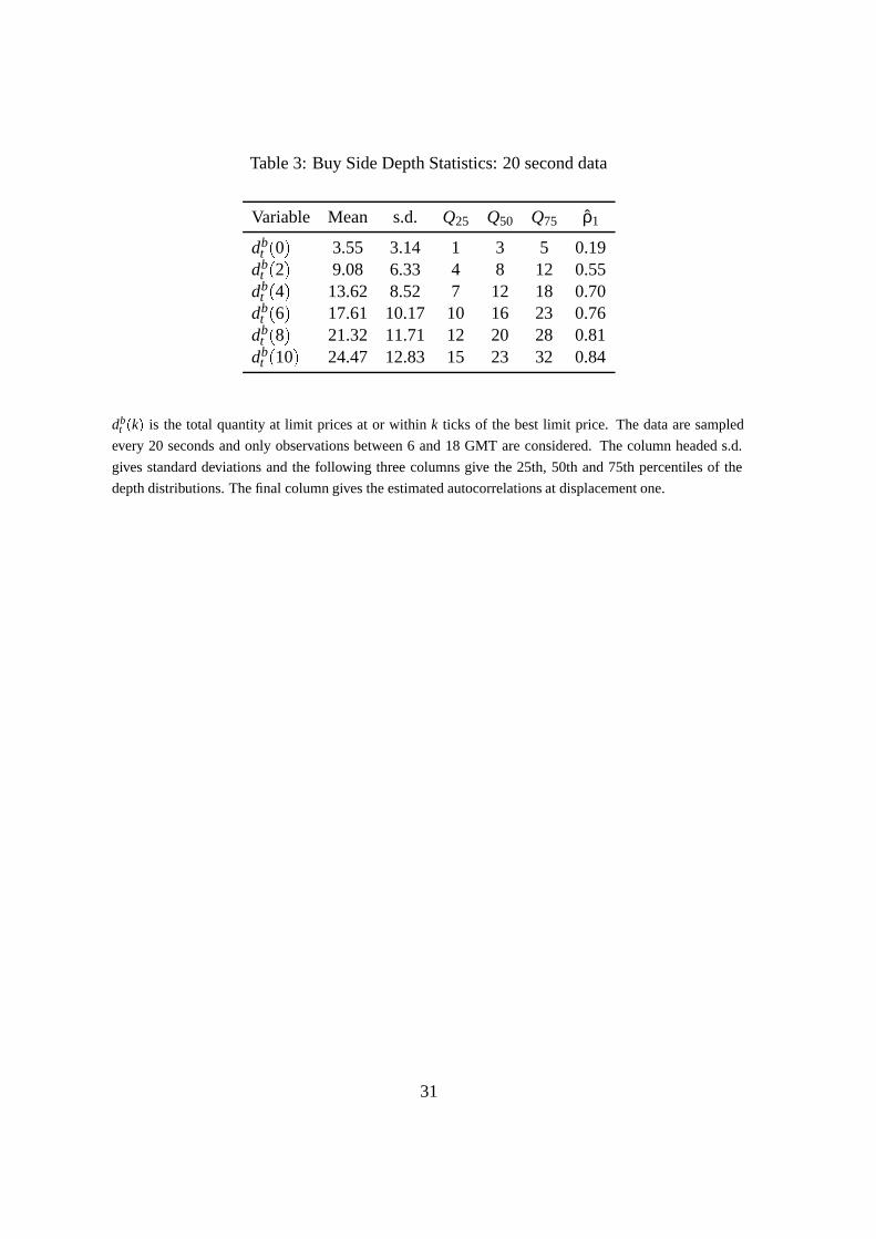
Table 3: Buy Side Depth Statistics: 20 second data

Variable Mean s.d. Q25 Q50 Q75 ρ1

dbt (0) 3.55 3.14 1 3 5 0.19

dbt (2) 9.08 6.33 4 8 12 0.55

dbt (4) 13.62 8.52 7 12 18 0.70

dbt (6) 17.61 10.17 10 16 23 0.76

dbt (8) 21.32 11.71 12 20 28 0.81

dbt (10) 24.47 12.83 15 23 32 0.84

dbt (k) is the total quantity at limit prices at or withink ticks of the best limit price. The data are sampled

every 20 seconds and only observations between 6 and 18 GMT are considered. The column headed s.d.

gives standard deviations and the following three columns give the 25th, 50th and 75th percentiles of the

depth distributions. The final column gives the estimated autocorrelations at displacement one.

31

Table 4: Transition Matrices for Order Data

Market orders Limit buy arrivals Limit sell arrivals Limit buy cancel Limit sell cancel

Mkt. sell Mkt. buy New SLB New BLB New SLS New BLS Cut SLB Cut BLB Cut SLS Cut BLS

Uncond. 0.0540 0.0565 0.1178 0.1571 0.1115 0.1556 0.1129 0.0656 0.1053 0.0638

(a) One-step transitions

Mkt. sell 0.1135 0.0259 0.0987 0.1010 0.0881 0.2286 0.0730 0.0572 0.1295 0.0845Mkt. buy 0.0243 0.1228 0.0974 0.2268 0.0866 0.1019 0.1358 0.0870 0.0675 0.0500New BLB 0.0360 0.0722 0.1479 0.1739 0.0972 0.1326 0.1278 0.0702 0.0847 0.0575New BLS 0.0708 0.0365 0.1003 0.1359 0.1448 0.1735 0.0890 0.0620 0.1217 0.0654Cut BLB 0.0296 0.0560 0.0821 0.1941 0.1025 0.1596 0.1013 0.1140 0.0965 0.0641Cut BLS 0.0559 0.0396 0.1144 0.1631 0.0795 0.1882 0.0993 0.0599 0.0916 0.1085

(b) Five-step transitions

Mkt. sell 0.1010 0.0258 0.1153 0.1257 0.1025 0.1956 0.0747 0.0431 0.1375 0.0788Mkt. buy 0.0267 0.0975 0.1025 0.1950 0.1106 0.1254 0.1467 0.0816 0.0698 0.0441New BLB 0.0447 0.0685 0.1202 0.1690 0.1000 0.1354 0.1336 0.0889 0.0869 0.0528New BLS 0.0636 0.0479 0.1053 0.1397 0.1155 0.1693 0.0930 0.0550 0.1253 0.0855Cut BLB 0.0421 0.0548 0.1131 0.1787 0.1138 0.1676 0.1092 0.0675 0.0918 0.0614Cut BLS 0.0551 0.0407 0.1228 0.1688 0.1023 0.1776 0.0998 0.0638 0.1011 0.0679

The first row of the table gives the unconditional probability of observing the event in the column head. The rest of the table gives the probability of

observing the event in the column head subsequent to the event in the row head. Panel (a) gives one-step ahead probabilities and panel (b) five-step

ahead probabilities. Probabilities may not sum to unity across rows due to rounding. The results are based on event-time data with all events outside 6

to 18 GMT omitted. SLB stands for subsidiary limit buy, BLB for best limit buy, SLS for subsidiary limit sell and BLS for best limit sell.

32

Table 5: Determination of order entry rates

Dep. Var. Coefficients andt-statistics on RHS variablesjRt�1j t-stat St�1 t-stat Dt�1 t-stat R2

LOt 147.43 17.90 - - - - 0.54MOt 16.14 4.31 - - - - 0.22NLOt 25.30 2.69 - - - - 0.11ORt 0.63 4.28 - - - - 0.98

LOt - - 0.35 8.91 - - 0.52MOt - - -0.10 -7.89 - - 0.22NLOt - - 0.27 8.96 - - 0.12ORt - - 0.01 13.99 - - 0.98

LOt - - - - 0.006 0.40 0.52MOt - - - - 0.031 5.71 0.22NLOt - - - - -0.075 -6.01 0.12ORt - - - - -0.001 -2.64 0.98

LOt 136.49 15.67 0.21 5.11 0.010 0.76 0.55MOt 21.02 5.60 -0.12 -8.63 0.031 5.69 0.23NLOt 17.09 1.75 0.25 7.93 -0.077 -6.29 0.13ORt 0.11 0.75 0.01 13.71 -0.001 -2.92 0.98

The table reports coefficients from regressions of the variables listed in the left-hand column on the variables

listed in the heads of the remaining columns plus 10 lags of the dependent variable. All data is calendar

time sampled at a 20 second frequency.t-values are heteroskedasticity robust.LO t measures the numbers

of limit orders entering in a given interval,MOt measures the number of market order entering,NLOt is the

number of limit order entries less the number of limits removed andOR t is the ratio of the number of limits

entering to the total number of limits and markets entering.Rt is the midquote return,St is the bid-ask spread

andDt = d(0)bt +d(0)s

t is total size at the best quotes. All variables used in this analysis exceptNLOt have

had their repeated intra-day patterns removed prior to the analysis. Allt-statistics are based on Newey-West

heteroskedasticity and autocorrelation robust standard errors.

33

Table 6: Correlations between limit buy and sell depth measures

Variables Correlation

dbt (0) ; da

t (0) 0.01db

t (2) ; dat (2) 0.06

dbt (4) ; da

t (4) 0.01db

t (6) ; dat (6) -0.03

dbt (8) ; da

t (8) -0.01db

t (10) ; dat (10) -0.01

The table reports cross-correlations between limit buy-side and sell-side depth measures whered bt (k) is the

total quantity at limit prices at or withink ticks of the best limit buy andd at (k) is the total quantity at limit

prices withink ticks of the best limit sell. The data used to construct these correlations is based on a 20 second

calendar-time sampling and only observations between 6 and 18 GMT are employed. Prior to computing the

correlations the repetitive intra-day pattern is filtered from all depth measures.

34

Table 7: VAR coefficients: volume, volatility and spreads

Regressor Volume eqn. Volatility eqn. Spread eqn.Coeff. t-value Coeff. t-value Coeff. t-value

Vt - - 0.448 17.34 0.134 8.6Vt�1 0.214 11.42 0.015 0.9 0.002 0.12Vt�2 0.072 4.73 -0.015 -1.01 -0.054 -3.89Vt�3 0.111 6.55 -0.048 -3.02 -0.037 -2.79Vt�4 0.079 3.53 -0.014 -0.99 -0.025 -2.05Vt�5 0.051 3.25 -0.019 -1.53 -0.035 -3.27Vt�6 0.066 3.96 -0.003 -0.22 -0.037 -3.05jRt j - - - - 0.086 4.15jRt�1j 0.067 4.73 0.108 5.06 0.027 1.54jRt�2j 0.041 2.31 0.057 4.03 0.048 2.52jRt�3j 0.035 2.2 0.063 4.63 0.000 0.02jRt�4j 0.014 1.15 0.022 1.46 0.002 0.12jRt�5j 0.003 0.27 0.018 0.83 0.018 1.37jRt�6j 0.02 1.79 0.034 2.85 0.004 0.25St - - - - - -St�1 -0.101 -7.67 0.179 8.34 0.249 7.69St�2 0.02 1.56 -0.025 -1.77 0.136 7.14St�3 -0.019 -1.69 -0.006 -0.46 0.063 2.85St�4 0.005 0.41 -0.013 -1.08 -0.003 -0.16St�5 0.027 2.12 0.033 2.18 0.059 3.46St�6 -0.005 -0.49 0.009 0.74 0.079 4.71

R2 - 0.23 - 0.32 - 0.23

Volume - 643.1 - 466.51 - 148.81Volatility - 47.47 - 130.89 - 38.39Spread - 73.27 - 89.05 - 220.77

The table reports coefficients from a 6-lag VAR involving trading volume, absolute returns and spreads.V t is

defined as the sum of market buy and market sell volume in a given interval. The data upon which the VAR

is estimated is sampled on a 20 second calendar-time basis and only observations between 6 and 18 GMT

are employed. Prior to estimation the repetitive intra-day pattern is filtered from all variables. Allt-statistics

andχ2-statistics are based on Newey-West heteroskedasticity and autocorrelation robust standard errors.

35

Table 8: Regressions of depth measures on volume, volatility and spreads

Regressor 2-tick depth eqn. 6 tick depth eqn. 10 tick depth eqn.Coeff. t-value Coeff. t-value Coeff. t-value

Vt -0.049 -3.34 -0.073 -5.61 -0.074 -6.15Vt�1 0.043 3.29 0.050 4.23 0.031 2.79Vt�2 0.053 3.94 0.056 4.83 0.050 4.27Vt�3 0.071 5.79 0.070 6.58 0.060 5.25Vt�4 0.034 2.79 0.058 5.16 0.048 4.34Vt�5 0.014 1.06 0.044 3.56 0.044 3.76Vt�6 0.032 2.51 0.042 3.14 0.046 3.48jRt j -0.085 -5.54 -0.115 -8.03 -0.114 -8.90jRt�1j -0.082 -6.27 -0.082 -6.50 -0.074 -6.48jRt�2j -0.059 -4.82 -0.066 -5.12 -0.059 -4.95jRt�3j -0.054 -4.85 -0.051 -4.78 -0.049 -4.66jRt�4j -0.024 -2.12 -0.038 -3.41 -0.036 -3.43jRt�5j -0.038 -3.24 -0.046 -3.94 -0.043 -3.86jRt�6j -0.046 -4.08 -0.052 -4.69 -0.048 -4.44St - - - - - -St�1 -0.059 -4.7 -0.069 -5.55 -0.068 -5.49St�2 -0.044 -4.04 -0.036 -3.43 -0.045 -4.17St�3 -0.028 -2.69 -0.038 -4.04 -0.045 -4.67St�4 -0.005 -0.47 -0.020 -2.22 -0.031 -3.14St�5 -0.016 -1.55 -0.048 -4.83 -0.049 -4.86St�6 -0.042 -3.79 -0.045 -4.16 -0.051 -5.06

R2 - 0.07 - 0.11 - 0.12

Volume - 75.67 - 133.50 - 122.45Volatility - 67.55 - 83.42 - 89.44Spread - 35.52 - 43.15 - 43.63

The table reports coefficients from a a regression of order book depth on trading volume, absolute returns

and spreads.Vt is defined as the sum of market buy and market sell volume in a given interval. Buy/sell

depth is measured as the quantity available in the order book at or withink ticks from the best limit buy/sell

price. The depth variables used here are sums of buy and sell side depth fork = 2;6;10. Hence, 2-tick depth

is equal todb(2)t +db(2)t . The data upon which the VAR is estimated is sampled on a 20 second calendar-

time basis and only observations between 6 and 18 GMT are employed. Prior to estimation the repetitive

intra-day pattern is filtered from all variables. Allt-statistics andχ2-statistics are based on Newey-West

heteroskedasticity and autocorrelation robust standard errors. The rows headed volume, volatility and spread

give χ2-statistics relevant to the null that coefficients on all current and lagged values of this variable are

zero.

36

Table 9:Regressions of buy and sell depth measures on buy and sell volume, volatility and spreads

Regressor 2-tick buy depth 2-tick sell depth 6-tick buy depth 6-tick sell depth 10-tick buy depth 10-tick sell depthCoeff. t-value Coeff. t-value Coeff. t-value Coeff. t-value Coeff. t-value Coeff. t-value

V Bt -0.019 -1.31 -0.026 -1.78 -0.075 -3.53 -0.017 -0.84 -0.105 -3.88 -0.012 -0.51

V Bt�1 0.082 4.93 -0.028 -1.98 0.181 9.47 -0.058 -3.05 0.187 7.86 -0.082 -3.71

V Bt�2 0.065 4.31 0.016 1.20 0.128 6.70 -0.005 -0.29 0.147 6.08 -0.013 -0.6

V Bt�3 0.084 5.91 0.009 0.70 0.170 8.98 -0.025 -1.46 0.215 9.01 -0.023 -1.19

V Bt�4 0.051 3.35 -0.018 -1.39 0.138 6.77 -0.043 -2.46 0.16 6.81 -0.054 -2.68

V Bt�5 0.055 3.40 -0.015 -1.13 0.140 7.11 -0.036 -1.87 0.171 7.81 -0.054 -2.3

V Bt�6 0.043 3.01 -0.025 -1.83 0.118 5.71 -0.075 -3.69 0.168 6.81 -0.096 -3.96

V St -0.049 -3.40 -0.031 -1.64 -0.053 -2.42 -0.127 -4.95 -0.01 -0.36 -0.214 -7.43

V St�1 -0.062 -4.30 0.112 6.85 -0.098 -5.23 0.146 6.46 -0.112 -4.88 0.131 5.03

V St�2 -0.001 -0.09 0.054 3.30 -0.024 -1.26 0.104 4.99 -0.035 -1.58 0.115 4.57

V St�3 0.007 0.49 0.077 4.84 -0.037 -2.08 0.146 7.35 -0.075 -3.48 0.144 5.66

V St�4 0.006 0.42 0.045 2.94 -0.040 -2.14 0.153 7.28 -0.074 -3.37 0.175 6.98

V St�5 -0.031 -2.17 0.027 1.57 -0.070 -3.57 0.130 5.37 -0.082 -3.59 0.164 5.61

V St�6 0.010 0.73 0.053 3.23 -0.032 -1.62 0.146 5.60 -0.058 -2.38 0.197 6.34

jRt j -0.430 -5.07 -0.368 -3.99 -0.842 -6.95 -0.711 -5.54 -1.045 -7.53 -0.841 -5.81

jRt�1j -0.306 -4.01 -0.465 -5.58 -0.479 -4.18 -0.630 -5.64 -0.545 -4.1 -0.691 -5.61

jRt�2j -0.322 -4.49 -0.229 -2.92 -0.581 -5.03 -0.319 -2.73 -0.602 -4.23 -0.403 -3.23

jRt�3j -0.253 -3.52 -0.255 -3.63 -0.332 -3.23 -0.378 -3.80 -0.36 -2.77 -0.482 -4.18

jRt�4j -0.227 -3.35 -0.003 -0.05 -0.399 -3.84 -0.130 -1.28 -0.417 -3.46 -0.202 -1.73

jRt�5j -0.224 -3.07 -0.130 -1.61 -0.437 -3.85 -0.195 -1.68 -0.552 -4.3 -0.176 -1.29

jRt�6j -0.289 -3.66 -0.136 -1.81 -0.593 -5.14 -0.101 -0.93 -0.598 -4.71 -0.189 -1.48St - - - - - - - - - - - -St�1 -0.171 -2.67 -0.310 -4.89 -0.361 -3.79 -0.444 -4.93 -0.455 -4.04 -0.512 -4.73St�2 -0.195 -3.30 -0.162 -3.01 -0.204 -2.48 -0.217 -3.07 -0.274 -2.69 -0.368 -4.28St�3 -0.134 -2.39 -0.094 -1.84 -0.189 -2.56 -0.248 -3.81 -0.355 -3.81 -0.288 -3.73St�4 -0.009 -0.18 -0.024 -0.44 -0.066 -0.91 -0.165 -2.35 -0.224 -2.36 -0.215 -2.65St�5 -0.031 -0.53 -0.099 -1.88 -0.262 -2.92 -0.297 -4.34 -0.303 -2.91 -0.381 -5.03St�6 -0.191 -2.96 -0.151 -2.70 -0.243 -2.41 -0.291 -3.93 -0.425 -3.64 -0.315 -3.97

R2 - 0.06 - 0.05 - 0.11 - 0.10 - 0.12 - 0.1

Buy volume - 100.80 - 17.20 - 287.58 - 27.58 - 266.7 - 33.61Sell volume - 33.25 - 96.21 - 43.88 - 197.64 - 44.7 - 243.17Volatility - 55.51 - 41.03 - 74.07 - 45.93 - 81.14 - 47.34Spreads - 20.67 - 35.61 - 19.44 - 50.71 - 23.73 - 45.46

The table reports coefficients from a regression of buy/sell depth on buy and sell volume, absolute returns and spreads. Buy/sell depth is measured as

the quantity in the order book at or withink ticks from the best limit buy/sell price. The depth variables used here are fork = 2;6;10. The data upon

which the VAR is estimated is sampled every 20 seconds and only observations between 6 and 18 GMT are employed. Prior to estimation the repetitive

intra-day pattern is filtered from each variable. Allt-statistics andχ 2-statistics are based on Newey-West heteroskedasticity and autocorrelation robust

standard errors. The rows headed volume, volatility and spread giveχ 2-statistics relevant to the null that coefficients on all current and lagged values of

this variable are zero.

37

Figure 1: Intra-day activity patterns in spreads and trade frequency

Figure 2: Intra-day activity patterns in limit buy depth

Figure 3: Limit Order Characteristics and Quantity Position

The x–axes give the quantity position of a limit entry computed as the aggregate quantity ahead of the incoming order in the execution

queue. The observations were fitted with a weighted spline, where the weight is the entry probability. The dotted lines are 2 standard

error bands, where the s.e. is computed using the weights.

Figure 4: Limit Order Characteristics and Price Position

The x–axes give the price position of a limit entry computed as the difference (in ticks) between the incoming limit price and the previous

best price. Price improvements are defined as positive for both limit buys and sells. The observations were fitted with a weighted spline,

where the weight is the entry probability. The dotted lines are 2 standard error bands, where the s.e. is computed using the weights.

38

Figure 1:

(a) Trade frequency (b) Bid-ask spread

39

Figure 2:

(a) Depth at best (b) Depth at and within 4 ticks

40

Figure 3:

5 10 15 20

0.0

0.1

0.2

0.3

Pro

babi

lity

Quantity Position

(a) Entry probability

5 10 15 20

0.3

0.4

0.5

Pro

babi

lity

Quantity Position

(b) Trade probability

5 10 15 20

0.5

1.0

1.5

2.0

2.5

3.0

Min

utes

Quantity Position

(c) Average lifetime

5 10 15 20

1.8

2.0

2.2

2.4

Mill

ions

Quantity Position

(d) Average size

41

Figure 4:

-5-10 5 10

0.0

0.1

0.2

0.3

0

Pro

babi

lity

Pip deviation from best price

(a) Entry probability

-5-10 5 10

0.2

0.3

0.4

0.5

0.6

0

Pro

babi

lity

Pip deviation from best price

(b) Trade probability

-5-10 5 10

0

0

24

68

Min

utes

Pip deviation from best price

(c) Average lifetime

-5-10 5 10

2.0

2.5

3.0

0

Mill

ions

Pip deviation from best price

(d) Average size

42