Measuring and allocating portfolio risk capital in the real world

Research Journal of Finance and Accounting www.iiste.org

ISSN 2222-1697 (Paper) ISSN 2222-2847 (Online) Vol 3, No 8, 2012

1

MEASURING AND ALLOCATING PORTFOLIO RISK

CAPITAL IN THE REAL WORLD: PRACTICAL APPLICATION

OF VALUE-AT-RISK AND EXPECTED SHORTFALL

Kofi A. Ababioa*

and Samuel D. Odurob

aMathematics and Statistics Department, Kumasi Polytechnic, Ghana

bInformation Services Division, NHS National Services Scotland, Edinburgh, U.K.

*Corresponding Author’s Email: [email protected]

Abstract

Financial risk professionals are constantly interested in the risk capital allocation especially when dealing with

management of portfolios under their control. This paper seeks to investigate two major risk measures namely the

Value-at-Risk (VaR) and Expected Shortfall (ES) in dealing with the risk capital allocation problem. Data from the

London Stock exchange was used for this study. Assuming no dividends payment, the Geometric Brownian motion

(Black-Scholes Model) and a fair per-unit capital allocation principle were applied to ascertain the coherence of the

two considered risk measures within a two year time horizon. It is evident from the results that stock with high mean

rate of log returns and low volatility turns to have a lower fair per unit capital allocation of risk in any selected

portfolio. Results of stocks with the least quantified risk (in pence) of all considered portfolios in this paper were

Portfolio I (Mining: BLT - 926), Portfolio II (Media: PSON - 175), Portfolio III (Financial services: SDRC - 459),

Portfolio IV (Bank: STAN - 739) and Portfolio V (FTSE 100 top 10 Companies: BATS - 1021) respectively.

Keywords: Coherent Risk Capital Allocation Value-at-Risk Expected Shortfall

1. Introduction

Financial risk professionals in their quest to boost investor and other market participant’s confidence in the financial

industry are always concerned with the future trends in market stocks. The problem of risk measurement and risk

capital allocation is not only important but also critical to industry players.

Capital allocation is the process of distributing capital to individual functional units of a business in which capital is

placed at risk for an expected return above the risk-free rate. The aim includes but not limited to profitability test of

business units and the determination of business units that can be improved in order to add value to the business.

Artzner et al., (1999) proposed some fundamental properties that a risk measure should exhibit and called them

"coherent". Risk is associated with the term "uncertainty" which is considered as an uncertain measurable random

variable. The theory views risk as uncertainty regarding the future net worth of an investment portfolio or company

at a specified point in time (Artzner et al, 1999). Generally, financial theory suggests coherent risk measure as the

one and only theoretically best way to measure risk. It measures risk as the additional amount of money needed to

ensure the future net worth will fall within a predefined set of acceptable outcomes, called the acceptance set

(Artzner et al, 1999). Artzner (1999), Meyers (2002), and Wirch and Hardy (2002), are among several authors who

have recommended the use of coherent risk measures in determining an appropriate capital requirement. In practice,

there are different approaches in measuring risk. Common among them are variance, standard deviation, Value at

Risk (VaR), the Proportional Hazard Transform (PHT) and Tail Value at Risk (TVaR) also referred to as Expected

Shortfall (ES). Apart from the Expected Shortfall (ES) and Proportional Hazard Transform (PHT) which have

proved to be coherent, the other risk measures violate one or more of the fundamental properties/axioms of coherent

risk measures.

This paper examines the application of risk measures to data from the London Stock Exchange (LSE) in the

determination of a coherent risk capital requirement. The London Stock Exchange (LSE) is one of the largest

international financial markets. The exchange trades in equities of over 2,500 companies including some of the

world’s most profitable companies across 50 different countries. The exchange has traded over 300 years and

currently has two markets, namely the Main Market and the Alternative Investment Market (AIM) with market

capitalisations of £3.5 billion and £59 billion respectively. The companies listed on the exchange can be grouped into

over 46 business sectors. In this paper we analyse and present results for a selection of The Financial Times Stock

Exchange (FTSE) 100 listed companies of the LSE that are categorised in the mining, media, financial services and

the banking sectors. The FTSE 100 consists of the 100 largest companies listed on the LSE in respect of market

capitalisation. The mining and media services sectors comprise of about 184 and 99 companies contributing 7% and

3% to the total LSE market capitalisation respectively. A total of 47 and 179 listed companies fall under the banking

and financial services sector respectively. These account for £457,048 and £39,869 respectively of the LSE market



2

capitalisation. By analysing data from the LSE, we hope to focus and capture those characteristics that are common

in large exchanges around the world.

This paper seeks to investigate the coherence or otherwise of Value-at-Risk and Expected Shortfall and the practical

application of the theory of risk measures to the allocation of risk capital to a portfolio of equities.

The remaining part of the paper is organized as follows: Section 2 describes the concept of methods employed in the

research. The empirical analysis, results and discussion are presented in Section 3. Section 4 provides the concluding

remarks.

2. Methodology

Real market data of different stocks prices in different sectors of the London Stock Exchange is used to measure the

underlying risk of the stock and the portfolio respectively within a given time horizon ( )∆ . The data was downloaded

from yahoo finance website (http://uk.finance.yahoo.com) consisting of 759 daily (2nd

Dec 2008 – 2nd

Dec 2011)

adjusted closing stock price of companies grouped under four (4) sectors namely Mining, Media, Financial Services

and Banks. A portfolio consisting of the FTSE 100 top 10 companies is also constructed. The underlying risks of

investing in these stocks are calculated using Value-at-Risk and Expected Shortfall at 05.0=α for an equally

weighted portfolio with portfolio value of £100,000. One thousand scenarios of future stock prices of each of the

respective company stocks in the respective sectors are simulated two years ahead (i.e. time horizon ( )2=∆ from

latest stock prices ( )0jS . The two widely used risk measures (Value-at-Risk and Expected Shortfall) are applied to

quantify the risk associated with the portfolios. A fair risk capital allocation principle is then implemented to allocate

a per-unit risk contribution ( )ja with respect to individual stocks in each of the portfolios. The portfolios are

organized as follows:

a) Portfolio I: Mining

b) Portfolio II: Media

c) Portfolio III: Financial Services

d) Portfolio IV: Banks

e) Portfolio V: FTSE 100 top 10 companies

The following chronological steps were followed in calculating the fair per unit risk capital allocations and the

portfolio risk.

2.1. Coherent Risk Measures

Let M be a set of real-valued random variables representing portfolio payoffs over some fixed time interval. We

define a risk measure ρ , as a real-valued function RM →:ρ mapping the payoffs to a set R of realisations. The

realisation ( )Xρ may be interpreted as the extra minimum amount of capital that should be added to a position with

payoff X in order that the position becomes acceptable to the investor. In other words, ( )Xρ is the amount of

capital required as a cushion/buffer against the payoff X . A position with ( ) 0≤Xρ indicates an acceptable payoff

which requires no further capital injection. Artzner et al (1999) defined a risk measure ρ to be "coherent" if it

satisfies all the following properties:

1. Monotonicity: If X and Y belongs to M, and X ≥ Y, then ( ) ( )YX ρρ ≥ .

Thus, given two portfolios with payoffs X and Y , the required risk capital ρ(X) should be more than the

required risk capital ρ(Y ), implying that positions that lead to higher payoffs require less risk capital.

2. Sub-Additivity: If X ,Y and MYX ∈+ , then ( ) ( ) ( )YXYX ρρρ +≤+ .

Sub-addivity reflects the fact that due to diversification effects, risk inherent in the union of two portfolios

should be at most the same as the sum of the risk of the two portfolios considered separately.

3. Positively- Homogeneous: If MX ∈ , λ > 0, then ( ) ( )XX λρλρ = .

This means that the risk capital required does not depend on any scale change in the unit of the risk being

measured. For example currency change will not affect the risk.

4. Translation invariance: If MX ∈ , and R∈φ , then ( ) ( ) φρφρ −=+ XX .

This axiom states that by adding or subtracting a risk free portfolio (a deterministic quantityφ ) to a

portfolio with payoff X creates no change in risk. That is we only alter our capital requirement by exactly

that amount ( )φ .

2.2. Definitions of Risk Measures



3

2.2.1. Value-at-Risk (VaR)

VaR is a statistical measure of downside risk that is easily and intuitively understood by non-specialists. It is

generally defined as the risk capital sufficient to cover losses from a portfolio over a fixed holding period. The VaR

can also be interpreted as a forecast of a given quantile, usually in the lower tail of the payoff distribution of a

portfolio for a fixed holding period. Formally the VaR of a portfolio, at a given confidence level 100*(1- α ) where

( )1,0∈α is defined as

( ) ( ){ }αα ≥≤−= xXPxXVaR :inf (1)

Even though VaR is very popular in practice, it is not a coherent measure of risk as it violates the sub-additive

property of coherent risk measures.

2.2.2. Expected Shortfall (ES)

Expected Shortfall (ES) or the Tail Conditional Expectation (TCE) is another informative measure of risk which

estimates the potential size of the loss −X exceeding VaR. The Expected shortfall has been proposed as an

alternative measure of risk to VaR since it satisfies all the properties of coherent risk measure. It measures the

expected value of a portfolio returns given that a specified threshold (usually the Value-at-Risk) has been exceeded.

Basically, the expected shortfall does not depend on the definition of the quantile (which are generally not sub -

additive) but rather on the distribution of payoffs and the confidence level. Given a portfolio with payoff X and

expectation ( )XE , if we assume that ( ) 1<XE and 10 << α , we define expected shortfall as

( ) ( )[ ]XVaRXXEXES αα −≤−= | (2)

2.3. Risk Capital Allocation Principle

Let’s consider an investment in a portfolio consisting of a fixed number of shares (d) with payoffs represented by the

random variables dXX ,,1 K . Estimation of contributory risk capital which is indeed a unique fair per - unit

allocation of considered investment options given a portfolio risk capital ( )Xρ . It is shown by Tasche (2000),

Aubin (1979) and Denault (2001) that, the most suitable way of finding a unique fair per-unit risk allocation is by the

gradient method. The gradient method looks at the partial derivative of the underlying risk measure with respect to

asset weights of the portfolio under consideration. However, not all risk measures are appropriate in allocating risk

capital. Hence for any feasible risk capital allocation, the differentiability of the risk measure ( )ρ must be

guaranteed (i.e. the risk measure must be "sufficiently smooth" for ensuring that the respective derivative exists). The

VaR and ES are considered quantile-based risk measures and not differentiable in general. Likewise the portfolio

base Bρ , will not be differentiable on nR since the considered risk measures are all quantile-based. The persistent

of this condition call for finding a suitable fair per-unit allocation of a given risk capital, else it will be meaningless

since the differentiability of the portfolio base must be guaranteed. Even though the ES is not differentiable, it is an

appropriate risk measure to be used for allocating risk capital as compared to VaR which is also not differentiable

and also lack the sub-additivity property of a coherent risk measure. For risk measure differentiability to be achieved,

at least one payoff has to possess a continuous density (Tasche, 2000). This condition puts a restriction on discrete

spaces, since not all portfolio payoff distributions are differentiable in nature. (e.g. insurance claims and credit

portfolios). Benfield, (2005) indicated that if the underlying payoff distribution is "sufficiently smooth", then ES is

partially differentiable with respect to the exposure weights (i.e. weights of the sub-portfolio ju ).

Assuming sufficient properties, results from Tasche (2000) show that

( ) ( )[ ]XVaRXXEuuu

ESjn

j

αα −≤=

∂

∂|,1 K (3)

Given a portfolio base with Bu and a risk measure ρ on

nR , a per-unit allocation in nRu ∈ is a vector

( ){ }uua Bj ;ρ such that



4

juu ∂∂ /)(ρ

( )∑=

=n

j

Bjj uau1

ρ (4)

Aubin (1979), Tasche (2000) and Denault (2001), also attest the fact that, in the case of a sub-additive, 1-

homogenous and coherent risk measure, differentiable at a portfolionRu ∈ ; the gradient is the

unique fair per - unit allocation. According to Fischer et al [2003] the total risk of a portfolio ( )u with respect to risk

contribution per unit sub-portfolio (uj * ej) 1≤ j ≤ d is given by the Euler theorem;

( ) ( )∑= ∂

∂∗=

n

j

B

j

jB uu

uu1

ρρ (5)

This gives the unique fair per - unit allocation to each of the sub-portfolio (uj * ej)1≤ j ≤ d.

Finding a fair per-unit capital allocation of the d stocks in a portfolio, the Brownian motion (i.e. Black Scholes

model) is used in forecasting future stock prices given historical data of the d-stocks. The mean rate ( )jµ of log-

returns is estimated from the historical data as well as the volatility ( )jσ . The two estimates are the main parameters

of the geometric Brownian motion. Simulated outcomes of the d-stocks will be the foundation of our quest of

measuring the underlying risk (i.e. using VaR and ES) associated with these stocks and the allocation of risk capital

in a very fair manner to the respective stocks.

3. Empirical Estimation and Forecasting

The mean rate of the log-returns and the volatility are estimated empirically from historical stock price data as

follows:

∑−= −

=

0

1 1,

,ln1

ˆMm mj

mjj S

S

tMδµ (6)

∑−= −

−

=

0

1

2

1,

,ˆln

1ˆ

Mm

j

mj

mj

j tS

S

tMµδ

δσ (7)

where ( )0,...:,...,1 MmdjS j −== is the historical price of stock j at the end of the mth

time interval. The

price process of stock j , according to the Black Scholes model is given as

( ) ( ) ( )jjjjj WtStS σµ ˆˆexp0 +∗= (8)

where ( )∆=t is the time horizon, Rj ∈µ is the drift (mean rate of log-return), +∈ Rjσ the diffusion

coefficient of the Brownian motion in the exponent (volatility of stock prices), jW is the jth Brownian motion at

time ( )t respectively.

The value of ( )∆jS during the time horizon can be regarded as the sum of increases in ( )∆jS in n intervals of

tδ (where n = ∆/δt). The value of the stock price at the end of the time horizon ( )∆ which cuts short of all the

intermediate price processes…...

Equation (8) above can be represented by a stochastic differential equation

( ) ( )jjjj WddtSd σµ ˆˆln += (9)

Solving Equation (9) we obtain



5

( )

( )( )

j

j

j

j

tjj

tS

tS

WtWσ

µ

ˆ

ˆ0

log

0,

−

== − (10)

where Wj,t-0 are un-correlated normal random variables such that Wj(0) 0 with E(Wj,t-0) and covariance matrix ∑~

.

For square-integrable random variables 2, LYX ∈ , the covariance is defined as the measure of dependence

between two random variables X and Y whereas correlation is the standardised measure of dependence between

random variables the two variables. We consider a d -dimensional Brownian motion ( )ddj WWW ,...,1,...,1 ==

where the 1-dimensional Brownian motion jW is assumed to be standard ( )),0(. 2

, stNWei stj −==≈− σµ

and correlated with covariance matrix ijσ=Σ . Then for st > such that )()(, sWtWW jjstj −=− , the covariance

and correlation are

( )ijstjsti stWWCov σ)(, ,, −=−− (11)

and

( )ij

ij

stjsti

st

stWWCor σ

σ=

−

−=−−

2,,

)(

)(, (12)

respectively.

For the purposes of the simulation in this paper, we use the empirical unbiased variance estimator

( )( )jmj

Mm

imiij NNNNM

−−= ∑+−=

,

0

1

,

1σ̂ (13)

where ∑=

=m

k

kii NN1

, and ∑

=

=m

k

kjj NN1

, . When ji = , we have the empirical unbiased covariance estimator. We

introduce the notation tNW mjmj ∗= ,, where mjN , are correlated standard normal random variables. From

(10), we get the Euler-approximation

tNtSS jjjmjmj σµ ˆˆlnln 1,, +=− − (14)

mjN , can easily be deduced from (14) given historical market data and a given time horizon ( )∆=t . To do that we

proceed by solving Equation (10) for the dM × historical uncorrelated normally distributed random variables

mjW ,

=

dMMM

d

d

mj

WWW

WWW

WWW

W

,2,1,

,22,21,2

,11,21,1

,

L

MOMM

L

L

where M is the number of historical stock prices. In order to make the assets in a portfolio correlated with each

other, we need to make the mjN , in Equation (14) correlated. The Cholesky decomposition of the covariance matrix

( )mjWCov ,

~=Σ is computed as follows

TCC *~=Σ

where



6

=

dddd CCC

CC

C

C

,,2,1

2,22,1

1,1

0

00

L

MOMM

L

L

(15)

is a lower triangular matrix and d is the number of stocks (assets) within each portfolio. The Cholesky

decomposition to simulate correlated standard normal random variables mjN , is computed by simulating

dk× independent identically distributed (i.i.d) standard normal random variables mjZ , .

=

kdkk

d

d

mj

ZZZ

ZZZ

ZZZ

Z

,,2,1

2,2,22,1

1,1,21,1

,

L

MOMM

L

L

such that ( ) Σ=~

* ,mjZCCov and ( ) 0, =mjNE . However such decomposition only exists if the covariance

matrix Σ~

is a symmetric definite matrix. Using mjW , and C we get a simulated dk× matrix of correlated

standard normal random variables mjN , for the d stocks as

[ ]

=

=

Kdkk

d

d

TT

mjmj

NNN

NNN

NNN

ZCN

,,2,1

2,2,22,1

1,1,21,1

,, )(*

L

MOMM

L

L

(16)

where k is the number of simulations.

Substituting tN mj. for mjW , in Equation (8) we have 2-year horizon k simulated prices

( ) ( ) ( )tNtStS mjjjmjmj ,,,ˆˆexp0 σµ +∗= (17)

for the stock j where dj ,,1 L= .

The payoff distribution mjX , for the stock (asset) j can also be calculated as

( ) ( )0,,, Mjmjmj StSX −= (18)

3.1. Results and Discussion

The results for a hundred thousand pounds (i.e. £100,000) investment in each of the five (5) portfolios are

summarised in tables 2 to 6 respectively. As part of the table, the mean rate of log returns and volatility of historical

stock prices of the assets are also presented. The required number of investment units for each asset, a fair per-unit

risk allocation and the corresponding risk capital is also presented. The Value –at-Risk and Expected Shortfall for

each portfolio are also shown in each table.

The respective total risk capital allocation known as portfolio risk for the constituent assets of each portfolio is also

shown. A numerical ranking (with 1 indicating a less risky asset) based on the quantified risk of each stock in each

portfolio is presented. Figures 1 to 5 show unitised stock price movements for each stock. It is the plot of the ratio



7

( )0,...1:,...,1,

, +−==−

MmdjS

S

Mj

mj of historical stock prices to the initial stock price value. It shows the

deviation of the stock price process from its initial value. For each of tables 2 to 6 we make the following definitions:

Mean rate (drift) of log returns for stock j , jµ , volatility of stock j , jσ last stock price of stock j , ( )0jS ,

number of units allocated to stock j , ju per unit risk allocation of stock j , ja risk capital allocation for stock

j , jj au * risk ranking for stock j , RR , portfolio risk, ( )Buρ .

Intuitively, if it is assumed that all assets in a portfolio have the same volatility, then an asset with higher returns

would require a lower risk capital allocation. Theoretically Fund managers expect to have higher returns on their

investments with a lower volatility in order to improve portfolio payoff. However in practice this assumption does

not hold as the volatility of a stock in a portfolio cannot remain constant irrespective of its price history. In all the

five portfolios considered, the portfolio risks were consistent with the Expected Shortfall estimate unlike the Value-

at-Risk which underestimates the true risk of the entire portfolios. This is seen through tables 1 to 5.

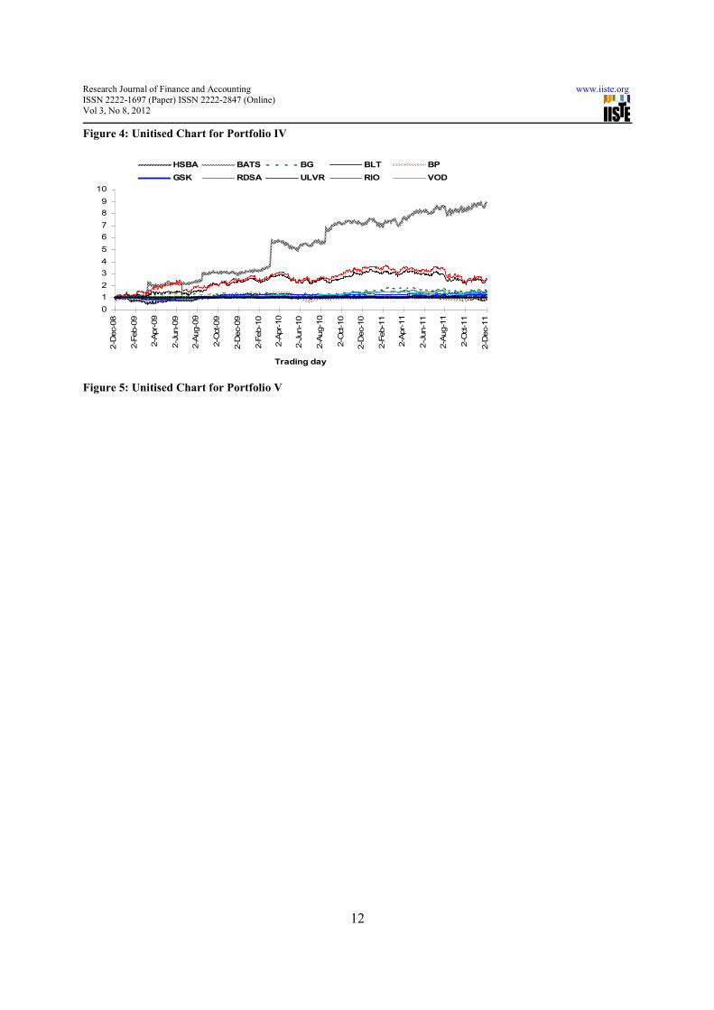
From table 6, which constitutes the top ten (10) FTSE 100 companies, the results are not only intuitive but very

simple and definite. BATS in the portfolio of the top 10 FTSE 100 companies had the highest mean rate of log

returns of 0.7275 and 0.5812 as its volatility. Even though the volatility was higher, it is compensated by its

apparently higher mean rate of log returns. HBSA on the other hand has a mean rate of log returns -0.0403 and

0.3921 as its volatility. Among the stocks considered in portfolio V, BATS ranked first as a stock with lowest risk

with HBSA ranking last, being the worse stock in the portfolio.

Also in table 5 (i.e. Portfolio IV), STAN and LLOY were the stocks with the lowest and highest risk in the portfolio.

STAN had the highest mean rate of log returns of 0.2555 whereas LLOY was -0.6218. The volatility of LLOY even

though not the highest in the portfolio has a correspondingly lower mean rate of log return making it the most risky

ranked asset. The results so far show STAN as the best stock to invest in as compared to the considered stocks in the

portfolio.

It is also evident in table 4 (i.e. Portfolio III); that SDRC is the best asset as IAP is the worse asset in the portfolio.

The mean rate of log return of SDRC is 0.2112 with 0.3661 as the volatility. On the other hand, IAP, the worse asset

in the portfolio has a mean rate of log return of 0.1027 and 0.454 respectively.

Last but not the least, PSON and ITV were the good and worse assets respectively in Portfolio II as shown in table 3.

The mean rate of log returns of PSON and ITV were 0.2088 and 0.2165 respectively. However, the volatility of

PSON is 0.2454 whereas ITV is 0.5184 which is significantly higher. PSON parameter looks more stable than ITV.

Lastly, in the case of the first portfolio as in table II, BLT, the safest asset in the portfolio has a mean rate of log

returns of 0.3100 and the worse asset, XTA as 0.3094. Volatility of BLT is lower as compared to XTA. BLT

volatility is 0.4268 which is lower than that of XTA which is 0.6111.

4. Conclusion

The mean rate of log returns and volatility of an asset remains the two main parameters of the Black Scholes model.

Their variations therefore have different effect on the type of risk measure being used to estimate the portfolio risk.

Consistently, it is evident throughout tables 2 to 6, that the Vale-at-Risk underestimates the true portfolio risk unlike

the Expected Shortfall whose estimate of the risk is the same as that of the portfolio risk. The fair per unit risk capital

allocation estimate associated with the respective stocks in all the five portfolios considered in this paper adds up to

the portfolio risk. This principle is also supported by the sub-additivity property of coherent risk measures. Expected

Shortfall is a coherent risk measure unlike Value-at-Risk which violates the sub-addivity property. It is therefore

evident that Value-at-Risk violates the sub-additivity property as shown consistently in tables 2 to 6. Hence, the

usage of Value-at-Risk as a risk measure by practitioners should serve as a rough estimate in taking decision rather

than as a true risk estimate. The Expected Shortfall as a risk measure apart from being coherent also estimates the

true portfolio risk as seen in tables 2 to 6.

Acknowledgement

The authors will like to thank Prof. Dr. Tom Fischer, Institute of Mathematics, University of Wuerzburg and Dr.

Z.K.M. Batse, Dean, Faculty of Science at Kumasi Polytechnic for reviewing an earlier version. All errors and

omissions remain with authors.

References



8

Acerbi C., Tasche D. (2000). “On the coherence of Expected Shortfall”. Journal of Banking and Finance, Vol.

26(7), pp. 1487-1503.

Aubin J. P. Mathematical Methods of Game and Economic Theory. North-Holland Publishing Co.,

Amsterdam, 1979.

Artzner, P., Delbaen, F., Eber J.M., Heath, D, (1999). “Coherent measures of risk”. Mathematical Finance, Vol. 9

(3), pp. 203-228.

Artzner, P., Delbaen, F., Eber J.M., Heath, D., (1999). “Coherent Measures of Risk”. Mathematical. Finance

vol. 9(3), pp. 203-229.

Artzner, P. (1999), “Application of Coherent Risk Measures to Capital Requirements in Insurance”, North

American Actuarial Journal, Vol. 3(2), pp 11-25.

Kaye P (2005). “Risk Measurement in Insurance: A Guide to Risk Measurement, Capital Allocation And Related

Decision Support Issues

Denault, M. (2000) “Coherent Allocation of Risk Capital.” Journal of Risk, 4, pp. 1-34.

Fischer Tom, Armin Roehrl. (2003), Risk and performance optimization for portfolios of bonds and stocks

Proceedings of the International AFIR Colloquium.

Tasche, D. (2000), “Conditional Expectation as Quantile Derivative”, Unpublished manuscript.

Meyers, G., (2002) “Setting Capital Requirements with Coherent Measures of Risk – Part 1”, Actuarial Review,

August 2002.

Wirch J. L and Hardy M. (2002), “Distortion Risk Measures: Coherence and Stochastic Dominance”,

International Congress on Insurance: Mathematics and Economics.

Table 1: List of Companies

Sector Company Name/Ticker Sector Company Name/Ticker

Mining Anglo American plc (AAL) Banks HSBC Holding plc (HSBA)

Rio Tinto plc (RIO) Barclays plc (BARC)

BHP Billiton Group plc (BLT) Lloyds Banking Group plc (LLOY)

XSTRATA plc (XTA)

Royal Bank of Scotland Group plc

(RBS)

Vedanta Resources plc (VED) Standard Chartered plc (STAN)

Media WPP plc (WPP) FTSE100 Top

10 companies British American Tobacco plc (BATS)

Reed Elsevier plc (REL) HSBC Holding plc (HSBA)

Pearson plc (PSON) BG Group plc (BG)

ITV plc (ITV) BHP Billiton Group plc (BLT)

British Sky Broadcasting Group

plc (BSY) BP Group plc (BP)

Financial

Services ICAP plc (IAP) GlaxoSmithKline plc (GSK)

Investec plc (INVP) Royal Dutch Shell plc ’A’ (RDSA)

Schroders plc (SDR) Unilever plc (ULVR)

Schroders plc (SDRc) Rio Tinto plc (RIO)

Vodafone Group plc (VOD)



9

Table 2: Parameter Estimate and Risk Measure for Portfolio I

STOCK j j Sj(0) uj aj uj*aj RRj

AAL 0.2432 0.4912 2,487.00 8 1576.73 12,680 3

RIO 0.3221 0.5363 3,346.50 6 2112.56 12,625 2

BLT 0.3100 0.4268 2,000.50 10 925.91 9,257 1*

XTA 0.3094 0.6111 1,036.00 19 733.69 14,164 5**

VED 0.2307 0.5723 1,086.00 18 768.86 14,159 4

B(u) 62,885

VaR 53,112

ES 62,885

* - (Portfolio Stock with lowest risk) ** - (Portfolio stock with highest risk)

Table 3: Parameter Estimate and Risk Measure for Portfolio II


WPP 0.2236 0.3198 673.50 30 219.65 6,523 3

REL -0.0016 0.2527 524.00 38 219.29 8,370 4

PSON 0.2088 0.2456 1,143.00 17 174.69 3,057 1*

ITV 0.2165 0.5184 65.20 307 35.28 10,823 5**

BSY 0.1958 0.2657 764.50 26 136.25 3,564 2

B(u) 32,337

VaR 23,420

ES 32,337


Table 4: Parameter Estimate and Risk Measure for Portfolio III


IAP 0.1027 0.4543 369.00 68 216.73 14,684 4**

INVP 0.6120 0.7200 372.50 67 194.49 13,053 3

SDR 0.1898 0.3718 1,383.00 18 617.22 11,157 2

SDRC 0.2112 0.3661 1,142.00 22 458.95 10,047 1*

B(u) 48,941

VaR 37,460

ES 48,941


Table 5: Parameter Estimate and Risk Measure for Portfolio IV


HBSA -0.0403 0.3921 511.20 39 342.77 13,410 2

BARC 0.0742 0.7622 190.65 105 160.64 16,852 3

LLOY -0.6218 0.8849 25.39 788 24.53 19,320 5**

RBS -0.3614 0.9465 21.58 927 20.54 19,041 4



10

STAN 0.2555 0.4306 1,452.50 14 739.16 10,178 1*

B(u) 78,800

VaR 73,246

ES 78,800


Table 6: Parameter Estimate and Risk Measures for Portfolio V


HBSA -0.0403 0.3921 511.20 20 272.67 5,334 10**

BATS 0.7275 0.5812 2,956.50 3 -1021.41 -3,455 1*

BG 0.1659 0.3475 1,364.00 7 460.22 3,374 7

BLT 0.3100 0.4268 2,000.50 5 624.36 3,121 6

BP 0.0100 0.3181 464.80 22 195.13 4,198 9

GSK 0.0791 0.2447 1,421.50 7 228.18 1,605 4

RDSA 0.1488 0.2527 2,239.00 4 571.98 2,555 5

ULVR 0.1193 0.2238 2,102.00 5 212.14 1,009 2

RIO 0.3221 0.5363 3,346.50 3 1,368.96 4,091 8

VOD 0.1128 0.2442 172.10 58 21.15 1,229 3

B(u) 23,061

VaR 13,100

ES 23,061


0

1

2

3

4

5

6

2-Dec-08

2-Feb-09

2-Apr-09

2-Jun-09

2-Aug-09

2-Oct-09

2-Dec-09

2-Feb-10

2-Apr-10

2-Jun-10

2-Aug-10

2-Oct-10

2-Dec-10

2-Feb-11

2-Apr-11

2-Jun-11

2-Aug-11

2-Oct-11

2-Dec-11

Trading day

AAL RIO BLT XTA VED

Figure 1: Unitised Chart for Portfolio I



11

0

1

2

3

2-Dec-08

2-Feb-09

2-Apr-09

2-Jun-09

2-Aug-09

2-Oct-09

2-Dec-09

2-Feb-10

2-Apr-10

2-Jun-10

2-Aug-10

2-Oct-10

2-Dec-10

2-Feb-11

2-Apr-11

2-Jun-11

2-Aug-11

2-Oct-11

2-Dec-11

Trading day

WPP REL PSON ITV BSY

Figure 2: Unitised Chart for Portfolio II

0

1

2

3

4

5

6

7

8

9

2-Dec-08

2-Feb-09

2-Apr-09

2-Jun-09

2-Aug-09

2-Oct-09

2-Dec-09

2-Feb-10

2-Apr-10

2-Jun-10

2-Aug-10

2-Oct-10

2-Dec-10

2-Feb-11

2-Apr-11

2-Jun-11

2-Aug-11

2-Oct-11

2-Dec-11

Trading day

IAP INVP SDR SDRC

Figure 3: Unitised Chart for Portfolio III

0

1

2

3

4

2-Dec-08

2-Feb-09

2-Apr-09

2-Jun-09

2-Aug-09

2-Oct-09

2-Dec-09

2-Feb-10

2-Apr-10

2-Jun-10

2-Aug-10

2-Oct-10

2-Dec-10

2-Feb-11

2-Apr-11

2-Jun-11

2-Aug-11

2-Oct-11

2-Dec-11

Trading day

HSBA BARC LLOY RBS STAN



12

Figure 4: Unitised Chart for Portfolio IV

0

1

2

3

4

5

6

7

8

9

10

2-Dec-08

2-Feb-09

2-Apr-09

2-Jun-09

2-Aug-09

2-Oct-09

2-Dec-09

2-Feb-10

2-Apr-10

2-Jun-10

2-Aug-10

2-Oct-10

2-Dec-10

2-Feb-11

2-Apr-11

2-Jun-11

2-Aug-11

2-Oct-11

2-Dec-11

Trading day

HSBA BATS BG BLT BP

GSK RDSA ULVR RIO VOD

Figure 5: Unitised Chart for Portfolio V

Measuring and allocating portfolio risk capital in the real world

Documents

Transcript of Measuring and allocating portfolio risk capital in the real world