Measures of Skewness And Kurtosis - e-Rho: Electronic...
17
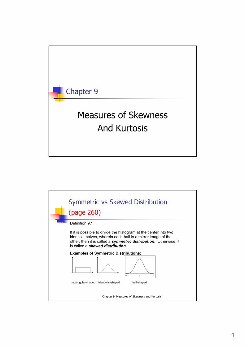
1 Chapter 9 Measures of Skewness And Kurtosis Chapter 9. Measures of Skewness and Kurtosis Symmetric vs Skewed Distribution (page 260) Definition 9.1 If it is possible to divide the histogram at the center into two identical halves, wherein each half is a mirror image of the other, then it is called a symmetric distribution. Otherwise, it is called a skewed distribution. Examples of Symmetric Distributions: rectangular-shaped triangular-shaped bell-shaped - 3.4 0 3.4
Transcript of Measures of Skewness And Kurtosis - e-Rho: Electronic...
1
Chapter 9
Measures of SkewnessAnd Kurtosis
Chapter 9. Measures of Skewness and Kurtosis
Symmetric vs Skewed Distribution
(page 260)Definition 9.1 If it is possible to divide the histogram at the center into two identical halves, wherein each half is a mirror image of the other, then it is called a symmetric distribution. Otherwise, it is called a skewed distribution.
Examples of Symmetric Distributions: rectangular-shaped triangular-shaped bell-shaped
- 3.4 0 3.4
2
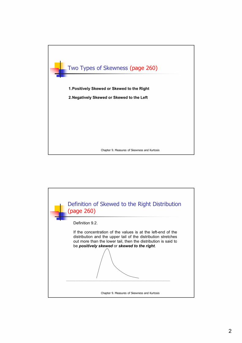
Chapter 9. Measures of Skewness and Kurtosis
Two Types of Skewness (page 260)
1. Positively Skewed or Skewed to the Right 2. Negatively Skewed or Skewed to the Left
Chapter 9. Measures of Skewness and Kurtosis
Definition of Skewed to the Right Distribution(page 260)
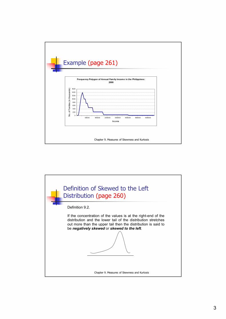
Definition 9.2. If the concentration of the values is at the left-end of the distribution and the upper tail of the distribution stretches out more than the lower tail, then the distribution is said to be positively skewed or skewed to the right.
_______________________________________________________________________________________
3
Chapter 9. Measures of Skewness and Kurtosis
Example (page 261)
Frequency Polygon of Annual Family Income in the Philippines: 2000
0
200
400
600
800
1000
1200
1400
1600
95000 195000 295000 395000 495000 595000 695000
Income
No.
of F
amilie
s (in
thou
sand
s)
Chapter 9. Measures of Skewness and Kurtosis
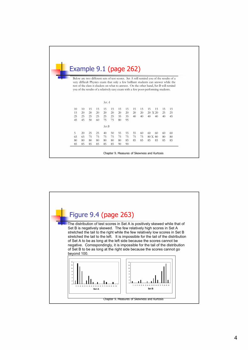
Definition of Skewed to the Left Distribution (page 260)
Definition 9.2. If the concentration of the values is at the right-end of the distribution and the lower tail of the distribution stretches out more than the upper tail then the distribution is said to be negatively skewed or skewed to the left.
4
Chapter 9. Measures of Skewness and Kurtosis
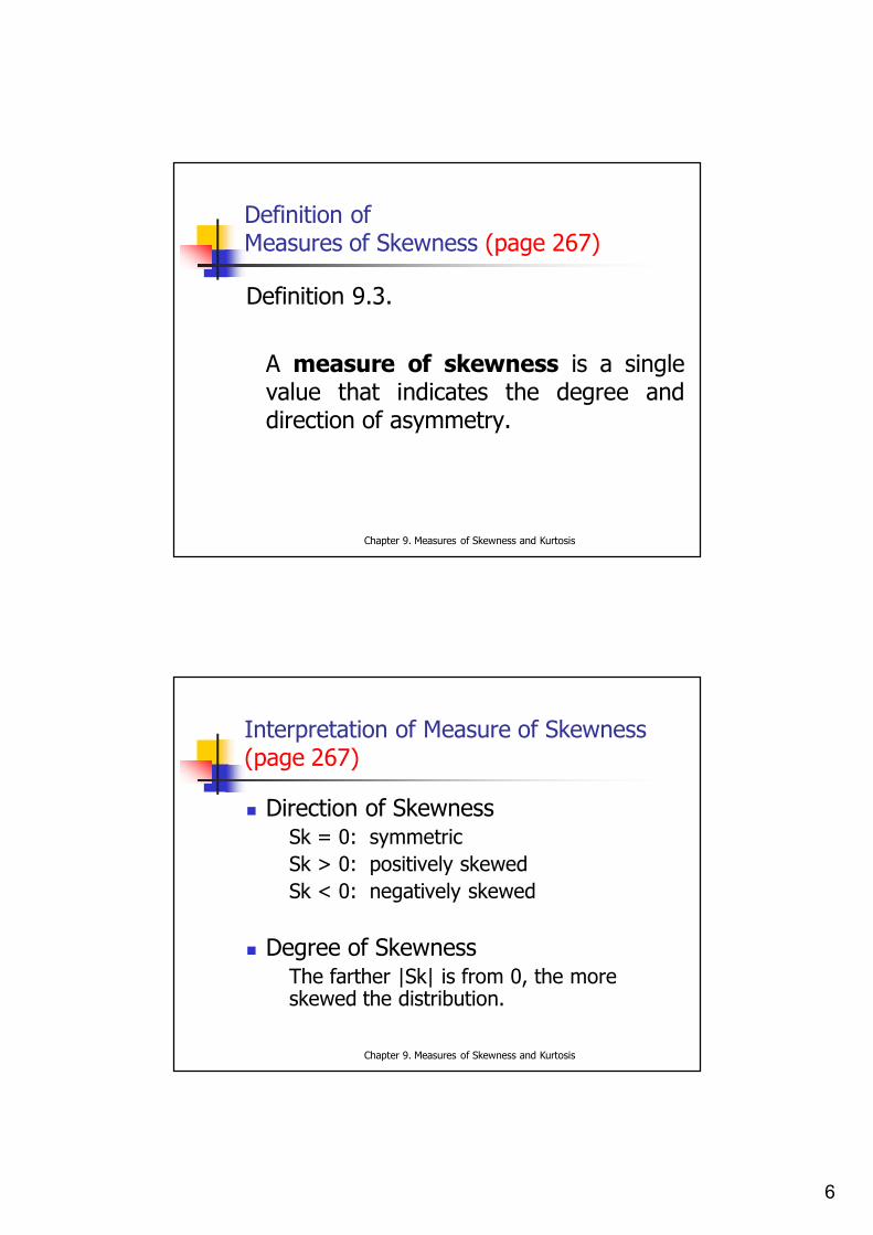
Example 9.1 (page 262)Below are two different sets of test scores. Set A will remind you of the results of a very difficult Physics exam that only a few brilliant students can answer while the rest of the class is clueless on what to answer. On the other hand, Set B will remind you of the results of a relatively easy exam with a few poor-performing students.
Set A
10 10 15 15 15 15 15 15 15 15 15 15 15 15 15 20 20 20 20 20 20 20 20 20 20 X 20 25 25 25 25 25 25 25 25 35 35 40 40 40 40 40 45 45 45 50 60 75 75 80 95
Set B
5 20 25 25 40 50 55 55 55 60 60 60 60 60 65 65 75 75 75 75 75 75 75 75 80 X 80 80 80 80 80 80 80 80 80 80 85 85 85 85 85 85 85 85 85 85 85 85 85 90 90
Chapter 9. Measures of Skewness and Kurtosis
Figure 9.4 (page 263)The distribution of test scores in Set A is positively skewed while that of Set B is negatively skewed. The few relatively high scores in Set A stretched the tail to the right while the few relatively low scores in Set B stretched the tail to the left. It is impossible for the tail of the distribution of Set A to be as long at the left side because the scores cannot be negative. Correspondingly, it is impossible for the tail of the distribution of Set B to be as long at the right side because the scores cannot go beyond 100.
0
2
4
6
8
10
12
14
10 15 20 25 30 35 40 45 50 55 60 65 70 75 80 85 90 95 100
Set A
0
2
4
6
8
10
12
14
5 10 15 20 25 30 35 40 45 50 55 60 65 70 75 80 85 90
Set B

5
Chapter 9. Measures of Skewness and Kurtosis
Importance of Detecting Skewness (page 263)
Skewness sometimes presents a problem in the analysis of data because it can adversely affect the behavior of certain summary measures. For this reason, certain procedures in statistics depend on symmetry assumptions. It would be inappropriate to use these procedures in the presence of severe skewness. Sometimes we need to perform special preliminary adjustments, such as transformations, before analyzing skewed data. Other times, we need to look for procedures that are not affected by skewness. What is important is that, at the onset, we are already able to detect skewness in order to prevent contamination of subsequent analysis. Or else, we will only end up with spurious conclusions.
Chapter 9. Measures of Skewness and Kurtosis
Relationship of the Three
Measures of Central Tendencyfor Unimodal Distributions (page 265)
Symmetric Distribution
Mean Median Mode
Mean = Median = Mode
Positively Skew ed Distribution
Mean > Median > Mode
Mode Median Mean
Negatively Skewed Distribution
Mean < Median < Mode
Mode Median Mean
6
Chapter 9. Measures of Skewness and Kurtosis
Definition of Measures of Skewness (page 267)
Definition 9.3.
A measure of skewness is a singlevalue that indicates the degree anddirection of asymmetry.
Chapter 9. Measures of Skewness and Kurtosis
Interpretation of Measure of Skewness (page 267)
Direction of SkewnessSk = 0: symmetricSk > 0: positively skewedSk < 0: negatively skewed
Degree of SkewnessThe farther |Sk| is from 0, the more skewed the distribution.
7
Chapter 9. Measures of Skewness and Kurtosis
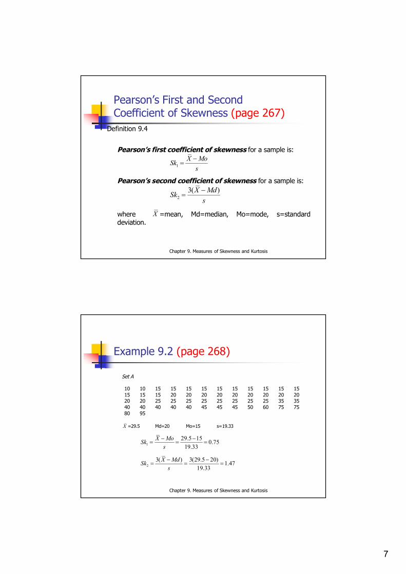
Pearson’s First and Second Coefficient of Skewness (page 267)
Definition 9.4
Pearson’s first coefficient of skewness for a sample is:
1X MoSks
Pearson’s second coefficient of skewness for a sample is:
23( )X MdSk
s
where X =mean, Md=median, Mo=mode, s=standard deviation.
Chapter 9. Measures of Skewness and Kurtosis
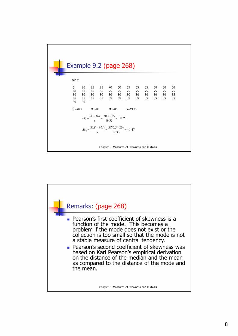
Example 9.2 (page 268)
Set A
10 10 15 15 15 15 15 15 15 15 15 15 15 15 15 20 20 20 20 20 20 20 20 20 20 20 25 25 25 25 25 25 25 25 35 35 40 40 40 40 40 45 45 45 50 60 75 75 80 95
X =29.5 Md=20 Mo=15 s=19.33
129.5 15 0.75
19.33X MoSks
23( ) 3(29.5 20) 1.47
19.33X MdSks
8
Chapter 9. Measures of Skewness and Kurtosis
Example 9.2 (page 268)
Set B
5 20 25 25 40 50 55 55 55 60 60 60 60 60 65 65 75 75 75 75 75 75 75 75 80 80 80 80 80 80 80 80 80 80 80 85 85 85 85 85 85 85 85 85 85 85 85 85 90 90
X =70.5 Md=80 Mo=85 s=19.33
170.5 85 0.75
19.33X MoSks
23( ) 3(70.5 80) 1.47
19.33X MdSks
Chapter 9. Measures of Skewness and Kurtosis
Remarks: (page 268)
Pearson’s first coefficient of skewness is a function of the mode. This becomes a problem if the mode does not exist or the collection is too small so that the mode is not a stable measure of central tendency.
Pearson’s second coefficient of skewness was based on Karl Pearson’s empirical derivation on the distance of the median and the mean as compared to the distance of the mode and the mean.
9
Chapter 9. Measures of Skewness and Kurtosis
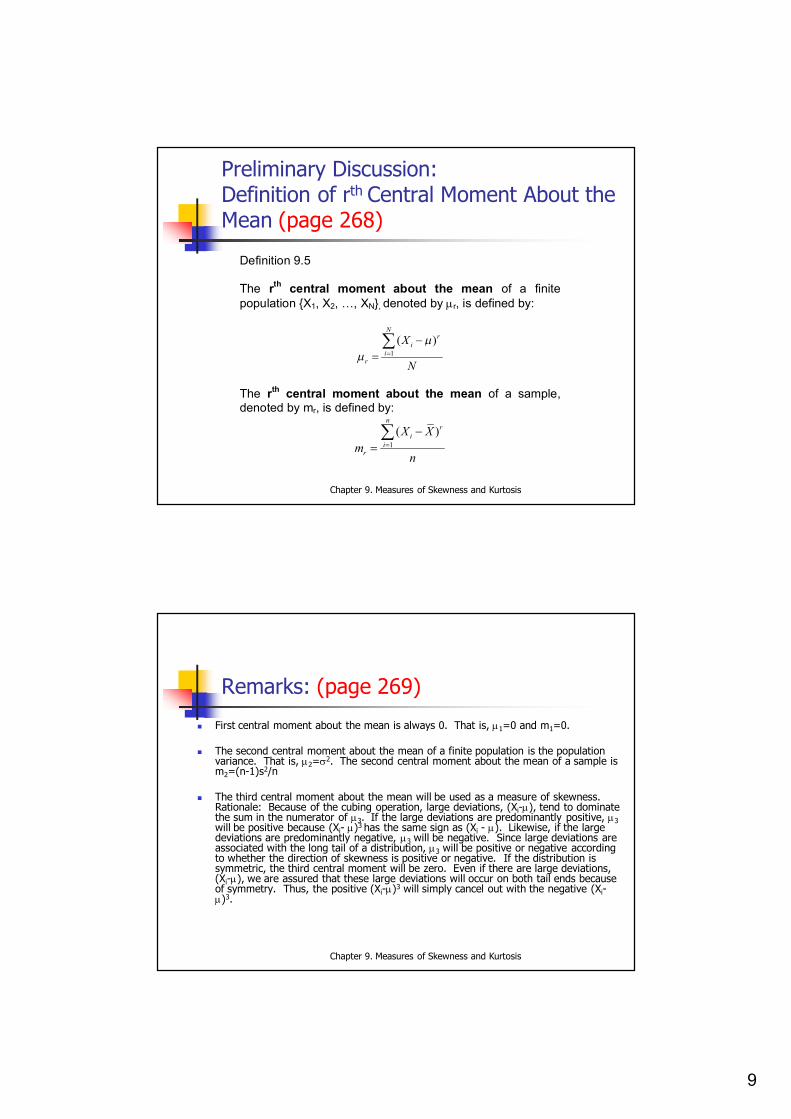
Preliminary Discussion:Definition of rth Central Moment About the Mean (page 268)
Definition 9.5 The rth central moment about the mean of a finite population {X1, X2, …, XN}, denoted by r, is defined by:
1( )
Nr
ii
r
X
N
The rth central moment about the mean of a sample,denoted by mr, is defined by:
1( )
nr
ii
r
X Xm
n
Chapter 9. Measures of Skewness and Kurtosis
Remarks: (page 269)
First central moment about the mean is always 0. That is, 1=0 and m1=0.
The second central moment about the mean of a finite population is the population variance. That is, 2=2. The second central moment about the mean of a sample is m2=(n-1)s2/n
The third central moment about the mean will be used as a measure of skewness. Rationale: Because of the cubing operation, large deviations, (Xi-), tend to dominate the sum in the numerator of 3. If the large deviations are predominantly positive, 3will be positive because (Xi- )3 has the same sign as (Xi - ). Likewise, if the large deviations are predominantly negative, 3 will be negative. Since large deviations are associated with the long tail of a distribution, 3 will be positive or negative according to whether the direction of skewness is positive or negative. If the distribution is symmetric, the third central moment will be zero. Even if there are large deviations, (Xi-), we are assured that these large deviations will occur on both tail ends because of symmetry. Thus, the positive (Xi-)3 will simply cancel out with the negative (Xi-)3.
10
Chapter 9. Measures of Skewness and Kurtosis
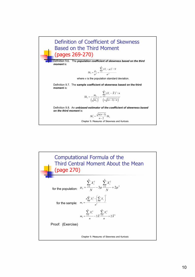
Definition of Coefficient of Skewness Based on the Third Moment (pages 269-270)
Definition 9.6. The population coefficient of skewness based on the third moment is:
3
3 13 3 3
( ) /N
ii
X NSk
where is the population standard deviation. Definition 9.7. The sample coefficient of skewness based on the third moment is:
3
3 13 3 3
2
( ) /
( 1) /
n
ii
X X nmSkm s n n
Definition 9.8. An unbiased estimator of the coefficient of skewness based on the third moment is:
*3 3
( 1)2
n nSk Sk
n
Chapter 9. Measures of Skewness and Kurtosis
Computational Formula of the Third Central Moment About the Mean(page 270)
for the population:
3 2
31 13 3 2
N N
i ii iX X
N N
for the sample:
22
1 12 2
n n
i ii in X X
mn
3 2
31 13 3 2
n n
i ii iX X
m X Xn n
Proof: (Exercise)
11
Chapter 9. Measures of Skewness and Kurtosis
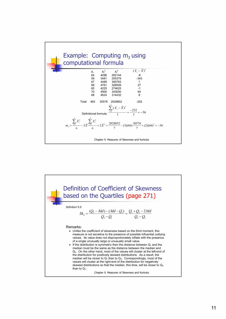
Example: Computing m3 using computational formula
Xi Xi2 Xi
3 3( )iX X
64 4096 262144 -8 59 3481 205379 -343 67 4489 300763 1 69 4761 328509 27 65 4225 274625 -1 70 4900 343000 64 68 4624 314432 8
Total 462 30576 2028852 -252
Definitional formula:
73
1( )
252 367 7
ii
X X
3 2
3 31 13
2028852 305763 2 (3)(66) (2)(66) 367 7
n n
i ii iX X
m X Xn n
Chapter 9. Measures of Skewness and Kurtosis
Definition of Coefficient of Skewness based on the Quartiles (page 271)
Definition 9.9.
3 1 1 34
3 1 3 1
( ) ( ) 2Q Md Md Q Q Q MdSkQ Q Q Q
Remarks: Unlike the coefficient of skewness based on the third moment, this
measure is not sensitive to the presence of possible influential outlying values. Its value does not disproportionately inflate with the presence of a single unusually large or unusually small value.
If the distribution is symmetric then the distance between Q1 and the median must be the same as the distance between the median and Q3. On the other hand, most of the values will cluster at the left-end of the distribution for positively skewed distributions. As a result, the median will be closer to Q1 than to Q3. Correspondingly, most of the values will cluster at the right-end of the distribution for negatively skewed distributions so that the median, this time, will be closer to Q3 than to Q1.
12
Chapter 9. Measures of Skewness and Kurtosis
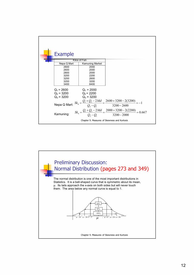
ExampleKilos of Fish
Nepa Q Mart Kamuning Market 2600 2000 2600 2000 2800 2000 3200 2200 3200 2600 3200 3200 3400 8400
Q1 = 2600 Q1 = 2000 Q2 = 3200 Q2 = 2200 Q3 = 3200 Q3 = 3200
Nepa Q Mart: 1 3
43 1
2 2600 3200 2(3200) 13200 2600
Q Q MdSkQ Q
Kamuning: 1 3
43 1
2 2000 3200 2(2200) 0.6673200 2000
Q Q MdSkQ Q
Chapter 9. Measures of Skewness and Kurtosis
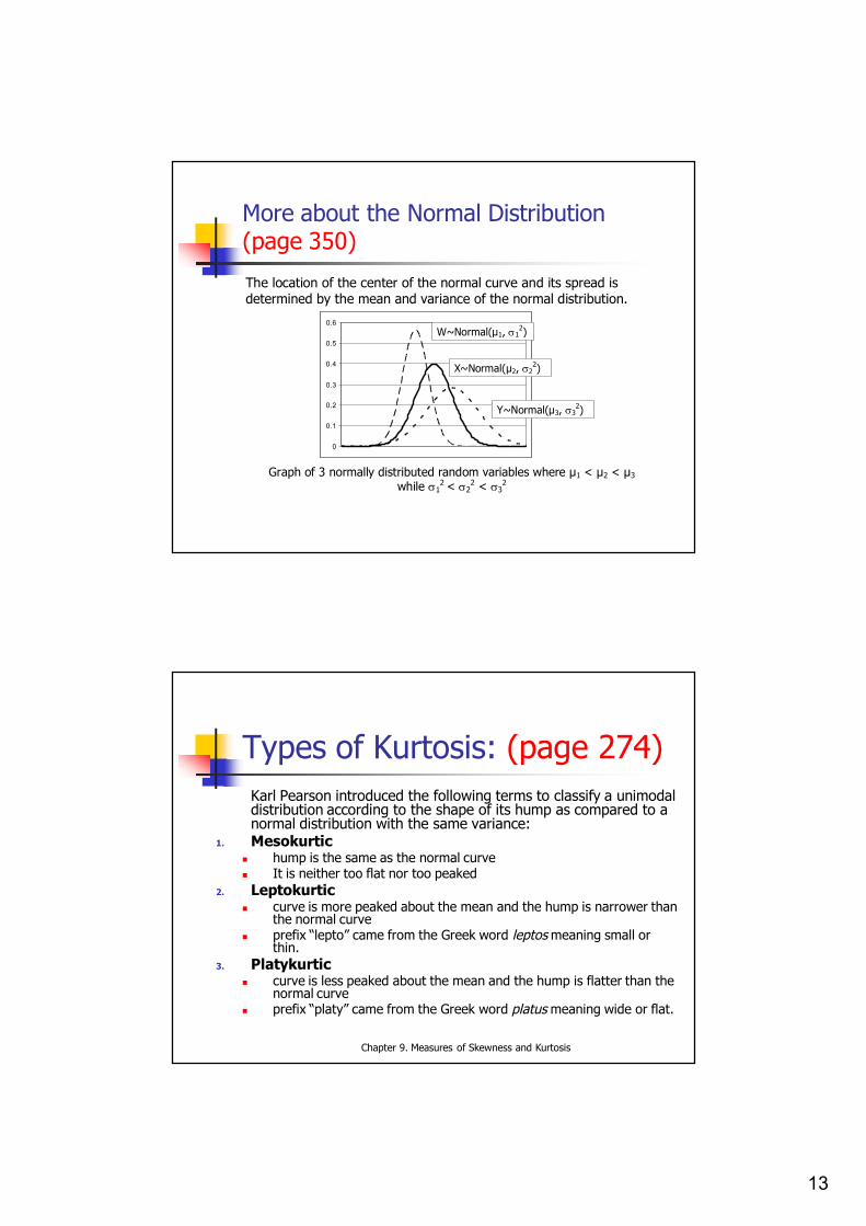
Preliminary Discussion: Normal Distribution (pages 273 and 349)
2 3 3
68%
95%
>99%
2
The normal distribution is one of the most important distributions in Statistics. It is a bell-shaped curve that is symmetric about its mean, µ. Its tails approach the x-axis on both sides but will never touch them. The area below any normal curve is equal to 1.
13
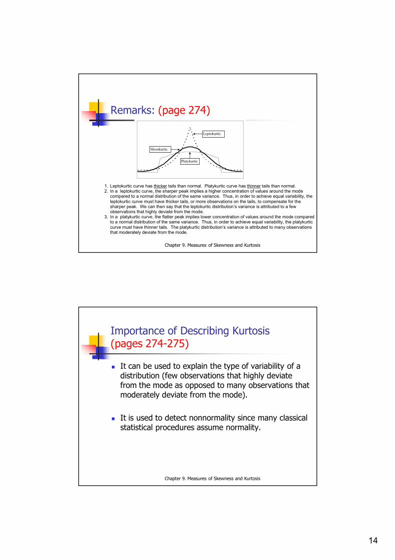
More about the Normal Distribution (page 350)
The location of the center of the normal curve and its spread is determined by the mean and variance of the normal distribution.
Graph of 3 normally distributed random variables where µ1 < µ2 < µ3 while 1
2 < 22 < 3
2
0
0.1
0.2
0.3
0.4
0.5
0.6W~Normal(µ1, 1
2)
X~Normal(µ2, 22)
Y~Normal(µ3, 32)
Chapter 9. Measures of Skewness and Kurtosis
Types of Kurtosis: (page 274)Karl Pearson introduced the following terms to classify a unimodal distribution according to the shape of its hump as compared to a normal distribution with the same variance:
1. Mesokurtic hump is the same as the normal curve It is neither too flat nor too peaked
2. Leptokurtic curve is more peaked about the mean and the hump is narrower than
the normal curve prefix “lepto” came from the Greek word leptos meaning small or
thin.3. Platykurtic
curve is less peaked about the mean and the hump is flatter than the normal curve
prefix “platy” came from the Greek word platus meaning wide or flat.
14
Chapter 9. Measures of Skewness and Kurtosis
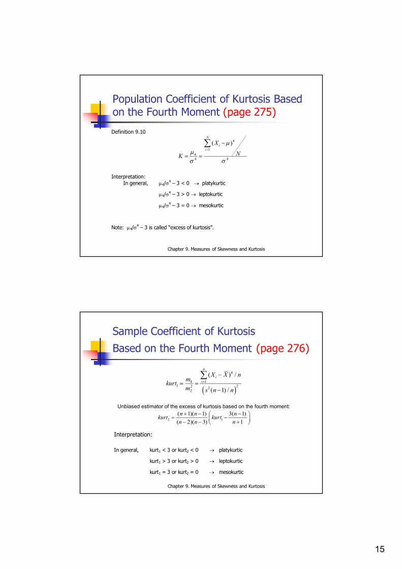
Remarks: (page 274)
Leptokurtic
Mesokurtic
Platykurtic
1. Leptokurtic curve has thicker tails than normal. Platykurtic curve has thinner tails than normal. 2. In a leptokurtic curve, the sharper peak implies a higher concentration of values around the mode
compared to a normal distribution of the same variance. Thus, in order to achieve equal variability, the leptokurtic curve must have thicker tails, or more observations on the tails, to compensate for the sharper peak. We can then say that the leptokurtic distribution’s variance is attributed to a few observations that highly deviate from the mode.
3. In a platykurtic curve, the flatter peak implies lower concentration of values around the mode compared to a normal distribution of the same variance. Thus, in order to achieve equal variability, the platykurtic curve must have thinner tails. The platykurtic distribution’s variance is attributed to many observations that moderately deviate from the mode.
Chapter 9. Measures of Skewness and Kurtosis
Importance of Describing Kurtosis (pages 274-275)
It can be used to explain the type of variability of a distribution (few observations that highly deviate from the mode as opposed to many observations that moderately deviate from the mode).
It is used to detect nonnormality since many classical statistical procedures assume normality.
15
Chapter 9. Measures of Skewness and Kurtosis
Population Coefficient of Kurtosis Based on the Fourth Moment (page 275)
Definition 9.10
4
144 4
( )N
ii
X
NK
Interpretation: In general, 4/4 – 3 < 0 platykurtic
4/4 – 3 > 0 leptokurtic
4/4 – 3 = 0 mesokurtic
Note: 4/4 – 3 is called “excess of kurtosis”.
Chapter 9. Measures of Skewness and Kurtosis
Sample Coefficient of Kurtosis
Based on the Fourth Moment (page 276)
4
141 22 2
2
( ) /
( 1) /
n
ii
X X nmkurtm s n n
Unbiased estimator of the excess of kurtosis based on the fourth moment:
2 1( 1)( 1) 3( 1)( 2)( 3) 1n n nkurt kurtn n n
Interpretation:
In general, kurt1 < 3 or kurt2 < 0 platykurtic
kurt1 > 3 or kurt2 > 0 leptokurtic
kurt1 = 3 or kurt2 = 0 mesokurtic
16
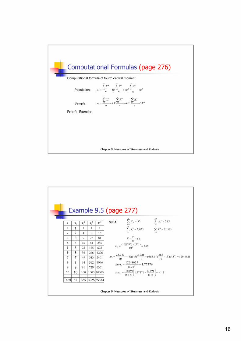
Computational Formulas (page 276)
Chapter 9. Measures of Skewness and Kurtosis
Computational formula of fourth central moment:
Population: 4 3 2
2 41 1 14 4 6 3
N N N
i i ii i i
X X X
N N N
Sample: 4 3 2
2 41 1 14 4 6 3
n n n
i i ii i iX X X
m X X Xn n n
Proof: Exercise
Example 9.5 (page 277)
i Xi Xi2 Xi
3 Xi4
1 1 1 1 1 2 2 4 8 16 3 3 9 27 81 4 4 16 64 256 5 5 25 125 625 6 6 36 216 1296 7 7 49 343 2401 8 8 64 512 4096 9 9 81 729 6561
10 10 100 1000 10000
Total 55 385 3025 25333
Chapter 9. Measures of Skewness and Kurtosis
Set A: 10
155i
iX
10
2
1
385iiX
10
3
13, 025i
iX
10
4
125, 333i
iX
55 5.510
X
2
2 2(10)(385) (55 ) 8.25
10m
2 4
425,333 3,025 385(4)(5.5) (6)(5.5 ) (3)(5.5 ) 120.8625
10 10 10m
1 2120.8625 1.77576
8.25kurt
2(11)(9) (3)(9)1.77576 1.2(8)(7) (11)
kurt

17
Chapter 9. Measures of Skewness and Kurtosis
AssignmentRefer to the data in Exercise for Section 9.4 in page 280. Compute the following summary measures for each section:
1. unbiased estimator of the coefficient of skewness based on the third moment
2. unbiased estimator of the excess of kurtosis based on the fourth moment
Note: Use the computational formula to compute for the third and fourth central moments. Show your solution.