3.1

Measures of Central Tendency

Ch. 3 Numerically Summarizing

Data • The arithmetic mean of a variable is

computed by determining the sum of all

the values of the variable in the data set

divided by the number of observations.

• The population arithmetic mean is

computed using all the individuals in a

population.

– The population mean is a parameter.

– The population arithmetic mean is denoted by

the symbol μ

Population Mean

• If x1, x2, …, xN are the N observations of a

variable from a population, then the population

mean, µ, is

1 2 Nx x x

N

Sample Mean

• The sample arithmetic mean is computed

using sample data.

• The sample mean is a statistic.

• The sample arithmetic mean is denoted by

x

Sample Mean

• If x1, x2, …, xN are the N observations of a

variable from a sample, then the sample mean

is

x

1 2 nx x xx

n

Sample Problem Computing a Population

Mean and a Sample Mean

• The following data represent the travel times

(in minutes) to work for all seven employees of

a start-up web development company.

23, 36, 23, 18, 5, 26, 43

a. Compute the population mean of this data.

b. Then take a simple random sample of n = 3

employees. Compute the sample mean.

Obtain a second simple random sample of n =

3 employees. Again compute the sample

mean.

EXAMPLE Computing a Population Mean and a Sample

Mean

(b) Obtain a simple random sample of size n = 3 from the

population of seven employees. Use this simple random sample

to determine a sample mean. Find a second simple random

sample and determine the sample mean.

1 2 3 4 5 6 7

23, 36, 23, 18, 5, 26, 43

3-7 © 2010 Pearson Prentice Hall. All rights reserved

Median

• The median of a variable is the value that

lies in the middle of the data when

arranged in ascending order. We use M to

represent the median.

3-9

EXAMPLE Computing a Median of a Data Set with an Odd

Number of Observations

The following data represent the travel times (in minutes)

to work for all seven employees of a start-up web

development company.

23, 36, 23, 18, 5, 26, 43

Determine the median of this data.

EXAMPLE Computing a Median of a Data Set with an

Even Number of Observations

Suppose the start-up company hires a new employee.

The travel time of the new employee is 70 minutes.

Determine the mean and median of the “new” data set.

23, 36, 23, 18, 5, 26, 43, 70

3-11

EXAMPLE Computing a Median of a Data Set with an

Even Number of Observations

The following data represent the travel times (in minutes) to

work for all seven employees of a start-up web development

company.

23, 36, 23, 18, 5, 26, 43

Suppose a new employee is hired who has a 130 minute

commute. How does this impact the value of the mean and

median?

3-12

EXAMPLE Computing a Median of a Data Set with an

Even Number of Observations

The following data represent the travel times (in minutes) to

work for all seven employees of a start-up web development

company.

23, 36, 23, 18, 5, 26, 43

Suppose a new employee is hired who has a 130 minute

commute. How does this impact the value of the mean and

median?

Mean before new hire: 24.9 minutes

Median before new hire: 23 minutes

Mean after new hire: 38 minutes

Median after new hire: 24.5 minutes 3-13

Resistance

• A numerical summary of data is said to be

resistant if extreme values (very large or

small) relative to the data do not affect its

value substantially.

3-15

EXAMPLE Describing the Shape of the Distribution

The following data represent the asking price of homes

for sale in Lincoln, NE.

Source: http://www.homeseekers.com

79,995 128,950 149,900 189,900

99,899 130,950 151,350 203,950

105,200 131,800 154,900 217,500

111,000 132,300 159,900 260,000

120,000 134,950 163,300 284,900

121,700 135,500 165,000 299,900

125,950 138,500 174,850 309,900

126,900 147,500 180,000 349,900

3-16

Sample Problem

• Find the mean and median. Use the mean

and median to identify the shape of the

distribution. Verify your result by drawing

a histogram of the data.

One-Variable Statistics Nspire

1. Create a list &

spreadsheets page

2. Title column

3. Enter data into

column

4. Create a calculator

page

5. Click Menu

6. 6:Statistics

– 1:Stat Calculations

– 1: One-Variable Stats

𝑥 = mean

Sx = sample S.D.

σx = population S.D.

Record min, Q1,

Median, Q3, Max

Find the mean and median. Use the mean

and median to identify the shape of the

distribution. Verify your result by drawing a

histogram of the data.

The mean asking price is $168,320 and the

median asking price is $148,700. Therefore, we

would conjecture that the distribution is skewed

right.

3-19

350000300000250000200000150000100000

12

10

8

6

4

2

0

Asking Price

Fre

qu

en

cy

Asking Price of Homes in Lincoln, NE

3-20

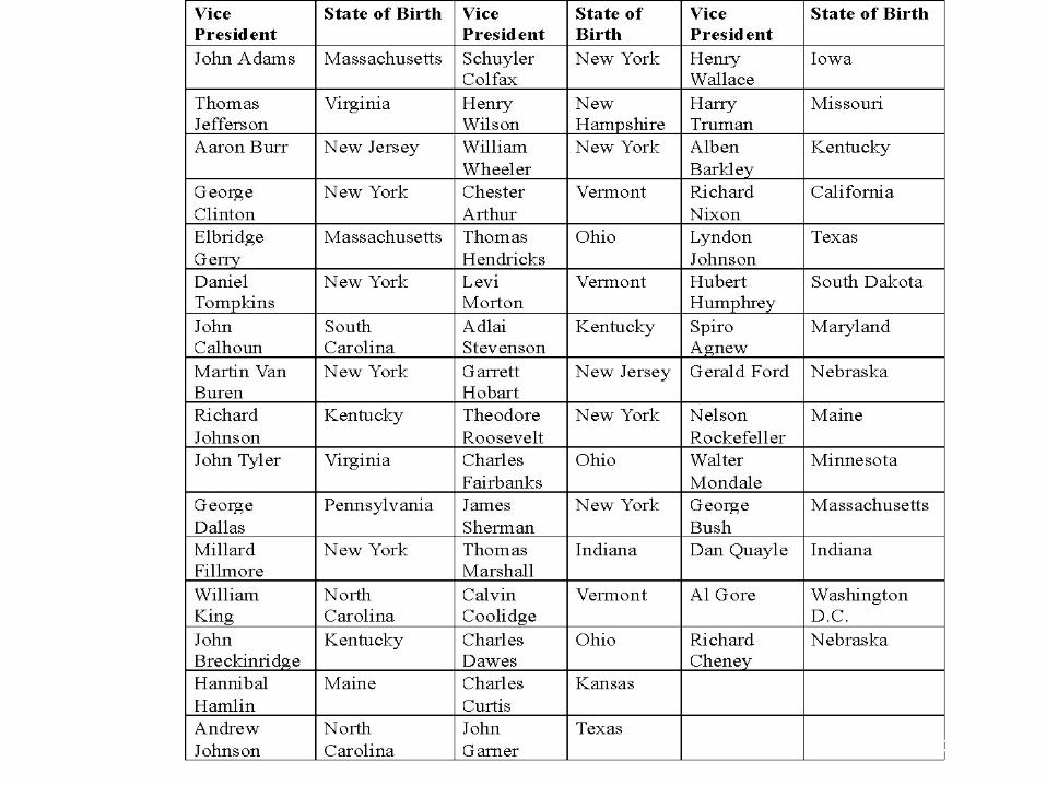
Mode

• The mode of a variable is the most

frequent observation of the variable that

occurs in the data set.

• If there is no observation that occurs with

the most frequency, we say the data has

no mode.

– The data on the next slide represent the Vice

Presidents of the United States and their state

of birth. Find the mode.

3-22

-23

Tally data to determine most

frequent observation

3-24

To order food at a McDonald’s Restaurant, one must

choose from multiple lines, while at Wendy’s

Restaurant, one enters a single line. The following

data represent the wait time (in minutes) in line for a

simple random sample of 30 customers at each

restaurant during the lunch hour. For each sample,

answer the following:

(a) What was the mean wait time?

(b) Draw a histogram of each restaurant’s wait time.

(c ) Which restaurant’s wait time appears more

dispersed? Which line would you prefer to wait in?

Why? 3-25

Sample Problem

1.50 0.79 1.01 1.66 0.94 0.67

2.53 1.20 1.46 0.89 0.95 0.90

1.88 2.94 1.40 1.33 1.20 0.84

3.99 1.90 1.00 1.54 0.99 0.35

0.90 1.23 0.92 1.09 1.72 2.00

3.50 0.00 0.38 0.43 1.82 3.04

0.00 0.26 0.14 0.60 2.33 2.54

1.97 0.71 2.22 4.54 0.80 0.50

0.00 0.28 0.44 1.38 0.92 1.17

3.08 2.75 0.36 3.10 2.19 0.23

Wait Time at Wendy’s

Wait Time at McDonald’s

3-

(b)

The mean wait time in

each line is 1.39

minutes.