Basic Definitions

• A distribution is a group of numbers that are being interpreted. o For example, the following is a distribution: [11, 13, 19, 23, 34, 47, 61] o Synonyms: Data, Data Set.

• A value is a specific number from our distribution o For example, 11 is a value from our distribution. o Synonyms: Score, Observation

• Data summary involves taking an entire distribution (for example, the GPAs of 200 randomly selected McGill students) and summarizing this distribution with just a few different values.

o The purpose of data summary is to describe the whole set of scores to someone with these few specific values, so that, without reading the entire data set, they can have a pretty good idea of what it looks like.

o The two main ways data are summarized are measures of central tendency and measures of variation.

Sample vs Population • Population refers to the entire group that we are interested in measuring with respect to the variable in

question. • Sample refers to a subset of this goup of interest. • For example, we may be interested in the IQ of current McGill undergrads.

o The population would be all McGill undergrad students. All 27,000 of them (according to Wikipedia).

o A sample would be, say, 100 randomly selected students from the entire undergrad student body. • The population mean is denoted as • The population standard deviation is denoted as • The sample mean is denoted as 𝑋 • The sample standard deviation is denoted as S.

o The population and sample mean are calculated the same way:

𝑋 =Σ𝑋𝑁

𝜇 =Σ𝑋𝑁

o There is a minor difference in how sample and population standard deviation are calculated:

𝑆 = √∑(𝑋 − 𝑋)2

𝑁 − 1 𝜎 = √∑(𝑋 − 𝜇)2

𝑁

You do not have to constantly worry about whether we are dealing with a sample or population in each example:

(1) Whether we are dealing with a sample or population, everything is calculated the same way, with the exception of standard deviation.

(2) In any given formula, you can replace 𝑋 and S with 𝜇 and 𝜎 or vice versa. This will always be fine. • For example, as we will soon see, the formula for calculating the Z-score of a specific value from

a distribution is as follows:

Population: Z(X) = X − μ

σ ⟷ Sample: Z(X) = X − X

S

• Therefore, even if you did not know whether you were dealing with a population or a sample, you would still get the exact same result when calculating the Z-score for a particular value of X.

(3) Unless explicitly stated that we are dealing with a population, you can safely assume we are dealing with a sample and calculate standard deviation accordingly.

Measures of Central Tendency

• Measures of central tendency let us know where most of our values are centered or clustered around. • The three most common ones are mean, median and mode. Mean • The Mean or Average is obtained by dividing the sum of all values in our distribution (Σ𝑋) by the number

of values in our distribution (𝑁).

Sample: X =ΣXN

Population: ∶ μ =ΣXN

Median The Median is the middle value in our distribution. The median is greater than half the values and less than half the values in our distribution.

o If we have an odd number of values (N = 5, for example), the median will be an actual value from our distribution (the 3rd value in this case).

o If we have an even number of values (N = 6, for example,), the median will be the average of the two middle values (the average of the 3rd and 4th values in this case).

• The median is also known as the 50th percentile. o A value’s percentile is the percentage of values which it is greater than the median is greater than

half, or 50% of the values in its distribution (and smaller than half of the values).

Example: Find the median in the following distribution: 29, 22, 23, 56, 37, 28, 33 ➢ First, arrange all values in ascending order:

[22, 23, 28, 29, 33, 37, 56] ➢ Next, calculate the sample size and find the rank of the median: Sample Size = N = 7

𝐌𝐞𝐝𝐢𝐚𝐧 𝐑𝐚𝐧𝐤 = 𝐊 = 𝐍 + 𝟏

𝟐 =7 + 1

2 = 4

➢ Finally, find the kth value in our distribution:

[22, 23, 28, 29, 33, 37, 56] The 4th value in our distribution, starting from the smallest, is 29.

Median = 29

• Suppose we had an odd number of values in our distribution. Let’s add 77 as the final value:

[22, 23, 28, 29, 33, 37, 56, 77]

Sample Size = N = 8

Median Rank = K = N + 1

2 =8 + 1

2 = 4.5

• In this case, K = 4.5 tells us that to find the median we must take the average of the 4th and 5th values: 29

and 33.

𝐌𝐞𝐝𝐢𝐚𝐧 = 𝟐𝟗 + 𝟑𝟑

𝟐= 𝟑𝟏

• That’s it! Mean vs Median • When there are extreme outliers (values that are significantly less than or greater than most other values),

the median is often preferred as a measure of central tendency. • This is because the mean is affected by outliers but the median is not. • For example, suppose we were interested in the salaries of students their first year our of McGill. • We randomly sample 10 such students, and their salaries (in thousands) are as follows:

[32, 36, 38, 44, 47, 48, 55, 65, 77, 675]

o Median Salary in this group = 47.5; Mean Salary = 111.7 o 9 of 10 students have salaries between $32,000 and $77, 000 o The Median ($47,500) in this case is therefore a pretty accurate measure of central tendency.

o The Mean ($111,700) in this case is a very misleading measure of central tendency. o The extreme outlier of $675,000 (a student who got rich starting her own business) has “pulled the

mean upwards”. The mean is sensitive to outliers; the median is unaffected by outliers. • If we were to replace the student whose salary was $675,000 with one whose salary was $90,000: [32, 36, 38, 44, 47, 48, 55, 65, 77, 90]

o The Median would still = 47.5 o The Mean would now = 52.2 o The Median has stayed the same at $47,500, while the Mean has fallen from $111,700 to $52,200!

Mode • The Mode is the most common value in our distribution. • For example, consider the following data set: [14, 16, 23, 27, 27, 32, 35, 35, 35, 43, 68]

o The most common value in this distribution is 35, which occurs three times. o Therefore, Mode = 35.

Measures of Variation

• Measures of variation let us known the general spread within our distribution. • In other words, they indicate how far apart values tend to be from one another: whether they are relatively

close together (17, 17, 18, 19, 21) or far apart (98, 225, 436, 879, 7473) Standard Deviation & Variance • The standard deviation tells us the average distance of each value from the mean. • The variance is equal to the standard deviation squared.

Sample Standard Deviation = S = √∑(X − X)2

N − 1 = √∑ X2 − (∑ X)2

nN − 1

Population Standard Deviation = σ = √∑(X − μ)2

N = √∑ X2 − (∑ X)2

nN

Sample Variance = S2 =∑(X − X)

2

N − 1 =∑ X2 − (∑ X)2

nN − 1

Population Variance = σ2 =∑(X − μ)2

N =∑ X2 − (∑ X)2

nN

Example: Calculate the mean and standard deviation for the following data set: [22, 25, 27, 28, 40] *Always assume we are dealing with a sample unless explicitly stated otherwise. ΣX = 22 + 25 + 27 + 28 + 43 = 145 ΣX2 = 222 + 252 + 272 + 282 + 432 = 4471

𝐗 =𝚺𝐗𝐍

= 𝟐𝟗

S2 =∑ X2 − (∑ X)2

nN − 1 =

4471 − (145)2

54 = 66.5

𝐒 = √𝐒𝟐 = √𝟔𝟔. 𝟓 = 𝟖. 𝟏𝟓𝟓 Range

• The Range is another measure of variation. • The range tells us the difference between the largest and smallest values: • Obviously, the greater the range, the greater the level of variation.

Range = MAX – MIN Example: Calculate the range in the following data set: [22, 23, 28, 29, 33, 37, 56, 77] Range = MAX – MIN = 77 -22 = 55

Percentiles • A score’s percentile score or ranking is the proportion of values that it is greater than in a distribution. • If you were to write the LSAT and score in the 85th percentile, this would mean that you did better than 85%

and worse than 15% of people who wrote that particular version of the LSAT. • In any data set:

QL = Lower Quartile = 25th percentile M = Middle Quartile = Median = 50th percentile QU = Upper Quartile = 75th percentile

Z-Scores • In any data set, the Z-Score of a particular value tells us the distance of that value from the mean. • This distance is expressed in units of standard deviations. • The sign (positive or negative) tells us whether this value is greater or less than the mean • The absolute value tells us how many standard deviations above or below the mean.

INTRO TO PROBABILITY Some Notation to Start A Æ event A happens

P(A) Æ probability that event A happens

AC Æ event A does not happen

P(AC) Æ probability that event A does not happen The probability of something happening means the “chances” or “likelihood” of it happening The probability of something happening is always somewhere between 0 and 1 0 Æ 0% Æ Impossible. It will never, ever happen. 1 Æ 100% Æ Guaranteed. It will happen every single time. “Percentage/Proportion of” and “Probability” mean the same thing 60% of McGill students are female Æ Probability a randomly selected McGill student is female is 60% Æ P(Female) = 0.6 The probability of some event happening + the probability of that event NOT happening = 1 • In other words, P(A) + P(AC) = 1 • By re-arranging the terms, we also get:

P(A) = 1 – P(AC) Æ the probability of something happening = 1 – the probability of it not happening P(AC) = 1 – P(A) Æ the probability of something not happening = 1 – the probability of it happening

P(Rain Tomorrow) + P(No Rain Tomorrow) = 1 P(Ben Affleck had eggs for breakfast today) + P(Ben Affleck didn’t have eggs for breakfast today) = 1

• We do not need to know either probability in order to know that their sum is equal to 1. • This is because… The sum of the probabilities of all possible outcomes in a scenario always equals 1. • When we roll a die, for example, there are six possible outcomes: it lands on 1, 2, 3, 4, 5 or 6. • The probability it lands on each number = 1

6

• Therefore: P(1) + P(2) + P(3) + P(4) + P(5) + P(6) = 16

• 6 = 1

• Example: 53% of McGill students are from Montreal, 12% are from Toronto, and 10% are from elsewhere in Canada. What % of McGill students are from outside of Canada?

P(MTL) + P(TO) + P(Elsewhere) + P(Outside) = 1 P(Outside) = 1 – P(MTL) – P(TO) – P(Elsewhere) = 1 – 0.53 -0.12 – 0.1 = 0.25 25% of McGill students come from outside of Canada.

HERE IS THE MOST IMPORTANT/BASIC DEFINITION OF PROBABILITY:

𝐏𝐑𝐎𝐁𝐀𝐁𝐈𝐋𝐈𝐓𝐘 𝐎𝐅 𝐄𝐕𝐄𝐍𝐓 "𝐀" 𝐇𝐀𝐏𝐏𝐄𝐍𝐈𝐍𝐆 =# 𝐎𝐟 𝐖𝐚𝐲𝐬 "𝐀" 𝐂𝐚𝐧 𝐇𝐚𝐩𝐩𝐞𝐧

𝐓𝐨𝐭𝐚𝐥 # 𝐎𝐟 𝐏𝐨𝐬𝐬𝐢𝐛𝐥𝐞 𝐎𝐮𝐭𝐜𝐨𝐦𝐞𝐬 • Example: A jar with 4 red and 6 black marbles. A marble is chosen at random. What is the probability of it

being red?

4 red marbles Æ 4 ways of choosing a red marble Æ # ways A can happen = 4 4 red + 6 black marbles Æ 10 total marbles to choose from Æ total # of possible outcomes = 10 P(Red) = 4/10

P(B|A) = probability that B happens/is true, given (taking into account) that A happened/is true • For example, let’s say that 70% of all McGill students like lollipops but only 40% of ECON students like

lollipops. • Let A = McGill student likes lollipops & let B = Student is in ECON

P(A) = 0.7 Æ The probability that a randomly selected McGill student likes lollipops is 0.7 P(A|B) = 0.4 Æ The probability that a randomly selected McGill student likes lollipops, taking into account that he/she is in ECON, is 0.4

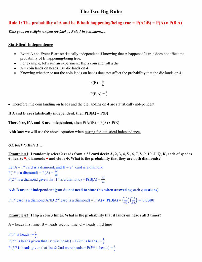
The Two Big Rules Rule 1: The probability of A and be B both happening/being true = P(A∩B) = P(A) • P(B|A) Time go to on a slight tangent (be back to Rule 1 in a moment….) Statistical Independence

• Event A and Event B are statistically independent if knowing that A happened/is true does not affect the probability of B happening/being true.

• For example, let’s run an experiment: flip a coin and roll a die • A = coin lands on heads, B= die lands on 4 • Knowing whether or not the coin lands on heads does not affect the probability that the die lands on 4:

P(B) = 1

6

P(B|A) = 1

6

• Therefore, the coin landing on heads and the die landing on 4 are statistically independent. If A and B are statistically independent, then P(B|A) = P(B) Therefore, if A and B are independent, then P(A∩B) = P(A) • P(B) A bit later we will use the above equation when testing for statistical independence. OK back to Rule 1… Example #1: I randomly select 2 cards from a 52 card deck: A, 2, 3, 4, 5 , 6, 7, 8, 9, 10, J, Q, K, each of spades ♠, hearts ♥, diamonds ♦ and clubs ♣. What is the probability that they are both diamonds? Let A = 1st card is a diamond, and B = 2nd card is a diamond P(1st is a diamond) = P(A) = 13

52

P(2nd is a diamond given that 1st is a diamond) = P(B|A) = 1251

A & B are not independent (you do not need to state this when answering such questions) P(1st card is a diamond AND 2nd card is a diamond) = P(A) • P(B|A) = (13

52) (12

51) = 0.0588

Example #2: I flip a coin 3 times. What is the probability that it lands on heads all 3 times? A = heads first time, B = heads second time, C = heads third time P(1st is heads) = 1

2

P(2nd is heads given that 1st was heads) = P(2nd is heads) = 12

P (3rd is heads given that 1st & 2nd were heads = P(3rd is heads) = 12

CONDITIONAL PROBABILITY

• We are dealing with a conditional probability question when a population is being described along 2 different dimensions/variables.

o In other words, there are two things we want to know about each member of the population. o For example, imagine the population of interest is McGill students. For each student, I may want to

know (1) Nationality and (2) Level of Religiosity o As you will see later, this is in contrast to the Binomial, Hypergeometric, Poisson/Exponential, and

Normal Distributions, in which each population member is only being described along one dimension. • Furthermore, in such a question both variables are categorical.

o In other words, there are only a few different possible “values” or “groups” into which each member of the population can fall.

o In the above example, I may choose to categorize each student’s nationality as either (a) Canadian, (b) American, or (c) International, and each student’s level of religiosity as either (a) Religious, (b) Agnostic, or (c) Atheist.

Note: In MATH 203, most problems will consist of just two categories for each variable.

o For example, in a particular population we may want to know whether each person is (a) religious (religious vs not religious) and (b) a Trump supporter (supporter vs nonsupporter).

o Aside from the first example in this course pack, all others will involve just having two categories per variable to as to simulate your exam questions.

Steps to solving conditional probability questions:

(1) Determine the population being described, the two variables of interest, and the categories for each variable.

(2) Draw a Joint Probability Table (JPT), arbitrarily placing one of the variables along the horizontal dimension and the other along the vertical dimension.

(3) Fill in all the cells we can based on the information provided in the question (usually we can fill in the

entire table).

(4) Solve each question using the data we have in our Joint Probability Table.

The dean of McGill has reported the following data regarding student demographics: 70% of McGill students are Canadian, 10% are American, and 20% are International. Furthermore, 20% of McGill students are religious, while 30% are agnostic and 50% atheist. Among Canadian students, 15% are religious and 25% are agnostic. Among International students 42.5% are religious and 47.5% are agnostic.

Step 1 Population: McGill Students Variables: Nationality (Canadian, American, Other) & Religiosity (Religious, Agnostic, Atheist) Step 2 Canadian American International Total Religious Agnostic Atheist Total 1

How to read & use this table: • Each cell contains a probability that is in reference to the entire population.

o For example, the cell where Religious & Canadian intersect tells us the percentage of all McGill students who are both religious and Canadian (the probability that a randomly selected McGill student is a religious Canadian).

o In other words, this cell tells us P(Religious ∩ Canadian). o This cell does not tell us the percentage of Canadian students who are religious, nor does it tell us the

percentage of religious students who are Canadian. o Once the table is filled, these is a way to determine the above probabilities, but the answer won’t be

directly in the table. o This is because % of Canadian students who are religious and % of religious students who are

Canadian are statements about a subset of the population, not the entire population. • It is essential to add in the Total column & row for the two variables in question. Sometimes the JPT

will already be provided in the question, but without the totals. Add these in; the table is useless without them. o The % of all McGill students who are Canadian for example, denoted as P(Canadian), falls into the cell

that intersects Canadian and Total.

Canadian American International Total Religious Agnostic Atheist Total

Binomial Probability Distribution We are dealing with a binomial distribution when the following four conditions are met:

(1) A specific number of trials (n) are being conducted as part of an experiment o Experiment: Flip a coin 7 times & observe # of heads o Trial: Flip a coin and observe whether it lands on heads or trails o Number of trials in our experiment: 7

(2) There are two possible outcomes in each trial (we arbitrarily label one success and the other failure)

o Flip a coin Æ heads or tails o Look out the window to check for rain Æ raining or not raining o Roll a die to see if it lands on 4 Æ lands on 4, or lands on any other number (1, 2, 3, 5, or 6)

(3) Independence: The probability of success in a given trial is not affected by the outcome in a previous

trial o P(Heads on 2nd trial) = 0.5 regardless of whether we got Heads or Tails in the 1st trial

(4) The probability of success (p) and therefore of failure (q, which equals 1-p) are known

o Let Heads = Success and Tails = Failure Æ p = P(Heads), q = P(Tails) o P(H) = 0.5, P(T) = 1 – 0.5 = 0.5 o Therefore, p = 0.5, q = 0.5 o Note that p + q must always = 1 since they cover all possible outcomes

• In a binomial probability distribution question, we are asked to calculate the probability of a specific

number of successes (x) occurring out of a certain (greater or equal) number of trials (n), using the follow equation:

P(x) = Cxnpxqn−x

o The purpose of using the binomial equation is when we need to calculate the probability of x successes out of n trials, without knowing which trials contain the successes.

o For example, if we are asked to calculate the probability of a die landing on “3” exactly twice when rolling the die 12 times, it is not specified (nor do we care) where the two 3s will occur amongst the 12 trials.

o The two “3”s could occur on the 1st & 2nd trial, or they could occur on the 5th & 11th trials. It’s the same to us.

o In cases like this, the binomial equation is necessary, since there are many possible ways to achieve two successes in the twelve trials.

• If x = n (all trials are successes) or x = 0 (all trials are failures), then we know the outcome of each trial in the experiment. o In the above two cases, we can use the binomial equation if we wish, but it is not necessary. o Example: If we flip a coin 5 times, find the probability of it landing on heads all 5 times, and find the

probability of it not landing on heads at all.

P(H all 5 times) = P(H 1st time) • P(H 2nd time) • P(H 3rd time) • P(H 4th time) • P(H 5th time) =(12)

5

P (No heads) = P(All Tails) = P(Tails all 5 times) = (12)

5

HOW TO SOLVE ALL THE BINOMIAL QUESTIONS On each day in June there is a 20% chance of rain, regardless of what the weather has been on previous days. (A) What is the probability that, between June 1st and June 10th, it rains exactly 3 times?

o We know this is a binomial distribution question because the four conditions are met: Experiment: Check the weather each day for 10 days and count the # of rainy days There are 10 trials (n = 10), each with 2 possible outcomes: Rain (success) or No Rain (failure) Trials are independent: If it rains on June 1st, P(Rain June 2nd) = 0.2. If it does not rain on June 1st,

P(Rain June 2nd) =0.8 Probability of success is known: P(Rain) = 0.2, P(No Rain) = 1 - 0.8 = 0.2

Recall that 𝐏(𝐱) = 𝐂𝐱

𝐧𝐩𝐱𝐪𝐧−𝐱 P(3 rainy days out of 10) = P(3 successes in 10 trials) = C3

100.230.87 = 0.2013 (B) What is the probability that, over the first 5 days of the month, it rains at least 3 times?

P(at least 3 rainy days) = P(3 or 4 or 5 rainy days) = P(3 rainy days) + P(4 rainy days) + P(5 rainy days) = P(3) + P(4) + P(5) P(3) = C3

50.230.82 = 0.0512 P(4) = C4

50.240.81 = 0.0064 P(5) = C5

50.250.80 = 0.00032

𝐏(𝟑) + 𝐏(𝟒) + 𝐏(𝟓) = 𝟎. 𝟎𝟓𝟏𝟐 + 𝟎. 𝟎𝟎𝟔𝟒 + 𝟎. 𝟎𝟎𝟎𝟑𝟐 = 𝟎. 𝟎𝟓𝟕𝟗𝟐

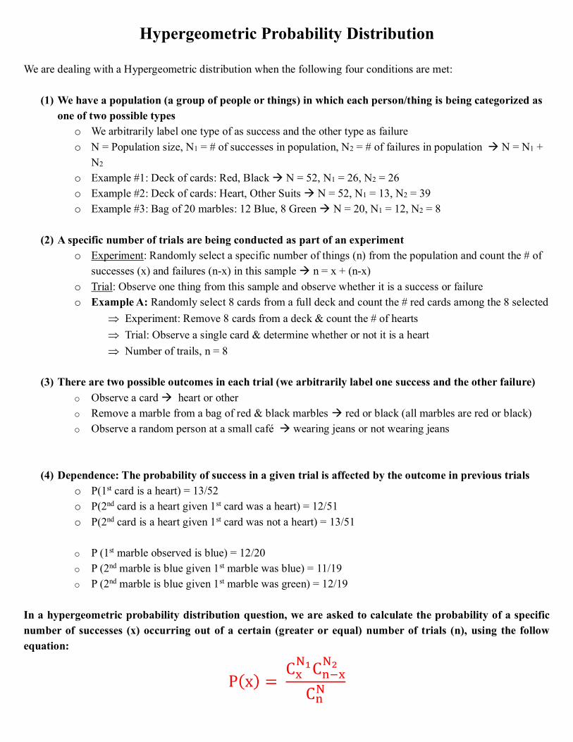
Hypergeometric Probability Distribution We are dealing with a Hypergeometric distribution when the following four conditions are met:

(1) We have a population (a group of people or things) in which each person/thing is being categorized as one of two possible types

o We arbitrarily label one type of as success and the other type as failure o N = Population size, N1 = # of successes in population, N2 = # of failures in population Æ N = N1 +

N2 o Example #1: Deck of cards: Red, Black Æ N = 52, N1 = 26, N2 = 26 o Example #2: Deck of cards: Heart, Other Suits Æ N = 52, N1 = 13, N2 = 39 o Example #3: Bag of 20 marbles: 12 Blue, 8 Green Æ N = 20, N1 = 12, N2 = 8

(2) A specific number of trials are being conducted as part of an experiment

o Experiment: Randomly select a specific number of things (n) from the population and count the # of successes (x) and failures (n-x) in this sample Æ n = x + (n-x)

o Trial: Observe one thing from this sample and observe whether it is a success or failure o Example A: Randomly select 8 cards from a full deck and count the # red cards among the 8 selected

Experiment: Remove 8 cards from a deck & count the # of hearts Trial: Observe a single card & determine whether or not it is a heart Number of trails, n = 8

(3) There are two possible outcomes in each trial (we arbitrarily label one success and the other failure)

o Observe a card Æ heart or other o Remove a marble from a bag of red & black marbles Æ red or black (all marbles are red or black) o Observe a random person at a small café Æ wearing jeans or not wearing jeans

(4) Dependence: The probability of success in a given trial is affected by the outcome in previous trials o P(1st card is a heart) = 13/52 o P(2nd card is a heart given 1st card was a heart) = 12/51 o P(2nd card is a heart given 1st card was not a heart) = 13/51

o P (1st marble observed is blue) = 12/20 o P (2nd marble is blue given 1st marble was blue) = 11/19 o P (2nd marble is blue given 1st marble was green) = 12/19

In a hypergeometric probability distribution question, we are asked to calculate the probability of a specific number of successes (x) occurring out of a certain (greater or equal) number of trials (n), using the follow equation:

P(x) = Cx

N1Cn−xN2

CnN

PRACTICE QUESTIONS BECAUSE PRACTICE MAKES PERFECT 1. I have produced the following joint probability table in order to describe the demographics of my crash

course clients:

Born in

Montreal Born

Elsewhere Male 0.15 0.2

Female 0.25 0.4 (A) What is the median number of females in a random sample size of 8?

(B) How large a class would we need to be 99% confident of there being at least 1 male? (C) I select a random sample of Montreal-born students and begin interviewing them, one by one. What is the

probability that the 4th student I interview is the second one who female? (D) What is the probability that the first 3 males I interview from the above sample are all non-Montrealers? 2. There are 40 cars parked on my block. 10 are black. 15 are SUVs. None of the SUVs are black. (A) What is the probability that there will be exactly 2 SUVs among the first 6 cars I observe? (B) I randomly select 10 cars. What is the probability that at least 3 are black? (C) I start walking down the block. What is the probability that the 6th car I pass is the 2nd black one observed? (D) I’ve walked by 5 cars on the block and still haven’t seen a black one or an SUV. What is the probability that, of

the next two cars I see, one will be an SUV and one will be black.

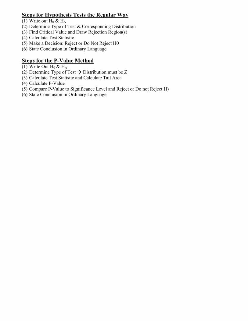
Steps for Hypothesis Tests the Regular Way (1) Write out H0 & HA (2) Determine Type of Test & Corresponding Distribution (3) Find Critical Value and Draw Rejection Region(s) (4) Calculate Test Statistic (5) Make a Decision: Reject or Do Not Reject H0 (6) State Conclusion in Ordinary Language Steps for the P-Value Method (1) Write Out H0 & HA (2) Determine Type of Test à Distribution must be Z (3) Calculate Test Statistic and Calculate Tail Area (4) Calculate P-Value (5) Compare P-Value to Significance Level and Reject or Do not Reject H) (6) State Conclusion in Ordinary Language

Confidence Intervals & Standard Errors For each of the 4 tests above, we may be asked to calculate a confidence interval or standard error. The formulas for each of these are below: Single Sample Mean

Confidence Interval: X ± (Z or t) SN

!

"#

$

%&

Standard Error: S

N Single Sample Proportion

Confidence Interval: P ± (Z ) P(1−P)N

"

#$$

%

&''

Standard Error: P(1−P)N

Difference Between 2 Means

Confidence Interval: X1 − X 2 ± t( ) s12

n1+s22

n2

Standard Error: s12

n1+s22

n2

Difference Between 2 Proportions

Confidence Interval: P1 −P2 ± Z( ) P1(1−P1)N1

+P2 (1−P2 )

N2

Standard Error: P1(1−P1)

N1+P2 (1−P2 )

N2

Intro to Hypothesis Testing The first 4 hypothesis tests you are taught are: Single Sample Mean, Single Sample Proportion, Independent Sample Means, & Independent Sample Proportions. Single Sample Mean

• In this test, we are interested in the mean of a certain variable, in one specific population. • Since we are interested in the mean of the variable, this must be a quantitative variable.

The dean of McGill would like to know if the mean IQ of McGill undergrad students is significantly greater than the population average of 100. She decides to take a sample of 75 students, and finds that the mean IQ in this sample is 107.83, with a standard deviation of 12.44. Is the mean IQ among McGill undergrads significantly greater than 100? Test at the 5% level. Step 1: Write out Hypotheses

• The first step to determining our hypotheses is to just identify the question being asked and then answer is in the only two possible ways: Yes and No.

Yes à The Mean IQ at McGill is greater than 100 NO à The Mean IQ at McGill is not greater than 100

• The next step is to convert these statements into mathematical Expressions:

Yes à! > 100 No à ! ≤ 100

• The last step is to identify which of these is H0 and which is HA. This is easy: the hypothesis that contains

an equality (= or ≤ or ≥ ) is H0, and the other one, by default is HA:

H0: ! ≤ 100 HA:! > 100

Step 2: Determine Type of Test and Corresponding Distribution

• We know this is a single sample mean test because we are interested in the mean of one variable (IQ) in one specific population (McGill undergrads). Furthermore, IQ is a quantitative variable.

• For single sample mean tests, the distribution we use is either t or Z. o If the sample size (n) is less than 30, we must use t. o If the n is 30 or greater, we have the option of using Z or t. o Easier to just use t no matter what, right? o Therefore, for the problem in question, t will be the distribution we use.

Step 3: Find Critical Value(s) and Draw Rejection Regions(s • The first thing to do is to draw the curve corresponding to the distribution we are using.

o Z and t distributions both have the same shape: that of the normal distribution. o Since we are using t for this problem, we draw the following curve:

wwwd

• Next, we determine if our test if 1 or 2 tailed.

o Our test is 1 tailed if HA has a “greater than” or “less than” sign (> or <) o Our test is 2 tailed if HA has an “unequal” sign (≠ )

• If our test is 2 tailed, we have 2 rejection regions: one on the far right side (the right tail) and one on the

far left side (the left tail). • If the test is 1 tailed, we must determine if it is right tailed or left tailed. • To do this, we look at HA • If the hypothesis has the parameter in question (µ or P) being greater than the value to which it is being

compared, we have a right tailed test (for example, µ > 20). • In this case, we only have 1 rejection region: on the far right side (the right tail) • If the hypothesis has the parameter being less than the value to which it is being compared (for example, µ<20), we have a left tailed test.

• In this case, we also only have 1 rejection region: on the far left side (the left tail)

In the test we are currently conducting, we have HA: ( > )** • This is therefore a 1 tailed test, to the right. • Here is our curve, with our rejection region shaded in:

• Now it is time to find the critical value. • We have one critical value associated with each rejection region.

o In this test, since we have only one rejection region, we have one critical value.

• For the t-distribution, to find the critical value, we need 2 pieces of information: the degrees of freedom and the area of the rejection region(s).

o The way we calculate degrees of freedom depends on the type of test. o For single sample mean, +, = . − ) o For this test, DF = 75 -1 = 74

• The area of the rejection region is then determined by the level of significance of the test (α ).

o If we have only 1 rejection region (1-tailed test), then the area of the rejection region=α . o If we have 2 rejection regions, then the area of each is equal to α /2. o For this test, the level of significance is 0.05 (we were told to test at the 5% level) and we

only have one rejection region, which therefore has an area = α = 0.05

• Finally, we look up DF=74, and tail area = 0.05 on our t-table, and we find our critical value: o For this test, critical t = 1.666

• Theoretically, whenever we are using the t-distribution, we are making 2 assumptions:

(1) The sample(s) were independently and randomly selected (2) The populations are normally distribued

Step 4: Calculate Test Statistic • For each type of test, these is a specific formula for calculating the test statistic. • For the single sample mean test, the formula for the test statistic is:

0 =1 − (2.

( is the mean meantioned in our hypotheses (100) 1is the mean of our sample s is the standard deviation of our sample

3 − !45

=107.83 − 100

12.4475

= 5.45

Step 5: Make a Decision: Reject or do not Reject H0

• If our test statistic falls into a rejection region, we reject H0 • If our test statistic does not fall into a rejection region, we do not reject H0.

o In this particular test, our test statistic falls into the rejection region, since 5.45>1.666. o Therefore, we reject H0.

Step 6: State Our Conclusion in Ordinary Language We conclude that the mean IQ at McGill is significantly greater than 100.

Chi Square • Chi- Square tests deal with frequencies. In other words, we are always dealing with categorical variables, not

quantitative variables. • There are two types of Chi-Square tests you need to know how to conduct: Chi-Square Goodness of Fit Test, and

Chi-Square Test of Independence

Goodness of Fit • In the Chi-Square Goodness of Fit test, we are interested in how a specific population is distributed with

regard to a certain categorical variable. • How does this differ from single sample proportion or difference between proportions? • In single sample proportion or difference between proportion tests, we are distributing the population(s) into

only two categories. • In a goodness of fit test, we are ditributing the population into 3 or more categories. • For example, we may be interested in what % of McGill students are from Montreal vs Toronto vs. Elsewhere

in Canada vs. USA vs. International. • Or we may be interested in what % of Montreal residents like the habs vs dislike the habs vs. are indifferent to the

habs. Example #1 300 McGill students took a survey, in which they were asked to choose their preferred alcoholic beverage between beer, wine, and liquor. 125 chose beer, 110 chose wine, and 65 chose liquor. Are beer, liquor and wineequally preferred among McGill students? Step 1 Yes, the 3 beverages are equally preferred à PB = PW = PL = 1/3à H0 No, the 3 beverages are not equally preferred à At least one proportion is different from 1/3 àHA

In a Goodness of Fit test, H0 will always have specific predictions regarding each of the proportions, whereas HA will simply state that H0 is not correct. Step 2 We know this is a Goodness of Fit test because we are interested in how a specific population (McGill students) is distributed with regard to a categorical variable (preferred alcoholic beverage) which has at least 3 categories (beer vs. liquor vs. wine). In a Goodness of Fit test, we use the Chi-Square Distribution

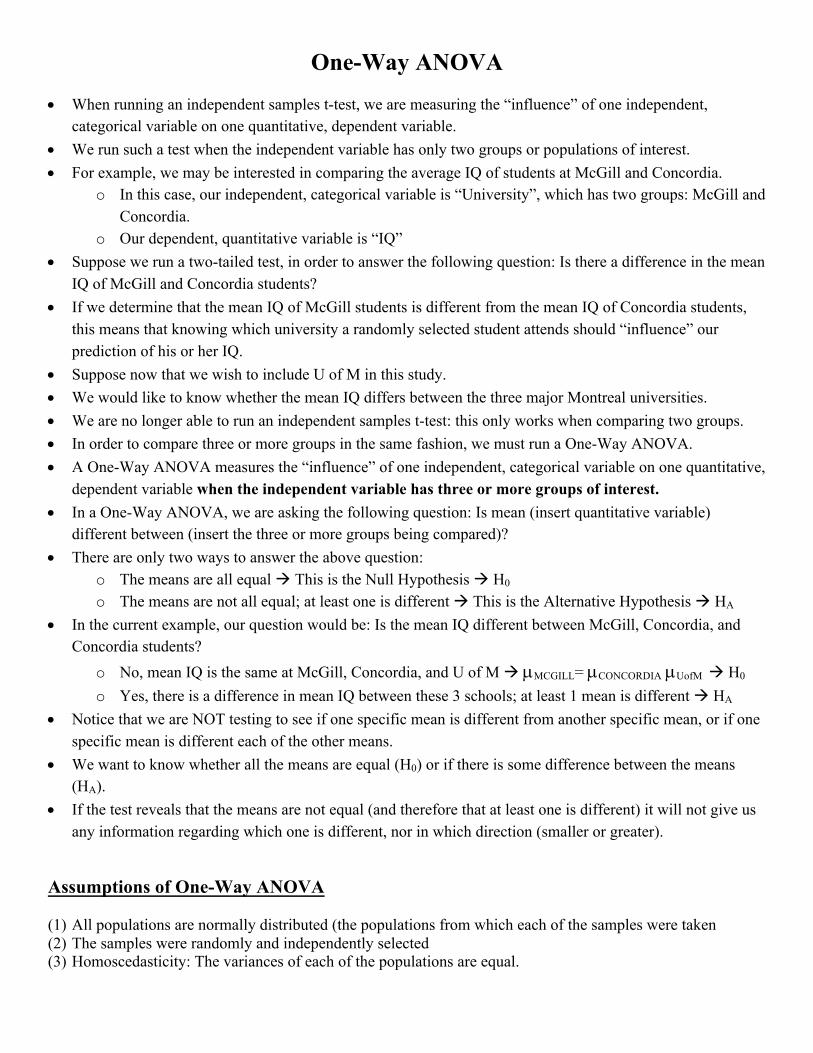
One-Way ANOVA • When running an independent samples t-test, we are measuring the “influence” of one independent,

categorical variable on one quantitative, dependent variable. • We run such a test when the independent variable has only two groups or populations of interest. • For example, we may be interested in comparing the average IQ of students at McGill and Concordia.

o In this case, our independent, categorical variable is “University”, which has two groups: McGill and Concordia.

o Our dependent, quantitative variable is “IQ” • Suppose we run a two-tailed test, in order to answer the following question: Is there a difference in the mean

IQ of McGill and Concordia students? • If we determine that the mean IQ of McGill students is different from the mean IQ of Concordia students,

this means that knowing which university a randomly selected student attends should “influence” our prediction of his or her IQ.

• Suppose now that we wish to include U of M in this study. • We would like to know whether the mean IQ differs between the three major Montreal universities. • We are no longer able to run an independent samples t-test: this only works when comparing two groups. • In order to compare three or more groups in the same fashion, we must run a One-Way ANOVA. • A One-Way ANOVA measures the “influence” of one independent, categorical variable on one quantitative,

dependent variable when the independent variable has three or more groups of interest. • In a One-Way ANOVA, we are asking the following question: Is mean (insert quantitative variable)

different between (insert the three or more groups being compared)? • There are only two ways to answer the above question:

o The means are all equal à This is the Null Hypothesis à H0 o The means are not all equal; at least one is different à This is the Alternative Hypothesis à HA

• In the current example, our question would be: Is the mean IQ different between McGill, Concordia, and Concordia students?

o No, mean IQ is the same at McGill, Concordia, and U of M à µMCGILL= µCONCORDIA µUofM à H0 o Yes, there is a difference in mean IQ between these 3 schools; at least 1 mean is different à HA

• Notice that we are NOT testing to see if one specific mean is different from another specific mean, or if one specific mean is different each of the other means.

• We want to know whether all the means are equal (H0) or if there is some difference between the means (HA).

• If the test reveals that the means are not equal (and therefore that at least one is different) it will not give us any information regarding which one is different, nor in which direction (smaller or greater).

Assumptions of One-Way ANOVA (1) All populations are normally distributed (the populations from which each of the samples were taken (2) The samples were randomly and independently selected (3) Homoscedasticity: The variances of each of the populations are equal.

The daily high temperature (Celsius) was recorded in the cities of New York, Miami, and Los Angeles, on random days last summer. The following data was produced:

Montreal Miami L.A. 21 25 27 33 19

24 27 31 40 22 18

25 28 35

Were the mean daily high temperatures in Montreal, Miami, and L.A. significantly different from each other last summer? Step 1 Yes à There was a significant difference in mean temperature between these three cities à HA

No à The mean temperature in all three cities were equal à à H0 • In a One-Way ANOVA, H0 always states that all means being compared are equal (that all populations

being compared have the same mean for the variable in question), whereas HA states that at least one mean is different.

Step 2 We know this is a One-Way ANOVA because we are being asked to compare the mean of a certain variable (daily temperature last summer, in Celsius) between more than 2 different populations (Montreal, Miami, and LA). • For the One Way ANOVA - for any sort of ANOVA, actually - we use the F-distribution.

Step 3 • The F-Distribution looks like this:

• The One way ANOVA is always a right-tailed test • Therefore, the rejection region is in the right tail, with the area equal to the significance level of the test (α ).

µMontreal

= µMiami

= µL.A.

Review Questions 1. A large group of McGill students have been polled and asked to indicate their favorite season. Here are the

results of the poll:

Fall Winter Spring Summer 245 175 215 265

(a) Test whether there is a significant difference in seasonal preference amongst McGill students.

(b) Another hypothesis test is performed on the data. Let P stand for the proportion of McGill students

whose favorite season is summer. The alternative hypothesis for this test is HA: P z 14. What is the P-

Value for this test?

(c) I have a textbook in which the value listed in the t-tables for 180 degrees of freedom in the column headed 0.025 is 1.972. If I look in the tables of the F-distribution with numerator DF equal to 1 and denominator DF equal to 180, what number should appear on the 0.05 page?

2. Yaholu Masokenchi has collected data on yearly income of families in three different affluent Montreal

neighborhoods: Westmount, Outremont, and TMR. The data thus far collected appears below. Incomes are listed in thousands of dollars.

Westmount Outremont T.M.R.

373 475 172 242 127 345 1242 224 468 565 96 112 186 222

(a) Test at the 5% level whether there is a significant difference in mean yearly income between families in

these three neighborhoods.

(b) What are the theoretical requirements for the test you used in part (a)?

(c) Form a 99% confidence interval for mean yearly income of Westmount families.

(d) Form a 90% confidence interval for the difference between mean yearly income in Westmount and Outremont families.

(e) Estimate the standard error of mean family income in TMR in samples of size 35.

(f) Estimate the standard error of the difference between mean family income in Westmount and TMR

based on the above data.