Measurement/Sampling - University of Arizona
115
Transcript of Measurement/Sampling - University of Arizona

Measurement/Sampling
315 Quantifying spatial heterogeneity in herbage mass and consumption in pasturesby Masahiko Hirata
Plant Animal322 Herbivore dunging and endozoochorous seed deposition in a Mediterranean
dehesa by J.E. Malo, B. Jiménez, and F. Suarez
329 Late season toxic alkaloid concentrations in tall larkspur (Delphinium spp.) byDale R. Gardner and James A. Pfister
Plant Ecology335 Western ragweed effects on herbaceous standing crop in Great Plains grass-
lands by Lance T. Vermeire and Robert L. Gillen
342 Age-stem diameter relationships of big sagebrush and theirmanagement impli-cations by Barry L. Perryman and Richard A. Olson
Reclamation
347 Characterization of Siberian wheatgrass germplasm from Kazakhstan(Poaceae: Triticeae) by Kevin B. Jensen, Kay H. Asay, Douglas A. Johnson, andBao Jun Li
Soils353 Soil properties and species diversity of grazed crested wheatgrass and native
rangelands by Maja Krzic, Klaas Broersma, Don J. Thompson, and Arthur A.Bomke
Book Review359 Shinners and Mahler’s Flora of North Central Texas by George M. Diggs, Jr.,
Barney L. Lipscomb, and Robert J. O’Kennon.
Published bimonthly—January, March, May, July,September, November
Copyright 2000 by the Society for RangeManagement
INDIVIDUALSUBSCRIPTION is by membership inthe Society for Range Management.
LIBRARY or other INSTITUTIONAL SUBSCRIP-TIONS on a calendar year basis are $95.00 for theUnited States postpaid and $112.00 for other coun-tries, postpaid. Payment from outside the UnitedStates should be remitted in US dollars by interna-tional money order or draft on a New York bank.
BUSINESS CORRESPONDENCE, concerningsubscriptions, advertising, reprints, back issues, andrelated matters, should be addressed to theManaging Editor, 445 Union Blvd., Suite 230,Lakewood, Colorado 80228.
E D I TO R I A L CORRESPONDENCE, concerningmanuscripts or other editorial matters, should beaddressed to the Editor, Gary Frasier, 7820 StagHollow Road, Loveland, Colorado 80538. Pageproofs should be returned to the Production Editor,445 Union Blvd., Lakewood, Colorado 80228.
INSTRUCTIONS FOR AUTHORS appear on theinside back cover of most issues. THE JOURNALO F RANGE MANAGEMENT (ISSN 0022-409X) ispublished bimonthly for $56.00 per year by theSociety for Range Management, 445 Union Blvd.,Ste 230, Lakewood, Colorado 80228. SECONDCLASS POSTAGE paid at Denver, Colorado andadditional off i c e s .
POSTMASTER: Return entire journal withaddress change —R E T U R N P O S TA G EG U A R A N-TEED to Society for Range Management, 445 UnionBlvd., Suite 230, Lakewood, Colorado 80228.
PRINTED IN USA
Managing EditorJ. CRAIG WHITTEKIEND
445 Union Blvd., Ste 230Lakewood, Colorado 80228(303) 986-3309Fax: (303) 986-3892e-mail address:[email protected]
Editor/Copy EditorGARY FRASIER/JOFRASIER
7820 Stag Hollow RoadLoveland, Colorado 80538e-mail address:[email protected]
Production EditorPATTYRICH
Society for Range Management445 Union Blvd., Ste 230Lakewood, Colorado 80228e-mail address:[email protected]
Book Review EditorDAVID L. SCARNECCHIA
Dept of Natural Res. Sci. Washington State UniversityPullman, Washington 99164-6410e-mail address:[email protected]
Electronic JRM EditorM. KEITH OWENS
Texas A&M UniversityResearch Center1619 Garner Field RoadUlvade, Texase-mail address: [email protected]
Associate EditorsVIVIEN G. ALLEN
Texas Tech UniversityDept. of Plant & Soil ScienceBox 42122Lubbock, Texas 79409-2122
YUGUANG BAIKamloops Range Res. Sta.Agr. and Agri-Food Canada3015 Ord RoadKamloops, British ColumbiaV2B 8A9CANADA
DAVID BELESKYUSDA-ARS1224 Airport RoadBeaver, West Virginia 25813
ROBERT R. BLANKUSDA-ARS920 Valley RoadReno, Nevada 89512
JOE E. BRUMMERMt. Meadows Res. Ctr.P.O. Box 598Gunnison, Colorado 81230
DAVID GANSKOPPUSDA-ARSHC-71 4.51 HWY 205Burns, Oregon 97720
ROBERT GILLENUSDA-ARSSouthern Plains Range Res. Sta.2000 18th StreetWoodward, Oklahoma 73801
ELAINE E. GRINGSUSDA-ARSFort Keogh-LARRLRoute 1, Box 2021Miles City, Montana 59301
MARK JOHNSONLouisiana State UniversityForestry and WIldlife ManagementBaton Rouge, Louisiana 70803
PAUL OHLENBUSCHKansas State UniversityDepartment of AgronomyThrockmorton HallManhattan, Kansas 66506
ROBERT PEARCEResources Concept340 N. Minnesota St.Carson City, Nevada 89703
MICHAELH. RALPHSUSDA-ARSPoisonous Plant Lab1150 E 1400 NLogan, Utah 84341-2881
FAISAL K. TAHAKISR-Aridland AgricultureBox 2488513109 SafatKUWAIT
ALLEN TORELLNew Mexico State UniversityAgricultural EconomicsBox 3169Las Cruces, New Mexico 88003
MIMI WILLIAMSUSDA-ARS22271 Chinsegut Hill RdBrooksville, Florida 34601-4672
PresidentJOHN L. McLAIN
340 N. Minnesota St.Carson City, Nevada 89703-4152
1st Vice-PresidentJAMES T. O’ROURKE
61 Country Club RoadChadron, Nebraska 69337
2nd Vice-PresidentRodney K. Heitschmidt
USDA-ARSFt. Keogh LARRLRt 1, Box 2021Miles City, Montana 59301-9801
Executive Vice-PresidentJ. CRAIG WHITTEKIEND
445 Union Blvd., Ste. 230Lakewood, Colorado 80228(303) 986-3309Fax: (303) 986-3892e-mail address:[email protected]
Directors1998-2000PATRICK L. SHAVER
2510 Meadow LaneWoodburn, Oregon 97071-3727
CAROLYNHULL SIEGForest &Range Experiment Station501 E. Saint Joseph StreetSchool of Mines CampusRapid City, South Dakota 57701-3901
1999-2001JAMES LINEBAUGH
3 Yhvona Dr.Carson City, NV89706-7717
GLENSECRISTIdaho Dept. of Agriculture3818 S. Varian Ave.
Boise, Idaho 83709-4703
2000-2002RICHARDH. Hart
USDA-ARSHigh Plains Grasslands Station8408 Hildreth Rd.Cheyenne, Wyoming 82009-8809
DONKIRBYNorth Dakota State UniversityAnimal &Range ScienceFargo, North Dakota 58105
The term of office of all elected officers anddirectors begins in February of each year duringthe Society’s annual meeting.
THE SOCIETY FOR RANGE MANAGEMENT, founded in 1948 asthe American Society of Range Management, is a nonprofit association incorporated under the lawsof the State of Wyoming. It is recognized exempt from Federal income tax, as a scientific and educa-tional organization, under the provisions of Section 501(c)(3) of the Internal Revenue Code, and alsois classed as a public foundation as described in Section 509(a)(2) of the Code. The name of theSociety was changed in 1971 by amendment of the Articles of Incorporation.
The objectives for which the corporation is established are:
—to properly take care of the basic rangeland resources of soil, plants, and water;
—to develop an understanding of range ecosystems and of the principles applicable to the management of range resources;
—to assist all who work with range resources to keep abreast of new findings and techniques in the science and art of range management;
—to improve the effectiveness of range management to obtain from range resources theproducts and values necessary for man’s welfare;
—to create a public appreciation of the economic and social benefits to be obtained fromthe range environment;
—to promote professional development of its members.
Membership in the Society for Range Management is open to anyone engaged in or interested inany aspect of the study, management, or use of rangelands. Please contact the Executive Vice-President for details.
The Journal of Range Management is a publication of the Society for RangeManagement. It serves as a forum for the presentation and discussion of facts, ideas, and philosophiespertaining to the study, management, and use of rangelands and their several resources. Accordingly, allmaterial published herein is signed and reflects the individual views of the authors and is not necessari-ly an official position of the Society. Manuscripts from anyone—nonmembers as well as members—arewelcome and will be given every consideration by the editors. Editorial comments by an individual arealso welcome and, subject to acceptance by the editor, will be published as a “Viewpoint.”
In Cooperation With: Some of the articles appearing in The Journal of Range Management (JRM)are presented in cooperation with The American Forage and Grassland Council (AFGC). This coopera-tion consists of JRM acceptance of professional papers in forage grazing management and related sub-ject areas from AFGC members and the appointment of two AFGC affiliated associate editorsto JRM’s Editorial Staff. The American Forage and Grassland Council Offices: P.O. Box 94,Georgetown, Texas 78627; Larry Jeffries, President; Dana Tucker, Executive Secretary.
Contribution Policy: The Society for Range Management may accept donations of realand/or personal property subject to limitations set forth by State and Federal law. All donations shall besubject to management by the Executive Vice President as directed by the Board of Directors and theirdiscretion in establishing and maintaining trusts, memorials, scholarships, or other types of funds.Individual endowments for designated purposes can be established according to Society policies. Gifts,bequests, legacies, devises, or donations not intended for establishing designated endowments will bedeposited into the SRM Endowment Fund. Donations or requests for further information on Society poli-cies can be directed to the Society for Range Management, Executive Vice-President, 445 Union Blvd.,Lakewood, Colorado 80228. We recommend that donors consult Tax Advisors in regard to any tax con-sideration that may result from any donation.

Eligibility
The Journal of Range Management is a publication for reporting anddocumenting results of original research and selected invitational papers.Previously published papers are unacceptable and will not be consideredfor publication. Exceptions to this criterion are research results that wereoriginally published as department research summaries, field stationreports, abstracts of presentations, and other obscure and nontechnicalhandout publications. Manuscripts submitted to the JRM are the propertyof the J o u r n a l until published or released back to the author(s).Manuscripts may not be submitted elsewhere while they are being con-sidered for this journal. Papers not accepted for publication are automat-ically released to the authors.
Kinds of ManuscriptsJournal Articles report original findings in Plant Physiology, Animal
Nutrition, Ecology, Economics, Hydrology, Wildlife Habitat,Methodology, Taxonomy, Grazing Management, Soils, Land Recla-mation (reseeding), and Range Improvement (fire, mechanical chemical).Technical Notes are short articles (usually less than 2 printed pages)reporting unique apparatus and experimental techniques. By invitation ofthe Editorial Board, a Review or Synthesis Paper may be printed in thejournal. Viewpoint articles or Research Observations discussing opinionor philosophical concepts regarding topical material or observational dataare acceptable. Such articles are identified by the word viewpoint orobservations in the title.
Manuscript SubmissionContributions are addressed to the Editor, Gary Frasier, Journal of
Range Management, 7820 Stag Hollow Road, Loveland, Colorado80538. Manuscripts are to be prepared according to the instructions in theJournal’s Handbook and Style Manual. If the manuscript is to be one ofa series, the Editor must be notified. Four copies of the complete manu-script, typed on paper with numbered line spaces are required. Authorsmay retain original tables and figures until the paper is accepted, and sendgood quality photocopies for the review process. Receipt of all manu-scripts is acknowledged at once, and authors are informed about subse-quent steps of review, approval or release, and publication.
Manuscripts that do not follow the directives and style in Journal hand-book will be returned to the authors before being reviewed. A manuscriptnumber and submission date will be assigned when the paper is receivedin the appropriate format.
Manuscript ReviewManuscripts are forwarded to an Associate Editor, who usually obtains
2 or more additional reviews. Reviewers remain anonymous. Thesereviewers have the major responsibility for critical evaluation to deter-mine whether or not a manuscript meets scientific and literary standards.Where reviewers disagree, the Associate Editor, at his discretion, mayobtain additional reviews before accepting or rejecting a manuscript. TheAssociate Editor may also elect to return to the author those manuscriptsthat require revision to meet format criteria before the Journal review.
The Associate Editor sends approved manuscripts, with recommenda-tions for publication, to the Editor, who notifies the author of a projectedpublication date. Manuscripts found inappropriate for the JRM arereleased to the author by the Associate Editor. Manuscripts returned to anauthor for revision are returned to the Associate Editor for final accept -ability of the revision. Revisions not returned within 6 months, are con-sidered terminated. Authors who consider that their manuscript has
received an unsatisfactory review may file an appeal with the Editor. TheEditor then may select another Associate Editor to review the appeal. TheAssociate Editor reviewing the appeal will be provided with copies of ancorrespondence relating to the original review of the manuscript. If theappeal is sustained, a new review of the manuscript may be implementedat the discretion of the Editor.
Authors should feel free to contact the Associate Editor assigned totheir manuscript at any stage of the review process: to find out where thepaper is in the process; to ask questions about reviewer comments; to askfor clarification or options if a paper has been rejected.
Page ProofsPage proofs are provided to give the author a final opportunity to make
corrections of errors caused by editing and production. Authors will becharged when extensive revision is required because of author changes,even if page charges are not assessed for the article. One author per paperwill receive page proofs. These are to be returned to the ProductionEditor, 445 Union Blvd., Suite 230, Lakewood, Colorado 80228, with-in 48 hours after being received. If a problem arises that makes thisimpossible, authors or their designates are asked to contact theProduction Editor immediately, or production and publication may pro-ceed without the author’s approval of his edited manuscript.
Page Charges and Reprint OrdersAuthors are expected to pay current page charges. Since most research
is funded for publication, it will be assumed that the authors are able topay page charges unless they indicate otherwise in writing, when submit-ting a manuscript. When funds are unavailable to an author, no pagecharges will be assessed. Only the Editor will have knowledge of fundstatus of page charges; the Associate Editors and reviewers will accept orreject a manuscript on content only.
An order form for reprints is sent to one author with the page proofs.Information as to price and procedure are provided at that time. The min-imum order is 100; no reprints are provided free of charge.
Basic Writing StyleEvery paper should be written accurately, clearly, and concisely. It
should lead the reader from a clear statement of purpose through materi-als and methods, results, and to discussion. The data should be reportedin coherent sequence, with a sufficient number of tables, drawings, andphotographs to clarify the text and to reduce the amount of discussion.Tables, graphs, and narrative should not duplicate each other.
Authors should have manuscripts thoroughly reviewed by colleaguesin their own institution and elsewhere before submitting them. Peerreview before submission insures that publications will present signifi-cant new information or interpretation of previous data and will speedJRM review process.
Particular attention should be given to literature cited: names ofauthors, date of publication, abbreviations or names of journals, titles,volumes, and page numbers.
It is not the task of Associate Editors or Journal reviewers to edit poor-ly prepared papers or to correct readily detectable errors. Papers not prop-erly prepared will be returned to the author.
INSTRUCTIONS FOR AUTHORS (from revised Handbook and Style Manual)
250 JOURNAL OF RANGE MANAGEMENT 53(3), May 2000
Abstract
A graduate seminar to select the 5 most important papers pub-lished in the first 50 years of the Journal of Range Management(J R M), 1948–1997, cultivated an appreciation for the develop-ment of the discipline of rangeland science and management, andprovided some historical perspective to judge the JRM. A reviewof textbooks, and papers describing early milestones and the useof citation counting were helpful in developing criteria to dis-criminate the importance of papers. The greatest disagreementamong the 9 participants focused on the use of citation counts asa criterion: 2 students used only counts and 3 students refused touse counts. Eighteen papers received at least 1 vote as a top 5paper, and 2 plant succession-vegetation monitoring papers wereclearly the most popular. The exercise revealed that discontentwith the JRM is not new. Although the JRM now covers a widervariety of topics, including both reductionist and syntheticworks, some students felt that it was less encompassing of multi-ple values of rangelands and the breadth of rangeland sciencethan recent texts. The students found that the selection of impor-tant papers expanded their understanding of the discipline andtheir resolve to publish in the JRM. Ideally, others will be chal-lenged to perform this review for the benefit of students, the dis-cipline, and the JRM.
Key Words: education, disciplinary history, citation counting
The proximate goal of a graduate seminar at the University ofArizona in the spring semester of 1998 was to select the 5 mostimportant papers published in the first 50 years (1948–1997) ofthe Journal of Range Management (JRM). The ultimate goal wasto cultivate an understanding and appreciation for the develop-ment of the discipline of rangeland science and management.The 50 continuous years of publication was a very efficient vehi-cle to move the students through the history of the discipline,while the selection of the 5 most important papers gave focus tothe journey. This experience was especially valuable for the grad-uate students with degrees in other disciplines, and for all partici-
pants to reflect on current concerns about the purpose and vitalityof the JRM.
This paper describes the course format and selected papers,briefly critiques the selections, summarizes students’ evaluations,and provides commentary about the J R M. The purpose of thepaper is to stimulate similar reviews and dialogue about thelessons available in the first 50 years of the JRM.
Course Form
Discussions about the criteria for selecting important paperstook place in the first 3 class sessions. The 9 subsequent sessionswere devoted to student presentations of selection criteria andselected papers to build a candidate list of papers for final consid-eration. The final class session was used to vote for and discussthe top 5 selections for the complete 50 years of the JRM1 and toevaluate the course.
Resumen
Durante un seminario entre estudiantes de nivel de posgrado,donde se seleccionaron las 5 artículos más importantes publica-dos por la Revista de Manejo de Pastizales durante los últimoscincuenta años (1948–1997), se cultivó una apreciación sobre eldesarrollo de la disciplina de manejo y ciencia de los pastizales,logrando también una perspectiva histórica para enjuiciar a laRevista. Una revisión de libros de texto y artículos que describenel inicio y el uso de conteo de citas fueron muy útiles en el desar-rollo de criterios para disernir la importancia de los artículos. Eldesacuerdo más grande entre los nueve participantes se dió porel uso conteo de citas como criterio. Dos estudiantes utilizaron elconteo como único criterio y 3 estudiantes se negarion a utilizar-lo. Dieciocho artículos recibieron cuando menos un voto como losmejores 5 y 2 artículos sobre el monitoreo de sucesión vegetalfueron los más populares. El ejercicio reveló que el descontentocon la Revista no es nada nuevo. Aunque actualmente, la Revistade Manejo de Pastizales cubre una gran variedad de temas,incluyendo artículos reduccionistas y de síntesis, algunos estudi-antes manifestaron que abarcaba menos de los múltiples valoresexistentes en los pastizales que algunos textos recientes. Los estu-diantes encontraron que la selección de artículos importantesexpandía el entendimiento de la disciplina y su decisión de pub-licar en la Revista de Manejo de Pastizales.
Viewpoint: Selecting the 5 most important papers in thefirst 50 years of the Journal of Range Management
MITCHEL P. McCLARAN
Author is associate professor of range management, School of Renewable Natural Resources, 325 Biological Sciences East, University of Arizona, Tucson,Ariz. 85721
Acknowledgments: This paper is dedicated to the students who participated inthis course: Carlos Alaca-Galvan, Deborah Angell, Sharon Biedenbender, JulieConely, Paulette Ford, Barry Imler, Wilma Renken, Carolyn Watson, and DaveWomack. I thank S. Clark Martin for attending most of our class sessions, andhelping us understand the context of developments and publications throughout thehistory of the Journal of Range Management. This manuscript was improved afterreceiving comments on an earlier version from David Briske, David Engle, LarryHowery, John Malechek, and 2 anonymous reviewers.
Manuscript accepted 3 Aug. 1999.1Full-text copies of all articles in volumes 1–47 of the JRM are now available
on the Internet at http://jrm.library.arizona.edu
J. Range Manage.53: 250–254 May 2000
251JOURNAL OF RANGE MANAGEMENT53(3), May 2000
Nine graduate students (5 Ph.D. and 4M.S.) were enrolled in the seminar, and 1to 3 faculty attended each weekly session.Two students had an undergraduate degreein rangeland science and management. Sixof the students were enrolled in the range-land science and management graduateprogram, and 1 student each in the wildlifeand fisheries management, watershedmanagement, and interdisciplinary renew-able natural resources studies graduateprograms. In general, student interests andprevious course work were focused invegetation ecology and management,wildlife ecology and management, andsoil science. Expertise and interest in ani-mal production and production economicswas under-represented: only 7 of 9 stu-dents had at least 1 course in these sub-jects and no student had more than 2courses in either subject.
Selection CriteriaChoosing selection criteria was the most
difficult aspect of this exercise becausethere are no objective measures to identifya significant paper. The inherent subjectiv-ity proved to be the basis for heated dis-cussions that made a much greater impactin the students’ appreciation for the devel-opment of the discipline than if they hadfollowed a predetermined set of criteria.
Student-led discussions about selectioncriteria were aided by assigned readings of10 textbooks (Heady 1975, Heady andChild 1994, Holechek et al. 1989, 1995,1998, Sampson 1923, 1952, Stoddart andSmith 1943, 1955, Stoddart et al. 1975), apaper describing early milestones in thediscipline (Chapline 1944), and a J R Mpaper illustrating the use of literature cita-tion statistics to describe the evolution ofscientific ideas (Joyce 1993). Textbookswere assigned because they reference theseminal works and synthesize the state-of-knowledge in a discipline. The textbookswere limited to those that had been revisedat least once because revisions can revealhow new J R M papers influenced theauthors to re-synthesize the discipline. Forexample, the Sampson (1923) andStoddart and Smith (1943) texts providedp r e -J R M baselines to judge the influenceof early J R M articles in their respectivetextbook revisions (Sampson 1952,Stoddart and Smith 1955); whereas thelater texts and their revisions providedbenchmarks for the importance of laterJ R M papers. Chapline (1944) groundedthe students in the state-of-knowledgeprior to the publication of the JRM. Joyce(1993) illustrated the use of the ScienceCitation Index (Institute for Scientific
Information 1955–1997) to measure thepopularity of JRM papers.
These references helped focus our dis-cussions on the biases of citation countingversus its utility for estimating the impor-tance of a paper. Students became awareof textbook and journal authors who fre-quently cited their own work, as well asthe greater probability of paper citation inrecent times because of the explosion ofpublishing scientists and periodicals.Furthermore, they discussed the problemof not knowing the context of the citation:was it used in a positive light or was itcited because it used flawed methods ormade erroneous conclusions? In hindsight,the “invisible college” paper by Hart(1993) would have been an excellent addi-tion to this list of readings because itexposed other sources of bias in the use ofcitation counting.
Each student developed their own selec-tion criteria to rate the J R M papers. Ingeneral, they applied 3 classes of criteria:citation counts, contribution to discipli-nary paradigms, and generality. Citationcounting used the 43 printings of theScience Citation Index (Institute forScientific Information 1955–1997), text-books, and the J R M. The contribution todisciplinary paradigms addressed manage-ment principles and underlying models ofrangeland science and management. Thecriterion for paradigms of managementprinciples favored papers that describedhow the sustainable use of rangelands isrelated to the intensity, season, frequencyand kind/class of use (where uses includeherbivore grazing, recreation, and vegeta-tion manipulations such as fire and fertil-ization). The criterion for underlyingmodels favored papers that proposed newmodels and methods to apply these mod-els. For example, Dyksterhuis (1949) pro-posed a method to operationalize theClementsian-based model of plant succes-sion. The generality criterion favoredpapers that focused on synthesis and uni-versality over papers that were specific toa few locations or species. For both theparadigm and generality criteria, studentsfavored papers that had longstanding sig-nificance or resolved some controversy.Citation counting was the sole criterionused by 2 students, 3 students rejectedcitation counting and used only paradigmsand generality, and 4 students used all thecriteria.
Selecting Top PapersFive or 6 consecutive volumes of the
JRM were assigned to each student to dis-tribute a uniform time period and amount
of work. All students were required toreview the papers in all of the J R M v o l-umes to foster informed discussions. Ineach of 9 class sessions, a different studentpresented their criteria and the 5 mostimportant papers in their 5 or 6 volumes.These presentations resulted in a list of 45important papers published in the first 50years of the J R M, and some intense dis-cussions about the criteria used and thepapers selected by students. Not all stu-dents were satisfied with their peers’selections, and therefore they added 5“wildcard” papers to make a candidate listof 50 papers.
The most consistent debate concernedthe reliance on citation counts as a surro-gate for importance. Three studentsrefused to use that criterion becausecounts reflected more on the popularity ofa paper than its content or importance, but2 students used counts as their only criteri-on. Debate about the importance of selec-tions was common, for example Mueggler(1965) was challenged because it relied onthe location of fecal material to infer ani-mal distribution compared to direct mea-sures of utilization used by Cook (1966).The third most common debate centeredon the absence of papers from the lists, forexample, economic analyses, grazing sys-tems, and riparian management wereamong the under-represented topics.
Selecting the Top 5 PapersStudents took a week to apply their own
criteria to select the 5 most importantpapers from the candidate list of 50papers. These selections included a rank-ing of the papers and written statementsjustifying their selections. Each student’srankings was computed based on a scoreof 5 for their most important paper, andscores of 4, 3, 2, and 1 for their second,third, fourth and fifth most importantpapers, respectively. Individual scoreswere summed to create a class-wide scorefor each paper. With this method, thehighest possible score would be 45 if all 9students cast a top-paper vote for the samepaper.
Eighteen papers received at least 1 vote,and papers by Dyksterhuis (1949),Westoby et al. (1989), Wilson and Tupper(1982), Bement (1969), and West (1993)were ranked as the 5 most importantpapers in the first 50 years of the J R M(Table 1). The students’ ratings clearlyelevated the papers by Dyksterhuis (1949)and Westoby et al. (1989) above the other16 papers receiving votes, and there waslittle distinction among those 16 papers.

252 JOURNAL OF RANGE MANAGEMENT 53(3), May 2000
Critique of Top PapersThis critique is brief for 3 reasons. First,
to maintain the focus on the selectionprocess rather than the selections. Second,the small class size, narrow specialties,and southwestern United States orientationcreated important biases. Third, themethod of selecting 5 candidate papersfrom 5 or 6 volumes assumed a regulardistribution of important papers.
The top 2 papers, Dyksterhuis (1949)and Westoby et al. (1989) focused onimportant underlying models of rangelandplant succession and operational tools toimplement the models for monitoringefforts. Two student comments illustratejustification for these rankings. AboutDyksterhuis, one student wrote:
“...spelled out the principles ofClementsian succession and their appli-cation to rangeland condition assess-ment and grazing management. Theseprinciples endured for more than fourdecades and were widely used onrangelands across the world.”
About Westoby et al. , one studentwrote:
“Theories proposing multiple succes-sional pathways and alternative stablestates were not new... and the short-comings of the traditional successional
model were well known, but theappearance of [this paper’s] state-and-transition model heralded serious con-sideration [of these ideas] by the rangeprofession. The state-and-transitionmodel and its variations promise tohave enduring and widespread impactson the science of range management...”
The time from the proposal of a model toits application for management may be ameasure of disciplinary progress.Dyksterhuis (1949) provided the opera-tional tools to implement Clementsianideas (Clements 1916) that were first artic-ulated and modified for rangeland manage-ment 30 years earlier in Sampson (1919).Whereas, in only 8 years, the revision ofthe National Range and Pasture Handbook(Natural Resource Conservation Service1997) began applying the concepts ofWestoby et al. (1989) to organize empiri-cal information about rangeland plant suc-cession that built on multiple stable statetheory (May 1977).
Student and Faculty Evaluations
Each student prepared a written evalua-tion of this exercise during the week thatthey were selecting their top 5 papers from
the list of 50 papers. The evaluations werelargely positive, except for complaintsabout the large amount of reading. Thestudents identified 3 types of benefits:acculturation with the rangeland scienceand management discipline, exposure torelevant information, and appreciation forthe evolution of the discipline. Aboutacculturation, 1 student wrote “I appreciat-ed the small treasures of the time periodsuch as photos of old faculty members,notorious quotes, and thought provokingbook reviews”. The benefit of exposure torelevant information is apparent in thiscomment: “Each student was able to iden-tify even the earliest papers published rel-evant to their research ...” Expressions ofincreased appreciation for the evolution ofthe discipline included statements like“This exercise provided exposure to thehistorical development of the most funda-mental ideas”, “... presented me with toolsand opportunities to develop my ownphilosophies of the range managementprofession”, and “I was surprised to dis-cover that many if not most of today’sissues already existed in 1948”.
One student’s summary of this exercisewas particularly gratifying because it sug-gests that the course achieved its goals ofcultivating an appreciation of past accom-plishments.
Table 1. Rank and score of students’ votes for papers considered to be part of the 5 most important published in the Journal of Range Managementvolumes 1–50, 1948–1997.
Rank Score Citation in the Journal of Range Management
1 44 Dyksterhuis, E.J. 1949. Condition and management of rangeland based on quantitative ecology. 2:104–115.
2 35 Westoby, M., B. Walker, and I. Noy–Meir. 1989. Opportunistic management for rangelands not at equilibrium. 42:266–274.
3 8 Wilson, A.D. and G.J. Tupper. 1982. Concepts and factors applicable to the measurement of range condition. 35:684–689.
4 tie 7 Bement, R.E. 1969. A stocking-rate guide for beef production on blue grama range. 22:83-86.
4 tie 7 West, N.E. 1993. Biodiversity of rangelands. 46:2-13.
6 6 Provenza, F.D. 1992. Mechanisms of learning in diet selection with reference to phytotoxicosis in herbivores. 45:36-45.
7 tie 4 Mueggler, W.F. 1965. Cattle distribution on steep slopes. 18:255-257.
7 tie 4 Friedel, M.H. 1991. Range condition assessment and the concept of thresholds: a viewpoint. 44:422-426.
9 tie 3 Heady, H.F. and D.T. Torrell. 1959. Forage preference exhibited by sheep with esophageal fistulas. 12:28-34.
9 tie 3 Reardon, P.O. and L.B. Merrill. 1976. Vegetation responses under various grazing management systems in the Edwards Plateau of Texas. 29:195–198
9 tie 3 Hanley, T.A. 1982. The nutritional basis for food selection by ungulates. 5:146-151.
9 tie 3 Task Group on Unity in Concepts and Terminology. 1995. New concepts for assessment of rangeland condition. 48:271-282.
13 tie 2 Campbell, R.S. 1948. Milestones in range management. 1:4-8.
13 tie 2 Lockwood, J.A. and D.R. Lockwood. 1993. Catastrophe theory: a unified paradigm for rangeland ecosystem dynamics. 46:282-287.
15 tie 1 Roach, M.E. 1950. Estimating perennial grass utilization on semidesert cattle ranges by percentage of ungrazed plants. 3:182-185.
15 tie 1 Cook, C.W. 1954. Common use of summer range by sheep and cattle. 7:10-13.
15 tie 1 Van Dyne, G.M. 1966. Application and interpretation of multiple linear regression and linear programming in renewable resources analysis. 19:356-362.
15 tie 1 Bailey, D.W., J.E. Gross, E.A. Laca, L.R. Rittenhouse, M.B. Coughenour, D.M. Smith and P.L. Sims. 1996. Mechanisms that result in large herbivore grazing distribution patterns. 49:386-400.
1Score is the sum of 9 students ranking their top 5 papers from 5 = most important to 1 = fifth most important.
253JOURNAL OF RANGE MANAGEMENT53(3), May 2000
“The value of this exercise is not inthe final list of articles; neither at theindividual student level, nor at the classlevel. It is in the journey through thehistory of the science of range manage-ment, the understanding of that history,and increasing understanding of thedriving forces and interests of otherindividuals, including your travelingpartners.”
This was one of the most rewardingteaching experiences of my career becausethe students learned a great deal about theJ R M and the discipline, they expressed asincere interest in doing the hard work tocomplete the assignment, and they tookseriously their commitment to expressopinions and respectfully engage in dis-cussions that included important differ-ences of opinion. Furthermore, it was avery efficient review of trends in the disci-pline. For example, they observed thatearly efforts at shrub management focusedon elimination using herbicides (e.g. Hulland Vaughn 1951), later publications doc-umented the shorter than expected life-span of shrub control treatments (e.g.Johnson 1969), a later publicationdescribed seemingly antithetical efforts toestablish shrubs (Giunta et al. 1975), andmore recently a publication presented amore integrated approach to shrub man-agement (Scifres 1987).
The entire experience resonates with ArtSmith’s (Smith 1952) sage commentarythat the goal of teaching should be moreabout ideas and less about facts: ‘When astudent has been stimulated to thinkingabout a particular field concerned, he canlater acquire details, and moreover, hemay uncover some new facts or providesome new tools in the process."
Future of the Journal
Completing this exercise gave all partic-ipants the license to contribute to the dis-cussion about the status and relevance ofthe J R M. One student suggested that theJRM
“...has always been and remains apublication devoted to livestock pro-duction ... and it needs to take a broad-er view in order to become a more rele-vant force in the future [and] this tran-sition seems to be underway in themodern textbooks which reflect theincreasing importance of other uses ofrangelands.”
There is a long history of criticism aboutthe JRM content in its first 50 years (e.g.
Schultz 1958). Recent, criticism includesdevotion to trivia at the expense of largersocio-ecologic issues (Starrs 1998), adecline in scientific impact, credibility,and relevancy (Fuhlendorf et al. 1999),and a lack of broader syntheses relative toemphasis on narrower primary research(Schultz and Zamudio 1998).
I join those who want the J R M to be amore significant journal in its content andbe recognized beyond the discipline.However, my assessment of the J R M i sdifferent from other commentators. First,the J R M is replete with detailed informa-tion found in many specific studies.Although this may appear to be trivial,detailed information definitely is requiredto build a disciplinary foundation for pre-dictions about resource responses to man-agement. Second, there has been anincreasing number of J R M articles in thepast 5–10 years that address the difficultsocial-ecological issues of rangeland poli-cy (e.g. Loomis et al. 1989, Huntsingerand Fortmann 1990, Collins andObermiller 1992, Rowan et al. 1994,Brunson and Steel 1996, Huntsinger andHopkinson 1996, Mitchell et al. 1996,Moote and McClaran 1997, Raymond1997) and I hope that trend will continue.Third, we should strive to attract a broaderaudience through the publication of bothreductionist primary research as well aspapers that synthesize and assess themerit, application and future challenges ofa specific topic. Apparently, the studentsrecognized that these are not mutuallyexclusive pursuits because 2 of the 9 invit-ed papers in the current J R M- s p o n s o r e dsynthesis series (started in 1987) wereincluded in their top 18 papers (i.e., West1993, Bailey et al. 1996; Table 1). Finally,we must recognize that the future of theJ R M rests primarily with those who pub-lish research results about rangelandresources and their use. Therefore, it isincumbent upon us to submit our bestwork to the JRM because it can only be asimportant, credible, and broadly read asthe quality of the manuscripts we submitfor publication.
Benefits and Challenges
The lasting value of this review was inthe students’ development of a more com-plete understanding of the discipline ofrangeland science and management. As aresult, their work is more likely to build onthe merits of past work, avoid repeatingpast mistakes, and be submitted for publi-cation in the J R M. The students’ list of
important papers will certainly be criti-cized for missing important works andover-valuing others because the studentgroup was small and narrow in expertise.Ideally, by sharing the students’ experi-ence, others will be challenged to com-plete a similar review of the first 50 yearsof the J R M to recognize seminal works,cultivate a deeper understanding of thediscipline, and stimulate submission ofoutstanding work for publication in theJRM.
Literature Cited
Bailey, D.W., J.E. Gross, E.A. Laca, L.R.Rittenhouse, M.B. Coughenour, D.M.Smith, and P.L. Sims. 1996. M e c h a n i s m sthat result in large herbivore grazing distribu-tion patterns. J. Range Manage. 49:386–400.
Bement, R.E. 1969. A stocking-rate guide forbeef production on blue grama range. J.Range Manage. 22:83–86.
Brunson, M.W. and B.S. Steel. 1996. Sourcesof variation in attitudes about federal range-land management. J. Range Manage.49:69–75.
Campbell, R.S. 1948. Milestones in rangemanagement. J. Range Manage. 1:4–8.
Chapline, W.R. 1944. The history of westernrange research. Ag. History 18:127–143.
Clements, F.E. 1916. Plant Succession, anAnalysis of the Development of Vegetation.Carnegie Institute of Washington,Washington, D.C.
Collins, A.R. and F.H. Obermiller. 1992.Interdependence between public and privateforage markets. J. Range Manage.45:183–188.
Cook, C.W. 1954. Common use of summerrange by sheep and cattle. J. Range Manage.7:10–13.
Cook, C.W. 1966. Factors affecting utilizationof mountain rangelands of the westernUnited States. J. Range Manage.19:200–204.
Dyksterhuis, E.J. 1949. Condition and man-agement of rangeland based on quantitativeecology. J. Range Manage. 2:104–115.
Friedel, M.H. 1991. Range condition assess-ment and the concept of thresholds: a view-point. J. Range Manage. 44:422–426.
Fuhlendorf, S.D., C.S. Boyd, and D.M Engle.1 9 9 9 . SRM philosophy: science or advoca-cy? Rangelands 21(1):20–23.
Giunta, B.C., D.R. Christensen, and S.B.Monsen. 1975. Interseeding shrubs in cheat-grass with a browse seeder–scalper. J. RangeManage. 28:398–402.
Hanley, T.A. 1982. The nutritional basis forfood selection by ungulates. J . RangeManage. 35:146–151.
Hart, R.H. 1993. Invisible colleges and cita-tion clusters in stocking rate research. J.Range Manage. 46:378–382.
Heady, H.F. 1975. Rangeland Management.McGraw–Hill, New York, N.Y.

254 JOURNAL OF RANGE MANAGEMENT 53(3), May 2000
Heady, H.F. and R.D. Child. 1994. RangelandEcology and Management. Westview Press,Boulder, Colo.
Heady, H.F. and D.T. Torrell. 1959. F o r a g epreference exhibited by sheep withesophageal fistulas. J. Range Manage.12:28–34.
Holechek, J.L., R.D. Pieper, and C.H.Herbel. 1989. Range Management:Principles and Practices. Prentice–Hall,Upper Saddle River, N.J.
Holechek, J.L., R.D. Pieper, and C.H.Herbel. 1995. Range Management:Principles and Practices. 2n d e d .Prentice–Hall, Upper Saddle River, N.J.
Holechek, J.L., R.D. Pieper, and C.H.Herbel. 1998. Range Management:Principles and Practices. 3 r d e d .Prentice–Hall, Upper Saddle River, N.J.
Hull, A.C. Jr. and W.T. Vaughn. 1951 .Controlling sagebrush with 2,4–D and otherchemicals. J. Range Manage. 4:158–165.
Huntsinger, L. and L.P. Fortmann. 1990.California’s privately owned oak woodlands:owners, use, and management. J. RangeManage. 42:147–152.
Huntsinger, L. and P. Hopkinson. 1996.Sustaining rangeland landscapes. J. RangeManage. 49:167–173.
Institute for Scientific Information.1955–1997. Science Citation Index. Institutefor Scientific Information, Philadelphia,Penn..
Johnson, W.M. 1969. Life expectancy of asagebrush control in Wyoming. J. RangeManage. 22:177–182.
Joyce, L.A. 1993. The life cycle of the rangecondition concept. J. Range Manage.46:132–138.
Lockwood, J.A. and D.R. Lockwood. 1993.Catastrophe theory: a unified paradigm forrangeland ecosystem dynamics. J. RangeManage. 46:282–287.
Loomis, J., D. Donnelly, and C.Sorg–Swanson. 1989. Comparing the eco-nomic value of forage on public lands forwildlife and livestock. J. Range Manage.42:134–138.
May, R.M. 1977. Thresholds and breakpointsin ecosystems with a multiplicity of stablestates. Nature 269:471–477.
Mitchell, J.E., G.N. Wallace, and M.D.Wells. 1996. Visitor perceptions about cattlegrazing on National Forest land. J. RangeManage. 49:81–86.
Moote, M.A. and M.P. McClaran. 1997.Implications of participatory democracy inpublic land planning. J. Range Manage.50:473–481.
Mueggler, W.F. 1965. Cattle distribution onsteep slopes. J. Range Manage. 18:255–257.
Natural Resource Conservation Service.1997. National Range and PastureHandbook. U.S. Department of Agriculture.
Provenza, F.D. 1992. Mechanisms of learningin diet selection with reference to phytotoxi-cosis in herbivores. J. Range Manage.45:36–45.
Raymond, L. 1997. Are grazing rights on pub-lic lands a form of private property? J. RangeManage. 49:431–438.
Reardon, P.O. and L.B. Merrill. 1976.Vegetation responses under various grazingmanagement systems in the Edwards Plateauof Texas. J. Range Manage. 29:195–198.
Roach, M.E. 1950. Estimating perennial grassutilization on semidesert cattle ranges by per-centage of ungrazed plants. J. RangeManage. 3:182–185.
Rowan, R.C., H.W. Ladewig, and L.D.White. 1994. Perceptions vs. recommenda-tions: a rangeland decision–making dilemma.J. Range Manage. 47:344–348.
Sampson, A.W. 1919. Plant succession in rela-tion to range management. USDA Bull. 791.
Sampson, A.W. 1923. Range and PastureManagement. John Wiley and Sons, NewYork, N.Y.
Sampson, A.W. 1952. Range Management:Practices and Principles. John Wiley andSons, New York, N.Y.
Schultz, A.M. 1958. I’m not satisfied with theJournal. J. Range Manage. 11:107–108 Letterto the Editor.
Schultz, B.W. and D.C. Zamudio. 1998.Bridging the gap between rangeland manage-ment and rangeland research: the need forregular inclusion of synthetic review articlesin the Journal of Range Management.Rangelands 20(5):30–35.
Scifres, C.J. 1987. Decision–analysis approachto brush management planning: ramificationsfor integrated range resources management.J. Range Manage. 40:482–490.
Smith, A.D. 1952. What should the goal ofrange education be? J. Range Manage.5:304–305.
Starrs, P. 1998. Let the cowboy ride: cattleranching in the American west. JohnsHopkins University Press, Baltimore, Md.
Stoddart, L.A. and A.D. Smith. 1943. RangeManagement. McGraw–Hill, New York,N.Y.
Stoddart, L.A. and A.D. Smith. 1955. RangeManagement. 2 n d ed. McGraw–Hill, NewYork, N.Y.
Stoddart, L.A., A.D. Smith, and T.W. Box.1 9 7 5 . Range Management. 3 r d e d .McGraw–Hill, New York, N.Y.
Task Group on Unity in Concepts andTerminology. 1995. New concepts forassessment of rangeland condition. J. RangeManage. 48:271–282.
Van Dyne, G.M. 1966. Application and inter-pretation of multiple linear regression andlinear programming in renewable resourcesanalysis. J. Range Manage. 19:356–362.
West, N.E. 1993. Biodiversity of rangelands. J.Range Manage. 46:2–13.
Westoby, M., B. Walker, and I. Noy–Meir.1 9 8 9 . Opportunistic management for range-lands not at equilibrium. J. Range Manage.42:266–274.
Wilson, A.D. and G.J. Tupper. 1982.Concepts and factors applicable to the mea-surement of range condition. J. RangeManage. 35:684–689.
255JOURNAL OF RANGE MANAGEMENT53(3), May 2000
Abstract
Wildlife water developments have been constructed and main-tained throughout the arid western United States to benefit biggame and upland gamebird populations. There is debate, howev-er, over possible detriments to wildlife from artificial watersources in deserts and other arid environments. One concern isthat water developments attract predators, which then impactthe prey populations that these developments are intended tobenefit. To examine the extent of predator activity around waterdevelopments, we examined 15 paired water and non-water (ran-dom) sites for sign (scats, tracks, visual observations, animalparts such as feathers and bones, and carcasses) of predators andprey. Predator sign was 7x greater around water sites than non-water sites (P = 0.002). Coyote (Canis latrans Say) sign accountedfor 79% of all predator sign and was 7x greater near water thanaway from water (P = 0.006). Amount of sign for all prey speciescombined was not different between paired sites (P = 0.6), butresults for individual species and groups of species was variable;passerine and gallinaceous bird sign was greater around watersites (P = 0.008), ungulate sign was not different between waterand non-water sites (P 0.20), and lagomorph sign was almost 2xgreater away from water than near water (P = 0.05). Predatorswere probably attracted to wildlife water developments to drinkrather than hunt; without water developments, predators may beeven more concentrated around the fewer natural water sites.
Key Words: carnivores, desert ecology, raptors, predator-preyrelationships, ungulates, wildlife management
Since the early 1900s, almost 6,000 wildlife water sites havebeen developed throughout the arid western United States in aneffort to increase, stabilize, or otherwise benefit wildlife popula-tions (Rosenstock et al. 1999). The Arizona Game and FishDepartment spends up to $500,000–1,000,000 annually to devel-op and maintain water sites (deVos et al. 1997b), and 9 otherwestern states currently have active water development programswith annual costs >$1,000,000 (Rosenstock et al. 1999).
In Arizona, the first wildlife water developments were built in1941 (Broyles 1995), and since then >800 have been constructed
(deVos et al. 1997b). Several designs have been used, includingdrinkers (cement, metal, or fiberglass troughs supplied by asphalt,metal, or fiberglass collection surfaces [aprons] capable of fillingthe drinker from 1 storm), tinajas (rain- or well-fed rock basinsand potholes in impervious granite and basalt), and tanks (largedepressions in soil or rock that collect and hold precipitation andrunoff) (Broyles 1997, deVos et al. 1997b). Above or belowground water holding tanks, which increase storage capacity andreduce the need for hauling water, have been added at many sites.
Water developments are thought to be important mitigationagainst extensive loss and degradation of natural waters, includ-ing springs and perennially and intermittently flowing streams,caused by agricultural and urban development (Campbell andRemington 1981, deVos et al. 1983, Tellman et al. 1997), and formanagement and recovery of the endangered Sonoran pronghorn
J. Range Manage.53: 255–258 May 2000
Observations of predator activity at wildlife water develop-ments in southern Arizona
STEPHEN DeSTEFANO, SARAH L. SCHMIDT, AND JAMES C. deVOS, JR.
Authors are assistant unit leader, U. S. Geological Survey, Arizona Cooperative Fish and Wildlife Research Unit, 104 Biological Sciences East, University ofArizona, Tucson , Ariz. 85721; graduate research assistant, School of Renewable Natural Resources, 104 Biological Sciences East, University of Arizona,Tucson, Ariz. 85721 and chief of research, Arizona Game and Fish Department, 2221 West Greenway Road, Phoenix, Ariz. 85023.
Research was funded by the Arizona Game and Fish Department, with logisticsupport from the Arizona Cooperative Fish and Wildlife Research Unit and theSchool of Renewable Natural Resources of the University of Arizona.
Authors wish to thank D. J. Griffin, C. L. Johnson and W. T. Rick for assistancein the field and B. Broyles, T. L. Cutler, D. J. Griffin and P. R. Krausman for pro-viding useful comments on the manuscript.
Manuscript accepted 17 Aug. 1999.
Resumen
A lo largo del árido oeste de Estados Unidos se han construidoy mantenido aguajes para fauna silvestre para beneficiar laspoblaciones de fauna silvestre mayor y las de aves para caceríade las mesetas. Sin embargo, hay un debate sobre los posiblesdetrimentos para la fauna silvestre en las fuentes artificiales deagua construidas en los desiertos y otros ambientes áridos. Unapreocupación es que los aguajes artificiales atraen predadores,los cuales impactan en las poblaciones de presas que con estosaguajes se intentan beneficiar. Para determinar la magnitud dela actividad de predadores alrededor de los aguajes, examinamos15 sitios apareados con aguaje y sin aguaje y elegidos al azar, enlos sitios se examinaron señales de predadores y presas (huellas,observaciones visuales, partes de animal tales como plumas yhuesos y cadáveres). La señal de predadores fue 7 veces mayoralrededor de los sitios con aguajes que en los sitios sin ellos (P =0.002). Las señales de coyote (Canis latrans Say) contribuyeroncon el 79% del total de las señales de predadores y fue 7 vecesmayor cerca del agua que lejos de ella (P = 0.006). La cantidadde señales combinando todas las especies de presas no fue difer-ente entre los sitios apareados (P= 0.6), pero los resultados porespecie individual y grupos de especies fue variable, las señalesde aves gallinaceas fue mayor alrededor de los aguajes (P =0.008), las señales de ungulados no fueron diferentes entre sitioscon y sin agua (P 0.20) y las señales de lagomorfos fue casi 2veces mayor lejos del agua que cerca de ella (P = 0.05). Los agua-jes para fauna silvestre probablemente atrajeron a lospredadores para tomar agua mas que para cazar, sin aguajes, lospredadores pueden estar aun mas concentrados alrededor de lospocos sitios con aguajes naturales.
256 JOURNAL OF RANGE MANAGEMENT 53(3), May 2000
(Antilocapra americana sonoriensis O r d )(Hervert et al. 1997).
There has been debate over the benefitof water developments for wildlife(Burkett and Thompson 1994, Broyles1995, Brown 1997, deVos et al. 1997b).Some researchers question whether artifi-cially provided water benefits nativewildlife that are adapted to desert or aridrangeland conditions, while others feelthat water developments may actually beharmful, either by spreading disease,encouraging exotic species, or increasingpredation (Broyles 1995, Brown 1997,Krausman and Czech 1997).
Avian and mammalian predators areattracted to water (Cutler 1996). Importantquestions are whether this attractionincreases predation rates directly byincreasing opportunities for predators, orindirectly by improving fitness (i.e.,improved survival or reproduction) andthus abundance of predators. These popula-tion-level questions are difficult to addressand require long-term study over broadgeographic areas to answer (deVos et al.1997a). Before that expense and effort areexpended, however, wildlife managersneed to know the extent or magnitude towhich local populations of predators areattracted to water developments andwhether there is evidence that predationoccurs around water sites. Our objectiveswere to compare predator and prey abun-dance around water sites versus non-watersites to determine which species wereattracted to water, to determine the magni-tude of that attraction, and to investigatewhether attraction to water sites increasedmortality of prey due to predation.
Study Site
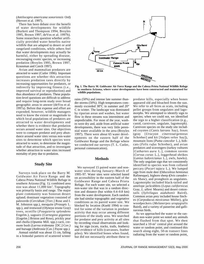
Surveys took place on the Barry M.Goldwater Air Force Range and theCabeza Prieta National Wildlife Refuge insouthern Arizona (Fig. 1); combined areasize was about 11,000 km2. Topographywas primarily basin and range. The majorplant community was Sonoran desertupland; dominant vegetation consisted ofpaloverde (C e r c i d i u m [Torr.] Rose and I.M. Johnston spp.), mesquite (P r o s o p i s L .spp.), and ironwood (Olyneya tesota G r a y )trees, ocotillo (Fouquieria splendensEngelm.), saguaro (Carnegiea gigantea[Engelm.] Britton and Rose), prickly pearand cholla (O p u n t i a Mill. spp.) cacti, cre-osote bush (Larrea tridentata [DC.] Cov.)and bursage (A m b r o s i a [Cav.] Payne spp.).
Annual rainfall was about 15 cm, fallingin a bimodal pattern of scattered winter
rains (50%) and intense late summer thun-der storms (50%). High temperatures com-monly exceeded 38°C in summer and 20°C in winter. The landscape was dominatedby riparian areas and washes, but waterflow in these streams was intermittent andunpredictable. For most of the year, wash-es were dry and, aside from artificial waterdevelopments, there was very little peren-nial water available in the area (Broyles1997). There were about 65 water devel-opments on the eastern half of theGoldwater Range and the Refuge wherewe conducted our surveys (T. L. Cutler,personal communication).
Methods
We surveyed 15 paired water and non-water sites during January–March of1995–97. Water sites were selected basedon accessibility in the eastern half of theGoldwater Range and Cabeza PrietaRefuge. For each water site, we selected anon-water site that was in a random direc-tion and distance (but within 0.4–0.8 km)from the water development. Each randomsite had similar topographic and vegetativeconditions as its paired water site. Weblocked by location (Kuehl 1994) to con-trol for some of the variation in predatoractivity that may occur among differentportions of the study area. We searchedfor predator and prey activity at all sitesby recording visual observations and look-ing for sign (scats, tracks, trails, feathers)and evidence of kills (carcasses, featherpiles). We identified bones when found,but did not necessarily attribute these to
predator kills, especially when bonesappeared old and bleached from the sun.We refer to all feces as scats, includingpellet groups from ungulates and lago-morphs. We attempted to identify sign tospecies; when we could not, we identifiedthe sign to a higher classification (e.g.,canid, carnivore, ungulate, lagomorph).Carnivore species on the study site includ-ed coyotes (Canis latrans Say), foxes(gray [Urocyon cinereoargenteusSchreber] and kit [Vulpes velox S a y ] ) ,mountain lions (Puma concolor L.), bob-cats (Felis rufus Schreber), and avianpredators and scavengers (turkey vultures[Cathartes aura L.], common ravens[Corvus corax L.], loggerhead shrikes[Lanius ludovicianus L.], owls, hawks).The only ungulate sign that we consistentlyidentified to species was from collaredpeccary (Pecari tajacu L.). We lumpedsign from mule deer (Odocoileus hemionusRafinesque), bighorn sheep (Ovis canaden -s i s Shaw), and pronghorn as ungulates.Lagomorphs included black-tailed andantelope jackrabbits (Lepus californicusGray, L. alleni Mearns) and desert cotton-tails (Sylvilagus audubonii B a i r d ) .Common avian prey included house finch-es (Carpodacus mexicanus Müller), gilawoodpeckers (Melanerpes uropygialisBaird), and a variety of passerine and galli-naceous birds.
As we approached the water or the ran-dom non-water point we noted any animalsthat flushed from that spot. We thensearched a 10-m2 central plot around thewater or random point, and continued thissearch along eight, 50-m transect linesradiating from the water or random point,
Fig. 1. The Barry M. Goldwater Air Force Range and the Cabeza Prieta National Wildlife Refugein southern Arizona, where water developments have been constructed and maintained forwildlife populations.

257JOURNAL OF RANGE MANAGEMENT 53(3), May 2000
looking for sign within about 5 m on eitherside of the transect. We tallied all sign andobservations by species or species groupfor the center plot and the 8 transects, andsummed that for each site. Groups of sign(pellet groups, a line of tracks, scatteredbut likely related bones, piles of feathers)were counted as 1 observation, but whenwe encountered similar sign (e.g., coyotetracks) at different points along a transector on different transects, each track or lineof tracks was counted as a separate obser-vation. Because we could not determine ifsign was from 1 or several individuals, wetallied total amount of sign, rather than try-ing to determine number of individuals thatmay have visited a site.
We used paired t-tests to compare dif-ferences in amount of predator and preysign between paired water and non-watersites. We report mean differences (x–D) and95% confidence intervals (CI) x–D for our15 paired sites; 95% CIs that do not con-tain 0 indicate a significant differencebetween water and non-water sites.
Results
Of 15 water sites examined, 73% (11)were drinkers; the remaining 4 wereimproved tinajas or rock potholes. For allwater and non-water sites combined, themajority of sign was scats or pellets(65%), followed by tracks (includingungulate trails) (12%) and visual observa-tions (7%). We also found bones (n = 23),feathers (n = 10), and carcasses (n = 4).Scats made up the majority of sign forboth types of site.
We recorded 20 observations of birds aswe approached water sites (where a flockcounted as 1 observation). Of these, housefinches (40%) and gila woodpeckers(20%) were most common. Other birdspecies observed at water sites includedblack-throated sparrows ( A m p h i s p i z ab i l i n e a t a Cassin), mourning and white-winged doves (Zenaida macroura L., Z .a s i a t i c a L.), and Gambel’s quail(Callipepla gambelii Gambel). No otherwildlife was seen at water sites except for1 black-tailed jackrabbit.
The most common predator sign atwater sites was from coyotes (79%), fol-lowed by foxes (7.5%), avian predatorsand scavengers (mostly turkey vultures)(7.5%), mountain lions (4%), and bobcats(2%). The most common prey sign atwater sites was from ungulates (deer,sheep, pronghorn) (40%), followed bylagomorphs (36%), passerine and gallina-ceous birds (19%), and peccaries (5%).
Comparison of paired water and non-water sites indicated that the amount ofsign for all predator species was greater atwater than non-water sites (P = 0.002).This was also the case for each species orgroup of predators, including coyotes,foxes, felids, and avian predators andscavengers (P ≤ 0.08; Table 1). Prey signwas not consistently more abundant atwater sites than non-water sites (P = 0.57).Of the species or groups of prey that weexamined (Table 1), sign was more abun-dant at water sites for only passerine andgallinaceous birds (P = 0.008). Sign forpeccaries and all other ungulates was notdifferent between water and non-water (P= 0.76 and 0.20, respectively). Sign forlagomorphs, although common at all waterand non-water sites, was 1.7x greater atnon-water sites than water sites (P = 0.05).
Discussion
Smith and Henry (1985) did not find adifference in predator sign on plotsbetween 6 water and 5 non-water sites inArizona. We, however, documented up to7x more predator sign at water sites thannon-water sites, indicating that predatoruse of water developments was high onour study area. This was especially truefor coyotes, sign from which made upalmost 80% of all predator sign that weobserved. Cutler (1996) also reported highvisitation rates by predators at water sitesin the same area, where she used remotecameras at 2 water sites to document useby wildlife. About 55% of all photographswere of coyotes. Golightly and Ohmart(1984) reported that water needs for coy-otes in deserts were greater during sum-mer than winter (this was not true for kitfoxes), and so the preponderance of coyotesign at our water sites could be evengreater during summer.
Despite the abundance of predator signat water sites, we found very little evi-dence of kills. This may be because notmany kills were made at these sites, or theevidence of kills disappeared quickly. Ofthe 4 carcasses that we found, 2 were gilawoodpeckers, 1 was a pecarry, and 1 wasa turkey vulture. The woodpeckers wereobviously predated by a raptor, probably aCooper hawk (Accipiter cooperiiBonaparte), as evidenced by whatappeared to be a sudden loss of largeamounts of feathers due to impact. Forpasserine and gallinaceous birds, webelieve that water sites may function in asimilar fashion to backyard bird feeders;birds are attracted to the site, congregateand linger there, and a few individuals aresubsequently killed by raptors. Some rap-tors may even include water sites in theirforaging territories, but we do not believethat this contributes in any significant wayto avian mortality. We could not deter-mine the cause of death of the peccary orthe turkey vulture because of the ages ofthe carcasses, but both were relativelyintact and did not appear to be predated oreven scavenged very much.
It is more difficult to speculate on theinfluence of water developments on inter-actions between large mammalian preda-tors and ungulates. Carnivore territoriesare large and distribution of kills wide-spread. Based on our findings, we canonly say that predators were attracted towater sites; we cannot say that waterincreased predation rates, improved preda-tor fitness, or that ungulates avoided watersites because of the periodic presence ofpredators. Although peccaries have beendocumented drinking at some of thesewater sites (Cutler 1996), in at least someinstances they do not need free-standingwater because of their diet of succulentplants (Zervanos and Day 1977). Thus, wewere not surprised to find no difference in
Table 1. Mean differences (x–D) and 95% confidence interval (CI) of the difference for amount ofpredator and prey sign between 15 paired water development and non–water (random) sites inthe Sonoran desert, Arizona.
Species x–D 95% CI tPaired P
Coyote 6.7 2, 11 3.24 0.006Fox 0.7 0.5, 1.3 2.32 0.04Felid 0.5 0, 1 1.97 0.07Avian predators1 0.7 –0.1, 1.4 0.67 0.08Avian prey2 2.3 1, 4 3.12 0.008Ungulate3 3.5 –2, 9 1.33 0.20Peccaries 0.1 –1, 1 0.31 0.76Lagomorph –3.8 –8, 0 –2.17 0.0481Includes predators and scavengers (turkey vulture, common raven, loggerhead shrike, hawks, owls).2Includes passerine and gallinaceous species.3Includes mule deer, bighorn sheep, and pronghorn.
258 JOURNAL OF RANGE MANAGEMENT53(3), May 2000
peccary sign between water and non-watersites. The need for free-standing water byother ungulates is less clear; some authorsreport that ungulates do not seem torespond to water developments (Krausmanand Leopold 1986, Krausman andEtchberger 1995), while others report thatwater developments are used by ungulatesand may be beneficial (Leslie and Douglas1979, Hervert and Krausman 1986,Ockenfels et al. 1991), depending on thespecies and season involved (deVos et al.1997b). We did not document a differencein ungulate sign between water and non-water sites, but because we lumped allungulate sign (except peccary) together,we cannot say how ungulate sign mayhave differed between water and non-water sites for individual species on ourstudy area during winter. Lagomorph wasthe only taxon for which we found moresign away from water sites than aroundwater sites. Although lagomorphs in desertenvironments will drink from water devel-opments (Cutler 1996), they may not needfree-standing water (Schmidt-Nielsen1964, Nagy et al. 1976) and may not becompelled to visit water sites. In years ofhigh numbers, rabbits and hares are proba-bly important prey, especially for coyotes,and may act to disperse predation awayfrom water sites.
Several researchers reported that freewater is unnecessary for a variety of carni-vores (Chevalier 1984, Golightly andOhmart 1984, Green et al. 1984). Schmidt-Nielsen (1964) believed that the diet ofmost carnivores provides them with thewater they need for most physiologicalfunctions, except perhaps heat regulation.Virtually all predators in the Sonoran desertwill use free-standing water if it is avail-able, and we suspect that predators come tothese sites primarily to drink rather than tohunt. Kills at water sites do occur (Monson1964, Cunningham and deVos 1992,Krausman and Etchberger 1993), but wespeculate that kills at water sites in southernArizona, when they do happen, are on anopportunistic basis and are trivial to preypopulation dynamics. We do not knowwhether providing water to predatorsincreases their survival or reproduction.
Research and ManagementRecommendations
It has been established through this andother studies that predators frequent waterdevelopments. The next step is to deter-mine what this means, if anything, to popu-
lation dynamics. The Arizona Game andFish Department identified key researchneeds for the study of water developmentsand their potential effects on wildlife popu-lations (deVos et al. 1997a, 1997b). Ofthese, the effects of water developments onpopulation performance (distribution, abun-dance, survival, reproduction) and preda-tion rates of mammalian predators wereconsidered important. Long-term experi-ments with marked animals are needed todetermine the influence of water develop-ments on predation rates and predatordemography, including experimentalapproaches where water sites are closed (ornew ones opened) while monitoring thedemographics of predator populations.
Literature Cited
Brown, D. E. 1997. Water for wildlife: beliefbefore science, p. 9–16. In: J. M. Feller and D.S. Strouse (eds.), Environmental, economic, andlegal issues related to rangeland water develop-ments. The Center for the Study of Law, Sci.and Tech., Arizona State Univ., Tempe. Ariz.
Broyles, B. 1995. Desert wildlife water develop-ments: questioning use in the Southwest. Wildl.Soc. Bull. 23:663–675.
Broyles, B. 1997. Wildlife water–developments insouthwestern Arizona. J. Arizona-Nevada Acad.Sci. 30:30–42.
Burkett, D. W. and B. C. Thompson. 1994.Wildlife association with human–altered watersources in semiarid vegetation communities.Conserv. Biol. 8:682–690.
Campbell, B. and R. Remington. 1981. Influenceof construction activities on water–use patternsof desert bighorn sheep. Wildl. Soc. Bull.9:63–65.
Chevalier, C. D. 1984. Water requirements offree–ranging and captive ringtail cats(Bassariscus astutus) in the Sonoran desert.M.S. Thesis, Arizona State Univ., Tempe, Ariz.98pp.
Cunningham, S. and J. C. deVos. 1992.Mortality of mountain sheep in the BlackCanyon area of northwest Arizona. DesertBighorn Counc. Trans. 36:27–29.
Cutler, P. L. 1996. Wildlife use of two artificialwater developments on the Cabeza PrietaNational Wildlife Refuge, southwesternArizona. M.S. Thesis, Univ. Arizona, Tucson,Ariz. 124pp.
deVos, J., W. Ballard, and S. S. Rosenstock.1997a. Research design considerations to evalu-ate efficacy of wildlife water developments, p.606–612. I n : J. M. Feller and D. S. Strouse(eds.), Environmental, economic, and legalissues related to rangeland water developments.The Center for the Study of Law, Sci. andTech., Arizona State Univ., Tempe, Ariz.
deVos, J., C. R. Miller, S. L. Walchuk, W. D.Ough and P. E. Taylor. 1983. B i o l o g i c a lresource inventory, Central Arizona Project. U.S. Bur. Reclamation, Phoenix, Ariz.
deVos, J., W. Ballard, G. Carmichael, V.Dickinson, E. Gardner, J. Gunn, R.Haughey, J.Hervert, R. Lee, and S.Rosenstock. 1997b. Wildlife water develop-
ments in Arizona: a technical review. ArizonaGame and Fish Dept., Tech. Rep., Phoenix,Ariz.
Golightly, R. T. and R. D. Ohmart. 1984. Watereconomy of two desert canids: coyote and kitfox. J. Mamm. 65:51–58.
Green, B., J. Anderson, and T. Whateley. 1984.Water and sodium turnover and estimated foodconsumption in free-living lions (Pantera leo)and spotted hyaenas ( C r o c u t a). J. Mamm.65:593–599.
Hervert, J. and P. R. Krausman. 1986. D e s e r tmule deer use of water developments inArizona. J. Wildl. Manage. 50:670–676.
Hervert, J., R. S. Henry, and M. T. Brown.1997. Preliminary investigations of Sonoranpronghorn use of free standing water, I n : p .126–137. J. M. Feller and D. S. Strouse (eds.),Environmental, economic, and legal issuesrelated to rangeland water developments. TheCenter for the Study of Law, Sci. and Tech.,Arizona State Univ., Tempe, Ariz.
Krausman, P. R. and B. Czech. 1997. W a t e rdevelopments and desert ungulates, p. 138–154.I n : J. M. Feller and D. S. Strouse (eds.),Environmental, economic, and legal issuesrelated to rangeland water developments. TheCenter for the Study of Law, Sci. and Tech.,Arizona State Univ., Tempe, Ariz.
Krausman, P. R. and R. C. Etchberger. 1993.Effectiveness of mitigation features for desertungulates along the Central Arizona Project. U.S. Bur. Reclamation, Phoenix, Ariz. 308pp.
Krausman, P. R. and R. C. Etchberger. 1995.Response of desert ungulates to a water projectin Arizona. J. Wildl. Manage. 59:292–300.
Krausman, P. R. and B. D. Leopold. 1986.Habitat components for desert bighorn sheep inthe Harquahala Mountains, Arizona. J. Wildl.Manage. 50:504–508.
Kuehl, R. O. 1994. Statistical principles ofresearch design and analysis. Duxbury Press,Belmont, Calif. 686pp.
Leslie, D. M., Jr. and C. L. Douglas. 1979.Desert bighorn sheep of the River Mountains,Nevada. Wildl. Monogr. 66. 56pp.
Monson, G. 1964. Group mortality in the desertbighorn sheep. Desert Bighorn Counc. Trans.9:55.
Nagy, K. A., V. H. Shoemaker, and W. R.Costa. 1976. Water, electrolyte, and nitrogenbudgets of jackrabbits (Lepus californicus) inthe Mojave Desert. Physiol. Zoo. 49:351– 363.
Ockenfels, R. A., D. E. Brooks, and C. H.Lewis. 1991. General ecology of Coueswhite–tailed deer in the Santa Rita Mountains.Arizona Game and Fish Dept., Tech. Rep.6,Phoenix, Ariz. 73pp.
Rosenstock, S. S., W. B. Ballard, and J. C.deVos, Jr. 1999. Viewpoint: benefits andimpacts of wildlife water developments. J.Range Manage. 52:302–311.
Schmidt–Nielsen, K. 1964. Desert animals: phys-iological problems of heat and water. OxfordUniv. Press, London, UK. 277pp.
Smith, N. S. and R. S. Henry. 1985. Short–termeffects of artificial oases on wildlife. U. S. Bur.of Reclamation, Tucson, Ariz. 133pp.
Tellman, B., R. Yarde, and M. G. Wallace.1 9 9 7 . Arizonas changing rivers: how peoplehave affected the rivers. Water Resources Res.Center, Univ. of Arizona, Tucson, Ariz. 198pp.
Zervanos, S. M. and G. I. Day. 1977. Water andenergy requirements of captive and free–livingcollared peccaries. J. Wildl. Manage.41:527–532.
259JOURNAL OF RANGE MANAGEMENT53(3), May 2000
Abstract
We surveyed the effectiveness of livestock guard dogs for reduc-ing predation on domestic sheep in Colorado during 1993. Thenumber of producers using dogs increased from about 25 in 1986to >159 in 1993. The proportion of sheep with dogs increasedfrom about 7% in 1986 to about 68% in 1993. Producers withdogs, compared to producers without dogs, lost smaller propor-tions of their lambs to predators, especially coyotes (Canis latransSay), and smaller proportions of ewes and lambs to black bears(Ursus americanus Pallas) and mountain lions (Felis concolor L . ) .Overall, producers who did not have guard dogs lost 5.9 and 2.1times greater proportions of lambs to predators than producerswho had dogs in 1986 and 1993, respectively. Proportions of sheepkilled by predators decreased with the number of years that pro-ducers used guard dogs. Mortalities of ewes to predators regard-less of type of operation and lamb mortality on open rangedecreased more from 1986 to 1993 for producers who obtaineddogs between these years compared to producers who did nothave dogs. Of 160 producers using dogs, 84% rated their dogsoverall predator control performance as excellent or good, 13%as fair, and 3% as poor. More producers (n = 105) indicated effec-tiveness of their dogs did not change with time, compared to pro-ducers (n = 54) indicating effectiveness changed. More producers(n = 35) also indicated their dogs became more effective over timecompared to producers (n =19) indicating their dogs became lesseffective. Estimates provided by 125 producers indicate that their392 dogs saved $891,440 of sheep from predation during 1993. Atotal of 154 of 161 (96%) producers recommend use of guard dogsto other producers.
Key Words: Akbash, black bear, Canis latrans, coyote, dog, Felisc o n c o l o r, Great Pyrenees, Komondor, mountain lion, sheep,Ursus americanus
Predators kill substantial numbers of domestic sheep in the 17western states (Pearson 1986, National Agricultural StatisticsService 1995). Several methods have been used to reduce thesemortalities (Andelt 1996) including livestock guard dogs (Linhartet al. 1979, McGrew and Blakesley 1982, Coppinger et al. 1983,1988, Green and Woodruff 1983b 1988 1990, Green et al. 1984,Andelt 1992). Andelt (1992) reported that producers with guard
dogs sustained lower sheep losses to coyotes than producers with-out dogs. However, no data were available to compare changes insheep mortalities for producers after they obtained dogs.
Green and Woodruff (1989) and Green et al. (1993) reportedthat guard dogs repelled black and grizzly bears (Ursus arctos L.)during most encounters. However, no studies have evaluated theeffectiveness of dogs against black bear or mountain lion preda-tion, nor have any authors reported on the relative effectivenessof guard dogs for deterring predation by different predators.
J. Range Manage.53: 259–267 May 2000
Livestock guard dogs reduce predation on domestic sheepin Colorado
WILLIAM F. ANDELT AND STUART N. HOPPER
Authors are assistant professor, Department of Fishery and Wildlife Biology, Colorado State University, Fort Collins, Colo. 80523; and former wildlife biol -ogy student, 305 Ruth, Fort Collins, Colo. 80525.
The authors wish to thank the many sheep producers that responded to this sur-vey. M. G. Fuentes obtained phone numbers of producers and entered the data. K.P. Burnham provided statistical advice. M. K. Johnson provided numerous editori-al suggestions which improved the manuscript.
Manuscript accepted 5 Sept. 1999.
Resumen
Durante 1993 realizamos un reconocimiento para determinarla efectividad de los perros guardianes de ganado bovino parareducir la predación de ovinos domésticos en Colorado. Elnúmero de productores que utilizan perros aumentó de aproxi-madamente 25 en 1986 a mas de 159 en 1993. La proporción deovinos con perros se incrementó de aproximadamente 7% en1896 a aproximadamente 68% en 1993. Los productores con per-ros, comparados con los productores sin perros, perdieronmenores proporciones de corderos debido a predadores, espe-cialmente coyotes, (Canis latrans Say) y menores proporciones deborregas debido a osos (Ursus americanus Pallas) y leones de lamontaña (Felis concolor L.). En general, las proporciones de per-dida de corderos debido a predadores registradas en 1986 y 1993fueron 5.9 y 2.1 veces mayores que las de los productores quetenían perros. Las proporciones de ovinos asesinados porpredadores disminuyo con el numero de años que los produc-tores han utilizado perros guardianes. La mortalidad de borre-gas por predadores, independientemente del tipo de operación, yla mortalidad de corderos en pastizales abiertos disminuyo masde 1986 a 1993 para los productores que obtuvieron perros enesos años comparado con los productores que no tenían perros.De 160 productores que utilizan perros, el 84% califico el controlde predadores de sus perros como excelente o bueno, el 13%como regular y el 3% como pobre. Mas productores (n = 105)indicaron que la efectividad de sus perros no cambio con el tiem-po, comparado con (n = 54) productores que indicaron que laefectividad si cambio. Mas productores (n = 35) tambiénseñalaron que con el tiempo sus perros llegan a ser mas efectivos,comparado con los productores (n = 19) que indicaron que con eltiempo sus perros fueron menos efectivos. Las estimaciones pro-porcionadas por 125 productores indican que durante 1993 sus392 perros evitaron perdidas de ovinos por predadores por unvalor de $ 891,440 dólares. De 161 productores un total de 154(96%) recomendaron a otros productores el uso de perrosguardianes.

260 JOURNAL OF RANGE MANAGEMENT53(3), May 2000
Additional data are also needed to ascertainrelationships between herd size, number ofdogs/herd, and number of sheep/dog versuspredation rates.
In this paper, we compare sheep mortal-ities to predators for producers inColorado who had and did not have guarddogs. We present the effects of herd size,sheep/dog, dogs/herd, and number of yearsdogs were used on predation rates. Wereport changes in proportions of sheepmortalities from 1986 to 1993 for produc-ers with and without dogs in both years,and producers who obtained dogs betweenthose years.
Materials and Methods
We determined the effectiveness ofguard dogs for protecting domestic sheepfrom predators by telephone surveys of182 livestock producers with dogs and 60producers without dogs during 1993. Webelieve that our survey included practical-ly all producers who used guard dogs inColorado. The 60 producers were a ran-dom sample of 143 producers who did nothave guard dogs and responded to a 1986survey (Andelt 1992).
We requested information on type ofoperation, number of ewes and lambs inthe operation, ewe and lamb mortalitiesfrom all causes (weather, disease, preda-tion, etc.), all predators, and specificallyfrom coyotes, black bears, mountain lionsand domestic dogs, ratings of effective-ness, and value of sheep saved based uponmortality rates before and after obtainingdogs, during 1993 or the last year that theyused dogs. We compared these data to sim-ilar data obtained in 1986 (Andelt 1992).
We classified producer operations withsheep in fenced pastures, open range,fenced pastures plus open range, fencedpastures plus open range and feedlots, andfenced pastures and feedlots as all opera-tions combined. We censored producerswith sheep solely in feedlots because theseoperations usually included large numbersof sheep and low mortalities to predators.We classified operations with sheep infenced pastures or in a combination offenced pastures and feedlots as fenced pas-tures. We conducted separate analyses onfenced pasture versus open range opera-tions because sheep were maintained underdifferent conditions, and we anticipatedthat sizes of herds and predation rates weredifferent. We defined all predators as thesum of all predators that killed sheep.
We compared the total number of ewesand lambs owned by producers with and
without guard dogs. We used total num-bers of ewes and lambs owned to calculatemortalities to all causes, but we used thenumbers of ewes and lambs that wereguarded by dogs, or were not guarded bydogs, when calculating proportions ofewes or lambs killed by predators. For the1993 survey, we compared mortalities tovarious predators only among producerswho indicated the specific predator wasfound in their area. Numbers of ewes andlambs killed by predators for producerswith guard dogs were reported only forperiods when dogs were with sheep. Whendogs were not with sheep for the entireyear, we extrapolated the mortalities bydividing by the percentage of the annualperiod that dogs were with sheep to stan-dardize the data for comparisons to pro-ducers without dogs.
We compared the numbers of ewes andlambs owned among producers with andwithout guard dogs using analysis of vari-ance (ANOVA, GLM Procedure, SASInst. Inc. 1988) after transforming herdsizes to natural logarithms to equalizevariances. We compared the numbers ofewe and lamb mortalities to all causes andto predators among respondents with andwithout dogs by testing the slopes ofregression lines obtained by regressing thenumber of mortalities against the numberof ewes or lambs owned or maintainedwith dogs. We conducted the analyseswith the GLM procedure after weightingthe number of mortalities by 1 divided bythe number of ewes or lambs owned or bythe number of ewes or lambs with dogs.When the overall F-test indicated signifi-cant treatment effects, we used 1-sided z-tests with a mean of 0 and a standard devi-ation of 1 to determine if mortalities forproducers with guard dogs were lowerthan for producers without dogs, whereas2-sided chi-square tests with 1 degree offreedom were used to determine if mortal-ities for producers with guard dogs and ifmortalities for producers without dogs dif-fered between years. We considered a P <0.0083 as significant in these 6-treatmentcomparisons to maintain an experiment-wise error rate of 0.05.
We used linear regression weighted bythe number of ewes or lambs with guarddogs (GLM Procedure) to determine theeffect of number of ewes or lambs withdogs, number of ewes or lambs/dog, num-ber of dogs/herd, and number of years thatdogs were maintained with sheep on theproportion of ewes or lambs killed bypredators in individual sheep operations.We determined changes in ewe and lambmortalities from 1986 to 1993 for produc-
ers with and without guard dogs duringboth years, and for producers who did nothave dogs in 1986 but used dogs by 1993.We assumed that coyotes, black bears,mountain lions, and domestic dogs werefound in a producers area during 1986, ifthey were reported there in 1993, and thusmade comparisons between our 1993 and1986 data for these predators. We deter-mined changes by subtracting proportionsof ewe or lamb mortalities in 1986 fromthose in 1993 for individual producers. Wecompared these differences among treat-ments with ANOVA after weighting thedifferences for each producer by the meannumber of ewes or lambs with dogs in1986 and 1993 in guarded herds.
We assigned rankings to producer rat-ings (excellent = 4, good = 3, fair = 2,poor = 1, unacceptable = 0) as to effec-tiveness of dogs for deterring predation byvarious predators, effectiveness in fencedpastures compared to open range, effec-tiveness during 1986 compared to 1993,and compared these rankings withANOVA using the GLM procedure. Weused a binomial probability distribution todetermine if the number of producers indi-cating effectiveness (effectiveness whensurveyed compared to effectiveness whenthe dogs first established normal guardingbehaviors) changed, or did not changewith time, and if the number of reportedpositive or negative changes varied fromequality. We used Spearman rank correla-tion to determine if ratings of effective-ness were associated with proportions ofewes or lambs killed by predators. Weestimated the value of sheep saved by eachguard dog by multiplying the averagenumber of ewes and lambs/producer bydifferences in predation rates for produc-ers with and without dogs, multiplying bythe average value of sheep ($77; ColoradoAgricultural Statistics Service 1994), anddividing by the average number ofdogs/producer. We used ANOVA to com-pare producer estimates of the value ofsheep saved/dog between 1986 and 1993,and between fenced pastures versus openrange operators after weighting the aver-age saving/dog by number of dogs ownedby each producer. We used the “protected”least significant difference test (Millikenand Johnson 1984:31–33) to determinewhich treatment pairs were different forthe average number of ewes and lambsowned, percent changes in ewe and lambherd sizes, changes in mortalities from1986 to 1993 and producer ratings ofeffectiveness of dogs when the overall F-test indicated significant (P < 0.05) treat-ment effects.
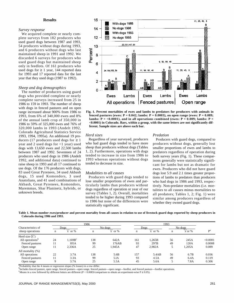
261JOURNAL OF RANGE MANAGEMENT53(3), May 2000
Results
Survey responseWe acquired complete or nearly com-
plete surveys from 182 producers whoused guard dogs between 1987 and 1993,54 producers without dogs during 1993,and 6 producers without dogs who lastmaintained sheep in 1991 and 1992. Wediscarded 6 surveys for producers whoused guard dogs but maintained sheeponly in feedlots. Of 161 producers whoused dogs for ≥ 1 year, 144 reported datafor 1993 and 17 reported data for the lastyear that they used dogs (1987 to 1992).
Sheep and dog demographicsThe number of producers using guard
dogs who provided complete or nearlycomplete surveys increased from 25 in1986 to 159 in 1993. The number of sheepwith dogs in fenced pastures and on openrange increased about 900% from 1986 to1993, from 6% of 340,000 ewes and 8%of the annual lamb crop of 350,000 in1986 to 59% of 325,000 ewes and 76% of320,000 lambs in 1993 (Andelt 1992,Colorado Agricultural Statistics Service1993, 1994, 1995a). An additional 19 pro-ducers (17 producers used dogs for ≥ 1year and 2 used dogs for <1 year) useddogs with 13,650 ewes and 22,500 lambsbetween 1987 and 1992. Seventeen of 24producers who used dogs in 1986 (Andelt1992, and additional data) continued toraise sheep in 1993 and all 17 continued touse dogs. Of the 176 producers with dogs,83 used Great Pyrenees, 34 used Akbashdogs, 15 used Komondors, 3 usedAnatolians, and 41 used combinations ofAkbash, Great Pyrenees, Komondors,Maremmas, Shar Planinetz, hybrids, orunknown breeds.
Herd sizesRegardless of year surveyed, producers
who had guard dogs tended to have moresheep than producers without dogs (Tables1, 2). Furthermore, operations with dogstended to increase in size from 1986 to1993 whereas operations without dogstended to decrease in size.
Modalities to all causesProducers with guard dogs tended to
lose smaller proportions of ewes and par-ticularly lambs than producers withoutdogs regardless of operation or year of oursurvey (Tables 1, 2). Overall, mortalitiestended to be higher during 1993 comparedto 1986 but none of the differences werestatistically significant.
PredationProducers with guard dogs, compared to
producers without dogs, generally lostsmaller proportions of ewes and lambs topredators regardless of operation duringboth survey years (Fig. 1). These compar-isons generally were statistically signifi-cant for lambs but not as dramatic forewes. Producers who did not have guarddogs lost 5.9 and 2.1 times greater propor-tions of lambs to predators than producerswho had dogs in 1986 and 1993, respec-tively. Non-predator mortalities (i.e. mor-talities to all causes minus mortalities toall predators; Tables 1, 2; Fig. 1) weresimilar among producers regardless ofwhether they owned guard dogs.
Table 1. Mean number ewes/producer and percent mortality from all causes in relation to use of livestock guard dogs reported by sheep producers inColorado during 1986 and 1993.
1986 1993 Characteristics of Dogs No dogs Dogs No dogs sheep operations n x— or % n x— or % n x— or % n —x or % Pa
Herd size (x—)All operationsb 24 1,169Bc 138 642A 161 1,265B 56 245A <0.0001Fenced pastures 11 l05A 99 176AB 93 297B 49 120A 0.0008Open range 11 2,336A 25 1,945A 47 2,982A 5 1,205A 0.089
All mortality (%)All operations 22 3.7A 138 5.6B 157 5.4AB 56 6.7B 0.036Fenced pastures 11 3.3A 99 5.lA 93 4.5A 49 6.4A 0.119Open range 9 3.7A 25 5.5A 45 5.6A 5 7.8A 0.306
aProbability that the 4 means or regression slopes (% losses) in a row differ. blncludes fenced pasture, open range, fenced pasture—open range, fenced pasture—open range—feedlot, and fenced pasture—feedlot operations.cMeans in a row followed by different letters are different (P < 0.0083/comparison to obtain an experiment-wise P ≤ 0.05).
Fig. 1. Percent mortalities of ewes and lambs to predators for producers with animals infenced pastures (ewes: P = 0.042; lambs: P = 0.0003), on open range (ewes: P = 0.089;lambs: P = <0.0001), and in all operations combined (ewes: P = 0.009; lambs: P =<0.0001) in Colorado. Bars, within a group, with the same letters are not significantly dif-ferent. Sample sizes are above each bar.

262 JOURNAL OF RANGE MANAGEMENT 53(3), May 2000
Regardless of guard dogs, producers lostsimilar proportions of ewes to coyotes, butproducers with dogs generally lost smallerproportions of lambs (Fig. 2). Producerswith guard dogs lost smaller proportionsof ewes and lambs to black bears (Fig.3)and mountain lions (Fig. 4) than producerswithout dogs in all operations combinedand on open range. However, guard dogsdid not appear to affect predation rates byblack bears and mountain lions in fencedpastures where these rates were relativelylow. Proportions of ewes and lambs killedby domestic dogs did not vary significant-ly regardless of the presence of guard dogsfor any type of operation (Fig. 5).Coyotes, black bears, and mountain lions
generally killed similar proportions ofewes, but coyotes killed 5 to >10 timesmore lambs than either bears or lions.
Five producers with guard dogs and 4producers without dogs reported that redfoxes (Vulpes vulpes L.) killed 262 and153 lambs, respectively. Four producerswith dogs and 1 producer without dogsreported eagles (likely Aquila chrysaetosL.) killed 446 and 40 lambs. In addition, 1producer with dogs reported Americancrows (Corvus brachyrhynchos B r e h m )killed 2 lambs, and 1 producer indicatedthat a guard dog killed 2 lambs.
Open range versus fenced pasturesMortalities of ewes to predators, and
specifically to coyotes, black bears, moun-
tain lions, and domestic dogs did not varysignificantly (F = 0.00–2.50; 1 15–132 df;P = 0.117–0.970, for the various compar-isons) between fenced pasture and openrange regardless of the presence of guarddogs during either year. However, ewemortalities to all predators combined weregreater (F = 5.78; 1,133 df; P = 0.018) onopen range than in fenced pastures for pro-ducers with dogs in 1993. Lamb mortali-ties were greater (F = 8.35–29.81;1,51–126 df; P = < 0.0001–0.005 for thevarious comparisons) on open range com-pared to fenced pastures to predators, andspecifically to coyotes, for producers with-out dogs both years and for producers withdogs in 1993. Lamb mortalities to moun-tain lions also were higher (F = 8.87; 1,22df; P = 0.007) on open range compared tofenced pastures for producers withoutdogs in 1993. In contrast, lamb mortalitiesto domestic dogs were higher (F = 4.29;1,100 df; P = 0.041) in fenced pasturescompared to open range for producerswith dogs during 1993.
Relationships: Dog numbers/experience Each producer used an average of 3.2
(SE = 0.3) dogs in all operations com-bined, 1.7 (SE = 0.1) dogs in fenced pas-tures, and 5.6 (SE = 0.7) dogs on openrange. Each producer used an average of1.8 (SE = 0.1) dogs/herd of sheep in alloperations combined, 1.6 (SE = 0.1)dogs/herd of sheep in fenced pastures, and2.2 (SE = 0.2) dogs/herd of sheep on openrange. Each producer had an average of716 (SE = 67) ewes and lambs/dog in alloperations combined, 414 (SE = 77) ewesand lambs/dog in fenced pastures, and1,245 (SE = 115) ewes and lambs/dog onopen range.
Proportions of ewes killed by predatorsincreased as the number of ewes main-tained with guard dogs increased in alloperations combined (intercept = 0.0057;
Table 2. Mean number lambs/producer and percent mortality from all causes in relation to use of livestock guard dogs reported by sheep producers inColorado during 1986 and 1993.
1986 1993 Characteristics of Dogs No dogs Dogs No dogs sheep operations n x— or % n x— or % n x— or % n —x or % Pa
Herd size (x—)All operationsb 23 1,524Bc 131 730A 157 1,451B 56 328A <0.0001Fenced pastures 10 193AB 92 184A 91 399B 49 175AB 0.0008Open range 11 2,851A 25 2,144A 46 3,386A 5 1,491A 0.057
All mortality (%)All operations 20 6.1A 131 11.5B 149 8.3A 56 12.3B <0.0001
Fenced pastures 9 4.5AB 92 10.2B 90 5.8A 49 9.5B <0.0001Open range 9 6.5A 25 12.2AB 41 8.9AB 5 17.9B 0.026
aProbability that the 4 means or regression slopes (% losses) in a row differ. blncludes fenced pasture, open range, fenced pasture—open range, fenced pasture—open range—feedlot, and fenced pasture—feedlot operations.cMeans in a row followed by different letters are different (P < 0.0083/comparison to obtain an experiment-wise P ≤ 0.05).
Fig. 2. Percent mortalities of ewes and lambs to coyotes for producers with animals in fencedpastures (ewes: P = 0.803; lambs: P = 0.005), on open range (ewes: P = 0.324; lambs: P=<0.0001), and in all operations combined (ewes: P = 0.022; lambs: P = 0.0001) in Colorado.Bars, within a group, with the same letters are not significantly different. Sample sizes areabove each bar.
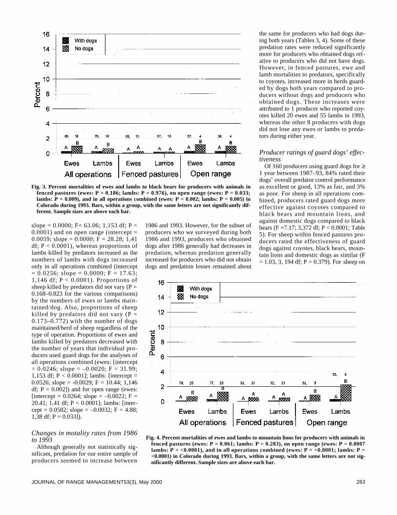
263JOURNAL OF RANGE MANAGEMENT53(3), May 2000
slope = 0.0000; F= 63.06; 1,153 df; P <0.0001) and on open range (intercept =0.0059; slope = 0.0000; F = 28.28; 1,41df; P < 0.0001), whereas proportions oflambs killed by predators increased as thenumbers of lambs with dogs increasedonly in all operations combined (intercept= 0.0256; slope = 0.0000; F = 17.63;1,146 df; P < 0.0001). Proportions ofsheep killed by predators did not vary (P =0.168–0.823 for the various comparisons)by the numbers of ewes or lambs main-tained/dog. Also, proportions of sheepkilled by predators did not vary (P =0.173–0.772) with the number of dogsmaintained/herd of sheep regardless of thetype of operation. Proportions of ewes andlambs killed by predators decreased withthe number of years that individual pro-ducers used guard dogs for the analyses ofall operations combined (ewes: [intercept= 0.0246; slope = –0.0020; F = 31.99;1,153 df; P < 0.0001]; lambs: [intercept =0.0526; slope = -0.0029; F = 10.44; 1,146df; P = 0.002]) and for open range (ewes:[intercept = 0.0264; slope = –0.0022; F =20.41; 1,41 df; P < 0.0001]; lambs: [inter-cept = 0.0582; slope = –0.0032; F = 4.88;1,38 df; P = 0.033]).
Changes in motality rates from 1986to 1993
Although generally not statistically sig-nificant, predation for our entire sample ofproducers seemed to increase between
1986 and 1993. However, for the subset ofproducers who we surveyed during both1986 and 1993, producers who obtaineddogs after 1986 generally had decreases inpredation, whereas predation generallyincreased for producers who did not obtaindogs and predation losses remained about
the same for producers who had dogs dur-ing both years (Tables 3, 4). Some of thesepredation rates were reduced significantlymore for producers who obtained dogs rel-ative to producers who did not have dogs.However, in fenced pastures, ewe andlamb mortalities to predators, specificallyto coyotes, increased more in herds guard-ed by dogs both years compared to pro-ducers without dogs and producers whoobtained dogs. These increases wereattributed to 1 producer who reported coy-otes killed 20 ewes and 55 lambs in 1993,whereas the other 8 producers with dogsdid not lose any ewes or lambs to preda-tors during either year.
Producer ratings of guard dogs’ effec-tiveness
Of 160 producers using guard dogs for ≥1 year between 1987–93, 84% rated theirdogs’ overall predator control performanceas excellent or good, 13% as fair, and 3%as poor. For sheep in all operations com-bined, producers rated guard dogs moreeffective against coyotes compared toblack bears and mountain lions, andagainst domestic dogs compared to blackbears (F =7.17; 3,372 df; P < 0.0001; Table5). For sheep within fenced pastures pro-ducers rated the effectiveness of guarddogs against coyotes, black bears, moun-tain lions and domestic dogs as similar (F= 1.03, 3, 194 df; P = 0.379). For sheep on
Fig. 3. Percent mortalities of ewes and lambs to black bears for producers with animals infenced pastures (ewes: P = 0.186; lambs: P = 0.976), on open range (ewes: P = 0.033;lambs: P = 0.009), and in all operations combined (ewes: P = 0.002; lambs: P = 0.005) inColorado during 1993. Bars, within a group, with the same letters are not significantly dif-ferent. Sample sizes are above each bar.
Fig. 4. Percent mortalities of ewes and lambs to mountain lions for producers with animals infenced pastures (ewes: P = 0.061; lambs: P = 0.283), on open range (ewes: P = 0.0007lambs: P = <0.0001), and in all operations combined (ewes: P = <0.0001; lambs: P =<0.0001) in Colorado during 1993. Bars, within a group, with the same letters are not sig-nificantly different. Sample sizes are above each bar.
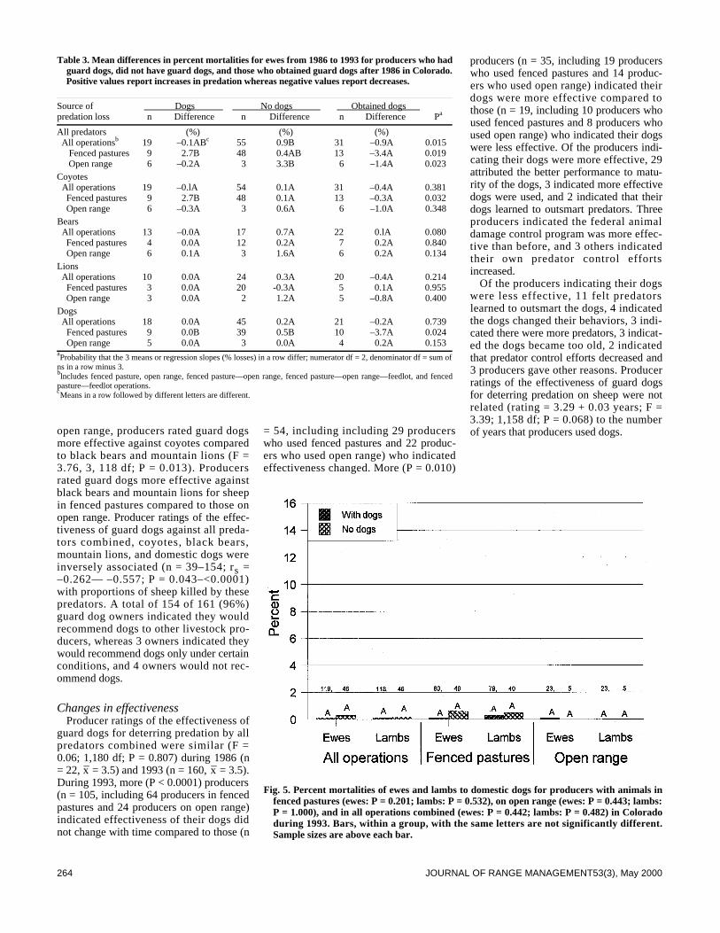
264 JOURNAL OF RANGE MANAGEMENT53(3), May 2000
open range, producers rated guard dogsmore effective against coyotes comparedto black bears and mountain lions (F =3.76, 3, 118 df; P = 0.013). Producersrated guard dogs more effective againstblack bears and mountain lions for sheepin fenced pastures compared to those onopen range. Producer ratings of the effec-tiveness of guard dogs against all preda-tors combined, coyotes, black bears,mountain lions, and domestic dogs wereinversely associated (n = 39–154; rs =–0.262— –0.557; P = 0.043–<0.0001)with proportions of sheep killed by thesepredators. A total of 154 of 161 (96%)guard dog owners indicated they wouldrecommend dogs to other livestock pro-ducers, whereas 3 owners indicated theywould recommend dogs only under certainconditions, and 4 owners would not rec-ommend dogs.
Changes in effectivenessProducer ratings of the effectiveness of
guard dogs for deterring predation by allpredators combined were similar (F =0.06; 1,180 df; P = 0.807) during 1986 (n= 22, x– = 3.5) and 1993 (n = 160, x– = 3.5).During 1993, more (P < 0.0001) producers(n = 105, including 64 producers in fencedpastures and 24 producers on open range)indicated effectiveness of their dogs didnot change with time compared to those (n
= 54, including including 29 producerswho used fenced pastures and 22 produc-ers who used open range) who indicatedeffectiveness changed. More (P = 0.010)
producers (n = 35, including 19 producerswho used fenced pastures and 14 produc-ers who used open range) indicated theirdogs were more effective compared tothose (n = 19, including 10 producers whoused fenced pastures and 8 producers whoused open range) who indicated their dogswere less effective. Of the producers indi-cating their dogs were more effective, 29attributed the better performance to matu-rity of the dogs, 3 indicated more effectivedogs were used, and 2 indicated that theirdogs learned to outsmart predators. Threeproducers indicated the federal animaldamage control program was more effec-tive than before, and 3 others indicatedtheir own predator control effortsincreased.
Of the producers indicating their dogswere less effective, 11 felt predatorslearned to outsmart the dogs, 4 indicatedthe dogs changed their behaviors, 3 indi-cated there were more predators, 3 indicat-ed the dogs became too old, 2 indicatedthat predator control efforts decreased and3 producers gave other reasons. Producerratings of the effectiveness of guard dogsfor deterring predation on sheep were notrelated (rating = 3.29 + 0.03 years; F =3.39; 1,158 df; P = 0.068) to the numberof years that producers used dogs.
Table 3. Mean differences in percent mortalities for ewes from 1986 to 1993 for producers who hadguard dogs, did not have guard dogs, and those who obtained guard dogs after 1986 in Colorado.Positive values report increases in predation whereas negative values report decreases.
Source of Dogs No dogs Obtained dogs predation loss n Difference n Difference n Difference Pa
All predators (%) (%) (%)All operationsb 19 –0.1ABc 55 0.9B 31 –0.9A 0.015
Fenced pastures 9 2.7B 48 0.4AB 13 –3.4A 0.019Open range 6 –0.2A 3 3.3B 6 –1.4A 0.023
CoyotesAll operations 19 –0.lA 54 0.1A 31 –0.4A 0.381Fenced pastures 9 2.7B 48 0.1A 13 –0.3A 0.032Open range 6 –0.3A 3 0.6A 6 –1.0A 0.348
Bears All operations 13 –0.0A 17 0.7A 22 0.lA 0.080Fenced pastures 4 0.0A 12 0.2A 7 0.2A 0.840Open range 6 0.1A 3 1.6A 6 0.2A 0.134
Lions All operations 10 0.0A 24 0.3A 20 –0.4A 0.214
Fenced pastures 3 0.0A 20 -0.3A 5 0.1A 0.955Open range 3 0.0A 2 1.2A 5 –0.8A 0.400
Dogs All operations 18 0.0A 45 0.2A 21 –0.2A 0.739
Fenced pastures 9 0.0B 39 0.5B 10 –3.7A 0.024Open range 5 0.0A 3 0.0A 4 0.2A 0.153
aProbability that the 3 means or regression slopes (% losses) in a row differ; numerator df = 2, denominator df = sum ofns in a row minus 3. blncludes fenced pasture, open range, fenced pasture—open range, fenced pasture—open range—feedlot, and fencedpasture—feedlot operations.cMeans in a row followed by different letters are different.
Fig. 5. Percent mortalities of ewes and lambs to domestic dogs for producers with animals infenced pastures (ewes: P = 0.201; lambs: P = 0.532), on open range (ewes: P = 0.443; lambs:P = 1.000), and in all operations combined (ewes: P = 0.442; lambs: P = 0.482) in Coloradoduring 1993. Bars, within a group, with the same letters are not significantly different.Sample sizes are above each bar.
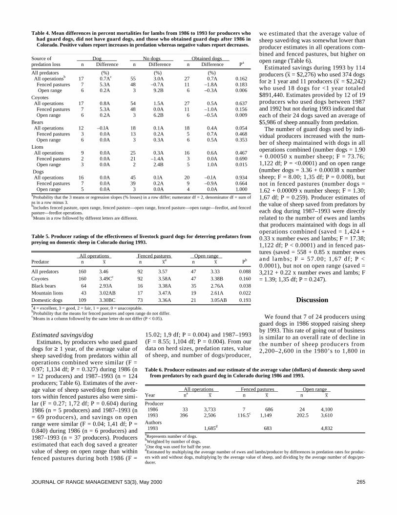
265JOURNAL OF RANGE MANAGEMENT 53(3), May 2000
Estimated savings/dog Estimates, by producers who used guard
dogs for ≥ 1 year, of the average value ofsheep saved/dog from predators within alloperations combined were similar (F =0.97; 1,134 df; P = 0.327) during 1986 (n= 12 producers) and 1987–1993 (n = 124producers; Table 6). Estimates of the aver-age value of sheep saved/dog from preda-tors within fenced pastures also were simi-lar (F = 0.27; 1,72 df; P = 0.604) during1986 (n = 5 producers) and 1987–1993 (n= 69 producers), and savings on openrange were similar (F = 0.04; 1,41 df; P =0.840) during 1986 (n = 6 producers) and1987–1993 (n = 37 producers). Producersestimated that each dog saved a greatervalue of sheep on open range than withinfenced pastures during both 1986 (F =
15.02; 1,9 df; P = 0.004) and 1987–1993(F = 8.55; 1,104 df; P = 0.004). From ourdata on herd sizes, predation rates, valueof sheep, and number of dogs/producer,
we estimated that the average value ofsheep saved/dog was somewhat lower thanproducer estimates in all operations com-bined and fenced pastures, but higher onopen range (Table 6).
Estimated savings during 1993 by 114producers (x– = $2,276) who used 374 dogsfor ≥ 1 year and 11 producers (x– = $2,242)who used 18 dogs for <1 year totaled$891,440. Estimates provided by 12 of 19producers who used dogs between 1987and 1992 but not during 1993 indicated thateach of their 24 dogs saved an average of$5,986 of sheep annually from predation.
The number of guard dogs used by indi-vidual producers increased with the num-ber of sheep maintained with dogs in alloperations combined (number dogs = 1.90+ 0.00050 x number sheep; F = 73.76;1,122 df; P = <0.0001) and on open range(number dogs = 3.36 + 0.00038 x numbersheep; F = 8.00; 1,35 df; P = 0.008), butnot in fenced pastures (number dogs =1.62 + 0.00009 x number sheep; F = 1.30;1,67 df; P = 0.259). Producer estimates ofthe value of sheep saved from predators byeach dog during 1987–1993 were directlyrelated to the number of ewes and lambsthat producers maintained with dogs in alloperations combined (saved = 1,424 +0.33 x number ewes and lambs; F = 17.38;1,122 df; P < 0.0001) and in fenced pas-tures (saved = 558 + 0.85 x number ewesand lambs; F = 57.00; 1 ,67 df ; P <0.0001), but not on open range (saved =3,212 + 0.22 x number ewes and lambs; F= 1.39; 1,35 df; P = 0.247).
Discussion
We found that 7 of 24 producers usingguard dogs in 1986 stopped raising sheepby 1993. This rate of going out of businessis similar to an overall rate of decline inthe number of sheep producers from2,200–2,600 in the 1980’s to 1,800 in
Table 4. Mean differences in percent mortalities for lambs from 1986 to 1993 for producers whohad guard dogs, did not have guard dogs, and those who obtained guard dogs after 1986 inColorado. Positive values report increases in predation whereas negative values report decreases.
Source of Dog No dogs Obtained dogs predation loss n Difference n Difference n Difference Pa
All predators (%) (%) (%)All operationsb 17 0.7Ac 55 3.0A 27 0.7A 0.162
Fenced pastures 7 5.3A 48 –0.7A 11 –1.8A 0.183Open range 6 0.2A 3 9.2B 6 –0.3A 0.006
CoyotesAll operations 17 0.8A 54 1.5A 27 0.5A 0.637
Fenced pastures 7 5.3A 48 0.0A 11 –1.0A 0.156Open range 6 0.2A 3 6.2B 6 –0.5A 0.009
BearsAll operations 12 –0.lA 18 0.1A 18 0.4A 0.054
Fenced pastures 3 0.0A 13 0.2A 5 0.7A 0.468Open range 6 0.0A 3 0.3A 6 0.5A 0.353
LionsAll operations 9 0.0A 25 0.3A 16 0.6A 0.467Fenced pastures 2 0.0A 21 –1.4A 3 0.0A 0.690Open range 3 0.0A 2 2.4B 5 1.0A 0.015
Dogs All operations 16 0.0A 45 0.lA 20 –0.lA 0.934
Fenced pastures 7 0.0A 39 0.2A 9 –0.9A 0.664Open range 5 0.0A 3 0.0A 4 0.0A 1.000
aProbability that the 3 means or regression slopes (% losses) in a row differ; numerator df = 2, denominator df = sum ofns in a row minus 3. blncludes fenced pasture, open range, fenced pasture—open range, fenced pasture—open range—feedlot, and fencedpasture—feedlot operations.cMeans in a row followed by different letters are different.
Table 5. Producer ratings of the effectiveness of livestock guard dogs for deterring predators frompreying on domestic sheep in Colorado during 1993.
All operations Fenced pastures Open range Predator n –x n –xa n –x Pb
All predators 160 3.46 92 3.57 47 3.33 0.088Coyotes 160 3.49Cc 92 3.58A 47 3.38B 0.160Black bears 64 2.93A 16 3.38A 35 2.76A 0.038 Mountain lions 43 3.02AB 17 3.47A 19 2.61A 0.022Domestic dogs 109 3.30BC 73 3.36A 21 3.05AB 0.193a4 = excellent, 3 = good, 2 = fair, 1 = poor, 0 = unacceptable.bProbability that the means for fenced pastures and open range do not differ. cMeans in a column followed by the same letter do not differ (P < 0.05).
Table 6. Producer estimates and our estimate of the average value (dollars) of domestic sheep savedfrom predators by each guard dog in Colorado during 1986 and 1993.
All operations Fenced pastures Open range Year na –x n –x n –x
Producer1986 33 3,733 7 686 24 4,1001993 396 2,506 116.5c 1,149 202.5 3,610
Authors1993 1,685d 683 4,832
aRepresents number of dogs.bWeighted by number of dogs. cOne dog was used for half the year. dEstimated by multiplying the average number of ewes and lambs/producer by differences in predation rates for produc-ers with and without dogs, multiplying by the average value of sheep, and dividing by the average number of dogs/pro-ducer.
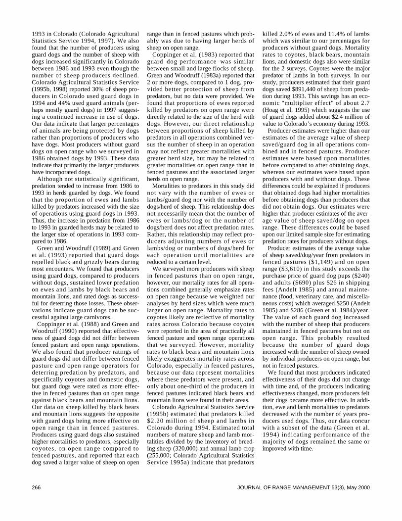
266 JOURNAL OF RANGE MANAGEMENT 53(3), May 2000
1993 in Colorado (Colorado AgriculturalStatistics Service 1994, 1997). We alsofound that the number of producers usingguard dogs and the number of sheep withdogs increased significantly in Coloradobetween 1986 and 1993 even though thenumber of sheep producers declined.Colorado Agricultural Statistics Service(1995b, 1998) reported 30% of sheep pro-ducers in Colorado used guard dogs in1994 and 44% used guard animals (per-haps mostly guard dogs) in 1997 suggest-ing a continued increase in use of dogs.Our data indicate that larger percentagesof animals are being protected by dogsrather than proportions of producers whohave dogs. Most producers without guarddogs on open range who we surveyed in1986 obtained dogs by 1993. These dataindicate that primarily the larger producershave incorporated dogs.
Although not statistically significant,predation tended to increase from 1986 to1993 in herds guarded by dogs. We foundthat the proportion of ewes and lambskilled by predators increased with the sizeof operations using guard dogs in 1993.Thus, the increase in predation from 1986to 1993 in guarded herds may be related tothe larger size of operations in 1993 com-pared to 1986.
Green and Woodruff (1989) and Greenet al. (1993) reported that guard dogsrepelled black and grizzly bears duringmost encounters. We found that producersusing guard dogs, compared to producerswithout dogs, sustained lower predationon ewes and lambs by black bears andmountain lions, and rated dogs as success-ful for deterring those losses. These obser-vations indicate guard dogs can be suc-cessful against large carnivores.
Coppinger et al. (1988) and Green andWoodruff (1990) reported that effective-ness of guard dogs did not differ betweenfenced pasture and open range operations.We also found that producer ratings ofguard dogs did not differ between fencedpasture and open range operators fordeterring predation by predators, andspecifically coyotes and domestic dogs,but guard dogs were rated as more effec-tive in fenced pastures than on open rangeagainst black bears and mountain lions.Our data on sheep killed by black bearsand mountain lions suggests the oppositewith guard dogs being more effective onopen range than in fenced pastures.Producers using guard dogs also sustainedhigher mortalities to predators, especiallycoyotes, on open range compared tofenced pastures, and reported that eachdog saved a larger value of sheep on open
range than in fenced pastures which prob-ably was due to having larger herds ofsheep on open range.
Coppinger et al. (1983) reported thatguard dog performance was similarbetween small and large flocks of sheep.Green and Woodruff (1983a) reported that2 or more dogs, compared to 1 dog, pro-vided better protection of sheep frompredators, but no data were provided. Wefound that proportions of ewes reportedkilled by predators on open range weredirectly related to the size of the herd withdogs. However, our direct relationshipbetween proportions of sheep killed bypredators in all operations combined ver-sus the number of sheep in an operationmay not reflect greater mortalities withgreater herd size, but may be related togreater mortalities on open range than infenced pastures and the associated largerherds on open range.
Mortalities to predators in this study didnot vary with the number of ewes orlambs/guard dog nor with the number ofdogs/herd of sheep. This relationship doesnot necessarily mean that the number ofewes or lambs/dog or the number ofdogs/herd does not affect predation rates.Rather, this relationship may reflect pro-ducers adjusting numbers of ewes orlambs/dog or numbers of dogs/herd foreach operation until mortalities arereduced to a certain level.
We surveyed more producers with sheepin fenced pastures than on open range,however, our mortality rates for all opera-tions combined generally emphasize rateson open range because we weighted ouranalyses by herd sizes which were muchlarger on open range. Mortality rates tocoyotes likely are reflective of mortalityrates across Colorado because coyoteswere reported in the area of practically allfenced pasture and open range operationsthat we surveyed. However, mortalityrates to black bears and mountain lionslikely exaggerates mortality rates acrossColorado, especially in fenced pastures,because our data represent mortalitieswhere these predators were present, andonly about one-third of the producers infenced pastures indicated black bears andmountain lions were found in their areas.
Colorado Agricultural Statistics Service(1995b) estimated that predators killed$2.20 million of sheep and lambs inColorado during 1994. Estimated totalnumbers of mature sheep and lamb mor-talities divided by the inventory of breed-ing sheep (320,000) and annual lamb crop(255,000; Colorado Agricultural StatisticsService 1995a) indicate that predators
killed 2.0% of ewes and 11.4% of lambswhich was similar to our percentages forproducers without guard dogs. Mortalityrates to coyotes, black bears, mountainlions, and domestic dogs also were similarfor the 2 surveys. Coyotes were the majorpredator of lambs in both surveys. In ourstudy, producers estimated that their guarddogs saved $891,440 of sheep from preda-tion during 1993. This savings has an eco-nomic "multiplier effect" of about 2.7(Hoag et al. 1995) which suggests the useof guard dogs added about $2.4 million ofvalue to Colorado’s economy during 1993.
Producer estimates were higher than ourestimates of the average value of sheepsaved/guard dog in all operations com-bined and in fenced pastures. Producerestimates were based upon mortalitiesbefore compared to after obtaining dogs,whereas our estimates were based uponproducers with and without dogs. Thesedifferences could be explained if producersthat obtained dogs had higher mortalitiesbefore obtaining dogs than producers thatdid not obtain dogs. Our estimates werehigher than producer estimates of the aver-age value of sheep saved/dog on openrange. These differences could be basedupon our limited sample size for estimatingpredation rates for producers without dogs.
Producer estimates of the average valueof sheep saved/dog/year from predators infenced pastures ($1,149) and on openrange ($3,610) in this study exceeds thepurchase price of guard dog pups ($240)and adults ($690) plus $26 in shippingfees (Andelt 1985) and annual mainte-nance (food, veterinary care, and miscella-neous costs) which averaged $250 (Andelt1985) and $286 (Green et al. 1984)/year.The value of each guard dog increasedwith the number of sheep that producersmaintained in fenced pastures but not onopen range. This probably resultedbecause the number of guard dogsincreased with the number of sheep ownedby individual producers on open range, butnot in fenced pastures.
We found that most producers indicatedeffectiveness of their dogs did not changewith time and, of the producers indicatingeffectiveness changed, more producers felttheir dogs became more effective. In addi-tion, ewe and lamb mortalities to predatorsdecreased with the number of years pro-ducers used dogs. Thus, our data concurwith a subset of the data (Green et al.1994) indicating performance of themajority of dogs remained the same orimproved with time.

267JOURNAL OF RANGE MANAGEMENT53(3), May 2000
Conclusions and ManagementRecommendations
Guard dogs are an important tool forreducing sheep mortalities to predators.Producers with guard dogs, compared toproducers without dogs, lost smaller pro-portions of their lambs to predators,specifically to coyotes, and also lost small-er proportions of their sheep to black bearsand mountain lions. Ewe and lamb preda-tion generally was lower for producerswho obtained dogs relative to producerswho had not obtained dogs. In addition,84% of producers rated the effectivenessof their dogs as excellent or good, mostproducers indicated that their dogs did notdecrease effectiveness with time, >96% ofproducers indicated that they would rec-ommend dogs to other producers, all 17producers that used dogs in 1986 and con-tinued in the sheep business still used dogsin 1993 and 125 producers using guarddogs in 1993 indicated that their dogssaved over $891,000 in sheep from preda-tors; these estimates of savings were con-servative because 32 producers did notprovide estimates. Thus, use of guard dogsis a successful method for combating pre-dation on domestic sheep.
In a recent synthesis of coyote anddepredation control literature, Knowlton etal. (1999) suggest that there may be a dif-ference in predation risk between pasturedsheep and those on open range. We foundlambs on open range are significantlymore likely to be killed by predators thanthose in fenced pastures. Knowlton et al.(1999) also report that no techniques tocontrol depredations are universally effec-tive and that guard dogs are effective insome situations but not in others. Based onour data and the opinions of nearly all pro-ducers, dogs, when properly used, areeffective in the majority of situationsagainst a variety of predators. However, itis interesting to note that according to ourdata, guard dogs do not significantlychange predation rates on ewes from coy-otes or domestic dogs regardless of theoperation, but do significantly protectlambs. Ewes might be more capable ofdefending themselves against canids, andthe effects of guard dogs may be lessapparent. On the other hand, lambs aremore vulnerable to coyotes, and they oftenare maintained with ewes which likelyreduces predation on ewes, and makes theeffects of guard dogs less apparent. Guarddogs do not eliminate all depredation loss-es but significantly reduce them, and theyare economically effective. On the basis ofour data and opinions of producers, we
recommend guard dogs as essential com-ponents of sheep production in Colorado,especially to protect lambs against coy-otes, to protect ewes and lambs againstblack bears, mountain lions, and domesticdogs, and especially for producers usingopen rangelands.
Literature Cited
Andelt, W. F. 1985. Livestock guarding dogsprotect domestic sheep from coyote preda-tion in Kansas. Proc. Great Plains Wildl.Damage Control Workshop 7:111–113.
Andelt, W. F. 1992. Effectiveness of livestockguarding dogs for reducing predation ondomestic sheep. Wildl. Soc. Bull. 20:55–62.
Andelt, W. F. 1996. Carnivores. p. 133–155.In: P. R. Krausman (ed.), Rangeland wildlife.The Soc. Range Manage., Denver, Colo.
Colorado Agricultural Statistics Service.1993. Colorado agricultural statistics 1993.Colo. Ag. Stat. Serv., Lakewood, Colo.
Colorado Agricultural Statistics Service.1 9 9 4 . Colorado agricultural statistics 1994.Colo. Ag. Stat. Serv., Lakewood, Colo.
Colorado Agricultural Statistics Service.1995a. Colorado Agricultural Statistics 1995.Colo. Ag. Stat. Serv., Lakewood, Colo.
Colorado Agricultural Statistics Service.1 9 9 5 b . Sheep and lamb death loss—1994.Colo. Ag. Stat. Serv., Lakewood, Colo.
Colorado Agricultural Statistics Service.1997. Colorado agricultural statistics 1997.Colo. Ag. Stat. Serv., Lakewood, Colo.
Colorado Agricultural Statistics Service.1998. Colorado sheep and lamb losses—1997. Colo. Ag. Stat. Serv., Lakewood, Colo.
Coppinger, R., J. Lorenz, and L. Coppinger.1983. Introducing livestock guarding dogs tosheep and goat producers. Proc. East. Wildl.Damage Contr. Conf. 1:129–132.
Coppinger, R., L. Coppinger, G. Langeloh,L. Gettler, and J. Lorenz. 1988. A decadeof use of livestock guarding dogs. Proc.Vertebr. Pest Conf. 13:209–214.
Green, J. S. and R. A. Woodruff. 1983a. Theuse of Eurasian dogs to protect sheep frompredators in North America: a summary ofresearch at the U.S. Sheep Exp. Station. Proc.East. Wildl. Damage Control Conf.1:119–124.
Green, J. S. and R. A. Woodruff. 1983b. Theuse of three breeds of dog to protect range-land sheep from predators. Appl. Anim.Ethol. 11:141–161.
Green, J. S. and R. A. Woodruff. 1988. Breedcomparisons and characteristics of use oflivestock guarding dogs. J. Range Manage.41:249–251.
Green, J. S. and R. A. Woodruff. 1989.Livestock-guarding dogs reduce depredationby bears. p. 49–54. I n : M. Bromley (ed.),Bear-people conflicts: proceedings of a sym-posium on management strategies. NorthwestTerr. Dep. Renew. Res., Yellowknife,Northwest Territories.
Green, J. S. and R. A. Woodruff. 1990. ADCguarding dog program update: a focus onmanaging dogs. Proc. Vertebr. Pest Conf.14:233–236.
Green, J. S., R. A. Woodruff, and W. F.Andelt. 1994. Do livestock guarding dogslose their effectiveness over time? Proc.Vertebr. Pest Conf. 16:41–44.
Green, J. S., R. A. Woodruff, and T. T.Tueller. 1984. Livestock-guarding dogs forpredator control: costs, benefits, and practi-cality. Wildl. Soc. Bull. 12:44–50.
Green, J. S., R. A. Woodruff, and P. J. Wick.1993. Bears, ostriches, and specialized graz-ing: putting guarding dogs to work. Proc.Great Plains Wildl. Damage ControlWorkshop 11:105-108.
Hoag, D. L., J. R. Fulton, and E. Hornbrook.1 9 9 5 . Colorado’s farm and food system: itscontribution to the state economy in 1992.Colo. State Univ. Coop. Ext. Bull. 551A,Fort Collins, Colo.
Knowlton, F. F, E. M. Gese, and M. M.Jaeger. 1999. Coyote depredation control:An interface between biology and manage-ment. J. Range Manage. 52:398–412.
Linhart, S. B., R. T. Sterner, T. C. Carrigan,and D. R. Henne. 1979. Komondor guarddogs reduce sheep losses to coyotes: a pre-liminary evaluation. J. Range Manage.32:238–241.
McGrew, J. C. and C. S. Blakesley. 1982.How Komondor dogs reduce sheep losses tocoyotes. J. Range Manage. 35:693–696.
Milliken, G.A. and D. E. Johnson. 1984.Analysis of messy data. Volume 1: Designedexperiments. Lifetime Learning Pub.,Belmont, Calif.
National Agricultural Statistics Service.1995. Sheep and Iamb death loss 1994.USDA, Nat. Agr. Statistics Service., NASSStaff Rep. LDP No. 95-01, Washington, D.C.
Pearson, E. W. 1986. A literature review oflivestock losses to predators in western U.S.U.S. Fish and Wildl. Serv. Final Rep.,Denver, Colo.
SAS Institute Inc. 1988. SAS/STAT User’sguide, release 6.03 edition, SAS Inst., Cary,N.C.
268 JOURNAL OF RANGE MANAGEMENT 53(3), May 2000
Abstract
Because of the relatively low cost of seed and ease of establish-ment, more than 0.4 million ha of weeping lovegrass (Eragrostiscurvula (Shrad.) Nees.) were planted on Conservation ReserveProgram (CRP) lands in the Southern High Plains. Drylandcropping alternatives including wheat and grain sorghum, giverelatively low and variable economic returns. The objective ofthis study was to evaluate the economics of the lovegrass grazingalternative. Using a tract of weeping lovegrass in Curry County,N.M., animal performance and the economics of 5 grazing man-agement treatments were evaluated, including 12-month and 6-month continuous grazing, seasonal grazing during only thespring and fall, and a 6-pasture rotation system. Fertilization ofthe pastures was also evaluated for the spring/fall grazing treat-ment. Average daily gain (ADG) for yearlings grazing weepinglovegrass pastures was found to decline rapidly as the grazingseason progressed. The ADG was over 1.36 kg day-1 in early Maybut gradually declined over the grazing season to less than 0.45kg day-1 by the end of August. To maximize profit, stocker cattlewould be sold in early September. All of the grazing systemsyielded similar net economic returns, but substantially highereconomic returns could be made by adjusting stocking rates tomarket conditions. Returning CRP land to dryland cropping orgrazing with stocker cattle was estimated to yield nearly identicaleconomic returns. Neither growing traditional crops or grazinglovegrass pastures appear to be economically viable alternativeswithout government assistance programs in place.
Key Words: Conservation Reserve Program, Eragrostis curvula(Shrad.) Ness., forage quality, optimal stocking rates, drylandfarming, grazing systems
One of the highest Conservation Reserve Program (CRP) par-ticipation rates in the nation was found in Eastern New Mexicoand West Texas. Nearly one-fourth the cropland acreage in thisregion was planted to perennial grasses as a result of the CRP, avoluntary long-term cropland retirement program. Dryland farm-ing in the area is risky with variable and limited profit potential.As reported by the New Mexico State University (NMSU) crop
cost and return series (Hawkes and Libbin 1997a, 1997b), returnto land and risk was negative in 7 of the most recent 13 years inQuay County and 4 of 13 years in Curry County. With averageNew Mexico CRP program payments of $94 ha-1 (Osborn et al.1995) many area farmers believed the CRP was a more profitablealternative and signed up for the program in the early years.
Because of its relatively low seeding cost and ease of establish-ment, weeping lovegrass (Eragrostis curvula (Shrad.) Nees.) wasone of the most prevalent grass species planted on CRP land inthe Southern Great Plains. It is a long-lived perennial bunchgrassthat grows and produces well on a wide variety of soils.Lovegrass is an excellent soil stabilizer and is drought tolerant.But, weeping lovegrass is generally considered to be a poor for-age for grazing livestock.
Under new guidelines and requirements for CRP participation(USDA-FSA 1997), many individuals who planted monoculturesof weeping lovegrass, especially those with a tighter less erodiblesoil, were not renewed into the continuing CRP program (person-
J. Range Manage.53: 268–276 May 2000
Economics of grazing weeping lovegrass with stockers inthe Southern Great Plains
L. ALLEN TORELL, REX E. KIRKSEY, GARY B. DONART, AND JAMES D. LIBBIN
Authors are professor, Dept. of Agr. Econ. and Agr. Business, New Mexico State University, Las Cruces, N.M. 88003; superintendent, Agricultural ScienceCenter, Tucumcari, N.M. 88401, professor, Department of Animal and Range Sciences, New Mexico State University, Las Cruces, N.M. 88003; and professor,Dept. of Agr. Econ. and Agr. Business, New Mexico State University, Las Cruces, N.M. 88003
Research was supported in part by a USDA SARE grant and the New MexicoAgricultural Experiment Station, New Mexico State University, Las Cruces. Theauthors thank Hildagard Van Voorthuizen and Scott Bailey for assistance in statis-tical analyses.
Manuscript accepted 6 Sept. 1999.
Resumen
Debido a su habilidad de establecimiento y al bajo costo de lasemilla, aproximadamente, 400,000 ha de Weeping Lovegrass(Eragrostis curvula (Shrad.) Ness.) fueron cultivadas en los ter-renos del Conservation Reserve Program (CRP) en la planiciedel Sur. En adición, cultivos como el Trigo y el Sorgo en zonassemidesérticas son asociados con pobres ganancias y tasas deretorno bajas. El objetivo fue evaluar la viabilidad económica deluso de Lovegrass en condiciones pastoreo con bovinos en CurryCounty, N.M. Los tratamientos fueron: 1)Pastoreo Continuo por12 meses, 2) Pastoreo continuo por seis meses, 3) Pastoreo enOtoño, 4) Pastoreo en Primavera, y 5) Sistema rotacional de seisdías. La ganancia de peso de los bovinos por día (GDP) pastore-ando Weeping Lovegrass disminuyó radpidamente conformeavanzó la estación de pastoreo. La ganancia de peso fue 1.36Kg/día a principios de Mayo y disminuyó gradualmente hasta .45Kg/día a finales de Agosto. Para maximizar las ganacias losbecerros destetados fueron vendidos a principios de Septiembre.Todos los sistemas de pastoreo produjeron retornos econ\micossimilares. Sin embargo, la rentabilidad financiera pudiera incre-mentarse ajustando la carga animal a las condiciones del merca-do. Retornos económicos similares fueron observados con cul-tivos de secano o pastoreo de bovinos en el CRP. El cultivo tradi-cional de granos y el pastoreo de Lovegrass con bovinos parecenser sistemas de producción poco rentables sin el apoyo de pro-gramas de cooperación técnica del Estado.
269JOURNAL OF RANGE MANAGEMENT 53(3), May 2000
al communication Richard Shaw, USDA-NRCS, Clovis, N.M. Field Office, 18August 1998). These producers must nowdecide the future use of their lands, andother CRP enrollees will eventually facesimilar decisions. A primary factor in thisdecision will be the relative productivityand profitability of using these lands forgrazing versus converting back to cropproduction. The objective of this studywas to evaluate the performance of stockercalves grazing weeping lovegrass underdifferent management strategies. The eco-nomics of alternative grazing systems forlovegrass pastures are compared to tradi-tional cropping alternatives.
Materials and Methods
Theoretical Grazing Concepts As shown by Hildreth and Riewe
(1963), Workman (1986) and Hart et al.(1988), determining the economicallyoptimal (profit maximizing) grazing strat-egy means selecting the stocking rate andgrazing system that maximizes net eco-nomic returns per ha for the definedprice/cost situation. Defining this optimalgrazing strategy requires definition ofexpected beef prices and costs over theplanning period. It also requires definitionof relevant biological input/output rela-tionships using the production function. Indefining the production function we usethe standard definition of stocking rate torelate the total demand for forage to thearea used to provide it. Stocking rate (SR)is defined to be the number of stocker cat-tle grazing per ha over a grazing period oflength T (Vallentine 1990)1.
In addition to the standard analysis ofhow SR affects animal performance andprofit, an additional consideration is howdeclining forage quality affects livestockproduction and profitability. This wouldbe especially important for a plant likeweeping lovegrass where forage qualitydeteriorates quickly over the grazing sea-son. Yet, few economic studies have con-sidered forage quality when making man-
agement prescriptions. Huffaker andWilen (1991) found that when nutrientdeterioration of tall fescue pastures inTennessee was high, an intensive earlygrazing strategy (IES) that doubled theconventional season-long stocking rateearly and then rested the pasture with nostocking as forage nutrients began to playout would be economically optimal. If thegrass cultivar exhibited low nutrient dete-rioration over the season then the conven-tional season-long grazing strategy outper -formed the IES.
To consider both stocking rate and dete-rioration of forage quality over the grazingseason, average daily gain (ADG) cannotbe defined in the typical way, with anaverage rate of gain for the grazing seasonassumed, or with ADG considered to be afunction of SR only (Workman 1986).Rather, diminished livestock gain must beexplicitly recognized. There are at least 2alternative ways to do this. First, the strat-egy used by Huffaker and Wilen (1991)can be employed with grazing animalsallocated between pasture grazing and thenext best feeding alternative. Dependingon pasture production and forage quality,cattle are allocated between alternativefeed sources so as to maximize profit. Thesecond alternative, as used here, is to stockthe pasture with animals at the start of thegrazing season. All animals are thenremoved at some point once forage qualityhas deteriorated to an unacceptable level,or when a threshold amount of forageremains. Cattle could be sold at this pointor they could be moved to alternative pas-tures or feedlots. Stocking rate of the pas-ture is a choice variable in the model andwith adequate data to define input/outputrelationships the stocking rate used couldbe an economically optimal rate.
To develop the economic model, letaverage daily gain (ADG) be defined as aconcave function of stocking rate (SR) andtime of year (t), with deteriorating foragequality (Q) the factor reducing ADG overtime.
ADG = f(SR,Q(t)), (1)
with ∂f/∂SR <0, ∂f/∂Q>0 and ∂Q/∂t<0over the economically relevant range ofproduction. Time (t) could also be used asa direct proxy for forage quality if recog-nition is given to the importance that for-age quality has it determining livestockperformance at different points in time.The time variable defines the day of thegrazing season, either as the Julian date oras the elapsed number of days that stockercattle have been in the pasture.
The total kg of beef sold per ha isdefined by multiplying the number of ani-
mals grazing per ha times the average saleweight (Ws), less a market shrink:
% Shrinkb(SR,T) = SR x Ws x (1 – ) (2)
100
The sale weight, given by Ws = [Wp + ∫ T
t = 1
f(SR,Q(t)) dt] , is determined by thestocking rate decision. Increasing stockingrates will decrease ADG and sale weight, butexcept in the extreme, more beef will be pro-duced per ha. Average sale weight will alsodepend on purchase weight (Wp) and thedecision about when to market the cattle (i.e.,the selection of sale period (T)). As thelength of time cattle remain in the pasture isextended there will be a continued decreasein ADG because of declining forage quality.
Heavier feeder cattle generally sell forless per kg (Sartwelle et al. 1995). Whilesale price is determined by market forcesoutside the livestock producer's control,the producer determines which marketprice to accept by the size and type of cat-tle produced. Size of cattle depends onstocking rate and marketing decisions,such that in addition to market forces, saleprice (Ps) is a function of SR, sale dateand livestock characteristics;
Px = g(Ws(SR,T),X) (3)
where X is a vector of exogenous vari-ables that identify relevant characteristicsof the stockers at time of sale (e.g., breed,frame size, health, fill, sex, muscling).
The livestock producer selling in thecompetitive market is faced with the prob-lem of choosing the stocking rate and saledate that maximizes profit, with profitdefined to be the residual return to landand risk ($/ha):
π(SR,T) = g(Ws(SR,T),X)xb(SR,T) -SR[(PpWp + r) + ∫ T C(t) dt]-a (4)
t=1
where Pp is stocker purchase price ($/kg),PpWp is per head animal purchase cost,and r is additional per head costs ofreceiving the cattle, including shipping,vaccinations, labor, and other miscella-neous charges. In addition to receivingcosts (r) and fixed costs (a), there are addi-tional daily costs [C(t)] to keep the stockercattle in the pasture, like periodic checkingof animals, supplemental feeds, salt, min-erals, and a pasture charge (if the forage isleased on a per-head basis by the month).This daily cost may be different at differ-ent times of the year because of weather orpasture conditions. Further, pasturecharges could be calculated on a cost perkg of gain. In this case, accumulated daily
1The budget and design of the grazing trialsconducted here did not allow us to compare netreturns at altnerative stocking rates (SR, i.e.,animals ha- 1, animal days of grazing ha1) orgrazing pressures (GP, i.e., animal or headdays of grazing per unit of herbage produced).The economic model used to evaluate optimalgrazing strategies is the same, however, withor without variation in stocking rate. In themore limited applications where SR is not achoice variable, grazing systems can only becompared at the rates used in the grazing trial.
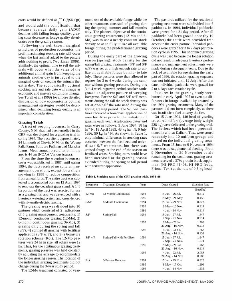
270 JOURNAL OF RANGE MANAGEMENT 53(3), May 2000
costs would be defined as ∫ T C(f(SR,Q(t)T=1
and would add the complication that because average daily gain (ADG)declines with falling forage quality, graz-ing costs decrease as forage quality deteri-orates over the grazing season.
Following the well known marginalprinciples of production economics, theprofit maximizing stocking rate will occurwhen the last animal added to the pastureadds nothing to profit (Workman 1986).Similarly, the optimal time to sell the ani-mals will occur when the value of theadditional animal gain from keeping theanimals another day is just equal to themarginal costs of keeping the animals thatextra day. The economically optimalstocking rate and sale date will change aseconomic and pasture conditions change.See Torell et al. (1999) for a more detaileddiscussion of how economically optimalmanagement strategies would be deter-mined when declining forage quality is animportant consideration.
Grazing Trials A tract of weeping lovegrass in Curry
County, N.M. that had been enrolled in theCRP was developed for a grazing trial inspring 1994. The tract site is approximately24 km north of Clovis, N.M. on the WaynePalla Farm. Soils are Pullman and Manskerloams. Mean annual precipitation in thearea is 44 cm (NOAA Various issues).
From the time the weeping lovegrasscover was established in 1987, until spring1994, the tract received no cultural man-agement operations, except for a singlemowing in 1988 to reduce competitionfrom annual forbs. The entire tract was sub-jected to a controlled burn on 13 April 1994to renovate the decadent grass stand. A 146ha portion of the tract was selected for useas a grazing trial and was developed with alivestock watering system and cross-fencedwith hi-tensile electric fencing.
The grazing area was divided into 10pastures which consisted of 2 replicationsof 5 grazing management treatments: 1)12-month continuous grazing (12-Mo), 2)6-month continuous grazing (6-Mo), 3)grazing only during the spring and fall(S/F), 4) spring/fall grazing with fertilizerapplication (S/F w/F), and 5) a 6-pasturerotation scheme (Rot). The 12-Mo pas-tures were 24 ha in size, all others were 12ha. Thus, for the continuous grazing treat-ments, grazing pressure was held constantby adjusting the acreage to accommodatethe longer grazing season. The location ofthe individual grazing treatments did notchange during the 3-year study period.
The 12-Mo treatment consisted of year-
round use of the available forage while theother treatments consisted of grazing dur-ing the spring, summer and fall monthsonly. The planned objective of the contin-uous grazing treatments (12-Mo and 6-Mo) was to use a nearly constant stockdensity so as to fully utilize all availableforage during the predetermined grazingperiod.
During the early part of the growingseason (spring), stock density for thespring/fall grazing treatments (S/F and S/Fw/F) was set at a high enough rate to uti-lize all available forage by mid- to lateJuly. These pastures were then allowed toregrow for 3 to 4 weeks during the sum-mer without grazing pressure. During this3 to 4 week regrowth period, stocker cattlegrazed an adjacent pasture of weepinglovegrass. For the S/F and S/F w/F treat-ments during the fall the stock density wasset at one-half the rate used during thespring grazing period. The S/F w/F pas-tures received a broadcast application ofurea fertilizer prior to the initiation ofgrazing each year. Application dates andrates were as follows: 3 June 1994, 38 kgha-1 N; 18 April 1995, 43 kg ha-1 N; 9 July1996, 50 kg ha-1 N. As shown in Table 1,only minimal differences in stocking ratesoccurred between the fertilized and unfer-tilized S/F treatments, but there wasunused forage at the end of the season onfertilized areas. Stocking rates could havebeen increased or the grazing seasonextended during the spring or fall periodwith fertilizer application.
The pastures utilized for the rotationalgrazing treatment were subdivided into 6paddocks. In 1994, individual paddockswere grazed for a 21-day period. After allpaddocks had been grazed once (by 19October) the cattle were provided freeaccess to the entire pasture. Individual pad-docks were grazed for 3 to 7 days per rota-tion cycle in 1995. This shortened grazingcycle was used because the longer rotationdid not result in adequate livestock perfor-mance and management adjustments weremade during subsequent years. Due to thelack of available forage during the earlypart of 1996, the rotation grazing sequencewas not initiated until 12 July. After thatdate, individual paddocks were grazed for2 to 4 days each rotation cycle.
Pastures in the grazing study wereburned in early April 1995 to even out dif-ferences in forage availability created bythe 1994 grazing treatments. Many of thepastures did not burn completely, as therewas insufficient fuel to carry the fire.
On 15 June 1994, 140 head of yearlingcrossbred heifers (average body weight228 kg) were delivered to the grazing trial.The heifers which had been precondi-tioned in a lot at Dalhart, Tex., were sortedrandomly into 10 uniform groups andplaced on the individual grazing treat-ments. From 15 June to 9 November 1994there was no supplemental feeding. From9 November to 29 November cattleremaining for the continuous grazing treat-ment received a 37% protein block supple-ment (HI-PRO #1406, HI-PRO feeds,Friona, Tex.) at the rate of 0.5 kg head- 1
Table 1. Stocking rates of the CRP grazing trials, 1994–96.
Treatment Treatment Description Year Dates Grazed Stocking Rate
(head/ha)12-Mo 12 Month Continuous 1994 15 Jun. - 26 Jul. 0.412
1995 9 May - 21 May 0.4506-Mo 6 Month Continuous 1994 15 Jun. - 29 Nov. 0.823
1995 9 May - 16 Nov. 0.9141996 4 Jun. - 14 Nov. 0.914
S/F Spring/Fall 1994 15 Jun. - 27 Jul. 1.6477 Sep. - 29 Nov. 0.914
1995 9 May - 26 Jul. 1.76323 Aug. - 16 Nov. 0.914
1996 4 Jun. - 23 Jul. 1.76320 Aug. - 14 Nov. 0.951
S/F w/F Spring/Fall with Fertilizer 1994 15 Jun. - 27 Jul. 1.6477 Sep. - 29 Nov. 1.074
1995 9 May - 26 Jul. 1.76323 Aug. - 16 Nov. 0.914
1996 4 Jun. - 23 Jul. 2.05820 Aug. - 14 Nov. 0.988
Rot 6-Pasture Rotation 1994 15 Jun. - 29 Nov. 0.8231995 9 May - 17 Oct. 1.2991996 4 Jun. - 14 Nov. 1.235

271JOURNAL OF RANGE MANAGEMENT53(3), May 2000
day-1. From 29 November to 4 April 1995,heifers on the 12-Mo treatment receivedthe equivalent of 0.86 kg of 37% proteinblock day-1.
One-hundred eighty steers for the 1995grazing trial were received from NMSU’sClayton Livestock Research Center(CLRC) on 9 May (average body weight207 kg). One-half of the steers had beenbackgrounded on winter wheat; the otherhalf had been backgrounded in a feedlot.Within each background group, steerswere sorted randomly into 10 groups(grazing treatments). Supplemental feed-ing began on 5 December 1995. From thatdate until 22 January 1996, steers on the12-Mo treatment received a 37% proteinblock supplement at a rate of 1 kg head-1
d a y- 1. From 22 January until the steerswere removed from the 12-Mo treatmenton 1 May 1996, the rate of supplementa-tion was 1.18 kg day-1.
On 4 June 1996, 196 yearling steers ofmixed breeding (average body weight 237kg) were received at the grazing trial fromthe CLRC. As in 1995, one-half the steerscame from a feedlot background; the otherhalf came from winter wheat pasture.Steers from each background group weresorted randomly into the grazing treat-ments. The 12-Mo treatment was notincluded during 1996. Consequently, therewas no supplemental feeding during the1996 grazing season.
Animal body weights were recorded at21-day intervals in 1994 and at 28-dayintervals in 1995 and 1996, except duringthe winter months. Body weights for theheifers and steers on the 12-Mo treatmentwere not recorded at regular intervals oncethe cattle were removed from the othertreatment groups. They were weighedagain before sale in the spring.
At all times during the grazing trial, cat-tle were provided free access to white saltand 12:12 (Ca:P) mineral block (HI-PRO#1406, HI-PRO feeds, Friona, Tex.). Thesupplemental feeding of protein blockswas done 3 times per week.
In this analysis, an economic compari-son is only made between grazing treat-ments at or near the level stocked in thegrazing trials. Although the economicmodel has been developed to evaluateoptimal stocking rates, SR is not a choicevariable in this application. The stockingrates used for each treatment may or maynot be an optimal rate for the definedprice/cost situation. However, with theexception of the S/F w/F treatment, by theend of the grazing period, the weepinglovegrass pastures had little unused for-age. A greatly increased stocking ratewould not have been possible.
Grazing Data Statistical Analysis Animal weights, recorded periodically
throughout the grazing season, were usedto evaluate animal performance under thevarious grazing treatments and at alterna-tive times during the grazing season.Average daily gain was the key measureof production estimated by the grazingtrial data. Other measures of animal per-formance including gain per ha, animalweights, and total beef production per hawere algebraically determined from theestimated average daily gain (ADG) func-tion for the given stocking rate. The ADGat time t was computed for each animal bydividing the change in weight betweenweigh periods by the number of daysbetween each weigh period. The mid-pointbetween weigh dates was used to definethe point in time of the calculation.
The computed ADG was used forregression analysis to estimate how ADGvaried throughout the grazing season forthe alternative grazing systems. Becausestocking rate was not a variable consid-ered in the grazing trials, SR was notincluded when estimating the ADG func-tions. Time was defined to be the numberof days past 1 May (i.e. 15 May = 14, 31July = 91). Dummy variables were alsoused to test for significant differences inADG between years, between seasons, forthe type of backgrounding used, and forfertilized versus unfertilized treatments.Only variables that were significant at theα = 0.10 level were included in the finalequations.
Economic Model Specification Economic comparisons were made
between stocker cattle grazing CRP landand representative dryland crops typicallygrown in Curry County and eastern QuayCounty, as reported in the NMSU cropcost and return estimate series. Thesecomparisons were made for all years thatthe series had been published, 1984–96.Annual differences in beef price situationswere used to compute a return to land andrisk (RLR)2 ($ ha- 1) that could be com-pared to returns from traditional crop pro-duction alternatives.
Historically reported whole-farm RLRestimates were adjusted to constant 1996real price levels using the unadjusted CPIfor all urban consumers. Because variation
in prices and yields were explicitly consid-ered in the annual crop cost and returnseries (Hawkes and Libbin 1997a, 1997b)both price and production risk were con-sidered.
Crop subsidy payments are graduallybeing phased out (USDA-ERS 1996) andthus were not included in the net returncomparison for future land use decisions.Government payments reported in the his-torical crop cost and return series wereremoved for this comparison.
In the beef production analysis, only theannual purchase price and sale price ofbeef were varied. Receiving costs, dailyexpenses, and overhead expenses, as fur-ther defined, remained unchanged at alevel appropriate for the 1996–97 produc-tion years. The ADG and beef productionper ha were defined by the estimatedregression equations without a stochasticelement. Thus, the stocker productionanalysis included only price risk. This isjustified somewhat by the results of the 3-year grazing trial. For predicting ADG ofall animals in the pasture, the 95% confi-dence interval for mean daily gain was rel-atively narrow (less than 0.05 kg day-1 forall grazing treatments until late in the fall).Thus, the results of the grazing trials indi-cated that the mean ADG of grazing ani-mals would be accurately estimated by theADG function with a narrow confidenceinterval. The confidence interval for anyone individual animal would of course bemuch wider.
The beef price models developed bySartwelle et al. (1995, 1996a, 1996b) wereused to relate purchase and selling price ofcalves and feeder steers to their weight(w). A reduced form of the Sartwelle et al.(1995) regression model that includedonly sale weight as the explanatory vari-able was used. By excluding otherexplanatory variables in the Sartwelleregression models, including lot size,health, breed, condition, and others, theassumption was made that the averageeffect of these other factors would be cap-tured in the base price defined for theClovis, N.M. market (Table 2). Purchaseprice (Pp) was based on 204 kg calves andsale price (Ps) on 295 kg feeder steers. A3% sale shrink was assumed at the time ofsale. The reduced beef price equationswere defined as:
Pp = Basec - 1.77x10⁻³(w – 204)2
– 1.46x10⁻⁶(w2 – 2042) (6a)Ps = Basef - 7.29x10⁻⁵(w – 295) –7.29x10⁻⁷(w2 – 2952) (6b)
Considering the 1995 average calf price(Basec) at the Clovis, N.M. market of
2Return to land and risk is the residual returnon the investment in the land, and for acceptingthe risk of the investment. All other productionexpenses and opportunity costs have been sub-tracted, including a return for management andoperator labor, and for investments in cattle,crops, and machinery.
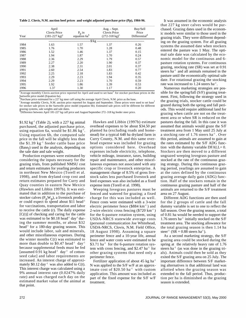
272 JOURNAL OF RANGE MANAGEMENT 53(3), May 2000
$1.92 kg-1 (Table 2), with a 227 kg animalpurchased, the adjusted purchase price,using equation 6a, would be $1.86 kg- 1.Using equation 6b, the computed saleprice in the fall will be slightly less thanthe $1.39 kg - 1 feeder cattle base price(Basef) used in the analysis, depending onthe sale date and sale weight.
Production expenses were estimated byconsidering the inputs necessary for thegrazing trials, from published NMSU costand return estimates for yearling producersin northeast New Mexico (Torell et al.1998), and from dryland crop cost andreturn estimates prepared for Curry andQuay counties in eastern New Mexico(Hawkes and Libbin 1997b). It was esti-mated that in addition to the purchase ofstocker calves (PpWp), a livestock produc-er could expect to spend about $11 head-1
for vaccinations, transportation and laborto receive the cattle (r). The daily expense[C(t)] of checking and caring for the cattlewas estimated to be $0.18 head-1 day-1 dur-ing the summer months, or about $32head-1 for a 180-day grazing season. Thiswould include labor, salt and minerals,and other miscellaneous expenses. Duringthe winter months C(t) was estimated tomore than double to $0.47 head -1 d a y- 1
because supplemental feeds must be fed[assumed 0.91 kg head-1 d a y-1 of cotton-seed cake] and labor requirements areincreased. An interest charge of approxi-mately $0.12 day-1 was also added to C(t).This interest charge was calculated using a9% annual interest rate (0.0247% dailyrate) and was charged each day on theestimated market value of the animal atthat point.
Hawkes and Libbin (1997b) estimateoverhead expenses to be about $34.50 perplanted ha (excluding roads and home-stead) for a typical 648 ha dryland farm inCurry County, N.M. and this same over-head expense was included for grazingoptions considered here. Overheadexpenses include electricity, telephone,vehicle mileage, insurance, taxes, buildingrepair and maintenance, and other miscel-laneous expenses not associated with anyspecific crop or livestock enterprise. Amanagement charge of 8.5% of gross live-stock sales less purchased livestock andfeed expenses was also included as a fixedexpense item (Torell et al. 1998).
Weeping lovegrass pastures must befenced and watered for grazing; a fixedcharge for this was included as well.Fence costs were estimated with a 3-wireelectric perimeter fence ($884 km-1 ) and2-wire electric cross fencing ($720 km-1 )for the 6-pasture rotation system, usingUSDA-NRCS statewide average costs(personal communication Joe Whitehead,USDA-NRCS, Clovis, N.M. Field Office,18 August 1998). Assuming a squareperimeter fence and a 10-year life, annualfence and water costs were estimated to be$3.71 ha-1 for the 6-pasture rotation sys-tem with cross fencing, and $2.47 ha-1 forother grazing systems that need only aperimeter fence.
Fertilizer application of about 45 kg ha-1
N was applied to the S/F w/F at an approx-imate cost of $20.50 ha -1 with customapplication. This amount was included aspart of the fixed expense for the S/F w/Ftreatment.
It was assumed in the economic analysisthat 227 kg steer calves would be pur-chased. Grazing dates used in the econom-ic models were similar to those used in thegrazing trials. They were different depend-ing on the grazing system. For all grazingsystems the assumed date when stockersentered the pasture was 1 May. The opti-mal sale date was calculated by the eco-nomic model for the continuous and 6-pasture rotation systems. For continuousgrazing, stocking rate (SR) was set at 0.91steers ha-1 and all animals remained in thepasture until the economically optimal saledate. For rotational grazing the stockingrate was increased to 1.24 steers ha-1 .
Numerous marketing strategies are pos-sible for the spring/fall (S/F) grazing treat-ment. First, following the strategy used inthe grazing trials, stocker cattle could begrazed during both the spring and fall peri-ods. This would require additional land forgrazing when cattle are not on the treat-ment area or when SR is reduced on thepastures during the fall. In this case it wasassumed that animals would graze the S/Ftreatment area from 1 May until 25 July ata stocking rate of 1.76 steers ha -1 . Overthis period, animals are assumed to gain atthe rates estimated by the S/F ADG func-tion with the dummy variable DFALL= 0.Stockers are then moved to a differentungrazed weeping lovegrass pasture andstocked at the rate of the continuous graz-ing strategy. During this continuous graz-ing period, yearlings are assumed to gainat the rates defined by the continuousgrazing average daily gain (ADG) func-tion. Half of the stockers remain in thecontinuous grazing pasture and half of theanimals are returned to the S/F treatmentarea on 27 August.
Different ADG functions are then usedfor the 2 groups of cattle and the falldummy variable is set to one to reflect thefall season. Over the grazing season, a totalof 0.81 ha would be needed to support the1.76 steers ha-1 initially stocked on the S/Ftreatment area. The stocking allowance forthe total grazing season is then 1.14 has t e e r-1 (SR = 0.88 steers ha-1 ).
As a second marketing strategy, the S/Fgrazing area could be stocked during thespring at the relatively heavy rate of 1.76steers ha-1 (as was done in the grazing tri-als). Animals could then be sold as theyexited the S/F grazing area on 25 July. Theimportant difference between S/F market-ing alternatives is that additional land wasallotted when the grazing season wasextended to the fall period. Thus, produc-tion per ha is diminished as the grazingseason is extended.
Table 2. Clovis, N.M. auction beef prices and weight adjusted purchase price (Pp), 1984-96.
April Aug. - Sept. Buy/SellClovis Price Pp in Clovis Price Price
Year (181-227 kg)a equation 6ab (272-318 kg)c Differentiald
---------------------------------------$/kg --------------------------------------------1984 1.63 1.57 1.37 0.261985 1.76 1.70 1.28 0.481986 1.52 1.46 1.37 0.151987 1.94 1.87 1.70 0.241988 2.36 2.29 1.79 0.571989 2.27 2.20 1.90 0.371990 2.38 2.31 2.01 0.371991 2.60 2.54 1.83 0.771992 2.25 2.18 1.83 0.421993 2.29 2.23 1.94 0.351994 2.29 2.23 1.70 0.591995 1.92 1.86 1.39 0.531996 1.37 1.30 1.17 0.20aAverage monthly Clovis auction price reported for April and used to set basec for stocker purchase prices in theSartwelle price model (Equation 6a).bPurchase price estimated for a 227 kg steer calf using the average April Clovis, N.M. price as the base.cAverage monthly Clovis, N.M. auction price reported for August and September. These prices were used to set basef
for stocker sale prices in the Sartwelle price model (equation 6b). Estimated sale prices will be different for differentgrazing systems, sale weights and sale dates.dDifference between April 181-227 kg calf price and August/September 272–318 kg feeder steer price.
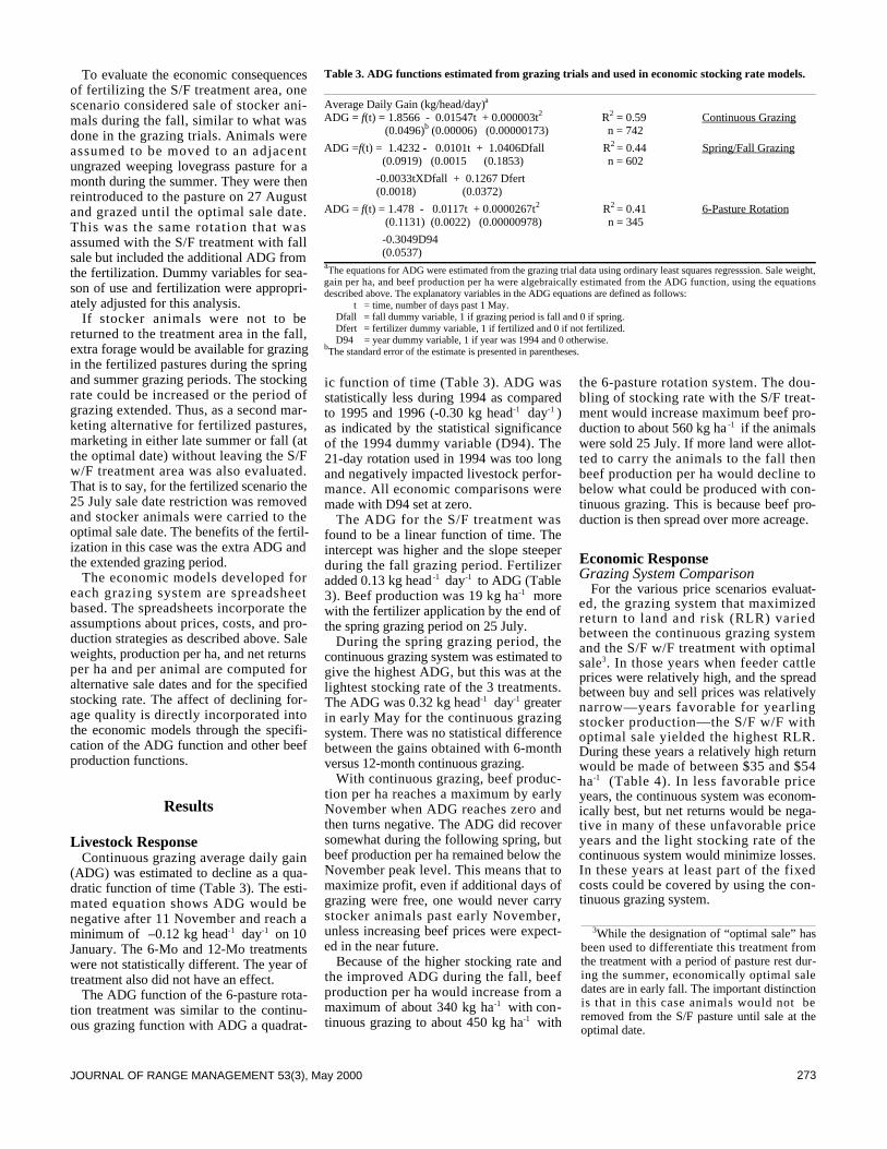
273JOURNAL OF RANGE MANAGEMENT 53(3), May 2000
To evaluate the economic consequencesof fertilizing the S/F treatment area, onescenario considered sale of stocker ani-mals during the fall, similar to what wasdone in the grazing trials. Animals wereassumed to be moved to an adjacentungrazed weeping lovegrass pasture for amonth during the summer. They were thenreintroduced to the pasture on 27 Augustand grazed until the optimal sale date.This was the same rotation that wasassumed with the S/F treatment with fallsale but included the additional ADG fromthe fertilization. Dummy variables for sea-son of use and fertilization were appropri-ately adjusted for this analysis.
If stocker animals were not to bereturned to the treatment area in the fall,extra forage would be available for grazingin the fertilized pastures during the springand summer grazing periods. The stockingrate could be increased or the period ofgrazing extended. Thus, as a second mar-keting alternative for fertilized pastures,marketing in either late summer or fall (atthe optimal date) without leaving the S/Fw/F treatment area was also evaluated.That is to say, for the fertilized scenario the25 July sale date restriction was removedand stocker animals were carried to theoptimal sale date. The benefits of the fertil-ization in this case was the extra ADG andthe extended grazing period.
The economic models developed foreach grazing system are spreadsheetbased. The spreadsheets incorporate theassumptions about prices, costs, and pro-duction strategies as described above. Saleweights, production per ha, and net returnsper ha and per animal are computed foralternative sale dates and for the specifiedstocking rate. The affect of declining for-age quality is directly incorporated intothe economic models through the specifi-cation of the ADG function and other beefproduction functions.
Results
Livestock Response Continuous grazing average daily gain
(ADG) was estimated to decline as a qua-dratic function of time (Table 3). The esti-mated equation shows ADG would benegative after 11 November and reach aminimum of –0.12 kg head-1 day-1 on 10January. The 6-Mo and 12-Mo treatmentswere not statistically different. The year oftreatment also did not have an effect.
The ADG function of the 6-pasture rota-tion treatment was similar to the continu-ous grazing function with ADG a quadrat-
ic function of time (Table 3). ADG wasstatistically less during 1994 as comparedto 1995 and 1996 (-0.30 kg head-1 day-1 )as indicated by the statistical significanceof the 1994 dummy variable (D94). The21-day rotation used in 1994 was too longand negatively impacted livestock perfor-mance. All economic comparisons weremade with D94 set at zero.
The ADG for the S/F treatment wasfound to be a linear function of time. Theintercept was higher and the slope steeperduring the fall grazing period. Fertilizeradded 0.13 kg head -1 day-1 to ADG (Table3). Beef production was 19 kg ha-1 m o r ewith the fertilizer application by the end ofthe spring grazing period on 25 July.
During the spring grazing period, thecontinuous grazing system was estimated togive the highest ADG, but this was at thelightest stocking rate of the 3 treatments.The ADG was 0.32 kg head-1 d a y- 1 g r e a t e rin early May for the continuous grazingsystem. There was no statistical differencebetween the gains obtained with 6-monthversus 12-month continuous grazing.
With continuous grazing, beef produc-tion per ha reaches a maximum by earlyNovember when ADG reaches zero andthen turns negative. The ADG did recoversomewhat during the following spring, butbeef production per ha remained below theNovember peak level. This means that tomaximize profit, even if additional days ofgrazing were free, one would never carrystocker animals past early November,unless increasing beef prices were expect-ed in the near future.
Because of the higher stocking rate andthe improved ADG during the fall, beefproduction per ha would increase from amaximum of about 340 kg ha-1 with con-tinuous grazing to about 450 kg ha-1 with
the 6-pasture rotation system. The dou-bling of stocking rate with the S/F treat-ment would increase maximum beef pro-duction to about 560 kg ha -1 if the animalswere sold 25 July. If more land were allot-ted to carry the animals to the fall thenbeef production per ha would decline tobelow what could be produced with con-tinuous grazing. This is because beef pro-duction is then spread over more acreage.
Economic Response Grazing System Comparison
For the various price scenarios evaluat-ed, the grazing system that maximizedreturn to land and risk (RLR) variedbetween the continuous grazing systemand the S/F w/F treatment with optimals a l e3. In those years when feeder cattleprices were relatively high, and the spreadbetween buy and sell prices was relativelynarrow—years favorable for yearlingstocker production—the S/F w/F withoptimal sale yielded the highest RLR.During these years a relatively high returnwould be made of between $35 and $54h a-1 (Table 4). In less favorable priceyears, the continuous system was econom-ically best, but net returns would be nega-tive in many of these unfavorable priceyears and the light stocking rate of thecontinuous system would minimize losses.In these years at least part of the fixedcosts could be covered by using the con-tinuous grazing system.
3While the designation of “optimal sale” hasbeen used to differentiate this treatment fromthe treatment with a period of pasture rest dur-ing the summer, economically optimal saledates are in early fall. The important distinctionis that in this case animals would not beremoved from the S/F pasture until sale at theoptimal date.
Table 3. ADG functions estimated from grazing trials and used in economic stocking rate models.
Average Daily Gain (kg/head/day)a
ADG = f(t) = 1.8566 - 0.01547t + 0.000003t2 R2 = 0.59 Continuous Grazing(0.0496)b (0.00006) (0.00000173) n = 742
ADG =f(t) = 1.4232 - 0.0101t + 1.0406Dfall R2 = 0.44 Spring/Fall Grazing(0.0919) (0.0015 (0.1853) n = 602
-0.0033tXDfall + 0.1267 Dfert(0.0018) (0.0372)
ADG = f(t) = 1.478 - 0.0117t + 0.0000267t2 R2 = 0.41 6-Pasture Rotation(0.1131) (0.0022) (0.00000978) n = 345
-0.3049D94(0.0537)
aThe equations for ADG were estimated from the grazing trial data using ordinary least squares regresssion. Sale weight,gain per ha, and beef production per ha were algebraically estimated from the ADG function, using the equationsdescribed above. The explanatory variables in the ADG equations are defined as follows:
t = time, number of days past 1 May.Dfall = fall dummy variable, 1 if grazing period is fall and 0 if spring.Dfert = fertilizer dummy variable, 1 if fertilized and 0 if not fertilized.D94 = year dummy variable, 1 if year was 1994 and 0 otherwise.
bThe standard error of the estimate is presented in parentheses.

274 JOURNAL OF RANGE MANAGEMENT 53(3), May 2000
These 2 grazing strategies are very simi-lar. By extending the grazing season to theoptimal sale date, the S/F w/F grazingtreatment is just like the continuous sys-tem, but at nearly twice the stocking rate.In fact, it is likely that the ADG differ-ences are not the result of the grazing sys-tem but rather stocking rate differences.This is consistent with the findings ofHart et al. (1988). These authors foundthat 3 alternative grazing systems, includ-ing season-long continuous grazing, rota-tionally deferred grazing and short dura-tion rotation, did not affect steer gains dif-ferentially when compared at the samestocking rates under proper management.It highlights that stocking rate (SR) needsto be a choice variable in the managementdecision.
There were 3 years (1985, 1991, and1995) when beef prices were such that notproducing at all and losing fixed costs($37 ha-1 ) would have minimized losses(Table 4). Recognizing these years obvi-ously take perfect foresight about futuremarket conditions. Yet, even without thisforesight, some generalizations and con-clusions from the analysis are obvious.First, grazing weeping lovegrass pastureswith yearlings is not an economicallyviable alternative, but if yearlings aregrazed, the optimal grazing strategy forweeping lovegrass pastures is a continuousgrazing scheme whereby stocker cattleenter the pasture and remain there untilbeing sold in early September. This wouldbe about a month earlier then when stock-ers are usually sold from native rangelandin New Mexico (Torell et al. 1998).Second, if yearlings are to be produced,annual planning and analysis will berequired to evaluate economic feasibility,to determine whether to fertilize the pas-tures, and to set the annual stocking rate.Different production strategies and stock-ing rates should be used each year depend-ing on market expectations. Forward con-tracting could potentially be very valuablein helping reduce price risk.
The net economic benefit of fertilizingthe pastures was found to be variable.When market conditions were such thatrelatively heavy stocking rates were mostprofitable, fertilizing to facilitate stockingrate increases resulted in positive econom-ic returns. As shown in Table 4, when theS/F w/F optimal sale was best (during the1986, 1987, 1989, 1990, and 1993 priceyears) fertilization of the pasture resultedin an average RLR increase of $11.56 ha-1,relative to the lightly stocked continuoustreatment without fertilizer. The annual
Table 4. Economic results for alternative stocker grazing systems.
S/F S/F w/F Optimaloptimal S/F with optimal S/F w/F Grazing
Year Continuous Rotation sale fall sale sale fall sale Systema
RLR ($ ha-1)1984 1.93 -4.10 -9.14 -38.11 -4.12 -54.61 1.931985 -48.34 -70.49 -100.28 -60.98 -98.65 -77.88 -37.051986 23.04 24.40 31.54 -27.84 36.58 -44.36 36.581987 36.93 37.99 35.54 -24.95 53.82 -39.17 53.821988 -18.11 -37.57 -76.82 -52.64 -54.91 -66.29 -18.111989 30.28 26.21 8.65 -30.21 35.15 -43.18 35.151990 40.73 38.80 20.85 -26.23 51.94 -38.48 51.941991 -51.97 -83.86 -145.19 -69.53 -121.47 -82.94 -37.051992 15.59 7.31 -14.94 -36.68 8.79 -50.07 15.591993 38.68 36.95 21.66 -26.53 49.99 -39.25 49.991994 -30.63 -53.18 -94.70 -57.80 -76.42 -72.03 -30.631995 -46.71 -70.10 -104.41 -62.15 -98.50 -78.47 -37.051996 -3.41 -7.95 -6.67 -36.83 -9.06 -54.34 -3.41
Average -0.92 -11.97 -33.38 -42.34 -17.45 -57.01 6.28Optimal Sale Date1984 04-Sep 19-Sep 25-Jul 05-Aug 27-Aug 03-Aug 04-Sep1985 01-Sep 13-Sep 25-Jul 16-Jul 24-Aug 29-Jul None1986 04-Sep 19-Sep 25-Jul 05-Aug 27-Aug 03-Aug 27-Aug1987 14-Sep 07-Oct 25-Jul 18-Sep 02-Sep 24-Sep 02-Sep1988 16-Sep 10-Oct 25-Jul 20-Sep 04-Sep 26-Sep 16-Sep1989 18-Sep 15-Oct 25-Jul 22-Sep 05-Sep 29-Sep 05-Sep1990 20-Sep 20-Oct 25-Jul 23-Sep 06-Sep 01-Oct 06-Sep1991 18-Sep 12-Oct 25-Jul 21-Sep 04-Sep 27-Sep None1992 17-Sep 13-Oct 25-Jul 20-Sep 04-Sep 27-Sep 17-Sep1993 19-Sep 17-Oct 25-Jul 22-Sep 05-Sep 29-Sep 05-Sep1994 15-Sep 06-Oct 25-Jul 18-Sep 02-Sep 24-Sep 15-Sep1995 05-Sep 20-Sep 25-Jul 06-Aug 28-Aug 15-Sep None1996 30-Aug 05-Sep 25-Jul 11-Jul 21-Aug 18-Jul 30-Aug
Optimal Sale Weight (kg head-1)1984 357 343 311 318 338 328 3571985 356 341 311 305 337 324 None1986 357 343 311 318 338 328 3381987 361 349 311 347 341 364 3411988 362 350 311 348 341 366 3621989 362 352 311 349 341 367 3411990 362 352 311 349 342 368 3421991 362 351 311 348 341 366 None1992 362 351 311 348 341 366 3621993 362 352 311 349 341 367 3411994 361 349 311 347 341 364 3611995 358 344 311 319 339 358 None1996 355 338 311 302 336 317 355Average 360 347 311 334 340 353
Optimal Beef Production (kg ha-1)1984 327 423 548 280 597 288 3271985 326 421 548 269 595 286 None1986 327 423 548 280 597 288 5971987 330 431 548 301 600 315 6001988 330 432 548 301 601 315 3301989 332 433 548 302 601 316 6011990 332 436 548 302 603 317 6031991 332 432 548 302 601 315 None1992 330 433 548 301 601 315 3301993 332 435 548 302 601 316 6011994 330 431 548 301 600 315 3301995 327 424 548 280 598 310 None1996 325 417 548 265 594 278 325Average 329 429 548 291 599 306aThe "Optimal Grazing System" column repeats production rates and returns for the grazing system that maximizes RLR for thespecified price year (as shown by boxes). If economic losses exceed the assumed fixed costs ($37.05 ha-1) then not producing atall would minimize losses and this is the indicated optimal strategy for that year.

275JOURNAL OF RANGE MANAGEMENT53(3), May 2000
average percentage increase in RLRranged from 29% to 45% during theseyears. However, during other years whenthe light stocking of the continuous treat-ment was economically optimal, fertiliza-tion of the pasture and management as S/Fw/F optimal sale would result in an aver-age loss of $21.78 ha-1 , slightly more thanthe cost of the fertilizer and application.
In the grazing trials, cattle wereremoved from the S/F treatment area eachyear near the end of July. Yet, with fertil-ization it was felt that the grazing seasoncould have been extended, and the eco-nomic analysis has considered that theseason would be extended to the computedoptimal sale date (Table 4). The relativelyheavy stocking rate and extension of thesale date to late August or early Septembermay not be possible during some yearsdepending on rainfall and forage condi-tions, but this extended grazing season isimportant for realizing positive economicreturns from the fertilizer treatment. Forthe S/F w/F treatment, if cattle were soldon 25 July instead of the optimal date, netreturns would have been reduced by anaverage of $16.25 ha-1 over the 1984 to1996 period.
Cropping Versus Grazing Comparison Average New Mexico CRP program
payments have been $93.86 ha-1 ( O s b o r net al. 1995), and the CRP clearly gaveeastern New Mexico farmers a higheraverage rate of return than cropping alter-natives. As a comparison, the CPI wasused to adjust traditional dryland crop pro-duction returns, as reported in Hawkes andLibbin (1997a, 1997b) for the 1984–96period, to constant 1996 levels. Thisanalysis shows that with crop subsidy pro-gram payments in place, Eastern NewMexico dryland farmers had an averagereturn of $37 ha -1 in Curry County and$10 ha -1 in Quay County (Fig. 1). If cropsubsidy payments are removed, as theysupposedly will be (USDA-ERS 1996),average returns over the 1984-96 periodwould have been –$14.94 ha -1 in CurryCounty and –$25.30 ha-1 in Quay County4.Positive returns would have been realizedin only 4 of the 13 years in Curry Countyand 3 of the years in Quay County.
Dryland farming in the Southern GreatPlains has traditionally yielded relativelylow rates of return and removal of cropsubsidies would be expected to causemajor changes in land use for these dry-land farming areas.
Leaving weeping lovegrass pastures inplace for yearling stocker production doesnot appear to provide a viable economicalternative either5. Average return to landand risk (RLR) from grazing yearlingswith beef prices realized over the 1984–96period was estimated to be $6.28 ha -1 i foptimal production strategies were fol-lowed (Table 4). Net returns actually real-
ized will likely be less because the after-the-fact knowledge about fall sale prices,as used in the economic analysis, will notbe available to farmers as they make annu-al production decisions. It is likely thatrealized net returns from grazing will benegative on average. This is similar toexpectations for cropping alternativeswithout price supports. If the estimatedaverage optimal RLR of $6.28 ha- 1 w e r erealized this would still be less than a 1%rate of return on an approximate $494 ha-1
average land investment value (personalcommunication, Trevor Ashby, FarmCredit Services, Clovis, N.M., 5November 1998). Further, positive eco-nomic returns from yearling stocker pro-duction only occurred in 6 of the 13 yearswith optimal production (stocking rate)adjustments (Fig. 1). These stocking rateadjustments must be made to take advan-tage of favorable market conditions and tominimize losses during unfavorable condi-
5This is not to say that grazing weeping love-grass pastures with other animal classes wouldnot be economically feasible. Using lovegrassin rotation with other native grass species or asa place to maintain brood animals may be fea-sible but these alternatives were not consideredin this research.
4This assumes no change in production prac-tices and input use. It would be anticipated thatwithout crop subsidies, crop supplies willdecrease and prices will increase. For this tohappen marginal producers must leave thebusiness. This may well be dryland farms inthe Southern Great Plains that are consideredhere.
Fig 1. Comparison of constant 1996 RLR ($/ha) for traditional cropping alternatives, withand without price support payments, versus grazing weeping lovegrass pastures withyearling stockers.

276 JOURNAL OF RANGE MANAGEMENT53(3), May 2000
tions if on average RLR is to remain posi-tive. As shown in Table 4, no one grazingsystem (constant stocking rate) wouldhave yielded an average positive RLRover the 1984-96 period.
Discussion
In hindsight, the decision to plant rela-tively low-cost weeping lovegrass whenentering the CRP program was an eco-nomic mistake. New CRP enrollmentguidelines (USDA-FSA 1997) have pre-cluded many of these lovegrass pasturesfrom continued enrollment in CRPbecause they do not provide the wildlifecover and habitat desired by the extendedCRP program. Cropping alternatives lookdismal without continued crop subsidies,and grazing the weeping lovegrass pas-tures with stocker cattle does not provide aviable economic alternative either.
Under provisions of the 1996 FederalAgriculture Improvement and Reform(FAIR) Act (P.L. 104-107) federal outlaysto the farm sector will decline until 2002,after which they are scheduled to be elimi-nated. The FAIR Act removes the linkbetween income support payments andfarm prices by providing for 7 annualfixed but declining market transition pay-ments (USDA-ERS 1996). Farmers in theSouthern Great Plains, and other areas,will receive these payments regardless ofwhether they crop or graze the land, pro-vided the acreage was included under pre-vious farm programs.
With these market transition payments,or with continued CRP enrollment, farm-ers have government support until 2002.However, without CRP and without cropsubsidies, dryland farmers in the SouthernGreat Plains face an increasingly uncertainfuture. Farmers have historically beenwilling to accept rates of return on invest-ment that are unacceptable by standardinvestment criteria. As a group, farmersand ranchers are optimists who alwaysbelieve the next season will be a good one.This analysis shows, however, that thefree market commodity pricing proposedfor the future will be especially hard ondryland farmers in the Southern GreatPlains.
What is the future for these lands? Somehave argued that great stretches of thearid, wind-swept Great Plains are not suit-ed to conventional settlement, and neverreally were. They contend that only withever expanding crop and water subsidyprograms was cropping of these marginallands possible, and that it is now time to
tear down the fences, replant native grass-es and restock buffalo and other nativespecies (Popper and Popper 1994,Matthews 1992). This research also findsthat dryland farming in the Southern GreatPlains is likely not economically sustain-able without subsidy programs. It is wide-ly believed that these government pro-grams have been capitalized into land val-ues as the continued perpetual existence ofthese programs came to be expected(Helmberger 1991). If elimination of theseprice support programs is in fact imple-mented, major market adjustments wouldbe expected. Land values should fall andmarginal farming areas should revert torangeland and natural vegetation. Somebelieve that this transition would be desir-able and that the Great Plains can providesustainable income only by reverting tothe natural rangeland vegetation and cropsoriginally found on the prairies (Eisenberg1989). The future use and management ofthese farming areas has major implicationsfor rural communities and the people wholive there.
Literature Cited
Eisenberg, E. 1989. Back to Eden. AtlanticMonthly, November:57–89.
Hart, R.H., M.J. Samuel, P.S. Test, and M.A.Smith. 1988. Cattle, vegetation, and eco-nomic responses to grazing systems andgrazing pressure. J. Range Manage.41:282–286.
Hawkes, J.M. and J.D. Libbin. 1997a. Along-term look at crop profitability in NewMexico: cost and return estimates for 1984–1993. New Mex. State Agr. Exp. Sta. Res.Rep. 718, Las Cruces, N.M..
Hawkes, J.M. and J.D. Libbin. 1997b. C r o pcost and return estimates in New Mexico,1995. New Mex. State Agr. Exp. Sta.Research Report 716, Las Cruces, N.M..
Helmberger, P.G. 1991. Economic analysis offarm programs. McGraw Hill, Inc., NewYork, N.Y.
Hildreth, R.J. and M.E. Riewe. 1963. Grazingproduction curves II. Determining the eco-nomic optimum stocking rate. Agron. J.55:367–372.
Huffaker, R.G. and J.E. Wilen. 1991. A n i m a lstocking under conditions of declining foragenutrients. Amer. J. Agr. Econ. 73:1213–1223.
Matthews, A. 1992. Where the buffalo roam.Grove Press, New York, N.Y.
National Oceanic and AtmosphericAdministration (NOAA). Various Issues.Climatological data, New Mexico monthlyprecipitation departure from individual sta-tions' normals. National Climatic DataCenter. Asheville, N.C.
Osborn, C.T., F. Llacuna, and M.Linsenbigler. 1995. The ConservationReserve Program: enrollment statistics for
signup periods 1-12 and fiscal years 1986-93.United States Dept. of Agr., Econ. Res. Serv.(ERS) Stat. Bull. 925, Washington, D.C.
Popper, F.J. and D.E. Popper. 1994. G r e a tPlains: checkered past, hopeful future. Forumfor Appl. Res. and Public Policy. Winter ‘94,9:89–100.
Sartwelle, J.D., III, J.R. Mintert, T.C.Schroeder, M.R. Langemeier, and F.Brazle. 1995. Feeder cattle price differen-tials: how much do they change over time?Paper presented at the Southern Agr. Econ.Assoc. Meetings, Jan. 29– Feb. 1, 1995.
Sartwelle, J.D., III , F.K. Brazle, J.R.Mintert, T.C. Schroeder, and M.R.Langemeier. 1996a. Buying and sellingfeeder cattle: the impact of selected charac-teristics on feeder cattle prices. CooperativeExtension Service, Kansas State University,Manhattan, Pub. MF-2162.
Sartwelle, J.D., III, F.K. Brazle, J.R.Mintert, T.C. Schroeder, and M.R.Langemeier. 1996b . Improving the value ofyour calf crop: the impact of selected charac-teristics on calf prices. CooperativeExtension Service, Kansas State University,Manhattan, Pub. MF-2142.
Torell, L.A., J.M. Hawkes, and T.D.Stromei. 1998. Range Livestock Cost andReturn Estimates for New Mexico, 1996.New Mex. State Agr. Exp. Sta. Res.Rep.726,Las Cruces, N.M.
Torell, L.A., R.E. Kirksey, G.B. Donart, andJ.D. Libbin. 1999. Economics of Croppingand Grazing Alternatives for CRP Lands inthe Southern Great Plains. I n : E.T. Bartlettand L.W. Van Tassell (eds). SymposiumProc. Sponsered by Western CoordinatingCommittee on Range Economics --(WCC-55),- Soc. Range Manage. Meetings, Omaha,Neb., Feb.
United States Department of Agriculture,Economic Research Service (USDA-ERS).1996. Provisions of the Federal AgricultureImprovement and Reform Act of 1996. Agr.Info. Bull. 729, Washington, D.C.
United States Department of Agriculture,Farm Service Agency (USDA-FSA). 1997.Fact sheet: Conservation Reserve Programsign-up 16 environmental benefits index.October. Washington, D.C.
Vallentine, J.F. 1990. Grazing management.Academic Press, Inc. New York, N.Y.
Workman, J.P. 1986. Range economics.MacMillan Publishing Co. New York, N.Y.

277JOURNAL OF RANGE MANAGEMENT 53(3), May 2000
Abstract
To examine the effect of grazing and potential interactionsamong grazing and biological traits of plants, we studied patchdynamics, seed production, and seedling survival in aMediterranean population of the perennial grass Phalaris aquati -ca L. in grazed and ungrazed plots in southern Spain. Grazing bycattle induced an important (70%) decrease in the abundance ofplants over 4 growing seasons. In the ungrazed plots, abundanceof plants remained stable. Within these plots there was some(30%) spatial replacement of plants. However, replacement wasby tillering and not by genets, genetically different individualsproduced from seeds. The lack of genet replacement within theungrazed plots agrees with results on mortality of young plantsthat were obtained from an independent field experiment, inwhich 85–95% of plants in different cohorts died within 1 to 3growing seasons. This mortality of seedlings and young plantswas concentrated in summers, especially when drought was pro-longed. In contrast, seed production was apparently not a limit-ing factor for plant recruitment in ungrazed plots as seed outputof the perennial grass (25,312 ± 3,255 seeds m-2) was of the samemagnitude as seed output in annual grasses that were abundantin the study site. Intensive grazing limited tiller production,patch size, and a summer drought limited recruitment of newadult individuals. These factors resulted in a low tolerance toepisodes of high stocking rates from which the perennial grasswas unable to recover.
Key Words: mediterranean grassland, overgrazing, perennialgrasses, plant recruitment, seedlings survival, summer-drought
Mediterranean grasslands in Spain, California, Israel, andAustralia are dominated by annuals (Rivas and Rivas 1963,Rossiter 1966, Gulmon 1977). In these grasslands perennialgrasses are much less abundant. However, the latter species showpotential for improving the value of grasslands for use by live-stock because they have longer growing seasons than annuals(Joffre et al. 1987).
Much evidence supports the hypothesis that overgrazing andother human disturbances are major causes of scarcity of perenni-al grasses in these grasslands (Joffre et al 1987, Rossiter 1966,Stoddart et al. 1975). For instance, in Spain and elsewhere in the
Mediterranean basin, grazing has been continuously important forat least 7000 years (Naveh 1987). In California, overgrazing bylivestock and an exceptional drought in the 1860s promotedexpansion of annuals at the expense of perennial bunchgrasses(Huenneke 1989, Heady et al. 1991). In Israel, perennial grassesconsistently decrease in grazed areas compared with adjacentungrazed plots (Noy-Meir et al. 1989). However, little is knownabout the mechanisms implied in the decrease of perennial grass-es. In this study we analyzed effects of grazing on vegetativegrowth and reproduction of a perennial grass, Phalaris aquaticaL., which occurs in Mediterranean grasslands of southern Spain.We also studied the inherent rate of recruitment of new individu-als in the population.
Materials and Methods
Farm description and managementThe study was conducted on a representative farm in Sierra
J. Range Manage.53: 277–281 May 2000
Effect of grazing on the population biology of P h a l a r i saquatica
MARÍA JOSÉ LEIVA AND ROCÍO FERNÁNDEZ ALÉS
Authors are assistant professor and full professor, Departamento de Biología Vegetal y Ecología, Universidad de Sevilla. Apartado 1095, 41080-Sevilla, Spain.
This study was supported with a grant from the Research and DevelopmentProgram of the Spanish Government. The authors wish to thank Imanuel Noy-Meirand Maricruz Diaz-Barradas for useful comments and corrections on this manu-script. We also thank Manuel Ojedo, Isabel Roldán, Jose Laffarga and Ana Cocafor field assistance.
Manuscript accepted 17 Aug. 1999.
Resumen
Para examinar el efecto del pastoreo y potenciales interac-ciones entre pastoreo y características biológicas de las plantasen una población del sur de España de la gramínea perennePhalaris aquatica L, se ha estudiado la dinámica de manchas, laproducción de semillas y la supervivencia de plántulas en parce-las pastadas y sin pastar. El pastoreo por ganado vacuno produ-jo importantes (70%) decrementos de abundancia a lo largo de 4estaciones de crecimiento. En las parcelas no pastadas la abun-dancia de las plantas se mantuvo constante pero hubo algún(30%) recambio espacial de las plantas. Este recambio fue porahijamiento y no por instalación de nuevos individuos. La fatiade reemplazamiento de individuos geneticamente distintos en lasparcelas no pastadas concuerda con los resultados sobre mortali-dad de plantas jóvenes obtenidos en un experimento independi-ente. Entre el 85 y el 95% de las plantas jóvenes de distintascohortes murieron durante 1 a 3 estaciones de crecimiento. Estamortalidad se concentró durante el verano, especialmente cuan-do le sequía fue prolongada. Por el contrario la producción desemillas no fue, aparentemente, un factor limitante en las parce-las no pastadas ya que dicha producción (25.3 ± 3.255 semillas m- 2)fue de la misma magnitud que la producción de semillas devarias gramíneas anuales abundantes en el área de estudio. Elefecto del intenso pastoreo limitando el ahijamiento y el tamañode las manchas y el efecto de la sequía estival limitando el reclu-tamiento, resultaron en una baja tolerancia a episodios de altaspresiones ganaderas de los que la gramínea perenne no pudorecuperarse.

278 JOURNAL OF RANGE MANAGEMENT 53(3), May 2000
Morena, 30 km north of Seville, southernSpain (370 40'N, 50 59'W, 280 m above sealevel), from 1988 through 1991. Climatewas Mediterranean with 720 mm meanannual precipitation and 16 °C mean annualtemperature. Rainfall was concentratedfrom mid-September to mid-May and wasusually negligible during the summer.However, the length of dry and wet peri-ods varies greatly among years in thisregion (Ortega 1987). The vegetation wasa holm oak savannah (40 trees ha- 1) withthe understory dominated by annuals. Thefarm was dedicated to extensive beef cat-tle production with a total of 350 head ofcattle on 1,200 ha of terrain. Cattle fol-lowed the breed composition of the majorbeef cattle of the region. Cows were of alocal land race called Retinta and bullswere Retinta and Charolais. Cattle man-agement followed the usual practices ofthe region. Animals were divided in lotswith different composition (cows in preg-nancy or lactation, dry cows, bulls,heifers) that moved rotationally among the10 paddocks of different size (20–200 ha)in which the farm was divided. The num-ber and kind of grazing animals in eachpaddock and the time they remained inthem during each year did not depend ongrassland offer but on other criteria suchas facility for handling animals (Daza1997). As a consequence, these parametersvaried greatly among paddocks and fromyear to year. The paddocks that were clos-er to the headquarters often had high graz-ing intensity at peak intervals and weregrazed by cows in late pregnancy and lac-tation because these paddocks wereequipped with feedings troughs and ani-mal health-care installations. Calves wereborn from September until January and theoff-spring were usually sold at weaning.
Study site The study was conducted in a paddock
about 31 ha in size that was close to theheadquarters. The terrain was flat andsoils, derived from granite rock, wereslightly acid. Grassland was composed ofan annual sward dominated by the grassesBromus hordeaceous L . , A g r o s t i s p o u r -retii Willd, and Vulpia geniculata ( L . )Link, the legume Trifolium glomeratumL., and the forbs Chamaemelun mixtum(L.) All. and Leontodon longirrostris(Finch & P.D. Sell) Talavera. There werealso interspersed patches of the perennialgrass Phalaris aquatica L. This perennialgrass was re-seeded in the paddock in1968 with seeds collected from scatteredindividuals naturally occurring in the sur-rounding area (Joaquin Terceño personal
comm. 1987). There was also a 0.25 hafenced plot, which excluded grazing, inthe middle of the paddock. This plot wasestablished 3 years before the beginning ofour study. At this time, species composi-tion inside and outside the fence was verysimilar (Joffre 1987).
Grazing treatmentThe fenced plot continued ungrazed dur-
ing the years of our study. For the rest ofthe paddock, information on the numberand kind of animals, grazing season, sup-plementary feedings and animal care wasobtained from the farmer (Miguel Hugespersonal comm. 1991 and 1999) and frompersonal observations during our visits tothe field. From these data we calculatedCattle Units (C.U.) following recommen-dations of the French Institute ofAgronomic Research (INRA), which arebased on energy requirements of the ani-mals (Jarrige 1990). A dry cow (500 kg)corresponded to 1 C.U., a cow in latepregnancy or lactation to 2 C.U., and aheifer (200 Kg) to 1.3 C.U. The stockingrate per month was calculated as the num-ber of C.U. that grazed the paddock eachmonth (during the grazing season) dividedby the size (in ha) of the paddock. We alsocalculated the mean stocking rate per yearas the stocking rate per month multipliedby the length (in months) of the grazingseason and divided by 12 (number ofmonths per year; Table 1).
Most animals that grazed our paddockwere cows in late pregnancy and lactation,especially during the first 2 years of thestudy. This was due to the proximity to theheadquarters and the facilities for supple-mentary feeding and vaccination of theoffspring in the site. The herd size wassimilar in 1988 and 1989 but i t wasincreased in 1990 and 1991 by adding 10replacement heifers. Animals were usually
moved to the paddock in early-winter,except for the year 1990 when they weremoved in mid-autumn. This year, cattleremained in the paddock for 8 monthsinstead of the 3 or 4 months of the otheryears (1987, 1988, and 1991). As a resultmean stocking rate per year was 3-foldhigher in 1990 than in the other years.Animals were supplemented yearly withstraw and dry fodder from November untilFebruary and were provided with salt.
Patch dynamics and seed production inPhalaris aquatica.
In December of 1987, 4 permanent tran-sects, 0.6 m x 10 m, were established inthe grasslands. Each transect was dividedinto 150, 20- x 20-cm cells. Transectswere placed on a mixed sward with patch-es of Phalaris and some patches of annu-als. Two transects were inside the fenceand the others were outside it, about 30 mapart from the former transects. In winterof 1988, a presence-absence map of eachtransect was recorded by hand, based onvisual observations. Cells in which 1 ormore shoots of P h a l a r i s occurred wereconsidered as present, and cells with noshoots of the species as absent. Mappingwas conducted twice a year (in winter andspring) until winter of 1991.
To study seed production, in summer of1988 we chose at random 15 presence-cells within each transect. All the spikes ofP h a l a r i s produced inside each cell weremarked and were measured for length. Thenumber of seeds per spike was estimatedusing a regression equation of the numberof seeds and the length of the spike(seeds/spike = 1.43 *length of the spike(in mm) + 26.23) (r = 0.67, p < 0.01). Thisequation was obtained on a set of 20spikes that were collected close to thetransects inside the fence. In the grazedtransects, all spikes that were marked were
Table 1. Grazing treatment. The length of the grazing seasons, the number and kind of animalsthat grazed the paddock each year and the calculated stocking rates are indicated.
Stocking rate Mean stockingYear Grazing season Herd composition per month1 rate per year1
-------------(C.U. ha -1)--------------- 1988 Jan. - April 17 Lp.2 and lactation cows 1.4 0.47
10 dry cows
1989 Jan. - April 18 Lp. and lactation cows 1.4 0.478 dry cows
1990 Oct.- May 23 Lp. and lactation cows 2 1.354 dry cows
10 replacement heifers
1991 Jan.- March 21 Lp and lactation cows 1.9 0.475 dry cows
10 replacement heifers1Cattle Units, calculated by procedure of Jarrige (1990)2Late pregnancy.

279JOURNAL OF RANGE MANAGEMENT53(3), May 2000
eaten by cattle before seed ripening. Thus,there was no seed input into the soil’s seedbank in these transects, and the spikes pro-duced within them were not considered inour study.
Plant recruitmentIn November 1987, eight, 50 cm x 50
cm plots were established at regular inter-vals inside the fence. Plots were sown at5,000 seeds m-2 with seeds of Phalaris thathad been collected in spring at the sitedescribed above. Plots were free of patch-es of P h a l a r i s or any other perennialbefore sowing and were about 30 m apartfrom the closest patches of the perennialgrass. To avoid competition among youngplants of Phalaris and annuals, weremoved all seedlings of annuals by handin early autumn, before sowing the peren-nial grass (treatment annuals-). In theother 4 plots, annual seedlings were notremoved (treatment annuals +). At the endof the first growing season (May 1988),the number of individuals of Phalaris thatwere established in each plot was recorded(the 1988 cohort). The censuses wererepeated at the beginning and at the end ofthe growing seasons of the next 3 years(1989–1991). Individuals of P h a l a r i soccurring inside each plot were assumedto belong to the initial seedling cohortbecause the newly established plants didnot produce seeds during our study, pre-sumably because they were too young.Moreover, seed drop from nearby patchesof P h a l a r i s inside the plots was unlikely tooccur because of the long distance. Insidethe annuals- plots, competition amongplants was assumed to be of low intensitybecause of the low density (100 seedlingsm - 2 ) of the established individuals ofP h a l a r i s from the beginning of the study.
Most annuals + plots were destroyed byrodent mounds during the first winter andwe had to discard these plots from theexperiment. A new experiment was per-formed in autumn of 1990 using 8 newplots that were assigned to identical treat-ments as in the first experiment, and theindividuals established from this sowing(the 1990 cohort) were similarly monitored.
Results
Annual rainfall and its distribution var-ied greatly among years (Fig. 1). Both1988 and 1990 were wet years with 1454and 1268 mm rainfall , respectively.However, in 1988, the dry season wasvery short (112 days), while in 1990 it wasvery long (169 days). The other 2 years,
1989 and 1991 were dry, with 553 and 585mm of rainfall, respectively. The length ofthe dry season in 1989 was intermediate(130 days).
In the grazed transects, frequency ofP h a l a r i s (i.e., presence cells/total numberof cells) decreased slowly from the begin-ning of the study until spring of 1990 (Fig.1). However, frequency of the speciesdecreased more rapidly (62% losses) inwinter of 1991, after the intensification ofgrazing. In the ungrazed transects, fre-quency of P h a l a r i s changed very littleduring the years of this study (Fig. 1). Themajority (67%) of cells in which thespecies occurred in autumn of 1989 (class1 cells) contained it also at the end of thestudy (Table 2). We called these cells“permanents.” Losses of Phalaris from therest of class 1 cells were compensated bycolonization of new cells (class 2 to 7cells). However, colonization wasephemeral and the species disappearedagain from most of these cells. Similarpatterns (i.e., ephemeral colonization ofsome cells) were found in the grazed tran-sects. However, in the latter transects, col-onization did not compensate losses of thespecies from class 1 cells and net changesin frequency were negative. Cell coloniza-tion took place in the border of permanentcells and was due to spread of vegetative
tillers. No seedlings of P h a l a r i s w e r eobserved in the transects during our study.
Protected transects of Phalaris produced25,312+3,255 seeds m-2 (mean + standarddeviation) in 1988. Although seed outputvaried greatly among years and productionin 1988 cannot be taken as an absolutevalue, we observed significant spike andseed production in P h a l a r i s during the 4years of this study.
Seedlings of P h a l a r i s that were estab-lished in experimental plots in spring of1988 (i.e., 1988 cohort) comprised 2% ofthe sown seeds. Seedlings that were estab-l ished in spring of 1990 (i .e . , 1990cohorts) comprised 1.5% and 0.9% of theseeds that were sown in the annuals - andannuals + plots. Seedling survival wasvery low in the 2 cohorts (Fig. 2). About91% of the individuals of the 1988 cohorthad died by the end of the experiment. Thehighest mortality (57%) was suffered dur-ing the first summer, when seedlings werevery young. Mortality was lowest (7%) inthe second summer when plants wereolder and drought length was intermediate.Mortality increased again (22%) the thirdsummer when drought was the longestduring the study period. During the lastdry season, the majority of seedlings ofthe 1990 cohort died also. In this cohortmortality was moderately lower (83%)
Fig. 1. Frequency of Phalaris (presence cells/total number of cells) in grazed and ungrazedtransects (each point represents the mean of 2 transects (SE bars). Bars indicate monthlyrainfall.
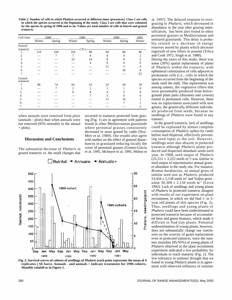
280 JOURNAL OF RANGE MANAGEMENT53(3), May 2000
when annuals were removed from plots(annuals - plots) than when annuals werenot removed (95% mortality in the annual+ plots).
Discussion and Conclusions
The substantial decrease of P h a l a r i s i ngrazed transects vs. the small changes that
occurred in transects protected from graz-ing (Fig. 1) are in agreement with patternsfound in other Mediterranean grasslandswhere perennial grasses consistentlydecreased in areas grazed by cattle (Noy-Meir et al. 1989). Our results also agreewith studies on the effect of general distur-bances in grassland reducing locally thecover of perennial grasses (Gomez-Garcíaet al. 1995, McIntyre et al. 1995, Milton et
al. 1997). The delayed response to over-grazing in P h a l a r i s, which decreased inabundance in the year after grazing inten-sification, has been also found in otherperennial grasses in Mediterranean andsemiarid grasslands. This delay is proba-bly related to a decrease of energyreserves stored by plants which decreaseregrowth of new tillers in autumn (Trlicaand Cook 1972, Singh et al. 1980).During the years of this study, there wassome (30%) spatial replacement of plantsof P h a l a r i s within the transects, withephemeral colonization of cells adjacent topermanent cells (i.e., cells in which thespecies occurred from the beginning of thestudy until the end). This replacement wasamong ramets, the vegetative tillers thatwere presumably produced from below-ground plant parts (rhizomes and crowns)rooted in permanent cells. However, therewas no replacement associated with newgenets, the genetically different individu-als produced from seeds, because noseedlings of P h a l a r i s were found in anytransect.
In the grazed transects, lack of seedlingscould be explained by almost completeconsumption of P h a l a r i s spikes by cattlebefore seed dispersal, effectively prevent-ing seed input to the soil. However,seedlings were also abscent in protectedtransects although P h a l a r i s plants pro-duced and dispersed abundant seeds eachyear. In 1988, seed output of P h a l a r i s(25,312 ± 3,255 seeds m- 2) was similar toseed output of representative annual grass-es abundant in the study site. For instance,Bromus hordeaceus , an annual grass ofsimilar seed size as P h a l a r i s, produced53,434 ± 2,138 seeds m- 2 and Vulpia genic -u l a t a 30,308 ± 2,150 seeds m - 2 ( L e i v a1992). Lack of seedlings and young plantsof Phalaris in protected transects disagreewith results of our experiment on plantrecruitment, in which we did find 1- to 3-year old plants of this species (Fig. 2).Thus, seedlings and young plants ofPhalaris could have been understimated inprotected transects because of accumulat-ed litter and green biomass, which made itdifficult to find tiny plants. Potentialunderestimation of young plants, however,does not substantially change our conclu-sion on the scarcity of genet replacementeven in protected transects, since the sum-mer mortality (85-95%) of young plants ofPhalaris observed in the plant recruitmentexperiment indicated a low probability forindividuals to reach maturity (Fig. 2). Thelow tolerance to summer drought that wefound in young Phalaris plants is in agree-ment with observed influence of summer
Table 2. Number of cells in which Phalaris occurred at different times (presences). Class 1 are cellsin which the species occurred at the beginning of the study. Class 2 are cells that were colonisedby the species in spring of 1988 and so on. Values are total number of cells in fenced and grazedtransects.
Cell class 1988 1989 1990 1991 Winter Spring Winter Spring Winter Spring Winter
Fencedtransects ---------------------------------------------( N )------------------------------------------------------------
1 119 104 104 98 94 86 802 — 7 7 4 4 4 23 — — 23 14 8 8 24 — — — 4 0 0 05 — — — — 11 5 46 — — — — — 20 87 — — — — — — 25
Grazedtransects
1 80 74 65 53 52 44 202 — 7 2 1 1 1 03 — — 6 4 4 2 04 — — — 7 5 0 05 — — — — 11 10 16 — — — — — 7 17 — — — — — — 2
Fig. 2. Survival curves of cohorts of seedlings of Phalaris (each point represents the mean of 4replicates ( SE bars). Annuals - and annuals + indicate treatments for 1990-cohorts.Monthly rainfall as in Figure 1.
281JOURNAL OF RANGE MANAGEMENT53(3), May 2000
drought on seedling survival in manyspecies in other Mediterranean ecosystems(Horton and Kraebel 1955, Keeley andZedler 1978, Aschman 1984, Frazer andDavis 1988). Populations of herbaceousperennials have been considered to be at aregressive stage when they have lost theirability to produce seeds and replace genets(Harper 1977). This stage can also bereached if, as in our case, mortality ofyoung plants is very high and there is alack of recruitment of adult plants.Mediterranean populations of some endan-gered plants that fail in recruitment of newindividuals also show high sensitiviy tograzing (Aparicio and Guisande 1997).
We conclude that in the Mediterraneanpopulation of P h a l a r i s studied, grazingdecreased tiller production and patch size.Summer drought limited recruitment ofnew adult individuals, resulting in a lowtolerance to episodes of heavy grazingfrom which the perennial grass was unableto recover. Recovery could have beenhigher under more favorable climatic andedaphic conditions. We propose that, inany given habitat, a grazing intensityshould be considered as overgrazing if itpromotes irreversible declines in popula-tions. Thus, the threshold level of over-grazing is species and habitat dependent.
Literature Cited
Aparicio, A. and R. Guisande. 1997.Replenishment of the endangeredEchinospartum algibicum ( G e n i s t e a e ,Fabaceae) from the soil seed bank. Biol.Conserv. 81:267–273.
Aschmann, H. 1984. A restrictive definition ofMediterranean climates. Bull. Soc. Bot. Fr.,Actual. Bot.131:21–30.
Daza, A. 1997. Sistemas de producción de vacunode carne en zonas de dehesa, p. 193–211. I n: C.Buxadé-Carbó (ed.), Vacuno de Carne: a s p e c-tos clave. Mundiprensa. Madrid, Spain.
Frazer, J. M. and S. D. Davis. 1988.Differential survival of chaparral seedlingsduring the first summer drought after wild-fire. Oecologia 76:215-221.
Gomez-García, D., C. E. Borghi, and S. M.Giannoni. 1995. Vegetation differencescaused by pine vole mound building in sub-alpine plant communities in the SpanishPyrenees. Vegetatio 117:61–67.
Gulmon, S.L. 1977. A comparative study ofthe grassland of California and Chile. Flora166: 261–278.
Harper, J.L. 1977. Population biology ofplants. Academic Press. London, England.
Heady, H. F., J.W. Bartolomew, M.D. Pitt,G. D. Savelle, and M.C. Stroud. 1991.California Prairie, p. 313-335. I n: CouplandR.T. (ed.), Ecosystems of the world, NaturalGrassl. Elsevier, Amsterdam, TheNetherlands.
Horton, J. S. and C. J. Kraebel. 1955.Development of vegetation after fire in thechamise chaparral of southern California.Ecol. 36:244–262.
Huenneke, L. F. 1989. Distribution andregional patterns of Californian grasslands, p.1-12. In: L. F. Huenneke and H. A. Mooney(eds.), Grassland structure and function:California annual grassland. KluwerAcademic Publisher, Dordrecht, So. Africa.
Jarrige, J. 1990. Alimentación de bovinos,ovinos y caprinos. Mundiprensa. Madrid,Spain.
Joffre, R. 1987. Contraintes du milieu etréponses de la végétation herbacée dans lesdehesas de la Sierra Norte (AndalousieEspagne) Thèse de doctorat USTLMontpellier, France.
Joffre, R., M. J. Leiva, S. Rambal, and R.Fernandez Alés. 1987. Dynamique racinaireet extraction de l´eau du sol par des gram-inées pérennes et annuelles méditer-ranéennes. (Ecol. Plant. 8:181-194.
Keeley, J. E. and P. J. Zedler. 1978.Reproduction of chaparral scrubs after fire: Acomparison of sprouting and seeding strate-gies. Amer. Midl. Nat. 99:142–161.
Leiva, M. J. 1992. Factores que limitan a lascomunidades de gramineas perennes en lospastos mediterráneos de la Sierra norte deSevilla. Tesis Doctoral Univ. Seville, Spain.
McIntyre, S., S. Lavorel, and R. M.Tremont. 1995. Plant life history attributes:Their relationship to disturbance response inherbaceous vegetation. J. Ecol. 83: 31-44.
Milton, S.J., W.R.J., Dean, and S. Klotz.1 9 9 7 . Effects of small-scale animal distur-bances on plant assemblages of set-aside landin Central Germany. J. Veget. Sci. 8: 45-54.
Naveh, Z. 1987. Landscape ecology, manage-ment and conservation of European and lev-ant Mediterranean uplands, p. 641-657. In: J.D. Tenhunen, F. M. Catarino, O. L. Lange,and W. C. Oechel (eds.), Plant response tostress. Functional analysis in Mediterraneanecosystems. Springer-Verlag, Berlin,Germany.
Noy-Meir, I., M. Gutman, and Y. Kaplan.1989. Responses of mediterranean grasslandplants to grazing and protection. J. Ecol. 77:290–310.
Ortega, F. 1987. Cambios temporales de lospastos anuales mediterráneos de la SierraNorte de Sevilla en relación con el régimende precipitación. Tesis Doctoral. Univ.Seville, Spain.
Rivas, S. and S. Rivas. 1963. Estudio y clasifi-caciún de los pastizales españoles.Publicaciones del Ministerio de Agricultura.Madrid, Spain.
Rossiter, R C. 1966. Ecology of the mediter-ranean annual-type pasture. Advan. Agron.18:1–56.
Singh, J. S., M. H. Trlica, P. G. Risser, R. E.Redmann, and J. K. Marshall. 1980.Autotrophic subsystem, p. 60-190. I n: A. I.Breymeyer and G. M. Van Dyne (eds.),Grasslands, systems analysis and man.Cambridge Univ. Press. Cambridge, England
Stoddart, L. A., A. D. Smith, and T. W. Box.1975. Range management 3rd ed., McGraw-Hill, New York, N.Y.
Trlica, M. J. and C. W. Cook. 1972.Carbohydrate reserves of crested wheatgrassand Russian wildrye as affected by develop-ment and defoliation. J. Range Manage.25:430-435.

282 JOURNAL OF RANGE MANAGEMENT53(3), May 2000
Abstract
Animals used in grazing trials with small paddocks usuallyhave not been exposed to the experimental site and relatedresearch procedures. Grazing trials conducted in May andAugust 1996 on smooth bromegrass (Bromus inermis L e y s s . )quantified forage removal and grazing time of heifers adapted ornot adapted to small paddocks. Treatments consisted of adaptingheifers for 4 days to small paddocks (0.054 ha) and a controltreatment of heifers continuously stocked in larger paddocks(>16 ha). On day 5, each group of heifers was moved to similarsmall paddocks and forage utilization and cattle grazing timeswere measured after 4 and 24 hours of grazing. In May, whensward structure was comparable in the large and small pad-docks, tiller height reduction, leaf length reduction, herbage bio-mass reduction, and grazing time were similar (P > 0.10) forexperienced and inexperienced heifers after 4 and 24 hours ofexposure to day-5 paddocks. In August, when sward structurediffered between the large and small paddocks, leaf length reduc-tion after 4 hours was greater (P < 0.10) by experienced cattlethan inexperienced cattle. Herbage reduction in August by expe-rienced cattle was 435 kg ha-1 greater (P < 0.05) than by inexperi-enced cattle after 24 hours. Cumulative grazing time was 76 min-utes (P < 0.10) greater at 4 hours for the experienced cattle thanthe inexperienced cattle. Grazing animals appear to adapt imme-diately to small paddocks but other unfamiliar grazing condi-tions, e.g., sward structure, may require short adaptation periodsfor experimental animals.
Key Words: grazing trials, ingestive behavior, sward structure
Reliability of information from grazing management researchdepends in part on the ingestive behavior of the experimental ani-mals. Grazing trials commonly are conducted in small paddocks(<0.5 ha) with high stock densities and short grazing periods(Binnie and Chestnutt 1991, Howard et al. 1992, Forbes andColeman 1993). Small paddocks greatly reduce logistic and fund-ing requirements and allow researchers to implement studies inwhich confounding variables can be controlled more effectively.Investigators generally assume that ingestive behavior of grazinganimals is not affected by paddock size, periodic movement inand out of small paddocks, or experience with different sward
structures. As a consequence, animals used in trials with smallpaddocks often lack experience or adaptation to grazing condi-tions in small paddocks. Various researchers (Forbes andHodgson 1985, Bailey et al. 1989, Dougherty et al. 1992, Krysland Hess 1993) have questioned experimental procedures that donot allow for exposure of animals to conditions unique to theexperimental design prior to initiation of a grazing trial.
Information is lacking on grazing animal response to smallexperimental paddocks that could influence results. The objectiveof this study was to quantify forage removal and grazing time ofcattle that were either adapted or not adapted to small paddocks(0.054 ha).
J. Range Manage.53: 282–286 May 2000
Forage removal and grazing time of cattle on smallpaddocks
ROBERT C. BROWELEIT, WALTER H. SCHACHT, BRUCE E. ANDERSON, AND ALEXANDER J. SMART
Authors are former graduate assistant, associate professor, professor, and technologist, Department of Agronomy, P.O. Box 830915, University of Nebraska,Lincoln, Neb. 68583-0915.
Authors thank Dr. J. Gosey and Dr. J. Kinder, UNL Animal ScienceDepartment, for providing animal and land resources.
Published as journal article 12311, Agriculture Research Division, University ofNebraska.
Manuscript accepted 19 Aug. 1999.
Resumen
Los animales utilizados en experimentos de apacentamientocon potreros pequeños usualmente no han sido expuestos al sitioexperimental y los procedimientos de investigación relacionados.En ensayos de apacentamiento, conducidos en mayo y agosto de1996 en praderas de "Smooth bromegrass" (Bromus inermisLeyss.), se cuantifico la remoción de forraje y el tiempo deapacentamiento de vaquillas adaptadas y no adaptadas apotreros pequeños. Los tratamientos consistieron en adaptar lasvaquillas a potreros pequeños (0.54 ha) durante un periodo de 4días y un tratamiento control de vaquillas que habían apacenta-do continuamente en potreros grandes (> 16 ha). En el día 5,cada grupo de vaquillas se movió a potreros pequeños similares ydespués de 4 y 24 horas de apacentamiento se midió la utilizaciónde forraje y los tiempos de apacentamiento. En Mayo, cuando laestructura de la pradera fue similar en los potreros grandes ypequeños, la reducción de altura de los hijuelos, la reducción dela longitud de las hojas, la reducción de biomasa del forraje y eltiempo de apacentamiento fueron similares (P > 0.01) tanto paralas vacas experimentadas como las vaca inexpertas a las 4 y 24horas de exposición en el día 5. En Agosto, cuando la estructurade la pradera difirió entre los potreros grandes y pequeños, lareducción de la longitud de la hoja a las 4 horas fue mayor (P <0.10) con el ganado experimentado que con el ganado inexperto.Después de 24 horas, la reducción de forraje por el ganadoexperimentado fue 435 kg ha-1 mayor (P < 0.01) que la reducciónocasionada por el ganado sin experiencia. A las 4 horas, el tiem-po acumulado de apacentamiento del ganado experimentado fue76 minutos (P < 0.01) mayor que el tiempo del ganado inexperto.Los animales en apacentamiento parecen adaptarse inmediata-mente a los potreros pequeños, pero ante otras condiciones deapacentamiento desconocidas, por ejemplo, la estructura de lapradera, los animales experimentales puede requerir depequeños periodos de adaptación.
283JOURNAL OF RANGE MANAGEMENT 53(3), May 2000
Study Site
Research was conducted at theUniversity of Nebraska’s AgriculturalResearch and Development Center, locat-ed 45 km northeast of Lincoln, Neb.(41°10'N, 96 °25'W) at an elevation of 350m. Soils are Sharpsburg silty clay loams(fine smectitic mesic Typic Argiudolls)derived from loess materials and with 0 to2% slopes. The climate is continental.Long-term average annual precipitation atthe research site is 68 cm with 50 cm asrain during the growing season from 1April to 30 September. Annual precipita-tion in 1996 was 69 cm with 57 cm com-ing during the growing season.
The study was conducted in a 2-ha, rec-tangular pasture with a smooth bromegrass(Bromus inermis Leyss.) monoculture andbordered by 4 rows of mature, eastern red-cedar (Juniperus virginiana L.) trees onthe north and south perimeters. The experi-mental site was cut for hay in 1995 andfertilized on 23 February 1996 with ammo-nium nitrate (34-0-0) at 18 kg N ha - 1.Pretrial management resulted in a rapidlygrowing sward that was free of standingdead residue in spring 1996. Six smallpaddocks (0.054 ha) were fenced at eachend of the 2-ha pasture. Hereafter, thesepaddocks are referred to as day-5 pad-docks. Distance between these 2 sets ofpaddocks was a minimum of 300 m.
Methods
Two grazing trials, each lasting 18 days,were conducted from 7 to 24 May (Trial1) and 31 July to 16 August 1996 (Trial2). Each trial was a randomized completeblock design with cattle allotted to 6 repli-cations of 2 treatments consisting of ani-mals experienced or inexperienced withdaily rotation among small paddocks.Source of cattle was a herd of 48 yearlingheifers of MARC III breeding (1/4Hereford, 1/4 Angus, 1/4 Red Poll, and1/4 Penzguaer). The heifers were born inspring 1995 and had grazed the surround-ing pastures of smooth bromegrass, rang-ing from 16 to 25 ha in area, since birth.
On the first day of each 18-day trial,heifers were allocated randomly in groupsof 8 to the 6 replications and kept in sepa-rate pastures of 16 ha or larger. Followingthe first day, a new replication of animalswas selected randomly every other day tobegin a 4-day adaptation period. Four of 8heifers per replication were left in theirassigned larger paddock until day 5. Theother 4 heifers were moved to adaptation
paddocks and rotated daily through 1 of 6sets of 4 ungrazed, contiguous 0.054-hapaddocks that were isolated from the day-5 paddocks. At 0700 hours on day 5, the 2treatment groups were placed at oppositeends of the 2-ha pasture in the day-5 pad-docks. Each group remained in its respec-tive paddock until 0700 hours of day 6when they were moved off the study site.All plant and animal data used to deter-mine heifers response to adaptation werecollected in the day-5 paddocks.
Starting date for each replication ofheifers was staggered to maintain treat-ment independence and avoid social inter-action among treatment groups while inthe day-5 paddocks. The adaptation pad-docks were out-of-sight of the day-5 pad-docks either south of the redcedar rows orin the area between the day-5 paddocks.Overall, the experimental protocol assuredminimal disturbance of the experimentalanimals caused by animal movement orproximity to other groups of grazing ani-mals. Similar trials conducted in 1995 onwarm-season, tallgrass pasture (Broweleit1997) indicated that proximity of treat-ment groups to each other likely affectsingestive behavior.
At the initiation of Trial 1, swards in allpaddocks were similar and in a vegetativestage of growth. Smooth bromegrass grewrapidly during Trial 1 and swards pro-gressed from an early elongation stage to a3-node s tage by the end of Trial 1 .Average tiller height and leaf length at thebeginning of Trial 1 (10 May) was 27 and59 cm, respectively. By the end of Trial 1,mean tiller height and leaf length was 44and 72 cm, respectively.
Trial 2 exposed cattle to a structurally-unique sward in small paddocks. Themonoculture of smooth brome in the day-5and adaptation paddocks was mowed to aheight of approximately 20 cm in June1996, and then allowed to regrow untilAugust. The sward consisted of new tillersthat initiated after mowing and a layer ofstubble about 20 cm tall. The larger pas-tures grazed by the inexperienced animalsuntil day 5 of a grazing period had notbeen mowed and lacked the stubble layer.
Live weight of cattle averaged 308 kghead-1 (±11.9 kg) and 343 kg head-1 (±9.3kg) for Trials 1 and 2, respectively. Meanstanding crop biomass, on a dry matter(DM) basis, at the beginning of Trial 1was 3,690 kg ha - 1 (±139 kg). Standingcrop was estimated by clipping vegetationat ground level from 20 quadrats (0.56 m2)randomly located across the day-5 pad-docks. Clipped samples were dried at65°C to a constant weight in a forced-air
oven, and weighed. Herbage allowance was74 kg DM per animal unit day (AUD- 1) andstocking density was 75 yearlings h a- 1. Atthe beginning of Trial 2, mean standingcrop biomass was 4,180 kg ha- 1 (±152 kg).Of the available standing crop in Trial 2,an estimated 30% was vegetative regrowthand 70% consisted of stubble thatremained following mowing in June.Allowance of vegetative regrowth wasabout 22.55 kg DM AUD - 1.These swardcomposition estimates were determined atthe beginning of Trial 2 by the samequadrat method as used in Trial 1. Tillersfrom the clip samples were hand separatedinto vegetative regrowth and stubble frac-tions before drying and weighing.
All heifers in Trial 1 were implantedwith norgestomet (Merial Limited, Iselin,N.J.) at the initiation of the 4-day adapta-tion period of each replication to reducereproductive function and estrous activityduring the trial. Heifers used in Trial 2were in their first trimester of pregnancyand did not exhibit estrous behavior.Heifers used on both grazing trials wereaccustomed to handling as would be typi-cal on many experiment stations. Effortswere made during the months prior to thetrials to minimize the number of timesthese animals were taken off pasture andplaced in corrals. All supplemental feed-ing had ceased 21 days prior to initiationof Trial 1.
At the beginning of each 4-day adapta-tion period, 2 heifers were selected ran-domly from each treatment group, fittedwith 8-day vibracorders (Stobbs 1970,Walker and Heitschmidt 1989), andallowed to adapt to the vibracorders untilday 5 when grazing time was measured.Data from the recording disc in a vibra-corder were interpreted as to the amountof total grazing time within each 30-minute period. Grazing time for contigu-ous sets of 2-hour intervals up to 24 hourswere summed on day 5 to compute cumu-lative grazing time. Interval grazing timewas based on amount of grazing time ineach 2-hour period within the 24 hours onday 5 and was used to determine whengrazing time responses occurred.
Tiller height reduction and leaf laminalength reduction of smooth bromegrass onday 5 were estimated based on measuring60 marked tillers in each paddock. On day4 of each grazing period, 20 tillers werelocated along each of three, 20-m transectsin each day-5 paddock. Tillers weremarked with colored wire and tiller heightand total length of leaf lamina were mea-sured. Tiller height was measured from thebase of the tiller at ground level to the

284 JOURNAL OF RANGE MANAGEMENT53(3), May 2000
highest point on the tiller with leavesextended upward (Briske and Stuth 1982).Leaf lamina length was measured from thetip of the leaf blade to the collar of eachleaf (Curll and Wilkins 1982).Measurements were taken again at 4 and24 hours after movement into the day-5paddocks. Marked tillers in Trial 2 wereclassified as either stubble or vegetativeregrowth and were located alternatelyalong 3 transects in each day-5 paddock.
Herbage removal by the grazing animalswas estimated by clipping standing cropbiomass in 8 large quadrats using a flailharvester before and after 24 hours ofgrazing in each of the day-5 paddocks(Matches 1966). Quadrat size was 0.9 mwide and quadrat length was variable butaveraged 3.0 m. The length of eachquadrat was measured immediately afterclipping. Clipping height was about 10cm. Subsamples were taken of the harvest-ed material and dried at 650C in a forced-air oven to a constant weight to estimateDM yields of the herbage.
Data were analyzed using the StatisticalAnalysis System (SAS Institute 1994)generalized linear models (GLM) proce-dures. The experimental unit was the day-5 paddock. Treatment means from eachday-5 paddock for tiller height reduction,leaf lamina reduction, grazing time, andherbage biomass reduction were used asobservations for the analysis, and wereevaluated separately by analysis of vari-ance using a randomized complete blockdesign. A separate analysis of variancewas conducted on data for each trial.When significant treatment differences (P< 0.10) were indicated by F-tests, treat-ment means were compared using leastsignificant differences.
Results and Discussion
Trial 1Tiller height reduction by experienced
and inexperienced cattle in the day-5 pad-docks did not differ in Trial 1 at 4 hours (P= 0.46) or at 24 hours (P = 0.31; Table 1).Leaf lamina length reduction also was notdifferent between treatments at either 4hours (P = 0.64) or 24 hours (P = 0.42).There was no treatment difference (P =0.26) in reduction of standing herbage bio-mass over the 24-hour period. Grazingtimes did not differ between treatments foreither cumulative grazing time (P = 0.97)or for any of the 2-hour intervals (P >0.10; Fig.1).
Cattle adapted readily to small paddockswhen sward structure was homogeneousand similar to previous grazing conditions.
Growing conditions during Trial 1 favoredrapid vegetative growth of the bromegrasssward that was similar for both the day 1through day 4 small paddocks grazed bythe experienced heifers and the larger pas-tures where the inexperienced cattlegrazed from day 1 through 4. Herbageallowance also was relatively high (72 kgDM AUD-1) which provided an abundanceof good quality forage.
Trial 2In Trial 2, tiller height (P = 0.11) and
leaf lamina length (P = 0.07) were reduced
more in the first 4 hours on the day-5 pad-docks by experienced than by inexperi-enced heifers (Table 1). The 24-hour mea-surements of these variables, however,were not different (P = 0.14 and P = 0.34,respectively) between treatments (Table2). Experienced heifers removed more (P= 0.03) standing herbage biomass after 24hours of grazing than did inexperiencedheifers.
Tiller height (P = 0.027) and leaf laminalength (P = 0.006) were reduced more onvegetative regrowth tillers than on stubbletillers after 24 hours of grazing (Table 2).
Fig. 1. Grazing time in 2-hour intervals for a 24-hour period beginning at 0700 hours on day5 for heifers experienced or not experienced with small paddocks in May 1996. There wereno differences (P > 0.10) between treatment means for any intervals during the 24-hourperiod.
Table 1. Mean reduction (±SE) in tiller height, leaf lamina length, and standing herbage biomass ina smooth bromegrass pasture grazed by heifers experienced or not experienced with the grazingenvironment in May 1996 (Trial 1) and August 1996 (Trial 2).
ReductionTreatment Tiller height Leaf lamina length Biomass
4 h 24 h 4 h 24 h 24 h
----------------------------------(cm)---------------------------------- ---- (kg ha-1)--- Trial 1 Experienced 2.1a ± 0.46 8.2a ± 1.05 7.1a ±1.34 27.0a ± 3.17 617a ± 147 Not experienced 1.6a ± 0.46 6.1a ± 0.43 6.1a ± 1.85 23.7a ± 1.51 872a ± 236
Trial 2Experienced 3.4a ± 0.77 6.8a ± 1.12 9.6a ±1.79 17.8a ± 2.62 972a ± 164 Not experienced 1.7a ± 0.49 5.3a ± 0.81 5.0b ±1.49 15.3a ± 2.61 537b ± 196
abDifferent letters in a column within a trial indicate means are different (P < 0.10).

285JOURNAL OF RANGE MANAGEMENT53(3), May 2000
Differences between vegetative regrowthand stubble tillers after 4 hours of expo-sure to grazing were detected (P = 0.068)only for leaf length. Both experienced andinexperienced heifers preferred the vegeta-tive regrowth over the stubble as the vege-tative regrowth tillers were defoliatedmost frequently (P < 0.001). There was nointeraction between treatment and tillertype as both experienced and inexperi-enced heifers defoliated marked tillers atsimilar frequencies (P > 0.10).
During the first 2 hours (0700–0900hours) following rotation onto the day-5paddocks, experienced heifers spent 64minutes more (P = 0.002) time grazingthan did inexperienced heifers (Fig. 2).For each remaining 2-hour interval of the
24 hours, grazing time for experienced andinexperienced heifers did not differ (P >0.10). Although grazing time did not differduring any of the remaining 2-hour timeintervals, cumulative grazing time over thefirst 8 hours was 50% greater (P < 0.10)for the experienced heifers than for theinexperienced heifers. A minimum differ-ence of 64 minutes in grazing time wasmaintained between treatments throughoutthe 24 hours; however, cumulative grazingtime did not differ (P = 0.33) from 8 hoursinto the trial until the end. Overall, theheifers adapted to novel conditions rapidlyand 8 hours appeared to be adequate as anadaptation period for this unique sward;however, estimates of forage removal andgrazing time were not collected beyond 24h o u r s .
Mean grazing time in Trial 2 was about3 hours greater than in Trial 1. Increasedgrazing time in Trial 2 may have beenrelated to the relatively low availability ofpalatable forage. Mean biomass of stand-ing herbage before grazing on the day-5paddocks was 490 kg ha-1 greater for Trial2 than for Trial 1; however, 70% of thetotal biomass in Trial 2 consisted of dry,mature bromegrass stubble that was con-siderably less palatable than the greenregrowth. Allowance of vegetativeregrowth was relatively low (22.5 kg DMA U D- 1) in the small paddocks and mayhave resulted in a lower intake rate.Furthermore, the vibracorder method usedto estimate grazing time did not discrimi-nate between actual grazing time andsearch time (Stobbs 1970). We observedthe heifers spending a high proportion oftheir time in Trial 2 with their heads downsearching for palatable forage rather thancontinuously prehending forage. Jamiesonand Hodgson (1979) and Hodgson (1981)also reported longer grazing times for cat-tle grazing stands of mature grass.
Differences in sward structure and for-age allowance in Trial 2 were created bymowing spring growth in adaptation andday-5 paddocks after stem elongation wascomplete. The resulting layer ofbromegrass stubble probably restrictedgrazing of the highly palatable youngtillers that regrew after mowing, similar tothe pseudostem barrier described byBarthram and Grant (1984). Until day 5,inexperienced cattle grazed in larger pas-tures where the sward consisted of smoothbromegrass that was allowed to regrow for45 days following moderate spring defoli-ation through mid-June by mature cattle.The larger pastures were not altered bymowing prior to Trial 2. Treatment differ-ences in the measured vegetation variablesmay have been due to the inability of inex-perienced animals to adjust immediately tothe unfamiliar sward structure and (or)low forage allowance within the smallpaddocks.
In summary, cattle readily adjusted tosmall paddocks in Trial 1 when forageresource characteristics were similar tothose of the larger pastures and required
Table 2. Mean (±SE) tiller height and leaf length reduction for vegetative regrowth and stubble tillers in smooth bromegrass paddocks grazed byheifers during August 1996 (Trial 2).
Beginning Tiller height reduction Beginning Leaf length reduction Tiller type tiller height 4 h 24 h leaf length 4 h 24 h
-------------------------------------------------------------------------(cm)-----------------------------------------------------------------------Vegetative regrowth 19.8 3.0a ± 0.33 7.1a ± 0.43 43.8 9.0a ± 0.96 21.0a ± 1.24 Stubble 25.2 2.2a ± 0.32 5.0b ± 0.43 27.2 5.6b ± 0.87 12.1b ± 1.14 abDifferent letters in a column indicate means are different (P < 0.10).
Fig. 2. Grazing time in 2-hour intervals for a 24-hour period beginning at 0700 hours on day5 for heifers experienced or not experienced with small paddocks in August 1996. Therewas a difference (P = 0.002) between treatment means for the first 2-hour interval (0700 to0900 hours) only; grazing time in all other intervals were not different. Cumulative grazingtime during the first 8 hours was higher (P < 0.10) for experienced than inexperiencedheifers.

286 JOURNAL OF RANGE MANAGEMENT 53(3), May 2000
only 8 hours in Trial 2 when sward struc-ture in the small paddocks was unique andheterogeneous. Even though the cattleadapted readily to new grazing conditions,we concluded that an adaptation periodshould be used when research protocolsinvolve novel grazing conditions and shortgrazing periods of 24 hours or less.
Literature Cited
Bailey, D.W., L.W. Rittenhouse, R.H. Hart,D.M. Swift, and R.W. Richards. 1989.Association of relative food availabilities andlocation by cattle. J. Range Manage.42:480–482.
Barthram, G.T. and S.A. Grant. 1984.Defoliation of ryegrass-dominated swards bysheep. Grass Forage Sci. 39:211–219.
Binnie, R.C. and D.M.B. Chestnutt. 1991.Effect of regrowth interval on the productivi-ty of swards defoliated by cutting and graz-ing. Grass Forage Sci. 46:343–350.
Briske, D.D. and J.W. Stuth. 1982. T i l l e rdefoliation in a moderate and heavy grazingregime. J. Range Manage. 35:511–514.
Broweleit, R.C. 1997. Conditioning cattle tosmall paddocks and its effects on ingestivebehavior. MS Thesis. Univ. Nebraska,Lincoln, Neb., pp. 103.
Curll, M.L. and R.J. Wilkins. 1982.Frequency and severity of defoliation ofgrass and clover by sheep at different stock-ing rates. Grass Forage Sci. 37:291–297.
Dougherty, C. T., N.W. Bradley, L.M.Lauriault, J.E. Arias, and P.L. Cornelius.1 9 9 2 . Allowance- intake relations of cattlegrazing vegetative tall fescue. Grass ForageSci. 47:211–219.
Forbes, T.D.A. and J. Hodgson. 1985.Comparative studies of the influence ofsward conditions on the ingestive behavior ofcows and sheep. Grass Forage Sci.40:69–77.
Forbes, T.D.A. and S.W. Coleman. 1993.Forage intake and ingestive behavior of cattlegrazing old world bluestems. Agron. J.85:808–816.
Hodgson, J. 1981. Variations in the surfacecharacteristics of the sward and the short-term rate of herbage intake by calves andlambs. Grass Forage Sci. 36:49–57.
Howard, M. D., R.B. Muntifering, N.W.Bradley, G.E. Mitchell, Jr., and S.R.Lowrey. 1992. Voluntary intake and inges-tive behavior of steers grazing Johnstone orendophyte infected Kentucky-31 tall fescue.J. Anim. Sci. 70:1227–1237.
Jamieson, W.S. and J. Hodgson. 1979. T h eeffect of daily herbage allowance and swardcharacteristics upon the ingestive behaviourand herbage intake of calves under strip-grazing management. Grass Forage Sci.34:261–271.
Krysl, L. J. and B.W. Hess. 1993. Influence ofsupplementation on behavior of grazing cat-tle. J. Anim. Sci. 71:2546–2555.
Matches, A.G. 1966. Sample size for mower-strip sampling of pastures. Agron. J.5 8 : 2 1 3 – 2 1 5 .
SAS Institute Inc. 1994. SAS Users Guide:Statistics. (Version 6). SAS Inst., Inc., Cary, N.C.
Stobbs, T.H. 1970. Automatic measurementof grazing time by dairy cows on tropicalgrass and legume pastures. Tropical Grassl.4:237–244.
Walker, J.W. and R.K. Heitschmidt. 1989.Some effects of a rotational grazing treat-ment on cattle grazing behavior. J. RangeManage. 42:337–342.
Your one-stop supplier for:
• Pasture and range grasses
• Alfalfa, shrubs, & wildflowers
• Custom seed blends
• Erosion control materials
• Environmental consulting services
Ask for our catalog featuring over 600
native species and named varieties.
Call or fax for our Catalog (801) 768-4422, fax (801) 768-3967
Granite Seed Co., 1697 W. 2100 North, Lehi, UT 84043
w w w . g r a n i t e s e e d . c o m
287JOURNAL OF RANGE MANAGEMENT53(3), May 2000
Abstract
Accurate measures of the relative resource impacts from elk(Cervus elaphus) and cattle (Bos taurus and B. indicus) improveland management planning wherever these species cohabitate.Comparisons of utilization inside and outside cattle exclosuresare often used for this purpose. The objectives of our study wereto determine if (1) elk presence differed inside and adjacent toseveral different-sized cattle exclosures; (2) there was a relation-ship between cattle exclosure size and elk presence in exclosures;and (3) a minimum cattle exclosure size is appropriate for assess-ing elk impacts. Seven different-sized cattle exclosures (4.00,2.00, 1.00, 0.50, 0.25, 0.10, and 0.05 ha) were compared in west-ern Montana during the spring of 1996 and 1997. Trackplots (1-m2 areas cleared of vegetation) were used to detect elk presence.Chi-square tests indicated elk presence inside all exclosures wasless (P < 0.10) than elk presence adjacent to the exclosures.Regression analysis indicated exclosure size and elk presencewere correlated (P < 0.03). Elk presence inside exclosuresincreased with increasing exclosure size. Our results did not sup-port the minimum exclosure size (0.4 ha) recommended in the lit-erature. Cattle exclosures larger than 4 ha appear needed toaccurately measure relative resource impacts from elk and cat-tle; however, this does not ensure that an exclosure > 4.0 ha insize will solve all of the problems associated with this technique.
Key Words: Cervus elaphus, exclosure size, livestock/wildliferelations, wild ungulates
Cattle (Bos taurus and B. indicus) and elk (Cervus elaphus)cohabitate extensive areas of western North America. When thecondition or trend of these rangelands is unacceptable, andchanges are considered to existing resource management plans, itis important to distinguish the relative impacts of elk versus cattle(Smith and Doell 1968). Accurate measurements of these relativeimpacts should improve planning efforts. The most widely usedtechnique to delineate cattle and elk impacts on rangeland is theuse of exclosures (Cook and Stubbendieck 1986, Laycock 1994).
Two types of exclosures are generally used. The first is a cattleexclosure constructed of 3 to 4-strand barbed wire fence 0.8 to1.0 m in height and the second is a big game exclosure construct-ed of 1.8 to 2.5 m tall woven wire fence (Young 1956, Austin etal. 1983, Austin and Urness 1986). By excluding cattle and/or elkfrom a given area, comparisons can be made between areasaccessible to both cattle and elk (generally located adjacent to anexclosure), areas accessible to elk only (inside cattle exclosures),
and areas to which neither have access (inside big game exclo-sures).
This approach assumes that elk accessibility to the area insidethe cattle exclosure is unimpeded by the fence. If elk are notfreely entering the cattle exclosure, differences between the areainside and adjacent to the cattle exclosure may lead to overesti-mation of impacts due to cattle alone.
Young (1958) suggested that elk were less likely to enter smalllivestock exclosures. Several other sources also have addressedthe effects of exclosure size on the likelihood that wild ungulateswill enter an exclosure (Young 1956, Julander 1958, Tueller andTower 1979, Yoakum et al. 1980, Cook and Stubbendieck 1986,Laycock 1994). These sources suggest livestock exclosuresshould be a minimum of 0.4 ha in size in areas populated by wildungulates. Young (1956), Julander (1958), and Tueller and Tower(1979) are the only sources we were able to find that scientifical-ly tested wild ungulate presence in livestock exclosures; however,none of these sources tested elk presence in exclosures.
J. Range Manage.53: 287–290 May 2000
Elk presence inside various-sized cattle exclosures
JEFFREY A. GROSS AND JAMES E. KNIGHT
Authors are graduate research assistant and professor, Department of Animal and Range Sciences, Montana State University, Bozeman, Mont. 59717.
Research was funded by the Montana Agricultural Experiment Station.Manuscript accepted 6 Sep. 1999.
Resumen
Las medidas precisas del impacto relativo del alce (Cervus ela -phus) y el ganado (Bos taurus y Bos indicus) sobre los recursosayudan a mejorar la planeación del manejo de los terrenosdonde estas especies cohabitan. A menudo la comparación delgrado de utilización dentro y fuera de exclusiones de ganado seutiliza para este propósito. Los objetivos de nuestro estudiofueron determinar si (1) la presencia del alce difirió dentro y enáreas adyacentes a exclusiones de ganado de diferente tamaño;(2) Si hubo una relación entre el tamaño de la exclusión paraganado y la presencia del alce en las exclusiones y (3) determinarel tamaño mínimo de exclusión para ganado necesario para eval-uar el impacto del alce. Se compraron exclusiones para ganadode 7 tamaños diferentes (4, 2, 1, 0.5, 0.25, 0.1 y 0.05 ha), la com-paración se realizo en el oeste de Monatana durante la primav-era de 1997 y 1998. Para detectar la presencia del alce se uti-lizaron parcelas de 1-m2 en la cuales se limpio la vegetación. Laspruebas de Chi-cuadrada indicaron que la presencia del alcedentro de las exclusiones fue menor (P < 0.10) que en las áreasadyacentes. Los análisis de regresión indicaron que el tamaño dela exclusión y la presencia del alce estuvieron correlacionadas (P< 0.03). La presencia del alce dentro de las exclusiones se incre-mento al aumentar el tamaño de la exclusión. Nuestros resulta-dos no confirman el tamaño mínimo de las exclusiones (0.4 ha)que es recomendado en la literatura. Las exclusiones de ganadomayores de 4 ha aparentemente requieren de medir en formaprecisa los impactos relativos del alce y el ganado en los recur-sos; sin embargo, esto no asegura que una exclusión mayor de 4ha resolverá todos los problemas asociados con esta técnica.
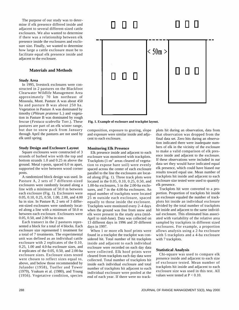
288 JOURNAL OF RANGE MANAGEMENT 53(3), May 2000
The purpose of our study was to deter-mine if elk presence differed inside andadjacent to several different-sized cattleexclosures. We also wanted to determineif there was a relationship between elkpresence inside the exclosures and exclo-sure size. Finally, we wanted to determinehow large a cattle exclosure must be tofacilitate equal elk presence inside andadjacent to the exclosure.
Materials and Methods
Study AreaIn 1995, livestock exclosures were con-
structed in 2 pastures on the BlackfootClearwater Wildlife Management Areaapproximately 70 km northeast ofMissoula, Mont. Pasture A was about 450ha and pasture B was about 250 ha.Vegetation in Pasture A was dominated bytimothy (Phleum pratense L.) and vegeta-tion in Pasture B was dominated by roughfescue (Festuca scabrella Torr.). Thesepastures are part of an elk winter range,but due to snow pack from Januarythrough April the pastures are not used byelk until spring.
Study Design and Exclosure LayoutSquare exclosures were constructed of 3
strands of barbed wire with the top andbottom strands 1.0 and 0.25 m above theground. Metal t-posts, spaced 6.0 m apart,supported the wire between wood cornerposts.
A randomized block design was used. InPasture A, 2 sets of 7 different-sizedexclosures were randomly located along aline with a minimum of 50.0 m betweeneach exclosure (Fig. 1). Exclosures were0.05, 0.10, 0.25, 0.50, 1.00, 2.00, and 4.00ha in size. In Pasture B, 2 sets of 3 differ-ent-sized exclosures were randomly locat-ed along a line with a minimum of 50.0 mbetween each exclosure. Exclosures were0.05, 0.50, and 2.00 ha in size.
Each transect in the 2 pastures repre-sented a block for a total of 4 blocks. Eachexclosure size represented 1 treatment fora total of 7 treatments. The experimentalunit was defined as an individual cattleexclosure with 2 replicates of the 0.10,0.25, 1.00 and 4.0-ha exclosure sizes, and4 replicates of the 0.05, 0.50, and 2.00-haexclosure sizes. Exclosure sizes testedwere chosen to reflect sizes equal to,above, and below those recommended byJulander (1958), Tueller and Tower(1979), Yoakum et al. (1980), and Young(1956). Vegetative condition, species
composition, exposure to grazing, slopeand exposure were similar inside and adja -cent to each exclosure.
Monitoring Elk PresenceElk presence inside and adjacent to each
exclosure was monitored with trackplots.Trackplots (1-m2 areas cleared of vegeta-tion to expose bare soil) were evenlyspaced across the center of each exclosureparallel to the line the exclosures are locat-ed along (Fig. 1). Three track plots werelocated in the 0.05, 0.10, 0.25, 0.50, and1.00-ha exclosures, 5 in the 2.00-ha exclo-sures, and 7 in the 4.00-ha exclosures. Anequal number of trackplots were located25 m outside each exclosure, spacedequally to those inside the exclosure.Trackplots were monitored every 2–4 dayswhen the ground was free from snow andelk were present in the study area (mid-April to mid-June). Data was collected on13 different days in 1996 and 20 differentdays in 1997.
When 1 or more elk hoof prints werefound in a trackplot the trackplot was con-sidered hit. Total number of hit trackplotsinside and adjacent to each individualexclosure were recorded on each day datawere collected. Elk hoof prints werecleared from trackplots each day data werecollected. Total number of trackplots hitinside each individual exclosure and totalnumber of trackplots hit adjacent to eachindividual exclosure were pooled at theend of each year. If there were no track-
plots hit during an observation, data fromthat observation was dropped from thefinal data set. Zero hits during an observa-tion indicated there were inadequate num-bers of elk in the vicinity of the exclosureto make a valid comparison of elk pres-ence inside and adjacent to the exclosure.If these observations were included in ourdata set they would have indicated equalelk presence, which could have biased ourresults toward equal use. Mean number oftrackplots hit inside and adjacent to eachexclosure size tested were used to quantifyelk presence.
Trackplots hit were converted to a pro-portion. Proportion of trackplots hit insidean exclosure equaled the number of track-plots hit inside an individual exclosuredivided by the total number of trackplotshit inside and adjacent to the same individ-ual exclosure. This eliminated bias associ-ated with variability of the relative areasampled by trackplots in different sizedexclosures. For example, a proportionallows analysis using a 2-ha exclosurewith 5 trackplots and a 4-ha exclosurewith 7 trackplots.
Statistical AnalysisChi-square was used to compare elk
presence inside and adjacent to each sizeof exclosure tested. Mean number oftrackplots hit inside and adjacent to eachexclosure size was used in this test. Allvalues were tested at P < 0.10.
Fig. 1. Example of exclosure and trackplot layout.

289JOURNAL OF RANGE MANAGEMENT 53(3), May 2000
Regression analysis was conducted,using the general linear model procedureof SAS (1985) to determine if there was acorrelation between trackplots hit andexclosure size (P < 0.10).
Results and Discussion
Elk Presence Inside and Adjacent toExclosures
Elk presence adjacent to exclosures wasgreater (P < 0.10) than elk presence insideexclosures (Table 1, Fig. 2). An explana-
tion of why elk presence was less insideour exclosures may be that sometimes elksimply choose not to cross fences. Wehave observed elk approach a fence andinstead of jumping over it, parallel thefence in an apparent attempt to find a wayaround. In addition, the 4 sides of anexclosure may present a greater visual
obstacle than a single stretch of fence(pasture perimeter fence). This increasedvisual obstacle may increase an elk’sreluctance to cross an exclosure fence.
Elk Presence in Different-SizedExclosures
Our regression analysis(R2=0.33) indi-cated elk presence inside exclosuresincreased as exclosure size increased (Fig.3). A possible explanation is that as exclo-sure size increases the elk is less likely tosee all sides of the exclosure, which coulddecrease the visual obstacle presented bythe exclosure and increase the likelihoodthat an elk will enter an exclosure.
The coefficient of determination for ourregression was 0.33. The logistics of thisexperiment limited our sample size, whichrestricted the level of power. This may par-tially explain the low coefficient of determi-nation. Our model indicates that an exclo-sure needs to be larger than 4 ha in size tofacilitate equal elk presence inside and adja-cent to the exclosure (Fig. 3). We are notsuggesting that simply building an exclo-sure > 4.0 ha in size will solve all of theproblems associated with this technique.
Young (1956) was the only study wefound that examined the effect of morethan one exclosure size on wild ungulatepresence inside exclosures. Young (1956)compared livestock exclosures from < 0.2to 1.7 ha in size and concluded that elkpresence differed among exclosure sizes.Young’s conclusion that elk presenceinside exclosures increases with increasingexclosure size is supported by our results.However, Young’s conclusion that a 0.4-ha exclosure had equal elk presence insideand adjacent to it was not supported byour results.
Conclusions and ManagementImplications
The results of this study have importantmanagement implications to federal, state,and private resource managers in areaswith elk and cattle. Accurate measures ofrelative resource impacts from cattle andelk are needed to make proper manage-ment decisions (Wisdom and Thomas1996). Previous management decisionsTable 1. Chi-square values comparing elk pres-
ence inside and adjacent to exclosures.
Exclosure Size χ2 Degrees of P-valueFredom
(ha)0.05 16.0 51 0.0070.10 6.6 32 0.0850.25 2.7 13 0.1000.50 13.3 3 0.0041 9.6 3 0.0222 18.3 3 0.003
4 11.6 3 0.0091χ2
0.1 with 5 d.f. = 9.22χ2
0.1 with 3 d.f. = 6.33χ2
0.1 with 1 d.f. = 2.7
Fig. 2. Elk presence inside and adjacent to exclosures on the Blackfoot Clearwater WildlifeManagement Area, Montana, April–June, 1996–97. Asterisk* indicates a significant chi-square value, P 0.10.
Fig. 3. Proportion of total trackplots hit inside exclosures, on the Blackfoot ClearwaterWildlife Management Area, Montana, April–June, 1996–97.

290 JOURNAL OF RANGE MANAGEMENT53(3), May 2000
based on information from cattle exclo-sures may have been incorrect, especiallyif cattle exclosures were ≤ 4.0 ha in size.
Logistically, it may be impractical tobuild an exclosure large enough to mini-mize the effects of size on elk presenceand there is no guarantee that an exclosure> 4.0 ha in size will eliminate all of theproblems associated with this technique.The reluctance of elk to cross fences couldstill pose a problem no matter how largean exclosure is built. A solution to thismay be to drop the fence of the exclosurewhen cattle are not present. This could beapplicable to an elk wintering area that isbeing grazed by cattle only during thegrowing season. Elk are generally dis-persed and in low numbers in these areaswhen cattle are present (during the grow-ing season) and concentrated when cattleare absent (winter) (Lyon 1985). Anothersolution may be to erect an exclosurewhen elk are not present in high densities(growing season), collect vegetation dataat the end of the growing season, and con-struct a new exclosure in a new locationthe following growing season. Althoughcattle exclosures may be used as an effec-tive management tool to separate elk andcattle impacts, precautions should beimplemented to minimize or account for
the potential biases resulting from the reluctance of elk to cross cattle fences.
Additional questions could be exploredconcerning this technique. How do elk useexclosure sizes above 4.0 ha? How is elkuse effected by fence design (fence height,fence materials, exclosure shape and lay-out), and exclosure location in the land-scape (vegetation condition, slope andexposure)?
Literature Cited
Austin, D.D. and P.J. Urness. 1986. Effects ofcattle grazing on mule deer diet and areaselection. J. Range Manage. 39:18–21.
Austin, D.D., P.J. Urness, and L.C. Fierro.1 9 8 3 . Spring livestock grazing effects oncrested wheatgrass regrowth and winter useby mule deer. J. Range Manage. 36:589–593.
Cook, C.W. and J. Stubbendieck (eds.). 1986.Range research: Basic problems and tech-niques. Soc. Range Manage., Denver, Colo.
Julander, O. 1958. Techniques in studyingcompetition between big game and livestock.J. Range Manage. 11:18–21.
Laycock, W.A. 1994. Implications of grazingvs. no grazing on today’s rangelands, p. 250-280. I n: M.V. Vavra, W.A. Laycock, andR.D. Pieper (eds.), Ecological implications oflivestock herbivory in the West. Soc. forRange Manage., Denver, Colo.
Lyon, L.J. 1985. Elk and cattle on the nationalforests: A simple question of allocation or acomplex management problem? WesternWildlands 11:16–19.
SAS Institute Inc. 1985. SAS userís guide:Statistics, version 5 edition. Cary, N.C.: SASInstitute Inc.
Smith, A.D. and D.D Doell. 1968. Guides toallocating forage between cattle and biggame on big game winter range. Utah StateDivision of Fish and Game, Salt Lake City,Utah.
Tueller, P.T. and J.D. Tower. 1979.Vegetation stagnation in three-phase biggame exclosures. J. Range Manage.32:258–263.
Wisdom, M.J. and J.W. Thomas. 1996. E l k ,p.157-181. I n: Paul R. Krausman (ed.),Rangeland Wildlife. Soc. for RangeManage., Denver, Colo.
Yoakum, J., W.P. Dasmann, H.R.Sanderson, C.M. Nixon, and H.S.Crawford. 1980. Habitat improvement tech-niques, p. 329-404. I n: S. D. Schemnitz(ed.), Wildlife management techniques man-ual. Wildl. Soc., Inc. Bethesda, Md.
Young, S. 1956. Survey and evaluation of biggame exclosures in Utah. Dep. InformationBull. 24. Salt Lake City, Utah.
Young, S. 1958. Exclosures in big game man-agement in Utah. J. Range Manage. 11:186-190.
291JOURNAL OF RANGE MANAGEMENT53(3), May 2000
Abstract
We evaluated reproduction and recruitment of the Columbiaspotted frog (Rana luteiventris Thompson) in 70 ponds used bybeef cattle and in 57 ponds not used by beef cattle in northeast-ern Oregon. No significant differences were detected in the num-ber of egg masses or recently metamorphosed frogs in grazedand ungrazed sites. No pond characteristic measured could pre-dict egg mass numbers, but percent aquatic vegetation and dis-solved oxygen had some ability to predict recently metamor-phosed frog numbers. Both variables explained 65% of the vari-ability in recently metamorphosed frog numbers in grazedponds. At ungrazed ponds, 4 additional variables (presence offish, elevation, percent of rock, and conductivity) were requiredto achieve the same level of variability in predicting recentlytransformed frog abundance. The egg mass volume was larger atgrazed than at ungrazed ponds suggesting that grazed pondsmay have a greater food abundance or larger (older) individuals.
Key Words: livestock grazing, northeastern Oregon, R a n aluteiventris Thompson
Global amphibian declines have precipitated the need to deter-mine the status of many amphibian populations and identify fac-tors influencing those populations. The recently describedColumbia spotted frog (Rana luteiventris Thompson) (Green etal. 1997) is known to reproduce in and occupy aquatic habitatsassociated with riparian zones (Turner 1960) and has experiencedsome declines within its range (Hovingh 1993, Munger et al.1996). Grazing is a prominent feature in many of these aquaticecosystems, including northeastern Oregon (Kauffman et al.1983, Green and Kauffman 1995). The influence of livestock onthe physical characteristics (Bohn and Buckhouse 1986), vegeta-tion (Roath and Krueger 1982, Sedgewick and Knopf 1991, Allenand Marlow 1994), fishes (Platts 1981), and avifauna (Thomas etal. 1979, Mosconi and Hutto 1982) in riparian ecosystems is rea-sonably well studied and could influence spotted frog habitat.Beyond discussions of potential impacts (Horusp et al. 1993,Jennings and Hayes 1994, Hayes 1997), the influence of livestock
on amphibians has been only recently addressed. In southwesternIdaho, Munger et al. (1994) found that sites with adult Columbiaspotted frogs had significantly less grazing pressure than siteswithout spotted frogs, but he found no differences in a subsequentyear (Munger 1996).
This paper describes our preliminary assessment of the rela-tionship between grazing and the Columbia spotted frog in north-eastern Oregon. Using the number and volume of egg masses andnumber of recently metamorphosed juveniles to assess spottedfrog reproduction and recruitment, respectively, we measuredbiotic and abiotic variables at 127 breeding sites of Columbiaspotted frogs to determine differences between grazed andungrazed sites.
Methods
Egg Masses (Reproduction)We searched for Columbia spotted frog breeding sites in 5
major watersheds (Grande Ronde River, Eagle Creek, John DayRiver, Malheur River, and Wallowa River) in Union, Umatilla,Baker, Grant, and Wallowa counties. Spotted frogs were known
J. Range Manage.53: 291–294 May 2000
Livestock effects on reproduction of the Columbia spottedfrog
EVELYN L. BULL AND MARC P. HAYES
Authors are research wildlife biologist, Pacific Northwest Research Station, 1401 Gekeler Lane, La Grande, Ore. 97850, [email protected], and adjunct assis -tant professor, Department of Biology, Portland State University, Portland, Ore. 97207-0751.
Thad W. Heater, Karen L. Gray, Janet E. Hohmann, Karen Kronner, ChrisPearl, and Jay F. Shepherd assisted with field work. The following private landowners allowed us to search for frogs on their property: Vic Coggans,Cunningham Sheep Co., Margarite Fahrenwald, Eastern Oregon AgriculturalResearch Center, La Grande Rifle and Pistol Club, Doug McDaniel, Nevada FirstCorp., Bob Schiller (deceased), Nyoda Scott, and Dick Snow.
Manuscript accepted 19 Aug. 1999.
Resumen
Evaluamos la reproducción y la iniciación de la rana"Columbia spotted" (Rana luteiventrisi Thompson) en 70estanques utilizados por ganado bovino para carne y en 57estanques no utilizados por bovinos para carne localizados en elnordeste de Oregon. No se detectaron diferencias significativasen el numero de masas de huevecillos o de ranas recientementemetamorfoseadas entre los sitios con y sin apacentamiento. Lascaracterísticas de los estanques que fueron medidas no pudieronpredecir el numero de masas de huevecillos, pero el porcentajede vegetación acuática y el oxigeno disuelto tienen cierta capaci-dad para predecir los números de ranas recientemente metamor-foseadas. Ambas variables explicaron el 65% de la variabilidadde ranas recientemente metamorfoseadas en los estanques desitios con apacentamiento. En estanques de sitios sin apacen-tamiento, 4 variables adicionales (presencia de peces, elevación,porcentaje de rocas y conductividad) se requirieron para lograrel mismo nivel de variabilidad para predecir la abundancia deranas recientemente transformadas. El volumen de la masa dehevecillos fue mayor en los estanque de sitios con apacentamien-to que en los de sitios sin apacentamiento, lo que sugiere que enlos estanques de áreas con apacentamiento puede haber unamayor abundancia de alimento o individuos mas viejos.
292 JOURNAL OF RANGE MANAGEMENT53(3), May 2000
to occur in these watersheds based on his-torical records (Ferguson 1952, 1954;Ferguson et al. 1958; unpublished data onfile at Pacific Northwest Research Station,La Grande, Ore.). We selected specificwatersheds to search based on several crite-ria: presence of a perennial stream withquiet water in the form of ponds, marshes,and backwaters nearby; streams with awide valley bottom (< 10% gradient) andopen meadows adjacent to coniferousforests (forest types of ponderosa pine[Pinus ponderosa Dougl. ex Laws], lodge-pole pine [P. c o n t o r t a Dougl. ex Loud], ormixed conifer); within 2 km of a road; andon public land or on private land for whichwe had permission to search. Beef cattlegrazing occurred in some of each watershedsometime between June and October,although significant portions of each water-shed were currently ungrazed. Grazing sys-tems had typically been in place withineach watershed for at least 5 years.
We searched for egg masses between 22March and 20 May 1997. The date a par-ticular site was searched depended onwater temperature. We conducted 1 searchat each site when the water temperatureexceeded 8°C, which was the water tem-perature above which successful embryon-ic development could occur (Johnson1965). Each site with eggs was revisitedweekly to count egg masses until no addi-tional egg masses were recorded in 2 suc-cessive visits. Eggs hatched in 13–23days, depending on the water temperature(Morris and Tanner 1969). The number ofegg masses at each breeding site werecounted if individual masses could be dis-tinguished. The length, width, and depthof individual masses were measured toestimate their volume. Egg masses thatoccurred in the same stream but were inseparate bodies of water (where larvaecould not interact) were considered inde-pendent samples.
Only standing water or very slowlymoving water was searched for egg mass-es and adults by walking along the edgeof the stream and checking all oxbows,backwaters, pools, marshy areas, andadjacent ponds using a modified form ofthe basic visual-encounter survey (Scottand Woodward 1994, Thoms et al. 1997).Searches were focused in shallow water(< 30 cm) because Columbia spotted frogegg masses occur in these situations(Turner 1960, Morris and Turner 1969,Hovingh 1993, Munger et al. 1996).
We classified each site as a pond exca -vated for livestock or wildlife, gravel pit,dredge tailings, marsh, oxbow, beaverp o n d , or o t h e r. We recorded e l e v a t i o n ,
surface area of breeding site ( m2), m a x i -mum water depth (m), and distance to apermanent stream. Substrate of the pondwas identified as mud, cobble, or s t o n e.The percent of water surface area that con-tained algae, suspended vegetation, a n dopen water were recorded at each site.Ground cover within 2 m of the pond edgewas recorded as the percent of g r a s s ,s h r u b , o r r o c k. The presence of b e a v e r s(Castor canadensis Linnaeus) was noted.
Recently Metamorphosed Individuals(Recruitment)
We selected 54 of the 127 breeding sitesbased on accessibility and grazing activityto assess frog recruitment; 29 wereungrazed, and 25 were grazed sites. Wesearched for recently metamorphosed indi-viduals between July and September bywalking the perimeter of each breedingsite and counting juvenile frogs seen inwater or on land. Searches continued at 1-week intervals until metamorphs were nolonger metamorphosing. The maximumnumber of recently metamorphosed juve-niles at each site was used for the analysis.
In August, we recorded the same habitatcharacteristics measured during the spring.Water quality variables (pH, conductivity,nitrates, and dissolved oxygen) were mea-sured at each site. Duration and intensityof grazing varied considerably amongsites, so evidence of livestock activity wasrecorded in 3 ways: degree of utilization,number of dung pats, and trampling (hoof-print density). All 3 characteristics weregiven a rating from 0 to 3 with 0 = none, 1= slight evidence, 2 = moderate evidence,and 3 = extensive evidence.
To determine abundance of potentialpredators, we recorded the number ofgarter snakes observed at ponds on eachvisit but used the maximum numberrecorded on any visit as the independentvariable. The presence and kind of fishwere recorded. We sampled aquatic inver-tebrates by taking 8 sweeps with a dip netat each site and counting leeches(Hirudinea), giant water bugs (Homoptera:Belostomatidae), diving beetles(Coleoptera: Dytiscidae), and backswim-mers (Homoptera: Notonectidae).
Analyses
Mann-Whitney tests (Conover 1980)were used to compare the number of eggmasses, volume of egg masses, number ofrecently metamorphosed individuals, andratio of recently metamorphosed individu-als per egg mass in grazed and ungrazed
sites. Nonparametric Spearman's rank cor-relations (Conover 1980) were used todetermine the relationship between num-ber of egg masses and elevation for allsites and for grazed and ungrazed sites.Simple linear regressions were used tocompare: (1) number of egg masses andelevation for grazed and ungrazed sites,(2) mean egg mass volume and elevationfor grazed and ungrazed sites, and (3)mean egg mass volume and elevation forsites with ≥ 3 egg masses at grazed andungrazed sites. Kruskal-Wallis nonpara-metric ANOVAs (Conover 1980) wereused to compare number of egg masses,mean egg mass volume, number of recent-ly metamorphosed juveniles, and the ratioof recently metamorphosed juveniles peregg mass among pond types. The habitatcharacteristics that best predicted numberof egg masses and abundance of recentlymetamorphosed juveniles were identifiedusing a stepwise logistic regression usingall ponds combined, only grazed ponds,and only ungrazed ponds.
Results and Discussion
We located 127 Columbia spotted frogbreeding sites across a 5-county area ineastern Oregon. Seventy (55%) pondswere grazed by cattle; the remaining 57(45%) were ungrazed. Thirty-nine percentof the breeding sites were dredge tailingp o n d s, 24% were o x b o w s, 17% wereexcavated for livestock or w i l d l i f e, 14%were marshes near streams, 3% were cre-ated by beaver dams, 2% were in g r a v e lpit ponds, and 1% was a natural spring-fedpond. Breeding sites were typically small;92% had a surface area <2,500 m 2 a n donly 8% were 2,500-30,000 m2. Thirty-four percent of the ponds were <1 m deepwhile the remainder were 1-5 m deep. Allponds had a fine benthic substrate (mostlymud).
Egg MassesThe number of egg masses at grazed siteswas not statistically different from thenumber at ungrazed sites (Table 1).Breeding sites occurred between 922 and1,860 m in elevation. The elevational dis-tribution of grazed and ungrazed pondsdiffered primarily because all grazed siteswere below 1,500 m. At grazed sites therewas a weak, but significant inverse corre-lation (p = 0.03, adjusted r 2 = 0.06)between number of egg masses and eleva-tion. At ungrazed sites, a weak but signifi-cant positive correlation (p = 0.05, r2 =0.05) existed between number of egg

293JOURNAL OF RANGE MANAGEMENT 53(3), May 2000
masses and elevation. Number of eggmasses did not differ among pond types.Egg mass volume differed significantlybetween grazed and ungrazed sites (Mann-Whitney U: Z = –2.07, p = 0.04) (Table1). No relationship existed between meanegg mass volume and elevation for eithergrazed or ungrazed sites. Because of vari-ability in egg mass volume and at manysites only one egg mass was available tomeasure, we compared the relationshipbetween mean egg mass volume and ele-vation at sites where 3 or more egg masseswere measured. A significant relationshipwas displayed between mean egg massvolume and elevation for both grazed (p =0.02, adjusted r2 = 0.15) and ungrazedsites (p < 0.01, adjusted r2 = 0.24) withvolume increasing with elevation. Becauseegg mass size increased with elevation andmore grazed sites were present at lowerelevations, we compared egg mass size atall sites and at sites with 3 or more eggmasses at or below 1,200 m and above1,200 m. The only significant comparisonwas between grazed and ungrazed sites ator below 1,200 m (Mann-Whitney U: U =69, U’ = 192, p = 0.03).
The larger egg mass volume at grazedsites suggests that grazing did not have anegative effect, in addition to our observa-tion that 6 of the 8 most productive sites(≥ 20 egg masses) were grazed. Becausegrazed sites were below 1,500 m, we con-sidered the possibility that variation in eggmass volume might be influenced by ele-vation. The possibility of such a confound-
ing factor was rejected because the datashowed that egg mass volume increasedwith elevation. Larger egg masses mayreflect larger females (Corn and Fogelman1984), which could be a result of a moreabundant food supply or an older popula-tion structure (Turner 1960).
No pond characteristics measured satis-factorily predicted the number of eggmasses. The stepwise logistic regressionselected elevation, percent aquatic vegeta-tion, and percent open water as able toachieve a maximal predictive value ofonly 7% of the total variability.
Recently Metamorphosed FrogsNeither the number of recently metamor-
phosed frogs nor the ratio of recently meta-morphosed frogs to number of egg masseswas significantly different between the 25grazed and 29 ungrazed sites (Table 1).There were also no significant differencesbetween grazed and ungrazed sites in watercharacteristics (dissolved oxygen, nitrates,pH, and conductivity). However, correla-tion analysis revealed that numbers ofrecently metamorphosed frogs wereinversely correlated with the presence offishes (Spearman's Rank, ρ = -0.41, p =0.0028) for all sites. Longnose dace(Rhinichthys cataractae dulcisValenciennes) and rainbow trout(Oncorhynchus mykiss Walbaum) wereidentified at the breeding sites with fish.Inverse correlations between frog larvaeand fish have been demonstrated often(Hayes and Jennings 1988, Bradford 1989,
Bradford et al. 1993) and may be reflectedby the inverse correlation between recentlymetamorphosed frogs and fish in this study.
Numbers of recently metamorphosedfrogs were positively correlated withgarter snakes (Spearmans's Rank, ρ =0.52, p < 0.01) for all sites. The commongarter snake (Thamnophis sirtalisLinnaeus) and the wandering garter snake( T . elegans vagrans Baird and Girard)were present in about equal proportions atthe ponds. Garter snakes were observedpreying on recently metamorphosed frogsat several sites. Most of the predation bygarter snakes occurred after or duringmetamorphosis, and after we had obtainedour highest counts of frogs. It is likely thatponds with high numbers of metamor-phosing frogs attracted more snakes thanponds with low numbers of frogs.
In comparisons of habitat variablesbetween grazed and ungrazed sites, onlypercent cattails (Mann-Whitney U: Z = -2.37, p = 0.02), utilization (Z = -4.55, p <0.01), trampling (Z = -4.97, p < 0.01), anddung pat density (Z = -5.01, p < 0.01) weresignificantly different (Table 1). A correla-tion analysis revealed that percent of cat-tails was positively correlated with pondsize (Spearman's Rank, ρ = 0.37, p < 0.01).
Selected habitat characteristics weresuccessful predictors of the abundance ofrecently metamorphosed frogs. For all 54ponds, 5 variables were retained in theanalysis with percent aquatic vegetationexplaining 25% of the variability; theremaining 4 variables (dissolved oxygen,
Table 1. Mean values, standard errors, and ranges of independent and dependent variables measured at Columbia spotted frog breeding ponds innortheastern Oregon, 1997.
Ungrazed GrazedVariable N –x± SE Range N –x± SE Range
Dependent No. egg masses 58 6.9 ± 2.34 1–25 65 6.9 ±2.52 1–30Egg mass volume (cm3)* 41 762 ± 18.44 340–1,872 55 888 ± 19.8 261–2,142Egg mass volume at sites < 1,200 m (cm3)* 9 688 ± 165.3 340–1,872 29 954 ± 77.7 261–2,172No. transfomed frogs 29 57 ± 20.62 0–563 25 39 ± 10.15 1–230
IndependentElevation (m) 58 1,317 ± 24.67 922–1,860 68 1,184 ± 16.78 940–1,470Surface area (m2) 55 1,434 ± 546.67 8–30,000 68 1,079 ± 323.42 12–19,872Water depth (m) 54 1.5 ± 0.27 0.5–5 67 1.2 ± 0.11 0.2–5Distance to stream (m) 58 80 ± 26.93 0–1,000 48 61 ± 15.01 0–600Aquatic vegetation (%) 56 44 ± 4.07 0–100 68 47 ± 3.98 0–100Algae (%) 56 11 ± 2.64 0–80 68 10 ± 2.24 0–80Cattails (%)* 29 7 ± 2.09 0–40 25 4 ± 2.82 0–60Utilization1* 47 0 ± 0.02 0–1 66 1.3 ± 0.11 0–3Trampling1* 49 0.2 ± 0.08 0–1 67 0.9 ± 0.12 0–3Dung pats1* 49 0.1 ± 0.06 0–1 68 1.3 ± 0.09 0–3pH 29 8.2 ± 0.16 6.0–10.6 23 8.1 ± 0.20 6.6–10.4Conductivity (µS/cm) 29 151 ± 15.48 14–376 25 144 ± 16.28 59–473Nitrates (ppm) 29 0.1 ± 0.1 0.1–0.1 25 0.1 ± 0.01 0–0.1Dissolved oxygen (ppm) 29 7.7 ± 0.70 1.0–16.0 25 6.2 ± 0.79 1.0–16.2
* Significant at p < 0.05.1These variables were coded from 0 to 3, indicating relative abundance of each variable.

294 JOURNAL OF RANGE MANAGEMENT 53(3), May 2000
elevation, utilization, and pond depth)explained another 16% of the variability.In ungrazed ponds, 6 variables (fish, per-cent aquatic vegetation, elevation, percentof rock on shore, dissolved oxygen, andconductivity) explained 65% of the vari-ability. In grazed ponds, percent aquaticvegetation explained 35%, and dissolvedoxygen explained 30% of the variability.Percent aquatic vegetation and dissolvedoxygen were the only variables that wereretained in all models (combined, grazed,and ungrazed).
Percent aquatic vegetation, dissolvedoxygen, and presence of fish all con-tributed significantly to predict the abun-dance of recently metamorphosed frogs,which may reflect a fundamental aquaticvegetation effect. Aquatic vegetation isknown to provide shelter for frog larvaeand metamorphs from fish and otherpredators (Licht 1969). Levels of dis-solved oxygen are directly linked to cover-age of aquatic vegetation (Carpenter andLodge 1986).
Conclusions
These data failed to reveal that grazinghad a negative effect on reproduction andrecruitment of the Columbia spotted frogin northeastern Oregon. The high variabil-ity in the results of this study may belinked to the breadth of the grazing vari-able encompassing a broad range of condi-tions in landform features, water quality,vegetation, predators, and invertebrates.Future studies need to pay particular atten-tion to measuring grazing intensity andtiming to detect potential effects onColumbia spotted frogs.
Literature Cited
Allen, D.R. and C.B. Marlow. 1994. S h o o tpopulation dynamics of beaked sedge follow-ing cattle grazing. J. Range Manage.47:65–69.
Bohn, C.C. and J.C. Buckhouse. 1986.Effects of grazing management on stream-banks. Trans. N. Amer. Wildl. and Natur.Resources Conf. 51:265–271.
Bradford, D.F. 1989. Allotropic distribution ofnative frogs and introduced fishes in the highSierra Nevada lakes of California. Copeia1989:775–778.
Bradford, D.F., D.M. Graber, and F.Tabatabai. 1993. Isolation of remainingpopulations of the native frog, R a n am u s c o s a, by introduced fishes in Sequoiaand Kings Canyon National Parks,California. Conserv. Biol. 7:882–888.
Carpenter, S.R. and D.M. Lodge. 1986.Effects of submersed macrophytes onecosystem processes. Aquat. Bot.26:341–370.
Conover, W.J. 1980. Practical nonparametricstatistics. 2 nd ed. John Wiley & Sons, NewYork, N.Y.
Corn, P.S. and J.C. Fogelman. 1984.Extinction of montane populations of thenorthern leopard frog (Rana pipiens ) inColorado. J. Herpetology 18:147–152.
Ferguson, D.E. 1952. The distribution ofamphibians and reptiles of Wallowa County,Oregon. Herpetologica 8:66–68.
Ferguson, D.E. 1954. An annotated list of theamphibians and reptiles of Union County,Oregon. Herpetologica 10:149–152.
Ferguson, D.E., K.E. Payne, and R.M.Storm. 1958. Notes on the herpetology ofBaker County, Oregon. Great Basin Natur.18:63–65.
Green, D.M. and J.B. Kauffman. 1995.Succession and livestock grazing in a north-eastern Oregon riparian ecosystem. J. RangeManage. 48:307–313.
Green, D.M., H. Kaiser, T.F. Sharbel, J.Kearsley, and K.R. McAllister. 1997.Cryptic species of spotted frogs, Rana pre -t i o s a complex, in western North America.Copeia 1997(1):1–8.
Hayes, M.P. 1997. Status of the Oregon spot-ted frog (Rana pretiosa sensu stricto) in theDeschutes Basin and selected other systemsin Oregon and north eastern California with arangewide synopsis of the species’ status.Final report to Nature Conserv., Portland,Ore.
Hayes, M.P. and M.R. Jennings. 1988.Habitat correlates of distribution of theCalifornia red–legged frog (Rana auroradraytonii) and the foothill yellow-legged frog(Rana boylii): implications for management,p 144–158. I n Proc. Sym. on the manage-ment of amphibians, reptiles, and smallmammals in North America. USDA For.Serv., Gen. Tech. Rep. GTR–RM–166, FortCollins, Colo..
Horsup, A., C. James, and G. Porter. 1993.Vertebrates of dry rainforest of south andmideastern Queensland. Memoirs of theQueensland Museum 34:215–228.
Hovingh, P. 1993. Aquatic habitats, life historyobservations, and zoogeographic considera-tions of the spotted frog (Rana pretiosa) inthe Tule Valley, Utah. Great Basin Natur.53:168–179.
Jennings, M.R. and M.P. Hayes. 1994.Amphibian and reptile species of special con-cern in California. Final report to Calif. Dept.Fish and Game, Rancho Cordova, Calif.
Johnson, O.W. 1965. Early development,embryonic temperature tolerance, and rate ofdevelopment in Rana pretiosa luteiventrisThompson. Ph.D. Thesis, Oregon State Univ.Corvallis, Ore.
Licht, L.E. 1969. Comparative breeding biolo-gy of the red–legged frog (Rana auroraa u r o r a) and the western spotted frog (R a n apretiosa pretiosa) in south western BritishColumbia. Can. J. Zool. 47:1287–1299.
Kauffman, J.B., W.C. Krueger, and M.Vavra. 1983. Impacts of cattle on stream-banks in northeastern Oregon. J. RangeManage. 36:683–685.
Morris, R.L and W.W. Tanner. 1969. T h eecology of the western spotted frog, R a n apretiosapretiosa Baird and Girard, a life his-tory study. Great Basin Natur. 29:45–81.
Mosconi, S.L. and R.L. Hutto. 1982. T h eeffect of grazing on land birds of a westernMontana riparian habitat, p 221–233. I n:Wildlife–livestock relationships symposium:proc. 10. Univ. of Idaho, Forest, Wildlife andRange Exp. Sta., Moscow, Ida.
Munger, J.C., M. Gerber, M. Carroll, K.Madrid, and C. Peterson. 1996. Status andhabitat associations of the spotted frog Ranap r e t i o s a in southwestern Idaho. Tech. Bull.No. 96–1. Idaho Bureau Land Manage.
Munger, J.C., L. Heberger, D. Logan, W.Peterson, L. Mealy, and M. Cauglin. 1994.A survey of the herpetofauna of the BruneauResource Areas, with focus on the spottedfrog, Rana pretiosa . Bureau LandManagement Tech. Bull.
Platts, W.S. 1981. Influence of forest andrangeland management on anadromous fishhabitat in western North American: effects oflivestock grazing. USDA For. Ser., Gen.Tech. Rep. GTR–PNW–124, Portland, Ore.
Roath, L.R. and W.C. Krueger. 1982. Cattlegrazing influence on a mountain riparianzone. J. Range Manage. 35:100–103.
Scott, N.J., Jr. and B.D. Woodward. 1994.Surveys at breeding sites. p. 118–125. I n:W.R. Heyer, M.A Donnelly, R.W.McDiarmid, and others (eds.). Measuring andmonitoring biological diversity: Standardmethods for amphibians. SmithsonianInstitution Press, Washington, D.C.
Sedgwick, J.A. and F.L. Knopf. 1991.Prescribed grazing as a secondary impact in awestern riparian floodplain. J. RangeManage. 44:369–373.
Thoms, C., C.C. Corkran, and D.H. Olson.1997. Chapter 3: Basic amphibian survey forinventory and monitoring in lentic habitats,p. 35–46. I n: D.H. Olson, W.P. Leonard,R.B. Bury (eds.), Sampling amphibians inlentic habitats. Northwest Fauna No. 4.
Thomas, J.W., C. Maser, and J.E. Rodiek.1 9 7 9 . Wildlife habitats in managed range-lands: the Great Basin of southeasternOregon: riparian zones. USDA For. Serv.,Gen. Tech. Rep. GTR–PNW–80, Portland,Ore.
Turner, F.B. 1960. Population structure anddynamics of the western spotted frog, R a n ap. pretiosa Baird & Girard, in YellowstonePark, Wyoming. Ecol. Monogr. 30:251–278.

295JOURNAL OF RANGE MANAGEMENT53(3), May 2000
Abstract
Cryptosporidium parvum is a fecal borne protozoan parasitethat can be carried by and cause gastrointestinal illness inhumans, cattle, and wildlife. The illness, cryptosporidiosis, can befatal to persons with compromised immune systems. At questionis the potential for C. parvum in cattle fecal deposits on rangelandwatersheds to contaminate surface water. First, C. parvumoocysts must be released from fecal deposits during rainfall,becoming available for transport. In 1996, we examined thetransport of C. parvum oocysts in overland flow from fecaldeposits under natural rainfall and rangeland conditions at theSan Joaquin Experimental Range in Madera County, Calif. Ournull hypothesis was that C. parvum oocysts are not released fromfecal pats and transported 1 m downslope as overland flow withrainfall. Paired plots were located on 10, 20, and 30% slope sites.Each plot was loaded with four, 200 g fecal pats dosed with 105
oocysts g-1. Pats were placed 1.0 m above the base of each plot.Composite runoff samples from each plot were analyzed foroocyst concentration following each of 4 storm events. Oocystswere transported during each storm. Slope was a significant fac-tor in oocyst transport, with oocyst transport increasing withslope. Although not significant, there was an apparent flushingeffect of oocysts across storms, with the majority transported inthe first 2 storms. A pilot rainfall simulation experiment alsorevealed a flushing phenomenon from pats during individualrainfall events. C. parvum oocysts in fecal pats on rangeland canbe transported from fecal deposits during rainfall events, becom-ing available for transport to water-bodies. Future studies needto examine surface and subsurface transport of oocysts on range-land hillslopes for distances greater than 1 m.
Key Words: pathogens, water quality, fate and transport, bufferstrip
Cryptosporidium parvum (Tyzzer 1912), a fecal-oral protozoanparasite, is an important etiologic agent of enterocolitis in mam-mals. C. parvum appears to be infectious for and is shed byhumans, domestic animals, and wildlife species (Casemore et al.1997). Waterborne transmission to humans has emerged as aleading public health problem here and abroad (MacKenzie et al.
1994, LeChevallier and Norton 1995). Public health officialshave considered cattle as possible sources of this parasite becauseof C. parvum infection within cattle populations (MacKenzie etal. 1994). In 1997, the City of San Francisco, Calif. proposed toterminate long-standing grazing leases and ban cattle from 12,000
J. Range Manage.53: 295–299 May 2000
Cryptosporidium parvum transport from cattle fecaldeposits on California rangelands
KENNETH W. TATE, EDWARD R. ATWILL, MELVIN R. GEORGE, NEIL K. MCDOUGALD, AND ROYCE E.LARSEN
Authors are rangeland watershed specialist, Agronomy and Range Science, University of California, Davis, Calif. 95616-8515; environmental health spe -cialist, School of Veterinary Medicine, University of California, Veterinary Medicine Teaching and Research Center, Tulare, Calif. 93274; range and pasturespecialist, Agronomy and Range Science, University of California, Davis, Calif. 95616-8515; natural resources and livestock advisor, University of CaliforniaCooperative Extension, Madera, Calif. 93637; and watershed advisor, University of California Cooperative Extension, San Luis Obispo, Calif. 93446.
Research was funded by UC Division of Agriculture and Natural Resources1995-96 Competitive Grants Program Grant #020.
Manuscript accepted 17 Aug. 1999.
Resumen
Cryptosporidium parvum es un protozoario parásito que setransporta en las heces fecales y que puede ser acarreado porhumanos, bovinos y fauna silvestre a los que puede causar enfer-medades gastrointestinales. La enfermedad cryptosporidiosispuede ser fatal para personas con un sistema inmunológico débil.Se cuestiona el potencial del C. parvum contenido en las hecesfecales de bovinos depositadas en las cuencas hidrológicas depastizal para contaminar las aguas superficiales. Primero, losoocistos del C. parvum deben ser liberados de las heces fecalesdurante la ocurrencia de lluvias para estar disponibles para sertransportados. En 1996, en la Estación Experimental dePastizales de San Joaquín en el condado de Madera, Calif.,examinamos el transporte de oocistos de C. parvum en el flujosuperficial proveniente de áreas con depósitos fecales bajo lluvianatural y en condiciones de pastizal. Nuestra hipótesis nula fueque los oocistos de C. parvum no son liberados de los depósitosfecales y transportados 1 m cuesta abajo como en el flujo super-ficial de la lluvia. Se localizaron parcelas apareadas en sitios con10, 20 y 30% de pendiente. En cada parcela se colocaron 4depósitos fecales de 200 g de dosificados con 105 oocistos g-1, lasheces fecales se colocaron 1 m arriba de la base de cada parcela.Se analizaron muestras compuestas del escurrimiento de cadaparcela para determinar la concentración de oocistos después decada uno de 4 eventos de lluvia. Los oocistos fueron transporta-dos durante cada tormenta. La pendiente fue un factor signifi-cante en el transporte de oocistos, incrementandose el transporteal aumentar la pendiente. Aunque no significante, hubo un efectoaparente de lavado de los oocistos a través de las tormentas, endonde la mayoría de ellos se transportaron en las primeras 2 tor-mentas. Un experimento piloto con simulador de lluvia tambiénrevelo este fenómeno de lavado durante eventos individuales delluvia. Los oocistos de C. parvum de heces fecales localizadas enpastizales pueden ser transportadas durante los eventos de llu-via, llegando a ser disponibles para su transporte a cuerpos deagua. Se necesitan estudios futuros para examinar el transportesuperficial y subterráneo de oocistos en las montañas de pastizala distancias mayores de 1 m.
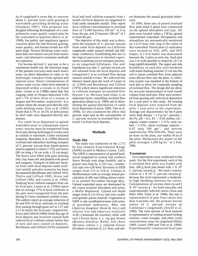
296 JOURNAL OF RANGE MANAGEMENT 53(3), May 2000
ha of rangeland it owns due to concernsabout C. parvum from cattle grazing inwatersheds providing drinking water(Stephens 1997). This proposal wasdropped following development of a com-prehensive water quality control plan forthe watershed in question (Barry et al.1998), but public and regulatory agencyconcerns about the link between grazing,water quality, and human health are stillquite high. Normal drinking water treat-ment does not remove oocysts from sourcewater, and alternative treatment methodsare expensive.
For bovine-derived C. parvum to be awaterborne health risk, the infectious stageof the parasite (oocysts) must reach sourcewater via direct deposition in water or viahydrologic transport from upland andriparian areas. Direct contamination ofsource water occurs when fecal material isdeposited within a stream or its floodplain. Larsen et al. (1988) report that freeranging cattle in Oregon deposited 3.4%and 1.7% of their feces in a stream inAugust and November, respectively. In asystem where the stream provided the onlycattle drinking water, Gary et al. (1983)found that 6.7% to 10.5% of defecationsby beef cattle were deposited directly intostreams.
For cattle feces deposited in uplandwatershed areas to contaminate sourcewater, oocysts must be transported fromfecal pats during hydrological events suchas rainfall or snowmelt. Under simulatedirrigation, Mawdsley et al. (1996) observedoverland and subsurface leaching transportof C. parvum oocysts from liquid manureslurries applied to tilted (7.5%) soil boxes(80 cm long x 56 cm wide x 25 cm deep).The boxes were filled with poor drainingsilty clay loam soil and planted with peren-nial ryegrass. Transport of indicator bacte-ria from cattle fecal deposits under artifi-cial rainfall and plot scenarios has beendocumented (Buckhouse and Gifford 1976,Thelin and Gifford 1983, Kress andGifford 1984, and Larsen at al. 1994).Studying fecal coliform transport from cat-tle fecal pats, Larsen et al. (1994) reportthat on average 17% of fecal coliforms inthe pats were transported from the patsduring 0.5 hour simulated rainfall events.The authors report an average reduction of83 and 95% of fecal coliforms in overlandflow passing through grass turf at 1.37 and2.13 m below the fecal pats, respectively.Kress and Gifford (1984) found that age offecal deposit and recurrent rainfall bothreduced fecal coliform release below thatof new and once rained on deposits.Buckhouse and Gifford (1976) examined
fecal and total coliform transport from 1month old fecal deposits on rangeland inUtah under simulated rainfall. They reportfecal coliform concentrations in overlandflow of 75,000 bacteria 100 ml- 1 at 0 mfrom the pat, and 23 bacteria 100 ml-1 at 1m from the pat..
The objective of this study was to docu-ment the transport of C. parvum o o c y s t sfrom cattle fecal deposits on Californiarangelands under natural rainfall and hill-slope conditions. Establishing this fact isthe logical precursor to detailed experi-ments examining oocyst transport process-es on rangeland hillslopes. Our nullhypothesis was that C. parvum oocysts arenot released from the fecal deposits andtransported 1 m as overland flow duringnatural rainfall events. We selected thisdistance based upon the work of Larsen etal. (1994) and Buckhouse and Gifford(1976) which shows significant reductionin coliform transport as overland flowbeyond 1 m. Because land slope is animportant factor controlling overland flowgeneration (Haan et al. 1994) and in deter-mining the spatial distribution of cattlefecal deposition (Larsen 1989, Tate et al.1998), we also examined the effect thatpercent slope had on the concentration ofC. parvum oocysts in overland flow col-lected 1 m from fecal deposits.
Methods
Study SiteThe study was conducted on the 1,772
ha San Joaquin Experimental Range(SJER) located in Madera County, Calif.The SJER is representative of grazed hard-wood rangeland in central and southernSierra Nevada west slope foothills, and isgrazed year-long by a 210 cow, commer-cial type cow-calf herd. Elevation at SJERranges from 213 to 518 m. Climate isMediterranean with an average annual pre-cipitation of 485 mm falling almost entire-ly as rainfall November through May.Upland watershed areas are dominated bythe coarse textured Ahwahnee soil series,a Mollic Haplustaif. Upland soil depthranges from 0.2 to 0.6 m, lain over weath-ered granitic parent material. Vegetation atSJER is oak woodland/savanna with annu-al grassland understory. Blue oak(Quercus douglasii Hook & Arn.) andinterior live oak ( Quercus wislizeniiA.DC.) dominate the overstory while wildoats ( Avena fatua L.), rip-gut brome(Bromus diandrus Roth), soft chess(Bromus rubens L.), redstem filaree(Erodium cicutarium (L.) L’Her), and oth-
ers dominate the annual grassland under-story.
In 1994, three sets of paired overlandflow plots (total 6 plots) were constructedon the upland Ahwahnee soil type. Allplots were located within a 138 ha, grazedexperimental watershed. Precipitation andstreamfiow are automatically monitoredon a 0.25 hour time step at the outlet ofthis watershed. Paired plots (2 replicates)were located on 10%, 20%, and 30%slopes. A 1.0 m buffer was maintainedbetween the 2 plots at each site. Each plotwas 2 m wide (parallel to slope) by 22.1 mlong (uphill-downhill). The upper and sideboundaries of each plot were borderedwith metal flashing inserted 15 cm into thesoil to insure overland flow from adjacentareas did not flow into the plots. A collec-tion system was installed at the bottom ofeach plot to allow for composite samplingof overland flow. The design did not allowfor accurate measurement of total runoffvolume from each plot. Plots were protect-ed from grazing and cattle fecal depositionfor a year prior to this study. All existingfecal deposits were removed from theplots 1 year prior to the experiment.Average soil characteristics for the 6 plotswere; bulk density = 1.5 g cm-3, porosity =44.1%, pH = 6.5, EC = 0.58 mmhos cm-1,organic matter content = 1.11%, total car-bon = 1.15%, cation exchange capacity =6.67 meq 100 gm - 1 , and percentsand/silt/clay 78%/18%/4%. There wereno trees on the plots, nor within 30 m ofthe plots. Herbaceous dry matter on theplots averaged 1,669 kg ha - 1 at 2 Feb.1996.
TreatmentsTwo experiments were conducted in this
study. For the first experiment, each of the6 overland flow plots was loaded withfour, 200 g fecal pats dosed with 1 X 10⁵
C. parvum oocysts g-1. We used a concen-tration of 1 X 10⁵ C. parvum oocysts g- 1
because this level represented a moderate-ly high shedding intensity for calves.Concentrations of oocysts often exceed IX 105 oocysts g- 1 for both naturally andexperimentally infected calves (Xiao andHerd 1994, Fayer et al. 1998). Pat size isrepresentative of pats from calves lessthan 4 months old, the primary bovinesource of C. parvum oocysts onCalifornia’s rangelands (Atwill et al.1999). The total amount of fecal materialis representative of loading around feedingstations, water troughs, and other cattleconcentration areas on rangeland (Hafez1969, Larsen 1989 and Tate et al. 1998).Experimentally constructed fecal pats

297JOURNAL OF RANGE MANAGEMENT 53(3), May 2000
allow us to control the load of C. parvumoocysts on each plot. Source of fecalmaterial for experimentally constructedfecal pats was fresh fecal material collect-ed from cattle at the SJER and which test-ed negative for C. parvum based onimmunofluorescent microscopy (MERI-FLUOR C r y p t o s p o r i d i u m / G i a r d i a d i r e c timmunofluorescent detection kit, MeridianDiagnostics, Inc. Cincinnati, Ohio).Source of C. parvum oocysts for experi-mentally constructed fecal pats were fromfeces from naturally-infected dairy calvesand were purified using a previouslydescribed technique (Arrowood andSterling 1987). The concentration of puri-fied oocysts was determined with a hema-cytometer. Naturally-infected calves werefrom several commercial dairies located inKings and Tulare counties, Calif.
On 2 February 1996, the 4 fecal patswere placed 1.0 m above the bottom ofeach plot. A composite overland flowsample was collected from each plot fol-lowing 4 subsequent storm events duringthe remainder of the 1 October 1995 to 30September 1996 water year. Runoff vol-ume from each plot was not measured.Concentrations of oocysts were measuredfor each sample by adding 2.5 ml of 10%Tween 80, 1Q% SDS solution to 250 mlaliquot of each sample, mixing 30 sec-onds, then filtering through mesh size 40,100, and 200 sieves. The suspension wascentrifuged, supernatant removed, and thepellet resuspended in 0.25 to 4 ml of 0.2%Tween 20 in distilled water. Ten ul of sus-pension was dried onto a commerciallyprepared glass slide and the directimmunofluorescent assay performedaccording to the manufacturer’s instruc-tions (MERIFLUOR C r y p t o s p o r i -d i u m / G i a r d i a direct immunofluorescentdetection kit, Meridian Diagnostics, Inc.Cincinnati, Ohio). The total number ofoocysts was enumerated for each sampleand the concentration of oocysts for eachwater sample determined by adjusting forthe estimated percent recovery of theimmunofluorescent assay. An ANOVAwith repeated measures (Dixon 1992) wasused to determine significance, with slope(3 levels) as the fixed factor and sampledate (4 storm events) as the repeated mea-sure whereby the runoff from 6 plots (3slopes x 2 replicates/slope) was sampledacross 4 storms.
In the second experiment, we conducteda single artificial rainfall experiment toprovide preliminary information for devel-opment of a future laboratory-based studyof the transport of oocysts t h r o u g h o u t arainfall event. Due to natural plot variabil-
ity, uncertain weather and flow, as well aslogistics it is difficult to obtain this type ofdetailed time-dependent information in-the-field under natural rainfall scenarios.For this trial, a sprinkler type rainfall sim-ulator (Wilcox et al. 1986) was used toapply rainfall at a rate of 7.62 cm hour-1 toa 0.5 m2, 10% slope, ungrazed plot locatedadjacent to the 10% slope overland flowplot site. This rainfall intensity exceeds theestimated 100 year return period 30minute duration rainfall event for the site.Rainfall was applied to the plot until equi-librium overland flow had been achieved.At that point four, 200 g fecal pats dosedwith 1 X 10 5 C. parvum oocysts g - 1 o ffeces were added to the plot. All overlandflow from the plot was captured for 90minutes starting immediately prior to andat 10 minute increments following fecalpat deposition. Concentrations of oocystsin the samples were measured for eachsample by the same method describedabove.
Results and Discussion
Precipitation and stream flow from the138 ha experimental watershed containingthe plots was recorded on a 0.25 hour time
step (Fig. 1). These data are presented toillustrate the timing and magnitude of thestorms experienced during this experi-ment. Overland flow generated by 4 dis-crete storm events commencing on 3February 1996,4 February 1996, 18February 1996, and 11 March 1996 wascomposite sampled during the study. Thestorm commencing 3 March 1996 generat-ed no overland flow from the plots.Composite overland flow samples fromthe plots were collected at approximately1500 hours on 4 February 1996, 8February 1996, 22 February 1996, and 12March 1996. Total rainfall for the 4February 1996, 8 February 1996, 22February 1996, and 12 March 1996 sam-ple periods was 46, 55, 64, and 32 mmrespectively. Following 12 March 1996,no overland flow was realized from theplots for the remainder of the 1995 wateryear.
Figure 2 illustrates C. parvum concen-tration by slope and sample date. ANOVAwith repeated measures (sample date)reveals that while the effect of slope wassignificant at the 0.05 confidence level,sample date (storm event) and the poten-tial interaction between slope and sampledate were not significant (Table 1). Tukeycomparison of means reveals that C .p a r v u m concentrations are significantly
Fig. 1. Rainfall (mm) and storm flow (liter sec-1) from the San Joaquin Experimental Rangewatershed during the study period.
Table 1. Analysis of variance with repeated measures of square root transformed C. parvum con-centration (No. oocysts liter-1), with slope as the fixed factor and sample date as the repeatedmeasure.
Source df Sum of Squares Mean Sum of Squares F P
Mean 1 28971 28971 28.06 0.01Slope effect 2 21523 10762 10.42 0.04Error 3 3097 1032SampleDate 3 11333 3778 2.15 0.16Slope x Sample Date 6 16534 2756 1.57 0.26Error 9 15842 1760
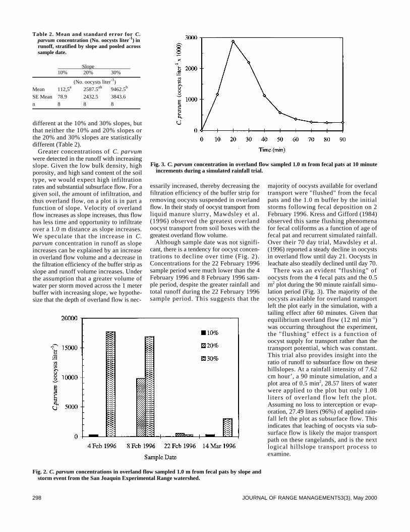
298 JOURNAL OF RANGE MANAGEMENT53(3), May 2000
different at the 10% and 30% slopes, butthat neither the 10% and 20% slopes orthe 20% and 30% slopes are statisticallydifferent (Table 2).
Greater concentrations of C. parvumwere detected in the runoff with increasingslope. Given the low bulk density, highporosity, and high sand content of the soiltype, we would expect high infiltrationrates and substantial subsurface flow. For agiven soil, the amount of infiltration, andthus overland flow, on a plot is in part afunction of slope. Velocity of overlandflow increases as slope increases, thus flowhas less time and opportunity to infiltrateover a 1.0 m distance as slope increases.We speculate that the increase in C .p a r v u m concentration in runoff as slopeincreases can be explained by an increasein overland flow volume and a decrease inthe filtration efficiency of the buffer strip asslope and runoff volume increases. Underthe assumption that a greater volume ofwater per storm moved across the 1 meterbuffer with increasing slope, we hypothe-size that the depth of overland flow is nec-
essarily increased, thereby decreasing thefiltration efficiency of the buffer strip forremoving oocysts suspended in overlandflow. In their study of oocyst transport fromliquid manure slurry, Mawdsley et al.(1996) observed the greatest overlandoocyst transport from soil boxes with thegreatest overland flow volume.
Although sample date was not signifi-cant, there is a tendency for oocyst concen-trations to decline over time (Fig. 2).Concentrations for the 22 February 1996sample period were much lower than the 4February 1996 and 8 February 1996 sam-ple period, despite the greater rainfall andtotal runoff during the 22 February 1996sample period. This suggests that the
majority of oocysts available for overlandtransport were "flushed" from the fecalpats and the 1.0 m buffer by the initialstorms following fecal deposition on 2February 1996. Kress and Gifford (1984)observed this same flushing phenomenafor fecal coliforms as a function of age offecal pat and recurrent simulated rainfall.Over their 70 day trial, Mawdsley et al.(1996) reported a steady decline in oocystsin overland flow until day 21. Oocysts inleachate also steadily declined until day 70.
There was an evident "flushing" ofoocysts from the 4 fecal pats and the 0.5m2 plot during the 90 minute rainfall simu-lation period (Fig. 3). The majority of theoocysts available for overland transportleft the plot early in the simulation, with atailing effect after 60 minutes. Given thatequilibrium overland flow (12 ml min- 1)was occurring throughout the experiment,the "flushing" effect is a function ofoocyst supply for transport rather than thetransport potential, which was constant.This trial also provides insight into theratio of runoff to subsurface flow on thesehillslopes. At a rainfall intensity of 7.62cm hour’, a 90 minute simulation, and aplot area of 0.5 min2, 28.57 liters of waterwere applied to the plot but only 1.08liters of overland flow left the plot.Assuming no loss to interception or evap-oration, 27.49 liters (96%) of applied rain-fall left the plot as subsurface flow. Thisindicates that leaching of oocysts via sub-surface flow is likely the major transportpath on these rangelands, and is the nextlogical hillslope transport process toexamine.
Table 2. Mean and standard error for C .parvum concentration (No. oocysts liter-1) inrunoff, stratified by slope and pooled acrosssample date.
Slope 10% 20% 30%
(No. oocysts liter-1)Mean 112,5a 2587.5ab 9462.5b
SE Mean 78.9 2432.5 3843.6n 8 8 8
Fig. 2. C. parvum concentrations in overland flow sampled 1.0 m from fecal pats by slope andstorm event from the San Joaquin Experimental Range watershed.
Fig. 3. C. parvum concentration in overland flow sampled 1.0 m from fecal pats at 10 minuteincrements during a simulated rainfall trial.
299JOURNAL OF RANGE MANAGEMENT53(3), May 2000
Conclusions
The hypothesis that C. parvum o o c y s t sare not transported at least 1.0 m as over-land flow from fecal deposits with naturalrainfall can be rejected. Transport of C .parvum oocysts increases as slope increas -es, which we hypothesize to be the resultof reduced filtration efficiency of thebuffer strip subsequent to the larger vol-ume and depth of water moving across thebuffer. There is an apparent "flushing" ofoocysts by the initial storms followingfecal deposition. The rainfall simulationexperiment also indicates a "flushing" ofoocysts during the first 20 minutes of astorm event. Under the realistic scenarioexamined in this study, it is clear that C .p a r v u m oocysts in fresh fecal pats onrangeland can be released with rainfall andbecome available for transport to water-bodies. Overland, as well as vertical andlateral subsurface, transport of oocysts onrangeland hillslopes needs further exami-nation at distances greater than 1 m and ona variety of soil types. This informationwill be important in assessing the potentialfor buffer strips to prevent surface watercontamination with this parasite frombovine and other fecal sources.
It is also important to note that in orderfor these bovine-derived oocysts tobecome a public health threat, oocystshave to be transported out of fecal pats,and they need to remain infective whilebeing transported to a susceptible host.Environmental conditions on rangeland,such as heating, freezing, or drying, canrapidly inactivate large numbers ofoocysts (Walker et al. 1998), but only afew oocysts would need to remain infec-tive in order to pose a risk to humans. Theillness can be fatal to persons with com-promised immune systems. Experimentalstudies in healthy humans determined thatas few as 30 bovine-derived oocysts werecapable of initiating cryptosporidiosis inhumans (DuPont al. 1995). Addressing thepotential for C. parvum in cattle fecaldeposits on rangeland watersheds tothreaten human health will require site-specific examination of the sources in thewatershed (Atwill et al. 1999), viability ofoocysts under harsh rangeland conditions(Walker et al. 1998), hydrologic transportof oocysts within the watershed, and thespatial and temporal distribution of fecalmaterial in relation to surface water bodies(Tate et al. 1998).
Literature Cited
Arrowood, M. J. and C. R. Sterling. 1987.Isolation of Cryptosporidium parvum a n dsporozoites using discontinuous sucrose andisopycnic Percoll gradients. J. Parasitol.73:314–319.
Atwill, E.R., E. Johnson, D.J. Klingborg,G.M. Veserat, G. Markegard, H.A.Jensen, D.W. Pratt, R.E. Delmas, HA.George, L.C. Forero, R.L. Phillips, A.O.Nelson, S.J. Barry, N.K. McDougald, R.R.Gildersleeve, and W.E. Frost. 1999. A g e ,geographic, and temporal distribution offecal shedding of Cryptosporidium parvumoocysts in cow-calf herds. Amer. J. Vet. Res.60:420–425.
Barry, S.J., E.R. Atwill, K.W. Tate, T.S.Koopmann, J. Cullor, and T. Huff. 1998.Developing and implementing aHACCP–based program to controlC r y p t o s p o r i d i u m and other waterbornepathogens in Alameda Creek Watershed: acase study. Proc. of Amer. Water WorksAssoc. Ann. Conf Dallas, Tex. (In press.)
Buckouse, J.C. and G.F. Gifford. 1976.Water quality implications of cattle grazingon a semiarid watershed in southeast Utah. J.Range Manage. 29:109–113.
Casemore, D.P., S.E. Wright, and R.L.Coop. 1997. Cryptosporidiosis—human andanimal epidemiology. p. 65–92. I n :C r y p t o s p o r i d i u m and Cryptosporidiosis.CRC Press, Inc. Boca Raton, Fla.
Dixon, W.J. 1992. BMDP Statistical softwaremanual. University of California Press.Berkeley, Calif. 678 pp.
DuPont, H.L., C. L. Chappell, C. R. Sterling,P. C. Okhuysen, J. B. Rose, and W.Jakubowski. 1995. The infectivity ofCryptosporidium parvum in healthy volun-teers. New England J. Medicine.332:855–859.
Fayer, R., L. Gasbarre, P. Pasquali, A.Canals, S. Almeria, and D. Zarlenga. 1998.Cryptosporidium parvum infection in bovineneaonates: dynamic clinical, parasitic andimmunologic patterns. Internat. J.Parasitology. 28:49–56.
Gary, H.L., S.R. Johnson, and S.L. Ponce.1983. Cattle grazing impact on surface waterquality in a Colorado front range stream. J.Soil and Water Conser. 38:124–128.
Haan, C.T., B.J. Barfield, and J.C. Hayes.1994. Design hydrology and sedimentologyfor small catchments. Academic Press. 588 pp.
Hafez, E.S.C. 1969. The behavior of domesticanimals. Williams and Wilkins Co. Baltimore,Md. 647 pp.
Kress, M. and G.F. Gifford. 1984. Fecal col-iform release from cattle fecal deposits.Water Res. Bull. 20:61–66.
Larsen, R.E. 1989. Water quality impacts offree ranging cattle in semi-arid environments.M.S. Thesis, Oregon State Univ. Corvallis,Ore. pp. 92
Larsen, R.E., JR. Miner, J.C. Buckhouse,and J.A. Moore. 1994. Water quality bene-fits of having cattle manure deposited awayfrom streams. Biores. Tech. 48:113–118.
Larsen, R.E., J.C. Buckhouse, J.A. Mooreand J.R. Miner. 1988. Rangeland cattle andmanure placement: a link to water quality.Oregon Acad. of Sci. 24:7–15.
LeChevallier, M.W. and W.D. Norton. 1995.Giardia and Cryptosporidium in raw and fin-ished water. Amer. Water Works Assoc.87:54–68.
MacKenzie, W.R., N.J. Hoxie, M.E. Proctor,M.S. Gradus, K.A. Blair, D.E. Peterson,J.J. Kazmierczak, D.G. Addiss, K.R. Fox,J.B. Rose, and J.P. Davis. 1994. A massiveoutbreak in Milwaukee of Cryptosporidiuminfection transmitted through the publicwater supply. New England J. Medicine331:161–167.
Mawdsley, J.L., A.E. Brooks, R.J. Perry,and B.F. Pain. 1996. Use of a novel soil tilt-ing table apparatus to demonstrate the hori-zontal and vertical movement of the proto-zoan pathogen Cryptosporidium parvum i nsoil. Biol, Fertil. Soil. 23:215–220.
Stephens, T. 1997. San Francisco water districttargets cattle. California Agr. 51:7.
Tate, K.W., N.K. McDougald, ER. Atwill,M.R. George, and D. Wiff. 1998. A RapidMethod for Estimating Livestock ManureDeposition on Rangeland Watersheds. p.135. In: Specialty Conference on RangelandManagement and Water Resources. Amer.Water Res. Assoc.
Thelin, R. and G.F. Gifford. 1983. Fecal col-iform release patterns from fecal material ofcattle. J. Environ. Qual. 12:57–63.
Tyzzer, E.E. 1912. Cryptosporidium parvum(sp. nov.), a coccidian found in the smallintestine of the common mouse. ArchivfurProtistenkunde. 26:394–412.
Walker, M.J., C.D. Montemagno, and M.B.Jenkins. 1998. Source water assessment andnonpoint sources of acutely toxic contami-nants: a review of research related to the sur-vival and transport of C r y p t o s p o r i d i u mparvum. Water Resour Res. 34:3383–3392.
Wilcox, B.P., M.K. Wood, J.T. Tromble, andT.J. Ward. 1986. A hand–portable singlenozzle rainfall simulator designed for use onsteep slopes. J. Range Manage. 39:375–377.
Xiao, L. and R.P. Herd. 1994. Infection pat-terns of C r y p t o s p o r i d i u m and G i a r d i a i ncalves. Veterinary Parasitology. 55:257–262.

300 JOURNAL OF RANGE MANAGEMENT 53(3), May 2000
Abstract
In Argentina, Paspalum quadrifarium Lam. (paja colorada)forms tall dense grassland communities in the flooding pampas.Referred to locally as “pajonales”, these grasslands generallyhave very low nutritional value for cattle, except at the post-burnregrowth stage. To improve forage quality and consumption bybreeding cattle, Lotus tenuis Walst et Kit. is over seeded immedi-ately after burning of paja colorada pajonales. The objectives ofthis experiment were to follow the after seeding cover of lotus,evaluate weed control, and assess disease incidence and severity.The experiment was carried out in Azul, Buenos Aires provinceof Argentina, between September 1993 to September 1996. Thepostburn seedbed was very favorable for lotus germination andestablishment. The most effective chemical weed control wasobtained with 2,4-DB used alone or in combination with dicam-ba. L o t u s increased markedly the quality of the pasture foragedue to its high crude protein content. Four fungus diseases werefound: Botrytis cinerea Pers., S t e m p h y l i u m sp. Wallroth,Uromyces loti Blytt. and F u s a r i um spp. Link ex Fr. However,these caused only light foliar damage and did not impair lotusgermination or establishment. The overseeding of lotus afterburning of P. quadrifarium pajonales, is a very effective tech-nique to improve carrying capacity and animal performance.
Key Words: Paspalum quadrifarium, Lotus tenuis, fire, weed con-trol, diseases, species diversity
Paspalum quadrifarium Lam. (paja colorada) forms dense tall(1-1.5 m) grassland communities referred to locally “pajonales”.Some researchers believe that it was the predominant vegetationof the Flooding Pampas at the end of the 19th Century (Vervoorst1967). Because of the low carrying capacity of the “pajonales”,ranchers tend to replace them with seeded pastures. There is con-cern about the impact that this replacement process has on thebiodiversity of the region by decreasing the native fauna that isstrongly attached to the pajonales communities.
Paja colorada has very low nutritional value for cattle except atthe postburn regrowth stage. In vitro digestibility varies around50%, crude fiber exceeds 70% and crude protein rarely reaches12% on a dry matter basis. Consequently, it does not provide suit-
able forage for young cattle or breeding females with high levelsof nutrient requirements. The over seeding of lotus (Lotus tenuisWalst et Kit. is a naturalized forage legume in the region) imme-diately after burning of paja colorada pajonales, appears to havepotential to improve forage quality and consumption by breedingcattle. However, a range of diseases caused by pathogens inArgentina (Wolcan and Dall Bello 1988, Dall Bello and Wolcan1992) could affect the lotus survival.
The adequacy of postburned “seedbed” (formed by ashes andbare ground) for lotus germination, the competition with perenni-al weeds and the effect of diseases, could affect the establishmentof the lotus plants. The objective of this experiment were to fol-low the after seeding cover development of lotus, evaluate theefficiency by weed control and to describe the diseases affectingits aerial plant parts.
J. Range Manage.53: 300–304 May 2000
Postburning legume seeding in the Flooding Pampas,Argentina
V. F. JUAN, L. MONTERROSO, M. B. SACIDO “EX AEQUO”, M. A. CAUHÉPÉ
Authors are respectively, research associate, Department of Vegetal Production , Facultad de AgronomÌa, Universidad Nacional del Centro de la Provincia de BuenosAires. CC. 178 ( 7300) Azul. Argentina, and researcher, Facultad de Ciencias Agrarias, Universidad Nacional de Mar del Plata, Argentina.
Authors wish to thank L. EcheverrÌa for facilities to work in his field; Dr.Domicio do Nascimiento Junior, S. Lerner and 2 anonymous reviewers forimproving the manuscript. Financial support was provided by the U.N.C.P.B.A.project 03/A025.
Manuscript accepted 17 Aug. 1999.
Resumen
En las pampas inundables de la Argentina el Paspalum quadri -f a r i u m Lamb. (Paja colorada) forma densas matas de pastizal.Estas comunidades son conocidas localmente como “pajonales” ygeneralmente tienen muy bajo valor nutritivo para los bovinosdomésticos, excepto en los rebrotes postquema.. Para mejorar lacalidad de forraje y el consumo de los pajonales de paja colora-da, se sobresembró Lotus tenuis al voleo postquema de dichospajonales. Los objetivos de este experimento fueron monitorearlas variaciones en la cobertura de Lotus y los demás compo-nentes del pastizal leugo de la siembra, evaluar el control de lasmalezas y la incidencia y severidad de enfermedades en lotus. Elexperimento se condujo entre setiembre de 1993 y setiembre de1996, en Azul, Provincia de Buenos Aires, Argentina. La cama desiembra postquema favoreció la germinación y establecimientodel Lotus. El control químico de mazezas más efectivo se obtuvocon 2,4-DB utilizado solo o en combinación con dicamba. ElLotus incrementó marcadamente la calidad del forraje del lotedebido a su alto contenido de proteína cruda. Fueron determi-nadas 4 enfermedades fúngicas en lotus: Botrytis cinera P e r s . ,S t e m p h y l i u m sp. Wallroth, Uromycetes Loti Blytt. y F u s a r i u mspp. Link ex Fr. las que solo causaron un ligero daño foliar y noimpidieron la germinación y establecimiento de esta especie. Lasiembra en cobertura de Lotus immediatamente luego de laquema de los pajonales de Paspalum quadrifarium es unta técni-ca muy efectiva para mejorar la capacidad de carga y la respues-ta animal.
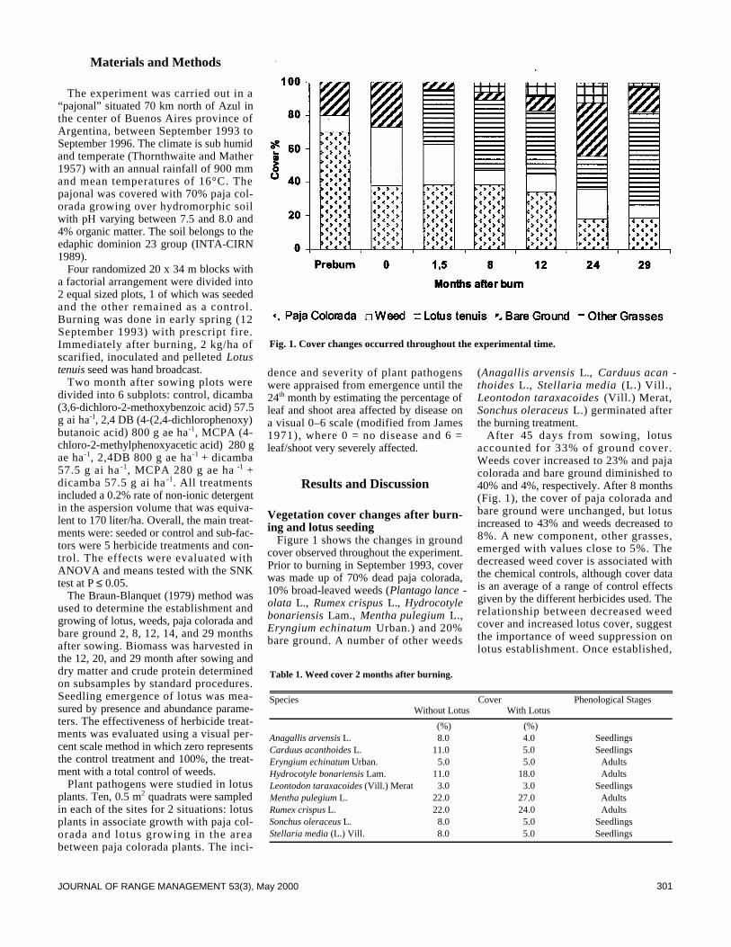
301JOURNAL OF RANGE MANAGEMENT 53(3), May 2000
Materials and Methods
The experiment was carried out in a“pajonal” situated 70 km north of Azul inthe center of Buenos Aires province ofArgentina, between September 1993 toSeptember 1996. The climate is sub humidand temperate (Thornthwaite and Mather1957) with an annual rainfall of 900 mmand mean temperatures of 16°C. Thepajonal was covered with 70% paja col-orada growing over hydromorphic soilwith pH varying between 7.5 and 8.0 and4% organic matter. The soil belongs to theedaphic dominion 23 group (INTA-CIRN1989).
Four randomized 20 x 34 m blocks witha factorial arrangement were divided into2 equal sized plots, 1 of which was seededand the other remained as a control.Burning was done in early spring (12September 1993) with prescript fire.Immediately after burning, 2 kg/ha ofscarified, inoculated and pelleted L o t u stenuis seed was hand broadcast.
Two month after sowing plots weredivided into 6 subplots: control, dicamba(3,6-dichloro-2-methoxybenzoic acid) 57.5g ai ha- 1, 2,4 DB (4-(2,4-dichlorophenoxy)butanoic acid) 800 g ae ha- 1, MCPA (4-chloro-2-methylphenoxyacetic acid) 280 gae ha - 1, 2,4DB 800 g ae ha -1 + dicamba57.5 g ai ha - 1, MCPA 280 g ae ha -1 +dicamba 57.5 g ai ha - 1. All treatmentsincluded a 0.2% rate of non-ionic detergentin the aspersion volume that was equiva-lent to 170 liter/ha. Overall, the main treat-ments were: seeded or control and sub-fac-tors were 5 herbicide treatments and con-trol. The effects were evaluated withANOVA and means tested with the SNKtest at P ≤ 0.05.
The Braun-Blanquet (1979) method wasused to determine the establishment andgrowing of lotus, weeds, paja colorada andbare ground 2, 8, 12, 14, and 29 monthsafter sowing. Biomass was harvested inthe 12, 20, and 29 month after sowing anddry matter and crude protein determinedon subsamples by standard procedures.Seedling emergence of lotus was mea-sured by presence and abundance parame-ters. The effectiveness of herbicide treat-ments was evaluated using a visual per-cent scale method in which zero representsthe control treatment and 100%, the treat-ment with a total control of weeds.
Plant pathogens were studied in lotusplants. Ten, 0.5 m2 quadrats were sampledin each of the sites for 2 situations: lotusplants in associate growth with paja col-orada and lotus growing in the areabetween paja colorada plants. The inci-
dence and severity of plant pathogenswere appraised from emergence until the24th month by estimating the percentage ofleaf and shoot area affected by disease ona visual 0–6 scale (modified from James1971), where 0 = no disease and 6 =leaf/shoot very severely affected.
Results and Discussion
Vegetation cover changes after burn-ing and lotus seeding
Figure 1 shows the changes in groundcover observed throughout the experiment.Prior to burning in September 1993, coverwas made up of 70% dead paja colorada,10% broad-leaved weeds (Plantago lance -o l a t a L., Rumex crispus L., H y d r o c o t y l eb o n a r i e n s i s Lam., Mentha pulegium L . ,Eryngium echinatum Urban.) and 20%bare ground. A number of other weeds
(Anagallis arvensis L., Carduus acan -t h o i d e s L., Stellaria media (L.) Vill.,Leontodon taraxacoides (Vill.) Merat,Sonchus oleraceus L.) germinated afterthe burning treatment.
After 45 days from sowing, lotusaccounted for 33% of ground cover.Weeds cover increased to 23% and pajacolorada and bare ground diminished to40% and 4%, respectively. After 8 months(Fig. 1), the cover of paja colorada andbare ground were unchanged, but lotusincreased to 43% and weeds decreased to8%. A new component, other grasses,emerged with values close to 5%. Thedecreased weed cover is associated withthe chemical controls, although cover datais an average of a range of control effectsgiven by the different herbicides used. Therelationship between decreased weedcover and increased lotus cover, suggestthe importance of weed suppression onlotus establishment. Once established,
Fig. 1. Cover changes occurred throughout the experimental time.
Table 1. Weed cover 2 months after burning.
Species Cover Phenological StagesWithout Lotus With Lotus
(%) (%)Anagallis arvensis L. 8.0 4.0 SeedlingsCarduus acanthoides L. 11.0 5.0 SeedlingsEryngium echinatum Urban. 5.0 5.0 AdultsHydrocotyle bonariensis Lam. 11.0 18.0 AdultsLeontodon taraxacoides (Vill.) Merat 3.0 3.0 SeedlingsMentha pulegium L. 22.0 27.0 AdultsRumex crispus L. 22.0 24.0 AdultsSonchus oleraceus L. 8.0 5.0 SeedlingsStellaria media (L.) Vill. 8.0 5.0 Seedlings

302 JOURNAL OF RANGE MANAGEMENT 53(3), May 2000
lotus is highly competitive with weeds(Ortega and Laterra 1995).
After 12 months, the cover percentageof paja colorada and lotus stabilized at 37and 40%, respectively. However, duringthe second year, a very severe winterdrought occurred which killed plantsthereby increasing the proportion of bareground. After the spring rains, lotus coverrecovered and in the 29th month occupiedmost of the vegetable cover. Paja coloradacover and bare ground decreased marked-ly. It was observed that cattle consumed alarger proportion of the paja coloradaplants when lotus grew together withthem. This probably explains the decreasein paja colorada cover when lotus is pre-sent.
Adults plants of Eryngium, Rumex,Mentha and Hydrocotyle spp. which werepresent prior to burning, sprouted afterburning and did not suffered the effect oflotus presence. The annual weeds(Anagallis arvensis, Carduus acanthoides,Sonchus oleraceus and Stellaria media)germinated after burning and showed asignificant lower plant cover on plots
where lotus were present, as compared toplots not sown with lotus (Table 1).
The chemical control of weeds (Table 2)was equally effective for 2,4-DB whenused alone or when combined with dicam-ba with values close to 80%. The leasteffective treatment was with dicamba.Intermediate control was obtained with theMCPAís formulas. Due to the low pres-ence of annual weeds, significant differ-ences were not detected on the chemicalcontrol between lotus seeded or unseededplots. Consequently, chemical control datawas analyzed independently from the lotusseeding treatment.
Mixtures of 2,4-DB with dicamba, aswell as dicamba used alone, were effectiveonly with the postburn regrowth of adultplants of Rumex crispus. This species, asall the p o l i g o n a c e a are not satisfactorilycontrolled by the herbicides 2,4-D, 2,4-DBand MCPA.
Biomass accumulationLotus dry biomass accumulated 86 g/m2
12 months after burning and seeding whichaccounted for 16 % of total dry biomass.The lotus biomass contribution to total bio-mass increased to 18 % and 28 % after 20and 29 months, respectively. There was nodifference in total biomass between theunseeded and seeded treatments. This indi-cates that the lotus growth occurred at theexpense of paja colorada growth. Also itseems to show that once established, lotushas the ability to maintain or even increasepasture biomass (Fig. 2).
The crude protein content of accumulat-ed biomass increased from 7 % for pajacolorada to 21% for lotus. The proteincontent in paja colorada is lower than thenutritional requirements for beef cattle.The lotus plots offered about 30g/m2 o fcrude protein compared to only 10 g/m2 inunseeded plots. In earlier studies, paja col-orada postburn regrowth reached a crudeprotein content of 12% for the firstregrowth after burning, but decreasedthereafter (Sacido et al. 1995). An increasein available soil nitrogen availability fromN fixed by legumes and liberation of N ofmicrobial biomass facilitated by the earlyheating of soil have been suggested aspossible explanations for this increase in
Table 2. Efficacy of chemical control.
Treatment Efficacy
(%)Dicamba 21 d2,4-DB 69 abMCPA 54 bc2,4-DB + Dicamba 79 aMCPA + Dicamba 47 c
Fig. 2. Dry biomass (kg m-2) of treatments with or without lotus.
Fig. 3. Pathogens on Lotus tenuis in a 24-month period.
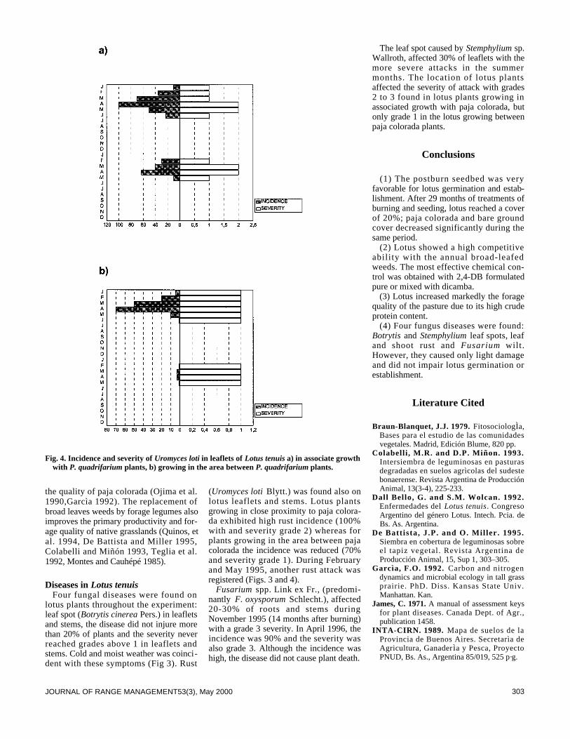
303JOURNAL OF RANGE MANAGEMENT53(3), May 2000
the quality of paja colorada (Ojima et al.1990,Garcìa 1992). The replacement ofbroad leaves weeds by forage legumes alsoimproves the primary productivity and for-age quality of native grasslands (Quinos, etal. 1994, De Battista and Miller 1995,Colabelli and Miñón 1993, Teglia et al.1992, Montes and Cauhépé 1985).
Diseases in Lotus tenuisFour fungal diseases were found on
lotus plants throughout the experiment:leaf spot (Botrytis cinerea Pers.) in leafletsand stems, the disease did not injure morethan 20% of plants and the severity neverreached grades above 1 in leaflets andstems. Cold and moist weather was coinci-dent with these symptoms (Fig 3). Rust
(Uromyces loti Blytt.) was found also onlotus leaflets and stems. Lotus plantsgrowing in close proximity to paja colora-da exhibited high rust incidence (100%with and severity grade 2) whereas forplants growing in the area between pajacolorada the incidence was reduced (70%and severity grade 1). During Februaryand May 1995, another rust attack wasregistered (Figs. 3 and 4).
F u s a r i u m spp. Link ex Fr., (predomi-nantly F. oxysporum Schlecht.), affected20-30% of roots and stems duringNovember 1995 (14 months after burning)with a grade 3 severity. In April 1996, theincidence was 90% and the severity wasalso grade 3. Although the incidence washigh, the disease did not cause plant death.
The leaf spot caused by Stemphylium sp.Wallroth, affected 30% of leaflets with themore severe attacks in the summermonths. The location of lotus plantsaffected the severity of attack with grades2 to 3 found in lotus plants growing inassociated growth with paja colorada, butonly grade 1 in the lotus growing betweenpaja colorada plants.
Conclusions
(1) The postburn seedbed was veryfavorable for lotus germination and estab-lishment. After 29 months of treatments ofburning and seeding, lotus reached a coverof 20%; paja colorada and bare groundcover decreased significantly during thesame period.
(2) Lotus showed a high competitiveability with the annual broad-leafedweeds. The most effective chemical con-trol was obtained with 2,4-DB formulatedpure or mixed with dicamba.
(3) Lotus increased markedly the foragequality of the pasture due to its high crudeprotein content.
(4) Four fungus diseases were found:B o t r y t i s and S t e m p h y l i u m leaf spots, leafand shoot rust and F u s a r i u m w i l t .However, they caused only light damageand did not impair lotus germination orestablishment.
Literature Cited
Braun-Blanquet, J.J. 1979. F i t o s o c i o l o g Ì a ,Bases para el estudio de las comunidadesvegetales. Madrid, Edición Blume, 820 pp.
Colabelli, M.R. and D.P. Miñon. 1993.Intersiembra de leguminosas en pasturasdegradadas en suelos agrìcolas del sudestebonaerense. Revista Argentina de ProducciónAnimal, 13(3-4), 225-233.
Dall Bello, G. and S.M. Wolcan. 1992.Enfermedades del Lotus tenuis. CongresoArgentino del género Lotus. Intech. Pcia. deBs. As. Argentina.
De Battista, J.P. and O. Miller. 1995.Siembra en cobertura de leguminosas sobreel tapiz vegetal. Revista Argentina deProducción Animal, 15, Sup 1, 303–305.
Garcìa, F.O. 1992. Carbon and nitrogendynamics and microbial ecology in tall grassprairie. PhD. Diss. Kansas State Univ.Manhattan. Kan.
James, C. 1971. A manual of assessment keysfor plant diseases. Canada Dept. of Agr.,publication 1458.
INTA-CIRN. 1989. Mapa de suelos de laProvincia de Buenos Aires. Secretarìa deAgricultura, Ganader ìa y Pesca, ProyectoPNUD, Bs. As., Argentina 85/019, 525 p·g.
Fig. 4. Incidence and severity of Uromyces loti in leaflets of Lotus tenuis a) in associate growthwith P. quadrifarium plants, b) growing in the area between P. quadrifarium plants.
304 JOURNAL OF RANGE MANAGEMENT 53(3), May 2000
Montes, L. and M.A. Cauhèpè. 1985.Intersiembra de Lotus tenuis en cobertura.Revista Argentina de Producción Animal,5(5-6), 313–321.
Ojima, D.S., W.J. Parton, D.S. Schimel, andC.E. Owensy. 1990. Simulated impacts ofannual burning on prairie ecosystems. pp.118-132. In: S. L. Collins and L. L. Wallace.(Editors) “Fire in North American Tall Grasson prairies”, Univ. of Oklahoma Press,Norman, Okla., USA.
Ortega, E.Z. and P. Laterra. 1995. I m p a c t ode Lotus tenuis sobre la abundancia deCarduus acanthoides y Cirsium vulgare e npajonales quemados de Paspalum quadrifar -i u m . Res˙menes de la XVII ReuniónArgentina de EcologÌa, Mar del Plata.
Quinos, P., P. Insausti, and A. Soriano. 1994.Papalum dilatatum responde a la vecindad deLotus tenuis en la Depresión del Salado.Revista Argentina de Producción Animal.Vol 14, Sup 1.
Sacido, M., L. Hidalgo and M. A. Cauhèpè.1995. Efecto del fuego y la defoliación sobreel valor nutritivo de matas de paja colorada(Paspalum quadri farium) Revista Argentinade Producción Animal, 15, Sup 1, 143-147.
Teglia, J., A. GarcÌa Espil and M.C.Saucede. 1992. Incorporación de especiesforrajeras en pastizales mediante distintasm·quinas intersembradoras. Revista de laFacultad de Agronomìa. Tomo 14 (3):285–289.
Thornthwaite, C. and J. Mather. 1957.Instructions and tables for computing poten-cial evapotranspiration and water balance.Drexel Institute of Technology, Published InClimatology, Vol. X, N 3. Centerton. (Trad.Castellana por A. Rodriguez Saenz y G.Juarez. INTA, Instituto de Suelos yAgrotecnia, Tirada Interna No 46, BuenosAires, 1967.)
Vervoorst, F.B. 1967. Las comunidades vege-tales de la Depresión del Salado (Prov. Bs.As.). La vegetación de la RepúblicaArgentina VII. INTA. Serie FitogeográficaNo 7. Buenos Aires.
Wolcan, S.M. and G. Dall Bello. 1988.Colletotrichum destructivum OíGara c a u s a lagent of a new disease on Lotus tenuis Walst.et Kit. Agronomie: 8, 741– 744
305JOURNAL OF RANGE MANAGEMENT 53(3), May 2000
Astract
Flea beetles (Aphthona spp.) were introduced into leafy spurge(E u p h o r b i a e s u l a L.)-infested rangeland in east-central NorthDakota. The study objectives were to evaluate the effects of theintroduced insects on leafy spurge cover, density, and yield, andgrass and grass-like yield of associated plant communities.A p h t h o n a spp. were released in 1988 and 1989 at 2 sites nearValley City, N.D. Aboveground vegetative sampling for leafyspurge cover, density and yield, and grass and grass-like yieldwas conducted between 1993 and 1995. Belowground sampling ofroot density, dry weight and root buds was conducted betweenthe release date and 1995. A p h t h o n a spp. reduced abovegroundcover, density and yield of leafy spurge and increased yield ofgrass and grass-like species. Leafy spurge root density, weight,and number of root buds decreased on insect release sitesbetween release dates and 1995. Reduced stem density of leafyspurge and increased grass and grass-like yield, should enhancecattle use and production from these sites.
Key Words: biological control, leafy spurge, insects, flea bee-tles, range improvement
Biological control of introduced noxious weeds using insectshas received limited use on rangelands (Vallentine 1989).Successful biological control efforts using insects has been report-ed for St. John’s-Wort (H y p e r i c u m p e r f o r a t u m L.) (Huffaker andKennett 1959), pricklypear (O p u n t i a spp.) (Goeden et al. 1968),and tansy ragwort (Senecio jacobaea L.) (Hawkes 1968). Effortsto control leafy spurge (E u p h o r b i a e s u l a L.) with insects has beenongoing since the 1960s with significant expansion in the 1970sand 1980s (Harris 1984, Pemberton 1985).
Leafy spurge is an introduced plant from Eurasia that isextremely persistent and competitive in grazed rangelands (Dunn1979). It is considered a prime candidate for biological controlbecause of its propensity to invade a variety of habitats such asgrasslands, woodlands, riparian areas and waterways where alter-native control efforts may be limited and it is a perennial weedproviding a continuous source of food to organisms capable ofutilizing portions of the plant. Unfortunately, leafy spurge’sdefense mechanisms such as the milky latex make utilization ofthe plant difficult except for well adapted insects that haveevolved means to overcome these defenses (Best et al. 1980).
Eight insects have been released to control leafy spurge inNorth Dakota since the 1980s (Lym and Zollinger 1995). Ofthese, flea beetles (Aphthona spp.) have been the most successfulfor establishment, reproduction and redistribution. However, lim-ited quantitative information is available regarding the impact ofAphthona spp. on leafy spurge and the associated plant communi-ty. The objectives of this study were to evaluate the effects ofAphthona spp. on leafy spurge cover, density and yield, and grassand grass-like yield of associated plant communities.
Material and Methods
Experiments to evaluate leafy spurge control with an introducedbiological control agent A p h t h o n a spp. were established at 2 sitesin east-central North Dakota. A total of 80 flea beetles werereleased in 1988 at a site that was approximately 15 km northwestof Valley City (North) on the Katie Olson Wildlife ManagementArea (98°10'N 47°15'W). Biological control agents at this site were
J. Range Manage.53: 305–308 May 2000
Biological control of leafy spurge with introduced fleabeetles (Aphthona spp.)
DONALD R. KIRBY, ROBERT B. CARLSON, KELLY D. KRABBENHOFT, DONALD MUNDAL, AND MATT M.KIRBY
Authors are professor, Animal and Range Sciences Department, North Dakota State University, Fargo, N.D. 58105; professor, Entomology Department,North Dakota State University, Fargo, N.D. 58105; research specialist, Animal and Range Sciences Department, North Dakota State University, Fargo, N.D.58105; research specialist, Entomology Department, North Dakota State University, Fargo, N.D. 58105; and undergraduate student, Animal and Range
Manuscript accepted 17 Aug. 1999.
Resumen
Se introdujeron "Flea beetles" (A p h t h o n a spp.) en pastizalesde la región centro-este de North Dakota los cuales estaban infes-tados con "leafy spurge" (Euphorbia esula L.). Los objetivos delestudio fueron evaluar los efectos de los insectos introducidos enla cobertura, densidad y rendimiento del "Leafy spurge" y en elrendimiento de zacates y planta similares a los zacates de lascomunidades vegetales asociadas. Los A p h t h o n a spp. Se liber-aron en 1988 y 1989 en 2 sitios cerca de Valley City, N.D. Elmuestreo de las partes vegetativas aéreas para determinar cober-tura, densidad y rendimiento del "Leafy spurge" y el rendimien-to de los zacates y plantas similares a zacates se condujo entre1993 y 1995. El muestreo de las partes subterráneas para deter-minar la densidad y peso seco de raíces y yemas radicales se con-dujo entre la fecha de liberación de los insectos y 1995. Lasespecies de Aphthona redujeron la cobertura, densidad yrendimiento de "leafy spurge" e incrementaron el rendimientode las especies de zacates y plantas similares a ellos. La densidadde raíces de "Leafy spurge", el peso y numero de yemas radi-cales disminuyo entre la fecha de liberación y 1995 en los sitiosen donde se liberaron los insectos. La reducción de tallos de"Leafy spurge" y el aumento del rendimiento de zacates y plan-tas similares a estos debe incrementar el uso de ganado bovino yla producción en estos sitios.

306 JOURNAL OF RANGE MANAGEMENT 53(3), May 2000
2 flea beetle species, A. czwalinae and A . l a c -e r t o s a. A second site was located approxi-mately 15 km southeast of Valley City(South) on private land (97°50'N 46° 50'W).Approximately 1,000 A. nigriscutis w e r ereleased at this site in 1989.
Both sites are located within theSheyenne River drainage system, which ishighly dissected and steeply sloping(>15%). Soils were a Koten silty clay loam(fine, montmorillonitic Udertic Haploboroll)at the North site and a Nutley silty clay(loamy, mixed Lithic Haploboroll) at theSouth site. Both sites supported northernmixed grass prairie (Barker and Whitman1989) with infestations of leafy spurgeexceeding 200 stems/m2. Annual averageprecipitation for east-central North Dakotais 45 cm with approximately 75% receivedduring the growing season (April throughSeptember). Annual precipitation receivedbetween 1988 and 1995 was similar to thelong-term average, 50 cm, with 80% occur-ring during the growing season.
Aboveground vegetative sampling wasinitially conducted at the North experimentin 1988. Sampling was abandoned after1990 because the insect colony migrated toan adjacent area. Vegetative samplingresumed between 1993 and 1995 after theinsect colony became permanently estab-lished. Vegetative sampling was initiatedin 1993 at the South experiment to allowtime for the insect colony to permanentlyestablish. Three random transects eachwere located in insect colonized and insectfree areas at both study sites. Leafy spurgecover and density were estimated fromeight 0.1 m2 quadrats positioned randomlyalong each transect. Leafy spurge, andgrass and grass-like yields were deter-mined by clipping and drying (60°C) thevegetation within four, 0.1 m2 q u a d r a t salong each transect. Vegetative measure-ments were conducted at the peak standingcrop in late July each year.
Soil samples for root characterizationwere initiated in 1988 at the North site and1989 at the South site. At North and Southsites, 4 and 3 random transects wereplaced at insect colonized and insect freeareas, respectively. The insect free transectsampling was terminated at both studylocations in 1991 due to movement of theinsects into these areas. On each transect,5 random soil cores 15-cm deep (12-cmdiameter) were collected using a 12-cmdiameter golf cup-cutter each October andstored in plastic bags at –4°C. The leafyspurge roots from each core were extract-ed from the soil and washed. The numberof individual root segments and root budsfor each segment were recorded. The root
segments were then dryed at 60°C for dryweight determinations.
The effect of flea beetle control on leafyspurge was evaluated as a randomizedcomplete block design at 2 locations with3 blocks (transects) and 2 treatments(insect free and insect colonized). Blockswere found to be nonsignificant betweenlocations so a completely randomizeddesign was utilized. Vegetative and rootdata by treatment and year were analyzedusing a one-way ANOVA (SPSS, Inc.1994) and mean differences were consid-ered significant at the 5% probability levelusing Tukey’s h test.
Results and Discussion
Foliar cover of leafy spurge was reduced(P < 0.05) on A p h t h o n a spp. colonizedsites compared to insect free sites (Fig. 1).Pre-treatment estimates (1988) of leafyspurge cover were 45% (data not shown)which was similar to the control sites in1994 and 1995. A 6- to 7-fold decrease inleafy spurge cover occurred on releasesites over this same time period. Strommeet al. (1996) reported a similar reductionin leafy spurge foliar cover, 40% to 1.7%,five years after A. nigriscutis w e r ereleased near Edmonton, Canada.
Leafy spurge stem densities werereduced on A p h t h o n a spp. release sites
compared to pre-study estimates (218/m2)and control si tes (Fig. 2). By 1994,A p h t h o n a spp. had reduced leafy spurgestem densities nearly 40-fold to only 5/m2.Stem density reductions have also beenreported by Hansen (1993), Baker et al.(1996), Lym et al. (1996) and Stromme etal. (1996). However, only Stromme et al.(1996) reported reductions in leafy spurgestem densities of the magnitude evaluatedin this study.
Stem densities of leafy spurge have beenreported to influence cattle grazing behav-ior (Lym and Kirby 1987). Stem densitiesexceeding 100/m2 decreased cattle use ofleafy spurge-infested rangeland. Leafyspurge stem densities on insect releasesites were reduced to a level that wouldallow cattle grazing.
Total herbaceous yields were greater oncontrol sites compared to the insect releasesites each year due to the biomass contri-bution from leafy spurge (Table 1). Leafyspurge biomass was reduced each year onthe insect release sites compared to thecontrols, while graminoid yields weregreater on A p h t h o n a spp. release sites in1994 and 1995 compared to the controls.Stromme et al. (1996) reported a decreasein leafy spurge biomass from 1,730 to 17kg/ha and an increased grass biomass from14 to 433 kg/ha which are comparable tothose reported in this study.
Fig. 1. Leafy spurge cover (%) following Aphthona spp. colonization of leafy spurge-infestedrangeland. Bars with different letters differ (P < 0.05).
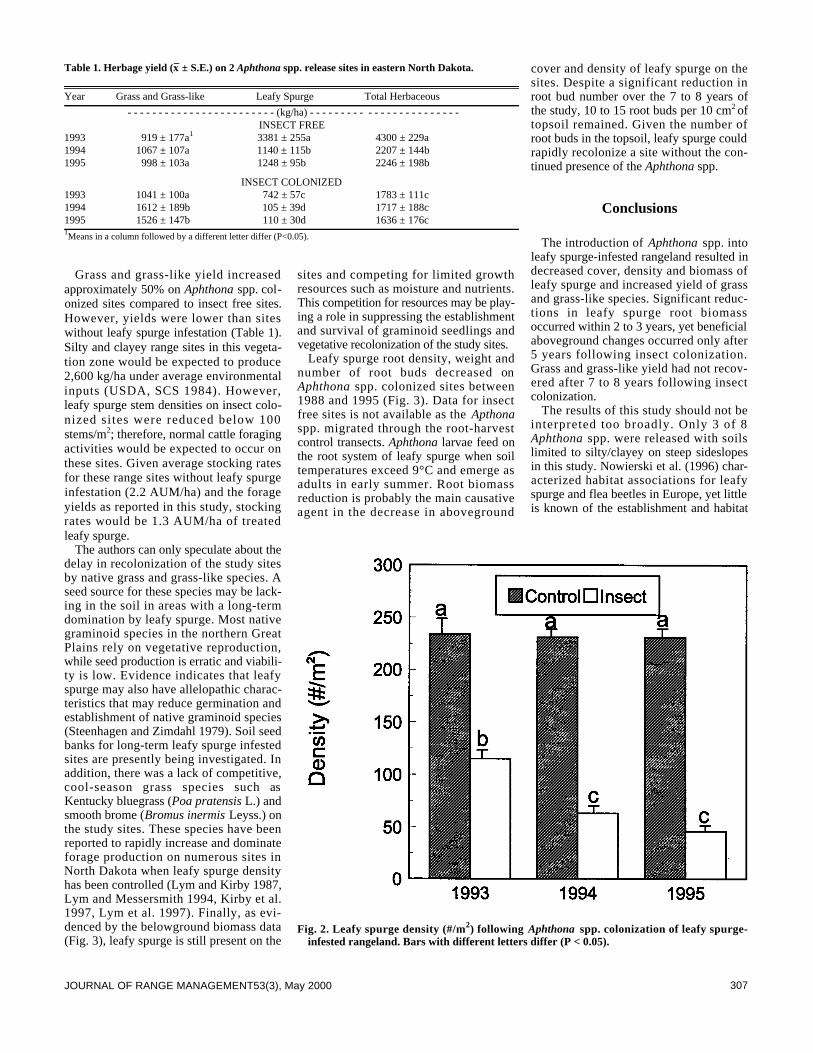
307JOURNAL OF RANGE MANAGEMENT53(3), May 2000
Grass and grass-like yield increasedapproximately 50% on Aphthona spp. col-onized sites compared to insect free sites.However, yields were lower than siteswithout leafy spurge infestation (Table 1).Silty and clayey range sites in this vegeta-tion zone would be expected to produce2,600 kg/ha under average environmentalinputs (USDA, SCS 1984). However,leafy spurge stem densities on insect colo-nized sites were reduced below 100stems/m2; therefore, normal cattle foragingactivities would be expected to occur onthese sites. Given average stocking ratesfor these range sites without leafy spurgeinfestation (2.2 AUM/ha) and the forageyields as reported in this study, stockingrates would be 1.3 AUM/ha of treatedleafy spurge.
The authors can only speculate about thedelay in recolonization of the study sitesby native grass and grass-like species. Aseed source for these species may be lack-ing in the soil in areas with a long-termdomination by leafy spurge. Most nativegraminoid species in the northern GreatPlains rely on vegetative reproduction,while seed production is erratic and viabili-ty is low. Evidence indicates that leafyspurge may also have allelopathic charac-teristics that may reduce germination andestablishment of native graminoid species(Steenhagen and Zimdahl 1979). Soil seedbanks for long-term leafy spurge infestedsites are presently being investigated. Inaddition, there was a lack of competitive,cool-season grass species such asKentucky bluegrass (Poa pratensis L.) andsmooth brome (Bromus inermis Leyss.) onthe study sites. These species have beenreported to rapidly increase and dominateforage production on numerous sites inNorth Dakota when leafy spurge densityhas been controlled (Lym and Kirby 1987,Lym and Messersmith 1994, Kirby et al.1997, Lym et al. 1997). Finally, as evi-denced by the belowground biomass data(Fig. 3), leafy spurge is still present on the
sites and competing for limited growthresources such as moisture and nutrients.This competition for resources may be play-ing a role in suppressing the establishmentand survival of graminoid seedlings andvegetative recolonization of the study sites.
Leafy spurge root density, weight andnumber of root buds decreased onA p h t h o n a spp. colonized sites between1988 and 1995 (Fig. 3). Data for insectfree sites is not available as the A p t h o n aspp. migrated through the root-harvestcontrol transects. Aphthona larvae feed onthe root system of leafy spurge when soiltemperatures exceed 9°C and emerge asadults in early summer. Root biomassreduction is probably the main causativeagent in the decrease in aboveground
cover and density of leafy spurge on thesites. Despite a significant reduction inroot bud number over the 7 to 8 years ofthe study, 10 to 15 root buds per 10 cm2 oftopsoil remained. Given the number ofroot buds in the topsoil, leafy spurge couldrapidly recolonize a site without the con-tinued presence of the Aphthona spp.
Conclusions
The introduction of A p h t h o n a spp. intoleafy spurge-infested rangeland resulted indecreased cover, density and biomass ofleafy spurge and increased yield of grassand grass-like species. Significant reduc-tions in leafy spurge root biomassoccurred within 2 to 3 years, yet beneficialaboveground changes occurred only after5 years following insect colonization.Grass and grass-like yield had not recov-ered after 7 to 8 years following insectcolonization.
The results of this study should not beinterpreted too broadly. Only 3 of 8A p h t h o n a spp. were released with soilslimited to silty/clayey on steep sideslopesin this study. Nowierski et al. (1996) char-acterized habitat associations for leafyspurge and flea beetles in Europe, yet littleis known of the establishment and habitat
Fig. 2. Leafy spurge density (#/m2) following Aphthona spp. colonization of leafy spurge-infested rangeland. Bars with different letters differ (P < 0.05).
Table 1. Herbage yield (x– ± S.E.) on 2 Aphthona spp. release sites in eastern North Dakota.
Year Grass and Grass-like Leafy Spurge Total Herbaceous
- - - - - - - - - - - - - - - - - - - - - - - - (kg/ha) - - - - - - - - - - - - - - - - - - - - - - - - INSECT FREE
1993 919 ± 177a1 3381 ± 255a 4300 ± 229a1994 1067 ± 107a 1140 ± 115b 2207 ± 144b1995 998 ± 103a 1248 ± 95b 2246 ± 198b
INSECT COLONIZED1993 1041 ± 100a 742 ± 57c 1783 ± 111c1994 1612 ± 189b 105 ± 39d 1717 ± 188c1995 1526 ± 147b 110 ± 30d 1636 ± 176c1Means in a column followed by a different letter differ (P<0.05).

308 JOURNAL OF RANGE MANAGEMENT53(3), May 2000
requirements of A p h t h o n a spp. in NorthAmerica. A p h t h o n a spp. establishment insandy soils, overflow or subirrigated rangesites, and in shrubby or riparian areas havenot been successful to date. Questionsconcerning successful establishment pro-cedures and habitat barriers such as soil,slope, aspect, root demographics, leafyspurge density, surface litter, initial releasesizes, over-winter survival, populationsize, persistence, rate of spread and moreremain to be answered.
Literature Cited
Baker, J.L., N.A.P. Webber, K.K. Johnson,and R.L. Lavigne. 1996. The behavior ofAphthona nigriscutis and the response ofleafy spurge over a four year period in
Fremont county Wyoming. Proc. WesternSoc. Weed Sci. 49:47–48.
Barker, W.T. and W.C. Whitman. 1989.Vegetation of the Northern Great Plains.Rangelands 10:266–272.
Best, K.F., G.G. Bowes, A.G. Thomas, andM.G. Maw. 1980. The biology of Canadianweeds. 39. E u p h o r b i a L. Canadian J. PlantSci. 60:651-663.
Dunn, P.H. 1979. The distribution of leafyspurge and other E u p h o r b i a spp. in theUnited States. Weed Sci. 27:509–516.
Goeden, R.D., C.A. Fleschner, and D.W.Ricker. 1968. Insects control prickly-pearcactus. Calif. Agr. 22:8–9.
Hansen, R. 1993. Effects of A p h t h o n a f l e abeetles and sheep grazing in leafy spurgestands. p. 47–48. I n : K.G. Beck (ed.) Proc.Leafy Spurge Symp., Silvercreek, Colo.
Harris, P. 1984. Euphorbia esula-virgata com-plex, leafy spurge and E. cyparissias L .cypress spurge (Euphorbiaceae), p. 159–169.
In: J.S. Kelleher and M.A. Hulme (eds.),Biological control programs against insectsand weeds in Canada 1969-80. Farnham Agr.Bur. Farnham Royal, U.K.
Hawkes, R.B. 1968. The cinnabar moth, Tyriaj a c o b a c e a e, for control of tansy ragwort. J.Econ. Entomol. 61:499–501.
Huffaker, C.B. and C.E. Kennett. 1959. Ten-year study of vegetational changes associatedwith biological control of Klamath weed. J.Range Manage. 12:69–82.
Kirby, D.R., T.P. Hanson, K.D. Krabbenhoft,and M.M. Kirby. 1997. Effects of simulateddefoliation of leafy spurge (Euphorbia esula) -infested rangeland. Weed Tech. 11:586–590.
Lym, R.G. and D.R. Kirby. 1987. Cattle for-aging behavior in leafy spurge (E u p h o r b i aL.) infested rangeland. Weed Tech.1:314–318.
Lym, R.G. and C.G. Messersmith. 1994.Leafy spurge (Euphorbia esula ) control, for-age production, and economic return withfall-applied herbicides. Weed Tech.8:824–829.
Lym, R.G. and R.K. Zollinger. 1995. I n t e g r a t e dmanagement of leafy spurge. North DakotaState Univ. Ext. Serv. Bull. W-866 (rev.). 4 pp.
Lym, R.G., K.K. Sedivec, and D.R. Kirby.1997. Leafy spurge control with angora goatsand herbicides. J. Range Manage.50:123–128.
Lym, R.G., R.B. Carlson, K.M. Christianson,D.A. Mundal, and C.G. Messersmith. 1996.Integration of herbicides with A p h t h o n a s p p .flea beetles for leafy spurge control. p. 64. I n :K. Pouteau (ed.), Proc. Leafy Spurge Symp.,Brandon, Manitoba.
Nowierski, R.M., Z. Zeng., D. Schroeder,and A. Gassmann. 1996. Habitat analyses ofEuphorbia species and associated flea beetlesin the A p h t h o n a complex from Europe: canwe learn something about habitat associa-tions of natural enemies prior to release? p.232. I n : V.C. Moran and J.H. Hoffmann(eds.), Proc. IX Internat. Symp. Biol. ControlWeeds, Stellenbosch, So Africa.
Pemberton, R.W. 1985. Native plant consider-ations in the biological control of leafyspurge. p. 365–390. I n : E.S. Delfosse (ed.),Proc. VI Internat. Symp. Biol. ControlWeeds, Vancouver, British Columbia.
SPSS, Inc. 1994. SPSS advanced statistics. 6.1.Chicago, Ill.
Steenhagen, D.A. and R.L. Zimdahl. 1979.Allelopathy of leafy spurge (E u p h o r b i a) .Weed Sci. 27:1–3.
Stromme, K., D.E. Cole, A.S. McClay, C.J.Richardson, and J. de Valois . 1996.Biocontrol of leafy spurge with A p h t h o n an i g r i s c u t i s in Alberta “The Beverly BridgeSite. p. 26-27. I n : K. Pouteau (ed.), Proc.Leafy Spurge Symp., Brandon, Manitoba.
USDA, SCS. 1984. Range Site TechnicalGuide Notice ND-35. Bismarck, N.D.
Vallentine, J.F. 1989. Range development andimprovements. Academic Press, Inc., NewYork, N.Y.
Abstract
Fig. 3. Root density, dry weight and root buds (—x ± S.E.) from soil cores at 2 locations follow-ing Aphthona spp. colonization of leafy spurge-infested rangeland. Means by location fol-lowed by a different letter differ (P < 0.05).

309JOURNAL OF RANGE MANAGEMENT53(3), May 2000
Abstract
Spotted knapweed (Centaurea maculosa Lam.) managementmay be enhanced by integrating strategies that stimulate andmaintain competitive grasses. The objective of this study was todetermine if picloram, fertilizer, and timing and frequency ofgrass defoliation could be integrated to minimize spotted knap-weed reinvasion. Sixteen chemical treatments [4 picloram rates(0.00, 0.14, 0.28, and 0.42 kg a.i. ha - 1) and 4 fertilizer rates(source: 16-20-0, N-P-K; material: 0.0, 66, 132, 198 kg ha-1)] wereapplied in the spring of 1994 to 4 by 4 m plots and factoriallyarranged in a randomized-complete-block design. Within eachplot, 6 grass defoliation treatments were randomly applied to 1by 1 m sub-plots. From 1994 through 1997, 60% of the aboveground grass biomass was hand clipped and removed from theplots during the spring, summer, fall, alternating spring/fall, all 3seasons. A control received no grass defoliation. The experimentwas replicated 4 times at 2 sites dominated by spotted knapweed.At peak standing crop in 1997 spotted knapweed density, grassand spotted knapweed biomass; and percent cover of spottedknapweed, grass, litter, and bare ground were measured. Datawere analyzed as a split-plot using analysis of variance. Fouryears after treatment all rates of picloram reduced spotted knap-weed density, biomass, and cover, and increased grass yield.Nitrogen and P fertilizer tended to increase spotted knapweeddensity and biomass. Nitrogen and P fertilizer plus defoliation inall 3 seasons caused a greater increase in spotted knapweed rein-vasion at the site with Kentucky bluegrass (Poa pratensis L.) thanthe site with timothy (Phleum pratense L.) and smooth brome(Bromus inermis Leys.). Fall-only defoliation and no defoliationappear to deter spotted knapweed reinvasion better than defolia-tion in all 3 seasons and alternately in the spring and fall.
Key Words: Centaurea maculosa , integrated weed management,grass defoliation, grazing management
Spotted knapweed (Centaurea maculosa Lam.), a short-livedperennial native to Eurasia, is rapidly invading rangelandthroughout western North America. This aggressive weed hasbeen spreading at about 27% per year and infests over 2.8 millionhectares in Montana, and adjoining states and Canadian provinces(Chicoine et al. 1985, Lacey et al. 1989). Spotted knapweed canbe found in 326 counties in the western United States (Sheley etal. 1998). Impacts associated with this species include reducedforage production (Watson and Renney 1974), plant species
diversity (Tyser and Key 1988), wildlife habitat (Bedunah andCarpenter 1989) and increased bare ground, surface water runfoffand stream sedimentation (Lacey et al. 1989), and managementcosts (Griffith and Lacey 1989).
Most broadleaf herbicides are effective in reducing spottedknapweed populations. Picloram (4-amino-3,5,6-trichloropicolin-ic acid) applied at a rate of 0.28 kg active ingredient (a.i.) ha- 1
provides control for 2 to 5 years (Davis 1990). Although the per-
J. Range Manage.53: 309–314 May 2000
Picloram, fertilizer, and defoliation interactions on spottedknapweed reinvasion
JAMES S. JACOBS, ROGER L. SHELEY, AND JOELLA R. CARTER
Authors are post-doctoral research associate; associate assistant professor; and graduate research assistant, Department of Land Resources andEnvironmental Sciences, Montana State University, Mont. 59717.
Manuscript accepted 6 Sept. 1999.
Resumen
El manejo de "Spotted knapweed"(Centaurea maculosa Lam.)puede ser mejorado mediante la integración de estrategias queestimulan y mantienen los zacates competitivos. El objetivo deeste estudio fue determinar si el picloram, la fertilización y laépoca y frecuencia de defoliación del zacate pudieran ser inte-grados para minimizar la reinvasión de "Spotted knapweed".En primavera de 1994 se aplicaron 16 tratamientos químicos [4dosis de picloram (0.00, 0.14, 0.28 y 0.42 kg i.a ha-1) y 4 dosis defertilizante(0.0, 66, 132 y 198 kg ha-1; fuente: 16-20-0, N-P-K)] enparcelas de 4 x 4 m bajo un diseño de bloques completos al azaren arreglo factorial. Dentro de cada parcela se aplicaron 6tratamientos de defoliación, los cuales se asignaron aleatoria-mente a subparcelas de 1 x 1 m. De 1994 a 1997, durante lasépocas de primavera, verano, otoño, alternadamente en primav-era/verano y en las tres estaciones del año, se corto y removiómanualmente el 60% de la biomasa aérea de las parcelas. Lasparcelas control no recibieron defoliación del zacate. El experi-mento se repitió 4 veces en 2 sitios en los que predominaba el"Spotted knapweed". En 1997, cuando se alcanzo la máximaproducción de biomasa en pie, se midió la densidad de "Spottedknapweed", la biomasas de los zacates y del "Spotted knap-weed", y el porcentaje de cobertura de "Spotted knapweed,zacates, mantillo y suelo desnudo. Los datos se analizaron medi-ante análisis de varianza y bajo el diseño experimental de parce-las divididas. Cuatro años después de aplicar los tratamientos,todas las dosis de picloram redujeron la densidad, biomasa ycobertura de "Spotted knapweed" e incrementaron elrendimiento de forraje de los zacates. La fertilización nitrogena-da y fosforada tendieron a incrementar la densidad y biomasa de"Spotted Knapweed". La fertilización nitrogenada y fosforadamas la defoliación en las tres estaciones causo una mayor rein-vasión de "Spotted knapweed" en el sitio con "Kentucky blue-grass" (Poa pratensis L.) que en el sitio con "Timothy (Ph l e u mpratense L.) y "Smooth brome" (Bromus inermis Leys.). Defoliarsolo en otoño y el no defoliar parece detener la reinvasión de"Spotted knapweed" mejor que la defoliación en todas las tresestaciones y alternativamente en primavera y otoño.
310 JOURNAL OF RANGE MANAGEMENT 53(3), May 2000
sistence of picloram in the soil affectsweeds for 12 to 30 months (Hamaker et al.1967), extended control is enhanced bycompetition from residual perennial grassesthat are released by the herbicide applica-tion (Sheley et al. 1998). Combining herbi-cide and fertilizer applications has increasedforage production on rangelands (Hart et al.1995); however, little is known about com-bining them to control knapweed andenhance forage production.
Intergrating picloram and fertilizers mayhave a synergistic effect on providing spot-ted knapweed control and enhanced grassproduction. In a pilot study, Sheley andRoché (1982) combined picloram (0.28 kga.i. ha- 1) and fertilizer (N + P: 17.9 + 22.4kg ha - 1) which increased grass yield from275 (control) and 660 (picloram alone) to2,200 (picloram plus fertilizer) kg ha- 1, 2years after application. In that study, knap-weed control was also greater where piclo-ram was combined with fertilization thanthe control and picloram alone. Morerecently, Sheley and Jacobs (1997) foundno picloram by N + P fertilizer interactionsin Montana. Picloram treatments (0.14 to0.42 kg a.i. ha- 1) reduced spotted knapweedto nearly zero, and fertilization at the high-est rate (180 kg ha - 1; 16-20-0 NPK)increased grass yield on the site with a sub-stantial grass understory.
Spotted knapweed seeds can remain dor-mant in the soil for up to 8 years and rein-vasion on sites treated with picloram usual-ly begins within 2–5 years after herbicideapplication (Davis et al. 1993). While manyfactors affect picloram persistence in thesoil including photodegredation, precipita-tion, and soil texture (Davis 1990), andtherefore longevity of spotted knapweedcontrol, it is believed that the competitiveability of the residual grass on treated sitesalso affects spotted knapweed reinvasion(Sheley et al. 1998). The competitive inter-action between weeds and perennial grassesis affected by frequency, timing and inten-sity of defoliation which in turn affects theability of perennial grass communities towithstand weed invasion (Maschinski andWhithan 1989, Jacobs and Sheley 1997).Although studies suggest that moderategrazing does not accelerate invasion ofknapweeds (Centaurea spp.) into rangeland(Sheley et al. 1997, Jacobs and Sheley1997), we found no studies that attempt toquantify the effects of defoliation on theirreinvasion after control.
An important concern of rangeland man-agers is how to prevent or reduce weedreinvasion on areas where weeds have beencontrolled. The overall objective of thisstudy was to determine the effect of the
timing and frequency of grass defoliationon spotted knapweed reinvasion on areastreated with picloram and fertilizer combi-nations. Specific objectives were to 1)determine if picloram and fertilizer interactto increase long-term spotted knapweedcontrol or grass yield, and 2) determine iftiming and frequency of grass defoliationaffected spotted knapweed reinvasion. Wehypothesized that picloram and fertilizerwould interact to increase spotted knapweedcontrol and grass yield, which would limitreinvasion. In addition, we believe that spot-ted knapweed reestablishment would begreater in areas with more frequent grassdefoliation and defoliation in the spring thansummer and fall defoliations.
Materials and Methods
Study SitesField studies were conducted from 1994
through 1997 on 2 sites located 15 kmwest of Bozeman, Mont. (111°5'36''W,45°35'26'' N). Both sites were within aFestuca idahoensis/Agropyron spicatumhabitat type (Mueggler and Stewart 1980),and dominated by spotted knapweed. Site1 was an abandoned hayfield. Spottedknapweed densities were 470 ± 140 plantsm-2. Associated grass species were smoothbromegrass (Bromus inermis Leys), timo-thy (Phleum pratense L.), and Kentuckybluegrass (Poa pratensis L.). Associatedgrass on site 2 was predominantlyKentucky bluegrass. Spotted knapweeddensity was 140 ± 107 plants m-2. Soils atboth sites consisted of 70% Beavertoncobbly loam (loamy-skeletal over sandy orsandy-skeletal mixed, Typic Argiborolls)and 30% Hyalite loam (fine-loamy, mixed,Typic Argiborolls). Sites were nearly leveland at an elevation of 1,340 m. Annualprecipitation ranges from 380 to 480 mmand the frost-free period ranges from 90 to110 days at both sites.
Experimental DesignSixteen chemical treatments (4 picloram
rates, 4 fertilizer rates) were applied to 4by 4 m plots and factorially arranged in arandomized-complete-block design.Within each plot, 6 different defoliationtreatments were randomly applied to 1 x 1m sub-plots. The experiment was replicat-ed 4 times at both sites.
Picloram rates of 0.0, 0.14, 0.28, and0.42 kg a.i. ha- 1 were applied using a 6 noz-zle backpack sprayer delivering 130 litersh a- 1 spray solution. Granular fertilizer wasbroadcast at N + P rates of 0.0 + 0.0, 10.5 +13.2, 21.1 + 26.4, and 31.7 + 39.6 kg ha- 1
(source: 16-20-0, N-P-K; material: 0.0, 66,132, 198 kg ha - 1) using a hand-cycloneapplicator. Both sites were treated on 2May 1994 when spotted knapweed was inthe rosette stage. Air temperature, soil tem-perature (surface), and relative humidtywere 17.5°C, 21°C, and 90%, respectively,at the time of application. Winds rangedfrom 0 to 6 km hr- 1. Individual 4 x 4 mplots were spatially separated from eachother by a 2.1 m buffer zone treated with0.28 k a.i. ha-1 of picloram to prevent spot-ted knapweed seed contamination fromneighboring plots.
From fall 1994 through fall 1997, sixdefoliation regimes differing in the fre-quency and timing of defoliation wereapplied as 1 x 1 m sub-plots. They werecontrol (no defoliation), spring, mid-sum-mer, fall, alternating spring/fall, andrepeated defoliations in spring, summer,and fall. Defoliation treatments wereapplied by hand-clipping grasses to 60%of the above-ground biomass. Defoliationlevel was calibrated by clipping grassfrom ten, 0.2 x 0.5 m plots estimated at60% and comparing their average weightwith the average weight of grass clipped tothe soil surface from ten, 0.2 x 0.5 m plots.All clippings were removed from theplots. Repeated defoliations removed 60%of the remaining foliage including allregrowth.
SamplingAt peak standing crop (August), above-
ground biomass within 1 randomly located0.5m2 hoop was harvested from each sub-plot in 1997. Grass and spotted knapweedwere separated and dried at 60°C untilweights were constant (48 hrs minimum)and then weighed. Juvenile (plants withoutflower stems) and total spotted knapweeddensity (plants m- 2) were counted withinrandomly located 0.2 x 0.5 m frames ineach sub-plot prior to biomass harvest.Within the same frame visual estimationsof percent cover were estimated for spot-ted knapweed, all grass species, litter, andbare ground.
Data AnalysisSites were analyzed separately. Data
were analyzed as a split-plot using analysisof variance (SAS Institute, Inc. 1990).Picloram and fertilizer were applied aswhole-plots. Defoliation was applied assub-plots. Picloram, fertilizer, and theirinteraction were tested using block*piclo-ram*fertilizer as the error term. Defoliation,picloram*defoliation, fertilizer*defoliation,and the 3-way interaction were tested usingthe residual error. When significant (P <
311JOURNAL OF RANGE MANAGEMENT 53(3), May 2000
0.05) F-test were calculated, diferencesamong means were tested using protectedleast significant differences procedures(Peterson 1985).
Results
DensityJuvenile (p < 0.001) and total spotted
knapweed (p < 0.001) density were affect-ed by picloram 4 years after treatment atsite 1. All picloram rates reduced juvenileand total spotted knapweed density belowthat of the control. Juvenile density wasreduced from 144 plants m- 2 (0.0 kg a.i. ha- 1
picloram) to 33, 6, and 1 plants m- 2 ( 0 . 1 4 ,0.28, 0.42 kg a.i. ha - 1 p i cloram, respective-ly, LSDα= 0 . 0 5 = 45.9). Picloram applica-tions of 0.14, 0.28, and 0.42 kg a.i. ha - 1
reduced total spotted knapweed densitiesto 49, 10, and 2 plants m- 2 from 192 plantsm- 2 in the control (LSDα= 0 . 0 5 = 53.9).
The effect of fertilizer on total spottedknapweed density was dependent upon therate of picloram at site 2 (p < 0.03).Without picloram, fertilizer applied at 132kg a.i. ha- 1 provided total spotted knapweeddensities higher than the other fertilizerrates (Table 1). At all other picloram rates,spotted knapweed densities were similar.
At site 2, the effect of defoliation ontotal spotted knapweed density was depen-dent upon the rate of fertilizer applied (p <0.03). Without fertilizer, all defoliationtreatments yielded similar total spottedknapweed density (Table 2). At 66 kg ha -1,defoliation in all 3 seasons had higherspotted knapweed density than plots defo-liated in the spring, summer, or fall.Alternating spring/fall grass defoliationyielded higher spotted knapweed densitiesthan spring defoliation. All other treat-ments had similar spotted knapweed den-sity at that fertilizer level. However, at 132kg ha-1 fertilzer, defoliating grass all 3 sea-sons had the highest total spotted knap-weed density, but was similar to thoseplots defoliated each spring. Total spottedknapweed density was lowest in plotswithout defoliation, but was similar toplots defoliated alternating spring/fall atthis fertilizer level. At 198 kg ha-1 fertiliz-er, all defoliation treatments yielded simi-lar total spotted knapweed density.Furthermore, total spotted knapweed den-sity at this fertilizer level was similar towhere fertilizer was not applied.
The effect of grass defoliation on thedensity of juvenile spotted knapweedplants was dependent upon the rate ofpicloram applied at site 2 (p < 0.05).When no picloram was applied, spring
defoliation resulted in the lowest juvenilespotted knapweed density, but was similarto alternating spring/fall defoliation (Table3). Defoliation in the summer, fall, and all3 seasons resulted in the highest densitiesof juvenile spotted knapweed plants.Picloram applied at 0.28 kg a.i. ha- 1, hadhigher juvenile spotted knapweed densi-ties when the plots were defoliated alter-nating spring/fall than when they were notdefoliated. There were no differences indefoliation treatments when picloram wasapplied at 0.14 kg a.i. ha-1 and at 0.42 kga.i. ha-1.
Four years after treatment, picloram alsointeracted with fertilizer to affect juvenilespotted knapweed density at site 2 (p <0.001). In the picloram control, juvenilespotted knapweed density was higher in the66 and 132 kg ha-1 fertilizer treatments thanthe 0 and 198 kg ha-1 treatments (Table 4).Juvenile spotted knapweed densities werehigher in plots treated with 66 kg ha-1 f e r t i l-izer than the fertilizer control when 0.14 kga.i. ha- 1 of picloram was applied. At the0.28 kg a.i. ha- 1 rate of picloram, juvenilespotted knapweed densities were higher inplots treated with 132 kg ha- 1 of fertilizer
compared to 0 and 198 kg ha- 1. Juvenilespotted knapweed density was similaramong all fertilizer treatments when piclo-ram was applied at 0.42 kg a.i. ha-1.
B i o m a s sBiomass of spotted knapweed (p < 0.001)
and grass (p < 0.001) were affected bypicloram on site 1, four years after treat-ment. Spotted knapweed biomass was thehighest (192 kg ha-1) when no picloram wasapplied (L S Dα= 0 . 0 5 = 54). Spotted knap-weed biomass was 49, 10, and 2 kg ha-1 atpicloram rates of 0.14, 0.28, and 0.42 kga.i. ha- 1, respectively. Grass biomass waslowest (2,250 kg ha- 1) when no picloramwas applied (L S Dα= 0 . 0 5 = 893). Plotstreated with 0.14 kg ha- 1 of picloram had5,060 kg ha-1 of grass which was less thanthose treated with 0.28 (5,960 kg ha-1) and0.42 kg a.i. ha-1 (5,830 kg ha-1).
Biomass of grass was also affected bygrass defoliation at site 1 (p < 0.001).Grass biomass was lower in plots defoliat-ed in all 3 seasons, (3,940 kg ha- 1), than inall other defoliation treatments (LSDα= 0 . 0 5= 561). The control (no defoliation) hadthe highest grass biomass of 5,600 kg ha- 1,
Table 1. Effect of picloram fertilizer combinations on total spotted knapweed density at site 1.
Fertilizer (N + P kg ha-1)
Picloram 0 66 132 198
(kg a.i. ha-1) - - - - - - - - - - - - - - - - - - - - - - - (plants m-2) - - - - - - - - - - - - - - - - - - - - - - -0.0 40 64 102 400.14 3 21 10 80.28 10 18 28 50.42 8 7 5 10LSDα=0.05 =25
Table 2. Effect of fertilizer and defoliation combinations on total spotted knapweed density at site 2.
Defoliation Fertilizer None Spring Summer Fall Alternate Sp-Su-Fa
(N + P kg ha-1) - - - - - - - - - - - - - - - - - - - - - - - (plants m-2) - - - - - - - - - - - - - - - - - - - - - - -0 18 13 23 18 13 766 29 14 21 21 38 41132 13 43 35 38 29 59198 11 13 24 14 14 20LSDα=0.05 = l9
Table 3. Effect of picloram and defoliation combinations on juvenile spotted knapweed density atsite 2.
Defoliation Fertilizer None Spring Summer Fall Alternate Sp-Su-Fa
(kg a.i. ha-1) - - - - - - - - - - - - - - - - - - - - - - - (plants m-2) - - - - - - - - - - - - - - - - - - - - - - -0.0 34 16 54 46 26 520.14 14 6 5 4 13 130.28 4 9 13 11 21 170.42 3 9 9 9 4 11LSDα=0.05 =15

312 JOURNAL OF RANGE MANAGEMENT53(3), May 2000
although it was similar to plots defoliatedin the fall (5,090 kg ha - 1). There were4,620, 4,630, and 4,530 kg ha- 1 of grass inthe spring, summer, and altneratingspring/fall defoliations, respectively.
The effect of defoliation on spottedknapweed biomass was dependent uponthe fertilizer treatment at site 2 (p < 0.05).When fertilizer was not applied, all defoli-ation treatments were similar (Table 5).When fertilizer was applied at 66 kg ha-1,defoliation in the spring resulted in thelowest spotted knapweed biomass,although it was similar to defoliation inthe summer, fall, and the control. At 132kg ha - 1 of fertilizer, defoliation in all 3seasons resulted in spotted knapweed bio-mass higher than all other defoliationtreatments. When fertilizer was applied at180 kg ha - 1, all defoliation treatmentsyielded similar spotted knapweed bio-mass.
The effect of defoliation on grass bio-mass was dependent upon the rate ofpicloram applied at site 2 (p < 0.05).When picloram was not applied, defolia-tion in all 3 seasons yielded the lowestgrass biomass, although it was similar tothe effect of defoliation in the summer,spring, and alternating spring/fall (Table6). The control, which was not defoliated,yielded the highest grass biomass and wassimilar to fall defoliation. When picloramwas applied at 0.14 kg a.i. ha-1, alternatingspring/fall defoliation resulted in the high-est grass biomass. However it was similarto all treatments except summer defoliationand defoliation in all 3 seasons, whichyielded lower biomass. At 0.28 kg a.i. ha- 1,picloram applications interacted with
alternating spring/fall grass defoliation toyield grass biomass lower than plots withno defoliation. When picloram wasapplied at 0.42 kg a.i. ha - 1, alternatingspring/fall defoliation resulted in the high-est grass biomass. This treatment was sim-ilar to summer defoliation and defoliationin the fall only. Grass defoliation in thespring resulted in the lowest grass bio-mass, and was similar to the control and todefoliation in all 3 seasons.
CoverAt site 1, there was a main effect of
picloram on spotted knapweed cover 4years after treatment (p < 0.001). Withoutpicloram spotted knapweed cover was26%, which was higher than all 3 picloramtreatments (LSDα= 0 . 0 5 = 7.6). Picloram,applied at 0.14 kg a.i. ha - 1, had spottedknapweed cover of 9% which was similar
to applications of 0.28 kg a.i. ha- 1 ( 2 % ) ,but was higher than applications of 0.42kg a.i. ha- 1 which had spotted knapweedcover of less than 1%. Picloram also hadthe only effect on grass cover at site 1 (p <0.01). Picloram applications (0.14, 0.28,
and 0.42 kg a.i. ha -1) increased grass cover(24, 31, and 30%) similarly over the con-trol which was 15% (LSDα=0.05 = 9).
Picloram had the only effect on spottedknapweed cover at site 2 (p < 0.001). Allpicloram treatments (0.14, 0.28, and 0.42kg a.i. ha-1) provided lower spotted knap-weed cover (4, 4, and 2%) than the controlwhich had a spotted knapweed cover of25% (LSDα=0.05 = 11).
Grass cover was affected by the interac-tion of picloram and fertilizer at site 2 (p <0.04). When picloram was applied at 0.28kg a.i. ha- 1, a fertilizer rate of 66 kg ha- 1
produced the highest grass cover, howev-er, it was similar to plots treated withpicloram at 0.42 kg a.i. ha-1 and fertilizerapplied at 132 kg ha-1 (Table 7).
Grass cover at site 2 was also affected bydefoliation treatments (p < 0.0l). Plots notdefoliated produced the highest grass cover(52%), although they were similar to thosedefoliated in the summer, which had grasscover of 47% (LSDα =0 . 0 5 = 8). Grasscover in plots defoliated in all 3 seasons(33%) was similar to grass cover in plotsdefoliated in alternate spring/fall (40%).
Percent cover of litter at site 1 wasaffected by fertilizer rate (p < 0.002).Fertilizer applied at the highest rate yield-ed a higher litter cover (43%) than appli-cations of 66 and 132 kg ha - 1 (30 and36%), however, it was similar to the cover(36%) in plots that received no fertilizer(LSDα=0.05 = 7.26).
The effect of defoliation on litter coverwas dependent upon the picloram rate atsite 1 (p < 0.04). When picloram was notapplied, plots that had not been defoliatedhad higher litter cover than those defoliat-ed alternating spring/fall and all 3 seasons(Table 8). When picloram was applied at0.14 kg a.i. ha-1, grass defoliation in all 3seasons had lower litter cover than allother defoliation treatments. Rates of 0.14,0.28, and 0.42 kg a.i. ha - 1 that were notclipped provided higher litter cover thanall other defoliation treatments. Also,when picloram was applied at 0.28 kg a.i.ha-1, defoliation in all 3 seasons producedlower litter cover than all other treatmentsexcept fall-only defoliation.
Table 4. Effect of picloram fertilizer combinations on juvenile spotted knapweed density site 2.
Fertilizer (N + P kg ha-1)
Picloram 0 66 132 198
(kg a.i. ha-1) - - - - - - - - - - - - - - - - - - - - - - - (plants m-2) - - - - - - - - - - - - - - - - - - - - - - -0.0 22 50 67 130.14 3 18 8 80.28 8 15 22 40.42 8 7 5 10LSDα=0.05 =14
Table 5. Effect of fertilizer and defoliation combinations of total spotted knapweed biomass at site 2.
Defoliation Fertilizer None Spring Summer Fall Alternate Sp-Su-Fa
- - - - - - - - - - - - - - - - - - - - - - - (kg ha-1) - - - - - - - - - - - - - - - - - - - - - - -0 18 13 23 18 13 766 29 14 21 21 38 41132 13 43 35 38 29 59198 11 13 24 14 14 20LSDα=0.05 =20
Table 6. Effect of picloram and defoliation combinations on grass biomass at site 2.
Defoliation Fertilizer None Spring Summer Fall Alternate Sp-Su-Fa
(kg a.i. ha-1) - - - - - - - - - - - - - - - - - - - - - - -(kg ha-1) - - - - - - - - - - - - - - - - - - - - - - -0.0 4995 2793 3200 4103 2850 19820.14 3165 2867 2531 4100 4161 26680.28 5205 4556 4261 4713 3553 38380.42 4315 3173 5710 5160 5990 3888LSDα=0.05 =1430
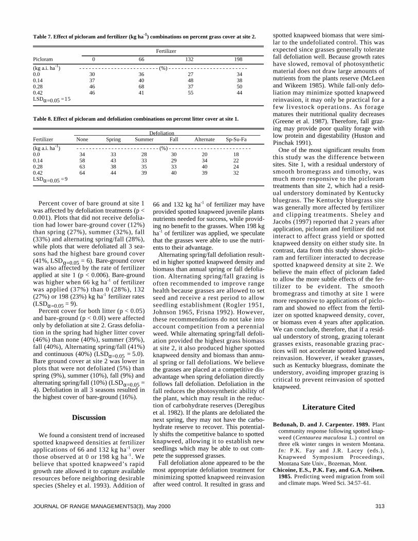
313JOURNAL OF RANGE MANAGEMENT53(3), May 2000
Percent cover of bare ground at site 1was affected by defoliation treatments (p <0.001). Plots that did not receive defolia-tion had lower bare-ground cover (12%)than spring (27%), summer (32%), fall(33%) and alternating spring/fall (28%),while plots that were defoliated all 3 sea-sons had the highest bare ground cover(41%, LSDα=0.05 = 6). Bare-ground coverwas also affected by the rate of fertilizerapplied at site 1 (p < 0.006). Bare-groundwas higher when 66 kg ha- 1 of fertilizerwas applied (37%) than 0 (28%), 132(27%) or 198 (23%) kg ha-1 fertilizer rates(LSDα=0.05 = 9).
Percent cover for both litter (p < 0.05)and bare-ground (p < 0.0l) were affectedonly by defoliation at site 2. Grass defolia-tion in the spring had higher litter cover(46%) than none (40%), summer (39%),fall (40%), Alternating spring/fall (41%)and continuous (40%) (LSDα=0.05 = 5.0).Bare ground cover at site 2 was lower inplots that were not defoliated (5%) thanspring (9%), summer (10%), fall (9%) andalternating spring/fall (10%) (LSDα=0.05 =4). Defoliation in all 3 seasons resulted inthe highest cover of bare-ground (16%).
Discussion
We found a consistent trend of increasedspotted knapweed densities at fertilizerapplications of 66 and 132 kg ha - 1 o v e rthose observed at 0 or 198 kg ha - 1. Webelieve that spotted knapweed’s rapidgrowth rate allowed it to capture availableresources before neighboring desirablespecies (Sheley et al. 1993). Addition of
66 and 132 kg ha-1 of fertilizer may haveprovided spotted knapweed juvenile plantsnutrients needed for success, while provid-ing no benefit to the grasses. When 198 kgha-1 of fertilizer was applied, we speculatethat the grasses were able to use the nutri-ents to their advantage.
Alternating spring/fall defoliation result-ed in higher spotted knapweed density andbiomass than annual spring or fall defolia-tion. Alternating spring/fall grazing isoften recommended to improve rangehealth because grasses are allowed to setseed and receive a rest period to allowseedling establishment (Rogler 1951,Johnson 1965, Frisna 1992). However,these recommendations do not take intoaccount competition from a perennialweed. While alternating spring/fall defoli-ation provided the highest grass biomassat site 2, it also produced higher spottedknapweed density and biomass than annu-al spring or fall defoliations. We believethe grasses are placed at a competitive dis-advantage when spring defoliation directlyfollows fall defoliation. Defoliation in thefall reduces the photosynthetic ability ofthe plant, which may result in the reduc-tion of carbohydrate reserves (Deregibuset al. 1982). If the plants are defoliated thenext spring, they may not have the carbo-hydrate reserve to recover. This potential-ly shifts the competitive balance to spottedknapweed, allowing it to establish newseedlings which may be able to out com-pete the suppressed grasses.
Fall defoliation alone appeared to be themost appropriate defoliation treatment forminimizing spotted knapweed reinvasionafter weed control. It resulted in grass and
spotted knapweed biomass that were simi-lar to the undefoliated control. This wasexpected since grasses generally toleratefall defoliation well. Because growth rateshave slowed, removal of photosyntheticmaterial does not draw large amounts ofnutrients from the plants reserve (McLeenand Wikeem 1985). While fall-only defo-liation may minimize spotted knapweedreinvasion, it may only be practical for afew livestock operations. As foragematures their nutritional quality decreases(Greene et al. 1987). Therefore, fall graz-ing may provide poor quality forage withlow protein and digestability (Huston andPinchak 1991).
One of the most significant results fromthis study was the difference betweensites. Site 1, with a residual understory ofsmooth bromegrass and timothy, wasmuch more responsive to the picloramtreatments than site 2, which had a resid-ual understory dominated by Kentuckybluegrass. The Kentucky bluegrass sitewas generally more affected by fertilizerand clipping treatments. Sheley andJacobs (1997) reported that 2 years afterapplication, picloram and fertilizer did notinteract to affect grass yield or spottedknapweed density on either study site. Incontrast, data from this study shows piclo-ram and fertilizer interacted to decreasespotted knapweed density at site 2. Webelieve the main effect of picloram fadedto allow the more subtle effects of the fer-tilizer to be evident. The smoothbromegrass and timothy at site 1 weremore responsive to applications of piclo-ram and showed no effect from the fertil-izer on spotted knapweed density, cover,or biomass even 4 years after application.We can conclude, therefore, that if a resid-ual understory of strong, grazing tolerantgrasses exists, reasonable grazing prac-tices will not accelerate spotted knapweedreinvasion. However, if weaker grasses,such as Kentucky bluegrass, dominate theunderstory, avoiding improper grazing iscritical to prevent reinvasion of spottedknapweed.
Literature Cited
Bedunah, D. and J. Carpenter. 1989. P l a n tcommunity response following spotted knap-weed (Centaurea maculosa L.) control onthree elk winter ranges in western Montana.I n : P.K. Fay and J.R. Lacey (eds.),Knapweed Symposium Proceedings,Montana Sate Univ., Bozeman, Mont.
Chicoine, E.S., P.K. Fay, and G.A. Neilsen.1 9 8 5 . Predicting weed migration from soiland climate maps. Weed Sci. 34:57–61.
Table 7. Effect of picloram and fertilizer (kg ha-1) combinations on percent grass cover at site 2.
Fertilizer
Picloram 0 66 132 198
(kg a.i. ha-1) - - - - - - - - - - - - - - - - - - - - - - - - - (%) - - - - - - - - - - - - - - - - - - - - - - - - -0.0 30 36 27 340.14 37 40 48 380.28 46 68 37 500.42 46 41 55 44LSDα=0.05 =15
Table 8. Effect of picloram and defoliation combinations on percent litter cover at site 1.
Defoliation Fertilizer None Spring Summer Fall Alternate Sp-Su-Fa
(kg a.i. ha-1) - - - - - - - - - - - - - - - - - - - - - - - - - - (%) - - - - - - - - - - - - - - - - - - - - - - - - - -0.0 34 33 28 30 20 180.14 58 43 33 29 34 220.28 63 38 35 33 40 240.42 64 44 39 40 39 32LSDα=0.05 =9

314 JOURNAL OF RANGE MANAGEMENT 53(3), May 2000
Davis E.S. 1990. Spotted knapweed (C e n t a u r e am a c u l o s a L.) seed longevity, chemical con-trol, and seed morphology. M.S. Thesis,Montana State Univ., Bozeman, Mont.
Davis E.S., P. K. Fay, T.K. Chicoine, andC.A. Lacey. 1993. Persistence of spottedknapweed. Weed Sci. 41:57–61.
Deregibus,V.A., M.J. Trlica, and D.A.Jameson. 1982. Organic reserves in herbageplants: their relationship to grassland man-agement. p.315-344. I n : M.J. Recheigl (ed.)Handbook of agricultural productivity. Vol.I. Plant productivity. CRC Press. Bocona, Fla
Frisna, M.R. 1992. Elk habitat use within arest-rotation grazing system. Rangelands14:93–96.
Greene, L.W., W.E. Pinchak, and R.K.Heitschmidt. 1987. Seasonal dynamics ofminerals in forages at the Texas experimentalranch. J. Range Manage. 40:502–506.
Griffith, D. and J. Lacey. 1989. Economics ofknapweed control. I n : P.K. Fay and J.R.Lacey (eds.), Knapweed SymposiumProceedings, Montana Sate Univ., Bozeman,Mont.
Hamaker, J.W., C.R. Youngson, and G.A.Goring. 1967. Predictions of the persistenceand activity of Tordon herbicide in soilsunder field conditions. Down to Earth.23:30–36.
Hart, R.H., M.C. Shoop, and M.M. Ashby.1995. Nitrogen and atrazine on shortgrass:vegetation, cattle, and economic responses. J.Range Manage. 48:165–171.
Huston, J.E. and W.E. Pinchak. 1991. Rangeanimal nutrition. I n : R.K. Heitschmidt andJ.W. Stuth (eds.) Grazing Management, anecological perspective. Timber Press.Portland, Ore.
Jacobs, J.S. and R.L. Sheley. 1997. R e l a t i o n s h i pamong Idaho fescue defoliation, soil water, andspotted knapweed emergence and growth. J.Range Manage. 50:258–262.
Johnson, W.M. 1965. Rotation, rest-rotation,and season-long grazing on a mountain rangein Wyoming. USDA Forest Service. Res.Paper RM-41. l6p.
Lacey J.R., C.B. Marlow, and J.R. Lane.1989. Influence of spotted knapweed(Centaurea maculosa) on surface runoff andsedimentation yield. Weed Technol.3:627–631.
Maschinski, J. and T.G. Whitman. 1989. Thecontinuum of plant responses to herbivory:the influence of plant association, nutrientavailability, and timing. Amer. Natur.134:1–19.
McLean, A. and S. Wikeem. 1985.Defoliation effects on three range grasses.Rangelands 7:61–63.
Meuggler, W.F. and W.L. Stewart. 1980.Grassland and Shrubland habitat types ofWestern Montana. USDA Forest Serv. Gen.Tech. Rep. INT-66.
Peterson, R.G. 1985. Design and analysis ofexperiments. Marcel Dekker, Inc. New York,N.Y.
Rogler, G.A. 1951. A twenty-five year com-parison of continuous and rotation grazing inthe Northern Plains. J. Range Manage.4:35–41.
SAS Institute, Inc. 1990. SAS/STAT User’sguide, Version 6, Fourth edition, Vol. 2, SASInst., Cary N.C.
Sheley, R.L. and J.S. Jacobs. 1997. Responseof spotted knapweed and grass to picloramand fertilizer combinations. J. RangeManage. 50:263–267.
Sheley, R.L. and B.F. Roché. 1982.Rehabilitation of spotted knapweed infestedrangeland in northwest Washington. Abstract.W. Soc. Weed Sci. Denver, Colo.
Sheley, R.L., J.S. Jacobs, and M.F.Carpinelli. 1998. Distribution, Biology, andManagement of Diffuse Knapweed(Centaurea diffusa) and Spotted Knapweed(Centaurea maculosa). Weed Tech. 12:353-362.
Sheley, R.L. and L.L. Larson, and D.E.Johnson. 1993. Germination and rootdynamics of Range Weeds and ForageSpecies Weed Tech. 7:243–237
Sheley, R.L, B.E. Olson, and L.L. Larson.1997. Effect of weed seed rate and grassdefoliation level on diffuse knapweed. J.Range Manage. 50:39–43.
Tyser, R.W. and C.H. Key. 1988. S p o t t e dknapweed in a natural area fescue grassland:an ecological assessment. Northwest Sci.62(4):151–166.
Watson, A.K. and A.J. Renney. 1974. T h ebiology of Canadian weed.6. Centaurea mac -u l o s a and C. diffusa . Can. J. Plant Sci.54:687–701.

315JOURNAL OF RANGE MANAGEMENT 53(3), May 2000
Abstract
A sward-based technique for quantifying the spatial hetero-geneity in herbage mass and consumption was developed andtested in a bahia grass (Paspalum notatum Flügge) pasturegrazed by cattle. For five, 2-day grazing periods from May toOctober, pre- and post-grazing herbage masses were nondestruc-tively estimated with an electronic capacitance probe at 182, 50x50 cm locations along 2 permanent line transects. At the sametime, undisturbed herbage accumulation during grazing wasmeasured inside exclosures and the results used to estimate accu-mulation under grazing at each location. Estimation of herbagemass was relatively good; R2 = 0.88 to 0.98. Spatial heterogeneityin herbage mass and the stability of the spatial pattern were wellquantified. The pattern of spatial heterogeneity observed early inthe grazing season remained quite stable for 5 months until thelate grazing season. Spatial heterogeneity in the rate of defolia-tion was also well quantified in spite of some negative values. Thetechnique is of potential value for quantifying the spatial hetero-geneity in herbage mass and consumption by animals in grazedpastures, though further studies are necessary for testing theapplicability of the technique to pastures of other plant species orof multiple species.
Key Words: electronic capacitance probe, patch grazing, patchstability, rate of defoliation, spatial pattern, Paspalum notatum
Vegetation of grazing systems is spatially heterogeneous(Vallentine 1990). Even in virtually monospecific pastures, vege-tation forms a mosaic in which short, heavily grazed patches hav-ing small herbage mass alternate with tall, ungrazed or lightlygrazed patches having large herbage mass, with a transitionalzone of intermediate height, utilization and mass (Illius et al.1987, Liu and Hirata 1995, Hirata and Fukuyama 1997, Cid andBrizuela 1998, Hirata 1998).
It is well known that such heterogeneity is created and main-tained by selective (spatially heterogeneous) grazing by animals:i.e., animals visit and graze heavily grazed patches more fre-quently than the surrounding patches (Illius et al. 1987), prefer-ring the higher digestibility and nitrogen concentration in heavilygrazed patches (Illius et al. 1987, Cid and Brizuela 1998).
However, few workers have measured the utilization of individ-ual patches in terms of herbage consumption or intake. Frequentgrazing of heavily grazed patches does not necessarily mean thatherbage consumption in these patches is greater than that in otherpatches, because low herbage availability of heavily grazedpatches may limit the intake rate of animals. Since herbage con-sumption, as well as herbage accumulation, is a factor determin-ing the changes in herbage mass, information on the herbage con-sumption in individual patches in a pasture is important in under-standing the mechanisms behind patch development and stability.
Hirata and Fukuyama (1997) developed a sward-based techniquefor estimating herbage consumption by grazing animals at a smallpatch scale and used the technique on a bahia grass (P a s p a l u mn o t a t u m Flügge) pasture grazed by cattle. An electronic capaci-tance probe was used to estimate herbage mass in a number offixed locations (50 ×50 cm) along permanent transects before andafter grazing, and herbage consumption in each location was esti-mated from the change in the herbage mass with g r a z i n g .
J. Range Manage.53: 315–321 May 2000
Quantifying spatial heterogeneity in herbage mass andconsumption in pastures
MASAHIKO HIRATA
Author is associate professor, Grassland and Animal Production Division, Faculty of Agriculture, Miyazaki University, Miyazaki 889-2192, Japan. E-mail:[email protected]
The author is grateful to Mr. Takuya Iwamoto, Mr. Waka Otozu and Mr.Daisuke Kiyota for field assistance, and to Mr. Kiichi Fukuyama and Mr. ShirouKuroki of the Sumiyoshi Livestock Farm for pasture and animal management.
Manuscript accepted 6 Sept. 1999.
Resumen
Se desarrollo una técnica basada en la pradera para cuan-tificar la heterogeneidad espacial de la masa de forraje y el con-sumo, y se probo en una pradera de "Bahia grass"(P a s p a l u mn o t a t u m Flügge) apacentada por bovinos. En 5 periodos deapacentamiento de 2 días comprendidos entre mayo y octubre, seestimo la masa de forraje antes y después del apacentamientomediante el método no destructivo de la sonda de capacitor elec-trónico, la estimación se realizó en 182 cuadrantes de 50 x 50 cmlocalizados en 2 transectos de línea permanentes. Al mismo tiem-po se midió la acumulación de forraje sin disturbio ocurridadurante el apacentamiento, lo cual se hizo dentro de exclusionesy los resultados se utilizaron para estimar la acumulación de for-raje bajo apacentamiento en cada localidad. La estimación deforraje fue relativamente buena; R2 = 0.88 a 0.98. La hetero-geneidad espacial de la masa de forraje y la estabilidad delpatrón espacial se cuantificaron bien. El patrón de la hetero-geneidad espacial observado al inicio de la estación de apacen-tamiento permaneció muy estable durante 5 meses hasta finalesde la estación de apacentamiento. La heterogeneidad espacial dela tasa de defoliación también fue bien cuantificada a pesar dealgunos valores negativos. La técnica es de valor potencial paracuantificar la heterogeneidad espacial de la masa de forraje yconsumo por animales en praderas apacentadas, aunque sonnecesarios mas estudios para probar la aplicabilidad de esta téc-nica en praderas de otra especies vegetales o praderas con masde una especie.

316 JOURNAL OF RANGE MANAGEMENT 53(3), May 2000
However, the results had limitationsbecause the herbage consumption wasestimated without taking the herbageaccumulation during grazing into account.The aims of the present study were toovercome such limitations and examinethe usefulness of the technique for quanti-fying the spatial heterogeneity in herbagemass and consumption in a grazed pasture.
Materials and Methods
Study site and grazing and pasturemanagement
The same paddock as in the previousstudy (Hirata and Fukuyama 1997), i.e., a1.1-ha paddock of a bahia grass pasture atthe Sumiyoshi Livestock Farm (31°59'N,131°28'E), Faculty of Agriculture,Miyazaki University, Japan, was used.The paddock was 1 of 5 paddocks rota-tionally grazed by Japanese Black Cows.The vegetation was highly dominated bybahia grass. According to the measure-ments in the previous year (1995), bahiagrass accounted for 87% of herbage mass(above a 3 cm height; on a dry matter(DM) basis) in May, and 97 to 100% fromJune to October (Hirata and Fukuyama1997).
During the grazing season (May-October) of 1996, the paddock was grazedby 28 to 32 animals with a 2 to 6-dayduration at intervals of 11 to 37 days. Thetotal duration of grazing periods was 23days. The annual fertilization rates in thepaddock were 77 kg N (split application in
March and August), 20 kg P (March) and30 kg K (March) ha-1. The meteorologicalconditions during the study are shown inFig. 1.
Measurement periodsFive, 2-day periods at approximately
monthly intervals were selected from therotational grazing periods as Periods 1 to 5(Table 1), representing the first 2 days of agrazing period. Pre- and post-grazingherbage mass, herbage accumulation andrate of defoliation were estimated for these5 selected periods. The duration of 2 dayswas selected to ensure enough reduction inherbage mass by grazing for detectionwith a capacitance probe.
Electronic capacitance probeAn electronic capacitance probe
( P a s t u r e P r o b eT M, Mosaic Systems Ltd.,New Zealand) was used to estimateherbage mass. PastureProbeTM is a singleprobe capacitance meter, which is light inweight and highly portable (Hirata et al.1993). There have been many reports eval-uating electronic capacitance probes, andresults indicate that the single-probecapacitance meter is at least as good andmore labor saving than any other alterna-tives for indirect herbage mass measure-ment (Frame 1993). The accuracy ofPastureProbeTM in estimating herbage massof bahia grass swards was tested by Hirataet al. (1993). Because the relationshipbetween herbage mass and corrected meterreading of electronic capacitance probe
(CMR) is known to vary with such factorsas sward type, season of growth (develop-mental stage), herbage moisture contentand ratio of green to dead material (Frame1993, Hirata et al. 1993), and was antici-pated to vary also with grazing, calibrationequations were developed separately forindividual measurement occasions asdescribed later.
Pre- and post-grazing herbage massHorizontal distribution of herbage mass
was measured both at the beginning andthe end of the 5 selected periods, i.e., on10 occasions. On each occasion, CMRwas measured at 1-m intervals along 2permanent line transects crossing the pad-dock. Each transect was 90 m long and,therefore, the CMR was determined at 182locations (including both ends of the tran-sect). For each location, the CMR was mea-sured at 6 points within an area of 50 ×5 0cm (4 at individual corners and 2 in thecenter), irrespective of the vegetation of thepoints (plant species and plant parts), andthe mean value was recorded as the CMRof the location. The area of 50x 50 cm wasselected based on the feeding station(Coleman et al. 1989) of cattle used.
Immediately after the measurements ofCMR along the transects, ten, 50x 50 cmlocations whose CMR values covered theCMR range of the transects were selectedin the paddock, avoiding the proximity ofthe transects, and the herbage was cut to a3-cm height. The samples were oven-driedat 85°C for 72 hours for dry matter deter-mination. In Period 5, the number of sam-ples was decreased to 5 to reduce laborrequirement.
Calibration equations for estimatingherbage mass (M, g DM (2500 cm 2)- 1)from CMR were developed fitting the fol-lowing model to data:
M = a0 + a1 ×CMR + a2×CMR2 (1)
where a0, a1 and a2 are constants. Theindependent variables, CMR and CMR2,were incorporated into the equation onlywhen their partial regression coefficients( a1 and a2, respectively) were significant (P
Fig. 1. Ten or 11 day average of maximum (- - - - -), mean (– – – – –), and minimum ( . . . . .)air temperatures, daily total shortwave solar radiation, and 10 or 11 day totals ofrainfall during the study period.
Table 1. Outlines of selected grazing periodsfor measurements.
Period Date Number of Meancows liveweight
(kg cow-1)1 25-26 May 28 4622 29-30 Jun. 28 4543 3-4 Aug. 28 4464 14-15 Sep. 29 4525 26-27 Oct. 32 468

317JOURNAL OF RANGE MANAGEMENT53(3), May 2000
<0.05). Using the equation developed foreach measurement occasion, the CMR ateach location along the transects was con-verted into herbage mass (DM in an area of5 0x 50 cm and above a height of 3 cm).
Characteristics of the spatial distributionof herbage mass were expressed by themean, minimum, maximum, SD and C.V.of data from the 182 locations along thetransects. Similarity of the spatial patternsof herbage mass on 2 occasions was repre-sented by a correlation coefficient (n=182).
Herbage accumulationUndisturbed herbage accumulation dur-
ing each selected period was measured at6 different herbage masses using exclosurecages (1 × 1 m in area and 75 cm inheight), to develop the relationshipbetween the accumulation rate andherbage mass (described later as Equation2, also see Fig. 6 and Equations 4 to 8). Atthe beginning of each selected period, six,50 ×50 cm areas whose CMR values cov-ered the CMR range of the transects atapproximately equal intervals were select-ed in the paddock, avoiding the proximityof the transects, and the cages were placedon these areas. Then, the CMR of theareas was measured again 7 to 10 daysafter the end of the selected period.Initially, I intended to measure the finalCMR at the end of the selected periods,but herbage accumulation during the 2days was too small to detect with thecapacitance probe. The initial and finalCMR of each area was determined as themean of 5 measurements (4 at individualcorners and 1 in the center), and convertedinto herbage mass (DM in an area of 50 ×50 cm and above a height of 3 cm) asdescribed above.
The rate of undisturbed herbage accu-mulation (Gu n d i s t, g DM (2500 cm2)- 1 d- 1)was related to the mean herbage mass dur-ing the accumulation period (Mmean, g DM(2500 cm 2)- 1) assuming the followingmodel:
Gundist = b0+b1 ×Mmean+b2 ×Mmean2 (2)
where b0, b1 and b2 are constants. Theindependent variables, Mmean and Mmean
2,were selected in the same way as inEquation 1.
Rate of defoliationRate of defoliation or daily herbage con-
sumption (D, g DM (2500 cm 2)- 1 d- 1) ateach location along the transects was cal-culated as:
D = (Mpre - Mpost)/tg + Gdist (3)
where Mpre and Mpost are respectively the
pre- and post-grazing herbage masses atthe location (g DM (2500 cm2)-1), tg is theduration of the selected grazing period (d),and Gd i s t is the rate of disturbed herbageaccumulation at the location during graz-ing (g DM (2500 cm 2)- 1 d- 1). The firstterm, (Mp r e- Mp o s t) / tg, corresponds to therate of decrease in herbage mass duringgrazing (apparent consumption). In thisstudy, tg = 2 (Table 1). Gdist was estimatedfrom the mean herbage mass during theselected grazing period (Mmean = (Mpre +
Mp o s t)/2) using Equation 2. Thus, the useof the model assumes that Gdist, the rate ofherbage accumulation under grazing,equals the rate of undisturbed herbageaccumulation when the herbage mass isthe same.
Characteristics of the spatial distributionof the rate of defoliation were expressedby the mean, minimum, maximum, SDand C.V. of data from the 182 locationsalong the transects.
Fig. 2. Relationships between herbage mass and corrected meter reading (CMR) by an elec-tronic capacitance probe. Three asterisks indicate significance at P < 0.001.

318 JOURNAL OF RANGE MANAGEMENT 53(3), May 2000
Results and Discussion
Labor requirementThe present technique required a rela-
tively small amount of labor. An operatorof a capacitance probe and a recorder whoalso calculated the mean corrected meterreading (CMR) at each location wereenough for the measurements. It tookapproximately 2.5 hours for 2 persons tomeasure CMR at the 182 locations and inthe 6 exclosures and collect 10 vegetationsamples for developing a calibration equa-tion. Reducing the number of samples to 5in Period 5 shortened the time by approxi-mately half an hour.
Estimation of herbage massHerbage mass was linearly or quadrati-
cally related to CMR (Fig. 2). The linearand quadratic terms were not incorporatedat the same time because their partialregression coefficients were not simultane-ously significant (P>0.05). All the calibra-tion equations were highly significant (R2 =0.88 to 0.98, P<0.001) with SE of estima-tion of 4.4 to 16.8 g DM (2500 cm2)- 1. TheSE tended to be greater as the range ofherbage mass broadened. Replacing the lin-ear term by the quadratic term in Periods 1,3, and 5 increased R2 by 0.00 to 0.06 anddecreased SE of estimation by 0.3 to 7.3 gDM (2500 cm2)- 1. These results are similarto those from the previous study (Hirata etal. 1993). The slope of the line was alwayssteeper, i.e., the regression coefficient wasalways greater, after grazing than beforegrazing. This may be mainly due to thedecreased leaf to stem ratio of the swardwith grazing.
Heterogeneity in herbage massPre- and post-grazing herbage masses
were spatially heterogeneous, as shown bythe C.V. values of 0.304 to 0.857 (Fig. 3).With grazing, the mean and minimumherbage masses always decreased and,contrarily, C.V. always increased. Such anincrease in C.V. with grazing accords withprevious observations (Shiyomi et al.1983, 1984, Hirata 1993a, 1993b, Liu andHirata 1995, Hirata and Fukuyama 1997)and confirms that grazing by animals is acrucial factor in the development andmaintenance of the heterogeneity (Bakkeret al. 1983, Edwards et al. 1996).
There were always positive correlationsbetween pre- and post-grazing herbagemasses along the transects (Fig. 4).Furthermore, pre-grazing herbage mass inPeriods 2 to 5 was always positively corre-
Fig. 3. Pre- and post-grazing distributions of herbage mass along the transects. The statistical parameters are minimum, maximum, mean,SD, and C.V.

319JOURNAL OF RANGE MANAGEMENT53(3), May 2000
lated with that in Period 1 (Fig. 5). Theseresults show that the spatial pattern ofherbage mass was more or less stable atleast for 5 months during the grazing sea-son, which agrees with previous reports(Bakker et al. 1983, Willms et al. 1988,Cid and Brizuela 1998, Hirata 1998). Thestability of the spatial pattern of herbagemass in the paddock during a 2 and a half-year period has been investigated and dis-cussed in Hirata (1998).
Herbage accumulation duringgrazing
The rate of undisturbed herbage accu-mulation (Gundist) was linearly or quadrati -cally related to the mean herbage mass
during the accumulation period (Mm e a n)(Fig. 6). The relationships in Periods 1, 2,3, 4, and 5 were expressed by Equations 4,5, 6, 7, and 8, respectively (SE given inbrackets):
The relationship between Gu n d i s t a n dMm e a n was mostly quadratic, with themaximal Gu n d i s t and the optimum Mm e a nfor the maximal Gundist changing with sea-son. This relationship was l inear in
Periods 1 and 2, apparently caused by thelow, narrow ranges of Mmean. The quadrat-ic relationship between growth rate andherbage mass which produces the logisticgrowth agrees with models developed byNoy-Meir (1978) and Hart (1989).
Heterogeneity in herbage consump-tion
The rate of defoliation was spatially het-erogeneous, as shown by the C.V. valuesof 0.428 to 0.904 (Fig. 7). The heterogene-ity (C.V.) tended to increase as the meanpre-grazing herbage mass increased (Fig.3) (r=0.87, P≈0.05). This phenomenonreflects the fact that animals are moreselective and patch grazing is more preva-lent under lower grazing pressure (Willmset al. 1988, Vallentine 1990, Cid andBrizuela 1998). In the present study, high-
Gundist = 0.117 (0.055) + 0.0203 (0.0022) Mmean(R2 = 0.96, P<0.001, SE of estimation = 0.079) (4)
Gundist = 0.575 (0.452) + 0.0299 (0.0092) Mmean(R2 = 0.73, P<0.05, SE of estimation = 0.493) (5)
Gundist = –0.253 (0.450) + 0.0534 (0.0104) Mmean – 2.61 ×10⁻⁴ (0.50x10⁻⁴) Mmean2
(R2 = 0.90, P<0.05, SE of estimation = 0.272) (6)Gundist = 0.307 (0.150) + 0.0207 (0.0026) Mmean – 1.11 ×10⁻⁴ (0.10x10⁻⁴) Mmean
2
(R2 = 0.99, P<0.001, SE of estimation = 0.041) (7)Gundist = 0.0029 (0.0036) + 0.00149 (0.00011) Mmean – 7.65 ×10⁻⁶ (0.66x10⁻⁶) Mmean
2
(R2 = 0.99, P<0.01, SE of estimation = 0.003) (8)
Fig. 4. Relationships between pre- and post-grazing herbage masses alongthe transects. Three asterisks indicate significance at P<0.001.
Fig. 5. Relationships between pre-grazing herbage masses alongthe transects in Period 1 and subsequent periods. Threeasterisks indicate significance at P<0.001.
Fig. 6. Relationships between rate of undisturbed herbage accumulation and mean herbagemass in Periods 1 (❍), 2 ( , 3 ( , 4(❑), and 5( ). See text for equations.
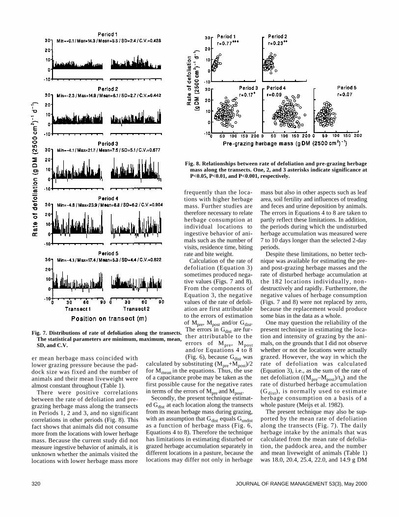
320 JOURNAL OF RANGE MANAGEMENT 53(3), May 2000
er mean herbage mass coincided withlower grazing pressure because the pad-dock size was fixed and the number ofanimals and their mean liveweight werealmost constant throughout (Table 1).
There were positive correlationsbetween the rate of defoliation and pre-grazing herbage mass along the transectsin Periods 1, 2 and 3, and no significantcorrelations in other periods (Fig. 8). Thisfact shows that animals did not consumemore from the locations with lower herbagemass. Because the current study did notmeasure ingestive behavior of animals, it isunknown whether the animals visited thelocations with lower herbage mass more
frequently than the loca-tions with higher herbagemass. Further studies aretherefore necessary to relateherbage consumption atindividual locations toingestive behavior of ani-mals such as the number ofvisits, residence time, bitingrate and bite weight.
Calculation of the rate ofdefoliation (Equation 3)sometimes produced nega-tive values (Figs. 7 and 8).From the components ofEquation 3, the negativevalues of the rate of defoli-ation are first attributableto the errors of estimationof Mpre, Mpost and/or Gdist.The errors in Gdist are fur-ther attributable to theerrors of Mp r e, Mp o s tand/or Equations 4 to 8(Fig. 6), because Gdist was
calculated by substituting (Mp r e+ Mp o s t) / 2for Mm e a n in the equations. Thus, the useof a capacitance probe may be taken as thefirst possible cause for the negative ratesin terms of the errors of Mpre and Mpost.
Secondly, the present technique estimat-ed Gd i s t at each location along the transectsfrom its mean herbage mass during grazing,with an assumption that Gd i s t equals Gu n d i s tas a function of herbage mass (Fig. 6,Equations 4 to 8). Therefore the techniquehas limitations in estimating disturbed orgrazed herbage accumulation separately indifferent locations in a pasture, because thelocations may differ not only in herbage
mass but also in other aspects such as leafarea, soil fertility and influences of treadingand feces and urine deposition by animals.The errors in Equations 4 to 8 are taken topartly reflect these limitations. In addition,the periods during which the undisturbedherbage accumulation was measured were7 to 10 days longer than the selected 2-dayp e r i o d s .
Despite these limitations, no better tech-nique was available for estimating the pre-and post-grazing herbage masses and therate of disturbed herbage accumulation atthe 182 locations individually, non-destructively and rapidly. Furthermore, thenegative values of herbage consumption(Figs. 7 and 8) were not replaced by zero,because the replacement would producesome bias in the data as a whole.
One may question the reliability of thepresent technique in estimating the loca-tion and intensity of grazing by the ani-mals, on the grounds that I did not observewhether or not the locations were actuallygrazed. However, the way in which therate of defoliation was calculated(Equation 3), i.e., as the sum of the rate ofnet defoliation ((Mp r e– Mp o s t) / tg) and therate of disturbed herbage accumulation( Gd i s t), is normally used to estimateherbage consumption on a basis of awhole pasture (Meijs et al. 1982).
The present technique may also be sup-ported by the mean rate of defoliationalong the transects (Fig. 7). The dailyherbage intake by the animals that wascalculated from the mean rate of defolia-tion, the paddock area, and the numberand mean liveweight of animals (Table 1)was 18.0, 20.4, 25.4, 22.0, and 14.9 g DM
Fig. 8. Relationships between rate of defoliation and pre-grazing herbagemass along the transects. One, 2, and 3 asterisks indicate significance atP<0.05, P<0.01, and P<0.001, respectively.
Fig. 7. Distributions of rate of defoliation along the transects.The statistical parameters are minimum, maximum, mean,SD, and C.V.

321JOURNAL OF RANGE MANAGEMENT53(3), May 2000
(kg LW) -1 d-1 for Periods 1, 2, 3, 4, and 5,respectively. These values agree closelywith the grazing intake of Japanese BlackCows (AFFRCS 1995) when the meanpre-grazing herbage mass (Fig. 3) and thedigestibility of a bahia grass pasture(Higashiyama and Hirata 1995) are takeninto account.
Furthermore, the present technique,owing to the large number of data setsfrom the pasture (n=182), is considered togive reliable trends of spatial distributionof herbage consumption. An example isthe increase in the spatial heterogeneity inherbage consumption with the increasedmean pre-grazing herbage mass (Figs. 3and 7) as discussed above. We can under-stand which locations of the pasture wereheavily defoliated or lightly defoliated.Because of the small labor requirement, itmay be possible to establish more loca-tions for measurements so that they cancover the whole area of a pasture.
Conclusions
Previous studies have mainly used 2techniques for quantifying the spatial het-erogeneity in vegetation in grazed pas-tures. One is a random sampling of swardheight (Gibb and Ridout 1986,1988) orherbage mass (Shiyomi et al.1983,1984,Hirata 1993a) from a pasture, and theother is a monitoring of degree of utiliza-tion (Bakker et al. 1983, Willms et al.1988, Cid and Brizuela 1998) or swardheight (Edwards et al. 1996) in some per-manent areas in a pasture. The latter tech-nique is advantageous over the formerbecause it can follow the temporal dynam-ics in vegetation characteristics in thesame locations in a pasture and thereforecan estimate the patch stability. However,few workers have used the latter techniqueto monitor herbage mass, i.e., a mostimportant vegetation characteristic,because estimation of herbage mass nor-mally requires destructive sampling.
The present technique, by using an elec-tronic capacitance probe, can follow thetemporal dynamics in herbage mass in anumber of fixed locations in a pasture witha relatively small amount of labor. Spatialheterogeneity in herbage mass and the sta-bility of the spatial pattern of herbagemass were well quantified (Figs. 3 to 5).Spatial heterogeneity in the rate of defolia-tion was also well quantified in spite ofsome negative values (Fig. 7). The presenttechnique is therefore considered to be ofpotential value for quantifying the spatialheterogeneity in herbage mass and con-
sumption by animals in grazed pastures,though further studies are necessary fortesting the applicability of the technique topastures of other plant species or of multi-ple species.
Literature Cited
[AFFRCS] Agriculture, Forestry andFisheries Research Council Secretariat.1995. Japanese feeding standard for beef cat-tle (1995). Central Association of LivestockIndustry, Tokyo, Japan.
Bakker, J.P., J. de Leeuw, and S.E. vanWieren. 1983. Micro-patterns in grasslandvegetation created and sustained by sheepgrazing. Vegetatio 55:153–161.
Cid, M.S. and M.A. Brizuela. 1998.Heterogeneity in tall fescue pastures createdand sustained by cattle grazing. J. RangeManage. 51:644–649.
Coleman, S.W., T.D.A. Forbes, and J.W.Stuth 1989. Measurements of the plant-ani-mal interface in grazing research. p. 37–51.I n: G.C. Marten (ed.), Grazing research:design, methodology, and analysis. Crop Sci.Soc. of Amer. and Amer. Soc. of Agron.,Madison, Wis.
Edwards, G.R., A.J. Parsons, J.A. Newman,and I.A. Wright. 1996. The spatial patternof vegetation in cut and grazed grass/whiteclover pastures. Grass Forage Sci.51:219–231.
Frame, J. 1993. Herbage mass. p. 39–67. I n:A. Davies, R.D. Baker, S.A. Grant, and A.S.Laidlaw (eds.), Sward measurement hand-book (2nd ed.). Brit. Grassl. Soc., Reading,UK.
Gibb, M.J. and M.S. Ridout. 1986. The fittingof frequency distributions to height measure-ments on grazed swards. Grass Forage Sci.41:247–249.
Gibb, M.J. and M.S. Ridout. 1988.Application of double normal frequency dis-tributions fitted to measurements of swardheight. Grass Forage Sci. 43:131–136.
Hart, R.H. 1989. SMART: A simple model toassess range technology. J. Range Manage.42:421–424.
Higashiyama, M. and M. Hirata. 1995.Analysis of a Japanese Black Cattle rearingsystem utilizing a bahiagrass (P a s p a l u mnotatum Flügge) pasture. 1. Variations in thefactors considered to affect animal produc-tion. Grassl. Sci. 41:104–113.
Hirata, M. 1993a. Changes in the variations inherbage mass of bahiagrass (Paspalum nota -t u m Flügge) pasture with the grazing bydairy heifers. Bull. Fac. Agr., Miyazaki Univ.40:1–5.
Hirata, M. 1993b. Distribution of herbagemass in bahiagrass ( Paspalum notatumFlügge) pasture as affected by grazing bybeef cattle, mowing, paddock area and sea-son. Bull. Fac. Agr., Miyazaki Univ.40:91–98.
Hirata, M. 1998. Dynamics of the horizontaldistribution of herbage mass in a bahiagrass
(Paspalum notatum Flügge) pasture grazedby cattle: Stability of spatial pattern ofherbage mass. Grassl. Sci. 44:169–172.
Hirata, M. and K. Fukuyama. 1997.Dynamics of the horizontal distribution ofherbage mass in a bahiagrass (P a s p a l u mnotatum Flügge) pasture with grazing by cat-tle. Grassl. Sci. 43:1–6.
Hirata, M., M. Higashiyama, M. Kikuchi,and S. Liu. 1993. Estimation of herbagemass of bahiagrass ( Paspalum notatumFlügge) swards with an electronic capaci-tance meter. Bull. Fac. Agr., Miyazaki Univ.40:83–89.
Illius, A.W., D.G.M. Wood-Gush, and J.C.Eddison. 1987. A study of the foragingbehaviour of cattle grazing patchy swards.Biol. Behav. 12:33–44.
Liu, S. and M. Hirata. 1995. Spatial distribu-tion of herbage mass in bahiagrass(Paspalum notatum Flügge) pasture undergrazing, resting and mowing. J. Japan.Grassl. Sci. 40:457–470.
Meijs, J.A.C., R.J.K. Walters, and A. Keen.1 9 8 2 . Sward methods. p. 11-36. I n: J.D.Leaver (ed.), Herbage intake handbook. Brit.Grassl. Soc., Maidenhead, UK.
Noy-Meir, I. 1978. Grazing and production inseasonal pastures: Analysis of a simplemodel. J. Applied Ecol. 15:809–835.
Shiyomi, M., T. Akiyama, and S. Takahashi.1 9 8 3 . A spatial pattern model of plant bio-mass in grazing pasture I. J. Japan. Grassl.Sci. 28:373–382.
Shiyomi, M., T. Akiyama, and S. Takahashi.1 9 8 4 . A spatial pattern model of plant bio-mass in grazing pasture II. J. Japan. Grassl.Sci. 30:40–48.
Vallentine, J.F. 1990. Grazing management.Academic Press, San Diego, Calif.
Willms, W.D., J.F. Dormaar, and G.B.Schaalje. 1988. Stability of grazed patcheson rough fescue grasslands. J. RangeManage. 41:503–508.
322 JOURNAL OF RANGE MANAGEMENT 53(3), May 2000
Abstract
Spatial patterns of herbivore defecation within grazing systemsare important as they directly affect pasture growth and compo-sition. These effects are partially linked to seed dispersal in dung,a little studied process. This paper focuses on: (i) quantificationof dung and seeds deposited by herbivores in a Mediterraneangrazing system, and (ii) analysis of the spatial variability of dungand seeds deposited within and among plant communities. Wecarried out year-long monthly quantifications of the depositionsof rabbit (Oryctolagus cuniculus), fallow deer (Dama dama), reddeer (Cervus elaphus), and cow (Bos taurus) dung to 32 plots dis-tributed in Quercus rotundifolia Lam. and Fraxinus angustifoliaVahl woodlands, mixed scrub, and Cistus ladanifer L. scrub. Wealso quantified the germinable seed content of dung. The resultsrevealed differences (p < 0.05) in dung deposition, varying (i)among the 4 species, (ii) within species (except for the red deer)among plant communities, and (iii) within plant communities. Anaverage of 735 seeds/m2 were returned to the soil via dung, withthe highest numbers in open woodlands (870–1,888 seeds/m2) andthe lowest numbers in scrubs (83–315 seeds/m2). Cows dispersedthe most seeds (68%), followed by red deer (20%), rabbits (7%),and fallow deer (5%). Spatial variability in deposition led toaccumulations of up to several thousand seeds at points coveredby the dung. The effect of seed input to the seed bank and on veg-etation may be low at large and medium-sized spatial scales, butit can be very important at small scales and for colonizationprocesses.
Key Words: spatial pattern, dispersal, dung, herbivores, endo-zoochory, Mediterranean pastures
Deposition and degradation of herbivore dung are key process-es that alter soil characteristics, botanical composition, and pro-ductivity in grazing lands (McNaughton 1984, Georgiadis andMcNaughton 1990, Malo and Suárez 1995a) but little informationexists concerning spatial patterns of herbivore defecation (e.g.Putman et al. 1991). Seed dispersal via herbivore dung (endozoo-chory) is known to happen, but effects on vegetation dynamicsare poorly defined (Janzen 1984) with the exception of dispersal
of woody legumes (Miller and Coe 1993) and attempts to uselivestock to sow pasture species (Ocumpaugh et al. 1996). Highseed densities were recorded in herbivore dung in theMediterranean (Russi et al. 1992, Malo and Suárez 1995b) andAustralia (Jones et al. 1991, Gardener et al. 1993) while muchlower densities occurred in other areas (Collins and Uno 1985,Welch 1985). However, information is lacking on quantificationof seeds dispersed endozoochorously by herbivores. Objectivesof this research were (i) to quantify herbivore dung and seedinput to soil in an extensive grazing system on the IberianPeninsula, and (ii) to analyse the spatial patterns of dung and seed
J. Range Manage.53: 322–328 May 2000
Herbivore dunging and endozoochorous seed deposition ina Mediterranean dehesa
J.E. MALO, B. JIMÉNEZ, AND F. SUAREZ
Authors are ecologists, Departamento Interuniversitario de Ecología. Facultad de Ciencias. Universidad Autónoma de Madrid. E-28049 Madrid. Spain.Malo’s is e-mail: [email protected]; and Departamento de Ecología. Facultad de Medicina Veterinaria y Zootecnia. Universidad Autónoma de Yucatán.Mérida, Yucatán. México.
Catherine Levassor helped us to identify seedlings, and Laparanza S.A. gave uspermission to work on its property, Castillo de Viñuelas. This study was partiallyfunded by the research projects DGICYT PB 91-0020, CICYT AMB 96-1231, andby the AECI Program "Incorporación de Jóvenes Doctores a UniversidadesMejicanas" (position nr. 43/98 to Juan E. Malo).
Manuscript accepted 18 Sep. 1999.
Resumen
Los patrones de defecación de los herbívoros en los sistemaspastorales son de gran importancia, dado que afectan a la com-posición y el crecimiento del pastizal, y sus efectos se encuentranparcialmente ligados a un proceso muy poco estudiado, la disper-sión de semillas en los excrementos. El presente estudio se centraen: (i) la cuantificación de los excrementos y semillas defecadospor los herbívoros en una dehesa de la Península Ibérica, y (ii) enel análisis de la variabilidad espacial de la deposición de excre-mentos y semillas entre formaciones vegetales y dentro de lasmismas. A lo largo de un año cuantificamos mensualmente losexcrementos de conejo (Oryctolagus cuniculus), gamo (D a m ad a m a), ciervo (Cervus elaphus) y vaca (Bos taurus) depositadosen 32 parcelas distribuidas en zonas adehesadas de Q u e r c u srotundifolia Lam. y de Fraxinus angustifolia Vahl, en matorralesmixtos, y en jarales de Cistus ladanifer L. Paralelamente, cuan-tificamos el contenido de semillas germinables de los excremen-tos de los cuatro herbívoros. Los resultados mostraron diferen-cias significativas (p < 0,05) en la deposición de excremento (i)entre los 4 herbívoros, (ii) individualmente para cada animal(excepto el ciervo) entre las cuatro formaciones vegetales, y (iii)dentro de cada una de éstas. Estimamos una deposición mediapara toda la finca de 735 semillas/m2, correspondiendo losvalores más altos a los pastizales arbolados (870-1.880 semil-l a s / m2) y los más bajos a los matorrales (83–315 semillas/m2) .La variabilidad de la deposición es muy grande, por lo que enlos lugares ocupados por los excrementos se producen acumu-laciones de miles de semillas. Las vacas son los principalesdispersantes (68% de las semillas), seguidos de los ciervos(20%), los conejos (7%) y los gamos (5%). El efecto de ladefecación de semillas sobre el banco de semillas y la veg-etación puede ser poco relevante a escalas espaciales grandesy medianas, pero a pequeña escala, y en los procesos de colo-nización vegetal, puede ser muy importante.

323JOURNAL OF RANGE MANAGEMENT53(3), May 2000
deposition at 3 spatial scales: among andwithin plant communities, and at the scaleof individual depositions.
Material and Methods
Study AreaThe field work was done on the Castillo
de Viñuelas estate, a roughly 3,000 had e h e s a (open woodland) 20 km north ofMadrid (Central Spain, 40°37' N, 3°38W,670 m above sea level). The dehesa ranch-ing system is based on multiple uses (graz-ing, firewood extraction, hunting, andploughing) of vegetation complexesformed by open woodlands, scrubland,and wooded pasture. Although humanmanagement has changed the former bal-ance of woodland, scrubland, and pastureareas, the dehesa systems are consideredto be similar to those that have existed inWestern Iberia since prehistoric times(Aschmann 1973).
The property lies on Tertiary sandsresulting from the erosion of the nearbySierra de Guadarrama in an area with adry mesomediterranean climate, an annualrainfall of around 550 mm and a dry sum-mer from June to mid-September. Thepotential vegetation of the area is sclero-phyllous forest dominated by Holm oak(Quercus rotundifolia Lam.) mixed withdifferent scrub communities and replacedon valley floors by stands of ash (Fraxinusa n g u s t i f o l i a Vahl). Due to the traditionaluse of the estate, 4 main plant communi-ties can now be distinguished (J.M. deMiguel, unpubl. manuscript): (i) pastureswith ash on the valley floors (ash wood-lands hereafter, 16% of the estate area),(ii) pastures with large Holm oaks on theupper terraces and in other more or lessflat areas (oak woodlands, 26%), (iii)mixed scrubland with S a n t o l i n a r o s -marinifolia L. and Thymus zygis L. alongwith small Holm oaks and a few Gum cis-tus (Cistus ladanifer L.) on the slopes,ploughed up occasionally to open up pas-tures (mixed scrub, 22%), and (iv) practi-cally monospecific scrubland of Gum cis-tus with a few Holm oaks in the highestzones (Cistus scrub, 36%).
The estate now has a grazing-huntingusage similar to the traditional one, with aherd of 400 free ranging cattle throughoutthe estate. The main wild herbivores arefallow deer (Dama dama, approximately0.28 individuals/ha), red deer (Cervus ela -p h u s, 0.14 individuals/ha) and rabbit(Oryctolagus cuniculus, 6–18 individu-als/ha, J.E. Malo unpubl. data).
Quantification of EndozoochoryTo ascertain the number of seeds deposit-
ed, we (i) measured the input of cow, redand fallow deer, and rabbit dung in each ofthe 4 main plant communities of the estate,and (ii) quantified the seed content of thedung of each of the 4 herbivores.
To quantify dung deposition by the 4herbivores over a year, we chose a roughly0.8 km2 section of the estate away fromhuman influence where the 4 vegetationtypes were in close proximity. On 25March 1991, we delineated 32 plots of 2 x25 m (8 in each vegetation type) in the ashwoodland, oak woodland, mixed scrub-land, and Cistus scrub. Plots were markedby pegs along the maximum slope line,parallel to each other, and 15 m apart. Atone corner of each plot we established a 1x 1 m subplot defined by string pegged tothe ground. After establishing the plots,we removed all dung of red deer, fallowdeer, and cows. In addition, rabbit pelletswere removed from each of the 1 x 1 msubplots.
At monthly intervals, coinciding withdung collections for seed content analysis(see dates in Fig. 1) we measured the dungdeposited in the 32 plots. For this purposewe collected all the red and fallow deerdung in each 2 x 25m plot and counted thenumber of dung groups containing morethan 5 pellets (Rowland et al. 1984). Wealso counted and measured the diameterand mean depth of each cow pat in theplots. These pats were then removed fromthe plots to prevent double counting onsubsequent visits. We also collected andcounted the rabbit pellets deposited in the1 x 1 m subplots.
The rabbit, fallow deer, and red deerdung was dried and stored in paper bags atroom temperature until it was weighed toa precision of ± 0.01 g in autumn 1992.The amount of cow dung was calculatedfrom the diameter and average depth ofthe pats and the density of dry cow dung(0.37 g/cm3, Malo and Suárez 1995c).
Viable seed content of the dung wasdetermined by greenhouse germination.Between April 1991 and April 1992, coin-ciding with dung collections from thesampling plots (see dates in Fig. 1), wecarried out 11 samplings of dung deposit-ed by the 4 herbivores. Each collectionconsisted of 8 independent samples offresh dung from each herbivore species,which were dried and stored at ambienttemperature. In autumn of the collectionyear, 3 g from each sample was crushedgently and prepared for greenhouse germi-nation in a mixture with 20 g of sterilesand over a bed of moist vermiculite. Thesamples were kept moist during the 2October–June periods following collection(1991–92 and 1992–93 for the first 7 col-lections, and 1992–93 and 1993–94 for therest). Given that in the field in this loca-tion, seeds germinate almost exclusivelyin autumn, this procedure simulated natur-al conditions. The proportion of ungermi-nated viable seeds in the samples after the2 germination cycles was minimal: afterkeeping the samples of the first 7 collec-tions in the greenhouse for another year(1993–94), only 49 germinations werefound in comparison with 5,715 germina-tions during the first 2 years (less than0.9%). For the purpose of simplicity,“seeds” refers hereafter to “seeds ger-minable during 2 seasons”.
Fig. 1. Seed content (mean ± standard error) of 3-g dung samples from 4 herbivore speciesover 1 year in the dehesa de Viñuelas. The red deer datum for 25-VII-1991 (249 ± 124,marked with a star) has been deleted to maintain the clarity of the representation.

324 JOURNAL OF RANGE MANAGEMENT53(3), May 2000
In our interspecific comparisons of defe-cation, we used the data on dung weightper plot (in g/m2). The data on the numberof seeds deposited (per m2 or per defeca-tion) were calculated from the averageseed content in the dung on each collec-tion date, and using individualized calcu-lations of the defecations for each plot anddate. In all calculations we assumed thatthe seed content in the herbivore dung wasconstant throughout plant communities.This assumption should be quite accuratefor the 3 ungulates due to (i) the scope oftheir daily movements in the context of thesize of the vegetation patches, permittingthem to feed and defecate indiscriminatelyin all of them, and (ii) the length of timetaken by the seeds to pass through the her-bivores’ digestive tracts, estimated to bebetween 2 and 6 days (Yamada andKawaguchi 1972, Courtney 1973). On theother hand, the much smaller home rangeof rabbits might have resulted in overrat-ing the dispersal role of rabbit dung inscrubs, although, as discussed below, thisbias had no significant effect on the mainconclusions.
The data were analysed using the SYS-TAT programme using standard non-para-metric procedures due to the lack of nor-mality in the data sets. Due to the lack ofprecision of the non-parametric multifactor-ial analyses (Seaman et al. 1994), the com-parisons between herbivores, plant commu-nities, and plots in each community weredone sequentially. The values obtained forp in each of the analyses are shown intables 1–4, but to ensure that these proba-bilities satisfy the requirements for multipleinferences on data sets, the level of statisti-cal significance taken as the base (p < 0.05)was corrected using the sequential proce-dure proposed by Rice (1989). Correctedvalues of the level of statistical significanceare shown in each table.
Results
Dung DepositionThe total amount of dung deposited in
the 32 sampling plots differed (p < 0.05)among the 4 herbivores (Table 1), rangingfrom a maximum for cows and rabbits(17–21 g dung/m2) to a minimum for thered deer and fallow deer (4-6 g dung/m2).There were also differences in amount ofdung deposited among the plant communi-ties by all herbivores except for red deer(Kruskal Wallis test; p < 0.05; Table 2).Cows and fallow deer had proportionallythe lowest defecation rates in both scrubtypes (especially C i s t u s scrub). The
amount of rabbit dung collected in themixed scrub was intermediate between thelevel in the 2 wooded pastures and appre-ciable, although lower, in the C i s t u s s c r u b .Finally, the defecation pattern of red deeramong vegetation types was more homo-geneus, though the difference among plantcommunities was close to statistical signif-icance. As a result of these defecation pat-terns, C i s t u s scrub received the least herbi-vore dung of the 4 plant communities (0–8g / m2 of each species), followed, with theexception of the rabbit (26 g/m2), by mixedscrub (2–11 g/m2). In contrast, woodedpastures received much higher amounts:7–45 g/m22 in the ash woodlands and 9–38g / m2 in the Holm oak woodlands.
There were large differences in amountof dung deposited by each herbivorespecies among the plots within each plantcommunity (Table 3). In some cases thesedifferences corresponded to defecation pat-terns that were maintained among samplecollection dates. Thus, there were differ-ences (p < 0.05) in amounts of rabbit dungcollected in the sub-plots of the 4 plantcommunities (Friedman test for repeatedsamples, Table 3). For fallow deer, differ-ences (p < 0.05) occurred among samplesfrom plots in ash and oak woodlands andfor red deer only among plots from the oakwoodlands. Cow dung showed no signifi-cant trends in spatial variation maintainedover the whole sampling period in any ofthe plant communities.
Dung Seed ContentA total of 527 seeds germinated from the
88 rabbit dung samples (equivalent to 2.0seeds/g of dry dung), 1,320 from fallowdeer dung (5.0 seeds/g), 3,265 from reddeer dung (12.4 seeds/g), and 982 fromcow dung (3.7 seeds/g). The germinableseed content showed large seasonal varia-tion in all 4 herbivore species, and the dis-persal pattern also differed among species(Fig. 1). Thus, the highest seed concentra-tion in dung was at the end of spring forrabbits and cows (4.7 and 10.7 seeds/grespectively), in mid-summer for red deer(83.0 seeds/g), and at the start of autumnfor fallow deer (11.5 seeds/g). However, afew germinable seeds were found in dungat almost any time of the year.
Seed DepositionDung deposition and seed content data
were used to calculate the number of seedsdefecated by each animal species in eachplant community and, using the proportionof each community on the estate, the aver-age number deposited on the entire proper-ty (Table 4). Across communities and her-bivores, this revealed an input of some 735s e e d s / m2 via dung. Cows were responsiblefor almost 500, red deer approximately140, rabbits 50, and fallow deer 40. Therewere also large differences among plantcommunities: nearly 1,900 seeds weredeposited per m2 of oak woodland, lessthan 900 in ash woodlands, a little over300 in mixed scrub and less than 100 inC i s t u s scrub. Differences in amount of
Table 1. Amount of dung (g dry weight/m2) deposited by 4 herbivore species in 32 permanent plotsin a Mediterranean grazing system during one yeara.
Herbivore species Friedman test Rabbit Fallow deer Red deer Cattle F p
----------------------------------(g/m2)----------------------------------21.6 4.3 5.7 17.1 15.9 0.001
Dung25.6±3.3 8.5±1.8 7.8±1.2 45.2±14.3
aUpper row: median values and result of their comparison using Friedman test for associated samples. Lower row: mean± s.e. for the data set. Level of statistical significance is p < 0.05.
Table 2. Mean dry dung weight (in g/m2) deposited during one year by 4 herbivore species in plotsin 4 plant communities in the dehesa of Viñuelas, a Mediterranean grazing systema.
Deposited dung Kruskal-Wallis Ash woodland Oak woodland Mixed scrub Cistus scrub
H p
----------------------------------(g/m2)----------------------------------Rabbit 32.5 18.9 26.3 8.5 11.4 0.010b
Fallow deer 7.1 18.4 2.3 0.9 24.0 <0.001b
Red deer 7.0 9.5 5.6 2.9 9.3 0.025Cattle 44.5 37.9 11.0 0.0 15.8 0.001b
aN=32 for each animal species.bProbabilities below the corrected level of statistical significance according to Rice (1989; p < 0.025).
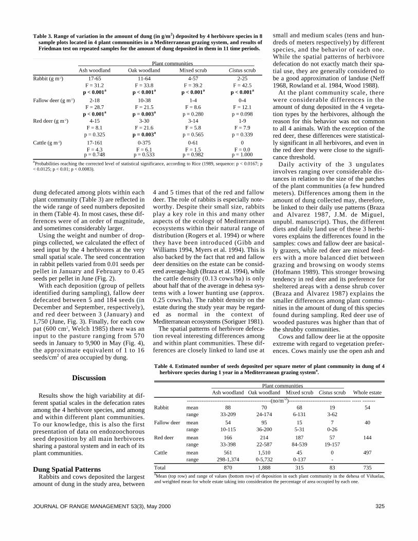
325JOURNAL OF RANGE MANAGEMENT 53(3), May 2000
dung defecated among plots within eachplant community (Table 3) are reflected inthe wide range of seed numbers depositedin them (Table 4). In most cases, these dif-ferences were of an order of magnitude,and sometimes considerably larger.
Using the weight and number of drop-pings collected, we calculated the effect ofseed input by the 4 herbivores at the verysmall spatial scale. The seed concentrationin rabbit pellets varied from 0.01 seeds perpellet in January and February to 0.45seeds per pellet in June (Fig. 2).
With each deposition (group of pelletsidentified during sampling), fallow deerdefecated between 5 and 184 seeds (inDecember and September, respectively),and red deer between 3 (January) and1,750 (June, Fig. 3). Finally, for each cowpat (600 cm2, Welch 1985) there was aninput to the pasture ranging from 570seeds in January to 9,900 in May (Fig. 4),the approximate equivalent of 1 to 16seeds/cm2 of area occupied by dung.
Discussion
Results show the high variability at dif-ferent spatial scales in the defecation ratesamong the 4 herbivore species, and amongand within different plant communities.To our knowledge, this is also the firstpresentation of data on endozoochorousseed deposition by all main herbivoressharing a pastoral system and in each of itsplant communities.
Dung Spatial PatternsRabbits and cows deposited the largest
amount of dung in the study area, between
4 and 5 times that of the red and fallowdeer. The role of rabbits is especially note-worthy. Despite their small size, rabbitsplay a key role in this and many otheraspects of the ecology of Mediterraneanecosystems within their natural range ofdistribution (Rogers et al. 1994) or wherethey have been introduced (Gibb andWilliams 1994, Myers et al. 1994). This isalso backed by the fact that red and fallowdeer densities on the estate can be consid-ered average-high (Braza et al. 1994), whilethe cattle density (0.13 cows/ha) is onlyabout half that of the average in dehesa sys-tems with a lower hunting use (approx.0.25 cows/ha). The rabbit density on theestate during the study year may be regard-ed as normal in the context ofMediterranean ecosystems (Soriguer 1981).
The spatial patterns of herbivore defeca-tion reveal interesting differences amongand within plant communities. These dif-ferences are closely linked to land use at
small and medium scales (tens and hun-dreds of meters respectively) by differentspecies, and the behavior of each one.While the spatial patterns of herbivoredefecation do not exactly match their spa-tial use, they are generally considered tobe a good approximation of landuse (Neff1968, Rowland et al. 1984, Wood 1988).
At the plant community scale, therewere considerable differences in theamount of dung deposited in the 4 vegeta-tion types by the herbivores, although thereason for this behavior was not commonto all 4 animals. With the exception of thered deer, these differences were statistical-ly significant in all herbivores, and even inthe red deer they were close to the signifi-cance threshold.
Daily activity of the 3 ungulatesinvolves ranging over considerable dis-tances in relation to the size of the patchesof the plant communities (a few hundredmeters). Differences among them in theamount of dung collected may, therefore,be linked to their daily use patterns (Brazaand Alvarez 1987, J.M. de Miguel,unpubl. manuscript). Thus, the differentdiets and daily land use of these 3 herbi-vores explains the differences found in thesamples: cows and fallow deer are basical-ly grazers, while red deer are mixed feed-ers with a more balanced diet betweengrazing and browsing on woody stems(Hofmann 1989). This stronger browsingtendency in red deer and its preference forsheltered areas with a dense shrub cover(Braza and Álvarez 1987) explains thesmaller differences among plant commu-nities in the amount of dung of this speciesfound during sampling. Red deer use ofwooded pastures was higher than that ofthe shrubby communities.
Cows and fallow deer lie at the oppositeextreme with regard to vegetation prefer-ences. Cows mainly use the open ash and
Table 3. Range of variation in the amount of dung (in g/m2) deposited by 4 herbivore species in 8sample plots located in 4 plant communities in a Mediterranean grazing system, and results ofFriedman test on repeated samples for the amount of dung deposited in them in 11 time periods.
Plant communities Ash woodland Oak woodland Mixed scrub Cistus scrub
Rabbit (g m-2) 17-65 11-64 4-57 2-25F = 31.2 F = 33.8 F = 39.2 F = 42.5
p < 0.001a p < 0.001a p < 0.001a p < 0.001a
Fallow deer (g m-2) 2-18 10-38 1-4 0-4F = 28.7 F = 21.5 F = 8.6 F = 12.1
p < 0.001a p = 0.003a p = 0.280 p = 0.098Red deer (g m-2) 4-15 3-30 3-14 1-9
F = 8.1 F = 21.6 F = 5.8 F = 7.9p = 0.325 p = 0.003a p = 0.565 p = 0.339
Cattle (g m-2) 17-161 0-375 0-61 0F = 4.3 F = 6.1 F = 1.5 F = 0.0
p = 0.748 p = 0.533 p = 0.982 p = 1.000aProbabilities reaching the corrected level of statistical significance, according to Rice (1989, sequence: p < 0.0167; p< 0.0125; p < 0.01; p < 0.0083).
Table 4. Estimated number of seeds deposited per square meter of plant community in dung of 4herbivore species during 1 year in a Mediterranean grazing systema.
Plant communities Ash woodland Oak woodland Mixed scrub Cistus scrub Whole estate
----------------------------------------------(no/m-2)---------------------------------- ----- -------Rabbit mean 88 70 68 19 54
range 33-209 24-174 6-131 3-62
Fallow deer mean 54 95 15 7 40range 10-115 36-200 5-31 0-26
Red deer mean 166 214 187 57 144range 33-398 22-587 84-539 19-157
Cattle mean 561 1,510 45 0 497range 298-1,374 0-5,732 0-137 -
Total 870 1,888 315 83 735aMean (top row) and range of values (bottom row) of deposition in each plant community in the dehesa of Viñuelas,and weighted mean for whole estate taking into consideration the percentage of area occupied by each one.
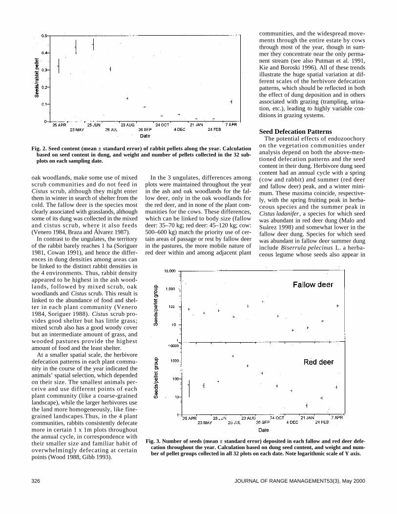
326 JOURNAL OF RANGE MANAGEMENT53(3), May 2000
oak woodlands, make some use of mixedscrub communities and do not feed inC i s t u s scrub, although they might enterthem in winter in search of shelter from thecold. The fallow deer is the species mostclearly associated with grasslands, althoughsome of its dung was collected in the mixedand cistus scrub, where it also feeds(Venero 1984, Braza and Álvarez 1987).
In contrast to the ungulates, the territoryof the rabbit barely reaches 1 ha (Soriguer1981, Cowan 1991), and hence the differ-ences in dung densities among areas canbe linked to the distinct rabbit densities inthe 4 environments. Thus, rabbit densityappeared to be highest in the ash wood-lands, followed by mixed scrub, oakwoodlands and Cistus scrub. This result islinked to the abundance of food and shel-ter in each plant community (Venero1984, Soriguer 1988). C i s t u s scrub pro-vides good shelter but has little grass;mixed scrub also has a good woody coverbut an intermediate amount of grass, andwooded pastures provide the highestamount of food and the least shelter.
At a smaller spatial scale, the herbivoredefecation patterns in each plant commu-nity in the course of the year indicated theanimals’ spatial selection, which dependedon their size. The smallest animals per-ceive and use different points of eachplant community (like a coarse-grainedlandscape), while the larger herbivores usethe land more homogeneously, like fine-grained landscapes.Thus, in the 4 plantcommunities, rabbits consistently defecatemore in certain 1 x 1m plots throughoutthe annual cycle, in correspondence withtheir smaller size and familiar habit ofoverwhelmingly defecating at certainpoints (Wood 1988, Gibb 1993).
In the 3 ungulates, differences amongplots were maintained throughout the yearin the ash and oak woodlands for the fal-low deer, only in the oak woodlands forthe red deer, and in none of the plant com-munities for the cows. These differences,which can be linked to body size (fallowdeer: 35–70 kg; red deer: 45–120 kg; cow:500–600 kg) match the priority use of cer-tain areas of passage or rest by fallow deerin the pastures, the more mobile nature ofred deer within and among adjacent plant
communities, and the widespread move-ments through the entire estate by cowsthrough most of the year, though in sum-mer they concentrate near the only perma-nent stream (see also Putman et al. 1991,Kie and Boroski 1996). All of these trendsillustrate the huge spatial variation at dif-ferent scales of the herbivore defecationpatterns, which should be reflected in boththe effect of dung deposition and in othersassociated with grazing (trampling, urina-tion, etc.), leading to highly variable con-ditions in grazing systems.
Seed Defecation PatternsThe potential effects of endozoochory
on the vegetation communities underanalysis depend on both the above-men-tioned defecation patterns and the seedcontent in their dung. Herbivore dung seedcontent had an annual cycle with a spring(cow and rabbit) and summer (red deerand fallow deer) peak, and a winter mini-mum. These maxima coincide, respective-ly, with the spring fruiting peak in herba-ceous species and the summer peak inCistus ladanifer, a species for which seedwas abundant in red deer dung (Malo andSuárez 1998) and somewhat lower in thefallow deer dung. Species for which seedwas abundant in fallow deer summer dunginclude Biserrula pelecinus L. a herba-ceous legume whose seeds also appear in
Fig. 2. Seed content (mean ± standard error) of rabbit pellets along the year. Calculationbased on seed content in dung, and weight and number of pellets collected in the 32 sub-plots on each sampling date.
Fig. 3. Number of seeds (mean ± standard error) deposited in each fallow and red deer defe-cation throughout the year. Calculation based on dung seed content, and weight and num-ber of pellet groups collected in all 32 plots on each date. Note logarithmic scale of Y axis.

327JOURNAL OF RANGE MANAGEMENT 53(3), May 2000
its dung in winter and spring (Malo andSuárez 1994), and Juncus bufonius L .Cow and rabbit dung contain seeds from alarge number of herbaceous species, par-ticularly Poa annua L., Cerastium glomer -atum Thuill. and Biserrula pelecinus in thecow, and Sisymbrium runcinatum Lag. exDC. and Sagina apetala Ard. in the rabbit.
These temporal patterns and the plantspecies of which seed was disseminatedwere quite similar to those found in thesame area in a 1990 spring–summer sam-pling campaign (Malo and Suárez 1995b),although inter-annual meteorological dif-ferences caused variations in the seed den-sities and composition. In 1990, a particu-larly rainy year, seed densities found indung, with the exception of the red deer,were between 2 and 3 times higher thanthose of spring-summer 1991–92. Thisdifference was due to the overall declinein the numbers of seed of herbaceousspecies in dung, countered only by a steeprise in Cistus ladanifer seeds in red deerdung and to a lesser extent in fallow deerdung. The dry 1990–91 and 1991–92 years(369 mm and 250 mm rainfall betweenSeptember and May contrasted to 575 mmin 1989–90) restricted the growth andfruiting of grasses, which led to a higherconsumption of the fruit (and possiblystems) of the predominant shrub species.
Using these data, we estimate an aver-age annual deposition by herbivores ofaround 735 seeds/m2 for the whole estate,a relatively low amount. The seed banksof Mediterranean grasslands contain30,000–40,000 seeds per m2 in normalyears, and can surpass 100,000 seeds perm2 in years of high production (Ortega et
al. 1997), while woody communities have800–66,000 seeds/m2 (Parker and Kelly1989). Although some of these seeds arepart of the permanent soil bank (Thomsonand Grime 1979), the relative importanceof endozoochory is still small in overallterms, even in years when there is a higherseed density in dung.
In the study area, most of the endozoo-chory was done by large animals. Cowswere responsible for dispersing almost68% of the seeds, followed by red deer(20%), rabbits (7%), and fallow deer (5%).Although these percentages may showinterannual variations, cows are obviouslythe main dispersers in the area due to thelarge amount of dung they deposit and itshigh seed content. In contrast, rabbits dis-perse a relatively small number of seedsdespite the fact that they deposit thelargest amount of dung in the area, alongwith cows. The number of seeds dissemi-nated by rabbits may actually be evenlower than our findings: in the scrubzones, rabbit have a mixed diet whichincludes a certain amount of shrubs(Soriguer 1988), and, thus, the seed con-tent in their dung may be slightly lower insuch areas.
The predominantly herbaceous plantcommunities received the highest seedinput via herbivore dung, although in nocase was the level comparable to theamount in the soil seed banks. Parallel tothe differences among plant communitiesin the volume of dung deposited, the num-ber of seeds deposited varied by more thanan order of magnitude. Thus, C i s t u s a n dmixed scrub only received 83 seeds/m2
and 315 seeds/m2 respectively, in contrastto 870 seeds/m 2 in ash woodlands and1,888 seeds/m2 in the oak woodlands.
However, at small spatial scales, seeddeposition along with herbivore dung canhave important effects on seed banks andvegetation. Given that the sustainablestocking density in a grazing system suchas the study area is relatively low, thedung density on the ground is somewhatlimited and its direct effect on vegetation,therefore, moderate. However, the areaswhich are covered by herbivore dungreceive a substantial density of seeds.Practically any defecation by a herbivorecontains some seeds, the number deposit-ed in a single spring–summer defecationpotentially being hundreds in the case offallow deer, more than 1,000 in red deer,and close to 10,000 in the case of cattle.
The effect of this seed input to the vege-tation ranges from the localized introduc-tion of species to the creation of gradientsassociated with grazing. On the one hand,the possibility that herbivores might causethe local introduction of species whoseseeds are dispersed in dung has beenproved (Malo and Suárez 1994,Ocumpaugh et al. 1996), and is also postu-lated as being the most important effect ofherbivore endozoochory (Gardener 1993,Zedler and Black 1992, Sevilla et al.1996). Species introduction may alsooccur with woody plants, leading to theinvasion of pastures by scrub (Miller andCoe 1993, Peinetti et al. 1993, Malo andSuárez 1998).
On the other hand, herbivore endozoo-chory can also change the interspecificcompetitive balance among plants, favour-ing those which are disseminated viadung. In the grasslands similar to the studyarea, the vegetation growing in areas occu-pied by cow pats has been found to bedetermined by the dung seed content(Malo and Suárez 1995a). Cow pats act aslocal disturbances which eliminate the pre-dominant perennial grass (Poa bulbosa L.)and introduce annual species, which growin the gap caused by the cow pat. Givenenough time, they are displaced by thePoa bulbosa recolonisation, which takesmore than 4 years to regain its cover(Malo and Suárez 1996). A less dramaticbut similar process probably takes placewith dung pellets, where hundreds ofseeds in deer pellets, and even the isolatedseeds in rabbit dung, are able to find aplace to germinate. However, the high ger-mination rates in dung can also lead tohigh mortality rates due to competition(Sevilla et al. 1996).
Fig. 4. Number of seeds (mean ± standard error) deposited within an average-sized (600 cm2)cow pat. Calculation based on (i) dung seed content, (ii) density of cow dung and (iii) meandepth of cow pats measured in all 32 plots on each date. As no cow pats were counted inthe sampling plots on 23-VIII or 26-IX, data for these dates (marked with stars) were cal-culated using mean depth of all pats measured during the study.

328 JOURNAL OF RANGE MANAGEMENT53(3), May 2000
Finally, the irregular spatial defecationpatterns of herbivores complicates thispanorama, and probably leads to vegetationmosaics associated with the different inputof nutrients and seeds via dung. The differ-ent feeding and defecation habits of herbi-vores thus help to increase plant diversity atdifferent scales in extensive grazing sys-tems such as the Iberian d e h e s a s.
Literature Cited
Aschmann, H. 1973. Man’s impact on the sev-eral regions with Mediterranean climates. p.11–19. I n: F. di Castri and H.A. Mooney(Eds.). Mediterranean type ecosystems.Origins and structure, Springer, Berlin.
Braza, F. and F. Álvarez. 1987. Habitat useby red deer and fallow deer in DoñanaNational Park. Miscellanea Zoologica11:363–367.
Braza, F., Soriguer, R.C., San José, C.,Delibes, J.R., Fandós, P., and L. León.1 9 9 4 . Métodos para el estudio y manejo decérvidos. Consejería de Agricultura y Pesca,Junta de Andalucía, Cádiz.
Collins, S.L. and G.E. Uno. 1985. Seed preda-tion, seed dispersal, and disturbance in grass-lands: a comment. Amer. Nat. 125:866–872.
Courtney. A.D. 1973. Wild oats and animalfeedstuffs. Agric. North. Irel. 47:389–390.
Cowan, D.P. 1991. The availability of burrowsin relation to dispersal in the wild rabbit(Oryctolagus cuniculus). Symposium of theZool. Soc. of London 63:213–230.
Gardener, C.J. 1993. The colonization of atropical grassland by Stylosanthes from seedtransported in cattle faeces. Aust. J. Agr. Res.44:299–315.
Gardener, C.J., J.G. McIvor, and A. Jansen.1 9 9 3 . Passage of legume and grass seedsthrough the digestive tract of cattle and theirsurvival in faeces. J. Appl. Ecol. 30:63–74.
Georgiadis, N.J. and S.J. McNaughton. 1990.Elemental and fibre contents of savannahgrasses: variation with grazing, soil type, sea-son and species. J. Appl. Ecol. 27:623–634.
Gibb, J.A. 1993. Sociability, time and space ina sparse population of rabbits (O r y c t o l a g u scuniculus). J. of Zool., London 229:581–607.
Gibb, J.A. and J.M. Williams. 1994. The rab-bit in New Zealand. p. 158-204. I n: H.V.Thomson and C.M. King (eds), TheEuropean rabbit. The history and biology of asuccessful colonizer, Oxford Univ. Press,Oxford.
Hofmann, R.R. 1989. Evolutionary steps ofecophysiological adaptation and diversifica-tion of runminants: a comparative view oftheir digestive system. Oecologia78:443–457.
Janzen D.H. 1984. Dispersal of small seeds bybig herbivores: foliage is the fruit. Amer.Nat. 123:338–353.
Jones, R.M., M. Noguchi, and B.G. Bunch.1 9 9 1 . Levels of germinable seed in topsoiland cattle faeces in legume-grass and nitro-gen-fertilized pastures in South-EastQueensland. Aust. J. Agr. Res. 42:953–968.
Kie, J.G. and B.B. Boroski. 1996. Cattle dis -tribution, habitats, and diets in the SierraNevada of California. J. Range Manage.49:482–488.
Malo, J.E. and F. Suárez. 1994. D i s p e r s i ó nendozoócora por el gamo (Dama dama) eintroducción de especies con el pastoreo.Pastos 24:47–56.
Malo, J.E. and F. Suárez. 1995a.Establishment of pasture species on cattledung. The role of endozoochorous seeds. J.Veg. Sci. 6:169–174.
Malo, J.E. and F. Suárez. 1995b. Herbivorousmammals as seed dispersers in aMediterranean dehesa. Oecologia104:246–255.
Malo, J.E. and F. Suárez. 1995c. Cattle dungand the fate of Biserrula pelecinus L .(Leguminosae) in a Mediterranean pasture:seed dispersal, germination and recruitment.Bot. J. Linn. Soc. 118:139–148.
Malo, J.E. and F. Suárez. 1996. Las boñigasde vaca, el encespedado de Poa bulbosa y ladiversidad de un pastizal de dehesa. Pastos16:61–75.
Malo, J.E. and F. Suárez. 1998. The dispersalof a dry-fruited shrub by red deer in aMediterranean ecosystem. Ecography21:204–211.
McNaughton, S.J. 1984. Grazing lawns: ani-mal in herds, plant form and coevolution.Amer. Nat. 124:863–886.
Miller, M.F. and M. Coe. 1993. Is it advanta-geous for Acacia seeds to be eaten by ungu-lates? Oikos 66:364–368.
Myers, K., I. Parer, D. Wood, and B.D.Cooke. 1994. The rabbit in Australia. p. 108-157. In: H.V. Thomson and C.M. King (eds),The European rabbit. The history and biolo-gy of a successful colonizer, Oxford Univ.Press, Oxford.
Neff, D.J. 1968. The pellet-group count tech-nique for big game trend, census, and distrib-ution: A review. J. of Wildl. Manage.32:597–614.
Ocumpaugh, W.R., S. Archer, and J.W.Stuth. 1996. Switchgrass recruitment frombroadcast seed vs. seed fed to cattle. J. RangeManage. 49 :368–371.
Ortega, M., C. Levassor, and B. Peco. 1997.Seasonal dynamics of Mediterranean pastureseed banks along environmental gradients. J.Biogeogr. 24:177–195.
Parker, V.T. and V.R. Kelly. 1989. S e e dbanks in California chaparral and otherMediterranean climate shrublands. p. 231-255. in: M.A. Leck, V.T. Parker and R.L.Simpson (eds.) Ecology of soil seed banks,Academic Press Inc., San Diego, Calif.
Peinetti, R., M. Pereyra, A. Kin, and A. Sosa.1993. Effects of cattle ingestion on viabilityand germination rate of calden (P r o s o p i sc a l d e n i a) seeds. J. Range Manage.46:483–486.
Putman, R.J., A.D. Fowler, and S. Tout.1991. Patterns of use of ancient grassland bycattle and horses and effects on vegetationalcomposition and structure. Biol. Conserv. 56:329–347.
Rice, W.R. 1989. Analyzing tables of statisti-cal tests. Evolution 43:223–225.
Rogers, P.M., C.P. Arthur, and C.R.Soriguer. 1994. The rabbit in continentalEurope. p. 22–63. I n: H.V. Thomson andC.M. King (eds), The European rabbit. Thehistory and biology of a successful colonizer,Oxford University Press, Oxford.
Rowland, M.M., G.C. White, and E. M.Karlen. 1984. Use of pellet-group plots tomeasure trends in deer and elk populations.Wildl. Soc. Bull. 12:147–155.
Russi, L., P.S. Cocks, and E.H. Roberts.1 9 9 2 . The fate of legume seeds eaten bysheep from a Mediterranean grassland. J.Appl. Ecol. 29:772–778.
Sevilla, G.H., O.N. Fernández, D.P. Minon,and L. Montes. 1996. Emergence andseedling survival of Lotus tenuis in F e s t u c aa r u n d i n a c e a pastures. J. Range Manage.49:509–511.
Seaman, J.W., S.C. Walls, S.E. Wise, andR.G. Jaeger. 1994. Caveat emptor: ranktransform methods and interaction. TREE9:261–263.
Soriguer, R.C. 1981. Biología y dinámica deuna población de conejos (O r y c t o l a g u scuniculus) en Andalucía Occidental. Doñana,Acta Vertebrata 8-3:1–379.
Soriguer, R.C. 1988. Alimentación del conejo(Oryctolagus cuniculus L. 1758) en Doñana.SO, España. Doñana, Acta Vertebrata15:141–150.
Thompson, K. and J.P. Grime. 1979.Seasonal variation in the seed banks ofherbaceous species in ten contrasting habi-tats. J. Ecol. 67:893–921.
Venero, J.L. 1984. Dieta de los grandes fitófa-gos si lvestres del Parque Nacional deDoñana, España. Doñana, Acta Vertebrata11-3:1–130.
Welch, D. 1985. Studies in the grazing ofheather moorland in North-East Scotland. IV.Seed dispersal and plant establishment indung. J. Appl. Ecol. 22:461–472.
Wood, D.H. 1988. Estimating rabbit density bycounting dung pellets. Aus. J. Wildl. Res.15:665-671.
Yamada, T. and T. Kawaguchi. 1972.Dissemination of pasture plants bylivestoock. II. Recovery, viability, and emer-gence of some pasture plant seeds passedthrough digestive track of dairy cows. J. Jpn.Grassl. Sci. 18:8–15.
Zedler, P.H. and C. Black. 1992. Seed disper-sal by a generalized herbivore: rabbits as dis-persal vectors in a semiarid California vernalpool landscape. Amer. Midland Nat.128:1–10.

329JOURNAL OF RANGE MANAGEMENT53(3), May 2000
Abstract
Tall larkspurs [Delphinium barbeyi (L. Huth), D. occidentale(Wats.), D. glaucescens (Rydb.), D. glaucum (Wats.)] pose a seri-ous poisoning threat to cattle on many summer ranges. Livestockproducers often defer grazing until larkspur is mature, but spe-cific information is lacking on toxic alkaloid concentrations inlarkspur from pod stage to senescence. Tall larkspur leaves andseed pods were collected about every 2 weeks during the podstage to senescence from marked plants in locations in Utah(Logan and Salina), Idaho (Ashton, Humphrey, and Oakley),Colorado (Yampa and Montrose), and California (Carson Pass)from 1995 to 1997. Toxic alkaloid concentions in pods (x– = 2.9mg/g) exceeded leaf alkaloid concentrations (x– = 1.5 mg/g in allspecies, but the magnitude of the difference varied among the 4species. Leaves showed a more rapid decrease in toxic alkaloidconcentration with plant maturity compared to pods. Seed podsdid not begin to lose substantial amounts of toxic alkaloid untillarkspur matured and pods began to dessicate. At seed shatter,D. glaucescens pods retained more toxic alkaloid than the otherspecies, and alkaloid concentration was sufficiently high afterpods had shattered (3.5 mg/g) to pose a moderate grazing risk.After seed shatter, the toxic alkaloid concentrations in leaves andpods of D. barbeyi, D. occidentale, and D. glaucum were generallyless than 2 mg/g; thus, risk of losing cattle would be low for theremainder of the grazing season.
Key Words: diterpenoid alkaloids, poisonous plants, grazingmanagement
Tall larkspurs (Delphinium barbeyi (L. Huth), D. occidentale(Wats.), D. glaucescens (Rydb.), D. glaucum (Wats.)) are toxicplants that are often fatally ingested by cattle on western range-lands. The presence of larkspur often dictates summer grazingmanagement of mountain rangeland as producers attempt toreduce or avoid livestock losses (Pfister et al. 1997). A long-established management practice is to defer grazing until larkspuris mature, vaguely defined as the late flower or pod stage ofgrowth (Marsh et al. 1916). Late-season grazing can provide 6 to8 weeks of grazing depending on larkspur phenology, elevation,available forage, and weather (Pfister, personal observations).
Major deficiencies in this recommendation include: (1) the con-centration of toxic alkaloids (i.e., toxicity) in tall larkspurs oftendecreases with maturation, but this decrease is not constant orconsistent (Pfister et al. 1994, Ralphs et al. 1997); (2) grazingduring the late-flower period may expose cattle to a high risk ofpoisoning (Pfister et al. 1997); and (3) information specific to latesummer and fall alkaloid concentrations and plant toxicity isinsufficient to make definitive grazing recommendations.
Previously we evaluated seasonal changes in tall larkspur toxici-ty, but usually stopped sampling during the early pod stage(Pfister et al. 1994, Ralphs et al. 1997). Seed pods may take longerthan 6 weeks to mature and shatter; furthermore, green leaves mayremain after pods have shattered (Pfister, personal observations).Information on late-season toxicity is necessary for livestock pro-
J. Range Manage.53: 329–334 May 2000
Late season toxic alkaloid concentrations in tall larkspur(Delphinium spp.)
DALE R. GARDNER AND JAMES A. PFISTER
Authors are research chemist and rangeland scientist, respectively, with the USDA-ARS Poisonous Plant Research Laboratory, 1150 E. 1400 N. Logan, Ut.84341.
Resumen
Las especies de "Tall larkspur" [Delphinium barbeyi (L. Huth),D. Occidentale (Wats.), D. glaucescens (Rydb), D. glaucum(Wats.)] son una seria amenaza de envenenamiento para el gana-do que apacenta en pastizales de verano. Los ganaderos amenudo difieren el apacentamiento hasta que el "Larkspur" estamaduro, sin embargo, se carece de información especificarespecto a las concentraciones de alcaloides tóxicos que contieneel "larkspur" desde la producción de vainas hasta la senescenciade la planta. De 1995 a 1997, durante la etapa de producción devainas a senescencia, se colectaron hojas y vainas "Tall lark-spur" aproximadamente cada 2 semanas, la colecta se realizó enplantas marcada en localidades de Utah (Logan y Salina), Idaho(Asthon, Humphrey y Oakley), Colorado (Yampa y Montrose) yCalifornia (Carson Pass). Las concentraciones de alcaloides tóxi-cos de las vainas de todas las especies fueron mayores (x– = 2.9mg/g) que las concentraciones de las hojas (x– = 1.5 mg/g), pero lamagnitud de la diferencia vario entre las 4 especies. Al madurar,la concentración de alcaloides tóxicos de las hojas descendiómas rápidamente que la concentración de las vainas. Las vainasno empezaron a perder cantidades substanciales de alcaloidestóxicos hasta que el "Larkspur" maduró y las vainas comen-zaron a desecarse. En la etapa de caída de semilla, las vainas deD. glaucescens retuvieron mas alcaloides tóxicos que otrasespecies y la concentración de alcaloides en ellas después dehaber liberados las semillas fue suficientemente alta (3.5 mg/g)para poseer un riesgo moderado durante el apacentamiento.Después de la caída de la semilla las concentraciones dealcaloides tóxicos en hojas y vainas de las especies D. barbeyi, D.occidentale y D. glaucum generalmente fueron menos de 2 mg/g;así, el riesgo de perder ganado sería bajo para el resto de laestación de apacentamiento.
The authors wish to thank Kermit Price, Mike Ralphs, Tom Schoch, andMelissa Blackham for assistance with sample collections and alkaloid analysis. Wethank Drs. Tom Jones and Dale Zobell for helpful comments on the mansucript.We also thank Dr. Don Sisson, Utah State University, for statistical advice.
Manuscript accepted 3 Aug. 1999.

330 JOURNAL OF RANGE MANAGEMENT53(3), May 2000
ducers to determine when the risk of poi-soning is sufficiently low to allow grazing.In this study we provide information fortoxic alkaloid concentrations in seed podsand leaves from the pod stage of growth tos e n e s c e n c e .
Methods
Sample CollectionWe collected tall larkspur leaves and
seed pods about every 2 weeks from theearly pod stage of growth to senescencefrom marked plants in each location (n =8), with some exceptions (Table 1).Generally, sampling occurred from earlyAugust to late September or early Octoberin each year, and where possible, wastimed to represent 4 phenological stages:early pod, pod, late pod, and seed shatter.We marked 20 individual plants with anumbered fiberglass rod. Tall larkspursgenerally have multiple stems, and sam-pling leaves and seed heads from a singlestem provides a representative sample ofthe entire plant (Manners and Pfister1996). Therefore, during each collectionwe selected an individual stem from eachplant at random, and we harvested all theleaves and the seed head (i.e., entire seedpod including stem from upper 15 to 20cm of the stem) from this stem. The har-vested leaves and seed heads mimic theplant parts that cattle generally select(Pfister et al. 1988). All plant parts weremaintained separately for alkaloid analy-sis. A sample size of 20 plants is usuallysufficient to provide an alkaloid concen-tration within ± 10% of the populationmean with 95% confidence (Manners andPfister 1996). We packed samples in ice
for transport to the laboratory, where theywere frozen at –20° C, freeze-dried, thenground to pass through a 1 mm screen forlater analysis. We did not mark individualplants at Humphrey, Ida. because D .g l a u c e s c e n s seldom has sufficient stemsfor repeated sampling of the same plant.Instead, during 1995 and 1997, we select-ed 20 plants at random during each collec-tion period, and collected leaves and seedheads. In 1996 at Ashton, Ida, we collect-ed leaf and pod samples from 20 differentplants on each date. We also collectedseeds during 1996 from plant populationsat Logan, Yampa, and Montrose; during1997 we collected seeds from Oakley,Yampa and Montrose.
Alkaloid analysisThe primary toxins in tall larkspurs are
2 norditerpenoid alkaloids: methyllyca-conitine (MLA) and 14-deacetylnudi-cauline (DAN). These alkaloids have near-ly identical mammalian toxicity (miceL D5 0 4.0 to 4.7 mg/kg; Manners et al.1995). The combined concentration ofthese 2 toxic alkaloids (i.e., MLA + DAN= toxic alkaloid concentration) was deter-mined by Fourier transform infrared spec-troscopy (FTIR, Gardner et al. 1997).
This methodology also provides a mea-surement of the total alkaloid (i.e., toxic +less-toxic alkaloids) concentration. Less-toxic alkaloids are 2 to 4 orders of magni-tude less toxic than MLA (Manners et al.1995) because they lack the correct struc-tural specificity to impart significant toxic-ity. The total alkaloid concentration hasrelevance when producers use sheep as amanagement tool to reduce cattle losses(Ralphs and Olsen 1992), as higher con-centrations of total alkaloids reduce lark-
spur consumption by sheep (Pfister et al.1996). Because total alkaloid concentra-tions are less important than toxic alka-loids, only a brief summary is presented.
Statistical AnalysisThe data were analyzed using the GLM
procedure of SAS (1988) with the follow-ing effects: years, species, locations nestedwithin species, plant part, phenologicalstage, and individual plants (subsamplingterm), and resulting interactions. Years,species, and the year x species interactionwere tested using the sum of the locationwithin species term and the year x locationwithin species term as the single errorterm. Plant parts, year x part, species xpart, and year x species x part were testedusing the sum of the part x location withinspecies and the part x year x location with-in species terms as the single error term.Phenological stage, year x stage, species xstage, year x species x stage, part x stage,year x part x stage, species x part x stage,species x part x stage, and the 4-way inter-action were tested using the sum of thepart x location within species x stage termand the part x year x location withinspecies x stage term as the single errorterm. When significant F-tests were found,the Duncan’s multiple range test was usedto compare means. Differences in loca-tions within each species (where applica-ble) were examined with the GLM proce-dure of SAS (1988) using a model withlocation, year within location, part, part xlocation, part x year within location, stage,stage x location, stage x year within loca-tion, stage x part, stage x part x locationand stage x part x year within location.The year within location term was used totest for differences in location; part and
Table 1. Location of each tall larkspur collection, years of collection, elevation, associated vegetation type, and sampling methods.
Delphinium Location Years Elevation Vegetation Type Sampling Method1
spp. (m)
D. barbeyi Montrose, Colo. 38°18'N 108°12'W 1995-97 2871 Conifer/Aspen Marked plantsYampa, Colo. 40°12'N 107°04'W 1995-97 2580 Conifer/Aspen Marked plantsSalina, Ut.2 38°44'N 111°39'W 1995-97 2895 Aspen Marked plants
D. occidentale Logan, Ut. 41°54'N 111°34'W 1996-97 2400 Conifer/Aspen Marked plantsAshton, Ida. 44°05'N 111°08'W 1995-96 1815 Aspen Marked plants3
Oakley, Ida. 42°10'N 114°11'W 1995-97 2247 Aspen Marked plants
D. glaucescens Humphrey, Ida. 44°32'N 112°10'W 1995,97 2396 Grass meadow No marked plants4
D. glaucum Carson Pass, Calif. 38°40'N 119°59'W 1996-97 2700 Wet meadow Marked plants5
1Unless noted otherwise, 20 individual plants were marked, and all leaves and the seed head were collected from 1 stem during each sample period; sampling recurred at approximate-ly 2 week intervals during the pod stage until senescence.2This larkspur population includes some D. occidentale, but is primarily D. barbeyi.3Twenty different unmarked plants were sampled during each collection in 1995; 20 plants were marked and sampled during 1996. 4Individual plants of D. glaucescens often do not have sufficient stems for multiple samples, therefore leaves and seed heads were collected from 20 different plants during each col-lection period during 1995 and 1997. Whole plants collected during 1996 were not included in the statistical analysis.5A composite sample from at least 20 plants was collected during each period in 1996; 20 plants were marked and sampled during 1997.

331JOURNAL OF RANGE MANAGEMENT 53(3), May 2000
the part x location interaction were testedusing the part x year within location errorterm; stage and stage x location were test-ed using the stage x year within locationterm; stage x part and stage x part x loca-tion were tested using the stage x part xyear within location error term.Correlation coefficients for alkaloid con-centrations in plants were determinedusing mean concentrations for each plantfor each location and year.
Results and Discussion
Years Overall, the toxic alkaloid concentration
averaged 2.1 mg/g (SE ± 0.05; range =17.4). Years did not differ and year xspecies did not interact (P > 0.1). Ralphset al. (1997) reported year differences inalkaloid concentrations for all speciesexcept D. glaucescens, but Pfister et al.(1994) found that concentrations in D .barbeyi in Colorado differed in only 1 of 3years. We speculate that years did not dif-fer in our study because sampling wasconfined to the late summer period whenconcentrations were relatively low, andtherefore more stable, relative to vegeta-tive and bud stages (Pfister et al. 1994,Ralphs et al. 1997). We caution that year-to-year variation in toxicity may be high,particularly at earlier stages of maturity.
Plant PartsThe plant part x species interaction was
significant, as toxic alkaloid concentra-tions in pods exceeded leaf alkaloid con-centrations in all species, but the magni-tude of the difference varied among the 4species (Fig. 1). We have noted in previ-ous studies that pod toxicity generallyexceeds that for leaves (Pfister et al. 1994,Ralphs et al. 1997). Seed pods apparentlyaccumulate both toxic and less-toxic alka-loids early in the maturation process,although the degree of accumulation dif-fers among species.
Phenological Stage and Species Toxic alkaloid concentrations declined
(P < 0.05) as tall larkspur matured. Leavesshowed a more rapid decrease in toxicalkaloid concentration than pods (Fig. 2).Seed pods began to lose substantialamounts of toxic alkaloid beginning at thelate pod stage (i.e., pods beginning todessicate). In all species except for D. bar -beyi at Salina, Utah, we found no indica-tion of the late-season increase in leaftoxic alkaloids that we previously reported
Fig. 1. Toxic (A) and total (B) alkaloid concentration (mg/g + SE) in leaves and pods of 4Delphinium species during the later portion of the growing season.
Fig. 2. Toxic alkaloid concentration (mg/g + SE) in Delphinium spp. pods and leaves in variousgrowth stages during the later portion of the growing season.

332 JOURNAL OF RANGE MANAGEMENT 53(3), May 2000
during one season in Colorado (Pfister etal. 1994). Pods apparently lose some alka-loids because of alkaloid-containing seedsdropping from the pods. Some alkaloidsmust be retained in the shattered podsbecause, as noted below, residual podsfrom D. glaucescens remained toxic afterseed shatter. Seeds collected from D. bar -b e y i in Colorado (Yampa and Montrose)averaged 5.4 mg/g of toxic alkaloid,whereas D. occidentale seeds fromOakley, Ida. and Logan, Utah contained7.1 and 0.25 mg/g of toxic alkaloid,respectively. No seeds were found in D .glaucescens plants at Humphrey, Ida. Wespeculate that the toxic alkaloid concentra-tion remained high in the residual pods ofD. glaucescens because seed formationand subsequent loss were incomplete.
D. glaucescens and g l a u c u m e x h i b i t e dhigher initial toxic alkaloid concentrationsthan D. barbeyi and o c c i d e n t a l e. At seedshatter, most tall larkspur species con-tained about the same concentrations oftoxic alkaloid, except D. glaucescensretained more toxic alkaloid than the otherspecies (Fig. 3). Previous work in our lab-oratory (Ralphs et al. 1997) determinedthat D. glaucum contained the highestoverall concentration of toxic alkaloid, butthe present study showed that toxic alka-loid concentration in D. glaucumdecreased greatly during pod formation.
Same Species at Different LocationsD. barbeyi was sampled at 3 locations
(Montrose, Salina, and Yampa). Therewere no location effects nor interactions(P > 0.1). We found a significant stage xpart interaction for toxic alkaloids in D .b a r b e y i . Toxic alkaloid concentrationsdecreased more with maturation in D. bar -beyi leaves than in pods (Fig. 4).
For D. occidentale the location x plantpart interaction was significant; stage of
growth was also a significant factor. Theinteraction with location occurred becausethe Logan tall larkspur population hadmuch lower toxic alkaloid concentrationsover the late summer compared to eitherAshton or Oakley, and concentrations atLogan were largely unaffected by stage ofgrowth (Fig. 5). Furthermore, leaves andpods at the Logan location had almostidentical, but very low, concentrations oftoxic alkaloids which changed little overtime. Conversely, at both Ashton andOakley, toxic alkaloid concentrationsdeclined as plants matured and were low-est at seed shatter (Fig. 5).
We offer no explanation for the muchlower concentration of toxic alkaloids inD. occidentale collected near Logan com-pared to collections from Oakley andAshton. Ralphs et al. (1997) similarlyreported that D. occidentale collected nearBozeman, Mont. and Jackson, Wyo. hadmuch lower concentrations than theOakley population. In the Ralphs et al.(1997) study, collections from Jacksonand Bozeman were from a single year;nonetheless, concentrations were similarto our results from Logan. The Logan pop-ulation was also unusual in that total alka-loid concentrations were high (pod x– =18.4 mg/g; leaf x– = 5.6 mg/g).
Correlation coefficients relating toxicand total alkaloid concentrations in leavesand pods from individual plants were low(r=0.2 to 0.5), indicating that generallytoxic and total alkaloid concentrations
Fig. 3. Toxic alkaloid concentration (mg/g + SE) for 4 Delphinium species at various growth stagesduring the later portion of the growing season.
Fig. 4. Toxic and total alkaloid concentrations (mg/g + SE) for Delphinium barbeyi leaves and podsat various growth stages during the later portion of the growing season.
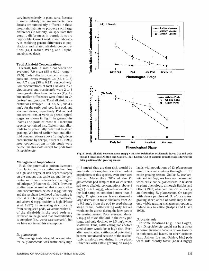
333JOURNAL OF RANGE MANAGEMENT53(3), May 2000
vary independently in plant parts. Becauseit seems unlikely that environmental con-ditions are sufficiently different in thesemountain habitats to produce such largedifferences in toxicity, we speculate thatgenetic differences in populations areresponsible. Current work in our laborato-ry is exploring genetic differences in pop-ulations and related alkaloid concentra-tions (Li, Gardner, Wang, and Ralphs,unpublished data).
Total Alkaloid ConcentrationsOverall, total alkaloid concentration
averaged 7.0 mg/g (SE ± 0.12; range =29.9). Total alkaloid concentrations inpods and leaves averaged 9.4 (SE ± 0.18)and 4.7 mg/g (SE ± 0.12), respectively.Pod concentrations of total alkaloids in D.g l a u c e s c e n s and o c c i d e n t a l e were 2 to 3times greater than found in leaves (Fig. 1),but smaller differences were found in D .b a r b e y i and g l a u c u m. Total alkaloid con-centrations averaged 10.3, 7.8, 5.0, and 4.4mg/g for the early pod, pod, late pod, andshattered stages, respectively. Pod and leafconcentrations at various phenologicalstages are shown in Fig. 4. In general, theleaves and pods of most tall larkspurspecies contained insufficient total alka-loids to be potentially deterrent to sheepgrazing. We found earlier that total alka-loid concentrations above 12 mg/g deterconsumption by sheep (Pfister et al. 1996);most concentrations in this study werebelow this threshold except for pods fromD. occidentale.
Management ImplicationsRisk, the potential to poison livestock
from larkspurs, is a continuum from lowto high, and degree of risk depends largelyon the amount that cattle eat and the con-centration of toxic alkaloids in the ingest-ed larkspur (Pfister et al. 1997). Previousstudies have determined that at toxic alka-loid concentrations below 3 mg/g, toxicityand the resultant likelihood of poisoning islow, at 3 to 6 mg/g toxicity is moderate,and above 6 mg/g toxicity is high (Pfisteret al. 1997). In assessing risk to cattlefrom eating seed pods, we assumed that allof the alkaloids in the seed pods areextracted in the gut and that bioavailabilityis complete (i.e., worst case scenario), butwe have not tested this assumption.
D. glaucescensThe average toxic alkaloid concentration
for D. glaucescens was sufficiently high
(4.4 mg/g) that grazing risk would bemoderate on rangelands with abundantpopulations of this species, even after seedshatter. More than 70% of the D .glaucescens pod samples that we collectedhad toxic alkaloid concentrations above 3mg/g (x– = 6.1 mg/g), whereas about 4% ofthe leaf samples contained more than 3mg/g. D. glaucescens leaves showed alarge decrease in toxic alkaloids from 2.5to 0.6 mg/g from the pod to seed-shatterstage. Thus, cattle eating only leaveswould not be at risk during the later part ofthe grazing season. Pods averaged almost9 mg/g of toxic alkaloid in the early podstage, and only declined to 3.5 mg/g whenshattered. Thus, cattle eating pods beforeseed shatter would be at high risk. Evenafter seed shatter, cattle could potentiallybecome intoxicated because of the residualtoxic alkaloids remaining in the plant.Ranchers with cattle grazing on range-
lands with populations of D. glaucescensmust exercise caution throughout theentire grazing season. Unlike D. occiden -tale and barbeyi, we have not determinedwhen cattle eat D. glaucescens in relationto plant phenology, although Ralphs andOlsen (1992) observed that cattle readilyate flowering D. glaucescens. On rangeswith dense patches of D. glaucescens ,grazing sheep ahead of cattle may be theonly viable grazing management option toreduce risk to cattle (Ralphs and Olsen1992).
D. occidentaleIn some locations (e.g., near Logan,
Ut.), D. occidentale would not be a threatto poison livestock because of low toxicityin both pods and leaves. At other locations(e.g., Ashton, Ida. and Oakley, Ida.) podswere sufficiently toxic (near 4 mg/g)
Fig. 5. Toxic alkaloid concentrations (mg/g + SE) for Delphinium occidentale leaves (A) and pods(B) at 3 locations (Ashton and Oakley, Ida.; Logan, Ut.) at various growth stages during thelater portion of the growing season.
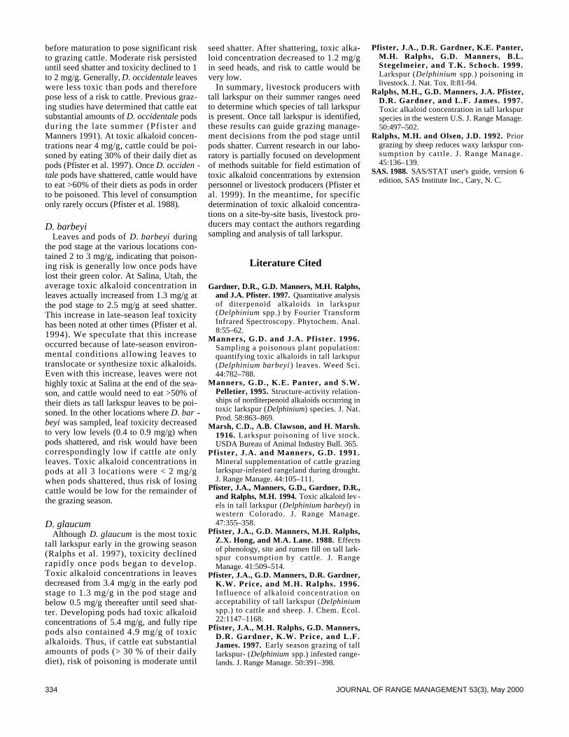
334 JOURNAL OF RANGE MANAGEMENT 53(3), May 2000
before maturation to pose significant riskto grazing cattle. Moderate risk persisteduntil seed shatter and toxicity declined to 1to 2 mg/g. Generally, D. occidentale l e a v e swere less toxic than pods and thereforepose less of a risk to cattle. Previous graz-ing studies have determined that cattle eatsubstantial amounts of D. occidentale p o d sduring the late summer (Pfister andManners 1991). At toxic alkaloid concen-trations near 4 mg/g, cattle could be poi-soned by eating 30% of their daily diet aspods (Pfister et al. 1997). Once D. occiden -t a l e pods have shattered, cattle would haveto eat >60% of their diets as pods in orderto be poisoned. This level of consumptiononly rarely occurs (Pfister et al. 1988).
D. barbeyiLeaves and pods of D. barbeyi d u r i n g
the pod stage at the various locations con-tained 2 to 3 mg/g, indicating that poison-ing risk is generally low once pods havelost their green color. At Salina, Utah, theaverage toxic alkaloid concentration inleaves actually increased from 1.3 mg/g atthe pod stage to 2.5 mg/g at seed shatter.This increase in late-season leaf toxicityhas been noted at other times (Pfister et al.1994). We speculate that this increaseoccurred because of late-season environ-mental conditions allowing leaves totranslocate or synthesize toxic alkaloids.Even with this increase, leaves were nothighly toxic at Salina at the end of the sea-son, and cattle would need to eat >50% oftheir diets as tall larkspur leaves to be poi-soned. In the other locations where D. bar -b e y i was sampled, leaf toxicity decreasedto very low levels (0.4 to 0.9 mg/g) whenpods shattered, and risk would have beencorrespondingly low if cattle ate onlyleaves. Toxic alkaloid concentrations inpods at all 3 locations were < 2 mg/gwhen pods shattered, thus risk of losingcattle would be low for the remainder ofthe grazing season.
D. glaucumAlthough D. glaucum is the most toxic
tall larkspur early in the growing season(Ralphs et al. 1997), toxicity declinedrapidly once pods began to develop.Toxic alkaloid concentrations in leavesdecreased from 3.4 mg/g in the early podstage to 1.3 mg/g in the pod stage andbelow 0.5 mg/g thereafter until seed shat-ter. Developing pods had toxic alkaloidconcentrations of 5.4 mg/g, and fully ripepods also contained 4.9 mg/g of toxicalkaloids. Thus, if cattle eat substantialamounts of pods (> 30 % of their dailydiet), risk of poisoning is moderate until
seed shatter. After shattering, toxic alka-loid concentration decreased to 1.2 mg/gin seed heads, and risk to cattle would bevery low.
In summary, livestock producers withtall larkspur on their summer ranges needto determine which species of tall larkspuris present. Once tall larkspur is identified,these results can guide grazing manage-ment decisions from the pod stage untilpods shatter. Current research in our labo-ratory is partially focused on developmentof methods suitable for field estimation oftoxic alkaloid concentrations by extensionpersonnel or livestock producers (Pfister etal. 1999). In the meantime, for specificdetermination of toxic alkaloid concentra-tions on a site-by-site basis, livestock pro-ducers may contact the authors regardingsampling and analysis of tall larkspur.
Literature Cited
Gardner, D.R., G.D. Manners, M.H. Ralphs,and J.A. Pfister. 1997. Quantitative analysisof diterpenoid alkaloids in larkspur(D e l p h i n i u m spp.) by Fourier TransformInfrared Spectroscopy. Phytochem. Anal.8:55–62.
Manners, G.D. and J.A. Pfister. 1996.Sampling a poisonous plant population:quantifying toxic alkaloids in tall larkspur(Delphinium barbeyi ) leaves. Weed Sci.44:782–788.
Manners, G.D., K.E. Panter, and S.W.Pelletier, 1995. Structure-activity relation-ships of norditerpenoid alkaloids occurring intoxic larkspur (D e l p h i n i u m) species. J. Nat.Prod. 58:863–869.
Marsh, C.D., A.B. Clawson, and H. Marsh.1 9 1 6 . Larkspur poisoning of live stock.USDA Bureau of Animal Industry Bull. 365.
Pfister, J.A. and Manners, G.D. 1991.Mineral supplementation of cattle grazinglarkspur-infested rangeland during drought.J. Range Manage. 44:105–111.
Pfister, J.A., Manners, G.D., Gardner, D.R.,and Ralphs, M.H. 1994. Toxic alkaloid lev-els in tall larkspur (Delphinium barbeyi) inwestern Colorado. J. Range Manage.47:355–358.
Pfister, J.A., G.D. Manners, M.H. Ralphs,Z.X. Hong, and M.A. Lane. 1988. E f f e c t sof phenology, site and rumen fill on tall lark-spur consumption by cattle. J. RangeManage. 41:509–514.
Pfister, J.A., G.D. Manners, D.R. Gardner,K.W. Price, and M.H. Ralphs. 1996.Influence of alkaloid concentration onacceptability of tall larkspur (D e l p h i n i u mspp.) to cattle and sheep. J. Chem. Ecol.22:1147–1168.
Pfister, J.A., M.H. Ralphs, G.D. Manners,D.R. Gardner, K.W. Price, and L.F.James. 1997. Early season grazing of talllarkspur- (D e l p h i n i u m spp.) infested range-lands. J. Range Manage. 50:391–398.
Pfister, J.A., D.R. Gardner, K.E. Panter,M.H. Ralphs, G.D. Manners, B.L.Stegelmeier, and T.K. Schoch. 1999.Larkspur (D e l p h i n i u m spp.) poisoning inlivestock. J. Nat. Tox. 8:81-94.
Ralphs, M.H., G.D. Manners, J.A. Pfister,D.R. Gardner, and L.F. James. 1997.Toxic alkaloid concentration in tall larkspurspecies in the western U.S. J. Range Manage.50:497–502.
Ralphs, M.H. and Olsen, J.D. 1992. P r i o rgrazing by sheep reduces waxy larkspur con-sumption by catt le. J . Range Manage.45:136–139.
SAS. 1988. SAS/STAT user's guide, version 6edition, SAS Institute Inc., Cary, N. C.

335JOURNAL OF RANGE MANAGEMENT 53(3), May 2000
Abstract
Western ragweed [Ambrosia psilostachya DC. ], a major forb species inmixed and tallgrass prairies, is considered to have little value for cattlegrazing but is an important food item for bobwhite quail [Colinus virgini -anus ]. While often thought to be a strong increaser with grazing pres-sure, information on the actual relationship between western ragweedand grasses is contradictory. Our objectives were to 1) determine theeffect of western ragweed on grass standing crop, and 2) determine theeffect of vegetation type and grazing on survival and shoot morphology ofwestern ragweed. Western ragweed did not appear to reduce grass stand-ing crop. Instead, standing crop (40 to 620 kg ha- 1) and density (6 to 41shoots m- 2) of western ragweed were positively related to grass and grass-forb standing crop in mixed prairie. Standing crop of western ragweedwas not related to grass standing crop in tallgrass prairie. Competitivethresholds for western ragweed in mixed and tallgrass prairies appear tobe above the levels observed in this study. Density of western ragweedshoots decreased over the growing season under both grazed andungrazed treatments. Survival of western ragweed shoots from June toSeptember was greater in mixed prairie (81%) than in tallgrass prairie(63%) and was greater in ungrazed (76%) than grazed plots (68%).Western ragweed shoots weighed less per unit of height in tallgrassprairie. Western ragweed shoots in ungrazed plots were taller than shootsin grazed plots but weighed less per unit of height. These differences inshoot morphology are consistent with increased competition for light intallgrass prairie and in ungrazed sites. Western ragweed may not directlyreduce grass standing crop but, rather, increase only when grasses arereduced by other stresses such as improper grazing.
Key Words: Ambrosia psilostachya, plant competition, grazingeffects
Western ragweed [Ambrosia psilostachya DC.] is often themost abundant forb in Great Plains grasslands. Western ragweedis considered a detriment to livestock production because of com-petition with forage grasses (Elder 1951). On the other hand,seeds of western ragweed are the most important single food itemfor bobwhite quail [ Colinus virginianus ] in Oklahoma(Baumgartner et al. 1952). The response of western ragweed tograzing is variable. Western ragweed increases with increasingstocking rates in tallgrass prairie (Elder 1951, Sims and Dwyer1965). In mixed prairie, western ragweed decreases with increas-ing stocking rates (Launchbaugh 1967, Heitschmidt et al. 1989).Brummer et al. (1994) and Reece et al. (1994) observed greater
western ragweed production when grazing was initiated early inthe growing season, but intensive-early stocking significantlyreduced western ragweed by mid July (Smith and Owensby 1978,McCollum et al. 1990). The impact of western ragweed on otherplants is also variable. Western ragweed reduced grass standingcrop in tallgrass prairie (Dwyer 1958). In mixed prairie, a posi-
J. Range Manage.53: 335–341 May 2000
Western ragweed effects on herbaceous standing crop inGreat Plains grasslands
LANCE T. VERMEIRE AND ROBERT L. GILLEN
Authors are research assistant, Department of Range, Wildlife, and Fisheries Management, Texas Tech University, Lubbock, Tex. 79409; and rangeland sci -entist, USDA-ARS, 2000 18th Street, Woodward, Okla. 73801. At the time of the research, authors were research assistant and professor, Department of Plantand Soil Sciences, Oklahoma State University, Stillwater, Okla. 74078.
Manuscript accepted 19 Aug. 1999.
Resumen
"Western ragweed" (Ambrosia psilostachya D.C.), una de lasprincipales especies herbáceas de los pastizales mixtos y altos, seconsidera de poco valor para el ganado bovino, pero es unimportante componente de la dieta del "Bobwhite quail"(Colinus virginanus). Mientras que a menudo se considera quecon presión de apacentamiento esta es un especie incresora, lainformación acerca de la relación actual entre el "Western rag-weed" y los zacates es contradictoria. Nuestros objetivos fueron1) determinar el efecto del "Western ragweed" en la biomasa enpie de los zacates y 2) determinar el efecto del tipo de vegetaciónen la sobrevivencia y morfología de las ramas del "Western rag-weed". El ‘Western ragweed" parece no reducir la biomasa enpie de los zacates. En cambio la biomasa en pie (40 a 620 kg ha-1)y la densidad (6 a 41 ramas m-2) del "Western ragweed" se cor-relacionaron positivamente con la biomasa en pie de los zacates yla biomasa en pie del conjunto zacates-hierbas de las praderasmixtas. La biomasa en pie del "Western ragweed" no se rela-ciono con la biomasa en pie de los zacates de las praderas altas.Los umbrales competitivos del "Western ragweed" en laspraderas mixtas y altas parece ser mayor de los niveles observa-dos en este estudio. La densidad de ramas de "Western rag-weed" disminuyo a través de la estación de crecimiento tanto enlos tratamientos con y sin apacentamiento. La sobrevivencia deramas de "Western ragweed’ en el periodo de Junio aSeptiembre fue mayor (81%) en las praderas mixtas que en laspraderas altas (63%), y fue mayor en las parcelas sin apacen-tamiento (76%) que en las que recibieron apacentamiento(68%). En las praderas altas las ramas de "Western ragweed"pesaron menos por unidad de altura. Las plantas de "Westernragweed" de los potreros sin apacentamiento fueron mas altasque las de los potreros con apacentamiento, pero pesaron menospor unidad de altura. Estas diferencias en la morfología de laplanta son consistentes con el aumento de competencia por luz enlos potreros sin apacentar de las praderas altas. El "Westernragweed" puede no reducir directamente la biomasa en pies delos zacates, mas bien se incrementa cuando los zacates sereducen por otras causas estresantes como el manejo inadecuadodel apacentamiento.

336 JOURNAL OF RANGE MANAGEMENT53(3), May 2000
tive relationship existed between westernragweed and grass standing crops as longas standing crop of western ragweed didnot exceed 1,230 kg ha - 1 ( L a u n c h b a u g h1967). It is difficult to determine the effectof western ragweed on grass growth fromherbicide studies because of the presenceof other forbs affected by the treatment(Dahl et al. 1989, Powell et al. 1982, Riceand Stritzke 1989). Given the conflictinginformation on the ecology of western rag-weed, it is difficult to prescribe manage-ment recommendations, especially theneed for and timing of control measures.The objectives of this study were to deter-mine: 1) the effect of western ragweed ongrass production, and 2) some basicgrowth characteristics of western ragweedin tallgrass and mixed prairies.
Materials and Methods
Study AreaThe first study area, supporting high-
seral tallgrass prairie was located in north-central Oklahoma on the Oklahoma StateUniversity Research Range, about 21 kmsouthwest of Stillwater (36°04'N, 97°13'W,elev. 280 m). The climate is continentalwith average annual precipitation of 831mm, 65% of which falls as rain from Mayto October (Myers 1982). The 204-dayfrost-free growing period occurs from Aprilto October. In January, daily minimum andmaximum temperatures average –4°C and9°C. Daily minimum and maximum tem-peratures in July average 21°C and 34°C.The study was conducted on shallowprairie ecological sites with slopes of 2 to3%. The soil was a Grainola clay loam(fine, mixed, thermic Vertic Haplustalf),with a clay loam surface, a clay subsoil,and a solum depth of 50 to 80 cm.Dominant plant species included bigbluestem [ Andropogon gerardii V i t m a n ] ,little bluestem [Schizachyrium scoparium(Michx. ) Nash], indiangrass [ S o r g h a s t r u mn u t a n s (L.) Nash], and tall dropseed[Sporobolus asper (Michx) Kunth]. Thesecond study area, supporting high seralmixed prairie, was in southwest Oklahomaon the Marvin Klemme Range ResearchStation near Clinton (35°22'N, 99°04'W,elev. 490 m). The climate at this site is alsocontinental. The average annual precipita-tion is 766 mm with 69 percent falling asrain from April to September. The frost-free growing period is 205 days from Aprilto October. Daily minimum and maximumtemperatures in January average –4°C and1 0 ° C. In July, daily minimum and maxi-mum temperatures average 21°C and 36°
C. The study was conducted on red shaleecological sites with slopes of 2 to 3%.The soil was a Cordell silty clay loam(loamy, mixed, thermic Lithic Ustochrept).Cordell soils are shallow with a depth of25 to 36 cm over hard siltstone (Moffattand Conradi 1979). Dominant plant speciesincluded sideoats grama [Bouteloua cur -tipendula (Michx.) Torr.], buffalograss[Buchloe dactyloides (Nutt.) Engelm. ],and blue grama [Bouteloua gracilis (H. B.K. ) Lag. ex Steud.].
Methods Four similar sites were selected for
study within each vegetation type. Siteswere 0.8 to 8 km apart and located in dif-ferent pastures. Pastures were 20 to 49 hain size. Two plots, each measuring 3 x 7m,were established at each site. One plot wasopen to grazing by yearling cattle fromlate April to September and one plot wasfenced to exclude grazing. Stocking rateswere 2.9 AUM ha-1 in the tallgrass prairiepastures and 1. 6 AUM ha-1 in the mixedprairie pastures. Conservative stockingrates are considered to be 2.2 AUM ha- 1
and 0.9 AUM ha - 1 for the tallgrass andmixed grass prairies, respectively. Cornersof grazed plots were marked with woodenstakes driven to near-ground level.Ungrazed plots were fenced with wirepanels and a 1-m strip was maintainedbetween the panels and subplots within theexclosure. Grazed and ungrazed plotswere 4 meters apart. Plots were dividedinto 21 subplots each measuring 1 x 1m.Fifteen of these subplots were sampled.Standing herbage levels were visually sim-ilar for grazed and ungrazed plots whenthe study began since plots were randomlyselected from within grazed pastures. Weremoved standing dead herbage in bothplots between the first and second years ofthe study to minimize any possible effectsof dead herbage accumulation in theungrazed plots. In early March of the sec-ond year, while vegetation was dormant,all plots were cut to a height of 14 cm witha rotary mower. The cut herbage was scat-tered over the plots by the mower and wasnot removed. Density of western ragweedwas determined by counting all emergedshoots in the subplots in early June, mid-July and early September. Standing cropsfor western ragweed, other forbs, andgrasses were determined by separatelyhand-clipping each component from 0.1 x1-m quadrats placed within the subplots inSeptember. Quadrats were clipped toground level. In the second year, heightand weight were determined for 1 shoot ofwestern ragweed clipped near the center of
each subplot. All herbage was oven-dried5 days at 48 °C. All variables were aver-aged over subplots within plots for furtheranalyses. In a separate series of measure-ments, shoots of western ragweed werecollected in each vegetation type to devel-op growth curves. A transect, open tograzing, was established in a north-southorientation within 50 meters of each pairof plots. The transect was paced at 2-weekintervals from mid-May through earlyOctober in the second year. At each pace,the height of the shoot of western ragweedlocated nearest to the toe of the technicianwas measured. The shoot was then clippedat ground level, oven-dried, and weighedin the laboratory. Twenty shoots weresampled on each transect for a total of 80shoots in each vegetation type for eachsample date. Only ungrazed shoots werecollected.
Analysis Analysis-of-variance was used to deter-
mine the effect of vegetation type and yearon standing crops of all vegetation compo-nents (SAS Institute 1985). Regressionmodels were than constructed to determinethe relationships between standing cropsof western ragweed and other vegetationcomponents. Separate regression modelswere constructed for the independent vari-ables of standing crop and density of west-ern ragweed. Dependent variables werestanding crops of grasses, forbs (other thanwestern ragweed), and the combination ofgrasses and forbs.
Density of western ragweed was ana-lyzed with a repeated measures analysis-of-variance. The model contained termsfor vegetation type, grazing treatment,year, sample date, and all interactions.Year and sample date were consideredrepeated variables. A square root transfor-mation was applied to the density databecause of heterogeneity of variances.Changes in shoot density were further ana-lyzed by expressing July and Septemberdensities as a percentage of the initial den-sity in June. These percentages were thenanalyzed with a repeated measures analy-sis-of- variance containing terms for vege-tation type, grazing treatment, year,month, and all interactions.
Regression models were constructed torelate western ragweed height, weight, andweight:height ratios to day of year. Themodels included terms for vegetation type,day of year, and their interactions. Bothlinear and quadratic terms were includedfor day of year. Vegetation type was aqualitative variable coded as 0 for mixedprairie and 1 for tallgrass prairie (Neter

337JOURNAL OF RANGE MANAGEMENT53(3), May 2000
and Wasserman 1974). The full model wasfitted and then terms were deleted until allremaining terms were significant (P =0.05).
End-of-season western ragweed stemheight, weight, and weight:height ratioswere analyzed by analysis-of-variance.The model contained terms for vegetationtype, grazing treatment, and their interac-tion. A square root transformation wasapplied to all of the dependent variablesbecause of heterogeneity of variances.
Where differences occurred in anyanalysis-of-variance, means were separat-ed by the least significant difference.Unless noted otherwise, an alpha level of0.05 was used for all hypothesis testing.
Results and Discussion
Precipitation Precipitation was favorable during the
May to September growing period at bothlocations and in both years (Fig. 1).Precipitation during this period was partic-ularly high at the mixed prairie locationwith 193% and 169% of normal receivedin 1994–95 and 1995–96, respectively. Atthe tallgrass prairie location, precipitationfrom May to September was 146% and109% of normal for the 2 study years.Winter-spring drought (November toApril) was severe at both study locationsin 1995-96. Precipitation in that periodwas 17% of average at the mixed prairielocation, a record low, and 30% of averageat the tallgrass prairie location.
Standing Crop Relationships Standing crop of grasses was lower in
mixed prairie than in tallgrass prairie(2,820 and 5,170 kg ha- 1). Standing cropof western ragweed and other forbs wasnot affected by vegetation type. Standingcrop of grasses and western ragweed wassimilar across years, but the standing cropof other forbs was greater in 1995 than in1996 (630 and 250 kg ha - 1). Based onthese results, data used to develop regres-sion models were pooled over years withinvegetation type (except for other forbs).
In mixed prairie, standing crop of west-ern ragweed ranged from 40 to 620 kg ha- 1.These levels of standing crop were posi-tively correlated with grass and grass-forbstanding crops (Fig. 2). No relationshipsexisted between the standing crops of grassand other forbs (P > 0.65) or the standingcrops of grass and total forbs (P > 0.12).Total forb standing crop ranged from 250to 1,350 kg ha- 1. Western ragweed densi-ties between 6 and 41 shoots m -2 were also
positively correlated with grass and grass -forb standing crops (Fig. 3).
Launchbaugh (1967) concluded forb
standing crop, almost entirely western rag-weed, had to exceed 1,230 kg ha-1 beforegrass production was reduced on clay
Fig. 1. Study period and long-term mean precipitation received by month at each study loca-tion.
Fig. 2. Relationships of grass (open symbols) and grass-forb (closed symbols) standing cropswith western ragweed standing crop in ungrazed mixed prairie.
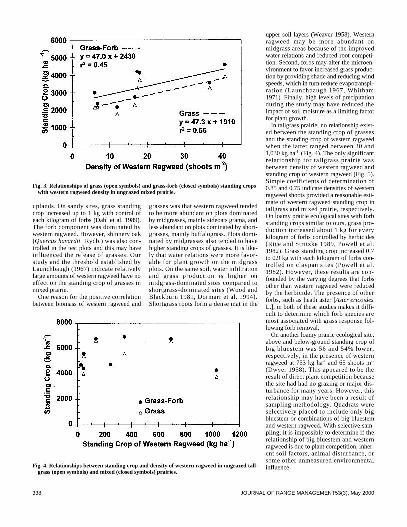
338 JOURNAL OF RANGE MANAGEMENT53(3), May 2000
uplands. On sandy sites, grass standingcrop increased up to 1 kg with control ofeach kilogram of forbs (Dahl et al. 1989).The forb component was dominated bywestern ragweed. However, shinnery oak(Quercus havardii Rydb.) was also con-trolled in the test plots and this may haveinfluenced the release of grasses. Ourstudy and the threshold established byLaunchbaugh (1967) indicate relativelylarge amounts of western ragweed have noeffect on the standing crop of grasses inmixed prairie.
One reason for the positive correlationbetween biomass of western ragweed and
grasses was that western ragweed tendedto be more abundant on plots dominatedby midgrasses, mainly sideoats grama, andless abundant on plots dominated by short-grasses, mainly buffalograss. Plots domi-nated by midgrasses also tended to havehigher standing crops of grasses. It is like-ly that water relations were more favor-able for plant growth on the midgrassplots. On the same soil, water infiltrationand grass production is higher onmidgrass-dominated sites compared toshortgrass-dominated sites (Wood andBlackburn 1981, Dormarr et al. 1994).Shortgrass roots form a dense mat in the
upper soil layers (Weaver 1958). Westernragweed may be more abundant onmidgrass areas because of the improvedwater relations and reduced root competi-tion. Second, forbs may alter the microen-vironment to favor increased grass produc-tion by providing shade and reducing windspeeds, which in turn reduce evapotranspi-ration (Launchbaugh 1967, Whitham1971). Finally, high levels of precipitationduring the study may have reduced theimpact of soil moisture as a limiting factorfor plant growth.
In tallgrass prairie, no relationship exist-ed between the standing crop of grassesand the standing crop of western ragweedwhen the latter ranged between 30 and1,030 kg ha-1 (Fig. 4). The only significantrelationship for tallgrass prairie wasbetween density of western ragweed andstanding crop of western ragweed (Fig. 5).Simple coefficients of determination of0.85 and 0.75 indicate densities of westernragweed shoots provided a reasonable esti-mate of western ragweed standing crop intallgrass and mixed prairie, respectively.On loamy prairie ecological sites with forbstanding crops similar to ours, grass pro-duction increased about 1 kg for everykilogram of forbs controlled by herbicides(Rice and Stritzke 1989, Powell et al.1982). Grass standing crop increased 0.7to 0.9 kg with each kilogram of forbs con-trolled on claypan sites (Powell et al.1982). However, these results are con-founded by the varying degrees that forbsother than western ragweed were reducedby the herbicide. The presence of otherforbs, such as heath aster [Aster ericoidesL.], in both of these studies makes it diffi-cult to determine which forb species aremost associated with grass response fol-lowing forb removal.
On another loamy prairie ecological site,above and below-ground standing crop ofbig bluestem was 56 and 54% lower,respectively, in the presence of westernragweed at 753 kg ha-1 and 65 shoots m-2
(Dwyer 1958). This appeared to be theresult of direct plant competition becausethe site had had no grazing or major dis-turbance for many years. However, thisrelationship may have been a result ofsampling methodology. Quadrats wereselectively placed to include only bigbluestem or combinations of big bluestemand western ragweed. With selective sam-pling, it is impossible to determine if therelationship of big bluestem and westernragweed is due to plant competition, inher-ent soil factors, animal disturbance, orsome other unmeasured environmentalinfluence.
Fig. 3. Relationships of grass (open symbols) and grass-forb (closed symbols) standing cropswith western ragweed density in ungrazed mixed prairie.
Fig. 4. Relationships between standing crop and density of western ragweed in ungrazed tall-grass (open symbols) and mixed (closed symbols) prairies.
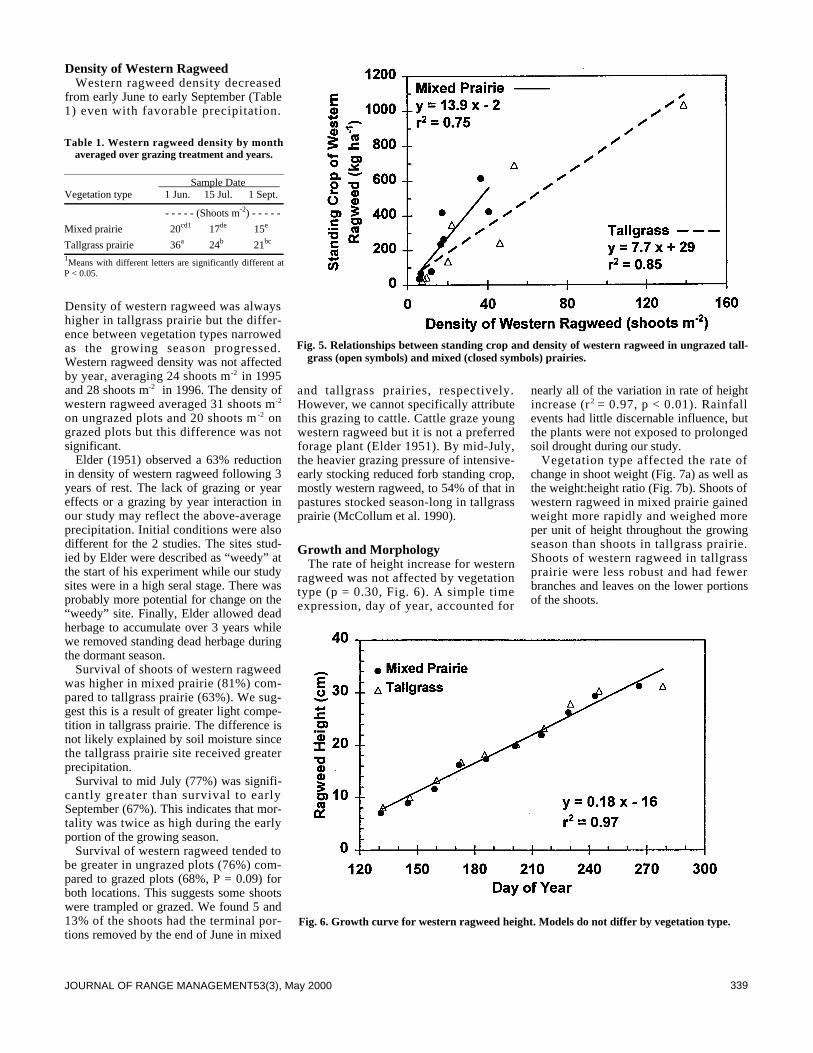
339JOURNAL OF RANGE MANAGEMENT53(3), May 2000
Density of Western Ragweed Western ragweed density decreased
from early June to early September (Table1) even with favorable precipitation.
Density of western ragweed was alwayshigher in tallgrass prairie but the differ-ence between vegetation types narrowedas the growing season progressed.Western ragweed density was not affectedby year, averaging 24 shoots m- 2 in 1995and 28 shoots m-2 in 1996. The density ofwestern ragweed averaged 31 shoots m- 2
on ungrazed plots and 20 shoots m - 2 o ngrazed plots but this difference was notsignificant.
Elder (1951) observed a 63% reductionin density of western ragweed following 3years of rest. The lack of grazing or yeareffects or a grazing by year interaction inour study may reflect the above-averageprecipitation. Initial conditions were alsodifferent for the 2 studies. The sites stud-ied by Elder were described as “weedy” atthe start of his experiment while our studysites were in a high seral stage. There wasprobably more potential for change on the“weedy” site. Finally, Elder allowed deadherbage to accumulate over 3 years whilewe removed standing dead herbage duringthe dormant season.
Survival of shoots of western ragweedwas higher in mixed prairie (81%) com-pared to tallgrass prairie (63%). We sug-gest this is a result of greater light compe-tition in tallgrass prairie. The difference isnot likely explained by soil moisture sincethe tallgrass prairie site received greaterprecipitation.
Survival to mid July (77%) was signifi-cantly greater than survival to earlySeptember (67%). This indicates that mor-tality was twice as high during the earlyportion of the growing season.
Survival of western ragweed tended tobe greater in ungrazed plots (76%) com-pared to grazed plots (68%, P = 0.09) forboth locations. This suggests some shootswere trampled or grazed. We found 5 and13% of the shoots had the terminal por-tions removed by the end of June in mixed
and tallgrass prairies, respectively.However, we cannot specifically attributethis grazing to cattle. Cattle graze youngwestern ragweed but it is not a preferredforage plant (Elder 1951). By mid-July,the heavier grazing pressure of intensive-early stocking reduced forb standing crop,mostly western ragweed, to 54% of that inpastures stocked season-long in tallgrassprairie (McCollum et al. 1990).
Growth and Morphology The rate of height increase for western
ragweed was not affected by vegetationtype (p = 0.30, Fig. 6). A simple timeexpression, day of year, accounted for
nearly all of the variation in rate of heightincrease (r 2 = 0.97, p < 0.01). Rainfallevents had little discernable influence, butthe plants were not exposed to prolongedsoil drought during our study.
Vegetation type affected the rate ofchange in shoot weight (Fig. 7a) as well asthe weight:height ratio (Fig. 7b). Shoots ofwestern ragweed in mixed prairie gainedweight more rapidly and weighed moreper unit of height throughout the growingseason than shoots in tallgrass prairie.Shoots of western ragweed in tallgrassprairie were less robust and had fewerbranches and leaves on the lower portionsof the shoots.
Table 1. Western ragweed density by monthaveraged over grazing treatment and years.
Sample Date Vegetation type 1 Jun. 15 Jul. 1 Sept.
- - - - - (Shoots m-2) - - - - -
Mixed prairie 20cd1 17de 15e
Tallgrass prairie 36a 24b 21bc
1Means with different letters are significantly different atP < 0.05.
Fig. 5. Relationships between standing crop and density of western ragweed in ungrazed tall-grass (open symbols) and mixed (closed symbols) prairies.
Fig. 6. Growth curve for western ragweed height. Models do not differ by vegetation type.

340 JOURNAL OF RANGE MANAGEMENT53(3), May 2000
Grazing also affected the morphology ofwestern ragweed shoots. Near the end ofthe grazing period, shoots of western rag-weed in grazed plots were shorter thanthose in ungrazed plots (Table 2). Shootweight was not influenced by grazingtreatment, but western ragweed shoots ingrazed plots weighed nearly twice asmuch per unit of height as those inungrazed plots. These differences wereconsistent over vegetation types. Previous
work in tallgrass prairie found that west-ern ragweed shoots were taller and lighterin ungrazed plots compared to grazedplots (Fahnestock and Knapp 1993).
Competition for light is a limiting factorfor growth of western ragweed in tallgrassprairie (Fahnestock and Knapp 1993).Competition for light is also an importantfactor in explaining the affect of vegetationtype and grazing on the morphology ofwestern ragweed shoots in this study.Plants with the least available light oftenhave elongated internodes and less branch-ing. Competition for light should be higherin tallgrass compared to mixed grassprairie and should also be higher inungrazed versus grazed sites. Our resultsare consistent with these relationships,especially with respect to the weight:heightratio. Because of greater light availabilityin areas with lower standing crops ofgrasses, robust western ragweed plants arelikely a result of, rather than the cause of,lower grass standing crop.
Management Implications
Western ragweed has long been consid-ered an aggressive competitor, but theresults of our study question this conven-tional wisdom. The density of western rag-weed decreases throughout the growingseason and shoot morphology changes asgrasses reduce the availability of light.Western ragweed’s prominence in the forbcomponent has likely led to the assump-tion that the majority of grass response toforb control is due to reduction of westernragweed.
Our study supports Launchbaugh (1967)who reported a positive relationshipbetween grass standing crop and westernragweed standing crop below 1,230 kg ha-1
in mixed prairie. An economic thresholdfor western ragweed control in mixedprairie has not been proposed, but ourresults suggest standing crops of at least600 kg ha-1 can be tolerated before controlshould be considered.
Western ragweed thrives where grassvigor has declined from grazing ordrought in tallgrass prairie (Elder 1951,Bovey et al. 1966). Shoots of western rag-weed are shorter in grazed environmentsbut have more weight per unit of height.An abundance of western ragweed in tall-grass prairie likely indicates that grassesare over-utilized. However, in such cases,high levels of western ragweed are a resultof, not a cause of, lower vigor of the grass-es. If a reduction in western ragweed isdesired, attention should first be directedtoward improved grazing management.Future research should focus on determin-ing competitive and economic thresholdsfor western ragweed in tallgrass andmixed prairies.
Literature Cited
Baumgartner, F. M., M. J. Morris, J. L.Steele, and J. E. Williams. 1952. Oklahomabobwhite food relations. Trans. North Amer.Wildl. Conf. 17:338–358.
Bovey, R. W., M. K. McCarty, and F. S.Davis. 1966. Perennial ragweed on westernNebraska rangeland. J. Range Manage.19:220–222.
Brummer, J. E., P. E. Reece, J. T. Nichols,and R. K. Engel. 1994. Western ragweedresponse to date and frequency of grazingsandhills vegetation. Soc for Range Manage.Abstracts for Ann. Meetings 47:63.
Dahl, B. E., J. C. Mosley, P. F. Cotter, andR. L. Dickerson, Jr. 1989. Winter forb con-trol for increased grass yield on sandy range-land. J. Range Manage. 42:400–403.
Table 2. Height, weight, and weight:height ratioof shoots of western ragweed at the end of thegrazing season as affected by grazing treat-ment averaged over vegetation type.
Treatment Management Grazed Ungrazed.
Height (cm) 24* 30
Weight (mg) 1,290 860
Weight:height ratio (mg cm-1) 56* 29
*Indicates means within row are significantly different atP < 0.05.
Fig. 7. Growth curves for western ragweed weight (R2 = 0.98 for system of equations) andweight:height ratio (R2 = 0.99 for system of equations). Models are significantly differentbetween vegetation types.
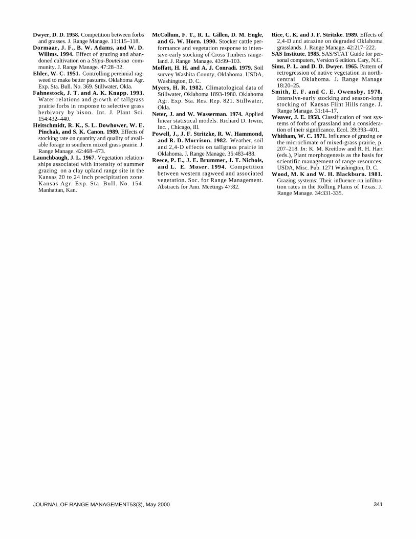
341JOURNAL OF RANGE MANAGEMENT53(3), May 2000
Dwyer, D. D. 1958. Competition between forbsand grasses. J. Range Manage. 11:115–118.
Dormaar, J. F., B. W. Adams, and W. D.Willms. 1994. Effect of grazing and aban-doned cultivation on a Stipa-Bouteloua com-munity. J. Range Manage. 47:28–32.
Elder, W. C. 1951. Controlling perennial rag-weed to make better pastures. Oklahoma Agr.Exp. Sta. Bull. No. 369. Stillwater, Okla.
Fahnestock, J. T. and A. K. Knapp. 1993.Water relations and growth of tallgrassprairie forbs in response to selective grassherbivory by bison. Int. J. Plant Sci.154:432–440.
Heitschmidt, R. K., S. L. Dowhower, W. E.Pinchak, and S. K. Canon. 1989. Effects ofstocking rate on quantity and quality of avail-able forage in southern mixed grass prairie. J.Range Manage. 42:468–473.
Launchbaugh, J. L. 1967. Vegetation relation-ships associated with intensity of summergrazing on a clay upland range site in theKansas 20 to 24 inch precipitation zone.Kansas Agr. Exp. Sta. Bull . No. 154.Manhattan, Kan.
McCollum, F. T., R. L. Gillen, D. M. Engle,and G. W. Horn. 1990. Stocker cattle per-formance and vegetation response to inten-sive-early stocking of Cross Timbers range-land. J. Range Manage. 43:99–103.
Moffatt, H. H. and A. J. Conradi. 1979. Soilsurvey Washita County, Oklahoma. USDA,Washington, D. C.
Myers, H. R. 1982. Climatological data ofStillwater, Oklahoma 1893-1980. OklahomaAgr. Exp. Sta. Res. Rep. 821. Stillwater,Okla.
Neter, J. and W. Wasserman. 1974. Appliedlinear statistical models. Richard D. Irwin,Inc. , Chicago, Ill.
Powell, J., J. F. Stritzke, R. W. Hammond,and R. D. Morrison. 1982. Weather, soiland 2,4-D effects on tallgrass prairie inOklahoma. J. Range Manage. 35:483-488.
Reece, P. E., J. E. Brummer, J. T. Nichols,and L. E. Moser. 1994. C o m p e t i t i o nbetween western ragweed and associatedvegetation. Soc. for Range Management.Abstracts for Ann. Meetings 47:82.
Rice, C. K. and J. F. Stritzke. 1989. Effects of2,4-D and atrazine on degraded Oklahomagrasslands. J. Range Manage. 42:217–222.
SAS Institute. 1985. SAS/STAT Guide for per-sonal computers, Version 6 edition. Cary, N.C.
Sims, P. L. and D. D. Dwyer. 1965. Pattern ofretrogression of native vegetation in north-central Oklahoma. J. Range Manage18:20–25.
Smith, E. F. and C. E. Owensby. 1978.Intensive-early stocking and season-longstocking of Kansas Flint Hills range. J.Range Manage. 31:14–17.
Weaver, J. E. 1958. Classification of root sys-tems of forbs of grassland and a considera-tion of their significance. Ecol. 39:393–401.
Whitham, W. C. 1971. Influence of grazing onthe microclimate of mixed-grass prairie, p.207–218. In: K. M. Kreitlow and R. H. Hart(eds.), Plant morphogenesis as the basis forscientific management of range resources.USDA, Misc. Pub. 1271 Washington, D. C.
Wood, M. K and W. H. Blackburn. 1981.Grazing systems: Their influence on infiltra-tion rates in the Rolling Plains of Texas. J.Range Manage. 34:331-335.
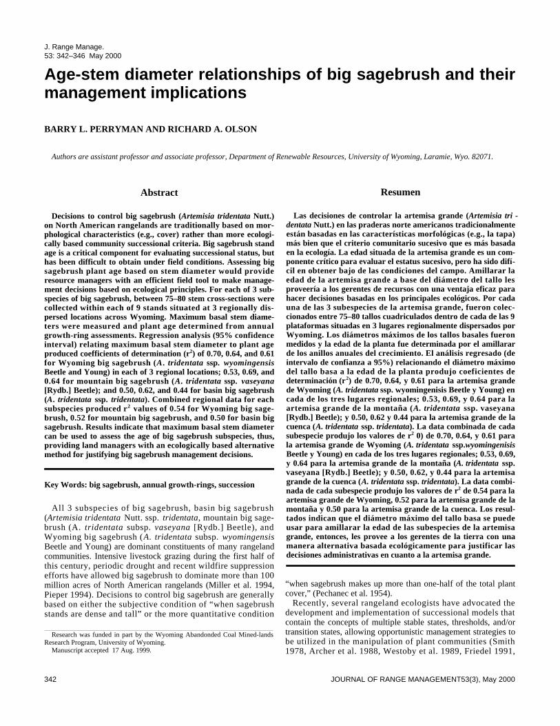
342 JOURNAL OF RANGE MANAGEMENT53(3), May 2000
Abstract
Decisions to control big sagebrush (Artemisia tridentata Nutt.)on North American rangelands are traditionally based on mor-phological characteristics (e.g., cover) rather than more ecologi-cally based community successional criteria. Big sagebrush standage is a critical component for evaluating successional status, buthas been difficult to obtain under field conditions. Assessing bigsagebrush plant age based on stem diameter would provideresource managers with an efficient field tool to make manage-ment decisions based on ecological principles. For each of 3 sub-species of big sagebrush, between 75–80 stem cross-sections werecollected within each of 9 stands situated at 3 regionally dis-persed locations across Wyoming. Maximum basal stem diame-ters were measured and plant age determined from annualgrowth-ring assessments. Regression analysis (95% confidenceinterval) relating maximum basal stem diameter to plant ageproduced coefficients of determination (r2) of 0.70, 0.64, and 0.61for Wyoming big sagebrush (A. t r i d e n t a t a ssp. w y o m i n g e n s i sBeetle and Young) in each of 3 regional locations; 0.53, 0.69, and0.64 for mountain big sagebrush (A. t r i d e n t a t a ssp. v a s e y a n a[Rydb.] Beetle); and 0.50, 0.62, and 0.44 for basin big sagebrush(A. t r i d e n t a t a ssp. t r i d e n t a t a). Combined regional data for eachsubspecies produced r2 values of 0.54 for Wyoming big sage-brush, 0.52 for mountain big sagebrush, and 0.50 for basin bigsagebrush. Results indicate that maximum basal stem diametercan be used to assess the age of big sagebrush subspecies, thus,providing land managers with an ecologically based alternativemethod for justifying big sagebrush management decisions.
Key Words: big sagebrush, annual growth-rings, succession
All 3 subspecies of big sagebrush, basin big sagebrush(Artemisia tridentata Nutt. ssp. t r i d e n t a t a, mountain big sage-brush (A. t r i d e n t a t a subsp. v a s e y a n a [Rydb.] Beetle), andWyoming big sagebrush (A. t r i d e n t a t a subsp. w y o m i n g e n s i sBeetle and Young) are dominant constituents of many rangelandcommunities. Intensive livestock grazing during the first half ofthis century, periodic drought and recent wildfire suppressionefforts have allowed big sagebrush to dominate more than 100million acres of North American rangelands (Miller et al. 1994,Pieper 1994). Decisions to control big sagebrush are generallybased on either the subjective condition of “when sagebrushstands are dense and tall” or the more quantitative condition
“when sagebrush makes up more than one-half of the total plantcover,” (Pechanec et al. 1954).
Recently, several rangeland ecologists have advocated thedevelopment and implementation of successional models thatcontain the concepts of multiple stable states, thresholds, and/ortransition states, allowing opportunistic management strategies tobe utilized in the manipulation of plant communities (Smith1978, Archer et al. 1988, Westoby et al. 1989, Friedel 1991,
J. Range Manage.53: 342–346 May 2000
Resumen
Las decisiones de controlar la artemisa grande (Artemisia tri -dentata Nutt.) en las praderas norte americanos tradicionalmenteestán basadas en las características morfológicas (e.g., la tapa)más bien que el criterio comunitario sucesivo que es más basadaen la ecología. La edad situada de la artemisa grande es un com-ponente crítico para evaluar el estatus sucesivo, pero ha sido difí-cil en obtener bajo de las condiciones del campo. Amillarar laedad de la artemisa grande a base del diámetro del tallo lesproveería a los gerentes de recursos con una ventaja eficaz parahacer decisiones basadas en los principales ecológicos. Por cadauna de las 3 subespecies de la artemisa grande, fueron colec-cionados entre 75–80 tallos cuadriculados dentro de cada de las 9plataformas situadas en 3 lugares regionalmente dispersados porWyoming. Los diámetros máximos de los tallos basales fueronmedidos y la edad de la planta fue determinada por el amillararde los anillos anuales del crecimiento. El análisis regresado (deintervalo de confianza a 95%) relacionando el diámetro máximodel tallo basa a la edad de la planta produjo coeficientes dedeterminación (r2) de 0.70, 0.64, y 0.61 para la artemisa grandede Wyoming (A. tridentata ssp. wyomingenisis Beetle y Young) encada de los tres lugares regionales; 0.53, 0.69, y 0.64 para laartemisa grande de la montaña (A. tridentata ssp. vaseyana[Rydb.] Beetle); y 0.50, 0.62 y 0.44 para la artemisa grande de lacuenca (A. tridentata ssp. tridentata). La data combinada de cadasubespecie produjo los valores de r2 0) de 0.70, 0.64, y 0.61 parala artemisa grande de Wyoming (A. tridentata ssp.wyomingenisisBeetle y Young) en cada de los tres lugares regionales; 0.53, 0.69,y 0.64 para la artemisa grande de la montaña (A. tridentata ssp.vaseyana [Rydb.] Beetle); y 0.50, 0.62, y 0.44 para la artemisagrande de la cuenca (A. tridentata ssp. tridentata). La data combi-nada de cada subespecie produjo los valores de r2 de 0.54 para laartemisa grande de Wyoming, 0.52 para la artemisa grande de lamontaña y 0.50 para la artemisa grande de la cuenca. Los resul-tados indican que el diámetro máximo del tallo basa se puedeusar para amillarar la edad de las subespecies de la artemisagrande, entonces, les provee a los gerentes de la tierra con unamanera alternativa basada ecológicamente para justificar lasdecisiones administrativas en cuanto a la artemisa grande.
Age-stem diameter relationships of big sagebrush and theirmanagement implications
BARRY L. PERRYMAN AND RICHARD A. OLSON
Authors are assistant professor and associate professor, Department of Renewable Resources, University of Wyoming, Laramie, Wyo. 82071.
Research was funded in part by the Wyoming Abandonded Coal Mined-landsResearch Program, University of Wyoming.
Manuscript accepted 17 Aug. 1999.

343JOURNAL OF RANGE MANAGEMENT53(3), May 2000
Laycock 1991, and SRM Task Group onUnity in Concepts and Terminology1995). Within these new models, the suc-cessional state of a given plant communityis usually identified in terms of recoverytime since the occurrence of some distur-bance. Fire is one important disturbanceprocess that drives successional changes ingrassland/shrubland ecosystems (Wrightand Bailey 1982). Fire suppression hasbeen practiced since European settlementin almost all areas where grassland sys-tems occur. On this basis, increased fire-return intervals have been cited as a pri-mary cause of invasion and encroachmentof fire-sensitive woody species into grass-lands (Kucera 1981, Bock and Bock 1984,Wright and Bailey 1982, Fisher et al.1987, Steinaur and Bragg 1987).
We believe that decisions to implementbig sagebrush control practices should bebased on ecological principles. A compari-son of the age of a big sagebrush stand andthe characteristic fire-return interval is anecological approach related to the succes-sional state of a given plant community.For example, if a particular stand of bigsagebrush is 50 years old and the character-istic fire-return interval is 10 years, controlpractices should be implemented irrespec-tive of the amount of big sagebrush cover.
Several investigators have used stemdiameter to quickly predict the age of indi-viduals or stands of woody plants.Hinchman and Birkeland (1995) devel-oped age-stem diameter relationships forFremont cottonwoods (Populus fremontiiS. Wats.) in Utah and Arizona, to aid indating fluvial surfaces such as channelbars in riparian environments. Brothersonet al. (1983) developed age-stem diameterrelationships for 8 tree species in theNavajo National Monument, Arizona.These species included: box elder maple(Acer negundo L.), Utah juniper (J u n i p e r u sosteosperma utahensis [Torr.] Little), piny-on pine (Pinus edulis Engelm.), Fremontcottonwood, quaking aspen (P o p u l u st r e m u l o i d e s Michx.), Douglas fir(Pseudotsuga taxifolia [Loudon] Britton),Gamble oak (Quercus gambelii Nutt.), andsalt cedar (Tamarisk ramosissima L e d e b . ) .In another study, Brotherson et al. (1984)investigated age-stem diameter relation-ships of salt cedar in central Utah to assessinvasion dynamics. Brotherson et al. (1980)also developed age-stem diameter relation-ships for 2 species of mountain mahogany(Cercocarpus montanus [Raf.] andCercocarpus ledifolius [Nutt.]) from popu-lations in Utah, Oregon, Nevada, andWyoming. In each case, investigatorsfound reasonable age-stem diameter rela-
tionships for individuals within stands.However, the regression models were notconsistent across stands or differing sitepotentials. Age-stem diameter relation-ships have not been developed for anysubspecies of big sagebrush.
Ferguson (1964) demonstrated thatannual growth-rings in big sagebrush wereeasily identified and reliable as a chrono-logic device. Given this characteristic, thepurpose of this study was to determine ifthe age of big sagebrush plants could bepredicted from maximum stem diameters.If big sagebrush plant or stand age can bequickly and accurately determined frommaximum stem diameter, land managerswill have a new method for identifyingareas that are in a stable ecological staterequiring sagebrush control. This is a moreecologically centered approach based onsuccession and fire frequency parametersrather than morphologic characteristics(e.g., cover) of big sagebrush plants.
Our specific objectives were: 1) deter-mine if an accurate age to maximum basalstem diameter relationship existed for the3 subspecies of big sagebrush; 2) deter-mine if the relationship was stand specificwithin the same geographic region; and 3)determine if the relationship was consis-tent across a larger geographic area.
Table 1. GPS coordinates and elevations for all big sagebrush stands.
Subspecies and location latitude longitude elevation (m)
wyomingensisNortheast WY 43° 34' 20.439"N 105° 10' 24.033"W 1538
43° 35' 20.184”N 104° 52' 02.262"W 138443° 28' 51.262”N 105° 03' 04.094"W 1355
Central WY 43° 08' 40.000"N 106° 34' 40.591"W 186643° 10' 02.433''N 106° 35' 46.319"W 186443° 04' 21.831''N 106° 34' 52.492"W 1899
Southwest WY 42° 52' 07.327"N 109° 57' 53.668"W 229542° 51' 41.114"N 109° 57' 21.097"W 228942° 51' 23.230"N 109° 57' 36.580"W 2359
vaseyanaSouthcentral WY 41° 42' 13.681"N 106° 34' 14.926"W 2244
41° 42' 19.279"N 106° 34' 03.639"W 224741° 42' 38.414"N 106° 33' 26.978"W 2269
Central WY 43° 55' 30.500"N 106° 45' 30.500"W 253043° 51' 15.144"N 106° 35' 45.100"W 259143° 30' 10.500"N 106° 28' 30.575"W 2743
Southwest WY 43° 00' 24.997"N 110° 00' 36.117"W 236142° 59' 26.545"N 110° 00’ 05.645"W 232342° 68' 12.283''N 110° 00' 12.478''W 2350
tridentataCentral WY 44° 59' 04.103"N 108° 15' 37.742"W 1500
44° 01' 25.918"N 108° 00' 40.873"W 127644° 02' 44.150"N 108° 04' 02.211"W 1222
Southwest WY1 42° 53' 32.871"N 110° 08' 10.433"W 223242° 47' 24.146"N 110° 01' 02.187"W 215142° 45' 13.367"N 110° 03' 39.924"W 2229
Southwest WY2 42° 47' 30.161"N 109° 57' 49.956"W 210442° 47' 57.983"N 109° 57' 48.782"W 211942° 48' 02.694"N 109° 57' 46.575"W 2108
1West slope of the Green River Basin2East slope of the Green River Basin

344 JOURNAL OF RANGE MANAGEMENT 53(3), May 2000
Methods
Big sagebrush stands having a variety ofcohorts, similar soil characteristics andtopography, and relatively free from her-bivory disturbance were selected for thisstudy. Sites were selected to minimizemicrosite effects that increase or decreasesupplemental moisture conditions. Thisapproach minimized variations in growthrates between sites (Bonham et al. 1991).
Stem sections for subspecies w y o m i n -gensis were collected from 3 stands innortheast Wyoming near Rochelle; 3stands in the South Fork of the PowderRiver watershed, northwest of Casper incentral Wyoming; and 3 stands in south-west Wyoming near Pinedale. Stem sec-tions for the subspecies t r i d e n t a t a w e r ecollected from 3 stands near Pinedale; 3stands near Worland, on the west slope ofthe Bighorn Mountains; and 3 stands nearFarson, in southwest Wyoming. Stem sec-tions for the subspecies v a s e y a n a w e r ecollected from 3 stands near Pinedale; 3stands near Buffalo, on the east slope ofthe Bighorn Mountains; and 3 stands westof Laramie, near Elk Mountain in southcentral Wyoming. The 3 stands in eachregional grouping were located within a15 mile radius. All stand locations werepermanently recorded with a GlobalPositioning System, and latitude/longitudecoordinates and elevations are listed inTable 1.
A stratified, random sampling methodwas used to collect stem cross-sectionsfrom each sagebrush stand. A permanentbaseline transect 100 m long was locatedwithin each sagebrush stand, and ten, 100m long perpendicular transects were estab-lished at randomly selected points alongthe baseline transect. Along each perpen-
dicular transect, 8 random points wereselected, and the closest individual bigsagebrush plant was selected for sampling.If the closest individual was not suitablefor aging (e.g., damaged stem), anotherrandom point was selected until a suitableindividual was encountered.
Stem cross-sections were obtained bysawing the plant off below ground level(Ferguson 1964) to ensure that the pithand first annual growth ring were includ-ed. The stem was then cut approximately10 cm from the bottom, providing a 10 cmlong stem section. Sampling was conduct-ed during the summer of 1997. Between75 and 80 stem sections were collectedfrom each stand (Cawker 1980).
In the laboratory, the bottom portion ofeach stem section was sanded sequentiallywith 60, 80, 320, and 400 grit sandingbelts. Annual growth-rings were examinedusing a 10 power stereo microscope, andenumerated once by 2 different techniciansfor a total of 2 observations per sample.
Basal stem diameters were measured atthe widest point across the face of eachcross-section. Maximum basal stem diam-eter was designated the dependent vari-able, and age the predictor variable in sim-ple linear regression analyses (Steel andTorrie 1980).
Regression models were constructed at3 geographic scales. A model was con-structed for each subspecies stand and foreach group of 3 stands within the samerelative geographic region. A comprehen-sive model for each subspecies was alsoconstructed by combining all stands of thesame subspecies to assess statewide con-sistency. All regression analyses were per-formed with the Microsoft Excel Version7.0 Statistics Module.
Results and Discussion
Annual growth rings were easily identi-fied making crossdating unnecessary.False rings have never been encounteredin big sagebrush in northern latitudes andat higher elevations (Diettert 1938, Moss1940, Ferguson 1964). Global positionand elevation of Wyoming fulfill both ofthese criteria. Locally absent rings dooccur, however complete absence of ringsare almost never encountered due to theunique nature of annual ring formation inbig sagebrush.
The annual growth-ring in big sagebrushis formed by an interxylary cork layerrather than increasing cell density bands asin most tree species. By nature, this makesthe creation of interannual bands impossi-ble. “This cork layer is produced duringthe growing season, between the newannual wood ring and that of the previousyear. With the beginning of growth in thespring a single layer of meristematic cells(the interxylary cork cambium) remainsbetween the last-formed xylem of the pre-vious year and the newly forming xylemtissue. With the onset of hot and dryweather, the innermost layer of these cellsbecomes suberized” (Ferguson 1964).
Simple linear regression of the numberof annual growth-rings against maximumbasal stem diameter yielded significantequations (p < 0.0001) for all 27 individualstands, all 9 regional stand combinations,and all 3 statewide combinations. Thecoefficient of determination for individualstands ranged from 0.22 to 0.73; 0.44 to0.70 for regional stand combinations; and0.50 to 0.54 for statewide combinations(Table 2). Ranges and means for maximumdiameter and age by subspecies are listedin Table 3. The residuals for each regres-sion model had normal distributions.
Table 2. Age prediction equations for each individual big sagebrush subspecies by regional stand locations along with coefficients of determination(r2), sample numbers (n), and p-values.
Subspecies and Location Age prediction equation r2 n p-value 95%CI
wyomingensisNortheast WY Age = 5.6910 + 0.6744(diameter) 0.70 220 0.0001 ± 0.12Central WY Age =16.6392 + 0.9404(diameter) 0.64 199 0.0001 ± 0.20Southwest WY Age = 5.4648 + 0.8514(diameter) 0.61 181 0.0001 ± 0.29
vaseyanaSouthcentral WY Age = 1.4846 + 0.6819(diameter) 0.53 211 0.0001 ± 0.18Central WY Age = 5.6688 + 0.4430(diameter) 0.69 229 0.0001 ± 0.08Southwest WY Age = 7.8955 + 0.8830(diameter) 0.64 191 0.0001 ± 0.19
tridentataCentral WY Age = 6.3189 + 0.3783(diameter) 0.50 229 0.0001 ± 0.10Southwest WY1 Age = 4.9916 + 0.3543(diameter) 0.62 223 0.0001 ± 0.07 Southwest WY2 Age = 6.1918 + 0.3020(diameter) 0.44 212 0.0001 ± 0.09
1West slope of the Green River Basin2East slope of the Green River Basin
345JOURNAL OF RANGE MANAGEMENT 53(3), May 2000
All samples including those whichseemed to be outliers were included in theanalyses. The effect of outliers is insignifi-cant considering the large sample sizesincorporated in each model. Inclusion ofpotential outliers also provides modelsthat are similar to conditions actuallyencountered in the field. A representativescatter plot for subspecies w y o m i n g e n s i sat the stand scale is shown in Fig. 1.Differences in intercept values were gen-erally small between individual stands,regional stand combinations, andstatewide combinations within the samesubspecies, and ranged from 1 to 17 years.Confidence intervals (95%) around thepopulation means ranged from + 0.10 to +0.48 for individual stands; +0.07 to +0.29for regional stand combinations; and +0.06 to + 0.14 for statewide combinations. Coefficient of determination values indi-cate that maximum stem diameter can pre-dict the age of big sagebrush plants. Therelationship was stronger for Wyomingand mountain big sagebrush than for basinbig sagebrush at the stand and regionalcombination scales. However, 2 individualstands of basin big sagebrush showed verystrong relationships (0.75 and 0.71 coeffi-cients of determination). We believe thatbecause basin big sagebrush often occurs inareas where groundwater can be relativelyshallow, some individual plants may beaccessing a reliable groundwater sourcedeep in the soil profile resulting in differen-
tial growth rates from plants not able toaccess the additional moisture. In areaswhere this additional moisture is not avail-able, the age-stem diameter relationshipappears to be similar to the other 2 sub-species.
The relationships are almost identical atthe statewide scale. At this large spatialscale, coefficient of determination valueswere 0.54 for Wyoming big sagebrush,0.52 for mountain big sagebrush, and 0.50for basin big sagebrush. This is a pre-dictable response when combining datasampled from areas that have significantvariations in precipitation timing andamount, and growing season temperaturesand lengths. Our models demonstratedefficacy at the stand and regional standcombination scales, however, inter-standvariations do exist. Our method has limita-tions similar to estimating abovegroundbiomass production with Robel et al.(1970) or other vegetation height-weightrelationship methods. An initial regressionmodel must be constructed before applica-tion to larger geographic areas. Once ini-tial baseline models are generated for anarea, maximum stem diameter measure-ments could serve as a useful tool for pre-dicting big sagebrush stand ages.
Results from this study have severalimplications for management. Based onour developed regression models, landmanagers could quickly assess the age ofbig sagebrush stands by measuring maxi-
mum basal stem diameter of the largestindividual plants in a stand. Stand agecould then be compared with fire frequen-cy information to determine if controlpractices should be implemented. This eco-logically based assessment providesstronger justification for management deci-sions. Likewise, this approach will clarifythe successional state (if stable state suc-cessional models are applicable) of any bigsagebrush stand for satisfying land usemanagement objectives in any situation.
Literature Cited
Archer, S., C.J. Scifres, and C.R. Bassham.1 9 8 8 . Autogenic succession in subtropicalsavanna: conversion of grassland to thornwoodland. Ecol. Mono., 58:111–127.
Bock, H.H. and C.E. Bock. 1984. The effectsof fire on virgin northern mixed grassland atCuster Battlefield National Monument. NPSResearch Center, Laramie, Final Report.
Bonham, C.D., T.R. Cottrell , and J.F.Mitchell. 1991. Inferences for life historystrategies of Artemisia tridentata subspecies.J. Vegetat. Sci., 2:339–344.
Brotherson, J.D., J.G. Carman, and L.A.Szyska. 1984. Stem-diameter age relation-ships of Tamarix ramosissma in CentralUtah. J. Range Manage., 37:362–364.
Brotherson, J.D., J.N. Davis, and L.Greenwood. 1980. Diameter-age relation-ships of two species of mountain mahogany.J. Range Manage., 33:367–370.
Brotherson, J.D., S.R. Rushforth, W.E.Evenson, J.R. Johansen and C. Morden.1983. Population dynamics and age relation-ships of 8 tree species in Navajo NationalMonument, Arizona. J. Range Manage.,36:250–256.
Cawker, K.B. 1980. Evidence of climatic con-trol from population age structure ofArtemisia tridentata Nutt. in southern BritishColumbia. J. Biogeogr., 7:237–248.
Diettert, R.A. 1938. The morphology ofArtemisia tridentata Nutt. Lloydia, 1:3–74.
Ferguson, C.W. 1964. Annual Rings in BigSagebrush. Papers of the Laboratory of Tree-Ring Research, No. 1. Univ. of ArizonaPress, Tuscon, Ariz. 95p.
Fisher, R.F., J.J. Jenkins, and W.F. Fisher.1 9 8 7 . Fire and the prairie-forest mosaic ofDevil’s Tower National Monument. Amer.Midl. Nat., 117:250–257.
Friedel, M.H. 1991. Range condition assess-ment and the concept of thresholds. A view-point. J. Range Manage., 44:422–426.
Hinchman, V.H. and K.W. Birkeland. 1995.Age prediction based on stem size for ripari-an cottonwood stands. The Southw. Nat.,40:406–-409.
Kucera, C.L. 1981. Grasslands and fire. I n :Fire Regimes and Ecosystem Properties.U.S.D.A. For. Serv. Gen. Tech. Rep. WO-26,594p.
Fig. 1. A representative scatter plot for subspecies wyomingensis at the individual standscale.
Table 3. Ranges and means for maximum stem diameter and age by subspecies.
Subspecies Diameter AgeMinimum Maximum Mean Minimum Maximum Mean
- - - - - - - - - - - - (mm) - - - - - - - - - - - - - - - - - - - - - - (years) - - - - - - - - - -wyomingensis 3 75 27.6 3 75 31.7vaseyana 5 82 27.3 3 79 23.4tridentata 2 145 29.5 3 54 16.0
346 JOURNAL OF RANGE MANAGEMENT53(3), May 2000
Laycock, W.A. 1991. Stable states and thresh-olds of range condition on North Americanrangelands: A viewpoint. J. Range Manage.,44:427–433.
Miller, R.F., T.J. Svejcar, and N.E. West.1994. Implications of livestock grazing in theintermountain sagebrush region: Plant com-position, pp. 101–146. I n: M. Vavra, W.A.Laycock, and R.D. Pieper (eds.), Ecologicalimplications of livestock herbivory in theWest. Society for Range Management,Denver, Colo.
Moss, E.H. 1940. Interxylary cork in Artemisiawith reference to its taxonomic significance.Amer. J. Bot., 27:762–68.
Pechanec, J.F., G. Stewart, A.P. Plummer,J.H. Robertson, and A.C. Hull Jr. 1954.Controlling sagebrush on rangelands. USDAFarmer’s Bull. No. 2072, Washington D.C.U.S. Gov. Printing Office, pp. 4-8.
Pieper, R.D. 1994. Ecological implications oflivestock grazing. pp. 177–211. I n : M.Vavra, W.A. Laycock, and R.D. Pieper(eds.), Ecological implications of livestockherbivory in the West. Soc. for RangeManagement, Denver, Colo.
Robel, R.J., J.N. Briggs, A.D. Dayton, andL.C. Hulbert. 1970. Relationships betweenvisual obstruction measurements and weightof grassland vegetation. J. Range Manage.,22:295–297.
Smith, E.L. 1978. A critical evaluation of therange condition concept. Inter. Natl.Rangeland Conf. Proc. 1st. Denver, Colo. p.266–267.
SRM Task Group on Unity in Concepts andTerminology. 1995. New concepts forassessment of rangeland condition. J. RangeManage., 48:271–283.
Steel, R.G.D. and J.H. Torrie. 1980.Principles and Procedures of Statistics: ABiometrical Approach, 2nd Ed. McGraw-Hill, New York.
Steinauer, E.M. and T.B. Bragg. 1987.Ponderosa pine (Pinus ponderosa) invasionof Nebraska Sandhills prairie. Amer. Midl.Nat., 118:358–365.
Westoby, M., B. Walker, and I. Noy-Meir.1 9 8 9 . Opportunistic management for range-lands not at equilibrium. J. Range Manage.,42:266–274.
Wright, H.A. and A.W. Bailey. 1982. F i r eEcology: United States and Canada. JohnWiley and Sons, New York.
347JOURNAL OF RANGE MANAGEMENT 53(3), May 2000
Abstract
Siberian wheatgrass [Agropyron fragile (Roth) Candargy] isknown for its establishment and persistence on sandy soils undersevere water limitations. Morphology, cytology, and forage andseed characteristics were studied on 59 accessions (JA) ofSiberian wheatgrass collected on sandy soils in the desert areas ofwestern Kazakhstan. Plants were grown at Nephi, Ut., from 1993to1996 and compared with the check cultivars of Vavilov and P-27 Siberian wheatgrass, and Nordan crested wheatgrass [A .desertorum (Fisch. ex Link) Schultes]. All JA-accessions wereautotetraploids, 2n = 4x = 28. The most frequently observed mei-otic association was 6 bivalents + 4 quadrivalents. The JA-acces-sions were morphologically diverse, ranging from short to tall instature and from dark-green, glaucous to blue-green, stronglypubescent. Mean forage yield, crude protein, and dry matterdigestibility were generally lower in the JA-accessions than thecheck varieties. Entry x year interactions were nonsignificant (P> 0.05) for all measured forage variables. Entries were signifi-cantly (P < 0.01) different for dry matter production. Seedweight of Vavilov and mean seed weight of JA-accessions weresignificantly (P < 0.01) greater than that for the check cultivarsP-27 and Nordan. Entries that were highly pubescent had theheaviest seed and greatest capacity to emerge from a 7.6-cmplanting depth. Seed yield plant- 1 was significantly (P < 0.01)lower in the JA-accessions than cultivars Vavilov, P-27, andNordan. Sufficient variations exist for seed yield, seed weight,seedling vigor, and forage yield within the JA-accessions to allowfor the development of an agronomically suitable, drought toler-ant Siberian wheatgrass through selection.
Key Words: Crested wheatgrass, morphology, meiosis, chromo-some pairing, taxonomy, forage and seed characteristics
The Siberian form of crested wheatgrass [Agropyron fragile(Roth) Candargy] is an important forage grass with a natural dis-tribution in the Steppe regions of European Russia and south-western Siberia. In its native habitat, the Siberian form of crestedwheatgrass is more drought tolerant than either standard (cvNordan) or fairway types of crested wheatgrass [A. d e s e r t o r u m(Fisch. ex Link) Schultes and A. cristatum (L.) Gaertner, respec-tively] and is better adapted to sandy soils that receive only 200to 450 mm of annual precipitation (Asay et al. 1995). There areonly 2 cultivars of Siberian wheatgrass, Vavilov and P-27. Bothcultivars are adapted to similar environments, however, on sandy
soils Vavilov out yields P-27 and has increased seedling vigor(Asay et al. 1995).
Under the current taxonomic treatment (Dewey 1984, Love1984), the genus Agropyron is restricted to 10 species, commonlyreferred to as the crested wheatgrass complex. Agropyron fragileis synonymous with the more traditional name, A. s i b i r i c u m(Willd.) P. Beauv. Tzvelev (1976) described 2 botanical varietieswithin A. f r a g i l e : (1) var. f r a g i l e (plants with pubescent leafsheaths) and (2) var. sibiricum (plants with glabrous leaf sheaths).Siberian wheatgrass is characterized by long, linear spikes.Most narrow-spiked crested wheatgrasses introduced to NorthAmerica, including the cultivars P-27 and Vavilov, have glabrousleaf sheaths and fall under A. fragile var. sibircum.
J. Range Manage.53: 347–352 May 2000
Characterization of Siberian wheatgrass germplasm fromKazakhstan (Poaceae: Triticeae)
KEVIN B. JENSEN, KAY H. ASAY, DOUGLAS A. JOHNSON, AND BAO JUN LI
Authors are research geneticists and plant physiologist, USDA-ARS Forage and Range Research Laboratory, Utah State University, Logan, Ut. 84322-6300;and assistant director, Grassland Research Institute, Xinjiang Academy of Animal Science, Urumqi, Xinjiang, People’s Republic of China, 830000.
Contribution of Utah Agr. Exp. Sta., Journal Paper 4880.Manuscript accepted 6 Sep. 1999.
Resumen
El zacate "Siberian wheatgrass" [Agropyron fragile ( R o t h )Candagry] es conocido por su establecimiento y persistencia ensuelos arenosos bajo severas limitaciones de agua. Se estudio lamorfología, citología y características del forraje y semilla de 59accesiones (JA) de "Siberian wheatgrass" obtenidas de suelosarenosos de las áreas desérticas del oeste de Kazakhstan. Lasplantas se cultivaron en Nephi, Ut de 1993 a 1996 y se compara-ron con los cultivares testigo Vavilov y P-27 de "Siberian wheat-grass" y Nordan de "Crested wheatgrass" [A. desewrtorum(Fisch. Ex. Link) Schultes]. Todas las accesiones de JA fueronautotetraploides, 2n = 4x = 28. La asociación meiótica mas fre-cuentemente observada fue 6 bivalentes + 4 cuadrivalentes. Lasaccesiones de JA fueron morfológicamente diversas, la estaturavario de corta a alta y de verde obscuro, glaucoso a azul-verde ymuy pubescente. Las medias de rendimiento de forraje, proteínacruda y digestibilidad de la materia seca fueron generalmentemas bajas que las de los cultivares testigo. Las interaccionesaccesión x año no fueron significativas (P > 0.05) para ningunade las variables de forraje que se evaluaron. Las accesionesfueron significativamente (P < 0.01) diferentes en producción deforraje. El peso de la semilla de Vavilov y la media de peso desemilla para las accesiones de JA fueron significativamente (P <0.01) mayores que la de los cultivares testigo P-27 y Nordan. Lascolectas muy pubescentes tuvieron la semilla mas pesada y lamayor capacidad de emerger cuando se sembraron a una pro-fundidad de 7.5 cm. El rendimiento de semilla por planta de lasaccesiones de JA fue significativamente (P < 0.01) menor que elde los cultivares Vavilov, P-27 y Nordan. Entre las colectas de JAexisten suficientes variaciones respecto al rendimiento de semilla,peso de semilla, vigor de plántula y rendimiento de forraje lo quepermite, mediante selección, el desarrollo de un cultivar del"Siberian wheatgrass" tolerante a sequía y agronómicamenteadecuada.

348 JOURNAL OF RANGE MANAGEMENT 53(3), May 2000
Fifty-nine accessions of Siberian wheat-grass recently obtained from westernKazakhstan (JA-accessions) were com-pared with Siberian wheatgrass cultivarsP-27 and Vavilov, and the crested wheat-grass cultivar Nordan. Objectives were todetermine: (1) the morphological variationand taxonomic placement among theaccessions, (2) the chromosome numberand pairing within the accessions, and (3)the potential of these accessions toimprove seedling vigor, productivity, andforage quality in a breeding program ofSiberian wheatgrass growing under dryconditions.
Materials and Methods
Plant materialsFifty-nine accessions of narrow-spiked
Siberian wheatgrasses from Kazakhstanwere obtained in 1992 by Drs. D. A.Johnson and K. H. Asay (JA-accessions).The 59-accessions where collected fromdesert areas of Kazakhstan that receivebetween 100 to 300 mm of annual precipi-tation. Check cultivars included Siberianwheatgrass P-27 and Vavilov, along withNordan crested wheatgrass.
Field plot designField plots were located 121 km south
of Salt Lake City, Ut., at the Utah StateUniversity Nephi Field Station at an eleva-tion of 1,615 m. The soil type is Nephi siltloam (fine-silty, mixed, mesic Calcic
Argixerolls). No supplemental irrigationwas used. Long-term (1903 to 1996) annu-al precipitation is 324 mm with about one-third occurring in March, April, and May.Total precipitation received from Octoberthrough September was 486 and 249 mmfor 1995 and 1996, respectively. Seedlingsfrom original seed lots of JA-accessionswere established in the greenhouse prior totransplanting in the field on 12 April 1993.Each field plot (1 x 10 m) consisted of 10plants, planted on 1-m centers. Field plotdesign was a randomized complete blockwith 4 replicates.
MorphologyEighteen morphological characters were
evaluated (Table 1) on 58 of the 59 JA-accessions plus the cultivars Vavilov, P-27, and Nordan. A total of 10 to 12 opera-tional taxonomic units (1 operational taxo-nomic unit = 1 complete, mature, flower-ing culm, with intact leaves and inflores-cence) were collected from each of the 58JA-accessions and check cultivars acrossreplicates. Leaf measurements were takenon the first leaf below the flag leaf.Spikelet and flower part measurementswere taken from spikelets collected midspike. During data collection of opera-tional taxonomic units, JA-85 was inad-vertently not included. Operational taxo-nomic units were measured between 5 to9 June 1995 at Nephi, Ut. Multivariateanalysis of the data was conducted on 700operational taxonomic units comprised of58 JA-accessions, (10 to 12 operational
taxonomic units per accession; 664 totaloperational taxonomic units), and cultivarsVavilov, P-27, and Nordan (1 populationand 12 operational taxonomic units percultivar). Data for the characters listed inTable 1 were standardized according tothe Standard Program on NT-SYS (Rohlf1993). All principal components werederived using correlation matrices.Principal component analysis explains thevariation observed between and withinpopulations by creating linear combina-tions and character weights from the orig-inal variables. All cluster analyses wereperformed using unweighted pair-groupmathematical average algorithms on thedistance matrices to provide a distancephenogram. The distance coefficient wasdefined as the average taxonomic distancecomputed by NT-SYS (Rohlf 1993).
Mitotic analysisSomatic cells of the 59 JA-accessions
were prepared from root tips of pottedseedlings grown from original seeds col-lected in Kaskhstan in a greenhouse. Roottips were treated in an aqueous solutioncontaining 0.05% colchicine plus 0.025%8-hydroxyquinoline and 25 drops 100 ml-1
of dimethylsulfoxide (DMSO) for 2 to 3hours at room temperature in darkness.They were then fixed and stained in 2%aceto-orcein at 40°C for a minimum of 3days. The meristematic portion of the roottip was squashed in 45% acetic acid.
Table 1. Morphological characters in Siberian wheatgrass accessions (JA) from Kazakhstan, Siberian wheatgrass cultivars Vavilov, and P-27, and thecrested wheatgrass cultivar Nordan.
Species/Cultivar JA1 Vavilov2 P-272 Nordan2
Character Mean SD Range Mean SD Mean SD Mean SD LSD
Plant height (cm) 58.2 10.2 43.3-72.3 65.7 5.5 64.5 4.9 61.8 5.6 7.0Leaf length (cm) 12.2 3.6 9.1-17.1 15.0 4.8 16.1 3.3 13.0 3.7 2.5Leaf width (mm) 5.9 1.2 5.0-7.7 5.8 0.9 6.1 1.1 7.7 2.4 0.9Spike length (cm) 13.0 2.2 7.6-13.8 10.7 1.5 10.4 2.0 5.9 0.8 1.6Spike width (mm) 6.3 1.5 4.9-7.9 9.1 2.5 8.1 1.3 13.0 2.9 1.1Spike Length/width (cm/cm) 18.5 6.1 7.0-41.2 12.9 5.4 13.2 3.4 4.9 1.5 4.2Spikelet length (mm) 12.9 2.3 11.1-16.8 10.4 2.0 11.1 1.4 7.5 1.6 1.7Spikelet width (mm) 4.1 0.7 3.7-4.9 4.7 1.1 4.3 0.6 3.7 0.6 0.5First glume length (mm) 6.4 1.2 5.3-7.6 8.0 1.6 6.5 1.0 5.3 1.3 0.9
Width (mm) 1.1 0.2 1.0-1.3 1.0 0.2 1.1 0.1 0.6 0.2 0.1Awn length(mm) 1.5 0.9 0.3-2.6 3.1 1.5 2.2 0.7 2.0 0.8 0.6
Second glume length (mm) 6.8 1.3 5.6-8.0 8.1 1.7 6.6 1.1 5.6 0.9 0.9Width (mm) 1.2 0.2 1.1-1.4 1.0 0.2 1.1 0.2 0.8 0.3 0.2Awn length (mm) 1.6 1.0 0.2-2.8 2.9 1.6 1.8 1.1 2.2 0.7 0.7
First lemma length (mm) 7.5 1.2 6.2-9.1 8.5 1.9 7.0 1.0 7.4 0.9 0.9Width (mm) 1.3 0.2 1.1-1.4 1.1 0.1 1.2 0.2 0.9 0.1 0.4Awn length (mm) 1.0 1.0 0.0-2.4 1.5 1.4 0.7 0.8 2.2 0.6 0.7
Palea length (mm) 5.8 0.6 5.3-6.3 6.1 1.0 5.6 0.3 4.5 0.6 0.4 1Mean based on between 628 to 664 operational taxonomic units.2Mean based on 12 operational taxonomic units.

349JOURNAL OF RANGE MANAGEMENT 53(3), May 2000
Meiotic analysisPollen mother cells from 6 randomly
selected accessions were preserved inCarnoy’s fixative (6 parts absolute alcohol:3 parts chloroform : 1 part glacial aceticacid) for 24 to 48 hours, transferred to 70%ethanol, and stored in a refrigerator untilanalyzed. Squashed preparations of thepollen mother cells were stained with 2%acetocarmine. Chromosome pairing wasanalyzed at metaphase I.
Seed characteristicsSeed yield and 100-seed weight were
obtained in 1995 and 1996 from open-pol-linated JA-accessions and checks at Nephi,Ut. The first 5 plants in each plot were har-vested for seed yield and 100-seed weight.Seedling vigor on open pollinated seedproduced in 1995 and 1996 was assessedbased on the ability of the seedling toemerge from a 7.6-cm seeding depth (Asayand Johnson 1980) and measured by therate of emergence (Maguire 1962).
Forage characteristicsFollowing several years of establishment
in 1993, the plants were harvested 1 to 2weeks post-anthesis with a sickle-barmower from the remaining 5 plants in the10-plant plot on 20 and 21 June 1995 and18 June 1996. Dry matter production (kgp l o t- 1) were measured on a subsample fromeach plot. Subsamples were dried at 60°Cin a forced-draft oven, and then firstground by a Wiley mill and then a Cyclonemill to pass through a 1-mm screen. Drymatter digestibility and crude protein weredetermined by near-infrared-reflectancespectroscopy on a dry matter basis accord-ing to procedures described by Marten etal. (1989). Validation of the calibrationequation within the NIRS (R2 = 0.93) forcrested and Siberian wheatgrass wasreported in Mayland et al. (1992).
Data analysisData were analyzed across years as a
split-plot-in-time design with a general lin-ear model (SAS 1985) using plot means.Single degree of freedom contrasts testedthe overall mean for the JA-accessionswith the check cultivars for forage yield,quality, and seed characteristics. For thecombined analysis, entry x block was usedas the error term to test entry effects, andyear effects were tested with year x blockinteraction. Due to a significant (P < 0.01)year x entry interaction for total seed yield,data were also analyzed within years. Aprotected LSD test was used to separateentry means within and across years.
Results and Discussion
Morphology It appears that genetic introgression has
occurred between Siberian and standardforms in nature. This introgression is evi-dent in the Siberian cultivars, P-27(Alderson and Sharp 1994) and Vavilov(Asay et al. 1995) (Fig. 1), by the morpho-logical cline that exists between the long,narrow spike of Siberian wheatgrass andthe shorter, wider spike of standard formsof crested wheatgrass.
Based on the 18 characters (Table 1),principal components of all operationaltaxonomic units accounted for 82% of thevariation in the first 4 axes (data notshown). Within the first principal compo-nent, 6 of the 18 morphological characterswere weighted greater than 0.80. Thecharacters and their weights were: spike
length (0.82), spike length/spike width(0.81), first glume awn length (0.93), sec-ond glume awn length (0.95), lemmalength (0.92), and lemma awn length(0.95). The first component accounted for40% of the variation observed. The secondand third components accounted for 32%of the variation, but were much less diag-nostic with no characters weighted morethan 0.80. Cluster analysis had acophenentic correlation of 0.88, which isconsidered a good fit (Rohlf 1993).
Examination of the 1 s t, 2 n d , and 3 r d
principal components suggests a clear sep-aration among the JA- accessions and thecheck cultivars P-27, Vavilov, and Nordan(data not shown). In most cases, theglumes and lemma awns were longer inthe check cultivars than in the JA-collec-tions (Table 1). The narrow-shaped (lin-ear) spike compared to the broad (pecti-nate) spike was the most discriminating
Fig. 1. Spike morphology of Standard crested wheatgrass ‘Nordan’ (A), Siberian wheatgrass JA-accessions (B), Siberian wheatgrass ‘Vavilov’ (C), and Siberian wheatgrass ‘P-27' (D).
Table 2. Chromosome pairing in selected (JA) accessions of Siberian wheatgrass and related crest-ed wheatgrasses
Chromosome associations (No. cell-1) No.Chromosome I II II IV+ cells
Species No. (2n) Ring Rod Total
A. fragileJA-accessions 28 0.27 1 6.04 1.08 7.17 0.17 3.14 ---
0-3 2 3-11 0-5 3-12 0-2 0-5 50A. desertorum 28 2.06 4.13 4.84 8.97 0.62 1.62 ---(Asay et al. 1992) 0-6 0-8 0-9 4-14 0-3 0-5 628A. cristatum X 28 0.97 9.85 0.63 1.66 ---A. desertorum ('Hycrest') 0-7 --- --- 4-15 0-4 0-4 155(Asay et al. 1986)
1Configuration mean number of chromosomes.2Configuration range of number of chromosomes.

350 JOURNAL OF RANGE MANAGEMENT53(3), May 2000
morphological character (Fig. 1). This isconsistent with Tzvelev (1976) who distin-guished between the broad-shaped spikeof crested wheatgrass types [A. c r i s t a t u mand A. desertorum] and the narrow-shapedspike types of Siberian wheatgrass [A.f r a g i l e and A. m o n g o l i c u m] based on thelength and width of the spike. The ratio ofspike length/width proved highly diagnos-tic when separating the Siberian wheat-grass collections from the standard crestedwheatgrass cultivar Nordan (Fig. 1, Table1). The spike shape for Nordan is typicallymore pectinate at the base than is Siberianwheatgrass as evidenced by the spikelength/width ratio ranging from 3.2 to 8.2for Nordan compared to 7.0 to 41.3 in theJA-accessions. This relationship wasobserved by Asay et al. (1992), who foundthat spike length/width ratio within A.m o n g o l i c u m (a diploid Siberian wheat-grass) was 12.0 compared to 3.6 and 6.0for A . c r i s t a t u m and A . d e s e r t o r u m ,respectively. This ratio was less definitivein separating the JA-accessions from P-27and Vavilov. However, the average spikelength/width ratio within the JA-acces-sions was 18.5 compared to 12.9 forVavilov and 13.2 for P-27. The spikelength/width ratio ranged from 7.8 to 24.9for Vavilov and 9.7 to 21.6 for P-27.These data suggest that during the devel-opment of Siberian wheatgrass cultivars P-27 (Alderson and Sharp 1994) andVavilov (Asay et al. 1995), genetic intro-gression occurred between the broad-spiked types (probably A. desertorum) andnarrow-spiked types.
JA-accessions 48, 49, 52, 58, 84, and 85had a blue-green leaf color and denselypubescent (pilose) leaves, leaf sheaths, andspikes, which corresponds to Tzvelev’s(1976) description of A. fragile var. f r a g i l e.All other JA-accessions had green leaf colorin varying shades and glabrous leaves, leafs h e a ths, and spikes. These latter accessionswould be classified as A. f r a g i l e var. s i b i r -i c u m according to Tzvelev (1976). Plantgrowth habit within the population rangedfrom strongly caespitose to moderately rhi-zomatous in JA-66.
CytologyThe crested wheatgrasses occur in an
autoploid series of diploid (2n = 2x = 14),tetraploid (2n = 4x = 28), and hexaploid( 2n = 6x = 42) species with tetraploidsoccuring most frequently (Dewey andAsay 1975). Hybridization among the var-ious crested wheatgrass taxa across allploidy levels supports the premise that thiscomplex is based on the ‘P’ genome (Asayand Dewey 1979), and should be treated
as one gene pool (Asay and Dewey 1983).Root tip chromosomes of all 59 JA-
accessions were tetraploids with a chro-mosome number of 2n = 4x = 28. The 6randomly selected JA-accessions did notdiffer in pairing behavior. Thus, the pair-ing data were bulked across accessions(Table 2). The most common associationswere 6 bivalents + 4 quadrivalents or 8bivalents + 3 quadrivalents (Fig. 2a),which occurred in 25 and 23% of themetaphase I cells observed, respectively.Multivalents, usually quadrivalents (Fig.
2bc), formed in more than 70% of themetaphase-I cells. Average chromosomeassociations per cell were 0.27 univalents+ 7.17 bivalents + 0.17 trivalents + 3.14quadrivalents-plus (Table 2). These valuesare similar to those reported for otherautotetraploid crested wheatgrasses(Dewey 1984, Asay et al. 1992). The highfrequency of quadrivalents is also consis-tent with previous reports (Asay andDewey 1979) that indicate that crestedwheatgrasses and now Siberian wheat-grass are true autotetraploids.
Fig. 2. Chromosome pairing at late diakinesis early metaphase I in Siberian wheatgrass (JA-acces-sions): (a) 8 II (small arrows) + 3 IV, (b) 2 II + 4 IV (small arrows) + 1 VIII (large arrows), and(c) 4 II (large arrows) + 5 IV (small arrows).
Table 3. Mean squares from analysis of variance for JA-accessions of Siberian Wheatgrass fromKazakhstan, 'Vavilov' and 'P-27' Siberian wheatgrass, and 'Nordan' crested wheatgrass for for-age production and quality and seed characteristics.
Character Entry Year Entry x Year
Seed yield (g plant-1)1995 1651.2**11996 234.6**1995-96 976.0** 15646.8** 756.5**100-seed weight (g)1995 0.014**1996 0.011**1995-96 0.025** 0.127** 0.00
Rate of emergence (seedlings day-1)1995 0.4941996 0.745**1995-96 0.552** 0.402 0.358
Dry matter production (kg ha-1)1995 7308268.6**1996 1691761.4**1995-96 7750158.2** 19527354.7** 1251452.9Crude protein (g kg-1)1995 86.31996 180.01995-96 88.7 69867.3** 17.9
Dry matter digestibility (g kg-1)1995 361.51996 169.41995-96 22.8 809028.5** 508.21 *, ** indicate significant differences at P < 0.05 and P < 0.01, respectively.

351JOURNAL OF RANGE MANAGEMENT53(3), May 2000
Based on chromosome pairing inhybrids between the narrow spikeddiploid, A . m o n g o l i c u m Keng fromMongolia, and the broad spiked diploid, A.cristatum from Eurasia, Dewey (1984) andAsay et al. (1992) concluded that bothgroups are comprised of the same basicgenome “P”. Most if not all A. m o n -g o l i c u m accessions are diploids andappear to be a smaller strain of thetetraploid Siberian wheatgrass (Dewey1984, Asay et al. 1992)
Seed characteristicsThe entry x year interaction was not sig-
nificant (P > 0.05) for 100-seed weightand rate of seedling emergence; however,it was significant (P < 0.01) for total seedyield plant- 1 (Table 3). This significancewas due to a rank change between culti-vars P-27 and Vavilov and JA-accessionsfrom 1995 to 1996. The overall 100-seedweight declined with reduced annual pre-cipitation received during 1996, whichwas 77% of normal compared to 150% ofnormal in 1995. However, the ability ofseedlings to rapidly emerge from a 7.6-cmdepth was not affected by the differentlevels of annual precipitation between1995 and 1996 (Table 4).
The Siberian wheatgrass cultivars P-27and Vavilov produced significantly moreseed than the JA-accessions and the crestedwheatgrass cultivar Nordan (Table 4).However, within the entire JA-collection,individual accessions (JA-96, 42, 95, 80,and 42) were not significantly (P > 0.05)different from the Siberian wheatgrasschecks (data not shown), suggesting that
sufficient variations exist within the JA-accessions for improvement in seed pro-duction.
The cultivar Vavilov and the mean of theJA-accessions had significantly (P < 0.01)heavier seeds (100-seed weight) than P-27and Nordan (Table 4). Within Siberianwheatgrass, no correlation (r = 0.03) wasapparent between seed yield plant - 1 a n dindividual seed weight (data not shown).Accessions JA-48, 46, 51, 98, 47, 50, and49 had heavier seeds than Vavilov.Morphologically, densely pubescent plantsproduced heavier seeds. Differences inseed weight were reflected in results from
seedling vigor trials. Of the 10 accessionswith the heaviest seeds, 6 had higher ratesof emergence (JA-48, 45, 98, 46, 51, and47). During the 1996 drought, JA-acces-sions 42, 43, 96, 75, and 95 exceeded thecheck cultivars with a total seed yieldgreater than 16 g plant- 1, suggesting thatunder harsh environments with limitedwater, total seed yield can be improvedthrough selection within the JA-accessions.
Forage characteristicsEntries differed significantly (P < 0.01)
for dry matter production between the JA-
Table 5. Means and ranges for dry matter production, crude protein, and dry matter digestibilityfor 59 JA-accessions of Siberian wheatgrass (SWG) from Kazakhstan, 'Vavilov' and 'P-27Siberian wheatgrass (SWG), and 'Nordan' crested wheatgrass (CWG). Data were combinedacross years.
Entry Dry matter production Crude protein Dry matter digestibility
(kg ha-1) (g kg-1) (g kg-1)
JA - SWGMean 1362 115.6 569.2Range 869-1823 104.8-126.7 536-583.2
Vavilov - SWGMean 2539 111.6 570.5
P-27 - SWGMean 2130 111.4 568.9
Nordan - CWGMean 2400 115.5 571.8
LSD 522 17.2 27Contrasts:
JA- vs. Vavilov **1 nsns
JA- vs. P-27 ** ns ns
JA- vs. Nordan ** ns ns1*, ** indicate significant differences at P ≤ 0.05 and P ≤ 0.01, respectively.
Table 4. Means and ranges for total seed yield, 100-seed weight, and rate of seedling emergence for 59 JA-accessions of Siberian wheatgrass (SWG)from Kazakhstan, 'Vavilov' and 'P-27' Siberian wheatgrass (SWG), and 'Nordan' crested wheatgrass (CWG).
Seed yield 100-Seed weight Rate of emergence Entry 1995 1996 1995-96 1995 1996 1995-96 1995 1996 1995-96
- - - - - - - - - - (g plant-1) - - - - - - - - - - - - - - - - - - - - - - - - (g) - - - - - - - - - - - - - - - - - - - - - - - - (seedlings day-1)- - - - - - - - - -JA - SWG
Mean 22.25 11.87 17.04 0.25 0.21 0.23 0.32 0.75 0.54 Range 8.3-37.4 5.2-20.0 7.8-26.8 0.21-0.31 0.18-0.26 0.19-0.27 0.03-1.1 0.23-1.7 0.14-1.12
Vavilov - SWGMean 48.30 12.19 30.24 0.26 0.25 0.25 0.37 0.89 0.63
P-27 - SWGMean 49.72 14.36 30.54 0.22 0.19 0.20 0.63 0.58 0.61
Nordan - CWGMean 21.09 4.61 12.85 0.15 0.13 0.14 0.16 0.03 0.10
LSD 17.5 6.15 8.83 0.04 0.04 0.03 0.45 0.48 0.25
Contrasts:
JA- vs. Vavilov **1 __ ** __ * * __ __ __
JA- vs. P-27 ** __ ** __ __ * __ __ __
JA- vs. Nordan __ ** __ ** ** ** __ ** **1*, ** indicate significant differences at P ≤ 0.05 and P ≤ 0.01, respectively.
352 JOURNAL OF RANGE MANAGEMENT53(3), May 2000
accessions and checks; however, differ-ences were relatively consistent acrossyears as indicated by the nonsignificantentry x year interaction (Table 3). Themean dry matter production for the 59 JA-accessions was significantly (P < 0.01)lower than Vavilov, P-27, and Nordanchecks. None of the individual JA-acces-sions had greater dry matter productionthan the checks. The mean range of drymatter production among the JA-acces-sions averaged across years, 869 to 1,823kg ha -1 (Table 5), indicated that substantialvariation was available to select for genet-ic improvement in this trait. Because ofthe difference in annual precipitationbetween 1995 (486 mm) and 1996 (249mm), a significant (P < 0.01) year effectwas observed for dry matter production(Table 3).
Differences between the JA-accessionsand check cultivars were nonsignificant (P> 0.05) for crude protein and dry matterdigestibility (Tables 3 and 5). The entry xyear interaction was also nonsignificant (P> 0.05). Similar to dry matter production,crude protein and dry matter digestibilityvaried significantly between years (P <0.01), possibly a result of the large varia-tion in annual precipitation between 1995and 1996.
Mean dry matter production increased inthe JA-accessions and the check cultivarP-27 in 1996 under dry conditions. Eventhough dry matter production within theJA-accessions was still significantly (P <0.05) lower than the check cultivars, theirability to produce more, rather than less,forage and seeds under drought suggeststhat they may be better adapted and subse-quently survive longer in extreme environ-ments. In their native environment ofwestern Kazakhstan, the smaller staturedSiberian wheatgrass accessions occupysandy soils that receive between 100 to300 mm of annual precipitation per year,while A. cristatum and A. desertorum a r etypically found in regions of higher rain-fall and better soils.
Conclusions and Implications
Morphological analysis suggests that, atpresent, no Siberian wheatgrass cultivarsare available with true narrow-shapedspikes. Based on spike shape, cultivars P-27 and Vavilov appear to have gene(s)from the broader-shaped (more pectinate)spike, which is characteristic of A. crista -tum and A. desertorum. Cytologically, theJA-accessions have the same chromosomenumber (2n = 4x = 28) and behave cyto-logically as true autotetraploids.
When developing new cultivars that arecapable of establishing and persistingunder environments with very low rainfall,characters such as seedling vigor and per-sistence are more important than forageyield and quality. Our results suggest thatthere are sufficient variations for seedyield, seed weight, seedling vigor, and for-age yield within the JA-accessions ofSiberian wheatgrass germplasm to allowfor the development of an agronomicallysuitable, drought-tolerant Siberian wheat-grass through breeding and selection.Variations in forage quality were muchless than that observed for other traits sothat prospects for improving forage qualityare considerably less.
Literature Cited
Alderson, J. and W.C. Sharp. 1994. G r a s svarieties in the United States. USDA Agr.Handb. 170. U.S. Government PrintingOffice, Washington, D.C.
Asay, K.H. and D.R. Dewey. 1979. B r i d g i n gploidy differences in crested wheatgrass withhexaploid x diploid hybrids. Crop Sci.19:519–523.
Asay, K.H. and D.R. Dewey. 1983. P o o l i n gthe genetic resources of the crested wheat-grass species-complex, p. 124–127. I n: J.A.Smith and V.W. Hays (eds.), Proc. Int.Grassl. Congr., Lexington, Ky.
Asay, K.H. and D.A. Johnson. 1980.Screening for improved stand establishmentin Russian wild ryegrass. Can. J. Plant Sci.60:1171–1177.
Asay, K. H., K. B. Jensen, C. Hsiao, and D.R. Dewey. 1992. Probable origin of standardcrested wheatgrass, Agropyron desertorum(Fisch. ex Link) Schultes. Can. J. Plant Sci.72:763–772.
Asay, K. H., D. R. Dewey, F. B. Gomm, W.H. Horton, and K. B. Jensen. 1986. Geneticprogress through hybridization of inducedand natural tetraploids in crested wheatgrass.J. Range Manage. 39:261–263.
Asay, K.H., D.A. Johnson, K.B. Jensen, N.J.Chatterton, W.H. Horton, W.T. Hansen,and S.A. Young. 1995. Registration of“Vavilov” Siberian crested wheatgrass. CropSci. 35:1510.
Dewey, D.R. 1984. The genomic system ofclassification as a guide to intergenerichybridization with the perennial Triticeae, p.209-279. I n : J.P. Gustafson (ed.), Genemanipulation in plant improvement. Proc.16th Stadler Genet. Symposium, Columbia,Mo. Plenum, New York.
Dewey, D.R. and K.H. Asay. 1975. The crest-ed wheatgrasses of Iran. Crop Sci. 15:844-849.
Love, A.A. 1984. Conspectus of the Triticeae.Feddes Repertorum 95:425–521.
Maguire, J.D. 1962. Speed of germination -aid in selection and evaluation for seedlingemergence and vigor. Crop Sci. 2:176–177.
Marten, G.C., J.S. Shenk, and F.E. BartonII. 1989. Near infrared reflectance spec-troscopy (NIRS): Analysis of forage quality.ARS Agr. Handb. 643, U.S. GovernmentPrinting Office, Washington, D.C.
Mayland, H.F., K.H. Asay, and D.H. Clark.1992. Seasonal trends in herbage yield andquality of Agropyrons. J. Range Manage.45:369–374.
Rohlf, E.J. 1993. NT-SYS numerical taxonom-ic system of multivariate statistical programs.State Univ. of New York at Stony Brook,N.Y.
[SAS] Statistical Analysis System Institute,Inc. 1985. The GLM procedure, p. 433-506.I n: SAS user’s guide: Statistics, Version 5Edition, SAS Insitute, Inc., Cary, N.C.
Tzvelev, N.N. 1976. Tribe 3. Triticeae Dum, p.1 0 5 - 2 0 6 . I n: A.A. Fedorov (ed.), PoaceaeURSS. Nauka Publ. House, Leningrad,USSR.
353JOURNAL OF RANGE MANAGEMENT53(3), May 2000
Abstract
Crested wheatgrass (Agropyron cristatum (L.) Gaertn.) is anintroduced grass used extensively for rangeland revegetation inthe semiarid and arid regions of western North America. Thelong-term effects of crested wheatgrass on soil properties andplant community were evaluated on 5 grazed sites in the south-ern interior of British Columbia, Canada. Each site includedplant communities of native bluebunch wheatgrass(Pseudoroegneria spicata (Pursh) Scribn. & Smith) and 14- to 60-year-old stands of crested wheatgrass. Soil samples and plantdata were collected in June 1997. Species numbers were similarfor native and crested wheatgrass rangelands, while the diversityindex of crested wheatgrass rangeland was lower due to lowerevenness. Crested wheatgrass and native grasses were observedto produce similar amounts of root biomass. Most soil propertieswere similar under the 2 rangelands. One of the exceptions wassoil carbon at 0–7.5 and 7.5–15 cm depths, which was higher oncrested wheatgrass than native rangeland. Soil nitrogen at 15–30cm depth was also higher on crested wheatgrass rangeland.Greater soil penetration resistance was observed at 7.5 and 9 cmdepths on crested wheatgrass than native rangeland. Higher soilcompaction was caused by grazing of crested wheatgrass earlierin the season when soils are wetter relative to the native range-land. The results of this study indicate that seeding of crestedwheatgrass combined with the long-term grazing by cattle didnot result in the degradation of soil properties, but plant diversi-ty was reduced relative to grazed native, bluebunch wheatgrassrangeland.
Key Words: Soil C, soil N, penetration resistance, aggregate sta-bility, root biomass, bluebunch wheatgrass
Crested wheatgrass (Agropyron cristatum (L.) Gaertn.), adrought- and cold-tolerant grass from the steppes of central Asia,has been seeded on about 5 million hectares in western NorthAmerica (Gomm 1981). It is an important cool-season grass, pro-viding nutritious, early spring forage that is converted intoincreased livestock gains. Although advantages of crested wheat-grass as a seeded forage grass are well known, data are lacking
regarding its long-term effects on physical and chemical proper-ties of the soil.
Past studies comparing crested wheatgrass seedings to adjacentnative rangeland have shown that crested wheatgrass is a strongcompetitor and usually produces a monoculture for 40 to 50 years(Looman and Heinrichs 1973, Anderson and Marlette 1986).When a native S t i p a - B o u t e l o u a community in the semiarid regionsof southern Alberta was altered to a crested wheatgrass monocul-ture, soil quality declined as a result of decreasing root biomass,
J. Range Manage.53: 353–358 May 2000
Soil properties and species diversity of grazed crestedwheatgrass and native rangelands
MAJA KRZIC, KLAAS BROERSMA, DON J. THOMPSON, AND ARTHUR A. BOMKE
Authors Krzic and Bomke are research associate and associate professor, Faculty of Agricultural Sciences, University of British Columbia, Vancouver, BC,Canada V6T 1Z4; Broersma and Thompson are soil scientist and range ecologist, Agriculture and Agri-Food Canada, Range Research Unit, 3015 Ord Road,Kamloops, BC, Canada V2B 8A9.
This work was supported by the Beef Cattle Industry Development Fund andthe Matching Investment Initiative of Agriculture and Agri-Food Canada. Thetechnical help of Bruce Roddan, Siri Sanderson, Barb Wheatley, and Norm Burnsin the field and laboratory was appreciated. Helpful suggestions from Drs. Marie-Claude Fortin and John Dormaar were greatly appreciated.
Manuscript accepted 18 Aug. 1999.
Resumen
El zacate "Crested wheatgrass" (Agropyron cristatum ( L . )Gaertn.) es una especie introducida utilizada ampliamente pararevegetar pastizales de las regiones áridas y semiáridas del oestede Norteamérica. Se evaluaron los efectos a largo plazo del"Crested wheatgrass" en las propiedades del suelo y la comu-nidad vegetal, la evaluación se llevo a cabo en 5 sitios conapacentamiento localizados en el interior de Columbia Británica,Canadá. Cada sitio incluía comunidades del zacate nativo"Bluebunch wheatgrass" (Pseudoroegeneria spicata ( P u r s h )Scribn. & Smith) y poblaciones de "Crested wheatgrass" deentre 14 y 60 años de edad. Las muestras de suelo y los datos delas plantas se colectaron en junio de 1997. Los números deespecie fueron similares para los pastizales nativos y de "Crestedwheatgrass", mientras el índice de diversidad del pastizal de"Crested wheatgrass" fue mas bajo debido a su uniformidad. Seobservo que los zacates nativos y el "Crested wheatgrass" pro-ducen cantidades similares de biomasa de raíz. La mayoría delas propiedades del suelo fueron similares en los dos tipos de pas-tizal. Una de las excepciones fue el carbón del suelo a las profun-didades de 0–7.5 y 7.5–15 cm, el cual fue mayor en el pastizal de"Crested wheatgrass" que en los pastizales nativos. El contenidode nitrógeno del suelo a la profundidad de 15–30 cm fue tambiénmayor en el pastizal de "Crested wheatgrass. En el pastizal de"Crested wheatgrass" la resistencia de penetración del suelo enlas profundidades de 7.5 y 9 cm fue mayor que la registrada enlos pastizales nativos. La mayor compactación del suelo la causoel apacentamiento del `"Crested wheatgrass" a inicios de laestación cuando los suelos estaban mas húmedos en relación a lossuelos de los pastizales nativos. Los resultados de este estudioindican que la siembra de "Crested wheatgrass" en combinacióncon el apacentamiento con ganado doméstico a largo plazo noresulta en la degradación de las propiedades del suelo, pero ladiversidad de especies vegetales fue reducida en relación conpastizales nativos de "Bluebunch wheatgrass" bajo apacen-tamiento.
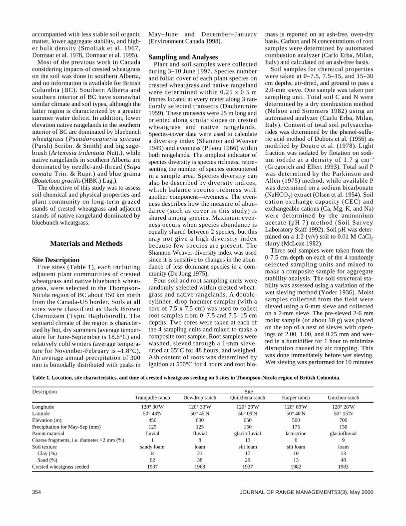
354 JOURNAL OF RANGE MANAGEMENT53(3), May 2000
accompanied with less stable soil organicmatter, lower aggregate stability, and high-er bulk density (Smoliak et al. 1967,Dormaar et al. 1978, Dormaar et al. 1995).
Most of the previous work in Canadaconsidering impacts of crested wheatgrasson the soil was done in southern Alberta,and no information is available for BritishColumbia (BC). Southern Alberta andsouthern interior of BC have somewhatsimilar climate and soil types, although thelatter region is characterized by a greatersummer water deficit. In addition, lowerelevation native rangelands in the southerninterior of BC are dominated by bluebunchwheatgrass ( Pseudoroegneria spicata(Pursh) Scribn. & Smith) and big sage-brush (Artemisia tridentata Nutt.), whilenative rangelands in southern Alberta aredominated by needle-and-thread (S t i p ac o m a t a Trin. & Rupr.) and blue grama(Bouteloua gracilis (HBK.) Lag.).
The objective of this study was to assesssoil chemical and physical properties andplant community on long-term grazedstands of crested wheatgrass and adjacentstands of native rangeland dominated bybluebunch wheatgrass.
Materials and Methods
Site DescriptionFive sites (Table 1), each including
adjacent plant communities of crestedwheatgrass and native bluebunch wheat-grass, were selected in the Thompson-Nicola region of BC about 150 km northfrom the Canada-US border. Soils at allsites were classified as Dark BrownChernozem (Typic Haploboroll). Thesemiarid climate of the region is character-ized by hot, dry summers (average temper-ature for June-September is 18.6°C) andrelatively cold winters (average tempera-ture for November-February is –1.8°C).An average annual precipitation of 300mm is bimodally distributed with peaks in
May–June and December–January(Environment Canada 1998).
Sampling and AnalysesPlant and soil samples were collected
during 3–10 June 1997. Species numberand foliar cover of each plant species oncrested wheatgrass and native rangelandwere determined within 0.25 x 0.5 mframes located at every meter along 3 ran-domly selected transects (Daubenmire1959). These transects were 25 m long andoriented along similar slopes on crestedwheatgrass and native rangelands.Species-cover data were used to calculatea diversity index (Shannon and Weaver1949) and evenness (Pileou 1966) withinboth rangelands. The simplest indicator ofspecies diversity is species richness, repre -senting the number of species encounteredin a sample area. Species diversity canalso be described by diversity indices,which balance species richness withanother component—evenness. The even-ness describes how the measure of abun-dance (such as cover in this study) isshared among species. Maximum even-ness occurs when species abundance isequally shared between 2 species, but thismay not give a high diversity indexbecause few species are present. TheShannon-Weaver-diversity index was usedsince it is sensitive to changes in the abun-dance of less dominant species in a com-munity (De Jong 1975).
Four soil and root sampling units wererandomly selected within crested wheat-grass and native rangelands. A double-cylinder, drop-hammer sampler (with acore of 7.5 x 7.5 cm) was used to collectroot samples from 0–7.5 and 7.5–15 cmdepths. Two cores were taken at each ofthe 4 sampling units and mixed to make acomposite root sample. Root samples werewashed, sieved through a 1-mm sieve,dried at 65°C for 48 hours, and weighed.Ash content of roots was determined byignition at 550°C for 4 hours and root bio-
mass is reported on an ash-free, oven-drybasis. Carbon and N concentrations of rootsamples were determined by automatedcombustion analyzer (Carlo Erba, Milan,Italy) and calculated on an ash-free basis.
Soil samples for chemical propertieswere taken at 0–7.5, 7.5–15, and 15–30cm depths, air-dried, and ground to pass a2.0-mm sieve. One sample was taken persampling unit. Total soil C and N weredetermined by a dry combustion method(Nelson and Sommers 1982) using anautomated analyzer (Carlo Erba, Milan,Italy). Content of total soil polysaccha-rides was determined by the phenol-sulfu-ric acid method of Dubois et al. (1956) asmodified by Doutre et al. (1978). Lightfraction was isolated by flotation on sodi-um iodide at a density of 1.7 g cm - 3
(Gregorich and Ellert 1993). Total soil Pwas determined by the Parkinson andAllen (1975) method, while available Pwas determined on a sodium bicarbonate(NaHCO3) extract (Olsen et al. 1954). Soilcation exchange capacity (CEC) andexchangeable cations (Ca, Mg, K, and Na)were determined by the ammoniumacetate (pH 7) method (Soil SurveyLaboratory Staff 1992). Soil pH was deter-mined on a 1:2 (v/v) soil to 0.01 M CaCl2slurry (McLean 1982).
Three soil samples were taken from the0-7.5 cm depth on each of the 4 randomlyselected sampling units and mixed tomake a composite sample for aggregatestability analysis. The soil structural sta-bility was assessed using a variation of thewet sieving method (Yoder 1936). Moistsamples collected from the field weresieved using a 6-mm sieve and collectedon a 2-mm sieve. The pre-sieved 2-6 mmmoist sample (of about 10 g) was placedon the top of a nest of sieves with open-ings of 2.00, 1.00, and 0.25 mm and wet-ted in a humidifier for 1 hour to minimizedisruption caused by air trapping. Thiswas done immediately before wet sieving.Wet sieving was performed for 10 minutes
Table 1. Location, site characteristics, and time of crested wheatgrass seeding on 5 sites in Thompson-Nicola region of British Columbia.
Description Site Tranquille ranch Dewdrop ranch Quilchena ranch Harper ranch Guichon ranch
Longitude 120° 30'W 120° 33'W 120° 29'W 120° 09'W 120° 26'WLatitude 50° 43'N 50° 45'N 50° 09'N 50° 40'N 50° 15'NElevation (m) 450 600 650 500 700Precipitation for May-Sep (mm) 125 125 150 175 150Parent material fluvial fluvial glaciofluvial lacustrine glaciofluvialCoarse fragments, i.e. diameter >2 mm (%) 1 8 13 0 9Soil texture sandy loam loam silt loam silt loam loam
Clay (%) 8 21 17 10 13Sand (%) 62 38 29 13 48
Crested wheatgrass seeded 1937 1968 1937 1982 1983

355JOURNAL OF RANGE MANAGEMENT53(3), May 2000
in a motor-driven mechanical device with avertical stroke of 2.5 cm at a rate of 30strokes per minute. The motion of the sys-tem had both a vertical stroke and an oscil-lating action through an angle of 30°. Aftersieves were removed from water, the pro-portion of material retained on each sievewas oven dried at 105°C for 24 hours,weighed, and expressed as a percentage ofthe total soil. The results were expressed asthe mean weight diameter, which repre-sents the sum of the mean diameter of eachsize fraction (Di) and the proportion of thesample weight occurring in the corre-sponding size fraction (Wi) (Van Bavel1949). The mean weight diameter wassummed over all 4 size fractions, includingthe one that passed the 0.25-mm sieve
4(MWD = ∑WiDi)
i=1Corrections were made for the coarse frac-tion retained on each sieve to avoid biasedinterpretations of water stable aggregates.
Intact soil samples were taken with adouble-cylinder, drop-hammer sampler(with a core of 7.5 x 7.5 cm) for bulk den-sity determination (Blake and Hartge1986). One core was taken per samplingunit from 0–7.5, 7.5–15, and 15–30 cmdepths on Tranquille, Dewdrop, andHarper sites, while stoniness restricted soilcoring below 15 cm on Guichon site andbelow 7.5 cm on Quilchena site. Soil sam-ples for bulk density determination weredried at 105°C for 48 hours in a forced-airoven. Coarse fragments (diameter >2 mm)within the sample were screened out andweighed. Volume of mineral coarse frag-ments was determined from dry mass andassumed to have a particle density of 2.65Mg m - 3. Soil bulk density was calculatedas the mass of dry, coarse, fragment-freemineral soil per volume of field-moist soil,where volume is also calculated on acoarse fragment-free basis.
Soil penetration resistance (Bradford1986) was measured to 30 cm depth onTranquille, Dewdrop, and Harper sites, to12 cm depth on Guichon site, and to 10.5cm depth on Quilchena site. Differentdepths determined were the result of soilstoniness. Measurements were recorded atdepth intervals of 1.5 cm, using a hand-pushed 13-mm diameter cone (30°) pen-etrometer with data logger (Agridry RimikPTY Ltd., Toowoomba, QLD, Australia).Three soil profiles were recorded on eachof the 4 randomly selected sampling units.
Rate of water infiltration in the field wasdetermined using a double-ring infiltrome-ter (Bouwer 1986). One measurement wasdone per sampling unit. Hence, at each sitea total of 8 sets of cylinders (with an outer
cylinder—56 cm diameter by 30 cmheight and inner cylinder—30 cm diame-ter by 30 cm height) were used. The cylin-ders were nested and pounded 5 cm intothe ground forming a watertight seal. Thechange in water depth of the inner cylinderwas measured over a period of 2 hours attime intervals of 5, 10, 15, 20, 30, 40, 50,60, 75, 90, 105, and 120 minutes. A headof 5–10 cm was maintained and readingswere taken with a floating gauge.Conditions for the measurement of unsatu-rated hydraulic conductivity were assumedto occur after 20 minutes.
Statistical AnalysesSpecies cover, diversity index, even-
ness, and species number data were ana-lyzed as randomized, complete blockdesign with 5 replications (i.e., sites). Soiland root samples taken at consecutivedepths from the same hole are dependenton each other. Hence, soil and root datawere analyzed separately for each depth ofsampling as a randomized, complete blockdesign with 5 replications. The general lin-ear model procedure in the SAS package(SAS Institute Inc. 1989) was used.
Results
VegetationTotal plant cover and bare ground were
similar for crested wheatgrass and native
rangelands (Table 2). Cover of grasseswas greater on crested wheatgrass thannative rangeland, while the opposite wastrue for shrub cover. Forb cover was simi-lar for the 2 rangelands.
Predominant species on native range-land were big sagebrush, bluebunchwheatgrass, needle-and-thread, Sandberg’sbluegrass (Poa secunda Presl.), and dwarfpussytoes (Antennaria dimorpha Nutt. T.& G.). Crested wheatgrass was the mostabundant species on seeded rangelandwith 23% of the total plant cover, whileSandberg’s bluegrass, needle-and-thread,dwarf pussytoes, and big sagebrushtogether contributed 8% to total plantcover (Table 2). Species number was simi-lar for crested wheatgrass and nativerangelands, but diversity of crested wheat-grass rangeland was lower due to lowerevenness.
Seeding of crested wheatgrass did notlead to reduction of root biomass relativeto native rangeland (Table 3). Root bio-mass was similar for crested wheatgrassand native grasses at both 0–7.5 and7.5–15 cm depths. In addition, roots of the2 grass communities contained similaramounts of C and N (Table 3).
SoilMost soil properties were not affected
by crested wheatgrass, although therewere several exceptions. Soil C and Nwere marginally greater under crestedwheatgrass than native grasses at the 2
Table 2. Botanical composition (% cover) on crested wheatgrass and native rangelands.
Rangeland Species Crested wheatgrass Native grasses P
--------------------(%) --------------------Grasses
Bluebunch wheatgrass 0.5 6.8 0.038Crested wheatgrass 23.4 1.1 0.000Sandberg’s bluegrass 2.3 3.4 0.512Needle-and-thread 1.4 6.7 0.116Junegrass 0.4 2.2 0.349Other grasses 0.3 1.7 0.024
Total grasses 28.3 21.9 0.028
ForbsDwarf pussytoes 1.7 2.1 0.806Other forbs 1.2 3.7 0.075
Total forbs 2.9 5.8 0.174
ShrubsBig sagebrush 1.4 7.8 0.109Pasture sage 0.7 1.1 0.493Rabbit-brush 0.8 1.5 0.332
Total shrubs 2.9 10.5 0.034
Total cover 34.5 37.6 0.493Bare ground 58.1 52.6 0.332
Diversity index 0.98 1.70 0.010Evenness 0.37 0.76 0.002Species number per 9.4 m2 14.0 17.0 0.470
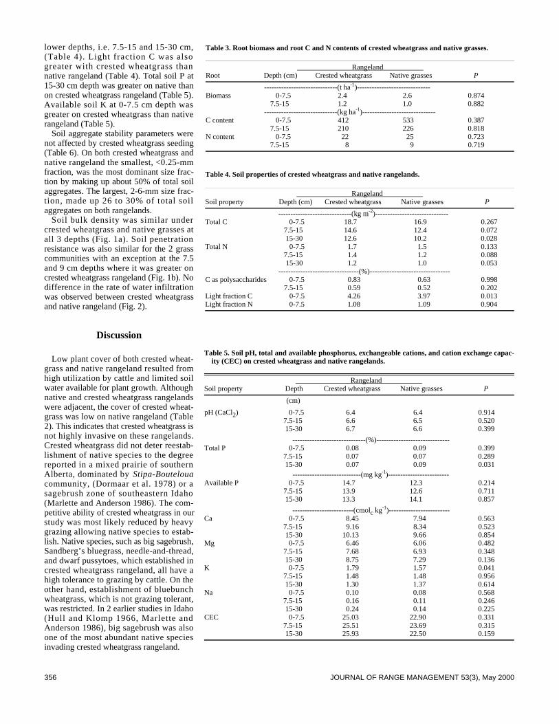
356 JOURNAL OF RANGE MANAGEMENT 53(3), May 2000
lower depths, i.e. 7.5-15 and 15-30 cm,(Table 4). Light fraction C was alsogreater with crested wheatgrass thannative rangeland (Table 4). Total soil P at15-30 cm depth was greater on native thanon crested wheatgrass rangeland (Table 5).Available soil K at 0-7.5 cm depth wasgreater on crested wheatgrass than nativerangeland (Table 5).
Soil aggregate stability parameters werenot affected by crested wheatgrass seeding(Table 6). On both crested wheatgrass andnative rangeland the smallest, <0.25-mmfraction, was the most dominant size frac-tion by making up about 50% of total soilaggregates. The largest, 2-6-mm size frac-tion, made up 26 to 30% of total soilaggregates on both rangelands.
Soil bulk density was similar undercrested wheatgrass and native grasses atall 3 depths (Fig. 1a). Soil penetrationresistance was also similar for the 2 grasscommunities with an exception at the 7.5and 9 cm depths where it was greater oncrested wheatgrass rangeland (Fig. 1b). Nodifference in the rate of water infiltrationwas observed between crested wheatgrassand native rangeland (Fig. 2).
Discussion
Low plant cover of both crested wheat-grass and native rangeland resulted fromhigh utilization by cattle and limited soilwater available for plant growth. Althoughnative and crested wheatgrass rangelandswere adjacent, the cover of crested wheat-grass was low on native rangeland (Table2). This indicates that crested wheatgrass isnot highly invasive on these rangelands.Crested wheatgrass did not deter reestab-lishment of native species to the degreereported in a mixed prairie of southernAlberta, dominated by S t i p a - B o u t e l o u acommunity, (Dormaar et al. 1978) or asagebrush zone of southeastern Idaho(Marlette and Anderson 1986). The com-petitive ability of crested wheatgrass in ourstudy was most likely reduced by heavygrazing allowing native species to estab-lish. Native species, such as big sagebrush,Sandberg’s bluegrass, needle-and-thread,and dwarf pussytoes, which established incrested wheatgrass rangeland, all have ahigh tolerance to grazing by cattle. On theother hand, establishment of bluebunchwheatgrass, which is not grazing tolerant,was restricted. In 2 earlier studies in Idaho(Hull and Klomp 1966, Marlette andAnderson 1986), big sagebrush was alsoone of the most abundant native speciesinvading crested wheatgrass rangeland.
Table 3. Root biomass and root C and N contents of crested wheatgrass and native grasses.
Rangeland Root Depth (cm) Crested wheatgrass Native grasses P
------------------------------(t ha-1)------------------------------Biomass 0-7.5 2.4 2.6 0.874
7.5-15 1.2 1.0 0.882------------------------------(kg ha-1)------------------------------
C content 0-7.5 412 533 0.3877.5-15 210 226 0.818
N content 0-7.5 22 25 0.7237.5-15 8 9 0.719
Table 4. Soil properties of crested wheatgrass and native rangelands.
Rangeland Soil property Depth (cm) Crested wheatgrass Native grasses P
------------------------------(kg m-2)------------------------------Total C 0-7.5 18.7 16.9 0.267
7.5-15 14.6 12.4 0.07215-30 12.6 10.2 0.028
Total N 0-7.5 1.7 1.5 0.1337.5-15 1.4 1.2 0.08815-30 1.2 1.0 0.053
---------------------------------(%)---------------------------------C as polysaccharides 0-7.5 0.83 0.63 0.998
7.5-15 0.59 0.52 0.202Light fraction C 0-7.5 4.26 3.97 0.013Light fraction N 0-7.5 1.08 1.09 0.904
Table 5. Soil pH, total and available phosphorus, exchangeable cations, and cation exchange capac-ity (CEC) on crested wheatgrass and native rangelands.
Rangeland Soil property Depth Crested wheatgrass Native grasses P
(cm)
pH (CaCl2) 0-7.5 6.4 6.4 0.9147.5-15 6.6 6.5 0.52015-30 6.7 6.6 0.399
------------------------------(%)------------------------------Total P 0-7.5 0.08 0.09 0.399
7.5-15 0.07 0.07 0.28915-30 0.07 0.09 0.031
----------------------------(mg kg-1)-------------------------Available P 0-7.5 14.7 12.3 0.214
7.5-15 13.9 12.6 0.71115-30 13.3 14.1 0.857
-------------------------(cmolc kg-1)-------------------------Ca 0-7.5 8.45 7.94 0.563
7.5-15 9.16 8.34 0.52315-30 10.13 9.66 0.854
Mg 0-7.5 6.46 6.06 0.4827.5-15 7.68 6.93 0.34815-30 8.75 7.29 0.136
K 0-7.5 1.79 1.57 0.0417.5-15 1.48 1.48 0.95615-30 1.30 1.37 0.614
Na 0-7.5 0.10 0.08 0.5687.5-15 0.16 0.11 0.24615-30 0.24 0.14 0.225
CEC 0-7.5 25.03 22.90 0.3317.5-15 25.51 23.69 0.31515-30 25.93 22.50 0.159
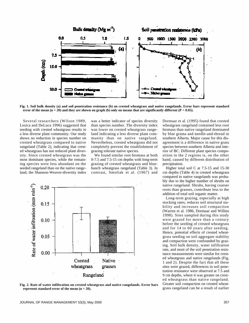
357JOURNAL OF RANGE MANAGEMENT 53(3), May 2000
Several researchers (Wilson 1989,Lesica and DeLuca 1996) suggested thatseeding with crested wheatgrass results ina less diverse plant community. Our studyshows no reduction in species number oncrested wheatgrass compared to nativerangeland (Table 2), indicating that crest-ed wheatgrass has not reduced plant diver-sity. Since crested wheatgrass was themost dominant species, while the remain-ing species were less abundant on theseeded rangeland than on the native range-land, the Shannon-Weaver-diversity index
was a better indicator of species diversitythan species number. The diversity indexwas lower on crested wheatgrass range-land indicating a less diverse plant com-munity than on native rangeland.Nevertheless, crested wheatgrass did notcompletely prevent the establishment ofgrazing tolerant native species.
We found similar root biomass at both0-7.5 and 7.5-15 cm depths with long-termgrazing of crested wheatgrass and blue-bunch wheatgrass rangeland (Table 3). Incontrast, Smoliak et al. (1967) and
Dormaar et al. (1995) found that crestedwheatgrass rangeland contained less rootbiomass than native rangeland dominatedby blue grama and needle-and-thread insouthern Alberta. Major cause for this dis-agreement is a difference in native grassspecies between southern Alberta and inte-rior of BC. Different plant species compo-sition in the 2 regions is, on the otherhand, caused by different distribution ofprecipitation.
Higher total soil C at 7.5-15 and 15-30cm depths (Table 4) in crested wheatgrasscompared to native rangelands was proba-bly due to the higher number of shrubs onnative rangeland. Shrubs, having coarserroots than grasses, contribute less to theaddition of total soil organic matter.
Long-term grazing, especially at highstocking rates, reduces soil structural sta-bility and increases soil compaction(Warren et al. 1986, Dormaar and Willms1998). Sites sampled during this studywere grazed for more than a centurybefore the seeding of crested wheatgrassand for 14 to 60 years after seeding.Hence, potential effects of crested wheat-grass seeding on soil aggregate stabilityand compaction were confounded by graz-ing. Soil bulk density, water infiltrationrate, and most of the soil penetration resis-tance measurements were similar for crest-ed wheatgrass and native rangelands (Fig.1 and 2). Despite the fact that all thesesites were grazed, differences in soil pene-tration resistance were observed at 7.5 and9 cm depths, where it was greater on crest-ed wheatgrass than native rangeland.Greater soil compaction on crested wheat-grass rangeland can be a result of earlier
Fig. 1. Soil bulk density (a) and soil penetration resistance (b) on crested wheatgrass and native rangelands. Error bars represent standarderror of the mean (n = 20) and they are shown on graph (b) only on means that are significantly different (P < 0.05).
Fig. 2. Rate of water infiltration on crested wheatgrass and native rangelands. Error barsrepresent standard error of the mean (n = 20).
358 JOURNAL OF RANGE MANAGEMENT53(3), May 2000
grazing of crested wheatgrass occurringunder wetter soil conditions relative tograzing of native grasses.
This study shed some light on theimpact of crested wheatgrass on rangelandsoil and plant composition in the southerninterior of British Columbia. Our findingsshow that seeding of crested wheatgrassdid not lead to a monoculture, althoughthe diversity of plant community wasreduced relative to native rangeland. Inaddition, crested wheatgrass introductionaccompanied with long-term grazing didnot significantly change soil properties rel-ative to the grazed native rangeland domi-nated by bluebunch wheatgrass.Responses of the rangeland soil to intro-duction of exotic grass species are strong-ly dependent on the rangeland vegetationand consequently they should be studiedtogether to achieve sustainable range man-agement.
Literature Cited
Anderson, J.E. and G.M. Marlette. 1986.Probabilities of seedling recruitment and thestability of crested wheatgrass stands. p.97–103. I n : K.L. Johnson (ed.) Crested wheat-grass: Its values, problems and myths.Symposium Proc. Utah State Univ., Logan, Ut.
Blake, G.R. and K.H. Hartge. 1986. B u l kdensity. I n : A. Klute (ed.), Methods of soilanalysis. Part 1. Physical and mineralogicalmethods. Agron. 9:363-375. Amer. Soc.Agron., Madison, Wisc.
Bouwer, H. 1986. Intake rate: cylinder infil-t r o m e t e r . I n : A. Klute (ed.) Methods of soilanalysis. Part 1. Physical and mineralogicalmethods. Agron. 9:825–844. Amer. Soc.Agron., Madison, Wisc.
Bradford, J.M. 1986. Penetrability. I n : A .Klute (ed.) Methods of soil analysis. Part 1.Physical and mineralogical methods. Agron.9:436–478. Amer. Soc. Agron., Madison,Wisc.
Daubenmire, R. 1959. A canopy-coveragemethod of vegetation analysis. Northw. Sci.33:43–65.
De Jong, T.M. 1975. A comparison of threediversity indicies based on their componentsof richness and evenness. Oikos 26:222–227.
Dormaar, J.F. and W.D. Willms. 1998. Effectof forty-four years of grazing on fescuegrassland soils. J. Range Manage. 51:122-126.
Dormaar, J.F., A. Johnston, and S. Smoliak.1978. Long-term soil changes associatedwith seeded stands of crested wheatgrass insoutheastern Alberta, Canada. p. 623–625.In: D.N. Hyder (ed.), Proc.1st Int. RangelandCongress Soc. Range Manage., Denver,Colo.
Dormaar, J.F., M.A. Naeth, W.D. Willms,and D.S. Chanasyk. 1995. Effect of nativeprairie, crested wheatgrass ( A g r o p y r o nc r i s t a t u m (L.) Gaertn.) and Russian wildrye(Elymus junceus Fisch.) on soil chemicalproperties. J. Range Manage. 48:258–263.
Doutre, D.A., G.W. Hay, A. Hood, and G.W.VanLoon. 1978. Spectrophotometric meth-ods to determine carbohydrates in soil. SoilBiol. Biochem. 10:457–462.
Dubois, M., K.A. Gilles, J.K. Hamilton, P.A.Rebers, and F. Smith. 1956. C o l o r i m e t r i cmethod for determination of sugars and relat -ed substances. Anal. Chem. 28:350–356.
Environment Canada. 1998. Canadian cli-mate normals 1961–1990. Kamloops airportmeteorological records. HTTP://www.cmc.ec.gc.ca/climate/normals/BCK002.htm.
Gomm, F.B. 1981. Letter on the value of crest -ed wheatgrass. Encl. 3-7. In: G. Ferry et al.(ed.) Review of the Bureau’s Oregon andWashington range seeding program. USDIBur. Land Manage., Portland, Ore.
Gregorich, E.G. and B.H. Ellert. 1993. Lightfraction and microorganic matter in mineralsoils. p. 397–407. In: M.R. Carter (ed.) Soilsampling and methods of analysis. Can. Soc.Soil Sci., Lewis Publ., Boca Raton, Fla.
Hull, A.C. and G.J. Klomp. 1966. Longevityof crested wheatgrass in the sagebrush-grasstype in southern Idaho. J. Range Manage.19:5–11.
Lesica, P. and T.H. DeLuca. 1996. Long-termharmful effects of crested wheatgrass onGreat Plains grassland ecosystems. J. SoilWater Conserv. 51:408–409.
Looman, J. and D.H. Heinrichs. 1973.Stability of crested wheatgrass pasturesunder long-term pasture use. Can. J. PlantSci. 53:501–506.
Marlette, G.M. and J.E. Anderson. 1986.Seed banks and propagule dispersal in crest-ed-wheatgrass stands. J. Appl. Ecol.23:161–175.
McLean, E.O. 1982. Soil pH and lime require-ment. In: A.L. Page, R.H. Miller, and D.R.Keeney (ed.) Methods of soil analysis. Part 2.Chemical and microbiological properties.Agron. 9:199–224. Amer. Soc. Agron.,Madison, Wisc.
Nelson, D.S. and L.E. Sommers. 1982. Totalcarbon, organic carbon, and organic matter.p. 539–579. In: A.L. Page, R.H. Miller, andD.R. Keeney (ed.) Methods of soil analysis.Part 2. Chemical and microbiological proper -ties. Agron. 9:539-579. Amer. Soc. Agron.,Madison, Wisc.
Olsen, S.R., C.V. Cole, F.S. Watanabe, andL.A. Dean. 1954. Estimation of availablephosphorus in soils by extraction with sodi-um bicarbonate. USDA, Circ. 939, U.S.Government Printing Office, Washington,D.C.
Parkinson, J.A. and S.E. Allen. 1975. A wetoxidation procedure suitable for the determi-nation of nitrogen and mineral nutrients inbiological materials. Commun. Soil Sci.Plant Anal. 6:1–11.
Pileou, E.C. 1966. The measurement of diver-sity in different types of biological collec-tions. J. Theor. Biol. 13:131–144.
SAS Institute Inc. 1989. SAS/STAT user’sguide. Version 6, 4th ed., Vol.2. SAS Inst.Inc., Cary, N.C.
Shannon, C.E. and W. Weaver. 1949. T h emathematical theory of communication.Univ. of Illinois Press, Urbana, Ill.
Smoliak, S., A. Johnston, and L.E. Lutwick.1967. Productivity and durability of crestedwheatgrass in southeastern Alberta. Can. J.Plant Sci. 47:539–548.
Soil Survey Laboratory Staff. 1992. Soil sur-vey laboratory methods manual. Soil Surv.Invest. Reps. 42. USDA-SCS, Washington,D.C.
Van Bavel, C.H.M. 1949. Mean weight diame-ter of soil aggregates as a statistical index ofaggregation. Soil Sci. Soc. Am. Proc. 14:20-23.
Warren, S.D., M.B. Nevill, W.H. Blackburn,and N.E. Garza. 1986. Soil response totrampling under intensive rotation grazing.Soil Sci. Soc. Amer. J. 50:1336–1341.
Wilson, S.D. 1989. The suppression of nativeprairie by alien species introduced for reveg-etation. Landscape and Urban Planning17:113–119.
Yoder, R.E. 1936. A direct method of aggre-gate analysis of soils and study of the physi-cal nature of soil erosion losses. Amer. Soc.Agron. J. 28:337-351.
Table 6. Soil aggregate stability parameters on crested wheatgrass and native rangelands at 0-7.5cm depth.
Rangeland Species Crested wheatgrass Native grasses P
---------------------(%)---------------------2-6 mm 26.2 29.7 0.455
1-2 mm 8.8 7.7 0.4710.25-1 mm 13.6 9.9 0.370<0.25 mm 51.5 52.7 0.799
--------------------(mm)--------------------Mean weight diameter 1.3 1.4 0.546
359JOURNAL OF RANGE MANAGEMENT 53(3), May 2000
Shinners and Mahler’s Flora of North Central Texas. B yGeorge M. Diggs, Jr., Barney L. Lipscomb, and Robert J.O’Kennon. 1999. Botanical Research Institute of Texas, Ft.Worth, Texas. 1626 p. US$89.95cloth. ISBN 1-889878-01-4.If some travelers who have motored in daylight through
North Central Texas have found the landscape uninspiring byWestern standards, the same would likely not be said ofShinners and Mahler’s Flora of North Central Texas, animpressive new flora of the cross timbers and prairies areas oflone star land. A compilation of the work of a number ofbotanists who have studied the region, the voluminous volumecombines elements of botanical history, community ecology,and floristic taxonomy with attractive graphics and a readabletext. The authors present it all in a stylish, efficient format thatmakes the book pleasantly functional compared with manyother floras, even while it inspires admiration of its scope anddetail.
More than just briefly summarizing all of the contents ofThe Flora of North Central Texas would be a significantundertaking. The book begins with about 15 pages of its ownsummary information on design and use of the flora. Matterssuch as nomenclature, sources of information, summary dataon the flora, and threatened and endangered taxa are addressedhere. Following this summary, a 60-page introduction to thenatural features of North Central Texas introduces the user tothe geology, soils, climate, botanical history, and vegetationareas of the region. Included are a number of black and whitemaps, several color maps, several historical drawings of earlyvegetation, and some drawings and black and white pho-tographs of early botanists who worked in the area. Thirtypages of color photographs, 4 or 5 to a page, of some of themore attractive flowering species follow the introduction. Youcan be sure that Texas bluebonnet (Lupinus texensis) is amongthem.
The preceding 3 sections would make an attractive, informa-tive book in themselves, but the over 1,200 pages of the taxo-nomic key to, and botanical descriptions of the flora of theregion which follow expand the book to Texan proportions.Both the keys and descriptions are admirably formatted, mak-ing this flora one of the most inviting to use that I haveencountered. The text is abbreviated in the manner of a flora,but the abbreviations are rarely cryptic, allowing the taxonom-ic text to be read comfortably. Most species descriptions areaccompanied by hand-drawn illustrations, on adjacent pages,4 to 9 to a page.
Following the keys and taxonomic descriptions are no fewerthan 15 appendices covering topics such as lists of endemicspecies, lists of conservation organizations, sources of nativeplants, collecting herbarium specimens, grass phylogeny, lar-val host plants of Lepidoptera, and 9 other topics. Theseappendices contain a wealth of information for the profession-al or amateur botanist. An extensive glossary of taxonomicterms, an illustrated glossary of morphological terms, 75pages of literature citations, and a 100-page index nearly com-
plete the book, but not without formal printing credits, creditsto authors and institutions, and a final map. The entire produc-tion is admirably detailed and polished in a kind of Texas tra-dition, reminding me of the high degree of dedication and pro-fessionalism I have observed in many recent and historicalnatural scientists of that state. It represents the work of manycontributors, and the book’s attractive format showcases theirefforts.
Many of the species described in this book are found inother parts of Texas, and in adjoining states, so that the bookshould be of interest somewhat beyond the area named in itstitle. Researchers, teachers, managers, students and amateurbotanists of North Central Texas, centered around Dallas-Ft.Worth, will certainly want this floristic survey of this oftensultry sub-state of Texas on their shelf. Like the summernights in North Central Texas, the stylish Flora of NorthCentral Texas is, at least for a flora, hotter than it is dry.—David L. Scarnecchia, Washington State University, Pullman,Washington.
Book Review

Eligibility
The Journal of Range Management is a publication for reporting anddocumenting results of original research and selected invitational papers.Previously published papers are unacceptable and will not be consideredfor publication. Exceptions to this criterion are research results that wereoriginally published as department research summaries, field stationreports, abstracts of presentations, and other obscure and nontechnicalhandout publications. Manuscripts submitted to the JRM are the propertyof the J o u r n a l until published or released back to the author(s).Manuscripts may not be submitted elsewhere while they are being con-sidered for this journal. Papers not accepted for publication are automat-ically released to the authors.
Kinds of ManuscriptsJournal Articles report original findings in Plant Physiology, Animal
Nutrition, Ecology, Economics, Hydrology, Wildlife Habitat,Methodology, Taxonomy, Grazing Management, Soils, Land Recla-mation (reseeding), and Range Improvement (fire, mechanical chemical).Technical Notes are short articles (usually less than 2 printed pages)reporting unique apparatus and experimental techniques. By invitation ofthe Editorial Board, a Review or Synthesis Paper may be printed in thejournal. Viewpoint articles or Research Observations discussing opinionor philosophical concepts regarding topical material or observational dataare acceptable. Such articles are identified by the word viewpoint orobservations in the title.
Manuscript SubmissionContributions are addressed to the Editor, Gary Frasier, Journal of
Range Management, 7820 Stag Hollow Road, Loveland, Colorado80538. Manuscripts are to be prepared according to the instructions in theJournal’s Handbook and Style Manual. If the manuscript is to be one ofa series, the Editor must be notified. Four copies of the complete manu-script, typed on paper with numbered line spaces are required. Authorsmay retain original tables and figures until the paper is accepted, and sendgood quality photocopies for the review process. Receipt of all manu-scripts is acknowledged at once, and authors are informed about subse-quent steps of review, approval or release, and publication.
Manuscripts that do not follow the directives and style in Journal hand-book will be returned to the authors before being reviewed. A manuscriptnumber and submission date will be assigned when the paper is receivedin the appropriate format.
Manuscript ReviewManuscripts are forwarded to an Associate Editor, who usually obtains
2 or more additional reviews. Reviewers remain anonymous. Thesereviewers have the major responsibility for critical evaluation to deter-mine whether or not a manuscript meets scientific and literary standards.Where reviewers disagree, the Associate Editor, at his discretion, mayobtain additional reviews before accepting or rejecting a manuscript. TheAssociate Editor may also elect to return to the author those manuscriptsthat require revision to meet format criteria before the Journal review.
The Associate Editor sends approved manuscripts, with recommenda-tions for publication, to the Editor, who notifies the author of a projectedpublication date. Manuscripts found inappropriate for the JRM arereleased to the author by the Associate Editor. Manuscripts returned to anauthor for revision are returned to the Associate Editor for final accept -ability of the revision. Revisions not returned within 6 months, are con-sidered terminated. Authors who consider that their manuscript has
received an unsatisfactory review may file an appeal with the Editor. TheEditor then may select another Associate Editor to review the appeal. TheAssociate Editor reviewing the appeal will be provided with copies of ancorrespondence relating to the original review of the manuscript. If theappeal is sustained, a new review of the manuscript may be implementedat the discretion of the Editor.
Authors should feel free to contact the Associate Editor assigned totheir manuscript at any stage of the review process: to find out where thepaper is in the process; to ask questions about reviewer comments; to askfor clarification or options if a paper has been rejected.
Page ProofsPage proofs are provided to give the author a final opportunity to make
corrections of errors caused by editing and production. Authors will becharged when extensive revision is required because of author changes,even if page charges are not assessed for the article. One author per paperwill receive page proofs. These are to be returned to the ProductionEditor, 445 Union Blvd., Suite 230, Lakewood, Colorado 80228, with-in 48 hours after being received. If a problem arises that makes thisimpossible, authors or their designates are asked to contact theProduction Editor immediately, or production and publication may pro-ceed without the author’s approval of his edited manuscript.
Page Charges and Reprint OrdersAuthors are expected to pay current page charges. Since most research
is funded for publication, it will be assumed that the authors are able topay page charges unless they indicate otherwise in writing, when submit-ting a manuscript. When funds are unavailable to an author, no pagecharges will be assessed. Only the Editor will have knowledge of fundstatus of page charges; the Associate Editors and reviewers will accept orreject a manuscript on content only.
An order form for reprints is sent to one author with the page proofs.Information as to price and procedure are provided at that time. The min-imum order is 100; no reprints are provided free of charge.
Basic Writing StyleEvery paper should be written accurately, clearly, and concisely. It
should lead the reader from a clear statement of purpose through materi-als and methods, results, and to discussion. The data should be reportedin coherent sequence, with a sufficient number of tables, drawings, andphotographs to clarify the text and to reduce the amount of discussion.Tables, graphs, and narrative should not duplicate each other.
Authors should have manuscripts thoroughly reviewed by colleaguesin their own institution and elsewhere before submitting them. Peerreview before submission insures that publications will present signifi-cant new information or interpretation of previous data and will speedJRM review process.
Particular attention should be given to literature cited: names ofauthors, date of publication, abbreviations or names of journals, titles,volumes, and page numbers.
It is not the task of Associate Editors or Journal reviewers to edit poor-ly prepared papers or to correct readily detectable errors. Papers not prop-erly prepared will be returned to the author.
INSTRUCTIONS FOR AUTHORS (from revised Handbook and Style Manual)