Measurements and Modeling - Society for Industrial … · Chapter 1 Measurements and Modeling...

Chapter 1

Measurements and Modeling

quantitative model of a physical system is expressed in the language of mathematics. Aqualitative model often precedes a quantitative model. For many years clinicians usedmedical x-ray images without employing a precise quantitative model. X-rays were thoughtof as high frequency ‘light’ with three very useful properties:

1. If x-rays are incident on a human body, some fraction of the incident radiation isabsorbed or scattered, though a sizable fraction is transmitted. The fraction absorbedor scattered is proportional to the total density of the material encountered. Theoverall decrease in the intensity of the x-ray beam is called attenuation.

2. A beam of x-ray light travels in a straight line.

3. X-rays darken photographic film. The opacity of the film is a monotone function ofthe incident energy.

Taken together, these properties mean that using x-rays one can “see through” a humanbody to obtain a shadow or projection of the internal anatomy on a sheet of film [Fig-ure 1.1(a)].

This model was adequate given the available technology. In their time, x-ray imagesled to a revolution in the practice of medicine because they opened the door to non-invasiveexamination of internal anatomy. They are still useful for locating bone fractures, den-tal caries, and foreign objects, but their ability to visualize soft tissues and more detailedanatomic structure is limited. There are several reasons for this. The principal difficulty isthat an x-ray image is a two-dimensional representation of a three-dimensional object. InFigure 1.1(b), the opacity of the film at a point on the film plane is inversely proportionalto an average of the density of the object, measured along the line joining the point to thex-ray source. This renders it impossible to deduce the spatial ordering in the missing thirddimension.

1

Copyright ©2007 by the Society for Industrial and Applied Mathematics.This electronic version is for personal use and may not be duplicated or distributed.

From "Introduction to the Mathematics of Medical Imaging, Second Edition" by Charles L. Epstein.This book is available for purchase at www.siam.org/catalog.

2 Chapter 1. Measurements and Modeling

(a) A old-fashioned chest x-ray image.(Image provided courtesy of Dr. DavidS. Feigin, ENS Sherri Rudinsky, and Dr.James G. Smirniotopoulos of the Uni-formed Services University of the HealthSciences, Dept. of Radiology, Bethesda,MD.)

Object

X-ray source

Film plane

(b) Depth information is lost in a projection.

Figure 1.1. The world of old fashioned x-rays imaging.

A second problem is connected to the “detector” used in traditional x-ray imaging.Photographic film is used to record the total energy in the x rays that are transmitted throughthe object. Unfortunately film is rather insensitive to x rays. To get a usable image, a lightemitting phosphor is sandwiched with the film. This increases the sensitivity of the overall“detector,” but even so, large differences in the intensity of the incident x-ray beam producesmall differences in the opacity of film. This means that the contrast between different softtissues is poor. Beyond this there are other problems caused by the scattering of x rays andnoise. Because of these limitations a qualitative theory was adequate for the interpretationof traditional x-ray images.

A desire to improve upon this situation led Alan Cormack, [24], and Godfrey Hounsfield,[64], to independently develop x-ray tomography or slice imaging. The first step in theirwork was to use a quantitative theory for the attenuation of x-rays. Such a theory alreadyexisted and is little more than a quantitative restatement of (1) and (2). It is not neededfor old fashioned x-ray imaging because traditional x-ray images are read “by eye,” andno further processing is done after the film is developed. Both Cormack and Hounsfieldrealized that mathematics could be used to infer three-dimensional anatomic structure froma large collection of different two-dimensional projections. The possibility for making thisidea work relied on two technological advances:

1. The availability of scintillation crystals to use as detectors

2. Powerful, digital computers to process the tens of thousands of measurements neededto form a usable image

A detector using a scintillation crystal is about a hundred times more sensitive than photo-graphic film. Increasing the dynamic range in the basic measurements makes possible much



1.1. Mathematical Modeling 3

finer distinctions. As millions of arithmetic operations are needed for each image, fast com-puters are a necessity for reconstructing an image from the available measurements. It is aninteresting historical note that the mathematics underlying x-ray tomography was done in1917 by Johan Radon, [105]. It had been largely forgotten, and both Hounsfield and Cor-mack worked out solutions to the problem of reconstructing an image from its projections.Indeed, this problem had arisen and been solved in contexts as diverse as radio astronomyand statistics.

This book is a detailed exploration of the mathematics that underpins the reconstruc-tion of images in x-ray tomography. While our emphasis is on understanding these math-ematical foundations, we constantly return to the practicalities of x-ray tomography. Ofparticular interest is the relationship between the mathematical treatment of a problem andthe realities of numerical computation and physical measurement. There are many differentimaging modalities in common use today, such as x-ray computed tomography (CT), mag-netic resonance imaging (MRI), positron emission tomography (PET), ultrasound, opticalimaging, and electrical impedance imaging. Because each relies on a different physicalprinciple, each provides different information. In every case the mathematics needed toprocess and interpret the data has a large overlap with that used in x-ray CT. We con-centrate on x-ray CT because of the simplicity of the physical principles underlying themeasurement process. Detailed descriptions of the other modalities can be found in [91],[76], or [6].

Mathematics is the language in which any quantitative theory or model is eventuallyexpressed. In this introductory chapter we consider a variety of examples of physical sys-tems, measurement processes, and the mathematical models used to describe them. Thesemodels illustrate different aspects of more complicated models used in medical imaging.We define the notion of degrees of freedom and relate it to the dimension of a vector space.The chapter concludes by analyzing the problem of reconstructing a region in the planefrom measurements of the shadows it casts.

1.1 Mathematical Modeling

The first step in giving a mathematical description of a system is to isolate that system fromthe universe in which it sits. While it is no doubt true that a butterfly flapping its wingsin Siberia in midsummer will affect the amount of rainfall in the Amazon rain forest adecade hence, it is surely a tiny effect, impossible to accurately quantify. A practical modelincludes the system of interest and the major influences on it. Small effects are ignored,though they may come back, as measurement error and noise, to haunt the model. Afterthe system is isolated, we need to find a collection of numerical parameters that describe itsstate. In this generality these parameters are called state variables. In the idealized worldof an isolated system the exact measurement of the state variables uniquely determines thestate of the system. It may happen that the parameters that give a convenient descriptionof the system are not directly measurable. The mathematical model then describes rela-tions among the state variables. Using these relations, the state of the system can oftenbe determined from feasible measurements. A simple example should help clarify these




abstract-sounding concepts.

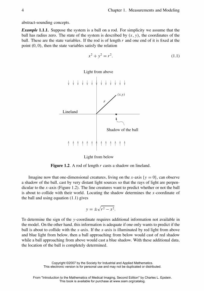
Example 1.1.1. Suppose the system is a ball on a rod. For simplicity we assume that theball has radius zero. The state of the system is described by (x, y), the coordinates of theball. These are the state variables. If the rod is of length r and one end of it is fixed at thepoint (0, 0), then the state variables satisfy the relation

x2 + y2 = r2. (1.1)

(x,y)

r

Lineland

Shadow of the ball

Light from below

Light from above

Figure 1.2. A rod of length r casts a shadow on lineland.

Imagine now that one-dimensional creatures, living on the x-axis {y = 0}, can observea shadow of the ball, cast by very distant light sources so that the rays of light are perpen-dicular to the x-axis (Figure 1.2). The line creatures want to predict whether or not the ballis about to collide with their world. Locating the shadow determines the x-coordinate ofthe ball and using equation (1.1) gives

y = ±√

r2 − x2.

To determine the sign of the y-coordinate requires additional information not available inthe model. On the other hand, this information is adequate if one only wants to predict if theball is about to collide with the x-axis. If the x-axis is illuminated by red light from aboveand blue light from below, then a ball approaching from below would cast of red shadowwhile a ball approaching from above would cast a blue shadow. With these additional data,the location of the ball is completely determined.




Ordered pairs of real numbers, {(x, y)}, are the state variables for the system in Ex-ample 1.1.1. Because of the constraint (1.1), not every pair defines a state of this system.Generally we define the state space to be values of state variables which correspond to ac-tual states of the system. The state space in Example 1.1.1 is the circle of radius r centeredat (0, 0).

ExercisesExercise 1.1.1. Suppose that in Example 1.1.1 light sources are located at (0,±R). Whatis the relationship between the x-coordinate and the shadow?

Exercise 1.1.2. Suppose that in Example 1.1.1 the ball is tethered to (0, 0) by a string oflength r. What relations do the state variables (x, y) satisfy? Is there a measurement theline creatures can make to determine the location of the ball? What is the state space forthis system?

Exercise 1.1.3. Suppose that the ball is untethered but is constrained to lie in the region{(x, y) : 0 ≤ y < R}. Assume that the points {(x1, y1), (x2, y2), (x3, y3)} do not lie ona line and have y j > R. Show that the shadows cast on the line y = 0 by light sourceslocated at these three points determine the location of the ball. Find a formula for (x, y) interms of the shadow locations. Why are three sources needed?

1.1.1 Finitely Many Degrees of Freedom

See: A.1, B.3, B.4, B.5.

The collection of ordered n-tuples of real numbers

{(x1, . . . , xn) : x j ∈ �, j = 1, . . . , n}is called Euclidean n-space and is denoted by �n. We often use boldface letters x, y todenote points in �n, which we sometimes call vectors. Recall that if x = (x1, . . . , xn) andy = (y1, . . . , yn), then their sum x + y is defined by

x + y = (x1 + y1, . . . , xn + yn), (1.2)

and if a ∈ �, then ax is defined by

ax = (ax1, . . . , axn). (1.3)

These two operations make �n into a real vector space.

Definition 1.1.1. If the state of a system is described by a finite collection of real numbers,then the system has finitely many degrees of freedom.




Euclidean n-space is the simplest state space for a system with n degrees of freedom.Most systems encountered in elementary physics and engineering have finitely many de-grees of freedom. Suppose that the state of a system is specified by a point x ∈ �n. Thenthe mathematical model is expressed as relations that these variables satisfy. These oftentake the form of functional relations,

f1(x1, . . . , xn) = 0...

...fm(x1, . . . , xn) = 0.

(1.4)

In addition to conditions like those in (1.4) the parameters describing the state of a systemmight also satisfy inequalities of the form

g1(x1, . . . , xn) ≥ 0...

...gl(x1, . . . , xn) ≥ 0.

(1.5)

The state space for the system is then the subset of �n consisting of solutions to (1.4) whichalso satisfy (1.5).

Definition 1.1.2. An equation or inequality that must be satisfied by a point belonging tothe state space of a system is called a constraint.

Example 1.1.1 considers a system with one degree of freedom. The state space for thissystem is the subset of �2 consisting of points satisfying (1.1). If the state variables satisfyconstraints, then this generally reduces the number of degrees of freedom.

A function f : �n → � is linear if it satisfies the conditions

f (x + y) = f (x)+ f (y) for all x, y ∈ �n and

f (ax) = a f (x) for all a ∈ � and x ∈ �n.(1.6)

Recall that the dot or inner product is the map from �n × �n → � defined by

〈x, y〉 =n∑

j=1

x j y j . (1.7)

Sometimes it is denoted by x · y. The Euclidean length of x ∈ �n is defined to be

‖x‖ = √〈x, x〉 =⎡⎣ n∑

j=1

x2j

⎤⎦12

. (1.8)

From the definition it is easy to establish that

〈x, y〉 = 〈y, x〉 for all x, y ∈ �n,

〈ax, y〉 = a〈x, y〉 for all a ∈ � and x ∈ �n,

〈x1 + x2, y〉 = 〈x1, y〉 + 〈x2, y〉 for all x1, x2, y ∈ �n.

‖cx‖ = |c|‖x‖ for all c ∈ � and x ∈ �n.

(1.9)




For y a point in �n, define the function f y(x) = 〈x, y〉. The second and third relationsin (1.9) show that f y is linear. Indeed, every linear function has a such a representation.

Proposition 1.1.1. If f : �n → � is a linear function, then there is a unique vector y fsuch that f (x) = 〈x, y f 〉.This fact is proved in Exercise 1.1.5. The inner product satisfies a basic inequality calledthe Cauchy-Schwarz inequality.

Proposition 1.1.2 (Cauchy-Schwarz inequality). If x, y ∈ �n, then

|〈x, y〉| ≤ ‖x‖‖y‖. (1.10)

A proof of this result is outlined in Exercise 1.1.6. The Cauchy-Schwarz inequalityshows that if neither x nor y is zero, then

−1 ≤ 〈x, y〉‖x‖‖y‖ ≤ 1;

this in turn allows us the define the angle between two vectors.

Definition 1.1.3. If x, y ∈ �n are both nonvanishing, then the angle θ ∈ [0, π ], between xand y is defined by

cos θ = 〈x, y〉‖x‖‖y‖ . (1.11)

In particular, two vector are orthogonal if 〈x, y〉 = 0.

The Cauchy-Schwarz inequality implies that the Euclidean length satisfies the triangleinequality.

Proposition 1.1.3. For x, y ∈ �n, the following inequality holds:

‖x + y‖ ≤ ‖x‖ + ‖y‖. (1.12)

This is called the triangle inequality.

Remark 1.1.1. The Euclidean length is an example of a norm on �n. A real-valued functionN defined on �n is a norm provided it satisfies the following conditions:

NON-DEGENERACY:N(x) = 0 if and only if x = 0,

HOMOGENEITY:N(ax) = |a|N(x) for all a ∈ � and x ∈ �n,

THE TRIANGLE INEQUALITY:N(x + y) ≤ N(x)+ N(y) for all x, y ∈ �n.




Any norm provides a way to measure distances. The distance between x and y is definedto be

dN (x, y)d= N(x − y).

Suppose that the state of a system is specified by a point in �n subject to the constraintsin (1.4). If all the functions { f1, . . . , fm} are linear, then we say that this is a linear model.This is the simplest type of model and also the most common in applications. In this casethe set of solutions to (1.4) is a subspace of �n. We recall the definition.

Definition 1.1.4. A subset S ⊂ �n is a subspace if

1. the zero vector belongs to S,

2. x1, x2 ∈ S, then x1 + x2 ∈ S,

3. if c ∈ � and x ∈ S, then cx ∈ S.

For a linear model it is a simple matter to determine the number of degrees of freedom.Suppose the state space consists of vectors satisfying a single linear equation. In light ofProposition 1.1.1, it can be expressed in the form

〈a1, x〉 = 0, (1.13)

with a1 a nonzero vector. This is the equation of a hyperplane in �n. The solutions to (1.13)are the vectors in �n orthogonal to a1. Recall the following definition:

Definition 1.1.5. The vectors {v1, . . . , vk} are linearly independent if the only linear combi-nation, c1v1+· · ·+ckvk, that vanishes has all its coefficients, {ci}, equal to zero. Otherwisethe vectors are linearly dependent.

The dimension of a subspace of �n can now be defined.

Definition 1.1.6. Let S ⊂ �n be a subspace. If there is a set of k linearly independentvectors contained in S but any set with k + 1 or more vectors is linearly dependent, thenthe dimension of S equals k. In this case we write dim S = k.

There is a collection of (n − 1) linearly independent n-vectors {v1, . . . , vn−1} so that〈a1, x〉 = 0 if and only if

x =n−1∑i=1

civi .

The hyperplane has dimension n − 1, and therefore a system described by a single linearequation has n − 1 degrees of freedom. The general case is not much harder. Suppose thatthe state space is the solution set of the system of linear equations

〈a1, x〉 = 0...

...〈am, x〉 = 0.

(1.14)




Suppose that k ≤ m is the largest number of linearly independent vectors in the collection{a1, . . . , am}. By renumbering, we can assume that {a1, . . . , ak} are linearly independent,and for any l > k the vector al is a linear combination of these vectors. Hence if x satisfies

〈ai , x〉 = 0 for 1 ≤ i ≤ k

then it also satisfies 〈al, x〉 = 0 for any l greater than k. The argument in the previousparagraph can be applied recursively to conclude that there is a collection of n − k linearlyindependent vectors {u1, . . . , un−k} so that x solves (1.14) if and only if

x =n−k∑i=1

ci ui .

Thus the system has n − k degrees of freedom.A nonlinear model can often be approximated by a linear model. If f is a differentiable

function, then the gradient of f at x is defined to be

∇ f (x) =(

∂ f

∂x1(x), . . . ,

∂ f

∂xn(x)).

From the definition of the derivative it follows that

f (x0 + x1) = f (x0)+ 〈x1,∇ f (x0)〉 + e(x1), (1.15)

where the error e(x1) satisfies

limx1→0

|e(x1)|‖x1‖ = 0.

In this case we writef (x0 + x1) ≈ f (x0)+ 〈x1,∇ f (x0)〉. (1.16)

Suppose that the functions in (1.4) are differentiable and f j (x0) = 0 for j = 1, . . . ,m.Then

f j (x0 + x1) ≈ 〈x1,∇ f j (x0)〉.For small values of x1 the system of equations (1.4) can be approximated, near to x0, by asystem of linear equations,

〈x1,∇ f1(x0)〉 = 0...

...〈x1,∇ fm(x0)〉 = 0.

(1.17)

This provides a linear model that approximates the non-linear model. The accuracy of thisapproximation depends, in a subtle way, on the collection of vectors {∇ f j(x)}, for x nearto x0. The simplest situation is when these vectors are linearly independent at x0. In thiscase the solutions to

f j (x0 + x1) = 0, j = 1, . . . ,m,




are well approximated, for small x1, by the solutions of (1.17). This is a consequence ofthe implicit function theorem; see [119].

Often the state variables for a system are divided into two sets, the input variables,(w1, . . . , wk), and output variables, (z1, . . . , zm), with constraints rewritten in the form

F1(w1, . . . , wk) = z1...

...Fm(w1, . . . , wk) = zm.

(1.18)

The output variables are thought of as being measured; the remaining variables must thenbe determined by solving this system of equations. For a linear model this amounts tosolving a system of linear equations. We now consider some examples of physical systemsand their mathematical models.

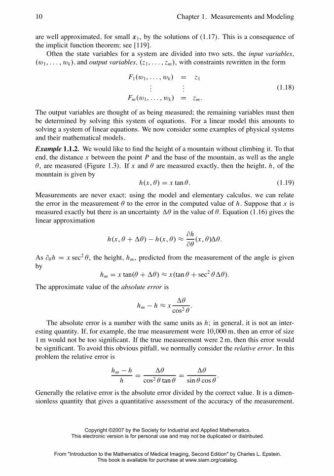
Example 1.1.2. We would like to find the height of a mountain without climbing it. To thatend, the distance x between the point P and the base of the mountain, as well as the angleθ, are measured (Figure 1.3). If x and θ are measured exactly, then the height, h, of themountain is given by

h(x, θ) = x tan θ. (1.19)

Measurements are never exact; using the model and elementary calculus, we can relatethe error in the measurement θ to the error in the computed value of h. Suppose that x ismeasured exactly but there is an uncertainty �θ in the value of θ. Equation (1.16) gives thelinear approximation

h(x, θ +�θ)− h(x, θ) ≈ ∂h

∂θ(x, θ)�θ.

As ∂θh = x sec2 θ, the height, hm, predicted from the measurement of the angle is givenby

hm = x tan(θ +�θ) ≈ x(tan θ + sec2 θ�θ).

The approximate value of the absolute error is

hm − h ≈ x�θ

cos2 θ.

The absolute error is a number with the same units as h; in general, it is not an inter-esting quantity. If, for example, the true measurement were 10,000 m, then an error of size1 m would not be too significant. If the true measurement were 2 m, then this error wouldbe significant. To avoid this obvious pitfall, we normally consider the relative error. In thisproblem the relative error is

hm − h

h= �θ

cos2 θ tan θ= �θ

sin θ cos θ.

Generally the relative error is the absolute error divided by the correct value. It is a dimen-sionless quantity that gives a quantitative assessment of the accuracy of the measurement.




P

x

hθ

Figure 1.3. Using trigonometry to find the height of a mountain.

If the angle θ is measured from a point too near to or too far from the mountain (i.e., θis very close to 0 or π/2), then small measurement errors result in a substantial loss ofaccuracy. A useful feature of a precise mathematical model is the possibility of estimatinghow errors in measurement affect the accuracy of the parameters we wish to determine. InExercise 1.1.13 we consider how to estimate the error entailed in using a linear approxima-tion.

Example 1.1.3. In a real situation we cannot measure the distance to the base of the moun-tain. Suppose that we measure the angles, θ1 and θ2, from two different points, P1 and P2,as well as the distance x2 − x1 between the two points, as shown in Figure 1.4.

P1

P2 1

h

x2

x1

θ 2 θ

Figure 1.4. A more realistic measurement.

From the previous example we know that

h = x1 tan θ1,

h = x2 tan θ2.(1.20)

Using these equations and elementary trigonometry, we deduce that

x1 = x2 − x1[tan θ1tan θ2

− 1] , (1.21)




which implies that

h = x1 tan θ1

= (x2 − x1)sin θ1 sin θ2

sin(θ1 − θ2).

(1.22)

Thus h can be determined from θ1, θ2 and x2 − x1. With d = x2 − x1, equation (1.22)expresses h as a function of (d, θ1, θ2). At the beginning of this example, (x1, θ1, x2, θ2, h)were the state variables describing our system; by the end we used (d, θ1, θ2, h). The firstthree are directly measurable, and the last is an explicit function of the others. The modelsin this and the previous example, as expressed by equations (1.22) and (1.19), respectively,are nonlinear models.

In this example there are many different ways that the model may fail to capture impor-tant features of the physical situation. We now consider a few potential problems.

1. If the shape of a mountain looks like that in Figure 1.5 and we measure the distanceand angle at the point P , we are certainly not finding the real height of the mountain.Some a priori information is always incorporated in a mathematical model.

P

Figure 1.5. Not exactly what we predicted!

2. The curvature of the earth is ignored. A more sophisticated geometric model isneeded to correct for such errors. This becomes a significant problem as soon as thedistances, x, x1, x2, are large compared to the distance to the horizon (about 25 kmfor a 2-meter-tall person). The approximations used in the model must be adapted tothe actual physical conditions of the measurements.

3. The geometry of the underlying measurements could be quite different from the sim-ple Euclidean geometry used in the model. To measure the angles θ1, θ2, we wouldnormally use a transit to sight the peak of the mountain. If the mountain is far away,then the light traveling from the mountain to the transit passes through air of varyingdensity. The light is refracted by the air and therefore the ray path is not a straightline, as assumed in the model. To include this effect would vastly complicate themodel. This is an important consideration in the similar problem of creating a mapof the sky from earth based observations of stars and planets.

Analogous problems arise in medical imaging. If the wavelength of the energy usedto probe the human anatomy is very small compared to the size of the structures that are




present, then it is reasonable to assume that the waves are not refracted. For example, x-rayscan be assumed to travel along straight lines. For energies with wavelengths comparable tothe size of structures present in the human anatomy, this assumption is simply wrong. Thewaves are then bent and diffracted by the medium, and the difficulty of modeling the raypaths is considerable. This is an important issue in ultrasound imaging that remains largelyunresolved.

Example 1.1.4. Refraction provides another example of a simple physical system. Supposethat we have two fluids in a tank, as shown in Figure 1.6, and would like to determine theheight of the interface between them. Suppose that the refractive indices of the fluids areknown. Let n1 be the refractive index of the upper fluid and n2 the refractive index of thelower one. Snell’s law states that

sin(θ1)

sin(θ2)= n2

n1.

Let h denote the total height of the fluid; then

h

h

n

n

1 1

2

l

θ

θ

1

2 2

Figure 1.6. Using refraction to determine the height of an interface.

h1 + h2 = h.

The measurement we make is the total displacement, l, of the light ray as it passes throughthe fluids. It satisfies the relationship

h1 tan(θ1)+ h2 tan(θ2) = l.

The heights h1 and h2 are easily determined from these three formulæ. The assumptionthat we know n1 implies, by Snell’s law, that we can determine θ1 from a measurement of




the angle of the light ray above the fluid. If n2 is also known, then using these observationswe can determine θ2 as well:

sin(θ2) = n1

n2sin(θ1).

The pair (h1, h2) satisfies the 2 × 2 linear system(1 1

tan(θ1) tan(θ2)

)(h1

h2

)=(

hl

). (1.23)

In Example 2.1.1 we consider a slightly more realistic situation where the refractive indexof the lower fluid in not known. By using more measurements, n2 can also be determined.

ExercisesExercise 1.1.4. Prove the formulæ in (1.9).

Exercise 1.1.5. Let e j ∈ �n, j = 1, . . . , n denote the vector with a 1 in the j th place andotherwise zero,

e1 = (1, 0, 0, . . . , 0), e2 = (0, 1, 0, . . . , 0), . . . , en = (0, . . . , 0, 1).

1. Show that if x = (x1, . . . , xn), then

x =n∑

j=1

x j e j .

2. Use the previous part to prove the existence statement in Proposition 1.1.1; that is,show that there is a vector y f so that f (x) = 〈x, y f 〉. Give a formula for y f .

3. Show that the uniqueness part of the proposition is equivalent to the statement “Ify ∈ �n satisfies

〈x, y〉 = 0 for all x ∈ �n,

then y = 0.” Prove this statement.

Exercise 1.1.6. In this exercise we use calculus to prove the Cauchy-Schwarz inequality.Let x, y ∈ �n be nonzero vectors. Define the function

F(t) = 〈x + t y, x + t y〉.Use calculus to find the value of t, where F assumes its minimum value. By using the factthat F(t) ≥ 0 for all t, deduce the Cauchy-Schwarz inequality.

Exercise 1.1.7. Show that (1.12) is a consequence of the Cauchy-Schwarz inequality. Hint:Consider ‖x + y‖2.




Exercise 1.1.8. Define a real-valued function on �n by setting

N(x) = max{|x1|, . . . , |xn|}.Show that N defines a norm.

Exercise 1.1.9. Let N be a norm on �n and define d(x, y) = N(x − y). Show that for anytriple of points x1, x2, x3, the following estimate holds:

d(x1, x3) ≤ d(x1, x2)+ d(x2, x3).

Explain why this is also called the triangle inequality.

Exercise 1.1.10. Let S ⊂ �n be a subspace of dimension k. Show that there exists a collec-tion of vectors {v1, . . . , vk} ⊂ S such that every vector x ∈ S has a unique representationof the form

x = c1v1 + · · · + ckvk .

Exercise 1.1.11. Let a be a nonzero n-vector. Show that there is a collection of n − 1linearly independent n-vectors, {v1, . . . , vn−1}, so that x solves 〈a, x〉 = 0 if and only if

x =n−1∑i=1

civi

for some real constants {c1, . . . , cn−1}.Exercise 1.1.12. Let {a1, . . . , ak} be linearly independent n-vectors. Show that there is acollection of n − k linearly independent n-vectors, {v1, . . . , vn−k}, so that x solves

〈a j , x〉 = 0 for j = 1, . . . , k

if and only if

x =n−k∑i=1

civi

for some real constants {c1, . . . , cn−k}. Hint: Use the previous exercise and an inductionargument.

Exercise 1.1.13. If a function f has two derivatives, then Taylor’s theorem gives a formulafor the error e(y) = f (x + y) − [ f (x) + f ′(x)y]. There exists a z between 0 and y suchthat

e(z) = f ′′(z)y2

2;

see (B.13). Use this formula to bound the error made in replacing h(x, θ + �θ) withh(x, θ) + ∂θh(x, θ)�θ. Hint: Find the value of z between 0 and �θ that maximizes theerror term.

Exercise 1.1.14. In Example 1.1.3 compute the gradient of h to determine how the absoluteand relative errors depend on θ1, θ2, and d.




1.1.2 Infinitely Many Degrees of Freedom

See: A.3, A.5.

In the previous section we examined some simple physical systems with finitely manydegrees of freedom. In these examples, the problem of determining the state of the sys-tem from feasible measurements reduces to solving systems of finitely many equations infinitely many unknowns. In imaging applications the state of a system is usually describedby a function or functions of continuous variables. These systems have infinitely manydegrees of freedom. In this section we consider several examples.

llout

inHidden object

Particle trajectory

Figure 1.7. Particle scattering can be used to explore the boundary of an unknown region.

Example 1.1.5. Suppose that we would like to determine the shape of a planar region,D, that cannot be seen. The object is lying inside a disk and we can fire particles at theobject. Assume that the particles bounce off according to a simple scattering process. Eachparticle strikes the object once and is then scattered along a straight line off to infinity(Figure 1.7). The outline of the object can be determined by knowing the correspondencebetween incoming lines, lin, and outgoing lines, lout. Each intersection point lin ∩ lout lieson the boundary of the object. Measuring {l j

out} for finitely many incoming directions {l jin}

determines finitely many points {l jin ∩ l j

out} on the boundary of D. In order to use this finitecollection of points to make any assertions about the rest of the boundary of D, moreinformation is required. If we know that D consists of a single piece or component, thenthese points would lie on a single closed curve, though it might be difficult to decide in what




order they should appear on the curve. On the other hand, these measurements provide alot of information about convex regions.

Definition 1.1.7.� A region D in the plane is convex if it has the following property: Foreach pair of points p and q lying in D, the line segment pq is also contained in D. SeeFigure 1.8.

Dp

q

(a) A convex region

p

q

(b) A non-convex region

Figure 1.8. Convex and non-convex regions.

Convex regions have many special properties. If p and q are on the boundary of D,then the line segment pq lies inside of D. From this observation we can show that if{p1, . . . , pN } are points on the boundary of a convex region, then the smallest polygonwith these points as vertices lies entirely within D [Figure 1.9(a)]. Convexity can also bedefined by a property of the boundary of D : For each point p on the boundary of D there isa line l p that passes through p but is otherwise disjoint from D. This line is called a supportline through p. If the boundary is smooth at p, then the tangent line to the boundary is theunique support line. A line divides the plane into two half-planes. Let l p be a support line toD at p. Since the interior of D does not meet l p it must lie entirely in one of the half-planesdetermined by this line [see Figure 1.9(b)]. If each support line meets the boundary of Dat exactly one point, then the region is strictly convex.




(a) Joining the vertices ly-ing on the boundary of aconvex region defines aninscribed polygon.

A support line

The half-spacecontaining

D

.

D

(b) A support line and half-space.

convex butnot strictly convex

region

Many support lines

A

(c) A triangle bounds a convexregion that is not strictly con-vex.

Figure 1.9. Inscribed polygons and support lines.

Example 1.1.6. A triangle is the boundary of a convex region, with each edge of the trianglea support line. As infinitely many points of the boundary belong to each edge, the regionbounded by a triangle in not strictly convex. On the other hand, through each vertex ofthe triangle, there are infinitely many support lines. These observations are illustrated inFigure 1.9(c).

Suppose that the object is convex and more is known about the scattering process:for example, that the angle of incidence is equal to the angle of reflection. From a finitenumber of incoming and outgoing pairs, {(l i

in, l iout) : i = 1, . . . , N}, we can now determine

an approximation to D with an estimate for the error. The intersection points, pi = l iin ∩ l i

outlie on the boundary of the convex region, D. If we use these points as the vertices of apolygon P in

N , then, as remarked previously, P inN is completely contained within D. On the

other hand, as the angle of incidence equals the angle of reflection, we can also determinethe tangent lines {l pi } to the boundary of D at the points {pi }. These lines are support linesfor D. Hence by intersecting the half-planes that contain D, defined by these tangent lines,we obtain another convex polygon, Pout

N , that contains D. Thus with these N -measurementswe obtain the both an inner and outer approximation to D :

P inN ⊂ D ⊂ Pout

N .

An example is shown in Figure 1.10.A convex region is determined by its boundary, and each point on the boundary is, in

effect, a state variable. Therefore, the collection of convex regions is a system with infinitelymany degrees of freedom. A nice description for the state space of smooth convex regionsis developed in Section 1.2.2. As we have seen, a convex region can be approximatedby polygons. Once the number of sides is fixed, then we are again considering a systemwith finitely many degrees of freedom. In all practical problems, a system with infinitelymany degrees of freedom must eventually be approximated by a system with finitely manydegrees of freedom.

Remark 1.1.1. For a non-convex body, the preceding method does not work as the corre-spondence between incoming and outgoing lines can be complicated: Some incoming lines



1.2. A Simple Model Problem for Image Reconstruction 19

may undergo multiple reflections before escaping, and in fact some lines might becomepermanently trapped.

Figure 1.10. An inner and an outer approximation to a convex region.

ExercisesExercise 1.1.15. Find state variables to describe the set of polygons with n-vertices in theplane. For the case of triangles, find the relations satisfied by your variables. Extra credit:Find a condition, in terms of your parameters, implying that the polygon is convex.

Exercise 1.1.16. Suppose that D1 and D2 are convex regions in the plane. Show that theirintersection D1 ∩ D2 is also a convex region.

Exercise 1.1.17.∗ Suppose that D is a possibly non-convex region in the plane. Define anew region D′ as the intersection of all the half-planes that contain D. Show that D = D′if and only if D is convex.

Exercise 1.1.18. Find an example of a planar region such that at least one particle trajectoryis trapped forever.

1.2 A Simple Model Problem for Image Reconstruction

The problem of image reconstruction in x-ray tomography is sometimes described as re-constructing an object from its “projections.” Of course, these are projections under theillumination of x-ray “light.” In this section we consider the analogous but simpler prob-lem of determining the outline of a convex object from its shadows. As is also the case in




medical applications, we consider a two-dimensional problem. Let D be a convex regionin the plane. Imagine that a light source is placed very far from D. Since the light sourceis very far away, the rays of light are all traveling in essentially the same direction. Wecan think of them as a collection of parallel lines. We want to measure the shadow thatD casts for each position of the light source. To describe the measurements imagine thata screen is placed on the “other side” of D perpendicular to the direction of the light rays(Figure 1.11). In a real apparatus sensors would be placed on the screen, allowing us todetermine where the shadow begins and ends.

D

shadow

Figure 1.11. The shadow of a convex region.

The region, D, blocks a certain collection of light rays and allows the rest to pass.Locating the shadow amounts to determining the “first” and “last” lines in this family ofparallel lines to intersect D. To describe the object completely, we need to rotate the sourceand detector through π radians, measuring, at each angle, where the shadow begins andends.

The first and last lines to intersect a region just meet it along its boundary. These linesare therefore tangent to the boundary of D. The problem of reconstructing a region fromits shadows is mathematically the same as the problem of reconstructing a region from aknowledge of the tangent lines to its boundary. As a first step in this direction we need agood way to organize our measurements. To that end we give a description for the space oflines in the plane.

1.2.1 The Space of Lines in the Plane�

A line in the plane is a set of points that satisfies an equation of the form

ax + by = c,




where a2 + b2 = 0. We could use (a, b, c) to parameterize the set of lines, but note that weget the same set of points if we replace this equation by

a√a2 + b2

x + b√a2 + b2

y = c√a2 + b2

.

The coefficients ( a√a2+b2

, b√a2+b2

) define a point ω on the unit circle, S1 ⊂ �2, and the

constant c√a2+b2

can be any number. The lines in the plane are parameterized by a pair

consisting of a unit vectorω = (ω1, ω2)

and a real number t. The line lt,ω is the set of points in �2 satisfying the equation

〈(x, y),ω〉 = t. (1.24)

The vector ω is perpendicular to this line (Figure 1.12).It is often convenient to parameterize the points on the unit circle by a real number; to

that end we setω(θ) = (cos(θ), sin(θ)). (1.25)

Since cos and sin are 2π -periodic, it clear that ω(θ) and ω(θ + 2π) are the same point on

the unit circle. Using this parameterization for points on the circle, the line lt,θd= lt,ω(θ) is

the set of solutions to the equation

〈(x, y), (cos(θ), sin(θ))〉 = t.

Both notations for lines and points on the circle are used in the sequel.While the parameterization provided by (t,ω) is much more efficient than that provided

by (a, b, c), note that the set of points satisfying (1.24) is unchanged if (t,ω) is replacedby (−t,−ω). Thus, as sets,

lt,ω = l−t,−ω. (1.26)

It is not difficult to show that if lt1,ω1 = lt2,ω2 then either t1 = t2 and ω1 = ω2 or t1 = −t2and ω1 = −ω2.

The pair (t,ω) actually specifies an oriented line. That is, we can use these data todefine the positive direction along the line. The vector

ω̂ = (−ω2, ω1)

is perpendicular to ω and is therefore parallel to lt,ω. In fact, ω̂ and −ω̂ are both unit vectorsthat are parallel to lt,ω. The vector ω̂ is selected by using the condition that the 2×2 matrix,(

ω1 −ω2

ω2 ω1

),

has determinant +1. The vector ω̂ defines the positive direction or orientation of the linelt,ω. This explains how the pair (t,ω) determines an oriented line. We summarize thesecomputations in a proposition.




Proposition 1.2.1. The pairs (t,ω) ∈ � × S1 are in one-to-one correspondence with theset of oriented lines in the plane.

t

θ

ωθ + π /2

ω

lt,ω

^

Unit circle

Figure 1.12. Parameterization of oriented lines in the plane.

The vector ω is the direction orthogonal to the line and the number t is called the affineparameter of the line; |t| is the distance from the line to the origin of the coordinate system.The pair (t,ω) defines two half-planes

H+t,ω = {x ∈ �2 | 〈x,ω〉 > t} and H−

t,ω = {x ∈ �2 | 〈x,ω〉 < t}; (1.27)

the line lt,ω is the common boundary of these half-planes. Facing along the line lt,ω in thedirection specified by ω̂, the half-plane H−

t,ω lies to the left.

ExercisesExercise 1.2.1.� Show that lt,ω is given parametrically as the set of points

lt,ω = {tω + sω̂ : s ∈ (−∞,∞)}.Exercise 1.2.2.� Show that if ω = (cos(θ), sin(θ)), then ω̂ = (− sin(θ), cos(θ)), and as afunction of θ :

ω̂(θ) = ∂θω(θ).

Exercise 1.2.3. Suppose that (t,ω) and (t1,ω1) are different points in � × S1 such thatlt1,ω1 = lt2,ω2 . Show that (t1,ω1) = (−t2,−ω2).




Exercise 1.2.4. Show that

|t| = min{√

x2 + y2 : (x, y) ∈ lt,ω}.Exercise 1.2.5. Show that if ω is fixed, then the lines in the family {lt,ω : t ∈ �} areparallel.

Exercise 1.2.6. Show that every line in the family {lt,ω̂ : t ∈ �} is orthogonal to every linein the family {lt,ω : t ∈ �}.Exercise 1.2.7. Each choice of direction ω defines a coordinate system on �2,

(x, y) = tω + sω̂.

Find the inverse, expressing (t, s) as functions of (x, y). Show that the area element in theplane satisfies

dx dy = dt ds.

1.2.2 Reconstructing an Object from Its Shadows

Now we can quantitatively describe the shadow. Because there are two lines in each familyof parallel lines that are tangent to the boundary of D, we need a way to select one of them.To do this we choose an orientation for the boundary of D; this operation is familiar fromGreen’s theorem in the plane. The positive direction on the boundary is selected so that,when facing in this direction the region lies to the left; the counterclockwise direction is,by convention, the positive direction (Figure 1.13).

Fix a source position ω(θ). In the family of parallel lines {lt,ω(θ) : t ∈ �} there are twovalues of t, t0 < t1, such that the lines lt0,ω(θ) and lt1,ω(θ) are tangent to the boundary ofD (Figure 1.13). Examining the diagram, it is clear that the orientation of the boundary atthe point of tangency and that of the oriented line agree for lt1,ω, and are opposite for lt0,ω.Define h D, the shadow function of D, by setting

h D(θ) = t1 and h D(θ + π) = −t0. (1.28)

The shadow function is completely determined by values of θ belonging to an interval oflength π. Because ω(θ) = ω(θ+2π), the shadow function can be regarded as a 2π -periodicfunction defined on the whole real line. The mathematical formulation of reconstructionproblem is as follows: Can the boundary of the region D be determined from h D?

As ω(θ) = (cos(θ), sin(θ)), the line lh D(θ),ω(θ) is given parametrically by

{h D(θ)(cos(θ), sin(θ))+ s(− sin(θ), cos(θ)) | s ∈ (−∞,∞)}.To determine the boundary of D, it would suffice to determine the point of tangency oflh D(θ),ω(θ) with the boundary of D; in other words, we would like to find the function s(θ)so that for each θ,

(x(θ), y(θ)) = h D(θ)(cos(θ), sin(θ))+ s(θ)(− sin(θ), cos(θ)) (1.29)




0

shadow

D ω

t1

t

Figure 1.13. The measurement of the shadow.

is a point on the boundary of D. For the remainder of this section we suppose that s isdifferentiable.

The function s is found by recalling that, at the point of tangency, the direction of thetangent line to D is ω̂(θ). For a curve in the plane given parametrically by differentiablefunctions (x(θ), y(θ)), the direction of the tangent line is found by differentiating. Ata parameter value θ0 the direction of the tangent line is the same as that of the vector(x ′(θ0), y′(θ0)). Differentiating the expression given in (1.29) and using the fact that ∂θω =ω̂, we find that

(x ′(θ), y′(θ)) = (h ′D(θ)− s(θ))ω(θ)+ (h D(θ)+ s′(θ))ω̂(θ). (1.30)

Since the tangent line at (x(θ), y(θ)) is parallel to ω̂(θ) it follows from (1.30) that

h ′D(θ)− s(θ) = 0. (1.31)

This gives a parametric representation for the boundary of a convex region in terms ofits shadow function: If the shadow function is h D(θ), then the boundary of D is givenparametrically by

(x(θ), y(θ)) = h D(θ)ω(θ)+ h ′D(θ)ω̂(θ). (1.32)

Note that we have assumed that D is strictly convex and the h D(θ) is a differentiable func-tion. This is not always true; for example, if the region D is a polygon, then neitherassumption holds.

Let D denote a convex region and h D its shadow function. We can think of D �→ h D

as a mapping from convex regions in the plane to 2π -periodic functions. It is reasonable




to enquire if every 2π -periodic function is the shadow function of a convex region. Theanswer to this question is no. For strictly convex regions with smooth boundaries, we areable to characterize the range of this mapping. If h is twice differentiable, then the tangentvector to the curve defined by

(x(θ), y(θ)) = h(θ)ω(θ) + h ′(θ)ω̂(θ) (1.33)

is given by(x ′(θ), y′(θ)) = (h ′′(θ)+ h(θ))ω̂(θ).

In our construction of the shadow function, we observed that the tangent vector to the curveat (x(θ), y(θ)) and the vector ω̂(θ) point in the same direction. From our formula for thetangent vector, we see that this implies that

h ′′(θ)+ h(θ) > 0 for all θ ∈ [0, 2π ]. (1.34)

This gives a necessary condition for a twice differentiable function h to be the shadowfunction for a strictly convex region with a smooth boundary. Mathematically we are de-termining the range of the map that takes a convex body D ⊂ �2 to its shadow functionh D, under the assumption that h D is twice differentiable. This is a convenient mathemati-cal assumption, though in an applied context it is likely to be overly restrictive. The statespace of the “system” which consists of strictly convex regions with smooth boundaries isparameterized by the set of smooth, 2π -periodic functions satisfying the inequality (1.34).This is an example of a system where the constraint defining the state space is an inequalityrather than an equality.

ExercisesExercise 1.2.8. Justify the definition of h D(θ+π) in (1.28) by showing that the orientationof the boundary at the point of tangency with lt0,ω(θ) agrees with that of l−t0,ω(θ+π).

Exercise 1.2.9. Suppose that Dn is a regular n-gon. Determine the shadow function h Dh(θ).

Exercise 1.2.10. Suppose that D is a bounded, convex planar region. Show that the shadowfunction h D is a continuous function of θ.

Exercise 1.2.11. Suppose that h is a 2π -periodic, twice differentiable function that satis-fies (1.34). Show that the curve given by (1.33) is the boundary of a strictly convex region.

Exercise 1.2.12. How is the assumption that D is strictly convex used in the derivationof (1.31)?

Exercise 1.2.13. If h is a differentiable function, then equation (1.33) defines a curve. Byplotting examples, determine what happens if the condition (1.34) is not satisfied.

Exercise 1.2.14. Suppose that h is a function satisfying (1.34). Show that the area of Dh isgiven by the

Area(Dh) = 1

2

2π∫0

[(h(θ))2 − (h ′(θ))2] dθ.




Explain why this implies that a function satisfying (1.34) also satisfies the estimate

2π∫0

(h ′(θ))2dθ <

2π∫0

(h(θ))2 dθ.

Exercise 1.2.15. Let h be a smooth 2π -periodic function that satisfies (1.34). Prove that thecurvature of the boundary of the region with this shadow function, at the point h(θ)ω(θ)+h ′(θ)ω̂(θ), is given by

κ(θ) = 1

h(θ)+ h ′′(θ). (1.35)

Exercise 1.2.16. Suppose that h is a function satisfying (1.34). Show that another para-metric representation for the boundary of the region with this shadow function is

θ �→⎛⎝−

θ∫0

(h(s) + h ′′(s))sin(s) ds,

θ∫0

(h(s) + h ′′(s))cos(s) ds

⎞⎠ .

Exercise 1.2.17. In this exercise we determine which positive functions κ defined on S1

are the curvatures of closed strictly convex curves. Prove the following result: A positivefunction κ on S1 is the curvature of a closed, strictly convex curve (parameterized by itstangent direction) if and only if

∞∫0

sin(s) ds

κ(s)= 0 =

∞∫0

cos(s) ds

κ(s).

Exercise 1.2.18. Let D be a convex region with shadow function h D. For a vector v ∈ �2,define the translated region

Dv = {x + v : x ∈ D}.Find the relation between h D and h Dv . Explain why this answer is inevitable in light of theformula (1.35) for the curvature.

Exercise 1.2.19. Let D be a convex region with shadow function h D. For a rotation A =(cosφ − sin φsinφ cosφ

), define the rotated region

D A = {Ax : x ∈ D}.Find the relation between h D and h D A .

Exercise 1.2.20.∗ If h1 and h2 are 2π -periodic functions satisfying (1.34) then they arethe shadow functions of convex regions D1 and D2. The sum h1 + h2 also satisfies (1.34)and so is the shadow function of a convex region, D3. Describe geometrically how D3 isdetermined by D1 and D2.

Exercise 1.2.21.∗ Suppose that D is non-convex planar region. The shadow function h D isdefined as before. What information about D is encoded in h D?




1.2.3 Approximate Reconstructions

See: A.6.2.

In a realistic situation the shadow function is measured at a finite set of angles

{θ1, . . . , θm}.How can the data, {h D(θ1), . . . , h D(θm)}, be used to construct an approximation to theregion D? We consider two different strategies; each relies on the special geometric prop-erties of convex regions. Recall that a convex region always lies in one of the half-planesdetermined by the support line at any point of its boundary. Since the boundary of D andlh(θ),ω(θ) have the same orientation at the point of contact, it follows that D lies in each ofthe half-planes

H−h(θ j ),ω(θ j )

, j = 1, . . . ,m;see (1.27). As D lies in each of these half-planes, it also lies in their intersection. Thisdefines a convex polygon

Pm =m⋂

j=1

H−h(θ j ),ω(θ j )

that contains D. This polygon provides one sort of approximation for D from the measure-ment of a finite set of shadows. It is a stable approximation to D because small errors inthe measurements of either the angles θ j or the corresponding affine parameters h(θ j) leadto small changes in the approximating polygon.

The difficulty with using the exact reconstruction formula (1.32) is that h is only knownat finitely many values, {θ j }. From this information it is not possible to compute the exactvalues of the derivatives, h ′(θ j ). We could use a finite difference approximation for thederivative to determine a finite set of points that approximate points on the boundary of D :

(x j , y j ) = h(θ j )ω(θ j )+ h(θ j )− h(θ j+1)

θ j − θ j+1ω̂(θ j ).

If the measurements were perfect, the boundary of D smooth and the numbers {|θ j −θ j+1|}small, then the finite difference approximations to h ′(θ j ) would be accurate and these pointswould lie close to points on the boundary of D. Joining these points in the given order givesa polygon, P ′, that approximates D. If {h ′(θ j } could be computed exactly, then P ′ wouldbe contained in D. With approximate values this cannot be asserted with certainty, thoughP ′ should be largely contained within D.

This gives a different way to reconstruct an approximation to D from a finite set ofmeasurements. This method is not as robust as the first technique because it requires themeasured data to be differentiated. In order for the finite difference h(θ j )−h(θ j+1)

θ j−θ j+1to be a good

approximation to h ′(θ j ), it is generally necessary for |θ j − θ j+1| to be small. Moreover,




the errors in the measurements of h(θ j ) and h(θ j+1) must also be small compared to |θ j −θ j+1|. This difficulty arises in solution of the reconstruction problem in x-ray CT; the exactreconstruction formula calls for the measured data to be differentiated.

In general, measured data are corrupted by noise, and noise is usually non-differentiable.This means that the measurements cannot be used directly to approximate the derivativesof a putative underlying smooth function. This calls for finding a way to improve the ac-curacy of the measurements. If the errors in individual measurements are random thenrepeating the same measurement many times and averaging the results should give a goodapproximation to the true value. This is the approach taken in magnetic resonance imag-ing. Another possibility is to make a large number of measurements at closely spacedangles {(h j , j�θ) : j = 1, . . . , N}, which are then averaged to give less noisy approx-imations on a coarser grid. There are many ways to do the averaging. One way is to finda differentiable function, H, belonging to a family of functions of dimension M < N thatminimizes the square error

e(H ) =N∑

j=1

(h j − H ( j�θ))2.

For example, H could be taken to be a polynomial of degree M − 1, or a continuouslydifferentiable, piecewise cubic function. The reconstruction formula can be applied to Hto obtain a different approximation to D. The use of averaging reduces the effects of noisebut fine structure in the boundary is also blurred by any such procedure.

ExercisesExercise 1.2.22. Suppose that the angles {θ j} can be measured exactly but there is anuncertainty of size ε in the measurement of the affine parameters, h(θ j ). Find a polygonPm,ε that gives the best possible approximation to D and certainly contains D.

Exercise 1.2.23. Suppose that we know that |h ′′(θ)| < M, and the measurement errorsare bounded by ε > 0. For what angle spacing �θ is the error, using a finite differenceapproximation for h ′, due to the uncertainty in the measurements equal to that caused bythe nonlinearity of h itself?

1.2.4 Can an Object Be Reconstructed from Its Width?

To measure the location of the shadow requires an expensive detector that can accuratelylocate a transition from light to dark. It would be much cheaper to build a device, similarto the exposure meter in a camera, to measure the length of the shadow region withoutdetermining its precise location. It is therefore an interesting question whether or not theboundary of a region can be reconstructed from measurements of the widths of its shadows.Let wD(θ) denote the width of the shadow in direction θ. A moment’s consideration showsthat

wD(θ) = h D(θ)+ h D(θ + π). (1.36)




Using this formula and Exercise 1.2.11, it is easy to show that wD does not determine D.From Exercise 1.2.11 we know that if h D has two derivatives such that h ′′

D + h D > 0, thenh D is the shadow function of a strictly convex region. Let e be an odd smooth function [i.e.,e(θ)+ e(θ + π) ≡ 0] such that

h ′′D + h D + e′′ + e > 0.

If e ≡ 0, then h D + e is the shadow function for D′, a different strictly convex region.Observe that D′ has the same width of shadow for each direction as D; that is,

wD(θ) = (h D(θ) + e(θ))+ (h D(θ + π)+ e(θ + π)) = wD′(θ).

To complete this discussion, note that any function expressible as a series of the form

e(θ) =∞∑j=0

[a j sin(2 j + 1)θ + b j cos(2 j + 1)θ]

is an odd function. This is an infinite-dimensional space of functions. This implies that ifwD is the width of the shadow function for a convex region D, then there is an infinite-dimensional set of regions with the same width of the shadow function. Consequently,the simpler measurement is inadequate to reconstruct the boundary of a convex region.Figure 1.14 shows the unit disk and another region that has constant shadow width equal to2.

Figure 1.14. Two regions of constant width 2.

ExercisesExercise 1.2.24. Justify the formula (1.36) for the shadow width.

Exercise 1.2.25. Show that the width function satisfies w′′D + wD > 0.

Exercise 1.2.26. Is it true that every twice differentiable, π -periodic function, w satisfyingw′′ + w > 0 is the width function of a convex domain?




Exercise 1.2.27. We considered whether or not a convex body is determined by the widthof its shadows in order use a less expensive detector. The cheaper detector can only measurethe width of the covered region. Can you find a way to use a detector that only measuresthe length of an illuminated region to locate the edge of the shadow? Hint: Cover only halfof the detector with photosensitive material.

1.3 Conclusion

By considering examples, we have seen how physical systems can be described using math-ematical models. The problem of determining the state of the system from measurementsis replaced by that of solving equations or systems of equations. It is important to keep inmind that mathematical models are just models, indeed often toy models. A good modelmust satisfy two opposing requirements: The model should accurately depict the systemunder study while at the same time being simple enough to be usable. In addition, it mustalso have accurate, finite-dimensional approximations.

In mathematics, problems of determining the state of a physical system from feasiblemeasurements are gathered under the rubric of inverse problems. The division of problemsinto inverse problems and direct problems is often a matter of history. Usually a physicaltheory that models how the state of the system determines feasible measurements precededa description of the inverse process: how to use measurements to determine the state ofthe system. While many of the problems that arise in medical imaging are consideredto be inverse problems, we do not give a systematic development of this subject. Thecurious reader is referred to the article by Joe Keller, [80], which contains analyses of manyclassical inverse problems or the book Introduction to Inverse Problems in Imaging, [10].

The models used in medical imaging usually involve infinitely many degrees of free-dom. The state of the system is described by a function of continuous variables. Ultimatelyonly a finite number of measurements can be made and only a finite amount of time isavailable to process them. Our analysis of the reconstruction process in x-ray CT passesthrough several stages. We begin with a description of the complete, perfect data situation.The measurement is described by a function on the space of lines. By finding an explicitinversion formula, we show that the state of the system can be determined from these mea-surements. The main tool in this analysis is the Fourier transform. We next consider theconsequences of having only discrete samples of these measurements. This leads us tosampling theory and Fourier series. In the next chapter we quickly review linear algebraand the theory of linear equations, recasting this material in the language of measurement.The chapter ends with a brief introduction to the issues that arise in the extension of linearalgebra to infinite-dimensional spaces.



Measurements and Modeling - Society for Industrial … · Chapter 1 Measurements and Modeling...

Documents

Transcript of Measurements and Modeling - Society for Industrial … · Chapter 1 Measurements and Modeling...