ì

Fluid Kinematics

Fundamentals of Fluid MechanicsFLUID DYNAMICSMaster Degree Programme in Physics - UNITSPhysics of the Earth and of the Environment

FABIO ROMANELLIDepartment of Mathematics & Geosciences

University of Triesteromanel@units.it

https://moodle2.units.it/course/view.php?id=5449

ì

Overview

Fluid Kinematics deals with the motion of fluids without necessarily considering the forces and moments which create the motion.

Items discussed: Material derivative and its relationship to Lagrangian and Eulerian descriptions of fluid flow.Flow visualization.Plotting flow data.Fundamental kinematic properties of fluid motion and deformation.Reynolds Transport Theorem

ì

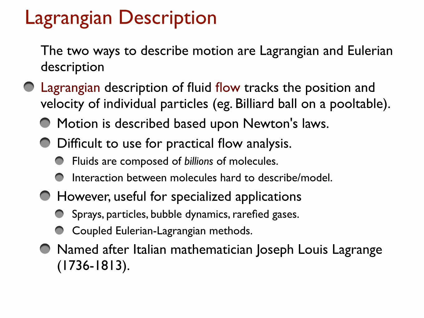
Lagrangian Description

The two ways to describe motion are Lagrangian and Eulerian description

Lagrangian description of fluid flow tracks the position and velocity of individual particles (eg. Billiard ball on a pooltable).

Motion is described based upon Newton's laws. Difficult to use for practical flow analysis.

Fluids are composed of billions of molecules.Interaction between molecules hard to describe/model.

However, useful for specialized applicationsSprays, particles, bubble dynamics, rarefied gases.Coupled Eulerian-Lagrangian methods.

Named after Italian mathematician Joseph Louis Lagrange (1736-1813).

ì

Eulerian Description

Eulerian description of fluid flow: a flow domain or control volume is defined by which fluid flows in and out.We define field variables which are functions of space and time.

Pressure field, P=P(x,y,z,t)

Velocity field,

Acceleration field,

These (and other) field variables define the flow field.Well suited for formulation of initial boundary-value problems (PDE's).Named after Swiss mathematician Leonhard Euler (1707-1783).

ì

Lagrangian vs. Eulerian description

A fluid flow field can be thought of as being comprised of a large number of finite sized fluid particles which have mass, momentum, internal energy, and other properties. Mathematical laws can then be written for each fluid particle. This is the Lagrangian description of fluid motion.

Another view of fluid motion is the Eulerian description. In the Eulerian description of fluid motion, we consider how flow properties change at a fluid element that is fixed in space and time (x,y,z,t), rather than following individual fluid particles.

Governing equations can be derived using each method and converted to the other form.

ì

Coupled Eulerian-Lagrangian Method

Forensic analysis of Columbia accident: simulation of shuttle debris trajectory using Eulerian CFD for flow field and Lagrangian method for the debris.

ì

A Steady Two-Dimensional Velocity Field

A steady, incompressible, two-dimensional velocity field is given by

A stagnation point is defined as a point in the flow field where the velocity is identically zero. (a) Determine if there are any stagnation points in this flow field and, if so, where? (b) Sketch velocity vectors at several locations in the domain between x = - 2 m to 2 m and y = 0 m to 5 m; qualitatively describe the flow field.

ì

Acceleration Field

Consider a fluid particle and Newton's second law,

The acceleration of the particle is the time derivative of the particle's velocity.

However, particle velocity at a point at any instant in time t is the same as the fluid velocity,

To take the time derivative of, chain rule must be used.

,t)

Where ∂ is the partial derivative operator and d is the total derivative operator.

ì

Acceleration Field

Since

In vector form, the acceleration can be written as

First term is called the local acceleration and is nonzero only for unsteady flows.Second term is called the advective acceleration and accounts for the effect of the fluid particle moving to a new location in the flow, where the velocity is different.

!a x, y, z,t( ) = d!Vdt

= ∂!V∂t

+!V i!∇( ) !V

dxparticledt

= u,dyparticledt

= v,dzparticledt

= w

!aparticle =∂!V∂t

+ u ∂!V∂x

+ v ∂!V∂y

+ w ∂!V∂z

ì

If we move a parcel in time ΔtUsing Taylor series expansion, assuming increments over Δt are small, and ignoring Higher Order Terms

HigherOrderTerms

Dividing by Δt and taking the small limit:

Δf = ∂ f∂t

Δt + ∂ f∂x

Δx + ∂ f∂y

Δy + ∂ f∂z

Δz +

dfdt

= ∂ f∂t

+ ∂ f∂xdxdt

+ ∂ f∂ydydt

+ ∂ f∂zdzdt

Introducing the convention of d( )/dt ≡ D( )/DtDxDt

= u, DyDt

= v, DzDt

= w

DfDt

= ∂ f∂t

+ u ∂ f∂x

+ v ∂ f∂y

+ w ∂ f∂z

DfDt

= ∂ f∂t

+V ⋅∇( f )

ì

AdvectionIn mathematics and continuum mechanics, including fluid dynamics, the substantive derivative (sometimes the Lagrangian derivative, material derivative), written D/Dt, is the rate of change of some property of a small parcel of fluid.

Note that if the fluid is moving, the substantive derivative is the rate of change of fluid within the small parcel, hence the other names like fluid following derivative.

Advection is transport of a some conserved scalar quantity in a vector field.

Advective acceleration is nonlinear: source of many phenomenon and primary challenge in solving fluid flow problems.Provides “transformation” between Lagrangian and Eulerian frames.

u∂ f∂x

+ v ∂ f∂y

+ w ∂ f∂z

= V ⋅∇( f )

ì

Material Acceleration of a Steady Velocity Field

Consider the same velocity field of first example. (a) Calculate the material acceleration at the point (x = 2 m, y = 3 m). (b) Sketch the material acceleration vectors at the same array of x- and y values as in Example A.

ì

Flow Visualization

Flow visualization is the visual examination of flow-field features.Important for both physical experiments and numerical (CFD) solutions.Numerous methods

Streamlines and streamtubes

Pathlines

Streaklines

Timelines

Refractive techniques

Surface flow techniques

While quantitative study of fluid dynamics requires advanced

mathematics, much can be learned from flow visualization

ì

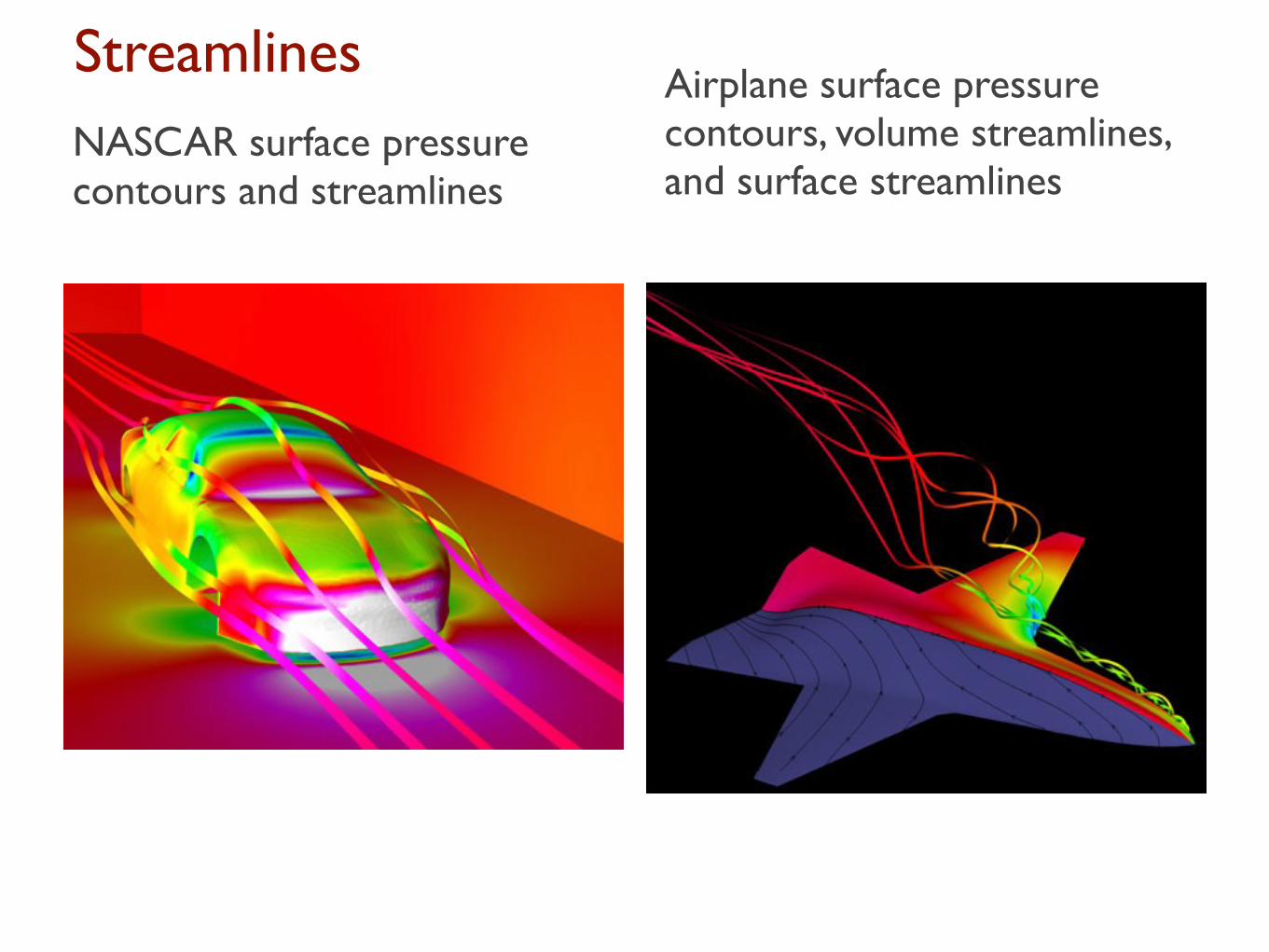
Streamlines

A Streamline is a curve that is everywhere tangent to the instantaneous local velocity vector.

Consider an arc length

must be parallel to the local velocity vector

Geometric arguments results in the equation for a streamline

ì

Streamlines in xy - analytical Solution

For the same velocity field of the example A, plot several streamlines in the right half of the flow (x > 0) and compare to the velocity vectors.

where C is a constant of integration that can be set to various values in order to plot the streamlines.

ì

StreamlinesNASCAR surface pressure contours and streamlines

Airplane surface pressure contours, volume streamlines, and surface streamlines

ì

StreamtubeA streamtube consists of a bundle of streamlines (both are instantaneous quantities).

Fluid within a streamtube must remain there and cannot cross the boundary of the streamtube.In an unsteady flow, the streamline pattern may change significantly with time⇒ the mass flow rate passing

through any cross-sectional slice of a given streamtube must remain the same

ì

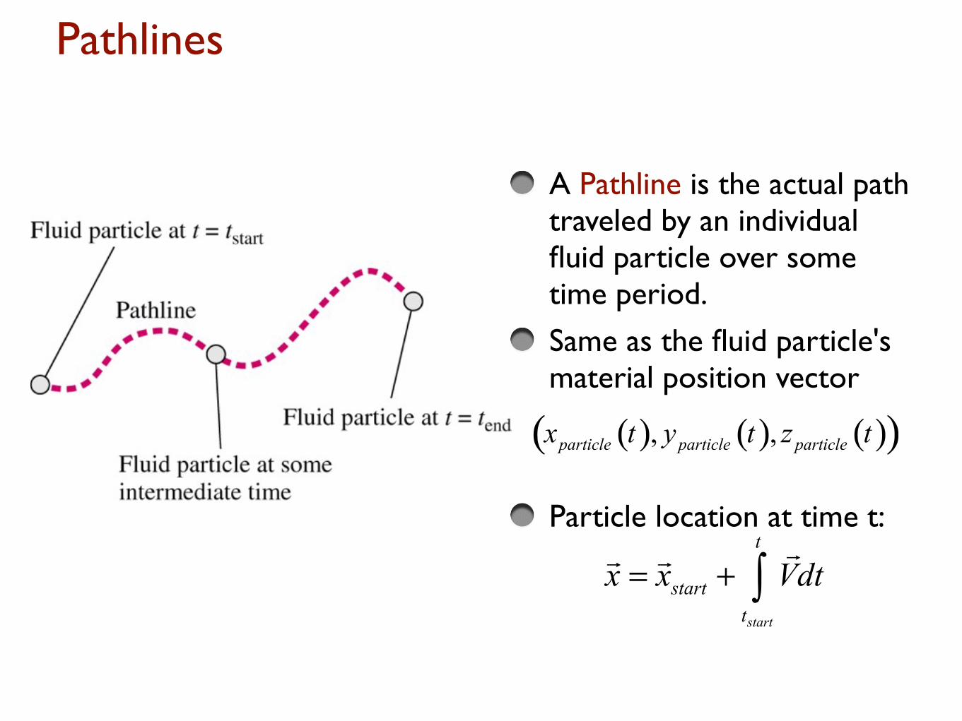
Pathlines

A Pathline is the actual path traveled by an individual fluid particle over some time period.

Same as the fluid particle's material position vector

Particle location at time t:

ì

Pathlines

A modern experimental technique called particle image velocimetry (PIV) utilizes (tracer) particle pathlines to measure the velocity field over an entire plane in a flow (Adrian, 1991).

ì

Streaklines

A Streakline is the locus of fluid particles that have passed sequentially through a prescribed point in the flow.

Easy to generate in experiments: dye in a water flow, or smoke in an airflow.

ì

Streaklines

ì

Streaklines

Cylinder

x/D

A smoke wire with mineral oil was heated to generate a rake of Streaklines

Karman Vortex street

ì

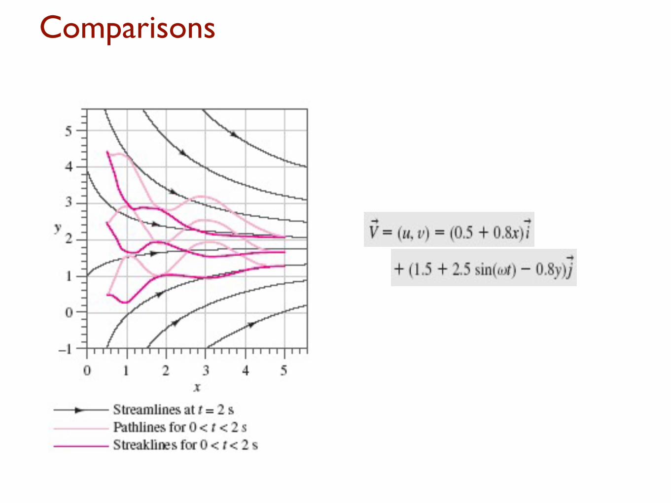
Comparisons

For steady flow, streamlines, pathlines, and streaklines are identical.

For unsteady flow, they can be very different. Streamlines are an instantaneous picture of the flow fieldPathlines and Streaklines are flow patterns that have a time history associated with them. Streakline: instantaneous snapshot of a time-integrated flow pattern.Pathline: time-exposed flow path of an individual particle.

ì

Comparisons

ì

Timelines

A Timeline is a set of adjacent fluid particles that were marked at the same (earlier) instant in time.

Timelines can be generated using a hydrogen bubble wire.

ì

Timelines

Timelines produced by a hydrogen bubble wire are used to visualize the boundary layer velocity profile shape.

ì

Plots of Flow Data

Flow data are the presentation of the flow properties varying in time and/or space.A Profile plot indicates how the value of a scalar property varies along some desired direction in the flow field.A Vector plot is an array of arrows indicating the magnitude and direction of a vector property at an instant in time.A Contour plot shows curves of constant values of a scalar property for the magnitude of a vector property at an instant in time.

ì

Profile plot

Profile plots of the horizontal component of velocity as a function of vertical distance; flow in the boundary layer growing along a horizontal flat plate.

ì

Vector plot

ì

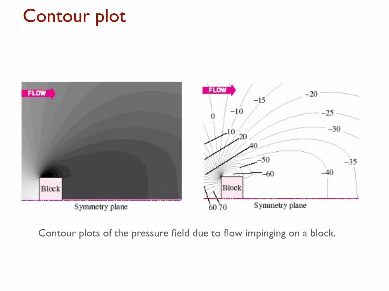
Contour plot

Contour plots of the pressure field due to flow impinging on a block.

ì

Kinematic Description

In fluid mechanics, an element may undergo four fundamental types of motion:

TranslationRotationLinear strainShear strain

Because fluids are in constant motion, motion and deformation is best described in terms of rates

velocity: rate of translationangular velocity: rate of rotationlinear strain rate: rate of linear strainshear strain rate: rate of shear strain

ì

Rate of Translation and Rotation

To be useful, these rates must be expressed in terms of velocity and derivatives of velocity

The rate of translation vector is described as the velocity vector. In Cartesian coordinates:

Rule of thumb for rotation

ì

Rate of Translation and Rotation

Rate of rotation at a point is defined as the average rotation rate of two initially perpendicular lines that intersect at that point. The rate of rotation vector in Cartesian coordinates:

ì

Linear Strain RateLinear Strain Rate is defined as the rate of increase in length per unit length.

In Cartesian coordinates:

Volumetric strain rate in Cartesian coordinates

Since the volume of a fluid element is constant for an incompressible flow, the volumetric strain rate must be zero.

ì

Shear Strain Rate

Shear Strain Rate at a point is defined as half of the rate of decrease of the angle between two initially perpendicular lines that intersect at a point.

Shear strain rate can be expressed in Cartesian coordinates as:

ì

Shear Strain Rate

We can combine linear strain rate and shear strain rate into one symmetric second-order tensor called the strain-rate tensor

ì

Shear Strain Rate

Purpose of our discussion of fluid element kinematics: Better appreciation of the inherent complexity of fluid dynamics Mathematical sophistication required to fully describe fluid motion

Strain-rate tensor is important for numerous reasons. For example,

Develop relationships between fluid stress and strain rate.

ì

Vorticity and Rotationality

The vorticity vector is defined as the curl of the velocity vector , a measure of rotation of a fluid particle.

Vorticity is equal to twice the angular velocity of a fluid particle Cartesian coordinates

Cylindrical coordinate

In regions where ζ = 0, the flow is called irrotational

Elsewhere, the flow is called rotational

ì

Vorticity and Rotationality

ì

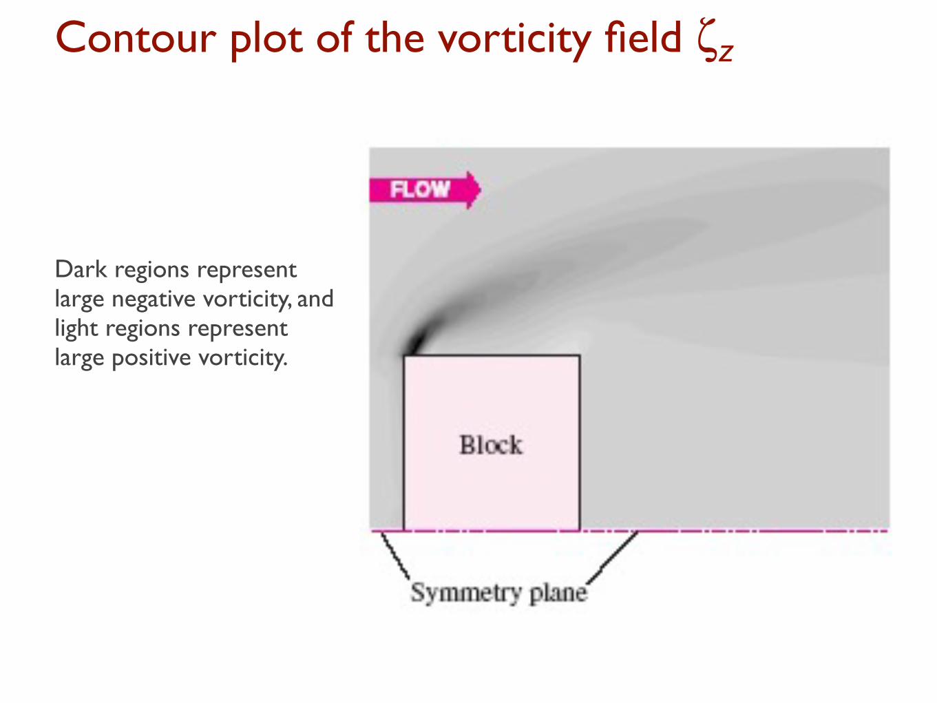
Contour plot of the vorticity field ζz

Dark regions represent large negative vorticity, and light regions represent large positive vorticity.

ì

Comparison of Two Circular Flows

Special case: consider two flows with circular streamlines

ì

Comparison

A Ferris wheelA merry-go-round orroundabout

ì

Reynolds—Transport Theorem (RTT)

A system is a quantity of matter of fixed identity. No mass can cross a system boundary.

A control volume is a region in space chosen for study. Mass can cross a control surface.

CVfixed,

nondeformable

Systemdeformable

ì

Reynolds—Transport Theorem (RTT)

The fundamental conservation laws (conservation of mass, energy, and momentum) apply directly to systems.However, in most fluid mechanics problems, control volume analysis is preferred over system analysis (for the same reason that the Eulerian description is usually preferred over the Lagrangian description).Therefore, we need to transform the conservation laws from a system to a control volume. This is accomplished with the Reynolds transport theorem (RTT).

ì

Reynolds—Transport Theorem (RTT)

ì

Reynolds—Transport Theorem (RTT)

the time rate of change of the property B of the system is equal to the time rate of change of B of the control volume plus the net flux of B out of the control volume by mass crossing the control surface.

ì

Reynolds—Transport Theorem (RTT)

The total amount of property B within the control volume must be determined by integration:

Therefore, the system-to-control-volume transformation for a fixed control volume:

ì

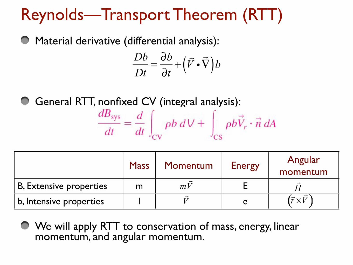
Reynolds—Transport Theorem (RTT)Material derivative (differential analysis):

General RTT, nonfixed CV (integral analysis):

We will apply RTT to conservation of mass, energy, linear momentum, and angular momentum.

Mass Momentum Energy Angular momentum

B, Extensive properties m E

b, Intensive properties 1 e

DbDt

= ∂b∂t

+!V i!∇( )b

ì

Reynolds—Transport Theorem (RTT)

Interpretation of the RTT:Time rate of change of the property B of the system is equal to (Term 1) + (Term 2)Term 1: the time rate of change of B of the control volumeTerm 2: the net flux of B out of the control volume by mass crossing the control surface

dBsysdt

= ∂∂t

ρb( )dV +CV∫ ρb

!V i !n dA

CS∫

ì

RTT Special Cases

For moving and/or deforming control volumes,

Where the absolute velocity V in the second term is replaced by the relative velocity Vr = V –VCS

Vr is the fluid velocity expressed relative to a coordinate system moving with the control volume.

ì

RTT Special Cases

For steady flow, the time derivative drops out,

For control volumes with well-defined inlets and outlets

0dBsysdt

= ∂∂t

ρb( )dV +CV∫ ρb

!Vr i!n dA

CS∫ = ρb!Vr i!n dA

CS∫

dBsysdt

= ddt

ρbdV +CV∫ ρavgbavg

out∑ Vr ,avg A− ρavgbavg

in∑ Vr ,avg A

ì

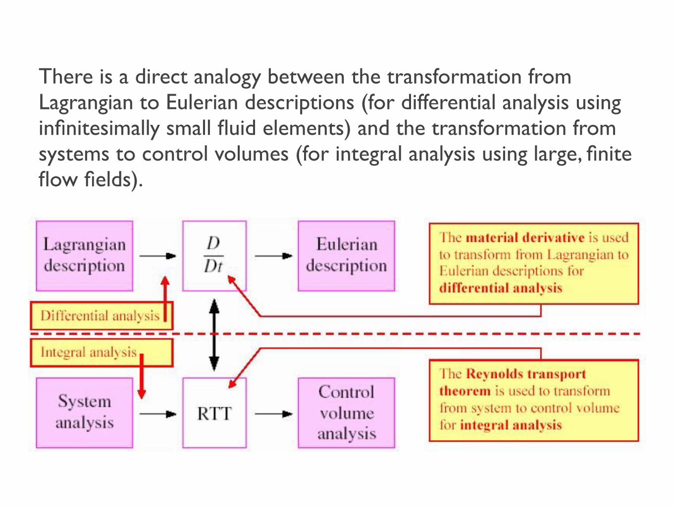
Reynolds—Transport Theorem (RTT)There is a direct analogy between the transformation from Lagrangian to Eulerian descriptions (for differential analysis using infinitesimally small fluid elements) and the transformation from systems to control volumes (for integral analysis using large, finite flow fields).