Fluid Flow Handouts

8/13/2019 Fluid Flow Handouts

http://slidepdf.com/reader/full/fluid-flow-handouts 1/6

26/10/20

Lauren Gust

October 26, 2010

Laminar and Turbulent Flow Laminar flow:

Capillaries, microfluidics, low velocities

Prediction of fluid movement and streamlines

Tur u ent ow:

Aerodynamics

House piping

Energy storage

Heat exchangers

M Van Dyke, “An Album of Fluid Motion”

(Parabolic Press, Stanford, CA, 1982), p. 89.

Vortex Shedding Major loss of energy in flying objects

Airplanes, flag waving

US Geological Survey Website, http://landsat.gsfc.nasa.go/earthasart/vortices.html

Objectives To determine the velocity profile for laminar,

turbulent, and transition flow regimes

To study vortex shedding from cylindrical objects in air



26/10/20

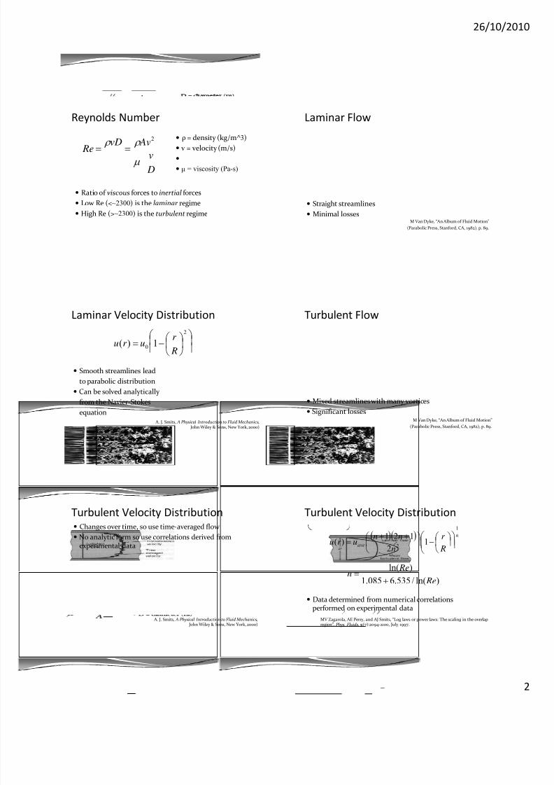
Reynolds Number

ρ = density (kg/m^3) v = velocity (m/s)

v

AvvD Re

2

μ = viscosity (Pa-s) D

Ratio of viscous forces to inertial forces

Low Re (<~2300) is the laminar regime

High Re (>~2300) is the turbulent regime

Laminar Flow

Straight streamlines

Minimal lossesM Van Dyke, “An Album of Fluid Motion”


Laminar Velocity Distribution

2

0 1)( R

r ur u

Smooth streamlines lead

to parabolic distribution

Can be solved analytically

from the Navier‐Stokes

equation A. J. Smits, A Physical Introduction to Fluid Mechanics,

John Wiley & Sons, New York, 2000)

Turbulent Flow

Mixed streamlines with many vortices

Significant lossesM Van Dyke, “An Album of Fluid Motion”


Turbulent Velocity Distribution Changes over time, so use time‐averaged flow

No analytic form so use correlations derived from

experimental data

A. J. Smits, A Physical Introduction to Fluid Mechanics, John Wiley & Sons, New York, 2000)

Turbulent Velocity Distribution

n

ave

R

r

n

nnur u

1

21

2

121)(

Data determined from numerical correlations performed on experimental data

)ln(/535.6085.1

)ln(

Re

Ren

MV Zagarola, AE Perry, and AJ Smits, “Log laws or power laws: The scaling in the overlap

region”, Phys. Fluids, 9(7):2094‐2100, July, 1997.



26/10/20

Entrance Considerations Assume that the flow is fully developed : the

measuring position is far enough from the entrance of the pipe that entrance effects are irrelevant

, e =0.03

For turbulent flow, vortices lead to more mixing, shorter entry lengths: Le=10D‐40D

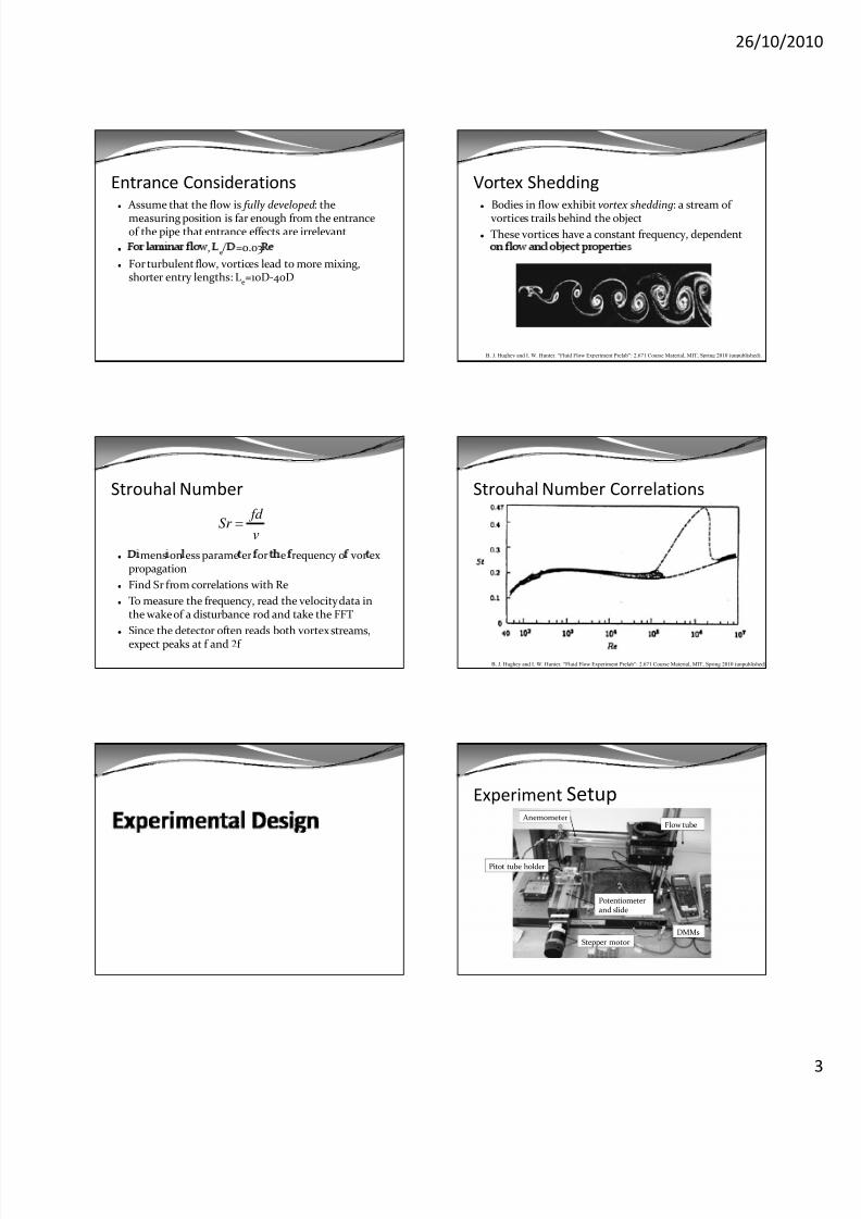
Vortex Shedding Bodies in flow exhibit vortex shedding: a stream of

vortices trails behind the object

These vortices have a constant frequency, dependent

B. J. Hughey and I. W. Hunter. “Fluid Flow Experiment Prelab”: 2.671 Course Material, MIT, Spring 2010 (unpublished).

Strouhal Number

v

fd Sr

mens on ess parame er or e requency o vor ex propagation

Find Sr from correlations with Re

To measure the frequency, read the velocity data in

the wake of a disturbance rod and take the FFT

Since the detector often reads both vortex streams,

expect peaks at f and 2f

Strouhal Number Correlations


Experiment Setup

Flow tube Anemometer

Stepper motor

Potentiometer and slide

DMMs

Pitot tube holder



26/10/20

Linear Potentiometer and Motor Anemometer is driven on a linear

slide using a stepper motor.

Distance moved is correlated

using voltage output from a

linear potentiometer.

Pitot Tube Flow measurement based on the Bernoulli equation

Neglect pipe friction

The gas velocity is given by:

1212

PPuug

g

Hot Film Anemometer Thin metal film is heated by a power supply

Increased gas velocity across the film requires more voltage to maintain a constant temperature

Anemometer vo tage s re ate to ow ve oc ty y:

ganem uC C V 10

2

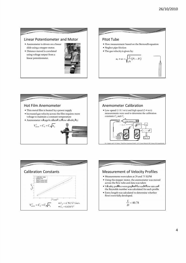
Anemometer Calibration Low‐speed (≤ 0.1 m/s) and high speed (2-4 m/s)

measurements were used to determine the calibration

constants C 0 and C 1

VanemVpress

8 V

N2 Gas, velocity ug

P2

2

1 P1 = ?

ug

Pa/mV

C0 , C 1

)(2

121 PPug

ganem uC C V 10

2


Calibration Constants

C0 = 4.791 V2/√m/s

C1 = 6.634 V2ganem uC C V 10

2

Measurement of Velocity Profiles Measurements were taken at 20 and 75 SLPM

Using the stepper motor, the anemometer was moved

across the flow tube and data was taken

Ve oc ty pro es were grap e or eac ow rate an

the Reynolds number was calculated for each profile

Entry length was calculated to determine whether flows were fully developed.

78.40 D

L



26/10/20

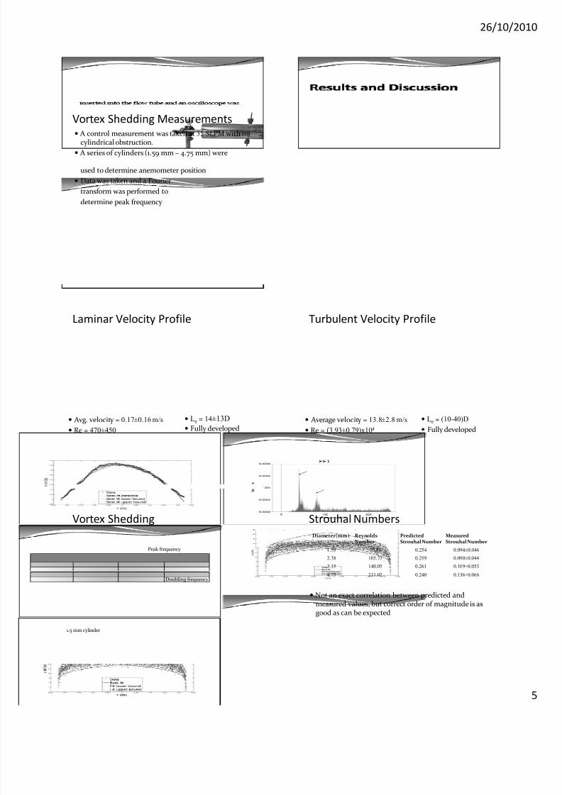
Vortex Shedding Measurements A control measurement was taken at 35 SLPM with no

cylindrical obstruction.

A series of cylinders (1.59 mm – 4.75 mm) were

used to determine anemometer position

Data was taken and a Fourier

transform was performed to

determine peak frequency

Laminar Velocity Profile

Avg. velocity = 0.17±0.16 m/s

Re = 470±450

Le = 14±13D Fully developed

Turbulent Velocity Profile

Average velocity = 13.8±2.8 m/s

Re = (3.93±0.79)x104

Le = (10-40)D

Fully developed

Vortex Shedding

Peak frequency

1.5 mm cylinder

Doubling frequency

Strouhal Numbers

Diameter(mm) ReynoldsNumber

Predicted Strouhal Number

MeasuredStrouhal Number

1.59 70.53 0.254 0.094±0.046

2.38 105.73 0.259 0.090±0.044

3.15 140.05 0.261 0.109±0.053

4.75 211.02 0.240 0.136±0.066

Not an exact correlation between predicted and

measured values, but correct order of magnitude is as good as can be expected



26/10/20

Conclusion Laminar and turbulent profiles fit theoretical profiles

Strouhal number in vortex shedding gave order of magnitude estimates

xper menta wea nesses

Noise in data

Anemometer motion

Air currents in environment

We can use our data to do analysis of laminar and turbulent systems.

Future experiments

AcknowledgementsThe authors would like to thank Robert Truax and Dr. Barbara Hughey for their assistance in collecting and

analyzing data and the generous donors who provided

lounge.

Fluid Flow Handouts

Documents

Transcript of Fluid Flow Handouts