MDP 631 Industrial Operations Research Lecture 3 Special cases in Simplex, Sensitivity analysis,...

MDP 631Industrial Operations Research

Lecture 3

Special cases in Simplex, Sensitivity analysis, Primal-Dual formulation of LP models and Interior Point Method

Today’s lecture

• Special cases in the Simplex Algorithm

• Adapting non-standard LP models

• Sensitivity Analysis

• Primal-Dual Formulation of LP models

• Interior point method for solving LP models

Special cases in the Simplex Algorithm

• Tie for entering variable

• Tie for leaving variable (degeneracy)

• No leaving variable

• Multiple optimal solutions

Tie for entering variable (Example)

Iteration Basic variable

Eq. Coefficient ofRHS ratio

Z x1 x2 x3 x4

0

Z (0) 1 -3 -3 0 0 0

x3 (1) 0 1 4 1 0 8

x4 (2) 0 1 2 0 1 4

Maximize Z = 3 x1 + 3 x2

Subject to: x1 + 4 x2 8

x1 + 2 x2 4

x1, x2 ≥ 0

Here, you may choose either x1 or x2 as the entering variable in the next simplex iteration.

Tie for entering variable

• If there are two negative coefficients in the Z row of the Simplex tableaux with the same maximum absolute values, you may choose arbitrarily any one of their corresponding non-basic variables to become the entering variable.

Tie for leaving variable—degeneracy (Example)



Z x1 x2 x3 x4

0

Z (0) 1 -3 -9 0 0 0

x3 (1) 0 1 4 1 0 8

x4 (2) 0 1 2 0 1 4

1

Z (0) 1 -3/4 0 9/4 0 18

x2 (1) 0 1/4 1 1/4 0 2

x4 (2) 0 1/2 0 -1/2 1 0

2

2

8

0

2

Z (0) 1 0 0 3/2 3/2 18

x2 (1) 0 0 1 1/2 -1/2 2

x1 (2) 0 1 0 -1 1 0



x1 + 2 x2 4

x1, x2 ≥ 0

Tie for leaving variable—degeneracy (Example)



Z x1 x2 x3 x4

0

Z (0) 1 -3 -9 0 0 0

x3 (1) 0 1 4 1 0 8

x4 (2) 0 1 2 0 1 4

1

Z (0) 1 3/2 0 0 9/2 18

x4 (1) 0 -1 0 1 -2 0

x2 (2) 0 1/2 1 0 1/2 2

2

2

2

Z (0)

x2 (1)

x1 (2)



x1 + 2 x2 4

x1, x2 ≥ 0

Degeneracy (example)



x1 + 2 x2 4

x1, x2 ≥ 0

Why degeneracy is not good?

• The previous example showed that degeneracy did not prevent Simplex from finding the optimal solution. It only showed that it may take longer to reach the optimal solution if it chooses one of the variables over the other as leaving variable.

Why degeneracy is not good?

• Unfortunately, on other examples, degeneracy may lead to cycling, i.e. a sequence of pivots that goes through the same tableaus and repeats itself indefinitely. In theory, cycling can be avoided by choosing the entering variable with smallest index, among all those with a negative coefficient in row 0, and by breaking ties in the minimum ratio test by choosing the leaving variable with smallest index (this is known as Bland's rule).

• This rule, although it guaranties that cycling will never occur, turns out to be somewhat inefficient. Actually, in commercial codes, no effort is made to avoid cycling. This may come as a surprise, since degeneracy is a frequent occurrence. But there are two reasons for this:

– Although degeneracy is frequent, cycling is extremely rare.

– The precision of computer arithmetic takes care of cycling by itself: round off errors accumulate and eventually gets the method out of cycling.

No leaving variable (Example)

Maximize Z = x1 + 2 x2

Subject to: x1 – x2 10

2 x1 40

x1, x2 ≥ 0


Eq. Coefficient of

RHS ratioZ x1 x2 x3 x4

0

Z (0) 1 -1 -2 0 0 0

x3 (1) 0 1 -1 1 0 10

x4 (2) 0 2 0 0 1 40

No leaving variable (unbounded Z)

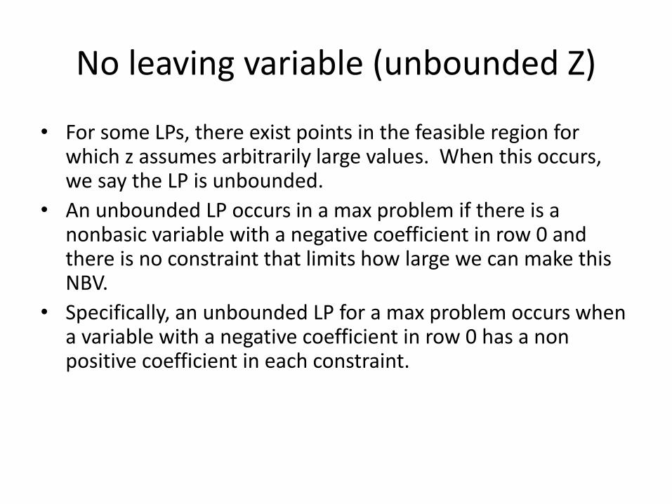
• For some LPs, there exist points in the feasible region for which z assumes arbitrarily large values. When this occurs, we say the LP is unbounded.

• An unbounded LP occurs in a max problem if there is a nonbasic variable with a negative coefficient in row 0 and there is no constraint that limits how large we can make this NBV.

• Specifically, an unbounded LP for a max problem occurs when a variable with a negative coefficient in row 0 has a non positive coefficient in each constraint.

Multiple optimal solutions (Example)

Here, x3 is a non-basic variable and its coefficient in the Z equation is zero. This indicates a case of multiple optimal solutions.

Multiple optimal solutions

• For some LPs, more than one extreme point is optimal. If an LP has more than one optimal solution, it has multiple optimal solutions or alternative optimal solutions.

• If there is no nonbasic variable (NBV) with a zero coefficient in row 0 of the optimal tableau, the LP has a unique optimal solution.

Adapting other LP forms

• Equality constraints

• Negative right-hand-sides

• Inequality constraints of the form ≥

• Minimization

• Variables that can be negative

Equality Constraints

When the third functional constraint becomes an equality constraint, the feasible region for the Wyndor Glass Co. problem becomes the line segment between (2, 6) and (4, 3).


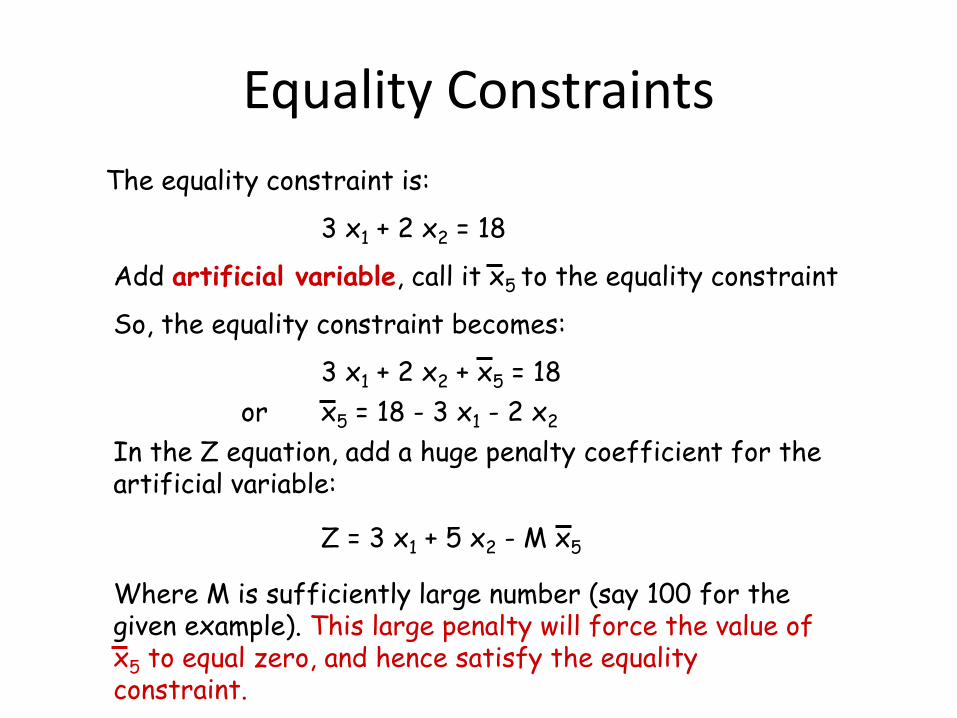
The equality constraint is:

3 x1 + 2 x2 = 18

Add artificial variable, call it x5 to the equality constraint

So, the equality constraint becomes:

3 x1 + 2 x2 + x5 = 18

In the Z equation, add a huge penalty coefficient for the artificial variable:

Z = 3 x1 + 5 x2 - M x5

Where M is sufficiently large number (say 100 for the given example). This large penalty will force the value of x5 to equal zero, and hence satisfy the equality constraint.

x5 = 18 - 3 x1 - 2 x2or


The standard (augmented) simplex form becomes:

Then, solve the problem using the standard simplex tableaux as usual.

So, we can rewrite the Z equation as:

Z = 3 x1 + 5 x2 - 100 x5

= 3 x1 + 5 x2 – 100 (18 - 3 x1 - 2 x2)

= 303 x1 + 205 x2 - 1800

(0) Z - 303 x1 - 205 x2 = - 1800

(1) x1 + x3 = 4

(2) 2 x2 + x4 = 12

(3) 3 x1 + 2 x2 + x5 = 18

x1 , x2 , x3 , x4 , x5 ≥ 0

Negative right-hand-sides

If you encounter a constraint with a negative RHS, you have to multiply the constraint by -1 to change the RHS to a positive quantity.

But, in doing that you should account for the reversal of the inequality.

Example: Consider the following constraint:

3 x1 – 2 x2 ≥ -6

This should be changed to

- 3 x1 + 2 x2 6

before writing the standard (augmented) simplex

form of your problem

Inequality constraints of the form ≥

Consider the following example:

This constraint is in the form ≥


Graphical representation of the feasible region of the previous example.


This is called surplus variable, which is firstly added to convert the inequality to an equality.

Then an artificial variable is added the same way we did for the equality constraint.

After treating the equality constraint as well, the LP model becomes:

Minimization

Minimization

In the previous example:

Variables that can be negative

• If a decision variable (y) is unrestricted in sign, it can be replaced in the model by:

y = y + - y –

Where y + and y – 0

In-Class Assignment

• Consider the following LP model. Construct the corresponding augmented form:

Minimize Z = 3 x1 + 2 x2

Subject to:x1 + 2 x2 6 (1)

2 x1 + x2 8 (2)- x1 + x2 2 (3)

x2 2 (4)3 x1 + 5 x2 ≥ 15 (5)x1 and x2 ≥ 0

The Simplex Standard LP Form

Maximize (-Z)Subject to:(-Z) + 3 x1 + 2 x2 + M x8 = 0 (0)

x1 + 2 x2 + x3 = 6 (1)2 x1 + x2 + x4 = 8 (2)- x1 + x2 + x5 = 2 (3)

x2 + x6 = 2 (4)3 x1 + 5 x2 - x7 + x8 = 15 (5)

Where M is sufficiently large number. We choose M = 100

Substituting artificial variable in Z equation

From equation (5), we get:x8 = 15 - 3 x1 - 5 x2 + x7

By substituting the value of x8 in equation (0), we rewrite it as follows:

(-Z) + 3 x1 + 2 x2 + 100 x8 = 0(-Z) - 297 x1 - 498 x2 + 100 x7 = -1500

Simplex iterations

Iter. Basic

Varia

ble

Eq. Coefficient of RHS Ratio

(-Z) x1 x2 x3 x4 x5 x6 x7 x8

0

-Z (0) 1 -297 -498 0 0 0 0 100 0 -1500

x3 (1) 0 1 2 1 0 0 0 0 0 6 3

x4 (2) 0 2 1 0 1 0 0 0 0 8 8

x5 (3) 0 -1 1 0 0 1 0 0 0 2 2

x6 (4) 0 0 1 0 0 0 1 0 0 2 2

x8 (5) 0 3 5 0 0 0 0 -1 1 15 3

1

-Z (0) 1 -297 0 0 0 0 498 100 0 -504

x3 (1) 0 1 0 1 0 0 -2 0 0 2 2

x4 (2) 0 2 0 0 1 0 -1 0 0 6 3

x5 (3) 0 -1 0 0 0 1 -1 0 0 0 X

x2 (4) 0 0 1 0 0 0 1 0 0 2 X

x8 (5) 0 3 0 0 0 0 -5 -1 1 5 5/3

2

-Z (0) 1 0 0 0 0 0 3 1 99 -9

x3 (1) 0 0 0 1 0 0 -1/3 1/3 -1/3 1/3

x4 (2) 0 0 0 0 1 0 7/3 2/3 -2/3 8/3

x5 (3) 0 0 0 0 0 1 -8/3 -1/3 1/3 5/3

x2 (4) 0 0 1 0 0 0 1 0 0 2

x1 (5) 0 1 0 0 0 0 -5/3 -1/3 1/3 5/3

Optimal solution has been found.

The optimal solution found using Simplex is: x1 = 5/3 and x2 = 2 with Z = 9. This solution is identical to that obtained using the graphical method.

Graphical solution and Simplex Iterations

Notice that as long as x8 has a value greater than zero at any Simplex iteration, the current

solution is infeasible

Sensitivity Analysis

What if there is uncertainly about one or more values in the LP model?

Sensitivity analysis allows us to determine how “sensitive” the optimal solution is to changes in data values.

This includes analyzing changes in:

1. An Objective Function Coefficient (OFC)

2. A Right Hand Side (RHS) value of a constraint

Graphical Sensitivity Analysis

We can use the graph of an LP to see what happens when:

1. An OFC changes, or

2. A RHS changes

Recall the Flair Furniture problem

Flair Furniture Problem

Max 7T + 5C (profit)

Subject to the constraints:

3T + 4C < 2400 (carpentry hrs)

2T + 1C < 1000 (painting hrs)

C < 450 (max # chairs)

T > 100 (min # tables)

T, C > 0 (nonnegativity)

Objective FunctionCoefficient (OFC) Changes

What if the profit contribution for tables changed from $7 to $8 per table?

8Max 7 T + 5 C (profit)

Clearly profit goes up, but would we want to make more tables and less chairs?(i.e. Does the optimal solution change?)

X

0 100 200 300 400 500 T

C

500

400

300

200

100

0

Optimal Corner

(T=320, C=360)

Still optimal

Feasible

Region

Original

Objective Function

7T + 5 C = $4040

Revised

Objective Function

8T + 5 C = $4360

C

1000

600

450

0

Feasible

Region

0 100 500 800 T

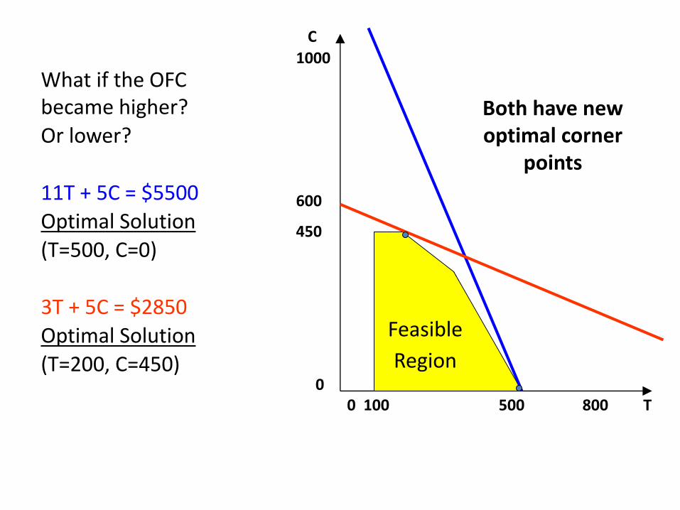
What if the OFC became higher?

Or lower?

11T + 5C = $5500

Optimal Solution

(T=500, C=0)

3T + 5C = $2850

Optimal Solution

(T=200, C=450)

Both have new optimal corner

points

Characteristics of OFC Changes

• There is no effect on the feasible region

• The slope of the level profit line changes

• If the slope changes enough, a different corner point will become optimal

• There is a range for each OFC where the current optimal corner point remains optimal.

• If the OFC changes beyond that range a new corner point becomes optimal.

• How can we determine that range?

Right Hand Side (RHS) Changes

What if painting hours available changed from 1000 to 1300?

13002T + 1C < 1000(painting hrs)

This increase in resources could allow us to increase production and profit.

X

0 100 200 300 400 500 600 T

C

500

400

300

200

100

0

Original

Feasible

Region

Feasible region becomes larger

New optimalcorner point

(T=560,C=180)Profit=$4820

Old optimal corner point

(T=320,C=360)Profit=$4040

Sensitivity Analysis Examples

Example 1

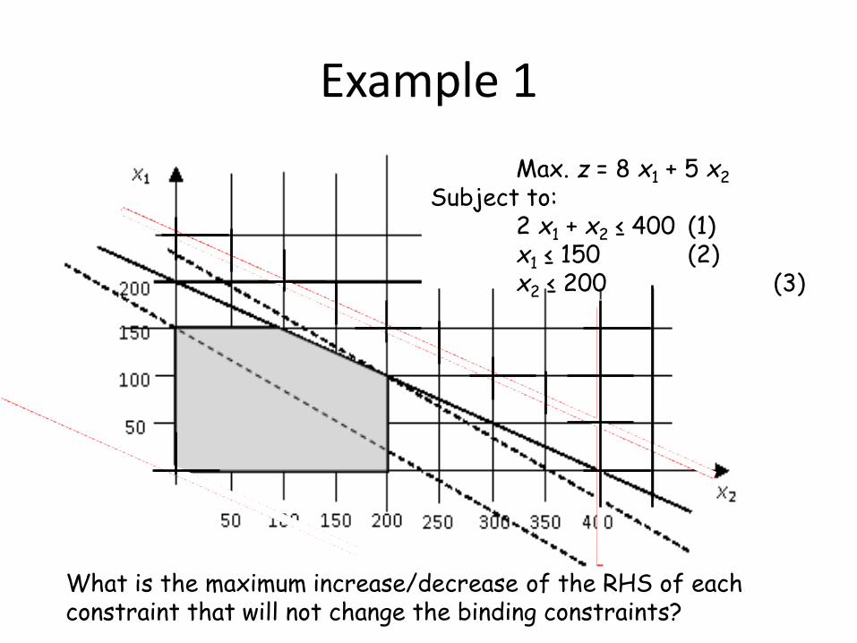
Max. z = 8 x1 + 5 x2

Subject to:2 x1 + x2 ≤ 400 (1)x1 ≤ 150 (2)x2 ≤ 200 (3)

The optimal solution is x1 = 100 and x2 = 200Constraints (1) and (3) are binding constraints

Example 1

Max. z = 8 x1 + 5 x2

Subject to:2 x1 + x2 ≤ 400 (1)x1 ≤ 150 (2)x2 ≤ 200 (3)

What is the maximum increase/decrease of the RHS of each constraint that will not change the binding constraints?

Example 1 (Cont.)

Max. z = 8 x1 + 5 x2

Subject to:2 x1 + x2 ≤ 400 (1)x1 ≤ 150 (2)x2 ≤ 200 (3)

What is the maximum increase/decrease of the RHS of each constraint that will not change the binding constraints?

Example 1 (Cont.)

Max. z = 8 x1 + 5 x2

Subject to:2 x1 + x2 ≤ 400 (1)x1 ≤ 150 (2)x2 ≤ 200 (3)

For each one of the binding constraints (1) and (3), by how much the objective value of the optimal solution will be increased if one unit is added to the RHS quantity?

Example 1 (Cont.)

The binding constraints are constraints (1) and (3), which give us the following two equations at the optimal point:

x2 = 200and 2 x1 + x2 = 400

By adding d1 to the RHS of constraint (1), we get2 x1 + 200 = 400 + d1 or x1 = 100 + d1/2

Now, by substituting x1 and x2 in the z equation, we getz = 8 (100 + d1/2) + 5 * 200 = 1800 + 4 d1

Max. z = 8 x1 + 5 x2

Subject to:2 x1 + x2 ≤ 400 (1)x1 ≤ 150 (2)x2 ≤ 200 (3)

Shadow price of constraint (1)

Example 1 (Cont.)

The binding constraints are constraints (1) and (3), which give us the following two equations at the optimal point:

x2 = 200and 2 x1 + x2 = 400By adding d3 to the RHS of the type 2 market share constraint (3), we get

x2 = 200 + d3 and 2 x1 + 200 + d3 = 400 → x1 = 100 – d3/2

Now, by substituting x1 and x2 in the z equation, we getz = 8 (100 – d3/2) + 5 * (200 + d3) = 1800 + d3

Max. z = 8 x1 + 5 x2

Subject to:2 x1 + x2 ≤ 400 (1)x1 ≤ 150 (2)x2 ≤ 200 (3)

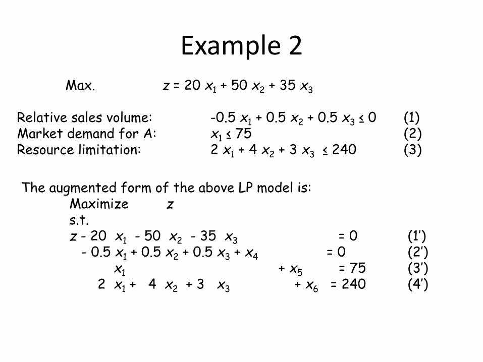
Example 2Max. z = 20 x1 + 50 x2 + 35 x3

Relative sales volume: -0.5 x1 + 0.5 x2 + 0.5 x3 ≤ 0 (1)Market demand for A: x1 ≤ 75 (2)Resource limitation: 2 x1 + 4 x2 + 3 x3 ≤ 240 (3)

The augmented form of the above LP model is:Maximize zs.t.z - 20 x1 - 50 x2 - 35 x3 = 0 (1’)

- 0.5 x1 + 0.5 x2 + 0.5 x3 + x4 = 0 (2’)x1 + x5 = 75 (3’)

2 x1 + 4 x2 + 3 x3 + x6 = 240 (4’)

Example 2 (Cont.)

Iteration

#

Basic

variables

Coefficient of RHS Ratio

z x1 x2 x3 x4 x5 x6

1 z 1 -20 -50 -35 0 0 0 0

x4 0 -0.5 0.5 0.5 1 0 0 0+d1 0

x5 0 1 0 0 0 1 0 75+d2 ---

x6 0 2 4 3 0 0 1 240+d3 60

2 z 1 -70 0 15 100 0 0 0+100d1

x2 0 -1 1 1 2 0 0 0+2d1 ---

x5 0 1 0 0 0 1 0 75+d2 75

x6 0 6 0 -1 -8 0 1 240+d3-8d1 40

3 z 1 0 0 10/3 20/3 0 70/6 2800+(20/3)d1+(70/6)d3

x2 0 0 1 5/6 2/3 0 1/6 40+(2/3)d1+(1/6)d3

x5 0 0 0 1/6 4/3 1 -1/6 35+(4/3)d1+d2-(1/6)d3

x1 0 1 0 -1/6 -4/3 0 1/6 40-(4/3)d1+(1/6)d3 ---

Example 2 (Cont.)To determine its allowable range for increasing/decreasing the resource limit constraint, put d1 = d2 = 0

Since all basic variables in the last Simplex tableau must be greater than or equal zero, we get:

40+ (1/6)d3 ≥ 0

35+-(1/6)d3 ≥ 0

and 40+(1/6)d3 ≥ 0

The above three inequalities will give us the following range for d3

-240 ≤ d3 ≤ 210

Primal-Dual Formulation of LP Models

What is dual problem?

• One of the most important discoveries in the early

development of linear programming was the concept

of duality.

• Every linear programming problem is associated with

another linear programming problem called the dual.

• The relationships between the dual problem and the

original problem (called the primal) prove to be

extremely useful in a variety of ways.

The dual problem uses exactly the same parameters as the primal problem, but in different location.

Primal and Dual Problems

Primal Problem Dual Problem

Max

s.t.

Min

s.t.

=

=n

j

jjxcZ1

, =

=m

i

ii ybW1

,

=

n

j

ijij bxa1

, =

m

i

jiij cya1

,

for for.,,2,1 mi = .,,2,1 nj =

for .,,2,1 mi =for .,,2,1 nj =,0jx ,0iy

In matrix notation

Primal Problem Dual Problem

Maximize

subject to

.0x .0y

Minimize

subject to

bAx cyA

,cxZ = ,ybW =

Where and are row

vectors but and are column vectors.

c myyyy ,,, 21 =b x

Example

Max

s.t.

Min

s.t.

Primal Problemin Algebraic Form

Dual Problem in Algebraic Form

,53 21 xxZ +=

,18124 321 yyyW ++=

1823 21 + xx

122 2 x41x

0x,0x 21

522 32 + yy

33 3 + y1y

0y,0y,0y 321

Max

s.t.

Primal Problem in Matrix Form

Dual Problem in Matrix Form

Min

s.t.

,5,32

1

=

x

xZ

18

12

4

,

2

2

0

3

0

1

2

1

x

x

.0

0

2

1

x

x .0,0,0,, 321 yyy

5,3

2

2

0

3

0

1

,, 321

yyy

=

18

12

4

,, 321 yyyW

Primal-dual table for linear programming

Primal Problem

Coefficient of: RightSide

Rig

ht

Sid

eDu

al P

rob

lem

Co

eff

icie

nt

of:

my

y

y

2

1

21

11

a

a

22

12

a

a

n

n

a

a

2

1

1x 2x nx

1c 2c ncVI VI VI

Coefficients forObjective Function

(Maximize)

1b

mna2ma1ma

2b

mb

Co

effi

cien

ts f

or

Obje

ctiv

e F

un

ctio

n(M

inim

ize)

One Problem Other Problem

Constraint Variable

Objective function Right sides

i i

Relationships between Primal and Dual Problems

Minimization Maximization

Variables

Variables

Constraints

Constraints

0

0

0

0

=

=

Unrestricted

Unrestricted

The feasible solutions for a dual problem are

those that satisfy the condition of optimality for

its primal problem.

A maximum value of Z in a primal problem

equals the minimum value of W in the dual

problem.

Rationale: Primal to Dual Reformulation

Max cx

s.t. Ax b

x 0L(X,Y) = cx - y(Ax - b)

= yb + (c - yA) x

Min yb

s.t. yA c

y 0

Lagrangian Function )],([ YXL

X

YXL

)],([= c-yA

The following relation is always maintained

yAx yb (from Primal: Ax b)

yAx cx (from Dual : yA c)

From (1) and (2), we have (Weak Duality)

cx yAx yb

At optimality

cx* = y*Ax* = y*b

is always maintained (Strong Duality).

(1)

(2)

(3)

(4)

Any pair of primal and dual problems can be

converted to each other.

The dual of a dual problem always is the primal

problem.

Min W = yb,

s.t. yA c

y 0.

Dual Problem

Max (-W) = -yb,

s.t. -yA -c

y 0.

Converted to Standard Form

Min (-Z) = -cx,

s.t. -Ax -b

x 0.

Its Dual Problem

Max Z = cx,

s.t. Ax b

x 0.

Converted toStandard Form

Min

s.t.

64.06.0

65.05.0

7.21.03.0

21

21

21

+

=+

+

xx

xx

xx

0,0 21 xx

21 5.04.0 xx +

Min

s.t.

][y 64.06.0

][y 65.05.0

][y 65.05.0

][y 7.21.03.0

321

-

221

221

121

+

−−−

+

−−−

+

xx

xx

xx

xx

0,0 21 xx

21 5.04.0 xx +

Max

s.t.

.0,0,0,0

5.04.0)(5.01.0

4.06.0)(5.03.0

6)(67.2

3221

3221

3221

3221

+−+−

+−+−

+−+−

−+

−+

−+

−+

yyyy

yyyy

yyyy

yyyy

Max

s.t.

.0, URS:,0

5.04.05.01.0

4.06.05.03.0

667.2

321

321

321

321

++−

++−

++−

yyy

yyy

yyy

yyy

Interior point method

• The most dramatic new development in operations

research (linear programming) during the 1980s.

• Opened in 1984 by a young mathematician at AT&T Bell

Labs, N. Karmarkar.

• Polynomial-time algorithm and has great potential for

solving huge linear programming problems beyond the

reach of the simplex method.

• Karmarkar’s method stimulated development in both

interior-point and simplex methods.

Interior-point methods for linear programming

Interior point method for solving LPs (Karmakar’s algorithm)

N. Karmakar, 1984, A New

Polynomial - Time

Algorithm for Linear

Programming,

Combinatorica 4 (4), 1984,

p. 373-395.

Interior Point Method vs. Simplex

• Interior point method becomes competitive for very “large” problems

• Certain special classes of problems have always been particularly difficult for the simplex method

e.g., highly degenerate problems (many different algebraic basic feasible solutions correspond to the same geometric extreme point)

10,000e vn n+

Difference between Interior point methods and the simplex method

The big difference between Interior point methods and the simplex

method lies in the nature of trial solutions.

Simplex methodInterior-point method

Trial solutions

CPF (Corner Point Feasible) solutions

Interior points (points inside the boundary of the feasible region)

complexityworst case:# iterations can increase exponentially in the number of variables n:

Polynomial time n2

The principal idea:

The algorithm creates a sequence of

points having decreasing values of the

objective function. In the kth step, the

current solution point is brought into the

center of the feasible region by a

projective transformation.

Karmarkar’s original Algorithm

Karmarkar’s projective scaling method (original algorithm)

LP problems should be expressed in the following form:

:with

1

:subject to

Minimize T

0X

1X

0AX

XC

=

=

=Z

where

=

nx

x

x

2

1

X

=

nc

c

c

2

1

C ( )n= 1111 1

=

mnmm

n

n

ccc

ccc

ccc

21

22221

11211

A 2nand

Karmarkar’s projective scaling method

It is also assumed that is a feasible solution and

Two other parameters are defined as: and .

=

n

n

n

1

1

1

0

X 0min =Z

( )1

1

−=

nnr

( )n

n

3

1−=

Karmarkar’s projective scaling method follows iterative steps to find the optimal solution


In general, kth iteration involves following computations

a) Compute ( ) T1TTCPPPPIC

−−=p

where

=

1

ADP

k

kDCCT=

( )

( )

( )

=

nk

k

k

k

X

X

X

D

000

000

0020

0001

If , ,any feasible solution becomes an optimal solution. Further iteration is not required. Otherwise, go to next step.

0C =p


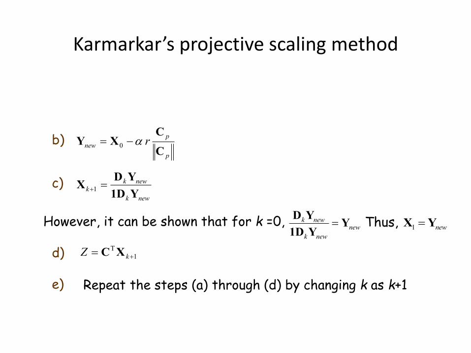
b)p

p

new rC

CXY −= 0

c)newk

newkk

Y1D

YDX =+1

However, it can be shown that for k =0, k newnew

k new

=D Y

Y1D Y

Thus, 1 new=X Y

1

T

+= kZ XCd)

Repeat the steps (a) through (d) by changing k as k+1e)

Karmarkar’s projective scaling method: Example

Consider the LP problem:

0,,

1

02 :subject to

2 Minimize

321

321

321

32

=++

=+−

−=

xxx

xxx

xxx

xxZ

3=nThus,

−

=

1

2

0

C 121 −=A

=

31

31

31

0

X

( ) ( ) 6

1

133

1

1

1=

−=

−=

nnr

( ) ( )9

2

33

13

3

1=

−=

−=

n

nand also,


Iteration 0 (k=0):

=

3/100

03/10

003/1

0D

3/13/20

3/100

03/10

003/1

1200

T −=

−== DCC

3/13/23/1

3/100

03/10

003/1

1210 −=

−=AD


Iteration 0 (k=0)…contd.:

−=

=

111

3/13/23/10

1

ADP

=

−

−=

30

03/2

13/1

13/2

13/1

111

3/13/23/1TPP

( )

=

−

3/10

05.11T

PP


( )

=−

5.005.0

010

5.005.0

1TT PPPP


( )

−

=−=−

6/1

0

6/1

T1TT CPPPPIC p

6

2)6/1(0)6/1( 22 =++=pC



=

−

−

=−=

3974.0

3333.0

2692.0

6/1

0

6/1

6

2

6

1

9

2

31

31

31

0

p

p

new rC

CXY

==

3974.0

3333.0

2692.0

1 newYX 2692.0

3974.0

3333.0

2692.0

1201

T =

−== XCZ


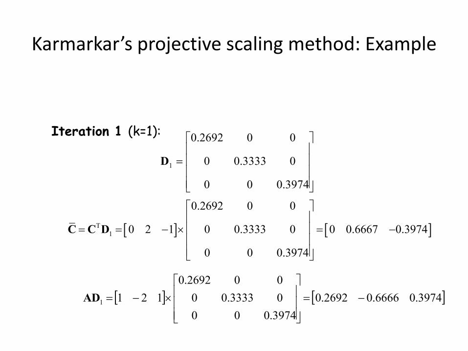
Iteration 1 (k=1):

=

3974.000

03333.00

002692.0

1D

T

1

0.2692 0 0

0 2 1 0 0.3333 0 0 0.6667 0.3974

0 0 0.3974

= = − = −

C C D

3974.06666.02692.0

3974.000

03333.00

002692.0

1211 −=

−=AD



1 0.2692 0.6667 0.3974

1 1 1

− = =

ADP

1

T

0.2692 10.2692 0.6667 0.3974 0.675 0

0.6667 11 1 1 0 3

0.3974 1

−

= − =

PP

( )1

T T

0.441 0.067 0.492

0.067 0.992 0.059

0.492 0.059 0.567

−

= − −

P PP P



( )1

T T T

0.151

0.018

0.132

p

−

= − = −

−

C I P PP P C

( )22 2(0.151) 0.018 ( 0.132) 0.2014p = + − + − =C

0

1 30.151 0.26532 1

1 3 9 60.018 0.3414

0.2014

0.132 0.39281 3

p

new

p

r

= − = − − = −

CY X

C



1

0.2692 0 0 0.2653 0.0714

0 0.3333 0 0.3414 0.1138

0 0 0.3974 0.3928 0.1561

new

= =

D Y

1

0.0714

1 1 1 0.1138 0.3413

0.1561

new

= =

1D Y



12

1

0.0714 0.2092

10.1138 0.3334

0.3413

0.1561 0.4574

new

new

= = =

D YX

1D Y

T

2

0.2092

0 2 1 0.3334 0.2094

0.4574

Z

= = − =

C X

Two successive iterations are shown. Similar iterations can be followed to get the final solution upto some predefined tolerance level

The Karmarkar’s LP Form

• The LP form of Karmarkar’s method

minimize z = CX

subject to

AX = 0

1X = 1 (1)

X ≥ 0

This LP must also satisfy

▪ satisfies AX = 0 (2)

▪ Optimal z-value = 0 (3)

• Where X= (x1, x2, …., xn)T , A is an m x n matrix

How to Transform any LP to the Karmarkar’s Form

• Step 1: set up the dual form of the LP

• Step 2: apply the dual optimal condition to form the combined feasible region “=“ form

• Step 3: Convert the combined feasible region to the homogeneous form: AX = 0

▪ Add the “ sum of all variables ≤ M” constraint

▪ Convert this constraint to “=“ form

▪ Introduce new dummy variable d2 = 1 to the system to convert the system to AX = 0 and 1X = M + 1

• Step 4: convert the system to Karmarkar’s form

▪ Introduce the set of new variables xj = (M +1)xj’ to convert the system to the form AX’ = 0 and 1X’ = 1

▪ Introduce new dummy variable d3’ to ensure (2) and (3)

MDP 631 Industrial Operations Research Lecture 3 Special cases in Simplex, Sensitivity analysis,...

Documents

Transcript of MDP 631 Industrial Operations Research Lecture 3 Special cases in Simplex, Sensitivity analysis,...