Maximum Likelihood Estimation Using Bayesian

Monte Carlo MethodsMaster’s Thesis

Danial Ali AkbariSupervisor: Umberto Picchini

Spring 2015

Abstract

The objective of this thesis is to give a general account of the MCMC estimation ap-proach dubbed data cloning, specifically performing maximum likelihood estimationvia Bayesian Monte Carlo methods. An account of the procedure will be given, and itwill applied to four different maximum likelihood estimation problems: simple linearregression, multiple linear regression, a stochastic dynamical model (Gompertz), anda state space model. In each case, different aspects of the method will be performed,and a comparison with the true or a approximative measure of the MLE will be done.In the final example, a comparison with the bootstrap particle filter is conducted. Thedata cloning approach was found to have several advantages over the SMC methods,some of these are simple implementation, fewer numerical issues and less complicatedchoice of proposal function. Most importantly, it avoids numerical optimization of afunction. Other benefits of the data cloning procedure is that the convergence of theestimates to the true MLE as the number of clones increases, is invariant to the choiceof the prior distribution. Furthermore, the approximative normality of the estimates,provides a convenient way of producing confidence intervals. The data cloning methodis also accompanied by several diagnostic tools which are mentioned in the study.

Key Words: Data cloning, maximum likelihood, Bayesian estimation, bootstrap par-ticle filter.

Acknowledgments

Writing a thesis seems always like an impossibility at the beginning. Often, however,this feeling fades as one receives support from those around. This thesis, like anyother, would not have been possible without the support of many others. I would,however, especially thank my supervisor, Umberto Picchini who always countered myfrustration with warm support, positive attitude and the provision of relevant feedbackand knowledge. For that, I am eternally grateful to him and hope to be able to liveup to that example.

List of Abbreviations

CIC Chain Increasing ClonesESS Effective Sample Size

MCMC Markov Chain Monte CarloMIC Mean Increasing ClonesMLE Maximum Likelihood EstimateQQ Quantile QuantileSIS Sequential Importance Sampling

SISR Sequential Importance Sampling with ResamplingSMC Sequential Monte Carlo

1

Contents

1 Introduction 31.1 The Metropolis-Hastings Algorithm . . . . . . . . . . . . . . . . . . . . 3

1.1.1 Random Walk Proposals . . . . . . . . . . . . . . . . . . . . . . 41.2 A Brief Account of Data Cloning . . . . . . . . . . . . . . . . . . . . . 5

1.2.1 Asymptotic Properties . . . . . . . . . . . . . . . . . . . . . . . 81.2.2 Diagnostics . . . . . . . . . . . . . . . . . . . . . . . . . . . . . 9

2 Static Models 102.1 Applying the Theory . . . . . . . . . . . . . . . . . . . . . . . . . . . . 102.2 Multiple Linear Regression . . . . . . . . . . . . . . . . . . . . . . . . . 11

2.2.1 Simple Linear Regression . . . . . . . . . . . . . . . . . . . . . . 182.3 Some Practical Issues . . . . . . . . . . . . . . . . . . . . . . . . . . . . 21

3 Stochastic Dynamical Models without Observational Noise 23

4 State Space Models 294.1 Theoretical Background . . . . . . . . . . . . . . . . . . . . . . . . . . 29

4.1.1 Data Cloning for State Space Models . . . . . . . . . . . . . . . 294.1.2 Approximative Maximum Likelihood Estimation . . . . . . . . . 32

4.2 A Practical Example . . . . . . . . . . . . . . . . . . . . . . . . . . . . 42

5 Concluding Remarks and Future Studies 50

6 References 52

7 Appendix - Omitted Figures 547.1 Static models . . . . . . . . . . . . . . . . . . . . . . . . . . . . . . . . 54

7.1.1 Simple Linear Regression . . . . . . . . . . . . . . . . . . . . . . 547.1.2 Multiple Linear Regression . . . . . . . . . . . . . . . . . . . . . 59

7.2 Stochastic Dynamical Models without Observational Noise . . . . . . . 647.3 State Space Models . . . . . . . . . . . . . . . . . . . . . . . . . . . . . 70

2

Chapter 1

Introduction

The objective of this thesis is to give a general account of the estimation approachdubbed data cloning, specifically performing maximum likelihood estimation via Bayesi-an Monte Carlo methods. In this section, firstly a brief account of MCMC meth-ods, specifically the Metropolis-Hastings algorithm will be presented. Then, the datacloning method will be introduced and some aspects of it discussed.

1.1 The Metropolis-Hastings Algorithm

Assume that ϕ = (ϕ1, ..., ϕd) is a stochastic variable with dimension d and probabilitydensity function f(ϕ). Let also ϕi, i = 1, ..., n be a finite i.i.d. sample from f of sizen, where ϕi = (ϕ1,i, ..., ϕd,i). If h(ϕ) is a properly defined measurable function, thenby the Law of Large Numbers it follows that:

1

n

n∑i=1

h(ϕi)

a.s.n→∞−→ Ef (h(ϕ))

Hence, if the calculation of Ef (h(ϕ)) is analytically cumbersome, one could simulateϕi ∼ f(ϕ), i = 1, ..., n, calculate h(ϕi) and evaluate the mean of the sample. Thismean is an estimate of the expected value above, provided that n is chosen largeenough.

Often, however, the target distribution f is either unknown or difficult to samplefrom. MCMC schemes provide an ailment for this problem, by introducing the conceptof the instrumental distribution or proposal function. The instrumental distribution,say q(ϕ), proposes values which are then accepted based on some probability thatreflects how likely it is that they are from the target distribution f . The Metropolis-Hastings algorithm is a specific and widely used version of such MCMC schemes.

In most of the Metropolis-Hastings algorithms, the proposed value at each itera-tive step of the MCMC chain, depends on the last accepted value. In other words, theMetropolis-Hastings algorithm allow for so called ”local updates” (Cosma and Evers,2010, pp. 53-56). A Bayesian version of the Metropolis-Hastings algorithm is men-tioned in Algorithm (1). In the Bayesian version, a prior π(ϕ) is also introduced, whichenables initialization of the MCMC Metropolis-Hastings scheme. In a non-Bayesian,setting the starting value ϕ0 is assumed to be fixed or given. Hastings (1970) provesthat this algorithm defines a Marokov chain that has as stationary distribution thedesired target posterior f .

3

Algorithm 1 Metropolis-Hastings Algorithm in a Bayesian setting.

Let q(ϕ) be a proposal function, π(ϕ) is a suitable prior and h(ϕ) a measurablefunction.

1. Initialization: Generate ϕ0 ∼ π(ϕ).

2. Simulation: Repeat the following steps for i ≤ n, where n is large enough.

2.1 Propose ϕ# ∼ q(ϕ|ϕi−1).

2.2 Compute

α = min{1,f(ϕ#)q(ϕi−1|ϕ#)π(ϕ#)

f(ϕi−1)q(ϕ#|ϕi−1)π(ϕi−1)} (1.1)

2.3 Draw ω ∼ U[0, 1]. If ω < α, set ϕi = ϕ#. Otherwise, set ϕi = ϕi−1.

3. Estimation: Calculate 1n

∑ni=1 h(ϕi).

1.1.1 Random Walk Proposals

There is a wide range of proposal functions that are frequently utilized. One suchproposal scheme, which is used in this study, is the random walk proposal scheme.In such a scheme, the proposal function q is chosen to be a conditionally symmetricdistribution. In other words,

q(ϕ#|ϕ∗) = q(ϕ∗|ϕ#)

Then the acceptance rate given in (1.1) is reduced to the following:

α = min{1, f(ϕ#)π(ϕ#)

f(ϕi−1)π(ϕi−1)}.

One such proposal scheme is the normal random walk, which is used in this study. Insuch a scheme, step (2.1) in Algorithm (1), is given by:

ϕ# = ϕi−1 + εi, εi ∼ N(0d, Ci)

where εi are the d-dimensional multivariate normal distribution with zero mean andvariance-covariance matrix Ci.

The variance-covariance matrix of the normal random walk proposal Ci, could bechosen as fixed. However, usually allowing the algorithm to adjust the covariance ofthe proposals, based on the history of the iterations, improves the acceptance rate,prompting it to approach the theoretically optimal acceptance rate of about 23% forrandom walk metropolis algorithms (Roberts et al., 1997, p. 113).1 In this study,the following Metropolis update scheme was chosen for the covariance matrix of theproposals(Haario, Saksman & Tamminen, 2001, p. 225):

Ci =

{C0, i ≤ i0,sd(cov(ϕ0, ...,ϕi−1) + εId) i > i0.

(1.2)

1Provided that certain stability conditions hold.

4

where C0 is the initial guess with regards to a proper covariance for the random walkproposals, i0 is the threshold for the update to commence, Id is the d-dimensionalidentity matrix, ε > 0 a control parameter avoiding Ci become singular or near singular,and sd is the update parameter which by Haario et al. (2001, p. 226) is suggested tobe put as sd = 2.42

d. Higher values of i0 indicates higher trust in the initial guess C0.

Another approach is to update could be done every nth0 MCMC iteration instead ofperforming the update every iteration after certain threshold:

Ci =

{C0, i ≤ n0,sd(cov(ϕ0, ...,ϕi−1) + εId) mod (i, n0) = 0.

(1.3)

1.2 A Brief Account of Data Cloning

The idea of the data cloning method is simple (Lele, Dennis, and Lutscher, 2007, p.553). Let the observed data be y = (y1, ..., yn), where n is the number of observed data.After constructing a full Bayesian model, with specified priors for the unknown pa-rameters instead of using the likelihood of the observed data, y, one uses the likelihoodfunction that corresponds to the vector containing K clones of the data, i.e.

y(K) = (y, ..., y)︸ ︷︷ ︸K times

. (1.4)

The clones are assumed be attained independently of each other, and K is assumedto be large enough. In other words, one performs Bayesian estimation as if one hady(K) as the obtained observed data set, where each observed data point, was attainedindependently of the others. The posterior, or the pseudo-posterior rather, is thencalculated through the familiar use of the MCMC scheme, such as Metropolis-Hastings.The process is mentioned in Algorithm (1.2). The pseudo-posterior is then used toperform the desired estimations for which, one would originally have used the regularposterior in a Bayesian setting.

Algorithm 2 A general account of the Data Cloning Approach.

Let the observed data be y = (y1, ..., yn), where n is the number of observed data.

1. Clone the data K times to attain y(K) in (1.4). Treat y(K) as if its elements havebeen attained independently of each other.

2. Target the pseudo-posterior through the use of an MCMC scheme upon theK-times cloned data. The pseudo-posterior is given by the following:

p(ϕ|y(K)) ∝ p(y(K)|ϕ)π(ϕ),

where ϕ are the unknown parameters for which π is a prior.

In this study, the interest lies in attaining an approximation of the MLE and itsconfidence. Consider the following setting. Let the observed data, Y , be assumed to

5

have the following hierarchical structure:

Y ∼ g(y|X;θ)X ∼ f(x|ϑ)Z = (Z1, ..., Zn) where Z is either y, x, Y or Xθ = (θ1, ..., θdy)ϑ = (ϑ1, ..., ϑdx)ϕ = (θ,ϑ)

(1.5)

Here X denotes the input variables that are stochastic with conditional density f , θ arethe unknown parameters of the observed state’s density function (with dimension dθ),ϑ are the unknown parameters of the input (hidden) state function (with dimensiondϑ), n the number of observations and ϕ the total collection of unknown parameters,with dimension d = dx + dy.

In this setting, the goal is to approximate the MLE of ϕ given the observed datay, dubbed ϕMLE. In the ordinary Bayesian setup, one attempts to evaluate the MLEthrough maximizing the likelihood function:

L(ϕ; y) = p(y|ϕ) =

∫g(y|X;θ)f(X|ϑ)dX (1.6)

The model in (1.5) may lack a stochastic input X, which reduces the structurefurther to the following:

Y ∼ g(y|ϕ)Z = (Z1, ..., Zn) where Z is either Y or yϕ = (ϕ1, ..., ϕd)

(1.7)

In such a case, the likelihood function is simply the conditional distribution:

L(ϕ; y) = p(y|ϕ) = g(y|ϕ). (1.8)

In the data-cloning method, the observed data y is substituted for the the K-timescloned observed data set y(k). In both settings mentioned, i.e. with hidden state in(1.5) and fixed effect in (1.7), one can prove that the likelihood function of the K-timescloned data is equal to the likelihood function of the original data to the power of K.2

In other words,L(ϕ; y(K)) = (L(ϕ; y))K . (1.9)

Furthermore, Lele (2007, et al., pp. 562-3) that the pseudo-posterior π(ϕ|Y (K)) isdegenerate at the true MLE. The proof of this property is mentioned in the sectionsbelow.

Model with Fixed Effects

Consider the model in (1.7), and let Φ be the parameter space of ϕ. Furthermore,let π(ϕ) be a prior distribution with support on the whole of the parameter space Φ.Then the posterior distribution is given by the following:

π(1)(ϕ|y) =g(y|ϕ)π(ϕ)∫g(y|ϕ)π(ϕ)dϕ

2The proof of this for the fixed effect case, is a direct result of the assumption that the copies areacquired independently of each other. The proof of this property for the model with latent stochasticstates is not very cumbersome either, and is mentioned in section (4.1.1) for state space models.

6

Using the new posterior as prior again, one obtains the following,

π(2)(ϕ|y) =g(y|ϕ)π(1)(ϕ)∫g(y|ϕ)π(1)(ϕ)dϕ

=[g(y|ϕ)]2π(ϕ)∫

[g(y|ϕ)]2π(ϕ)dϕ

Then, by induction, one arrives at the following result,

π(K)(ϕ|y) =[g(y|ϕ)]Kπ(ϕ)∫

[g(y|ϕ)]Kπ(ϕ)dϕ(1.10)

Moreover, it is clear that π(K)(ϕ|y) is equal to the pseudo-posterior distribution re-sulting from employing the cloned data y(K) within the likelihood function. In otherwords,

π(ϕ|y(K)) = π(K)(ϕ|y)

Now let ϕMLE be the MLE of the unknown parameter given the data y. Then, bydefinition of the MLE, it follows that

g(y|ϕMLE) > g(y|ϕ). (1.11)

Since the prior π has the entire parameter space as its support, then by (1.10) and(1.11) it follows that,

limK→∞

π(K)(ϕ|y)

π(K)(ϕMLE|y)=

[g(y|ϕ)]Kπ(ϕ)

[g(y|ϕMLE)]Kπ(ϕMLE)= κ

κ =

{0, ϕ 6= ϕMLE

1, ϕ = ϕMLE

Hence, as the number of clones (K) increases, the pseudo-posterior converges to adegenerate distribution with its probability density concentrated at the MLE.

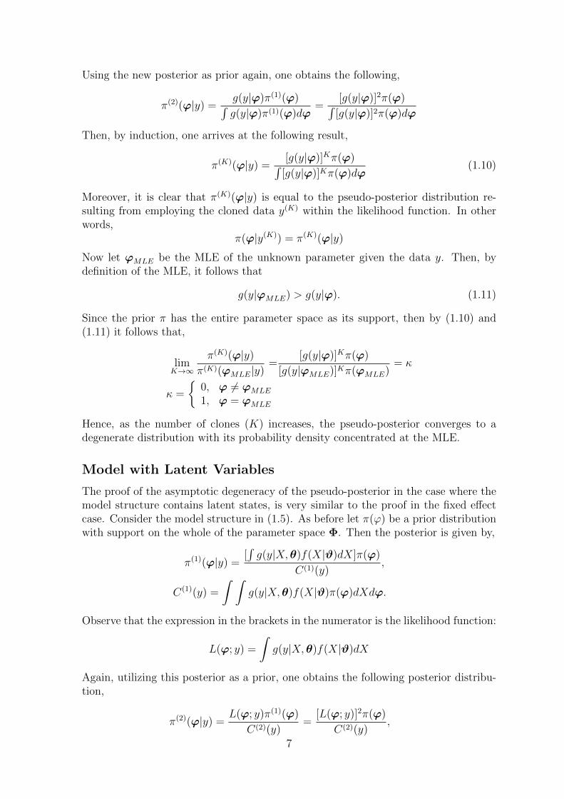
Model with Latent Variables

The proof of the asymptotic degeneracy of the pseudo-posterior in the case where themodel structure contains latent states, is very similar to the proof in the fixed effectcase. Consider the model structure in (1.5). As before let π(ϕ) be a prior distributionwith support on the whole of the parameter space Φ. Then the posterior is given by,

π(1)(ϕ|y) =[∫g(y|X,θ)f(X|ϑ)dX]π(ϕ)

C(1)(y),

C(1)(y) =

∫ ∫g(y|X,θ)f(X|ϑ)π(ϕ)dXdϕ.

Observe that the expression in the brackets in the numerator is the likelihood function:

L(ϕ; y) =

∫g(y|X,θ)f(X|ϑ)dX

Again, utilizing this posterior as a prior, one obtains the following posterior distribu-tion,

π(2)(ϕ|y) =L(ϕ; y)π(1)(ϕ)

C(2)(y)=

[L(ϕ; y)]2π(ϕ)

C(2)(y),

7

where C(2)(y) is given by,

C(2)(y) =

∫ ∫g(y|X,θ)f(X|ϑ)π(1)(ϕ)dXdϕ

=

∫[∫g(y|X,θ)f(X|ϑ)dX]2π(ϕ)dϕ

C(1)(y).

Hence, by induction the following is obtained:

π(K)(ϕ|y) =[L(ϕ; y)]Kπ(ϕ)

C(K)(y), (1.12)

C(K)(y) =

∫[∫g(y|X,θ)f(X|ϑ)dX]Kπ(ϕ)dϕ

C(K−1)(y). (1.13)

As before, it is clear that π(K)(ϕ|y) is equal to the pseudo-posterior distribution re-sulting from employing the cloned data y(K) within the likelihood function. In otherwords,

π(ϕ|y(K)) = π(K)(ϕ|y)

Similarly, assume that ϕMLE is the MLE of the unknown parameter given the data y.Then, by definition of the MLE, it follows that

L(ϕMLE; y) > L(ϕ; y). (1.14)

Since the prior π has the entire parameter space as its support, then by (1.12) and(1.14) it follows that,

limK→∞

π(K)(ϕ|y)

π(K)(ϕMLE|y)=

[L(ϕ; y)]Kπ(ϕ)

[L(ϕMLE; y)]Kπ(ϕMLE)= κ

κ =

{0, ϕ 6= ϕMLE

1, ϕ = ϕMLE

Hence, as the number of clones (K) increases, the pseudo-posterior converges to adegenerate distribution with its probability density concentrated at the MLE.

1.2.1 Asymptotic Properties

We have already mentioned one asymptotic property of the pseudo-posterior retrievedthrough data cloning, namely that it is asymptotically degenerate at the MLE. Thisresult also indicates that the convergence to the true MLE is invariant to the prior.

Lele et. al. (2010) further proves the asymptotic normality for each fixed K largeenough and given certain regularity conditions:

ϕ(K) ∼︸︷︷︸approximately

N(ϕMLE,1

KI−1(ϕMLE)), (1.15)

where ϕ(K) is the sample mean of the draws given the K-times cloned data. Hence,the mean of the accepted parameters targeting ϕ, is an approximation of the trueMLE and, likewise, the variance-covariance matrix of those simulated parameters, isan approximation of the variance-covariance matrix of the true MLE divided by thenumber of clones K.

8

1.2.2 Diagnostics

Lele et al. (2010), suggests two asymptotic measures for correct convergence of theestimate of the MLE via the data cloning procedure: the ω- and the r2-statisticsmentioned in equations (1.17) and (1.18). They are derived through the followingreasoning (Withanage, 2013, p. 43). As the number of clones K increased, the Maha-lanobis distance between realizations of the vector of the parameters being estimated(ϕ) and its expected value has a χ2-distribution with d degrees of freedom:

(ϕ− E(ϕ))T cov−1(ϕ|y(K))(ϕ− E(ϕ)) ∼ χ2d (1.16)

where y(K) is the K-times cloned observation and d the dimension of ϕ. Hence, a χ2-quantile-quantile plot could be used to determine whether the estimates are convergingcorrectly or not. This would be done by replacing the expected value E(ϕ) by itsestimate given the simulations, that is ϕ = 1

M

∑Mi=1ϕi (M is the number of MCMC

simulations), which also is the approximation of the MLE through the data cloningmethod.

A modified approach is, however, to create other statistics based on this relation-ship between the actual quantiles (those attained through the simulations) and thetheoretical ones (corresponding to χ2

d). The following ones were suggested by Lele etal. (2010):

ω =1

M

M∑i=1

(Q(i) −Qi)2 (1.17)

r2 = 1− corr2(Q,Q) (1.18)

where Q(1) ≤ ... ≤ Q(M) are the ordered estimated quantiles

Qi = (ϕi − ϕ)T cov−1(ϕ|y(K))(ϕi − ϕ),ϕ = (ϕ1, ...,ϕM),

Q = (Q(1), ..., Q(M)), Qi = χ2d,(i−0.5)/M the theoretical quantiles (the (i − 0.5)/M th

quantiles) from the corresponding χ2d-distribution, and Q = (Q1, ..., QM). When the

data cloning procedure is done properly, both ω and r2 should be close to zero, orbetter yet, converge to zero with increasing number of clones K.

Furthermore, the convergence of the standardized largest eigenvalue to zero is alsosuggested as a measure of estimability. The standardized largest eigenvalue of thecovariance matrix of the simulations with number of clones K - i.e. λSK - is the largesteigenvalue of the covariance matrix of the simulations with K number of clones (λK)divided by the the largest eigenvalue of the covariance matrix of the simulations withone clone (λ1), that is λSK = λK

λ1. As proven by Lele et al. (2010), if ϕ is estimable, this

value (λSK) should decrease to zero at the rate of 1/K. Hence, a comparison of the λSKand 1/K, can inform the researcher of the estimability of the parameter in question.

Furthermore, the assessment of normality of the pseudo-posterior is carried out bythe use of quantile-quantile plots of the chain as suggested by Jacquier et al. (2007)for maximum likelihood estimations via MCMC simulations.

9

Chapter 2

Static Models

2.1 Applying the Theory

In the case of static models, there is only one level of hierarchy in the statistical model,i.e. that of the observational process Y = (Y1, ..., Yn), where n is the number of theobservations. This is due to the fact that the quantities, x = (x1, ..., xn), affecting theobservations are assumed to be fixed and known. Hence, the model could be summa-rized in the following way:

Y ∼ f(y;x,ϕ) (2.1)

where f is a joint probability density function and ϕ = (ϕ1, ..., ϕd), is a vector ofunknown parameters affecting the observations.

A Data-cloning MCMC algorithm for static models is mentioned in algorithm (3).Observe that all the calculations could be done using logarithmic transform. In fact,such transformation will avoid the problem of the quotas being of very different magni-tudes and the subsequent computational problems that arises. Hence, operating withsuch transformations is recommended.

Furthermore, using a symmetric random walk proposal scheme, for the proposalfunction v(ϕ), would entail that v(ϕ#|ϕ∗) = v(ϕ∗|ϕ#). Hence, for such a scheme,

acceptance probability α is reduced to α = min(1, q#

q∗). This is the scheme used in this

section.Two different methods of increasing the number of clones K was experimented

with. In one method, one increases the number of clones every T number of algorithmiciterations.1 Hence, when moving from one block of iteration with K1 number of clones,to another with K2 number of clones (K2 > K1), one remains in the last acceptedproposal, until a new proposal is accepted. For reference purposes, this method isdubbed Chain Increasing Clones (CIC).

In another method, one increases the number of clones every T number of MCMCiterations as well. However, instead of using the last accepted proposal, one uses theestimate of the MLE of ϕ, i.e. the mean of the states for the previous number ofclones K (excluding a certain burn-in period if necessary). Let’s dub this method

1One should of course correct for the increase in power along the iterations, so as to avoid com-paring the pseudo-posterior for states with different number of clones.

10

Mean Increasing Clones (MIC). Both methods seem to function well and have no clearadvantages to one another.

Algorithm 3 A Data-cloning MCMC algorithm for static models

1. Initialization: Fix starting value ϕ∗ or generate it from its prior π(ϕ). Setnumbers of copies equal to K. Set ϕ1 = ϕ∗.

2. Calculate the pseudo-posterior at this state: q∗ = (f(y;x,ϕ∗))K · π(ϕ∗).

3. Propose a new state from the MCMC-algorithm’s proposal function: ϕ# ∼v(ϕ#|ϕ∗).

4. Calculate the pseudo-posterior at the newly proposed state (q# =(f(y;x,ϕ#))K · π(ϕ#)) and compare its value with the last accepted state i.e.

q∗. In other words, calculate the acceptance probability α = min(1, q#·v(ϕ∗|ϕ#)

q∗·v(ϕ#|ϕ∗)).

5. Generate a uniform random variable u ∼ U(0, 1). If u < α, set ϕj+1 = ϕ#,ϕ∗ = ϕ# and q∗ = q#. Otherwise set ϕj+1 = ϕj .

6. Repeat 3-5 for j ≤M number of simulations, i.e. repeat until the chain for ϕ isdeemed to have converged.

2.2 Multiple Linear Regression

In the case of multiple linear regression, the model scheme above (in (2.1)) will amountto:

Yi = β0 + β1x1,i + ....+ βqxq,i + ηi, i = 1, ..., n,

where ηi is the noise process, for instance, ηi ∼ N(0, σ2) iid. In such a framework,ϕ = (β0, ..., βq, σ

2).It is worth to take a look at an example and some of its practical aspects. For a

model, the following was chosen:

Yi = β0 + β1xi + β2x2i + β3x

3i + ηi, ηi ∼ N(0, σ2) (2.2)

where xi as 101 equidistant points between 0 and 1, i.e. (0, 0.01, 0.02, ..., 1), and(β0, ..., β3, σ

2) = (0.01, 10,−20, 30, 0.09). To improve the acceptance rate over time aMetropolis adaptive scheme was employed. Updating the variance-covariance matrixof the random walk proposal was done through the update mechanism in (1.3) withupdates done every 100th MCMC iteration. Furthermore, the priors were all uniform inthe following manner: β0 ∼ U(−1, 1), σ2 ∼ U(0, 10) and βq ∼ U(−50, 50), q = 1, 2, 3.A realization of the simulations through the CIC method is illustrated in Figure (2.1).2

The simulations converge to the MLE and the deviation from MLE decreases as thenumber of clones is increased.

2The corresponding plots for the MIC-method (Figure (7.2)) are very similar and can be viewedin section (7.1.1) in the Appendix.

11

Figure 2.1: MCMC chain of simulations with increasing number of copies (by one,starting at one) every 104 algorithmic iterations, applying the CIC method to themultiple linear regression model in (2.2). The red line is the true MLE.

In Figure (2.2) the increase of the number of clones has been conducted continu-ously, i.e. by increasing the number of clones K by one after each block of simulation,starting at K = 1. For each block, the number of Monte Carlo simulations conductedhas been ten thousand regular simulations plus a thousand for burn-in. This proce-dure was conducted 20 times and the average of the estimates and their correspondingstatistics were calculated in order to present a smoother result.

Both methods, CIC and MIC, have an acceptance rate in the chain, which is about28%, and hence is close to the theoretically desirable value of 23% (see Figure (2.2c)).They both perform fairly well with respect to convergence to the actual MLE andits variance covariance matrix (see Figure (2.2a,b)). However, the precision of theestimate of the variance-covariance matrix, does not seem to improve visibly afterK = 5.

The ω- and the r2-statistics (Figure (2.2)d,e) converge to zero in the beginning,but remain only close to zero afterwards. This is not problematic from a theoreticalstand point, since, in theory, the ω- and the r2 do not necessarily converge to zero,but should merely be close to zero.

Moreover, the convergence of the standardized largest eigenvalues of the covariance

12

β0 β1 β2 β3 σ2

True Val. -0.01 10 -30 20 0.09MLE 0.2373 (0.1303) 8.7999 (1.1339) -28.0060 (2.6422) 18.9064 (1.7364) 0.1153 (0.0162)CICK=1 0.2485 (0.1290) 8.7322 (1.1051) -27.8987 (2.5774) 18.8548 (1.6990) 0.1248 (0.0181)K=5 0.2331 (0.1256) 8.8406 (1.0989) -28.0956 (2.5436) 18.9612 (1.6597) 0.1165 (0.0167)K=10 0.2385 (0.1289) 8.7749 (1.0883) -27.9442 (2.5248) 18.8674 (1.6622) 0.1162 (0.0172)K=40 0.2365 (0.1371) 8.8012 (1.1817) -28.0061 (2.7319) 18.9058 (1.7860 ) 0.1154 (0.0166)MICK=1 0.2476 (0.1377) 8.7115 (1.1951) -27.8172 (2.7725) 18.7869 (1.8171) 0.1256 (0.0191)K=5 0.2335 (0.1360) 8.8196 (1.1818) -28.0459 (2.7705) 18.9306 (1.8278) 0.1177 (0.0168)K=10 0.2362 (0.1352) 8.8065 (1.1818) -28.0192 (2.7569) 18.9143 (1.8099) 0.1166 (0.0164)K=40 0.2373 (0.1331) 8.8062 (1.1277) -28.0264 (2.6441) 18.9222 (1.7506) 0.1155 (0.0159)

Table 2.1: Summary of the estimates of the multiple regression model: the true values, the MLE

and the estimates via the MIC and CIC methods of data cloning. The standard errors are mentioned

in the parenthesis. The increase of the number of clones has been conducted continuously, i.e. by

increasing the number of clones by one after each block of simulation. For each block, the number of

Monte Carlo simulations conducted has been ten thousand regular simulations plus a thousand for

burn-in. The Metropolis update of the covariance of the random walk proposals was performed every

100th MCMC iteration. The initial value (guess) of ϕ was the true values of the parameters added

with some minor zero-mean normal noise.

matrices (λSK) to zero is equal to the theoretical rate of 1/K (Figure 2.2f). Theconvergence to zero correctly illustrates estimability of the unknown parameters. Asummary of the estimates for some different number of copies is mentioned in table(2.1) for both the CIC and the MIC method.

Similar results are found when we increase the number of clones sporadically (Fig-ure (2.7)). The increase was done sporadically. The number of clones were 1, 2, 5, 10, 20and 40. For each block, the number of Monte Carlo simulations conducted has beenten thousand regular simulations plus a thousand for burn-in. As before, this proce-dure was conducted 20 times and the average of the estimates and their correspondingstatistics were calculated in order to present a smoother result. No visible disadvan-tages are observed compared to increasing the number of clones continuously ratherthan sporadically, indicating that one should perform the estimation through the latterprocedure, saving computational time.

One can further check the normality of the pseudo-posterior using QQ-plots. TheQQ-plots of pseudo-posteriors of the estimates of β0 and that of β3, through the CIC-method, are illustrated in Figures (2.4) and (2.5) respectively.3 The distribution ofthe pseudo-posteriors appear to be fairly normal.

3For the QQ-plots of the other parameters and those through the MIC-method see the Appendix(section (7.1.2)).

13

Figure 2.2: Some aspects of the estimates of the MLE via the MIC and CIC methods of data

cloning. The increase of the number of clones has been conducted continuously, i.e. by increasing the

number of clones K by one after each block of simulation. For each block, the number of Monte Carlo

simulations conducted has been ten thousand regular simulations plus a thousand for burn-in. This

procedure was conducted 20 times and the average of the estimates and their corresponding statistics

were calculated in order to present a smoother result. All is expressed as a function of number of

clone (K): (a) Precision of the estimates of the MLE (the 2-norm of the difference), (b) Precision

of the estimates of the variance covariance matrix of the MLE (the 2-norm of the difference) (c) the

acceptance rate, (d) the ω-statistic (e) the r2-statistic (f) the standardized largest eigenvalue (λSK) of

the covariance matrix.

14

Figure 2.3: Some aspects of the estimates of the MLE via the MIC and CIC methods of data cloning.

The increase was done sporadically. The number of clones were 1, 2, 5, 10, 20 and 40. For each block,

the number of Monte Carlo simulations conducted has been ten thousand regular simulations plus a

thousand for burn-in. This procedure was conducted 20 times and the average of the estimates and

their corresponding statistics were calculated in order to present a smoother result. All is expressed

as a function of number of clone (K): (a) Precision of the estimates of the MLE (the 2-norm of the

difference), (b) Precision of the estimates of the variance covariance matrix of the MLE (the 2-norm

of the difference) (c) the acceptance rate, (d) the ω-statistic (e) the r2-statistic (f) the standardized

largest eigenvalue (λSK) of the covariance matrix.

15

Figure 2.4: Quantile-quantile plots for the simulations of β0 using the CIC-method,and for different number of clones (K). The increase of the number of clones has beenconducted continuously, i.e. by increasing the number of clones K by one after eachblock of simulation. For each block, the number of Monte Carlo simulations conductedhas been ten thousand regular simulations plus a thousand for burn-in.

16

Figure 2.5: Quantile-quantile plots for the simulations of β3 using the CIC-method,and for different number of clones (K). The increase of the number of clones has beenconducted continuously, i.e. by increasing the number of clones K by one after eachblock of simulation. For each block, the number of Monte Carlo simulations conductedhas been ten thousand regular simulations plus a thousand for burn-in.

17

2.2.1 Simple Linear Regression

When performing the estimations for a simple linear regression example, some dis-crepancies from the results in the multiple linear regression case was observed. Theexample and the results are therefore briefly mentioned here.

In the case of simple linear regression, the model scheme above (in (2.1)) willamount to:

Yi = β0 + β1xi + ηi, i = 1, ..., n, (2.3)

where ηi is the noise process. For instance, ηi might be independent identically dis-tributed random variables, normally distributed withe mean zero and variance σ2, i.e.ηi ∼ N(0, σ2). In such a framework, ϕ = (β0, β1, σ

2) where ϕ, from (2.1), is all theunknown parameters affecting the observations.

Here, it is worth to take a look at an example and some of its practical aspects. Fora model, this author chose x = (1, ..., 20) and ϕ = (10, 2, 4). To improve the acceptancerate over time, a Metropolis adaptive scheme was employed. Updating the covariancematrix of the random walk proposal was done through the update mechanism in (1.3)with updates done every 100th algorithmic iterations. The priors that were chosenwere all uniform in the following manner: β0 ∼ U(−100, 100), β1 ∼ U(−20, 20) andσ2 ∼ U(0, 900). They are all indeed fairly wide and non-informative.

Figure (2.6) illustrates certain features of continuously increasing the number ofclones through both the CIC and the MIC methods. The increase of the number ofclones has been conducted continuously, i.e. by increasing the number of clones K byone after each block of simulation, starting at K = 1. For each block, the number ofMonte Carlo simulations conducted has been ten thousand regular simulations plusa thousand for burn-in. This procedure was conducted 20 times and the average ofthe estimates and their corresponding statistics were calculated in order to present asmoother result.

The precision of the estimates of the MLE and that of the covariance matrix of theMLE seems to increase as the number of clones increase (a,b), and the convergence tothe MLE is at a faster rate than the multiple linear regression case. The acceptancerates seems also to stabilize around 31%. This satisfactory since according to Robertset al. (1997, p. 113), the theoretically optimal acceptance rate for random walkmetropolis algorithms (under certain stability conditions) is about 23%. Moreover, theω- and r2-statistics are close to zero and even converge to that value as the number ofclones K is increased (d,e).

Furthermore, the standardized largest eigenvalue of the variance covariance matrix(λSK) seems to converge to zero, indicating estimability of the MLE of ϕ = (β0, β1, σ

2),which is correct (f). However the rate of convergence is faster than 1/K. The con-vergence is, nevertheless, correct as the diagnostic statistics are close to zero. Thefaster rate of convergence may be due to the additional information provided by eachblock of simulation when increasing the number of clones, rather than running eachsimulation separately for each number of copies. The multiple linear regression casedoes not manifest the same advantageous behavior. Hence, the simplicity of the modelmay also be a factor in the manifestation of the observed behavior. A summary of theestimates for some different number of copies is mentioned in table (2.2) for both theCIC and the MIC method.

18

β0 β1 σ2

True Val. 10 2 4MLE 8.6194 (1.1298) 2.0636 (0.0943) 5.9157 (1.8707)CICK=1 8.6587 (1.3802) 2.0607 (0.1160) 8.4918 (3.4653)K=5 8.6273 (1.1700) 2.0621 (0.0984) 6.3005 (2.1249)K=10 8.6311 (1.1035) 2.0628 (0.0929) 6.0901 (1.8783)K=40 8.6123 (1.1160) 2.0641 (0.0951) 5.9716 (1.9278)MICK=1 8.6506 (1.3473) 2.0626 (0.1160) 8.4165 (3.2683)K=5 8.6115 (1.1765) 2.0634 (0.0965) 6.2805 (2.0590)K=10 8.6267 (1.1261) 2.0636 (0.0946) 6.1292 (2.0266)K=40 8.6174 (1.1533) 2.0636 (0.0949) 5.9689 (1.8847)

Table 2.2: Summary of the estimates of the simple linear regression model: the true values, the

MLE and the estimates via the MIC and CIC methods of data cloning (DC) for some different number

of clones. The standard errors are mentioned in the parenthesis. The increase of the number of clones

has been conducted continuously, i.e. by increasing the number of clones by one after each block of

simulation. For each block, the number of Monte Carlo simulations conducted has been ten thousand

regular simulations plus a thousand for burn-in. The Metropolis update of the covariance of the

random walk proposals was performed every 100th algorithmic iterations. The initial value (guess) of

ϕ was the true values of the parameters added with some minor zero-mean normal noise.

There are some differences between the behavior of the estimates of the parametersof simple and multiple linear regression models. It has already been mentioned thatthe convergence to the MLE, in the simple linear regression model is at a faster ratethan the multiple linear regression case. These are the behavior of the standardizedlargest eigenvalues and that of the ω- and the r2-statistics. While in the simple linearregression case, the ω- and the r2-statistics converge to zero (Figure (2.6)d,e), in themultiple linear regression case (Figure (2.2)d,e) they converge to zero in the beginning,but remain only close to zero afterwards. This is not problematic from a theoreticalstand point, since, in theory, the ω- and the r2-statistics do not necessarily convergeto zero, but should merely be close to zero. In other words, the performance of thealgorithm for the simple linear regression case is too well, and for the multiple linearregression case in line with theory.

The same is true with respect to the convergence of the standardized largest eigen-values of the covariance matrices (λSK). In the simple linear regression case (Figure(2.6f), the convergence to zero is faster than the theoretical rate of 1/K. In the multi-ple linear regression case, however, the rate of convergence is visibly equal to that value(Figure 2.2f). The convergence to zero in both cases correctly illustrates estimabilityof the unknown parameters.

In short, the simplicity of the model, in the simple linear regression case, togetherwith the additional information provided by each block of simulation when increasingthe number of clones (rather than running each simulation separately for each numberof copies) may be the factors in the manifestation of the observed behavior.

19

Figure 2.6: Some aspects of the estimates of the MLE via the MIC and CIC methods of data

cloning. The increase of the number of clones has been conducted continuously, i.e. by increasing the

number of clones K by one after each block of simulation. For each block, the number of Monte Carlo

simulations conducted has been ten thousand regular simulations plus a thousand for burn-in. This

procedure was conducted 20 times and the average of the estimates and their corresponding statistics

were calculated in order to present a smoother result. All is expressed as a function of number of

clone (K): (a) Precision of the estimates of the MLE (the 2-norm of the difference), (b) Precision

of the estimates of the variance covariance matrix of the MLE (the 2-norm of the difference) (c) the

acceptance rate, (d) the ω-statistic (e) the r2-statistic (f) the standardized largest eigenvalue (λSK) of

the covariance matrix.

Similar results are found when one increases the number of clones sporadically(Figure (2.7)). The number of clones were 1, 2, 5, 10, 20 and 40. For each block,the number of Monte Carlo simulations conducted has been ten thousand regularsimulations plus a thousand for burn-in. As before, this procedure was conducted20 times and the average of the estimates and their corresponding statistics werecalculated in order to present a smoother result. No visible disadvantages are observedto increasing the number of clones continuously rather and sporadically, indicating thatone should perform the estimation through the latter one, saving computational time.

20

Figure 2.7: Some aspects of the estimates of the MLE via the MIC and CIC methods of data cloning.

The increase was done sporadically. The number of clones were 1, 2, 5, 10, 20 and 40. For each block,

the number of Monte Carlo simulations conducted has been ten thousand regular simulations plus a

thousand for burn-in. This procedure was conducted 20 times and the average of the estimates and

their corresponding statistics were calculated in order to present a smoother result. All is expressed

as a function of number of clone (K): (a) Precision of the estimates of the MLE (the 2-norm of the

difference), (b) Precision of the estimates of the variance covariance matrix of the MLE (the 2-norm

of the difference) (c) the acceptance rate, (d) the ω-statistic (e) the r2-statistic (f) the standardized

largest eigenvalue (λSK) of the covariance matrix.

2.3 Some Practical Issues

Some practical matters are worth mentioning. The choice of the initial value given tothe MCMC data cloning procedure affects how many iterations is needed (as burn-in)before the process converges to the neighborhood of the true MLE. The choice of priorshas a similar affect. Informative priors speeds up the convergence of the MCMC chain.As mentioned in section (1.2), however, the convergence itself is invariant to the choiceof priors. This state of invariance was tested, by choosing the priors differently andgetting similar results.

Another crucial issue is the tuning of the random walk proposals. The initial guess

21

of the covariance matrix, C0 in (1.2) and (1.3), speeds up the process and yields moresuitable acceptance rates. The choice could be done by letting the MCMC chain run fora while and adapt, and then restart the process, with the adapted covariance matrixCt. Furthermore, one should make use of the whole information in the covarianceupdates Ct and not just the variances on the diagonal. Otherwise, the proposals tendto deteriorate in quality and the acceptance rate diminishes drastically.

22

Chapter 3

Stochastic Dynamical Modelswithout Observational Noise

Applying the data cloning method to stochastic dynamical models, without observa-tional noise, is very similar to the case of static models. The only difference is indeedhow the likelihood function is calculated, which depends on the model. In other words,Algorithm (3) applies in this case as well. In the notation used in this chapter, theY in Algorithm (3) corresponds to the variable Z in this section. Hence the model in(2.1) is replaced by:

Z ∼ f(z;x,ϕ).

The example that was chosen here was the Gompertz model which has been usedin agronomy , e.g. for modeling the growth of chickens (Ditlevsen and Samson, 2013,pp. 29-35):

x(t) = Ae−Be−Ct

, (3.1)

which depends on the parameters A, B and C (all positive), and verifies the ordinarydifferential equation (ODE) below:

x′(t) = BCe−Ctx(t), x(0) = Ae−B (3.2)

From (3.1), one can see that x(t) → A as t → ∞. Hence, A can be interpreted asthe equilibrium weight of the chicken. The interpretation of the parameters B and C,on the other hand, is not as straightforward. The parameter B, could be seen as aparameter determining what ratio of the equilibrium weight the chicken has at birth,since x(0) = Ae−B. The parameter C, on the other hand, determines at what rate theweight of the chicken approaches the equilibrium value A. The larger C is, the fasterthe weight of the chicken approaches the value A.

Accommodating for heteroscedasticity, the stochastic differential equation (SDE)derived from the equation (3.2) will then be the following:

dXt = BCe−CtXtdt+ σXtdWt, X0 = Ae−B (3.3)

whereWt is a Wiener process, and σXt is the diffusion coefficient (σ > 0). The equation(3.3) is an Ito process that belongs to the family of Geometric Brownian motions withtime inhomogeneous drift, and hence has an explicit solution. By setting Zt = ln(Xt)and applying Ito’s formula, the conditional distribution of Zt+h|(Zs)s≤t, h > 0 is givenby:

Zt+h|(Zs)s≤t ∼ N(Zt −Be−Ct(e−Ch − 1)− 1

2σ2h, σ2h), Z0 = ln(A)−B,

23

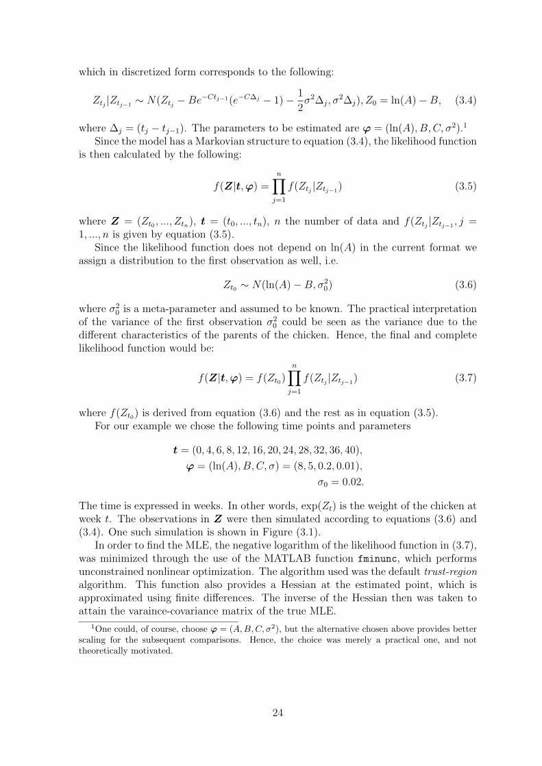
which in discretized form corresponds to the following:

Ztj |Ztj−1∼ N(Ztj −Be−Ctj−1(e−C∆j − 1)− 1

2σ2∆j, σ

2∆j), Z0 = ln(A)−B, (3.4)

where ∆j = (tj − tj−1). The parameters to be estimated are ϕ = (ln(A), B, C, σ2).1

Since the model has a Markovian structure to equation (3.4), the likelihood functionis then calculated by the following:

f(Z|t,ϕ) =n∏j=1

f(Ztj |Ztj−1) (3.5)

where Z = (Zt0 , ..., Ztn), t = (t0, ..., tn), n the number of data and f(Ztj |Ztj−1, j =

1, ..., n is given by equation (3.5).Since the likelihood function does not depend on ln(A) in the current format we

assign a distribution to the first observation as well, i.e.

Zt0 ∼ N(ln(A)−B, σ20) (3.6)

where σ20 is a meta-parameter and assumed to be known. The practical interpretation

of the variance of the first observation σ20 could be seen as the variance due to the

different characteristics of the parents of the chicken. Hence, the final and completelikelihood function would be:

f(Z|t,ϕ) = f(Zt0)n∏j=1

f(Ztj |Ztj−1) (3.7)

where f(Zt0) is derived from equation (3.6) and the rest as in equation (3.5).For our example we chose the following time points and parameters

t = (0, 4, 6, 8, 12, 16, 20, 24, 28, 32, 36, 40),

ϕ = (ln(A), B, C, σ) = (8, 5, 0.2, 0.01),

σ0 = 0.02.

The time is expressed in weeks. In other words, exp(Zt) is the weight of the chicken atweek t. The observations in Z were then simulated according to equations (3.6) and(3.4). One such simulation is shown in Figure (3.1).

In order to find the MLE, the negative logarithm of the likelihood function in (3.7),was minimized through the use of the MATLAB function fminunc, which performsunconstrained nonlinear optimization. The algorithm used was the default trust-regionalgorithm. This function also provides a Hessian at the estimated point, which isapproximated using finite differences. The inverse of the Hessian then was taken toattain the varaince-covariance matrix of the true MLE.

1One could, of course, choose ϕ = (A,B,C, σ2), but the alternative chosen above provides betterscaling for the subsequent comparisons. Hence, the choice was merely a practical one, and nottheoretically motivated.

24

Figure 3.1: A simulation of a stochastic dynamic model based on the Gompertz model.

As in the static model case, when performing the data-cloning procedure one needsto choose prior distributions for the unknown parameters. Here the following werechosen,

ln(A) ∼ U(ln(500), ln(5000))

B,C, σ ∼ U(0, 10)

which are fairly uninformative. The number of iterations for each K number of cloneswas ten thousand regular plus ten thousand burn-in. The covariance of the proposalfunction was updated every 100th step. The starting values in the simulations arethe true values of the parameters, not to be confused with the true MLE. Using theMCMC method via data cloning the following simulations were attained (Figures 3.2and 7.18). The simulations via both the MIC and the CIC methods prove to convergeto the true MLE, and approach it as the number of copies is increased.

25

Figure 3.2: MCMC chain of simulations with increasing number of copies (by one,starting at one) every 104 iterations, applying the CIC method to the Gompertz model.The red line is the true MLE. The starting values in the simulation are the true valuesof the parameters, not to be confused with the true MLE.

Some of the properties of the CIC and MIC method applied to the Gompertz modelare summarized in Figure (3.3). We see that the estimates and their respective vari-ance covariance matrices converge to each other as the number of clones (K) increase(Figures a,b). Furthermore, both stabilize with respect to the acceptance rate (Figurec). Moreover, the ω- and r2-statistics are close to zero and even converge to that valueas the number of clones K is increased (d,e). In addition, the largest standardizedeigenvalue (λSK) approaches zero as the number of clones increase. However, the rateof convergence is faster than 1/K. This may be due to the additional informationprovided by continuously increasing the number of clones, rather than running eachsimulation separately for each number of copies. The convergence is, nevertheless,correct as the diagnostic statistics are close to zero. The rate of convergence of λSKtowards zero seems to be improved by a factor 4 in this way. Increasing the numberof clones sporadically does not seem to have any significant effect on the convergenceof the chain either (Figure (7.19)). Hence, in order to reduce computational time, the

26

latter should be preferred.

Figure 3.3: Some aspects of the estimates of the MLE via the MIC and CIC methods of data

cloning. The increase of the number of clones has been conducted continuously, i.e. by increasing

the number of clones K by one after each block of simulation. For each block, the number of Monte

Carlo simulations conducted has been ten thousand regular simulations plus a thousand for burn-in.

All is expressed as a function of number of clone (K): (a) Precision of the estimates of the MLE (the

2-norm of the difference), (b) Precision of the estimates of the variance covariance matrix of the MLE

(the 2-norm of the difference) (c) the acceptance rate, (d) the ω-statistic (e) the r2-statistic (f) the

standardized largest eigenvalue (λSK) of the covariance matrix.

As seen in Figure (3.4), increasing the number clones drastically improves thenormality of the pseudo-posterior for the B parameter. This is true for all the otherparameters as well.2 As seen in the case of data cloning performed on static models,the CIC and MIC methds do not seem to have any advantages over the other. Asummary of the estimates are mentioned in table (3.1). Observe that, the practicalissues mentioned in section (2.3) is also applicable for Bayesian estimation of the MLEvia data cloning in the case of the type of models of this chapter, i.e. stochasticdynamical models without observational noise.

2See section (7.2).

27

Figure 3.4: Quantile-quantile plots for the simulations of B using the CIC-method,and for different number of clones (K). The increase of the number of clones has beenconducted continuously, i.e. by increasing the number of clones K by one after eachblock of simulation. For each block, the number of Monte Carlo simulations conductedhas been ten thousand regular simulations plus ten thousand for burn-in.

ln(A) B C σTrue Val. 8 5 0.2 0.01

MLE 8.0336 (0.0746) 5.0323 (0.0719) 0.2010 (0.4543·1e-2) 0.0155 (0.4575·1e-2)CICK=1 8.0235 (0.1627) 5.0223 (0.1615) 0.2024 (1.2415·1e-2) 0.0321 (2.0671·1e-2)K=5 8.0353 (0.0810) 5.0346 (0.0788) 0.2009 (0.4990·1e-2) 0.0170 (0.5518·1e-2)K=10 8.0356 (0.0759) 5.0342 (0.0729) 0.2009 (0.4591·1e-2) 0.0162 (0.4757·1e-2)K=40 8.0342 (0.0763) 5.0326 (0.0738) 0.2009 (0.4582·1e-2) 0.0157 (0.4557·1e-2)MICK=1 8.0375 (0.1380) 5.0354 (0.1361) 0.2010 (0.9031·1e-2) 0.0281 (1.4492·1e-2)K=5 8.0337 (0.0784) 5.0318 (0.0754) 0.2010 (0.4750·1e-2) 0.0167 (0.5217·1e-2)K=10 8.0331 (0.0794) 5.0317 (0.0777) 0.2009 (0.4926·1e-2) 0.0161 (0.5186·1e-2)K=40 8.0341 (0.0767) 5.0327 (0.0740) 0.2009 (0.4646·1e-2) 0.0157 (0.4635·1e-2)

Table 3.1: Summary of the estimates of the Gompertz model: the true values, the MLE and the

estimates via the MIC and CIC methods of data cloning (DC). The standard errors are mentioned

in the parenthesis.

28

Chapter 4

State Space Models

4.1 Theoretical Background

In state space models (or hidden Markov models), there are at least two levels ofhierarchy: {

Hidden state: X t ∼ f(xt|Xt−1;ϑ)Observed state: Y t ∼ g(yt|Xt;θ)

(4.1)

where f the distribution for the hidden state with the parameters ϑ = (ϑ1, ..., ϑdx),and g the distribution for the observed state with the parameters θ = (θ1, ..., θdy).Hence the total parameter space ϕ = (ϑ,θ) has the dimension d = dx + dy.

4.1.1 Data Cloning for State Space Models

As performed in the previous section,when performing Bayesian inference via data-cloning, we start from a prior regarding the parameters, say π(ϕ), in order to sample

from the pseudo-posterior π(ϕ|y(K)1:t ), where

y(K)1:t = (y1:t, ..., y1:t)︸ ︷︷ ︸

K times

where, y1:t = (y1, ..., yt). When K = 1, classical Bayesian inference is performed.The samples from the pseudo-posterior is then used to conduct Bayesian inferenceon the posterior with increased numerical accuracy, where the asymptotic propertiesof said inference are discussed in section (1.2). Ultimately, data-cloning is a Bayesianapproach to approximated maximum likelihood estimation, that converges to the MLEasymptotically. Hence, as in earlier sections, we are concerned with the likelihoodfunction L(ϕ; y1:t) = p(y1:t|ϕ).

For the the state space model in (4.1), the likelihood function is the following:

L(ϕ; y1:t) = p(y1:t|ϕ) = p(y1)t∏i=2

p(yi|y1:i−1;ϕ) (4.2)

=

∫g(y1:t|x1:t;ϕ)p(x1:t|ϕ)dx1:t (4.3)

=

∫ t∏i=1

g(yi|xi,θ)t∏i=1

f(xi|xi−1,ϑ)dx1:t (4.4)

29

where xi, i = 1, .., t are the hidden states,1 and appropriately x1:t = (x1, ..., xt) anddx1:t = (dx1, ..., dxt). The second equality exploits Bayes’ theorem, and the fourthequality exploits the conditional independence between the observed states and theMarkovian structure of the hidden states.

When performing data-cloning, as mentioned before, we assume that K indepen-dent copies of the observed states are gathered (y

(K)1:t ). Then, y

(K)1:t is assumed to be the

actual available observed data set. The independence of the copied observed states,in turn, assumes that K independent realizations of the hidden process {X1:t} have

produced K identical observed states y1:t. Let these states be x(k)1:t , k = 1, ..., K. Then

the likelihood function for the cloned data set would be the following:

L(ϕ; y(K)1:t ) = p(y

(K)1:t |ϕ) =

∫...

∫ K∏k=1

[g(y1:t|x(k)

1:t ;ϕ)p(x(k)1:t |ϕ)

]dx

(1)1:t ...dx

(K)1:t (4.5)

=K∏k=1

[∫g(y1:t|x(k)

1:t ;ϕ)p(x(k)1:t |ϕ)dx

(k)1:t

]= (L(ϕ; y1:t))

K , (4.6)

where the last equality follows from (4.2) and (4.3), and

g(y1:t|x(k)1:t ;ϕ) =

t∏i=1

g(yi|x(k)i ;θ),

p(x(k)1:t |ϕ) =

t∏i=1

f(x(k)i |x

(k)i−1,ϑ),

as indicated by the arguments motivating the equality in (4.4). By (4.5) and (4.6), the

likelihood function of the K-copied observations (y(K)1:t ), is the likelihood of the actual

observed state (y1:t) to the power of the number of copies K. Therefore, the argument

that maximizes L(ϕ; y(K)1:t ) is the same as the one which maximizes L(ϕ; y1:t), indicating

that the data-cloning approach will target the same estimate. The fact that this targetis the MLE, is proven by Lele et al. (2010). Indeed the asymptotic degeneracy of thepseudo-posterior at the true MLE was proven in section (1.2).

A procedure for parameter estimation via data-cloning is mentioned in Algorithm(4). A convenient choice of the proposal function for the hidden states is of course:

v(x1:t|ϕ) = p(x1:t|ϕ).

This choice reduces the acceptance rate to the following:

α = min(1,q#

q∗× u(ϕ∗|ϕ#)

u(ϕ#|ϕ∗)),

where the q# and q∗ are as defined in (4.7) and (4.8). The acceptance rate, however,could be simplified further. Using random walk proposals (for instance normal randomwalks), the acceptance rate becomes the following:

α = min(1,q#

q∗),

since u(ϕ#|ϕ∗) = u(ϕ∗|ϕ#) due to the known property of random walks.

1Observe that x0 is assumed to be fixed.

30

Algorithm 4 A General Data Cloning MCMC process for Parameter Estimation inState Space Models using Metropolis Hastings Algorithm.

Assume a model format as in (4.1).

1. Initialization: Fix starting value ϕ∗ or generate it from its prior π(ϕ). Setnumbers of copies equal to K. Set ϕ1 = ϕ∗.

2. Generate K independent trajectories of the hidden state from a hidden stateproposal function: x

∗(k)1:t ∼ v(x

(k)1:t |ϕ∗), k = 1, ..., K.

3. Calculate the pseudo-posterior at this state:

q∗ = π(ϕ∗)K∏k=1

g(y1:t|x∗(k)1:t ;ϕ∗)︸ ︷︷ ︸

=:q∗

p(x∗(k)1:t |ϕ∗). (4.7)

4. Propose a new state from the parameter proposal function: ϕ# ∼ u(ϕ#|ϕ∗).Generate K independent trajectories of the hidden state from a hidden state pro-posal function: x

#(k)1:t ∼ v(x

(k)1:t |ϕ#), k = 1, ..., K. Calculate the pseudo-posterior

at this state:

q# = π(ϕ#)K∏k=1

g(y1:t|x#(k)1:t ;ϕ#)︸ ︷︷ ︸

=:q#

p(x#(k)1:t |ϕ#). (4.8)

5. Compare its value with the last accepted state i.e. q∗. In other words, calculatethe acceptance probability

α = min[1,q#

q∗︸︷︷︸ratio of posteriors

× u(ϕ∗|ϕ#)∏K

k=1 v(x∗(k)1:t |ϕ∗)

u(ϕ#|ϕ∗)∏K

k=1 v(x#(k)1:t |ϕ#)︸ ︷︷ ︸

ratio of proposals

]. (4.9)

6. Generate a uniform random variable ω ∼ U(0, 1). If ω < α, set ϕj+1 = ϕ#,ϕ∗ = ϕ# and q∗ = q#. Otherwise set ϕj+1 = ϕj.

7. Repeat 3-6 for j ≤ N number of simulations, i.e. repeat until the chain for ϕ isdeemed to have converged, where N is a large enough integer.

8. Set ϕ = 1N

∑Nj=1ϕj.

The value ϕ is an approximation of the MLE.

31

4.1.2 Approximative Maximum Likelihood Estimation

Estimating the true MLE in state space models are not usually feasible. Therefore,an approximation of the MLE is needed. In order to estimate the correct MLE,we’ll simulate different realizations of the hidden state X

(r)t , r = 1, ..., R, and use a

special version of Sequential Importance Sampling with Resampling (SISR) called thebootstrap particle filter to find the best possible hidden states corresponding to theobserved values. This method is a specific form of Sequential Monte-Carlo (SMC)methods. Below, is an introduction to the concept.

Importance Sampling

When performing MCMC-simulations, often the situation arises where the distributionwhich one wants to sample from, i.e. the target distribution, say, is either too complexand/or analytically ambiguous. In such a situation, one can use a so called instrumentaldistribution which is easy to sample from. Mathematically, the generalized idea ofimportance sampling could be expressed in terms of calculating an expectation (Cosma& Evers, 2010, pp. 35-37). Let X be a random variable with the target distributionp(x) with support S, q(x) an instrumental distribution and h(x) a measurable function.Then,

Ep(h(X)) =

∫S

p(x)h(x)dx =

∫S

q(x)p(x)

q(x)︸ ︷︷ ︸=:w(x)

h(x)dx =

∫S

q(x)w(x)h(x)dx = Eq(w(X) ·h(X)), (4.10)

if q(x) > 0 for (almost) all with p(x) · h(x) 6= 0, when x ∈ S.Hence, given a sample X1, ..., XM ∼ q and provided that Eq |w(X)h(X)| exists,

then by the Law of Large Numbers:

1

M

M∑k=1

w(Xk)h(Xk)

a.s.M →∞−→ Eq(w(X) · h(X))

which then by (4.10) yields

1

M

M∑k=1

w(Xk)h(Xk)

a.s.M →∞−→ Ep(h(X)).

Hence, in practice, µ = 1M

∑Mk=1 w(Xk)h(Xk) could be used as an estimator of the the

expectation Ep(h(X)).The weights w(Xk), k = 1, ...,M do not necessarily sum up to M , and therefore,

sometimes the normalized weights are used: w(Xk) = w(Xk)∑Mk=1 w(Xk)

. Then the following

two estimators act as candidates:

µ = 1M

∑Mk=1w(Xk)h(Xk)

µ =∑M

k=1 w(Xk)h(Xk)(4.11)

The first estimator, µ, is unbiased, while the second one, µ, is only asymptotically so(ibid.).

Not any distribution q could be instrumentally useful when estimating the estima-tion through any particular target distribution p. The first condition that needs to be

32

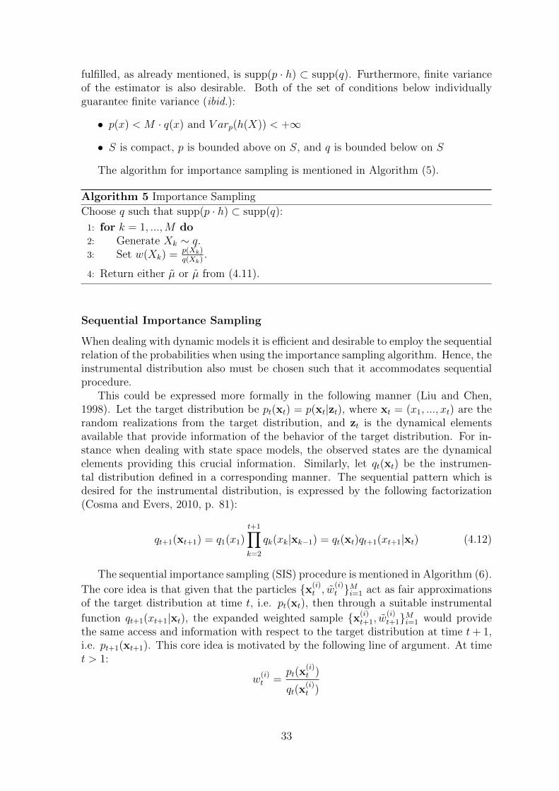
fulfilled, as already mentioned, is supp(p · h) ⊂ supp(q). Furthermore, finite varianceof the estimator is also desirable. Both of the set of conditions below individuallyguarantee finite variance (ibid.):

• p(x) < M · q(x) and V arp(h(X)) < +∞

• S is compact, p is bounded above on S, and q is bounded below on S

The algorithm for importance sampling is mentioned in Algorithm (5).

Algorithm 5 Importance Sampling

Choose q such that supp(p · h) ⊂ supp(q):

1: for k = 1, ...,M do2: Generate Xk ∼ q.3: Set w(Xk) = p(Xk)

q(Xk).

4: Return either µ or µ from (4.11).

Sequential Importance Sampling

When dealing with dynamic models it is efficient and desirable to employ the sequentialrelation of the probabilities when using the importance sampling algorithm. Hence, theinstrumental distribution also must be chosen such that it accommodates sequentialprocedure.

This could be expressed more formally in the following manner (Liu and Chen,1998). Let the target distribution be pt(xt) = p(xt|zt), where xt = (x1, ..., xt) are therandom realizations from the target distribution, and zt is the dynamical elementsavailable that provide information of the behavior of the target distribution. For in-stance when dealing with state space models, the observed states are the dynamicalelements providing this crucial information. Similarly, let qt(xt) be the instrumen-tal distribution defined in a corresponding manner. The sequential pattern which isdesired for the instrumental distribution, is expressed by the following factorization(Cosma and Evers, 2010, p. 81):

qt+1(xt+1) = q1(x1)t+1∏k=2

qk(xk|xk−1) = qt(xt)qt+1(xt+1|xt) (4.12)

The sequential importance sampling (SIS) procedure is mentioned in Algorithm (6).

The core idea is that given that the particles {x(i)t , w

(i)t }Mi=1 act as fair approximations

of the target distribution at time t, i.e. pt(xt), then through a suitable instrumental

function qt+1(xt+1|xt), the expanded weighted sample {x(i)t+1, w

(i)t+1}Mi=1 would provide

the same access and information with respect to the target distribution at time t+ 1,i.e. pt+1(xt+1). This core idea is motivated by the following line of argument. At timet > 1:

w(i)t =

pt(x(i)t )

qt(x(i)t )

33

Hence, for the following step,

w(i)t+1 =

pt+1(x(i)t+1)

qt+1(x(i)t+1)

=pt+1(x

(i)t+1)

qt(x(i)t )qt+1(x

(i)t+1|x

(i)t )

= w(i)t

pt+1(x(i)t+1)

pt(x(i)t )qt+1(x

(i)t+1|x

(i)t )︸ ︷︷ ︸

=:u(i)t+1

(4.13)

where the second step follows from equation (4.12), and u(i)t is called the incremental

weight. Since {x(i)t , w

(i)t }Mi=1 act as fair approximations of pt(xt), they could be used to

make estimations of the target distribution, which otherwise would have been impossi-ble. For instance, let h be a fixed measurable function, such that supp(p·h) ⊂ supp(q),then, under suitable regularity conditions, by the Law of Large Numbers,

M∑i=1

w(i)t h(X

(i)t )→ Ept(h(X)) as M → +∞. (4.14)

Algorithm 6 Sequential Importance Sampling

Let p be the target distribution and q the instrumental one.For i = 1, ...,M and t = 1, ..., T − 1:

1. Set t = 1.

1.1 Propagation: Sample x(i)1 ∼ q1(x1).

1.2 Updating: Set w(i)1 = p1(x

(i)1 )/q1(x

(i)1 ). Normalize the the weights: w

(i)1 =

w(i)1∑M

j=1 w(j)1

.

Set t = 2.

2. At time t > 1,

2.1 Propagation: Draw sample x(i)t ∼ qt(xt|x(i)

t−1), i = 1, ...,M .

2.2 Updating: Set x(i)t = (x

(i)t−1, x

(i)t ). Set u

(i)t =

pt(x(i)t )

pt−1(x(i)t−1)qt(x

(i)t |x

(i)t−1)

(the in-

cremental weight) and let w(i)t = u

(i)t w

(i)t−1. Normalize the the weights:

w(i)t =

w(i)t∑M

j=1 w(j)t

.

Set t to t+ 1.

The particles {x(i)t , w

(i)t }Mi=1 act as approximations of the target distribution at time t:

pt(xt).

Doucet et al. (2000, p. 199) prove that the SIS-algorithm suffers from the phe-nomenon of weight degeneracy, which indicates that in the long run, certain fewweighted particles accommodate most of the probability mass, while most other parti-cles have (normalized) weights close to zero. Formally, this translates into the varianceof the weights increasing over time (Cosma and Evers, 2010, p. 82). Hence, it is im-perative to find a suitable instrumental distribution that minimizes said variance. The

34

optimal instrumental distribution, according to Doucet et al. (2000, p. 199), is,

qt+1(x(i)t+1|x

(i)t ) = pt+1(x

(i)t+1|x

(i)t ) (4.15)

which usually is difficult to sample from. When the instrumental distribution is chosenas in (4.15), then the weights simplify to pt+1(x

(i)t+1)/pt(x

(i)t+1). This method is called the

bootstrap filter, and fundamentally boils down to using pt(xt) to predict xt+1 (Cosmaand Evers, 2010, pp. 82).

Sequential Importance Sampling with Resampling

In the previous section, the problem of weight degeneracy of the SIS algorithm wasmentioned. Furthermore, it was mentioned that choosing an optimal or semi-optimalinstrumental distribution function, would alleviate said problem. A second approachis to perform resampling after each propagation and updating step. In such a manner,the sample is rejuvenated at each step.

The outline of the idea is as follows. Assume that through sequential importancesampling, the weighted sample is available {x(i)

t , w(i)t }Mi=1 ∼ pt(xt), where the weights

are normalized. Then the empirical density is given by the following:

pt(xt) =M∑i=1

w(i)t δx(i)t

(xt) (4.16)

where δx(i)t

(xt) is the Dirac delta function with the density centered at x(i)t . Let h be

a fixed measurable function. Then, given suitable regularity conditions, by (4.14), itfollows

Ept(h(X))→ Ept(h(X)) as M → +∞. (4.17)

where Ept(h(X)) =∑M

i=1 w(i)t h(X

(i)t ).

Instead of using the particles {x(i)t , w

(i)t }Mi=1, however, one could use a sample from

them instead. In other words, take a sample of size M ′ ≤ M from said particles withreplacement: x

(j)t = x

(i)t , j = 1, ...,M ′ with probability w

(i)t . The new particles, have

now equal weights: {x(j)t , 1/M ′}Mj=1. Then again, by the Law of Large Numbers,

1

M ′

M ′∑j=1

h(X(j)t )→

M∑i=1

w(i)t h(X

(i)t ) = Ept(h(X)) as M ′ → +∞. (4.18)

Hence, by (4.17) and (4.18),

1

M ′

M ′∑j=1

h(X(j)t )→ Ept(h(X)) as M,M ′ → +∞. (4.19)

In the SIS algorithm, the resampling step is applied to the whole trajectory x(i)t = x

(i)1:t,

rather than the last particle. The extended algorithm is referred to as Sequential Im-portance Sampling with Resampling (SISR). The procedure is mentioned in Algorithm(7). Notice that due to the fact that resampling adds extra randomness to the sample,estimation is to be conducted before resampling.

35

Algorithm 7 Sequential Importance Sampling with Resampling

Let p be the target distribution and q the instrumental one.For i = 1, ...,M and t = 1, ..., T − 1:

1. Set t = 1.

1.1 Propagation: Sample x(i)1 ∼ q1(x1).

1.2 Updating: Set w(i)1 = p1(x

(i)1 )/q1(x

(i)1 ). Normalize the the weights: w

(i)1 =

w(i)1∑M

j=1 w(j)1

.

1.3 Resampling: Sample x(j)1 = x

(i)1 , j = 1, ...,M ′ with probability w

(i)1 . Set

w(i)1 = 1/M ′.

Set M = M ′ and t = 2.

2. At time t > 1,

2.1 Propagation: Draw sample x(i)t ∼ qt(xt|x(i)

t−1), i = 1, ...,M .

2.2 Updating: Set x(i)t = (x

(i)t−1, x

(i)t ). Set u

(i)t =

pt(x(i)t )

pt−1(x(i)t−1)qt(x

(i)t |x

(i)t−1)

(the in-

cremental weight) and let w(i)t = u

(i)t w

(i)t−1. Normalize the the weights:

w(i)t =

w(i)t∑M

j=1 w(j)t

.

2.3 Resampling: Sample x(j)t = x

(i)t , j = 1, ...,M ′ with probability w

(i)t . Set

w(i)t = 1/M ′.

Set M = M ′ and t to t+ 1.

The particles {x(i)t , w

(i)t }Mi=1 act as approximations of the target distribution at time t:

pt(xt). In other words, estimation is done before resampling.

Since the resampled trajectories become dependent of each other, the varianceof the estimate is increased. Therefore, there is a trade-off between the resamplingfrequency and the variance of the estimator. This notion, begs the question what theeffective sample size (ESS) is. According to Kong et al. (1994, pp. 283-4), the effectivesample size is given by:

ESS =M

1 + Varqt+1(xt+1)(wt+1)(4.20)

Since Eqt+1(xt+1)(wt+1) = 1 (i.e. the weights are normalized), (4.20) can be simplified,in the following manner (Cosma and Evers, 2010, pp. 86-7).,

M

1 + Varqt+1(xt+1)(wt+1)=

M

1 + Eqt+1(xt+1)[wt+1)2]− (Eqt+1(xt+1)[wt+1])2=

M

Eqt+1(xt+1)[(wt+1)2](4.21)

Since Varqt+1(xt+1)(wt+1) and, consequently Eqt+1(xt+1)[(wt+1)2], are not often analyti-cally attainable, an approximation is needed. One such approximation is the following:

Eqt+1(xt+1)[(wt+1)2] ≈Eqt+1(xt+1)[(wt+1)2]

(Eqt+1(xt+1)[∑M

i=1w(i)t+1])2

≈M−1

∑Mi=1(w

(i)t+1)2

M−2(∑M

i=1w(i)t+1)2

= MM∑i=1

(w(i)t+1)2

36

Then, by (4.20) and (4.21), the effective sample size could be approximated by,

˜ESS =1∑M

i=1(w(i)t+1)2

. (4.22)

Furthermore, from (4.20), one notices that:

ESS→M as Varqt(xt)(wt)→ 0.

Hence, a value of ˜ESS close to M indicates that the sample contains almost as muchinformation as an i.i.d. sample of size M from the target distribution pt(xt). In practicea threshold, thM , lower than M (often M/2) is chosen. When ˜ESS < thM , resamplingis performed (ibid.).

Bootstrap Particle Filter

Wilkinson (2012, p. 294) describe the bootstrap particle filter as a simple SISR-technique for estimating the hidden states in a state space model conditional on theobservations and the parameters. Consider the state-space model given in (4.1) andassume that the parameters ϕ = (ϑ,θ) are known. Similar to the case of employing thebootstrap filter through SIS, when using the bootstrap particle filter, the instrumentalfunction is

qt(x(i)1:t) = p(xt|x(i)

1:t−1, y1:t−1;ϕ) = f(xt|x(i)t−1;ϑ). (4.23)

Then, the incremental weight u(i)t , defined in (4.13) is given by the following:

u(i)t =

p(x(i)1:t|y1:t;ϕ)

p(x(i)1:t−1|y1:t−1;ϕ)f(x

(i)t |x

(i)t−1;ϑ)

(4.24)

The numertor, p(x(i)1:t|y1:t;ϕ), can however, be simplified. Given the hidden Markovian

relation described in (4.1), the joint distribution of the hidden and observed statetrajectories has the following recursive relation (Cosma and Evers, 2010, pp. 74-75),

p(x1:t, y1:t|ϕ) = p(x1)g(y1|x1;θ)t∏

k=1

p(xk, yk|x1:k−1, y1:k−1)

= p(x1)g(y1|x1;θ)t∏

k=1

f(xk|xk−1;ϑ)g(yk|xk;θ)

= p(x1:t−1, y1:t−1|ϕ)f(xt|xt−1;ϑ)g(yt|xt;θ)

Hence, by Bayes’ theorem, the conditional density of interest satisfies the following,

p(x1:t|y1:t;ϕ) ∝ p(x1:t−1|y1:t−1;ϕ)f(xt|xt−1;ϑ)g(yt|xt;θ) (4.25)

Then, by (4.24), the the incremental weight of the bootstrap particle filter has thefollowing property,

u(i)t ∝

p(x(i)1:t−1|y1:t−1;ϕ)f(x

(i)t |x

(i)t−1;ϑ)g(yt|x(i)

t ;θ)

p(x(i)1:t−1|y1:t−1;ϕ)f(x

(i)t |x

(i)t−1;ϑ)

= g(yt|x(i)t ;θ) (4.26)

37

Therefore, the incremental weight, in practice, could be used as u(i)t = g(yt|x(i)

t ;θ),which is very convenient.

The bootstrap particle filter, employing the effective sample size approach, is sum-marized by Algorithm (8). One may notice the addition of an initialization step com-pared to Algorithm (7). This step is necessary, since the distribution of the hiddenstate is only conditionally known.

Algorithm 8 Bootstrap Particle Filter

Let thM < M .For i = 1, ...,M and while t ≤ T ,

1. Initialization: Set t = 0.

1.1 Propagation: Sample x(i)0 ∼ π(x0) from some prior or choose x

(i)0 fixed.

1.2 Updating: Set w(i)0 = 1/M . Set t=1.

2. At time t = 1.

2.1 Propagation: Sample x(i)1 ∼ f(x1|x(i)

0 ;ϑ).

2.2 Updating: Set w(i)1 = g(y1|x(i)

1 ;θ). Normalize the the weights: w(i)1 =

w(i)1∑M

j=1 w(j)1

.

2.3 Resampling: Set ˜ESS = 1∑Mi=1(w

(i)1 )2

. If ˜ESS < thM , then sample x(j)1 =

x(i)1 , j = 1, ...,M ′ with probability w

(i)1 . Set w

(i)1 = 1/M ′ .

Set M = M ′ and t = 2.

3. At time t > 1,

3.1 Propagation: Sample x(i)t ∼ f(xt|x(i)

1:t−1;ϑ).

3.2 Updating: Set x(i)1:t = (x

(i)1:t−1, x

(i)t ). Set u

(i)t = g(yt|x(i)

t ;θ) (the incremental

weight) and let w(i)t = u

(i)t w

(i)t−1. Normalize the the weights: w

(i)t =

w(i)t∑M

j=1 w(j)t

.

3.3 Resampling: Set ˜ESS = 1∑Mi=1(w

(i)t )2

. If ˜ESS < thM , then sample x(j)1:t =

x(i)1:t, j = 1, ...,M ′ with probability w

(i)t . Set w

(i)t = 1/M ′.

Set M = M ′ and t to t+ 1.

Parameter Estimation

The calculations leading up to Algorithm (8) were conducted under the assumptionthat the parameters ϕ = (ϑ,θ) in the model (4.1), are known. If, however, theyare not known, then maximum likelihood inference is concerned with maximizing thelikelihood function p(y1:t|ϕ). The likelihood function of the state space model is given

38

by,

p(y1:t|ϕ)︸ ︷︷ ︸=:L(ϕ)

= p(y1)︸ ︷︷ ︸=:L1

T∏t=2

p(yt|y1:t−1;ϕ)︸ ︷︷ ︸=:Lt(ϕ)

(4.27)

where,

p(yt|y1:t−1;ϕ) =

∫p(yt|xt, y1:t−1;ϕ)p(xt|y1:t−1;ϕ)dxt.

Due to the conditional independence of the data (yt) given the latent states (xt),p(yt|xt, y1:t−1;ϕ) = p(yt|xt;ϕ) = g(yt|xt;ϕ), and the integral reduces to:

p(yt|y1:t−1;ϕ) =

∫g(yt|xt;ϕ)p(xt|y1:t−1;ϕ)dxt.

In an ideal scenario, on would sample from x(i)t ∼ p(xt|y1:t−1;ϕ), i = 1, ...,M , and

perform the following approximation:

p(yt|y1:t−1;ϕ) ≈ p(yt|y1:t−1;ϕ) =:1

M

M∑i=1

g(yt|x(i)t ;ϕ).

where,

p(yt|y1:t−1;ϕ)

a.s.M →∞−→ p(yt|y1:t−1;ϕ),

by the Law of Large Numbers.The distribution p(xt|y1:t−1;ϕ), however, is not usually accessible, so an instru-

mental distribution needs to be chosen. As mentioned in the previous section, forthe bootstrap particle filter, the instrumental distribution is f(xt|xt−1;ϑ), which, by(4.26) results in the following incremental weights:

u(i)t = g(yt|x(i)

t ;θ), i = 1, ...,M. (4.28)

So, the incremental weights themselves, are the target of estimation. Hence, theapproximation of the MLE, ϕMLE, would be achieved by:

ϕMLE = argmaxϕ

L(ϕ)

L(ϕ) = L1(ϕ)∏T

t=2 Lt(ϕ)

Lt(ϕ) = 1M

∑Mi=1 u

(i)t , t = 1, ..., T

(4.29)

where u(i)t is given by (4.28) with x

(i)t ∼ f(xt|x(i)

t−1;ϑ), i = 1, ..,M . Observe that

L, Lt, t = 1, ..., T are approximations of the corresponding likelihoods defined in (4.27).The result is the procedure mentioned in Algorithm (9).

Resampling Techniques

Performing resampling could be summarized in selecting M ′ ≤M number of particlesx(j) with replacement among an original sample {x(i)}Mi=1, where P(x(j) = x(i)) = wj,

39

Algorithm 9 Parameter Estimation through the Bootstrap Particle Filter

Let thM < M .For i = 1, ...,M and while t < T ,

1. Initialization: Set t = 0.

1.1 Propagation: Sample x(i)0 ∼ π(x0) from some prior or choose x

(i)0 fixed.

1.2 Updating: Set w(i)0 = 1/M . Set t=1.

2. At time t = 1.

2.1 Propagation: Sample x(i)1 ∼ f(x1|x(i)

0 ;ϑ∗).

2.2 Updating: Set w(i)1 = g(y1|x(i)

1 ;θ∗). Normalize the the weights: w(i)1 =

w(i)1∑M

j=1 w(j)1

.

2.3 Estimation: Set L1 = 1M

∑Mi=1 w

(i)1 .

2.4 Resampling: Set ˜ESS = 1∑Mi=1(w

(i)1 )2

. If ˜ESS < thM , then sample x(j)1 =

x(i)1 , j = 1, ...,M ′ with probability w

(i)1 . w

(i)1 = 1/M ′

Set M = M ′ and t = 2.

3. At time t > 1,

3.1 Propagation: Sample x(i)t ∼ f(xt|x(i)

1:t−1;ϑ∗).

3.2 Updating: Set x(i)1:t = (x

(i)1:t−1, x

(i)t ). Set u

(i)t = g(yt|x(i)

t ;θ∗) (the incremental

weight) and let w(i)t = u

(i)t w

(i)t−1. Normalize the the weights: w

(i)t =

w(i)t∑M

j=1 w(j)t

.

3.3 Estimation: Set Lt = 1M

∑Mi=1 u

(i)t .

3.4 Resampling: Set ˜ESS = 1∑Mi=1(w

(i)t )2

. If ˜ESS < thM , then sample x(j)1:t =

x(i)1:t, j = 1, ...,M ′ with probability w

(i)t . Set w

(i)t = 1/M ′.

Set M = M ′ and t to t+ 1.

Set L =∏T

t=1 Lt. Then, ϕMLE = argmaxϕ

L.

40

and∑M

j=1 wj = 1 . For simplicity, we choose M ′ < M . The line of thought in caseswhen M ′ 6= M is very similar.

Choosing a new particle could be seen as an event within the framework of prob-ability theory. It could be thought of letting the random variable of the index of theselected particle, Ij, being equal to the index of one of the particles in the sample{x(i)}Mi=1. In other words, Ij = i. Hol (2004, p. 13) summarizes an event generationalgorithm in the following manner:

Algorithm 10 Event generation.

The generation of an event Ij with P(Ij = i) = wj is obtained by

1. Simulate uj ∼ U[0, 1),

2. Assign Ij = i, if Si−1 < uj ≤ Si, where Si =∑i

s=1 ws, and 1 ≤ i, j ≤M .

The resampling methods used in this study are stratified and systematic resampling.They are both based on Algorithm (10) and are very similar. According to Hol (2004,pp. 18-19), an enhanced version of stratified resampling in one dimension could beseen as partitioning the index space, [0, 1) into M disjoint strata of equal size [ j

M, j+1M

)for j = 0, ...,M − 1 and then choosing one particle within each interval. Hence, theresampled particles are sampled independently of each other. The returned sequencewould then be a random permutation of the stratified samples. In other words,

Ij = ij where ij =πj−1 + uj

M,uj ∼ U[0, 1), j = 0, ...,M − 1

where π is a uniform random permutation of 0, ...,M − 1.In systematic resampling, however, the samples are no longer independent, and are

positioned in the same manner in each strata relative to each other:

Ij = ij where ij =πj−1 + u

M, u ∼ U[0, 1), j = 0, ...,M − 1

The lack of independence sometimes may lead to higher variance of the resampledindex random variable compared to the stratified resampling method. However, sys-tematic resampling produces samples that are more uniform and are to have minimaldiscrepancy (ibid). Both are suitable resampling techniques in one dimension.

Log Sum of Exponentials

When summing up the normalized weights wj, j = 1, ...,M , the magnitude of theweights may differ, sometimes significantly, which numerically will result in the pro-gram (here MATLAB) evaluating the insignificant ones as zero due to software finitenumerical representation capabilities, compared to the larger weights. Blevins (2008)argues that such numerical phenomenon may often result in underflow and overflow inthe representation of the particles when resampling is carried out. In order to avoidthis problem the log sum exponential approach is used.

Hence, the sum of the weights needs to be adjusted in a manner. Let v = (a, b),then for any c, we can write:

exp(a) + exp(b) = (exp(a− c) + exp(b− c)) exp(c)

41

which when taking the logarithm of both sides becomes:

log(exp(a) + exp(b)) = log(exp(a− c) + exp(b− c)) + c

Choosing c properly will reduce the incidence of overflow or underflow.Now let v = (v1, ..., vM), where vj = log(wj), j = 1, ...,M . Furthermore, let ‖v‖ =

(|v1|, ..., |vM |). The version of the log sum exponential approach employed in this studydistinguishes between two situations. In one case, the vector v contains negative valueswith very high absolute values, i.e. maxvj‖v‖ > maxvjv. In other words, the someof the weights are really small compared to the larger weights. This increases theprobability of underflow occurring. In this case, c is chosen as: c = minvjv.

In the other case, it holds that maxvj‖v‖ = maxvjv, which indicates that there arevery large weights. In this case there is a possibility of overflow occurring. Hence, cis chosen as the following, c = maxvjv. The process boils down to what is presentedin Algorithm (11). The method however, does not guarantee the absence of overflowand underflow, but merely reduces their frequency of occurrence.

Algorithm 11 Log Sum Exponential Approach.

Let v = (v1, ..., vM), where vj = log(wj), j = 1, ...,M . Furthermore, let ‖v‖ =

(|v1|, ..., |vM |). Furthermore, let S =∑M

j=1 wj.

1. If maxvj‖v‖ > maxvjv, set c = minvjv. Otherwise, set c = maxvjv.

2. Calculate ˆlog(S) = log(∑M

j=1 exp(vj − c))

+ c,

where ˆlog(S) is numerically closer to the actual value of log(S).

4.2 A Practical Example

As a practical example the process Z in chapter (3) was chosen as the hidden processand some Gaussian noise was added to arrive at the observed states Yt0:tj . In otherwords,

Ytj = Ztj + εj, (4.30)

where εj ∼ N(0, γ2) i.i.d. and Ztj is as defined in equation (3.5). The parameter spaceis then increased by one dimension:

ϕ = (ln(A), B, C, σ, γ) (4.31)

where A,B,C are the parameters of the now hidden Gompertz model in (3.1), σ isthe diffusion parameter in (3.3), and γ is the standard deviation of the observationalnoise.

As in the example with dynamical models in the previous chapter, a distributionis assigned to the first latent state. Otherwise the likelihood function does not dependon ln(A). The choice of this distribution is identical to the one in (3.6), where σ2

0 isagain a meta-parameter and assumed to be known. The practical interpretation ofthis parameter is the same as before.

42

For our example we chose the following time points and parameters:2

t = (0, 2, 3, 3.5, 7, 11, 20, 24, 25, 26, 30, 33, 34, 40),

ϕ = (ln(A), B, C, σ, γ) = (8, 5, 0.2, 0.01, 0.15),

σ0 = 0.02.

The time is expressed in weeks. In other words, exp(Zt) is the true weight of thechicken at week t, and exp(Yt) is the observed weight of the same chicken at the sametime point. The observations in Z were then simulated according to equations (3.6)and (3.4), while Z is simulated in accordance with (4.30). One such simulation isshown in Figure (4.1), where both the latent and observed processes are mentioned.

In order to find the MLE, the negative logarithm of the likelihood function in(4.29), attained through the bootstrap particle filter mentioned in Algorithm (9), wasminimized. Resampling was performed via both stratefied and systematic methods.The settings used for the bootstrap particle filter were the following:

M ′ = M = 1000thM = M/2

x(i)0 = ln(A)−Bx

(i)t1 |x

(i)0 ∼ N(x

(i)0 , σ

20)

(4.32)

where σ0 = 0.02 is the same meta-parameter in the initialization of the process andi = 1, ..,M .

The minimization could have been done through the use the MATLAB functionfmincon, which performs constrained nonlinear optimization. However, the Hessianprovided by this function was unstable. Instead the MATLAB function fminsearch

was utilized, which finds minimum of an unconstrained multivariable function usingderivative-free methods, another form of unconstrained nonlinear optimization.

This function, however, does not provide an inbuilt Hessian. The variance-covariancematrix was instead attained indirectly though the following scheme (Seber & Wild,2003, pp. 42-48):

cov(ϕMLE|y) = s2(J ′J)−1

where J is the Jacobian of at the MLE, and s2 is the unbiased estimate of the varianceof the errors, i.e. the difference between the observations and the predicted values. TheJacobian was estimated using the function jacobianest provided by D’Errico (2014).It is worth mentioning that even after performing the estimation of the variance-covariance matrix of the MLE in this manner, the stability of said matrix was notcompletely optimal. Higher values of standard error of the estimates obtained via thebootstrap particle filter, compared to the the ones obtained through data cloning, couldalso be explained partially by the fact that resampled trajectories become dependentof each other and therefore the variance of the estimates increase.

2It is worth commenting why the choice of the time points in this section, differs from those usedin the dynamic models example without observational noise. As the rest of the study will mention,using the former time-points the parameter σ, was declining towards zero through the simulations.The intuition was, that this may very well be due to the constant time lapses between the time pointsin the dynamic models example. Hence, the time lapses was set in such a manner, so that the intervalsbetween them were not constant. The results seemed, however, to be invariant to the choice of thesample intervals, as will be mentioned later on.

43

As before, when performing the data-cloning procedure one needs to choose priordistributions for the unknown parameters. Here, the following were chosen,

ln(A) ∼ U(ln(500), ln(5000))

B,C, σ, γ ∼ U(0, 10)

which are fairly uninformative. The number of iterations for each K number of cloneswas ten thousand regular plus ten thousand burn-in. The covariance of the proposalfunction was updated every 100th step. The starting values in the simulations are thetrue values of the parameters, not to be confused with the true MLE.

A problem that arose when dealing with the state space model in this chapter, wasthat the acceptance rate, at first, dramatically decreased to about 5%. To relive thisissue, the stability parameter sd in the covariance update scheme mentioned in (1.2)and (1.3), was chosen as 0.4 instead of the theoretically motivated value of 2.42/d,where d is the dimension of the space of the unknown parameters.

Figure 4.1: A simulation of a hidden stochastic dynamic model based on the Gompertzmodel (exp(Zt)) together with the observed state (exp(Yt)).

Decreasing sd makes the the Metropolis update scheme susceptible to producingnear singular covariances. Here, the MIC method showed a significant advantage overthe CIC one, rarely falling into that trap. For the CIC method, this instability wasmuch more frequently observed, stable cases being almost an exception.

Using the MCMC method via data cloning the following simulations were attained(Figures 4.2 and 7.27). The simulations via both the MIC and the CIC methods prove

44

to converge closely to the approximations of the MLE via the bootstrap particle filter,and approach it as the number of copies is increased. This is true in both cases of theresampling technique being stratified and systematic.

Figure 4.2: MCMC chain of simulations with increasing number of copies (by one,starting at one) every 104 iterations, applying the MIC method to the state spacemodel. The red and green lines are the aprroximative MLEs obtained via SMC viaSISR, where the resampling techniques are stratified and systematic respectively. Thestarting values in the simulation are the true values of parameter, not to be confusedwith the true MLE.

Figure (4.3) shows the estimates of the parameters through the MIC methodagainst the number of clones, together with the approximations of the MLE throughthe bootstrap particle filter. The values are close and both approximations of theMLE through the bootstrap method are within the interval of one standard error ofthe estimates.

45

Figure 4.3: Estimates of the the MLE via the data cloning approach with increasingnumber of copies (by one, starting at one) every 104 iterations, applying the MICmethod to the Gompertz model. The red and the green dashed lines are the approx-imative MLE via, respectively, the stratified and systematic resampling techniquesof the bootstrap particle filter. The dashed blue lines are the data cloning estimateplus and minus one standard error (about 70% of confidence under the assumption ofnormality).

One of the estimates however, proves to be a bit peculiar. The estimate of σ seemsto approach zero. This is also observed in Figure (4.2). It seems as if the data cloningmethod strives to put this value to zero. This cannot be a result of the time intervalsof the simulation being constant due to the choice of the time points of the simulation.It may very well be that the low number of observations (14 in total) are too few tomake a good estimation of this value.3

3 To confirm this further, a new simulation was done where the parameter σ, was replaced withthe parameter ln(σ), and prior distribution ln(σ) ∼ U[−106, 10]. During those simulations, ln(σ) asapproaches the minimum value of the prior, the simulation suddenly deteriorates. This due to thefact that, the exponential transformations of ln(σ) is necessary to attain the standard deviation foruse in calculation of the posterior. However, small enough values of ln(σ), will numerically yield zero

46

ln(A) B C σ γTrue Val. 8 5 0.2 0.01 0.15

App. MLEStrat. 8.0955 (0.0846) 5.1264 (0.1900) 0.2029 (1.3331·1e-2) 0.5075·1e-2 (1.5789·1e-2) 0.1603 (7.2880·1e-2)Sys. 8.1020 (0.1740) 5.1386 (0.3368) 0.2005 (3.7918·1e-2) 0.4879·1e-2 (2.5139·1e-2) 0.1750 (16.4241·1e-2)CICK = 1 8.0108 (0.2016) 5.0591 (0.2490) 0.2072 (2.0915·1e-2) 3.5305·1e-2 (2.1042·1e-2) 0.1844 (3.4294·1e-2)K = 5 8.1111 (0.0751) 5.1466 (0.1611) 0.1999 (1.5151·1e-2) 0.6070·1e-2 (1.1142·1e-2) 0.1668 (3.1389·1e-2)K = 10 8.1123 (0.0678) 5.1421 (0.1548) 0.1994 (1.4408·1e-2) 0.3393·1e-2 (0.8095·1e-2) 0.1634 (3.2647·1e-2)K = 40 8.1123 (0.0662) 5.1446 (0.1437) 0.1994 (1.3247·1e-2) 0.1585·1e-2 (0.7031·1e-2) 0.1608 (3.0224·1e-2)

MICK = 1 8.0406 (0.0550) 5.1477 (0.2177) 0.2091 (1.3002·1e-2) 3.1297·1e-2 (2.2905·1e-2) 0.1864 (3.5659·1e-2)K = 5 8.1090 (0.0836) 5.1540 (0.1653) 0.2002 (1.7005·1e-2) 0.6223·1e-2 (1.1102·1e-2) 0.1683 (3.5479·1e-2)K = 10 8.1117 (0.0678) 5.1399 (0.1479) 0.1991 (1.3769·1e-2) 0.3052·1e-2 (0.7670·1e-2) 0.1639 (3.1280·1e-2)K = 40 8.1133 (0.0603) 5.1456 (0.1540) 0.1992 (1.3159·1e-2) 0.1488·1e-2 (0.7412·1e-2) 0.1609 (3.1682·1e-2)

Table 4.1: Summary of the estimates of the state space model: the true values; the approximative

MLE through the bootstrap particle filter with the conditions mentioned in (4.32) (both via stratified

and systematic resampling); and the estimates via the MIC and CIC methods of data cloning (DC).

The standard errors are mentioned in the parenthesis.

Some of the properties of the CIC and MIC method applied to the state space modelin question are summarized in Figure (4.4). We see that the estimates via the datacloning method converge to the approximations of the MLE via the bootstrap particlefilter as the number of clones (K) increase (Figures a,b). Furthermore, both stabilizewith respect to the acceptance rate (Figure c). The acceptance rates indeed starts ata very low value (around 10%) but stabilize around the theoretically motivated valuesof 23%.

Moreover, the ω- and r2-statistics are close to zero and even converge to that valueas the number of clones K is increased (d,e). With respect to these statistics, theMIC method proves to b less volatile. It has already been mentioned that the MICmethod is more stable when decreasing the values of the stability parameter (sd) inthe covariance update scheme. These to issues may be related.

In addition, the largest standardized eigenvalue (λSK) approaches zero as the numberof clones increase. However, the rate of convergence is faster than 1/K. This may,as mentioned before, be due to the additional information provided by continuouslyincreasing the number of clones, rather than running each simulation separately foreach number of copies. The convergence is, nevertheless, correct as the diagnosticstatistics are close to zero. Increasing the number of clones sporadically does not seemto have any significant effect on the convergence of the chain either (Figure (7.28)).Hence, in order to reduce computational time, the latter should be preferred.

Table (4.1) provides a summary of the approximations and estimates of the MLE.The estimates provided through the bootstrap particle filter are generally close tothose calculated through the data cloning approach. In the standard errors, however,

when the exponential is taken. This renders ln(σ) irrelevant after it has become small enough.Another interesting observation was that, in such a setting, the standardized largest eigenvalue

(λSK) of the covariance matrix, does not converge to zero. This result would, according to Lele (2010)be an indication of the non-estimability of the parameters. However, this is not the case here, as thisis merely a numerical problem. Therefore, the study of the convergence pattern of the standardizedlargest eigenvalue (λSK) as a test of estimability of the parameters should be performed with caution,excluding the possibility of numerical issues.

47

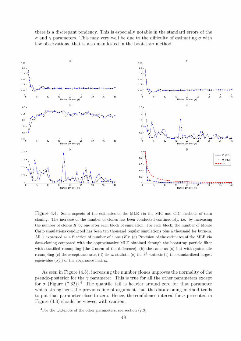
there is a discrepant tendency. This is especially notable in the standard errors of theσ and γ parameters. This may very well be due to the difficulty of estimating σ withfew observations, that is also manifested in the bootstrap method.

Figure 4.4: Some aspects of the estimates of the MLE via the MIC and CIC methods of data

cloning. The increase of the number of clones has been conducted continuously, i.e. by increasing

the number of clones K by one after each block of simulation. For each block, the number of Monte

Carlo simulations conducted has been ten thousand regular simulations plus a thousand for burn-in.

All is expressed as a function of number of clone (K): (a) Precision of the estimates of the MLE via

data-cloning compared with the approximative MLE obtained through the bootstrap particle filter

with stratified resampling (the 2-norm of the difference), (b) the same as (a) but with systematic

resampling (c) the acceptance rate, (d) the ω-statistic (e) the r2-statistic (f) the standardized largest

eigenvalue (λSK) of the covariance matrix.

As seen in Figure (4.5), increasing the number clones improves the normality of thepseudo-posterior for the γ parameter. This is true for all the other parameters exceptfor σ (Figure (7.32)).4 The quantile tail is heavier around zero for that parameterwhich strengthens the previous line of argument that the data cloning method tendsto put that parameter close to zero. Hence, the confidence interval for σ presented inFigure (4.3) should be viewed with caution.

4For the QQ-plots of the other parameters, see section (7.3).

48

Observe that, the practical issues mentioned in section (2.3) is also applicable forBayesian estimation of the MLE via data cloning in the case of the type of models ofthis chapter, i.e. hidden Markov models.

Figure 4.5: Quantile-quantile plots for the simulations of γ using the MIC-method,and for different number of clones (K). The increase of the number of clones has beenconducted continuously, i.e. by increasing the number of clones K by one after eachblock of simulation. For each block, the number of Monte Carlo simulations conductedhas been ten thousand regular simulations plus ten thousand for burn-in.

49

Chapter 5

Concluding Remarks and FutureStudies

As a student of Monte Carlo methods, when this author was introduced to the subject,the initial impression was one of surprise. Too many topics of the subject matterresembled the strive to put out continuously erupting fires.

While the MCMC methods were theoretically attractive, the use of blind simula-tions was not always successful even with the use of informative priors in a Bayesiansetting.1 That fire was then put out by using smarter simulations for instance throughthe use of SMC methods. However, the estimation power and rate of convergenceachieved through the SMC methods, is too often too dependent on the choice of theinstrumental distribution. Hence, importance sampling was introduced.

Nevertheless, importance sampling suffered from its own numerical problems, namelythe weight degeneracy problem and the curse of dimensionality. Too often the weights,being too small in comparison to some other particles in the chain, were numericallyequated with zero, rendering few particles carrying the whole weight of the chain. Torelieve this issue, different approaches were introduced such as antithetic sampling andresampling techniques, which in turn had issues of their own. For instance, there werea wide range of resampling techniques to be chosen, no one universally successful.

The data cloning approach takes the researcher back to the initial fire, the lowsuccess rate of blind simulations in MCMC methods, and provides a simple tool tocombat that problem, namely copying the data. The method is surprisingly successful,and improves the accuracy of the estimates when approximating the MLE.

The data cloning procedure have clear advantages over ordinary maximum like-lihood estimation. It avoids analytic and numerical evaluation of high-dimensionalintegrals. Moreover, it avoids numerical optimization of a function, and numericalcomputation of the curvature of the likelihood function. Of course not all of the tun-ing issues related to MCMC methods can be avoided and the convergence rate shouldbe monitored.

The data cloning approach has also several advantages over the SMC methods.First and foremost, it is significantly simpler to implement. Furthermore, it com-paratively raises fewer numerical issues to deal with. Moreover, data-cloning, as anyMCMC approach, is done through blind simulations, which means that the choice ofthe proposal function becomes simpler. Most importantly, it avoids numerical opti-

1Blind simulations refer to simulations that do not depend on the observed data, as in the MCMCmethods.

50

mization of a function.The data cloning procedure has other benefits in its own rights. Firstly, the con-

vergence to the true MLE as the number of clones increases, is invariant to the choiceof the prior distribution. This was mentioned in section (1.2), where it was proventhat the pseudo-posterior of the K times cloned data was degenerate at the true MLE.Furthermore the approximative normality of the estimates, provides a convenient wayof producing confidence intervals.

The data cloning method is also accompanied by several diagnostic tools, namelythe ω, r2 and the standardized largest eigenvalues of the variance-covariance matrixλSK . The first two ones are to be close to, or better yet converge to, zero if the estimationprocess is successful. The standardized largest eigenvalues of the variance-covariancematrix λSK is also supposed to converge to zero if the estimation process is successful.Failure to do so could be a symptom of the non-estimability of the parameters. Theconclusion of non-estimability should, however, be drawn with caution, as failure toconverge could be a result of numerical transformations.2

The data-cloning method, however, has some disadvantages. A prominent oneappears when dealing with very large data sets, especially when dealing with statespace models. In such cases, the simulation of the latent process (in step 3 in Algorithm(4)) may be very inaccurate and too far away from the true latent state. The reasonfor this phenomenon is the broad spectrum of possible trajectories. In such cases SMCmethods are more suitable, since the proposals depend on the observations, and arenot obtained blindly as in the data cloning method.3

The two data cloning procedures MIC and CIC, seem to function largely similarly.However, as the complexity of the problem was increased in the state space model (seesection (4.2)), the MIC method proved to be more stable. This could be explained bythe fact that, in the MIC method as the mean is taken after each block of iterations foreach fixed number of clones K, the chain is drawn to a point with higher likelihood.In the CIC method, however, the chain may be stuck in the tail producing singularcovariance updates in update of the variance-covariance matrix of the random walkproposal mechanism.

For future studies, one may want to study how the data cloning approach han-dles even more complex scenarios. Furthermore, combining the data cloning approachwith other estimations techniques would be of particular interest. Moreover, a rig-orous assessment of the theoretical grounds of the data cloning method is of utmostimportance.

All in all, the data cloning approach seems to have a lot of potential. It increasesthe numerical accuracy of the estimates of the MLE significantly, while adding almostno further complexity to the simple MCMC process in a Bayesian setting. Consideringfurther its relative simplicity to the SMC methods and its tuning issues, it could helprelieve many researchers of considerable burdens when performing statistical estima-tions.

2See footnote (3) in section (4.2).3One should make a distinction, however, between two different kinds of large data sets: long data

sets and rich data sets. Long data sets contain a large number of data points corresponding to alarge interval over a certain dimension, say time. Rich data sets, on the other hand, contain also alarge number of data points, but over a short interval. The data-cloning method is very suitable forrich data sets, but performs poorly for long ones. SMC methods are more suitable for long data sets.

51

Chapter 6

References

Blevins, Jason (2008), ”Calculating the Log Sum of Exponentials,” [Online] Availablefrom: http://jblevins.org/log/log-sum-exp. [Accessed: 1st June 2015].

Cosma, Iona A. & Evers, Ludger (2010) ”Markov Chains and Monte Carlo Meth-ods,” [Online] AIMS. Available from: http://users.aims.ac.za/ ioana/notes.pdf/. [Accessed:12th May 2015].

D’Errico, J. (2014). ”Adaptive Robust Numerical Differentiation,” [Online] Math-Works. Available from: http://www.mathworks.com/matlabcentral/fileexchange/13490-adaptive-

robust-numerical-differentiation. [Accessed: 4th June 2015].

Ditlevsen, S. and Samson, A. (2013) ”Introduction to Stochastic Models in Biology.”In Bachar M., Batzel J. J. and Ditlevsen, S. (eds.). Stochastic Mathematical Modelswith Applications to Neuronal Modeling. Berlin Heidelberg, Springer-Verlag.

Doucet, Arnaud; Godsill, Simon; & Andriue, Christophe (2000) ”On sequential MonteCarlo sampling methods for Bayesian filtering,” Statistics and Computing, vol. 10, pp.197-208.

Haario, Heikki; Saksman, Eero, & Tamminen Johanna (2001), ”An adaptive Metropo-lis algorithm”, Bernoulli, vol. 7, no. 2, pp. 223-242.

Hastings, W. K. (1970) ”Monte Carlo Sampling Methods Using Markov Chains andTheir Applications,” Biometrika, vol. 57, no. 1., pp. 97-109.

Hol, Jeroen D. (2004) ”Resampling in particle filters” [Online] Linkoping: Depart-ment of Electrical Engineering, Linkoping University. Available from:http://www.control.isy.liu.se/student/exjobb/xfiles/0283.pdf. [Accessed: 26th May 2015].

Jacquier, Eric; Johannes, Michael, & Polson, Nicholas (2007) ”MCMC maximum like-lihood for latent state models,” Journal of Econometrics, vol. 137, pp. 615-640.

Lele, Subhash R.; Dennis, Brian, & Lutscher, Fritjof (2007), ”Data cloning: easymaximum likelihood estimation for complex ecological models using Bayesian Markovchain Monte Carlo methods,” Ecology Letters, vol. 10, pp. 551-563.

52

Lele, Subhash R.; Nadeem, Khurram, & Schmuland, Byron (2010), ”Estimabilityand Likelihood Inference for Generalized Linear Mixed Models Using Data Cloning,”Journal of the American Statistical Association, vol. 105, no. 492, December, pp.1617-1625.

Liu, Jun S.; & Chen, Rong (1998, ”Srquential Monte Carlo Methods for DynamicSystems,” Journal of the American Statistical Association, vol. 93, no. 443, pp. 1032-1044.

Kong, Augustine; Liu, Jun S., & Wong, Hung Wing (1994) ”Sequential Imputationsand Bayesian Missing Data Problems,” Journal of the American Statistical Associa-tion, vol. 89, no. 425, pp. 278-288.

Roberts, G. O.; Gelman, A., & Gilks, W. R. (1997), ”Weak Convergence and optimalScaling of Random Walk Metropolis Algorithms”, The Annals of Applied Probability,vol. 7, no. 1, pp. 110-120.

Seber, G. A. F.; & Wild, C. J. (2003), Nonlinear Regression. Wiley series in probabil-ity and statistics. New Jersey, John Wiley & Sons Inc.

Wilkinson D. J. (2012), Stochastic Modeling for Systems Biology. 2nd Ed. Boca Raton,CRC Press.

Withange, Norishan N. K. P. (2013), ”Methods and Applications in the Analysis ofCorrelated Non-Gaussian Data,” [Online] University of Calgary, Alberta. Availablefrom: http://theses.ucalgary.ca/bitstream/11023/848/2/ucalgary 2013 withanage niroshan.pdf/.

[Accessed: 5th May 2015]

53

Chapter 7

Appendix - Omitted Figures

7.1 Static models

7.1.1 Simple Linear Regression

Figure 7.1: MCMC chain of simulations with increasing number of copies (by one,starting at one) every 104 iterations, applying the CIC method to the simple linearregression model in (2.3). The red line is the true MLE.

54

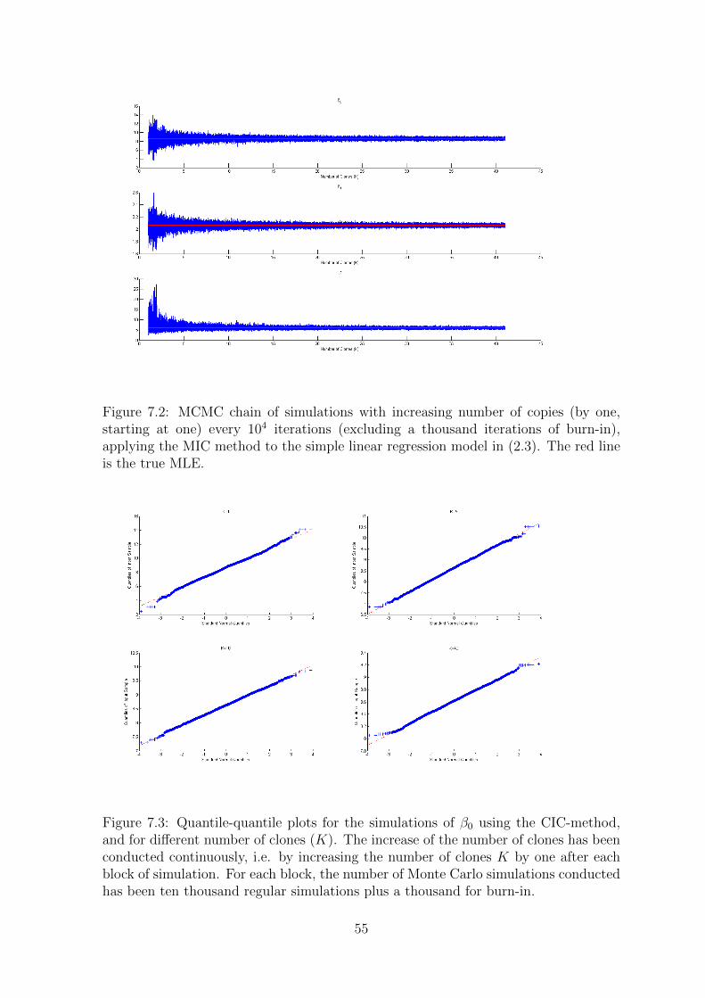
Figure 7.2: MCMC chain of simulations with increasing number of copies (by one,starting at one) every 104 iterations (excluding a thousand iterations of burn-in),applying the MIC method to the simple linear regression model in (2.3). The red lineis the true MLE.

Figure 7.3: Quantile-quantile plots for the simulations of β0 using the CIC-method,and for different number of clones (K). The increase of the number of clones has beenconducted continuously, i.e. by increasing the number of clones K by one after eachblock of simulation. For each block, the number of Monte Carlo simulations conductedhas been ten thousand regular simulations plus a thousand for burn-in.

55

Figure 7.4: Quantile-quantile plots for the simulations of β0 using the MIC-method,and for different number of clones (K). The increase of the number of clones has beenconducted continuously, i.e. by increasing the number of clones K by one after eachblock of simulation. For each block, the number of Monte Carlo simulations conductedhas been ten thousand regular simulations plus a thousand for burn-in.

Figure 7.7: Quantile-quantile plots for the simulations of β1 using the CIC-method,and for different number of clones (K). The increase of the number of clones has beenconducted continuously, i.e. by increasing the number of clones K by one after eachblock of simulation. For each block, the number of Monte Carlo simulations conductedhas been ten thousand regular simulations plus a thousand for burn-in.

56

Figure 7.5: Quantile-quantile plots for the simulations of β1 using the MIC-method,and for different number of clones (K). The increase of the number of clones has beenconducted continuously, i.e. by increasing the number of clones K by one after eachblock of simulation. For each block, the number of Monte Carlo simulations conductedhas been ten thousand regular simulations plus a thousand for burn-in.

Figure 7.8: Quantile-quantile plots for the simulations of σ2 using the CIC-method,and for different number of clones (K). The increase of the number of clones has beenconducted continuously, i.e. by increasing the number of clones K by one after eachblock of simulation. For each block, the number of Monte Carlo simulations conductedhas been ten thousand regular simulations plus a thousand for burn-in.

57

Figure 7.6: Quantile-quantile plots for the simulations of σ2 using the MIC-method,and for different number of clones (K). The increase of the number of clones has beenconducted continuously, i.e. by increasing the number of clones K by one after eachblock of simulation. For each block, the number of Monte Carlo simulations conductedhas been ten thousand regular simulations plus a thousand for burn-in.

58

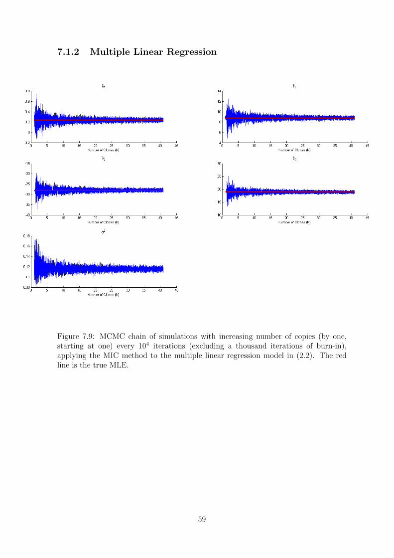
7.1.2 Multiple Linear Regression

Figure 7.9: MCMC chain of simulations with increasing number of copies (by one,starting at one) every 104 iterations (excluding a thousand iterations of burn-in),applying the MIC method to the multiple linear regression model in (2.2). The redline is the true MLE.

59

Figure 7.10: Quantile-quantile plots for the simulations of β1 using the CIC-method,and for different number of clones (K). The increase of the number of clones has beenconducted continuously, i.e. by increasing the number of clones K by one after eachblock of simulation. For each block, the number of Monte Carlo simulations conductedhas been ten thousand regular simulations plus a thousand for burn-in.

Figure 7.11: Quantile-quantile plots for the simulations of β2 using the CIC-method,and for different number of clones (K). The increase of the number of clones has beenconducted continuously, i.e. by increasing the number of clones K by one after eachblock of simulation. For each block, the number of Monte Carlo simulations conductedhas been ten thousand regular simulations plus a thousand for burn-in.

60

Figure 7.12: Quantile-quantile plots for the simulations of σ2 using the MIC-method,and for different number of clones (K). The increase of the number of clones has beenconducted continuously, i.e. by increasing the number of clones K by one after eachblock of simulation. For each block, the number of Monte Carlo simulations conductedhas been ten thousand regular simulations plus a thousand for burn-in.

Figure 7.13: Quantile-quantile plots for the simulations of β0 using the MIC-method,and for different number of clones (K). The increase of the number of clones has beenconducted continuously, i.e. by increasing the number of clones K by one after eachblock of simulation. For each block, the number of Monte Carlo simulations conductedhas been ten thousand regular simulations plus a thousand for burn-in.

61

Figure 7.14: Quantile-quantile plots for the simulations of β1 using the MIC-method,and for different number of clones (K). The increase of the number of clones has beenconducted continuously, i.e. by increasing the number of clones K by one after eachblock of simulation. For each block, the number of Monte Carlo simulations conductedhas been ten thousand regular simulations plus a thousand for burn-in.

Figure 7.15: Quantile-quantile plots for the simulations of β2 using the MIC-method,and for different number of clones (K). The increase of the number of clones has beenconducted continuously, i.e. by increasing the number of clones K by one after eachblock of simulation. For each block, the number of Monte Carlo simulations conductedhas been ten thousand regular simulations plus a thousand for burn-in.

62

Figure 7.16: Quantile-quantile plots for the simulations of β3 using the MIC-method,and for different number of clones (K). The increase of the number of clones has beenconducted continuously, i.e. by increasing the number of clones K by one after eachblock of simulation. For each block, the number of Monte Carlo simulations conductedhas been ten thousand regular simulations plus a thousand for burn-in.

Figure 7.17: Quantile-quantile plots for the simulations of σ2 using the MIC-method,and for different number of clones (K). The increase of the number of clones has beenconducted continuously, i.e. by increasing the number of clones K by one after eachblock of simulation. For each block, the number of Monte Carlo simulations conductedhas been ten thousand regular simulations plus a thousand for burn-in.

63

7.2 Stochastic Dynamical Models without Obser-

vational Noise

Figure 7.18: MCMC chain of simulations with increasing number of copies (by one,starting at one) every 104 steps, applying the MIC method to the Gompertz model.The red line is the true MLE. The starting values in the simulation are the true valuesof parameter, not to be confused with the true MLE.

64

Figure 7.19: Some aspects of the estimates of the MLE via the MIC and CIC methods of data

cloning. The increase was done sporadically. The number of clones were 1, 2, 5, 10, 20 and 40. For each

block, the number of Monte Carlo simulations conducted has been ten thousand regular simulations

plus a thousand for burn-in. All is expressed as a function of number of clone (K): (a) Precision

of the estimates of the MLE (the 2-norm of the difference), (b) Precision of the estimates of the

variance covariance matrix of the MLE (the 2-norm of the difference) (c) the acceptance rate, (d) the

ω-statistic (e) the r2-statistic (f) the standardized largest eigenvalue (λSK) of the covariance matrix.

65

Figure 7.20: Quantile-quantile plots for the simulations of ln(A) using the CIC-method,and for different number of clones (K). The increase of the number of clones has beenconducted continuously, i.e. by increasing the number of clones K by one after eachblock of simulation. For each block, the number of Monte Carlo simulations conductedhas been ten thousand regular simulations plus ten thousand for burn-in.

Figure 7.21: Quantile-quantile plots for the simulations of C using the CIC-method,and for different number of clones (K). The increase of the number of clones has beenconducted continuously, i.e. by increasing the number of clones K by one after eachblock of simulation. For each block, the number of Monte Carlo simulations conductedhas been ten thousand regular simulations plus ten thousand for burn-in.

66

Figure 7.22: Quantile-quantile plots for the simulations of σ using the CIC-method,and for different number of clones (K). The increase of the number of clones has beenconducted continuously, i.e. by increasing the number of clones K by one after eachblock of simulation. For each block, the number of Monte Carlo simulations conductedhas been ten thousand regular simulations plus ten thousand for burn-in.

Figure 7.23: Quantile-quantile plots for the simulations of ln(A) using the MIC-method, and for different number of clones (K). The increase of the number of cloneshas been conducted continuously, i.e. by increasing the number of clones K by oneafter each block of simulation. For each block, the number of Monte Carlo simulationsconducted has been ten thousand regular simulations plus ten thousand for burn-in.

67

Figure 7.24: Quantile-quantile plots for the simulations of B using the MIC-method,and for different number of clones (K). The increase of the number of clones has beenconducted continuously, i.e. by increasing the number of clones K by one after eachblock of simulation. For each block, the number of Monte Carlo simulations conductedhas been ten thousand regular simulations plus ten thousand for burn-in.

Figure 7.25: Quantile-quantile plots for the simulations of C using the MIC-method,and for different number of clones (K). The increase of the number of clones has beenconducted continuously, i.e. by increasing the number of clones K by one after eachblock of simulation. For each block, the number of Monte Carlo simulations conductedhas been ten thousand regular simulations plus ten thousand for burn-in.

68

Figure 7.26: Quantile-quantile plots for the simulations of σ using the MIC-method,and for different number of clones (K). The increase of the number of clones has beenconducted continuously, i.e. by increasing the number of clones K by one after eachblock of simulation. For each block, the number of Monte Carlo simulations conductedhas been ten thousand regular simulations plus ten thousand for burn-in.

69

7.3 State Space Models

Figure 7.27: MCMC chain of simulations with increasing number of copies (by one,starting at one) every 104 iterations, applying the CIC method to the Gompertz model.The red line is the true MLE. The starting values in the simulation are the true valuesof parameter, not to be confused with the true MLE.

70

Figure 7.28: Some aspects of the estimates of the MLE via the MIC and CIC methods of data

cloning. The increase was done sporadically. The number of clones were 1, 2, 5, 10, 20 and 40. For each

block, the number of Monte Carlo simulations conducted has been ten thousand regular simulations

plus a thousand for burn-in. All is expressed as a function of number of clone (K): (a) Precision of

the estimates of the MLE via data-cloning compared with the approximative MLE obtained through

the bootstrap particle filter with stratified resampling (the 2-norm of the difference), (b) the same as

(a) but with systematic resampling (c) the acceptance rate, (d) the ω-statistic (e) the r2-statistic (f)

the standardized largest eigenvalue (λSK) of the covariance matrix.

71

Figure 7.29: Quantile-quantile plots for the simulations of ln(A) using the MIC-method, and for different number of clones (K). The increase of the number of cloneshas been conducted continuously, i.e. by increasing the number of clones K by oneafter each block of simulation. For each block, the number of Monte Carlo simulationsconducted has been ten thousand regular simulations plus ten thousand for burn-in.

Figure 7.30: Quantile-quantile plots for the simulations of B using the MIC-method,and for different number of clones (K). The increase of the number of clones has beenconducted continuously, i.e. by increasing the number of clones K by one after eachblock of simulation. For each block, the number of Monte Carlo simulations conductedhas been ten thousand regular simulations plus ten thousand for burn-in.

72

Figure 7.31: Quantile-quantile plots for the simulations of C using the MIC-method,and for different number of clones (K). The increase of the number of clones has beenconducted continuously, i.e. by increasing the number of clones K by one after eachblock of simulation. For each block, the number of Monte Carlo simulations conductedhas been ten thousand regular simulations plus ten thousand for burn-in.

Figure 7.32: Quantile-quantile plots for the simulations of σ using the MIC-method,and for different number of clones (K). The increase of the number of clones has beenconducted continuously, i.e. by increasing the number of clones K by one after eachblock of simulation. For each block, the number of Monte Carlo simulations conductedhas been ten thousand regular simulations plus ten thousand for burn-in.

73