A Comparison of a Bayesian and Maximum Likelihood ...

A Comparison of a Bayesian and Maximum Likelihood Algorithms for

Estimation of a Multilevel IRT Model

by

Insuk Kim

(Under the direction of Deborah Bandalos)

Abstract

Multilevel Item Response Theory (IRT) models provide an analytic approach that formally

incorporates the hierarchical structure characteristic of much educational and psychological

data. In this study, maximum likelihood (ML) estimation, which is the method most

widely used in current applied multilevel IRT analyses and Bayesian estimation, which has

become a viable alternative to ML-based estimation techniques were examined. Item and

ability parameter estimates from Bayesian and ML methods were compared using both

empirical data and simulated data. It was found that Bayesian estimation using WinBUGS

performed better than ML estimations in all conditions with regard to the item parameter

estimates. For the individual (Level 2) variance estimates, PQL estimation using HLM

showed less bias than the others. However, Bayesian and ML estimations performed

similarly to each other for the group (Level 3) variance parameter estimates.

Index words: Multilevel Item Response Theory, Maximum Likelihood Estimation,Bayesian Estimation



by

Insuk Kim

B.A., The Korea University, 1996

M.A., The University of Georgia, 2001

A Dissertation Submitted to the Graduate Faculty

of The University of Georgia in Partial Fulfillment

of the

Requirements for the Degree

Doctor of Philosophy

Athens, Georgia

2007

c© 2007

Insuk Kim

All Rights Reserved



by

Insuk Kim

Approved:

Major Professor: Deborah Bandalos

Committee: Allan Cohen

Steve Olejnik

Ted Baumgartner

Electronic Version Approved:

Maureen Grasso

Dean of the Graduate School

The University of Georgia

May 2007

Acknowledgments

I believe that the completion of this dissertation is not the end of study but the

opportunity to begin new study. I thank many people who give me this opportunity.

First I would like to express my gratitude to my advisor, Dr. Deborah Bandalos. Without

her consideration and help, I would not have completed this dissertation. I must express my

sincere appreciation to Dr. Allan Cohen. I am deeply indebted to him for his guidance and

support throughout this study. I would also like to thank the other committee members,

Drs. Steve Olejnik and Ted Baumgartner, for their advice and valuable comments.

I thank my family and friends who always encourage me throughout my graduate study.

The friendship of Hong-i Moon is much appreciated. Also, I owe special thanks to Sunjoo

Cho who is always willing to help me with my study.

Last, but not least, I thank my husband, Kiung Ryu for his understanding and our

daughter, Grace Ryu for her love. His support and encouragement was in the end what

made this dissertation possible in a timely fashion.

iv

Table of Contents

Page

Acknowledgments . . . . . . . . . . . . . . . . . . . . . . . . . . . . . . . . . iv

List of Figures . . . . . . . . . . . . . . . . . . . . . . . . . . . . . . . . . . . viii

List of Tables . . . . . . . . . . . . . . . . . . . . . . . . . . . . . . . . . . . ix

Chapter

1 Introduction . . . . . . . . . . . . . . . . . . . . . . . . . . . . . . . . 1

1.1 Preview of the Study . . . . . . . . . . . . . . . . . . . . . . 1

1.2 Significance of the Study . . . . . . . . . . . . . . . . . . . . 3

1.3 Overview of Later Chapters . . . . . . . . . . . . . . . . . . 4

2 Literature Review . . . . . . . . . . . . . . . . . . . . . . . . . . . . . 5

2.1 Hierarchical Linear Model . . . . . . . . . . . . . . . . . . . 5

2.2 Item Response Theory . . . . . . . . . . . . . . . . . . . . . . 7

2.3 Multilevel Item Response Theory . . . . . . . . . . . . . . . 9

2.4 Maximum Likelihood Estimation . . . . . . . . . . . . . . . . 11

2.5 Bayesian Estimation . . . . . . . . . . . . . . . . . . . . . . . . 14

2.6 Markov Chain Monte Carlo . . . . . . . . . . . . . . . . . . 16

2.7 Research Questions . . . . . . . . . . . . . . . . . . . . . . . . 18

3 Methodology . . . . . . . . . . . . . . . . . . . . . . . . . . . . . . . . 20

3.1 Multilevel Item Response Theory . . . . . . . . . . . . . . . 20

3.2 Computer Programs . . . . . . . . . . . . . . . . . . . . . . . 24

3.3 Empirical Study . . . . . . . . . . . . . . . . . . . . . . . . . . 33

v

vi

3.4 Simulation Study . . . . . . . . . . . . . . . . . . . . . . . . . 36

4 Results . . . . . . . . . . . . . . . . . . . . . . . . . . . . . . . . . . . . 39

4.1 Empirical Data . . . . . . . . . . . . . . . . . . . . . . . . . . . 39

4.2 Simulated Data . . . . . . . . . . . . . . . . . . . . . . . . . . . 50

5 Discussion . . . . . . . . . . . . . . . . . . . . . . . . . . . . . . . . . . 88

5.1 Summary . . . . . . . . . . . . . . . . . . . . . . . . . . . . . . . 88

5.2 Limitations and Suggestions . . . . . . . . . . . . . . . . . . . 90

Bibliography . . . . . . . . . . . . . . . . . . . . . . . . . . . . . . . . . . . . 92

Appendix

A Mplus Code . . . . . . . . . . . . . . . . . . . . . . . . . . . . . . . . . 100

A.1 The Unconditional Model . . . . . . . . . . . . . . . . . . . . 100

A.2 The Model with Level-2 Predictor Variable . . . . . . . . 101

A.3 The Model with Level-2 and Level-3 Predictor Variables 102

B WinBUGS Code . . . . . . . . . . . . . . . . . . . . . . . . . . . . . . . 103

B.1 The Unconditional Model . . . . . . . . . . . . . . . . . . . . 103

B.2 The Model with Level-2 Predictor Variable . . . . . . . . 105

B.3 The Model with Level-2 and Level-3 Predictor Variables 107

C Convergence Diagnostics . . . . . . . . . . . . . . . . . . . . . . . . 109

C.1 Geweke . . . . . . . . . . . . . . . . . . . . . . . . . . . . . . . 109

C.2 Raftery and Lewis . . . . . . . . . . . . . . . . . . . . . . . . 110

D Estimated Parameter Means From Five Replications . . . . . . . 111

D.1 The Unconditional Model . . . . . . . . . . . . . . . . . . . . 111

D.2 The Model with Level-2 Predictor Variable . . . . . . . . 112

D.3 The Model with Level-2 and Level-3 Predictor Variables 113

vii

E Line Graphs Of Estimated Parameter Means From Five Replica-

tions . . . . . . . . . . . . . . . . . . . . . . . . . . . . . . . . . . . . . 114

E.1 The Unconditional Model . . . . . . . . . . . . . . . . . . . . 114

E.2 The Model with Level-2 Predictor Variable . . . . . . . . 115

E.3 The Model with Level-2 and Level-3 Predictor Variables 116

List of Figures

3.1 A Sample of History Plot from WinBUGS . . . . . . . . . . . . . . . . . . . 31

3.2 A Sample of Gelman and Rubin Statistic from WinBUGS . . . . . . . . . . 32

4.1 History Plots of Parameter Estimates . . . . . . . . . . . . . . . . . . . . . . 52

4.2 Density Plots of Parameter Estimates . . . . . . . . . . . . . . . . . . . . . . 53

4.3 The RMSEs of Item Parameters . . . . . . . . . . . . . . . . . . . . . . . . . 58

4.4 The RMSEs of Item Parameters . . . . . . . . . . . . . . . . . . . . . . . . . 59





4.9 The RMSEs of the Coefficient of Level-3 Predictor . . . . . . . . . . . . . . . 77

4.10 The RMSEs of the Coefficient of Level-3 Predictor . . . . . . . . . . . . . . . 78

4.11 The RMSEs for the Item Parameters . . . . . . . . . . . . . . . . . . . . . . 81

4.12 The RMSEs for the Individual Variance Parameters . . . . . . . . . . . . . . 83

4.13 The RMSEs for the Group Variance Parameters . . . . . . . . . . . . . . . . 85



viii

List of Tables

3.1 FCAT Data Description . . . . . . . . . . . . . . . . . . . . . . . . . . . . . 34

3.2 The Empirical Data Sets Used . . . . . . . . . . . . . . . . . . . . . . . . . . 35

3.3 Generating Parameters for the Models . . . . . . . . . . . . . . . . . . . . . 38

4.1 Results for the Unconditional Model . . . . . . . . . . . . . . . . . . . . . . 39

4.2 Results for the Model with Level-2 Predictor Variables . . . . . . . . . . . . 40

4.3 Parameter Estimates of the FCAT Data . . . . . . . . . . . . . . . . . . . . 42

4.4 Parameter Estimates of the FCAT Data . . . . . . . . . . . . . . . . . . . . 44

4.5 Item Difficulty Estimates of the TIMSS Data . . . . . . . . . . . . . . . . . . 45

4.6 Parameter Estimates of the TIMSS Data . . . . . . . . . . . . . . . . . . . . 46

4.7 Parameter Estimates of the CFSEI Data . . . . . . . . . . . . . . . . . . . . 47

4.8 Parameter Estimates of the CFSEI Data . . . . . . . . . . . . . . . . . . . . 48

4.9 Item Fixed Effects for FCAT Data for the Unconditional Model . . . . . . . 49

4.10 Group Variance Estimates for the Unconditional Model . . . . . . . . . . . . 50

4.11 RMSEs for the Unconditional Model . . . . . . . . . . . . . . . . . . . . . . 55

4.12 RMSEs for the Unconditional Model . . . . . . . . . . . . . . . . . . . . . . 56

4.13 Tests of Within-Subjects Effects . . . . . . . . . . . . . . . . . . . . . . . . . 57

4.14 Tests of Between-Subjects Effects . . . . . . . . . . . . . . . . . . . . . . . . 58





4.19 RMSEs for the Model with the Level-2 Predictor Variable . . . . . . . . . . 66


ix

x









4.29 Item Parameter Estimates for the Unconditional Model, . . . . . . . . . . . 79







Chapter 1

Introduction

1.1 Preview of the Study

Hierarchical linear models (HLM) allow the natural multilevel structure characteristics of

much educational and psychological data to be represented formally in the analysis of the

data (Bryk & Raudenbush, 1992; Goldstein, 1987; Longford, 1993). Multilevel item

response theory (IRT) models have been proposed as extensions of hierarchical generalized

linear models (HGLM: Stiratelli, Laird, & Ware, 1984; Wong & Mason, 1985). The

multilevel IRT models provide an analytic approach that formally incorporates the

hierarchical structure characteristics of much educational and psychological data. The

combination of HLM with IRT incorporates measurement error in estimates of the latent

trait, θ, into the estimation of model parameters (Adams, Wilson, & Wu, 1997; Maier,

2001). Adams et al. (1997) and Patz and Junker (1999b) note that even the simplest of

IRT models can be viewed as a multilevel model in which item responses are nested within

persons. In this view, multilevel modeling provides a framework covering most IRT models

and applications, for example, equating and differential item functioning (Rijmen,

Tuerlinckx, De Boeck, & Kuppens, 2003).

In this study, some estimation issues in fitting multilevel IRT models were examined.

The combination of HLM and IRT has led to the development of psychometric models for

item response data that contain a hierarchical structure thus enabling a researcher to study

the impact of covariates (e.g., schools, curriculum) on the lower level units such as students

(e.g., Adams et al., 1997; Kamata, 2001; Maier, 2001). Adams et al. (1997), for example,

describe a two-level model, in which person-characteristics are added as fixed parameters.

1

2

Kamata (2001) extended this model to a three-level formulation in which person-level

variables are incorporated as random effects.

Kamata’s multilevel model is a Rasch model (Rasch, 1960) and was estimated using the

computer program HLM (Raudenbush, Bryk, Cheong, & Congdon, 2000) under a

maximum likelihood (ML) algorithm. The HLM software uses the penalized or predictive

quasi-likelihood (PQL) method to approximate a maximum likelihood. One problem with

the PQL method is that it is known to underestimate the variances for dichotomous

responses with small samples at level-3 (Rodriguez & Goldman, 1995; Goldstein &

Rashbash, 1996). This may be a potential source of problems when estimating multilevel

IRT models for tests scored dichotomously. An alternative estimation method, such as a

Bayesian estimation (Maier, 2001), however, may be able to improve the variance estimates

of the level-3 parameters. In this study a Bayesian alternative to the HLM approach with a

focus on improvement in the variance estimates for the level-3 parameters was considered.

Multilevel models can become complex, making ML estimation difficult. Bayesian

estimation can be particularly useful when models become complex, as is the case when

additional linear constraints are added or when more complicated item formats are used on

a test. In reality, there could be situations in which the assumption of normality is not met

or for which sample sizes are too small for typical estimation of IRT model parameters. For

situations in which these assumptions cannot be met, Bayesian estimation procedures may

provide a useful alternative (Maier, 2001).

Efforts to estimate model parameters using a Bayesian algorithm are not new (e.g.,

Swaminathan & Gifford, 1982) although comparisons of Bayesian and ML algorithms in a

multilevel context are. Swaminathan and Gifford (1982) found Bayesian estimation to be

more accurate than ML estimation procedures for a Rasch model when the numbers of

items and examinees were small. More recently, Patz and Junker (1999a, 1999b) described

a fully Bayesian approach in the context of a multilevel IRT model and noted that

Bayesian estimation is particularly useful when models become very complex, as is easily

3

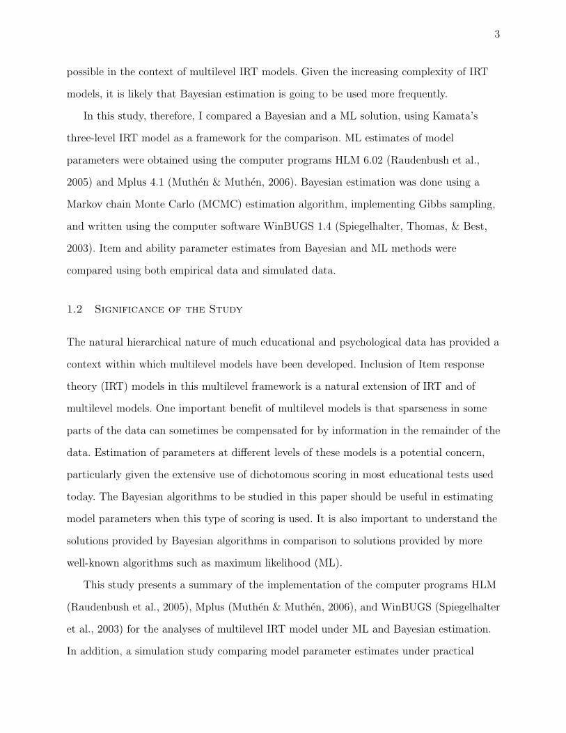
possible in the context of multilevel IRT models. Given the increasing complexity of IRT

models, it is likely that Bayesian estimation is going to be used more frequently.

In this study, therefore, I compared a Bayesian and a ML solution, using Kamata’s

three-level IRT model as a framework for the comparison. ML estimates of model

parameters were obtained using the computer programs HLM 6.02 (Raudenbush et al.,

2005) and Mplus 4.1 (Muthen & Muthen, 2006). Bayesian estimation was done using a

Markov chain Monte Carlo (MCMC) estimation algorithm, implementing Gibbs sampling,

and written using the computer software WinBUGS 1.4 (Spiegelhalter, Thomas, & Best,

2003). Item and ability parameter estimates from Bayesian and ML methods were

compared using both empirical data and simulated data.

1.2 Significance of the Study

The natural hierarchical nature of much educational and psychological data has provided a

context within which multilevel models have been developed. Inclusion of Item response

theory (IRT) models in this multilevel framework is a natural extension of IRT and of

multilevel models. One important benefit of multilevel models is that sparseness in some

parts of the data can sometimes be compensated for by information in the remainder of the

data. Estimation of parameters at different levels of these models is a potential concern,

particularly given the extensive use of dichotomous scoring in most educational tests used

today. The Bayesian algorithms to be studied in this paper should be useful in estimating

model parameters when this type of scoring is used. It is also important to understand the

solutions provided by Bayesian algorithms in comparison to solutions provided by more

well-known algorithms such as maximum likelihood (ML).

This study presents a summary of the implementation of the computer programs HLM

(Raudenbush et al., 2005), Mplus (Muthen & Muthen, 2006), and WinBUGS (Spiegelhalter

et al., 2003) for the analyses of multilevel IRT model under ML and Bayesian estimation.

In addition, a simulation study comparing model parameter estimates under practical

4

testing conditions should provide useful information for interpreting model results. Studies

such as this one will provide useful information for researchers seeking to use ML as well as

Bayesian estimation for estimation of multilevel IRT model parameters.

1.3 Overview of Later Chapters

In the remaining chapters of this dissertation, Chapter 2 provides some background on

Hierarchical Linear Model (HLM), Item Response Theory (IRT), and Multilevel IRT

including reviews of the statistical methods used for these models. Chapter 3 describes the

multilevel IRT model; especially Kamata’s three-level IRT model used as a framework for

the comparison and the corresponding methods of parameter estimation including Bayesian

estimation based on Gibbs sampling as well as Maximum Likelihood (ML) using both

simulated data and real data. Chapter 4 shows results of the analyses. Chapter 5

summarizes the results and discusses limitations and possible future work.

Chapter 2

Literature Review

2.1 Hierarchical Linear Model

In educational and any other research, data with hierarchical structures are fairly common.

These types of data exist when individuals are grouped in some way. For example, in

educational research students are nested in classrooms or schools.

Traditionally, data collected within groups have been analyzed using different types of

ordinary-least-squares (OLS) techniques. There are some known problems when

hierarchical data are analyzed using these traditional methods. Hierarchical data often

violate statistical assumptions such as linearity, normality, homoscedasticity, and

independence. For example, hierarchical data generally violate the statistical assumption

that observations or individuals are independent of each other, because individuals in the

same group are likely to be more similar than individuals in different groups. Ignoring

violations of the assumption of independence can result in mis-estimating the errors, which

can lead to incorrect inferences.

Osborne (2000) cites three problems with this traditional approach. (1) Under

aggregation, the properties of a higher-level (e.g., group) are described in terms of the sums

of the properties of a lower-level (e.g., individual) nested in that group, resulting in loss of

statistical power because in this process all individual information is lost. (2) Under

disaggregation, the assignment of a group characteristic to an individual, does not satisfy

the assumption of independence of observations, which can lead to over-optimistic

estimates of significance. (3) Under either aggregation or disaggregation, there is the

danger of the ecological fallacy: there is no necessary correspondence between

5

6

individual-level and group-level variable relationships (e.g., race and literacy correlate little

at the individual-level but correlate well at the group-level).

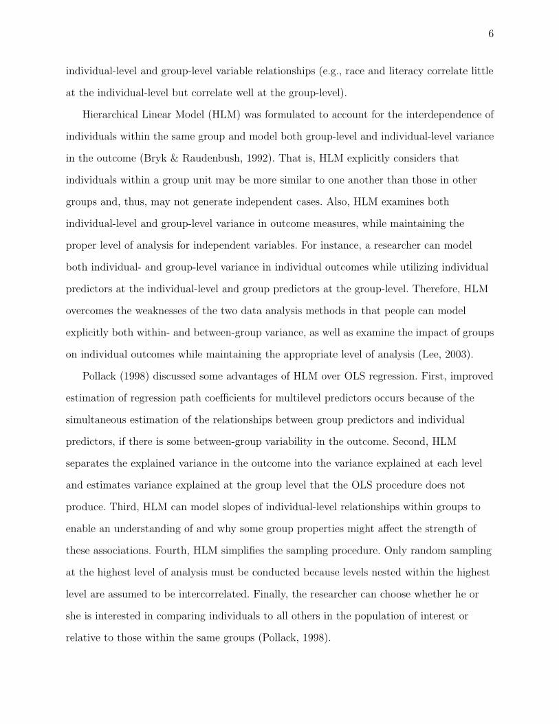
Hierarchical Linear Model (HLM) was formulated to account for the interdependence of

individuals within the same group and model both group-level and individual-level variance

in the outcome (Bryk & Raudenbush, 1992). That is, HLM explicitly considers that

individuals within a group unit may be more similar to one another than those in other

groups and, thus, may not generate independent cases. Also, HLM examines both

individual-level and group-level variance in outcome measures, while maintaining the

proper level of analysis for independent variables. For instance, a researcher can model

both individual- and group-level variance in individual outcomes while utilizing individual

predictors at the individual-level and group predictors at the group-level. Therefore, HLM

overcomes the weaknesses of the two data analysis methods in that people can model

explicitly both within- and between-group variance, as well as examine the impact of groups

on individual outcomes while maintaining the appropriate level of analysis (Lee, 2003).

Pollack (1998) discussed some advantages of HLM over OLS regression. First, improved

estimation of regression path coefficients for multilevel predictors occurs because of the

simultaneous estimation of the relationships between group predictors and individual

predictors, if there is some between-group variability in the outcome. Second, HLM

separates the explained variance in the outcome into the variance explained at each level

and estimates variance explained at the group level that the OLS procedure does not

produce. Third, HLM can model slopes of individual-level relationships within groups to

enable an understanding of and why some group properties might affect the strength of

these associations. Fourth, HLM simplifies the sampling procedure. Only random sampling

at the highest level of analysis must be conducted because levels nested within the highest

level are assumed to be intercorrelated. Finally, the researcher can choose whether he or

she is interested in comparing individuals to all others in the population of interest or

relative to those within the same groups (Pollack, 1998).

7

As mentioned previously with regard to hierarchical data, individuals in the same group

are likely to be more similar than individuals in different groups. Due to this, the variations

in outcome may be due to differences between groups, and to individual differences within

a group. The IntraClass Correlation (ICC) is the proportion of the variance in the outcome

that is between groups, which tells the extent to which observations are not independent of

a grouping variable (ex., schools). This value is computed using the following equation:

ρ =τ00

σ2 + τ00

where σ2 is the Level-one variance component and τ00 is the Level-two variance component.

Kreft (1996) concluded that multilevel modeling can be more useful for revealing

differences in variance among units in different groups which comprise the levels. Also,

multilevel modeling may be a preferred method when data are sparse, including studies

(e.g., twin studies) where groups are sparse. Kreft (1996) compared estimates of regression

parameters from multilevel analysis with those obtained from more traditional regression

techniques. In both cases, the fixed effects estimates were unbiased. The main difference,

however, was that the standard errors of these parameters were underestimated if

significant intraclass correlation was present and traditional regression analyses were used.

The presence of a significant intraclass correlation, in other words, is an indicator of the

need to employ multilevel modeling rather than conventional regression.

2.2 Item Response Theory

Item response theory (IRT) provides a family of mathematical models that specify the

relation of item characteristics to a person’s item responses (Embretson & Reise, 2000).

That is, an IRT model provides a prediction that a given person will provide a given

response to a given item. IRT requires stronger assumptions than Classical Test Theory

(CTT) to provide these item-level predictions. It does so using a modeling approach that

has a number of advantages over CTT. In IRT, the true score is defined on the latent trait

of interest rather than on the test, as is the case in CTT.

8

IRT assumes a single common factor accounts for all item covariances. This is stated as

unidimensionality, meaning the test measures only one latent trait. This trait is commonly

referred to as ‘ability’. If unidimensionality holds, then local independence holds as well and

ability, as considered in the model, fully determines the response to a given item. Also, IRT

assumes item and sample invariance for parameter estimates. Item invariance means that

all items that are calibrated to a given scale measure that scale. Any subset of those same

items measures the same scale. Sample invariance means that any simple random sample of

examinees from the population will yield calibrations that are invariant from the first

sample, up to a normalizing constant.

The simplest IRT model is a one-parameter logistic (1PL) model, which is also known as

the Rasch model. The Rasch model has only one parameter to describe an item, difficulty,

commonly denoted as β. In addition, each person has an ability parameter, denoted with θ.

This model is given as

Pi(θ) =exp(θ − βi)

1 + exp(θ − βi), (2.1)

where Pi(θ) is the probability that a person with ability θ answers item i correctly. The βi

is the difficulty parameter of item i. The difficulty is the value of ability at which a person

has a 50% probability of responding correctly to the item. Usually, the difficulty is

standardized and typically ranges from −3 to +3 with higher values indicating more

difficult items. The Rasch model assumes that all items are equally discriminating.

The Rasch model is known to be appropriate for modeling dichotomous responses and

models the probability of an individual’s correct response on a dichotomous item. The

logistic item characteristic curve (ICC) forms the boundary between the probability areas

of answering an item incorrectly and answering the item correctly. This one-parameter

logistic model assumes that the discriminations of all items are equal to one.

9

2.3 Multilevel Item Response Theory

Both hierarchical linear models (HLM) and item response theory (IRT) are used in a

variety of social science research applications. The use of HLM allows the natural

multilevel structure present in so much social science data to be represented formally in

data analysis (Bryk & Raudenbush, 1992; Goldstein, 1987; Longford, 1993). IRT allows

connections to be made between observed categorical responses provided by students and

an underlying unobservable trait, such as ability or attitude (Hambleton & Swaminathan,

1985; Lord & Novick, 1968).

The borrowing of strength advantage of multilevel modeling can be used to obtain

accurate estimates of the relationships within groups, regardless of sample size

(Raudenbush & Bryk, 2002). Person-level characteristics have been included in IRT models

to help improve estimation of item difficulty parameters, or to model the effects of person

characteristics upon the estimated latent trait measures (Mislevy, 1987; Patz & Junker,

1999a; Patz & Junker, 1999b). That is, the combination of HLM with IRT, called

multilevel IRT, incorporates the hierarchical structure directly in the estimation of model

parameters including persons’ ability for person-level and group-level item characteristics

and effects of covariates (Kamata, 2001).

An IRT model can be formulated as a multilevel model where item responses (level-1)

are nested within persons (level-2) and random effect variance terms (persons’ ability) vary

across the items at level-1 (e.g. Hedeker, 2004; Kamata, 2001; Rijmen et al., 2003). There

have been some attempts to reformulate IRT models as multilevel models (Stiratelli et al.,

1984; Wong & Mason, 1985; Adams et al., 1997; Kamata, 1998 & 2001).

Multilevel item response theory (IRT) models have been proposed as extensions of

hierarchical generalized linear models (HGLM: Stiratelli et al, 1984; Wong & Mason, 1985).

The intent of such extensions is to incorporate the estimation of IRT item and ability

parameters into the multilevel framework provided by HGLM.

10

Adams et al. (1997) described the reformulation of a regular IRT model as a multi-level

model, in which person-characteristic variables are added as fixed parameters that are

related to a latent trait. This was a two-level model in which person-level variables were

included as linear constraints in a multilevel framework. Within a multilevel framework,

the item response function can be viewed as a within person model and the person

population distribution model can be viewed as a between persons model. The person

population parameters are assumed to be random variables and used mainly for the

purpose of parameter estimation. They are decomposed into a linear combination of

multiple parameters. However, it is limited to a two-level model.

Kamata (1998, 2001) formulated a two-level item analysis model by the use of a

hierarchical generalized linear model (HGLM) and showed that it is algebraically

equivalent to the Rasch model. The level-1 model is an item level where the logit link

function is utilized to relate the probability of answering correctly to linear predictors of

item dummy codes. The level-2 model is the person level where the intercept coefficient of

level-1 is assumed to be a random effect across persons, but the item coefficients or slope

parameters are constrained to be constant across persons. When level-1 and level-2 are

combined, the model is algebraically equivalent to the Rasch model.

Kamata (1998) also showed the advantages of casting IRT models as multilevel models

by including person variables at the level-2 and extending to a three-level model to model

group variations and group characteristic variables. Pastor (2003) also discussed this

expansion of multilevel IRT models to three levels, allowing not only the dependency

typically found in hierarchical data to be accommodated, but also the estimation of (a)

latent traits at different levels and (b) the relationships between predictor variables and

latent traits at different levels.

11

2.4 Maximum Likelihood Estimation

A variety of methods have been used to estimate the parameters of these expanded Item

response theory (IRT) models. Maximum likelihood (ML) estimation is the method most

widely used in current applied multilevel IRT analyses. In ML estimation, population

parameters (e.g., item difficulty, ability) are treated as unknown but fixed quantities. That

is, the ability estimates are considered to be a random sample from an underlying ability

distribution and are integrated out to allow for maximization of likelihood for item

parameters.

In the IRT model, an individual’s ability is based on the probability of a given response

as a function of characteristics of items presented to an individual. For instance, a person

taking a test with i items can obtain one of i + 1 observed scores (0, 1, . . . , i). However, the

number of the possible responses to the test (the response patterns) is 2i. Each response

pattern has a certain probability. Also, IRT assumes local independence, which means that

the responses given to the separate items in a test are mutually independent given ability.

The probability that a person of ability θ will respond to the test with a certain pattern,

which is the likelihood function is written as:

L(θ) =∏

Pij(θj, βi)uiQij(θj, βi)

1−ui (2.2)

where ui ∈ (0, 1) is the score on item i, Pij(θj, βi) is the probability of the correct response

from the interaction between the individual ability θj and the item parameter βi, and

Qij(θj, βi) is the probability of the wrong response, equal to 1 − Pij(θj, βi). In ML, the

ability estimate will be the ability which has the highest likelihood given the observed

pattern and the item parameters.

In the context of multilevel IRT model, to maximize a likelihood two steps are required:

first, evaluating an integral and, second, maximizing that integral (Raudenbush & Bryk,

2002, p. 455).

12

Let Y denote a vector of all level-1 outcomes, let u denote the vector of all

random effects at level 2 and higher, and let ω denote a vector containing all

parameters to be estimated. Then we can denote as f(Y |u, ω) the probability

distribution of the outcome at level 1, given the random effects and parameters.

The higher-level models specify as p(u|ω) the distribution of the random effects

given the parameters. The likelihood of the data given only the parameters is

then

L(Y |ω) =∫

f(Y |u, ω)p(u|ω)du.

The aim of ML is to maximize the integral with respect to ω in order to make inferences

about ω.

Among the procedures commonly used are full maximum likelihood (FML, Goldstein,

1986; Longford, 1987) and restricted maximum likelihood estimation (RML, Mason, Wong,

& Entwistle, 1983; Bryk & Raudenbush, 1986). Under FML, variance-covariance

parameters and second-level fixed coefficients are estimated by maximizing their joint

likelihood. Under RML, variance-covariance components are estimated via maximum

likelihood, averaging over all possible values of the fixed effects, and fixed effects are

estimated via Generalized Least Squares (GLS) given these variance-covariance estimates

(Raudenbush, Bryk, Cheong, & Congdon, 2001, p. 7). GLS is then used to obtain estimates

and standard errors for the fixed effects (Goldstein, 1995; Raudenbush & Bryk, 2002).

According to Jones and Steenbergen (1997), the variance components for FML will

tend to be underestimated with small sample sizes since FML does not adjust for the

number of fixed effects that are estimated. Because RML estimates variance components

after removing the fixed effects from the model, it can lead theoretically to less bias than

FML (Raudenbush & Bryk, 2002). However, many authors (e.g., Rodriguez & Goldman,

1995; Goldstein & Rashbash, 1996; Breslow & Clayton, 1993) have reported that these

approximation methods exhibit downward biases for both the fixed effects and the variance

components for dichotomous responses with small cluster sizes.

13

A number of approaches to compute and maximize the likelihood have been developed.

The techniques to obtain full information ML can be classified along two dimensions

(Rijmen et al., 2003): the method of numerical integration of the intractable integrals used

to approximate the marginal likelihood and the type of algorithm used to maximize the

approximate marginal likelihood.

The performance of estimation methods has been the subject of several studies.

Rodriguez and Goldman (2001) reviewed several types of approximate procedures: the first

order MQL, the second order MQL, the first order PQL (PQL-1), and the second order

PQL (PQL-2, Goldstein & Rasbash, 1996) and a bootstrapped version (PQL-B) of PQL-1

and compared them, in estimating a three-level model, against the exact maximum

likelihood and the Gibbs sampling. The results showed that even PQL-2 sometimes

produces biased estimates, particulary when the clusters are small.

Snijders and Bosker (2000) are critical of such an estimation technique, arguing that

the algorithms for PQL are not very stable; whether or not algorithms converge may be

dependent upon the data set, the complexity of the model, and the starting values. To

overcome these problems with PQL, Raudenbush, Yang, and Yosef (2000) proposed a sixth

order Laplace approximation, known as LaPlace6, to approximate the maximum likelihood.

HLM provides this for two-level models with dichotomous responses.

Recently, Callens and Croux (2004) compared the performance of three different

likelihood-based estimation procedures: PQL, non-adaptive Gaussian quadrature, and

adaptive Gaussian quadrature (AGQ) in estimating parameters for multilevel logistic

regression models. In their study, comparing PQL with AGQ showed that the bias, as

measured by mean squared error (MSE), was larger for PQL.

I focus on two likelihood-based estimation procedures implemented in two of the most

commonly used statistical programs currently available for multilevel analysis, HLM and

Mplus.

14

As mentioned, HLM uses the PQL approach, which approximates the joint posterior

density of a parameter with a multivariate normal density having the same mode and

curvature at the mode as the true posterior. When Taylor series expansions around the

approximate posterior mode are used, this approach is called PQL.

Mplus performs full information ML estimation via an EM algorithm, solving the

integrals with adaptive Gaussian quadrature. In a Gaussian approach, the integral is

approximated by numerical integration and then the likelihood with approximate values for

the integrals is maximized. Using the adaptive approach, the variable of integration is

centered around its approximate posterior mode.

2.5 Bayesian Estimation

Bayesian methods have become a viable alternative to traditional maximum

likelihood-based estimation techniques and may be the only solution currently available for

more complex psychometric data structures (Rupp, Dey, & Zumbo, 2004). Given the

increasing complexity of Item Response Theory (IRT) models, it is likely that Bayesian

estimation is going to become used more frequently.

Even though the use of multilevel IRT model is advantageous when the assumptions of

independence of observations as well as independence and identical distribution of errors

are not met, it also requires satisfying the assumptions of both Hierarchical Linear Model

(HLM) and IRT such as (1) a single dimension underlying the item responses and (2) the

latent trait is a random parameter, is normally distributed within and between groups, and

the variance of which is the same across groups (Pastor, 2003). In reality, there could be

situations in which these assumptions cannot be met. Maier (2001) recommended the use of

fully Bayesian estimation procedures for situations in which the assumption of normality is

not met or when sample sizes are too small for typical estimation of IRT model parameters.

In contrast to Maximum Likelihood (ML), Bayesian inference does not rely on

asymptotic approximations to sampling distributions. In the Bayesian paradigm, the model

15

parameters are treated as random variables that follow a certain distribution. The

distributions of these parameters are conditional on the observed data, which are assumed

to be fixed.

Bayesian analysis proceeds by assuming a model f(Y |θ) for the data Y conditional

upon the unknown parameters θ. When f(Y |θ) is considered as a function of θ for fixed Y ,

it is referred to as the likelihood L(θ). A prior probability distribution f(θ) describes our

knowledge of the model parameters before the data is actually observed. Then, the

likelihood and prior distributions are combined according to Bayes’ theorem1 in order to

form the conditional distribution of θ given the observed data, Y , that is,

f(θ|Y ) ∝ f(θ)L(θ)

This conditional distribution is the posterior distribution for the model parameters and

describes our knowledge of the data after they have been observed.

Bayesian methods were first introduced by Edwards, Lindman, & Savage (1963), but it

was not long ago that Bayesian methods became the preferred approach for many

researchers, especially for relatively complex models or when data were sparse and

asymptotic theory was unlikely to hold.

Efforts to estimate model parameters using a Bayesian algorithm are not new (e.g.,

Swaminathan & Gifford, 1982). Swaminathan and Gifford (1982) compared Bayesian and

ML estimation procedures for a Rasch model. In their study, Bayesian estimation was

found to be more accurate than ML when the numbers of items and examinees were small.

In the context of a multilevel IRT model, Patz and Junker (1999a, 1999b) described a fully

Bayesian approach utilizing MCMC estimation. As Patz and Junker note, Bayesian

1A rule for computing the conditional probability distribution of a random variable A given B interms of the conditional probability distribution of variable B given A and the marginal probabilitydistribution of A alone

P (A|B) =P (A and B)

P (B)=

P (B|A)P (A)

P (B)

16

estimation is particularly useful when models become very complex. This is easily possible

in the context of multilevel IRT models.

Also, researchers have expanded traditional IRT models in a number of ways that are

appropriate in a variety of applications. Maier (2001) presented the integration of a

hierarchical linear model and a one-parameter logistic item response model using an

estimation method that does not rely on large-sample theory and normal approximations.

According to her study, simultaneous estimation allows for better estimation of the true

relationship by incorporating the standard errors of the latent traits into the model. More

recently, Browne and Draper (2006) compared Bayesian and likelihood-based methods for

fitting variance-components (VC) and random-effects logistic regression (RELR) models.

They found that quasi-likelihood methods for estimating random effects variances perform

poorly with respect to bias and coverage in the simulated example and Bayesian methods

were well-calibrated in estimation for all parameters of the model.

2.6 Markov Chain Monte Carlo

A major limitation to more widespread use of Bayesian estimation is that obtaining the

posterior distribution often requires integration which can be computationally very

difficult, but several approaches have been proposed. The main emphasis is placed on one

Markov Chain Monte Carlo (MCMC) method known as the Gibbs sampling, which was

used in this study. MCMC is a particular Bayesian data analysis method used to estimate

model parameters. A specific MCMC technique, Gibbs sampling, is a method for

generating random variables from a distribution by sampling from the collection of full

conditional distributions of the complete posterior distribution (Gelfand, Hills,

Racine-Poon, & Smith, 1990).

As the name suggests, MCMC methods produce chains in which each of the simulated

values is dependent on the preceding values. A Markov chain is a stochastic process with

the property that any specified state in the series, θ[t], is dependent only on the previous

17

value of the chain, θ[t−1], and is therefore conditionally independent of all other previous

values: θ[0], θ[1], . . . , θ[t−1]. This can be stated:

P (θ[t] ∈ A|θ[0], θ[1], . . . , θ[t−2], θ[t−1]) = P (θ[t] ∈ A|θ[t−1]) (2.3)

where t is time and A is any event.

Gibbs sampling is a widely used MCMC technique. It requires specific knowledge about

the conditional nature of the relationship between the variables of interest. The basic idea

is that if it is possible to express each of the coefficients to be estimated as conditional on

all of the others, then by cycling through these conditional statements we can eventually

reach the true joint distribution of interest. Gibbs sampling uses the following steps

(Casella & George, 1992).

1. The first step involves the selection of a starting value for φ, say φ0.

2. Then, one needs to generate a random value of θ1 from the conditional distribution

p(θ|y, φ = φ0).

3. Next, φ1 is generated from the conditional distribution p(φ|y, θ = θ1).

4. This procedure continues for a large number of iterations, generating θi from

p(θ|y, φ = φi−1 and φi from p(φ|y, θ = θi) for i = 1, 2, 3, . . ..

5. After a large enough number of iterations, the samples θi drawn from this process

converge to the target posterior distribution p(θ|y).

where φ is a vector of unknown parameters.

Geman and Geman (1984) described the Gibbs sampler as a method for obtaining

difficult posterior quantities. Gelfand and Smith (1990) illustrated the power of the Gibbs

sampler to address a wide variety of statistical issues. Gibbs sampling was first applied by

Albert (1992) for estimating the posterior distribution of the item and person parameters

of the two-parameter normal ogive model. Patz and Junker (1999a) demonstrated MCMC

18

techniques that are particularly well-suited to complex models with IRT assumptions and

showed MCMC methods which treat item and subject parameters at the same time by

incorporating standard errors of item estimates into trait inferences, and vice versa. More

recently, Browne and Draper (2006) developed a hybrid Metropolis-Gibbs approach in

which Gibbs sampling is used for variance components and univariate-update random-walk

Metropolis sampling with Gaussian proposal distributions is used for fixed effects and

residuals. MCMC methods have significantly simplified Bayesian estimation, yet bring

along with them new issues such as convergence and specification of proposal densities

(Rupp, Dey, & Zumbo, 2004), which are discussed in a later chapter.

2.7 Research Questions

As previously stated, the penalized or predictive quasi-likelihood (PQL) estimation method

is known to underestimate the variance estimates for dichotomous responses with small

level-3 sizes (Rodriguez & Goldman, 1995; Goldstein & Rashbash, 1996). Some researchers

(i.e., Kamata & Binici, 2003) found that the variance estimates produced by HLM

software, which uses the PQL method, are substantially negatively biased. This study

extends their work by considering a Bayesian alternative to the HLM approach with a

focus on improvement in the variance estimates for the level-3 parameters.

This study is designed to compare the performance of parameter estimates of Bayesian

and Maximum likelihood (ML) estimation in the context of Kamata’s three-level IRT

model to assess how varying sample sizes at each level affects parameter estimates of

interest. This is done using simulated multilevel data, which have values similar to those

obtained from HLM analysis conducted by the researcher on actual data. Bayesian

estimates of model parameters are obtained from a Gibbs sampler run of 11,000 iterations

after eliminating the first 4,000 iterations as burn-in, using the computer software

WinBUGS 1. 4 (Spiegelhalter et al., 2003). ML estimates of model parameters are obtained

using the computer programs HLM 6.02 (Raudenbush et al., 2005) and Mplus 4.1 (Muthen

19

& Muthen, 2006). Results of a recovery study of generating parameters for the models are

presented. The magnitude of the bias of estimation from the true value is estimated by the

root mean squared error (RMSE), which is the square root of the averaged squared

deviation between the estimated parameter values and the generating parameter.

RMSE =

√

∑Rr=1(ar − ar)2

R(2.4)

where R is the total number of replications (i.e., R = 5), ar is the estimate for the

generated value ar in the rth simulated sample. A non-zero bias means the estimate is, on

the average, overestimating the parameters (positive bias) or underestimating the

parameter (negative bias).

I hypothesize: First, the larger the sample size at each level, the smaller the bias of the

estimators. Second, the RMSEs of the estimators from Bayesian estimation are smaller

than those from ML methods under the conditions which have the smallest sample sizes at

each level (i.e., I = 10, J = 450, and G = 15). Third, the RMSEs of the estimators from

Bayesian and ML methods are similar under the conditions which have the largest sample

sizes at each level (i.e., I = 20, J = 1500, and G = 60).

Chapter 3

Methodology

3.1 Multilevel Item Response Theory

For present purposes, groups are defined as collections of individuals. Below, a description

of Kamata’s (2002) three-level IRT model is presented to provide a context for the

comparisons. The models used in this study are (1) the unconditional model, (2) the model

with Level-2 predictor variable(s), and (3) the model with Level-2 and Level-3 predictor

variables. In each model, Level 1 is the item-level model, Level 2 is the individual-level

model, and Level 3 is the group-level model.

3.1.1 The Unconditional Model

The unconditional model is one which includes no Level-2 or Level-3 predictor variables

and is estimated before adding any predictors to the model. In this model, ability estimates

are allowed to vary randomly across individuals within a group and randomly across

groups. This enables determination as to whether or not to include individual-level or

group-level predictors.

The first level of the unconditional model is used to show variation of item responses

within individuals, given below as the log-odds of the probability that individual j

(j = 1, . . . , J) in group g (g = 1, . . . , G) answers item i (i = 1, . . . , k − 1) correctly:

log( pijg

1−pijg) = β0jg + β1jgX1ijg + β2jgX2ijg + . . . + β(k−1)jgX(k−1)ijg

= β0jg +∑k−1

q=1 βqjgXqijg

(3.1)

where Pijg is the probability of answering item i correctly by individual j in group g; Xqijg

is the qth dummy variable (q = 1, . . . , k − 1) for item i for individual j in group g with

20

21

values 1 when q = i and 0 otherwise; β0jg is the effect of the reference item and βqjg

represents the effect of the qth item compared to the reference item. The classical item

difficulty is used to determine the easiest item. The usual procedure in multilevel IRT

modeling, which is also used in this study, is to take the easiest item as the reference item.

The second level considers only variation of individual ability within groups, so the

item effects (β1jg, . . . , β(k−1)jg) are fixed across students.

β0jg = γ00g + u0jg

β1jg = γ10g

...

β(k−1)jg = γ(k−1)0g

(3.2)

where u0jg ∼ N(0, τβ). τβ represents the variation among individuals within groups and is

assumed to be homogeneous across groups (Pastor, 2003). Here γ00g is an effect of the

reference item in group g, and γq0g is the effect of the ith item (for i = q) in group g. u0jg

indicates the deviation of individual j from the average in group g.

The third level models variation among groups, so item effects are constant across

groups.

γ00g = π000 + r00g

γ10g = π100

γ20g = π200

...

γ(k−1)0g = π(k−1)00

(3.3)

where r00g ∼ N(0, τγ). τγ is the variation among groups. Here π000 is the ability

estimate of the overall sample, or the effect of the reference item in the overall sample. γ00g

is the average ability of individuals in group g. Again, item effects are fixed across groups

(as specified in Level 3) and across individuals (as specified in Level 2), such that all

groups and all individuals receive the same item effect estimates.

22

Kamata (2001) suggested the following combined model:

pijg =1

1 + exp(−[(r00g + u0jg) − (−πq00 − π000)])(3.4)

where −πq00 − π000 is an item difficulty for item i for i = q (i = 1, . . . , k − 1), and −π000

is the item difficulty for item i. In addition, r00g + u0jg can be considered to be the ability

for individual j in group g.

3.1.2 The Model with Level-2 Predictor Variables

If the unconditional model indicates significant variation within and between groups, within

group variation is modeled followed by between group variation. A predictor variable(s),

(for example, Age and Gender of individuals), can be included at the second level of the

model in order to determine if variation is associated with the predictor variable(s). An

interaction between predictor variables would indicate that the relationship of ability with

one predictor differed for another predictor variable. In this case, the Level 1 model would

remain the same as in equation 1 and the Level 2 model would be specified as follows:

β0jg = γ00g + γ01g(first)jg + γ02g(second)jg

+γ03g(interact)jg + u0jg

β1jg = γ10g

...

β(k−1)jg = γ(k−1)0g

(3.5)

Here, γ01g is the first predictor variable (first) effect in group g controlling for all other

variables in the model. γ02g is the second predictor variable (second) effect for group g

controlling for all other variables in the model. γ03g is the interaction effect of the first

predictor variable and the second predictor variable (interact) in group g controlling for all

other variables in the model. The residual, u0jg, or latent ability estimate for individual j

in group g is individual j’s level of ability controlling for the effects of the first predictor,

the second predictor, and the first predictor by the second predictor variable interaction.

23

The Level 3 model contains no group-level predictor variables and is specified as follows:

γ00g = π000 + r00g

γ01g = π010 + r01g

γ02g = π020 + r02g

γ03g = π030 + r03g

γ10g = π100

γ20g = π200

...

γ(k−1)0g = π(k−1)00

(3.6)

where the effects of the individual-level predictor variables of Level 2 are allowed to

vary randomly over groups. The parameters π000, π010, π020, and π030, have similar

interpretation as γ00g, γ01g, γ02g, and γ03g except that the interpretation now applies to the

overall sample, not just to the group. If the fixed effect for the variable is not significant

and if the variation of the random effect is not significant, the variable is deleted from the

model. This is the model building process recommended by Raudenbush and Bryk (2002).

3.1.3 The Model with Level-2 and Level-3 Predictor Variables

If the results indicate that there is significant variation in ability across groups even after

the Level-2 predictor variable(s) is in the model, it is necessary to build a model with a

Level-3 predictor variable (i.e., teachers’ experience in students’ school). In this model, the

first and second level would remain the same as in equations 3.1 and 3.5.

24

The third level of the model can be specified as follows:

γ00g = π000 + π001(third)g + r00g

γ01g = π010 + π011(third)g + r01g

γ10g = π100

γ20g = π200

...

γ(k−1)0g = π(k−1)00

(3.7)

Here, π001 is the level-3 predictor (third) effect, π011 indicates the magnitude of the

interaction effect between the first Level-2 predictor variable and the Level-3 predictor

variable. The associated p-value indicates whether the effect of the first Level-2 predictor

variable is significantly different across groups depending on the Level-3 predictor variable.

3.2 Computer Programs

There are a variety of statistical programs currently available that can be directly used for

multilevel analysis. In this study, Maximum Likelihood estimates of model parameters were

obtained using the computer programs HLM 6.02 (Raudenbush et al., 2005) and Mplus 4.1

(Muthen & Muthen, 2006). Bayesian estimation was done using a Markov chain Monte

Carlo (MCMC) estimation algorithm, implementing Gibbs sampling, and written using the

computer software WinBUGS 1.4 (Spiegelhalter et al., 2003). Item and ability parameter

estimates from Bayesian and ML methods were compared using both empirical data and

simulated data.

3.2.1 HLM

The HLM program can fit models to outcome variables that generate a linear model with

explanatory variables that account for variation at each level, utilizing variables specified

at each level. HLM not only estimates model coefficients at each level, but it also predicts

the random effects associated with each sampling unit at every level.

25

The HLM3 component of the software program HLM 6.02 (Raudenbush et al., 2005)

was used to perform the analyses. The estimation procedure used in the HLM3 component

of HLM 6 is PQL estimation (Breslow & Clayton, 1993), one of the more frequently used

estimation procedures for hierarchical generalized linear models (Guo & Zhao, 2000). Also,

HLM produces two separate residual files for a three-level model, one for Level-2 and

another for Level-3. The variable labelled as eb00 is an empirical Bayes estimate of group

ability, while the variable labelled as ol00 is an ordinary least square estimate of group

ability. According to Kamata (2000), empirical Bayes estimates behave in a way that is

similar to Bayesian estimates, and least squares estimates behave similarly to maximum

likelihood estimates from the usual Item Response Theory (IRT) estimation. For further

information on how to use the HLM software to estimate multilevel IRT models, see

Kamata (2002).

3.2.2 Mplus

Mplus estimates a 2-parameter normal ogive model assuming a single factor to obtain Item

Response Theory (IRT) model estimates. The conditional probability formulation is used:

P (yij = 1|θj) = Logistic[αi(θj − βi)] (3.8)

where yij is the response of item i by individual j, θj is latent ability for individual j,

which has a normality assumption, αi is item discrimination or factor loading, and βi is

item difficulty or threshold.

A transformation to the usual IRT parameters such as item discrimination, α and item

difficulty, β is straightforward (e.g., Muthen, Kao, & Burstein, 1991). A Rasch model can

be estimated by holding factor loadings equal across items. The thresholds in this model

translate to the Rasch difficulties in terms of the logistic IRT model as

logit = α(factor − β) and β = threshold ÷ factor loading, where factor is ability (θ),

threshold is item difficulty (β), and factor loading is item discrimination (α).

26

For the multilevel IRT model, Level 1 and Level 2 are combined into the “within” part

of the model, i.e., the part describing variation across individuals. The “between” part

describes across-group variation and corresponds to Level 3 of HLM. The conditional

probability formulation for the Unconditional model for multilevel IRT can be specified as

follows:

P (yijg = 1|θjg) = Logistic[αi(θjg − βi)] (3.9)

where yijg is the response of item i by individual j in group g, θjg is latent ability for

individual j in group g, αi is item discrimination, and βi is item difficulty.

Following is the Mplus input file for the Unconditional model of TIMSS data.

TITLE: TIMMS DATA

DATA: FILE IS K_TIMSS.DAT;

FORMAT IS F3.0 17F1.0;

VARIABLE: NAMES ARE SCH Q1-Q17;

CLUSTER = SCH;

USEVARIABLES ARE Q1-Q17;

CATEGORICAL ARE Q1-Q17;

ANALYSIS: TYPE = TWOLEVEL GENERAL;

ESTIMATOR = ML;

MODEL:

%WITHIN%

THETA BY Q1-Q16*(1);

THETA BY Q17@1;

%BETWEEN%

THETAB BY Q1-Q16*(1);

THETAB BY Q17@1;

OUTPUT: STANDARDIZED TECH1 TECH8;

The TITLE command is used to provide a title for the analysis. The title specified will

be printed in the output.

The DATA command is used to provide information about the data set to be analyzed.

27

The FILE option is used to specify the name of the file that contains the data to be

analyzed.

The FORMAT option is used to describe the format of the data to be analyzed.

The VARIABLE command is used to provide information about the variables in the

data set to be analyzed.

The NAMES option is used to assign names to the variables in the data set. The data

set in this example contains 18 variables: school code (SCH) and 17 items (Q1-Q17).

The CLUSTER option is used to identify the variable that contains clustering

information.

The USEVARIABLES option identifies the variables that will be used in an analysis.

Variables with special functions such as grouping variables are not included in the

USEVARIABLES statement.

The CATEGORICAL option is used to specify which variables are treated as binary in

the model and its estimation. In the example above, Q1-Q17 are binary variables.

The ANALYSIS command is used to describe the technical details of the analysis.

The TYPE option is used to describe the type of analysis that is to be carried out.

Here, TWOLEVEL indicates to Mplus that a multilevel model is to be estimated.

The ESTIMATOR option can be used to select a different estimator. Here, ML, which

is maximum likelihood parameter estimates with conventional standard errors and

chi-square test statistic is used.

The MODEL command is used to describe the model to be estimated. In multilevel

models, a model is specified for both within and between parts of the model.

The WITHIN option is used to identify variation across individuals.

The BETWEEN option is used to identify variation across groups.

In these models, the continuous latent variables, which are ‘THETA’ and ‘THETAB’

represent factors and random effects. That is, a single continuous factor, which is ‘THETA’

28

or ‘THETAB’ is measured by 17 binary factor indicators. To get factor variances, one

factor loading is fixed to one.

The OUTPUT command is used to request additional output not included as the

default.

The STANDARDIZED option is used to request two types of standardized coefficients.

The TECH1 option is used to request the arrays containing parameter specifications

and starting values for all free parameters in the model.

The TECH8 option is used to request the optimization history in estimating the model.

When TECH8 is requested, it is printed to the screen during the computations. The

TECH8 screen printing is useful for determining how long the analysis takes.

The Mplus codes used for the other models are provided in the Appendices A.

3.2.3 WinBUGS

Bayesian estimation was done using a Markov Chain Monte Carlo (MCMC) estimation

algorithm with Gibbs sampling as implemented in the computer software WinBUGS

(Spiegelhalter et al., 2003). MCMC estimation with Gibbs sampling simulates a Markov

chain in which the values representing parameters of the model are sampled repeatedly

from their full conditional posterior distributions typically over a large number of iterations.

The multilevel IRT formulation in WinBUGS is set as follows:

P (yijg = 1|θjg) =G

∑

g=1

exp(ujg − βi)

1 + exp(ujg − βi)(3.10)

where i = 1, . . . , I items, j = 1, . . . , J individuals, g = 1, . . . , G groups, ujg is the latent

ability of an individual j within group g, and βi is the difficulty parameter of item i.

The unconditional model for multilevel IRT can be specified as follows:

rijg ∼ Bernoulli(pijg)

logit(pijg) = u2jg + u3g − βi

29

where

• i = 1, 2, . . . , I items, j = 1, 2, . . . , J individuals, and g = 1, 2, . . . , G groups

• u2jg is the ability of individual j. It is a random effect and is assumed to be normally

distributed (i.e., u2jg ∼ N(µ1, τβ)). µ1 is the mean of individual ability and τβ is the

variance of the individual ability.

• u3g is the random effect for group g. It is assumed to be normally distributed (i.e.,

u3g ∼ N(µ2, τγ)). µ2 is the mean of group ability and τγ is the variance of the group

ability.

• βi is a fixed effect representing the difficulty of item i.

As a first step in Bayesian estimation, the prior distributions for all model parameters

must be specified. Then posterior distributions are calculated from prior distributions and

the likelihood function. It is clear that different choices of the prior distribution may make

the integral more or less difficult to calculate. For certain choices of the prior, the posterior

has the same algebraic form as the prior. Such a choice is a conjugate prior.

In our prior distributions, the fixed effects (item difficulty, βi and mean of individual

ability, µ1) and the random effect parameters (individual ability, u2jg and group ability,

u3g) were assumed to be normally distributed. According to Lord and Novick (1968), it is

reasonable to assume that the latent trait is drawn from a normal distribution. For the

standard deviation parameters (τβ and τγ), the gamma distribution is the conjugate prior

for precision in the normal distribution. It is the most commonly used prior for a variance

component (Gelman, Carlin, Stern, & Rubin, 1995, p. 71) and was used in this study as

well.

For the initial values of the fixed effect parameters and standard deviation parameters

in this model, the values obtained from the maximum likelihood estimation were used. In

MCMC sampling with multilevel models it is natural to use as starting values the

30

likelihood and quasi-likelihood results (Browne & Draper, 2006). The initial values for the

remaining model parameters were generated by WinBUGS 1.4 (Spiegelhalter et al., 2003).

The final estimates are taken as the means of the posteriors for each parameter

estimated following the discarding of the burn-in iterations, which are some information

from the initial iterations. Results from the convergence analyses (which will be discussed

in a later chapter) indicated that a conservative burn-in of 4,000 iterations would be

appropriate. After eliminating the first 4,000 iterations, the results were obtained from a

Gibbs sampler run of 11,000 iterations. However, determining how long is “sufficiently

long” in particular settings is an ongoing topic of research (Rosenthal, 1995; Polson, 1996;

Roberts, 1996) and is discussed in the next section.

The WinBUGS code used for the models are given in the Appendices B.

3.2.4 Convergence Diagnostics

MCMC methods have significantly simplified Bayesian estimation, yet bring along with

them new issues such as convergence (Rupp et al., 2004). Convergence refers to the idea

that the Gibbs Sampling or other MCMC technique will eventually reach a stationary

distribution. There are several strategies for monitoring convergence, but there is no

systematic, universal, guaranteed way. The basic idea is to solve for the number of

iterations required to estimate some quantile of interest within an acceptable range of

accuracy, at a specified probability level.

In this study, I considered the following: First, one intuitive and easily implemented

diagnostic tool is a trace plot (or history plot) which plots the parameter value at time t

against the iteration number, which is provided by WinBUGS. If the model has converged,

the plot will move around the mode of the distribution (See Figure 3.1).

Second, Geweke’s test (Geweke, 1992) is based on a time-series analysis approach. It

splits the sample into two parts: say the first 10% and last 50%. If the chain is at

stationarity, the means of the two samples should be equal. A modified z-test, referred to

31

Figure 3.1: A Sample of History Plot from WinBUGS

b[1]

iteration

1 5000 10000 15000

-0.4

-0.2

0.0

0.2

0.4

as a Geweke z-score, larger than 2 indicates that the mean of the series is still drifting, and

a longer burn-in is required before monitoring the chain can begin.

Third, Gelman and Rubin (1992) proposed a test based on output from two or more

runs of the MCMC simulation. The Gelman-Rubin approach was improved by Brooks and

Gelman (1998). This diagnostic requires multiple Markov chains. Two separate sets of

Markov chains were run for each of the simulated data sets, assuming two different starting

values for the parameters of interest (i.e., βi, τβ, and τγ for the Unconditional Model).

These starting values were provided in the WinBUGS code (See Appendices B). This

method compares the within and between chain variances for each variable. On the

computer monitor, one (green) line presents the width of the central 80% interval of the

pooled runs. Another (blue) line represents the average width of the 80% interval within

the individual runs. The third (red) line represents the ratio of pooled over within (= R).

When the chains have converged, the variance within each sequence and the variance

between sequences for each variable will be roughly equal, so R should approximately equal

one. The Gelman-Rubin statistic based on this intuition is reported by WinBUGS (See

Figure 3.2).

Fourth, the method of Raftery and Lewis (1992) is based on how many iterations are

necessary to estimate the posterior for a given quantity. Here, a particular quantile (q) of

32

Figure 3.2: A Sample of Gelman and Rubin Statistic from WinBUGS

the distribution of interest (typically 2.5% and 97.5%, to give a 95% confidence interval),

an accuracy of the quantile, and a power for achieving this accuracy on the specified

quantile need to be specified. With these three parameters set, the Raftery-Lewis test

breaks the chain into a (1, 0) sequence (i.e., 1 if θt ≤ q, zero otherwise). This generates a

two-state Markov chain, and the Raftery-Lewis test uses the sequence to estimate the

transition probabilities. With these probabilities in hand, the number of addition burn-ins

required to approach stationarity and the total chain length required to achieve the preset

level of accuracy can be estimated.

According to the comprehensive review of 13 diagnostics by Cowles and Carlin (1996),

the convergence diagnostics of Gelman and Rubin (1992) and of Raftery and Lewis (1992)

currently are the most popularly used. These are used in this study.

WinBUGS does not estimate Geweke’s and Raftery and Lewis’s statistics. In order to

get these, we export the CODA (Best, Cowles, & Vines, 2005) chain for each parameter of

interest to S-PLUS (Insightful Corp., 2006) software. The program BOA (Bayesian Output

Analysis) reports the Geweke statistic and Raftery and Lewis statistic. Examples of

convergence diagnostics for item parameters for the TIMSS data are included in the

Appendices C.

33

After the model has converged, samples from the conditional distributions are used to

summarize the posterior distribution of parameters of interest, in this case, item difficulty,

β and variance, τ .

3.3 Empirical Study

I provide two different types of comparisons, real data examples using data sets from (1)

the Florida Comprehensive Assessment Test (FCAT: Florida Department of Education,

2003), (2) the Third International Mathematics and Science Study (TIMSS), and (3) the

third edition of the Culture Free Self-Esteem Inventories (CFSEI-3; Battle, 2002) and a

simulation study designed to explore possible differences in estimation for practical

measurement situations.

3.3.1 FCAT

The Florida Comprehensive Assessment Test (FCAT: Florida Department of Education,

2003) is a standards-based statewide measure of student achievement in reading and

mathematics in Grades 3 through 10 and in science in Grades 5, 8, and 10. The sample

consists of 33 item responses from 5th graders born between 1990 and 1992 to the 2003

FCAT Mathematics Test. The sample of students was randomly drawn from all students in

Grade 5 by sampling proportionally from districts with at least 400 students in Grade 5.

The final sample consisted of 1,855 students from 15 Florida school districts (see Table

3.1). Students’ gender and age, and the interaction between gender and age created by

multiplying the values of age by the values of gender are used as Level-2 predictor

variables. Two Level-3 predictor variables, the percentage of free lunch in a district and

sample size for each district are considered.

34

Table 3.1: FCAT Data Description

District N Male Female 1990 1991 1992 Lunch (%)5 83 43 40 3 36 44 28.96 320 178 142 13 133 174 45.6

13 428 237 191 15 156 257 65.917 59 36 23 3 27 29 66.127 21 12 9 0 6 15 47.629 213 112 101 12 86 115 53.131 18 12 6 0 8 10 5036 84 36 48 1 33 50 5637 40 23 17 4 17 19 47.548 177 94 83 3 68 106 42.449 52 28 24 2 19 31 5050 189 87 102 8 76 105 48.753 99 47 52 6 53 40 61.659 63 37 26 3 26 34 28.666 9 4 5 0 3 6 66.7

3.3.2 TIMSS

The Third International Mathematics and Science Study (TIMSS) data set was selected for

purposes of illustrating the comparison of two different estimation approaches, because it is

relatively accessible and because a part of it has previously been analyzed in Kamata

(2002). The data consisted of 1,130 high school seniors from 68 schools. A multiple-choice

test consisting of 17 science literacy items was used for the example. A dichotomous

student variable was included indicating whether the student studied at home or not, and a

school characteristic variable was included indicating what the percentage was of teachers

with five or more years of experience in the school.

35

3.3.3 CFSEI

The third edition of the Culture Free Self-Esteem Inventories (CFSEI-3; Battle, 2002) is a

norm-referenced, self-report instrument used to measure both the global and specific

dimensions of child and adolescent self-esteem. Eight Academic Self Esteem (ASE) items

that were used by Pastor (2003) using the hierarchical generalized linear models (HGLM)

component of the software program HLM 5 (Raudenbush et al., 1999) were analyzed. Data

were collected between the fall of 1998 and the fall of 2000 for the norming of the CFSEI-3

from adolescents between the ages of 12 and 18 years. The final sample consisted of 905

respondents from 13 data collection sites located throughout the United States.

Three Level-2 predictor variables were used. They are students’ gender, where 0 =

female and 1 = male, age, and the interaction between gender and age created by

multiplying the values of age by the values of gender. The education index, which is the

number of years of education for a typical person in the site, and sample size for each site

are used for the Level-3 predictor variables.

3.3.4 Summary

The following Table (see Table 3.2) is the summary for the empirical data sets used in this

study.

Table 3.2: The Empirical Data Sets Used

Data Item Size Sample Size Group SizeTIMSS 17 1130 68CFSEI 8 905 13FCAT 33 1855 15

36

3.4 Simulation Study

I used a simulation study, whose design is realistic for educational research, to compare

Bayesian and Maximum Likelihood (ML) estimation for fitting multilevel IRT models.

Estimated parameter values are compared across the conditions using root mean squared

errors (RMSEs) between estimated and true parameter values.

Statistical power in multilevel models depends on the total sample sizes for each level

(Snijders, 2005). That is, power for individual-level estimates depends on the number of

individuals observed, and power for group-level estimates depends on the number of

groups. Also, the efficiency and power of multilevel tests rests on pooled data across the

units comprising two or more levels, which implies large data sets. For instance, simulation

studies by Kreft (1996) found there was adequate statistical power for parameter estimates

of interest with 30 groups of 30 observations each; 60 groups with 25 observations each;

and 150 groups with 5 observations each. The number of groups has a greater effect on

statistical power than the number of observations, though both are important. In a series

of sampling simulations, Mok (1995) found that for smaller samples (N < 800) there is less

bias in designs involving relatively more level-2 units and fewer subjects per unit, than in

sample designs involving fewer units and more subjects per unit. Therefore, in this study,

combinations of three conditions for each level were used: two item sizes (I = 10 and 20

items), three individual sizes (J = 450, 750, and 1500 individuals), and three group sizes

(G = 15, 30, and 60 groups).

In addition, multilevel IRT modeling is advantageous in that it can obtain more

accurate estimates of the relationship between predictor variables and the latent traits by

simultaneous estimation of not only the IRT item and latent trait parameters, but also the

parameters that describe the effects of the predictor variables (Pastor, 2003). In order to

examine the effect of predictor variables at each level on the latent trait parameters, binary

(i.e., 0 or 1) variables with equal sample sizes are considered for Level-2 and Level-3

predictor variables.

37

In this study, informative priors were used on the parameters of interest. That is, item

difficulty, individual ability, and group ability are assumed to be normally distributed.

According to Lord and Novick (1968), it is reasonable to assume that the latent trait is

drawn from a normal distribution. For the variance parameters, the gamma distribution,

which is the conjugate distribution of the normal distribution are used. The use of priors

helps Bayesian estimation with model identification, which leads to the accuracy of the

estimates. If convergence has not been reached, different priors would be considered.

Gelman (2006) suggests to use a uniform prior on the hierarchical standard deviation.

3.4.1 Conditions

Data were simulated under the following conditions: two test lengths (I = 10 and 20

items), three individual-level sample sizes (J = 450, 750, and 1500 individuals), and three

group-level sample sizes (G = 15, 30, and 60 groups). The values used in the simulations

are given in Table 3.3, where the item difficulty b[i] for item i = 1, . . . , I, the variance of

the individual ability τβ, the variance of the group ability τγ, the coefficient for Level-2

Predictor Variable γ01, and the Coefficient for Level-3 Predictor Variable π001.

Ability was simulated as ∼ Normal (0, 1). Item difficulty parameter values were

determined so that values were roughly uniformly spaced, when items were ordered by

difficulty, with a range between −2 and +2. The 10-item difficulty values that were used in

this study are (-2.0, -1.5, -1.0, -0.5, 0.0, 0.0, 0.5, 1.0, 1.5, and 2.0). For the 20-item

conditions, the pattern of item difficulties for the 10-item test was repeated twice. Five

replications were simulated for each of the two test lengths × three individual-level sample

sizes × three group-level sample sizes. All data were simulated by running the computer

program WinBUGS 1.4 (Spiegelhalter et al, 2003) for one iteration after fixing the true

parameters and saving the current state of the sampler only for item responses.

38

Table 3.3: Generating Parameters for the Models

Parameter Valueb[1] -2.0b[2] -1.5b[3] -1.0b[4] -0.5b[5] 0.0b[6] 0.0b[7] 0.5b[8] 1.0b[9] 1.5b[10] 2.0b[11] -2.0b[12] -1.5b[13] -1.0b[14] -0.5b[15] 0.0b[16] 0.0b[17] 0.5b[18] 1.0b[19] 1.5b[20] 2.0τβ 1.0τγ 0.2γ01 0.5π001 0.1

Chapter 4

Results

4.1 Empirical Data

4.1.1 Analysis of the FCAT Data

Maximum Likelihood Estimation

Maximum likelihood estimates of model parameters were obtained using the computer

programs HLM 6.02 (Raudenbush et al., 2005) and Mplus 4.1 (Muthen & Muthen, 2006).

The Unconditional Model. Significant within-district, τβ11, and between-district

variation, τγ11, were observed (see Table 4.1). These indicated that mathematics

Table 4.1: Results for the Unconditional Modelof the FCAT Data from HLM Program

Estimates ofFixed Effects Coefficient SE t df pπ000 Intercept -1.096 0.073 -14.956 14 < .000Estimates ofRandom Effects Reliability Variance SE df χ2 pLevel 2τβ11 Intercept 0.849 0.981 0.038 1840 10273.461 < .000Level 3τγ11 Intercept 0.556 0.020 0.012 14 39.415 .001

performance varied within and between districts before any predictor variables were

included in the model. Although the between-district variation was statistically different

from zero, it accounted for only 2% of the between- and within-district variance combined.

Again, the effect for π000 represents the estimate in the overall sample, or the effect of the

39

40

reference item (item 14). How items relate to one another was estimated by subtracting the

effect for each item, πq00 from the fixed effect, π000, of the reference item.

The Model with Level-2 Predictor Variables. The final model (see Table 4.2)

yielded a significant effect for gender (π010 = 0.149), indicating a gender difference when

age was controlled for. The positive coefficient for gender, where 0 = female and 1 = male,

Table 4.2: Results for the Model with Level-2 Predictor Variablesof the FCAT Data from HLM Program

Estimates ofFixed Effects Coefficient SE t df pπ000 Intercept -1.584 0.103 -15.398 14 < .000π010 Gender 0.149 0.050 3.015 1852π020 Age 0.271 0.043 6.273 1852Estimates ofRandom Effects Reliability Variance SE df χ2 pLevel 2τβ11 Intercept 0.845 0.951 0.037 1838 9998.910 < .000Level 3τγ11 Intercept 0.572 0.021 0.012 14 41.027 .001

indicated that mathematics performance for males was higher than for females. Controlling

for gender, there was also a significant effect for age (π020 = 0.271), with performance

increasing with age.

Including gender and age in the model reduced the student-to-student variation by only

3% relative to the unconditional model. After the student level predictor variables were

added into the model, the district random effect was no longer significant indicating that

the gender and age effects applied to all districts. As the results indicated that there was

no significant variation in mathematics performance across districts, it was not necessary

to build a model with Level-3 predictors.

41

Bayesian Estimation

Bayesian estimates of model parameters were obtained from a Gibbs sampler run of 11,000

iterations after eliminating the first 4,000 iterations using the computer software

WinBUGS 1. 4 (Spiegelhalter et al., 2003).

The Unconditional Model. The parameters we focus on in this study are the item

difficulty parameter (bi) and ability variance parameters (the variance of the individual

ability, τβ and the variance of the group ability, τγ). Examining the results (see Table 4.3)

for the item difficulty parameter estimates of the FACT data sets first reveals that the

agreement between the mean of the posterior distribution of the estimate and the

parameter estimates by maximum likelihood estimation is quite good, which is not

surprising because the number of items used are large. Also, a repeated measures one-way

ANOVA was conducted to determine whether item parameter estimates differed across the

three estimation methods. Mauchly’s test indicated that the assumption of sphericity had

been violated (χ2(2) = 171.835, p < .000), therefore degrees of freedom were corrected

using Greenhouse-Geisser estimates of sphericity (ǫ = .501). The results revealed that there

were no significant differences in the item parameter estimates between the three

estimation methods, F(1.002,32.063) = .000, p = .998, η2p = .000.

The Model with Level-2 Predictor Variables. This model, in WinBUGS, can be

written as:

rijg ∼ Bernoulli(pijg)

logit(pijg) = u2jg + u3g − bi

u2jg ∼ N(µjg, τβ)

µjg = α × genderjg + β × agejg

where α is the gender effect in district g controlling for all other variables in the model and

β is the age effect for district g controlling for all other variables in the model. The other

terms are defined as in the unconditional model.

42

Table 4.3: Parameter Estimates of the FCAT Datafor the Unconditional Model

WinBUGS HLM MplusParameter Mean SD Estimate SE Estimate SEb[1] -2.096 0.082 -2.059 0.102 -1.681 0.099b[2] -1.261 0.064 -1.231 0.086 -1.010 0.083b[3] -0.529 0.056 -0.514 0.079 -0.426 0.076b[4] -0.172 0.053 -0.165 0.077 -0.141 0.074b[5] 0.531 0.051 0.518 0.075 0.418 0.072b[6] -0.157 0.052 -0.151 0.077 -0.130 0.074b[7] -0.137 0.053 -0.132 0.077 -0.115 0.073b[8] 0.065 0.052 0.066 0.076 0.047 0.073b[9] 0.377 0.050 0.369 0.076 0.296 0.072b[10] 0.131 0.052 0.129 0.076 0.099 0.073b[11] 0.665 0.051 0.649 0.075 0.524 0.072b[12] 1.614 0.055 1.570 0.078 1.281 0.075b[13] 0.814 0.051 0.793 0.076 0.643 0.072b[14] 1.737 0.055 1.689 0.073 1.548 0.070b[15] -0.169 0.053 -0.162 0.077 -0.139 0.074b[16] -0.148 0.052 -0.143 0.077 -0.123 0.074b[17] -0.093 0.052 -0.088 0.077 -0.078 0.073b[18] 1.435 0.054 1.395 0.077 1.138 0.074b[19] -1.624 0.071 -1.589 0.091 -1.300 0.089b[20] -0.518 0.055 -0.502 0.079 -0.416 0.076b[21] -0.758 0.058 -0.738 0.081 -0.609 0.077b[22] -0.681 0.057 -0.662 0.080 -0.547 0.077b[23] -0.998 0.060 -0.972 0.083 -0.799 0.080b[24] 0.080 0.051 0.079 0.076 0.058 0.073b[25] 0.700 0.051 0.682 0.075 0.552 0.072b[26] -0.824 0.058 -0.802 0.081 -0.661 0.078b[27] 0.002 0.052 0.004 0.076 -0.003 0.073b[28] 1.304 0.053 1.269 0.077 1.034 0.074b[29] 0.316 0.050 0.310 0.076 0.247 0.072b[30] 0.567 0.051 0.554 0.075 0.447 0.072b[31] 0.950 0.051 0.925 0.076 0.752 0.072b[32] -0.358 0.054 -0.347 0.078 -0.290 0.075b[33] -0.766 0.059 -0.744 0.081 -0.614 0.077τβ 1.068 0.045 0.981 0.038 0.681 0.111τγ 0.028 0.021 0.020 0.012 0.014 0.010

43

Table 4.4 reports the model parameter estimates from maximum likelihood estimation

and Bayesian estimation. This also showed agreement between the mean of the posterior

distribution of the Bayesian estimate and the parameter estimates by maximum likelihood

estimation is quite good. Also, a repeated measures one-way ANOVA was conducted to

determine whether the item parameter estimates differed across the three estimation

methods. Mauchly’s test indicated that the assumption of sphericity was violated (χ2(2) =

171.192, p < .000). As a result, degrees of freedom were corrected using Greenhouse-Geisser

estimates of sphericity (ǫ = .501). The results revealed that there were no significant

differences in the item parameter estimates between the three estimation methods,

F(1.002,32.064) = .000, p = .999, η2p = .000.

4.1.2 Example using the TIMSS Data

The Unconditional Model. The results from HLM, Mplus, and WinBUGS indicated

that all programs yielded comparable parameter estimates of Kamata’s 3-level IRT models.

After mean-centering the parameters by subtracting them from their mean, item parameter

estimates from the HLM, Mplus, and WinBUGS runs of the TIMSS data under the

unconditional model are presented in Table 4.5. For the item parameter estimates, a

repeated measures one-way ANOVA was conducted to determine whether there was a

difference across the three estimation methods. Mauchly’s test indicated that the

assumption of sphericity had been violated (χ2(2) = 79.865, p < .000). As a result, the

degrees of freedom were corrected using Greenhouse-Geisser estimates of sphericity (ǫ =

.501). The results revealed that there were no significant differences in the item parameter

estimates between the three estimation methods, F(1.002,16.039) = .000, p = .996, η2p =

.000.

The Model with Level-2 Predictor Variables. The Level-2 predictor is an

indicator variable (i.e., scistud) of whether the student studies science regularly at home or

not, where 0 = no and 1 = yes. In this model, the primary interest is the magnitude of the

44

Table 4.4: Parameter Estimates of the FCAT Datafor the Model with Level-2 Predictor Variables

WinBUGS HLM MplusParameter Mean SD Estimate SE Estimate SEb[1] -2.098 0.083 -2.060 0.102 -1.681 0.122b[2] -1.262 0.063 -1.231 0.086 -1.010 0.109b[3] -0.530 0.055 -0.514 0.079 -0.427 0.103b[4] -0.171 0.053 -0.165 0.077 -0.142 0.102b[5] 0.531 0.051 0.518 0.075 0.417 0.101b[6] -0.156 0.053 -0.151 0.077 -0.130 0.102b[7] -0.138 0.053 -0.132 0.077 -0.114 0.102b[8] 0.065 0.051 0.066 0.076 0.048 0.101b[9] 0.378 0.051 0.369 0.076 0.295 0.101b[10] 0.131 0.051 0.130 0.076 0.099 0.101b[11] 0.665 0.051 0.649 0.075 0.525 0.101b[12] 1.615 0.055 1.570 0.078 1.282 0.103b[13] 0.813 0.051 0.793 0.075 0.643 0.101b[14] 1.738 0.055 1.689 0.103 1.547 0.092b[15] -0.169 0.053 -0.162 0.077 -0.139 0.102b[16] -0.148 0.052 -0.143 0.077 -0.123 0.102b[17] -0.092 0.052 -0.088 0.077 -0.078 0.101b[18] 1.435 0.054 1.395 0.077 1.138 0.102b[19] -1.624 0.071 -1.589 0.091 -1.300 0.113b[20] -0.517 0.055 -0.502 0.079 -0.416 0.103b[21] -0.758 0.057 -0.738 0.081 -0.609 0.104b[22] -0.680 0.057 -0.662 0.080 -0.547 0.104b[23] -0.998 0.061 -0.972 0.083 -0.800 0.106b[24] 0.079 0.051 0.079 0.076 0.058 0.101b[25] 0.699 0.051 0.682 0.075 0.552 0.101b[26] -0.823 0.058 -0.802 0.081 -0.661 0.105b[27] 0.002 0.052 0.004 0.076 -0.003 0.101b[28] 1.304 0.053 1.269 0.077 1.034 0.102b[29] 0.315 0.051 0.310 0.076 0.247 0.101b[30] 0.568 0.051 0.554 0.075 0.447 0.101b[31] 0.951 0.052 0.926 0.076 0.751 0.101b[32] -0.359 0.054 -0.347 0.078 -0.290 0.102b[33] -0.766 0.057 -0.744 0.081 -0.614 0.104α 0.157 0.051 0.149 0.050 0.067 0.037β 0.281 0.045 0.271 0.043 0.130 0.047τβ 1.038 0.043 0.981 0.038 0.678 0.110τγ 0.028 0.022 0.020 0.012 0.015 0.015

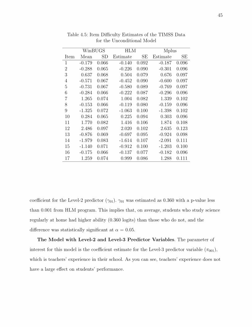
45

Table 4.5: Item Difficulty Estimates of the TIMSS Datafor the Unconditional Model

WinBUGS HLM MplusItem Mean SD Estimate SE Estimate SE1 -0.179 0.066 -0.140 0.092 -0.187 0.0962 -0.288 0.065 -0.226 0.090 -0.301 0.0963 0.637 0.068 0.504 0.079 0.676 0.0974 -0.571 0.067 -0.452 0.090 -0.600 0.0975 -0.731 0.067 -0.580 0.089 -0.769 0.0976 -0.284 0.066 -0.222 0.087 -0.296 0.0967 1.265 0.074 1.004 0.082 1.339 0.1028 -0.153 0.066 -0.119 0.080 -0.159 0.0969 -1.325 0.072 -1.063 0.100 -1.398 0.10210 0.284 0.065 0.225 0.094 0.303 0.09611 1.770 0.082 1.416 0.106 1.874 0.10812 2.486 0.097 2.020 0.102 2.635 0.12313 -0.876 0.069 -0.697 0.095 -0.924 0.09814 -1.979 0.083 -1.614 0.107 -2.091 0.11115 -1.140 0.071 -0.912 0.100 -1.203 0.10016 -0.175 0.066 -0.137 0.077 -0.182 0.09617 1.259 0.074 0.999 0.086 1.288 0.111

coefficient for the Level-2 predictor (γ01). γ01 was estimated as 0.360 with a p-value less

than 0.001 from HLM program. This implies that, on average, students who study science

regularly at home had higher ability (0.360 logits) than those who do not, and the

difference was statistically significant at α = 0.05.

The Model with Level-2 and Level-3 Predictor Variables. The parameter of

interest for this model is the coefficient estimate for the Level-3 predictor variable (π001),

which is teachers’ experience in their school. As you can see, teachers’ experience does not

have a large effect on students’ performance.

46

The following Table 4.6 shows the results from three programs for the individual

variance (τβ), the group variance (τγ), the coefficient for the Level-2 predictor (γ01), and

the coefficient estimate for the Level-3 predictor variable (π001)

Table 4.6: Parameter Estimates of the TIMSS Datafor the Model with Level-2 and Level-3 Predictor Variables

WinBUGS HLM MplusParameter Mean SD Estimate SE Estimate SEτβ 1.082 0.070 0.931 0.055 1.260 0.232τγ 0.244 0.060 0.201 0.048 0.252 0.075γ01 0.436 0.075 0.359 0.069 0.385 0.077π001 -0.003 0.003 -0.002 0.002 -0.004 0.003

Examining the result for the group variance estimates (τγ) reveals that there is

agreement between Bayesian estimation and Maximum Likelihood estimation, which is not

surprising since there are large group sizes (i.e., 68 schools).

4.1.3 Example with the CFSEI Data

The Unconditional Model. For this model, the comparisons of the parameters of

interest, item effect (b), the individual variance (τβ), and the group variance (τγ), are

presented in Table 4.7. For the item parameter estimates, a repeated measures one-way

ANOVA was conducted to determine whether there was a difference across the three

estimation methods. Mauchly’s test indicated that the assumption of sphericity had been

violated (χ2(2) = 10.975, p = .004), therefore degrees of freedom were corrected using

Greenhouse-Geisser estimates of sphericity (ǫ = .544). The results revealed that there were

no significant differences in the item parameter estimates between the three estimation

methods, F(1.087,7.611) = .000, p = .994, η2p = .000.

There was statistically significant within-site, τβ, and between-site, τγ, variation in

academic self-esteem (ASE). To examine if ASE variation between students was associated

with their characteristics, the model with Level-2 predictor variables is considered.

47

Table 4.7: Parameter Estimates of the CFSEI Datafor the Unconditional Model

WinBUGS HLM MplusParameter Mean SD Estimate SE Estimate SEb[1] 0.010 0.078 0.008 0.054 0.020 0.222b[2] -0.512 0.082 -0.344 0.195 -0.384 0.225b[3] -0.445 0.080 -0.297 0.147 -0.332 0.224b[4] 1.225 0.081 0.810 0.156 0.965 0.222b[5] 0.453 0.078 0.303 0.157 0.365 0.221b[6] -0.117 0.078 -0.077 0.094 -0.078 0.223b[7] -0.423 0.081 -0.282 0.178 -0.315 0.224b[8] -0.191 0.079 -0.124 0.155 -0.237 0.177τβ 2.957 0.241 1.938 0.128 1.789 0.352τγ 0.539 0.363 0.279 0.140 0.236 0.144

The Model with Level-2 Predictor Variables. For this model, the comparisons of

the parameters of interest, item effect (b), the individual variance (τβ), the group variance

(τγ), and the coefficients for student-level predictors (gender effect, γ01, and age effect, γ02)

are presented in Table 4.8. The negative coefficient for gender effects indicates that female

academic self-esteem (ASE) is higher than male ASE. Also, the coefficient for age means

that ASE decreased as the age of the students increased. For the item parameter estimates,

a repeated measures one-way ANOVA was conducted to see that there was a difference

across the three estimation methods. Mauchly’s test indicated that the assumption of

sphericity had been violated (χ2(2) = 10.915, p < .004), therefore, degrees of freedom were

corrected using Greenhouse-Geisser estimates of sphericity (ǫ = .544). The results revealed

that there were no significant differences in the item parameter estimates between the three

estimation methods, F(1.088,7.618) = .000, p = .998, η2p = .000.

The Model with Level-2 and Level-3 Predictor Variables. After the student

level predictor variables were added into the model, the site random effect was no longer

48

Table 4.8: Parameter Estimates of the CFSEI Datafor the Model with Level-2 Predictor Variables

WinBUGS HLM MplusParameter Mean SD Estimate SE Estimate SEb[1] 0.006 0.078 0.009 0.059 0.019 0.230b[2] -0.510 0.082 -0.350 0.210 -0.391 0.233b[3] -0.443 0.081 -0.303 0.162 -0.338 0.233b[4] 1.224 0.082 0.828 0.162 0.979 0.228b[5] 0.452 0.078 0.309 0.165 0.369 0.229b[6] -0.119 0.079 -0.078 0.106 -0.081 0.231b[7] -0.421 0.081 -0.287 0.193 -0.321 0.233b[8] -0.189 0.079 -0.126 0.167 -0.235 0.200τβ 2.768 0.224 1.821 0.123 1.791 0.352τγ 0.331 0.265 0.287 0.142 0.149 0.109γ01 -0.633 0.128 -0.432 0.101 -0.275 0.064γ02 -0.204 0.038 -0.145 0.074 -0.165 0.035

significant indicating that the gender and age effects applied to all sites. As the results

indicated that there was no significant variation in academic self-esteem across sites, it was

not necessary to build a model with Level-3 predictors.

4.1.4 Summary of Real Data Analyses

It should be noted that the item fixed effects remained fairly constant across models (i.e.,

the unconditional model, the model with Level-2 predictor variable(s), and the model with

Level-2 and Level-3 predictor variables), as would be expected. Kamata (1998) noted that

including predictor variables in the multilevel IRT model should not alter the item effect

estimates. This study lends support to such a conclusion.

As can be seen in Table 4.9, there was little difference between the fixed effect estimates

for the items obtained using the unconditional model and those obtained using the model

with level-2 predictor variables for the FCAT data.

49

Table 4.9: Item Fixed Effects for FCAT Data for the Unconditional Modeland the Model with Level-2 Predictor Variables

from HLM program

The Unconditional The Model withItem Model SE Level-2 Variables SE1 3.748 0.102 3.749 0.1022 2.920 0.086 2.920 0.0863 2.204 0.079 2.203 0.0794 1.854 0.077 1.854 0.0775 1.171 0.075 1.171 0.0756 1.840 0.077 1.840 0.0777 1.821 0.077 1.821 0.0778 1.623 0.076 1.623 0.0769 1.320 0.076 1.320 0.07610 1.560 0.076 1.559 0.07611 1.041 0.075 1.040 0.07512 0.119 0.078 0.119 0.07813 0.896 0.076 0.896 0.07514 -1.096 0.073 -1.584 0.10315 1.852 0.077 1.851 0.07716 1.832 0.077 1.832 0.07717 1.777 0.077 1.777 0.07718 0.294 0.077 0.294 0.07719 3.278 0.091 3.278 0.09120 2.191 0.079 2.191 0.07921 2.427 0.081 2.427 0.08122 2.351 0.080 2.351 0.08023 2.661 0.083 2.661 0.08324 1.610 0.076 1.610 0.07625 1.007 0.075 1.007 0.07526 2.491 0.081 2.491 0.08127 1.685 0.076 1.685 0.07628 0.420 0.077 0.420 0.07729 1.380 0.076 1.379 0.07630 1.135 0.075 1.135 0.07531 0.764 0.076 0.763 0.07632 2.036 0.078 2.036 0.07833 2.433 0.081 2.433 0.081

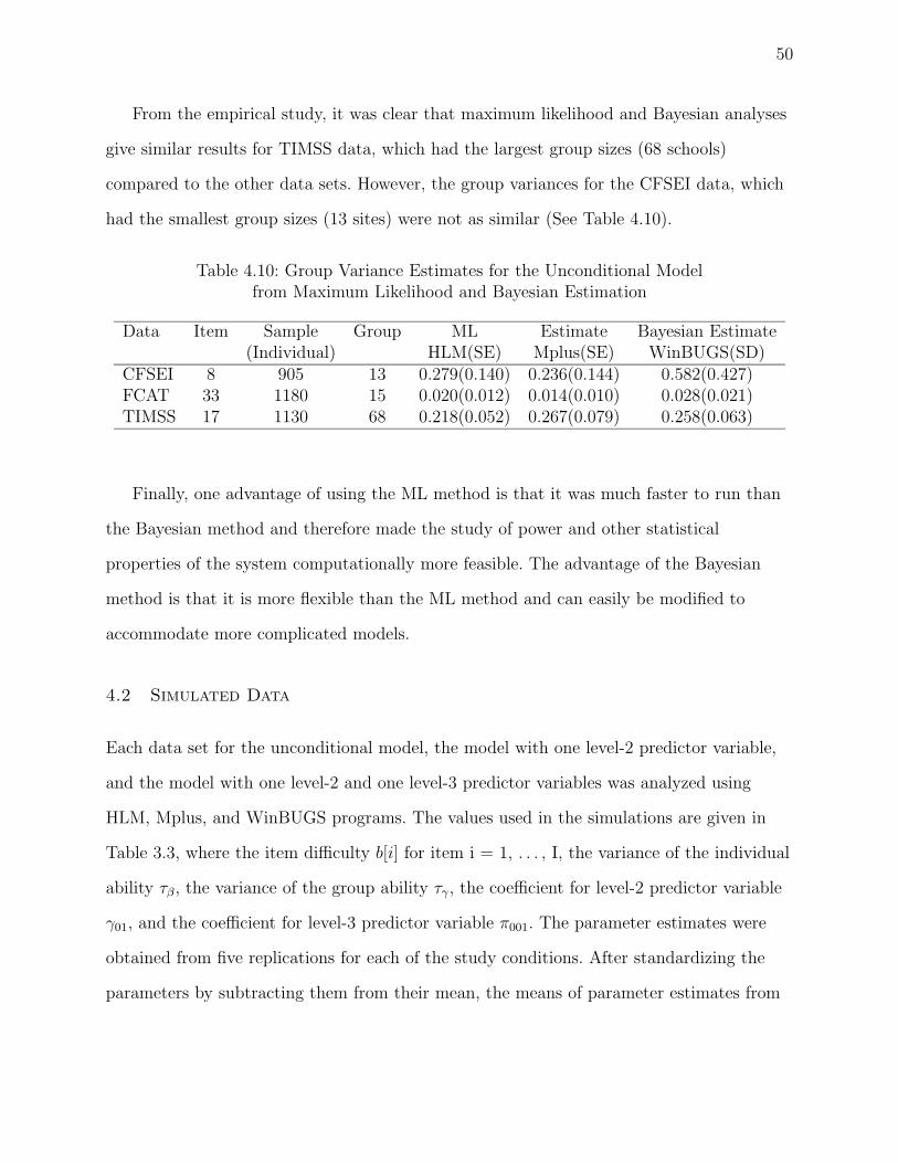
50

From the empirical study, it was clear that maximum likelihood and Bayesian analyses

give similar results for TIMSS data, which had the largest group sizes (68 schools)

compared to the other data sets. However, the group variances for the CFSEI data, which

had the smallest group sizes (13 sites) were not as similar (See Table 4.10).

Table 4.10: Group Variance Estimates for the Unconditional Modelfrom Maximum Likelihood and Bayesian Estimation

Data Item Sample Group ML Estimate Bayesian Estimate(Individual) HLM(SE) Mplus(SE) WinBUGS(SD)

CFSEI 8 905 13 0.279(0.140) 0.236(0.144) 0.582(0.427)FCAT 33 1180 15 0.020(0.012) 0.014(0.010) 0.028(0.021)TIMSS 17 1130 68 0.218(0.052) 0.267(0.079) 0.258(0.063)

Finally, one advantage of using the ML method is that it was much faster to run than

the Bayesian method and therefore made the study of power and other statistical

properties of the system computationally more feasible. The advantage of the Bayesian

method is that it is more flexible than the ML method and can easily be modified to

accommodate more complicated models.

4.2 Simulated Data

Each data set for the unconditional model, the model with one level-2 predictor variable,

and the model with one level-2 and one level-3 predictor variables was analyzed using

HLM, Mplus, and WinBUGS programs. The values used in the simulations are given in

Table 3.3, where the item difficulty b[i] for item i = 1, . . . , I, the variance of the individual

ability τβ, the variance of the group ability τγ , the coefficient for level-2 predictor variable

γ01, and the coefficient for level-3 predictor variable π001. The parameter estimates were

obtained from five replications for each of the study conditions. After standardizing the

parameters by subtracting them from their mean, the means of parameter estimates from

51

five replications and their line graphs for one condition from each model are presented in

Appendices D and E.

In this study, recovery of item and variance parameters was assessed using root mean

squared errors (RMSEs) between the generating parameter and the parameter estimate,

which is a common measure of the robustness of parameter estimates. RMSEs for each

parameter under ML and Bayesian were collected for all conditions. These RMSEs are

provided in Tables 4.11, 4.12, 4.19, 4.20, and 4.23 to 4.26, for each parameter of interest

from each model.

4.2.1 The Unconditional Model

The parameters I focus on in this model are the item difficulty (b[i] for item i = 1, . . . , I)

and ability variance parameters (the variance of the individual ability, τβ and the variance

of the group ability, τγ). The values used in the simulations are given in Table 3.3.

First, I illustrate some typical Gibbs sample output using one data set from the model

(I = 10, J = 750, and G = 30). Sample history (trace) plots and density plots are given for

selected parameters for 11,000 iterations after eliminating the first 4,000 iterations and the

values used in the simulations are circled. The trace plots for the parameters of interest are

shown in Figure 4.1, where b[1] is the item difficulty for item 1, b[10] is the item difficulty

for item 10, sigma2 is the individual variance estimate, and sigma3 is the group variance

estimate. Each parameter of interest becomes stationary by 4,000 iterations, indicating

that convergence has been reached by 4,000 iterations.

The density plots (Figures 4.2) show unimodal distributions which are nearly

symmetric, and look close to normal except for the plot of sigma3, which is the group

variance estimate. It has a long right tail and a high peak close to zero. This result is likely

due to the values of sigma3 being close to zero, the lower boundary of the parameter space.

For HLM, the classical item difficulty was used to determine the easiest item. The usual

procedure in multilevel IRT modeling, which was also used in this study, is to take the

52

Figure 4.1: History Plots of Parameter Estimatesfor the Unconditional Model

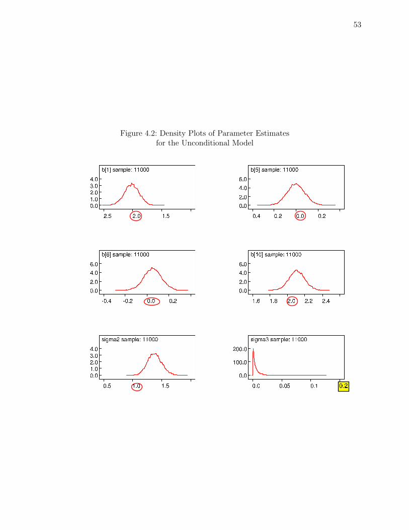
53

Figure 4.2: Density Plots of Parameter Estimatesfor the Unconditional Model

54

easiest item as the reference item. Again, the effect for π000 represents the effect of the

reference item (item 1), or the difficulty of the reference item, b[1]. The item difficulties for

the others (b[i], for i = 2, . . . , I) were estimated by subtracting the effect for each item,

πq00 from the effect of the reference item, π000.

Item parameters were mean-centered by subtracting them from their mean. The means

of the centered parameter estimates from five replications and their line graphs for one

condition (I = 10, J = 750, and G = 30) for the model are presented in Appendices D and

E. From this table, we see that the means of each parameter estimates from HLM are

smaller than those from the other programs, WinBUGS and Mplus. This makes sense since

the HLM software uses the penalized or predictive quasi-likelihood (PQL) method to

estimate the parameter estimates for dichotomous responses. Many authors (e.g.,

Rodriguez & Goldman, 1995; Goldstein & Rashbash, 1996; Breslow & Clayton, 1993) have

reported that these approximation methods exhibit downward (i.e., estimated parameters

are smaller than generated parameters) biases for both the fixed effects and the variance

components for dichotomous responses with small cluster sizes. This conclusion was

supported by the present study.

In order to study the effect of varying the number of items (I), individuals (J), and

groups (G) on the bias, the RMSEs under each condition for the unconditional model are

presented in Table 4.11 for 20 items and Table 4.12 for 10 items, where β = Item Difficulty

(averaged over all the items), τβ = Individual Variance, and τγ = Group Variance.

For each parameter in the unconditional model, a repeated measures ANOVA with the

three estimation method (M) as the repeated factor and item (I), individual (J), and group

(G) size as the independent variables was performed using the RMSEs across all the

conditions used in this study as the dependent variable. For the item parameter estimates

(β), Mauchly’s criterion showed that there was not a problem with the sphericity

assumption (χ2(2) = 5.047, p = .080). Univariate tests of within-subjects effects showed

that the significant effects were method, method × test length interaction, method ×

55

Table 4.11: RMSEs for the Unconditional Modelfrom Maximum Likelihood and Bayesian Estimation

Item = 20Sample Group Parameter Bayesian Maximum LikelihoodSize Size Estimate WinBUGS HLM Mplus1500 60 β 0.077 0.251 0.143

τβ 0.595 0.360 0.835τγ 0.174 0.172 0.163

30 β 0.067 0.266 0.100τβ 0.633 0.398 0.762τγ 0.187 0.189 0.185

15 β 0.067 0.263 0.178τβ 0.562 0.341 0.546τγ 0.190 0.195 0.194

750 60 β 0.098 0.254 0.199τβ 0.531 0.306 0.703τγ 0.163 0.160 0.150

30 β 0.096 0.267 0.153τβ 0.566 0.338 0.658τγ 0.173 0.171 0.164

15 β 0.099 0.260 0.165τβ 0.493 0.284 0.727τγ 0.193 0.199 0.199

450 60 β 0.142 0.285 0.211τβ 0.629 0.371 0.718τγ 0.041 0.042 0.050

30 β 0.119 0.262 0.179τβ 0.680 0.434 0.400τγ 0.178 0.183 0.184

15 β 0.136 0.287 0.222τβ 0.607 0.374 0.841τγ 0.160 0.168 0.162

56

Table 4.12: RMSEs for the Unconditional Modelfrom Maximum Likelihood and Bayesian Estimation

Item = 10Sample Group Parameter Bayesian Maximum Likelihood

Size Size Estimate WinBUGS HLM Mplus1500 60 β 0.053 0.237 0.100

τβ 0.335 0.074 0.427τγ 0.175 0.177 0.171

30 β 0.066 0.227 0.119τβ 0.320 0.055 0.474τγ 0.184 0.187 0.184

15 β 0.063 0.234 0.138τβ 0.271 0.025 0.480τγ 0.189 0.193 0.190

750 60 β 0.078 0.228 0.167τβ 0.374 0.059 0.326τγ 0.157 0.154 0.148

30 β 0.096 0.234 0.130τβ 0.291 0.092 0.250τγ 0.190 0.195 0.196

15 β 0.093 0.240 0.174τβ 0.260 0.073 0.364τγ 0.184 0.190 0.187

450 60 β 0.117 0.278 0.316τβ 0.346 0.151 0.934τγ 0.138 0.139 0.246

30 β 0.113 0.237 0.262τβ 0.419 0.156 0.861τγ 0.150 0.161 0.146

15 β 0.150 0.273 0.264τβ 0.417 0.134 0.648τγ 0.174 0.182 0.175

57

individual sample size interaction, and method × *test length × individual sample size

interaction (See Table 4.13). Significant method effect means that mean RMSEs of β

Table 4.13: Tests of Within-Subjects Effectsfor the Item Parameters

from the Unconditional Model

Source SS df MS F p η2p

Method (M) .226 2 .113 491.817 .000 .992M * I .003 2 .002 6.522 .021 .620M * J .012 4 .003 13.506 .001 .871M * G .002 4 .000 2.024 .184 .503

M * I * J .005 4 .001 5.596 .019 .737M * I * G .001 4 .000 1.129 .408 .361M * J * G .002 8 .000 1.190 .406 .543

Error .002 8 .000

changes across the three estimation methods. The mean RMSEs of β were .096 for

WinBUGS, .255 for HLM, and .179 for Mplus, respectively. Post hoc tests revealed that

the three means were significantly different from each other at the α = .05 level. A

significant two-way interaction effect means that the influence of test length or individual

sizes on RMSEs of β depends on the estimation method. (M × I and M × J). A significant

three-way interaction effect means that the influence of test length on RMSEs of β depends

on individual sample size and the estimation method (M × I × J). This three-way

interaction is broken down into a series of two-way interactions, one two-way within each

level of test length (See Figure 4.3).

Among the between-subjects effects, the individual and group main effects and the

interaction effect of test length × individual sample size were significant (See Table 4.14).

There was a significant interaction effect between test length and individual sample size,

F(2,4) = 12.462, p = .019, η2p = .862. Although the RMSEs for β decreas ed as total sample

increased, the results indicate that there was a strong tendency for the RMSEs of β under

each individual sample size condition to increase as number of items increased, except for

the condition, J = 450 (See Figure 4.4, where b indicates item parameter estimates). Also,

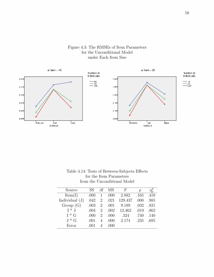
58

Figure 4.3: The RMSEs of Item Parametersfor the Unconditional Model

under Each Item Size

Table 4.14: Tests of Between-Subjects Effectsfor the Item Parameters



Item(I) .000 1 .000 2.882 .165 .419Individual (J) .042 2 .021 129.437 .000 .985

Group (G) .003 2 .001 9.189 .032 .821I * J .004 2 .002 12.462 .019 .862I * G .000 2 .000 .324 .740 .140J * G .001 4 .000 2.174 .235 .685Error .001 4 .000

59

Figure 4.4: The RMSEs of Item Parametersfor the Unconditional Model

there was a significant difference between the RMSEs of β under each group size, F(2,4) =

9.189, p = .032, η2p = .821. The mean RMSEs of β across all the conditions were .184 for G

= 15, .166 for G = 30, and .180 for G = 60. Post hoc tests revealed that there was a

difference only between the group size of 15 and the group size of 30 (p = .045).

For the individual variance estimates (i.e., τβ), Mauchly’s criterion showed that there

was not a problem with the sphericity assumption (χ2(2) = 5.783, p = .055). Univariate

tests of within-subjects effects only found estimation method to differ (See Table 4.15).

Significant method effect means that mean RMSEs of τβ changes across the three

estimation methods. The mean RMSEs of τβ were .463 for WinBUGS, .224 for HLM, and

.609 for Mplus, respectively. Post hoc tests revealed that there was a difference only

between WinBUGS and HLM (p < .000), and between HLM and Mplus (p = .002).

Among the between-subjects effects, the main effects of item and individual were

significant (See Table 4.16). There was a significant difference between the RMSEs for τβ

60

Table 4.15: Tests of Within-Subjects Effectsfor the Individual Variance Parameters



Method (M) 1.360 2 .680 57.115 .000 .935M * I .030 2 .015 1.275 .331 .242M * J .041 4 .010 .863 .525 .302M * G .026 4 .007 .555 .702 .217

M * I * J .162 4 .040 3.399 .066 .630M * I * G .018 4 .004 .369 .824 .156M * J * G .034 8 .004 .358 .916 .263

Error .095 8 .012

Table 4.16: Tests of Between-Subjects Effectsfor the Individual Variance Parameters



Item(I) .684 1 .684 77.886 .001 .951Individual (J) .170 2 .085 9.667 .029 .829

Group (G) .011 2 .005 .624 .581 .238I * J .090 2 .045 5.113 .079 .719I * G .001 2 .000 .037 .964 .018J * G .012 4 .003 .347 .835 .258Error .035 4 .009

61

under each test length, F(1,4) = 77.886, p = .001, η2p = .951. The mean RMSEs for τβ were

.319 for I = 10 and .544 for I = 20. Also, there was a significant difference between the

RMSEs of β under each individual size, F(2,4) = 9.667, p = .029, η2p = .829. The mean

RMSEs of τβ across all models were .507 for J = 450, .372 for J = 750, and .416 for J =

1500. Post hoc tests revealed that there was a difference only between the individual

sample sizes of 450 and 1500 (p = .038).

For the group variance (τγ) estimates, Mauchly’s test indicated that the assumption of

sphericity had been violated (χ2(2) = 12.371, p = .002), therefore, degrees of freedom were

corrected using Greenhouse-Geisser estimates of sphericity (ǫ = .504). However, there was

no significant within-subjects effect (See Table 4.17).

Table 4.17: Tests of Within-Subjects Effectsfor the Group Variance Parameters



Method (M) .000 1.008 .000 .603 .482 .131M * I .000 1.008 .000 .942 .387 .191M * J .001 2.016 .001 1.430 .340 .417M * G .001 2.016 .000 .830 .500 .293

M * I * J .000 2.016 .000 .533 .624 .210M * I * G .001 2.016 .000 1.123 .410 .360M * J * G .003 4.033 .001 1.695 .310 .629

Error .002 4.033 .000

For this parameter, there was no significant between-subjects effect, either (See Table

4.18).

Next, in order to examine the effect of predictor variables at each level on the latent

trait parameters, dichotomous (i.e., coded 0 or 1) variables with equal sample sizes were

considered for level-2 and level-3 predictor variables.

62

Table 4.18: Tests of Between-Subjects Effectsfor the Group Variance Parameters



Item(I) .003 1 .003 .662 .461 .142Individual (J) .012 2 .006 1.534 .320 .434

Group (G) .016 2 .008 2.033 .246 .504I * J .004 2 .002 .515 .632 .205I * G .006 2 .003 .758 .526 .275J * G .004 4 .001 .243 .900 .196Error .016 4 .004

4.2.2 The Model with Level-2 Predictor Variables

If the unconditional model indicates significant variation within and between groups,

within group variation is modeled followed by between group variation. A predictor

variable was included at the second level of the model in order to determine if variation

was associated with the predictor variable. The values used in the simulations are in Table

3.3. γ01 was generated as 0.5, which implies that, on average, individuals who are coded 1

have higher ability (0.5 logits) than those who are coded 0.

For this model, sample history (trace) plots and density plots are given for selected

parameters for 11,000 iterations after eliminating the first 4,000 iterations (I = 20, J =

1500, and G = 60) and the values used in the simulations are circled. The trace plots are

shown in Figure 4.5, where b[1] is the item difficulty for item 1, sigma2 is the individual

variance estimate, sigma3 is the group variance estimate, and alpha is the coefficient for

Level-2 predictor variable. All parameter converged by 4,000 iterations.

The density plots (Figures 4.6) show unimodal distributions which are nearly

symmetric, and look close to normal except for the plot of sigma3, which is the group

variance estimate. It has a long right tail and a high peak close to zero.

63

Figure 4.5: History Plots of Parameter Estimatesfor the Model with Level-2 Predictor Variable

64

Figure 4.6: Density Plots of Parameter Estimatesfor the Model with Level-2 Predictor Variable

65

The RMSEs under each condition for the model with a level-2 predictor variable are

presented in Tables 4.19 and 4.20, where β = item difficulty (averaged over all the items),

τβ = individual variance, τγ = group variance, and γ01 = the coefficient for the Level-2

predictor variable. Individual-level characteristics have been included in the models to see

the differences in the estimation of item difficulty parameters and to model the effects of

individual characteristics upon the estimated latent trait measures. The use of an

individual predictor variable did not change the item or group variance parameter

estimates, but appeared to provide an improvement in the recovery of individual variance

parameter estimates. The RMSEs of individual variance estimates (τβ) with the individual

predictor variable was slightly lower than those without a predictor variable. The mean

RMSEs of τβ were .385 for this model and .432 for the unconditional model, respectively.

In this model, the primary interest was in the coefficient estimates for the Level-2

predictor variable (γ01). For this parameter estimate, Mauchly’s criterion showed that

sphericity was not violated (χ2(2) = 5.687, p = .058). Univariate tests of within-subjects

effects showed that the significant effect was only method (See Table 4.21). Significant

method effect means that mean RMSEs of γ01 changes across the three estimation

methods. The mean RMSEs of γ01 were .316 for WinBUGS, .355 for HLM, and .371 for

Mplus, respectively. Post hoc tests revealed that there was a difference only between

WinBUGS and HLM (p = .005).

There was no significant between-subjects effect for γ01 (See Table 4.22).

For the other parameters (i.e., item difficulty, individual variance, and group variance

estimates), the results were consistent with those from the unconditional model.

4.2.3 The Model with Level-2 and Level-3 Predictor Variables

If after the individual level predictor variables are added in the model, the group random

effect is still significant, it is necessary to build a model with Level-3 predictors. The values

66

Table 4.19: RMSEs for the Model with the Level-2 Predictor Variablefrom Maximum Likelihood and Bayesian Estimation


τβ 0.638 0.400 0.805τγ 0.185 0.187 0.181γ01 0.352 0.386 0.408

30 β 0.065 0.255 0.118τβ 0.553 0.333 0.675τγ 0.193 0.198 0.196γ01 0.287 0.331 0.425

15 β 0.074 0.258 0.123τβ 0.520 0.306 0.338τγ 0.193 0.197 0.197γ01 0.411 0.434 0.436

750 60 β 0.102 0.256 0.143τβ 0.551 0.313 0.656τγ 0.157 0.151 0.135γ01 0.402 0.436 0.440

30 β 0.112 0.245 0.124τβ 0.478 0.288 0.456τγ 0.178 0.179 0.176γ01 0.510 0.517 0.511

15 β 0.104 0.220 0.135τβ 0.493 0.286 0.537τγ 0.194 0.199 0.200γ01 0.227 0.280 0.313

450 60 β 0.148 0.279 0.303τβ 0.567 0.310 1.129τγ 0.083 0.070 0.099γ01 0.066 0.126 0.214

30 β 0.140 0.284 0.165τβ 0.575 0.342 0.482τγ 0.169 0.174 0.168γ01 0.170 0.249 0.267

15 β 0.140 0.282 0.197τβ 0.466 0.253 0.216τγ 0.173 0.180 0.178γ01 0.534 0.532 0.534

67

Table 4.20: RMSEs for the Model with the Level-2 Predictor Variablefrom Maximum Likelihood and Bayesian Estimation

Item = 10Sample Group Parameter Bayesian Maximum Likelihood

Size Size Estimate WinBUGS HLM Mplus1500 60 β 0.060 0.220 0.142

τβ 0.354 0.068 0.668τγ 0.169 0.173 0.165γ01 0.237 0.290 0.317

30 β 0.055 0.228 0.159τβ 0.208 0.079 0.097τγ 0.176 0.179 0.179γ01 0.334 0.369 0.345

15 β 0.070 0.233 0.126τβ 0.274 0.062 0.084τγ 0.182 0.188 0.187γ01 0.266 0.310 0.297

750 60 β 0.072 0.244 0.164τβ 0.334 0.137 0.212τγ 0.160 0.154 0.157γ01 0.530 0.559 0.538

30 β 0.104 0.241 0.164τβ 0.357 0.057 0.488τγ 0.187 0.193 0.191γ01 0.363 0.390 0.398

15 β 0.087 0.231 0.133τβ 0.305 0.070 0.493τγ 0.180 0.187 0.181γ01 0.327 0.359 0.372

450 60 β 0.132 0.263 0.339τβ 0.347 0.142 0.649τγ 0.034 0.028 0.134γ01 0.338 0.370 0.350

30 β 0.122 0.250 0.335τβ 0.378 0.057 1.149τγ 0.164 0.168 0.147γ01 0.102 0.179 0.217

15 β 0.107 0.236 0.189τβ 0.321 0.054 0.398τγ 0.157 0.165 0.159γ01 0.240 0.286 0.288

68

Table 4.21: Tests of Within-Subjects Effectsfor the Coefficient of the Level-2 Predictor

from the Model with the Level-2 Predictor Variable


Method (M) .028 2 .014 12.568 .003 .759M * I .002 2 .001 .864 .457 .178M * J .002 4 .000 .411 .796 .170M * G .001 4 .000 .254 .900 .113M * I * J .000 4 .000 .090 .983 .043M * I * G .001 4 .000 .228 .915 .102M * J * G .006 8 .001 .624 .740 .384Error .009 8 .001

Table 4.22: Tests of Between-Subjects Effectsfor the Coefficient of the Level-2 Predictor

from the Model with the Level-2 Predictor Variable


Item(I) .013 1 .013 .320 .602 .074Individual (J) .161 2 .081 2.037 .245 .505Group (G) .007 2 .004 .093 .914 .044I * J .023 2 .011 .289 .763 .126I * G .083 2 .042 1.051 .430 .345J * G .231 4 .058 1.459 .362 .593Error .158 4 .040

69

used in the simulations are in Table 3.3. π001 was generated as 0.1, which implies that, on

average, groups that are coded 1 have higher ability (0.1 logits) than those that are coded 0.

For this model, sample history (trace) plots and density plots are given for selected

parameters for 11,000 iterations after eliminating the first 4,000 iterations (I = 10, J = 450,

and G = 15) and the values used in the simulations are circled. The trace plots are shown

in Figure 4.7, where sigma2 is the individual variance estimate, sigma3 is the group

variance estimate, alpha is the coefficient for the Level-2 predictor variable, and beta is the

coefficient for the Level-3 predictor variable. Each parameter of interest becomes stationary

by 4,000 iterations, indicating that convergence has been reached by 4,000 iterations. The

density plots (Figures 4.8) show unimodal distributions which are nearly symmetric, and

look close to normal except for the plot of sigma3, which is the group variance estimate. It

has a long right tail and a high peak close to zero.

The RMSEs under each condition for the model with level-2 and level-3 predictor

variables are presented in Tables 4.23 to 4.26, where β = Item Difficulty (averaged over all

the items), τβ = Individual Variance, τγ = Group Variance, γ01 = the coefficient for the

level-2 predictor variable, and π001 = the coefficient for the level-3 predictor variable.

The RMSEs of the individual variance parameter estimates (τβ) across all the

conditions from this model were larger in comparison to those from the unconditional

model or the model with a Level-2 predictor variable. The mean RMSEs of τβ across all

conditions were .431 for the unconditional model, and .385 for the model with a Level-2

predictor variable, and .441 for the model with a Level-2 and a Level-3 predictor variables.

It suggests that the use of a group predictor variable does not appear to provide an

improvement in the recovery of individual variance parameters.

Also, the inclusion of a group-level (Level 3) predictor variable in the model leads to a

loss of efficiency for the individual level (Level 2) predictor variable for small individual

sample sizes (J = 450). This means that choosing a group-level predictor variable is costly

in terms of the RMSEs. The mean RMSEs of the coefficient of individual level predictor

70

Figure 4.7: History Plots of Parameter Estimatesfor the Model with Level-2 and Level-3 Predictor Variables

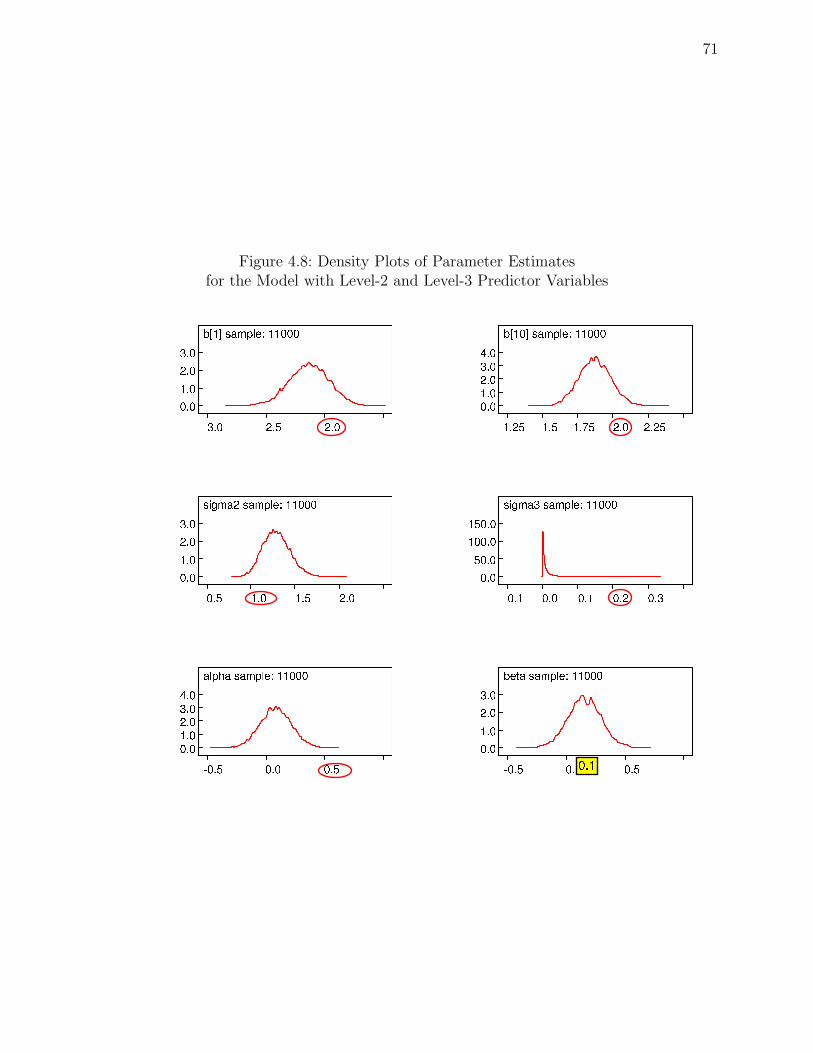
71

Figure 4.8: Density Plots of Parameter Estimatesfor the Model with Level-2 and Level-3 Predictor Variables

72

Table 4.23: RMSEs for the Model with the Level-2 Predictor Variableand the Level-3 Predictor Variable

from Maximum Likelihood and Bayesian Estimation


τβ 0.646 0.402 0.726τγ 0.184 0.184 0.179γ01 0.353 0.395 0.414π001 0.156 0.148 0.135

30 β 0.059 0.249 0.138τβ 0.485 0.275 0.665τγ 0.191 0.195 0.194γ01 0.296 0.336 0.364π001 0.135 0.132 0.125

15 β 0.067 0.252 0.143τβ 0.625 0.389 0.894τγ 0.191 0.197 0.196γ01 0.366 0.400 0.422π001 0.053 0.049 0.058

750 60 β 0.116 0.245 0.202τβ 0.581 0.338 0.565τγ 0.162 0.160 0.154γ01 0.447 0.462 0.463π001 0.096 0.056 0.057

30 β 0.096 0.267 0.129τβ 0.539 0.311 0.576τγ 0.167 0.171 0.164γ01 0.492 0.501 0.493π001 0.217 0.151 0.123

15 β 0.100 0.248 0.154τβ 0.509 0.296 0.938τγ 0.193 0.199 0.199γ01 0.218 0.279 0.317π001 0.057 0.029 0.023

73


from Maximum Likelihood and Bayesian Estimation - Continued


τβ 0.472 0.238 0.936τγ 0.089 0.084 0.081γ01 0.073 0.132 0.191π001 0.251 0.217 0.199

30 β 0.108 0.268 0.203τβ 0.499 0.285 0.854τγ 0.180 0.190 0.181γ01 0.153 0.229 0.278π001 0.312 0.281 0.237

15 β 0.114 0.290 0.386τβ 0.662 0.410 1.762τγ 0.170 0.184 0.178γ01 0.524 0.519 0.514π001 0.193 0.121 0.045

74


from Maximum Likelihood and Bayesian Estimation


τβ 0.284 0.093 0.378τγ 0.188 0.192 0.187γ01 0.204 0.260 0.263π001 0.036 0.045 0.044

30 β 0.055 0.233 0.111τβ 0.281 0.034 0.355τγ 0.184 0.189 0.185γ01 0.335 0.368 0.372π001 0.069 0.070 0.070

15 β 0.082 0.221 0.107τβ 0.263 0.035 0.162τγ 0.192 0.198 0.198γ01 0.251 0.298 0.294π001 0.156 0.144 0.145

750 60 β 0.110 0.225 0.119τβ 0.382 0.096 0.374τγ 0.175 0.178 0.172γ01 0.473 0.485 0.490π001 0.104 0.103 0.102

30 β 0.087 0.234 0.140τβ 0.421 0.156 0.427τγ 0.190 0.197 0.197γ01 0.316 0.359 0.368π001 0.118 0.117 0.115

15 β 0.099 0.233 0.209τβ 0.276 0.127 0.305τγ 0.183 0.192 0.190γ01 0.320 0.358 0.339π001 0.104 0.109 0.115

75


from Maximum Likelihood and Bayesian Estimation - Continued


τβ 0.471 0.116 0.769τγ 0.123 0.109 0.138γ01 0.287 0.338 0.353π001 0.064 0.076 0.076

30 β 0.148 0.265 0.283τβ 0.409 0.093 0.905τγ 0.117 0.130 0.091γ01 0.148 0.220 0.277π001 0.097 0.094 0.090

15 β 0.127 0.255 0.224τβ 0.333 0.069 0.332τγ 0.167 0.199 0.199γ01 0.355 0.375 0.369π001 0.086 0.079 0.083

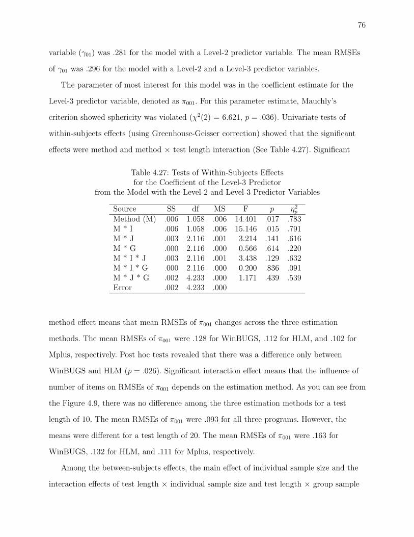
76

variable (γ01) was .281 for the model with a Level-2 predictor variable. The mean RMSEs

of γ01 was .296 for the model with a Level-2 and a Level-3 predictor variables.

The parameter of most interest for this model was in the coefficient estimate for the

Level-3 predictor variable, denoted as π001. For this parameter estimate, Mauchly’s

criterion showed sphericity was violated (χ2(2) = 6.621, p = .036). Univariate tests of

within-subjects effects (using Greenhouse-Geisser correction) showed that the significant

effects were method and method × test length interaction (See Table 4.27). Significant

Table 4.27: Tests of Within-Subjects Effectsfor the Coefficient of the Level-3 Predictor

from the Model with the Level-2 and Level-3 Predictor Variables


Method (M) .006 1.058 .006 14.401 .017 .783M * I .006 1.058 .006 15.146 .015 .791M * J .003 2.116 .001 3.214 .141 .616M * G .000 2.116 .000 0.566 .614 .220M * I * J .003 2.116 .001 3.438 .129 .632M * I * G .000 2.116 .000 0.200 .836 .091M * J * G .002 4.233 .000 1.171 .439 .539Error .002 4.233 .000

method effect means that mean RMSEs of π001 changes across the three estimation

methods. The mean RMSEs of π001 were .128 for WinBUGS, .112 for HLM, and .102 for

Mplus, respectively. Post hoc tests revealed that there was a difference only between

WinBUGS and HLM (p = .026). Significant interaction effect means that the influence of

number of items on RMSEs of π001 depends on the estimation method. As you can see from

the Figure 4.9, there was no difference among the three estimation methods for a test

length of 10. The mean RMSEs of π001 were .093 for all three programs. However, the

means were different for a test length of 20. The mean RMSEs of π001 were .163 for

WinBUGS, .132 for HLM, and .111 for Mplus, respectively.

Among the between-subjects effects, the main effect of individual sample size and the

interaction effects of test length × individual sample size and test length × group sample

77

Figure 4.9: The RMSEs of the Coefficient of Level-3 Predictorfor the Model with Level-2 and Level-3 Predictor Variables

size were significant (See Table 4.28). There was a significant interaction effect between test

length and individual sample size, F(2,4) = 9.100, p = .032, η2p = .820. As can be seen from

Figure 4.10, there was a positive relationship between the RMSEs of π001 and test length

for the small (J = 450) and large (J = 1500) individual sample sizes, but not for the

medium (J = 750) individual sample size. There was a significant interaction effect between

test length and group sample size, F(2,4) = 9.598, p = .030, η2p = .828. Although the

RMSEs for π001 diminished as test length decreased for the conditions of group sample

sizes are 30 and 60, the results indicated that there was a tendency for the RMSEs of π001

to decrease as number of items increased for group sample size of 15 (See Figure 4.10).

For the other parameter estimates (i.e., item difficulty, individual variance, group

variance, and the coefficient of level-2 predictor), the results were consistent with those

from the previous models.

78

Table 4.28: Tests of Between-Subjects Effectsfor the Coefficient of the Level-3 Predictor

from the Model with the Level-2 and Level-3 Predictor Variables


Item(I) .024 1 .024 9.100 .039 .695Individual (J) .025 2 .012 4.648 .090 .699Group (G) .023 2 .012 4.383 .098 .687I * J .049 2 .024 9.100 .032 .820I * G .051 2 .026 9.598 .030 .828J * G .013 4 .003 1.241 .420 .554Error .011 4 .003

Figure 4.10: The RMSEs of the Coefficient of Level-3 Predictorfor the Model with Level-2 and Level-3 Predictor Variables

79

4.2.4 All Models

This study compared item parameters (β), variances of latent ability at different levels (τβ

and τγ), and the relationship between predictor variables at different levels and latent

ability (γ01 and π001, respectively) from WinBUGS, HLM, and Mplus programs. As

Kamata (1998) has suggested, inclusion of predictor variables in the multilevel IRT model

did not change the item effect estimates from those in the unconditional model. As can be

seen in Table 4.29, there was little difference between the item parameter estimates

obtained from the unconditional model and those obtained from the model with a level-2

predictor variables or the model with a level-2 and a level-3 predictor variables using

Mplus. This holds for the other two programs.

Table 4.29: Item Parameter Estimates for the Unconditional Model,the Model with Level-2 Predictor Variable,

and the Model with Level-2 and Level-3 Predictor Variablesfrom Mplus program (I = 10, J = 450, G = 15)

The The Model The Model withUnconditional with Level-2 and

Item Model SE Level-2 Variable SE Level-3 Variables SE1 -2.162 0.223 -2.162 0.223 -2.162 0.2232 -1.389 0.173 -1.389 0.173 -1.388 0.1733 -0.913 0.152 -0.913 0.152 -0.912 0.1524 -0.653 0.144 -0.653 0.144 -0.653 0.1445 0.163 0.126 0.163 0.126 0.163 0.1266 0.105 0.127 0.106 0.127 0.106 0.1277 0.518 0.122 0.518 0.122 0.518 0.1228 1.132 0.121 1.132 0.121 1.132 0.1219 1.368 0.123 1.368 0.123 1.368 0.12310 1.832 0.134 1.833 0.134 1.836 0.135

For the common parameters of interest across all models used in this study (i.e., β, τβ,

and τγ), a repeated measures ANOVA with the three estimation method as the repeated

factor and item, individual, and group size as the independent variables was performed

using the RMSEs across all models used in this study as the dependent variable. Mauchly’s

80

Table 4.30: Tests of Within-Subjects Effectsfor the Item Parameters from All Models


Method (M) .643 1.147 .561 493.829 .000 .925M * I .007 1.147 .006 5.359 .021 .118M * J .053 2.294 .023 20.166 .000 .502M * G .001 2.294 .001 .468 .655 .023M * I * J .002 2.294 .001 .889 .431 .043M * I * G .006 2.294 .003 2.218 .114 .100M * J * G .003 4.588 .001 .540 .730 .051Error .052 45.878 .001

criterion showed that sphericity was violated for item parameter estimates (β) from all

conditions in all models. Univariate tests of within-subjects effects (using

Greenhouse-Geisser correction) showed that the significant effects were method, method ×

test length interaction, and method × individual sample size interaction (See Table 4.30).

Significant method effect means that mean RMSEs of β changes across the three

estimation methods. Significant interaction effect means that the influence of test length or

individual sample sizes on RMSEs of β depends on the estimation method (See Figure

4.11). As you can see from the figure, WinBUGS has the lowest RMSEs under all the

conditions for this parameter.

Among the between-subjects effects, only the main effect of individual sample size was

significant (See Table 4.31). That is, decreasing sample size, particularly at the individual

level (Level 2), increased the RMSEs of β, F(2,40) = 110.302, p < .000, η2p = .847. The

mean RMSEs of β across all models were .217 for J = 450, .165 for J = 750, and .145 for J

=1500. Post hoc tests revealed that all three means were significantly different at the

α = .05 level.

81

Figure 4.11: The RMSEs for the Item Parametersfrom All Models

Table 4.31: Tests of Between-Subjects Effectsfor the Item Parameters from All Models


Item(I) .002 1 .002 2.412 .128 .057Individual (J) .149 2 .074 110.302 .000 .847Group (G) .002 2 .001 1.349 .271 .063I * J .002 2 .001 1.580 .218 .073I * G .003 2 .002 2.335 .110 .105J * G .002 4 .001 .919 .462 .084Error .027 40 .001

82

Table 4.32: Tests of Within-Subjects Effectsfor the Individual Variance Parameters from All Models


Method (M) 4.174 1.035 4.031 107.648 .000 .729M * I .002 1.035 .002 .058 .819 .001M * J .443 2.071 .214 5.719 .006 .222M * G .032 2.071 .015 .409 .674 .020M * I * J .082 2.071 .040 1.063 .357 .050M * I * G .154 2.071 .074 1.984 .149 .090M * J * G .124 4.142 .030 .800 .536 .074Error 1.551 41.418 .037

Mauchly’s criterion showed that sphericity assumption was violated for bias for the

individual variance parameter estimates (τβ) from all conditions in all models. Univariate

tests of within-subjects effects (using Greenhouse-Geisser correction) showed that the only

significant effects wer method and method × individual sample size (See Table 4.32).

Significant method effect means that mean RMSEs of τβ changes across the three

estimation methods. Significant interaction effect means that the influence of individual

sample sizes on RMSEs of τβ depends on the estimation method (See Figure 4.12). As you

can see from the figure, HLM has the lowest RMSEs under all the conditions for this

parameter.

Among the between-subjects effects, the main effects of item and individual were

significant (See Table 4.33). That is, the RMSEs of τβ for test length of 10 were smaller

than those for test length of 20, F(1,40) = 81.530, p < .000, η2p = .671. The mean RMSEs

of τβ across all models were .301 for I = 10 and .537 for I = 20. Also, there was a

significant difference among the RMSEs at each individual sample size, F(2,40) = 7.760,

p = .001, η2p = .280. The mean RMSEs of τβ across all models were .492 for J = 450, .378

for J = 750, and .388 for J = 1500. Post hoc tests revealed that there were significant

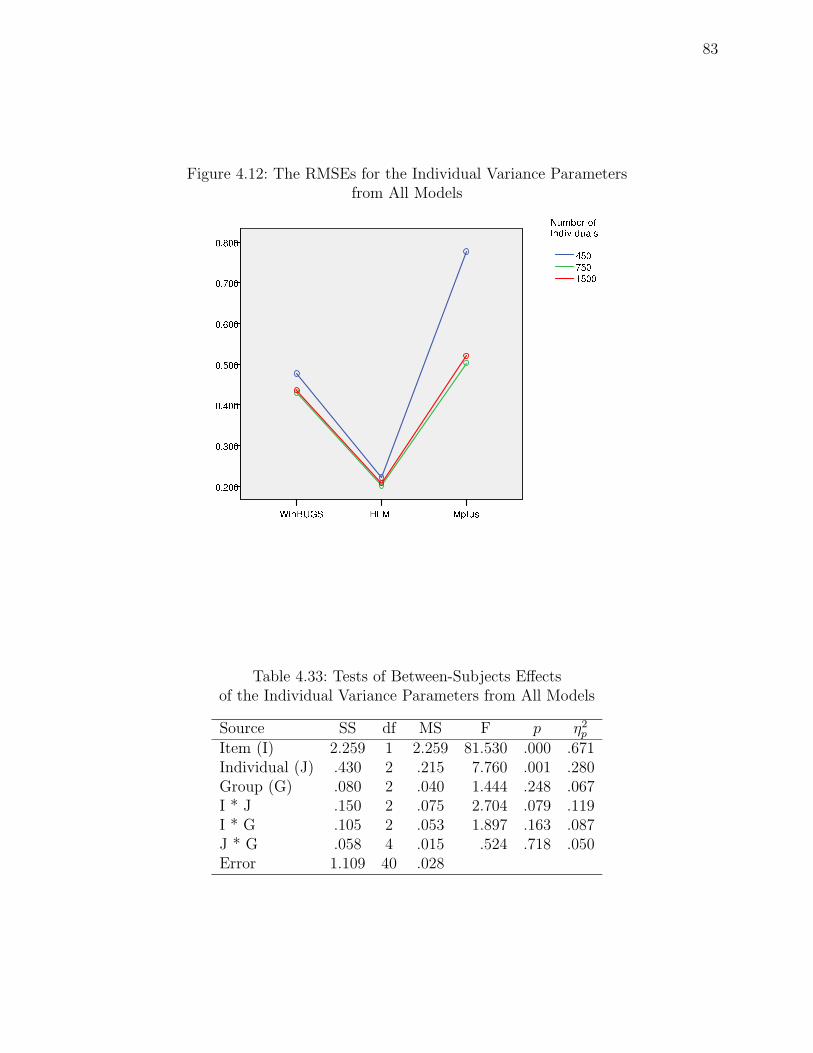
83

Figure 4.12: The RMSEs for the Individual Variance Parametersfrom All Models

Table 4.33: Tests of Between-Subjects Effectsof the Individual Variance Parameters from All Models


Item (I) 2.259 1 2.259 81.530 .000 .671Individual (J) .430 2 .215 7.760 .001 .280Group (G) .080 2 .040 1.444 .248 .067I * J .150 2 .075 2.704 .079 .119I * G .105 2 .053 1.897 .163 .087J * G .058 4 .015 .524 .718 .050Error 1.109 40 .028

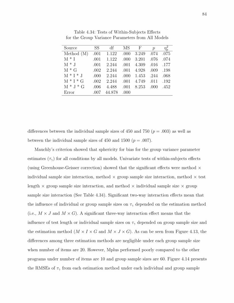
84

Table 4.34: Tests of Within-Subjects Effectsfor the Group Variance Parameters from All Models


Method (M) .001 1.122 .000 3.249 .074 .075M * I .001 1.122 .000 3.201 .076 .074M * J .001 2.244 .001 4.309 .016 .177M * G .002 2.244 .001 4.928 .009 .198M * I * J .000 2.244 .000 1.453 .244 .068M * I * G .002 2.244 .001 4.749 .011 .192M * J * G .006 4.488 .001 8.253 .000 .452Error .007 44.878 .000

differences between the individual sample sizes of 450 and 750 (p = .003) as well as

between the individual sample sizes of 450 and 1500 (p = .007).

Mauchly’s criterion showed that sphericity for bias for the group variance parameter

estimates (τγ) for all conditions by all models. Univariate tests of within-subjects effects

(using Greenhouse-Geisser correction) showed that the significant effects were method ×

individual sample size interaction, method × group sample size interaction, method × test

length × group sample size interaction, and method × individual sample size × group

sample size interaction (See Table 4.34). Significant two-way interaction effects mean that

the influence of individual or group sample sizes on τγ depended on the estimation method

(i.e., M × J and M × G). A significant three-way interaction effect means that the

influence of test length or individual sample sizes on τγ depended on group sample size and

the estimation method (M × I × G and M × J × G). As can be seen from Figure 4.13, the

differences among three estimation methods are negligible under each group sample size

when number of items are 20. However, Mplus performed poorly compared to the other

programs under number of items are 10 and group sample sizes are 60. Figure 4.14 presents

the RMSEs of τγ from each estimation method under each individual and group sample

85

Figure 4.13: The RMSEs for the Group Variance Parametersunder Each Test Length from All Models

size. The differences among the three estimation methods were found between Mplus and

the other two programs under the group sample sizes are 60 under each sample size.

Among the between-subjects effects, significant main effects were found for individual

and group sample size as well as for individual × group sample size interaction (See Table

4.35). A significant interaction effect means that the influence of number of individuals on

RMSEs of τγ depends on number of groups (See Figure 4.15). The biases of the group

variance estimates were inversely related to amount of information in the data that they

are based on. As you can see from the figure, this bias became smaller as the number of

groups increased under each individual sample size.

This implies that the robustness of the group-level variance estimates (τγ) seemed to

depend largely on the group sample size, particularly when sample size was small at the

individual level (J = 450). The mean RMSEs of τγ were .096 for G = 60, .160 for G = 30,

and .174 for G = 15, respectively under J = 450. These results are consistent with the

previous findings indicated by Kasim and Raudenbush (1998), which showed that

group-level variance components are more biased when sample size was small. These

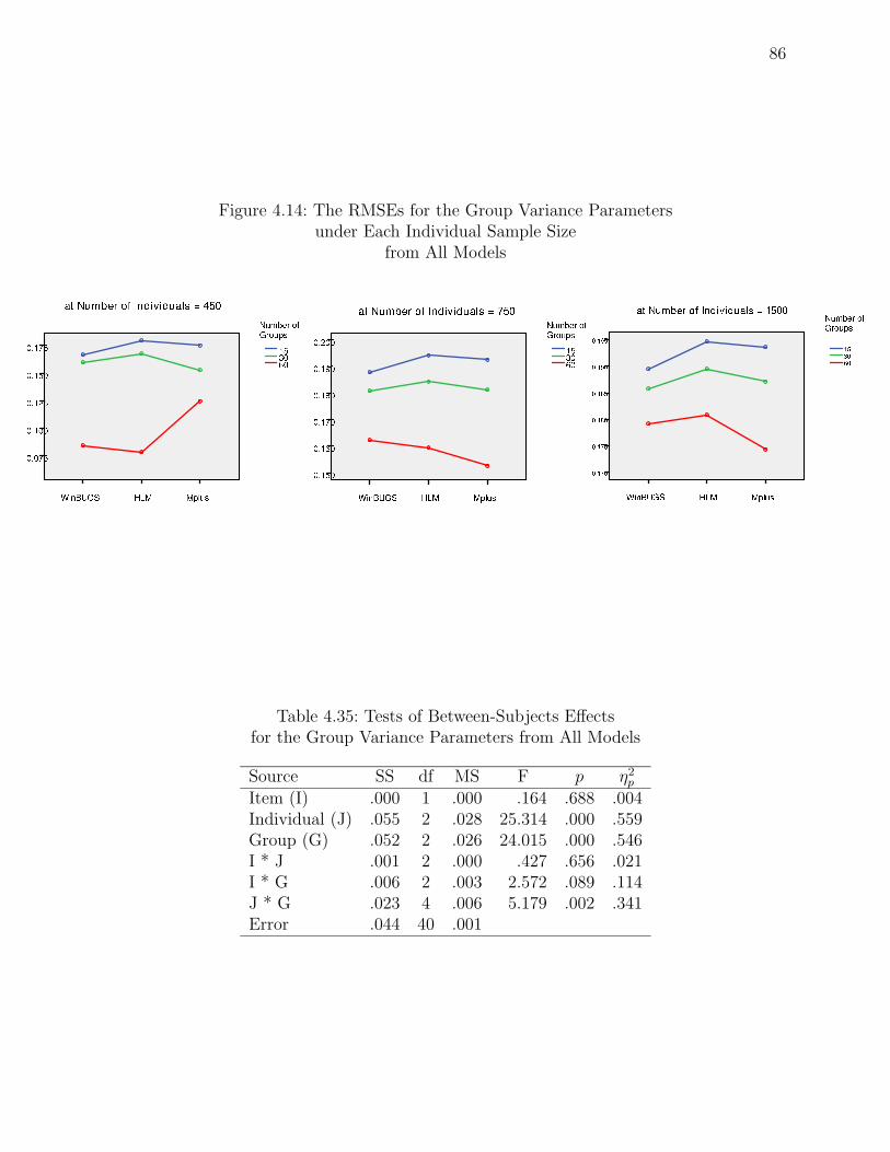
86

Figure 4.14: The RMSEs for the Group Variance Parametersunder Each Individual Sample Size

from All Models

Table 4.35: Tests of Between-Subjects Effectsfor the Group Variance Parameters from All Models


Item (I) .000 1 .000 .164 .688 .004Individual (J) .055 2 .028 25.314 .000 .559Group (G) .052 2 .026 24.015 .000 .546I * J .001 2 .000 .427 .656 .021I * G .006 2 .003 2.572 .089 .114J * G .023 4 .006 5.179 .002 .341Error .044 40 .001

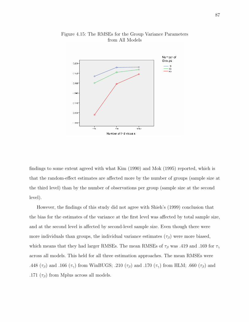
87

Figure 4.15: The RMSEs for the Group Variance Parametersfrom All Models

findings to some extent agreed with what Kim (1990) and Mok (1995) reported, which is

that the random-effect estimates are affected more by the number of groups (sample size at

the third level) than by the number of observations per group (sample size at the second

level).

However, the findings of this study did not agree with Shieh’s (1999) conclusion that

the bias for the estimates of the variance at the first level was affected by total sample size,

and at the second level is affected by second-level sample size. Even though there were

more individuals than groups, the individual variance estimates (τβ) were more biased,

which means that they had larger RMSEs. The mean RMSEs of τβ was .419 and .169 for τγ

across all models. This held for all three estimation approaches. The mean RMSEs were

.448 (τβ) and .166 (τγ) from WinBUGS; .210 (τβ) and .170 (τγ) from HLM; .660 (τβ) and

.171 (τβ) from Mplus across all models.

Chapter 5

Discussion

This chapter presents the general summary and interpretation of the results, the

limitations of the study, and suggestions for future research.

5.1 Summary

This study compared the performance of parameter estimates of maximum likelihood (ML)

estimation, which is the method most widely used in current applied multilevel IRT

analyses and Bayesian estimation, which has become a viable alternative to ML-based

estimation techniques in the context of Kamata’s three-level IRT model. The unconditional

model, the model with a level-2 predictor variable, and the model with a level-2 and a

level-3 predictor variable were used to assess how varying sample sizes at each level affects

on parameter estimates of interest using simulated data as well as actual data.

Bayesian estimation using WinBUGS was found to perform better than ML estimations

in all conditions for item parameter estimates. For the individual (Level 2) variance

estimates, PQL estimation using HLM showed less bias than the other two methods.

However, Bayesian and ML estimations performed similarly for the other parameters of

interest, the group variance (Level 3) estimates and the coefficient estimates of level-2 and

level-3 predictor variables.

Overall, the findings of the present study were consistent with those of previous studies

with regard to the effect of sample size on bias of parameter estimates. As expected, there

was an inverse relationship between magnitude of RMSEs of parameter estimates and the

sample size. However, RMSEs increased as test length increased. The use of a predictor

88

89

variable did not change the item parameter estimates, but appeared to provide an

improvement in the recovery of variance parameters. However, the inclusion of a

group-level (Level 3) predictor variable in the model leads to a loss of efficiency for the

individual level (Level 2) predictor variable.

This study also presented a summary of the implementation of the computer programs

HLM (Raudenbush et al., 2005), Mplus (Muthen & Muthen, 2006), and WinBUGS

(Spiegelhalter et al., 2003) for the analyses of multilevel IRT model. Studies such as this

one will provide useful information for researchers seeking to use ML as well as Bayesian

estimation for estimation of multilevel IRT model parameters.

Even though HLM has some disadvantages such as inflexibility of creating data files

and convergence problems, it is a fast estimation method. In applying these models, it was

also found that the choice of reference item in the multilevel IRT model does not have an

impact on the results. The estimates of the fixed effects for individual-level and group-level

predictor variables, the estimates of the random effects, and the rank order and distance

between item parameters are not affected by which item is chosen as the reference item.

Mplus showed good performance on item parameter and group variance parameter

estimates even with small sample sizes. To get factor variances, one factor loading was

fixed to one. It was not examined whether the choice of item had an impact on the results.

Currently, Mplus cannot handle cross-level interactions.

WinBUGS appears to be a time-consuming method, but has the advantage of simple

code changes needed for each model used in this study and the results are straightforward.

One important aspect of this study should be noted here. Uninformative priors (i.e., γ01

∼ N(0, 1.0E − 6)) were used to obtain parameter estimates in Bayesian estimation. When

the information used by the estimating algorithm comes solely from the data, or when

priors are uninformative, then a Bayesian estimate would be comparable to that obtained

from a non-Bayesian algorithm such as a maximum likelihood algorithm.

90

Another important ML-Bayesian comparison should be noted is computational speed,

where ML approaches have a distinct advantage. For example, for a test length of 20 items,

individual sample size od 1500, and group sample size of 15, HLM or Mplus took just a

couple of minutes, but WinBUGS took about 12 hours using a PC with 3GB RAM and a

clock speed of 3.6GHz. However, steady improvements in recent years in both hardware

speed and efficiency of Monte Carlo algorithms make MCMC-based Bayesian fitting of

multilevel models an attractive approach, even with rather large data sets.

5.2 Limitations and Suggestions

There are several limitations in this study. As with any simulation study, this one includes

only a small subset of all possible interesting conditions. Issues of sample sizes at each

level, which plays an important role in item parameter and ability estimation, were mainly

addressed. In addition, the range of conditions was limited due to computational time with

Bayesian estimation using WinBUGS.

The present study was limited to balanced (that is, equal sample sizes) for group-level

data. An extension to unbalanced data would be useful. Raudenbush and Bryk (2002)

reported that ML bias with unbalanced data can be smaller than that with balanced data.

The models used were restricted to those modeling binary data. Moreover, individual-

and group-level predictor variables were limited in the simulated data set. Dichotomous

equal size Level-2 predictor variable and Level-3 predictor variables were used in order to

look at their effect on estimates of ability. There are other factors which also might be

examined for their influence on these estimates such as unequal numbers of individuals in a

group.

Also, the generalization of the results was limited by the design of the study. This study

employed only the unconditional model, the model with one level-2 predictor variable, and

the model with one level-2 and one level-3 predictor variable. Neither the interaction

between level-2 predictor variables nor the interaction between level-3 predictor variables

91

was considered. The cross-level interaction (i.e., the effect of the group-level predictors on

the relationship between the individual-level predictor variable and individual ability) was

not considered in the study, either. Future research studying interaction effects of predictor

variables would be useful.

The true values of item and ability parameters used were selected from previous studies

and the data used. Clearly, these values could have affected the results. Other values for

the parameters are possible and could be adequate for other educational or non-educational

settings and might lead to different conclusions. Therefore, more comprehensive simulation

studies that resemble real data should be conducted to predict the pattern of effects

associated with data structure, or assumption violations. Multilevel IRT models require

satisfying the assumptions such as (1) a single dimension underlying the item responses

and (2) the latent trait is a random parameter, is normally distributed within and between

groups, and the variance of which is the same across groups (Pastor, 2003). It was

suggested that this assumption violations should be taken into consideration, particularly

when using samples with small sizes (Darandari, 2004).

Finally, the results of this study provide important information for the application of

multilevel IRT models. In particular, the strengths and weaknesses of three different

algorithms were compared, providing useful information as to their respective utility for

this type of situation.

Bibliography

[1] Albert, J. H. (1992). Bayesian estimation of normal ogive item response curves using

Gibbs sampling. Journal of Educational Statistics, 17, 251-269.

[2] Adams, R. J., Wilson, M., & Wu, M. (1997). Multilevel item response models: An

approach to errors in variables regression. Journal of Educational and Behavioral

Statistics, 22(1), 47-76.

[3] Battle, J. (2002). Culture Free Self-Esteem InventoriesThird Edition. Austin, TX:

Pro-Ed.

[4] Best, N. G., Cowles, M. K., & Vines, K. (1995). CODA: Convergence Diagnosis and

Output Analysis Software for Gibbs Sampling Output Technical report. MRC

Biostatistics Unit, University of Cambridge.

[5] Breslow, N. E., & Clayton, D. G. (1993). Approximate inference in generalized linear

mixed models. Journal of the American Statistical Association, 88, 9-25.

[6] Browne, W. J., & Draper, D. (2006). A comparison of Bayesian and likelihood-based

methods for fitting multilevel models. Bayesian Analysis, 1, 473-514.

[7] Brooks, S. & Gelman, A. (1998). Methods for monitoring convergence of iterative

simulations. Journal of Computational and Graphical Statistics, 7, 434-455.

[8] Bryk, A. S., & Raudenbush, S. W. (1986). A hierarchical model for studying school

effects. Sociology of Education, 59(1), 1-17.

[9] Bryk, A. S., & Raudenbush, S. W. (1992). Application of hierarchical linear models to

assessing change. Psychological Bulletin, 101, 147-158.

92

93

[10] Callens, M., & Croux, C. (2005). Performance of likelihood-based estimation methods

for multilevel binary regression models. Journal of Statistical Computation and

Simulation, 75(12), 1003-1017.

[11] Casella, G., & George, E. I. (1992). Explaining the Gibbs sampler. The American

Statistician, 46, 167-174.

[12] Cowles, M. K., & Carlin, B. P. (1996). Markov Chain Monte Carlo converge

diagnostics: A comparative review. Journal of the American Statistical Association,

91, 883-904.

[13] Darandari, E. (2004). Robustness of hierarchical linear model parameter estimates

under violations of second-level residual homoskedasticity and independent

assumptions. Unpublished doctoral dissertation. The Florida State University, FL.

[14] Edwards, W., Lindman, H., & Savage, L. J. (1963). Bayesian statistical inferencee for

psychological research. Psychological Review, 70, 193-242.

[15] Embretson, S. E., & Reise, S. P. (2000). Item response theory for psychologists.

Mahwah, NJ: Lawrence Erlbaum Associates.

[16] Florida Department of Education. (2003, March). Florida Comprehensive Assessment

Test. Tallahassee, FL: Author.

[17] Gelfand, A. E., Hills, S. E., Racine-Poon, A., & Smith, A. F. M. (1990). Illustration of

Bayesian inference in normal data models using Gibbs sampling. Journal of the

American Statistical Association, 85(412), 972-985.

[18] Gelfand, A. E., & Smith, A. F. M. (1990). Sampling-based approaches to calculating

marginal densities. Journal of the American Statistical Association, 85, 398-409.

94

[19] Geman, S., & Geman, D. (1984). Stochastic relaxation, Gibbs distributions, and the

Bayesian restoration of images. ITTT Transactions on Pattern Analysis and Machine

Intelligence, 6, 721-741.

[20] Gelman, A., & Rubin, D. B. (1992). Inference from iterative simulation using multiple

sequences. Statistical Sciences, 7(4), 457-472.

[21] Gelman, A., Carlin, J. B., Stern, H. S., & Rubin, D. B. (1995). Bayesian data analysis.

London: Chapman and Hall.

[22] Gelman, A. (2006). Prior distributions for variance parameters in hierarchical models.

Bayesian Analysis, 1(3), 515-533.

[23] Geweke, J. (1992). Evaluating the accuracy of sampling-based approaches to calculating

posterior moments. In Bayesian Statistics 4, 169-193. Oxford: Oxford University Press.

[24] Goldstein, H. (1986). Multilevel mixed linear model analysis using iterative generalised

least squares. Biometrika, 73, 43-56.

[25] Goldstein, H. (1987). Multilevel models in education and social research. London:

Charles Griffin and Co.

[26] Goldstein, H. (1995). Multilevel statistical models. London: Edward Arnold; New York:

Halstead Press.

[27] Goldstein, H., & Rasbash, J. (1996). Improved approximations for multilevel models

with binary responses. Journal of the Royal Statistical Society, A-159, 505-513.

[28] Guo, G., & Zhao, H. (2000). Multilevel modeling for binary data. Annual Review of

Sociology, 26, 441-462.

[29] Hambleton, R., & Swaminathan, H. (1985). Item response theory: Principles and

applications. Boston: Kluwer-Nijhoff Publishing.

95

[30] Hedeker, D. (2004). An introduction to growth modeling. In D. Kaplan (Ed.),

Quantitative Methodology for the Social Sciences. CA: Thousand Oaks.

[31] Insightful Corp. (2006). S-PLUS [Computer Program]. Reinach, Switzerland.

[32] Jones, B. S., & Steenbergen, M. R. (1997). Modeling multilevel data structures. Paper

presented at the annual meeting of the Political Methodology Society, Columbus, OH.

[33] Kasim, R. M. & Raudenbush, S. W. (1998). Application of Gibbs sampling to nested

variance components models with heterogeneous within-group variance. Journal of

Educational and Behavioral Statistics, 23, 93-116.

[34] Kamata, A. (1998). Some generalizations of the Rasch model: An application of the

hierarchical generalized linear model. Unpublished doctoral dissertation, Michigan

State University, East Lansing.

[35] Kamata, A. (2000, April). Precision of person ability estimates from one-parameter

hierarchical generalized linear logistic model. Paper presented at the annual meeting of

American Educational Research Association, New Orleans, LA.

[36] Kamata, A. (2001). Item analysis by the hierarchical generalized linear model. Journal

of Educational Measurement, 38(1), 79-93.

[37] Kamata, A. (2002, April). Procedure to perform item response analysis by hierarchical

generalized linear model. Paper presented at the annual meeting of the American

Educational Research Association, New Orleans, LA.

[38] Kamata, A., & Binici, S. (2003). Random-effect DIF analysis via hierarchical

generalized linear models. Paper presented at the Annual International Meeting of the

Psychometric Society, Sardinia, Italy.

[39] Kim, K. S. (1990). Multilevel data analysis: A comparison of analytical alternatives.

Unpublished doctoral dissertation. University of California, Los Angeles, CA.

96

[40] Kreft, I. G. G. (1996). Are multilevel techniques necessary? An overview, including

simulation studies. Unpublished Report. Los Angeles, CA: University of California,

Department of Statistics.

[41] Lee, B. (2003). Using hierarchical linear modeling to illustrate industry and group

effects on organizational commitment in a sales context. Journal of Managerial Issues,

15(3), 353-368.

[42] Longford, N. T. (1987). A fast scoring algorithm for maximum likelihood estimation in

unbalanced mixed models with nested random effects. Biometrika, 74, 817-827.

[43] Longford, N. T. (1993). Random coefficient models. New York: Oxford University

Press.

[44] Lord, F. M., & Novick, M. R. (1968). Statistical theory of mental test scores. Reading,

MA: Addison-Wesley.

[45] Maier, K. S. (2001). A Rasch hierarchical measurement model. Journal of Educational

Behavioral Statistics, 26(3), 307-330.

[46] Mason, W., Wong, G., & Entwistle, B. (1983). Contextual analysis through the

multilevel linear model. Sociological Methodology, 13, 72-103.

[47] Mislevy, R. J. (1987). Exploiting auxiliary information about examinees in the

estimation of item parameters. Applied Psychological Measurement, 11(1), 81-91.

[48] Mok, M. (1995). Sample Size Requirements for 2-level designs in educational research.

Sydney, Australia: Mcquarie University.

[49] Muthen, B., Kao, C-F., & Burstein, L. (1991). Instructional sensitivity in mathematics

achievement test items: Applications of a new IRT-based detection technique. Journal

of Educational Measurement, 28, 1-22.

97

[50] Muthen, B., & Muthen, L. (2006). Mplus [Computer software]. Los Angeles: Muthen

& Muthen.

[51] Osborne, J. W. (2000). Advantages of hierarchical linear modeling. Practical

Assessment, Research & Evaluation, 7(1), Available online at

http://ericae.net/pare/getvn.asp?v=7&n=1.

[52] Pastor, D. A. (2003). The use of multilevel item response theory modeling in applied

research: An illustration. Applied Measurement in Education, 16(3), 223-243.

[53] Patz, R. J., & Junker, B. W. (1999a). A straightforward approach to Markov chain

Monte Carlo methods for item response models. Journal of Educational and


[54] Patz, R. J., & Junker, B. W. (1999b). Applications and extensions of MCMC in IRT:

Multiple item types, missing data, and rated responses. Journal of Educational and


[55] Pollack, B. N. (1998). Hierarchical linear modeling and the “Unit of analysis”

problem: A solution for analyzing responses of intact group members. Group

Dynamics: Theory, Research, and Practice, 2(4), 299-312.

[56] Polson, N. G. (1996). Convergence of Markov chain Monte Carlo algorithms. In

Bayesian Statistics, 5, 297-321. Oxford, U.K.: Oxford University Press.

[57] Raftery, A. E., & Lewis, S. (1992). How many iterations in the Gibbs sampler? In

Bayesian Statistics, 4, 763-773. Oxford, U.K.: Oxford University Press.

[58] Rasch, G. (1960). Probabhilistic models for some intelligence and attainmnent tests.

Chicago: University of Chicago.

[59] Raudenbush, S. W., & Bryk, A. G. (2002). Hierarchical linear models: Applications

and data analysis methods (2nd ed.). Newbury Park, CA: Sage.

98

[60] Raudenbush, S. W., Bryk, A. S., Cheong, Y. F., & Congdon, R. T. (2000-2006). HLM:

Hierarchical Linear and Nonlinear Modeling [Computer Program]. Chicago: Scientific

Software International.

[61] Raudenbush, S. W., Yang, M.-L., & Yosef, M. (2000). Maximum likelihood for

generalized linear models with nested random effects via high-order, multivariate

Laplace approximation. Journal of Computational and Graphical Statisticss, 9,

141-145.

[62] Rijmen, F., Tuerlinckx, F., De Boeck, P., & Kuppens, P. (2003). A nonlinear mixed

model framework for item response theory. Psychological Methods, 8, 185-205.

[63] Roberts, G. O. (1996). Methods for estimating L2 convergence of Markov chain Monte

Carlo. In Bayesian Statistics and Econometrics: Essays in Honor of Arnold Zellner,

373-384. Amsterdam, North-Holland.

[64] Rodriguez, G., & Goldman, N. (1995). An assessment of estimation procedures for

multilevel models with binary responses. Journal of the Royal Statistical Society,

A-158, 73-90.

[65] Rodriguez, G., & Goldman, N. (2001). Improved estimation procedures for multilevel

models with binary responses: A case-study. Journal of the Royal Statistical Society,

A-164, 339-355.

[66] Rosenthal, J. S. (1995). Minorization conditions and convergence rates for Markov

chain Monte Carlo. Journal of the American Statistical Association, 90, 558-566.

[67] Rupp, A., Dey, D., & Zumbo, B. (2004). To Bayes or not to Bayes, from whether to

when: Applications of Bayesian methodology to modeling. Structural Equation

Modeling, 11(3), 424-451.

[68] Shieh, Y. (1999). An evaluation of mixed effects multilevel modeling under conditions

of error term normality. Austin: University of Texas.

99

[69] Snijders, T., & Bosker, R. (2000). Multilevel Analysis: An Introduction to Basic and

Advanced Multilevel Modeling. London: Sage.

[70] Snijders, T. (2005). Power and Sample Size in Multilevel Linear Models. In

Encyclopedia of Statistics in Behavioral Science, 3, 1570-1573. Chicester (etc.): Wiley.

[71] Spiegelhalter, D., Thomas, A., & Best, N. (2003). WinBUGS 1.4 [Computer Program].

Robinson Way, Cambridge CB2 2SR, UK: MRC Biostatistics Unit, Institute of Public

Health.

[72] Stiratelli, R., Laird, N., & Ware, J. H. (1984). Random-effects models for serial

observations with binary responses. Biometrics, 40, 961-971.

[73] Swaminathan, H., & Gifford, J. (1982). Bayesian estimation in the Rasch model.

Journal of Educational Statistics, 7(3), 175-191.

[74] Wong, G. Y., & Mason, W. M. (1985). The hierarchical logistic regression model for

multilevel analysis. Journal of the American Statistical Association, 80, 513-524.

Appendix A

Mplus Code

A.1 The Unconditional Model

TITLE: TIMMS DATA

DATA: FILE IS K_TIMSS.DAT;


VARIABLE: NAMES ARE SCH Q1-Q17;

CLUSTER = SCH;

USEVARIABLES ARE Q1-Q17;

CATEGORICAL ARE Q1-Q17;


ESTIMATOR = ML;

MODEL:

%WITHIN%


THETA BY Q17@1;

%BETWEEN%


THETAB BY Q17@1;


100

101

A.2 The Model with Level-2 Predictor Variable

TITLE: TIMMS DATA

DATA: FILE IS K_TIMSS_P2.DAT;


VARIABLE: NAMES ARE SCH Q1-Q17 SCISTUD;

WITHIN = SCISTUD;

CLUSTER = SCH;

USEVARIABLES ARE Q1-Q17 SCISTUD;

CATEGORICAL ARE Q1-Q17 SCISTUD;


ESTIMATOR = ML;

MODEL:

%WITHIN%


THETA BY Q17@1;

THETA BY SCISTUD;

%BETWEEN%


THETAB BY Q17@1;


102

A.3 The Model with Level-2 and Level-3 Predictor Variables

TITLE: TIMMS DATA

DATA: FILE IS K_TIMSS_P3.DAT;

FORMAT IS F3.0 18F1.0 F2.0;

VARIABLE: NAMES ARE SCH Q1-Q17 SCISTUD EXP;

WITHIN = SCISTUD EXP;

CLUSTER = SCH;

USEVARIABLES ARE Q1-Q17 SCISTUD EXP;

CATEGORICAL ARE Q1-Q17 SCISTUD;


ESTIMATOR = ML;

MODEL:

%WITHIN%


THETA BY Q17@1;

THETA BY SCISTUD;

THETA ON EXP;

%BETWEEN%


THETAB BY Q17@1;


Appendix B

WinBUGS Code

B.1 The Unconditional Model

# The Unconditional Model for the TIMSS Data

# CONDITION: I=17, J=1130, G=68

# I : # of items

# J : # of examinees

# G : # of groups

model

{

for (j in 1:J) {

for (i in 1:I) {

r[j,i]<-resp[j,i]

}}

# 1PL model

for (j in 1:J) {

for (i in 1:I) {

logit(p[j,i]) <- u2[j] + u3[group[j]] - b[i]

r[j,i] ~ dbern(p[j,i])

}}

# Higher level definition

for (j in 1:J) {

u2[j] ~ dnorm(mu, tau.u2)

}

for (g in 1:G){

u3[g] ~ dnorm(0, tau.u3)

}

103

104

# Priors

mu ~ dnorm(0,1)

tau.u2 ~ dgamma(0.1, 0.001)

sigma2 <- 1/tau.u2 # Variance of ability for level 2

tau.u3 ~ dgamma(0.1, 0.001)


# added for identification

for (i in 1:I) {

bb[i]~dnorm(mub,sigb)

b[i] <- bb[i] - mean(bb[1:I])

}

mub ~ dnorm(0,1)

sigb ~ dchisqr(.5)

}

# First Initial Values

list(b=c(-2,-2,-2,-2,-2,-2,-2,-2,-2,-2,-2,-2,-2,-2,-2,-2,-2) ,

tau.u2=1, tau.u3=5)

# Second Initial Values

list(b=c(2,2,2,2,2,2,2,2,2,2,2,2,2,2,2,2,2 ) , tau.u2=2, tau.u3=10)

list(I=17, J=1130, G=68, group=c( 1,

1,

...

68,

68 ) ,

resp=structure(.Data=c(0,0,0,0,0,0,0,0,0,0,0,0,1,1,0,0,0,

0,1,0,0,0,0,0,1,1,0,1,0,0,0,0,1,0,

...

1,1,1,0,0,1,1,1,1,1,0,0,1,1,1,0,1,

0,1,1,1,1,0,0,0,0,1,0,0,1,0,0,0,0 ), .Dim=c(1130,17 )))

105

B.2 The Model with Level-2 Predictor Variable

# The Model with Level-2 Predictor Variable for the TIMSS Data

# CONDITION: I=17, J=1130, G=68

# I : # of items


# G : # of groups

model

{

for (j in 1:J) {

for (i in 1:I) {

r[j,i]<-resp[j,i]

}}

# 1PL model

for (j in 1:J) {

for (i in 1:I) {


r[j,i]~dbern(p[j,i])

}}


for (j in 1:J) {

u2[j] ~ dnorm(mu1[j], tau.u2)

}

for (j in 1:J) {

mu1[j] <- alpha*scistud[j]

}

for (g in 1:G){

u3[g] ~ dnorm(mu2, tau.u3)

}

# Priors

alpha ~ dnorm(0,1.0E-6)

mu2 ~ dnorm(0,1)

106

tau.u2 ~ dgamma(0.1, 0.001)


tau.u3 ~ dgamma(0.1, 0.001)



for (i in 1:I) {



}

mub ~ dnorm(0,1)

sigb ~ dchisqr(.5)

}

list(tau.u2=1, tau.u3=5, alpha=0.393)

list(I=17, J=1130, G=68, group=c( 1,

1,

...

68,

68 ) ,

scistud=c(1,

1,

...

1,

1 ) ,


0,1,0,0,0,0,0,1,1,0,1,0,0,0,0,1,0,

...

1,1,1,0,0,1,1,1,1,1,0,0,1,1,1,0,1,

0,1,1,1,1,0,0,0,0,1,0,0,1,0,0,0,0 ), .Dim=c(1130,17 )))

107

B.3 The Model with Level-2 and Level-3 Predictor Variables

# The Model with Level-2 and Level-3 Predictor Variables

# CONDITION: I=17, J=1130, G=68

# I : # of items


# G : # of groups

model

{

for (j in 1:J) {

for (i in 1:I) {

r[j,i]<-resp[j,i]

}}

# 1PL model

for (j in 1:J) {

for (i in 1:I) {


r[j,i]~dbern(p[j,i])

}}


for (j in 1:J) {

u2[j] ~ dnorm(mu1[j], tau.u2)

}

for (j in 1:J) {

mu1[j] <- alpha*scistud[j] + beta*exp[j]

}

for (g in 1:G){

u3[g] ~ dnorm(mu2, tau.u3)

}

# Priors

alpha ~ dnorm(0,1.0E-6)

beta ~ dnorm(0,1.0E-6)

tau.u2 ~ dgamma(0.1, 0.001)

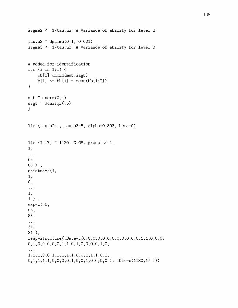
108


tau.u3 ~ dgamma(0.1, 0.001)



for (i in 1:I) {



}

mub ~ dnorm(0,1)

sigb ~ dchisqr(.5)

}

list(tau.u2=1, tau.u3=5, alpha=0.393, beta=0)

list(I=17, J=1130, G=68, group=c( 1,

1,

...

68,

68 ) ,

scistud=c(1,

1,

0,

...

1,

1 ) ,

exp=c(85,

85,

85,

...

31,

31 ),


0,1,0,0,0,0,0,1,1,0,1,0,0,0,0,1,0,

...

1,1,1,0,0,1,1,1,1,1,0,0,1,1,1,0,1,

0,1,1,1,1,0,0,0,0,1,0,0,1,0,0,0,0 ), .Dim=c(1130,17 )))

Appendix C

Convergence Diagnostics

C.1 Geweke

GEWEKE CONVERGENCE DIAGNOSTIC:

==============================

Fraction in first window = 0.1

Fraction in last window = 0.5

Chain: b

--------

numeric matrix: 2 rows, 17 columns.

b[10] b[11] b[12] b[13] b[14] b[15]

Z-Score -0.8858132 3.163559312 7.416149e+000 -1.5441484 -0.7823772 -0.9010875

p-value 0.3757182 0.001558526 1.205702e-013 0.1225524 0.4339929 0.3675418

b[16] b[17] b[1] b[2] b[3] b[4]

Z-Score 0.08318674 -0.2368495 -1.2664404 -1.7952147 -1.4092248 -1.78364199

p-value 0.93370305 0.8127735 0.2053554 0.0726195 0.1587687 0.07448186

b[5] b[6] b[7] b[8] b[9]

Z-Score -2.13921383 -1.4652862 -1.106207 -1.82312174 0.09608914

p-value 0.03241835 0.1428429 0.268637 0.06828496 0.92344978

109

110

C.2 Raftery and Lewis

RAFTERY AND LEWIS CONVERGENCE DIAGNOSTIC:

=========================================

Quantile = 0.025

Accuracy = +/- 0.005

Probability = 0.95

Chain: b

--------

numeric matrix: 17 rows, 5 columns.

Thin Burn-in Total Lower Bound Dependence Factor

b[10] 1 2 3757 3746 1.002936

b[11] 1 2 4008 3746 1.069941

b[12] 1 2 3847 3746 1.026962

b[13] 1 2 3792 3746 1.012280

b[14] 1 2 3745 3746 0.999733


b[15] 1 2 3805 3746 1.015750

b[16] 1 2 3914 3746 1.044848

b[17] 1 3 4052 3746 1.081687

b[1] 1 2 3929 3746 1.048852

b[2] 1 2 3895 3746 1.039776


b[3] 1 1 3726 3746 0.994661

b[4] 1 2 3788 3746 1.011212

b[5] 1 2 3882 3746 1.036305

b[6] 1 2 3851 3746 1.028030

b[7] 1 2 3923 3746 1.047250


b[8] 1 2 3819 3746 1.019487

b[9] 1 2 3890 3746 1.038441

Appendix D

Estimated Parameter Means From Five Replications

D.1 The Unconditional Model

For the Condition I = 10, J = 750, G = 30

True WinBUGS HLM MplusParameter Value Mean SD Estimate SE Estimate SE

b[1] -2.0 -1.986 0.130 -1.677 0.092 -1.897 0.151b[2] -1.5 -1.426 0.110 -1.180 0.114 -1.357 0.128b[3] -1.0 -1.120 0.101 -0.915 0.099 -1.062 0.119b[4] -0.5 -0.488 0.089 -0.381 0.109 -0.469 0.105b[5] 0.0 0.020 0.083 0.034 0.097 0.013 0.098b[6] 0.0 -0.012 0.083 0.010 0.104 -0.011 0.098b[7] 0.5 0.552 0.080 0.464 0.102 0.518 0.094b[8] 1.0 1.033 0.081 0.848 0.099 0.975 0.093b[9] 1.5 1.415 0.083 1.154 0.105 1.334 0.095b[10] 2.0 2.019 0.089 1.644 0.104 1.956 0.111τβ 1.0 1.263 0.118 0.986 0.067 1.141 0.324τγ 0.2 0.010 0.012 0.006 0.015 0.004 0.005

where item parameter estimate b[i] for item i = 1, . . . , I,

the individual variance estimate τβ, and

the group variance estimate τγ

111

112

D.2 The Model with Level-2 Predictor Variable



b[1] -2.0 -1.924 0.097 -1.570 0.098 -2.031 0.109b[2] -1.5 -1.527 0.086 -1.223 0.111 -1.608 0.097b[3] -1.0 -1.014 0.075 -0.789 0.107 -1.066 0.086b[4] -0.5 -0.510 0.068 -0.378 0.101 -0.534 0.079b[5] 0.0 -0.010 0.062 0.018 0.100 -0.008 0.074b[6] 0.0 0.036 0.062 0.053 0.102 0.041 0.074b[7] 0.5 0.506 0.060 0.416 0.096 0.536 0.071b[8] 1.0 0.986 0.059 0.781 0.098 1.040 0.070b[9] 1.5 1.484 0.060 1.161 0.097 1.564 0.071b[10] 2.0 2.018 0.063 1.569 0.098 2.125 0.073b[11] -2.0 -2.054 0.102 -1.684 0.119 -2.167 0.113b[12] -1.5 -1.518 0.086 -1.215 0.115 -1.599 0.097b[13] -1.0 -0.994 0.074 -0.773 0.098 -1.043 0.086b[14] -0.5 -0.431 0.066 -0.314 0.102 -0.451 0.078b[15] 0.0 0.004 0.062 0.027 0.101 0.006 0.074b[16] 0.0 -0.021 0.063 0.009 0.094 -0.019 0.074b[17] 0.5 0.514 0.060 0.423 0.095 0.545 0.071b[18] 1.0 0.968 0.059 0.769 0.097 1.020 0.070b[19] 1.5 1.541 0.060 1.203 0.102 1.625 0.071b[20] 2.0 1.948 0.062 1.516 0.099 2.026 0.079τβ 1.0 1.610 0.082 1.371 0.064 1.769 0.266τγ 0.2 0.015 0.014 0.014 0.015 0.020 0.020γ01 0.5 0.149 0.095 0.115 0.052 0.092 0.044


the individual variance estimate τβ,

the group variance estimate τγ , and

the coefficient estimate for level-2 predictor variable γ01

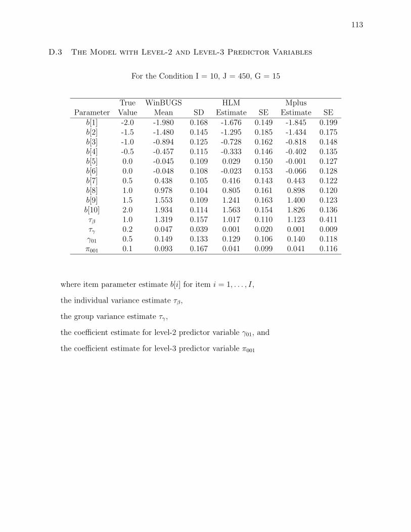
113

D.3 The Model with Level-2 and Level-3 Predictor Variables



b[1] -2.0 -1.980 0.168 -1.676 0.149 -1.845 0.199b[2] -1.5 -1.480 0.145 -1.295 0.185 -1.434 0.175b[3] -1.0 -0.894 0.125 -0.728 0.162 -0.818 0.148b[4] -0.5 -0.457 0.115 -0.333 0.146 -0.402 0.135b[5] 0.0 -0.045 0.109 0.029 0.150 -0.001 0.127b[6] 0.0 -0.048 0.108 -0.023 0.153 -0.066 0.128b[7] 0.5 0.438 0.105 0.416 0.143 0.443 0.122b[8] 1.0 0.978 0.104 0.805 0.161 0.898 0.120b[9] 1.5 1.553 0.109 1.241 0.163 1.400 0.123b[10] 2.0 1.934 0.114 1.563 0.154 1.826 0.136τβ 1.0 1.319 0.157 1.017 0.110 1.123 0.411τγ 0.2 0.047 0.039 0.001 0.020 0.001 0.009γ01 0.5 0.149 0.133 0.129 0.106 0.140 0.118π001 0.1 0.093 0.167 0.041 0.099 0.041 0.116


the individual variance estimate τβ,

the group variance estimate τγ ,

the coefficient estimate for level-2 predictor variable γ01, and

the coefficient estimate for level-3 predictor variable π001

Appendix E

Line Graphs Of Estimated Parameter Means From Five Replications

E.1 The Unconditional Model


where I[i] is the item parameter estimate for item i = 1, . . . , I,

SIGMA2 is the individual variance estimate, and

SIGMA3 is the group variance estimate

114

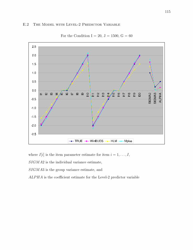
115

E.2 The Model with Level-2 Predictor Variable



SIGMA2 is the individual variance estimate,

SIGMA3 is the group variance estimate, and

ALPHA is the coefficient estimate for the Level-2 predictor variable

116

E.3 The Model with Level-2 and Level-3 Predictor Variables



SIGMA2 is the individual variance estimate,

SIGMA3 is the group variance estimate,

ALPHA is the coefficient estimate for the Level-2 predictor variable, and

BETA is the coefficient estimate for the Level-3 predictor variable

A Comparison of a Bayesian and Maximum Likelihood ...

Documents

Transcript of A Comparison of a Bayesian and Maximum Likelihood ...