Matrix Computations and the Secular Equation - avcr.cz · What is the secular equation? “The term...

Matrix Computationsand

the Secular Equation

Gene H. Golub

Stanford University

Introduction 1 / 35

What is the secular equation?

“The term secular (‘continuing through long ages’ OED2) recallsthat one of the origins of spectral theory was in the problem of thelong-run behavior of the solar system investigated by Laplace andLagrange. [...] The 1829 paper in which Cauchy established that theroots of a symmetric determinant are real has the title, ‘Surl’equation a l’aide de laquelle on determine les inegalites seculairesdes mouvements des planetes’; this signified only that Cauchyrecognized that his problem, of choosing x to maximize xTAxsubject to xTx = 1 (to use modern notation), led to an equationlike that studied in celestial mechanics. Sylvester’s title ‘On theEquation to the Secular Inequalities in the Planetary Theory’ [...]was even more misleading as to content. In this tradition the‘Sakulargleichung’ of Courant and Hilbert’s Methoden derMathematischen Physik (1924) and the ‘secular equation’ of E. T.Browne’s ‘On the Separation Property of the Roots of the SecularEquation’ American Journal of Mathematics, 52, (1930), 843-850refer to the characteristic equation of a symmetric matrix.”

From http://members.aol.com/jeff570/e.htmlIntroduction 1 / 35

http://members.aol.com/jeff570/e.html

Outline

1 Introduction

2 Applications

3 Approximations

4 An example

5 Numerical Comparison

6 Conclusion

Introduction 2 / 35

Applications

Applications 3 / 35

Constrained Eigenvalue Problem

A = AT

maxx6=0

xTAx

s.t. xTx = 1cTx = 0

φ(x;λ, µ) = xTAx− λ(xTx− 1) + 2µxTc

grad φ = 0 =⇒ Ax− λx + µc = 0

x = −µ(A− λI)−1c

cTx = 0 =⇒ cT (A− λI)−1c = 0

Constrained Eigenvalue Secular Equation

A = QΛQT ,d = QTcn∑i=1

d2i

(λi − λ)= 0

Applications 4 / 35

Rank One Change

Ax = λx

(A+ ccT )y = µy

Rank One Change Secular Equation

1 + cT (A− µI)−1c = 0

Rank k-change

(A+ CCT )y = µy

det(I + CT (A− µI)−1C

)= 0

Applications 5 / 35

Another secular equation

Consider (A bbT c

) (xy

)= λ

(xy

).

Then(A− λI)x = −yb

and hence,(c− λ− b(AT − λI)−1b)y = 0.

Hence we must solve another secular equation when the matrix isexpanded.

Applications 6 / 35

Quadratic Constraint

A = AT , positive definite

minx

xTAx− 2cTx

s.t. xTx = α2

φ(x;λ) = xTAx− 2cTx− λ(xTx− α2)

grad φ = 0 =⇒(A− λI)x− c = 0

Quadratic Constraint Secular Equation

cT (A− λI)−2c = α2

Least Squares with a Quadratic Constraint

bTA(ATA− λI)−2ATb = α2

Applications 7 / 35

Total Least Squares (TLS)

(A+ E)x = b + r, A : m× n(A b

) (x−1

)+

(E r

) (x−1

)= 0

(C + F )z = 0;C : m× n+ 1

Determine F and z so that

rank (C + F ) ≤ n and ||F ||F = min.

Equivalently, findmin

z

||Cz||2||z||2 ≡ σmin(C)

Applications 8 / 35

Total Least Squares (cont.)

CTCz = σ2z

Total Least Squares Secular Equation

bTA(ATA− σ2I)−1ATb− bTb− σ2 = 0

σ < σmin(A)

xTLS = (ATA− σ2I)−1ATb

Data Least Squares (DLS)

(A+ E)x = b

bTA(ATA− τ2I)−1ATb− bTb = 0

τ < σmin(A)

Applications 9 / 35

Regularized total least squares (Fischer/G.)Note, that the TLS solution is equivalent to

min‖b−Ax‖2

2

1 + ‖x‖22

= min‖Cz‖2

2

‖z‖22

= σmin(C),

whereC = (A,b) and zn+1 = −1.

For the regularized TLS we consider

min‖b−Ax‖2

2

1 + xTV x, subject to xTV x = α2,

where V is a given symmetric positive definite matrix. Now, let

W =(V 00 1

)= F TF

and observe that

min‖b−Ax‖2

2

1 + xTV x= min

‖Cz‖22

zTWzwith ‖z‖2

2 = 1 + α2, zn+1 = −1.Applications 10 / 35

Least squares with linear and quadratic constraints

Withy = Fz, B = F−TCTCF−1, c = eTn+1F

−1,

γ2 = 1 + α2, and β = −1

we may rewrite our regularized TLS problem in terms of a leastsquares problem with linear and quadratic constraints

minyTByyTy

, s. t. ‖y‖22 = γ2, cTy = β.

where γ and β are non-zero.Lagrange multipliers

ψ(y;λ, µ) = yTBy − λ(yTy − γ2)− 2µ(cTy − β).

grad ψ = 0 whenBy − λy − µc = 0.

Applications 11 / 35

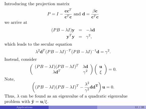
Introducing the projection matrix

P = I − ccT

cTcand d =

βccTc

we arrive at

(PB − λI)y = −λdyTy = γ2,

which leads to the secular equation

λ2dT (PB − λI)−T (PB − λI)−1d = γ2.

Instead, consider((PB − λI)(PB − λI)T λd

λdT γ2

) (uξ

)= 0.

Note, ((PB − λI)(PB − λI)T − λ2

γ2ddT

)u = 0.

Thus, λ can be found as an eigenvalue of a quadratic eigenvalueproblem with y = u/ξ.

Applications 12 / 35

Approximating the secular equation

Approximations 13 / 35

How do we approximate the secular equation for largen?

The problems we have described are closely associated with estimatinga quadratic form

uTF (A)u

where u is a given vector and A is a symmetric matrix.


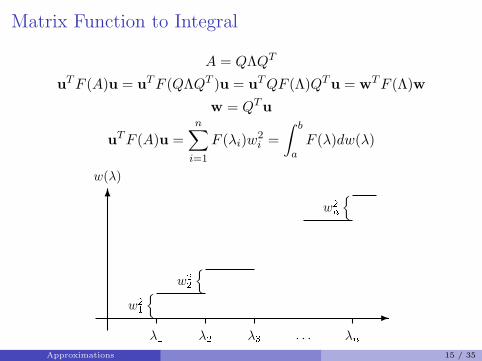
Matrix Function to Integral

A = QΛQT

uTF (A)u = uTF (QΛQT )u = uTQF (Λ)QTu = wTF (Λ)w

w = QTu

uTF (A)u =n∑i=1

F (λi)w2i =

∫ b

aF (λ)dw(λ)


Gauss-Radau Quadrature Rules

L ≤∫ b

aF (λ)dw(λ) ≤ U

µr =∫λrdw(λ) (r = 0, 1, . . . , 2k +m− 1)∫ b

aF (λ)dw(λ) = I[F ] +R[F ]

I[F ] =k∑i=1

AiF (ti) +m∑j=1

BjF (zj)

{Ai, ti}ki=1 unknown weights and nodes{zj}mj=1 prescribed nodes

{Bj}mj=1 calculated weights


Gauss-Radau Quadrature Rules (cont.)

I(λr) = µr

µr =k∑i=1

Aitri +

m∑j=1

Bjzrj

System of non-linear equations.

R[F ] =F (2k+m)(η)(2k +m)!

∫ b

a

m∏j=1

(λ− zj)

[k∏i=1

(λ− ti)

]2

dw(λ)

a < η < b

m = 1

F (2k+1)(η) ≤ 0 and z1 = a R[F ] ≤ 0 I[F ] = U

F (2k+1)(η) ≤ 0 and z1 = b R[F ] ≥ 0 I[F ] = L


Gauss Quadrature∫pr(λ)ps(λ)dα(λ) = 0, r 6= s, (r, s = 0, 1, . . . , k)

pj+1(λ) = (λ− ξj+1)pj(λ)− η2j pj−1(λ)

pk(ti) = 0, i = 1, 2, . . . , k

Jk =

ξ1 η1

η1 ξ2 η2

η2. . . . . .. . . . . . ηk−1

ηk−1 ξk

µ0 = 1

Jkvj = tjvj , j = 1, 2, . . . , k

Aj = v21j , j = 1, 2, . . . , k


Gauss-Radau (Inverse Eigenvalue Problem)

Jk+1 =

0

Jk...ηk

0 · · · ηk ξk+1

0 = pk+1(t0) = (t0 − ξk+1)pk(t0)− η2

kpk−1(t0)

ξk+1 = t0 − η2k

pk−1(t0)pk(t0)

or

(Jk − t0I)δ = η2kek

ξk+1 = t0 + δk


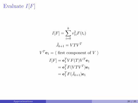
Evaluate I[F ]

I[F ] =k∑i=0

v21iF (ti)

Jk+1 = V TV T

V Te1 = 〈 first component of V 〉

I[F ] = eT1 V F (T )V Te1

= eT1 F (V TV T )e1

= eT1 F (Jk+1)e1


Orthonormal polynomials w.r.t the measure w(λ)How do we build these polynomials?

pj+1(λ) = (λ− ξj+1)pj(λ)− η2j pj−1(λ)

pj+1(A) = (A− ξj+1I)pj(A)− η2j pj−1(A)

pj+1(A)u = (A− ξj+1I)pj(A)u− η2j pj−1(A)u

Set wj = pj(A)u.We define ξj+1 and η2

j so that

wTj+1wj = 0

wTj+1wj−1 = 0,

and thenwTj+1wr = 0 for r < j − 1

ξj+1 =(wj , Awj)(wj ,wj)

and η2j =

(wj ,wj)(wj−1,wj−1)


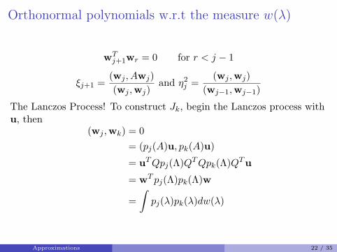
Orthonormal polynomials w.r.t the measure w(λ)

wTj+1wr = 0 for r < j − 1

ξj+1 =(wj , Awj)(wj ,wj)

and η2j =

(wj ,wj)(wj−1,wj−1)

The Lanczos Process! To construct Jk, begin the Lanczos process withu, then

(wj ,wk) = 0= (pj(A)u, pk(A)u)

= uTQpj(Λ)QTQpk(Λ)QTu

= wT pj(Λ)pk(Λ)w

=∫pj(λ)pk(λ)dw(λ)


Examples


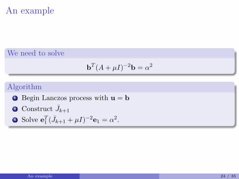
An example

We need to solve

bT (A+ µI)−2b = α2

Algorithm1 Begin Lanczos process with u = b2 Construct Jk+1

3 Solve eT1 (Jk+1 + µI)−2e1 = α2.

An example 24 / 35

Numerical Comparison

Numerical Comparison 25 / 35

Numerical Comparison with Total Least Squares

minE,r

||(E r

)||F

s.t. (A+ E)x = b + r

ψ(σ2) = bTA(ATA− σ2I)−1AT b− bT b− σ2 = 0

Algorithms

Approximate bTA(ATA− σ2I)−1AT b using moment theory andLanczos on ATAApproximate bTA(ATA− σ2I)−1AT b using moment theory andLanczos bidiagonalization on ASolve a set of non-linear equations derived from the normalequations. (Bjorck’s algorithm)


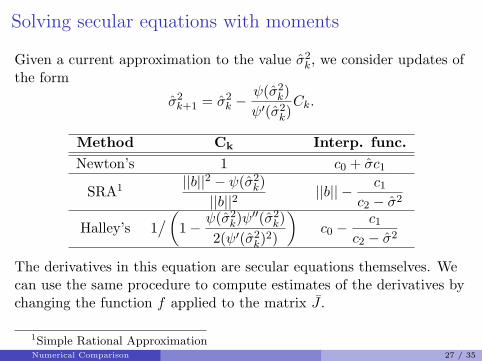
Solving secular equations with moments

Given a current approximation to the value σ2k, we consider updates of

the form

σ2k+1 = σ2

k −ψ(σ2

k)ψ′(σ2

k)Ck.

Method Ck Interp. func.Newton’s 1 c0 + σc1

SRA1 ||b||2 − ψ(σ2k)

||b||2||b|| − c1

c2 − σ2

Halley’s 1/(

1−ψ(σ2

k)ψ′′(σ2

k)2(ψ′(σ2

k)2)

)c0 −

c1c2 − σ2

The derivatives in this equation are secular equations themselves. Wecan use the same procedure to compute estimates of the derivatives bychanging the function f applied to the matrix J .

1Simple Rational ApproximationNumerical Comparison 27 / 35

Solving secular equations with momentsRecall that we need an estimate of λmin and λmax of ATA to use forthe upper and lower bounds in the quadrature rules. We set

b = ||A||1||A||∞ > λmax and a = 10−9 ?< λmin.

In the TLS problem, we need σ < σmin(A) and employ bisection toguarantee this condition.

Algorithm

1 σ2min = min |aij |2

2 While not converged...3 Compute an approximation to the secular functionφ(σ2

k), φ′(σ2

k), φ′′(σ2

k)4 If the approximation failed because the bounds on the secular

function are not monotone, set σ2min = σ2

k and σ2k+1 = (1/2)σ2

k

5 Otherwise, set σ2k+1 = σ2

k −ψ(σ2

k)

ψ′(σ2k)Ck, repeat.


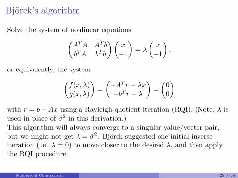
Bjorck’s algorithm

Solve the system of nonlinear equations(ATA AT bbTA bT b

) (x−1

)= λ

(x−1

),

or equivalently, the system(f(x, λ)g(x, λ)

)=

(−AT r − λx−bT r + λ

)=

(00

)with r = b−Ax using a Rayleigh-quotient iteration (RQI). (Note, λ isused in place of σ2 in this derivation.)This algorithm will always converge to a singular value/vector pair,but we might not get λ = σ2. Bjorck suggested one initial inverseiteration (i.e. λ = 0) to move closer to the desired λ, and then applythe RQI procedure.


Details of the matrix moments based algorithm

Algorithm 2 uses the Golub-Kahan bidiagonalization of A andapplies the moment algorithm to T = BTB instead of computingT directly from the Lanczos process on ATA.Algorithm 1 restarts the Lanczos process at each iteration.Algorithm 2 never restarts the bidiagonalization process andsimply continues the process at each iteration.


Problems

Jo’s problems, 15× 8 and 750× 400Bjorck’s problem 1: 30× 15 matrixLarge scale problems with 10000× 5000 and 100000× 60000matrices.

The large scale problems were generated using random Householdermatrices to build the SVD of

[A b

]in product form. Each large-scale

matrix was available solely as an operator to all of the algorithms. Thesingular values of [

A b]

areσi = log(i) + |N(0, 1)|,

where N(0, 1) is a standard normal random variable.


Parameter choicesAlgorithm 1 (Tridiag...) Algorithm 2 (Bidiag...)

λ(0) = 0 λ(0) = 1 λ(0) = ρ λ(0) = 0 λ(0) = 1 λ(0) = ρ

1newton 6 4 5 6 4 5

sra 5 5 5 5 5 5halley 5 5 6 5 5 6

2newton ++ ++ – *8 *8 *7

sra ++ – ++ *12 *24 *7halley ++ ++ ++ *14 *23 *6

3newton – – – *20 *7 *10

sra – – – *20 25 *64halley – – – *55 55 *12

4newton – – – *15 *11 *11

sra ++ – – *15 *25 *14halley – – – *20 *57 *11

5newton 100 – – ++ ++ ++

sra 100 -5 – ++ ++ –halley 100 – – ++ ++ –

* wrong root; ++ correct w/o convergence; – no convergence

ρ = ||A ∗ xls||2/(||xls||2 + 1)

Problem 1 2 3 4 5Size (15,8) (750,400) (10000,5000) (100000,60000) (30,15)


Convergence

Test Alg Iters Error Time Lanz.

jo bjorck 6 1.0× 10−14 0(15, 8) Alg 1 5 4.4× 10−16 0

σ2 = 5.6× 10−1 Alg 2 5 3.3× 10−14 0 12jo bjorck 7 8.5× 100 0.2

(750, 400) Alg 1 >100 8.5× 10−14 52.5σ2 = 1.8× 101 Alg 2 23 5.0× 10−1 0.7 163large-scale bjorck 8 1.1× 10−16 0.5(10000, 5000) Alg 1 >100 1.0× 10−3 36.1σ2 = 1.9× 10−1 Alg 2 55 8.3× 10−16 1.5 152large-scale bjorck 5 3.9× 10−17 5.1

(100000, 60000) Alg 1 >100 5.5× 10−7 324.9σ2 = 3.5× 10−3 Alg 2 57 5.3× 10−8 14.6 155

bjorck bjorck 7 2.6× 10−19 0(30, 15) Alg 1 >100 σ2 0.3

σ2 = 9.9× 10−12 Alg 2 18 2.9× 104 0 33


Conclusions

The secular equation unifies many problems in matrix theory.We can approximate the secular equation using Gaussianquadrature and derive upper and lower bounds.When combined with robust root-finding procedures, we can usethese bounds in algorithms to solve large scale problems.Finding zeros is difficult!

Conclusion 34 / 35

Thanks to colleagues and co-authors

Zhajun BaiDavid GleichSung-Eun JoGerard MeurantBernd Fischer

Conclusion 35 / 35

Matrix Computations and the Secular Equation - avcr.cz · What is the secular equation? “The term...

Documents

Transcript of Matrix Computations and the Secular Equation - avcr.cz · What is the secular equation? “The term...