maths.ucd.ie · Chapter 4 Differential Equations with the Laplace Transform remark In this chapter...
37
Chapter 4 Differential Equations with the Laplace Transform remark In this chapter we will meet only real valued functions defined for positive time, i.e of the form, f :0 ∞ R t ft C n 0 ∞ will denote the (vector space) of such functions which, in addition, are differentiable with continu- ous derivatives, up to and including the n–th order. Note that f C n 0 ∞ f C n 1 0 ∞ f C n 1 0 ∞ remark We will study two simple but very important classes of differential equations, both of the second order with constant coefficients, see 4.9 and 4.10. SOCCLHODE A typical second order constant coefficient linear homogeneous differential equation is of the form. a ¨ xt b ˙ xt cx t 0 t 0 where the constants abc R are called coefficients. SOCCLIHODE A typical second order constant coefficient linear inhomogeneous differential equa- tion is of the form. a ¨ xt b ˙ xt cx t ht t 0 where the constants abc R are called coefficients and h :0 ∞ t ft R is called the driving function. These differential equations will be solved using L the Laplace transform, see 4.4. The general solution will involve convolution, see 4.3. The differential equations describing mechanical damped oscillation and the all important electronic LRC circuit are SOCCLIHODE’s 4.1 Classical functions Solutions of the differential equations above will generally involve the following classical functions. oscillations The functions cos at and sin at are viewed as oscillations, see figure 4.1. decay and growth The functions e at is viewed as decay or growth according a a 0 or a 0, see figure 4.2. sympathy The functions tt 2 and t 3 appear when sympathy is present, see 4.11. 73
Transcript of maths.ucd.ie · Chapter 4 Differential Equations with the Laplace Transform remark In this chapter...
Chapter 4
Differential Equations with the LaplaceTransform
remark In this chapter we will meet only real valued functions defined for positive time, i.e of the form,
f :�0 � ∞ � � R
t �� f � t �C n � 0 � ∞ � will denote the (vector space) of such functions which, in addition, are differentiable with continu-ous derivatives, up to and including the n–th order. Note that
f � C n � 0 � ∞ � � f �� C n 1 � 0 � ∞ � � � f � C n � 1 � 0 � ∞ �remark We will study two simple but very important classes of differential equations, both of the secondorder with constant coefficients, see 4.9 and 4.10.
SOCCLHODE A typical second order constant coefficient linear homogeneous differential equationis of the form.
ax � t �� bx � t ��� cx � t ��� 0 � t � 0
where the constants a � b � c � R are called coefficients.
SOCCLIHODE A typical second order constant coefficient linear inhomogeneous differential equa-tion is of the form.
ax � t ��� bx � t �� cx � t ��� h � t ��� t � 0
where the constants a � b � c � R are called coefficients and h :�0 � ∞ ��� t �� f � t ��� R is called the driving
function. These differential equations will be solved using L the Laplace transform, see 4.4. Thegeneral solution will involve convolution, see 4.3. The differential equations describing mechanicaldamped oscillation and the all important electronic LRC circuit are SOCCLIHODE’s
4.1 Classical functions
Solutions of the differential equations above will generally involve the following classical functions.
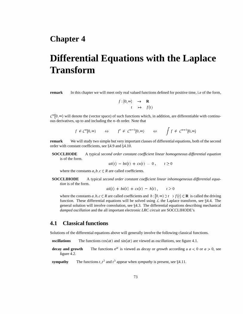
oscillations The functions cos � at � and sin � at � are viewed as oscillations, see figure 4.1.
decay and growth The functions eat is viewed as decay or growth according a a � 0 or a � 0, seefigure 4.2.
sympathy The functions t � t2 and t3 appear when sympathy is present, see 4.11.
73

74 CHAPTER 4. DIFFERENTIAL EQUATIONS WITH THE LAPLACE TRANSFORM
-1
-0.5
0
0.5
1
-3p -2p -p 0 p 2p 3p
x
y
x
y
y=1
y=-1
Figure 4.1: (i) oscillation cos (ii) damped oscillation exp � cos
x
y
y=1
x
y
y=1
Figure 4.2: (i) decay, eat � a � 0 (ii) growth, eat � a � 0
c�
jbquig-UCD February 13, 2003
4.2. HEAVYSIDE STEP AND DIRAC DELTA FUNCTIONS 75
t
y
1
0
a
t
y
t-a
a
0
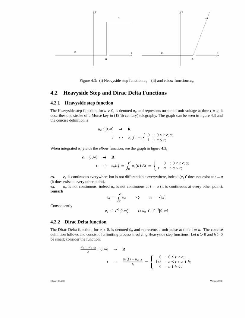
Figure 4.3: (i) Heavyside step function ua (ii) and elbow functions ea
4.2 Heavyside Step and Dirac Delta Functions
4.2.1 Heavyside step function
The Heavyside step function, for a � 0, is denoted ua and represents turnon of unit voltage at time t � a, itdescribes one stroke of a Morse key in (19’th century) telegraphy. The graph can be seen in figure 4.3 andthe concise definition is
ua :�0 � ∞ � � R
t �� ua � t ��� �0 : 0 � t � a;1 : a � t;
When integrated ua yields the elbow function, see the graph in figure 4.3,
ea :�0 � ∞ � � R
t �� ea � t ��� � t
0ua � α � dα � �
0 : 0 � t � a;t � a : a � t;
ex. ea is continuous everywhere but is not differentiable everywhere, indeed � ea � � does not exist at t � a(it does exist at every other point).ex. ua is not continuous, indeed ua is not continuous at t � a (it is continuous at every other point).remark
ea � � t
0ua � ua � � ea � �
Consequentlyea � C 0 � 0 � ∞ � � ua � C 1 � 0 � ∞ �
4.2.2 Dirac Delta function
The Dirac Delta function, for a � 0, is denoted δa and represents a unit pulse at time t � a. The concisedefinition follows and consist of a limiting process involving Heavyside step functions. Let a � 0 and h � 0be small; consider the function,
ua � ua � h
h:�0 � ∞ � � R
t �� ua � t ��� ua � h
h� �� � 0 : 0 � t � a;
1 � h : a � t � a � h;0 : a � h � t
February 13, 2003 c�
jbquig-UCD
76 CHAPTER 4. DIFFERENTIAL EQUATIONS WITH THE LAPLACE TRANSFORM
t
y
h 1/h t
y
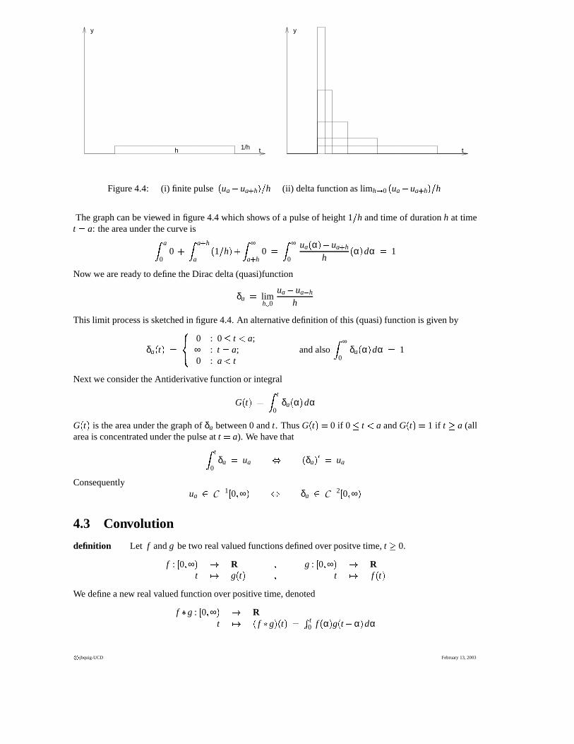
Figure 4.4: (i) finite pulse � ua � ua � h � � h (ii) delta function as limh � 0 � ua � ua � h � � h
The graph can be viewed in figure 4.4 which shows of a pulse of height 1 � h and time of duration h at timet � a: the area under the curve is
� a
00 � � a � h
a� 1 � h � � � ∞
a � h0 � � ∞
0
ua � α ��� ua � h
h� α � dα � 1
Now we are ready to define the Dirac delta (quasi)function
δa � limh�0
ua � ua � h
h
This limit process is sketched in figure 4.4. An alternative definition of this (quasi) function is given by
δa � t ��� �� � 0 : 0 � t � a;∞ : t � a;0 : a � t
and also � ∞
0δa � α � dα � 1
Next we consider the Antiderivative function or integral
G � t ��� � t
0δa � α � dα
G � t � is the area under the graph of δa between 0 and t. Thus G � t ��� 0 if 0 � t � a and G � t ��� 1 if t � a (allarea is concentrated under the pulse at t � a). We have that
� t
0δa � ua � � δa � � � ua
Consequentlyua � C 1 � 0 � ∞ � � δa � C 2 � 0 � ∞ �
4.3 Convolution
definition Let f and g be two real valued functions defined over positve time, t � 0.
f :�0 � ∞ � � R � g :
�0 � ∞ � � R
t �� g � t � � t �� f � t �We define a new real valued function over positive time, denoted
f � g :�0 � ∞ � � R
t �� � f � g � � t � ��� t0 f � α � g � t � α � dα
c�
jbquig-UCD February 13, 2003
4.3. CONVOLUTION 77
Note that
� t
0f � α � g � t � α � dα � � 0
tf � t � β � g � β � � � 1 � dβ
��put β � t � α � α � t � βthen dβ � � dα � dα � � dβalso α � 0 � β � t � α � t � β � 0
��� � t
0f � t � β � g � β � dβ
� � t
0f � t � α � g � α � dα switch dummy variables α and β
summary
f � g � t � � � t
0f � t � α � g � α � dα � � t
0f � α � g � t � α � dα � � t � 0
and this implies thatf � g � g � f
4.3.1 commutativity, associativity of �theorem 5 Let f � g and h :
�0 � ∞ � � R be functions.
� i � f � g � g � f � � ii � f � � g � h � � � f � g � � hproofs
proofs The proof of (i) is above. We will assume and use (ii) from now on. The proof is quite strenousbut is postponed until theorem 6. Assuming (ii) we can write f � g � h without ambiguity.remark Trivial results about convolution will be clearly stated if needed and left as easy exercises; suchasex. f � � g � h � � f � g � f � h.
ex. Compute, eat � ebt ,i.e. if a � b � R and f � t � � eat and g � t � � ebt for all t � 0 find f � g � t � for all t � 0.
f � g � t � � � t
0f � α � g � t � α � dα
� � t
0eaαeb � t α � dα
� � t
0ebt e � a b � α dα use next, ebt independent w.r.t. dα
� ebt � t
0e � a b � α dα beware!, special case a � b, see below
� ebt 1a � b
e � a b � α ��� tα 0since � ekx dx � ekx � k
� ebt 1a � b e � a b � t � 1 �
� eat � ebt
a � b
We now take up the case a � b: continuing from the warning line above
� ebt � t
0e � a b � α dα now we look at the case a � b
� ebt � t
01dα
� tebt
conclusion
eat � ebt � eat � ebt
a � b� if a �� b � eat � eat � teat
February 13, 2003 c�
jbquig-UCD
78 CHAPTER 4. DIFFERENTIAL EQUATIONS WITH THE LAPLACE TRANSFORM
In the latter case we are convoluting two sympathetic decays. As promised in 4.1, where there is sympathythere is t.eg. Now would be a good time to attempt the following example which appears inproblem sheet, 4.13.Comput the convolution of unsympathetic and of sympathetic oscillation
cosat � cosbt � a �� b and cosat � cosat
remark on the concept of convolutionThe value
f � g � t � � � t
0f � α � g � t � α � dα � � t
0f � t � α � g � α � dα
of the convolute f � g at the instant t involves the entire history of both f and g with time running forwardfor one and backward for the other.
eg. Let n � m � 0 be integers, compute tn � tm.
tn � tm � � t
0αn � t � α � m dα prepare for an int. by parts
� � t
0� t � α � m 1
n � 1d � αn � 1 � next integrate by parts
� 1n � 1
� t � α � m αn � 1 ���� tα 0� � t
α 0
1n � 1
αn � 1 d � t � α � m after integration by parts
� �0 � 0 � � m
n � 1� t
α 0αn � 1 � t � α � m 1 � � 1 � dα
� mn � 1
� t
α 0αn � 1 � t � α � m 1 dα
� mn � 1
tn � 1 � tm 1
summary to date tn � tm � mn � 1
tn � 1 � tm 1 if m � 1.
Applying this process repeatedly, until m � 1 is reduced to 0
tn � t � m � mn � 1
tn � 1 � tm 1
� m � � m � 1 �� n � 1 � � � n � 2 � tn � 2 � tm 2
� m � � m � 1 � � � m � 2 �� n � 1 � � � n � 2 � � � n � 3 � tn � 3 � tm 3
...
...
� m � � m � 1 � � � m � 2 � � � � 2 � 1� n � 1 � � � n � 2 � � � n � 3 � � � � � n � m � 1 � � � n � m � tn � m � t0
� �1 � 2 � 3 � 3 � n � 1 � n ��� �
�m � � m � 1 � � � m � 2 � � � � 2 � 1 ��
1 � 2 � 3 � 3 � n � 1 � n ��� �
� � n � 1 � � � n � 2 � � � n � 3 � � � � � n � m � 1 � � � n � m ��� tn � m � 1
� n!m!� n � m � ! tn � m � 1
� n!m!n � m!
� t
0αn � m 1 � t � α � dα
� n!m!� n � m � ! �t
0αn � m 1dα
� n!m!� n � m � ! 1n � m � 1
tn � m � 1
� n!m!� n � m � 1 � ! tn � m � 1
c�
jbquig-UCD February 13, 2003
4.3. CONVOLUTION 79
Conclusion, for integers n � m � 0
tn � tm � n!m!� n � m � 1 � ! tn � m � 1
eg.
1 � t � t0 � t1 � t2 � 2 � 1 � t2 � t0 � t2 � t3 � 3 � 1 � tn � t0 � tn � tn � 1 � � n � 1 �t2 � t3 � t6 � 60 � t4 � t5 � 4!5! t6 � 10! �
remark The first three seem to indicate that the process of integration can be carried out by convolutionwith 1 � u0, see 4.4.
ex. Now would be a good time to compute (see problems 4.13)
eat � cos � bt � � t � cos � at � � t � eat
4.3.2 Integration and Shift operators
Recall that C 2 � 0 � ∞ � or C 2 � for short denotes the vector space of functions defined over positive time�0 � ∞ �
and which become continuous if integrated twice. This space contains at least the continuous functions,the step and delta functions. We study two operations on this space, the integration operator and the shiftoperator.
integration operator Let a � 0 be arbitrary
� : C 2 � C 1
f �� F
Here
F � t � � � t
0f � α � dα � � t � 0
shift operator
Sha : C 2 � C 2
f �� Sha � f �Here
Sha � f � � t � � ua � t � � f � t � a � � �0 : 0 � t � a;
f � t � a � : a � t;� � t � 0
The shift operator simply shifts the origin from 0 to a. Naively one expects the definition to beSha � f � � t � � f � t � a � , but this gives wrong results in examples. The difficulty is caused by the factthat f is not defined for t � a so that f � t � a � is undefined for 0 � t � a. Using the correct defini-tion Sha � f � � t ��� ua � t � f � t � a � clearly states that Sha � f � � t ��� 0 in the range 0 � t � a, which is correct.example
Sh1t2 � u1 � t � � � t � 1 � 2 � �0 : 0 � t � 1;� t � 1 � 2 : 1 � t;
Contrast this with the naive wrong result Sh1t2 � � t � 1 � 2. See figure 4.5
4.3.3 convolution with ua and δa
Convolution of standard classical functions is an exercise in elementary integration, albeit at times strenous.Soon we will have a new easy method to perform convolutions by using the Laplace transform L , see section
February 13, 2003 c�
jbquig-UCD

80 CHAPTER 4. DIFFERENTIAL EQUATIONS WITH THE LAPLACE TRANSFORM
t
y
t
y
t
y
Figure 4.5: (i) t2 (ii) � t � 1 � 2,inappropriate (iii) Sh � t2 ��� u1 � t � � t � 1 � 2
4.4. Now we study convolution with the Heavyside Step and the Dirac Delta functions. Let f � g :�0 � ∞ � � R
be well behaved C 0 functions; we need to fill out the table.
� ub δb gua (vi) (iv) (ii)δa (iv) (v) (iii)f (ii) (iii) (i)
Since � is commutative there are really only six not nine computations to be carried out. Also entry (i) ismerely the definition of convolution
(i) f � g � � t
0f � α � g � t � α � dα .
(ii) ua � f
ua � f � t � � � t0 ua � α � f � t � α � dα
� ����� � t
00dα : if t � a;
� a
00dα � � t
a1 � f � t � α � dα : if a � t
by defn. of ua
� �� � 0 : if t � a;
0 � � t
af � t � α � dα : if a � t
next put β � t � α
� �� � 0 : if t � a;
� 0
t af � β � � � 1 � dβ : if a � t
dα � � dβ
� �� � 0 : if t � a;
� t a
0f � β � dβ : if a � t
� �0 : if t � a;
F � t � a � : if a � twhere F � t � � � t
0f � α � dα
� ua � t � F � t � a �conclusion Convoluting with ua can be performed by (α) integrating, followed by (β) shifting; inother words
ua � f � ua � t � F � t � a � � Sha
� � t
0f � α � dα � (4.1)
In particular, if a � 0
u0 � f � u0 � t � F � t � 0 � � F � t ��� � � t
0f � α � dα � (4.2)
c�
jbquig-UCD February 13, 2003
4.3. CONVOLUTION 81
(ii) δa � f Given a � 0 and t � � 0 � ∞ �δa � f � t � � �
limh�0
ua � ua � h
h� f � � t � by defn. of δa
� limh�0
� ua � f � � t ��� � ua � h � f � � t �h
� f
In the latter fraction, there are three cases to consider
t � a In this case t � a and t � a � h, by two applications of 4.1, ua � f � t ��� 0 � ua � h � f � t � . Weconclude that δa � f � t ��� 0 for all t � a.
a � t � a � h In the limit as h�
0 eventually a � h will be less than t. We may ignore this case, itbecomes the next case.
t � a � h In this case
δa � f � t � � limh�0
� ua � f � � t � � � ua � h � f � � t �h
recall F � t ��� � t
0f
� limh�0
F � t � a ��� F � t � a � h �h
since ua � f � t � � F � t � a � � t � a
� limk�0
F � t � a ��� F � t � a � k �� ksince k � � h � 0 as h � 0
� limk�0
F � t � a � k ��� F � t � a �k
this is differentiation from first principles
� F � � t � a � next use the fundamental theorem of calculus� f � t � a �Gathering all this we have proven
� δa � f � � t ��� Sha � f � � t � � �0 : if t � a;
f � t � a � : if a � t
In other words, convolution with δa is the shift (by a) operator.
(iv) δa � ub
δa � ub � Sha � ub ��� ua � b
(v) δa � δb
δa � δb � Shaδb � δa � b
(vi) ua � ub
ua � ub � � ua � � � ub �� � δa � u0 � � � δb � u0 �� � δa � δb � � � u0 � u0 �� � δa � b � � � u0 � 1 �� � δa � b � � � � t
01 �
� � δa � b � � t� Sha � b t� ua � b � t � � � t � a � b �� �
0 : if t � a � b;t � � a � b � : if a � b � t
February 13, 2003 c�
jbquig-UCD

82 CHAPTER 4. DIFFERENTIAL EQUATIONS WITH THE LAPLACE TRANSFORM
4.4 The Laplace Transform
definition Given a real valued function f :�0 � ∞ ��� t �� f � t ��� R of positive time, we determine a number
a � R called the abscissa of convergence of f and define a new function called the Laplace transform of fand denoted
L � f � : � a � ∞ � � R
s : �� L � f � � s � � � ∞
0e st f � t � dt for s � a only
revision Recall that � ∞
0e st f � t � dt is called an improper integral (infinite range of integration), and is
defined by a limit process
� ∞
0e st f � t � dt � lim
α � ∞ � α
0e st f � t � dt
Generally there is a number a such that if s � a this limit process converges (and if s � a it diverges); such ais called the abscissa of convergence of f ; enough for now, see the the next few examples.
4.5 Laplace transform of classical functions
4.5.1 L�eat �
L � eat � � s � � � ∞
0e st eat dt
� limα � ∞ � α
0e steat dt
� limα � ∞ � α
0e � a s � t dt
� limα � ∞ e � a s � t
a � s
�����α
0
� limα � ∞ � e � a s � α � 1
a � s �� lim
α � ∞ 1s � a 1 � e � a s � α �
� 1s � a
� 1s � a
�limα � ∞ e � a s � α �
The latter limit does not exist if a � s � 0 and exists and equals 0 if a � s � 0. Finally
L � eat � � s ���� 1s � a
� if s � a only
The abscissa of convergence of f � t ��� eat is a.
c�
jbquig-UCD February 13, 2003
4.5. LAPLACE TRANSFORM OF CLASSICAL FUNCTIONS 83
A less concise but faster and acceptable way to write this proof is
L � eat � � s � � � ∞
0e steat dt
� � ∞
0e � a s � t dt
� e � a s � t
s � a
�����∞
0� 1a � s e � a s � t � ��� ∞0� 1a � s e � a s � ∞ � e0 �
� 1a � s
� e ∞ � e0 � but only if s � a
� 1a � s
� 0 � 1 � but only if s � a
� 1s � a
but only if s � a
4.5.2 L�cosat � and L
�sinat �
The direct method is correct but leads to onerous computation
L � cos � at � � � s � � � ∞
0e st cos � at � dt
This integration can be carried out by two integration by parts, followed by a clever trick (you will find thisin a first course on integration). There is quicker slicker way to proceed.
L � cos � at � � � s �� iL � sin � at � � � s � � L � cos � at ��� isin � at � � � s �� L � eiat � � s �� � ∞
0e st eiat � dt
� � ∞
0e � ia s � � t � dt
� e � ia s � � t
ia � s
�����∞
0� 1s � ia e0 � e � ia s � � ∞ �
� 1s � ia
� 1 � 0 � but only for s � 0, see note below
� 1s � ia
but only for s � 0
� s � ias2 � a2 but only for s � 0
Extracting real and imaginary parts
L � cos � at � � � s ��� ss2 � a2 � L � sin � at � � � s ��� a
s2 � a2 � but only for s � 0
For both cos and sin the abscissa of convergence is 0.note Here we used ��� e � ia s � ∞ ��� � lim
α � ∞ ��� e � ia s � α ���� limα � ∞ �� eiaαe sα ��
� limα � ∞ �� eiaα �� �� e sα ��
February 13, 2003 c�
jbquig-UCD
84 CHAPTER 4. DIFFERENTIAL EQUATIONS WITH THE LAPLACE TRANSFORM
� limα � ∞ 1 � �� e sα ��
� limα � ∞ �� e sα ��� 0 but only for s � 0
4.5.3 L�tn �
Let n � 0 be an integer
L � tn � � s � � � ∞
0e st tn dt
� � 1s� ∞
0tn d � e st � prepare for integration by parts
� � 1s
tne st �� ∞0 � � 1s� ∞
0e st d � tn � used integration by parts
� � 1s
� ∞ne ∞ � 0ne0 � � � 1s� ∞
0e std � tn � but only for s � 0
� � 1s� 0 � 0 � � � n
s� ∞
0e st tn 1 dt ∞ne ∞ � 0, see note below
� � ns
L � tn 1 � � s �Summing up to date
L � tn � � s � � � ns
L � tn 1 � but only for s � 0
Repeating this step
L � tn � � s � � � � 1 � �
ns
L � tn 1 �� � � 1 � �
n � n � 1 �s2 L � tn 2 �
� � � 1 � �
n � n � 1 � � n � 2 �s3 L � tn 3 �
� ...
� ...
� � � 1 � n �
n!sn L � t0 �
� � � 1 � n �
n!sn L � 1 �
� � � 1 � n �
n!sn L � u0 �
� � � 1 � n �
n!sn
1s
� � � 1 � n n!sn � 1
Finally
L � tn � � s � � � � 1 � n n!sn � 1 but only if s � 0
The abscissa of convergence of tn is 0 for any integer n � 0.example L � coshat � and L � sinhat �left to reader, see section 4.13
c�
jbquig-UCD February 13, 2003
4.6. LAPLACE TRANSFORM WITH STEP AND DELTA FUNCTIONS 85
4.6 Laplace transform with step and delta functions
4.6.1 L�ua�
L � ua � � s � � � ∞
0ua � t � � e st dt
� � a
00 � e st dt � � ∞
a1 � e st dt by defn. of ua
� � ∞
ae st dt
� e st� s
���� ∞a� 1s
� e as � e s∞ �� 1
s� e as � 0 � but only if s � 0
To sum up
L � ua � � s � � e as
sbut only for s � 0
The abscissa of convergence for ua is 0.
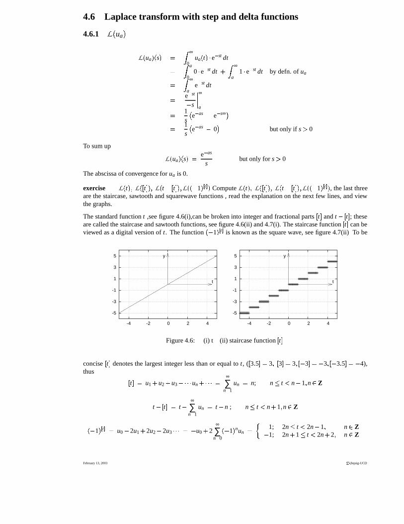
exercise L � t � � L � � t � � � L � t � � t � � � L � � � 1 ��� t � � Compute L � t � � L � � t � � � L � t � � t � � � L � � � 1 ��� t � � , the last threeare the staircase, sawtooth and squarewave functions , read the explanation on the next few lines, and viewthe graphs.
The standard function t ,see figure 4.6(i),can be broken into integer and fractional parts�t � and t � � t � ; these
are called the staircase and sawtooth functions, see figure 4.6(ii) and 4.7(i). The staircase function�t � can be
viewed as a digital version of t. The function � � 1 ��� t � is known as the square wave, see figure 4.7(ii) To be
-5
-3
-1
1
3
5
-4 -2 0 2 4
t
y
-5
-3
-1
1
3
5
-4 -2 0 2 4
t
y
Figure 4.6: (i) t (ii) staircase function�t �
concise�t � denotes the largest integer less than or equal to t, (
�3 � 5 � � 3 � � 3 � � 3 � � � 3 � � � 3 � � � 3 � 5 � � � 4),
thus �t � � u1 � u2 � u3 � � � � un � � � � � ∞
∑n 1
un � n; n � t � n � 1 � n � Z
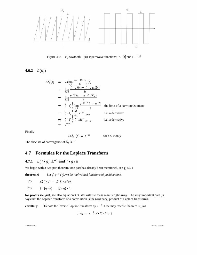
t � � t ��� t � ∞
∑n 1
un � t � n ; n � t � n � 1 � n � Z
� � 1 � � t � � u0 � 2u1 � 2u2 � 2u3 � � � � � u0 � 2∞
∑n 0� � 1 � nun � �
1; 2n � t � 2n � 1 � n � Z� 1; 2n � 1 � t � 2n � 2 � n � Z
February 13, 2003 c�
jbquig-UCD
86 CHAPTER 4. DIFFERENTIAL EQUATIONS WITH THE LAPLACE TRANSFORM
t
y1
t
y1
-1
Figure 4.7: (i) sawtooth (ii) squarewave functions; t � � t � and � � 1 ��� t �
4.6.2 L�δa�Lδa � s � � L � lim
h�0
ua � ua � h
h� � s �
� limh�0
L � ua � � s ��� L � ua � h � � s �h
� limh�0
e as � s � e � a � h � s � sh
� � � 1 � 1s
limh�0
e � a � h � s � e as
hthe limit of a Newton Quotient
� � � 1 � 1s
ddx
e xs �� x a i.e. a derivative
� � � 1 � 1s� � s � exs �
x a i.e. a derivative� e as
FinallyL � δa � � s � � e as for s � 0 only
The abscissa of convergence of δa is 0.
4.7 Formulae for the Laplace Transform
4.7.1 L�f � g ��� L � 1 and f � g � h
We begin with a two part theorem; one part has already been mentioned, see 4.3.1
theorem 6 Let f � g � h :�0 � ∞ � be real valued functions of positive time.
(i) L � f � g � � L � f � � L � g �(ii) f � � g � h � � � f � g � � h
for proofs see 4.8, see also equation 4.3. We will use these results right away. The very important part (i)says that the Laplace transform of a convolution is the (ordinary) product of Laplace transforms.
corollary Denote the inverse Laplace transform by L 1. One may rewrite theorem 6(i) as
f � g � L 1 � L � f � � L � g � �c
�jbquig-UCD February 13, 2003
4.7. FORMULAE FOR THE LAPLACE TRANSFORM 87
remark This gives a fast easy way to convolute (up to now a strenous business). There is an integrationformula for the inverse Laplace transform, but we will not use it. Instead to compute L 1 of any givenfunction we rely on a table, see 4.12, of known Laplace transforms and formulae which we wield in reverse.
It is known that L is a special case of a more general transform F called the Fourier transform. The inverseFourier transform is easily described in terms of integration. We do not pursue the question of L 1 beyondthese few remarks.
remark Here is a proof of
f � � g � h � � � f � g � � h (4.3)
being part(ii) of theorem 6. This proof uses part(i), but see also 4.8.2.
f � � g � h � � L 1 � L � f � � g � h � � �� L 1 � L � f � � L � g � h � � � by part(i)� L 1 � L � f � � � L � g � � L � h � � � by part(i) again� L 1 � � L � f � � L � g � � � L � h � � by associativity of ordinary multiplication� L 1 � � L � f � g � � L � h � � by part(i)� L 1 � L � � f � g � � h � � � by part(i) again� � f � g � � h �example
eat � ebt � L 1L � eat � ebt �� L 1 � L � eat � � L � ebt � �� L 1 � 1
s � a�
1s � b
�� L 1
�1� s � a � � s � b � �
� L 1
�A
s � a� B
s � b�
� AL 1
�1
s � a� � BL 1
�1
s � b�
� Aeat � Bebt
Above the theory of partial fractions (as used in integration of fractional polynomials in FY calculus) hasbeen used.
1� s � a � � s � b � � As � a
� Bs � b
1 � A � s � b � � B � s � a �Putting s � b we get B � 1 � b � a Putting s � a we get A � 1 � a � b Putting it all together
� eat � ebt � � s � � eat � ebt
a � b
But all this works for a �� b only. If there is sympathy a � b we instead obtain.
� eat � ebt � � s � � L 1
�1� s � a � 2 �
See ahead 4.7.3 to deal with this very important atomic (it can’t be broken up or simplified) partial fraction.
February 13, 2003 c�
jbquig-UCD
88 CHAPTER 4. DIFFERENTIAL EQUATIONS WITH THE LAPLACE TRANSFORM
4.7.2 L and differentiation L�f � ��� L � f � n � � and L
���f � and also L
�tn f �
To wield L and solve SOCCLHDE’s one must compute the Laplace transform of the integral and of deriva-tives of all orders � f � L � f � � � L � f � � � � L � f � � � � � � � L � f � n � � � �
of functions f :�0 � ∞ ��� R.
L � f � � � s � � sL � f � � s ��� f � 0 � (4.4)
proof
L � f � � � s � � � ∞
0e st f � � t � dt
� � ∞
t 0e st d f
� e st f � t � �� ∞0 � � ∞
t 0f � t � d � e st � after integration by parts
� � e s∞ f � ∞ � � e0 f � 0 ��� � � ∞
t 0f � t � d � e st � see below for meaning of e s∞ f � ∞ �
� �0 � f � 0 � � � � ∞
t 0f � t � d � e st � but only for s � a, the abs. of cgce. of f
� � f � 0 � � � ∞
t 0f � t � e st � � � s � dt
� s � ∞
t 0f � t � e st � dt � f � 0 �
� sL � f � � s � � f � 0 �remark e s∞ f � ∞ � denotes the limit
limt � ∞
e st f � ∞ � if this limit actually exists
definition f � t � is said to be exponentially bounded by eAt iff for large t � 0 � f � t � � � eAt .
In that case it is easy to see (exercise) that the abscissa of convergence of f is no larger than A. Moreover,since �� e st f � t � �� � e � A s � t for large t � 0
the latter limit exists (and equals 0) for s � A.
example Let f � t � � eat � t � 0 . Then f � � a f . apply L to both sides of this equation. L � f � � � aL � f � .Thus sL � f ��� f � 0 � � aL � f � . But f � 0 ��� 1. Thus � s � a � L � f � � f � 0 � � 1
L � eat � � s � � L � f � � s � � 1s � a
L � f � � � � s � � s2L � f � � s ��� s f � 0 � � f � � 0 � (4.5)
proofL � f � � � � s � � L � � f � � � � � s �� sL � f � � � � s � � f � � 0 � by 4.4� s
�sL � f � � � s � � f � 0 � � � f � � 0 � again by 4.4� s2L � f � � � s � � s f � 0 � � f � � 0 �
L � f � n � � � s � � snL � f � � s � � sn 1 f � 0 � � sn 2 f � � 0 � � sn 2 f � � � 0 � � � � � � � s2 f � n 3 � � 0 � � s f � n 2 � � 0 � � f � n 1 � � 0 �(4.6)
� snL � f � � s � � n 1
∑0
sn j 1 f � j � � 0 � (4.7)
textbfexample. Using the L � f � � � formula one can calculate. L � cos � at � � � L � sin � at � � � L � cosh � at � � and L � sinh � at � � .c
�jbquig-UCD February 13, 2003
4.7. FORMULAE FOR THE LAPLACE TRANSFORM 89
Three of these are left as exercises, here we calculate only L � cosh � at � � . Note that cosh � � at ��� asinh � at �and cosh � � � at � � a2 cosh � at � . Applying the Laplace transform to both sides of the latter equation we obtainL � cosh � � � at � ��� a2L � cosh � at � � . Thus
s2L � cosh � at � � � s � � scosh � 0 � � cosh� � 0 ��� L � cosh � at � � s � � (4.8)
� s2 � a2 � L � cosh � at � � � s � � scosh � 0 � � cosh � � 0 ��� scosh � 0 � � asinh � 0 ��� s � 0 (4.9)
ThusL � cosh � at � � � s ��� s
s2 � a2 (4.10)
proof This is a more elaborate version of formula 4.5. The proof is left as an exercise, do it for n=3 and 4.Then use induction to obtain a proof for a general integer n � 0
Writing F � t ��� � t
0f
L � F � � s � � 1s
L � f � � s � (4.11)
proof Since F � � f by formula 4.4
L � f � � s � � sL � F � � s � � F � 0 ��� sL � F � � s � � 0 � sL � F � � s �The reader may prefer the alternative proof
L � F � � s � � L � � t
0f � � s � � L � u0 � f � � s � � L � u0 � � s � � L � f � � s � � 1
s� L � f � � s �
Now we study L and differentiation in the imaginary frequency s we study
L � t f � t � � � s � � � ∞
0e stt f � t � dt
� � ∞
0
dds
� e st f � t � � dt
� � ∞
0� d
ds� e st f � t � � dt
� � dds
� � ∞
0e st f � t � dt �
� � dds
L � f � � s �Applying this result once, twice or even n times we have
L � t f � � s � � � dds
L � f � � s �L � t2 f � � s � � d2
ds2 L � f � � s �L � tn f � � s � � � � d
ds� n
L � f � � s �example
L � tn � � s � � L � tn� 1 � � s �
� � � dds
� n
L � 1 � � s �� � � d
ds� n 1
s
� n!sn � 1
February 13, 2003 c�
jbquig-UCD
90 CHAPTER 4. DIFFERENTIAL EQUATIONS WITH THE LAPLACE TRANSFORM
4.7.3 L and shifting L�Sha f � and Shb
�L f �
There are two shift formulae involving the Laplace transform. One involves shift in real time t, discussed indetail above. The second involves shifting in the imaginary frequency s: fortunately there are no difficulties(as experienced when shifting in t). In fact, let G be a function of s and b � R.
Shb � G � � s � � G � s � b � de f inition
� L � Sha f � � � s � � � L � δa � f � � � s � � e asL � f � � s � (4.12)
proof � L � δa � f � � � s � � L � δa � � s � � L � f � � s � � e asL � f � � s �� L � eat f � t � � � � s � � Shb � L � f � � � s � � L � f � � � s � a � (4.13)
proof
� L � eat � f � t � � � � s � � � t
0e st eat f � t � dt � � t
0e � s a � t f � t � dt � � L f � � s � b � � � Shb � L f � � � s �
4.7.4 L and periodicity
Let f :�0 � ∞ � � t �� f � t � � R be periodic with period p � 0, i.e. f � t � p � � f � t � for all t � 0, then
L � f � � s � � � p0 e st f � t � dt
1 � e sp (4.14)
proof
L � f � � s � � � ∞
0e st f � t � dt
� � � p
0� � 2p
p� � � � � � � k � 1 � p
kp� � � � � e st f � t � dt
� ∞
∑k 0
� � k � 1 � p
kpe st f � t � dt put t � τ � kp
� ∞
∑k 0
� p
0e s � τ � kp � f � τ � kp � dτ by periodicity f � τ � kp � � f � τ �
� ∞
∑k 0
� p
0e s � τ � kp � f � τ � dτ use e s � τ � kp � � e staue kp
� ∞
∑k 0
� p
0e sτe skp � f � τ � dτ use e kp � � e p � k in indepent of dτ
� ∞
∑k 0
� e p � k � p
0e sτ f � τ � dτ
��
∞
∑k 0
� e p � k � � p
0e sτ f � τ � dτ
� �1
1 � e sp � � p
0e sτ f � τ � dτ recall for � x � � 1,
∞
∑0
xn � 1 � � 1 � x �� � p
0 e sτ f � τ � dτ1 � e sp being the sum of a geometric progression
example, Laplace transform of square wave Recall the square wave function � � 1 � � t � , see 4.6.1 andfigure 4.7. f is periodic with period 2
L � � 1 � � t � � � � 2
0e st � � 1 � � t � dt
1 � e 2t
c�
jbquig-UCD February 13, 2003
4.8. TWO DIFFICULT PROOFS 91
� 11 � e 2t
� � 1
0� � 2
1� e � � st � � � 1 � � t �
� 11 � e 2t
� � 1
0� 1 � e st dt � � 2
1� � 1 � e st dt �
� 11 � e 2t
� � 1
0e st dt � � 2
1� � 1 � e st dt �
� 11 � e 2t
�e st� s
���� 10 � e st� s
���� 21 �� 1
s � 1 � e 2t � � � 1 � e t � � � e t � e 2t � �� 1 � 2e t � e 2t
s � 1 � e 2t �� � 1 � e t � 2
s � 1 � e t � � 1 � e t �� 1 � e t
s � 1 � e t �exercise The reader might now apply the same formula to compute L � t � � t � � , see figure4.7 and 4.6.1. Thesawtooth function t � � t � has period 1.
4.8 Two difficult proofs
4.8.1 full proof that L�f � g � � s ��� L
�f � � s ��� L � g � � s �
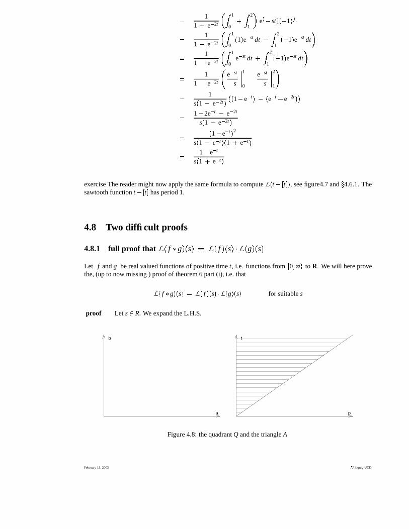
Let f and g be real valued functions of positive time t, i.e. functions from�0 � ∞ � to R. We will here prove
the, (up to now missing ) proof of theorem 6 part (i), i.e. that
L � f � g � � s ��� L � f � � s � � L � g � � s � for suitable s
proof Let s � R. We expand the L.H.S.
a
b
p
t
Figure 4.8: the quadrant Q and the triangle A
February 13, 2003 c�
jbquig-UCD
92 CHAPTER 4. DIFFERENTIAL EQUATIONS WITH THE LAPLACE TRANSFORM
L � f � g � � s � � � ∞
0e st � f � g � � t � dt by defn. of L
� � ∞
0e st � t
0f � p � g � t � p � dpdt by defn. of convolution �
� � ∞
0� t
0e st f � p � g � t � p � dpdt since e st is independent of p
� � �A
e st f � p � g � t � p � d � p � t � here A� R2 is the infinite triangle
A � � �pt
� ���� 0 � p � t � ∞�
see figure 4.8
Next we expand the R.H.S.
L � f � � s � � L � g � � s � � � ∞
0e sa f � a � da � � ∞
0e sbg � b � db by defn. of L , used twice
� � ∞
0
� � ∞
0e sa f � a � da � e sbg � b � db since the da integral, being
constant is independent of b
� � ∞
0e sbg � b � � ∞
0e sa f � a � dadb after rearrangement
� � ∞
0� ∞
0e sa f � a � � e sbg � b � dadb e sbg � b � is indep. of a
� � �Q
e s � a � b � f � a � g � b � d � a � b � where Q� R2 is the quadrant
Q � � �ab
� ���� a � b � 0
�
see figure 4.8
For convenience writeG � p � t ��� e st f � p � g � t � p � (4.15)
Define the bijective mapping or transformation h from R2 to R2 by
h : Q � A�ab
� �� �p � a �
t � a � b � � � �1 01 1
� �ab
� � �a
a � b�
This h is linear (i.e. a matrix mapping) with det � h � � 1 �� 0 and so h is bijective as claimed.h carries Q onto A, i.e.
h � Q ��� A
Indeeda � 0 and b � 0 � 0 � a � a � b � ∞ � 0 � p � t � ∞
Since h is linear, Dh � h , and so the Jacobian of h is
det � Dh ��� det � h ��� 1
Finally
L � f � g � � s �� � �
Ae st f � p � g � t � p � d � p � t �
� � �A h � Q � G � p � t � d � p � t �
c�
jbquig-UCD February 13, 2003

4.8. TWO DIFFICULT PROOFS 93
� � �Q
G � h � a � b � �� det � Dh � � a � b � � d � a � b � by the COV theorem
� � �Q
G � p � a � b � � t � a � b � � � 1d � a � b �� � �
Qe st � a � b � f � p � a � b � � g � t � a � b ��� p � a � b � � d � a � b �
� � �Q
e s � a � b � f � a � g � a � b � a � d � a � b �� � �
Qe s � a � b � f � a � g � b � d � a � b �
� L � f � � s � � L � g � � s �4.8.2 full proof that
�f � g � � h � � f � � g � h �
Let f � g and g be real valued functions of positive time t, i.e. functions from�0 � ∞ � to R. We will here give
the (skipped over) proof that
� � f � g � � h � � t � � � f � � g � h � � � t � for t � 0
see theorem 6, 4.3.1 and 4.3.
a
b b=t
p
qt
t
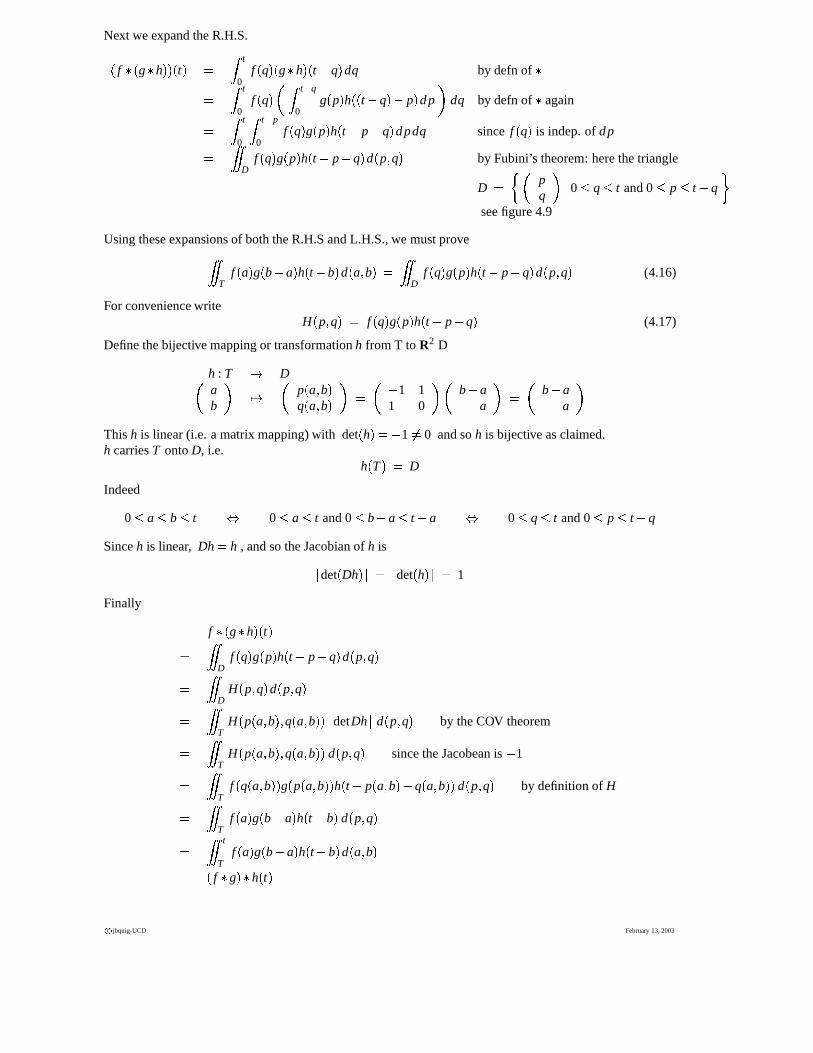
Figure 4.9: triangles (ii) T ; a � b � t (ii) D; 0 � q � t and 0 � p � t � q
proof Let t � R. We expand the L.H.S.
� � f � g � � h � � t � � � t
0� f � g � � b � h � t � b � db by defn of �
� � t
0
� � b
0f � a � g � b � a � da � h � t � b � db by defn of � again
� � t
0h � t � b � � � a
0f � a � g � b � a � da � db after a slight rearrangement
� � t
0� a
0f � a � g � b � a � h � t � b � dadb since h � t � b � is independent of da
� � � t
Tf � a � g � b � a � h � t � b � d � a � b � by Fubini’s theorem: here the triangle
T � � �ab
� ���� 0 � a � b � t
� � R2
see figure 4.9
February 13, 2003 c�
jbquig-UCD
94 CHAPTER 4. DIFFERENTIAL EQUATIONS WITH THE LAPLACE TRANSFORM
Next we expand the R.H.S.
� f � � g � h � � � t � � � t
0f � q � � g � h � � t � q � dq by defn of �
� � t
0f � q � � � t q
0g � p � h � � t � q ��� p � dp � dq by defn of � again
� � t
0� t p
0f � q � g � p � h � t � p � q � dpdq since f � q � is indep. of dp
� � �D
f � q � g � p � h � t � p � q � d � p � q � by Fubini’s theorem: here the triangle
D � � �pq
� ���� 0 � q � t and 0 � p � t � q
�
see figure 4.9
Using these expansions of both the R.H.S and L.H.S., we must prove
� �T
f � a � g � b � a � h � t � b � d � a � b � � � �D
f � q � g � p � h � t � p � q � d � p � q � (4.16)
For convenience writeH � p � q ��� f � q � g � p � h � t � p � q � (4.17)
Define the bijective mapping or transformation h from T to R2 D
h : T � D�ab
� �� �p � a � b �q � a � b � � � � � 1 1
1 0� �
b � aa
� � �b � a
a�
This h is linear (i.e. a matrix mapping) with det � h � � � 1 �� 0 and so h is bijective as claimed.h carries T onto D, i.e.
h � T ��� D
Indeed
0 � a � b � t � 0 � a � t and 0 � b � a � t � a � 0 � q � t and 0 � p � t � q
Since h is linear, Dh � h , and so the Jacobian of h is
� det � Dh � � � � det � h � � � 1
Finally
f � � g � h � � t �� � �
Df � q � g � p � h � t � p � q � d � p � q �
� � �D
H � p � q � d � p � q �� � �
TH � p � a � b � � q � a � b � � � detDh � d � p � q � by the COV theorem
� � �T
H � p � a � b � � q � a � b � � d � p � q � since the Jacobean is � 1
� � �T
f � q � a � b � � g � p � a � b � � h � t � p � a � b ��� q � a � b � � d � p � q � by definition of H
� � �T
f � a � g � b � a � h � t � b � d � p � q �� � � t
Tf � a � g � b � a � h � t � b � d � a � b �
� f � g � � h � t �c
�jbquig-UCD February 13, 2003

4.9. HOMOGENOUS DIFFERENTIAL EQUATIONS AND THE LAPLACE TRANSFORM 95
4.9 Homogenous Differential equations and the Laplace Transform
4.9.1 characteristic polynomial of a differential equation
The most general CCHDE of any order n takes the form
(HDE) a0 x � n � � t �� a1 x � n 1 � � t �� � � � � ak x � n k � � t � � � � � � an 1 x � t ��� anx � t � � 0 (4.18)
here ak � R � 0 � k � n are called coefficients Suitable general initial conditions are
(IC) x � k � � 0 � given for 0 � k � n � 1 (4.19)
definition The characteristicpolynomial associated with this HDE is
p � λ ��� n
∑k 0
akλn k � a0λn � a1λn 1 � � � � � akλn k � � � � � an 1λ � an (4.20)
This, polynomial (of degree n) will appear frequently below.
4.9.2 example HDE of degree 1
Solve
(HDE) x � t ��� 3x � t ��� 0 with (IC) x � 0 ��� 7 (4.21)
Apply the L , ignore IC for now
L � x � � s �� 3L � x � � s � � L � 0 �� �sL � x � � s � � x � 0 ��� � 3L � x � � s � � 0 see 4.12 formula 4.69� � s � 3 � L � x � � s � � 7 after rearranging and using the IC
� L � x � � s � � 7s � 3
divide across by p � s ��� s � 3
� x � t � � L 1
�7
s � 3� inverse L applied
� x � t � � 7L 1
�1
s � � � 3 � �� x � t � � 7e 3t see 4.12 formula 4.53
4.9.3 example HDE of degree 2
Solve
(HDE) x � t � � 5x � t ��� 6x � t ��� 0 with (IC) x � 0 ��� � 2 � x � 0 � � 9 (4.22)
Apply the L , ignore IC for now
L � x � � s �� 5L � x � � s �� 6L � x � � s � � L � 0 � next use 4.12 formulae 4.69 and 4.70� �s2L � x � � s � � sx � 0 � � x � 0 ���� 5
�sL � x � � s � � x � 0 ���� 6�L � x � � s ��� � 0 next use the IC� �
s2L � x � � s � � � � 2 � s � 9 �� 5�sL � x � � s � � � � 2 ���� 6�L � x � � s ��� � 0 rearrange� �
s2 � 5s � 6 � L � x � � s � � � 2s � 1 next divide by p � s � � s2 � 5s � 6
� L � x � � s � � � 2s � 1s2 � 5s � 6
next apply the inverse Laplace transform
February 13, 2003 c�
jbquig-UCD
96 CHAPTER 4. DIFFERENTIAL EQUATIONS WITH THE LAPLACE TRANSFORM
Thus
x � t � � L 1
� � 2s � 1s2 � 5s � 6
�� L 1
� � 2s � 1� s � 3 � � s � 2 � � next we split up the partial fraction
� L 1
�A
1s � 2
� B1
s � 3� where A and B soon will be calculated
� AL 1
�1
s � � � 2 � � � BL 1
�1
s � � � 3 � � next use 4.12 formula 4.53
� Ae 2t � Be 3t
We calculate the constants A and B using� 2s � 1� s � 2 � � s � 3 � � As � 2
� Bs � 3� � 2s � 1 � A � s � 3 � � B � s � 2 �
Put s � � 3 and obtain B � � 5. Put s � � 2 and obtain A � 3. Finally
x � t � � 3e 3t � 5e 2t
4.9.4 example HDE of degree 2 with natural sympathy
Solve
(HDE) x � t � � 10x � t �� 25x � t � � 0 with (IC) x � 0 ��� � 2 � x � 0 � � 9 (4.23)
Apply the L , ignore IC for now
L � x � � s � � 10L � x � � s �� 15L � x � � s � � L � 0 � next use formulae 4.12 formulae 4.69 4.70� �s2L � x � � s � � sx � 0 � � x � 0 ���� 10
�sL � x � � s � � x � 0 ���� 25�L � x � � s ��� � 0 next use the IC� �
s2L � x � � s � � � � 2 � s � 9 �� 10�sL � x � � s � � � � 2 ���� 25�L � x � � s ��� � 0 rearrange� �
s2 � 10s � 25 � L � x � � s � � � 2s � 11 next divide by p � s ��� s2 � 10s � 25
� L � x � � s � � � 2s � 11s2 � 10s � 25
next apply the inverse Laplace transform
� x � t � � L 1� � 2s � 11
s2 � 10s � 25�
� x � t � � L 1
� � 2s � 11� s � 5 � 2 � get ready for the second shift formula
� x � t � � L 1
� � 2 � s � 5 ��� 1� s � 5 � 2 � use 4.12 formula 4.52
� x � t � � e 5t L 1
� � 2s � 1s2 � break up the partial fraction
� x � t � � e 5t L 1
� � � 1 � 1s2 � 2
1s
� see 4.12 formulae 4.57, 4.58
� x � t � � e 5t � � 1 � 2t �Finally
x � t ��� � e 5t � 1 � 2t �The important thing is to note the term te 5t ; “where there is sympathy there is t”.
c�
jbquig-UCD February 13, 2003

4.9. HOMOGENOUS DIFFERENTIAL EQUATIONS AND THE LAPLACE TRANSFORM 97
4.9.5 example HDE of degree 2, complex roots
Solve
(HDE) x � t ��� 8x � t �� 25x � t � � 0 with (IC) x � 0 ��� 4 � x � 0 � � 7 (4.24)
Apply the L , ignore IC for now
L � x � � s �� 8L � x � � s �� 25L � x � � s � � L � 0 � next use 4.12 formulae 4.69, 4.70� �s2L � x � � s � � sx � 0 � � x � 0 ���� 8
�sL � x � � s � � x � 0 ���� 25�L � x � � s ��� � 0 next use the IC� �
s2L � x � � s � � � 4 � s � 7 �� 8�sL � x � � s � � � 2 ���� 25�L � x � � s ��� � 0 rearrange� �
s2 � 8s � 25 � L � x � � s � � 4s � 23 next divide by p � s � � s2 � 8s � 25
� L � x � � s � � 4s � 23s2 � 8s � 25
next apply the inverse Laplace transform
x � t � � L 1
�4s � 23
s2 � 8s � 25� irreducible quadratic denominator
� L 1�
4 � s � 4 � � 7� s � 4 � 2 � 32 � completed the square
� e 4t L 1
�4s � 7s2 � 32 � used 4.12 formula 4.52
� e 4t
�43L 1 s
s2 � 32 � 73
L 1 3s2 � 32 � prepare to use trig formulae
� e 4t
�43cos � 3t ��� 7
3sin � 3t � � used 4.12 formulae 4.54, 4.55
Finally
x � t ��� 43e 4t cos � 3t � � 73
e 4t sin � 3t �The solution will involve damped vibration if the characteristic polynomial of a HDE has complex roots.
4.9.6 solving a general CCHDEwIC of order 4
After these examples it is easy to solve the general HDE of any order n. First consider the most generalCCHOLDEwIC of order four only.
� HDE � ax � 4 � � t �� bx � 3 � � t ��� cx � t ��� dx � t ��� ex � t � � 0; t � 0� IC � x � 0 ��� α � x � 0 ��� β � x � 0 � � γ � x � 3 � � 0 ��� δ
here the coefficients a � b � c � d and e are assumed constant as are the initial conditions α � β � γ and δ. ApplyL to the HDE,
aL x � 4 � � s �� bL x � 3 � � s �� cL x � s �� dL x � s �� eLx � s � � 0 (4.25)
Use the differentiation formulae for L , 4.12 formula 4.56
a�s4L x � s �� s3x � 0 ��� s2x � 0 ��� sx � 0 ��� x � 3 � � 0 � �� b�s3L x � s �� s2x � 0 ��� sx � 0 � � x � 0 � �� c�s2L x � s � � sx � 0 �� x � 0 ���� d�sL x � s � � x � 0 � �� e�Lx � s � �� 0
February 13, 2003 c�
jbquig-UCD
98 CHAPTER 4. DIFFERENTIAL EQUATIONS WITH THE LAPLACE TRANSFORM
Use the IC, initial conditions
a�s4L x � s �� αs3 � βs2 � γs � δ �� b�s3L x � s �� αs2 � βs � γ �� c�s2L x � s �� αs � β �� d�sL x � s �� α �� e�Lx � s � �� 0
Rearrange �as4 � bs3 � cs2 � � e � L x � s � � As3 � Bs2 � Cs � D (4.26)
where the constants A � b � C and D are easily calculated as expressions in terms of the initial conditions. TheR.H.S can be written
As3 � Bs2 � Cs � D (4.27)� α � as3 � bs2 � cs d �� β � bs2 � cs d � γ � cs d ��� δd (4.28)� � p � s � � s � � x � 0 ��� � p � s � � s2 � � x � 0 � � � p � s � � s3 � � x � 0 ��� � p � s � � s4 � � x � 3 � � 0 � (4.29)
Dividing across
Lx � s � � � p � s � � s � � x � 0 ��� � p � s � � s2 � � x � 0 ��� � p � s � � s3 � � x � 0 �� � p � s � � s4 � � x � 3 � � 0 �p � s � (4.30)
Apply the inverse Laplace transform
x � t ��� L 1
�����
� 3
∑k 0
p � s �sk � 1 x � k � � 0 �
p � s ��
����
�(4.31)
4.9.7 solving the most general CCHDEwIC of order n
The general case of a HDE of order n is no harder than the for order 4: here is a terse statement of the HDE,t � 0, IC and solution
(HDE)n
∑j 0
a jx� n j � � t ��� 0 with given (IC) xk � 0 � for 0 � k � n � 1 (4.32)
(solution) x � t ��� L 1
�����
� n 1
∑k 0
p � s �sk � 1 x � k � � 0 �
p � s ��
����
�; t � 0 (4.33)
4.9.8 natural response
A particularly important case is when all IC are zero except that x � n 1 � � 0 � � 1. The solution in that case iscalled the natural response of the undriven (homogenous) system
(HDE)n
∑j 0
a jx� n j � � t � � 0 with (IC) xk � 0 ��� 0 for 0 � k � n � 2 but x � n 1 � � 0 � � 1 (4.34)
(solution) x � t � � L 1
�1
p � s � � ; t � 0 (4.35)
c�
jbquig-UCD February 13, 2003

4.10. INHOMOGENEOUS DIFFERENTIAL EQUATIONS AND THE LAPLACE TRANSFORM 99
4.10 Inhomogeneous Differential equations and the Laplace Trans-form
4.10.1 example unsympathetically driven IHDE of degree 1
Solve
(IHDE) x � t �� 3x � t ��� e 2t cos � t � with (IC) x � 0 ��� 7 (4.36)
Apply the L , ignore IC for now
L � x � � s �� 3L � x � � s � � L � e 2t cos � t � �� �sL � x � � s � � x � 0 ���� 3L � x � � s � � Sh 2Lcos � t � used formula 4.12 4.68� � s � 3 � L � x � � s � � 7 � Sh 2
ss2 � 1
used 4.12 4.54
� � s � 3 � L � x � � s � � 7 � s � 2� s � 2 � 2 � 1used the 4.12 4.52
� L � x � � s � � 7s � 3
�s � 2� s � 3 � � s2 � 4s � 5 � divided across by p � s ��� s � 3
� x � t � � L 1
�7
s � 3� �
L 1
�s� s � 3 � � s2 � 4s � 5 � � L 1 applied
� x � t � � L 1
�7
s � 3� �
L 1
�1
s � 3�
s � 2s2 � 4s � 5
�� x � t � � L 1
�7
s � 3� �
L 1
�1
s � 3� � L 1
�s � 2
s2 � 4s � 5� used 4.12 4.66
� x � t � � 7e 3t � e 3t � e 2t cos � t � see 4.12
The solution of the IHDEwIC is formed by summing the solution of the correcponding HDEwIC and thenatural response convoluted with the driving (RHS) function. The natural response (a decay) is not in sym-pathy with the driving function (a decaying oscillation). But this is all too abstract. To hack out the answergo back to line
x � t � � L 1
�7
s � 3� � L 1
�1
s � 3�
s � 2s2 � 4s � 5
� next decompose the PF
� L 1�
7s � 3
� � L 1�
As � 3
� Bs � Cs2 � 4s � 5
� see below for A, B, C
� L 1
�7
s � 3� � L 1
�A
s � 3� B � s � 2 � � � C � 2B �� s � 2 � 2 � 1
� completed the square
� e 3t �L 1
�AL 1 1
s � 3� B
s � 2� s � 2 � 2 � 1� � C � 2B � 1� s � 2 � 2 � 1
� use 4.12 4.52
� e 3t �L 1
�AL 1 1
s � 3� e 2tB
ss2 � 1
� � C � 2B � e 2t 1s2 � 1
� see table 4.12
� e 3t � � Ae 3t � Be 2t cos � t �� � C � 2B � e 2t sin � t � � see table 4.12
February 13, 2003 c�
jbquig-UCD
100 CHAPTER 4. DIFFERENTIAL EQUATIONS WITH THE LAPLACE TRANSFORM
The constants A � B and C are found from
s� s � 3 � � s2 � 4s � 5 � � A1
s � 3� Bs � C
s2 � 4s � 5� s � A � s2 � 4s � 5 � � � Bs � C � � s � 3 �Putting s � � 3 obtain A � � 3 � 2. Equating the coeff of s2 on RHS and LHS obtain 0 � A � B, B � � A � 3 � 2.Equating the constant term on RHS and LHS obtain 0 � 5A � 3C, 0 � � 15 � 2 � 3C, C � 5 � 2.
4.10.2 sympathetically driven IHDE of degree 1
Solve
(IHDE) x � t �� 3x � t ��� e 3t with (IC) x � 0 � � 7 (4.37)
Apply the L , ignore IC for now
L � x � � s � � 3L � x � � s � � L � e 3t �� �
sL � x � � s � � x � 0 ��� � 3L � x � � s � � 1s � 3� � s � 3 � L � x � � s � � 7 � 1
s � 3rearranged and used the IC
� L � x � � s � � 7s � 3
� 1� s � 3 � 2 divided across by p � s ��� s � 3
� x � t � � L 1
�7
s � 3� �
L 1
�s� s � 3 � 2 � inverse L applied
� x � t � � L 1�
7s � 3
� �L 1
�1
s � 3�
1s � 3
�� x � t � � L 1
�7
s � 3� �
L 1
�1
s � 3� � L 1
�1
s � 3� used 4.12 formula 4.66
� x � t � � 7e 3t � e 3t � e 3t
The solution of the IHDEwIC is formed by summing the solution of the correcponding HDEwIC and thenatural response convoluted with the driving (RHS) function. The natural response (a decay) is fully insympathy with the driving function (the same decay). But this is all too abstract. To hack out the answer goback to line
� x � t � � L 1
�7
s � 3� � L 1
�1� s � 3 � 2 � next use 4.12 4.68
� x � t � � 7e 3tL 1
�1s
� � e 3tL 1
�1s2 �
� x � t � � 7e 3tL 1
�1s
� � e 3t � 7 � t �4.10.3 example unsympathetically driven IHDE of degree 2
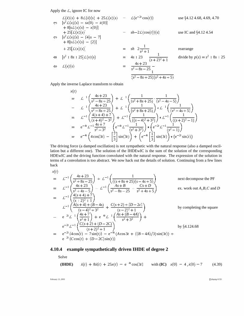
Solve
(IHDE) x � t � � 8x � t ��� 25x � t � � e 2t cos � t � with (IC) x � 0 � � 4 � x � 0 ��� 7 (4.38)
c�
jbquig-UCD February 13, 2003
4.10. INHOMOGENEOUS DIFFERENTIAL EQUATIONS AND THE LAPLACE TRANSFORM 101
Apply the L , ignore IC for now
L � x � � s �� 8L � x � � s �� 25L � x � � s � � L � e 2t cos � t � � use 4.12 4.68, 4.69, 4.70� �s2L � x � � s � � sx � 0 � � x � 0 ���� 8
�sL � x � � s � � x � 0 ���� 25�L � x � � s ��� � sh � 2L � cos � t � � � s � use IC and 4.12 4.54� �
s2L � x � � s � � � 4 � s � 7 �� 8�sL � x � � s � � � 2 ���
� 25�L � x � � s ��� � sh � 2
1s2 � 1
rearrange
� �s2 � 8s � 25 � L � x � � s � � 4s � 23 � 1� s � 2 � 2 � 1
divide by p � s ��� s2 � 8s � 25
� L � x � � s � � 4s � 23s2 � 8s � 25
�1� s2 � 8s � 25 � � s2 � 4s � 5 �
Apply the inverse Laplace transform to obtain
x � t �� L 1
�4s � 23
s2 � 8s � 25� � L 1
�1� s2 � 8s � 25 � �
1� s2 � 4s � 5 � �� L 1
�4s � 23
s2 � 8s � 25� � L 1
�1� s2 � 8s � 25 � � � L 1
�1� s2 � 4s � 5 � �
� L 1
�4 � s � 4 � � 7� s � 4 � 2 � 32 � � L 1
�1� � s � 4 � 2 � 32 � � � L 1
�1� � s � 2 � 2 � 1 � �
� e 4tL 1 4s � 7s2 � 32 �
�e 4t L 1 1� s2 � 32 � � � �
e 2tL 1 1� s2 � 1 � �� e 4t
�4cos � 3t ��� �
73 � sin � 3t � � � �
e 4t
�13 � sin � 3t � � � � e 2t sin � t � �
The driving force (a damped oscillation) is not sympathetic with the natural response (also a damped oscil-lation but a different one). The solution of the IHDEwIC is the sum of the solution of the correspondingHDEwIC and the driving function convoluted with the natural response. The expression of the solution interms of a convolution is too abstract. We now hack out the details of solution. Continuing from a few linesback
x � t �� L 1
�4s � 23
s2 � 8s � 25� � L 1
�1� � s � 8s � 25 � � s � 4s � 5 � � next decompose the PF
� L 1
�4s � 23
s2 � 4s � 5� � L 1
�As � B
s2 � 8s � 25� Cs � D
s2 � 4s � 5� ex. work out A � B � C and D
� L 1�
4 � s � 4 � � 7� s � 2 � 2 � 1� �
L 1
�A � s � 4 � � � B � 4s �� s � 4 � 2 � 32 � C � s � 2 � � � D � 2c �� s � 2 � 2 � 1
� by completing the square
� e 2tL 1
�4s � 7s2 � 1
� � e 4t L 1
�As � � B � 4A �
s2 � 32 � �e 2tL 1
�C � s � 2 � � � D � 2C �� s � 2 � 2 � 1
� by 4.124 � 68
� e 2t � 4cos � t �� 7sin � t � �� e 4t � Acos3t � � � B � 4A � � 3 � sin � 3t � � �e 2t � C cos � t � � � D � 2C � sin � t � �
4.10.4 example sympathetically driven IHDE of degree 2
Solve
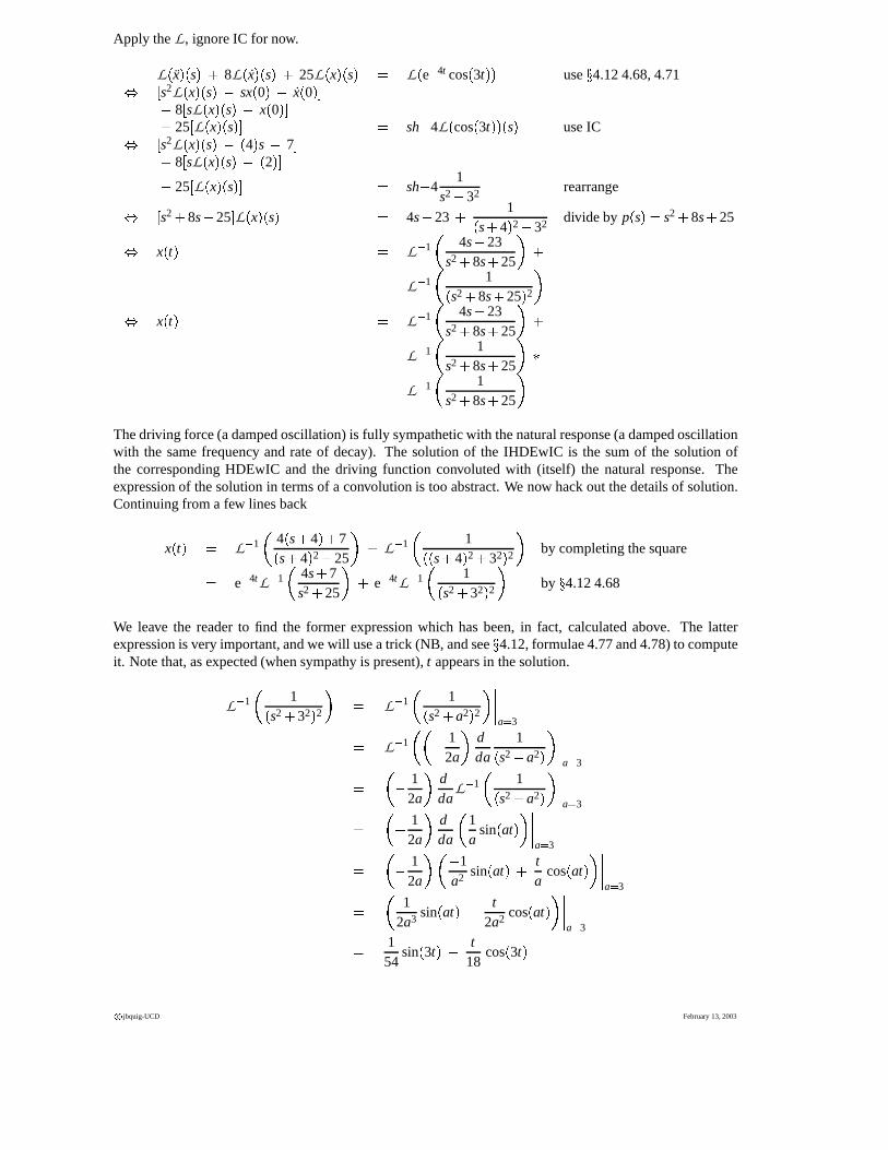
(IHDE) x � t ��� 8x � t �� 25x � t � � e 4t cos � 3t � with (IC) x � 0 � � 4 � x � 0 � � 7 (4.39)
February 13, 2003 c�
jbquig-UCD
102 CHAPTER 4. DIFFERENTIAL EQUATIONS WITH THE LAPLACE TRANSFORM
Apply the L , ignore IC for now.
L � x � � s � � 8L � x � � s � � 25L � x � � s � � L � e 4t cos � 3t � � use 4.12 4.68, 4.71� �s2L � x � � s � � sx � 0 � � x � 0 ���� 8
�sL � x � � s � � x � 0 ���� 25�L � x � � s ��� � sh � 4L � cos � 3t � � � s � use IC� �
s2L � x � � s � � � 4 � s � 7 �� 8�sL � x � � s � � � 2 ���
� 25�L � x � � s ��� � sh � 4
1s2 � 32 rearrange
� �s2 � 8s � 25 � L � x � � s � � 4s � 23 � 1� s � 4 � 2 � 32 divide by p � s � � s2 � 8s � 25
� x � t � � L 1
�4s � 23
s2 � 8s � 25� �
L 1
�1� s2 � 8s � 25 � 2 �
� x � t � � L 1
�4s � 23
s2 � 8s � 25� �
L 1�
1s2 � 8s � 25
� �L 1
�1
s2 � 8s � 25�
The driving force (a damped oscillation) is fully sympathetic with the natural response (a damped oscillationwith the same frequency and rate of decay). The solution of the IHDEwIC is the sum of the solution ofthe corresponding HDEwIC and the driving function convoluted with (itself) the natural response. Theexpression of the solution in terms of a convolution is too abstract. We now hack out the details of solution.Continuing from a few lines back
x � t � � L 1
�4 � s � 4 � � 7� s � 4 � 2 � 25
� � L 1
�1� � s � 4 � 2 � 32 � 2 � by completing the square
� e 4tL 1
�4s � 7s2 � 25
� � e 4tL 1
�1� s2 � 32 � 2 � by 4.12 4.68
We leave the reader to find the former expression which has been, in fact, calculated above. The latterexpression is very important, and we will use a trick (NB, and see 4.12, formulae 4.77 and 4.78) to computeit. Note that, as expected (when sympathy is present), t appears in the solution.
L 1�
1� s2 � 32 � 2 � � L 1�
1� s2 � a2 � 2 � ���� a 3
� L 1
� � � 12a
� dda
1� s2 � a2 � � ���� a 3
� � � 12a
� dda
L 1�
1� s2 � a2 � � ���� a 3
� � � 12a
� dda
�1a
sin � at � � ���� a 3
� � � 12a
� � � 1a2 sin � at ��� t
acos � at � � ���� a 3
� �1
2a3 sin � at � � t2a2 cos � at � � ���� a 3
� 154
sin � 3t � � t18
cos � 3t �
c�
jbquig-UCD February 13, 2003
4.11. SYMPATHY 103
4.10.5 solving the most general CCIHDEwIC of order n
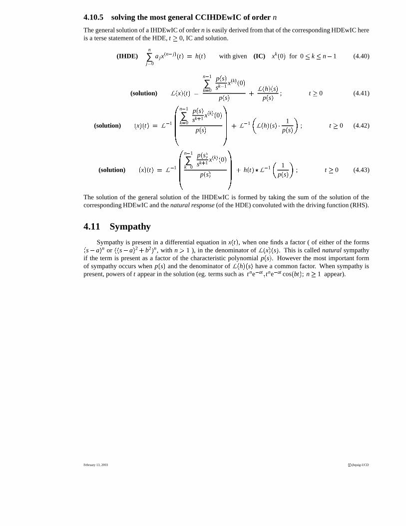
The general solution of a IHDEwIC of order n is easily derived from that of the corresponding HDEwIC hereis a terse statement of the HDE, t � 0, IC and solution.
(IHDE)n
∑j 0
a jx� n j � � t ��� h � t � with given (IC) xk � 0 � for 0 � k � n � 1 (4.40)
(solution) L � x � � t � �n 1
∑k 0
p � s �sk � 1 x � k � � 0 �
p � s � � L � h � � s �p � s � ; t � 0 (4.41)
(solution) � x � � t � � L 1
�����
� n 1
∑k 0
p � s �sk � 1 x � k � � 0 �
p � s ��
����
� � L 1
�L � h � � s � �
1p � s � � ; t � 0 (4.42)
(solution) � x � � t � � L 1
�����
� n 1
∑k 0
p � s �sk � 1 x � k � � 0 �
p � s ��
����
� � h � t � � L 1�
1p � s � � ; t � 0 (4.43)
The solution of the general solution of the IHDEwIC is formed by taking the sum of the solution of thecorresponding HDEwIC and the natural response (of the HDE) convoluted with the driving function (RHS).
4.11 Sympathy
Sympathy is present in a differential equation in x � t � , when one finds a factor ( of either of the forms� s � a � n or � � s � a � 2 � b2 � n, with n � 1 ), in the denominator of L � x � � s � . This is called natural sympathyif the term is present as a factor of the characteristic polynomial p � s � . However the most important formof sympathy occurs when p � s � and the denominator of L � h � � s � have a common factor. When sympathy ispresent, powers of t appear in the solution (eg. terms such as tne at � tne at cos � bt � ; n � 1 appear).
February 13, 2003 c�
jbquig-UCD
104 CHAPTER 4. DIFFERENTIAL EQUATIONS WITH THE LAPLACE TRANSFORM
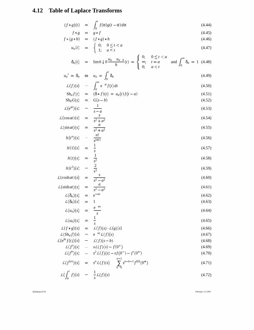
4.12 Table of Laplace Transforms
� f � g � � t � � � t
0f � α � g � t � α � dα (4.44)
f � g � g � f (4.45)
f � � g � h � � � f � g � � h (4.46)
ua � t � � �0; 0 � t � a1; a � t
(4.47)
δa � t � � limh�
0ua � ua � h
h� t ��� �� � 0; 0 � t � a
∞; t � a0; a � t
and � ∞
0δa � 1 (4.48)
ua � � δa � ua � � t
0δa (4.49)
L � f � � s � � � ∞
0e st f � t � dt (4.50)
Sha f � t � � � δ � f � � t � � ua � t � f � t � a � (4.51)
ShbG � s � � G � s � b � (4.52)
L � eat � � s � � 1s � a
(4.53)
L � cosat � � s � � ss2 � a2 (4.54)
L � sinat � � s � � as2 � a2 (4.55)
lt � tn � � s � � n!sn � 1 (4.56)
lt � 1 � � s � � 1s
(4.57)
lt � t � � s � � 1s2 (4.58)
lt � t2 � � s � � 2s3 (4.59)
L � coshat � � s � � ss2 � a2 (4.60)
L � sinhat � � s � � as2 � a2 (4.61)
L � δa � � s � � e as (4.62)
L � δ0 � � s � � 1 (4.63)
L � ua � � s � � e as
s(4.64)
L � u0 � � s � � 1s
(4.65)
L � f � g � � s � � L � f � � s � � L � g � � s � (4.66)
L � Sha f � � s � � e asL � f � � s � (4.67)
L � ebt f � t � � � s � � L � f � � s � b � (4.68)
L � f � � � s � � sL � f � � s ��� f � 0 � � (4.69)
L � f � � � � s � � s2L � f � � s ��� s f � 0 � ��� f � � 0 � � (4.70)
L � f � n � � � s � � snL � f � � s � � n 1
∑k 0
sn k 1 f � k � � 0 � � (4.71)
L � � t
0f � � s � � 1
sL � f � � s � (4.72)
c�
jbquig-UCD February 13, 2003
4.12. TABLE OF LAPLACE TRANSFORMS 105
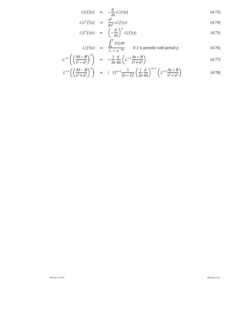
L � t f � � s � � � dds
L � f � � s � (4.73)
L � t2 f � � s � � d2
ds2 L � f � � s � (4.74)
L � tn f � � s � � � � dds
� n
L � f � � s � (4.75)
L � f � � s � � � p
0f � t � dt
1 � e sp if f is periodic with period p (4.76)
L 1
� �AS � Bs2 � a2 � 2 � � � 1
2adda
�L 1 As � B
s2 � a2 � (4.77)
L 1
� �AS � Bs2 � a2 � n � � � � 1 � n 1 1� n � 1 � !
�12a
dda
� n 1 �L 1 As � B
s2 � a2 � (4.78)
February 13, 2003 c�
jbquig-UCD
106 CHAPTER 4. DIFFERENTIAL EQUATIONS WITH THE LAPLACE TRANSFORM
4.13 problem set
Differential Equations and the Laplace transformDo not attempt all these; there are too many; I will give a selection. jbq
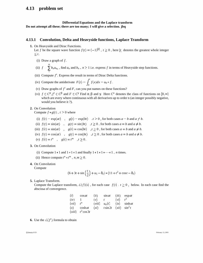
4.13.1 Convolution, Delta and Heavyside functions, Laplace Transform
1. On Heavyside and Dirac Functions.Let f be the square wave function f � t � � � � 1 � � t � � t � 0 , here
�t � denotes the greatest whole integer� t.
(i) Draw a graph of f .
(ii) f � ∞
∑1
bnuan , find an and bn � n � 1 i.e. express f in terms of Heavyside step functions.
(iii) Compute f � . Express the result in terms of Dirac Delta functions.
(iv) Compute the antiderivate F � t ��� � t
0f � x � dx � u0 � f .
(v) Draw graphs of f � and F , can you put names on these functions?
(vi) f � Cα, f � � Cβ and F � Cγ Find α � β and γ. Here Cn denotes the class of functions on�0 � ∞ �
which are every where continuous with all derivarives up to order n (an integer possibly negative,would you believe it ?).
2. On ConvolutionCompute f � g � t � � t � 0 where
(i) f � t ��� exp � at � � g � t � � exp � bt � � t � 0 � for both cases a � b and a �� b.
(ii) f � t ��� sin � at � � g � t � � sin � bt � � t � 0 � for both cases a � b and a �� b.
(iii) f � t ��� sin � at � � g � t � � cos � bt � � t � 0 � for both cases a � b and a �� b.
(iv) f � t ��� cos � at � � g � t � � cos � bt � � t � 0 � for both cases a � b and a �� b.
(v) f � t ��� tn � g � t � � tm � t � 0.
3. On Convolution
(i) Compute 1 � 1 and 1 � 1 � 1 and finally 1 � 1 � 1 � � � � � 1 � n times.
(ii) Hence compute tn � tm � n � m � 0.
4. On ConvolutionCompute � 6 � 3t � sin t
2� � u5 � δ2 � � � 11 � t2 � cost � δ3 �
5. Laplace Transform.Compute the Laplace transform, L � f � � s � , for each case f � t � � t � 0 � below. In each case find theabscissa of convergence.
� i � cosat � ii � sinat � iii � expat� iv � 1 � v � t � vi � t2� vii � tn � viii � ua � t � � ix � sinhat� x � coshat � xi � t sin2t � xii � sin2 t� xiii � t2 cos3t
6. Use the L � f � � formula to obtain
c�
jbquig-UCD February 13, 2003
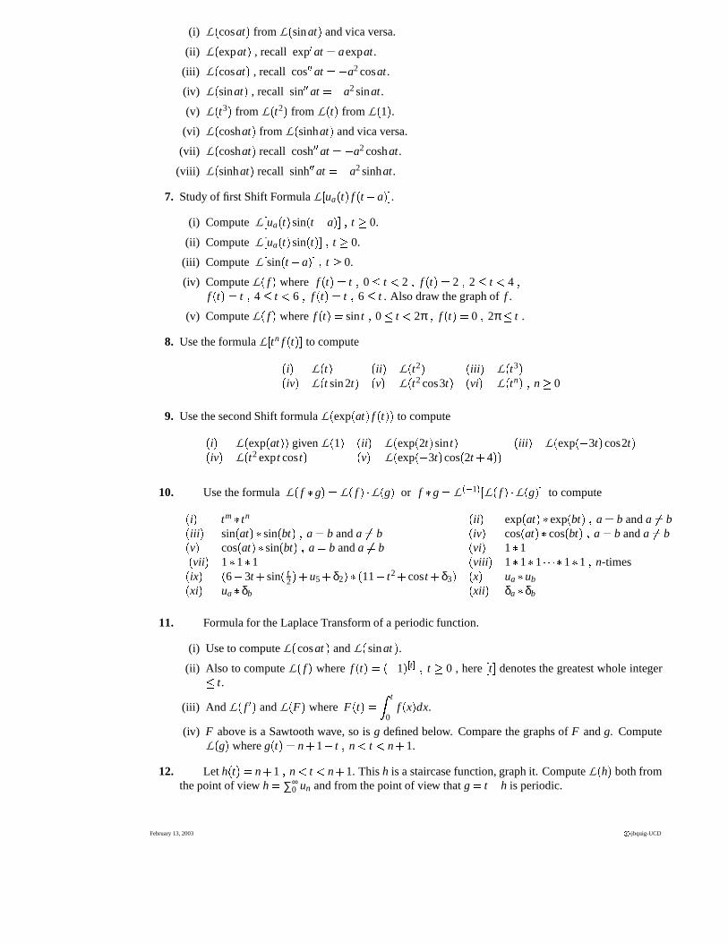
4.13. PROBLEM SET 107
(i) L � cosat � from L � sinat � and vica versa.
(ii) L � expat � , recall exp � at � aexpat.
(iii) L � cosat � , recall cos � � at � � a2 cosat.
(iv) L � sinat � , recall sin � � at � � a2 sinat.
(v) L � t3 � from L � t2 � from L � t � from L � 1 � .(vi) L � coshat � from L � sinhat � and vica versa.
(vii) L � coshat � recall cosh � � at � � a2 coshat.
(viii) L � sinhat � recall sinh � � at � � a2 sinhat.
7. Study of first Shift Formula L�ua � t � f � t � a ��� .
(i) Compute L�ua � t � sin � t � a ��� � t � 0.
(ii) Compute L�ua � t � sin � t ��� � t � 0.
(iii) Compute L�sin � t � a ��� � t � 0.
(iv) Compute L � f � where f � t ��� t � 0 � t � 2 � f � t ��� 2 � 2 � t � 4 �f � t ��� t � 4 � t � 6 � f � t ��� t � 6 � t . Also draw the graph of f .
(v) Compute L � f � where f � t � � sin t � 0 � t � 2π � f � t ��� 0 � 2π � t .
8. Use the formula L�tn f � t ��� to compute
� i � L � t � � ii � L � t2 � � iii � L � t3 �� iv � L � t sin2t � � v � L � t2 cos3t � � vi � L � tn � � n � 0
9. Use the second Shift formula L � exp � at � f � t � � to compute
� i � L � exp � at � � given L � 1 � � ii � L � exp � 2t � sin t � � iii � L � exp � � 3t � cos2t �� iv � L � t2 expt cos t � � v � L � exp � � 3t � cos � 2t � 4 � �10. Use the formula L � f � g � � L � f � � L � g � or f � g � L � 1 � �L � f � � L � g ��� to compute
� i � tm � tn � ii � exp � at � � exp � bt � � a � b and a �� b� iii � sin � at � � sin � bt � � a � b and a �� b � iv � cos � at � � cos � bt � � a � b and a �� b� v � cos � at � � sin � bt � � a � b and a �� b � vi � 1 � 1� vii � 1 � 1 � 1 � viii � 1 � 1 � 1 � � � � 1 � 1 � n-times� ix � � 6 � 3t � sin � t2 � � u5 � δ2 � � � 11 � t2 � cost � δ3 � � x � ua � ub� xi � ua � δb � xii � δa � δb
11. Formula for the Laplace Transform of a periodic function.
(i) Use to compute L � cosat � and L � sinat � .(ii) Also to compute L � f � where f � t � � � � 1 � � t � � t � 0 , here
�t � denotes the greatest whole integer� t.
(iii) And L � f � � and L � F � where F � t ��� � t
0f � x � dx.
(iv) F above is a Sawtooth wave, so is g defined below. Compare the graphs of F and g. ComputeL � g � where g � t � � n � 1 � t � n � t � n � 1.
12. Let h � t � � n � 1 � n � t � n � 1. This h is a staircase function, graph it. Compute L � h � both fromthe point of view h � ∑∞
0 un and from the point of view that g � t � h is periodic.
February 13, 2003 c�
jbquig-UCD
108 CHAPTER 4. DIFFERENTIAL EQUATIONS WITH THE LAPLACE TRANSFORM
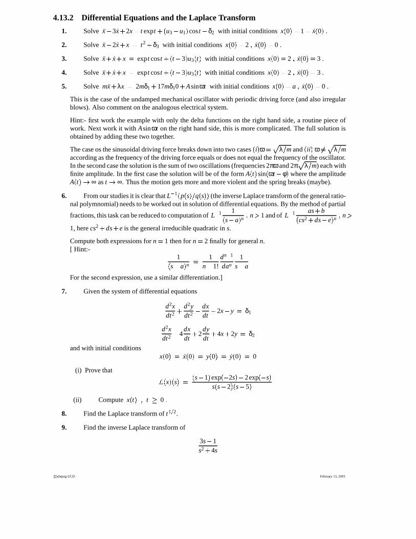
4.13.2 Differential Equations and the Laplace Transform
1. Solve x � 3x � 2x � t expt � � u3 � u1 � cos t � δ2 with initial conditions x � 0 ��� 1 � x � 0 � .
2. Solve x � 2x � x � t2 � δ3 with initial conditions x � 0 � � 2 � x � 0 ��� 0 .
3. Solve x � x � x � expt cos t � � t � 3 � u3 � t � with initial conditions x � 0 ��� 2 � x � 0 ��� 3 .
4. Solve x � x � x � expt cos t � � t � 3 � u3 � t � with initial conditions x � 0 ��� 2 � x � 0 ��� 3 .
5. Solve mx � λx � 2mδ1 � 17mδ10 � Asinωt with initial conditions x � 0 ��� a � x � 0 ��� 0 .
This is the case of the undamped mechanical oscillator with periodic driving force (and also irregularblows). Also comment on the analogous electrical system.
Hint:- first work the example with only the delta functions on the right hand side, a routine piece ofwork. Next work it with Asinωt on the right hand side, this is more complicated. The full solution isobtained by adding these two together.
The case os the sinusoidal driving force breaks down into two cases � i � ω ��� λ � m and � ii � ω ���� λ � maccording as the frequency of the driving force equals or does not equal the frequency of the oscillator.In the second case the solution is the sum of two oscillations (frequencies 2πω and 2π � λ � m) each withfinite amplitude. In the first case the solution will be of the form A � t � sin � ωt � φ � where the amplitudeA � t � � ∞ as t � ∞. Thus the motion gets more and more violent and the spring breaks (maybe).
6. From our studies it is clear that L 1 � p � s � � q � s � � (the inverse Laplace transform of the general ratio-nal polymnomial) needs to be worked out in solution of differential equations. By the method of partial
fractions, this task can be reduced to computation of L 1 1� s � a � n � n � 1 and of L 1 as � b� cs2 � ds � e � n � n �1, here cs2 � ds � e is the general irreducible quadratic in s.
Compute both expressions for n � 1 then for n � 2 finally for general n.[ Hint:-
1� s � a � n � 1n � 1!
dn 1
dan
1s � a
For the second expression, use a similar differentiation.]
7. Given the system of differential equations
d2xdt2 � d2y
dt2 � dxdt� 2x � y � δ1
d2xdt2 � 4
dxdt� 2
dydt� 4x � 2y � δ2
and with initial conditionsx � 0 � � x � 0 ��� y � 0 ��� y � 0 ��� 0
(i) Prove that
L � x � � s � � � s � 1 � exp � � 2s ��� 2exp � � s �s � s � 2 � � s � 5 �
(ii) Compute x � t � � t � 0 �8. Find the Laplace transform of t1 � 2.
9. Find the inverse Laplace transform of
3s � 1s2 � 4s
c�
jbquig-UCD February 13, 2003
4.13. PROBLEM SET 109
10. Using Laplace transforms, or otherwise, solve the coupled differential equations
x � 2y � 1 x � y � x � 0
for x � t � � y � t � , when x � 0 ��� y � 0 � � 0.
11. Assuming that all transforms exist, show that
L�y � � s2L
�y � � sy � 0 ��� y � 0 �
and
L�ty � � � d
dsL�y �
12. Using Laplace transforms, solve the differential equation
ty � � 1 � t � y � 3y � 0
where y � 0 ��� 1.
13. Given the differential equation
d2xdt2 � 2
dxdt� 2x � g � t ��� t � 0
with initial conditionsx � 0 ��� x � 0 ��� 0
where g � t ��� 1 � 0 � t � 1 and g � t ��� 0 � t � 1 �(i) Prove that
L � x � � s � � 1 � exp � � s �s � s2 � 2s � 2 �
(ii) Compute x � t � � t � 0 �
February 13, 2003 c�
jbquig-UCD