
Mathematical Programming: An Overview
539
Mathematical Programming: An Overview 1 Management science is characterized by a scientific approach to managerial decision making. It attempts to apply mathematical methods and the capabilities of modern computers to the difficult and unstructured problems confronting modern managers. It is a young and novel discipline. Although its roots can be traced back to problems posed by early civilizations, it was not until World War II that it became identified as a respectable and well defined body of knowledge. Since then, it has grown at an impressive pace, unprecedented for most scientific accomplishments; it is changing our attitudes toward decision-making, and infiltrating every conceivable area of application, covering a wide variety of business, industrial, military, and public-sector problems. Management science has been known by a variety of other names. In the United States, operations research has served as a synonym and it is used widely today, while in Britain operational research seems to be the more accepted name. Some people tend to identify the scientific approach to managerial problem- solving under such other names as systems analysis, cost–benefit analysis, and cost-effectiveness analysis. We will adhere to management science throughout this book. Mathematical programming, and especially linear programming, is one of the best developed and most used branches of management science. It concerns the optimum allocation of limited resources among competing activities, under a set of constraints imposed by the nature of the problem being studied. These constraints could reflect financial, technological, marketing, organizational, or many other considerations. In broad terms, mathematical programming can be defined as a mathematical representation aimed at program- ming or planning the best possible allocation of scarce resources. When the mathematical representation uses linear functions exclusively, we have a linear-programming model. In 1947, George B. Dantzig, then part of a research group of the U.S. Air Force known as Project SCOOP (Scientific Computation Of Optimum Programs), developed the simplex method for solving the general linear-programming problem. The extraordinary computational efficiency and robustness of the simplex method, together with the availability of high-speed digital computers, have made linear programming the most powerful optimization method ever designed and the most widely applied in the business environment. Since then, many additional techniques have been developed, which relax the assumptions of the linear- programming model and broaden the applications of the mathematical-programming approach. It is this spectrum of techniques and their effective implementation in practice that are considered in this book. 1.1 AN INTRODUCTION TO MANAGEMENT SCIENCE Since mathematical programming is only a tool of the broad discipline known as management science, let us first attempt to understand the management-science approach and identify the role of mathematical programming within that approach. 1
Transcript of Mathematical Programming: An Overview

Mathematical Programming:An Overview
1
Management science is characterized by a scientific approach to managerial decision making. It attemptsto apply mathematical methods and the capabilities of modern computers to the difficult and unstructuredproblems confronting modern managers. It is a young and novel discipline. Although its roots can betraced back to problems posed by early civilizations, it was not until World War II that it became identifiedas a respectable and well defined body of knowledge. Since then, it has grown at an impressive pace,unprecedented for most scientific accomplishments; it is changing our attitudes toward decision-making, andinfiltrating every conceivable area of application, covering a wide variety of business, industrial, military, andpublic-sector problems.
Management science has been known by a variety of other names. In the United States,operationsresearchhas served as a synonym and it is used widely today, while in Britainoperational researchseemsto be the more accepted name. Some people tend to identify the scientific approach to managerial problem-solving under such other names as systems analysis, cost–benefit analysis, and cost-effectiveness analysis.We will adhere tomanagement sciencethroughout this book.
Mathematical programming, and especially linear programming, is one of the best developed and mostused branches of management science. It concerns the optimum allocation of limited resources amongcompeting activities, under a set of constraints imposed by the nature of the problem being studied. Theseconstraints could reflect financial, technological, marketing, organizational, or many other considerations. Inbroad terms, mathematical programming can be defined as a mathematical representation aimed at program-ming or planning the best possible allocation of scarce resources. When the mathematical representation useslinear functions exclusively, we have a linear-programming model.
In 1947, George B. Dantzig, then part of a research group of the U.S. Air Force known as Project SCOOP(Scientific Computation Of Optimum Programs), developed thesimplex methodfor solving the generallinear-programming problem. The extraordinary computational efficiency and robustness of the simplexmethod, together with the availability of high-speed digital computers, have made linear programming themost powerful optimization method ever designed and the most widely applied in the business environment.
Since then, many additional techniques have been developed, which relax the assumptions of the linear-programming model and broaden the applications of the mathematical-programming approach. It is thisspectrum of techniques and their effective implementation in practice that are considered in this book.
1.1 AN INTRODUCTION TO MANAGEMENT SCIENCE
Since mathematical programming is only a tool of the broad discipline known as management science,let us first attempt to understand the management-science approach and identify the role of mathematicalprogramming within that approach.
1

2 Mathematical Programming: An Overview 1.2
It is hard to give a noncontroversial definition of management science. As we have indicated before,this is a rather new field that is renewing itself and changing constantly. It has benefited from contributionsoriginating in the social and natural sciences, econometrics, and mathematics, much of which escape therigidity of a definition. Nonetheless it is possible to provide a general statement about the basic elements ofthe management-science approach.
Management science is characterized by the use ofmathematical modelsin providing guidelines tomanagers for making effective decisions within the state of the current information, or in seeking furtherinformation if current knowledge is insufficient to reach a proper decision.
There are several elements of this statement that are deserving of emphasis. First, the essence of manage-ment science is the model-building approach—that is, an attempt to capture the most significant features of thedecision under consideration by means of a mathematical abstraction. Models are simplified representationsof the real world. In order for models to be useful in supporting management decisions, they have to be simpleto understand and easy to use. At the same time, they have to provide a complete and realistic representationof the decision environment by incorporating all the elements required to characterize the essence of theproblem under study. This is not an easy task but, if done properly, it will supply managers with a formidabletool to be used in complex decision situations.
Second, through this model-design effort, management science tries to provide guidelines to managers or,in other words, to increase managers’ understanding of the consequences of their actions. There is never anattempt to replace or substitute for managers, but rather the aim is tosupportmanagement actions. It is critical,then, to recognize the strong interaction required between managers and models. Models can expedientlyand effectively account for the many interrelationships that might be present among the alternatives beingconsidered, and can explicitly evaluate the economic consequences of the actions available to managers withinthe constraints imposed by the existing resources and the demands placed upon the use of those resources.Managers, on the other hand, should formulate the basic questions to be addressed by the model, and theninterpret the model’s results in light of their own experience and intuition, recognizing the model’s limitations.The complementarity between the superior computational capabilities provided by the model and the higherjudgmental capabilities of the human decision-maker is the key to a successful management-science approach.
Finally, it is the complexity of the decision under study, and not the tool being used to investigate thedecision-making process, that should determine the amount of information needed to handle that decisioneffectively. Models have been criticized for creating unreasonable requirements for information. In fact,this is not necessary. Quite to the contrary, models can be constructed within the current state of availableinformation and they can be used to evaluate whether or not it is economically desirable to gather additionalinformation.
The subject of proper model design and implementation will be covered in detail in Chapter 5.
1.2 MODEL CLASSIFICATION
The management-science literature includes several approaches to classifying models. We will begin with acategorization that identifies broad types of models according to the degree of realism that they achieve inrepresenting a given problem. The model categories can be illustrated as shown in Fig. 1.1.
Operational Exercise
The first model type is anoperational exercise. This modeling approach operates directly with the realenvironment in which the decision under study is going to take place. The modeling effort merely involvesdesigning a set of experiments to be conducted in that environment, and measuring and interpreting the resultsof those experiments. Suppose, for instance, that we would like to determine what mix of several crude oilsshould be blended in a given oil refinery to satisfy, in the most effective way, the market requirements forfinal products to be delivered from that refinery. If we were to conduct an operational exercise to support thatdecision, we would try different quantities of several combinations of crude oil types directly in the actual

1.2 Model Classification 3
refinery process, and observe the resulting revenues and costs associated with each alternative mix. Afterperforming quite a few trials, we would begin to develop an understanding of the relationship between the
Fig. 1.1 Types of model representation.
crude oil input and the net revenue obtained from the refinery process, which would guide us in identifyingan appropriate mix.
In order for this approach to operate successfully, it is mandatory to design experiments to be conductedcarefully, to evaluate the experimental results in light of errors that can be introduced by measurement inac-curacies, and to draw inferences about the decisions reached, based upon the limited number of observationsperformed. Many statistical and optimization methods can be used to accomplish these tasks properly. Theessence of the operational exercise is an inductive learning process, characteristic of empirical research in thenatural sciences, in which generalizations are drawn from particular observations of a given phenomenon.
Operational exercises contain the highest degree of realism of any form of modeling approach, sincehardly any external abstractions or oversimplifications are introduced other than those connected with theinterpretation of the observed results and the generalizations to be drawn from them. However, the methodis exceedingly, usually prohibitively, expensive to implement. Moreover, in most cases it is impossible toexhaustively analyze the alternatives available to the decision-maker. This can lead to severesuboptimizationin the final conclusions. For these reasons, operational exercises seldom are used as a pure form of modelingpractice. It is important to recognize, however, that direct observation of the actual environment underliesmost model conceptualizations and also constitutes one of the most important sources of data. Consequently,even though they may not be used exclusively, operational exercises produce significant contributions to theimprovement of managerial decision-making.
Gaming
The second type of model in this classification isgaming. In this case, a model is constructed that is anabstract and simplified representation of the real environment. This model provides a responsive mechanismto evaluate the effectiveness of proposed alternatives, which the decision-maker must supply in an organizedand sequential fashion. The model is simply a device that allows the decision-maker to test the performanceof the various alternatives that seem worthwhile to pursue. In addition, in a gaming situation, all the humaninteractions that affect the decision environment are allowed to participate actively by providing the inputsthey usually are responsible for in the actual realization of their activities. If a gaming approach is used in ourprevious example, the refinery process would be represented by a computer or mathematical model, whichcould assume any kind of structure.
The model should reflect, with an acceptable degree of accuracy, the relationships between the inputs andoutputs of the refinery process. Subsequently, all the personnel who participate in structuring the decisionprocess in the management of the refinery would be allowed to interact with the model. The production man-ager would establish production plans, the marketing manager would secure contracts and develop marketing

4 Mathematical Programming: An Overview 1.2
strategies, the purchasing manager would identify prices and sources of crude oil and develop acquisitionprograms, and so forth. As before, several combinations of quantities and types of crude oil would be tried,and the resulting revenues and cost figures derived from the model would be obtained, to guide us in for-mulating an optimal policy. Certainly, we have lost some degree of realism in our modeling approach withrespect to the operational exercise, since we are operating with an abstract environment, but we have retainedsome of the human interactions of the real process. However, thecost of processing each alternativehas beenreduced, and thespeed of measuring the performanceof each alternative has been increased.
Gaming is used mostly as a learning device for developing some appreciation for those complexitiesinherent in a decision-making process. Several management games have been designed to illustrate howmarketing, production, and financial decisions interact in a competitive economy.
Simulation
Simulationmodels are similar to gaming models except that all human decision-makers are removed fromthe modeling process. The model provides the means to evaluate the performance of a number of alterna-tives, supplied externally to the model by the decision-maker, without allowing for human interactions atintermediate stages of the model computation.
Like operational exercises and gaming, simulation models neither generate alternatives nor produce anoptimum answer to the decision under study. These types of models are inductive and empirical in nature;they are useful only to assess the performance of alternatives identified previously by the decision-maker.
If we were to conduct a simulation model in our refinery example, we would program in advance a largenumber of combinations of quantities and types of crude oil to be used, and we would obtain the net revenuesassociated with each alternative without any external inputs of the decision-makers. Once the model resultswere produced, new runs could be conducted until we felt that we had reached a proper understanding of theproblem on hand.
Many simulation models take the form of computer programs, where logical arithmetic operations areperformed in a prearranged sequence. It is not necessary, therefore, to define the problem exclusively inanalytic terms. This provides an added flexibility in model formulation and permits a high degree of realismto be achieved, which is particularly useful when uncertainties are an important aspect of the decision.
Analytical Model
Finally, the fourth model category proposed in this framework is theanalytical model. In this type of model,the problem is represented completely in mathematical terms, normally by means of a criterion or objective,which we seek to maximize or minimize, subject to a set of mathematical constraints that portray the conditionsunder which the decisions have to be made. The model computes an optimal solution, that is, one that satisfiesall the constraints and gives the best possible value of the objective function.
In the refinery example, the use of an analytical model implies setting up as an objective themaximizationof the net revenuesobtained from the refinery operation as a function of the types and quantities of the crudeoil used. In addition, the technology of the refinery process, the final product requirements, and the crudeoil availabilities must be represented in mathematical terms to define the constraints of our problem. Thesolution to the model will be the exact amount of each available crude-oil type to be processed that willmaximize the net revenues within the proposed constraint set. Linear programming has been, in the last twodecades, the indisputable analytical model to use for this kind of problem.
Analytical models are normally the least expensive and easiest models to develop. However, they intro-duce the highest degree of simplification in the model representation. As a rule of thumb, it is better to beas much to the right as possible in the model spectrum (no political implication intended!), provided that theresulting degree of realism is appropriate to characterize the decision under study.
Most of the work undertaken by management scientists has been oriented toward the development andimplementation of analytical models. As a result of this effort, many different techniques and methodologieshave been proposed to address specific kinds of problems. Table 1.1 presents a classification of the mostimportant types of analytical and simulation models that have been developed.
1.3 Formulation of Some Examples 5
Table 1.1 Classification of Analytical and Simulation Models
Strategy evaluation Strategy generation
Certainty Deterministic simulation Linear programmingEconometric models Network modelsSystems of simultaneous Integer and mixed-integer
equations programmingInput-output models Nonlinear programming
Control theory
Uncertainty Monte Carlo simulation Decision theoryEconometric models Dynamic programmingStochastic processes Inventory theoryQueueing theory Stochastic programmingReliability theory Stochastic control theory
Statistics and subjective assessment are used in all models to determine values forparameters of the models and limits on the alternatives.
The classification presented in Table 1.1 is not rigid, since strategy evaluation models are used forimproving decisions by trying different alternatives until one is determined that appears ‘‘best.’’ The importantdistinction of the proposed classification is that, for strategy evaluation models, the user must first chooseand construct the alternative and then evaluate it with the aid of the model. For strategy generation models,the alternative is not completely determined by the user; rather, the class of alternatives is determined byestablishing constraints on the decisions, and then an algorithmic procedure is used to automatically generatethe ‘‘best’’ alternative within that class. The horizontal classification should be clear, and is introduced becausethe inclusion of uncertainty (or not) generally makes a substantial difference in the type and complexity ofthe techniques that are employed. Problems involving uncertainty are inherently more difficult to formulatewell and to solve efficiently.
This book is devoted to mathematical programming—a part of management science that has a commonbase of theory and a large range of applications. Generally, mathematical programming includes all ofthe topics under the heading of strategy generation except for decision theory and control theory. Thesetwo topics are entire disciplines in themselves, depending essentially on different underlying theories andtechniques. Recently, though, the similarities between mathematical programming and control theory arebecoming better understood, and these disciplines are beginning to merge. In mathematical programming,the main body of material that has been developed, and more especially applied, is under the assumption ofcertainty. Therefore, we concentrate the bulk of our presentation on the topics in the upper righthand cornerof Table 1.1. The critical emphasis in the book is on developing those principles and techniques that leadto good formulationsof actual decision problems andsolution proceduresthat are efficient for solving theseformulations.
1.3 FORMULATION OF SOME EXAMPLES
In order to provide a preliminary understanding of the types of problems to which mathematical programmingcan be applied, and to illustrate the kind of rationale that should be used in formulating linear-programmingproblems, we will present in this section three highly simplified examples and their corresponding linear-programming formulations.
Charging a Blast Furnace∗ An iron foundry has a firm order to produce 1000 pounds of castings containingat least 0.45 percent manganese and between 3.25 percent and 5.50 percent silicon. As these particular castingsare a special order, there are no suitable castings on hand. The castings sell for $0.45 per pound. The foundryhas three types of pig iron available in essentially unlimited amounts, with the following properties:
∗ Excel spreadsheet available athttp://web.mit.edu/15.053/www/Sect1.3_Blast_Furnace.xls

6 Mathematical Programming: An Overview 1.3
Type of pig iron
A B C
Silicon 4 % 1 % 0.6%Manganese 0.45% 0.5% 0.4%
Further, the production process is such that pure manganese can also be added directly to the melt. The costsof the various possible inputs are:
Pig A $21/thousand pounds
Pig B $25/thousand pounds
Pig C $15/thousand pounds
Manganese $ 8/pound.
It costs 0.5 cents to melt down a pound of pig iron. Out of what inputs should the foundry produce the castingsin order to maximize profits?
The first step in formulating a linear program is to define thedecision variablesof the problem. These arethe elements under the control of the decision-maker, and their values determine the solution of the model.In the present example, these variables are simple to identify, and correspond to the number of pounds of pigA, pig B, pig C, and pure manganeseto be used in the production of castings. Specifically, let us denote thedecision variables as follows:
x1 = Thousands of pounds of pig iron A,
x2 = Thousands of pounds of pig iron B,
x3 = Thousands of pounds of pig iron C,
x4 = Pounds of pure manganese.
The next step to be carried out in the formulation of the problem is to determine the criterion the decision-maker will use to evaluate alternative solutions to the problem. In mathematical-programming terminology,this is known as theobjective function.In our case, we want to maximize the total profit resulting from theproduction of 1000 pounds of castings. Since we are producing exactly 1000 pounds of castings, the totalincome will be the selling price per pound times 1000 pounds. That is:
Total income= 0.45× 1000= 450.
To determine the total cost incurred in the production of the alloy, we should add the melting cost of$0.005/pound to the corresponding cost of each type of pig iron used. Thus, the relevant unit cost of the pigiron, in dollars per thousand pounds, is:
Pig iron A 21+ 5 = 26,
Pig iron B 25+ 5 = 30,
Pig iron C 15+ 5 = 20.
Therefore, the total cost becomes:
Total cost= 26x1+ 30x2+ 20x3+ 8x4, (1)
and the total profit we want to maximize is determined by the expression:
Total profit= Total income− Total cost.
Thus,
Total profit= 450− 26x1− 30x2− 20x3− 8x4. (2)

1.3 Formulation of Some Examples 7
It is worthwhile noticing in this example that, since the amount of castings to be produced was fixed inadvance, equal to 1000 pounds, the maximization of the total profit, given by Eq. (2), becomes completelyequivalent to the minimization of the total cost, given by Eq. (1).
We should now define theconstraintsof the problem, which are the restrictions imposed upon the valuesof the decision variables by the characteristics of the problem under study. First, since the producer does notwant to keep any supply of the castings on hand, we should make the total amount to be produced exactlyequal to 1000 pounds; that is,
1000x1+ 1000x2+ 1000x3+ x4 = 1000. (3)
Next, the castings should contain at least 0.45 percent manganese, or 4.5 pounds in the 1000 pounds ofcastings to be produced. This restriction can be expressed as follows:
4.5x1+ 5.0x2+ 4.0x3+ x4 ≥ 4.5. (4)
The term 4.5x1 is the pounds of manganese contributed by pig iron A since each 1000 pounds of this pig ironcontains 4.5 pounds of manganese. Thex2, x3, andx4 terms account for the manganese contributed by pigiron B, by pig iron C, and by the addition of pure manganese.
Similarly, the restriction regarding the silicon content can be represented by the following inequalities:
40x1+ 10x2+ 6x3 ≥ 32.5, (5)
40x1+ 10x2+ 6x3 ≤ 55.0. (6)
Constraint (5) establishes that the minimum silicon content in the castings is 3.25 percent, while constraint(6) indicates that the maximum silicon allowed is 5.5 percent.
Finally, we have the obvious nonnegativity constraints:
x1 ≥ 0, x2 ≥ 0, x3 ≥ 0, x4 ≥ 0.
If we choose to minimize the total cost given by Eq. (1), the resulting linear programming problem canbe expressed as follows:
Minimize z= 26x1+ 30x2 + 20x3 + 8x4,
subject to:1000x1 + 1000x2 + 1000x3 + x4 = 1000,
4.5x1 + 5.0x2 + 4.0x3 + x4 ≥ 4.5,
40x1 + 10x2 + 6x3 ≥ 32.5,
40x1 + 10x2 + 6x3 ≤ 55.0,
x1 ≥ 0, x2 ≥ 0, x3 ≥ 0, x4 ≥ 0.
Often, this algebraic formulation is represented intableau formas follows:
Decision variablesx1 x2 x3 x4 Relation Requirements
Total lbs. 1000 1000 1000 1 = 1000Manganese 4.5 5 4 1 ≥ 4.5Silicon lower 40 10 6 0 ≥ 32.5Silicon upper 40 10 6 0 ≤ 55.0Objective 26 30 20 8 = z (min)(Optimal solution) 0.779 0 0.220 0.111 25.54
The bottom line of the tableau specifies theoptimal solutionto this problem. The solution includesthe values of the decision variables as well as the minimum cost attained, $25.54 per thousand pounds; thissolution was generated using a commercially available linear-programming computer system. The underlyingsolution procedure, known as thesimplex method, will be explained in Chapter 2.
8 Mathematical Programming: An Overview 1.3
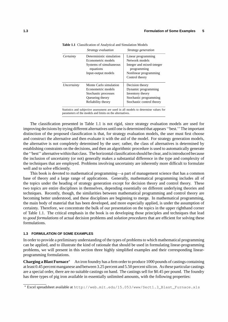
Fig. 1.2 Optimal cost of castings as a function of the cost of pure manganese.
It might be interesting to see how the solution and the optimal value of the objective function is affectedby changes in the cost of manganese. In Fig. 1.2 we give the optimal value of the objective function as thiscost is varied. Note that if the cost of manganese rises above $9.86/lb., thennopure manganese is used. In therange from $0.019/lb. to $9.86 lb., the values of the decision variables remain unchanged. When manganesebecomes extremelyinexpensive, less than $0.019/lb., a great deal of manganese is used, in conjuction withonly one type of pig iron.
Similar analyses can be performed to investigate the behavior of the solution as other parameters of theproblem (for example, minimum allowed silicon content) are varied. These results, known as parametricanalysis, are reported routinely by commercial linear-programming computer systems. In Chapter 3 we willshow how to conduct such analyses in a comprehensive way.
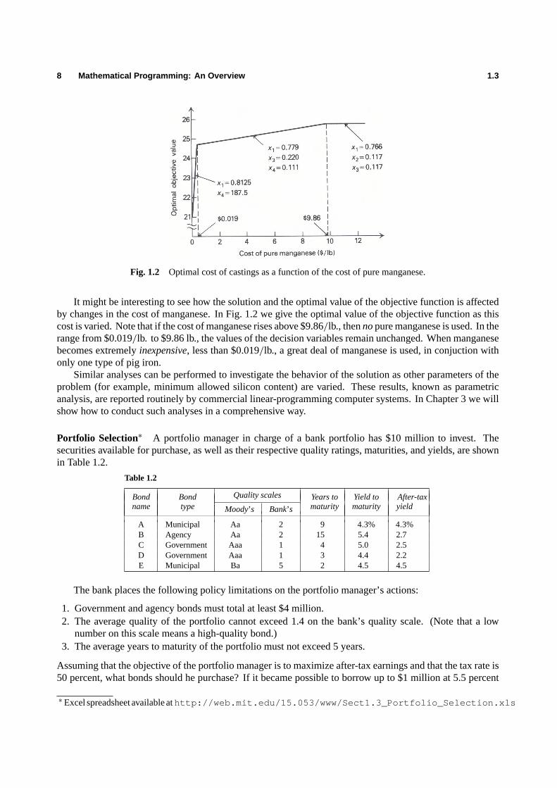
Portfolio Selection∗ A portfolio manager in charge of a bank portfolio has $10 million to invest. Thesecurities available for purchase, as well as their respective quality ratings, maturities, and yields, are shownin Table 1.2.
Table 1.2
Bond Bond Quality scales Years to Yield to After-taxname type Moody’s Bank’s maturity maturity yield
A Municipal Aa 2 9 4.3% 4.3%B Agency Aa 2 15 5.4 2.7C Government Aaa 1 4 5.0 2.5D Government Aaa 1 3 4.4 2.2E Municipal Ba 5 2 4.5 4.5
The bank places the following policy limitations on the portfolio manager’s actions:
1. Government and agency bonds must total at least $4 million.2. The average quality of the portfolio cannot exceed 1.4 on the bank’s quality scale. (Note that a low
number on this scale means a high-quality bond.)3. The average years to maturity of the portfolio must not exceed 5 years.
Assuming that the objective of the portfolio manager is to maximize after-tax earnings and that the tax rate is50 percent, what bonds should he purchase? If it became possible to borrow up to $1 million at 5.5 percent
∗Excel spreadsheet available athttp://web.mit.edu/15.053/www/Sect1.3_Portfolio_Selection.xls

1.3 Formulation of Some Examples 9
before taxes, how should his selection be changed?Leaving the question of borrowed funds aside for the moment, the decision variables for this problem are
simply the dollar amount of each security to be purchased:
xA =Amount to be invested in bond A; in millions of dollars.xB =Amount to be invested in bond B; in millions of dollars.xC =Amount to be invested in bond C; in millions of dollars.xD =Amount to be invested in bond D; in millions of dollars.xE =Amount to be invested in bond E; in millions of dollars.
We must now determine the form of the objective function. Assuming that all securities are purchased at par(face value) and held to maturity and that the income on municipal bonds is tax-exempt, the after-tax earningsare given by:
z= 0.043xA + 0.027xB + 0.025xC+ 0.022xD + 0.045xE.
Now let us consider each of the restrictions of the problem. The portfolio manager has only a total of tenmillion dollars to invest, and therefore:
xA + xB + xC+ xD + xE ≤ 10.
Further, of this amount at least $4 million must be invested in government and agency bonds. Hence,
xB + xC+ xD ≥ 4.
The average quality of the portfolio, which is given by the ratio of the total quality to the total value of theportfolio, must not exceed 1.4:
2xA + 2xB + xC+ xD + 5xE
xA + xB + xC+ xD + xE≤ 1.4.
Note that the inequality is less-than-or-equal-to, since a low number on the bank’s quality scale means ahigh-quality bond. By clearing the denominator and re-arranging terms, we find that this inequality is clearlyequivalent to the linear constraint:
0.6xA + 0.6xB − 0.4xC− 0.4xD + 3.6xE ≤ 0.
The constraint on the average maturity of the portfolio is a similar ratio. The average maturity must notexceed five years:
9xA + 15xB + 4xC+ 3xD + 2xE
xA + xB + xC+ xD + xE≤ 5,
which is equivalent to the linear constraint:
4xA + 10xB − xC− 2xD − 3xE ≤ 0.
Note that the two ratio constraints are, in fact,nonlinear constraints, which would require sophisticatedcomputational procedures if included in this form. However, simply multiplying both sides of each ratioconstraint by its denominator (which must be nonnegative since it is the sum of nonnegative variables)transforms this nonlinear constraint into a simple linear constraint. We can summarize our formulation intableau form, as follows:
xA xB xC xD xE Relation LimitsCash 1 1 1 1 1 ≤ 10Governments 1 1 1 ≥ 4Quality 0.6 0.6 −0.4 −0.4 3.6 ≤ 0Maturity 4 10 −1 −2 −3 ≤ 0Objective 0.043 0.027 0.025 0.022 0.045 = z (max)(Optimal solution) 3.36 0 0 6.48 0.16 0.294

10 Mathematical Programming: An Overview 1.3
The values of the decision variables and the optimal value of the objective function are again given in the lastrow of the tableau.
Now consider the additional possibility of being able to borrow up to $1 million at 5.5 percent beforetaxes. Essentially, we can increase our cash supply above ten million by borrowing at an after-tax rate of 2.75percent. We can define a new decision variable as follows:
y = amount borrowed in millions of dollars.
There is an upper bound on the amount of funds that can be borrowed, and hence
y ≤ 1.
The cash constraint is then modified to reflect that the total amount purchased must be less than or equal tothe cash that can be made available including borrowing:
xA + xB + xC+ xD + xE ≤ 10+ y.
Now, since the borrowed money costs 2.75 percent after taxes, the new after-tax earnings are:
z= 0.043xA + 0.027xB + 0.025xC+ 0.022xD + 0.045xE − 0.0275y.
We summarize the formulation when borrowing is allowed and give the solution in tableau form as follows:
xA xB xC xD xE y Relation LimitsCash 1 1 1 1 1 −1 ≤ 10Borrowing 1 ≤ 1Governments 1 1 1 ≥ 4Quality 0.6 0.6 −0.4 −0.4 3.6 ≤ 0Maturity 4 10 −1 −2 −3 ≤ 0Objective 0.043 0.027 0.025 0.022 0.045−0.0275 = z (max)(Optimal solution) 3.70 0 0 7.13 0.18 1 0.296
Production and Assembly A division of a plastics company manufactures three basic products: sporks,packets, and school packs. A spork is a plastic utensil which purports to be a combination spoon, fork, andknife. The packets consist of a spork, a napkin, and a straw wrapped in cellophane. The school packs areboxes of 100 packets with an additional 10 loose sporks included.
Production of 1000 sporks requires 0.8 standard hours of molding machine capacity, 0.2 standard hoursof supervisory time, and $2.50 in direct costs. Production of 1000 packets, including 1 spork, 1 napkin, and 1straw, requires 1.5 standard hours of the packaging-area capacity, 0.5 standard hours of supervisory time, and$4.00 in direct costs. There is an unlimited supply of napkins and straws. Production of 1000 school packsrequires 2.5 standard hours of packaging-area capacity, 0.5 standard hours of supervisory time, 10 sporks,100 packets, and $8.00 in direct costs.
Any of the three products may be sold in unlimited quantities at prices of $5.00, $15.00, and $300.00 perthousand, respectively. If there are 200 hours of production time in the coming month, what products, andhow much of each, should be manufactured to yield the most profit?
The first decision one has to make in formulating a linear programming model is the selection of theproper variables to represent the problem under consideration. In this example there are at least two differentsets of variables that can be chosen as decision variables. Let us represent them byx’s andy’s and definethem as follows:
x1 = Total number of sporks produced in thousands,
x2 = Total number of packets produced in thousands,
x3 = Total number of school packs produced in thousands,

1.3 Formulation of Some Examples 11
and
y1 = Total number of sporks sold as sporks in thousands,
y2 = Total number of packets sold as packets in thousands,
y3 = Total number of school packs sold as school packs in thousands.
We can determine the relationship between these two groups of variables. Since each packet needs onespork, and each school pack needs ten sporks, the total number of sporks sold as sporks is given by:
y1 = x1− x2− 10x3. (7)
Similarly, for the total number of packets sold as packets we have:
y2 = x2− 100x3. (8)
Finally, since all the school packs are sold as such, we have:
y3 = x3. (9)
From Eqs. (7), (8), and (9) it is easy to express thex’s in terms of they’s, obtaining:
x1 = y1+ y2+ 110y3, (10)x2 = y2+ 100y3, (11)x3 = y3. (12)
As a matter of exercise, let us formulate the linear program corresponding to the present example in twoforms: first, using thex’s as decision variables, and second, using they’s as decision variables.
The objective function is easily determined in terms of bothy- andx-variables by using the informationprovided in the statement of the problem with respect to the selling prices and the direct costs of each of theunits produced. The total profit is given by:
Total profit= 5y1+ 15y2+ 300y3− 2.5x1− 4x2− 8x3. (13)
Equations (7), (8), and (9) allow us to express this total profit in terms of thex-variables alone. Afterperforming the transformation, we get:
Total profit= 2.5x1+ 6x2− 1258x3. (14)
Now we have to set up the restrictions imposed by the maximum availability of 200 hours of productiontime. Since the sporks are the only items requiring time in the injection-molding area, and they consume 0.8standard hours of production per 1000 sporks, we have:
0.8x1 ≤ 200. (15)
For packaging-area capacity we have:1.5x2+ 2.5x3 ≤ 200, (16)
while supervisory time requires that
0.2x1+ 0.5x2+ 0.5x3 ≤ 200. (17)
In addition to these constraints, we have to make sure that the number of sporks, packets, and school packssold as such (i.e., they-variables) are nonnegative. Therefore, we have to add the following constraints:
x1 − x2 − 10x3 ≥ 0, (18)
x2− 100x3 ≥ 0, (19)
x3 ≥ 0. (20)

12 Mathematical Programming: An Overview 1.4
Finally, we have the trivial nonnegativity conditions
x1 ≥ 0, x2 ≥ 0, x3 ≥ 0. (21)
Note that, besides the nonnegativity of all the variables, which is a condition always implicit in themethods of solution in linear programming, this form of stating the problem has generated six constraints,(15) to (20). If we expressed the problem in terms of they-variables, however, conditions (18) to (20)correspond merely to the nonnegativity of they-variables, and these constraints are automatically guaranteedbecause they’s are nonnegative and thex’s expressed by (10), (11), and (12), in terms of they’s, are the sumof nonnegative variables, and therefore thex’s are always nonnegative.
By performing the proper changes of variables, it is easy to see that the linear-programming formulationin terms of they-variables is given in tableau form as follows:
y1 y2 y3 Relation LimitsMolding 0.8 0.8 88 ≤ 200Packaging 1.5 152.5 ≤ 200Supervisory 0.2 0.7 72.5 ≤ 200Objective 2.5 8.5 −383 = z (max)(Optimal solution) 116.7 133.3 0 1425
Since the computation time required to solve a linear programming problem increases roughly with thecube of the number of rows of the problem, in this example they’s constitute better decision variables thanthex’s. The values of thex’s are easily determined from Eqs. (10), (11), and (12).
1.4 A GEOMETRICAL PREVIEW
Although in this introductory chapter we are not going to discuss the details of computational procedures forsolving mathematical programming problems, we can gain some useful insight into the characteristics of theprocedures by looking at the geometry of a few simple examples. Since we want to be able to draw simplegraphs depicting various possible situations, the problem initially considered has only two decision variables.
The Problem∗ Suppose that a custom molder has one injection-molding machine and two different dies tofit the machine. Due to differences in number of cavities and cycle times, with the first die he can produce 100cases of six-ounce juice glasses in six hours, while with the second die he can produce 100 cases of ten-ouncefancy cocktail glasses in five hours. He prefers to operate only on a schedule of 60 hours of production perweek. He stores the week’s production in his own stockroom where he has an effective capacity of 15,000cubic feet. A case of six-ounce juice glasses requires 10 cubic feet of storage space, while a case of ten-ouncecocktail glasses requires 20 cubic feet due to special packaging. The contribution of the six-ounce juiceglasses is $5.00 per case; however, the only customer available will not accept more than 800 cases per week.The contribution of the ten-ounce cocktail glasses is $4.50 per case and there is no limit on the amount thatcan be sold. How many cases of each type of glass should be produced each week in order to maximize thetotal contribution?
Formulation of the Problem
We first define the decision variables and the units in which they are measured. For this problem we areinterested in knowing the optimal number of cases of each type of glass to produce per week. Let
x1 = Number of cases of six-ounce juice glasses produced perweek (in hundreds of cases per week), and
x2 = Number of cases of ten-ounce cocktail glasses producedper week (in hundreds of cases per week).
∗ Excel spreadsheet available athttp://web.mit.edu/15.053/www/Sect1.4_Glass_Problem.xls

1.4 A Geometrical Preview 13
The objective function is easy to establish since we merely want to maximize the contribution to overhead,which is given by:
Contribution= 500x1+ 450x2,
since the decision variables are measured in hundreds of cases per week. We can write the constraints ina straightforward manner. Because the custom molder is limited to 60 hours per week, and production ofsix-ounce juice glasses requires 6 hours per hundred cases while production of ten-ounce cocktail glassesrequires 5 hours per hundred cases, the constraint imposed on production capacity in units of productionhours per week is:
6x1+ 5x2 ≤ 60.
Now since the custom molder has only 15,000 cubic feet of effective storage space and a case of six-ouncejuice glasses requires 10 cubic feet, while a case of ten-ounce cocktail glasses requires 20 cubic feet, theconstraint on storage capacity, in units of hundreds of cubic feet of space per week, is:
10x1+ 20x2 ≤ 150.
Finally, the demand is such that no more than 800 cases of six-ounce juice glasses can be sold each week.Hence,
x1 ≤ 8.
Since the decision variables must be nonnegative,
x1 ≥ 0, x2 ≥ 0,
and we have the following linear program:
Maximizez= 500x1+ 450x2,
subject to:
6x1+ 5x2 ≤ 60 (production hours)
10x1+ 20x2 ≤ 150 (hundred sq. ft. storage)
x1 ≤ 8 (sales limit 6 oz. glasses)
x1 ≥ 0, x2 ≥ 0.
Graphical Representation of the Decision Space
We now look at the constraints of the above linear-programming problem. All of the values of the decisionvariablesx1 and x2 that simultaneously satisfy these constraints can be represented geometrically by theshaded area given in Fig. 1.3. Note that each line in this figure is represented by a constraint expressed asan equality. The arrows associated with each line show the direction indicated by the inequality sign in eachconstraint. The set of values of the decision variablesx1 andx2 that simultaneously satisfy all the constraintsindicated by the shaded area are the feasible production possibilities orfeasible solutionsto the problem.Any production alternative not within the feasible region must violate at least one of the constraints of theproblem. Among these feasible production alternatives, we want to find the values of the decision variablesx1 andx2 that maximize the resulting contribution to overhead.
Finding an Optimal Solution
To find an optimal solution we first note that any point in the interior of the feasible region cannot be anoptimal solution since the contribution can be increased by increasing eitherx1 or x2 or both. To make thispoint more clearly, let us rewrite the objective function
z= 500x1+ 450x2,

14 Mathematical Programming: An Overview 1.4
Fig. 1.3 Graphical representation of the feasible region.
in terms ofx2 as follows:
x2 =1
450z−
(500
450
)x1.
If z is held fixed at a given constant value, this expression represents a straight line, where1450z is the
intercept with thex2 axis (i.e., the value ofx2 whenx1 = 0), and−500450 is the slope (i.e., the change in the
value ofx2 corresponding to a unit increase in the value ofx1). Note that the slope of this straight line isconstant, independent of the value ofz. As the value ofz increases, the resulting straight lines move parallelto themselves in a northeasterly direction away from the origin (since the intercept1
450z increases whenzincreases, and the slope is constant at−500
450). Figure 1.4 shows some of these parallel lines for specific valuesof z. At the point labeled P1, the line intercepts the farthest point from the origin within the feasible region,and the contributionz cannot be increased any more. Therefore, point P1 represents the optimalsolution.Since reading the graph may be difficult, we can compute the values of the decision variables by recognizingthat point P1 is determined by the intersection of the production-capacity constraint and the storage-capacityconstraint. Solving these constraints,
6x1+ 5x2 = 60,
10x1+ 20x2 = 150,
yieldsx1 = 637, x2 = 42
7; and substituting these values into the objective function yieldsz = 514267 as the
maximum contribution that can be attained.Note that the optimal solution is at a corner point, orvertex,of the feasible region. This turns out to be a
general property of linear programming: if a problem has an optimal solution, there is always a vertex that isoptimal. Thesimplex methodfor finding an optimal solution to a general linear program exploits this propertyby starting at a vertex and moving from vertex to vertex, improving the value of the objective function witheach move. In Fig. 1.4, the values of the decision variables and the associated value of the objective functionare given for each vertex of the feasible region. Any procedure that starts at one of the vertices and looks foran improvement among adjacent vertices would also result in the solution labeled P1.
An optimal solution of a linear program in its simplest form gives the value of the criterion function, thelevels of the decision variables, and the amount of slack or surplus in the constraints. In the custom-molder

1.4 A Geometrical Preview 15
Fig. 1.4 Finding the optimal solution.
example, the criterion wasmaximum contribution, which turned out to bez = $514267; the levels of the
decision variables arex1 = 637 hundred cases of six-ounce juice glasses andx2 = 42
7 hundred cases often-ounce cocktail glasses. Only the constraint on demand for six-ounce juice glasses has slack in it, sincethe custom molder could have chosen to make an additional 14
7 hundred cases if he had wanted to decreasethe production of ten-ounce cocktail glasses appropriately.
Shadow Prices on the Constraints
Solving a linear program usually provides more information about an optimal solution than merely the valuesof the decision variables. Associated with an optimal solution areshadow prices(also referred to asdualvariables, marginal values,or pi values) for the constraints. The shadow price on a particular constraintrepresents the change in the value of the objective function per unit increase in the righthand-side value ofthat constraint. For example, suppose that the number of hours of molding-machine capacity was increasedfrom 60 hours to 61 hours. What is the change in the value of the objective function from such an increase?Since the constraints on production capacity and storage capacity remain binding with this increase, we needonly solve
6x1+ 5x2 = 61,
10x1+ 20x2 = 150,
to find a new optimal solution. The new values of the decision variables arex1 = 657 andx2 = 41
7, and thenew value of the objective function is:
z= 500x1+ 450x2 = 500(65
7
)+ 450
(41
7
)= 5,2213
7.
The shadow price associated with the constraint on production capacity then becomes:
522137 − 51426
7 = 7847.
The shadow price associated with production capacity is $7847 per additional hour of production time. This
is important information since it implies that it would be profitable to invest up to $7847 each week to increase
production time by one hour. Note that the units of the shadow price are determined by the ratio of the unitsof the objective function and the units of the particular constraint under consideration.

16 Mathematical Programming: An Overview 1.4
Fig. 1.5 Range on the slope of the objective function.
We can perform a similar calculation to find the shadow price 267 associated with the storage-capacity
constraint, implying that an addition of one hundred cubic feet of storage capacity is worth $267. The shadow
price associated with the demand for six-ounce juice glasses clearly must be zero. Since currently we are notproducing up to the 800-case limit, increasing this limit will certainly not change our decision and thereforewill not be of any value.
Finally, we must consider the shadow prices associated with the nonnegativity constraints. These shadowprices often are called thereduced costsand usually are reported separately from the shadow prices on theother constraints; however, they have the identical interpretation. For our problem, increasing either of thenonnegativity constraints separately will not affect the optimal solution, so the values of the shadow prices,or reduced costs, are zero for both nonnegativity constraints.
Objective and Righthand-Side Ranges
The data for a linear program may not be known with certainty or may be subject to change. When solving lin-ear programs, then, it is natural to ask about thesensitivityof the optimal solution tovariations in the data. Forexample, over what range can a particular objective-function coefficient vary without changing the optimal so-lution?
It is clear from Fig. 1.5 that some variation of the contribution coefficients is possible without a changein the optimal levels of the decision variables. Throughout our discussion of shadow prices, we assumed thattheconstraintsdefining the optimal solution did not change when the values of their righthand sides werevaried. Further, when we made changes in the righthand-side values we made them one at a time, leavingthe remaining coefficients and values in the problem unchanged. The question naturally arises, over whatrange can a particular righthand-side value change without changing the shadow prices associated with thatconstraint? These questions of simple one-at-a-time changes in either the objective-function coefficients orthe right-hand-side values are determined easily and therefore usually are reported in any computer solution.
Changes in the Coefficients of the Objective Function
We will consider first the question of making one-at-a-time changes in the coefficients of the objective function.Suppose we consider the contribution per one hundred cases of six-ounce juice glasses, and determine therange for that coefficient such that the optimal solution remains unchanged. From Fig. 1.5, it should be clearthat the optimal solution remains unchanged as long as the slope of the objective function lies between the

1.4 A Geometrical Preview 17
slope of the constraint on production capacity and the slope of the constraint on storage capacity.We can determine the range on the coefficient of contribution from six-ounce juice glasses, which we
denote byc1, by merely equating the respective slopes. Assuming the remaining coefficients and values inthe problem remain unchanged, we must have:
Production slope≤ Objective slope≤ Storage slope.
Sincez= c1x1+ 450x2 can be written asx2 = (z/450)− (c1/450)x1, we see, as before, that the objectiveslope is−(c1/450). Thus
−6
5≤ −
c1
450≤ −
1
2
or, equivalently,
225≤ c1 ≤ 540,
where the current values ofc1 = 500.Similarly, by holdingc1 fixed at 500, we can determine the range of the coefficient of contribution from
ten-ounce cocktail glasses, which we denote byc2:
−6
5≤ −
500
c2≤ −
1
2
or, equivalently,
41623 ≤ c2 ≤ 1000,
where the current value ofc2 = 450. The objective ranges are therefore the range over which a particularobjective coefficient can be varied, all other coefficients and values in the problem remaining unchanged, andhave the optimal solution (i.e., levels of the decision variables) remain unchanged.
From Fig. 1.5 it is clear that the same binding constraints will define the optimal solution. Althoughthe levels of the decision variables remain unchanged, thevalueof the objective function, and therefore theshadow prices, will change as the objective-function coefficients are varied.
It should now be clear that an optimal solution to a linear program is not always unique. If the objectivefunction is parallel to one of the binding constraints, then there is an entire set of optimal solutions. Supposethat the objective function were
z= 540x1+ 450x2.
It would be parallel to the line determined by the production-capacity constraint; and all levels of the decisionvariables lying on the line segment joining the points labeled P1 and P2 in Fig. 1.6 would be optimal solutions.
Changes in the Righthand-Side Values of the Constraints
Now consider the question of making one-at-a-time changes in the righthand-side values of the constraints.Suppose that we want to find the range on the number of hours of production capacity that will leave all ofthe shadow prices unchanged. The essence of our procedure for computing the shadow prices was to assumethat the constraints defining the optimal solution would remain the same even though a righthand-side valuewas being changed. First, let us consider increasing the number of hours of production capacity. How muchcan the production capacity be increased and still give us an increase of $784
7 per hour of increase? Lookingat Fig. 1.7, we see that we cannot usefully increase production capacity beyond the point where storagecapacity and the limit on demand for six-ounce juice glasses become binding. This point is labeled P3 inFig. 1.7. Any further increase in production hours would be worth zero since they would go unused. We candetermine the number of hours of production capacity corresponding to the point labeled P3, since this point

18 Mathematical Programming: An Overview 1.4
Fig. 1.6 Objective function coincides with a constraint.
Fig. 1.7 Ranges on the righthand-side values.
is characterized byx1 = 8 andx2 = 312. Hence, the upper bound on the range of the righthand-side value
for production capacity is 6(8)+ 5(312) = 651
2 hours.Alternatively, let us see how much the capacity can bedecreasedbefore the shadow prices change. Again
looking at Fig. 1.7, we see that we can decrease production capacity to the point where the constraint onstorage capacity and the nonnegativity constraint on ten-ounce cocktail glasses become binding. This pointis labeled P4 in Fig. 1.7 and corresponds to only 371
2 hours of production time per week, sincex1 = 0 andx2 = 71
2. Any further decreases in production capacity beyond this point would result in lost contribution of$90 per hour of further reduction. This is true since at this point it is optimal just to produce as many casesof the ten-ounce cocktail glasses as possible while producing no six-ounce juice glasses at all. Each hourof reduced production time now causes a reduction of1
5 of one hundred cases of ten-ounce cocktail glassesvalued at $450, i.e.,15(450) = 90. Hence, the range over which the shadow prices remain unchanged is therange over which the optimal solution is defined by the same binding constraints. If we take the righthand-side value of production capacity to beb1, the range on this value, such that the shadow prices will remain

1.4 A Geometrical Preview 19
unchanged, is:371
2 ≤ b1 ≤ 6512,
where the current value of production capacityb1 = 60 hours. It should be emphasized again that thisrighthand-side range assumes that all other righthand-side values and all variable coefficients in the problemremain unchanged.
In a similar manner we can determine the ranges on the righthand-side values of the remaining constraints:
128≤ b2 ≤ 240,
637 ≤ b3.
Observe that there is no upper bound on six-ounce juice-glass demandb3, since this constraint is nonbindingat the current optional solution P1.
We have seen that both cost and righthand-side ranges are valid if the coefficient or value is varied byitself, all other variable coefficients and righthand-side values being held constant. The objective rangesare the ranges on the coefficients of the objective function, varied one at a time, such that the levels of thedecision variables remain unchanged in the optimal solution. The righthand-side ranges are the ranges on therighthand-side values, varied one at a time, such that the shadow prices associated with the optimal solutionremain unchanged. In both instances, the ranges are defined so that the binding constraints at the optimalsolution remain unchanged.
Computational Considerations
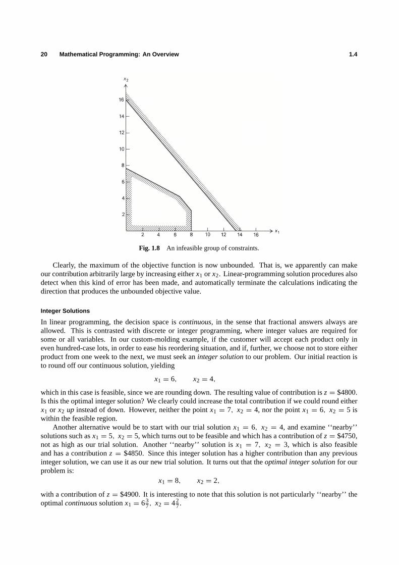
Until now we have described a number of the properties of an optimal solution to a linear program, assumingfirst that there was such a solution and second that we were able to find it. It could happen that a linear programhasnofeasible solution. An infeasible linear program might result from a poorly formulated problem, or froma situation where requirements exceed the capacity of the existing available resources. Suppose, for example,that an additional constraint was added to the model imposing a minimum on the number of production hoursworked. However, in recording the data, an error was made that resulted in the following constraint beingincluded in the formulation:
6x1+ 5x2 ≥ 80.
The graphical representation of this error is given in Fig. 1.8.The shading indicates the direction of the inequalities associated with each constraint. Clearly, there are
no points that satisfy all the constraints simultaneously, and the problem is therefore infeasible. Computerroutines for solving linear programs must be able to tell the user when a situation of this sort occurs. Ingeneral, on large problems it is relatively easy to have infeasibilities in the initial formulation and not knowit. Once these infeasibilities are detected, the formulation is corrected.
Another type of error that can occur is somewhat less obvious but potentially more costly. Suppose thatwe consider our original custom-molder problem but that a control message was typed into the computerincorrectly so that we are, in fact, attempting to solve our linear program with ‘‘greaterthan or equal to’’constraints instead of ‘‘lessthan or equal to’’ constraints. We would then have the following linear program:
Maximizez= 500x1+ 450x2,
subject to:6x1 + 5x2 ≥ 60,
10x1 + 20x2 ≥ 150,
x1 ≥ 8,
x1 ≥ 0, x2 ≥ 0.
The graphical representation of this error is given in Fig. 1.9.
20 Mathematical Programming: An Overview 1.4
Fig. 1.8 An infeasible group of constraints.
Clearly, the maximum of the objective function is now unbounded. That is, we apparently can makeour contribution arbitrarily large by increasing eitherx1 or x2. Linear-programming solution procedures alsodetect when this kind of error has been made, and automatically terminate the calculations indicating thedirection that produces the unbounded objective value.
Integer Solutions
In linear programming, the decision space iscontinuous, in the sense that fractional answers always areallowed. This is contrasted with discrete or integer programming, where integer values are required forsome or all variables. In our custom-molding example, if the customer will accept each product only ineven hundred-case lots, in order to ease his reordering situation, and if, further, we choose not to store eitherproduct from one week to the next, we must seek aninteger solutionto our problem. Our initial reaction isto round off our continuous solution, yielding
x1 = 6, x2 = 4,
which in this case is feasible, since we are rounding down. The resulting value of contribution isz= $4800.Is this the optimal integer solution? We clearly could increase the total contribution if we could round eitherx1 or x2 up instead of down. However, neither the pointx1 = 7, x2 = 4, nor the pointx1 = 6, x2 = 5 iswithin the feasible region.
Another alternative would be to start with our trial solutionx1 = 6, x2 = 4, and examine ‘‘nearby’’solutions such asx1 = 5, x2 = 5, which turns out to be feasible and which has a contribution ofz= $4750,not as high as our trial solution. Another ‘‘nearby’’ solution isx1 = 7, x2 = 3, which is also feasibleand has a contributionz = $4850. Since this integer solution has a higher contribution than any previousinteger solution, we can use it as our new trial solution. It turns out that theoptimal integer solutionfor ourproblem is:
x1 = 8, x2 = 2,
with a contribution ofz= $4900. It is interesting to note that this solution is not particularly ‘‘nearby’’ theoptimalcontinuoussolutionx1 = 63
7, x2 = 427.

1.4 A Geometrical Preview 21
Fig. 1.9 An unbounded solution.
Basically, the integer-programming problem is inherently difficult to solve and falls in the domain ofcombinatorial analysisrather than simple linear programming. Special algorithms have been developed tofind optimal integer solutions; however, the size of problem that can be solved successfully by these algorithmsis an order of magnitude smaller than the size of linear programs that can easily be solved. Whenever it ispossible to avoid integer variables, it is usually a good idea to do so. Often what at first glance seem to be integervariables can be interpreted as production or operatingrates, and then the integer difficulty disappears. In ourexample, if it is not necessary to ship in even hundred-case lots, or if the odd lots are shipped the followingweek, then it still is possible to produce at ratesx1 = 63
7 andx2 = 427 hundred cases per week. Finally, in
any problem where the numbers involved are large, rounding to a feasible integer solution usually results ina good approximation.
Nonlinear Functions
In linear programming the variables are continuous and the functions involved are linear. Let us now considerthe decision problem of the custom molder in a slightly altered form. Suppose that the interpretation ofproduction in terms of rates is acceptable, so that we need not find an integer solution; however, we now haveanonlinearobjective function. We assume that the injection-molding machine is fairly old and that operatingnear capacity results in a reduction in contribution per unit for each additional unit produced, due to highermaintenance costs and downtime. Assume that the reduction is $0.05 per case of six-ounce juice glasses and$0.04 per case of ten-ounce cocktail glasses. In fact, let us assume that we have fit the following functions toper-unit contribution for each type of glass:
z1(x1) = 60− 5x1 for six-ounce juice glasses,
z2(x2) = 80− 4x2 for ten-ounce cocktail glasses.
The resulting total contribution is then given by:
(60− 5x1)x1+ (80− 4x2)x2.
Hence, we have the following nonlinear programming problem to solve:
Maximizez= 60x1− 5x21 + 80x2− 4x2
2,

22 Mathematical Programming: An Overview 1.5
subject to:6x1 + 5x2 ≤ 60,
10x1 + 20x2 ≤ 150,
x1 ≤ 8,
x1 ≥ 0, x2 ≥ 0.
This situation is depicted in Fig. 1.10. The curved lines represent lines of constant contribution.Note that the optimal solution is no longer at a corner point of the feasible region. This property alone
makes finding an optimal solution much more difficult than in linear programming. In this situation, wecannot merely move from vertex to vertex, looking for an improvement at each iteration. However, thisparticular problem has the property that, if you have a trial solution and cannot find an improving directionto move in, thenthe trial solution is an optimal solution. It is this property that is generally exploited incomputational procedures for nonlinear programs.
Fig. 1.10 The nonlinear program.
1.5 A CLASSIFICATION OF MATHEMATICAL PROGRAMMING MODELS
We are now in a position to provide a general statement of the mathematical programming problem andformally summarize definitions and notation introduced previously. Let us begin by giving a formal repre-sentation of the general linear programming model.
In mathematical terms, the linear programming model can be expressed as the maximization (or mini-mization) of anobjective(or criterion)function, subject to a given set of linearconstraints. Specifically, thelinear programming problem can be described as finding the values ofn decision variables,x1, x2, . . . , xn,such that they maximize the objective functionz where
z= c1x1+ c2x2+ · · · + cnxn, (22)
subject to the following constraints:a11x1 + a12x2 + · · · + a1nxn ≤ b1,
a21x1 + a22x2 + · · · + a2nxn ≤ b2,
......
am1x1 + am2x2 + · · · + amnxn ≤ bm,
(23)
and, usually,x1 ≥ 0, x2 ≥ 0, . . . , xn ≥ 0, (24)

1.5 A Classification of Mathematical Programming Models 23
wherec j , ai j , andbi are given constants.It is easy to provide an immediate interpretation to the general linear-programming problem just stated
in terms of a production problem. For instance, we could assume that, in a given production facility, therearen possible products we may manufacture; for each of these we want to determine the level of productionwhich we shall designate byx1, x2, . . . , xn. In addition, these products compete form limited resources,which could be manpower availability, machine capacities, product demand, working capital, and so forth,and are designated byb1, b2, . . . , bm. Letai j be the amount of resourcei required by productj and letc j bethe unit profit of productj . Then the linear-programming model seeks to determine the production quantityof each product in such a way as to maximize the total resulting profitz (Eq. 22), given that the availableresources should not be exceeded (constraints 23), and that we can produce onlypositiveor zeroamounts ofeach product (constraints 24).
Linear programming is not restricted to the structure of the problem presented above. First, it is perfectlypossible to minimize, rather than maximize, the objective function. In addition, ‘‘greater than or equal to’’ or‘‘equal to’’ constraints can be handled simultaneously with the ‘‘less than or equal to’’ constraints presentedin constraints (23). Finally, some of the variables may assume both positive and negative values.
There is some technical terminology associated with mathematical programming, informally introducedin the previous section, which we will now define in more precise terms. Values of the decision variablesx1, x2, . . . , xn that satisfy all the constraints of (23) and (24) simultaneously are said to form afeasiblesolutionto the linear programming problem. The set ofall values of the decision variables characterized byconstraints (23) and (24) form thefeasible regionof the problem under consideration. A feasible solutionthat in addition optimizes the objective function (22) is called anoptimal feasible solution.
As we have seen in the geometric representation of the problem, solving a linear program can result inthree possible situations.
i) The linear program could be infeasible, meaning that there are no values of the decision variablesx1, x2, . . . , xn that simultaneously satisfy all the constraints of (23) and (24).
ii) It could have an unbounded solution, meaning that, if we are maximizing, the value of the objectivefunction can be increased indefinitely without violating any of the constraints. (If we are minimizing, thevalue of the objective function may be decreased indefinitely.)
iii) In most cases, it will have at least one finite optimal solution and often it will have multiple optimalsolutions.
The simplex methodfor solving linear programs, which will be discussed in Chapter 2, provides anefficient procedure for constructing an optimal solution, if one exists, or for determining whether the problemis infeasible or unbounded.
Note that, in the linear programming formulation, the decision variables are allowed to take any continuousvalue. For instance, values such thatx1 = 1.5, x2 = 2.33, are perfectly acceptable as long as they satisfyconstraints (23) and (24). An important extension of this linear programming model is to require that all orsome of the decision variables be restricted to be integers.
Another fundamental extension of the above model is to allow the objective function, or the constraints,or both, to be nonlinear functions. The general nonlinear programming model can be stated as finding thevalues of the decision variablesx1, x2, . . . , xn that maximize the objective functionz where
z= f0(x1, x2, . . . , xn), (25)
subject to the following constraints:f1(x1, x2, . . . , xn) ≤ b1,
f2(x1, x2, . . . , xn) ≤ b2,
...
fm(x1, x2, . . . , xn) ≤ bm,
(26)

24 Mathematical Programming: An Overview
and sometimesx1 ≥ 0, x2 ≥ 0, . . . , xn ≥ 0. (27)
Often in nonlinear programming the righthand-side values are included in the definition of the functionfi (x1, x2, . . . , xn), leaving the righthand side zero. In order to solve a nonlinear programming problem,some assumptions must be made about the shape and behavior of the functions involved. We will leavethe specifics of these assumptions until later. Suffice it to say that the nonlinear functions must be ratherwell-behaved in order to have computationally efficient means of finding a solution.
Optimization models can be subject to various classifications depending on the point of view we adopt.According to the number of time periods considered in the model, optimization models can be classified asstatic (single time period) ormultistage(multiple time periods). Even when all relationships are linear, ifseveral time periods are incorporated in the model the resulting linear program could become prohibitivelylarge for solution by standard computational methods. Fortunately, in most of these cases, the problemexhibits some form of special structure that can be adequately exploited by the application of special typesof mathematical programming methods. Dynamic programming, which is discussed in Chapter 11, is oneapproach for solving multistage problems. Further, there is a considerable research effort underway today, inthe field of large-scale linear programming, to develop special algorithms to deal with multistage problems.Chapter 12 addresses these issues.
Another important way of classifying optimization models refers to the behavior of the parameters ofthe model. If the parameters are known constants, the optimization model is said to bedeterministic. If theparameters are specified as uncertain quantities, whose values are characterized by probability distributions,the optimization model is said to bestochastic. Finally, if some of the parameters are allowed to vary systema-tically, and the changes in the optimum solution corresponding to changes in those parameters are determined,the optimization model is said to beparametric. In general, stochastic and parametric mathematical program-ming give rise to much more difficult problems than deterministic mathematical programming. Althoughimportant theoretical and practical contributions have been made in the areas of stochastic and parametricprogramming, there are still no effective general procedures that cope with these problems. Deterministiclinear programming, however, can be efficiently applied to very large problems of up to 5000 rows and analmost unlimited number of variables. Moreover, in linear programming, sensitivity analysis and parametricprogramming can be conducted effectively after obtaining the deterministic optimum solution, as will be seenin Chapter 3.
A third way of classifying optimization models deals with the behavior of the variables in the optimalsolution. If the variables are allowed to take any value that satisfies the constraints, the optimization modelis said to becontinuous. If the variables are allowed to take on only discrete values, the optimization modelis calledintegeror discrete. Finally, when there are some integer variables and some continuous variablesin the problem, the optimization model is said to bemixed. In general, problems with integer variablesare significantly more difficult to solve than those with continuous variables. Network models, which arediscussed in Chapter 8, are a class of linear programming models that are an exception to this rule, as theirspecial structure results in integer optimal solutions. Although significant progress has been made in thegeneral area of mixed and integer linear programming, there is still no algorithm that can efficiently solve allgeneral medium-size integer linear programs in a reasonable amount of time though, for special problems,adequate computational techniques have been developed. Chapter 9 comments on the various methodsavailable to solve integer programming problems.
EXERCISES
1. Indicate graphically whether each of the following linear programs has a feasible solution. Graphically determinethe optimal solution, if one exists, or show that none exists.
a) Maximizez= x1+ 2x2,
Exercises 25
subject to:x1− 2x2 ≤ 3,
x1+ x2 ≤ 3,
x1 ≥ 0, x2 ≥ 0.
b) Minimize z= x1+ x2,
subject to:x1− x2 ≤ 2,
x1− x2 ≥ −2,
x1 ≥ 0, x2 ≥ 0.
c) Redo (b) with the objective function
Maximizez= x1+ x2.
d) Maximizez= 3x1+ 4x2,
subject to:x1− 2x2 ≥ 4,
x1+ x2 ≤ 3,
x1 ≥ 0, x2 ≥ 0.
2. Consider the following linear program:
Maximizez= 2x1+ x2,
subject to:
12x1 + 3x2 ≤ 6,
−3x1 + x2 ≤ 7,
x2 ≤ 10,
x1 ≥ 0, x2 ≥ 0.
a) Draw a graph of the constraints and shade in the feasible region. Label the vertices of this region with theircoordinates.
b) Using the graph obtained in (a), find the optimal solution and the maximum value of the objective function.c) What is the slack in each of the constraints?d) Find the shadow prices on each of the constraints.e) Find the ranges associated with the two coefficients of the objective function.f) Find the righthand-side ranges for the three constraints.
3. Consider the bond-portfolio problem formulated in Section 1.3. Reformulate the problem restricting the bondsavailable only to bonds A and D. Further add a constraint that the holdings of municipal bonds must be less than orequal to $3 million.
a) What is the optimal solution?b) What is the shadow price on the municipal limit?c) How much can the municipal limit be relaxed before it becomes a nonbinding constraint?d) Below what interest rate is it favorable to borrow funds to increase the overall size of the portfolio?e) Why is this rate less than the earnings rate on the portfolio as a whole?
4. A liquor company produces and sells two kinds of liquor: blended whiskey and bourbon. The company purchasesintermediate products in bulk, purifies them by repeated distillation, mixes them, and bottles the final product undertheir own brand names. In the past, the firm has always been able to sell all that it produced.
The firm has been limited by its machine capacity and available cash. The bourbon requires 3 machine hours perbottle while, due to additional blending requirements, the blended whiskey requires 4 hours of machine time perbottle. There are 20,000 machine hours available in the current production period. The direct operating costs, whichare principally for labor and materials, are $3.00 per bottle of bourbon and $2.00 per bottle of blended whiskey.

26 Mathematical Programming: An Overview
The working capital available to finance labor and material is $4000; however, 45% of the bourbon sales revenuesand 30% of the blended-whiskey sales revenues from production in the current period will be collected during thecurrent period and be available to finance operations. The selling price to the distributor is $6 per bottle of bourbonand $5.40 per bottle of blended whiskey.
a) Formulate a linear program that maximizes contribution subject to limitations on machine capacity and workingcapital.
b) What is the optimal production mix to schedule?c) Can the selling prices change without changing the optimal production mix?d) Suppose that the company could spend $400 to repair some machinery and increase its available machine hours
by 2000 hours. Should the investment be made?e) What interest rate could the company afford to pay to borrow funds to finance its operations during the current
period?
5. The truck-assembly division of a large company produces two different models: the Aztec and the Bronco. Theirbasic operation consists of separate assembly departments: drive-train, coachwork, Aztec final, and Bronco final.The drive-train assembly capacity is limited to a total of 4000 units per month, of either Aztecs or Broncos, since ittakes the same amount of time to assemble each. The coachwork capacity each month is either 3000 Aztecs or 6000Broncos. The Aztecs, which are vans, take twice as much time for coachwork as the Broncos, which are pickups.The final assembly of each model is done in separate departments because of the parts availability system. Thedivision can do the final assembly of up to 2500 Aztecs and 3000 Broncos each month.
The profit per unit on each model is computed by the firm as follows:
Aztec Bronco
Selling Price $4200 $4000Material cost $2300 $2000Labor cost 400 2700 450 2450
Gross Margin $1500 $1550Selling & Administrative∗ $ 210 $ 200Depreciation† 60 180Fixed overhead† 50 150Variable overhead 590 910 750 1280
Profit before taxes $ 590 $ 270
∗ 5% of selling price.† Allocated according to planned production of 1000 Aztecs and 3000 Broncos per monthfor the coming year.
a) Formulate a linear program to aid management in deciding how many trucks of each type to produce per month.b) What is the proper objective function for the division?c) How many Aztecs and Broncos should the division produce each month?
6. Suppose that the division described in Exercise 5 now has the opportunity to increase its drive-train capacity bysubcontracting some of this assembly work to a nearby firm. The drive-train assembly department cost breakdownper unit is as follows:
Aztec Bronco
Direct labor $ 80 $ 60Fixed overhead 20 60Variable overhead 200 150
$300 $270
The subcontractor will pick up the parts and deliver the assembled drive-trains back to the division. What is themaximum amount that the division would be willing to pay the subcontractor for assembly of each type of drive-train?

Exercises 27
7. Suppose that the division described in Exercises 5 and 6 has decided against subcontracting the assembly of drive-trains but now is considering assembling drive-trains on overtime. If there is a 50% overtime labor premium on eachdrive-train assembled on overtime and increased fixed overhead of $150,000 per month, should the division go onovertime drive-train production? Formulate a linear program to answer this question, but do not solve explicitly.
8. A manufacturer of wire cloth products can produce four basic product lines: (1) industrial wire cloth; (2) insectscreen; (3) roofing mesh; and (4) snow fence. He can sell all that he can produce of each product line for the nextyear.
The production process for each product line is essentially the same. Aluminum wire is purchased in largediameters of approximately 0.375 inches and drawn down to finer diameters of 0.009 to 0.018 inches. Then the finewire is woven on looms, in much the same manner as textiles. Various types of different wire meshes are produced,depending on product line. For example, industrial wire cloth consists of meshes as fine as 30 wires per inch, whilesnow fence has approximately 6 wires per inch. The production process is limited by both wire-drawing capacityand weaving capacity, as well as the availability of the basic raw material, large-diameter aluminum wire.
For the next planning period, there are 600 hours of wire-drawing machine capacity, 1000 hours of loom capacity,and 15 cwt (hundred weight) of large-diameter aluminum wire. The four product lines require the following inputsto make a thousand square feet of output:
Aluminum Wire drawing Weavingwire (cwt) (100’s of hrs) (100’s of hrs)
Industrial cloth 1 1 2Insect screen 3 1 1Roofing mesh 3 2 1.5Snow fence 2.5 1.5 2
The contributions from industrial cloth, insect screen, roofing mesh, and snow fence are 2.0, 3.0, 4.2, and 4.0,respectively, in 100’s of dollars per thousand square feet.
a) Formulate a linear program to maximize the firm’s contribution from the four product lines.b) Since roofing mesh and snow fence are really new product lines, analyze the problem graphically, considering
only industrial wire cloth and insect screen.
i) What is the optimal solution using only these two product lines?ii) Over what range of contribution of screen cloth will this solution remain optimal?
iii) Determine the shadow prices on the resources for this solution. Give an economic interpretation of theseshadow prices.
iv) Suppose that the manufacturer is considering adding wire-drawing capacity. Over what range of wire-drawing capacity will the shadow price on this constraint remain unchanged? In this range, what happens tothe other shadow prices?
c) Now, considering thefull line of four products, answer the following, making use of the information developedin (b).
i) Will it pay to transfer resources into the production of roofing mesh or snow fence?ii) Without performing the calculations, what will be the form of the optimal solution of the full product line?
What is the largest number of product lines that will be produced?iii) Suppose that in the future some new product line is developed. Is it possible that one of the product linesnot
presently included in the optimal solution will then be included? Explain.
9. The Candid Camera Company manufactures three lines of cameras: the Cub, the Quickiematic and the VIP, whosecontributions are $3, $9, and $25, respectively. The distribution center requires that at least 250 Cubs, 375 Quick-iematics, and 150 VIPs be produced each week.
Each camera requires a certain amount of time in order to: (1) manufacture the body parts; (2) assemble theparts (lenses are purchased from outside sources and can be ignored in the production scheduling decision); and (3)inspect, test, and package the final product. The Cub takes 0.1 hours to manufacture, 0.2 hours to assemble, and 0.1hours to inspect, test, and package. The Quickiematic needs 0.2 hours to manufacture, 0.35 hours to assemble, and0.2 hours for the final set of operations. The VIP requires 0.7, 0.1, and 0.3 hours, respectively. In addition, thereare 250 hours per week of manufacturing time available, 350 hours of assembly, and 150 hours total to inspect, test,and package.
Formulate this scheduling problem as a linear program that maximizes contribution.

28 Mathematical Programming: An Overview
10. A leather-goods factory manufactures five styles of handbags, whose variable contributions are $30, $40, $45, $25,and $60 per dozen, respectively. The products must pass through four work centers and the man-hours availablein each are: clicking (700), paring (600), stitching (400), and finishing (900). Hourly requirements for each dozenhandbags are:
Style Click Pare Stitch Finish
341 3 8 2 6262 4 3 1 0
43 2 2 0 2784 2 1 3 4
5-A 5 4 4 3
To prevent adding to inventory levels already on hand, the production manager, after reviewing the weekly salesforecasts, has specified that no more than 100, 50, 90, 70, and 30 dozen of each style respectively may be produced.Each handbag is made from five materials as specified in the following table:
Style Leather Fabric Backing Lining Accessories
341 0 1 4 2 3262 4 0 7 4 443 5 7 6 2 0
784 6 4 1 1 25-A 2 3 3 0 4
Totalavailable 300 400 1000 900 1600
Formulate a linear program for next week’s optimum manufacturing schedule if overall contribution is to be maxi-mized.
11. A corporation that produces gasoline and oil specialty additives purchases three grades of petroleum distillates, A, B,and C. The company then combines the three according to specifications of the maximum or minimum percentagesof grades A or C in each blend.
Max % Min % Sellingallowed for allowed for price
Mixture AdditiveA AdditiveC $/gallon
Deluxe 60% 20% 7.9Standard 15% 60% 6.9Economy — 50% 5.0
Supplies of the three basic additives and their costs are:
Maximum quantity CostDistillate available per day(gals) $/gallon
A 4000 0.60B 5000 0.52C 2500 0.48
Show how to formulate a linear program to determine the production policy that will maximize profits.
12. Universal Aviation currently is investigating the possibility of branching out from its passenger service into thesmall-plane air-freight business. With $4,000,000 available to invest in the purchase of new twin-engined cargoaircraft, Universal is considering three types of planes. Aircraft A, costing $80,000, has a ten-ton payload and isexpected to cruise at 350 knots, while airplane B can haul 20 tons of goods at an average speed of 300 knots. Aircraft

Exercises 29
B will cost $130,000. The third aircraft is a modified form of B with provisions for a copilot, a 300-knot cruisingspeed, a reduced capacity of 18 tons, and a cost of $150,000.
Plane A requires one pilot and, if flown for three shifts, could average 18 hours a day in the air, as couldaircraft B. While transports B and C both require a crew of two, C could average 21 hours of flying per day on athree-shift pilot basis due to superior loading equipment. Universal’s operations department currently estimates that150 pilot-shifts will be available for each day’s cargo operations. Limitations on maintenance facilities indicate thatno more than thirty planes can be purchased. The contributions of planes A, B, and C per ton-mile are, respectively,$1, $8, and $120. 3,500,000 ton-miles of shipping must be completed each day, but deliveries not completed by thein-house fleet can still be sub-contracted to outside air carriers at a contribution of $0.20 per ton mile. What ‘‘mix’’of aircraft should be purchased if the company desires to maximize its contribution per day? (Note.Consider a knot= 1 mile/hour.)
13. A mobile-home manufacturer in Indiana channels its mobile-home units through distribution centers located inElkhart, Ind., Albany, N.Y., Camden, N.J., and Petersburg, Va. An examination of their shipping department recordsindicates that, in the upcoming quarter, the distribution centers will have in inventory 30, 75, 60, and 35 mobilehomes, respectively. Quarterly orders submitted by dealerships serviced by the distribution centers require thefollowing numbers of mobile home units for the upcoming quarter:
Number of units Number of units
Dealer A 25 Dealer D 25Dealer B 40 Dealer E 50Dealer C 15 Dealer F 45
Transportation costs (in dollars per unit) between each distribution center and the dealerships are as shown in thetable below.
Dealers
Distributioncenters A B C D E F
Elkhart 75 65 175 90 110 150Albany 90 30 45 50 105 130Camden 40 55 35 80 70 75Petersburg 95 150 100 115 55 55
a) Formulate this problem as a linear-programming problem with the objective of minimizing the transportationcosts from the distribution centers to the dealerships.
b) Suppose Dealer E had placed an order for 65 units, assuming all other data remain unchanged. How does thisaffect the problem? (Note that total supply is less than total demand.)
14. A strategic planner for an airline that flies to four different cities from its Boston base owns 10 large jets (B707’s),15 propeller-driven planes (Electra’s), and two small jets (DC9’s).
Assuming constant flying conditions and passenger usage, the following data is available.

30 Mathematical Programming: An Overview
Average flyingCity Trip cost* Trip revenue time(hours)
B707 A $ 6,000 $ 5,000 1B 7,000 7,000 2C 8,000 10,000 5D 10,000 18,000 10
Electra A $ 1,000 $ 3,000 2B 2,000 4,000 4C 4,000 6,000 8D 20
DC9 A $ 2,000 $ 4,000 1B 3,500 5,500 2C 6,000 8,000 6D 10,000 14,000 12
* Data is for a round trip.
Formulate constraints to take into account the following:
i) city D must be served twice daily; cities A, B, and C must be served four times daily;ii) limitation on number of planes available, assuming that each plane can fly at most 18 hours/day.
Formulate objective functions for:
i) cost minimization;ii) profit maximization;
iii) fleet flying-time minimization.
Indicate when a continuous linear-programming formulation is acceptable, and when an integer-programming for-mulation is required.
15. The Temporary Help Company must provide secretaries to its clients over the next year on the following estimatedschedule: spring, 6000 secretary-days; summer, 7500 secretary-days; fall, 5500 secretary-days; and winter, 9000secretary-days. A secretary must be trained for 5 days before becoming eligible for assignment to clients.
There are 65 working days in each quarter, and at the beginning of the spring season there are 120 qualifiedsecretaries on the payroll. The secretaries are paid by the company and not the client; they earn a salary of $800 amonth. During each quarter, the company loses 15% of its personnel (including secretaries trained in the previousquarter).
Formulate the problem as a linear-programming problem. (Hint: Usext as the number of secretaries hired atthe beginning of seasont , andSt as the total number of secretaries at the beginning of seasont .)
16. An imaginary economy has six distinct geographic regions; each has its own specific economic functions, as follows:
Region Function
A Food producingB Manufacturing—MachineryC Manufacturing—Machinery and consumer durablesD AdministrativeE Food-producingF Manufacturing—Consumer durables and nondurables
The regions also have the following annual requirements (all quantities measured in tons):

Exercises 31
Consumer ConsumerRegion Food Machinery durables nondurables
A 5 30 20 10B 15 100 40 30C 20 80 50 40D 30 10 70 60E 10 60 30 20F 25 60 60 50
Using the national railroad, shipping costs are $1/ton per 100 miles for all hauls over 100 miles. Within 100miles, all goods are carried by truck at a cost of $1.25/ton per 100 miles ($1/ton minimum charge). The distances(in miles) between regions are as follows:
A B C D E F
AB 500C 200 400D 75 500 150E 600 125 350 550F 300 200 100 400 300
Assume producing regions can meet all requirements, but that, due to government regulation, food production insector A is restricted to half that of sector E.
Formulate a linear program that will meet the requirements and minimize the total transportation costs in theeconomy.
17. The Environmental Protection Agency (EPA) wants to restrict the amount of pollutants added by a company to theriver water. The concentrations of phenol and nitrogen in the water are to be restricted to, respectively,P and Nlbs. MG (million gallons) on a daily basis. The river has a flow ofM MG/day. The company diverts a portion ofthe river water, adds the pollutants, namely, phenol and nitrogen, to it, and sends the water back to the river. Thecompany has four possible ways to treat the water it uses before returning it to the river. The characteristics of eachtreatment are given in the following table:
(lbs. of pollutant)/MG after treatment
Treatment 1 2 3 4
Phenol P1 P2 P3 P4Nitrogen N1 N2 N3 N4
Cost/MG c1 c2 c3 c4
Assume: (i) that the river is initially free of pollutants; (ii) that addition of pollutants does not affect the amountof water flow; and (iii) that the company has to process at leastK (MG/day) of river water.
a) Set up a linear program to solve for the amount of water to be processed by each treatment, so that total cost oftreatment is minimized.
b) How does the formulation change if the EPA regulations apply not to total river concentration downstream fromthe plant, but rather to the concentration of effluent from the plant?
18. Suppose the company of Exercise 17 has three plants, A, B, and C, in a river network as shown below:
River water can be clean enough for (1) swimming, or (2) to support bio-life (but not clean enough for swimming).Maximum permissible concentrations of pollutants for both cases are given in the table below.

32 Mathematical Programming: An Overview
Maximum permissible concentrations(lbs./MG)
Swimming Biological life
Phenol PS PB
Nitrogen NS NB
Assume again that each plant has four different alternatives for water treatment, as in the table of Exercise 17,and that A, B, and C must process at leastKA , KB, KC MG/day, respectively. It is necessary that water in sections(1) and (3) be clean enough for swimming and that water in section (2) be clean enough to support bio-life.
Further, assume: (i) that the river is free of pollutants upstream from plants A and B; and (ii) that addingpollutants does not affect the amount of water flow.
a) Formulate a linear program, including plants A, B, and C, that minimizes total treatment costs.b) How would the formulation change if all the plants did not necessarily have the same capabilities and cost
structure for each treatment? Indicate modifications only—do not reformulate completely.19. ‘‘Chemico’’ company produces 3 products from a certain mineral. The production process consists of 2 stages:
mining the crude mineral, and processing the mineral to produce 3 different products.The crude mineral can be mined by one of 5 methods. The quality of the mineral depends on the method used
and is measured by the percentage of the quantity of the final products that are produced from 1 ton of crude mineral.Furthermore, the distribution of products obtained from 1 ton of crude mineral depends on the mining method used.
A limited amount of the crude mineral can be mined by each method. In addition, the capacity of the productionprocess is limited to 850 tons of crude mineral. The following table gives the relevant data.
Mining Cost Production Production(per ton of No. of hours capacity Distribution
Mining final products) per 1 ton of (tons of Product Product ProductMine Method ($) final productsQuality crude material) I II III
A 1 250 50 65% 300 20% 30% 50%2 320 62 80% 280 25% 35% 40%3 260 63 76% 400 15% 45% 40%
B 4 210 55 76% 250 7% 24% 69%5 350 60 78% 500 35% 40% 25%
Note that the mining costs are per 1 ton of final products, and not per 1 ton of crude mineral. The productioncapacity of each mining method is in terms of crude material.
There are 2 mines: Mine A uses methods 1 and 2, whereas Mine B uses methods 3, 4, and 5. The total numberof work hours available in Mines A and B are 13,000 and 15,000, respectively (for the planning period). It is possibleto transfer workers from A to B and vice versa, but it costs $2 to transfer 1 work hour, and 10% of the transferredwork hours are wasted.
The company sells its products in 5 markets. The selling price depends on the market, and in each market theamount that can be sold is limited. The relevant data are given in a second table:

Exercises 33
Price per 1 ton Max. amountMarket Product ($) (tons)
1 I 1550 150
2 I 1600 100
3 II 1400 200
4 III 1000 50
5 III 850 400
Management wants to plan the production for the next period such that the profit will be maximized. They wantto know how many work hours to assign to each mine, what amount to sell in each market, and what is the expectedprofit. Formulate the problem as a linear program.
20. From past data, the production manager of a factory knows that, by varying his production rate, he incurs additionalcosts. He estimates that his cost per unit increases by $0.50 when production is increased from one month to the next.Similarly, reducing production increases costs by $0.25 per unit. A smooth production rate is obviously desirable.
Sales forecasts for the next twelve months are (in thousands):
July 4 October 12 January 20 April 6August 6 November 16 February 12 May 4September 8 December 20 March 8 June 4
June’s production schedule already has been set at 4000 units, and the July 1 inventory level is projected to be 2000units. Storage is available for only 10,000 units at any one time. Ignoring inventory costs, formulate a productionschedule for the coming year that will minimize the cost of changing production rates while meeting all salesdemands. (Hint: Express the change in production from montht to montht + 1 in terms of nonnegative variablesx+t andx−t asx+t − x−t . Variablex+t is the increase in production andx−t the decrease. It is possible for bothx+tandx−t to be positive in the optimal solution?)
21. Videocomp, Inc., a new manufacturer of cathode ray tube (CRT) devices for computer applications, is planning toenlarge its capacity over the next two years. The company’s primary objective is to grow as rapidly as possible overthese two years to make good on its marketing claims.
The CRT’s are produced in sets of 200 units on modular assembly lines. It takes three months to produce aset of 200 units from initial chemical coating to final assembly and testing. To ensure quality control, none of theunits in a set is shipped until the entire set has been completed. Videocomp has three modular assembly lines andthus currently can produce up to 600 units in a quarter. Each set of 200 units requires $15,000 at the beginning ofthe quarter when production is initiated for purchasing component parts and paying direct labor expenses. Each setproduces revenue of $35,000, of which 20% is received at the time of shipment and the remaining 80% a full threemonths later.
Videocomp has negotiated the terms for adding modular assembly lines with a number of contractors andhas selected two possible contractors. The first contractor requires an investment of $60,000 paid in advance andguarantees that the assembly line will be completed in three months. For the same assembly line, the secondcontractor requires an investment of $20,000 in advance and an additional investment of $20,000 upon completion;however, his completion time is six months.
The present assets of Videocomp for investment in new modular assembly lines and financing current operationsare $150,000. No further funds will be made available except those received from sales of CRT’s. However, as themarket is expanding rapidly, all CRT’s produced can be sold immediately.
Formulate a linear program to maximize Videocomp’s productive capacity at the end of two years using eightplanning periods of three months’ duration each.
22. A rent-a-car company operates a rental-agent training program, which students complete in one month. The teachersin this program are trained rental agents, at a ratio of one for every fifteen students. Experience has shown that
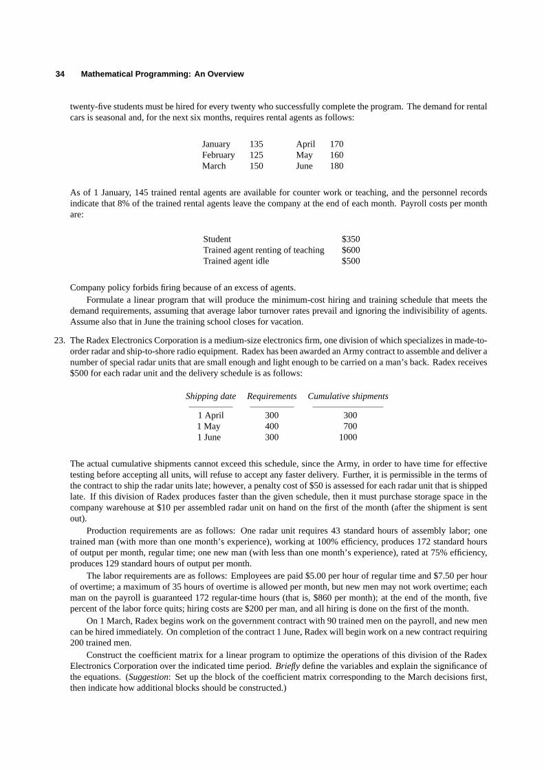
34 Mathematical Programming: An Overview
twenty-five students must be hired for every twenty who successfully complete the program. The demand for rentalcars is seasonal and, for the next six months, requires rental agents as follows:
January 135 April 170February 125 May 160March 150 June 180
As of 1 January, 145 trained rental agents are available for counter work or teaching, and the personnel recordsindicate that 8% of the trained rental agents leave the company at the end of each month. Payroll costs per monthare:
Student $350Trained agent renting of teaching $600Trained agent idle $500
Company policy forbids firing because of an excess of agents.Formulate a linear program that will produce the minimum-cost hiring and training schedule that meets the
demand requirements, assuming that average labor turnover rates prevail and ignoring the indivisibility of agents.Assume also that in June the training school closes for vacation.
23. The Radex Electronics Corporation is a medium-size electronics firm, one division of which specializes in made-to-order radar and ship-to-shore radio equipment. Radex has been awarded an Army contract to assemble and deliver anumber of special radar units that are small enough and light enough to be carried on a man’s back. Radex receives$500 for each radar unit and the delivery schedule is as follows:
Shipping date Requirements Cumulative shipments
1 April 300 3001 May 400 7001 June 300 1000
The actual cumulative shipments cannot exceed this schedule, since the Army, in order to have time for effectivetesting before accepting all units, will refuse to accept any faster delivery. Further, it is permissible in the terms ofthe contract to ship the radar units late; however, a penalty cost of $50 is assessed for each radar unit that is shippedlate. If this division of Radex produces faster than the given schedule, then it must purchase storage space in thecompany warehouse at $10 per assembled radar unit on hand on the first of the month (after the shipment is sentout).
Production requirements are as follows: One radar unit requires 43 standard hours of assembly labor; onetrained man (with more than one month’s experience), working at 100% efficiency, produces 172 standard hoursof output per month, regular time; one new man (with less than one month’s experience), rated at 75% efficiency,produces 129 standard hours of output per month.
The labor requirements are as follows: Employees are paid $5.00 per hour of regular time and $7.50 per hourof overtime; a maximum of 35 hours of overtime is allowed per month, but new men may not work overtime; eachman on the payroll is guaranteed 172 regular-time hours (that is, $860 per month); at the end of the month, fivepercent of the labor force quits; hiring costs are $200 per man, and all hiring is done on the first of the month.
On 1 March, Radex begins work on the government contract with 90 trained men on the payroll, and new mencan be hired immediately. On completion of the contract 1 June, Radex will begin work on a new contract requiring200 trained men.
Construct the coefficient matrix for a linear program to optimize the operations of this division of the RadexElectronics Corporation over the indicated time period.Briefly define the variables and explain the significance ofthe equations. (Suggestion: Set up the block of the coefficient matrix corresponding to the March decisions first,then indicate how additional blocks should be constructed.)

Exercises 35
24. Construct the coefficient matrix, define each of the variables, and explain briefly the significance of each equationor inequality in the linear-programming model for optimal operation, during March and April, of the hydroelectricpower system described as follows:
The system consists of two dams and their associated reservoirs and power plants on a river. The importantflows of power and water are shown in the accompanying diagram.
In the following table, all quantities measuring water are in units of 103 acre-feet (KAF). Power is measured inmegawatt hours (MWH).
A B Units
Storage capacity 2,000 1,500 KAFMinimum allowable level 1,200 800 KAFPredicted inflow:
March 200 40 KAFApril 130 15 KAF
March 1 level 1,900 850 KAFWater-power conversion 400 200 MWH/KAFPower-plant capacity 60,000 35,000 MWH/per month
Power can be sold at $5.00 per MWH for up to 50,000 MWH each month, and excess power above that figure canbe sold for $3.50 per MWH.
Assume flow rates in and out through the power plants are constant within the month. If the capacity of thereservoir is exceeded, the excess water runs down the spillway and by-passes the power plant. A consequence ofthese assumptions is that the maximum and minimum water-level constraints need to be satisfied only at the end ofthe month. (Suggestion: First set up the model for the March operating decisions, then modify it as necessary toextend the planning horizon to the end of April.)
25. A problem common to many different industries entails ‘‘trim’’ losses in cutting rolls of paper, textiles, foil, orother material in the process of filling the orders of its customers. The problem arises from the fact that, due toproduction economies, a factory normally produces rolls of material in standard widths (for example, 100 inches) offixed length (say, 500 feet). Customers who order from the factory, however, usually require rolls of smaller widthfor the purposes of their own industrial uses. The rolls are cut on a large cutting machine, the knives of which canbe set for virtually any combination of widths so long as the combined total does not exceed the width of the roll.Thus the problem becomes one of assigning the orders in such a manner that the number of standard rolls used to fillthe orders is minimized. All wasted material, or ‘‘trim loss,’’ represents a loss to the firm. This loss can sometimesbe alleviated, however, through recycling or selling as ‘‘scrap’’ or ‘‘seconds.’’
For purposes of illustration, assume that a factory produces newsprint in standard rolls, each having a width of100 inches, and a fixed length of 500 feet. The factory must fill the following orders: 75 rolls of 24-inch width; 50rolls of 40-inch width; and 110 rolls of 32-inch width. For simplicity, assume that the factory delivers all orders (nomatter what the width) in the standard length of 500 feet. Further, assume that there are on hand as many standardrolls as necessary, and that only the widths on order are cut. Set up the problem as a linear program with integervariables that minimizes the trim losses.
(Hint: Completely itemize the number of possible waysn in which a 100-inch roll can be cut into combinationsof 24-, 40-, and 32-inch widths; i.e., one 24-inch roll, one 40-inch roll, one 32-inch roll, with 4 inches of trim waste.Then let the decision variablexi represent the number of rolls cut as combinationi, i = 1, 2, . . . , n. For simplicityin itemizing the possible combinations, assume that each standard roll is cut into as many smaller rolls as possible.Thus, if any smaller rolls are produced in excess of the number ordered, they are counted as waste.)

36 Mathematical Programming: An Overview
26. For the trim problem described in Exercise 25, assume that the factory has two cutting machines available; machine#1 is capable of cutting a standard roll of 100 inches, and machine #2 is capable of cutting a standard roll of 90inches. Each machine can be used to cut no more than 400 rolls. The following orders must be filled: 225 rolls of40-inch width; 180 rolls of 32-inch width; and 300 rolls of 24-inch width. Using applicable assumptions and hintsgiven in the statement of Exercise 25, formulate this problem as a linear program to allocate the orders to the twocutting machines so as to minimize trim losses.
27. The U.S. Supreme Court decision of 1954 onde juresegregation of schools, and recent decisions denyingde factosegregation and barring ‘‘freedom-of-choice’’ pupil assignments, have forced school districts to devise plans forintegrating public schools. Finding a feasible method of achieving racially balanced schools is, at best, difficult. Agreat number of factors must be taken into consideration.
For a given school district the following is known. There areG grades andJ schools. Each school has acapacityC jg for gradeg. In each ofI neighborhoods in the district, there is student populationSig for neighborhoodi and gradeg. Let the distance from neighborhoodi to school j be represented bydi j .
a) Formulate a model to assign all students to schools, minimizing total distance.b) Now let Sikg = the number of students in neighborhoodi of racek and gradeg; ak = the maximum percent of
racial groupk assigned to a school; andbk = the minimum percent of racial groupk. Reformulate the modelwhile also satisfying the racial-balance constraints.
c) Minimizing total distance might lead to some students having to travel great distances by bus, while others wouldbe within walking distance. Reformulate the problems in (a) and (b) to minimize the maximum distance traveledby any student.
28. The selling prices of a number of houses in a particular section of the city overlooking the bay are given in thefollowing table, along with the size of the lot and its elevation:
Selling price Lot size(sq. ft.) Elevation(feet)Pi L i Ei
$155,000 $12,000 350120,000 10,000 300100,000 9,000 10070,000 8,000 20060,000 6,000 100
100,000 9,000 200
A real-estate agent wishes to construct a model to forecast the selling prices of other houses in this section ofthe city from their lot sizes and elevations. The agent feels that a linear model of the form
P = b0 + b1L + b2E
would be reasonably accurate and easy to use. Hereb1 andb2 would indicate how the price varies with lot size andelevation, respectively, whileb0 would reflect a base price for this section of the city.
The agent would like to select the ‘‘best’’ linear model in some sense, but he is unsure how to proceed. It heknew the three parametersb0, b1 andb2, the six observations in the table would each provide a forecast of the sellingprice as follows:
Pi = b0 + b1L i + b2Ei i = 1, 2, . . . , 6.
However, sinceb0, b1, andb2 cannot, in general, be chosen so that the actual pricesPi are exactly equal to the forecastpricesPi for all observations, the agent would like to minimize the absolute value of the residualsRi = Pi − Pi .
Formulate mathematical programs to find the ‘‘best’’ values ofb0, b1, andb2 by minimizing each of the followingcriteria:
a)6∑
i=1
(Pi − Pi )2, Least squares

2.7 Acknowledgments 37
b)6∑
i=1
|Pi − Pi |, Linear absolute residual
c) Max1≤i≤6
|Pi − Pi |, Maximum absolute residual
(Hint: (b) and (c) can be formulated as linear programs. How should (a) be solved?)
29. A firm wishes to maximize its total funds accumulated afterN time periods. It receivesdi dollars in externalincome in periodi , where i = 1, 2, . . . , N, and can generate additional income by making any of 10 invest-ments in each time period. An investment of $1 in thej th investment in periodi produces nonnegative income(a j
i,i+1
),(a j
i,i+2
), . . . ,
(a j
i,N
)in periodsi +1, i +2, . . . , N respectively. For example,a3
1,N is the return in period
N for investing $1 in the third investment opportunity in period 1. The total cash available for investment in eachperiod equalsdi, plus yield in periodi from previous investments, plus savings of money from previous periods.Thus, cash can be saved, invested, or partially saved and the rest invested.
a) Formulate a linear program to determine the investment schedule that maximizes the accumulated funds in time periodN.b) How does the formulation change if the investment opportunities vary (in number and kind) from period to
period?c) What happens if savings earn 5% per time period?
ACKNOWLEDGMENTS
Exercise 4 is based on the Rectified Liquor case, written by V.L. Andrews. Exercises 5, 6, and 7 areinspired by the Sherman Motor Company case, written by Charles J. Christenson, which in turn is adaptedfrom an example used by Robert Dorfman in ‘‘Mathematical or ‘Linear’ Programming: a NonmathematicalApproach,’’American Economic Review, December 1953. Exercises 17, 18, and 24 are variations of problemsused by Professor C. Roger Glassey of the University of California, Berkeley.

Solving Linear Programs
2
In this chapter, we present a systematic procedure for solving linear programs. This procedure, called thesimplex method,proceeds by moving from one feasible solution to another, at each step improving the valueof the objective function. Moreover, the method terminates after a finite number of such transitions.
Two characteristics of the simplex method have led to its widespread acceptance as a computational tool.First, the method is robust. It solvesany linear program; it detects redundant constraints in the problemformulation; it identifies instances when the objective value is unbounded over the feasible region; and itsolves problems with one or more optimal solutions. The method is also self-initiating. It uses itself eitherto generate an appropriate feasible solution, as required, to start the method, or to show that the problem hasno feasible solution. Each of these features will be discussed in this chapter.
Second, the simplex method provides much more than just optimal solutions. As byproducts, it indicateshow the optimal solution varies as a function of the problem data (cost coefficients, constraint coefficients,and righthand-side data). This information is intimately related to a linear program called thedual to thegiven problem, and the simplex method automatically solves this dual problem along with the given problem.These characteristics of the method are of primary importance for applications, since data rarely is knownwith certainty and usually is approximated when formulating a problem. These features will be discussed indetail in the chapters to follow.
Before presenting a formal description of the algorithm, we consider some examples. Though elementary,these examples illustrate the essential algebraic and geometric features of the method and motivate the generalprocedure.
2.1 SIMPLEX METHOD—A PREVIEW
Optimal Solutions
Consider the following linear program:
Maximizez= 0x1+ 0x2− 3x3− x4+ 20, (Objective 1)
subject to:
x1 − 3x3+ 3x4 = 6, (1)
x2− 8x3+ 4x4 = 4, (2)
x j ≥ 0 ( j = 1, 2, 3, 4).
Note that as stated the problem has a very special form. It satisfies the following:
1. All decision variables are constrained to be nonnegative.
2. All constraints, except for the nonnegativity of decision variables, are stated as equalities.
38

2.1 Simplex Method—A Preview 39
3. The righthand-side coefficients are all nonnegative.
4. One decision variable is isolated in each constraint with a+1 coefficient (x1 in constraint (1) andx2 inconstraint (2)). The variable isolated in a given constraint does not appear in any other constraint, andappears with a zero coefficient in the objective function.
A problem with this structure is said to be incanonical form. This formulation might appear to be quitelimited and restrictive; as we will see later, however,anylinear programming problem can be transformed sothat it is in canonical form. Thus, the following discussion is valid for linear programs in general.
Observe that, given any values forx3 andx4, the values ofx1 andx2 are determined uniquely by theequalities. In fact, settingx3 = x4 = 0 immediately gives a feasible solution withx1 = 6 andx2 = 4.Solutions such as these will play a central role in the simplex method and are referred to asbasic feasiblesolutions. In general, given a canonical form for any linear program, a basic feasible solution is given bysetting the variable isolated in constraintj , called thej th basic-variable, equal to the righthand side of thej th constraint and by setting the remaining variables, callednonbasic, all to zero. Collectively the basicvariables are termed abasis.∗
In the example above, the basic feasible solutionx1 = 6, x2 = 4, x3 = 0, x4 = 0, is optimal. For anyother feasible solution,x3 andx4 must remain nonnegative. Since their coefficients in the objective functionare negative, if eitherx3 or x4 is positive,z will be less than 20. Thus the maximum value forz is obtainedwhenx3 = x4 = 0.
To summarize this observation, we state the:
Optimality Criterion. Suppose that, in a maximization problem, every nonbasic variable has a non-positive coefficient in the objective function of a canonical form. Then the basic feasible solution givenby the canonical form maximizes the objective function over the feasible region.
Unbounded Objective Value
Next consider the example just discussed but with a new objective function:
Maximizez= 0x1+ 0x2+ 3x3− x4+ 20, (Objective 2)
subject to:
x1 − 3x3+ 3x4 = 6, (1)
x2− 8x3+ 4x4 = 4, (2)
x j ≥ 0 ( j = 1, 2, 3, 4).
Sincex3 now has a positive coefficient in the objective function, it appears promising to increase the valueof x3 as much as possible. Let us maintainx4 = 0, increasex3 to a valuet to be determined, and updatex1andx2 to preserve feasibility. From constraints (1) and (2),
x1 = 6+ 3t,
x2 = 4+ 8t,
z= 20+ 3t.
∗ We have introduced the new termscanonical, basis, andbasic variableat this early point in our discussion becausethese terms have been firmly established as part of linear-programming vernacular.Canonicalis a word used in manycontexts in mathematics, as it is here, to mean ‘‘a special or standard representation of a problem or concept,’’ usuallychosen to facilitate study of the problem or concept.Basisandbasicare concepts in linear algebra; our use of theseterms agrees with linear-algebra interpretations of the simplex method that are discussed formally in Appendix A.

40 Solving Linear Programs 2.1
No matter how larget becomes,x1 andx2 remain nonnegative. In fact, ast approaches+∞, z approaches+∞. In this case, the objective function is unbounded over the feasible region.
The same argument applies to any linear program and provides the:
Unboundedness Criterion. Suppose that, in a maximization problem, some nonbasic variable has apositive coefficient in the objective function of a canonical form. If that variable has negative or zerocoefficients in all constraints, then the objective function is unbounded from above over the feasibleregion.
Improving a Nonoptimal Solution
Finally, let us consider one further version of the previous problem:
Maximizez= 0x1+ 0x2− 3x3+ x4+ 20, (Objective 3)
subject to:
x1 − 3x3+ 3x4 = 6, (1)
x2− 8x3+ 4x4 = 4, (2)
x j ≥ 0 ( j = 1, 2, 3, 4).
Now asx4 increases,z increases. Maintainingx3 = 0, let us increasex4 to a valuet , and updatex1 andx2to preserve feasibility. Then, as before, from constraints (1) and (2),
x1 = 6− 3t,
x2 = 4− 4t,
z= 20+ t.
If x1 andx2 are to remain nonnegative, we require:
6− 3t ≥ 0, that is, t ≤ 63 = 2
and
4− 4t ≥ 0, that is, t ≤ 44 = 1.
Therefore, the largest value fort that maintains a feasible solution ist = 1. Whent = 1, the new solutionbecomesx1 = 3, x2 = 0, x3 = 0, x4 = 1, which has an associated value ofz = 21 in the objectivefunction.
Note that, in the new solution,x4 has a positive value andx2 has become zero. Since nonbasic variableshave been given zero values before, it appears thatx4 has replacedx2 as a basic variable. In fact, it is fairlysimple to manipulate Eqs. (1) and (2) algebraically to produce a new canonical form, wherex1 andx4 becomethe basic variables. Ifx4 is to become a basic variable, it should appear with coefficient+1 in Eq. (2), andwith zero coefficients in Eq. (1) and in the objective function. To obtain a+1 coefficient in Eq. (2), wedivide that equation by 4, changing the constraints to read:
x1 − 3x3+ 3x4 = 6, (1)14x2− 2x3+ x4 = 1. (2′)
Now, to eliminatex4 from the first constraint, we may multiply Eq. (2′) by 3 and subtract it from constraint(1), giving:
x1 −34x2+ 3x3 = 3, (1′)

2.1 Simplex Method—A Preview 41
14x2− 2x3+ x4 = 1. (2′)
Finally, we may rearrange the objective function and write it as:
(−z) − 3x3+ x4 = −20 (3)
and use the same technique to eliminatex4; that is, multiply (2′) by−1 and add to Eq. (1) giving:
(−z)− 14x2− x3 = −21.
Collecting these equations, the system becomes:
Maximizez= 0x1−14x2− x3+ 0x4+ 21,
subject to:
x1−34x2+ 3x3 = 3, (1′)14x2− 2x3+ x4 = 1, (2′)
x j ≥ 0 ( j = 1, 2, 3, 4).
Now the problem is in canonical form withx1 and x4 as basic variables, andz has increased from20 to 21. Consequently, we are in a position to reapply the arguments of this section, beginning withthis improved solution. In this case, the new canonical form satisfies the optimality criterion since allnonbasic variables have nonpositive coefficients in the objective function, and thus the basic feasible solutionx1 = 3, x2 = 0, x3 = 0, x4 = 1, is optimal.
The procedure that we have just described for generating a new basic variable is calledpivoting. It isthe essential computation of the simplex method. In this case, we say that we have just pivoted onx4 in thesecond constraint. To appreciate the simplicity of the pivoting procedure and gain some additional insight, letus see that it corresponds to nothing more than elementary algebraic manipulations to re-express the problemconveniently.
First, let us use constraint (2) to solve forx4 in terms ofx2 andx3, giving:
x4 =14(4− x2+ 8x3) or x4 = 1 −
14x2 + 2x3. (2′)
Now we will use this relationship to substitute forx4 in the objective equation:
z = 0x1+ 0x2− 3x3+
(1 −
14x2 + 2x3
)+ 20,
z = 0x1−14x2− x3+ 0x4+ 21,
and also in constraint (1)
x1 − 3x3+ 3(
1 −14x2 + 2x3
)= 6,
or, equivalently,
x1−34x2+ 3x3 = 3. (1′)
Note that the equations determined by this procedure for eliminating variables are the same as those givenby pivoting. We may interpret pivoting the same way, even in more general situations, as merely rearrangingthe system by solving for one variable and then substituting for it. We pivot because, for the new basicvariable, we want a+1 coefficient in the constraint where it replaces a basic variable, and 0 coefficients inall other constraints and in the objective function.
Consequently, after pivoting, the form of the problem has been altered, but the modified equations stillrepresent the original problem and have the same feasible solutions and same objective value when evaluatedat any given feasible solution.
Indeed, the substitution is merely the familiar variable-elimination technique from high-school algebra,known more formally as Gauss–Jordan elimination.

42 Solving Linear Programs 2.1
In summary, the basic step for generating a canonical form with an improved value for the objectivefunction is described as:
Improvement Criterion. Suppose that, in a maximization problem, some nonbasic variable has apositive coefficient in the objective function of a canonical form. If that variable has a positive coefficientin some constraint, then a new basic feasible solution may be obtained by pivoting.
Recall that we chose the constraint to pivot in (and consequently the variable to drop from the basis) bydeterminingwhich basic variablefirst goes to zero as we increase the nonbasic variablex4. The constraint isselected by taking the ratio of the righthand-side coefficients to the coefficients ofx4 in the constraints, i.e.,by performing theratio test:
min{
63, 4
4
}.
Note, however, that if the coefficient ofx4 in the second constraint were−4 instead of+4, the values forx1 andx2 would be given by:
x1 = 6− 3t,
x2 = 4+ 4t,
so that asx4 = t increases from 0,x2 never becomes zero. In this case, we would increasex4 to t = 63 = 2.
This observation applies in general for any number of constraints, so that we need never compute ratios fornonpositive coefficients of the variable that is coming into the basis, and we establish the following criterion:
Ratio and Pivoting Criterion. When improving a given canonical form by introducing variablexs intothe basis, pivot in a constraint that gives the minimum ratio of righthand-side coefficient to correspondingxs coefficient. Compute these ratios only for constraints that have a positive coefficient forxs.
Observe that the valuet of the variable being introduced into the basis is the minimum ratio. This ratio iszero if the righthand side is zero in the pivot row. In this instance, a new basis will be obtained by pivoting,but the values of the decision variables remain unchanged sincet = 0.
As a final note, we point out that a linear program may have multiple optimal solutions. Suppose that theoptimality criterion is satisfied and a nonbasic variable has a zero objective-function coefficient in the finalcanonical form. Since the value of the objective function remains unchanged for increases in that variable,we obtain an alternative optimal solution whenever we can increase the variable by pivoting.
Geometrical Interpretation
The three simplex criteria just introduced algebraically may be interpreted geometrically. In order to representthe problem conveniently, we have plotted the feasible region in Figs. 2.1(a) and 2.1(b) in terms of only thenonbasic variablesx3 andx4. The values ofx3 andx4 contained in the feasible regions of these figures satisfythe equality constraints and ensure nonnegativity of the basic and nonbasic variables:
x1 = 6+ 3x3− 3x4 ≥ 0, (1)
x2 = 4+ 8x3− 4x4 ≥ 0, (2)
x3 ≥ 0, x4 ≥ 0.

2.1 Simplex Method—A Preview 43

44 Solving Linear Programs 2.2
Consider the objective function that we used to illustrate the optimality criterion,
z= −3x3− x4+ 20. (Objective 1)
For any value ofz, sayz= 17, the objective function is represented by a straight line in Fig. 2.1(a). Asz increases to 20, the line corresponding to the objective function moves parallel to itself across the feasibleregion. Atz = 20, it meets the feasible region only at the pointx3 = x4 = 0; and, forz > 20, it no longertouches the feasible region. Consequently,z= 20 is optimal.
The unboundedness criterion was illustrated with the objective function:
z= 3x3− x4+ 20, (Objective 2)
which is depicted in Fig.2.1(b). Increasingx3 while holdingx4 = 0 corresponds to moving outward fromthe origin (i.e., the pointx3 = x4 = 0) along thex3-axis. As we move along the axis, we never meet eitherconstraint (1) or (2). Also, as we move along thex3-axis, the value of the objective function is increasing to+∞.
The improvement criterion was illustrated with the objective function
z= −3x3+ x4+ 20, (Objective 3)
which also is shown in Fig. 2.1(b). Starting fromx3 = 0, x4 = 0, and increasingx4 corresponds to movingfrom the origin along thex4-axis. In this case, however, we encounter constraint (2) atx4 = t = 1 andconstraint (3) atx4 = t = 2. Consequently, to maintain feasibility in accordance with the ratio test, we moveto the intersection of thex4-axis and constraint (2), which is the optimal solution.
2.2 REDUCTION TO CANONICAL FORM
To this point we have been solving linear programs posed in canonical form with (1) nonnegative variables,(2) equality constraints, (3) nonnegative righthand-side coefficients, and (4) one basic variable isolated in eachconstraint. Here we complete this preliminary discussion by showing how to transform any linear programto this canonical form.
1. Inequality constraints
In Chapter 1, the blast-furnace example contained the two constraints:
40x1+ 10x2+ 6x3 ≤ 55.0,
40x1+ 10x2+ 6x3 ≥ 32.5.
The lefthand side in these constraints is the silicon content of the 1000-pound casting being produced. Theconstraints specify the quality requirement that the silicon content must be between 32.5 and 55.0 pounds.To convert these constraints to equality form, introduce two new nonnegative variables (the blast-furnaceexample already includes a variable denotedx4) defined as:
x5 = 55.0− 40x1− 10x2− 6x3,
x6 = 40x1+ 10x2+ 6x3− 32.5.
Variablex5 measures the amount that the actual silicon content fallsshortof the maximum content that canbe added to the casting, and is called aslack variable; x6 is the amount of silicon inexcessof the minimumrequirement and is called asurplus variable. The constraints become:
40x1+ 10x2+ 6x3 + x5 = 55.0,
40x1+ 10x2+ 6x3 − x6 = 32.5.
Slack or surplus variables can be used in this way to convert any inequality to equality form.

2.2 Reduction to Canonical Form 45
2. Free variables
To see how to treat free variables, or variables unconstrained in sign, consider the basic balance equation ofinventory models:
xt + I t−1 = dt + I t .(Productionin periodt
) (Inventory
from period(t − 1)
) (Demand in
periodt
) (Inventory at
end of periodt
)In many applications, we may assume that demand is known and that productionxt must be nonnegative.InventoryI t may be positive or negative, however, indicating either that there is a surplus of goods to be storedor that there is a shortage of goods and some must be produced later. For instance, ifdt − xt − I t−1 = 3, thenI t = −3 units must be produced later to satisfy current demand. To formulate models with free variables,we introduce two nonnegative variablesI +t and I −t , and write
I t = I +t − I −t
as a substitute forI t everywhere in the model. The variableI +t represents positive inventory on hand andI −t represents backorders (i.e., unfilled demand). WheneverI t ≥ 0, we setI +t = I t and I −t = 0, and whenI t < 0, we setI +t = 0 and I −t = −I t . The same technique converts any free variable into the differencebetween two nonnegative variables. The above equation, for example, is expressed with nonnegative variablesas:
xt + I +t−1− I −t−1− I +t + I −t = dt .
Using these transformations, any linear program can be transformed into a linear program with nonnega-tive variables and equality constraints. Further, the model can be stated with only nonnegative righthand-sidevalues by multiplying by−1 any constraint with a negative righthand side. Then, to obtain a canonical form,we must make sure that, in each constraint, one basic variable can be isolated with a+1 coefficient. Someconstraints already will have this form. For example, the slack variablex5 introduced previously into thesilicon equation,
40x1+ 10x2+ 6x3+ x5 = 55.0,
appears in no other equation in the model. It can function as an intial basic variable for this constraint. Note,however, that the surplus variablex6 in the constraint
40x1+ 10x2+ 6x3− x6 = 32.5
does not serve this purpose, since its coefficient is−1.
3. Artificial variables
There are several ways to isolate basic variables in the constraints where one is not readily apparent. Oneparticularly simple method is just to add a new variable to any equation that requires one. For instance, thelast constraint can be written as:
40x1+ 10x2+ 6x3− x6+ x7 = 32.5,
with nonnegative basic variablex7. This new variable is completely fictitious and is called anartificialvariable. Any solution withx7 = 0 is feasible for the original problem, but those withx7 > 0 are notfeasible. Consequently, we should attempt to drive the artificial variable to zero. In a minimization problem,this can be accomplished by attaching a high unit costM (>0) to x7 in th objective function (for maximization,add the penalty−Mx7 to the objective function). ForM sufficiently large,x7 will be zero in the final linearprogramming solution, so that the solution satisfies the original problem constraint without the artificialvariable. Ifx7 > 0 in the final tableau, then there is no solution to the original problem where the artificialvariables have been removed; that is, we have shown that the problem is infeasible.

46 Solving Linear Programs 2.2
Let us emphasize the distinction between artificial and slack variables. Whereas slack variables havemeaning in the problem formulation, artificial variables have no significance; they are merely a mathematicalconvenience useful for initiating the simplex algorithm.
This procedure for penalizing artificial variables, called thebig M method, is straightforward conceptuallyand has been incorporated in some linear programming systems. There are, however, two serious drawbacksto its use. First, we don’t knowa priori how largeM must be for a given problem to ensure that all artificialvariables are driven to zero. Second, using large numbers forM may lead to numerical difficulties on acomputer. Hence, other methods are used more commonly in practice.
An alternative to the bigM method that is often used for initiating linear programs is called thephaseI–phase II procedureand works in two stages. Phase I determines a canonical form for the problem by solvinga linear program related to the original problem formulation. The second phase starts with this canonicalform to solve the original problem.
To illustrate the technique, consider the linear program:
Maximizez= −3x1+ 3x2+ 2x3− 2x4− x5+ 4x6,
subject to:
x1− x2+ x3− x4− 4x5+ 2x6− x7 + x9 = 4,
−3x1+ 3x2+ x3− x4− 2x5 + x8 = 6,
− x3+ x4 + x6 + x10 = 1,
x1− x2+ x3− x4− x5 + x11︸ ︷︷ ︸ = 0,
x j ≥ 0 ( j = 1, 2, . . . , 11). Artificial variablesadded
Assume thatx8 is a slack variable, and that the problem has been augmented by the introduction of artificialvariablesx9, x10, andx11 in the first, third and fourth constraints, so thatx8, x9, x10, andx11 form a basis.The following elementary, yet important, fact will be useful:
Any feasible solution to the augmented system with all artificial variables equal to zero provides a feasiblesolution to the original problem. Conversely, every feasible solution to the original problem provides a feasiblesolution to the augmented system by setting all artificial variables to zero.
Next, observe that since the artificial variablesx9, x10, andx11 are all nonnegative, they are all zero onlywhen their sumx9+x10+x11 is zero. For the basic feasible solution just derived, this sum is 5. Consequently,the artificial variables can be eliminated by ignoring the original objective function for the time being andminimizing x9+ x10+ x11 (i.e., minimizing the sum of all artificial variables). Since the artificial variablesare all nonnegative, minimizing their sum means driving their sum towards zero. If the minimum sum is 0,then the artificial variables are all zero and a feasible, but not necessarily optimal, solution to the originalproblem has been obtained. If the minimum is greater than zero, then every solution to the augmented systemhasx9+ x10+ x11 > 0, so thatsomeartificial variable is still positive. In this case, the original problem hasno feasible solution.
The essential point to note is that minimizing the infeasibility in the augmented system is a linear program.Moreover, adding the artificial variables has isolated one basic variable in each constraint. To complete thecanonical form of the phase I linear program, we need to eliminate the basic variables from the phase I objectivefunction. Since we have presented the simplex method in terms of maximizing an objective function, for thephase I linear program we will maximizew defined to beminusthe sum of the artificial variables, rather thanminimizing their sum directly. The canonical form for the phase I linear program is then determined simplyby adding the artificial variables to thew equation. That is, we add the first, third, and fourth constraints inthe previous problem formulation to:
(−w)− x9− x10− x11 = 0,

2.3 Simplex Method—A Full Example 47
and express this equation as:
w = 2x1− 2x2+ x3− x4− 5x5+ 3x6− x7+ 0x9+ 0x10+ 0x11− 5.
The artificial variables now have zero coefficients in the phase I objective.Note that the initial coefficients for the nonartificial variablex j in the w equation is the sum of the
coefficients ofx j from the equations with an artificial variable (see Fig. 2.2).If w = 0 is the solution to the phase I problem, then all artificial variables are zero. If, in addition, every
artificial variable is nonbasic in this optimal solution, then basic variables have been determined from theoriginal variables, so that a canonical form has been constructed to initiate the original optimization problem.(Some artificial variables may be basic at value zero. This case will be treated in Section 2.5.) Observe thatthe unboundedness condition is unnecessary. Since the artificial variables are nonnegative,w is boundedfrom above by zero (for example,w = −x9− x10− x11 ≤ 0) so that the unboundedness condition will neverapply.
To recap, artificial variables are added to place the linear program in canonical form. Maximizingw
either
i) gives maxw < 0. The original problem is infeasible and the optimization terminates; orii) gives maxw = 0. Then a canonical form has been determined to initiate the original problem. Apply
the optimality, unboundedness, and improvement criteria to the original objective functionz, startingwith this canonical form.
In order to reduce a general linear-programming problem to canonical form, it is convenient to performthe necessary transformations according to the following sequence:
1. Replace each decision variable unconstrained in sign by a difference between two nonnegative variables.This replacement applies to all equations including the objective function.
2. Change inequalities to equalities by the introduction of slack and surplus variables. For≥ inequalities,let the nonnegativesurplus variablerepresent the amount by which the lefthand side exceeds therighthand side; for≤ inequalities, let the nonnegativeslack variablerepresent the amount by which therighthand side exceeds the lefthand side.
3. Multiply equations with a negative righthand side coefficient by−1.4. Add a (nonnegative) artificial variable to any equation that does not have an isolated variable readily
apparent, and construct the phase I objective function.
To illustrate the orderly application of these rules we provide, in Fig. 2.2, a full example of reduction tocanonical form. The succeeding sets of equations in this table represent the stages of problem transformationas we apply each of the steps indicated above. We should emphasize that at each stage the form of the givenproblem is exactly equivalent to the original problem.
2.3 SIMPLEX METHOD—A FULL EXAMPLE
The simplex method for solving linear programs is but one of a number of methods, or algorithms, for solvingoptimization problems. By an algorithm, we mean a systematic procedure, usually iterative, for solving a classof problems. The simplex method, for example, is an algorithm for solving the class of linear-programmingproblems. Any finite optimization algorithm should terminate in one, and only one, of the following possiblesituations:
1. by demonstrating that there is no feasible solution;2. by determining an optimal solution; or3. by demonstrating that the objective function is unbounded over the feasible region.

48 Solving Linear Programs 2.3
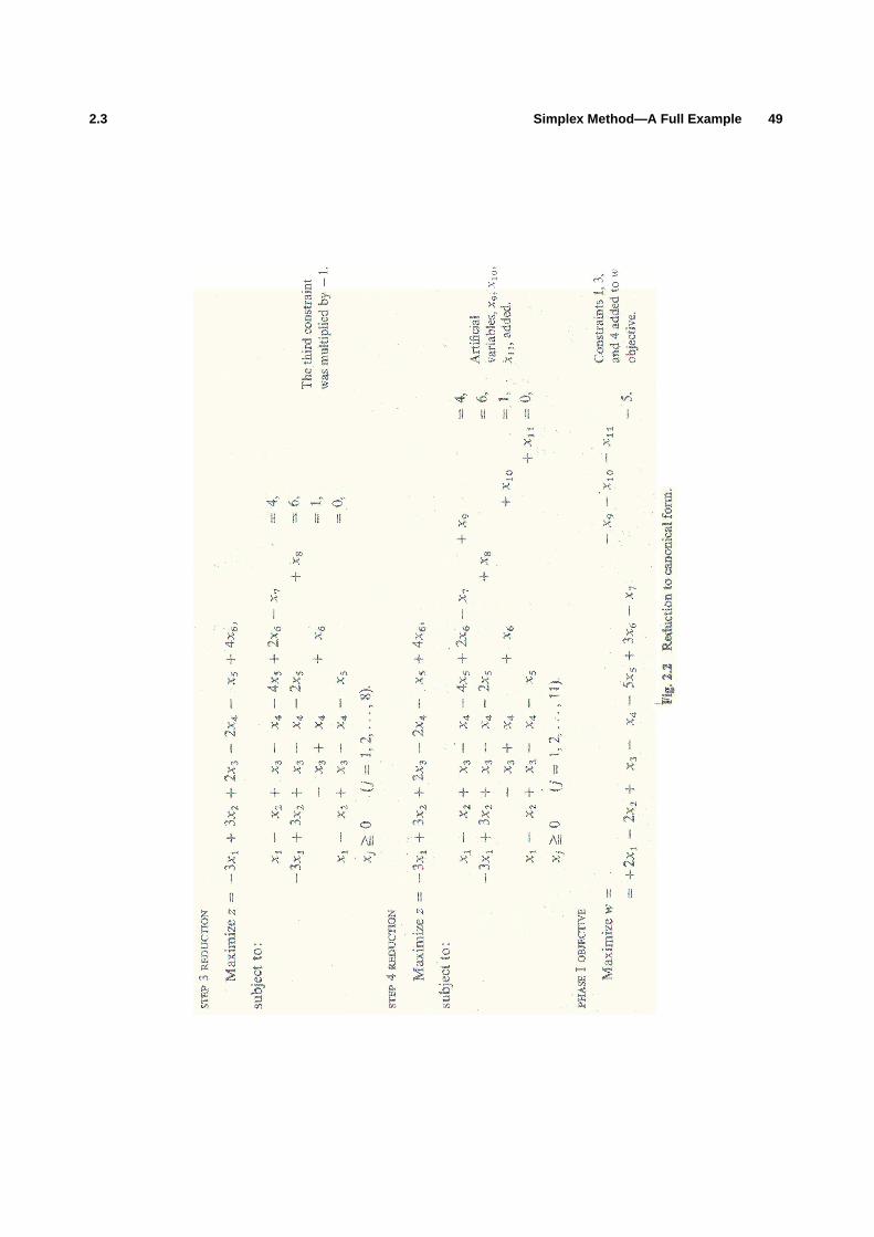
2.3 Simplex Method—A Full Example 49

50 Solving Linear Programs 2.3
We will say that an algorithm solves a problem if it always satisfies one of these three conditions. As we shallsee, a major feature of the simplex method is that it solves any linear-programming problem.
Most of the algorithms that we are going to consider are iterative, in the sense that they move from onedecision pointx1, x2, . . . , xn to another. For these algorithms, we need:
i) a starting point to initiate the procedure;ii) a termination criterion to indicate when a solution has been obtained; and
iii) an improvement mechanism for moving from a point that is not a solution to a better point.
Every algorithm that we develop should be analyzed with respect to these three requirements.In the previous section, we discussed most of these criteria for a sample linear-programming problem.
Now we must extend that discussion to give a formal and general version of the simplex algorithm. Beforedoing so, let us first use the improvement criterion of the previous section iteratively to solve a completeproblem. To avoid needless complications at this point, we select a problem that does not require artificialvariables.
Simple Example.∗ The owner of a shop producing automobile trailers wishes to determine the best mix forhis three products: flat-bed trailers, economy trailers, and luxury trailers. His shop is limited to working 24days/month on metalworking and 60 days/month on woodworking for these products. The following tableindicates production data for the trailers.
Usage per unit of trailer Resources
Flat-bed Economy Luxury availabilities
Metalworking days 12 2 1 24
Woodworking days 1 2 4 60Contribution ($× 100) 6 14 13
Let the decision variables of the problem be:
x1 =Number of flat-bed trailers produced per month,
x2 =Number of economy trailers produced per month,
x3 =Number of luxury trailers produced per month.
Assuming that the costs for metalworking and woodworking capacity are fixed, the problem becomes:
Maximizez= 6x1+ 14x2+ 13x3,
subject to:12x1+ 2x2+ x3 ≤ 24,
x1+ 2x2+ 4x3 ≤ 60,
x1 ≥ 0, x2 ≥ 0, x3 ≥ 0.
Letting x4 and x5 be slack variables corresponding to unused hours of metalworking and woodworkingcapacity, the problem above is equivalent to the linear program:
Maximizez= 6x1+ 14x2+ 13x3,
subject to:12x1+ 2x2+ x3+ x4 = 24,
x1+ 2x2+ 4x3+ x5 = 60,
∗ Excel spreadsheet available athttp://web.mit.edu/15.053/www/Sect2.3_Simple_Example.xls

2.3 Simplex Method—A Full Example 51
x j ≥ 0 ( j = 1, 2, . . . , 5).
This linear program is in canonical form with basic variablesx4 andx5. To simplify our exposition and tomore nearly parallel the way in which a computer might be used to solve problems, let us adopt a tabularrepresentation of the equations instead of writing them out in detail. Tableau 1 corresponds to the givencanonical form. The first two rows in the tableau are self-explanatory; they simply represent the constraints,but with the variables detached. The third row represents thez-equation, which may be rewritten as:
(−z)+ 6x1+ 14x2+ 13x3 = 0.
By convention, we say that(−z) is the basic variable associated with this equation. Note that no formalcolumn has been added to the tableau for the(−z)-variable.
The data to the right of the tableau is not required for the solution. It simply identifies the rows andsummarizes calculations. The arrow below the tableau indicates the variable being introduced into the basis;the circled element of the tableau indicates the pivot element; and the arrow to the left of the tableau indicatesthe variable being removed from the basis.
By the improvement criterion, introducing eitherx1, x2, or x3 into the basis will improve the solution.The simplex method selects the variable with best payoff per unit (largest objective coefficient), in this casex2. By the ratio test, asx2 is increased,x4 goes to zero beforex5 does; we should pivot in the first constraint.After pivoting,x2 replacesx4 in the basis and the new canonical form is as given in Tableau 2.
Next,x3 is introduced in place ofx5 (Tableau 3).
Finally, x1 is introduced in place ofx2 (Tableau 4).Tableau 4 satisfies the optimality criterion, giving an optimal contribution of $29,400 with a monthly
production of 36 flat-bed trailers and 6 luxury trailers.Note that in this example,x2 entered the basis at the first iteration, but does not appear in the optimal
basis. In general, a variable might be introduced into (and dropped from) the basis several times. In fact, itis possible for a variable to enter the basis at one iteration and drop from the basis at the very next iteration.

52 Solving Linear Programs 2.4
Variations
The simplex method changes in minor ways if the canonical form is written differently. Since these modi-fications appear frequently in the management-science literature, let us briefly discuss these variations. Wehave chosen to consider the maximizing form of the linear program (maxz) and have written the objectivefunction in the canonical form as:
(−z)+ c1x1+ c2x2+ · · · + cnxn = −z0,
so that the current solution hasz= z0. We argued that, if allc j ≤ 0, thenz= z0+c1x1+c2x2+· · ·+cnxn ≥ z0for any feasible solution, so that the current solution is optimal. If instead, the objective equation is writtenas:
(z)+ c′1x1+ c′2x2+ · · · + c′nxn = z0,
wherec′j = −c j , thenz is maximized if each coefficientc′j ≥ 0. In this case, the variable with the mostnegative coefficientc′j < 0 is chosen to enter the basis. All other steps in the method are unaltered.
The same type of association occurs for the minimizing objective:
Minimize z= c1x1+ c2x2+ · · · + cnxn.
If we write the objective function as:
(−z)+ c1x1+ c2x2+ · · · + cnxn = −z0,
then, sincez = z0 + c1x1 + · · · + cnxn, the current solution is optimal if everyc j ≥ 0. The variablexs tobe introduced is selected fromcs = minc j < 0, and every other step of the method is the same as for themaximizing problem. Similarly, if the objective function is written as:
(z)+ c′1x1+ c′2x2+ · · · + c′nxn = z0,
wherec′j = −c j , then, for a minimization problem, we introduce the variable with the most positivec j intothe basis.
Note that these modifications affect only the way in which the variable entering the basis is determined.The pivoting computations are not altered.
Given these variations in the selection rule for incoming variables, we should be wary of memorizingformulas for the simplex algorithm. Instead, we should be able to argue as in the previous example and as inthe simplex preview. In this way, we maintain flexibility for almost any application and will not succumb tothe rigidity of a ‘‘formula trap.’’
2.4 FORMAL PROCEDURE
Figure 2.3 summarizes the simplex method in flow-chart form. It illustrates both the computational steps ofthe algorithm and the interface between phase I and phase II. The flow chart indicates how the algorithm isused to show that the problem is infeasible, to find an optimal solution, or to show that the objective functionis unbounded over the feasible region. Figure 2.4 illustrates this algorithm for a phase I–phase II example

by solving the problem introduced in Section 2.2 for reducing a problem to canonical form.∗ The remainderof this section specifies the computational steps of the flow chart in algebraic terms.
At any intermediate step during phase II of the simplex algorithm, the problem is posed in the followingcanonical form:
x1 + a1, m+1xm+1 + · · · + a1sxs + · · · + a1nxn = b1,
x2 + a2, m+1xm+1 + · · · + a2nxn = b2,. . .
......
...
xr + ar, m+1xm+1 + · · · + ars xs + · · · + arnxn = br ,
. . ....
......
xm + am, m+1xm+1 + · · · + amsxs + · · · + amnxn = bm,
(−z) + cm+1xm+1 + · · · + csxs + · · · + cnxn = −z0,
x j ≥ 0 ( j = 1, 2, . . . , n).
∗ Excel spreadsheet available athttp://web.mit.edu/15.053/www/Fig2.4_Pivoting.xls
53

54 Solving Linear Programs 2.4
Figure 2.1 Simplex phase I–phase II maximization procedure.
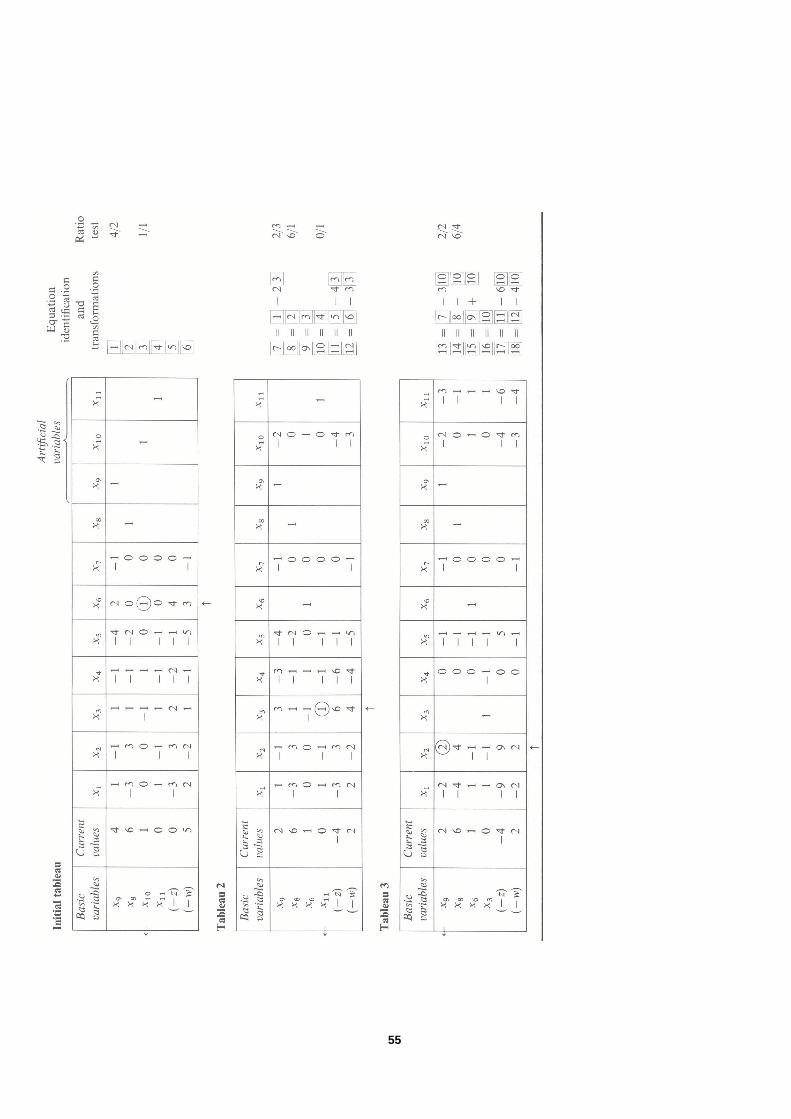
55

56

2.4 Formal Procedure 57
Originally, this canonical form is developed by using the procedures of Section 2.2. The dataai j , bi , z0, w0,andc j are known. They are either the original data (without bars) or that data as updated by previous stepsof the algorithm. We have assumed (by reindexing variables if necessary) thatx1, x2, . . . , xm are the basicvariables. Also, since this is a canonical form,bi ≥ 0 for i = 1, 2, . . . , m.
Simplex Algorithm (Maximization Form)
STEP (0) The problem is initially in canonical form and allbi ≥ 0.
STEP (1) Ifc j ≤ 0 for j = 1, 2, . . . , n, thenstop; we are optimal. If we continue thenthere exists somec j > 0.
STEP (2) Choose the column to pivot in (i.e., the variable to introduce into the basis)by:
cs = maxj{c j |c j > 0}.∗
If ais ≤ 0 for i = 1, 2, . . . , m, thenstop; the primal problem is unbounded.If we continue, thenais > 0 for somei = 1, 2, . . . , m.
STEP (3) Choose rowr to pivot in (i.e., the variable to drop from the basis) by theratio test:
br
ars= min
i
{bi
ais
∣∣∣∣ ais > 0
}.
STEP (4) Replace the basic variable in rowr with variables and re-establish thecanonical form (i.e., pivot on the coefficientars).
STEP (5) Go to step (1).
These steps are the essential computations of the simplex method. They apply to either the phase I orphase II problem. For the phase I problem, the coefficientsc j are those of the phase I objective function.
The only computation remaining to be specified formally is the effect that pivoting in step (4) has on theproblem data. Recall that we pivot on coefficientars merely to isolate variablexs with a+1 coefficient inconstraintr . The pivot can be viewed as being composed of two steps:
i) normalizing ther th constraint so thatxs has a+1 coefficient, andii) subtracting multiples of the normalized constraint from the order equations in order to eliminate variable
xs.
These steps are summarized pictorially in Fig. 2.5.The last tableau in Fig. 2.5 specifies the new values for the data. The new righthand-side coefficients,
for instance, are given by:
bnewr =
br
arsand b
newi = bi − ais
(br
ars
)≥ 0 for i 6= r .
Observe that the new coefficients for the variablexr being removed from the basis summarize the computa-tions. For example, the coefficient ofxr in the first row of the final tableau is obtained from the first tableauby subtractinga1s/ars times ther th row from the first row. The coefficients of the other variables in thefirst row of the third tableau can be obtained from the first tableau by performing this same calculation. Thisobservation can be used to partially streamline the computations of the simplex method. (See Appendix Bfor details.)
∗ The vertical bar within braces is an abbreviation for the phrase ‘‘such that.’’

58 Solving Linear Programs 2.4
Figure 2.5 Algebra for a pivot operation.

2.4 Formal Procedure 59
Note also that the new value forz will be given by:
z0+
(br
ars
)cs.
By our choice of the variablexs to introduce into the basis,cs > 0. Sincebr ≥ 0 andars > 0, this impliesthatznew
≥ zold. In addition, ifbr > 0, thenznew is strictly greater thanzold.
Convergence
Though the simplex algorithm has solved each of our previous examples, we have yet to show that it solvesany linear program. A formal proof requires results from linear algebra, as well as further technical materialthat is presented in Appendix B. Let us outline a proof assuming these results. We assume that the linearprogram hasn variables andm equality constraints.
First, note that there are only a finite number of bases for a given problem, since a basis containsmvariables (one isolated in each constraint) and there are a finite number of variables to select from. A standardresult in linear algebra states that, once the basic variables have been selected, all the entries in the tableau,including the objective value, are determined uniquely. Consequently, there are only a finite number ofcanonical forms as well. If the objective valuestrictly increases after every pivot, the algorithm never repeatsa canonical form and must determine an optimal solution after afinite number of pivots (any nonoptimalcanonical form is transformed to a new canonical form by the simplex method).
This argument shows that the simplex method solves linear programs as long as the objective value strictlyincreases after each pivoting operation. As we have just seen, each pivot affects the objective function byadding a multiple of the pivot equation to the objective function. The current value of thez-equation increasesby a multiple of the righthand-side coefficient; if this coefficient is positive (not zero), the objective valueincreases. With this in mind, we introduce the following definition:
A canonical form is callednondegenerateif each righthand-side coefficient is strictly positive. Thelinear-programming problem is called nondegenerate if, starting with an initial canonical form, everycanonical form determined by the algorithm is nondegenerate.
In these terms, we have shown that the simplex method solves every nondegenerate linear program usinga finite number of pivoting steps. When a problem is degenerate, it is possible to perturb the data slightlyso that every righthand-side coefficient remains positive and again show that the method works. Details aregiven in Appendix B. A final note is that, empirically, the finite number of iterations mentioned here to solvea problem frequently lies between 1.5 and 2 times the number of constraints (i.e., between 1.5m and 2m).
Applying this perturbation, if required, to both phase I and phase II, we obtain the essential property ofthe simplex method.
Fundamental Property of the Simplex Method. The simplex method (with perturbation if necessary)solves any given linear program in a finite number of iterations. That is, in a finite number of iterations,it shows that there is no feasible solution; finds an optimal solution; or shows that the objective functionis unbounded over the feasible region.
Although degeneracy occurs in almost every problem met in practice, it rarely causes any complications.In fact, even without the perturbation analysis, the simplex method never has failed to solve a practicalproblem, though problems that are highly degenerate with many basic variables at value zero frequently takemore computational time than other problems.
Applying this fundamental property to the phase I problem, we see that, if a problem is feasible, thesimplex method finds a basic feasible solution. Since these solutions correspond to corner or extreme pointsof the feasible region, we have the

60 Solving Linear Programs 2.5
Fundamental Property of Linear Equations. If a set of linear equations in nonnegative variables isfeasible, then there is an extreme-point solution to the equations.
2.5 TRANSITION FROM PHASE I TO PHASE II
We have seen that, if an artificial variable is positive at the end of phase I, then the original problem has nofeasible solution. On the other hand, if all artificial variables are nonbasic at value zero at the end of phaseI, then a basic feasible solution has been found to initiate the original optimization problem. Section 2.4furnishes an example of this case. Suppose, though, that when phase I terminates, all artificial variables arezero, but that some artificial variable remains in the basis. The following example illustrates this possibility.
Problem. Find a canonical form forx1, x2, and x3 by solving the phase I problem (x4, x5, and x6 areartificial variables):
Maximizew = −x4− x5− x6,
subject to:
x1− 2x2 + x4 = 2,
x1− 3x2− x3 + x5 = 1,
x1− x2+ ax3 + x6 = 3,
x j ≥ 0 ( j = 1, 2, . . . , 6).
To illustrate the various terminal conditions, the coefficient ofx3 is unspecified in the third constraint. Laterit will be set to either 0 or 1. In either case, the pivoting sequence will be the same and we shall merely carrythe coefficient symbolically.
Putting the problem in canonical form by eliminatingx4, x5, andx6 from the objective function, thesimplex solution to the phase I problem is given in Tableaus 1 through 3.
For a = 0 or 1, phase I is complete sincec3 = a− 1 ≤ 0, but withx6 still part of the basis. Note thatin Tableau 2, eitherx4 or x6 could be dropped from the basis. We have arbitrarily selectedx4. (A similarargument would apply ifx6 were chosen.)

2.5 Transition from Phase I to Phase II 61
First, assumea = 0. Then we can introducex3 into the basis in place of the artificial variablex6, pivotingon the coefficienta− 1 or x3 in the third constraint, giving Tableau 4.
Note that we have pivoted on a negative coefficient here. Since the righthand-side element of the thirdequation is zero, dividing by a negative pivot element will not make the resulting righthand-side coefficientnegative. Droppingx4, x5, andx6, we obtain the desired canonical form. Note thatx6 is now set to zero andis nonbasic.
Next, suppose thata = 1. The coefficient(a−1) in Tableau 3 is zero, so we cannot pivotx3 into the basisas above. In this case, however, dropping artificial variablesx4 andx5 from the system, the third constraintof Tableau 3 readsx6 = 0. Consequently, even thoughx6 is a basic variable, in the canonical form for theoriginal problem it will always remain at value zero during phase II. Thus, throughout phase II, a feasiblesolution to the original problem will be maintained as required. When more than one artificial variable is inthe optimal basis for phase I, these techniques can be applied to each variable.
For the general problem, the transition rule from phase I to phase II can be stated as:
Phase I–Phase II Transition Rule. Suppose that artificial variablexi is thei th basic variable at theend of Phase I (at value zero). Letai j be the coefficient of the nonartificial variablex j in thei th constraintof the final tableau. If someai j 6= 0, then pivot on any suchai j , introducingx j into the basis in place ofxi . If all ai j = 0, then maintainxi in the basis throughout phase II by including thei th constraint, whichreadsxi = 0.
As a final note, observe that if allai j = 0 above, then constrainti is a redundant constraint in the originalsystem, for, by adding multiples of the other equation to constrainti via pivoting, we have produced theequation (ignoring artificial variables):
0x1+ 0x2+ · · · + 0xn = 0.
For example, whena = 1 for the problem above, (constraint 3) = 2 times (constraint 1)–(constraint 2), andis redundant.
Phase I–Phase II Example
Maximizez= −3x1 + x3,

62 Solving Linear Programs 2.5
subject to:
x1+ x2+ x3+ x4 = 4,
−2x1+ x2− x3 = 1,
3x2+ x3+ x4 = 9,
x j ≥ 0 ( j = 1, 2, 3, 4).
Adding artificial variablesx5, x6, andx7, we first minimizex5 + x6 + x7 or, equivalently, maximizew = −x5− x6− x7. The iterations are shown in Fig. 2.6.∗ The first tableau is the phase I problem statement.Basic variablesx5, x6 andx7 appear in the objective function and, to achieve the initial canonical form, wemust add the constraints to the objective function to eliminate these variables.
Tableaus 2 and 3 contain the phase I solution. Tableau 4 gives a feasible solution to the original problem.Artificial variable x7 remains in the basis and is eliminated by pivoting on the−1 coefficient forx4. Thispivot replacesx7 = 0 in the basis byx4 = 0, and gives a basis from the original variables to initiate phase II.
Tableaus 5 and 6 give the phase II solution.
∗ Excel spreadsheet available athttp://web.mit.edu/15.053/www/Fig2.6_Pivoting.xls

2.5 Transition from Phase I to Phase II 63
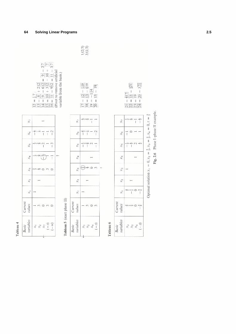
64 Solving Linear Programs 2.5

2.6 Linear Programs with Bounded Variables 65
2.6 LINEAR PROGRAMS WITH BOUNDED VARIABLES
In most linear-programming applications, many of the constraints merely specify upper and lower bounds onthe decision variables. In a distribution problem, for example, variablesx j representing inventory levels mightbe constrained by storage capacitiesu j and by predetermined safety stock levels` j so that j ≤ x j ≤ u j .We are led then to consider linear programs withbounded variables:
Maximizez=n∑
j=1
c j x j ,
subject to:n∑
j=1
ai j x j = bi , (i = 1, 2, . . . , m) (3)
` j ≤ x j ≤ u j , ( j = 1, 2, . . . , n). (4)
The lower bounds j may be−∞ and/or the upper boundsu j may be+∞, indicating respectively thatthe decision variablex j is unbounded from below or from above. Note that when each` j = 0 and eachu j = +∞, this problem reduces to the linear-programming form that has been discussed up until now.
The bounded-variable problem can be solved by the simplex method as discussed thus far, by addingslack variables to the upper-bound constraints and surplus variables to the lower-bound constraints, therebyconverting them to equalities. This approach handles the bounding constraints explicitly. In contrast, theapproach proposed in this section modifies the simplex method to consider the bounded-variable constraintsimplicitly. In this new approach, pivoting calculations are computed only for the equality constraints (3) ratherthan for the entire system (3) and (4). In many instances, this reduction in pivoting calculations will providesubstantial computational savings. As an extreme illustration, suppose that there is one equality constraintand 1000 nonnegative variables with upper bounds. The simplex method will maintain 1001 constraints inthe tableau, whereas the new procedure maintains only the single equality constraint.
We achieve these savings by using a canonical form with one basic variable isolated in each of the equalityconstraints, as in the usual simplex method. However, basic feasible solutions now are determined by settingnonbasic variables to either their lower or upper bound. This method for defining basic feasible solutionsextends our previous practice of setting nonbasic variables to their lower bounds of zero, and permits us toassess optimality and generate improvement procedures much as before.
Suppose, for example, thatx2 andx4 are nonbasic variables constrained by:
4 ≤ x2 ≤ 15,
2 ≤ x4 ≤ 5;
and that
z = 4− 14x2+
12x4,
x2 = 4,
x4 = 5,
in the current canonical form. In any feasible solution,x2 ≥ 4, so−14x2 ≤ −1; also,x4 ≤ 5, so that
12x4 ≤
12(5) = 21
2. Consequently,
z= 4− 14x2+
12x4 ≤ 4− 1+ 21
2 = 512
for any feasible solution. Since the current solution withx2 = 4 andx4 = 5 attains this upper bound, itmust be optimal. In general, the current canonical form represents the optimal solution whenever nonbasicvariables at their lower bounds have nonpositive objective coefficients, and nonbasic variables at their upperbound have nonnegative objective coefficients.

66 Solving Linear Programs 2.6
Bounded Variable Optimality Condition. In a maximization problem in canonical form, if everynonbasic variable at its lower bound has a nonpositive objective coefficient, and every nonbasic variableat its upper bound has a nonnegative objective coefficient, then the basic feasible solution given by thatcanonical form maximizes the objective function over the feasible region.
Improving a nonoptimal solution becomes slightly more complicated than before. If the objective coef-ficient c j of nonbasic variablex j is positive andx j = ` j , then we increasex j ; if c j < 0 andx j = u j , wedecreasex j . In either case, the objective value is improving.
When changing the value of a nonbasic variable, we wish to maintain feasibility. As we have seen, forproblems with only nonnegative variables, we have to test, via the ratio rule, to see when a basic variable firstbecomes zero. Here we must consider the following contingencies:
i) the nonbasic variable being changed reaches its upper or lower bound; orii) some basic variable reaches either its upper or lower bound.
In the first case, no pivoting is required. The nonbasic variable simply changes from its lower to upperbound, or upper to lower bound, and remains nonbasic. In the second case, pivoting is used to remove thebasic variable reaching either its lower or upper bound from the basis.
These ideas can be implemented on a computer in a number of ways. For example, we can keep track ofthe lower bounds throughout the algorithm; or every lower bound
x j ≥ ` j
can be converted to zero by defining a new variable
x′′j = x j − ` j ≥ 0,
and substitutingx′′j + ` j for x j everywhere throughout the model. Also, we can always redefine variablesso that every nonbasic variable is at its lower bound. Letx′j denote the slack variable for the upper-boundconstraintx j ≤ u j ; that is,
x j + x′j = u j .
Wheneverx j is nonbasic at its upper boundu j , the slack variablex′j = 0. Consequently, substitutingu j − x′jfor x j in the model makesx′j nonbasic at value zero in place ofx j . If, subsequently in the algorithm,x′jbecomes nonbasic at its upper bound, which is alsou j , we can make the same substitution forx′j , replacingit with u j − x j , andx j will appear nonbasic at value zero. These transformations are usually referred to astheupper-bounding substitution.
The computational steps of the upper-bounding algorithm are very simple to describe if both of thesetransformations are used. Since all nonbasic variables (eitherx j or x′j ) are at value zero, we increase a variablefor maximization as in the usual simplex method if its objective coefficient is positive. We use the usual ratiorule to determine at what valuet1 for the incoming variable, a basic variable first reaches zero. We also mustensure that variables do not exceed their upper bounds. For example, when increasing nonbasic variablexsto valuet , in a constraint withx1 basic, such as:
x1− 2xs = 3,
we require that:
x1 = 3+ 2t ≤ u1
(that is, t ≤
u1− 3
2
).
We must perform such a check in every constraint in which the incoming variable has a negative coefficient;thusxs ≤ t2 where:
t2 = mini
{uk − bi
−ais
∣∣∣∣∣ais < 0
},

2.6 Linear Programs with Bounded Variables 67
anduk is the upper bound for the basic variablexk in thei th constraint,bi is the current value for this variable,andais are the constraint coefficients for variablexs. This test might be called theupper-bounding ratio test.Note that, in contrast to the usual ratio test, the upper-bounding ratio uses negative coefficientsais < 0 forthe nonbasic variablexs being increased.
In general, the incoming variablexs (or x′s) is set to:
xs = min {us, t1, t2}.If the minimum is
i) us, then the upper bounding substitution is made forxs (or x′s);ii) t1, then a usual simplex pivot is made to introducexs into the basis;
iii) t2, then the upper bounding substitution is made for the basic variablexk (or x′k) reaching its upper boundandxs is introduced into the basis in place ofx′k (or xk) by a usual simplex pivot.
The procedure is illustrated in Fig. 2.7. Tableau 1 contains the problem formulation, which is in canonicalform with x1, x2, x3, andx4 as basic variables andx5 andx6 as nonbasic variables at value zero. In the firstiteration, variablex5 increases, reaches its upper bound, and the upper bounding substitutionx′5 = 1− x5is made. Note that, after making this substitution, the variablex′5 has coefficients opposite in sign from thecoefficients ofx5. Also, in going from Tableau 1 to Tableau 2, we have updated the current value of the basicvariables by multiplying the upper bound ofx5, in this caseu5 = 1, by the coefficients ofx5 and movingthese constants to the righthand side of the equations.
In Tableau 2, variablex6 increases, basic variablex2 reaches zero, and a usual simplex pivot is performed.After the pivot, it is attractive to increasex′5 in Tableau 3. Asx′5 increases basic variablex4 reaches its upperbound atx4 = 5 and the upper-bounding substitutionx′4 = 5− x4 is made. Variablex′4 is isolated as the basicvariable in the fourth constraint in Tableau 4 (by multiplying the constraint by−1 after the upper-boundingsubstitution); variablex′5 then enters the basis in place ofx′4. Finally, the solution in Tableau 5 is optimal,since the objective coefficients are nonpositive for the nonbasic variables, each at value zero.

68

69

70 Solving Linear Programs
EXERCISES
1. Given:
x1 + 2x4 = 8,
x2 + 3x4 = 6,
x3+ 8x4 = 24,
−z + 10x4 = −32,
x1 ≥ 0, x2 ≥ 0, x3 ≥ 0, x4 ≥ 0.
a) What is the optimal solution of this problem?b) Change the coefficient ofx4 in thez-equation to−3. What is the optimal solution now?c) Change the signs on allx4 coefficients to be negative. What is the optimal solution now?
2. Consider the linear program:
Maximizez= 9x2+ x3 − 2x5− x6,
subject to:
5x2+ 50x3+ x4+ x5 = 10,
x1− 15x2+ 2x3 = 2,
x2+ x3 + x5+ x6 = 6,
x j ≥ 0 ( j = 1, 2, . . . , 6).
a) Find an initial basic feasible solution, specify values of the decision variables, and tell which are basic.b) Transform the system of equations to the canonical form for carrying out the simplex routine.c) Is your initial basic feasible solution optimal? Why?d) How would you select a column in which to pivot in carrying out the simplex algorithm?e) Having chosen a pivot column, now select a row in which to pivot and describe the selection rule. How does this
rule guarantee that the new basic solution is feasible? Is it possible that no row meets the criterion of your rule?If this happens, what does this indicate about the original problem?
f) Without carrying out the pivot operation, compute the new basic feasible solution.g) Perform the pivot operation indicated by (d) and (e) and check your answer to (f). Substitute your basic feasible
solution in the original equations as an additional check.h) Is your solution optimal now? Why?
3. a) Reduce the following system to canonical form. Identify slack, surplus, and artificial variables.
−2x1+ x2 ≤ 4 (1)
3x1+ 4x2 ≥ 2 (2)
5x1+ 9x2 = 8 (3)
x1+ x2 ≥ 0 (4)
2x1+ x2 ≥ −3 (5)
−3x1− x2 ≤ −2 (6)
3x1+ 2x2 ≤ 10 (7)
x1 ≥ 0, x2 ≥ 0.
b) Formulate phase I objective functions for the following systems withx1 ≥ 0 andx2 ≥ 0:
i) expressions 2 and 3 above.

Exercises 71
ii) expressions 1 and 7 above.iii) expressions 4 and 5 above.
4. Consider the linear program
Maximizez= x1,
subject to:
−x1+ x2 ≤ 2,
x1+ x2 ≤ 8,
−x1+ x2 ≥ −4,
x1 ≥ 0, x2 ≥ 0.
a) State the above in canonical form.b) Solve by the simplex method.c) Solve geometrically and also trace the simplex procedure steps graphically.d) Suppose that the objective function is changed toz= x1+ cx2. Graphically determine the values ofc for which
the solution found in parts (b) and (c) remains optimal.e) Graphically determine the shadow price corresponding to the third constraint.
5. The bartender of your local pub has asked you to assist him in finding the combination of mixed drinks that willmaximize his revenue. He has the following bottles available:
1 quart (32 oz.) Old Cambridge (a fine whiskey—cost $8/quart)1 quart Joy Juice (another fine whiskey—cost $10/quart)1 quart Ma’s Wicked Vermouth ($10/quart)2 quarts Gil-boy’s Gin ($6/quart)
Since he is new to the business, his knowledge is limited to the following drinks:
Whiskey Sour 2 oz. whiskey Price $1
Manhattan 2 oz. whiskey $21 oz. vermouth
Martini 2 oz. gin $21 oz. vermouth
Pub Special 2 oz. gin $32 oz. whiskey
Use the simplex method to maximize the bar’s profit. (Is the cost of the liquor relevant in this formulation?)
6. A company makes three lines of tires. Its four-ply biased tires produce $6 in profit per tire, its fiberglass belted line$4 a tire, and its radials $8 a tire. Each type of tire passes through three manufacturing stages as a part of the entireproduction process.
Each of the three process centers has the following hours of available production time per day:
Process Hours
1 Molding 122 Curing 93 Assembly 16
The time required in each process to produce one hundred tires of each line is as follows:

72 Solving Linear Programs
Hours per 100 units
Tire Molding Curing Assembly
Four-ply 2 3 2Fiberglass 2 2 1
Radial 2 1 3
Determine the optimum product mix for each day’s production, assuming all tires are sold.
7. An electronics firm manufactures printed circuit boards and specialized electronics devices. Final assembly oper-ations are completed by a small group of trained workers who labor simultaneously on the products. Because oflimited space available in the plant, no more then ten assemblers can be employed. The standard operating budgetin this functional department allows a maximum of $9000 per month as salaries for the workers.
The existing wage structure in the community requires that workers with two or more years of experience receive$1000 per month, while recent trade-school graduates will work for only $800. Previous studies have shown thatexperienced assemblers produce $2000 in ‘‘value added" per month while new-hires add only $1800. In order tomaximize the value added by the group, how many persons from each group should be employed? Solve graphicallyand by the simplex method.
8. The processing division of the Sunrise Breakfast Company must produce one ton (2000 pounds) of breakfast flakesper day to meet the demand for its Sugar Sweets cereal. Cost per pound of the three ingredients is:
Ingredient A $4 per pound
Ingredient B $3 per pound
Ingredient C $2 per pound
Government regulations require that the mix contain at least 10% ingredient A and 20% ingredient B. Use ofmore than 800 pounds per ton of ingredient C produces an unacceptable taste.
Determine the minimum-cost mixture that satisfies the daily demand for Sugar Sweets. Can the bounded-variable simplex method be used to solve this problem?
9. Solve the following problem using the two phases of the simplex method:
Maximizez= 2x1+ x2+ x3,
subject to:
2x1+ 3x2− x3 ≤ 9,
2x2 + x3 ≥ 4,
x1 + x3 = 6,
x1 ≥ 0, x2 ≥ 0, x3 ≥ 0.
Is the optimal solution unique?
10. Consider the linear program:
Maximizez= −3x1+ 6x2,
subject to:
5x1+ 7x2 ≤ 35,
−x1+ 2x2 ≤ 2,
x1 ≥ 0, x2 ≥ 0.

Exercises 73
a) Solve this problem by the simplex method. Are there alternative optimal solutions? How can this be determinedat the final simplex iteration?
b) Solve the problem graphically to verify your answer to part (a).
11. Solve the following problem using the simplex method:
Minimize z= x1− 2x2− 4x3+ 2x4,
subject to:
x1 − 2x3 ≤ 4,
x2 − x4 ≤ 8,
−2x1+ x2+ 8x3+ x4 ≤ 12,
x1 ≥ 0, x2 ≥ 0, x3 ≥ 0, x4 ≥ 0.
12. a) Set up a linear program that will determine a feasible solution to the following system of equations and inequalitiesif one exists.Do not solvethe linear program.
x1− 6x2+ x3− x4 = 5,
−2x2+ 2x3− 3x4 ≥ 3,
3x1 − 2x3 + 4x4 = −1,
x1 ≥ 0, x3 ≥ 0, x4 ≥ 0.
b) Formulate a phase I linear program to find a feasible solution to the system:
3x1+ 2x2− x3 ≤ −3,
−x1− x2+ 2x3 ≤ −1,
x1 ≥ 0, x2 ≥ 0, x3 ≥ 0.
Show, from the phase I objective function, that the system contains no feasible solution (no pivoting calculationsare required).
13. The tableau given below corresponds to a maximization problem in decision variablesx j ≥ 0 ( j = 1, 2, . . . , 5):
Basic Currentvariables values x1 x2 x3 x4 x5
x3 4 −1 a1 1x4 1 a2 −4 1x5 b a3 3 1
(−z) −10 c −2
State conditions on all five unknownsa1, a2, a3, b, andc, such that the following statements are true.
a) The current solution is optimal. There are multiple optimal solutions.b) The problem is unbounded.c) The problem is infeasible.d) The current solution is not optimal (assume thatb ≥ 0). Indicate the variable that enters the basis, the variable
that leaves the basis, and what the total change in profit would be for one iteration of the simplex method for allvalues of the unknowns that are not optimal.

74 Solving Linear Programs
14. Consider the linear program:
Maximizez= αx1+ 2x2+ x3− 4x4,
subject to:
x1+ x2 − x4 = 4+ 21 (1)
2x1− x2+ 3x3− 2x4 = 5+ 71 (2)
x1 ≥ 0, x2 ≥ 0, x3 ≥ 0, x4 ≥ 0,
whereα and1 are viewed as parameters.
a) Form two new constraints as (1′) = (1)+ (2) and (2′) = −2(1)+ (2). Solve forx1 andx2 from (1′) and (2′), andsubstitute their values in the objective function. Use these transformations to express the problem in canonicalform with x1 andx2 as basic variables.
b) Assume1 = 0 (constant). For what values ofα arex1 andx2 optimal basic variablesin the problem?c) Assumeα = 3. For what values of1 do x1 andx2 form an optimal basic feasible solution?
15. Let
(−w)+ d1x1+ d2x2+ · · · + dmxm = 0 (∗)
be the phase I objective function when phase I terminates for maximizingw. Discuss the following two proceduresfor making the phase I to II transition when an artificial variable remains in the basis at value zero. Show, usingeither procedure, that every basic solution determined during phase II will be feasible for theoriginal problemformulation.
a) Multiply each coefficient in (∗) by−1. Initiate phase II with the original objective function, but maintain (∗) inthe tableau as a new constraint with (w) as the basic variable.
b) Eliminate (∗) from the tableau and at the same time eliminate from the problem any variablex j with d j < 0.Any artificial variable in the optimal phase I basis is now treated as though it were a variable from the originalproblem.
16. In our discussion of reduction to canonical form, we have replaced variables unconstrained in sign by the differencebetween two nonnegative variables. This exercise considers an alternative transformation that does not introduce asmany new variables, and also a simplex-like procedure for treating free variables directly without any substitutions.For concreteness, suppose thaty1, y2, andy3 are the only unconstrained variables in a linear program.a) Substitute fory1, y2, andy3 in the model by:
y1 = x1− x0,
y2 = x2− x0,
y3 = x3− x0,
with x0 ≥ 0, x1 ≥ 0, x2 ≥ 0, andx3 ≥ 0. Show that the models are equivalent before and after thesesubstitutions.
b) Apply the simplex method directly withy1, y2, and y3. When are these variables introduced into the basisat positive levels? At negative levels? Ify1 is basic, will it ever be removed from the basis? Is the equationcontainingy1 as a basic variable used in the ratio test? Would the simplex method be altered in any other way?
17. Apply the phase I simplex method to find a feasible solution to the problem:
x1− 2x2+ x3 = 2,
−x1− 3x2+ x3 = 1,
2x1− 3x2+ 4x3 = 7,
x1 ≥ 0, x2 ≥ 0, x3 ≥ 0.
Does the termination of phase I show that the system contains a redundant equation? How?
3.7 Exercises 75
18. Frequently, linear programs are formulated withinterval constraintsof the form:
5≤ 6x1− x2+ 3x3 ≤ 8.
a) Show that this constraint is equivalent to the constraints
6x1− x2+ 3x3+ x4 = 8,
0 ≤ x4 ≤ 3.
b) Indicate how the generalinterval linear program
Maximizez=n∑
j=1
c j x j ,
subject to:
b′i ≤n∑
j=1
ai j x j ≤ bi (i = 1, 2, . . . , m),
x j ≥ 0 ( j = 1, 2, . . . , n),
can be formulated as a bounded-variable linear program withm equality constraints.
19. a) What is the solution to the linear-programming problem:
Maximizez= c1x1+ c2x2+ · · · + cnxn,
subject to:a1x1+ a2x2+ · · · + anxn ≤ b,
0 ≤ x j ≤ u j ( j = 1, 2, . . . , n),
with bounded variables and one additional constraint? Assume that the constantsc j , a j , andu j for j =1, 2, . . . , n, andb are all positive and that the problem has been formulated so that:
c1
a1≥
c2
a2≥ · · · ≥
cn
an.
b) What will be the steps of the simplex method for bounded variables when applied to this problem (in what orderdo the variables enter and leave the basis)?
20. a) Graphically determine the steps of the simplex method for the problem:
Maximize 8x1+ 6x2,
subject to:
3x1+ 2x2 ≤ 28,
5x1+ 2x2 ≤ 42,
x1 ≤ 8,
x2 ≤ 8,
x1 ≥ 0, x2 ≥ 0.
Indicate on the sketch the basic variables at each iteration of the simplex algorithm in terms of the given variablesand the slack variables for the four less-than-or-equal-to constraints.
b) Suppose that the bounded-variable simplex method is applied to this problem. Specify how the iterations in thesolution to part (a) correspond to the bounded-variable simplex method. Which variables fromx1, x2, and theslack variable for the first two constraints, are basic at each iteration? Which nonbasic variables are at their upperbounds?
c) Solve the problem algebraically, using the simplex algorithm for bounded variables.

Sensitivity Analysis
3
We have already been introduced to sensitivity analysis in Chapter 1 via the geometry of a simple example.We saw that the values of the decision variables and those of the slack and surplus variables remain unchangedeven though some coefficients in the objective function are varied. We also saw that varying the righthand-side value for a particular constraint alters the optimal value of the objective function in a way that allows usto impute a per-unit value, orshadow price, to that constraint. These shadow prices and the shadow priceson the implicit nonnegativity constraints, calledreduced costs, remain unchanged even though some of therighthand-side values are varied. Since there is always some uncertainty in the data, it is useful to know overwhat range and under what conditions the components of a particular solution remain unchanged. Further,the sensitivity of a solution to changes in the data gives us insight into possible technological improvementsin the process being modeled. For instance, it might be that the available resources are not balanced properlyand the primary issue is not to resolve the most effective allocation of these resources, but to investigate whatadditional resources should be acquired to eliminate possible bottlenecks. Sensitivity analysis provides aninvaluable tool for addressing such issues.
There are a number of questions that could be asked concerning the sensitivity of an optimal solution tochanges in the data. In this chapter we will address those that can be answered most easily. Every commerciallinear-programming system provides this elementary sensitivity analysis, since the calculations are easy toperform using the tableau associated with an optimal solution. There are two variations in the data thatinvariably are reported: objective function and righthand-side ranges. The objective-function ranges refer tothe range over which an individual coefficient of the objective function can vary, without changing the basisassociated with an optimal solution. In essence, these are the ranges on the objective-function coefficientsover which we can be sure the values of the decision variables in an optimal solution will remain unchanged.The righthand-side ranges refer to the range over which an individual righthand-side value can vary, againwithout changing the basis associated with an optimal solution. These are the ranges on the righthand-sidevalues over which we can be sure the values of the shadow prices and reduced costs will remain unchanged.Further, associated with each range is information concerning how the basis would change if the range wereexceeded. These concepts will become clear if we deal with a specific example.
3.1 AN EXAMPLE FOR ANALYSIS
We will consider for concreteness the custom-molder example from Chapter 1; in order to increase thecomplexity somewhat, let us add a third alternative to the production possibilities. Suppose that, besidesthe six-ounce juice glassesx1 and the ten-ounce cocktail glassesx2, our molder is approached by a newcustomer to produce a champagne glass. The champagne glass is not difficult to produce except that it mustbe molded in two separate pieces—the bowl with stem and then base. As a result, the production time for thechampagne glass is 8 hours per hundred cases, which is greater than either of the other products. The storagespace required for the champagne glasses is 1000 cubic feet per hundred cases; and the contribution is $6.00
76
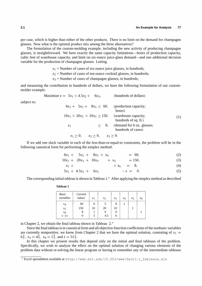
3.1 An Example for Analysis 77
per case, which is higher than either of the other products. There is no limit on the demand for champagneglasses. Now what is the optimal product mix among the three alternatives?
The formulation of the custom-molding example, including the new activity of producing champagneglasses, is straightforward. We have exactly the same capacity limitations—hours of production capacity,cubic feet of warehouse capacity, and limit on six-ounce juice-glass demand—and one additional decisionvariable for the production of champagne glasses. Letting
x1 = Number of cases of six-ounce juice glasses, in hundreds;x2 = Number of cases of ten-ounce cocktail glasses, in hundreds;x3 = Number of cases of champagne glasses, in hundreds;
and measuring the contribution in hundreds of dollars, we have the following formulation of our custom-molder example:
Maximizez= 5x1+ 4.5x2+ 6x3, (hundreds of dollars)
subject to:6x1 + 5x2 + 8x3 ≤ 60, (production capacity;
hours)10x1 + 20x2 + 10x3 ≤ 150, (warehouse capacity;
hundreds of sq. ft.)x1 ≤ 8, (demand for 6 oz. glasses;
hundreds of cases)
(1)
x1 ≥ 0, x2 ≥ 0, x3 ≥ 0.
If we add one slack variable in each of the less-than-or-equal-to constraints, the problem will be in thefollowing canonical form for performing the simplex method:
6x1 + 5x2 + 8x3 + x4 = 60, (2)
10x1 + 20x2 + 10x3 + x5 = 150, (3)
x1 + + x6 = 8, (4)
5x1 + 4.5x2 + 6x3 − z = 0. (5)
The corresponding initial tableau is shown in Tableau 1.∗ After applying the simplex method as described
Tableau 1
Basic Currentvariables values x1 x2 x3 x4 x5 x6
x4 60 6 5 8 1
x5 150 10 20 10 1x6 8 1 0 0 1
(−z) 0 5 4.5 6
in Chapter 2, we obtain the final tableau shown in Tableau 2.∗
Since the final tableau is in canonical form and all objective-function coefficients of the nonbasic variablesare currently nonpositive, we know from Chapter 2 that we have the optimal solution, consisting ofx1 =
637, x2 = 42
7, x6 = 147, andz= 513
7.In this chapter we present results that depend only on the initial and final tableaus of the problem.
Specifically, we wish to analyze the effect on the optimal solution of changing various elements of theproblem data without re-solving the linear program or having to remember any of the intermediate tableaus
∗ Excel spreadsheet available athttp://web.mit.edu/15.053/www/Sect3.1_Tableaus.xls

78 Sensitivity Analysis 3.2
Tableau 2
Basic Currentvariables values x1 x2 x3 x4 x5 x6
x2 427 1 −
27 −
17
335
x6 147 −
117 −
27
114 1
x1 637 1 11
727 −
114
(−z) −5137 −
47 −
1114 −
135
generated in solving the problem by the simplex method. The type of results that can be derived in this way areconservative, in the sense that they provide sensitivity analysis for changes in the problem data small enoughso that the same decision variables remain basic, but not for larger changes in the data. The example presentedin this section will be used to motivate the discussions of sensitivity analysis throughout this chapter.
3.2 SHADOW PRICES, REDUCED COSTS, AND NEW ACTIVITIES
In our new variation of the custom-molder example, we note that the new activity of producing champagneglasses is not undertaken at all. An immediate question arises, could we have known this without performingthe simplex method on the entire problem? It turns out that a proper interpretation of the shadow prices inthe Chapter 1 version of the problem would have told us that producing champagne glasses would not beeconomically attractive. However, let us proceed more slowly. Recall the definition of the shadow priceassociated with a particular constraint.
Definition. Theshadow priceassociated with a particular constraint is the change in the optimal valueof the objective function per unit increase in the righthand-side value for that constraint, all other problemdata remaining unchanged.
In Chapter 1 we implied that the shadow prices were readily available when a linear program is solved.Is it then possible to determine the shadow prices from the final tableau easily? The answer is yes, in general,but let us consider our example for concreteness.
Suppose that the production capacity in the first constraint of our model
6x1+ 5x2+ 8x3+ x4 = 60 (6)
is increased from 60 to 61 hours. We then essentially are procuring one additional unit of production capacityat no cost. We can obtain the same result algebraically by allowing the slack variablex4 to take on negativevalues. Ifx4 is replaced byx4− 1 (i.e., from its optimal valuex4 = 0 to x4 = −1), Eq.(6) becomes:
6x1+ 5x2+ 8x3+ x4 = 61,
which is exactly what we intended.Sincex4 is a slack variable, it does not appear in any other constraint of the original model formulation,
nor does it appear in the objective function. Therefore, this replacement does not alter any other righthand-side value in the original problem formulation. What is the contribution to the optimal profit of this additionalunit of capacity? We can resolve this question by looking at the objective function of the final tableau, whichis given by:
z= 0x1+ 0x2−47x3−
1114x4−
135x5+ 0x6+ 513
7. (7)
The optimality conditions of the simplex method imply that the optimal solution is determined by setting thenonbasic variablesx3 = x4 = x5 = 0, which results in a profit of 5137. Now, if we are allowed to makex4 = −1, the profit increases by11
14 hundred dollars for each additional unit of capacity available. This, then,is the marginal value, or shadow price, for production hours.
3.2 Shadow Prices, Reduced Costs, and New Activities 79
The righthand side for every constraint can be analyzed in this way, so that the shadow price for aparticular constraint is merely the negative of the coefficient of the appropriate slack (or artificial) variablein the objective function of the final tableau. For our example, the shadow prices are11
14 hundred dollars perhour of production capacity,135 hundred dollars per hundred cubic feet of storage capacity, and zero for thelimit on six-ounce juice-glass demand. It should be understood that the shadow prices are associated withthe constraints of the problem and not the variables. They are in fact the marginal worth of an additional unitof a particular righthand-side value.
So far, we have discussed shadow prices for the explicit structural constraints of the linear-programmingmodel. The nonnegativity constraints also have a shadow price, which, in linear-programming terminology,is given the special name of reduced cost.
Definition. Thereduced costassociated with the nonnegativity constraint for each variable is the shadowprice of that constraint (i.e., the corresponding change in the objective function per unit increase in thelower bound of the variable).
The reduced costs can also be obtained directly from the objective equation in the final tableau. In ourexample, the final objective form is
z= 0x1+ 0x2−47x3−
1114x4−
135x5+ 0x6+ 513
7. (8)
Increasing the righthand side ofx3 ≥ 0 by one unit tox3 ≥ 1 forces champagne glasses to be used in the finalsolution. From (8), the optimal profit decreases by−4
7. Since the basic variables have valuesx1 = 637 and
x2 = 427, increasing the righthand sides ofx1 ≥ 0 andx2 ≥ 0 by a small amount does not affect the optimal
solution, so their reduced costs are zero. Consequently, in every case, the shadow price for the nonnegativityconstraint on a variable is the objective coefficient for this variable in the final canonical form. For basicvariables, these reduced costs are zero.
Alternatively, the reduced costs for all decision variables can be computed directly from the shadowprices on the structural constraints and the objective-function coefficients. In this view, the shadow pricesare thought of as the opportunity costs associated with diverting resources away from the optimal productionmix. For example, considerx3. Since the new activity of producing champagne glasses requires 8 hours ofproduction capacity per hundred cases, whose opportunity cost is11
14 hundred dollars per hour, and 10 hundredcubic feet of storage capacity per hundred cases, whose opportunity cost is1
35 hundred dollars per hundredcubic feet, the resulting total opportunity cost of producing one hundred cases of champagne glasses is:(
1114
)8+
(135
)10= 46
7 = 647.
Now the contribution per hundred cases is only 6 hundred dollars so that producing any champagne glassesis not as attractive as producing the current levels of six-ounce juice glasses and ten-ounce cocktail glasses.In fact, if resources were diverted from the current optimal production mix to produce champagne glasses,the optimal value of the objective function would be reduced by4
7 hundred dollars per hundred cases ofchampagne glasses produced. This is exactly the reduced cost associated with variablex3. This operationof determining the reduced cost of an activity from the shadow price and the objective function is generallyreferred to aspricing out an activity.
Given the reduced costs, it becomes natural to ask how much the contribution of the new activity wouldhave to increase to make producing champagne glasses attractive? Using the opportunity-cost interpretation,the contribution clearly would have to be $64
7 in order for the custom-molder to be indifferent to transferringresources to the production of champagne glasses. Since the reduced cost associated with the new activity6− 64
7 = −47 is negative, the new activity will not be introduced into the basis. If the reduced cost had been
positive, the new activity would have been an attractive candidate to introduce into the basis.The shadow prices determined for the Chapter 1 version of the custom-molder example are the same
as those determined here, since the optimal solution is unchanged by the introduction of the new activity

80 Sensitivity Analysis 3.2
of producing champagne glasses. Had the new activity been priced out at the outset, using the shadowprices determined in Chapter 1, we would have immediately discovered that the opportunity cost of divertingresources from the current solution to the new activity exceeded its potential contribution. There would havebeen no need to consider the new activity further. This is an important observation, since it implies that theshadow prices provide a mechanism for screening new activities that were not included in the initial modelformulation. In a maximization problem, if any new activity prices out negatively using the shadow pricesassociated with an optimal solution, it may be immediately dropped from consideration. If, however, a newactivity prices out positively with these shadow prices, it must be included in the problem formulation andthe new optimal solution determined by pivoting.
General Discussion
The concepts presented in the context of the custom-molder example can be applied to any linear program.Consider a problem in initial canonical form:
Shadowprice
a11x1 + a12x2 +· · · + a1nxn +xn+1 = b1 y1a21x1 + a22x2 +· · · + a2nxn + xn+2 = b2 y2...
......
am1x1+am2x2 +· · · + amnxn+ · · · + xn+m = bm ym
(−z) + c1x1 +c2x2 +· · · + cnxn + 0xn+1+0xn+2+ · · · +0xn+m= 0
The variablesxn+1, xn+2, . . . , xn+m are either slack variables or artificial variables that have been introducedin order to transform the problem into canonical form.
Assume that the optimal solution to this problem has been foundand the corresponding final form of theobjective function is:
(−z)+ c1x1+ c2x2+ · · · + cnxn + cn+1xn+1
+ cn+2xn+2+ · · · + cn+mxn+m = −z0. (9)
As we have indicated before,c j is the reduced cost associated with variablex j . Since (9) is in canonical form,c j = 0 if x j is a basic variable. Letyi denote the shadow price for thei th constraint. The arguments fromthe example problem show that the negative of the final objective coefficient of the variablexn+i correspondsto the shadow price associated with thei th constraint. Therefore:
cn+1 = −y1, cn+2 = −y2, . . . , cn+m = −ym. (10)
Note that this result applies whether the variablexn+i is a slack variable (i.e., thei th constraint is a less-than-or-equal-to constraint), or whetherxn+i is an artificial variable (i.e., thei th constraint is either an equality ora greater-than-or-equal-to constraint).
We now shall establish a fundamental relationship between shadow prices, reduced costs, and the prob-lem data. Recall that, at each iteration of the simplex method, the objective function is transformed bysubtracting from it a multiple of the row in which the pivot was performed. Consequently, the final form ofthe objective function could be obtained by subtracting multiples of the original constraints from the originalobjective function. Consider first the final objective coefficients associated withthe original basic variablesxn+1, xn+2, . . . , xn+m. Letπ1, π2, . . . , πn be the multiples of each row that are subtracted from the originalobjective function to obtain its final form (9). Sincexn+i appears only in thei th constraint and has a+1coefficient, we should have:
cn+i = 0− 1πi .
Combining this expression with (10), we obtain:
cn+i = −πi = −yi .

3.3 Variations in the Objective Coefficients 81
Thus the shadow pricesyi are the multiplesπi .Since these multiples can be used to obtain every objective coefficient in the final form (9), the reduced
costc j of variablex j is given by:
c j = c j −
m∑i=1
ai j yi ( j = 1, 2, . . . , n), (11)
and the current value of the objective function is:
−z0 = −
m∑i=1
bi yi
or, equivalently,
z0 =
m∑i=1
bi yi (12)
Expression (11) links the shadow prices to the reduced cost of each variable, while (12) establishes therelationship between the shadow prices and the optimal value of the objectivefunction.
Expression (11) also can be viewed as a mathematical definition of the shadow prices. Sincec j = 0 forthem basic variables of the optimal solution, we have:
0= c j −
m∑i=1
ai j yi for j basic.
This is a system ofm equations inm unknowns that uniquely determines the values of the shadow pricesyi .
3.3 VARIATIONS IN THE OBJECTIVE COEFFICIENTS
Now let us consider the question of how much the objective-function coefficients can vary without changingthe values of the decision variables in the optimal solution. We will make the changes one at a time, holdingall other coefficients and righthand-side values constant. The reason for this is twofold: first, the calculationof the range on one coefficient is fairly simple and therefore not expensive; and second, describing rangeswhen more than two coefficients are simultaneously varied would require a system of equations instead of asimple interval.
We return to consideration of the objective coefficient ofx3, a nonbasic variable in our example. Clearly,if the contribution is reduced from $6 per case to something less it would certainly not become attractiveto produce champagne glasses. If it is now not attractive to produce champagne glasses, thenreducingthecontribution from their production only makes it less attractive. However, if the contribution from productionof champagne glasses is increased, presumably there is some level of contribution such that it becomesattractive to produce them. In fact, it was argued above that the opportunity cost associated with divertingresources from the optimal production schedule was merely the shadow price associated with a resourcemultiplied by the amount of the resource consumed by the activity. For this activity, the opportunity costis $64
7 per case compared to a contribution of $6 per case. If the contribution were increased above thebreak-even opportunity cost, then it would become attractive to produce champagne glasses.
Let us relate this to the procedures of the simplex method. Suppose that we increase the objective functioncoefficient ofx3 in the original problem formulation (5) by1c3, giving us:
5x1+ 4.5x2+ (6+1c3)︸ ︷︷ ︸= cnew
3
x3− z= 0.

82 Sensitivity Analysis 3.3
Tableau 3
Basic Currentvariables values x1 x2 x3 x4 x5 x6
x2 427 1 −
27 −
17
335
x6 147 −
117 −
27
114 1
x1 637 1 11
727 −
114
(−z) −5137 −
47 +1c3 −
1114 −
135
In applying the simplex method, multiples of the rows were subtracted from the objective function to yieldthe final system of equations. Therefore, the objective function in the final tableau will remain unchangedexcept for the addition of1c3x3. The modified final tableau is given in Tableau 3 .
Now x3 will become a candidate to enter the optimal solution at a positive level, i.e., to enter the basis,only when its objective-function coefficient is positive. The optimal solution remains unchanged so long as:
−47 +1c3 ≤ 0 or 1c3 ≤
47.
Equivalently, we know that the range on the original objective-function coefficient ofx3, saycnew3 , must
satisfy
−∞ < cnew3 ≤ 64
7
if the optimal solution is to remain unchanged.Next, let us consider what happens when the objective-function coefficient of a basic variable is varied.
Consider the range of the objective-function coefficient of variablex1. It should be obvious that if thecontribution associated with the production of six-ounce juice glasses is reduced sufficiently, we will stopproducing them. Also, a little thought tells us that if the contribution wereincreasedsufficiently, we mightend up producingonly six-ounce juice glasses. To understand this mathematically, let us start out as we didbefore by adding1c1 to the objective-function coefficient ofx1 in the original problem formulation (5) toyield the following modified objective function:
(5+1c1)x1 + 4.5x2 + 6x3− z= 0.
If we apply the same logic as in the case of the nonbasic variable, the result is Tableau 4.
Tableau 4
Basic Currentvariables values x1 x2 x3 x4 x5 x6
x2 427 1 −
27 −
17
335
x6 147 −
117 −
27
114 1
x1 637 1 11
727 −
114
(−z) −5137 1c1 −
47 −
1114 −
135
However, the simplex method requires that the final system of equations be in canonical form with respectto the basic variables. Since the basis is to be unchanged, in order to make the coefficient ofx1 zero in thefinal tableau we must subtract1c1 times row 3 from row 4 in Tableau 4. The result is Tableau 5.
By the simplex optimality criterion, all the objective-function coefficients in the final tableau must be

3.3 Variations in the Objective Coefficients 83
Tableau 5
Basic Currentvariables values x1 x2 x3 x4 x5 x6
x2 427 1 2
7 −17
335
x6 147 −
117 −
27
114 1
x1 637 1 11
727 −
114
(−z) −5137 − 63
71c1 −47 −
117 1c1 −
1114 −
271c1 −
135 +
1141c1
nonpositive in order to have the current solution remain unchanged. Hence, we must have:
−47 −
117 1c1 ≤ 0
(that is, 1c1 ≥ −
411
),
−1114 −
271c1 ≤ 0
(that is, 1c1 ≥ −
114
),
−135 +
1141c1 ≤ 0
(that is, 1c1 ≤ +
25
);
and, taking the most limiting inequalities, the bounds on1c1 are:
−411 ≤ 1c1 ≤
25.
If we let cnew1 = c1+1c1 be the objective-function coefficient ofx1 in the initial tableau, then:
4 711 ≤ cnew
1 ≤ 525,
where the current value ofc1 = 5.It is easy to determine which variables will enter and leave the basis when the new cost coefficient reaches
either of the extreme values of the range. Whencnew1 = 52
5, the objective coefficient ofx5 in the final tableaubecomes 0; thusx5 enters the basis for any further increase ofcnew
1 . By the usual ratio test of the simplexmethod,
Mini
{bi
ais
∣∣∣∣ ais > 0
}= Min
{42
7335
,14
7114
}= Min {50, 22},
and the variablex6, which is basic in row 2, leaves the basis whenx5 is introduced. Similarly, whencnew
1 = 4 711, the objective coefficient ofx3 in the final tableau becomes 0, andx3 is the entering variable. In
this case, the ratio test shows thatx1 leaves the basis.
General Discussion
To determine the ranges of the cost coefficients in the optimalsolution of any linear program, it is useful todistinguish between nonbasic variables and basic variables.
If x j is a nonbasic variable and we let its objective-function coefficientc j be changed by an amount1c jwith all other data held fixed, then the current solution remains unchanged so long as the new reduced costcnew
j remains nonnegative, that is,
cnewj = c j +1c j −
m∑i=1
ai j yi = c j +1c j ≤ 0.
The range on the variation of the objective-function coefficient of a nonbasic variable is then given by:
−∞ < 1c j ≤ −c j , (13)

84 Sensitivity Analysis 3.4
so that the range on the objective-function coefficientcnewj = c j +1c j is:
−∞ < cnewj ≤ c j − c j .
If xr is a basic variable in rowk and we let its original objective-function coefficientcr be changed by anamount1cr with all other data held fixed, then the coefficient of the variablexr in the final tableau changesto:
cnewr = cr +1cr −
m∑i=1
air yi = cr +1cr .
Sincexr is a basic variable,cr = 0; so, to recover a canonical form withcnewr = 0, we subtract1cr times the
kth constraint in the final tableau from the final form of the objective function, to give new reduced costs forall nonbasic variables,
cnewj = c j −1cr ak j . (14)
Hereak j is the coefficient of variablex j in thekth constraint of the final tableau. Note thatcnewj will be zero
for all basic variables.The current basis remains optimal ifcnew
j ≤ 0. Using this condition and (14), we obtain the range on thevariation of the objective-function coefficient:
Maxj
{c j
ak j
∣∣∣∣ ak j > 0
}≤ 1cr ≤ Min
j
{c j
ak j
∣∣∣∣ ak j < 0
}. (15)
The range on the objective-function coefficientcnewr = cr + 1cr of the basic variablexr is determined by
addingcr to each bound in (15).The variable transitions that occur at the limits of the cost ranges are easy to determine. For nonbasic
variables, the entering variable is the one whose cost is being varied. For basic variables, the enteringvariable is the one giving the limiting value in (15). The variable that leaves the basis is then determined bythe minimum-ratio rule of the simplex method. Ifxs is the entering variable, then the basic variable in rowr , determined by:
br
ars= Min
i
{bi
ais
∣∣∣∣ ais > 0
},
is dropped from the basis.Since the calculation of these ranges and the determination of the variables that will enter and leave
the basis if a range is exceeded are computationally inexpensive to perform, this information is invariablyreported on any commercially available computer package. These computations are easy since no iterationsof the simplex method need be performed. It is necessary only (1) to check the entering variable conditionsof the simplex method to determine the ranges, as well as the variable that enters the basis, and (2) to checkthe leaving variable condition (i.e., the minimum-ratio rule) of the simplex method to compute the variablethat leaves the basis.
3.4 VARIATIONS IN THE RIGHTHAND-SIDE VALUES
Now let us turn to the questions related to the righthand-side ranges. We already have noted that a righthand-side range is the interval over which an individual righthand-side value can be varied, all the other problemdata being held constant, such that variables that constitute the basis remain the same. Over these ranges,thevaluesof the decision variables are clearly modified. Of what use are these righthand-side ranges? Anychange in the righthand-side values that keep the current basis, and therefore the canonical form, unchangedhas no effect upon the objective-function coefficients. Consequently, the righthand-side ranges are such thattheshadow prices(which are the negative of the coefficients of the slack or artificial variables in the finaltableau) and thereduced costsremain unchanged for variations of a single value within the stated range.

3.4 Variations in the Righthand-Side Values 85
We first consider the righthand-side value for the demand limit on six-ounce juice glasses in our example.Since this constraint is not binding, the shadow price associated with it is zero and it is simple to determinethe appropriate range. If we add an amount1b3 to the righthand side of this constraint (4), the constraintchanges to:
x1+ x6 = 8+1b3.
In the original problem formulation, it should be clear that, sincex6, the slack in this constraint, is a basicvariable in the final system of equations,x6 is merely increased or decreased by1b3. In order to keep thecurrent solution feasible,x6 must remain greater than or equal to zero. From the final tableau, we see that thecurrent value ofx6 = 14
7; thereforex6 remains in the basis if the following condition is satisfied:
x6 = 147 +1b3 ≥ 0.
This implies that:1b3 ≥ −14
7
or, equivalently, that:bnew
3 = 8+1b3 ≥ 637.
Now let us consider changing the righthand-side value associated with the storage-capacity constraint ofour example. If we add1b2 to the righthand-side value of constraint (3), this constraint changes to:
10x1+ 20x2+ 10x3+ x5 = 150+1b2.
In the original problem formulation, as was previously remarked, changing the righthand-side value is essen-tially equivalent to decreasing the value of the slack variablex5 of the corresponding constraint by1b2; thatis, substitutingx5−1b2 for x5 in the original problem formulation. In this case,x5, which is zero in the finalsolution, is changed tox5 = −1b2. We can analyze the implications of this increase in the righthand-sidevalue by using the relationships among the variables represented by the final tableau. Since we are allowingonly one value to change at a time, we will maintain the remaining nonbasic variables,x3 andx4, at zero level,and we letx5 = −1b2. Making these substitutions in the final tableau provides the following relationships:
x2 −3351b2 = 42
7,
x6 −1141b2 = 14
7,
x1 +1141b2 = 63
7.
In order for the current basis to remain optimal, it need only remain feasible, since the reduced costs willbe unchanged by any such variation in the righthand-side value. Thus,
x2 = 427 +
3351b2 ≥ 0 (that is, 1b2 ≥ −50),
x6 = 147 +
1141b2 ≥ 0 (that is, 1b2 ≥ −22),
x1 = 637 −
1141b2 ≥ 0 (that is, 1b2 ≤ 90),
which implies:−22≤ 1b2 ≤ 90,
or, equivalently,128≤ bnew
2 ≤ 240,
where the current value ofb2 = 150 andbnew2 = 150+1b2.
Observe that these computations can be carried out directly in terms of the final tableau. When changingthei th righthand side by1bi , we simply substitute−1bi for the slack variable in the corresponding constraintand update the current values of the basic variables accordingly. For instance, the change of storage capacityjust considered is accomplished by settingx5 = −1b2 in the final tableau to produce Tableau 6 with modifiedcurrent values.
Note that the change in the optimal value of the objective function is merely the shadow price on thestorage-capacity constraint multiplied by the increased number of units of storage capacity.

86 Sensitivity Analysis 3.4
Tableau 6
Basic Currentvariables values x1 x2 x3 x4 x5 x6
x2 427 +
3351b2 1 −
27 −
17
335
x6 147 +
1141b2 −
117 −
27
114 1
x1 637 −
1141b2 1 11
727 −
114
(−z) −5137 −
1351b2 −
47 −
1114 −
135
Variable Transitions
We have just seen how to compute righthand-side ranges so that the current basis remains optimal. Forexample, when changing demand on six-ounce juice glasses, we found that the basis remains optimal if
bnew3 ≥ 63
7,
and that forbnew3 < 63
7, the basic variablex6 becomes negative. Ifbnew3 were reduced below 637, what change
would take place in the basis? First,x6 would have to leave the basis, since otherwise it would becomenegative. What variable would then enter
the basis to take its place? In order to have the new basis be an optimal solution, the entering variablemust be chosen so that the reduced costs are not allowed to become positive.
Regardless of which variable enters the basis, the entering variable will be isolated in row 2 of the finaltableau to replacex6, which leaves the basis. To isolate the entering variable, we must perform a pivotoperation, and a multiple, sayt , of row 2 in the final tableau will be subtracted from the objective-functionrow. Assuming thatbnew
3 were set equal to 637 in the initial tableau, the results are given in Tableau 7.
Tableau 7
Basic Currentvariables values x1 x2 x3 x4 x5 x6
x2 427 1 −
27 −
17
335
x6 0 −117 −
27
114 1
x1 637 1 11
727 −
114
(−z) −5137 −
47 +
117 t −
1114 +
27 t −
135 −
114t −t
In order that the new solution be an optimal solution, the coefficients of the variables in the objectivefunction of the final tableau must be nonpositive; hence,
−47 +
117 t ≤ 0
(that is,t ≤ 4
11
),
−1114 +
27t ≤ 0
(that is,t ≤ 11
4
),
−135 −
114t ≤ 0
(that is,t ≥ −2
5
),
−t ≤ 0 (that is,t ≥ 0) ,
which implies:0 ≤ t ≤ 4
11.
Since the coefficient ofx3 is most constraining ont, x3 will enter the basis. Note that the range on the righthand-side value and the variable transitions that would occur if that range were exceeded by a small amount are

3.4 Variations in the Righthand-Side Values 87
easily computed. However, the pivot operation actually introducingx3 into the basis and eliminatingx6 neednot be performed.
As another example, when the change1b2 in storage capacity reaches−22 in Tableau 6, thenx6, theslack on six-ounce juice glasses, reaches zero and will drop from the basis, and againx3 enters the basis.When1b2 = 90, though, thenx1, the production of six-ounce glasses, reaches zero and will drop fromthe basis. Sincex1 is a basic variable in the third constraint of Tableau 6, we must pivot in the third row,subtractingt times this row from the objective function. The result is given in Tableau 8.
Tableau 8
Basic Currentvariables values x1 x2 x3 x4 x5 x6
x2 12 1 −27 −
17
335
x6 8 −117 −
27
114 1
x1 0 1 117
27 −
114
(−z) −54 −t −47 −
117 t −
117 −
27 t −
135 +
114t
The new objective-function coefficients must be nonpositive in order for the new basis to be optimal;hence,
−t ≤ 0 (that is, t ≥ 0) ,
−47 −
117 t ≤ 0
(that is, t ≥ − 4
11
),
−117 −
27t ≤ 0
(that is, t ≥ −11
2
),
−135 +
114t ≤ 0
(that is, t ≤ 2
5
),
which implies 0≤ t ≤ 25. Consequently,x5 enters the basis. The implication is that, if the storage capacity
were increased from 150 to 240 cubic feet, then we would produce only the ten-ounce cocktail glasses, whichhave the highest contribution per hour of production time.
General Discussion
In the process of solving linear programs by the simplex method, the initial canonical form:
a11x1 + a12x2 + · · · + a1nxn + xn+1 = b1,
a21x1 + a22x2 + · · · + a2nxn + xn+2 = b2,...
......
. . ....
am1x1 + am2x2 + · · · + amnxn + xn+m = bm︸ ︷︷ ︸Original basic variables
is transformed into a canonical from:
a11x1 + a12x2 + · · · + a1nxn + β11xn+1 + β12xn+2 + · · · + β1mxn+m = b1,
a21x1 + a22x2 + · · · + a2nxn + β21xn+1 + β22xn+2 + · · · + β2mxn+m = b2,...
...
am1x1 + am2x2 + · · · + amnxn + βm1xn+1 + βm2xn+2 + · · · + βmnxn+m = bm.
Of course, because this is a canonical form, the updated dataai j andβi j will be structured so that one basicvariable is isolated in each constraint. Since the updated coefficients of the initial basic (slack or artificial)

88 Sensitivity Analysis 3.5
variablesxn+1, xn+2, . . . , xn+m in the final tableau play such an important role in sensitivity analysis, wespecifically denote these values asβi j .
We can change the coefficientbk of thekth righthand side in the initial tableau by1bk with all the other dataheld fixed, simply by substitutingxn+k−1bk for xn+k in the original tableau. To see how this change affectsthe updated righthand-side coefficients, we make the same substitution in the final tableau. Only the termsβikxn+k for i = 1, 2, . . . , mchange in the final tableau. They becomeβik(xn+k−1bk) = βikxn+k−βik1bk.Sinceβik1bk is a constant, we move it to the righthand side to give modified righthand-side values:
bi + βik1bk (i = 1, 2, . . . , m).
As long as all of these values are nonnegative, the basis specified by the final tableau remains optimal, sincethe reduced costs have not been changed. Consequently, the current basis is optimal wheneverbi+βik1bk ≥ 0for i = 1, 2, . . . , m or, equivalently,
Maxi
{−bi
βik
∣∣∣∣βik > 0
}≤ 1bk ≤ Min
i
{−bi
βik
∣∣∣∣βik < 0
}. (16)
The lower bound disappears if allβik ≤ 0, and the upper bound disappears if allβik ≥ 0.When1bk reaches either its upper or lower bound in Eq. (16), any further increase (or decrease) in its
value makes one of the updated righthand sides, saybr + βrk1bk, negative. At this point, the basic variablein row r leaves the basis, and we must pivot in rowr in the final tableau to find the variable to be introduced inits place. Since pivoting subtracts a multiplet of the pivot row from the objective equation, the new objectiveequation has coefficients:
c j − t ar j ( j = 1, 2, . . . , n). (17)
For the new basis to be optimal, each of these coefficients must be nonpositive. Sincec j = 0 for the basicvariable being dropped and its coefficient in constraintr is ar j = 1, we must havet ≥ 0. For any nonnegativet , the updated coefficientc j − t ar j for any other variable remains nonpositive ifar j ≥ 0. Consequently weneed only considerar j < 0, andt is given by
t = Minj
{c j
ar j
∣∣∣∣ar j < 0
}. (18)
The indexs giving this minimum hascs− t ars = 0, and the corresponding variablexs can become the newbasic variable in rowr by pivoting onars. Note that this pivot is made on a negative coefficient.
Since the calculation of the righthand-side ranges and the determination of the variables that will enterand leave the basis when a range is exceeded are computationally easy to perform, this information is reportedby commercially available computer packages. For righthand-side ranges, it is necessary to check only thefeasibility conditions to determine the ranges as well as the variable that leaves, and it is necessary to checkonly the entering variable condition (18) to complete the variable transitions. This condition will be usedagain in Chapter 4, since it is the minimum-ratio rule of the so-called dual simplex method.
3.5 ALTERNATIVE OPTIMAL SOLUTIONS AND SHADOW PRICES
In many applied problems it is important to identify alternative optimal solutions when they exist. Whenthere is more than one optimal solution, there are often good external reasons for preferring one to the other;therefore it is useful to be able to easily determine alternative optimal solutions.
As in the case of the objective function and righthand-side ranges, the final tableau of the linear programtells us something conservative about the possibility of alternative optimal solutions. First, if all reducedcosts of the nonbasic variables are strictly negative (positive) in a maximization (minimization) problem,then there isnoalternative optimal solution, because introducing any variable into the basis at a positive levelwould reduce (increase) the value of the objective function. On the other hand, if one or more of the reducedcosts are zero, theremayexist alternative optimal solutions. Suppose that, in our custom-molder example,

3.5 Alternative Optimal Solutions and Shadow Prices 89
the contribution from champagne glasses,x3, had been 647. From Section 3.1 we know that the reduced costassociated with this activity would be zero. The final tableau would look like Tableau 9.
Tableau 9
Basic Current Ratiovariables values x1 x2 x3 x4 x5 x6 test
x2 427 1 −
27 −
17
335
x6 147 −
117 −
27
114 1
← x1 637 1 11
727 −
114 63
7/117
(−z) −5137 0 −
1114 −
135
↑
This would imply thatx3, production of champagne glasses, could be introduced into the basis withoutchanging the value of the objective function. The variable that would be dropped from the basis would bedetermined by the usual minimum-ratio rule:
Mini
{bi
ai 3
∣∣∣∣ai 3 > 0
}= Min
{42
727
,63
7117
}= Min
{14, 45
11
}.
In this case, the minimum ratio occurs for row 3 so thatx1 leaves the basis. The alternative optimal solutionis then found by completing the pivot that introducesx3 and eliminatesx1. The values of the new basicvariables can be determined from the final tableau as follows:
x3 =4511,
x2 = 427 −
27x3 = 42
7 −27
(4511
)= 3 9
77,
x6 = 147 +
117 x3 = 14
7 +117
(4511
)= 8,
x1 = 637 −
117 x3 = 63
7 −117
(4511
)= 0,
z = 5137.
Under the assumption that the contribution from champagne-glass production is 647, we have found an
alternative optimal solution. It should be pointed out that any weighted combination of these two solutionsis then also an alternative optimal solution.
In general, we can say that theremayexist an alternative optimal solution to a linear program if one ormore of the reduced costs of the nonbasic variables are zero. Theredoesexist an alternative optimal solutionif one of the nonbasic variables with zero reduced cost can be introduced into the basis at a positive level.In this case, any weighted combination of these solutions is also an alternative optimal solution. However,if it is not possible to introduce a new variable at a positive level, then no such alternative optimal solutionexists even though some of the nonbasic variables have zero reduced costs. Further, the problem of findingall alternative optimal solutions cannot be solved by simply considering the reduced costs of the final tableau,since there can in general exist alternative optimal solutions that cannot be reached by asinglepivot operation.
Independent of the question of whether or not alternative optimal solutions exist in the sense that differentvalues of the decision variables yield the same optimal value of the objective function, there may existalternative optimal shadow prices. The problem is completely analogous to that of identifying alternativeoptimal solutions. First, if all righthand-side values in the final tableau are positive, then there do not existalternative optimal shadow prices. Alternatively, if one or more of these values are zero, then theremayexist

90 Sensitivity Analysis 3.6
alternative optimal shadow prices. Suppose, in our custom-molder example, that the value of storage capacityhad been 128 hundred cubic feet rather than 150. Then from Tableau 6 in Section 3.4, setting1b2 = −22,we illustrate this situation in Tableau 10.
Tableau 10
Basic Currentvariables values x1 x2 x3 x4 x5 x6
x2125 1 −
27 −
17
335
x6 0 −117 −
27
114 1
x1 8 1 117
27 −
114
(−z) −5045 −
47 −
1114 −
270
Since the righthand-side value in row 2 of Tableau 10 is zero, it is possible to dropx6, the basic variablein row 2 of the final tableau, from the basis as long as there is a variable to introduce into the basis. Thevariable to be introduced into the basis can be determined from the entering variable condition, Eq. (18):
Minj
{c j
a2 j
∣∣∣∣a2 j < 0
}= Min
{−
47
−117
,−
1114
−27
}= Min
{4
11,
11
4
}.
In this case the minimum ratio implies that the production of champagne glasses,x3, enters the basis. Thevalues of the reduced costs for the new basis can be determined by subtracting4
11 times row 2 in the finaltableau from the objective function in the final tableau. Thus we have:
c3 = −47 +
117
(411
)= 0,
c4 = −1114 +
27
(411
)= −
1522,
c5 = −135 −
114
(411
)= −
355,
c6 = −411.
Since the shadow prices are the negative of the objective-function coefficients of the slack variables in thefinal tableau, the alternative optimal shadow prices in this case are15
22,355, and 4
11 for the three constraints,respectively.
In general we can say that theremayexist alternative optimal shadow prices for a linear program if oneor more of the righthand-side values in the final tableau are zero. Theredoesexist an alternative set ofoptimal shadow prices if the variable to enter the basis determined by the minimum-ratio rule has a strictlynegative reduced cost. As in the case of alternative optimal solutions, any weighted combination of thesesets of shadow prices is also an alternative set of optimal shadow prices. Finding all such sets of alternativeoptimal shadow prices is of the same degree of complexity as finding all alternative optimal solutions, sincein general there can exist alternative sets of shadow prices that cannot be reached in asinglepivot. Finally, itshould be pointed out that all four cases can take place: unique solution with unique shadow prices; uniquesolution with alternative optimal shadow prices; alternative optimal solutions with unique shadow prices; andalternative optimal solutions and alternative shadow prices simultaneously.
3.6 THE COMPUTER OUTPUT—AN EXAMPLE
We have remarked that any commercially available linear-programming package routinely reports a greatdeal of information besides the values of the decision variables at the optimal solution. In this section we
3.7 The Computer Output—An Example 91
illustrate the typical computer output for the variation of the custom-molder example presented in the first fewsections of this chapter. The results shown in Fig. 3.1 were obtained on a commercial time-sharing system.∗
Note that the output includes a tabular display of the problem as stated in Eq. (1).The first four numbered sections of this output should be compared to Tableau 12 for this example, given
in Section 3.1. The optimal value of the objective function isz = 5137 hundred dollars, while the associated
values of the decision variables are as follows: production of six-ounce juice glassesx1 = 637 hundred cases,
and production of ten-ounce cocktail glassesx2 = 427 hundred cases. Note that there is slack in the constraint
on demand for six-ounce juice glasses of 147 hundred cases, which corresponds to variablex6. Finally,
champagne glasses are not produced, and hencex3 = 0. Note that the reduced cost associated with productionof champagne glasses is−4
7, which is the amount the objective function would decrease per hundred cases ifchampagne glasses were in fact produced.
In our discussion of shadow prices in Section 3.2, it is pointed out that the shadow prices are the negativeof the reduced costs associated with the slack variables. Thus the shadow price on production capacity is11
14hundred dollars per hour of production time, and the shadow price on storage capacity is1
35 hundred dollarsper hundred square feet of storage space. The shadow price on six-ounce juice glasses demand is zero, sincethere remains unfulfilled demand in the optimal solution. It is intuitive that, in general, either the shadowprice associated with a constraint is nonzero or the slack (surplus) in that constraint is nonzero, but both willnot simultaneously be nonzero. This property is referred to ascomplementary slackness, and is discussed inChapter 4.
Sections∗5∗ and∗7∗ of the computer output give the ranges on the coefficients of the objective functionand the variable transitions that take place. (This material is discussed in Section 3.3.) Note that the rangeon the nonbasic variablex3, production of champagne glasses, is one-sided. Champagne glasses are notcurrently produced when their contribution is $6 per case, so that, if their contribution were reduced, wewould certainly not expect this to change. However, if the contribution from the production of champagneglasses is increased to $64
7 per case, their production becomes attractive, so that variablex3 would enter thebasis and variablex1, production of six-ounce juice glasses, would leave the basis. Consider now the rangeon the coefficient ofx1, production of six-ounce juice glasses, where the current contribution is $5 per case. Ifthis contribution were raised to $52
5 per case, the slack in storage capacity would enter the basis, and the slackin juice glass, demand would leave. This means we would meet all of the juice-glass demand and storagecapacity would no longer be binding. On the other hand, if this contribution were reduced to $44
7 per case,variablex3, production of champagne glasses, would enter the basis and variablex1, production of six-ouncejuice-glasses, would leave. In this instance, juice glasses would no longer be produced.
Sections∗6∗ and∗8∗ of the computer output give the ranges on the righthand-side values and the variabletransitions that result. (This material is discussed in Section 3.4.) Consider, for example, the range on therighthand-side value of the constraint on storage capacity, where the current storage capacity is 150 hundredsquare feet. If this value were increased to 240 hundred square feet, the slack in storage capacity would enterthe basis and variablex1, production of six-ounce glasses, would leave. This means we would no longerproduce six-ounce juice glasses, but would devote all our production capacity to ten-ounce cocktail glasses. Ifthe storage capacity were reduced to 128 hundred square feet, we would begin producing champagne glassesand the slack in the demand for six-ounce juice glasses would leave the basis. The other ranges have similarinterpretations.
Thus far we have covered information that is available routinely when a linear program is solved. Theformat of the information varies from one computer system to another, but the information available is alwaysthe same. The role of computers in solving linear-programming problems is covered more extensively inChapter 5.
∗ Excel spreadsheets available athttp://web.mit.edu/15.053/www/Sect3.6_Glasses.xls andhttp://web.mit.edu/15.053/www/Sect3.6_Sensitivity.xls

92 Sensitivity Analysis 3.7
Figure 3.1 Solution of the custom-molder example.

3.7 Simultaneous Variations Within the Ranges 93
3.7 SIMULTANEOUS VARIATIONS WITHIN THE RANGES
Until now we have described the sensitivity of an optimal solution in the form of ranges on the objective-function coefficients and righthand-side values. These ranges were shown to be valid for changes inoneobjective-function coefficient or righthand-side value, while the remaining problem data are held fixed. It isthen natural to ask what can be said about simultaneously changingmorethan one coefficient or value withinthe ranges. In the event that simultaneous changes are madeonlyin objective-function coefficients ofnonbasicvariables and righthand-side values ofnonbindingconstraints within their appropriate ranges, the basis willremain unchanged. Unfortunately, it is not true, in general, that when the simultaneous variations within theranges involve basic variables or binding constraints the basis will remain unchanged. However, for both theranges on the objective-function coefficients when basic variables are involved, and the righthand-side valueswhen binding constraints are involved, there is a conservative bound on these simultaneous changes that werefer to as the ‘‘100 percent rule.’’
Let us consider first, simultaneous changes in the righthand-side values involving binding constraints forwhich the basis, and therefore the shadow prices and reduced costs, remain unchanged. The righthand-sideranges, as discussed in Section 3.4, give the range over whichoneparticular righthand-side value may bevaried, with all other problem data being held fixed, such that the basis remains unchanged. As we haveindicated, it is not true that simultaneous changes of more than one righthand-side value within these rangeswill leave the optimal basis unchanged. However, it turns out that if these simultaneous changes are made insuch a way that the sum of the fractions of allowable range utilized by these changes is less than or equal toone, the optimal basis will be unchanged.
Let us consider our custom-molder example, and make simultaneous changes in the binding productionand storage capacity constraints. The righthand-side range on production capacity is 37.5 to 65.5 hundredhours, with the current value being 60. The righthand-side range on storage capacity is 128 to 240 hundredcubic feet, with the current value being 150. Although it is not true that the optimal basis remains unchangedfor simultaneous changes in the current righthand-side values anywhere within these ranges, it is true that theoptimal basis remains unchanged for any simultaneous change that is a weighted combination of values withinthese ranges. Figure 3.2 illustrates this situation. The horizontal and vertical lines in the figure are the rangesfor production and storage capacity, respectively. The four-sided figure includes all weighted combinationsof these ranges and is the space over which simultaneous variations in the values of production and storagecapacity can be made while still ensuring that the basis remains unchanged. If we consider moving from thecurrent righthand-side values of 60 and 150 tobnew
1 andbnew2 respectively, wherebnew
1 ≤ 60 andbnew2 ≥ 150,
we can ensure that the basis remains unchanged if
60− bnew1
60− 37.5+
bnew2 − 150
240− 150≤ 1.
As long as the sum of the fractions formed by the ratio of the change to the maximum possible change inthat direction is less than or equal to one, the basis remains unchanged. Hence, we have the 100 percent rule.Since the basis remains unchanged, the shadow prices and reduced costs also are unchanged.
A similar situation exists in the case of simultaneous variations in the objective-function coefficientswhen basic variables are involved. It is not true that the basis remains unchanged for simultaneous changes inthese coefficients anywhere within their individual ranges. However, it is true that the optimal basis remainsunchanged for any simultaneous change in the objective-function coefficients that is a weighted combinationof the values within these ranges. If, for example, we were to increase all cost coefficients simultaneously,the new optimal basis would remain unchanged so long as the new valuescnew
1 , cnew2 , andcnew
3 satisfy:
cnew1 − 5
5.4− 5+
cnew2 − 4.5
6.5− 4.5+
cnew3 − 6
6.5714− 6≤ 1.
Again, the sum of the fractions formed by the ratio of the change in the coefficient to the maximum possiblechange in that direction must be less than or equal to one.

94 Sensitivity Analysis 3.7
Figure 3.2 Simultaneous variation of righthand-side values.
General Discussion
Let us analyze the 100 percent rule more formally. If we first consider simultaneous variations in the righthand-side values, the 100 percent rule states that the basis remains unchanged so long as the sum of the fractions,corresponding to the percent of maximum change in each direction, is less than or equal to one. To seethat this must indeed be true, we look at weighted combinations of the solution for the current values andthe solutions corresponding to particular boundaries of the ranges. In Fig. 3.2, the shaded area contains allweighted combinations of the current values, the lower bound onb1, and the upper bound onb2.
Let x0j , j = 1, 2, . . . , n, be an optimal solution to the given linear program, and letai j be the coefficients
of the initial tableau corresponding to the basic variables. Then,∑jB
ai j x0j = bi (i = 1, 2, . . . , m), (19)
where jB indicates that the sum is taken only over basic variables. Further, letxkj , j = 1, 2, . . . , n, be the
optimal solution at either the upper or lower limit of the range when changingbk alone, depending on thedirection of the variation being considered. Since the basis remains unchanged for these variations, thesesolutions satisfy: ∑
jB
ai j xkj = b′i =
{bk +1bmax
k for i = k,
bi for i 6= k.(20)
It is now easy to show that any nonnegative, weighted combination of these solutions must be an optimalfeasible solution to the problem with simultaneous variations. Letλ0 be the weight associated with the

3.7 Simultaneous Variations Within the Ranges 95
optimal solution corresponding to the current values, Eq. (19), and letλk be the weight associated with theoptimal solution corresponding to the variation inbk in Eq. (20). Consider all solutions that are nonnegativeweighted combinations of these solutions, such that:
m∑k=0
λk = 1. (21)
The corresponding weighted solution must be nonnegative; that is,
x j =
m∑k=0
λkxkj ≥ 0 ( j = 1, 2, . . . , n), (22)
since bothλk andxkj are nonnegative. By multiplying theith constraint of Eq. (19) byλ0 and theith constraint
of Eq. (20) byλk and adding, we have
m∑k=0
λk
∑jB
ai j xkj
= m∑k=0
λkb′i .
Since the righthand-side reduces to:m∑
k=0
λkb′i =∑k 6=i
λkbk + λi (bi +1bmaxi ) = bi + λi 1bmax
i ,
we can rewrite this expression by changing the order of summation as:
∑jB
ai j
(m∑
k=0
λkxkj
)= bi + λi 1bmax
i (i = 1, 2, . . . , m). (23)
Expressions (22) and (23) together show that the weighted solutionx j , j = 1, 2, . . . , n, is a feasible solution tothe righthand-side variations indicated in Eq. (20) and has the same basis as the optimal solution correspondingto the current values in Eq. (19). This solution must also be optimal, since the operations carried out do notchange the objective-function coefficients.
Hence, the basis remains optimal so long as the sum of the weights is one, as in Eq. (21). However,this is equivalent to requiring that the weightsλk, k = 1, 2, . . . , m, corresponding to the solutions associatedwith the ranges, whileexcludingthe solution associated with the current values, satisfy:
m∑k=1
λk ≤ 1. (24)
The weightλ0 on the solution corresponding to the current values is then determined from Eq. (21). Expres-sion (24) can be seen to be the 100 percent rule by defining:
1bk ≡ λk1bmaxk
or, equivalently,
λk =1bk
1bmaxk
which, when substituted in Eq. (24) yields:
m∑k=1
1bk
1bmaxk≤ 1. (25)

96 Sensitivity Analysis 3.8
Since it was required thatλk ≥ 0, 1bk and1bmaxk must have the same sign. Hence, the fractions in the 100
percent rule are the ratio of the actual change in a particular direction to the maximum possible change inthat direction.
A similar argument can be made to establish the 100 percent rule for variations in the objective-functioncoefficients. The argument will not be given, but the form of the rule is:
n∑k=1
1ck
1cmaxk≤ 1. (26)
3.8 PARAMETRIC PROGRAMMING
In the sensitivity analysis discussed thus far, we have restricted our presentation to changes in the problemdata that can be made without changing the optimal basis. Consequently, what we have been able to say isfairly conservative. We did go so far as to indicate the variable that would enter the basis and the variablethat would leave the basis when a boundary of a range was encountered. Further, in the case of alternativeoptimal solutions and alternative optimal shadow prices, the indicated pivot was completed at least far enoughto exhibit the particular alternative. One important point in these discussions was the ease with which wecould determine the pivot to be performed at a boundary of a range. This seems to indicate that it is relativelyeasy to make systematic calculations beyond the indicated objective-function or righthand-side ranges. This,in fact, is the case; and the procedure by which these systematic calculations are made is calledparametricprogramming.
Preview
Consider once again our custom-molder example, and suppose that we are about to negotiate a contract forstorage space and are interested in knowing the optimal value of the objective function for all values ofstorage capacity. We know from Section 3.2 that the shadow price on storage capacity is1
35 hundred dollarsper hundred cubic feet, and that this shadow price holds over the range of 128 to 240 hundred cubic feet.As long as we are negotiating within this range, we know the worth of an additional hundred cubic feet ofstorage capacity. We further know that if we go above a storage capacity of 240,x5, the slack variable inthe storage-capacity constraint, enters the basis andx1, the production of six-ounce juice glasses, leaves thebasis. Since slack in storage capacity exists beyond 240, the shadow price beyond 240 must be zero. If we gobelow 128, we know thatx3, production of champagne glasses, will enter the basis and the slack in six-ouncejuice-glass demand leaves the basis. However, we do not know the shadow price on storage capacity below128.
To determine the shadow price on storage capacity below 128, we need to perform the indicated pivotand exhibit the new canonical form. Once we have the new canonical form, we immediately know the newshadow prices and can easily compute the new righthand-side ranges such that these shadow prices remainunchanged. The new shadow price on storage capacity turns out to be3
55 and this holds over the range 95 to128. We can continue in this manner until the optimal value of the objective function for all possible valuesof storage capacity is determined.
Since the shadow price on a particular constraint is the change in the optimal value of the objectivefunction per unit increase in the righthand-side value of that constraint, theoptimal value of the objective function within some range must be a linear function of the righthand-side valuewith a slope equal to the corresponding shadow price. In Fig. 3.3, the optimal value of the objective functionis plotted versus the available storage capacity. Note that this curve consists of a number of straight-linesegments. The slope of each straight-line segment is equal to the shadow price on storage capacity, and thecorresponding interval is the righthand-side range for storage capacity. For example, the slope of this curveis 1
35 over the interval 128 to 240 hundred cubic feet.In order to determine the curve given in Fig. 3.3, we essentially need to compute the optimal solution for
all possible values of storage capacity. It is intuitive that this may be done efficiently since the breakpoints

3.8 Parametric Programming 97
Figure 3.3 Righthand-side parametrics.
Figure 3.4 Objective parametrics.
in the curve correspond to changes in the basis, and the optimal solution need only be calculated at thesebreakpoints. From a given solution the next breakpoint may be determined, since this is the same as computinga righthand-side range.
Now let us fix the storage capacity again at 150 hundred cubic feet and consider solving our custom-molderexample as a function of the contribution from six-ounce juice glasses. Since the basis will remain unchangedfor variations within the objective-function ranges, we might expect results similar to those obtained by varyinga righthand-side value. In Fig. 3.4, the optimal value of the objective function is plotted versus the contributionfrom six-ounce juice glasses. Note that this curve also consists of a number of straight-line segments. Thesesegments correspond to ranges on the objective-function coefficient of six-ounce juice glasses such that theoptimal basis does not change. Since the curve is a function of the contribution from production of six-ouncejuice glasses, and the basis remains unchanged over each interval, the slope of the curve is given by the valueof x1 in the appropriate range.
In general then, it is straightforward to find the optimal solution to a linear program as a function ofanyoneparameter: hence, the nameparametric programming. In the above two examples, we first found

98 Sensitivity Analysis 3.8
the optimal solution as a function of the righthand-side valueb2, and then found the optimal solution as afunction of the objective-function coefficientc1. The procedure used in these examples is easily generalizedto include simultaneous variation of more than one coefficient, as long as the variation is made a function ofoneparameter.
Righthand-Side Parametrics
To illustrate the general procedure in detail, consider the trailer-production problem introduced in Chapter2. That example included two constraints, a limit of 24 days/month on metalworking capacity and a limitof 60 days/month on woodworking capacity. Suppose that, by reallocating floor space and manpower inthe workshop, we can exchange any number of days of woodworking capacity for the same number of daysof metalworking capacity. After such an exchange, the capacities will become(24+ θ) days/month formetalworking capacity and(60− θ) days/month for woodworking. The initial tableau for this problem isthen given in Tableau 11. What is the optimal contribution to overhead that the firm can obtain for each valueof θ? In particular, what value ofθ provides the greatest contribution to overhead?
Tableau 11
Basic Currentvariables values x1 x2 x3 x4 x5
x4 24+ θ 12 2 1 1
x5 60− θ 1 2 4 1
(−z) 0 +6 +14 +13
We can answer these questions by performing parametric righthand-side analysis, starting with the finallinear-programming tableau that was determined in Chapter 2 and is repeated here as Tableau 12.
In Tableau 12 we have introduced the changes in the current values of the basic variables implied by theparametric variation. These are obtained in the usual way. Increasing metalworking capacity byθ units isequivalent to setting its slack variablex4 = −θ , and decreasing woodworking capacity byθ is equivalent tosetting its slack variablex5 = +θ . Making these substitutions simultaneously in the tableau and moving theparameterθ to the righthand side gives the current values specified in Tableau 12.
Since the reduced costs are not affected by the value ofθ , we see that the basis remains optimal in thefinal tableau so long as the basic variablesx1 andx2 remain nonnegative. Hence,
x1 = 36+ 5θ ≥ 0(that is, θ ≥ −71
5
),
x2 = 6− 32θ ≥ 0 (that is, θ ≤ 4),
which implies that the optimal contribution is given by
z= 294+ 1012θ for − 71
5 ≤ θ ≤ 4.
At θ = 4, variablex3 becomes zero, while atθ = −715, variablex1 becomes zero, and in each case a pivot
operation is indicated. As we saw in Section 5 on variable transitions associated with righthand-side ranges,

3.8 Parametric Programming 99
Tableau 13
Basic Currentvariables values x1 x2 x3 x4 x5
x5 −36− 5θ −1 −6 −4 1at θ = −24← x3 24 +θ 1
2 2 1 1
(−z) −312− 13θ −12 −12 −13
the variable to be introduced at these values ofθ is determined by pivoting on the negative coefficient in theappropriate pivot rowr that gives the minimum ratio as follows:
cs
ars= Min
j
{c j
ar j
∣∣∣∣ ar j < 0
}.
At θ = −715, only variablex5 has a negative coefficient in the pivot row, so we pivot to introducex5 into
the basis in place ofx1. The result is given in Tableau 13.Tableau 13 is optimal for:
x5 = −36− 5θ ≥ 0 (that is, θ ≤ −715),
and
x3 = 24− θ ≥ 0 (that is, θ ≥ −24),
and the optimal contribution is then:
z= 312+ 13θ for− 24≤ θ ≤ −715.
At θ = −24, x3 is zero and becomes a candidate to drop from the basis. We would like to replacex3 inthe basis with another decision variable forθ < −24. We cannot perform any such pivot, however, becausethere is no negative constraint coefficient in the pivot row. The row reads:
12x1+ 2x2+ x3+ x4 = 24+ θ.
Forθ < −24, the righthand side is negative and the constraint cannot be satisfied by the nonnegative variablesx1, x2, x3, andx4. Consequently, the problem is infeasible forθ < −24. This observation reflects the obviousfact that the capacity(24+ θ) in the first constraint of the original problem formulation becomes negativefor θ < −24 and so the constraint is infeasible.
Having now investigated the problem behavior forθ ≤ 4, let us return to Tableau 12 withθ = 4. At thisvalue,x2 replacesx3 in the basis. Performing the pivot gives Tableau 14.
The basic variables are nonegative in Tableau 14 for 4≤ θ ≤18 with optimal objective valuez= 348−3θ .At θ = 18, we must perform another pivot to introducex4 into the basis in place ofx1, giving Tableau 15.
The basic variables are nonnegative in Tableau 15 for 18≤ θ ≤ 60 with optimal objective valuez= 420−7θ . At θ = 60, no variable can be introduced into the basis for the basic variablex2, which reaches

100 Sensitivity Analysis 3.8
Tableau 15
Basic Currentvariables values x1 x2 x3 x4 x5
x4 2θ − 36 −12 −3 1 −1
at θ = 60← x2 30− 12θ 1
2 1 2 12
(−z) −420+ 7θ −1 −15 −7
Figure 3.5 Parametric righthand-side analysis.
zero. This is caused by an infeasibility in the original problem formulation, since the woodworking capacity60− θ becomes negative for any value ofθ in excess of 60.
By collecting the various pieces of the optimal contribution as a function of the parameterθ , we determinethe graph given in Fig. 3.5. The highest contribution that can be obtained is $33,600 per month, which occursat θ = 4, with
24+ θ = 28 days/month of metalworking capacity,
and60− θ = 56 days/month of woodworking capacity.
By exchanging 4 days of capacity, we can increase contribution by more than 15 percent from its originalvalue of $29,400 permonth. This increase must be weighed against the costs incurred in the changeover.
Objective-Function Parametrics
To illustrate parametric programming of the objective-function coefficients, we will consider the trailer-production example once again. However, this time we will keep the capacities unchanged and vary thecontribution coefficients in the objective function. Suppose that our trailer manufacturer is entering a periodof extreme price competition and is considering changing his prices in such a way that his contribution wouldbecome:
c1 = 6+ θ,
c2 = 14+ 2θ,
c3 = 13+ 2θ.
How does the optimal production strategy change when the contribution is reduced (i.e., asθ becomes moreand more negative)?
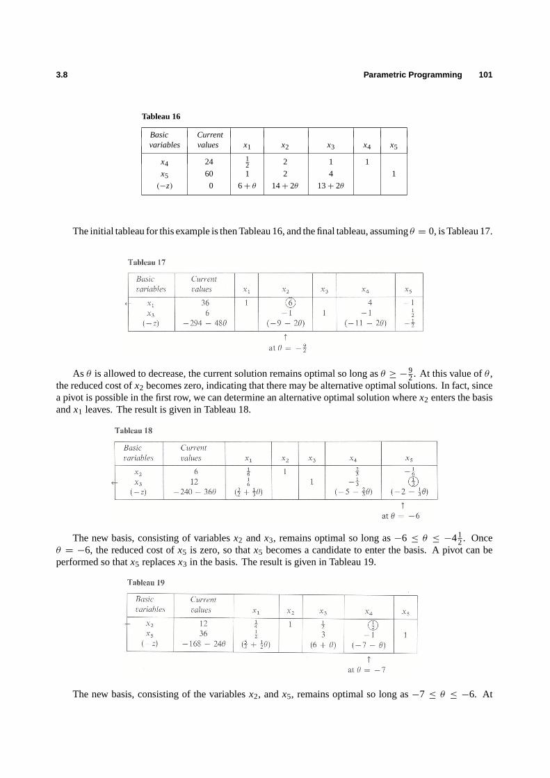
3.8 Parametric Programming 101
Tableau 16
Basic Currentvariables values x1 x2 x3 x4 x5
x4 24 12 2 1 1
x5 60 1 2 4 1
(−z) 0 6+ θ 14+ 2θ 13+ 2θ
The initial tableau for this example is then Tableau 16, and the final tableau, assumingθ = 0, is Tableau 17.
As θ is allowed to decrease, the current solution remains optimal so long asθ ≥ −92. At this value ofθ ,
the reduced cost ofx2 becomes zero, indicating that there may be alternative optimal solutions. In fact, sincea pivot is possible in the first row, we can determine an alternative optimal solution wherex2 enters the basisandx1 leaves. The result is given in Tableau 18.
The new basis, consisting of variablesx2 andx3, remains optimal so long as−6 ≤ θ ≤ −412. Once
θ = −6, the reduced cost ofx5 is zero, so thatx5 becomes a candidate to enter the basis. A pivot can beperformed so thatx5 replacesx3 in the basis. The result is given in Tableau 19.
The new basis, consisting of the variablesx2, andx5, remains optimal so long as−7 ≤ θ ≤ −6. At
102 Sensitivity Analysis
θ = −7, x4 enters the basis, replacingx2, and the resulting tableau is identical to Tableau 16 that has theslack basisx4 andx5 and so will not be repeated here.
Figure 3.6 Parametric objective-function analysis.
In Fig. 3.6, we plot the optimal value of the objective function as a function ofθ . As θ is decreased to−41
2, the contributions of the three products become 112, 5, and 4, respectively, andx1 is replaced in the basis
by x2. As we continue to decreaseθ to−6, the contributions become 0, 2, and 1, andx2 replacesx3 in thebasis. It is interesting to note thatx2 is not in the optimal basis withθ = 0, but eventually is the only productproduced. Atθ = 0, even thoughx2 has the highest contribution, it is not produced because a combination ofx1 andx3 is a better match with the productive resources available. As the relative contributions are reduced,x2 eventually becomes more attractive thanx1 and finally is the only product manufactured.
The algorithm for objective-function parametrics is clearly straightforward to apply and consists ofcomputing a sequence of optimal bases by the primal simplex method. At each stage, a range is computed onthe parameterθ such that the current basis remains optimal. The variable transition at the boundary of thisrange is easily determined, and one pivot operation determines a new basis that is optimal for some adjacentrange.
EXERCISES
1. [Excel spreadsheet available athttp://web.mit.edu/15.053/www/Exer3.1.xls ] Outdoors, Inc. has,as one of its product lines, lawn furniture. They currently have three items in that line: a lawn chair, a standardbench, and a table. These products are produced in a two-step manufacturing process involving the tube-bendingdepartment and the welding department. The time required by each item in each department is as follows:
ProductPresent
Lawn chair Bench Table capacity
Tube bending 1.2 1.7 1.2 1000
Welding 0.8 0 2.3 1200
The contribution that Outdoors, Inc. receives from the manufacture and sale of one unit of each product is $3for a chair, $3 for a bench, and $5 for a table.
The company is trying to plan its production mix for the current selling season. It feels that it can sell anynumber it produces, but unfortunately production is further limited by available material, because of a prolonged

Exercises 103
strike. The company currently has on hand 2000 lbs. of tubing. The three products require the following amountsof this tubing: 2 lbs. per chair, 3 lbs. per bench, and 4.5 lbs. per table.
In order to determine the optimal product mix, the production manager has formulated the linear program shownin Fig. E3.1 and obtained the results shown in Fig. E3.2.
Figure E3.1 Formulation of Outdoors, Inc.
Figure E3.2 Solution of Outdoors, Inc.
a) What is the optimal production mix? What contribution can the firm anticipate by producing this mix?b) What is the value of one unit more of tube-bending time? of welding time? of metal tubing?c) A local distributor has offered to sell Outdoors, Inc. some additional metal tubing for $0.60/lb. Should Outdoors
buy it? If yes, how much would the firm’s contribution increase if they bought 500 lbs. and used it in an optimalfashion?
d) If Outdoors, Inc. feels that it must produce at least 100 benches to round out its product line, what effect willthat have on its contribution?

104 Sensitivity Analysis
e) The R&D department has been redesigning the bench to make it more profitable. The new design will require1.1 hours of tube-bending time, 2.0 hours of welding time, and 2.0 lbs. of metal tubing. If it can sell one unit ofthis bench with a unit contribution of $3, what effect will it have on overall contribution?
f) Marketing has suggested a new patio awning that would require 1.8 hours of tube-bending time, 0.5 hours ofwelding time, and 1.3 lbs. of metal tubing. What contribution must this new product have to make it attractiveto produce this season?
g) Outdoors, Inc. has a chance to sell some of its capacity in tube bending at cost+ $1.50/hour. If it sells 200 hoursat that price, how will this affect contribution?
h) If the contribution on chairs were to decrease to $2.50, what would be the optimal production mix and whatcontribution would this production plan give?
2. [Excel spreadsheet available athttp://web.mit.edu/15.053/www/Exer3.2.xls ] A commercial print-ing firm is trying to determine the best mix of printing jobs it should seek, given its current capacity constraints inits four capital-intensive departments: typesetting, camera, pressroom, and bindery. It has classified its commercialwork into three classes: A, B, and C, each requiring different amounts of time in the four major departments.
The production requirements in hours per unit of product are as follows:
Class of work
Department A B C
Typesetting 0 2 3Camera 3 1 3
Pressroom 3 6 2Bindery 5 4 0
Assuming these units of work are produced using regular time, the contribution to overhead and profit is $200for each unit of Class A work, $300 for each unit of Class B work, and $100 for each unit of Class C work.
The firm currently has the following regular-time capacity available in each department for the next time period:typesetting, 40 hours; camera, 60 hours; pressroom, 200 hours; bindery, 160 hours. In addition to this regular time,the firm could utilize an overtime shift in typesetting, which would make available an additional 35 hours in thatdepartment. The premium for this overtime (i.e., incremental costs in addition to regular time) would be $4/hour.
Since the firm wants to find the optimal job mix for its equipment, management assumes it can sell all it produces.However, to satisfy long-established customers, management decides to produce at least 10 units of each class ofwork in each time period.
Assuming that the firm wants to maximize its contribution to profit and overhead, we can formulate the abovesituation as a linear program, as follows:
Decision variables:
XAR = Number of units of Class A work produced on regular time;
XBR = Number of units of Class B work produced on regular time;
XCR = Number of units of Class C work produced on regular time;
XBO = Number of units of Class B work produced on overtime typesetting;
XCO = Number of units of Class C work produced on overtime typesetting.
Objective function:
Maximizez= 200XAR + 300XBR + 100XCR+ 292XBO+ 88XCO,
Exercises 105
Constraints:
Regular Typesetting 2XBR+ 3XCR ≤ 40,
Overtime Typesetting 2XBO + 3XCO ≤ 35,
Camera 3XAR + XBR + 3XCR+ XBO + 3XCO ≤ 60,
Pressroom 3XAR + 6XBR + 2XCR+ 6XBO + 2XCO ≤ 200,
Bindery 5XAR + 4XBR + 4XBO ≤ 160,
Class A—minimum XAR ≥ 10,
Class B—minimum XBR + XBO ≥ 10,
Class C—minimum XCR + XCO ≥ 10,
XAR ≥ 0, XBR ≥ 0, XCR ≥ 0, XBO ≥ 0, XCO ≥ 0.
The solution of the firm’s linear programming model is given in Fig. E3.3.
a) What is the optimal production mix?b) Is there any unused production capacity?c) Is this a unique optimum? Why?d) Why is the shadow price of regular typesetting different from the shadow price of overtime typesetting?e) If the printing firm has a chance to sell a new type of work that requires 0 hours of typesetting, 2 hours of camera,
2 hours of pressroom, and 1 hour of bindery, what contribution is required to make it attractive?f) Suppose that both the regular and overtime typesetting capacity are reduced by 4 hours. How does the solution
change? (Hint: Does the basis change in this situation?)
3. Jean-Pierre Leveque has recently been named the Minister of International Trade for the new nation of New France.In connection with this position, he has decided that the welfare of the country (and his performance) could best beserved by maximizing the net dollar value of the country’s exports for the coming year. (The net dollar value ofexports is defined as exportslessthe cost of all materials imported by the country.)
The area that now constitutes New France has traditionally made three products for export: steel, heavymachinery, and trucks. For the coming year, Jean-Pierre feels that they could sell all that they could produce ofthese three items at existing world market prices of $900/unit for steel, $2500/unit for machinery, and $3000/unitfor trucks.
In order to produce one unit of steel with the country’s existing technology, it takes 0.05 units of machinery,0.08 units of trucks, two units of ore purchased on the world market for $100/unit, and other imported materialscosting $100. In addition, it takes .5 man-years of labor to produce each unit of steel. The steel mills of New Francehave a maximum usable capacity of 300,000 units/year.
To produce one unit of machinery requires.75 units of steel, 0.12 units of trucks, and 5 man-years of labor. Inaddition, $150 of materials must be imported for each unit of machinery produced. The practical capacity of thecountry’s machinery plants is 50,000 units/year.
In order to produce one unit of trucks, it takes one unit of steel, 0.10 units of machinery, three man-years oflabor, and $500 worth of imported materials. Existing truck capacity is 550,000 units/year.
The total manpower available for production of steel, machinery, and trucks is 1,200,000 men/year.
To help Jean-Pierre in his planning, he had one of his staff formulate the model shown in Fig. E3.4 and solvedin Fig. E3.5. Referring to these two exhibits, he has asked you to help him with the following questions:
a) What is the optimal production and export mix for New France, based on Fig.E3.5? What would be the net dollarvalue of exports under this plan?
b) What do the first three constraint equations (STEEL, MACHIN, and TRUCK) represent? Why are they equalityconstraints?
c) The optimal solution suggests that New France produce 50,000 units of machinery. How are those units to beutilized during the year?
d) What would happen to the value of net exports if the world market price of steel increased to $1225/unit and thecountry chose to export one unit of steel?

106 Sensitivity Analysis
Figure E3.3 Solution for commericial printing firm.
e) If New France wants to identify other products it can profitably produce and export, what characteristics shouldthose products have?
f) There is a chance that Jean-Pierre may have $500, 000 to spend on expanding capacity. If this investment willbuy 500 units of truck capacity, 1000 units of machine capacity, or 300 units of steel capacity, what would be thebest investment?
g) If the world market price of the imported materials needed to produce one unit of trucks were to increase by$400, what would be the optimal export mix for New France, and what would be the dollar value of their netexports?

Exercises 107
Variables:
X1 = Steel production for export (EXSTEE),
X2 = Machinery production for export (EXMACH),
X3 = Truck production for export (EXTRUC),
X4 = Total steel production (TOSTEE),
X5 = Total machinery production (TOMACH),
X6 = Total truck production (TOTRUC).
Constraints:
Steel output (STEEL)
Machinery ouput (MACHIN)
Truck output (TRUCK)
Steel capacity (CAPSTE)
Machinery capacity (CAPMAC)
Truck capacity (CAPTRU)
Manpower available (AVAMAN)
Figure E3.4 Formulation of optimal production and export for New France.
h) The Minister of Defense has recently come to Jean-Pierre and said that he would like to stockpile (inventory) anadditional 10,000 units of steel during the coming year. How will this change the constraint equation STEEL,and what impact will it have on net dollar exports?
i) A government R&D group has recently come to Jean-Pierre with a new product, ProductX, that can be producedfor export with 1.5 man-years of labor and 0.3 units of machinery for each unit produced. What must ProductXsell for on the world market to make it attractive for production?
j) How does this particular formulation deal with existing inventories at the start of the year and any desiredinventories at the end of the year?
4. Another member of Jean-Pierre’s staff has presented an alternative formulation of New France’s planning problem

108 Sensitivity Analysis
Figure E3.5 Solution of New France model.
as described in Exercise 3, which involves only three variables. This formulation is as follows:
Y1 = Total steel production,
Y2 = Total machinery production,
Y3 = Total truck production.
Maximizez = 900(Y1− 0.75Y2− Y3)− 300Y1+ 2500(Y2− 0.05Y1− 0.10Y3)
−150Y2+ 3000(Y3− 0.80Y1− 0.12Y2)− 500Y3,

Exercises 109
subject to:
Y1 ≤ 300,000,
Y2 ≤ 50,000,
Y3 ≤ 550,000,
0.5Y1 + 5Y2+ 3Y3 ≤ 1,200,000, Y1, Y2, Y3 ≥ 0.
a) Is this formulation equivalent to the one presented in Fig. E3.4 of Exercise 3? How would the optimal solutionhere compare with that found in Fig. E3.5?
b) If we had the optimal solution to this formulation in terms of total production, how would we find the optimalexports of each product?
c) What assumption does this formulation make about the quantities and prices of products that can be exportedand imported?
d) New France is considering the production of automobiles. It will take 0.5 units of steel, 0.05 units of machinery,and 2.0 man-years to produce one unit of automobiles. Imported materials for this unit will cost $250 and thefinished product will sell on world markets at a price of $2000. Each automobile produced will use up.75 units ofthe country’s limited truck capacity. How would you alter this formulation to take the production of automobilesinto account?
5. Returning to the original problem formulation shown in Fig. E3.4 of Exercise 3, Jean-Pierre feels that, with existinguncertainties in international currencies, there is some chance that the New France dollar will be revalued upwardrelative to world markets. If this happened, the cost of imported materials would go down by the same percent asthe devaluation, and the market price of the country’s exports would go up by the same percent as the revaluation.Assuming that the country can always sell all it wishes to export how much of a revaluation could occur before theoptimal solution in Fig. E3.5 would change?
6. After paying its monthly bills, a family has $100 left over to spend on leisure. The family enjoys two types ofactivities: (i) eating out; and (ii) other entertainment, such as seeing movies and sporting events. The family hasdetermined the relative value (utility) of these two activities—each dollar spend on eating out provides 1.2 unitsof value for each dollar spent on other entertainment. Suppose that the family wishes to determine how to spendthis money to maximize the value of its expenditures, but that no more than $70 can be spent on eating out and nomore than $50 on other entertainment (if desired, part of the money can be saved). The family also would like toknow:
a) How the total value of its expenditures for leisure would change if there were only $99 to spend.b) How the total value would change if $75 could be spend on eating out.c) Whether it wouldsaveany money if each dollar of savings would provide 1.1 units of value for each dollar spent
on other entertainment.
Formulate the family’s spending decision as a linear program. Sketch the feasible region, and answer each ofthe above questions graphically. Then solve the linear program by the simplex method, identify shadow prices onthe constraints, and answer each of these questions, using the shadow prices.
7. [Excel spreadsheet available athttp://web.mit.edu/15.053/www/Exer3.7.xls ] Consider the linearprogram:
Maximizez= x1+ 3x2,
subject to:
x1+ x2 ≤ 8 (resource 1),
−x1+ x2 ≤ 4 (resource 2),
x1 ≤ 6 (resource 3),
x1 ≥ 0, x2 ≥ 0.
a) Determine graphically:

110 Sensitivity Analysis
i) the optimal solution;ii) the shadow prices on the three constraints;
iii) the range on the objective coefficient of each variable, holding the coefficient of the other variable at its currentvalue, for which the solution to part (i) remains optimal;
iv) the range on the availability of each resource, holding the availability of the other resources at their currentvalues, for which the shadow prices in part (ii) remain optimal.
b) Answer the same question, using the following optimal tableau determined by the simplex method:
Basic Currentvariables values x1 x2 x3 x4 x5
x1 2 1 12 −
12
x2 6 1 12
12
x5 4 −12
12 1
(−z) −20 −2 −1
8. Determine the variable transitions for the previous problem, when each objective coefficient or righthand-side valueis varied by itself to the point where the optimal basis no longer remains optimal. Carry out this analysis using theoptimal tableau, and interpret the transitions graphically on a sketch of the feasible region.
9. [Excel spreadsheet available athttp://web.mit.edu/15.053/www/Exer3.9.xls ] A wood-productscompany produces four types of household furniture. Three basic operations are involved: cutting, sanding, andfinishing. The plant’s capacity is such that there is a limit of 900 machine hours for cutting, 800 hours for sanding,and 480 hours for finishing. The firm’s objective is to maximize profits. The initial tableau is as follows:
Basic Currentvariables values x1 x2 x3 x4 x5 x6 x7
x5 480 2 8 4 2 1x6 800 5 4 8 5 1x7 900 7 8 3 5 1
(−z) 0 +90 +160 +40 +100
Using the simplex algorithm, the final tableau is found to be:
Basic Currentvariables values x1 x2 x3 x4 x5 x6 x7
x2 25 0 1 18
532 −
116
x4 140 1 32 1 −
18
14
x7 0 2 −112 −
58 −
34 1
(−z) −18,000 −10 −130 −1212 −15
a) What are the shadow prices on each of the constraints?b) What profit forx3 would justify its production?c) What are the limits on sanding capacity that will allow the present basic variables to stay in the optimal solution?d) Suppose management had to decide whether or not to introduce a new product requiring 20 hours of cutting, 3
hours of sanding, and 2 hours of finishing, with an expected profit of $120. Should the product be produced?e) If another saw to perform cutting can be rented for $10/hour, should it be procured? What about a finisher at the
same price? If either is rented, what will be the gain from the first hour’s use?
10. [Excel spreadsheet available athttp://web.mit.edu/15.053/www/Exer3.10.xls ] The ReclamationMachining Company makes nuts and bolts from scrap material supplied from the waste products of three steel-using

Exercises 111
firms. For each 100 pounds of scrap material provided by firm A, 10 cases of nuts and 4 cases of bolts can be made,with a contribution of $46. 100 pounds from firm B results in 6 cases of nuts, 10 cases of bolts, and a contributionof $57. Use of 100 pounds of firm C’s material will produce 12 cases of nuts, 8 of bolts, and a contribution of$60. Assuming Reclamation can sell only a maximum of 62 cases of nuts and 60 of bolts, the final tableau for alinear-programming solution of this problem is as follows:
Basic Currentvariables values x1 x2 x3 x4 x5
x1 3.421 1 0.947 0.132 −0.079
x2 4.632 1 0.421 −0.052 0.132
(−z) −421.368 −7.759 −3.053 −3.868
a) What is the optimal solution?b) Is the solution unique? Why?c) For each of the three sources, determine the interval of contribution for which the solution in part (a) remains
optimal.d) What are the shadow prices associated with the optimal solution in (a), and what do they mean?e) Give an interval for each sales limitation such that the shadow prices in (d) remain unchanged.
11. [Excel spreadsheet available athttp://web.mit.edu/15.053/www/Exer3.11.xls ] Consider the linearprogram:
Maximizez= 2x1+ x2+ 10x3,
subject to:x1− x2 + 3x3 = 10,
x2 + x3 + x4 = 6,
x j ≥ 0 ( j = 1, 2, 3, 4).
The optimal tableau is:
Basic Currentvariables values x1 x2 x3 x4
x3 4 14 1 1
4
x2 2 −14 1 3
4
(−z) −24 −14 −31
4
a) What are the optimal shadow prices for the two constraints? Can the optimal shadow price for the first constraintbe determined easily from the final objective coefficient forx1? (Hint: The initial problem formulation is incanonical form if the objective coefficient ofx1 is changed to 0x1.)
b) Suppose that the initial righthand-side coefficient of the first constraint is changed to 10+ δ. For what valuesof δ do x2 andx3 form an optimal basis for the problem?
12. [Excel spreadsheet available athttp://web.mit.edu/15.053/www/Exer3.12.xls ] Consider the fol-lowing linear program:
Minimize z= 2xi + x2 + 2x3 − 3x4,
subject to:8x1 − 4x2 − x3 + 3x4 ≤ 10,2x1 + 3x2 + x3 − x4 ≤ 7,
− 2x2 − x3 + 4x4 ≤ 12,
x1 ≥ 0, x2 ≥ 0, x3 ≥ 0, x4 ≥ 0.
After several iterations of the simplex algorithm, the following tableau has been determined:

112 Sensitivity Analysis
Basic Currentvariables values x1 x2 x3 x4 x5 x6 x7
x5 11 10 12 1 1 −
12
x2 4 45 1 3
1025
110
x4 5 25 −
110 1 1
5310
(−z) −11 125
75
15
45
a) What are the values of the decision variables? How do you know this is the optimal solution?b) For each nonbasic variable of the solution, find the interval for its objective-function coefficient such that the
solution remains optimal.c) Do the same for each basis variable.d) Determine the interval for each righthand-side value such that the optimal basis determined remains unchanged.
What does this imply about the shadow prices? reduced costs?
13. A cast-iron foundry is required to produce 1000 lbs. of castings containing at least 0.35 percent manganese andnot more than 3.2 percent silicon. Three types of pig iron are available in unlimited amounts, with the followingproperties:
Type of pig iron
A B C
Silicon 4% 1% 5%
Manganese 0.35% 0.4% 0.3%
Cost/1000 lbs. $28 $30 $20
Assuming that pig iron is melted with other materials to produce cast iron, a linear-programming formulation thatminimizes cost is as follows:
Minimize z= 28x1+ 30x2+ 20x3,
subject to:4x1 + x2 + 5x3 ≤ 3.2 (lb. Si× 10),
3.5x1 + 4x2 + 3x3 ≥ 3.5 (lb. Mn),x1 + x2 + x3 = 1 (lb. × 103),
x1 ≥ 0, x2 ≥ 0, x3 ≥ 0.
Initial tableau
Surplus Slack Artificial
Basic Currentvariables values x1 x2 x3 x4 x5 v1 v2
x5 3.2 4 1 5 0 1
v1 3.5 3.5 4 3 −1 1
v2 1 1 1 1 0 1
(−z) 0 28 30 20 0
Final tableau

Exercises 113
Basic Currentvariables values x1 x2 x3 x4 x5 v1 v2
x5 0.2 1 −4 1 4 −17
x3 0.5 0.5 1 −1 1 −3
x2 0.5 0.5 1 1 −1 4
(−z) −25 3 10 −10 10
a) At what cost does pig type A become a candidate for entry into the optimal basis? What activity would it replace?b) How much can we afford to pay for pure manganese to add to the melt?c) How much can the manganese requirement be reduced without changing the basis? What are the values of the
other basic variables when this happens?d) How much can the cost of pig type B change without changing the optimal basis? What are the new basic
variables when such a change occurs?e) How can the final tableau be optimal if the reduced cost ofv1 is−10?
14. [Excel spreadsheet available athttp://web.mit.edu/15.053/www/Exer3.14.xls ] The Classic StoneCutter Company produces four types of stone sculptures: figures, figurines, free forms, and statues. Each productrequires the following hours of work for cutting and chiseling stone and polishing the final product:
Type of product
Operation Figures Figurines Free Forms Statues
Cutting 30 5 45 60Chiseling 20 8 60 30Polishing 0 20 0 120
Contribution/unit $280 $40 $500 $510
The last row in the above table specifies the contribution to overhead for each product.Classic’s current work force has production capacity to allocate 300 hours to cutting, 180 hours to chiseling,
and 300 hours to polishing in any week. Based upon these limitations, it finds its weekly production schedule fromthe linear-programming solution given by the following tableau.
Cutting Chiseling Polishingslack, slack, slack,
Basic Current Figures Figurines Forms Statues hours hours hours
variables values x1 x2 x3 x4 x5 x6 x7
Statues 2 −715 −6 1 1
15 −110
Figures 6 1 1110
152 −
110
15
Slack 60 76 360 −8 12 1
−Contrib. −2700 −30 −70 −6 −5
a) Determine a range on the cutting capacity such that the current solution remains optimal.b) Busts have the following characteristics:
Cutting 15 hrs.Chiseling 10 hrs.Polishing 20 hrs.Contribution/unit $240
Should Classic maintain its present line or expand into busts?
114 Sensitivity Analysis
c) Classic can buy 5 hours of cutting capacity and 5 hours of chiseling capacity from an outside contractor at a totalcost of $75. Should Classic make the purchase or not?
d) By how much does the contribution from free forms have to be increased to make free forms profitable to produce?e) Give a range on the contribution from figures such that the current solution remains optimal. What activities
enter the basis at the bounds of this range?
15. [Excel spreadsheet available athttp://web.mit.edu/15.053/www/Exer3.15.xls ] The Concrete Prod-ucts Corporation has the capability of producing four types of concrete blocks. Each block must be subjected tofour processes: batch mixing, mold vibrating, inspection, and yard drying. The plant manager desires to maximizeprofits during the next month. During the upcoming thirty days, he has 800 machine hours available on the batchmixer, 1000 hours on the mold vibrator, and 340 man-hours of inspection time. Yard-drying time is unconstrained.The production director has formulated his problem as a linear program with the following initial tableau:
Basic Currentvariables values x1 x2 x3 x4 x5 x6 x7
x5 800 1 2 10 16 1
x6 1000 1.5 2 4 5 1
x7 340 0.5 0.6 1 2 1
(−z) 0 8 14 30 50
wherex1, x2, x3, x4 represent the number of pallets of the four types of blocks. After solving by the simplex method,the final tableau is:
Basic Currentvariables values x1 x2 x3 x4 x5 x6 x7
x2 200 1 +11 19 15 −1
x1 400 1 −12 −22 −2 2x7 20 0.4 1.6 0.1 −0.4 1
(−z) 6000 −28 −40 −5 −2
a) By how much must the profit on a pallet of number 3 blocks be increased before it would be profitable tomanufacture them?
b) What minimum profit onx2 must be realized so that it remains in the production schedule?c) If the 800 machine-hours capacity on the batch mixer is uncertain, for what range of machine hours will it remain
feasible to produce blocks 1 and 2?d) A competitor located next door has offered the manager additional batch-mixing time at a rate of $4.00 per hour.
Should he accept this offer?e) The owner has approached the manager with a thought about producing a new type of concrete block that would
require 4 hours of batch mixing, 4 hours of molding, and 1 hour of inspection per pallet. What should be theprofit per pallet if block number 5 is to be included in the optimal schedule?
16. [Excel spreadsheet available athttp://web.mit.edu/15.053/www/Exer3.16.xls ] The linear-programmingprogram:
Maximizez= 4x4+ 2x5− 3x6,
subject to:x1 + x4 − x5 + 4x6 = 2,
x2 + x4 + x5 − 2x6 = 6,
x3 − 2x4 + x5 − 3x6 = 6,
x j ≥ 0 ( j = 1, 2, . . . , 6)
has an optimal canonical form given by:

Exercises 115
Basic Currentvariables values x1 x2 x3 x4 x5 x6
x4 4 12
12 1 1
x5 2 −12
12 1 −3
x3 12 32
12 1 2
(−z) −20 −1 −3 −1
Answer the following questions. All parts are independent and refer to changes in theoriginal problemformulation as stated above. That is, do not consider parts (a), (b), and (c) together, but refer to the original problemformulation in each part.
a) Suppose that the objective function changes to
z= 4x4+ 2x5+ 0x6.
Find the new optimal solution. Is the solution to the new problem unique? Explain your answer.b) Consider the parametric-programming problem with the objective function:
Maximizez= (4+ 2θ)x4+ (2− 4θ)x5+ (−3+ θ)x6.
For what valuesθ ≤ θ ≤ θ of θ do the variablesx4, x5, andx3 remain in the optimal basis (e.g., ifθ = −1 andθ = 2, then the interval is−1≤ θ ≤ 2). What are the variable transitions atθ = θ andθ = θ?
c) Consider the parametric programming problem with the righthand sides
2 + 4θ,
6 − 2θ,
6 − θ.
For what valuesθ ≤ θ ≤ θ of θ do the variablesx4, x5, andx3 remain in the optimal basis? What are the variabletransitions atθ = θ andθ = θ?
17. The Massachusetts Electric Company is planning additions to its mix of nuclear and conventional electric powerplants to cover a ten-year horizon. It measures the output of plants in terms of equivalent conventional plants.Production of electricity must satisfy the state’s additional requirements over the planning horizon for guaranteedpower (kW), peak power (kW), and annual energy (MWh). The state’s additional requirements, and the contributionof each type of plant to these requirements, are as follows:
Requirements
Guaranteed Peak power Annual energypower(kW) (kW) (MWh)
Conventional 1 3 1Nuclear 1 1 4
Additionalrequirements 20 30 40
The costs for each type of plant include fixed investment costs and variable operating costs per year. Theconventional plants have very high operating costs, since they burn fossil fuel, while the nuclear plants have veryhigh investment costs. These costs are as follows:
Investment costs Annual operating costsType of plant (millions) (millions)
Conventional $ 30 $20Nuclear 100 5

116 Sensitivity Analysis
For simplicity, we will assume that the annual operating costs are an infinite stream discounted at a rate of(1/(1+r ))
per year. The present value of this infinite stream of operating costs is:
PV =∞∑
n=1
(1
1+ r
)n
c =
[1
1− [1/(1+ r )]− 1
]c =
1
rc
and the term 1/r is sometimes referred to as thecoefficient of capitalization.a) Formulate a linear program to decide what mix of conventional and nuclear power plants to build, assuming
that you must meet or exceed the state’s three requirements and you want to minimize thetotal investment plusdiscounted operating costs.
b) There has been a debate at Massachusetts Electric as to what discount rater to use in making this calculation.Some have argued for a low ‘‘social’’ rate of about 2 or 3 percent, while others have argued for the private ‘‘costof capital’’ rate of from 10 to 15 percent. Graphically determine the optimal solution for all values of the discountrater , to aid in settling this question. Comment on the implications of the choice of discount rate.
c) Another difficulty is that there may not be sufficient investment funds to make the decisions independently ofan investment limitation. Assuming the ‘‘social’’ discount rate of 2 percent, find the optimal solution for allconceivable budget levels for total investment. What is the impact of limiting the budget for investment?
18. [Excel spreadsheet available athttp://web.mit.edu/15.053/www/Exer3.18.xls ] Consider the parametric-programming problem:
Maximizez= (−3+ 3θ)x1+ (1− 2θ)x2,
subject to:−2x1 + x2 ≤ 2,
x1 − 2x2 ≤ 2,
x1 − x2 ≤ 4,
x1 ≥ 0, x2 ≥ 0.
Letting x3, x4, andx5 be slack variables for the constraints, we write the optimal canonical form atθ = 0 as:
Basic Currentvariables values x1 x2 x3 x4 x5
x2 2 −2 1 1
x4 6 −3 2 1
x5 6 −1 1 1
(−z) −2 −1 −1
a) Place the objective function in this tableau in canonical form for values ofθ other than 0. For what values ofθ
is this canonical form optimal?b) What are the variable transitions when this canonical form is no longer optimal? Does the problem become
unbounded at either of the transition points?c) Use the parametric programming algorithm to find the optimal solution for all values ofθ . Plot the optimal
objective value as a function ofθ .d) Graph the feasible region and interpret the parametric algorithm on the graph.
19. [Excel spreadsheet available athttp://web.mit.edu/15.053/www/Exer3.19.xls ] Consider the fol-lowing parametric linear program:
z∗(θ) = Max x1+ 2x2,
subject to:2x1 + x2 ≤ 14,x1 + x2 ≤ 10,x1 ≤ 1+ 2θ,
x2 ≤ 8− θ,
x1 ≥ 0, x2 ≥ 0.

Exercises 117
a) Graph the feasible region and indicate the optimal solution forθ = 0, θ = 1, andθ = 2.b) For what values ofθ is this problem feasible?c) From the graphs in part (a), determine the optimal solution for all values ofθ . Graph the optimal objective value
z∗(θ).d) Starting with the optimal canonical form given below forθ = 0, use the parametric simplex algorithm to solve
for all values ofθ .
Basic Currentvariables values x1 x2 x3 x4 x5 x6
x3 4− 3θ 1 −2 −1
x4 1− θ 1 −1 −1
x1 1+ 2θ 1 1
x2 8− θ 1 1
(−z) −17 −1 −2
20. Consider the linear program:
Minimize z= −10x1+ 16x2− x,
subject to:x1 − 2x2 + x3 ≤ 2 + 2θ,
x1 − x2 ≤ 4 + θ,
x1 ≥ 0, x2 ≥ 0, x3 ≥ 0,
whereθ is a parameter.
a) Forθ = 0
i) Solve the linear program.ii) What are the optimal shadow prices?
iii) Suppose that the constant on the righthand side of the second inequality is changed from 4 to 6. What is thenew optimal value ofz?
b) For what values ofθ does the optimal basis to part a(i) remain optimal?c) Solve the linear program for all values ofθ .
21. When discussing parametric analysis in Section 3.8, we considered reallocating floor space for a trailer-productionproblem to trade off woodworking capacity for metalworking capacity. The trade-off was governed by the parameterθ in the following tableau:
Basic Currentvariables values x1 x2 x3 x4 x5
x4 24+ θ 12 2 1 1 Woodworking capacity
x5 60− θ 1 2 4 1 Metalworking capacity
(−z) 0 6 14 13
We found that the following tableau was optimal for values ofθ in the range 0≤ θ ≤ 4:
Basic Currentvariables values x1 x2 x3 x4 x5
x1 35+ 5θ 1 6 4 −1
x3 6− 32θ −1 1 −1 1
2
(−z) −294− 1012θ −9 −11 −
12

118 Sensitivity Analysis
Figure E3.6 Risk-return trade-off.
The optimal solution atθ = 4 is x1 = 56, x2 = x3 = x4 = x5 = 0, andz = 336. At θ = 5, we found thatthe optimal basic variables arex1 = 52, x2 = 1.5, and that the optimal objective value isz = 348− 3(5) = 333.Therefore asθ increases from 4 to 5,
1z= 333− 336= −3.
The previous optimal tableau tells us that for 0≤ θ ≤ 4, woodworking capacity is worth $11/day andmetalworking capacity is worth $0.50/day. Increasingθ from 4 to 5 increases woodworking capacity by oneday. Using the prices $11/day and $0.50/day, the change in the optimal objective value should be:
1z= 11(1)+ 0.50(−1) = 10.50.
We have obtained two different values for the change in the optimal objective value,1z= −3 and1z= 10.50.Reconcile the difference between these values.
22. An investor has $5000 and two potential investments. Letx j for j = 1 and j = 2 denote her allocation to investmentj in thousands of dollars. From historical data, investments 1 and 2 are known to have an expected annual return of20 and 16 percent, respectively. Also, the total risk involved with investments 1 and 2, as measured by the varianceof total return, is known to be given by 2x1+ x2+ (x1+ x2), so that risk increases with total investment(x1+ x2)
and with the amount of each individual investment. The investor would like to maximize her return and at the sametime minimize her risk. Figure E3.6 illustrates the conflict between these two objectives. PointA in this figurecorresponds to investing nothing, pointB to investing all $5000 in the second alternative, and pointC to investingcompletely in the first alternative. Every other point in the shaded region of the figure corresponds to some otherinvestment strategy; that is, to a feasible solution to the constraints:
x1+ x2 ≤ 5,
x1 ≥ 0, x2 ≥ 0.(27)
To deal with the conflicting objectives, the investor decides to combine return and risk into a single objectivefunction.
Objective = Return− θ (Risk)
= 20x1+ 16x2− θ [2x1+ x2+ (x1+ x2)]. (28)
She uses the parameterθ in this objective function to weigh the trade-off between the two objectives.
Because the ‘‘most appropriate’’ trade-off parameter is difficult to assess, the investor would like to maximizethe objective function (28) subject to the constraints (27), for all values ofθ , and then use secondary considerations,not captured in this simple model, to choose from the alternative optimal solutions.

Exercises 119
a) Use parametric linear programming to solve the problem for all nonnegative values ofθ .b) Plot the optimal objective value, the expected return, and the risk as a function ofθ .c) Interpret the solutions on Fig. E3.6.d) Suppose that the investor can save at 6% with no risk. For what values ofθ will she save any money using the
objective function (28)?
23. An alternative model for the investment problem discussed in the previous exercise is:
Maximizez= 20x1+ 16x2,
subject to:x1 + x2 ≤ 5,
2x1 + x2 + (x1+ x2) ≤ γ,
x1 ≥ 0, x2 ≥ 0.
In this model, the investor maximizes her expected return, constraining the risk that she is willing to incur by theparameterγ .
a) Use parametric linear programming to solve the problem for all nonnegative values ofγ .b) Plot the expected return and risk as a function ofγ .c) Interpret the solutions on Fig. E3.6 of Exercise 22.
24. The shadow-price concept has been central to our development of sensitivity analysis in this chapter. In this ex-ercise, we consider how changing the initial problem formulation alters the development. Suppose that the initialformulation of the model is given by:
Maximizez=n∑
j=1
c j x j ,
subject to:
n∑j=1
ai j x j ≤ bi (i = 1, 2, . . . , m),
x j ≥ 0 ( j = 1, 2, . . . , n).
Solving this problem by the simplex method determines the shadow prices for the constraints asy1, y2, . . . , ym.
a) Suppose that the first constraint were multiplied by 2 and stated instead as:
n∑j=1
(2a1 j )x j ≤ (2b1).
Let y1 denote the value of the shadow price for this constraint. How isy1 related toy1?b) What happens to the value of the shadow prices if every coefficientc j is multiplied by 2 in the original problem
formulation?c) Suppose that the first variablex1 in the model is rescaled by a factor of 3. That is, letx′1 = 3x1 and replacex1
everywhere in the model by(x′1/3). Do the shadow prices change? Would it be possible forx′1 to appear in anoptimal basis, ifx1 could not appear in an optimal basis of the original formulation for the problem?
d) Do the answers to parts (a), (b), and (c) change if the original problem is stated with all equality constraints:
n∑j=1
ai j x j = bi (i = 1, 2, . . . , m)?

120 Sensitivity Analysis
25. [Excel spreadsheet available athttp://web.mit.edu/15.053/www/Exer3.25.xls ] Shortly after thebeginning of the oil embargo, the Eastern District Director of the Government Office of Fuel Allocation wasconcerned that he would soon have to start issuing monthly allocations specifying the amounts of heating oil thateach refinery in the district would send to each city to ensure that every city would receive its quota.
Since different refineries used a variety of alternative sources of crude oil, both foreign and domestic, the costof products at each refinery varied considerably. Consequently, under current government regulations, the pricesthat could be charged for heating oil would vary from one refinery to another. To avoid political criticism, it wasfelt that, in making allocations of supplies from the refineries to the cities, it was essential to maintain a reasonablyuniform average refinery price for each city. In fact, the Director felt that the average refinery price paid by any cityshould not be more than 3% above the overall average.
Another complication had arisen in recent months, since some of the emergency allocations of supplies to certaincities could not be delivered due to a shortage in tanker capacity. If deliveries of the allocated supplies were to befeasible, the limited transportation facilities on some of the shipping routes would have to be recognized. Finally,it would be most desirable to maintain distribution costs as low as possible under any allocation plan, if charges ofgovernment inefficiency were to be avoided.
Data for a simplified version of the problem, with only three refineries and four cities, are given in Fig. E3.7.The allocation problem can be formulated as the linear program shown in Fig. E3.8. The decision variables aredefined as follows:
A− n = Barrels of heating oil (in thousands) to be supplied from Refinery A toCity n wheren = 1, 2, 3, or 4.
B− n = Barrels of heating oil (in thousands) to be supplied from Refinery B toCity n wheren = 1, 2, 3, or 4.
C − n = Barrels of heating oil (in thousands) to be supplied by Refinery C toCity n wheren = 1, 2, 3, or 4.
PMAX = A value higher than the average refinery price paid by any of the fourcities.
There are four types of constraints that must be satisfied:
1. Supply constraints at each refinery.2. Quota restrictions for each city.3. Average price restrictions which impose an upper limit to the average refinery price which will be paid by any
city.4. Shipping capacity limits on some of the routes.
All the constraints are straightforward except possibly the average price reductions. To restrict the average refineryprice paid by City 1 to be less than the variable PMAX, the following expression is used:
(10.53)(A− 1)+ (9.39)(B− 1)+ (12.43)(C − 1)
55≤ PMAX
or0.1915(A− 1)+ 0.1701(B− 1)+ 0.2260(C − 1)− PMAX ≤ 0.
Such a restriction is included for each city, to provide a uniform upper bound on average prices. The value of PMAXis limited by the prescribed maximum of 11.40= 11.07× 1.03 by the constraint
PMAX ≤ 11.40.
The computer analysis of the linear programming model is given in Fig. E3.9
a) Determine the detailed allocations that might be used for December.b) Evaluate the average refinery prices paid by each city under these allocations.c) Determine the best way to utilize an additional tanker-truck capacity of 10,000 barrels per month.d) Discuss the inefficiency in distribution costs resulting from the average refinery price restrictions.e) Evaluate the applicability of the model in the context of a full allocation system.
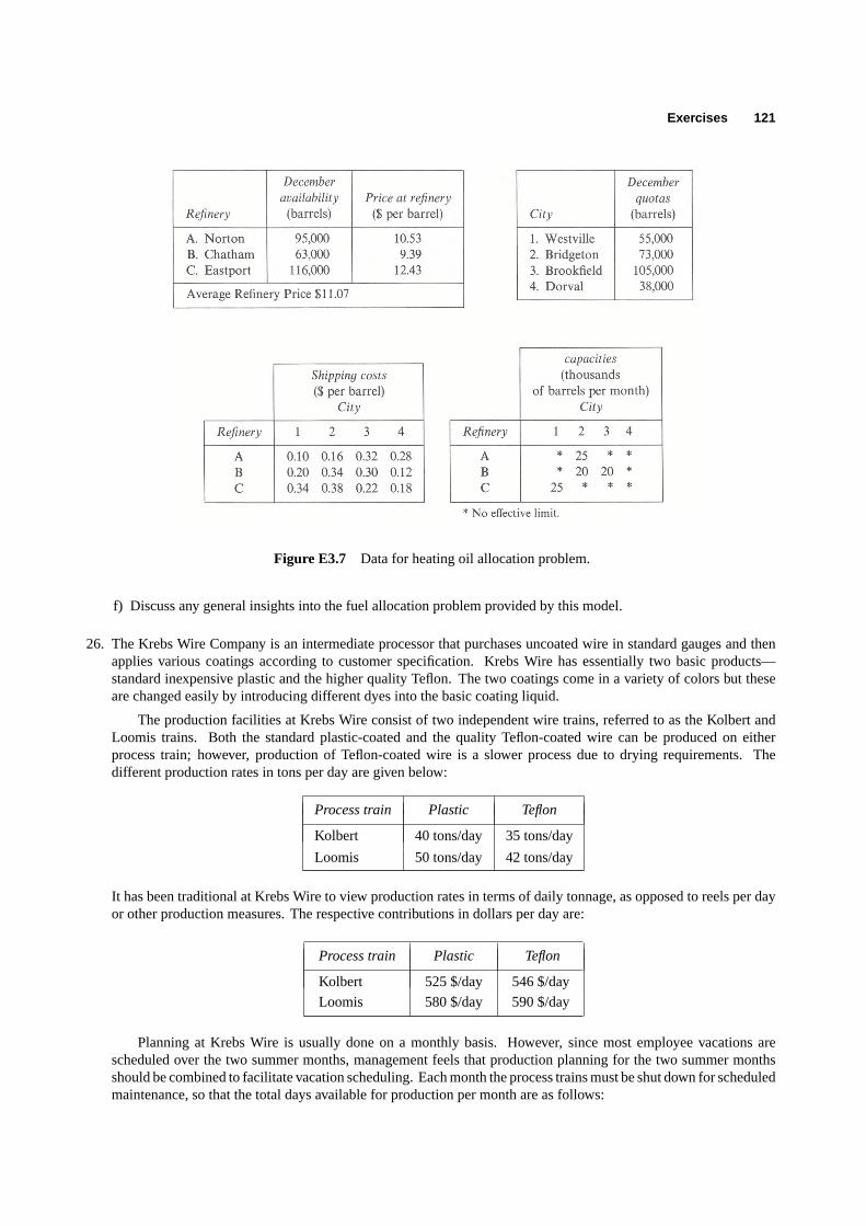
Exercises 121
Figure E3.7 Data for heating oil allocation problem.
f) Discuss any general insights into the fuel allocation problem provided by this model.
26. The Krebs Wire Company is an intermediate processor that purchases uncoated wire in standard gauges and thenapplies various coatings according to customer specification. Krebs Wire has essentially two basic products—standard inexpensive plastic and the higher quality Teflon. The two coatings come in a variety of colors but theseare changed easily by introducing different dyes into the basic coating liquid.
The production facilities at Krebs Wire consist of two independent wire trains, referred to as the Kolbert andLoomis trains. Both the standard plastic-coated and the quality Teflon-coated wire can be produced on eitherprocess train; however, production of Teflon-coated wire is a slower process due to drying requirements. Thedifferent production rates in tons per day are given below:
Process train Plastic Teflon
Kolbert 40 tons/day 35 tons/day
Loomis 50 tons/day 42 tons/day
It has been traditional at Krebs Wire to view production rates in terms of daily tonnage, as opposed to reels per dayor other production measures. The respective contributions in dollars per day are:
Process train Plastic Teflon
Kolbert 525 $/day 546 $/day
Loomis 580 $/day 590 $/day
Planning at Krebs Wire is usually done on a monthly basis. However, since most employee vacations arescheduled over the two summer months, management feels that production planning for the two summer monthsshould be combined to facilitate vacation scheduling. Each month the process trains must be shut down for scheduledmaintenance, so that the total days available for production per month are as follows:

122 Sensitivity Analysis
Figure E3.8 Formulation of the heating-oil allocation model.
Process train July August
Kolbert 26 days 26 days
Loomis 28 days 27 days
The scheduling process is further complicated by the fact that, over the two summer months, the total amount oftime available for production is limited to 102 machine days due to vacation schedules.
The amounts of wire that the management feels it can sell in the coming two months are:
Product July August
Plastic 1200 tons 1400 tons
Teflon 800 tons 900 tons
Both types of wire may be stored for future delivery. Space is available in Krebs’ own warehouse, which has acapacity of 20 tons. The inventory and carrying costs in dollars per ton for wire produced in July and delivered inAugust are:
Product Inventory and carrying costs
Plastic 1.00 $/ton
Teflon 1.20 $/ton
Due to a commitment of warehouse capacity to other products in September, it is not possible to stock any wirein inventory at the end of August.
To help in planning production for the two summer months, Krebs Wire management has formulated and solveda linear program (see Figs. E3.10 and E3.11) in order to determine the production schedule that will maximizecontribution from these products.
a) What does the output in Fig. E3.12 tell the production manager about the details of scheduling his machines?

Exercises 123
b) There is the possibility that some employees might be persuaded to take their vacations in June or September.Should this be encouraged?
c) The solution in Fig. E3.12 suggests that Teflon should be made only on the Loomis train in July and only on theKolbert train in August. Why?
d) Should Krebs Wire lease additional warehouse capacity at a cost of $2.00 above the inventory and carrying costs?If so, how would the optimal solution change?
e) The sales manager feels that future sales might be affected if the firm could not meet demand for plastic-coatedwire in August. What, if anything, should be done?
f) One of Krebs’ customers has requested a special run of twenty tons of corrosion-resistant wire to be deliveredat the end of August. Krebs has made this product before and found that it can be produced only on the Loomismachine, due to technical restrictions. The Loomis machine can produce this special wire at a rate of 40 tonsper day, and the customer will pay $12 per ton. Krebs cannot start production before the 1st of August due to ashortage of raw materials. Should the firm accept the order?
27. Consider the computer output for the Krebs Wire case in Exercise 26. What does the ‘‘100 percent rule’’ tell us ineach of the following situations?
Figure E3.9 Solution of the allocation model. (Continued on next page.)

124 Sensitivity Analysis
Figure E3.9 (Cont.)
a) The objective-function coefficients changed as follows:
K-T-J from 546 to 550,L-T-A from 590 to 600.
b) The objective-function coefficients changed as follows:
L-P-J from 580 to 585,L-T-J from 590 to 585.
c) The objective-function coefficients changed as follows:
L-P-J from 580 to 585,L-T-J from 590 to 588.
d) The righthand-side values changed as follows:
L-Day-J from 28 to 25,War-Cap from 20 to 24.
e) The righthand-side values changed as follows:
L-Day-J from 28 to 23,P-Dem-A from 1400 to 1385.
28. [Excel spreadsheet available athttp://web.mit.edu/15.053/www/Exer3.28.xls ] Mr. Watson has100 acres that can be used for growing corn or soybeans. His yield is 95 bushels per acre per year of corn of 60bushels of soybeans. Any fraction of the 100 acres can be devoted to growing either crop. Labor requirements are4 hours per acre per year, plus 0.70 hour per bushel of corn and 0.15 hour per bushel of soybeans. Cost of seed,fertilizer, and so on is 24 cents per bushel of corn and 40 cents per bushel of soybeans. Corn can be sold for $1.90per bushel, and soybeans for $3.50 per bushel. Corn can be purchased for $3.00 per bushel, and soybeans for $5.00per bushel.

Exercises 125
Figure E3.10 Formulation of the Krebs Wire linear program.
In the past, Mr. Watson has occasionally raised pigs and calves. He sells the pigs or calves when they reachthe age of one year. A pig sells for $80 and a calf for $160. One pig requires 20 bushels of corn or 25 bushelsof soybeans, plus 25 hours of labor and 25 square feet of floor space. One calf requires 50 bushels of corn or 20bushels of soybeans, 80 hours of labor, and 30 square feet of floor space.
Mr. Watson has 10,000 square feet of floor space. He has available per year 2000 hours of his own time andanother 4000 hours from his family. He can hire labor at $3.00 per hour. However, for each hour of hired labor,0.15 hour of his time is required for supervision.
Mr. Watson’s son is a graduate student in business, and he has formulated a linear program to show his father howmuch land should be devoted to corn and soybeans and in addition, how many pigs and/or calves should be raisedto maximize profit.
In Fig. 3.12, Tableau 1 shows an initial simplex tableau for Watson’s farm using the definitions of variables andconstraints given below, and Tableau 2 shows the results of several iterations of the simplex algorithm.
Variables
1. Grow 1 acre of corn 7. Raise 1 pig on corn2. Grow 1 acre of soybeans 8. Raise 1 pig on soybeans3. Buy 1 bu. of corn 9. Raise 1 calf on corn4. Buy 1 bu. of soybeans 10. Raise 1 calf on soybeans5. Sell 1 bu. of corn 11. Hire 1 hour of labor6. Sell 1 bu. of soybeans 12–15. Slack variables
Constraints

126 Sensitivity Analysis
Figure E3.11 Solution of the Krebs Wire model.

Exercises 127
Figure E3.12 Initial and final tableaus for Watson’s model.
1. Acres of land 4. Hundreds of sq. ft. floor space2. Bushels of corn 5. Hundreds of labor hours3. Bushels of soybeans 6. Hundreds of farmer hours
Objective
Dollars of cost to be minimized.
a) What is the optimal solution to the farmer’s problem?
b) What are the binding constraints and what are the shadow prices on these constraints? [Hint: The initial tableauis not quite in canonical form.]
c) At what selling price for corn does the raising of corn become attractive? At this price+$0.05, what is an optimalbasic solution?
d) The farmer’s city nephew wants a summer job, but because of his inexperience he requires 0.2 hours of supervisionfor each hour he works. How much can the farmer pay him and break even? How many hours can the nephewwork without changing the optimal basis? What activity leaves the basis if he works more than that amount?
e) One of the farmer’s sons wants to leave for the city. How much can the old man afford to pay him to stay? Sincethat is not enough, he goes, reducing the family labor pool by 2000 hours/year. What is the optimal programnow?
f) How much can the selling price of soybeans increase without changing the basis? Decrease? For both of thesebasis changes, what activity leaves the basis? Are these basis changes intuitively obvious?
g) Does there exist an alternative optimal solution to the linear program? Alternative optimal shadow prices? If so,how can they be found?
29. The initial data tableau, in canonical form, for a linear program to be minimized is given below:

128 Sensitivity Analysis
Basic Currentvariables values x1 x2 x3 x4 x5 x6 x7
x5 3 1 1 1 1 1
x6 2 3 4 1 1 1
x7 1 1 3 2 1 1
(−z) 0 −4 −6 −1 −3
A standard commercial linear-programming code employing therevised simplex methodwould have the followinginformation at its disposal: (1) the above initial data tableau; (2) the current values of the basic variables and therow in which each is basic; and (3) the current coefficients of the initial unit columns. Items (2) and (3) are givenbelow:
Basic Currentvariables values x5 x6 x7
x5125 1 −
25
15
x125
35 −
45
x215 −
15
35
(−z) 145
65
25
a) What is the current basic feasible solution?b) We can definesimplex multipliersto be the shadow prices associated with the current basic solution even if the
solution is not optimal. What are the values of the simplex multipliers associated with the current solution?c) The current solution is optimal if the reduced costs of the nonbasic variables are nonnegative. Which variables
are nonbasic? Determine the reduced cost of the nonbasic variables and show that the current solution isnotoptimal.
d) Suppose that variablex4 should now be introduced into the basis. To determine the variable to drop from thebasis, we use the minimum-ratio rule, which requires that we know not only the current righthand-side valuesbut also the coefficients ofx4 in the current tableau. These coefficients ofx4 need to be computed.
In performing the simplex method, multiples of the initial tableau have been added to and subtracted from oneanother to produce the final tableau. The coefficients in the current tableau of the initial unit columns summarizethese operations.
i) What multiple of rows 1, 2, and 3, when added together,mustproduce the current row 1 (even though we donot know all the current coefficients in row 1)? The current row 2? The current row 3?
ii) Using the rationale of (i) determine the coefficients ofx4 in the current tableau. Note that it is unnecessary todetermine any of the other unknown columns.
iii) How should the pivot operation be performed to update the tableau consisting of onlyx5, x6, andx7?
You have now completed an iteration of the simplex algorithm usingonly (1) the initial data, (2) the currentvalues of the basic variables and the row in which each is basic, and (3) the current coefficients of the initial unitcolumns. This is the essence of the revised simplex method. (See Appendix B for further details.)
ACKNOWLEDGMENTS
Exercises 1 and 2 are due to Steven C. Wheelwright of the Harvard Business School. Exercises 3, 4, and 5are based on the Land of Milk and Honey case, written by Steven Wheelwright, which in turn is based on aformulation exercise fromQuantitative Analysis of Business Decisions, by H. Bierman, C. P. Bonnini, andW. H. Hausman, Third Edition, Richard D. Irwin, Inc., 1969.

4.9 Exercises 129
Exercises 13 and 28 are variations of problems used by C. Roger Glassey of the University of California,Berkeley, and Exercise 28 is in turn based on a formulation exercise fromLinear Programming, by G. Hadley,Addison-Wesley Pyblishing Company, Inc., 1963.Exercise 17 is inspired by the French Electric Power Industry case written by John E. Bishop, based on‘‘Application of Linear Programming to Investments in the Electric Power Industry,’’ by P. Masse and R.Gibrat, which appeared inManagement Science, 1957.Exercise 25 is based on the Holden Consulting Company case written by Basil A. Kalyman.Exercise 26 is based on the Krebs Wire Company case written by Ronald S. Frank, based on a case of one ofthe authors.

Duality in Linear Programming
4
In the preceding chapter on sensitivity analysis, we saw that the shadow-price interpretation of the optimalsimplex multipliers is a very useful concept. First, these shadow prices give us directly the marginal worthof an additional unit of any of the resources. Second, when an activity is ‘‘priced out’’ using these shadowprices, the opportunity cost of allocating resources to that activity relative to other activities is determined.Duality in linear programming is essentially a unifying theory that develops the relationships between agiven linear program and another related linear program stated in terms of variables with this shadow-priceinterpretation. The importance of duality is twofold. First, fully understanding the shadow-price interpretationof the optimal simplex multipliers can prove very useful in understanding the implications of a particularlinear-programming model. Second, it is often possible to solve the related linear program with the shadowprices as the variables in place of, or in conjunction with, the original linear program, thereby taking advantageof some computational efficiencies. The importance of duality for computational procedures will becomemore apparent in later chapters on network-flow problems and large-scale systems.
4.1 A PREVIEW OF DUALITY
We can motivate our discussion of duality in linear programming by considering again the simple examplegiven in Chapter 2 involving the firm producing three types of automobile trailers. Recall that the decisionvariables are:
x1 = number of flat-bed trailers produced per month,
x2 = number of economy trailers produced per month,
x3 = number of luxury trailers produced per month.
The constraining resources of the production operation are the metalworking and woodworking capacitiesmeasured in days per month. The linear program to maximize contribution to the firm’s overhead (in hundredsof dollars) is:
Maximizez= 6x1+ 14x2+ 13x3,
subject to:
12x1+ 2x2+ x3 ≤ 24,
x1+ 2x2+ 4x3 ≤ 60, (1)
x1 ≥ 0, x2 ≥ 0, x3 ≥ 0.
After adding slack variables, the initial tableau is stated in canonical form in Tableau 1.In Chapter 2, the example was solved in detail by the simplex method, resulting in the final tableau,
repeated here as Tableau 2.
130
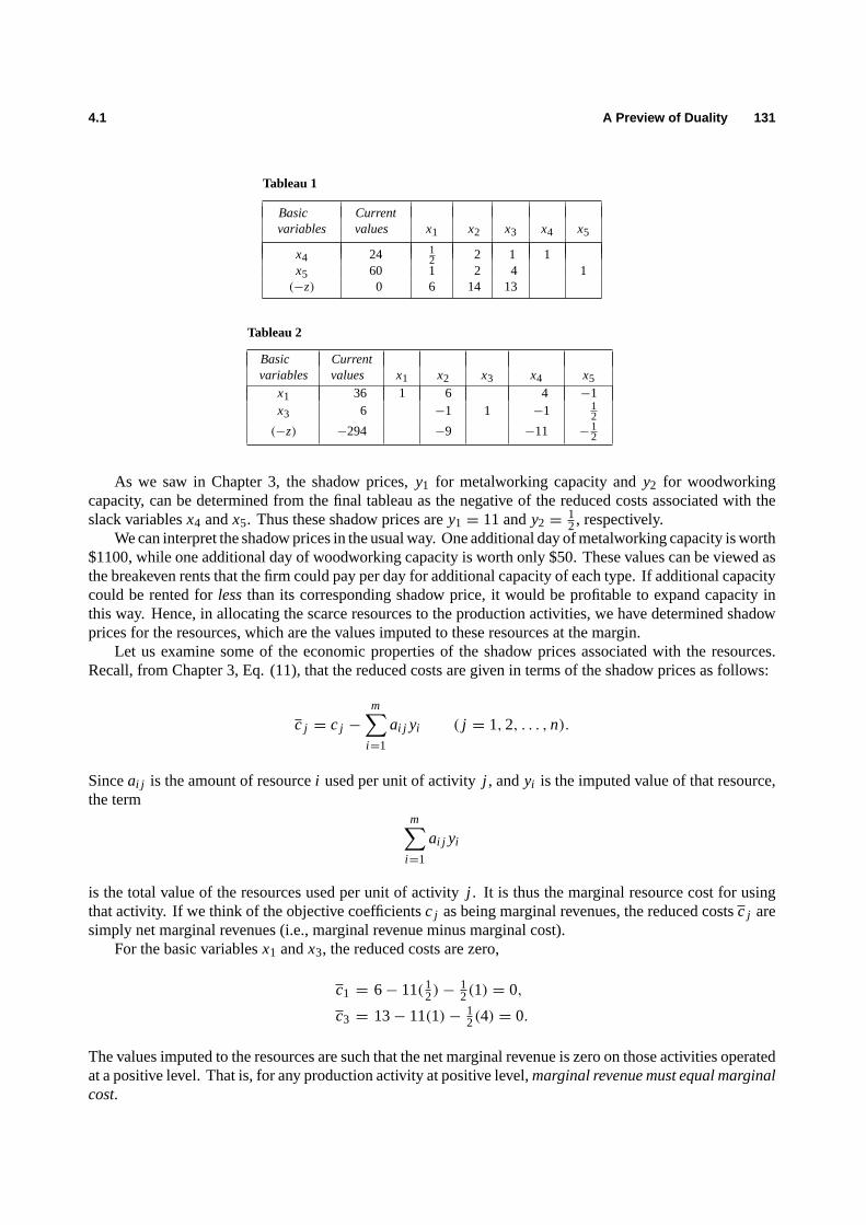
4.1 A Preview of Duality 131
Tableau 1
Basic Currentvariables values x1 x2 x3 x4 x5
x4 24 12 2 1 1
x5 60 1 2 4 1(−z) 0 6 14 13
Tableau 2
Basic Currentvariables values x1 x2 x3 x4 x5
x1 36 1 6 4 −1x3 6 −1 1 −1 1
2(−z) −294 −9 −11 −
12
As we saw in Chapter 3, the shadow prices,y1 for metalworking capacity andy2 for woodworkingcapacity, can be determined from the final tableau as the negative of the reduced costs associated with theslack variablesx4 andx5. Thus these shadow prices arey1 = 11 andy2 =
12, respectively.
We can interpret the shadow prices in the usual way. One additional day of metalworking capacity is worth$1100, while one additional day of woodworking capacity is worth only $50. These values can be viewed asthe breakeven rents that the firm could pay per day for additional capacity of each type. If additional capacitycould be rented forlessthan its corresponding shadow price, it would be profitable to expand capacity inthis way. Hence, in allocating the scarce resources to the production activities, we have determined shadowprices for the resources, which are the values imputed to these resources at the margin.
Let us examine some of the economic properties of the shadow prices associated with the resources.Recall, from Chapter 3, Eq. (11), that the reduced costs are given in terms of the shadow prices as follows:
c j = c j −
m∑i=1
ai j yi ( j = 1, 2, . . . , n).
Sinceai j is the amount of resourcei used per unit of activityj , andyi is the imputed value of that resource,the term
m∑i=1
ai j yi
is the total value of the resources used per unit of activityj . It is thus the marginal resource cost for usingthat activity. If we think of the objective coefficientsc j as being marginal revenues, the reduced costsc j aresimply net marginal revenues (i.e., marginal revenue minus marginal cost).
For the basic variablesx1 andx3, the reduced costs are zero,
c1 = 6− 11(12)− 1
2(1) = 0,
c3 = 13− 11(1)− 12(4) = 0.
The values imputed to the resources are such that the net marginal revenue is zero on those activities operatedat a positive level. That is, for any production activity at positive level,marginal revenue must equal marginalcost.

132 Duality in Linear Programming 4.1
The situation is much the same for the nonbasic variablesx2, x4, andx5, with corresponding reducedcosts:
c2 = 14− 11(2)− 12(2) = −9,
c4 = 0− 11(1)− 12(0) = −11,
c5 = 0− 11(0)− 12(1) = −1
2.
The reduced costs for all nonbasic variables are negative. The interpretation is that, for the values imputedto the scarce resources,marginal revenue is less than marginal costfor these activities, so they should not bepursued. In the case ofx2, this simply means that we should not produceanyeconomy trailers. The cases ofx4 andx5 are somewhat different, since slack variables represent unused capacity. Since the marginal revenueof a slack activity is zero, its reduced cost equalsminus its marginal cost, which is just the shadow price ofthe corresponding capacity constraint, as we have seen before.
The above conditions interpreted for the reduced costs of the decision variables are the familiar optimalityconditions of the simplex method. Economically we can see why they must hold. If marginal revenue exceedsmarginal cost for any activity, then the firm would improve its contribution to overhead byincreasingthatactivity. If, however, marginal cost exceeds marginal revenue for an activity operated at a positive level, thenthe firm would increase its contribution bydecreasingthat activity. In either case, a new solution could befound that is an improvement on the current solution. Finally, as we have seen in Chapter 3, those nonbasicvariables with zero reduced costs represent possible alternative optimal solutions.
Until now we have used the shadow prices mainly to impute the marginal resource cost associated witheach activity. We then selected the best activities for the firm to pursue by comparing the marginal revenue ofan activity with its marginal resource cost. In this case, the shadow prices are interpreted as the opportunitycosts associated with consuming the firm’s resources. If we now value the firm’s total resources at theseprices, we find their value,
v = 11(24)+ 12(60) = 294,
is exactly equal to the optimal value of the objective function of the firm’s decision problem. The implicationof this valuation scheme is that the firm’s metalworking and woodworking capacities have an imputed worthof $264 and $30, respectively. Essentially then, the shadow prices constitute aninternal pricing system forthe firm’s resources that:
1. permits the firm to select which activity to pursue by considering only the marginal profitability of itsactivities; and
2. allocates the contribution of the firm to its resources at the margin.
Suppose that we consider trying to determine directly the shadow prices that satisfy these conditions,without solving the firm’s production-decision problem. The shadow prices must satisfy the requirementthat marginal revenue be less than or equal to marginal cost for all activities. Further, they must be non-negative since they are associated with less-than-or-equal-to constraints in a maximization decision problem.Therefore, the unknown shadow pricesy1 on metalworking capacity andy2 on woodworking capacity mustsatisfy:
12 y1+ y2 ≥ 6,
2y1+ 2y2 ≥ 14,
y1+ 4y2 ≥ 13,
y1 ≥ 0, y2 ≥ 0.
These constraints require that the shadow prices be chosen so that the net marginal revenue for each activityis nonpositive. If this were not the case, an improvement in the firm’s total contribution could be made bychanging the choice of production activities.

4.1 A Preview of Duality 133
Recall that the shadow prices were interpreted as breakeven rents for capacity at the margin. Imagine forthe moment that the firm does not own its productive capacity but has to rent it. Now consider any values forthe shadow prices, or rental rates, that satisfy the above constraints, sayy1 = 4 andy2 = 4. The total worthof the rented capacities evaluated at these shadow prices isv = 24(4)+ 60(4) = 336, which is greater thanthe maximum contribution of the firm. Since the imputed value of the firm’s resources is derived solely fromallocating the firm’s contribution to its resources,v = 336 is too high a total worth to impute to the firm’sresources. The firm clearly could not break even if it had to rent its production capacity at such rates.
If we think of the firm as renting all of its resources, then surely it should try to rent them at least cost.This suggests that we might determine the appropriate values of the shadow prices by minimizing the totalrental cost of the resources, subject to the above constraints. That is, solve the following linear program:
Minimize v = 24y1+ 60y2,
subject to:12 y1 + y2 ≥ 6,
2y1 + 2y2 ≥ 14,
y1 + 4y2 ≥ 13, (2)
y1 ≥ 0, y2 ≥ 0.
If we solve this linear program by the simplex method, the resulting optimal solution isy1 = 11, y2 =12,
andv = 294. These are exactly the desired values of the shadow prices, and the value ofv reflects thatthe firm’s contribution is fully allocated to its resources. Essentially, the linear program (2), in terms of theshadow prices, determines rents for the resources that would allow the firm to break even, in the sense that itstotal contribution would exactly equal the total rental value of its resources. However, the firm in fact ownsits resources, and so the shadow prices are interpreted as the breakeven rates for rentingadditionalcapacity.
Thus, we have observed that, by solving (2), we can determine the shadow prices of (1) directly. Problem(2) is called thedual of Problem (1). Since Problem (2) has a name, it is helpful to have a generic name forthe original linear program. Problem (1) has come to be called theprimal.
In solving any linear program by the simplex method, we also determine the shadow prices associatedwith the constraints. In solving (2), the shadow prices associated with its constraints areu1 = 36, u2 = 0,andu3 = 6. However, these shadow prices for the constraints of (2) are exactly the optimal values of thedecision variables of the firm’s allocation problem. Hence, in solving the dual (2) by the simplex method,we apparently have solved the primal (1) as well. As we will see later, this will always be the case since ‘‘thedual of the dual is the primal.’’ This is an important result since it implies that the dual may be solved insteadof the primal whenever there are computational advantages.
Let us further emphasize the implications of solving these problems by the simplex method. The opti-mality conditions of the simplex method require that the reduced costs of basic variables be zero. Hence,
if x1 > 0, thenc1 = 6− 12 y1− y2 = 0;
if x3 > 0, thenc3 = 13− y1− 4y2 = 0.
These equations state that, if a decision variable of the primal is positive, then the corresponding constraintin the dual must hold with equality. Further, the optimality conditions require that the nonbasic variables bezero (at least for those variables with negative reduced costs); that is,
if c2 = 14− 2y1− 2y2 < 0, thenx2 = 0.
These observations are often referred to ascomplementary slacknessconditions since, if a variable is positive,its corresponding (complementary) dual constraint holds with equality while, if a dual constraint holds withstrict inequality, then the corresponding (complementary) primal variable must be zero.

134 Duality in Linear Programming 4.2
These results are analogous to what we have seen in Chapter 3. If some shadow price is positive, thenthe corresponding constraint must hold with equality; that is,
if y1 > 0, then 12 x1+ 2x2+ x3 = 24;
if y2 > 0, then x1+ 2x2+ 4x3 = 60.
Further, if a constraint of the primal is not binding, then its corresponding shadow price must be zero. Inour simple example there do not happen to be any nonbinding constraints, other than the implicit nonnega-tivity constraints. However, the reduced costs have the interpretation of shadow prices on the nonnegativityconstraints, and we see that the reduced costs ofx1 andx3 are appropriately zero.
In this chapter we develop these ideas further by presenting the general theory of duality in linearprogramming.
4.2 DEFINITION OF THE DUAL PROBLEM
The duality principles we have illustrated in the previous sections can be stated formally in general terms.Let the primal problem be:
Primal
Maximizez=n∑
j=1
c j x j ,
subject to:n∑
j=1
ai j x j ≤ bi (i = 1, 2, . . . , m), (3)
x j ≥ 0 ( j = 1, 2, . . . , n).
Associated with this primal problem there is a corresponding dual problem given by:
Dual
Minimize v =
m∑i=1
bi yi ,
subject to:m∑
i=1
ai j yi ≥ c j ( j = 1, 2, . . . , n), (4)
yi ≥ 0 (i = 1, 2, . . . , m).
These primal and dual relationships can be conveniently summarized as in Fig. 4.1.Without the variablesy1, y2, . . . , ym, this tableau is essentially the tableau form utilized in Chapters 2
and 3 for a linear program. The firstm rows of the tableau correspond to the constraints of the primal problem,while the last row corresponds to the objective function of the primal problem. If the variablesx1, x2, . . . xn,
are ignored, the columns of the tableau have a similar interpretation for the dual problem. The firstn columnsof the tableau correspond to the constraints of the dual problem, while the last column corresponds to theobjective function of the dual problem. Note that there is one dual variable for each explicit constraint in theprimal, and one primal variable for each explicit constraint in the dual. Moreover, the dual constraints are thefamiliar optimality condition of ‘‘pricing out’’ a column. They state that, at optimality, no activity shouldappear to be profitable from the standpoint of its reduced cost; that is,
c j = c j −
m∑i=1
ai j yi ≤ 0.

4.2 Definition of the Dual Problem 135
Figure 4.1 Primal and dual relationships.
To illustrate some of these relationships, let us consider an example formulated in Chapter 1. Recall theportfolio-selection problem, where the decision variables are the amounts to invest in each security type:
Maximizez= 0.043xA + 0.027xB + 0.025xC+ 0.022xD + 0.045xE,
subject to:
Cash xA + xB + xC + xD + xE ≤ 10,Governments xB + xC + xD ≥ 4,
Quality 0.6xA + 0.6xB− 0.4xC− 0.4xD + 3.6xE ≤ 0,Maturity 4xA + 10xB − xC − 2xD − 3xE ≤ 0,
xA ≥ 0, xB ≥ 0, xC ≥ 0, xD ≥ 0, xE ≥ 0.
The dual of this problem can be found easily by converting it to the standard primal formulation given in (3).This is accomplished by multiplying the second constraint by−1, thus changing the ‘‘greater than or equalto’’ constraint to a ‘‘less than or equal to’’ constraint. The resulting primal problem becomes:
Maximizez= 0.043xA + 0.027xB + 0.025xC+ 0.022xD + 0.045xE,
subject to:xA + xB + xC + xD + xE ≤ 10,− xB − xC − xD ≤ −4,
0.6xA + 0.6xB − 0.4xC − 0.4xD + 3.6xE ≤ 0,
4xA + 10xB − xC − 2xD − 3xE ≤ 0,
xA ≥ 0, xB ≥ 0, xC ≥ 0, xD ≥ 0, xE ≥ 0.
According to expression (4), the corresponding dual problem is:
Minimize v = 10y1− 4y2,
subject to:y1 + 0.6y3+ 4y4 ≥ 0.043,
y1− y2+ 0.6y3+ 10y4 ≥ 0.027,
y1− y2− 0.4y3− y4 ≥ 0.025,
y1− y2− 0.4y3− 2y4 ≥ 0.022,
y1 + 3.6y3− 3y4 ≥ 0.045,

136 Duality in Linear Programming 4.2
y1 ≥ 0, y2 ≥ 0, y3 ≥ 0, y4 ≥ 0.
By applying the simplex method, the optimal solution to both primal and dual problems can be found to be:∗
Primal: xA = 3.36, xB = 0, xC = 0, xD = 6.48,
xE = 0.16, andz= 0.294;
Dual: y1 = 0.0294, y2 = 0, y3 = 0.00636,
y4 = 0.00244, andv = 0.294.
As we have seen before, the optimal values of the objective functions of the primal and dual solutionsare equal. Furthermore, an optimal dual variable is nonzero only if its associated constraint in the primal isbinding. This should be intuitively clear, since the optimal dual variables are the shadow prices associated withthe constraints. These shadow prices can be interpreted as values imputed to the scarce resources (bindingconstraints), so that the value of these resources equals the value of the primal objective function.
To further develop that the optimal dual variables are the shadow prices discussed in Chapter 3, we notethat they satisfy the optimality conditions of the simplex method. In the final tableau of the simplex method,the reduced costs of the basic variables must be zero. As an example, consider basic variablexA . The reducedcost ofxA in the final tableau can be determined as follows:
cA = cA −
5∑i=1
ai A yi
= 0.043− 1(0.0294)− 0(0)− 0.6(0.00636)− 4(0.00244) = 0.
For nonbasic variables, the reduced cost in the final tableau must be nonpositive in order to ensure that noimprovements can be made. Consider nonbasic variablexB, whose reduced cost is determined as follows:
cB = cB −
5∑i=1
ai Byi
= 0.027− 1(0.0294)− 1(0)− 0.6(0.00636)− 10(0.00244) = −0.0306.
The remaining basic and nonbasic variables also satisfy these optimality conditions for the simplex method.Therefore, the optimal dual variables must be the shadow prices associated with an optimal solution.
Since any linear program can be put in the form of (3) by making simple transformations similar to thoseused in this example, then any linear program must have a dual linear program. In fact, since the dual problem(4) is a linear program, it must also have a dual. For completeness, one would hope that the dual of the dualis the primal (3), which is indeed the case. To show this we need only change the dual (4) into the form of(3) and apply the definition of the dual problem. The dual may be reformulated as a maximization problemwith less-than-or-equal-to constraints, as follows:
Maximizev′ =
m∑i=1
−bi yi ,
subject to:
m∑i=1
− ai j yi ≤ −c j ( j = 1, 2, . . . , n), (5)
yi ≥ 0 (i = 1, 2, . . . , m).
∗ Excel spreadsheet available athttp://web.mit.edu/15.053/www/Sect4.2_Primal_Dual.xls

4.3 Finding the Dual in General 137
Applying the definition of the dual problem and letting the dual variables bex j , j = 1, 2, . . . , n, we have
Minimize z′ =n∑
j=1
−c j x j ,
subject to:n∑
j=1
− ai j x j ≥ −bi (i = 1, 2, . . . , m), (6)
x j ≥ 0 ( j = 1, 2, . . . , n),
which, by multiplying the constraints by minus one and converting the objective function to maximization,is clearly equivalent to the primal problem. Thus, thedual of the dual is the primal.
4.3 FINDING THE DUAL IN GENERAL
Very often linear programs are encountered in equality form with nonnegative variables. For example, thecanonical form, which is used for computing a solution by the simplex method, is in equality form. It is ofinterest, then, to find the dual of the equality form:
Maximizez=n∑
j=1
c j x j ,
subject to: n∑j=1
ai j x j = bi (i = 1, 2, . . . , m), (7)
x j ≥ 0 ( j = 1, 2, . . . , n).
A problem in equality form can be transformed into inequality form by replacing each equation by twoinequalities. Formulation (7) can be rewritten as
Maximizez=n∑
j=1
c j x j ,
subject to:n∑
j=1
ai j x j ≤ bi
n∑j=1
−ai j x j ≤ −bi
(i = 1, 2, . . . , m),
x j ≥ 0 ( j = 1, 2, . . . , n).
The dual of the equality form can then be found by applying the definition of the dual to this problem. Lettingy+i and y−i (i = 1, 2, . . . , m) be the dual variables associated with the firstm and secondm constraints,respectively, from expression (4), we find the dual to be:
Minimize v =
m∑i=1
bi y+
i +
m∑i=1
−bi y−
i ,
subject to:
m∑i=1
ai j y+i +m∑
i=1
−ai j y−i ≥ c j ( j = 1, 2, . . . , n),

138 Duality in Linear Programming 4.3
y+i ≥ 0, y−i ≥ 0 (i = 1, 2, . . . , m).
Collecting terms, we have:
Minimize v =
m∑i=1
bi (y+i − y−i ),
subject to:m∑
i=1
ai j (y+i − y−i ) ≥ c j ( j = 1, 2, . . . , n),
y+i ≥ 0, y−i ≥ 0 (i = 1, 2, . . . , m).
Letting yi = y+i − y−i , and noting thatyi is unrestricted in sign, gives us the dual of the equality form (7):
Minimize v =
m∑i=1
bi yi ,
subject to:m∑
i=1
ai j yi ≥ c j ( j = 1, 2, . . . , n), (8)
yi unrestricted (i = 1, 2, . . . , m).
Note that the dual variables associated with equality constraints are unrestricted.There are a number of relationships between primal and dual, depending upon whether the primal problem
is a maximization or a minimization problem and upon the types of constraints and restrictions on the variables.To illustrate some of these relationships, let us consider a general maximization problem as follows:
Maximizez=n∑
j=1
c j x j ,
subject to:
n∑j=1
ai j x j ≤ bi (i = 1, 2, . . . , m′),
n∑j=1
ai j x j ≥ bi (i = m′ + 1, m′ + 2, . . . , m′′), (9)
n∑j=1
ai j x j = bi (i = m′′ + 1, m′′ + 2, . . . , m),
x j ≥ 0 ( j = 1, 2, . . . , n).
We can change the general primal problem to equality form by adding the appropriate slack and surplusvariables, as follows:
Maximizez=n∑
j=1
c j x j ,

4.3 Finding the Dual in General 139
subject to:
n∑j=1
ai j x j + xn+i = bi (i = 1, 2, . . . , m′),
n∑j=1
ai j x j − xn+i = bi (i = m′ + 1, m′ + 2, . . . , m′′),
n∑j=1
ai j x j = bi (i = m′′ + 1, m′′ + 2, . . . , m),
x j ≥ 0 ( j = 1, 2, . . . , n+m′′).
Letting yi , y′i , andy′′i be dual variables associated respectively with the three sets of equations, the dual of(9) is then
Minimize v =
m′∑i=1
bi yi +
m′′∑i=m′+1
bi y′
i +
m∑i=m′′+1
bi y′′
i ,
subject to:
m′∑i=1
ai j yi +
m′′∑i=m′+1
ai j y′i +m∑
i=m′′+1
ai j y′′i ≥ c j (10)
yi ≥ 0,
−y′i ≥ 0,
wherey′′i is unrestricted in sign and the last inequality could be writteny′i ≤ 0. Thus, if the primal problemis a maximization problem, the dual variables associated with the less-than-or-equal-to constraints are non-negative, the dual variables associated with the greater-than-or-equal-to constraints are nonpositive, and thedual variables associated with the equality constraints are unrestricted in sign.
These conventions reflect the interpretation of the dual variables as shadow prices of the primal problem.A less-than-or-equal-to constraint, normally representing a scarce resource, has a positive shadow price,since the expansion of that resource generates additional profits. On the other hand, a greater-than-or-equal-to constraint usually represents an external requirement (e.g., demand for a given commodity). If thatrequirement increases, the problem becomes more constrained; this produces a decrease in the objectivefunction and thus the corresponding constraint has a negative shadow price. Finally, changes in the righthandside of an equality constraint might produce either negative or positive changes in the value of the objectivefunction. This explains the unrestricted nature of the corresponding dual variable.
Let us now investigate the duality relationships when the primal problem is cast inminimization, ratherthan maximization form:
Minimize z=n∑
j=1
c j x j ,
140 Duality in Linear Programming 4.4
subject to:
n∑j=1
ai j x j ≤ bi (i = 1, 2, . . . , m′),
n∑j=1
ai j x j ≥ bi (i = m′ + 1, m′ + 2, . . . , m′′), (11)
n∑j=1
ai j x j = bi (i = m′′ + 1, m′′ + 2, . . . , m),
x j ≥ 0 ( j = 1, 2, . . . , n).
Since the dual of the dual is the primal, we know that the dual of a minimization problem will be a maximizationproblem. The dual of (11) can be found by performing transformations similar to those conducted previously.The resulting dual of (11) is the following maximization problem:
Maximize v =
m′∑i=1
bi yi +
m′′∑i=m′+1
bi y′
i +
m∑i=m′′+1
bi y′′
i ,
subject to:m′∑
i=1
ai j yi +
m′′∑i=m′+1
ai j y′i +m∑
i=m′′+1
ai j y′′i ≥ c j (12)
yi ≤ 0 (i = 1, 2, . . . , m′),
y′i ≥ 0 (i = m′ + 1, m′ + 2, . . . , m′′).
Observe that now the sign of the dual variables associated with the inequality constraints has changed,as might be expected from the shadow-price interpretation. In a cost-minimization problem, increasing theavailable resources will tend to decrease the total cost, since the constraint has been relaxed. As a result, thedual variable associated with a less-than-or-equal-to constraint in a minimization problem is nonpositive. Onthe other hand, increasing requirements could only generate a cost increase. Thus, a greater-than-or-equal-toconstraint in a minimization problem has an associated nonnegative dual variable.
The primal and dual problems that we have just developed illustrate one further duality correspondence.If (12) is considered as the primal problem and (11) as its dual, then unrestricted variables in the primal areassociated with equality constraints in the dual.
We now can summarize the general duality relationships. Basically we note that equality constraints in theprimal correspond to unrestricted variables in the dual, while inequality constraints in the primal correspondto restricted variables in the dual, where the sign of the restriction in the dual depends upon the combination ofobjective-function type and constraint relation in the primal. These various correspondences are summarizedin Table 4.1. The table is based on the assumption that the primal is a maximization problem. Since the dualof the dual is the primal, we can interchange the words primal and dual in Table 4.1 and the correspondenceswill still hold.
4.4 THE FUNDAMENTAL DUALITY PROPERTIES
In the previous sections of this chapter we have illustrated many duality properties for linear programming. Inthis section we formalize some of the assertions we have already made. The reader not interested in the theoryshould skip over this section entirely, or merely read the statements of the properties and ignore the proofs.We consider the primal problem in inequality form so that the primal and dual problems are symmetric. Thus,

4.4 The Fundamental Duality Properties 141
Table 4.1
Primal (Maximize) Dual (Minimize)
i th constraint≤ i th variable≥ 0i th constraint≥ i th variable≤ 0i th constraint= i th variable unrestrictedj th variable≥ 0 j th constraint≥j th variable≤ 0 j th constraint≤j th variable unrestricted j th constraint=
any statement that is made about the primal problem immediately has an analog for the dual problem, andconversely. For convenience, we restate the primal and dual problems.
Primal
Maximizez=n∑
j=1
c j x j ,
subject to:
n∑j=1
ai j x j ≤ bi (i = 1, 2, . . . , m), (13)
x j ≥ 0 ( j = 1, 2, . . . , n).
Dual
Minimize v =
m∑i=1
bi yi ,
subject to:m∑
i=1
ai j yi ≥ c j ( j = 1, 2, . . . , n), (14)
yi ≥ 0 (i = 1, 2, . . . , m).
The first property is referred to as ‘‘weak duality’’ and provides a bound on the optimal value of theobjective function of either the primal or the dual. Simply stated, the value of the objective function for anyfeasible solution to the primal maximization problem is bounded from above by the value of the objectivefunction for any feasible solution to its dual. Similarly, the value of the objective function for its dual isbounded from below by the value of the objective function of the primal. Pictorially, we might represent thesituation as follows:
Dualfeasible
y v decreasing
Primalfeasible
x z increasing
The sequence of properties to be developed will lead us to the ‘‘strong duality" property, which statesthat the optimal values of the primal and dual problems are in fact equal. Further, in developing this result,we show how the solution of one of these problems is readily available from the solution of the other.

142 Duality in Linear Programming 4.4
Weak Duality Property. If x j , j = 1, 2, . . . , n, is a feasible solution to the primal problem andyi , i = 1, 2, . . . , m, is a feasible solution to the dual problem, then
n∑j=1
c j x j ≤
m∑i=1
bi yi .
The weak duality property follows immediately from the respective feasibility of the two solutions. Primalfeasibility implies:
n∑j=1
ai j x j ≤ bi (i = 1, 2, . . . , m) and x j ≥ 0 ( j = 1, 2, . . . , n),
while dual feasibility implies
m∑i=1
ai j yi ≥ c j ( j = 1, 2, . . . , n) and yi ≥ 0 (i = 1, 2, . . . , m).
Hence, multiplying thei th primal constraint byyi and adding yields:
m∑i=1
n∑j=1
ai j x j yi ≤
m∑i=1
bi yi ,
while multiplying the j th dual constraint byx j and adding yields:
n∑j=1
m∑i=1
ai j yi x j ≥
n∑j=1
c j x j .
Since the lefthand sides of these two inequalities are equal, together they imply the desired result that
n∑j=1
c j x j ≤
m∑i=1
bi yi .
There are a number of direct consequences of the weak duality property. If we have feasible solutionsto the primal and dual problems such that their respective objective functions are equal, then these solutionsare optimal to their respective problems. This result follows immediately from the weak duality property,since a dual feasible solution is an upper bound on the optimal primal solution and this bound is attainedby the given feasible primal solution. The argument for the dual problem is analogous. Hence, we have anoptimality property of dual linear programs.
Optimality Property. If x j , j = 1, 2, . . . , n, is a feasible solution to the primal problem andyi , i =1, 2, . . . , m, is a feasible solution to the dual problem, and, further,
n∑j=1
c j x j =
m∑i=1
bi yi ,
then x j , j = 1, 2, . . . , n, is an optimal solution to the primal problem andyi , i = 1, 2, . . . , m, is anoptimal solution to the dual problem.
Furthermore, if one problem has an unbounded solution, then the dual of that problem is infeasible. Thismust be true for the primal since any feasible solution to the dual would provide an upper bound on the primalobjective function by the weak duality theorem; this contradicts the fact that the primal problem is unbounded.Again, the argument for the dual problem is analogous. Hence, we have an unboundedness property of duallinear programs.

4.4 The Fundamental Duality Properties 143
Unboundedness Property.If the primal (dual) problem has an unbounded solution, then the dual (pri-mal) problem is infeasible.
We are now in a position to give the main result of this section, the ‘‘strong duality’’ property. Theimportance of this property is that it indicates that we may in fact solve the dual problem in place of orin conjunction with the primal problem. The proof of this result depends merely on observing that theshadow prices determined by solving the primal problem by the simplex method give a dual feasible solution,satisfying the optimality property given above.
Strong Duality Property. If the primal (dual) problem has a finite optimal solution, then so does thedual (primal) problem, and these two values are equal. That is,z= v where
z= Maxn∑
j=1
c j x j , v = Minm∑
i=1
bi yi ,
subject to: subject to:
n∑j=1
ai j x j ≤ bi ,
m∑i=1
ai j yi ≥ c j ,
x j ≥ 0; yi ≥ 0.
Let us see how to establish this property. We can convert the primal problem to the equivalent equalityform by adding slack variables as follows:
Maximizez=n∑
j=1
c j x j ,
subject to:
n∑j=1
ai j x j + xn+i = bi (i = 1, 2, . . . , m),
x j ≥ 0 ( j = 1, 2, . . . , n+m).
Suppose that we have applied the simplex method to the linear program andx j , j = 1, 2, . . . , n, is the resultingoptimal solution. Letyi , i = 1, 2, . . . , m, be the shadow prices associated with the optimal solution. Recallthat the shadow prices associated with the original constraints are the multiples of those constraints which,when subtracted from the original form of the objective function, yield the form of the objective function inthe final tableau [Section 3.2, expression (11)]. Thus the following condition holds:
−z+n∑
j=1
c j x j = −
m∑i=1
bi yi , (15)
where, due to the optimality criterion of the simplex method, the reduced costs satisfy:
c j = c j −
m∑i=1
ai j yi ≤ 0 ( j = 1, 2, . . . , n), (16)
andc j = 0− yi ≤ 0 ( j = n+ 1, n+ 2, . . . , n+m). (17)

144 Duality in Linear Programming 4.5
Conditions (16) and (17) imply thatyi , for i = 1, 2, . . . , m, constitutes a feasible solution to the dual problem.Whenx j is replaced by the optimal valuex j in expression (15), the term
n∑j=1
c j x j
is equal to zero, sincec j = 0 whenx j is basic, andx j = 0 whenx j is nonbasic. Therefore, the maximumvalue ofz, sayz, is given by:
−z= −m∑
i=1
bi yi .
Moreover, sincex j , for j = 1, 2, . . . , n, is an optimal solution to the primal problem,
n∑j=1
c j x j = z=m∑
i=1
bi yi .
This is theoptimality propertyfor the primal feasible solutionx j , j = 1, 2, . . . , n, and the dual feasiblesolution yi , i = 1, 2, . . . , m, so they are optimal for their respective problems. (The argument in terms ofthe dual problem is analogous.)
It should be pointed out that it isnot true that if the primal problem is infeasible, then the dual problemis unbounded. In this case the dual problem may be either unbounded or infeasible. All four combinationsof feasibility and infeasibility for primal and dual problems may take place. An example of each is indicatedin Table 4.2.
In example (2) of Table 4.2 it should be clear thatx2 may be increased indefinitely without violatingfeasibility while at the same time making the objective function arbitrarily large. The constraints of the dualproblem for this example are clearly infeasible sincey1+ y2 ≥ 2 andy1+ y2 ≤ −1 cannot simultaneouslyhold. A similar observation is made for example (3), except that the primal problem is now infeasible whilethe dual variabley1 may be increased indefinitely. In example (4), the fact that neither primal nor dualproblem is feasible can be checked easily by multiplying the first constraint of each by minus one.
4.5 COMPLEMENTARY SLACKNESS
We have remarked that the duality theory developed in the previous section is a unifying theory relating theoptimal solution of a linear program to the optimal solution of the dual linear program, which involves theshadow prices of the primal as decision variables. In this section we make this relationship more precise bydefining the concept of complementary slackness relating the two problems.
Complementary Slackness Property.If, in an optimal solution of a linear program, the value of the dualvariable (shadow price) associated with a constraint is nonzero, then that constraint must be satisfied withequality. Further, if a constraint is satisfied with strict inequality, then its corresponding dual variablemust be zero.
For the primal linear program posed as a maximization problem with less-than-or-equal-to constraints,this means:
i) if yi > 0, thenn∑
j=1
ai j x j = bi ;
ii) ifn∑
j=1
ai j x j < bi , thenyi = 0.

4.5 Complementary Slackness 145
Table 4.2
1 Primal feasible Dual feasible
Maximizez= 2x1+ x2, Minimize v = 4y1+ 2y2,
subject to: subject to:x1+ x2 ≤ 4,
x1− x2 ≤ 2,
x1 ≥ 0, x2 ≥ 0.
y1+ y2 ≥ 2,
y1− y2 ≥ 1,
y1 ≥ 0, y2 ≥ 0.
2 Primal feasible and unbounded Dual infeasible
Maximizez= 2x1+ x2, Minimize v = 4y1+ 2y2,
subject to: subject to:x1− x2 ≤ 4,
x1− x2 ≤ 2,
x1 ≥ 0, x2 ≥ 0.
y1+ y2 ≥ 2,
−y1− y2 ≥ 1,
y1 ≥ 0, y2 ≥ 0.
3 Primal infeasible Dual feasible and unbounded
Maximizez= 2x1+ x2, Minimize v = −4y1+ 2y2,
subject to: subject to:−x1− x2 ≤ −4,
x1 + x2 ≤ 2,
x1 ≥ 0, x2 ≥ 0.
−y1+ y2 ≥ 2,
−y1+ y2 ≥ 1,
y1 ≥ 0, y2 ≥ 0.
4 Primal infeasible Dual infeasible
Maximizez= 2x1+ x2, Minimize v = −4y1+ 2y2,
subject to: subject to:−x1+ x2 ≤ −4,
x1− x2 ≤ 2,
x1 ≥ 0, x2 ≥ 0.
−y1+ y2 ≥ 2,
y1− y2 ≥ 1,
y1 ≥ 0, y2 ≥ 0.
We can show that the complementary-slackness conditions follow directly from the strong duality propertyjust presented. Recall that, in demonstrating the weak duality property, we used the fact that:
n∑j=1
c j x j ≤
m∑i=1
n∑j=1
ai j x j yi ≤
m∑i=1
bi yi (18)
for any x j , j = 1, 2, . . . , n, andyi , i = 1, 2, . . . , m, feasible to the primal and dual problems, respectively.Now, since these solutions are not only feasible but optimal to these problems, equality must hold throughout.Hence, considering the righthand relationship in (18), we have:
m∑i=1
n∑j=1
ai j x j yi =
m∑i=1
bi yi ,
which implies:
m∑i=1
n∑j=1
ai j x j − bi
yi = 0.

146 Duality in Linear Programming 4.5
Since the dual variablesyi are nonnegative and their coefficients
n∑j=1
ai j x j − bi
are nonpositive by primal feasibility, this condition can hold only if each of its terms is equal to zero; that is, n∑j=1
ai j x j − bi
yi = 0 (i = 1, 2, . . . , m).
These latter conditions are clearly equivalent to (i) and (ii) above.For the dual linear program posed as a minimization problem with greater-than-or-equal-to constraints,
the complementary-slackness conditions are the following:
iii) if x j > 0, thenm∑
i=1
ai j yi = c j ,
iv) ifm∑
i=1
ai j yi > c j , thenx j = 0.
These conditions also follow directly from the strong duality property by an argument similar to that givenabove. By considering the lefthand relationship in (18), we can easily show that[
m∑i=1
ai j yi − c j
]x j = 0 ( j = 1, 2, . . . , n),
which is equivalent to (iii) and (iv).The complementary-slackness conditions of the primal problem have a fundamental economic interpre-
tation. If the shadow price of thei th resource (constraint) is strictly positive in the optimal solutionyi > 0,then we should require that all of this resource be consumed by the optimal program; that is,
n∑j=1
ai j x j = bi .
If, on the other hand, thei th resource is not fully used; that is,n∑
j=1
ai j x j < bi ,
then its shadow price should be zero,yi = 0.The complementary-slackness conditions of the dual problem are merely the optimality conditions for
the simplex method, where the reduced costc j associated with any variable must be nonpositive and is givenby
c j = c j −
m∑i=1
ai j yi ≤ 0 ( j = 1, 2, . . . , n).
If x j > 0, thenx j must be a basic variable and its reduced cost is defined to be zero. Thus,
c j =
m∑i=1
ai j yi .

4.6 The Dual Simplex Method 147
If, on the other hand,
c j −
m∑i=1
ai j yi < 0,
thenx j must be nonbasic and set equal to zero in the optimal solution;x j = 0.We have shown that the strong duality property implies that the complementary-slackness conditions
must hold for both the primal and dual problems. The converse of this also is true. If the complementary-slackness conditions hold for both problems, then the strong duality property holds. To see this, letx j , j =1, 2, . . . , n, andyi , i = 1, 2, . . . , m, be feasible solutions to the primal and dual problems, respectively. Thecomplementary-slackness conditions (i) and (ii) for the primal problem imply:
m∑i=1
n∑j=1
ai j x j − bi
yi = 0,
while the complementary-slackness conditions (iii) and (iv) for the dual problem imply:
n∑j=1
[m∑
i=1
ai j yi − c j
]x j = 0.
These two equations together imply:
n∑j=1
c j x j =
m∑i=1
n∑j=1
ai j x j yi =
m∑i=1
bi yi ,
and hence the values of the primal and dual objective functions are equal. Since these solutions are feasibleto the primal and dual problems respectively, theoptimality propertyimplies that these solutions are optimalto the primal and dual problems. We have, in essence, shown that the complementary-slackness conditionsholding for both the primal and dual problems is equivalent to thestrong duality property. For this reason,the complementary-slackness conditions are often referred to as theoptimality conditions.
Optimality Conditions. If x j , j = 1, 2, . . . , n, and yi , i = 1, 2, . . . , m, are feasible solutions to theprimal and dual problems, respectively, then they are optimal solutions to these problems if, and only if,the complementary-slackness conditions hold for both the primal and the dual problems.
4.6 THE DUAL SIMPLEX METHOD
One of the most important impacts of the general duality theory presented in the previous section has beenon computational procedures for linear programming. First, we have established that the dual can be solvedin place of the primal whenever there are advantages to doing so. For example, if the number of constraintsof a problem is much greater than the number of variables, it is usually wise to solve the dual instead of theprimal since the solution time increases much more rapidly with the number of constraints in the problemthan with the number of variables. Second, new algorithms have been developed that take advantage of theduality theory in more subtle ways. In this section we present the dual simplex method. We have alreadyseen the essence of the dual simplex method in Section 3.5, on righthand-side ranging, where the variabletransitions at the boundaries of each range are essentially computed by the dual simplex method. Further, inSection 3.8, on parametric programming of the righthand side, the dual simplex method is the cornerstone ofthe computational approach. In this section we formalize the general algorithm.

148 Duality in Linear Programming 4.6
Recall the canonical form employed in the simplex method:
x1 + a1,m+1xm+1+ · · · + a1,nxn = b1,
x2 + a2,m+1xm+1+ · · · + a2,nxn = b2,. . .
......
...
xm+ am,m+1xm+1+ · · · + am,nxn= bm,
(−z) + cm+1xm+1+ · · · + cnxn = −z0.
The conditions forx1, x2, . . . , xm to constitute an optimal basis for a maximization problem are:
i) c j ≤ 0 ( j = 1, 2, . . . , n),
ii ) bi ≥ 0 (i = 1, 2, . . . , m).
We could refer to condition (i) as primal optimality (or equivalently, dual feasibility) and condition (ii) asprimal feasibility. In the primal simplex method, we move from basic feasible solution to adjacent basicfeasible solution, increasing (not decreasing) the objective function at each iteration. Termination occurswhen the primal optimality conditions are satisfied. Alternatively, we could maintain primal optimality (dualfeasibility) by imposing (i) and terminating when the primal feasibility conditions (ii) are satisfied. This latterprocedure is referred to as thedual simplex methodand in fact results from applying the simplex methodto the dual problem. In Chapter 3, on sensitivity analysis, we gave a preview of the dual simplex methodwhen we determined the variable to leave the basis at the boundary of a righthand-side range. In fact, thedual simplex method is most useful in applications when a problem has been solved and a subsequent changeon the righthand side makes the optimal solution no longer primal feasible, as in the case of parametricprogramming of the righthand-side values.
The rules of the dual simplex method are identical to those of the primal simplex algorithm, except forthe selection of the variable to leave and enter the basis. At each iteration of the dual simplex method, werequire that:
c j = c j −
m∑i=1
yi ai j ≤ 0;
and sinceyi ≥ 0 for i = 1, 2, . . . , m, these variables are a dual feasible solution. Further, at each iterationof the dual simplex method, the most negativebi is chosen to determine the pivot row, corresponding tochoosing the most positivec j to determine the pivot column in the primal simplex method.
Prior to giving the formal rules of the dual simplex method, we present a simple example to illustrate theessence of the procedure. Consider the following maximization problem with nonnegative variables givenin Tableau 3. This problem is in ‘‘dual canonical form" since the optimality conditions are satisfied, but thebasic variables are not yet nonnegative.
Table 4.3
Basic Currentvariables values x1 x2 x3 x4
x3 −1 −1 −1 1← x4 −2 −2 −3 1
(−z) 0 −3 −1↑
In the dual simplex algorithm, we are attempting to make all variables nonnegative. The procedure isthe opposite of the primal method in that it first selects the variable to drop from the basis and then the newvariable to introduce into the basis in its place. The variable to drop is the basic variable associated withthe constraint with the most negative righthand-side value; in this casex4. Next we have to determine theentering variable. We select from only those nonbasic variables that have a negative coefficient in the pivot
4.6 The Dual Simplex Method 149
row, since then, after pivoting, the righthand side becomes positive, thus eliminating the primal infeasibilityin the constraint. If all coefficients are positive, then the primal problem is clearly infeasible, because thesum of nonnegative terms can never equal the negative righthand side.
In this instance, both nonbasic variablesx1 andx2 are candidates. Pivoting will subtract some multiple,sayt , of the pivot row containingx4 from the objective function, to give:
(−3+ 2t)x1+ (−1+ 3t)x2− t x4− z= 2t.
Since we wish to maintain the optimality conditions, we want the coefficient of each variable to remainnonpositive, so that:
−3+ 2t ≤ 0 (that is, t ≤ 32),
−1+ 3t ≤ 0 (that is, t ≤ 13),
− t ≤ 0 (that is, t ≥ 0).
Settingt = 13 preserves the optimality conditions and identifies the new basic variable with a zero coefficient
in the objective function, as required to maintain the dual canonical form.These steps can be summarized as follows: the variable to leave the basis is chosen by:
br = Mini{bi } = Min {−1,−2} = b2.
The variable to enter the basis is determined by the dual ratio test:
cs
ars= Min
j
{c j
ar j
∣∣∣∣ar j < 0
}= Min
{−3
−2,−1
−3
}=
c2
a22.
Pivoting inx2 in the second constraint gives the new canonical form in Tableau 4.
Table 4.4
Basic Currentvariables values x1 x2 x3 x4
← x3 −13 −
13 1 −
13
x223
23 1 −
13
(−z) 23 −
73 −
13↑
Clearly,x3 is the leaving variable sinceb1 = −13 is the only negative righthand-side coefficient; andx4 is
the entering variable sincec4/a14 is the minimum dualratio in the first row. After pivoting, the new canonicalform is given in Tableau 5
Table 4.5
Basic Currentvariables values x1 x2 x3 x4
x4 1 1 −3 1
x2 1 1 1 −1
(−z) 1 −2 −1
Sincebi ≥ 0 for i = 1, 2, andc j ≤ 0 for j = 1, 2, . . . , 4, we have the optimal solution.Following is a formal statement of the procedure. The proof of it is analogous to that of the primal
simplex method and is omitted.

150 Duality in Linear Programming 4.7
Dual Simplex Algorithm
STEP (0) The problem is initially in canonical form and allc j ≤ 0.
STEP (1) Ifbi ≥ 0, i = 1, 2, . . . , m, thenstop, we are optimal. If we continue, thenthere exists somebi < 0.
STEP (2) Choose the row to pivot in (i.e., variable to drop from the basis) by:
br = Mini
{bi |bi < 0
}.
If ar j ≥ 0, j = 1, 2, . . . , n, thenstop; the primal problem is infeasible (dualunbounded). If we continue, then there existsar j < 0 for somej = 1, 2, . . . , n.
STEP (3) Choose columns to enter the basis by:
cs
ars= Min
j
{c j
ar j
∣∣∣∣ar j < 0
}.
STEP (4) Replace the basic variable in rowr with variables and reestablish the canonicalform (i.e., pivot on the coefficientars).
STEP (5) Go to Step (1).
Step (3) is designed to maintainc j ≤ 0 at each iteration, and Step (2) finds the most promising candidate foran improvement in feasibility.
4.7 PRIMAL-DUAL ALGORITHMS
There are many other variants of the simplex method. Thus far we have discussed only the primal and dualmethods. There are obvious generalizations that combine these two methods. Algorithms that perform bothprimal and dual steps are referred to as primal-dual algorithms and there are a number of such algorithms. Wepresent here one simple algorithm of this form called theparametric primal-dual. It is most easily discussedin an example.
x1 ≥ 0, x2 ≥ 0,
x1 + x2 ≤ 6,
−x1 + 2x2 ≤ −12,
x1 − 3x2 ≤ −1,
−2x1 + 3x2 = z(max).
The above example can easily be put in canonical form by addition of slack variables. However, neitherprimal feasibility nor primal optimality conditions will be satisfied. We will arbitrarily consider the aboveexample as a function of the parameterθ in Tableau 6.
Clearly, if we chooseθ large enough, this system of equations satisfies the primal feasibility and primaloptimality conditions. The idea of the parametric primal-dual algorithm is to chooseθ large initially sothat these conditions are satisfied, and attempt to reduceθ to zero through a sequence of pivot operations.If we start withθ = 4 and letθ approach zero, primal optimality is violated whenθ < 3. If we were toreduceθ below 3, the objective-function coefficient ofx2 would become positive. Therefore we perform aprimal simplex pivot by introducingx2 into the basis. We determine the variable to leave the basis by theminimum-ratio rule of the primal simplex method:
br
ars= Min
i
{bi
ais
∣∣∣∣∣ais > 0
}=
{6
1,
212
2
}=
b2
a22.
x4 leaves the basis and the new canonical form is then shown in Tableau 7.

4.8 Mathematical Economics 151
Tableau 6Basic Currentvariables values x1 x2 x3 x4 x5
x3 6 1 1 1← x4 −
12 + θ −1 2 1
x5 −1+ θ 1 −3 1(−z) 0 −2 (3− θ)
↑
Tableau 7
Basic Currentvariables values x1 x2 x3 x4 x5
x3 614 −
12θ 3
2 1 −12
x2 −14 +
12θ −
12 1 1
2
← x5 −74 +
52θ −
12
32 1
(−z) −(3− θ)(−14 +
12θ) (−1
2 −12θ) (−3
2 +12θ)
↑
The optimality conditions are satisfied for710 ≤ θ ≤ 3. If we were to reduceθ below 7
10, the righthand-side value of the third constraint would become negative. Therefore, we perform a dual simplex pivot bydroppingx5 from the basis. We determine the variable to enter the basis by the rules of the dual simplexmethod:
Minj
{c j
a3 j
∣∣∣∣a3 j < 0
}=
{−
12 +−
12θ
−12
}=
c1
a31.
After the pivot is performed the new canonical form is given in Tableau 8.
Tableau 8
Basic Currentvariables values x1 x2 x3 x4 x5
x3 1+ 7θ 1 4 3
x232 − 2θ 1 −1 −1
x172 − 5θ 1 −3 −2
(−z) −(3− θ)(−
14 +
12θ)
(−3− θ) (−1− θ)
+(12 +
12θ)(7
2 − 5θ)
As we continue to decreaseθ to zero, the optimality conditions remain satisfied. Thus the optimal finaltableau for this example is given by settingθ equal to zero.
Primal-dual algorithms are useful when simultaneous changes of both righthand-side and cost coefficientsare imposed on a previous optimal solution, and a new optimal solution is to be recovered. When parametricprogramming of both the objective-function coefficients and the righthand-side values is performed simulta-neously, a variation of this algorithm is used. This type of parametric programming is usually referred to astherim problem. (See Appendix B for further details.)
4.8 MATHEMATICAL ECONOMICS
As we have seen in the two previous sections, duality theory is important for developing computationalprocedures that take advantage of the relationships between the primal and dual problems. However, there isanother less obvious area that also has been heavily influenced by duality, and that is mathematical economics.

152 Duality in Linear Programming 4.8
In the beginning of this chapter, we gave a preview of duality that interpreted the dual variables as shadowprices imputed to the firm’s resources by allocating the profit (contribution) of the firm to its resources atthe margin. In a perfectly competitive economy, it is assumed that, if a firm could make profits in excessof the value of its resources, then some other firm would enter the market with a lower price, thus tendingto eliminate these excess profits. The duality theory of linear programming has had a significant impact onmathematical economics through the interpretation of the dual as the price-setting mechanism in a perfectlycompetitive economy. In this section we will briefly sketch this idea.
Suppose that a firm may engage in anyn production activities that consume and/or producem resourcesin the process. Letx j ≥ 0 be the level at which thej th activity is operated, and letc j be the revenue perunit (minus means cost) generated from engaging in thej th activity. Further, letai j be the amount of thei th resource consumed (minus means produced) per unit level of operation of thej th activity. Assume thatthe firm starts with a position ofbi units of thei th resource and may buy or sell this resource at a priceyi ≥ 0 determined by an external market. Since the firm generates revenues and incurs costs by engaging inproduction activities and by buying and selling resources, its profit is given by:
n∑j=1
c j x j +
m∑i=1
yi
bi −
n∑j=1
ai j x j
, (19)
where the second term includes revenues from selling excess resources and costs of buying additional re-sources.
Note that ifbi >∑n
j=1 ai j x j , the firm sellsbi −∑n
j=1 ai j x j units of resourcesi to the marketplace ata priceyi . If, however,bi <
∑nj=1 ai j x j , then the firm buys
∑nj=1 ai j x j − bi units of resourcei from the
marketplace at a priceyi .Now assume that the market mechanism for setting prices is such that it tends to minimize the profits of
the firm, since these profits are construed to be at the expense of someone else in the market. That is, givenx j for j = 1, 2, . . . , n, the market reacts to minimize (19). Two consequences immediately follow. First,consuming any resource that needs to be purchased from the marketplace, that is,
bi −
n∑j=1
ai j x j < 0,
is clearly uneconomical for the firm, since the market will tend to set the price of the resource arbitrarily highso as to make the firm’s profits arbitrarily small (i.e., the firm’s losses arbitrarily large). Consequently, ourimaginary firm will always choose its production activities such that:
n∑j=1
ai j x j ≤ bi (i = 1, 2, . . . , m).
Second, if any resource were not completely consumed by the firm in its own production and therefore becameavailable for sale to the market, that is,
bi −
n∑j=1
ai j x j > 0,
this ‘‘malevolent market" would set a price of zero for that resource in order to minimize the firm’s profit.Therefore, the second term of (19) will be zero and the firm’s decision problem of choosing productionactivities so as to maximize profits simply reduces to:
Maximizen∑
j=1
c j x j ,

4.8 Mathematical Economics 153
subject to:
n∑j=1
ai j x j ≤ bi (i = 1, 2, . . . , m), (20)
x j ≥ 0 ( j = 1, 2, . . . , n),
the usual primal linear program.Now let us look at the problem from the standpoint of the market. Rearranging (19) as follows:
n∑j=1
(c j −
m∑i=1
ai j yi
)x j +
m∑i=1
bi yi , (21)
we can more readily see the impact of the firm’s decision on the market. Note that the term∑m
i=1 ai j yi isthe market opportunity cost for the firm using the resourcesa1 j , a2 j , . . . , amj, in order to engage in thej thactivity at unit level. Again, two consequences immediately follow. First, if the market sets the prices so thatthe revenue from engaging in an activity exceeds the market cost, that is,
c j −
m∑i=1
ai j yi > 0,
then the firm would be able to make arbitrarily large profits by engaging in the activity at an arbitrarily highlevel, a clearly unacceptable situation from the standpoint of the market. The market instead will alwayschoose to set its prices such that:
m∑i=1
ai j yi ≥ c j ( j = 1, 2, . . . , n).
Second, if the market sets the price of a resource so that the revenue from engaging in that activity does notexceed the potential revenue from the sale of the resources directly to the market, that is,
c j −
m∑i=1
ai j yi < 0,
then the firm will not engage in that activity at all. In this latter case, the opportunity cost associated withengaging in the activity is in excess of the revenue produced by engaging in the activity. Hence, the first termof (21) will always be zero, and the market’s ‘‘decision" problem of choosing the prices for the resources soas to minimize the firm’s profit reduces to:
Minimizem∑
i=1
bi yi ,
subject to:
m∑i=1
ai j yi ≥ c j ( j = 1, 2, . . . , n), (22)
yi ≥ 0 (i = 1, 2, . . . , m).
The linear program (22) is thedualof (20).The questions that then naturally arise are ‘‘When do these problems have solutions?" and ‘‘What is the
relationship between these solutions?" In arriving at the firm’s decision problem and the market’s ‘‘decision"

154 Duality in Linear Programming 4.9
problem, we assumed that the firm and the market would interact in such a manner that an equilibrium wouldbe arrived at, satisfying: bi −
n∑j=1
ai j x j
yi = 0 (i = 1, 2, . . . , m),
(23)(c j −
m∑i=1
ai j yi
)x j = 0 ( j = 1, 2, . . . , n).
These equations are just thecomplementary-slackness conditionsof linear programming. The first conditionimplies that either theamountof resourcei that is unused (slack in thei th constraint of the primal) is zero, orthepriceof resourcei is zero. This is intuitively appealing since, if a firm has excess of a particular resource,then the market should not be willing to pay anything for the surplus of that resource since the maket wishesto minimize the firm’s profit. There may be a nonzero market price on a resource only if the firm is consumingall of that resource that is available. The second condition implies that either the amount of excess profit onthe j th activity (slack in thej th constraint of the dual) is zero or the level of activityj is zero. This is alsoappealing from the standpoint of the perfectly competitive market, which acts to eliminate any excess profits.
If we had an equilibrium satisfying (23), then, by equating (19) and (21) for this equilibrium, we canquickly conclude that the extreme values of the primal and dual problems are equal; that is,
n∑j=1
c j x j =
m∑i=1
bi yi .
Observe that this condition has the usual interpretation for a firm operating in a perfectly competitive market.It states that the maximum profit that the firm can make equals the market evaluation of its initial endowmentof resources. That is, the firm makes no excess profits. The important step is to answer the question of whensuch equilibrium solutions exist. As we have seen, if the primal (dual) has a finite optimal solution, then sodoes the dual (primal), and the optimal values of these objective functions are equal. This result is just thestrong duality property of linear programming.
4.9 GAME THEORY
The example of the perfectly competitive economy given in the previous section appears to be a game ofsome sort between the firm and the malevolent market. The firm chooses its strategy to maximize its profitswhile the market behaves (‘‘chooses" its strategy) in such a way as to minimize the firm’s profits. Dualitytheory is, in fact, closely related to game theory, and in this section we indicate the basic relationships.
In many contexts, a decision-maker does not operate in isolation, but rather must contend with otherdecision-makers with conflicting objectives. Consider, for example, advertising in a competitive market,portfolio selection in the presence of other investors, or almost any public-sector problem with its multifacetedimplications. Each instance contrasts sharply with the optimization models previously discussed, since theyconcern a single decision-maker, be it an individual, a company, a government, or, in general, any groupacting with a common objective and common constraints.
Game theory is one approach for dealing with these ‘‘multiperson" decision problems. It views thedecision-making problem as agamein which each decision-maker, orplayer, chooses astrategyor an actionto be taken. When all players have selected a strategy, each individual player receives apayoff. As anexample, consider the advertising strategies of a two-firm market. There are two players firm R (row player)and firm C (column player). The alternatives open to each firm are its advertising possibilities; payoffs aremarket shares resulting from the combined advertising selections of both firms. The payoff table in Tableau9 summarizes the situation.

4.9 Game Theory 155
Since we have assumed a two-firm market, firm R and firm C share the market, and firm C receiveswhatever share of the market R does not. Consequently, firm R would like to maximize the payoff entry fromthe table and firm B would like to minimize this payoff. Games with this structure are calledtwo-person,zero-sum games. They arezero-sum, since the gain of one player is the loss of the other player.
To analyze the game we must make some behavioral assumptions as to how the players will act. Let ussuppose, in this example, that both players are conservative, in the sense that they wish to assure themselvesof their possible payoff level regardless of the strategy adopted by their opponent. It selecting its alternative,firm R chooses a row in the payoff table. The worst that can happen from its viewpoint is for firm C to selectthe minimum column entry in that row. If firm R selects its first alternative, then it can be assured of securing30% of the market, but no more, whereas if it selects its second alternative it is assured of securing 10%, butno more. Of course, firm R, wishing to secure as much market share as possible, will select alternative 1,to obtain the maximum of these security levels. Consequently, it selects the alternative giving the maximumof the column minimum, known as amaximinstrategy. Similarly, firm C’s security levels are given by themaximum row entries; if it selects alternative 1, it can be assured of losing only 30% of the market, and nomore, and so forth. In this way, firm C is led to aminimaxstrategy of selecting the alternative that minimizesits security levels of maximum row entries (see Tableau 10).
For the problem at hand, the maximin and minimax are both 30 and we say that the problem has asaddlepoint. We might very well expect both players to select the alternatives that lead to this commonvalue—both selecting alternative 1. Observe that, by the way we arrived at this value, the saddlepoint is anequilibriumsolution in the sense that neither player will move unilaterally from this point. For instance, iffirm R adheres to alternative 1, then firm C cannot improve its position by moving to either alternative 2 or 3since then firm R’s market share increases to either 40% or 60%. Similarly, if firm C adheres to alternative 1,then firm R as well will not be induced to move from its saddlepoint alternative, since its market share dropsto 20% if it selects alternative 2.
The situation changes dramatically if we alter a single entry in the payoff table (see Tableau 11).Now the security levels for the two players do not agree, and moreover, given any choice of decisions
by the two firms, one of them can always improve its position by changing its strategy. If, for instance, bothfirms choose alternative 1, then firm R increases its market share from 30% to 60% by switching to alternative2. After this switch though, it is attractive for firm C then to switch to its second alternative, so that firm R’smarket share decreases to 10%. Similar movements will continue to take place as indicated by the arrows inthe table, and no single choice of alternatives by the players will be ‘‘stable".
Is there any way for the firms to do better in usingrandomized strategies? That is, instead of choosinga strategy outright, a player selects one according to some preassigned probabilities. For example, suppose

156 Duality in Linear Programming 4.9
that firm C selects among its alternatives with probabilitiesx1, x2, andx3, respectively. Then the expectedmarket share of firm R is
30x1+ 40x2+ 60x3 if firm R selects alternative 1,
or60x1+ 10x2+ 30x3 if firm R selects alternative 2.
Since any gain in market share by firm R is a loss to firm C, firm C wants to make the expected marketshare of firm R as small as possible, i.e., maximize its own expected market share. Firm C can minimize themaximum expected market share of firm R by solving the following linear program.
Minimize v,
subject to:30x1 + 40x2+ 60x3− v ≤ 0,
60x1 + 10x2+ 30x3− v ≤ 0, (24)
x1 + x2+ x3 = 1,
x1 ≥ 0, x2 ≥ 0, x3 ≥ 0.
The first two constraints limit firm R’s expected market share to be less than or equal tov for each of firmR’s pure strategies. By minimizingv, from C limits the expected market share of firm R as much as possible.The third constraint simply states that the chosen probabilities must sum to one. The solution to this linearprogram isx1 =
12, x2 =
12, x3 = 0, andv = 35. By using a randomized strategy (i.e., selecting among
the first two alternatives with equal probability), firm C has improved its security level. Its expected marketshare has increased, since the expected market share of firm R has decreased from 40 percent to 35 percent.
Let us now see how firm R might set probabilitiesy1 andy2 on its alternative selections to achieve itsbest security level. When firm R weights its alternatives byy1 andy2, it has an expected market share of:
30y1+ 60y2 if firm C selects alternative 1,
40y1+ 10y2 if firm C selects alternative 2,
60y1+ 30y2 if firm C selects alternative 3.
Firm R wants its market share as large as possible, but takes a conservative approach in maximizing itsminimum expected market share from these three expressions. In this case, firm R solves the following linearprogram:
Maximizew,
subject to:
30y1 + 60y2− w ≥ 0,
40y1 + 10y2− w ≥ 0,
60y1 + 30y2− w ≥ 0, (25)
y1 + y2 = 1,

4.9 Game Theory 157
y1 ≥ 0, y2 ≥ 0.
The first three constraints require that, regardless of the alternative selected by firm C, firm R’s market sharewill be at leastw, which is then maximized. The fourth constraint again states that the probabilities mustsum to one. In this case, firm R acts optimally by selecting its first alternative with probabilityy1 =
56 and
its second alternative with probabilityy2 =16, giving an expected market share of 35 percent.
Note that the security levels resulting from each linear program are identical. On closer examinationwe see that (25) is in fact the dual of (24)! To see the duality correspondence, first convert the inequalityconstraints in (24) to the standard(≥) for a minimization problem by multiplying by−1. Then the dualconstraint derived from ‘‘pricing-out"x1, for example, will read−30y1 − 60y2 + w ≤ 0, which is the firstconstraint in (25). In this simple example, we have shown that two-person, zero-sum games reduce to primaland dual linear programs. This is true in general, so that the results presented for duality theory in linearprogramming may be used to draw conclusions about two-person, zero-sum games. Historically, this tookplace in the reverse, since game theory was first developed by John von Neumann in 1928 and then helpedmotivate duality theory in linear programming some twenty years later.
General Discussion
The general situation for a two-person, zero-sum game has the same characteristics as our simple example.The payoff table in Tableau 12 and the conservative assumption on the player’s behavior lead to the primaland dual linear programs discussed below.
The column player must solve the linear program:
Minimize v,
subject to:ai 1x1 + ai 2x2 + · · ·+ ainxn −v ≤ 0 (i = 1, 2, . . . , m),
x1 + x2 + · · ·+ xn = 1,
x j ≥ 0 ( j = 1, 2, . . . , n);
and the row player the dual linear program:
Maximizew,
subject to:a1 j y1 + a2 j y2 + · · ·+ amnym −w ≥ 0 ( j = 1, 2, . . . , n),
y1 + y2 + · · ·+ ym = 1,
yi ≥ 0 (i = 1, 2, . . . , m).
The optimal values forx1, x2, . . . , xn, and y1, y2, . . . , ym, from these problems are the probabilities thatthe players use to select their alternatives. The optimal solutions give(minv) = (maxw) and, as before,
158 Duality in Linear Programming
these solutions provide a stable equilibrium, since neither player has any incentive for improved value byunilaterally altering its optimal probabilities.
More formally, if the row player uses probabilitiesyi and the column player uses probabilitiesx j , thenthe expected payoff of the game is given by:
m∑i=1
n∑j=1
yi ai j x j .
By complementary slackness, the optimal probabilitiesyi andx j of the dual linear programs satisfy:
yi = 0 ifn∑
j=1
ai j x j < v
and
yi = 0 only ifn∑
j=1
ai j x j = v.
Consequently, multiplying thei th inequality in the primal byyi , and adding gives
m∑i=1
n∑j=1
yi ai j x j =
m∑i=1
yi v = v, (26)
showing that the primal and dual solutionsx j and yi lead to the payoffv. The last equality uses the fact thatthe probabilitiesyi sum to 1.
Next, consider any other probabilitiesyi for the row player. Multiplying thei th primal equation
n∑j=1
ai j x j ≤ v
by yi and adding, we find that:m∑
i=1
n∑j=1
yi ai j x j ≤
m∑i=1
yi v = v. (27)
Similarly, multiplying the j th dual constraint
m∑i=1
yi ai j ≥ w
by any probabilitiesx j and adding gives:
m∑i=1
n∑j=1
yi ai j x j ≥
n∑j=1
wx j = w. (28)
Sincev = w by linear programming duality theory, Eqs. (26), (27), and (28) imply that:
m∑i=1
n∑j=1
yi ai j x j ≤
m∑i=1
n∑j=1
yi ai j x j ≤
m∑i=1
n∑j=1
yi ai j x j .
This expression summarizes the equilibrium condition. By unilaterally altering its selection of probabilitiesyi to yi , the row player cannot increase its payoff beyondv.Similarly, the column player cannotreducethe row player’s payoffbelow v by unilaterally changingitsselection of probabilitiesx j to x j . Therefore, the probabilitiesyi andx j acts as an equilibrium, since neitherplayer has an incentive to move from these solutions.

Game Theory 159
EXERCISES
1. Find the dual associated with each of the following problems:
a) Minimizez= 3x1+ 2x2− 3x3+ 4x4,
subject to:
x1− 2x2+ 3x3+ 4x4 ≤ 3,
x2+ 3x3+ 4x4 ≥ −5,
2x1− 3x2− 7x3− 4x4 = 2,
x1 ≥ 0, x4 ≤ 0.
b) Maximizez= 3x1+ 2x2,
subject to:
x1+ 3x2 ≤ 3,
6x1− x2 = 4,
x1+ 2x2 ≤ 2,
x1 ≥ 0, x2 ≥ 0.
2. Consider the linear-programming problem:
Maximizez= 2x1+ x2+ 3x3+ x4,
subject to:
x1+ x2+ x3+ x4 ≤ 5,
2x1− x2+ 3x3 =−4,
x1 − x3 + x4 ≥ 1,
x1 ≥ 0, x3 ≥ 0, x2 andx4 unrestricted.
a) State this problem with equality constraints and nonnegative variables.b) Write the dual to the given problem and the dual to the transformed problem found in part (a). Show that these
two dual problems are equivalent.
3. The initial and final tableaus of a linear-programming problems are as follows:
Initial Tableau
Basic Currentvariables values x1 x2 x3 x4 x5 x6
x5 6 4 9 7 10 1x6 4 1 1 3 40 1
(−z) 0 12 20 18 40
a) Find the optimal solution for the dual problem.b) Verify that the values of the shadow prices are the dual feasible, i.e., that they satisfy the following relationship:
c j = c j −
m∑i=1
ai j yi ≤ 0,
where the terms with bars refer to data in the final tableau and the terms without bars refer to data in the initialtableau.

160 Duality in Linear Programming
Final Tableau
Basic Currentvariables values x1 x2 x3 x4 x5 x6
x143 1 7
353
415 −
115
x4115 −
130
130 1 −
1150
275
(−z) −563 −
203 −
103 −
4415 −
415
c) Verify the complementary-slackness conditions.
4. In the second exercise of Chapter 1, we graphically determined the shadow prices to the following linear program:
Maximizez= 2x1+ x2,
subject to:
12x1 + x2 ≤ 6,
−3x1 + x2 ≤ 7,
x2 ≤ 10,
x1 ≥ 0, x2 ≥ 0.
a) Formulate the dual to this linear program.b) Show that the shadow prices solve the dual problem.
5. Solve the linear program below as follows: First, solve the dual problem graphically. Then use the solution to thedual problem to determine which variables in the primal problem are zero in the optimal primal solution. [Hint:Invoke complementary slackness.] Finally, solve for the optimal basic variables in the primal, using the primalequations.
Primal
Maximize − 4x2+ 3x3+ 2x4− 8x5,
subject to:
3x1 + x2 + 2x3 + x4 = 3,
x1 − x2 + x4 − x5 ≥ 2,
x j ≥ 0 ( j = 1, 2, 3, 4, 5).
6. A dietician wishes to design a minimum-cost diet to meet minimum daily requirements for calories, protein, car-bohydrate, fat, vitamin A and vitamin B dietary needs. Several different foods can be used in the diet, with data asspecified in the following table.
Game Theory 161
Content and costs per pound consumed
Food Food .... Food .... Food Daily1 2 j n requirements
Calories a11 a12 a1 j a1n b1
Protein a21 a22 a2 j a2n b2(grams)
Carbohydrate a31 a32 a3 j a3n b3(grams)
Fat a41 a42 a4 j a4n b4(grams)
VitaminA a51 a52 a5 j a5n b5(milligrams)
VitaminB a61 a62 a6 j a6n b6(milligrams)
Costs c1 c2 c j cn
(dollars)
a) Formulate a linear program to determine which foods to include in the minimum cost diet. (More than theminimum daily requirements of any dietary need can be consumed.)
b) State the dual to the diet problem, specifying the units of measurement for each of the dual variables. Interpretthe dual problem in terms of a druggist who sets prices on the dietary needs in a manner to sell a dietary pill withb1, b2, b3, b4, b5, andb6 units of the given dietary needs at maximum profit.
7. In order to smooth its production scheduling, a footwear company has decided to use a simple version of a linearcost model for aggregate planning. The model is:
Minimize z=N∑
i=1
T∑t=1
(vi Xi t + ci I i t )+
T∑t=1
(rWt + oOt ),
subject to:
Xi t + I i,t−1− I i t = di t
{t = 1, 2, . . . , Ti = 1, 2, . . . , N
N∑i=1
ki Xi t −Wt − Ot = 0 t = 1, 2, . . . , T
0 ≤ Wt ≤ (rm) t = 1, 2, . . . , T
−pWt + Ot ≤ 0 t = 1, 2, . . . , T
Xi t , I i t ≥ 0
{i = 1, 2, . . . , Nt = 1, 2, . . . , T
with parameters:

162 Duality in Linear Programming
vi = Unit production cost for producti in each period,
ci = Inventory-carrying cost per unit of producti in each period,r = Cost per man-hour of regular labor,
o = Cost per man-hour of overtime labor,
di t = Demand for producti in periodt ,
ki = Man-hours required to produce one unit of producti ,
(rm) = Total man-hours of regular labor available in each period,
p = Fraction of labor man-hours available as overtime,
T = Time horizon in periods,
N = Total number of products.
The decision variables are:Xi t = Units of producti to be produced in periodt ,
I i t = Units of producti to be left over as inventory at the end of periodt ,
Wt = Man-hours of regular labor used during period (fixed work force),
Ot = Man-hours of overtime labor used during peirodt .
The company has two major products, boots and shoes, whose production it wants to schedule for the next threeperiods. It costs $10 to make a pair of boots and $5 to make a pair of shoes. The company estimates that it costs $2to maintain a pair of boots as inventory through the end of a period and half this amount for shoes. Average wagerates, including benefits, are three dollars an hour with overtime paying double. The company prefers a constantlabor force and estimates that regular time will make 2000 man-hours available per period. Workers are willingto increase their work time up to 25% for overtime compensation. The demand for boots and shoes for the threeperiods is estimated as:
Period Boots Shoes
1 300 pr. 3000 pr.2 600 pr. 5000 pr.3 900 pr. 4000 pr.
a) Set up the model using 1 man-hour and12 man-hour as the effort required to produce a pair of boots and shoes,
respectively.b) Write the dual problem.c) Define the physical meaning of the dual objective function and the dual constraints.
8. In capital-budgeting problems within the firm, there is a debate as to whether or not the appropriate objective functionshould be discounted. The formulation of the capital-budgeting problem without discounting is as follows:
MaximizevN,
subject to Shadowprices
J∑j=1
(−ci j x j ) ≤ fi (i = 0, 1, 2, . . . , N − 1)
J∑j=1
(−cN j x j )+ vN ≤ fN , yN
0 ≤ x j ≤ u j ( j = 1, 2, . . . , J),

Game Theory 163
whereci j is the cash outflow(ci j < 0) or inflow (ci j > 0) in periodi for project j ; the righthand-side constantfiis the net exogenous funds made available to( fi > 0) or withdrawn from( fi < 0) a division of the firm in periodi ; the decision variablex j is the level of investment in projectj ; u j is an upper bound on the level of investment inproject j ; andvN is a variable measuring the value of the holdings of the division at the end of the planning horizon.
If the undiscounted problem is solved by the bounded variable simplex method, the optimal solution isx∗j forj = 1, 2, . . . , J with associated shadow prices (dual variables)y∗i for i = 0, 1, 2, . . . , N.
a) Show thaty∗N = 1.b) The discount factor for timei is defined to be the present value (timei = 0) of one dollar received at timei .
Show that the discount factor for timei , ρ∗i is given by:
ρ∗i =y∗iy∗0
(i = 0, 1, 2, . . . , N).
(Assume that the initial budget constraint is binding so thaty∗0 > 0.)c) Why shouldρ∗0 = 1?
9. Thediscountedformulation of the capital-budgeting problem described in the previous exercise can be stated as:
MaximizeJ∑
j=1
(N∑
i=0
ρi ci j
)x j ,
subject to Shadowprices
J∑j=1
(−ci j x j ) ≤ fi (i = 0, 1, 2, . . . , N), λi
0 ≤ x j ≤ u j ( j = 1, 2, . . . , J),
where the objective-function coefficientN∑
i=0
ρi ci j
represents the discounted present value of the cash flows from investing at unit level in projectj , andλi fori = 1, 2, . . . , N are the shadow prices associated with the funds-flow constraints.
Suppose that we wish to solve the above discounted formulation of the capital-budgeting problem, using thediscount factors determined by the optimal solution of the previous exercise, that is, setting:
ρi = ρ∗i =y∗iy∗0
(i = 0, 1, 2, . . . , N).
Show that the optimal solutionx∗j for j = 1, 2, . . . , J, determined from the undiscounted case in the previousexercise, is also optimal to the above discounted formulation, assuming:
ρi = ρ∗i (i = 0, 1, 2, . . . , N).
[Hint: Write the optimality conditions for the discounted problem, using shadow-price valuesλ∗i = 0 for i =1, 2, . . . , N. Doesx∗j ( j = 1, 2, . . . , J) satisfy these conditions? Do the shadow prices on the upper boundingconstraints for the discounted model differ from those of the undiscounted model?]

164 Duality in Linear Programming
10. An alternative formulation of the undiscounted problem developed in Exercise 8 is to maximize the totalearningson the projects rather than the horizon value. Earnings of a project are defined to be the net cash flow from a projectover its lifetime. The alternative formulation is then:
MaximizeJ∑
j=1
(N∑
i=0
ci j
)x j ,
subject to Shadowprices
J∑j=1
(−ci j x j ) ≤ fi (i = 0, 1, 2, . . . , N), y′i
0 ≤ x j ≤ u j ( j = 1, 2, . . . , J).
Let x∗j for j = 1, 2, . . . , J solve this earnings formulation, and suppose that the funds constraints are binding at alltimesi = 0, 1, . . . , N for this solution.
a) Show thatx∗j for j = 1, 2, . . . , J also solves the horizon formulation given in Exercise 8.b) Denote the optimal shadow prices of the funds constraints for the earnings formulation asy′i for i = 0, 1, 2, . . . , N.
Show thatyi = 1+ y′i for i = 0, 1, 2, . . . , N are optimal shadow prices for the funds constraints of the horizonformulation.
11. Suppose that we now consider a variation of the horizon model given in Exercise 8, that explicitly includes one-periodborrowingbi at raterb and one-period lendingi at rater`. The formulation is as follows:
MaximizevN,
subject to
Shadowprices
J∑j=1
(−c0 j x j )+ `0 − b0 ≤ f0, y0
J∑j=1
(−ci j x j )− (1+ r`)`i−1+ `i + (1+ rb)bi−1− bi ≤ fi (i = 1, 2, . . . , N − 1), yi
J∑j=1
(−cN j x j )− (1+ r`)`N−1+ (1− rb)bN−1+ vN ≤ fN , yN
bi ≤ Bi (i = 0, 1, . . . , N − 1), wi
0 ≤ x j ≤ u j ( j = 1, 2, . . . , J),
bi ≥ 0, `i ≥ 0 (i = 0, 1, . . . , N − 1).
a) Suppose that the optimal solution includes lending in every time period; that is,`∗i > 0 for i = 0, 1, . . . , N − 1.Show that the present value of a dollar in periodi is
ρi =
(1
1+ r`
)i
.
b) Suppose that there is no upper bound on borrowing; that is,Bi = +∞ for i = 0, 1, . . . , N − 1, and that theborrowing rate equals the lending rate,r = rb = r`. Show that
yi−1
yi= 1+ r,

Game Theory 165
and that the present value of a dollar in periodi is
ρi =
(1
1+ r
)i
.
c) Letwi be the shadow prices on the upper-bound constraintsbi ≤ Bi , and letr = rb = r`. Show that the shadowprices satisfy:
1+ r ≤yi−1
yi≤ 1+ r + wi−1.
d) Assume that the borrowing rate is greater than the lending rate,rb > r`; show that the firm will not borrow andlend in the same period if it uses this linear-programming model for its capital budgeting decisions.
12. As an example of the present-value analysis given in Exercise 8, consider four projects with cash flows and upperbounds as follows:
End of End of End of UpperProject year 0 year 1 year 2 bound
A −1.00 0.60 0.60 ∞
B −1.00 1.10 0 500C 0 −1.00 1.25 ∞
D −1.00 0 1.30 ∞
A negative entry in this table corresponds to a cash outflow and a positive entry to a cash inflow.
The horizon-value model is formulated below, and the optimal solution and associated shadow prices are given:
a) Explain exactly howoneadditional dollar at the end of year 2 would be invested to return the shadow price 1.25.Similarly, explain how to use the projects in the portfolio to achieve a return of 1.35 for an additional dollar atthe end of year 0.
b) Determine the discount factors for each year, from the shadow prices on the constraints.c) Find the discounted present value
∑Ni=0 ρi ci j of each of the four projects. How does the sign of the discounted
present value of a project compare with the sign of the reduced cost for that project? What is the relationshipbetween the two? Can discounting interpreted in this way be used for decision-making?
d) Consider the two additional projects with cash flows and upper bounds as follows:
End of End of End of UpperProject year 0 year 1 year 2 bound
E −1.00 0.75 0.55 ∞
F −1.00 0.30 1.10 ∞
What is the discounted present value of each project? Both appear promising. Suppose that fun ds are transferredfrom the current portfolio into projectE, will project F still appear promising? Why? Do the discount factorschange?

166 Duality in Linear Programming
13. In the exercises following Chapter 1, we formulated the absolute-value regression problem:
Minimizem∑
i=1
|yi − xi 1β1− xi 2β2− · · · − xinβn|
as the linear program:
Minimizem∑
i=1
(Pi + Ni ),
subject to:
xi 1β1+ xi 2β2+ · · · + xinβn + Pi − Ni = yi s for i = 1, 2, . . . , m,
Pi ≥ 0, Ni ≥ 0 for i = 1, 2, . . . , m.
In this formulation, theyi are measurements of the dependent variable (e.g., income), which is assumed to beexplained by independent variables (e.g., level of education, parents’ income, and so forth), which are measured asxi 1, xi 2, . . . , xin . A linear model assumes thaty depends linearly upon theβ ’s, as:
yi = xi 1β1+ xi 2β2+ · · · + xinβn. (29)
Given any choice of the parametersβ1, β2, . . . , βn, yi is an estimate ofyi . The above formulation aims to minimizethe deviations of the estimates ofyi from yi as measured by the sum of absolute values of the deviations. Thevariables in the linear-programming model are the parametersβ1, β2, . . . , βn as well as thePi andNi . The quantitiesyi , xi 1, xi 2, . . . , xin are known data found by measuring several values for the dependent and independent variablesfor the linear model (29).
In practice, the number of observationsm frequently is much larger than the number of parametersn. Showhow we can take advantage of this property by formulating the dual to the above linear program in the dual variablesu1, u2, . . . , um. How can the special structure of the dual problem be exploited computationally?
14. The following tableau is in canonical form for maximizingz, except that one righthand-side value is negative.
Basic Currentvariables values x1 x2 x3 x4 x5 x6
x1 14 1 2 3 −2x2 6 1 1 −2 −2x3 −10 1 −1 −2 0
(−z) −40 −1 −4 −2
However, the reduced costs of the nonbasic variables all satisfy the primal optimality conditions. Find the optimalsolution to this problem, using the dual simplex algorithm to find a feasible canonical form while maintaining theprimal optimality conditions.
15. In Chapter 2 we solved a two-constraint linear-programming version of a trailer-production problem:
Maximize 6x1+ 14x2+ 13x3,
subject to:
12x1+ 2x2+ 4x3 ≤ 24 (Metalworking capacity),
x1+ 2x2+ 4x3 ≤ 60 (Woodworking capacity),
x1 ≥ 0, x2 ≥ 0, x3 ≥ 0,
obtaining an optimal tableau:

Game Theory 167
Basic Currentvariables values x1 x2 x3 x4 x5
x1 36 1 6 4 −1x3 6 −1 1 −1 1
2
(−z) −294 −9 −11 −12
Suppose that, in formulating this problem, we ignored a constraint limiting the time available in the shop forinspecting the trailers.
a) If the solutionx1 = 36, x2 = 0, andx3 = 6 to the original problem satisfies the inspection constraint, is itnecessarily optimal for the problem when we impose the inspection constraint?
b) Suppose that the inspection constraint is
x1+ x2+ x3+ x6 = 30,
wherex6 is a nonnegative slack variable. Add this constraint to the optimal tableau withx6 as its basic variableand pivot to eliminate the basic variablesx1 andx3 from this constraint. Is the tableau now in dual canonicalform?
c) Use the dual simplex method to find the optimal solution to the trailer-production problem with the inspectionconstraint given in part (b).
d) Can the ideas used in this example be applied to solve a linear program whenever a new constraint is added afterthe problem has been solved?
16. Apply the dual simplex method to the following tableau for maximizingz with nonnegative decision variablesx1, x2, . . . , x5.
Basic Currentvariables values x1 x2 x3 x4 x5
x1 −3 1 −1 2 −2x2 7 1 3 −4 8
(−z) −5 −1 −5 −6
Is the problem feasible? How can you tell?
17. Consider the linear program:
Minimize z= 2x1+ x2,
subject to:
−4x1+ 3x2− x3 ≥ 16,
x1+ 6x2+ 3x3 ≥ 12,
xi ≥ 0 for i = 1, 2, 3.
a) Write the associated dual problem.b) Solve the primal problem, using the dual simplex algorithm.c) Utilizing the final tableau from part (b), find optimal values for the dual variablesy1 and y2. What is the
corresponding value of the dual objective function?
18. For what values of the parameterθ is the following tableau in canonical form for maximizing the objective valuez?

168 Duality in Linear Programming
Basic Currentvariables values x1 x2 x3 x4 x5
x1 −2+ θ 1 −1 2 −3x2 1 1 1 0 1
(−z) −20 3− θ 4− θ −6
Starting with this tableau, use the parametric primal-dual algorithm to solve the linear program atθ = 0.
19. After solving the linear program:
Maximizez= 5x1+ 7x2+ 2x3,
subject to: 2x1+ 3x2+ x3+ x4 = 5,12x1+ x2 + x5 = 1,
x j ≥ 0 ( j = 1, 2, . . . , 5),
and obtaining the optimal canonical form
Basic Currentvariables values x1 x2 x3 x4 x5
x3 1 −1 1 1 −4
x1 2 1 2 0 2
(−z) −12 −1 −2 −2
we discover that the problem was formulated improperly. The objective coefficient forx2 should have been 11 (not7) and the righthand side of the first constraint should have been 2 (not 5).
a) How do these modifications in the problem formulation alter the data in the tableau above?b) How can we use the parametric primal-dual algorithm to solve the linear program after these data changes,
starting withx1 andx3 as basic variables?c) Find an optimal solution to the problem after the data changes are made, using the parametric primal-dual
algorithm.
20. Rock, Paper, and Scissors is a game in which two players simultaneously reveal no fingers (rock), one finger (paper),or two fingers (scissors). The payoff to player 1 for the game is governed by the following table:
Note that the game is void if both players select the same alternative: otherwise, rock breaks scissors and wins,scissors cut paper and wins, and paper covers rock and wins.
Use the linear-programming formulation of this game and linear-programming duality theory, to show that bothplayers’ optimal strategy is to choose each alternative with probability1
3.
21. Solve for an optimal strategy for both player 1 and player 2 in a zero-sum two-person game with the followingpayoff table:
Is the optimal strategy of each player unique?

Game Theory 169
22. In a game of tic-tac-toe, the first player has three different choices at the first move: the center square, a cornersquare, or a side square. The second player then has different alternatives depending upon the move of the firstplayer. For instance, if the first player chooses a corner square, the second player can select the center square, theopposite corner, an adjacent corner, an opposite side square, or an adjacent side square. We can picture the possibleoutcomes for the game in a decision tree as follows:
Figure E4.1
Nodes h1 correspond to decision points for the first player; nodesh2 are decision points for the second player.The tree is constructed in this manner by considering the options available to each player at a given turn, until eitherone player has won the game (i.e., has selected three adjacent horizontal or vertical squares or the squares along oneof the diagonals), or all nine squares have been selected. In the first case, the winning player receives 1 point; in thesecond case the game is a draw and neither player receives any points.
The decision-tree formulation of a game like that illustrated here is called anextensive formformulation. Showhow the game can be recast in the linear-programming form (called anormal form) discussed in the text. Do notattempt to enumerate every strategy for both players. Just indicate how to construct the payoff tables.
[Hint: Can you extract a strategy for player 1 by considering his options at each decision point? Does hisstrategy depend upon how player 2 reacts to player 1’s selections?]The remaining exercises extend the theory developed in this chapter, providing new results and relating some of theduality concepts to other ideas that arise in mathematical programming.

170 Duality in Linear Programming
23. Consider a linear program with bounded variables:
Maximizez=n∑
j=1
c j x j ,
subject to: Dualvariables
n∑j=1
ai j x j = bi (i = 1, 2, . . . , m), yi
x j ≤ u j ( j = 1, 2, . . . , n), w j
x j ≥ 0 ( j = 1, 2, . . . , n),
where the upper boundsu j are positive constants. Letyi for i = 1, 2, . . . , mandw j for j = 1, 2, . . . , mbe variablesin the dual problem.
a) Formulate the dual to this bounded-variable problem.b) State the optimality conditions (that is, primal feasibility, dual feasibility, and complementary slackness) for the
problem.c) Letc j = c j−
∑mi=1 yi ai j denote the reduced costs for variablex j determined by pricing out theai j constraints and
not the upper-bounding constraints. Show that the optimality conditions are equivalent to the bounded-variableoptimality conditions
c j ≤ 0 if x j = 0,
c j ≥ 0 if x j = u j ,
c j = 0 if 0 < x j < u j ,
given in Section 2.6 of the text, for any feasible solutionx j ( j = 1, 2, . . . , n) of the primal problem.
24. Letx∗j for j = 1, 2, . . . , n be an optimal solution to the linear program with
Maximizen∑
j=1
c j x j ,
subject to: Shadowprices
n∑j=1
ai j x j ≤ bi (i = 1, 2, . . . , m), yi
n∑j=1
ei j x j ≤ di (i = 1, 2, . . . , q), wi
x j ≥ 0 ( j = 1, 2, . . . , n),
two groups of constraints, theai j constraints and theei j constraints. Letyi for i = 1, 2, . . . , m and wi fori = 1, 2, . . . , q denote the shadow prices (optimal dual variables) for the constraints.
a) Show thatx∗j for j = 1, 2, . . . , n also solves the linear program:
Maximizen∑
j=1
[c j −
m∑i=1
yi ai j
]x j ,
subject to:
n∑j=1
ei j x j ≤ di (i = 1, 2, . . . , q),
x j ≥ 0 ( j = 1, 2, . . . , n),

Game Theory 171
in which theai j constraints have been incorporated into the objective function as in the method of Lagrangemultipliers. [Hint: Apply the optimality conditions developed in Section 4.5 to the original problem and this‘‘Lagrangian problem.’’]
b) Illustrate the property from part (a) with the optimal solutionx∗1 = 2, x∗2 = 1, and shadow pricesy1 =12, w1 =
12, w2 = 0, to the linear program:
Maximizex1,
subject to:
x1+ x2 ≤ 3 [ai j constraint],
x1− x2 ≤ 1x2 ≤ 2
}[ei j constraints],
x1 ≥ 0, x2 ≥ 0.
c) Show that an optimal solutionx j for j = 1, 2, . . . , n for the ‘‘Lagrangian problem’’ from part (a) need not beoptimal for the original problem [see the example in part (b)]. Under what conditions is an optimal solution tothe Lagrangian problem optimal in the original problem?
d) We know that if the ‘‘Lagrangian problem’’ has an optimal solution, then it has an extreme-point solution. Doesthis imply that there is an extreme point to the Lagrangian problem that is optimal in the original problem?
25. The payoff matrix(ai j ) for a two-person zero-sum game is said to beskew symmetricif the matrix has as many rowsas columns andai j = −a j i for each choice ofi and j . The payoff matrix for the game Rock, Paper and Scissorsdiscussed in Exercise 20 has this property.
a) Show that if players 1 and 2 use the same strategy,
x1 = y1, x2 = y2, . . . , xn = yn,
then the payoffn∑
i=1
n∑j=1
yi ai j x j
from the game is zero.b) Given any strategyx1, x2, . . . , xn for player 2, i.e., satisfying:
a11x1 + a12x2 + · · · + a1nxn ≥ w,
a21x1 + a22x2 + · · · + a2nxn ≥ w,...
...
an1x1 + an2x2 + · · · + annxn ≥ w,
x1 + x2 + · · · + xn = 1,
multiply the first n constraints byy1 = x1, y2 = x2, . . . , and yn = xn, respectively, and add. Use thismanipulation, together with part (a), to show thatw ≤ 0. Similarly, show that the value to the player 1 problemsatisfiesv ≥ 0. Use linear-programming duality to conclude thatv = w = 0 is the value of the game.
26. In Section 4.9 we showed how to use linear-programming duality theory to model the column and row players’decision-making problems in a zero-sum two-person game. We would now like to exhibit a stronger connectionbetween linear-programming duality and game theory.
Consider the linear-programming dual problems
Maximizez=n∑
j=1
c j x j , Minimize w =
m∑i=1
yi bi ,

172 Duality in Linear Programming
subject to: subject to
n∑j=1
ai j x j ≤ bi ,
m∑i=1
yi ai j ≥ c j ,
x j ≥ 0, yi ≥ 0,
where the inequalities apply fori = 1, 2, . . . , m and j = 1, 2, . . . , n; in addition, consider a zero-sum two-persongame with the following payoff table:
y1 y2 · · · ym x1 x2 · · · xm t
0 0 · · · 0 a11 a12 · · · a1n −b10 0 · · · 0 a21 a22 · · · a2n −b2...
......
0 0 · · · 0 am1 am2 · · · amn −bm
−a11 −a21 · · · −am1 0 0 · · · 0 c1−a12 −a22 · · · −am2 0 0 · · · 0 c2
......
...
−a1n −a2n · · · −amn 0 0 · · · 0 cn
b1 b2 · · · bm −c1 −c2 · · · −cn 0
The quantitiesx j , yi , andt shown above the table are the column players’ selection probabilities.
a) Is this game skew symmetric? What is the value of the game? (Refer to the previous exercise.)b) Suppose thatx j for j = 1, 2, . . . , n andyi for i = 1, 2, . . . , m solve the linear-programming primal and dual
problems. Let
t =1∑n
j=1 x j +∑m
i=1 yi + 1,
let x j = t x j for j = 1, 2, . . . , n, and letyi = tyi for i = 1, 2, . . . , m. Show thatx j , yi , andt solve the givengame.
c) Let x j for j = 1, 2, . . . , n, yi for i = 1, 2, . . . , m, andt solve the game, and suppose thatt > 0. Show that
x j =x j
tandyi =
yi
t
solve the primal and dual linear programs. (SeeHint.)[Hint: Use the value of the game in parts (b) and (c), together with the conditions for strong duality in linearprogramming.]
27. Suppose we approach the solution of the usual linear program:
Maximizen∑
j=1
c j x j ,
subject to:n∑
j=1
ci j x j ≤ bi (i = 1, 2, . . . , m), (30)
x j ≥ 0 ( j = 1, 2, . . . , n),
by the method of Lagrange multipliers. Define the Lagrangian maximization problem as follows:
L(λ1, λ2, . . . , λm) = Maximize
n∑
j=1
c j x j −
m∑i=1
λi
n∑j=1
ci j x j − bi

Game Theory 173
subject to:x j ≥ 0 ( j = 1, 2, . . . , n).
Show that the dual of (30) is given by:
Minimize L(λ1, λ2, . . . , λm),
subject to:λi ≥ 0 (i = 1, 2, . . . , m).
[Note: The Lagrangian functionL(λ1, λ2, . . . , λm) may equal+∞ for certain choices of the Lagrange multipliersλ1, λ2, . . . , λm. Would these values for the Lagrange multipliers ever be selected when minimizingL(λ1, λ2, . . . , λm)?]
28. Consider the bounded-variable linear program:
Maximizen∑
j=1
c j x j ,
subject to:
n∑j=1
ai j x j ≤ bi (i = 1, 2, . . . , m),
` j ≤ x j ≤ u j ( j = 1, 2, . . . , n).
Define the Lagrangian maximization problem by:
L(λ1, λ2, . . . , λm) = Maximize
n∑
j=1
c j x j −
m∑i=1
λi
n∑j=1
ai j x j − bi
subject to:
` j ≤ x j ≤ u j ( j = 1, 2, . . . , n).
Show that the primal problem is bounded above byL(λ1, λ2, . . . , λm) so long asλi ≥ 0 for i = 1, 2, . . . , m.
29. Consider the bounded-variable linear program and the corresponding Lagrangian maximization problem defined inExercise 28.
a) Show that:
Maximizen∑
j=1
c j x j = MinimizeL(λ1, λ2, . . . , λm),
subject to: subject to
n∑j=1
ai j x j ≤ bi , λi ≥ 0,
` j ≤ x j ≤ u j , ,
which is a form of strong duality.b) Why is it thatL(λ1, λ2, . . . , λm) in this case does not reduce to the usual linear-programming dual problem?
30. Suppose that we define the function:
f (x1, x2, . . . , xn; y1, y2, . . . , ym) =
n∑j=1
c j x j −
m∑i=1
n∑j=1
ai j x j y j +
m∑i=1
bi yi .

174 Duality in Linear Programming 5.9
Show that the minimax property
Maxx j≥0
Miny j≥0
f (x1, . . . , xn; y1, . . . , ym) = Miny j≥0
Maxx j≥0
f (x1, . . . , xn; y1, . . . , ym)
implies the strong duality property.
ACKNOWLEDGMENTS
In Exercise 6, the pill interpretation of the diet problem appears inThe Theory of Linear Economic Models,by David Gale, McGraw-Hill Book Company, Inc., 1960.Exercises 8 and 11 are based on material contained inMathematical Programming and the Analysis of CapitalBudgeting Problems, by H. Martin Weingartner, Prentice-Hall, Inc. 1963.Exercise 12 is based on the Gondon Enterprises case written by Paul W. Marshall and Colin C. Blaydon.
Mathematical Programmingin Practice
5
In management science, as in most sciences, there is a natural interplay between theory andpractice. Theoryprovides tools for applied work and suggests viable approaches to problem solving, whereas practice addsfocus to the theory by suggesting areas for theoretical development in its continual quest for problem-solvingcapabilities. It is impossible, then, to understand fully either theory or practice in isolation. Rather, they needto be considered ascontinually interactingwith one another.
Having established linear programming as a foundation for mathematical programming theory, we noware in a position to appreciate certain aspects of implementing mathematical programming models. In thenext three chapters, we address several issues of mathematical-programming applications, starting with ageneral discussion and followed by specific applications. By necessity, at this point, the emphasis is on linearprogramming; however, most of our comments apply equally to other areas of mathematical programming,and we hope they will provide a useful perspective from which to view forthcoming developments in the text.
This chapter begins by presenting two frameworks that characterize the decision-making process. Theseframeworks suggest how modeling approaches to problem solving have evolved; specify those types ofproblems for which mathematical programming has had most impact; and indicate how other techniquescan be integrated with mathematical-programming models. The remainder of the chapter concentrates onmathematical programming itself in terms of problem formulation and implementation, including the role ofthe computer. Finally, an example is presented to illustrate much of the material.
5.1 THE DECISION-MAKING PROCESS
Since management science basically aims to improve the quality of decision-making by providing managerswith a better understanding of the consequences of their decisions, it is important to spend some time reflectingupon the nature of the decision-making process and evaluating the role that quantitative methods, especiallymathematical programming, can play in increasing managerial effectiveness.
There are several ways to categorize the decisions faced by managers. We would like to discuss twoframeworks, in particular, since they have proved to be extremely helpful in generating better insights intothe decision-making process, and in defining the characteristics that a sound decision-support system shouldpossess. Moreover, each framework leads to new perceptions concerning model formulation and the role ofmathematical programming.
175

176 Mathematical Programming in Practice 5.1
Anthony’s Framework: Strategic, Tactical, and Operational Decisions
The first of these frameworks was proposed by Robert N. Anthony.∗He classified decisions in three categories:strategic planning, tactical planning, and operations control. Let us briefly comment on the characteristics ofeach of these categories and review their implications for a model-based approach to support managementdecisions.
The examples given to illustrate specific decisions belonging to each category are based primarily onthe production and distribution activities of a manufacturing firm. This is done simply for consistency andconvenience; the suggested framework is certainly appropriate for dealing with broader kinds of decisions.
a) Strategic Planning
Strategic planning is concerned mainly with establishing managerial policies and with developing the neces-sary resources the enterprise needs to satisfy its external requirements in a manner consistent with its specificgoals. Examples of strategic decisions are major capital investments in new production capacity and expan-sions of existing capacity, merger and divestiture decisions, determination of location and size of new plantsand distribution facilities, development and introduction of new products, and issuing of bonds and stocks tosecure financial resources.
These decisions are extremely important because, to a great extent, they are responsible for maintainingthe competitive capabilities of the firm, determining its rate of growth, and eventually defining its successor failure. An essential characteristic of these strategic decisions is that they have long-lasting effects, thusmandating long planning horizons in their analysis. This, in turn, requires the consideration of uncertaintiesand risk attitudes in the decision-making process. Moreover, strategic decisions are resolved at fairly highmanagerial levels, and are affected by information that is both external and internal to the firm. Thus, anyform of rational analysis of these decisions necessarily has a very broad scope, requiring information to beprocessed in a very aggregate form so that all the dimensions of the problem can be included and so that topmanagers are not distracted by unnecessary operational details.
b) Tactical Planning
Once the physical facilities have been decided upon, the basic problem to be resolved is the effective alloca-tion of resources (e.g., production, storage, and distribution capacities; work-force availabilities; marketing,financial, and managerial resources) to satisfy demand and technologicalrequirements, taking into accountthe costs and revenues associated with the operation of the resources available to the firm. When we aredealing with several plants, many distribution centers, and regional and local warehouses, having productsthat require complex multistage fabrication and assembly processes, and serving broad market areas affectedby strong randomness and seasonalities in their demand patterns, these decisions are far from simple. Theyusually involve the consideration of a medium-range time horizon divided into several periods, and requiresignificant aggregation of the information to be processed. Typical decisions to be made within this con-text are utilization of regular and overtime work force, allocation of aggregate capacity resources to productfamilies, definition of distribution channels, selection of transportation and transshipment alternatives, andallocation of advertising and promotional budgets.
c) Operations Control
After making an aggregate allocation of the resources of the firm, it is necessary to deal with the day-to-dayoperational and scheduling decisions. This requires the completedisaggregation of the information generatedat higher levels into the details consistent with the managerial procedures followed in daily activities. Typicaldecisions at this level are the assignment of customer orders to individual machines, the sequencing of these
∗ Robert N. Anthony,Planning and Control Systems: A Framework for Analysis, Harvard University Graduate Schoolof Business Administration, Boston, 1965.

5.1 The Decision-Making Process 177
orders in the work shop, inventory accounting and inventory control activities, dispatching, expediting andprocessing of orders, vehicular scheduling, and credit granting to individual customers.
These three types of decisions differ markedly in various dimensions. The nature of these differences,expressed in relative terms, can be characterized as in Table 5.1.
Table E5.1 Distinct Characteristics of Strategic, Tactical, andOperational Decisions
Strategic Tactical OperationsCharacteristics planning planning control
Objective Resource Resource Executionacquisition utilization
Time horizon Long Middle Short
Level of managementinvolvement Top Medium Low
Scope Broad Medium Narrow
Source ofinformation (External & Internal) Internal
Level of detail Highly Moderately Lowof information aggregate aggregate
Degree ofuncertainty High Moderate Low
Degree of risk High Moderate Low
Implications of Anthony’s Framework: A Hierarchical Integrative Approach
There are significant conclusions that can be drawn from Anthony’s classification, regarding the nature of themodel-based decision-support systems. First, strategic, tactical, and operational decisions cannot be madeinisolation because they interact strongly with one another. Therefore, an integrated approach is required in orderto avoid suboptimization. Second, this approach, although essential, cannot be made without decomposingthe elements of the problem in some way, within the context of a hierarchical system that links higher-leveldecisions with lower-level ones in an effective manner. Decisions that are made at higher levels of the systemprovide constraints for lower-level decision making, and decision-makers must recognize their impact uponlower-level operations.
This hierarchical approach recognizes the distinct characteristics of the type of management participation,the scope of the decision, the level of aggregation of the required information, and the time frame in whichthe decision is to be made. In our opinion, it would be a serious mistake to attempt to deal with all thesedecisions at once via a monolithic system (or model). Even if computer and methodological capabilitieswould permit the solution of large, detailed integrated models—clearly not the case today—that approach isinappropriate because it is not responsive to management needs at each level of the organization, and wouldprevent interactions between models and managers at each organization echelon.
In designing a system to support management decision-making, it is imperative, therefore, to identifyways in which the decision process can be partitioned, to select adequate models to deal with the individualdecisions at each hierarchical level, to design linking mechanisms for the transferring of the higher-levelresults to the lower hierarchical levels, which include means to disaggregate information, and to providequantitative measures to evaluate the resulting deviations from optimal performance at each level.
Mathematical programming is suited particularly well for supporting tactical decisions. This categoryof decisions, dealing with allocation of resources through a middle-range time horizon, lends itself quitenaturally to representation by means of mathematical-programming models. Typically, tactical decisionsgenerate models with a large number of variables and constraints due to the complex interactions amongthe choices available to the decision-maker. Since these choices are hard to evaluate on merely intuitive

178 Mathematical Programming in Practice 5.1
grounds, a decision-maker could benefit greatly from a model-based support effort. Historically, mathematicalprogramming has been the type of model used most widely in this capacity, and has contributed a great dealto improving the quality of decision-making at the tactical level.
As we indicated before, tactical decisions are affected by only moderate uncertainties. This characteristicis useful for the application of linear programming, since models of this kind do not handle uncertaintiesdirectly. The impact of moderate uncertainties, however, can be assessed indirectly by performing sensitivityanalysis. Furthermore, sensitivity tests and shadow price information allow the decision-maker to evaluatehow well the resources of the firm are balanced.
For example, a tactical linear-programming model designed to support production-planning decisionsmight reveal insufficient capacity in a given stage of the production process. The shadow price associatedwith that capacity constraint provides a local indication of the payoff to be obtained from a unit increase inthat limited capacity.
The role of mathematical programming in supporting strategic and operational decisions has been morelimited. The importance of uncertainties and risk in strategic decisions, and the great amount of detailedinformation necessary to resolve operational problems work against the direct use of mathematical program-ming at these levels. In the decision-making hierarchy, mathematical-programming models become the linksbetween strategic and operational decisions. By carefully designing a sequence of model runs, the decision-maker can identify bottlenecks or idle facilities; and this information provides useful feedback for strategicdecisions dealing with acquisition or divestment of resources. On the other hand, by contributing to theoptimalallocation of the aggregate resources of the firm, mathematical-programming models generate thebroad guidelines for detailed implementation. Operational decisions are reduced, therefore, to producing theappropriate disaggregation of the tactical plans suggested by the mathematical-programming model againstthe day-to-day requirements of the firm.
The design of a hierarchical system to support the overall managerial process is an art that demands agreat deal of pragmatism and experience. In Chapter 6 we describe anintegrated system to deal with strategicand tactical decisions in the aluminum industry. The heart of the system is formed by two linear-programmingmodels that actively interact with one another. In Chapter 10 we analyze a hierarchical system to decideonthe design of a job-shop facility. In that case a mixed-integer programming model and a simulation modelrepresent tactical and operational decisions, respectively. Chapter 7 presentsanother practical application oflinear programming, stressing the role of sensitivity analysis in coping with future uncertainties. Chapter 14discusses the use of decomposition for bond-portfolio decisions.
Simon’s Framework: Programmed and Nonprogrammed Decisions
A second decision framework that is useful in analyzing the role of models in managerial decision-makingwas proposed by Herbert A. Simon.∗ Simon distinguishes two types of decisions:programmedandnon-programmed, which also are referred to asstructuredandunstructureddecisions, respectively. Althoughdecisions cover a continuous spectrum between these two extremes, it is useful first to analyze the character-istics of these two kinds.
a)Programmed Decisions
Programmed decisions are those that occur routinely and repetitively. They can be structured into specificprocedural instructions, so they can be delegated without undue supervision to the lower echelons of theorganization. As Simon put it, programmed decisions are normally the domain of clerks. This does notnecessarily imply that high-level managers do not have their share of programmed decision-making; it simplyindicates that the incidence of programmed decisions increases the lower we go in the hierarchy of theorganization.
∗ Herbert A. Simon,The Shape of Automation for Men and Management, Harper and Row, 1965.

5.1 The Decision-Making Process 179
b) Nonprogrammed Decisions
Nonprogrammed decisions are complex, unique, and unstructured. They usually do not lend themselves to awell defined treatment, but rather require a large amount of good judgment and creativity in order for themto be handled effectively. Normally, top managers are responsible for the more significant nonprogrammeddecisions of any organization.
Implications of Simon’s Framework: The Degree ofAutomation of the Decision-Making Process
Simon’s framework is also very helpful in identifying the role of models in the decision-making process. Itsimplications are summarized in Table 5.2 which shows the contribution of both conventional and modernmethods to support programmed and nonprogrammed decisions.
Table E5.2 The Implications of Simon’s Taxonomy
Type of Conventional Moderndecision methods methods
Programmed Organizational Structure Electronic data processing(Structured) Procedures and Mathematical models
Routine regulationsRepetitive Habit-forming
Nonprogrammed Policies Hierarchical system design(Unstructured) Judgment and intuition Decision theory
Unique Rules of thumb Heuristic problem solvingComplex Training and promotion
A major issue regarding programmed decisions is how to develop a systematic approach to cope withroutine situations that an organization faces on a repetitive basis. A traditional approach is the preparation ofwritten procedures and regulations that establish what to do under normal operating conditions, and that signalhigher-management intervention whenever deviations from current practices occur. If properly designed andimplemented, these procedures tend to create desirable patterns of behavior and habits among the personneldealing with routine decisions. Control mechanisms normally are designed to motivate people, to measurethe effectiveness of the decisions, and to take corrective actions if necessary.
What allows the proper execution and management of programmed decisions is the organizational struc-ture of the firm, which breaks the management functions into problems of smaller and smaller scope. At thelower echelons of the organization, most of the work assumes highly structured characteristics and, therefore,can be delegated easily to relatively unskilled personnel.
During the last twenty years, we have witnessed a tremendous change in the way programmed decisionsare made. First, the introduction of computers has created new capabilities to store, retrieve, and processhuge amounts of information. When these capabilities are used intelligently, significant improvements canbe made in the quality of decision-making at all levels. Second, the data bank that usually is developedin the preliminary stages of computer utilization invites the introduction of models to support managementdecisions. In many situations, these models have been responsible for adding to the structure of a givendecision. Inventory control, production planning, and capital budgeting are just a few examples of managerialfunctions that were thought of as highly nonprogrammed, but now have become significantly structured.
Conventional methods for dealing with nonprogrammed decisions rely quite heavily on the use of judg-ment. Policies and rules of thumb sometimes can be formulated to guide the application of sound judgmentand lessen the chances that poor judgment is exercised. Since good judgment seems to be the most preciouselement for securing high-quality decision-making in nonprogrammed decisions, part of the conventionalefforts are oriented toward the recognition of those individuals who possess this quality. Management-development programs attempt to stimulate the growth of qualified personnel, and promotions tend to raisethe level of responsibility of those who excel in their managerial duties.

180 Mathematical Programming in Practice 5.2
One of the greatest disappointments for the advocates of management science is that, in its presentform, it has not had a strong impact in dealing with nonprogrammed decisions. Broad corporate modelshave been constructed to help the coordination of the high-level managerial functions. Also, hierarchicalsystems are beginning to offer meaningful ways to approach problems of the firm in which various echelonsof managers are involved. In addition, disciplines like decision theory and heuristic problem-solving havemade contributions to the effective handling of nonprogrammed decisions. However, it is fair to say that weare quite short of achieving all the potentials of management science in this area of decision-making. Thissituation is changing somewhat with all the interest in unstructured social problems such as energy systems,population control, environmental issues, and so forth.
We can conclude, therefore, that the more structured the decision, the more it is likely that a meaningfulmodel can be developed to support that decision.
5.2 STAGES OF FORMULATION, SOLUTION, AND IMPLEMENTATION
Having seen where mathematical programming might be most useful and indicated its interplay with othermanagerial tools, we will now describe an orderly sequence of steps that can be followed for a systematicformulation, solution, and implementation of a mathematical-programming model. These steps could beapplied to the development of any management-science model. However, due to the nature of this book, wewill limit our discussions to the treatment of mathematical-programming models.
Although the practical applications of mathematical programming cover a broad range of problems, itis possible to distinguish five general stages that the solution of any mathematical-programming problemshould follow.
A. Formulating the model.B. Gathering the data.C. Obtaining an optimal solution.D. Applying sensitivity analysis.E. Testing and implementing the solution.
Obviously, these stages are not defined very clearly, and they normally overlap and interact with eachother. Nevertheless we can analyze, in general terms, the main characteristics of each stage.
A) Formulating the Model
The first step to be taken in a practical application is the development of the model. The following areelements that define the model structure:
a) Selection of a Time Horizon
One of the first decisions the model designer has to make, when applying mathematical programming to aplanning situation, is the selection of the time horizon (also referred to as planning horizon, or cutoff date).The time horizon indicates how long we have to look into the future to account for all the significant factors ofthe decision under study. Its magnitude reflects the future impact of the decision under consideration. It mightcover ten to twenty years in a major capital-investment decision, one year in an aggregate production-planningproblem, or just a few weeks in a detailed scheduling issue.
Sometimes it is necessary to divide the time horizon into several time periods. This is done in order toidentify the dynamic changes that take place throughout the time horizon. For example, in a production-planning problem it is customary to divide the one-year time horizon into time periods of one month’s durationto reflect fluctuations in the demand pattern due to product seasonalities. However, if the model is going tobe updated and resolved at the beginning of each month with a rolling one-year time horizon, it could beadvantageous to consider unequal time periods; for example, to consider time periods of one month’s durationduring the first three months, and then extend the duration of the time periods to three months, up to the end

5.2 Stages of Formulation, Solution, and Implementation 181
of the time horizon. This generally will not adversely affect the quality of the decisions and will reduce thecomputational burden on the model significantly.
b) Selection of Decision Variables and Parameters
The next step in formulating the mathematical-programming model is to identify the decision variables, whichare those factors under the control of the decision-maker, and the parameters, which are beyond the controlof the decision-maker and are imposed by the external environment.
The decision variables are the answers the decision-maker is seeking. If we are dealing with production-planning models, some relevant decision variables might be the amount to be manufactured of each product ateach time period, the amount of inventory to accumulate at each time period, and the allotment of man-hoursof regular and overtime labor at each time period.
On some occasions, a great amount of ingenuity is required to select those decision variables that mostadequately describe the problem being examined. In some instances it is possible to decrease the number ofconstraints drastically or to transform an apparent nonlinear problem into a linear one, by merely definingthe decision variables to be used in the model formulation in a different way.
The parameters represent those factors which affect the decision but are not controllable directly (such asprices, costs, demand, and so forth). In deterministic mathematical-programming models, all the parametersare assumed to take fixed, known values, where estimates are provided via point forecasts. The impact of thisassumption can be tested by means of sensitivity analysis. Examples of some of the parameters associatedwith a production-planning problem are: product demands, finished product prices and costs, productivity ofthe manufacturing process, and manpower availability.
The distinction made between parameters and decision variables is somewhat arbitrary and one couldargue that, for a certain price, most parameters can be controlled to some degree by the decision-maker.For instance, the demand for products can be altered by advertising and promotional campaigns; costs andprices can be increased or decreased within certain margins, and so on. We always can start, however, froma reference point that defines the appropriate values for the parameters, and insert as additional decisionvariables those actions the decision-maker can make (like promotions or advertising expenditures) to createchanges in the initial values of the parameters. Also, shadow-price information can be helpful in assessingthe consequences of changing the values of the initial parameters used in the model.
c) Definition of the Constraints
The constraint set reflects relationships among decision variables and parameters that are imposed by thecharacteristics of the problem under study (e.g., the nature of the production process, the resources available tothe firm, and financial, marketing, economical, political, and institutional considerations). These relationshipsshould be expressed in a precise, quantitative way. The nature of the constraints will, to a great extent,determine the computational difficulty of solving the model.
It is quite common, in the initial representation of the problem, to overlook some vital constraints or tointroduce some errors into the model description, which will lead to unacceptable solutions. However, themathematical programming solution of the ill-defined model provides enough information to assist in thedetection of these errors and their prompt correction. The problem has to be reformulated and a new cyclehas to be initiated.
d) Selection of the Objective Function
Once the decision variables are established, it is possible to determine the objective function to be minimizedor maximized, provided that a measure of performance (or effectiveness) has been established and can beassociated with the values that the decision variables can assume. This measure of performance providesa selection criterion for evaluating the various courses of action that are available in the situation beinginvestigated. The most common index of performance selected in business applications isdollar value; thus,we define the objective function as the minimization of cost or the maximization of profit. However, other

182 Mathematical Programming in Practice 5.2
objective functions could become more relevant in some instances. Examples of alternative objectives are:
Maximize total production, in units.Minimize production time.Maximize share of market for all or some products.Maximize total sales, in dollars or units.Minimize changes of production pattern.Minimize the use of a particular scarce (or expensive) commodity.
The definition of an acceptable objective function might constitute a serious problem in some situations,especially when social and political problems are involved. In addition, there could be conflicting objectives,each important in its own right, that the decision-maker wants to fulfill. In these situations it is usually helpfulto define multiple objective functions and to solve the problem with respect to each one of them separately,observing the values that all the objective functions assume in each solution. If no one of these solutionsappears to be acceptable, we could introduce as additional constraints the minimum desirable performancelevel of each of the objective functions we are willing to accept, and solve the problem again, having as anobjective the most relevant of those objective functions being considered. Sequential tests and sensitivityanalysis could be quite valuable in obtaining satisfactory answers in this context.
Another approach available to deal with the problem of multiple objectives is to unify all the conflictingcriteria into a single objective function. This can be accomplished by attaching weights to the various measuresof performance established by the decision-maker, or by directly assessing a multiattribute preference (orutility function) of the decision-maker. This approach, which is conceptually extremely attractive but requiresa great deal of work in implementation, is the concern of a discipline calleddecision theory(or decisionanalysis) and is outside the scope of our present work.∗
B) Gathering the Data
Having defined the model, we must collect the data required to define the parameters of the problem. The datainvolves the objective-function coefficients, the constraint coefficients (also called the matrix coefficients)and the righthand side of the mathematical-programming model. This stage usually represents one of themost time-consuming and costly efforts required by the mathematical-programming approach.
C) Obtaining an Optimal Solution
Because of the lengthy calculations required to obtain the optimal solution of a mathematical-programmingmodel, a digital computer is invariably used in this stage of model implementation. Today, all the computermanufacturers offer highly efficient codes to solve linear-programming models. These codes presently canhandle general linear-programming problems of up to 4000 rows, with hundreds of thousands of decisionvariables, and are equipped with sophisticated features that permit great flexibility in their operation andmake them extraordinarily accurate and effective. Instructions for use of these codes are provided by themanufacturers; they vary slightly from one computer firm to another.
Recently, very efficient specialized codes also have become available for solving mixed-integer program-ming problems, separable programming problems, and large-scale problems with specific structures (usinggeneralized upper-bounding techniques, network models, and partitioning techniques). Models of this natureand their solution techniques will be dealt with in subsequent chapters.
When dealing with large models, it is useful, in utilizing computer programs, to input the required dataautomatically. These programs, often called matrix generators, are designed to cover specific applications.Similarly, computer programs often are written to translate the linear-programming output, usually too tech-nical in nature, into meaningful managerial reports ready to be used by middle and top managers. In the next
∗ For an introduction to decision theory, the reader is referred to Howard Raiffa,Decision Analysis—IntroductoryLectures on Choices under Uncertainty, Addison-Wesley, 1970.
5.3 Stages of Formulation, Solution, and Implementation 183
section, dealing with the role of the computer in solving mathematical-programming models, we will discussthese issues more extensively.
D) Applying Sensitivity Analysis
One of the most useful characteristics of linear-programming codes is their capability to perform sensitivityanalysis on the optimalsolutions obtained for the problem originally formulated. These postoptimum analysesare important for several reasons:
a) Data Uncertainty
Much of the information that is used in formulating the linear program is uncertain. Future productioncapacities and product demand, product specifications and requirements, cost and profit data, among otherinformation, usually are evaluated through projections and average patterns, which are far from being knownwith complete accuracy. Therefore, it is often significant to determine how sensitive the optimal solutionisto changes in those quantities, and how the optimal solutionvaries when actual experience deviates from thevalues used in the original model.
b) Dynamic Considerations
Even if the data were known with complete certainty, we would still want to perform sensitivity analysison the optimal solution to find out how the recommended courses ofaction should be modified after sometime, when changes most probably will have taken place in the original specification of the problem. In otherwords, instead of getting merely a static solution to the problem, it is usually desirable to obtain at least someappreciation for a dynamic situation.
c) Input Errors
Finally, we want to inquire how errors we may have committed in the original formulation of the problemmay affect the optimalsolution.
In general, the type of changes that are important to investigate are changes in the objective-functioncoefficients, in the righthand-side elements, and in the matrix coefficients. Further, it is sometimes necessary toevaluate the impact on the objective function of introducing new variables or new constraints into the problem.Although it is often impossible to assess all of these changes simultaneously, good linear-programming codesprovide several means of obtaining pertinent information about the impact of these changes with a minimumof extra computational work.
Further discussions on this topic, including a description of the types of output generated by computercodes, are presented in the next section of this chapter.
E) Testing and implementing the Solution
The solution should be tested fully to ensure that the model clearly represents the real situation. We alreadyhave pointed out the importance of conducting sensitivity analysis as part of this testing effort. Should thesolution be unacceptable, new refinements have to be incorporated into the model and new solutions obtaineduntil the mathematical-programming model is adequate.
When testing is complete, the model can be implemented. Implementation usually means solving themodel with real data to arrive at a decision or set of decisions. We can distinguish two kinds of implementation:a single or one-time use, such as a plant location problem; and continual or repeated use of the model, suchas production planning or blending problems. In the latter case, routine systems should be established toprovide input data to the linear-programming model, and to transform the output into operating instructions.Care must be taken to ensure that the model is flexible enough to allow for incorporating changes that takeplace in the real operating system.
184 Mathematical Programming in Practice 5.3
5.3 THE ROLE OF THE COMPUTER
Solving even small mathematical-programming problems demands a prohibitive amount of computationaleffort, if undertaken manually. Thus, all practical applications of mathematical programming require the useof computers.
In this section we examine the role of digital computers in solving mathematical-programming models.The majority of our remarks will be directed to linear-programming models, since they have the most advancedcomputer support and are the models used most widely in practice.
The task of solving linear programs is greatly facilitated by the very efficient linear-programming codesthat most computer manufacturers provide for their various computer models. In a matter of one or two days,a potential user can become familiar with the program instructions (control language or control commands)that have to be followed in order to solve a given linear-programming problem by means of a specificcommercial code. The ample availability of good codes is one of the basic reasons for the increasing impactof mathematical programming on management decision-making.
Commercial mathematical-programming codes have experienced an interesting evolution during the lastdecade. At the beginning, they were simple and rigid computer programs capable of solving limited-sizemodels. Today, they are sophisticated and highly flexible information-processing systems, with modules thathandle incoming information, provide powerful computational algorithms, and report the model results ina way that is acceptable to a manager or an application-oriented user. Most of the advances experiencedin the design of mathematical-programming codes have been made possible by developments in softwareand hardware technology, as well as break-throughs in mathematical-programming theory. The continualimprovement in mathematical-programming computational capabilities is part of the trend to reduce runningtimes and computational costs, to facilitate solutions of larger problems (by using network theory and large-scale system theory), and to extend the capabilities beyond the solution of linear-programming models intononlinear and integer-programmingproblems.
The field mathematical-programming computer systems is changing rapidly and the number of computercodes currently available is extremely large. For these reasons, we will not attempt to cover the specificinstructions of any linear-programming code in detail. Rather, we will concentrate on describing the basicfeatures common to most good commercial systems, emphasizing those important concepts the user has tounderstand in order to make sound use of the currently existing codes.
Input Specifications
The first task the user is confronted with, when solving a linear-programming model by means of a commercialcomputer code, is the specification of the model structure and the input of the corresponding values of theparameters. There are several options available to the user in the performance of this task. We will examinesome of the basic features common to most good codes in dealing with input descriptions.
In general, a linear-programming problem has the following structure:
Maximize (or Minimize)z=n∑
j=1
c j x j , (1)
subject to:
n∑j=1
ai j x j (≥,=,≤) bi , (i = 1, 2, . . . , m), (2)
x j ≥ 0, for some or allj, (3)
x j free, for some or allj, (4)
x j ≥ ` j , (` j 6= 0), for some or allj, (5)
x j ≤ u j , (u j 6= ∞), for some or allj . (6)

5.3 The Role of the Computer 185
This model formulation permits constraints to be specified either as ‘‘greater than or equal to’’(≥)
inequalities, ‘‘less than or equal to’’(≤) inequalities, or simple equalities(=). It also allows for somevariables to be nonnegative, some to be unconstrained in sign, and some to have lower and/or upper bounds.
a) Reading the Data
The most important elements the user has to specify in order to input the problem data are:
Names of the decision variables, constraints, objective function(s), and righthand side(s). Names haveto be given to each of this model’s elements so that they can be identified easily by the user. The namescannot exceed a given number of characters (normally 6 or 8), depending on the code being used. Moreover,it is important to adopt proper mnemonics in assigning names to these elements for easy identification of theactual meaning of the variables and constraints. For instance, instead of designating by X37 and X38 theproduction of regular and white-wall tires during the month of January, it would be better to designate themby RTJAN and WTJAN, respectively.
Numerical values of the parametersai j , bi , andc j . Only nonzero coefficients have to be designated. Thisleads to significant savings in the amount of information to be input, since a great percentage of coefficientsarezero in most linear-programming applications. The specification of a nonzero coefficient requires three piecesof information: the row name, the column name, and the numerical value corresponding to the coefficient.
Nature of the constraint relationship.The user should indicate whether a given constraint has a=,≥, or≤relationship. Also, many systems permit the user to specify a range on a constraint consisting of both the≥
and≤ relationships.
Free and bounded variables.Almost all codes assume the variables to be nonnegative unless specifiedotherwise. This reduces the amount of data to be input, since in most practical applications the variables areindeed nonnegative. Thus the user need only specify those variables that are ‘‘free’’ (i.e., bounded neitherfrom above nor from below), and those variables that have lower and upper bounds. The lower and upperbounds may be either positive or negative numbers.
Nature of the optimization command.Instructions have to establish whether the objective function is to beminimized or maximized. Moreover, most linear-programming codes allow the user to specify, if so desired,several objective functions and righthand sides. The code then proceeds to select one objective function andone righthand side at a time, in a sequence prescribed by the user, and the optimal solution is found for eachofthe resulting linear programs. This is a practical and effective way to perform sensitivity analysis. Wheneverseveral objective functions and righthand sides are input, the user should indicate which one of these elementsto use for a given optimization run.
Title of problem and individual runs.It is useful to assign a title to the overall problem and to each of thesensitivity runs that might be performed. These titles have to be supplied externally by the user.
The information given to the computer is stored in the main memory core or, if the problem is extremelylarge, in auxiliary memory devices. Needless to say, the computational time required to solve a problemincreases significantly whenever auxiliary memory is required, due to the added information-processingtime. Within the state of the current computer technology, large computers (e.g., IBM 370/195) can handleproblems with up to 4000 constraints without using special large-scale theoretical approaches.
b) Retrieving a Summary of the Input Data
Most codes permit the user to obtain summarized or complete information on the input data. This informationis useful in identifying possible errors due to careless data specification, or to inappropriate model formulation.In addition, the input summary can be of assistance in detecting any special structure of the model that canbe exploited for more efficient computational purposes.

186 Mathematical Programming in Practice 5.3
The following are examples of types of summary information on the data input that are available in manycodes:
Number of rows and columns in the coefficient matrix,Number of righthand sides and objective functions,Density of the coefficient matrix (i.e., the percentage of nonzero coefficients in thetotal number of coefficients),Number of nonzero elements in each row and column,Value of the largest and smallest element in the coefficient matrix, righthand side(s),and objective function(s),Printout of all equations in expanded form,Picture of the full coefficient matrix or a condensed form of the coefficient matrix.
c) Scaling the Input Data
The simultaneous presence of both large and small numbers in the matrix of coefficients should be avoidedwhenever possible, because it tends to create problems of numerical instability. This can be avoided bychanging the unit of measure of a given variable (say, from lbs to 100 lbs, or from $1000 to $)—this changewill reduce (or increase) the numerical values on a given column; or by dividing (or multiplying) a row by aconstant, thus reducing (or increasing) the numerical values of the coefficients belonging to that row.
d) Matrix Generators
When dealing with large linear-programming models, the task of producing the original matrix of coeffi-cients usually requires an extraordinary amount of human effort and elapsed time. Moreover, the chance ofperforming these tasks without errors is almost nil. For example, a problem consisting of 500 rows and 2000variables, with a matrix density of 10 percent, has 500×2000×0.10= 100,000 nonzero coefficients that needto be input. As we indicated before, most linear-programming codes require three pieces of information tobe specified when reporting a nonzero coefficient; these are the corresponding row name, column name, andcoefficient value. Thus, in our example the user will need to input 300,000 elements. If the input operationsare to be performed manually, the chance of absolute freedom from error is extremely low.
Moreover, in most practical applications, there is a great need for restructuring the matrix of coefficientsdue to dynamic changes in the problem under study, to model-formulation alternatives to be analyzed, and tosensitivity runs to be performed. A matrix generator helps address these difficulties by providing an effectivemechanism to produce and revise the coefficient matrix.
A matrix generator is a computer program that allows the user to input the linear-programming data in aconvenient form by prescribing only a minimum amount of information. Normally, it takes advantage of therepetitive structure that characterizes most large linear-programming models, where many of the coefficientsare+1,−1, or zero. The matrix generator fills in those coefficients automatically, leaving to the user thetask of providing only the input of those coefficients the program cannot anticipate or compute routinely.Multistage or multiperiod models have the tendency to repeat a given submatrix of coefficients several times.The matrix generator automatically duplicates this submatrix as many times as necessary to produce the finalmodel structure. Matrix generators also provide consistency checks on input data to help detect possiblesources of error.
Matrix generators also can be used to compute the values of some of the model coefficients directly fromraw data provided by the user (e.g., the program might calculate the variable unit cost of an item by firstevaluating the raw material costs, labor costs, and variable overhead). Moreover, the matrix generator canprovide validity checks to ensure that no blunt errors have been introduced in the data. Simple checks consistof counting the number of nonzero coefficients in some or all of the rows andcolumns, in analyzing the signsof some critical variable coefficients,and so forth.
Sophisticated mathematical-programming codes have general-purpose matrix generators as part of their

5.3 The Role of the Computer 187
system. Instances are also quite common where the user can prepare his own special-purpose matrix generatorto be used as part of the linear-programming computations.
Solution Techniques
There has been considerable concern in the development of mathematical-programming systems to reducethe computational time required to solve a linear-programming problem by improving the techniques usedin the optimization stage of the process. This has been accomplished primarily by means of refinements inthe matrix-inversion procedures (derived from matrix triangularization concepts), improvements in the path-selection criterion (by allowing multiple pricing of several columns to be considered as possible incomingvariables), and use of more efficient presolution techniques (by providingcrashingoptions to be used in orderto obtain an initial feasible solution, or by permitting the user to specify starting columns in the initial basis).
Other important issues associated with the use computers in solving linear-programming problems arethe presence of numerical errors and the tolerances allowed in defining the degree of accuracy sought inperforming the computations. Most codes permit the user to exercise some options with regard to theseissues. We will comment briefly on some of the most important features of those options.
A. Reinversion
Since the simplex method is a numeric computational procedure, it is inevitable for roundoff errors to beproduced and accumulated throughout the sequence of iterations required to find the optimal solution. Theseerrors could create infeasibility ornonoptimal conditions; that is, when the final solution is obtained and thecorresponding values of the variables are substituted in the original set of constraints, either the solution mightnot satisfy the original requirements, or the pricing-out computations might generate some nonzero reducedcosts for the basic variables.
To address these problems, most codes use the original values of the coefficient matrix to reinvert thebasis periodically, thus maintaining its accuracy. The frequency of reinversion can be specified externally bythe user; otherwise, it will be defined internally by the mathematical-programming system. Some computercodes fix the automatic reinversion frequency at a constant number of iterations performed; e.g., the basisis reinverted every 50 to 100 iterations. Other codes define the reinversion frequency as a multiple of thenumber of rows in the problem to be optimized; e.g., the basis is reinverted every 1.25 to 1.40m iterations,wherem is the number of constraints.
Most codes compute a basis reinversion when the final solution has been obtained to assure its feasibilityand optimality.
B. Tolerances
In order to control the degree of accuracy obtained in the numerical computations, most linear-programmingcodes permit the user to specify the tolerances he is willing to accept. Feasibility tolerances are designed tocheck whether or not the values of the nonbasic variables and the reduced cost of the basic variables are zero.Unless otherwise specified by the user, these checks involve internally set-up tolerance limits. Typical limitsare−0.000001 and+0.000001.
There are also pivot rejection tolerances that prevent a coefficient very close to zero from becoming apivot element in a simplex iteration. Again, 10−6 is a normal tolerance to use for this purpose, unless theuser specifies his own limits.
C. Errors
As we have indicated before, errors usually are detected when the optimal values of the variables are substitutedin theoriginal set of constraints.Row errorsmeasure the difference between the computed values of the

188 Mathematical Programming in Practice 5.3
lefthand sides of the constraints, and the original righthand-side value, i.e., for equality constraints:
n∑j=1
ai j x0j − bi = i th row error,
where thex0j ’s are the corresponding optimal values ofthe variable. Similarly, there arecolumn errors, which
are calculated by performing similar computations with the dual problem, i.e., for a basic column:
m∑i=1
ai j y0i − ci = j th column error,
where they0i ’s are the corresponding optimal values for thedual variables. Some codes have an internally
determined or externally specified error frequency, which dictates how often errors are calculated and checkedagainst the feasibility tolerances. If the computed errors exceed the prescribed tolerances, abasis reinversionis called for automatically. Restoring feasibility might demand a Phase I computation, or a dual simplexcomputation.
Many codes offer options to the user with regard to the output of the error calculations. The user mightopt for a detailed printout of all column and row errors, or might be satisfied with just the maximum columnand row error.
Whenever extra accuracy is required, some codes allowdouble precisionto be used. This means that thespace reserved in the computer for the number of significant figures to represent the value of each variableis doubled. Computing with the additional significant digits provides additional precision in the calculationsrequired by the solution procedure.
Output Specifications
Once the optimal solution has been obtained, most computer codesprovide the user with a great amount ofinformation that describes in detail the specific values of the optimal solution and itssensitivity to changesin some of the parameters of the original linear-programming problem. We will review some of the mostimportant features associated with output specifications.
a) Standard Output Reports
Typical information produced by standard commercial codes might include:
Optimal value of the objective function.This isobtained by substituting the optimal values of the decision-variables in the original objective function. When the model has been constructed properly, the value ofthe objective function is a finite number. If no feasible solution exists, the computerprogram will indicatethat the problem is infeasible, and no specific value of the objective function will be given. The remainingalternative occurs when the objective function can be increased (if we are maximizing) or decreased (if weare minimizing) indefinitely. In this situation, the program will report an unbounded solution, which is aclear indication in any practical application that an error has been made in the model formulation.
Optimal values of the decision variables.For each ofthe decision variables the program specifies its optimalvalue.Except for degenerate conditions, all the basic variables assume positive values. Invariably, all nonbasicvariables have zero values. There are as many basic variables as constraints in the original problem.
Slacks and surpluses in the constraints.‘‘Less than or equal to’’(≤) constraints might have positive slacksassociated with them. Correspondingly, ‘‘greater than or equal to’’(≥) constraints might have positivesurpluses associated with them. The program reports the amount of these slacks and surpluses in the optimalsolution. Normally, a slackcorresponds to an unused amount of a given resource, and a surplus corresponds

5.3 The Role of the Computer 189
to an excess above a minimum requirement.
Shadow prices for constraints.The shadow price associated with a given constraint corresponds to thechange in the objective function when the original righthand side of that constraint is increased by one unit.Shadow prices usually can be interpreted as marginal costs (if we are minimizing) or marginal profits (if weare maximizing). Constraints that have positive slacks or surpluses have zero shadow prices.
Reduced costs for decision variables.Reduced cost can be interpreted as the shadow prices corresponding tothe nonnegativity constraints. All basic variables have zero reduced costs. The reduced cost associated witha nonbasic variable corresponds tothe change in the objective function whenever the corresponding value ofthe nonbasic variable is increased from 0 to 1.
Ranges on coefficients of the objective function.Ranges are given for each decision variable, indicating thelower and upper bound the cost coefficient of the variable can take without changing the current value of thevariable in the optimalsolution.
Ranges on coefficients of the righthand side.Ranges are given for the righthand-side element of each con-straint, indicating the lower and upper value the righthand-side coefficient of a given constraint can takewithout affecting the value of the shadow price associated with that constraint.
Variable transitions resulting from changes in the coefficients of the objective function.Whenever a coeffi-cient of the objective function is changed beyond the range prescribed above, a change of the basis will takeplace. This element of the output report shows, for each variable, what variable will leave the basis and whatnew variable will enter the basis if the objective-function coefficient of the corresponding variable were toassume a value beyond its current range. If there is no variable to drop, the problem becomes unbounded.
Variable transitions resulting from changes in thecoefficient of the righthand side.Similarly, whenever acoefficient of the righthand side of a constraint is changed beyond the range prescribed above, a change inthe current basis will occur. This portion of the report shows, for each constraint, which variable will leavethe basis and which new variable will enter the basis if the righthand-side coefficient of the correspondingconstraint were to assume a value beyond its current range. If there is no variable to enter, the problembecomes infeasible.
In the next section we present a simple illustration of these output reports.
b) Sensitivity and Parametric Analyses
In addition to providing the information just described, most codes allow the user to perform a variety ofsensitivity and parametric runs, which permit an effective analysis of the changes resulting in the optimalsolution when theoriginal specifications of the problem are modified. Quite often the user is not interested inobtaining a single solution to a problem, but wants to examine thoroughly a series of solutions to a numberof cases. Some of the system features to facilitate this process are:
Multiple objective functions and righthand sides.We noticed before that provisions are made in many codesfor the user to input several objective functions. The problem is solved with one objective function at a time,the optimal solution of oneproblem serving as an initial solution for the new problem. Sometimes only a fewiterations are required to determine the new optimum, so that this process is quite effective. In this fashion,changes of the optimal solution with changes in the cost or revenue structure of the model can be assessedvery rapidly. Similar options are available for processing the problem with one righthand side at a time,through a sequence of righthand sides provided by the user. Some codes use the dual simplex method for thispurpose.
Parametric Variation. Another way to assess sensitivity analysis with regard to objective functions andrighthand sides is to allow continuous changes to occur from a specified set of coefficients for the objectivefunction or the righthand side to another specified set. This continuous parametrization exhaustively exploresthe pattern of the solution sensitivity in a very efficient manner. Some codes allow for a joint parametrization
190 Mathematical Programming in Practice 5.4
of cost coefficients and righthand-side elements.
Revisions of the original model formulation.Finally, many codes allow revisions to be incorporated in themodel structure without requiring a complete reprocessing of the new problem. These revisions might effectchanges in specific parameters of the model, as well as introduce new variables andnew constraints.
c) Report generators
Given the massive amount of highly technical information produced by a linear-programming code, it ismost desirable to translate the output into a report directed to an application-oriented user. This is almostmandatory when using linear programming as an operational tool to support routine managerial decision-making. The most sophisticated mathematical-programming systems contain capabilities for the generationof general-purpose reports. Special-purpose reports easily can be programmed externally in any one of thehigh-level programming languages (like FORTRAN, APL, or BASIC).
5.4 A SIMPLE EXAMPLE
The basic purpose of this section is to illustrate, via a very small and simple example, the elements contained ina typical computer output of a linear-programming model. The example presented is a multistage production-planning problem. In order tosimplify our discussion and to facilitate the interpretation of the computer output,we have limited the size of the problem by reducing to a bare minimum the number of machines, products, andtime periods being considered. This tends to limit the degree of realism of the problem, but greatly simplifiesthe model formulation. For some rich and realistic model-formulation examples, the reader is referred to theexercises at the end of this chapter, and to Chapters 6, 7, 10,and 14.
A Multistage Planning Problem
An automobile tire company has the ability to produce both nylon and fiberglass tires. During the next threemonths they have agreed to deliver tires as follows:
Date Nylon Fiberglass
June 30 4,000 1,000July 31 8,000 5,000August 31 3,000 5,000
Total 15,000 11,000
The company has two presses, a Wheeling machine and a Regal machine, and appropriate molds that canbe used to produce these tires, with the following production hours available in the upcoming months:
Wheeling Regalmachine machine
June 700 1500July 300 400August 1000 300
The production rates for each machine-and-tire combination, in terms ofhours per tire, are as follows:
Wheeling Regalmachine machine
Nylon 0.15 0.16Fiberglass 0.12 0.14
The variable costs of producing tires are $5.00 per operating hour, regardless of which machine is beingused or which tire is being produced. There is also an inventory-carrying charge of $0.10 per tire per month.Material costs for the nylon and fiberglass tires are $3.10 and $3.90 per tire, respectively. Finishing, packaging

5.4 A Simple Example 191
and shipping costs are $0.23 per tire. Prices have been set at $7.00 per nylon tire and $9.00 per fiberglasstire.
The following questions have been raised by the production manager of the company:
a) How should the production be scheduled in order to meet the delivery requirements at minimum costs?
b) What would be the total contribution to be derived from this optimal schedule?
c) A new Wheeling machine is due to arrive at the beginning of September. For a $200 fee, it would bepossible to expedite the arrival of the machine to August 2, making available 172 additional hours ofWheeling machine time in August. Should the machine be expedited?
d) When would it be appropriate to allocate time for the yearly maintenance check-up of the two machines?
Model Formulation
We begin by applying the steps in model formulation recommended in Section 5.2.
Selection of a Time Horizon
In this particular situation the time horizon covers three months, divided into three time periods of a month’sduration each. More realistic production-planning models normally have a full-year time horizon.
Selection of Decision Variables and Parameters
We can determine what decision variables are necessary by defining exactly what information the plantforeman must have in order to schedule the production. Essentially, he must know the number of each type oftire to be produced on each machine in each month and the number of each type of tire to place in inventoryat the end of each month. Hence, we have the following decision variables:
Wn,t = Number of nylon tires to be produced on the Wheeling machine duringmontht ;
Rn,t = Number of nylon tires to be produced on the Regal machine duringmontht ;
Wg,t = Number of fiberglass tires to be produced on the Wheeling machine inmontht ;
Rg,t = Number of fiberglass tires to be produced on the Regal machine inmontht ;
In,t = Number of nylon tires put into inventory at the end of montht ;Ig,t = Number of fiberglass tires put into inventory at the end of montht .
In general there are six
variables per time period and since there are three months under consideration, we have a total of eighteenvariables. However, it should be clear that it would never be optimal to put tires into inventory at the end ofAugust since all tires must bedeliveredby then. Hence, we can ignore the inventory variables for August.
The parameters of the problem are represented by the demand requirements, the machine availabilities,the machine productivity rates, and the cost and revenue information. All these parameters are assumed tobe known deterministically.
Definition of the Constraints
There are two types of constraint in this problem representing production-capacity available and demandrequirements at each month.
Let us develop the constraints for the month of June. The production-capacity constraints can be writtenin terms of production hours on each machine. For the Wheeling machine in June we have:
0.15Wn,1+ 0.12Wg,1 ≤ 700,

192 Mathematical Programming in Practice 5.4
while, for the Regal machine in June, we have:
0.16Rn,1+ 0.14Rg,1 ≤ 1500.
The production constraints for future months differ only in the available number of hours of capacity for therighthand side.
Now consider the demand constraints for June. For each type of tire produced in June we must meet thedemand requirement and then put any excess production into inventory. The demand constraint for nylontires in June is then:
Wn,1+ Rn,1− In,1 = 4000,
while for fiberglass tires in June it is:
Wg,1+ Rg,1− Ig,1 = 1000.
In July, however, the tires put into inventory in June are available to meet demand. Hence, the demandconstraint for nylon tires in July is:
In,1+Wn,2+ Rn,2− In,2 = 8000,
while for fiberglass tires in July it is:
Ig,1+Wg,2+ Rg,2− Ig,2 = 5000.
In August it is clear that tires willnotbe put into inventory at the end of the month, so the demand constraintfor nylon tires in August is:
In,2+Wn,3+ Rn,3 = 3000,
while for fiberglass tires in August it is:
Ig,2+Wg,3+ Rg,3 = 5000.
Finally, we have the nonnegativity constraints on all of the decision variables:
Wn,t ≥ 0, Wg,t ≥ 0, (t = 1, 2, 3);
Rn,t ≥ 0, Rg,t ≥ 0, (t = 1, 2, 3);
In,t ≥ 0, Ig,t ≥ 0, (t = 1, 2).
Selection of the Objective Function
The total revenues to be obtained in this problem are fixed, because we are meeting all the demand re-quirements, and maximization of profit becomes equivalent to minimization of cost. Also, the material-costcomponent is fixed, since we know the total amount of each product to be produced during the model time hori-zon. Thus, a proper objective function to select is the minimization of the variable relevant cost components:variable production costs plus inventory-carrying costs.
Now, since each kind of tire on each machine has a different production rate, the cost of producing a tireon a particular machine will vary, even though the variable cost per hour is constant for each tire-and-machinecombination. The variable production cost per tire for the fiberglass tires made on the Regal machine canbe determined by multiplying the production rate (in hours/tire) by the variable production cost (in $/hour)resulting in(0.14)(5) = $0.70/tire. The remaining costs for producing each tire on each machine can becomputed similarly, yielding
Wheeling machine Regal machine
Nylon 0.75 0.80Fiberglass 0.60 0.70

5.4 A Simple Example 193
Given the inventory-carrying cost of $0.10 per tire per month, we have the following objective functionfor minimizing costs:
3∑t=1
(0.75Wn, t + 0.80Rn, t + 0.60Wg, t + 0.70Rg, t + 0.10In, t + 0.10Ig, t );
and we understand thatIn, 3 = 0 andIg, 3 = 0.The formulation of this problem is summarized in Table 5.3. This problem is what we call a multistage
model, because it contains more than one time period. Note that the constraints of one time period are linkedto the constraints of another only by the inventory variables. This type of problem structure is very commonin mathematical programming. Note that there are very few elements different from 0, 1, and−1 in thetableau given in Table 5.3. This problem structure can be exploited easily in the design of a matrix generator,to provide the input for the linear-programming computation.
Computer Results
We will now present the computer output obtained by solving the linear-programming model set forth inTable 5.3 by means of an interactive system operated from a computer terminal.The notation describing the decision variables has been changed slightly, in order to facilitate computerprintouts. For example:
WN–T = Number of nylon tires producedon the Wheeling machine in month T.
Similar interpretations can be given to variables WG–T (number of fiberglass tires on the Wheelingmachine), RN–T, and RG–T (number of nylon and fiberglass tires, respectively, produced on the Regalmachine at month T). IN–T and IG–T denote the number of nylon and fiberglass tires, respectively, left overat the end of period T.
The production constraints are represented by W–T and R–T, meaning the hours of Wheeling and Regalmachine availability at period T. N–T and G–T stand for the demand at period T of nylon and fiberglass tires,respectively.
194 Mathematical Programming in Practice 5.4
Figure 5.1 is the computer output of the problem. The reader should reflect about the meaning of eachof the elements of the output. The output provides exactly the same information discussed under the titleStandard Output Reports in Section 5.3. The reader is referred to that section for a detailed explanation ofeach output element.
Answering the Proposed Questions
With the aid of the optimal solution of the linear-programmingmodel, we can answer the questions that wereformulated at the beginning of this problem.
a) Production Scheduling
Examination of the optimal values of the decision variables in thelinear-programming solution reveals thatthe appropriate production schedule should be:
Wheeling Regalmachine machine
1867 7633June
No. of nylon tiresNo. of fiberglass tiresHrs. of unused capacity
3500 00 279
0 2500July
No. of nylon tiresNo. of fiberglass tiresHrs. of unused capacity
2500 00 0
2667 333August
No. of nylon tiresNo. of fiberglass tiresHrs. of unused capacity
5000 00 247
The unused hours of each machine are the slack variables of the computer output.The resulting inventory at the end of each month for the two types of products is as follows:
June July August
Inventory of nylon tires 5500 0 0Inventory of fiberglass tires 2500 0 0

5.4 A Simple Example 195
Figure 5.1 Computer printout of solution of the problem. (Cont. on next page.)

196 Mathematical Programming in Practice 5.4
Figure 5.1 (Concluded)

5.4 A Simple Example 197
b) Summary of Costs and Revenues
Total costs.The total costs are the variable production costs, the inventory costs, the cost of raw materials,and the finishing, packaging, and shipping costs.
The variable production and inventory costs are obtained directly from the optimal value of the objectivefunction of thelinear-programming model. These costs are equal to $19,173.30.
Raw-material costs are $3.10 per nylon tire and $3.90 per fiberglass tire. The total production of nylonand fiberglass tires is given in the delivery schedule. The total material costs are therefore:
Raw material cost for nylon tires 3.10× 15,000= $46,500Raw material cost for fiberglass tires 3.90× 11,000= 42,900
Total raw material cost $89,400
The finishing, packaging, and shipping costs are $0.23 per tire. Since we are producing 26,000 tires, thiscost amounts to 0.23× 26,000= $5,980.
Thus the total costs are:
Variable production and inventory $19,173.30Raw material 89,400.00Finishing, packaging and shipping 5,980.00
Total cost $114,553.30
Total revenues.Prices per tire are $7.00 for nylon and $9.00 for fiberglass. Therefore, the total revenue is:
Nylon revenues $7.00× 15,000= $105,000Fiberglass revenues $9.00× 11,000= 99,000
Total revenues $204,000
Contribution. The contribution to the company is:
Total revenues $204,000.00Total cost 114,553.30
Total contribution $ 89,446.70
From this contribution we should subtract the corresponding overhead cost to be absorbed by this contract,in order to obtain thenet contribution before taxesto the company.
c) Expediting of the New Machine
The new machine is a Wheeling machine, which is preferred to the Regal equipment. The question iscan itbe used, andhow much? Even if the machine were fully utilized, the hourly marginal cost would be:
$200
172 hrs= $1.16/hr.
Examination of the shadow price for Wheeling machines in August reveals that it would be worth only$0.33 to have an additional hour of time on Wheeling equipment. We should therefore recommendagainstexpediting the additional machine.

198 Mathematical Programming in Practice
d) Maintenance Schedule
We are not told in the problem statement the amount of time required to service a given machine, or whethermaintenance can just as well be performed later, or how much it would cost to do it at night and on weekends.We therefore cannot tell the maintenance department exactly what to do. We can, however, tell them that theWheeling machines are completely used, but 278 hours are available on the Regal machines in June and 246in August. These hours would be ‘‘free.’’
The shadow prices show that, by adjusting the production schedule, Wheeling machine time could bemade available in June and August at a cost of $0.33/hr. During June we can have, at this cost, a total of261.25 hours (the difference between the current availability, 700 hours, and the lower bound of the rangefor the W–1 righthand-side coefficient, 438.75). During August we will have available at $0.33/hr a total of231.25 hours (the difference betweenthe current availability, 1000 hours, and the lower bound of the rangefor the W–3 righthand-side coefficient, 768.75).
EXERCISES
1. The Pearce Container Corporation manufactures glass containers for a variety of products including soft drinks,beer, milk, catsup and peanut butter. Pearce has two products that account for 34% of its sales: container Type 35and container Type 42. Pearce is interested in using a linear program to allocate production of these two containersto the five plants at which they are manufactured. The following is the estimated demand for the two types ofcontainers for each quarter of next year: (1 unit= 100,000 containers)
Type Plant 1st Qtr. 2nd Qtr. 3rd Qtr. 4th Qtr.
35 1 1388 1423 1399 140435 2 232 257 256 25735 3 661 666 671 67535∗ 4 31 32 34 36
42 1 2842 2787 3058 322842 2 2614 2551 2720 289342 3 1341 1608 1753 188742 4 1168 1165 1260 130542 5 1106 1138 1204 1206
∗ Plant 5 does not produce Type 35.
Pearce has ten machines at the five plants; eight of the machines can produce both Types 35 and 42, but twoof the machines can produce only Type 42. Because the ten machines were purchased singly over a long period oftime, no two machines have the same production rate or variable costs. After considerable research, the followinginformation was gathered regarding the production of 1 unit (100,000 containers) by each of the ten machines:
Exercises 199
Plant Machine Type Cost Machine-days Man-days
1 D5 35 760 0.097 0.019442 454 0.037 0.0037
D6 35 879 0.103 0.020642 476 0.061 0.0088
C4 35 733 0.080 0.020442 529 0.068 0.0083
2 T 42 520 0.043 0.0109
U2 35 790 0.109 0.014542 668 0.056 0.0143
3 K4 35 758 0.119 0.015942 509 0.061 0.0129
J6 35 799 0.119 0.015942 521 0.056 0.0118
70 35 888 0.140 0.020242 625 0.093 0.0196
4 1 35 933 0.113 0.010042 538 0.061 0.0081
5 V1 42 503 0.061 0.0135
During production a residue from the glass containers is deposited on the glass machines; during the course ofa year machines are required to be shut down in order to clean off the residue. However, four of the machines arerelatively new and will not be required to be shut down at all during the year; these are machines: C4, D5, K4, andV1. The following table shows the production days available for each machine by quarters:
Machine 1st Qtr. 2nd Qtr. 3rd Qtr. 4th Qtr.
C4 88 89 89 88D5 88 89 89 88D6 72 63 58 65U2 81 88 87 55T 88 75 89 88K4 88 89 89 88J6 37 89 39 8670 54 84 85 731 42 71 70 68V1 88 89 89 88
Days in quarter 88 89 89 88
In order to meet demands most efficiently, Pearce ships products from plant to plant. This transportation processensures that the most efficient machines will be used first. However, transportation costs must also be considered.The following table shows transportation costs for shipping one unit between the five plants; the cost is the samefor Type 35 and Type 42; Type 35 is not shipped to or from Plant 5.
Inter-plant transport(100,000 containers)
To Plant
From Plant 1 2 3 4 5
1 — 226 274 933 3572 226 — 371 1022 4433 274 371 — 715 1684 941 1032 715 — 7155 357 443 168 715 —

200 Mathematical Programming in Practice
It is possible to store Type 35 and Type 42 containers almost indefinitely without damage to the containers.However, there is limited storage space at the five plants. Also, due to storage demands for other products, theavailable space varies during each quarter. The space available for Types 35 and 42 is as follows:
Inventory capacity(100,000 bottles= 1 unit)
Plant 1st Qtr. 2nd Qtr. 3rd Qtr. 4th Qtr.
1 376 325 348 4102 55 48 62 583 875 642 573 8134 10 15 30 245 103 103 103 103
It was found that there was no direct cost for keeping the containers in inventory other than using up storagespace. However, there were direct costs for handling items, i.e., putting inand taking out of inventory. The costsfor handling containers was as follows by type and by plant for one unit:
Handling costs(in $/unit)
Plant Type 35 Type 42
1 85 702 98 983 75 754 90 805 — 67
a) Apply the stages of model formulation discussed in Section 5.2 to the Pearce Container Corp. problem. Preciselyinterpret the decision variables, the constraints, and the objective function to be used in the linear-programmingmodel.
b) Indicate how to formulate the linear program mathematically. It is not necessary to write out the entire initialtableau of the model.
c) Determine the number of decision variables and constraints involved in the model formulation.
2. The Maynard Wire Company was founded in 1931 primarily to capitalize on the telephone company’s expandingneed for high-quality color-coded wire. As telephone services were rapidly expanding at that time, the need forquality color-coded wire was also expanding. Since then, the Maynard Wire Company has produced a variety ofwire coatings, other wire products, and unrelated molded-plastic components. Today a sizable portion of its businessremains in specially coated wire. Maynard Wire has only one production facility for coated wire, located in easternMassachusetts, and has sales over much of the northeastern United States.
Maynard Wire is an intermediate processor, in that it purchases uncoated wire in standard gauges and thenapplies the various coatings that its customers desire. Basically there are only two types of coatings requested—standard inexpensive plastic and the higher-quality Teflon. The two coatings then come in a variety of colors,achieved by putting special dyes in the basic coating liquid. Since changing the color of the coating during theproduction process is a simple task, Maynard Wire has essentially two basic products.
Planning at Maynard Wire is done on a quarterly basis, and for the next quarter the demands for each type ofwire in tons per month are:
Product July August September
Plastic coated 1200 1400 1300Quality Teflon 800 900 1150
The production of each type of wire must then be scheduled to minimize the cost of meeting this demand.
The Production process at Maynard Wire is very modern and highly automated. The uncoated wire arrives inlarge reels, which are put on spindles at one end of the plant. The uncoated wire is continuously drawn off eachsuccessive reel over some traverse guides and through a coating bath containing either the standard plastic or the

Exercises 201
more expensive Teflon. The wire then is pulled through an extruder, so that the coating liquid adheres evenly to thewire, which then continues through a sequence of four electric drying ovens to harden the coating. Finally, the wireis reeled up on reels similar to those it arrived on. Different dyes are added to the coating liquid during the processto produce the various colors of wire ordered.
Maynard Wire has two, basically independent, wire trains within the plant, one engineered by the KolbertEngineering Corporation and the other purchased secondhand from the now defunct Loomis Wire Company. Boththe standard plastic and the quality Teflon types of wire can be produced on either process train. The productionrates in tons per day are:
Process train Plastic Quality Teflon
Kolbert 40 35Loomis 50 42
Producing the quality Teflon wire is a slower process due to the longer drying time required. The associatedvariable operating cost for the month of July in dollars per day are:
Process train Plastic Quality Teflon
Kolbert 100 102Loomis 105 108
However, because each month the process trains must be shut down for scheduled maintenance, there are fewerdays available for production than days in the month. The process-train availabilities in days per month are:
Process train July August September
Kolbert 26 26 29Loomis 28 27 30
Both types of wire may be stored for future delivery. Space is available in Maynard Wire’s own warehouse,but only up to 100 tons. Additional space is available essentially without limit on a leased basis. The warehousingcosts in dollars per ton between July and August are:
Product Warehouse Leased
Plastic 8.00 12.00Quality Teflon 9.00 13.00
A linear program has been formulated and solved that minimizes the total discounted manufacturing andwarehousing costs. Future manufacturing and warehousing costs have been discounted at approximately ten percentper month. The MPS input format∗, picture, and solution of the model are presented (see Figs. E5.1 and E5.2). Also,there is a parametric righthand-side study that increases the demand for standard plastic-coated wire in Septemberfrom 1300 to 1600 tons. Finally, there is a parametric cost run that varies the warehousing cost for quality Teflon-coated wire from $8.00 to $12.00.
Typical rows and columns of the linear program are defined as follows:
∗MPS stands for Mathematical Programming System. It is a software package that IBM has developed to solve generallinear-programming models.
RowsCOST Objective functionDCOST Change row for PARAOBJ1P Demand for plastic-coated wire in month 11K Process-train availability in month 12WS Warehouse limitation in month 2
Columns1K-P Production of plastic-coated wire on Kolbert train in month 1WP12 Warehousing plastic-coated wire from the end of month 1 to the end of month 2LP12 Leasing warehouse space for plastic-coated wire from the end of month 1 to the
end of month 2RHS1 Righthand sideRHS2 Change column for PARARHS
a) Explain the optimal policy for Maynard Wire Company when the objective function is COST and the righthandside is RHS1.
b) What is the resulting production cost for the 300-ton incremental production of plastic-coated wire in month 3?c) How does the marginal production cost of plastic-coated wire vary when its demand in month 3 is shifted from
1300 to 1600 tons?d) How does the operating strategy vary when the warehousing cost for quality Teflon-coated wire shifts from $8.00
to $12.00 with the demand for plastic-coated wire in month 3 held at 1600 tons?
3. Toys, Inc., is a small manufacturing company that produces a variety of children’s toys. In the past, water pistolshave been an exceptionally profitable item, especially the miniature type which can be hidden in the palm of onehand. However, children recently have been buying water rifles, which permit the stream of water to be projectedmuch farther. Recognizing that this industry trend was not a short-lived fad, Toys, Inc., started to produce a line ofwater rifles.
After several months of production, Toys’ General Manager, Mr. Whett, ran into a storage problem. The olderand smaller water pistols had not occupied much space, but the larger water rifles were quite bulky. Consequently,Mr. Whett was forced to rent storage space in a public warehouse at 28c/ per case per month, plus 44c/ per case forcost of handling. This made Mr. Whett wonder whether producing water rifles was profitable. In addition, Mr.Whett wondered whether it might not be better to increase his production capacity so that fewer cases would bestored in the slack season.
Data:
The following information was obtained from Toys’ accounting department:
Desired return on investment: 10% after taxes
Tax rate: 55% (including state taxes)
Variable manufacturing cost: $21.00/case, or $9.50/case after taxes
(Variable costs include all overhead and so-called ‘‘fixed" costs, except for the cost of production equipment. Thisseems appropriate, since the company has expanded so rapidly that ‘‘fixed" costs have actually been variable.)
Warehousing: $0.28/case per month, or $0.126/case per month after taxes
Handling: $0.44/case, or $0.198/case after taxes
Opporturnity cost of tying up capital in inventory: ($21.00× 10%)÷ 12 months= $0.18/case per month
Selling price: $28.10/case, or $12.61 after taxes
Existing production capacity: 2750 cases per month
Cost of additional production capacity: $6400/year after taxes, for each additional 1000 cases/month. This figuretakes into account the investment tax credit and the discounted value of the tax shield arising out of future depreciation.
The anticipated demand, based on past sales data, for the next 12 months is given below. The first month isOctober, and the units are in cases.
202

Exercises 203
Month Demand(Cases)
October 1490November 2106December 2777January 843February 1105March 2932April 1901May 4336June 4578July 1771August 4745September 3216
Total 31800
Formulating the model:
The program variables are defined as follows:
PRD-1 to PRD12 identify theproductionconstraints for the 12 periods.
DEM-1 to DEM12 identify thedemand constraints for the 12 periods.
CAP-1 to CAP12 identify thecapacity constraints for the 12 periods.
CNG-1 to CNG12 identify the constraints describing changesin inventory levels for the 12 periods.
X1 to X12 are the cases produced in each period. Associated with these variables are production costs of $9.50.
S1 to S12 are the cases sold in each period. Associated with these variables are revenues of $12.61 per case.
Y1 to Y12 are the cases in inventory at the beginning of the designated period. Associated with these variables arestorage and cost of capital charges, totaling $0.306/case per month.
U1 to U12 are the unfilled demand in each period. No attempt has been made to identify a penalty cost associatedwith these variables.
Q1 to Q11 are the changes in inventory levels from one period to the next. Since a handling charge of $0.198/caseis associated only with increases in inventory, these variables have been further designated as Q1+, Q1−, etc. toindicate increases (+) and decreases (−) in inventory levels.
+CAP-1 to+CAP12 are the slack variables supplied by the computer to represent unused production capacity inthe designated period.
A typical production constraint, PRD-2, is shown below:
Y2+ X2− S2− Y3 = 0.
This expression indicates that the beginning inventory, plus the production, minus the sales must equal the endinginventory.
In the beginning of period 1 and at the end of period 12, the inventory level is set equal to zero. Hence, theseequations become:
X1− S1− Y2 = 0 and Y12+ X12− S12= 0.
A typical demand constraint, DEM-2, is shown below:
S2+ U2= 2106.
This expression indicates that the cases sold, plus the unfilled demand, must equal the total demand for that period.A typical capacity constraint, CAP-2, is shown below:
X2 ≤ 2750.

204 Mathematical Programming in Practice
This inequality indicates that the maximum number of cases that can be produced in any given month is 2750.And lastly, a typical inventory level constraint, CNG-2, is shown below:
Y3− Y2 = Q2= (Q2+)− (Q2−).
This expression indicates that Q2 must equal the change in inventory level that occurs during period 2.Since there is no beginning inventory, the change in inventory level that occurs during period 1 must equal the
beginning inventory for period 2. Hence,
Y2 = Q1+ Q1– must be zero, since negative inventories are impossible.
Theobjective functionis to maximize the contribution, which equals:
$12.6112∑
i=1
Si − 9.5012∑
i=1
Xi − 0.30612∑
i=1
Yi − 0.19812∑
i=1
Qi+
The following 9 pages provide the output to be used in discussing the Toys, Inc. problem.Page 257 gives the optimum solution for the initial problem statement. Capacity is fixed at 2750 cases per
month at every time period.Pages 258 and 259 contain, respectively, the cost ranges and righthand-side ranges associated with the optimum
solution of the initial problem.Pages 260 through 264 give details pertaining to a parametric analysis of the capacity availability. In each time
period, the capacity is increased from its original value of 2750 to 2750+ THETA × 1375. The computer reportsonly solutions corresponding to a change of basis. Such changes have taken place at values of THETA equal to0.235, 0.499, 1.153, 1.329, and 1.450, which are reported on pages 260 to 264, respectively.
Page 265 presents a parametric study for the cost associated with unfilled demand. The cost of unfilled demandis increased from its initial value of 0 to PHI× 1, for every demand period. Page 257 gives the optimum solutionfor PHI= 0; page 265 provides the optimum solution for PHI= 0.454. Beyond this value of PHI the solution doesnot change.

Exercises 205
Figure E5.1 Model of program for manufacturing and warehousing costs. (Continued on next page.)

206 Mathematical Programming in Practice
Figure E5.1 (Continued)
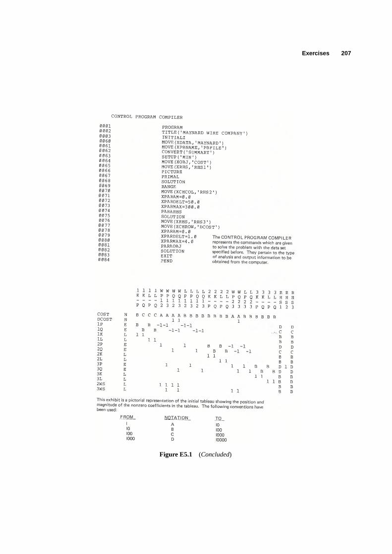
Exercises 207
Figure E5.1 (Concluded)

208 Mathematical Programming in Practice
Figure E5.2 Solution of program. (Cont.)

Exercises 209
Figure E5.2 Solution of program.

210 Mathematical Programming in Practice
Figure E5.2 (Cont.)

Exercises 211
Figure E5.2 (Cont.)

212 Mathematical Programming in Practice
Figure E5.2 (Cont.)

Exercises 213
Figure E5.2 (Cont.)

214 Mathematical Programming in Practice
Figure E5.2 (Cont.)

Exercises 215
Figure E5.2 (Concluded)

Figure E5.3 Optimum solution for Toys, Inc., cost and righthand-side ranges; parametric RHSanalysis, and parametric cost ranging. (Cont.)
216

Figure E5.3 (Cont.)
217

Figure E5.3 (Cont.)
218

Figure E5.3 (Cont.)
219

Figure E5.3 (Cont.)
220

Figure E5.3 (Cont.)
221
Figure E5.3 (Cont.)
222
Figure E5.3 (Cont.)
223

Figure E5.3 (Concluded)
224

Exercises 225
Using the computer output supplied, answer the following questions.
a) Draw a graph depicting the following as a function of time, assuming a capacity of 2750 cases per month.
i) Cases demandedii) Cases produced
iii) Cases in inventoryiv) Cases of unfilled demand
Explain thoroughly what this graph implies about the optimal operations of Toys, Inc.b) Give a complete economic interpretation of the dual variables.c) Give a concise explanation of the righthand-side and cost ranging output.d) Use the parametric programming of the righthand side as a basis for discussion the optimal production capacity.e) Use the parametric programming of the cost function as a basis for discussing the ‘‘value" of goodwill loss
associated with unfilled demand. (When demand is not met, we lose some goodwill of our customer. What isthis loss worth?)
4. Solving an LP by computer.Your doctor has found in you a very rare disease, ordinarily incurable, but, in yourcase, he believes that perhaps something can be done by a series of very elaborate treatments coupled with a strictdiet. The treatments are so expensive that it becomes necessary to minimize the cost of the diet.
The diet must provide minimum amounts of the following items: calories, calcium, vitamin A, riboflavin, andascorbic acid. Your daily requirement for these items (in the above order) may be determined by reading off thenumerical values corresponding to the first five letters of your name on Table 5.4. The following are the units used:102 calories, 10−2 grams, 102 international units, 10−1 milligrams, and milligrams.
Table E5.4 Diet Requirements
Diet ProductX Diet ProductX
A 7 63 N 6 91B 60 52 O 10 45C 83 59 P 32 82D 10 85 Q 51 98E 39 82 R 47 67F 59 58 S 20 97G 38 50 T 66 28H 30 69 U 78 54I 65 44 V 81 33J 27 26 W 81 59K 91 30 X 61 61L 68 43 Y 0 39M 49 90 Z 86 83
Your choice of foods is somewhat limited because you find it financially advantageous to trade at a discountstore that has little imagination. You can buy: (1) wheat flour (enriched), (2) evaporated milk, (3) cheddar cheese,(4) beef liver, (5) cabbage, (6) spinach, (7) sweet potatoes, (8) lima beans (dried).
The nutritional values per dollar spent have been tabulated by Dantzig (who regularly patronizes the store) inTable 5.5. In addition, the store features a grayish powder, Product X, sold in bulk, whose nutritional values per unitcost are also given in Table 5.4. The units (same order of items as before) are 103 calories/dollar, 10−1 grams/dollar,103 international units/dollar, 10−1 milligrams/dollar, milligrams/dollar.
Your doctor has coded your diet requirements and the nutritional properties of Product X under the first fiveletters of your name in Table 5.4.
a) Find your minimum-cost diet and its cost.b) How much would you be willing to pay for pure vitamin A? pure riboflavin?

226 Mathematical Programming in Practice 8.5
Table E5.5 Nutritive Values of Common Foods Per Dollar of Expenditure∗
AscorbicCalories Protein Calcium Iron Vitamin A ThiamineRiboflavin Niacin Acid
Commodity (1000) (grams) (grams) (mg.) (1000 I.U.) (mg.) (mg.) (mg.) (mg.). . .1. Wheat flour (enriched) 44.7 1411 2.0 365 — 55.4 33.3 441 —
5. Corn meal 36.0 897 1.7 99 30.9 17.4 7.9 106 —15. Evaporated milk (can) 8.4 422 15.1 9 26.0 3.0 23.5 11 6017. Oleomargarine 20.6 17 .6 6 55.8 .2 — — —19. Cheese (cheddar) 7.4 448 16.4 19 28.1 .8 10.3 4 —21. Peanut butter 15.7 661 1.0 48 — 9.6 8.1 471 —24. Lard 41.7 — — — .2 — .5 5 —30. Liver (beef) 2.2 333 .2 139 169.2 6.4 50.8 316 52534. Pork loin roast 4.4 249 .3 37 — 18.2 3.6 79 —40. Salmon, pink (can) 5.8 705 6.8 45 3.5 1.0 4.9 209 —45. Green beans 2.4 138 3.7 80 69.0 4.3 5.8 37 86246. Cabbage 2.6 125 4.0 36 7.2 9.0 4.5 26 536950. Onions 5.8 166 3.8 59 16.6 4.7 5.9 21 118451. Potatoes 14.3 336 1.8 118 6.7 29.4 7.1 198 252252. Spinach 1.1 106 — 138 918.4 5.7 13.8 33 275553. Sweet potatoes 9.6 138 2.7 54 290.7 8.4 5.4 83 191264. Peaches, dried 8.5 87 1.7 173 86.8 1.2 4.3 55 5765. Prunes, dried 12.8 99 2.5 154 85.7 3.9 4.3 65 25768. Lima beans, dried 17.4 1055 3.7 459 5.1 26.9 38.2 93 —69. Navy beans, dried 26.9 1691 11.4 792 — 38.4 24.6 217 —∗ Source: G. B. Dantzig,Linear Programming and Extension, Princeton University Press, Princeton, N.J., 1963.
c) A new food has come out (called GLUNK) having nutritional values per dollar of 83, 17, 25, 93, 07 (values arein the same order and same units as for Product X). Would you want to include the new food in your diet?
d) By how much would the cost of lima beans have to change before it would enter (or leave, as the case may be)your diet?
e) Over what range of values of cost of beef liver would your diet contain this wonderful food?f) Suppose the cost of foods 1, 3, 5, 7, and 9 went up 10% but you continued on the diet found in (a). How much
would you be willing to pay for pure vitamin A? pure riboflavin?g) If the wheat flour were enriched by 10 units of vitamin A without additional cost, would this change your diet?
ACKNOWLEDGMENTS
Exercise 1 is based on Chapter 14 ofApplied Linear Programming,by Norman J. Driebeck, Addison-WesleyPublishing Company, Inc., 1969.Exercises 2 and 3 are based on cases with the same names written by one of the authors.Exercise 4 is a variation of the diet problem used by John D.C. Little of the Massachusetts Institute ofTechnology.

Network Models
8
There are several kinds of linear-programming models that exhibit a special structure that can be exploitedin the construction of efficient algorithms for their solution. The motivation for taking advantage of theirstructure usually has been the need to solve larger problems than otherwise would be possible to solve withexisting computer technology. Historically, the first of these special structures to be analyzed was the trans-portation problem, which is a particular type of network problem. The development of an efficient solutionprocedure for this problem resulted in the first widespread application of linear programming to problems ofindustrial logistics. More recently, the development of algorithms to efficiently solve particular large-scalesystems has become a major concern in applied mathematical programming.
Network models are possibly still the most important of the special structures in linear programming. Inthis chapter, we examine the characteristics of network models, formulate some examples of these models,and give one approach to their solution. The approach presented here is simply derived from specializing therules of the simplex method to take advantage of the structure of network models. The resulting algorithms areextremely efficient and permit the solution of network models so large that they would be impossible to solveby ordinary linear-programming procedures. Their efficiency stems from the fact that a pivot operation forthe simplex method can be carried out by simple addition and subtraction without the need for maintainingand updating the usual tableau at each iteration. Further, an added benefit of these algorithms is that theoptimal solutions generated turn out to beintegerif the relevant constraint data are integer.
8.1 THE GENERAL NETWORK-FLOW PROBLEM
A common scenario of a network-flow problem arising in industrial logistics concerns the distribution of asingle homogeneous product from plants (origins) to consumer markets (destinations). The total number ofunits produced at each plant and the total number of units required at each market are assumed to be known.The product need not be sent directly from source to destination, but may be routed through intermediarypoints reflecting warehouses or distribution centers. Further, there may be capacity restrictions that limitsome of the shipping links. The objective is to minimize the variable cost of producing and shipping theproducts to meet the consumer demand.
The sources, destinations, and intermediate points are collectively callednodesof the network, and thetransportation links connecting nodes are termedarcs. Although a production/distribution problem has beengiven as the motivating scenario, there are many other applications of the general model. Table E8.1 indicatesa few of the many possible alternatives.
A numerical example of a network-flow problem is given in Fig 8.1. The nodes are represented bynumbered circles and the arcs by arrows. The arcs are assumed to bedirectedso that, for instance, materialcan be sent from node 1 to node 2, but not from node 2 to node 1. Generic arcs will be denoted byi – j , sothat 4–5 means the arcfrom node 4to node 5. Note that some pairs of nodes, for example 1 and 5, are notconnected directly by an arc.
227

228 Network Models 8.1
Table E8.1 Examples of Network Flow Problems
Urban Communication Watertransportation systems resources
Product Buses, autos, etc.Messages Water
Nodes Bus stops, CommunicationLakes, reservoirs,street intersectionscenters, pumping stations
relay stations
Arcs Streets (lanes) CommunicationPipelines, canals,channels rivers
Figure 8.1 exhibits several additional characteristics of network flow problems. First, a flow capacity isassigned to each arc, and second, a per-unit cost is specified for shipping along each arc. These characteristicsare shown next to each arc. Thus, the flow on arc 2–4 must be between 0 and 4 units, and each unit of flowon this arc costs $2.00. The∞’s in the figure have been used to denote unlimited flow capacity on arcs 2–3and 4–5. Finally, the numbers in parentheses next to the nodes give the material supplied or demanded at thatnode. In this case, node 1 is an origin orsource nodesupplying 20 units, and nodes 4 and 5 are destinationsor sink nodesrequiring 5 and 15 units, respectively, as indicated by the negative signs. The remaining nodeshave no net supply or demand; they are intermediate points, often referred to astransshipment nodes.
The objective is to find the minimum-cost flow pattern to fulfill demands from the source nodes. Suchproblems usually are referred to asminimum-cost flowor capacitated transshipmentproblems. To transcribethe problem into a formal linear program, let
xi j = Number of units shipped from nodei to j using arci – j .
Then the tabular form of the linear-programming formulation associated with the network of Fig. 8.1 isas shown in Table 8.2.
The first five equations are flow-balance equations at the nodes. They state the conservation-of-flow law,(Flow outof a node
)−
(Flow intoa node
)=
(Net supplyat a node
).
As examples, at nodes 1 and 2 the balance equations are:
x12 + x13 = 20x23 + x24 + x25 − x12 = 0.
It is important to recognize the special structure of these balance equations. Note that there is one balanceequation for each node in the network. The flow variablesxi j have only 0,+1, and−1 coefficients in these
Figure 8.1 Minimum-cost flow problem.

8.2 Special Network Models 229
Table E8.2 Tableau for Minimum-Cost Flow Problem
Righthandx12 x13 x23 x24 x25 x34 x35 x45 x53 side
Node 1 1 1 20
Node 2 −1 1 1 1 0
Node 3 −1 −1 1 1 −1 0
Node 4 −1 −1 1 −5
Node 5 −1 −1 −1 1 −15
Capacities 15 8 ∞ 4 10 15 5 ∞ 4
Objectivefunction 4 4 2 2 6 1 3 2 1 (Min)
equations. Further, each variable appears in exactly two balance equations, once with a+1 coefficient,corresponding to the node from which the arc emanates; and once with a−1 coefficient, corresponding tothe node upon which the arc is incident. This type of tableau is referred to as anode–arc incidence matrix; itcompletely describes the physical layout of the network. It is this particular structure that we shall exploit indeveloping specialized, efficient algorithms.
The remaining two rows in the table give the upper bounds on the variables and the cost of sending oneunit of flow across an arc. For example,x12 is constrained by 0≤ x12 ≤ 15 and appears in the objectivefunction as 2x12. In this example the lower bounds on the variables are taken implicitly to be zero, althoughin general there may also be nonzero lower bounds.
This example is an illustration of the following generalminimum-cost flowproblem withn nodes:
Minimize z=∑
i
∑j
ci j xi j ,
subject to: ∑j
xi j −∑
k
xki = bi (i = 1, 2, . . . , n), [Flow balance]
l i j ≤ xi j ≤ ui j . [Flow capacities]
The summations are taken only over the arcs in the network. That is, the first summation in thei th flow-balance equation is over all nodesj such thati – j is an arc of the network, and the second summation is overall nodesk such thatk–i is an arc of the network. The objective function summation is over arcsi – j thatare contained in the network and represents the total cost of sending flow over the network. Thei th balanceequation is interpreted as above: it states that the flow out of nodei minus the flow intoi must equal thenet supply (demand ifbi is negative) at the node.ui j is the upper bound on arc flow and may be+∞ if thecapacity on arci – j is unlimited. `i j is the lower bound on arc flow and is often taken to be zero, as in theprevious example. In the following sections we shall study variations of this general problem in some detail.
8.2 SPECIAL NETWORK MODELS
There are a number of interesting special cases of the minimum-cost flow model that have received a greatdeal of attention. This section introduces several of these models, since they have had a significant impacton the development of a general network theory. In particular, algorithms designed for these specific modelshave motivated solution procedures for the more general minimum-cost flow problem.
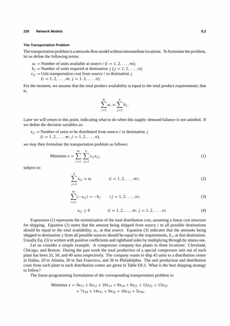
230 Network Models 8.2
The Transportation Problem
The transportation problem is a network-flow model without intermediate locations. To formulate the problem,let us define the following terms:
ai =Number of units available at sourcei (i = 1, 2, . . . , m);b j =Number of units required at destinationj ( j = 1, 2, . . . , n);ci j =Unit transportation cost from sourcei to destinationj
(i = 1, 2, . . . , m; j = 1, 2, . . . , n).
For the moment, we assume that the total product availability is equal to the total product requirements; thatis,
m∑i=1
ai =
n∑j=1
b j .
Later we will return to this point, indicating what to do when this supply–demand balance is not satisfied. Ifwe define the decision variables as:
xi j =Number of units to be distributed from sourcei to destinationj(i = 1, 2, . . . , m; j = 1, 2, . . . , n),
we may then formulate the transportation problem as follows:
Minimize z=m∑
i=1
n∑j=1
ci j xi j , (1)
subject to:n∑
j=1
xi j = ai (i = 1, 2, . . . , m), (2)
m∑i=1
(−xi j ) = −b j ( j = 1, 2, . . . , n), (3)
xi j ≥ 0 (i = 1, 2, . . . , m; j = 1, 2, . . . , n) (4)
Expression (1) represents the minimization of the total distribution cost, assuming a linear cost structurefor shipping. Equation (2) states that the amount being shipped from sourcei to all possible destinationsshould be equal to the total availability,ai , at that source. Equation (3) indicates that the amounts beingshipped to destinationj from all possible sources should be equal to the requirements,b j , at that destination.Usually Eq. (3) is written with positive coefficients and righthand sides by multiplying through by minus one.
Let us consider a simple example. A compressor company has plants in three locations: Cleveland,Chicago, and Boston. During the past week the total production of a special compressor unit out of eachplant has been 35, 50, and 40 units respectively. The company wants to ship 45 units to a distribution centerin Dallas, 20 to Atlanta, 30 to San Francisco, and 30 to Philadelphia. The unit production and distributioncosts from each plant to each distribution center are given in Table E8.3. What is the best shipping strategyto follow?
The linear-programming formulation of the corresponding transportation problem is:
Minimize z= 8x11+ 6x12+ 10x13+ 9x14+ 9x21+ 12x22+ 13x23
+ 7x24+ 14x31+ 9x32+ 16x33+ 5x34,

8.2 Special Network Models 231
Table E8.3 Unit Production and Shipping Costs
Distribution centers
San AvailabilityPlants Dallas Atlanta Francisco Phila. (units)
Cleveland 8 6 10 9 35Chicago 9 12 13 7 50Boston 14 9 16 5 40
Requirements(units) 45 20 30 30 [125]
subject to:
x11 + x12 + x13 + x14 = 35,x21 +x22 + x23 + x24 = 50,
x31 + x32 + x33 + x34 = 40,−x11 −x21 −x31 = −45,
−x12 −x22 −x32 = −20,−x13 −x23 −x33 = −30,
−x14 −x24 −x34 = −30,
xi j ≥ 0 (i=1,2,3; j=1,2,3,4).
Because there is no ambiguity in this case, the same numbers normally are used to designate the origins anddestinations. For example,x11 denotes the flow from source 1 to destination 1, although these are two distinctnodes. The network corresponding to this problem is given in Fig. 8.2.
The Assignment Problem
Though the transportation model has been cast in terms of material flow from sources to destinations, themodel has a number of additional applications. Suppose, for example, thann people are to be assigned tonjobs and thatci j measures the performance of personi in job j . If we let
xi j =
{1 if personi is assigned to jobj,0 otherwise,
Figure 8.2 Transportation network.

232 Network Models 8.2
we can find the optimal assignment by solving the optimization problem:
Maximizez=n∑
i=1
n∑j=1
ci j xi j ,
subject to:n∑
j=1
xi j = 1 (i = 1, 2, . . . , n),
n∑i=1
xi j = 1 ( j = 1, 2, . . . , n),
xi j = 0 or 1 (i = 1, 2, . . . , n; j = 1, 2, . . . , n).
The first set of constraints shows that each person is to be assigned to exactly one job and the second set ofconstraints indicates that each job is to be performed by one person. If the second set of constraints weremultiplied by minus one, the equations of the model would have the usual network interpretation.
As stated, this assignment problem is formally an integer program, since the decision variablesxi j arerestricted to be zero or one. However, if these constraints are replaced byxi j ≥ 0, the model becomes a specialcase of the transportation problem, with one unit available at each source (person) and one unit required byeach destination (job). As we shall see, network-flow problems have integer solutions, and therefore formalspecification of integrality constraints is unnecessary. Consequently, application of the simplex method, ormost network-flow algorithms, will solve such integer problems directly.
The Maximal Flow Problem
For the maximal flow problem, we wish to send as much material as possible from a specified nodes in anetwork, called thesource, to another specified nodet , called thesink. No costs are associated with flow. Ifv denotes the amount of material sent from nodes to nodet andxi j denotes the flow from nodei to node jover arci – j the formulation is:
Maximizev,
subject to:
∑j
xi j −∑
k
xki =
v if i = s (source),
−v if i = t (sink),
0 otherwise,
0 ≤ xi j ≤ ui j (i = 1, 2, . . . , n; j = 1, 2, . . . , n).
As usual, the summations are taken only over the arcs in the network. Also, the upper boundui j for the flowon arci – j is taken to be+∞ if arc i – j has unlimited capacity. The interpretation is thatv units are suppliedats and consumed att .
Let us introduce a fictitious arct–s with unlimited capacity; that is,uts = +∞. Now xts represents thevariablev, sincexts simply returns thev units of flow from nodet back to nodes, and no formal externalsupply of material occurs. With the introduction of the arct–s, the problem assumes the following specialform of the general network problem:
Maximizexts,
subject to: ∑j
xi j −∑
k
xki = 0 (i = 1, 2, . . . , n),

8.2 Special Network Models 233
Figure 8.3
0 ≤ xi j ≤ ui j (i = 1, 2, . . . , n; j = 1, 2, . . . , n).
Let us again consider a simple example. A city has constructed a piping system to route water from a laketo the city reservoir. The system is now underutilized and city planners are interested in its overall capacity.The situation is modeled as finding the maximum flow from node 1, the lake, to node 6, the reservoir, in thenetwork shown in Fig. 8.3.
The numbers next to the arcs indicate the maximum flow capacity (in 100,000 gallons/day) in that sectionof the pipeline. For example, at most 300,000 gallons/day can be sent from node 2 to node 4. The city nowsends 100,000 gallons/day along each of the paths 1–2–4–6 and 1–3–5–6. What is the maximum capacity ofthe network for shipping water from node 1 to node 6?
The Shortest-Path Problem
The shortest-path problem is a particular network model that has received a great deal of attention for bothpractical and theoretical reasons. The essence of the problem can be stated as follows: Given a network withdistanceci j (or travel time, or cost, etc.) associated with each arc, find a path through the network from aparticular origin (source) to a particular destination (sink) that has the shortest total distance. The simplicityof the statement of the problem is somewhat misleading, because a number of important applications can beformulated as shortest- (or longest-) path problems where this formulation is not obvious at the outset. Theseinclude problems of equipment replacement, capital investment, project scheduling, and inventory planning.The theoretical interest in the problem is due to the fact that it has a special structure, in addition to beinga network, that results in very efficient solution procedures. (In Chapter 11 on dynamic programming, weillustrate some of these other procedures.) Further, the shortest-path problem often occurs as a subproblem inmore complex situations, such as the subproblems in applying decomposition to traffic-assignment problemsor the group-theory problems that arise in integer programming.
In general, the formulation of the shortest-path problem is as follows:
Minimize z=∑
i
∑j
ci j xi j ,
subject to: ∑j
xi j −∑
k
xki =
1 if i = s (source),
0 otherwise,
−1 if i = t (sink)
xi j ≥ 0 for all arcsi – j in the network.
We can interpret the shortest-path problem as a network-flow problem very easily. We simply want to sendone unit of flow from the source to the sink at minimum cost. At the source, there is a net supply of one unit;at the sink, there is a net demand of one unit; and at all other nodes there is no net inflow or outflow.

234 Network Models 8.3
As an elementary illustration, consider the example given in Fig. 8.4, where we wish to find the shortestdistance from node 1 to node 8. The numbers next to the arcs are the distance over, or cost of using, that arc.For the network specified in Fig. 8.4, the linear-programming tableau is given in Tableau 1.
Tableau E8.4 Node–Arc Incidence Tableau for a Shortest-PathProblem
Rela-x12 x13 x24 x25 x32 x34 x37 x45 x46 x47 x52 x56 x58 x65 x67 x68 x76 x78 tions RHS
Node1 1 1 = 1Node2 −1 1 1 −1 −1 = 0
Node3 −1 1 1 1 = 0
Node4 −1 −1 1 1 1 = 0
Node5 −1 −1 1 1 1 −1 = 0
Node6 −1 −1 1 1 1 −1 = 0
Node7 −1 −1 −1 1 1 = 0
Node8 −1 −1 −1 = −1
Distance 5.1 3.4 0.5 2.0 1.0 1.5 5.0 2.0 3.0 4.2 1.0 3.0 6.0 1.5 0.5 2.2 2.0 2.4= z (min)
8.3 THE CRITICAL-PATH METHOD
The Critical-Path Method (CPM) is a project-management technique that is used widely in both governmentand industry to analyze, plan, and schedule the various tasks of complex projects. CPM is helpful in identifyingwhich tasks are critical for the execution of the overall project, and in scheduling all the tasks in accordancewith their prescribedprecedence relationshipsso that the total project completion date is minimized, or atarget date is met at minimum cost.
Typically, CPM can be applied successfully in large construction projects, like building an airport or ahighway; in large maintenance projects, such as those encountered in nuclear plants or oil refineries; andin complex research-and-development efforts, such as the development, testing, and introduction of a newproduct. All these projects consist of a well specified collection of tasks that should be executed in a certainprescribed sequence. CPM provides a methodology to define the interrelationships among the tasks, and todetermine the most effective way of scheduling their completion.
Although the mathematical formulation of the scheduling problem presents a network structure, this isnot obvious from the outset. Let us explore this issue by discussing a simple example.
Suppose we consider the scheduling of tasks involved in building a house on a foundation that alreadyexists. We would like to determine in what sequence the tasks should be performed in order to minimize
Figure 8.4 Network for a shortest-path problem.

8.3 The Critical-Path Method 235
the total time required to execute the project. All we really know is how long it takes to carry out each taskand which tasks must be completed before commencing any particular task. In fact, it will be clear that weneed only know the tasks thatimmediatelyprecede a particular task, since completion of allearlier tasks willbe implied by this information. The tasks that need to be performed in building this particular house, theirimmediate predecessors, and an estimate of their duration are give in Table E8.4.
It is clear that there is no need to indicate that the siding must be put up before the outside painting canbegin, since putting up the siding precedes installing the windows, which precedes the outside painting. Itis always convenient to identify a ‘‘start’’ task, that is, an immediate predecessor to all tasks, which in itselfdoes not have predecessors; and a ‘‘finish’’ task, which has, as immediate predecessors,all tasks that inactuality have no successors.
Table E8.4 Tasks and Precedence Relationships
Immediate EarliestNo. Task predecessorsDuration starting times
0 Start — 0 —1 Framing 0 2 t12 Roofing 1 1 t23 Siding 1 1 t24 Windows 3 2.5 t35 Plumbing 3 1.5 t36 Electricity 2, 4 2 t47 Inside Finishing 5, 6 4 t58 Outside Painting 2, 4 3 t49 Finish 7, 8 0 t6
Although it is by no means required in order to perform the necessary computations associated with thescheduling problem, often it is useful to represent the interrelations among the tasks of a given project bymeans of a network diagram. In this diagram, nodes represent the corresponding tasks of the project, andarcs represent the precedence relationships among tasks. The network diagram for our example is shown inFig. 8.5.
Figure 8.5 Task-oriented network.
As we can see, there are nine nodes in the network, each representing a given task. For this reason, thisnetwork representation is called a task- (or activity-) oriented network.
If we assume that our objective is to minimize the elapsed time of the project, we can formulate a linear-programming problem. First, we define the decision variablesti for i = 1, 2, . . . , 6, as the earliest startingtimes for each of the tasks. Table 8.4. gives the earliest starting times where the same earliest starting timeis assigned to tasks with the same immediate predecessors. For instance, tasks 4 and 5 have task 3 as their

236 Network Models 8.3
immediate predecessor. Obviously, they cannot start until task 3 is finished; therefore, they should have thesameearliest starting time. Lettingt6 be the earliest completion time of the entire project, out objective is tominimize the project duration given by
Minimize t6− t1,
subject to the precedence constraints among tasks. Consider a particular task, say 6, installing the electricity.The earliest starting time of task 6 ist4, and its immediate predecessors are tasks 2 and 4. The earliest startingtimes of tasks 2 and 4 aret2 and t3, respectively, while their durations are 1 and 2.5 weeks, respectively.Hence, the earliest starting time of task 6 must satisfy:
t4 ≥ t2+ 1,
t4 ≥ t3+ 2.5.
In general, ift j is the earliest starting time of a task,ti is the earliest starting time of an immediate predecessor,anddi j is the duration of the immediate predecessor, then we have:
t j ≥ ti + di j .
For our example, these precedence relationships define the linear program given in Tableau E8.2.
Tableau E8.2
t1 t2 t3 t4 t5 t6 Relation RHS
−1 1 ≥ 2
−1 1 ≥ 3
−1 1 ≥ 1
−1 1 ≥ 2.5
−1 1 ≥ 1.5
−1 1 ≥ 2
−1 1 ≥ 3
−1 1 ≥ 4
−1 1 = T (min)
We do not yet have a network flow problem; the constraints of (5) do not satisfy our restriction that eachcolumn have only a plus-one and a minus-one coefficient in the constraints. However, thisis true for therows, so let us look at the dual of (5). Recognizing that the variables of (5) have not been explicitly restrictedto the nonnegative, we will have equalityconstraints in the dual. If we letxi j be the dual variable associatedwith the constraint of (5) that has a minus one as a coefficient forti and a plus one as a coefficient oft j , thedual of (5) is then given in Tableau 3.
Tableau E8.3
x12 x23 x24 x34 x35 x45 x46 x56 Relation RHS
−1 = −11 −1 −1 = 0
1 −1 −1 = 0
1 1 −1 −1 = 0
1 1 −1 = 0
1 1 = 1
2 3 1 2.5 1.5 2 3 4 = z(max)

8.4 Capacitated Production—A Hidden Network 237
Now we note that each column of (6) has only one plus-one coefficient and one minus-one coefficient, andhence the tableau describes a network. If we multiply each equation through by minus one, we will have theusual sign convention with respect to arcs emanating from or incident to a node. Further, since the righthandside has only a plus one and a minus one, we have flow equations for sending one unit of flow from node 1 tonode 6. The network corresponding to these flow equations is given in Fig. 8.6; this network clearly maintainsthe precedence relationships from Table 8.4. Observe that we have a longest-path problem, since we wish tomaximizez (in order to minimize the project completion dateT). Note that, in this network, the arcs represent
Figure 8.6 Event-oriented network.
the tasks, while the nodes describe the precedence relationships among tasks. This is the opposite of the net-work representation given in Fig. 8.5. As we can see, the network of Fig. 8.6. contains 6 nodes, which is thenumber of sequencing constraints prescribed in the task definition of Table 8.4. since only six earliest startingtimes were required to characterize these constraints. Because the network representation of Fig. 8.6 empha-sizes the event associated with the starting of each task, it is commonly referred to as an event-oriented network.
There are several other issues associated with critical-path scheduling that also give rise to network-modelformulations. In particular, we can consider allocating funds among the various tasks in order to reduce thetotal time required to complete the project. The analysis of the cost-vs.-time tradeoff for such a change is animportant network problem. Broader issues of resource allocation and requirements smoothing can also beinterpreted as network models, under appropriate conditions.
8.4 CAPACITATED PRODUCTION—A HIDDEN NETWORK
Network-flow models are more prevalent than one might expect, since many models not cast naturally asnetworks can be transformed into a network format. Let us illustrate this possibility by recalling the strategic-planning model for aluminum production developed in Chapter 6. In that model,bauxite ore is converted toaluminum products in several smelters, to be shipped to a number of customers. Production and shipmentare governed by the following constraints:∑
a
∑p
Qsap− Ms = 0 (s= 1, 2, . . . , 11), (7)
∑a
Qsap − Esp= 0 (s= 1, 2, . . . , 11; p = 1, 2, . . . , 8), (8)
∑s
Qsap = dap (a= 1, 2, . . . , 40; p= 1, 2, . . . , 8), (9)
ms ≤ Ms ≤ ms (s= 1, 2, . . . , 11),
esp≤ Esp≤ esp (p= 1, 2, . . . , 40).

238 Network Models 8.4
VariableQsapis the amount of product p to be produced at smelter s and shipped to customer a. The constraints(7) and (8) merely define the amountMs produced at smelter s and the amountEsp of product p (ingots) to be‘‘cast’’ at smelter s. Equations (9) state that the total production from all smelters must satisfy the demanddap for product p of each customer a. The upper bounds ofMs andEsp reflect smelting and casting capacity,whereas the lower bounds indicate minimum economically attractive production levels.
As presented, the model is not in a network format, since it does not satisfy the property that every variableappear in exactly two constraints, once with a+1 coefficient and once with a−1 coefficient. It can be statedas a network, however, by making a number of changes. Suppose, first, that we rearrange all the constraintsof (7), as ∑
p
(∑a
Qsap
)− Ms = 0,
and substitute, for the term in parenthesis,Esp defined by (8). Let us also multiply the constraints of (9) by(−1). The model is then rewritten as:∑
p
Esp− Ms = 0 (s= 1, 2, . . . , 11), (10)
∑a
Qsap− Esp = 0 (s= 1, 2, . . . , 11; p= 1, 2, . . . , 8), (11)
∑s
−Qsap = −dap (a= 1, 2, . . . , 40; p= 1, 2, . . . , 8), (12)
ms ≤ Ms ≤ ms (s= 1, 2, . . . , 11),
esp ≤ Esp≤ esp (p= 1, 2, . . . , 8).
Each variableEsp appears once in the equations of (10) with a+1 coefficient and once in the equations of(11) with a−1 coefficient; each variableQsapappears once in the equations of (11) with a+1 coefficient andonce in the equations of (12) with a−1 coefficient. Consequently, except for the variablesMs, the problemis in the form of a network. Now, suppose that weadd all the equations to form one additional redundantconstraint. As we have just noted, the terms involving the variablesQsapandEsp will all vanish, so that theresulting equation, when multiplied by minus one, is:∑
s
Ms =∑
a
∑p
dap. (13)
Each variableMs now appears once in the equations of (10) with a+1 coefficient and once in the equations of(13) with a−1 coefficient, so appending this constraint to the previous formulation gives the desired networkformulation.
The network representation is shown Fig. 8.7. As usual, each equation in the model defines a node in thenetwork. The topmost node corresponds to the redundant equation just added to the model; it just collectsproduction from the smelters. The other nodes correspond to the smelters, the casting facilities for products atthe smelters, and the customer–product demand combinations. The overall supply to the system,
∑a∑
p dap,as indicated at the topmost node, is the total production at the smelters, and must equal the demand for allproducts.
In practice, manipulations like these just performed for re-expressing problems can be used frequentlyto exhibit network structure that might be hidden in a model formulation. They may not always lead to purenetwork-flow problems, as in this example, but instead might show that the problem has a substantial networkcomponent. The network features might then be useful computationally in conjunction with large-scalesystems techniques that exploit the network structure.

8.5 Solving the Transportation Problem 239
Figure 8.7 Network formulation of the aluminum production-planning model.
Finally, observe that the network in Fig. 8.7 contains only a small percentage of the arcs that couldpotentially connect the nodes since, for example, the smelters do not connect directly with customer demands.This low density of arcs is common in practice, and aids in both the information storage and the computationsfor network models.
8.5 SOLVING THE TRANSPORTATION PROBLEM
Ultimately in this chapter we want to develop an efficient algorithm for the general minimum-cost flow problemby specializing the rules of the simplex method to take advantage of the problem structure. However, beforetaking a somewhat formal approach to the general problem, we will indicate the basic ideas by developinga similar algorithm for the transportation problem. The properties of this algorithm for the transportationproblem will then carry over to the more general minimum-cost flow problem in a straightforward manner.Historically, the transportation problem was one of the first special structures of linear programming forwhich an efficient special-purpose algorithm was developed. In fact, special-purpose algorithms have beendeveloped for all of the network structures presented in Section 8.1, but they will not be developed here.
As we have indicated before, many computational algorithms are characterized by three stages:
1. obtaining an initial solution;2. checking an optimality criterion that indicates whether or not a termination condition has been met (i.e.,
in the simplex algorithm, whether the problem is infeasible, the objective is unbounded over the feasibleregion, or an optimal solution has been found);
3. developing a procedure to improve the current solution if a termination condition has not been met.
After an initial solution is found, the algorithm repetitively applies steps 2 and 3 so that, in most cases, after

240 Network Models 8.5
Tableau E8.4
Destinations
Sources 1 2 · · · n Supply
c11 c12 c1n1 x11 x12 · · · x1n a1
c21 c22 c2n2 x21 x22 · · · x2n a2
......
......
...
cm1 cm2 cmnm xm1 xm2 · · · xmn am
Demand b1 b2 · · · bn Total
a finite number of steps, a termination condition arises. The effectiveness of an algorithm depends upon itsefficiency in attaining the termination condition.
Since the transportation problem is a linear program, each of the above steps can be performed by thesimplex method. Initial solutions can be found very easily in this case, however, so phase I of the simplexmethod need not be performed. Also, when applying the simplex method in this setting, the last two stepsbecome particularly simple.
The transportation problem is a special network problem, and the steps of any algorithm for its solutioncan be interpreted in terms of network concepts. However, it also is convenient to consider the transporta-tion problem in purely algebraic terms. In this case, the equations are summarized very nicely by a tabularrepresentation like that in Tableau E8.4.
Each row in the tableau corresponds to a source node and each column to a destination node. The numbersin the final column are the supplies available at the source nodes and those in the bottom row are the demandsrequired at the destination nodes. The entries in celli – j in the tableau denote the flow allocationxi j fromsourcei to destinationj and the corresponding cost per unit of flow isci j . The sum ofxi j across rowi mustequalai in any feasible solution, and the sum ofxi j down columnj must equalb j .
Initial Solutions
In order to apply the simplex method to the transportation problem, we must first determine a basic feasiblesolution. Since there are(m+ n) equations in the constraint set of the transportation problem, one mightconclude that, in a nondegenerate situation, a basic solution will have(m + n) strictly positive variables. Weshould note, however, that, since
m∑i=1
ai =
n∑j=1
b j =
m∑i=1
n∑j=1
xi j ,
one of the equations in the constraint set is redundant. In fact, any one of these equations can be eliminatedwithout changing the conditions represented by the original constraints. For instance, in the transportationexample in Section 8.2, the last equation can be formed by summing the first three equations and subtractingthe next three equations. Thus, the constraint set is composed of(m+ n− 1) independent equations, and acorresponding nondegenerate basic solution will have exactly(m+ n− 1) basic variables.
There are several procedures used to generate an initial basic feasible solution, but we will consider onlya few of these. The simplest procedure imaginable would be one that ignores the costs altogether and rapidlyproduces a basic feasible solution. In Fig. 8.8, we have illustrated such a procedure for the transportationproblem introduced in Section 8.2. We simply send as much as possible from origin 1 to destination 1, i.e.,the minimum of the supply and demand, which is 35. Since the supply at origin 1 is then exhausted but thedemand at destination 1 is not, we next fulfill the remaining demand at destination 1 from that available atorigin 2. At this point destination 1 is completely supplied, so we send as much as possible (20 units) of the

8.5 Solving the Transportation Problem 241
Table E8.5 Finding an Initial Basis by the Northwest Corner Method
Distribution centers
Plants 1. Dallas2. Atlanta 3. San Fran.4. Phila. Supply
1. Cleveland 35 35�2. Chicago 10 20 20 50� 40� 20�3. Boston 10 30 40� 30�Demand 45� 20� 30� 30�
10� 10�
remaining supply of 40 at origin 2 to destination 2, exhausting the demand there. Origin 2 still has a supplyof 20 and we send as much of this as possible to destination 3, exhausting the supply at origin 2 but leaving ademand of 10 at destination 3. This demand is supplied from origin 3, leaving a supply there of 30, exactlycorresponding to the demand of 30 needed at destination 4. The available supply equals the required demandfor this final allocation because we have assumed that the total supply equals the total demand, that is,
m∑i=1
ai =
n∑j=1
b j .
This procedure is called thenorthwest-cornerrule since, when interpreted in terms of the transportationarray, it starts with the upper leftmost corner (the northwest corner) and assigns the maximum possible flowallocation to that cell. Then it moves to the right, if there is any remaining supply in the first row, or to thenext lower cell, if there is any remaining demand in the first column, and assigns the maximum possible flowallocation to that cell. The procedure repeats itself until one reaches the lowest right corner, at which pointwe have exhausted all the supply and satisfied all the demand.
Table E8.5 summarizes the steps of the northwest-corner rule, in terms of the transportation tableau, whenapplied to the transportation example introduced in Section 8.2.
The availabilities and requirements at the margin of the table are updated after each allocation assignment.Although the northwest-corner rule is easy to implement, since it does not take into consideration the cost ofusing a particular arc, it will not, in general, lead to a cost-effective initial solution.
An alternative procedure, which is cognizant of the costs and straightforward to implement, is theminimummatrixmethod. Using this method, we allocate as much as possible to the available arc with the lowest cost.Figure 8.9 illustrates the procedure for the example that we have been considering. The least-cost arc joinsorigin 3 and destination 4, at a cost of $5/unit, so we allocate the maximum possible, 30 units, to this arc,
Figure 8.8 Finding an initial basis by the northwest-corner method.

242 Network Models 8.5
Figure 8.9 Finding an initial basis by the minimum-matrix method.
completely supplying destination 4. Ignoring the arcs entering destination 4, the least-cost remaining arcjoins origin 1 and destination 2, at a cost of $6/unit, so we allocate the maximum possible, 20 units, to this arc,completely supplying destination 2. Then, ignoring the arcs entering either destination 2 or 4, the least-costremaining arc joins origin 1 and destination 1, at a cost of $8/unit, so we allocate the maximum possible,15 units, to this arc, exhausting the supply at origin 1. Note that this arc is the least-costremainingarcbut not the next-lowest-cost unused arc in the entire cost array. Then, ignoring the arcs leaving origin 1 orentering destinations 2 or 4, the procedure continues. It should be pointed out that the last two arcs used bythis procedure are relatively expensive, costing $13/unit and $16/unit. It is often the case that the minimummatrix method produces a basis that simultaneously employs some of the least expensive arcs and some ofthe most expensive arcs.
There are many other methods that have been used to find an initial basis for starting the transportationmethod. An obvious variation of the minimum matrix method is theminimum rowmethod, which allocatesas much as possible to the available arc with least costin each rowuntil the supply at each successive originis exhausted. There is clearly the analogousminimum columnmethod.
It should be pointed out that any comparison among procedures for finding an initial basis should bemade only by comparingsolution times, including both finding the initial basisanddetermining an optimalsolution. For example, the northwest-corner method clearly requires fewer operations to determine an initialbasis than does the minimum matrix rule, but the latter generally requires fewer iterations of the simplexmethod to reach optimality.
The two procedures for finding an initial basic feasible solution resulted in different bases; however, bothhave a number of similarities. Each basis consists of exactly(m+ n− 1) arcs, one less than the number ofnodes in the network. Further, each basis is a subnetwork that satisfies the following two properties:
1. Every node in the network is connected to every other node by a sequence of arcs from the subnetwork,where the direction of the arcs is ignored.
2. The subnetwork contains no loops, where a loop is a sequence of arcs connecting a node to itself, whereagain the direction of the arcs is ignored.
A subnetwork that satisfies these two properties is called aspanning tree.It is the fact that a basis corresponds to a spanning tree that makes the solution of these problems by the
simplex method very efficient. Suppose you were told that a feasible basis consists of arcs 1–1, 2–1, 2–2, 2–4,3–2, and 3–3. Then the allocations to each arc can be determined in a straightforward way without algebraicmanipulations of tableaus. Start by selecting anyend(a node with only 1 arc connecting it to the rest of thenetwork) in the subnetwork. The allocation to the arc joining that end must be the supply or demand availableat that end. For example, source 1 is an end node. The allocation on arc 1–1 must then be 35, decreasing

8.5 Solving the Transportation Problem 243
Figure 8.10 Determining the values of the basic variables.
the unfulfilled demand at destination 1 from 45 to 10 units. The end node and its connecting arc are thendropped from the subnetwork and the procedure is repeated. In Fig. 8.10, we use these end-node evaluationsto determine the values of the basic variables for our example.
This example also illustrates that the solution of a transportation problem by the simplex method resultsin integervalues for the variables. Since any basis corresponds to a spanning tree, as long as the supplies anddemands are integers the amount sent across any arc must be an integer. This is true because, at each stageof evaluating the variables of a basis, as long as the remaining supplies and demands are integer the amountsent to any end must also be an integer. Therefore, if the initial supplies and demands are integers, any basicfeasible solution will be an integer solution.
Optimization Criterion
Because it is so common to find the transportation problem written with+1 coefficients for the variablesxi j (i.e., with the demand equations of Section 8.2 multiplied by minus one), we will give the optimalityconditions for this form. They can be easily stated in terms of the reduced costs of the simplex method. Ifxi j for i = 1, 2, . . . , m and j = 1, 2, . . . , n is a feasible solution to the transportation problem:
Minimize z=m∑
i=1
n∑j=1
ci j xi j ,
subject to: Shadowprices
n∑j=1
xi j = ai (i = 1, 2, . . . , m), ui
m∑i=1
xi j = b j ( j = 1, 2, . . . , n), v j
xi j ≥ 0,
then it is optimal if there exist shadow prices (or simplex multipliers)ui associated with the origins andv jassociated with the destinations, satisfying:
ci j = ci j − ui − v j ≥ 0 if xi j = 0, (14)

244 Network Models 8.5
Figure 8.11 Determining the simplex multipliers.
and
ci j = ci j − ui − v j = 0 if xi j > 0. (15)
The simplex method selects multipliers so that condition (15) holds for all basic variables, even if some basicvariablexi j = 0 due to degeneracy.
These conditions not only allow us to test whether the optimalsolution has been found or not, but provideus with the necessary foundation to reinterpret the characteristics of the simplex algorithm in order to solvethe transportation problem efficiently. The algorithm will proceed as follows: after a basic feasible solutionhas been found (possibly by applying the northwest-corner method or the minimum matrix method), wechoose simplex multipliersui andv j (i = 1, 2, . . . , m; j = 1, 2, . . . , n) that satisfy:
ui + v j = ci j (16)
for basic variables. With these values for the simplex multipliers, we compute the corresponding values ofthe reduced costs:
ci j = ci j − ui − v j (17)
for all nonbasic variables. If everyci j is nonnegative, then the optimal solution has been found; otherwise,we attempt to improve the current solution by increasing as much as possible the variable that correspondsto the most negative (since this is a minimization problem) reduced cost.
First, let us indicate the mechanics of determining from (16) the simplex multipliers associated with aparticular basis. Conditions (16) consist of(m + n − 1) equations in(m + n) unknowns. However, anyone of the simplex multipliers can be given an arbitrary value since, as we have seen, any one of the(m + n)
equations of the transportation problem can be considered redundant. Since there are(m+ n−1) equations in(16), once one of the simplex multipliers has been specified, the remaining values ofui andv j are determineduniquely. For example, Fig. 8.11 gives the initial basic feasible solution produced by the minimum matrixmethod. The simplex multipliers associated with this basis are easily determined by first arbitrarily settingu1 = 0. Givenu1 = 0, v1 = 8 andv2 = 6 are immediate from (16); thenu2 = 1 is immediate fromv1, andso on. It should be emphasized that the set of multipliers is not unique, since any multiplier could have beenchosen and set to any finite value, positive or negative, to initiate the determination.
Once we have determined the simplex multipliers, we can then easily find the reduced costs for allnonbasic variables by applying (17). These reduced costs are given in Tableau 5. The —’s indicate thebasic variable, which therefore has areduced cost of zero. This symbol is used to distinguish between basicvariables and nonbasic variables at zero level.
Since, in Tableau 5,c13 = −2 andc32 = −1, the basis constructed by the minimum matrixmethod doesnot yield an optimal solution. We, therefore, need to find an improved solution.
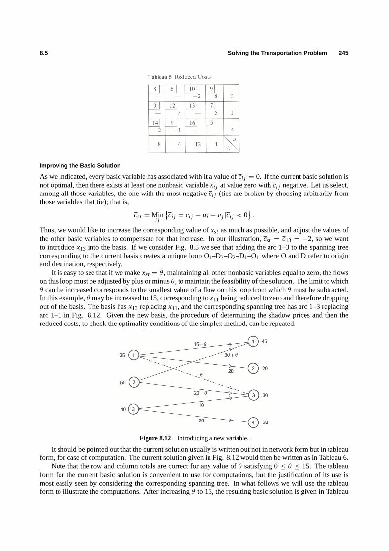
8.5 Solving the Transportation Problem 245
Improving the Basic Solution
As we indicated, every basic variable has associated with it a value ofci j = 0. If the current basic solution isnot optimal, then there exists at least one nonbasic variablexi j at value zero withci j negative. Let us select,among all those variables, the one with the most negativeci j (ties are broken by choosing arbitrarily fromthose variables that tie); that is,
cst = Mini j
{ci j = ci j − ui − v j |ci j < 0
}.
Thus, we would like to increase the corresponding value ofxst as much as possible, and adjust the values ofthe other basic variables to compensate for that increase. In our illustration,cst = c13 = −2, so we wantto introducex13 into the basis. If we consider Fig. 8.5 we see that adding the arc 1–3 to the spanning treecorresponding to the current basis creates a unique loop O1–D3–O2–D1–O1 where O and D refer to originand destination, respectively.
It is easy to see that if we makexst = θ , maintaining all other nonbasic variables equal to zero, the flowson this loop must be adjusted by plus or minusθ , to maintain the feasibility of the solution. The limit to whichθ can be increased corresponds to the smallest value of a flow on this loop from whichθ must be subtracted.In this example,θ may be increased to 15, corresponding tox11 being reduced to zero and therefore droppingout of the basis. The basis hasx13 replacingx11, and the corresponding spanning tree has arc 1–3 replacingarc 1–1 in Fig. 8.12. Given the new basis, the procedure of determining the shadow prices and then thereduced costs, to check the optimality conditions of the simplex method, can be repeated.
Figure 8.12 Introducing a new variable.
It should be pointed out that the current solution usually is written out not in network form but in tableauform, for case of computation. The current solution given in Fig. 8.12 would then be written as in Tableau 6.
Note that the row and column totals are correct for any value ofθ satisfying 0≤ θ ≤ 15. The tableauform for the current basic solution is convenient to use for computations, but the justification of its use ismost easily seen by considering the corresponding spanning tree. In what follows we will use the tableauform to illustrate the computations. After increasingθ to 15, the resulting basic solution is given in Tableau

246 Network Models 8.6
7 (ignoringθ ) and the new multipliers and reduced costs in Tableau 8.
Since the only negative reduced cost corresponds toc32 = −3, x32 is next introduced into the basis.Adding the arc 3–2 to the spanning tree corresponds to increasing the allocation to cell 3–2 in the tableau andcreates a unique loop O3–D2–O1–D3–O3. The flowθ on this arc may be increased untilθ = 10, correspondingto x33 dropping from the basis. The resulting basic solution is Tableau 9 and the new multipliers and reducedcosts are given in Tableau 10.
Since all of the reduced costs are now nonnegative, we have the optimal solution.
8.6 ADDITIONAL TRANSPORTATION CONSIDERATIONS
In the previous section, we described how the simplex method has been specialized in order to solve trans-portation problems efficiently. There are three steps to the approach:
1. finding an initial basic feasible solution;
2. checking the optimality conditions; and
3. constructing an improved basic feasible solution, if necessary.

8.6 Additional Transportation Considerations 247
The problem we solved was quite structured in the sense that total supply equaled total demand, shippingbetween all origins and destinations was permitted, degeneracy did not occur, and so forth. In this section,we address some of the important variations of the approach given in the previous section that will handlethese situations.
Supply Not Equal to Demand
We have analyzed the situation where the total availability is equal to the total requirement. In practice, this isusually not the case, since often either demand exceeds supply or supply exceeds demand. Let us see how totransform a problem in which this assumption does not hold to the previously analyzed problem with equalityof availability and requirement. Two situations will exhaust all the possibilities:
First, assume that the total availability exceeds the total requirement; that is,
m∑i=1
ai −
n∑j=1
b j = d > 0.
In this case, we create an artificial destinationj = n + 1, with corresponding ‘‘requirement’’bn+1 = d,and make the corresponding cost coefficients to this destination equal to zero, that is,ci,n+1 = 0 for i =1, 2, . . . , m. The variablexi,n+1 in the optimal solution will show how the excess availability is distributedamong the sources.
Second, assume that the total requirement exceeds the total availability, that is,
n∑j=1
b j −
m∑i=1
ai = d > 0.
In this case, we create an artificial origini = m+1, with corresponding ‘‘availability’’am+1 = d, and assignzero cost coefficients to this destination, that is,cm+1, j = 0 for j = 1, 2, . . . , n. The optimal value for thevariablexm+1, j will show how the unsatisfied requirements are allocated among the destinations.
In each of the two situations, we have constructed an equivalent transportation problem such that the total‘‘availability’’ is equal to the total ‘‘requirement.’’
Prohibited Routes
If it is impossible to shipany goods from sourcei to destinationj , we assign a very high cost to thecorresponding variablexi j , that is, ci j = M , where M is a very large number, and use the procedurepreviously discussed. If these prohibited routes cannot be eliminated from the optimal solution then theproblem is infeasible.
Alternatively, we can use the two-phase simplex method. We start with any initial basic feasible solution,which may use prohibited routes. The first phase will ignore the given objective function and minimize thesum of the flow along the prohibited routes. If the flow on the prohibited routes cannot be driven to zero, thenno feasible solution exists without permitting flow on at least one of the prohibited routes. If, on the otherhand, flow on the prohibited routescanbe made zero, then an initial basic feasible solutionwithoutpositiveflow on prohibited routes has been constructed. It is necessary then simply to prohibit flow on these routesin the subsequent iterations of the algorithm.
Degeneracy
Degeneracy can occur on two different occasions during the computational process described in the previoussection. First, during the computation of the initial solution of the transportation problem, we can simultane-ously eliminate a row and a column at an intermediate step. This situation gives rise to a basic solution withless than(m+ n− 1) strictly positive variables. To rectify this, one simply assigns a zero value to a cell in

248 Network Models 8.6
either the row or column to be simultaneously eliminated, and treats that variable as a basic variable in theremaining computational process.
As an example, let us apply the northwest-corner rule to the case in Tableau 11.
In this instance, when makingx12 = 5, we simultaneously satisfy the first row availability and the secondcolumn requirement. We thus makex13 = 0, and treat it as a basicvariable in the rest of the computation.
A second situation where degeneracy arises is while improving a current basic solution. A tie might befound when computing the new value to be given to the entering basic variable,xst = θ . In this case, morethan one of the old basic variables will take the value zero simultaneously, creating a new basic solutionwith less than(m+ n − 1) strictly positive values. Once again, the problem is overcome by choosing thevariable to leave the basis arbitrarily from among the basic variables reaching zero atxst = θ , and treatingthe remaining variables reaching zero atxst = θ as basic variables at zero level.
Vogel Approximation
Finally, we should point out that there have been a tremendous number of procedures suggested for findingan initial basic feasible solution to the transportation problem. In the previous section, we mentioned fourmethods: northwest corner, minimum matrix, minimum column, and minimum row.
The first of these ignores the costs altogether, while the remaining methods allocate costs in such a waythat the last fewassignments of flows often results in very high costs being incurred. The high costs are dueto the lack of choice as to how the final flows are to be assigned to routes, once the initial flows have beenestablished. The initial flows are not chosen with sufficient foresight as to how they might impair later flowchoices.
The Vogel approximation method was developed to overcome this difficulty and has proved to be so effec-tive that it is sometimes used to obtain an approximation to the optimal solution of the problem. The method,instead of sequentially using the least-cost remaining arc, bases its selection on the difference between thetwo lowest-cost arcs leaving an origin or entering a destination. This difference indicates where departurefrom the lowest-cost allocations will bring the highest increase in cost. Therefore, one assigns the maximumpossible amount to that arc that has the lowest cost in that row or column having the greatest cost difference.If this assignment exhausts the demand at that destination, the corresponding column is eliminated fromfurther consideration; similarly, if the assignment exhausts the supply at that origin, the corresponding rowis eliminated. In either case, the origin and destination cost differences are recomputed, and the procedurecontinues in the same way.
The Vogel approximation method is applied to our illustrative example in Tableau 12, and the result-ing basic feasible solution is given in Fig. 8.13. It is interesting to note that the approximation finds theoptimal solution in this particular case, as can be seen by comparing the initial basis from the Vogel approx-imation in Fig. 8.13 with the optimal basis in Tableau 7. This, of course, does not mean that the Vogelapproximation is the best procedure for determining the initial basic feasible solution. Any such compari-son among computational procedures must compare total time required, from preprocessing to final optimal

8.6 Additional Transportation Considerations 249
Figure 8.13 Initial basis for Vogel approximation method.
solution.
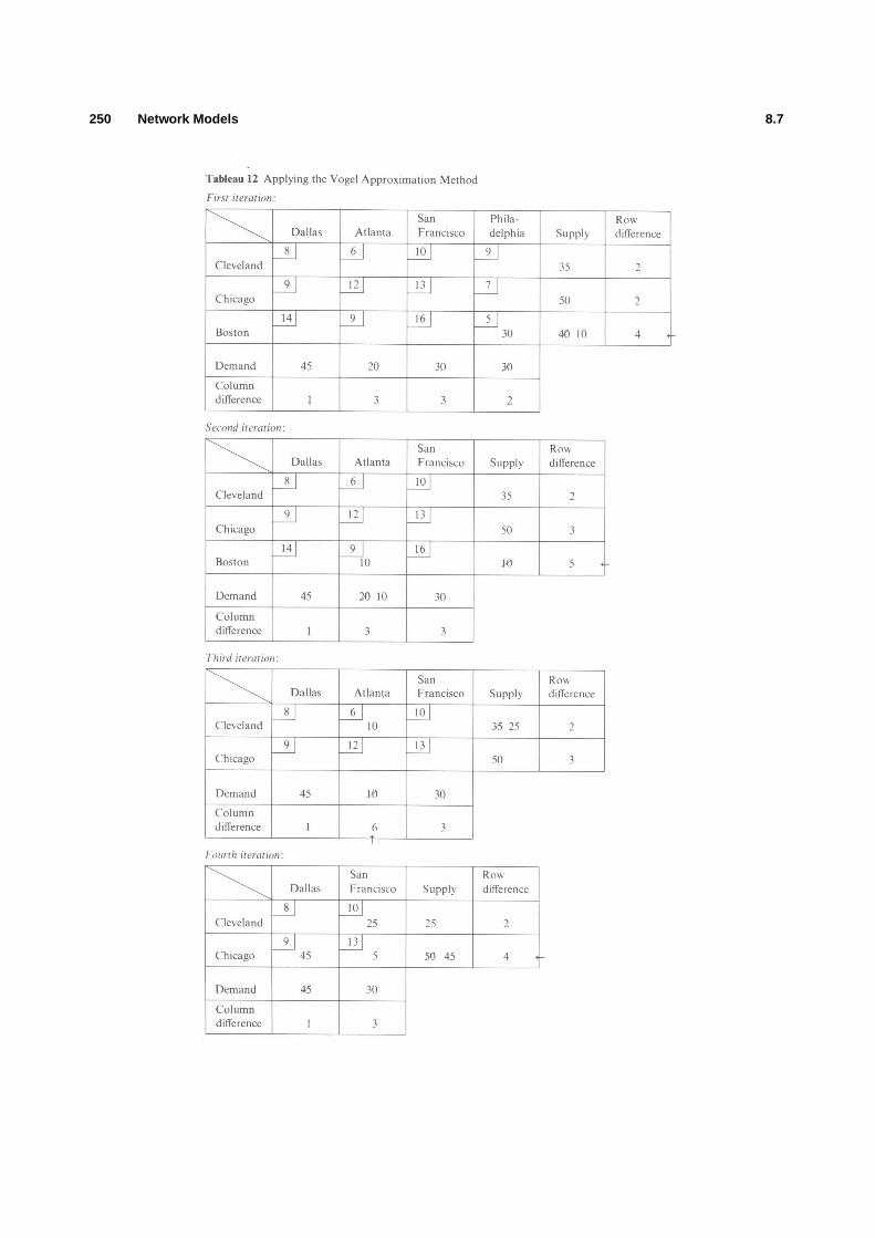
250 Network Models 8.7

8.7 The Simplex Method for Networks 251
8.7 THE SIMPLEX METHOD FOR NETWORKS
The application of the simplex method to the transportation problem presented in the previous section takesadvantage of the network structure of the problem and illustrates a number of properties that extend to thegeneral minimum-cost flow problem. All of the models formulated in Section 8.2 are examples of the generalminimum-cost flow problem, althougha number, including the transportation problem, exhibit further special structure of their own. Historically,many different algorithms have been developed for each of these models; but, rather than consider each modelseparately, we will develop the essential step underlying the efficiency of all of the simplex-based algorithmsfor networks.
We already have seen that, for the transportation problem, a basis corresponds to a spanning tree, andthat introducing a new variable into the basis adds an arc to the spanning tree that forms a unique loop. Thevariable to be dropped from the basis is then determined by finding which variable in the loop drops to zerofirst when flow is increased on the new arc. It is this property, that bases correspond to spanning trees, thatextends to the general minimum-cost flow problem and makes solution by the simplex method very efficient.
In what follows, network interpretations of the steps of the simplex method will be emphasized; there-fore, it is convenient todefine some of the network concepts that will be used. Though these concepts arequite intuitive, the reader should be cautioned that the terminology of network flow models has not beenstandardized, and that definitions vary from one author to another.
Formally, anetworkis defined to be any finite collection of points, called nodes, together with a collectionof directed arcs that connect particular pairs of these nodes. By convention, we do not allow an arc to connecta node to itself, but we do allow more than one arc to connect the same two nodes. We will be concernedonly with connectednetworks in the sense thateverynode can be reached from every other node by followinga sequence of arcs, where the direction of the arcs is ignored. In linear programming, if a network isdisconnected, then the problem it describes can be treated as separate problems, one for each connectedsubnetwork.
A loop is a sequence of arcs, where the direction of the arcs is ignored, connecting a particular node toitself. In Fig. 8.1, the node sequences 3–4–5–3 and 1–2–3–1 are both examples of loops.
A spanning treeis a connected subset of a network including all nodes and containing no loops. Figure8.7 shows two examples of spanning trees for the minimum-cost flow problem of Fig. 8.1.
It is the concept of a spanning tree, which proved most useful in solving the transportation problem in theprevious section, that will be the foundation of the algorithm for the general minimum-cost flow problem.
Finally, anendis a node of a network with exactly one arc incident to it. In the first example of Fig. 8.7,nodes 1,2, and 4 are ends, and in the second examples, nodes 1, 2, and 5 are ends. It is easy to see that everytree must have at least two ends. If you start with any nodei in a tree and follow any arc away from it, youeventually come to an end, since the tree contains no loops. If nodei is an end, then you have two ends. Ifnodei is not an end, there is another arc from nodei that will lead to a second end, since again there are noloops in the tree.
In the transportation problem we saw that there are(m + n − 1) basic variables, since any one of theequations is redundant under the assumption that the sum of the supplies equals the sum of the demands. Thisimplies that the number of arcs in any spanning tree corresponding to a basis in the transportation problem is
Figure 8.14 Examples of spanning trees.

252 Network Models 8.7
Tableau E8.13 Tree Variables
x13 x25 x34 x35 Righthand side
1 20
1 0
−1 1 1 0
−1 −5−1 −1 −15
alwaysone less thanthe number of nodes in the network. Note that the number of arcs is one less than thenumber of nodes in each of the trees shown in Fig. 8.14, since they each contain 5 nodes and 4 arcs. In fact,this characterization of spanning trees holds for the general minimum-cost flow problem.
Spanning-Tree Characterization. A subnetwork of anetwork withn nodes is a spanning tree if andonly if it is connected and contains(n− 1) arcs.
We can briefly sketch an inductive proof to show the spanning-tree characterization. The result is clearlytrue for the two node networks containing one arc. First, we show that is a subnetwork of ann-node networkis a spanning tree, it contains(n− 1) arcs. Remove any end and incident arc from then-node network. Thereduced network with(n− 1) nodes is still a tree, and by our inductive assumption it must have(n− 2) arcs.Therefore, the original network withn nodes must have had(n− 1) arcs. Next, we show that if ann-nodeconnected subnetwork has(n − 1) arcs and no loops, it is a spanning tree. Again, remove any end and itsincident arc from then-node network. The reduced network is connected, has(n− 1) nodes,(n− 2) arcs,and no loops; and by our inductive assumption, it must be a spanning tree. Therefore, the original networkwith n nodes and(n− 1) arcs must be a spanning tree.
The importance of the spanning-tree characterization stems from the relationship between a spanningtree and a basis in the simplex method. We have already seen that a basis for the transportation problemcorresponds to a spanning tree, and it is this property that carries over to the general network-flow model.
Spanning-Tree Property of Network Bases. In a general minimum-cost flow model, a spanningtree for the network corresponds to a basis for the simplex method.
This is an important property since, together with the spanning-tree characterization, it implies that thenumber of basic variables is always one less than the number of nodes in a general network-flow problem. Nowlet us intuitively argue that the spanning-tree property holds, first by showing that the variables correspondingto a spanning tree constitute a basis, and second by showing that a set of basic variables constitutes a spanningtree.
First, assume that we have a network withn nodes, which is a spanning tree. In order to show that thevariables corresponding to the arcs in the tree constitute a basis, it is sufficient to show that the(n − 1) treevariables are uniquely determined. In the simplex method, this corresponds to setting the nonbasic variablesto specific values and uniquely determining the basic variables. First, set the flows on all arcs not in the treeto either their upper or lower bounds, and update the righthand-side values by their flows. Then choose anynode corresponding to an end in the subnetwork, say nodek. (There must be at least two ends in the spanningtree since it contains no loops.) Nodek corresponds to a row in the linear-programming tableau for the treewith exactly one nonzero coefficient in it. To illustrate this the tree variables of the first example in Fig. 8.14are given in Tableau 13.
Since there is only one nonzero coefficient in rowk, the corresponding arc incident to nodek must haveflow across it equal to the righthand-side value for that row. In the example above,x13 = 20. Now, drop nodek from further consideration and bring the determined variable over to the righthand side, so that the righthandside of the third constraint becomes+20. Now we have an(n − 1)-node subnetwork with(n − 2) arcs andno loops. Hence, we have a tree for the reduced network, and the process may be repeated. At each iteration

8.7 The Simplex Method for Networks 253
exactly one flow variable is determined. On the last iteration, there are two equations corresponding to twonodes, and one arc joining them. Since we have assumed that the total net flow into or out of the network iszero, the last tree variable will satisfy the last two equations. Hence we have shown that a spanning tree in anetwork corresponds to a basis in the simplex method. Further, since we have already shown that a tree for aconnected network withn nodes contains(n− 1) arcs, we have shown that the number of basic variables fora connected network-flow problem is(n− 1).
Now assume that we have a network withn nodes and that we know the(n − 1) basic variables. Toshow that these variables correspond to a tree, we need only show that the subnetwork corresponding to thebasic variables does not contain any loops. We establish this property by assuming that thereis a loop andshowing that this leads to a contradiction. In Fig. 8.15, we have a four-arc network containing a loop and itsassociated tableau.
Figure 8.15 Network containing a loop.
If there exists a loop, then choose weights for the column corresponding to arcs in the loop such that theweight is+1 for a forward arc in the loop and−1 for a backward arc in the loop. If we then add the columnscorresponding to the loop weighted in this manner, we produce a column containing all zeros. In Fig. 8.15,the loop is 2–5–3–2, and adding the columns for the variablesx25, x53, andx32 with weights 1,−1, and−1, respectively, produces a zero column. This implies that the columns corresponding to the loop are notindependent. Since a basis consists of a set of(n− 1) independent columns, any set of variables containinga loop cannot be a basis. Therefore,(n− 1) variables corresponding to a basis in the simplex method mustbe a spanning tree for the network.
If a basis in the simplex method corresponds to a tree, what, then, is the interpretation of introducing anew variable into the basis? Introducing a new variable into the basis adds an arc to the tree, and since everynode of the tree is connected to every other node by a sequence of arcs, the addition will form a loop in thesubnetwork corresponding to the tree. In Fig. 8.16, arc 4–5 is being introduced into the tree, forming the loop4–5–3–4. It is easy to argue that adding an arc to a tree creates auniqueloop in the augmented network.Atleast one loopmust be created, since adding the arc connects two nodes that were already connected. Further,no more than one loopis created, since, if adding the one arc created more than one loop, the entering arcwould have to be common to two distinct loops, which, upon removal of their common arcs, would yield asingle loop that was part of the original network.
Figure 8.16 Introducing a new arc in a tree.

254 Network Models 8.7
To complete a basis change in the simplex method, one of the variables currently in the basis must bedropped. It is clear that the variable to be dropped must correspond to one of the arcs in the loop, since droppingany arc not in the loop would leave the loop in the network and hence would not restore the spanning-treeproperty. We must then be able to determine the arcs that form the loop.
This is accomplished easily by starting with the subnetwork including the loop and eliminating all endsin this network. If the reduced network has no ends,it must be the loop. Otherwise, repeat the process ofeliminating all the ends in the reduced network, and continue. Since there is a unique loop created by addingan arc to a spanning tree, dropping any arc in that loop will create a new spanning tree, since each node will beconnected to every other node by a sequence of arcs, and the resulting network will contain no loops. Figure8.16 illustrates this process by dropping arc 3–5. Clearly, any arc in the loop could have been dropped, toproduce alternative trees.
In the transportation problem, the unique loop was determined easily, although we did not explicitly showhow this could be guaranteed. Once the loop is determined, we increased the flow on the incoming arc andadjusted the flows on the other arcs in the loop, until the flow in one of the arcs in the loop was reduced to zero.The variable corresponding to the arc whose flow was reduced to zero was then dropped out of the basis. Thisis essentially the same procedure that will be employed by the general minimum-cost flow problem, exceptthat the special rules of the simplex method with upper and lower bounds on the variables will be employed.In the next section an example is carried out that applies the simplex method to the general minimum-costflow problem.
Finally, we should comment on the integrality property of the general minimum-cost flow problem. Wesaw that, for the transportation problem, since the basis corresponds to a spanning tree, as long as the suppliesand demands are integers, the flows on the arcs for a basic solution are integers. This is also true for thegeneral minimum-cost flow problem, so long as the net flows at any node are integers and the upper and lowerbounds on the variables are integers.
Integrality Property. In the general minimum-cost flow problem, assuming that the upper and lowerbounds on the variables are integers and the righthand-side values for the flow-balance equations areintegers, the values of the basic variables are also integers when the nonbasic variables are set to theirupper or lower bounds.
In the simplex method with upper and lower bounds on the variables, the nonbasic variables are at eithertheir upper orlower bound. If these bounds are integers, then the net flows at all nodes, when the flowson the nonbasic arcs are included, are also integers. Hence, the flows on the arcs corresponding to thebasic variables also will be integers, since these flows are determined by first considering all ends in thecorresponding spanning tree and assigning a flow to the incident arc equal to the net flow at the node. Theseassigned flows must clearly be integers. The ends and the arcs incident to them are then eliminated, and theprocess is repeated, yielding an integer assignment of flows to the arcs in the reduced tree at each stage.
Tableau E8.14 Basis variables
x13 x25 x34 x35 Righthand sideRow no.
1 20 1
1 0 2
−1 1 1 0 3
−1 −5 4
−1 −1 −15 5
The integrality property of the general minimum-cost flow problem was established easily by using thefact that a basis corresponds to a spanning tree. Essentially, all ends could be immediately evaluated, theneliminated, and the procedure repeated. We were able to solve a system of equations by recognizing that atleast one variable in the system could be evaluated by inspection at each stage, since at each stage at least
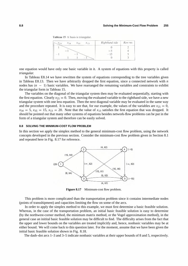
8.8 Solving the Minimum-Cost Flow Problem 255
one equation would have only one basic variable in it. A system of equations with this property is calledtriangular.
In Tableau E8.14 we have rewritten the system of equations corresponding to the tree variables givenin Tableau E8.13. Then we have arbitrarily dropped the first equation, since a connected network withnnodes has(n − 1) basic variables. We have rearranged the remaining variables and constraints to exhibitthe triangular form in Tableau 15.
The variables on the diagonal of the triangular system then may be evaluated sequentially, starting withthe first equation. Clearlyx25 = 0. Then, moving the evaluated variable to the righthand side, we have a newtriangular system with one less equation. Then the next diagonal variable may be evaluated in the same wayand the procedure repeated. It is easy to see that, for our example, the values of the variables arex25 = 0,x34 = 5, x35 = 15, x13 = 20. Note that the value ofx13 satisfies the first equation that was dropped. Itshould be pointed out that many other systems of equations besides network-flow problems can be put in theform of a triangular system and therefore can be easily solved.
8.8 SOLVING THE MINIMUM-COST FLOW PROBLEM
In this section we apply the simplex method to the general minimum-cost flow problem, using the networkconcepts developed in the previous section. Consider the minimum-cost flow problem given in Section 8.1and repeated here in Fig. 8.17 for reference.
Figure 8.17 Minimum-cost flow problem.
This problem is more complicated than the transportation problem since it contains intermediate nodes(points of transshipment) and capacities limiting the flow on some of the arcs.
In order to apply the simplex method to this example, we must first determine a basic feasible solution.Whereas, in the case of the transportation problem, an initial basic feasible solution is easy to determine(by the northwest-corner method, the minimum matrix method, or the Vogel approximation method), in thegeneral case an initital basic feasible solution may be difficult to find. The difficulty arises from the fact thatthe upper and lower bounds on the variables are treated implicitly and, hence, nonbasic variables may be ateither bound. We will come back to this question later. For the moment, assume that we have been given theinitial basic feasible solution shown in Fig. 8.18.
The dash–dot arcs 1–3 and 3–5 indicate nonbasic variables at their upper bounds of 8 and 5, respectively.

256 Network Models 8.8
Figure 8.18 Initial basic feasible solution.
The arcs not shown are nonbasic at their lower bounds of zero. The solid arcs form a spanning tree for thenetwork and constitute a basis for the problem.
To detemine whether this initial basic feasible solution is optimal, we must compute the reduced costsof all nonbasic arcs. To do this, we first determine multipliersyi (i = 1, 2, . . . , n) and, if these multiplierssatisfy:
ci j = ci j − yi + y j ≥ 0 if xi j = `i j ,
ci j = ci j − yi + y j = 0 if `i j < xi j < ui j ,
ci j = ci j − yi + y j ≤ 0 if xi j = ui j ,
then we have an optimal solution. Since the network-flow problem contains a redundant constraint, any onemultiplier may be chosen arbitrarily, as was indicated in previous sections. Supposey2 = 0 is set arbitrarily;the remaining multipliers are determined from the equations:
ci j − yi + y j = 0
for basic variables. The resulting multipliers for the initial basis are given as node labels in Fig. 8.19. Thesewere determined from the cost data given in Fig. 8.17.
Figure 8.19 Iteration 1.
Given these multipliers, we can compute the reduced costs of the nonbasis variables byci j = ci j −yi+y j .The reduced costs are determined by using the given cost data in Fig. 8.17 as:
c13 = 4− 4+ (−1) = −1,
c23 = 2− 0+ (−1) = 1,
c35 = 3− (−1)+ (−6) = −2,
c45 = 2− (−2)+ (−6) = −2,←
c53 = 1− (−6)+ (−1) = 6.
In the simplex method with bounded variables, the nonbasic variables are at either their upper or lowerbounds. An improved solution can be found by either:

8.8 Solving the Minimum-Cost Flow Problem 257
1. increasing a variable that has a negative reduced cost and is currently at its lower bound; or2. decreasing a variable that has a positive reduced cost and is currently at its upper bound.
In this case, the only promising candidate isx45, since the other two negative reduced costs correspond tononbasic variables at their upper bounds. In Fig. 8.19 we have added the arc 4–5 to the network, forming theunique loop 4–5–2–4 with the basic variables. If the flow on arc 4–5 is increased byθ , the remaining arcs inthe loop must be appropriately adjusted. The limit on how far we can increaseθ is given by arc 2–4, whichhas an upper bound of 4. Hence,θ = 2 andx24 becomes nonbasic at its upper bound. The correspondingbasic feasible solution is given in Fig. 8.20, ignoring the dashed arc 2–3.
Figure 8.20 Iteration 2.
The new multipliers are computed as before and are indicated as node labels in Fig. 8.20. Note that notall of the multipliers have to be recalculated. Those multipliers corresponding to nodes that are connected tonode 2 by the same sequence of arcs as before will not change labels. The reduced costs for the new basisare then:
c13 = 4− 4+ (−3) = −3,
c23 = 2− 0+ (−3) = −1,←
c24 = 2− 0+ (−4) = −2,
c35 = 3− (−3)+ (−6) = 0,
c53 = 1− (−6)+ (−3) = 4.
Again there is only one promising candidate,x23, since the other two negative reduced costs correspondto nonbasic variables at their upper bounds. In Fig. 8.20 we have added the arc 2–3 to the network, formingthe unique loop 2–3–4–5–2 with the basic variables. If we increase the flow on arc 2–3 byθ and adjust theflows on the remaining arcs in the loop to maintain feasibility, the increase inθ is limited by arc 2–5. Whenθ = 8, the flow on arc 2–5 is reduced to zero andx25 becomes nonbasic at its lower bound. Figure 8.21shows the corresponding basic feasible solution.
The new multipliers are computed as before and are indicated as node labels in Fig. 8.8. The reducedcosts for the new basis are then:
c13 = 4− 4+ (−2) = −2,
c24 = 2− 0+ (−3) = −1,
c25 = 6− 0+ (−5) = 1,
c35 = 3− (−2)+ (−5) = 0,
c53 = 1− (−5)+ (−2) = 4.

258 Network Models
Figure 8.21 Optimal solution.
This is an optimal solution, since all negative reduced costs correspond to nonbasic variables at their upperbounds and all positive reduced costs correspond to nonbasic variables at their lower bounds.
The reduced costc35 = 0 indicates that alternative optimal solutions may exist. In fact, it is easily verifiedthat the solution given in Fig. 8.22 is an alternative optimal solution.
Figure 8.22 Alternative optimal solution.
Hence, given an initial basic feasible solution, it is straightforward to use the concepts developed inthe previous section to apply the simplex method to the general minimum-cost flow problem. There aretwo essential points to recognize: (1) a basis for the simplex method corresponds to a spanning tree for thenetwork, and (2) introducing a new variable into the basis forms a unique loop in the spanning tree, and thevariable that drops from the basis is the limiting variable in this loop.
Finally, we must briefly discuss how to find an initial basic feasible solution if one is not readily available.There are a number of good heuristics for doing this, depending on the particular problem, but almost all ofthese procedures involve adding some artificial arcs at some point. It is always possible to add uncapacitatedarcs from the points of supply to the points of demand in such a fashion that a basis is formed. In ourillustrative example, we could have simply added the artificial arcs 1–4 and 1–5 and had the initial basis givenin Fig. 8.23.
Then either a phase I procedure is performed, minimizing the sum of the flows on the artificial arcs, ora very high cost is attached to the artificial arcs to drive them out of the basis. Any heuristic procedure forfinding an initial basis usually attempts to keep the number of artificial arcs that have to be added as small aspossible.
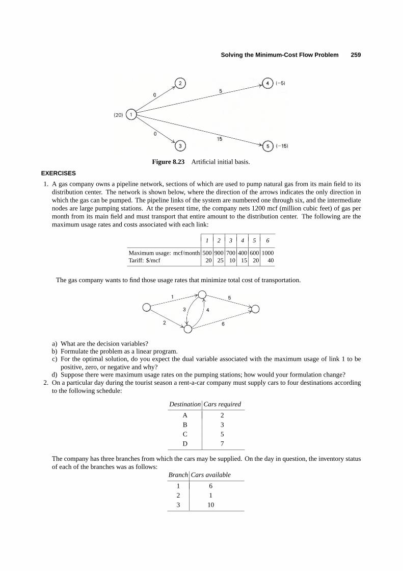
Solving the Minimum-Cost Flow Problem 259
Figure 8.23 Artificial initial basis.
EXERCISES
1. A gas company owns a pipeline network, sections of which are used to pump natural gas from its main field to itsdistribution center. The network is shown below, where the direction of the arrows indicates the only direction inwhich the gas can be pumped. The pipeline links of the system are numbered one through six, and the intermediatenodes are large pumping stations. At the present time, the company nets 1200 mcf (million cubic feet) of gas permonth from its main field and must transport that entire amount to the distribution center. The following are themaximum usage rates and costs associated with each link:
1 2 3 4 5 6
Maximum usage: mcf/month500 900 700 400 600 1000Tariff: $/mcf 20 25 10 15 20 40
The gas company wants to find those usage rates that minimize total cost of transportation.
a) What are the decision variables?b) Formulate the problem as a linear program.c) For the optimal solution, do you expect the dual variable associated with the maximum usage of link 1 to be
positive, zero, or negative and why?d) Suppose there were maximum usage rates on the pumping stations; how would your formulation change?
2. On a particular day during the tourist season a rent-a-car company must supply cars to four destinations accordingto the following schedule:
DestinationCars required
A 2
B 3
C 5
D 7
The company has three branches from which the cars may be supplied. On the day in question, the inventory statusof each of the branches was as follows:
Branch Cars available
1 6
2 1
3 10
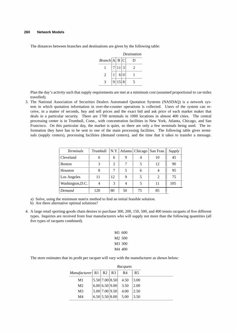
260 Network Models
The distances between branches and destinations are given by the following table:
Destination
Branch A B C D
1 7 11 3 2
2 1 6 0 1
3 9 15 8 5
Plan the day’s activity such that supply requirements are met at a minimum cost (assumed proportional to car-milestravelled).
3. The National Association of Securities Dealers Automated Quotation Systems (NASDAQ) is a network sys-tem in which quotation information in over-the-counter operations is collected. Users of the system can re-ceive, in a matter of seconds, buy and sell prices and the exact bid and ask price of each market maker thatdeals in a particular security. There are 1700 terminals in 1000 locations in almost 400 cities. The centralprocessing center is in Trumbull, Conn., with concentration facilities in New York, Atlanta, Chicago, and SanFrancisco. On this particular day, the market is quiet, so there are only a few terminals being used. The in-formation they have has to be sent to one of the main processing facilities. The following table gives termi-nals (supply centers), processing facilities (demand centers), and the time that it takes to transfer a message.
Terminals Trumbull N.Y. Atlanta Chicago San Fran. Supply
Cleveland 6 6 9 4 10 45
Boston 3 2 7 5 12 90
Houston 8 7 5 6 4 95
Los Angeles 11 12 9 5 2 75
Washington,D.C. 4 3 4 5 11 105
Demand 120 80 50 75 85
a) Solve, using the minimum matrix method to find an initial feasible solution.b) Are there alternative optimal solutions?
4. A large retail sporting-goods chain desires to purchase 300, 200, 150, 500, and 400 tennis racquets of five differenttypes. Inquiries are received from four manufacturers who will supply not more than the following quantities (allfive types of racquets combined).
M1 600
M2 500
M3 300
M4 400
The store estimates that its profit per racquet will vary with the manufacturer as shown below:
Racquets
Manufacturer R1 R2 R3 R4 R5
M1 5.50 7.00 8.50 4.50 3.00
M2 6.00 6.50 9.00 3.50 2.00
M3 5.00 7.00 9.50 4.00 2.50
M4 6.50 5.50 8.00 5.00 3.50
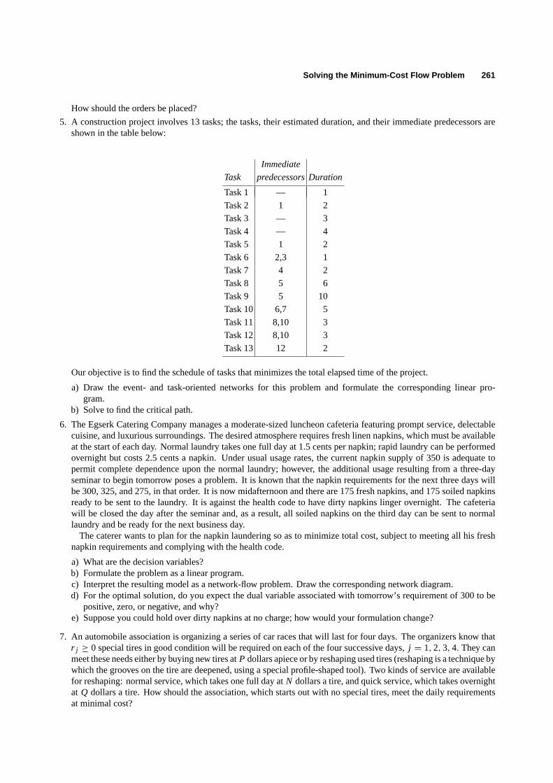
Solving the Minimum-Cost Flow Problem 261
How should the orders be placed?
5. A construction project involves 13 tasks; the tasks, their estimated duration, and their immediate predecessors areshown in the table below:
Immediate
Task predecessorsDuration
Task 1 — 1
Task 2 1 2
Task 3 — 3
Task 4 — 4
Task 5 1 2
Task 6 2,3 1
Task 7 4 2
Task 8 5 6
Task 9 5 10
Task 10 6,7 5
Task 11 8,10 3
Task 12 8,10 3
Task 13 12 2
Our objective is to find the schedule of tasks that minimizes the total elapsed time of the project.
a) Draw the event- and task-oriented networks for this problem and formulate the corresponding linear pro-gram.
b) Solve to find the critical path.
6. The Egserk Catering Company manages a moderate-sized luncheon cafeteria featuring prompt service, delectablecuisine, and luxurious surroundings. The desired atmosphere requires fresh linen napkins, which must be availableat the start of each day. Normal laundry takes one full day at 1.5 cents per napkin; rapid laundry can be performedovernight but costs 2.5 cents a napkin. Under usual usage rates, the current napkin supply of 350 is adequate topermit complete dependence upon the normal laundry; however, the additional usage resulting from a three-dayseminar to begin tomorrow poses a problem. It is known that the napkin requirements for the next three days willbe 300, 325, and 275, in that order. It is now midafternoon and there are 175 fresh napkins, and 175 soiled napkinsready to be sent to the laundry. It is against the health code to have dirty napkins linger overnight. The cafeteriawill be closed the day after the seminar and, as a result, all soiled napkins on the third day can be sent to normallaundry and be ready for the next business day.
The caterer wants to plan for the napkin laundering so as to minimize total cost, subject to meeting all his freshnapkin requirements and complying with the health code.
a) What are the decision variables?b) Formulate the problem as a linear program.c) Interpret the resulting model as a network-flow problem. Draw the corresponding network diagram.d) For the optimal solution, do you expect the dual variable associated with tomorrow’s requirement of 300 to be
positive, zero, or negative, and why?e) Suppose you could hold over dirty napkins at no charge; how would your formulation change?
7. An automobile association is organizing a series of car races that will last for four days. The organizers know thatr j ≥ 0 special tires in good condition will be required on each of the four successive days,j = 1, 2, 3, 4. They canmeet these needs either by buying new tires atP dollars apiece or by reshaping used tires (reshaping is a technique bywhich the grooves on the tire are deepened, using a special profile-shaped tool). Two kinds of service are availablefor reshaping: normal service, which takes one full day atN dollars a tire, and quick service, which takes overnightat Q dollars a tire. How should the association, which starts out with no special tires, meet the daily requirementsat minimal cost?

262 Network Models
a) Formulate a mathematical model for the above problem. Does it exhibit the characteristics of a network prob-lem? Why? (Hint. Take into account the fact that, at the end of dayj , some used tires may not be sent toreshaping.)
b) If the answer to (a) isno, how can the formulation be manipulated to become a network problem? Draw theassociated network. (Hint. Add a redundant constraint introducing a fictitious node.)
c) Assume that a tire may be reshaped only once. How does the above model change? Will it still be networkproblem?
8. Conway Tractor Company has three plants located in Chicago, Austin (Texas), and Salem (Oregon). Three cus-tomers located respectively in Tucson (Arizona), Sacramento (California), and Charlestown (West Virginia) haveplaced additional orders with Conway Tractor Company for 10, 8, and 10 tractors, respectively. It is customary forConway Tractor Company to quote to customers a price on adeliveredbasis, and hence the company absorbs thedelivery costs of the tractors. The manufacturing cost does not differ significantly from one plant to another, andthe following tableau shows the delivery costs incurred by the firm.
Destination
Plant TucsonSacramentoCharlestown
Chicago 150 200 70
Austin 70 120 80
Salem 80 50 170
The firm is now facing the problem of assigning the extra orders to its plants to minimize delivery costs andto meet all orders (The Company, over the years, has established a policy of first-class service, and this includesquick and reliable delivery of all goods ordered). In making the assignment, the company has to take into accountthe limited additional manufacturing capacity at its plants in Austin and Salem, of 8 and 10 tractors, respectively.There are no limits on the additional production capacity at Chicago (as far as these extra orders are concerned).
a) Formulate as a transportation problem.b) Solve completely.
9. A manufacturer of electronic calculators produces its goods in Dallas, Chicago, and Boston, and maintains regionalwarehousing distribution centers in Philadelphia, Atlanta, Cleveland, and Washington, D.C. The company’s staffhas determined that shipping costs are directly proportional to the distances from factory to storage center, as listedhere.
Warehouses
Mileage from: Philadelphia Atlanta Cleveland Washington
Boston 300 1000 500 400
Chicago 500 900 300 600
Dallas 1300 1000 1100 1200
The cost per calculator-mile is $0.0002 and supplies and demands are:
Supply Demand
Boston 1500Philadelphia 2000
Chicago 2500Atlanta 1600
Dallas 4000Cleveland 1200
Washington 3200
a) Use the Vogel approximation method to arrive at an initial feasible solution.b) Show that the feasible solution determined in (a) is optimal.

Solving the Minimum-Cost Flow Problem 263
c) Why does the Vogel approximation method perform so well, compared to other methods of finding an initialfeasible solution?
10. Colonel Cutlass, having just taken command of the brigade, has decided to assign men to his staff based on previousexperience. His list of major staff positions to be filled is adjutant (personnel officer), intelligence officer, operationsofficer, supply officer, and training officer. He has five men he feels could occupy these five positions. Below aretheir years of experience in the several fields.
Adjutant Intelligence Operations Supply Training
Major Muddle 3 5 6 2 2
Major Whiteside 2 3 5 3 2
Captain Kid 3 — 4 2 2
Captain Klutch 3 — 3 2 2
Lt. Whiz — 3 — 1 —
Who, based on experience, should be placed in which positions to give the greatest total years of experience for alljobs? (Hint. A basis, even if degenerate, is a spanning tree.)
11. Consider the following linear program:Minimize z= 3x12+ 2x13+ 5x14+ 2x41+ x23+ 2x24+ 6x42+ 4x34+ 4x43,
subject to:
x12 + x13 + x14 − x41 ≤ 8,
x12 − x23 − x24 + x42 ≥ 4,
x34 − x13 − x23 − x43 ≤ 4,
x14 + x34 + x24 − x42 − x42 − x43 ≥ 5,
all xi j ≥ 0.
a) Show that this is a network problem, stating it in general minimum-cost flow form. Draw the associated networkand give an interpretation to the flow in this network.
b) Find an initial feasible solution. (Hint. Exploit the triangular property of the basis.)c) Show that your initial solution is a spanning tree.d) Solve completely.
12. A lot of three identical items is to be sequenced through three machines. Each item must be processed first onmachine 1, then on machine 2, and finally on machine 3. It takes 20 minutes to process one item on machine 1, 12minutes on machine 2, and 25 minutes on machine 3. The objective is to minimize the total work span to completeall the items.
a) Write a linear program to achieve our objective. (Hint. Let xi j be the starting time of processing itemi onmachinej . Two items may not occupy the same machine at the same time; also, an item may be processed onmachine( j + 1) only after it has been completed on machinej .)
b) Cast the model above as a network problem. Draw the associated network and give an interpretation in terms offlow in networks. (Hint. Formulate and interpret the dual problem of the linear program obtained in (a).)
c) Find an initial feasible solution; solve completely.13. A manufacturer of small electronic calculators is working on setting up his production plans for the next six months.
One product is particularly puzzling to him. The orders on hand for the coming season are:
Month Orders
January 100
February 150
March 200
April 100
May 200
June 150

264 Network Models
The product will be discontinued after satisfying the June demand. Therefore, there is no need to keep any inventoryafter June. The production cost, using regular manpower, is $10 per unit. Producing the calculator on overtime costsan additional $2 per unit. The inventory-carrying cost is $0.50 per unit per month. If the regular shift productionis limited to 100 units per month and overtime production is limited to an additional 75 units per month, whatis the optimal production schedule? (Hint. Treat regular and overtime capacities as sources of supply for eachmonth.)
14. Ships are available at three ports of origin and need to be sent to four ports of destination. The number of shipsavailable at each origin, the number required at each destination, and the sailing times are given in the tableau below.Our objective is to minimize the total number of sailing days.
a) Find an initial basic feasible solution.b) Show that your initial basis is a spanning tree.c) Find an initial basic feasible solution using the other two methods presented in the text. Solve completely, starting
from the three initial solutions found in parts (a) and (c). Compare how close these solutions were to the optimalone.
d) Which of the dual variables may be chosen arbitrarily, and why?e) Give an economic interpretation of the optimal simplex multipliers associated with the origins and destinations.
15. A distributing company has two major customers and three supply sources. The corresponding unit from eachsupply center to each customer is given in the following table, together with the total customer requirements andsupply availabilities.
CustomerAvailable
Supply center1 2 supplies
1 −1 3 300
2 1 6 400
3 1 5 900
Customer
requirements800 500
Note that Customer 1 has strong preferences for Supplier 1 AND will be willing not only to absorb all the trans-portation costs but also to pay a premium price of $1 per unit of product coming from Supplier 1.
a) The top management of the distributing company feels it is obvious that Supply Center 1 should send all itsavailable products to Customer 1. Is this necessarily so? (Hint. Obtain the least-cost solution to the problem.Explore whether alternative optimal solutions exist where not all the 300 units available in Supply Center 1 areassigned to Customer 1.)
b) Assume Customer 2 is located in an area where all shipments will be subject to taxes defined as a percentage ofthe unit cost of a product. Will this tax affect the optimal solution of part (a)?
c) Ignore part (b). What will be the optimal solution to the original problem if Supply Center 1 increases its productavailability from 300 units to 400 units?
16. After solving a transportation problem with positive shipping costsci j along all arcs, we increase the supply atone source and the requirement at one destination in a manner that will maintain equality of total supply and totaldemand.

Solving the Minimum-Cost Flow Problem 265
a) Would you expect the shipping cost in the modified problem with a larger total shipment of goods to be higherthan the optimal shipping plan from the original problem?
b) Solve the following transportation problem:
Unit shipping costs to destinations
Source D1 D2 D3 Supplies
S1 4 2 4 15
S2 12 8 4 15
Requirements10 10 10
c) Increase the supply at source S1 by 1 unit and the demand at demand centerD3 by 1 unit, and re-solve theproblem. Has the cost of the optimal shipping plan decreased? Explain this behavior.
17. Consider a very elementary transportation problem with only two origins and two destinations. The supplies,demands, and shipping costs per unit are given in the following tableau.
Since the total number of units supplied equals the total number of units demanded, the problem may be formulatedwith equality constraints. An optimal solution to the problem is:
x11 = 20, x12 = 0, x21 = 30, x22 = 50;
and a corresponding set of shadow prices on the nodes is:ys1 = 4, ys2 = 0, yd1 = 1, yd2 = 4.
a) Why is the least expensive route not used?b) Are the optimal values of the decision variables unique?c) Are the optimal values of the shadow prices unique?d) Determine the ranges on the righthand-side values, changed one at a time, for which the basis remains un-
changed.e) What happens when the ranges determined in (d) are exceeded by some small amount?
18. Consider a transportation problem identical to the one given in Exercise 17. One way the model may be formulatedis as a linear program with inequality constraints. The formulation and solution are given below.
For this formulation of the model:

266 Network Models
a) Are the optimal values of the shadow prices unique?b) Determine the ranges on the righthand-side values, changed one at a time, for which the basis remains un-
changed.c) Reconcile the results of (b) with those obtained in Exercise 17.
19. Suppose that there are three suppliersS1, S2, and S3 in a distribution system that can supply 5, 5, and 6 units,respectively, of the company’s good. The distribution system contains five demand centers, that require 2, 2, 4, 4,and 3 units each of the good. The transportation costs, in dollars per unit, are as follows:
a) Compute an optimum shipping schedule. Is the optimal solution unique?b) Find the range over which the cost of transportation fromS1 to D3 can vary while maintaining the optimal basis
found in part (a).c) To investigate the sensitivity of the solution to this problem, we might consider what happens if the amount
supplied from anyonesupplier and the amount demanded by anyonedemand center were both increased. Isit possible for the total shipping costs to decrease by increasing the supply and the demand for any particularchoice of supply and demand centers? Establish a limit on these increases as specific pairs of supply and demandcenters are selected.
d) A landslide has occurred on the route fromS2 to D5. If you bribe the state highway crew with $10, they willclear the slide. If not, the route will remain closed. Should you pay the bribe?
20. An oil company has three oil fields and five refineries. The production and transportation costs from each oil fieldeach refinery, in dollars per barrel, are given in the table below:
Refineries
Oil field R1 R2 R3 R4 R5 Availability
OF1 5 3 3 3 7 4
OF2 5 4 4 2 1 6
OF3 5 4 2 6 2 7
Requirements2 2 3 4 4
The corresponding production capacity of each field and requirements of each refinery, inmillions of barrelsperweek, are also given.
a) What is the optimum weekly production program? Parts (b), (c), and (d) are independent, each giving modifica-tions to part (a).
b) Suppose that field OF1 has workedundercapacity so far, and that its production increases by one unit (i.e.,1 million barrels). What is the new optimal production plan? Has the optimal basis changed? How does theobjective function change? What is the range within which the production of field OF1 may vary?
c) Because of pipeline restrictions, it is impossible to send more than 1 million barrels from OF2 to R5. How wouldyou have formulated the problem if it has been stated in this form from the very beginning? (Hint. DecomposeR5 into two destinations: one with a requirement of one unit (i.e., 1 million barrels), the other with a requirementof three. Prohibit the route from OF2 to the second destination of R5.) Change the optimum solution in (a) tofind the new optimum program.
Solving the Minimum-Cost Flow Problem 267
d) Suppose that fields OF1, OF2, and OF3 have additional overtime capacities of 1, 1, and 1.5 units, respectively(that is, 1, 1, and 1.5 million barrels, respectively). This causes an increase in the corresponding production costsof 0.5, 1.5, and 2 dollars per barrel, respectively. Also assume that the refinery requirements are increased byone million barrels at each refinery and that there is no convenient route to ship oil from field OF2 to refineryR3. What is the optimum program?
21. Consider the following transshipment problem where goods are shipped from two plants to either a warehouse ortwo distribution centers and then on to the two end markets.
The production rates in units per month are 250 and 450 for plants 1 and 2, respectively. The demands of the twomarkets occur at rates 200 and 500 units per month. The costs of shipping one unit over a particular route is shownadjacent to the appropriate arc in the network.
a) Redraw the above transshipment network as a network consisting of only origins and destinations, by replacingall intermediate nodes by two nodes, an origin and destination, connected by an arc, from the destination backto the origin, whose cost is zero.
b) The network in (a) is a transportation problem except that a backwards arc, with flowxi i , from newly createddestinationi to its corresponding newly created source, is required. Convert this to a transportation network bysubstitutingx′i i = B− xi i . How do you choose a value for the constantB?
c) Certain arcs are inadmissible in the original transshipment formulation; how can these be handled in the refor-mulated transportation problem?
d) Interpret the linear-programming tableau of the original transshipment network and that of the reformulatedtransportation network.
e) Can any transshipment problem be transformed into an equivalent transportation problem?
22. Consider the following minimum-cost flow model:
We wish to send eight units from node 1 to node 5 at minimum cost. The numbers next to the arcs indicateupper bounds for the flow on an arc and the cost per unit of flow. The following solution has been proposed, wherethe numbers next to the arcs are flows.
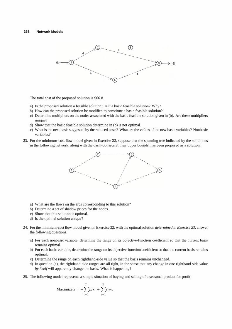
268 Network Models
The total cost of the proposed solution is $66.8.
a) Is the proposed solution a feasible solution? Is it a basic feasible solution? Why?b) How can the proposed solution be modified to constitute a basic feasible solution?c) Determine multipliers on the nodes associated with the basic feasible solution given in (b). Are these multipliers
unique?d) Show that the basic feasible solution determine in (b) is not optimal.e) What is the next basis suggested by the reduced costs? What are thevaluesof the new basic variables? Nonbasic
variables?
23. For the minimum-cost flow model given in Exercise 22, suppose that the spanning tree indicated by the solid linesin the following network, along with the dash–dot arcs at their upper bounds, has been proposed as a solution:
a) What are the flows on the arcs corresponding to this solution?b) Determine a set of shadow prices for the nodes.c) Show that this solution is optimal.d) Is the optimal solution unique?
24. For the minimum-cost flow model given in Exercise 22, with the optimal solutiondetermined in Exercise 23, answerthe following questions.
a) For each nonbasic variable, determine the range on its objective-function coefficient so that the current basisremains optimal.
b) For each basic variable, determine the range on its objective-function coefficient so that the current basis remainsoptimal.
c) Determine the range on each righthand-side value so that the basis remains unchanged.d) In question (c), the righthand-side ranges are all tight, in the sense that any change in one righthand-side value
by itselfwill apparently change the basis. What is happening?
25. The following model represents a simple situation of buying and selling of a seasonal product for profit:
Maximizez= −T∑
t=1
pt xt +
T∑t=1
st yt ,

Solving the Minimum-Cost Flow Problem 269
subject to:
I +t∑
j=1
(x j − yi ) ≤ C (t = 1, 2, . . . , T),
y1 ≤ I ,
y2 ≤ I + (x1− y1),
y3 ≤ I + (x1− y1)+ (x2− y2),
yt ≤ I +t−1∑j=1
(x j − y j ) (t = 4, 5, . . . , T),
xt ≥ 0, yt ≥ 0 for t = 1, 2, . . . , T.
In this formulation, the decision variablesxt andyt denote, respectively, the amount of the product purchased andsold, in time periodt . The given data is:
pt = per unit purchase price in periodt ,st = per unit selling price in periodt ,I = amount of the product on hand initially,
C = capacity for storing the product in any period.
The constraints state (i) that the amount of the product on hand at the end of any period cannot exceed the storagecapacityC, and (ii) that the amount of the product sold at the beginning of periodt cannot exceed its availabilityfrom previous periods.
a) Let
wt = C − I −t∑
j=1
(x j − y j ) and zt = I +t−1∑j=1
(x j − y j )− yt ,
denote slack variables for the constraints (withz1 = I − y1). Show that the given model is equivalent to theformulation on page 363.
b) State the dual to the problem formulation in part (a), lettingui denote the dual variable for the constraint+xi ,andv j denote the dual variable for the constraint containing+y.
c) Into what class of problems does this model fall? Determine the nature of the solution forT = 3.
26. A set of words (for example, ace, bc, dab, dfg, fe) is to be transmitted as messages. We want to investigate the possibil-ity of representing each word by one of the lettersin the wordsuch that the words will be represented uniquely. If sucha representation is possible, we can transmit a single letter instead of a complete word for a message we want to send.
a) Using as few constraints and variables as possible, formulate the possibility of transmitting letters to representwords as the solution to a mathematical program. Is there anything special about the structure of this programthat facilitates discovery of a solution?
b) Suppose that you have a computer code that computes the solution to the following transportation problem:
Minimize z=∑
i
∑j
zi j xi j ,
subject to:
n∑j=1
xi j = ai (i = 1, 2, . . . , n),
m∑i=1
xi j = b j ( j = 1, 2, . . . , m),
xi j ≥ 0 (i = 1, 2, . . . , m; j = 1, 2, . . . , n).
and requires that:

270 Network Models
(i) ai , b j , ci j ≥ 0 and integer (i = 1, 2, . . . , m; j = 1, 2, . . . , n),
(ii)m∑
i=1
ai =
n∑j=1
b j .
Maximizez= −T∑
t=1
pt xt +
T∑t=1
st yt ,
subject to:
x1 − y1 + w1 = C − I ,x2 − y2 − w1 + w2 = 0,
x3 − y3 − w2 + w3 = 0,
. . .. . .
. . ....
xT − yT − wT− 1 + wT = 0,
y1 + z1 = I ,− x1 + y2 − z1 + z2 = 0,
− x2 + y3 − z2 + z3 = 0,
. . .. . .
. . ....
− xT− 1 + yT − zT−1 + zT = 0,
xt ≥ 0, yt ≥ 0, wt ≥ 0, zt ≥ 0 for t = 1, . . . , T.
How would you use this code to solve the problem posed in (a)? Answer the question in general, and use thespecific problem defined above as an illustration.
27. The Defense Communications Agency is responsible for operating and maintaining a world-wide communicationssystem. It thinks of costs as being proportional to the ‘‘message units’’ transmitted in one direction over a particularlink in the system. Hence, under normal operating conditions it faces the following minimum-cost flow problem:
Minimize z=∑
i
∑j
ci j xi j ,
subject to: ∑j
xi j −∑
k
xki = bi (i = 1, 2, . . . , n),
0 ≤ xi j ≤ ui j ,
where
ci j = cost per message unit over link(i − j ).bi = message units generated (or received) at stationi ,ui j = upper bound on number of message units that can be
transmitted over link(i − j ).
Suppose that the agency has been given a budget ofB dollars to spend on increasing the capacity of any link inthe system. The price for increasing capacity on link(i − j ) is pi j .
a) Formulate a linear program (not necessarily a network) with only(n+ 1) constraints, that will minimize operatingcosts subject to this budget constraint. (Hint. You must allow for investing in additional capacity for each link.)
b) How can the ‘‘near’’ network model formulated in (a) be analyzed by network-programming techniques? (Hint.How could parametric programming be used?)
28. The general minimum-cost flow problem is given as follows:
Minimize z=∑
i
∑j
ci j xi j ,

9.8 Solving the Minimum-Cost Flow Problem 271
subject to: ∑j
xi j −∑
k
xki = bi (i = 1, 2, . . . , n),
`i j ≤ xi j ≤ ui j .
a) Assuming that the lower bounds on the variables are all finite, this is,`i j > −∞, show that any problem of thisform can be converted to a transportation problem with lower bounds on the variables of zero and nonnegative,or infinite, upper bounds. (Hint. Refer to Exercise 22.)
b) Comment on the efficiency of solving minimum-cost flow problems by a bounded-variables transportationmethod, versus the simplex method for general networks.
29. One difficulty with solving the general minimum-cost flow problem with upper and lower bounds on the variableslies in determining an initial basic feasible solution. Show that an initial basic feasible solution to this problemcan be determined by solving an appropriate maximum-flow problem. (Hints. (1) Make a variable substitution toeliminate the nonzero lower bounds on the variables. (2) Form a ‘‘super source,’’ connected to all the source nodes,and a ‘‘super sink,’’ connected to all the sink nodes, and maximize the flow from super sink to super source.)
ACKNOWLEDGMENTS
Exercises 1 and 6 are due to Sherwood C. Frey, Jr., of the Harvard Business School.Exercise 6, in turn, is based on ‘‘The Caterer Problem,’’ inFlows in Networksby L. R. Ford and D. R. Fulk-erson, Princeton University Press, 1962. In their 1955 article ‘‘Generalizations of the Warehousing Model,’’from theOperational Research Quarterly, A. Charnes and W. W. Cooper introduced the transformation usedin Exercise 25.

Integer Programming
9
The linear-programming models that have been discussed thus far all have beencontinuous, in the sense thatdecision variables are allowed to be fractional. Often this is a realistic assumption. For instance, we mighteasily produce 10234 gallons of a divisible good such as wine. It also might be reasonable to accept a solutiongiving an hourly production of automobiles at 581
2 if the model were based upon average hourly production,and the production had the interpretation ofproduction rates.
At other times, however, fractional solutions are not realistic, and we must consider the optimizationproblem:
Maximizen∑
j=1
c j x j ,
subject to:n∑
j=1
ai j x j = bi (i = 1, 2, . . . , m),
x j ≥ 0 ( j = 1, 2, . . . , n),
x j integer (for some or allj = 1, 2, . . . , n).
This problem is called the (linear)integer-programming problem. It is said to be amixedinteger programwhen some, but not all, variables are restricted to be integer, and is called apure integer program whenalldecision variables must be integers. As we saw in the preceding chapter, if the constraints are of a networknature, then an integer solution can be obtained by ignoring the integrality restrictions and solving the resultinglinear program. In general, though, variables will be fractional in the linear-programming solution, and furthermeasures must be taken to determine the integer-programming solution.
The purpose of this chapter is twofold. First, we will discuss integer-programming formulations. Thisshould provide insight into the scope of integer-programming applications and give some indication ofwhy many practitioners feel that the integer-programming model is one of the most important models inmanagement science. Second, we consider basic approaches that have been developed for solving integerand mixed-integer programming problems.
9.1 SOME INTEGER-PROGRAMMING MODELS
Integer-programming models arise in practically every area of application of mathematical programming. Todevelop a preliminary appreciation for the importance of these models, we introduce, in this section, threeareas where integer programming has played an important role in supporting managerial decisions. We donot provide the most intricate available formulations in each case, but rather give basic models and suggestpossible extensions.
272

9.1 Some Integer-Programming Models 273
Capital Budgeting In a typical capital-budgeting problem, decisions involve the selection of a number ofpotential investments. The investment decisions might be to choose among possible plant locations, to selecta configuration of capital equipment, or to settle upon a set of research-and-development projects. Often itmakes no sense to consider partial investments in these activities, and so the problem becomes ago–no-gointeger program, where the decision variables are taken to bex j = 0 or 1, indicating that thej th investmentis rejected or accepted. Assuming thatc j is the contribution resulting from thej th investment and thatai j isthe amount of resourcei , such as cash or manpower, used on thej th investment, we can state the problemformally as:
Maximizen∑
j=1
c j x j ,
subject to:n∑
j=1
ai j x j ≤ bi (i = 1, 2, . . . , m),
x j = 0 or 1 ( j = 1, 2, . . . , n).
The objective is to maximize total contribution from all investments without exceeding the limited availabilitybi of any resource.
One important special scenario for the capital-budgeting problem involves cash-flow constraints. In thiscase, the constraints
n∑j=1
ai j xi ≤ bi
reflect incremental cash balance in each period. The coefficientsai j represent the net cash flow from in-vestmentj in period i . If the investment requires additional cash in periodi , thenai j > 0, while if theinvestmentgeneratescash in periodi , thenai j < 0. The righthand-side coefficientsbi represent the incre-mental exogenous cash flows. If additional funds are made available in periodi , thenbi > 0, while if fundsare withdrawn in periodi , thenbi < 0. These constraints state that the funds required for investment mustbe less than or equal to the funds generated from prior investments plus exogenous funds made available (orminusexogenous funds withdrawn).
The capital-budgeting model can be made much richer by including logical considerations. Suppose, forexample, that investment in a new product line is contingent upon previous investment in a new plant. Thiscontingencyis modeled simply by the constraint
x j ≥ xi ,
which states that ifxi = 1 and projecti (new product development) is accepted, then necessarilyx j = 1 andproject j (construction of a new plant) must be accepted. Another example of this nature concerns conflictingprojects. The constraint
x1+ x2+ x3+ x4 ≤ 1,
for example, states that only one of the first four investments can be accepted. Constraints like this commonlyare calledmultiple-choice constraints. By combining these logical constraints, the model can incorporatemany complex interactions between projects, in addition to issues of resource allocation.
The simplest of all capital-budgeting models has just one resource constraint, but has attracted muchattention in the management-science literature. It is stated as:
Maximizen∑
j=1
c j x j ,

274 Integer Programming 9.1
subject to:
n∑j=1
a j x j ≤ b,
x j = 0 or 1 ( j = 1, 2, . . . , n).
Usually, this problem is called the 0–1knapsackproblem, since it is analogous to a situation in which ahiker must decide which goods to include on his trip. Herec j is the ‘‘value’’ or utility of including good j ,which weighsa j > 0 pounds; the objective is to maximize the ‘‘pleasure of the trip,’’ subject to the weightlimitation that the hiker can carry no more thanb pounds. The model is altered somewhat by allowing morethan one unit of any good to be taken, by writingx j ≥ 0 andx j -integer in place of the 0–1 restrictions onthe variables. The knapsack model is important because a number of integer programs can be shown to beequivalent to it, and further, because solution procedures for knapsack models have motivated procedures forsolving general integer programs.
Warehouse Location In modeling distribution systems, decisions must be made about tradeoffs betweentransportation costs and costs for operating distribution centers. As an example, suppose that a manager mustdecide which ofn warehouses to use for meeting the demands ofm customers for a good. The decisions tobe made are which warehouses to operate and how much to ship from any warehouse to any customer. Let
yi =
{1 if warehousei is opened,0 if warehousei is not opened;
xi j = Amount to be sent from warehousei to customerj .
The relevant costs are:fi = Fixed operating cost for warehousei , ifopened (for example, a cost to
lease the warehouse),ci j = Per-unit operating cost at warehousei plus the transportation cost for
shipping from warehousei to customerj .
There are two types of constraints for the model:
i) the demandd j of each customer must be filled from the warehouses; and
ii) goods can be shipped from a warehouse only if it is opened.
The model is:
Minimizem∑
i=1
n∑j=1
ci j xi j +
m∑i=1
fi yi , (1)
subject to:m∑
i=1
xi j = d j ( j = 1, 2, . . . , n), (2)
n∑j=1
xi j − yi
n∑j=1
d j
≤ 0 (i = 1, 2, . . . , m), (3)
xi j ≥ 0 (i = 1, 2, . . . , m; j = 1, 2, . . . , n),
yi = 0 or 1 (i = 1, 2, . . . , m).
9.1 Some Integer-Programming Models 275
The objective function incorporates transportation and variable warehousing costs, in addition to fixedcosts for operating warehouses. The constraints (2) indicate that each customer’s demand must be met. Thesummation over the shipment variablesxi j in thei th constraint of (3) is the amount of the good shipped fromwarehousei . When the warehouse is not opened,yi = 0 and the constraint specifies that nothing can beshipped from the warehouse. On the other hand, when the warehouse is opened andyi = 1, the constraintsimply states that the amount to be shipped from warehousei can be no larger than the total demand, whichis always true. Consequently, constraints (3) imply restriction (ii) as proposed above.
Although oversimplified, this model forms the core for sophisticated and realistic distribution modelsincorporating such features as:1. multi-echelon distribution systems from plant to warehouse to customer;2. capacity constraints on both plant production and warehouse throughput;3. economies of scale in transportation and operating costs;4. service considerations such as maximum distribution time from warehouses to customers;5. multiple products; or6. conditions preventing splitting of orders (in the model above, the demand for any customer can be supplied
from several warehouses).These features can be included in the model by changing it in several ways. For example, warehouse
capacities are incorporated by replacing the term involvingyi in constraint (3) withyi K i , whereK i is thethroughput capacity of warehousei ; multi-echelon distribution may require triple-subscripted variablesxi jkdenoting the amount to be shipped, from planti to customerk through warehousej . Further examples ofhow the simple warehousing model described here can be modified to incorporate the remaining featuresmentioned in this list are given in the exercises at the end of the chapter.
Scheduling The entire class of problems referred to as sequencing, scheduling, and routing are inherentlyinteger programs. Consider, for example, the scheduling of students, faculty, and classrooms in such a waythat the number of students who cannot take their first choice of classes is minimized. There are constraints onthe number and size of classrooms available at any one time, the availability of faculty members at particulartimes, and the preferences of the students for particular schedules. Clearly, then, thei th studentis scheduledfor the j th class during thenth time period ornot; hence, such a variable is either zero or one. Otherexamples of this class of problems include line-balancing, critical-path scheduling with resource constraints,and vehicle dispatching.
As a specific example, consider the scheduling of airline flight personnel. The airline has a number ofrouting ‘‘legs’’ to be flown, such as 10 A.M. New York to Chicago, or 6 P.M.Chicago to Los Angeles. Theairline must schedule its personnel crews on routes to cover these flights. One crew, for example, might bescheduled to fly a route containing the two legs just mentioned. The decision variables, then, specify thescheduling of the crews to routes:
x j =
{1 if a crew is assigned to routej,0 otherwise.
Let
ai j =
{1 if leg i is included on routej,0 otherwise,
andc j = Cost for assigning a crew to routej .
The coefficientsai j define the acceptable combinations of legs and routes, taking into account such charac-teristics as sequencing of legs for making connections between flights and for including in the routes groundtime for maintenance. The model becomes:
Minimizen∑
j=1
c j x j ,

276 Integer Programming 9.1
subject to:
n∑j=1
ai j x j = 1 (i = 1, 2, . . . , m), (4)
x j = 0 or 1 ( j = 1, 2, . . . , n).
The i th constraint requires that one crew must be assigned on a route to fly legi . An alternative formulationpermits a crew to ride as passengers on a leg. Then the constraints (4) become:
n∑j=1
ai j x j ≥ 1 (i = 1, 2, . . . , m). (5)
If, for example,n∑
j=1
a1 j x j = 3,
then two crews fly as passengers on leg 1, possibly to make connections to other legs to which they have beenassigned for duty.
These airline-crew scheduling models arise in many other settings, such as vehicle delivery problems,political districting, and computer data processing. Often model (4) is called aset-partitioning problem, sincethe set of legs will be divided, or partitioned, among the various crews. With constraints (5), it is called aset-covering problem, since the crews then will cover the set of legs.
Another scheduling example is the so-calledtraveling salesman problem. Starting from his home, asalesman wishes to visit each of(n−1) other cities and return home at minimal cost. He must visit each cityexactly once and it costsci j to travel from cityi to city j . What route should he select? If we let
xi j =
{1 if he goes from cityi to city j,0 otherwise,
we may be tempted to formulate his problem as the assignment problem:
Minimizen∑
i=1
n∑j=1
ci j xi j ,
subject to:n∑
i=1
xi j = 1 ( j = 1, 2, . . . , n),
n∑j=1
xi j = 1 (i = 1, 2, . . . , n),
xi j ≥ 0 (i = 1, 2, . . . , n; j = 1, 2, . . . , n).
The constraints require that the salesman must enter and leave each city exactly once. Unfortunately, theassignment model can lead to infeasible solutions. It is possible in a six-city problem, for example, for theassignment solution to route the salesman through two disjoint subtours of the cities instead of on a singletrip or tour. (See Fig. 9.1.)
Consequently, additional constraints must be included in order to eliminate subtour solutions. There area number of ways to accomplish this. In this example, we can avoid the subtour solution of Fig. 9.1 byincluding the constraint:
x14+ x15+ x16+ x24+ x25+ x26+ x34+ x35+ x36 ≥ 1.
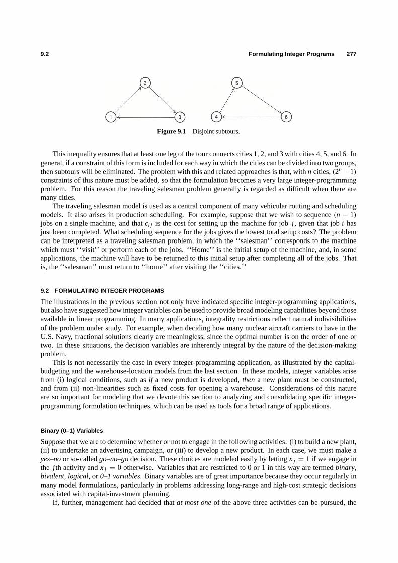
9.2 Formulating Integer Programs 277
Figure 9.1 Disjoint subtours.
This inequality ensures that at least one leg of the tour connects cities 1, 2, and 3 with cities 4, 5, and 6. Ingeneral, if a constraint of this form is included for each way in which the cities can be divided into two groups,then subtours will be eliminated. The problem with this and related approaches is that, withn cities,(2n
−1)
constraints of this nature must be added, so that the formulation becomes a very large integer-programmingproblem. For this reason the traveling salesman problem generally is regarded as difficult when there aremany cities.
The traveling salesman model is used as a central component of many vehicular routing and schedulingmodels. It also arises in production scheduling. For example, suppose that we wish to sequence(n − 1)
jobs on a single machine, and thatci j is the cost for setting up the machine for jobj , given that jobi hasjust been completed. What scheduling sequence for the jobs gives the lowest total setup costs? The problemcan be interpreted as a traveling salesman problem, in which the ‘‘salesman’’ corresponds to the machinewhich must ‘‘visit’’ or perform each of the jobs. ‘‘Home’’ is the initial setup of the machine, and, in someapplications, the machine will have to be returned to this initial setup after completing all of the jobs. Thatis, the ‘‘salesman’’ must return to ‘‘home’’ after visiting the ‘‘cities.’’
9.2 FORMULATING INTEGER PROGRAMS
The illustrations in the previous section not only have indicated specific integer-programming applications,but also have suggested how integer variables can be used to provide broad modeling capabilities beyond thoseavailable in linear programming. In many applications, integrality restrictions reflect natural indivisibilitiesof the problem under study. For example, when deciding how many nuclear aircraft carriers to have in theU.S. Navy, fractional solutions clearly are meaningless, since the optimal number is on the order of one ortwo. In these situations, the decision variables are inherently integral by the nature of the decision-makingproblem.
This is not necessarily the case in every integer-programming application, as illustrated by the capital-budgeting and the warehouse-location models from the last section. In these models, integer variables arisefrom (i) logical conditions, such asif a new product is developed,thena new plant must be constructed,and from (ii) non-linearities such as fixed costs for opening a warehouse. Considerations of this natureare so important for modeling that we devote this section to analyzing and consolidating specific integer-programming formulation techniques, which can be used as tools for a broad range of applications.
Binary (0–1) Variables
Suppose that we are to determine whether or not to engage in the following activities: (i) to build a new plant,(ii) to undertake an advertising campaign, or (iii) to develop a new product. In each case, we must make ayes–noor so-calledgo–no–godecision. These choices are modeled easily by lettingx j = 1 if we engage inthe j th activity andx j = 0 otherwise. Variables that are restricted to 0 or 1 in this way are termedbinary,bivalent, logical, or 0–1 variables. Binary variables are of great importance because they occur regularly inmany model formulations, particularly in problems addressing long-range and high-cost strategic decisionsassociated with capital-investment planning.
If, further, management had decided thatat most oneof the above three activities can be pursued, the

278 Integer Programming 9.2
following constraint is appropriate:3∑
j=1
x j ≤ 1.
As we have indicated in the capital-budgeting example in the previous section, this restriction usually isreferred to as amultiple-choiceconstraint, since it limits our choice of investments to beat most oneof thethree available alternatives.
Binary variables are useful whenever variables can assume one of two values, as in batch processing. Forexample, suppose that a drug manufacturer must decide whether or not to use a fermentation tank. If he usesthe tank, the processing technology requires that he makeB units. Thus, his productiony must be 0 orB,and the problem can be modeled with the binary variablex j = 0 or 1 by substitutingBxj for y everywherein the model.
Logical Constraints
Frequently, problem settings impose logical constraints on the decision variables (like timing restrictions,contingencies, or conflicting alternatives), which lend themselves to integer-programming formulations. Thefollowing discussion reviews the most important instances of these logical relationships.
Constraint Feasibility
Possibly the simplest logical question that can be asked in mathematical programming is whether a givenchoice of the decision variables satisfies a constraint. More precisely,whenis the general constraint
f (x1, x2, . . . , xn) ≤ b (6)
satisfied?We introduce a binary variabley with the interpretation:
y =
{0 if the constraint is known to be satisfied,
1 otherwise,
and writef (x1, x2, . . . , xn)− By≤ b, (7)
where the constantB is chosen to be large enough so that the constraint always is satisfied ify = 1; that is,
f (x1, x2, . . . , xn) ≤ b+ B,
for every possible choice of the decision variablesx1, x2, . . . , xn at our disposal. Whenevery = 0 gives afeasible solution to constraint (7), we know that constraint (6) must be satisfied. In practice, it is usually veryeasy to determine a large number to serve asB, although generally it is best to use the smallest possible valueof B in order to avoid numerical difficulties during computations.
Alternative Constraints
Consider a situation with thealternativeconstraints:
f1(x1, x2, . . . , xn) ≤ b1,
f2(x1, x2, . . . , xn) ≤ b2.
At least one, but not necessarily both, of these constraints must be satisfied. This restriction can be modeledby combining the technique just introduced with a multiple-choice constraint as follows:
f1(x1, x2, . . . , xn) − B1y1 ≤ b1,
f2(x1, x2, . . . , xn) − B2y2 ≤ b2,
y1+ y2 ≤ 1,
y1, y2 binary.

9.2 Formulating Integer Programs 279
The variablesy1 and y2 and constantsB1 and B2 are chosen as above to indicate when the constraints aresatisfied. The multiple-choice constrainty1 + y2 ≤ 1 implies that at least one variabley j equals 0, so that,as required, at least one constraint must be satisfied.
We can save one integer variable in this formulation by noting that the multiple-choice constraint can bereplaced byy1+ y2 = 1, or y2 = 1− y1, since this constraint also implies that eithery1 or y2 equals 0. Theresulting formulation is given by:
f1(x1, x2, . . . , xn) − B1y1 ≤ b1,
f2(x1, x2, . . . , xn) − B2(1− y1) ≤ b2,
y1 = 0 or 1.
As an illustration of this technique, consider again the custom-molder example from Chapter 1. Thatexample included the constraint
6x1+ 5x2 ≤ 60, (8)
which represented the production capacity for producingx1 hundred cases of six-ounce glasses andx2 hundredcases of ten-ounce glasses. Suppose that there were an alternative production process that could be used,having the capacity constraint
4x1+ 5x2 ≤ 50. (9)
Then the decision variablesx1 andx2 must satisfyeither(8) or (9), depending upon which production processis selected. The integer-programming formulation replaces (8) and (9) with the constraints:
6x1 + 5x2 − 100y ≤ 60,4x1 + 5x2 − 100(1− y) ≤ 50,
y = 0 or 1.
In this case, bothB1 andB2 are set to 100, which is large enough so that the constraint is not limiting for theproduction processnotused.
Conditional Constraints
These constraints have the form:
f1(x1, x2, . . . , xn) > b1 implies that f2(x1, x2, . . . , xn) ≤ b2.
Since this implication is not satisfiedonly when both f1(x1, x2, . . . , xn) > b1 andf2(x1, x2, . . . , xn) > b2, the conditional constraint is logically equivalent to the alternative constraints
f1(x1, x2, . . . , xn) ≤ b1 and/or f2(x1, x2, . . . , xn) ≤ b2,
whereat least onemust be satisfied. Hence, this situation can be modeled by alternative constraints asindicated above.
k-Fold Alternatives
Suppose that we must satisfy at leastk of the constraints:
f j (x1, x2, . . . , xn) ≤ b j ( j = 1, 2, . . . , p).
For example, these restrictions may correspond to manpower constraints forppotential inspection systemsfor quality control in a production process. If management has decided to adopt at leastk inspection systems,then thek constraints specifying the manpower restrictions for these systems must be satisfied, and the

280 Integer Programming 9.2
remaining constraints can be ignored. Assuming thatB j for j = 1, 2, . . . , p, are chosen so that the ignoredconstraints will not be binding, the general problem can be formulated as follows:
f j (x1, x2, . . . , xn)− B j (1− y j ) ≤ b j ( j = 1, 2, . . . , p),
p∑j=1
y j ≥ k,
y j = 0 or 1 ( j = 1, 2, . . . , p).
That is,y j = 1 if the j th constraint is to be satisfied, and at leastk of the constraints must be satisfied. Ifwe definey′j ≡ 1− y j , and substitute fory j in these constraints, the form of the resulting constraints isanalogous to that given previously for modeling alternative constraints.
Compound Alternatives
The feasible region shown in Fig. 9.2 consists of three disjoint regions, each specified by a system ofinequalities. The feasible region is defined by alternative sets of constraints, and can be modeled by thesystem:
f1(x1, x2)− B1y1 ≤ b1f2(x1, x2)− B2y1 ≤ b2
}Region 1constraints
f3(x1, x2)− B3y2 ≤ b3f4(x1, x2)− B4y2 ≤ b4
}Region 2constraints
f5(x1, x2)− B5y3 ≤ b5f6(x1, x2)− B6y3 ≤ b6f7(x1, x2)− B7y3 ≤ b7
Region 3constraints
y1+ y2+ y3 ≤ 2,
x1 ≥ 0, x2 ≥ 0,
y1, y2, y3 binary.
Note that we use the same binary variabley j for eachconstraint defining one of the regions, and that the
Figure 9.2 An example of compound alternatives.

9.2 Formulating Integer Programs 281
Figure 9.3 Geometry of alternative constraints.
constrainty1 + y2 + y3 ≤ 2 implies that the decision variablesx1 andx2 lie in at least oneof the requiredregions. Thus, for example, ify3 = 0, then each of the constraints
f5(x1, x2) ≤ b5, f6(x1, x2) ≤ b6, and f7(x1, x2) ≤ b7
is satisfied.The regions do not have to be disjoint before we can apply this technique. Even the simple alternative
constraintf1(x1, x2) ≤ b1 or f2(x1, x2) ≤ b2
shown in Fig. 9.3 contains overlapping regions.
Representing Nonlinear Functions
Nonlinear functions can be represented by integer-programming formulations. Let us analyze the most usefulrepresentations of this type.
i) Fixed CostsFrequently, the objective function for a minimization problem contains fixed costs (preliminary design costs,fixed investment costs, fixed contracts, and so forth). For example, the cost of producingx units of a specificproduct might consist of a fixed cost of setting up the equipment and a variable cost per unit produced on theequipment. An example of this type of cost is given in Fig. 9.4.
Assume that the equipment has a capacity ofB units. Definey to be a binary variable that indicates whenthe fixed cost is incurred, so thaty = 1 whenx > 0 andy = 0 whenx = 0. Then the contribution to costdue tox may be written as
K y+ cx,
with the constraints:
x ≤ By,
x ≥ 0,
y = 0 or 1.
As required, these constraints imply thatx = 0 when the fixed cost is not incurred, i.e., wheny = 0. Theconstraints themselves do not imply thaty = 0 if x = 0. But whenx = 0, the minimization will clearly

282 Integer Programming 9.2
Figure 9.4 A fixed cost.
Figure 9.5 Modeling a piecewise linear curve.
selecty = 0, so that the fixed cost is not incurred. Finally, observe that ify = 1, then the added constraintbecomesx ≤ B, which reflects the capacity limit on the production equipment.
ii) Piecewise Linear RepresentationAnother type of nonlinear function that can be represented by integer variables is a piecewise linear curve.Figure 9.5 illustrates a cost curve for plant expansion that contains three linear segments with variable costsof 5, 1, and 3 million dollars per 1000 items of expansion.
To model the cost curve, we express any value ofx as the sum of three variablesδ1, δ2, δ3, so that thecost for each of these variables is linear. Hence,
x = δ1+ δ2+ δ3,
where
0 ≤ δ1 ≤ 4,
0 ≤ δ2 ≤ 6, (10)
0 ≤ δ3 ≤ 5;
and the total variable cost is given by:
Cost= 5δ1+ δ2+ 3δ3.

9.2 Formulating Integer Programs 283
Note that we have defined the variables so that:
δ1 corresponds to the amount by whichx exceeds 0, but is less than or equal to 4;δ2 is the amount by whichx exceeds 4, but is less than or equal to 10; andδ3 is the amount by whichx exceeds 10, but is less than or equal to 15.
If this interpretation is to be valid, we must also require thatδ1 = 4 wheneverδ2 > 0 and thatδ2 = 6wheneverδ3 > 0. Otherwise, whenx = 2, say, the cost would be minimized by selectingδ1 = δ3 = 0 andδ2 = 2, since the variableδ2 has the smallest variable cost. However, these restrictions on the variables aresimply conditional constraints and can be modeled by introducing binary variables, as before.
If we let
w1 =
{1 if δ1 is at its upper bound,0 otherwise,
w2 =
{1 if δ2 is at its upper bound,0 otherwise,
then constraints (10) can be replaced by
4w1 ≤ δ1 ≤ 4,
6w2 ≤ δ2 ≤ 6w1,
0 ≤ δ3 ≤ 5w2, (11)
w1 and w2 binary,
to ensure that the proper conditional constraints hold. Note that ifw1 = 0, thenw2 = 0, to maintain feasibilityfor the constraint imposed uponδ2, and (11) reduces to
0 ≤ δ1 ≤ 4, δ2 = 0, and δ3 = 0.
If w1 = 1 andw2 = 0, then (11) reduces to
δ1 = 4, 0 ≤ δ2 ≤ 6, and δ3 = 0.
Finally, if w1 = 1 andw2 = 1, then (11) reduces to
δ1 = 4, δ2 = 6, and 0≤ δ3 ≤ 5.
Hence, we observe that there are three feasible combinations for the values ofw1 andw2:
w1 = 0, w2 = 0 corresponding to 0≤ x ≤ 4 sinceδ2 = δ3 = 0;
w1 = 1, w2 = 0 corresponding to 4≤ x ≤ 10 sinceδ1 = 4 andδ3 = 0;
and
w1 = 1, w2 = 1 corresponding to 10≤ x ≤ 15 sinceδ1 = 4 andδ2 = 6.
The same general technique can be applied to piecewise linear curves with any number of segments. Thegeneral constraint imposed upon the variableδ j for the j th segment will read:
L j w j ≤ δ j ≤ L j w j−1,
whereL j is the length of the segment.
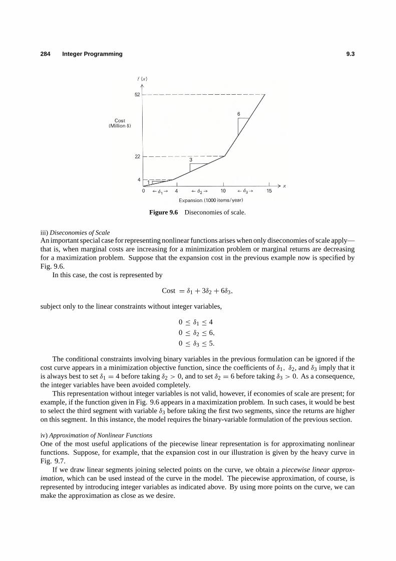
284 Integer Programming 9.3
Figure 9.6 Diseconomies of scale.
iii) Diseconomies of ScaleAn important special case for representing nonlinear functions arises when only diseconomies of scale apply—that is, when marginal costs are increasing for a minimization problem or marginal returns are decreasingfor a maximization problem. Suppose that the expansion cost in the previous example now is specified byFig. 9.6.
In this case, the cost is represented by
Cost = δ1+ 3δ2+ 6δ3,
subject only to the linear constraints without integer variables,
0 ≤ δ1 ≤ 4
0 ≤ δ2 ≤ 6,
0 ≤ δ3 ≤ 5.
The conditional constraints involving binary variables in the previous formulation can be ignored if thecost curve appears in a minimization objective function, since the coefficients ofδ1, δ2, andδ3 imply that itis always best to setδ1 = 4 before takingδ2 > 0, and to setδ2 = 6 before takingδ3 > 0. As a consequence,the integer variables have been avoided completely.
This representation without integer variables is not valid, however, if economies of scale are present; forexample, if the function given in Fig. 9.6 appears in a maximization problem. In such cases, it would be bestto select the third segment with variableδ3 before taking the first two segments, since the returns are higheron this segment. In this instance, the model requires the binary-variable formulation of the previous section.
iv) Approximation of Nonlinear FunctionsOne of the most useful applications of the piecewise linear representation is for approximating nonlinearfunctions. Suppose, for example, that the expansion cost in our illustration is given by the heavy curve inFig. 9.7.
If we draw linear segments joining selected points on the curve, we obtain apiecewise linear approx-imation, which can be used instead of the curve in the model. The piecewise approximation, of course, isrepresented by introducing integer variables as indicated above. By using more points on the curve, we canmake the approximation as close as we desire.

9.3 A Sample Formulation † 285
Figure 9.7 Approximation of a nonlinear curve.
9.3 A SAMPLE FORMULATION †
Proper placement of service facilities such as schools, hospitals, and recreational areas is essential to efficienturban design. Here we will present a simplified model for firehouse location. Our purpose is to showformulation devices of the previous section arising together in a meaningful context, rather than to give acomprehensive model for the location problemper se. As a consequence, we shall ignore many relevantissues, including uncertainty.
Assume that population is concentrated inI districts within the city and that districti containspi people.Preliminary analysis (land surveys, politics, and so forth) has limited the potential location of firehouses toJ sites. Letdi j ≥ 0 be the distance from the center of districti to site j . We are to determine the ‘‘best’’ siteselection and assignment of districts to firehouses. Let
y j =
{1 if site j is selected,0 otherwise;
and
xi j =
{1 if district i is assigned to sitej,0 otherwise.
The basic constraints are that every district should be assigned to exactly one firehouse, that is,
J∑j=1
xi j = 1 (i = 1, 2, . . . , I ),
and that no district should be assigned to an unused site, that is,y j = 0 impliesxi j = 0 (i = 1, 2, . . . , I ).The latter restriction can be modeled as alternative constraints, or more simply as:
I∑i=1
xi j ≤ y j I ( j = 1, 2, . . . , J).
Sincexi j are binary variables, their sum never exceedsI , so that ify j = 1, then constraintj is nonbinding.If y j = 0, thenxi j = 0 for all i .
† This section may be omitted without loss of continuity.

286 Integer Programming 9.3
Next note thatdi , the distance from districti to its assigned firehouse, is given by:
di =
J∑j=1
di j xi j ,
since onexi j will be 1 and all others 0.Also, the total population serviced by sitej is:
sj =
I∑i=1
pi xi j .
Assume that a central district is particularly susceptible to fire and that either sites 1 and 2 or sites 3 and4 can be used to protect this district. Then one of a number of similar restrictions might be:
y1+ y2 ≥ 2 or y3+ y4 ≥ 2.
We let y be a binary variable; then these alternative constraints become:
y1+ y2 ≥ 2y,
y3+ y4 ≥ 2(1− y).
Next assume that it costsf j (sj ) to build a firehouse at sitej to servicesj people and that a total budgetof B dollars has been allocated for firehouse construction. Then
J∑j=1
f j (sj ) ≤ B.
Finally, one possible social-welfare function might be to minimize the distance traveled to the districtfarthest from its assigned firehouse, that is, to:
Minimize D,
where
D = maxdi ;
or, equivalently,‡ to
Minimize D,
subject to:
D ≥ di (i = 1, 2, . . . , I ).
Collecting constraints and substituting above fordi in terms of its defining relationship
di =
J∑j=1
di j xi j ,
we set up the full model as:
Minimize D,
‡ The inequalitiesD ≥ di imply that D ≥ maxdi . The minimization ofD then ensures that it will actually be themaximum of thedi .

9.4 Some Characteristics Of Integer Programs—A Sample Problem 287
subject to:
D−J∑
j=1
di j xi j ≥ 0 (i = 1, 2, . . . , I ),
J∑j=1
xi j = 1 (i = 1, 2, . . . , I ),
I∑i=1
xi j ≤ y j I ( j = 1, 2, . . . , J),
Sj−
I∑i=1
pi xi j = 0 ( j = 1, 2, . . . , J),
J∑j=1
f j (sj ) ≤ B,
y1+ y2− 2y ≥ 0,
y3+ y4+ 2y ≥ 2,
xi j , y j , y binary (i = 1, 2, . . . , I ; j = 1, 2, . . . , J).
At this point we might replace each functionf j (sj )by an integer-programming approximation to completethe model. Details are left to the reader. Note that iff j (sj ) contains a fixed cost, then new fixed-cost variablesneed not be introduced—the variabley j serves this purpose.
The last comment, and the way in which the conditional constraint ‘‘y j = 0 implies xi j = 0 (i =1, 2, . . . , I )’’ has been modeled above, indicate that the formulation techniques of Section 9.2 should notbe applied without thought. Rather, they provide a common framework for modeling and should be used inconjunction with good modeling ‘‘common sense.’’ In general, it is best to introduce as few integer variablesas possible.
9.4 SOME CHARACTERISTICS OF INTEGER PROGRAMS—A SAMPLE PROBLEM
Whereas the simplex method is effective for solving linear programs, there is no single technique for solvinginteger programs. Instead, a number of procedures have been developed, and the performance of any particulartechnique appears to be highly problem-dependent. Methods to date can be classified broadly as followingone of three approaches:
i) enumeration techniques, including the branch-and-bound procedure;ii) cutting-plane techniques; and
iii) group-theoretic techniques.
In addition, several composite procedures have been proposed, which combine techniques using several ofthese approaches. In fact, there is a trend in computer systems for integer programming to include a numberof approaches and possibly utilize them all when analyzing a given problem. In the sections to follow, weshall consider the first two approaches in some detail. At this point, we shall introduce a specific problemand indicate some features of integer programs. Later we will use this example to illustrate and motivate thesolution procedures. Many characteristics of this example are shared by the integer version of the custom-molder problem presented in Chapter 1.
The problem is to determinez∗ where:
z∗ = maxz= 5x1+ 8x2,
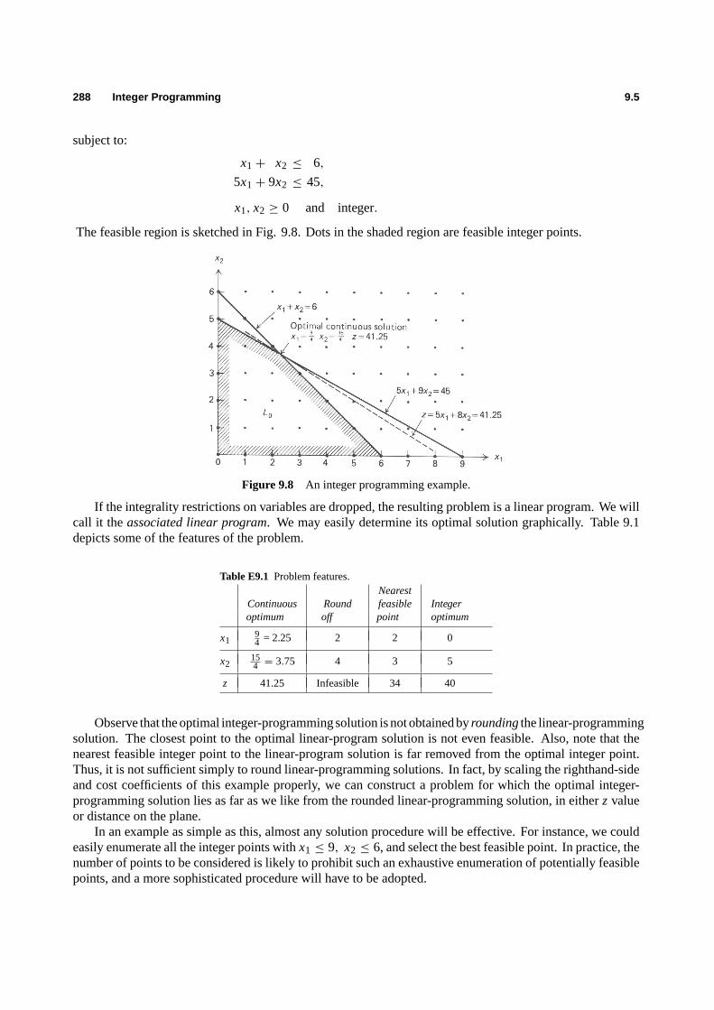
288 Integer Programming 9.5
subject to:
x1+ x2 ≤ 6,
5x1+ 9x2 ≤ 45,
x1, x2 ≥ 0 and integer.
The feasible region is sketched in Fig. 9.8. Dots in the shaded region are feasible integer points.
Figure 9.8 An integer programming example.
If the integrality restrictions on variables are dropped, the resulting problem is a linear program. We willcall it theassociated linear program. We may easily determine its optimal solution graphically. Table 9.1depicts some of the features of the problem.
Table E9.1 Problem features.Nearest
Continuous Round feasible Integeroptimum off point optimum
x194 = 2.25 2 2 0
x2154 = 3.75 4 3 5
z 41.25 Infeasible 34 40
Observe that the optimal integer-programming solution is not obtained byroundingthe linear-programmingsolution. The closest point to the optimal linear-program solution is not even feasible. Also, note that thenearest feasible integer point to the linear-program solution is far removed from the optimal integer point.Thus, it is not sufficient simply to round linear-programming solutions. In fact, by scaling the righthand-sideand cost coefficients of this example properly, we can construct a problem for which the optimal integer-programming solution lies as far as we like from the rounded linear-programming solution, in eitherz valueor distance on the plane.
In an example as simple as this, almost any solution procedure will be effective. For instance, we couldeasily enumerate all the integer points withx1 ≤ 9, x2 ≤ 6, and select the best feasible point. In practice, thenumber of points to be considered is likely to prohibit such an exhaustive enumeration of potentially feasiblepoints, and a more sophisticated procedure will have to be adopted.

9.5 Branch-And-Bound 289
Figure 9.9 Subdividing the feasible region.
9.5 BRANCH-AND-BOUND
Branch-and-boundis essentially a strategy of ‘‘divide and conquer.’’ The idea is to partition the feasibleregion into more manageable subdivisions and then, if required, to further partition the subdivisions. Ingeneral, there are a number of ways to divide the feasible region, and as a consequence there are a number ofbranch-and-bound algorithms. We shall consider one such technique, for problems with only binary variables,in Section 9.7. For historical reasons, the technique that will be described next usually is referred to asthebranch-and-bound procedure.
Basic Procedure
An integer linear program is a linear program further constrained by the integrality restrictions. Thus, in amaximization problem, the value of the objective function, at the linear-program optimum, will always be anupper bound on the optimal integer-programming objective. In addition, any integer feasible point is alwaysa lower bound on the optimal linear-program objective value.
The idea of branch-and-bound is to utilize these observations to systematically subdivide the linear-programming feasible region and make assessments of the integer-programming problem based upon thesesubdivisions. The method can be described easily by considering the example from the previous section.At first, the linear-programming region is not subdivided: The integrality restrictions are dropped and theassociated linear program is solved, giving an optimal valuez0. From our remark above, this gives the upperbound onz∗, z∗ ≤ z0
= 4114. Since the coefficients in the objective function are integral,z∗ must be integral
and this implies thatz∗ ≤ 41.Next note that the linear-programming solution hasx1 = 21
4 andx2 = 334. Both of these variables must
be integer in the optimal solution, and we can divide the feasible region in an attempt tomakeeither integral.We know that, in any integer programming solution,x2 must be either an integer≤ 3 or an integer≥ 4. Thus,our first subdivision is into the regions wherex2 ≤ 3 andx2 ≥ 4 as displayed by the shaded regionsL1 andL2 in Fig. 9.9. Observe that, by making the subdivisions, we have excluded the old linear-program solution.(If we selectedx1 instead, the region would be subdivided withx1 ≤ 2 andx1 ≥ 3.)
The results up to this point are pictured conveniently in anenumeration tree(Fig. 9.10). HereL0represents the associated linear program, whose optimal solution has been included within theL0 box, andthe upper bound onz∗ appears to the right of the box. The boxes below correspond to the new subdivisions;the constraints that subdivideL0 are included next to the lines joining the boxes. Thus, the constraints ofL1are those ofL0 together with the constraintx2 ≥ 4, while the constraints ofL2 are those ofL0 together withthe constraintx2 ≤ 3.
The strategy to be pursued now may be apparent: Simply treat each subdivision as we did the originalproblem. ConsiderL1 first. Graphically, from Fig. 9.9 we see that the optimal linear-programming solution

290 Integer Programming 9.5
Figure 9.10 Enumeration tree.
Figure 9.11 Subdividing the regionL1.
lies on the second constraint withx2 = 4, giving x1 =15(45− 9(4)) = 9
5 and an objective valuez =5(9
5
)+8(4) = 41. Sincex1 is not integer, we subdivideL1 further, into the regionsL3 with x1 ≥ 2 andL4 with
x1 ≤ 1. L3 is an infeasible problem and so this branch of the enumeration tree no longer needs to be considered.The enumeration tree now becomes that shown in Fig. 9.12. Note that the constraints of any subdivision
are obtained by tracing back toL0. For example,L4 contains the original constraints together withx2 ≥ 4andx1 ≤ 2. The asterisk (∗) below boxL3 indicates that the region need not be subdivided or, equivalently,that the tree will not be extended from this box.
At this point, subdivisionsL2 and L4 must be considered. We may select one arbitrarily; however,in practice, a number of useful heuristics are applied to make this choice. For simplicity, let us select thesubdivision most recently generated, hereL4. Analyzing the region, we find that its optimal solution has
x1 = 1, x2 =19(45− 5) = 40
9 .
Sincex2 is not integer,L4 must be further subdivided intoL5 with x2 ≤ 4, andL6 with x2 ≥ 5, leavingL2,L5 andL6 yet to be considered.
TreatingL5 first (see Fig. 9.13), we see that its optimum hasx1 = 1, x2 = 4, andz = 37. Since this isthe best linear-programming solution forL5 and the linear program contains every integer solution inL5, nointeger point in that subdivision can give a larger objective value than this point. Consequently, other points
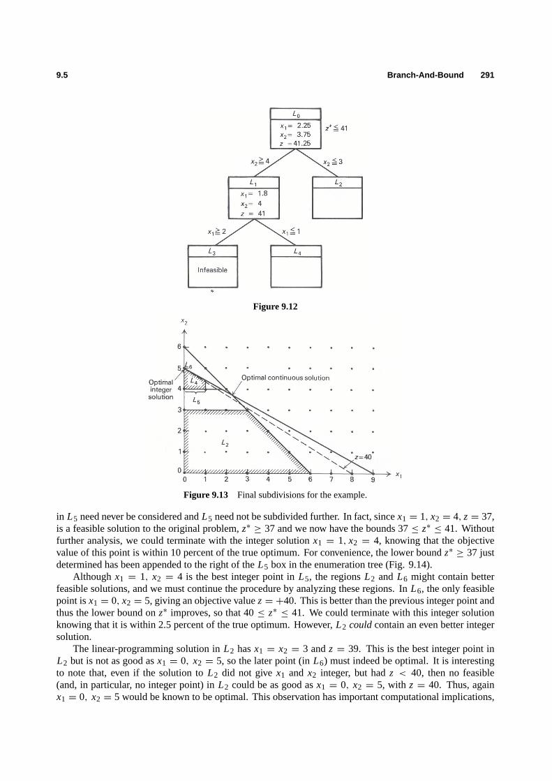
9.5 Branch-And-Bound 291
Figure 9.12
Figure 9.13 Final subdivisions for the example.
in L5 need never be considered andL5 need not be subdivided further. In fact, sincex1 = 1, x2 = 4, z= 37,is a feasible solution to the original problem,z∗ ≥ 37 and we now have the bounds 37≤ z∗ ≤ 41. Withoutfurther analysis, we could terminate with the integer solutionx1 = 1, x2 = 4, knowing that the objectivevalue of this point is within 10 percent of the true optimum. For convenience, the lower boundz∗ ≥ 37 justdetermined has been appended to the right of theL5 box in the enumeration tree (Fig. 9.14).
Although x1 = 1, x2 = 4 is the best integer point inL5, the regionsL2 and L6 might contain betterfeasible solutions, and we must continue the procedure by analyzing these regions. InL6, the only feasiblepoint isx1 = 0, x2 = 5, giving an objective valuez= +40. This is better than the previous integer point andthus the lower bound onz∗ improves, so that 40≤ z∗ ≤ 41. We could terminate with this integer solutionknowing that it is within 2.5 percent of the true optimum. However,L2 couldcontain an even better integersolution.
The linear-programming solution inL2 hasx1 = x2 = 3 andz = 39. This is the best integer point inL2 but is not as good asx1 = 0, x2 = 5, so the later point (inL6) must indeed be optimal. It is interestingto note that, even if the solution toL2 did not givex1 and x2 integer, but hadz < 40, then no feasible(and, in particular, no integer point) inL2 could be as good asx1 = 0, x2 = 5, with z = 40. Thus, againx1 = 0, x2 = 5 would be known to be optimal. This observation has important computational implications,

292 Integer Programming 9.5
Figure 9.14
since it is not necessary to drive every branch in the enumeration tree to an integer or infeasible solution, butonly to an objective value below the best integer solution.
The problem now is solved and the entire solution procedure can be summarized by the enumeration treein Fig. 9.15.
Figure 9.15
Further Considerations
There are three points that have yet to be considered with respect to the branch-and-bound procedure:
i) Can the linear programs corresponding to the subdivisions be solved efficiently?ii) What is the best way to subdivide a given region, and which unanalyzed subdivision should be considered
next?

9.5 Branch-And-Bound 293
iii) Can the upper bound (z= 41, in the example) on the optimal valuez∗ of the integer program be improvedwhile the problem is being solved?
The answer to the first question is an unqualifiedyes. When moving from a region to one of its subdivisions,we add one constraint that is not satisfied by the optimal linear-programming solution over the parent region.Moreover, this was one motivation for the dual simplex algorithm, and it is natural to adopt that algorithmhere.
Referring to the sample problem will illustrate the method. The first two subdivisionsL1 andL2 in thatexample were generated by adding the following constraints to the original problem:
For subdivision 1: x2 ≥ 4 or x2− s3 = 4 (s3 ≥ 0);
For subdivision 2: x2 ≤ 3 or x2 + s4 = 3 (s4 ≥ 0).
In either case we add the new constraint to the optimal linear-programming tableau. For subdivision 1, thisgives:
(−z) −54s1 −
34s2 = −411
4
x1 +94s1 −
14s2 =
94jx2 −
54s1 +
14s2 =
154
Constraints from theoptimal canonicalform
−x2 + s3 = −4, Added constraintx1, x2, s1, s2, s3 ≥ 0,
wheres1 ands2 are slack variables for the two constraints in the original problem formulation. Note thatthe new constraint has been multiplied by−1, so that the slack variables3 can be used as a basic variable.Since the basic variablex2 appears with a nonzero coefficient in the new constraint, though, we must pivotto isolate this variable in the second constraint to re-express the system as:
(−z) −54s1 −
34s2 = −411
4,
x1 +94s1 −
14s2 =
94,
x2 −54s1 +
14s2 =
154 ,
����−
54s1 +
14s2 +s3 = −
14,
x1, x2, s1, s2, s3 ≥ 0.
These constraints are expressed in the proper form for applying the dual simplex algorithm, which will pivotnext to makes1 the basic variable in the third constraint. The resulting system is given by:
(−z) − s2 − s3 = −41,x1 +
15s2 +
95s3 =
95,
x2 − s3 = 4,
s1 −15s2 −
45s3 =
15,
x1, x2, s1, s2, s3 ≥ 0.
This tableau is optimal and gives the optimal linear-programming solution over the regionL1 asx1 =95, x2 =
4, andz= 41. The same procedure can be used to determine the optimal solution inL2.When the linear-programming problem contains many constraints, this approach for recovering an optimal
solution is very effective. After adding a new constraint and making the slack variable for that constraintbasic, we always have a starting solution for the dual-simplex algorithm with only one basic variable negative.Usually, only a few dual-simplex pivoting operations are required to obtain the optimal solution. Using theprimal-simplex algorithm generally would require many more computations.

294 Integer Programming 9.5
Figure 9.16
Issue (ii) raised above is very important since, if we can make our choice of subdivisions in such a wayas to rapidly obtain a good (with luck, near-optimal) integer solutionz, then we can eliminate many potentialsubdivisions immediately. Indeed, if any region has its linear programming valuez ≤ z, then the objectivevalue of no integer point in that region can exceedz and the region need not be subdivided. There is nouniversal method for making the required choice, although several heuristic procedures have been suggested,such as selecting the subdivision with the largest optimal linear-programming value.†
Rules for determining which fractional variables to use in constructing subdivisions are more subtle.Recall that any fractional variable can be used to generate a subdivision. One procedure utilized is to lookahead one step in the dual-simplex method for every possible subdivision to see which is most promising. Thedetails are somewhat involved and are omitted here. For expository purposes, we have selected the fractionalvariable arbitrarily.
Finally, the upper boundzon the valuez∗ of the integer program can be improved as we solve the problem.Suppose for example, that subdivisionL2 was analyzed before subdivisionsL5 or L6 in our sample problem.The enumeration tree would be as shown in Fig. 9.16.
At this point, the optimal solution must lie in eitherL2 or L4. Since, however, the largest value forany feasible point in either of these regions is 405
9, the optimal value for the problemz∗ cannotexceed4059.
Becausez∗ must be integral, this implies thatz∗ ≤ 40 and the upper bound has been improved from the value41 provided by the solution to the linear program onL0. In general, the upper bound is given in this way asthe largest value of any ‘‘hanging’’ box (one that has not been divided) in the enumeration tree.
Summary
The essential idea of branch-and-bound is to subdivide the feasible region to developboundsz < z∗ < z on z∗.For a maximization problem, the lower boundz is the highest value of any feasible integer point encountered.The upper bound is given by the optimal value of the associated linear program or by the largest value forthe objective function at any ‘‘hanging’’ box. After considering a subdivision, we mustbranchto (move to)another subdivision and analyze it. Also, ifeither
† One common method used in practice is to consider subdivisions on a last-generated–first-analyzed basis. We usedthis rule in our previous example. Note that data to initiate the dual-simplex method mentioned above must be stored foreach subdivision that has yet to be analyzed. This data usually is stored in a list, with new information being added to thetop of the list. When required, data then is extracted from thetopof this list, leading to the last-generated–first-analyzedrule. Observe that when we subdivide a region into two subdivisions, one of these subdivisions will be analyzed next.The data required for this analysis already will be in the computer core and need not be extracted from the list.

9.6 Branch-And-Bound 295
i) the linear program overL j is infeasible;
ii) the optimal linear-programming solution overL j is integer;or
iii) the value of the linear-programming solutionz j overL j satisfiesz j≤ z (if maximizing),
then L j need not be subdivided. In these cases, integer-programming terminology says thatL j has beenfathomed.† Case (i) is termed fathoming by infeasibility, (ii) fathoming by integrality, and (iii) fathoming bybounds.
The flow chart in Fig. 9.17 summarizes the general procedure.
Figure 9.17 Branch-and-bound for integer-programming maximization.
† To fathomis defined as ‘‘to get to the bottom of; to understand thoroughly.’’ In this chapter,fathomedmight be moreappropriately defined as ‘‘understood enough or already considered.’’

296 Integer Programming 9.7
Figure 9.18
9.6 BRANCH-AND-BOUND FOR MIXED-INTEGER PROGRAMS
The branch-and-bound approach just described is easily extended to solve problems in which some, but notall, variables are constrained to be integral. Subdivisions then are generated solely by the integral variables.In every other way, the procedure is the same as that specified above. A brief example will illustrate themethod.
z∗ = maxz= −3x1− 2x2+ 10,
subject to:
x1 − 2x2+ x3 =52,
2x1 + x2 + x4 =32,
x j ≥ 0 ( j = 1, 2, 3, 4),
x2 and x3 integer.
The problem, as stated, is in canonical form, withx3 andx4 optimal basic variables for the associated linearprogram.
The continuous variablex4 cannot be used to generate subdivisions since any value ofx4 ≥ 0 potentiallycan be optimal. Consequently, the subdivisions must be defined byx3 ≤ 2 andx3 ≥ 3. The completeprocedure is summarized by the enumeration tree in Fig. 9.18.
The solution inL1 satisfies the integrality restrictions, soz∗ ≥ z= 812. The only integral variable with a
fractional value in the optimal solution ofL2 is x2, so subdivisionsL3 andL4 are generated from this variable.Finally, the optimal linear-programming value ofL4 is 8, so no feasible mixed-integer solution in that regioncan be better than the value 81
2 already generated. Consequently, that region need not be subdivided and thesolution inL1 is optimal.
The dual-simplex iterations that solve the linear programs inL1, L2, L3, and L4 are given below inTableau 1. The variablessj in the tableaus are the slack variables for theconstraints added to generate the subdivisions. The coefficients in the appended constraints are determinedas we mentioned in the last section, by eliminating the basic variablesx j from the new constraint that isintroduced. To follow the iterations, recall that in the dual-simplex method, pivots are made on negativeelements in the generating row; if all elements in this row arepositive, as in regionL3, then the problem isinfeasible.

9.7 Implicit Enumeration 297
9.7 IMPLICIT ENUMERATION
A special branch-and-bound procedure can be given for integer programs with only binary variables. Thealgorithm has the advantage that it requires no linear-programming solutions. It is illustrated by the followingexample:
z∗ = max z= −8x1 − 2x2− 4x3 − 7x4 − 5x5+ 10,
subject to:−3x1 − 3x2 + x3 + 2x4 + 3x5 ≤ −2,
−5x1 − 3x2 − 2x3 − x4 + x5 ≤ −4,
x j = 0 or 1 ( j = 1, 2, . . . , 5).
One way to solve such problems is complete enumeration. List all possible binary combinations of thevariables and select the best such point that is feasible. The approach works very well on a small problemsuch as this, where there are only a few potential 0–1 combinations for the variables, here 32. In general,though, ann-variable problem contains 2n 0–1 combinations; for large values ofn, the exhaustive approachis prohibitive. Instead, one might implicitly consider every binary combination, just as every integer pointwas implicitlyconsidered, but not necessarily evaluated, for the general problem via branch-and-bound.
Recall that in the ordinary branch-and-bound procedure, subdivisions were analyzed by maintaining thelinear constraints and dropping the integrality restrictions. Here, we adopt the opposite tactic of always

298 Integer Programming 9.7
maintaining the 0–1 restrictions, but ignoring the linear inequalities.The idea is to utilize a branch-and-bound (or subdivision) process to fix some of the variables at 0 or
1. The variables remaining to be specified are calledfree variables. Note that, if the inequality constraintsare ignored, the objective function is maximized by setting the free variables to zero, since their objective-function coefficients are negative. For example, ifx1 andx4 are fixed at 1 andx5 at 0, then the free variablesarex2 andx3. Ignoring the inequality constraints, the resulting problem is:
max[−8(1)− 2x2− 4x3− 7(1)− 5(0)+ 10] = max[−2x2− 4x3− 5],
subject to:x2 and x3 binary.
Since the free variables have negative objective-function coefficients, the maximization setsx2 = x3 = 0.
The simplicity of this trivial optimization, as compared to a more formidable linear program, is what wewould like to exploit.
Returning to the example, we start withnofixed variables, and consequently every variable is free and setto zero. The solution does not satisfy the inequality constraints, and we must subdivide to search for feasiblesolutions. One subdivision choice might be:
For subdivision 1: x1 = 1,
For subdivision 2: x1 = 0.
Now variablex1 is fixed in each subdivision. By our observations above, if the inequalities are ignored, theoptimal solution over each subdivision hasx2 = x3 = x4 = x5 = 0. The resulting solution in subdivision 1gives
z= −8(1)− 2(0)− 4(0)− 7(0)− 5(0)+ 10= 2,

9.7 Implicit Enumeration 299
and happens to satisfy the inequalities, so that the optimal solution to the original problem isat least2, z∗ ≥ 2.Also, subdivision 1 has been fathomed: The above solution is best among all 0–1 combinations withx1 = 1;thus it must be best among those satisfying the inequalities. No other feasible 0–1 combination in subdivision1 needs to be evaluated explicitly. These combinations have been considered implicitly.
The solution withx2 = x3 = x4 = x5 = 0 in subdivision 2 is the same as the original solution withevery variable at zero, and is infeasible. Consequently, the region must be subdivided further, say withx2 = 1 or x2 = 0, giving:
For subdivision 3: x1 = 0, x2 = 1;For subdivision 4: x1 = 0, x2 = 0.
The enumeration tree to this point is as given in Fig. 9.19.
Figure 9.19
Observe that this tree differs from the enumeration trees of the previous sections. For the earlier proce-dures, the linear-programming solution used to analyze each subdivision was specified explicitly in a box.Here the 0–1 solution (ignoring the inequalities) used to analyze subdivisions is not stated explicitly, sinceit is known simply by setting free variables to zero. In subdivisioni3 , for example,x1 = 0 andx2 = 1 arefixed, and the free variablesx3, x4 andx5 are set to zero.
Continuing to fix variables and subdivide in this fashion produces the complete tree shown in Fig. 9.20.The tree is not extended after analyzing subdivisions 4, 5, 7, 9, and 10, for the following reasons.
i) At i5 , the solutionx1 = 0, x2 = x3 = 1 , with free variablesx4 = x5 = 0, is feasible, withz = 4 ,thus providing an improved lower bound onz∗.
ii) At i7 , the solutionx1 = x3 = 0, x2 = x4 = 1, and free variablex5 = 0, hasz = 1 < 4, so that nosolution in that subdivision can be as good as that generated ati5 .
iii) At i9 and i10 , every free variable is fixed. In each case, the subdivisions contain only a single point,which is infeasible, and further subdivision is not possible.
iv) At i4 , the second inequality (with fixed variablesx1 = x2 = 0) reads:
−2x3− x4+ x5 ≤ −4.
No 0–1 values ofx3, x4, or x5 ‘‘completing’’ the fixed variablesx1 = x2 = 0 satisfy this constraint,since the lowest value for the lefthand side of this equation is−3 whenx3 = x4 = 1 andx5 = 0. Thesubdivision then has no feasible solution and need not be analyzed further.
The last observation is completely general. If, at any point after substituting for the fixed variables,the sum of the remaining negative coefficients in any constraint exceeds the righthand side, then the regiondefined by these fixed variables has no feasible solution. Due to the special nature of the 0–1 problem, thereare a number of other such tests that can be utilized to reduce the number of subdivisions generated. Theefficiency of these tests is measured by weighing the time needed to perform them against the time saved byfewer subdivisions.
The techniques used here apply to any integer-programming problem involving only binary variables,so that implicit enumeration is an alternative branch-and-bound procedure for this class of problems. In thiscase, subdivisions are fathomed if any of three conditions hold:

300 Integer Programming 9.7
Figure 9.20
i) the integer program is known to be infeasible over the subdivision, for example, by the above infeasibilitytest;
ii) the 0–1 solution obtained by setting free variables to zero satisfies the linear inequalities; oriii) the objective value obtained by setting free variables to zero is no larger than the best feasible 0–1
solution previously generated.
These conditions correspond to the three stated earlier for fathoming in the usual branch-and-bound procedure.If a region is not fathomed by one of these tests, implicit enumeration subdivides that region by selecting anyfree variable and fixing its values to 0 or 1.
Our arguments leading to the algorithm were based upon stating the original 0–1 problem in the followingstandard form:
1. the objective is a maximization with all coefficients negative; and2. constraints are specified as ‘‘less than or equal to’’ inequalities.
As usual, minimization problems are transformed to maximization by multiplying cost coefficients by−1.If x j appears in the maximization form with a positive coefficient, then the variable substitutionx j = 1− x′jeverywhere in the model leaves the binary variablex′j with a negative objective-function coefficient. Finally,‘‘greater than or equal to’’ constraints can be multiplied by−1 to become ‘‘less than or equal to’’ constraints;and general equality constraints are converted to inequalities by the special technique discussed in Exercise17 of Chapter 2.
Like the branch-and-bound procedure for general integer programs, the way we choose to subdivideregions can have a profound effect upon computations. In implicit enumeration, we begin with the zerosolutionx1 = x2 = · · · = xn = 0 and generate other solutions by setting variables to 1. One natural approachis to subdivide based upon the variable with highest objective contribution. For the sample problem, thiswould imply subdividing initially withx2 = 1 or x2 = 0.
Another approach often used in practice is to try to drive toward feasibility as soon as possible. Forinstance, whenx1 = 0, x2 = 1, andx3 = 0 are fixed in the example problem, we could subdivide basedupon eitherx4 or x5. Settingx4 or x5 to 1 and substituting for the fixed variables, we find that the constraintsbecome:

9.8 Cutting Planes 301
x4 = 1, x5(free)= 0 : x5 = 1, x4(free)= 0 :−3(0)− 3(1)+ (0)+ 2(1)+ 3(0) ≤ −2, −3(0)− 3(1)+ (0)+ 2(0)+ 3(1) ≤ −2,
−5(0)− 3(1)− 2(0)− 1(1)+ (0) ≤ −4, −5(0)− 3(1)− 2(0)− 1(0)+ (1) ≤ −4.
For x4 = 1, the first constraint is infeasible by 1 unit and the second constraint is feasible, giving 1 total unitof infeasibility. Forx5 = 1, the first constraint is infeasible by 2 units and the second by 2 units, giving 4total units of infeasibility. Thusx4 = 1 appears more favorable, and we would subdivide based upon thatvariable. In general, the variable giving theleast total infeasibilitiesby this approach would be chosen next.Reviewing the example problem the reader will see that this approach has been used in our solution.
9.8 CUTTING PLANES
The cutting-plane algorithm solves integer programs by modifying linear-programming solutions until theinteger solution is obtained. It does not partition the feasible region into subdivisions, as in branch-and-boundapproaches, but instead works with a single linear program, which it refines by adding new constraints. Thenew constraints successively reduce the feasible region until an integer optimal solution is found.
In practice, the branch-and-bound procedures almost always outperform the cutting-plane algorithm.Nevertheless, the algorithm has been important to the evolution of integer programming. Historically, it wasthe first algorithm developed for integer programming that could be proved to converge in a finite number ofsteps. In addition, even though the algorithm generally is considered to be very inefficient, it has providedinsights into integer programming that have led to other, more efficient, algorithms.
Again, we shall discuss the method by considering the sample problem of the previous sections:
z∗ = max 5x1+ 8x2,
subject to:
x1 + x2 + s1 = 6,
5x1 + 9x2 + s2 = 45,
x1, x2, s1, s2 ≥ 0.
(11)
s1 ands2 are, respectively, slack variables for the first and second constraints.Solving the problem by the simplex method produces the following optimal tableau:
(−z) −54s1 −
34s2 = −411
4,
x1 +94s1 −
14s2 =
94,
x2 −54s1 +
14s2 =
154 ,
x1, x2, s1, s2, s3 ≥ 0.
Let us rewrite these equations in an equivalent but somewhat altered form:
(−z) −2s1 −s2 +42 = 34 −
34s1 −
14s2,
x1 +2s1 −s2 − 2 = 14 −
14s1 −
34s2,
x2 −2s1 − 3 = 34 −
34s1 −
14s2,
x1, x2, s1, s2 ≥ 0.
These algebraic manipulations have isolated integer coefficients to one side of the equalities and fractions tothe other, in such a way that the constant terms on the righthand side are all nonnegative and the slack variablecoefficients on the righthand side are all nonpositive.

302 Integer Programming 9.8
In any integer solution, the lefthand side of each equation in the last tableau must be integer. Sinces1 ands2 are nonnegative and appear to the right with negative coefficients, each righthand side necessarily mustbe less than or equal to the fractional constant term. Taken together, these two observations show that bothsides of every equation must be an integer less than or equal to zero (if an integer is less than or equal to afraction, it necessarily must be 0 or negative). Thus, from the first equation, we may write:
34 −
34s1−
14s2 ≤ 0 and integer,
or, introducing a slack variables3,
34 −
34s1−
14s2+ s3 = 0, s3 ≥ 0 and integer. (C1)
Similarly, other conditions can be generated from the remaining constraints:
14 −
14s1−
34s2+ s4 = 0, s4 ≥ 0 and integer (C2)
34 −
34s1−
14s2+ s5 = 0, s5 ≥ 0 and integer. (C3)
Note that, in this case,(C1) and(C3) are identical.
The new equations(C1), (C2), and(C3) that have been derived are calledcutsfor the following reason:Their derivation did not exclude any integer solutions to the problem, so that any integer feasible point to theoriginal problem must satisfy the cut constraints. The linear-programming solution hads1 = s2 = 0; clearly,these donot satisfy the cut constraints. In each case, substitutings1 = s2 = 0 gives eithers3, s4, or s5 < 0.Thus the net effect of a cut is to cut away the optimal linear-programming solution from the feasible regionwithout excluding any feasible integer points.
The geometry underlying the cuts can be established quite easily. Recall from (11) that slack variabless1 ands2 are defined by:
s1 = 6 − x1 − x2,
s2 = 45 − 5x1 − 9x2.
Substituting these values in the cut constraints and rearranging, we may rewrite the cuts as:
2x1+ 3x2 ≤ 15, (C1 or C3)
4x1+ 7x2 ≤ 35. (C2)
In this form, the cuts are displayed in Fig. 9.21. Notethat they exhibit the features suggested above. In eachcase, the added cut removes the linear-programming solutionx1 =
94, x2 =
154 , from the feasible region, at
the same time including every feasible integer solution.The basic strategy of the cutting-plane technique is to add cuts (usually only one) to the constraints
defining the feasible region and then to solve the resulting linear program. If the optimal values for thedecision variables in the linear program are all integer, they are optimal; otherwise, a new cut is derived fromthe new optimal linear-programming tableau and appended to the constraints.
Note from Fig. 9.21 that the cutC1 = C3 leads directly to the optimal solution. CutC2 does not, andfurther iterations will be required if this cut is appended to the problem (without the cutC1 = C3). Alsonote thatC1 cuts deeper into the feasible region than doesC2. For problems with many variables, it isgenerally quite difficult to determine which cuts will be deep in this sense. Consequently, in applications, thealgorithm frequently generates cuts that shave very little from the feasible region, and hence the algorithm’spoor performance.
A final point to be considered here is the way in which cuts are generated. The linear-programmingtableau for the above problem contained the constraint:
x1+94s1−
14s2 =
94.

9.8 Cutting Planes 303
Figure 9.21 Cutting away the linear-programming solution.
Suppose that we rounddown the fractional coefficients to integers, that is,94 to 2,−1
4 to −1, and 94 to 2.
Writing these integers to the left of the equality and the remaining fractions to the right, we obtain as before,the equivalent constraint:
x1+ 2s1− s2− 2= 14 −
14s1−
34s2.
By our previous arguments, the cut is:
14 −
14s1−
34s2 ≤ 0 and integer.
Another example may help to clarify matters. Suppose that the final linear-programming tableau to aproblem has the constraint
x1 +16x6−
76x7+ 3x8 = 45
6.
Then the equivalent constraint is:
x1 − 2x7+ 3x8− 4= 56 −
16x6−
56x7,
and the resulting cut is:56 −
16x6−
56x7 ≤ 0 and integer.
Observe the way that fractions are determined for negative coefficients. The fraction in the cut constraintdetermined by thex7 coefficient−7
6 = −116 is not 1
6, but rather it is the fraction generated by rounding downto−2; i.e., the fraction is−11
6 − (−2) = 56.
Tableau 2 shows the complete solution of the sample problem by the cutting-plane technique. Since cutC1 = C3 leads directly to the optimal solution, we have chosen to start with cutC2. Note that, if the slackvariable for any newly generated cut is taken as the basic variable in that constraint, then the problem is inthe proper form for the dual-simplex algorithm. For instance, the cut in Tableau 2(b) generated from thex1constraint
x1+73s1−
13s2 =
73 or x1+ 2s1− s2− 2= 1
3 −13s1−
23s2
is given by:13 −
13s1−
23s2 ≤ 0 and integer.
Lettings4 be the slack variable in the constraint, we obtain:
−13s1−
23s2+ s4 = −
13.
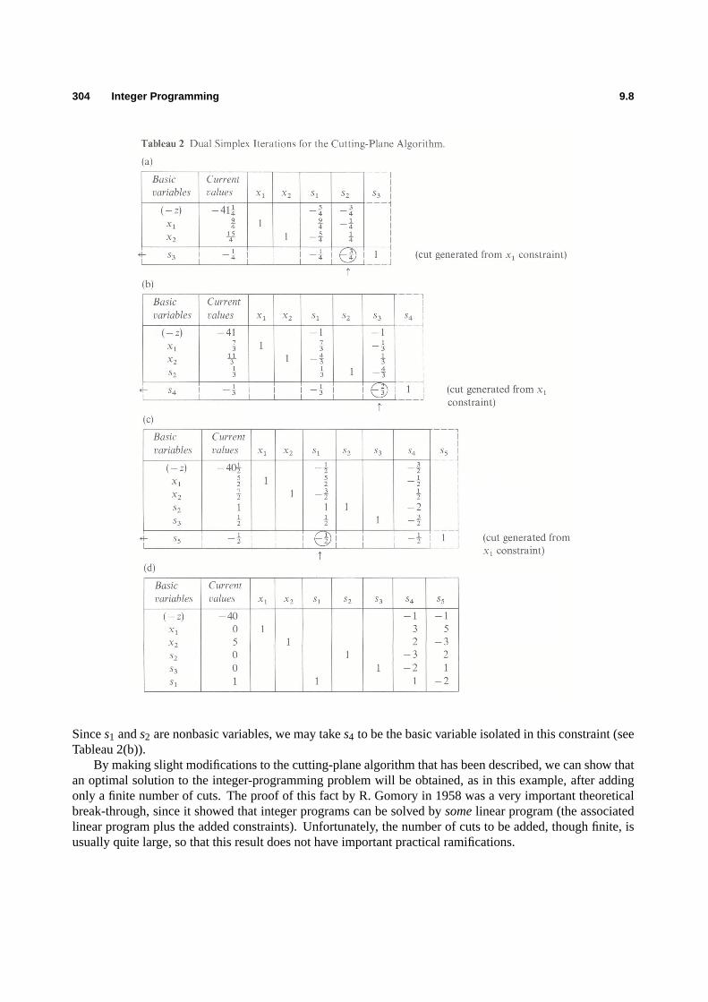
304 Integer Programming 9.8
Sinces1 ands2 are nonbasic variables, we may takes4 to be the basic variable isolated in this constraint (seeTableau 2(b)).
By making slight modifications to the cutting-plane algorithm that has been described, we can show thatan optimal solution to the integer-programming problem will be obtained, as in this example, after addingonly a finite number of cuts. The proof of this fact by R. Gomory in 1958 was a very important theoreticalbreak-through, since it showed that integer programs can be solved bysomelinear program (the associatedlinear program plus the added constraints). Unfortunately, the number of cuts to be added, though finite, isusually quite large, so that this result does not have important practical ramifications.

9.8 Cutting Planes 305
EXERCISES
1. As the leader of an oil-exploration drilling venture, you must determine the least-cost selection of 5 out of 10 possiblesites. Label the sitesS1, S2, . . . , S10, and the exploration costs associated with each asC1, C2, . . . , C10.
Regional development restrictions are such that:
i) Evaluating sitesS1 and S7 will prevent you from exploring siteS8.
ii) Evaluating siteS3 or S4 prevents you from assessing siteS5.
iii) Of the groupS5, S6, S7, S8, only two sites may be assessed.
Formulate an integer program to determine the minimum-cost exploration scheme that satisfies these restrictions.
2. A company wishes to put together an academic ‘‘package’’ for an executive training program. There are five areacolleges, each offering courses in the six fields that the program is designed to touch upon.
The package consists of 10 courses; each of the six fields must be covered.
The tuition (basic charge), assessed when at least one course is taken, at collegei is Ti (independent ofthe number of courses taken). Moreover, each college imposes an additional charge (covering course materials,instructional aids, and so forth) foreachcourse, the charge depending on the college and the field of instructions.
Formulate an integer program that will provide the company with the minimum amount it must spend to meetthe requirements of the program.
3. The marketing group of A. J. Pitt Company is considering the options available for its next advertising campaignprogram. After a great deal of work, the group has identified a selected number of options with the characteristicsshown in the accompanying table.
TotalTrade Popular Promotional resource
TV magazineNewspaper Radio magazinecampaign available
Customersreached 1,000,000 200,000 300,000 400,000 450,000 450,000 −
Cost ($) 500,000 150,000 300,000 250,000 250,000 100,000 1,800,000
Designers
needed
(man-hours) 700 250 200 200 300 400 1,500
Salesmen
needed
(man-hours) 200 100 100 100 100 1,000 1,200
The objective of the advertising program is to maximize the number of customers reached, subject to thelimitation of resources (money, designers, and salesman) given in the table above. In addition, the followingconstraints have to be met:
i) If the promotional campaign is undertaken, it needs either a radio or a popular magazine campaign effort tosupport it.
ii) The firm cannot advertise in both the trade and popular magazines.
Formulate an integer-programming model that will assist the company to select an appropriate advertising campaignstrategy.
4. Three different items are to be routed through three machines. Each item must be processed first on machine 1, thenon machine 2, and finally on machine 3. The sequence of items may differ for each machine. Assume that the timesti j required to perform the work on itemi by machinej are known and are integers. Our objective is to minimizethe total time necessary to process all the items.
a) Formulate the problem as an integer programming problem. [Hint. Let xi j be the starting time of processingitem i on machinej . Your model must prevent two items from occupying the same machine at the same time;also, an item may not start processing on machine (j + 1) unless it has completed processing on machinej .]

306 Integer Programming 9.8
b) Suppose we want the items to be processed in the same sequence on each machine. Change the formulation inpart (a) accordingly.
5. Consider the problem:
Maximizez= x1+ 2x2,
subject to:
x1 + x2 ≤ 8,
−x1 + x2 ≤ 2,
x1 − x2 ≤ 4,
x2 ≥ 0 and integer,
x1 = 0, 1, 4, or 6.
a) Reformulate the problem as an equivalent integer linear program.b) How would your answer to part (a) change if the objective function were changed to:
Maximizez= x21 + 2x2?
6. Formulate, butdo not solve,the following mathematical-programming problems. Also, indicate the type of algorithmused in general to solve each.
a) A courier traveling to Europe can carry up to 50 kilograms of a commodity, all of which can be sold for $40 perkilogram. The round-trip air fare is $450 plus $5 per kilogram of baggage in excess of 20 kilograms (one way).Ignoring any possible profits on the return trip, should the courier travel to Europe and, if so, how much of thecommodity should be taken along in order to maximize his profits?
b) A copying service incurs machine operating costs of:
$0.10 for copies 1 to 4,0.05 for copies 5 to 8,0.025 for copies 9 and over,
and has a capacity of 1000 copies per hour. One hour has been reserved for copying a 10-page article to be soldto MBA students. Assuming that all copies can be sold for $0.50 per article, how many copies of the articleshould be made?
c) A petrochemical company wants to maximize profit on an item that sells for $0.30 per gallon. Suppose thatincreased temperature increases output according to the graph in Fig. E9.1. Assuming that production costs aredirectly proportional to temperature as $7.50 per degree centigrade, how many gallons of the item should beproduced?
7. Suppose that you are a ski buff and an entrepreneur. You own a set of hills, any or all of which can be developed.Figure E9.2 illustrates the nature of the cost for putting ski runs on any hill.
The cost includes fixed charges for putting new trails on a hill. For each hillj , there is a limitd j on the numberof trails that can be constructed and a lower limitt j on the number of feet of trail that must be developed if the hillis used.
Use a piecewise linear approximation to formulate a strategy based on cost minimization for locating the skiruns, given that you desire to haveM total feet of developed ski trail in the area.
8. Consider the following word game. You are assigned a number of tiles, each containing a lettera, b, . . . , or z fromthe alphabet. For any letterα from the alphabet, your assignment includesNα (a nonnegative integer) tiles withthe letterα. From the letters you are to construct any of the wordsw1, w2, . . . , wn. This list might, for example,contain all words from a given dictionary.
You may construct any word at most once, and use any tile at most once. You receivev j ≥ 0 points for makingwordw j and an additional bonus ofbi j ≥ 0 points for makingbothwordswi andw j (i = 1, 2, …,n; j = 1, 2, …,n).
a) Formulate alinear integer program to determine your optimal choice of words.

9.8 Cutting Planes 307
Figure E9.1
Figure E9.2
b) How does the formulation change if you are allowed to select 100 tiles with no restriction on your choice ofletters?
9. In Section 9.1 of the text, we presented the following simplified version of the warehouse-location problem:
Minimize∑
i
∑j
ci j xi j +∑
i
fi yi ,
subject to: ∑i
xi j = d j ( j = 1, 2, . . . , n)
∑j
xi j − yi
(∑j
d j
)≤ 0 (i = 1, 2, . . . , m)
xi j ≥ 0 (i = 1, 2, . . . , m; j = 1, 2, . . . , n)
yi = 0 or 1 (i = 1, 2, . . . , m).
a) The above model assumes only one product and two distribution stages (from warehouse to customer). Indicatehow the model would be modified if there were three distribution stages (from plant to warehouse to customer)andL different products. [Hint. Define a new decision variablexi jkl equal to the amount to be sent from planti , through warehousej , to customerk, of product`.]

308 Integer Programming 9.8
b) Suppose there are maximum capacities for plants and size limits (both upper and lower bounds) for warehouses.What is the relevant model now?
c) Assume that each customer has to be served from a single warehouse; i.e., no splitting of orders is allowed. Howshould the warehousing model be modified? [Hint. Define a new variablez jk = fraction of demand of customerk satisfied from warehousej .]
d) Assume that each warehousei experiences economies of scale when shipping above a certain threshold quantityto an individual customer; i.e., the unit distribution cost isci j whenever the amount shipped is between 0 anddi j , andc′i j (lower thanci j ) whenever the amount shipped exceedsdi j . Formulate the warehouse location modelunder these conditions.
10. Graph the following integer program:
Maximizez= x1+ 5x2,
subject to :
−4x1+ 3x2 ≤ 6,
3x1+ 2x2 ≤ 18,
x1, x2 ≥ 0 and integer.
Apply the branch-and-bound procedure, graphically solving each linear-programming problem encountered. Inter-pret the branch-and-bound procedure graphically as well.
11. Solve the following integer program using the branch-and-bound technique:
Minimize z= 2x1− 3x2− 4x3,
subject to:
−x1 + x2 + 3x3 ≤ 8,
3x1 + 2x2 − x3 ≤ 10,
x1, x2, x3 ≥ 0 and integer.
The optimal tableau to the linear program associated with this problem is:
Basic Current
variables values x1 x2 x3 x4 x5
x367 −
57 1 2
7 −17
x2387
87 1 1
737
(−z) 1387
187
117
57
The variablesx4 andx5 are slack variables for the two constraints.
12. Use branch-and-bound to solve the mixed-integer program:
Maximizez= −5x1− x2− 2x3+ 5,
subject to:
−2x1 + x2 − x3 + x4 =72,
2x1 + x2 + x3 + x5 = 2,
x j ≥ 0 ( j = 1, 2, . . . , 5)
x3 andx5 integer.

9.8 Cutting Planes 309
13. Solve the mixed-integer programming knapsack problem:
Maximizez= 6x1+ 4x2+ 4x3+ x4+ x5,
subject to:
2x1 + 2x2 + 3x3 + x4 + 2x5 = 7,
x j ≥ 0 ( j = 1, 2, . . . , 5) ,
x1 andx2 integer.
14. Solve the following integer program using implicit enumeration:
Maximizez= 2x1 − x2 − x3+ 10,
subject to:2x1 + 3x2 − x3 ≤ 9,
2x2 + x3 ≥ 4,
3x1 + 3x2 + 3x3 = 6,
x j = 0 or 1 ( j = 1, 2, 3).
15. A college intramural four-man basketball team is trying to choose its starting line-up from a six-man roster so as tomaximize average height. The roster follows:
Player NumberHeight∗ Position
Dave 1 10 Center
John 2 9 Center
Mark 3 6 Forward
Rich 4 6 Forward
Ken 5 4 Guard
Jim 6 −1 Guard
∗ In inches over 5′ 6′′.
The starting line-up must satisfy the following constraints:
i) At least one guard must start.ii) Either John or Ken must be held in reserve.
iii) Only one center can start.iv) If John or Rich starts, then Jim cannot start.
a) Formulate this problem as an integer program.b) Solve for the optimal starting line-up, using the implicit enumeration algorithm.
16. Suppose that one of the following constraints arises when applying the implicit enumeration algorithm to a 0−1integer program:
−2x1− 3x2+ x3+ 4x4 ≤ −6, (1)
−2x1− 6x2+ x3+ 4x4 ≤ −5, (2)
−4x1− 6x2− x3+ 4x4 ≤ −3. (3)
In each case, the variables on the lefthand side of the inequalities are free variables and the righthand-side coefficientsinclude the contributions of the fixed variables.

310 Integer Programming 9.8
a) Use the feasibility test to show that constraint (1) contains no feasible completion.b) Show thatx2 = 1 andx4 = 0 in any feasible completion to constraint (2). State a general rule that shows when a
variablex j , like x2 or x4 in constraint (2), must be either 0 or 1 in any feasible solution. [Hint. Apply the usualfeasibility test after settingx j to 1 or 0.]
c) Suppose that the objective function to minimize is:
z= 6x1+ 4x2+ 5x3+ x4+ 10,
and thatz = 17 is the value of an integer solution obtained previously. Show thatx3 = 0 in a feasible completionto constraint (3) that is a potential improvement uponz with z < z. (Note that eitherx1 = 1 or x2 = 1 in anyfeasible solution to constraint (3) havingx3 = 1.)
d) How could the tests described in parts (b) and (c) be used to reduce the size of the enumeration tree encounteredwhen applying implicit enumeration?
17. Although the constraintx1− x2 ≤ −1
and the constraint−x1+ 2x2≤ −1
to a zero–one integer program both have feasible solutions, the system composed of both constraints is infeasible.One way to exhibit the inconsistency in the system is to add the two constraints, producing the constraint
x2 ≤ −1,
which has no feasible solution withx2 = 0 or 1.
More generally, suppose that we multiply thei th constraint of a system
Multipliersa11x1 + a12x2 + · · ·+ a1nxn ≤ b1, u1...
......
ai 1x1 + ai 2x2 + · · ·+ ainxn ≤ bi , ui...
......
am1x1 + am2x2 + · · ·+ amnxn ≤ bm, um
x j = 0 or 1 ( j = 1, 2, . . . , n),
by nonnegative constraintsui and add to give the composite, orsurrogate, constraint:(m∑
i=1
ui ai 1
)x1+
(m∑
i=1
ui ai 2
)x2+ · · · +
(m∑
i=1
ui ain
)xn ≤
m∑i=1
ui bi .
a) Show that any feasible solutionx j = 0 or 1( j = 1, 2, . . . , n) for the system of constraints must also be feasibleto the surrogate constraint.
b) How might the fathoming tests discussed in the previous exercise be used in conjunction with surrogate constraintsin an implicit enumeration scheme?
c) A ‘‘best’’ surrogate constraint might be defined as one that eliminates as many nonoptimal solutionsx j = 0 or 1as possible. Consider the objective value of the integer program when the system constraints are replaced by thesurrogate constraint; that is the problem:
v(u) = Min c1x1 + c2x2+ · · · + cnxn,
subject to: (m∑
i=1
ui ai 1
)x1+
(m∑
i=1
ui ai 2
)x2+ · · · +
(m∑
i=1
ui ain
)xn ≤
m∑i=1
ui bi ,
x j = 0 or 1 ( j = 1, 2, . . . , n).

9.8 Cutting Planes 311
Let us say that a surrogate constraint with multipliersu1, u2 . . . , um is strongerthan another surrogate constraintwith multipliersu1, u2, . . . , um, if the valuev(u) of the surrogate constraint problem with multipliersu1, u2, . . . , um
is larger than the value ofv(u) with multipliers u1, u2, . . . , um. (The larger we makev(u), the more nonoptimalsolutions we might expect to eliminate.)
Suppose that we estimate the value ofv(u) defined above by replacingx j = 0 or 1 by 0≤ x j ≤ 1 forj = 1, 2, . . . , n. Then, to estimate the strongest surrogate constraint, we would need to find those values of themultipliersu1, u2, . . . , um to maximizev(u), where
v(u) = Min c1x1+ c2x2+ · · · + cnxn,
subject to:0 ≤ x j ≤ 1 (1)
and the surrogate constraint.
Show that the optimal shadow prices to the linear program
Maximizec1x1+ c2x2+ · · · + cnxn,
subject to:
ai 1x1+ ai 2x2+ · · · + ainxn ≤ bi (i = 1, 2, . . . , m),
0 ≤ x j ≤ 1 ( j = 1, 2, . . . , n),
solve the problem of maximizingv(u) in (1).
18. The following tableau specifies the solution to the linear program associated with the integer program presentedbelow.
Basic Currentvariables values x1 x2 x3 x4
x1165 1 2
5 −15
x2235 1 1
525
(−z) −1335 −
115 −
25
Maximizez= 4x1+ 3x2,
subject to:
2x1 + x2 + x3 = 11,−x1 + 2x2 + x4 = 6,
x j ≥ 0 and integer ( j = 1, 2, 3, 4).
a) Derive cuts from each of the rows in the optimal linear-programming tableau, including the objective function.b) Express the cuts in terms of the variablesx1 andx2. Graph the feasible region forx1 andx2 and illustrate the
cuts on the graph.c) Append the cut derived from the objective function to the linear program, and re-solve. Does the solution to this
new linear program solve the integer program? If not, how would you proceed to find the optimal solution to theinteger program?
19. Given the following integer linear program:
Maximizez= 5x1+ 2x2,

312 Integer Programming 9.8
subject to:
5x1+ 4x2 ≤ 21,x1, x2 ≥ 0 and integer,
solve, using the cutting-plane algorithm. Illustrate the cuts on a graph of the feasible region.
20. The following knapsack problem:
Maximizen∑
j=1
cxj ,
subject to:
n∑j=1
2x j ≤ n,
x j = 0 or 1 ( j = 1, 2, . . . , n),
which has the same ‘‘contribution’’ for each item under consideration, has proved to be rather difficult to solve formost general-purpose integer-programming codes whenn is anoddnumber.
a) What is the optimal solution whenn is even? whenn is odd?b) Comment specifically on why this problem might be difficult to solve on general integer-programming codes
whenn is odd.
21. Suppose that a firm hasN large rolls of paper, eachW inches wide. It is necessary to cutNi rolls of width Wi fromthese rolls of paper. We can formulate this problem by defining variables
xi j = Number of smaller rolls of widthWi cut from large roll j .
We assume there arem different widthsWi . In order to cut all the required rolls of widthWi , we need constraintsof the form:
N∑j=1
xi j = Ni (i = 1, 2, . . . , m).
Further, the number of smaller rolls cut from a large roll is limited by the widthW of the large roll. Assuming noloss due to cutting, we have constraints of the form:
m∑i=1
Wi xi j ≤ W ( j = 1, 2, . . . , N).
a) Formulate an objective function to minimize the number of large rolls of widthW used to produce the smallerrolls.
b) Reformulate the model to minimize the total trim loss resulting from cutting. Trim loss is defined to be that partof a large roll that is unusable due to being smaller than any size needed.
c) Comment on the difficulty of solving each formulation by a branch-and-bound method.d) Reformulate the problem in terms of the collection of possible patterns that can be cut from a given large roll.
(Hint. See Exercise 25 in Chapter 1.)e) Comment on the difficulty of solving the formulation in (d), as opposed to the formulations in (a) or (b), by a
branch-and-bound method.
22. The Bradford Wire Company produces wire screening woven on looms in a process essentially identical to that ofweaving cloth. Recently, Bradford has been operating at full capacity and is giving serious consideration to a majorcapital investment in additional looms. They currently have a total of 43 looms, which are in production all of theiravailable hours. In order to justify the investment in additional looms, they must analyze the utilization of theirexisting capacity.
Of Bradford’s 43 looms, 28 are 50 inches wide, and 15 are 80 inches wide. Normally, one or two widths totalingless than the width of the loom are made on a particular loom. With the use of a ‘‘center-tucker,’’ up to three widths

9.8 Cutting Planes 313
can be simultaneously produced on one loom; however, in this instance the effective capacities of the 50-inch and80-inch looms are reduced to 49 inches and 79 inches, respectively. Under no circumstance is it possible to makemore than three widths simultaneously on any one loom.
Figure E9.3 gives a typical loom-loading configuration at one point in time. Loom #1, which is 50 inches wide,has two 24-inch widths being produced on it, leaving 2 inches of unused or ‘‘wasted’’ capacity. Loom #12 hasonly a 31-inch width on it, leaving 19 inches of the loom unused. If there were an order for a width of 19 inches orless, then it could be produced at zero marginal machine cost along with the 31-inch width already being producedon this loom. Note that loom #40 has widths of 24, 26, and 28 inches, totaling 78 inches. The ‘‘waste’’ here isconsidered to be only 1 inch, due to the reduced effective capacity from the use of the center-tucker. Note also thatthe combination of widths 24, 26, and 30 is not allowed, for similar reasons.
Figure E9.3
The total of 38334 inches of ‘‘wasted’’ loom capacity represents roughly seven and one-half 50-inch looms;and members of Bradford’s management are sure that there must be a more efficient loom-loading configurationthat would save some of this ‘‘wasted’’ capacity. As there are always numerous additional orders to be produced,any additional capacity can immediately be put to good use.
The two types of looms are run at different speeds and have different efficiencies. The 50-inch looms areoperated at 240 pics per second, while the 80-inch looms are operated at 214 pics per second. (There are 16 picsto the inch). Further, the 50-inch looms are more efficient, since their ‘‘up time’’ is about 85% of the total time, ascompared to 65% for the 80-inch looms.
The problem of scheduling the various orders on the looms sequentially over time is difficult. However, asa first cut at analyzing how efficiently the looms are currently operating, the company has decided to examine theloom-loading configuration at one point in time as given in Fig. E9-3. If these same orders can be rearranged in

314 Integer Programming 9.8
such a way as to free up one or two looms, then it would be clear that a closer look at the utilization of existingequipment would be warranted before additional equipment is purchased.
a) Since saving an 80-inch loom is not equivalent to saving a 50-inch loom, what is an appropriate objective functionto minimize?
b) Formulate an integer program to minimize the objective function suggested in part (a).
23. In the export division of Lowell Textile Mills, cloth is woven in lengths that are multiples of the piece-length requiredby the customer. The major demand is for 18-meter piece-lengths, and the cloth is generally woven in 54-meterlengths.
Cloth cannot be sold in lengths greater than the stipulated piece-length. Lengths falling short are classified intofour groups. For 18-meter piece-lengths, the categories and the contribution per meter are as follows:
Length Contribution/Category Technical term (Meters) Meter
A First sort 18 1.00
B Seconds 11–17 0.90
C Short lengths 6–10 0.75
D Rags 1–5 0.60
J Joined parts∗ 18 0.90
∗ Joined parts consist of lengths obtained by joining two piecessuch that the shorter piece is at least 6 meters long.
The current cutting practice is as follows. Each woven length is inspected and defects are flagged prominently.The cloth is cut at these defects and, since the cloth is folded in exact meter lengths, the lengths of each cut piece isknown. The cut pieces are then cut again, if necessary, to obtain as many pieces of first sort as possible. The shortlengths are joined wherever possible to make joined parts.
Since the process is continuous, it is impossible to pool all the woven lengths and then decide on a cuttingpattern. Each woven length has to be classified for cutting before it enters the cutting room.
As an example of the current practice, consider a woven length of 54 meters with two defects, one at 19 metersand one at 44 meters. The woven length is first cut at the defects, giving three pieces of lengths 19, 25, and 10meters each. Then further cuts are made as follows: The resulting contribution is
Piece length Further cuts
25 18 + 7
19 18 + 110 10
2× 18× 1.00+ (7+ 10)× 0.75+ 1× 0.60= 49.35.
It is clear that this cutting procedure can be improved upon by the following alternative cutting plan: By joining 7
Piece length Further cuts
25 18 + 7
19 8 + 11
10 10
+ 11 and 8 + 10 to make two joined parts, the resulting contribution is:
18× 1.00+ 18× 2× 0.90= 50.40.

9.8 Cutting Planes 315
Thus with one woven length, contribution can be increased by $1.05 by merely changing the cutting pattern. With adaily output of 1000 such woven lengths (two defects on average), substantial savings could be realized by improvedcutting procedures.
a) Formulate an integer program to maximize the contribution from cutting the woven length described above.b) Formulate an integer program to maximize the contribution from cutting a general woven length with no more
than four defects. Assume that the defects occur at integral numbers of meters.c) How does the formulation in (b) change when the defects arenotat integral numbers of meters?
24. Custom Pilot Chemical Company is a chemical manufacturer that produces batches of specialty chemicals to order.Principal equipment consists of eight interchangeable reactor vessels, five interchangeable distillation columns, fourlarge interchangeable centrifuges, and a network of switchable piping and storage tanks. Customer demand comesin the form of orders for batches of one or more (usually not more than three) specialty chemicals, normally to bedelivered simultaneously for further use by the customer. Customer Pilot Chemical fills these orders by means of asort of pilot plant for each specialty chemical formed by inter-connecting the appropriate quantities of equipment.Sometimes a specialty chemical requires processing by more than one of these ‘‘pilot’’ plants, in which case one ormore batches of intermediate products may be produced for further processing. There is no shortage of piping andholding tanks, but the expensive equipment (reactors, distillation columns, and centrifuges) is frequently inadequateto meet the demand.
The company’s schedules are worked out in calendar weeks, with actual production always taking an integermultiple of weeks. Whenever a new order comes in, the scheduler immediately makes up a precedence tree-chart forit. The precedence tree-chart breaks down the order into ‘‘jobs.’’ For example, an order for two specialty chemicals,of which one needs an intermediate stage, would be broken down into three jobs (Fig. E9.4). Each job requirescertain equipment, and each is assigned a preliminary time-in-process, or ‘‘duration.’’ The durations can always bepredicted with a high degree of accuracy.
Figure E9.4
Currently, Custom Pilot Chemical has three orders that need to be scheduled (see the accompanying table).Orders can be started at the beginning of their arrival week and should be completed by the end of theirweek due.
Resource requirementsOrder Job PrecedenceArrival Duration Week Distillation Centri-
numbernumber relations week in weeks due Reactors columns fugesAK14 1 None 15 4 22 5 3 2
2 (1) 15 3 22 0 1 13 None 15 3 22 2 0 2
AK15 1 None 16 3 23 1 1 12 None 16 2 23 2 0 03 (1) 16 2 23 2 2 0
AK16 1 None 17 5 23 2 1 12 None 17 1 23 1 3 0
For example, AK14 consists of three jobs, where Job 2 cannot be started until Job 1 has been completed.Figure E9-4 is an appropriate precedence tree for this order. Generally, the resources required are tied up for theentire duration of a job. Assume that Custom Pilot Chemical is just finishing week 14.
a) Formulate an integer program that minimizes the total completion time for all orders.

316 Integer Programming 9.8
b) With a more complicated list of orders, what other objective functions might be appropriate? How would thesebe formulated as integer programs?
25. A large electronics manufacturing firm that produces a single product is faced with rapid sales growth. Its planninggroup is developing an overall capacity-expansion strategy, that would balance the cost of building new capacity,the cost of operating the new and existing facilities, and the cost associated with unmet demand (that has to besubcontracted outside at a higher cost).
The following model has been proposed to assist in defining an appropriate strategy for the firm.
Decision variablesYi t A binary integer variable that will be 1 if a facility exists at site
i in periodt , and 0 otherwise.(IY)i t A binary integer variable that will be 1 if facility is constructed
at sitei in periodt , and 0 otherwise.Ai t Capacity (sq ft) at sitei in periodt .(I A)i t The increase in capacity at sitei in periodt .(D A)i t The decrease in capacity at sitei in periodt .Pi t Total units produced at sitei in periodt .Ut Total unmet demand (subcontracted) units in periodt .
Forecast parameters
Dt Demand in units in periodt .
Cost parameters–Capacitysi t Cost of operating a facility at sitei in periodt .di t Cost of building a facility at sitei in periodt .ai t Cost of occupying 1 sq ft of fully equipped capacity at sitei
in periodt .bi t Cost of increasing capacity by 1 sq ft at sitei in periodt .ci t Cost of decreasing capacity by 1 sq ft at sitei in periodt .
Cost parameters–Productionot Cost of unmet demand (subcontracting+ opportunity cost)
for one unit in periodt .vi t Tax-adjusted variable cost (material+ labor+ taxes) of
producing one unit at sitei in periodt .
Productivity parameters(pa)i t Capacity needed (sq ft years) at sitei in periodt to produce
one unit of the product.
Policy parameters
F i t , F i t Maximum, minimum facility size at sitei in periodt (if thesite exists).
Gi t Maximum growth (sq ft) of sitei in periodt .
Objective function
The model’s objective function is to minimize total cost:
MinT∑
t=1
N∑i=1
si t Yi t + di t (IY)i t
+
T∑t=1
N∑i=1
ai t Ai t + bi t (I A)i t + sci t (D A)i t
+
T∑t=1
N∑i=1
vi t Pi t +
T∑t=1
otUt
9.8 Cutting Planes 317
Description of constraints
1. Demand constraintN∑
i=1
Pi t +Ut = Dt
2. Productivity constraint
(pa)i t Pi t ≤ Ai t
{for i = 1, 2, . . . , N,
for t = 1, 2, . . . , T,
3. Facility-balance constraint
Yi t−1+ (IY)i t = Yi t
{for i = 1, 2, . . . , N,
for t = 1, 2, . . . , T,
4. Area-balance constraint
Ai t−1+ (I A)i t − (D A)i t = Ai t
{for i = 1, 2, . . . , N,
for t = 1, 2, . . . , T,
5. Facility-size limits
Ai t ≥ Yi t F i tAi t ≤ Yi t F i t
{for i = 1, 2, . . . , N,
for t = 1, 2, . . . , T,
6. Growth constraint
(I A)i t − (D A)i t ≤ Gi t
{for i = 1, 2, . . . , N,
for t = 1, 2, . . . , T,
7. Additional constraints
0 ≤ Yi t ≤ 1Yi t integer
{for i = 1, 2, . . . , N,
for t = 1, 2, . . . , T,
All variables nonnegative.
Explain the choice of decision variables, objective function, and constraints. Make a detailed discussion of themodel assumptions. Estimate the number of constraints, continuous variables, and integer variables in the model.Is it feasible to solve the model by standard branch-and-bound procedures?
26. An investor is considering a total ofI possible investment opportunities(i = 1, 2, . . . , I ), during a planning horizoncoveringT time periods(t = 1, 2, . . . , T). A total of bi t dollars is required to initiate investmenti in period t .Investment in projecti at time periodt provides an income streamai, t +1, ai, t +2, . . . , ai, T in succeeding timeperiods. This money is available for reinvestment in other projects. The total amount of money available to theinvestor at the beginning of the planning period isB dollars.
a) Assume that the investor wants to maximize the net present value of the net stream of cash flows (ct is thecorresponding discount factor for periodt). Formulate an integer-programming model to assist in the investor’sdecision.
b) How should the model be modified to incorporate timing restrictions of the form:
i) Project j cannot be initiated until after projectk has been initiated; orii) Projects j andk cannot both be initiated in the same period?
c) If the returns to be derived from these projects are uncertain, how would you consider the risk attitudes of thedecision-maker? [Hint. See Exercises 22 and 23 in Chapter 3.]
27. The advertising manager of a magazine faces the following problem: For weekt, t = 1, 2 . . . , 13, she has beenallocated a maximum ofnt pages to use for advertising. She has received requestsr1, r2, . . . , r B for advertising,bid rk indicating:
i) the initial weekik to run the ad,

318 Integer Programming 9.8
ii) the durationdk of the ad (in weeks),iii) the page allocationak of the ad (half-, quarter-, or full-page),iv) a price offerpk.
The manager must determine which bids to accept to maximize revenue, subject to the following restrictions:
i) Any ad that is accepted must be run in consecutive weeks throughout its duration.ii) The manager cannot accept conflicting ads. Formally, subsetsTj and Tj for j = 1, 2, . . . , n of the bids are
given, and she may not select an ad from bothTj andTj ( j = 1, 2, . . . , n). For example, ifT1 = {r1, r2}, T1 =
{r3, r4, r5}, and bidr1 or r2 is accepted, then bidsr3, r4, or r5 must all be rejected; if bidr3, r4, or r5 is accepted,then bidsr1 andr2 must both be rejected.
iii) The manager must meet the Federal Communication Commission’s balanced advertising requirements. Formally,subsetsSj andSj for j = 1, 2, . . . , m of the bids are given; if she selects a bid fromSj , she must also select abid from Sj ( j = 1, 2, . . . , m). For example, ifS1 = {r1, r3, r8} andS2 = {r4, r6}, then either requestr4 or r6must be accepted if any of the bidsr1, r3, or r8 are accepted.
Formulate as an integer program.
28. Them-traveling-salesman problem is a variant of the traveling-salesman problem in whichm salesmen stationedat a home base, city 1, are to make tours to visit other cities, 2, 3, . . . , n. Each salesman must be routed throughsome, but not all, of the cities and return to his (or her) home base; each city must be visited by one salesman. Toavoid redundancy, the sales coordinator requires that no city (other than the home base) be visited by more than onesalesman or that any salesman visit any city more than once.
Suppose that it costci j dollars for any salesman to travel from cityi to city j .
a) Formulate an integer program to determine the minimum-cost routing plan. Be sure that your formulation doesnot permit subtour solutions for any salesman.
b) Them-traveling-salesman problem can be reformulated as a single-salesman problem as follows: We replacethe home base (city 1) bym fictitious cities denoted 1′, 2′, . . . , m′. We link each of these fictitious cities to eachother with an arc with high costM >
∑ni=1
∑nj=1 |ci j |, and we connect each fictitious cityi ′ to every city j at
costci ′ j = ci j . Figure E9.5 illustrates this construction form= 3.
Figure E9.5
Suppose that we solve this reformulation as a single-traveling-salesman problem, but identify each portion ofthe tour that travels from one of the fictitious citiesi ′ through the original network and back to another fictitious cityj ′ as a tour for one of them salesmen. Show that these tours solve them-traveling-salesman problem. [Hint. Canthe solution to the single-salesman problem ever use any of the arcs with a high costM? How many times must thesingle salesman leave from and return to one of the fictitious cities?]
29. Many practical problems, such as fuel-oil delivery, newspaper delivery, or school-bus routing, are special cases ofthe generic vehicle-routing problem. In this problem, a fleet of vehicles must be routed to deliver (or pick up) goodsfrom a depot, node 0, ton drop-points,i = 1, 2, . . . , n.
Let

11.8 Cutting Planes 319
Qk = Loading capacity of thek th vehicle in the fleet(k = 1, 2, . . . , m);
di = Number of items to be left at drop-pointi (i = 1, 2, . . . , n);
tki = Time to unload vehiclek at drop-pointi (i = 1, 2, . . . n; k = 1, 2, . . . , m);
tki j = Time for vehiclek to travel from drop-pointi to drop-point
j (i = 0, 1, . . . , n; j = 0, 1, . . . , n; k = 1, 2, . . . , m)
cki j = Cost for vehiclek to travel from nodei to node j (i = 0, 1, . . . , n;
j = 0, 1, . . . , n; k = 1, 2, . . . , m).
If a vehicle visits drop-pointi , then it fulfills the entire demanddi at that drop-point. As in the traveling orm-traveling salesman problem, only one vehicle can visit any drop-point, and no vehicle can visit the same drop-point more than once. The routing pattern must satisfy the service restriction that vehiclek’s route take longer thanTk time units to complete.
Define the decision variables for this problem as:
xki j =
{1 if vehiclek travels from drop-pointi to drop-point j,0 otherwise.
Formulate an integer program that determines the minimum-cost routing pattern to fulfill demand at the drop-pointsthat simultaneously meets the maximum routing-time constraints and loads no vehicle beyond its capacity. Howmany constraints and variables does the model contain when there are 400 drop-points and 20 vehicles?
ACKNOWLEDGMENTS
Exercise 22 is based on the Bradford Wire Company case written by one of the authors. Exercise 23 isextracted from the Muda Cotton Textiles case written by Munakshi Malya and one of the authors.Exercise 24 is based on the Custom Pilot Chemical Co. case, written by Richard F. Meyer and Burton Rothberg,which in turn is based on ‘‘Multiproject Scheduling with Limited Resources: A Zero–One ProgrammingApproach,’’Management Science1969, by A. A. B. Pritsken, L. J. Watters, and P. M. Wolfe.In his master’s thesis (Sloan School of Management, MIT, 1976), entitled ‘‘A Capacity Expansion PlanningModel with Bender’s Decomposition,’’ M. Lipton presents a more intricate version of the model describedin Exercise 25.The transformation used in Exercise 28 has been proposed by several researchers; it appears in the 1971bookDistribution Managementby S. Eilson, C. Watson-Gandy, and N. Christofides, Hafner Publishing Co.,1971.

Dynamic Programming
11
Dynamic programming is an optimization approach that transforms a complex problem into a sequence ofsimpler problems; its essential characteristic is the multistage nature of the optimization procedure. More sothan the optimization techniques described previously, dynamic programming provides a general frameworkfor analyzing many problem types. Within this framework a variety of optimization techniques can beemployed to solve particular aspects of a more general formulation. Usually creativity is required beforewe can recognize that a particular problem can be cast effectively as a dynamic program; and often subtleinsights are necessary to restructure the formulation so that it can be solved effectively.
We begin by providing a general insight into the dynamic programming approach by treating a simpleexample in some detail. We then give a formal characterization of dynamic programming under certainty,followed by an in-depth example dealing with optimal capacity expansion. Other topics covered in thechapter include the discounting of future returns, the relationship between dynamic-programming problemsand shortest paths in networks, an example of a continuous-state-space problem, and an introduction todynamic programming under uncertainty.
11.1 AN ELEMENTARY EXAMPLE
In order to introduce the dynamic-programming approach to solving multistage problems, in this section weanalyze a simple example. Figure 11.1 represents a street map connecting homes and downtown parkinglots for a group of commuters in a model city. The arcs correspond to streets and the nodes correspond tointersections. The network has been designed in a diamond pattern so that every commuter must traverse fivestreets in driving from home to downtown. The design characteristics and traffic pattern are such that the totaltime spent by any commuter between intersections is independent of the route taken. However, substantialdelays, are experienced by the commuters in the intersections. The lengths of these delays in minutes, areindicated by the numbers within the nodes. We would like to minimize the total delay any commuter canincur in the intersections while driving from his home to downtown. Figure 11.2 provides a compact tabularrepresentation for the problem that is convenient for discussing its solution by dynamic programming. In thisfigure, boxes correspond to intersections in the network. In going from home to downtown, any commutermust move from left to right through this diagram, moving at each stage only to an adjacent box in the nextcolumn to the right. We will refer to the ‘‘stages to go," meaning the number of intersections left to traverse,not counting the intersection that the commuter is currently in.
The most naive approach to solving the problem would be to enumerate all 150 paths through the diagram,selecting the path that gives the smallest delay. Dynamic programming reduces the number of computationsby moving systematically from one side to the other, building the best solution as it goes.
Suppose that we move backward through the diagram from right to left. If we are in any intersection (box)with no further intersections to go, we have no decision to make and simply incur the delay corresponding tothat intersection. The last column in Fig. 11.2 summarizes the delays with no (zero) intersections to go.
320

11.1 An Elementary Example 321
Figure 11.1 Street map with intersection delays.
Figure 11.2 Compact representation of the network.
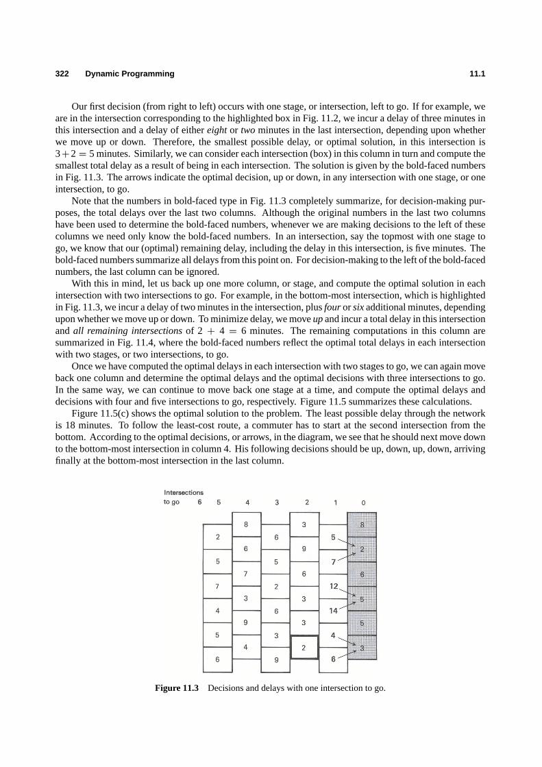
322 Dynamic Programming 11.1
Our first decision (from right to left) occurs with one stage, or intersection, left to go. If for example, weare in the intersection corresponding to the highlighted box in Fig. 11.2, we incur a delay of three minutes inthis intersection and a delay of eithereightor two minutes in the last intersection, depending upon whetherwe move up or down. Therefore, the smallest possible delay, or optimal solution, in this intersection is3+2= 5 minutes. Similarly, we can consider each intersection (box) in this column in turn and compute thesmallest total delay as a result of being in each intersection. The solution is given by the bold-faced numbersin Fig. 11.3. The arrows indicate the optimal decision, up or down, in any intersection with one stage, or oneintersection, to go.
Note that the numbers in bold-faced type in Fig. 11.3 completely summarize, for decision-making pur-poses, the total delays over the last two columns. Although the original numbers in the last two columnshave been used to determine the bold-faced numbers, whenever we are making decisions to the left of thesecolumns we need only know the bold-faced numbers. In an intersection, say the topmost with one stage togo, we know that our (optimal) remaining delay, including the delay in this intersection, is five minutes. Thebold-faced numbers summarize all delays from this point on. For decision-making to the left of the bold-facednumbers, the last column can be ignored.
With this in mind, let us back up one more column, or stage, and compute the optimal solution in eachintersection with two intersections to go. For example, in the bottom-most intersection, which is highlightedin Fig. 11.3, we incur a delay of two minutes in the intersection, plusfourorsixadditional minutes, dependingupon whether we move up or down. To minimize delay, we moveupand incur a total delay in this intersectionandall remaining intersectionsof 2 + 4 = 6 minutes. The remaining computations in this column aresummarized in Fig. 11.4, where the bold-faced numbers reflect the optimal total delays in each intersectionwith two stages, or two intersections, to go.
Once we have computed the optimal delays in each intersection with two stages to go, we can again moveback one column and determine the optimal delays and the optimal decisions with three intersections to go.In the same way, we can continue to move back one stage at a time, and compute the optimal delays anddecisions with four and five intersections to go, respectively. Figure 11.5 summarizes these calculations.
Figure 11.5(c) shows the optimal solution to the problem. The least possible delay through the networkis 18 minutes. To follow the least-cost route, a commuter has to start at the second intersection from thebottom. According to the optimal decisions, or arrows, in the diagram, we see that he should next move downto the bottom-most intersection in column 4. His following decisions should be up, down, up, down, arrivingfinally at the bottom-most intersection in the last column.
Figure 11.3 Decisions and delays with one intersection to go.

11.1 An Elementary Example 323
Figure 11.4 Decisions and delays with two intersections to go.
However, the commuters are probably not free to arbitrarily choose the intersection they wish to startfrom. We can assume that their homes are adjacent to only one of the leftmost intersections, and thereforeeach commuter’s starting point is fixed. This assumption does not cause any difficulty since we have, infact, determined the routes of minimum delay from the downtown parking lots toall the commuter’s homes.Note that this assumes that commuters do not care in which downtown lot they park. Instead of solving theminimum-delay problem for only a particular commuter, we haveembeddedthe problem of the particularcommuter in the more general problem of finding the minimum-delay paths from all homes to the groupof downtown parking lots. For example, Fig. 11.5 also indicates that the commuter starting at the topmostintersection incurs a delay of 22 minutes if he follows his optimal policy of down, up, up, down, and thendown. He presumably parks in a lot close to the second intersection from the top in the last column. Finally,note that three of the intersections in the last column are not entered by any commuter. The analysis hasdetermined the minimum-delay paths from each of the commuter’s homes to the group of downtown parkinglots, not to each particular parking lot.
Using dynamic programming, we have solved this minimum-delay problem sequentially by keeping trackof how many intersections, or stages, there were to go. In dynamic-programming terminology, each pointwhere decisions are made is usually called astageof the decision-making process. At any stage, we needonly know which intersection we are in to be able to make subsequent decisions. Our subsequent decisions donot depend upon how we arrived at the particular intersection. Information that summarizes the knowledgerequired about the problem in order to make the current decisions, such as the intersection we are in at aparticular stage, is called astateof the decision-making process.
In terms of these notions, our solution to the minimum-delay problem involved the following intuitiveidea, usually referred to as theprinciple of optimality.
Any optimal policy has the property that, whatever the current state and decision, the remaining decisionsmust constitute an optimal policy with regard to the state resulting from the current decision.
To make this principle more concrete, we can define theoptimal-value functionin the context of theminimum-delay problem.
vn(sn) = Optimal value (minimum delay) over the current and sub-sequent stages (intersections), given that we are in statesn(in a particular intersection) withn stages (intersections) to go.
The optimal-value function at each stage in the decision-making process is given by the appropriate column

324 Dynamic Programming 11.1
Figure 11.5 Charts of optimal delays and decisions.

11.1 An Elementary Example 325
of Fig. 11.5(c). We can write down arecursiverelationship for computing the optimal-value function byrecognizing that, at each stage, the decision in a particular state is determined simply by choosing theminimum total delay. If we number the states at each stage assn = 1 (bottom intersection) up tosn = 6 (topintersection), then
vn(sn) = Min {tn(sn)+ vn−1(sn−1)} , (1)
subject to:
sn−1 =
sn + 1 if we choose up andn even,
sn − 1 if we choose down andn odd,
sn otherwise,
wheretn(sn) is the delay time in intersectionsn at stagen.The columns of Fig. 11.5(c) are then determined by starting at the right with
v0(s0) = t0(s0) (s0 = 1, 2, . . . , 6), (2)
and successively applying Eq. (1). Corresponding to this optimal-value function is anoptimal-decisionfunction, which is simply a list giving the optimal decision for each state at every stage. For this example,the optimal decisions are given by the arrows leaving each box in every column of Fig. 11.5(c).
The method of computation illustrated above is calledbackward induction, since it starts at the right andmoves back one stage at a time. Its analog,forward induction, which is also possible, starts at the left andmoves forward one stage at a time. The spirit of the calculations is identical but the interpretation is somewhatdifferent. The optimal-value function for forward induction is defined by:
un(sn) = Optimal value (minimum delay) over the current andcompletedstages (intersections), given that we are in statesn(in a particular intersection) withn stages (intersections) to go.
The recursive relationship for forward induction on the minimum-delay problem is
un−1(sn−1) = Min {un(sn)+ tn−1(sn−1)} , (3)
subject to:
sn−1 =
sn + 1 if we choose up andn even,sn − 1 if we choose down andn odd,sn otherwise,
where the stages are numbered in terms of intersections to go. The computations are carried out by setting
u5(s5) = t5(s5) (s5 = 1, 2, . . . , 6), (4)
and successively applying (3). The calculations for forward induction are given in Fig. 11.6. When performingforward induction, the stages are usually numbered in terms of the number of stagescompleted(rather thanthe number of stages to go). However, in order to make a comparison between the two approaches easier, wehave avoided using the ‘‘stages completed" numbering.
The columns of Fig. 11.6(f) give the optimal-value function at each stage for the minimum-delay problem,computed by forward induction. This figure gives the minimum delays from each particular downtown parkinglot to thegroupof homes of the commuters. Therefore, this approach will only guarantee finding the minimumdelay path from the downtown parking lots tooneof the commuters’ homes. The method, in fact, finds theminimum-delay path to a particular origin only if that origin may be reached from a downtown parking lotby a backward sequence of arrows in Fig. 11.6(f).
If we select the minimum-delay path in Fig. 11.6(f), lasting 18 minutes, and follow the arrows backward,we discover that this path leads to the intersection second from the bottom in the first column. This is thesame minimum-delay path determined by backward induction in Fig. 11.5(c).

326 Dynamic Programming 11.1
Figure 11.6 Solution by forward induction.

11.2 Formalizing the Dynamic-Programming Approach 327
Forward induction determined the minimum-delay paths from each individual parking lot to thegroupof homes, while backward induction determined the minimum-delay paths from each individual home to thegroup of downtown parking lots. The minimum-delay path between the two groups is guaranteed to be thesame in each case but, in general, the remaining paths determined may be different. Therefore, when usingdynamic programming, it is necessary to think about whether forward or backward induction is best suitedto the problem you want to solve.
11.2 FORMALIZING THE DYNAMIC-PROGRAMMING APPROACH
The elementary example presented in the previous section illustrates the three most important characteristicsof dynamic-programming problems:
Stages
The essential feature of the dynamic-programming approach is the structuring of optimization problemsinto multiple stages, which are solved sequentially one stage at a time. Although each one-stage problemis solved as an ordinary optimization problem, its solution helps to define the characteristics of the nextone-stage problem in the sequence.
Often, the stages represent different time periods in the problem’s planning horizon. For example, theproblem of determining the level of inventory of a single commodity can be stated as a dynamic program.The decision variable is the amount to order at the beginning of each month; the objective is to minimize thetotal ordering and inventory-carrying costs; the basic constraint requires that the demand for the product besatisfied. If we can order only at the beginning of each month and we want an optimal ordering policy forthe coming year, we coulddecompose the problem into 12 stages, each representing the ordering decision atthe beginning of the corresponding month.
Sometimes the stages do not have time implications. For example, in the simple situation presentedin the preceding section, the problem of determining the routes of minimum delay from the homes of thecommuters to the downtown parking lots was formulated as a dynamic program. The decision variable waswhether to chooseupor downin any intersection, and the stages of the process were defined to be the numberof intersections to go. Problems that can be formulated as dynamic programs with stages that do not havetime implications are often difficult to recognize.
States
Associated with each stage of the optimization problem are thestatesof the process. The states reflectthe information required to fully assess the consequences that the current decision has upon future actions.In the inventory problem given in this section, each stage has only one variable describing the state: theinventory level on hand of the single commodity. The minimum-delay problem also has one state variable:the intersection a commuter is in at a particular stage.
The specification of the states of the system is perhaps the most critical design parameter of the dynamic-programming model. There are no set rules for doing this. In fact, for the most part, this is an art oftenrequiring creativity and subtle insight about the problem being studied. The essential properties that shouldmotivate the selection of states are:
i) The states should convey enough information to make future decisions without regard to how the processreached the current state; and
ii) The number of state variables should be small, since the computational effort associated with the dynamic-programming approach is prohibitively expensive when there are more than two, or possibly three, statevariables involved in the model formulation.
This last feature considerably limits the applicability of dynamic programming in practice.

328 Dynamic Programming 11.2
Recursive Optimization
The final general characteristic of the dynamic-programming approach is the development of arecursiveoptimizationprocedure, which builds to a solution of the overallN-stage problem by first solving a one-stageproblem and sequentially including one stage at a time and solving one-stage problems until the overalloptimum has been found. This procedure can be based on abackward inductionprocess, where the first stageto be analyzed is the final stage of the problem and problems are solved moving back one stage at a time untilall stages are included. Alternatively, the recursive procedure can be based on aforward inductionprocess,where the first stage to be solved is the initial stage of the problem and problems are solved moving forwardone stage at a time, until all stages are included. In certain problem settings, only one of these inductionprocesses can be applied (e.g., only backward induction is allowed in most problems involving uncertainties).
The basis of the recursive optimization procedure is the so-calledprinciple of optimality, which hasalready been stated: an optimal policy has the property that, whatever the current state and decision, theremaining decisions must constitute an optimal policy with regard to the state resulting from the currentdecision.
General Discussion
In what follows, we will formalize the ideas presented thus far. Suppose we have a multistage decisionprocess where thereturn (or cost) for a particularstageis:
fn(dn, sn), (5)
wheredn is a permissibledecisionthat may be chosen from the setDn, andsn is thestateof the process withn stages to go. Normally, the set of feasible decisions,Dn, available at a given stage depends upon the stateof the process at that stage,sn, and could be written formally asDn(sn). To simplify our presentation, wewill denote the set of feasible decisions simply asDn. Now, suppose that there are a total ofN stages in theprocess and we continue to think ofn as the number of stagesremainingin the process. Necessarily, thisview implies a finite number of stages in the decision process and therefore a specific horizon for a probleminvolving time. Further, we assume that the statesn of the system withn stages to go is a full description ofthe system for decision-making purposes and that knowledge of prior states is unnecessary. The next stateof the process depends entirely on the current state of the process and the current decision taken. That is, wecan define atransition functionsuch that, givensn, the state of the process withn stages to go, the subsequentstate of the process with(n− 1) stages to go is given by
sn−1 = tn(dn, sn), (6)
wheredn is the decision chosen for the current stage and state. Note that there is no uncertainty as to whatthe next state will be, once the current state and current decision are known. In Section 11.7, we will extendthese concepts to include uncertainty in the formulation.
Our multistage decision process can be described by the diagram given in Fig. 11.7. Given the currentstatesn which is a complete description of the system for decision-making purposes withn stages to go, wewant to choose the decisiondn that will maximize the total return over the remaining stages. The decisiondn, which must be chosen from a setDn of permissible decisions, produces a return at this stage offn(dn, sn)
and results in a new statesn−1 with (n − 1) stages to go. The new state at the beginning of the next stageis determined by the transition functionsn−1 = tn(dn, sn), and the new state is a complete description of thesystem for decision-making purposes with(n− 1) stages to go. Note that the stage returns are independentof one another.
In order to illustrate these rather abstract notions, consider a simple inventory example. In this case, thestatesn of the system is the inventory levelIn with n months to go in the planning horizon. The decisiondnis the amountOn to order this month. The resulting inventory levelIn−1 with (n− 1) months to go is givenby the usual inventory-balance relationship:
In−1 = In + On − Rn,
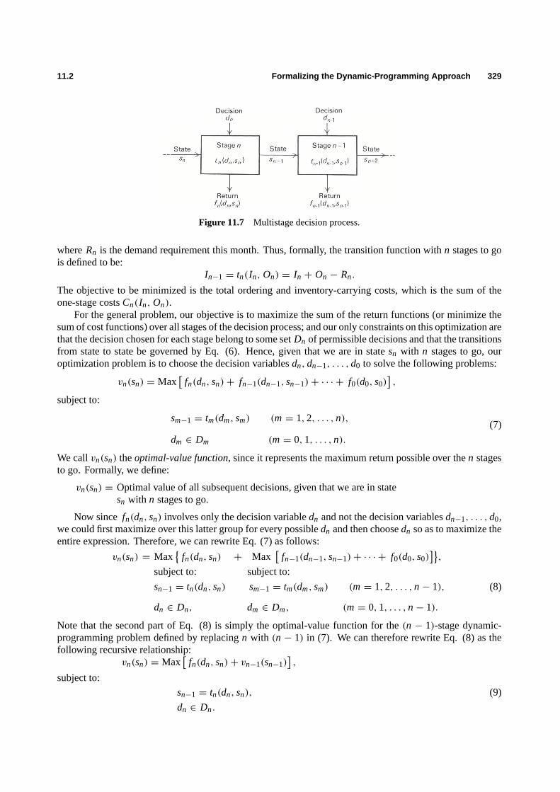
11.2 Formalizing the Dynamic-Programming Approach 329
Figure 11.7 Multistage decision process.
whereRn is the demand requirement this month. Thus, formally, the transition function withn stages to gois defined to be:
In−1 = tn(In, On) = In + On − Rn.
The objective to be minimized is the total ordering and inventory-carrying costs, which is the sum of theone-stage costsCn(In, On).
For the general problem, our objective is to maximize the sum of the return functions (or minimize thesum of cost functions) over all stages of the decision process; and our only constraints on this optimization arethat the decision chosen for each stage belong to some setDn of permissible decisions and that the transitionsfrom state to state be governed by Eq. (6). Hence, given that we are in statesn with n stages to go, ouroptimization problem is to choose the decision variablesdn, dn−1, . . . , d0 to solve the following problems:
vn(sn) = Max[
fn(dn, sn)+ fn−1(dn−1, sn−1)+ · · · + f0(d0, s0)],
subject to:
sm−1 = tm(dm, sm) (m= 1, 2, . . . , n),(7)
dm ∈ Dm (m= 0, 1, . . . , n).
We callvn(sn) theoptimal-value function, since it represents the maximum return possible over then stagesto go. Formally, we define:
vn(sn) = Optimal value of all subsequent decisions, given that we are in statesn with n stages to go.
Now since fn(dn, sn) involves only the decision variabledn and not the decision variablesdn−1, . . . , d0,we could first maximize over this latter group for every possibledn and then choosedn so as to maximize theentire expression. Therefore, we can rewrite Eq. (7) as follows:
vn(sn) = Max{
fn(dn, sn) + Max[
fn−1(dn−1, sn−1)+ · · · + f0(d0, s0)]}
,
subject to: subject to:
sn−1 = tn(dn, sn) sm−1 = tm(dm, sm) (m= 1, 2, . . . , n− 1), (8)
dn ∈ Dn, dm ∈ Dm, (m= 0, 1, . . . , n− 1).
Note that the second part of Eq. (8) is simply the optimal-value function for the(n − 1)-stage dynamic-programming problem defined by replacingn with (n − 1) in (7). We can therefore rewrite Eq. (8) as thefollowing recursive relationship:
vn(sn) = Max[
fn(dn, sn)+ vn−1(sn−1)],
subject to:
sn−1 = tn(dn, sn), (9)
dn ∈ Dn.

330 Dynamic Programming 11.2
To emphasize that this is an optimization overdn, we can rewrite Eq. (9) equivalently as:
vn(sn) = Max{ fn(dn, sn)+ vn−1[tn(dn, sn)]} , (10)
subject to:dn ∈ Dn.
The relationship in either Eq. (9) or (10) is a formal statement of theprinciple of optimality. As we haveindicated, this principle says that an optimal sequence of decisions for a multistage problem has the propertythat, regardless of the current decisiondn and current statesn, all subsequent decisions must be optimal, giventhe statesn−1 resulting from the current decision.
Sincevn(sn) is defined recursively in terms ofvn−1(sn−1), in order to solve Eqs. (9) or (10) it isnecessary to initiate the computation by solving the ‘‘stage-zero" problem. The stage-zero problem is notdefined recursively, since there are no more stages after the final stage of the decision process. The stage-zeroproblem is then the following:
v0(s0) = Max f0(d0, s0), (11)
subject to:d0 ∈ D0.
Often thereis no stage-zero problem, asv0(s0) is identically zero for all final stages. In the simple example ofthe previous section, where we were choosing the path of minimum delay through a sequence of intersections,the stage-zero problem consisted of accepting the delay for the intersection corresponding to each final state.
In this discussion, we have derived the optimal-value function forbackward induction. We could easilyhave derived the optimal-value function forforward induction, as illustrated in the previous section. However,rather than develop the analogous result, we will only state it here. Assuming that we continue to number thestates ‘‘backwards," we can define the optimal-value function for forward induction as follows:
un(sn) = Optimal value of all prior decisions, given that we are in statesnwith n stages to go.
The optimal-value function is then given by:un−1(sn−1) = Max[un(sn)+ fn(dn, sn)] , (12)
subject to:
sn−1 = tn(dn, sn),
dn ∈ Dn,
where the computations are usually initialized by setting
un(sn) = 0,
or by solving some problem, external to the recursive relationship, that gives a value to being in a particularinitial state. Note that, for forward induction, you need to think of the problem as one of examining all thecombinations of current states and actions that produce a specific state at the next stage, and then chooseoptimally among these combinations.
It should be pointed out that nothing has been said about the specific form of the stage-return functionsor the set of permissible decisions at each stage. Hence, what we have said so far holds regardless of whetherthe decisions are discrete, continuous, or mixtures of the two. All that is necessary is that the recursiverelationship be solvable for the optimal solution at each stage, and then aglobal optimal solution to theoverall problem is determined. The optimization problem that is defined at each stage could lead to theapplication of a wide variety of techniques, i.e., linear programming, network theory, integer programming,and so forth, depending on the nature of the transition function, the constraint setDn, and the form of thefunction to be optimized.

11.3 Optimal Capacity Expansion 331
It should also be pointed out that nowhere in developing the fundamental recursive relationship of dynamicprogramming was any use made of the fact that there were a finite number of states at each stage. In fact,Eqs. (9), (10), and (12) hold independent of the number of states. The recursive relationship merely needs tobe solved for all possible states of the system at each stage. If the state space, i.e., the set of possible states, iscontinuous, and therefore an infinite number of states are possible at each stage, then the number of states isusually made finite by making a discrete approximation of the set of possible states, and the same proceduresare used. An example of a dynamic-programming problem with a continuous state space is given in Section11.6.
Finally, we have assumed certainty throughout out discussion so far; this assumption will be relaxed inSection 11.7, and a very similar formal structure will be shown to hold.
11.3 OPTIMAL CAPACITY EXPANSION
In this section, we further illustrate the dynamic-programming approach by solving a problem of optimalcapacity expansion in the electric power industry.
A regional electric power company is planning a large investment in nuclear power plants over the nextfew years. A total of eight nuclear power plants must be built over the next six years because of both increasingdemand in the region and the energy crisis, which has forced the closing of certain of their antiquated fossil-fuel plants. Suppose that, for a first approximation, we assume that demand for electric power in the region isknown with certainty and that we must satisfy the minimum levels of cumulative demand indicated in Table11.1. The demand here has been converted into equivalent numbers of nuclear power plants required by theend of each year. Due to the extremely adverse public reaction and subsequent difficulties with the publicutilities commission, the power company has decided at least to meet this minimum-demand schedule.
The building of nuclear power plants takes approximately one year. In addition to a cost directly associatedwith the construction of a plant, there is a common cost of $1.5 million incurred when any plants areconstructed in any year, independent of the number of plants constructed. This common cost results fromcontract preparation and certification of the impact statement for the Environmental Protection Agency. Inany given year, at most three plants can be constructed. The cost of construction per plant is given in Table11.1 for each year in the planning horizon. These costs are currently increasing due to the elimination of aninvestment tax credit designed to speed investment in nuclear power. However, new technology should beavailable by 1984, which will tend to bring the costs down, even given the elimination of the investment taxcredit.
We can structure this problem as a dynamic program by defining the state of the system in terms ofthe cumulative capacity attained by the end of a particular year. Currently, we have no plants under con-struction, and by the end of each year in the planning horizon we must have completed a number of plantsequal to or greater than the cumulative demand. Further, it is assumed that there is no need ever to con-struct more than eight plants. Figure 11.8 provides a graph depicting the allowable capacity (states) overtime. Any node of this graph is completely described by the corresponding year number and level ofcumulative capacity, say the node(n, p). Note that we have chosen to measure time in terms ofyears to goin the planning horizon. The cost of traversing any upward-sloping arc is the common cost of $1.5 million
Table E11.1 Demand and cost per plant ($×1000)
Cumulative demand Cost per plantYear (in number of plants) ($× 1000)
1981 1 54001982 2 56001983 4 58001984 6 57001985 7 55001986 8 5200

332 Dynamic Programming 11.3
Figure 11.8 Allowable capacity (states) for each tage
plus the plant costs, which depend upon the year of construction and whether 1, 2, or 3 plants are completed.Measured in thousands of dollars, these costs are
1500+ cnxn,
wherecn is the cost per plant in the yearn andxn is the number of plants constructed. The cost for traversingany horizontal arc is zero, since these arcs correspond to a situation in which no plant is constructed in thecurrent year.
Rather than simply developing the optimal-value function in equation form, as we have done previously,we will perform the identical calculations in tableau form to highlight the dynamic-programming methodol-ogy. To begin, we label the final state zero or, equivalently define the ‘‘stage-zero" optimal-value function tobe zero for all possible states at stage zero. We will define a state as the cumulative total number of plantscompleted. Since the only permissible final state is to construct the entire cumulative demand of eight plants,we haves0 = 8 and
v0(8) = 0.Now we can proceed recursively to determine the optimal-value function with one stage remaining. Since thedemand data requires 7 plants by 1985, with one year to go the only permissible states are to have completed7 or 8 plants. We can describe the situation by Tableau 1.
The dashes indicate that the particular combination of current state and decision results in a state that isnot permissible. In this table there are no choices, since, if we have not already completed eight plants, wewill construct one more to meet the demand. The cost of constructing the one additional plant is the $1500common cost plus the $5200 cost per plant, for a total of $6700. (All costs are measured in thousands ofdollars.) The column headedd∗1(s1) gives the optimal decision function, which specifies the optimal numberof plants to construct, given the current state of the system.
Now let us consider what action we should take with two years (stages) to go. Tableau 2 indicates thepossible costs of eachstate:

11.3 Optimal Capacity Expansion 333
Tableau 1
Tableau 2
If we have already completed eight plants with two years to go, then clearly we will not construct anymore. If we have already completed seven plants with two years to go, then we can either construct the oneplant we need this year or postpone its construction. Constructing the plant now costs $1500 in commoncosts plus $5500 in variable costs, and results in state 8 with one year to go. Since the cost of state 8 with oneyear to go is zero, the total cost over the last two years is $7000. On the other hand, delaying constructioncosts zero this year and results in state 7 with one year to go. Since the cost of state 7 with one year to go is$6700, the total cost over the last two years is $6700. If we arrive at the point where we have two years to goand have completed seven plants, it pays to delay the production of the last plant needed. In a similar way,we can determine that the optimal decision when in state 6 with two years to go is to construct two plantsduring the next year.
To make sure that these ideas are firmly understood, we will determine the optimal-value function andoptimal decision with three years to go. Consider Tableau 3 for three years to go:
Tableau 3
Now suppose that, with three years to go, we have completed five plants. We need to construct at leastone plant this year in order to meet demand. In fact, we can construct either 1, 2, or 3 plants. If we constructone plant, it costs $1500 in common costs plus $5700 in plant costs, and results in state 6 with two years togo. Since the minimum cost following the optimal policy for the remaining two years is then $12,500, ourtotal cost for three years would be $19,700. If we construct two plants, it costs the $1500 in common costsplus $11,400 in plant costs and results in state 7 with two years to go. Since the minimum cost following theoptimal policy for the remaining two years is then $6700, our total cost for three years would be $19,600.Finally, if we construct three plants, it costs the $1500 in common costs plus $17,100 in plant costs andresults in state 8 with two years to go. Since the minimum cost following the optimal policy for the remaining

334 Dynamic Programming 11.4
Figure 11.9 Tableaus to complete power-plant example.
two years is then zero, our total cost for three years would be $18,600. Hence, the optimal decision, havingcompleted five plants (being in state 5) with three years (stages) to go, is to construct three plants this year.The remaining tableaus for the entire dynamic-programming solution are determined in a similar manner (seeFig. 11.9).
Since we start the construction process with no plants (i.e., in state 0) with six years (stages) to go, wecan proceed to determine the optimal sequence of decisions by considering the tableaus in the reverse order.With six years to go it is optimal to construct three plants, resulting in state 3 with five years to go. It is thenoptimal to construct three plants, resulting in state 6 with four years to go, and so forth. The optimal policyis then shown in the tabulation below:
Years Resultingto go Construct state
6 3 35 3 64 0 63 0 62 2 81 0 8
Hence, from Tableau 6, the total cost of the policy is $48.8 million.
11.4 DISCOUNTING FUTURE RETURNS
In the example on optimal capacity expansion presented in the previous section, a very legitimate objectionmight be raised that thepresent value of moneyshould have been taken into account in finding the optimalconstruction schedule. The issue here is simply that a dollar received today is clearly worth more than a

11.4 Discounting Future Returns 335
dollar received one year from now, since the dollar received today could be invested to yield some additionalreturn over the intervening year. It turns out that dynamic programmingis extremely well suited to take thisinto account.
We will define, in the usual way, the one-perioddiscount factorβ as the present value of one dollarreceivedone period from now. In terms of interest rates, if the interest rate for the period werei , then onedollar invested now would accumulate to(1 + i ) at the end of one period. To see the relationship betweenthe discount factorβ and the interest ratei , we ask the question ‘‘How much must be invested now to yieldone dollar one period from now?" This amount is clearly the present value of a dollar received one periodfrom now, so thatβ(1+ i ) = 1 determines the relationship betweenβ andi , namely,β = 1/(1 + i ). If weinvest one dollar now forn periods at an interest rate per period ofi , then theaccumulated value at the endof n periods, assuming the interest is compounded, is(1 + i )n. Therefore, the present value of one dollarreceivedn periods from now is 1/(1+ i )n or, equivalently,βn.
The concept of discounting can be incorporated into the dynamic-programming framework very easilysince we often have a return per period (stage) that we may wish to discount by the per-period discount factor.If we have ann-stage dynamic-programming problem, the optimal-value function, including the appropriatediscounting of future returns, is given by
vn(sn) = Max [ fn(dn, sn) +β fn−1(dn−1, sn−1)+ β2 fn−2(dn−2, sn−2)
+ · · · + βn f0(d0, s0)],
subject to:sm−1 = tm(dm, sm)(m= 1, 2, . . . , n),
(13)dm ∈ Dm, (m= 0, 1, . . . , n),
where the stages (periods) are numbered in terms ofstages to go. Making the same argument as in Section11.3 and factoring out theβ, we can rewrite Eq. (13) as:
vn(sn) = Max { fn(dn, sn)+ β Max [ fn−1(dn−1, sn−1) + β fn−2(dn−2, sn−2)
+ · · · + βn−1 f0(d0, s0)],
subject to: subject to:sn−1 = tn(dn, sn) sm−1 = tm(dm, sm) (m= 1, 2, . . . , n− 1),
dn ∈ Dn dm ∈ Dm (m= 0, 1, . . . , n− 1).
(14)
Since the second part of Eq. (14) is simply the optimal-value function for the(n−1)-stage problem multipliedby β, we can rewrite Eq. (14) as
vn(sn) = Max[ fn(dn, sn)+ βvn−1(sn−1)],
subject to:sn−1 = tn(dn, sn), (15)
dn ∈ Dn,
which is simply the recursive statement of the optimal-value function for backward induction with discounting.If β = 1, we have the case ofno discountingand Eq. (15) is identical to Eq. (9). Finally, if the discount ratedepends on the period,β can be replaced byβn and (15) still holds.
We can look at the impact of discounting future-stage returns by considering again the optimal capacityexpansion problem presented in the previous section. Suppose that the alternative uses of funds by the electricpower company result in a 15 percent return on investment. This corresponds to a yearly discount factor ofapproximately 0.87. If we merely apply backward induction to the capacity expansion problem according toEq. (15), usingβ = 0.87, we obtain the optimal-value function for each stage as given in Fig. 11.10.

336 Dynamic Programming 11.4
Figure 11.10 Optimal-value and decision functions with discounting.

∗11.5 Shortest Paths in a Network 337
Given that the system is in state zero with six stages to go, we determine the optimal construction strategyby considering the optimal decision functiond∗n(sn) from stage 6 to stage 0. The optimal constructionsequence is then shown in the following tabulation:
Stages Resultingto go Construct state
6 2 25 0 24 2 43 3 72 0 71 1 8
and the optimal value of the criterion function,present value of total future costs, is $37.8 million for thisstrategy. Note that this optimal strategy is significantly different from that computed in the previous sectionwithout discounting. The effect of the discounting of future costs is to delay construction in general, whichis what we would expect.
∗11.5 SHORTEST PATHS IN A NETWORK
Although we have not emphasized this fact, dynamic-programming and shortest-path problems are verysimilar. In fact, as illustrated by Figs. 11.1 and 11.8, our previous examples of dynamic programming canboth be interpreted as shortest-path problems.
In Fig. 11.8, we wish to move through the network from the starting node (initial state) at stage 6, withno plants yet constructed, to the end node (final state) at stage 0 with eight plants constructed. Every path inthe network specifies a strategy indicating how many new plants to construct each year.
Since the cost of a strategy sums the cost at each stage, the total cost corresponds to the ‘‘length" of apath from the starting to ending nodes. The minimum-cost strategy then is just the shortest path.
Figure 11.11 illustrates a shortest-path network for the minimum-delay problem presented in Section11.1. The numbers next to the arcs are delay times. An end node representing the group of downtownparking lots has been added. This emphasizes the fact that we have assumed that the commuters do not carein which lot they park. A start node has also been added to illustrate that the dynamic-programming solutionby backwardinduction finds the shortest path from the end node to the start node. In fact, it finds the shortestpaths from the end node toall nodes in the network, thereby solving the minimum-delay problem for eachcommuter. On the other hand, the dynamic-programming solution byforward induction finds the shortestpath from the start node to the end node. Although theshortest pathwill be the same for both methods,forward induction willnotsolve the minimum-delay problem forall commuters, since the commuters are notindifferent to which home they arrive.
To complete the equivalence that we have suggested between dynamic programming and shortest paths,we next show how shortest-path problems can be solved by dynamic programming. Actually, several differentdynamic-programming solutions can be given, depending upon the structure of the network under study. Asa general rule, the morestructuredthe network, the more efficient the algorithm that can be developed. Toillustrate this point we give two separate algorithms applicable to the following types of networks:
i) Acyclic networks.These networks contain no directed cycles. That is, we cannot start from any node andfollow the arcs in their given directions to return to the same node.
ii) Networks without negative cycles.These networks may contain cycles, but the distance around any cycle(i.e., the sum of the lengths of its arcs) must be nonnegative.
In the first case, to take advantage of the acyclic structure of the network, we order the nodes so that, if thenetwork contains the arci – j , theni > j . To obtain such an ordering, begin with the terminal node, which canbe thought of as having only entering arcs, and number it ‘‘one." Then ignore that node and the incident arcs,and number any node that has only incoming arcs as the next node. Since the network is acyclic, there must be

338 Dynamic Programming ∗11.5
Figure 11.11 Shortest-path network for minimum-delay problem.
such a node. (Otherwise, from any node, we can move along an arc to another node. Starting from any nodeand continuing to move away from any node encountered, we eventually would revisit a node, determininga cycle, contradicting the acyclic assumption.) By ignoring the numbered nodes and their incident arcs, theprocedure is continued until all nodes are numbered.
This procedure is applied, in Fig. 11.12, to the longest-path problem introduced as a critical-path schedul-ing example in Section 8.1.
Figure 11.12 Finding the longest path in an acyclic network.
We can apply the dynamic-programming approach by viewing each node as a stage, using either backwardinduction to consider the nodes in ascending order, or forward induction to consider the nodes in reverse order.For backward induction,vn will be interpreted as the longest distance from noden to the end node. Settingv1 = 0, dynamic programming determinesv2, v3, . . . , vN in order, by the recursion
vn = Max[dnj + v j ], j < n,
wherednj is the given distance on arcn– j . The results of this procedure are given as node labels in Fig. 11.12for the critical-path example.
For a shortest-path problem, we use minimization instead of maximization in this recursion. Note thatthe algorithm finds the longest (shortest) paths from every node to the end node. If we want only the longestpath to the start node, we can terminate the procedure once the start node has been labeled. Finally, we couldhave found the longest distances from the start node to all other nodes by labeling the nodes in the reverseorder, beginning with the start node.

∗11.5 Shortest Paths in a Network 339
Figure 11.13 Shortest paths in a network without negative cycles.
A more complicated algorithm must be given for the more general problem of finding the shortest pathbetween two nodes, say nodes 1 andN, in a network without negative cycles. In this case, we can devise adynamic-programming algorithm based upon a value function defined as follows:
vn( j ) = Shortest distance from node 1 to nodej along paths using atmostn intermediate nodes.
By definition, then,v0( j ) = d1 j for j = 2, 3, . . . , N,
the lengthd1 j of arc 1–j since no intermediate nodes are used. The dynamic-programming recursion is
vn( j ) = Min {di j + vn−1(i )}, 1≤ j ≤ N, (16)
which uses the principle of optimality: that any path from node 1 to nodej , using at mostn intermediatenodes, arrives at nodej from nodei along arci – j after using the shortest path with at most(n− 1) interme-diate nodes from nodej to nodei . We allowi = j in the recursion and taked j j = 0, since the optimal pathusing at mostn intermediate nodes may coincide with the optimal path with lengthvn−1( j ) using at most(n− 1) intermediate nodes.
The algorithm computes the shortest path from node 1 to every other node in the network. It terminateswhenvn( j ) = vn−1( j ) for every nodej , since computations in Eq. (16) will be repeated at every stage fromn on. Because no path (without cycles) uses any more than(N − 1) intermediate nodes, whereN is the totalnumber of nodes, the algorithm terminates after at most(N − 1) steps.
As an application of the method, we solve the shortest-path problem introduced in Chapter 8 and givenin Fig. 11.13.
Initially the valuesv0( j ) are given by
v0(1) = 0, v0(2) = d12 = 5.1, v0(3) = d13 = 3.4,
andv0( j ) = ∞ for j = 4, 5, 6, 7, 8,
since these nodes are not connected to node 1 by an arc. The remaining steps are specified in Tableaus 7,8, and 9. The computations are performed conveniently by maintaining a table of distancesdi j . If the listv0(i ) is placed to the left of this table, then recursion Eq. (14) states thatv1( j ) is given by the smallest of thecomparisons:
v0(i )+ di j for i = 1, 2, . . . , 8.
That is, place the columnv0(i ) next to thej th column of thedi j table, add the corresponding elements, andtakev1( j ) as the smallest of the values. Ifv1( j ) is recorded below thej th column, the next iteration to findv2( j ) is initiated by replacing the columnv0(i ) with the elementsv1( j ) from below the distance table.
As the reader can verify, the next iteration givesv4( j ) = v3( j ) for all j . Consequently, the valuesv3( j )recorded in Tableau 9 are the shortest distances from node 1 to each of the nodesj = 2, 3, . . . , 8.
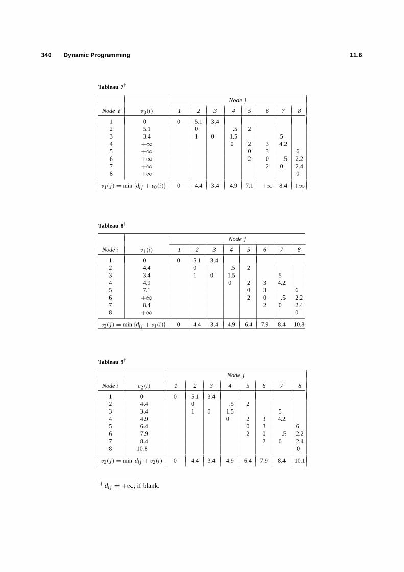
340 Dynamic Programming 11.6
Tableau 7†
Node j
Node i v0(i ) 1 2 3 4 5 6 7 8
1 0 0 5.1 3.42 5.1 0 .5 23 3.4 1 0 1.5 54 +∞ 0 2 3 4.25 +∞ 0 3 66 +∞ 2 0 .5 2.27 +∞ 2 0 2.48 +∞ 0
v1( j ) = min {di j + v0(i )} 0 4.4 3.4 4.9 7.1 +∞ 8.4 +∞
Tableau 8†
Node j
Nodei v1(i ) 1 2 3 4 5 6 7 8
1 0 0 5.1 3.42 4.4 0 .5 23 3.4 1 0 1.5 54 4.9 0 2 3 4.25 7.1 0 3 66 +∞ 2 0 .5 2.27 8.4 2 0 2.48 +∞ 0
v2( j ) = min {di j + v1(i )} 0 4.4 3.4 4.9 6.4 7.9 8.4 10.8
Tableau 9†
Node j
Nodei v2(i ) 1 2 3 4 5 6 7 8
1 0 0 5.1 3.42 4.4 0 .5 23 3.4 1 0 1.5 54 4.9 0 2 3 4.25 6.4 0 3 66 7.9 2 0 .5 2.27 8.4 2 0 2.48 10.8 0
v3( j ) = min di j + v2(i ) 0 4.4 3.4 4.9 6.4 7.9 8.4 10.1
† di j = +∞, if blank.

11.6 Continuous State-Space Problems 341
11.6 CONTINUOUS STATE-SPACE PROBLEMS
Until now we have dealt only with problems that have had a finite number of states associated with eachstage. Since we also have assumed a finite number of stages, these problems have been identical to findingthe shortest path through a network with special structure. Since the development, in Section 11.3, of thefundamental recursive relationship of dynamic programming did not depend on having a finite number ofstates at each stage, here we introduce an example that has a continuous state space and show that the sameprocedures still apply.
Suppose that some governmental agency is attempting to perform cost/benefit analysis on its programs inorder to determine which programs should receive funding for the next fiscal year. The agency has managed toput together the information in Table 11.2. The benefits of each program have been converted into equivalenttax savings to the public, and the programs have been listed by decreasing benefit-to-cost ratio. The agencyhas taken the position that there will be no partial funding of programs. Either a programwill be funded atthe indicated level or it willnotbe considered for this budget cycle. Suppose that the agency is fairly sure ofreceiving a budget of $34 million from the state legislature if it makes a good case that the money is beingused effectively. Further, suppose that there is some possibility that the budget will be as high as $42 million.How can the agency make the most effective use of its funds ateitherpossible budget level?
Table 11.2 Cost/benefit information by program.
Program Expected benefit Expected cost Benefit/Cost
A $ 59.2 M $ 2.8 M 21.1B 31.4 1.7 18.4C 15.7 1.0 15.7D 30.0 3.2 9.4E 105.1 15.2 6.9F 11.6 2.4 4.8G 67.3 16.0 4.2H 2.3 .7 3.3I 23.2 9.4 2.5J 18.4 10.1 1.8
$364.2 M $62.5 M
We should point out that mathematically this problem is an integer program. Ifb j is the benefit of thej th program andc j is the cost of that program, then an integer-programming formulation of the agency’sbudgeting problem is determined easily.Letting
x j =
{1 if program j is funded,
0 if program j is not funded,
the integer-programming formulation is:
Maximizen∑
j=1
b j x j ,
subject to:n∑
j=1
c j x j ≤ B,
x j = 0 or 1 ( j = 1, 2, . . . , n),

342 Dynamic Programming 11.6
whereB is the total budget allocated. This cost/benefit example is merely a variation of the well-knownknapsack problem that was introduced in Chapter 9.We will ignore, for the moment, this integer-programmingformulation and proceed to develop a highly efficient solution procedure using dynamic programming.
In order to approach this problem via dynamic programming, we need to define the stages of the system,the state space for each stage, and the optimal-value function.Let
vk(B) = Maximum total benefit obtainable, choosing from the firstk programs, with budget limitationB.
With this definition of the optimal-value function, we are letting the firstk programs included be the numberof ‘‘stages to go" and the available budget at each stage be the state space. Since the possible budget mighttake on any value, we are allowing for a continuous state space for each stage. In what follows the order ofthe projects is immaterial although the order given in Table 11.2 may have some computational advantages.
Let us apply the dynamic-programming reasoning as before. It is clear that withk = 0 programs, thetotal benefit must be zero regardless of the budget limitation. Therefore
v0(B0) = 0 for B0 ≥ 0.
If we now letk = 1, it is again clear that the optimal-value function can be determined easily since the budgetis either large enough to fund the first project, ornot. (See Tableau 10.)
Tableau 10
Now consider which programs to fund when the first two programs are available. The optimal-valuefunctionv2(B2) and optimal decision functiond∗2(B2) are developed in Tableau 11.
Tableau 11
Here again the dash means that the current state and decision combination will result in a state that is notpermissible. Since this tableau is fairly simple, we will go on and develop the optimal-value functionv3(B3)
and optimal decision functiond∗3(B3) when the first three programs are available (see Tableau 12).For any budget level, for example, $4.0 M, we merely consider the two possible decisions: either funding
programC (x3 = 1) or not (x3 = 0). If we fund programC, then we obtain a benefit of $15.7 M whileconsuming $1.0 M of our own budget. The remaining $3.0 M of our budget is then optimally allocated to theremaining programs, producing a benefit of $59.2 M, which we obtain from the optimal-value function withthe first two programs included (Tableau 11). If we do not fund programC, then the entire amount of $4.0 Mis optimally allocated to the remaining two programs (Tableau 11), producing a benefit of $59.2. Hence, weshould clearly fund programC if our budget allocation is $4.0 M. Optimal decisions taken for other budgetlevels are determined in a similar manner.

11.7 Dynamic Programming under Uncertainty 343
Tableau 12
Although it is straightforward to continue the recursive calculation of the optimal-value function forsucceeding stages, we will not do so since the number of ranges that need to be reported rapidly becomesrather large. The general recursive relationship that determines the optimal-value function at each stage isgiven by:
vn(Bn) = Max [cnxn + vn−1(Bn − cnxn)],
subject to:xn = 0 or 1.
The calculation is initialized by observing that
v0(B0) = 0
for all possible values ofB0. Note that the state transition function is simply
Bn−1 = tn(xn, Bn) = Bn − cnxn.
We can again illustrate the usual principle of optimality: Given budgetBn at stagen, whatever decision ismade with regard to funding thenth program, the remaining budget must be allocated optimally among thefirst (n− 1) programs. If these calculations were carried to completion, resulting inv10(B10) andd∗10(B10),then the problem would be solved for all possible budget levels, not just $3.4 M and $4.2 M.
Although this example has a continuous state space, a finite number of ranges can be constructed becauseof the zero–one nature of the decision variables. In fact, all breaks in the range of the state space either arethe breaks from the previous stage, or they result from adding the cost of the new program to the breaks inthe previous range. This is not a general property of continuous state space problems, and in most casessuch ranges cannot be determined. Usually, what is done for continuous state space problems is that theyare converted into discrete state problems by defining an appropriate grid on the continuous state space. Theoptimal-value function is then computed only for the points on the grid. For our cost/benefit example, thetotal budget must be between zero and $62.5 M, which provides a range on the state space, although at anystage a tighter upper limit on this range is determined by the sum of the budgets of the firstn programs. Anappropriate grid would consist of increments of $0.1 M over the limits of the range at each stage, since thisis the accuracy with which the program costs have been estimated. The difference between problems withcontinuous state spaces and those with discrete state spaces essentially then disappears for computationalpurposes.
11.7 DYNAMIC PROGRAMMING UNDER UNCERTAINTY
Up to this point we have considered exclusively problems with deterministic behavior. In a deterministicdynamic-programming process, if the system is in statesn with n stages to go and decisiondn is selectedfrom the set of permissible decisions for this stage and state, then the stage returnfn(dn, sn) and the state of

344 Dynamic Programming 11.7
Figure 11.14 Decision tree for deterministic dynamic programming.
the system at the next stage, given bysn−1 = tn(dn, sn), are both known with certainty. This deterministicprocess can be represented by means of the decision tree in Fig. 11.14. As one can observe, given the currentstate, a specific decision leads with complete certainty to a particular state at the next stage. The stage returnsare also known with certainty and are associated with the branches of the tree.
When uncertainty is present in a dynamic-programming problem, a specific decision for a given state andstage of the process does not, by itself, determine the state of the system at the next stage; this decision maynot even determine the return for the current stage. Rather, in dynamic programming under uncertainty, giventhe state of the systemsn with n stages to go and the current decisiondn, an uncertain event occurs which isdetermined by a random variableen whose outcomeen is not under the control of the decision maker. Thestage return function may depend on this random variable, that is,
fn(dn, sn, en),
while the state of the systemsn−1 with (n− 1) stages to go invariably will depend on the random variable by
sn−1 = tn(dn, sn, en).
The outcomes of the random variable are governed by a probability distribution,pn(en|dn, sn), whichmay be the same for every stage or may be conditional on the stage, the state at the current stage, and eventhe decision at the current stage.
Figure 11.15 depicts dynamic programming under uncertainty as adecision tree, where squares representstates where decisions have to be made and circles represent uncertain events whose outcomes are not underthe control of the decision maker. These diagrams can be quite useful in analyzing decisions under uncertaintyif the number of possible states is not too large. The decision tree provides a pictorial representation of thesequence of decisions, outcomes, and resulting states,in the order in whichthe decisions must be made andthe outcomes become known to the decision maker. Unlike deterministic dynamic programming wherein the

11.7 Dynamic Programming under Uncertainty 345
optimal decisions at each stage can be specified at the outset, in dynamic programming under uncertainty,the optimal decision at each stage can be selected only after we know the outcome of the uncertain event atthe previous stage. At the outset, all that can be specified is a set of decisions that would be madecontingenton the outcome of a sequence of uncertain events.
Figure 11.15 Decision tree for dynamic programming under uncertainty.
In dynamic programming under uncertainty, since the stage returns and resulting stage may both beuncertain at each stage, we cannot simply optimize the sum of the stage-return functions. Rather, we mustoptimize theexpected returnover the stages of the problem, taking into account the sequence in whichdecisions can be made and the outcomes of uncertain events become known to the decision maker. In thissituation, backward induction can be applied to determine the optimal strategy, but forward induction cannot.The difficulty with forward induction is that it is impossible to assign values to states at the next stage thatare independent of the uncertain evolution of the process from that future state on. With backward induction,on the other hand, no such difficulties arise since the states with zero stages to go are evaluated first, and thenthe states with one stage to go are evaluated by computing the expected value of any decision and choosing

346 Dynamic Programming 11.7
optimally.We start the backward induction process by computing the optimal-value function at stage 0. This
amounts to determining the value of ending in each possible stage with 0 stages to go. This determinationmay involve an optimization problem or the value of the assets held at the horizon. Next, we compute theoptimal-value function at the previous stage. To do this, we first compute the expected value of each uncertainevent, weighting the stage return plus the value of the resulting state for each outcome by the probability ofeach outcome. Then, for each state at the previous stage, we select the decision that has the maximum (orminimum) expected value. Once the optimal-value function for stage 1 has been determined, we continue ina similar manner to determine the optimal-value functions at prior stages by backward induction.
The optimal-value function for dynamic programming under uncertainty is then defined in the followingrecursive form:
vn(sn) = Max E[
fn(dn, sn, en)+ vn−1(sn−1)], (17)
subject to:sn−1 = tn(dn, sn, en),
dn ∈ Dn,
whereE[·] denotes the expected value of the quantity in brackets. To initiate the recursive calculations weneed to determine the optimal-value function with zero stages to go, which is given by:
v0(s0) = Max E[
f0(d0, s0, e0)],
subject to:d0 ∈ D0.
The optimization problems that determine the optimal-value function with zero stages to go are not determinedrecursively, and therefore may be solved in a straight-forward manner. If the objective function is to maximizethe expected discounted costs, then Eq. (17) is modified as in Section 11.4 by multiplying the termvn−1(sn−1)
by βn, the discount factor for periodn.We can make these ideas more concrete by considering a simple example. A manager is in charge of
the replenishment decisions during the next two months for the inventory of a fairly expensive item. Theproduction cost of the item is $1000/unit, and its selling price is $2000/unit. There is an inventory-carryingcost of $100/unit per month on each unit left over at the end of the month. We assume there is no setup costassociated with running a production order, and further that the production process has a short lead time;therefore any amount produced during a given month is available to satisfy the demand during that month.At the present time, there is no inventory on hand. Any inventory left at the end of the next two months hasto be disposed of at a salvage value of $500/unit.
The demand for the item is uncertain, but its probability distribution is identical for each of the comingtwo months. The probability distribution of the demand is as follows:
Demand Probability
0 0.251 0.402 0.203 0.15
The issue to be resolved is how many units to produce during the first month and,depending on the actualdemand in the first month, how many units to produce during the second month. Since demand is uncertain,the inventory at the end of each month is also uncertain. In fact, demand could exceed the available unitson hand in any month, in which case all excess demand results in lost sales. Consequently, our productiondecision must find the proper balance between production costs, lost sales, and final inventory salvage value.

11.7 Dynamic Programming under Uncertainty 347
The states for this type of problem are usually represented by the inventory levelIn at the beginning ofeach month. Moreover, the problem is characterized as a two-stage problem, since there are two monthsinvolved in the inventory-replenishment decision. To determine the optimal-value function, let
vn(In) = Maximum contribution, given that we haveIn units of inventorywith n stages to go.
We initiate the backward induction procedure by determining the optimal-value function with 0 stages togo. Since the salvagevalue is $500/unit, we have:
I0 v0(I0)
0 01 5002 10003 1500
To compute the optimal-value function with one stage to go, we need to determine, for each inventorylevel (state), the corresponding contribution associated with each possible production amount (decision) andlevel of sales (outcome). For each inventory level, we select the production amount that maximizes theexpected contribution.
Table 11.3 provides all the necessary detailed computations to determine the optimal-value function withone stage to go. Column 1 gives the state (inventory level) of the process with one stage to go. Column 2 givesthe possible decisions (amount to produce) for each state, and, since demand cannot be greater than three, theamount produced is at most three. Column 3 gives the possible outcomes for the uncertain level of sales foreach decision and current state, and column 4 gives the probability of each of these possible outcomes. Notethat, in any period, it is impossible to sell more than the supply, which is the sum of the inventory currentlyon hand plus the amount produced. Hence, the probability distribution of sales differs from that of demandsince, whenever demand exceeds supply, the entire supply is sold and the excess demand is lost. Column 5 isthe resulting state, given that we currently haveI1 on hand, produced1, and sells1. The transition functionin general is just:
In−1 = In + dn − sn,
where the tildes(∼) indicate that the level of sales is uncertain and, hence, the resulting state is also uncertain.Columns 6, 7, and 8 reflect the revenue and costs for each state, decision, and sales level, and column 9 reflectsthe value of being in the resulting state at the next stage. Column 10 merely weights the sum of columns6 through 9 by the probability of their occurring, which is an intermediate calculation in determining theexpected value of making a particular decision, given the current state. Column 11 is then just this expectedvalue; and the asterisk indicates the optimal decision for each possible state.

348 Dynamic Programming 11.7
Table 11.3 Computation of optimal-value function with one stage to go.
(1) (2) (3) (4) (5) (6) (7) (8) (9) (10) (11)Pro- Proba- Resulting Produc- Sales Inven- Proba- Expected
State duce Sell bility state tion rev- tory bility contri-I1 d1 s1 (s1 = s1) I0 cost enue cost v0(I0) × $ bution
0 0 0 1. 0 0 0 0 0 0 01 0 .25 1 −1000 0 −100 500 −150
1 .75 0 −1000 2000 0 0 750
}600∗
2 0 .25 2 −2000 0 −200 1000 −3001 .40 1 −2000 2000 −100 500 1602 .35 0 −2000 4000 0 0 700
560
3 0 .25 3 −3000 0 −300 1500 −4501 .40 2 −3000 2000 −200 1000 −802 .20 1 −3000 4000 −100 500 2803 .15 0 −3000 6000 0 0 450
200
1 0 0 .25 1 0 0 −100 500 1001 .75 0 0 2000 0 0 1500
}1600∗
1 0 .25 2 −1000 0 −200 1000 −501 .40 1 −1000 2000 −100 500 5602 .35 0 −1000 4000 0 0 1050
1560
2 0 .25 3 −2000 0 −300 1500 −2001 .40 2 −2000 2000 −200 1000 3202 .20 1 −2000 4000 −100 500 4803 .15 0 −2000 6000 0 0 600
1200
2 0 0 .25 2 0 0 −200 1000 2001 .40 1 0 2000 −100 500 9602 .35 0 0 4000 0 0 1400
2560∗
1 0 .25 3 −1000 0 −300 1500 501 .40 2 −1000 2000 −200 1000 7202 .20 1 −1000 4000 −100 500 6803 .15 0 −1000 6000 0 0 750
2200
3 0 0 .25 3 0 0 −300 1500 3001 .40 2 0 2000 −200 1000 11202 .20 1 0 4000 −100 500 8803 .15 0 0 6000 0 0 900
3200∗

11.7 Dynamic Programming under Uncertainty 349
The resulting optimal-value function and the corresponding optimal-decision function are determineddirectly from Table 11.3 and are the following:
I1 v1(I1) d∗1(I1)
0 600 11 1600 02 2560 03 3200 0
Next we need to compute the optimal-value function with two stagesto go. However, since we haveassumed that there is no initial inventory on hand, it is not necessary to describe the optimal-value functionfor every possible state, but only forI2 = 0. Table 11.4 is similar to Table 11.3 and gives the detailedcomputations required to evaluate the optimal-value function for this case.
Table 11.4 Computation of optimal-value function with two stages to go,I2 = 0 only.
(1) (2) (3) (4) (5) (6) (7) (8) (9) (10) (11)Pro- Proba- Result- Produc- Sales Inven- Proba- Expected
State duce Sell bility ing tion rev- tory bility contri-I2 d2 s2 (s2 = s2) state I1 cost enue cost v1(I1) × $ bution
0 0 0 1. 0 0 0 0 650. 650 6501 0 .25 1 −1000 0 0 1600. 150
1 .75 0 −1000 2000 0 600. 1200
}1350
2 0 .25 2 −2000 0 −200 2560. 901 .40 1 −2000 2000 −100 1600. 6002 .35 0 −2000 4000 0 600 910
1600.∗
3 0 .25 3 −3000 0 −300 3200. −251 .40 2 −3000 2000 −200 2560. 5442 .20 1 −3000 4000 −100 1600. 5003 .15 0 −3000 6000 0 600. 540
1559
The optimal-value function and the corresponding decision function forI2 = 0 are taken directly fromTable 11.4 and are the following:
I2 v2(I2) d∗2(I2)
0 1600 2
The optimal strategy can be summarized by the decision tree given in Fig. 11.16. The expected contri-bution determined by the dynamic-programming solution corresponds to weighting the contribution of everypath in this tree by theprobability that this path occurs. The decision tree in Fig. 11.16 emphasizes thecontingent nature of the optimal strategy determined by dynamic programming under uncertainty.
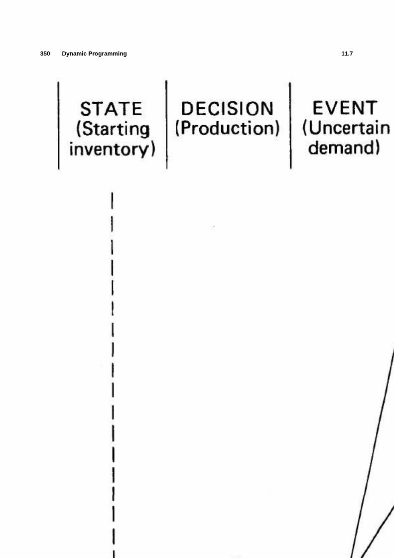
350 Dynamic Programming 11.7
Exercises 351
EXERCISESSolutions to exercises marked with an asterisk (∗) involve extensive computations. Formulate these problems as dynamicprograms and provide representative computations to indicate the nature of the dynamic programming recursions; solveto completion only if a computer system is available.
1. In solving the minimum-delay routing problem in Section 11.1, we assumed the same delay along each street (arc)in the network. Suppose, instead, that the delay when moving along any arc upward in the network is 2 units greaterthan the delay when moving along any arc downward. The delay at the intersections is still given by the data inFig. 11.1. Solve for the minimum-delay route by both forward and backward induction.
2. Decatron Mills has contracted to deliver 20 tons of a special coarsely ground wheat flour at the end of the currentmonth, and 140 tons at the end of the next month. The production cost, based on which the Sales Department hasbargained with prospective customers, isc1(x1) = 7500+ (x1 − 50)2 per ton for the first month, andc2(x2) =
7500+ (x2 − 40)2 per ton for the second month;x1 andx2 are the number of tons of the flour produced in thefirst and second months, respectively. If the company chooses to produce more than 20 tons in the first month, anyexcess production can be carried to the second month at a storage cost of $3 per ton.
Assuming that there is no initial inventory and that the contracted demands must be satisfied in each month(that is, no back-ordering is allowed), derive the production plan that minimizes total cost. Solve by both backwardand forward induction. Considerx1 andx2 as continuous variables, since any fraction of a ton may be produced ineither month.
3. A construction company has four projects in progress. According to the current allocation of manpower, equipment,and materials, the four projects can be completed in 15, 20, 18, and 25 weeks. Management wants to reduce thecompletion times and has decided to allocate an additional $35,000 to all four projects. The new completion timesas functions of the additional funds allocated to each projects are given in Table E11.1.
How should the $35,000 be allocated among the projects to achieve the largest total reduction in completiontimes? Assume that the additional funds can be allocated only in blocks of $5000.
Table E11.1 Completion times (in weeks)
Additional funds(×1000 dollars) Project 1 Project 2 Project 3 Project 4
0 15 20 18 255 12 16 15 21
10 10 13 12 1815 8 11 10 1620 7 9 9 1425 6 8 8 1230 5 7 7 1135 4 7 6 10
4. The following table specifies the unit weights and values of five products held in storage. The quantity of each itemis unlimited.
Product Weight(Wi ) Value(Vi )
1 7 92 5 43 4 34 3 25 1 1
2
352 Dynamic Programming
A plane with a capacity of 13 weight units is to be used to transport the products. How should the plane beloaded to maximize the value of goods shipped? (Formulate the problem as an integer program and solve by dynamicprogramming.)
5. Any linear-programming problem withn decision variables andm constraints can be converted into ann-stagedynamic-programming problem withm state parameters.
Set up a dynamic-programming formulation for the following linear program:
Minimizen∑
j=1
c j x j ,
subject to:n∑
j=1
ai j x j ≤ bi (i = 1, 2, . . . , m),
x j ≥ 0 ( j = 1, 2, . . . , n).
Why is it generally true that the simplex method rather than dynamic programming is recommended for solvinglinear programs?
6. Rambling Roger, a veteran of the hitchhiking corps, has decided to leave the cold of a Boston winter and head forthe sunshine of Miami. His vast experience has given him an indication of the expected time in hours it takes tohitchhike over certain segments of the highways. Knowing he will be breaking the law in several states and wishingto reach the warm weather quickly, Roger wants to know the least-time route to take. He summarized his expectedtravel times on the map in Fig. E11.1. Find his shortest time route.
7. J. J. Jefferson has decided to move from the West Coast, where he lives, to a mid-western town, where he intendsto buy a small farm and lead a quiet life. Since J. J. is single and has accumulated little furniture, he decides torent a small truck for $200 a week or fraction of a week (one-way, no mileage charge) and move his belongingsby himself. Studying the map, he figures that his trip will require four stages, regardless of the particular routing.Each node shown in Fig. E11.2 corresponds to a town where J. J. has either friends or relatives and where he plansto spend one day resting and visiting if he travels through the town. The numbers in brackets in Fig. E11.2 specifythe travel time in days between nodes. (The position of each node in the network is not necessarily related to itsgeographical position on the map.) As he will travel through different states, motel rates, tolls, and gas prices varysignificantly; Fig. E11.2 also shows the cost in dollars for traveling (excluding truck rental charges) between everytwo nodes. Find J. J.’s cheapest route between towns 1 and 10, including the truck rental charges.
8. At THE CASINO in Las Vegas, a customer can bet only in dollar increments. Betting a certain amount is called‘‘playing a round.’’ Associated with each dollar bet on a round, the customer has a 40% chance to win another dollarand a 60% chance to lose his, or her, dollar. If the customer starts with $4 and wants to maximize the chances offinishing with at least $7 after two rounds, how much should be bet on each round? [Hint. Consider the numberof dollars available at the beginning of each round as the state variable.]
∗9. In a youth contest, Joe will shoot a total of ten shots at four different targets. The contest has been designed so thatJoe will not know whether or not he hits any target until after he has made all ten shots. He obtains 6 points if anyshot hits target 1, 4 points for hitting target 2, 10 points for hitting target 3, and 7 points for hitting target 4. At eachshot there is an 80% chance that he will miss target 1, a 60% chance of missing target 2, a 90% chance of missingtarget 3, and a 50% chance of missing target 4, given that he aims at the appropriate target.
If Joe wants to maximize his expected number of points, how many shots should he aim at each target?
10. A monitoring device is assembled from five different components. Proper functioning of the device depends uponits total weightq so that, among other tests, the device is weighted; it is accepted only ifr1 ≤ q ≤ r2, where thetwo limits r1 andr2 have been prespecified.
The weightq j ( j = 1, 2, . . . , 5) of each component varies somewhat from unit to unit in accordance with anormal distribution with meanµ j and varianceσ 2
j . As q1, q2, . . . , q5 are independent, the total weightq will also
be a normal variable with meanµ =∑5
j=1 µ j and varianceσ 2=∑5
j=1 σ 2j .

Exercises 353
Figure E11.1 Travel times to highways.
Figure E11.2 Routing times and costs.

354 Dynamic Programming
Clearly, even ifµ can be adjusted to fall within the interval [r1, r2], the rejection rate will depend uponσ 2; inthis case, the rejection rate can be made as small as desired by making the varianceσ 2 sufficiently small. The designdepartment has decided thatσ 2
= 5 is the largest variance that would make the rejection rate of the monitoringdevice acceptable. The cost of manufacturing componentj is c j = 1/σ 2
j .
Determine values for the design parametersσ 2j for j = 1, 2, . . . , 5 that would minimize the manufacturing cost
of the components while ensuring an acceptable rejection rate. [Hint. Each component is a stage; the state variableis that portion of the total varianceσ 2 not yet distributed. Considerσ 2
j ’s as continuous variables.]
∗11. A scientific expedition to Death Valley is being organized. In addition to the scientific equipment, the expeditionalso has to carry a stock of spare parts, which are likely to fail under the extreme heat conditions prevailing in thatarea. The estimated number of times that the six critical parts, those sensitive to the heat conditions, will fail duringthe expedition are shown below in the form of probability distributions.
Part 1
# of Failures Probability
0 0.51 0.32 0.2
Part 2
# of Failures Probability
0 0.41 0.32 0.23 0.1
Part 3
# of Failures Probability
0 0.71 0.22 0.1
Part 4
# of Failures Probability
0 0.91 0.1
Part 5
# of Failures Probability
0 0.81 0.12 0.1
Part 6
# of Failures Probability
0 0.81 0.2
The spare-park kit should not weight more than 30 pounds. If one part is needed and it is not available in thespare-park kit, it may be ordered by radio and shipped by helicopter at unit costs as specified in Table E11.2, whichalso gives the weight of each part.
Table E11.2 Spare-Part Data
Weight Shipping costPart (pounds/unit) ($/unit)
1 4 1002 3 703 2 904 5 805 3 606 2 50
Determine the composition of the spare-park kit to minimize total expected ordering costs.
∗12. After a hard day at work I frequently wish to return home as quickly as possible. I must choose from several alternateroutes (see Fig. E11.3); the travel time on any road is uncertain and depends upon the congestion at the nearest major
Exercises 355
Table E11.3 Travel time on the road
Travel-time distribution
Congestion at initial Travel time
Road i–j intersection(i ) (minutes) Probability
5–4 Heavy 4 14
6 12
10 14
Light 2 13
3 13
5 13
5–3 Heavy 5 12
12 12
Light 3 12
6 12
4–2 Heavy 7 13
14 23
Light 4 12
6 12
3–2 Heavy 5 14
11 34
Light 3 13
5 13
7 13
3–1 Heavy 3 12
5 12
Light 2 12
3 12
2–1 Heavy 2 12
4 12
Light 1 12
2 12
intersection preceding that route. Using the data in Table E11.3, determine my best route, given that the congestionat my starting point is heavy.
Assume that if I am at intersectioni with heavy congestion and I take roadi–j, then
Prob (intersectionj is heavy)= 0.8.
If the congestion is light at intersectioni and I take roadi–j, then
Prob (intersectionj is heavy)= 0.3.

356 Dynamic Programming
Figure E11.3
13. Find the shortest path from node 1 to every other node in the network given in Fig. E11.4, using the shortest-routealgorithm for acyclic networks. The number next to each arc is the ‘‘length’’ of that arc.
Figure E11.4
14. Find the shortest path from node 1 to every other node in the network given in Fig. E11.5.
Figure E11.5
15. a) Give a dynamic-programming recursion for finding the shortest path from every node to a particular node, nodek, in a network without negative cycles.
b) Apply the recursion from part (a) to find the shortest path from every node to node 6 in the network specified inthe previous exercise.
16. A state’s legislature hasR representatives. The state is sectioned intos districts, where Districtj has a populationp j ands < R. Under strictly proportional representation. Districtj would receiveRpj /(
∑sj=1 p j ) = r j represen-
tatives; this allocation is not feasible, however, becauser j may not be integer-valued. The objective is to allocatey j
representatives to Districtj for j = 1, 2, . . . , s, so as to minimize, over all the districts, the maximum differencebetweeny j andr j ; that is, minimize [maximum(|y1− r1|, |y2− r2|, . . . , |ys− rs|)].
a) Formulate the model in terms of a dynamic-programming recursion.b) Apply your method to the dataR= 4, s= 3, andr1 = 0.4, r2 = 2.4, andr3 = 1.2.c) Discuss whether the solution seems reasonable, given the context of the problem.
17. In a textile plant, cloth is manufactured in rolls of lengthL. Defects sometimes occur along the length of the cloth.Consider a specific roll with(N − 1) defects appearing at distancesy1, y2, . . . , yN−1 from the start of the roll(yi+1 > yi for all i ). Denote the start of the roll byy0, the end byyN .

Exercises 357
The roll is cut into pieces for sale. The value of a piece depends on its length and the number of defects. Let
v(x, m) = Value of a piece of lengthx havingm defects.
Assume that all cuts are madethroughdefects and that such cutting removes the defect.
Specify how to determine where to cut the cloth to maximize total value.
18. A manufacturing company, receiving an order for a special product, has worked out a production plan for the next 5months. All components will be manufactured internally except for one electronic part that must be purchased. Thepurchasing manager in charge of buying the electronic part must meet the requirements schedule established by theproduction department. After negotiating with several suppliers, the purchasing manager has determined the bestpossible price for the electronic part for each of the five months in the planning horizon. Table E11.4 summarizesthe requirement schedule and purchase price information.
Table E11.4 Requirements schedule andpurchasing prices
Requirements Purchasing price
Month (thousands) ($/thousand pieces)
1 5 102 10 113 6 134 9 105 4 12
The storage capacity for this item is limited to 12,000 units; there is no initial stock, and after the five-monthperiod the item will no longer be needed. Assume that the orders for the electronic part are placed once everymonth (at the beginning of each month) and that the delivery lead time is very short (delivery is made practicallyinstantaneously). No back-ordering is permitted.
a) Derive the monthly purchasing schedule if total purchasing cost is to be minimized.b) Assume that a storage charge of $250 is incurred for each 1000 units found in inventory at the end of a month.
What purchasing schedule would minimize the purchasing and storage costs?
Table E11.5 Profits in response to advertising
Additionalinvestment Profits(in $100,000)
in advertising Product Product Product Product Product(in $100,000) A B C D E
0 0 0 0 0 01 0.20 0.18 0.23 0.15 0.252 0.35 0.30 0.43 0.30 0.453 0.50 0.42 0.60 0.45 0.654 0.63 0.54 0.75 0.58 0.805 0.75 0.64 0.80 0.70 0.906 0.83 0.74 0.92 0.81 0.957 0.90 0.84 0.98 0.91 0.988 0.95 0.92 1.02 1.00 1.019 0.98 1.00 1.05 1.04 1.02
10 0.98 1.05 1.06 1.07 1.03
19. Rebron, Inc., a cosmetics manufacturer, markets five different skin lotions and creams: A, B, C, D, E. The companyhas decided to increase the advertising budget allocated to this group of products by 1 million dollars for next year.The marketing department has conducted a research program to establish how advertising affects the sales levels

358 Dynamic Programming
of these products. Table E11.5 shows the increase in each product’s contribution to net profits as a function of theadditional advertisement expenditures.
Given that maximization of net profits is sought, what is the optimal allocation of the additional advertisingbudget among the five products? Assume, for simplicity, that advertising funds must be allocated in blocks of$100,000.
∗20. A machine tool manufacturer is planning an expansion program. Up to 10 workers can be hired and assigned tothe five divisions of the company. Since the manufacturer is currently operating with idle machine capacity, no newequipment has to be purchased.
Hiring new workers adds $250/day to the indirect costs of the company. On the other hand, new workers addvalue to the company’s output (i.e., sales revenues in excess of direct costs) as indicated in Table E11.6. Note thatthe value added depends upon both the number of workers hired and the division to which they are assigned.
Table E11.6 Value added by new workers
New Increase in contribution to overhead($/day)
workers Division Division Division Division Division(xn) 1 2 3 4 5
0 0 0 0 0 01 30 25 35 32 282 55 50 65 60 533 78 72 90 88 734 97 90 110 113 915 115 108 120 133 1096 131 124 128 146 1277 144 138 135 153 1458 154 140 140 158 1609 160 150 144 161 170
10 163 154 145 162 172
The company wishes to hire workers so that the value that they add exceeds the $250/day in indirect costs.What is the minimum number of workers the company should hire and how should they be allocated among the fivedivisions?
21. A retailer wishes to plan the purchase of a certain item for the next five months. Suppose that the demand in thesemonths is known and given by:
Month Demand(units)
1 102 203 304 305 20
The retailer orders at the beginning of each month. Initially he has no units of the item. Any units left at the end ofa month will be transferred to the next month, but at a cost of 10 c/ per unit. It costs $20 to place an order. Assumethat the retailer can order only in lots of 10, 20, . . . units and that the maximum amount he can order each month is60 units. Further assume that he receives the order immediately (no lead time) and that the demand occurs just afterhe receives the order. He attempts to stock whatever remains but cannot stock more than 40 units—units in excessof 40 are discarded at no additional cost and with no salvage value. How many units should the retailer order eachmonth?
∗22. Suppose that the retailer of the previous exercise does not know demand with certainty. All assumptions are as inExercise 21 except as noted below. The demand for the item is the same for each month and is given by the followingdistribution:
Exercises 359
Demand Probability
10 0.230 0.530 0.3
Each unit costs $1. Each unit demanded in excess of the units on hand is lost, with a penalty of $2 per unit. Howmany units should be ordered each month to minimize total expected costs over the planning horizon? Outline adynamic-programming formulation and complete the calculations for the last two stages only.
∗23. The owner of a hardware store is surprised to find that he is completely out of stock of ‘‘Safe-t-lock,’’ an extremelypopular hardened-steel safety lock for bicycles. Fortunately, he became aware of this situation before anybody askedfor one of the locks; otherwise he would have lost $2 in profits for each unit demanded but not available. He decidesto use his pickup truck and immediately obtain some of the locks from a nearby warehouse.
Although the demand for locks is uncertain, the probability distribution for demand is known; it is the same ineach month and is given by:
Demand Probability
0 0.1100 0.3200 0.4300 0.2
The storage capacity is 400 units, and the carrying cost is $1 per unit per month, charged to the month’saverageinventory[i.e., (initial + ending)/2]. Assume that the withdrawal rate is uniform over the month. The lock isreplenished monthly, at the beginning of the month, in lots of one hundred.
What is the replenishment strategy that minimizes the expected costs (storage and shortage costs) over a planninghorizon of four months? No specific inventory level is required for the end of the planning horizon.
∗24. In anticipation of the Olympic games, Julius, a famous Danish pastry cook, has opened a coffee-and-pastry shop notfar from the Olympic Village. He has signed a contract to sell the shop for $50,000 after operating it for 5 months.
Julius has several secret recipes that have proved very popular with consumers during the last Olympic season,but now that the games are to be held on another continent, variations in tastes and habits cast a note of uncertaintyover his chances of renewed success.
The pastry cook plans to sell all types of common pastries and to use his specialties to attract large crowdsto his shop. He realizes that the popularity of his shop will depend upon how well his specialties are received;consequently, he may alter the offerings of these pastries from month to month when he feels that he can improvebusiness. When his shop is not popular, he may determine what type of specialties to offer by running two-daymarket surveys. Additionally, Julius can advertise in theOlympic Herald Dailyand other local newspapers to attractnew customers.
The shop’s popularity may change from month to month. These transitions are uncertain and depend uponadvertising and market-survey strategies. Table E11.7 summarizes the various possibilities. The profit figures inthis table include advertising expenditures and market-survey costs.
Note that Julius has decided either to advertise or to run the market survey whenever the shop is not popular.Assume that, during his first month of operation, Julius passively waits to see how popular his shop will be.
What is the optimal strategy for him to follow in succeeding months to maximize his expected profits?
25. A particular city contains six significant points of interest. Figure E11.6 depicts the network of major two-wayavenues connecting the points; the figure also shows travel time (in both directions) along each avenue. Otherstreets, having travel times exceeding those along the major avenues, link the points but have been dropped fromthis analysis.
In an attempt to reduce congestion of traffic in the city, the city council is considering converting some two-wayavenues to one-way avenues.
The city council is considering two alternative planning objectives:

360 Dynamic Programming
Table E11.7 Profit possibilities (p = probability;E = expected profit)
Popular next month Not popular next month
Popular this month,no advertising p = 6
10, E = $6000 p = 410, E = $2000
Popular this month,advertising p = 3
4, E = $4000 p = 110, E = $3000
Not popular this month,market survey p = 1
3, E = $3000 p = 23, E = −$2000
Not popular this month,advertising p = 6
10, E = $1000 p = 410, E = −$5000
a) Given that point (1) is the tourist information center for the city, from which most visitors depart, which avenuesshould be made one-way so as to minimize the travel times from point (1) to every other point?
b) If the travel times from each point to every other point were to be minimized, which avenues would be convertedto one-way?
In both cases, assume that the travel times shown in Fig E11.6 would not be affected by the conversion. If thetotal conversion cost is proportional to the number of avenues converted to one-way, which of the above solutionshas the lowest cost?
∗26. Consider the following one-period problem: a certain item is produced centrally in a factory and distributed to fourwarehouses. The factory can produce up to 12 thousand pieces of the item. The transportation cost from the factoryto warehousen is tn dollars per thousand pieces.
From historical data, it is known that the demand per period from warehousen for the item is governed by aPoisson distribution† with meanλn (in thousands of pieces). If demand exceeds available stock a penalty ofπn
dollars per thousand units out of stock is charged at warehousen.The current inventory on hand at warehousen is qn thousand units.
a) Formulate a dynamic program for determining the amount to be produced and the optimal allocation to eachwarehouse, in order to minimize transportation and expected stockout costs.
b) Solve the problem for a four-warehouse system with the data given in Table E11.8.
† The Poisson distribution is given by Prob.(k = k) = λke−λ
k! .
Figure E11.6

Exercises 361
Table E11.8
Demand Inventory Transportation cost Stockout penalty
λn qnWarehouse (thousand (thousand tn πn
(n) units) units) ($ per 1000 units) ($ per 1000 units)
1 3 1 100 15002 4 2 300 20003 5 1 250 17004 2 0 200 2200
∗27. Precision Equipment, Inc., has won a government contract to supply 4 pieces of a high precision part that is usedin the fuel throttle-valve of an orbital module. The factory has three different machines capable of producing theitem. They differ in terms of setup cost, variable production cost, and the chance that every single item will meetthe high-quality standards (see Table E11.9).
Table E11.9
Setup cost Variable cost Probability ofMachine ($) ($/unit) meeting standards
A 100 20 0.50B 300 40 0.80C 500 60 0.90
After the parts are produced, they are sent to the engine assembly plant where they are tested. There is no wayto recondition a rejected item. Any parts in excess of four, even if good, must be scrapped. If less than 4 parts aregood, the manufacturer has to pay a penalty of $200 for each undelivered item.
How many items should be produced on each machine in order to minimize total expected cost? [Hint. Considereach machine as a stage and define the state variable as the number of acceptable parts still to be produced.]
∗28. One of the systems of a communications satellite consists of five electronic devices connected in series; the system asa whole would fail if any one of these devices were to fail. A common engineering design to increase the reliabilityof the system is to connect several devices of the same type in parallel, as shown in Fig E11.7. The parallel devicesin each group are controlled by a monitoring system, so that, if one device fails, another one immediately becomesoperative.
The total weight of the system may not exceed 20 pounds. Table E11.10 shows the weight in pounds and theprobability of failure for each device in groupj of the system design. How many devices should be connected in
Figure E11.7
parallel in each group so as to maximize the reliability of the overall system?
∗29. The production manager of a manufacturing company has to devise a production plan for item AK102 for the

362 Dynamic Programming 12.8
Table E11.10
Weight Probability of failureGroup (lbs./device) for each device
1 1 0.202 2 0.103 1 0.304 2 0.155 3 0.05
next four months. The item is to be produced at most once monthly; because of capacity limitations the monthlyproduction may not exceed 10 units. The cost of one setup for any positive level of production in any month is $10.
The demand for this item is uncertain and varies from month to month; from past experience, however, themanager concludes that the demand in each month can be approximated by a Poisson distribution with parameterλn (n shows the month to which the distribution refers).
Inventory is counted at the end of each month and a holding cost of $10 is charged for each unit; if there arestockouts, a penalty of $20 is charged for every unit out of stock. There is no initial inventory and no outstandingback-orders; no inventory is required at the end of the planning period. Assume that the production lead time isshort so that the amount released for production in one month can be used to satisfy demand within the same month.
What is the optimal production plan, assuming that the optimality criterion is the minimum expected cost?Assume thatλ1 = 3, λ2 = 5, λ3 = 2, λ4 = 4 units.
∗30. Just before the Christmas season, Bribham of New England, Inc., has signed a large contract to buy four varietiesof Swiss chocolate from a local importer. As it was already late, the distributor could arrange for only a limitedtransportation of 20 tons of Swiss chocolate to be delivered in time for Christmas.
Chocolate is transported in containers; the weight and the transportation cost per container are given in TableE11.11.
Table E11.11
Weight Transportation Shortage cost λnVariety (tons/container) ($/container) ($/container) (tons)
1 2 50 500 32 3 100 300 43 4 150 800 24 4 200 1000 1
A marketing consulting firm has conducted a study and has estimated the demand for the upcoming holidayseason as a Poisson distribution with parameterλn(n = 1, 2, 3, 4 indicates the variety of the chocolate). Bribhamloses contribution (i.e., shortage cost) for each container that can be sold (i.e., is demanded) but is not available.
How many containers of each variety should the company make available for Christmas in order to minimizetotal expected cost (transportation and shortage costs)?
ACKNOWLEDGMENTS
The example in Section 11.6 is taken from the State Department of Public Health case by Richard F. Meyer.Exercise 10 is based on Section 10.6 ofNonlinear and Dynamic Programming, Addison-Wesley, 1962, byGeorge Hadley.Exercise 24 is inspired byDynamic Programming and Markov Processes, John Wiley & Sons, 1960, byRonald A. Howard.

Large-Scale Systems
12
As mathematical-programming techniques and computer capabilities evolve, the spectrum of potential appli-cations also broadens. Problems that previously were considered intractable, from a computational point ofview, now become amenable to practical mathematical-programming solutions. Today, commercial linear-programming codes can solve general linear programs of about 4000 to 6000 constraints. Although this isan impressive accomplishment, many applied problems lead to formulations that greatly exceed this existingcomputational limit. Two approaches are available to deal with these types of problems.
One alternative, that we have discussed in Chapter 5, leads to the partitioning of the overall problem intomanageable subproblems, which are linked by means of a hierarchical integrative system. An application ofthis approach was presented in Chapter 6, where two interactivelinear-programming models were designedto support strategic and tactical decisions in the aluminum industry, including resource acquisition, swappingcontracts, inventory plans, transportation routes, production schedules and market-penetration strategies.This hierarchical method of attacking large problems is particularly effective when the underlying managerialprocess involves various decision makers, whose areas of concern can be represented by a specific part ofthe overall problem and whose decisions have to be coordinated within the framework of a hierarchicalorganization.
Some large-scale problems are not easily partitioned in this way. They present a monolithic structurethat makes the interaction among the decision variables very hard to separate, and lead to situations whereinthere is a single decision maker responsible for the actions to be taken, and where the optimal solution isverysensitive to the overall variable interactions. Fortunately, these large-scale problems invariably contain specialstructure. The large-scale system approach is to treat the problem as a unit, devising specialized algorithmsto exploit the structure of the problem. This alternative will be explored in this chapter, where two of the mostimportant large-scale programming procedures—decomposition and column generation—will be examined.
The idea of taking computational advantage of the special structure of a specific problem to develop anefficient algorithm is not new. The upper-bounding technique introduced inChapter 2, the revised simplex method presented in Appendix B, and the network-solution procedures dis-cussed in Chapter 8 all illustrate this point. This chapter further extends these ideas.
12.1 LARGE-SCALE PROBLEMS
Certain structural forms of large-scale problems reappear frequently in applications, and large-scale systemstheory concentrates on the analysis of these problems. In this context, structure means the pattern of zero andnonzero coefficients in the constraints; the most important such patterns are depicted in Fig. 12.8. The firstillustration represents a problem composed of independent subsystems. It can be written as:
Minimizer∑
j=1
c j x j +
s∑j=r+1
c j x j +
n∑j=s+1
c j x j ,
363

364 Large-Scale Systems 12.1
subject to:
r∑j=1
ai j x j = bi (i = 1, 2, . . . , t),
s∑j=r+1
ai j x j = bi (i = t + 1, t + 2, . . . , u),
n∑j=s+1
ai j x j = bi (i = u+ 1, u+ 2, . . . , m),
x j ≥ 0 ( j = 1, 2, . . . , n).
Observe that the variablesx1, x2, . . . , xr , the variablesxr+1, xr+2, . . . , xs,and the variablesxs+1, xs+2, . . . , xndo not appear in common constraints. Consequently, these variables are independent, and the problem can beapproached by solving one problem in the variablesx1, x2, . . . , xr , another in the variablesxr+1, xr+2, . . . , xsand a third in the variablesxs+1, xs+2, . . . , xn. This separation into smaller and independent subproblemshas several important implications.
First, it provides significant computational savings, since the computations for linear programs are quitesensitive tom, the number of constraints, in practice growing proportionally tom3. If each subproblem abovecontains1
3 of the constraints, then the solution to each subproblem requires on the order of(m/3)3= m3/27
computations. All three subproblems then require about 3(m3/27) = m3/9 computations, or approximately19 the amount for anm-constraint problem without structure. If the number of subsystems werek, thecalculations would be only 1/k2 times those required for an unstructured problem of comparable size.
Figure 12.8

12.1 Large-Scale Problems 365
Second, each of the independent subproblems can be treated separately. Data can be gathered, analyzed,and stored separately. The problem also can be solved separately and, in fact, simultaneously. Each ofthese features suggests problems composed solely with independent subsystems as the most appealing of thestructured problems.
The most natural extensions of this model are to problems withnearly independent subsystems, asillustrated by the next three structures in Fig. 12.8. In the primal block angular structure, the subsystemvariables appear together, sharing common resources in the uppermost ‘‘coupling’’ constraints. For example,the subsystems might interact via a corporate budgetary constraint specifying thattotal capital expendituresof all subsystems cannot exceed available corporate resources.
The dual block angular structure introduces complicating ‘‘coupling’’ variables. In this case, the subsys-tems interact only by engaging in some common activities. For example, a number of otherwise independentsubsidiaries of a company might join together in pollution-abatement activities that utilize some resourcesfrom each of the subsidiaries.
The bordered angular system generalizes these models by including complications from both couplingvariables and coupling constraints. To solve any of these problems, we would like to decompose the system,removing the complicating variables or constraints, to reduce the problem to one with independent subsystems.Several of the techniques in large-scale system theory can be given this interpretation.
Dynamic models, in the sense of multistage optimization, provide another major source of large-scaleproblems. In dynamic settings, decisions must be made at several points in time, e.g., weekly ormonthly.Usually decisions made in any time period have an impact upon other time periods, so that, even whenevery instantaneous problem is small, timing effects compound the decision process and produce large,frequentlyextremelylarge, optimization problems. The staircase and block triangular structures of Fig. 12.8are common forms for these problems. In the staircase system, some activities, such as holding of inventory,couple succeeding time periods. In the block triangular case, decisions in each time period can directly affectresource allocation in any future time period.
The last structure in Fig. 12.8 concerns problems with large network subsystems. In these situations, wewould like to exploit the special characteristics of network problems.
It should be emphasized that the special structures introduced here do not exhaust all possibilities. Otherspecial structures, like Leontief systems arising in economic planning, could be added. Rather, the examplesgiven are simply types of problems that arise frequently in applications. To develop a feeling for potentialapplications, let us consider a few examples.
Multi-Item Production Scheduling
Many industries must schedule production and inventory for a large number of products over several periodsof time, subject to constraints imposed by limited resources. These problems can be cast as large-scaleprograms as follows. Let
θ jk =
{1 if thekth production schedule is used for itemj,0 otherwise;
K j = Number of possible schedules for itemj .
Each production schedule specifies how itemj is to be produced in each time periodt = 1, 2, . . . , T ;for example, ten items in period 1 on machine 2, fifteen items in period 2 on machine 4, and so forth.The schedules must be designed so that production plus available inventory in each period is sufficient tosatisfy the (known) demand for the items in that period. Usually it is not mandatory to consider everypotential production schedule; under common hypotheses, it is known that at most 2T−1 schedules must beconsidered for each item in aT-period problem. Of course, this number can lead to enormous problems; forexample, withJ = 100 items andT = 12 time periods, the total number of schedules (θ jk variables) will be100× 211
= 204, 800.

366 Large-Scale Systems 12.1
Next, we let
c jk = Cost of thekth schedule for itemj (inventory plus production cost,including machine setup costs for production),
bi = Availability of resourcei (i = 1, 2, . . . , m),
aijk = Consumption of resourcei in thekth production plan for itemj .
The resources might include available machine hours or labor skills, as well as cash-flow availability. Wealso can distinguish among resource availabilities in each time period; e.g.,b1 andb2 might be the supply ofa certain labor skill in the first and second time periods, respectively.
The formulation becomes:
MinimizeK1∑
k=1
c1kθ1k +
K2∑k=1
c2kθ2k + · · · +
K J∑k=1
cJkθJk,
subject to:
K1∑k=1
ai1kθ1k +
K2∑k=1
ai2kθ2k + · · · +
K J∑k=1
aiJkθJk ≤ bi (i = 1, 2, . . . , m),
K1∑k=1
θ1k = 1
K2∑k=1
θ2k = 1
. . ....
K J∑k=1
θJk = 1
J constraints
θ jk ≥ 0 and integer, allj andk.
The J equality restrictions, which usually comprise most of the constraints, state that exactly one schedulemust be selected for each item. Note that any basis for this problem contains(m+ J) variables, and at leastone basic variable must appear in each of the lastJ constraints. The remainingm basic variables can appearin no more thanm of these constraints. Whenm is much smaller thanJ, this implies that most (at leastJ −m) of the last constraints contain one basic variable whose value must be 1. Therefore, most variableswill be integral in any linear-programming basis. In practice, then, the integrality restrictions on the variableswill be dropped to obtain an approximate solution by linear programming. Observe that the problem has ablock angular structure. It is approached conveniently by either the decomposition procedure discussed inthis chapter or a technique referred to as generalized upper bounding (GUB), which is available on manycommercial mathematical-programming systems.
Exercises 11–13 at the end of this chapter discuss this multi-item production scheduling model in moredetail.
Multicommodity Flow
Communication systems such as telephone systems or national computer networks must schedule messagetransmission over communication links with limited capacity. Let us assume that there areK types of messagesto be transmitted and that each type is to be transmitted from its source to a certain destination. For example, aparticular computer program might have to be sent to a computer with certain running or storage capabilities.

12.1 Large-Scale Problems 367
The communication network includes sending stations, receiving stations, and relay stations. For notation,let:
xki j = Number of messages of typek transmitted along the
communication link from stationi to station j ,
ui j = Message capacity for linki, j ,
cki j = Per-unit cost for sending a type-k message along linki, j ,
bki = Net messages of typek generated at stationi .
In this context,bki < 0 indicates thati is a receiving station for type-k messages;(−bk
i ) > 0 then is thenumber of type-k messages that this station will process;bk
i = 0 for relay stations. The formulation is:
Minimize∑i, j
c1i j x1
i j +∑i, j
c2i j x2
i j + · · · +∑i, j
cKi j xK
i j ,
subject to:
x1i j + x2
i j + · · ·+ xKi j ≤ ui j , all i, j∑
j
x1i j −
∑r
x1r i
)= b1
i , all i∑j
x2i j −
∑r
x2r i
)= b2
i , all i
. . ....
...∑j
xKi j −
∑r
xKri
)= bK
i , all i
xki j ≥ 0, all i, j, k.
The summations in each term are made only over indices that correspond to arcs in the underlying network.The first constraints specify the transmission capacitiesui j for the links. The remaining constraints give flowbalances at the communication stationsi . For each fixedk, they state that the total messages of typek sentfrom stationi must equal the number received at that station plus the number generated there. Since theseare network-flow constraints, the model combines both the block angular and the near-network structures.
There are a number of other applications for this multicommodity-flow model. For example, the messagescan be replaced by goods in an import–export model. Stations then correspond to cities and, in particular,include airport facilities and ship ports. In a traffic-assignment model, as another example, vehicles replacemessages and roadways replace communication links. A numerical example of the multicommodity-flowproblem is solved in Section 12.5.
Economic Development
Economic systems convert resources in the form of goods and services into output resources, which are othergoods and services. Assume that we wish to plan the economy to consumebt
i units of resourcei at timet (i = 1, 2, . . . , m; t = 1, 2, . . . , T). Thebt
i ’s specify a desired consumptionschedule. We also assumethat there aren production (service) activities for resource conversion, which are to be produced to meet the

368 Large-Scale Systems 12.2
consumption schedule. Let
x j = Level of activity j ,
ati j = Number of units of resourcei that activity j ‘‘produces’’ at timet
per unit of the activity level.
By convention,ati j < 0 means that activityj consumes resourcei at time t in its production of another
resource; this consumption is internal to the production process and does not count toward thebti desired by
the ultimate consumers. For example, ifa11 j = −2, a1
2 j = −3, anda13 j = 1, it takes 2 and 3 units of goods
one and two, respectively, to produce 1 unit of good three in the first time period.It is common to assume that activities are defined so that each produces exactly one output; that is, for
each j, ati j > 0 forone combination ofi andt . An activity that produces output in periodt is assumed to
utilize input resources only from the current or previous periods (for example, to produce at timet we mayhave to train workers at timet −1, ‘‘consuming’’ a particular skill from the labor market during the previousperiod). If Jt are the activities that produce an output in periodt and j is an activity fromJt , then the lastassumption states thataτ
i j = 0 wheneverτ > t . The feasible region is specified by the following linearconstraints:∑
j in J1
a1i j x j +
∑j in J2
a1i j x j +
∑j in J3
a1i j x j + · · · +
∑j in JT
a1i j x j = b1
i (i = 1, 2, . . . , m),
∑j in J2
a2i j x j +
∑j in J3
a2i j x j + · · · +
∑j in JT
a2i j x j = b2
i (i = 1, 2, . . . , m),
∑j in J3
a3i j x j + · · · +
∑j in JT
a3i j x j = b3
i (i = 1, 2, . . . , m),
. . ....
...∑j in JT
aTi j x j = bT
i (i = 1, 2, . . . , m),
x j ≥ 0 ( j = 1, 2, . . . , n).
One problem in this context is to see if a feasible plan exists and to find it by linear programming. Anotherpossibility is to specify one important resource, such as labor, and to
Minimizen∑
j=1
c j x j ,
wherec j is the per-unit consumption of labor for activityj .In either case, the problem is a large-scale linear program with triangular structure. The additional feature
that each variablex j has a po sitive coefficient in exactly one constraint (i.e., it produces exactly one output) canbe used to devise a special algorithm that solves the problem as several small linear programs, one at each pointin timet = 1, 2, . . . , T .
12.2 DECOMPOSITION METHOD—A PREVIEW
Several large-scale problems including any with block angular or near-network structure become much easierto solve when some of their constraints are removed. The decomposition method is one way to approach theseproblems. It essentially considers the problem in two parts, one with the ‘‘easy’’ constraints and one withthe ‘‘complicating’’ constraints. It uses the shadow prices of the second problem to specify resource pricesto be used in the first problem. This leads to interesting economic interpretations, and the method has had an

12.2 Decomposition Method—A Preview 369
important influence upon mathematical economics. It also has provided a theoretical basis for discussing thecoordination of decentralized organization units, and for addressing the issue of transfer prices among suchunits.
This section will introduce the algorithm and motivate its use by solving a small problem. Followingsections will discuss the algorithm formally, introduce both geometric and economic interpretations, anddevelop the underlying theory.
Consider a problem with bounded variables and a single resource constraint:
Maximizez= 4x1+ x2+ 6x3,
subject to:
3x1+ 2x2+ 4x3 ≤ 17 ( Resource constraint),−−−−−−−−−−−
x1 ≤ 2,
x2 ≤ 2,
x3 ≤ 2,
x1 ≥ 1,
x2 ≥ 1,
x3 ≥ 1.
We will use the problem in this section to illustrate the decomposition procedure, though in practice it wouldbe solved by bounded-variable techniques.
First, note that the resource constraint complicates the problem. Without it, the problem is solved triviallyas the objective function is maximized by choosingx1, x2, andx3 as large as possible, so that the solutionx1 = 2, x2 = 2, andx3 = 2 is optimal.
In general, given any objective function, the problem
Maximizec1x1+ c2x2+ c3x3,
subject to:
x1 ≤ 2,
x2 ≤ 2,
x3 ≤ 2,
x1 ≥ 1,
x2 ≥ 1,
x3 ≥ 1,
(1)
is also trivial to solve: One solution is to setx1, x2, or x3 to 2 if its objective coefficient is positive, or to 1 ifits objective coefficient is nonpositive.
Problem (1) contains some but not all of the original constraints and is referred to as asubproblemofthe original problem. Any feasible solution to the subproblem potentially can be a solution to the originalproblem, and accordingly may be called a subproblemproposal. Suppose that we are given two subproblemproposals and that we combine them with weights as in Table 12.1.
Observe that if the weights are nonnegative and sum to 1, then the weighted proposal also satisfies thesubproblem constraints and is also a proposal. We can ask for those weights that make this composite proposalbest for the overall problem, by solving the optimization problem:
Maximizez= 22λ1+ 17λ2,Optimalshadowprices

370 Large-Scale Systems 12.2
subject to:18λ1 + 13λ2 ≤ 17, 1
λ1 + λ2 = 1, 4
λ1 ≥ 0, λ2 ≥ 0.
The first constraint states that the composite proposal should satisfy the resource limitation. The remainingconstraints defineλ1 andλ2 as weights. The linear-programming solution to this problem hasλ1 =
45, λ2 =
15,
andz= 21.We next consider the effect of introducing any new proposal to be weighted with the two above. Assuming
that each unit of this proposal contributesp1 to the objective function and usesr1 units of the resource, wehave the modified problem:
Maximize 22λ1 + 17λ2+ p1λ3,
subject to:18λ1 + 13λ2 + r1λ3 ≤ 17,
λ1 + λ2 + λ3 = 1,
λ1 ≥ 0, λ2 ≥ 0, λ3 ≥ 0.
To discover whether any new proposal would aid the maximization, we price out the general new activity todetermine its reduced cost coefficientp1. In this case, applying the shadow prices gives:
p1 = p1− (1)r1− (4)1. (2)
Note that we must specify the new proposal by giving numerical values top1 and r1 before p1 can bedetermined.
By the simplex optimality criterion, the weighting problem cannot be improved ifp1 ≤ 0 for every newproposal that the subproblem can submit. Moreover, ifp1 > 0, then the proposal that givesp1 improves theobjective value. We can check both conditions by solving maxp1 over all potential proposals.
Recall, from the original problem statement, that, for any proposalx1, x2, x3,
p1 is given by 4x1+ x2+ 6x3, (3)
andr1 is given by 3x1+ 2x2+ 4x3.
Substituting in (2), we obtain:
p1 = (4x1+ x2+ 6x3)− 1(3x1+ 2x2+ 4x3)− 4(1),
= x1− x2+ 2x3− 4,
andMax p1 = Max (x1− x2+ 2x3− 4).
Checking potential proposals by using this objective in the subproblem, we find that the solution isx1 =
2, x2 = 1, x3 = 2, and p1 = (2)− (1)+ 2(2)− 4= 1 > 0. Equation (3) givesp1 = 21 andr1 = 16.
Table E12.1 Weighting subproblem proposals.
Activity levels Resource Objective
x1 x2 x3 usage value Weights
Proposal 1 2 2 2 18 22 λ1
Proposal 2 1 1 2 13 17 λ2
Weighted
proposal 2λ1 + λ2 2λ1 + λ2 2λ1 + 2λ2 18λ1 + 13λ2 22λ1 + 17λ2

12.3 Geometrical Interpretation of Decomposition 371
Consequently, the new proposal is useful, and the weighting problem becomes:
OptimalMaximizez= 22λ1+ 17λ2+ 21λ3, shadow
subject to: prices
18λ1+ 13λ2+ 16λ3 ≤ 17, 12
λ1+ λ2+ λ3 = 1, 13λ1 ≥ 0, λ2 ≥ 0, λ3 ≥ 0.
(4)
The solution isλ1 = λ3 =12, and z has increased from 21 to 211
2. Introducing a new proposal withcontributionp2, resource usager2, and weightλ4, we now may repeat the same procedure. Using the newshadow prices and pricing out this proposal to determine its reduced cost, we find that:
p2 = p2−12r2− 13(1),
= (4x1+ x2+ 6x3)−12(3x1+ 2x2+ 4x3)− 13,
=52x1+ 4x3− 13. (5)
Solving the subproblem again, but now with expression (5) as an objective function, givesx1 = 2, x2 =
1, x3 = 2, andp2 =
52(2)+ 4(2)− 13= 0.
Consequently, no new proposal improves the current solution to the weighting problem (4). The optimalsolution to the overall problem is given by weighting the first and third proposals each by1
2; see Table 12.2.
Table E12.2 Optimal weighting of proposals.
Activity levels Resource Objective
x1 x2 x3 usage value Weights
Proposal 1 2 2 2 18 22 12
Proposal 3 2 1 2 16 21 12
Optimalsolution 2 3
2 2 17 2112
The algorithm determines an optimal solution by successively generating a new proposal from the sub-problem at each iteration, and then finding weights that maximize the objective function among all combi-nations of the proposals generated thus far. Each proposal is an extreme point of the subproblem feasibleregion; because this region contains a finite number of extreme points, at most a finite number of subproblemsolutions will be required.
The following sections discuss the algorithm more fully in terms of its geometry, formal theory, andeconomic interpretation.
12.3 GEOMETRICAL INTERPRETATION OF DECOMPOSITION
The geometry of the decomposition procedure can be illustrated by the problem solved in the previous section:
Maximize 4x1+ x2+ 6x3,
subject to:
3x1+ 2x2+ 4x3 ≤ 17, (Complicating resource constraint)
−−−−−−−−−−
1≤ x j ≤ 2 ( j = 1, 2, 3). (Subproblem)

372 Large-Scale Systems 12.4
Figure 12.2 Geometry of the decomposition method. (a) First approximation to feasible region; (b) finalapproximation to feasible region.
The feasible region is plotted in Fig. 12.2.The feasible region to the subproblem is the cube 1≤ x j ≤ 2, and the resource constraint
3x1+ 2x2+ 4x3 ≤ 17
cuts away one corner from this cube.The decomposition solution in Section 12.2 started with proposals (1) and (2) indicated in Fig. 12.2(a).
Note that proposal (1) is not feasible since it violates the resource constraint. The initial weighting problemconsiders all combinations of proposals (1) and (2); these combinations correspond to the line segment joiningpoints (1) and (2). The solution lies at (∗) on the intersection of this line segment and the resource constraint.
Using the shadow prices from the weighting problem, the subproblem next generates the proposal (3).The new weighting problem considers all weighted combinations of (1), (2) and (3). These combinationscorrespond to the triangle determined by these points, as depicted in Fig. 12.2(b). The optimal solution lieson the midpoint of the line segment joining (1) and (3), or at the pointx1 = 2, x2 =
32, andx3 = 2. Solving
the subproblem indicates that no proposal can improve upon this point and so it is optimal.Note that the first solution to the weighting problem at (∗) is not an extreme point of the feasible region.
This is a general characteristic of the decomposition algorithm that distinguishes it from the simplex method.In most applications, the method will consider many nonextreme points while progressing toward the optimalsolution.
Also observe that the weighting problem approximates the feasible region of the overall problem. Asmore subproblem proposals are added, the approximation improves by including more of the feasible region.The efficiency of the method is predicated on solving the problem before the approximation becomes too fineand many proposals are generated. In practice, the algorithm usually develops a fairly good approximationquickly, but then expends considerable effort refining it. Consequently, when decomposition is applied, theobjective value usually increases rapidly and then ‘‘tails off’’ by approaching the optimal objective valuevery slowly. This phenomenon is illustrated in Fig. 12.3 which plots the progress of the objective functionfor a typical application of the decomposition method.
Fortunately, as discussed in Section 12.7, one feature of the decomposition algorithm is that it providesan upper bound on the value of the objective function at each iteration (see Fig. 12.3). As a result, theprocedure can be terminated, prior to finding an optimal solution, with a conservative estimate of how far thecurrent value of the objective function can be from its optimal value. In practice, since the convergence ofthe algorithm has proved to be slow in the final stages, such a termination procedure is employed fairly often.

12.4 The Decomposition Algorithm 373
Figure 12.3 Objective progress for a typical application of decomposition.
12.4 THE DECOMPOSITION ALGORITHM
This section formalizes the decomposition algorithm, discusses implementation issues, and introduces avariation of the method applicable to primal block angular problems.
Formal Algorithm
Decomposition is applied to problems with the following structure.
Maximizez= c1x1+ c2x2+ · · · + cnxn,
subject to:
a11x1 + a12x2 + · · · + a1nxn = b1...
...
am1x1 + am2x2 + · · · + amnxn = bm
Complicatingresourceconstraints
−−−−−−−−−−−−−−−−−−
e11x1 + e12x2 + · · · + e1nxn = d1...
...
eq1x1 + eq2x2 + · · · + eqnxn = dqx j ≥ 0 ( j = 1, 2, . . . , n).
Subproblemconstraints
The constraints are divided into two groups. Usually the problem is much easier to solve if the complicatingai j constraints are omitted, leaving only the ‘‘easy’’ei j constraints.
Given any subproblem proposalx1, x2, . . . , xn (i.e., a feasible solution to the subproblem constraints),we may compute:
r i = ai 1x1+ ai 2x2+ · · · + ainxn (i = 1, 2, . . . , m), (6)
andp = c1x1+ c2x2+ · · · + cnxn,
which are, respectively, the amount of resourcer i used in thei th complicating constraint and the profitpassociated with the proposal.

374 Large-Scale Systems 12.4
Whenk proposals to the subproblem are known, the procedure acts to weight these proposals optimally.Let superscripts distinguish between proposals so thatr j
i is the use of resourcei by the j th proposal andp j
is the profit for thej th proposal. Then the weighting problem is written as:
Maximize[
p1λ1 + p2λ2 + · · · + pkλk
],
Optimalshadowprices
subject to:r 11λ1 + r 2
1λ2 + · · · + r k1λk = b1, π1
r 12λ1 + r 2
2λ2 + · · · + r k2λk = b2, π1
......
r 1mλ1 + r 2
mλ2 + · · · + r kmλk = bm, πm
λ1 + λ2 + · · · + λk = 1, σ
(7)
λ j ≥ 0 ( j = 1, 2, . . . , k).
The weightsλ1, λ2, . . . , λk are variables andr ji and p j are known data in this problem.
Having solved the weighting problem and determined optimal shadow prices, we next consider addingnew proposals. As we saw in Chapters 3 and 4, the reduced cost for a new proposal in the weighting linearprogram is given by:
p = p−m∑
i=1
πi r i − σ.
Substituting from the expressions in (6) forp and ther i , we have
p =n∑
j=1
c j x j −
m∑i=1
πi
n∑j=1
ai j x j
− σ
or, rearranging,
p =n∑
j=1
(c j −
m∑i=1
πi ai j
)x j − σ.
Observe that the coefficient forx j is the same reduced cost that was used in normal linear programming whenapplied to the complicating constraints. The additional termσ , introduced for the weighting constraint inproblem (7), is added because of the subproblem constraints.
To determine whether any new proposal will improve the weighting linear program, we seek maxp bysolving the subproblem
vk= Max
n∑j=1
(c j −
m∑i=1
πi ai j
)x j , (8)
subject to the subproblem constraints. There are two possible outcomes:
i) If vk≤ σ , then maxp ≤ 0. No new proposal improves the weighting linear program, and the procedure
terminates. The solution is specified by weighting the subproblem proposals by the optimal weightsλ∗1, λ
∗
2, . . . , λ∗
k to problem (7).
ii) If vk > σ , then the optimal solutionx∗1, x∗2, . . . , x∗n to the subproblem is used in the weighting problem,by calculating the resource usagesr k+1
1 , r k+12 , . . . , r k+1
m and profit pk+1 for this proposal from theexpressions in (6), and adding these coefficients with weightλk+1. The weighting problem is solvedwith this additional proposal and the procedure is repeated.

12.4 The Decomposition Algorithm 375
Section 12.7 develops the theory of this method and shows that it solves the original problem after afinitenumber of steps. This property uses the fact that the subproblem is a linear program, so that the simplexmethod for its solution determines each new proposal as an extreme point of the subproblem feasible region.Finite convergence then results, since there are only a finite number of potential proposals (i.e., extremepoints) for the subproblem.
Computation Considerations
Initial Solutions
When solving linear programs, initial feasible solutions are determined by Phase I of the simplex method.Since the weighting problem is a linear program, the same technique can be used to find an initial solution forthe decomposition method. Assuming that each righthand-side coefficientbi is nonnegative, we introduceartificial variablesa1, a2, . . . , am and solve the Phase I problem:
w = Maximize(−a1− a2− · · · − am),
subject to:
ai + r 1i λ1 + r 2
i λ2 + · · · + r ki λk = bi (i = 1, 2, . . . , m),
λ1 + λ2 + · · · + λk = 1,
λ j ≥ 0 ( j = 1, 2, . . . , k),
ai ≥ 0 (i = 1, 2, . . . , m).
This problem weights subproblem proposals as in the original problem and decomposition can be used in itssolution. To initiate the procedure, we might include only the artificial variablesa1, a2, . . . , am and any knownsubproblem proposals. If no subproblem proposals are known, one can be found by ignoring the complicatingconstraints and solving a linear program with only the subproblem constraints. New subproblem proposalsare generated by the usual decomposition procedure. In this case, though, the profit contribution of everyproposal is zero for the Phase I objective; i.e., the pricing calculation is:
p = 0−∑
πi r i − σ.
Otherwise, the details are the same as described previously.If the optimal objective valuew∗ < 0, then the originalconstraints are infeasible and the procedure
terminates. Ifw∗ = 0, the final solution to the phase I problem identifiesproposals and weights that arefeasible in the weighting problem. We continue by applying decomposition with the phase II objectivefunction, starting with these proposals.
The next section illustrates this phase I procedure in a numerical example.
Resolving Problems
Solving the weighting problem determines an optimal basis. After a new column (proposal) is added fromthe subproblem, this basis can be used as a starting point to solve the new weighting problem by the revisedsimplex method (see Appendix B). Usually, the old basis is near-optimal and few iterations are required forthe new problem. Similarly, the optimal basis for the last subproblem can be used to initiate the solution tothat problem when it is considered next.
Dropping Nonbasic Columns
After many iterations the number of columns in the weighting problem may become large. Any nonbasicproposal to that problem can be dropped to save storage. If it is required, it is generated again by thesubproblem.
376 Large-Scale Systems 12.4
Variation of the Method
The decomposition approach can be modified slightly for treating primal block-angular structures. Fornotational convenience, let us consider the problem with only two subsystems:
Maximizez= c1x1+ c2x2+ · · · + ct xt + ct+1xt+1+ · · · + cnxn,
subject to:
ai 1x1+ ai 2x2 · · · + ai t xt + ai,t+1xt+1+ · · · + ainxn = bi (i = 1, 2, . . . , m),
es1x1+ es2x2 · · · + estxt = ds (s= 1, 2, . . . , q),
es,t+1xt+1+ · · · + esnxn = ds (s= q + 1, q + 2, . . . , q)
x j ≥ 0, ( j = 1, 2, . . . , n).
The easyei j constraints in this case are composed of two independent subsystems, one containing the variablesx1, x2, . . . , xt and the other containing the variablesxt+1, xt+2, . . . , xn.
Decomposition may be applied by viewing theei j constraints as a single subproblem. Alternately, eachsubsystem may be viewed as a separate subproblem. Each will submit its own proposals and the weightingproblem will act to coordinate these proposals in the following way. For any proposalx1, x2, . . . , xt fromsubproblem 1, let
r i 1 = ai 1x1+ ai 2x2+ · · · + ai t xt (i = 1, 2, . . . , m),
andp1 = c1x1+ c2x2+ · · · + ct xt
denote the resource usager i 1 in the i th ai j constraint and profit contributionp1 for this proposal. Similarly,for any proposalxt+1, xt+2, . . . , xn from subproblem 2, let
r i 2 = ai,t+1xt+1+ ai,t+2xt+2+ · · · + ainxn (i = 1, 2, . . . , m),
andp2 = ct+1xt+1+ ct+2xt+2+ · · · + cnxn
denote its corresponding resource usage and profit contribution.Suppose that, at any stage in the algorithm,k proposals are available from subproblem 1, and` proposals
are available from subproblem 2. Again, letting superscripts distinguish between proposals, we have theweighting problem:
Max p11λ1+ p2
1λ2 + · · · + pk1λk + p1
2µ1 + p22µ2+ · · · + p`
2µ`, Optimalshadow
subject to: prices
r 1i 1λ1+ r 2
i 1λ2+ · · · + r ki 1λk + r 1
i 2µ1+ r 2i 2µ2+ · · · + r `
i 2µ` = bi
(i = 1, . . . , m) πi
λ1+ λ2+ · · · + λk = 1, σ1
µ1 + µ2+ · · · + µ` = 1, σ2
λ j ≥ 0, µs ≥ 0 ( j = 1, 2, . . . , k; s= 1, 2, . . . , `).
The variablesλ1, λ2, . . . , λk weight subproblem 1 proposals and the variablesµ1, µ2, . . . , µ` weightsubproblem 2 proposals. The objective function adds the contribution from both subproblems and thei thconstraint states that the total resource usage from both subsystems should equal the resource availabilitybiof the i th resource.

12.5 An Example of the Decomposition Procedure 377
After solving this linear program and determining the optimal shadow pricesπ1, π2, . . . , πm andσ1, σ2,optimality is assessed by pricing out potential proposals from each subproblem:
p1 = p1−
m∑i=1
πi r i 1− σ1 for subproblem 1,
p2 = p2−
m∑i=1
πi r i 2− σ2 for subproblem 2.
Substituting forp1, p2, r i 1, andr i 2 in terms of the variablex j , we make these assessments, as in the usualdecomposition procedure, by solving the subproblems:
Subproblem 1
v1 = Maxt∑
j=1
(c j −
m∑i=1
πi ai j
)x j ,
subject to:
es1x1+ es2x2+ · · · + estxt = ds (s= 1, 2, . . . , q),
x j ≥ 0, ( j = 1, 2, . . . , t).
Subproblem 2
v2 = Maxn∑
j=t+1
(c j −
m∑i=1
πi ai j
)x j ,
subject to:
es,t+1xt+1+ es,t+2xt+2+ · · · + esnxn = ds (s= q + 1, q + 2, . . . , q),
x j ≥ 0, ( j = t + 1, t + 2, . . . , n).
If vi ≤ σi for i = 1 and 2, thenp1 ≤ 0 for every proposal from subproblem 1 andp2 ≤ 0 for every proposalfrom subproblem 2; the optimal solution has been obtained. Ifv1 > σ1, the optimal proposal to the firstsubproblem is added to the weighting problem; ifv2 > σ2, the optimal proposal to the second subproblem isadded to the weighting problem. The procedure then is repeated.
This modified algorithm easily generalizes when the primal block-angular system contains more thantwo subsystems. There then will be one weighting constraint for each subsystem. We should point out thatit is not necessary to determine a new proposal from each subproblem at every iteration. Consequently, it isnot necessary to solve each subproblem at every iteration, but rather subproblems must be solved until theconditionvi > σi (that, is,pi > 0) is achieved for one solution, so that at least one new proposal is added tothe weighting problem at each iteration.
12.5 AN EXAMPLE OF THE DECOMPOSITION PROCEDURE
To illustrate the decomposition procedure with an example that indicates some of its computational advantages,we consider a special case of the multicommodity-flow problem introduced as an example in Section 12.1.
An automobile company produces luxury and compact cars at two of its regional plants, for distributionto three local markets. Tables 12.3 and 12.4 specify the transportation characteristics of the problem on a per-month basis, including the transportation solution. The problem is formulated in terms of profit maximization.
One complicating factor is introduced by the company’s delivery system. The company has contractedto ship from plants to destinations with a trucking company.

378 Large-Scale Systems 12.5
The routes from plant 1 to both markets 1 and 3 are hazardous, however; for this reason, the trucking contractspecifies that no more than 30 cars in total should be sent along either of these routes in any single month.The above solutions sending 35 cars (15 luxury and 20 compact) from plant 1 to market 1 does not satisfythis restriction, and must be modified.
Let superscript 1 denote luxury cars, superscript 2 denote compact cars, and letxki j be the number of cars
of typek sent from planti to market toj . The model is formulated as a primal block-angular problem withobjective function
Maximize[100x1
11+ 120x112+ 90x1
13+ 80x121+ 70x1
22+ 140x123
+40x211+ 20x2
12+ 30x213+ 20x2
21+ 40x222+ 10x2
23
].
The five supply and demand constraints of each transportation table and the following two trucking restrictionsmust be satisfied.
x111+ x2
11 ≤ 30 (Resource 1),
x113+ x2
13 ≤ 30 (Resource 2).
This linear program is easy to solve without the last two constraints, since it then reduces to two separatetransportation problems. Consequently, it is attractive to use decomposition, with the transportation problemsas two separate subproblems.
The initial weighting problem considers the transportation solutions as one proposal from each subprob-lem. Since these proposals are infeasible, a Phase I version of the weighting problem with artificial variablea1 must be solved first:
Maximize(−a1), Optimalshadow
subject to: prices−a1+ 15λ1+ 20µ1+ s1 = 30, π1 = 1
0λ1+ 20µ1 + s2 = 30, π2 = 0λ1 = 1, σ1 = −15
µ1 = 1, σ2 = −20λ1 ≥ 0, µ1 ≥ 0, s1 ≥ 0, s2 ≥ 0.
In this problem,s1 ands2 are slack variables for the complicating resource constraints. Since the two initialproposals ship 15+ 20 = 35 cars on route 1− 1, the first constraint is infeasible, and we must introducean artificial variable in this constraint. Only 20 cars are shipped on route 1− 3, so the second constraint isfeasible, and the slack variables2 can serve as an initial basic variable in this constraint. No artificial variableis required.

12.5 An Example of the Decomposition Procedure 379
The solution to this problem isa1 = 5, λ1 = 1, µ1 = 1, s1 = 0, s2 = 10, with the optimal shadow pricesindicated above. Potential new luxury-car proposals are assessed by using the Phase I objective function andpricing out:
p1 = 0− π1r11+ π2r21− σ1
= 0− (1)r11− (0)r21+ 15.
Since the two resources for the problem are the shipping capacities from plant 1 to markets 1 and 3,r11 = x111
andr21 = x113, and this expression reduces to:
p1 = −x111+ 15.
The subproblem becomes the transportation problem for luxury cars with objective coefficients as shown inTable 12.5. Note that this problem imposes a penalty of $1 for sending a car along route 1− 1.The solution indicated in the transportation tableau has an optimal objective valuev1 = −5. Sincep1 =
v1+ 15 > 0, this proposal, using 5 units of resource 1 and 10 units of resource 2, is added to the weightingproblem. The inclusion of this proposal causesa1 to leave the basis, so that Phase I is completed.
Using the proposals now available, we may formulate the Phase II weighting problem as:Optimal
Maximize 4500λ1+ 3800λ2+ 2800µ1, shadow
subject to:prices
15λ1+ 5λ2+ 20µ1+ s1 = 30, π1 = 700λ1+ 10λ2+ 20µ1 + s2 = 30, π2 = 0
λ1+ λ2 = 1, σ1 = 3450µ1 = 1, σ2 = 1400
λ1 ≥ 0, λ2 ≥ 0, µ1 ≥ 0, s1 ≥ 0, s2 ≥ 0.
The optimal solution is given byλ1 = λ2 =12, µ1 = 1, s1 = 0, ands2 = 5, with an objective value of $6950.
Using the shadow prices to price out potential proposals gives:
p j= p j
− π1r1 j − π2r2 j − σ j
= p j− π1(x
j11)− π2(x
j13)− σ j ,
or
p1= p1
− 70(x111)− 0(x1
13)− 3450= p1− 70x1
11− 3450,
p2= p2
− 70(x211)− 0(x2
13)− 1400= p2− 70x2
11− 1400.
380 Large-Scale Systems 12.5
In each case, the per-unit profit for producing in plant 1 for market 1 has decreased by $70. The decompositionalgorithm has imposed a penalty of $70 on route 1−1 shipments, in order to divert shipments to an alternativeroute. The solution for luxury cars is given in Table 12.6. Sincev1 − σ1 = 3450= 0, no new luxury-car
proposal is profitable, and we must consider compact cars, as in Table 12.7.
Herev2 − σ2 = 2000− 1400> 0, so that the given proposal improves the weighting problem. It usesno units of resource 1, 20 units of resource 2, and its profit contribution is 2000, which in this case happensto equalv2. Inserting this proposal in the weighting problem, we have:
Maximize 4500λ1+ 3800λ2+ 2800µ1+ 2000µ2, Optimalshadow
subject to: prices15λ1+ 5λ2+ 20µ1+ 0µ2+ s1 = 30, π1 = 400λ1+ 10λ2+ 20µ1+ 20µ2+ +s2 = 30, π2 = 0
λ1+ λ2 = 1, σ1 = 3900µ1+ = 1, σ2 = 2000
λ1 ≥ 0, λ2 ≥ 0, µ1 ≥ 0, µ2 ≥ 0, s1 ≥ 0, s2 ≥ 0.
The optimal basic variables areλ1 = 1, µ1 =34, µ2 =
14,ands2 = 10, with objective value $7100, and the
pricing-out operations become:
p1= p1
− 40(x111)− 0(x1
13)− 3900 for luxury cars,
andp2= p2
− 40(x211)− 0(x2
13)− 2000 for compact cars.
The profit contribution for producing in plant 1 for market 1 now is penalized by $40 per unit for both typesof cars. The transportation solutions are given by Tables 12.8 and 12.9.
12.6 Economic Interpretation of Decomposition 381
Sincev1− σ1 = 0 andv2− σ2 = 0, neither subproblem can submit proposals to improve the last weightingproblem and the optimal solution uses the first luxury car proposal, sinceλ1 = 1, and weights the two compactcar proposals withµ1 =
34, µ2 =
14, giving the composite proposal shown in Table 12.10.
Table 12.10 Compact cars
MarketPlant 1 2 3
1 15 15 202 5 25 0
=34
Market1 2 3
20 10 200 30 0
+14
Market1 2 30 30 20
20 10 0
Observe that, although both of the transportation proposals shown on the righthand side of this expressionsolve the final transportation subproblem for compact cars with valuev2 = 2000, neither is an optimal solutionto the overall problem. The unique solution to the overall problem is the composite compact-car proposalshown on the left together with the first luxury-car proposal.
12.6 ECONOMIC INTERPRETATION OF DECOMPOSITION
The connection between prices and resource allocation has been a dominant theme in economics for sometime. The analytic basis for pricing systems is rather new, however, and owes much to the development ofmathematical programming. Chapter 4 established a first connection between pricing theory and mathematicalprogramming by introducing an economic interpretation of linear-programming duality theory. Decomposi-tion extends this interpretation to decentralized decision making. It provides a mechanism by which pricescan be used to coordinate the activities of several decision makers.
For convenience, let us adopt the notation of the previous section and discuss primal block-angular systemswith two subsystems. We interpret the problem as a profit maximization for a firm with two divisions. Thereare two levels of decision making—corporate and subdivision. Subsystem constraints reflect the divisions’allocation of their own resources, assuming that these resources are not shared. The complicating constraintslimit corporate resources, which are shared and used in any proposal from either division.
Frequently, it is very expensive to gather detailed information about the divisions in a form usable byeither corporate headquarters or other divisions, or to gather detailed corporate information for the divisions.Furthermore, each level of decision making usually requires its own managerial skills with separate respon-sibilities. For these reasons, it is often best for each division and corporate headquarters to operate somewhatin isolation, passing on only that information required to coordinate the firm’s activities properly.
As indicated in Fig. 12.4, in a decomposition approach the information passed on areprices, fromcorporate headquarters to the divisions, andproposals, from the divisions to the corporate coordinator. Onlythe coordinator knows the full corporate constraints and each division knows its own operating constraints.The corporate coordinator acts to weight subproblem proposals by linear programming, to maximize profits.From the interpretation of duality given in Chapter 4, the optimal shadow prices from its solution establish a

382 Large-Scale Systems 12.6
Figure 12.4 Information transfer in decomposition.
per-unit value for each resource. These prices are an internal evaluation of resources by the firm, indicatinghow profit will be affected by changes in the resource levels.
To ensure that the divisions are cognizant of the firm’s evaluation of resources, the coordinator ‘‘charges’’the divisions for their use of corporate resources. That is, whatever decisionsx1, x2, . . . , xt the first divisionmakes, its gross revenue is
p1 = c1x1+ c2x2+ · · · + ct xt ,
and its use of resourcei is given by
r i 1 = ai 1x1+ ai 2x2+ · · · + ai t xt .
Consequently, its net profit is computed by:
(Net profit) = (Gross revenue)− (Resource cost)
= p1− π1r11− π2r21− · · · − πmrm1,
or, substituting in terms of thex j ’s and rearranging,
(Net profit) =t∑
j=1
(c j −
m∑i=1
πi ai j
)x j .
In this objective,c j is the per-unit gross profit for activityx j . The shadow priceπi is the value of thei thcorporate resource,πi ai j is the cost of resourcei for activity j , and
∑mi=1 πi ai j is the total corporate resource
cost, or opportunity cost, to produce each unit of this activity.The cost
∑mi=1 πi ai j imposes a penalty upon activityj that reflects impacts resulting from this activity
that are external to the division. That is, by engaging in this activity, the firm uses additional unitsai j of thecorporate resources. Because the firm has limited resources, the activities of other divisions must be modified

12.6 Economic Interpretation of Decomposition 383
to compensate for this resource usage. The term∑m
i=1 πi ai j is the revenue lost by the firm as a result of themodifications that the other divisions must make in their use of resources.
Once each division has determined its optimal policy with respect to its net profit objective, it conveysthis information in the form of a proposal to the coordinator. If the coordinator finds that nonewproposalsare better than those currently in use in the weighting problem, then pricesπi have stabilized (since theformer linear-programming solution remains optimal), and the procedure terminates. Otherwise, new pricesare determined, they are transmitted to the divisions, and the process continues.
Finally, the coordinator assesses optimality by pricing out the newly generated proposal in the weightingproblem. For example, for a new proposal from division 1, the calculation is:
p1 = (p1− π1r11− π2r21− · · · − πmrm1)− σ1,
whereσ1 is the shadow price of the weighting constraint for division 1 proposals. The first term is the netprofit of the new proposal as just calculated by the division. The termσ1 is interpreted as the value (grossprofit− resource cost) of the optimal composite or weighted proposal from the previous weighting problem.If p1 > 0, the new proposal’s profit exceeds that of the composite proposal, and the coordinator alters theplan. The termination condition is thatp1 ≤ 0 andp2 ≤ 0, when no new proposal is better than the currentcomposite proposals of the weighting problem.
Example: The final weighting problem to the automobile example of the previous section was:
Maximize 4500λ1+ 3800λ2+ 2800µ1,+2000µ2, Optimalshadow
subject to: prices15λ1+ 5λ2+ 20µ1+ 0µ2+ s1 = 30, π1 = 400λ1+ 10λ2+ 20µ1+ 20µ2+ s2 = 30, π2 = 0
λ1+ λ2 = 1, σ1 = 3900µ1+ µ2 = 1, σ2 = 2000
λ j , µ j , sj ≥ 0 ( j = 1, 2),
with optimal basic variablesλ1 = 1, µ1 =34, µ2 =
14, ands2 = 10. The first truck route from plant 1 to
market 1 (constraint 1) is used to capacity, and the firm evaluates sending another car along this route at $40.The second truck route from plant 1 to market 3 is not used to capacity, and accordingly its internal evaluationis π2 = $0.
The composite proposal for subproblem 1 is simply its first proposal withλ1 = 1. Since this proposalsends 15 cars on the first route at $40 each, its net profit is given by:
σ1 = (Gross profit)− (Resource cost)
= $4500− $40(15) = $3900.
Similarly, the composite proposal for compact cars sends
20(34)+ 0(1
4) = 15
cars along the first route. Its net profit is given by weighting its gross profit coefficients withµ1 =34 and
µ2 =14 and subtracting resource costs, that is, as
σ2 = [$2800(34)+ $2000(1
4)] − $40(15) = $2000.
By evaluating its resources, the corporate weighting problem places a cost of $40 on each car sent alongroute 1–1. Consequently, when solving the subproblems, the gross revenue in the transportation array must

384 Large-Scale Systems 12.7
be decreased by $40 along the route 1–1; the profit of luxury cars along route 1–1 changes from $100 to$60(= $100− $40), and the profit of compact cars changes from $40 to $0(= $40− $40).
To exhibit the effect of externalities between the luxury and compact divisions, suppose that the firmships 1 additional luxury car along route 1–1. Then the capacity along this route decreases from 30 to 29 cars.Sinceλ1 = 1 is fixed in the optimal basic solution,µ1 must decrease by120 to preserve equality in the firstresource constraint of the basic solution. Sinceµ1+ µ2 = 1, this means thatµ2 must increase by120. Profitfrom the compact-car proposals then changes by $2800(− 1
20) + $2000(+ 120) = −$40 , as required. Note
that the 1-unit change in luxury-car operations induces a change in the composite proposal of compact carsfor subproblem 2. The decomposition algorithm allows the luxury-car managers to be aware of this externalimpact through the price information passed on from the coordinator.
Finally, note that, although the price concept introduced in this economic interpretation provides aninternal evaluation of resources that permits the firm to coordinate subdivision activities, the prices by them-selves do not determine the optimal production plan at each subdivision. As we observed in the last section,the compact-car subdivision for this example has several optimal solutions to its subproblem transportationproblem with respect to the optimal resource prices ofπ1 = $40 andπ2 = $0. Only one of these solutionshowever, is optimal for theoverallcorporate plan problem. Consequently, the coordinator must negotiate thefinal solution used by the subdivision; merely passing on the optimal resources will not suffice.
12.7 DECOMPOSITION THEORY
In this section, we assume that decomposition is applied to a problem with only one subproblem:
Maximizez= c1x1+ c2x2+ · · · + cnxn,
subject to:
ai 1x1+ ai 2x2 + · · · + ainxn = bi
(i = 1, 2, . . . , m), (Complicating constants)
es1x1+ es2x2 + · · · + esnxn = ds
(s= 1, 2, . . . , q), (Subproblem)
x j ≥ 0 ( j = 1, 2, . . . , n).
The discussion extends to primal block-angular problems in a straightforward manner.The theoretical justification for decomposition depends upon a fundamental result from convex analysis.
This result is illustrated in Fig. 12.5 for a feasible region determined by linear inequalities. The region isbounded and has five extreme points denotedx1, x2, . . . , x5. Note that any pointy in the feasible region canbe expressed as a weighted (convex) combination of extreme points. For example, the weighted combinationof the extreme pointsx1, x2, andx5 given by
y = λ1x1+ λ2x2
+ λ3x5,
for some selection ofλ1 ≥ 0, λ2 ≥ 0, and λ3 ≥ 0,
withλ1+ λ2+ λ3 = 1,
determines the shaded triangle in Fig. 12.5. Note that the representation ofy as an extreme point is notunique;y can also be expressed as a weighted combination ofx1, x4, andx5, or x1, x3, andx5.
The general result that we wish to apply is stated as the Representation Property, defined as:

12.7 Decomposition Theory 385
Figure 12.5 Extreme point representation.
Representation Property. Let x1, x2, . . . , xK be the extreme points [eachxk specifies values for eachvariablex j as(xk
1, xk2, . . . , xk
n)] of a feasible region determined by the constraints
es1x1+ es2x2+ · · · + esnxn = ds (s= 1, 2, . . . , q),
x j ≥ 0 ( j = 1, 2, . . . , n),
and assume that the points in this feasible region are bounded. Then any feasible pointx = (x1, x2, . . . , xn)
can be expressed as a convex (weighted) combination of the pointsx1, x2, . . . , xK , as
x j = λ1x1j + λ2x2
j + · · · + λK xKj ( j = 1, 2, . . . , n)
with
λ1 + λ2 + · · · + λK = 1,
λk ≥ 0 (k = 1, 2, . . . , K ).
By applying this result, we can express the overall problem in terms of the extreme pointsx1, x2, . . . , xK
of the subproblem. Sinceeveryfeasible point to the subproblem is generated as the coefficientsλk vary, theoriginal problem can be re-expressed as a linear program in the variablesλk:
Max z= c1(λ1x11 + λ2x2
1 + · · · + λK xK1 ) + · · · + cn ( λ1x1
n + λ2x2n + · · · + λK xK
n ),
subject to:
ai 1 (λ1x11 + λ2x2
1 + · · · + λK xK1 ) + · · · + ain( λ1x1
n + λ2x2n + · · · + λK xK
n )
= bi (i = 1, 2, . . . , m),
λ1 + λ2 + · · · + λK = 1,
λk≥ 0 (k = 1, 2, . . . , K ).
or, equivalently, by collecting coefficients for theλk:
Max z = p1λ1+ p2λ2 + · · · + pK λK ,

386 Large-Scale Systems 12.7
subject to:
r 1i λ1+ r 2
i λ2 + · · · + r Ki λK = bi (Resource constraint)
(i = 1, 2, . . . , m)
λ1+ λ2 + · · · + λK = 1, (Weighting constraint)λk ≥ 0 (k = 1, 2, . . . , K ),
wherepk = c1xk
1 + c2xk2 + · · · + cnxk
n,
andr ki = ai 1xk
1 + ai 2xk2 + · · · + ainxk
n (i = 1, 2, . . . , m)
indicate, respectively, the profit and resource usage for thekth extreme point xk=
(xk1, xk
2, . . . , xkn).Observe that this notation corresponds to that used in Section 12.4. Extreme points here
play the role of proposals in that discussion.It is important to recognize that the new problem is equivalent to the original problem. The weights ensure
that the solutionx j = λ1x1j + λ2x2
j + · · · + λK xKj satisfies the subproblem constraints, and the resource
constraints forbi are equivalent to the original complicating constraints. The new form of the problemincludes all the characteristics of the original formulation and is often referred to as themaster problem.
Note that the reformulation has reduced the number of constraints by replacing the subproblem constraintswith the single weighting constraint. At the same time, the new version of the problem usually has many morevariables, since the number of extreme points in the subproblem may be enormous (hundreds of thousands).For this reason, it seldom would be tractable to generate all the subproblem extreme points in order to solvethe master problem directly by linear programming.
Decomposition avoids solving the full master problem. Instead, it starts with a subset of the subproblemextreme points and generates the remaining extreme pointsonly as needed. That is, it starts with therestrictedmaster problem
OptimalzJ= Max z= p1λ1+ p2λ2+ · · · + pJλJ, shadow
subject to: pricesr 1i λ1+ r 2
i λ2+ · · · + r Ji λJ = bi (i = 1, 2, . . . , m), πi
λ1+ λ2+ · · · + λJ = 1, σ
λk ≥ 0 (k = 1, 2, . . . , J),
whereJ is usually so much less thanK that the simplex method can be employed for its solution.Any feasible solution to the restricted master problem is feasible for the master problem by taking
λJ+1 = λJ+2 = · · · = λK = 0. The theory of the simplex method shows that the solution to the restrictedmaster problem is optimal for the overall problem if every column in the master problem prices out to benonnegative; that is, if
pk − π1r k1 − π2r k
2 − · · · − πmr km− σ ≤ 0 (k = 1, 2, . . . , K )
or, equivalently, in terms of the variablesxkj generatingpk and ther k,
i s,
n∑j=1
[c j −
m∑i=1
πi ai j
]xk
j − σ ≤ 0 (k = 1, 2, . . . , K ). (9)
This condition can be checked easily without enumerating every extreme point. We must solve only thelinear-programming subproblem
vJ= Max
n∑j=1
[c j −
m∑i=1
πi ai j
]x j ,
12.7 Decomposition Theory 387
subject to:
es1x1+ es2x2+ · · · + esnxn = ds (s= 1, 2, . . . , q),
x j ≥ 0 ( j = 1, 2, . . . , n).
If vJ− σ ≤ 0, then the optimality condition (9) is satisfied, and the problem has been solved. The optimal
solutionx∗1, x∗2, . . . , x∗n is given by weighting the extreme pointsx1j , x2
j , . . . , xJj used in the restricted master
problem by the optimal weightsλ∗1, λ∗
2, . . . , λ∗
J to that problem, that is,
x∗j = λ∗1x1j + λ∗2x2
j + · · · + λ∗j xJj ( j = 1, 2, . . . , n).
If vJ− σ > 0, then the optimal extreme point solution to the subproblemxJ+1
1 ,
xJ+12 , . . . , xJ+1
n is usedat the(J + 1)st extreme point to improve the restricted master. A new weightλJ+1 is added to the restricted master problem with coefficients
pJ+1 = c1xJ+11 + c2xJ+1
2 + · · · + cnxJ+1n ,
r J+1i = ai 1xJ+1
1 + ai 2xJ+12 + · · · + ainxJ+1
n (i = 1, 2, . . . , m),
and the process is then repeated.
Convergence Property. The representation property has shown that decomposition is solving themaster problem by generating coefficient data as needed. Since the master problem is a linear program,the decomposition algorithm inherits finite convergence from the simplex method. Recall that the simplexmethod solves linear programs in a finite number of steps. For decomposition, the subproblem calculationensures that the variable introduced into the basis has a positive reduced cost, just as in applying the simplexmethod to the master problem. Consequently, from the linear-programming theory, the master problemis solved in a finite number of steps; the procedure thus determines an optimal solution by solving therestricted master problem and subproblem alternately afinitenumber of times.
Bounds on the Objective value
We previously observed that the valuezJ to the restricted master problem tends to tail off and approachz∗,the optimal value to the overall problem, very slowly. As a result, we may wish to terminate the algorithmbefore an optimal solution has been obtained, rather than paying the added computational expense to improvethe current solution only slightly. An important feature of the decomposition approach is that it permits us toassess the effect of terminating with a suboptimal solution by indicating how farzJ is removed fromz∗.
For notation letπ J1 , π J
2 , . . . , π Jm, andσ J denote the optimal shadow prices for them resource constraints
and the weighting constraint in the current restricted master problem. The current subproblem is:
vJ= Max
n∑j=1
(c j −
m∑i=1
π Ji ai j
)x j ,
Optimalsubject to: shadow
pricesn∑
j=1
es jx j = ds (s= 1, 2, . . . , q), αs
x j ≥ 0 ( j = 1, 2, . . . , n),

388 Large-Scale Systems 12.7
with optimal shadow pricesα1, α2, . . . , αq. By linear programming duality theory these shadow prices solvethe dual to the subproblem, so that
c j −
m∑i=1
π Ji ai j −
q∑s=1
αses j ≤ 0 ( j = 1, 2, . . . , n)
andq∑
s=1
αsds = vJ . (10)
But these inequalities are precisely the dual feasibility conditions of the original problem, and so the solutionto every subproblem provides a dual feasible solution to that problem. The weak duality property of linearprogramming, though, shows that every feasible solution to the dual gives an upper bound to the primalobjective valuez∗. Thus
m∑i=1
π Ji bi +
q∑s=1
αsds ≥ z∗. (11)
Since the solution to every restricted master problem determines a feasible solution to the original problem(via the master problem), we also know that
z∗ ≥ zJ .
As the algorithm proceeds, the lower boundszJ increase and approachz∗. There is, however, no guaranteethat the dual feasible solutions are improving. Consequently, theupper bound generated at any step may beworse than those generated at previous steps, and we always record thebestupper bound generated thus far.
The upper bound can be expressed in an alternative form. Since the variablesπ Ji andσ J are optimal
shadow prices to the restricted master problem, they solve its dual problem, so that:
zJ=
m∑i=1
π Ji bi + σ J
= Dual objective value.
Substituting this value together with the equality (10), in expression (11), gives the alternative form for thebounds:
zJ≤ z∗ ≤ zJ
− σ J+ vJ .
This form is convenient since it specifies the bounds in terms of the objective values of the subproblemand restricted master problem. The only dual variable used corresponds to the weighting constraint in therestricted master.
To illustrate these bounds, reconsider the preview problem introduced in Section 12.2. The first restrictedmaster problem used two subproblem extreme points and was given by:
Optimalz2= Max z= 22λ1+ 17λ2, shadow
subject to: prices
18λ1+ 13λ2 ≤ 17, π21 = 1
λ1+ λ2 = 1, σ 2= 4
λ1 ≥ 0, λ2 ≥ 0.
Herez2= 21 and the subproblem
v2= Max(x1− x2+ 2x3),
subject to:1≤ x j ≤ 2 ( j = 1, 2, 3),

12.7 Decomposition Theory 389
has the solutionv2= 5. Thus,
21≤ z∗ ≤ 21− 4+ 5= 22.
At this point, computations could have been terminated, with the assurance that the solution of the currentrestricted master problem is within 5 percent of the optimal objective value, which in this case isz∗ = 211
2.
Unbounded Solution to the Subproblem
For expositional purposes, we have assumed that every subproblem encountered has an optimal solution, eventhough its objective value might be unbounded. First, we should note that an unbounded objective value to asubproblem does not necessarily imply that the overall problem is unbounded, since the constraints that thesubproblem ignores may prohibit the activity levels leading to an unbounded subproblem solution from beingfeasible to the full problem. Therefore, we cannot simply terminate computations when the subproblem isunbounded; a more extensive procedure is required; reconsidering the representation property underlying thetheory will suggest the appropriate procedure.
When the subproblem is unbounded, the representation property becomes more delicate. For example,the feasible region in Fig. 12.6 contains three extreme points. Taking the weighted combination of thesepoints generates only the shaded portion of the feasible region. Observe, though, that by moving from theshaded region in adirection parallel to either of the unbounded edges, every feasible point can be generated.This suggests that the general representation property should includedirectionsas well as extreme points.Actually, we do not require all possible movement directions, but only those that are analogous to extremepoints.
Before exploring this idea, let us introduce a definition.
Definition.
i) A direction d = (d1, d2, . . . , dn) is called aray for the subproblem if, wheneverx1, x2, . . . , xn is afeasible solution, then the point
x1+ θd1, x2+ θd2, . . . , xn + θdn
also is feasible for any choice ofθ ≥ 0.ii) A ray d = (d1, d2, . . . , dn) is called anextreme rayif it cannot be expressed as a weighted combination
of two other rays; that is, if there are no two raysd′ = (d′1, d′2, . . . , d′n) andd′′ = (d′′1 , d′′2 , . . . , d′′n) and
Figure 12.6 Representing an unbounded region.

390 Large-Scale Systems 12.7
weight 0< λ < 1 such that
d j = λd′j + (1− λ)d′′j ( j = 1, 2, . . . , n).
A ray is a direction that points from any feasible point only toward other feasible points. An extreme ray isan unbounded edge of the feasible region. In Fig. 12.6,d1 andd2 are the only two extreme rays. Any otherray such asd can be expressed as a weighted combination of these two rays; for example,
d = (1, 4) = 2d1+ d2
= 2(0, 1)+ (1, 2).
The extended representation result states that there are only a finite number of extreme raysd1, d2, . . . , dL
to the subproblem and that any feasible solutionx = (x1, x2, . . . , xn) to the subproblem can be expressedas a weighted combination of extreme points plus a nonnegative combination of extreme rays, as:
x j = λ1x1j + λ2x2
j + · · · + λkxkj + θ1d1
j + θ2d2j + · · · + θLdL
j ( j = 1, 2, . . . , n),
λ1 + λ2 + · · · + λk = 1,
λk ≥ 0, θ` ≥ 0 (k = 1, 2, . . . , K ; ` = 1, 2, . . . , L).
Observe that theθ j need not sum to one.Let pk andr k
i denote, respectively, the per-unit profit and thei th resource usage of thekth extreme ray;that is,
pk = c1dk1 + c2dk
2 + · · · + cndkn,
r ki = ai 1dk
1 + ai 2dk2 + · · · + aindk
n (i = 1, 2, . . . , m).
Substituting as before forx j in the complicating constraints in terms of extreme points and extreme rays givesthe master problem:
Max z= p1λ1+ p2λ2+ · · · + pK λK + p1θ1+ p2θ2+ · · · + pLθL ,
subject to:
r 1i λ1 +r 2
i λ2 + · · · +r Ki λK +r 1
i θ1 +r 2i θ2 + · · · +r L
i θL = bi (i = 1, 2, . . . , m),
λ1 + λ2 + · · · + λK = 1,
λk ≥ 0 θ` ≥ 0 (k = 1, 2, . . . , K ; ` = 1, 2, . . . , L).
The solution strategy parallels that given previously. At each step, we solve a restricted master problemcontaining only a subset of the extreme points and extreme rays, and use the optimal shadow prices to define asubproblem. If the subproblem has an optimal solution, a new extreme point is added to the restricted masterproblem and it is solved again. When the subproblem is unbounded, though, an extreme ray is added to therestricted master problem. To be precise, we must specify how an extreme ray is identified. It turns out thatan extreme ray is determined easily as a byproduct of the simplex method, as illustrated by the followingexample.
Example
Maximizez= 5x1− x2,
subject to: x1 ≤ 8, (Complicating constraint)x1 − x2 + x3 = 42x1 − x2 + x4 = 10x j ≥ 0 ( j = 1, 2, 3, 4).
(Subproblem)
The subproblem has been identified as above solely for purposes of illustration. The feasible region to thesubproblem was given in terms ofx1 andx2 in Fig. 12.6 by viewingx3 andx4 as slack variables.

12.7 Decomposition Theory 391
As an initial restricted master problem, let us use the extreme points(x1, x2, x3, x4) = (4, 0, 0, 2), (x1, x2, x3, x4) =
(6, 2, 0, 0), and no extreme rays. These extreme points, respectively, use 4 and 6 units of the complicatingresource and contribute 20 and 28 units to the objective function. The restricted master problem is given by:
Optimalz2= Max 20λ1+ 28λ2, shadow
subject to: prices4λ1 + 6λ2 ≤ 8, 0λ1 + λ2 = 1, 28
λ1 ≥ 0, λ2 ≥ 0.
The solution isλ1 = 0, λ2 = 1, z2= 28, with a price of 0 on the complicating constraint.
The subproblem isv2= Max 5x1− x2,
subject to:x1 − x2 + x3 = 4,
2x1 − x2 + x4 = 10,x j ≥ 0 ( j = 1, 2, 3, 4).
Solving by the simplex method leads to the canonical form:
Maximizez= 3x3− 4x4+ 28,
subject to:
x1 − x3+ x4 = 6,
x2− 2x3+ x4 = 2,
x j ≥ 0 ( j = 1, 2, 3, 4).
Since the objective coefficient forx3 is positive andx3 does not appear in any constraint with a positivecoefficient, the solution is unbounded. In fact, as we observed when developing the simplex method, bytakingx3 = θ , the solution approaches+∞ by increasingθ and setting
z = 28+ 3θ,
x1 = 6+ θ,
x2 = 2+ 2θ.
This serves to alterx1, x2, x3, x4, from x1 = 6, x2 = 2, x3 = 0, x4 = 0, tox1 = 6+θ, x2 = 2+2θ, x3 =
θ, x4 = 0, so that we move in the directiond = (1, 2, 1, 0) by a multiple ofθ . This direction has a per-unitprofit of 3 and uses 1 unit of the complicating resource. It is the extreme ray added to the restricted masterproblem, which becomes:
Optimalz3= Max 20λ1+ 28λ2+ 3θ1, shadow
subject to: prices4λ1+ 6λ2+ θ1 ≤ 8, 3λ1+ λ2 = 1, 10
λ1 ≥ 0, λ2 ≥ 0, θ1 ≥ 0,
and has optimal solutionλ1 = 0, λ2 = 1, θ1 = 2, andz3= 34.

392 Large-Scale Systems 12.8
Since the price of the complicating resource is 3, the new subproblem objective function becomes:
v3= Max 5x1− x2− 3x1 = Max 2x1− x2.
Graphically we see from Fig. 12.6, that an optimal solution isx1 = 6, x2 = 2, x3 = x4 = 0, v3= 10.
Sincev3≤ σ 3
= 10, the last solution solves the full master problem and the procedure terminates. Theoptimal solution uses the extreme point(x1, x2, x3, x4) = (6, 2, 0, 0), plus two times the extreme rayd = (1, 2, 1, 0); that is,
x1 = 6+ 2(1) = 8, x2 = 2+ 2(2) = 6,
x3 = 0+ 2(1) = 2, x4 = 0+ 2(0) = 0.
In general, whenever the subproblem is unbounded, the simplex method determines a canonical formwith c j > 0 andai j ≤ 0 for each coefficient of some non-basic variablex j . As above, the extremeray d = (d1, d2, . . . , dn) to be submitted to the restricted master problem has a profit coefficientc j andcoefficientsdk given by
dk =
1 if k = s (increasing nonbasicxs);
−ai j if xk is thei th basic variable(changing the basis to compensatefor xs);
0 if xk is nonbasic andk 6= s (hold other nonbasics at 0).
The coefficients of this extreme ray simply specify how the values of the basic variables change per unitchange in the nonbasic variablexs being increased.
12.8 COLUMN GENERATION
Large-scale systems frequently result in linear programs with enormous numbers of variables, that is, linearprograms such as:
z∗ = Max z= c1x1+ c2x2 + · · · + cnxn,
subject to:
ai 1x1+ ai 2x2+ · · · + ainxn = bi (i = 1, 2, . . . , m), (12)
x j ≥ 0 ( j = 1, 2, . . . , n),
wheren is very large. These problems arise directly from applications such as the multi-item productionscheduling example from Section 12.1, or the cutting-stock problem to be introduced below. They may arisein other situations as well. For example, the master problem in decomposition has this form; in this case,problem variables are the weights associated with extreme points and extreme rays.
Because of the large number of variables, direct solution by the simplex method may be inappropriate.Simply generating all the coefficient dataai j usually will prohibit this approach. Column generation extendsthe technique introduced in the decomposition algorithm, of using the simplex method, but generating thecoefficient data only as needed. The method is applicable when the data has inherent structural properties thatallow numerical values to be specified easily. In decomposition, for example, we exploited the fact that thedata for any variable corresponds to an extreme point or extreme ray of another linear program. Consequently,new data could be generated by solving this linear program with an appropriate objective function.
The column-generation procedure very closely parallels the mechanics of the decomposition algorithm.The added wrinkle concerns the subproblem, which now need not be a linear program, but can be any type ofoptimization problem, including nonlinear, dynamic, or integer programming problems. As in decomposition,we assumea priori that certain variables, sayxJ+1, xJ+2, . . . , xn are nonbasic and restrict their values to
12.8 Column Generation 393
zero. The resulting problem is:
zJ= Max c1x1 +c2x2 + · · · + cJxJ, Optimal
shadowsubject to: prices
ai 1x1 +ai 2x2 + · · · +ai J xJ = bi (i = 1, 2, . . . , m), π Ji
x j ≥ 0 ( j = 1, 2, . . . , J);
(13)
this is now small enough so that the simplex method can be employed for its solution. The original problem(12) includes all of the problem characteristics and again is called amaster problem, whereas problem (13)is called therestricted master problem.
Suppose that the restricted master problem has been solved by the simplex method and thatπ J1 , π J
2 , . . . , π Jm
are the optimal shadow prices. The optimal solution together withxJ+1 = xJ+2 = · · · = xn = 0 is feasibleand so potentially optimal for the master problem (12). It is optimal if the simplex optimality conditionholds, that is, ifc j = c j −
∑mi=1 π J
i ai j ≤ 0 for every variablex j . Stated in another way, the solution to therestricted master problem is optimal ifvJ
≤ 0 where:
vJ= Max
1≤ j≤n
[c j −
m∑i=1
π Ji ai j
]. (14)
If this condition is satisfied, the original problem has been solved without specifying all of theai j data orsolving the full master problem.
If vJ= cs −
∑mi=1 π J
i ais > 0, then the simplex method, when applied to the master problem, wouldintroduce variablexs into the basis. Column generation accounts for this possibility by adding variablexsas a new variable to the restricted master problem. The new restricted master can be solved by the simplexmethod and the entire procedure can be repeated.
This procedure avoids solving the full master problem; instead it alternately solves a restricted masterproblem and makes the computations (14) to generate dataa1s, a2s, . . . , ams for a new variablexs. Observethat (14) is itself an optimization problem, with variablesj = 1, 2, . . . , n. It is usually referred to as asubproblem.
The method is specified in flow-chart form in Fig. 12.7. Its efficiency is predicated upon:
i) Obtaining an optimal solution before many columns have been added to the restricted master problem.Otherwise the problems inherent in the original formulation are encountered.
ii) Being able to solve the subproblem effectively.
Details concerning the subproblem depend upon the structural characteristics of the problem being studied.By considering a specific example, we can illustrate how the subproblem can be an optimization problemother than a linear program.
Example.
(Cutting-stock problem) A paper (textile) company must produce various sizes of its paper products to meetdemand. For most grades of paper, the production technology makes it much easier to first produce the paperon large rolls, which are then cut into smaller rolls of the required sizes. Invariably, the cutting processinvolves some waste. The company would like to minimize waste or, equivalently, to meet demand using thefewest number of rolls.
For notational purposes, assume that we are interested in one grade of paper and that this paper isproduced only in rolls of length for cutting. Assume, further, that the demand requiresdi rolls of size`i (i = 1, 2, . . . , m) to be cut. In order for a feasible solution to be possible, we of course need`i ≤ `.

394 Large-Scale Systems 12.8
Figure 12.7 Column generation.

12.8 Column Generation 395
One approach to the problem is to use the possible cutting patterns for the rolls as decision variables.Consider, for example, = 200 inches and rolls required for 40 different lengths`i ranging from 20 to 80inches. One possible cutting pattern produces lengths of
35′′, 40′′, 40′′, 70′′,
with a waste of 15 inches. Another is
20′′, 25′′, 30′′, 50′′, 70′′,
with a waste of 5 inches. In general, letn = Number of possible cutting patterns,x j = Number of times cutting patternj is used,ai j = Number of rolls of size i used on thej th cutting pattern.
Thenai j x j is the number of rolls of sizei cut using patternj , and the problem of minimizing total rollsused to fulfill demand becomes:
Minimize x1+ x2+ · · · + xn,
subject to:
ai 1x1+ ai 2x2+ · · · + ainxn ≥ di (i = 1, 2, . . . , m),
x j ≥ 0 and integer ( j = 1, 2, . . . , n).
For the above illustration, the number of possible cutting patterns,n, exceeds 10 million, and this problemis alarge-scale integer-programming problem. Fortunately, the demandsdi are usually high, so that roundingoptimal linear-programming solutions to integers leads to good solutions.
If we drop the integer restrictions, the problem becomes a linear program suited for the column-generationalgorithm. The subproblem becomes:
vJ= Min
1≤ j≤n
[1−
m∑i=1
π Ji ai j
], (15)
since each objective coefficient is equal to one. Note that the subproblem is a minimization, since the restrictedmaster problem is a minimization problem seeking variablesx j with c j < 0 (as opposed to seekingc j > 0for maximization).
The subproblem considers all potential cutting plans. Since a cutting planj is feasible wheneverm∑
i=1
`i ai j ≤ `, (16)
ai j ≥ 0 and integer,
the subproblem must determine the coefficientsai j of a new plan to minimize (15). For example, if the rolllength is given by = 100′′ and the various lengthsi to be cut are 25, 30, 35, 40, 45, and 50′′, then thesubproblem constraints become:
25a1 j+ 30a2 j + 35a3 j+ 40a4 j + 45a5 j + 50a6 j ≤ 100,
ai j ≥ 0 and integer (i = 1, 2, . . . , 6).
The optimal values forai j indicate how many of each length`i should be included in the new cutting patternj . Because subproblem (15) and (16) is a one-constraint integer-programming problem (called aknapsackproblem), efficient special-purpose dynamic-programming algorithms can be used for its solution.
As this example illustrates, column generation is a flexible approach for solving linear programs withmany columns. To be effective, the algorithm requires that the subproblem can be solved efficiently, as indecomposition or the cutting-stock problem, to generate a new column or to show that the current restrictedmaster problem is optimal. In the next chapter, we discuss another important application by using columngeneration to solvenonlinearprograms.

396 Large-Scale Systems 12.8
EXERCISES
1. Consider the following linear program:
Maximize 9x1+ x2 − 15x3− x4,
subject to:− 3x1 + 2x2 + 9x3 + x4 ≤ 7,
6x1 + 16x2 − 12x3 − 2x4 ≤ 10,
0 ≤ x j ≤ 1 ( j = 1, 2, 3, 4).
Assuming no bounded-variable algorithm is available, solve by the decomposition procedure, using 0≤ x j ≤
1 ( j = 1, 2, 3, 4) as the subproblem constraints.
Initiate the algorithm with two proposals: the optimum solution to the subproblem and the proposalx1 = 1, x2 =
x3 = x4 = 0.
Consider the following linear-programming problem with special structure:
Maximizez= 15x1+ 7x2 + 15x3 + 20y1 + 12y2,
subject to:
x1 + x2 + x3 + y1 + y2 ≤ 53x1 + 2x2 + 4x3 + 5y1 + 2y2 ≤ 16
}Master problem
4x1 + 4x2 + 5x3 ≤ 202x1 + x2 ≤ 4x1 ≥ 0, x2 ≥ 0, x3 ≥ 0
Subproblem I
y1 +12 y2 ≤ 3
12 y1 +
12 y2 ≤ 2
y1 ≥ 0, y2 ≥ 0.
Subproblem I
Tableau 1 represents the solution of this problem by the decomposition algorithm in the midst of the calculations.The variabless1 ands2 are slack variables for the first two constraints of the master problem; the variablesa1 anda2 are artificial variables for the weighting constraints of the master problem.
The extreme points generated thus far are:
x1 x2 x3 Weights
2 0 0 λ1
0 0 4 λ2
for subproblem I and

12.8 Column Generation 397
y1 y2 Weights
0 4 µ1
0 0 µ2
for subproblem II
a) What are the shadow prices associated with each constraint of the restricted master?b) Formulate the two subproblems that need to be solved at this stage using the shadow prices determined in part (a).c) Solve each of the subproblems graphically.d) Add any newly generated extreme points of the subproblems to the restricted master.e) Solve the new restricted master by the simplex method continuing from the previous solution. (See Exercise 29
in Chapter 4.)f) How do we know whether the current solution is optimal?
3. Consider a transportation problem for profit maximization:
Maximizez= c11x11 + c12x12 + c13x13 + c21x21 + c22x22 + c23x23,
subject to:
x11 + x12 + x13 = a1,
x21 + x22 + x23 = a2,
x11 + x21 = b1,
x12 + x22 = b2,
x13 + x23 = b3,
xi j ≥ 0 (i = 1, 2; j = 1, 2, 3).
a) Suppose that we solve this problem by decomposition, letting the requirementbi constraints and nonnegativityxi j ≥ 0 constraints compose the subproblem. Is it easy to solve the subproblem at each iteration? Does therestricted master problem inherit the network structure of the problem, or is the network structure ‘‘lost’’ at themaster-problem level?
b) Use the decomposition procedure to solve for the data specified in the following table:
Distribution profits(ci j ) Availabilitiesai
100 150 200 20
50 50 75 40
Requirementsbi 10 30 20
Initiate the algorithm with two proposals:
Activity levels
x11 x12 x13 x21 x22 x23 Profit
Proposal 1 0 0 0 10 30 20 9500
Proposal 2 10 30 20 0 0 0 3500
To simplify calculations, you may wish to use the fact that a transportation problem contains a redundant equationand remove the second supply equation from the problem.

398 Large-Scale Systems 12.8
4. A small city in the northeast must racially balance its 10 elementary schools or sacrifice all federal aid being issuedto the school system. Since the recent census indicated that approximately 28% of the city’s population is composedof minorities, it has been determined that each school in the city must have a minority student population of 25%to 30% to satisfy the federal definition of ‘‘racial balance.’’ The decision has been made to bus children in orderto meet this goal. The parents of the children in the 10 schools are very concerned about the additional travel timefor the children who will be transferred to new schools. The School Committee has promised these parents that thebusing plan will minimize the total time that the children of the city have to travel. Each school district is dividedinto 2 zones, one which is close to the local school and one which is far from the school, as shown in Fig. E12.1.
Figure E12.1
The School Committee has also promised the parents of children who live in a ‘‘close zone’’ that they will attemptto discourage the busing of this group of children (minority and nonminority) away from their present neighborhoodschool. The School Committee members are intent on keeping their promises to this group of parents.
An additional problem plaguing the Committee is that any school whose enrollment drops below 200 students mustbe closed; this situation would be unacceptable to the Mayor and to the taxpayers who would still be supporting a‘‘closed school’’ serving no one.
The available data include the following:
For each districti = 1, 2, . . . , 10, we have
NNONci = Number of nonminority children in the close zone of school districti .
NMINci = Number of minority children in the close zone of school districti .
NNONfi = Number of nonminority children in the far zone of school districti .
NMINfi = Number of minority children in the far zone of school districti .
For each pair(i, j ), of school districts, we have the travel timeti j .
For each schooli , the capacityDi is known (allDi > 200 and there is enough school capacity to accommodateall children).
a) Formulate the problem as a linear program. [Hint. To discourage the busing of students who live close to theirneighborhood school, you may add a penalty,p, to the travel time to any student who lives in the close zone ofschool districti and is assigned to school districtj (i 6= j ). Assume that a student who lives in the close zoneof schooli and is assigned to schooli does not have to be bused.]
b) There is only a small-capacity minicomputer in the city, which cannot solve the linear program in its entirety.Hence, the decomposition procedure could be applied to solve the problem. If you were a mathematical pro-gramming specialist hired by the School Committee, how would you decompose the program formulated in part(a)? Identify the subproblem, the weighting program, and the proposal-generating program. Do not attempt tosolve the problem.
5. A food company blames seasonality in production for difficulties that it has encountered in scheduling its activitiesefficiently. The company has to cope with three major difficulties:
I) Its food products are perishable. On the average, one unit spoils for every seven units kept in inventory from onemonth to another.

12.8 Column Generation 399
II) It is costly to change the level of the work force to coincide with requirements imposed by seasonal demands. Itcosts $750 to hire and train a new worker, and $500 to fire a worker.
III) On the average, one out of eight workers left idle in any month decides to leave the firm.
Because of the ever-increasing price of raw materials, the company feels that it should design a better schedulingplan to reduce production costs, rather than lose customers by increasing prices of its products.
The task of the team hired to study this problem is made easier by the following operating characteristics offirm:
i) Practically, the firm has no problems procuring any raw materials that it requires;ii) Storage capacity is practically unlimited at the current demand level; and
iii) The products are rather homogeneous, so that all output can be expressed in standard units (by using certainequivalence coefficients).
The pertinent information for decision-making purposes is:iv) The planning horizon hasT = 12 months (one period= one month);v) DemandDi is known for each period(i = 1, 2, . . . , 12);
vi) Average productivity is 1100 units per worker per month;vii) The level of the work force at the start of period 1 isL1; S0 units of the product are available in stock at the start
of period 1;viii) An employed worker is paidWt as wages per month in periodt ;
ix) An idle worker is paid a minimum wage ofMt in montht , to be motivated not to leave;x) It costsI dollars to keep one unit of the product in inventory for one month.
With the above information, the company has decided to construct a pilot linear program to determine work-forcelevel, hirings, firings, inventory levels, and idle workers.
a) Formulate the linear program based on the data above. Show that the model has a staircase structure.b) Restate the constraints in terms of cumulative demand and work force; show that the model now has block
triangular structure.
6. A firm wishing to operate with as decentralized an organizational structure as possible has two separate operatingdivisions. The divisions can operate independently except that they compete for the firm’s two scarce resources—working capital and a particular raw material. Corporate headquarters would like to set prices for the scarce resourcesthat would be paid by the divisions, in order to ration the scarce resources. The goal of the program is to let eachdivision operate independently with as little interference from corporate headquarters as possible.
Division #1 produces 3 products and faces capacity constraints as follows:
4x1 + 4x2 + 5x3 ≤ 20,4x1 + 2x2 ≤ 8,
x1 ≥ 0, x2 ≥ 0, x3 ≥ 0.
The contribution to the firm per unit from this division’s products are 2.50, 1.75, and 0.75, respectively. Division#2 produces 2 different products and faces its own capacity constraints as follows:
2y1 + y2 ≤ 6,
y1 + y2 ≤ 4,
y1 ≥ 0, y2 ≥ 0.
The contribution to the firm per unit from this division’s products are 3 and 2, respectively. The joint constraints thatrequire coordination among the divisions involve working capital and one raw material. The constraint on workingcapital is
x1+ x2+ x3+ y1+ y2 ≤ 7,
and the constraint on the raw material is
3x1+ 2x2+ 4x3+ 5y1+ 2y2 ≤ 16.
Corporate headquarters has decided to use decomposition to set the prices for the scarce resources. The optimalsolution using the decomposition algorithm indicated that division #1 should producex1 = 1, x2 = 2, andx3 = 0,

400 Large-Scale Systems 12.8
while division #2 should producey1 =12 andy2 = 31
2. The shadow prices turned out to be23 and 1
3 for workingcapital and raw material, respectively. Corporate headquarters congratulated itself for a fine price of analysis. Theythen announced these prices to the divisions and told the divisions to optimize their own operations independently.Division #1 solved its subproblem and reported an operating schedule ofx1 = 0, x2 = 4, x3 = 0. Similarly, division#2 solved its subproblem and reported an operating schedule ofy1 = 2, y2 = 2.
Corporate headquarters was aghast—together the divisions requested more of both working capital and the rawmaterial than the firm had available!
a) Did the divisions cheat on the instructions given them by corporate headquarters?b) Were the shadow prices calculated correctly?c) Explain the paradox.d) What can the corporate headquarters do with the output of the decomposition algorithm to produce overall optimal
operations?
7. For the firm described in Exercise 6, analyze the decomposition approach in detail.
a) Graph the constraints of each subproblem, division #1 in three dimensions and division #2 in two dimensions.b) List all the extreme points for each set of constraints.c) Write out the full master problem, including all the extreme points.d) The optimal shadow prices are2
3 and13 on the working capital and raw material, respectively. The shadow prices
on the weighting constraints are58 and 83 for divisions #1 and #2, respectively. Calculate the reduced costs of all
variables.e) Identify the basic variables and determine the weights on each extreme point that form the optimal solution.f) Solve the subproblems using the above shadow prices. How do you know that the solution is optimal after solving
the subproblems?g) Show graphically that the optimal solution to the overall problem is not an extreme solution to either subproblem.
8. To plan for long-range energy needs, a federal agency is modeling electrical-power investments as a linear program.The agency has divided its time horizon of 30 years into six periodst = 1, 2, . . . , 6, of five years each. By the endof each of these intervals, the government can construct a number of plants (hydro, fossil, gas turbine, nuclear, andso forth). Letxi j denote the capacity of plantj when initiated at the end of intervali , with per-unit constructioncost ofci j . Quantitiesx0 j denote capacities of plants currently in use.
Given the decisionsxi j on plant capacity, the agency must decide how to operate the plants to meet energy needs.Since these decisions require more detailed information to account for seasonal variations in energy demand, theagency has further divided each of the time intervalst = 1, 2, . . . , 6 into 20 subintervalss = 1, 2, . . . , 20. Theagency has estimated the electrical demand in each (intervalt , subintervals) combination asdts. Let oi j ts denotethe operating level during the time periodts of plant j that has been constructed in intervali . The plants must beused to meet demand requirements and incur per-unit operating costs ofvi j ts . Because of operating limitations andaging, the plants cannot always operate at full construction capacity. Letai j t denote the availability during timeperiodt of plant j that was constructed in time intervali . Typically, the coefficientai j t will be about 0.9. Note thatai j t = 0 for t ≤ i , since the plant is not available until after the end of its construction intervali .
To model uncertainties in its demand forecasts, the agency will further constrain its construction decisions byintroducing a marginm of reserve capacity; in each period the total operating capacity from all plants must be atleast as large asdts(1+m).
Finally, the total output of hydroelectric power in any time intervalt cannot exceed the capacityHi t imposed byavailability of water sources. (In a more elaborate model, we might incorporateHi t as a decision variable.)
The linear-programming model developed by the agency is:
Minimize20∑j=1
6∑i=1
ci j xi j +
20∑j=1
6∑t=1
6∑i=0
20∑s=1
vi j tsoi j tsθs,
12.8 Column Generation 401
subject to:
20∑j=1
6∑i=0
oi j ts ≥ dts (t = 1, 2, . . . , 6; s= 1, 2, . . . , 20),
oi j ts ≤ ai j t xi j (i = 0, 1, . . . , 6; t = 1, 2, . . . , 6;j = 1, 2, . . . , 20; s= 1, 2, . . . , 20),
20∑s=1
oihts θs ≤ Hi t (t = 1, 2, . . . , 6; i = 0, 1, . . . , 6),
20∑j=1
6∑i=0
xi j ≥ dts(1+m) (t = 1, 2, . . . , 6; s= 1, 2, . . . , 20),
xi j ≥ 0, oi j ts ≥ 0 (i = 0, 1, . . . , 6; t = 1, 2, . . . , 6;j = 1, 2, . . . , 20; s= 1, 2, . . . , 20).
In this formulation,θs denotes the length of time periods; the values ofxi j are given. The subscripth denoteshydroelectric.
a) Interpret the objective function and each of the constraints in this model. How large is the model?b) What is the structure of the constraint coefficients for this problem?c) Suppose that we apply the decomposition algorithm to solve this problem; for each plantj and time periodt , let
the constraints
oi j ts ≤ ai j t xi j (i = 0, 1, . . . , 6; s= 1, 2, . . . , 20),
oi j ts ≥ 0, xi j ≥ 0 (i = 0, 1, . . . , 6; s= 1, 2, . . . , 20),
form a subproblem. What is the objective function to the subproblem at each step? Show that each subproblemeither solves atoi j ts = 0 andxi j = 0 for all i and s, or is unbounded. Specify the steps for applying thedecomposition algorithm with this choice of subproblems.
d) How would the application of decomposition discussed in part (c) change if the constraints
20∑s=1
oihtsθs ≤ Hi t , (i = 0, 1, . . . , 6),
are added to each subproblem in whichj = h denotes a hydroelectric plant?
9. The decomposition method can be interpreted as a ‘‘cutting-plane’’ algorithm. To illustrate this viewpoint, considerthe example:
Maximizez= 3x1+ 8x2,
subject to:
2x1+ 4x2 ≤ 3,
0 ≤ x1 ≤ 1,
0 ≤ x2 ≤ 1.
Applying decomposition with the constraints 0≤ x1 ≤ 1 and 0≤ x2 ≤ 1 as the subproblem, we have four extremepoints to the subproblem:
WeightsExtreme point 1:x1 = 0, x2 = 0 λ1Extreme point 2:x1 = 0, x2 = 1 λ2Extreme point 3:x1 = 1, x2 = 0 λ3Extreme point 4:x1 = 1, x2 = 1 λ4
Evaluating the objective function 3x1+ 8x2 and resource usage 2x1+ 4x2 at these extreme-point solutions givesthe following master problem:

402 Large-Scale Systems 12.8
Maximizez= 0λ1+ 8λ2+ 3λ3+ 11λ4, Dualvariablessubject to:
0λ1+ 4λ2+ 2λ3+ 6λ4 ≤ 3, π
λ1+ λ2+ λ3+ λ4 = 1, σ
λ j ≥ 0 ( j = 1, 2, 3, 4).
a) Let the variablew be defined in terms of the dual variablesπ andσ asw = σ + 3π . Show that the dual to themaster problem in terms ofw andπ is:
Minimize w,
subject to:w − 3π ≥ 0,
w + π ≥ 8,
w − π ≥ 3,
w + 3π ≥ 11.
b) Figure E12.2 depicts the feasible region for the dual problem. Identify the optimal solution to the dual problemin this figure. What is the value ofz∗, the optimal objective value of the original problem?
c) Suppose that we initiate the decomposition with a restricted master problem containing only the third extremepoint x1 = 1 andx2 = 0. Illustrate the feasible region to the dual of this restricted master in terms ofw andπ ,and identify its optimal solutionw∗ andπ∗. Does this dual feasible region contain the feasible region to the fulldual problem formulated in part (a)?
Figure E12.2 Dual feasible region.
d) Show that the next step of the decomposition algorithm adds a new constraint to the dual of the restricted masterproblem. Indicate which constraint in Fig. E12.2 is added next. Interpret the added constraint as ‘‘cutting away’’the optimal solutionw∗ andπ∗ found in part (c) from the feasible region. What are the optimal values of the dualvariables after the new constraint has been added?
e) Note that the added constraint is found by determining which constraint is most violated atπ = π∗; that is, bymoving vertically in Fig. E12.2 atπ = π∗, crossing all violated constraints until we reach the dual feasible regionatw = w. Note that the optimal objective valuez∗ to the original problem satisfies the inequalities:
w∗ ≤ z∗ ≤ w.
Relate this bound to the bounds discussed in this chapter.f) Solve this problem to completion, using the decomposition algorithm. Interpret the solution in Fig. E12.2,
indicating at each step the cut and the bounds onz∗.g) How do extreme rays in the master problem alter the formulation of the dual problem? How would the cutting-plane
interpretation discussed in this problem be modified when the subproblem is unbounded?
12.8 Column Generation 403
10. In this exercise we consider a two-dimensional version of the cutting stock problem.
a) Suppose that we have aW-by-L piece of cloth. The material can be cut into a number of smaller pieces and sold.Let πi j denote the revenue for a smaller piece with dimensionswi by ` j (i = 1, 2, . . . , m; j = 1, 2, . . . , n).
Operating policies dictate that we first cut the piece along its width into strips of sizewi . The strips are then cutinto lengths of size j . Any waste is scrapped, with no additional revenue.
For example, a possible cutting pattern for a 9-by-10 piece might be that shown in Fig. E12.3. The shadedregions correspond to trim losses. Formulate a (nonlinear) integer program for finding the maximum-revenue
Figure E12.3
cutting pattern. Can we solve this integer program by solving several knapsack problems? [Hint. Can we usethe same-length cuts in any strips with the same width? What is the optimal revenuevi obtained from a strip ofwidth wi ? What is the best way to choose the widthswi to maximize the total value of thevi ’s?]
b) A firm has unlimited availabilities ofW-by-L pieces to cut in the manner described in part (a). It must cutthese pieces into smaller pieces in order to meet its demand ofdi j units for a piece with widthwi and length` j (i = 1, 2, . . . , m; j = 1, 2, . . . , n). The firm wishes to use as fewW-by-L pieces as possible to meet its salescommitments.
Formulate the firm’s decision-making problem in terms of cutting patterns. How can column generation be usedto solve the linear-programming approximation to the cutting-pattern formulation?
11. In Section 12.1 we provided a formulation for a large-scale multi-item production-scheduling problem. The purposeof this exercise (and of Exercises 12 and 13) is to explore the implications of the suggested formulation, as well astechniques that can be developed to solve the problem.
The more classical formulation of the multi-item scheduling problem can be stated as follows:
Minimize z=J∑
j=1
T∑t=1
[sj t δ(x j t )+ v j t x j t + h j t I j t ],
subject to:
x j t + I j,t−1 − I j t = d j t (t = 1, 2, . . . , T; j = 1, 2, . . . , J),J∑
j=1[` j δ(x j t ) + k j x j t ] ≤ bt (t = 1, 2, . . . , T),
x j t ≥ 0, I j t ≥ 0 (t = 1, 2, . . . , T; j = 1, 2, . . . , J),
where
δ(x j t ) =
{0 if x j t = 0,
1 if x j t > 0,
404 Large-Scale Systems 12.8
and x j t =Units of item j to be produced in periodt ,I j t =Units of inventory of itemj left over at the end of periodt ,sj t =Setup cost of itemj in periodt ,v j t =Unit production cost of itemj in periodt ,h j t = Inventory holding cost for itemj in periodt ,d j t =Demand for itemj in periodt ,` j =Down time consumed in performing a setup for itemj ,k j =Man-hours required to produce one unit of itemj ,bt = Total man-hours available for periodt .
a) Interpret the model formulation. What are the basic assumptions of the model? Is there any special structure tothe model?
b) Formulate an equivalent (linear) mixed-integer program for the prescribed model. IfT = 12 (that is, we areplanning for twelve time periods) andJ = 10,000 (that is, there are 10,000 items to schedule), how many integervariables, continuous variables, and constraints does the model have? Is it feasible to solve a mixed-integerprogramming model of this size?
12. Given the computational difficulties associated with solving the model presented in Exercise 11, A. S. Manneconceived of a way to approximate the mixed-integer programming model as a linear program. This transformationis based on defining for each itemj a series of production sequences over the planning horizonT . Each sequenceis a set ofT nonnegative integers that identify the amount to be produced of itemj at each time periodt during theplanning horizon, in such a way that demand requirements for the item are met. It is enough to consider productionsequences such that, at a given time period, the production is either zero or the sum of consecutive demands forsome number of periods into the future. This limits the number of production sequences to a total of 2T−1 for eachitem. Let
x jkt = amount to be produced of itemj in periodt by means ofproduction sequencek.
To illustrate how the production sequences are constructed, assume thatT = 3. Then the total number of productionsequences for itemj is 23−1
= 4. The corresponding sequences are given in Table E12.1.
Table 12.11
Time periodSequence
number t = 1 t = 2 t = 3
k = 1 x j 11 = d j 1+ d j 2 + d j 3 x j 12 = 0 x j 13 = 0
k = 2 x j 21 = d j 1+ d j 2 x j 22 = 0 x j 23 = d j 3
k = 3 x j 31 = d j 1 x j 32 = d j 2 + d j 3 x j 33 = 0
k = 4 x j 41 = d j 1 x j 42 = d j 2 x j 43 = d j 3
The total cost associated with sequencek for the production of itemj is given by
c jk =
T∑t=1
[sj t δ(x jkt )+ v j t x jkt + h j t I j t ],
and the corresponding man-hours required for this sequence in periodt is
a jkt = ` j δ(x jkt )+ k j x jkt .
a) Verify that, if the model presented in Exercise 11 is restricted to producing each item in production sequences,then it can be formulated as follows:
Minimize z=J∑
j=1
K∑k=1
c jkθ jk,
12.8 Column Generation 405
subject to:J∑
j=1
K∑k=1
a jktθ jk ≤ bt (t = 1, 2, . . . , T),
J∑j=1
θ jk = 1 (k = 1, 2, . . . , K ),
θ jk ≥ 0 and integer ( j = 1, 2, . . . , J; k = 1, 2, . . . , K ).
b) Study the structure of the resulting model. How could you define the structure? ForT = 12 andJ = 10,000,how many rows and columns does the model have?
c) Under what conditions can we eliminate the integrality constraints imposed on variablesθ jk without significantlyaffecting the validity of the model? [Hint. Read the comment made on the multi-term scheduling problem inSection 12.1 of the text.]
d) Propose a decomposition approach to solve the resulting large-scale linear-programming model. What advantagesand disadvantages are offered by this approach? (Assume that at this point the resulting subproblems are easy tosolve. See Exercise 13 for details.)
13. Reconsider the large-scale linear program proposed in the previous exercise:
Minimize z=J∑
j=1
K∑k=1
c jkθ jk,
subject to:
J∑j=1
K∑k=1
a jktθ jk ≤ bt (t = 1, 2, . . . , T), (1)
J∑j=1
θ jk = 1 (k = 1, 2, . . . , K ), (2)
θ jk ≥ 0 ( j = 1, 2, . . . , J; k = 1, 2, . . . , K ), (3)
a) Let us apply the column-generation algorithm to solve this problem. At some stage of the process, letπt fort = 1, 2, . . . , T be the shadow prices associated with constraints (1), and letπT+k for k = 1, 2, . . . , K be theshadow prices associated with constraints (2), in the restricted master problem. The reduced costc jk for variableθ jk is given by the following expression:
c jk = c jk −
T∑t=1
πta jkt − πT+k.
Show, in terms of the original model formulation described in Exercise 11, thatc jk is defined as:
c jk =
T∑t=1
[(sj t − πt` j )δ(x jkt )+ (v j t − πtk j )x jkt + h j t I j t
]− πT+k.
b) The subproblem has the form:
Minimizej[minimize
kc jk].
The inner minimization can be interpreted as finding the minimum-cost production sequence for a specific itemj . This problem can be interpreted as an uncapacitated single-item production problem under fluctuating demandrequirementsd j t throughout the planning horizont = 1, 2, . . . , T . Suggest an effective dynamic-programmingapproach to determine the optimum production sequence under this condition.
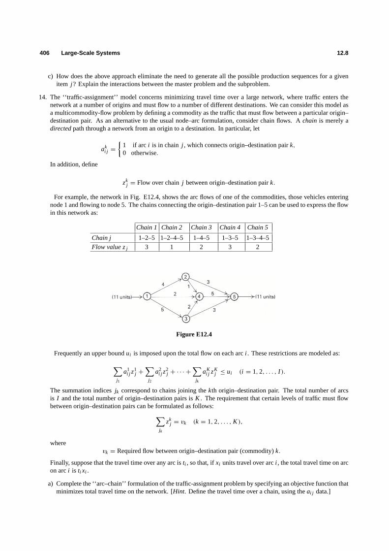
406 Large-Scale Systems 12.8
c) How does the above approach eliminate the need to generate all the possible production sequences for a givenitem j ? Explain the interactions between the master problem and the subproblem.
14. The ‘‘traffic-assignment’’ model concerns minimizing travel time over a large network, where traffic enters thenetwork at a number of origins and must flow to a number of different destinations. We can consider this model asa multicommodity-flow problem by defining a commodity as the traffic that must flow between a particular origin–destination pair. As an alternative to the usual node–arc formulation, consider chain flows. Achain is merely adirectedpath through a network from an origin to a destination. In particular, let
aki j =
{1 if arc i is in chain j , which connects origin–destination pairk,
0 otherwise.
In addition, define
zkj = Flow over chainj between origin–destination pairk.
For example, the network in Fig. E12.4, shows the arc flows of one of the commodities, those vehicles enteringnode 1 and flowing to node 5. The chains connecting the origin–destination pair 1–5 can be used to express the flowin this network as:
Chain 1 Chain 2 Chain 3 Chain 4 Chain 5
Chain j 1–2–5 1–2–4–5 1–4–5 1–3–5 1–3–4–5
Flow valuez j 3 1 2 3 2
Figure E12.4
Frequently an upper boundui is imposed upon the total flow on each arci . These restrictions are modeled as:∑j1
a1i j z
1j +
∑j2
a2i j z
2j + · · · +
∑jk
aKi j zK
j ≤ ui (i = 1, 2, . . . , I ).
The summation indicesjk correspond to chains joining thekth origin–destination pair. The total number of arcsis I and the total number of origin–destination pairs isK . The requirement that certain levels of traffic must flowbetween origin–destination pairs can be formulated as follows:∑
jk
zkj = vk (k = 1, 2, . . . , K ),
wherevk = Required flow between origin–destination pair (commodity)k.
Finally, suppose that the travel time over any arc isti , so that, ifxi units travel over arci , the total travel time on arcon arci is ti xi .
a) Complete the ‘‘arc–chain’’ formulation of the traffic-assignment problem by specifying an objective function thatminimizes total travel time on the network. [Hint. Define the travel time over a chain, using theai j data.]

12.8 Column Generation 407
b) In reality, generating all the chains of a network is very difficult computationally. Suppose enough chains havebeen generated to determine a basic feasible solution to the linear program formulated in part (a). Show how tocompute the reduced cost of the next chain to enter the basis from those generated thus far.
c) Now consider the chains not yet generated. In order for the current solution to be optimal, the minimum reducedcosts of these chains must be nonnegative. How would you find the chain with the minimum reduced cost foreach ‘‘commodity’’? [Hint. The reduced costs are, in general,
ckj =
∑i
ai j (ti − πi )− uk,
whereπi anduk are the shadow prices associated with the capacity restriction on thei th constraint and flowrequirement between thekth origin–destination pair. What is the sign ofπi ?]
d) Give an economic interpretation ofπi . In the reduced cost of part (c), do the values ofπi depend on whichcommodity flows over arci ?
15. Consider the node–arc formulation of the ‘‘traffic-assignment’’ model. Define a ‘‘commodity’’ as the flow from anorigin to a destination. Let
xki j = Flow over arci − j of commodityk.
The conservation-of-flow equations for each commodity are:
∑i
xkin −
∑j
xknj =
vk if n = origin for commodityk,
−vk if n = destination for commodityk,
0 otherwise.
The capacity restrictions on the arcs can be formulated as follows:
K∑k=1
xki j ≤ ui j for all arcsi − j,
assuming thatti j the travel time on arci − j . To minimize total travel time on the network, we have the followingobjective function:
Minimize∑
k
∑i
∑j
ti j xki j .
a) Let the conservation-of-flow constraints for a commodity correspond to a subproblem, and the capacity restrictionson the arcs correspond to the master constraints in a decomposition approach. Formulate the restricted master,and the subproblem for thekth commodity. What is the objective function of this subproblem?
b) What is the relationship between solving the subproblems of the node–arc formulation and finding the minimumreduced cost for each commodity in the arc–chain formulation discussed in the previous exercise?
c) Show that the solution of the node–arc formulation by decomposition is identical to solving the arc–chain formu-lation discussed in the previous exercise. [Hint. In the arc–chain formulation, define new variables
λkj =
xkj
vk.
]16. In the node–arc formulation of the ‘‘traffic-assignment’’ problem given in Exercise 15, the subproblems correspond
to finding the shortest path between thekth origin–destination pair. In general, there may be a large number of origin–destination pairs and hence a large number of such subproblems. However, in Chapter 11 on dynamic programming,we saw that we can solve simultaneously for the shortest paths from a particular origin to all destinations. We can thenconsolidate the subproblems by defining one subproblem for each node where traffic originates. The conservation-of-flow constraints become:
∑i
ysin −
∑j
ysnj =
∑
vk if n = origin nodes,−vk if n = a destination node in the origin–destination pairk = (s, n)
0 otherwise,

408 Large-Scale Systems 12.8
where the summation∑
vk is the total flow emanating from origins for all destination nodes. In this formulation,ys
i j =∑
xki j denotes the total flow on arci − j that emanates from origins; that is, the summation is carried over
all origin–destination pairsk = (s, t) whose origin is nodes.
a) How does the decomposition formulation developed in Exercise 15 change with this change in definition of asubproblem? Specify the new formulation precisely.
b) Which formulation has more constraints in its restricted master?c) Which restricted master is more restricted? [Hint. Which set of constraints implies the other?]d) How does the choice of which subproblems to employ affect the decomposition algorithm? which choice would
you expect to be more efficient? Why?
17. Consider a ‘‘nested decomposition’’ as applied to the problem
Maximizen∑
j=1
c j x j ,
subject to:n∑
j=1ai j x j = bi (i = 1, 2, . . . , k), (1)
n∑j=1
di j x j = di (i = k+ 1, k+ 2, . . . , `), (2)
n∑j=1
gi j x j = gi (i = `+ 1, `+ 2, . . . , m), (3)
(P)
x j ≥ 0 ( j = 1, 2, . . . , n).
Let (1) be the constraints of the (first) restricted master problem. Ifπi (i = 1, 2, . . . , k) are shadow prices for theconstraints (1) in the weighting problem, then
Maximizen∑
j=1
(c j −
k∑i=1
πi ai j
)x j ,
subject to:
n∑j=1
di j x j = di (i = k+ 1, k+ 2, . . . , `), (2′)
n∑j=1
gi j x j = gi (i = `+ 1, `+ 2, . . . , m), (3′) (Subproblem 1)
x j ≥ 0, ( j = 1, 2, . . . , n),
constitutes subproblem 1 (the proposal-generating problem).
Suppose, though, that the constraints(3′) complicate this problem and make it difficult to solve. Therefore, tosolve the subproblem we further apply decomposition on subproblem 1. Constraints(2′) will be the constraints ofthe ‘‘second’’ restricted master. Given any shadow pricesαi (i = k + 1, k + 2, . . . , `) for constraints(2′) in theweighting problem, the subproblem 2 will be:
Maximizen∑
j=1
c j −
k∑i=1
πi ai j −∑
i=k+1
αi di j
x j ,
subject to:
n∑j=1
gi j x j = gi (i = `+ 1, `+ 2, . . . , m), (Subproblem 2)
x j ≥ 0 ( j = 1, 2, . . . , n).

13.8 Column Generation 409
a) Consider the following decomposition approach: Given shadow pricesπi , solve subproblem (1) to completionby applying decomposition with subproblem (2). Use the solution to this problem to generate a new weightingvariable to the first restricted master problem, or show that the original problem (P) [containing all constraints(1), (2), (3)] has been solved. Specify details of this approach.
b) Show finite convergence and bounds on the objective function to (P).c) Now consider another approach: Subproblem 1 need not be solved to completion, but merely until a solution
x j ( j = 1, 2, . . . , n) is found, so that
n∑j=1
(c j −
k∑i=1
πi ai j
)x j > γ,
whereγ is the shadow price for the weighting constraint to the first restricted master. Indicate how to identifysuch a solutionx j ( j = 1, 2, . . . , n) while solving the second restricted master problem; justify this approach.
d) Discuss convergence and objective bounds for the algorithm proposed in part (c).
ACKNOWLEDGMENTS
A number of the exercises in this chapter are based on or inspired by articles in the literature. Exercise 8:D. Anderson, ‘‘Models for Determining Least-Cost Investments in Electricity Supply,’’The Bell Journal ofEconomics and Management Science, 3, No. 1, Spring 1972.Exercise 10: P. E. Gilmore and R. E. Gomory, ‘‘A Linear Programming Approach to the Cutting StockProblem-II,’’ Operations Research, 11, No. 6, November–December 1963.Exercise 12: A. S. Manne, ‘‘Programming of Economic Lot Sizes,’’Management Science, 4, No. 2, January1958.Exercise 13: B. P. Dzielinski and R. E. Gomory, ‘‘Optimal Programming of Lot Sizes, Inventory, and LaborAllocations,’’ Management Science, 11, No. 9, July 1965; and L. S. Lasdon and R. C. Terjung, ‘‘An EfficientAlgorithm for Multi-Item Scheduling,’’Operation Research, 19, No. 4, July–August 1971.Exercises 14 through 16: S. P. Bradley, ‘‘Solution Techniques for the Traffic Assignment Problem,’’ Op-erations Research Center Report ORC 65–35, University of California, Berkeley. Exercise 17: R. Glassey,‘‘Nested Decomposition and Multi-Stage Linear Programs,’’Management Science, 20, No. 3, 1973.

Nonlinear Programming
13
Numerous mathematical-programming applications, including many introduced in previous chapters, arecast naturally as linear programs. Linear programming assumptions or approximations may also lead toappropriate problem representations over the range of decision variables being considered. At other times,though, nonlinearities in the form of either nonlinear objectivefunctions or nonlinear constraints are crucialfor representing an application properly as a mathematical program. This chapter provides an initial steptoward coping with such nonlinearities, first by introducing several characteristics of nonlinear programs andthen by treating problems that can be solved using simplex-like pivoting procedures. As a consequence, thetechniques to be discussed are primarily algebra-based. The final two sections comment on some techniquesthat do not involve pivoting.
As our discussion of nonlinear programming unfolds, the reader is urged to reflect upon the linear-programming theory that we have developed previously, contrasting the two theories to understand why thenonlinear problems are intrinsically more difficult to solve. At the same time, we should try to understandthe similarities between the two theories, particularly since the nonlinear results often are motivated by, andare direct extensions of, their linear analogs. The similarities will be particularly visible for the material ofthis chapter where simplex-like techniques predominate.
13.1 NONLINEAR PROGRAMMING PROBLEMS
A general optimization problem is to selectn decision variablesx1, x2, . . . , xn from a given feasible regionin such a way as to optimize (minimize or maximize) a given objective function
f (x1, x2, . . . , xn)
of the decision variables. The problem is called anonlinear programming problem(NLP) if the objectivefunction is nonlinear and/or thefeasible region is determined by nonlinear constraints. Thus, in maximizationform, the general nonlinear program is stated as:
Maximize f (x1, x2, . . . , xn),
subject to:
g1(x1, x2, . . . , xn) ≤ b1,
......
gm(x1, x2, . . . , xn) ≤ bm,
where each of the constraint functionsg1 throughgm is given. A special case is the linear program that hasbeen treated previously. The obvious association for this case is
f (x1, x2, . . . , xn) =
n∑j=1
c j x j ,
410

13.1 Nonlinear Programming Problems 411
and
gi (x1, x2, . . . , xn) =
n∑j=1
ai j x j (i = 1, 2, . . . , m).
Note that nonnegativity restrictions on variables can be included simply by appending the additional con-straints:
gm+i (x1, x2, . . . , xn) = −xi ≤ 0 (i = 1, 2, . . . , n).
Sometimes these constraints will be treated explicitly, just like any other problem constraints. At other times,it will be convenient to consider them implicitly in the same way that nonnegativity constraints are handledimplicitly in the simplex method.
For notational convenience, we usually letx denote the vector ofn decision variablesx1, x2, . . . , xn —that is,x = (x1, x2, . . . , xn) — and write the problem more concisely as
Maximize f (x),
subject to:
gi (x) ≤ bi (i = 1, 2, . . . , m).
As in linear programming, we are not restricted to this formulation. To minimizef (x), we can of coursemaximize− f (x). Equality constraintsh(x) = b can be written as two inequality constraintsh(x) ≤ b and−h(x) ≤ −b. In addition, if we introduce a slack variable, each inequality constraint is transformed to anequality constraint. Thus sometimes we will consider an alternative equality form:
Maximize f (x),
subject to:
hi (x) = bi (i = 1, 2, . . . , m)
x j ≥ 0 ( j = 1, 2, . . . , n).
Usually the problem context suggests either an equality or inequality formulation (or a formulation with bothtypes of constraints), and we will not wish to force the problem into either form.
The following three simplified examples illustrate how nonlinear programs can arise in practice.
Portfolio Selection An investor has $5000 and two potential investments. Letx j for j = 1 and j = 2denote his allocation to investmentj in thousands of dollars. From historical data, investments 1 and 2 havean expected annual return of 20 and 16 percent, respectively. Also, the total risk involved with investments 1and 2, as measured by the variance of total return, is given by 2x2
1+x22+(x1+x2)
2, so that risk increases withtotal investment and with the amount of each individual investment. The investor would like to maximize hisexpected return and at the same time minimize his risk. Clearly, both of these objectives cannot, in general, besatisfied simultaneously. There are several possible approaches. For example, he can minimize risk subjectto a constraint imposing a lower bound on expected return. Alternatively, expected return and risk can becombined in an objective function, to give the model:
Maximize f (x) = 20x1+ 16x2− θ [2x21 + x2
2 + (x1+ x2)2],
subject to:g1(x) = x1+ x2 ≤ 5,
x1 ≥ 0, x2 ≥ 0, (that is,g2(x) = −x1, g3(x) = −x2).
The nonnegative constantθ reflects his tradeoff between risk and return. Ifθ = 0, the model is a linearprogram, and he will invest completely in the investment with greatest expected return. For very largeθ , theobjective contribution due to expected return becomes negligible and he is essentially minimizing his risk.
412 Nonlinear Programming 13.1
Water Resources Planning In regional water planning, sources emitting pollutants might be required toremove waste from the water system. Letx j be the pounds of Biological Oxygen Demand (an often-usedmeasure of pollution) to be removed at sourcej .
One model might be to minimize total costs to the region to meet specified pollution standards:
Minimizen∑
j=1
f j (x j ),
subject to:
n∑j=1
ai j x j ≥ bi (i = 1, 2, . . . , m)
0 ≤ x j ≤ u j ( j = 1, 2, . . . , n),
where
f j (x j ) = Cost of removingx j pounds of Biological Oxygen Demand atsourcej ,
bi = Minimum desired improvement in water quality at pointi in thesystem,
ai j = Quality response, at pointi in the water system, caused by removingone pound of Biological Oxygen Demand at sourcej ,
u j = Maximum pounds of Biological Oxygen Demand that can beremoved at sourcej .
Constrained Regression A university wishes to assess the job placements of its graduates. For simplicity,it assumes that each graduate accepts either a government, industrial, or academic position. Let
N j = Number of graduates in yearj ( j = 1, 2, . . . , n),
and letG j , I j , andA j denote the number entering government, industry, and academia, respectively, in yearj (G j + I j + A j = N j ).
One model being considered assumes that a given fraction of the student population joins each jobcategory each year. If these fractions are denoted asλ1, λ2, andλ3, then the predicted number entering thejob categories in yearj is given by the expressions
G j = λ1N j ,
I j = λ2N j ,
A j = λ3N j .
A reasonable performance measure of the model’s validity might be the difference between the actual numberof graduatesG j , I j , andA j entering the three job categories and the predicted numbersG j , I j , and A j , asin the least-squares estimate:
Minimizen∑
j=1
[(G j − G j )2+ (I j − I j )
2+ (A j − A j )
2],
subject to the constraint that all graduates are employed in one of the professions. In terms of the fractionsentering each profession, the model can be written as:
Minimizen∑
j=1
[(G j − λ1N j )2+ (I j − λ2N j )
2+ (A j − λ3N j )
2],

13.2 Local vs. Global optimum 413
subject to:
λ1 + λ2+ λ3 = 1,
λ1 ≥ 0, λ2 ≥ 0, λ3 ≥ 0.
This is a nonlinear program in three variablesλ1, λ2, andλ3.There are alternative ways to approach this problem. For example, the objective function can be changed
to:
Minimizen∑
j=1
[∣∣G j − G j | + |I j − I j | + |A j − A j∣∣] .†
This formulation is appealing since the problem now can be transformed into a linear program. Exercise 28(see also Exercise 20) from Chapter 1 illustrates this transformation.
The range of nonlinear-programming applications is practically unlimited. For example, it is usually simpleto give a nonlinear extension to any linear program. Moreover, the constraintx = 0 or 1 can be modeledasx(1− x) = 0 and the constraintx integer as sin(πx) = 0. Consequently,in theoryany application ofinteger programming can be modeled as a nonlinear program. We should not be overly optimistic about theseformulations, however; later we shall explain why nonlinear programming is not attractive for solving theseproblems.
13.2 LOCAL vs. GLOBAL OPTIMUM
Geometrically, nonlinear programs can behave much differently from linear programs, even for problemswith linear constraints. In Fig. 13.1, the portfolio-selection example from the last section has been plotted forseveral values of the tradeoff parameterθ . For each fixed value ofθ , contours of constant objective valuesare concentric ellipses. As Fig. 13.1 shows, the optimal solution can occur:
a) at an interior point of the feasible region;b) on the boundary of the feasible region, which is not an extreme point; orc) at an extreme point of the feasible region.
As a consequence, procedures, such as the simplex method, that search only extreme points may not determinean optimal solution.
Figure 13.2 illustrates another feature of nonlinear-programming problems. Suppose that we are tominimize f (x) in this example, with 0≤ x ≤ 10. The pointx = 7 is optimal. Note, however, that in theindicated dashed interval, the pointx = 0 is the best feasible point; i.e., it is an optimal feasible point in thelocal vicinity of x = 0 specified by the dashed interval.
The latter example illustrates that a solution optimal in a local sense need not be optimal for the overallproblem. Two types of solution must be distinguished. A global optimum is a solution to the overalloptimization problem. Its objective value is as good as any other point in the feasible region. A localoptimum, on the other hand, is optimal only with respect to feasible solutionsclose to that point. Pointsfar removed from a local optimum play no role in its definition and may actually be preferred to the localoptimum. Stated more formally,
Definition. Let x = (x1, x2, . . . , xn) be a feasiblesolution to a maximization problem with objectivefunction f (x). We callx
1. A global maximumif f (x) ≥ f (y) for every feasible pointy = (y1, y2, . . . , yn);
†| | denotes absolute value; that is,|x| = x if x ≥ 0 and|x| = −x if x < 0.

414 Nonlinear Programming 13.2
Figure 13.1 Portfolio-selection example for various values ofθ . (Lines are contours of constant objective values.)

13.3 Convex and Concave Functions 415
Figure 13.2 Local and global minima.
2. A local maximumif f (x) ≥ f (y) for every feasible pointy = (y1, y2, . . . , yn) sufficiently close tox.That is, if there is a numberε > 0 (possibly quite small) so that, whenever each variabley j is withinε of x j — that is,x j − ε ≤ y j ≤ x j + ε —andy is feasible, thenf (x) ≥ f (y).
Global and local minima are defined analogously. The definition of local maximum simply says that if weplace ann-dimensional box (e.g., a cube in three dimensions) aboutx, whose side has length 2ε, then f (x)
is as small asf (y) for every feasible pointy lying within the box. (Equivalently, we can usen-dimensionalspheres in this definition.) For instance, ifε = 1 in the above example, the one-dimensional box, or interval,is pictured about the local minimumx = 0 in Fig. 13.2.
The concept of a local maximum is extremely important. As we shall see, most general-purpose nonlinear-programming procedures are near-sighted and can do no better than determine local maxima. We shouldpoint out that, since every global maximum is also a local maximum, the overall optimization problem canbe viewed as seeking the best local maxima.
Under certain circumstances, local maxima and minima are known to be global. Whenever a function‘‘curves upward’’ as in Fig. 13.3(a), a local minimum will be global. These functionsare calledconvex.Whenever a function ‘‘curves downward’’ as in Fig. 13.3(b) a local maximum will be a global maximum.These functions are calledconcave.† For this reason we usually wish to minimize convex functions andmaximize concave functions. These observations are formalized below.
13.3 CONVEX AND CONCAVE FUNCTIONS
Because of both their pivotal role in model formulation and their convenient mathematical properties, certainfunctional forms predominate in mathematical programming. Linear functions are by far the most important.Next in importance are functions which are convex or concave. These functions are so central to the theorythat we take some time here to introduce a few of their basic properties.
An essential assumption in a linear-programming model for profit maximization is constant returns to scalefor each activity. This assumption implies that if the level of one activity doubles, then that activity’s profitcontribution also doubles; if the first activity level changes fromx1 to 2x1, then profit increases proportionallyfrom say $20 to $40 [i.e., fromc1x1 to c1(2x1)]. In many instances, it is realistic to assume constant returnsto scale over the range of the data. At other times, though, due to economies of scale, profit might increasedisproportionately, to say $45; or, due to diseconomies of scale (saturation effects), profit may be only $35.In the former case, marginal returns are increasing with the activity level, and we say that the profit function
† As a mnemonic, the ‘‘A’’ in concAve reflects the shape of these functions.

416 Nonlinear Programming 13.3
Figure 13.3 a) Convex function b) concave function (c) nonconvex, nonconcave function.
is convex(Fig. 13.3(a)). In the second case, marginal returns are decreasing with the activity level and wesay that the profit function isconcave(Fig.13.3(b)). Of course, marginal returns may increase over parts ofthe data range and decrease elsewhere, giving functions that are neither convex nor concave (Fig. 13.3(c)).
An alternative way to view a convex function is to note that linear interpolation overestimates its values.That is, for any pointsy andz, the line segment joiningf (y) and f (z) lies above the function (see Fig. 13.3).More intuitively, convex functions are ‘‘bathtub like’’ and hold water. Algebraically,
Definition. A function f (x) is calledconvexif,for every y andz and every 0≤ λ ≤ 1,
f [λy+ (1− λ)z] ≤ λ f (y)+ (1− λ) f (z).
It is calledstrictly convexif, for every two distinct pointsy andz and every 0< λ < 1,
f [λy+ (1− λ)z] < λ f (y)+ (1− λ) f (z).
The lefthand side in this definition is the function evaluation on the line joiningx andy; the righthand side isthe linear interpolation. Strict convexity corresponds to profit functions whose marginal returns are strictlyincreasing.
Note that although we have picturedf above to be a function of one decision variable, this is not a restric-tion. If y = (y1, y2, . . . , yn) andz = (z1, z2, . . . , zn), we must interpretλy + (1− λ)z only as weightingthe decision variables one at a time, i.e., as the decision vector (λy1+ (1− λ)z1, . . . , λyn + (1− λ)zn).
Concave functions are simply the negative of convex functions. In this case, linear interpolation under-estimates the function. The definition above is altered by reversing the direction of the inequality. Strictconcavity is defined analogously. Formally,
Definition. A function f (x) is calledconcaveif,for every y andz and every 0≤ λ ≤ 1,
f [λy+ (1− λ)z] ≥ λ f (y)+ (1− λ) f (z).
It is calledstrictly concaveif, for every y andz and every 0< λ < 1,
f [λy+ (1− λ)z] > λ f (y)+ (1− λ) f (z).

13.3 Convex and Concave Functions 417
Figure 13.4 Convex and nonconvex sets.
We can easily show that a linear function is both convex and concave. Consider the linear function:
f (x) =
n∑j=1
c j x j ,
and let 0≤ λ ≤ 1. Then
f (λy+ (1− λ)z) =n∑
j=1
c j (λy j + (1− λ)z j )
= λ
n∑j=1
c j y j
+ (1− λ)
n∑j=1
c j z j
= λ f (y)+ (1− λ) f (z).
These manipulations state, quite naturally, that linear interpolation gives exact values forf and consequently,from the definitions, that a linear function is both convex and concave. This property is essential, permittingus to either maximize or minimize linear functions by computationally attractive methods such as the simplexmethod for linear programming.
Other examples of convex functions arex2, x4, ex, e−x or –logx. Multiplying each example by minusone gives aconcave function. The definition of convexity implies that the sum of convex functions is convexand that any nonnegative multiple of a convex function also is convex. Utilizing this fact, we can obtain alarge number of convex functions met frequently in practice by combining these simple examples, giving, forinstance,
2x2+ ex, ex
+ 4x,
or−3 log x + x4.
Similarly, we can easily write several concave functions by multiplying these examples by minus one.A notion intimately related to convex and concave functions is that of aconvex set. These sets are ‘‘fat,’’
in the sense that, whenevery andz are contained in the set, every point on the line segment joining thesepoints is also in the set (see Fig. 13.4). Formally,
Definition. A set of pointsC is calledconvexif, for all λ in the interval 0≤ λ ≤ 1, λy+ (1− λ)z iscontained inC wheneverx andy are contained inC.
Again we emphasize thaty andz in this definition are decision vectors; in the example, each of these vectorshas two components.

418 Nonlinear Programming 13.4
We have encountered convex sets frequently before, since the feasible region for a linear program isconvex. In fact, the feasible region for a nonlinear program is convex if it is specified by less-than-or-equal-toequalities with convex functions. That is, iffi (x) for i = 1, 2, . . . , m, are convex functions and if the pointsx = y andx = z satisfy the inequalities
fi (x) ≤ bi (i = 1, 2, . . . , m),
then, for any 0≤ λ ≤ 1, λy+ (1− λ)z is feasible also, since the inequalities
fi (λy+ (1− λ)z) ≤ λ fi (y) + (1− λ) fi (z) ≤ λbi + (1− λ)bi = bi↑ ↑
Convexity Feasibility ofy andz
hold for every constraint. Similarly, if the constraints are specified by greater-than-or-equal-to inequali-ties and the functions are concave, then the feasible region is convex. In sum, for convex feasible regionswe want convex functions for less-than-or-equal-to constraints and concave functions for greater-than-or-equal-to constraints. Since linear functions are both convex and concave, they may be treated as equali-ties.
An elegant mathematical theory, which is beyond the scope of this chapter, has been developed for convexand concave functions and convex sets. Possibly the most important property for the purposes of nonlinearprogramming was previewed in the previous section. Under appropriate assumptions, a local optimumcanbe shown to be a global optimum.
Local Minimum and Local Maximum Property
1. A local
{minimummaximum
}of a
{convexconcave
}function on a convex feasible region is also a
global
{minimummaximum
}.
2. A local
{minimummaximum
}of a strictly
{convexconcave
}function on a convex feasible region
is the unique global
{minimummaximum
}.
We can establish this property easily by reference to Fig. 13.5. The argument is for convex functions;the concave case is handled similarly. Suppose thaty is a local minimum. Ify is not a global minimum,then, by definition, there is a feasible pointz with f (z) < f (y). But then if f is convex, the function mustlie on or below the dashed linear interpolation line. Thus, in any box abouty, there must be anx on the linesegment joiningy andz, with f (x) < f (y). Since the feasible region is convex, thisx is feasible and wehave contradicted the hypothesis thaty is a local minimum. Consequently, no such pointz can exist and anylocal minimum such asy must be a global minimum.
To see the second assertion, suppose thaty is a local minimum. By Property 1 it is also a global minimum.If there is another global minimumz (so that f (z) = f (y)), then 1
2x + 12z is feasible and, by the definition
of strict convexity,
f(
12x + 1
2z)
< 12 f (y)+ 1
2 f (z) = f (y).
But this states that12x + 12z is preferred toy, contradicting our premise thaty is a global minimum.
Consequently, no other global minimum such asz can possibly exist; that is,y must be the unique globalminimum.

13.4 Problem Classification 419
Figure 13.5 Local minima are global minima for convex function
13.4 PROBLEM CLASSIFICATION
Many of the nonlinear-programming solution procedures that have been developed do not solve the generalproblem
Maximize f (x),
subject to:
gi (x) ≤ bi (i = 1, 2, . . . , m),
but rather some special case. For reference, let us list some of these special cases:
1. Unconstrained optimization:f general, m= 0 (noconstraints).
2. Linear programming:
f (x) =
n∑j=1
c j x j , gi (x) =∑n
j=1 ai j x j (i = 1, 2, . . . , m),
gm+i (x) = −xi (i = 1, 2, . . . , n).
3. Quadratic programming:
f (x) =
n∑j=1
c j x j +12
n∑i=1
n∑j=1
qi j xi x j (Constraints of case 2),
(qi j are given constants).
4. Linear constrained problem:
f (x) general, gi (x) =
n∑j=1
ai j x j (i = 1, 2, . . . , m),
(Possiblyx j ≥ 0 will be included as well).

420 Nonlinear Programming 13.5
5. Separable programming:
f (x) =
n∑j=1
f j (x j ), gi (x) =
n∑j=1
gi j (x j ) (i = 1, 2, . . . , m);
i.e., the problem ‘‘separates’’ into functions of single variables. The functionsf j andgi j are given.
6. Convex programming:
f is a concave function. The functionsgi (i = 1, 2, . . . , m)
(In a minimization problem, are all convex.f would be a convex function.)
Note that cases 2, 3, and 4 are successive generalizations. In fact linear programming is a special case ofevery other problem type except for case 1.
13.5 SEPARABLE PROGRAMMING
Our first solution procedure is for separable programs, which are optimization problems of the form:
Maximizen∑
j=1
f j (x j ),
subject to:n∑
j=1
gi j (x j ) ≤ 0 (i = 1, 2, . . . , m),
where each of the functionsf j andgi j is known. These problems are called separable because the decisionvariables appear separately, one in each functiongi j in the constraints and one in each functionf j in theobjective function.
Separable problems arise frequently in practice, particularly for time-dependent optimization. In this case,the variablex j usually corresponds to an activity level for time periodj and the separable model assumesthat the decisions affecting resource utilization and profit (or cost) are additive over time. The model alsoarises when optimizing over distinct geographical regions, an example being the water-resources planningformulation given in Section 13.1.
Actually, instead of solving the problem directly, we make an appropriate approximation so that linearprogramming can be utilized. In practice, two types of approximations, called theδ-methodand theλ-method,are often used. Since we have introduced theδ-method when discussing integer programming, we considertheλ-method in this section.
The general technique is motivated easily by solving a specific example. Consider the portfolio-selectionproblem introduced in Section 13.1. Takingθ = 1, that problem becomes:
Maximize f (x) = 20x1+ 16x2− 2x21 − x2
2 − (x1+ x2)2,
subject to:
x1 + x2 ≤ 5,
x1 ≥ 0, x2 ≥ 0.
As stated, the problem is not separable, because of the term(x1 + x2)2 in the objective function. Letting
x3 = x1+ x2, though, we can re-express it in separable form as:
Maximize f (x) = 20x1+ 16x2− 2x21 − x2
2 − x23,

13.5 Separable Programming 421
subject to:
x1 + x2 ≤ 5,
x1 + x2− x3 = 0,
x1 ≥ 0, x2 ≥ 0, x3 ≥ 0.
The objective function is now written asf (x) = f1(x1)+ f2(x2)+ f3(x3), where
f1(x1) = 20x1− 2x21,
f2(x2) = 16x2− x22,
and
f3(x3) = −x23.
Thus it is separable. Clearly, the linear constraints are also separable.To form the approximation problem, we approximate each nonlinear term by a piecewise-linear curve,
as pictured in Fig. 13.6. We have used three segments to approximate the functionf1 and two segments toapproximate the functionsf2 and f3. Note that the constraints imply that
x1 ≤ 5, x2 ≤ 5, and x3 ≤ 5,
so that we need not extend the approximation beyond these bounds on the variables.The dashed approximation curves forf1(x1), f2(x2), and f3(x3) are determined by linear approximation
between breakpoints. For example, if 1≤ x1 ≤ 3, then the approximationf a1 for f1 is given by weighting
the function’s values atx1 = 1 andx1 = 3; that is, as
f a1 (x1) = 18λ1+ 42λ2,
where the nonnegative variablesλ1 andλ2 expressx1 as a weighted combination of 1 and 3; thus,
x1 = 1λ1+ 3λ2, λ1+ λ2 = 1.
For instance, evaluating the approximation atx1 = 1.5 gives
f a1 (1.5) = 18
(34
)+ 42
(14
)= 24,
since1.5= 1
(34
)+ 3
(14
).
The overall approximation curvef a1 (x1) for f1(x1) is expressed as:
f a1 (x1) = 0λ0+ 18λ1+ 42λ2+ 50λ3,
(1)
Figure 13.6 Approximating separable functions.

422 Nonlinear Programming 13.5
where
x1 = 0λ0+ 1λ1+ 3λ2+ 5λ3, (2)
λ0+ λ1+ λ2+ λ3 = 1,
λ j ≥ 0 ( j = 1, 2, 3, 4),
with the provision that theλ j variables satisfy the following restriction:
Adjacency Condition. At most twoλ j weights arepositive. If two weights are positive, then they areadjacent, i.e., of the formλ j andλ j+1. A similar restriction applies to each approximation.
Figure 13.7 illustrates the need for the adjacency condition. If the weightsλ0 =13 andλ2 =
23, then the
approximation (1) gives
f a1 (x1) = 0
(13
)+ 42
(23
)= 28,
x1 = 0(
13
)+ 3
(23
)= 2,
as shown in Fig. 13.7(a) by the light curve joiningλ0 andλ2. In contrast, atx1 = 2 the approximation curvegives f a
1 (2) = 30.An essential point to note here is that, forconcaveobjective functions, the adjacency condition will
always be enforced by the maximization and can be ignored. This property is easy to see geometrically byconsidering Fig 13.7(a). Suppose that the weightsλ0 andλ2 are positive. By concavity, the function valueof 18 atx1 = 1 associated with the intermediate weightλ1 lies above the line segment joiningλ0 andλ2 inthe figure. Consequently, the approximation curve must also lie above this line segment. The maximization,therefore, will select the dashed approximation curve with only the adjacent weightsλ0 andλ1, or λ1 andλ2, positive, rather than any solution with bothλ0 andλ2 positive. A similar argument applies if three ormore weights are positive. For example, ifλ0, λ2, andλ3 are all positive, then the additional weightλ3 canbe viewed as weighting a point on the line segment joiningλ0 andλ2 with the point atλ3. Again, concavityimplies that this point lies below the approximation curve and will not be accepted by the maximization.Note, however, that for the nonconcave function of Fig. 13.7(b), nonadjacent weightsλ0 andλ2 are actuallypreferred to the approximation curve. Consequently, for nonconcave functions some effort must be expendedto ensure that the adjacency condition is satisfied.
Returning to the portfolio-selection example, we can write the approximation problem:
Maximizez= f a1 (x1)+ f a
2 (x2)+ f a3 (x3),
Figure 13.7 Need for the adjacency condition

13.5 Separable Programming 423
subject to:
x1 + x2 ≤ 5,
x1 + x2 − x3 = 0,
x1 ≥ 0, x2 ≥ 0, x3 ≥ 0,
in terms of weighting variablesλi j . Here we use the first subscripti to denote the weights to attach tovariablei . The weightsλ0, λ1, λ2, andλ3 used above for variablex1 thus becomeλ10, λ11, λ12, andλ13.The formulation is:
Maximizez=
0λ10+ 18λ11+ 42λ12+ 50λ13+ 0λ20+ 39λ21+ 55λ22− 0λ30− 4λ31− 25λ32,
subject to:
0λ10 + 1λ11 + 3λ12 + 5λ13 + 0λ20 + 3λ21 + 5λ22 ≤ 5,
0λ10 + 1λ11 + 3λ12 + 5λ13 + 0λ20 + 3λ21 + 5λ22 − 0λ30 − 2λ31 − 5λ32 = 0,
λ10 + λ11 + λ12 + λ13 = 1λ20 + λ21 + λ22 = 1
λ30 + λ31 + λ32 = 1
λi j ≥ 0, for all i and j .
Since each of the functionsf1(x1), f2(x2), and f3(x3) is concave, the adjacency condition can be ignored andthe problem can be solved as alinear program. Solving by the simplex method gives an optimal objectivevalue of 44 withλ11 = λ12 = 0.5, λ21 = 1, andλ32 = 1 as the positive variables in the optimal solution.The corresponding values for the original problem variables are:
x1 = (0.5)(1)+ (0.5)(3) = 2, x2 = 3, and x3 = 5.
This solution should be contrasted with the true solution
x1 =73, x2 =
83, x3 = 5, and f (x1, x2, x3) = 461
3,
which we derive in Section 13.7.Note that the approximation problem has added severalλ variables and that one weighting constraint in
(2) is associated with eachx j variable. Fortunately, these weighting constraints are of a special generalizedupper-bounding type, which add little to computational effort and keep the number of effective constraintsessentially unchanged. Thus, the technique can be applied to fairly large nonlinear programs, depending ofcourse upon the capabilities of available linear-programming codes.
Once the approximation problem has been solved, we can obtain a better solution by introducing morebreakpoints. Usually more breakpoints will be added near the optimal solution given by the original approx-imation.
Adding a single new breakpoint atx1 = 2 leads to an improved approximation for this problem with alinear-programming objective value of 46 and
x1 = 2, x2 = 3, and x3 = 5.
In this way, an approximate solution can be found as close as desired to the actual solution.
General Procedure
The general problem must be approached more carefully, since linear programming can give nonadjacentweights. The procedure is to express each variable∗ in terms of breakpoints, e.g., as above
x1 = 0λ10+ 1λ11+ 3λ12+ 5λ13,
∗ Variables that appear in the model in only a linear fashion should not be approximated and remain asx j variables.

424 Nonlinear Programming 13.5
and then use these breakpoints to approximate the objective function and each constraint, giving the approx-imation problem:
Maximizen∑
j=1
f aj (x j ),
subject to: (3)
n∑j=1
gai j (x j ) ≤ bi (i = 1, 2, . . . , m).
If each original functionf j (x j ) is concave and eachgi j (x j ) convex,† then theλi j version is solved as a linearprogram. Otherwise, the simplex method is modified to enforce the adjacency condition. A natural approachis to apply the simplex method as usual, except for a modified rule that maintains the adjacency condition ateach step. The alteration is:
Restricted-Entry Criterion. Use the simplex criterion, butdo not introduce aλik variable into the basisunless there is only oneλi j variable currently in the basis and it is of the formλi,k−1 or λi,k+1, i.e.,it isadjacent toλik .
Note that, when we use this rule, the optimal solution may contain a nonbasic variableλik that wouldordinarily be introduced into the basis by the simplex method (since its objective cost in the canonical form ispositive), but is not introduced because of the restricted-entry criterion. If the simplex method would choosea variable to enter the basis that is unacceptable by the restricted-entry rule, then we choose the next bestvariable according to the greatest positive reduced cost.
An attractive feature of this procedure is that it can be obtained by making very minor modifications toany existing linear-programming computer code. As a consequence, most commercial linear-programmingpackages contain a variation of this separable-programming algorithm. However, the solution determined bythis method in the general case can only be shown to be a localoptimum to the approximation problem (3).
Inducing Separability
Nonseparable problems frequently can be reduced to a separable form by a variety of formulation tricks. Anumber of such transformations are summarized in Table 13.1.
Table 13.1 Representative transformations
Term Substitution Additional constraints Restriction
x1x2 x1x2 = y21 − y2
2 y1 =12(x1+ x2)
Noney2 =
12(x1− x2)
x1x2 x1x2 = y1 log y1 = logx1+ logx2 x1 > 0, x2 > 0
xx21 xx2
1 = y1 y1 = 10y2x2∗
x1 > 0x1 = 10y2
2x1+x22 2x1+x2
2 = y1 log y1 = (log 2)(x1+ x22) None
∗ The termy2x2 should now be separated by the first transformation, followed byan application of the last transformation to separate the resulting power-of-10 term.
† Because the constraints are written as (≤), the constraints should be convex; they should be concave for (≥) inequalities.Similarly, for a minimization problem, the objective functionsf j (x j ) should be convex.

13.6 Linear Approximations of Nonlinear Programs 425
To see the versatility of these transformations, suppose that the nonseparable termx1x22/(1+ x3) appears
either in the objective function or in a constraint of a problem. Lettingy1 = 1/(1+ x3), the term becomesx1x2
2 y1. Now if x1 > 0, x22 > 0, andy1 > 0 over the feasible region, thenlettingy2 = x1x2
2 y1, the originalterm is replaced byy2 and the separable constraints
y1 =1
1 + x3
andlog y2 = logx1+ logx2
2 + log y1
are introduced. If the restrictionsx1 > 0, x22 > 0, y1 > 0 arenot met, we may lety2 = x1x2
2, substitutey1y2for the original term, and append the constraints:
y1 =1
1 + x3, y2 = x1x2
2.
The nonseparable termsy1y2 andx1x22 can now be separated using the first transformation in Table 13.1 (for
the last expression, letx22 replacex2 in the table).
Using the techniques illustrated by this simple example, we may, in theory, state almost any optimizationproblem as a separable program. Computationally, though, the approach is limited since the number of addedvariables and constraints may make the resulting separable program too large to be manageable.
13.6 LINEAR APPROXIMATIONS OF NONLINEAR PROGRAMS
Algebraic procedures such as pivoting are so powerful for manipulating linear equalities and inequalities thatmany nonlinear-programming algorithms replace the given problem by an approximating linear problem.Separable programming is a prime example, and also one of the most useful, of these procedures. As inseparable programming, these nonlinear algorithms usually solve several linear approximations by letting thesolution of the last approximation suggest a new one.
By using different approximation schemes, this strategy can be implemented in several ways. This sectionintroduces three of these methods, all structured to exploit the extraordinary computational capabilities of thesimplex method and the wide-spread availability of its computer implementation.
There are two general schemes for approximating nonlinear programs. The last section used linear ap-proximation for separable problems by weighting selected values of each function. This method is frequentlyreferred to asinner linearizationsince, as shown in Fig. 13.8 when applied to a convex programming prob-lem (i.e., constraintsgi (x) ≥ 0 with gi concave, orgi (x) ≤ 0 with gi convex), the feasible region for theapproximating problem lies inside that of the original problem. In contrast, other approximation schemes useslopes to approximate each function. These methods are commonly referred to asouter linearizationssince,for convex-programming problems, the feasible region for the approximating problem encompasses that ofthe original problem. Both approaches are illustrated further in this section.
Frank–Wolfe Algorithm
Let x0= (x0
1, x02, . . . , x0
n) be any feasible solution to a nonlinear program with linear constraints:
Maximize f (x1, x2, . . . , xn),
subject to:
n∑j=1
ai j x j ≤ bi (i = 1, 2, . . . , m),
x j ≥ 0 ( j = 1, 2, . . . , n).

426 Nonlinear Programming 13.6
Figure 13.8 Inner and outer linearizations ofg(x) ≥ 0.
Herex0 might be determined by phase I of the simplex method. This algorithm forms a linear approximationat the pointx0 by replacing the objective function with its current value plus a linear correction term; that is,by the linear objective
f (x0)+
n∑j=1
c j (x j − x0j ),
wherec j is the slope, or partial derivative, off with respect tox j , evaluated at the pointx0. Since f (x0), c j ,andx0
j are fixed, maximizing this objective function is equivalent to maximizing:
z=n∑
j=1
c j x j .
The linear approximation problem is solved, giving an optimal solutiony = (y1, y2, . . . , yn). At thispoint the algorithm recognizes that, although the linear approximation problem indicates that the objectiveimproves steadily fromx0 to y, thenonlinearobjective might not continue to improve fromx0 to y. Therefore,the algorithm uses a procedure to determine the maximum value forf (x1, x2, . . . , xn) along the line segmentjoining x0 to y. Special methods for performing optimization along the line segment are discussed in Section13.9. For now, let us assume that there is a method to accomplish this line-segment maximization for us.
Letting x1= (x1
1, x12, . . . , x1
n) denote the optimal solution of the line-segment optimization, we repeatthe procedure by determining a new linear approximation to the objective function with slopesc j evaluatedat x1. Continuing in this way, we determine a sequence of pointsx1, x2, . . . , xn, . . . ; any pointx∗ =(x∗1, x∗2, . . . , x∗n) that these points approach in the limit is an optimal solution to the original problem.
Let us illustrate the method with the portfolio-selection example from Section 13.1:
Maximize f (x) = 20x1+ 16x2− 2x21 − x2
2 − (x1+ x2)2,
subject to:
x1 + x2 ≤ 5,
x1 ≥ 0, x2 ≥ 0.
The partial derivatives of the objective function at any pointx = (x1, x2) are given by:
c1 = 20− 4x1− 2(x1+ x2) = 20− 6x1− 2x2,
c2 = 16− 2x2− 2(x1+ x2) = 16− 2x1− 4x2.

13.6 Linear Approximations of Nonlinear Programs 427
Suppose that the initial point isx0= (0, 0). At this pointc1 = 20 andc2 = 16 and the linear approximation
uses the objective function 20x1 + 16x2. The optimal solution to this linear program isy1 = 5, y2 = 0,and the line-segment optimization is made on the line joiningx0
= (0, 0) to y = (5, 0); that is, with0 ≤ x1 ≤ 5, x2 = 0. The optimal solution can be determined to bex1 = 31
3, x2 = 0, so that the procedure isrepeated fromx1
= (313, 0).
The partial derivatives are nowc1 = 0, c2 = 913, and the solution to the resulting linear program of
maximizing 0x1+ 913x2 is y1 = 0, y2 = 5. The line segment joiningx1 andy is given by
x1 = θy1+ (1− θ)x11 = 31
3(1− θ),
x2 = θy2+ (1− θ)x12 = 5θ,
asθ varies between 0 and 1. The optimal value ofθ over the line segment isθ = 715, so that the next point is:
x21 =
(103
) (815
)= 17
9 and x22 = 21
3.
Figure 13.9 illustrates these two steps of the algorithm and indicates the next few pointsx4, x5, andx6
that it generates.
Figure 13.9 Example of the Frank–Wolfe algorithm.
The Frank–Wolfe algorithm is convenient computationally because it solves linear programs with thesame constraints as the original problem. Consequently, any structural properties of these constraints are

428 Nonlinear Programming 13.6
available when solving the linear programs. In particular, network-flow techniques or large-scale systemmethods can be used whenever the constraints have the appropriate structure. Also, note from Fig. 13.9that the pointsx1, x2, x3, . . . oscillate. The even-numbered pointsx2, x4, x6, . . . lie on one line directedtoward the optimal solution, and the odd-numbered pointsx1, x3, x5, . . . , lie on another such line. Thisgeneral tendency of the algorithm slows its convergence. One approach for exploiting this property to speedconvergence is to make periodic optimizations along the line generated by every other pointxk+2 andxk forsome values ofk.
MAP (Method of Approximation Programming)
The Frank–Wolfe algorithm can be extended to general nonlinear programs by making linear approximationsto the constraints as well as the objective function. When the constraints are highly nonlinear, however, thesolution to the approximation problem can become far removed from feasible region since the algorithmpermits large moves from any candidate solution. The Method of Approximation Programming (MAP) is asimple modification of this approach that limits the size of any move. As a result, it is sometimes referred toas asmall-step procedure.
Let x0= (x0
1, x02, . . . , x0
n) be any candidate solution to the optimization problem:
Maximize f (x1, x2, . . . , xn),
subject to:gi (x1, x2, . . . , xn) ≤ 0 (i = 1, 2, . . . , m).
Each constraint can be linearized, using its current valuegi (x0) plus a linear correction term, as:
gi (x) = gi (x0)+
n∑j=1
ai j (x j − x0j ) ≤ 0,
whereai j is the partial derivative of constraintgi with respect to variablex j evaluated at the pointx0. Thisapproximation is a linear inequality, which can be written as:
n∑j=1
ai j x j ≤ b0i ≡
n∑j=1
ai j x0j − gi (x
0),
since the terms on the righthand side are all constants.The MAP algorithm uses these approximations, together with the linear objective-function approximation,
and solves the linear-programming problem:
Maximizez=n∑
j=1
c j x j ,
subject to:
n∑j=1
ai j x j ≤ b0i (i = 1, 2, . . . , m), (4)
x0j − δ j ≤ x j ≤ x0
j + δ j ( j = 1, 2, . . . , n).
The last constraints restrict the step size; they specify that the value forx j can vary fromx0j by no more than
the user-specified constantδ j .When the parametersδ j are selected to be small, the solution to this linear program is not far removal
from x0. We might expect then that the additional work required by the line-segment optimization of the
13.6 Linear Approximations of Nonlinear Programs 429
Frank–Wolfe algorithm is not worth the slightly improved solution that it provides. MAP operates on thispremise, taking the solution to the linear program (4) as the new pointx1. The partial-derivative dataai j , bi ,andc j is recalculated atx1, and the procedure is repeated. Continuing in this manner determines pointsx1, x2, . . . , xk, . . . and as in the Frank–Wolfe procedure, any pointx∗ = (x∗1, x∗2, . . . , x∗n) that these pointsapproach in the limit is considered a solution.
Steps of the MAP Algorithm
STEP (0): Letx0= (x0
1, x02, . . . , x0
n) be any candidate solution, usually selected to be feasible or near-feasible. Setk = 0.
STEP (1): Calculatec j and ai j (i = 1, 2, . . . , m), the partial derivatives of the objective function andconstraints evaluated atxk
= (xk1, xk
2, . . . , xkn). Let bk
i = ai j xk− gi (xk).
STEP (2): Solve the linear-approximation problem (4) withbki andxk
j replacingb0i andx0
j , respectively.
Let xk+1= (xk+1
1 , xk+12 , . . . , xk+1
n ) be its optimal solution. Incrementk to k+ 1 and return toSTEP 1.
Since many of the constraints in the linear approximation merely specify upper and lower bounds on thedecision variablesx j , the bounded-variable version of the simplex method is employed in its solution. Also,usually the constantsδ j are reduced as the algorithm proceeds. There are many ways to implement this idea.One method used frequently in practice, is to reduce eachδ j by between 30 and 50 percent at each iteration.
To illustrate the MAP algorithm, consider the problem:
Maximize f (x) = [(x1− 1)2+ x2
2],
subject to:
g1(x) = x21 + 6x2− 36≤ 0,
g2(x) = −4x1+ x22 − 2x2 ≤ 0,
x1 ≥ 0, x2 ≥ 0.
The partial derivatives evaluated at the pointx = (x1, x2) are given by:
c1 = 2x1− 2, c2 = 2x2,
a11 = 2x1, a12 = 6,
a21 = −4, a22 = 2x2− 2.
Since linear approximations of any linear function gives that function again, no data needs to be calculatedfor the linear constraintsx1 ≥ 0 andx2 ≥ 0.
Using these relationships and initiating the procedure atx0= (0, 2) with δ1 = δ2 = 2 gives the linear-
approximation problem:
Maximizez= −2x1+ 4x2,
subject to:
0x1+ 6x2 ≤ 0(0)+ 6(2)− (−24) = 36,
−4x1+ 2x2 ≤ −4(0)+ 2(2)− 0 = 4.
−2 ≤ x1 ≤ 2, 0 ≤ x2 ≤ 4.
The righthand sides are determined as above by evaluatingai 1x01 + ai 2x0
2 − gi (x0).

430 Nonlinear Programming 13.6
The feasible region and this linear approximation are depicted in Fig. 13.10. Geometrically, we see thatthe optimalsolution occurs atx1
1 = 1, x12 = 4. Using this point and reducing bothδ1 andδ2 to 1 generates
the new approximation:
Maximizez= 0x1+ 8x2,
subject to:
2x1+ 6x2 ≤ 2(1)+ 6(4)− (−11) = 37,
−4x1+ 6x2 ≤ −4(1)+ 6(4)− (4) = 16,
0 ≤ x1 ≤ 2, 3≤ x2 ≤ 5.
The solution indicated in Fig. 13.10 occurs atx21 = 2, x2
2 = 4.
Figure 13.10 Example of the MAP algorithm.
If the procedure is continued, the pointsx3, x4, . . . that it generates approach the optimal solutionx∗
shown in Fig. 13.10. As a final note, let us observe that the solutionx1 is not feasible for the linear programthat was constructed by making linear approximations atx1. Thus, in general, both Phase I and Phase II ofthe simplex method may be required to solve each linear-programming approximation.

13.6 Linear Approximations of Nonlinear Programs 431
Generalized Programming
This algorithm is applied to the optimization problem of selecting decision variablesx1, x2, . . . , xn from aregionC to:
Maximize f (x1, x2, . . . , xn),
subject to:gi (x1, x2, . . . , xn) ≤ 0 (i = 1, 2, . . . , m).
The procedure uses inner linearization and extends the decomposition and column-generation algorithmsintroduced in Chapter 12. When the objective function and constraintsgi are linear andC consists of thefeasible points for a linear-programming subproblem, generalized programming reduces to the decompositionmethod.
As in decomposition, the algorithm starts withk candidate solutionsx j= (x j
1, x j2, . . . , x j
n) for j =1, 2, . . . , k, all lying the regionC. Weighting these points byλ1, λ2, . . . , λk generates the candidate solution:
xi = λ1x1i + λ2x2
i + · · · + λkxki (i = 1, 2, . . . , n). (5)
Any choices can be made for the weights as long as they are nonnegative and sum to one. The ‘‘best’’ choiceis determined by solving the linear-approximation problem in the variablesλ1, λ2, . . . , λk:
Maximize λ1 f (x1)+ λ2 f (x2)+ · · · + λk f (xk), Optimalsubject to: shadow
prices
λ1g1(x1)+ λ2g1(x2)+ · · · + λkg1(xk) ≤ 0, y1...
......
... (6)λ1gm(x1)+ λ2gm(x2)+ · · · + λkgm(xk) ≤ 0, ym
λ1 + λ2 + λk = 1. σ
λ j ≥ 0 ( j = 1, 2, . . . , k).
The coefficientsf (x j ) andgi (x j ) of the weightsλ j in this linear program are fixed by our choice of thecandidate solutionsx1, x2, . . . , xk. In this problem, the original objective function and constraints havebeen replaced by linear approximations. Whenx is determined from expression (5) by weighting the pointsx1, x2, . . . , xk by the solution of problem (6), the linear approximations atx are given by applying the sameweights to the objective function and constraints evaluated at these points; that is,
f a(x) = λ1 f (x1)+ λ2 f (x2)+ · · · + λk f (xk)
andga
i (x) = λ1gi (x1)+ λ2gi (x
2)+ · · · + λkgi (xk).
The approximation is refined by applying column generation to this linear program. In this case, a newcolumn with coefficientsf (xk+1), g1(xk+1), . . . , gm(xk+1) is determined by the pricing-out operation:
v = Max [ f (x)− y1g1(x)− y2g2(x)− · · · − ymgm(x)],
subject to:x ∈ C.
This itself is a nonlinear programming problem but without thegi constraints. Ifv − σ ≤ 0, then no newcolumn improves the linear program and the procedure terminates. Ifv − σ > 0, then the solutionxk+1

432 Nonlinear Programming 13.6
giving v determines a new column to be added to the linear program (6) and the procedure continues.The optimal weightsλ∗1, λ
∗
2, . . . , λ∗
k to the linear program provide a candidate solution
x∗i = λ∗1x1i + λ∗2x2
i + · · · + λ∗kxki
to the original optimization problem. This candidate solution is most useful whenC is a convex set and eachconstraint is convex, for thenx∗i is a weighted combination of pointsx1, x2, . . . , xk in C and thus belongs toC; and, since linear interpolation overestimates convex functions,
gi (x∗) ≤ λ∗1gi (x
1)+ λ∗2gi (x2)+ · · · + λ∗kgi (x
k).
The righthand side is less than or equal to zero by the linear-programming constraints; hence,gi (x∗) ≤ 0andx∗ is a feasible solution to the original problem.
As an illustration of the method, consider the nonlinear program:
Maximize f (x) = x1− (x2− 5)2+ 9,
subject to:
g(x) = x21 + x2
2 − 16≤ 0,
x1 ≥ 0, x2 ≥ 0.
We letC be the region withx1 ≥ 0 andx2 ≥ 0, and start with the three pointsx1= (0, 0), x2
= (5, 0), andx3= (0, 5) from C. The resulting linear approximation problem:
Maximizez= −16λ1− 11λ2+ 9λ3, Optimalsubject to: shadow
prices
−16λ1+ 9λ2+ 9λ3 ≤ 0, y = 1
λ1+ λ2+ λ3 = 1, σ = 0
λ1 ≥ 0, λ2 ≥ 0, λ2 ≥ 0,
is sketched in Fig. 13.11, together with the original problem. The feasible region for the approximationproblem is given by plotting the points defined by (5) that correspond to feasible weights in this linearprogram.
Figure 13.11 An example of generalized programming.
The solution to the linear program is:
λ∗1 = 0.36, λ∗2 = 0, and λ∗3 = 0.64,

13.7 Quadratic Programming 433
orx∗ = 0.36(0, 0)+ 0.64(0, 5) = (0, 3.2).
The nonlinear programming subproblem is:
Maximize[ f (x)− yg(x)] = x1− (x2− 5)2− yx2
1 − yx22 + 16y+ 9,
subject to:x1 ≥ 0, x2 ≥ 0.
For y > 0 the solution to this problem can be shown to bex1 = 1/(2y) andx2 = 5/(1+ y), by setting thepartial derivatives off (x)− yg(x), with respect tox1 andx2, equal to zero.
In particular, the optimal shadow pricey = 1 gives the new pointx4=
(12, 21
2
). Since f (x4) = 31
4 and
g(x4) = −912, the updated linear programming approximation is:
Maximizez= −16λ1− 11λ2+ 9λ3+ 314λ4, Optimal
subject to: shadowprices
−16λ1+ 9λ2+ 9λ3− 912λ4 ≤ 0, y = 23
74
λ1+ λ2+ λ3+ λ4 = 1, σ = 45974
λ j ≥ 0 ( j = (1, 2, 3, 4).
The optimal solution hasλ3 andλ4 basic withλ∗3 =1937, λ
∗
4 =1837. The corresponding value forx is:
x∗ = λ∗3(0, 5)+ λ∗4
(12, 21
2
)=
1937(0, 5)+ 18
37
(12, 21
2
)=
(937, 329
37
).
As we continue in this way, the approximate solutions will approach the optimal solutionx1 = 1.460 andx2 = 3.724 to the original problem.
We should emphasize that the generalized programming is unlike decomposition for linear programs inthat it does not necessarily determine the optimal solution in a finite number of steps. This is true becausenonlinearity does not permit a finite number of extreme points to completely characterize solutions to thesubproblem.
13.7 QUADRATIC PROGRAMMING
Quadratic programming concerns the maximization of a quadratic objective function subject to linear con-straints, i.e., the problem:
Maximize f (x) =
n∑j=1
c j x j +12
n∑j=1
n∑k=1
q jkx j xk,
subject to:
n∑j=1
ai j x j ≤ bi (i = 1, 2, . . . , m),
x j ≥ 0 ( j = 1, 2, . . . , n).
The datac j , ai j , andbi are assumed to be known, as are the additionalq jk data. We also assume the sym-metry conditionq jk = qk j . This condition is really no restriction, sinceq jk can be replaced by12(q jk + qk j ).The symmetry condition is then met, and a straightforward calculation shows that the old and newq jk co-efficients give the same quadratic contribution to the objective function. The factor1
2 has been included to

434 Nonlinear Programming 13.7
simplify later calculations; if desired, it can be incorporated into theq jk coefficients. Note that, if everyq jk = 0, then the problem reduces to a linear program.
The first and third examples of Section 13.1 show that the quadratic-programming model arises in con-strained regression and portfolio selection. Additionally, the model is frequently applied to approximateproblems of maximizing general functions subject to linear constraints.
In Chapter 4 we developed the optimality conditions for linear programming. Now we will indicatethe analogous results for quadratic programming. The motivating idea is to note that, for a linear objectivefunction
f (x) =
n∑j=1
c j x j ,
the derivative (i.e., the slope or marginal return) off with respect tox j is given byc j , whereas, for a quadraticprogram, the slope at a point is given by
c j +
n∑k=1
q jkxk.
The quadratic optimality conditions are then stated by replacing everyc j in the linear-programming optimalityconditions byc j +
∑nk=1q jkxk. (See Tableau 1.)
Tableau 1 Optimality conditions
Linear program Quadratic program
Primalfeasibility
n∑j=1
ai j x j ≤ bi ,n∑
j=1ai j x j ≤ bi ,
x j ≥ 0 x j ≥ 0
Dualfeasibility
m∑i=1
yi ai j ≥ c j ,m∑
i=1yi ai j ≥ c j +
n∑k=1
q jk xk,
yi ≥ 0 yi ≥ 0
Complementary
slackness yi
[bi −
n∑j=1
ai j x j
]= 0, yi
[bi −
n∑j=1
ai j x j
]= 0,[
m∑i=1
yi ai j − c j
]x j = 0
[m∑
i=1yi ai j − c j −
n∑k=1
q jk xk
]x j = 0
Note that the primal and dual feasibility conditions for the quadratic program are linear inequalities innonnegative variablesx j and yi . As such, they can be solved by the Phase I simplex method. A simplemodification to that method will permit the complementary-slackness conditions to be maintained as well.To discuss the modification, let us introduce slack variablessi for the primal constraints and surplus variablesv j for the dual constraints; that is,
si = bi −
n∑j=1
ai j x j ,
v j =
m∑i=1
yi ai j − c j −
n∑k=1
q jkxk.
Then the complementary slackness conditions become:
yi si = 0 (i = 1, 2, . . . , m),

13.8 Quadratic Programming 435
andv j x j = 0 ( j = 1, 2, . . . , n).
The variablesyi andsi are calledcomplementary, as are the variablesv j andx j . With this notation, thetechnique is to solve the primal and dual conditions by the Phase I simplex method, but not to allow anycomplementary pair of variables to appear in the basis both at the same time. More formally, the Phase Isimplex method is modified by the:
Restricted-Entry Rule. Never introduce avariable into the basis if its complementary variable is alreadya member of the basis, even if the usual simplex criterion says to introduce the variable.
Otherwise, the Phase I procedure is applied as usual. If the Phase I procedure would choose a variable to enterthe basis that is unacceptable by the restricted-entry rule, then we choose the next best variable according tothe greatest positive reduced cost in the Phase I objective function.
An example should illustrate the technique. Again, the portfolio-selection problem of Section 13.1 willbe solved withθ = 1; that is,
Maximize f (x) = 20x1+ 16x2− 2x21 − x2
2 − (x1+ x2)2,
subject to:x1+ x2 ≤ 5,
x1 ≥ 0, x2 ≥ 0.
Expanding(x1 + x2)2 asx2
1 + 2x1x2 + x22 and incorporating the factor12, we rewrite the objective function
as:Maximize f (x) = 20x1+ 16x2+
12(−6x1x1− 4x2x2− 2x1x2− 2x2x1),
so thatq11 = −6, q12 = −2, q21 = −2, q22 = −4, and the optimality conditions are:
s1 = 5− x1− x2, (Primal constraint)v1 = y1− 20+ 6x1+ 2x2v2 = y1− 16+ 2x1+ 4x2
}(Dual constraints)
x1, x2, s1, v1, v2, y1 ≥ 0, (Nonnegativity)
y1s1 = 0, v1x1 = 0, v2x2 = 0. (Complementary slackness)
Letting s1 be the basic variable isolated in the first constraint and adding artificial variablesa1 anda2 in thesecond and third constraints, the Phase I problem is solved in Table 13.2.
For this problem, the restricted-entry variant of the simplex Phase I procedure has provided the optimalsolution. It should be noted, however, that the algorithm willnot solve every quadratic program. As anexample, consider the problem:
Maximize f (x1, x2) =1
4(x1− x2)
2,
subject to:x1+ x2 ≤ 5,
x1 ≥ 0, x2 ≥ 0.
As the reader can verify, the algorithm gives the solutionx1 = x2 = 0. But this solution is not even alocal optimum, since increasing eitherx1 or x2 increases the objective value.
It can be shown, however, that the algorithm does determine an optimal solution iff (x) is strictly concavefor a maximization problem or strictly convex for a minimization problem. For the quadratic problem,f (x)
is strictly concave whenevern∑
i=1
n∑j=1
αi qi j α j < 0 for every choice ofα1, α2, . . . , αn,
such that someα j 6= 0. In this case, the matrix of coefficients(qi j ) is callednegative definite. Thus thealgorithm will always work for a number of important applications including the least-square regression andportfolio-selection problems introduced previously.

436 Nonlinear Programming 13.8
Table 13.2 Solving a quadratic program.
Basic Currentvariables values x1 x2 s1 y∗1 v1 v2 a1 a2
s1 5 1 1 1 0 0 0← a1 20 ©6 2 1 −1 0 1
a2 16 2 4 1 0 −1 1(−w) 36 8 6 2 −1 −1
↑
Basic Currentvariables values x1 x2 s1 y∗1 v∗1 v2 a1 a2
← s153 ©
23 1 −
16
16 0 −1
6x1
103 1 1
316 −
16 0 1
6a2
283
103
23
13 −1 −1
3 1
(−w) 283
103
23
13 0 −4
3
↑
Basic Currentvariables values x1 x2 s1 y1 v∗1 v∗2 a1 a2
x252 1 3
2 −14
14 0 −1
4
x152 1 −
12
14 −
14 0 1
4← a2 1 −5 ©
32 −
12 −1 1
2 1
(−w) 1 −5 32 −
12 0 −1
2
↑
Basic Currentvariables values x1 x2 s∗1 y1 v∗1 v∗2 a1 a2
x283 1 2
316 −
16 −
16
16
x173 1 1
3 −16
16
16 −
16
y123
103 1 1
3 −23
13
23
(−w) 0 0 0 1 −1 −1
* Starred variables cannot be introduced into the basis since theircomplementary variable is in the basis
.13.8 UNCONSTRAINED MINIMIZATION AND SUMT
Conceptually, the simplest type of optimization is unconstrained. Powerful solution techniques have beendeveloped for solving these problems, which are based primarily upon calculus, rather than upon algebra andpivoting, as in the simplex method. Because the linear-programming methods and unconstrained-optimizationtechniques are so efficient, both have been used as the point of departure for constructing more general-purpose nonlinear-programming algorithms. The previous sections have indicated some of the algorithmsusing the linear-programming-based approach. This section briefly indicates the nature of the unconstrained-optimization approaches by introducing algorithms for unconstrained maximization and showing how theymight be used for problems with constraints.
Unconstrained Minimization
Suppose that we want to maximize the functionf (x) of n decision variablesx = (x1, x2, . . . , xn) and thatthis function is differentiable. Let∂ f/∂x j denote the partialderivative off with respect tox j , defined by
∗ This section requires some knowledge of differential calculus.

13.8 Unconstrained Minimization and SUMT 437
∂ f∂x j= lim
θ→0
f (x+θu j )− f (x)
θ, (7)
whereu j is a decision vectoru j = (0, 0, . . . , 0, 1, 0, . . . , 0), with all zeros except for thej th component,which is 1. Thus,x + θu j corresponds to the decisions(x1, x2, . . . , x j−1, x j + θ, x j+1, . . . , xn), in whichonly the j th decision variable is changed from the decision vectorx.
Note that if∂ f/∂x j > 0, then
f (x + θu j )− f (x)
θ> 0 for θ > 0 small enough,
and thereforex + θu j is preferred tox for a maximization problem. Similarly, if∂ f/∂x j < 0, then
f (x + θu j )− f (x)
θ< 0 for θ < 0 small enough,
and x + θu j is again preferred tox. Therefore, at any given point with at least one partial derivative∂ f/∂x j > 0, we can improve the value off by making a one dimensional search
Maximizeθ≥0
f (x1, x2, . . . , x j−1, x j + θ, x j+1, . . . , xn),
in which only the value ofx j is varied. Similarly, if∂ f/∂x j < 0, we can alterx j to x j − θ and search onθ ≥ 0 to improve the function’s value. The one-dimensional search can be made by using any of a numberof procedures that are discussed in the next section. One algorithm using this idea, calledcyclic coordinateascent, searches by optimizing in turn with respect tox1, thenx2, thenx3 and so on, holding all other variablesconstant at stagej when optimizing with respect to variablex j . After optimizing withxn, the method startsover again withx1.
In fact, there is a large class of algorithms known asascent algorithmsthat implement the ‘‘uphillmovement’’ philosophy of cyclic coordinate ascent. Suppose that we consider moving in a general directiond = (d1, d2, . . . , dn) instead of in a coordinate, or unit, direction. Then, instead of considering the partialderivative, as in (7), we consider thedirectionalderivative. The directional derivative, which indicates howthe function varies as we move away fromx in the directiondis defined by:
limθ→0
f (x + θd)− f (x)
θ=
∂ f
∂x1d1+
∂ f
∂x2d2+ · · · +
∂ f
∂xndn. (8)
The directional derivative is just the slope of the functionf (x) in the directiond and reduces to the definitionof the partial derivative∂ f/∂x j in Eq. (7) when the direction is taken to bed = u j . Just as in the case ofpartial derivatives, if the directional derivative in Eq. (8) is positive, thenf increases in the directiond; thatis,
f (x1+ θd1, x2+ θd2, . . . , xn + θdn) > f (x1, x2, . . . , xn)
for θ > 0 small enough. At any given pointx, the ascent algorithms choose an increasing directiond (i.e.,such that Eq. (8) is positive), and then select the next pointxi = xi + θdi as the solutionθ = θ to theone-dimensional problem
Maximizeθ≥0
f (x1+ θd1, x2+ θd2, . . . , xn + θdn).
From x, the ascent algorithms select a new direction and solve another one-dimensional problem, and thencontinue by repeating this procedure. Cyclic coordinate ascent is a special case in which, at each step, all butoned j , saydi , is set to zero;di is set todi = +1 if ∂ f/∂xi > 0 anddi = −1 if ∂ f/∂xi < 0.
One natural choice for the directiond for this general class of algorithms is:
d1 =∂ f
δx1, d2
∂ f
∂x2, . . . , dn =
∂ f
∂xn,
438 Nonlinear Programming 13.8
since then Eq. (8) is positive as long as∂ f/∂x j 6= 0 for some variablex j . This choice ford is known asCauchy’s method, or steepest ascent.
To illustrate the ascent algorithms, consider the objective function
f (x1, x2) = 20x1+ 16x2− 2x21 − x2
2 − (x1+ x2)2
introduced earlier in this chapter for a portfolio-selection problem. The partial derivatives of this functionare: ∂ f
∂x1= 20− 6x1− 2x2 and
∂ f
∂x2= 16− 2x1− 4x2.
Figure 13.12 shows the result of applying the first few iterations of both cyclic coordinate ascent and steepestascent for maximizing this function, starting at the pointx1 = x2 = 0.
Cyclic coordinate ascent first increasesx1 from the starting pointx1 = x2 = 0 since∂ f /∂x1 = 20 > 0.Holding x2 = 0 and setting∂ f /∂x1 = 0 gives the solution to the first one-dimensional problem at©2 asx1 = 31
3 andx2 = 0. At this point∂ f /∂x2 = 913 > 0 and we increasex2, holdingx1 = 31
3. The optimum tothis one-dimensional problem occurs at point©3 with ∂ f /∂x2 = 0 andx1 = 31
3, x2 = 213. We now decrease
x1 since∂ f /∂x1 = −423, generating the next pointx1 = 2.56 andx2 = 21
3. The last point©5 shown hasx1 = 2.56 andx2 = 2.72. Continuing in this way from this point, the algorithm approaches the optimalsolutionx1 = 2.4 andx2 = 2.8.
Since the partial derivatives atx1 = x2 = 0 are∂ f/∂x1 = 20 and∂ f/∂x2 = 16, the first direction forsteepest ascent isd1 = 20 andd2 = 16, giving the one-dimensional problem:
Maximizeθ≥0
f (0+ 20θ, 0+ 16θ) = 20(20θ)+ 16(16θ)− 2(20θ)2− (16θ)2
−(20θ + 16θ)2= 656θ − 2352θ2.
Setting the derivative with respect toθ equal to zero gives the optimal solution
θ =656
2(2352)= 0.1395
and the next pointx1 = 0+ 20θ = 2.79 and x2 = 0+ 16θ = 2.23.
At this point, the partial derivatives off are
∂ f
∂x1= 20− 6x1− 2x2 = 20− 6(2.79)− 2(2.23) = −1.2,
and∂ f
∂x2= 16− 2x1− 4x2 = 16− 2(2.79)− 4(2.23) = 1.5.
Figure 13.12 Ascent algorithms.

13.8 Unconstrained Minimization and SUMT 439
Therefore, the next one-dimensional optimization is in the directiond1 = −1.2 andd2 = 1.5 from the lastpoint; that is,
Maximizeθ≥0
f (2.79− 1.2θ, 2.23+ 1.5θ).
The optimal choice forθ is θ = 0.354, giving
x1 = 2.79− 1.2(0.354) = 2.37 and x2 = 2.23+ 1.5(0.354) = 2.76
as the next point. Evaluating derivatives gives the directiond1 = 0.26 andd2 = 0.22 and the point©4 withx1 = 2.40 andx2 = 2.79, which is practically the optimal solutionx1 = 2.4 andx2 = 2.8.
As we have noted, if any partial derivative is nonzero, then the current solution can be improved by anascent algorithm. Therefore any optimal solution must satisfy the(first order) optimality conditions
∂ f
∂x j= 0 for j = 1, 2, . . . . , n. (9)
As Fig. 13.13 illustrates, these conditions can be satisfied for nonoptimal points as well. Nevertheless,solving the system (9) permits us to generate potential solutions. In fact, we have used this observation aboveby setting∂ f/∂θ to zero to find the solution to the one-dimensional problems. Usually, though, we cannoteasily solve for a point that gives zero derivatives, and must rely on numerical methods such as those givenin the next section.
Figure 13.13 Partial derivatives are zero at maximum points.
Since the partial derivatives of the objective function are zero at an optimal solution, ‘‘first-order’’ methodslike those described in this section, which rely only upon first-derivative information, may encounter numericaldifficulties near an optimal solution. Also, in general, first-order methods do not converge to an optimalsolution particularly fast. Other methods that use curvature, or second-derivative, information (or more often,approximations to the inverse of the matrix of second partial derivatives) overcome these difficulties, at theexpense of more computational work at each step. TheNewton–Raphsonalgorithm, which is described in thenext section for the special case of one-dimensional optimization, is one popular example of these methods.An entire class of methods known asconjugate directionalgorithms also use second-derivative information.Instead of reviewing these more advanced methods here, we show how unconstrained algorithms can be usedto solve constrained optimization problems.
SUMT (Sequential Unrestrained Maximization Technique)
In principle, any optimization problem can be converted into an unconstrained optimization, as illustrated bythe example
Minimize x2,
440 Nonlinear Programming 13.8
subject to:
x ≤ 4,
x ≥ 1. (10)
Suppose that we letP(x) denote a penalty for being infeasible, given by:
P(x) =
{+∞ if x is infeasible (that is, x > 4 or x > 1),
0 if x is feasible (that is, 1≤ x ≤ 4).
Then the constrained optimization problem (10) can be restated in unconstrained form as
Minimize {x2+ P(x)},
since the objective function with the penalty term agrees with the original objective function for any feasiblepoint and is+∞ for every infeasible point.
Although this conceptualization in terms of penalties is useful, the method cannot be implemented easilybecause of numerical difficulties caused by the+∞ terms. In fact, even if a large penaltyM > 0 is used toreplace the+∞ penalty, the method is difficult to implement, since the objective function is discontinuous(i.e., jumps) at the boundary of the feasible region; for example, withM = 1000, the termx2
+ P(x) wouldequalx2
+ 1000 to the left ofx = 1 and onlyx2 at x = 1. Consequently, we cannot use the algorithms forunconstrained optimization presented in this section, which require differentiability.
We can overcome this difficulty by approximating the penalty term by a smooth function and refining theapproximation sequentially by a method known as theSequential Unconstrained Maximization Technique,or SUMT. In this method, instead of giving every infeasible point the same penalty, such as+∞ or a largeconstantM, we impose a penalty that increases the more a point becomes infeasible.
The curve withr = 1 in Fig. 13.14 shows a penalty term used frequently in practice, in which the penaltyP(x) grows quadratically as points move farther from the feasible region. In this case, the penalty is zero forfeasible points 1≤ x ≤ 4. To the left ofx = 1, the penalty is the quadratic term(1− x)2, and to the right ofx = 4, the penalty is the quadratic term(x − 4)2, and to the right ofx = 4, the penalty is the quadratic term(x − 4)2; that is,
P(x) =
(1− x)2 if x ≤ 1,
0 if 1 ≤ x ≤ 4,
(x − 4)2 if x ≥ 4,
(11)
which is stated compactly as:
P(x) = Max (1− x, 0)2+Max (x − 4, 0)2.
Note that when 1≤ x ≤ 4, both maximum terms in this expression are zero and no penalty is incurred; when
Figure 13.14 Imposing penalty terms sequentially.

13.8 Unconstrained Minimization and SUMT 441
x ≤ 1 or x ≥ 4, the last expression reduces to the appropriate penalty term in (11).As Fig. 13.14 illustrates, the infeasible pointx = 1
2 solves the problem
Minimize { f (x)+ P(x)} = Minimize {x2+ P(x)},
since the quadratic penalty term does not impose a stiff enough penalty for near-feasible points. Note,however, that if the penalty termP(x) is replaced by 2P(x), 3P(x), 4P(x), or, in general,r P(x) for r > 1,the penalty increases for any infeasible point. As the penalty scale-factorr becomes very large, the penaltyassociated with any particular infeasible point also becomes large, so that the solution to the modified penaltyproblem
Minimize { f (x)+ r P(x)}
is driven closer and closer to the feasible region. The example problem illustrates this behavior. From Fig.13.14 we see that, for anyr > 1, the solution to the penalty problem occurs to the left ofx = 1, where thepenalty term isr (1− x)2. In this region, the penalty problem of minimizingx2
+ r P(x) reduces to:
Minimize {x2+ r (1− x)2
}.
Setting the first derivative of this objective function to zero gives
2x − 2r (1− x) = 0
orx =
r
r + 1as the optimal solution. At this point, the objective value of the penalty problem is:
x2+ r Max (1− x, 0)2
+ r Max (4− x, 0)2=
(r
r + 1
)2
+ r
(1−
r
r + 1
)2
+ r (0)2
=r
r + 1.
Consequently, asr approaches+∞, both the optimal solutionr/(r + 1) and the optimal valuer/(r + 1) tothe penalty problem approach the optimal valuesx∗ = 1 and f (x∗) = 1 to the original problem.
Although the penalty function cannot always be visualized as nicely as in this simple example, andthe computations may become considerably more involved for more realistic problems, the convergenceproperties exhibited by this example are valid for any constrained problem. The general problem
z∗ = Min f (x),
subject to:gi (x) ≤ bi for i = 1, 2, . . . , m,
is converted into a sequence of unconstrained penalty problems
Minimize { f (x)+ r P(x)} (12)
asr increases to+∞. The penalty term
P(x) =
m∑i=1
Max (gi (x)− bi , 0)2
introduces a quadratic penalty[gi (x) − bi ]2 for any constrainti that is violated; that is,gi (x) > bi . If xr
denotes the solution to the penalty problem (12) when the penalty scale factor is r, then any pointx∗ that

442 Nonlinear Programming 13.8
these points approach in the limit solves the original constrained problem. Moreover, the optimal objectivevalues f (xr )+ r P(xr ) to the penalty problems approach the optimal valuez∗ to the constrained optimizationproblem.
The general theory underlying penalty-function approaches to constrained optimization permits manyvariations to the methodology that we have presented, but most are beyond the scope of our introduction to thesubject. For example, the absolute value, or any of several other functions of the terms Max(gi (x)− bi , 0),
can be used in place of the quadratic terms. When equality constraintshi (x) = bi appear in the problemformulation, the termr (hi (x)− bi )
2 is used in the penalty function.In addition,barrier methodscan be applied, in which the penalty terms are replaced by barrier terms:
1
r
m∑i=1
1
(gi (x)− bi )2. (13)
In contrast to the SUMT procedure, these methods always remain within the feasible region. Since thebarrier term 1/(gi (x) − bi )
2 becomes infinite asx approaches the boundary of the constraintgi (x) ≤ bi ,wheregi (x) = bi , if the method starts with an initial feasible point, the minimization will not let it crossthe boundary and become infeasible. Asr becomes large, the barrier term decreases near the boundary andthe terms (13) begin to resemble the penalty function withP(x) = 0 whenx is feasible andP(x) = +∞
whenx is infeasible. Figure 13.15 illustrates this behavior when the barrier method is applied to our exampleproblem withr = 1 andr = 4.
To conclude this section, let us see how the standard penalty procedure, without any of these variations,performs on the portfolio-selection problem that has been solved by several other methods in this chapter.The problem formulation
Maximize{20x1+ 16x2− 2x21 − x2
2 − (x1+ x2)2},
subject to:
x1+ x2 ≤ 5,
x1 ≥ 0 (or − x1 ≤ 0)
x2 ≥ 0 (or − x2 ≤ 0)
Figure 13.15 The barrier method.

13.9 One-Dimensional Optimization 443
leads to the penalty problem∗:
Max [20x1+ 16x2− 2x21 − x2
2 − (x1+ x2)2− r Max (x1+ x2− 5, 0)2
− r Max (−x1, 0)2− r Max (−x2, 0)2
].
We can find the solution to this problem for any value ofr by setting to zero the partial derivatives of theterms in braces with respect to bothx1 andx2, that is, by solving the equations.†
20− 6x1− 2x2− 2r Max (x1+ x2− 5, 0)− 2r Max (−x1, 0) = 0,
16− 2x1− 4x2− 2r Max (x1+ x2− 5, 0)− 2r Max (−x2, 0) = 0.
The solution to these equations is given by
x1 =7r 2+ 33r + 36
3r 2+ 14r + 15
and
x2 =8r + 14
3r + 5,
as can be verified by substitution in the equations. Figure 13.16 shows how the solutions approach the optimalsolutionx∗1 = 21
3, x∗2 = 223, and the optimal objective value 461
3 asr increases.
Figure 13.16 Penalty method for portfolio selection.
13.9 ONE-DIMENSIONAL OPTIMIZATION
Many algorithms in optimization are variations on the following general approach: given a current feasiblesolution x = (x1, x2, . . . , xn), find a direction of improvementd = (d1, d2, . . . , dn) and determine thenext feasible solutionx = (x1, x2, . . . , xn) as the point that optimizes the objective function along the linesegmentxi = xi + θdi pointing away fromx in the directiond. For a maximization problem, the new pointis the solution to the problem
Maximizeθ≥0
f (x1+ θd1, x2+ θd2, . . . , xn + θdn).
∗ Note that we subtract the penalty term from the objective function in this example because we are maximizing ratherthan minimizing.† The partial derivative of Max(x1+ x2−5, 0)2 with respect tox1 or x2 equals 2(x1+22−5) if x1+ x2 ≥ 5 and equalszero ifx1+ x2 ≤ 5. Therefore it equals 2 Max(x1+ x2−5, 0). Generally, the partial derivative of Max(gi (x)−bi , 0)2
with respect tox j equals
2 Max (gi (x)− bi , 0)∂gi (x)
∂x j.

444 Nonlinear Programming 13.9
Figure 13.17 Bolzano search for a concave function.
Since the current point(x1, x2, . . . , xn) and direction(d1, d2, . . . , dn) are fixed, this problem is a one-dimensional optimization in the variableθ . The directiond used in this method is chosen so that the solutionto this one-dimensional problem improves upon the previous point; that is,
f (x1, x2, . . . , xn) > f (x1, x2, . . . , xn).
Choosing the direction-finding procedure used to implement this algorithm in various ways gives rise tomany different algorithms. The Frank-Wolfe algorithm discussed in Section 13.6, for example, determinesthe direction from a linear program related to the given optimization problem; algorithms for unconstrainedoptimization presented in the last section select the direction based upon the partial derivatives of the objectivefunction evaluated at the current pointx. This section briefly discusses procedures for solving the one-dimensional problem common to this general algorithmic approach; i.e., it considers maximizing a functiong(θ) of a single variableθ .
Search Techniques
Wheneverg(θ) is concave and differentiable, we can eliminate certain points as non-optimal by evaluatingthe slopeg′(θ) of the function as shown in Fig. 13.17; ifg′(θ1) > 0, then no pointθ ≤ θ1 can maximizeg,and if g′(θ2) < 0, then no pointθ ≥ θ2 can maximizeg. This observation is the basis for a method knownasbisectionor Bolzano search.
Suppose that the maximum ofg(θ) is known to occur in some interval such as 0≤ θ ≤ 5 in Fig. 13.17.Then, evaluating the slope at the midpointθ = 21
2 of the interval permits us to eliminate half of the inervalfrom further consideration—here, 21
2 ≤ θ ≤ 5. By evaluating the slope again at the midpointθ = 114 of
the remaining interval, we can eliminate half ofthis interval. Continuing, we can halve the search intervalin which the optimum is known to lie at each step, until we obtain a very small interval. We can then find apoint as close as we like to a point that optimizes the given function.
The same type of procedure can be used without evaluating slopes. This extension is important, sincederivatives must be evaluated numerically in many applications. Such numerical calculations usually requireseveral function calculations. Instead of evaluating the slope at any pointθ = θ , we make function evaluationsat two pointsθ = θ1 andθ = θ2 close toθ = θ , separated from each other only enough so that we candistinguish between the valuesg(θ1) and g(θ2). If g(θ1) < g(θ2), then every point withθ ≤ θ1 can beeliminated from further consideration; ifg(θ1) > g(θ2), then points withθ ≥ θ2 can be eliminated. With thismodification; Bolzano search can be implemented by making two function evaluations near the midpoint ofany interval, in place of the derivative calculation.
Bolzano’s method does not require concavity of the function being maximized. All that it needs is that,if θ1 ≤ θ2, then (i)g(θ1) ≤ g(θ2) implies thatg(θ) ≤ g(θ1) for all θ ≤ θ1, and (ii) g(θ1) ≥ g(θ2) impliesthat g(θ) ≤ g(θ2) for all θ ≥ θ2. We call such functionsunimodal,or single-peaked, since they cannotcontain any more than a single local maximum. Any concave function, of course, is unimodal. Figure 13.18illustrates Bolzano’s method, without derivative evaluations, for a unimodal function.
The Bolzano search procedure for unimodal functions can be modified to be more efficient by a method

13.9 One-Dimensional Optimization 445
Figure 13.18 Bolzano search for a unimodal function.
Figure 13.19 Fibonacci search.
known asFibonacci search. This method is designed to reduce the size of the search interval at each step bymaking only a single function evaluation instead of two evaluations or a derivative calculation, as in Bolzanosearch.
Figure 13.19 illustrates the method for the previous example. The first two points selected atθ1 = 2andθ2 = 3 eliminate the intervalθ ≤ 2 from further consideration, by the unimodal property. Note thatθ2 = 3stays within the search interval that remains. By selecting the next point atθ3 = 4, we eliminateθ ≥ 4 from further consideration. Finally, by selecting the last point close toθ2 at θ = 3, we eliminateθ ≥ 3. Consequently, by making four function evaluations, Fibonacci search has reduced the length of thefinal search interval to 1 unit, whereas four function evaluations (or two, usually more expensive, derivativecalculations) in Bolzano search reduced the length of the final search interval to only 11
4.In general, Fibonacci search chooses the function evaluations so that each new point is placed symmetri-
cally in the remaining search interval with respect to the point already in that interval. As Fig. 13.19 illustratesfor k = 1, the symmetry in placing the function evaluations implies that the length`k of successive searchintervals is given by:
`k = `k+1+ `k+2. (14)
This expression can be used to determine how many function evaluations are required in order to reduce thefinal interval to length n. By scaling our units of measurement, let us assume that`n = 1 (for example, if wewant the final interval to have length 0.001, we measure in units of 0.001). Since the final function evaluationjust splits the last interval in two, we know that the second-to-last interval has length`n−1 = 2. Then, fromEq. 14, the length of succeeding intervals for function evaluations numbered 3, 4, 5, 6, 7, . . . , is given by

446 Nonlinear Programming 13.9
Figure 13.20 A seven-point Fibonacci search.
the ‘‘Fibonacci numbers’’:∗
3= 1+ 2, 5= 2+ 3, 8= 3+ 5,
13= 5+ 8, 21= 8+ 13, . . . (15)
Consequently, if the initial interval has length 21 (i.e., 21 times larger than the desired length of the finalinterval), then seven function evaluations are required, with the initial two evaluations being placed atθ = 8andθ = 13, and each succeeding evaluation being placed symmetrically with respect to the point remainingin the search interval to be investigated further. Figure 13.20 shows a possibility for the first three steps of thisapplication. Fibonacci search is known to be optimal in the sense that, of all search methods guaranteed toreduce the length of the final interval to`n, it uses the fewest function evaluations. Unfortunately, the length ofthe final interval must be known in advance, before the location of the initial two function evaluations can bedetermined. Thisa priori determination of n may be inconvenient in practice. Therefore, an approximationto Fibonacci search, called themethod of golden sections, is used frequently. As the number of functionevaluations becomes large, the ratio between succeeding Fibonacci numbers approaches 1/γ ≈ 0.618, whereγ = (1+
√5)/2 is known as thegolden ratio. This observation suggests that the first two evaluations be
placed symmetrically in the initial interval, 61.8 percent of the distance between the two endpoints, as ingolden-section search. Each succeeding point then is placed, as in Fibonacci search, symmetrically withrespect to the point remaining in the search interval. Note that this approximation is very close to Fibonaccisearch even for a procedure with as few as seven points, as in the example shown in Fig. 13.20, since theinitial points are at13
21 = 0.619, or 61.9 percent, of the distance between the two endpoints when applyingFibonacci search. When applied to this example, the first five golden-section points areθ1 = 8.022, θ2 =
12.978, θ3 = 4.956, θ4 = 9.912, andθ5 = 6.846, as compared toθ1 = 8, θ2 = 13, θ3 = 5, θ4 = 10, andθ5 = 7 from Fibonacci search.
Curve Fitting and Newton’s Method
Another technique for one-dimensional optimization replaces the given function to be maximized by anapproximation that can be optimized easily, such as a quadratic or cubic function. Figure 13.21, for instance,illustrates a quadratic approximation to our previous example. By evaluating the given functiong(θ) at threepointsθ = θ1, θ2, andθ3, we can determine a quadratic function
q(θ) = aθ2+ bθ + c,
which agrees withg(θ) at θ1, θ2, andθ3. In this case, the resulting quadratic approxi- mation is:
q(θ) = −25
8θ2+
65
4θ + 10.
By setting the first derivativeq′(θ) of the approximation to 0, we can solve for an approximate optimal
∗ The method is called Fibonacci search because the numbers in expression (15), which arise in many other applications,are called the Fibonacci numbers.

13.9 One-Dimensional Optimization 447
Figure 13.21 Quadratic approximation.
solutionθ . Here,
q′(θ) = −50
8θ +
65
4,
and
θ =(65/4)
(50/8)= 2.6 with q(θ) = 31.1.
After determining this approximation, we can use the new pointθ , together with two of the pointsθ1, θ2,
andθ3, to define a new approximation. We select the three points,θ and two others, so that the middle pointhas the highest value for the objective function, since then the approximating quadratic function has to beconcave. Sinceg(θ) = g(2.6) > 30 in this case, we takeθ2, θ , andθ3 as the new points. Ifg(θ) ≤ 30, wewould takeθ1, θ2, andθ as the three points to make the next approximation. By continuing to make quadraticapproximations in this way, the pointsθ1, θ2, . . . determined at each step converge to an optimal solutionθ∗.† In practice, the method maynotfind an optimal solutionθ∗ and stop in a finite number of steps; therefore,some finite termination rule is used. For example, we might terminate when the function valuesg(θ j ) andg(θ j+1) for two succeeding points become sufficiently small—say, withinε = 0.00001 of each other.
Similar types of approximation methods can be devised by fitting with cubic functions, or by using otherinformation such as derivatives of the function for the approximation.Newton’s methodfor example, whichis possibly the most famous of all the approximating schemes, uses a quadratic approximation based uponfirst- and second-derivative information at the current pointθ j , instead of function evaluations at three pointsas in the method just described. The approximation is given by the quadratic function:
q(θ) = g(θ j )+ g′(θ j )(θ − θ j )+12g′′(θ j )(θ − θ j )
2. (16)
Note that theq(θ j ) = g(θ j ) and that the first and second derivatives ofq(θ) agree with the first derivativeg′(θ j ) and the second derivativeg′′(θ j ) of g(θ) at θ = θ j .
The next pointθ j+1 is chosen as the point maximizingq(θ). Setting the first derivative ofq(θ) in Eq. 16to zero and solving forθ j+1 gives the general formula
θ j+1 = θ j −g′(θ j )
g′′(θ j ), (17)
† In the sense that for any givenε > 0, infinitely many of theθ j are withinε of θ∗; that is,
θ∗ − ε ≤ θ j ≤ θ∗ + ε.

448 Nonlinear Programming
Figure 13.22 Newton’s method for solvingh θ = 0.
for generating successive points by the algorithm.Lettingh(θ) = g′(θ) denote the first derivative ofg(θ) suggests an interesting interpretation of expression
(17). Sinceg′(θ) = 0 at any pointθ maximizing g(θ), θ must be a solution to the equationh(θ) = 0.Newton’s method for solving this equation approximatesh(θ) at any potential solutionθ j by a line tangentto the function atθ = θ j given by:
Approximation: y = h(θ j )+ h′(θ j )(θ − θ j ).
Sinceh(θ j ) = g′(θ j ) andh′(θ j ) = g′′(θ j ), the solutiony = 0 to this approximation is the pointθ j+1 specifiedin (17). It is because of this association with Newton’s well- known method for solving equationsh(θ) = 0that the quadratic-approximation scheme considered here is called Newton’s method.
To illustrate Newton’s method, letg(θ) = (θ − 3)4. Thenh(θ) = g′(θ) = 4(θ − 3)3 andh′(θ) =
g′′(θ) = 12(θ − 3)2. Starting withθ0 = 0, Newton’s method gives:
θ j+1 = θ j −h(θ j )
h′(θ j )= θ j −
4(θ j − 3)3
12(θ j − 3)2= θ j −
θ j − 3
3=
23θ j + 1.
The pointsθ1 = 1, θ2 = 123, θ3 = 21
9, θ3 = 21127, θ4 = 249
81, . . . that the method generates converge to theoptimal solutionθ∗ = 3. Figure 13.22 shows the first twoapproximations toh(θ) for this example.
Newton’s method is known to converge to an optimal solutionθ∗ that maximizesg(θ) as long asg′′(θ∗) 6=0 and the initial pointθ0 is close enough toθ∗. The precise definition of what is meant by ‘‘close enoughto θ∗’’ depends upon the problem data and will not be developed here. We simply note that, because therate of convergence to an optimal solution has been shown to be good for Newton’s method, it often is usedin conjunction with other procedures for one-dimensional optimizations that are used first to find a pointθ0close to an optimal solution.
EXERCISES
1. a) Over what region is the functionf (x) = x3 convex? Over what region isf concave?b) Over what region is the functionf (x) = −12x + x3 convex (concave)?c) Plot the functionf (x) = −12x + x3 over the region−3 ≤ x ≤ 3. Identify local minima and local
maxima of f over this region. What is the global minimum and what is the global maximum?2. a) Which of the following functions are convex, which are concave, and which are neither convex nor
concave?
i) f (x) = |x|.ii) f (x) = 1
x over the regionx > 0.

Exercises 449
iii) f (x) = log (x) over the regionx > 0.iv) f (x) = e−x2
.v) f (x1, x2) = x1x2.
vi) f (x1, x2) = x21 + x2
2.
b) Graph the feasible solution region for each of the following constraints:
i) x21 + x2
2 ≤ 4.ii) x2
1 + x22 = 4.
iii) x21 + x2
2 ≥ 4.iv) x2 − |x1| ≤ 0.v) x2 − |x1| ≥ 0.
Which of these regions is convex?c) Is the functionf (x1, x2) = x2− |x1| concave?
3. Because of the significance of convexity in nonlinear programming, it is useful to be able to identifyconvex sets and convex (or concave) functions easily. Apply the definitions given in this chapter toestablish the following properties:
a) If C1 andC2 are two convex sets, then the intersection ofC1 andC2 (that is, points lying in both) isa convex set. For example, since the setC1 of solutions to the inequality
x21 + x2
2 ≤ 4
is convex and the setC2 of points satisfying
x1 ≥ 0 and x2 ≥ 0
is convex, then the feasible solution to the system
x21 + x2
2 ≤ 4,
x1 ≥ 0, x2 ≥ 0,
which is the intersection ofC1 andC2, is also convex. Is the intersection of more than two convexsets a convex set?
b) Let f1(x), f2(x), . . . , fm(x) be convex functions and letα1, α2, . . . , αm be nonnegative numbers;then the function
f (x) =
m∑j=1
α j f j (x)
is convex. For example, sincef1(x1, x2) = x21 and f2(x1, x2) = |x2| are both convex functions ofx1
andx2, the functionf (x1, x2) = 2x2
1 + |x1|
is convex.c) Let f1(x) and f2(x) be convex functions; then the functionf (x) = f1(x) f2(x) need not be convex.
[Hint. See part (a(v)) of the previous exercise.]d) Let g(y) be a convex and nondecreasing function [that is,y1 ≤ y2 implies thatg(y1) ≤ g(y2)] and
let f (x) be a convex function; then the composite functionh(x) = g[ f (x)] is convex. For example,since the functioney is convex and nondecreasing, and the functionf (x1, x2) = x2
1 + x22 is convex,
the functionh(x1, x2) = ex2
1+x22
is convex.

450 Nonlinear Programming
4. One of the equivalent definitions for convexity of a differentiable functionf of single variablex givenin this chapter is that the slopes of the function be nondecreasing with respect to the variablex; that is,
d f
dx
∣∣∣∣x=y≥
d f
dx
∣∣∣∣x=z
whenevery ≥ z∗.
For a strictly convex function, the condition becomes:
d f
dx
∣∣∣∣x=y
>d f
dx
∣∣∣∣x=z
whenevery > z.
Similar conditions can be given for concave functions. If the functionf has second derivations, theseconditions are equivalent to the very useful second-order criteria shown in Table E13.1.
Table E13.1
Condition on the second derivative
Function property d2fdx2 implying the function property
Convex d2fdx2 ≥ 0 for all values ofx
Concave d2fdx2 ≤ 0 for all values ofx
Strictly convex d2fdx2 > 0 for all values ofx
Strictly concave d2fdx2 < 0 for all values ofx
For example, iff (x) = x2, thend2 f
dx2= 2,
implying thatx2 is strictly convex.
Not only do the second-order conditions imply convexity or concavity, but any convex or concavefunction must also satisfy the second-order condition. Consequently, since
d2 f
dx2= 6x
can be both positive and negative for the functionf (x) = x3, we know thatx3 is neither convex norconcave.
Use these criteria to show which of the following functions are convex, concave, strictly convex, orstrictly concave.
a) 4x + 2 b)ex
c) 1x for x > 0 d) 1
x for x < 0
e) x5 f) log(x) for x > 0
g) log(x2) for x > 0 h) f (x) =
{0 if x ≤ 0,
x2 if x > 0.
i) x4 [Hint. Can a function be strictly convex even if its second derivative is zero at some point?]
∗d fdx
∣∣∣x= y
means the derivative off with respect tox evaluated atx = y.

Exercises 451
5. Brite-lite Electric Company produces two types of electric lightbulbs; a 100-watt bulb and a 3-way(50–100–150) bulb. The machine that produces the bulbs is fairly old. Due to higher maintenance costsand down time, the contribution per unit for each additional unit produced decreases as the machine isused more intensely. Brite-lite has fit the following functions to per-unit contribution (in $) for the twotypes of lightbulbs it produces:
f1(x1) = 50− 2x1, for x1 units of 100-watt bulbs;
f2(x2) = 70− 3x2, for x2 units of 3-way bulbs.
The Brite-lite Company is in the unusual position of being able to determine the number of units demandedof a particular type of lightbulb from the amount (in $) it spends on advertisements for that particularbulb.
The equations are:
150−1000
10+ y1= Number of units of 100-watt bulbs demanded,
250−2000
10+ y2= Number of units of 3-way bulbs demanded,
wherey1 is the amount (in $) spent on advertisements for 100-watt bulbs, andy2 is the amount (in $)spent on advertisements for 3-way bulbs.
Brite-lite has an advertising budget of $1500. Its management is committed to meeting demand.Present production capacity is 125 and 175 units of 100-watt and 3-way bulbs, respectively.
Finally, the production of a unit of lightbulbj consumesai j units of resourcei for i = 1, 2, . . . , m,
of which onlybi units are available.6. Besides its main activity of providing diaper service, Duke-Dee Diapers, a small workshop owned by a
large fabrics firm, produces two types of diapers. The diapers are constructed from a special thin clothand an absorbent material. Although both materials are manufactured by the fabrics company, onlylimited monthly amounts,b1 andb2, respectively, are available because this activity always has beenconsidered as secondary to production of other fabrics. Management has decided to analyze the activityof the workshop in terms of profits, to decide whether or not to continue its diaper-service operation.A limited market survey showed that the following linear functions give good approximations of thedemand curves for the two types of diapers:
p j = β j − α j 1x1− α j 2x2 ( j = 1, 2),
wherep j = Unit price for the diapers,β j = Constant,
α jk = Coefficient related to the substitutability of the two types of diapers(if α11 = 1, α12 = 0, α22 = 1, α21 = 0, there is no substitutability), and
xk = Units of diapers of typek sold.
Each unit of typej
diaper costsc j ( j = 1, 2) to produce and usesai j (i = 1, 2; j = 1, 2) units of resourcei.
a) Formulate a model to determine the profits from diaper production.b) Show how you would transform the model into a separable program.
7. A connoisseur hasm bottles of rare wine in his cellar. Bottlej is currentlyt j years old. Starting nextyear, he wishes to drink one bottle each year on his birthday, until his supply is exhausted. Supposethat his utility for drinking bottlej is given byU j (t) (t is its age when consumed) and that utility isadditive. The connoisseur wishes to know in what order to drink the wine to maximize his total utilityof consumption.
452 Nonlinear Programming
E
Figure E13.1 Network with arc costs.
a) Formulate his decision problem of which bottle to select each year as an integer linear program. Whatis the special structure of the formulation? How can this structure help in solving the problem?
b) Suppose that the utility for consuming each bottle of wine is the same, given by a convex functionU (t). Show that it is optimal to select the youngest available bottle each year.
8. Consider a directed communications network, where each arc represents the communication link betweentwo geographically distant points. Each communication link between pointsi and j has a probabilityof failure of pi j . Then, for any path through the network, the probability of that particular path beingoperative is the product of the probabilities(1− pi j )(1− p jk)(1− pkl) . . . of the communication linksconnecting the two points of interest.
a) Formulate a network model to determine the path froms to t having the highest probability of beingoperative.
b) In what class does the problem formulated in (a) fall?c) How can this formulation be transformed into a network problem?
9. In Section 4 of Chapter 1, we formulated the following nonlinear-programming version of the custom-molder example:
Maximize 60x1− 5x21 + 80x2− 4x2
2,subject to:
6x1 + 5x2 ≤ 60,
10x1 + 12x2 ≤ 150,
x1 ≤ 8,
x1 ≥ 0, x2 ≥ 0.
Using the following breakpoints, indicate a separable-programming approximation to this problem:
x1 = 2, x1 = 4, x1 = 6,
andx2 = 3, x2 = 6, x2 = 10.
Do notsolve the separable program.10. In the network of Fig. E13.1, we wish to ship 10 units from node 1 to node 4 as cheaply as possible.
The flow on each arc is uncapacitated. The costs on arcs 1–2, 2–3, and 3–4 are linear, with costs perunit of 8, 2, and 4, respectively; the costs on arcs 1–3 and 2–4 are quadratic and are given byx2
13 andx2
24.
a) Suppose that we apply the separable-programmingδ-technique discussed in Chapter 9, using thebreakpoints
x13 = 0, x13 = 2, x13 = 6, x13 = 10
Exercises 453
Figure E13.2 Linear approximation with parallel arcs.
andx24 = 0, x24 = 2, x24 = 6, x24 = 10.
Interpret the resulting linear-programming approximation as a network-flow problem with parallelarcs joining nodes 1 and 3 and nodes 2 and 4, as in Fig. E13.2. Specify the per-unit cost and the arccapacity for each arc in the linear approximation.
b) Solve the separable-programming approximation from part (a), comparing the solution with theoptimal solution
x12 = 5, x13 = 5, x23 = 3.5, x24 = 1.5, x34 = 8.5,
and minimum cost= 110.25, to the original nonlinear problem formulation.
11. a) What is the special form of the linear approximation problem when the Frank-Wolfe algorithm isapplied to the network example in the previous exercise?
b) Complete Table E13.2 for applying the first two steps of the Frank-Wolfe algorithm to this example.
Table E13.2
Initial Solution to linear SecondSolution to linear NextArc solution approximation solution approximation solution
1–2 101–3 02–3 102–4 03–4 10
Total cost 140 ———— ————
12. Solve the following nonlinear program using theλ-method of separable programming described in thischapter.
Maximize 2x1− x21 + x2,
subject to:
x21 + x2
2 ≤ 4,
x2 ≤ 1.8,
x1, x2 ≥ 0.
Carry out calculations using two decimal places. For each decision variable, use a grid of 5 points(including the extreme values).

454 Nonlinear Programming
13. Two chemicals can be produced at one facility, and each takes one hour per ton to produce. Both exhibitdiseconomies of scale: Ifx1 tons of the first are produced, the contribution is 6x1 − (x2
1/2); for thesecond chemical, the contribution is
√50x2 for x2 tons produced. The facility can work 23 hours per
day (one hour is required for maintenance) and, because of raw materials availability, no more than 10tons of the first chemical and 18 tons of the second can be produced daily. What is the optimal dailyproduction schedule, to maximize contribution?
Solve by separable programming, using theδ-method described in Chapter 9. Forx1 use a grid: 0,3, 6, 10, and forx2 use a grid 0, 2, 5, 18.
14. A young R & D engineer at Carron Chemical Company has synthesized a sensational new fertilizermade of just two interchangeable basic raw materials. The company wants to take advantage of thisopportunity and produce as much as possible of the new fertilizer. The company currently has $40, 000to buy raw materials at a unit price of $8000 and $5000 per unit, respectively. When amountsx1 andx2of the basic raw materials are combined, a quantityq of fertilizer results given by:
q = 4x1+ 2x2− 0.5x21 − 0.25x2
2.
a) Formulate as a nonlinear program.b) Apply four iterations of the Frank-Wolfe algorithm; graphically identify the optimal point, using the
property that even- and odd-numbered points lie on lines directly toward the optimum. Start fromx0= (0, 0) and use three decimal places in your computations.
c) Solve the problem using the algorithm for quadratic programming discussed in Section 13.7.
15. A balloon carrying an x-ray telescope and other scientific equipment must be designed and launched. Arough measure of performance can be expressed in terms of the height reached by the balloon and theweight of the equipment lifted. Clearly, the height itself is a function of the balloon’s volume.
From past experience, it has been concluded that a satisfactory performance function to be maximizedis P = f (V, W) = 100V − 0.3V2
+ 80W − 0.2W2 whereV is the volume, andW the equipmentweight.
The project to be undertaken has a budget constraint of $1040. The cost associated with the volumeV is 2V, and the cost of the equipment is 4W. In order to ensure that a reasonable balance is obtainedbetween performance due to the height and that due to the scientific equipment, the designer has to meetthe constraint 80W ≥ 100V .
Find the optimal design in terms of volume and equipment weight, solving by the Frank-Wolfealgorithm.
16. Consider the nonlinear-programming problem:
Maximize 2x1− x21 + x2,
subject to:
x21 + x2
2 ≤ 4,
x2 ≤ 1.8,
x1 ≥ 0, x2 ≥ 0.
a) Carry out two iterations of the generalized programming algorithm on this problem. Let
C = {(x1, x2)|x1 ≥ 0, 0 ≤ x2 ≤ 1.8},
leaving only one constraint to handle explicitly. Start with the following two initial candidate solutions:
x1 = 0, x2 = 1.8, and x1 = 2, x2 = 0.
Is the solution optimal after these two iterations?

Exercises 455
b) Carry out two iterations of the MAP algorithm on the same problem. Start withx1 = 0, x2 = 0, as theinitial solution, and set the parametersδ1 = δ2 = 2 at iteration 1 andδ1 = δ2 = 1 at iteration 2. Is thesolution optimal after these two iterations?
17. An orbital manned scientific lab is placed on an eccentric elliptical orbit described byx2+5y2
+x+3y =10, the reference system(x, y) being the center of the earth. All radio communications with the groundstations are going to be monitored via a satellite that will be fixed with respect to the reference system.The power required to communicate between the satellite and the lab is proportional to the square of thedistance between the two.
Assuming that the satellite will be positioned in the plane of the ellipse, what should be the positionof the satellite so that the maximum power required for transmissions between the lab and the satellitecan be minimized? Formulate as a nonlinear program.
18. An investor has $2 million to invest. He has 5 opportunities for investment, with the following charac-teristics:
i) The yield on the first investment is given by a linear function:
r1 = 3+ 0.000012x1,
wherer1 = yield per year (%), andx1 = amount invested ($).
Minimum required: $ 100,000Maximum allowed: $1,000,000Years to maturity: 6
ii) The second investment yields:r2 = 2+ 0.000018x2,
wherer2 = yield per year (%), andx2 = amount invested ($).
Minimum required: $ 200,000Maximum allowed: $1,000,000Years to maturity: 10
iii) An investment at 5% per year with interest continuously compounded. (An amountA invested at 5%per year with continuously compounded interest becomesAe0.05 after one year.)
Years to maturity: 1
iv) Category 1 of government bonds that yield 6% per year.
Years to maturity: 4
v) Category 2 of government bonds that yield 5.5% per year.
Years to maturity: 3
The average years to maturity of the entire portfolio must not exceed 5 years.
a) The objective of the investor is to maximize accumulated earnings at the end of the first year. Formulatea model to determine the amounts to invest in each of the alternatives. Assume all investments areheld to maturity.
b) Identify the special type of nonlinear program obtained in part (a).

456 Nonlinear Programming
19. Since its last production diversification, New Home Appliances, Inc. (NHA), a kitchen equipmentmanufacturer, has encountered unforeseen difficulty with the production scheduling and pricing of itsproduct line. The linear model they have used for a number of years now no longer seems to be a validrepresentation of the firm’s operations.
In the last decade, the output of the firm has more than tripled and they have become the majorsupplier of kitchen equipment in the southeastern United States market. After conducting a marketsurvey as well as a production-cost analysis, the consulting firm hired by NHA has concluded that theold linear model failed to optimize the activity of the firm because it did not incorporate the followingnew characteristics of NHA as a major supplier in the southeastern market;
I. NHA was no longer in a perfectly competitive situation, so that it had to take into account the marketdemand curve for its products. The consulting firm found that for NHA’s 15 principal products, theprice elasticity of demand was roughly 1.2; hence, the market demand curve can be expressed by:
x j p1.2j = 1, 600, 000 ( j = 1, 2, . . . , 15), (1)
wherex j = units of productj sold; andp j = unit price of productj . For the remaining 25 products,the price is known and can be considered constant for all levels of sales.
II. Since output has increased, the firm has reached the stage where economies of scale prevail; thus, theper-unit production costc j decreases according to:
c j = γ j − δ j x j ( j = 1, 2, . . . , 15), (2)
whereγ j and δ j are coefficients determined individually for the 15 principal products. For theremaining 25 products, constant returns to scale is a reasonable assumption (i.e., a linear relationshipexists between the amount produced and the cost); consider the production costs per unit as known.
III. Production of each unit of productj consumesai j units of resourcei . Resource utilization is limitedby a budget ofB dollars, which is available for the purchase of raw materials and labor. The suppliersof sheet steel and aluminum are offering discount prices for larger quantities. Linear regression leadsto the following equations that show the relationship between the amount ordered and the unit priceof each:
µs = αs− βsbs,
µa = αa − βaba,
Whereµs, µa are the unit prices for steel and aluminum, respectively;bs, ba are the amounts con-tracted, andαs, αa, βs, βa are coefficients. No discounts are available for other resources, becauseNHA’s consumption falls below the level at which such discounts are offered. Unit prices for allother resources are constant and known. Besides steel and aluminum, 51 resources are used.
Formulate a mathematical program that incorporates the above information; the objective is themaximization of contribution (revenues – costs). what type of nonlinear program have you obtained?
20. A rent-a-car company operating in New York City serves the three major airports—Kennedy, La Guardia,and Newark—and has two downtown distribution centers. On Sunday evenings most of the cars arereturned to the downtown locations by city residents returning from weekend travels. On Mondaymorning, most of the cars are needed at the airports and must be ‘‘deadheaded’’ by company drivers.
The two downtown distribution centers haveai (i = 1, 2) excess cars available. The three airportsmust be supplied with cars at a transportation cost ofci j (i = 1, 2; j = 1, 2, 3) for deadheading fromdistribution centeri to airport j . The Monday morning demandr j for cars at airportj is uncertainand is described by the probability distributionp j (r j ). If the demand exceeds supply at airportj , theunsatisfied demand is lost, with an average lost contribution per car ofu j .

Exercises 457
a) Formulate a mathematical program to minimize total deadheading transportation cost plus expectedlost contribution.
b) Suppose now that the manager of fleet allocation is also concerned with supply over demand. Allcars in excess of 50 cars above demand must be parked in an overflow lot at a cost ofsj per car.Reformulate the program to include these expected average costs.
21. After the admissions decisions have been made for the graduate engineering school, it is the ScholarshipCommittee’s job to award financial aid. There is never enough money to offer as much scholarship aidas each needy applicant requires.
Each admitted applicant’s financial need is determined by comparing an estimate of his sourcesof revenue with a reasonable school and personal expense budget for the normal academic year. Anadmittee’s need, if any, is the difference between the standard budget and the expected contributionfrom him and his family. Scholarship offers provide an amount of aid equal to some fraction of eachapplicant’s need. In cases where need is not met in full, the school is able to supply low-cost loans tocover the difference between scholarships and need.
Besides receiving funds from the university, a needy admittee might receive a scholarship fromnonuniversity funds. In this case the admittee, if he decides to matriculate, is expected to accept theoutside funds. His total scholarship award is then the greater of the university offer or the outside offer,because the university supplements any outside offer up to the level awarded by the scholarship commit-tee. Prior to the deadline for determining a school scholarship-offer policy, the committee has a goodestimate of the amount of outside aid that each needy admittee will be offered.
The most important function of the scholarship policy is to enroll thehighest-qualityneedy admitteespossible. The admissions committee’s rank list of all needy admittees is used as the measurement ofquality for the potential students.
In using this list, the top 100α% of the needy group ordered by quality is expected to yield at leastβTenrollees, whereT is the total desired number of enrollees from the needy group. In addition to satisfyingthe above criteria, the dean wants to minimize the total expected cost of the scholarship program to theuniversity.
As a last point,Pi , the probability that needy admitteei enrolls, is an increasing function ofyi , thefraction of the standard budgetB covered by the total scholarship offer. An estimate of this function isgiven in Fig. E13.3.Here,xi B is the dollar amount of aid offered admitteei andni B is the dollar amountof need for admitteei .
Figure E13.2
a) Formulate a nonlinear-programming model that will have an expected numberT of enrolling needyadmittees, and minimize the scholarship budget. (Assume thatPi can be approximated by a linearfunction.)
b) Suggest two different ways of solving the model formulated in (a). [Hint. What special form doesthe objective function have?]
c) Reformulate the model so as to maximize the expected number of enrolling needy students from thetop 100α% of the need group, subject to a fixed total scholarship budget. Comment on how to solvethis variation of the model.

458 Nonlinear Programming
d) suppose that, in the formulation proposed in (a), the probabilityPi that admitteei enrolls is approx-imated byPi = ai + bi y
1/2i . Comment on how to solve this variation of the model.
22. A well-known model to solve the aggregate production-planning problem that permits quadratic costfunctions in the model’s objective was developed by Holt, Modigliani, Muth, and Simon.∗ The modelallocates manpower, production, and inventories during a prescribed planning horizon, divided intottime periods denoted byt = 1, 2, . . . , T . The decision variables of the model are:
Pt = Production rate for periodt ;Wt = Work-force size used in periodt ;I t = Ending inventory at periodt .
If dt is the demand to be satisfied during periodt , the constraints of the model are:
Pt + I t−1− I t = dt (t = 1, 2, . . . , T).
The objective function is to minimize the sum of the cost elements involved in the production process.Holt, Modigliani, Muth, and Simon identified the following cost elements for each time period:
i) Regular payroll cost =c1Wt + c13;
ii) Hiring and firing cost =c2(Wt −Wt−1− c11)2;
iii) Overtime and idle cost =c3(Pt − c4Wt )2+ c5Pt − c6Wt + c12Pt Wt ;
iv) Inventory and back-order cost =c7[I t − (c8+ c9dt )]2.
a) Discuss and interpret the assumption made on the behavior of the cost components. Is it reasonableto assume quadratic functions to characterize costs (ii), (iii), and (iv)?
b) Formulate the overall objective function and the constraints of the model.c) Suggest a procedure to obtain the optimum solution to the model.
23. In an application of the Holt, Modigliani, Muth, and Simon model (see Exercise 22) to a paint factory,the following decision rules were derived for optimal values ofPt andWt for a twelve-month periodstarting with the forthcoming month,t .
Pt =
+0.458dt+0.233dt+1+0.111dt+2+0.046dt+3+0.014dt+4−0.001dt+5−0.007dt+6−0.008dt+7−0.008dt+8−0.007dt+9−0.005dt+10−0.004dt+11
+ 1.005Wt−1+ 153− 0.464I t−1
∗Holt, C. C., F. Modigliani, J. F. Muth, H. A. Simon,Planning Production, Inventories, and Work-Force, Prentice-Hall,Inc., Englewood Cliffs, N.J., 1960.

Exercises 459
Wt = 0.742Wt−1+ 2.00− 0.010I t−1+
+0.0101dt+0.0088dt+1+0.0071dt+2+0.0055dt+3+0.0042dt+4+0.0031dt+5+0.0022dt+6+0.0016dt+7+0.0011dt+8+0.0008dt+9+0.0005dt+10+0.0004dt+11
a) Study the structure of the decision rules. How would you apply them? Are you surprised that the
decision rules are linear (as opposed to quadratic)?b) Note the weights that are given to the demand forecastdt (t = 1, 2, . . . , T). Comment on the
implication of these weights.c) How would you obtain the resulting optimum inventory levels,I t?
24. An important problem in production management is the allocation of a given production quantity (deter-mined by an aggregate model or by subjective managerial inputs) among a group of items. For example,let us assume that we have decided to produceP = 6000 units of a given product line consisting ofthree individual items. The allocation of the total quantity among the three items will be decided by thefollowing mathematical model:
Minimize c =3∑
i=1
(hi
Qi
2+ Si
di
Qi
)subject to:
3∑i=1
Qi = P,
whereQi = Production quantity for itemi (in units),hi = Inventory holding cost for itemi (in $ /month× unit),Si = Setup cost for itemi (in $),di = Demand for itemi (in units/month),P = Total amount to be produced (in units).
a) Interpret the suggested model. What is the meaning of the objective function? What implicit as-sumption is the model making?
b) The model can be proved to be equivalent to the following unconstrained minimization problem (bymeans of Lagrange multiplier theory):
Minimize L =3∑
i=1
(hi
Qi
2+ Si
di
Qi
)+ λ
(3∑
i=1
Qi − P
).
State the optimality conditions for this unconstrained problem (see Section 13.8). Note that theunknowns areQi , i = 1, 2, 3, andλ. What is the interpretation ofλ?
c) Given the following values for the parameters of the problem, establish a procedure to obtain theoptimal values ofQi .

460 Nonlinear Programming
Items
Parameter 1 2 3
hi 1 1 2Si 100 50 400di 20,00040,00040,000
Q = 6000
[Hint. Perform a search onλ; plot the resulting values ofQ andλ. Select the optimum value ofλ from the graph corresponding toQ = 6000.]
d) Apply the SUMT method to the original model. How do you compare the SUMT procedure with theapproach followed in part (c)?
25. When applying the Frank-Wolfe algorithm to the optimization problem
Maximize f (x1, x2, . . . , xn),
subject to:
n∑j=1
ai j x j ≤ bi (i = 1, 2, . . . , m), (1)
x j ≥ 0 ( j = 1, 2, . . . , n),
we replace the given problem by a linear approximation at the current solutionx∗ = (x∗1, x∗2, . . . , x∗n)
given by
Maximize
[f (x∗)+
∂ f
∂x1x1+
∂ f
∂x2x2+ · · · +
∂ f
∂xnxn
],
subject to:
n∑j=1
ai j x j ≤ bi (i = 1, 2, . . . , m) (2)
x j ≥ 0 ( j = 1, 2, . . . , n).
The Partial derivatives(∂ f /∂x j ) are evaluated at the pointx∗. We then perform a one-dimensionaloptimization along the line segment joiningx∗ with the solution to the linear approximation.
a) Suppose thatx∗ solves the linear approximation problem so that the solution does not change aftersolving the linear approximation problem. Show that there are ‘‘Lagrange multipliers"λ1, λ2, . . . , λmsatisfying theKuhn-Tucker Optimality Conditionsfor linearly-constrained nonlinear programs:

Exercises 461
Primal feasibility
n∑
j=1ai j x∗j ≤ bi
x∗j ≥ 0
(i = 1, 2, . . . , m),
( j = 1, 2, . . . , n),
Dual feasibility
∂ f∂x j−
m∑i=1
λi ai j ≤ 0
λi ≥ 0
( j = 1, 2, . . . , n)
(i = 1, 2, . . . , m),
Complementary
[
∂ f∂x j−
m∑i=1
λi ai j
]x∗j = 0
λi
[n∑
j=1ai j x∗j − bi
]= 0
( j = 1, 2, . . . , m).
slackness (i = 1, 2, . . . , m).b) What is the form of these Kuhn-Tucker conditions when (1) is a linear program or a quadratic program?c) Suppose thatx∗ = (x∗1, x∗2, . . . , x∗n) solves the original optimization problem (1). Show thatx∗
also solves the linear approximation problem (2) and therefore satisfies the Kuhn-Tucker conditions.[Hint. Recall that
limθ→0
f (x∗ + θx j )− f (x∗)
θ=
∂ f
∂x1x1+
∂ f
∂x2x2+ · · · +
∂ f
∂xnxn.
]d) Suppose thatf (x1, x2, . . . , xn) is a convex function. Show that ifx∗ = (x∗1, x∗2, . . . , x∗n) solves the
Kuhn-Tucker conditions, thenx∗ is a global minimum to the original non-linear program (1).
26. When discussing sensitivity analysis of linear programs in Chapter ??, we indicated that the optimalobjective value of a linear program is a concave function of the righthand-side values. More generally,consider the optimization problem
v(b1, b2, . . . , bm) = Maximize f (x),
subject to:
gi (x) ≤ bi (i = 1, 2, . . . , m)
wherex = (x1, x2, . . . , xn) are the problem variables; for linear programs
f (x) =
n∑j=1
c j x j and gi (x) =
n∑j=1
ai j x j for i = 1, 2, . . . , m.
a) Show that if eachgi (x) is a convex function, then the values ofb1, b2, . . . , bm for which the problemhas a feasible solution form a convex setC.
b) Show that if, in addition,f (x) is a concave function, then the optimal objective valuev(b1, b2, . . . , bm)
is a concave function of the righthand-side valuesb1, b2, . . . , bm on the setC.
27. In many applications, the ratio of two linear functions is to be maximized subject to linear constraints.The linear fractional programming problem is:
Maximize
∑nj=1 c j x j + c0∑nj=1 d j x j + d0
,
subject to:n∑
j=1
ai j x j ≤ bi (i = 1, 2, . . . , m), (1)
x j ≥ 0 ( j = 1, 2, . . . , n).

462 Nonlinear Programming
A related linear program is
Maximizen∑
j=1
c j y j + c0y0,
subject to:
n∑j=1
ai j y j − bi y0 ≤ 0 (i = 1, 2, . . . , m), (2)
n∑j=1
d j y j + d0y0 = 1,
y j ≥ 0 ( j = 0, 1, 2, . . . , n).
a) Assuming that the optimal solution to the linear fractional program occurs in a region where thedenominator of the objective function is strictly positive, show that:
i) If y∗j ( j = 0, 1, 2, . . . , n) is a finite optimal solution to (2) withy∗0 > 0, thenx∗j = y∗j /y∗0 is a finiteoptimal solution to (1).
ii) If λy∗j ( j = 0, 1, 2, . . . , n) is an unbounded solution to (2) asx → ∞ and y∗0 > 0, thenλx∗j = λy∗j /y∗0( j = 1, 2, . . . , n) is an unbounded solution of (1) asλ→∞.
b) Assuming that it is not known whether the optimal solution to the linear fractional program occurs ina region where the denominator is positive or in a region where it is negative, generalize the approachof (a) to solve this problem.
28. A primal optimization problem is:
Maximize f (x),
subject to:
gi (x) ≤ 0 (i = 1, 2, . . . , m),
x ∈ X
wherex is understood to mean(x1, x2, . . . , xn) and the setX usually meansx j ≥ 0 ( j = 1, 2, . . . , n)
but allows other possibilities as well. The related Lagrangian form of the problem is:
L(y) = Maximizex∈X
[f (x)−
m∑i=1
yi gi (x)
].
Thedualproblem is defined to be:
Minimize L(y),
subject to:
yi ≥ 0 (i = 1, 2, . . . , m).
Without making any assumptions on the functionsf (x) andgi (x), show the following:
a) (Weak duality) If x j ( j = 1, 2, . . . , n) is feasible to the primal andyi (i = 1, 2, . . . , m) is feasibleto the dual, thenf (x) ≤ L(y).

Exercises 463
b) (Unboundedness) If the primal (dual) is unbounded, then the dual (primal) is infeasible.c) (Optimality) If x j ( j = 1, 2, . . . , n) is feasible to the primal andyi (i = 1, 2, . . . , m) is feasi-
ble to the dual, and, further, iff (x) = L(y), then x j ( j = 1, 2, . . . , n) solves the primal andyi (i = 1, 2, . . . , m) solves the dual.
29. Supposex = (x1, x2, . . . , xn) and y = (y1, y2, . . . , ym) satisfy the following saddlepoint condition:
f (x)−
m∑i=1
yi gi (x)≤
↑f (x)−
m∑i=1
yi gi (x)≤
↑f (x)−
m∑i=1
yi gi (x),
All (x1, x2, . . . , xn) ∈ X All yi ≥ 0 (i = 1, 2, . . . , m)
a) Show thatx solves the nonlinear program
Maximize f (x),
subject to:
gi (x) ≤ 0 (i = 1, 2, . . . , m),
x ∈ X
wherex refers to(x1, x2, . . . , xn). [Hint. (1) Show that complementary slackness holds;i .e.,∑m
i=1 yi gi (x) =
0, using the righthand inequality withyi = 0 (i = 1, 2, . . . , m) to show ’’≥’’, and the signs ofyiandgi (x) to ’’≤’’. (2) Use the lefthand inequality and the sign ofgi (x) to complete the proof.]
b) Show that the saddlepoint condition implies a strong duality of the form
Maximize f (x) = Minimize L(y)
subject to: subject to:
gi (x) ≤ 0 yi ≥ 0
x ∈ X
whereL(y) is defined in Exercise 28.
30. In linear programming, the duality property states that, whenever the primal (dual) has a finite optimalsolution, then so does the dual (primal), and the values of their objective functions are equal. In nonlinearprogramming, this is not necessarily the case.
a) (Duality gap) Consider the nonlinear program:
Maximize{Min|(x1x2)1/2;1|},
subject to:
x1 = 0,
x1 ≥ 0, x2 ≥ 0.
The optimal objective-function value for the primal problem is clearly 0. The Lagrangian problemis:
L(y) = Maximize{Min|(x1x2)1/2;1| + yx1},

464 Nonlinear Programming 14.10
subject to:
x1 ≥ 0, x2 ≥ 0.
Show that the optimal objective value of the dual problemMinimize
yL(y)
is 1. (Note thaty is unrestricted in the dual, since it is associated with an equality constraint in theprimal.)
b) (No finite shadow prices) Consider the nonlinear program:
Minimize x1,
subject to:
x21 ≤ 0,
x1 unrestricted.
The optimal solution to this problem is clearlyx1 = 0. The Lagrangian problem is:
L(y) = Maximizex1
{x1− yx21},
wherex1 is unrestricted. Show that the optimal solution to the dual does not exist but thatL(y)→ 0asy→∞.
ACKNOWLEDGMENTS
A number of the exercises in this chapter are based on or inspired by articles in the literature.Exercise 21: L. S. White, ’’Mathematical Programming Models for Determining Freshman ScholarshipOffers,’’ M.I.T. Sloan School Working Paper No. 379–9g.Exercises 22 and 23:C. C. Holt, F. Modigliani, J. F. Muth, and H. A. Simon,Planning Production, Inventories,and Work-Force, Prentice-Hall, Inc., Englewood Cliffs, New Jersey, 1960.Exercise 24: P. R. Winters, ’’Constrained Inventory Rules for Production Smoothing,’’Management Science,8, No. 4, July 1962.Exercise 27: A. Charnes and W. W. Cooper, ’’Programming with Linear Fractional Functionals,’’NavalResearch Logistics Quarterly,9, 1962; and S. P. Bradley and S. C. Frey, Jr. ’’Fractional Programming withHomogeneous Functions,’’Operations Research,22, No.2, March-April 1974.Exercise 30: M. Slater, ’’Lagrange Multipliers Revisited: A Contribution to Nonlinear Programming,’’Cowles Commission Paper, Mathematics 403, November 1950; and R. M. van Slyke and R. J. Wets, ’’ADuality Theory for Abstract Mathematical Programs with Applications to Optimal Control Theory,’’Journalof Mathematical Analysis and Applications,22, No. 3, June 1968.

A System for BankPortfolio Planning
14
Commercial banks and, to a lesser degree, other financial institutions have substantial holdings of varioustypes of federal, state, and local government bonds. At the beginning of 1974, approximately twenty-fivepercent of the assets of commercial banks were held in these types of securities. Banks hold bonds for avariety of reasons. Basically, bonds provide banks with a liquidity buffer against fluctuations in demandfor funds in the rest of the bank, generate needed taxable income, satisfy certain legal requirements tied tospecific types of deposits, and make up a substantial part of the bank’s investments that are low-risk in theeyes of the bank examiners.
In this chapter, we present a stochastic programming model to aid the investment-portfolio managerin his planning. The model does not focus on the day-to-day operational decisions of bond trading butrather on the strategic and tactical questions underlying a successful management policy over time. In thehierarchical framework presented in Chapter 5, the model is generally used for tactical planning, with certainof its constraints specified outside the model by general bank policy; the output of the model then providesguidelines for the operational aspects of daily bond trading.
The model presented here is a large-scale linear program under uncertainty. The solution procedureemploys the decomposition approach presented in Chapter 12, while the solution of the resulting subproblemscan be carried out by dynamicprogramming, as developed in Chapter 11. The presentation does not requireknowledge of stochastic programming in general but illustrates one particular aspect of this discipline, thatof ‘‘scenario planning.’’ The model is tested by managing a hypothetical portfolio of municipal bonds withinthe environment of historical interest rates.
14.1 OVERVIEW OF PORTFOLIO PLANNING
The bond-portfolio management problem can be viewed as a multiperiod decision problem under uncertainty,in which portfolio decisions are periodically reviewed and revised. At each decision point, the portfoliomanager has an inventory of securities and funds on hand. Based on present credit-market conditions and hisassessment of future interest-rate movements and demand for funds, the manager must decide which bondsto hold in the portfolio over the next time period, which bonds to sell, and which bonds to purchase from themarketplace. These decisions are made subject to constraints on total portfolio size, exposure to risk in thesense of realized and unrealized capital losses,∗ and other policy limitations on the makeup of the portfolio.At the next decision point, the portfolio manager faces a new set of interest rates and bond prices, and possiblynew levels for the constraints, and he must then make another set of portfolio decisions that take the newinformation into account.
∗ Realizedcapital losses refer to actual losses incurred on bonds sold, whileunrealizedcapital losses refer to losses thatwould be incurred if bonds currently held had to be sold.
465

466 A System for BankPortfolio Planning 14.1
Figure 14.1 (Typical yield curve for good-grade municipal bonds.
Before describing the details of the portfolio-planning problem, it is useful to point out some of theproperties of bonds. A bond is a security with a known fixed life, called its maturity, and known fixedpayment schedule, usually a semiannual coupon rate plus cash value at maturity. Bonds are bought and soldin the market-place, sometimes above their face value, or par value, and sometimes below this value. If wethink of a bond as having a current price, coupon schedule, and cash value at maturity, there is an internalrate of return that makes the price equal to the present value of the subsequent cash flows, including both theinterest income from the coupon schedule and the cash value at maturity. This rate of return is known as the‘‘yield to maturity’’ of a bond.
Given the attributes of a bond, knowing the price of a bond is equivalent to knowing the yield to maturityof that bond. Since the payment schedule is fixed when the bond is first issued, as bond prices rise the yieldto maturity falls, and as bond prices fall the yield to maturity rises. Bond prices are a function of generalmarket conditions and thus rise and fall with the tightening and easing of credit. Usually the fluctuations inbond prices are described in terms of yields to maturity, since these can be thought of as interest rates in theeconomy. Hence, bond prices are often presented in the form of yield curves. Figure 14.1 gives a typicalyield curve for ‘‘good-grade’’ municipal bonds. Usually the yield curve for a particular class of securitiesrises with increasing maturity, reflecting higher perceived market risk associated with the longer maturities.
One final point concerns the transaction costs associated with bond trading. Bonds are purchased at the‘‘asked’’ price and, if held to maturity, have no transaction cost. However, if bonds are sold before theirmaturity, they are sold at the ‘‘bid’’ price, which is lower than the ‘‘asked’’ price. The spread between theseprices can be thought of as thetransaction costpaid at the time the securities are sold.
At the heart of the portfolio-planning problem is the question of what distribution of maturities to holdduring the next period and over the planning horizon in general. The difficulty of managing an invest-ment portfolio stems not only from the uncertainty in future interest-rate movements but from the con-flicting uses made of the portfolio. On the one hand, the portfolio is used to generate income, whichargues for investing in the highest-yielding securities. On the other hand, the portfolio acts as a liquid-ity buffer, providing or absorbing funds for the rest of the bank, depending upon other demand for funds.Since this demand on the portfolio is often high when interest rates are high, a conflict occurs, since this isexactly when bond prices are low and the selling of securities could produce capital losses that a bank isunwilling to take. Since potential capital losses on longer maturities are generally higher than on shortermaturities, this argues for investing in relatively shorter maturities.
Even without using the portfolio as a liquidity buffer, there is a conflict over what distribution of maturitiesto hold. When interest rates are low, the bank often has a need for additional income from the portfolio;this fact argues for investing in longer maturities with their correspondingly higher yields. However, sinceinterest rates are generally cyclical, if interest rates are expected to rise, the investment in longer maturitiescould build up substantial capital losses in the future, thus arguing for investing in shorter maturities. Theopposite is also true. When interest rates are high, the short-term rates approach (and sometimes exceed) the

14.1 Overview of Portfolio Planning 467
long-term rates; this fact argues for investing in shorter maturities with their associated lower risk. However,if interest rates are expected to fall, this is exactly the time to invest in longer maturities with their potentialfor substantial capital gains in a period of falling interest rates.
Many commercial banks manage their investment portfolio using a ‘‘laddered’’ maturity structure, inwhich the amount invested in each maturity is the same for all maturities up to some appropriate length, say15 years. Generally, the longer the ladder, the more risky the portfolio is considered. Figure 14.2(a) illustratesa 15-year ladder. Each year one fifteenth (i.e., 62
3 percent) of the portfolio matures and needs to be reinvested,along with the usual interest income. In a laddered portfolio, the cash from maturing securities is reinvestedin fifteen-year bonds while the interest income is reinvested equally in all maturities to maintain the ladderedstructure. The advantages of a laddered portfolio are: no transaction costs or realized losses, since bondsare always held to maturity rather than sold; generally high interest income, since the yield curve is usuallyrising with increasing maturity; and ease of implementation, since theoretically no forecasting is needed anda relatively small percentage of the portfolio needs to be reinvested each year.
Figure 14.2 (a) Typical laddered portfolio. (b) Typical barbell portfolio.
Some banks, on the other hand, manage their portfolio using a ‘‘barbell’’ maturity structure, in which thematurities held are clustered at the short and long ends of the maturity spectrum, say 1 to 5 years and 26 to30 years, with little if any investment in intermediate maturities. Figure 14.2(b) illustrates a typical barbellportfolio structure with 70 percent short- and 30 percent long-term maturities. The riskiness of the portfoliois judged by the percentage of the portfolio that is invested in the long maturities. Each end of the barbellportfolio is managed similarly to a ladder. On the short end, the maturing securities are reinvested in 5-yearbonds, while on the long end the 25-year securities are sold and the proceeds reinvested in 30-year securities.The interest income is then used to keep the percentages of the portfolio in each maturity roughly unchanged.
The advantages of a barbell portfolio are usually stated in terms of being more ‘‘efficient’’ than a ladderedportfolio. The securities on the long end provide relatively high interest income, as well as potential forcapital gains in the event of falling interest rates, while the securities on the short end provide liquid assets tomeet various demands for cash from the portfolio for other bank needs. In the barbell portfolio illustrated inFig. 14.2(b), 20 percent of the portfolio is reinvested each year, since 14 percent matures on the short end androughly 6 percent is sold on the long end. Comparing this with the 62
3 percent maturing in the 15-year ladder,it is argued that a barbell portfolio is more flexible than a laddered portfolio for meeting liquidity needs oranticipating movements in interest rates.

468 A System for BankPortfolio Planning 14.2
However, effectively managing a barbell portfolio over time presents a number of difficulties. First,significant transaction costs are associated with maintaining a barbell structure since, as time passes, thelong-term securities become shorter and must be sold and reinvested in new long-term securities. Second, theshort-term securities are not risk-free, since the income and capital received at maturity must be reinvested innew securities at rates that are currently uncertain. To what extent is a barbell portfolio optimal to maintainover time? One might conjecture that often it would not be advantageous to sell the long-term securities ofthe barbell structure and, hence, that over time the barbell would eventually evolve into a laddered structure.
In order to systematically address the question of what distribution of maturities should be held over time,a stochastic programming model was developed. The basic approach of this model, referred to as the BONDSmodel, is one of ‘‘scenario planning.’’ The essential idea of scenario planning is that a limited number ofpossible evolutions of the economy, or scenarios, is postulated, and probabilities are assigned to each. Allthe uncertainty in the planning process is then reduced to the question of which scenario will occur. For eachscenario, a fairly complex set of attributes might have to be determined; but, given a particular scenario, theseattributes are known with certainty.
We can illustrate this process by considering the tree of yield curves given in Fig. 14.3. We can define acollection of scenarios in terms of the yield curves assumed to be possible. Actually, a continuum of yieldcurves can occur in each of the future planning periods; however, we approximate our uncertainty as to whatwill occur by selecting a few representative yield curves. Suppose we say that in a three-period example,interest rates can rise, remain unchanged, or fall, in each period with equal probability. Further, althoughthe levelsof interest rates are serially correlated, there is satistical evidence that the distributions ofchangesin interest rates from one period to the next are independent. If we make this assumption, then there arethree possible yield curves by the end of the first period, nine at the end of the second, and twenty-seven bythe end of the third. (The yield curves at the end of the third period have not been shown in Fig. 14.3.) Ascenario refers toone specific sequenceof yield curves that might occur; for example, rates might rise, remainunchanged, and then fall over the three periods. The total number of scenarios in this example is 3× 9× 27,or 729. Of course, the large number of scenarios results from our independence assumption, and it might bereasonable to eliminate some of these alternatives to reduce the problem size.
A scenario, defined by a sequence of yield curves, will have additional characteristics that place constraintson the portfolio strategy for that scenario. Since rising interest rates mean a tightening of credit, often fundsare withdrawn from the portfolio, under such scenarios, to meet the demands for funds in the rest of the bank.When interest rates are falling, funds are usually plentiful, and additional funds are often made availableto the portfolio. Further, a limitation on the investment strategy is imposed by the level of risk the bank iswilling to tolerate. This can be expressed for each scenario by limiting the losses that may be realized withina tax year, as well as by limiting the unrealized capital losses that are allowed to build up in the portfolioover the planning horizon. Another limitation on investment strategy results from the bank’s ‘‘pledging’’requirements. The holdings of government securities, as well as the holdings of some state and local bonds,are affected by the levels of certain types of deposits. The fluctuations of these deposits are then forecastfor each planning scenario, to indicate the minimum holdings of the securities that will satisfy the pledgingrequirements. The minimum holdings of government securities may also be affected by the bank’s needfor taxable income, although this taxable-income requirement also could be a characteristic of each scenariodirectly specified by the portfolio manager.
Scenario planning is the key to being able to concentrate on the investment portfolio. The interfacebetween the investment portfolio and the rest of the bank is accounted for by using consistent definitions ofscenarios for planning throughout the bank. For planning the investment portfolio, this interface is charac-terized by the demand on the portfolio for funds, the allowable levels of realized and unrealized losses in theportfolio, the limits on the holdings of certain broad categories of securities, as well as any other element of ascenario that the portfolio manager deems important for the planning problem being addressed. These char-acteristics of the scenarios are then tied to interest-rate movements by using the same definitions of scenariosfor assessing them as for forecasting yield-curve movements. The scenario-planning process is illustrated inSection 14.4 where we discuss managing a hypothetical portfolio.

14.2 Formulation of the BONDS Model 469
Figure 14.3 Tree of yield curves; probability in parentheses.
14.2 FORMULATION OF THE BONDS MODEL
The most important assumption in the formulation of the model is that the planning is being carried outwith a limited number of economic scenarios. The scenarios are usually keyed to the movement of someappropriate short-term interest rate, such as the 90-day treasury bill rate. The possible movements of theshort-term rate generate a collection of scenarios each of which consists of a particular sequence of yieldcurves and exogenous cash flows, as well as other characteristics for each period in the planning horizon.The assumption of a finite number of scenarios is equivalent to making a discrete approximation of thecontinuous distribution ofchangesin the short-term rate, and this in turn, along with the finite number ofplanning periods, permits the formulation of an ordinary linear program that explicitly takes uncertainty intoaccount. Associated with any particular scenario is its probability of occurrence, which is used to structurethe objective function of the linear program so as to maximize the expected horizon value of the portfolio.
The remaining characteristics of the economic scenarios are policy considerations involving the interfacebetween the investment portfolio and the rest of the bank. For each tax year in the planning horizon, amaximum level of losses that may be realized is usually specified for each scenario. Further, the maximumlevel of unrealized losses that potentially could build up in the portfolio over the planning horizon is oftenspecified. In the situation where more than one broad category of securities is being analyzed, either maximumor minimum levels of the holdings of a particular category might be specified. For example, a minimum levelof U.S. Treasury holdings typically is specified, to cover the pledging of specific securities to secure certaintypes of state and municipal deposits.
For any particular analysis that the portfolio manager is considering, he must first group the securities tobe included in the planning by broad categories, and then aggregate the securities available for purchase into a

470 A System for BankPortfolio Planning 14.2
number of security classes within each category. The broad categories usually refer to securities described bythe same yield curve, such as U.S. Treasury bonds or a particular grade of municipal bonds. The aggregationof securities within these broad categories is bytime to maturity, such as 3 months, 6 months, 1 year, 2years,. . . , 30 years. These security classes will usually not include all maturities that are available but someappropriate aggregation of these maturities.
The remainder of the section specifies the details of the mathematical formulation of the BONDS model.The discussion is divided into three parts: the decision variables, the constraints, and the objective function.
Decision Variables
At the beginning of each planning period, a particular portfolio of securities is currently held, and funds areeither available for investment or required from the portfolio. The portfolio manager must decide how muchof each security classk to buy, bk
n(en), and how much of each security class currently held tosell skm,n(en)
or continue tohold hkm,n(en). The subscriptn identifies the current period andm indicates the period when
the security class was purchased. Since the amount of capital gain or loss when a security class is sold willdepend on the difference between its purchase price and sale price, the portfolio manager must keeptrackof the amount of each security class held, by its period of purchase. Further, since the model computes theoptimal decisions at the beginning of every period for each scenario, the variables that represent decisions atthe start of periodn must be conditional on the scenario evolutionen up to the start of periodn. An example ofa scenario evolution up to the start of period 3 would be ‘‘interest rates rise in period 1 and remain unchangedin period 2.’’ More precisely, the decision variables are defined as follows:
bkn(en) = Amount of security classk purchasedat the beginning of
periodn, conditional on scenario evolutionen; in dollarsof initial purchase price.
skm,n(en) = Amount of security classk, which had been purchased at the
beginning of periodm, soldat the beginning of periodn,conditional on scenario evolutionen; in dollars of initialpurchase price.
hkm,n(en) = Amount of security classk, which had been purchased at the
beginning of periodm, held(as opposed to sold) at thebeginning of periodn, conditional on scenario evolutionen;in dollars of initial purchase price.
It should be pointed out that liabilities, as well as assets, can be included in the model at the discretion ofthe planner. Banks regularly borrow funds by participating in various markets open to them, such as the CD(negotiable certificate of deposit) or Eurodollar markets. The portfolio manager can then usethese ‘‘purchasedfunds’’ for either financing a withdrawal of funds from the portfolio or increasing the size of the portfolio.However, since the use of these funds is usually a policy decision external to the investment portfolio, anelaborate collection of liabilities is not needed. The portfolio planner may include in the model a short-termliability available in each period with maturity equal to the length of that period and cost somewhat abovethe price of a short-term asset with the same maturity.
Constraints
The model maximizes the expected value of the portfolio at the end of the planning horizon subject to five typesof constraints on the decision variables as well as nonnegativity of thesevariables. The types of constraints,each of which will be discussed below, include the following: funds flow, inventory balance, current holdings,net capital loss (realized andunrealized), and broad category limits. In general, there are separate constraintsfor every time period in each of the planning scenarios. The mathematical formulation is given in Table14.1, whereen is a particular scenario evolution prior to periodn andEn is the set ofall possible scenario

14.2 Formulation of the BONDS Model 471
Table 14.1 Formulation of the BONDS model
Objective
function Maximize∑
eN∈EN
p(eN)
K∑k=1
[N−1∑m=0
(ykm(em)+ vk
m,N(eN))hkm,N(eN)
+ (ykN(eN)+ vk
N,N(eN))bkN(eN)
]
Funds flowK∑
k=1
bkn(en)−
K∑k=1
[n−2∑m=0
ykm(em)hk
m,n−1(en−1)+ ykn−1(en−1)bk
n−1(en−1)
]
−
K∑k=1
n−1∑m=0
(1+ gkm,n(en)sk
m,n(en)) = fn(en)
∀en ∈ En (n = 1, 2, . . . , N)
Inventory −hkm,n−1(en−1)+ sk
m,n(en)+ hkm,n(en) = 0 (m= 0, 1, . . . , n− 2)
balance −bkn−1(en−1)+ sk
n−1,n(en)+ hkn−1,n(en) = 0
∀en ∈ En (n = 1, 2, . . . , N; k = 1, 2, . . . , K )
Initialhk
0,0(e0) = hk0 (k = 1, 2, . . . , K )
holdings
Capital losses −
K∑k=1
n∑m=n′
gkm,n(en)sk
m,n(en) ≤ Ln(en) ∀en ∈ En, ∀n ∈ N′
Category∑
k∈K i
[bk
n(en)+
n−1∑m=0
hkm,n(en)
]≥
(≤)Ci
n(en) ∀en ∈ En
limits (n = 1, 2, …,N; i = 1, 2, …, I )
Nonnegativity bkn(en) ≥ 0, sk
m,n(en) ≥ 0, hkm,n(en) ≥ 0 ∀en ∈ En,
(m= 1, 2, . . . , n− 1;n = 1, 2, . . . , N; k = 1, 2, . . . , K )
evolutionsprior to periodn.
Funds Flow
The funds-flow constraints require that the funds used for purchasing securities be equal to the sum of thefunds generated from the coupon income on holdings during the previous period, funds generated fromsales of securities, and exogenous funds flow. We need to assess coefficients reflecting the incomeyieldstemming from the semiannual coupon interest from holding a security and the capitalgain or lossfromselling a security, where each is expressed as a percent of initial purchase price. It is assumed that taxes arepaid when income and/or gains are received, so that these coefficients are defined as after-tax. Transactioncosts are taken into account by adjusting the gain coefficient for the broker’s commission; i.e., bonds arepurchased at the ‘‘asked’’ price and sold at the ‘‘bid’’ price. We also need to assess the exogenous fundsflow, reflecting changes in the level of funds made available to the portfolio. The exogenous funds flow maybe either positive or negative, depending on whether funds are being made available to or withdrawn fromthe portfolio, respectively.
The income yield from coupon interest, the capital gain or loss from selling a security, and the exogenousfunds flow can be defined as follows:
gkm,n(en) = Capital gain or loss on security classk, which had been
purchased at the beginning of periodm and was sold at thebeginning of periodn conditional on scenario evolutionen;per dollar of initial purchase price.
472 A System for BankPortfolio Planning 14.2
ykm(en) = Income yield from interest coupons on security classk, which
was purchased at the beginning of periodm, conditional onscenario evolutionen; per dollar of initial purchase price.
fn(en) = Incremental amount of funds either made available to orwithdrawn from the portfolio at the beginning of periodn,conditional on scenario evolutionen; in dollars.
Since it is always possible to purchase a one-period security that has no transaction cost, the funds-flowconstraints hold with equality implying that the portfolio is at all times fully invested. Finally, if short-termliabilities are included in the model, then these funds-flow constraints would also reflect the possibility ofgenerating additional funds by selling a one-period liability.
Inventory Balance
The current holdings of each security class purchased in a particular period need to be accounted for in orderto compute capital gains and losses. The inventory-balance constraints state that the amount of these holdingssold, plus the remaining amount held at the beginning of a period, must equal the amount on hand at the endof the previous period. The amount on hand at the end of the previous period is either the amount purchasedat the beginning of the previous period or the amount held from an earlier purchase.
It is important to point out that this formulation of the problem includes security classes that maturebefore the time horizon of the model. This is accomplished by setting the hold variable for a matured securityto zero (actually dropping the variable from the model). This has the effect, through the inventory-balanceconstraints, of forcing the ‘‘sale’’ of the security at the time the security matures. In this case, the gaincoefficient reflects the fact that there are no transaction costs when securities mature.
Initial Holdings
The inventory-balance constraints also allow us to take into account the securities held in the initial portfolio.If the amounts of these holdings are:
hk0 = Amount of security classk held in the initial portfolio; in
dollars of initial purchase price,
the values of the variables that refer to the holdings of securities in the initial portfolio,hk0,0(e0), are set to
these amounts.
Capital Losses
Theoretically, we might like to maximize the bank’s expected utility for coupon income and capital gainsover time. However, such a function would be difficult for a portfolio manager to specify; and further,management would be unlikely to have much confidence in recommendations based on such a theoreticalconstruct. Therefore, in lieu of management’s utility function, a set of constraints is added that limit the netrealizedcapital loss during any year, as well as the netunrealizedcapital loss that is allowed to build up overthe planning horizon.
Loss constraints are particularly appropriate for banks, in part because of a general aversion to capitallosses, but also because of capital adequacy and tax considerations. Measures of adequate bank capital,such as that of the Federal Reserve Board of Governors, relate the amount of capital required to the amountof ‘‘risk’’ in the bank’s assets. Thus, a bank’s capital position affects its willingness to hold assets withcapital-loss potential. Further, capital losses can be offset against taxable income to reduce the size of theafter-tax loss by roughly 50 percent. As a result, the amount of taxable income, which is sometimes relativelysmall in commercial banks, imposes an upper limit on the level of losses a bank is willing to absorb.
The loss constraints sum over the periods contained in a particular year the gains or losses from sales of

14.2 Formulation of the BONDS Model 473
securities in that year, and limit this value to:
Ln(en) = Upper bound on the realized net capital loss (after taxes)from sales during the year ending with periodn, conditionalon scenario evolutionen; in dollars.
In Table 14.1,N′ is the set of indices of periods that correspond to the end of fiscal years, andn′ is the indexof the first period in a year defined by an element ofN′. Thus the loss constraints sum the losses incurredin all periods that make up a fiscal year. Since the model forces the ‘‘sale’’ of all securities at the horizonwithout transaction costs, the unrealized loss constraints have the same form as the realized loss constraints.
Category Limits
It may be of considerable interest to segment the portfolio into a number of broad asset categories each ofwhich is described by different yield curves, transaction costs, income-tax rates, and distribution of maturities.There is no conceptual difficulty with this; however, some computational difficulties may arise due to problemsize. Typically the investment portfolio might be segmented into U.S. Treasury and tax-exempt securities. Inaddition, the tax-exempt securities might be further segmented by quality such as prime-, good-, and medium-grade municipals. In making such a segmentation, we often impose upper- or lower-bound constraints on thetotal holdings of some of the asset categories. The example cited earlier involved placing lower limits on theamount of U.S. Treasury bonds held for pledging purposes. Defining
Cin(ei ) = Lower (upper) bound on the level of holdings of asset
categoryi , at the beginning of periodn, conditional onscenario evolutionen; in dollars of initial purchase price,
and lettingK i be the index set of thei th asset category, the constraints in Table ?? merely place an upper orlower bound on the holdings of a particular broad asset category.
Objective Function
The objective of the model is to maximize the expected value of the portfolio at the end of the final period.It should be pointed out that this assumes that the portfolio manager is indifferent between revenues receivedfrom interest and revenues received from capital gains, since each add equivalent dollars to the value at thehorizon. If desired, it would be possible to include interest-income constraints to ensure that sufficient incomewould be achieved by the portfolio during each period.
The final value of the portfolio consists of the interest income received in the final period, plus the valueof securities held at the horizon. It is not obvious, though, how the value of the portfolio holdings shouldbe measured, since they are likely to contain some unrealized gains and losses. Should these gains or lossesbe calculated before or after taxes? Before or after transaction costs? At one extreme, it would be possibleto assume that the portfolio would be sold at the horizon, so that its final value would be after taxes andtransaction costs. This approach would tend to artifically encourage short maturities in the portfolio, sincethey have low transaction costs. The alternative approach of valuing the portfolio before taxes and transactioncosts in equally unrealistic. For simplicity, it is usually assumed that the value of the securities at the horizonis after taxes but before transaction costs.
The objective function can be defined in terms of the decisions made at the start of the final period,which are conditional on the evolution of each scenario up to that point. For each scenario, the value of anyholdings at the start of the final period should reflect the expected capital gain or loss over the final period andthe coupon income to be received in the final period. The objective function can be formalized by definingtheprobability of scenario evolution and thevalueof the noncash holdings at the start of the final period as

474 A System for BankPortfolio Planning 14.3
follows:vm,N(eN) = Expected (over periodN) cash value perdollar of initial
purchase price of security classk, which had been purchasedat the beginning of periodm, and held at the start ofperiodN, conditional on scenario evolutionen;
p(eN) = Probability that scenario evolutioneN occurs prior toperiodN.
The expected horizon value of the portfolio given in Table 14.1 is then determined by weight-ing the valueof the holdings at the start of the final period by the probability of each scenario.14.3 PROBLEM SIZE AND STRUCTURE
In order to have a feeling for the potential size of the model formulated, the number of constraints impliedunder various model assumptions can be computed. Assume for the moment that the number of events ineach time period is the same, and equal toD. Thus there areD scenario evolutions for the first period,D2 forthe second, and so forth. Further, let there be a total ofn time periods withni periods in yeari . Then if K isthe total number of different security classes in all categories, andI is the number of broad asset categories,the number of equations can be calculated as follows:
Cash flow: 1+ D + D2+ · · · + Dn−1
Net capital loss: Dn1 + Dn1+n2 + · · ·
Category limits: (I − 1)[1+ D + D2
+ · · · + Dn−1]
Inventory balance: K [D + 2D2+ · · · + nDn−1
]
Table 14.2 indicates the number of each type of constraint under a variety of assumptions. It is clear that,for even a relatively small number of events and time periods, the problem size rapidly becomes completelyunmanageable. However, it is also clear that the main difficulty lies with the number of inventory-balanceconstraints. Hence, an efficient solution procedure is likely to treat these constraints implicitly instead ofexplicitly.
Table 14.2 Number of constraints in various models
I = 2, K = 8
D = 3 D = 5
n1 = 1, n2 = 1 n1 = 2, n2 = 1 n1 = 3, n2 = 1 n1 = 2, n2 = 1 n1 = 2, n2 = 1 n1 = 3, n2 = 1
Period/year n3 = 1 n3 = 1 n3 = 1 n3 = 1 n3 = 1 n3 = 1
Cash flow 13 40 121 31 160 781
Net capital loss 39 117 350 155 775 3,875
Category limit 13 40 121 31 160 781
Inventory balance 168 816 3408 440 3440 23,440
Total constraints 233 1613 4000 657 4535 28,877
Figure 14.4 illustrates the structure of the linear-programming tableau for a model involving three timeperiods and three securities. Note that the inventory-balance constraints exhibit a block diagonal structure.Given this structure, the inventory-balance constraints can be treated implicitly rather than explicitly by anumber of techniques of large-scale mathematical programming. For this particular application, the decom-position approach, which was introduced in Chapter 12, was used, since the resulting special structure ofthe subproblems could be exploited readily, both in the solution of the subproblems and in structuring therestricted master. In this approach, there is one subproblem for each diagonal block of inventory-balance

14.3 Problem Size and Structure 475
Figure 14.4 Tableau structure for three security classes.
constraints, while the restricted master linear program that must be solved at each iteration has constraintscorresponding to the funds flow, net capital loss, and category limit constraints.
The subproblems correspond to purchasing each security class at the start of a given period, conditionalon every scenario evolution up to that period. For example, purchasing security classk at the start of periodone defines one subproblem and purchasing the same security class at the start of period two defines oneadditional subproblem for each scenario evolution in period one. This is indicated in the tableau structuregiven in Fig. 14.4 by the three small rectangles following one large one on the diagonal. The decisionvariables of a subproblem involve selling and holding in subsequent periods the security class purchased.This allows capital gains and losses on sales of securities to be determined.
To illustrate the subproblems further, consider first the period 1 subproblems. Security classk is availablefor purchase at the start of period 1. If a decision to purchase is made, this security class is then availablefor sale at the start of period 2, or it may be held during the second period. The amount that is held is thenavailable for sale or holding at the start of the third period. This multistage problem, involving a sequence ofsell and hold decisions after a purchase, can be solved by a recursive procedure. The problem has a dynamic-programming structure (see Chapter 11) where the state of the systemat timen is defined by the amount ofthe initial purchase still held. This amount is constrained by the inventory-balance equations, which limit theamount sold in any period to be less than or equal to the amount on hand.
Note that if security classk is purchased at the start of period 2, its purchase price and income yield areconditional on the scenario evolution which occurred during period 1. Thus, one subproblem is defined foreach security class that can be purchased and every possible scenario evolution that precedes the purchaseperiod of that class. As would be expected, the subproblems have no decision variables in common with oneanother, since each set of inventory-balance constraints simply keeps track of the remaining holdings of aparticular purchase. This approach leads to a relatively large number of subproblems; however, the rationaleis that the subproblems should be efficient to solve, since the state variable of each is one-dimensional.
Another interesting point to note about the subproblem constraints is that they are homogeneous systems

476 A System for BankPortfolio Planning 14.4
of equations (i.e., zero righthand sides). As we saw in Chapter 12, the fundamental theorem employed indecomposition is that the feasible region defined by a system of linear equations may be represented by aconvex combination of its extreme points, plus a nonnegative combination of its extreme rays. The solutionsof any subproblem have only one extreme point, all decision variables equal to zero. For any nonzero pointsatisfying the subproblem constraints, a scalar times that point also satisfies the constraints; and hence, witha linear objective function, there exists an associated unbounded solution. As a result we need consider onlythe extreme rays of the subproblems. These extreme rays may be constructed in an efficient manner either bydynamic programming or by exploiting the triangular structure of the dual of a related ‘‘ray-finding’’ linearprogram. The ray-finding problem is defined by setting the ‘‘buy’’ variable of any subproblem to one, andthen determining the optimal sequence of sell and hold decisions for this one unit.
The restricted master for this decomposition scheme reflects the fact that only extreme rays of the subprob-lems need to be considered. The usual constraints that require that the solution be a convex combination ofextreme points of the subproblems are not necessary, since the only restriction on the weights on the extremerays is that they be nonnegative. When the model is solved, all profitable rays found at an iteration are addedas columns to the restricted master. The restricted master is then solved by continuing the simplex methodfrom the previous solution, which yields new shadow prices, or dual variables. The shadow prices are thenused to modify the objective functions of the subproblems and the process is repeated. If no profitable ray isfound for any subproblem, then the algorithm terminates, and we have an optimal solution.
The value of the optimal solution is merely given by the nonnegative weighted combination of the sub-problem solutions when the weights are determined by the values of the variables in the final restricted master.In general, we neednotadd any unprofitable ray to the restricted master. However, a ray that is unprofitableat one iteration may become profitable at a future iteration, as the objective functions of the subproblems aremodified by the shadow prices. Hence, if one profitable ray is generated for any subproblem at an iteration,all new rays generated, profitable or not, are in fact added to the restricted master as columns.
As the restricted master is augmented by more and more columns, those columns not in the current basisare retained, provided storage limitations permit. As storage limitations become binding, those columns thatprice out most negatively are dropped. Any dropped column will be regenerated automatically if needed.
Further details in the computational procedure are included in the exercises.
14.4 MANAGING A HYPOTHETICAL PORTFOLIO
In the remainder of this chapter, the use of the BONDS model is illustrated by addressing the question ofwhat portfolio strategy should be adopted over time. The model is used to ‘‘manage’’ a hypothetical portfolioof municipal securities over a 10-year historical period. The important advantage derived from using such amodel to aid in planning the portfolio maturity structure is that it gives the portfolio manager the opportunityto take explicitly into account the characteristics of the current portfolio, as well as expected interest-rateswings, liquidity needs, programs for realized losses, and exposure to unrealized losses.
Ideally, the performance of the model should be evaluated using Monte Carlo simulation. However, suchan experiment would involve a significant number of simulation trials, where portfolio revisions would haveto be made by the optimization model at the beginning of each year of the simulation. Updating and runningthe BONDS model such a large number of times would be prohibitively expensive, from the standpoints ofboth computer and analyst time.
As an alternative to the Monte Carlo simulation, it is possible to perform ahistorical simulation, whichconsiders how interest rates actually behaved over a particular period of time,and then attempts to plan aportfolio strategy that could have been followed over this period. To implement this approach, the ten-yearhistorical period starting with January 1, 1964 was chosen. In order to keep the simulation simple, portfoliodecisions were allowed to be made once a year and the resulting portfolio was held for the entire year. Itis not suggested that any bank would have followed the strategy proposed by the model for the entire year;however, it can be considered a rough approximation of such a strategy over the ten-year period.
It should be strongly emphasized that it is difficult to draw firm conclusions from the results of a historical

14.4 Managing a Hypothetical Portfolio 477
Figure 14.5 Yields of good-grade municipals.
simulation against one particular realization of interest rates. A strategy that performed well against thatparticular sequence of rates might have performed poorly against some other sequence of rates that had arelatively high likelihood of occurring. The opposite is, of course, also true. However, it does allow us tomake comparisons between strategies for a particular sequence of interest rates that indeed did occur.
The historical simulation covered January 1964 through January 1974, a period of ten years. However, anumber of years of history prior to the beginning of the simulation period were included, since it was neces-sary to assess interest-rate expectations for a portfolio manager at the beginning of 1964. Figure 14.5 givesthe yields on one-, ten-, and thirty-year maturities for good-grade municipal bonds covering the appropriateperiod. Although some years exhibited a great deal of variation within a year, with a potential for improvingperformance through an active trading policy, this variation was not included, since in the historical simulationthe portfolio was revised only at the beginning of each year.
The basic approach of the historical simulation was to use the BONDS model to make portfolio decisionsat the beginning of each year, given the current actual yield curve and the portfolio manager’s ‘‘reasonableexpectations’’ of future interest-rate movements. These decisions were then implemented, the actual per-formance of the portfolio in that year was revealed, and the process was repeated. There were two steps inmodeling the yield curves needed for the simulation. First, eleven actual yield curves were of interest—onefor the beginning of each year when portfolio decisions were made, and one for the final performance evalu-ation. These yield curves were developed by fitting a functional form to historical data. Second, the portfoliomanager’s reasonable expectations about future interest-rate fluctuations were modeled by constructing a treeof yield curves, similar to those given in Fig. 14.3, for each year in the simulation.
Modeling the eleven yield curves that occurred was relatively straightforward. Data were available fromthe actual yield curves at each point in time covering the 1-, 2-, 5-, 10-, 20-, and 30-year maturities. Since yieldcurves are generally considered to be smooth curves, the data for each curve were fitted with the followingfunctional form:
Rm = ambecm,

478 A System for BankPortfolio Planning 14.4
whereRm is the yield to maturity on securities withm years to maturity, anda, b, andc are constants to bedetermined from the data. In the simulation, the yield for any maturity was then taken from the derived yieldcurve for the appropriate year.
Modeling the tree of yield curves reflecting the portfolio manager’s reasonable expectations of futureinterest-rate movements was more complicated. In the historical simulation, portfolio decisions were madeas if it were January 1964; it was important not to use any information that wasnot availableto a portfoliomanager at that time. It is difficult to imagine or reconstruct exactly what a portfolio manager would haveforecast for future interest-rate changes in January 1964. Therefore, for the purpose of the simulation, theportfolio manager’s interest-rate assessments were mechanically based on the previous seven years of data ateach stage. The simulation started with the interest-rate data for the years 1957 through and including 1963;and, based on these data, a tree of yield curves reflecting the portfolio manager’s expectations of interest rateswas constructed. This tree of yield curves was then used in making portfolio decisions for the year 1964. Foreach subsequent year, the data corresponding to the year just past was added to the data base and the datamore than seven years old were dropped; a new tree of yield curves was then constructed.
Two separate analyses were performed to estimate the tree of yield curves representing the portfolio man-ager’s reasonable expectations of interest rates at the beginning of each of the ten years of the simulation.
First, the distributions of one-year changes in the one-year rate were estimated for each year in the sim-ulation. A monthly time series covering the prior seven years was used to determine the actual distributionof the one-year changes in the one-year rate. Table 14.3 gives the means and standard deviations of thesedistributions.
Table 14.3 Distribution of one-year changesin one-year rate
Mean Standard deviation
Year (Basis points)* (Basis points)
′64 −0.2 74.6′65 −3.3 72.4′66 12.4 59.8′67 15.2 61.9′68 11.6 59.0′69 24.4 52.3′70 41.9 68.6′71 37.7 83.5′72 11.2 109.5′73 6.7 110.5
∗100 basis-point change equals 1 percentage-pointchange.
Second, the changes in two other rates, the twenty- and thirty-year rates, were forecast,conditionalonthe changes in the one-year rate. Then, given a forecast change in the one-year rate, three points on thecorresponding forecast future-yield curve could be determined, by adding the current levels for these rates tothe forecast changes in these rates. The new levels for the one-, twenty-, and thirty-year rates then determinedthe constantsa, b, andc for the functional form of the yield curve given above.
To forecast the changes in the twenty- and thirty-year rates, conditional on the changes in the one-yearrate, two regressions were performed for each year in the simulation. The changes in each of these two rateswere separately regressed against changes in the one-year rate. The two regression equations were then usedto compute the changes in these rates as deterministic functionsof the changes in the one-year rate. Table 14.4shows the means and standard deviations of the regression coefficients as well as a goodness-of-fit measure.The mean of the regression coefficient gives the change in the twenty-year rate or the change in the thirty-year

14.4 Managing a Hypothetical Portfolio 479
rate as a fraction of the change in the one-year rate. Given a forecast change in the one-year rate, forecasts ofthe changes in the twenty- and thirty-year rates were determined by multiplying the change in the one-yearrate by the appropriate fraction.
Table 14.4 Changes in the 20- and 30-year rates as a fraction of the changes in theone-year rate
20-year fraction 30-year fraction
Year Mean Standard deviation R-squareMean Standard deviation R-square
′64 .3615 .0416 85.6 .3289 .0398 86.8′65 .2820 .0312 91.9 .2473 .0274 93.7′66 .3010 .0354 89.1 .2762 .0298 92.3′67 .3862 .0331 90.4 .3222 .0261 94.0′68 .3578 .0399 86.3 .2792 .0358 88.9′69 .4413 .0501 74.7 .3609 .0504 74.3′70 .6753 .0421 79.8 .6187 .0478 74.0′71 .6777 .0507 74.3 .6176 .0549 69.8′72 .6585 .0431 84.4 .6004 .0468 81.6′73 .6702 .0437 84.1 .6119 .0478 81.0
An important question to address regarding the assessment of future scenarios for each year of thesimulation concerned the handling of the time trend in the interest-rate data. In Table14.4, the mean of thedistribution of one-year changes in the one-year rate is almost always positive, indicating increasing rates,on the average. Would a portfolio manager have assumed that interest rates would continue to increaseaccording to these historical means, when he was forecasting future rates at the beginning of each year of thesimulation? It was assumed that a portfolio manager would have initially forecast the upward drift in ratesprior to 1970, corresponding to the mean based on the previous seven years of data. In 1969, interest ratesdropped precipitously and uncertainty increased about the direction of future changes. Hence, from 1970until the end of the simulation, it was assumed that the portfolio manager would have forecast no net drift ininterest rates, but would have had a variance of that forecast corresponding to that observed in the previousseven years.
Finally, a tree of scenarios for bank planning purposes was determined at each stage by making a discreteapproximation of the distribution of changes in the one-year rate. For ease of computation, it was assumedthat there were only three possible changes that could occur during each period in the planning horizon.Further, the distribution of one-year changes in the one-year rate was approximately normal; this allowedthese changes to be approximated by the mean and the mean plus-or-minus one standard deviation.
By approximating the distribution of one-year changes in the one-year rate with three points, the numberof branches on the scenario-planning tree at each stage is 3 in the first period, 9 in the second period, and 27in the third period. The method just described generates a yield curve for each branch of the planning treesimilar to those given in Fig. 14.3. Normally, theportfolio manager would also assess the exogenous cashflow either to or from the portfolio on each branch of the scenario. However, since the main interest was inevaluating the performance of the portfolio, the assumption was made that all cash generated by the portfoliowas reinvested, and that no net cash was either made available to or withdrawn from the portfolio after theinitial investment.
The only securities under consideration in the stimulation were good-grade municipal bonds. The purchaseof nine different maturities was allowed—1-, 2-, 3-, 4-, 5-, 10-, 15-, 20-, and 30-years. This is a robust enoughcollection to show how the model behaves, although at times some of the maturities that were not includedmight have been slightly preferable. Trading these securities involves a cost, which is paid at the point ofsale of the securities and amounts to the spread between the ‘‘bid" and ‘‘asked" prices of the market. Forbond prices quoted in terms of $100 per bond, the bid–asked spread ranged from1
8 for bonds with two years

480 A System for BankPortfolio Planning 14.5
or less to maturity, to34 for bonds with 11 years or more to maturity.The planning horizon for the bank was taken to be three years. Since this was a yearly simulation,
three one-year periods were then used in structuring the model. Assuming a three-year horizon for planningpurposes indicates that the bank is willing to say that its objective is to maximize the value of the portfolioat the end of three years. Therefore, at any point in time, the bank is planning as if it wants to maximize itsportfolio value at the end of the next three years, but in fact it is always rolling over the horizon, so the endis never reached.
Throughout the simulation, the limit on realized losses within any one year on any scenario was held to0.5 percent of the initial book value of the portfolio. That is, at the beginning of each year in the simulation,the current book value of the portfolio was computed and the losses that were allowed to be realized thatyear and planned for over each of the years of the planning horizon were limited to 0.5 percent of thisvalue.
The unrealized losses were handled differently. Since the actual interest rates rose over the course ofthe simulation, fairly large amounts of unrealized losses tended to build up in the portfolio. The potentialunrealized losses were constrained to be the same for all scenarios, and the level of these unrealized losses,under moderately adverse circumstances, was kept as small as possible. With this view, the limits on potentialunrealized losses were as low as 1 percent and as high as 5 percent, depending on how much the interest rateshad risen to date. In the first year of the simulation, the allowable unrealized losses on all scenarios at theend of the three years in the planning horizon were limited to 1 percent of the initial book value.
14.5 EVALUATING THE PERFORMANCE OF THE MODEL
Rather than examine the details of the transactions each time the portfolio was revised, let us consider only thegeneral structure of the portfolio over time. Figure 14.6 illustrates theholdings of the portfolio over time inbroad maturity categories. It is interesting to note the extent to which a roughly barbell portfolio strategy wasmaintained. Initially, some intermediate maturities (15- and 20-year) were purchased. However, the 15-yearmaturity was sold off as soon as the program for realized losses would allow, and the 20-year maturity wasgradually sold off. No other investments in intermediate securities were made during the simulation. Thefinal portfolio was essentially a barbell structure with 1-, 2-, 3-, and 5-year maturities on the short end; and26-, 28-, and 30-year maturities on the long end.
We can get an idea of how the value of the portfolio increased over time from Table 14.5. It should beemphasized that the period of the simulation shows a very large increase in interest rates in general, andtherefore a potential for large capital losses for programs involving active trading of securities. The generallyhigh interest income exhibited by the portfolio is not completely reflected in the increased book value of theportfolio the next year, because losses resulting from trading have reduced the book value of the portfolio.However, the year-to-year increase in the book value of the portfolio generally follows the interest-rate pattern.The final value of $141,269 for the portfolio in January 1974 corresponds to a compounded rate of return onthe initial investment of 3.52 percent per year.
Table 14.5 also indicates the level of the losses realized by selling securities, and the limit placed on thelevel of unrealized losses that could potentially build up in the portfolio. The realized losses were constrainedin each year on every scenario to be less than or equal to one-half percent of the current book value of theportfolio. In the years 1966 through 1971, the maximum level of realized losses was attained. In each yearthe potential unrealized losses at the horizon three years hence were approximately equal to the level of lossesalready built up in the portfolio.
The performance of the BONDS model can be compared with the results of applying various ladderedand barbell strategies to the same historical interest-rate sequence. Alternative portfolio strategies wereimplemented essentially the same way as in the BONDS model, except that no forecasting procedure wasneeded since the strategies were applied in a mechanical manner. For the laddered portfolios, at the beginningof each year of the simulation, the funds from maturing securities were reinvested in the longest securityallowed in the ladder, and the coupon income was distributed equally among all maturities to keep the

14.5 Evaluating the Performance of the Model 481
Figure 14.6 Maturity distributions of managed portfolios (beginning of year).
proportions in each fixed. For the barbell portfolios, at the beginning of each year of the simulation, theshortest securities in the long end of the barbell were sold and reinvested in the longest security allowed.Similarly, the maturing securities were reinvested in the longest security allowed on the short end. The couponincome was allocated between the long or short ends of the barbell to maintain the stated proportions, andwithin either end it was distributed equally among the maturities included.
Table 14.6 summarizes the results of using various laddered portfolio strategies in the same historicalenvironment. Any relatively short ladder would seem to be a good strategy against such a rising interest-ratesequence. The five-year ladder gives the highest final value, which is slightly less than that obtained by theBONDS model. However, had the interest-rate sequence been decreasing or had it shown more fluctuation,the BONDS model would have performed significantly better than the five-year ladder, by being able tobalance capital losses against gains in each period while retaining a relatively large proportion of the portfolioin longer maturities with higher interest income.
Table 14.7 summarizes the performance of using various barbell portfolio strategies in the same historicalenvironment. The column labeled ‘‘Strategy’’ gives the maturities held in the portfolio at all times and thepercentage of the portfolio that was reinvested in the long end of the barbell. For example, 1–7, 24–30, 20%means a barbell portfolio structure with seven bonds on the short end, and seven bonds on the long end, butwith only twenty percent of the total value of the portfolio invested in the long end.
It is useful to compare laddered portfolios with barbell portfolios having the same number of bonds onthe short end. It is clear that, for this particular realization of interest rates, the laddered portfolios did betterthan the comparable barbell portfolios. This is due to the fact that, although the barbell portfolios had higherinterest incomes, these were offset by having to realize losses from selling a relatively long maturity during aperiod of increasing interest rates. If interest rates had fallen, the barbell portfolios would still have had higheraverage interest incomes than the ladders but would have realized capital gains rather than losses. Hence, forthis historicalsimulation in a period of rising rates, the laddered portfolios outperformed the barbell portfoliosbut this will not generally be the case.
Within any barbell structure, as the percent of the portfolio invested in the long end was increased, theperformance of the portfolio deteriorated. This is again due to the fact that the realized losses were so large
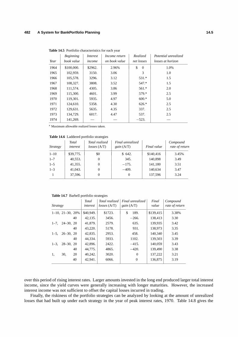
482 A System for BankPortfolio Planning 14.5
Table 14.5 Portfolio characteristics for each year
Beginning Interest Income return Realized Potential unrealized
Year book value income on book value net losses losses at horizon
1964 $100,000. $2962. 2.96% $ 0 1.0%
1965 102,959. 3150. 3.06 3 1.0
1966 105,578. 3296. 3.12 531.* 1.5
1967 108,327. 3808. 3.52 547.* 1.5
1968 111,574. 4305. 3.86 561.* 2.0
1969 115,300. 4601. 3.99 579.* 2.5
1970 119,301. 5935. 4.97 600.* 5.0
1971 124,610. 5358. 4.30 626.* 2.5
1972 129,631. 5635. 4.35 337. 2.5
1973 134,729. 6017. 4.47 537. 2.5
1974 141,269. — — −523. —
∗ Maximum allowable realized losses taken.
Table 14.6 Laddered portfolio strategies
Total Total realized Final unrealized CompoundStrategy interest losses(A/T) gain (A/T) Final value rate of return
1–10 $39,775. $0 $ 642. $140,416 3.45%
1–7 40,553. 0 345. 140,898 3.49
1–5 41,355. 0 −175. 141,180 3.51
1–3 41,043. 0 −409. 140,634 3.47
1 37,596. 0 0 137,596 3.24
Table 14.7 Barbell portfolio strategies
Total Total realized Final unrealized Final CompoundStrategy interest losses(A/T) gain (A/T) value rate of return
1–10, 21–30, 20% $40,949. $1723. $ 189. $139,415 3.38%
40 42,135. 3456. −266. 138,413 3.30
1–7, 24–30, 20 41,879. 2579. 635. 139,935 3.42
40 43,220. 5178. 931. 138,973 3.35
1–5, 26–30, 20 42,835. 2953. 458. 140,340 3.45
40 44,334. 5933. 1102. 139,503 3.39
1–3, 28–30, 20 42,896. 2422. −415. 140,059 3.43
40 44,775. 4865. −420. 139,490 3.38
1, 30, 20 40,242. 3020. 0 137,222 3.21
40 42,941. 6066. 0 136,875 3.19
over this period of rising interest rates. Larger amounts invested in the long end produced larger total interestincome, since the yield curves were generally increasing with longer maturities. However, the increasedinterest income was not sufficient to offset the capital losses incurred in trading.
Finally, the riskiness of the portfolio strategies can be analyzed by looking at the amount of unrealizedlosses that had built up under each strategy in the year of peak interest rates, 1970. Table 14.8 gives the

14.5 Evaluating the Performance of the Model 483
book value, market value, and unrealized after-tax losses as a percent of book value, for the strategy followedby the BONDS model and for various laddered and barbell strategies. In a period of rising rates, strategiesthat keep most of their assets in short-term securities would be expected to have lower unrealized losses. Inthe extreme case, a ladder consisting of only the one-year maturity would havezerounrealized losses at thebeginning of each year, since the entire portfolio would mature at the end of each period.
Table 14.8 Unrealized losses, January 1, 1970
Unrealized
after-tax
Type of portfolio Book value Market value losses
BONDS $119,299 $107,536 4.93%
Ladder 1–5 119,198 115,252 1.66
1–10 119,403 113,958 4.56
Barbell 1–5, 26–30, 20% 118,051 113,688 3.70
1–5, 26–30, 40% 116,889 110,107 5.80
Barbell 1–10, 21–30, 20% 119,222 111,200 6.73
1–10, 21–30, 40% 119,039 108,415 8.92
On this dimension, the strategy followed by the BONDS model builds up significant losses, roughlycomparable to a ten-year ladder, or a barbell with five maturities on each end and, say, thirty percent of theportfolio value invested in the long end. However, this general level of unrealized losses in the credit crunchof 1969 might have been considered very reasonable. Any strategy that places a significant proportion of itsassets in relatively short-term securities will not develop unrealized losses. However, just as there is potentialfor losses with these strategies, there is also potential for similar gains.
We can sum up the performance of the BONDS model by comparing it to the best of the mechanically-managed laddered or barbell strategies. The performance of the five-year laddered portfolio was almost asgood as that of the BONDS model against the particular sequence of interest rates that occurred. However,it should be noted that a portfolio laddered out only to five years is a very conservative strategy, which israther unlikely to be followed in practice. It happened to turn out, after the fact, that this was a good strategyto have adopted; but it is not clear that any portfolio manager would have been motivated to adopt such aconservative strategy consistently over the period of the simulation.
Finally, had interest rates been level or falling, the BONDS model would certainly have outperformed thefive-year ladder. In these instances, some other laddered or barbell portfolio might perform competitivelywith the BONDS model. However, the important characteristic of the BONDS model is that it produces astrategy that is adaptive to the environment over time. The BONDS model should perform well againstanyinterest-rate sequence, while a particular laddered or barbell portfolio will perform well for some realizationsof interest rates and poorly for others. In actual practice, the portfolio manager would beactively forecastinginterest rates, and the BONDS model provides a method of systematically taking advantage of these forecasts.
EXERCISES
1. A bank considering using the BONDS model to aid in portfolio planning divides its portfolio into two pools offunds—U.S. Governments and all grades of municipals. The bank managers forecast a yield curve for their groupof municipals and are willing to treat them as one category. The investment portfolio decisions are revised monthly,but no securities with less than three months to maturity are purchased.
a) Assuming that the bank employs a two-year planning horizon with four planning periods of 3 months, 3 months,6 months, and one year, how many constraints of each type will their model have, using 5-point approximations

484 A System for BankPortfolio Planning 14.5
to the uncertainties in the first two periods and 3-point approximations in the last two periods? (Assume no initialholdings, but include the remaining constraints of Table 14.1.)
b) The bank feels that it can aggregate the purchase decisions on individual securities into the following maturities:3 months, 6 months, 1, 2, 3, 5, 10, and 20 years for U.S. Governments and 1, 2, 3, 4, 5, 10, 20, and 30 yearsfor the municipal group. How many decision variables will the model sketched in (a) have? (Again, assume noinitial holdings.)
c) In fact, the bank does have initial holdings of both Governments and municipals. The bank is willing to aggregatethese holdings in the same maturities as used for new purchases. How many additional constraints and variablesneed to be added to account for the initial holdings?
d) How is a subproblem defined for the model described in (a), (b), and (c)? How many such subproblems are there?Why is it impossible to combine the subproblem from initial holdings with those of subsequent purchases?
e) How many constraints does the restricted master have? How would you find an initial basic feasible solution tothe restricted master?
2. For the model described in Exercise 1, the demands for information from the portfolio manager are extensive.
a) How many yield curves need to be assessed to use the proposed planning model?b) How would you think about the problem of assessing the exogenous cash flows in such a way that they are
consistent with the yield curves assessed?c) What is the interpretation of using the same level of realized and unrealized losses on all scenarios? Which
scenarios are likely to produce the binding realized and unrealized loss constraints? Can the loss constraints onthe remaining scenarios be dropped?
d) Suppose that the lower-bound constraint on the holdings of government securities could be dropped from themodel. How might this change in the model formulation affect the optimal solution? Could the value of theobjective function decrease?
3. The objective function of the BONDS model is given in terms of the horizon value of the portfolio. Suppose thatwe wish to reformulate the model in terms of the interest income and capital gains in each period. The decisionvariables remain the same; all constraints are unchanged, but the objective function changes.
a) Formulate a new objective function that maximizes the expectedincreasein the size of the portfolio by summing,over all time periods, the interest income plus capital gains (or losses) in each time period.
b) Show that the two formulations are equivalent, in the sense that the optimal values of the decision variable usingeach objective function are identical.
c) Show that the difference between the optimal values of the two objective functions is the expected exogenouscash flow.
4. Upon seeing your formulation in Exercise 2, the portfolio manager argues that the cash flows in the objective functionshould be discounted.
a) Will discounting the cash flows change the optimal values of the decision variables?b) What are the arguments for and against discounting in this situation? How could a single discount rate be chosen?c) What is the relationship between the shadow prices on the funds-flow constraints of the undiscounted formulation
and the discount rate? (See exercises in Chapter 4.)d) Suppose you win the argument with the portfolio manager and do not use a discounted objective function. Other
departments in the bank place demands on the portfolio for funds in various time periods. Can you suggest anapproach to choosing among various requests for funds? How does the approach relate to discounting the cashflows?
5. Consider the subproblems generated by the decomposition approach. Formulate the subproblem corresponding tobuying a 20-year U.S. Government security at the beginning of the first period of a model consisting of 3 one-yearperiods. The generic decision variables to use are as follows:
b1, S21(e2), h21(e2), S31(e3), h31(e3).
(Do not include buying a similar security at the beginning of the second or third periods.)

14.5 Evaluating the Performance of the Model 485
a) How many constraints and decision variables does the subproblem have?b) The constraints of the subproblems are homogeneous (i.e., zero righthand sides). Suppose that purchasing 1 unit
of this security,b1 = 1, gives a positive rate of return. What can be said about purchasingλb1 units of thissecurity?
c) Formulate a dynamic-programmig model to solve this subproblem, assuming thatb1 = 1. Show that this solutiondetermines aray of the subproblem.
6. Suppose that, for the subproblems formulated in Exercise 5, we define aray-findingsubproblem as follows:b1 isset equal to 1 and moved to the righthand side; the resulting subproblem is solved by linear programming.
a) Formulate the ray-finding problem.b) Find the dual of the ray-finding problem.c) Show that a basis for the dual problem is triangular.d) Write down a recursive method for calculating the optimal solution of the dual of the ray-finding problem. [Hint.
Exploit the triangular property of the basis to solve for the dual variables by back-substitution.]e) How is the solution of the primal ray-finding problem determined from the solution of the dual?
7. As a follow-up to Exercises 5 and 6, once the subproblems have been solved, the rays generated are added to therestricted master:
a) Describe how the columns of the restricted master are computed.b) Why are weighting constraintsnotneeded for the restricted master in this particular application?c) What is the stopping rule for this variation of the decomposition algorithm?d) Suppose that storage limitations force you to drop some of the nonbasic columns from the restricted master at
some iteration. Is it possible that the algorithm will be unable to find the overall optimal solution as a result?
8. There are at least two ways to define subproblems for this model. First, a subproblem can be defined for eachmaturity and each year it can be purchased. In Fig. 14.4 there are a total of 12 subproblems using this definition.Second, a subproblem can be defined for each maturity regardless of when it is purchased. In Fig. 14.4 there are atotal of 3 subproblems using this definition.
a) Explain why the choice of subproblem definitions need have no impact on the solution procedure adopted forthe subproblems.
b) Explain how the restricted master will differ under each definition of the subproblmes.c) Which choice of subproblem definitions will make the restricted master more efficient to solve? Why?d) If there was a weighting constraint for each subproblem, how would your answer to (c) be affected? [Hint.
Which definition would add more weighting constraints?]
9. Suppose that a new objective function is to be considered that is a nonlinear function of the holdings entering thefinal period. More precisely, assume that we wish to maximize theexpectedutility of these holdings, with the utilityfunction given by:
u(x) = ax1−c,
wherea > 0 and 0< c < 1. The objective function is then of the form:
∑eN∈EN
p(eN)u
{K∑
k=1
[N−1∑m=0
(ykm(em)+ vk
m,N(eN))hkm,N(eN)+ (yk
N(eN)+ vkN,N(eN))bk
N(eN)
]}.
a) Show that this problem cannot be handled directly by decomposition. [Hint. Is this objective function separablein the appropriate way?]
b) If the nonlinear-programming problem were solved by the Frank-Wolfe algorithm, a sequence of linear programswould be solved. How can the decomposition approach presented in this chapter be used to solve one of theselinear programs?
c) How can the Frank-Wolfe algorithm be efficiently combined with the decomposition approach presented in thischapter, to find the optimal solution to the nonlinear program defined by maximizing the expected utility givenabove?

486 A System for BankPortfolio Planning A.5
d) Does your proposed method generalize to other nonlinear problems?
10. Describe the method of producing scenarios used in the historical simulation over the first three decisions (twoyears).
a) How many yield curves need to be assessed at the beginning of ’64 for the years ’64, ’65, and ’66?b) Draw a decision tree depicting the probability that each of the yield curves indicated in (a) occurs. What use is
made of the uncertainty in the estimates of the change in the twenty-year rate (thirty-year rate) as a fraction ofthe change in the one-year rate? How could this be modified?
c) Show how to compute the parameters of the functional form for each of the yield curves forecast for the start of’65.
d) Explain how you might assess the required information in actual practice, using a model similar to that describedin Exercise 1. Draw a distinction between short-term forecasting (3 months) and long-term forecasting (2 years).
11. The performance of the laddered portfolio structure with five equally spaced maturities proved to be the best amongthe ladders investigated. Similarly, the performance of the 1–5, 26–30 barbell, with 20% invested in the long end,proved the best among the barbells. The BONDS model outperformed these strategies in the historical simulationover a period of rising rates.
a) How would you expect these strategies to compare with the BONDS model in a period of falling rates?b) How would you choose an appropriate ladder or barbell strategy without the benefit of 20/20 hindsight?c) What benefits does the BONDS model have over either a ladder or barbell approach to portfolio management?
ACKNOWLEDGMENTS
This chapter is based primarily on material drawn from ‘‘Managing a Bank Bond Portfolio Over Time,’’ byS. P. Bradley and D. B. Crane, to appear inStochastic Programming(ed. M. A. H. Dempster), AcademicPress, in press. A broad coverage of the area is contained inManagement of Bank Portfoliosby S. P. Bradleyand D. B. Crane, John Wiley & Sons, New York, 1975.

Vectors andMatrices
Appendix A
Vectors and matrices are notational conveniences for dealing with systems of linear equations and inequalities.In particular, they are useful for compactly representing and discussing the linear programming problem:
Maximizen∑
j=1
c j x j ,
subject to:n∑
j=1
ai j x j = bi (i = 1, 2, . . . , m),
x j ≥ 0 ( j = 1, 2, . . . , n).
This appendix reviews several properties of vectors and matrices that are especially relevant to thisproblem. We should note, however, that the material contained here is more technical than is required forunderstanding the rest of this book. It is included for completeness rather than for background.
A.1 VECTORS
We begin by defining vectors, relations among vectors, and elementary vector operations.
Definition. A k-dimensional vector yis an ordered collection ofk real numbersy1, y2, . . . , yk, and iswritten asy = (y1, y2, . . . , yk). The numbersy j ( j = 1, 2, . . . , k) are called thecomponentsof thevectory.
Each of the following are examples of vectors:
i) (1, −3, 0, 5) is a four-dimensional vector. Its first component is 1, its second component is−3, and itsthird and fourth components are 0 and 5, respectively.
ii) The coefficientsc1, c2, . . . , cn of the linear-programming objective function determine then-dimensionalvectorc = (c1, c2, . . . , cn).
iii) The activity levelsx1, x2, . . . , xn of a linear program define then-dimensional vectorx = (x1, x2, . . . , xn).iv) The coefficientsai 1, ai 2, . . . , ain of the decision variables in thei th equation of a linear program deter-
mine ann-dimensional vectorAi= (ai 1, ai 2, . . . , ain).
v) The coefficientsa1 j , a2 j , . . . , anj of the decision variablex j in constraints 1 throughm of a linearprogram define anm-dimensional vector which we denote asA j = (a1 j , a2 j , . . . , amj).
487

488 Vectors and Matrices A.2
Equality and ordering of vectors are defined by comparing the vectors’ individual components. Formally,let y = (y1, y2, . . . , yk) andz= (z1, z2, . . . , zk) be twok-dimensional vectors. We write:
y = z wheny j = z j ( j = 1, 2, . . . , k),
y ≥ z or z≤ y wheny j ≥ z j ( j = 1, 2, . . . , k),
y > z or z < y wheny j > z j ( j = 1, 2, . . . , k),
and say, respectively, thaty equals z, yis greater than or equal to zand thaty is greater than z. In the last twocases, we also say thatz is less than or equal to yandless than y. It should be emphasized thatnot all vectorsare ordered. For example, ify = (3, 1,−2) andx = (1, 1, 1), then the first two components ofy are greaterthan or equal to the first two components ofx but the third component ofy is lessthan the correspondingcomponent ofx.
A final note: 0 is used to denote thenull vector (0, 0, …, 0), where the dimension of the vector isunderstood from context. Thus, ifx is ak-dimensional vector,x ≥ 0 means that each componentx j of thevectorx is nonnegative.
We also define scalar multiplication and addition in terms of the components of the vectors.
Definition. Scalar multiplicationof a vectory = (y1, y2, . . . , yk) and a scalarα is defined to be a newvectorz= (z1, z2, . . . , zk), writtenz= αy or z= yα, whose components are given byz j = αy j .
Definition. Vector additionof twok-dimensional vectorsx = (x1, x2, . . . , xk) andy = (y1, y2, . . . , yk)
is defined as a new vectorz= (z1, z2, . . . , zk), denotedz= x+y, with components given byz j = x j+y j .
As an example of scalar multiplication, consider
4(3, 0,−1, 8) = (12, 0,−4, 32),
and for vector addition,(3, 4, 1,−3)+ (1, 3,−2, 5) = (4, 7,−1, 2).
Using both operations, we can make the following type of calculation:
(1, 0)x1+ (0, 1)x2+ (−3,−8)x3 = (x1, 0)+ (0, x2)+ (−3x3,−8x3)
= (x1 −3x3, x2 −8x3).
It is important to note thaty and z must have the same dimensions for vector addition and vectorcomparisons. Thus(6, 2,−1)+ (4, 0) is notdefined, and(4, 0,−1) = (4, 0) makesnosense at all.
A.2 MATRICES
We can now extend these ideas to any rectangular array of numbers, which we call amatrix.
Definition. A matrix is defined to be a rectangular array of numbers
A =
a11 a12 · · · a1na21 a22 · · · a2n...
...
am1 am2 · · · amn
,
whosedimensionis m by n. A is calledsquareif m= n. The numbersai j are referred to as theelementsof A.
The tableau of a linear programming problem is an example of a matrix.We define equality of two matrices in terms of their elements just as in the case of vectors.

A.2 Matrices 489
Definition. Two matricesA andB are said to beequal, written A = B, if they have the same dimensionand their corresponding elements are equal, i.e.,ai j = bi j for all i and j .
In some instances it is convenient to think of vectors as merely beingspecial casesof matrices. However, wewill later prove a number of properties of vectors that do not have straightforward generalizations to matrices.
Definition. A k-by-1 matrix is called acolumn vectorand a 1-by-k matrix is called arow vector.
The coefficients in rowi of the matrixAdetermine a row vectorAi = (ai 1, ai 2, …,ain), and the coefficientsof column j of A determine a column vectorA j = 〈a1 j , a2 j , . . . , amj〉. For notational convenience, columnvectors are frequently written horizontally in angular brackets.
We can define scalar multiplication of a matrix, and addition of two matrices, by the obvious analogs ofthese definitions for vectors.
Definition. Scalar multiplicationof a matrix A and a real numberα is defined to be a new matrixB,written B = αA or B = Aα, whose elementsbi j are given bybi j = αai j .
For example,
3
[1 20 −3
]=
[3 60 −9
].
Definition. Additionof two matricesA andB, both with dimensionm by n, is defined as a new matrixC, writtenC = A+ B, whose elementsci j are given byci j = ai j + bi j .
For example, [1 2 40 −3 1
]+
[2 6 −3−1 4 0
]=
[3 8 1−1 1 1
](A) (B) (C)
If two matricesA andB do not have the same dimension, thenA+ B is undefined.The product of two matrices can also be defined if the two matrices have appropriate dimensions.
Definition. Theproductof anm-by-p matrix A and ap-by-n matrix B is defined to be a newm-by-nmatrixC, writtenC = AB, whose elementsci j are given by:
ci j =
p∑k=1
aikbk j .
For example, 1 20 −33 1
[ 2 6 −31 4 0
]=
4 14 −3−3 −12 0
7 22 −9
and [
2 6 −31 4 0
] 1 20 −33 1
= [−7 −171 −10
].
If the number of columns ofA does not equal the number of rows ofB, thenAB is undefined. Further,from these examples, observe that matrix multiplication isnot commutative; that is,AB 6= B A, in general.
If π = (π1, π2, . . . , πm) is a row vector andq = 〈q1, q2, . . . , qm〉 a column vector, then the special case
πq =m∑
i=1
πi qi

490 Vectors and Matrices A.2
of matrix multiplication is sometimes referred to as aninner product. It can be visualized by placing theelements ofπ next to those ofq andadding, as follows:
π1× q1 = π1q1,
π2× q2 = π2q2,
......
πm× qm = πmqm.
πq =m∑
i=1
πi qi .
In these terms, the elementsci j of matrix C = AB are found by taking the inner product ofAi (the i th rowof A) with B j (the j th column ofB); that is,ci j = Ai B j .
The following properties of matrices can be seen easily by writing out the appropriate expressions in eachinstance and rearranging the terms:
A+ B = B+ A (Commutative law)
A+ (B+ C) = (A+ B)+ C (Associative law)
A(BC) = (AB)C (Associative law)
A(B+ C) = AB+ AC (Distributive law)
As a result,A+ B+ C or ABC is well defined, since the evaluations can be performed in any order.There are a few special matrices that will be useful in our discussion, so we define them here.
Definition. The identity matrixof orderm, written Im (or simply I , when no confusion arises) is asquarem-by-m matrix withonesalong the diagonal andzeroselsewhere.
For example,
I3 =
1 0 00 1 00 0 1
.
It is important to note that for anym-by-m matrix B, BIm = ImB = B. In particular,ImIm = Im orI I = I .
Definition. Thetransposeof a matrixA, denotedAt , is formed byinterchangingthe rows and columnsof A; that is,at
i j = a j i .
IfA =
[2 4 −1−3 0 4
],
then the transpose ofA is given by:
At=
2 −34 0−1 4
.
We can show that(AB)t= Bt At since thei j th element of both sides of the equality is
∑k a jkbki .
Definition. An elementary matrixis a square matrix with one arbitrary column, but otherwiseonesalong the diagonal andzeroselsewhere (i.e., an identify matrix with the exception of one column).
A.3 Linear Programming in Matrix Form 491
For example,
E =
1 0 −1 00 1 3 00 0 2 00 0 4 1
is an elementary matrix.
A.3 LINEAR PROGRAMMING IN MATRIX FORM
The linear-programming problem
Maximizec1x1+ c2x2+ · · · + cnxn,
subject to:a11x1+ a12x2 + · · · + a1nxn ≤ b1,
a12x1+ a22x2 + · · · + a2nxn ≤ b2,
......
...
a1mx1+ a2mx2+ · · · + amnxn ≤ bm,
x1 ≥ 0, x2 ≥ 0, . . . , xn ≥ 0,
can now be written in matrix form in a straightforward manner. If we let:
x =
x1x2...
xn
and b =
b1b2...
bm
be column vectors, the linear system of inequalities is written in matrix form asAx ≤ b. Letting c =(c1, c2, . . . , cn) be a row vector, the objective function is written ascx. Hence,the linear program assumesthe following compact form:
Maximizecx,
subject to:Ax ≤ b, x ≥ 0.
The same problem can also be written in terms of the column vectorsA j of the matrixA as:
Maximizec1x1+ c2x2 + · · · + cnxn,subject to:
A1x1 + A2x2+ · · · + Anxn ≤ b,
x j ≥ 0 ( j = 1, 2, . . . , n).
At various times it is convenient to use either of these forms.The appropriatedual linear program is given by:
Minimize b1y1+ b2y2+ · · · + bmym,
subject to:
a11y1+ a21y2+ · · · + am1ym ≥ c1,
a12y1+ a22y2+ · · · + am2ym ≥ c2,
......
...
a1ny1+ a2ny2+ · · · + amnym ≥ cn,
y1 ≥ 0, y2 ≥ 0, . . . , ym ≥ 0.

492 Vectors and Matrices A.4
Letting
yt=
y1y2...
yn
be a column vector, since the dual variables are associated with the constraints of the primal problem, we canwrite the dual linear program in compact form as follows:
Minimize bt yt ,
subject to:At yt≥ ct , yt
≥ 0.
We can also write the dual in terms of the untransposed vectors as follows:
Minimize yb,
subject to:y A≥ c, y ≥ 0.
In this form it is easy to write the problem in terms of the row vectorsAi of the matrixA, as:
Minimize y1b1+ y2b2+ · · · + ymbm,
subject to:
y1A1+ y2A2
+ · · · + ymAm≥ c,
yi ≥ 0 (i = 1, 2, . . . , m).
Finally, we can write the primal and dual problems in equality form. In the primal, we merely define anm-dimensional column vectors measuring the amount of slack in each constraint, and write:
Maximizecx,
subject to:Ax + I s = b,
x ≥ 0, s ≥ 0.
In the dual, we define ann-dimensional row vectoru measuring the amount of surplus in each dual constraintand write:
Minimize yb,
subject to:y A− uI = c,
y ≥ 0, u ≥ 0.
A.4 THE INVERSE OF A MATRIX
Definition. Given a squarem-by-m matrix B, if there is anm-by-m matrix D such that
DB = B D = I ,
thenD is called theinverseof B and is denotedB−1.
Note thatB−1 does not mean 1/B or I /B, since division isnotdefined for matrices. The symbolB−1 is justa convenient way to emphasize the relationship between the inverse matrixD and the original matrixB.
There are a number of simple properties of inverses that are sometimes helpful to know.

A.4 The Inverse of a Matrix 493
i) The inverse of a matrixB is unique if it exists.
Proof. Suppose thatB−1 andA are both inverses ofB. Then
B−1= I B−1
= (AB)B−1= A(B B−1) = A.
ii) I −1= I sinceI I = I .
iii) If the inverse ofA andB exist, then the inverse ofAB exists and is given by(AB)−1= B−1A−1.
Proof. (AB)(B−1A−1) = A(B B−1)A−1= AI A−1
= AA−1= I .
iv) If the inverse ofB exists, then the inverse ofB−1 exists and is given by(B−1)−1= B.
Proof. I = I −1= (B−1B)−1
= B−1(B−1)−1.
v) If the inverse ofB exists, then the inverse ofBt exists and is given by(Bt )−1= (B−1)t .
Proof. I = I t= (B−1B)t
= Bt (B−1)t .
The natural question that arises is: Under what circumstances does the inverse of a matrix exist? Considerthe square system of equations given by:
Bx = I y = y.
If B has an inverse, then multiplying on the left byB−1 yields
I x = B−1y,
which ‘‘solves’’ the original square system of equations for any choice ofy. The second system of equationshas a unique solution in terms ofx for any choice ofy, since one variablex j is isolated in each equation.The first system of equations can be derived from the second by multiplying on the left byB; hence, thetwo systems are identical in the sense that anyx, y that satisfies one system will also satisfy the other. Wecan now show that a square matrixB has an inverse if the square system of equationsBx = y has a uniquesolutionx for an arbitrary choice ofy.
The solution to this system of equations can be obtained by successively isolating one variable in eachequation by a procedure known asGauss–Jordan elimination, which is just the method for solving squaresystems of equations learned in high-school algebra. Assumingb11 6= 0, we can use the first equation toeliminatex1 from the other equations, giving:
x1 +b12b11
x2 + · · · +b1mb11
xm =1
b11y1,
(b22− b21
b12b11
)x2 + · · · +
(b2m− b21
b1mb11
)xm = −
b21b11
y1 + y2,
......
. . .(bm2− bm1
b12b11
)x2 + · · · +
(bmm− bm1
b1mb11
)xm = −
bm1b11
y1 + ym.
494 Vectors and Matrices A.4
If b11 = 0, we merely choose some other variable to isolate in the first equation. In matrix form, the newmatrices of thex andy coefficients are given respectively byE1B andE1I , whereE1 is an elementary matrixof the form:
E1 =
k1 0 0 · · · 0k2 1 0 · · · 0k3 0 1 · · · 0...
. . .
km 0 0 · · · 1
,
k1 =1
b11,
...
ki = −bi 1b11
(i = 2, 3, . . . , m).
Further, sinceb11 is chosen to be nonzero,E1 has an inverse given by:
E−11 =
1/k1 0 0 · · · 0−k2 1 0 · · · 0−k3 0 1 · · · 0
.... . .
−km 0 0 · · · 1
.
Thus by property (iii) above, ifB has an inverse, thenE1B has an inverse and the procedure may be repeated.Somex j coefficient in the second row of the updated systemmust be nonzero, or no variable can be isolatedin the second row, implying that the inverse does not exist. The procedure may be repeated by eliminatingthis x j from the other equations. Thus, a new elementary matrixE2 is defined, and the new system
(E2E1B)x = (E2E1)y
hasx1 isolated in equation 1 andx2 in equation 2.Repeating the procedure finally gives:
(EmEm−1 · · · E2E1B)x = (EmEm−1 · · · E2E1)y
with one variable isolated in each equation. If variablex j is isolated in equationj , the final system reads:
x1 = β11y1+β12y2+ · · · + β1mym,
x2 = β21y1+β22y2+ · · · + β2mym,. . .
...
xm = βm1y1+βm2y2+ · · · + βmmym,
and
B−1=
β11 β12 · · · β1mβ21 β22 · · · β2m...
...
βm1 βm2 · · · βmm
.
Equivalently,B−1= EmEm−1 · · · E2E1 is expressed inproduct formas the matrix product of elementary
matrices. If, at any stage in the procedure, it is not possible to isolate a variable in the row under consideration,then the inverse of the original matrix does not exist.
If x j has not been isolated in thej th equation, the equations may have to be permuted to determineB−1.This point is illustrated by the following example:

A.4 The Inverse of a Matrix 495
Rearranging the first and second rows of the last table gives the desired transformation ofB into theidentity matrix, and shows that:
B−1=
0 32 −
12
0 −1 12
14
12 −
14
.
Alternately, if the first and second columns of the last table are interchanged, an identity matrix is produced.Interchanging the first and second columns ofB, and performing the same operations as above, has this sameeffect. Consequently,
E3E2E1 =
0 −1 12
0 32 −
12
14
12 −
14
is the inverse of
2 0 4
2 2 0
6 4 0
.
In many applications the column order, i.e., the indexing of the variablesx j , is arbitrary, and this last procedureis utilized. That is, one variable is isolated in each row and the variable isolated in rowj is considered thej th basic variable (above, the second basic variable would bex1). Then the product form gives the inverseof the columns toB, reindexed to agree with the ordering of the basic variables.
In computing the inverse of a matrix, it is often helpful to take advantage of any special structure that thematrix may have. To take advantage of this structure, we maypartition a matrix into a number of smallermatrices, by subdividing its rows and columns.
For example, the matrixA below is partitioned into four submatricesA11, A12, A21, andA22:
A =
a11 a12 a13a21 a22 a23
a31 a32 a33a41 a42 a43
= [ A11 A12
A21 A22
].
The important point to note is that partitioned matrices obey the usual rules of matrix algebra. For example,

496 Vectors and Matrices A.5
multiplication of two partitioned matrices
A =
A11 A12A21 A22A31 A32
, and B =
[B11 B12B21 B22
]results in
AB=
A11B11+ A12B21 A11B12+ A12B22A21B11+ A22B21 A21B12+ A22B22A31B11+ A32B21 A31B12+ A32B22
,
assuming the indicated products are defined; i.e., the matricesAi j andB jk have the appropriate dimensions.To illustrate that partitioned matrices may be helpful in computing inverses, consider the following
example. Let
M =
[I Q0 R
],
where 0 denotes a matrix with all zero entries. Then
M−1=
[A BC D
]satisfies
M M−1= I or
[I Q0 R
] [A BC D
]=
[I 00 I
],
which implies the following matrix equations:
A+ QC = I , B+ QD = 0,
RC= 0, RD= I .
Solving these simultaneous equations gives
C = 0, A = I , D = R−1, and B = −QR−1;
or, equivalently,
M−1=
[I −QR−1
0 R−1
].
Note that we need only computeR−1 in order to determineM−1 easily. This type of use of partitionedmatrices is the essence of many schemes for handling large-scale linear programs with special structures.
A.5 BASES AND REPRESENTATIONS
In Chapters 2, 3, and 4, the concept of a basis plays an important role in developing the computationalprocedures and fundamental properties of linear programming. In this section, we present the algebraicfoundations of this concept.
Definition. m-dimensional real spaceRm is defined as the collection of allm-dimensional vectorsy = (y1, y2, . . . , ym).
Definition. A set of m-dimensional vectorsA1, A2, . . . , Ak is linearly dependentif there exist realnumbersα1, α2, . . . , αk, not all zero, such that
α1A1+ α2A2+ · · · + αk Ak = 0. (1)
If the only set ofα j ’s for which (1) holds isα1 = α2 = · · · = αk = 0, then them-vectorsA1, A2, . . . , Akare said to belinearly independent.

A.5 Bases and Representations 497
For example, the vectors(4, 1, 0,−1), (3, 1, 1,−2), and(1, 1, 3,−4) are linearly dependent, since
2(4, 1, 0,−1)− 3(3, 1, 1,−2)+ 1(1, 1, 3,−4) = 0.
Further, theunit m-dimensional vectorsu j = (0, . . . , 0, 1, 0, . . . , 0) for j = 1, 2, . . . , m, with aplus oneinthe j th component and zeros elsewhere, are linearly independent, since
m∑j=1
α j u j = 0
implies that
α1 = α2 = · · · = αm = 0.
If any of the vectorsA1, A2, . . . , Ak, sayAr , is the 0 vector (i.e., has all zero components), then, takingαr = 1 and all otherα j = 0 shows that the vectors are linearly dependent. Hence, the null vector is linearlydependent on any set of vectors.
Definition. An m-dimensional vectorQ is said to bedependenton the set ofm-dimensional vectorsA1, A2, . . . , Ak if Q can be written as a linear combination of these vectors; that is,
Q = λ1A1+ λ2A2+ · · · + λk Ak
for some real numbersλ1, λ2, . . . , λk. The k-dimensional vector(λ1, λ2, . . . , λk) is said to be therepresentationof Q in terms ofA1, A2, . . . , Ak.
Note that(1, 1, 0) is not dependent upon(0, 4, 2) and (0,−1, 3), sinceλ1(0, 4, 2) + λ2(0,−1, 3) =
(0, 4λ1− λ2, 2λ1+ 3λ2) and can never have 1 as its first component.Them-dimensional vector(λ1, λ2, . . . , λm) is dependent upon them-dimensional unit vectorsu1, u2, . . . , um,
since
(λ1, λ2, . . . , λm) =
m∑j=1
λ j u j .
Thus, anym-dimensional vector is dependent on them-dimensional unit vectors. This suggests the followingimportant definition.
Definition. A basisof Rm is a set of linearly independentm-dimensional vectors with the property thatevery vector ofRm is dependent upon these vectors.
Note that them-dimensional unit vectorsu1, u2, . . . , um are a basis forRm, since they are linearly independentand anym-dimensional vector is dependent on them.
We now sketch the proofs of a number of important properties relating bases of real spaces, representationsof vectors in terms of bases, changes of bases, and inverses of basis matrices.
Property 1. A set ofm-dimensional vectorsA1, A2, . . . , Ar is linearly dependent if and only if one ofthese vectors is dependent upon the others.
Proof. First, suppose that
Ar =
r−1∑j=1
λ j A j ,

498 Vectors and Matrices A.5
so thatAr is dependent uponA1, A2, . . . , Ar−1. Then, settingλr = −1, we have
r−1∑j=1
λ j A j − λr Ar = 0,
which shows thatA1, A2, . . . , Ar are linearly dependent.
Next, if the set of vectors is dependent, then
r∑j=1
α j A j = 0,
with at least oneα j 6= 0, sayαr 6= 0. Then,
Ar =
r−1∑j=1
λ j A j ,
where
λ j = −
(α j
αr
),
andAr depends uponA1, A2, . . . , Ar−1. �
Property 2. The representation of any vectorQ in terms of basis vectorsA1, A2, . . . , Am is unique.
Proof. Suppose thatQ is represented as both
Q =m∑
j=1
λ j A j and Q =m∑
j=1
λ′j A j .
EliminatingQ gives 0=∑m
j=1 (λ j − λ′j )A j . SinceA1, A2, . . . , Am constitute a basis, they are linearlyindependent and each(λ j − λ′j ) = 0. That is,λ j = λ′j , so that the representation must be unique.�
This proposition actually shows that ifQ can be represented in terms of the linearly independent vectorsA1, A2, . . . , Am, whether a basis or not, then the representation is unique. IfA1, A2, . . . , Am is a basis, thenthe representation is always possible because of the definition of a basis.
Several mathematical-programming algorithms, including the simplex method for linear programming,move from one basis to another by introducing a vector into the basis in place of one already there.
Property 3. Let A1, A2, . . . , Am be a basis forRm; let Q 6= 0 be anym-dimensional vector; and let(λ1, λ2, . . . , λm) be the representation ofQ in terms of this basis; that is,
Q =m∑
j=1
λ j A j . (2)
Then, if Q replaces any vectorAr in the basis withλr 6= 0, the new set of vectors is a basis forRm.

A.5 Bases and Representations 499
Proof. Suppose thatλm 6= 0. First, we show that the vectorsA1, A2, . . . , Am−1, Q are linearly indepen-dent. Letα j for j = 1, 2, . . . , m andαQ be any real numbers satisfying:
m−1∑j=1
α j A j + αQQ = 0. (3)
If αQ 6= 0, then
Q =m−1∑j=1
(−
α j
αQ
)A j ,
which with (2) gives two representations ofQ in terms of the basisA1, A2, . . . , Am. By Property 2, thisis impossible, soαQ = 0. But then,α1 = α2 = · · · = αm−1 = 0, sinceA1, A2, . . . , Am−1 are linearlyindependent. Thus, as required,α1 = α2 = · · · = αm−1 = αQ = 0 is the only solution to (3).
Second, we show that anym-dimensional vectorP can be represented in terms of the vectorsA1, A2, . . . , Am−1, Q.SinceA1, A2, . . . , Am is a basis, there are constantsα1, α2, . . . , αm such that
P =m∑
j=1
α j A j .
Using expression (2) to eliminateAm, we find that
P =m−1∑j=1
[α j − αm
(λ j
λm
)A j
]+
αm
λmQ,
which by definition shows thatA1, A2, . . . , Am−1, Q is a basis.�
Property 4. Let Q1, Q2, . . . , Qk be a collection of linearly independentm-dimensional vectors, and letA1, A2, . . . , Ar be a basis forRm. ThenQ1, Q2, . . . , Qk can replacek vectors fromA1, A2, . . . , Ar toform a new basis.
Proof. First recall that the 0 vector is not one of the vectorsQ j , since 0 vector is dependent on any setof vectors. Fork = 1, the result is a consequence of Property 3. The proof is by induction. Suppose,by reindexing if necessary, thatQ1, Q2, . . . , Q j , A j+1, A j+2, . . . , Ar is a basis. By definition of basis,there are real numbersλ1, λ2, . . . , λr such that
Q j+1 = λ1Q1+ λ2Q2+ · · · + λ j Q j + λ j+1A j+1+ λ j+2A j+2+ · · · + λr Ar .
If λi = 0 for i = j + 1, j + 2, . . . , r, then Q is represented in terms ofQ1, Q2, . . . , Q j , which,by Property 1, contradicts the linear independence ofQ1, Q2, . . . , Qk. Thus some,λi 6= 0 for i =j + 1, j + 2, . . . , r , say,λ j+1 6= 0. By Property 3, then,Q1, Q2, . . . , Q j+1, A j+1, A j+2, . . . , Ar isalso a basis. Consequently, wheneverj < k of the vectorsQi can replacej vectors fromA1, A2, . . . , Arto form a basis,( j +1) of them can be used as well, and eventuallyQ1, Q2, . . . , Qk can replacek vectorsfrom A1, A2, . . . , Ar to form a basis.�
Property 5. Every basis forRm containsm vectors.

500 Vectors and Matrices A.5
Proof. If Q1, Q2, . . . , Qk and A1, A2, . . . , Ar are two bases, then Property 4 implies thatk ≤ r . Byreversing the roles of theQ j and Ai , we also haver ≤ k and thusk = r , and every two bases containthe same number of vectors. But the unitm-dimensional vectorsu1, u2, . . . , um constitute a basis withm-dimensional vectors, and consequently, every basis ofRm must containm vectors.�
Property 6. Every collectionQ1, Q2, . . . , Qk of linearly independentm-dimensional vectors is con-tained in a basis.
Proof. Apply Property 4 withA1, A2, . . . , Am the unitm-dimensional vectors.�
Property 7. Everym linearly-independent vectors ofRm form a basis. Every collection of(m+ 1) ormore vectors inRm are linearly dependent.
Proof. Immediate, from Properties 5 and 6.�
If a matrix B is constructed withm linearly-independent column vectorsB1, B2, . . . , Bm, the propertiesjust developed for vectors are directly related to the concept of abasis inverseintroduced previously. Wewill show the relationships by defining the concept of a nonsingular matrix in terms of the independence ofits vectors. The usual definition of a nonsingular matrix is that the determinant of the matrix is nonzero.However, this definition stems historically from calculating inverses by the method of cofactors, which is oflittle computational interest for our purposes and will not be pursued.
Definition. An m-by-m matrix B is said to benonsingularif both its column vectorsB1, B2, . . . , Bmand rows vectorsB1, B2, . . . , Bm are linearly independent.
Although we will not establish the property here, defining nonsingularity ofB merely in terms of linearindependence ofeither its column vectors or row vectors is equivalent to this definition. That is, linearindependence of either its column or row vectors automatically implies linear independence of the othervectors.
Property 8. An m-by-m matrix B has an inverse if and only if it is nonsingular.
Proof. First, suppose thatB has an inverse and that
B1α1+ B2α2+ · · · + Bmαm = 0.
Lettingα = 〈α1, α2, . . . , αm〉, in matrix form, this expression says that
Bα = 0.
Thus(B−1)(Bα) = B−1(0) = 0 or (B−1B)α = I α = α = 0. That is,α1 = α2 = · · · = αm = 0, sothat vectorsB1, B2, . . . , Bm are linearly independent. Similarly,αB = 0 implies that
α = α(B B−1) = (αB)B−1= 0B−1
= 0,
so that the rowsB1, B2, . . . , Bm are linearly independent.

A.6 Extreme Points of Linear Programs 501
Next, suppose thatB1, B2, . . . , Bm are linearly independent. Then, by Property 7, these vectors are abasis forRm, so that each unitm-dimensional vectoru j is dependent upon them. That is, for eachj ,
B1λj1 + B2λ
j2 + · · · + Bmλ
jm = u j (4)
for some real numbersλ j1, λ
j2, . . . , λ
jm. Letting D j be the column vectorD j = 〈λ
j1, λ
j2, . . . , λ
jm〉, Eq. (4)
says thatB D j = u j or B D = I ,
where D is a matrix with columnsD1, D2, . . . , Dm. The same argument applied to the row vectorsB1, B2, . . . , Bm shows that there is a matrixD′ with D′B = I . But D = I D = (D′B)D = D′(B D) =
D′ I = D′, so thatD = D′ is the inverse ofB. �
Property 8 shows that the rows and columns of a nonsingular matrix inherit properties of bases forRm
and suggests the following definition.
Definition. Let A be anm-by-n matrix andB be anym-by-m submatrix ofA. If B is nonsingular, it iscalled abasisfor A.
Let B be a basis forA and let A j be any column ofA. Then there is a unique solutionA j =
〈a1 j , a2 j , . . . , anj 〉 to the system of equationsBA j = A j given by multiplying both sides of the equalityby B−1; that is,A = B−1A j . Since
BA j = B1a1 j + B2a2 j + · · · + Bmanj = A j ,
the vectorA j is the representation of the columnA j in terms of the basis. Applying Property 3, wesee thatA j can replace columnBk to form a new basis ifak j 6= 0. This result is essential for severalmathematical-programming algorithms, including the simplex method for solving linear programs.
A.6 EXTREME POINTS OF LINEAR PROGRAMS
In our discussion of linear programs in the text, we have alluded to the connection between extreme points,or corner points, of feasible regions and basic solutions to linear programs. the material in this sectiondelineates this connection precisely, using concepts of vectors and matrices. In pursuing this objective, thissection also indicates why a linear program can always be solved at a basic solution, an insight which adds toour seemingly ad hoc choice of basic feasible solutions in the text as the central focus for the simplex method.
Definition. Let Sbe a set of points inRn. A point y in S is called anextreme pointof S if y cannot bewritten asy = λw + (1− λ)x for two distinct pointsw andx in S and 0< λ < 1. That is,y does notlie on the line segment joining any two points ofS.
For example, ifS is the set of feasible points to the system
x1+ x2 ≤ 6,
x2 ≤ 3, x1 ≥ 0, x2 ≥ 0,
then the extreme points are (0, 0), (0, 3), (3, 3), and (6, 0) (see Fig. (A.1).The next result interprets the geometric notion of an extreme point for linear programs algebraically in
terms of linear independence.
Feasible Extreme Point Theorem.Let S be the set of feasible solutions to the linear programAx =b, x ≥ 0. Then the feasible pointy = (y1, y2, . . . , yn) is an extreme point ofS if and only if the columnsof A with yi > 0 are linearly independent.

502 Vectors and Matrices A.6
Figure A.1
Proof. By reindexing if necessary, we may assume that only the firstr components ofy are positive; thatis,
y1 > 0, y2 > 0, . . . , yr > 0, yr+1 = yr+2 = · · · = yn = 0.
We must show that any vectory solving Ay = b, y ≥ 0, is an extreme point if and only if the firstrcolumnA1, A2, . . . , Ar of A are linearly independent. First, suppose that these columns are not linearlyindependent, so that
A1α1+ A2α2+ · · · + Ar αr = 0 (5)
for some real numbersα1, α2, . . . , αr not all zero. If we letx denote the vectorx = (α1, α2, . . . , αr , 0, . . . , 0),then expression (5) can be written asAx = 0. Now letw = y + λx andw = y − λx. Then, as longasλ is chosen small enough to satisfyλ|α j | ≤ y j for each componentj = 1, 2, . . . , r, bothw ≥ 0 andw ≥ 0. But then, bothw andw are contained inS, since
A(y+ λx) = Ay+ λAx = Ay+ λ(0) = b,
and, similarly,A(y− λx) = b. However, sincey = 12(w + w), we see thaty is not an extreme point of
S in this case. Consequently, every extreme point ofSsatisfies the linear independence requirement.
Conversely, suppose thatA1, A2, . . . Ar are linearly independent. Ify = λw+ (1− λ)x for some pointsw andx of S and some 0< λ < 1, then y j = λw j + (1− λ)x j . Sincey j = 0 for j ≥ r + 1 andw j ≥ 0, x j ≥ 0, then necessarilyw j = x j = 0 for j ≥ r + 1. Therefore,
A1y1+ A2y2+ · · · + Ar yr = A1w1+ A2w2+ · · · + Ar wr= A1x1+ A2x2+ · · · + Ar xr = b.
Since, by Property 2 in Section A.5, the representation of the vectorb in terms of the linearly independentvectorsA1, A2, . . . , Ar is unique, theny j = z j = x j . Thus the two pointsw andx cannot be distinctand thereforey is an extreme point ofS. �
If A contains a basis (i.e., the tows ofA are linearly independent), then, by Property 6, any collectionA1, A2, . . . , Ar of linearly independent vectors can be extended to a basisA1, A2, . . . , Am. The extreme-point theorem shows, in this case, that every extreme pointy can be associated with a basic feasible solution,i.e., with a solution satisfyingy j = 0 for nonbasic variablesy j , for j = m+ 1, m+ 2, . . . , n.
Chapter 2 shows that optimal solutions to linear programs can be found at basic feasible solutions orequivalently, now, at extreme points of the feasible region. At this point, let us use the linear-algebra tools

A.6 Extreme Points of Linear Programs 503
of this appendix to drive this result independently. This will motivate the simplex method for solving linearprograms algebraically.
Suppose thaty is a feasible solution to the linear program
Maximizecx,
subject to:Ax = b, x ≥ 0, (6)
and, by reindexing variables if necessary, thaty1 > 0, y2 > 0, . . . , yr+1 > 0 andyr+2 = yr+3 = · · · =
yn = 0. If the columnAr+1 is linearly dependent upon columnsA1, A2, . . . , Ar , then
Ar+1 = A1α1+ A2α2+ · · · + Ar αr , (7)
with at least one of the constantsα j nonzero forj = 1, 2, . . . , r . Multiplying both sides of this expressionby θ gives
Ar+1θ = A1(α1θ)+ A2(α2θ)+ · · · + Ar (αr θ), (8)
which states that we may simulate the effect of settingxr+1 = θ in (6) by settingx1, x2, . . . , xr , respectively,to (α1θ), (α2θ), . . . , (αr θ). Takingθ = 1 gives:
cr+1 = α1c1+ α2c2+ · · · + αr cr
as the per-unit profit from the simulated activity of usingα1 units of x1, α2 units of x2, throughαr units ofxr , in place of 1 unit ofxr+1.
Letting x = (−α1,−α2, . . . ,−αr , + 1, 0, . . . , 0), Eq. (8) is rewritten asA(θx) = θ Ax = 0. Herex isinterpreted as settingxr+1 to 1 and decreasing the simulated activity to compensate. Thus,
A(y+ θ x) = Ay+ θ Ax = Ay+ 0= b,
so thaty+ θ x is feasible as long asy+ θ x ≥ 0 (this condition is satisfied ifθ is chosen so that|θα j | ≤ y jfor every componentj = 1, 2, . . . , r ). The return fromy+ θ x is given by:
c(y+ θ x) = cy+ θcx = cy+ θ(cr+1− cr+1).
Consequently, ifcr+1 < cr+1, the simulated activity is less profitable than the(r + 1)st activity itself, andreturn improves by increasingθ . If cr+1 >cr+1, return increases by decreasingθ (i.e., decreasingyr+1 andincreasing the simulated activity). Ifcr+1 = cr+1, return is unaffected byθ .
These observation imply that, if the objective function is bounded from above over the feasible region,then by increasing the simulated activity and decreasing activityyr+1, or vice versa, we can find a new feasiblesolution whose objective value is at least as large ascy but which contains at least one more zero componentthany.
For, suppose thatcr+1 ≥ cr+1. Then by decreasingθ from θ = 0, c(y + θ x) ≥ cy; eventuallyy j + θ x j = 0 for some componentj = 1, 2, . . . , r + 1 (possiblyyr+1 + θ xr+1 = yr+1 + θ = 0). On theother hand, ifcr+1 < cr+1, thenc(y+ θ x) > cy asθ increases fromθ = 0; if some component ofα j from(7) is positive, then eventuallyy j + θ x j = y j − θα j reaches 0 asθ increases. (If everyα j ≤ 0, then wemay increaseθ indefinitely,c(y + θ x) → +∞, and the objective value is unbounded over the constraints,contrary to our assumption.) Therefore, if
eithercr+1 ≥ cr+1 or cr+1 < cr+1,
we can find a value forθ such that at least one component ofy j + θ x j becomes zero forj = 1, 2, . . . , r + 1.Sincey j = 0 andx j = 0 for j > r + 1, y j + θ x j remains at 0 forj > r + 1. Thus, the entire vectory+ θ xcontains at least one more positive component thany andc(y+ θ x) ≥ cy.
With a little more argument, we can use this result to show that there must be an optimal extreme-pointsolution to a linear program.

504 Vectors and Matrices B.6
Optimal Extreme-Point Theorem. If the objective function for a feasible linear program is boundedfrom above over the feasible region, then there is an optimal solution at an extreme point of the feasibleregion.
Proof. If y is any feasible solution and the columnsA j of A, with y j > 0, are linearly dependent, thenone of these columns depends upon the others (Property 1).
From above, there is a feasible solutionx to the linear program with bothcx ≥ cy andx having oneless positive component thany. Either the columns ofA with x j > 0 are linearly independent, or theargument may be repeated to find another feasible solution withone lesspositive component. Continuing,we eventually find a feasible solutionw with cw ≥ cy, and the columns ofA with w j > 0 are linearlyindependent. By thefeasible extreme-point theorem, w is an extreme point of the feasible region.
Consequently, given any feasible point, there is always an extreme point whose objective value is at leastas good. Since the number of extreme points is finite (the number of collections of linear independentvectors ofA is finite), the extreme point giving the maximum objective value solves the problem.�

Linear Programmingin Matrix Form
Appendix B
We first introduce matrix concepts in linear programming by developing a variation of the simplex methodcalled therevised simplex method. This algorithm, which has become the basis of all commercial computercodes for linear programming, simply recognizes that much of the information calculated by the simplexmethod at each iteration, as described in Chapter 2, is not needed. Thus, efficiencies can be gained bycomputing only what is absolutely required.
Then, having introduced the ideas of matrices, some of the material from Chapters 2,3, and 4 is recastin matrix terminology. Since matrices are basically a notational convenience, this reformulation providesessentially nothing new to the simplex method, the sensitivity analysis, or the duality theory. However, theeconomy of the matrix notation provides added insight by streamlining the previous material and, in theprocess, highlighting the fundamental ideas. Further, the notational convenience is such that extending someof the results of the previous chapters becomes more straightforward.
B.1 A PREVIEW OF THE REVISED SIMPLEX METHOD
The revised simplex method, or the simplex methodwith multipliers, as it is often referred to, is a modificationof the simplex method that significantly reduces the total number of calculations that must be performed ateach iteration of the algorithm. Essentially, the revised simplex method, rather than updating the entire tableauat each iteration, computesonly those coefficients that are needed to identify the pivot element. Clearly, thereduced costs must be determined so that the entering variable can be chosen. However, the variable thatleaves the basis is determined by the minimum-ratio rule, so that only the updated coefficients of the enteringvariable and the current righthand-side values are needed for this purpose. The revised simplex method thenkeeps track of only enough information to compute the reduced costs and the minimum-ratio rule at eachiteration.
The motivation for the revised simplex method is closely related to our discussion of simple sensitivityanalysis in Section 3.1, and we will re-emphasize some of that here. In that discussion of sensitivity analysis,we used the shadow prices to help evaluate whether or not the contribution from engaging in a new activitywas sufficient to justify diverting resources from the current optimal group of activities. The procedure wasessentially to ‘‘price out’’ the new activity by determining the opportunity cost associated with introducingone unit of the new activity, and then comparing this value to the contribution generated by engaging in oneunit of the activity. The opportunity cost was determined by valuing each resource consumed, by introducingone unit of the new activity, at the shadow price associated with that resource. The custom-molder exampleused in Chapter 3 to illustrate this point is reproduced in Tableau B.1. Activity 3, producing one hundredcases of champagne glasses, consumes 8 hours of production capacity and 10 hundred cubic feet of storagespace. The shadow prices, determined in Chapter 3, are $11
14 per hour of hour of production time and $135 per
hundred cubic feet of storage capacity, measured in hundreds of dollars. The resulting opportunity cost of
505

506 Linear Programming in Matrix Form B.1
Tableau B.1
Basic Currentvariables values x1 x2 x3 x4 x5 x6 −z
x4 60 6 5 8 1 0x5 150 10 20 10 1 0
x6 8 1 0 0 1 0(−z) 0 5 4.5 6 1
diverting resources to produce champagne glasses is then:(1114
)8+
(135
)10= 46
7 = 647.
Comparing this opportunity cost with the $6 contribution results in a net loss of $47 per case, or a loss of
$5717 per one hundred cases. It would clearly not be advantageous to divert resources from the current basic
solution to the new activity. If, on the other hand, the activity had priced out positively, then bringing thenew activity into the current basic solution would appear worthwhile. The essential point is that, by using theshadow prices and the original data, it is possible to decide, without elaborate calculations, whether or not anew activity is a promising candidate to enter the basis.
It should be quite clear that this procedure of pricing out a new activity is not restricted to knowing inadvance whether the activity will be promising or not. The pricing-out mechanism, therefore, could in factbe used at each iteration of the simplex method to compute the reduced costs and choose the variable to enterthe basis. To do this, we need to define shadow prices at each iteration.
In transforming the initial system of equations into another system of equations at some iteration, wemaintain the canonical form at all times. As a result, the objective-function coefficients of the variablesthat are currently basic are zero at each iteration. We can therefore define simplex multipliers, which areessentially the shadow prices associated with a particular basic solution, as follows:
Definition. The simplex multipliers(y1, y2, . . . , ym) associated with a particular basic solution are themultiples of their initial system of equations such that, when all of these equations are multiplied by theirrespective simplex multipliers and subtracted from the initial objective function, the coefficients of thebasic variables are zero.
Thus the basic variables must satisfy the following system of equations:
y1a1 j + y2a2 j + · · · + ymamj = c j for j basic.
The implication is that the reduced costs associated with the nonbasic variables are then given by:
c j = c j − (y1a1 j + y2a2 j + · · · + ymamj) for j nonbasic.
If we then performed the simplex method in such a way that we knew the simplex multipliers, it would bestraightforward to find the largest reduced cost by pricing out all of the nonbasic variables and comparingthem.
In the discussion in Chapter 3 we showed that the shadow prices were readily available from the finalsystem of equations. In essence, since varying the righthand side value of a particular constraint is similar toadjusting the slack variable, it was argued that the shadow prices are the negative of the objective-functioncoefficients of the slack (or artificial) variables in the final system of equations. Similarly, the simplexmultipliers at each intermediate iteration are the negative of the objective-function coefficients of thesevariables. In transforming the initial system of equations into any intermediate system of equations, anumber of iterations of the simplex method are performed, involving subtracting multiples of a row fromthe objective function at each iteration. The simplex multipliers, or shadow prices in the final tableau, then

B.1 A Preview of the Revised Simplex Method 507
Tableau B.2
Basic Currentvariables values x4 x5 x6
x2 427 −
17
335
x6 147 −
27
114 1
x1 637
27 −
114
(−z) −5137 −
1114 −
135
reflect a summary of all of the operations that were performed on the objective function during this process.If we then keep track of the coefficients of the slack (or artificial) variables in the objective function at eachiteration, we immediately have the necessary simplex multipliers to determine the reduced costsc j of thenonbasic variables as indicated above. Finding the variable to introduce into the basis, sayxs, is then easilyaccomplished by choosing the maximum of these reduced costs.
The next step in the simplex method is to determine the variablexr to drop from the basis by applyingthe minimum-ratio rule as follows:
br
ars= Min
i
{bi
ais
∣∣∣∣ais > 0
}.
Hence, in order to determine which variable to drop from the basis, we need both the current righthand-sidevalues and the current coefficients, in each equation, of the variable we are considering introducing into thebasis. It would, of course, be easy to keep track of the current righthand-side values for each iteration, sincethis comprises only a single column. However, if we are tosignificantly reducethe number of computationsperformed in carrying out the simplex method, we cannot keep track of the coefficients of each variable ineach equation on every iteration. In fact, the only coefficients we need to carry out the simplex method arethose of the variable to be introduced into the basis at the current iteration. If we could find a way to generatethese coefficients after we knew which variable would enter the basis, we would have a genuine economy ofcomputation over the standard simplex method.
It turns out, of course, that there is a way to do exactly this. In determining the new reduced costs for aniteration, we used only the initial data and the simplex multipliers, and further, the simplex multipliers werethe negative of the coefficients of the slack (or artificial) variables in the objective function at that iteration.In essence, the coefficients of these variables summarize all of the operations performed on the objectivefunction. Since we began our calculations with the problem in canonical form with respect to the slack (orartificial) variables and−z in the objective function, it would seem intuitively appealing that the coefficientsof these variables in any equation summarize all of the operations performed on that equation.
To illustrate this observation, suppose that we are given only the part of the final tableau that correspondsto the slack variables for our custom-molder example. This is reproduced from Chapter 3 in Tableau B.2.
In performing the simplex method, multiples of the equations in the initial Tableau B.1 have been addedto and subtracted from one another to produce the final Tableau B.2. What multiples of Eq. 1 have beenadded to Eq. 2? Sincex4 is isolated in Eq. 1 in the initial tableau, any multiples of Eq. 1 that have beenadded to Eq. 2 must appear as the coefficient ofx4 in Eq. 2 of the final tableau. Thus, without knowing theactual sequence of pivot operations, we know theirneteffect has been to subtract2
7 times Eq. 1 from Eq. 2in the initial tableau to produce the final tableau. Similarly, we can see that2
7 times Eq. 1 has been added toEq. 3 Finally, we see that Eq. 1 (in the initial tableau) has been scaled by multiplying it by−
17 to produce the
final tableau. The coefficient ofx5 andx6 in the final tableau can be similarly interpreted as the multiples ofEqs. 2 and 3, respectively, in the initial tableau that have been added to each equation of the initial tableau toproduce the final tableau.
We can summarize these observations by remarking that the equations of the final tableau must be given

508 Linear Programming in Matrix Form B.1
in terms of multiples of the equations of the initial tableau as follows:
Eq. 1: (−17)(Eq. 1)+ ( 3
35)(Eq. 2)+ 0(Eq. 3);
Eq. 2: (−27)(Eq. 1)+ ( 1
14)(Eq. 2)+ 1(Eq. 3);
Eq. 3: (27)(Eq. 1)+ (− 1
14)(Eq. 2)+ 0(Eq. 3).
The coefficients of the slack variables in the final tableau thus summarize the operations performed on theequations of the initial tableau to produce the final tableau.
We can now use this information to determine the coefficients in the final tableau ofx3, the productionof champagne glasses, from the initial tableau and the coefficients of the slack variables in the final tableau.From the formulas developed above we have:
Eq.1: (−17)(8)+ ( 3
35)(10)+ (0)(0) = −27;
Eq.2: (−27)(8)+ ( 1
14)(10)+ (1)(0) = −117 ;
Eq.3: (27)(8)+ (− 1
14)(10)+ (0)(0) = 117 .
The resulting values are, in fact, the appropriate coefficients ofx3 for each of the equations in the final tableau,as determined in Chapter 3. Hence, we have found that it is only necessary to keep track of the coefficientsof the slack variables at each iteration.
The coefficients of the slack variables are what is known as the ‘‘inverse’’ of the current basis. To see thisrelationship more precisely, let us multiply the matrix∗ corresponding to the slack variables by the matrixof columns from the initial tableau corresponding to the current basis, arranged in the order in which thevariables are basic. In matrix notation, we can write these multiplications as follows:−
17
335 0
−27
114 1
27 −
114 0
5 0 6
20 0 100 1 1
= 1 0 0
0 1 00 0 1
,
which, in symbolic form, isB−1B = I . The information contained in the coefficients of the slack variablesis then theinverseof the current basis, since the multiplication produces the identity matrix. In general,to identify the basis corresponding to the inverse, it is only necessary to order the variables so that theycorrespond to the rows in which they are basic. In this case, the order isx2, x6, andx1.
In matrix notation, the coefficientsA j of any column in the current tableau can then be determined fromtheir coefficientsA j in the initial tableau and the basis inverse byB−1A j . For example,
A3 = B−1A3 =
−17
335 0
−27
114 0
27 −
114 0
= 8
10
0
= −
27
−117117
.
If we now consider the righthand-side values as just another columnb in the initial tableau, we can, byanalogy, determine the current righthand–side values by:
b = B−1b =
−17
335 0
−27
114 0
27 −
114 1
= 60
150
8
= 42
7
147
637
.
∗A discussion of vectors and matrices is included in Appendix A.

B.2 Formalizing the Approach 509
Figure B.1
Hence, hadx3 been a promising variable to enter the basis, we could have easily computed the variable todrop from the basis by the minimum-ratio rule, once we had determinedA3 andb.
In performing the revised simplex method, then, we need not compute all of the columns of the tableauat each iteration. Rather, we need only keep track of the coefficients of the slack variables in all the equationsincluding the objective function. These coefficients contain the simplex multipliersy and inverse of thecurrent basisB−1. Using the original data and the simplex multipliers, the reduced costs can be calculatedeasily and the entering variable selected. Using the original data and the inverse of the current basis, we caneasily calculate the coefficients of the entering variable in the current tableau and the current righthand-sidevalues. The variable to drop from the basis is then selected by the minimum-ratio rule. Finally, the basisinverse and the simplex multipliers are updated by performing the appropriate pivot operation on the currenttableau, as will be illustrated, and the procedure then is repeated.
B.2 FORMALIZING THE APPROACH
We can formalize the ideas presented in the previous section by developing the revised simplex method inmatrix notation. We will assume from here on that the reader is familiar with the first three sections of thematrix material presented in Appendix A.
At any point in the simplex method, the initial canonical form has been transformed into a new canonicalform by a sequence of pivot operations. The two canonical forms can be represented as indicated in Fig. B.1.
The basic variables in the initial basis may include artificial variables, as well as variables from theoriginal problem; the initial canonical form is determined by the procedures discussed in Chapter 2. The newbasis may, of course, contain variables in common with the initial basis. To make Fig. B.1 strictly correct,we need to imagine including some of these variablestwice.
We can derive the intermediate tableau from the initial tableau in a straight-forward manner. The initialsystem of equations in matrix notation is:
xB≥ 0, xN
≥ 0, x I≥ 0,
BxB+ N xN
+ I x I= b, (1)
cBxB+ cNxN
− z= 0,

510 Linear Programming in Matrix Form B.2
where the superscriptsB, N and I refer to basic variables, nonbasic variables, and variables in the initialidentity basis, respectively. The constraints of the intermediate system of equations are determined bymultiplying the constraints of the initial system (1) on the left byB−1. Hence,
I x B+ B−1N xN
+ B−1x I= B−1b, (2)
which implies that the updated nonbasic columns and righthand-side vector of the intermediate canonicalforms are givenN = B−1N andb = B−1b, respectively.
Since the objective function of the intermediate canonical form must have zeros for the coefficients of thebasic variables, this objective function can be determined by multiplying each equation of (2) by the cost ofthe variable that is basic in that row and subtracting the resulting equations from the objective function of (1).In matrix notation, this means multiplying (2) bycB on the left and subtracting from the objective functionof (1), to give:
0xB+ (cN
− cB B−1N)xN− cB B−1x I
− z= −cB B−1b. (3)
We can write the objective function of the intermediate tableau in terms of the simplex multipliers by recallingthat the simplex multipliers are defined to be themultiples ofthe equations in the initial tableau thatproducezerofor the coefficients of the basic variables whensubtracted fromthe initial objective function. Hence,
cB− yB= 0 which implies y = cB B−1. (4)
If we now use (4) to rewrite (3) we have
0xB+ (cN
− yN)xN− yxI
− z= −yb, (5)
which corresponds to the intermediate canonical form in Fig. B.1. The coefficients in the objective functionof variables in the initial identity basis are the negative of the simplex multipliers as would be expected.
Note also that, since the matrixN is composed of the nonbasic columnsA j from the initial tableau,the relationN = B−1N states that each updated columnA j of N is given byA j = B−1A j . Equivalently,A j = BA j or
A j = B1a1 j + B2a2 j + · · · + Bmamj.
This expression states that the column vectorA j can be written as a linear combination of columnsB1, B2, . . . , Bmof the basis, using the weightsa1 j , a2 j , . . . , amj. In vector terminology, we express this by saying that thecolumn vector
A j = 〈a1 j , a2 j , . . . , amj〉
is therepresentationof A j in terms of the basisB.Let us review the relationships that we have established in terms of the simplex method. Given the current
canonical form, the current basic feasible solution is obtained by setting the nonbasic variables to their lowerbounds, in this case zero, so that:
xB= B−1b = b ≥ 0, xN
= 0.
The value of the objective function associated with this basis is then
z= yb= z.
To determine whether or not the current solution is optimal, we look at the reduced costs of the nonbasicvariables.
c j = c j − y Aj .

B.2 Formalizing the Approach 511
If c j ≤ 0 for all j nonbasic, then the current solution is optimal. Assuming that the current solution isnot optimal and that the maximumc j corresponds toxs, then, to determine the pivot element, we need therepresentation of the entering columnAs in the current basis and the current righthand side,
As = B−1As and b = B−1b, respectively.
If cs > 0 andAs ≤ 0, the problem is unbounded. Otherwise, the variable to drop from the basisxr isdetermined by the usual minimum-ratio rule. The new canonical form is then found by pivoting on theelementars.
Note that, at each iteration of the simplex method, only the column corresponding to the variable enteringthe basis needs to be computed. Further, since this column can be obtained byB−1As, only the initial dataand the inverse of the current basis need to be maintained. Since the inverse of the current basis can beobtained from the coefficients of the variables that were slack (or artificial) in the initial tableau, we needonly perform the pivot operation on these columns to obtain the updated basis inverse. This computationalefficiency is the foundation of the revised simplex method.
Revised Simplex Method
STEP (0) : An initial basis inverseB−1 is given withb = B−1b ≥ 0. The columns ofB are[A j1, A j2, . . . , A jm]
andy = cB B−1 is the vector of simplex multipliers.
STEP (1) : The coefficients ofc for the nonbasic variablesx j are computed by pricing out the original dataA j , that is,
c j = c j − y Aj = c j −
m∑i=1
yi ai j for j nonbasic.
If all c j ≤ 0 thenstop; we are optimal. If we continue, then there exists somec j > 0.
STEP (2) : Choose the variable to introduce into the basis by
cs = Maxj{c j |c j > 0}.
ComputeAs = B−1As. If As ≤ 0, thenstop; the problem is unbounded. If we continue, there existsais > 0 for somei = 1, 2, . . . , m.
STEP (3) : Choose the variable to drop from the basis by the minimum-ratio rule:
brars= Mini
{biais
∣∣∣ais > 0}
.
The variable basic in rowr is replaced by variablesgiving the new basisB = [A ji , . . . , A jr−1, As, A jr+1, . . . , A jm].
STEP (4) : Determine the new basis inverseB−1, the new righthand-side vectorb, and new vector of simplexmultipliers y = cB B−1, by pivoting onars.
STEP (5) : Go to STEP (1).
We should remark that the initial basis in STEP (0) usually is composed of slack variables and artificialvariables constituting an identity matrix, so thatB = I andB−1
= I , also. The more general statement ofthe algorithm is given, since, after a problem has been solved once, a good starting feasible basis is generallyknown, and it is therefore unnecessary to start with the identity basis.
The only detail that remains to be specified is how the new basis inverse, simplex multipliers, andrighthand-side vector are generated in STEP (4). The computations are performed by the usual simplexpivoting procedure, as suggested by Fig. B.2. We know that the basis inverse for any canonical form isalways given by the coefficients of the slack variables in the initial tableau. Consequently, the new basisinverse will be given by pivoting in the tableau onars as usual. Observe that whether we compute the new

512 Linear Programming in Matrix Form B.3
Figure B.2 Updating the basis inverse and simplex multipliers.
columnsA j for j 6= s or not, pivoting has the same effect uponB−1 andb. Therefore we need only use thereduced tableau of Fig. B.2.
After pivoting, the coefficients in place of theβi j andbi will be, respectively, the new basis inverse andthe updated righthand-side vector, while the coefficients in the place of−y and−z will be the new simplexmultipliers and the new value of the objective function, respectively. These ideas will be reinforced by lookingat the example in the next section.
B.3 THE REVISED SIMPLEX METHOD—AN EXAMPLE
To illustrate the procedures of the revised simplex method, we will employ the same example used at theend of Chapter 2. It is important to keep in mind that the revised simplex method is merely a modificationof the simplex method that performs fewer calculations by computing only those quantities that are essentialto carrying out the steps of the algorithm. The initial tableau for our example is repeated as Tableau B.3.Note that the example has been put in canonical form by the addition of artificial variables, and the necessaryPhase I objective function is included.
At each iteration of the revised simplex method, the current inverse of the basis, and a list of the basicvariables and the rows in which they are basic, must be maintained. This information, along with the initialtableau, is sufficient to allow us to carry out the steps of the algorithm. As in Chapter 2, we begin withthe Phase I objective, maximizing the negative of the sum of the artificial variables, and carry along thePhase II objective in canonical form. Initially, we have the identity basis consisting of the slack variablex8,the artificial variablesx9, x10, andx11, as well as−z and−w, the Phase II and Phase I objective values,respectively. This identity basis is shown in Tableau B.4. Ignore for the moment the column labeledx6,which has been appended.
Now, to determine the variable to enter the basis, findds = Max d j for j nonbasic. From the initialtableau, we can see thatds = d6 = 3, so that variablex6 will enter the basis and is appended to the current

B.3 The Revised Simplex Method—An Example 513
Tableau B.4 Initial basis.
Basic variables Current values x9 x8 x10 x11 x6 Ratio
x9 4 1 2 42
x8 6 1 0
x10 1 1 j1 11
x11 0 1 0(−z) 0 4
(−w) 5 3
basis in Tableau B.4. We determine the variable to drop from the basis by the minimum-ratio rule:
br
ar 6= Min
i
{bi
ai 6
∣∣∣∣∣ai 6 > 0
}= Min
{4
2,
1
1
}= 1.
Since the minimum ratio occurs in row 3, variablex10 drops from the basis. We now perform the calculationsimplied by bringingx3 into the basis and droppingx10, but only on that portion of the tableau where the basisinverse will be stored. To obtain the updated inverse, we merely perform a pivot operation to transform thecoefficients of the incoming variablex6 so that a canonical form is maintained. That is, the column labeledx6 should be transformed into all zeros except for aonecorresponding to the circled pivot element, sincevariablex6 enters the basis and variablex10 is dropped from the basis. The result is shown in Tableau B.5including the list indicating which variable is basic in each row. Again ignore the column labeledx3 whichhas been appended.
Tableau B.5 After iteration 1.
Basic variables Current values x9 x8 x10 x11 x3 Ratio
x9 2 1 −2 3 23
x8 6 1 0 1 61
x6 1 1 −1
x11 0 0 1 j1 01
(−z) −4 −4 6
(−w) 2 −3 4
We again find the maximum reduced cost,ds = Max d j , for j nonbasic, whered j = d j − y Aj .Recalling that the simplex multipliers are the negative of the coefficients of the slack (artificial) variables inthe objective fuction, we havey = (0, 0, 3, 0). We can compute the reduced costs for the nonbasic variablesfrom: d j = d j − y1a1 j − y2a2 j − y3a3 j − y4a4 j , which yields the following values:
d1 d2 d3 d4 d5 d7 d10
2 −2 4 −4 −5 −1 −3
Sinced3 = 4 is the largest reduced cost,x3 enters the basis. To find the variable to drop from the basis, wehave to apply the minimum-ratio rule:
br
ar 3= Min
i
{bi
ai 3
∣∣∣∣ai 3 > 0
}.
Now to do this, we need the representation ofA3 in the current basis. For this calculation, we consider the

514 Linear Programming in Matrix Form B.3
Phase II objective function to be a constraint, but never allow−z to drop from the basis.
A3 = B−1A3 =
1 −2
1 010 1−4 1
11−1
12
=
31−1
16
Hence,
b1
a13=
2
3,
b2
a23=
6
1,
b4
a43=
0
1,
so that the minimum ratio is zero and variablex11, which is basic in row 4, drops from the basis. The updatedtableau is found by a pivot operation, such that the columnA3 is transformed into a column containing allzeros except for aonecorresponding to the circled in pivot element in Tableau B.5, sincex3 enters the basisandx11 drops from the basis. The result (ignoring the column labeledx2) is shown in Tableau B.6.
Tableau B.6 After iteration 2
Basic variables Current values x9 x8 x10 x11 x2 Ratio
x9 2 1 −2 −3 j2 22
x8 6 1 0 −1 4 64
x6 1 1 1 −1x3 0 0 1 −1
(−z) −4 −4 6 9
(−w) 2 −3 −4 2
Now again findds = Max d j for j nonbasic. Sincey = (0, 0, 3, 4) andd j = d j − y Aj , we haveSinced2 = 2 is the largest reduced cost,x2 enters the basis. To find the variable to drop from the basis,
we find the representation ofA2 in the current basis:
A2 = B−1A2 =
1 −2 −3
1 0 −11 10 1−4 −6 1
−1
30−1
3
=
24−1−1
9
,
and append it to Tableau B.6. Applying the minimum-ratio rule gives:
b1
a12=
2
2,
b2
a22=
6
4,
andx9, which is basic in row 1, drops from the basis. Again a pivot is performed on the circled element inthe column labeledx2 in Tableau B.6, which results in Tableau B.7 (ignoring the column labeledx5).
Since the value of the Phase I objective is equal to zero, we have found a feasible solution. We end PhaseI, dropping the Phase I objective function from any further consideration, and proceed to Phase II. We mustnow find the maximum reduced cost of the Phase II objective function. That is, findcs = Max c j, for jnonbasic, wherecs = c j − y Aj . The simplex multipliers to initiate Phase II are the negative of the coefficients
d1 d2 d4 d5 d7 d10 d11
−2 2 0 −1 −1 −3 −4

∗B.4 The Revised Simplex Method—An Example 515
Tableau B.7 After iteration 3
Basic variables Current values x9 x8 x10 x11 x5
x2 1 12 −1 −
32 −
12
x8 2 −2 1 4 5 ©1
x6 2 12 0 −
12 −
32
x3 1 12 −1 −
12 −
32
(−z) 12 −92 5 15
2−92
(−w) 0 −1 −1 −1
c1 c4 c5 c7 c9 c10 c11
0 0 192
92 −
192 5 15
2
of the slack (artificial) variables in the−z equation. Therefore,y = (92, 0,−5,−15
2 ), and the reduced costsfor the nonbasic variables are: Sincec5 is the maximum reduced cost, variablex5 enters the basis. To findthe variable to drop from the basis, compute:
A5 = B−1A5 =
12 −1 −
32
−2 1 4 512 0 −
12
12 −1 −
12
−4−2
0−1
=−
121−
32
−32
.
Since onlya25 is greater than zero, variablex8, which is basic in row 2, drops from the basis. Again apivot operation is performed on the circled element in the column labeledx5 in Tableau B.7 and the result isshown in Tableau B.8.
Tableau B.8 Final reduced tableau
Basic variables Current values x9 x8 x10 x11
x2 2 −12
12 1 1
x5 2 −2 1 4 5
x6 5 −52
32 6 7
x3 4 −52
32 5 7
(−z) 32 292 −
192 −33 −40
We again findcs = Max c j for j nonbasic. Sincey = (−292 , 19
2 , 33, 40) andc j = c j − y Aj , wehave: The only positive reduced cost is associated with the artificial variablex9. Since artificial variables are
c1 c4 c7 c8 c9 c10 c11
0 0 −292 −
192
292 −33 −40
never reintroduced into the basis once they have become nonbasic, we have determined an optimal solutionx2 = 2, x5 = 2, x6 = 5, x3 = 4, andz= −32.
Finally, it should be pointed out that the sequence of pivots produced by the revised simplex method isexactly the same as that produced by the usual simplex method. (See the identical example in Chapter 2).

516 Linear Programming in Matrix Form ∗B.4
∗B.4 COMPUTER CONSIDERATIONS AND THE PRODUCT FORM
The revised simplex method is used in essentially all commercial computer codes for linear programming,both for computational and storage reasons.
For any problem of realistic size, the revised simplex method makes fewer calculations than the ordinarysimplex method. This is partly due to the fact that, besides the columns corresponding to the basis inverse andthe righthand side, only the column corresponding to the variable entering the basis needs to be computed ateach iteration. Further, in pricing out the nonbasic columns, the method takes advantage of the low densityof nonzero elements in the initial data matrix of most real problems, since the simplex multipliers need to bemultiplied only by the nonzero coefficients in a nonbasic column. Another reason for using the revised simplexmethod is that roundoff error tends to accumulate in performing these algorithms. Since the revised simplexmethod maintains the original data, the inverse of the basis may be recomputed from this data periodically,to significantly reduce this type of error. Many large problems could not be solved without such a periodicreinversion of the basis to reduce roundoff error.
Equally important is the fact that the revised simplex method usually requires less storage than doesthe ordinary simplex method. Besides the basis inverseB−1 and the current righthand-side vectorb, whichgenerally contain few zeros, the revised simplex method must store the original data. The original data, onthe other hand, generally contains many zeros and can be stored compactly using the following methods.First, we eliminate the need to store zero coefficients, by packing the nonzero coefficients in an array, withreference pointers indicating their location. Second, often the number of significant digits in the original datais small—say, three or fewer—so that these can be handled compactly by storing more than one coefficientin a computer word. In contrast, eight to ten significant digits must be stored for every nonzero coefficient ina canonical form of the usual simplex method, and most coefficients will be nonzero.
There is one further refinement of the revised simplex method that deserves mention, since it was afundamental breakthrough in solving relatively large-scale problems on second-generation computers. Theproduct formof the inverse was developed as an efficient method of storing and updating the inverse of thecurrent basis, when this inverse has to be stored on a peripheral device.
Fig. B.3 Reduced tableau.
When recomputingB−1 andb in the revised simplex method, we pivot onars, in a reduced tableau,illustrated by Fig. B.3. The pivot operation first multiplies rowr by 1/ars, and then subtractsais/ars timesrow r from row i for i = 1, 2,…,m andi 6= r . Equivalently, pivoting premultiplies the above tableau by theelementary matrix.

B.5 Computer Considerations and the Product Form 517
E =
1 η11 η2
. . ....
1ηr
1...
. . .
ηm 1
↑
Columnr
whereηr = 1/ars andηi = −ais/ars for i 6= r .An elementary matrix is defined to be an identity matrix except for one column. If the new basis isB∗,
then the new basis inverse(B∗)−1 and new righthand-side vectorb∗ are computed by:
(B∗)−1= E B−1 and b∗ = Eb. (6)
After the next iteration, the new basis inverse and righthand-side vector will be given by premultiplyingby another elementary matrix. Assuming that the initial basis is the identity matrix and lettingE j be theelementary matrix determined by thej th pivot step, afterk iterations the basis inverse can be expressed as:
B−1= EkEk−1 · · · E2E1.
This product formof the inverse is used by almost all commercial linear-programming codes. In thesecodes,b is computed and maintained at each step by (6), but the basis inverse is not computed explicitly.Rather, the elementary matrices are stored and used in place ofB−1. These matrices can be stored compactlyby recording only the special column〈η1, η2, . . . , ηm〉, together with a marker indicating the location of thiscolumn inE j . Using a pivoting procedure for determining the inverse,B−1 can always be expressed as theproduct of no more thanm elementary matrices. Consequently, whenk is large, the product form forB−1
is recomputed. Special procedures are used in this calculation to express the inverse very efficiently and,consequently, to cut down on the number of computations required for the revised simplex method. Thedetails are beyond the scope of our coverage here.
Since the basis inverse is used only for computing the simplex multipliers and finding the representationof the incoming column in terms of the basis, the elementary matrices are used only for the following twocalculations:
y = cB B−1= cBEkEk−1 · · · E1 (7)
and
As = B−1As = EkEk−1 · · · E1As. (8)
Most commercial codes solve problems so large that the problem data cannot be kept in the computer itself,but must be stored on auxiliary storage devices. The product form of the inverse is well suited for sequential-access devices such as magnetic tapes or drums. The matricesEk, Ek−1, . . . , E1 are stored sequentiallyon the device and, by accessing the device in one direction, the elementary matrices are read in the orderEk, Ek−1, . . . , E1 and applied sequentially tocB for computing (7). When rewinding the device, they areread in opposite orderE1, E2, . . . , Ek and applied toAs for computing (8). The new elementary matrixEk+1is then added to the device next toEk. Given this procedure and the form of the above calculations, (7) issometimes referred to as theb-tran(backward transformation) and (8) as thef-tran (forward transformation).

518 Linear Programming in Matrix Form B.5
B.5 SENSITIVITY ANALYSIS REVISITED
In Chapter 3 we gave a detailed discussion of sensitivity analysis in terms of a specific example. There theanalysis depended upon recognizing certain relationships between the initial and final tableaus of the simplexmethod. Now that we have introduced the revised simplex method, we can review that discussion and makesome of it more rigorous. Since the revised simplex method is based on keeping track of only the originaldata tableau, the simplex multipliers, the inverse of the current basis, and which variable is basic in each row,the final tableau for the simplex method can be computed from this information. Therefore, all the remarksthat we made concerning sensitivity analysis may be derived formally by using these data.
We will review, in this section, varying the coefficients of the objective function, the values of the righthandside, and the elements of the coefficient matrix. We will not need to review our discussion of the existence ofalternative optimal solutions, since no simplifications result from the introduction of matrices. Throughoutthis section, we assume that we have a maximization problem, and leave to the reader the derivation of theanalogous results for minimization problems.
To begin with, we compute the ranges on the coefficients of the objective function so that the basis remainsunchanged. Since only the objective-function coefficients are varied, and the values of the decision variablesare given byxB
= B−1b, these values remain unchanged. However, since the simplex multipliers are givenby y = cB B−1, varying any of the objective-function coefficients associated with basic variables will alterthe values of the simplex multipliers.
Suppose that variablex j is nonbasic, and we let its coefficient in the objective functionc j be changed byan amount1c j , with all other data held fixed. Sincex j is currently not in the optimal solution, it should beclear that1c j may be made an arbitrarily large negative number withoutx j becoming a candidate to enterthe basis. On the other hand, if1c j is increased,x j will not enter the basis so long as its new reduced costcnew
j satisfies:cnew
j = c j +1c j − y Aj ≤ 0,
which implies that1c j ≤ y Aj − c j = −c j ,
or that−∞ < c j +1c j ≤ y Aj . (9)
At the upper end of the range,x j becomes a candidate to enter the basis.Now suppose thatx j is abasicvariable and, further that it is basic in rowi . If we let its coefficient in
the objective functionc j = cBi be changed by an amount1cB
i , the first thing we note is that the value of thesimplex multipliers will be affected, since:
y = (cB+1cB
i ui )B−1, (10)
whereui is a row vector of zeros except for aone in position i . The basis will not change so long as thereduced costs of all nonbasic variables satisfy:
cnewj = c j − y Aj ≤ 0. (11)
Substituting in (11) fory given by (10),
cnewj = c j − (cB
+1cBi ui )B−1A j ≤ 0,
and noting thatB−1A j is just the representation ofA j in the current basis, we have
cnewj = c j − (cB
+1cBi ui )A j ≤ 0. (12)
Condition (12) may be rewritten as:c j −1cB
i ui A j ≤ 0,

B.5 Sensitivity Analysis Revisited 519
which implies that:
1cBi ≥
ci
ai jfor ai j > 0,
and
1cBi ≤
ci
ai jfor ai j < 0, (13)
are no limit forai j = 0.Finally, since (13) must be satisfied for all nonbasic variables, we can define upper and lower bounds on
1cBi as follows:
Maxj
{c j
ai j
∣∣∣∣ai j > 0
}≤ 1cB
i ≤ Minj
{c j
ai j
∣∣∣∣ai j < 0
}. (14)
Note that, sincec j ≤ 0, the lower bound on1cBi is nonpositive and the upper bound is nonnegative, so that
the range on the cost coefficientcBi +1cB
i is determined by addingcBi to each bound in (14). Note that1cB
imay be unbounded in either direction if there are noai j of appropriate sign.
At the upper bound in (14), the variable producing the minimum ratio is a candidate to enter the basis,while at the lower bound in (14), the variable producing the maximum ratio is a candidate to enter the basis.These candidate variables are clearly not the same, since they have opposite signs forai j . In order for anycandidate to enter the basis, the variable to drop from the basisxr is determined by the usual minimum-ratiorule:
br
arsMin
i
{bi
ais
∣∣∣∣∣ais > 0
}. (15)
If As ≤ 0, then variablexs can be increased without limit and the objective function is unbounded. Otherwise,the variable corresponding to the minimum ratio in (15) will drop from the basis ifxs is introduced into thebasis.
We turn now to the question of variations in the righthand-side values. Suppose that the righthand-sidevaluebk is changed by an amount1bk, with all other data held fixed. We will compute the range so thatthe basis remains unchanged. The values of the decision variables will change, since they are given byxB= B−1b, but the values of the simplex multipliers, given byy = cB B−1, will not. The new values of the
basic variables,xnew must be nonnegative in order for the basis to remain feasible. Hence,
xnew= B−1(b+ uk1bk) ≥ 0, (16)
Whereuk is a column vector of all zeros except for aone in position k. Nothing thatB−1b is just therepresentation of the righthand side in the current basis, (16) becomes
b+ B−1uk1bk ≥ 0;
and, lettingβi j be the elements of the basis inverse matrixB−1, we have:
bi + βik1bk ≥ 0 (i = 1, 2, . . . , m), (17)
which implies that:
1bi ≥−bi
βikfor βik > 0,
and1bi ≤
−bi
βikfor βik < 0,

520 Linear Programming in Matrix Form B.6
and no limit forβik = 0.Finally, since (18) must be satisfied for all basic variables, we can define upper and lower bounds on1bi
as follows:
Maxi
{−bi
βik
∣∣∣∣∣βik > 0
}≤ 1bk ≤ Min
i
{−bi
βik
∣∣∣∣∣βik < 0
}. (19)
Note that sincebi ≥ 0, the lower bound on1bk is nonpositive and the upper bound is nonnegative. Therange on the righthand-side valuebk +1bk is then determined by addingbk to each bound in (19).
At the upper bound in (19) the variable basic in the row producing the minimum ratio is a candidateto be dropped from the basis, while at the lower bound in (19) the variable basic in the row producing themaximum ratio is a candidate to be dropped from the basis. The variable to enter the basis in each of thesecases can be determined by the ratio test of the dual simplex method. Suppose the variable basic in rowr isto be dropped; then the entering variablexs is determined from:
cs
ars= Min
j
{c j
ar j
∣∣∣∣ar j < 0
}. (20)
If there does not existar j < 0, then no entering variable can be determined. When this is the case, theproblem is infeasible beyond this bound.
Now let us turn to variations in the coefficients in the equations of the model. In the case where thecoefficient corresponds to a nonbasic activity, the situation is straightforward. Suppose that the coefficientai j is changed by an amount1ai j . We will compute the range so that the basis remains unchanged. In thiscase, both the values of the decision variables and the shadow prices also remain unchanged. Sincex j isassumed nonbasic, the current basis remains optimal so long as the new reduced costcnew
j satisfies
cnewj = c j − y
(A j + ui 1ai j
)≤ 0, (21)
whereui is a column vector of zeros except for aonein positioni . Sincec j = c j − y Aj , (21) reduces to:
cnewj = c j − yi 1ai j ≤ 0. (22)
Hence, (22) gives either an upper or a lower bound on1ai j . If yi > 0, the appropriate range is:c j
yi≤ 1ai j < +∞, (23)
and if yi < 0, the range is:−∞ < 1ai j ≤
c j
yi. (24)
The range on the variable coefficientai j +1ai j is simply given by addingai j to the bounds in (23) and (24).In either situation, somexs becomes a candidate to enter the basis, and the corresponding variable to dropfrom the basis is determined by the usual minimum-ratio rule given in (15).
The case where the coefficient to be varied corresponds to a basic variable is a great deal more difficultand will not be treated in detail here. Up until now, all variations in coefficients and righthand-side valueshave been such that the basis remains unchanged. The question we are asking here violates this principle.We could perform a similar analysis, assuming that the basic variables should remain unchanged, but thebasis and its inverse will necessarily change. There are three possible outcomes from varying a coefficientof a basic variable in a constraint. Either (1) the basis may become singular; (2) the basic solution maybecome infeasible; or (3) the basic solution may become nonoptimal. Any one of these conditions woulddefine an effective bound on the range of1ai j . A general derivation of these results is beyond the scope ofthis discussion.

B.6 Parametric Programming 521
B.6 PARAMETRIC PROGRAMMING
Having discussed changes in individual elements of the data such that the basis remains unchanged, thenatural question to ask is what happens when we make simultaneous variations in the data or variations thatgo beyond the ranges derived in the previous section. We can give rigorous answers to these questions forcases where the problem is made a function of one parameter. Here we essentially compute ranges on thisparameter in a manner analogous to computing righthand-side and objective-function ranges.
We begin by defining three different parametric-programming problems, where each examines the optimalvalue of a linear program as a function of the scalar (notvector) parameterθ . In Chapter 3, we gave examplesand interpreted the first two problems.
Parametric righthand side
P(θ) = Max cx,
subject to:Ax = b1
+ θb2, (25)
x ≥ 0.
Parametric objective function
Q(θ) = Max (c1+ θc2)x,
subject to:
Ax = b, (26)
x ≥ 0.
Parametric rim problem
R(θ) = Max (c1+ θc2)x,
subject to:Ax = b1
+ θb2, (27)
x ≥ 0.
Note that, when the parameterθ is fixed at some value, each type of problem becomes a simple linearprogram.
We first consider the parametric righthand-side problem. In this case, the feasible region is being modifiedas the parameterθ is varied. Suppose that, forθ andθ , (25) is a feasible linear program. Then, assumingthatθ < θ , (25) must be feasible for allθ in the intervalθ ≤ θ ≤ θ . To see this, first note that anyθ in theinterval may be written asθ = λθ + (1− λ)θ , where 0≤ λ ≤ 1. (This is called a convex combination ofθ
andθ .) Since (25) is feasible forθ andθ , there must exist correspondingx andx satisfying:
Ax = b1+ θb2, x ≥ 0. Ax = b1
+ θb2, x ≥ 0.
Multiplying the former byλ and the latter by(1− λ) and adding yields:
λAx+ (1− λ)Ax = λ(b1+ θb2)+ (1− λ)(b1
+ θb2), λx + (1− λ)x ≥ 0,
which may be rewritten as:
A(λx + (1− λ)x) = b1+ (λθ + (1− λ)θ)b2, λx + (1− λ)x ≥ 0. (28)
Equation (28) implies that there exists a feasible solution for anyθ in the intervalθ ≤ θ ≤ θ .The implication for the parameteric righthand-side problem is that, when increasing (decreasing)θ , once
the linear program becomes infeasible it will remain infeasible for any further increases (decreases) inθ .

522 Linear Programming in Matrix Form B.6
Let us assume that (25) is feasible forθ = θ0 and examine the implications of varyingθ . Forθ = θ0, letB be the optimal basis with decision variablesxB
= B−1(b1+ θ0b2
)and shadow pricesy = cB B−1. The
current basisB remains optimal asθ is varied, so long as the current solution remains feasible; that is,
b(θ) = B−1(b1+ θb2) ≥ 0,
or, equivalently,
b1+ θb
2≥ 0. (29)
Equation (29) may imply both upper and lower bounds, as follows:
θ ≥−b
1i
b2i
for b2i > 0,
θ ≤−b
1i
b2i
for b2i < 0;
and these define the following range onθ :
Maxi
{−b
1i
b2i
∣∣∣∣∣b2i > 0
}≤ θ ≤ Min
i
{−b
1i
b2i
∣∣∣∣∣b2i < 0
}. (30)
If we now moveθ to either its upper or lower bound, a basis change can take place. At the upper bound, thevariable basic in the row producing the minimum ratio becomes a candidate to drop from the basis, while atthe lower bound the variable producing the maximum ratio becomes a candidate to drop from the basis. Ineither case, assuming the variable to drop is basic in rowr , the variable to enter the basis is determined bythe usual rule of the dual simplex method:
cs
ars= Min
j
{c j
ar j
∣∣∣∣ar j < 0
}. (31)
If ar j ≥ 0 for all j , then no variable can enter the basis and the problem is infeasible beyond this bound. Ifan entering variable is determined, then a new basis is determined and the process is repeated. The range onθ such that thenewbasis remains optimal, is then computed in the same manner.
On any of these successive intervals where the basis is unchanged, the optimal value of the linear programis given by P(θ) = y(b1
+ θb2), where the vectory = cB B−1 of shadow prices is not a function ofθ .Therefore,P(θ) is a straight line with slopeyb2 on a particular interval.
Further, we can easily argue thatP(θ) is also a concave function ofθ , that is,
P(λθ + (1− λ)θ) ≥ λP(θ)+ (1− λ)P(θ) for 0 ≤ λ ≤ 1.
Suppose that we letθ andθ be two values ofθ such that the corresponding linear programs defined byP(θ)
and P(θ) in (25) have finite optimal solutions. Let their respective optimal solutions bex andx. We havealready shown in (28) thatλx+(1−λ)x is a feasible solution to the linear program defined byP(λθ+(1−λ)θ)
in (25). However,λx + (1− λ)x may not be optimal to this linear program, and hence
P(λθ + (1− λ)θ) ≥ c(λx + (1− λ)x).
Rearranging terms and noting thatx andx are optimal solutions toP(θ) andP(θ), respectively, we have:
c(λx + (1− λ)x) = λcx+ (1− λ)cx = λP(θ)+ (1− λ)P(θ).
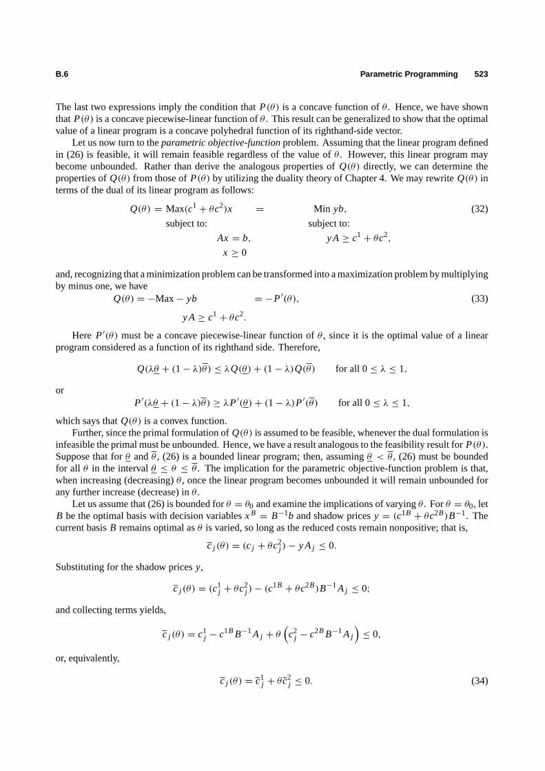
B.6 Parametric Programming 523
The last two expressions imply the condition thatP(θ) is a concave function ofθ . Hence, we have shownthat P(θ) is a concave piecewise-linear function ofθ . This result can be generalized to show that the optimalvalue of a linear program is a concave polyhedral function of its righthand-side vector.
Let us now turn to theparametric objective-functionproblem. Assuming that the linear program definedin (26) is feasible, it will remain feasible regardless of the value ofθ . However, this linear program maybecome unbounded. Rather than derive the analogous properties ofQ(θ) directly, we can determine theproperties ofQ(θ) from those ofP(θ) by utilizing the duality theory of Chapter 4. We may rewriteQ(θ) interms of the dual of its linear program as follows:
Q(θ) = Max(c1+ θc2)x = Min yb, (32)
subject to: subject to:
Ax = b, y A≥ c1+ θc2,
x ≥ 0
and, recognizing that a minimization problem can be transformed into a maximization problem by multiplyingby minus one, we have
Q(θ) = −Max− yb = −P′(θ), (33)
y A≥ c1+ θc2.
Here P′(θ) must be a concave piecewise-linear function ofθ , since it is the optimal value of a linearprogram considered as a function of its righthand side. Therefore,
Q(λθ + (1− λ)θ) ≤ λQ(θ)+ (1− λ)Q(θ) for all 0≤ λ ≤ 1,
orP′(λθ + (1− λ)θ) ≥ λP′(θ)+ (1− λ)P′(θ) for all 0≤ λ ≤ 1,
which says thatQ(θ) is a convex function.Further, since the primal formulation ofQ(θ) is assumed to be feasible, whenever the dual formulation is
infeasible the primal must be unbounded. Hence, we have a result analogous to the feasibility result forP(θ).Suppose that forθ andθ , (26) is a bounded linear program; then, assumingθ < θ , (26) must be boundedfor all θ in the intervalθ ≤ θ ≤ θ . The implication for the parametric objective-function problem is that,when increasing (decreasing)θ , once the linear program becomes unbounded it will remain unbounded forany further increase (decrease) inθ .
Let us assume that (26) is bounded forθ = θ0 and examine the implications of varyingθ . Forθ = θ0, letB be the optimal basis with decision variablesxB
= B−1b and shadow pricesy = (c1B+ θc2B)B−1. The
current basisB remains optimal asθ is varied, so long as the reduced costs remain nonpositive; that is,
c j (θ) = (c j + θc2j )− y Aj ≤ 0.
Substituting for the shadow pricesy,
c j (θ) = (c1j + θc2
j )− (c1B+ θc2B)B−1A j ≤ 0;
and collecting terms yields,
c j (θ) = c1j − c1B B−1A j + θ
(c2
j − c2B B−1A j
)≤ 0,
or, equivalently,
c j (θ) = c1j + θc2
j ≤ 0. (34)

524 Linear Programming in Matrix Form B.6
Equation (34) may imply both upper and lower bounds, as follows:
θ ≥−c1
j
c2j
for c2j < 0,
θ ≤−c1
j
c2j
for c2j > 0;
and these define the following range onθ :
Maxj
{−c1
j
c2j
∣∣∣∣∣ c2j < 0
}≤ θ ≤ Min
j
{−c1
j
c2j
∣∣∣∣∣ c2j > 0
}. (35)
If we moveθ to either its upper or lower bound, a basis change can take place. At the upper bound, thevariable producing the minimum ratio becomes a candidate to enter the basis, while at the lower bound, thevariable producing the maximum ratio becomes a candidate to enter the basis. In either case, the variable todrop from the basis is determined by the usual rule of the primal simplex method.
br
ars= Min
i
{bi
ais
∣∣∣∣∣ais > 0
}. (36)
If As ≤ 0, thenxs may be increased without limit and the problem is unbounded beyond this bound. Ifa variable to drop is determined, then a new basis is determined and the process is repeated. The range onθ
such that thenewbasis remains optimal is then again computed in the same manner.On any of these successive intervals where the basis is unchanged, the optimal value of the linear program
is given by:
Q(θ) =(c1B+ θc2B
)xB,
wherexB= B−1b and is not a function ofθ . Therefore,Q(θ) is a straight line with slopec2BxB on a
particular interval.Finally, let us consider theparametric rim problem, which has the parameter in both the objective function
and the righthand side. As would be expected, the optimal value of the linear program defined in (27) is neithera concave nor a convex function of the parameterθ . Further,R(θ) is not a piecewise-linear function, either.Let us assume that (27) is feasible forθ = θ0, and examine the implications of varyingθ . Forθ = θ0, let Bbe the optimal basis with decision variablesxB
= B−1(b1+θb2) and shadow pricesy =
(c1B+ θc2B
)B−1.
The current basis remains optimal so long as the current solution remains feasible and the reduced costsremain nonpositive. Hence, the current basis remains optimal so long as both ranges onθ given by (30) and(35) are satisfied. Suppose we are increasingθ . If the upper bound of (30) is reached before the upper boundof (34), then a dual simplex step is performed according to (31). If the opposite is true, then a primal simplexstep is performed according to (36). Once the new basis is determined, the process is repeated. The sameprocedure is used when decreasingθ .
For a given basis, the optimal value of the objective function is given by multiplying the basic costs bythe value of the basic variablesxB; that is,
R(θ) =(c1B+ θc2B
)B−1(b1
+ θb2),
which can be rewritten as
R(θ) = c1B B−1b1+ θ
(c2B B−1b1
+ c1B B−1b2)+ θ2
(c2B B−1b2
).

B.7 Duality Theory in Matrix Form 525
Hence, the optimal value of the parametric rim problem is a quadratic function ofθ for a fixed basisB. Ingeneral, this quadratic may be either a concave or convex function over the range implied by (30) and (35).
It should be clear that the importance of parametric programming in all three cases is the efficiency ofthe procedures in solving a number of different cases. Once an optimal solution has been found for somevalue of the parameter, sayθ = θ0, increasing or decreasingθ amounts to successively computing the pointsat which the basis changes and then performing a routine pivot operation.
B.7 DUALITY THEORY IN MATRIX FORM
The duality theory introduced in Chapter 4 can be stated very concisely in matrix form. As we saw there, anumber of variations of the basic duality results can be formulated by slightly altering the form of the primalproblem. For ease of comparison with the Chapter 4 results, we will again employ the symmetric version ofthe dual linear programs:
Primal Dual
Max z= cx, Min v = yb,
subject to: subject to:
Ax ≤ b, y A≥ c,
x ≥ 0. y ≥ 0.
Note thaty andc are row vectors whilex andb are column vectors. Letzandv denote the optimal valuesof the objective functions for the primal and dual problems, respectively. We will review the three key resultsof duality theory.
Weak duality. If x is a feasible solution to the primal andy is a feasible solution to the dual, thencx ≤ yb,and consequently,z≤ v.
Strong duality. If the primal (dual) has a finite optimal solution, then so does the dual (primal), and the twoextremes are equal,z= v.
Complementary slackness.If x is a feasible solution to the primal andy is a feasible solution to the dual,thenx andy are optimal solutions to the primal and dual, respectively, if and only if
y(Ax − b) = 0 and (y A− c)x = 0.
The arguments leading to these results were given in Chapter 4 but will be briefly reviewed here.Weakduality is a consequence of primal and dual feasibility, since multiplying the primal constraints on the left byy and the dual constraints on the right byx and combining gives:
cx ≤ y Ax ≤ yb.
Since the optimal values must be at least as good as any feasible value,
z= Maxx
cx ≤ Miny
yb= v.
Weak duality implies that ifcx = yb for some primal feasiblex and dual feasibley, thenx andy are optimalsolutions to the primal and dual, respectively.
The termination conditions of the simplex method and the concept of simplex multipliers provides thestrong duality property. Suppose that the simplex method has found an optimal basic feasible solutionx to

526 Linear Programming in Matrix Form B.7
the primal with optimal basisB. The optimal values of the decision variables and simplex multipliers arexB= B−1b andy = cB B−1, respectively. The simplex optimality conditions imply:
z = cBxB= cB B−1b = yb, (37)
cN= cN
− yN ≤ 0. (38)
The latter condition (38), plus the definition of the simplex multipliers, which can be restated as:
cB= cB
− yB= 0,
imply thatc− y A≤ 0, so thaty ≥ 0 is a dual feasible solution. NowxN= 0 and (37) implies that:
cx = cBxB+ cNxN
= yb. (39)
Sincex andy are feasible solutions to the primal and dual respectively, (39) impliesz= cx = yb= v whichis the desired result.
Finally, complementary slacknessfollows directly from the strong-duality property. First, we assumethat complementary slackness holds, and show optimality.
If x andy are feasible to the primal and dual, respectively, such that
y(Ax − b) = 0 and (y A− c)x = 0,
thencx = y Ax = yb. (40)
Condition (40) implies thex and y are optimal to the primal and dual, respectively. Second, we assumeoptimality holds, and show complementary slackness. Letx and y be optimal to the primal and dual,respectively; that is,
cx = yb.
Then0= cx − yb≤ cx − y Ax = (c− y A)x (41)
by primal feasibility, andy ≥ 0. Now since 0≥ c− y A by dual feasibility, andx ≥ 0, we have
0 ≥ (c− y A)x, (42)
and (41) and (42) together imply:(c− y A)x = 0.
An analogous argument using dual feasibility andx ≥ 0 implies the other complementary slackness condition,
y(Ax − b) = 0.
These results are important for applications since they suggest algorithms other than straightforwardapplications of the simplex method to solve specially structured problems. The results are also central tothe theory of systems of linear equalities and inequalities, a theory which itself has a number of importantapplications. In essence, duality theory provides a common perspective for treating such systems and, in theprocess, unifies a number of results that appear scattered throughout the mathematics literature. A thoroughdiscussion of this theory would be inappropriate here, but we indicate the flavor of this point of view.
A problem that has interested mathematicians since the late 1800’s has been characterizing the situationwhen a system of linear equalities and inequalities does not have a solution. Consider for example the system:
Ax = b, x ≥ 0.

B.8 Resolving degeneracy in the Simplex Method 527
Suppose thaty is a row vector. We multiply the system of equations byy to produce a single new equation:
(y A)x = yb.
If x is feasible in the original system, then it will certainly satisfy this new equation. Suppose, though, thatyb > 0 and thaty A ≤ 0. Sincex ≥ 0, y Ax ≤ 0, so that nox ≥ 0 solves the new equation, and thusthe original system is infeasible. We have determined a single inconsistent equation that summarizes theinconsistencies in the original system. The characterization that we are working towards states that such asummarizing inconsistent equation always can be found when the system has no solution. It is given by:
Farkas’ Lemma. Exactly one of the following two systems has a solution:
I Ax = b, II y A≤ 0,
or
x ≥ 0. yb > 0.
The proof of the lemma is straightforward, by considering the Phase I linear-programming program thatresults from adding artificial variables to System (I):
Minimize et,
subject to:
Ax+ I t = b, (43)
x ≥ 0, t ≥ 0,
wheree is the sum vector consisting of all ones andt is the vector of artificial variables. Suppose that thesimplex method is applied to (43), and the optimal solution is(x, t) with shadow pricesy. By the terminationconditions of the simplex method, the shadow prices satisfy:
0− y A≥ 0 (that is, y A≤ 0). (44)
By the duality property, we knowet = yb, and since (43) is a Phase I linear program, we have:
yb = et = 0 if and only if I is feasible,
yb = et > 0 if and only if I is infeasible.(45)
Equations (44) and (45) together imply the lemma.We can give a geometrical interpretation of Farkas’ Lemma by recalling that, if the inner product of two
vectors is positive, the vectors make an acute angle with each other, while if the inner product is negative, thevectors make an obtuse angle with each other. Therefore, any vectory that solves System II must make acuteangles with all the column vectors ofA and a strictly obtuse angle with the vectorb. On the other hand, inorder for System I to have a feasible solution, there must exist nonnegative weightsx that generateb fromthe column vectors ofA. These two situations are given in Figs. B.4 and B.5.
B.8 RESOLVING DEGENERACY IN THE SIMPLEX METHOD
In Chapter 2 we showed that the simplex method solves any linear program in a finite number of steps if weassume that the righthand-side vector is strictly positive for each canonical form generated. Such a canonicalform is callednondegenerate.
The motivation for this assumption is to ensure that the new value of the entering variablex∗s , which isgiven by:
x∗s =br
ars
528 Linear Programming in Matrix Form B.8
Fig. B.4 System I has a solution.
Fig. B.5 System II has a solution.
is strictly positive; and hence, that the new value of the objective functionz∗, given by:
z∗ = z+ csx∗s ,
shows a strict improvement at each iteration. Since the minimum-ratio rule to determine the variable to dropfrom the basis ensuresars > 0, the assumption thatbi > 0 for all i implies thatx∗s > 0. Further, introducingthe variablexs requires thatcs > 0 and therefore thatz∗ > z. This implies that there is a strict improvementin the value of the objective function at each iteration, and hence that no basis is repeated. Since there is afinite number of possible bases, the simplex method must terminate in a finite number of iterations.
The purpose of this section is to extend the simplex method so that, without the nondegeneracy assumption,it can be shown that the method will solve any linear program in a finite number of iterations. In Chapter 2we indicated that we would do this by perturbing the righthand-side vector. However, a simple perturbationof the righthand side by a scalar will not ensure that the righthand side will be positive for all canonicalforms generated. As a result, we introduce a vector perturbation of the righthand side and the concept oflexicographic ordering.

B.8 Resolving degeneracy in the Simplex Method 529
An m-element vectora = (a1, a2, . . . , am) is said to belexico-positive, written a � 0, if at least oneelement is nonzero and the first such element is positive. The term lexico-positive is short for lexicographicallypositive. Clearly, any positive multiple of a lexico-positive vector is lexico-positive, and the sum of twolexico-positive vectors is lexico-positive. Anm-element vectora is lexico-greaterthan anm-element vectorb, writtena � b, if (a− b) is lexico-positive; that is, ifa− b � 0. Unless two vectors are identical, they arelexicographically ordered, and therefore the ideas oflexico-maxandlexico-minare well-defined.
We will use the concept of lexicographic ordering to modify the simplex method so as to produce a uniquevariable to drop at each iteration and a strict lexicographic improvement in the value of the objective functionat each iteration. The latter will ensure the termination of the method after a finite number of iterations.
Suppose the linear program is in canonical form initially withb ≥ 0. We introduce a unique perturbationof the righthand-side vector by replacing the vectorb with them× (m+ 1) matrix [b, I ]. By making thevectorx ann× (m+ 1) matrix X, we can write the initial tableau as:
XB≥ 0, XN
≥ 0, X I≥ 0,
B XB+ N XN
+ I X I= [b, I ],
cB XB+ cN XN
−Z = [0, 0],
whereXB, XN , andX I are the matrices associated with the basic variables, the non-basic variables, and thevariables in the initial identity basis, respectively. The intermediate tableau corresponding to the basisB isdetermined as before by multiplying the constraints of (46) byB−1 and subtractingcB times the resultingconstraints from the objective function. The intermediate tableau is then:
XB≥ 0, XN
≥ 0, X I≥ 0,
I X B+ N XN
+ B−1X I= [b, B−1
] = B, (47)
cN XN− yXI
− Z = [−z,−y] = −Z,
whereN = B−1N, y = cB B−1, cN= cN
− yN, andz = yb as before. Note that if the matricesXN andX I are set equal to zero, a basic solution of the linear program is given byXB
= [b, B−1], where the first
column ofXB, sayXB1 , gives the usual values of the basic variablesXB
1 = b.We will formally prove that the simplex method, with a lexicographic resolution of degeneracy, solves
any linear program in a finite number of iterations. An essential aspect of the proof is that at each iterationof the algorithm, each row vector of the righthand-side perturbation matrix is lexico-positive.
In the initial tableau, each row vector of the righthand-side matrix is lexico-positive, assumingb ≥ 0. Ifbi > 0, then the row vector is lexico-positive, since its first element is positive. Ifbi = 0, then again the rowvector is lexico-positive since the first nonzero element is a plusonein position(i + 1).
DefineBi to be rowi of the righthand-side matrix[b, B−1] of the intermediate tableau. In the following
proof, we will assume that each such row vectorBi is lexico-positive for a particular canonical form, andargue inductively that they remain lexico-positive for the next canonical form. Since this condition holds forthe initial tableau, it will hold for all subsequent tableaus.
Now consider the simplex method one step at a time.
STEP (1): Ifc j ≤ 0 for j = 1, 2, . . . , n, thenstop; the current solution is optimal.
SinceXB= B = [b, I ], the first component ofXB is the usual basic feasible solutionXB
1 = b.Since the reduced costs associated with this solution arecN
≤ 0, we have:
z= z+ cN XN1 ≤ z,
and hencez is an upper bound on the maximum value ofz. The current solutionXB1 = b attains this
upper bound and is therefore optimal. If we continue the algorithm, there exists somec j > 0.
STEP (2): Choose the columns to enter the basis by:
cs = Maxj
{c j∣∣c j > 0
}.

530 Linear Programming in Matrix Form C.8
If As ≤ 0, thenstop; there exists an unbounded solution. SinceAs ≤ 0, then
XB1 = b− Asxs ≥ 0 for all xs ≥ 0,
which says that the solutionXB1 is feasible for all nonnegativexs. Sincecs > 0,
z= z+ csxs
implies that the objective function becomes unbounded asxs is increased without limit. If we continuethe algorithm, there exists someais > 0.
STEP (3): Choose the row to pivot in by the following modified ratio rule:
Br
ars= lexico-min
i
{Bi
ais
∣∣∣∣∣ais > 0
}.
We should point out that the lexico-min produces auniquevariable to drop from the basis. There mustbe a unique lexico-min, since, if not, there would exist two vectorsBi /ais that are identical. This wouldimply that two rows ofB are proportional and, hence, that two rows ofB−1 are proportional, which isa clear contradiction.
STEP (4): Replace the variable basic in rowr with variables and re-establish the canonical form by pivotingon the coefficientars.
We have shown that, in the initial canonical form, the row vectors of the righthand-side matrixare each lexico-positive. It remains to show that, assuming the vectorsBi are lexico-positive at aniteration, they remain lexico-positive at the next iteration. Let the new row vectors of the righthand-sidematrix beB
∗
i . First,
B∗
r =Br
ars� 0,
sinceBr � 0, by assumption, andars > 0. Second,
B∗
i = Bi − aisBr
ars. (48)
If ais ≤ 0, thenB∗
i � 0, since it is then the sum of two lexico-positive vectors. Ifais > 0, then (48)can be rewritten as:
B∗
i = ais
[Bi
ais−
Br
ars
]. (49)
SinceBr /ars is the unique lexico-min in the modified ratio rule, (49) impliesB∗
i � 0 for ais > 0, also.
STEP (5): Go to STEP (1)
We would like to show that there is a strict lexicographic improvement in the objective-valuevector at each iteration. Letting−Z = [−z,−y] be the objective-value vector, andZ
∗be the new
objective-value vector, we have:Z∗= Z + csX∗s;
then, sincecs > 0 andX∗s = B∗
r � 0, we have
Z∗= Z + csX∗s � Z,
which states thatZ∗
is lexico-greater thanZ. Hence we have a strict lexicographic improvement in theobjective-value vector at each iteration.
Finally, since there is a strict lexicographic improvement in the objective-value vector for each new basis,no basis can then be repeated. Since there are a finite number of bases and no basis is repeated, the algorithmsolves any linear program in a finite number of iterations.

A Labeling Algorithm forthe Maximum-Flow
Network Problem
Appendix C
Network-flow problems can be solved by several methods. In Chapter 8 we introduced this topic by exploringthe special structure of network-flow problems and by applying the simplex method to this structure. Thisappendix continues the analysis of network problems by describing the application of the labeling algorithm tothe maximum-flow network problem. Labeling methods provide an alternative approach for solving networkproblems. The basic idea behind the labeling procedure is to systematically attach labels to the nodes of anetwork until the optimum solution is reached.
Labeling techniques can be used to solve a wide variety of network problems, such as shortest-pathproblems, maximal-flow problems, general minimal-cost network-flow problems, and minimal spanning-tree problems. It is the purpose of this appendix to illustrate the general nature of the labeling algorithms bydescribing a labeling method for the maximum-flow problem.
C.1 THE MAXIMAL-FLOW PROBLEM
The maximal-flow problem was introduced in Section 8.2 of the text. Ifv denotes the amount of materialsent from nodes, called the source, to notet , called the sink, the problem can be formulated as follows:
Maximizev,
subject to: ∑j
xi j −∑
k
xki =
v if i = s,−v if i = t,
0 otherwise,
0 ≤ xi j ≤ ui j , (i = 1, 2, . . . , n; j = 1, 2, . . . , n).
We assume that there is no arc fromt to s. Also, ui j = +∞ if arc i – j has unlimited capacity. Theinterpretation is thatv units are supplied ats and consumed att .
Letting xts denote the variablev and rearranging, we see that the problem assumes the following specialform of the general network problem:
Maximizexts′
subject to: ∑j
xi j −∑
k
xki = 0 (i = 1, 2, . . . , n)
0 ≤ xi j ≤ ui j (i = 1, 2, . . . , n; j = 1, 2, . . . , n).
531
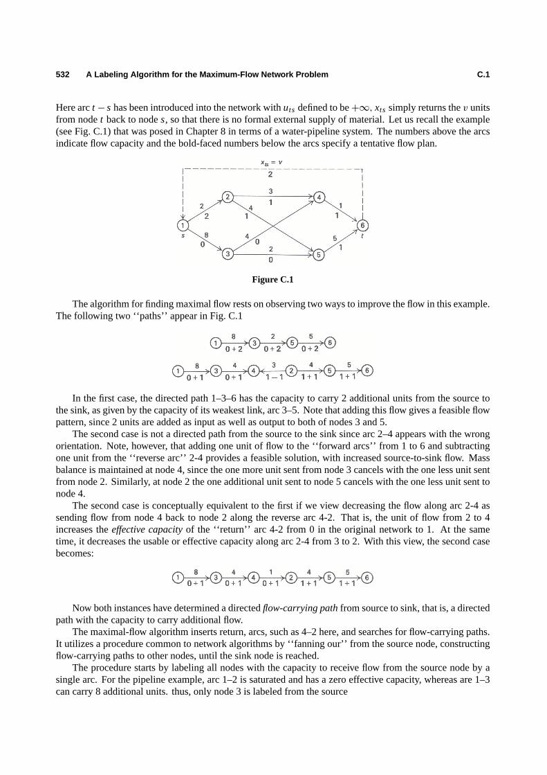
532 A Labeling Algorithm for the Maximum-Flow Network Problem C.1
Here arct − s has been introduced into the network withuts defined to be+∞, xts simply returns thev unitsfrom nodet back to nodes, so that there is no formal external supply of material. Let us recall the example(see Fig. C.1) that was posed in Chapter 8 in terms of a water-pipeline system. The numbers above the arcsindicate flow capacity and the bold-faced numbers below the arcs specify a tentative flow plan.
Figure C.1
The algorithm for finding maximal flow rests on observing two ways to improve the flow in this example.The following two ‘‘paths’’ appear in Fig. C.1
In the first case, the directed path 1–3–6 has the capacity to carry 2 additional units from the source tothe sink, as given by the capacity of its weakest link, arc 3–5. Note that adding this flow gives a feasible flowpattern, since 2 units are added as input as well as output to both of nodes 3 and 5.
The second case is not a directed path from the source to the sink since arc 2–4 appears with the wrongorientation. Note, however, that adding one unit of flow to the ‘‘forward arcs’’ from 1 to 6 and subtractingone unit from the ‘‘reverse arc’’ 2-4 provides a feasible solution, with increased source-to-sink flow. Massbalance is maintained at node 4, since the one more unit sent from node 3 cancels with the one less unit sentfrom node 2. Similarly, at node 2 the one additional unit sent to node 5 cancels with the one less unit sent tonode 4.
The second case is conceptually equivalent to the first if we view decreasing the flow along arc 2-4 assending flow from node 4 back to node 2 along the reverse arc 4-2. That is, the unit of flow from 2 to 4increases theeffective capacityof the ‘‘return’’ arc 4-2 from 0 in the original network to 1. At the sametime, it decreases the usable or effective capacity along arc 2-4 from 3 to 2. With this view, the second casebecomes:
Now both instances have determined a directedflow-carrying pathfrom source to sink, that is, a directedpath with the capacity to carry additional flow.
The maximal-flow algorithm inserts return, arcs, such as 4–2 here, and searches for flow-carrying paths.It utilizes a procedure common to network algorithms by ‘‘fanning our’’ from the source node, constructingflow-carrying paths to other nodes, until the sink node is reached.
The procedure starts by labeling all nodes with the capacity to receive flow from the source node by asingle arc. For the pipeline example, arc 1–2 is saturated and has a zero effective capacity, whereas are 1–3can carry 8 additional units. thus, only node 3 is labeled from the source
C.1 The Maximal-Flow Problem 533
The procedure is repeated by labeling all nodes with the capacity to receive flow directly from node 3 bya single arc. In this case, nodes 4 and 5 are labeled and the labeled nodes become:
Additional nodes can now be labeled from either node 4 or 5. If node 4 is selected next, then node 2 islabeled, since the effective capacity (return capacity) of arc 4-2 is positive (node 6 cannot be labeled fromnode 4 since arc 4-6 is saturated). The labeled nodes are:
At any point in the algorithm, some of the labeled nodes, here nodes 1, 3 and 4, will already have beenused to label additional nodes. We will say that these nodes have beenscanned.Any unscanned labeled nodecan be selected and scanned next.
Scanning node 2 produces no additional labelings, since node 2 can only send flow directly to nodes 1,4, and 5, and these have been labeled previously. Node 6 is labeled when node 5 is scanned, and the labelednodes are:
A flow-carrying path has been identified, since the sink has been labeled. In this case, the path discoveredis 1–3–5–6, which was the first path given above. The flow along this path is updated by increasing theflow along each arc in the path by the flow capacity of the path, here 2 units. Effective capacities are nowrecomputed and the labeling procedure is repeated, starting with only the source node labeled.
Following is a formal description of the algorithm and a solution of the water-pipeline example. Noticethat the flow value on the arcs need not be recorded from step to step in the algorithm since this informationis computed easily from the effective (or usable) capacities of the arcs and their return arcs. For the exampleabove, the effective capacity on arc 2–4 is less than its initial capacity.
The difference 3= 2− 1 must be the flow value on that arc that resulted in the reduced capacity. Theeffective capacity on arc 4–2 has been increased from 0 to 1 by adding return-flow capacity to that arc, not
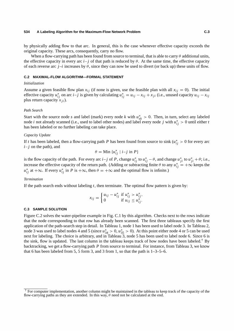
534 A Labeling Algorithm for the Maximum-Flow Network Problem C.3
by physically adding flow to that arc. In general, this is the case whenever effective capacity exceeds theoriginal capacity. These arcs, consequently, carry no flow.
When a flow-carrying path has been found from source to terminal, that is able to carryθ additional units,the effective capacity in every arci – j of that path is reduced byθ . At the same time, the effective capacityof each reverse arcj –i increases byθ , since they can now be used to divert (or back up) these units of flow.
C.2 MAXIMAL-FLOW ALGORITHM—FORMAL STATEMENT
Initialization
Assume a given feasible flow planxi j (if none is given, use the feasible plan with allxi j = 0). The initialeffective capacityu∗i j on arci – j is given by calculatingu∗i j = ui j − xi j + x j i (i.e., unused capacityui j − xi jplus return capacityx j i ).
Path Search
Start with the source nodes and label (mark) every nodek with u∗sk > 0. Then, in turn, select any labelednodei not already scanned (i.e., used to label other nodes) and label every nodej with u∗i j > 0 until eitherthas been labeled or no further labeling can take place.
Capacity Update
If t has been labeled, then a flow-carrying pathP has been found from source to sink (u∗i j > 0 for every arci – j on the path), and
θ = Min {u∗i j | i – j in P}
is the flow capacity of the path. For every arci – j of P, changeu∗i j to u∗i j − θ , and changeu∗j i to u∗j i + θ ; i.e.,increase the effective capacity of the return path. (Adding or subtracting finiteθ to anyu∗i j = +∞ keeps theu∗i j at+∞. If everyu∗i j in P is+∞, thenθ = +∞ and the optimal flow is infinite.)
Termination
If the path search ends without labelingt , then terminate. The optimal flow pattern is given by:
xi j =
{ui j − u∗i j if u∗i j > u∗i j ,0 if ui j ≤ u∗i j .
C.3 SAMPLE SOLUTION
Figure C.2 solves the water-pipeline example in Fig. C.1 by this algorithm. Checks next to the rows indicatethat the node corresponding to that row has already been scanned. The first three tableaus specify the firstapplication of the path-search step in detail. In Tableau 1, node 1 has been used to label node 3. In Tableau 2,node 3 was used to label nodes 4 and 5 (sinceu∗34 > 0, u∗35 > 0). At this point either node 4 or 5 can be usednext for labeling. The choice is arbitrary, and in Tableau 3, node 5 has been used to label node 6. Since 6 isthe sink, flow is updated. The last column in the tableau keeps track of how nodes have been labeled.† Bybacktracking, we get a flow-carrying pathP from source to terminal. For instance, from Tableau 3, we knowthat 6 has been labeled from 5, 5 form 3, and 3 from 1, so that the path is 1–3–5–6.
† For computer implementation, another column might be maintained in the tableau to keep track of the capacity of theflow-carrying paths as they are extended. In this way,θ need not be calculated at the end.

C.3 Sample Solution 535
Figure C.2 Tableaus for the maximal-flow algorithm.

536 A Labeling Algorithm for the Maximum-Flow Network Problem C.3
Figure C.2 (Cont.)

C.4 Verifying the Algorithm—Max-Flow/Min-Cut 537
Tableau 4 contains the updated capacities and a summary of the next path search, which used nodes 1, 3,4, 2, and 5 for labeling. The fifth tableau contains the final updated capacities and path search. Only nodes1, 3, and 4 can be labeled in this tableau, so the algorithm is completed.
The flow at any point in the algorithm is obtained by subtracting effective capacities from initial capacities,ui j − u∗i j , and discarding negative numbers. For Tableaus 1, 2, or 3, the flow is given by Fig. C.1. Aftermaking the two indicated flow changes to obtain Tableau 4 and then Tableau 5, the solutions are given in twonetworks shown in Figs. C.3 and C.4. The optimal solution sends two units along each of the paths 1–2–5–6and 1–3–5–6 and one unit along 1–3–4–6.
Figure C.3
Figure C.4
C.4 VERIFYING THE ALGORITHM—MAX-FLOW/MIN-CUT
The final solution to the sample problem shown in Fig. C.4 illustrates an important conceptual feature of themaximum-flow problem. The heavy dashed line in that figure ‘‘cuts" the network in two, in the sense that itdivides the nodes into two groups, one group containing the source node and one group containing the sinknode. Note that the most that can ever be sent across this cut to the sink is two units from node 1 to node 2,one unit from 4 to 6, and two units from 3 to 5, for a total of 5 units (arc 2–5 connects nodes that are both tothe right of the cut and is not counted). Since no flow pattern can ever send more than these 5 units and thefinal solution achieves this value, it must be optimal.
Similarly, the cut separating labeled from unlabeled nodes when the algorithm terminates (see Fig. C.5)shows that the final solution will be optimal.
By conservation of mass,v equals the net flow from left to right across this cut, so thatv can be nogreater than the total capacity of all arcsi – j pictured. In fact, this observation applies to any cut separating

538 A Labeling Algorithm for the Maximum-Flow Network Problem C.4
Figure C.5
the source nodes from the sink nodet .Any
feasible flowv from
nodes tonodet
≤ Capacity of
any cut separatingnodes and nodet
.
As in the example discussed above, the capacity of any cut is defined as the total capacity of all arcs directed‘‘from left to right" across the cut.
By virtue of the labeling scheme, however, every arci – j directed from left to right across the cutseparating the labeled and unlabeled nodes must haveu∗i j = 0; otherwisej would have been labeled fromi .This observation implies that
xi j = ui j and xi j = 0,
since if eitherxi j < ui j or x j i > 0, thenu∗i j = (ui j − xi j ) + x j i would be positive. Consequently, the netflow across the cut, and thusv, equals the cut capacity. Since no flow can do any better, this flow pattern isoptimal.
We can recast this observation in a slightly different way. The inequality stated above shows that anyfeasible flowv form source to sink is bounded from above by the capacity of any cut. Consequently, themaximum flow from source to sink is bounded by the capacity ofanycut separating the source and sink. Inparticular, the maximum flow from source to sink is bounded from above by the minimum capacity of any cut.We have just shown, though, that the maximum flowv equals the capacity of the cut separating the labeledand unlabeled nodes when the algorithm terminates; therefore, we have verified the famousmax-flow/min-cuttheorem. The maximum flow
v from nodes tonodet
=The minimum capacity
of any cut separatingnodes and nodet
.
There are many important ramifications of this theorem. It can be used, for example, to establish elegantresults in combinatorial theory. Although such results lead to many useful applications of combinatorialanalysis, their development is beyond the scope of our coverage here. We have merely shown how the max-flow/min-cut theorem arises, and used the theorem to show that when the maximum flow-labeling algorithmterminates, it has found the maximum possible flow from the source node to the sink node.
Finally, we should note that the maximum-flow procedure eventually terminates, as in the above example,and does not continue to find flow-carrying paths froms to t forever. For certain cases this is easy to show.If the capacity dataui j is all integral and everyxi j in the original flow plan is an integer, then everyu∗i j andθ encountered will be integral. But then, if the maximal flowv is not+∞, we approach it in integral stepsand must eventually reach it. Similarly, if the original data and flow is fractional,v increases at each stepby at least a given fractional amount and the procedure terminates in a finite number of steps. If the data is

C.4 Verifying the Algorithm—Max-Flow/Min-Cut 539
irrational, then it is known that the algorithm finds the maximum flow in a finite number of steps as long asthe nodes are considered during path search on a first-labeled–first-scanned basis.
Note that starting with an integral flow planxi j when allui j are integral leads to integralu∗i j . Consequently,the final (and optimal) flow plan will be integral. This is a special instance of the network integrality propertyintroduced in Chapter 8.