Mathematical model for manoeuvrability of a riverine...

Mathematical model for manoeuvrability of a riverine support

patrol vessel with a pump-jet propulsion system

J. E. Carreñoa*

, J. D. Moraa, F. L. Pérez

b

a COTECMAR, Mamonal Industrial Zone km 9, Cartagena, Colombia

b Naval Architecture School of Madrid, Universidad Politécnica de Madrid,

Avenida Arco de la Victoria SN, 28040 Madrid, Spain

______________________________________________________

Abstract

A study on the manoeuvrability of a riverine support patrol vessel is made to derive a mathematical model and simulate

maneuvers with this ship. The vessel is mainly characterized by both its wide-beam and the unconventional propulsion system, that

is, a pump-jet type azimuthal propulsion. By processing experimental data and the ship characteristics with diverse formulae to find

the proper hydrodynamic coefficients and propulsion forces, a system of three differential equations is completed and tuned to carry

out simulations of the turning test. The simulation is able to accept variable speed, jet angle and water depth as input parameters and

its output consists of time series of the state variables and a plot of the simulated path and heading of the ship during the maneuver.

Thanks to the data of full-scale trials previously performed with the studied vessel, a process of validation was made, which shows

a good fit between simulated and full-scale experimental results, especially on the turning diameter.

Keywords: shallow water, azimuthal propulsion, riverine support patrol vessel, manoeuvrability model, numerical simulation,

validation

* Corresponding author. E-mail: [email protected]

1. Introduction

The research on mathematical models for ship manoeuvrability in the relevant publications has recently

shown a broad variety of formulations which include the effects of the hull resistance, propulsion system

thrust, rudder resistance and even other external actions, such as wind and current forces (Bertram, 2000).

The reliability on certain method can only be claimed after a successful validation process has been

completed (ITTC, 2.002), but carrying out this task may turn into an inconvenience when no useable

validation data are available. According to the recommendations by the international committees and

academic researchers, full-scale trial results of well-known ships are a proper source of validation data, but

only if the mathematical model used deals with the same type of ships and if its operating ranges enclose the

specific vessel whose manoeuvrability parameters have been measured. This is the reason why some models

derived to simulate alternative ship designs could lack of the appropriate information for its validation.

In this paper, a set of full-scale trials with a Riverine Support Patrol Vessel (RSPV), constructed by

COTECMAR (Science and Technology Corporation for the Development of the Colombian Naval, Marine

and Riverine Industries), were performed in order to measure the standard parameters of the turning circle test

and assess the manoeuvrability characteristics of the RSPV (Carreño, Jimenez, & Sierra, Ship

Manoeuvrability: Full Scale Trials Of Colombian Navy Riverine Support Patrol Vessel, 2.011). This vessel

has two main remarkable design features which are a non-conventional propulsion system and a large beam-

draft ratio (wide-beam vessel), among other particulars described below. Consequently, this collected

information is useful for the validation of a manoeuvrability formulation specifically derived to model the

manoeuvrability of a ship with those characteristics.

The wide-beam vessels have shown a particular manoeuvrability behavior when varying the water depth of

the maneuver from deep to shallow water, which is opposite to the usual trend of conventional vessels. In the

former case, the main maneuver parameters of the turning circle decrease as the depth decreases, that is,

improves its manoeuvrability properties, while in the latter case the manoeuvrability parameters worsen when

changing from deep to shallow water. Such behavior seen on wide-beam vessels has been named NS (likely

initials for non-standard) effect, which was first studied and computationally reproduced by (Yoshimura &

Sakurai, 1.988), who worked with a beam-draft ratio of 5.36 in comparison with a conventional ship with

ratio 3.60. That effect was later observed again on ship model experiments by (Yasukawa & Kobayashi,

1.995).

This paper is focused on the development of a mathematical formulation which may model the

manoeuvrability of the RSPV, by incorporating the pump-jet propulsion model and the specific geometric and

hydrodynamic data of the vessel, in order to finally simulate the turning circle under variable input conditions

and validate the model by means of the corresponding full-scale experimental tests. Firstly a description of

the studied vessel is presented, followed by a stepwise explanation of the mathematical model derivation,

which allows carrying on with a simulation and validation stage, which, after the result analysis, leads to the

final conclusions.

2. Study case: vessel description

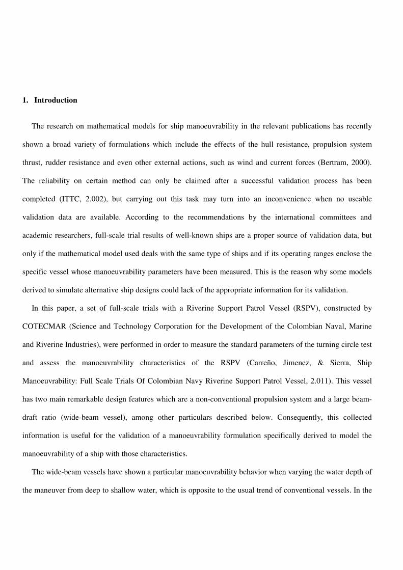
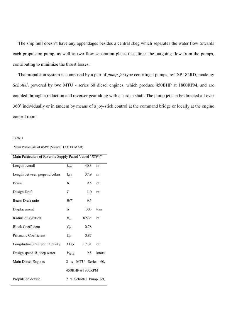
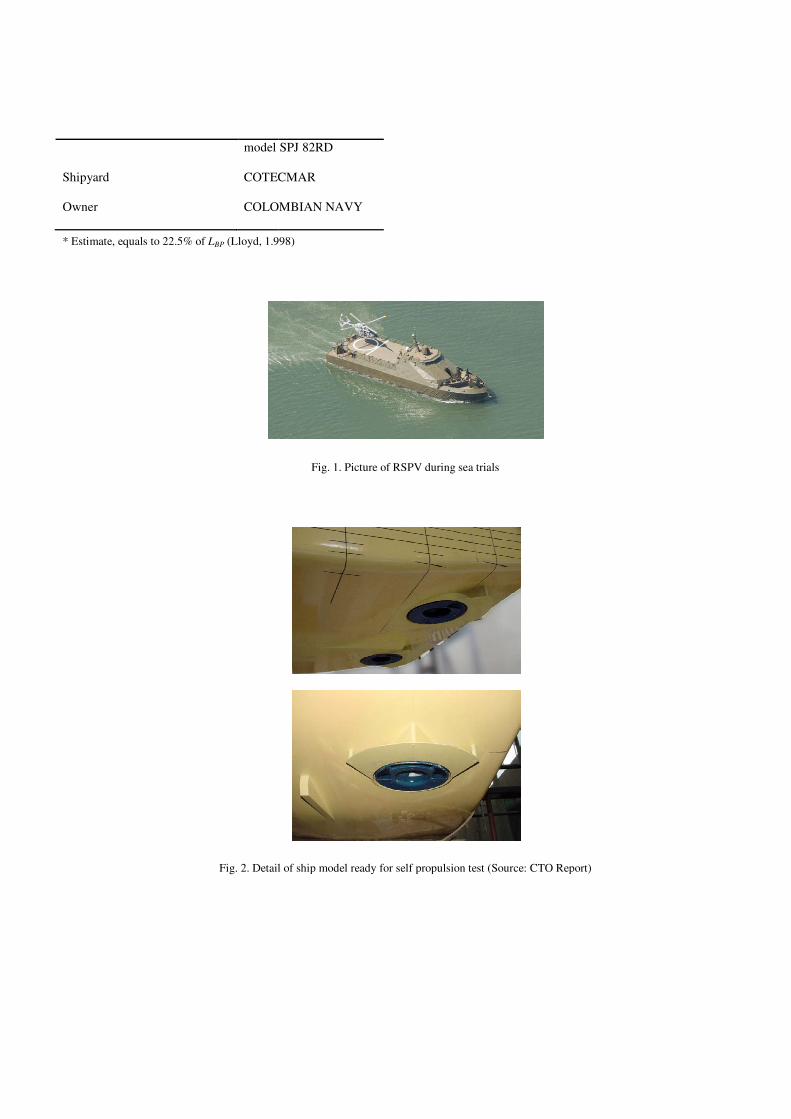
The main particulars of the RSPV are listed in Table 1. Its hull corresponds to a riverine ship with small

deadrise and with a high beam-draft ratio, designed to navigate on very shallow water. A photograph of the

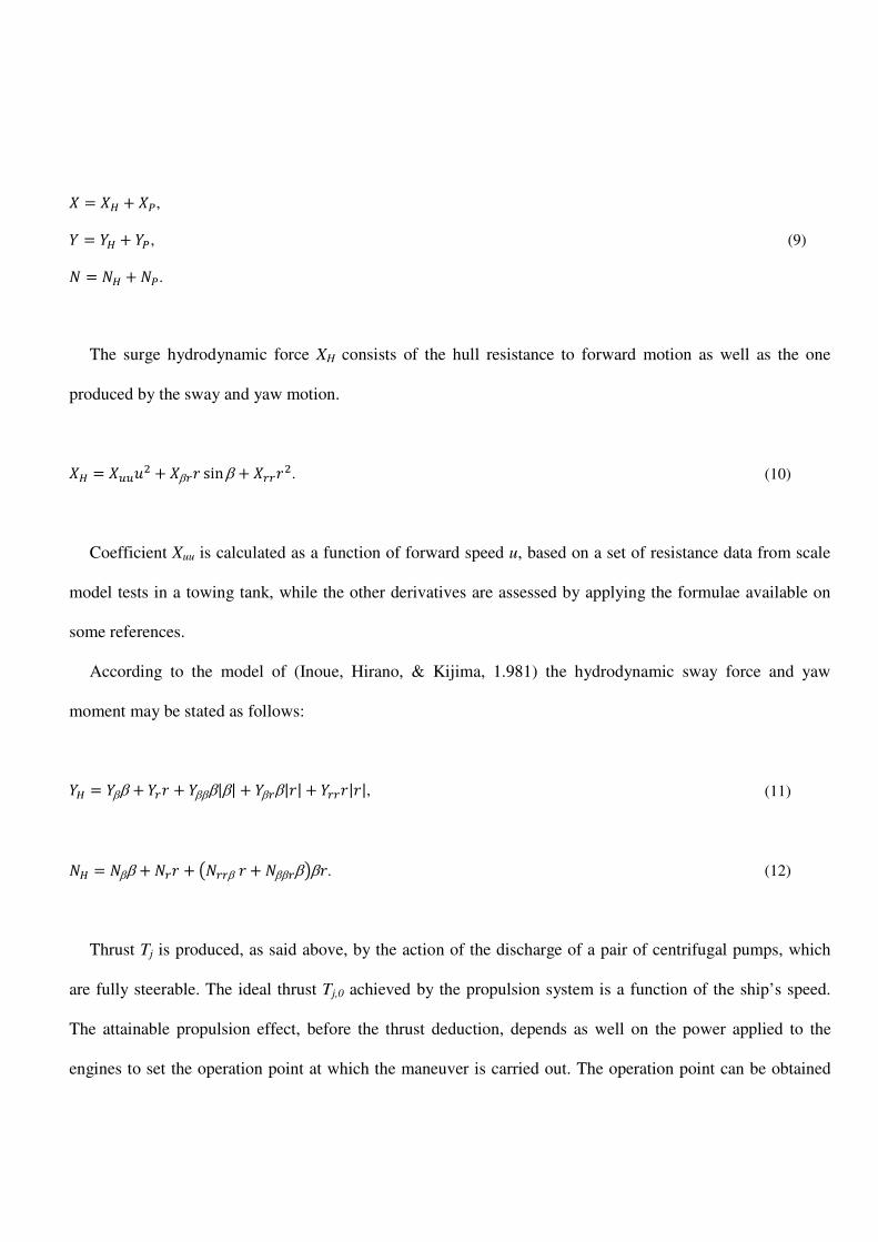
ship while being operated is shown in Fig. 1. In Fig. 2 a close-up of the propellers location is presented. These

last photographs were taken from the ship scale model that was built for the self-propulsion test in a towing

tank. As it is shown, the propulsion pumps are located by the ship’s sternpost and there are no exposed

surfaces.

The ship hull doesn’t have any appendages besides a central skeg which separates the water flow towards

each propulsion pump, as well as two flow separation plates that direct the outgoing flow from the pumps,

contributing to minimize the thrust losses.

The propulsion system is composed by a pair of pump-jet type centrifugal pumps, ref. SPJ 82RD, made by

Schottel, powered by two MTU - series 60 diesel engines, which produce 450BHP at 1800RPM, and are

coupled through a reduction and reverser gear along with a cardan shaft. The pump jet can be directed all over

360° individually or in tandem by means of a joy-stick control at the command bridge or locally at the engine

control room.

Table 1

Main Particulars of RSPV (Source: COTECMAR)

Main Particulars of Riverine Supply Patrol Vessel "RSPV"

Length overall LOA 40.3 m

Length between perpendiculars LBP 37.9 m

Beam B 9.5 m

Design Draft T 1.0 m

Beam-Draft ratio B/T 9.5

Displacement ∆ 303 tons

Radius of gyration Rzz 8.53* m

Block Coefficient CB 0.78

Prismatic Coefficient CP 0.87

Longitudinal Center of Gravity LCG 17.31 m

Design speed @ deep water VMAX 9.5 knots

Main Diesel Engines 2 x MTU Series 60,

450BHP@1800RPM

Propulsion device 2 x Schottel Pump Jet,

model SPJ 82RD

Shipyard COTECMAR

Owner COLOMBIAN NAVY

* Estimate, equals to 22.5% of LBP (Lloyd, 1.998)

Fig. 2. Detail of ship model ready for self

model SPJ 82RD

COTECMAR

COLOMBIAN NAVY

(Lloyd, 1.998)

Fig. 1. Picture of RSPV during sea trials

. Detail of ship model ready for self propulsion test (Source: CTO Report)propulsion test (Source: CTO Report)

3. Derivation of the mathematical model

3.1 Reference system

The reference system to be used in order to develop

the studied vessel is shown in Fig. 3, which takes into account two translational directions

direction (PMM: Planar Motion Model

Fig. 3. Reference system for a 3

3.2 Derivation of the mathematical

The dynamic model is represented by a system of three ordinary differential equations, in order to find in

time domain the value of the three degrees of freedom.

the one proposed by (Fossen, 2.011).

and the forces present in the studied ship body:

athematical model

The reference system to be used in order to develop the equations of the state variables in time

, which takes into account two translational directions

Model.)

. Reference system for a 3-DOF manoeuvrability model

model


the value of the three degrees of freedom. The notation used from here on is strongly based on

The general model basically consists of a balance between accelerations

and the forces present in the studied ship body:

the state variables in time domain for

, which takes into account two translational directions and one rotational


he notation used from here on is strongly based on

The general model basically consists of a balance between accelerations

�υυυυ� + �υυυυ = � , (1)

where the velocity vector υ contains the three degrees of freedom considered in a typical manoeuvrability

approach: velocity in x (u), velocity in y (v), and rotational speed over axis z (r), that is:

υυυυ = ��. (2)

In equation (1), the inertia matrix M is multiplied by the acceleration vector υυυυ� , and includes the static mass

and moment of inertia of the ship (m and Izz), besides the portions of mass and moment of inertia added

because of the motion through a fluid (mx, my and Jzz). This matrix also includes other added mass terms,

which represent cross effects between motions, such as − �� and −�� .

� = �� + �� 0 00 � + �� − ��0 −�� + ��. (3)

The second term in right hand side of equation (1) comprises a rigid body component (CRB) and another

component generated by the added masses (CA).

�υυυυ = (�� + ��)υυυυ (4)

The first component equals to:

��υυυυ = �−��0 � (5)

while the component which corresponds to added inertia comprises the following terms:

��υυυυ = � −�� + ! ( �� + �� )!��−"�� − ��#� + ! ( �� + �� )�$. (6)

The force vector f is defined as follows:

� = %& �', (7)

which includes the surge force (X), the sway force (Y) and the yaw moment (N). By composing all the above

definitions regarding the ship manoeuvrability model, a three-equation system is obtained, that is:

(� + ��)�� − "� + ��# + ! ( �� + �� )! = &,

"� + ��#� − �� + (� + ��)� = ,

(�� + ��)� − �� − "�� − ��#� + ! ( �� + �� )� = �.

(8)

The mentioned acting forces and moment are composed by the hydrodynamic effects of the ship hull (H),

and by the propulsion effect (P), in the modular form introduced by the MMG model (Ogawa & Kasai, 1.978)

and has been used by other authors (Pérez, y otros, 2.007). Here, it is remarkable the absence of a rudder force

term, due to the pump-jet propulsion system unlike the conventional propeller-rudder system equations.

& = &( + &),

= ( + ),

� = �( + �).

(9)

The surge hydrodynamic force XH consists of the hull resistance to forward motion as well as the one

produced by the sway and yaw motion.

&( = &**�! + &β� sinβ + &��!. (10)

Coefficient Xuu is calculated as a function of forward speed u, based on a set of resistance data from scale

model tests in a towing tank, while the other derivatives are assessed by applying the formulae available on

some references.

According to the model of (Inoue, Hirano, & Kijima, 1.981) the hydrodynamic sway force and yaw

moment may be stated as follows:

( = ββ + � + βββ|β| + β�β|| + ��||, (11)

�( = �ββ + �� + "��β + �ββ�β#β. (12)

Thrust Tj is produced, as said above, by the action of the discharge of a pair of centrifugal pumps, which

are fully steerable. The ideal thrust Tj,0 achieved by the propulsion system is a function of the ship’s speed.

The attainable propulsion effect, before the thrust deduction, depends as well on the power applied to the

engines to set the operation point at which the maneuver is carried out. The operation point can be obtained

out of the maneuver conditions, and synthesized into a numeric factor, which in this context has been named

factor of maneuver Fm, a parameter really close to the widely known concept of service factor, and it is

associated to both the initial speed and the depth. The speed to be used to calculate the thrust force and thrust

deduction is the actual flow velocity present at the location of each pump. Finally, the formulae to calculate

the thrust before deduction, for the port side (p) and starboard side (s) pump-jets, are given by:

01,3"41,3, ℎ# = 67(ℎ)01,8(41,3),

01,9"41,9, ℎ# = 67(ℎ)01,8(41,9),

(13)

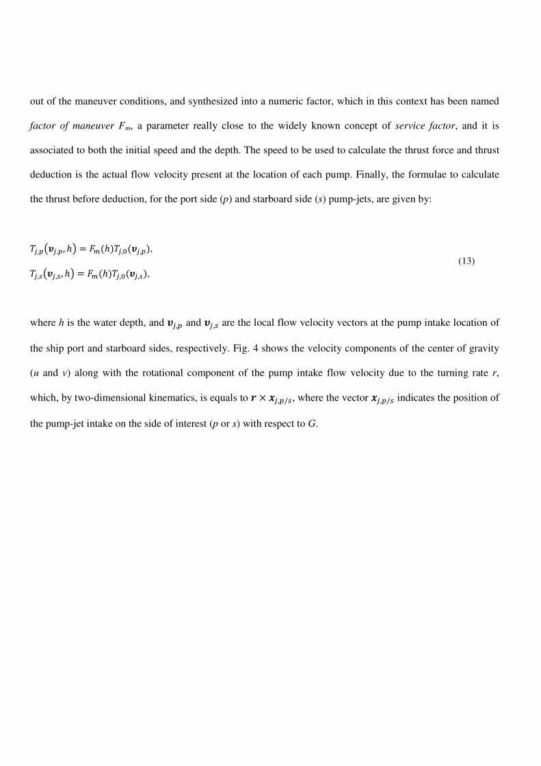
where h is the water depth, and 41,3 and 41,9 are the local flow velocity vectors at the pump intake location of

the ship port and starboard sides, respectively. Fig. 4 shows the velocity components of the center of gravity

(u and v) along with the rotational component of the pump intake flow velocity due to the turning rate r,

which, by two-dimensional kinematics, is equals to : × <1,3/9, where the vector <1,3/9 indicates the position of

the pump-jet intake on the side of interest (p or s) with respect to G.

Fig. 4. Velocity vectors at the center of gravity and components due to rotation at the pump intake locations

From Fig. 4 the vector components of 41,3 and 41,9 can be obtained, which yield:

41,3 = >�? + : × <1,3, (14)

>�1,31,3? = >�? + >−@1A1 ?, (15)

41,9 = >�? + : × <1,9, (16)

>�1,91,9? = >�? + >@1A1?. (17)

The variation of thrust is actually related to the magnitude (B1,3 and B1,9) of the mentioned velocity vectors

(41,3 and 41,9). According to the definitions in equations (14)-(17), these magnitudes are:

B1,3 = C"� − @1#! + " + A1#!, (18)

B1,9 = C"� + @1#! + " + A1#!. (19)

The actual thrust exerted by the propulsion system over the ship is a product of the previously defined

thrust after subtracting the thrust deduction t. This parameter is taken as a function of the flow velocity and

water depth. After taking into account the decomposition of the thrust with respect to the jet angle δ, the two

equations of propulsion force are obtained, as well as the one to model the generated moment by them:

&) = "(1 − E)901,9 + (1 − E)301,3# cos H, (20)

) = −"(1 − E)901,9 + (1 − E)301,3# sin H. (21)

�) = )A1 + "(1 − E)301,3 − (1 − E)901,9#@1 cos H. (22)

3.3 Normalization of variables

The non-dimensional form of all of the variables involved in the model is the one obtained by using the

Prime system - II (Fossen, 2.011). To get the non-dimensional value, each variable type must be divided by

the terms of the second column of Table 2. The normalization variables used here are the water density (ρ),

the length between perpendiculars (L), the absolute speed magnitude (U) and the draft (T).

Table 2

Normalization of variables – Prime system II

Variable Normalization terms

Distance I

Linear velocity B

Angular velocity B/I

Acceleration B!/I

Mass I!0J/2

Moment of Inertia IL0J/2

Force I0B!J/2

Moment I!0B!J/2

4. Detailed setup of the mathematical model

4.1 Added masses and added moment of inertia

The values of the inner variables must be set in order to complete the definition of the model, and thereby

by means of the reviewing the literature some formulae were collected to calculate the added mass in x, the

added mass in y and the added moment of inertia around the axis z. Table 3 shows some results of those

formulae given as percentage of the original mass or the original moment of inertia.

Table 3

Possible values for added masses and added moment of inertia

Parameter Option 1 Option 2

Added mass in x

(m’x)

5% of m’

(Fossen, 1.994)

3.55% of m’

(Bertram, 2000)

Added mass in y

(m’y)

20.15% of m’

(Fossen, 1.994)

37.62% of m’

(Clarke et al., 1.982)

Added moment

of inertia (J’zz)

33.69% of I’zz

(Fossen, 1.994)

50.46% of I’zz

(Clarke et al., 1.982)

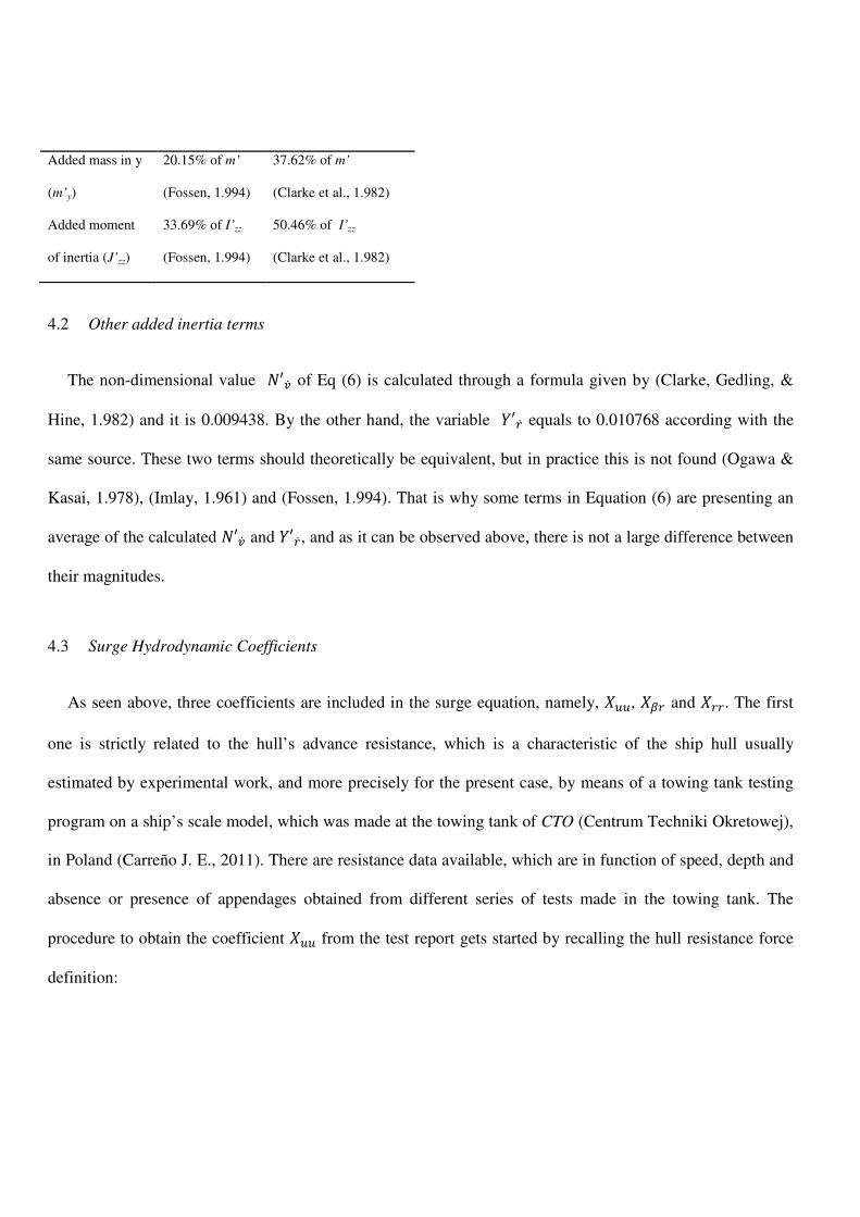
4.2 Other added inertia terms

The non-dimensional value �′�� of Eq (6) is calculated through a formula given by (Clarke, Gedling, &

Hine, 1.982) and it is 0.009438. By the other hand, the variable ′�� equals to 0.010768 according with the

same source. These two terms should theoretically be equivalent, but in practice this is not found (Ogawa &

Kasai, 1.978), (Imlay, 1.961) and (Fossen, 1.994). That is why some terms in Equation (6) are presenting an

average of the calculated �′�� and ′�� , and as it can be observed above, there is not a large difference between

their magnitudes.

4.3 Surge Hydrodynamic Coefficients

As seen above, three coefficients are included in the surge equation, namely, &**, &N� and &��. The first

one is strictly related to the hull’s advance resistance, which is a characteristic of the ship hull usually

estimated by experimental work, and more precisely for the present case, by means of a towing tank testing

program on a ship’s scale model, which was made at the towing tank of CTO (Centrum Techniki Okretowej),

in Poland (Carreño J. E., 2011). There are resistance data available, which are in function of speed, depth and

absence or presence of appendages obtained from different series of tests made in the towing tank. The

procedure to obtain the coefficient &** from the test report gets started by recalling the hull resistance force

definition:

&( = &′( O! I0B!, (23)

where &′( is the non-dimensional form of XH. In pure surge condition, it turns out that the hull resistance is in

function of velocity component u only, since by following eq. (10), and as P = = 0, the hydrodynamic

surge force simplifies into:

&′( = &′**�′!. (24)

Then,

&( = (&′**�′!) O! IQB!. (25)

Considering the notation on towing tank’s report, the following definition is made:

RS9 = TS O! U9B!, (26)

where RTs is the ship’s total hull resistance to advance, CT is the total resistance coefficient, and Ss is the

ship’s wet surface. Considering that −RS9 = &( for pure surge motion, the preceding equations yield:

−TS O! U9B! = (&V**�V!) O! IQB!. (27)

From the previous equation it is finally deduced that:

&V** = −TS WXYS*VZ. (28)

Another form to present the conversion of the available data into the coefficient &** is the following:

&V** = [\]XZYS*Z. (29)

The mentioned report provides the non-dimensional CT values, as well as the resistance force in kN, which

could be used by giving the advance speed as the input variable. Those data of resistance were used to obtain

a polynomial regression equation, which fully fits the known values. Fig. 5 displays the resulting polynomial

curve describing the hull resistance force behavior with respect to the forward speed u in m/s, when sailing in

deep water (blue line) and that of shallow water (red line). The first polynomial is:

RS >_S = 24? = 0.1042�L − 0.3813�d + 0.4793�! + 2.3554� [kN]. (30)

Fig. 5. Hull Resistance as a function of ship speed

The resistance for shallow water was adjusted to the maximum value that could be balanced by the

available thrust at maximum speed (8.4 knots). Thus the following function was derived by using a regression

method over the adjusted resistance data. Since the data available to find the polynomial was valid only over a

speed of 5 knots (2.572m/s), for lower speeds it is assumed that the hull resistance in shallow water is equals

to the corresponding to deep water (see Fig. 5).

RS >_S = 2.2? =hijik

−0.0579�d + 8.3�! − 37.4� −49.8 ∶ � ≥ 2.572RS >_S = 24? ∶ � < 2.572

o [kN]. (31)

According to (Ogawa & Kasai, 1.978), the rest of coefficients involved in the surge equation play the role

of incrementing the resistance due to motion other than pure advance. The value for the coupling coefficient

&′N� is estimated by a formula presented by (Ishiguro, Tanaka, & Yoshimura, 1.996), which defines:

&′N� = −�′�(−1.66Tu + 1.5). (32)

Additionally, (Yoshimura & Ma, 2.003) gave a formula for the coefficient &′��, which is:

&′�� = 0.03 − 0.09v, (33)

where τ is the trim-draft ratio. This term is associated with a radial acceleration of the added mass, as stated

by (Ogawa & Kasai, 1.978).

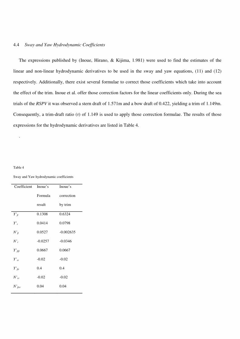
4.4 Sway and Yaw Hydrodynamic Coefficients

The expressions published by (Inoue, Hirano, & Kijima, 1.981) were used to find the estimates of the

linear and non-linear hydrodynamic derivatives to be used in the sway and yaw equations, (11) and (12)

respectively. Additionally, there exist several formulae to correct those coefficients which take into account

the effect of the trim. Inoue et al. offer those correction factors for the linear coefficients only. During the sea

trials of the RSPV it was observed a stern draft of 1.571m and a bow draft of 0.422, yielding a trim of 1.149m.

Consequently, a trim-draft ratio (τ) of 1.149 is used to apply those correction formulae. The results of those

expressions for the hydrodynamic derivatives are listed in Table 4.

.

Table 4

Sway and Yaw hydrodynamic coefficients

Coefficient Inoue’s

Formula

result

Inoue’s

correction

by trim

Y’β 0.1308 0.6324

Y’r 0.0414 0.0798

N’β 0.0527 -0.002635

N’r -0.0257 -0.0346

Y’ββ 0.0667 0.0667

Y’rr -0.02 -0.02

Y’βr 0.4 0.4

N’rr -0.02 -0.02

N’βrr 0.04 0.04

N’ββr -0.25 -0.25

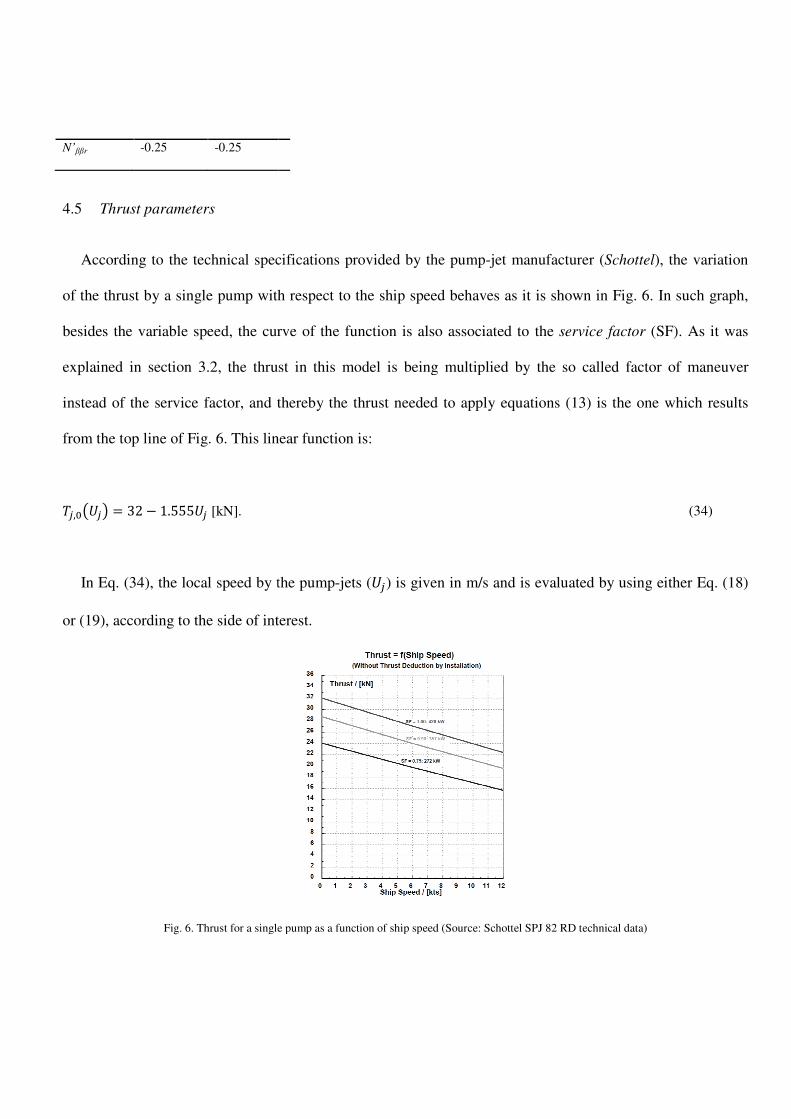
4.5 Thrust parameters

According to the technical specifications provided by the pump

of the thrust by a single pump with respect to the ship speed behaves as it is shown in

besides the variable speed, the curve of the

explained in section 3.2, the thrust in this model is being multiplied by the so called factor of maneuver

instead of the service factor, and thereby the thrust needed to apply equations (13

from the top line of Fig. 6. This linear function is:

01,8"B1# = 32 − 1.555B1 [kN].

In Eq. (34), the local speed by the pump

or (19), according to the side of interest.

Fig. 6. Thrust for a single pump as a function of ship speed (Source: Schottel SPJ 82 RD technical data)

According to the technical specifications provided by the pump-jet manufacturer (

of the thrust by a single pump with respect to the ship speed behaves as it is shown in

besides the variable speed, the curve of the function is also associated to the

, the thrust in this model is being multiplied by the so called factor of maneuver

instead of the service factor, and thereby the thrust needed to apply equations (13

This linear function is:

In Eq. (34), the local speed by the pump-jets (B1) is given in m/s and is evaluated by using either Eq. (18)

or (19), according to the side of interest.

a single pump as a function of ship speed (Source: Schottel SPJ 82 RD technical data)

jet manufacturer (Schottel), the variation

of the thrust by a single pump with respect to the ship speed behaves as it is shown in Fig. 6. In such graph,

function is also associated to the service factor (SF). As it was

, the thrust in this model is being multiplied by the so called factor of maneuver

instead of the service factor, and thereby the thrust needed to apply equations (13) is the one which results

(34)

) is given in m/s and is evaluated by using either Eq. (18)

a single pump as a function of ship speed (Source: Schottel SPJ 82 RD technical data)

The thrust deduction factor is inferred by contrasting the ideal thrust generated by the two pump-jets and

the hull total resistance to advance. This task was done through a self-propulsion test carried out at CTO as

well. The data is available from a speed of 5 knots through 9 knots. For a ship speed less than 5 knots, a

constant thrust deduction is considered. The resulting function of (1-t) is shown in Fig. 7.

1 − E = w0.0122B1! − 0.1804B1 + 1.3229 xy B1 ≥ 2.5720.971 xy B1 < 2.572o (35)

Fig. 7. Thrust deduction as a function of ship speed

For the shallow water condition, i.e. when h/T=2.2 a constant thrust deduction t = 10% was used, since

there was not any experimental data available.

4.6 Coefficient correction by water depth effect

Several sets of formulae can be found in the specialized publications concerning the effects of a depth

decrement on the hydrodynamic coefficients of a ship dynamic model. Since there are several choices to

make this correction, and a long list of parameters have to be affected by them, the results are summarized in

Table 5, according to the source of the correction.

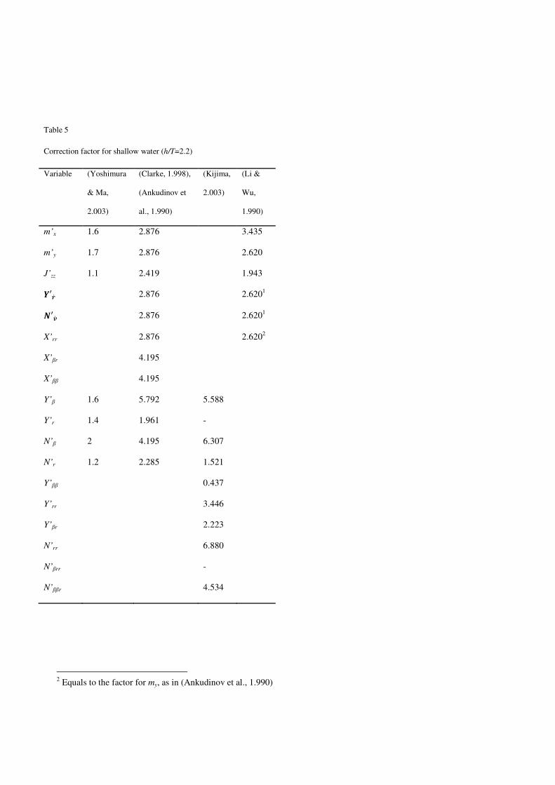
Table 5

Correction factor for shallow water (h/T=2.2)

Variable (Yoshimura

& Ma,

2.003)

(Clarke, 1.998),

(Ankudinov et

al., 1.990)

(Kijima,

2.003)

(Li &

Wu,

1.990)

m’x 1.6 2.876 3.435

m’y 1.7 2.876 2.620

J’zz 1.1 2.419 1.943

z′:� 2.876 2.6201

{′|� 2.876 2.6201

X’rr 2.876 2.6202

X’βr 4.195

X’ββ 4.195

Y’β 1.6 5.792 5.588

Y’r 1.4 1.961 -

N’β 2 4.195 6.307

N’r 1.2 2.285 1.521

Y’ββ 0.437

Y’rr 3.446

Y’βr 2.223

N’rr 6.880

N’βrr -

N’ββr 4.534

2 Equals to the factor for my, as in (Ankudinov et al., 1.990)

5. Simulation setup and results

5.1 About the algorithm and the tests

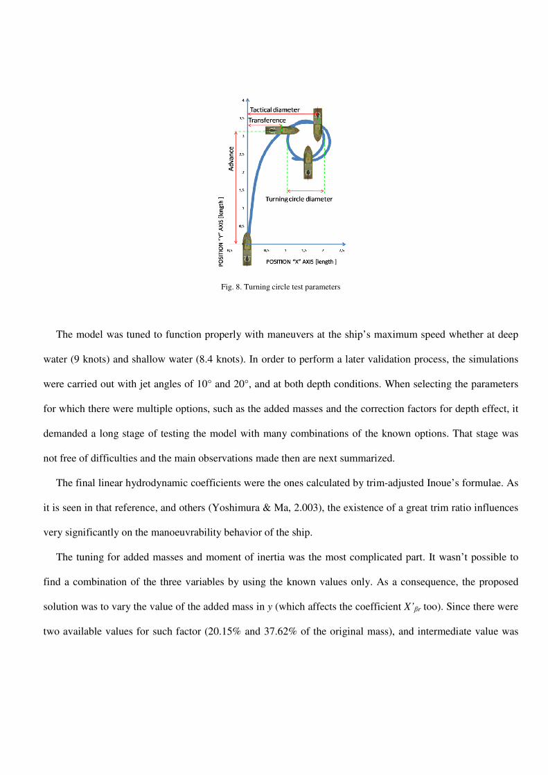
In order to assess the reliability of the constructed mathematical model, the decision of carrying out

simulations of a standard turning circle test was made, which could be compared with actual experimental

data. That test is the turning circle, managing several initial speeds and rudder angles (or jet angles). The test

consists of the measurement of several geometric parameters to evaluate the manoeuvrability of the ship.

Those parameters are illustrated on Fig. 8.

The integration scheme of the numerical model that was implemented was the 4th-order Runge-Kutta

method. For its execution it was necessary to fix a time step, but due to both the high order accuracy and the

stability of the selected method, it didn’t demand a very small value of this important simulation parameter.

The algorithm that was written is based on the open license MSS GNC simulation package, developed by

Thor I. Fossen and Tristan Perez. As the setting up of the present model was progressing, the algorithm went

under as many modifications as it was needed, and some new functions were added to the package. All the

feasible combinations of the distinct choices shown in the previous section for every variable were run using

the algorithm, in addition to several other variable values that were temporarily used when debugging or

testing the program code.

The model was tuned to function properly with maneuvers at the ship’s maximum speed whether at deep

water (9 knots) and shallow water (8.4 knots). In order to perform a later validation process, the simulations

were carried out with jet angles of 10° and 2

for which there were multiple options

demanded a long stage of testing

not free of difficulties and the main

The final linear hydrodynamic coefficients were the ones calculated by trim

it is seen in that reference, and others

very significantly on the manoeuvrability behavior of the ship.

The tuning for added masses and moment of inertia was the most complicated

find a combination of the three variables by using the known values only. As a consequence, the proposed

solution was to vary the value of the added mass in

two available values for such factor (20.15% and 37.62% of the original mass), and intermediate value was

Fig. 8. Turning circle test parameters



were carried out with jet angles of 10° and 20°, and at both depth conditions. When selecting

options, such as the added masses and the correction factors for depth effect, it

the model with many combinations of the known

t free of difficulties and the main observations made then are next summarized.

hydrodynamic coefficients were the ones calculated by trim-

others (Yoshimura & Ma, 2.003), the existence

euvrability behavior of the ship.

The tuning for added masses and moment of inertia was the most complicated


the value of the added mass in y (which affects the coefficient

for such factor (20.15% and 37.62% of the original mass), and intermediate value was



When selecting the parameters

and the correction factors for depth effect, it

many combinations of the known options. That stage was

are next summarized.

-adjusted Inoue’s formulae. As

, the existence of a great trim ratio influences

The tuning for added masses and moment of inertia was the most complicated part. It wasn’t possible to


(which affects the coefficient X’βr too). Since there were

for such factor (20.15% and 37.62% of the original mass), and intermediate value was

sought which guaranteed the model to work appropriately. The final set value for my was 24.1% of m. For mx,

it was used the 5% of m, and for the added moment of inertia, Fossen’s result was selected.

Finally, for the depth effect correction factors there was a more complex combination, by using several

sources of the available ones. In general, the factors given by Kijima were applied, but the correction for

several variables was replaced by other alternatives when the first one didn’t make the model work fine.

Consequently, the parameters set to run the simulations were as it is shown in

Table 6.

Table 6

Settings and values for simulation parameters

Simulation parameters Value

Initial speed 9 knots for deep water; 8.4 knots for shallow water (h/T=2.2)

Time of rudder execution 1 s

Total simulation time 1000 s

Time step 1 s

Integration scheme 4th

order Runge-Kutta

Added mass in x 5% of m (Fossen, 1.994)

Added mass in y 24.1% of m (between Fossen’s and Clarke’s)

Added moment of inertia 33.69% of Iz (Fossen, 1.994)

Shallow water correction factors Correction factor for hydrodynamic coefficients, in general (Kijima & Nakiri, 2.003).

Correction factor for Yr (Clarke, 1.998).

Correction factor for Nβrr is replaced by the one for Yβrr.

Correction factors for added inertia (Li & Wu, 1.990).

For �′�� , ′�� , and Xrr it was used the factor corresponding to my.

For Xβr it was used the factor corresponding to Nv from (Ankudinov et al., 1.990).

5.2

5.3

5.4

Table 6.

The trend found, besides proving the model consistency, turns out a coherent result with respect to the full-

scale experimentation, in which it was observed a good manoeuvrability of the studied ship, and the

improvement of this feature when sailing in little depth (the already cited NS effect).

Fig. 9 and Fig. 10 present a graphic comparison of the ship path and heading calculated in the simulation

and the experimental data obtained in full-scale trials. The contrasted maneuvers are the one with a jet angle

of 20° and at maximum speed for two different depth conditions (9 knots in deep water, 8.4 knots in shallow

water).

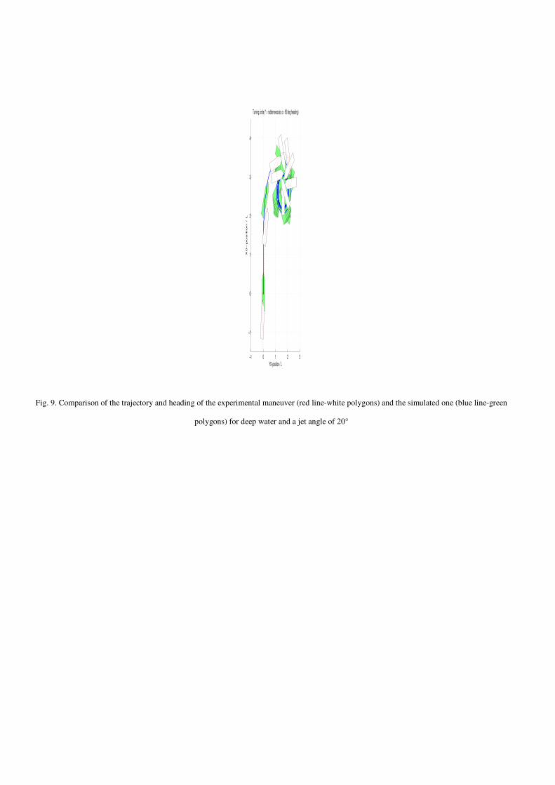
Fig. 9. Comparison of the trajectory and heading of the experimental maneuver (red line-white polygons) and the simulated one (blue line-green

polygons) for deep water and a jet angle of 20°

−1 0 1 2 3

−1

0

1

2

3

4

Turning circle (* = rudder execute, o = 90 deg heading)

Y0−position / L

X0

−p

ositio

n / L

Fig. 10. Comparison of the trajectory and heading of the experimental maneuver (red line-white polygons) and the simulated one (blue line-purple

polygons) for shallow water and jet angle of 20°

In addition to the preceding figures, by using the reported results of the full-scale maneuvers, it was

possible to summarize the data and register the results of the simulation, in order to evaluate how good the

approximation was. The results contained in Table 7 other than the turning circle measurements (turning

diameter, tactical diameter, advance and transfer) represent the value of state variables when the motion has

reached the steady state (drift angle, yaw rate and the final speed).

−3 −2.5 −2 −1.5 −1 −0.5 0 0.5 1−1

−0.5

0

0.5

1

1.5

2

2.5

3

3.5

4

Y0−position / L

X0

−p

ositio

n /

L

Turning circle (* = rudder execute, o = 90 deg heading)

Table 7

Present model simulation results and relative error with respect to full-scale trials

Initial

speed

Jet

angle

Depth

Turning

diameter

Tactical

diameter

Advance Transfer

Drift

angle

Yaw

rate

Final

speed

Speed

ratio Method

(knots) (deg.) (h/T) /Length /Length /Length /Length (deg.) (deg/s) (m/s) (U/U0)

9 20 24 0,978 1,920 2,561 1,127 70,22 3,812 1,709 0,369 FULL SCALE

0,821 2,155 3,415 0,999 42,47 4,565 1,241 0,268 PRESENT MODEL

-16% 12% 33% -11% -40% 20% -27% -27% RELATIVE ERROR

8,4 20 2,2 0,473 1,099 1,200 0,376 70,34 4,066 1,229 0,285 FULL SCALE

0,634 2,186 3,213 1,353 25,17 3,811 0,800 0,185 PRESENT MODEL

34% 99% 168% 260% -64% -6% -35% -35% RELATIVE ERROR

9 10 24 2,195 3,061 2,765 1,968 - - 2,379 0,514 FULL SCALE

2,186 3,048 4,319 1,452 20,46 3,641 2,633 0,569 PRESENT MODEL

0% 0% 56% -26% - - 11% 11% RELATIVE ERROR

8,4 10 2,2 1,732 2,596 2,061 1,642 87,59 4,249 1,952 0,452 FULL SCALE

1,401 3,921 4,420 2,201 8,551 3,847 1,784 0,413 PRESENT MODEL

-19% 51% 114% 34% -90% -9% -9% -9% RELATIVE ERROR

6. Conclusions

A complete and useful mathematical model was developed with the purpose of simulating the

manoeuvrability behavior of an azimuthally propelled riverine ship. Despite the lack of some information

regarding the behavior of the RSPV’s pump-jet system thrust in shallow water, the assumptions and

adjustments made in the model showed a final good performance since the results obtained from it were

consistent.

A sensitivity analysis shows that the model can work properly between some specified limits by using

certain parameter values that were found after an algorithm tuning stage.

Even though the turning diameter was the one variable which had a good approximation in all cases and

that was able to be validated due to the existence of complete information, some other variables like the

steady yaw rate had a really good approach too, but the data were incomplete for that case. Moreover, some of

the remaining output variables were a good estimate for only one of the depth conditions (tactical diameter

and transfer for deep water), or for just one of the applied jet angles (final speed for the angle of 10°). These

facts suggest that the model herein developed is a valid tool to simulate wide-beam vessels with azimuthal

propulsion though not all the conditions may offer very good approximation.

The available experimental data used to validate the developed model allowed the acceptance of it only

within the known ranges but, as to the jet angle, this is a very limited result if taking into account that the

pump-jet type is an azimuthal propulsion system and therefore it can cover any jet angle, and the model has

been validated only for 10° through 20°.

Besides the formerly published results of the full-scale trials made with the RSPV, through the

mathematical model, the good manoeuvrability features of this ship were again proven. Specifically, it is

remarkable that the turning ability is improved when the water depth decreases from deep water (h/T=24) to

shallow water (h/T=2.2). This result is related to the existence of the NS effect for wide-beam vessels, a

phenomenon described to be associated exclusively to this kind of ships (Yoshimura & Sakurai, 1.988) and

(Yasukawa & Kobayashi, 1.995).

References

Ankudinov, V., Miller, E., Jakobsen, B., & Dagget, L. (1.990). Maneuvering Performance of Tugbarge Assemblies in Restricted

Waterways. Proceedings of MARSIM'90 , 515-525. Tokyo, Japan.

Bertram, V. (2000). Practical Ship Hydrodynamics. Oxford.

Carreño, J. E. (2011). Simulación de maniobras de buques con sistemas de propulsión no convencional en aguas poco profundas.

Madrid, España: Universidad Politécnica de Madrid, PhD thesis (preliminary submission).

Carreño, J. E., Jimenez, V. H., & Sierra, E. Y. (2.011). Ship Manoeuvrability: Full Scale Trials Of Colombian Navy Riverine

Support Patrol Vessel. Ship Science and Technology , 5 (9).

Carreño, J. E., Jimenez, V. H., & Sierra, E. Y. (2.011). Ship Manoeuvrability: Full Scale Trials Of Colombian Navy Riverine

Support Patrol Vessel. Ship Science and Technology , 5 (9).

Clarke, D. (1.998). The effect of shallow water on manoeuvring derivatives using conformal mapping. Control Engineering

Practice (6), 629-634.

Clarke, D., Gedling, P., & Hine, G. (1.982, April 12). The Application of Manoeuvring Criteria in Hull Using Linear Theory.

London, UK: The Royal Institution of Naval Architects.

Fossen, T. I. (1.994). Guidance and Control of Ocean Vehicles. U.K.: John Wiley & Sons Ltd.

Fossen, T. I. (2.011). Handbook of Marine Craft Hydrodynamics and Motion Control (First ed.). Chichester, U.K.: John Wiley &

Sons.

Imlay, F. H. (July de 1.961). The complete expressions for "Added Mass" of a rigid body moving in an ideal fluid. Report 1528,

Hydromechanics Laboratory, Research an Development Report . Arlington, USA: David Taylor Model Basin.

Inoue, S., Hirano, M., & Kijima, K. (1.981). Hydrodynamic Derivatives on Ship Manoeuvring. International Shipbuilding Progress

, 28 (321), 112-125.

Inoue, S., Hirano, M., & Kijima, K. (1.981). Hydrodynamic Derivatives on Ship Manoeuvring. International Shipbuilding Progress

, 28 (321), 112-125.

Ishiguro, T., Tanaka, S., & Yoshimura, Y. (1.996). A Study on the Accuracy of recent Prediction Technique of Ship's

Manoeuvrability at the Early Design Stage. Proceedings of MARSIM'96 , 547-561. Copenhagen, Denmark.

ITTC. (2.002). ITTC Recommended Procedures. Testing and Extrapolation Methods, Manoeuvrability, Validation of Manoeuvring

Simulation Models (7.5-02-06-03) , 1-11.

Kijima, K., & Nakiri, Y. (2.003). On the practical prediction method for ship manoeuvring characteristics. Proceedings of

MARSIM'03 , III (RC-6) . Kanazawa, Japan.

Li, M., & Wu, X. (1.990). Simulation calculation and comprehensive assessment on ship maneuverabilities in wind, wave, current

and shallow water. Proceedings of MARSIM'90 , 403-411. Tokyo, Japan.

Lloyd, A. R. (1.998). Seakeeping: Ship Behaivor in Rough Weather (2nd ed.). U.K.: Ellis Horwood Limited.

Ogawa, A., & Kasai, H. (1.978). On the Mathematical Model of Manoeuvring Motion of Ships. International Shipbuilding

Progress , 25, 306-319.

Pérez, F. L., & Clemente, J. A. (2.007). The influence of some ship parameters on manoeuvrability studied at the design stage.

Ocean Engineering (34), 518-525.

Yasukawa, H., & Kobayashi, E. (1.995). Shallow water model experiments on ship turning performance. Mini Symposium on Ship

Manoeuvrability , 71-83. Fukuoka, Japan: The West-Japan Society of Naval Architects.

Yoshimura, Y., & Ma, N. (2.003). Manoeuvring Prediction of Fishing Vessels. Proceedings of MARSIM'03 (RC-29) . Kanazawa,

Japan.

Yoshimura, Y., & Sakurai, H. (1.988). Mathematical Model for the Manoeuvring Ship Motion in Shallow Water (3rd Report).

Journal of KSNAJ , 211, 115-126.

Yoshimura, Y., & Sakurai, H. (1.988). Mathematical Model for the Manoeuvring Ship Motion in Shallow Water (3rd Report).

Journal of KSNAJ , 211, 115-126.

Mathematical model for manoeuvrability of a riverine...

Documents

Transcript of Mathematical model for manoeuvrability of a riverine...