MATH 350: Introduction to Computational Mathematics - Applied

MATH 350: Introduction to ComputationalMathematics

Chapter III: Interpolation

Greg Fasshauer

Department of Applied MathematicsIllinois Institute of Technology

Spring 2011

[email protected] MATH 350 – Chapter 3 1

http://math.iit.edu/~fass

Outline

1 Motivation and Applications

2 Polynomial Interpolation

3 Piecewise Polynomial Interpolation

4 Spline Interpolation

5 Interpolation in Higher Space Dimensions



Motivation and Applications


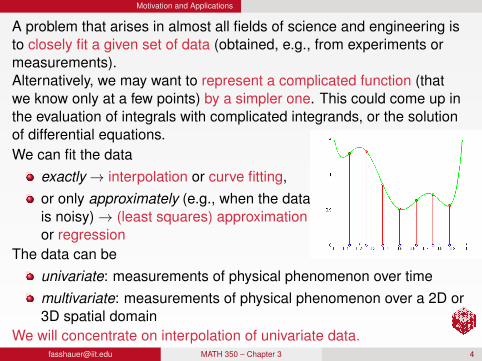
A problem that arises in almost all fields of science and engineering isto closely fit a given set of data (obtained, e.g., from experiments ormeasurements).Alternatively, we may want to represent a complicated function (thatwe know only at a few points) by a simpler one. This could come up inthe evaluation of integrals with complicated integrands, or the solutionof differential equations.We can fit the data

exactly→ interpolation or curve fitting,or only approximately (e.g., when the datais noisy)→ (least squares) approximationor regression

The data can beunivariate: measurements of physical phenomenon over timemultivariate: measurements of physical phenomenon over a 2D or3D spatial domain

We will concentrate on interpolation of univariate data.



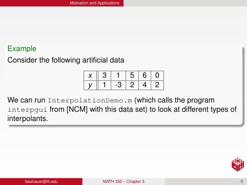
ExampleConsider the following artificial data

x 3 1 5 6 0y 1 -3 2 4 2

We can run InterpolationDemo.m (which calls the programinterpgui from [NCM] with this data set) to look at different types ofinterpolants.




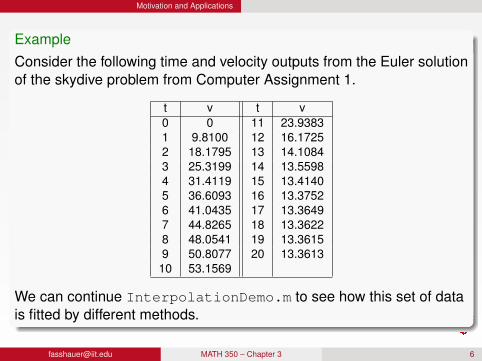
ExampleConsider the following time and velocity outputs from the Euler solutionof the skydive problem from Computer Assignment 1.

t v t v0 0 11 23.93831 9.8100 12 16.17252 18.1795 13 14.10843 25.3199 14 13.55984 31.4119 15 13.41405 36.6093 16 13.37526 41.0435 17 13.36497 44.8265 18 13.36228 48.0541 19 13.36159 50.8077 20 13.361310 53.1569

We can continue InterpolationDemo.m to see how this set of datais fitted by different methods.



Polynomial Interpolation Linear Interpolation

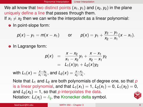
We all know that two distinct points (x1, y1) and (x2, y2) in the planeuniquely define a line that passes through them.If x1 6= x2 then we can write the interpolant as a linear polynomial:

In point-slope form:

p(x)− y1 = m(x − x1) or p(x) = y1 +y2 − y1

x2 − x1(x − x1).

In Lagrange form:

p(x) =x − x2

x1 − x2y1 +

x − x1

x2 − x1y2

= L1(x)y1 + L2(x)y2

with L1(x) =x−x2x1−x2

, and L2(x) =x−x1x2−x1

.

Note that L1 and L2 are both polynomials of degree one, so that pis a linear polynomial, and that L1(x1) = 1, L2(x1) = 0, L1(x2) = 0,and L2(x2) = 1, so that p interpolates the data.Notation: Li(xj) = δij , the Kronecker delta symbol.



Polynomial Interpolation Quadratic Interpolation

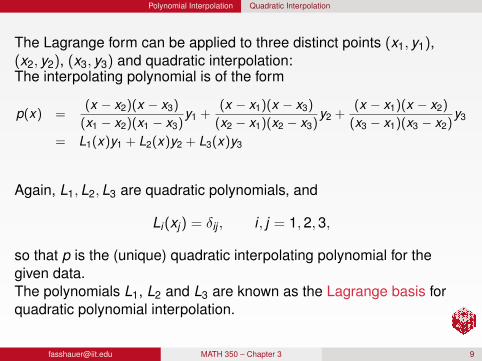
The Lagrange form can be applied to three distinct points (x1, y1),(x2, y2), (x3, y3) and quadratic interpolation:The interpolating polynomial is of the form

p(x) =(x − x2)(x − x3)

(x1 − x2)(x1 − x3)y1 +

(x − x1)(x − x3)

(x2 − x1)(x2 − x3)y2 +

(x − x1)(x − x2)

(x3 − x1)(x3 − x2)y3

= L1(x)y1 + L2(x)y2 + L3(x)y3

Again, L1,L2,L3 are quadratic polynomials, and

Li(xj) = δij , i , j = 1,2,3,

so that p is the (unique) quadratic interpolating polynomial for thegiven data.The polynomials L1, L2 and L3 are known as the Lagrange basis forquadratic polynomial interpolation.




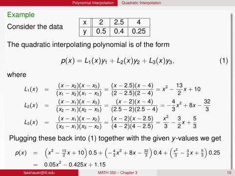
Example

Consider the datax 2 2.5 4y 0.5 0.4 0.25

The quadratic interpolating polynomial is of the form

p(x) = L1(x)y1 + L2(x)y2 + L3(x)y3, (1)

where

L1(x) =(x − x2)(x − x3)

(x1 − x2)(x1 − x3)=

(x − 2.5)(x − 4)(2 − 2.5)(2 − 4)

= x2 − 132

x + 10

L2(x) =(x − x1)(x − x3)

(x2 − x1)(x2 − x3)=

(x − 2)(x − 4)(2.5 − 2)(2.5 − 4)

= −43

x2 + 8x − 323

L3(x) =(x − x1)(x − x2)

(x3 − x1)(x3 − x2)=

(x − 2)(x − 2.5)(4 − 2)(4 − 2.5)

=x2

3− 3

2x +

53

Plugging these back into (1) together with the given y -values we get

p(x) =(

x2 − 132 x + 10

)0.5 +

(− 4

3 x2 + 8x − 323

)0.4 +

(x2

3 − 32 x + 5

3

)0.25

= 0.05x2 − 0.425x + [email protected] MATH 350 – Chapter 3 10



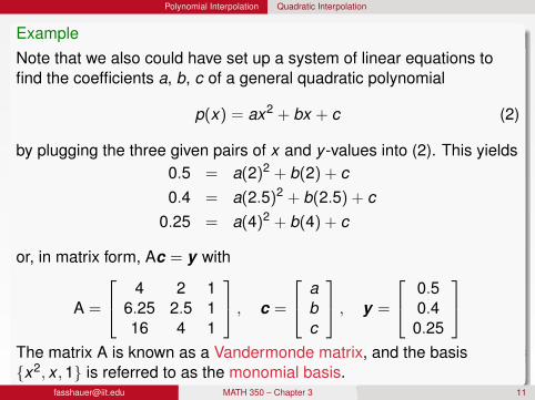
ExampleNote that we also could have set up a system of linear equations tofind the coefficients a, b, c of a general quadratic polynomial

p(x) = ax2 + bx + c (2)

by plugging the three given pairs of x and y -values into (2). This yields0.5 = a(2)2 + b(2) + c0.4 = a(2.5)2 + b(2.5) + c

0.25 = a(4)2 + b(4) + c

or, in matrix form, Ac = y with

A =

4 2 16.25 2.5 116 4 1

, c =

abc

, y =

0.50.4

0.25

The matrix A is known as a Vandermonde matrix, and the basis{x2, x ,1} is referred to as the monomial basis.



Polynomial Interpolation General Polynomial Interpolation

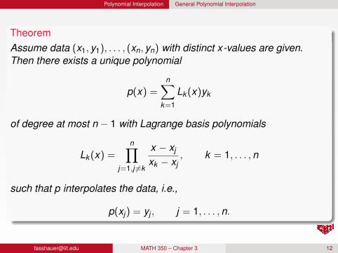
TheoremAssume data (x1, y1), . . . , (xn, yn) with distinct x-values are given.Then there exists a unique polynomial

p(x) =n∑

k=1

Lk (x)yk

of degree at most n − 1 with Lagrange basis polynomials

Lk (x) =n∏

j=1,j 6=k

x − xj

xk − xj, k = 1, . . . ,n

such that p interpolates the data, i.e.,

p(xj) = yj , j = 1, . . . ,n.




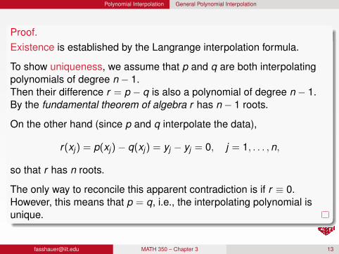
Proof.Existence is established by the Langrange interpolation formula.

To show uniqueness, we assume that p and q are both interpolatingpolynomials of degree n − 1.Then their difference r = p − q is also a polynomial of degree n − 1.By the fundamental theorem of algebra r has n − 1 roots.

On the other hand (since p and q interpolate the data),

r(xj) = p(xj)− q(xj) = yj − yj = 0, j = 1, . . . ,n,

so that r has n roots.

The only way to reconcile this apparent contradiction is if r ≡ 0.However, this means that p = q, i.e., the interpolating polynomial isunique.




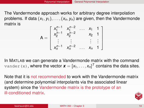
The Vandermonde approach works for arbitrary degree interpolationproblems. If data (x1, y1), . . . , (xn, yn) are given, then the Vandermondematrix is

A =

xn−1

1 xn−21 . . . x1 1

xn−12 xn−2

2 x2 1...

......

...xn−1

n xn−2n . . . xn 1

In MATLAB we can generate a Vandermonde matrix with the commandvander(x), where the vector x = [x1, . . . , xn]

T contains the data sites.

Note that it is not recommended to work with the Vandermonde matrix(and determine polynomial interpolants via the associated linearsystem) since the Vandermonde matrix is the prototype of anill-conditioned matrix.




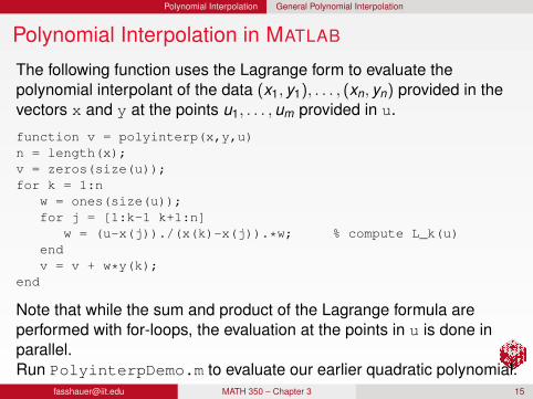
Polynomial Interpolation in MATLAB

The following function uses the Lagrange form to evaluate thepolynomial interpolant of the data (x1, y1), . . . , (xn, yn) provided in thevectors x and y at the points u1, . . . ,um provided in u.

function v = polyinterp(x,y,u)n = length(x);v = zeros(size(u));for k = 1:n

w = ones(size(u));for j = [1:k-1 k+1:n]

w = (u-x(j))./(x(k)-x(j)).*w; % compute L_k(u)endv = v + w*y(k);

end

Note that while the sum and product of the Lagrange formula areperformed with for-loops, the evaluation at the points in u is done inparallel.Run PolyinterpDemo.m to evaluate our earlier quadratic polynomial.



Piecewise Polynomial Interpolation

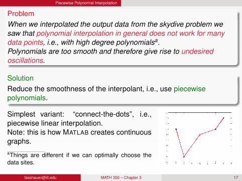
ProblemWhen we interpolated the output data from the skydive problem wesaw that polynomial interpolation in general does not work for manydata points, i.e., with high degree polynomialsa.Polynomials are too smooth and therefore give rise to undesiredoscillations.

SolutionReduce the smoothness of the interpolant, i.e., use piecewisepolynomials.

Simplest variant: “connect-the-dots”, i.e.,piecewise linear interpolation.Note: this is how MATLAB creates continuousgraphs.aThings are different if we can optimally choose thedata sites.



Piecewise Polynomial Interpolation Piecewise Linear Interpolation

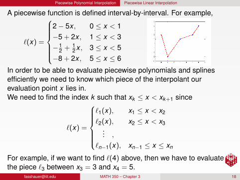
A piecewise function is defined interval-by-interval. For example,

`(x) =

2− 5x , 0 ≤ x < 1−5 + 2x , 1 ≤ x < 3−1

2 + 12x , 3 ≤ x < 5

−8 + 2x , 5 ≤ x ≤ 6

In order to be able to evaluate piecewise polynomials and splinesefficiently we need to know which piece of the interpolant ourevaluation point x lies in.We need to find the index k such that xk ≤ x < xk+1 since

`(x) =

`1(x), x1 ≤ x < x2

`2(x), x2 ≤ x < x3... ,

`n−1(x), xn−1 ≤ x ≤ xn

For example, if we want to find `(4) above, then we have to evaluatethe piece `3 between x3 = 3 and x4 = 5.




Since a linear function connecting (x1, y1) and (x2, y2) can be writtenas

y = y1 + δ(x − x1)

with slope δ, the k -th piece of the piecewise linear interpolant is givenby

`k (x) = yk +yk+1 − yk

xk+1 − xk(x − xk ).

The points xk are sometimes called breakpoints or knots.




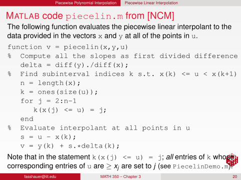
MATLAB code piecelin.m from [NCM]The following function evaluates the piecewise linear interpolant to thedata provided in the vectors x and y at all of the points in u.function v = piecelin(x,y,u)% Compute all the slopes as first divided difference

delta = diff(y)./diff(x);% Find subinterval indices k s.t. x(k) <= u < x(k+1)

n = length(x);k = ones(size(u));for j = 2:n-1

k(x(j) <= u) = j;end

% Evaluate interpolant at all points in us = u - x(k);v = y(k) + s.*delta(k);

Note that in the statement k(x(j) <= u) = j; all entries of k whosecorresponding entries of u are ≥ xj are set to j (see PiecelinDemo.m).



Piecewise Polynomial Interpolation Piecewise Cubic Hermite Interpolation

If we want something a bit fancier (i.e., smoother), then we can workwith a cubic polynomial piece on each subinterval.Just as a linear polynomial naturally matches the two function valuesgiven at the endpoints of the subinterval, the four coefficients of thecubic polynomial can be determined by matching function andderivative values at the endpoints.If these derivative values are given, then we can directly use them. Theresulting method is known as piecewise cubic Hermite interpolation.If we don’t have this additional data, we can somehow approximate it:

The piecewise cubic interpolant, pchip, used in MATLAB

generates the additional derivative data so that the resultinginterpolant is continuously differentiable and shape preserving,i.e., the interpolant does not have any oscillations, over- orundershoots that are not present in the data.For the cubic spline the derivatives are determined so that thepieces are twice continuously differentiable at the breakpoints.




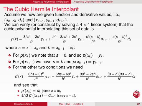
The Cubic Hermite InterpolantAssume we now are given function and derivative values, i.e.,(xk , yk ,dk ) and (xk+1, yk+1,dk+1).We can verify (or construct by solving a 4× 4 linear system) that thecubic polynomial interpolating this set of data is

p(x) =3hs2 − 2s3

h3 yk+1 +h3 − 3hs2 + 2s3

h3 yk +s2(s − h)

h2 dk+1 +s(s − h)2

h2 dk

where s = x − xk and h = xk+1 − xk :

For p(xk ) we note that s = 0, and so p(xk ) = yk .For p(xk+1) we have s = h and p(xk+1) = yk+1.For the other two conditions we need

p′(x) =6hs − 6s2

h3 yk+1 −6hs − 6s2

h3 yk +3s2 − 2sh

h2 dk+1 +(s − h)(3s − h)

h2 dk

and see thatp′(xk ) = dk (since s = 0),and p′(xk+1) = dk+1 (since s = h).




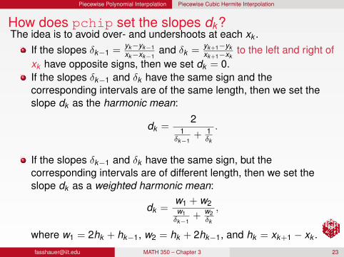
How does pchip set the slopes dk?The idea is to avoid over- and undershoots at each xk .

If the slopes δk−1 =yk−yk−1xk−xk−1

and δk =yk+1−ykxk+1−xk

to the left and right ofxk have opposite signs, then we set dk = 0.If the slopes δk−1 and δk have the same sign and thecorresponding intervals are of the same length, then we set theslope dk as the harmonic mean:

dk =2

1δk−1

+ 1δk

.

If the slopes δk−1 and δk have the same sign, but thecorresponding intervals are of different length, then we set theslope dk as a weighted harmonic mean:

dk =w1 + w2w1δk−1

+ w2δk

,

where w1 = 2hk + hk−1, w2 = hk + 2hk−1, and hk = xk+1 − xk [email protected] MATH 350 – Chapter 3 23



How does pchip set the slopes dk? (cont.)

The slopes at the endpoints are set by slightly different rules.

Run PchipDemo.m to see an example of the shape-preservingC1-cubic Hermite interpolant, and view pchiptx.m from [NCM] formore details (for example, how the slopes at the endpoints aredetermined).




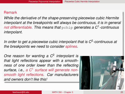
RemarkWhile the derivative of the shape-preserving piecewise cubic Hermiteinterpolant at the breakpoints will always be continuous, it is in generalnot differentiable. This means that pchip generates a C1-continuousinterpolant.

In order to get a piecewise cubic interpolant that is C2-continuous atthe breakpoints we need to consider splines.

One reason for wanting a C2 interpolant isthat light reflections appear with a smooth-ness of one order lower than the reflectingsurface, i.e., a C1 surface will generate non-smooth light reflections. Car manufacturersand owners don’t like this!



Spline Interpolation

History of Splines

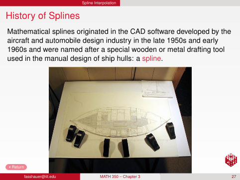
Mathematical splines originated in the CAD software developed by theaircraft and automobile design industry in the late 1950s and early1960s and were named after a special wooden or metal drafting toolused in the manual design of ship hulls: a spline.


Return


Spline Interpolation

General Splines

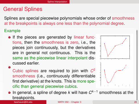
Splines are special piecewise polynomials whose order of smoothnessat the breakpoints is always one less than the polynomial degree.

ExampleIf the pieces are generated by linear func-tions, then the smoothness is zero, i.e., thepieces join continuously, but the derivativesare in general not continuous. This is thesame as the piecewise linear interpolant dis-cussed earlier.

Cubic splines are required to join with C2

smoothness (i.e., continuously differentiablefirst derivative) at the knots. This is more spe-cific than general piecewise cubics.In general, a spline of degree k will have Ck−1 smoothness at thebreakpoints.



Spline Interpolation Cubic Spline Interpolation

The most interesting — and also most commonly used — splines arethe cubic splines.We can start exactly as with the pchip interpolant, i.e.,

p(x) =3hs2 − 2s3

h3 yk+1 +h3 − 3hs2 + 2s3

h3 yk +s2(s − h)

h2 dk+1 +s(s − h)2

h2 dk

where s = x − xk , h = xk+1− xk , and dk and dk+1 are slopes at xk andxk+1 (to be determined by the spline method). Moreover (as before),

p′(x) =6hs − 6s2

h3 yk+1 −6hs − 6s2

h3 yk +3s2 − 2sh

h2 dk+1 +(s − h)(3s − h)

h2 dk

and now also

p′′(x) =6h − 12s

h3 yk+1 −6h − 12s

h3 yk +6s − 2h

h2 dk+1 +6s − 4h

h2 dk

=(6h − 12s)δk + (6s − 2h)dk+1 + (6s − 4h)dk

h2 ,

where δk =yk+1−yk

h =yk+1−ykxk+1−xk

.




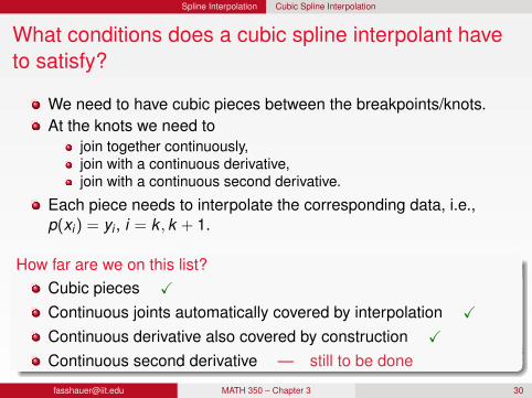
What conditions does a cubic spline interpolant haveto satisfy?

We need to have cubic pieces between the breakpoints/knots.At the knots we need to

join together continuously,join with a continuous derivative,join with a continuous second derivative.

Each piece needs to interpolate the corresponding data, i.e.,p(xi) = yi , i = k , k + 1.

How far are we on this list?Cubic pieces X

Continuous joints automatically covered by interpolation X

Continuous derivative also covered by construction X

Continuous second derivative — still to be done




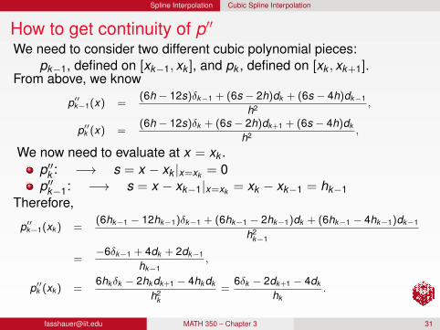
How to get continuity of p′′We need to consider two different cubic polynomial pieces:

pk−1, defined on [xk−1, xk ], and pk , defined on [xk , xk+1].From above, we know

p′′k−1(x) =(6h − 12s)δk−1 + (6s − 2h)dk + (6s − 4h)dk−1

h2 ,

p′′k (x) =(6h − 12s)δk + (6s − 2h)dk+1 + (6s − 4h)dk

h2 ,

We now need to evaluate at x = xk .p′′k : −→ s = x − xk |x=xk = 0p′′k−1: −→ s = x − xk−1|x=xk = xk − xk−1 = hk−1

Therefore,

p′′k−1(xk ) =(6hk−1 − 12hk−1)δk−1 + (6hk−1 − 2hk−1)dk + (6hk−1 − 4hk−1)dk−1

h2k−1

=−6δk−1 + 4dk + 2dk−1

hk−1,

p′′k (xk ) =6hkδk − 2hk dk+1 − 4hk dk

h2k

=6δk − 2dk+1 − 4dk

hk.




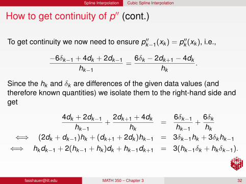
How to get continuity of p′′ (cont.)

To get continuity we now need to ensure p′′k−1(xk ) = p′′k (xk ), i.e.,

−6δk−1 + 4dk + 2dk−1

hk−1=

6δk − 2dk+1 − 4dk

hk.

Since the hk and δk are differences of the given data values (andtherefore known quantities) we isolate them to the right-hand side andget

4dk + 2dk−1

hk−1+

2dk+1 + 4dk

hk=

6δk−1

hk−1+

6δk

hk

⇐⇒ (2dk + dk−1)hk + (dk+1 + 2dk )hk−1 = 3δk−1hk + 3δkhk−1

⇐⇒ hkdk−1 + 2(hk−1 + hk )dk + hk−1dk+1 = 3(hk−1δk + hkδk−1).




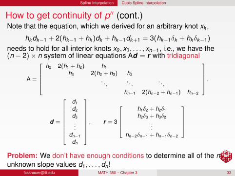
How to get continuity of p′′ (cont.)Note that the equation, which we derived for an arbitrary knot xk ,

hkdk−1 + 2(hk−1 + hk )dk + hk−1dk+1 = 3(hk−1δk + hkδk−1)

needs to hold for all interior knots x2, x3, . . . , xn−1, i.e., we have the(n − 2)× n system of linear equations Ad = r with tridiagonal

A =

h2 2(h1 + h2) h1

h3 2(h2 + h3) h2

. . .. . .

. . .hn−1 2(hn−2 + hn−1) hn−2

,

d =

d1

d2

d3...

dn−1

dn

, r = 3

h1δ2 + h2δ1

h2δ3 + h3δ2...

hn−2δn−1 + hn−1δn−2

Problem: We don’t have enough conditions to determine all of the nunknown slope values d1, . . . ,dn!




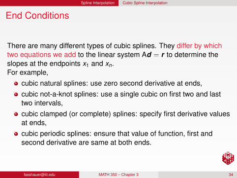
End Conditions

There are many different types of cubic splines. They differ by whichtwo equations we add to the linear system Ad = r to determine theslopes at the endpoints x1 and xn.For example,

cubic natural splines: use zero second derivative at ends,cubic not-a-knot splines: use a single cubic on first two and lasttwo intervals,cubic clamped (or complete) splines: specify first derivative valuesat ends,cubic periodic splines: ensure that value of function, first andsecond derivative are same at both ends.




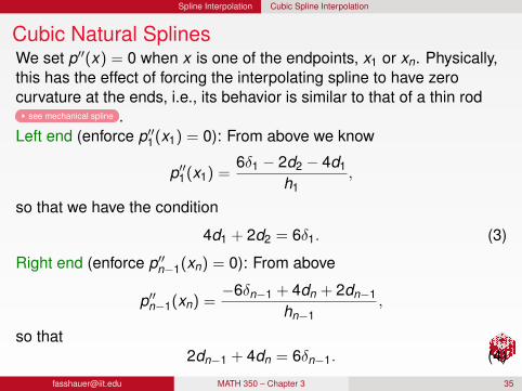
Cubic Natural SplinesWe set p′′(x) = 0 when x is one of the endpoints, x1 or xn. Physically,this has the effect of forcing the interpolating spline to have zerocurvature at the ends, i.e., its behavior is similar to that of a thin rod

see mechanical spline .Left end (enforce p′′1(x1) = 0): From above we know

p′′1(x1) =6δ1 − 2d2 − 4d1

h1,

so that we have the condition

4d1 + 2d2 = 6δ1. (3)

Right end (enforce p′′n−1(xn) = 0): From above

p′′n−1(xn) =−6δn−1 + 4dn + 2dn−1

hn−1,

so that2dn−1 + 4dn = 6δn−1. (4)




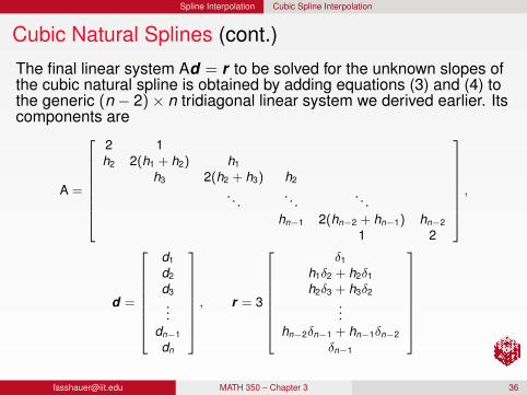
Cubic Natural Splines (cont.)

The final linear system Ad = r to be solved for the unknown slopes ofthe cubic natural spline is obtained by adding equations (3) and (4) tothe generic (n − 2)× n tridiagonal linear system we derived earlier. Itscomponents are

A =

2 1h2 2(h1 + h2) h1

h3 2(h2 + h3) h2

. . .. . .

. . .hn−1 2(hn−2 + hn−1) hn−2

1 2

,

d =

d1

d2

d3...

dn−1

dn

, r = 3

δ1

h1δ2 + h2δ1

h2δ3 + h3δ2...

hn−2δn−1 + hn−1δn−2

δn−1




Cubic Natural Splines (cont.)

Remark

The cubic natural spline is that interpolating C2 function whichminimizes the model for the bending energy of a thin rod. Thus thename seems justified.

The modified version splinetx_natural.m of the [NCM] routinesplinetx.m performs cubic spline interpolation with natural endconditions.

See SplineDemo.m for an example.




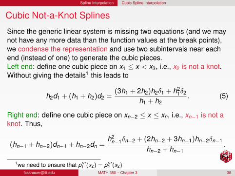
Cubic Not-a-Knot Splines

Since the generic linear system is missing two equations (and we maynot have any more data than the function values at the break points),we condense the representation and use two subintervals near eachend (instead of one) to generate the cubic pieces.Left end: define one cubic piece on x1 ≤ x < x3, i.e., x2 is not a knot.Without giving the details1 this leads to

h2d1 + (h1 + h2)d2 =(3h1 + 2h2)h2δ1 + h2

1δ2

h1 + h2. (5)

Right end: define one cubic piece on xn−2 ≤ x ≤ xn, i.e., xn−1 is not aknot. Thus,

(hn−1 + hn−2)dn−1 + hn−2dn =h2

n−1δn−2 + (2hn−2 + 3hn−1)hn−2δn−1

hn−2 + hn−1.

(6)1we need to ensure that p′′′1 (x2) = p′′′2 (x2)




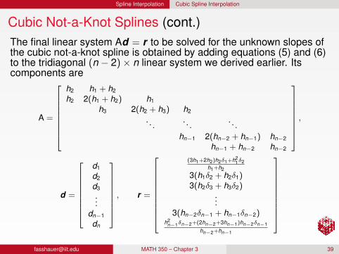
Cubic Not-a-Knot Splines (cont.)The final linear system Ad = r to be solved for the unknown slopes ofthe cubic not-a-knot spline is obtained by adding equations (5) and (6)to the tridiagonal (n − 2)× n linear system we derived earlier. Itscomponents are

A =

h2 h1 + h2

h2 2(h1 + h2) h1

h3 2(h2 + h3) h2

. . .. . .

. . .hn−1 2(hn−2 + hn−1) hn−2

hn−1 + hn−2 hn−2

,

d =

d1

d2

d3...

dn−1

dn

, r =

(3h1+2h2)h2δ1+h21δ2

h1+h23(h1δ2 + h2δ1)3(h2δ3 + h3δ2)

...3(hn−2δn−1 + hn−1δn−2)

h2n−1δn−2+(2hn−2+3hn−1)hn−2δn−1

hn−2+hn−1




Splines in MATLAB

[NCM] includes the function splinetx.m that works similarly topchiptx.m discussed earlier. It is a simplified version of the built-inspline function and evaluates a cubic not-a-knot interpolating spline.MATLAB’s built-in spline function allows us to perform cubic clampedspline interpolation by setting the values of the derivatives of the splineat the left and right ends in the vector y (which now must contain twomore entries than x).See the script SplineDemo.m for an example of cubic not-a-knot,natural, and clamped spline interpolation.It can be shown that for generic interpolation problems (when we don’tknow much about the behavior near the endpoints) the cubicnot-a-knot spline is the most accurate of the three cubic splinemethods discussed here.There is also an entire toolbox for splines written by Carl de Boor, oneof the leaders in the field (see also [de Boor]).




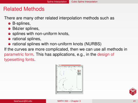
Related Methods

There are many other related interpolation methods such asB-splines,Bézier splines,splines with non-uniform knots,rational splines,rational splines with non-uniform knots (NURBS)

If the curves are more complicated, then we can use all methods inparametric form. This has applications, e.g., in the design oftypesetting fonts.



Interpolation in Higher Space Dimensions Theoretical Insights

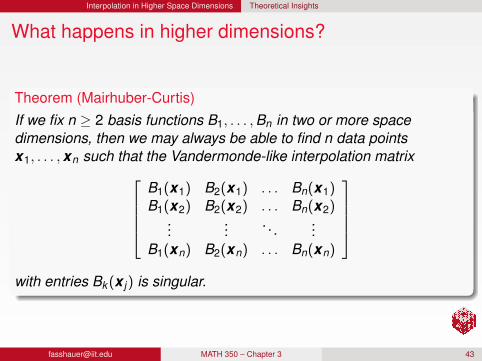
What happens in higher dimensions?

Theorem (Mairhuber-Curtis)If we fix n ≥ 2 basis functions B1, . . . ,Bn in two or more spacedimensions, then we may always be able to find n data pointsx1, . . . ,xn such that the Vandermonde-like interpolation matrix

B1(x1) B2(x1) . . . Bn(x1)B1(x2) B2(x2) . . . Bn(x2)

......

. . ....

B1(xn) B2(xn) . . . Bn(xn)

with entries Bk (x j) is singular.




What does the Mairhuber-Curtis theorem actually say?

The M-C theorem implies that we can’t choose our basisindependent of the data locations, i.e., the basis has to be chosenafter the data sites. It has to be a data-dependent basis.

As a consequence we can no longer use (multivariate)polynomials for arbitrary data in higher dimensions.

Radial basis functions present one way to circumvent the problempresented by the Mairhuber-Curtis theorem.




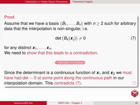
Proof.Assume that we have a basis {B1, . . . ,Bn} with n ≥ 2 such for arbitrarydata that the interpolation is non-singular, i.e.

det(Bk (x j)

)6= 0 (7)

for any distinct x1, . . . ,xn.We need to show that this leads to a contradiction.

Mairhuber-Curtis Maplet

Since the determinant is a continuous function of x1 and x2 we musthave had det = 0 at some point along the continuous path in ourinterpolation domain. This contradicts (7).



Interpolation in Higher Space Dimensions A Few More Applications

Gasoline Engine Design


Variables:

spark timing exhaust gas re-circulation rate fuel injection timingspeed intake valve timingload exhaust valve timingair-fuel ratio



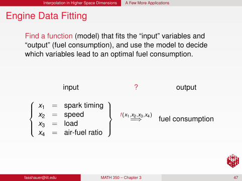
Engine Data Fitting

input ? outputx1 = spark timingx2 = speedx3 = loadx4 = air-fuel ratio

f (x1,x2,x3,x4)

=⇒ fuel consumption


Find a function (model) that fits the “input” variables and“output” (fuel consumption), and use the model to decidewhich variables lead to an optimal fuel consumption.



Fuel Consumption Model


Tanya Morton, The MathWorks



Rapid Prototyping

An important application of interpolation (or very good approximation)methods is the creation of computer models by scanning physicalobjects such as historic artifacts or even household appliance parts,and then using interpolation to produce a surface or solid model thatcan be fed into the manufacturing process.

Special 3D printers can then be used to quickly and easily generate“clones” of the original object.

See, e.g.,[Prof. Qian’s website] in IIT’s MMAE department,[The Digital Michelangelo Project] at Stanford University,this article [about 3D printers].




Special Movie Effects http://www.fastscan3d.com

trollscanning.mpeg

Source is here [FastSCAN]. Also look at this [Lord of the Rings][email protected] MATH 350 – Chapter 3 50

trollscanning.mpeg


Appendix References

References I

C. de Boor.A Practical Guide to Splines.Springer, revised edition, 2001.

G. E. Fasshauer.Meshfree Approximation Methods with MATLAB.World Scientific Publishers, 2007.

C. Moler.Numerical Computing with MATLAB.SIAM, Philadelphia, 2004.Also http://www.mathworks.com/moler/.

L. L. Schumaker.Spline Functions: Basic Theory (3rd ed.).Cambridge University Press, 2007.

’Printers’ that can make 3-D solid objects soon to enter mainstream.http://www.sciencedaily.com/releases/2007/09/070925081418.htm.


http://www.mathworks.com/moler/

http://www.sciencedaily.com/releases/2007/09/070925081418.htm


Appendix References

References II

X. Qian.Computational Design and Manufacturing Lab.http://mmae.iit.edu/cadcam/research.htm.

The Digital Michelangelo Project.http://graphics.stanford.edu/projects/mich/.

FastSCAN.http://www.fastscan3d.com/media/trollscanning.mpg.

The Lord of the Rings.Enter “The Prologue” and select “Digital Scanning” from “Orcs”; and “DigitalLands” from “The Battlefield” http://www.lordoftherings.net/effects/.


http://mmae.iit.edu/cadcam/research.htm

http://graphics.stanford.edu/projects/mich/

http://www.fastscan3d.com/media/trollscanning.mpg

http://www.lordoftherings.net/effects/


MATH 350: Introduction to Computational Mathematics - Applied

Documents

Transcript of MATH 350: Introduction to Computational Mathematics - Applied