Computational Methods for Oil Recovery - Boston · PDF fileOil Reservoir Simulation General...
61
Oil Reservoir Simulation General Math & Num Models Computational Approach References Computational Methods for Oil Recovery PASI: Scientific Computing in the Americas The Challenge of Massive Parallelism Luis M. de la Cruz Salas Instituto de Geof´ ısica Universidad Nacional Aut´ onoma de M´ exico January 2011 Valpara´ ıso, Chile Comp EOR LMCS 1 / 43
-
Upload
nguyenminh -
Category
Documents
-
view
217 -
download
3
Transcript of Computational Methods for Oil Recovery - Boston · PDF fileOil Reservoir Simulation General...

Oil Reservoir Simulation General Math & Num Models Computational Approach References
Computational Methods for Oil RecoveryPASI: Scientific Computing in the Americas
The Challenge of Massive Parallelism
Luis M. de la Cruz Salas
Instituto de Geofısica
Universidad Nacional Autonoma de Mexico
January 2011
Valparaıso, Chile
Comp EOR LMCS 1 / 43

Oil Reservoir Simulation General Math & Num Models Computational Approach References
Mathematical and Computational Group (GMMC)
Natural Resources Dept.
Dr. Ismael Herrera Revilla
Dra. Graciela Herrera Zamarron
Dr. Luis M. de la Cruz Salas
Dr. Guillermo Hernandez Garcıa
Dr. Norberto Vera Guzman
Students
Esther Leyva
Antonio Carrillo
Ivan Contreras
Alberto Rosas
Emilio Zavala
Ricardo Flores
Computational Group
Daniel A. Cervantes Cabrera
Alejandro Salazar Sanchez
Daniel Monsivais Velazquez
Renato Leriche Vazquez
Hector U. Barron Garcıa
Ismael Herrera Zamarron
Eduardo Murrieta Leon
http://www.mmc.geofisica.unam.mx
Comp EOR LMCS 2 / 43

Oil Reservoir Simulation General Math & Num Models Computational Approach References
Table of contents
1 Oil Reservoir SimulationMotivation
2 General Math & Num ModelsAxiomatic FormulationNumerical MethodsFinite Volume Method
3 Computational ApproachTUNA
4 References
Comp EOR LMCS 3 / 43

Oil Reservoir Simulation General Math & Num Models Computational Approach References
Motivation
Table of contents
1 Oil Reservoir SimulationMotivation
2 General Math & Num ModelsAxiomatic FormulationNumerical MethodsFinite Volume Method
3 Computational ApproachTUNA
4 References
Comp EOR LMCS 4 / 43

Oil Reservoir Simulation General Math & Num Models Computational Approach References
Motivation
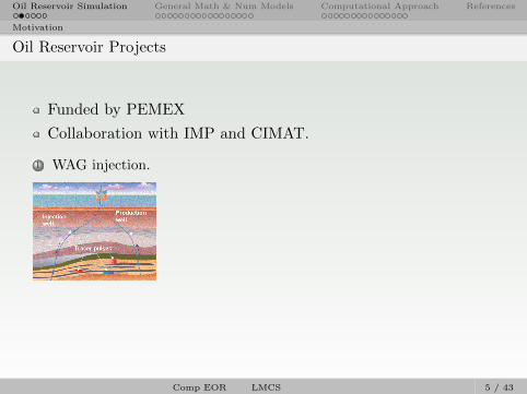
Oil Reservoir Projects
Funded by PEMEX
Collaboration with IMP and CIMAT.
1 WAG injection. 2 AIR injection. 3 SLS method.
Oil reservoir simulation is a grand challenge.
Comp EOR LMCS 5 / 43

Oil Reservoir Simulation General Math & Num Models Computational Approach References
Motivation
Oil Reservoir Projects
Funded by PEMEX
Collaboration with IMP and CIMAT.
1 WAG injection. 2 AIR injection. 3 SLS method.
Oil reservoir simulation is a grand challenge.
Comp EOR LMCS 5 / 43
Oil Reservoir Simulation General Math & Num Models Computational Approach References
Motivation
Oil Reservoir Projects
Funded by PEMEX
Collaboration with IMP and CIMAT.
1 WAG injection.
2 AIR injection. 3 SLS method.
Oil reservoir simulation is a grand challenge.
Comp EOR LMCS 5 / 43
Oil Reservoir Simulation General Math & Num Models Computational Approach References
Motivation
Oil Reservoir Projects
Funded by PEMEX
Collaboration with IMP and CIMAT.
1 WAG injection. 2 AIR injection.
3 SLS method.
Oil reservoir simulation is a grand challenge.
Comp EOR LMCS 5 / 43

Oil Reservoir Simulation General Math & Num Models Computational Approach References
Motivation
Oil Reservoir Projects
Funded by PEMEX
Collaboration with IMP and CIMAT.
1 WAG injection. 2 AIR injection. 3 SLS method.
Oil reservoir simulation is a grand challenge.
Comp EOR LMCS 5 / 43

Oil Reservoir Simulation General Math & Num Models Computational Approach References
Motivation
Oil Reservoir Projects
Funded by PEMEX
Collaboration with IMP and CIMAT.
1 WAG injection. 2 AIR injection. 3 SLS method.
Oil reservoir simulation is a grand challenge.
Comp EOR LMCS 5 / 43

Oil Reservoir Simulation General Math & Num Models Computational Approach References
Motivation
The major goal of reservoir simulation is to predict futureperformance of reservoir and find ways and means of optimizingthe recovery of some of the hydrocarbons under various operatingconditions.
It involves four main interrelated modeling stages:
And requires a combination of skills of physicists, mathematicians,reservoir engineers, and computer scientists.
Comp EOR LMCS 6 / 43

Oil Reservoir Simulation General Math & Num Models Computational Approach References
Motivation
The major goal of reservoir simulation is to predict futureperformance of reservoir and find ways and means of optimizingthe recovery of some of the hydrocarbons under various operatingconditions.It involves four main interrelated modeling stages:
And requires a combination of skills of physicists, mathematicians,reservoir engineers, and computer scientists.
Comp EOR LMCS 6 / 43

Oil Reservoir Simulation General Math & Num Models Computational Approach References
Motivation
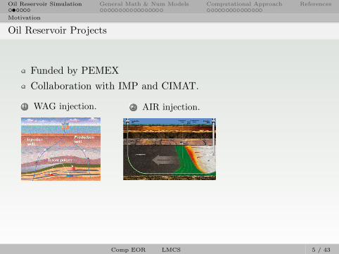
Software Engineering (IEEE Comput Society’s Software Eng. Body of Knowledge)
Application of a systematic, disciplined, quantifiable approach to the development,operation, and maintenance of software, and the study of these approaches; that is, theapplication of engineering to software.
Unified Process (UP, Booch et al. [2])
Comp EOR LMCS 7 / 43
Oil Reservoir Simulation General Math & Num Models Computational Approach References
Motivation
Software Engineering (IEEE Comput Society’s Software Eng. Body of Knowledge)
Application of a systematic, disciplined, quantifiable approach to the development,operation, and maintenance of software, and the study of these approaches; that is, theapplication of engineering to software.
Unified Process (UP, Booch et al. [2])
Requirements
EfficiencyAccuracyAbstraction
We get a software:
ModularMantainableReliableEfficientProductive
Comp EOR LMCS 8 / 43

Oil Reservoir Simulation General Math & Num Models Computational Approach References
Motivation
Oil production stages
First stage of oil reservoir production, primary recovery, the oilis extracted by natural drive mechanism.
The reservoir pressure can be maintained, using techniques such asgas or water injection. This is known as secondary recovery.
Tertiary or Enhanced Oil Recovery (EOR) is a generic termthat embraces several techniques used to increase the amount ofcrude oil that can be extracted from an oil field.
These techniques are based on the injection of materials notnormally present in the reservoir, and is the most advanced stage ofthe exploitation of a reservoir.
Primary recovery techniques produce 10 – 15 % of the reservoir’soil content. Combining the processes of secondary andtertiary recovery techniques, it is possible to produce 30 –60 % of the reservoir’s total oil content.
Comp EOR LMCS 9 / 43
Oil Reservoir Simulation General Math & Num Models Computational Approach References
Axiomatic Formulation
Table of contents
1 Oil Reservoir SimulationMotivation
2 General Math & Num ModelsAxiomatic FormulationNumerical MethodsFinite Volume Method
3 Computational ApproachTUNA
4 References
Comp EOR LMCS 10 / 43

Oil Reservoir Simulation General Math & Num Models Computational Approach References
Axiomatic Formulation
Extensive and Intensive Properties
In the physical sciences, intensive property (also called a bulkproperty, intensive quantity, or intensive variable), is a physicalproperty of a system that does not depend on the system size orthe amount of material in the system: it is scale invariant.
Density
By contrast, an extensive property (also extensive quantity,extensive variable, or extensive parameter) of a system is directlyproportional to the system size or the amount of material in thesystem.
Mass
Comp EOR LMCS 11 / 43

Oil Reservoir Simulation General Math & Num Models Computational Approach References
Axiomatic Formulation
Axiomatic Formulation, (Herrera et al. [3, 4]) I
1 To find extensive E and intensive ψ properties :
E(t) =
∫B(t)
ψ(~x, t)d~x
2 To establish balances:
dE
dt=
d
dt
∫B(t)
ψ(~x, t)d~x =
∫B(t)
q(~x, t)d~x+
∫∂B(t)
~τ(~x, t) · ~ndS (1)
where q(~x, t) y ~τ(~x, t) are the source term in B(t) and the fluxvector through the boundary ∂B(t), respectively
Comp EOR LMCS 12 / 43

Oil Reservoir Simulation General Math & Num Models Computational Approach References
Axiomatic Formulation
Axiomatic Formulation, (Herrera et al. [3, 4]) II
Global balance∫B(t)
{∂ψ
∂t+∇ · (~vψ)
}d~x =
∫B(t)
qd~x+
∫B(t)
∇ · ~τd~x (2)
Local balance∂ψ
∂t+∇ · (~vψ) = q +∇ · ~τ (3)
Comp EOR LMCS 13 / 43

Oil Reservoir Simulation General Math & Num Models Computational Approach References
Axiomatic Formulation
Conservative form
Defining a “flux function” (see [5]) as ~f = ~vψ − ~τ we get:
∂
∂t
∫B(t)
ψd~x+
∫B(t)
∇ · ~fd~x =
∫B(t)
qd~x (4)
and therefore
∂ψ
∂t+∇ · ~f = q (5)
Equivalently (4) can be written as follows
∂
∂t
∫B(t)
ψd~x+
∫∂B(t)
~f · ~ndS =
∫B(t)
qd~x (6)
Comp EOR LMCS 14 / 43

Oil Reservoir Simulation General Math & Num Models Computational Approach References
Numerical Methods
Table of contents
1 Oil Reservoir SimulationMotivation
2 General Math & Num ModelsAxiomatic FormulationNumerical MethodsFinite Volume Method
3 Computational ApproachTUNA
4 References
Comp EOR LMCS 15 / 43

Oil Reservoir Simulation General Math & Num Models Computational Approach References
Numerical Methods
In general, the equations governing a mathematical model of areservoir cannot be solved by analytical methods.
Instead, a numerical model can be produced in a form that isamenable to solution by digital computers.
Since the 1950s, numerical models have been used to predict,understand, and optimize complex physical fluid flow processes inpetroleum reservoirs.
Recent advances in computational capabilities have greatlyexpanded the potential for solving larger problems and hencepermitting the incorporation of more physics into the differentialequations.
Comp EOR LMCS 16 / 43
Oil Reservoir Simulation General Math & Num Models Computational Approach References
Numerical Methods
1 Finite Diferences Method (FDM)
The FDM can be very easy to implement.Faster than FEM.High accuracy difference schemes can be constructed.In its basic form is restricted to handle only rectangular shapes.Introduce considerable geometrical error and grid orientation effects.Curvilinear coordinates can be used.
2 Finite Element Method (FEM)
The FEM cand handle complicated geometries.Reduce the grid orientation effects.Solid theoretical foundations.Can manage local grid refinement.The quality of a FEM approximation is often higher than in thecorresponding FDM approach.FEM is the method of choice in structural mechanics.It is not easy to implement and is slower than FDM.
Comp EOR LMCS 17 / 43

Oil Reservoir Simulation General Math & Num Models Computational Approach References
Numerical Methods
3 Finite Volume Method (FVM)
Values are calculated at control volumes.Conservative method: the flux entering a given volume is identicalto that leaving the adjacent volume.Can easily be formulated to allow for unstructured meshes.Used in many computational fluid dynamics packages.FVM is in between FDM and FEM: faster and easier to implementthan FEM; and more accurate and versatile than FDM.
In oil-reservoir problems we usually require a large number of cells(105 – 106), therefore cost of the solution favors simpler and lowerorder approximation within each cell.
About 80% – 90% of the total simulation time is spent on thesolution of linear systems.
Fast linear solvers are crucial to solve sparse, highly non–symmetric,and ill–conditioned systems.Krylov subspace (preconditioned) algorithms are preferred.
Comp EOR LMCS 18 / 43

Oil Reservoir Simulation General Math & Num Models Computational Approach References
Finite Volume Method
Table of contents
1 Oil Reservoir SimulationMotivation
2 General Math & Num ModelsAxiomatic FormulationNumerical MethodsFinite Volume Method
3 Computational ApproachTUNA
4 References
Comp EOR LMCS 19 / 43

Oil Reservoir Simulation General Math & Num Models Computational Approach References
Finite Volume Method
Finite volume methods are derived on the basis of the conservativeform of the balance equations [3, 4, 5].
∂
∂t
∫B(t)
ψd~x+
∫B(t)
∇ · ~fd~x =
∫B(t)
qd~x or∂
∂t
∫B(t)
ψd~x+
∫∂B(t)
~f · ~ndS =
∫B(t)
qd~x
FVM is conservative.
Comp EOR LMCS 20 / 43

Oil Reservoir Simulation General Math & Num Models Computational Approach References
Finite Volume Method
Conservative form of general balance equation:
∂
∂t
∫B(t)
ψd~x+
∫B(t)
∇ · ~fd~x =
∫B(t)
qd~x
Integrating on ∆t and taking B(t) ≡ ∆V :∫∆t
∂
∂t
∫∆V
ψdV dt+
∫∆t
∫∆V
∇ · ~fdV dt =
∫∆t
∫∆V
qdV dt
∆x∆z
∆y
E
W
N
S
F
B
Pee
ww
nn
ss
ff
bb
∆V = ∆x∆y∆z
Notation:
NB idP i, j, kE i+ 1, j, kW i− 1, j, kN i, j + 1, kS i, j − 1, kF i, j, k + 1B i, j, k − 1
nb id
e i+ 12, j, k
w i− 12, j, k
n i, j + 12, k
s i, j − 12, k
f i, j, k + 12
b i, j, k − 12
t ≡ n; t+ ∆t ≡ n+ 1∫∆t
g dt ≡n+1∫n
g dt
∫∆V
g dV ≡f∫
b
n∫s
e∫w
g dx dy dz
Comp EOR LMCS 21 / 43

Oil Reservoir Simulation General Math & Num Models Computational Approach References
Finite Volume Method
Approximation of the integrals:
n+1∫n
∂
∂t
∫∆V
ψdV dt ≈(ψn+1
P− ψn
P
)∆V
n+1∫n
∫∆V
∇ · ~fdV dt ≈n+1∫n
F(~fnb )dt
∫∆t
∫∆V
qdV dt ≈n+1∫n
Q∆V dt
∆x∆z
∆y
E
W
N
S
F
B
Pee
ww
nn
ss
ff
bb
∆V = ∆x∆y∆z
Theta scheme:
n+1∫n
F dt =(θFn+1 + (1− θ)Fn
)∆t, 0 ≤ θ ≤ 1
Explicit (Forward–Euler) θ = 0 Fn∆t.Implicit (Backward–Euler) θ = 1 Fn+1∆t.Crank–Nicolson θ = 1/2 (Fn + Fn+1)∆t/2.
Comp EOR LMCS 22 / 43

Oil Reservoir Simulation General Math & Num Models Computational Approach References
Finite Volume Method
Recall that ~f = ~vψ − ~τ :
F(~fnb ) ≈∫
∆V
∇ · ~fdV =
e∫w
n∫s
f∫b
(∂(vxψ − τx)
∂x+∂(vyψ − τy)
∂y+∂(vzψ − τz)
∂z
)dxdydz
∆x∆z
∆y
E
W
N
S
F
B
Pee
ww
nn
ss
ff
bb
∆V = ∆x∆y∆z
Discretized flux function:
F(~fnb) =[(vxψ − τx)e − (vxψ − τx)w
]Ax+[
(vyψ − τy)n − (vyψ − τy)s]Ay +
[(vzψ − τz)f − (vzψ − τz)b
]Az
where Ax = ∆y ×∆z, Ay = ∆x×∆z, Az = ∆x×∆y, represents the area ofthe faces.
Advective ~vψ and Diffusive terms ~τ need to be approximated on the faces.
Comp EOR LMCS 23 / 43
Oil Reservoir Simulation General Math & Num Models Computational Approach References
Finite Volume Method
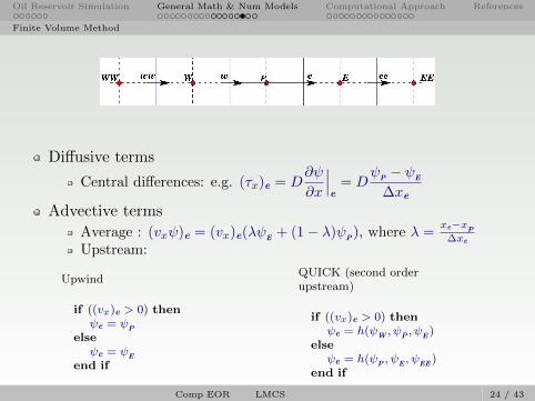
Diffusive terms
Central differences: e.g. (τx)e = D∂ψ
∂x
∣∣∣e
= Dψ
P− ψ
E
∆xeAdvective terms
Average : (vxψ)e = (vx)e(λψE+ (1− λ)ψ
P), where λ =
xe−xP
∆xe
Upstream:
Upwind
if ((vx)e > 0) thenψe = ψP
elseψe = ψE
end if
QUICK (second orderupstream)
if ((vx)e > 0) thenψe = h(ψW , ψP , ψE )
elseψe = h(ψP , ψE , ψEE )
end if
Comp EOR LMCS 24 / 43
Oil Reservoir Simulation General Math & Num Models Computational Approach References
Finite Volume Method
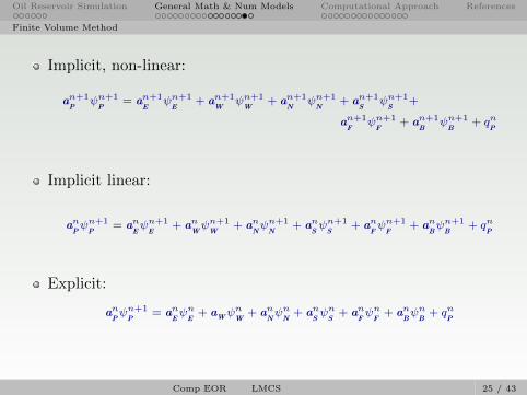
Implicit, non-linear:
an+1P
ψn+1P
= an+1E
ψn+1E
+ an+1W
ψn+1W
+ an+1N
ψn+1N
+ an+1S
ψn+1S
+
an+1F
ψn+1F
+ an+1B
ψn+1B
+ qnP
Implicit linear:
anPψn+1
P= an
Eψn+1
E+ an
Wψn+1
W+ an
Nψn+1
N+ an
Sψn+1
S+ an
Fψn+1
F+ an
Bψn+1
B+ qn
P
Explicit:
anPψn+1
P= an
Eψn
E+ aWψ
nW
+ anNψn
N+ an
Sψn
S+ an
Fψn
F+ an
Bψn
B+ qn
P
Comp EOR LMCS 25 / 43
Oil Reservoir Simulation General Math & Num Models Computational Approach References
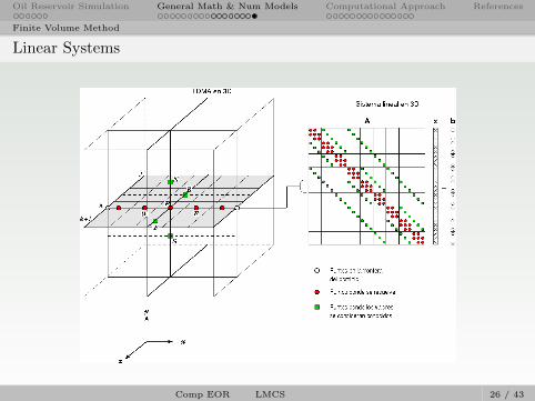
Finite Volume Method
Linear Systems
Comp EOR LMCS 26 / 43
Oil Reservoir Simulation General Math & Num Models Computational Approach References
TUNA
Table of contents
1 Oil Reservoir SimulationMotivation
2 General Math & Num ModelsAxiomatic FormulationNumerical MethodsFinite Volume Method
3 Computational ApproachTUNA
4 References
Comp EOR LMCS 27 / 43
Oil Reservoir Simulation General Math & Num Models Computational Approach References
TUNA
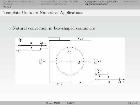
Template Units for Numerical Applications
Natural convection in box-shaped containers
Comp EOR LMCS 28 / 43

Oil Reservoir Simulation General Math & Num Models Computational Approach References
TUNA
f1(t) =
0.5 sin2(4t) for 0 ≤ t < π/8
1 for π/8 ≤ t < 7π/80.5 sin2(4t− 3π) for 7π/8 ≤ t < π
0 for π ≤ t < 2π
f2(t) =
0 for 0 ≤ t < π
−0.5 sin2(4t− 3π) for π ≤ t < 9π/81 for 9π/8 ≤ t < 15π/8
−0.5 sin2(4t− 6π) for 15π/8 ≤ t < 2π
Comp EOR LMCS 29 / 43

Oil Reservoir Simulation General Math & Num Models Computational Approach References
TUNA
Navier-Stokes equations
Mass balance:∂uj
∂xj= 0
Momentum balance (Navier-Stokes):
ρ0
[∂ui
∂t+ uj
∂ui
∂xj
]= − ∂p
∂xi+ µ
∂2ui
∂xj∂xj+ ρbi
Energy balance:∂T
∂t+ uj
∂T
∂xj= α
∂2T
∂xj∂xj
Equations of state:
ρ = ρ0 [1− β(T − T0)] , β = − 1
ρ0
(∂ρ
∂T
)T=T0
Comp EOR LMCS 30 / 43

Oil Reservoir Simulation General Math & Num Models Computational Approach References
TUNA
Template Units for Numerical Applications I
TUNA use several C++ template techniques (Blitz++).
Comp EOR LMCS 31 / 43

Oil Reservoir Simulation General Math & Num Models Computational Approach References
TUNA
Template Units for Numerical Applications II
http://mmc.geofisica.unam.mx/ (then go to my homepage).
Examples : programs that use TUNA
|--- tuna-cfd-rules.in => rules to compile the examples
|--- 01StructMesh => uniform structured meshes
|--- 02NonUniformMesh => non uniform structured meshes
|--- 03Laplace => Solution of Laplace equation
|--- 04HeatDiffusion => Solution of heat conduction problems
|--- 05ConvDiffForced => Solution of forced convection
|--- 06ConvDiff => Solution of natural convection problems
|--- 07ConvDiffLES => Solution of turbulent natural convection
|--- README.pdf => Explanation of the examples of each directory
1) Unpack TUNA and change to the TUNA dir:
% tar zxvf TUNA.tar.gz
% cd TUNA
2) Blitz++: http://www.oonumerics.org/blitz/
Comp EOR LMCS 32 / 43

Oil Reservoir Simulation General Math & Num Models Computational Approach References
TUNA
Template Units for Numerical Applications III
- Unpack with: tar zxvf blitz-09.tar.gz
- Change to blitz-0.9 with: cd blitz-0.9
- Config blitz with: ./configure --prefix=$PWD/../BLITZ
- Compile and install blitz with: make install
These instruction will install Blitz in the TUNA/BLITZ directory
3) Run the examples
- Change to the Examples directory: cd Examples
- Edit the files tuna-cfd-rules.in
Change the environment variable BASE according to your paths.
(e.g. BASE = /home/luiggi/TUNA)
- Then, e.g. change to the 06ConvDiff dir:
% cd 06ConvDiff
% make <--- this creates: convdiff1 and convdiff2
- Visualization: CXXFLAGS: Add -DWITH_GNUPLOT or -DWITH_DX.
Comp EOR LMCS 33 / 43
Oil Reservoir Simulation General Math & Num Models Computational Approach References
TUNA
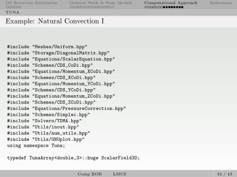
Example: Natural Convection I
#include "Meshes/Uniform.hpp"
#include "Storage/DiagonalMatrix.hpp"
#include "Equations/ScalarEquation.hpp"
#include "Schemes/CDS_CoDi.hpp"
#include "Equations/Momentum_XCoDi.hpp"
#include "Schemes/CDS_XCoDi.hpp"
#include "Equations/Momentum_YCoDi.hpp"
#include "Schemes/CDS_YCoDi.hpp"
#include "Equations/Momentum_ZCoDi.hpp"
#include "Schemes/CDS_ZCoDi.hpp"
#include "Equations/PressureCorrection.hpp"
#include "Schemes/Simplec.hpp"
#include "Solvers/TDMA.hpp"
#include "Utils/inout.hpp"
#include "Utils/num_utils.hpp"
#include "Utils/GNUplot.hpp"
using namespace Tuna;
typedef TunaArray<double,3>::huge ScalarField3D;
Comp EOR LMCS 34 / 43
Oil Reservoir Simulation General Math & Num Models Computational Approach References
TUNA
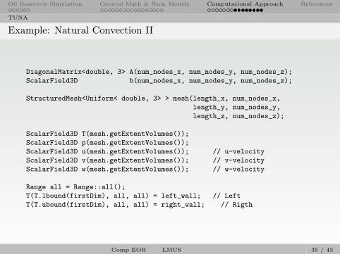
Example: Natural Convection II
DiagonalMatrix<double, 3> A(num_nodes_x, num_nodes_y, num_nodes_z);
ScalarField3D b(num_nodes_x, num_nodes_y, num_nodes_z);
StructuredMesh<Uniform< double, 3> > mesh(length_x, num_nodes_x,
length_y, num_nodes_y,
length_z, num_nodes_z);
ScalarField3D T(mesh.getExtentVolumes());
ScalarField3D p(mesh.getExtentVolumes());
ScalarField3D u(mesh.getExtentVolumes()); // u-velocity
ScalarField3D v(mesh.getExtentVolumes()); // v-velocity
ScalarField3D w(mesh.getExtentVolumes()); // w-velocity
Range all = Range::all();
T(T.lbound(firstDim), all, all) = left_wall; // Left
T(T.ubound(firstDim), all, all) = right_wall; // Rigth
Comp EOR LMCS 35 / 43

Oil Reservoir Simulation General Math & Num Models Computational Approach References
TUNA
Example: Natural Convection III
ScalarEquation<CDS_CoDi<double,3> > energy(T, A, b, mesh.getDeltas());
energy.setDeltaTime(dt);
energy.setNeumann(TOP_WALL);
energy.setNeumann(BOTTOM_WALL);
energy.setDirichlet(LEFT_WALL, left_wall);
energy.setDirichlet(RIGHT_WALL, right_wall);
energy.setNeumann(FRONT_WALL);
energy.setNeumann(BACK_WALL);
energy.setUvelocity(us);
energy.setVvelocity(vs);
energy.setWvelocity(ws);
energy.print();
Momentum_XCoDi<CDS_XCoDi<double, 3> > mom_x(us, A, b, mesh.getDeltas());
Momentum_YCoDi<CDS_YCoDi<double, 3> > mom_y(vs, A, b, mesh.getDeltas());
Momentum_ZCoDi<CDS_ZCoDi<double, 3> > mom_z(ws, A, b, mesh.getDeltas());
PressureCorrection<Simplec<double, 3> > press(pp, A, b, mesh.getDeltas());
Comp EOR LMCS 36 / 43

Oil Reservoir Simulation General Math & Num Models Computational Approach References
TUNA
Example: Natural Convection IV
template<typename Tprec, int Dim>
class CDS_CoDi : public ScalarEquation< CDS_CoDi< Tprec, Dim > >
{
public:
typedef Tprec prec_t;
typedef typename TunaArray<prec_t, Dim >::huge ScalarField;
CDS_CoDi() : ScalarEquation<CDS_CoDi<prec_t, Dim> >() { }
~CDS_CoDi() { };
inline void calcCoefficients1D();
inline void calcCoefficients2D();
inline void calcCoefficients3D();
inline void printInfo() { std::cout << " CDS_CoDi "; }
};
anPψn+1
P= an
Eψn+1
E+ an
Wψn+1
W+ an
Nψn+1
N+ an
Sψn+1
S+ an
Fψn+1
F+ an
Bψn+1
B+ qn
P
Comp EOR LMCS 37 / 43

Oil Reservoir Simulation General Math & Num Models Computational Approach References
TUNA
Example: Natural Convection V
template<class Tprec, int Dim>
inline void CDS_CoDi<Tprec, Dim>::calcCoefficients2D() {
prec_t Gdy_dx = Gamma * dy / dx, Gdx_dy = Gamma * dx / dy;
prec_t dxy_dt = dx * dy / dt;
aE = 0.0; aW = 0.0; aN = 0.0; aS = 0.0; aP = 0.0; sp = 0.0;
for (int i = bi; i <= ei; ++i)
for (int j = bj; j <= ej; ++j) {
aE (i,j) = Gdy_dx - u(i , j) * dy * 0.5 ;
aW (i,j) = Gdy_dx + u(i-1, j) * dy * 0.5 ;
aN (i,j) = Gdx_dy - v(i, j ) * dx * 0.5;
aS (i,j) = Gdx_dy + v(i, j-1) * dx* 0.5;
aP (i,j) = aE (i,j) + aW (i,j) + aN (i,j) + aS (i,j) + dxy_dt;
sp (i,j) = phi_0(i,j) * dxy_dt ;
}
applyBoundaryConditions2D();
}
anPψn+1
P= an
Eψn+1
E+ an
Wψn+1
W+ an
Nψn+1
N+ an
Sψn+1
S+ an
Fψn+1
F+ an
Bψn+1
B+ qn
P
Comp EOR LMCS 38 / 43

Oil Reservoir Simulation General Math & Num Models Computational Approach References
TUNA
Example: Natural Convection VI
for(iteration = 1; iteration <= max_time_steps; ++iteration) {
sorsum = SIMPLEC(energy, mom_x, mom_y, mom_z, press, max_iter, tolerance);
}
template<class T_e, class T_x, class T_y, class T_z, class T_p>
double SIMPLEC(T_e &energy, T_x &mom_x, T_y &mom_y, T_z &mom_z, T_p &press,
int max_iter, double tolerance)
{
double sorsum = 10.0, tol_simplec = 1e-02;
int counter = 0;
while ( (sorsum > tol_simplec) && (counter < 20) ) {
energy.calcCoefficients();
Solver::TDMA3D(energy, tolerance, max_iter);
errorT = energy.calcErrorL2();
energy.update();
mom_x.calcCoefficients();
Solver::TDMA3D(mom_x, tolerance, max_iter);
errorX = mom_x.calcErrorL2();
mom_x.update();
Comp EOR LMCS 39 / 43

Oil Reservoir Simulation General Math & Num Models Computational Approach References
TUNA
Example: Natural Convection VII
mom_y.calcCoefficients();
Solver::TDMA3D(mom_y, tolerance, max_iter);
errorY = mom_y.calcErrorL2();
mom_y.update();
mom_z.calcCoefficients();
Solver::TDMA3D(mom_z, tolerance, max_iter);
errorZ = mom_z.calcErrorL2();
mom_z.update();
press.calcCoefficients();
Solver::TDMA3D(press, tolerance, max_iter);
press.correction();
sorsum = fabs( press.calcSorsum() );
++counter;
}
return sorsum;
}
Comp EOR LMCS 40 / 43
Oil Reservoir Simulation General Math & Num Models Computational Approach References
TUNA
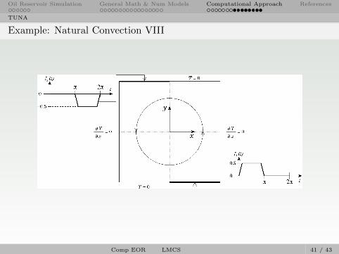
Example: Natural Convection VIII
Comp EOR LMCS 41 / 43

Oil Reservoir Simulation General Math & Num Models Computational Approach References
References I
[1] R.A. Tapia and C. Lanius,Computational Science: Tools for a Changing Worldhttp://ceee.rice.edu/Books/CS/chapter1/intro52.html, 2001.
[2] I. Jacobson and G. Booch and J. RumbaughPrimer,The Unified Software Development Process,Addison – Wesley, 1999.
[3] I. Herrera and M. B. Allen and G. F. Pinder,Numerical modeling in science and engineering,John Wiley & Sons., USA, 1988.
[4] I. Herrera and G. F. Pinder,General principles of mathematical computational modeling,John Wiley, in press.
Comp EOR LMCS 42 / 43

Oil Reservoir Simulation General Math & Num Models Computational Approach References
References II
[5] R.J. Leveque,Finite Volume Method for Hyperbolic Problems,Cambridge University Press, 2004.
Comp EOR LMCS 43 / 43