Math 138 Calculus II for Honours Mathematics
305
Math 138 Calculus II for Honours Mathematics Course Notes Barbara A. Forrest and Brian E. Forrest Version 1.51
Transcript of Math 138 Calculus II for Honours Mathematics

Math 138
Calculus IIfor Honours Mathematics
Course Notes
Barbara A. Forrest and Brian E. Forrest
Version 1.51


Copyright c© Barbara A. Forrest and Brian E. Forrest.
All rights reserved.
September 1, 2021
All rights, including copyright and images in the content of these course notes, areowned by the course authors Barbara Forrest and Brian Forrest. By accessing thesecourse notes, you agree that you may only use the content for your own personal,non-commercial use. You are not permitted to copy, transmit, adapt, or change inany way the content of these course notes for any other purpose whatsoever withoutthe prior written permission of the course authors.
Author Contact Information:
Barbara Forrest ([email protected])
Brian Forrest ([email protected])
i
QUICK REFERENCE PAGE 1
Right Angle Trigonometry
sin θ =opposite
hypotenuse cos θ =ad jacent
hypotenuse tan θ =oppositead jacent
csc θ = 1sin θ sec θ = 1
cos θ cot θ = 1tan θ
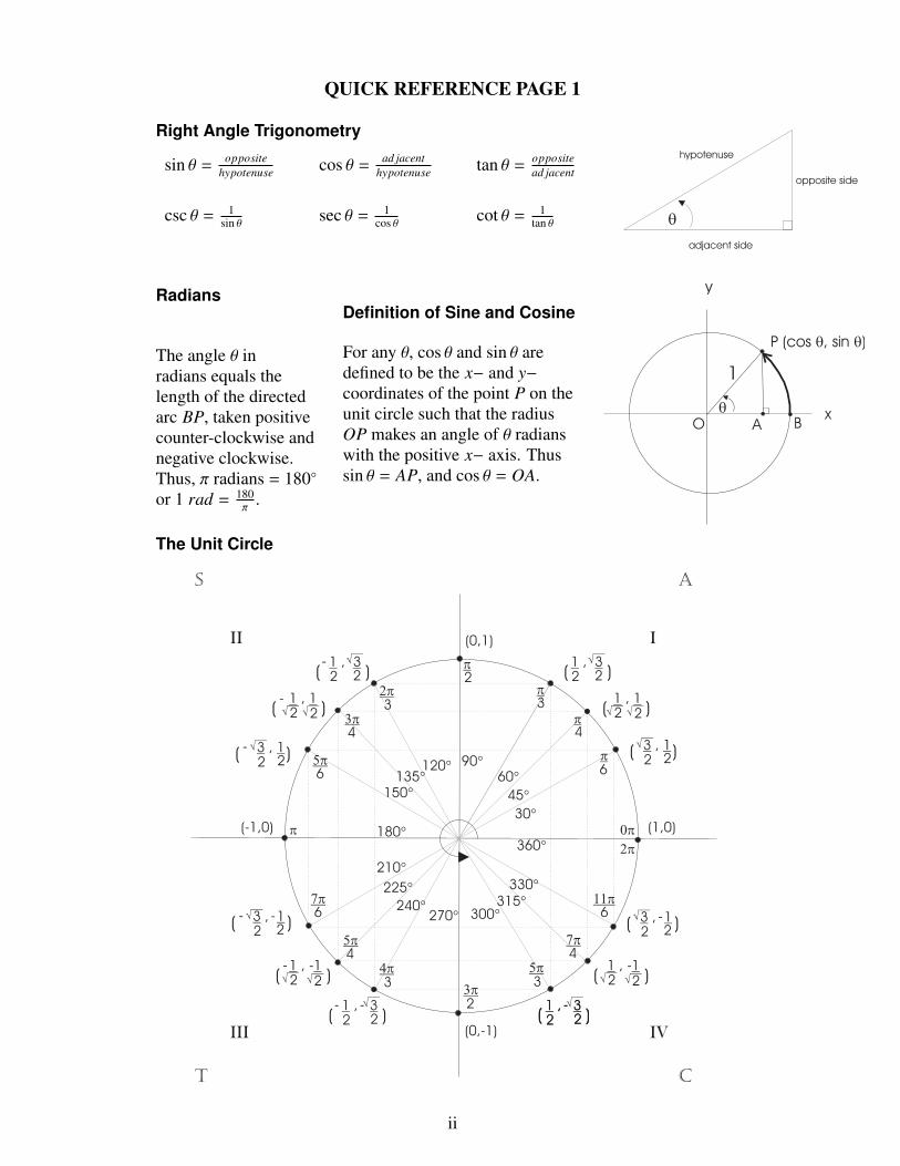
Radians
The angle θ inradians equals thelength of the directedarc BP, taken positivecounter-clockwise andnegative clockwise.Thus, π radians = 180◦
or 1 rad = 180π
.
Definition of Sine and Cosine
For any θ, cos θ and sin θ aredefined to be the x− and y−coordinates of the point P on theunit circle such that the radiusOP makes an angle of θ radianswith the positive x− axis. Thussin θ = AP, and cos θ = OA.
The Unit Circle
ii
QUICK REFERENCE PAGE 2
Trigonometric Identities
Pythagorean cos2 θ + sin2 θ = 1
Identity
Range −1 ≤ cos θ ≤ 1
−1 ≤ sin θ ≤ 1
Periodicity cos(θ ± 2π) = cos θ
sin(θ ± 2π) = sin θ
Symmetry cos(−θ) = cos θ
sin(−θ) = − sin θ
Sum and Difference Identities
cos(A + B) = cos A cos B − sin A sin B
cos(A − B) = cos A cos B + sin A sin B
sin(A + B) = sin A cos B + cos A sin B
sin(A − B) = sin A cos B − cos A sin B
Complementary Angle Identities
cos(π2 − A) = sin A
sin(π2 − A) = cos A
Double-Angle cos 2A = cos2 A − sin2 A
Identities sin 2A = 2 sin A cos A
Half-Angle cos2 θ = 1+cos 2θ2
Identities sin2 θ = 1−cos 2θ2
Other 1 + tan2 A = sec2 A
iii
QUICK REFERENCE PAGE 3
Differentiation RulesFunction Derivative
f (x) = cxa , a , 0, c ∈ R f ′(x) = caxa−1
f (x) = sin(x) f ′(x) = cos(x)
f (x) = cos(x) f ′(x) = − sin(x)
f (x) = tan(x) f ′(x) = sec2(x)
f (x) = sec(x) f ′(x) = sec(x) tan(x)
f (x) = arcsin(x) f ′(x) =1
√1 − x2
f (x) = arccos(x) f ′(x) = −1
√1 − x2
f (x) = arctan(x) f ′(x) =1
1 + x2
f (x) = ex f ′(x) = ex
f (x) = ax with a > 0 f ′(x) = ax ln(a)
f (x) = ln(x) for x > 0 f ′(x) =1x
Table of Integrals∫xn dx =
xn+1
n + 1+ C∫ 1
xdx = ln(| x |) + C∫
ex dx = ex + C∫sin(x) dx = − cos(x) + C∫cos(x) dx = sin(x) + C∫sec2(x) dx = tan(x) + C∫ 11 + x2 dx = arctan(x) + C
∫ 1√
1 − x2dx = arcsin(x) + C
∫ −1√
1 − x2dx = arccos(x) + C
∫sec(x) tan(x) dx = sec(x) + C∫ax dx =
ax
ln(a)+ C
Inverse Trigonometric Substitutions
Integral Trig Substitution Trig Identity∫ √a2 − b2x2 dx bx = a sin(u) sin2(x) + cos2(x) = 1∫ √a2 + b2x2 dx bx = a tan(u) sec2(x) − 1 = tan2(x)∫ √b2x2 − a2 dx bx = a sec(u) sec2(x) − 1 = tan2(x)
Additional FormulasIntegration by Parts
∫f (x)g′(x) dx = f (x)g(x) −
∫f ′(x)g(x) dx
Areas Between Curves A =∫ b
a |g(t) − f (t)| dt
Volumes of Revolutions: Disk I V =∫ b
a π f (x)2 dx
Volumes of Revolutions: Disk II V =∫ b
a π(g(x)2 − f (x)2) dx
Volumes of Revolutions: Shell V =∫ b
a 2πx(g(x) − f (x)) dx
Arc Length S =∫ b
a
√1 + ( f ′(x))2 dx
Taylor Series (Maclaurin Series)1
1−x =∞∑
n=0xn = 1 + x + x2 + x3 + · · · R = 1
ex =∞∑
n=0
xn
n! = 1 + x1! + x2
2! + x3
3! + · · · R = ∞
cos(x) =∞∑
n=0(−1)n x2n
(2n)! = 1 − x2
2! + x4
4! −x6
6! + · · · R = ∞
sin(x) =∞∑
n=0(−1)n x2n+1
(2n+1)! = x − x3
3! + x5
5! −x7
7! + · · · R = ∞
Differential Equations
Separable y′ = f (x)g(y)
Solve g(y) ?= 0,
∫1
g(y) dy =∫
f (x)dx
FOLDE y′ = f (x)y + g(x)
Solve y =
∫g(x)I(x)dx
I(x) , I(x) = e−∫
f (x) dx
iv
QUICK REFERENCE PAGE 4
LIST of THEOREMS:
Chapter 1: IntegrationIntegrability Theorem
for Continuous FunctionsProperties of Integrals TheoremIntegrals over Subintervals TheoremAverage Value Theorem
(Mean Value Theorem for Integrals)Fundamental Theorem of Calculus (Part 1)Extended Version of the
Fundamental Theorem of CalculusPower Rule for AntiderivativesFundamental Theorem of Calculus (Part 2)Change of Variables Theorem
Chapter 2: Techniques of IntegrationIntegration by Parts TheoremIntegration of Partial Fractionsp-Test for Type I Improper IntegralsProperties of Type I Improper IntegralsThe Monotone Convergence Theorem
for FunctionsComparison Test
for Type I Improper IntegralsAbsolute Convergence Theorem
for Improper Integralsp-Test for Type II Improper Integrals
Chapter 3: Applications of IntegationArea Between CurvesVolumes of Revolution: Disk MethodsVolumes of Revolution: Shell MethodArc Length
Chapter 4: Differential EquationsTheorem for Solving
First-order Linear Differential EquationsExistence and Uniqueness Theorem
for FOLDE
Chapter 5: Numerical SeriesGeometric Series TestDivergence TestArithmetic for Series TheoremsThe Monotone Convergence Theorem
for SequencesComparison Test for SeriesLimit Comparison TestIntegral Test for Convergencep-Series TestAlternating Series Test (AST) and
the Error in the ASTAbsolute Convergence TheoremRearrangement TheoremRatio TestPolynomial versus Factorial Growth TheoremRoot Test
Chapter 6: Power SeriesFundamental Convergence Theorem
for Power SeriesTest for the Radius of ConvergenceEquivalence of Radius of ConvergenceAbel’s Theorem: Continuity of Power SeriesAddition of Power SeriesMultiplication of Power Series by (x − a)m
Power Series of Composite FunctionsTerm-by-Term Differentiation of Power SeriesUniqueness of Power Series RepresentationsTerm-by-Term Integration of Power SeriesTaylor’s TheoremTaylor’s Approximation Theorem IConvergence Theorem for Tayor SeriesBinomial TheoremGeneralized Binomial Theorem
v
Table of Contents
Page
1 Integration 11.1 Areas Under Curves . . . . . . . . . . . . . . . . . . . . . . . . . 1
1.1.1 Estimating Areas . . . . . . . . . . . . . . . . . . . . . . 11.1.2 Approximating Areas Under Curves . . . . . . . . . . . . 21.1.3 The Relationship Between Displacement and Velocity . . 8
1.2 Riemann Sums and the Definite Integral . . . . . . . . . . . . . . 131.3 Properties of the Definite Integral . . . . . . . . . . . . . . . . . . 18
1.3.1 Additional Properties of the Integral . . . . . . . . . . . . 191.3.2 Geometric Interpretation of the Integral . . . . . . . . . . 22
1.4 The Average Value of a Function . . . . . . . . . . . . . . . . . . 271.4.1 An Alternate Approach to the Average Value of a Function 28
1.5 The Fundamental Theorem of Calculus (Part 1) . . . . . . . . . . 301.6 The Fundamental Theorem of Calculus (Part 2) . . . . . . . . . . 40
1.6.1 Antiderivatives . . . . . . . . . . . . . . . . . . . . . . . . 411.6.2 Evaluating Definite Integrals . . . . . . . . . . . . . . . . 43
1.7 Change of Variables . . . . . . . . . . . . . . . . . . . . . . . . . 471.7.1 Change of Variables for the Indefinite Integral . . . . . . . 481.7.2 Change of Variables for the Definite Integral . . . . . . . . 52
2 Techniques of Integration 562.1 Inverse Trigonometric Substitutions . . . . . . . . . . . . . . . . . 562.2 Integration by Parts . . . . . . . . . . . . . . . . . . . . . . . . . 622.3 Partial Fractions . . . . . . . . . . . . . . . . . . . . . . . . . . . 712.4 Introduction to Improper Integrals . . . . . . . . . . . . . . . . . . 80
2.4.1 Properties of Type I Improper Integrals . . . . . . . . . . 862.4.2 Comparison Test for Type I Improper Integrals . . . . . . 882.4.3 The Gamma Function . . . . . . . . . . . . . . . . . . . . 942.4.4 Type II Improper Integrals . . . . . . . . . . . . . . . . . . 96
3 Applications of Integration 1003.1 Areas Between Curves . . . . . . . . . . . . . . . . . . . . . . . 1003.2 Volumes of Revolution: Disk Method . . . . . . . . . . . . . . . . 1083.3 Volumes of Revolution: Shell Method . . . . . . . . . . . . . . . . 1143.4 Arc Length . . . . . . . . . . . . . . . . . . . . . . . . . . . . . . 118
4 Differential Equations 1224.1 Introduction to Differential Equations . . . . . . . . . . . . . . . . 1224.2 Separable Differential Equations . . . . . . . . . . . . . . . . . . 1244.3 First-Order Linear Differential Equations . . . . . . . . . . . . . . 131
vi
4.4 Initial Value Problems . . . . . . . . . . . . . . . . . . . . . . . . 1364.5 Graphical and Numerical Solutions to Differential Equations . . . 140
4.5.1 Direction Fields . . . . . . . . . . . . . . . . . . . . . . . 1404.5.2 Euler’s Method . . . . . . . . . . . . . . . . . . . . . . . . 142
4.6 Exponential Growth and Decay . . . . . . . . . . . . . . . . . . . 1454.7 Newton’s Law of Cooling . . . . . . . . . . . . . . . . . . . . . . 1494.8 Logistic Growth . . . . . . . . . . . . . . . . . . . . . . . . . . . 152
5 Numerical Series 1625.1 Introduction to Series . . . . . . . . . . . . . . . . . . . . . . . . 1625.2 Geometric Series . . . . . . . . . . . . . . . . . . . . . . . . . . 1675.3 Divergence Test . . . . . . . . . . . . . . . . . . . . . . . . . . . 1695.4 Arithmetic of Series . . . . . . . . . . . . . . . . . . . . . . . . . 1735.5 Positive Series . . . . . . . . . . . . . . . . . . . . . . . . . . . . 177
5.5.1 Comparison Test . . . . . . . . . . . . . . . . . . . . . . . 1805.5.2 Limit Comparison Test . . . . . . . . . . . . . . . . . . . 185
5.6 Integral Test for Convergence of Series . . . . . . . . . . . . . . 1895.6.1 Integral Test and Estimation of Sums and Errors . . . . . 199
5.7 Alternating Series . . . . . . . . . . . . . . . . . . . . . . . . . . 2025.8 Absolute versus Conditional Convergence . . . . . . . . . . . . . 2135.9 Ratio Test . . . . . . . . . . . . . . . . . . . . . . . . . . . . . . . 2185.10 Root Test . . . . . . . . . . . . . . . . . . . . . . . . . . . . . . . 227
6 Power Series 2296.1 Introduction to Power Series . . . . . . . . . . . . . . . . . . . . 229
6.1.1 Finding the Radius of Convergence . . . . . . . . . . . . 2366.2 Functions Represented by Power Series . . . . . . . . . . . . . . 240
6.2.1 Building Power Series Representations . . . . . . . . . . 2416.3 Differentiation of Power Series . . . . . . . . . . . . . . . . . . . 2446.4 Integration of Power Series . . . . . . . . . . . . . . . . . . . . . 2536.5 Review of Taylor Polynomials . . . . . . . . . . . . . . . . . . . . 2576.6 Taylor’s Theorem and Errors in Approximations . . . . . . . . . . 2696.7 Introduction to Taylor Series . . . . . . . . . . . . . . . . . . . . . 2776.8 Convergence of Taylor Series . . . . . . . . . . . . . . . . . . . . 2816.9 Binomial Series . . . . . . . . . . . . . . . . . . . . . . . . . . . 2856.10 Additional Examples and Applications of Taylor Series . . . . . . 290
vii


Chapter 1
Integration
Many operations in mathematics have an inverse operation: addition and subtraction;multiplication and division; raising a number to the nth power and finding its nthroot; taking a derivative and finding its antiderivative. In each case, one operation“undoes” the other. In this chapter, we begin the study of the integral and integration.Soon you will understand that integration is the inverse operation of differentiation.
1.1 Areas Under Curves
The two most important ideas in calculus - differentiation and integration - are bothmotivated from geometry. The problem of finding the tangent line led to the definitionof the derivative. The problem of finding area will lead us to the definition of thedefinite integral.
1.1.1 Estimating Areas
Our objective is to find the area under the curve of some function.
What do we mean by the area under a curve?
The question about how to calculate areas is actually thousands of years old and it isone with a very rich history. To motivate this topic, let’s first consider what we knowabout finding the area of some familiar shapes. We can easily determine the area ofa rectangle or a right-angled triangle, but how could we explain to someone why thearea of a circle with radius r is πr2?
The problem of calculating the area of a circle was studied by the ancient Greeks. Inparticular, both Archimedes and Eudoxus of Cnidus used the Method of Exhaustionto calculate areas. This method used various regular inscribed polygons of knownarea to approximate the area of an enclosed region.
Chapter 1: Integration 2
In the case of a circle, as the number of sides of the inscribed polygon increased, theerror in using the area of the polygon to approximate the area of the circle decreased.As a result, the Greeks had effectively used the concept of a limit as a key techniquein their calculation of the area.
1.1.2 Approximating Areas Under Curves
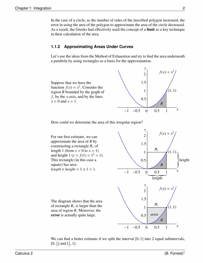
Let’s use the ideas from the Method of Exhaustion and try to find the area underneatha parabola by using rectangles as a basis for the approximation.
Suppose that we have thefunction f (x) = x2. Consider theregion R bounded by the graph off , by the x-axis, and by the linesx = 0 and x = 1.
(1, 1)
f (x) = x2y
x
1.5
1
0.5
−1 −0.5 0 0.5 1
R
2
How could we determine the area of this irregular region?
For our first estimate, we canapproximate the area of R byconstructing a rectangle R1 oflength 1 (from x = 0 to x = 1)and height 1 (y = f (1) = 12 = 1).This rectangle (in this case asquare) has arealength × height = 1 × 1 = 1.
(1, 1)
f (x) = x2y
x
1.5
1
0.5
−1 −0.5 0 0.5 1
R
2
R1
height
length
The diagram shows that the areaof rectangle R1 is larger than thearea of region R. Moreover, theerror is actually quite large.
(1, 1)
f (x) = x2y
x
1.5
1
0.5
−1 −0.5 0 0.5 1
errorR
2
R1
We can find a better estimate if we split the interval [0, 1] into 2 equal subintervals,[0, 1
2 ] and [ 12 , 1].
Calculus 2 (B. Forrest)2
Section 1.1: Areas Under Curves 3
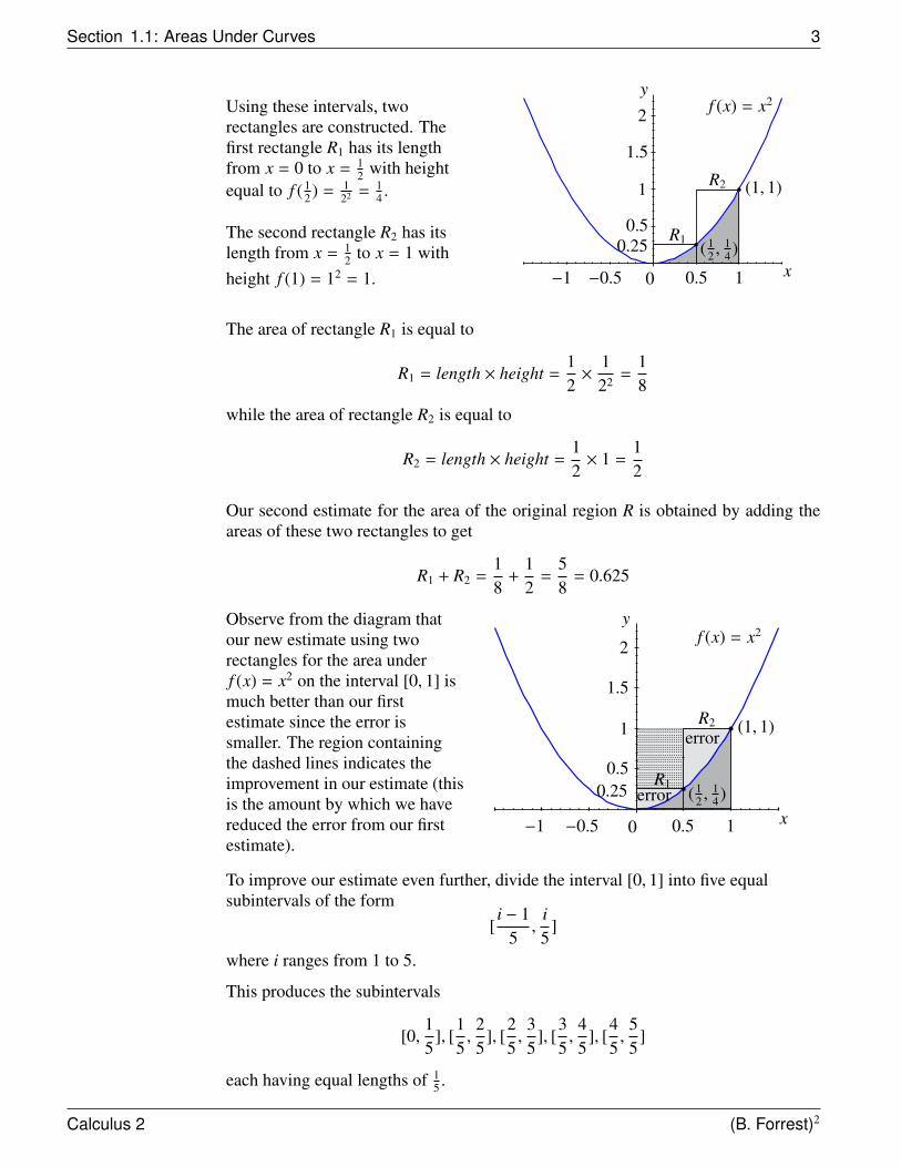
Using these intervals, tworectangles are constructed. Thefirst rectangle R1 has its lengthfrom x = 0 to x = 1
2 with heightequal to f ( 1
2 ) = 122 = 1
4 .
The second rectangle R2 has itslength from x = 1
2 to x = 1 withheight f (1) = 12 = 1.
(1, 1)
f (x) = x2y
x
1.5
1
0.5
−1 −0.5 0 0.5 1
2
R2
R10.25 (12 ,
14 )
The area of rectangle R1 is equal to
R1 = length × height =12×
122 =
18
while the area of rectangle R2 is equal to
R2 = length × height =12× 1 =
12
Our second estimate for the area of the original region R is obtained by adding theareas of these two rectangles to get
R1 + R2 =18
+12
=58
= 0.625
Observe from the diagram thatour new estimate using tworectangles for the area underf (x) = x2 on the interval [0, 1] ismuch better than our firstestimate since the error issmaller. The region containingthe dashed lines indicates theimprovement in our estimate (thisis the amount by which we havereduced the error from our firstestimate).
(1, 1)
f (x) = x2y
x
1.5
1
0.5
−1 −0.5 0 0.5 1
2
R2
R10.25 (12 ,
14 )
error
error
To improve our estimate even further, divide the interval [0, 1] into five equalsubintervals of the form
[i − 1
5,
i5
]
where i ranges from 1 to 5.
This produces the subintervals
[0,15
], [15,
25
], [25,
35
], [35,
45
], [45,
55
]
each having equal lengths of 15 .
Calculus 2 (B. Forrest)2
Chapter 1: Integration 4
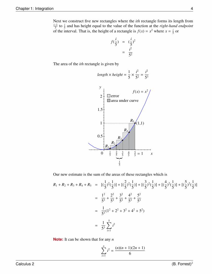
Next we construct five new rectangles where the ith rectangle forms its length fromi−15 to i
5 and has height equal to the value of the function at the right-hand endpointof the interval. That is, the height of a rectangle is f (x) = x2 where x = i
5 or
f (i5
) = (i5
)2
=i2
52
The area of the ith rectangle is given by
length × height =15×
i2
52 =i2
53
(1,1)
R1
f (x) = x2
errorarea under curve
R2
R3
R4
R5
x
y
1.5
1
0.5
0
2
15
25
35
55 = 14
515
Our new estimate is the sum of the areas of these rectangles which is
R1 + R2 + R3 + R4 + R5 = [(15
)2(15
)] + [(25
)2(15
)] + [(35
)2(15
)] + [(45
)2(15
)] + [(55
)2(15
)]
=12
53 +22
53 +32
53 +42
53 +52
53
=153 (12 + 22 + 32 + 42 + 52)
=153
5∑i=1
i2
Note: It can be shown that for any n
n∑i=1
i2 =(n)(n + 1)(2n + 1)
6
Calculus 2 (B. Forrest)2
Section 1.1: Areas Under Curves 5
This means that the sum of the areas of the rectangles is
153
5∑i=1
i2 =153 ×
(5)(5 + 1)(2(5) + 1)6
=153 ×
(5)(6)(11)6
=1125
= 0.44
So far the estimates for the area under the curve of f (x) = x2 on the interval [0, 1]are:
Number of Subintervals(Rectangles)
Length of Subinterval(Width of Rectangle)
Estimate for Areaunder Curve
1 1 1
2 12 0.625
5 15 0.44
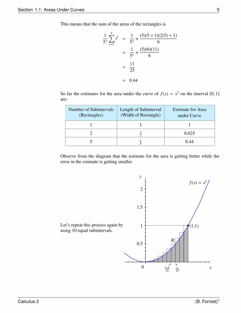
Observe from the diagram that the estimate for the area is getting better while theerror in the estimate is getting smaller.
Let’s repeat this process again byusing 10 equal subintervals.
(1,1)
f (x) = x2
Ri
x
y
1.5
1
0.5
0
2
i−110
i10
Calculus 2 (B. Forrest)2
Chapter 1: Integration 6
In this case, the sum of the areas of the 10 rectangles will be10∑i=1
Ri = R1 + R2 + R3 + R4 + R5 + R6 + R7 + R8 + R9 + R10
=1
103
10∑i=1
i2
=1
103
(10)(10 + 1)(2(10) + 1)6
=77
200
= 0.385
If we were to use 1000 subintervals, the estimate for the area would be
1000∑i=1
Ri = R1 + R2 + R3 + . . . + R1000
=1
10003
1000∑i=1
i2
=1
10003
(1000)(1000 + 1)(2(1000) + 1)6
= 0.3338335
You should begin to notice that as we increase the number of rectangles (numberof subintervals), the total area of these rectangles seems to be getting closer andcloser to the actual area of the original region R. In particular, if we were to producean accurate diagram that represents 1000 rectangles, we would see no noticeabledifference between the estimated area and the true area. For this reason we wouldexpect that our latest estimate of 0.3338335 is actually very close to the true value ofthe area of region R.
We could continue to divide the interval [0, 1] into even more subintervals. In fact,we can repeat this process with n subintervals for any n ∈ N. In this generic case, theestimated area Rn would be
Rn =1n3
n∑i=1
i2
=1n3
(n)(n + 1)(2(n) + 1)6
=
1n3 (2n3 + 3n2 + n)
6
=2 + 3
n + 1n2
6
Calculus 2 (B. Forrest)2
Section 1.1: Areas Under Curves 7
Note that if we let the number of subintervals n approach∞, then
limn→∞
Rn = limn→∞
2 + 3n + 1
n2
6
=26
=13
By calculating the area under the graph of f (x) = x2 using an increasing number ofrectangles, we have constructed a sequence of estimates where each estimate is largerthan the actual area. Though it appears that the limiting value 1
3 is a plausible guessfor the actual value of the area, at this point the best that we can say is that the areashould be less than or equal to 1
3 .
Number of Subintervals(Rectangles)
Length of Subinterval(Width of Rectangle)
Estimate for Areaunder Curve
1 1 1
2 12 0.625
5 15 0.44
10 110 0.385
1000 11000 0.3338335
approaches∞ approaches 0 approaches 13
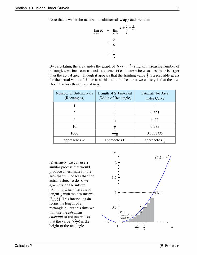
Alternately, we can use asimilar process that wouldproduce an estimate for thearea that will be less than theactual value. To do so weagain divide the interval[0, 1] into n subintervals oflength 1
n with the i-th interval[ i−1
n ,in ]. This interval again
forms the length of arectangle Li, but this time wewill use the left-handendpoint of the interval sothat the value f ( i−1
n ) is theheight of the rectangle.
(1,1)
f (x) = x2
x
y
1.5
1
0.5
0
2
i−1n
in
Li
Firstrectangle hasheight 0
Calculus 2 (B. Forrest)2
Chapter 1: Integration 8
In this case, notice that since f (0) = 0 the first rectangle is really just a horizontalline with area 0. Then the estimated area Ln for this generic case would be
Ln =1n3
n∑i=1
(i − 1)2
=1n3
(n − 1)(n + 1 − 1)(2(n − 1) + 1)6
=1n3
(n − 1)(n)(2n − 1)6
=1n3
2n3 − 3n2 + n6
=2 − 3
n + 1n2
6
Finally, observe that
limn→∞
Ln = limn→∞
2 − 3n + 1
n2
6=
13
.
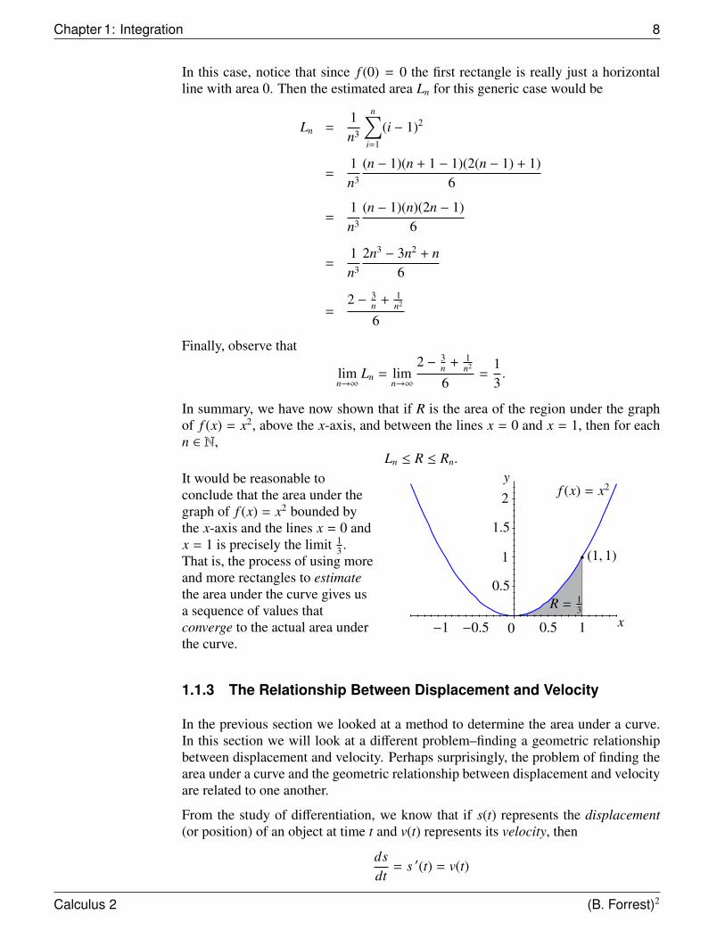
In summary, we have now shown that if R is the area of the region under the graphof f (x) = x2, above the x-axis, and between the lines x = 0 and x = 1, then for eachn ∈ N,
Ln ≤ R ≤ Rn.
It would be reasonable toconclude that the area under thegraph of f (x) = x2 bounded bythe x-axis and the lines x = 0 andx = 1 is precisely the limit 1
3 .That is, the process of using moreand more rectangles to estimatethe area under the curve gives usa sequence of values thatconverge to the actual area underthe curve.
(1, 1)
f (x) = x2y
x
1.5
1
0.5
−1 −0.5 0 0.5 1
R = 13
2
1.1.3 The Relationship Between Displacement and Velocity
In the previous section we looked at a method to determine the area under a curve.In this section we will look at a different problem–finding a geometric relationshipbetween displacement and velocity. Perhaps surprisingly, the problem of finding thearea under a curve and the geometric relationship between displacement and velocityare related to one another.
From the study of differentiation, we know that if s(t) represents the displacement(or position) of an object at time t and v(t) represents its velocity, then
dsdt
= s ′(t) = v(t)
Calculus 2 (B. Forrest)2
Section 1.1: Areas Under Curves 9
In other words, the derivative of the displacement (position) function is the velocityfunction. By implementing the method we used to calculate area in the last section,we will now see that another relationship exists between displacement and velocity.
Suppose that we are going to take a trip in a car along a highway. Our task is todetermine how far we have travelled after two hours. Unfortunately, the odometer inthe car is broken. However, the speedometer is in working condition.
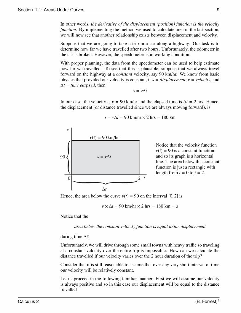
With proper planning, the data from the speedometer can be used to help estimatehow far we travelled. To see that this is plausible, suppose that we always travelforward on the highway at a constant velocity, say 90 km/hr. We know from basicphysics that provided our velocity is constant, if s = displacement, v = velocity, and∆t = time elapsed, then
s = v∆t
In our case, the velocity is v = 90 km/hr and the elapsed time is ∆t = 2 hrs. Hence,the displacement (or distance travelled since we are always moving forward), is
s = v∆t = 90 km/hr × 2 hrs = 180 km
s = v∆t
v
0 2 t
v(t) = 90 km/hr
∆t
90
Notice that the velocity functionv(t) = 90 is a constant functionand so its graph is a horizontalline. The area below this constantfunction is just a rectangle withlength from t = 0 to t = 2.
Hence, the area below the curve v(t) = 90 on the interval [0, 2] is
v × ∆t = 90 km/hr × 2 hrs = 180 km = s
Notice that the
area below the constant velocity function is equal to the displacement
during time ∆t!
Unfortunately, we will drive through some small towns with heavy traffic so travelingat a constant velocity over the entire trip is impossible. How can we calculate thedistance travelled if our velocity varies over the 2 hour duration of the trip?
Consider that it is still reasonable to assume that over any very short interval of timeour velocity will be relatively constant.
Let us proceed in the following familiar manner. First we will assume our velocityis always positive and so in this case our displacement will be equal to the distancetravelled.
Calculus 2 (B. Forrest)2
Chapter 1: Integration 10
Next let’s separate the 2 hour duration of the trip into 120 one minute intervals
0 = t0 < t1 < t2 < t3 < · · · < ti−1 < ti < · · · < t120 = 2 hours
so that ti = i minutes = i60 hours. Let si be the distance travelled during time ti−1 until
ti. In other words, each si is the distance travelled in the i th minute of our trip. Thenif s is the total displacement (distance travelled), we have
s = (distance travelled in 1st minute) + (distance travelled in 2nd minute) + · · ·
. . . + (distance travelled in i th minute) + · · · + (distance travelled in 120th minute)= s1 + s2 + s3 + · · · + si + · · · + s120
=
120∑i=1
si
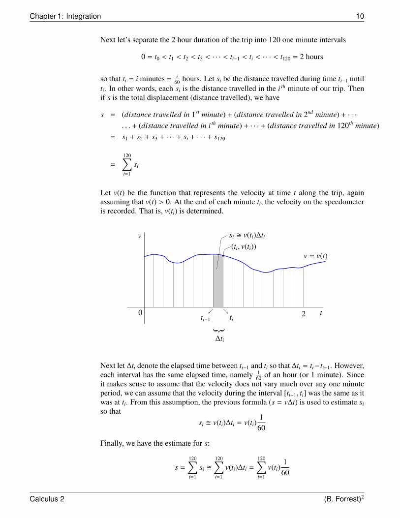
Let v(t) be the function that represents the velocity at time t along the trip, againassuming that v(t) > 0. At the end of each minute ti, the velocity on the speedometeris recorded. That is, v(ti) is determined.
v
0 2 t
v = v(t)
si � v(ti)∆ti
ti−1 ti
∆ti
(ti, v(ti))
Next let ∆ti denote the elapsed time between ti−1 and ti so that ∆ti = ti− ti−1. However,each interval has the same elapsed time, namely 1
60 of an hour (or 1 minute). Sinceit makes sense to assume that the velocity does not vary much over any one minuteperiod, we can assume that the velocity during the interval [ti−1, ti] was the same as itwas at ti. From this assumption, the previous formula (s = v∆t) is used to estimate si
so thatsi � v(ti)∆ti = v(ti)
160
Finally, we have the estimate for s:
s =
120∑i=1
si �120∑i=1
v(ti)∆ti =
120∑i=1
v(ti)160
Calculus 2 (B. Forrest)2

Section 1.1: Areas Under Curves 11
To find an even better estimate, we could measure the velocity every second. Thismeans we would divide the two hour period into equal subintervals [ti−1, ti] each oflength 1
3600 hours (i.e., 1 hr × 60 min/hr × 60 sec/min = 3600 sec/hr and 2 hrs ×3600 seconds/hr = 7200 seconds). We again let si denote the distance travelled overthe i th interval. This time we have
si � v(ti)∆ti = v(ti)1
3600
and
s =
7200∑i=1
si �7200∑i=1
v(ti)∆ti =
7200∑i=1
v(ti)1
3600
In fact, for any Natural number n > 0, we can divide the interval [0, 2] into n equalparts of length 2
n by choosing
0 = t0 < t1 < t2 < t3 < · · · < ti−1 < ti < · · · < tn = 2
where ti = 2in for each i = 1, 2, 3, . . . , n. If we let
S n =
n∑i=1
v(ti)∆ti =
n∑i=1
v(ti)2n
then it can be shown that the sequence {S n} converges and that
limn→∞{S n} = s
Let’s consider what this last statement means geometrically. The diagram shows thegraph of velocity as a function of time over the interval [0, 2] partitioned into n equalsubintervals.
v
t0 = 0 tn = 2t
v = v(t)
ti−1 ti
We have thatsi � v(ti)∆ti
butv(ti)∆ti
is just the area of the shaded rectangle with height v(ti) and length ∆ti.
Calculus 2 (B. Forrest)2
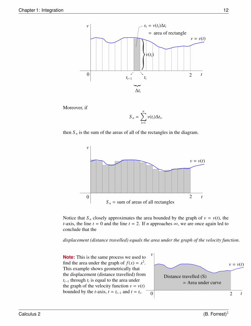
Chapter 1: Integration 12
v
0 2 t
v = v(t)
v(ti)
si = v(ti)∆ti
= area of rectangle
ti−1 ti
∆ti
Moreover, if
S n =
n∑i=1
v(ti)∆ti,
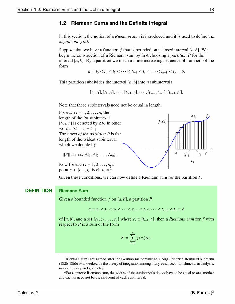
then S n is the sum of the areas of all of the rectangles in the diagram.
0
v
t
v = v(t)
2S n = sum of areas of all rectangles
Notice that S n closely approximates the area bounded by the graph of v = v(t), thet-axis, the line t = 0 and the line t = 2. If n approaches ∞, we are once again led toconclude that the
displacement (distance travelled) equals the area under the graph of the velocity function.
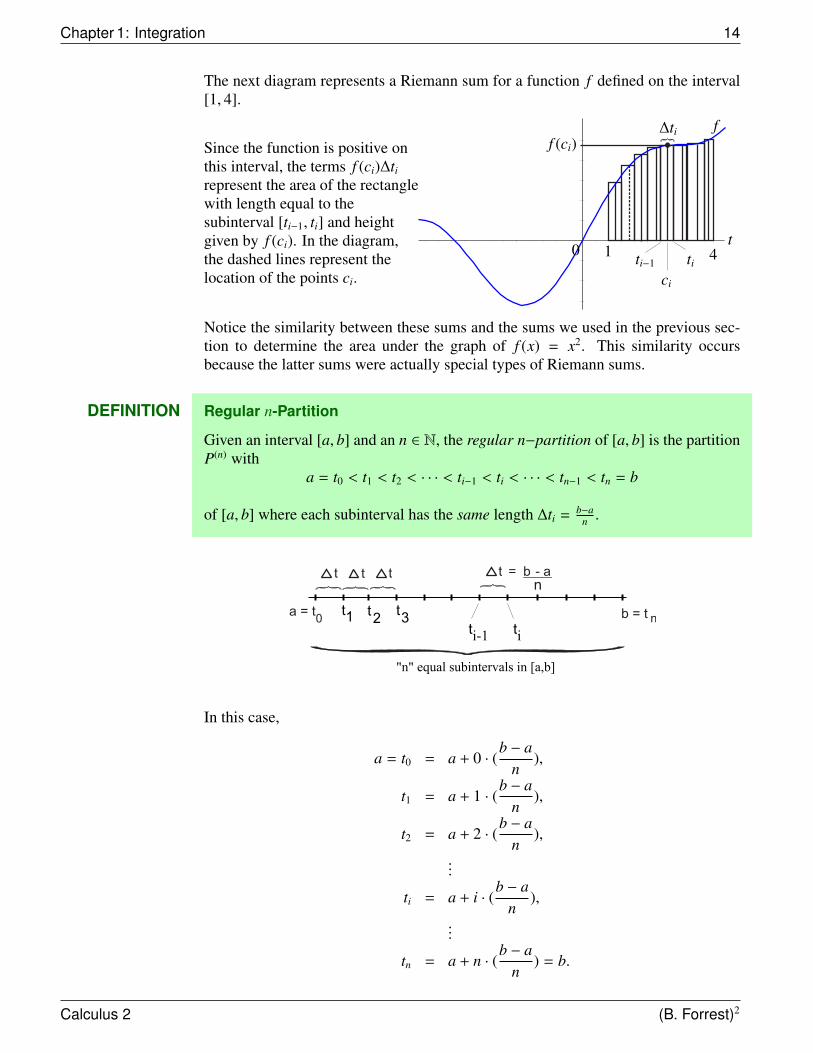
Note: This is the same process we used tofind the area under the graph of f (x) = x2.This example shows geometrically thatthe displacement (distance travelled) fromti−1 through ti is equal to the area underthe graph of the velocity function v = v(t)bounded by the t-axis, t = ti−1 and t = ti.
v
0 2 t
v = v(t)
Distance travelled (S)= Area under curve
Calculus 2 (B. Forrest)2
Section 1.2: Riemann Sums and the Definite Integral 13
1.2 Riemann Sums and the Definite Integral
In this section, the notion of a Riemann sum is introduced and it is used to define thedefinite integral.1
Suppose that we have a function f that is bounded on a closed interval [a, b]. Webegin the construction of a Riemann sum by first choosing a partition P for theinterval [a, b]. By a partition we mean a finite increasing sequence of numbers of theform
a = t0 < t1 < t2 < · · · < ti−1 < ti < · · · < tn−1 < tn = b.
This partition subdivides the interval [a, b] into n subintervals
[t0, t1], [t1, t2], · · · , [ti−1, ti], · · · , [tn−2, tn−1], [tn−1, tn].
Note that these subintervals need not be equal in length.
For each i = 1, 2, . . . , n, thelength of the ith subinterval[ti−1, ti] is denoted by ∆ti. In otherwords, ∆ti = ti − ti−1.The norm of the partition P is thelength of the widest subintervalwhich we denote by
‖P‖ = max{∆t1,∆t2, . . . ,∆tn}.
Now for each i = 1, 2, . . . , n, apoint ci ∈ [ti−1, ti] is chosen.2
f (ci)∆ti f
tba0
ci
titi−1
Given these conditions, we can now define a Riemann sum for the partition P.
DEFINITION Riemann Sum
Given a bounded function f on [a, b], a partition P
a = t0 < t1 < t2 < · · · < ti−1 < ti < · · · < tn−1 < tn = b
of [a, b], and a set {c1, c2, . . . , cn} where ci ∈ [ti−1, ti], then a Riemann sum for f withrespect to P is a sum of the form
S =
n∑i=1
f (ci)∆ti.
1Riemann sums are named after the German mathematician Georg Friedrich Bernhard Riemann(1826-1866) who worked on the theory of integration among many other accomplishments in analysis,number theory and geometry.
2For a generic Riemann sum, the widths of the subintervals do not have to be equal to one anotherand each ci need not be the midpoint of each subinterval.
Calculus 2 (B. Forrest)2
Chapter 1: Integration 14
The next diagram represents a Riemann sum for a function f defined on the interval[1, 4].
Since the function is positive onthis interval, the terms f (ci)∆ti
represent the area of the rectanglewith length equal to thesubinterval [ti−1, ti] and heightgiven by f (ci). In the diagram,the dashed lines represent thelocation of the points ci.
f (ci)∆ti f
t410
ci
titi−1
Notice the similarity between these sums and the sums we used in the previous sec-tion to determine the area under the graph of f (x) = x2. This similarity occursbecause the latter sums were actually special types of Riemann sums.
DEFINITION Regular n-Partition
Given an interval [a, b] and an n ∈ N, the regular n−partition of [a, b] is the partitionP(n) with
a = t0 < t1 < t2 < · · · < ti−1 < ti < · · · < tn−1 < tn = b
of [a, b] where each subinterval has the same length ∆ti = b−an .
In this case,
a = t0 = a + 0 · (b − a
n),
t1 = a + 1 · (b − a
n),
t2 = a + 2 · (b − a
n),
...
ti = a + i · (b − a
n),
...
tn = a + n · (b − a
n) = b.
Calculus 2 (B. Forrest)2
Section 1.2: Riemann Sums and the Definite Integral 15
DEFINITION Right-hand Riemann Sum
The right-hand Riemann sum for f with respect to the partition P is the Riemann sumR obtained from P by choosing ci to be ti, the right-hand endpoint of [ti−1, ti]. That is
R =
n∑i=1
f (ti)∆ti.
If P(n) is the regular n-partition, we denote the right-hand Riemann sum by
Rn =
n∑i=1
f (ti)∆ti =
n∑i=1
f (ti)b − a
n
=
n∑i=1
f(a + i
(b − a
n
)) (b − a
n
)
DEFINITION Left-hand Riemann Sum
The left-hand Riemann sum for f with respect to the partition P is the Riemann sumL obtained from P by choosing ci to be ti−1, the left-hand endpoint of [ti−1, ti]. That is
L =
n∑i=1
f (ti−1)∆ti.
If P(n) is the regular n-partition, we denote the left-hand Riemann sum by
Ln =
n∑i=1
f (ti−1)∆ti =
n∑i=1
f (ti−1)b − a
n
=
n∑i=1
f(a + (i − 1)
(b − a
n
)) (b − a
n
)
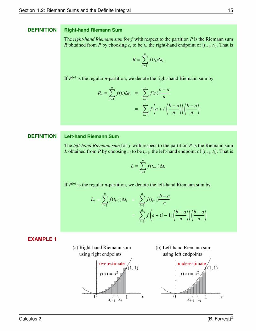
EXAMPLE 1
overestimate underestimate
f (x) = x2 f (x) = x2(1, 1) (1, 1)
0 1 xxi−1 xi0 1 xxi−1 xi
(b) Left-hand Riemann sum(a) Right-hand Riemann sumusing left endpointsusing right endpoints
Calculus 2 (B. Forrest)2
Chapter 1: Integration 16
A closer look at the examples in the previous section reveals that the sums usedto estimate the area under the graph of f (x) = x2 were right-hand Riemann sums.Similarly, the sums used to find the distance travelled were right-hand Riemann sumsof the velocity function v(t). Moreover, we saw that if we let n approach ∞, thenthese sequences of Riemann sums converged to the area under the graph of f (x) = x2
and the total distance travelled, respectively. These examples motivate the followingdefinition:
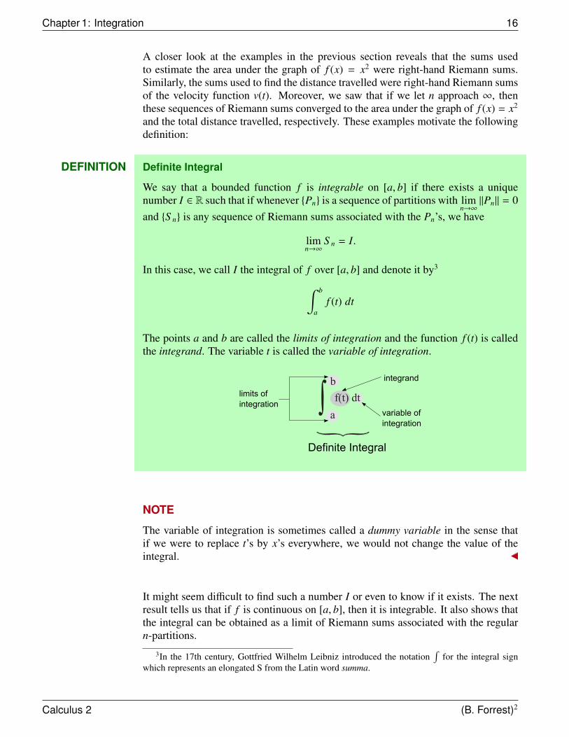
DEFINITION Definite Integral
We say that a bounded function f is integrable on [a, b] if there exists a uniquenumber I ∈ R such that if whenever {Pn} is a sequence of partitions with lim
n→∞‖Pn‖ = 0
and {S n} is any sequence of Riemann sums associated with the Pn’s, we have
limn→∞
S n = I.
In this case, we call I the integral of f over [a, b] and denote it by3
∫ b
af (t) dt
The points a and b are called the limits of integration and the function f (t) is calledthe integrand. The variable t is called the variable of integration.
NOTE
The variable of integration is sometimes called a dummy variable in the sense thatif we were to replace t’s by x’s everywhere, we would not change the value of theintegral.
It might seem difficult to find such a number I or even to know if it exists. The nextresult tells us that if f is continuous on [a, b], then it is integrable. It also shows thatthe integral can be obtained as a limit of Riemann sums associated with the regularn-partitions.
3In the 17th century, Gottfried Wilhelm Leibniz introduced the notation∫
for the integral signwhich represents an elongated S from the Latin word summa.
Calculus 2 (B. Forrest)2
Section 1.2: Riemann Sums and the Definite Integral 17
THEOREM 1 Integrability Theorem for Continuous Functions
Let f be continuous on [a, b]. Then f is integrable on [a, b]. Moreover,∫ b
af (t) dt = lim
n→∞S n
where
S n =
n∑i=1
f (ci)∆ti
is any Riemann sum associated with the regular n-partitions. In particular,∫ b
af (t) dt = lim
n→∞Rn = lim
n→∞
n∑i=1
f (ti)b − a
n
and ∫ b
af (t) dt = lim
n→∞Ln = lim
n→∞
n∑i=1
f (ti−1)b − a
n
REMARK
This theorem also holds if f is bounded and has finitely many discontinuities on[a, b]. The proof of this theorem is beyond the scope of this course.
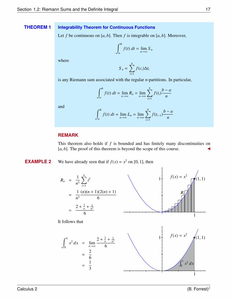
EXAMPLE 2 We have already seen that if f (x) = x2 on [0, 1], then
Rn =1n3
n∑i=1
i2
=1n3
(n)(n + 1)(2(n) + 1)6
=2 + 3
n + 1n2
6
1
1
Ri
(1, 1)f (x) = x2
It follows that
∫ 1
0x2 dx = lim
n→∞
2 + 3n + 1
n2
6
=26
=13
1 f (x) = x2(1, 1)
1
∫ 1
0x2 dx
Calculus 2 (B. Forrest)2
Chapter 1: Integration 18
Soon we will see how to calculate integrals by means other than using limits ofRiemann sums. However, before ending this section, consider the followingimportant example.
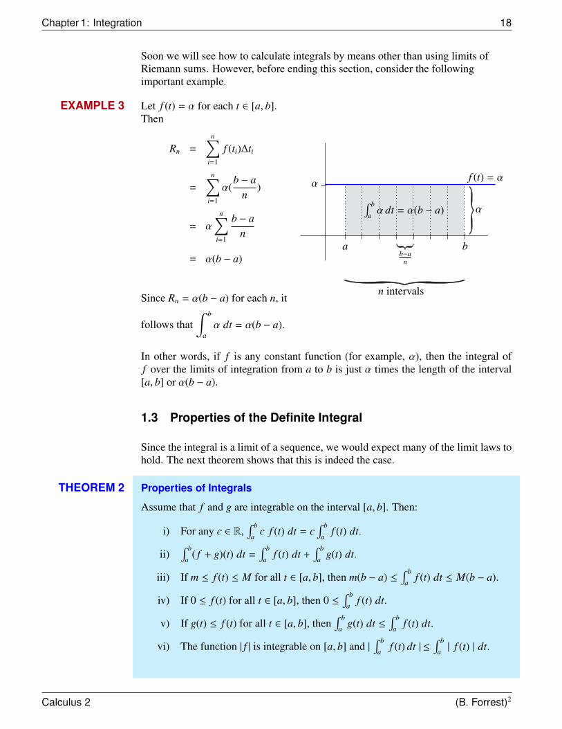
EXAMPLE 3 Let f (t) = α for each t ∈ [a, b].Then
Rn =
n∑i=1
f (ti)∆ti
=
n∑i=1
α(b − a
n)
= α
n∑i=1
b − an
= α(b − a)
Since Rn = α(b − a) for each n, it
follows that∫ b
aα dt = α(b − a).
α
a b
α
f (t) = α
n intervals
b−an
∫ b
aα dt = α(b − a)
In other words, if f is any constant function (for example, α), then the integral off over the limits of integration from a to b is just α times the length of the interval[a, b] or α(b − a).
1.3 Properties of the Definite Integral
Since the integral is a limit of a sequence, we would expect many of the limit laws tohold. The next theorem shows that this is indeed the case.
THEOREM 2 Properties of Integrals
Assume that f and g are integrable on the interval [a, b]. Then:
i) For any c ∈ R,∫ b
ac f (t) dt = c
∫ b
af (t) dt.
ii)∫ b
a( f + g)(t) dt =
∫ b
af (t) dt +
∫ b
ag(t) dt.
iii) If m ≤ f (t) ≤ M for all t ∈ [a, b], then m(b − a) ≤∫ b
af (t) dt ≤ M(b − a).
iv) If 0 ≤ f (t) for all t ∈ [a, b], then 0 ≤∫ b
af (t) dt.
v) If g(t) ≤ f (t) for all t ∈ [a, b], then∫ b
ag(t) dt ≤
∫ b
af (t) dt.
vi) The function | f | is integrable on [a, b] and |∫ b
af (t) dt | ≤
∫ b
a| f (t) | dt.
Calculus 2 (B. Forrest)2

Section 1.3: Properties of the Definite Integral 19
Properties (i) and (ii) in the previous theorem follow immediately from the rules ofarithmetic for convergent sequences. Property (iv) can be deduced from Property (iii)and Property (v) can be obtained from Properties (i), (ii) and (iv).
Let’s consider why Property (iii) is true.
Assume that
m ≤ f (t) ≤ M
for all t ∈ [a, b].m
Mf
tLet
a = t0 < t1 < t2 < · · · < ti−1 < ti < · · · < tn−1 < tn = b
be any partition of [a, b]. We first observe thatn∑
i=1∆ti = b − a. Then since
m ≤ f (ti) ≤ M,
m(b − a) =
n∑i=1
m∆ti ≤
n∑i=1
f (ti)∆ti ≤
n∑i=1
M∆ti = M(b − a).
It then follows
m(b − a) ≤∫ b
af (t) dt ≤ M(b − a)
as expected.M
m
f
ta b
M(b − a)
ta b
M
m
f∫ b
af (t) dt
m(b − a)
M
m
t
f
a b
Property (vi) can be derived by applying the triangle inequality to the Riemann sumsassociated with
∫ b
af (t) dt.
1.3.1 Additional Properties of the Integral
Up until now, in defining the definite integral we have always considered integrals ofthe form ∫ b
af (t) dt
where a < b. However, it is necessary to give meaning to∫ a
af (t) dt
Calculus 2 (B. Forrest)2
Chapter 1: Integration 20
and to ∫ a
bf (t) dt.
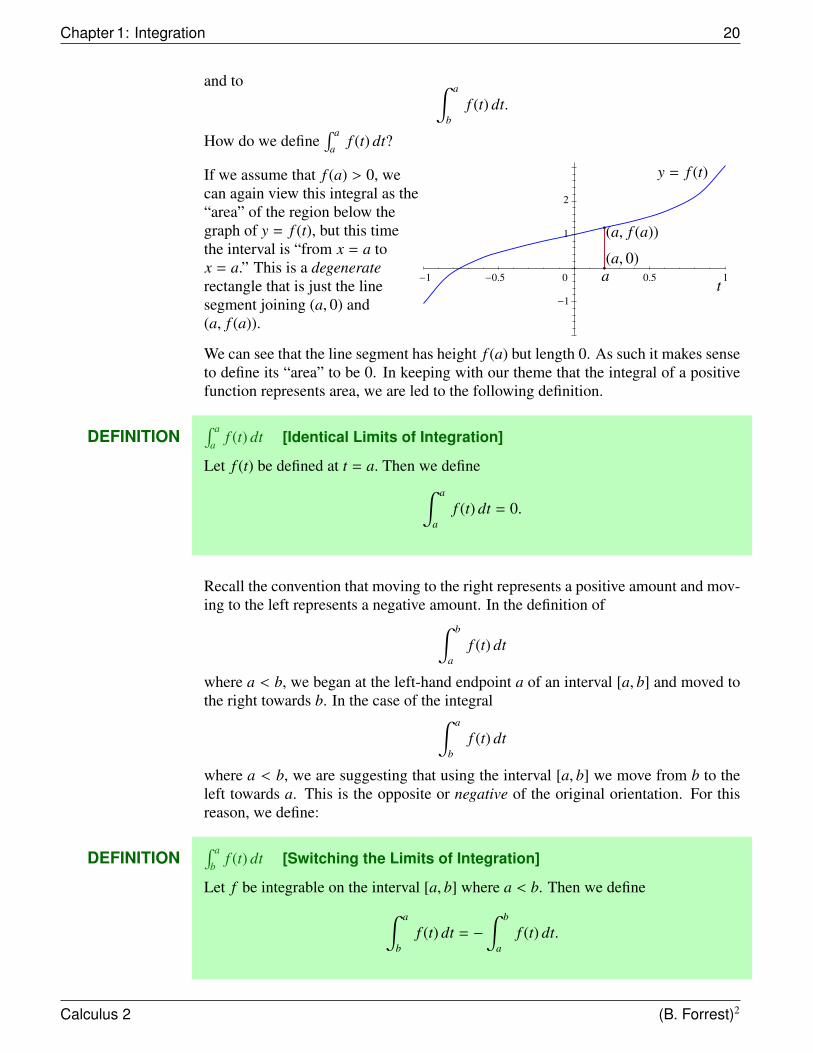
How do we define∫ a
af (t) dt?
If we assume that f (a) > 0, wecan again view this integral as the“area” of the region below thegraph of y = f (t), but this timethe interval is “from x = a tox = a.” This is a degeneraterectangle that is just the linesegment joining (a, 0) and(a, f (a)).
ta(a, 0)
(a, f (a))
y = f (t)
−1
0
1
2
−1 −0.5 0.5 1
We can see that the line segment has height f (a) but length 0. As such it makes senseto define its “area” to be 0. In keeping with our theme that the integral of a positivefunction represents area, we are led to the following definition.
DEFINITION∫ a
af (t) dt [Identical Limits of Integration]
Let f (t) be defined at t = a. Then we define∫ a
af (t) dt = 0.
Recall the convention that moving to the right represents a positive amount and mov-ing to the left represents a negative amount. In the definition of∫ b
af (t) dt
where a < b, we began at the left-hand endpoint a of an interval [a, b] and moved tothe right towards b. In the case of the integral∫ a
bf (t) dt
where a < b, we are suggesting that using the interval [a, b] we move from b to theleft towards a. This is the opposite or negative of the original orientation. For thisreason, we define:
DEFINITION∫ a
bf (t) dt [Switching the Limits of Integration]
Let f be integrable on the interval [a, b] where a < b. Then we define∫ a
bf (t) dt = −
∫ b
af (t) dt.
Calculus 2 (B. Forrest)2
Section 1.3: Properties of the Definite Integral 21
EXAMPLE 4 Recall that we have already seen ∫ 1
0x2 dx =
13.
It follows that ∫ 0
1x2 dx = −
13.
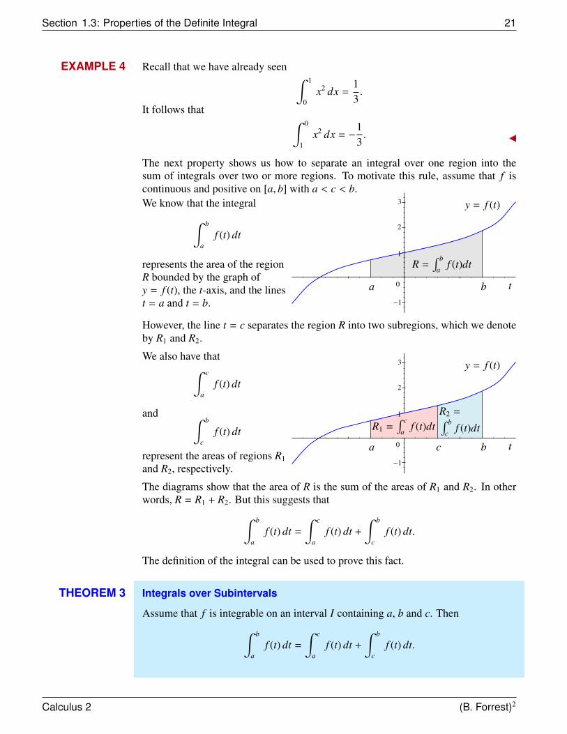
The next property shows us how to separate an integral over one region into thesum of integrals over two or more regions. To motivate this rule, assume that f iscontinuous and positive on [a, b] with a < c < b.We know that the integral∫ b
af (t) dt
represents the area of the regionR bounded by the graph ofy = f (t), the t-axis, and the linest = a and t = b.
y = f (t)
tba 0
−1
3
2
1
R =∫ b
af (t)dt
However, the line t = c separates the region R into two subregions, which we denoteby R1 and R2.
We also have that∫ c
af (t) dt
and ∫ b
cf (t) dt
represent the areas of regions R1
and R2, respectively.
y = f (t)
tbca 0
−1
3
2
1
R1 =∫ c
af (t)dt
R2 =∫ b
cf (t)dt
The diagrams show that the area of R is the sum of the areas of R1 and R2. In otherwords, R = R1 + R2. But this suggests that∫ b
af (t) dt =
∫ c
af (t) dt +
∫ b
cf (t) dt.
The definition of the integral can be used to prove this fact.
THEOREM 3 Integrals over Subintervals
Assume that f is integrable on an interval I containing a, b and c. Then∫ b
af (t) dt =
∫ c
af (t) dt +
∫ b
cf (t) dt.
Calculus 2 (B. Forrest)2
Chapter 1: Integration 22
Note: The proof of this theorem is not part of this course.
This theorem also holds when c lies outside the interval [a, b]. Consider the followingexample.
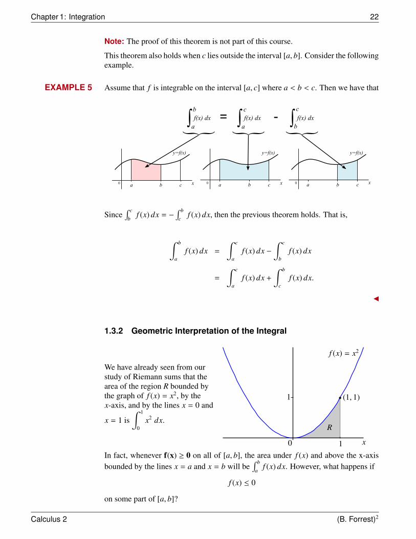
EXAMPLE 5 Assume that f is integrable on the interval [a, c] where a < b < c. Then we have that
Since∫ c
bf (x) dx = −
∫ b
cf (x) dx, then the previous theorem holds. That is,
∫ b
af (x) dx =
∫ c
af (x) dx −
∫ c
bf (x) dx
=
∫ c
af (x) dx +
∫ b
cf (x) dx.
1.3.2 Geometric Interpretation of the Integral
We have already seen from ourstudy of Riemann sums that thearea of the region R bounded bythe graph of f (x) = x2, by thex-axis, and by the lines x = 0 and
x = 1 is∫ 1
0x2 dx.
f (x) = x2
1
0 1
(1, 1)
x
R
In fact, whenever f(x) ≥ 0 on all of [a, b], the area under f (x) and above the x-axisbounded by the lines x = a and x = b will be
∫ b
af (x) dx. However, what happens if
f (x) ≤ 0
on some part of [a, b]?
Calculus 2 (B. Forrest)2
Section 1.3: Properties of the Definite Integral 23
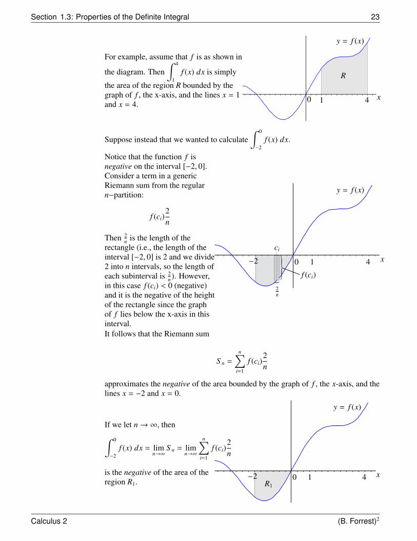
For example, assume that f is as shown in
the diagram. Then∫ 4
1f (x) dx is simply
the area of the region R bounded by thegraph of f , the x-axis, and the lines x = 1and x = 4.
y = f (x)
10 4 x
R
Suppose instead that we wanted to calculate∫ 0
−2f (x) dx.
Notice that the function f isnegative on the interval [−2, 0].Consider a term in a genericRiemann sum from the regularn−partition:
f (ci)2n
Then 2n is the length of the
rectangle (i.e., the length of theinterval [−2, 0] is 2 and we divide2 into n intervals, so the length ofeach subinterval is 2
n ). However,in this case f (ci) < 0 (negative)and it is the negative of the heightof the rectangle since the graphof f lies below the x-axis in thisinterval.
y = f (x)
10 4 x−2
2n
ci
f (ci)
It follows that the Riemann sum
S n =
n∑i=1
f (ci)2n
approximates the negative of the area bounded by the graph of f , the x-axis, and thelines x = −2 and x = 0.
If we let n→ ∞, then∫ 0
−2f (x) dx = lim
n→∞S n = lim
n→∞
n∑i=1
f (ci)2n
is the negative of the area of theregion R1.
y = f (x)
10 4 x−2R1
Calculus 2 (B. Forrest)2
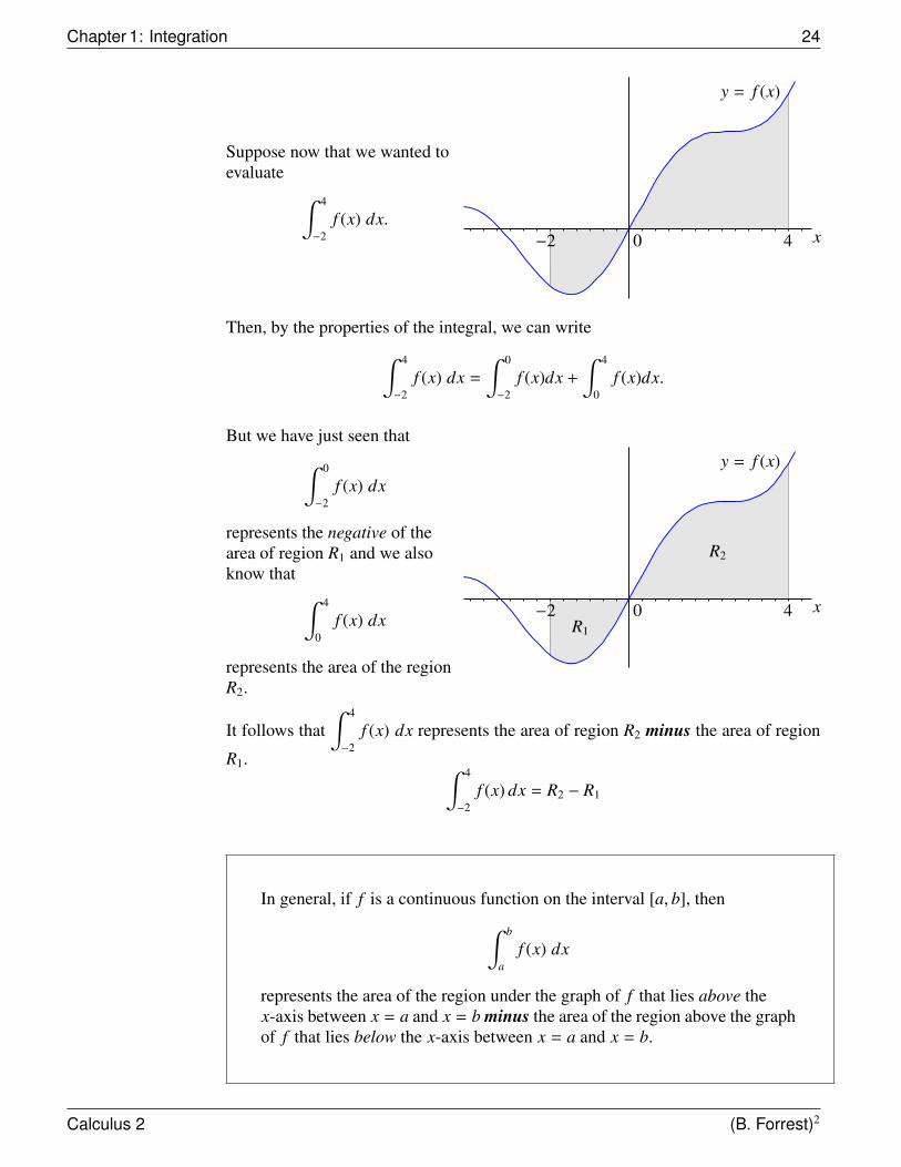
Chapter 1: Integration 24
Suppose now that we wanted toevaluate ∫ 4
−2f (x) dx.
y = f (x)
−2 0 4 x
Then, by the properties of the integral, we can write∫ 4
−2f (x) dx =
∫ 0
−2f (x)dx +
∫ 4
0f (x)dx.
But we have just seen that∫ 0
−2f (x) dx
represents the negative of thearea of region R1 and we alsoknow that ∫ 4
0f (x) dx
represents the area of the regionR2.
y = f (x)
−2 0 4 x
R2
R1
It follows that∫ 4
−2f (x) dx represents the area of region R2 minus the area of region
R1. ∫ 4
−2f (x) dx = R2 − R1
In general, if f is a continuous function on the interval [a, b], then∫ b
af (x) dx
represents the area of the region under the graph of f that lies above thex-axis between x = a and x = b minus the area of the region above the graphof f that lies below the x-axis between x = a and x = b.
Calculus 2 (B. Forrest)2
Section 1.3: Properties of the Definite Integral 25
If you are not yet convinced that for f (x) ≤ 0 on [a, b],∫ b
af (x) dx is simply the
negative of the area of the region above the graph of f , below the x-axis, and betweenx = a and x = b, then the following example may convince you.
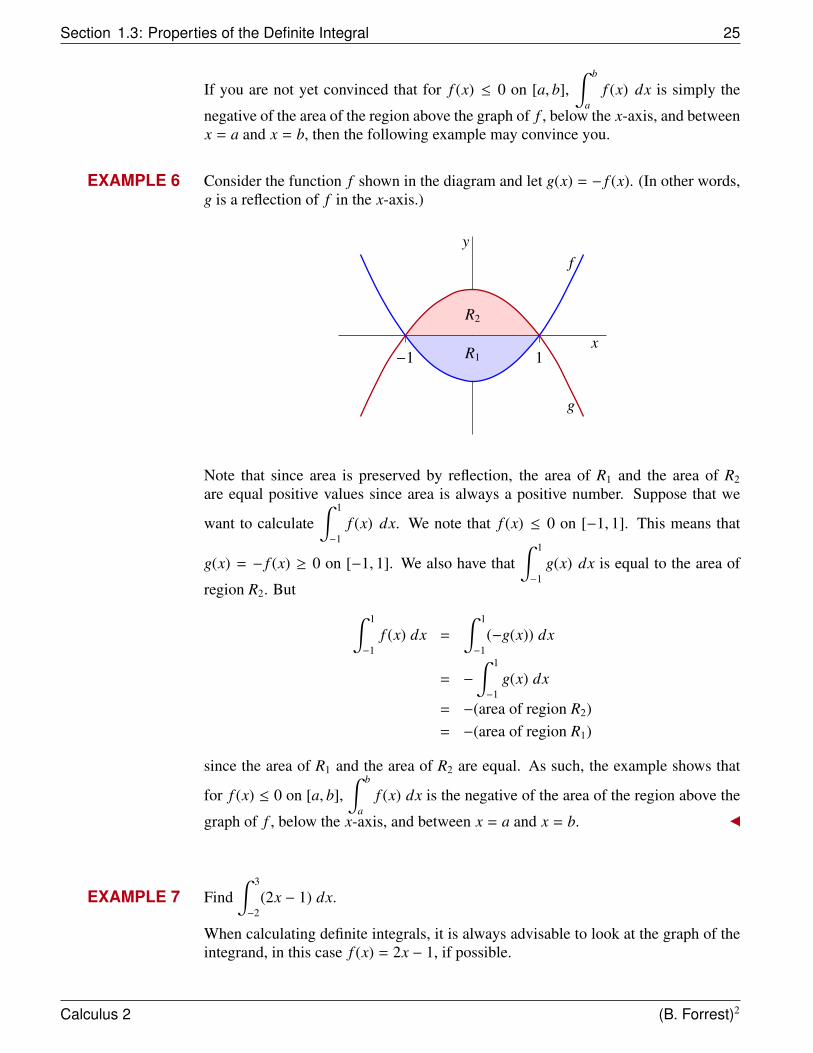
EXAMPLE 6 Consider the function f shown in the diagram and let g(x) = − f (x). (In other words,g is a reflection of f in the x-axis.)
−1 1
g
f
x
y
R2
R1
Note that since area is preserved by reflection, the area of R1 and the area of R2
are equal positive values since area is always a positive number. Suppose that we
want to calculate∫ 1
−1f (x) dx. We note that f (x) ≤ 0 on [−1, 1]. This means that
g(x) = − f (x) ≥ 0 on [−1, 1]. We also have that∫ 1
−1g(x) dx is equal to the area of
region R2. But ∫ 1
−1f (x) dx =
∫ 1
−1(−g(x)) dx
= −
∫ 1
−1g(x) dx
= −(area of region R2)= −(area of region R1)
since the area of R1 and the area of R2 are equal. As such, the example shows that
for f (x) ≤ 0 on [a, b],∫ b
af (x) dx is the negative of the area of the region above the
graph of f , below the x-axis, and between x = a and x = b.
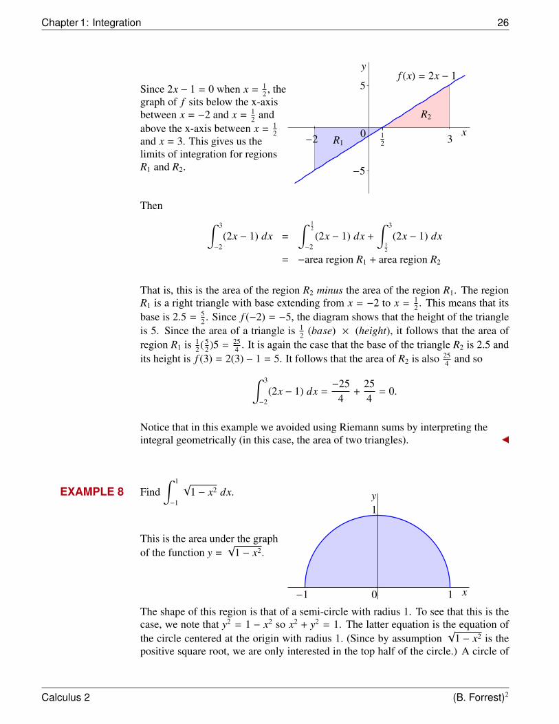
EXAMPLE 7 Find∫ 3
−2(2x − 1) dx.
When calculating definite integrals, it is always advisable to look at the graph of theintegrand, in this case f (x) = 2x − 1, if possible.
Calculus 2 (B. Forrest)2
Chapter 1: Integration 26
Since 2x − 1 = 0 when x = 12 , the
graph of f sits below the x-axisbetween x = −2 and x = 1
2 andabove the x-axis between x = 1
2and x = 3. This gives us thelimits of integration for regionsR1 and R2.
5
−5
0 12
x
y
3−2
f (x) = 2x − 1
R1
R2
Then ∫ 3
−2(2x − 1) dx =
∫ 12
−2(2x − 1) dx +
∫ 3
12
(2x − 1) dx
= −area region R1 + area region R2
That is, this is the area of the region R2 minus the area of the region R1. The regionR1 is a right triangle with base extending from x = −2 to x = 1
2 . This means that itsbase is 2.5 = 5
2 . Since f (−2) = −5, the diagram shows that the height of the triangleis 5. Since the area of a triangle is 1
2 (base) × (height), it follows that the area ofregion R1 is 1
2 ( 52 )5 = 25
4 . It is again the case that the base of the triangle R2 is 2.5 andits height is f (3) = 2(3) − 1 = 5. It follows that the area of R2 is also 25
4 and so∫ 3
−2(2x − 1) dx =
−254
+254
= 0.
Notice that in this example we avoided using Riemann sums by interpreting theintegral geometrically (in this case, the area of two triangles).
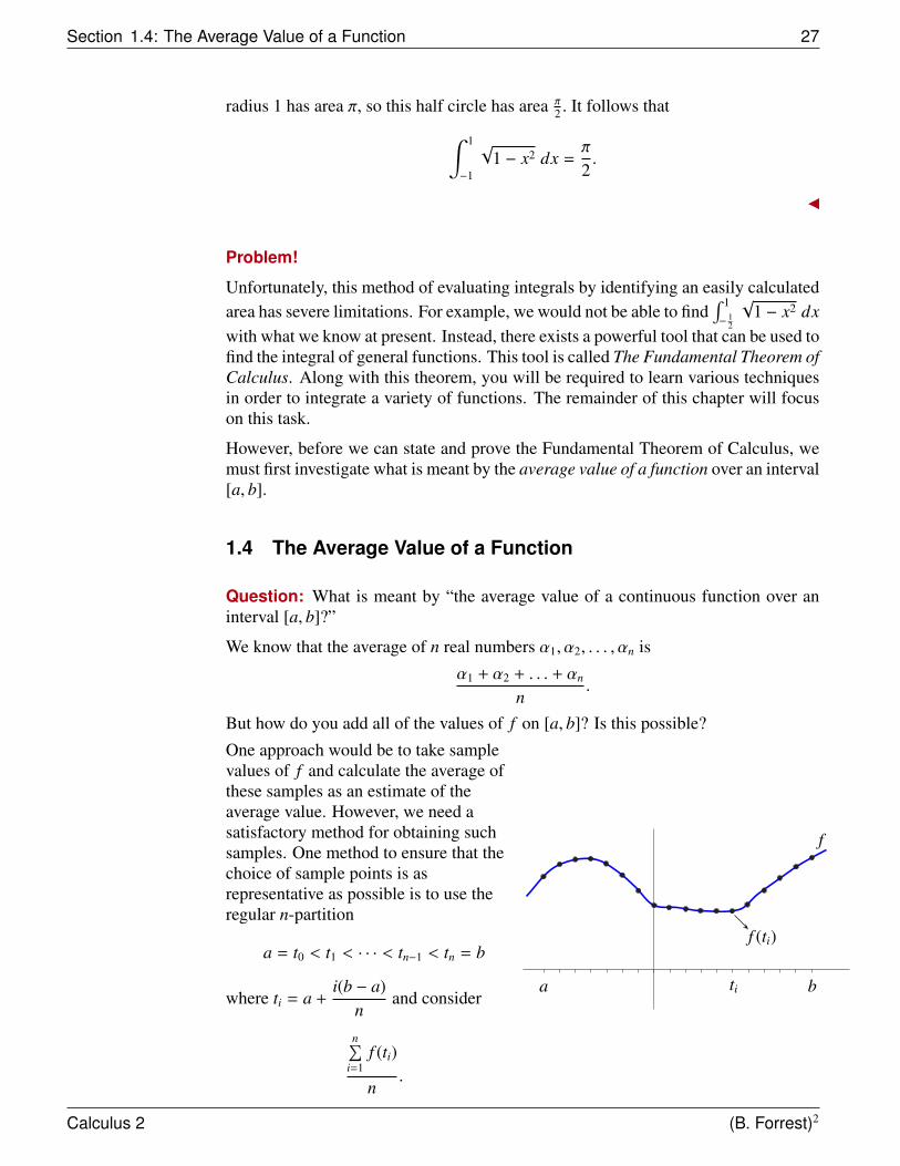
EXAMPLE 8 Find∫ 1
−1
√1 − x2 dx.
This is the area under the graphof the function y =
√1 − x2.
1
−1 10 x
y
The shape of this region is that of a semi-circle with radius 1. To see that this is thecase, we note that y2 = 1 − x2 so x2 + y2 = 1. The latter equation is the equation ofthe circle centered at the origin with radius 1. (Since by assumption
√1 − x2 is the
positive square root, we are only interested in the top half of the circle.) A circle of
Calculus 2 (B. Forrest)2
Section 1.4: The Average Value of a Function 27
radius 1 has area π, so this half circle has area π2 . It follows that∫ 1
−1
√1 − x2 dx =
π
2.
Problem!
Unfortunately, this method of evaluating integrals by identifying an easily calculatedarea has severe limitations. For example, we would not be able to find
∫ 1
− 12
√1 − x2 dx
with what we know at present. Instead, there exists a powerful tool that can be used tofind the integral of general functions. This tool is called The Fundamental Theorem ofCalculus. Along with this theorem, you will be required to learn various techniquesin order to integrate a variety of functions. The remainder of this chapter will focuson this task.
However, before we can state and prove the Fundamental Theorem of Calculus, wemust first investigate what is meant by the average value of a function over an interval[a, b].
1.4 The Average Value of a Function
Question: What is meant by “the average value of a continuous function over aninterval [a, b]?”
We know that the average of n real numbers α1, α2, . . . , αn is
α1 + α2 + . . . + αn
n.
But how do you add all of the values of f on [a, b]? Is this possible?
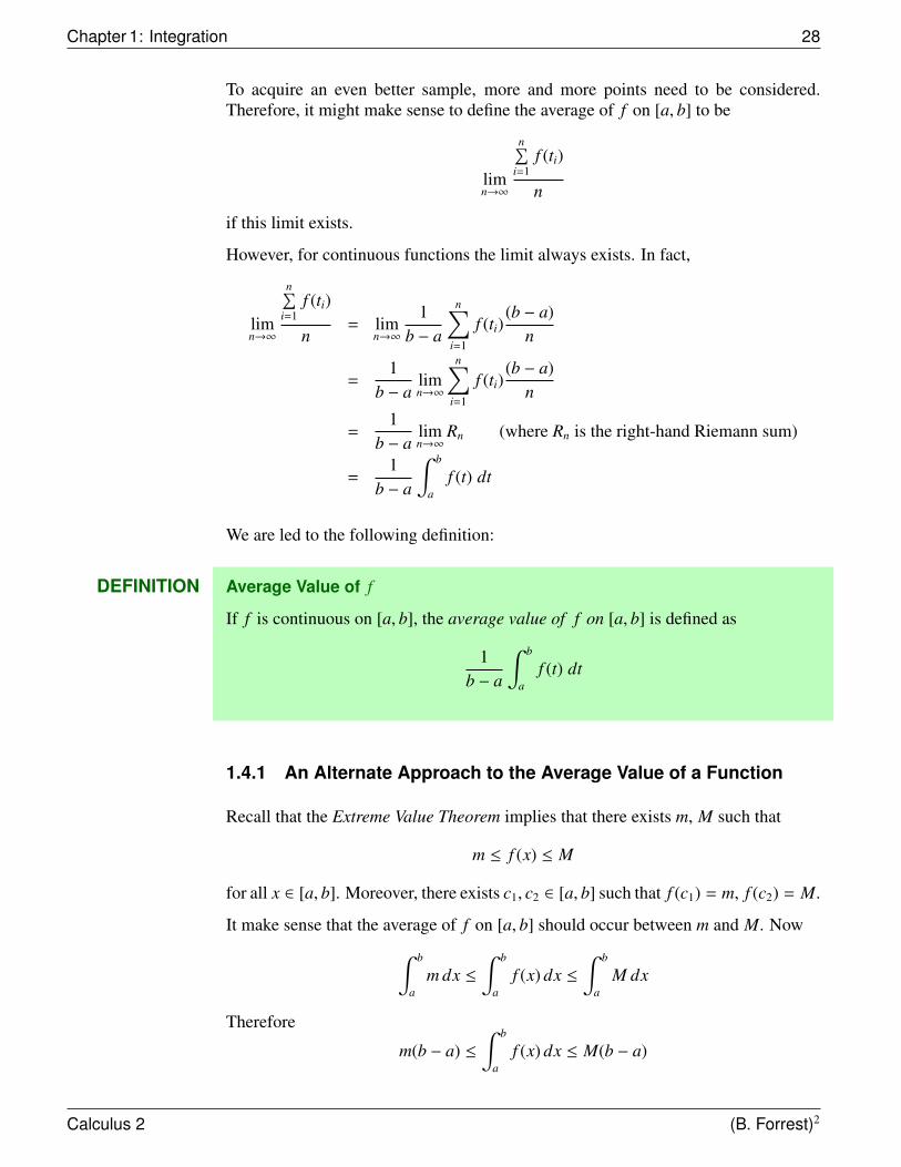
One approach would be to take samplevalues of f and calculate the average ofthese samples as an estimate of theaverage value. However, we need asatisfactory method for obtaining suchsamples. One method to ensure that thechoice of sample points is asrepresentative as possible is to use theregular n-partition
a = t0 < t1 < · · · < tn−1 < tn = b
where ti = a +i(b − a)
nand consider
n∑i=1
f (ti)
n.
a bti
f
f (ti)
Calculus 2 (B. Forrest)2
Chapter 1: Integration 28
To acquire an even better sample, more and more points need to be considered.Therefore, it might make sense to define the average of f on [a, b] to be
limn→∞
n∑i=1
f (ti)
n
if this limit exists.
However, for continuous functions the limit always exists. In fact,
limn→∞
n∑i=1
f (ti)
n= lim
n→∞
1b − a
n∑i=1
f (ti)(b − a)
n
=1
b − alimn→∞
n∑i=1
f (ti)(b − a)
n
=1
b − alimn→∞
Rn (where Rn is the right-hand Riemann sum)
=1
b − a
∫ b
af (t) dt
We are led to the following definition:
DEFINITION Average Value of f
If f is continuous on [a, b], the average value of f on [a, b] is defined as
1b − a
∫ b
af (t) dt
1.4.1 An Alternate Approach to the Average Value of a Function
Recall that the Extreme Value Theorem implies that there exists m, M such that
m ≤ f (x) ≤ M
for all x ∈ [a, b]. Moreover, there exists c1, c2 ∈ [a, b] such that f (c1) = m, f (c2) = M.
It make sense that the average of f on [a, b] should occur between m and M. Now∫ b
am dx ≤
∫ b
af (x) dx ≤
∫ b
aM dx
Therefore
m(b − a) ≤∫ b
af (x) dx ≤ M(b − a)
Calculus 2 (B. Forrest)2

Section 1.4: The Average Value of a Function 29
Equivalently,
m ≤1
b − a
∫ b
af (x) dx ≤ M
Let α =1
b − a
∫ b
af (x) dx. Then
f (c1) ≤ α ≤ f (c2).
By the Intermediate Value Theorem, there exists c between c1 and c2 such that
f (c) = α =1
b − a
∫ b
af (x) dx
Geometrically, it follows that
Area R1 + Area R3 = Area R2
a b
c
R1
R2
y = f (x)
R3
α = f (c)
In other words, the area above α = f (c) but below y = f (x) equals the area belowα = f (c) but above y = f (x).
Once again it makes sense to say that
f (c) =1
b − a
∫ b
af (x) dx
represents the average value of the function f on [a, b].
The following theorem is established.
THEOREM 4 Average Value Theorem (Mean Value Theorem for Integrals)
Assume that f is continuous on [a, b].
Then there exists a ≤ c ≤ b such that
f (c) =1
b − a
∫ b
af (t) dt
Calculus 2 (B. Forrest)2

Chapter 1: Integration 30
Important Note:
If b < a and if f is continuous on [b, a], then there exists b < c < a with
f (c) =1
a − b
∫ a
bf (t)dt
=1
a − b
(−
∫ b
af (t)dt
)
=1
b − a
∫ b
af (t)dt
so the Average Value Theorem holds even if b < a.
You have now been presented with all of the background information required tounderstand the The Fundamental Theorem of Calculus. It is so named because it isone of the most important results in mathematics!
1.5 The Fundamental Theorem of Calculus (Part 1)
The goal in this section is to introduce the Fundamental Theorem of Calculus whichis attributed independently to Sir Issac Newton and to Gottfried Leibniz. As the namesuggests, this is perhaps the most important theorem in Calculus and many would ar-gue, one of the most important discoveries in the history of mathematics. Despite thislofty claim, the Fundamental Theorem is at its heart a simple rule of differentiation.However, from this simple rule, we can derive a method that will allow us to evaluatemany types of integrals without having to appeal to the complicated process involv-ing Riemann sums. Consequently, the Fundamental Theorem of Calculus enables usto link together differential calculus and integral calculus in a very profound way.
Let’s begin by assuming that the function f is continuous on an interval [a, b].
Let’s also define the integral function
G(x) =
∫ x
af (t) dt.
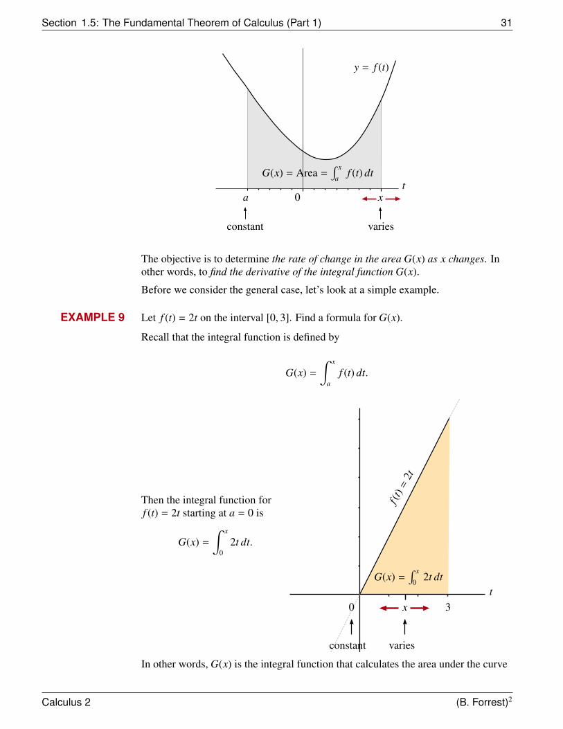
What does this integral function do? If f ≥ 0, then G(x) is the function thatcalculates the area under the graph of y = f (t) as x varies over an interval [a, b]starting from a.
Calculus 2 (B. Forrest)2
Section 1.5: The Fundamental Theorem of Calculus (Part 1) 31
y = f (t)
tx0a
G(x) = Area =∫ x
af (t) dt
constant varies
The objective is to determine the rate of change in the area G(x) as x changes. Inother words, to find the derivative of the integral function G(x).
Before we consider the general case, let’s look at a simple example.
EXAMPLE 9 Let f (t) = 2t on the interval [0, 3]. Find a formula for G(x).
Recall that the integral function is defined by
G(x) =
∫ x
af (t) dt.
Then the integral function forf (t) = 2t starting at a = 0 is
G(x) =
∫ x
02t dt.
f (t)
=2t
tx0
G(x) =∫ x
02t dt
constant varies
3
In other words, G(x) is the integral function that calculates the area under the curve
Calculus 2 (B. Forrest)2
Chapter 1: Integration 32
of f (t) = 2t as x varies over the interval [0, 3] starting at t = 0.
Let’s try to calculate the area under f (t) as t varies from x = 0, x = 1, x = 2 andx = 3. We will use these values to see if we can determine G(x).
Case x = 0:
If x = 0, we have that G(0) =∫ 0
02t dt = 0 since the limits of integration are
identical. (There is no area to calculate.) Thus we have the area under f (t) on theinterval [0, 0] is 0 and G(0) = 0 .
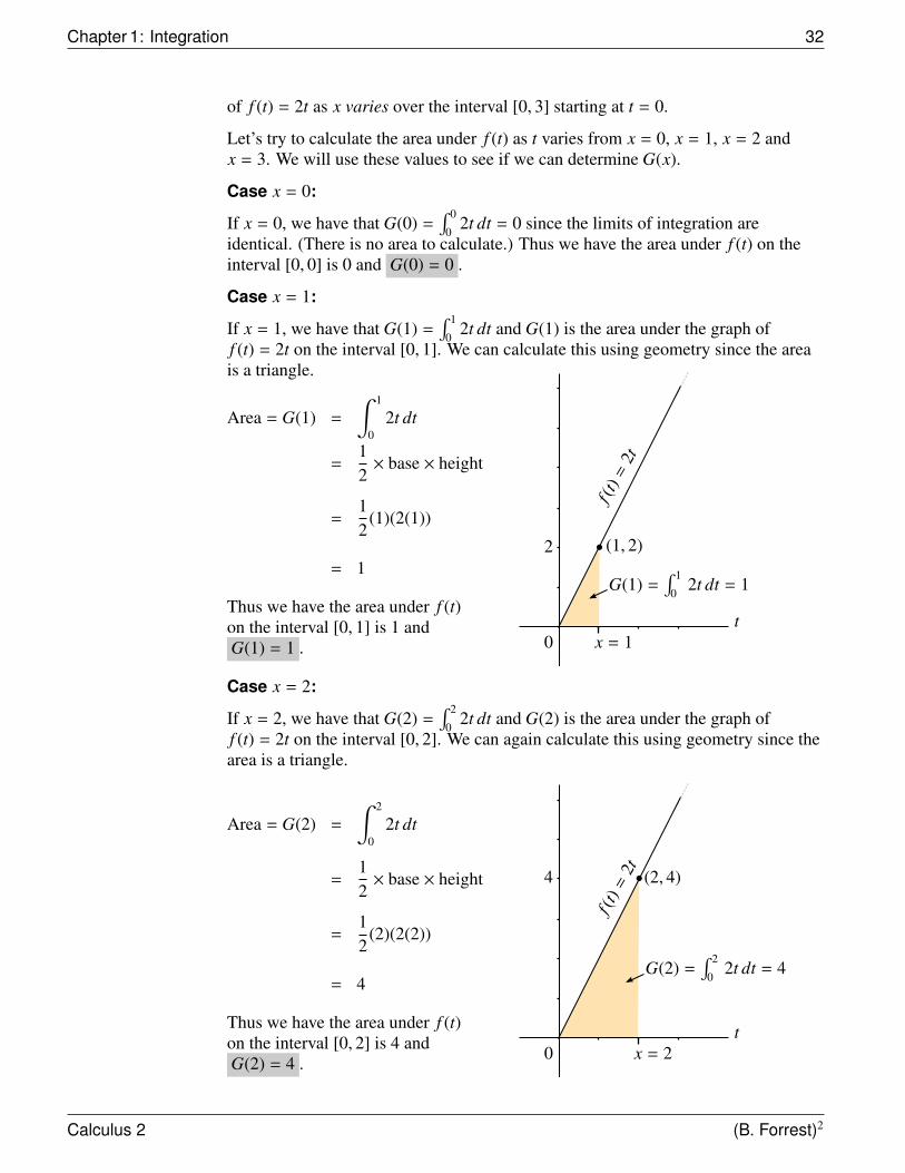
Case x = 1:
If x = 1, we have that G(1) =∫ 1
02t dt and G(1) is the area under the graph of
f (t) = 2t on the interval [0, 1]. We can calculate this using geometry since the areais a triangle.
Area = G(1) =
∫ 1
02t dt
=12× base × height
=12
(1)(2(1))
= 1
Thus we have the area under f (t)on the interval [0, 1] is 1 andG(1) = 1 .
f (t)
=2t
tx = 10
G(1) =∫ 1
02t dt = 1
(1, 2)2
Case x = 2:
If x = 2, we have that G(2) =∫ 2
02t dt and G(2) is the area under the graph of
f (t) = 2t on the interval [0, 2]. We can again calculate this using geometry since thearea is a triangle.
Area = G(2) =
∫ 2
02t dt
=12× base × height
=12
(2)(2(2))
= 4
Thus we have the area under f (t)on the interval [0, 2] is 4 andG(2) = 4 .
f (t)
=2t
tx = 20
G(2) =∫ 2
02t dt = 4
(2, 4)4
Calculus 2 (B. Forrest)2
Section 1.5: The Fundamental Theorem of Calculus (Part 1) 33
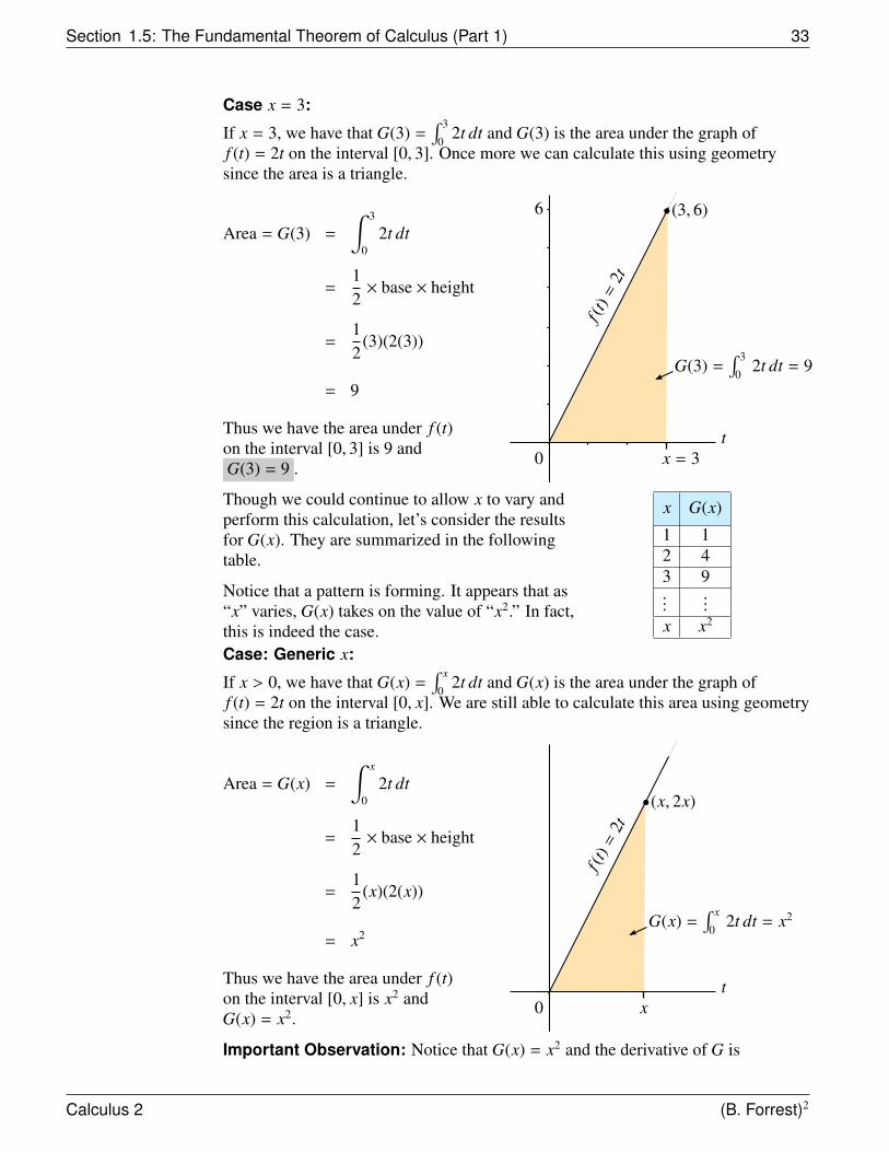
Case x = 3:
If x = 3, we have that G(3) =∫ 3
02t dt and G(3) is the area under the graph of
f (t) = 2t on the interval [0, 3]. Once more we can calculate this using geometrysince the area is a triangle.
Area = G(3) =
∫ 3
02t dt
=12× base × height
=12
(3)(2(3))
= 9
Thus we have the area under f (t)on the interval [0, 3] is 9 andG(3) = 9 .
f (t)
=2t
tx = 30
G(3) =∫ 3
02t dt = 9
(3, 6)6
Though we could continue to allow x to vary andperform this calculation, let’s consider the resultsfor G(x). They are summarized in the followingtable.
Notice that a pattern is forming. It appears that as“x” varies, G(x) takes on the value of “x2.” In fact,this is indeed the case.
x G(x)
1 12 43 9...
...x x2
Case: Generic x:
If x > 0, we have that G(x) =∫ x
02t dt and G(x) is the area under the graph of
f (t) = 2t on the interval [0, x]. We are still able to calculate this area using geometrysince the region is a triangle.
Area = G(x) =
∫ x
02t dt
=12× base × height
=12
(x)(2(x))
= x2
Thus we have the area under f (t)on the interval [0, x] is x2 andG(x) = x2.
f (t)
=2t
tx0
G(x) =∫ x
02t dt = x2
(x, 2x)
Important Observation: Notice that G(x) = x2 and the derivative of G is
Calculus 2 (B. Forrest)2

Chapter 1: Integration 34
G′(x) = 2x. In other words, we have just seen that
G′(x) = f (x).
This means thatG′(x) =
ddx
∫ x
0f (t) dt = f (x).
In the previous example, we were able to calculate the area geometrically because fwas a linear function and the region under the graph of f was always triangular.Normally we will not have an integrand that has its area calculated so easily. Wewill now discuss the case where f is a generic function.
Again we begin by assuming that f (t) ≥ 0is continuous on the interval [a, b] and letthe integral function be defined by
G(x) =
∫ x
af (t) dt.
In this case, G(x) represents the areabounded by the graph of f (t), the t-axis,and the lines t = a and t = x.
y = f (t)
tx0a
G(x) = Area =∫ x
af (t) dt
constant varies
The objective is to determine the rate of change in the area G(x) as x changes. Inother words, to find the derivative G′(x) of the integral function G(x).
First we increment x by adding asmall amount denoted by h. ThenG(x + h) is the area obtained byadding the first region G(x) withthe shaded area between the linest = x and t = x + h.
y = f (t)
tx0a
G(x)G(x + h)
x + h
h
Calculus 2 (B. Forrest)2
Section 1.5: The Fundamental Theorem of Calculus (Part 1) 35
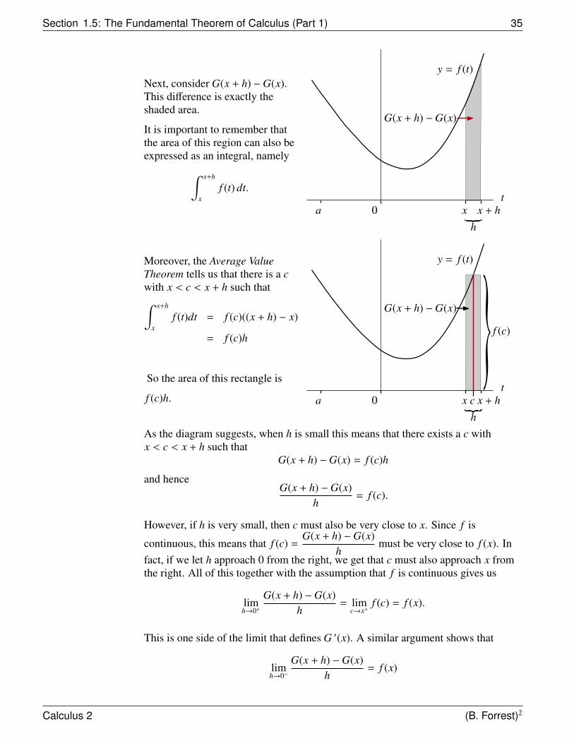
Next, consider G(x + h) −G(x).This difference is exactly theshaded area.
It is important to remember thatthe area of this region can also beexpressed as an integral, namely∫ x+h
xf (t) dt.
y = f (t)
tx0a
G(x + h) −G(x)
x + h
h
Moreover, the Average ValueTheorem tells us that there is a cwith x < c < x + h such that∫ x+h
xf (t)dt = f (c)((x + h) − x)
= f (c)h
So the area of this rectangle is
f (c)h.
y = f (t)
tx0a
G(x + h) −G(x)
x + h
hc
f (c)
As the diagram suggests, when h is small this means that there exists a c withx < c < x + h such that
G(x + h) −G(x) = f (c)h
and henceG(x + h) −G(x)
h= f (c).
However, if h is very small, then c must also be very close to x. Since f is
continuous, this means that f (c) =G(x + h) −G(x)
hmust be very close to f (x). In
fact, if we let h approach 0 from the right, we get that c must also approach x fromthe right. All of this together with the assumption that f is continuous gives us
limh→0+
G(x + h) −G(x)h
= limc→x+
f (c) = f (x).
This is one side of the limit that defines G ′(x). A similar argument shows that
limh→0−
G(x + h) −G(x)h
= f (x)
Calculus 2 (B. Forrest)2
Chapter 1: Integration 36
and hence thatlimh→0
G(x + h) −G(x)h
= f (x).
That is,G ′(x) = f (x).
Note: When we calculated the one-sided limit we made a number of assumptions.First, we assumed that f was continuous. This was used in two places. First, so thatwe could apply the Average Value Theorem to get that
G(x + h) −G(x)h
= f (c)
and second, to conclude thatlimc→x+
f (c) = f (x).
The other assumptions were that f (t) ≥ 0 and that the increment h was positive.
The assumption that f be continuous is essential, but the other two assumptionswere only for our convenience and they can actually be omitted. This gives us a verysimple rule of differentiation for integral functions, though a rule with a profoundimpact.
THEOREM 5 Fundamental Theorem of Calculus (Part 1) [FTC1]
Assume that f is continuous on an open interval I containing a point a. Let
G(x) =
∫ x
af (t) dt.
Then G(x) is differentiable at each x ∈ I and
G ′(x) = f (x).
Equivalently,
G ′(x) =ddx
∫ x
af (t) dt = f (x).
PROOF
Assume that G(x) =∫ x
af (t)dt and that f is continuous at x0 ∈ I. Let ε > 0. Then
there exists a δ > 0 so that if 0 < |c − x0| < δ, then
| f (c) − f (x0)| < ε.
Calculus 2 (B. Forrest)2
Section 1.5: The Fundamental Theorem of Calculus (Part 1) 37
Now let 0 < |x − x0| < δ. Then
G(x) −G(x0)x − x0
=
∫ x
af (t)dt −
∫ x0
af (t)dt
x − x0
=1
x − x0
∫ x
x0
f (t)dt
But then there exists a c between x and x0 with
f (c) =1
x − x0
∫ x
x0
f (t)dt
by the Average Value Theorem.
This means that if 0 < |x − x0| < δ, then since 0 < |c − x0| < δ as well∣∣∣∣∣ G(x) −G(x0)x − x0
− f (x0)∣∣∣∣∣ = | f (c) − f (x0) | < ε.
By the definition of a limit we get that
G′(x0) = limx→x0
G(x) −G(x0)x − x0
= f (x0).
NOTE
If we use Leibniz notation for derivatives, the Fundamental Theorem ofCalculus (Part 1) can be written as
ddx
∫ x
af (t) dt = f (x)
This equation roughly states that if you first integrate f and then differentiate theresult, you will return back to the original function f .
In the following example, a physical interpretation of the Fundamental Theorem ispresented.
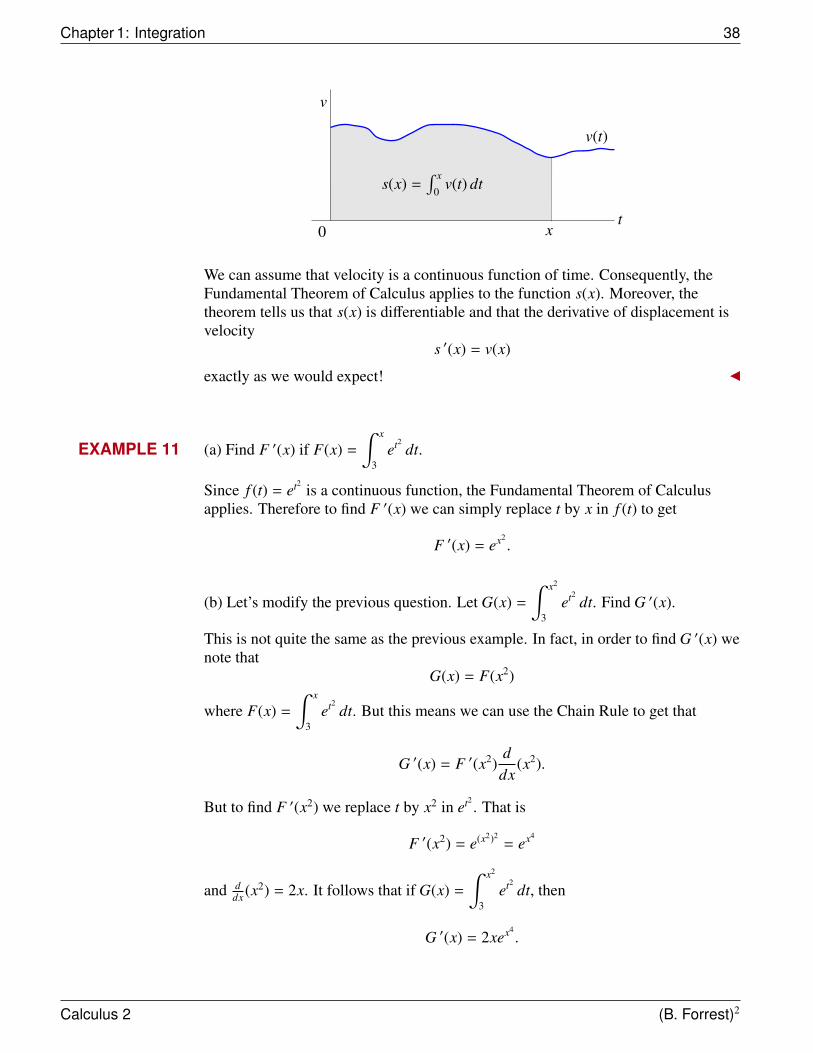
EXAMPLE 10 Assume that a vehicle travels forward along a straight road with a velocity at time tgiven by the function v(t). If we fix a starting point at t = 0, then we saw from thesection about Riemann sums that the displacement s(x) up to time t = x is the area
under the velocity graph. That is, s(x) =
∫ x
0v(t) dt.
Calculus 2 (B. Forrest)2
Chapter 1: Integration 38
0 xt
v(t)
s(x) =∫ x
0v(t) dt
v
We can assume that velocity is a continuous function of time. Consequently, theFundamental Theorem of Calculus applies to the function s(x). Moreover, thetheorem tells us that s(x) is differentiable and that the derivative of displacement isvelocity
s ′(x) = v(x)
exactly as we would expect!
EXAMPLE 11 (a) Find F ′(x) if F(x) =
∫ x
3et2 dt.
Since f (t) = et2 is a continuous function, the Fundamental Theorem of Calculusapplies. Therefore to find F ′(x) we can simply replace t by x in f (t) to get
F ′(x) = ex2.
(b) Let’s modify the previous question. Let G(x) =
∫ x2
3et2 dt. Find G ′(x).
This is not quite the same as the previous example. In fact, in order to find G ′(x) wenote that
G(x) = F(x2)
where F(x) =
∫ x
3et2 dt. But this means we can use the Chain Rule to get that
G ′(x) = F ′(x2)ddx
(x2).
But to find F ′(x2) we replace t by x2 in et2 . That is
F ′(x2) = e(x2)2= ex4
and ddx (x2) = 2x. It follows that if G(x) =
∫ x2
3et2 dt, then
G ′(x) = 2xex4.
Calculus 2 (B. Forrest)2
Section 1.5: The Fundamental Theorem of Calculus (Part 1) 39
There is an alternate method to solve this problem. First let u = x2 since the goal isto get an integral in the form
∫ x
a. Then
G ′(x) =ddx
∫ x2
3et2 dt
=ddx
∫ u
3et2 dt (substituting u = x2)
=ddu
(∫ u
3et2 dt
)dudx
(by the Chain Rule)
= eu2 dudx
(by FTCI)
= ex4· 2x
which is the same answer we calculated by the previous method.
In the statement of the Fundamental Theorem of Calculus, the lower limit of theintegral was always fixed. That is, it did not vary with x. We can now make ourexample even more complicated by letting the lower limit of the integral vary as afunction of x. Let
H(x) =
∫ x2
cos(x)et2 dt.
How would we find H ′(x)?
We can cleverly use the properties of the integral. In fact, we can write
H(x) =
∫ x2
cos(x)et2 dt =
∫ 3
cos(x)et2 dt +
∫ x2
3et2 dt.
Furthermore, we know that ∫ 3
cos(x)et2 dt = −
∫ cos(x)
3et2 dt
and this integral is in the form where we can use the Fundamental Theorem.Therefore, we have that
H(x) =
∫ x2
cos(x)et2 dt =
∫ x2
3et2dt −
∫ cos(x)
3et2dt.
If we now let
H1(x) =
∫ cos(x)
3et2 dt
thenH(x) = G(x) − H1(x)
where G(x) is defined as before. But then
H ′(x) = G ′(x) − H1′(x)
Calculus 2 (B. Forrest)2
Chapter 1: Integration 40
and we already know thatG ′(x) = 2xex4
.
This means that we only need to find H1′(x). To accomplish this we do exactly what
we did to find G′(x). We note that
H1(x) = F(cos(x))
so
H1′(x) = F ′(cos(x))
ddx
(cos(x))
= − sin(x)e(cos(x))2
Combining all of this together gives us that
H ′(x) = G ′(x) − H1′(x)
= 2xex4− (− sin(x)e(cos(x))2
)= 2xex4
+ sin(x)e(cos(x))2
The previous example leads us to an extended version of the Fundamental Theoremof Calculus.
THEOREM 6 Extended Version of the Fundamental Theorem of Calculus
Assume that f is continuous and that g and h are differentiable. Let
H(x) =
∫ h(x)
g(x)f (t) dt.
Then H(x) is differentiable and
H ′(x) = f (h(x))h ′(x) − f (g(x))g ′(x).
1.6 The Fundamental Theorem of Calculus (Part 2)
We have seen that the Fundamental Theorem of Calculus provides us with a simplerule for differentiating integral functions and so it provides the key link betweendifferential and integral calculus. However, we will soon see it also provides us witha powerful tool for evaluating integrals. First we must briefly review the topic ofantiderivatives from your study of differential calculus.
Calculus 2 (B. Forrest)2
Section 1.6: The Fundamental Theorem of Calculus (Part 2) 41
1.6.1 Antiderivatives
We know a number of techniques for calculating derivatives. In this section, we willreview how we can sometimes “undo” differentiation. That is, given a function f ,we will look for a new function F with the property that F ′(x) = f (x).
DEFINITION Antiderivative
Given a function f , an antiderivative is a function F such that
F ′(x) = f (x).
If F ′(x) = f (x) for all x in an interval I, we say that F is an antiderivative for f on I.
EXAMPLE 12 Let f (x) = x3. Let F(x) = x4
4 . Then
F ′(x) =4x4−1
4= x3 = f (x),
so F(x) = x4
4 is an antiderivative of f (x) = x3.
While the derivative of a function is always unique, this is not true of antiderivatives.In the previous example, if we let G(x) = x4
4 + 2, then G ′(x) = x3. Therefore, bothF(x) = x4
4 and G(x) = x4
4 + 2 are antiderivatives of the same function f (x) = x3.
This holds in greater generality: if F is an antiderivative of a given function f , thenso is G(x) = F(x) + C for every C ∈ R. A question naturally arises–are these all ofthe antiderivatives of f ?
To answer this question, we appeal to the Mean Value Theorem. Assume that F andG are both antiderivatives of a given function f . Let
H(x) = G(x) − F(x).
Then
H ′(x) = G ′(x) − F ′(x)= f (x) − f (x)= 0
for every x.
The Mean Value Theorem showed that there exists a constant C such that
H(x) = G(x) − F(x) = C.
But this means thatG(x) = F(x) + C.
Calculus 2 (B. Forrest)2

Chapter 1: Integration 42
It follows that once we have one antiderivative F of a function f , we can find all ofthe antiderivatives by considering all functions of the form
G(x) = F(x) + C.
EXAMPLE 13 Let f (x) = x3. Find all of the antiderivatives of f .
We have already seen that F(x) = x4
4 is an antiderivative of x3. It follows that thefamily of all antiderivatives consists of functions of the form
G(x) =x4
4+ C
for C ∈ R.
Notation: We will denote the family of antiderivatives of a function f by∫f (x) dx.
For example, ∫x3 dx =
x4
4+ C.
The symbol ∫f (x) dx
is called the indefinite integral of f . The function f is called the integrand.
We will be content to find the antiderivatives of many of the basic functions that wewill use in this course. The next theorem tells us how to find the antiderivatives ofone of the most important classes of functions, the powers of x.
THEOREM 7 Power Rule for Antiderivatives
If α , −1, then ∫xα dx =
xα+1
α + 1+ C.
To see that this theorem is correct we need only differentiate. Since
ddx
(xα+1
α + 1+ C) = xα,
we have found all of the antiderivatives.
The following table lists the antiderivatives of several basic functions. You can usedifferentiation to verify each antiderivative.
Calculus 2 (B. Forrest)2
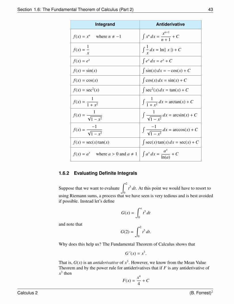
Section 1.6: The Fundamental Theorem of Calculus (Part 2) 43
Integrand Antiderivative
f (x) = xn where n , −1∫
xn dx =xn+1
n + 1+ C
f (x) =1x
∫ 1x
dx = ln(| x |) + C
f (x) = ex∫
ex dx = ex + C
f (x) = sin(x)∫
sin(x) dx = − cos(x) + C
f (x) = cos(x)∫
cos(x) dx = sin(x) + C
f (x) = sec2(x)∫
sec2(x) dx = tan(x) + C
f (x) =1
1 + x2
∫ 11 + x2 dx = arctan(x) + C
f (x) =1
√1 − x2
∫ 1√
1 − x2dx = arcsin(x) + C
f (x) =−1√
1 − x2
∫ −1√
1 − x2dx = arccos(x) + C
f (x) = sec(x) tan(x)∫
sec(x) tan(x) dx = sec(x) + C
f (x) = ax where a > 0 and a , 1∫
ax dx =ax
ln(a)+ C
1.6.2 Evaluating Definite Integrals
Suppose that we want to evaluate∫ 2
0t3 dt. At this point we would have to resort to
using Riemann sums, a process that we have seen is very tedious and is best avoidedif possible. Instead let’s define
G(x) =
∫ x
0t3 dt
and note that
G(2) =
∫ 2
0t3 dt.
Why does this help us? The Fundamental Theorem of Calculus shows that
G ′(x) = x3.
That is, G(x) is an antiderivative of x3. However, we know from the Mean ValueTheorem and by the power rule for antiderivatives that if F is any antiderivative ofx3 then
F(x) =x4
4+ C
Calculus 2 (B. Forrest)2
Chapter 1: Integration 44
where C is some unknown constant. This means that
G(x) =
∫ x
0t3 dt =
x4
4+ C1
for some constant C1. If we knew C1 we would be done.
To determine C1 we know that
G(x) =
∫ x
0t3 dt =
x4
4+ C1
and
0 =
∫ 0
0t3 dt = G(0) =
04
4+ C1 = C1
so
G(x) =
∫ x
0t3 dt =
x4
4.
Finally, ∫ 2
0t3 dt = G(2) =
24
4= 4.
Question: Did we really need to find C1?
To answer this question we will make the following very important observation.
Key Observation: Let F and G be any two antiderivatives of the same function f .Then
G(x) = F(x) + C
Let a, b ∈ R. Then
G(b) −G(a) = (F(b) + C) − (F(a) + C)= F(b) − F(a)
Assume that f is continuous. We want to calculate∫ b
af (t) dt.
LetG(x) =
∫ x
af (t) dt.
Then the Fundamental Theorem of Calculus (Part1) shows that G is anantiderivative of f . Moreover, if F is any other antiderivative of f , then∫ b
af (t) dt = G(b)
= G(b) −G(a) (since G(a) =
∫ a
af (t) dt = 0)
= F(b) − F(a)
Calculus 2 (B. Forrest)2
Section 1.6: The Fundamental Theorem of Calculus (Part 2) 45
For example, to evaluate ∫ 2
0t3 dt,
we know that
F(x) =x4
4is an antiderivative for f (x) = x3. It follows from the previous observation that∫ 2
0t3 dt = F(2) − F(0)
=24
4−
04
4
= 4
This example shows us how we can now use antiderivatives to help us evaluate anintegral, which is further evidence that the two branches of calculus–differentiationand integration–are intimately linked. Moreover, the observation we have just madeestablishes a procedure for evaluating definite integrals that works in generalbecause of the Fundamental Theorem of Calculus (Part 1). This is summarized inthe following theorem. Because this procedure is essentially a consequence of theFundamental Theorem of Calculus (Part 1), this result is called the FundamentalTheorem of Calculus (Part 2).
THEOREM 8 Fundamental Theorem of Calculus (Part 2) [FTC2]
Assume that f is continuous and that F is any antiderivative of f .
Then ∫ b
af (t)dt = F(b) − F(a).
Going forward, it is no longer necessary to use Riemann sums to calculate integrals;we can use the Fundamental Theorem of Calculus (Part 2) instead.
We will now introduce the following notation to use in evaluating integrals. Wewrite
F(x)∣∣∣∣ba
= F(b) − F(a)
to indicate that the value of the antiderivative F evaluated at b minus the value of theantiderivative F evaluated at a.
Calculus 2 (B. Forrest)2
Chapter 1: Integration 46
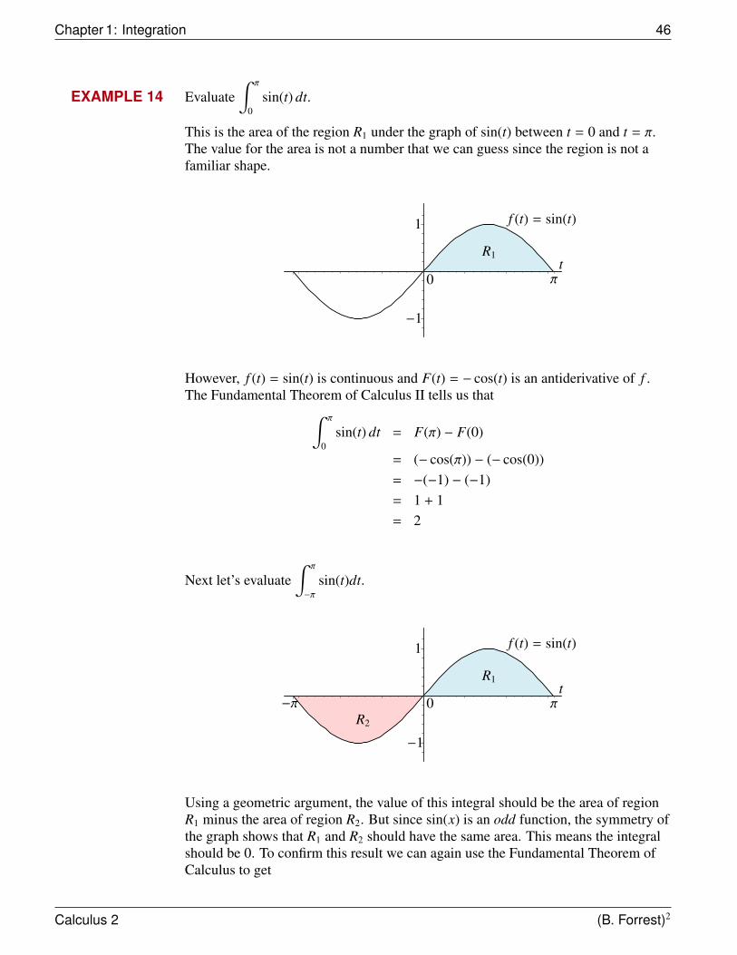
EXAMPLE 14 Evaluate∫ π
0sin(t) dt.
This is the area of the region R1 under the graph of sin(t) between t = 0 and t = π.The value for the area is not a number that we can guess since the region is not afamiliar shape.
t
f (t) = sin(t)
R1
π
−1
1
0
However, f (t) = sin(t) is continuous and F(t) = − cos(t) is an antiderivative of f .The Fundamental Theorem of Calculus II tells us that∫ π
0sin(t) dt = F(π) − F(0)
= (− cos(π)) − (− cos(0))= −(−1) − (−1)= 1 + 1= 2
Next let’s evaluate∫ π
−π
sin(t)dt.
t
f (t) = sin(t)
R1
R2
π−π
−1
1
0
Using a geometric argument, the value of this integral should be the area of regionR1 minus the area of region R2. But since sin(x) is an odd function, the symmetry ofthe graph shows that R1 and R2 should have the same area. This means the integralshould be 0. To confirm this result we can again use the Fundamental Theorem ofCalculus to get
Calculus 2 (B. Forrest)2
Section 1.7: Change of Variables 47
∫ π
−π
sin(t) dt = (− cos(t)) |π−π
= (− cos(π)) − (− cos(−π))= (−(−1)) − (−(−1))= 1 − 1= 0
as expected.
Before we end this section, it is important that we emphasize the difference betweenthe meaning of ∫ b
af (t) dt and
∫f (t)dt
The first expression, ∫ b
af (t) dt
is called a definite integral. It represents a number that is defined as a limit ofRiemann sums.
The second expression, ∫f (t)dt
is called an indefinite integral. It represents the family of all functions that areantiderivatives of the given function f .
The use of similar notation for these very distinct objects is a direct consequence ofthe Fundamental Theorem of Calculus.
1.7 Change of Variables
While the Fundamental Theorem of Calculus is a very powerful tool for evaluatingdefinite integrals, the ability to use this tool is limited by our ability to identifyantiderivatives.
Finding antiderivatives is essentially “undoing differentiation.” While we haveantiderivative rules for polynomials and for some of the trigonometric andexponential functions, unfortunately it is generally much more difficult to findantiderivatives than it is to differentiate. For example, it is actually possible to prove(using sophisticated algebra that is well beyond this course) that the function
f (x) = ex2
does not have an antiderivative that we can state in terms of any functions withwhich we are familiar. This is a serious flaw in our process since, for example,
Calculus 2 (B. Forrest)2

Chapter 1: Integration 48
integrals involving such functions are required for statistical analysis. However, inthe next section a method is presented that can undo the most complex rule ofdifferentiation—the Chain Rule. By using this technique, you will be able toevaluate many more types of integrals.
1.7.1 Change of Variables for the Indefinite Integral
Assume that we have two functions f (u) and h(u) with
h ′(u) = f (u).
Then using the notation of antiderivatives we have∫f (u) du = h(u) + C.
Now let u = g(x) be a function of x. The Chain Rule says that if H(x) = h(g(x)) then
H′(x) = h ′(g(x))g ′(x)= f (g(x))g ′(x) (since h ′(u) = f (u))
Integrating both sides we get∫f (g(x))g ′(x) dx = H(x) + C
= h(g(x)) + C (since H(x) = h(g(x)))
However, this shows that∫f (g(x))g ′(x) dx = h(g(x)) + C
= h(u)∣∣∣∣u=g(x)
+ C
=
∫f (u) du
∣∣∣∣u=g(x)
where the symbol h(u)∣∣∣∣u=g(x)
means replace u by g(x) in the formula for h(u) and the
symbol∫
f (u) du∣∣∣∣u=g(x)
means replace u by g(x) once the antiderivative has been
found.
Let’s see how this works in practice.
EXAMPLE 15 Evaluate∫
2xex2dx.
In this case, note that if we let u = g(x) = x2, then g ′(x) = 2x. If we also letf (u) = eu, then
Calculus 2 (B. Forrest)2
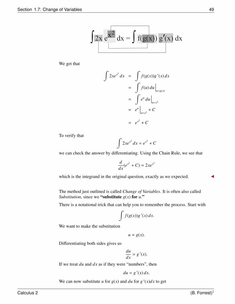
Section 1.7: Change of Variables 49
2x e dx = f(g(x)) g (x) dxx2
We get that ∫2xex2
dx =
∫f (g(x))g ′(x) dx
=
∫f (u) du
∣∣∣∣u=g(x)
=
∫eu du
∣∣∣∣u=x2
= eu∣∣∣∣u=x2
+ C
= ex2+ C
To verify that ∫2xex2
dx = ex2+ C
we can check the answer by differentiating. Using the Chain Rule, we see that
ddx
(ex2+ C) = 2xex2
which is the integrand in the original question, exactly as we expected.
The method just outlined is called Change of Variables. It is often also calledSubstitution, since we “substitute g(x) for u.”
There is a notational trick that can help you to remember the process. Start with∫f (g(x))g ′(x) dx.
We want to make the substitution
u = g(x).
Differentiating both sides gives us
dudx
= g ′(x).
If we treat du and dx as if they were “numbers”, then
du = g ′(x) dx.
We can now substitute u for g(x) and du for g ′(x)dx to get
Calculus 2 (B. Forrest)2
Chapter 1: Integration 50
f(g(x)) g (x) dx = f(u) duu = g(x)
which is the Change of Variables formula.
It is important to note that the expression
du = g ′(x) dx
does not really have any mathematical meaning. None the less, this trick works andit is how integrals are actually computed in practice.
EXAMPLE 16 Evaluate∫
2x1 + x2 dx by making the substitution u = 1 + x2.
Ifu = 1 + x2,
thendu = 2x dx.
Substituting u = 1 + x2 and du = 2x dx into the original integral gives us∫2x
1 + x2 dx =
∫1u
du∣∣∣∣u=1+x2
but ∫1u
du = ln(| u |) + C.
Hence ∫2x
1 + x2 dx =
∫1u
du∣∣∣∣u=1+x2
= ln(| u |)∣∣∣∣u=1+x2
+ C
= ln(| 1 + x2 |) + C
= ln(1 + x2) + C
where the last equality holds since 1 + x2 > 0.
Until you become comfortable with this technique it is always a good idea to checkyour answer by differentiating. (In this case, the answer is f (x) = ln(1 + x2) + C.Differentiating we get f ′(x) = 1
(1+x2)ddx (1 + x2) = 2x
(1+x2) which is the originalintegrand for the question . . . so the answer is correct!)
Calculus 2 (B. Forrest)2
Section 1.7: Change of Variables 51
EXAMPLE 17 Evaluate∫
x cos(x2) dx.
In this example, using the substitution u = x2 causes us to be out by a constantfactor. However, this will not be a problem by proceeding as follows.
The method of substitution suggests letting u = x2 and f (u) = cos(u). In this casewe have
du = 2x dx (∗)
However, it appears that we really wanted
du = x dx.
We can rearrange equation (∗) to get that
12
du = x dx.
Then substituting 12 du for x dx and u for x2 we get∫
x cos(x2) dx =
∫12
cos(u) du∣∣∣∣u=x2
=12
∫cos(u) du
∣∣∣∣u=x2
=12
sin(u)∣∣∣∣u=x2
+ C
=12
sin(x2) + C
You should check that this answer is correct by differentiating 12 sin(x2) + C to
ensure it equals the integrand.
The next unusual substitution allows us to evaluate an important trigonometricintegral.
EXAMPLE 18 Evaluate∫
sec(θ) dθ.
At first glance this does not appear to be an integral that can be evaluated by usingsubstitution. However, we can make the following clever observation:
sec(θ) = sec(θ)(sec(θ) + tan(θ)sec(θ) + tan(θ)
)
=sec2(θ) + sec(θ) tan(θ)
sec(θ) + tan(θ)
Calculus 2 (B. Forrest)2
Chapter 1: Integration 52
Let u = sec(θ) + tan(θ). Then
du = sec(θ) tan(θ) + sec2(θ) dθ.
It follows that ∫sec(θ) dθ =
∫sec2(θ) + sec(θ) tan(θ)
sec(θ) + tan(θ)dθ
=
∫duu
The antiderivative rules give us that
∫duu
= ln(|u|) + C.
Letting u = sec(θ) + tan(θ), we get
∫sec(θ) dθ = ln(| sec(θ) + tan(θ)|) + C.
1.7.2 Change of Variables for the Definite Integral
We can also use the Change of Variables technique for definite integrals. However,for the case of definite integrals, we must be careful with the limits of integration.
Suppose that we want to evaluate∫ b
af (g(x))g ′(x) dx
where f and g ′ are continuous functions. We have just seen that if h(u) is anantiderivative of f (u), then
H(x) = h(g(x))
is an antiderivative off (g(x))g ′(x).
This means that we can apply the Fundamental Theorem of Calculus to get
∫ b
af (g(x))g ′(x) dx = H(b) − H(a)
= h(g(b)) − h(g(a))
Calculus 2 (B. Forrest)2
Section 1.7: Change of Variables 53
However, since h ′(u) = f (u), the Fundamental Theorem of Calculus also shows usthat ∫ g(b)
g(a)f (u) du = h(g(b)) − h(g(a)).
Combining these two results shows that∫ b
af (g(x))g ′(x) dx =
∫ g(b)
g(a)f (u) du.
THEOREM 9 Change of Variables
Assume that g′(x) is continuous on [a, b] and f (u) is continuous on g([a, b]),
then
∫ x=b
x=af (g(x))g ′(x) dx =
∫ u=g(b)
u=g(a)f (u) du.
Let’s see what this theorem implies by looking at some examples. Notice that youmust give special attention to the limits of integration.
EXAMPLE 19 Evaluate∫ 4
2(5x − 6)3 dx.
Let u = g(x) = 5x − 6. Then f (u) = u3. Since
du = g ′(x) dx = 5 dx,
we have15
du = dx.
The Change of Variables Theorem shows us that
∫ 4
2(5x − 6)3 dx =
∫ u=g(b)
u=g(a)f (u) du
=
∫ u=g(4)
u=g(2)u3 1
5du
Now since g(a) = g(2) = 5(2) − 6 = 4 and g(b) = g(4) = 5(4) − 6 = 14 we have
Calculus 2 (B. Forrest)2
Chapter 1: Integration 54
=15
∫ 14
4u3 du
=15
(14
u4)∣∣∣∣∣∣14
4
=1
20(144 − 44)
= 1908
EXAMPLE 20 Evaluate∫ 1
0
x dx√
x2 + 1.
Let u = g(x) = x2 + 1. Then
du = g ′(x) dx = 2x dx,
so12
du = x dx.
We also have,
f (u) =1√
u= u−
12 .
The Change of Variables Theorem shows us that∫ 1
0
x dx√
x2 + 1=
∫ u=g(b)
u=g(a)f (u) du
=
∫ u=g(1)
u=g(0)(u−
12 ) (
12
du)
Now since g(a) = g(0) = 02 + 1 = 1 and g(b) = g(1) = 12 + 1 = 2 we have
=12
∫ 2
1u−
12 du
=12
(2 u
12) ∣∣∣∣2
1
= 212 − 1
12
=√
2 − 1� 0.41
Calculus 2 (B. Forrest)2
Section 1.7: Change of Variables 55
EXAMPLE 21 Evaluate∫ π
4
0−2 cos2(2x) sin(2x) dx.
Let u = g(x) = cos(2x) and f (u) = u2. Then since
du = g ′(x) dx = −2 sin(2x) dx
the Change of Variables Theorem shows us that
∫ π4
0−2 cos2(2x) sin(2x) dx =
∫ u=g(b)
u=g(a)f (u) du
=
∫ cos(2( π4 ))
cos(2(0))u2 du
=
∫ cos( π2 )
cos(0)u2 du
=
∫ 0
1u2 du
=u3
3
∣∣∣∣∣∣01
=03
3−
13
3
=−13
Calculus 2 (B. Forrest)2
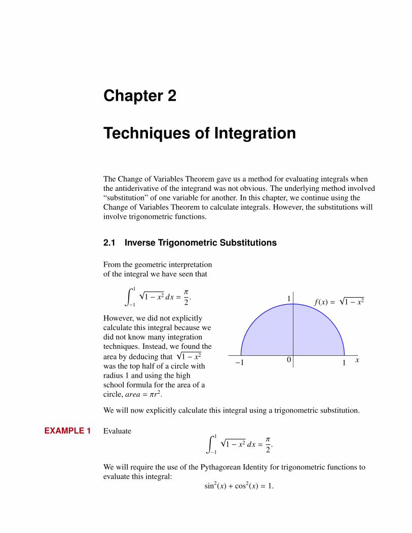
Chapter 2
Techniques of Integration
The Change of Variables Theorem gave us a method for evaluating integrals whenthe antiderivative of the integrand was not obvious. The underlying method involved“substitution” of one variable for another. In this chapter, we continue using theChange of Variables Theorem to calculate integrals. However, the substitutions willinvolve trigonometric functions.
2.1 Inverse Trigonometric Substitutions
From the geometric interpretationof the integral we have seen that∫ 1
−1
√1 − x2 dx =
π
2.
However, we did not explicitlycalculate this integral because wedid not know many integrationtechniques. Instead, we found thearea by deducing that
√1 − x2
was the top half of a circle withradius 1 and using the highschool formula for the area of acircle, area = πr2.
x10−1
1 f (x) =√
1 − x2
We will now explicitly calculate this integral using a trigonometric substitution.
EXAMPLE 1 Evaluate ∫ 1
−1
√1 − x2 dx =
π
2.
We will require the use of the Pythagorean Identity for trigonometric functions toevaluate this integral:
sin2(x) + cos2(x) = 1.
Section 2.1: Inverse Trigonometric Substitutions 57
Letx = sin(u)
for−π
2≤ u ≤
π
2.
This might seem like an unusual suggestion since the substitution rule usually asksus to make a substitution of the form
u = g(x).
However, we have actually done this! To see why this is the case, recall that on theinterval [−π2 ,
π2 ], the function x = sin(u) has a unique inverse given by u = arcsin(x).
In fact, we are really making the substitution u = arcsin(x) and this method is calledinverse trigonometric substitution.
Using the substitution x = sin(u), the integrand
√1 − x2
becomes √1 − sin2(u) =
√cos2(u)
= | cos(u) |= cos(u)
where the last equality holds since cos(u) ≥ 0 on the interval [−π2 ,π2 ].
We can differentiatex = sin(u)
to getdx = cos(u) du.
This means that ∫ 1
−1
√1 − x2 dx =
∫ arcsin(1)
arcsin(−1)cos(u) cos(u) du
=
∫ π2
− π2
cos2(u) du
Note: Since u = g(x) = arcsin(x), we have that the new limits of integration areu = g(−1) = arcsin(−1) = −π2 and u = g(1) = arcsin(1) = π
2 .
To finish the integral calculation we need to use the following trigonometric identity:
cos2(u) =1 + cos(2u)
2.
Calculus 2 (B. Forrest)2
Chapter 2: Techniques of Integration 58
This means that ∫ 1
−1
√1 − x2 dx =
∫ π2
− π2
cos2(u) du
=
∫ π2
− π2
1 + cos(2u)2
du
=
∫ π2
− π2
12
du +
∫ π2
−π2
cos(2u)2
du
=12
∫ π2
− π2
1 du +12
∫ π2
− π2
cos(2u) du
The first integral is
12
∫ π2
− π2
1 du =12
u∣∣∣∣∣ π2− π2
=12
(π
2−
(−π
2
))=
π
2
To evaluate the second integral
12
∫ π2
− π2
cos(2u) du
use the substitutionv = 2u
withdv = 2 du.
If u = π2 , then v = π and if u = −π2 , then v = −π. We can apply the Change of
Variable Formula to get that
12
∫ π2
− π2
cos(2u) du =12
∫ π
−π
cos(v)dv2
=14
∫ π
−π
cos(v) dv
=14
sin(v)∣∣∣∣∣π−π
=14
(sin(π) − sin(−π))
Calculus 2 (B. Forrest)2
Section 2.1: Inverse Trigonometric Substitutions 59
=14
(0 − 0)
= 0
We have then shown that∫ 1
−1
√1 − x2 dx =
∫ π2
− π2
cos2(u) du
=12
∫ π2
− π2
1 du +12
∫ π2
− π2
cos(2u) du
=π
2+ 0
=π
2
which agrees with our previous argument.
REMARK
In general, there are three main classes of inverse trigonometric substitutions. Thefirst class are integrals with integrands of the form
√a2 − b2x2.
The substitution, based on the pythagorean identity sin2(x) + cos2(x) = 1, is
bx = a sin(u).
The previous example demonstrated this class.
The second class of trigonometric substitution covers integrands of the form√
a2 + b2x2.
The substitution is based on the identity sec2(x) − 1 = tan2(x) and is given by
bx = a tan(u).
The third type of substitution covers integrands of the form√
b2x2 − a2.
The substitution is again based on the identity sec2(x) − 1 = tan2(x) and is given by
bx = a sec(u).
Calculus 2 (B. Forrest)2
Chapter 2: Techniques of Integration 60
The next example illustrates the third class of trigonometric substitution.
EXAMPLE 2 Evaluate∫ 3
√3
√4x2 − 9
xdx.
Consider the expression√
4x2 − 9. We could try to substitute u = 4x2 − 9 giving usdu = 8x dx or dx = du
8x . This would have worked if the integral had been∫ 3
√3
x√
4x2 − 9 dx
because then the x’s would cancel. (You should verify this statement.) However, thesubstitution u = 4x2 − 9 does not help in this example.
Since the numerator of the integrand takes the form√
b2x2 − a2 where b = 2 anda = 3, the correct substitution is
2x = 3 sec(u)
or
u = arcsec(2x3
)where 0 ≤ u < π
2 .
Since 4x2 = (2x)2, we have (3 sec(u))2 = 9 sec2(u). Therefore,√
4x2 − 9 =√
9 sec2(u) − 9
=√
9(sec2(u) − 1)
= 3√
sec2(u) − 1
= 3√
tan2(u)= 3 | tan(u) |= 3 tan(u)
with the last equality holding since if 0 ≤ u < π2 , then tan(u) ≥ 0.
Since 2x = 3 sec(u) we also have that
2dx = 3 sec(u) tan(u) du
ordx =
32
sec(u) tan(u) du.
Next, we must find the new limits of integration for this integral. When x =√
3, wehave
sec(u) =2√
33
=2√
3
Calculus 2 (B. Forrest)2
Section 2.1: Inverse Trigonometric Substitutions 61
This means that
cos(u) =1
sec(u)
=
√3
2
The only angle u with 0 ≤ u < π2 and cos(u) =
√3
2 , is u = π6 . (Verify this fact by
considering the Unit Circle.)
Similarly, if x = 3, then sec(u) = 2 so cos(u) = 12 . This means that u = π
3 .
Finally, we must also substitute for the x in the denominator of the integrand
√4x2 − 9
x
since it has not cancelled in the substitution. However, we know that x = 32 sec(u).
Combining everything we know gives us
∫ 3
√3
√4x2 − 9
xdx =
∫ π3
π6
3 tan(u)32 sec(u)
(32
)sec(u) tan(u) du
= 3∫ π
3
π6
tan2(u) du
= 3∫ π
3
π6
(sec2(u) − 1) du
= 3(tan(u) − u)∣∣∣∣ π3π
6
= 3(tan
(π
3
)−π
3
)− 3
(tan
(π
6
)−π
6
)=
(3√
3 − π)−
(3√
3−π
2
)= 2
√3 −
π
2
In general, when presented with an integral that you are unsure of how to solve, beaware of the following classes of trigonometric substitutions to see if they can helpyou evaluate the integral.
Calculus 2 (B. Forrest)2
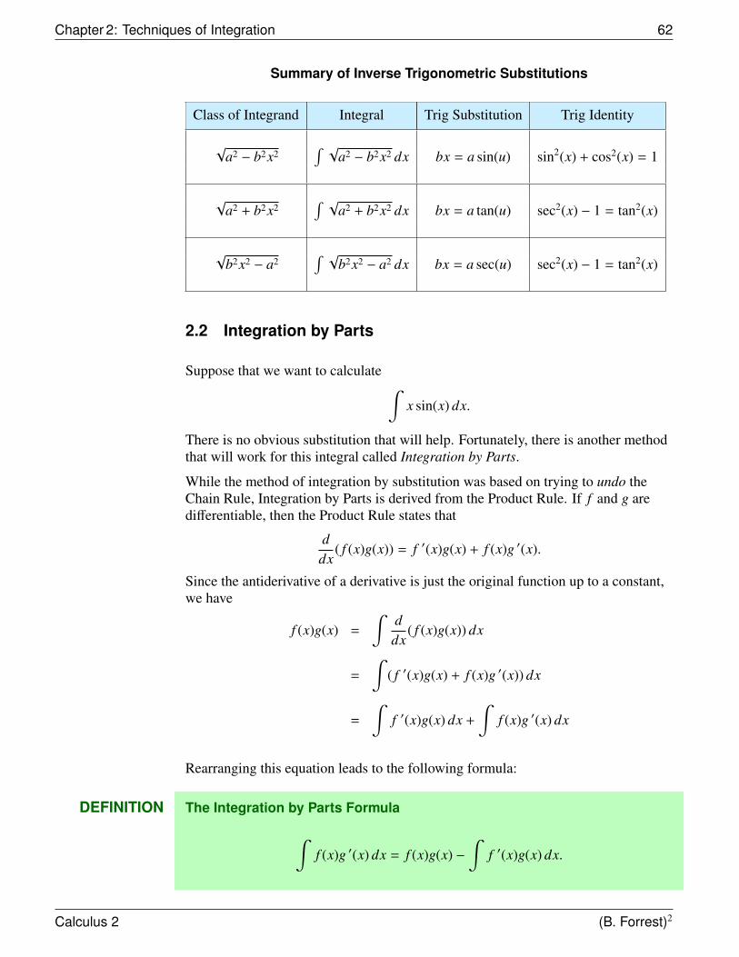
Chapter 2: Techniques of Integration 62
Summary of Inverse Trigonometric Substitutions
Class of Integrand Integral Trig Substitution Trig Identity
√a2 − b2x2
∫ √a2 − b2x2 dx bx = a sin(u) sin2(x) + cos2(x) = 1
√a2 + b2x2
∫ √a2 + b2x2 dx bx = a tan(u) sec2(x) − 1 = tan2(x)
√b2x2 − a2
∫ √b2x2 − a2 dx bx = a sec(u) sec2(x) − 1 = tan2(x)
2.2 Integration by Parts
Suppose that we want to calculate ∫x sin(x) dx.
There is no obvious substitution that will help. Fortunately, there is another methodthat will work for this integral called Integration by Parts.
While the method of integration by substitution was based on trying to undo theChain Rule, Integration by Parts is derived from the Product Rule. If f and g aredifferentiable, then the Product Rule states that
ddx
( f (x)g(x)) = f ′(x)g(x) + f (x)g ′(x).
Since the antiderivative of a derivative is just the original function up to a constant,we have
f (x)g(x) =
∫ddx
( f (x)g(x)) dx
=
∫( f ′(x)g(x) + f (x)g ′(x)) dx
=
∫f ′(x)g(x) dx +
∫f (x)g ′(x) dx
Rearranging this equation leads to the following formula:
DEFINITION The Integration by Parts Formula
∫f (x)g ′(x) dx = f (x)g(x) −
∫f ′(x)g(x) dx.
Calculus 2 (B. Forrest)2
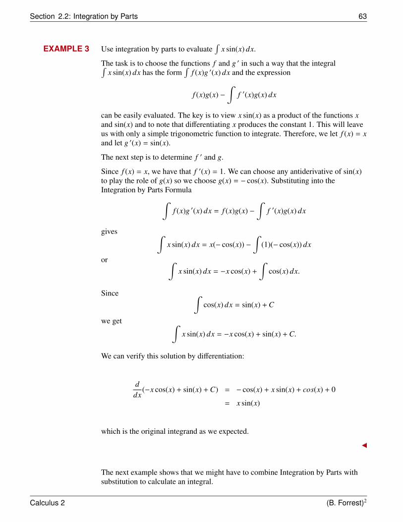
Section 2.2: Integration by Parts 63
EXAMPLE 3 Use integration by parts to evaluate∫
x sin(x) dx.
The task is to choose the functions f and g ′ in such a way that the integral∫x sin(x) dx has the form
∫f (x)g ′(x) dx and the expression
f (x)g(x) −∫
f ′(x)g(x) dx
can be easily evaluated. The key is to view x sin(x) as a product of the functions xand sin(x) and to note that differentiating x produces the constant 1. This will leaveus with only a simple trigonometric function to integrate. Therefore, we let f (x) = xand let g ′(x) = sin(x).
The next step is to determine f ′ and g.
Since f (x) = x, we have that f ′(x) = 1. We can choose any antiderivative of sin(x)to play the role of g(x) so we choose g(x) = − cos(x). Substituting into theIntegration by Parts Formula∫
f (x)g ′(x) dx = f (x)g(x) −∫
f ′(x)g(x) dx
gives ∫x sin(x) dx = x(− cos(x)) −
∫(1)(− cos(x)) dx
or ∫x sin(x) dx = −x cos(x) +
∫cos(x) dx.
Since ∫cos(x) dx = sin(x) + C
we get ∫x sin(x) dx = −x cos(x) + sin(x) + C.
We can verify this solution by differentiation:
ddx
(−x cos(x) + sin(x) + C) = − cos(x) + x sin(x) + cos(x) + 0
= x sin(x)
which is the original integrand as we expected.
The next example shows that we might have to combine Integration by Parts withsubstitution to calculate an integral.
Calculus 2 (B. Forrest)2
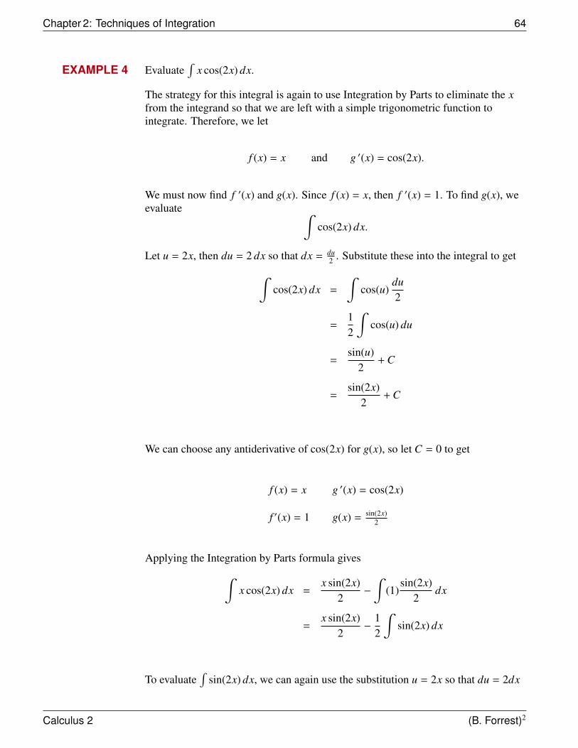
Chapter 2: Techniques of Integration 64
EXAMPLE 4 Evaluate∫
x cos(2x) dx.
The strategy for this integral is again to use Integration by Parts to eliminate the xfrom the integrand so that we are left with a simple trigonometric function tointegrate. Therefore, we let
f (x) = x and g ′(x) = cos(2x).
We must now find f ′(x) and g(x). Since f (x) = x, then f ′(x) = 1. To find g(x), weevaluate ∫
cos(2x) dx.
Let u = 2x, then du = 2 dx so that dx = du2 . Substitute these into the integral to get∫
cos(2x) dx =
∫cos(u)
du2
=12
∫cos(u) du
=sin(u)
2+ C
=sin(2x)
2+ C
We can choose any antiderivative of cos(2x) for g(x), so let C = 0 to get
f (x) = x g ′(x) = cos(2x)
f ′(x) = 1 g(x) =sin(2x)
2
Applying the Integration by Parts formula gives∫x cos(2x) dx =
x sin(2x)2
−
∫(1)
sin(2x)2
dx
=x sin(2x)
2−
12
∫sin(2x) dx
To evaluate∫
sin(2x) dx, we can again use the substitution u = 2x so that du = 2dx
Calculus 2 (B. Forrest)2
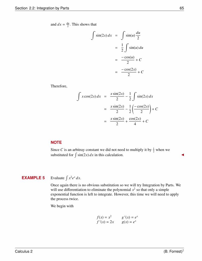
Section 2.2: Integration by Parts 65
and dx = du2 . This shows that∫
sin(2x) dx =
∫sin(u)
du2
=12
∫sin(u) du
=− cos(u)
2+ C
=− cos(2x)
2+ C
Therefore, ∫x cos(2x) dx =
x sin(2x)2
−12
∫sin(2x) dx
=x sin(2x)
2−
12
(− cos(2x)
2
)+ C
=x sin(2x)
2+
cos(2x)4
+ C
NOTE
Since C is an arbitray constant we did not need to multiply it by 12 when we
substituted for∫
sin(2x) dx in this calculation.
EXAMPLE 5 Evaluate∫
x2ex dx.
Once again there is no obvious substitution so we will try Integration by Parts. Wewill use differentiation to eliminate the polynomial x2 so that only a simpleexponential function is left to integrate. However, this time we will need to applythe process twice.
We begin with
f (x) = x2 g ′(x) = ex
f ′(x) = 2x g(x) = ex
Calculus 2 (B. Forrest)2
Chapter 2: Techniques of Integration 66
Applying the Integration by Parts formula gives∫x2ex dx = x2ex −
∫(2x)ex dx
= x2ex − 2∫
xex dx
We are left to evaluate∫
xex dx. This integral is again an ideal candidate forIntegration by Parts. Let
f (x) = x g ′(x) = ex
f ′(x) = 1 g(x) = ex
to get ∫xex dx = xex −
∫(1)ex dx
= xex −
∫ex dx
= xex − ex + C
We can now substitute for∫
xex dx to get,∫x2ex dx = x2ex − 2
∫xex dx
= x2ex − 2(xex − ex) + C= x2ex − 2xex + 2ex + C
REMARK
You might guess from the previous example that the integral∫x3ex dx
could be evaluated with three applications of Integration by Parts since we wouldhave to differentiate three times to eliminate the polynomial x3.
The next example illustrates another class of functions that are ideally suited toIntergation by Parts.
Calculus 2 (B. Forrest)2
Section 2.2: Integration by Parts 67
EXAMPLE 6 Evaluate∫
ex sin(x) dx.
This example presents a different type of problem than any of the previousexamples. It is not clear which function should be f and which should be g ′ sinceno amount of differentiation will eliminate either ex or sin(x). In this case, we willsimply choose g ′ to be the easiest function to integrate. For this example, thismeans that g ′(x) = ex. Therefore, we have
f (x) = sin(x) g ′(x) = ex
f ′(x) = cos(x) g(x) = ex
The Integration by Parts Formula gives∫ex sin(x) dx = ex sin(x) −
∫ex cos(x) dx.
This result may appear somewhat discouraging because there is no reason to believethat the integral ∫
ex cos(x) dx
is any easier to evaluate than the original integral∫
ex sin(x) dx.
The key is to apply the formula again to the integral∫
ex cos(x) dx with
f (x) = cos(x) g ′(x) = ex
f ′(x) = − sin(x) g(x) = ex
to get ∫ex cos(x) dx = ex cos(x) −
∫ex(− sin(x)) dx
= ex cos(x) +
∫ex(sin(x)) dx
We seem to be left with having to evaluate∫
ex(sin(x)) dx which is exactly wherewe started! However, if we substitute ex cos(x) +
∫ex(sin(x)) dx for
∫ex cos(x) dx
in the original equation something interesting happens. We get∫ex sin(x) dx = ex sin(x) −
∫ex cos(x) dx
= ex sin(x) − (ex cos(x) +
∫ex(sin(x)) dx)
= ex sin(x) − ex cos(x) −∫
ex(sin(x)) dx
Calculus 2 (B. Forrest)2
Chapter 2: Techniques of Integration 68
You will notice that∫
ex(sin(x)) dx appears on both sides of our equation but withopposite signs. We can treat this expression as some unknown variable and thengather like terms as we would in basic algebra. This means adding
∫ex(sin(x)) dx to
both sides of the expression to get
2(∫
ex(sin(x)) dx)
= ex sin(x) − ex cos(x).
Divide by 2 so that ∫ex(sin(x)) dx =
ex sin(x) − ex cos(x)2
.
At this point, you might notice that the constant of integration is missing in thisexpression yet all general antiderivatives must include a constant. In fact, this is dueto the way that the Integration by Parts formula handles these constants (theconstants are always there implicitly even if they are not explicitly written). Wehave identified just one possible antiderivative for the function ex sin(x). To state allof the antiderivatives we know that we simply add an arbitrary constant so that∫
ex(sin(x)) dx =ex sin(x) − ex cos(x)
2+ C.
Observation: The method we outlined in the previous example works because ofthe cyclic nature of the derivatives for sin(x) and ex. This statement is also true ofboth cos(x) and ex. Therefore, it should not be surprising to discover that∫
ex cos(x) dx can be evaluated in the same manner.
Important Note: In summary, the Integration by Parts formula is ideally suited toevaluating integrals of the following types:
•∫
xn cos(x) dx
•∫
xn sin(x) dx
•∫
xnex dx
•∫
ex cos(x) dx
•∫
ex sin(x) dx
However, there are other more unusual examples of integrals that are also suitablefor Integration by Parts.
Calculus 2 (B. Forrest)2
Section 2.2: Integration by Parts 69
EXAMPLE 7 Evaluate ∫arctan(x) dx.
At first glance this integral does not seem to be of the form∫f (x)g ′(x) dx
since there is no product in the integrand. However, the key is to rewrite theintegrand as
arctan(x) = (1) arctan(x).
Since arctan(x) is easy to differentiate and 1 is easily integrated, we can now tryIntegration by Parts with f (x) = arctan(x) and g′(x) = 1. This leads to
f (x) = arctan(x) g ′(x) = 1f ′(x) = 1
1+x2 g(x) = x
Applying the Integration by Parts formula gives∫arctan(x) dx = x arctan(x) −
∫x(
11 + x2
)dx
= x arctan(x) −∫
x1 + x2 dx
The integral∫
x1+x2 dx can be handled by substitution. Let u = 1 + x2 so du = 2xdx
and dx = du2x . Substitution gives∫
x1 + x2 dx =
∫xu
du2x
=12
∫1u
du
=ln(| u |)
2+ C
=ln(| 1 + x2 |)
2+ C
=ln(1 + x2)
2+ C
since 1 + x2 > 0.
Calculus 2 (B. Forrest)2

Chapter 2: Techniques of Integration 70
Returning to the original equation, we have∫arctan(x) dx = x arctan(x) −
∫x
1 + x2 dx
= x arctan(x) −(ln(1 + x2)
2
)+ C
We can check this answer by differentiating:
ddx
(x arctan(x) −
ln(1 + x2)2
+ C)
= arctan(x) + x(
11 + x2
)−
12
(1
1 + x2
)(2x)
= arctan(x) +x
1 + x2 −x
1 + x2
= arctan(x)
exactly as expected.
EXAMPLE 8 Evaluate∫
ln(x) dx.
Notice
ln(x) = 1 · ln(x)↑ ↑
g ′(x) f (x)
This gives
f (x) = ln(x) g ′(x) = 1
f ′(x) = 1x g(x) = x
Applying the Integration by Parts Formula∫ln(x) dx = x ln(x) −
∫x(1x
)dx
= x ln(x) −∫
1 dx
= x ln(x) − x + C
It is important to be cautious when trying to evaluate an integral. For example, the
Calculus 2 (B. Forrest)2
Section 2.3: Partial Fractions 71
integral ∫xex2
dx
appears to be a candidate for Integration by Parts. However, this is not the case.Instead, it can be evaluated by using the substitution u = x2.
The Integration by Parts Formula can also be applied to definite integrals. Thefollowing theorem is a direct consequence of combining the Integration by Partsformula with the Fundamental Theorem of Calculus.
THEOREM 1 Integration by Parts
Assume that f and g are such that both f ′ and g ′ are continuous on an intervalcontaining a and b. Then∫ b
af (x)g ′(x) dx = f (x)g(x)|ba −
∫ b
af ′(x)g(x) dx.
EXAMPLE 9 Evaluate∫ 1
0xex dx.
Letf (x) = x g ′(x) = ex
f ′(x) = 1 g(x) = ex
Integration by Parts shows that∫ 1
0xex dx = xex
∣∣∣∣10−
∫ 1
0ex dx
= [e − 0] − ex∣∣∣∣10
= e − [e − 1]= 1
2.3 Partial Fractions
Recall that a rational function is a function of the form
f (x) =p(x)q(x)
where p and q are polynomials. In this section, we will discuss a method forintegrating rational functions called Partial Fractions. We will illustrate this methodwith an example.
Calculus 2 (B. Forrest)2
Chapter 2: Techniques of Integration 72
EXAMPLE 10 Evaluate∫
1x2−1dx.
Step 1:
First factor the denominator to get that
1x2 − 1
=1
(x − 1)(x + 1).
Step 2:
Find constants A and B so that
1(x − 1)(x + 1)
=A
x − 1+
Bx + 1
(*)
To find A and B, we multiply both sides of the identity (∗) by (x − 1)(x + 1) to get
1 = A(x + 1) + B(x − 1) (**)
The two roots of the denominator were x = 1 and x = −1. If we substitute x = 1 intoequation (**), we have
1 = A(1 + 1) + B(1 − 1)
or1 = 2A.
Therefore,
A =12
.
If we then substitute x = −1 into equation (**), we get
1 = A(−1 + 1) + B(−1 − 1)
or1 = −2B
andB = −
12
.
Using these values of A and B we have
1x2 − 1
=1
(x − 1)(x + 1)=
12
x − 1+−1
2
x + 1.
Therefore ∫1
x2 − 1dx =
12
∫1
x − 1dx −
12
∫1
x + 1dx.
Recall that ∫1
x − adx = ln(| x − a |) + C.
Calculus 2 (B. Forrest)2
Section 2.3: Partial Fractions 73
Hence ∫1
x2 − 1dx =
12
∫1
x − 1dx −
12
∫1
(x + 1)dx
=12
ln(| x − 1 |) −12
ln(| x + 1 |) + C
=12
ln(| x − 1 || x + 1 |
)+ C
since ln(b) − ln(a) = ln(
ba
).
The method we have just outlined required us to separate the function f (x) = 1x2−1
into rational functions with first degree denominators. This is called a partialfraction decomposition of f .
DEFINITION Type I Partial Fraction Decomposition
Assume thatf (x) =
p(x)q(x)
where p and q are polynomials such that
1. degree(p(x)) < degree(q(x)) = k,
2. q(x) can be factored into the product of linear terms each with distinct roots.That is
q(x) = a(x − a1)(x − a2)(x − a3) · · · (x − ak)
where the ai’s are unique and none of the ai’s are roots of p(x).
Then there exists constants A1, A2, A3, · · · , Ak such that
f (x) =1a
[A1
x − a1+
A2
x − a2+
A3
x − a3+ · · · +
Ak
x − ak
]
we say that f admits a Type I Partial Fraction Decomposition.
Key Observation: The existence of the constants A1, A2, · · · , Ak follows fromsome basic algebra. However, what is important to us is that if the rational functionf (x) =
p(x)q(x) has a Type I Decomposition, then it is easy to find its integral.
Calculus 2 (B. Forrest)2
Chapter 2: Techniques of Integration 74
THEOREM 2 Integration of Type I Partial Fractions
Assume that f (x) =p(x)q(x) admits a Type I Partial Fraction Decomposition of the form
f (x) =1a
[A1
x − a1+
A2
x − a2+ · · · +
Ak
x − ak
].
Then∫f (x) dx =
1a
[∫A1
x − a1dx +
∫A2
x − a2dx + · · · +
∫Ak
x − akdx
]=
1a
[A1 ln(| x − a1 |) + A2 ln(| x − a2 |)) + · · · + Ak ln(| x − ak |)] + C
EXAMPLE 11 Evaluate∫
x + 2x(x − 1)(x − 3)
dx.
In this case, p(x) = x + 2 and q(x) = x(x − 1)(x − 3). Notice that1 = degree(p(x)) < degree(q(x)) = 3. Since q(x) has the distinct roots 0, 1 and 3, wehave a Type I Decomposition. Therefore, there are constants A, B, and C such that
x + 2x(x − 1)(x − 3)
=Ax
+B
x − 1+
Cx − 3
.
Step 1: Cross-multiply to get
x + 2 = A(x − 1)(x − 3) + B(x)(x − 3) + C(x)(x − 1) (*)
Step 2: To find the constants we will substitute each of the roots into the identity(*). If x = 0, then
0 + 2 = A(0 − 1)(0 − 3) + B(0)(0 − 3) + C(0)(0 − 1)
or2 = 3A.
HenceA =
23
.
Let x = 1 to get
1 + 2 = A(1 − 1)(1 − 3) + B(1)(1 − 3) + C(1)(1 − 1).
Therefore,3 = −2B
Calculus 2 (B. Forrest)2
Section 2.3: Partial Fractions 75
so thatB = −
32
.
Finally, with x = 3
3 + 2 = A(3 − 1)(3 − 3) + B(3)(3 − 3) + C(3)(3 − 1)
so5 = 6C
andC =
56
.
Notice that when we substitute the root a j into identity (*), we get back thecoefficient A j corresponding to this root.
This means thatx + 2
x(x − 1)(x − 3)=
23
x+−3
2
x − 1+
56
x − 3.
Therefore∫x + 2
x(x − 1)(x − 3)dx =
23
∫1x
dx −32
∫1
x − 1dx +
56
∫1
x − 3dx
=23
ln(| x |) −32
ln(| x − 1 |) +56
ln(| x − 3 |) + c
DEFINITION Type II Partial Fraction Decomposition
Assume thatf (x) =
p(x)q(x)
where p(x) and q(x) are polynomials such that
1. degree(p(x)) < degree(q(x)) = k,
2. q(x) can be factored into the product of linear terms with non-distinct roots.That is
q(x) = a(x − a1)m1(x − a2)m2(x − a3)m3 · · · (x − al)ml
where at least one of the m j’s is greater than 1.
We say that f admits a Type II Partial Fraction Decomposition.
In this case, the partial fraction decomposition can be built as follows.
Calculus 2 (B. Forrest)2
Chapter 2: Techniques of Integration 76
Each expression (x − a j)m j in the factorization of q(x) will contribute m j terms to thedecomposition, one for each power of x − a j from 1 to m j, which when combinedwill be of the form
p(x)q(x)
=
l∑j=1
A j,1
x − a j+
A j,2
(x − a j)2 +A j,3
(x − a j)3 + · · · +A j,m j
(x − a j)m j.
The number m j is called the multiplicity of the root a j.
EXAMPLE 12 Evaluate∫
1x2(x − 1)
dx.
In this case, p(x) = 1 and q(x) = x2(x − 1). The roots of q(x) are 0 and 1 and sincethe root 0 has multiplicity 2, this is a Type II Partial Fraction. Therefore, we can findconstants A, B and C such that
1x2(x − 1)
=Ax
+Bx2 +
Cx − 1
.
To find the constants A, B and C, we follow a similar procedure.
Step 1: Cross-multiply to get
1 = Ax(x − 1) + B(x − 1) + Cx2 (*)
Step 2: Substitute the roots x = 0 and x = 1 into identity (*).
If x = 0, then1 = A(0)(0 − 1) + B(0 − 1) + C(02)
or1 = −B
soB = −1.
Notice that substituting x = 0 only gave us the coefficient of the term with thehighest power of x in the decomposition.
Next, let x = 1. Then
1 = A(1)(1 − 1) + B(1 − 1) + C(12)
and hence1 = C.
Step 3: We have not yet found the coefficient A. There are a number of methods wecould use to find A. We could, for example, substitute into the identity (*) any value
Calculus 2 (B. Forrest)2
Section 2.3: Partial Fractions 77
other than 0 and 1 and use the fact that we already know B and C to solve for A. Forexample, if we let x = 2, we have
1 = A(2)(2 − 1) + B(2 − 1) + C(22)
or1 = 2A + B + 4C.
Substituting B = −1 and C = 1 gives
1 = 2A − 1 + 4
or−2 = 2A.
HenceA = −1.
Perhaps an easier method is to compare coefficients. If we expand the expressionson the right-hand side of identity (*) we get
1 = A(x2 − x) + B(x − 1) + C(x2) = (A + C)x2 + (B − A)x − B.
We can rewrite this as
0x2 + 0x + 1 = (A + C)x2 + (B − A)x − B.
Since the two sides must agree for all x, they must both be the same polynomial.This means that the coefficients must be equal. In particular, the coefficients of x2
must agree so that0 = A + C
orA = −C.
Since C = 1, this tells us thatA = −1.
Therefore, ∫1
x2(x − 1)dx =
∫Ax
dx +
∫Bx2 dx +
∫C
x − 1dx
=
∫−1x
dx +
∫−1x2 dx +
∫1
x − 1dx
= −
∫1x
dx −∫
1x2 dx +
∫1
x − 1dx
= − ln(| x |) +1x
+ ln(| x − 1 |) + c
Calculus 2 (B. Forrest)2
Chapter 2: Techniques of Integration 78
since ∫1x2 dx =
∫x−2 dx
=x−1
(−1)+ c
= −1x
+ c
Unfortunately, not all polynomials factor over the real numbers into products oflinear terms. For example, the polynomial x2 + 1 cannot be factored any further.This is an example of an irreducible quadratic. In fact, a quadratic ax2 + bx + c isirreducible if its discriminant b2 − 4ac < 0.
However, the Fundamental Theorem of Algebra shows that every polynomial q(x)factors in the form
q(x) = a(p1(x))m1(p2(x))m2(p3(x))m3 · · · (pk(x))mk
where each pi(x) is either of the form (x − a) or it is an irreducible quadratic of theform x2 + bx + c.
DEFINITION Type III Partial Fraction Decomposition
Let f (x) =p(x)q(x) be a rational function with degree(p(x)) < degree(q(x)), but q(x)
does not factor into linear terms. We say that f admits a Type III Partial FractionDecomposition.
In this case, the partial fraction decomposition can be built as follows:
Suppose that q(x) has an irreducible factor x2 + bx + c with multiplicity m. Then thisfactor will contribute terms of the form
B1x + C1
x2 + bx + c+
B2x + C2
(x2 + bx + c)2 + · · · +Bmx + Cm
(x2 + bx + c)m
to the decomposition.
The linear terms are handled exactly as they were in the previous cases.
Note: We will not consider the case where m > 1 for some irreducible quadratic inevaluating integrals of rational functions with Type III Partial FractionDecompositions.
The method for finding the constants in a Type III Partical Fraction Decompositionis very similar to that of the first two types. We illustrate this with an example.
Calculus 2 (B. Forrest)2
Section 2.3: Partial Fractions 79
EXAMPLE 13 Evaluate∫
1x3 + x
dx.
First observe thatf (x) =
1x3 + x
=1
x(x2 + 1)so there will be constants A, B and C such that
f (x) =1
x3 + x=
1x(x2 + 1)
=Ax
+Bx + Cx2 + 1
.
Step 1: To find the constants, we begin by cross-multiplying to obtain the identity
1 = A(x2 + 1) + (Bx + C)x (*)
Step 2: Substitute x = 0, the only Real root, to find the coefficient A. This gives
1 = A(02 + 1) + (B(0) + C)(0)
orA = 1.
Step 3: The remaining constants are found by comparing coefficients. Expandingthe identity (*) gives
1 = (A + B)x2 + Cx + A.
Comparing the coefficients of x2 gives
0 = A + B
orB = −A
Since A = 1, we getB = −1.
Comparing the coefficients of x gives
C = 0.
Therefore,1
x(x2 + 1)=
1x−
xx2 + 1
and ∫1
x3 + xdx =
∫1
x(x2 + 1)dx
=
∫1x
dx −∫
xx2 + 1
dx
= ln(| x |) −∫
xx2 + 1
dx
Calculus 2 (B. Forrest)2
Chapter 2: Techniques of Integration 80
To finish the calculation, we use the substitution u = x2 + 1, so du = 2x dx anddx = du
2x to get ∫x
x2 + 1dx =
∫xu
du2x
=12
∫1u
du
=12
ln(| u |) + c
=12
ln(x2 + 1) + c
Putting this all together we get that∫1
x3 + xdx = ln(| x |) −
12
ln(x2 + 1) + c.
NOTE
1. Since C = 0 in the previous example, the integral was straightforward toevaluate. Unfortunately, this is not the case for most Type III Partial Fractions.
2. All of the Partial Fraction Decompositions required the rational function tosatisfy degree(p(x)) < degree(q(x)). If this is not the case, then we need touse division of polynomials to find new polynomials r(x) and p1(x) such that
p(x)q(x)
= r(x) +p1(x)q(x)
with degree(p1(x)) < degree(q(x)).
2.4 Introduction to Improper Integrals
The Riemann Integral was defined for certain bounded functions on closed intervals[a, b]. In many applications, most notably for statistical and data analysis, we wantto be able to integrate functions over intervals of infinite length. However, at thispoint ∫ ∞
af (x) dx
Calculus 2 (B. Forrest)2
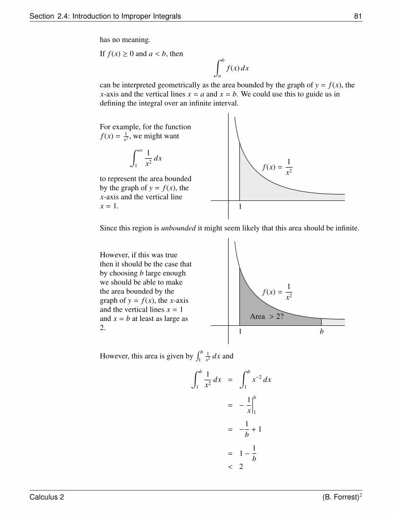
Section 2.4: Introduction to Improper Integrals 81
has no meaning.
If f (x) ≥ 0 and a < b, then ∫ b
af (x) dx
can be interpreted geometrically as the area bounded by the graph of y = f (x), thex-axis and the vertical lines x = a and x = b. We could use this to guide us indefining the integral over an infinite interval.
For example, for the functionf (x) = 1
x2 , we might want∫ ∞
1
1x2 dx
to represent the area boundedby the graph of y = f (x), thex-axis and the vertical linex = 1.
f (x) =1x2
1
Since this region is unbounded it might seem likely that this area should be infinite.
However, if this was truethen it should be the case thatby choosing b large enoughwe should be able to makethe area bounded by thegraph of y = f (x), the x-axisand the vertical lines x = 1and x = b at least as large as2.
f (x) =1x2
1 b
Area > 2?
However, this area is given by∫ b
11x2 dx and∫ b
1
1x2 dx =
∫ b
1x−2 dx
= −1x
∣∣∣∣∣b1
= −1b
+ 1
= 1 −1b
< 2
Calculus 2 (B. Forrest)2
Chapter 2: Techniques of Integration 82
This shows that no matter how large b is the area bounded by the graph of y = f (x),the x-axis and the vertical lines x = 1 and x = b will always be less than 2. In fact, itis always less than 1. This suggests that the original region should have finite areadespite the fact that it is unbounded.
We are now in a position similar to when we first defined the integral. While wehave an intuitive idea of what area means, we do not have a formal definition of areathat applies to such unbounded regions. One method to avoid this problem would beto define the area of the unbounded region as the limit of the bounded areas as bgoes to∞. That is
Area = limb→∞
∫ b
1
1x2 dx.
In particular, we would have
Area = limb→∞
∫ b
1
1x2 dx
= limb→∞
1 −1b
= 1
In this case, we would like to have∫ ∞
1
1x2 dx = 1.
This motivates the following definition:
DEFINITION Type I Improper Integral
1) Let f be integrable on [a, b] for each a ≤ b. We say that the Type I ImproperIntegral ∫ ∞
af (x) dx
converges if
limb→∞
∫ b
af (x) dx
exists. In this case, we write∫ ∞
af (x) dx = lim
b→∞
∫ b
af (x) dx.
Otherwise, we say that∫ ∞
af (x) dx diverges.
Calculus 2 (B. Forrest)2
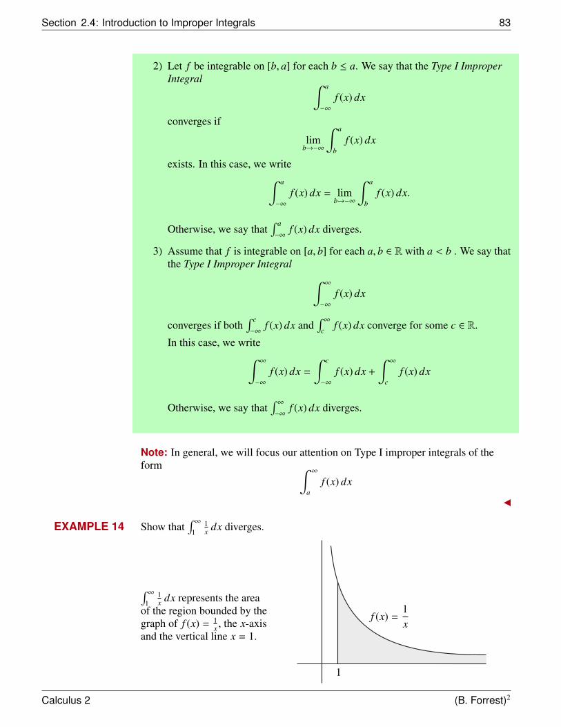
Section 2.4: Introduction to Improper Integrals 83
2) Let f be integrable on [b, a] for each b ≤ a. We say that the Type I ImproperIntegral ∫ a
−∞
f (x) dx
converges if
limb→−∞
∫ a
bf (x) dx
exists. In this case, we write∫ a
−∞
f (x) dx = limb→−∞
∫ a
bf (x) dx.
Otherwise, we say that∫ a
−∞f (x) dx diverges.
3) Assume that f is integrable on [a, b] for each a, b ∈ R with a < b . We say thatthe Type I Improper Integral ∫ ∞
−∞
f (x) dx
converges if both∫ c
−∞f (x) dx and
∫ ∞c
f (x) dx converge for some c ∈ R.
In this case, we write∫ ∞
−∞
f (x) dx =
∫ c
−∞
f (x) dx +
∫ ∞
cf (x) dx
Otherwise, we say that∫ ∞−∞
f (x) dx diverges.
Note: In general, we will focus our attention on Type I improper integrals of theform ∫ ∞
af (x) dx
EXAMPLE 14 Show that∫ ∞
11x dx diverges.
∫ ∞1
1x dx represents the area
of the region bounded by thegraph of f (x) = 1
x , the x-axisand the vertical line x = 1.
f (x) =1x
1
Calculus 2 (B. Forrest)2
Chapter 2: Techniques of Integration 84
This unbounded region looks very similar to the region discussed previously.However, this time ∫ ∞
1
1x
dx = limb→∞
∫ b
1
1x
dx
= limb→∞
ln(x)∣∣∣∣b1
= limb→∞
(ln(b) − ln(1))
= limb→∞
ln(b)
= ∞
This shows that∫ ∞
11x dx diverges to∞ and hence that the area of the region bounded
by the graph of f (x) = 1x , the x-axis and the vertical line x = 1 is also infinite.
We have seen that∫ ∞
11x2 dx converges while
∫ ∞1
1x dx diverges. More generally, we
have the following natural question.
Question: For which p does ∫ ∞
1
1xp dx
converge? In fact, the answer to this question will be crucial to our study of series.Since we already know what happens if p = 1, we can assume that p , 1.
To answer this question we require the following facts. If α > 0, then
limb→∞
bα = ∞
and if α < 0, thenlimb→∞
bα = 0.
For any b > 1, ∫ b
1
1xp dx =
∫ b
1x−p dx
=x−p+1
−p + 1
∣∣∣∣b1
=b1−p
1 − p−
1−p + 1
=b1−p
1 − p+
1p − 1
Calculus 2 (B. Forrest)2
Section 2.4: Introduction to Improper Integrals 85
If p < 1, then 1 − p > 0. Therefore,
limb→∞
b1−p
1 − p= ∞
since the exponent is positive. This means that
limb→∞
b1−p
1 − p+
1p − 1
= ∞
and hence that∫ ∞
11xp dx diverges.
However, if p > 1, then 1 − p < 0. This time since the exponent is negative,
limb→∞
b1−p
1 − p= 0
and hence
limb→∞
b1−p
1 − p+
1p − 1
=1
p − 1.
Therefore, if p > 1,∫ ∞
11xp dx converges and
∫ ∞
1
1xp dx =
1p − 1
.
This is summarized in the following important theorem.
THEOREM 3 p-Test for Type I Improper Integrals
The improper integral ∫ ∞
1
1xp dx
converges if and only if p > 1.
If p > 1, then ∫ ∞
1
1xp dx =
1p − 1
.
We end this section with one more important example of a convergent improperintegral.
Calculus 2 (B. Forrest)2
Chapter 2: Techniques of Integration 86
EXAMPLE 15 Evaluate∫ ∞
0e−x dx.
We have ∫ ∞
0e−x dx = lim
b→∞
∫ b
0e−x dx
= limb→∞−e−x
∣∣∣∣b0
= limb→∞
(−e−b + e0)
= limb→∞
(−e−b + 1)
= 1
since limb→∞−e−b = 0.
2.4.1 Properties of Type I Improper Integrals
Since the evaluation of an improper integral results from taking limits at∞, it makessense that improper integrals should inherit many of the properties of these types oflimits.
THEOREM 4 Properties of Type I Improper Integrals
Assume that∫ ∞
af (x) dx and
∫ ∞a
g(x) dx both converge.
1.∫ ∞
ac f (x) dx converges for each c ∈ R and∫ ∞
ac f (x) dx = c
∫ ∞
af (x) dx.
2.∫ ∞
a( f (x) + g(x)) dx converges and∫ ∞
a( f (x) + g(x)) dx =
∫ ∞
af (x) dx +
∫ ∞
ag(x) dx.
3. If f (x) ≤ g(x) for all a ≤ x, then∫ ∞
af (x) dx ≤
∫ ∞
ag(x) dx.
4. If a < c < ∞, then∫ ∞
cf (x) dx converges and∫ ∞
af (x) dx =
∫ c
af (x) dx +
∫ ∞
cf (x) dx.
Calculus 2 (B. Forrest)2
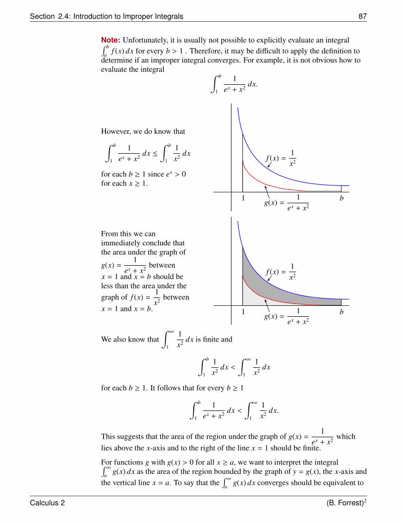
Section 2.4: Introduction to Improper Integrals 87
Note: Unfortunately, it is usually not possible to explicitly evaluate an integral∫ b
af (x) dx for every b > 1 . Therefore, it may be difficult to apply the definition to
determine if an improper integral converges. For example, it is not obvious how toevaluate the integral ∫ b
1
1ex + x2 dx.
However, we do know that∫ b
1
1ex + x2 dx ≤
∫ b
1
1x2 dx
for each b ≥ 1 since ex > 0for each x ≥ 1.
f (x) =1x2
1 bg(x) =1
ex + x2
From this we canimmediately conclude thatthe area under the graph of
g(x) =1
ex + x2 betweenx = 1 and x = b should beless than the area under thegraph of f (x) =
1x2 between
x = 1 and x = b.
f (x) =1x2
1 bg(x) =1
ex + x2
We also know that∫ ∞
1
1x2 dx is finite and
∫ b
1
1x2 dx <
∫ ∞
1
1x2 dx
for each b ≥ 1. It follows that for every b ≥ 1∫ b
1
1ex + x2 dx <
∫ ∞
1
1x2 dx.
This suggests that the area of the region under the graph of g(x) =1
ex + x2 whichlies above the x-axis and to the right of the line x = 1 should be finite.
For functions g with g(x) > 0 for all x ≥ a, we want to interpret the integral∫ ∞a
g(x) dx as the area of the region bounded by the graph of y = g(x), the x-axis andthe vertical line x = a. To say that the
∫ ∞a
g(x) dx converges should be equivalent to
Calculus 2 (B. Forrest)2
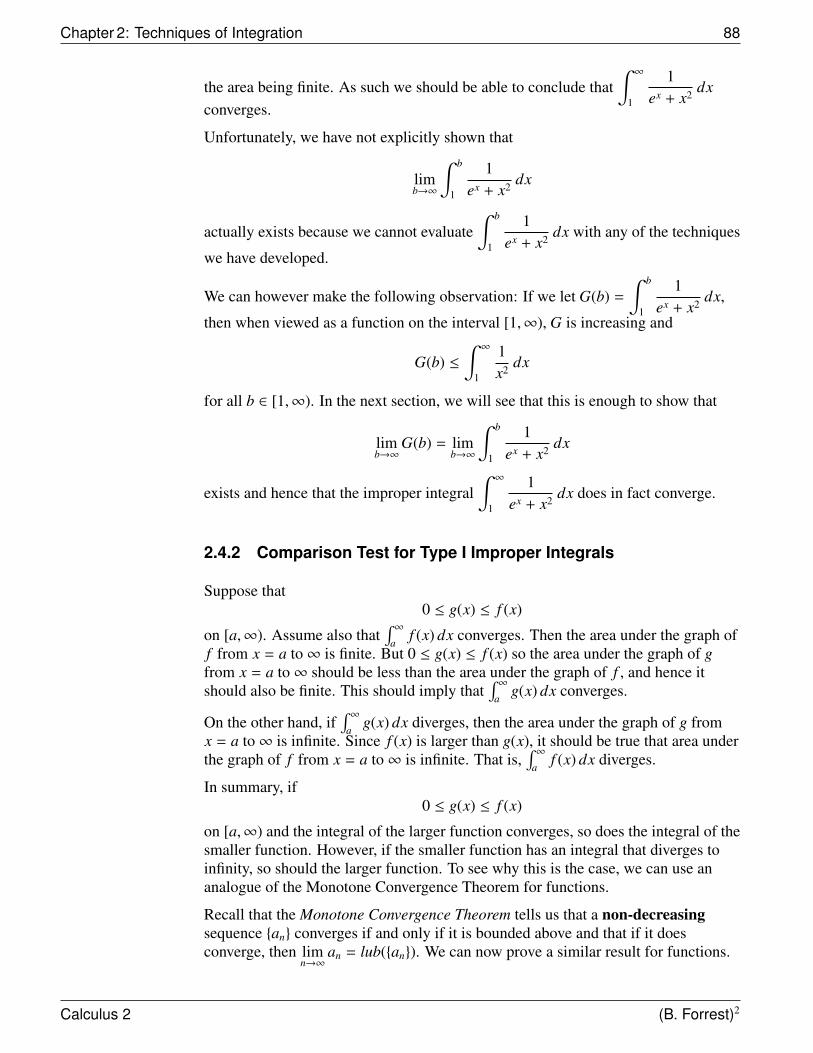
Chapter 2: Techniques of Integration 88
the area being finite. As such we should be able to conclude that∫ ∞
1
1ex + x2 dx
converges.
Unfortunately, we have not explicitly shown that
limb→∞
∫ b
1
1ex + x2 dx
actually exists because we cannot evaluate∫ b
1
1ex + x2 dx with any of the techniques
we have developed.
We can however make the following observation: If we let G(b) =
∫ b
1
1ex + x2 dx,
then when viewed as a function on the interval [1,∞), G is increasing and
G(b) ≤∫ ∞
1
1x2 dx
for all b ∈ [1,∞). In the next section, we will see that this is enough to show that
limb→∞
G(b) = limb→∞
∫ b
1
1ex + x2 dx
exists and hence that the improper integral∫ ∞
1
1ex + x2 dx does in fact converge.
2.4.2 Comparison Test for Type I Improper Integrals
Suppose that0 ≤ g(x) ≤ f (x)
on [a,∞). Assume also that∫ ∞
af (x) dx converges. Then the area under the graph of
f from x = a to∞ is finite. But 0 ≤ g(x) ≤ f (x) so the area under the graph of gfrom x = a to∞ should be less than the area under the graph of f , and hence itshould also be finite. This should imply that
∫ ∞a
g(x) dx converges.
On the other hand, if∫ ∞
ag(x) dx diverges, then the area under the graph of g from
x = a to∞ is infinite. Since f (x) is larger than g(x), it should be true that area underthe graph of f from x = a to∞ is infinite. That is,
∫ ∞a
f (x) dx diverges.
In summary, if0 ≤ g(x) ≤ f (x)
on [a,∞) and the integral of the larger function converges, so does the integral of thesmaller function. However, if the smaller function has an integral that diverges toinfinity, so should the larger function. To see why this is the case, we can use ananalogue of the Monotone Convergence Theorem for functions.
Recall that the Monotone Convergence Theorem tells us that a non-decreasingsequence {an} converges if and only if it is bounded above and that if it doesconverge, then lim
n→∞an = lub({an}). We can now prove a similar result for functions.
Calculus 2 (B. Forrest)2
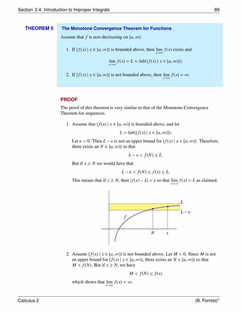
Section 2.4: Introduction to Improper Integrals 89
THEOREM 5 The Monotone Convergence Theorem for Functions
Assume that f is non-decreasing on [a,∞).
1. If { f (x) | x ∈ [a,∞)} is bounded above, then limx→∞
f (x) exists and
limx→∞
f (x) = L = lub({ f (x) | x ∈ [a,∞)}).
2. If { f (x) | x ∈ [a,∞)} is not bounded above, then limx→∞
f (x) = ∞.
PROOF
The proof of this theorem is very similar to that of the Monotone ConvergenceTheorem for sequences.
1. Assume that { f (x) | x ∈ [a,∞)} is bounded above, and let
L = lub({ f (x) | x ∈ [a,∞)}).
Let ε > 0. Then L − ε is not an upper bound for { f (x) | x ∈ [a,∞)}. Therefore,there exists an N ∈ [a,∞)} so that
L − ε < f (N) ≤ L.
But if x ≥ N we would have that
L − ε < f (N) ≤ f (x) ≤ L.
This means that if x ≥ N, then | f (x) − L| < ε so that limx→∞
f (x) = L as claimed.
f
N x
L
L − ε
2. Assume { f (x) | x ∈ [a,∞)} is not bounded above. Let M > 0. Since M is notan upper bound for { f (x) | x ∈ [a,∞)}, there exists an N ∈ [a,∞)} so thatM < f (N). But if x ≥ N, we have
M < f (N) ≤ f (x)
which shows that limx→∞
f (x) = ∞.
Calculus 2 (B. Forrest)2

Chapter 2: Techniques of Integration 90
f
N x
M
We can now establish one of the most important tools for determining theconvergence or divergence of improper integrals.
THEOREM 6 Comparison Test for Type I Improper Integrals
Assume that 0 ≤ g(x) ≤ f (x) for all x ≥ a and that both f and g are continuous on[a,∞).
1. If∫ ∞
af (x) dx converges, then so does
∫ ∞a
g(x) dx.
2. If∫ ∞
ag(x) dx diverges, then so does
∫ ∞a
f (x) dx.
PROOF
The two statements are logically equivalent (why?). This means that we only haveto prove the first statement and then the second statement follows. As such, assumethat
∫ ∞a
f (x) dx converges. Next let
F(t) =
∫ t
af (x) dx.
Since f (x) ≥ 0, we have that F is non-decreasing on [a,∞) and that
limt→∞
F(t) = limt→∞
∫ t
af (x) dx =
∫ ∞
af (x) dx < ∞.
Let
G(t) =
∫ t
ag(x) dx.
Calculus 2 (B. Forrest)2
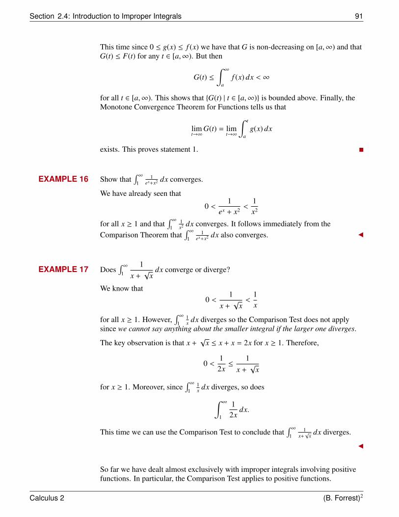
Section 2.4: Introduction to Improper Integrals 91
This time since 0 ≤ g(x) ≤ f (x) we have that G is non-decreasing on [a,∞) and thatG(t) ≤ F(t) for any t ∈ [a,∞). But then
G(t) ≤∫ ∞
af (x) dx < ∞
for all t ∈ [a,∞). This shows that {G(t) | t ∈ [a,∞)} is bounded above. Finally, theMonotone Convergence Theorem for Functions tells us that
limt→∞
G(t) = limt→∞
∫ t
ag(x) dx
exists. This proves statement 1.
EXAMPLE 16 Show that∫ ∞
11
ex+x2 dx converges.
We have already seen that
0 <1
ex + x2 <1x2
for all x ≥ 1 and that∫ ∞
11x2 dx converges. It follows immediately from the
Comparison Theorem that∫ ∞
11
ex+x2 dx also converges.
EXAMPLE 17 Does∫ ∞
1
1x +√
xdx converge or diverge?
We know that0 <
1x +√
x<
1x
for all x ≥ 1. However,∫ ∞
11x dx diverges so the Comparison Test does not apply
since we cannot say anything about the smaller integral if the larger one diverges.
The key observation is that x +√
x ≤ x + x = 2x for x ≥ 1. Therefore,
0 <12x≤
1x +√
x
for x ≥ 1. Moreover, since∫ ∞
11x dx diverges, so does∫ ∞
1
12x
dx.
This time we can use the Comparison Test to conclude that∫ ∞
11
x+√
x dx diverges.
So far we have dealt almost exclusively with improper integrals involving positivefunctions. In particular, the Comparison Test applies to positive functions.
Calculus 2 (B. Forrest)2
Chapter 2: Techniques of Integration 92
Moreover the Monotone Convergence Theorem for Functions allows us to establishthe following important fact.
Fact
If f is integrable on [a, b) for every b ≥ a and if f (x) ≥ 0 on [a,∞), then∫ ∞a
f (x) dx converges if and only if there exists an M such that∫ b
af (x) dx ≤ M
for all b > a.
Note: The previous statement is not true without the assumption that f (x) ≥ 0 asthe following example illustrates.
EXAMPLE 18 Show that∫ ∞
0cos(x) dx diverges.
By definition, ∫ ∞
0cos(x) dx = lim
b→∞
∫ b
0cos(x) dx
= limb→∞
sin(x)∣∣∣∣b0
= limb→∞
(sin(b) − sin(0))
= limb→∞
sin(b)
However, sin(b) oscillates between −1 and 1 as b→ ∞ so that limb→∞
sin(b) does not
exist. Therefore,∫ ∞
0cos(x) dx diverges despite the fact that
−1 ≤∫ b
0cos(x) dx = sin(b) ≤ 1
for all b > 0.
However, we can still often use our tools for improper integrals of positive functionsto determine convergence of some improper integrals of more general functions. Todo so we introduce the notion of absolute convergence which is an analog ofabsolute convergence for sequences.
Calculus 2 (B. Forrest)2
Section 2.4: Introduction to Improper Integrals 93
DEFINITION Absolute Convergence for Type I Improper Integrals
Let f be integrable on [a, b) for all b ≥ a. We say that the improper integral∫ ∞a
f (x) dx converges absolutely if∫ ∞
a| f (x) | dx
converges.
Similar to the case for sequences we will now see that absolute convergence impliesconvergence for improper integrals.
THEOREM 7 Absolute Convergence Theorem for Improper Integrals
Let f be integrable on [a, b] for all b > a. Then | f | is also integrable on [a, b] for allb > a. Moreover, if we assume that∫ ∞
a| f (x) | dx
converges, then so does ∫ ∞
af (x) dx.
In particular, if 0 ≤ | f (x)| ≤ g(x) for all x ≥ a, both f and g are integrable on [a, b]for all b ≥ a, and if
∫ ∞a
g(x) dx converges, then so does∫ ∞
af (x) dx.
PROOF
Assume that∫ ∞
a| f (x) | dx converges. Then so does∫ ∞
a2 | f (x) | dx.
We also have that0 ≤ f (x) + | f (x)| ≤ 2| f (x)|
so by the Comparison Theorem∫ ∞
af (x)+ | f (x) | dx
converges. Finally, since
f (x) = [ f (x) + | f (x)|] − | f (x)|
Calculus 2 (B. Forrest)2
Chapter 2: Techniques of Integration 94
we get that∫ ∞
af (x) dx converges with∫ ∞
af (x) dx =
∫ ∞
af (x)+ | f (x) | dx −
∫ ∞
a| f (x) | dx.
To prove the second statement, assume that∫ ∞
ag(x) dx converges. The Comparison
Test shows that ∫ ∞
a| f (x) | dx
also converges. We can now apply the first statement to conclude that∫ ∞
af (x) dx
converges.
EXAMPLE 19 Show that∫ ∞
3cos(x)
x2+2x+1 dx converges.
We know ∣∣∣∣∣ cos(x)x2 + 2x + 1
∣∣∣∣∣ ≤ 1x2 + 2x + 1
≤1x2
for all x ≥ 3.
The p-Test shows that∫ ∞
31x2 dx converges.
Therefore, by the Comparison Test,∫ ∞
3
∣∣∣∣∣ cos(x)x2 + 2x + 1
∣∣∣∣∣ dx
converges.
The Absolute Convergence Theorem shows that∫ ∞
3cos(x)
x2+2x+1 dx converges.
2.4.3 The Gamma Function
An important class of examples of improper integrals arise as values of a functioncalled the Gamma function.
Calculus 2 (B. Forrest)2
Section 2.4: Introduction to Improper Integrals 95
DEFINITION The Gamma Function
For each x ∈ R, define
Γ(x) =
∫ ∞
0tx−1e−tdt.
The function Γ is called the Gamma function.
Observation: In order to properly define the Γ function we should really show thatthe improper integral that arises from each choice of x is actually convergent. Wehave actually already seen this to be true for x = 1 as the example below reminds us.Later we will provide strong evidence of why this is so in general, but theverification of convergence is left as an exercise.
EXAMPLE 20 CalculateΓ(1) =
∫ ∞
0t0e−tdt =
∫ ∞
0e−tdt.
By definition
Γ(1) =
∫ ∞
0e−tdt
= limb→∞
∫ b
0e−tdt
= limb→∞−e−t
∣∣∣∣b0
= limb→∞
(−e−b) − (−e−0)
= 1
Note: To see why the integrals involved in the definition of the Gamma functionalways converge we first note that by modifying the previous example we can showthat for any M > 0, the improper integral∫ ∞
Me−
t2 dt
also converges. Next we observe that the Fundamental Log Limit shows that for anyx ∈ R we have that
limt→∞
tx−1e−t2 = 0.
Combining these two observations and using the Comparison Test for ImproperIntegrals we can show that
∫ ∞0
tx−1e−tdt is always convergent.
Calculus 2 (B. Forrest)2
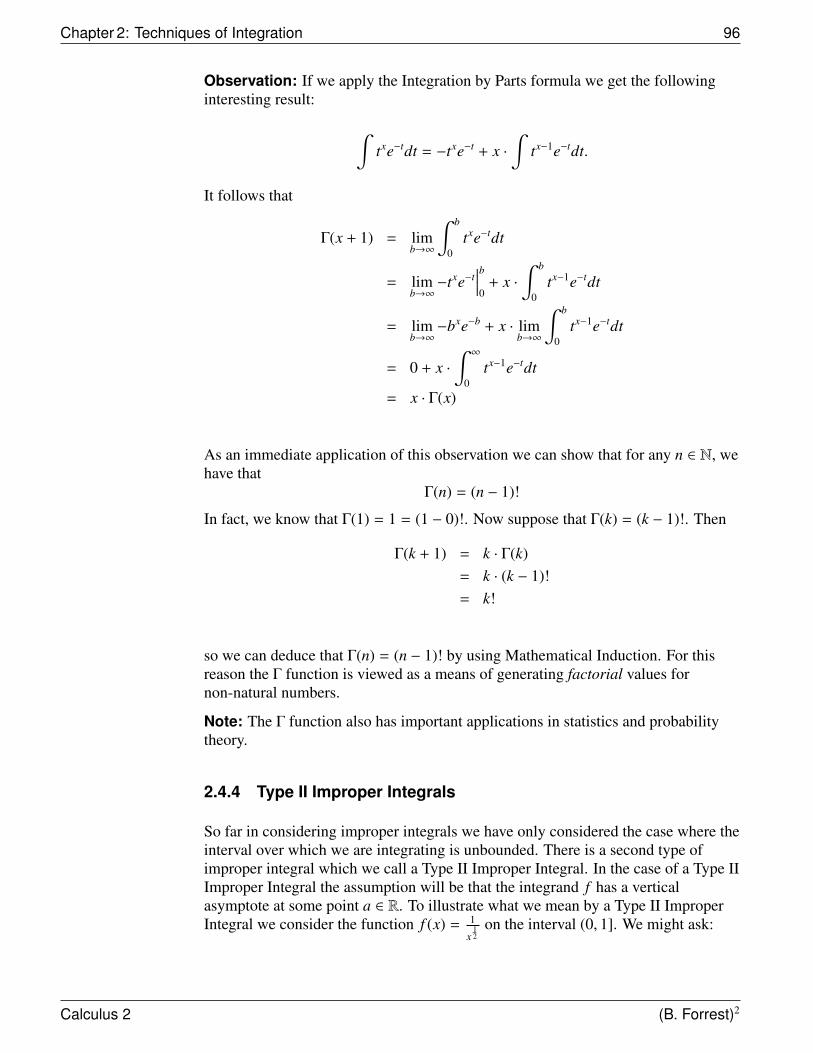
Chapter 2: Techniques of Integration 96
Observation: If we apply the Integration by Parts formula we get the followinginteresting result:
∫txe−tdt = −txe−t + x ·
∫tx−1e−tdt.
It follows that
Γ(x + 1) = limb→∞
∫ b
0txe−tdt
= limb→∞−txe−t
∣∣∣∣b0
+ x ·∫ b
0tx−1e−tdt
= limb→∞−bxe−b + x · lim
b→∞
∫ b
0tx−1e−tdt
= 0 + x ·∫ ∞
0tx−1e−tdt
= x · Γ(x)
As an immediate application of this observation we can show that for any n ∈ N, wehave that
Γ(n) = (n − 1)!
In fact, we know that Γ(1) = 1 = (1 − 0)!. Now suppose that Γ(k) = (k − 1)!. Then
Γ(k + 1) = k · Γ(k)= k · (k − 1)!= k!
so we can deduce that Γ(n) = (n − 1)! by using Mathematical Induction. For thisreason the Γ function is viewed as a means of generating factorial values fornon-natural numbers.
Note: The Γ function also has important applications in statistics and probabilitytheory.
2.4.4 Type II Improper Integrals
So far in considering improper integrals we have only considered the case where theinterval over which we are integrating is unbounded. There is a second type ofimproper integral which we call a Type II Improper Integral. In the case of a Type IIImproper Integral the assumption will be that the integrand f has a verticalasymptote at some point a ∈ R. To illustrate what we mean by a Type II ImproperIntegral we consider the function f (x) = 1
x12
on the interval (0, 1]. We might ask:
Calculus 2 (B. Forrest)2

Section 2.4: Introduction to Improper Integrals 97
Problem: What is the area under thegraph of f above the x-axis and betweenthe lines x = 0 and x = 1?We note that f has a vertical asymptote atx = 0 and as a consequence this region(which we denote by R) is alsounbounded.
0 1
R
f (x) =1
x12
However, if this was the case, then for any M > 0 we should be able to find ab ∈ (0.1] so that the area under the graph of f above the x-axis and between the linesx = b and x = 1 should be at least M. We know that this latter area is∫ 1
b
1
x12
dx = 2x12
∣∣∣∣1b
= 2(1 −√
b)< 2
Just as we deduced that the unbounded area under the graph of f (x) = 1x2 on the
interval [1,∞) could be finite, we again see that the area of this unbounded region Rcould be finite. In fact, similar to Improper Integrals of Type I, we could define thearea A of region R to be
A = limb→0+
∫ 1
b
1
x12
dx = limb→0+
2x12
∣∣∣∣1b
= limb→0+
2(1 −√
b) = 2.
DEFINITION Type II Improper Integral
1) Let f be integrable on [t, b] for every t ∈ (a, b] with either limx→a+
f (x) = ∞ orlimx→a+
f (x) = −∞ . We say that the Type II Improper Integral∫ b
af (x) dx
converges if
limt→a+
∫ b
tf (x) dx
exists. In this case, we write∫ b
af (x) dx = lim
t→a+
∫ b
tf (x) dx.
Otherwise, we say that∫ b
af (x) dx diverges.
Calculus 2 (B. Forrest)2

Chapter 2: Techniques of Integration 98
2) Let f be integrable on [a, t] for every t ∈ [a, b) with either limx→b−
f (x) = ∞ orlimx→b−
f (x) = −∞ . We say that the Type II Improper Integral
∫ b
af (x) dx
converges if
limt→b−
∫ t
af (x) dx
exists. In this case, we write∫ b
af (x) dx = lim
t→b−
∫ t
af (x) dx.
Otherwise, we say that∫ b
af (x) dx diverges.
3) If f has an infinite discontinuity at x = c where a < c < b, then we say that theType II Improper Integral ∫ b
af (x) dx
converges if both∫ c
af (x) dx and
∫ b
cf (x) dx converge. In this case, we write
∫ b
af (x) dx =
∫ c
af (x) dx +
∫ b
cf (x) dx.
If one or both of these integrals diverge, then we say that∫ b
af (x) dx diverges.
Remark: In determining the convergence or divergence of a Type I ImproperIntegral the p-test was an important tool. There is a natural analog of the p-test forType II Improper Integrals.
THEOREM 8 p-Test for Type II Improper Integrals
The improper integral ∫ 1
0
1xp dx
converges if and only if p < 1.
If p < 1, then ∫ 1
0
1xp dx =
11 − p
.
Calculus 2 (B. Forrest)2
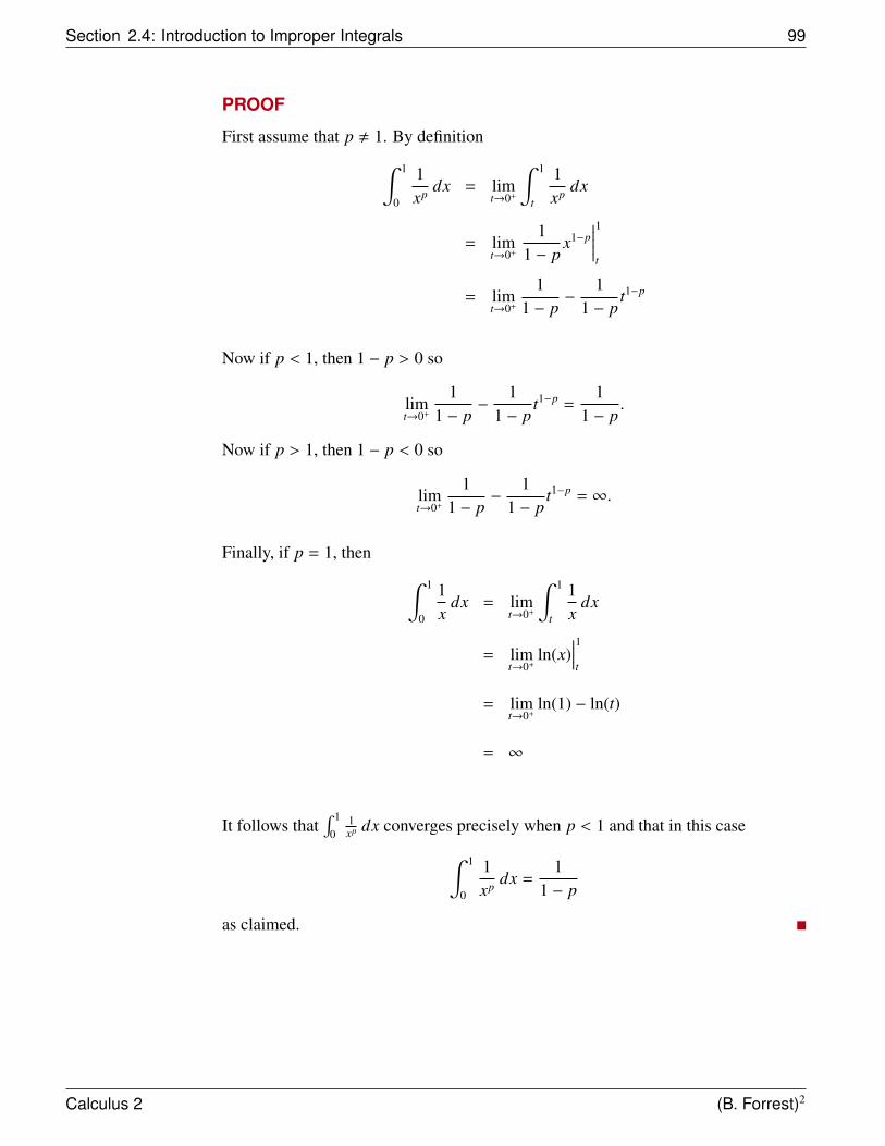
Section 2.4: Introduction to Improper Integrals 99
PROOF
First assume that p , 1. By definition∫ 1
0
1xp dx = lim
t→0+
∫ 1
t
1xp dx
= limt→0+
11 − p
x1−p∣∣∣∣∣1t
= limt→0+
11 − p
−1
1 − pt1−p
Now if p < 1, then 1 − p > 0 so
limt→0+
11 − p
−1
1 − pt1−p =
11 − p
.
Now if p > 1, then 1 − p < 0 so
limt→0+
11 − p
−1
1 − pt1−p = ∞.
Finally, if p = 1, then ∫ 1
0
1x
dx = limt→0+
∫ 1
t
1x
dx
= limt→0+
ln(x)∣∣∣∣1t
= limt→0+
ln(1) − ln(t)
= ∞
It follows that∫ 1
01xp dx converges precisely when p < 1 and that in this case∫ 1
0
1xp dx =
11 − p
as claimed.
Calculus 2 (B. Forrest)2
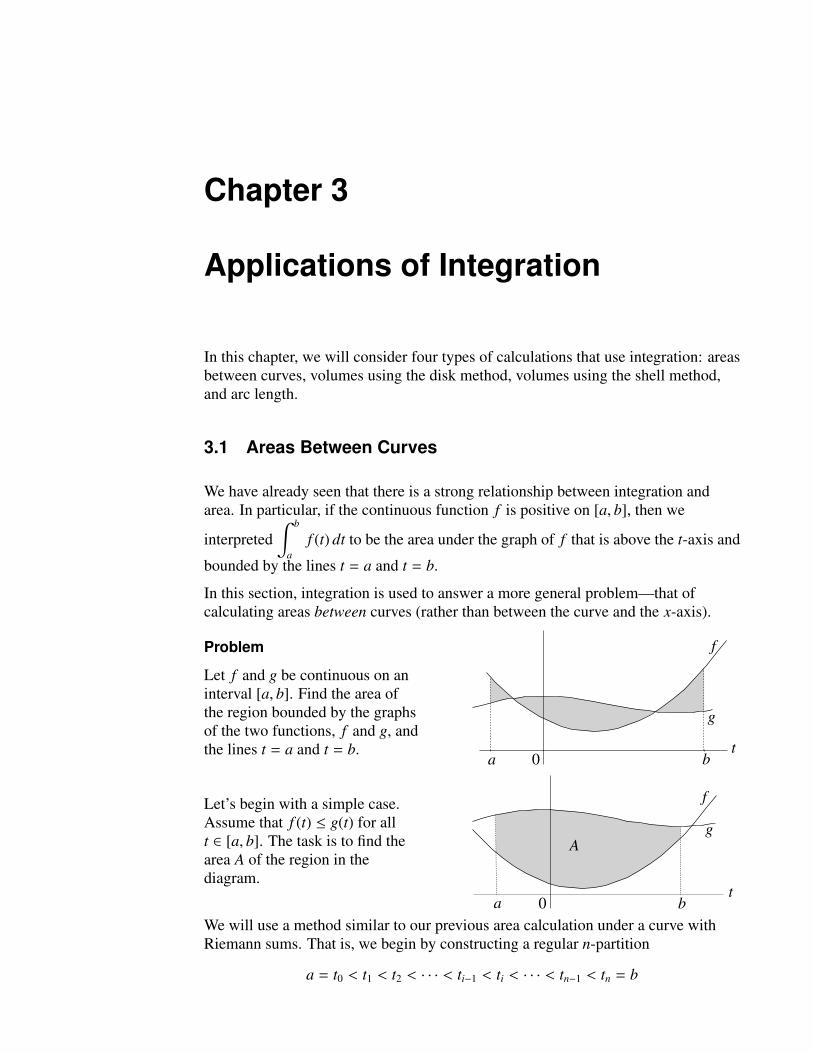
Chapter 3
Applications of Integration
In this chapter, we will consider four types of calculations that use integration: areasbetween curves, volumes using the disk method, volumes using the shell method,and arc length.
3.1 Areas Between Curves
We have already seen that there is a strong relationship between integration andarea. In particular, if the continuous function f is positive on [a, b], then we
interpreted∫ b
af (t) dt to be the area under the graph of f that is above the t-axis and
bounded by the lines t = a and t = b.
In this section, integration is used to answer a more general problem—that ofcalculating areas between curves (rather than between the curve and the x-axis).
Problem
Let f and g be continuous on aninterval [a, b]. Find the area ofthe region bounded by the graphsof the two functions, f and g, andthe lines t = a and t = b.
a 0
f
g
bt
Let’s begin with a simple case.Assume that f (t) ≤ g(t) for allt ∈ [a, b]. The task is to find thearea A of the region in thediagram.
a 0 b
g
f
A
t
We will use a method similar to our previous area calculation under a curve withRiemann sums. That is, we begin by constructing a regular n-partition
a = t0 < t1 < t2 < · · · < ti−1 < ti < · · · < tn−1 < tn = b
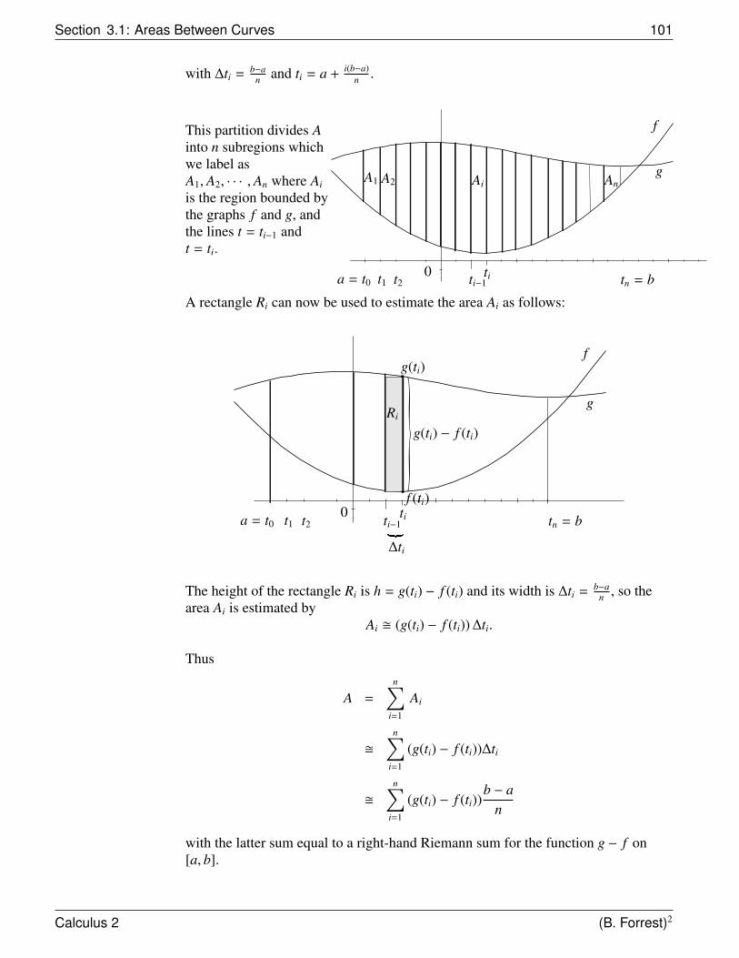
Section 3.1: Areas Between Curves 101
with ∆ti = b−an and ti = a +
i(b−a)n .
This partition divides Ainto n subregions whichwe label asA1, A2, · · · , An where Ai
is the region bounded bythe graphs f and g, andthe lines t = ti−1 andt = ti.
f
g
tn = b0a = t0 t1 t2 ti−1ti
A1 A2 Ai An
A rectangle Ri can now be used to estimate the area Ai as follows:
f
g
tn = b0a = t0 t1 t2 ti−1
ti
∆ti
Ri
g(ti)
f (ti)
g(ti) − f (ti)
The height of the rectangle Ri is h = g(ti) − f (ti) and its width is ∆ti = b−an , so the
area Ai is estimated byAi � (g(ti) − f (ti)) ∆ti.
Thus
A =
n∑i=1
Ai
�n∑
i=1
(g(ti) − f (ti))∆ti
�n∑
i=1
(g(ti) − f (ti))b − a
n
with the latter sum equal to a right-hand Riemann sum for the function g − f on[a, b].
Calculus 2 (B. Forrest)2
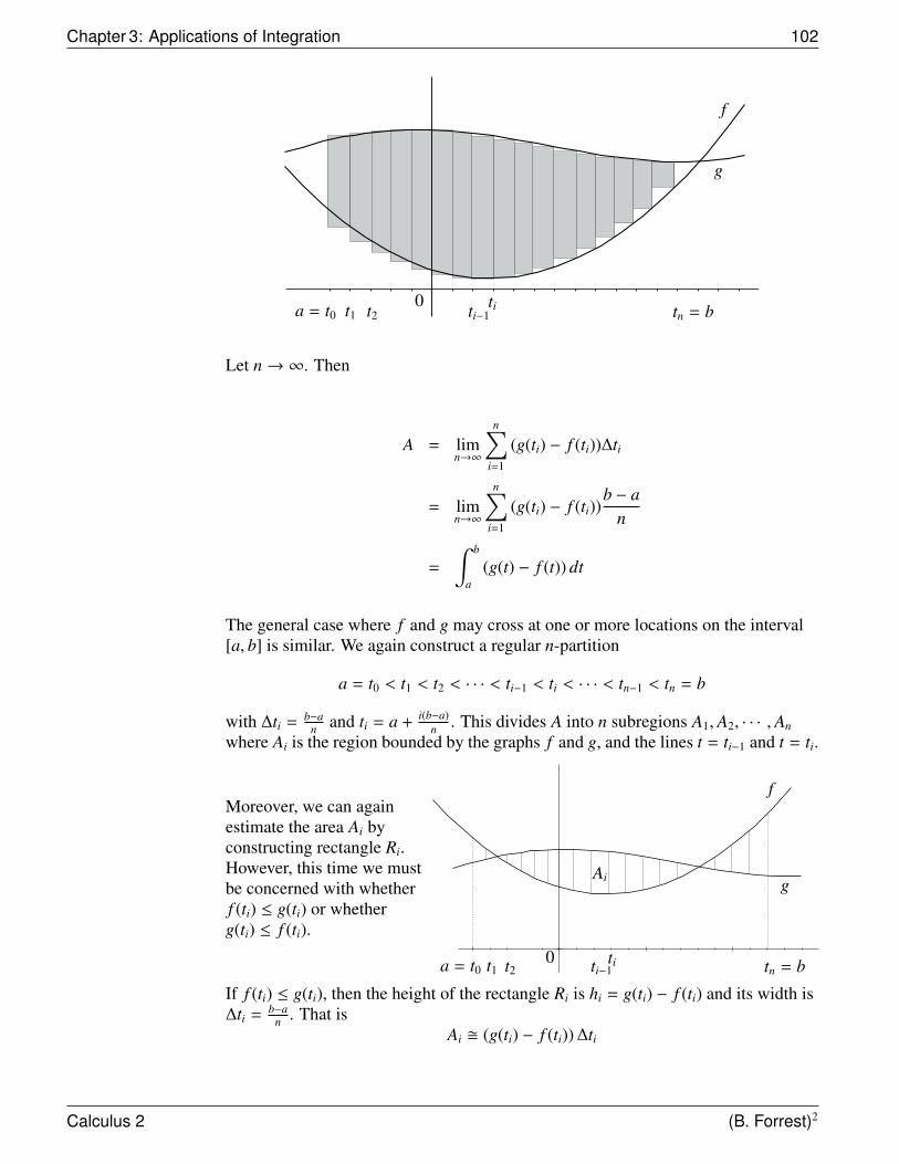
Chapter 3: Applications of Integration 102
tn = b0a = t0 t1 t2 ti−1
ti
g
f
Let n→ ∞. Then
A = limn→∞
n∑i=1
(g(ti) − f (ti))∆ti
= limn→∞
n∑i=1
(g(ti) − f (ti))b − a
n
=
∫ b
a(g(t) − f (t)) dt
The general case where f and g may cross at one or more locations on the interval[a, b] is similar. We again construct a regular n-partition
a = t0 < t1 < t2 < · · · < ti−1 < ti < · · · < tn−1 < tn = b
with ∆ti = b−an and ti = a +
i(b−a)n . This divides A into n subregions A1, A2, · · · , An
where Ai is the region bounded by the graphs f and g, and the lines t = ti−1 and t = ti.
Moreover, we can againestimate the area Ai byconstructing rectangle Ri.However, this time we mustbe concerned with whetherf (ti) ≤ g(ti) or whetherg(ti) ≤ f (ti).
tn = b0a = t0 t1 t2 ti−1ti
f
gAi
If f (ti) ≤ g(ti), then the height of the rectangle Ri is hi = g(ti) − f (ti) and its width is∆ti = b−a
n . That isAi � (g(ti) − f (ti)) ∆ti
Calculus 2 (B. Forrest)2

Section 3.1: Areas Between Curves 103
tn = b0a = t0 t1 t2 ti−1
ti
f
g
∆ti
g(ti)
f (ti)
g(ti) − f (ti)
However, if g(ti) ≤ f (ti), then the height of the rectangle is now hi = f (ti) − g(ti).The width remains as ∆ti = b−a
n , so
Ai � ( f (ti) − g(ti)) ∆ti
tn = b0a = t0 t1 t2 ti−1
ti
f
g
∆ti
f (ti)
g(ti)
f (ti) − g(ti)
To summarize, we have thatAi � hi ∆ti
where
hi =
{g(ti) − f (ti) if g(ti) − f (ti) ≥ 0f (ti) − g(ti) if g(ti) − f (ti) < 0
Calculus 2 (B. Forrest)2
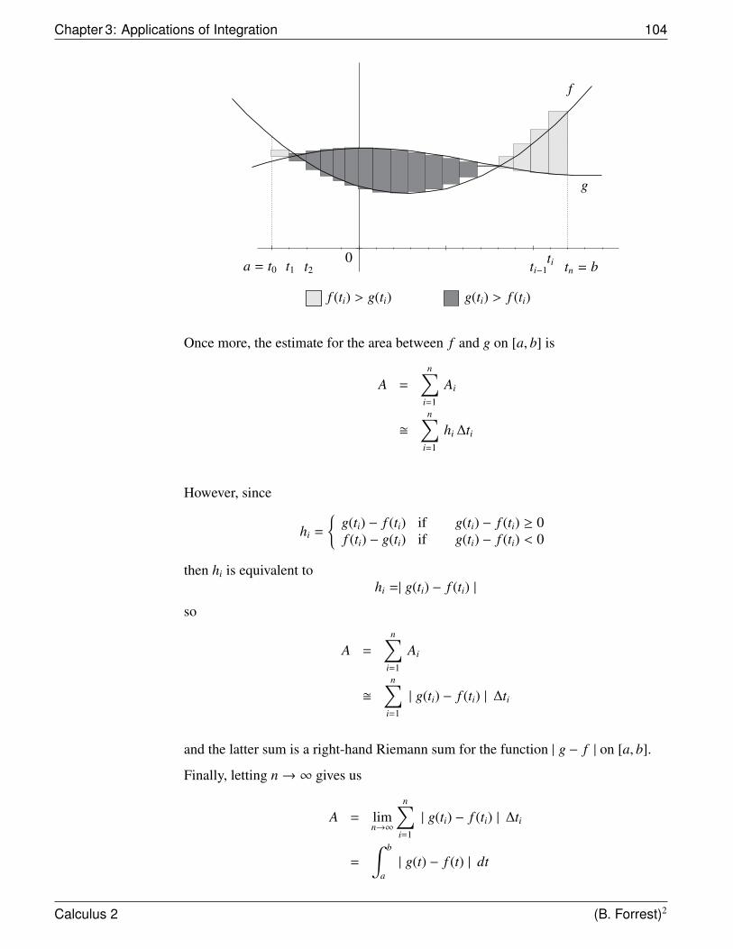
Chapter 3: Applications of Integration 104
tn = b0a = t0 t1 t2 ti−1
ti
f
g
f (ti) > g(ti) g(ti) > f (ti)
Once more, the estimate for the area between f and g on [a, b] is
A =
n∑i=1
Ai
�n∑
i=1
hi ∆ti
However, since
hi =
{g(ti) − f (ti) if g(ti) − f (ti) ≥ 0f (ti) − g(ti) if g(ti) − f (ti) < 0
then hi is equivalent tohi =| g(ti) − f (ti) |
so
A =
n∑i=1
Ai
�n∑
i=1
| g(ti) − f (ti) | ∆ti
and the latter sum is a right-hand Riemann sum for the function | g − f | on [a, b].
Finally, letting n→ ∞ gives us
A = limn→∞
n∑i=1
| g(ti) − f (ti) | ∆ti
=
∫ b
a| g(t) − f (t) | dt
Calculus 2 (B. Forrest)2
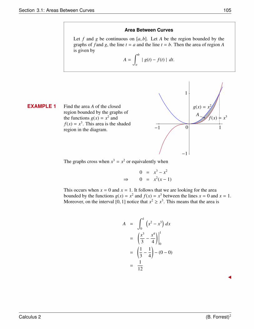
Section 3.1: Areas Between Curves 105
Area Between Curves
Let f and g be continuous on [a, b]. Let A be the region bounded by thegraphs of f and g, the line t = a and the line t = b. Then the area of region Ais given by
A =
∫ b
a| g(t) − f (t) | dt.
EXAMPLE 1 Find the area A of the closedregion bounded by the graphs ofthe functions g(x) = x2 andf (x) = x3. This area is the shadedregion in the diagram.
g(x) = x2
f (x) = x3
1
1
−1
−1
0
A
The graphs cross when x3 = x2 or equivalently when
0 = x3 − x2
⇒ 0 = x2(x − 1)
This occurs when x = 0 and x = 1. It follows that we are looking for the areabounded by the functions g(x) = x2 and f (x) = x3 between the lines x = 0 and x = 1.Moreover, on the interval [0, 1] notice that x2 ≥ x3. This means that the area is
A =
∫ 1
0
(x2 − x3
)dx
=
(x3
3−
x4
4
) ∣∣∣∣∣∣10
=
(13−
14
)− (0 − 0)
=1
12
Calculus 2 (B. Forrest)2
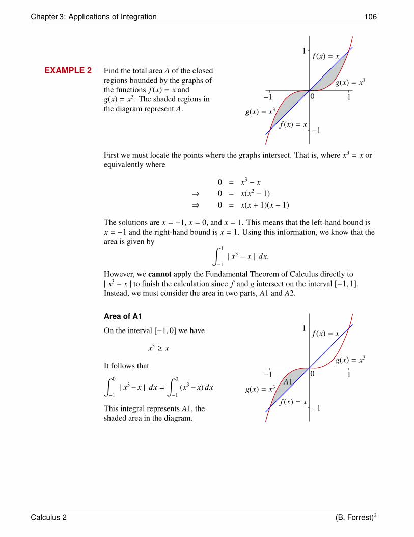
Chapter 3: Applications of Integration 106
EXAMPLE 2 Find the total area A of the closedregions bounded by the graphs ofthe functions f (x) = x andg(x) = x3. The shaded regions inthe diagram represent A.
1
1
−1
−1
0
f (x) = x
g(x) = x3
f (x) = x
g(x) = x3
First we must locate the points where the graphs intersect. That is, where x3 = x orequivalently where
0 = x3 − x⇒ 0 = x(x2 − 1)⇒ 0 = x(x + 1)(x − 1)
The solutions are x = −1, x = 0, and x = 1. This means that the left-hand bound isx = −1 and the right-hand bound is x = 1. Using this information, we know that thearea is given by ∫ 1
−1| x3 − x | dx.
However, we cannot apply the Fundamental Theorem of Calculus directly to| x3 − x | to finish the calculation since f and g intersect on the interval [−1, 1].Instead, we must consider the area in two parts, A1 and A2.
Area of A1
On the interval [−1, 0] we have
x3 ≥ x
It follows that∫ 0
−1| x3− x | dx =
∫ 0
−1(x3− x) dx
This integral represents A1, theshaded area in the diagram.
1
1
−1
−1
0
f (x) = x
g(x) = x3
f (x) = x
g(x) = x3
A1
Calculus 2 (B. Forrest)2
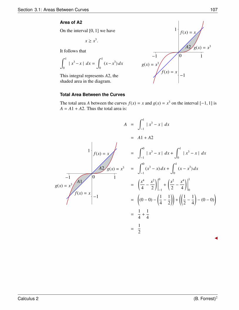
Section 3.1: Areas Between Curves 107
Area of A2
On the interval [0, 1] we have
x ≥ x3.
It follows that∫ 1
0| x3− x | dx =
∫ 1
0(x− x3) dx
This integral represents A2, theshaded area in the diagram.
1
1
−1
−1
0
f (x) = x
g(x) = x3
f (x) = x
g(x) = x3A2
Total Area Between the Curves
The total area A between the curves f (x) = x and g(x) = x3 on the interval [−1, 1] isA = A1 + A2. Thus the total area is:
1
1
−1
−1
0
f (x) = x
g(x) = x3
f (x) = x
g(x) = x3A2
A1
A =
∫ 1
−1| x3 − x | dx
= A1 + A2
=
∫ 0
−1| x3 − x | dx +
∫ 1
0| x3 − x | dx
=
∫ 0
−1(x3 − x) dx +
∫ 1
0(x − x3) dx
=
(x4
4−
x2
2
) ∣∣∣∣∣∣0−1
+
(x2
2−
x4
4
) ∣∣∣∣∣∣10
=
((0 − 0) −
(14−
12
))+
((12−
14
)− (0 − 0)
)=
14
+14
=12
Calculus 2 (B. Forrest)2
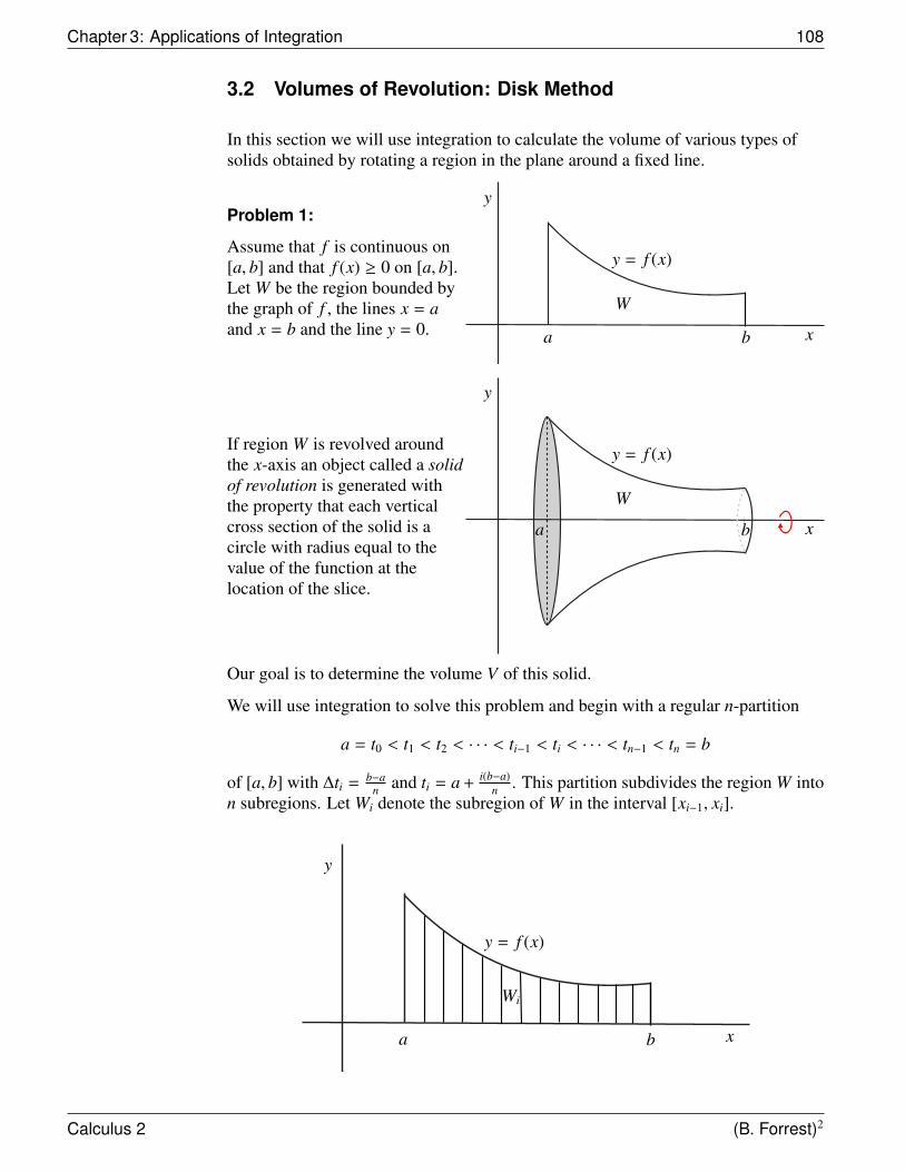
Chapter 3: Applications of Integration 108
3.2 Volumes of Revolution: Disk Method
In this section we will use integration to calculate the volume of various types ofsolids obtained by rotating a region in the plane around a fixed line.
Problem 1:
Assume that f is continuous on[a, b] and that f (x) ≥ 0 on [a, b].Let W be the region bounded bythe graph of f , the lines x = aand x = b and the line y = 0. b
y = f (x)
W
a
y
x
If region W is revolved aroundthe x-axis an object called a solidof revolution is generated withthe property that each verticalcross section of the solid is acircle with radius equal to thevalue of the function at thelocation of the slice.
b
y = f (x)
W
a
y
x
Our goal is to determine the volume V of this solid.
We will use integration to solve this problem and begin with a regular n-partition
a = t0 < t1 < t2 < · · · < ti−1 < ti < · · · < tn−1 < tn = b
of [a, b] with ∆ti = b−an and ti = a +
i(b−a)n . This partition subdivides the region W into
n subregions. Let Wi denote the subregion of W in the interval [xi−1, xi].
b
y = f (x)
Wi
a
y
x
Calculus 2 (B. Forrest)2
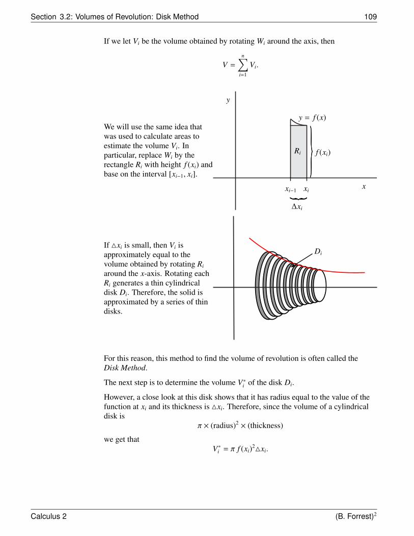
Section 3.2: Volumes of Revolution: Disk Method 109
If we let Vi be the volume obtained by rotating Wi around the axis, then
V =
n∑i=1
Vi.
We will use the same idea thatwas used to calculate areas toestimate the volume Vi. Inparticular, replace Wi by therectangle Ri with height f (xi) andbase on the interval [xi−1, xi].
Ri
xi−1 xi
f (xi)
y = f (x)
y
x
∆xi
If 4xi is small, then Vi isapproximately equal to thevolume obtained by rotating Ri
around the x-axis. Rotating eachRi generates a thin cylindricaldisk Di. Therefore, the solid isapproximated by a series of thindisks.
Di
For this reason, this method to find the volume of revolution is often called theDisk Method.
The next step is to determine the volume V∗i of the disk Di.
However, a close look at this disk shows that it has radius equal to the value of thefunction at xi and its thickness is 4xi. Therefore, since the volume of a cylindricaldisk is
π × (radius)2 × (thickness)
we get thatV∗i = π f (xi)24xi.
Calculus 2 (B. Forrest)2
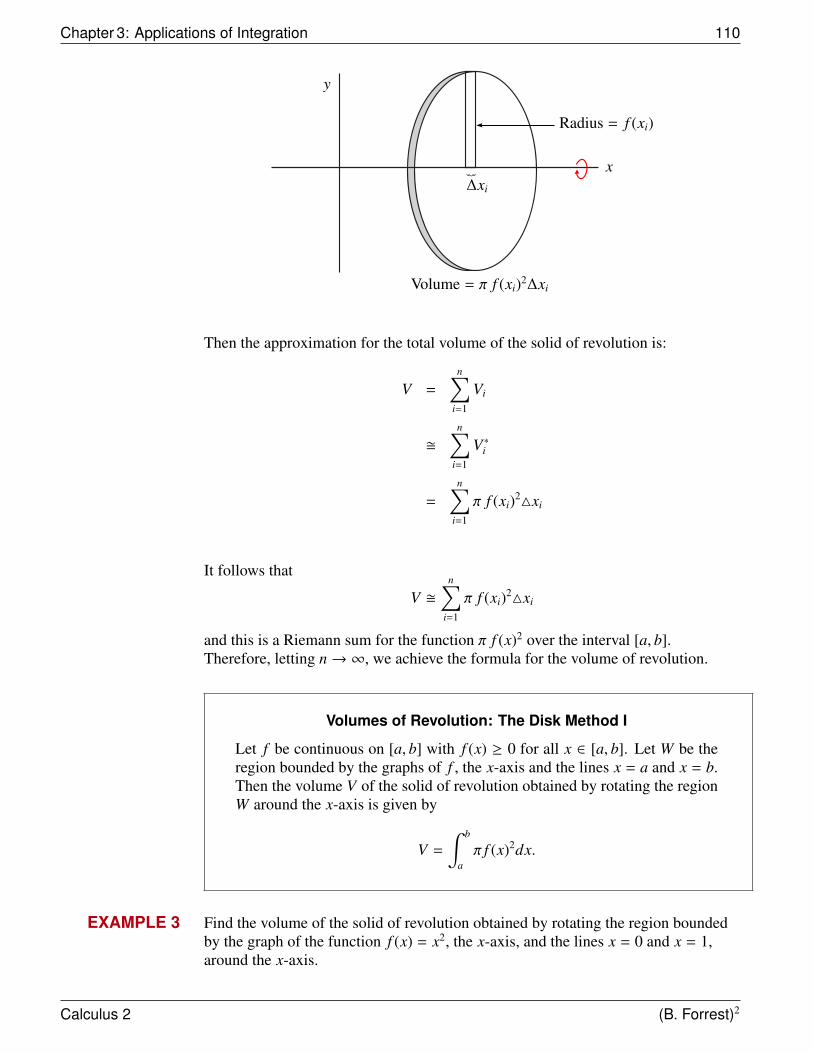
Chapter 3: Applications of Integration 110
∆xi
Radius = f (xi)
Volume = π f (xi)2∆xi
x
y
Then the approximation for the total volume of the solid of revolution is:
V =
n∑i=1
Vi
�n∑
i=1
V∗i
=
n∑i=1
π f (xi)24xi
It follows that
V �n∑
i=1
π f (xi)24xi
and this is a Riemann sum for the function π f (x)2 over the interval [a, b].Therefore, letting n→ ∞, we achieve the formula for the volume of revolution.
Volumes of Revolution: The Disk Method I
Let f be continuous on [a, b] with f (x) ≥ 0 for all x ∈ [a, b]. Let W be theregion bounded by the graphs of f , the x-axis and the lines x = a and x = b.Then the volume V of the solid of revolution obtained by rotating the regionW around the x-axis is given by
V =
∫ b
aπ f (x)2dx.
EXAMPLE 3 Find the volume of the solid of revolution obtained by rotating the region boundedby the graph of the function f (x) = x2, the x-axis, and the lines x = 0 and x = 1,around the x-axis.
Calculus 2 (B. Forrest)2
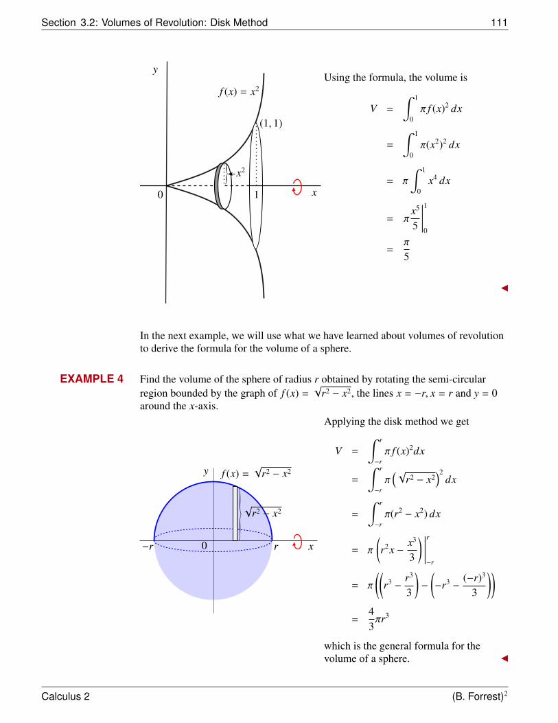
Section 3.2: Volumes of Revolution: Disk Method 111
f (x) = x2
(1, 1)
1
x2
y
x0
Using the formula, the volume is
V =
∫ 1
0π f (x)2 dx
=
∫ 1
0π(x2)2 dx
= π
∫ 1
0x4 dx
= πx5
5
∣∣∣∣∣∣10
=π
5
In the next example, we will use what we have learned about volumes of revolutionto derive the formula for the volume of a sphere.
EXAMPLE 4 Find the volume of the sphere of radius r obtained by rotating the semi-circularregion bounded by the graph of f (x) =
√r2 − x2, the lines x = −r, x = r and y = 0
around the x-axis.
x
y
r−r
f (x) =√
r2 − x2
0
√r2 − x2
Applying the disk method we get
V =
∫ r
−rπ f (x)2dx
=
∫ r
−rπ(√
r2 − x2)2
dx
=
∫ r
−rπ(r2 − x2) dx
= π
(r2x −
x3
3
) ∣∣∣∣∣∣r−r
= π
((r3 −
r3
3
)−
(−r3 −
(−r)3
3
))=
43πr3
which is the general formula for thevolume of a sphere.
Calculus 2 (B. Forrest)2
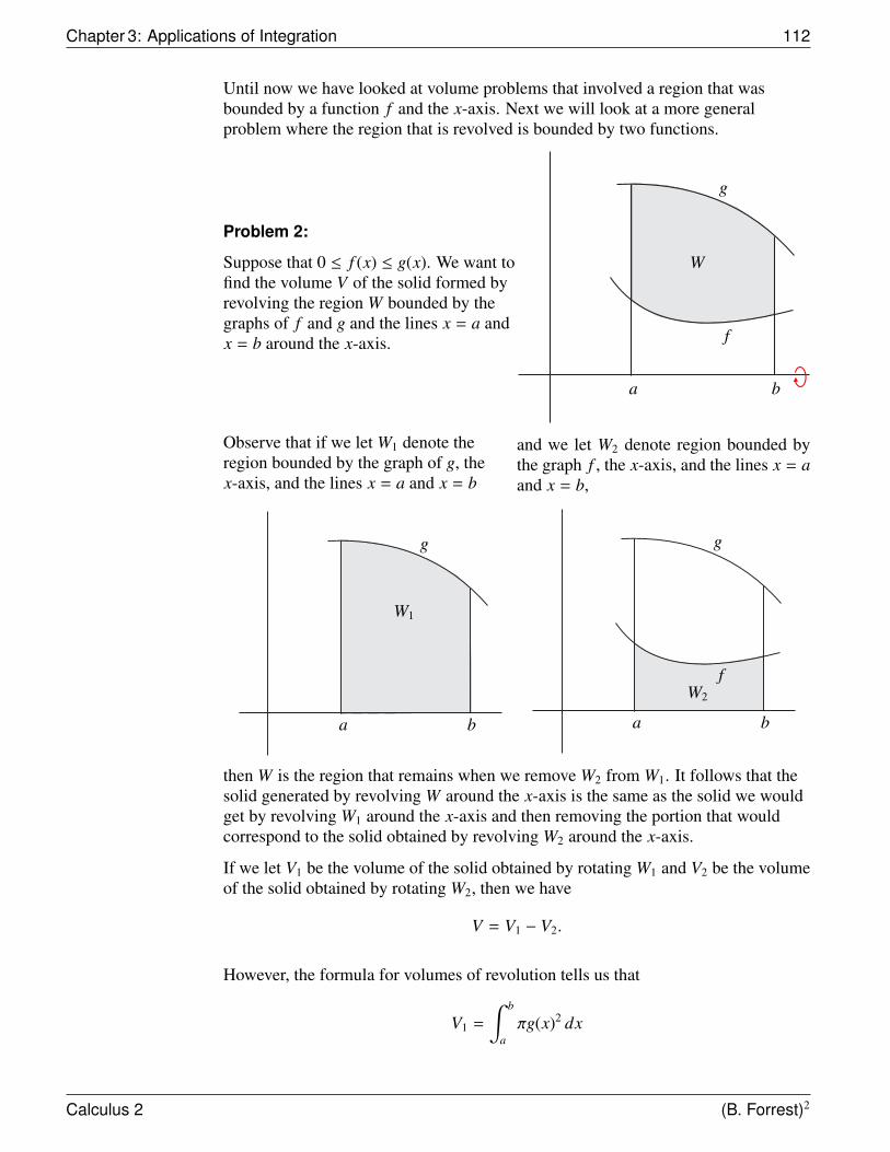
Chapter 3: Applications of Integration 112
Until now we have looked at volume problems that involved a region that wasbounded by a function f and the x-axis. Next we will look at a more generalproblem where the region that is revolved is bounded by two functions.
Problem 2:
Suppose that 0 ≤ f (x) ≤ g(x). We want tofind the volume V of the solid formed byrevolving the region W bounded by thegraphs of f and g and the lines x = a andx = b around the x-axis.
W
g
f
a b
Observe that if we let W1 denote theregion bounded by the graph of g, thex-axis, and the lines x = a and x = b
W1
g
a b
and we let W2 denote region bounded bythe graph f , the x-axis, and the lines x = aand x = b,
W2
g
f
a b
then W is the region that remains when we remove W2 from W1. It follows that thesolid generated by revolving W around the x-axis is the same as the solid we wouldget by revolving W1 around the x-axis and then removing the portion that wouldcorrespond to the solid obtained by revolving W2 around the x-axis.
If we let V1 be the volume of the solid obtained by rotating W1 and V2 be the volumeof the solid obtained by rotating W2, then we have
V = V1 − V2.
However, the formula for volumes of revolution tells us that
V1 =
∫ b
aπg(x)2 dx
Calculus 2 (B. Forrest)2
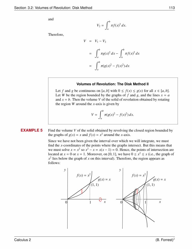
Section 3.2: Volumes of Revolution: Disk Method 113
and
V2 =
∫ b
aπ f (x)2 dx.
Therefore,
V = V1 − V2
=
∫ b
aπg(x)2 dx −
∫ b
aπ f (x)2 dx
=
∫ b
aπ(g(x)2 − f (x)2) dx
Volumes of Revolution: The Disk Method II
Let f and g be continuous on [a, b] with 0 ≤ f (x) ≤ g(x) for all x ∈ [a, b].Let W be the region bounded by the graphs of f and g, and the lines x = aand x = b. Then the volume V of the solid of revolution obtained by rotatingthe region W around the x-axis is given by
V =
∫ b
aπ(g(x)2 − f (x)2) dx.
EXAMPLE 5 Find the volume V of the solid obtained by revolving the closed region bounded bythe graphs of g(x) = x and f (x) = x2 around the x-axis.
Since we have not been given the interval over which we will integrate, we mustfind the x-coordinates of the points where the graphs intersect. But this means thatwe must solve x = x2 so x2 − x = x(x − 1) = 0. Hence, the points of intersection arelocated at x = 0 or x = 1. Moreover, on [0, 1], we have 0 ≤ x2 ≤ x (i.e., the graph ofx2 lies below the graph of x on this interval). Therefore, the region appears asfollows:
f (x) = x2
(1, 1)
1
y
x0
g(x) = xf (x) = x2
(1, 1)
1
y
x0
g(x) = x
Calculus 2 (B. Forrest)2
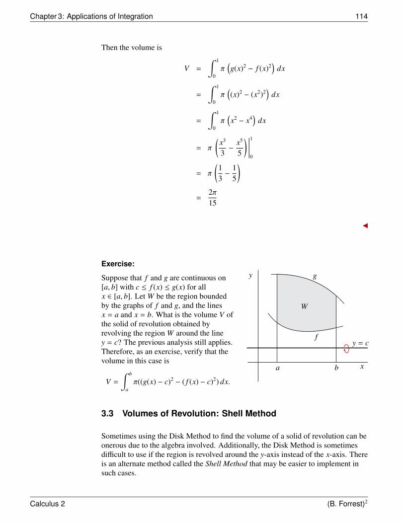
Chapter 3: Applications of Integration 114
Then the volume is
V =
∫ 1
0π
(g(x)2 − f (x)2
)dx
=
∫ 1
0π
((x)2 − (x2)2
)dx
=
∫ 1
0π
(x2 − x4
)dx
= π
(x3
3−
x5
5
) ∣∣∣∣∣∣10
= π
(13−
15
)=
2π15
Exercise:
Suppose that f and g are continuous on[a, b] with c ≤ f (x) ≤ g(x) for allx ∈ [a, b]. Let W be the region boundedby the graphs of f and g, and the linesx = a and x = b. What is the volume V ofthe solid of revolution obtained byrevolving the region W around the liney = c? The previous analysis still applies.Therefore, as an exercise, verify that thevolume in this case is
V =
∫ b
aπ((g(x) − c)2 − ( f (x) − c)2) dx.
W
g
f
a b x
y
y = c
3.3 Volumes of Revolution: Shell Method
Sometimes using the Disk Method to find the volume of a solid of revolution can beonerous due to the algebra involved. Additionally, the Disk Method is sometimesdifficult to use if the region is revolved around the y-axis instead of the x-axis. Thereis an alternate method called the Shell Method that may be easier to implement insuch cases.
Calculus 2 (B. Forrest)2
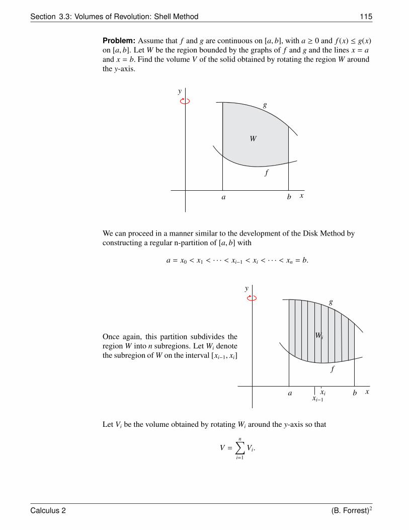
Section 3.3: Volumes of Revolution: Shell Method 115
Problem: Assume that f and g are continuous on [a, b], with a ≥ 0 and f (x) ≤ g(x)on [a, b]. Let W be the region bounded by the graphs of f and g and the lines x = aand x = b. Find the volume V of the solid obtained by rotating the region W aroundthe y-axis.
W
g
f
a b
y
x
We can proceed in a manner similar to the development of the Disk Method byconstructing a regular n-partition of [a, b] with
a = x0 < x1 < · · · < xi−1 < xi < · · · < xn = b.
Once again, this partition subdivides theregion W into n subregions. Let Wi denotethe subregion of W on the interval [xi−1, xi]
Wi
g
f
a b
y
xxixi−1
Let Vi be the volume obtained by rotating Wi around the y-axis so that
V =
n∑i=1
Vi.
Calculus 2 (B. Forrest)2
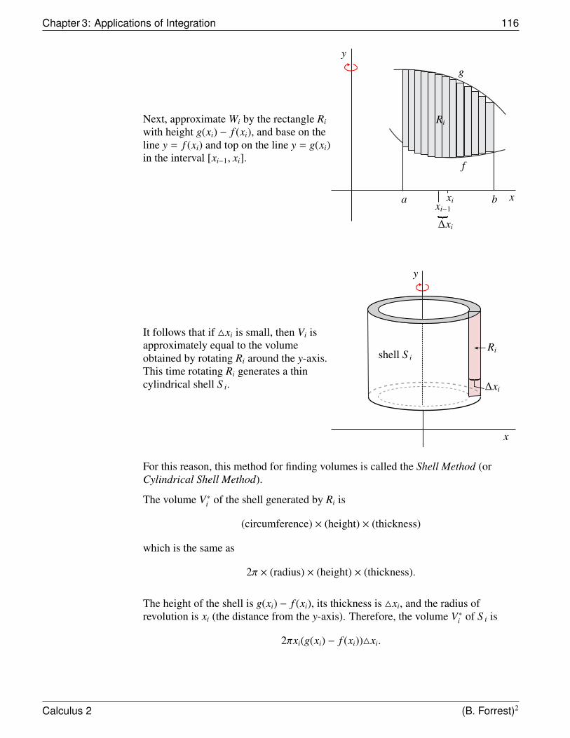
Chapter 3: Applications of Integration 116
Next, approximate Wi by the rectangle Ri
with height g(xi) − f (xi), and base on theline y = f (xi) and top on the line y = g(xi)in the interval [xi−1, xi].
g
f
a b
y
xxixi−1
Ri
∆xi
It follows that if 4xi is small, then Vi isapproximately equal to the volumeobtained by rotating Ri around the y-axis.This time rotating Ri generates a thincylindrical shell S i.
y
x
Ri
∆xi
shell S i
For this reason, this method for finding volumes is called the Shell Method (orCylindrical Shell Method).
The volume V∗i of the shell generated by Ri is
(circumference) × (height) × (thickness)
which is the same as
2π × (radius) × (height) × (thickness).
The height of the shell is g(xi) − f (xi), its thickness is 4xi, and the radius ofrevolution is xi (the distance from the y-axis). Therefore, the volume V∗i of S i is
2πxi(g(xi) − f (xi))4xi.
Calculus 2 (B. Forrest)2
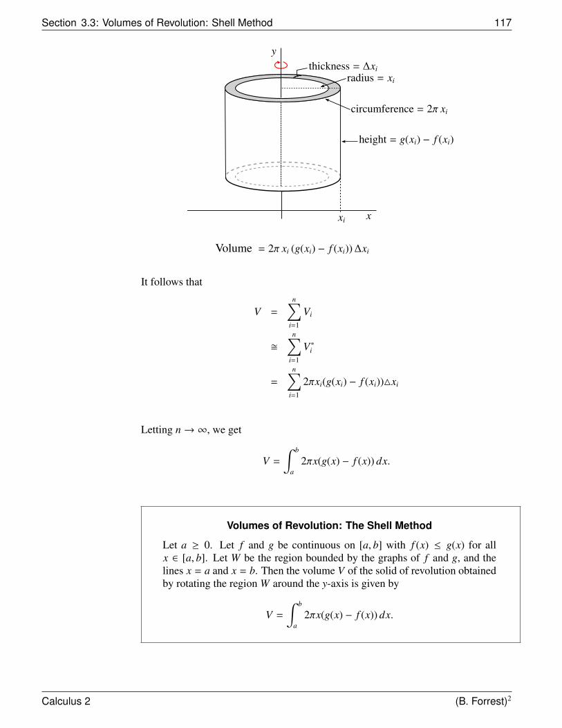
Section 3.3: Volumes of Revolution: Shell Method 117
y
x
thickness = ∆xi
circumference = 2π xi
height = g(xi) − f (xi)
xi
radius = xi
Volume = 2π xi (g(xi) − f (xi)) ∆xi
It follows that
V =
n∑i=1
Vi
�n∑
i=1
V∗i
=
n∑i=1
2πxi(g(xi) − f (xi))4xi
Letting n→ ∞, we get
V =
∫ b
a2πx(g(x) − f (x)) dx.
Volumes of Revolution: The Shell Method
Let a ≥ 0. Let f and g be continuous on [a, b] with f (x) ≤ g(x) for allx ∈ [a, b]. Let W be the region bounded by the graphs of f and g, and thelines x = a and x = b. Then the volume V of the solid of revolution obtainedby rotating the region W around the y-axis is given by
V =
∫ b
a2πx(g(x) − f (x)) dx.
Calculus 2 (B. Forrest)2
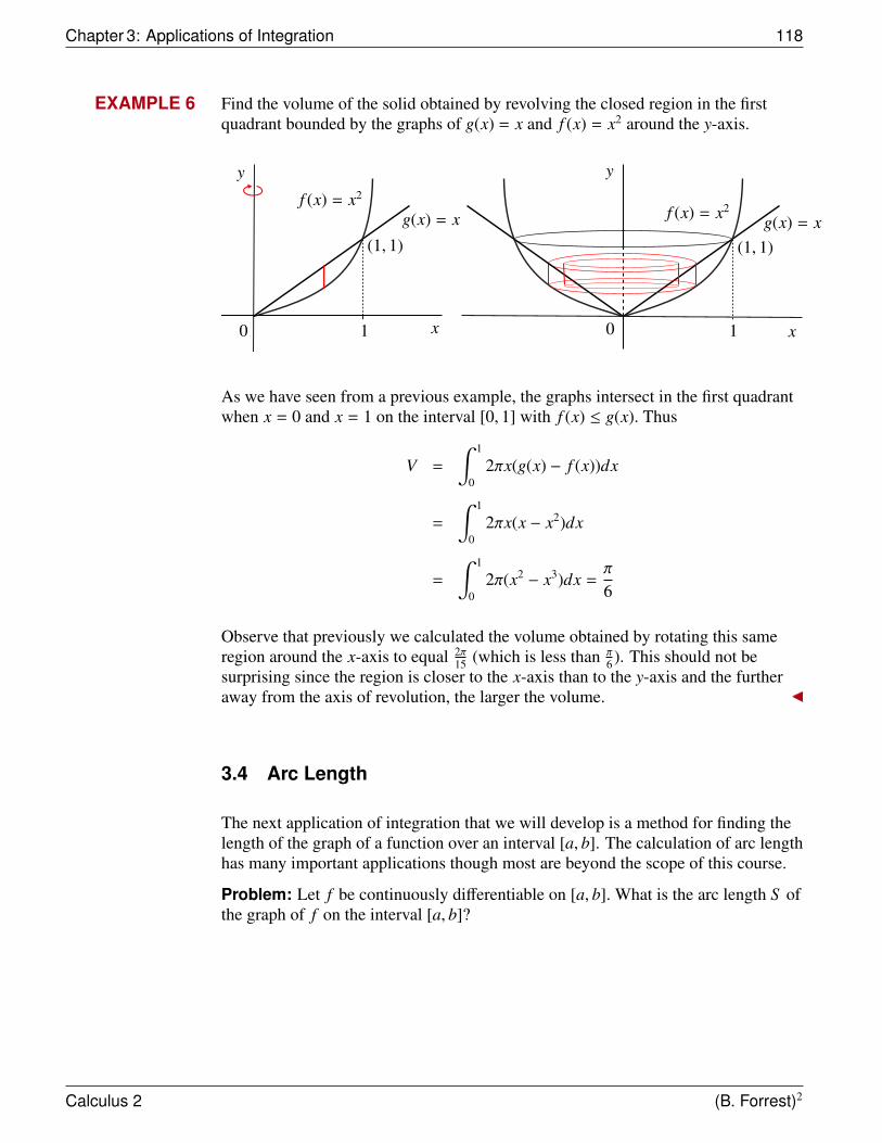
Chapter 3: Applications of Integration 118
EXAMPLE 6 Find the volume of the solid obtained by revolving the closed region in the firstquadrant bounded by the graphs of g(x) = x and f (x) = x2 around the y-axis.
f (x) = x2
(1, 1)
1
y
x0
g(x) = xf (x) = x2
(1, 1)
1
y
x0
g(x) = x
As we have seen from a previous example, the graphs intersect in the first quadrantwhen x = 0 and x = 1 on the interval [0, 1] with f (x) ≤ g(x). Thus
V =
∫ 1
02πx(g(x) − f (x))dx
=
∫ 1
02πx(x − x2)dx
=
∫ 1
02π(x2 − x3)dx =
π
6
Observe that previously we calculated the volume obtained by rotating this sameregion around the x-axis to equal 2π
15 (which is less than π6 ). This should not be
surprising since the region is closer to the x-axis than to the y-axis and the furtheraway from the axis of revolution, the larger the volume.
3.4 Arc Length
The next application of integration that we will develop is a method for finding thelength of the graph of a function over an interval [a, b]. The calculation of arc lengthhas many important applications though most are beyond the scope of this course.
Problem: Let f be continuously differentiable on [a, b]. What is the arc length S ofthe graph of f on the interval [a, b]?
Calculus 2 (B. Forrest)2
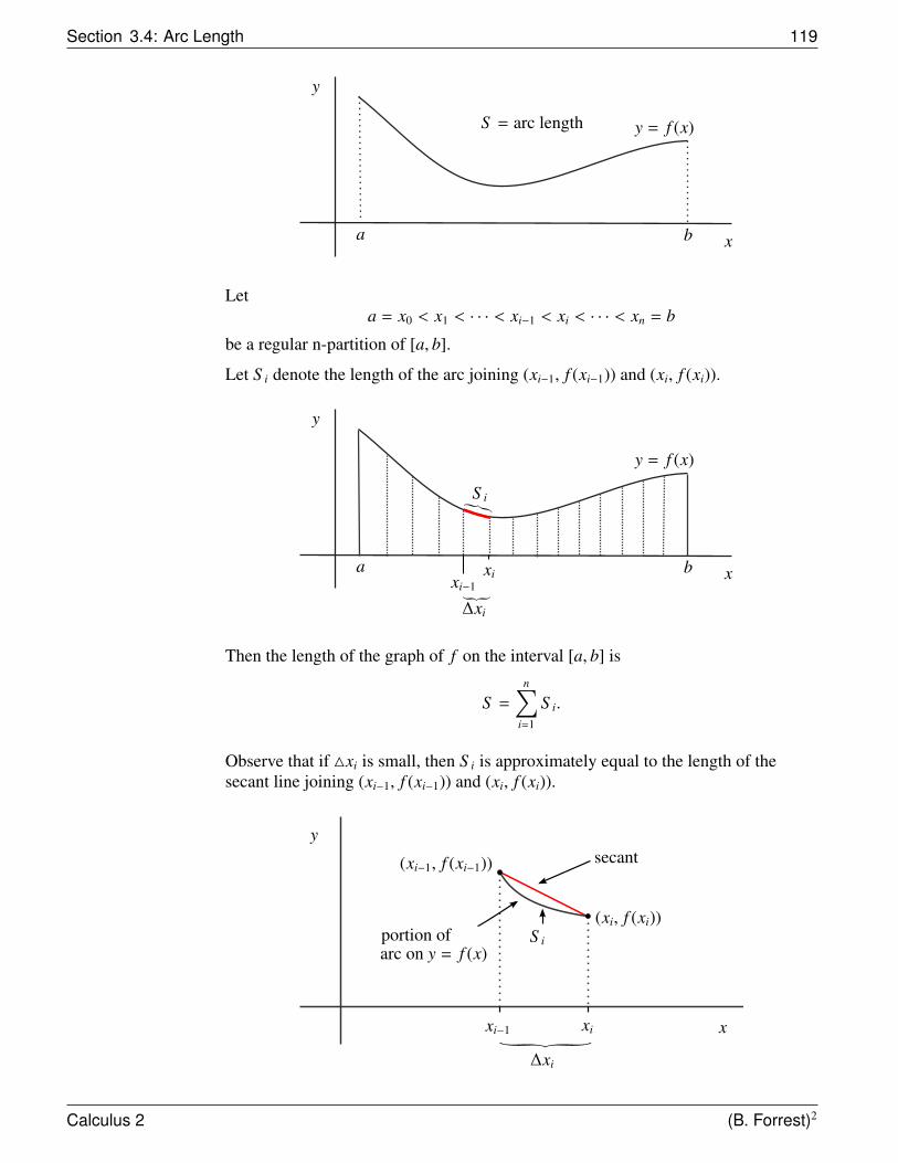
Section 3.4: Arc Length 119
a b
y = f (x)S = arc length
x
y
Leta = x0 < x1 < · · · < xi−1 < xi < · · · < xn = b
be a regular n-partition of [a, b].
Let S i denote the length of the arc joining (xi−1, f (xi−1)) and (xi, f (xi)).
a b
y = f (x)
x
y
S i
xi−1xi
∆xi
Then the length of the graph of f on the interval [a, b] is
S =
n∑i=1
S i.
Observe that if 4xi is small, then S i is approximately equal to the length of thesecant line joining (xi−1, f (xi−1)) and (xi, f (xi)).
S i
(xi, f (xi))
(xi−1, f (xi−1)) secant
portion ofarc on y = f (x)
xi−1 xi
∆xi
x
y
Calculus 2 (B. Forrest)2
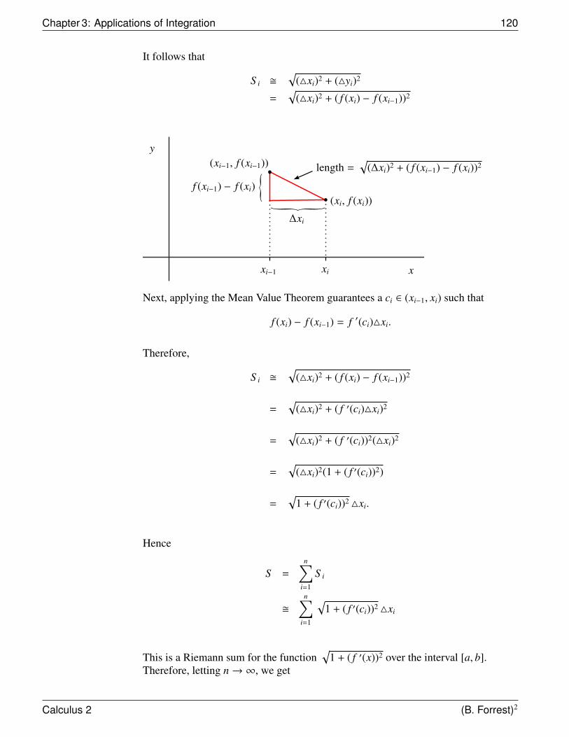
Chapter 3: Applications of Integration 120
It follows that
S i �√
(4xi)2 + (4yi)2
=√
(4xi)2 + ( f (xi) − f (xi−1))2
(xi, f (xi))
(xi−1, f (xi−1)) length =√
(∆xi)2 + ( f (xi−1) − f (xi))2
xi−1 xi
∆xi
x
y
f (xi−1) − f (xi)
Next, applying the Mean Value Theorem guarantees a ci ∈ (xi−1, xi) such that
f (xi) − f (xi−1) = f ′(ci)4xi.
Therefore,
S i �√
(4xi)2 + ( f (xi) − f (xi−1))2
=√
(4xi)2 + ( f ′(ci)4xi)2
=√
(4xi)2 + ( f ′(ci))2(4xi)2
=√
(4xi)2(1 + ( f ′(ci))2)
=√
1 + ( f ′(ci))2 4xi.
Hence
S =
n∑i=1
S i
�n∑
i=1
√1 + ( f ′(ci))2 4xi
This is a Riemann sum for the function√
1 + ( f ′(x))2 over the interval [a, b].Therefore, letting n→ ∞, we get
Calculus 2 (B. Forrest)2
Section 3.4: Arc Length 121
S =
∫ b
a
√1 + ( f ′(x))2 dx.
Arc Length
Let f be continuously differentiable on [a, b]. Then the arc length S of thegraph of f over the interval [a, b] is given by
S =
∫ b
a
√1 + ( f ′(x))2 dx
REMARK
The derivation of the arc length formula has many important applications that arebeyond the scope of this course. Unfortunately, due to the square root in theintegrand of the formula, there are very few functions for which we can calculate thearc length explicitly. Even calculating the arc length of the graph of f (x) = x3 overthe interval [0, 1] is beyond our current ability. However, there are a few examplesthat we can evaluate explicitly.
EXAMPLE 7 Find the length S of the portion of the graph of the function f (x) =2x
32
3between
x = 1 and x = 2.
In this case, f ′(x) = x12 . Hence
S =
∫ 2
1
√1 + ( f ′(x))2 dx
=
∫ 2
1
√1 + (x
12 )2 dx
=
∫ 2
1
√1 + x dx
=2(1 + x)
32
3
∣∣∣∣∣∣2
1
=2(3)
32
3−
2(2)32
3
=23
(332 − 2
32 )
� 1.578
Calculus 2 (B. Forrest)2
Chapter 4
Differential Equations
In this chapter we introduce and study differential equations. Differential equationsare equations involving functions and their derivatives. These equations are used tomodel problems in the physical, biological, and social sciences.
4.1 Introduction to Differential Equations
Differential equations (DEs) often arise from studying real world problems. Forexample, if we let
P(t)
denote the population of a colony of bacteria at time t, then empirical evidencesuggests that in an environment with unlimited resources the population will grow ata rate that is proportional to its size. This makes sense since the more bacteria thatare present, the more “offspring” they will produce. Mathematically, this gives riseto the differential equation
P ′(t) = kP(t)
where k is the constant of proportionality. If a function satisfying this equation canbe determined, it would be helpful in predicting how the population will evolve.
The goal of this section is to introduce differential equations and to see how to findsolutions for some basic examples.
DEFINITION Differential Equation
A differential equation is an equation involving an independent variable such as x, afunction y = y(x) and various derivatives of y. In general, we will write
F(x, y, y ′, y ′′, · · · , y(n)) = 0.
A solution to the differential equation is a function ϕ such that
F(x, ϕ(x), ϕ ′(x), · · · , ϕ(n)(x)) = 0.
The highest order of a derivative appearing in the equation is called the order of thedifferential equation.
Section 4.2: Introduction to Differential Equations 123
EXAMPLE 1 Consider the equation
F(x, y, y ′′) = (cos(x))y + y ′′ = 0.
This is an example of a differential equation of order 2. The constant functionϕ(x) = 0 is a solution to this equation since
cos(x)ϕ + ϕ ′′ = cos(x) · 0 + 0 = 0.
However, at this point we have no tools to find any other solutions should they exist.
NOTE
1) In this course, we will typically consider only first-order differentialequations. Such DEs can be written in the form
y ′ = f (x, y).
A solution for a first-order differentiable equation is a function ϕ for which
ϕ ′(x) = f (x, ϕ(x)).
2) The simplest first-order DE is the equation
y ′ = f (x).
Hence y = y(x) is a solution if and only if y is an antiderivative of f .Therefore, the solutions to this equation are given by∫
f (x) dx = F(x) + C
where F is any antiderivative of f and C ∈ R is an arbitrary constant. Thisshows that differential equations do not need to have unique solutions. Inparticular, each different choice of C results in a new solution. The constant Cis called a parameter and the collection of solutions {F(x) + C | C ∈ R} iscalled a one parameter family.
EXAMPLE 2 Solve the differential equation y ′ = cos(x).
We have thaty =
∫cos(x) dx = sin(x) + C
where C is an arbitrary constant.
Calculus 2 (B. Forrest)2
Chapter 4: Differential Equations 124
4.2 Separable Differential Equations
In this section we consider an important class of first-order differential equationsand outline a technique for finding their solutions.
DEFINITION Separable Differential Equation
A first-order differentiable equation is separable if there exists functions f = f (x)and g = g(y) such that the differentiable equation can be written in the form
y ′ = f (x)g(y).
EXAMPLE 3 Consider the following differentiable equations:
i) y ′ = xy2 is separable. In this case, f (x) = x and g(y) = y2.
ii) y ′ = y is separable. In this case, f (x) = 1 and g(y) = y.
iii) y ′ = cos(xy) is not separable since it can not be written in theform y ′ = f (x)g(y).
Solving Separable Differential Equations
There is a simple process to follow to find the solutions to a separable differentialequation y ′ = f (x)g(y). The steps are:
Step 1: Identify f (x) and g(y)
Step 2: Find all constant (equilibrium) solutions
Step 3: Find the implicit solution
Step 4: Find the explicit solutions
We will illustrate this process with a series of examples.
Step 1: Identify f (x) and g(y)
Often when you are presented with a differential equation, it will not be obviouswhether the DE is separable. You may have to factor the differential equation inorder to identify f (x) and g(y).
Calculus 2 (B. Forrest)2
Section 4.2: Separable Differential Equations 125
EXAMPLE 4 Let y′ = xy2 + x. Determine if this DE is separable.
In this case, the DE must be factored first in order to identify f (x) and g(y). Notethat
y′ = xy2 + x= x(y2 + 1)
so f (x) = x and g(y) = y2 + 1. Since this differential equation can be rewritten in theform y ′ = f (x)g(y), it is a separable DE.
Step 2: Find all constant (equilibrium) solutions
Lety′ = f (x)g(y)
be a separable DE.
Suppose that g(y0) = 0 for some y0. Then the constant function
y = ϕ(x) = y0
is a solution to the separable differential equation since
ϕ ′(x) = 0 = f (x)g(y0) = f (x)g(ϕ(x))
for every x.
DEFINITION Constant (Equilibrium) Solution to a Separable Differential Equation
Ify ′ = f (x)g(y)
is a separable differential equation and if y0 ∈ R is such that g(y0) = 0, then
φ(x) = y0
is called a constant or equilibrium solution to the differential equation.
EXAMPLE 5 Consider the separable differential equation
y ′ = y(1 − y).
Then f (x) = 1 and g(y) = y(1 − y). Moreover, g(y) = 0 if y = 0 or y = 1.
Let ϕ(x) = 0 for each x. Then, since ϕ is constant ϕ ′(x) = 0,
0 = ϕ ′(x) = ϕ(x)(1 − ϕ(x))
Calculus 2 (B. Forrest)2
Chapter 4: Differential Equations 126
and hence ϕ(x) = 0 is a constant (equilibrium) solution.
If ψ(x) = 1 for all x, then ψ ′(x) = 0 and (1 − ψ(x)) = 0 for each x. Therefore,
0 = ψ ′(x) = ψ(x)(1 − ψ(x))
for each x. Hence ψ(x) = 1 is also a constant solution of the differential equation.These are the only two constant solutions to this separable differential equation.
Step 3: Find the implicit solution
If y′ = f (x)g(y) is a separable differential equation, when g(y) , 0 we can divide byg(y) to get
y ′
g(y)= f (x).
Integrating both sides with respect to x gives∫y ′
g(y)dx =
∫f (x) dx.
However, if we note that y = y(x), we can apply the Change of Variables theorem tothe left-hand integral to get∫
y ′
g(y)dx =
∫1
g(y(x))y ′(x) dx
=
∫1
g(y)dy
This gives us the formula
∫1
g(y)dy =
∫f (x) dx
Evaluating these integrals gives us an implicit solution to the differential equation ofthe form
G(y) = F(x) + C
where C is an arbitrary real constant.
This step will be successful only if we are able to evaluate∫ 1
g(y)dy and
∫f (x) dx.
Step 4: Find the explicit solutions
Calculus 2 (B. Forrest)2
Section 4.2: Separable Differential Equations 127
Try to solve the implicit equation
G(y) = F(x) + C
for y in terms of x. This will be the explicit solution to the differential equation.Unfortunately, it is not always easy to solve this equation for y in terms of x.
The next example illustrates all four of the steps required to solve a separabledifferential equation.
EXAMPLE 6 Solve the separable differential equation
y ′ = x(y2 + 1).
Step 1: Identify f (x) and g(y)
Since this separable differential equation is already in factored form, we can see thatf (x) = x and g(y) = y2 + 1.
Step 2: Find all constant (equilibrium) solutions
We must find all values y0 such that g(y0) = (y20 + 1) = 0. Since y2 + 1 > 0 for all y,
there are no such y0’s. Thus we conclude that there are no constant solutions.
Step 3: Find the implicit solution
Using the formula∫ 1
g(y)dy =
∫f (x) dx, we get
∫1
y2 + 1dy =
∫x dx.
Since ∫1
y2 + 1dy = arctan(y) + C1
and ∫x dx =
x2
2+ C2
evaluating the integrals gives the implicit solution
arctan(y) =x2
2+ C (∗)
Note: We only need to include the constant once since it is arbitrary.
Step 4: Find the explicit solutions
To find the explicit solutions, we must try to solve equation (∗) for y. Observe that
tan (arctan(y)) = y
Calculus 2 (B. Forrest)2
Chapter 4: Differential Equations 128
so that we can apply the tangent function to both sides of the implicit solution (∗) toget
y = tan (arctan(y)) = tan(
x2
2+ C
).
Therefore, the explicit solutions to the separable differential equation
y ′ = x(y2 + 1)
are all functions of the form
y = tan(
x2
2+ C
)where C is an arbitrary constant. There were no constant solutions.
Check your work: You can verify that these are the correct solutions bydifferentiating.
If y = tan(
x2
2 + C), then
y ′ = sec2(
x2
2+ C
) (2x2
)= x sec2
(x2
2+ C
)
The trigonometric identity sec2(θ) = 1 + tan2(θ) give us that
y ′ = x sec2(
x2
2+ C
)= x
(1 + tan2
(x2
2+ C
))= x(1 + y2)
which was the original separable differential equation, exactly as expected.
EXAMPLE 7 Solve the differentiable equation
y ′ = xy + y.
Step 1: Identify f (x) and g(y) (if possible) to determine if the DE is separable
This DE factors asy ′ = (x + 1)y
so f (x) = x + 1 and g(y) = y, so this DE is separable.
Calculus 2 (B. Forrest)2
Section 4.2: Separable Differential Equations 129
Step 2: Find all the constant (equilibrium) solutions
Since g(y) = y, the only y0 such that g(y0) = 0 is y0 = 0. Therefore,
y = 0
is the only constant solution.
Step 3: Find the implicit solution
If y , 0, using the formula∫ 1
g(y)dy =
∫f (x) dx, we get
∫1y
dy =
∫(x + 1) dx
so
ln(| y |) =x2
2+ x + C (∗)
where C is an arbitrary constant.
Step 4: Find the explicit solutions
To solve the implicit equation (∗) for y, we first exponentiate both sides to get
eln(|y|) = ex22 +x+C
so
| y | = eCex22 +x
= C1ex22 +x
where C1 = eC > 0.
However,| y |= C1e
x22 +x
means that
y = ±C1ex22 +x
= C2ex22 +x
where C2 = ±C1 , 0.
Therefore, the solutions are
y = 0 (equilibrium solution)
Calculus 2 (B. Forrest)2
Chapter 4: Differential Equations 130
ory = C2e
x22 +x (explicit solutions)
where C2 , 0.
Finally, sincey = 0 = 0e
x22 +x
we actually have that all of the solutions are of the form
y = C3ex22 +x
where C3 is an arbitrary constant.
Strategy [Solving Separable Differential Equations]
Solving the separable differential equation
y ′ = f (x)g(y)
consists of 4 steps.
Step 1: Determine whether the DE is separable. You may have tofactor the DE to identify f (x) and g(y).
Step 2: Determine the constant solution(s) by finding all the values y0
such that g(y0) = 0. For each such y0, the constant function
y = y(x) = y0
is a solution.
Step 3: If g(y) , 0, integrate both sides of the following equation∫1
g(y)dy =
∫f (x) dx
to solve the differential equation implicitly.
Step 4: Solve the implicit equation from Step 3 explicitly for y in termsof x.
Step 5: [Optional] Check your solution by differentiating y todeterimine if this derivative is equal to the original DE y′.
Calculus 2 (B. Forrest)2
Section 4.3: First-Order Linear Differential Equations 131
NOTE
Each of these steps could be difficult or even impossible to complete! For thisreason, it is often necessary to find qualitative solutions or numerical solutions forthe differential equation. We will discuss qualitative solutions later in the chapter.
4.3 First-Order Linear Differential Equations
Linear differential equations form one of the most important classes of differentialequations. There is a very well developed theory for dealing with these equationsboth algebraically and numerically. Furthermore, a common strategy for handlingmany differential equations that arise in real world problems is to use approximationtechniques to replace the given equation by a linear one. In this section, we willdevelop an algorithm for solving first-order linear differential equations thatprovides a rather simple formula for determining all solutions to this class ofequations.
DEFINITION First-Order Linear Differentiable Equations [FOLDE]
A first-order differential equation is said to be linear if it can be written in the form
y ′ = f (x)y + g(x).
EXAMPLE 8 Consider the following differential equations:
i) The separable differential equation
y ′ = 3x(y − 1)
may be rewritten asy ′ = 3xy − 3x
so it is also linear.
ii) The differentiable equationy ′ = x2y3
is not linear since the term y3 is of third degree.
The next example will introduce a method for solving first-order linear differentialequations.
Calculus 2 (B. Forrest)2
Chapter 4: Differential Equations 132
EXAMPLE 9 Solve the first-order linear differential equation
y ′ = 3xy − 3x.
The first step is to rewrite the differential equation so that “g(x)” is alone on theright-hand side of the equation,
y ′ − 3xy = −3x.
The next step is to multiply both sides of the equation by a nonzero function I = I(x)to get
Iy ′ − 3xIy = −3xI (1)
The goal is to find the nonzero function I = I(x) such that if we differentiate I(x)y(x)we will get the left-hand side of equation (1). That is,
ddx
(I(x)y(x)) = Iy ′ − 3xIy
Using the Product Rule we see that
ddx
(I(x)y(x)) = Iy ′ + I ′y
so we require thatIy ′ + I ′y = Iy ′ − 3xIy (2)
A close look at equation (2) shows us that we need
I ′ = −3xI (3)
Equation (3) is a separable differential equation which we know how to solve.
Since the only constant solution is I = I(x) = 0 and we require a nonzero function,we proceed to Step 2 of the algorithm for solving separable equations.
Write ∫1I
dI =
∫(−3x) dx.
This gives
ln(| I |) = −32
x2 + C.
Exponentiating shows that| I |= C1e−
32 x2
where C1 = eC > 0 and hence that
I = C2e−32 x2
with C2 , 0.
Calculus 2 (B. Forrest)2
Section 4.3: First-Order Linear Differential Equations 133
We only require one such function, so choose C2 = 1. Then
I = I(x) = e−32 x2
.
With this choice of I we now have an equation of the form
ddx
(I(x)y(x)) = −3xI
where I = I(x) = e−32 x2
.
Integrating both sides of this equation gives us
I(x)y =
∫ (ddx
(I(x)y(x)))
dx
=
∫−3xI(x) dx
=
∫−3xe−
32 x2
dx
Let u = −32 x2 to get that du = −3xdx so dx = du
−3x which gives∫(−3xI(x)) dx =
∫−3xe
−32 x2
dx
=
∫eu du
= eu + C
= e−32 x2
+ C
This meansI(x)y = e
−32 x2
+ C.
Solving for y gives us
y =e−32 x2
+ CI(x)
=e−32 x2
+ C
e−32 x2
= 1 + Ce32 x2
where C is an arbitrary constant.
Calculus 2 (B. Forrest)2
Chapter 4: Differential Equations 134
Finally, we can verify this answer by differentiating y to get
y ′ = Ce32 x2
(3x)= (3x)(y − 1)= 3xy − 3x
which, as we expected, is the original DE that we were trying to solve.
The function I = I(x) in the previous example is called the integrating factor. Thereasons for introducing such a function may look a little mysterious. However, ingeneral, the use of I(x) works for solving all first-order linear differential equations.
Strategy [Solving First-Order Linear Differential Equations]
Solving the first-order linear differential equation
y ′ = f (x)y + g(x)
consists of 3 steps.
Step 1: Determine whether the DE is linear. Write the equation inthe form
y ′ − f (x)y = g(x)
and identify f (x) and g(x).
Step 2: Calculate the integrating factor I(x) with I(x) , 0. Solve for Iby using
I = e−∫
f (x) dx
Step 3: Since I(x) , 0, the solution is
y =
∫g(x)I(x) dx
I(x)
Step 4: [Optional] Check your solution by differentiating y.
We can now state the following theorem which summarizes what we have learnedabout solving first-order linear differential equations.
Calculus 2 (B. Forrest)2
Section 4.3: First-Order Linear Differential Equations 135
THEOREM 1 Solving First-Order Linear Differential Equations
Let f and g be continuous and let
y ′ = f (x)y + g(x)
be a first-order linear differential equation. Then the solutions to this equation are ofthe form
y =
∫g(x)I(x) dx
I(x)
where I(x) = e−∫
f (x) dx.
Note: In theory, the method we have just outlined provides us with a means ofsolving all first-order linear differential equations. However, in practice this onlyworks provided that we can perform the required integrations.
EXAMPLE 10 Solve the first-order linear differential equation
y ′ = x − y.
First we rewrite the DE in the form y ′ − f (x)y = g(x) to get
y ′ − (−1y) = x
so this DE is linear and we have f (x) = −1 and g(x) = x.
The integrating factor isI(x) = e−
∫(−1) dx = ex.
The general solution can be found by using
y =
∫g(x)I(x) dx
I(x)
=
∫xex dx
ex
Integration by parts can be used to show∫xex dx = xex − ex + C.
Calculus 2 (B. Forrest)2
Chapter 4: Differential Equations 136
It then follows that
y =
∫xex dx
ex
=xex − ex + C
ex
= x − 1 + Ce−x
The general solution is y = x − 1 + Ce−x.
Check your work. You can verify that this is the correct solution by differentiatingy. Since
y = x − 1 + Ce−x
theny′ = 1 −Ce−x.
We get
y′ = 1 −Ce−x
= x − (x − 1 + Ce−x)= x − y
which is the original FOLDE. This verifies that y = x − 1 + Ce−x is the correctsolution.
4.4 Initial Value Problems
We have seen that a first-order differential equation
y ′ = f (x, y)
generally produces infinitely many solutions.
However, there are times when we are looking for a particular solution. Thishappens, for example, when a real world problem dictates that the solution musttake particular values at a set of predetermined points. That is, we must satisfyconstraints such as
y(x0) = y0
y(x1) = y1
y(x2) = y2
y(x3) = y3...
Calculus 2 (B. Forrest)2
Section 4.4: Initial Value Problems 137
These constraints are called initial values or initial conditions and a differentialequation specified with initial values is called an initial value problem.
The use of initial values are often important in real world problems. For example,we have seen that with unlimited resources, we can expect the population P(t) of abacteria colony to satisfy the differential equation
P ′ = kP
for some k. It is then easy to verify that the general solution to this equation is
P(t) = Cekt
where C is arbitrary and k is potentially unknown.
In this form, it is impossible to use the solutions to derive information about thepopulation at a specific time. However, suppose we knew that the initial populationat time t = 0 was P0. This specifies the initial condition
P(0) = P0.
Substituting t = 0 into the general solution gives us
P0 = P(0) = Cek(0) = Ce0 = C.
Therefore, we now know thatP(t) = P0ekt.
If we also knew that the population at t = 1 was P1 we would have
P1 = P0ek(1) = P0ek.
This gives us that
ek =P1
P0
and hence that
k = ln(
P1
P0
).
The population function has now been completely determined. (In fact, knowing thepopulation at any two distinct times completely determines the population function).
We have just seen how initial values can help us to determine which of thepotentially infinitely many solutions to a differential equation arising from a realworld problem gives the desired solution. For linear equations, this fact is illustratedby the next theorem.
THEOREM 2 Existence and Uniqueness Theoremfor First-Order Linear Differential Equations
Assume that f and g are continuous functions on an interval I. Then for each x0 ∈ Iand for all y0 ∈ R, the initial value problem
y ′ = f (x)y + g(x)y(x0) = y0
has exactly one solution y = ϕ(x) on the interval I.
Calculus 2 (B. Forrest)2
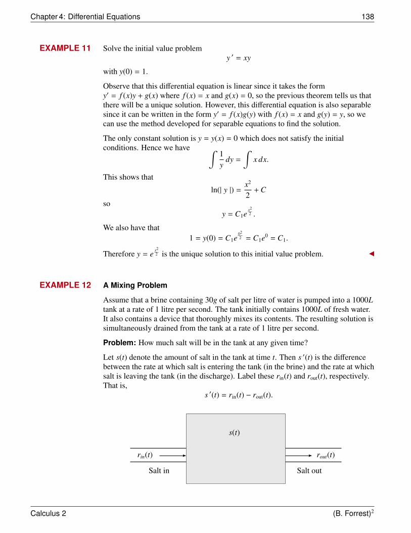
Chapter 4: Differential Equations 138
EXAMPLE 11 Solve the initial value problemy ′ = xy
with y(0) = 1.
Observe that this differential equation is linear since it takes the formy′ = f (x)y + g(x) where f (x) = x and g(x) = 0, so the previous theorem tells us thatthere will be a unique solution. However, this differential equation is also separablesince it can be written in the form y′ = f (x)g(y) with f (x) = x and g(y) = y, so wecan use the method developed for separable equations to find the solution.
The only constant solution is y = y(x) = 0 which does not satisfy the initialconditions. Hence we have ∫
1y
dy =
∫x dx.
This shows that
ln(| y |) =x2
2+ C
soy = C1e
x22 .
We also have that1 = y(0) = C1e
022 = C1e0 = C1.
Therefore y = ex22 is the unique solution to this initial value problem.
EXAMPLE 12 A Mixing Problem
Assume that a brine containing 30g of salt per litre of water is pumped into a 1000Ltank at a rate of 1 litre per second. The tank initially contains 1000L of fresh water.It also contains a device that thoroughly mixes its contents. The resulting solution issimultaneously drained from the tank at a rate of 1 litre per second.
Problem: How much salt will be in the tank at any given time?
Let s(t) denote the amount of salt in the tank at time t. Then s ′(t) is the differencebetween the rate at which salt is entering the tank (in the brine) and the rate at whichsalt is leaving the tank (in the discharge). Label these rin(t) and rout(t), respectively.That is,
s ′(t) = rin(t) − rout(t).
s(t)
Salt in Salt out
rin(t) rout(t)
Calculus 2 (B. Forrest)2
Section 4.4: Initial Value Problems 139
To find rin(t) we note that the concentration of salt in the brine entering the tank isconstant at 30g per litre. The flow rate is 1L per second and the rate at which the saltis entering the tank is the product of the concentration and the flow rate. Hence
rin(t) = 30gL× 1
Ls
= 30gs
and so the rate at which salt is entering the tank is 30 grams per second.
Calculating rout(t) is similar. It is the concentration of the discharge times the rate offlow. The rate of flow is again 1L per second but this time the concentration is notconstant. In fact the concentration of the discharge is the same as that of the tank.Since the concentration of salt in the tank is s(t)
1000 , we get
rout(t) =s(t)
1000× 1 =
s(t)1000
grams per second. It follows that
s ′(t) = 30 −s(t)
1000.
This is a first-order linear differential equation with f (t) = − 11000 and g(t) = 30.
(Note: It is also a separable DE). To solve the equation as a FOLDE, the integratingfactor I(t) is
I(t) = e−∫−1
1000 dt = et
1000 .
Using the FOLDE formula
y =
∫g(t)I(t)dt
I(t)
gives us
s(t) =
∫30e
t1000 dt
et
1000
=30000e
t1000 + C
et
1000
= 30000 + Ce−t
1000
Since s(0) = 0, we get
0 = 30000 + Ce0 = 30000 + C
and henceC = −30000.
Calculus 2 (B. Forrest)2
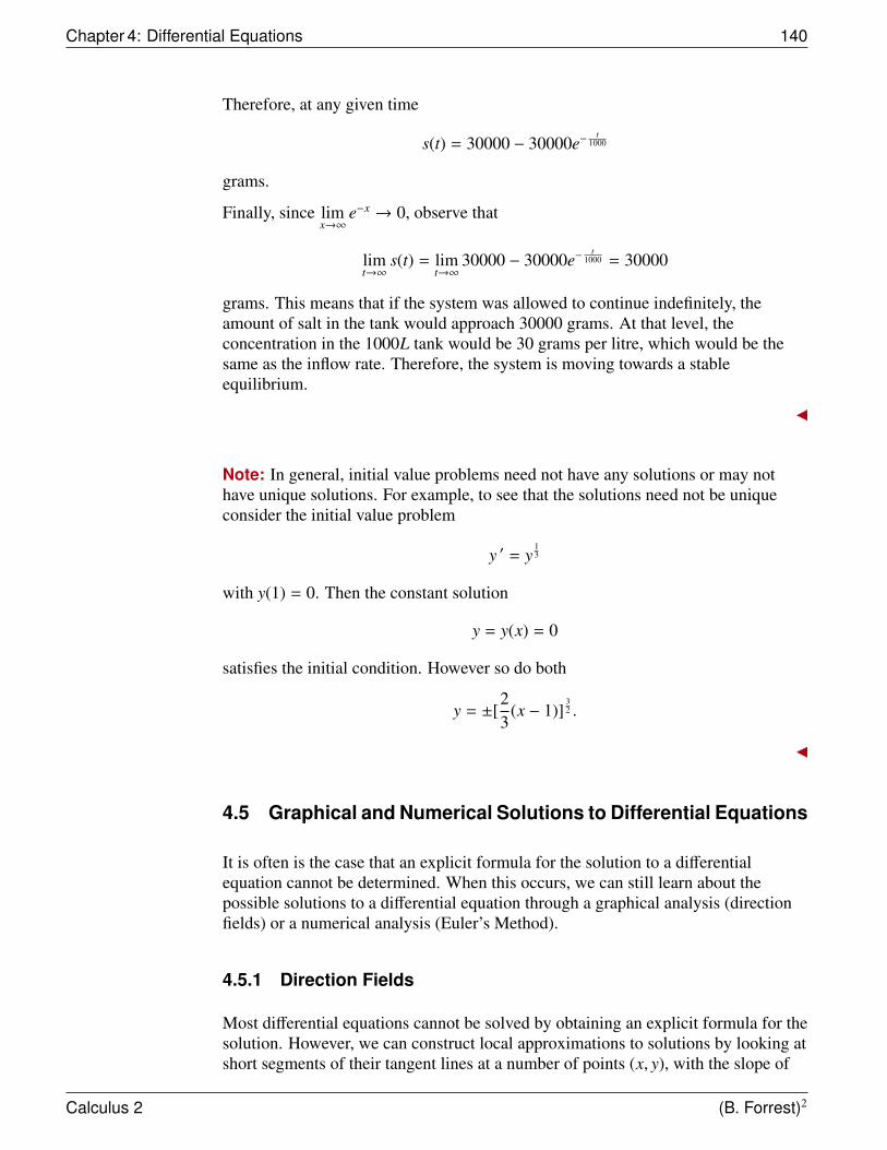
Chapter 4: Differential Equations 140
Therefore, at any given time
s(t) = 30000 − 30000e−t
1000
grams.
Finally, since limx→∞
e−x → 0, observe that
limt→∞
s(t) = limt→∞
30000 − 30000e−t
1000 = 30000
grams. This means that if the system was allowed to continue indefinitely, theamount of salt in the tank would approach 30000 grams. At that level, theconcentration in the 1000L tank would be 30 grams per litre, which would be thesame as the inflow rate. Therefore, the system is moving towards a stableequilibrium.
Note: In general, initial value problems need not have any solutions or may nothave unique solutions. For example, to see that the solutions need not be uniqueconsider the initial value problem
y ′ = y13
with y(1) = 0. Then the constant solution
y = y(x) = 0
satisfies the initial condition. However so do both
y = ±[23
(x − 1)]32 .
4.5 Graphical and Numerical Solutions to Differential Equations
It is often is the case that an explicit formula for the solution to a differentialequation cannot be determined. When this occurs, we can still learn about thepossible solutions to a differential equation through a graphical analysis (directionfields) or a numerical analysis (Euler’s Method).
4.5.1 Direction Fields
Most differential equations cannot be solved by obtaining an explicit formula for thesolution. However, we can construct local approximations to solutions by looking atshort segments of their tangent lines at a number of points (x, y), with the slope of
Calculus 2 (B. Forrest)2

Section 4.5: Graphical and Numerical Solutions to Differential Equations 141
these tangent lines determined by the differential equation. This set of tangent linesegments form a direction field and the direction field helps to visualize the solutioncurve that passes through any point that sits on a solution to the differential equation.
For example, consider the differential equation
y ′ = x + y.
This differential equation tells us that the derivative y ′ (or slope of the tangent line)of any solution whose graph contains the point (x, y) is the sum of the componentsof the points, x + y.
Let’s consider a set of points (x, y) chosen at random. For each pair (x, y) thecorresponding value of y ′ is calculated. This information is listed in the followingtable. The tangent line segments through (x, y) with the given slopes y ′ are thenplotted.
x y tangent line slope from DEy ′ = x + y
-2 0 y ′ = −2 + 0 = −2-1 0 y ′ = −1 + 0 = −10 0 y ′ = 0 + 0 = 01 0 y ′ = 1 + 0 = 12 0 y ′ = 2 + 0 = 20 1 y ′ = 0 + 1 = 11 1 y ′ = 1 + 1 = 22 1 y ′ = 2 + 1 = 3-1 3 y ′ = −1 + 3 = 2-1 -1 y ′ = −1 + −1 = −2
For example, at the origin (0, 0), we have y ′ = 0 + 0 = 0, so the tangent line hasslope 0 at the origin which gives us a horizontal line segment there. Similarly, at(1, 1), the tangent line has slope 2 so a line segment rising to the right is drawn. At(−1,−1), the tangent line has slope −2 so a line segment falling to the right is drawn.
The more tangent line segments that are drawn in the direction field, the easier it isto visualize the solution curves to this differential equation. However, this exercisecan become tedious if done by hand. Instead, a mathematical software program isnormally used to render the direction field.
The completed direction fieldfor
y ′ = x + y
is shown.
Calculus 2 (B. Forrest)2
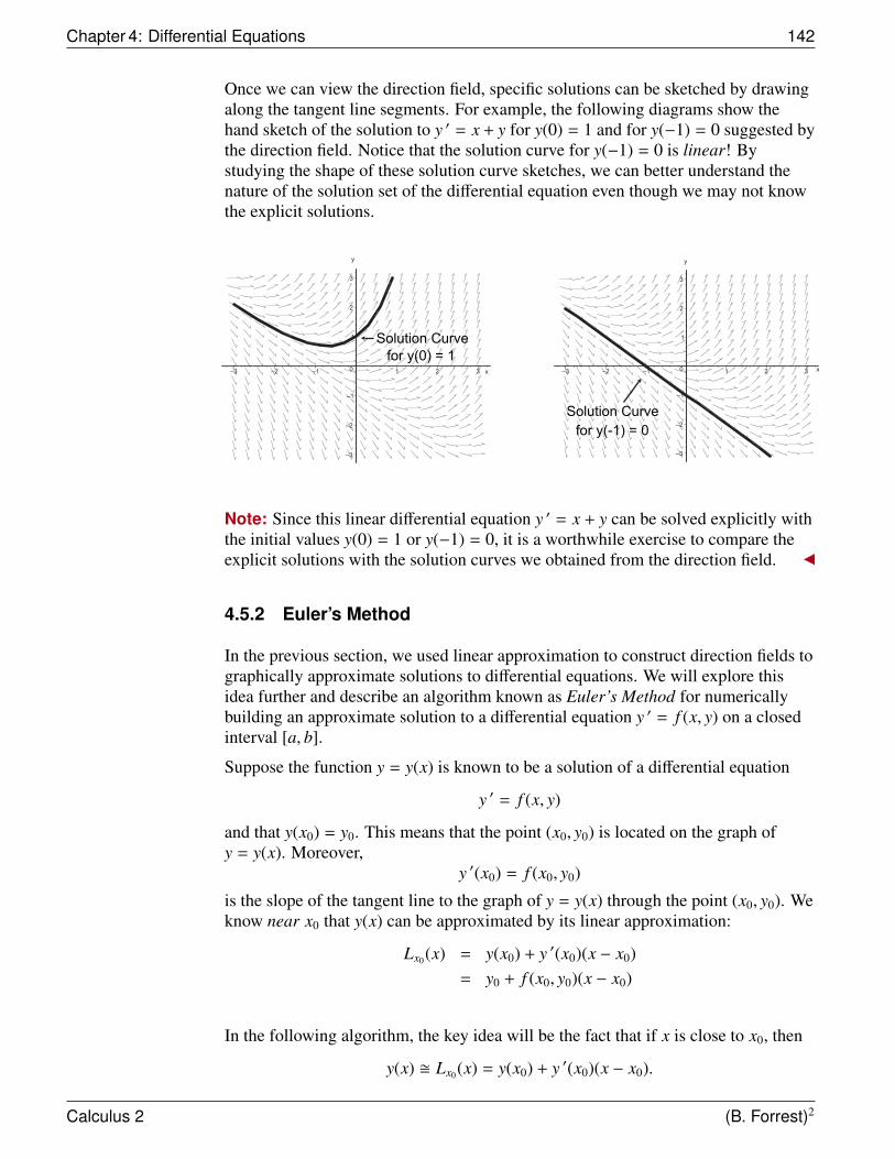
Chapter 4: Differential Equations 142
Once we can view the direction field, specific solutions can be sketched by drawingalong the tangent line segments. For example, the following diagrams show thehand sketch of the solution to y ′ = x + y for y(0) = 1 and for y(−1) = 0 suggested bythe direction field. Notice that the solution curve for y(−1) = 0 is linear! Bystudying the shape of these solution curve sketches, we can better understand thenature of the solution set of the differential equation even though we may not knowthe explicit solutions.
Note: Since this linear differential equation y ′ = x + y can be solved explicitly withthe initial values y(0) = 1 or y(−1) = 0, it is a worthwhile exercise to compare theexplicit solutions with the solution curves we obtained from the direction field.
4.5.2 Euler’s Method
In the previous section, we used linear approximation to construct direction fields tographically approximate solutions to differential equations. We will explore thisidea further and describe an algorithm known as Euler’s Method for numericallybuilding an approximate solution to a differential equation y ′ = f (x, y) on a closedinterval [a, b].
Suppose the function y = y(x) is known to be a solution of a differential equation
y ′ = f (x, y)
and that y(x0) = y0. This means that the point (x0, y0) is located on the graph ofy = y(x). Moreover,
y ′(x0) = f (x0, y0)
is the slope of the tangent line to the graph of y = y(x) through the point (x0, y0). Weknow near x0 that y(x) can be approximated by its linear approximation:
Lx0(x) = y(x0) + y ′(x0)(x − x0)= y0 + f (x0, y0)(x − x0)
In the following algorithm, the key idea will be the fact that if x is close to x0, then
y(x) � Lx0(x) = y(x0) + y ′(x0)(x − x0).
Calculus 2 (B. Forrest)2
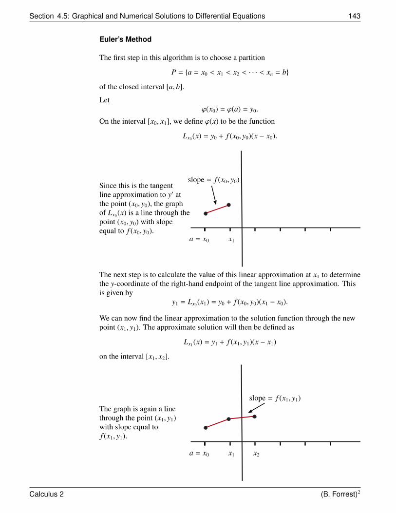
Section 4.5: Graphical and Numerical Solutions to Differential Equations 143
Euler’s Method
The first step in this algorithm is to choose a partition
P = {a = x0 < x1 < x2 < · · · < xn = b}
of the closed interval [a, b].
Letϕ(x0) = ϕ(a) = y0.
On the interval [x0, x1], we define ϕ(x) to be the function
Lx0(x) = y0 + f (x0, y0)(x − x0).
Since this is the tangentline approximation to y′ atthe point (x0, y0), the graphof Lx0(x) is a line through thepoint (x0, y0) with slopeequal to f (x0, y0).
slope = f (x0, y0)
a = x0 x1
The next step is to calculate the value of this linear approximation at x1 to determinethe y-coordinate of the right-hand endpoint of the tangent line approximation. Thisis given by
y1 = Lx0(x1) = y0 + f (x0, y0)(x1 − x0).
We can now find the linear approximation to the solution function through the newpoint (x1, y1). The approximate solution will then be defined as
Lx1(x) = y1 + f (x1, y1)(x − x1)
on the interval [x1, x2].
The graph is again a linethrough the point (x1, y1)with slope equal tof (x1, y1).
slope = f (x1, y1)
a = x0 x1 x2
Calculus 2 (B. Forrest)2
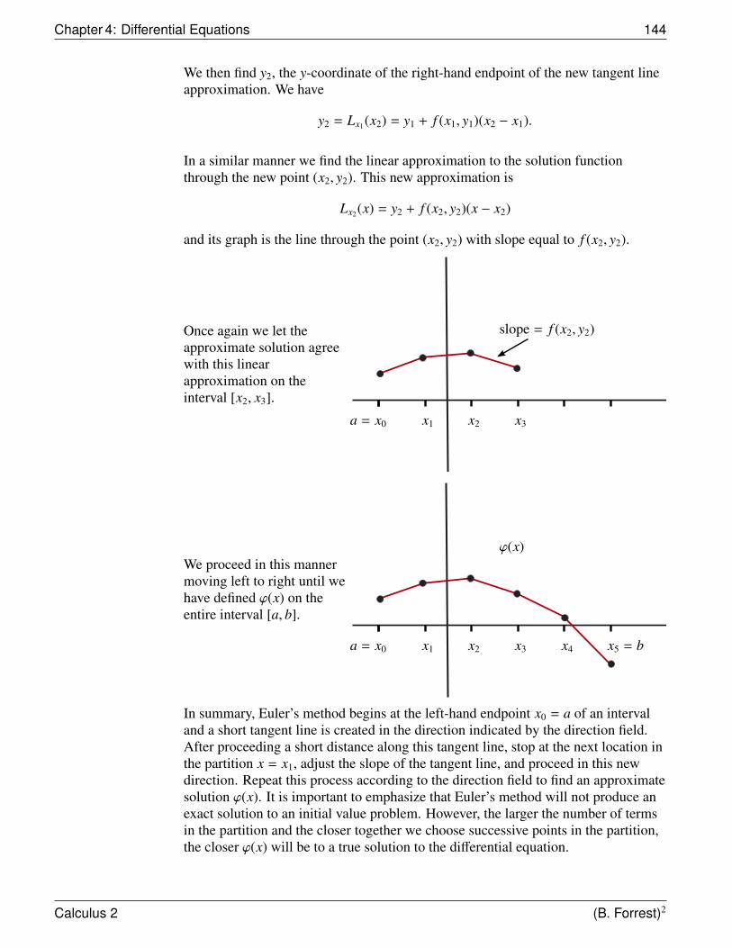
Chapter 4: Differential Equations 144
We then find y2, the y-coordinate of the right-hand endpoint of the new tangent lineapproximation. We have
y2 = Lx1(x2) = y1 + f (x1, y1)(x2 − x1).
In a similar manner we find the linear approximation to the solution functionthrough the new point (x2, y2). This new approximation is
Lx2(x) = y2 + f (x2, y2)(x − x2)
and its graph is the line through the point (x2, y2) with slope equal to f (x2, y2).
Once again we let theapproximate solution agreewith this linearapproximation on theinterval [x2, x3].
slope = f (x2, y2)
a = x0 x1 x2 x3
We proceed in this mannermoving left to right until wehave defined ϕ(x) on theentire interval [a, b].
ϕ(x)
a = x0 x1 x2 x3 x4 x5 = b
In summary, Euler’s method begins at the left-hand endpoint x0 = a of an intervaland a short tangent line is created in the direction indicated by the direction field.After proceeding a short distance along this tangent line, stop at the next location inthe partition x = x1, adjust the slope of the tangent line, and proceed in this newdirection. Repeat this process according to the direction field to find an approximatesolution ϕ(x). It is important to emphasize that Euler’s method will not produce anexact solution to an initial value problem. However, the larger the number of termsin the partition and the closer together we choose successive points in the partition,the closer ϕ(x) will be to a true solution to the differential equation.
Calculus 2 (B. Forrest)2
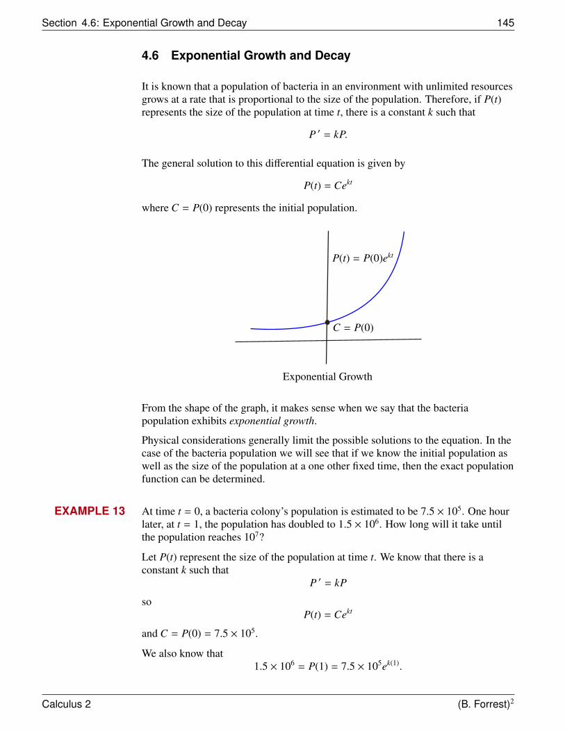
Section 4.6: Exponential Growth and Decay 145
4.6 Exponential Growth and Decay
It is known that a population of bacteria in an environment with unlimited resourcesgrows at a rate that is proportional to the size of the population. Therefore, if P(t)represents the size of the population at time t, there is a constant k such that
P ′ = kP.
The general solution to this differential equation is given by
P(t) = Cekt
where C = P(0) represents the initial population.
P(t) = P(0)ekt
Exponential Growth
C = P(0)
From the shape of the graph, it makes sense when we say that the bacteriapopulation exhibits exponential growth.
Physical considerations generally limit the possible solutions to the equation. In thecase of the bacteria population we will see that if we know the initial population aswell as the size of the population at a one other fixed time, then the exact populationfunction can be determined.
EXAMPLE 13 At time t = 0, a bacteria colony’s population is estimated to be 7.5 × 10⁵. One hourlater, at t = 1, the population has doubled to 1.5 × 10⁶. How long will it take untilthe population reaches 107?
Let P(t) represent the size of the population at time t. We know that there is aconstant k such that
P ′ = kP
soP(t) = Cekt
and C = P(0) = 7.5 × 10⁵.
We also know that1.5 × 106 = P(1) = 7.5 × 10⁵ek(1).
Calculus 2 (B. Forrest)2
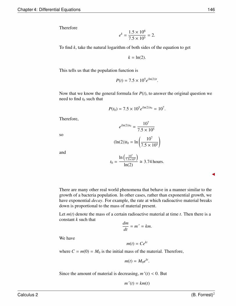
Chapter 4: Differential Equations 146
Therefore
ek =1.5 × 10⁶
7.5 × 105 = 2.
To find k, take the natural logarithm of both sides of the equation to get
k = ln(2).
This tells us that the population function is
P(t) = 7.5 × 10⁵e(ln(2))t.
Now that we know the general formula for P(t), to answer the original question weneed to find t0 such that
P(t0) = 7.5 × 10⁵e(ln(2))t0 = 107.
Therefore,
e(ln(2))t0 =107
7.5 × 10⁵
so
(ln(2))t0 = ln(
107
7.5 × 10⁵
)and
t0 =ln
(107
7.5×10⁵
)ln(2)
� 3.74 hours.
There are many other real world phenomena that behave in a manner similar to thegrowth of a bacteria population. In other cases, rather than exponential growth, wehave exponential decay. For example, the rate at which radioactive material breaksdown is proportional to the mass of material present.
Let m(t) denote the mass of a certain radioactive material at time t. Then there is aconstant k such that
dmdt
= m ′ = km.
We havem(t) = Cekt
where C = m(0) = M0 is the initial mass of the material. Therefore,
m(t) = M0ekt.
Since the amount of material is decreasing, m ′(t) < 0. But
m ′(t) = km(t)
Calculus 2 (B. Forrest)2
Section 4.6: Exponential Growth and Decay 147
and m(t) > 0 so it follows that k < 0. Therefore, the graph of m(t) appears asfollows:
m(t) = M0ekt
Exponential Decay
C = m(0) = M0
In particular, notice thatlimt→∞
m(t) = limt→∞
M0ekt = 0
since k < 0.
We call such a process exponential decay.
All radioactive materials have associated with them a quantity th known as thehalf-life of the material. This is the amount of time it would take for one-half of thematerial to decay. The half-life is a fundamental characteristic of the material.
Mathematically, ifm(t) = M0ekt
then th is the time at which
m(th) = M0ekth =M0
2.
Dividing by M0 shows that
ekth =12
and hence that
kth = ln(12
)= − ln(2).
Therefore, the half-life is given by the formula
th =− ln(2)
k.
In particular, this shows that the half-life of a material is independent of the originalmass.
Calculus 2 (B. Forrest)2

Chapter 4: Differential Equations 148
m(t) = M0ekt
C = m(0) = M0
Half-life
M02
th = −ln(2)
k
EXAMPLE 14 Carbon Dating
All living organisms contain a small amount of radioactive carbon-14. Moreover,each type of organism has a particular equilibrium ratio of carbon-14 compared tothe stable isotope carbon-12.
When an organism dies the equilibrium is no longer maintained since theradioactive carbon-14 slowly breaks down into carbon-12. It is also known thatcarbon-14 breaks down at a rate of 1 part in 8000 per year. This means that after 1year an initial quantity of 8000 particles will be reduced to 7999. Hence
7999 = m(1) = 8000ek(1)
so that
k = ln(79998000
).
Problem 1: Find the half-life of carbon-14.
From the previous discussion, we know that
th =− ln(2)
k
=− ln(2)
ln(
79998000
)� 5544.83 years
Problem 2: After a fossil was found research showed that the amount of carbon-14was 23% of the amount that would have been present at the time of death. How oldwas the fossil?
Calculus 2 (B. Forrest)2
Section 4.7: Newton’s Law of Cooling 149
Let M0 be the expected amount of carbon-14 in the fossil and let to be the age of thefossil. Then the research shows that
(0.23)M0 = m(t0) = M0ekt0 .
We must solve this equation for t0. The first step is to recognize that
ekt0 =(0.23)M0
M0= 0.23
This shows that we did not need to find the quantity M0 explicitly to solve thisquestion.
Taking the natural logarithm of both sides of the equation gives
kt0 = ln(0.23)
and hence that
t0 =ln(0.23)
k
=ln(0.23)
ln(
79998000
)= 11 756 years
4.7 Newton’s Law of Cooling
Newton’s law of cooling states that an object will cool (or warm) at a rate that isproportional to the difference between the temperature of the object and the ambienttemperature Ta of its surroundings. Therefore, if T (t) denotes the temperature of anobject at time t, then there is a constant k such that
T ′ = k(T − Ta).
If D = D(t) = T (t) − Ta, thenD ′ = T ′ = kD
so D satisfies the equation for exponential growth (or decay). We know
D = Cekt.
It follows thatT (t) = Cekt + Ta
Calculus 2 (B. Forrest)2
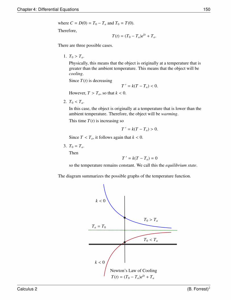
Chapter 4: Differential Equations 150
where C = D(0) = T0 − Ta and T0 = T (0).
Therefore,T (t) = (T0 − Ta)ekt + Ta.
There are three possible cases.
1. T0 > Ta.
Physically, this means that the object is originally at a temperature that isgreater than the ambient temperature. This means that the object will becooling.
Since T (t) is decreasingT ′ = k(T − Ta) < 0.
However, T > Ta, so that k < 0.
2. T0 < Ta.
In this case, the object is originally at a temperature that is lower than theambient temperature. Therefore, the object will be warming.
This time T (t) is increasing so
T ′ = k(T − Ta) > 0.
Since T < Ta, it follows again that k < 0.
3. T0 = Ta.
ThenT ′ = k(T − Ta) = 0
so the temperature remains constant. We call this the equilibrium state.
The diagram summarizes the possible graphs of the temperature function.
Newton’s Law of CoolingT (t) = (T0 − Ta)ekt + Ta
k < 0
k < 0
Ta = T0
T0 > Ta
T0 < Ta
Calculus 2 (B. Forrest)2
Section 4.7: Newton’s Law of Cooling 151
Notice that in all three cases,limt→∞
T (t) = Ta.
Regardless of the initial starting point, if a process always moves towards aparticular equilibrium value, we call this value a stable equilibrium.
EXAMPLE 15 A cup of boiling water at 100◦C is allowed to cool in a room where the ambienttemperature is 20◦C. If after 10 minutes the water has cooled to 70◦C, what will bethe temperature after the water has cooled for 25 minutes?
Let T (t) denote the temperature of the water at time t minutes after coolingcommences. The initial temperature is T0 = 100◦C and the ambient temperature isTa = 20◦C. Newton’s Law of Cooling shows that there is a constant k < 0 such that
T (t) = (T0 − Ta)ekt + Ta
= (100 − 20)ekt + 20= 80ekt + 20
The next step is to determine k. Note that
70 = T (10) = 80ek(10) + 20
so50 = 80e10k.
Hence,
10k = ln(5080
)and
k =ln
(5080
)10
= −0.047
We can now evaluate T (25) to get that the temperature after 25 minutes is
T (25) = 80e−0.047(25) + 20= 44.71
degrees Celsius.
Calculus 2 (B. Forrest)2
Chapter 4: Differential Equations 152
4.8 Logistic Growth
We have seen that a population with unlimited resources grows at a rate that isproportional to its size. This leads to the differential equation
P ′ = kP.
However, the assumption that resources will be unlimited is usually unrealistic.More likely, there is a maximum population M that the surrounding environmentcan sustain. This means that as the population P(t) approaches M, resources willbecome more scarce and the growth rate of the population will slow. On the otherhand, when the population is small in comparison to the maximum populationpossible, the growth rate will be similar to that of the unrestricted case since therewill be little resource pressure. It is known that such a population satisfies adifferential equation of the form
P ′ = kP(M − P).
This equation means that the rate of growth is proportional to the product of thecurrent population and the difference from the maximum sustainable population.
Populations of this type are said to satisfy logistic growth and the differentialequation
y ′ = ky(M − y)
is called the logistic equation.
The logistic equation need not only model a population. However, in the specialcase where we are trying to describe the behavior of a population, we have theadditional constraint that P(t) > 0.
Let P0 = P(0) be the initial population at the beginning of a study.
Observe that if the initial population is smaller than M, then the population will begrowing. This means that we would have
0 < P ′ = kP(M − P)
since both P and M − P are positive. As such, we would expect that k > 0.
However, if the initial population exceeds the maximum sustainable population,then the population would decrease so
0 > P ′ = kP(M − P)
and again we would have k > 0 since P > 0 and M − P < 0.
A third possible case occurs when the initial population is already at the maximum.In this case,
P ′ = kP(M − P) = 0
so the population would remain constant. This shows that P(t) = M is anequilibrium solution.
Calculus 2 (B. Forrest)2
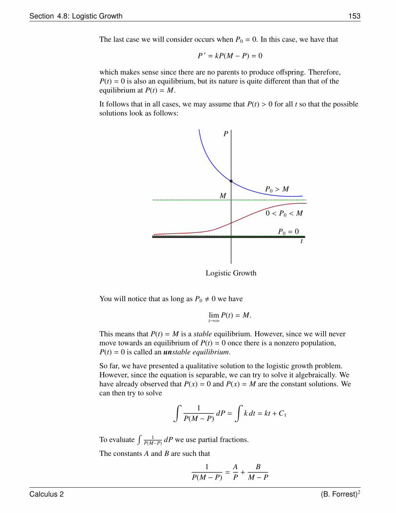
Section 4.8: Logistic Growth 153
The last case we will consider occurs when P0 = 0. In this case, we have that
P ′ = kP(M − P) = 0
which makes sense since there are no parents to produce offspring. Therefore,P(t) = 0 is also an equilibrium, but its nature is quite different than that of theequilibrium at P(t) = M.
It follows that in all cases, we may assume that P(t) > 0 for all t so that the possiblesolutions look as follows:
Logistic Growth
P0 > M
0 < P0 < M
M
P0 = 0
P
t
You will notice that as long as P0 , 0 we have
limt→∞
P(t) = M.
This means that P(t) = M is a stable equilibrium. However, since we will nevermove towards an equilibrium of P(t) = 0 once there is a nonzero population,P(t) = 0 is called an unstable equilibrium.
So far, we have presented a qualitative solution to the logistic growth problem.However, since the equation is separable, we can try to solve it algebraically. Wehave already observed that P(x) = 0 and P(x) = M are the constant solutions. Wecan then try to solve ∫
1P(M − P)
dP =
∫k dt = kt + C1
To evaluate∫
1P(M−P) dP we use partial fractions.
The constants A and B are such that
1P(M − P)
=AP
+B
M − P
Calculus 2 (B. Forrest)2
Chapter 4: Differential Equations 154
or1 = A(M − P) + B(P).
Letting P = 0 gives1 = A(M)
soA =
1M
.
Letting P = M, we get1 = B(M)
and again
B =1M
.
Therefore1
P(M − P)=
1M
[1P
+1
M − P
].
It follows that ∫1
P(M − P)dP =
1M
[∫1P
dP +
∫1
M − PdP
]=
1M
[ln(| P |) − ln(| M − P |)] + C2
=1M
ln(| P |
| M − P |
)+ C2
We now have that1M
ln(| P(t) |
| M − P(t) |
)+ C2 = kt + C1.
Therefore,
ln(| P(t) |
| M − P(t) |
)= Mkt + C3
where C3 is arbitrary.
This shows that| P(t) |
| M − P(t) |= CeMkt
where C = eC3 > 0.
There are two cases to consider.
Case 1: Assume that 0 < P(t) < M. Then
| P(t) || M − P(t) |
=P(t)
M − P(t)= CeMkt.
Calculus 2 (B. Forrest)2
Section 4.8: Logistic Growth 155
Solving for P(t) would give
P(t) = (M − P(t))CeMkt
= MCeMkt − P(t)CeMkt
so thatP(t) + P(t)CeMkt = MCeMkt.
We then haveP(t)(1 + CeMkt) = MCeMkt
and finally that
P(t) =MCeMkt
1 + CeMkt
= MCeMkt
1 + CeMkt
There are two important observations we can make about this solution.
(a) Since C > 0, the denominator is never 0 so the function P(t) is continuous and
0 <CeMkt
1 + CeMkt < 1
so that0 < P(t) < M
which agrees with our assumption.
(b) Since k > 0, we have that
limt→∞
P(t) = limt→∞
MCeMkt
1 + CeMkt
= M limt→∞
CeMkt
1 + CeMkt
= M
and
limt→−∞
P(t) = limt→−∞
MCeMkt
1 + CeMkt = 0.
This shows that the population would eventually approach the maximumpopulation M but if you went back in time far enough, the population wouldbe near 0. Both of these limits are consistent with our expectations.
Calculus 2 (B. Forrest)2
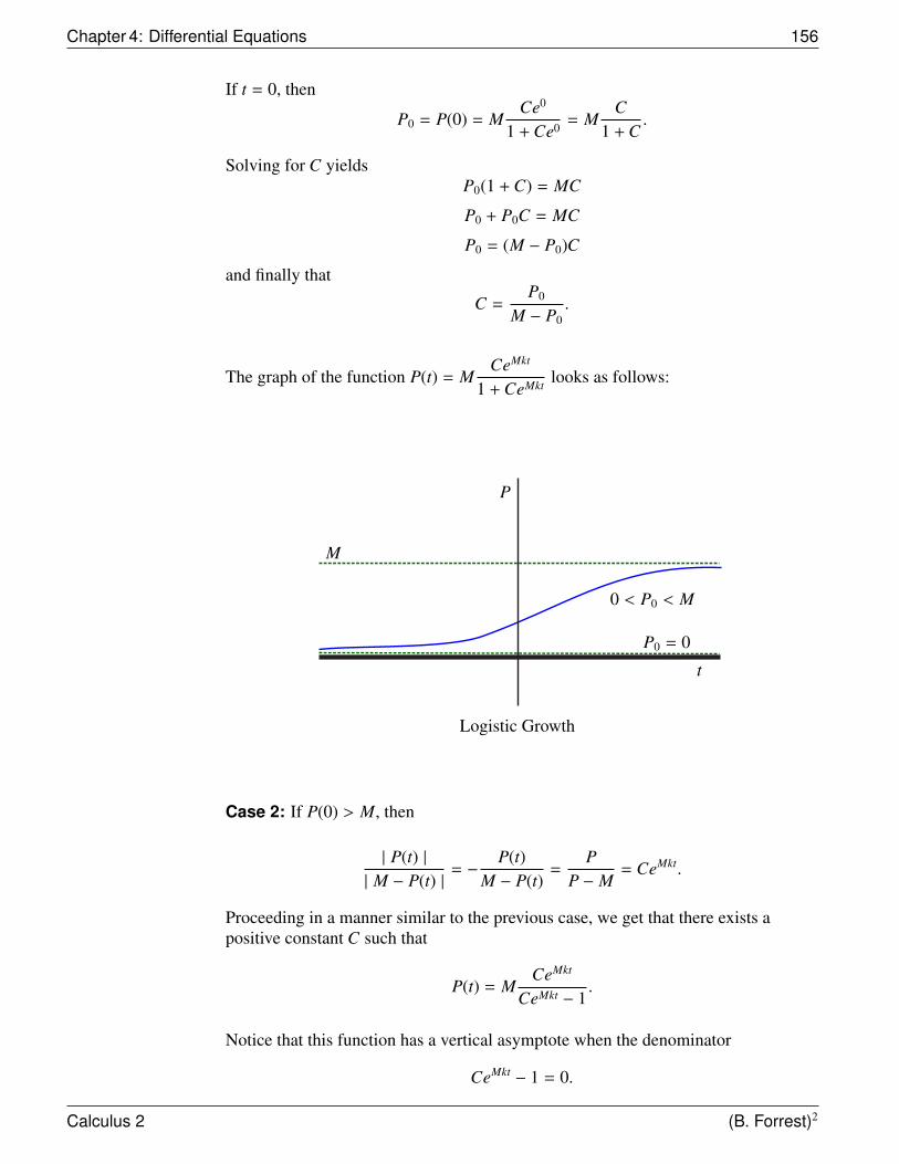
Chapter 4: Differential Equations 156
If t = 0, then
P0 = P(0) = MCe0
1 + Ce0 = MC
1 + C.
Solving for C yieldsP0(1 + C) = MC
P0 + P0C = MC
P0 = (M − P0)C
and finally that
C =P0
M − P0.
The graph of the function P(t) = MCeMkt
1 + CeMkt looks as follows:
Logistic Growth
M
0 < P0 < M
t
P
P0 = 0
Case 2: If P(0) > M, then
| P(t) || M − P(t) |
= −P(t)
M − P(t)=
PP − M
= CeMkt.
Proceeding in a manner similar to the previous case, we get that there exists apositive constant C such that
P(t) = MCeMkt
CeMkt − 1.
Notice that this function has a vertical asymptote when the denominator
CeMkt − 1 = 0.
Calculus 2 (B. Forrest)2
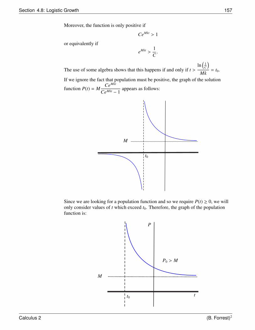
Section 4.8: Logistic Growth 157
Moreover, the function is only positive if
CeMkt > 1
or equivalently if
eMkt >1C.
The use of some algebra shows that this happens if and only if t >ln
(1C
)Mk
= t0.
If we ignore the fact that population must be positive, the graph of the solution
function P(t) = MCeMkt
CeMkt − 1appears as follows:
t0
M
Since we are looking for a population function and so we require P(t) ≥ 0, we willonly consider values of t which exceed t0. Therefore, the graph of the populationfunction is:
t0
M
P0 > M
P
t
Calculus 2 (B. Forrest)2
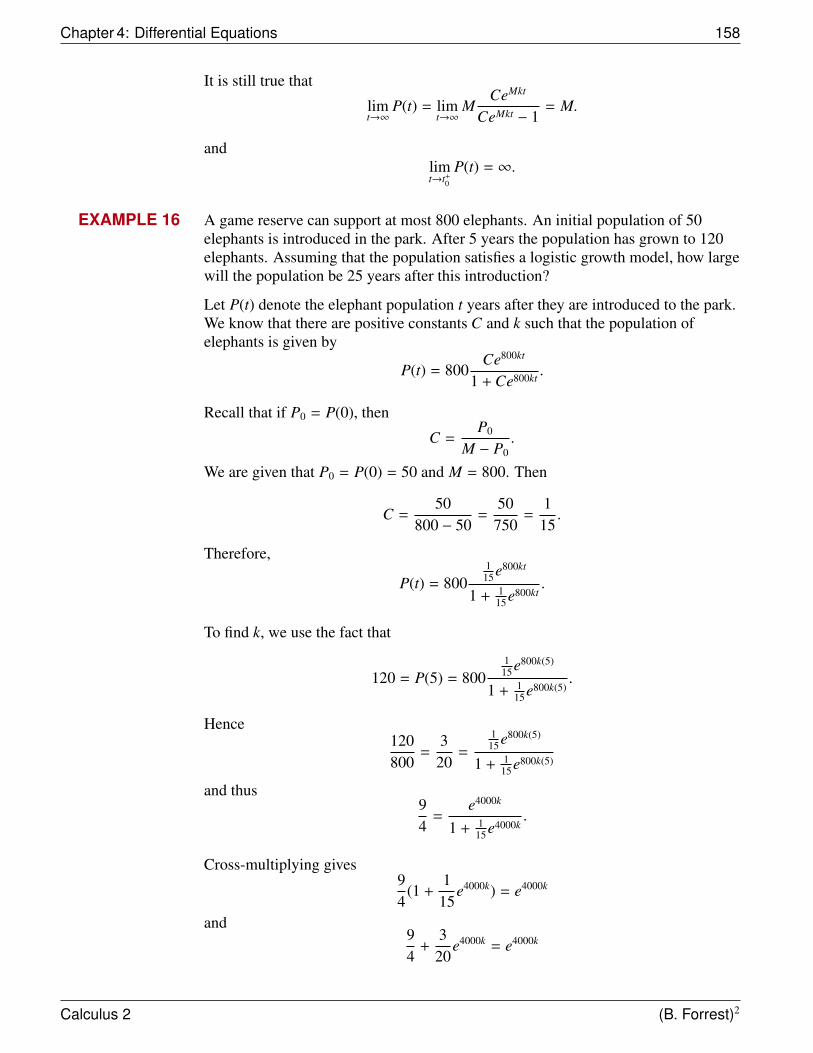
Chapter 4: Differential Equations 158
It is still true that
limt→∞
P(t) = limt→∞
MCeMkt
CeMkt − 1= M.
andlimt→t+0
P(t) = ∞.
EXAMPLE 16 A game reserve can support at most 800 elephants. An initial population of 50elephants is introduced in the park. After 5 years the population has grown to 120elephants. Assuming that the population satisfies a logistic growth model, how largewill the population be 25 years after this introduction?
Let P(t) denote the elephant population t years after they are introduced to the park.We know that there are positive constants C and k such that the population ofelephants is given by
P(t) = 800Ce800kt
1 + Ce800kt .
Recall that if P0 = P(0), then
C =P0
M − P0.
We are given that P0 = P(0) = 50 and M = 800. Then
C =50
800 − 50=
50750
=115
.
Therefore,
P(t) = 800115e800kt
1 + 115e800kt
.
To find k, we use the fact that
120 = P(5) = 8001
15e800k(5)
1 + 115e800k(5)
.
Hence120800
=3
20=
115e800k(5)
1 + 115e800k(5)
and thus94
=e4000k
1 + 115e4000k
.
Cross-multiplying gives94
(1 +1
15e4000k) = e4000k
and94
+3
20e4000k = e4000k
Calculus 2 (B. Forrest)2
Section 4.8: Logistic Growth 159
so94
=1720
e4000k.
This means4517
= e4000k
and finally that
k =ln
(4517
)4000
.
Substituting k back into the population model and evaluating at t = 25 we get
P(25) = 800115e800
ln( 4517 )
4000 (25)
1 + 115e800
ln( 4517 )
4000 (25)
= 800115e5 ln( 45
17 )
1 + 115e5 ln( 45
17 )
= 717 elephants
It follows that after 25 years the population has very nearly reached its maximum(800 elephants).
Logistic growth also applies to many other situations.
EXAMPLE 17 A rumor is circulating around a university campus. A survey revealed that at onepoint only 5% of the students in the school were aware of the rumor. However, sincenews on campus spreads quickly, after 10 hours the rumor is known by 10% of thestudent body. How long will it take until 30% of the students are aware of therumor?
Let r(t) be the fraction of the student body at time t that have heard this rumor. Then0 ≤ r(t) ≤ 1.
Experiments have shown that the rate at which a rumor spreads through a populationis proportional to the product of the fraction of the population that have heard therumor and the fraction that have not. Therefore, there is a constant k such that
r ′ = kr(1 − r)
and so this is a logistic growth model with M = 1. It follows that there is a positiveconstant C such that
r(t) =Cekt
1 + Cekt .
Calculus 2 (B. Forrest)2
Chapter 4: Differential Equations 160
We know that at r(0) = 0.05 so
C =r(0)
1 − r(0)=
0.050.95
= 0.0526315
and hence that
0.1 = r(10)
=
0.050.95e10k
1 + 0.050.95e10k
Therefore0.1 +
0.0050.95
e10k =0.050.95
e10k
and0.1 =
0.0450.95
e10k.
This gives
e10k =0.0950.045
and
k =ln
(0.0950.045
)10
= 0.07472
Finally, we want to find t0 such that
0.3 =Cekt0
1 + Cekt .
Therefore,0.3(1 + Cekt) = Cekt0
so0.3 = 0.7Cekt0
andekt0 =
0.30.7C
.
This shows that
t0 =ln
(0.3
0.7C
)k
=ln
(0.3
0.7(0.0526315)
)0.07472
= 28.07
hours.
After 28.07 hours, 30% of the student population had heard the rumor.
Calculus 2 (B. Forrest)2

Section 4.8: Logistic Growth 161
There are many other important examples of logistic models that are similar to theprevious example. For example, the spread of disease through a population alsobehaves like the spread of a rumor and as such can be studied with a logistic growthmodel.
Calculus 2 (B. Forrest)2
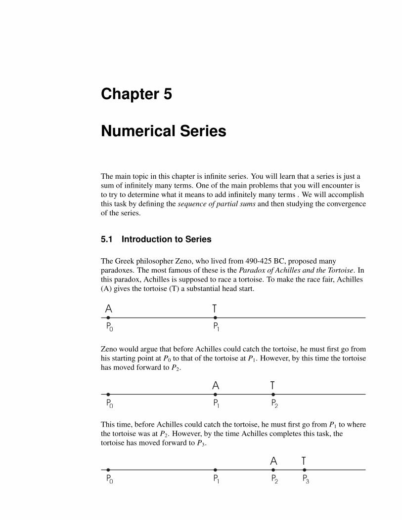
Chapter 5
Numerical Series
The main topic in this chapter is infinite series. You will learn that a series is just asum of infinitely many terms. One of the main problems that you will encounter isto try to determine what it means to add infinitely many terms . We will accomplishthis task by defining the sequence of partial sums and then studying the convergenceof the series.
5.1 Introduction to Series
The Greek philosopher Zeno, who lived from 490-425 BC, proposed manyparadoxes. The most famous of these is the Paradox of Achilles and the Tortoise. Inthis paradox, Achilles is supposed to race a tortoise. To make the race fair, Achilles(A) gives the tortoise (T) a substantial head start.
P0
P1
A T
Zeno would argue that before Achilles could catch the tortoise, he must first go fromhis starting point at P0 to that of the tortoise at P1. However, by this time the tortoisehas moved forward to P2.
P0
P1
A T
P2
This time, before Achilles could catch the tortoise, he must first go from P1 to wherethe tortoise was at P2. However, by the time Achilles completes this task, thetortoise has moved forward to P3.
P0
P1
A T
P2
P3
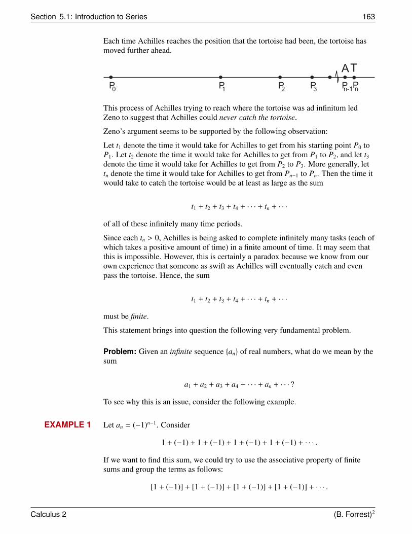
Section 5.1: Introduction to Series 163
Each time Achilles reaches the position that the tortoise had been, the tortoise hasmoved further ahead.
P0 P1
AT
P2 P3 Pn-1Pn
This process of Achilles trying to reach where the tortoise was ad infinitum ledZeno to suggest that Achilles could never catch the tortoise.
Zeno’s argument seems to be supported by the following observation:
Let t1 denote the time it would take for Achilles to get from his starting point P0 toP1. Let t2 denote the time it would take for Achilles to get from P1 to P2, and let t3
denote the time it would take for Achilles to get from P2 to P3. More generally, lettn denote the time it would take for Achilles to get from Pn−1 to Pn. Then the time itwould take to catch the tortoise would be at least as large as the sum
t1 + t2 + t3 + t4 + · · · + tn + · · ·
of all of these infinitely many time periods.
Since each tn > 0, Achilles is being asked to complete infinitely many tasks (each ofwhich takes a positive amount of time) in a finite amount of time. It may seem thatthis is impossible. However, this is certainly a paradox because we know from ourown experience that someone as swift as Achilles will eventually catch and evenpass the tortoise. Hence, the sum
t1 + t2 + t3 + t4 + · · · + tn + · · ·
must be finite.
This statement brings into question the following very fundamental problem.
Problem: Given an infinite sequence {an} of real numbers, what do we mean by thesum
a1 + a2 + a3 + a4 + · · · + an + · · · ?
To see why this is an issue, consider the following example.
EXAMPLE 1 Let an = (−1)n−1. Consider
1 + (−1) + 1 + (−1) + 1 + (−1) + 1 + (−1) + · · · .
If we want to find this sum, we could try to use the associative property of finitesums and group the terms as follows:
[1 + (−1)] + [1 + (−1)] + [1 + (−1)] + [1 + (−1)] + · · · .
Calculus 2 (B. Forrest)2
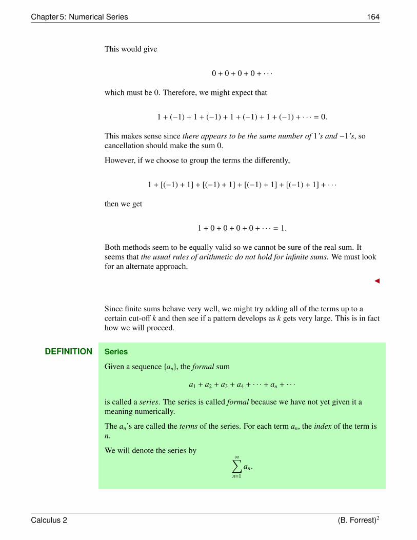
Chapter 5: Numerical Series 164
This would give
0 + 0 + 0 + 0 + · · ·
which must be 0. Therefore, we might expect that
1 + (−1) + 1 + (−1) + 1 + (−1) + 1 + (−1) + · · · = 0.
This makes sense since there appears to be the same number of 1’s and −1’s, socancellation should make the sum 0.
However, if we choose to group the terms the differently,
1 + [(−1) + 1] + [(−1) + 1] + [(−1) + 1] + [(−1) + 1] + · · ·
then we get
1 + 0 + 0 + 0 + 0 + · · · = 1.
Both methods seem to be equally valid so we cannot be sure of the real sum. Itseems that the usual rules of arithmetic do not hold for infinite sums. We must lookfor an alternate approach.
Since finite sums behave very well, we might try adding all of the terms up to acertain cut-off k and then see if a pattern develops as k gets very large. This is in facthow we will proceed.
DEFINITION Series
Given a sequence {an}, the formal sum
a1 + a2 + a3 + a4 + · · · + an + · · ·
is called a series. The series is called formal because we have not yet given it ameaning numerically.
The an’s are called the terms of the series. For each term an, the index of the term isn.
We will denote the series by∞∑
n=1
an.
Calculus 2 (B. Forrest)2
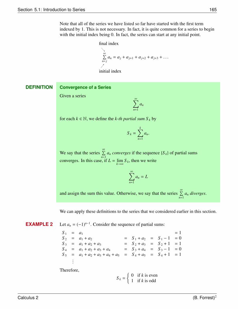
Section 5.1: Introduction to Series 165
Note that all of the series we have listed so far have started with the first termindexed by 1. This is not necessary. In fact, it is quite common for a series to beginwith the initial index being 0. In fact, the series can start at any initial point.
∞∑n= j
an = a j + a j+1 + a j+2 + a j+3 + . . .
initial index
final index
DEFINITION Convergence of a Series
Given a series∞∑
n=1
an
for each k ∈ N, we define the k-th partial sum S k by
S k =
k∑n=1
an.
We say that the series∞∑
n=1an converges if the sequence {S k} of partial sums
converges. In this case, if L = limk→∞
S k, then we write
∞∑n=1
an = L
and assign the sum this value. Otherwise, we say that the series∞∑
n=1an diverges.
We can apply these definitions to the series that we considered earlier in this section.
EXAMPLE 2 Let an = (−1)n−1. Consider the sequence of partial sums:
S 1 = a1 = 1S 2 = a1 + a2 = S 1 + a2 = S 1 − 1 = 0S 3 = a1 + a2 + a3 = S 2 + a3 = S 2 + 1 = 1S 4 = a1 + a2 + a3 + a4 = S 3 + a4 = S 3 − 1 = 0S 5 = a1 + a2 + a3 + a4 + a5 = S 4 + a5 = S 4 + 1 = 1
...
Therefore,
S k =
{0 if k is even1 if k is odd
Calculus 2 (B. Forrest)2
Chapter 5: Numerical Series 166
This shows that the sequence of partial sums {S k} diverges, and hence so does∞∑
n=1(−1)n−1.
EXAMPLE 3 Determine if the series∞∑
n=1
1n2 + n
converges or diverges.
Observe thatan =
1n2 + n
=1
n(n + 1).
Moreover, we can write
an =1
n(n + 1)=
1n−
1n + 1
.
Therefore the series becomes∞∑
n=1
(1n−
1n + 1
).
To calculate S k note that
S k =
k∑n=1
(1n−
1n + 1
)= (1 −
12
) + (12−
13
) + (13−
14
) + (14−
15
) + · · · + (1k−
1k + 1
)
If we regroup these terms, we get
S k = (1 −12
) + (12−
13
) + (13−
14
) + (14−
15
) + · · · + (1k−
1k + 1
)
= 1 − (12−
12
) − (13−
13
) − (14−
14
) − (15−
15
) − · · · − (1k−
1k
) −1
k + 1
= 1 − 0 − 0 − 0 − 0 − · · · − 0 −1
k + 1
= 1 −1
k + 1
Then
limk→∞
S k = limk→∞
(1 −
1k + 1
)= 1.
Calculus 2 (B. Forrest)2
Section 5.2: Geometric Series 167
Since the sequence of partial sums {S k} converges to 1, the series∞∑
n=1
1n2+n converges
and∞∑
n=1
1n2 + n
= 1.
What is remarkable about the previous series is not that we were able to show that itconverges, but rather that we could find its sum so easily. Generally, this will not bethe case. In fact, even if we know a series converges, it may be very difficult or evenimpossible to determine the exact value of its sum. In most cases, we will have to becontent with either showing that a series converges or that it diverges and, in thecase of a convergent series, estimating its sum.
The next section deals with an important class of series known as geometric series.Not only can we determine if such a series converges, but we can easily find thesum.
5.2 Geometric Series
Perhaps the most important type of series are the geometric series.
DEFINITION Geometric Series
A geometric series is a series of the form
∞∑n=0
rn = 1 + r + r2 + r3 + r4 + · · ·
The number r is called the ratio of the series.
If r = (−1), the series is
∞∑n=0
(−1)n = 1 + (−1) + 1 + (−1) + 1 + (−1) + 1 + (−1) + · · ·
which we have already seen diverges.
If r = 1, the series is∞∑
n=0
1n = 1 + 1 + 1 + 1 + 1 + · · ·
which again diverges since S k =k∑
n=01n = k + 1 diverges to∞.
Question: Which if any of the geometric series converge?
Calculus 2 (B. Forrest)2

Chapter 5: Numerical Series 168
Assume that r , 1. Let
S k = 1 + r + r2 + r3 + r4 + · · · + rk.
Then
rS k = r(1 + r + r2 + r3 + r4 + · · · + rk)= r + r2 + r3 + r4 + · · · + rk+1
Therefore
S k − rS k = (1 + r + r2 + r3 + r4 + · · · + rk) − (r + r2 + r3 + r4 + · · · + rk + rk+1)= 1 − rk+1
Hence(1 − r)S k = S k − rS k = 1 − rk+1
and since r , 1,
S k =1 − rk+1
1 − r.
The only term in this expression that depends on k is rk+1, so limk→∞
S k exists if and
only if limk→∞
rk+1 exists. However, if | r |< 1, then rk+1 becomes very small for large k.
That is limk→∞
rk+1 = 0.
If | r |> 1, then | rk+1 | becomes very large as k grows. That is, limk→∞| rk+1 |= ∞.
Hence, limk→∞
rk+1 does not exist.
Finally, if r = −1, then rk+1 alternates between 1 and −1, so limk→∞
rk+1 again diverges.
This shows that rk+1, and hence the series∞∑
n=0rn, converges if and only if | r |< 1.
Moreover, in this case,
limk→∞
S k = limk→∞
1 − rk+1
1 − r
=
1 − limk→∞
rk+1
1 − r
=1
1 − r
Calculus 2 (B. Forrest)2
Section 5.3: Divergence Test 169
THEOREM 1 Geometric Series Test
The geometric series∞∑
n=0rn converges if | r |< 1 and diverges otherwise.
If | r |< 1, then∞∑
n=0
rn =1
1 − r.
EXAMPLE 4 Evaluate∞∑
n=0
(12
)n.
SOLUTION This is a geometric series with ratio r = 12 . Since 0 < 1
2 < 1, the
Geometric Series Test shows that∞∑
n=0
(12
)nconverges. Moreover,
∞∑n=0
(12
)n
=1
1 − 12
= 2
5.3 Divergence Test
It makes sense that if we are to add together infinitely many positive numbers andget something finite, then the terms must eventually be small. We will now see thatthis statement holds for any convergent series.
THEOREM 2 Divergence Test
Assume that∞∑
n=1an converges. Then
limn→∞
an = 0.
Equivalently, if limn→∞
an , 0 or if limn→∞
an does not exist, then∞∑
n=1an diverges.
The Divergence Test gets its name because it can identify certain series as beingdivergent, but it cannot show that a series converges.
EXAMPLE 5 Consider the geometric series∞∑
n=0rn with | r |≥ 1. Then lim
n→∞rn = 1 if r = 1 and it
does not exist for all other r with | r |≥ 1 (in other words, if r = −1 or if |r| > 1). The
Divergence Test shows that if | r |≥ 1, then∞∑
n=0rn diverges.
Calculus 2 (B. Forrest)2
Chapter 5: Numerical Series 170
The Divergence Test works for the following reason. Assume that∞∑
n=1an converges
to L. This is equivalent to saying that
limk→∞
S k = L.
By the basic properties of convergent sequences, we get that
limk→∞
S k−1 = L
as well.
However, for k ≥ 2,
S k − S k−1 =
k∑n=1
an −
k−1∑n=1
an
= (a1 + a2 + a3 + a4 + · · · + ak−1 + ak) − (a1 + a2 + a3 + a4 + · · · + ak−1)= ak
Therefore,
limk→∞
ak = limk→∞
(S k − S k−1)
= limk→∞
S k − limk→∞
S k−1
= L − L= 0.
EXAMPLES
1. Consider the sequence { nn+1 }. Then
limn→∞
nn + 1
= 1.
Therefore, the Divergence Test shows that∞∑
n=1
nn + 1
diverges.
2. While it is difficult to do so, it is possible to show that
limn→∞
sin(n)
does not exist. Therefore, the Divergence Test shows that the series∞∑
n=1
sin(n)
diverges.
Calculus 2 (B. Forrest)2

Section 5.3: Divergence Test 171
3. The Divergence Test shows that if either limn→∞
an , 0 or if limn→∞
an does not
exist, then∞∑
n=1an diverges. It would seem natural to ask if the converse
statement holds. That is:
Question: If limn→∞
an = 0, does this mean that∞∑
n=1an converges?
We will see that the answer to the question above is: No, the fact that
limn→∞
an = 0, does not mean that∞∑
n=1an converges.
Let an = 1n and
S k =
k∑n=1
1n
= 1 +12
+13
+14
+15
+ · · · +1k
.
Then
S 1 = 1
S 2 = 1 +12
S 4 = 1 +12
+13
+14
= 1 +12
+ (13
+14
)
> 1 +12
+ (14
+14
)
= 1 +12
+12
= 1 +22
S 8 = 1 +12
+13
+14
+15
+16
+17
+18
= 1 +12
+ (13
+14
) + (15
+16
+17
+18
)
> 1 +12
+ (14
+14
) + (18
+18
+18
+18
)
= 1 +12
+12
+12
= 1 +32
...
We have seen thatS 1 = S 20 = 1 + 0
2S 2 = S 21 = 1 + 1
2S 4 = S 22 > 1 + 2
2S 8 = S 23 > 1 + 3
2...
Calculus 2 (B. Forrest)2
Chapter 5: Numerical Series 172
A pattern has emerged. In general, we can show that for any m
S 2m ≥ 1 +m2.
However, the sequence 1 + m2 grows without bounds. It follows that the partial
sums of the form S 2m also grow without bound. This shows that the series∞∑
n=1
1n diverges to∞ as well.
This example shows that even if limn→∞
an = 0, it is still possible for∞∑
n=1an to diverge!!!
Note:
1. The sequence { 1n } was first studied in detail by Pythagoras who felt that theseratios represented musical harmony. For this reason the sequence { 1n } is called
the Harmonic Progression and the series∞∑
n=1
1n is called the Harmonic Series.
We have just shown that the Harmonic Series∞∑
n=1
1n diverges to∞. However,
the argument to do this was quite clever. Instead, we might ask if we coulduse a computer to add up the first k terms for some large k and show that thesums are getting large? In this regard, we may want to know how many termsit would take so that
S k = 1 +12
+13
+14
+15
+ · · · +1k> 100 ?
The answer to this question is very surprising. It can be shown that k must beat least 1030, which is an enormous number. No modern computer could everperform this many additions!!!
2. Recall that in Zeno’s paradox, Achilles had to travel infinitely many distancesin a finite amount of time to catch the tortoise. If Dn represents the distancebetween points Pn−1 (where Achilles is after n − 1 steps) and Pn (where thetortoise is currently located), then the Dn’s are becoming progressivelysmaller.
If tn is the time it takes Achilles to cover the distance Dn, then the tn’s are alsobecoming progressively smaller. In fact, they are so small that lim
n→∞tn = 0 and
indeed it is reasonable to assume that∞∑
n=1
tn
converges! This is how we can resolve Zeno’s paradox.
Calculus 2 (B. Forrest)2
Section 5.4: Arithmetic of Series 173
5.4 Arithmetic of Series
Since convergent series can be viewed as the limit of their sequences of partialsums, the arithmetic rules for sequences can be applied whenever they areappropriate. With this in mind, we get:
THEOREM 3 Arithmetic for Series I
Assume that∞∑
n=1an and
∞∑n=1
bn both converge.
1. The series∞∑
n=1can converges for every c ∈ R and
∞∑n=1
can = c∞∑
n=1
an.
2. The series∞∑
n=1(an + bn) converges and
∞∑n=1
(an + bn) =
∞∑n=1
an +
∞∑n=1
bn.
These rules should not be surprising. They follow immediately from thecorresponding rules for sequences.
There is one other rule that we will need that does not have an analog for sequences.
Given a series∞∑
n=1an, let j ∈ N. Let
∞∑n= j
an = a j + a j+1 + a j+2 + a j+3 + · · · .
We say that∞∑
n= jan converges if
limk→∞
Tk
exists, where
Tk =
j+k−1∑n= j
an = a j + a j+1 + a j+2 + a j+3 + · · · + a j+k−1.
The following theorem relates the convergence of the series∞∑
n= jan with that of the
original series∞∑
n=1an.
Calculus 2 (B. Forrest)2
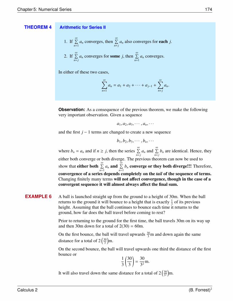
Chapter 5: Numerical Series 174
THEOREM 4 Arithmetic for Series II
1. If∞∑
n=1an converges, then
∞∑n= j
an also converges for each j.
2. If∞∑
n= jan converges for some j, then
∞∑n=1
an converges.
In either of these two cases,
∞∑n=1
an = a1 + a2 + · · · + a j−1 +
∞∑n= j
an.
Observation: As a consequence of the previous theorem, we make the followingvery important observation. Given a sequence
a1, a2, a3, · · · , an, · · ·
and the first j − 1 terms are changed to create a new sequence
b1, b2, b3, · · · , bn, · · ·
where bn = an and if n ≥ j, then the series∞∑
n= jan and
∞∑n= j
bn are identical. Hence, they
either both converge or both diverge. The previous theorem can now be used to
show that either both∞∑
n=1an and
∞∑n=1
bn converge or they both diverge!!! Therefore,
convergence of a series depends completely on the tail of the sequence of terms.Changing finitely many terms will not affect convergence, though in the case of aconvergent sequence it will almost always affect the final sum.
EXAMPLE 6 A ball is launched straight up from the ground to a height of 30m. When the ballreturns to the ground it will bounce to a height that is exactly 1
3 of its previousheight. Assuming that the ball continues to bounce each time it returns to theground, how far does the ball travel before coming to rest?
Prior to returning to the ground for the first time, the ball travels 30m on its way upand then 30m down for a total of 2(30) = 60m.
On the first bounce, the ball will travel upwards 303 m and down again the same
distance for a total of 2(
303
)m.
On the second bounce, the ball will travel upwards one third the distance of the firstbounce or
13
(303
)=
3032 m.
It will also travel down the same distance for a total of 2(
3032
)m.
Calculus 2 (B. Forrest)2
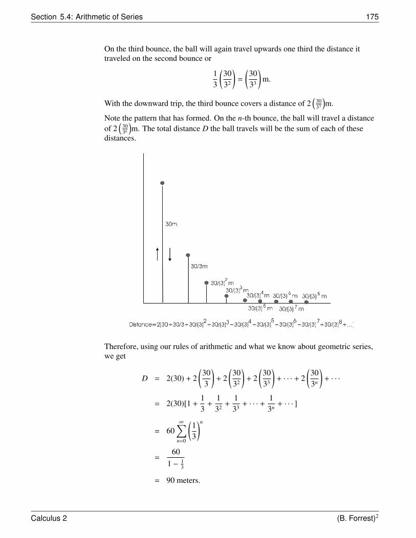
Section 5.4: Arithmetic of Series 175
On the third bounce, the ball will again travel upwards one third the distance ittraveled on the second bounce or
13
(3032
)=
(3033
)m.
With the downward trip, the third bounce covers a distance of 2(
3033
)m.
Note the pattern that has formed. On the n-th bounce, the ball will travel a distanceof 2
(303n
)m. The total distance D the ball travels will be the sum of each of these
distances.
Therefore, using our rules of arithmetic and what we know about geometric series,we get
D = 2(30) + 2(303
)+ 2
(3032
)+ 2
(3033
)+ · · · + 2
(303n
)+ · · ·
= 2(30)[1 +13
+132 +
133 + · · · +
13n + · · · ]
= 60∞∑
n=0
(13
)n
=60
1 − 13
= 90 meters.
Calculus 2 (B. Forrest)2
Chapter 5: Numerical Series 176
Since we are assuming that the ball will bounce infinitely often, we might expectthat this process would continue forever. However, this is not the case. In fact, thereasoning is very similar to that of the resolution of Zeno’s paradox since theamount of time it takes for the ball to complete each bounce decreases very rapidly.Indeed, by using some basic physics, we can actually calculate the total time itwould take for the ball to complete its travels.
It is known from physics that if a ball is dropped, it will fall a distance
S =12
gt2
meters in t seconds, where g = 9.81 m/(sec)2 is the acceleration due to gravity.Therefore, if a ball is dropped from a height h we can determine how long it willtake to reach the ground. We have
h =12
gt2
so that
t2 =2hg
or
t =
√2hg.
In our case, the ball will take the same amount of time to make the upward trip asthe downward trip. Therefore, the total time it will take to complete the n-th bounce(the 0-th bounce is the original trip) will be
tn = 2
√2hn
g
where hn is the height of the n-th bounce. But
hn =303n
so
tn = 2
√2(30)g(3n)
=
2√
60g
( 1√
3
)n
It follows that the total time it will take for the ball to complete all of the bounces is
Calculus 2 (B. Forrest)2
Section 5.5: Positive Series 177
∞∑n=0
tn =
∞∑n=0
2√
60g
( 1√
3
)n
= 2
√60g
∞∑n=0
(1√
3
)n
= 2
√60g
11 − 1
√3
= 11.708 seconds.
5.5 Positive Series
We will soon see that the Monotone Convergence Theorem can help us determinethe convergence of series, particularly those series with positive terms. Recall thefollowing definition:
DEFINITION Monotonic Sequences
Given a sequence {an}, we say that the sequence is
i) non-decreasing if an+1 ≥ an for every n ∈ N.
ii) increasing if an+1 > an for every n ∈ N.
iii) non-increasing if an+1 ≤ an for every n ∈ N.
iv) decreasing if an+1 < an for every n ∈ N.
We say that {an} is monotonic if it satisfies one of these four conditions.
The Monotone Convergence Theorem gives us a simple criterion for determiningthe convergence or divergence of a monotonic sequence.
THEOREM 5 Monotone Convergence Theorem (MCT)
Let {an} be a non-decreasing sequence.
1. If {an} is bounded above, then {an} converges to L = lub({an}).
2. If {an} is not bounded above, then {an} diverges to∞.
In particular, {an} converges if and only if it is bounded above.
Calculus 2 (B. Forrest)2
Chapter 5: Numerical Series 178
Note: A similar statement can be made about non-increasing sequences byreplacing the least upper bound with the greatest lower bound and∞ by −∞.
DEFINITION Positive Series
We call a series∞∑
n=1an positive if the terms an ≥ 0 for all n ∈ N.
Assume that an ≥ 0 for all n. Let
S k =
k∑n=1
an = a1 + a2 + · · · + ak
be the k-th partial sum of the series with terms {an}. Then
S k+1 − S k =
k+1∑n=1
an −
k∑n=1
an
= (a1 + a2 + · · · + ak + ak+1) − (a1 + a2 + · · · + ak)= ak+1
≥ 0
This shows thatS k+1 ≥ S k
so {S k} is a non-decreasing sequence. The Monotone Convergence Theorem tells usthat there are two possibilities for the sequence {S k}:
1. {S k} is bounded and therefore, by the MCT it converges.
2. {S k} diverges to∞.
In terms of the series this is equivalent to
1.∞∑
n=1an converges.
2.∞∑
n=1an diverges to∞.
Key Observation: Therefore, for positive series, the convergence of the seriesessentially depends only on how large are the terms an. Generally speaking, thelarger the an’s, the more likely it is that a series will diverge to∞ and the smaller thean’s, the more likely it is that a series will converge.
Calculus 2 (B. Forrest)2
Section 5.5: Positive Series 179
To make this statement more precise, assume that we have two series,∞∑
n=1
an and∞∑
n=1
bn
with 0 ≤ an ≤ bn for all n ∈ N. Assume also that the series∞∑
n=1bn with the larger
terms converges to some number L. Since an ≤ bn for all n ∈ N, we would not
expect∞∑
n=1an to diverge to∞. In fact, if we let
S k =
k∑n=1
an
and
Tk =
k∑n=1
bn,
then
S k = a1 + a2 + · · · + ak
≤ b1 + b2 + · · · + bk
= Tk
≤ L
since L = limk→∞
Tk.
We have shown that for each k,
S k ≤ L =
∞∑n=1
bn.
However, the sequence {S k} is increasing and we have just shown that it is boundedabove by L. The Monotone Convergence Theorem shows that {S k} converges tosome M with M ≤ L. In other words,
∞∑n=1
an = M.
On the other hand, if the series∞∑
n=1an with the smaller terms diverges to infinity, then
we can make the partial sum S k as large as we like. But, S k ≤ Tk, so that we canmake the Tk’s as large as we like. This shows that
limk→∞
Tk = ∞
so that∞∑
n=1bn diverges to∞.
This leads us to one of the most important tools we will have for determining theconvergence or divergence of positive series.
Calculus 2 (B. Forrest)2
Chapter 5: Numerical Series 180
5.5.1 Comparison Test
THEOREM 6 Comparison Test for Series
Assume that 0 ≤ an ≤ bn for each n ∈ N.
1. If∞∑
n=1bn converges, then
∞∑n=1
an converges.
2. If∞∑
n=1an diverges, then
∞∑n=1
bn diverges.
Remark: We must make three important observations concerning the ComparisonTest.
1. If∞∑
n=1an converges, then we cannot say anything about
∞∑n=1
bn.
2. If∞∑
n=1bn diverges, then we cannot say anything about
∞∑n=1
an.
3. Since the first few terms do not affect whether or not a series diverges, for theComparison Test to hold, we really only need that
0 ≤ an ≤ bn
for each n ≥ K, where K ∈ N. That is, the conditions of the theorem need onlybe satisfied by the elements of the tails of the two sequences.
EXAMPLE 7 We have seen that the Harmonic Series∞∑
n=1
1n diverges. We also know that
0 <1n≤
1√
n
for all n ∈ N. Let an = 1n and bn = 1
√n . Then the Comparison Test shows that the
series∞∑
n=1
1√
n also diverges.
EXAMPLE 8 Consider the series∞∑
n=2
1n2 − n
=
∞∑n=2
1n(n − 1)
.
If we use a method similar to that of the Partial Fraction decomposition, we get that
1n(n − 1)
=1
n − 1−
1n.
Calculus 2 (B. Forrest)2
Section 5.5: Positive Series 181
Let
S k =
k∑n=2
1n2 − n
=
k∑n=2
1n − 1
−1n
=
(1 −
12
)+
(12−
13
)+
(13−
14
)+ · · · +
(1
k − 2−
1k − 1
)+
(1
k − 1−
1k
)= 1 −
(12−
12
)−
(13−
13
)−
(14−
14
)− · · · −
(1
k − 2−
1k − 2
)−
(1
k − 1−
1k − 1
)−
1k
= 1 −1k
Since limk→∞
S k = limk→∞
1 − 1k = 1, the series
∞∑n=2
1n2−n converges with
∞∑n=2
1n2 − n
= 1.
Next, observe that for n ≥ 2, we have n2 > n2 − n and hence that
0 <1n2 <
1n2 − n
.
However, we have just shown that∞∑
n=2
1n2−n converges to 1. We can use the
Comparison Test to conclude that∞∑
n=2
1n2 converges and that
∞∑n=2
1n2 ≤ 1.
We can now immediately conclude that the series∞∑
n=1
1n2 also converges and
∞∑n=1
1n2 =
112 +
∞∑n=2
1n2 ≤ 1 + 1 = 2.
In fact, using techniques that are beyond the scope of this course, it can be shown
that∞∑
n=1
1n2 = π2
6 � 1.64493.
Calculus 2 (B. Forrest)2
Chapter 5: Numerical Series 182
EXAMPLE 9 Let p ∈ R with p ≥ 2. Then for each n ∈ N, n2 ≤ np. Hence
0 ≤1np ≤
1n2 .
Since∞∑
n=1
1n2 converges, the Comparison Test shows that if p ≥ 2,
∞∑n=1
1np also
converges.
If p ≤ 1, then np ≤ n for each n ∈ N. It follows that
0 ≤1n≤
1np .
This time, we know that the series∞∑
n=1
1n diverges. The Comparison Test shows that
∞∑n=1
1np also diverges.
Therefore,∞∑
n=1
1np converges if p ≥ 2 and diverges if p ≤ 1. It would be natural to ask
about what happens when 1 < p < 2. For example, does∞∑
n=1
1
n32
converge?
Unfortunately, we have1n2 ≤
1
n32
≤1n.
Since∞∑
n=1
1n2 converges and 1
n2 ≤1
n32, this tells us nothing about
∞∑n=1
1
n32. Similarly,
since∞∑
n=1
1n diverges and 1
n32≤ 1
n , this tells us nothing about∞∑
n=1
1
n32.
By making use of what we know about Improper Integrals, we will see later that∞∑
n=1
1
n32
actually converges.
EXAMPLE 10 Recall thatn! = 1 · 2 · 3 · · · n
for n ≥ 1 and that0! = 1.
Problem: Show that∞∑
n=0
1n! converges and that
2 <∞∑
n=0
1n!< 3.
Note: In fact∞∑
n=0
1n! = e.
Calculus 2 (B. Forrest)2
Section 5.5: Positive Series 183
First consider that
∞∑n=0
1n!
=10!
+11!
+12!
+ · · ·
= 1 +
∞∑n=1
1n!
We will show that∞∑
n=1
1n! converges and that
1 <∞∑
n=1
1n!< 2.
Let an = 1n! and let bn = 1
2n−1 .
Then
a1 =11
=120 =
121−1 = b1
a2 =1
1 · 2=
12
= b2
a3 =1
1 · 2 · 3<
11 · 2 · 2
=122 = b3
a4 =1
1 · 2 · 3 · 4<
11 · 2 · 2 · 2
=123 = b4
...
an =1
1 · 2 · 3 · 4 · · · n<
11 · 2 · 2 · 2 · · · 2
=1
2n−1 = bn
This shows that 0 < an ≤ bn for each n ∈ N.
Now
∞∑n=1
bn =
∞∑n=1
12n−1
=120 +
121 +
122 + · · ·
=
∞∑j=0
12 j
=1
1 − 12
= 2
Calculus 2 (B. Forrest)2
Chapter 5: Numerical Series 184
Since 0 < an ≤ bn for each n ∈ N and∞∑
n=1bn converges, the Comparison Test shows
that∞∑
n=1an =
∞∑n=1
1n! also converges and that
0 <∞∑
n=1
1n!≤
∞∑n=1
bn = 2.
However, since an < bn for each n ≥ 3, we have that
0 <∞∑
n=1
1n!<
∞∑n=1
bn = 2.
But∞∑
n=1
1n! = 1
1! + 12! + 1
3! + · · · > 1. Therefore,
1 <∞∑
n=1
1n!< 2.
Finally, since∞∑
n=0
1n!
= 1 +
∞∑n=1
1n!,
we get that
2 = 1 + 1 <∞∑
n=0
1n!< 1 + 2 = 3.
We have seen that the Comparison Test can help determine whether certain seriesconverge. We will now present a variation of the Comparison Test that will work fora significant collection of series, including all of those series where the terms areratios of polynomials in n. We begin with such an example.
EXAMPLE 11 Let an = 2nn3−n+1 . Notice that if n is very large, then (−n + 1) is negligible in
comparison to n3. Therefore, we could say that for large n
n3 − n + 1 � n3
and soan =
2nn3 − n + 1
�2nn3 =
2n2 .
In other words, for very large n the terms an = 2nn3−n+1 are roughly comparable in size
to 2n2 .
Calculus 2 (B. Forrest)2
Section 5.5: Positive Series 185
We know that∞∑
n=1
1n2 converges and hence so does
∞∑n=1
2n2 . Since
an =2n
n3 − n + 1�
2n2
we might guess that∞∑
n=1
2nn3−n+1 also converges. Unfortunately,
0 <2n2 ≤
2nn3 − n + 1
for all n. This means that we cannot immediately apply the Comparison Test toestablish the convergence. However, we will be able to show that the next theoremwill work in this case. It is essentially an upgraded version of the Comparison Test.
5.5.2 Limit Comparison Test
THEOREM 7 Limit Comparison Test (LCT)
Assume that an > 0 and bn > 0 for each n ∈ N. Assume also that
limn→∞
an
bn= L
where either L ∈ R or L = ∞.
1. If 0 < L < ∞, then∞∑
n=1an converges if and only if
∞∑n=1
bn converges.
2. If L = 0 and∞∑
n=1bn converges, then
∞∑n=1
an converges. Equivalently, if∞∑
n=1an
diverges, then so does∞∑
n=1bn.
3. If L = ∞ and∞∑
n=1an converges, then
∞∑n=1
bn converges. Equivalently, if∞∑
n=1bn
diverges, then so does∞∑
n=1an.
PROOF
Assume thatlimn→∞
an
bn= L.
Calculus 2 (B. Forrest)2
Chapter 5: Numerical Series 186
1) If 0 < L < ∞, the interval ( L2 , 2L) is an open interval containing L. It follows
that we can find a cutoff N ∈ N so that if n ≥ N, thenL2<
an
bn< 2L
or equivalently thatL2· bn < an < 2Lbn
Now if∞∑
n=1an converges, then the Comparison Test shows that
∞∑n=1
L2· bn
converges and hence so does∞∑
n=1
bn.
If∞∑
n=1bn converges, then so does
∞∑n=1
2L · bn.
But again we can use the Comparison Test to show that∞∑
n=1
an
converges.
2) If L = 0, then we can find a cut off N ∈ N so that if n ≥ N, then
0 <an
bn< 1
or equivalently that0 < an < bn.
In this case, if∞∑
n=1bn converges, then
∞∑n=1
an converges as well by the
Comparison Test. Equivalently, if∞∑
n=1an diverges, then so does
∞∑n=1
bn.
3) If L = ∞, then we can find a cut off N ∈ N so that if n ≥ N, thenan
bn> 1
or equivalently thatbn < an.
If∞∑
n=1an converges, then
∞∑n=1
bn converges by the Comparison Test.
Equivalently, if∞∑
n=1bn diverges, then so does
∞∑n=1
an.
Calculus 2 (B. Forrest)2
Section 5.5: Positive Series 187
Remarks:
We can informally summarize why the Limit Comparison Test works.
If limn→∞
anbn
= L where 0 < L < ∞, then for large n we have
an
bn� L
oran � Lbn.
This suggests that∞∑
n=1an converges if and only if
∞∑n=1
Lbn converges. However, the
properties of convergent series show that if 0 < L < ∞, then∞∑
n=1Lbn converges if and
only if∞∑
n=1bn converges. Combining these statements gives us that
∞∑n=1
an converges if
and only if∞∑
n=1bn converges.
When limn→∞
anbn
= L where 0 < L < ∞, we say that an and bn have the same order ofmagnitude. We write
an ≈ bn.
The Limit Comparison Test says that two positive series with terms of the sameorder of magnitude will have the same convergence properties.
If limn→∞
anbn
= 0, then bn must eventually be much larger than an. In this case, we writean � bn and we say that the order of magnitude of an is smaller than the order ofmagnitude of bn.
In this case, if the smaller series∞∑
n=1an diverges to∞, it would make sense that
∞∑n=1
bn
also diverges to∞.
Finally, if limn→∞
anbn
= ∞, then an must eventually be much larger than bn. That is
bn � an. This time, if the larger series∞∑
n=1an converges, it would make sense that
∞∑n=1
bn would converge as well.
Calculus 2 (B. Forrest)2
Chapter 5: Numerical Series 188
EXAMPLE 12 Let an = 2nn3−n+1 and bn = 1
n2 . Then
an
bn=
2nn3−n+1
1n2
=2n3
n3 − n + 1
=n3
n3
21 − 1
n2 + 1n3
=
21 − 1
n2 + 1n3
Therefore,
limn→∞
an
bn= lim
n→∞
21 − 1
n2 + 1n3
=21
= 2.
This confirms for large n that an = 2nn3−n+1 � 2bn = 2
n2 .
Since∞∑
n=1
1n2 converges, the first statement in the Limit Comparison Test shows that
∞∑n=1
2nn3−n+1 converges as we expected.
EXAMPLE 13 Show that∞∑
n=1sin
(1n
)diverges.
It can be shown that for any 0 < x ≤ 1 that 0 < sin(x) < x and hence that
0 < sin(1n
)<
1n
for each n ∈ N. However, since∞∑
n=1
1n diverges, we cannot use the Comparison Test
directly to show that∞∑
n=1sin
(1n
)diverges. (Why?)
Recall that the Fundamental Trigonometric Limit states that as x→ 0, sin(x)x → 1. As
n→ ∞, we have 1n → 0. Therefore, by the Sequential Characterization of Limits
limn→∞
sin(
1n
)1n
= 1.
If we let an = sin(
1n
)and bn = 1
n , then we have just shown that
limn→∞
an
bn= 1.
Since∞∑
n=1
1n diverges, the Limit Comparison Test shows that
∞∑n=1
sin(
1n
)diverges.
Calculus 2 (B. Forrest)2
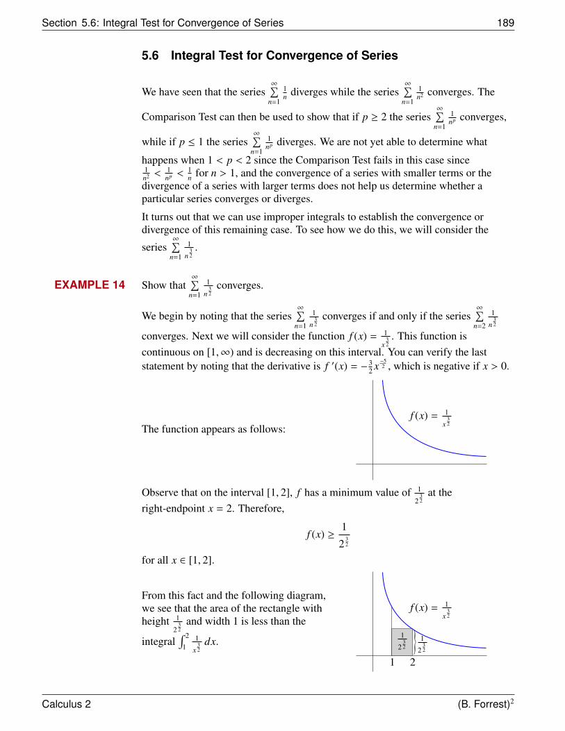
Section 5.6: Integral Test for Convergence of Series 189
5.6 Integral Test for Convergence of Series
We have seen that the series∞∑
n=1
1n diverges while the series
∞∑n=1
1n2 converges. The
Comparison Test can then be used to show that if p ≥ 2 the series∞∑
n=1
1np converges,
while if p ≤ 1 the series∞∑
n=1
1np diverges. We are not yet able to determine what
happens when 1 < p < 2 since the Comparison Test fails in this case since1n2 <
1np <
1n for n > 1, and the convergence of a series with smaller terms or the
divergence of a series with larger terms does not help us determine whether aparticular series converges or diverges.
It turns out that we can use improper integrals to establish the convergence ordivergence of this remaining case. To see how we do this, we will consider the
series∞∑
n=1
1
n32.
EXAMPLE 14 Show that∞∑
n=1
1
n32
converges.
We begin by noting that the series∞∑
n=1
1
n32
converges if and only if the series∞∑
n=2
1
n32
converges. Next we will consider the function f (x) = 1
x32. This function is
continuous on [1,∞) and is decreasing on this interval. You can verify the laststatement by noting that the derivative is f ′(x) = −3
2 x−52 , which is negative if x > 0.
The function appears as follows:f (x) = 1
x32
Observe that on the interval [1, 2], f has a minimum value of 1
232
at theright-endpoint x = 2. Therefore,
f (x) ≥1
232
for all x ∈ [1, 2].
From this fact and the following diagram,we see that the area of the rectangle withheight 1
232
and width 1 is less than the
integral∫ 2
11
x32
dx.
f (x) = 1
x32
1 2
1
232
1
232
Calculus 2 (B. Forrest)2
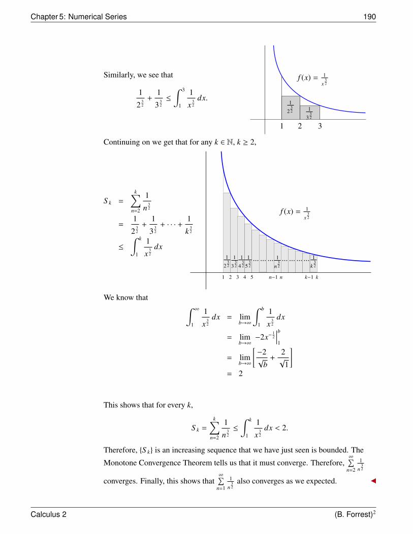
Chapter 5: Numerical Series 190
Similarly, we see that
1
232
+1
332
≤
∫ 3
1
1
x32
dx.
f (x) = 1
x32
1 2
1
232 1
332
3
Continuing on we get that for any k ∈ N, k ≥ 2,
S k =
k∑n=2
1
n32
=1
232
+1
332
+ · · · +1
k32
≤
∫ k
1
1
x32
dx... ... ... ... ... ... ...
f (x) = 1
x32
1
232
1
332
1
432
1
532
1
n32
1
k32
1 2 3 4 5 n−1 n k−1 k
We know that ∫ ∞
1
1
x32
dx = limb→∞
∫ b
1
1
x32
dx
= limb→∞
−2x−12
∣∣∣∣b1
= limb→∞
[−2√
b+
2√
1
]= 2
This shows that for every k,
S k =
k∑n=2
1
n32
≤
∫ k
1
1
x32
dx < 2.
Therefore, {S k} is an increasing sequence that we have just seen is bounded. The
Monotone Convergence Theorem tells us that it must converge. Therefore,∞∑
n=2
1
n32
converges. Finally, this shows that∞∑
n=1
1
n32
also converges as we expected.
Calculus 2 (B. Forrest)2
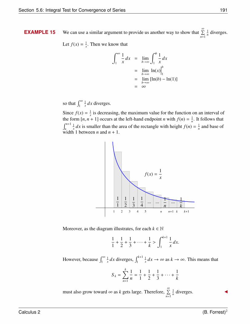
Section 5.6: Integral Test for Convergence of Series 191
EXAMPLE 15 We can use a similar argument to provide us another way to show that∞∑
n=1
1n diverges.
Let f (x) = 1x . Then we know that∫ ∞
1
1x
dx = limb→∞
∫ b
1
1x
dx
= limb→∞
ln(x)∣∣∣∣b1
= limb→∞
[ln(b) − ln(1)]= ∞
so that∫ ∞
11x dx diverges.
Since f (x) = 1x is decreasing, the maximum value for the function on an interval of
the form [n, n + 1] occurs at the left-hand endpoint n with f (n) = 1n . It follows that∫ n+1
n1x dx is smaller than the area of the rectangle with height f (n) = 1
n and base ofwidth 1 between n and n + 1.
... ... ...
f (x) =1x
1 2 3 4 5 n+1n k+1k
11
12
13
14
1n
1k
Moreover, as the diagram illustrates, for each k ∈ N
11
+12
+13
+ · · · +1k>
∫ k+1
1
1x
dx.
However, because∫ ∞
11x dx diverges,
∫ k+1
11x dx→ ∞ as k → ∞. This means that
S k =
k∑n=1
1n
=11
+12
+13
+ · · · +1k
must also grow toward∞ as k gets large. Therefore,∞∑
n=1
1n diverges.
Calculus 2 (B. Forrest)2
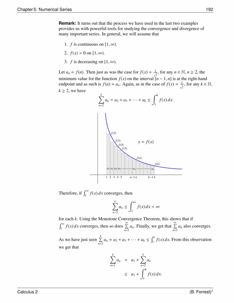
Chapter 5: Numerical Series 192
Remark: It turns out that the process we have used in the last two examplesprovides us with powerful tools for studying the convergence and divergence ofmany important series. In general, we will assume that
1. f is continuous on [1,∞).
2. f (x) > 0 on [1,∞).
3. f is decreasing on [1,∞).
Let an = f (n). Then just as was the case for f (x) = 1
x32, for any n ∈ N, n ≥ 2, the
minimum value for the function f (x) on the interval [n − 1, n] is at the right-handendpoint and as such is f (n) = an. Again, as in the case of f (x) = 1
x32, for any k ∈ N,
k ≥ 2, we havek∑
n=2
an = a2 + a3 + · · · + ak ≤
∫ k
1f (x) dx.
......... ............
y = f (x)
a2 a3 a4 a5 an ak
1 2 3 4 5 n−1 n k−1 k
f (2)
f (3)f (4)
f (5)
f (n)
f (k)
Therefore, if∫ ∞
1f (x) dx converges, then
k∑n=2
an ≤
∫ ∞
1f (x) dx < ∞
for each k. Using the Monotone Convergence Theorem, this shows that if∫ ∞1
f (x) dx converges, then so does∞∑
n=2an. Finally, we get that
∞∑n=1
an also converges.
As we have just seenk∑
n=2an = a2 + a3 + · · · + ak ≤
∫ k
1f (x) dx. From this observation
we get that
k∑n=1
an = a1 +
k∑n=2
an
≤ a1 +
∫ k
1f (x) dx.
Calculus 2 (B. Forrest)2
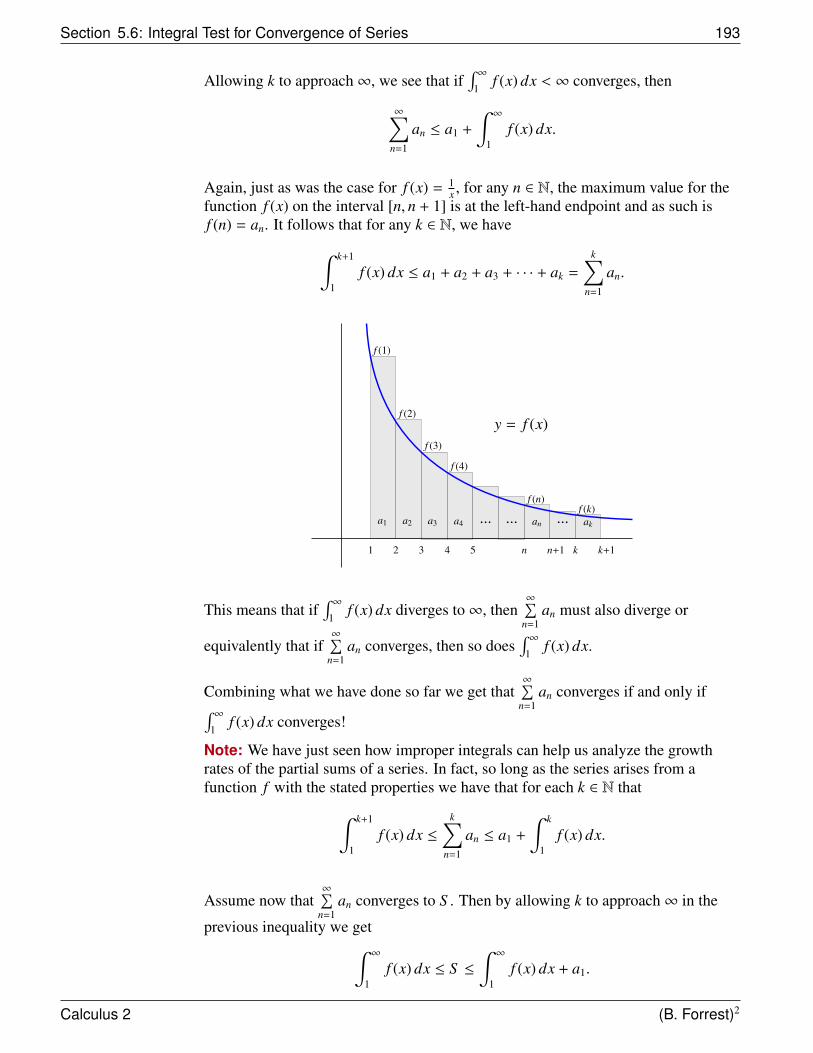
Section 5.6: Integral Test for Convergence of Series 193
Allowing k to approach∞, we see that if∫ ∞
1f (x) dx < ∞ converges, then
∞∑n=1
an ≤ a1 +
∫ ∞
1f (x) dx.
Again, just as was the case for f (x) = 1x , for any n ∈ N, the maximum value for the
function f (x) on the interval [n, n + 1] is at the left-hand endpoint and as such isf (n) = an. It follows that for any k ∈ N, we have∫ k+1
1f (x) dx ≤ a1 + a2 + a3 + · · · + ak =
k∑n=1
an.
...... ...
y = f (x)
1 2 3 4 5 n+1n k+1k
f (2)
f (3)
f (4)
f (1)
f (n)f (k)
a2 a3 a4a1 an ak
This means that if∫ ∞
1f (x) dx diverges to∞, then
∞∑n=1
an must also diverge or
equivalently that if∞∑
n=1an converges, then so does
∫ ∞1
f (x) dx.
Combining what we have done so far we get that∞∑
n=1an converges if and only if∫ ∞
1f (x) dx converges!
Note: We have just seen how improper integrals can help us analyze the growthrates of the partial sums of a series. In fact, so long as the series arises from afunction f with the stated properties we have that for each k ∈ N that∫ k+1
1f (x) dx ≤
k∑n=1
an ≤ a1 +
∫ k
1f (x) dx.
Assume now that∞∑
n=1an converges to S . Then by allowing k to approach∞ in the
previous inequality we get∫ ∞
1f (x) dx ≤ S ≤
∫ ∞
1f (x) dx + a1.
Calculus 2 (B. Forrest)2
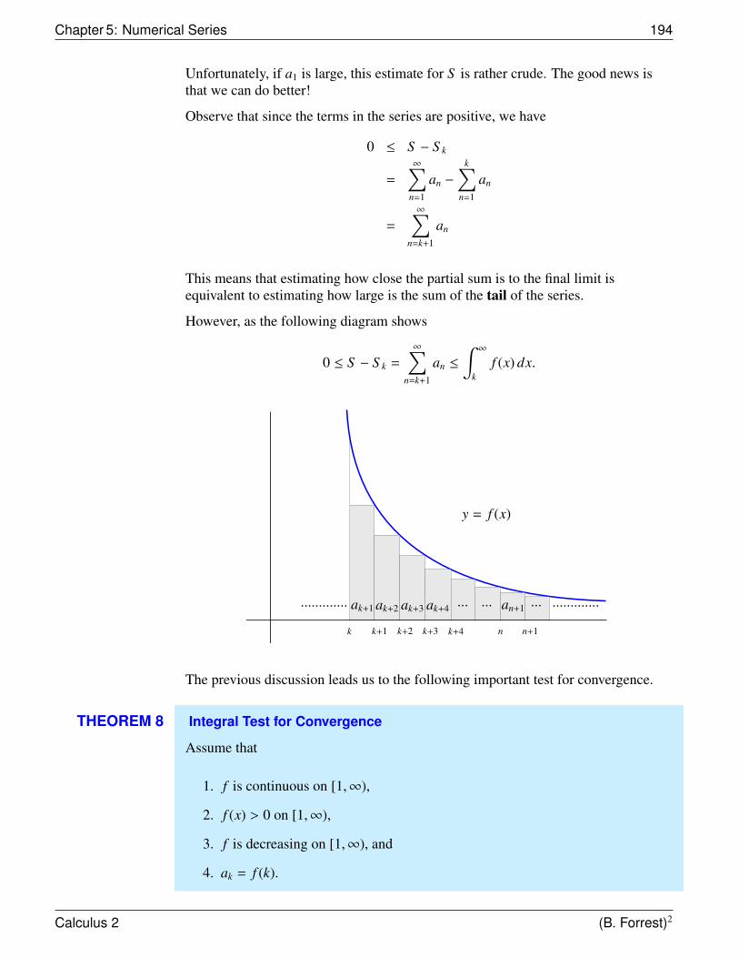
Chapter 5: Numerical Series 194
Unfortunately, if a1 is large, this estimate for S is rather crude. The good news isthat we can do better!
Observe that since the terms in the series are positive, we have
0 ≤ S − S k
=
∞∑n=1
an −
k∑n=1
an
=
∞∑n=k+1
an
This means that estimating how close the partial sum is to the final limit isequivalent to estimating how large is the sum of the tail of the series.
However, as the following diagram shows
0 ≤ S − S k =
∞∑n=k+1
an ≤
∫ ∞
kf (x) dx.
...... ................ .............
y = f (x)
k k+1 n+1k+4 nk+2 k+3
ak+1 ak+2 ak+3 ak+4 an+1
The previous discussion leads us to the following important test for convergence.
THEOREM 8 Integral Test for Convergence
Assume that
1. f is continuous on [1,∞),
2. f (x) > 0 on [1,∞),
3. f is decreasing on [1,∞), and
4. ak = f (k).
Calculus 2 (B. Forrest)2
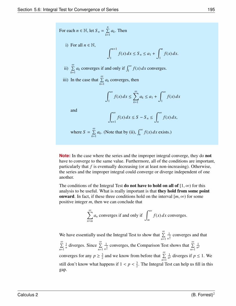
Section 5.6: Integral Test for Convergence of Series 195
For each n ∈ N, let S n =n∑
k=1ak. Then
i) For all n ∈ N, ∫ n+1
1f (x) dx ≤ S n ≤ a1 +
∫ n
1f (x) dx.
ii)∞∑
k=1ak converges if and only if
∫ ∞1
f (x) dx converges.
iii) In the case that∞∑
k=1ak converges, then
∫ ∞
1f (x) dx ≤
∞∑k=1
ak ≤ a1 +
∫ ∞
1f (x) dx
and ∫ ∞
n+1f (x) dx ≤ S − S n ≤
∫ ∞
nf (x) dx,
where S =∞∑
k=1ak. (Note that by (ii),
∫ ∞n
f (x) dx exists.)
Note: In the case where the series and the improper integral converge, they do nothave to converge to the same value. Furthermore, all of the conditions are important,particularly that f is eventually decreasing (or at least non-increasing). Otherwise,the series and the improper integral could converge or diverge independent of oneanother.
The conditions of the Integral Test do not have to hold on all of [1,∞) for thisanalysis to be useful. What is really important is that they hold from some pointonward. In fact, if these three conditions hold on the interval [m,∞) for somepositive integer m, then we can conclude that
∞∑n=m
an converges if and only if∫ ∞
mf (x) dx converges.
We have essentially used the Integral Test to show that∞∑
n=1
1
n32
converges and that∞∑
n=1
1n diverges. Since
∞∑n=1
1
n32
converges, the Comparison Test shows that∞∑
n=1
1np
converges for any p ≥ 32 and we know from before that
∞∑n=1
1np diverges if p ≤ 1. We
still don’t know what happens if 1 < p < 32 . The Integral Test can help us fill in this
gap.
Calculus 2 (B. Forrest)2
Chapter 5: Numerical Series 196
THEOREM 9 p-Series Test
The series∞∑
n=1
1np converges if and only if p > 1.
PROOF
We already know that∞∑
n=1
1np converges if p ≥ 2 and it diverges for p ≤ 1. We can use
the Integral Test to address the missing interval.
Consider, the function f (x) = 1xp . It is easy to see that if p > 0, then f (x) satisfies the
three hypotheses of the Integral Test. If we let an = f (n) = 1np , then for any p > 0,
the series∞∑
n=1
1np will converge if and only if the improper integral
∫ ∞1
1xp dx
converges. However, we know that ∫ ∞
1
1xp dx
converges if and only if p > 1. Since we know that∞∑
n=1
1np diverges if p ≤ 0, this tells
us that∞∑
n=1
1np will converge if and only if p > 1.
EXAMPLE 16 Show that∞∑
n=1
1
n32 − n + 1
converges.
We will use the Limit Comparison Test and the p-Series Test.
A close look at the terms of the series shows that for large n,
1
n32 − n + 1
�1
n32
.
In fact
limn→∞
1
n32
1
n32 −n+1
= limn→∞
n32 − n + 1
n32
= limn→∞
(1 −1
n12
+1
n32
)
= 1
Calculus 2 (B. Forrest)2
Section 5.6: Integral Test for Convergence of Series 197
Therefore, the Limit Comparison Test shows that∞∑
n=1
1
n32 −n+1
converges if and only if∞∑
n=1
1
n32
converges. However, the p-Series test shows that∞∑
n=1
1
n32
converges. We can
conclude that∞∑
n=1
1
n32 −n+1
converges as well.
EXAMPLE 17 Determine whether the series∞∑
n=2
1n ln(n) converges.
Consider the function f (x) = 1x ln(x) . Then
1. f (x) is continuous on [2,∞).
2. f (x) > 0 on [2,∞).
3. f (x) is decreasing on [2,∞).
While all of these claims are easy to verify, we will explicitly show that condition 3holds. To do this, note that from the quotient rule it follows that
f ′(x) =(x ln(x))(0) − (ln(x) + 1)(1)
x2(ln(x))2
=−(ln(x) + 1)
x2(ln(x))2
< 0
if x ≥ 2.
This shows that f ′(x) < 0 for every x ∈ [2,∞). Hence, f (x) is decreasing on [2,∞).Alternatively, we could have observed that the function x ln(x) is increasing on[2,∞) and as such its reciprocal 1
x ln(x) must be decreasing.
We can apply the Integral Test to see that∞∑
n=2
1n ln(n) converges if and only if∫ ∞
21
x ln(x) dx converges.
Now ∫ ∞
2
1x ln(x)
dx = limb→∞
∫ b
2
1x ln(x)
dx.
To evaluate∫ b
21
x ln(x) dx use the substitution u = ln(x), du = dxx to get∫ b
2
1x ln(x)
dx =
∫ ln(b)
ln(2)
1u
du
= ln(u)∣∣∣∣ln(b)
ln(2)
= ln(ln(b)) − ln(ln(2))
Calculus 2 (B. Forrest)2
Chapter 5: Numerical Series 198
Therefore, ∫ ∞
2
1x ln(x)
dx = limb→∞
∫ b
2
1x ln(x)
dx
= limb→∞
ln(ln(b)) − ln(ln(2))
= ∞
Since∫ ∞
21
x ln(x) dx diverges, the Integral Test shows that∞∑
n=2
1n ln(n) also diverges.
EXAMPLE 18 Show that∞∑
n=2
1n(ln(n))2 converges.
Let f (x) = 1x(ln(x))2 . It is easy to verify that
1. f is continuous on [2,∞).
2. f (x) > 0 on [2,∞).
Moreover, since x(ln(x))2 is increasing for x ≥ 2, it follows that f (x) = 1x(ln(x))2 is
decreasing. Alternatively, f ′(x) = −2+ln(x)
x2(ln(x))3 which is negative for x ≥ 2. Therefore,
the Integral Test can be used to conclude that∞∑
n=2
1n(ln(n))2 converges if and only if∫ ∞
21
x(ln(x))2 dx converges.
To evaluate∫ b
21
x(ln(x))2 dx, use the substitution u = ln(x), du = dxx to get∫ b
2
1x(ln(x))2 dx =
∫ ln(b)
ln(2)
1u2 du
= −1u
∣∣∣∣∣ln(b)
ln(2)
=1
ln(2)−
1ln(b)
Therefore, ∫ ∞
2
1x(ln(x))2 dx = lim
b→∞
∫ b
2
1x(ln(x))2 dx
= limb→∞
1ln(2)
−1
ln(b)
=1
ln(2)
Calculus 2 (B. Forrest)2

Section 5.6: Integral Test for Convergence of Series 199
Since∫ ∞
21
x(ln(x))2 dx converges, so does∞∑
n=2
1n(ln(n))2 .
5.6.1 Integral Test and Estimation of Sums and Errors
The Integral Test is a powerful tool for determining the convergence or divergenceof many important series. However, much more can be said. In fact, we have seenthat if
1. f is continuous on [1,∞),
2. f (x) > 0 on [1,∞),
3. f (x) is decreasing on [1,∞),
4. an = f (n), and
5. S k =k∑
n=1an,
then ∫ k+1
1f (x) dx ≤ S k ≤
∫ k
1f (x) dx + a1.
Therefore, we can use integration to estimate the value of the partial sum S k of the
series∞∑
n=1an.
EXAMPLE 19 How large is the k-th partial sum S k of the harmonic series∞∑
n=1
1n?
In this case, f (x) = 1x and a1 = 1. But we know that∫ k+1
1
1x
dx ≤ S k =11
+12
+ · · · +1k≤
∫ k
1
1x
dx + a1
Since ∫ c
1
1x
dx = ln(x)∣∣∣∣c1
= ln(c) − ln(1) = ln(c)
for any value of c > 0, this inequality becomes
ln(k + 1) ≤11
+12
+ · · · +1k≤ ln(k) + 1
If we let k = 1000, we see that ln(1001) = 6.908754779 andln(1000) = 6.907755279. This tells us that
6.908754779 ≤11
+12
+ · · · +1
1000≤ 7.907755279
Calculus 2 (B. Forrest)2
Chapter 5: Numerical Series 200
If k = 109, then the inequality would show us that
20.72326584 ≤11
+12
+ · · · +1
109 ≤ 21.72326584
What is remarkable about these estimates is not their accuracy in estimating aparticular partial sum, but that while we know the harmonic series will diverge to∞,after 1000 terms the sum has not yet exceeded 8, and after 1 billion terms, the sum isstill less than 22! This shows us that we would not have been able to guess that thisseries diverged by testing some partial sums on a computer.
To emphasize home this last comment consider how many terms one would have toadd together so that
S k =11
+12
+ · · · +1k> 1000.
We know thatS k � ln(k).
As such to have S k > 1000 we would need enough terms so that
1000 < ln(k).
This means that we should have
k > e1000 � 10434.
This is an enormous number.
EXAMPLE 20 The p-Series Test shows that the series∞∑
n=1
1n4 converges. Let
S k =
k∑n=1
1n4 and S =
∞∑n=1
1n4 .
Estimate the error in using the first 100 terms in the series to approximate S . That is,estimate |S − S 100|.
The first observation we make is that since all the terms are positive we have thatS − S 100 > 0 and hence that
|S − S 100| = S − S 100.
But we also know from the Integral Test that∫ ∞
101
1x4 dx ≤ S − S 100 ≤
∫ ∞
100
1x4 dx.
Calculus 2 (B. Forrest)2

Section 5.6: Integral Test for Convergence of Series 201
But for any m ∈ N, we have that∫ ∞
m
1x4 dx = lim
b→∞
∫ b
m
1x4 dx
= limb→∞−
13x3
∣∣∣∣bm
= limb→∞
13m3 −
13b3
=1
3m3
Substituting m = 101 and m = 100 respectively in 13m3 we get that
13(101)3 ≤ S − S 100 ≤
13(100)3
or3.2353 × 10−7 ≤ S − S 100 ≤ 3.3333 × 10⁻⁷.
Now if we calculate S 100 we get S 100 = 1.082322905 (up to 9 decimal places) andhence our prediction would be that
1.082323229 ≤ S ≤ 1.082323238
In fact, it is actually known that
S =
∞∑n=1
1n4 =
π4
90= 1.082323234
which does indeed lie within our range.
EXAMPLE 21 The Integral Test tells us that the series∞∑
n=2
1n(ln(n))2 converges. But it can also show us
that the series converges very slowly. For example, suppose that S =∞∑
n=2
1n(ln(n))2 and
S k =k∑
n=2
1n(ln(n))2 . Then we know that
S − S k �
∫ ∞
k
1x(ln(x))2 dx.
But ∫ b
k
1x(ln(x))2 dx =
∫ ln(b)
ln(k)
1u2 du
= −1u
∣∣∣∣∣ln(b)
ln(k)
Calculus 2 (B. Forrest)2
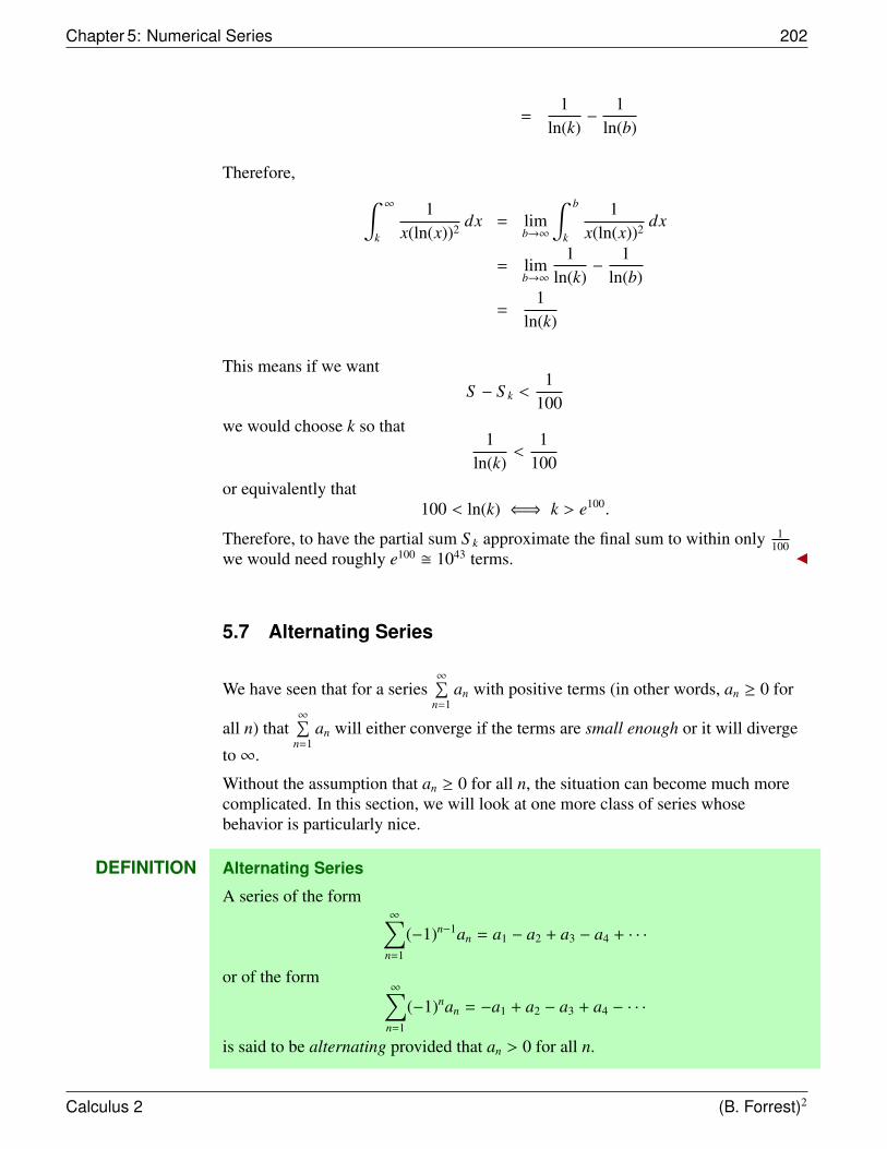
Chapter 5: Numerical Series 202
=1
ln(k)−
1ln(b)
Therefore, ∫ ∞
k
1x(ln(x))2 dx = lim
b→∞
∫ b
k
1x(ln(x))2 dx
= limb→∞
1ln(k)
−1
ln(b)
=1
ln(k)
This means if we wantS − S k <
1100
we would choose k so that1
ln(k)<
1100
or equivalently that100 < ln(k) ⇐⇒ k > e100.
Therefore, to have the partial sum S k approximate the final sum to within only 1100
we would need roughly e100 � 1043 terms.
5.7 Alternating Series
We have seen that for a series∞∑
n=1an with positive terms (in other words, an ≥ 0 for
all n) that∞∑
n=1an will either converge if the terms are small enough or it will diverge
to∞.
Without the assumption that an ≥ 0 for all n, the situation can become much morecomplicated. In this section, we will look at one more class of series whosebehavior is particularly nice.
DEFINITION Alternating Series
A series of the form∞∑
n=1
(−1)n−1an = a1 − a2 + a3 − a4 + · · ·
or of the form∞∑
n=1
(−1)nan = −a1 + a2 − a3 + a4 − · · ·
is said to be alternating provided that an > 0 for all n.
Calculus 2 (B. Forrest)2
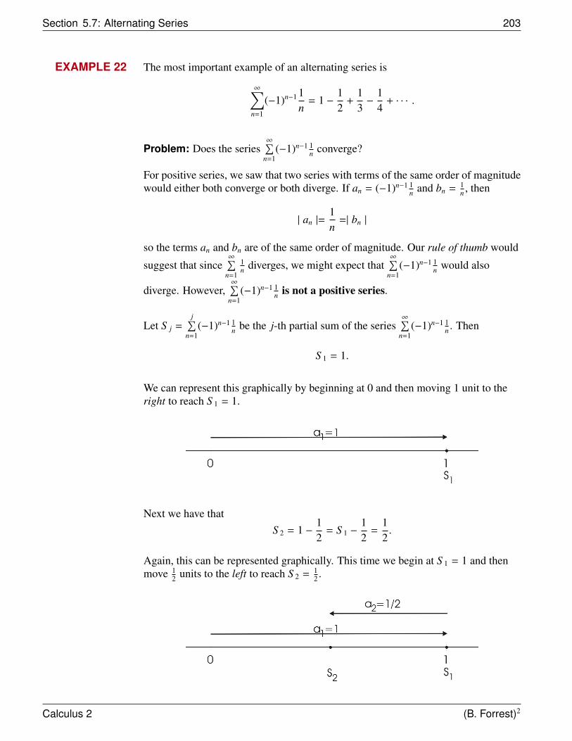
Section 5.7: Alternating Series 203
EXAMPLE 22 The most important example of an alternating series is
∞∑n=1
(−1)n−1 1n
= 1 −12
+13−
14
+ · · · .
Problem: Does the series∞∑
n=1(−1)n−1 1
n converge?
For positive series, we saw that two series with terms of the same order of magnitudewould either both converge or both diverge. If an = (−1)n−1 1
n and bn = 1n , then
| an |=1n
=| bn |
so the terms an and bn are of the same order of magnitude. Our rule of thumb would
suggest that since∞∑
n=1
1n diverges, we might expect that
∞∑n=1
(−1)n−1 1n would also
diverge. However,∞∑
n=1(−1)n−1 1
n is not a positive series.
Let S j =j∑
n=1(−1)n−1 1
n be the j-th partial sum of the series∞∑
n=1(−1)n−1 1
n . Then
S 1 = 1.
We can represent this graphically by beginning at 0 and then moving 1 unit to theright to reach S 1 = 1.
Next we have thatS 2 = 1 −
12
= S 1 −12
=12.
Again, this can be represented graphically. This time we begin at S 1 = 1 and thenmove 1
2 units to the left to reach S 2 = 12 .
Calculus 2 (B. Forrest)2
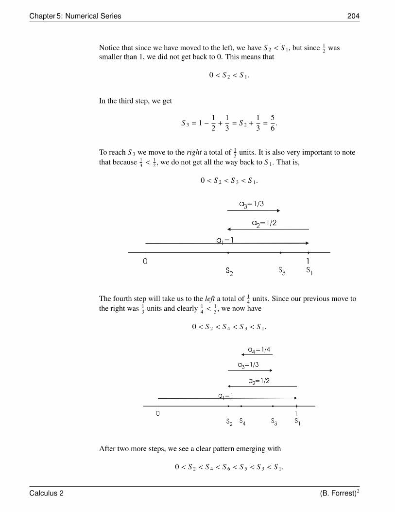
Chapter 5: Numerical Series 204
Notice that since we have moved to the left, we have S 2 < S 1, but since 12 was
smaller than 1, we did not get back to 0. This means that
0 < S 2 < S 1.
In the third step, we get
S 3 = 1 −12
+13
= S 2 +13
=56.
To reach S 3 we move to the right a total of 13 units. It is also very important to note
that because 13 <
12 , we do not get all the way back to S 1. That is,
0 < S 2 < S 3 < S 1.
The fourth step will take us to the left a total of 14 units. Since our previous move to
the right was 13 units and clearly 1
4 <13 , we now have
0 < S 2 < S 4 < S 3 < S 1.
After two more steps, we see a clear pattern emerging with
0 < S 2 < S 4 < S 6 < S 5 < S 3 < S 1.
Calculus 2 (B. Forrest)2
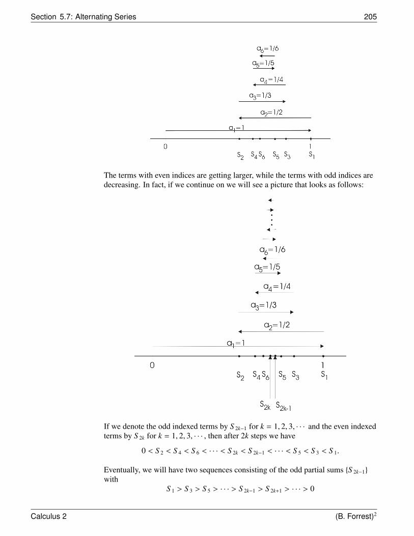
Section 5.7: Alternating Series 205
The terms with even indices are getting larger, while the terms with odd indices aredecreasing. In fact, if we continue on we will see a picture that looks as follows:
If we denote the odd indexed terms by S 2k−1 for k = 1, 2, 3, · · · and the even indexedterms by S 2k for k = 1, 2, 3, · · · , then after 2k steps we have
0 < S 2 < S 4 < S 6 < · · · < S 2k < S 2k−1 < · · · < S 5 < S 3 < S 1.
Eventually, we will have two sequences consisting of the odd partial sums {S 2k−1}
withS 1 > S 3 > S 5 > · · · > S 2k−1 > S 2k+1 > · · · > 0
Calculus 2 (B. Forrest)2
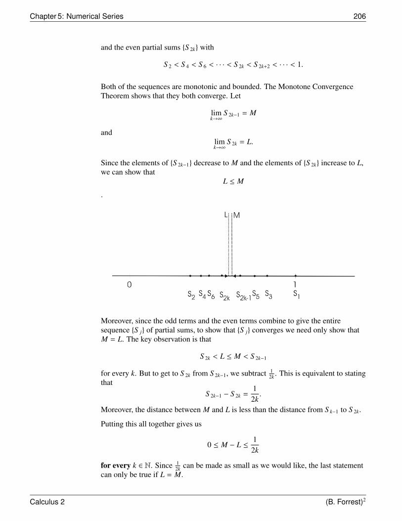
Chapter 5: Numerical Series 206
and the even partial sums {S 2k} with
S 2 < S 4 < S 6 < · · · < S 2k < S 2k+2 < · · · < 1.
Both of the sequences are monotonic and bounded. The Monotone ConvergenceTheorem shows that they both converge. Let
limk→∞
S 2k−1 = M
andlimk→∞
S 2k = L.
Since the elements of {S 2k−1} decrease to M and the elements of {S 2k} increase to L,we can show that
L ≤ M
.
Moreover, since the odd terms and the even terms combine to give the entiresequence {S j} of partial sums, to show that {S j} converges we need only show thatM = L. The key observation is that
S 2k < L ≤ M < S 2k−1
for every k. But to get to S 2k from S 2k−1, we subtract 12k . This is equivalent to stating
thatS 2k−1 − S 2k =
12k.
Moreover, the distance between M and L is less than the distance from S k−1 to S 2k.
Putting this all together gives us
0 ≤ M − L ≤12k
for every k ∈ N. Since 12k can be made as small as we would like, the last statement
can only be true if L = M.
Calculus 2 (B. Forrest)2
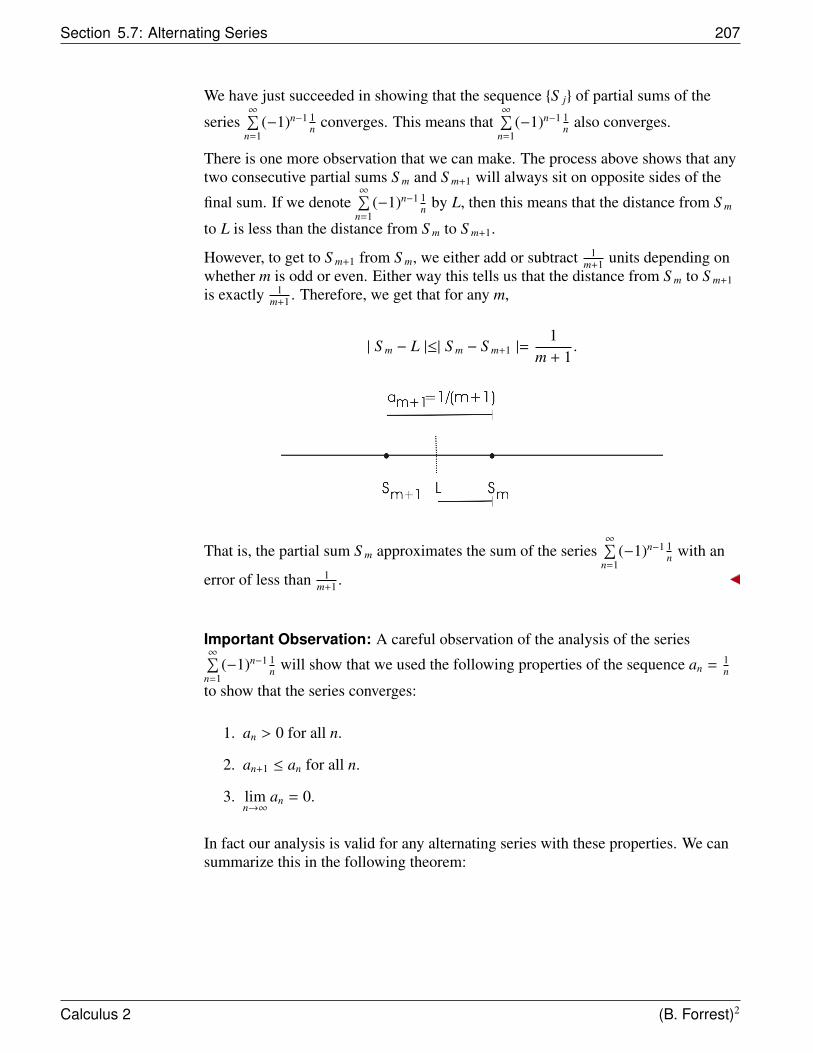
Section 5.7: Alternating Series 207
We have just succeeded in showing that the sequence {S j} of partial sums of the
series∞∑
n=1(−1)n−1 1
n converges. This means that∞∑
n=1(−1)n−1 1
n also converges.
There is one more observation that we can make. The process above shows that anytwo consecutive partial sums S m and S m+1 will always sit on opposite sides of the
final sum. If we denote∞∑
n=1(−1)n−1 1
n by L, then this means that the distance from S m
to L is less than the distance from S m to S m+1.
However, to get to S m+1 from S m, we either add or subtract 1m+1 units depending on
whether m is odd or even. Either way this tells us that the distance from S m to S m+1
is exactly 1m+1 . Therefore, we get that for any m,
| S m − L |≤| S m − S m+1 |=1
m + 1.
That is, the partial sum S m approximates the sum of the series∞∑
n=1(−1)n−1 1
n with an
error of less than 1m+1 .
Important Observation: A careful observation of the analysis of the series∞∑
n=1(−1)n−1 1
n will show that we used the following properties of the sequence an = 1n
to show that the series converges:
1. an > 0 for all n.
2. an+1 ≤ an for all n.
3. limn→∞
an = 0.
In fact our analysis is valid for any alternating series with these properties. We cansummarize this in the following theorem:
Calculus 2 (B. Forrest)2
Chapter 5: Numerical Series 208
THEOREM 10 Alternating Series Test (AST)
Assume that
1. an > 0 for all n.
2. an+1 ≤ an for all n.
3. limn→∞
an = 0.
Then the alternating series∞∑
n=1
(−1)n−1an
converges.
If S k =k∑
n=1(−1)n−1an, then S k approximates the sum S =
∞∑n=1
(−1)n−1an with an error
that is at most ak+1. That is| S k − S |≤ ak+1.
PROOF
We will show that the two subsequences of partial sums {S 2k−1} and {S 2k} convergeto the same limit L.
We first prove that both subsequences are monotonic. We have
S 2(k+1)−1 − S 2k−1 = S 2k+1 − S 2k−1
=
2k+1∑n=1
(−1)n−1an −
2k−1∑n=1
(−1)n−1an
= (−1)2k−1a2k + (−1)(2k+1)−1a2k+1
= −a2k + a2k+1
≤ 0
This shows that {S 2k−1} is decreasing. Similarly,
S 2(k+1) − S 2k = S 2k+2 − S 2k
=
2k+2∑n=1
(−1)n−1an −
2k∑n=1
(−1)n−1an
= (−1)(2k+1)−1a2k+1 + (−1)(2k+2)−1a2k+2
= a2k+1 − a2k+2
≥ 0
This shows that {S 2k} is increasing.
Calculus 2 (B. Forrest)2
Section 5.7: Alternating Series 209
Now we will show that both subsequences are bounded. We have
S 2k−1 = (a1 − a2) + (a3 − a4) + · · · + (a2k−3 − a2k−2) + a2k−1
≥ 0 + 0 + · · · + 0 + a2k−1
≥ 0
and
S 2k = a1 − (a2 − a3) − (a4 − a5) − · · · − (a2k−2 − a2k−1) − a2k
≤ a1 − 0 − 0 − · · · − 0 − a2k
≤ a1
Hence {S 2k−1} is bounded below by 0 and {S 2k} is bounded above by a1. By theMonotone Convergence Theorem, lim
k→∞S 2k−1 = L ∈ R and lim
k→∞S 2k = M ∈ R.
Next we show that L = M. To see why this is the case we note that
|S 2k − S 2k−1| =
∣∣∣∣∣∣∣2k∑
n=1
(−1)n−1an −
2k−1∑n=1
(−1)n−1an
∣∣∣∣∣∣∣ = a2k.
Then
|M − L| = limk→∞|S 2k − S 2k−1|
= limk→∞
a2k
= 0
so L = M and the series converges. Next we let
S =
∞∑n=1
(−1)n−1an.
Finally, since {S 2k} increases to S and {S 2k−1} decreases to S , we have
S 2k ≤ S ≤ S 2k−1
for all k ∈ N. This shows that S sits between S k and S k+1 for each k ∈ N.
Thus we get that
|S k − S | ≤ |S k − S k+1| = |(−1)kak+1| = ak+1
for all k ∈ N. This proves the last part of the theorem.
Calculus 2 (B. Forrest)2
Chapter 5: Numerical Series 210
Remark: There are a few important observations we should make concerning thistheorem.
1. Historically, the series∞∑
n=1(−1)n−1 1
n is the most important of the alternating
series. For this reason it is usually called The Alternating Series.
2. All three of the conditions in the statement of the theorem are important forthe theorem to be valid. However, it is actually sufficient for the first two tohold for all n ≥ M where M is some fixed integer. In this case, the errorestimate will only be valid when k ≥ M.
3. For the series∞∑
n=1(−1)n−1an, we have
0 ≤ S 2 ≤ S 4 ≤ S 6 ≤ · · · ≤ S 2k ≤ · · ·
∞∑n=1
(−1)n−1an
· · · ≤ S 2k−1 ≤ · · · ≤ S 5 ≤ S 3 ≤ S 1 = a1.
Therefore, if j is even, S j under estimates the sum and if j is odd, S j overestimates the sum.
4. With the obvious changes, the theorem remains valid for series of the form∞∑
n=1
(−1)nan
provided that the three assumptions on the sequence {an} hold.
EXAMPLE 23 Show that the series∞∑
n=1(−1)n−1 1
n3 converges and determine how large k must be so
that
| S k −
∞∑n=1
(−1)n−1 1n3 |< 10−6.
Let an = 1n3 . Then
0 <1
(n + 1)3 <1n3
and limn→∞
1n3 = 0. Therefore, the series
∞∑n=1
(−1)n−1 1n3 converges by the Alternating
Series Test.
The Alternating Series Test tells us that
| S k −
∞∑n=1
(−1)n−1 1n3 |≤ ak+1 =
1(k + 1)3 .
We must choose k large enough so that
1(k + 1)3 < 10−6.
Calculus 2 (B. Forrest)2
Section 5.7: Alternating Series 211
After cross-multiplying this inequality is equivalent to
106 < (k + 1)3.
Taking cube roots of both sides gives
102 < k + 1
and hence that99 < k.
Therefore, if k ≥ 100, then
| S k −
∞∑n=1
(−1)n−1 1n3 |< 10−6.
It is not surprising that this series converges since the terms become quite small very
quickly. In fact, the series∞∑
n=1
1n3 also converges.
We can use the Integral Test to see how many terms are needed so that
| Tk −
∞∑n=1
1n3 |< 10−6
where Tk =k∑
n=1
1n3 . The Integral Test tells us that
| Tk −
∞∑n=1
(−1)n−1 1n3 |<
∫ ∞
k
1x3 dx.
Now ∫ ∞
k
1x3 dx = lim
b→∞
∫ b
k
1x3 dx
= limb→∞
−12x2
∣∣∣∣∣bk
= limb→∞
(−12b2 +
12k2
)=
12k2
We would like to choose k large enough so that
12k2 < 10−6
Calculus 2 (B. Forrest)2
Chapter 5: Numerical Series 212
or equivalently so that106
2< k2.
Taking square roots of both sides of this inequality shows us that we require
1000√
2< k
and since 1000√
2= 707.1068, we get that k must be at least 708 to ensure that the error
in approximating∞∑
n=1(−1)n−1 1
n3 by Tk is no more than 10−6.
EXAMPLE 24 The previous example illustrates the fact that alternating series converge much morequickly than positive series with terms of equal magnitude. An even more extremeexample of this phenomenon can be seen by comparing the number of terms itwould take for the partial sums of the alternating series
∞∑n=2
(−1)n−1 1n(ln(n))2
versus the partial sums of the positive series
∞∑n=2
1n(ln(n))2
to be within 10−2 of the corresponding sum.
In the case of the series∞∑
n=2
(−1)n−1 1n(ln(n))2
we can use the Alternating Series Test to show not only that the series converges,but also that∣∣∣∣∣∣∣
k∑n=2
(−1)n−1 1n(ln(n))2 −
∞∑n=2
(−1)n−1 1n(ln(n))2
∣∣∣∣∣∣∣ ≤ 1(k + 1)(ln(k + 1))2 .
If we sum up to k = 14, then since
1(k + 1)(ln(k + 1))2 =
1(15)(ln(15))2 = 0.009091 <
1100
we will be within 10−2 of the final sum.
We can show that the series∞∑
n=2
1n(ln(n))2
Calculus 2 (B. Forrest)2
Section 5.8: Absolute versus Conditional Convergence 213
converges using the Integral Test. Moreover, we have already seen that the IntegralTest shows us that to approximate the final sum within a tolerance of 10−2 we wouldneed to use approximately e100 terms. This number is larger than 1043 which as wementioned before is unimaginably big! In particular, this example shows us that wecould not find a reasonable approximation to this latter sum by simply asking acomputer to add the terms one by one.
5.8 Absolute versus Conditional Convergence
Recall that the Harmonic Series∞∑
n=1
1n diverges, while the Alternating Series
∞∑n=1
(−1)n−1 1n converges even though the terms have the same order of magnitude. In
fact, ∣∣∣∣∣1n∣∣∣∣∣ =
1n
=
∣∣∣∣∣(−1)n−1 1n
∣∣∣∣∣and the second series converges because of the cancellation that occurs as the termsof the series alternate in sign.
On the other hand, both∞∑
n=1
1n2 and
∞∑n=1
(−1)n−1 1n2 converge because 1
n2 is small enough!
We will see that there are differences between series that converge because themagnitude of the terms is small and those that rely on cancellation. We begin withthe following definition:
DEFINITION Absolute vs Conditional Convergence
A series∞∑
n=1an is said to converge absolutely if
∞∑n=1
| an |
converges.
A series∞∑
n=1an is said to converge conditionally if
∞∑n=1
| an |
diverges while∞∑
n=1
an
converges.
Calculus 2 (B. Forrest)2
Chapter 5: Numerical Series 214
EXAMPLE 25 The series∞∑
n=1(−1)n−1 1
n converges by the Alternating Series Test. However,∞∑
n=1| (−1)n−1 1
n |=∞∑
n=1
1n diverges so that
∞∑n=1
(−1)n−1 1n is conditionally convergent.
EXAMPLE 26 If an ≥ 0 for each n, then | an |= an, so the series∞∑
n=1an either converges absolutely or
it diverges.
EXAMPLE 27 The series∞∑
n=0(−1
2 )n converges absolutely since∞∑
n=0| (−1
2 )n |=∞∑
n=0( 1
2 )n converges by the
Geometric Series Test.
The terminology for absolute versus conditional convergence seems to suggest thatif a series converges absolutely it should also converge without the absolute values.
Question: Is it possible that∞∑
n=1| an | converges while
∞∑n=1
an does not?
It turns out that such a scenario is not possible as the following theorem illustrates.
THEOREM 11 Absolute Convergence Theorem
If∞∑
n=1| an | converges, then so does
∞∑n=1
an.
Note: The sums∞∑
n=1| an | and
∞∑n=1
an will converge to different values unless an ≥ 0
for all n.
PROOF
The proof is an application of the Comparison Test.
Assume that∞∑
n=1| an | converges. Then so does
∞∑n=1
2 | an | .
Next observe that0 ≤ an+ | an |≤ 2 | an | .
(This is true because if an ≥ 0, then an =| an |, so an+ | an |= 2 | an | and if an < 0,then an = − | an | so an+ | an |= 0.)
Calculus 2 (B. Forrest)2
Section 5.8: Absolute versus Conditional Convergence 215
Since 0 ≤ an+ | an |≤ 2 | an |, we can apply the Comparison Test to show that
∞∑n=1
(an+ | an |)
converges. Finally, we have that
an = (an+ | an |)− | an |
and hence∞∑
n=1
an =
∞∑n=1
(an+ | an |) −∞∑
n=1
| an | .
The two series on the right-hand side both converge. Therefore,∞∑
n=1an will also
converge.
Remark: This theorem is very useful because there are many more tests fordetermining the convergence of positive series than there are for general series. Infact, the only test we have so far that will determine if a non-positive seriesconverges is the Alternating Series Test. However, the conditions under which theAlternating Series Test applies are rather restrictive.
EXAMPLE 28 Show that the series∞∑
n=1
cos(n)n2 converges.
It can be shown that as n goes from 1 to∞ the values of cos(n) will be positiveinfinitely often and negative infinitely often. Moreover, since
cos(1) = -0.540cos(2) = -0.416cos(3) = -0.9899cos(4) = -0.6536cos(5) = -0.2836
∞∑n=1
cos(n)n2 is not an alternating series. Strictly speaking, none of the tests we have
discussed up to this point apply to this series. However, if we can show that∞∑
n=1
∣∣∣ cos(n)n2
∣∣∣ converges, then∞∑
n=1
cos(n)n2 also converges.
We know that | cos(x) |≤ 1 for any value of x. Therefore, for every n
0 ≤∣∣∣∣∣cos(n)
n2
∣∣∣∣∣ ≤ 1n2 .
Calculus 2 (B. Forrest)2
Chapter 5: Numerical Series 216
The p-Series Test shows that∞∑
n=1
1n2 converges. Therefore, by the Comparison Test
∞∑n=1
∣∣∣∣∣cos(n)n2
∣∣∣∣∣converges. Hence, by the Absolute Convergence Theorem, the series
∞∑n=1
cos(n)n2
converges.
EXAMPLE 29 Show that the series∞∑
n=0
xn
2n(n + 1)converges absolutely if | x |< 2, converges
conditionally at x = −2 and diverges if x = 2.
Choose x0 with | x0 |< 2. Let an =xn
0
2n(n + 1). Then
| an | =
∣∣∣∣∣∣ xn0
2n(n + 1)
∣∣∣∣∣∣=
1n + 1
∣∣∣∣∣∣ xn0
2n
∣∣∣∣∣∣=
1n + 1
∣∣∣∣∣ x0
2
∣∣∣∣∣n≤
∣∣∣∣∣ x0
2
∣∣∣∣∣nIf | x0 |< 2, then | x0
2 |< 1 and so by the Geometric Series Test,
∞∑n=0
∣∣∣∣∣ x0
2
∣∣∣∣∣nconverges. The Comparison Test shows that
∞∑n=0
∣∣∣∣∣∣ xn0
2n(n + 1)
∣∣∣∣∣∣converges.
If x = 2, the series becomes
∞∑n=0
2n
2n(n + 1)=
∞∑n=0
1n + 1
=11
+12
+13
+ · · ·
Calculus 2 (B. Forrest)2
Section 5.8: Absolute versus Conditional Convergence 217
which is the Harmonic Series and as such diverges.
If x = −2, the series is
∞∑n=0
(−2)n
2n(n + 1)=
∞∑n=0
(−1)n
n + 1
=11−
12
+13− · · ·
This is the Alternating Series and as such it converges conditionally.
Remark: We have seen that absolutely convergent series also converge and thattesting for absolute convergence allows us to use most of the tools we havedeveloped. There is one more important reason why we would want to know if aseries converges absolutely.
If we have a finite suma1 + a2 + a3
we can add the terms in any order and we will get the same sum. For example,
a1 + a2 + a3 = a3 + a2 + a1
anda1 + a2 + a3 = a2 + a3 + a1.
We would hope that this would also be true for infinite series. Unfortunately, this isnot the case. However, if the series converges absolutely then it is true. That is, nomatter how we rearrange the terms, the result will be a new series that has thesame sum as the original. Hence,
a17 + a357 + a45 + a10437 + · · · = a1 + a2 + a3 + a4 + · · · .
Alternately, if a series∞∑
n=1an converges conditionally, then given any α ∈ R or
α = ±∞, there is a new series∞∑
n=1bn consisting of exactly the same terms as our
original series except in a different order but with
∞∑n=1
bn = α.
This means that absolutely convergent series are very stable, whereas conditionallyconvergent series are not.
We can make this remark more formal.
Calculus 2 (B. Forrest)2
Chapter 5: Numerical Series 218
DEFINITION Rearrangement of a Series
Given a series∞∑
n=1an and a 1-1 and onto function φ : N→ N, if we let
bn = aφ(n),
then the series∞∑
n=1
bn
is called a rearrangement of∞∑
n=1an.
This definition leads to the following theorem.
THEOREM 12 Rearrangement Theorem
1) Let∞∑
n=1an be an absolutely convergent series. If
∞∑n=1
bn is any rearrangement of∞∑
n=1an, then
∞∑n=1
bn also converges and
∞∑n=1
bn =
∞∑n=1
an.
2) Let∞∑
n=1an be a conditionally convergent series. Let α ∈ R or α = ±∞. Then
there exists a rearrangement∞∑
n=1bn of
∞∑n=1
an such that
∞∑n=1
bn = α.
Remark: In summary, whenever you must test a series with terms of mixed signsfor convergence it is always a good idea to first check if the series convergesabsolutely.
5.9 Ratio Test
Recall that the Geometric Series Test states that a geometric series
∞∑n=0
rn
Calculus 2 (B. Forrest)2
Section 5.9: Ratio Test 219
will converge if and only if | r |< 1.
Suppose that we had a series where
limn→∞
∣∣∣∣∣an+1
an
∣∣∣∣∣ =12.
Then, for a large number N, we would have
| aN+1 | �12| aN |
| aN+2 | �12| aN+1 |�
(12
)2
| aN |
| aN+3 | �12| aN+2 |�
(12
)3
| aN |
| aN+4 | �12| aN+3 |�
(12
)4
| aN |
...
| aN+k | �12| aN+k−1 |�
(12
)k
| aN |
Since | aN |= 1· | aN |=(
12
)0| aN | this would suggest that
∞∑k=0
| aN+k |�∞∑
k=0
| aN |
(12
)k
The series∞∑
k=0
| aN |
(12
)k
=| aN |
∞∑k=0
(12
)k
converges by the Geometric Series Test. Therefore, we might expect that
∞∑k=0
| aN+k |
also converges. Since∞∑
k=0
| aN+k |=
∞∑n=N
| an |,
if∞∑
k=0| aN+k | converges, so does
∞∑n=N| an |. Finally, from the properties for series, we
could conclude that∞∑
n=1| an | would converge.
This argument seems plausible, but can we make the argument above morerigorous? In fact we can.
Calculus 2 (B. Forrest)2
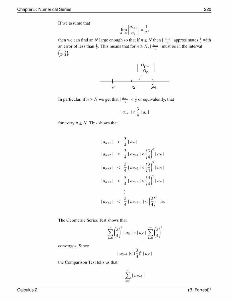
Chapter 5: Numerical Series 220
If we assume thatlimn→∞
∣∣∣∣∣an+1
an
∣∣∣∣∣ =12,
then we can find an N large enough so that if n ≥ N then | an+1an| approximates 1
2 withan error of less than 1
4 . This means that for n ≥ N, | an+1an| must be in the interval(
14 ,
34
).
In particular, if n ≥ N we get that | an+1an|< 3
4 or equivalently, that
| an+1 |<34| an |
for every n ≥ N. This shows that
| aN+1 | <34| aN |
| aN+2 | <34| aN+1 |<
(34
)2
| aN |
| aN+3 | <34| aN+2 |<
(34
)3
| aN |
| aN+4 | <34| aN+3 |<
(34
)4
| aN |
...
| aN+k | <34| aN+k−1 |<
(34
)k
| aN |
The Geometric Series Test shows that∞∑
k=0
(34
)k
| aN |= | aN |
∞∑k=0
(34
)k
converges. Since
| aN+k |< (34
)k | aN |
the Comparison Test tells us that
∞∑k=0
| aN+k |
Calculus 2 (B. Forrest)2
Section 5.9: Ratio Test 221
also converges. From this we can conclude that
∞∑n=0
| an |
converges.
In fact, if limn→∞|
an+1an|= L and 0 ≤ L < 1, then a similar method would show that
∞∑n=0| an | converges.
On the other hand, if limn→∞|
an+1an|= 2, then for large n we would have that
| an+1 |� 2 | an | .
This means that rather than going to 0, the terms in the tail are getting larger. Since
we would then have that limn→∞
an , 0, the Divergence Test would tell us that∞∑
n=0an
diverges.
A similar statement would hold whenever limn→∞|
an+1an|= L and L > 1.
This is summarized in the next theorem which gives us one of the most importanttests for convergence of series.
THEOREM 13 Ratio Test
Given a series∞∑
n=0an, assume that
limn→∞
∣∣∣∣∣an+1
an
∣∣∣∣∣ = L
where L ∈ R or L = ∞.
1. If 0 ≤ L < 1, then∞∑
n=0an converges absolutely.
2. If L > 1, then∞∑
n=0an diverges.
3. If L = 1, then no conclusion is possible.
Remarks:
1) If 0 ≤ L < 1, the Ratio Test shows that the given series converges absolutelyand hence that the original series also converges.
2) If limn→∞|
an+1an|= L exists with L , 1, then the series
∞∑n=0
an behaves like the
geometric series∞∑
n=0Ln as far as convergence is concerned.
Calculus 2 (B. Forrest)2
Chapter 5: Numerical Series 222
3) While the Ratio Test is one of the most important tests for convergence, wewill see that it cannot detect convergence or divergence for many of the serieswe have seen so far. In fact, it can only detect convergence if the terms an
approach 0 very rapidly, and it can only detect divergence if limn→∞|an| = ∞.
This means that the Ratio Test is appropriate for a very special class of series.
EXAMPLE 30 Show that∞∑
n=0
1n!
converges.
We have already seen how this could be done using the Comparison Test. However,the Ratio Test is perfectly suited to series involving factorials.
With an = 1n! , we see that
an+1
an=
1(n+1)!
1n!
=n!
(n + 1)!
=1
n + 1
Thereforelimn→∞
an+1
an= lim
n→∞
1n + 1
= 0.
The Ratio Test shows that∞∑
n=0
1n!
converges.
EXAMPLE 31 In the previous example, we saw how that Ratio Test could be used to show that the
series∞∑
n=0
1n!
converges. This series actually converges very rapidly since n! grows
very quickly. However, if we let
an =1000000n
n!
the situation is quite different. For example, a10 > 1050.
Still,
an+1
an=
1000000n+1
(n+1)!1000000n
n!
=1000000n+1n!
1000000n(n + 1)!
=1000000
n + 1
Calculus 2 (B. Forrest)2
Section 5.9: Ratio Test 223
and so we again have that
limn→∞
an+1
an= lim
n→∞
1000000n + 1
= 0.
This means that despite the enormous size of 1000000n in the numerator, n!eventually dominates. Consequently, we can use the Ratio Test to show that∞∑
n=0
1000000n
n! converges.
EXAMPLE 32 Based on the two previous examples, for which values of x would the series
∞∑n=0
xn
n!
converge?
To answer this question, we first note that if x = 0
∞∑n=0
0n
n!= 1 + 0 + 0 + 0 + · · · = 1
so the series converges when x = 0. Next fix a value for x , 0.
If an =xn
n!, then
∣∣∣∣∣an+1
an
∣∣∣∣∣ =
∣∣∣∣∣∣∣∣xn+1
(n+1)!xn
n!
∣∣∣∣∣∣∣∣=
| x |n+1 n!| x |n (n + 1)!
=| x |
n + 1
Thenlimn→∞
∣∣∣∣∣an+1
an
∣∣∣∣∣ = limn→∞
| x |n + 1
= 0.
The Ratio Test shows that∞∑
n=0
∣∣∣∣∣ xn
n!
∣∣∣∣∣converges and hence that
∞∑n=0
xn
n!
also converges.
Calculus 2 (B. Forrest)2
Chapter 5: Numerical Series 224
Remark: One final observation can be made from the previous example. Since∞∑
n=0
xn
n!converges for any x and since the Divergence Test tells us that the terms of a
convergent series must approach 0 we have the following theorem.
THEOREM 14 Polynomial vs Factorial Growth
For any x ∈ R
limn→∞
xn
n!= 0.
Remark: This important limit tells us that exponentials are of a lower order ofmagnitude compared to factorials. That is, for any fixed x0 ∈ R, | x0 |
n� n!
Note: We know that the series∞∑
n=0rn will diverge if | r |= 1. Therefore, since the
conclusions of the Ratio Test are based on the Geometric Series Test, it might besurprising that if L = 1, the Ratio Test would not show that the series diverges.However, it is important to recognize that lim
n→∞|
an+1an|= 1 does not actually mean that
| aN+k |=| aN | for large N as would be the case if the ratio was exactly 1.
The next two examples show that when L = 1 we could have either convergence ordivergence.
EXAMPLE 33 Apply the Ratio Test to the divergent series∞∑
n=1
1n .
In this example, an = 1n so that ∣∣∣∣∣an+1
an
∣∣∣∣∣ =
1n+1
1n
=n
n + 1
=1
1 + 1n
Therefore, limn→∞
an+1an
= limn→∞
11+ 1
n= 1 and the Ratio Test fails.
EXAMPLE 34 Apply the Ratio Test to the convergent series∞∑
n=1
1n2 .
In this example, an = 1n2 so that
Calculus 2 (B. Forrest)2
Section 5.9: Ratio Test 225
∣∣∣∣∣an+1
an
∣∣∣∣∣ =
1(n+1)2
1n2
=n2
n2 + 2n + 1
=1
1 + 2n + 1
n2
Therefore, limn→∞
an+1an
= limn→∞
11+ 2
n + 1n2
= 1 and the Ratio Test fails again.
We see that the Ratio Test cannot detect convergence or divergence of many otherseries similar to the previous two examples.
Fact: If p(x) = a0 + a1x + · · · + akxk and q(x) = b0 + b1x + · · · + bmxm are twopolynomials, then the Ratio Test will always fail for the series
∞∑n=1
p(n)q(n)
EXAMPLE 35 Consider the series∞∑
n=1
nn
n!.
It is even more difficult to predict how the growth of nn compares with that of n!than it was for xn versus n!. Since the base is increasing as well as the exponent, nn
will get very large, very quickly. However, this is also true of n!. For example, there
is no easy way to determine the value of (106)106
106! . Instead, observe that
nn
n!=
n · n · n · · · n1 · 2 · 3 · · · n
=n1·
n2·
n3· · · ·
nn· ≥ 1.
Since the terms of the series are always larger than 1, they cannot converge to 0 andhence the series diverges.
Calculus 2 (B. Forrest)2
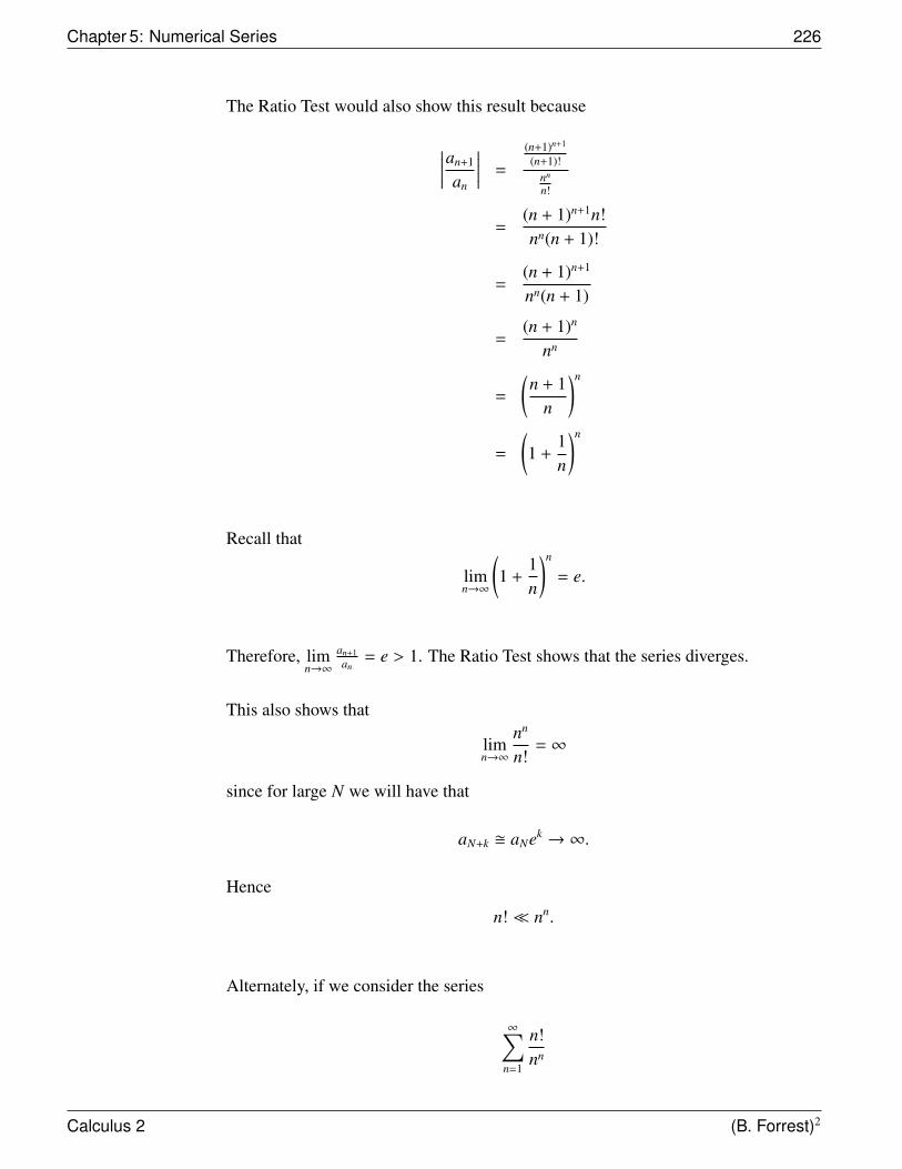
Chapter 5: Numerical Series 226
The Ratio Test would also show this result because
∣∣∣∣∣an+1
an
∣∣∣∣∣ =
(n+1)n+1
(n+1)!nn
n!
=(n + 1)n+1n!nn(n + 1)!
=(n + 1)n+1
nn(n + 1)
=(n + 1)n
nn
=
(n + 1
n
)n
=
(1 +
1n
)n
Recall that
limn→∞
(1 +
1n
)n
= e.
Therefore, limn→∞
an+1an
= e > 1. The Ratio Test shows that the series diverges.
This also shows that
limn→∞
nn
n!= ∞
since for large N we will have that
aN+k � aNek → ∞.
Hence
n! � nn.
Alternately, if we consider the series
∞∑n=1
n!nn
Calculus 2 (B. Forrest)2
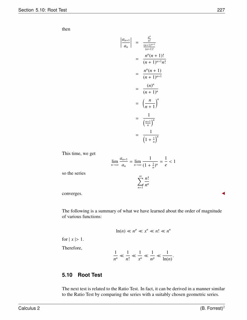
Section 5.10: Root Test 227
then ∣∣∣∣∣an+1
an
∣∣∣∣∣ =
nn
n!(n+1)n+1
(n+1)!
=nn(n + 1)!
(n + 1)n+1n!
=nn(n + 1)(n + 1)n+1
=(n)n
(n + 1)n
=
( nn + 1
)n
=1(
n+1n
)n
=1(
1 + 1n
)n
This time, we get
limn→∞
an+1
an= lim
n→∞
1(1 + 1
n )n=
1e< 1
so the series∞∑
n=1
n!nn
converges.
The following is a summary of what we have learned about the order of magnitudeof various functions:
ln(n) � np � xn � n! � nn
for | x |> 1.
Therefore,1nn �
1n!�
1xn �
1np �
1ln(n)
.
5.10 Root Test
The next test is related to the Ratio Test. In fact, it can be derived in a manner similarto the Ratio Test by comparing the series with a suitably chosen geometric series.
Calculus 2 (B. Forrest)2
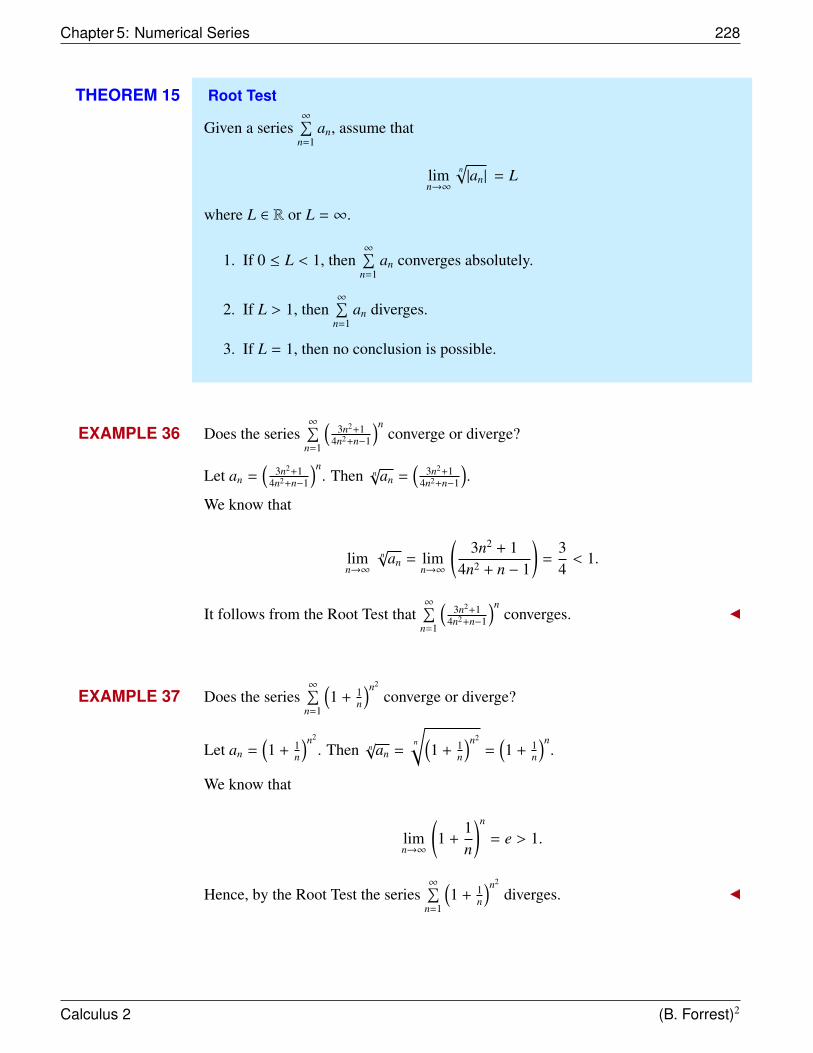
Chapter 5: Numerical Series 228
THEOREM 15 Root Test
Given a series∞∑
n=1an, assume that
limn→∞
n√|an| = L
where L ∈ R or L = ∞.
1. If 0 ≤ L < 1, then∞∑
n=1an converges absolutely.
2. If L > 1, then∞∑
n=1an diverges.
3. If L = 1, then no conclusion is possible.
EXAMPLE 36 Does the series∞∑
n=1
(3n2+1
4n2+n−1
)nconverge or diverge?
Let an =(
3n2+14n2+n−1
)n. Then n
√an =
(3n2+1
4n2+n−1
).
We know that
limn→∞
n√
an = limn→∞
(3n2 + 1
4n2 + n − 1
)=
34< 1.
It follows from the Root Test that∞∑
n=1
(3n2+1
4n2+n−1
)nconverges.
EXAMPLE 37 Does the series∞∑
n=1
(1 + 1
n
)n2
converge or diverge?
Let an =(1 + 1
n
)n2
. Then n√
an =n
√(1 + 1
n
)n2
=(1 + 1
n
)n.
We know that
limn→∞
(1 +
1n
)n
= e > 1.
Hence, by the Root Test the series∞∑
n=1
(1 + 1
n
)n2
diverges.
Calculus 2 (B. Forrest)2
Chapter 6
Power Series
So far all of the series we have considered have been numerical. That is, they haveconsisted of an infinite sum of real numbers which either converged or diverged. Inthis chapter, we will introduce a type of series called a power series whichresembles a polynomial of infinite degree.
6.1 Introduction to Power Series
In this section, we will introduce an important class of series called power series.
DEFINITION Power Series
A power series centered at x = a is a series of the form
∞∑n=0
an(x − a)n
where x is considered a variable and the value an is called the coefficient of the term(x − a)n.
Once we assign a value to the variable x, the series becomes a numerical series. Inparticular, the following is the fundamental problem that we must answer.
Problem: For which values of x does the power series∞∑
n=0an(x − a)n converge?
Note that if x = a, the series becomes
∞∑n=0
an(0)n.
Since our convention is that 00 = 1, we have
Chapter 6: Power Series 230
∞∑n=0
an(0)n = a0(1) + a1(0) + a2(0) + · · ·
= a0 + 0 + 0 + 0 + · · ·
= a0
This shows that every power series centered at x = a will converge at x = a to thevalue a0. The problem now is to determine what happens for other values of x.
As you might expect, the answer depends on the coefficients an.
Note: Before we proceed to study the convergence properties for power series wenote that if we let u = x − a, then
∞∑n=0
an(x − a)n =
∞∑n=0
anun.
This allows us to transform a power series centered at x = a into a power series
centered at u = 0. Moreover, the power series∞∑
n=0an(x − a)n converges at a point x0 if
and only if the power series∞∑
n=0anun converges at x0 − a. This means that if we know
all of the values of u at which the series∞∑
n=0anun converges, then we know all the
values of x for which the series∞∑
n=0an(x − a)n converges. For this reason, in studying
the basic properties of convergence of power series we can focus almost exclusivelyon the case where a = 0. Therefore, unless otherwise specified, we will be dealingwith power series of the form
∞∑n=0
anxn.
EXAMPLE 1 If we choose an = 1 for each n, we get the power series
∞∑n=0
xn.
We know from the Geometric Series Test that this series will converge if and only if| x |< 1.
EXAMPLE 2 We saw as an application of the Ratio Test that the series
∞∑n=0
xn
n!
Calculus 2 (B. Forrest)2
Section 6.1: Introduction to Power Series 231
will converge no matter what value we assign to x. Moreover, it convergesabsolutely for each x.
EXAMPLE 3 For which values of x does the series∞∑
n=0
xn
n + 1
converge?
We can use the Ratio Test to answer this question.
Fix a value for x and letbn =
xn
n + 1.
Then
limn→∞
∣∣∣∣∣bn+1
bn
∣∣∣∣∣ = limn→∞
∣∣∣∣∣∣∣(x)n+1
n+2(x)n
n+1
∣∣∣∣∣∣∣= lim
n→∞
(n + 1)(n + 2)
| x |n+1
| x |n
= limn→∞
(n + 1)(n + 2)
| x |
= | x | limn→∞
(n + 1)(n + 2)
= | x | ·1
= | x |
The Ratio Test shows that the series∞∑
n=0
xn
n+1 =∞∑
n=0bn converges (absolutely) if
limn→∞|
bn+1
bn|= | x |< 1
and it diverges if
limn→∞|
bn+1
bn|= | x |> 1.
The Ratio Test fails to tell us what happens if | x |= 1, so we must consider this caseseparately.
When x = 1, the series is∞∑
n=0
1n + 1
Calculus 2 (B. Forrest)2
Chapter 6: Power Series 232
which is just the Harmonic Series written in a different form. Therefore, whenx = 1, the series diverges.
When x = −1 the series becomes∞∑
n=0
(−1)n
n + 1.
This is just the Alternating Series and as such when x = −1, the series converges.
In summary, the power series∞∑
n=0
xn
n+1 converges absolutely if | x |< 1, diverges if
| x |> 1 and if x = 1, and converges conditionally at x = −1. That is, the seriesconverges if
x ∈ [−1, 1)
If we take a closer look at these three examples we will see that they have certain
common features. First observe that the series∞∑
n=0xn converges if x ∈ (−1, 1). In fact
it converges absolutely on this interval. The series∞∑
n=0
xn
n! converges absolutely on the
interval (−∞,∞). The series∞∑
n=0
xn
n+1 converges if x ∈ [−1, 1) and it converges
absolutely if x ∈ (−1, 1).
These three power series have the following two properties:
Property 1: The set of points on which the power series converge is an intervalcentered around x = 0.
Property 2: There exists an R with either R ∈ [0,∞) or R = ∞ such that the powerseries converges absolutely if | x |< R and it diverges if | x |> R when R ∈ [0,∞),and the series converges absolutely at each x ∈ R when R = ∞. In the first and thirdexamples R = 1, while in the second example R = ∞.
We will now show that two properties are shared by all power series centered atx = 0. Moreover, if a power series is centered at x = a, then Property 1 will holdwith an interval centered around x = a and Property 2 will hold if we replace | x | by| x − a |.
Key Observation:
Assume that the power series∞∑
n=0anxn converges at x = x0. If 0 ≤| x1 |<| x0 |, then we
claim that the series∞∑
n=0
| anxn1 |
Calculus 2 (B. Forrest)2
Section 6.1: Introduction to Power Series 233
also converges. To see why this is the case, we first note that since
∞∑n=0
anxn0
converges, the Divergence Test shows that
limn→∞|anxn
0| = 0.
It follows that there exists an N0 such that
|anxn0| < 1
for all n ≥ N0.
Next observe that|anxn
1| = |anxn0| ·
∣∣∣∣∣ x1
x0
∣∣∣∣∣n ≤ ∣∣∣∣∣ x1
x0
∣∣∣∣∣nfor all n ≥ N0. But
∣∣∣∣ x1x0
∣∣∣∣ < 1 so the series
∞∑n=N0
∣∣∣∣∣ x1
x0
∣∣∣∣∣nconverges by the Geometric Series Test. Since we know that |anxn
1| ≤
∣∣∣∣ x1x0
∣∣∣∣n theComparison Test shows that
∞∑n=N0
|anxn1|
also converges. Finally we get that
∞∑n=0
|anxn1|
converges as claimed.
Summary: We have actually shown that if we are given a series∞∑
n=0anxn then the set
I = {x0 |
∞∑n=0
| anxn0 converges}
is an interval centered at x = 0. Moreover, a similar result is true for a series of the
form∞∑
n=0an(x − a)n.
This leads us to the following definition:
Calculus 2 (B. Forrest)2
Chapter 6: Power Series 234
DEFINITION Interval and Radius of Convergence
Given a power series of the form∞∑
n=0an(x − a)n, the set
I = {x0 ∈ R |∞∑
n=0
an(x0 − a)n converges}
is an interval centered at x = a which we call the interval of convergence for thepower series.
Let
R :=
lub({|x0 − a| | x0 ∈ I}) if I is bounded,∞ if I is not bounded.
Then R is called the radius of convergence of the power series.
The following theorem summarizes what we now know about convergence of apower series.
THEOREM 1 Fundamental Convergence Theorem for Power Series
Given a power series∞∑
n=0an(x − a)n centered at x = a, let R be the radius of
convergence.
1. If R = 0, then∞∑
n=0an(x − a)n converges for x = a but it diverges for all other
values of x.
2. If 0 < R < ∞, then the series∞∑
n=0an(x − a)n converges absolutely for every
x ∈ (a − R, a + R) and diverges if | x − a |> R.
3. If R = ∞, then the series∞∑
n=0an(x − a)n converges absolutely for every x ∈ R.
In particular,∞∑
n=0an(x − a)n converges on an interval that is centered at x = a which
may or may not include one or both of the endpoints.
The following are some important observations concerning the interval ofconvergence.
1. As the previous theorem states, if 0 < R < ∞, the power series∞∑
n=0anxn
converges absolutely on the interval (−R,R). It may or may not converge atx = R or at x = −R. These points must be tested separately. As we will seelater, the interval of convergence could be (−R,R), [−R,R), (−R,R] or [−R,R].The next few examples show that all four cases are possible.
Calculus 2 (B. Forrest)2
Section 6.1: Introduction to Power Series 235
2. If R = ∞, then the power series has interval of convergence (−∞,∞) and it
converges absolutely at each point. For example, the series∞∑
n=0
xn
n! has (−∞,∞)
as its interval of convergence.
3. If R = 0, then the power series only converges at x = 0. That is, “the intervalof convergence” is just the single point {0}. An example of such a power
series is∞∑
n=0n!xn.
EXAMPLE 4 The following power series all have radius of convergence R = 1. The interval ofconvergence is specified.
1.∞∑
n=0xn has interval of convergence (−1, 1) since when x = 1, the series
∞∑n=0
1n
diverges and when x = −1, the series
∞∑n=0
(−1)n
also diverges.
2.∞∑
n=1
xn
n has interval of convergence [−1, 1) since when x = 1, the series
∞∑n=1
1n
diverges but when x = −1, the series
∞∑n=1
(−1)n
n
converges.
3.∞∑
n=1
(−1)n xn
n has interval of convergence (−1, 1] since when x = 1, the series
∞∑n=1
(−1)n
n
converges but when x = −1, the series
∞∑n=1
1n
diverges.
Calculus 2 (B. Forrest)2
Chapter 6: Power Series 236
4.∞∑
n=1
xn
n2 has interval of convergence [−1, 1] since when x = 1, the series
∞∑n=1
1n2
converges and when x = −1, the series
∞∑n=1
(−1)n
n2
also converges.
6.1.1 Finding the Radius of Convergence
Given a power series∞∑
n=0anxn, we have seen that we can often use the Ratio Test to
find the radius of convergence. To see how this works in general, assume that
limn→∞
∣∣∣∣∣an+1
an
∣∣∣∣∣ = L
where 0 ≤ L < ∞ For x , 0, letbn = anxn.
Then
limn→∞
∣∣∣∣∣bn+1
bn
∣∣∣∣∣ = limn→∞
∣∣∣∣∣∣an+1xn+1
anxn
∣∣∣∣∣∣= lim
n→∞| x |
∣∣∣∣∣an+1
an
∣∣∣∣∣= | x | lim
n→∞
∣∣∣∣∣an+1
an
∣∣∣∣∣= L | x |
The Ratio Test shows that the series∞∑
n=0bn =
∞∑n=0
anxn converges absolutely if
L | x |< 1 and diverges if L | x |> 1.
Assume that 0 < L < ∞. Then L | x |< 1 if and only if | x |< 1L . Therefore, the radius
of convergence is R = 1L .
Calculus 2 (B. Forrest)2
Section 6.1: Introduction to Power Series 237
If L = 0, then no matter what x is, we have L | x |= 0 < 1. Therefore, R = ∞. At thispoint we might be tempted to cheat with our notation and write∞ � 1
0 , since this isconsistent with the first case. However, the symbol
10
actually has no numerical meaning.
Iflimn→∞
∣∣∣∣∣an+1
an
∣∣∣∣∣ = L = ∞,
then the same calculation would show
limn→∞|
bn+1
bn|= ∞
and so the series diverges for all non-zero x. However, we know that the series mustconverge at x = 0 so the radius of convergence is 0. Again, we might be temptedwrite 0 = 1
∞but once more
1∞
is not actually defined. Instead we can simply make use of the following theoremwhich summarizes what we have just discussed.
THEOREM 2 Test for the Radius of Convergence
Let∞∑
n=0an(x − a)n be a power series for which
limn→∞
∣∣∣∣∣an+1
an
∣∣∣∣∣ = L
where 0 ≤ L < ∞ or L = ∞. Let R be the radius of convergence of the power series.
1. If 0 < L < ∞, then R = 1L .
2. If L = 0, then R = ∞.
3. If L = ∞, then R = 0.
EXAMPLE 5 Find the radius and interval of convergence for the power series
∞∑n=0
xn
3n(n2 + 1).
We begin by trying to calculate limn→∞|
an+1an|. In this case, an = 1
3n(n2+1) .
Calculus 2 (B. Forrest)2
Chapter 6: Power Series 238
Therefore
limn→∞
∣∣∣∣∣an+1
an
∣∣∣∣∣ = limn→∞
∣∣∣∣∣∣∣1
3n+1((n+1)2+1)1
3n(n2+1)
∣∣∣∣∣∣∣= lim
n→∞
∣∣∣∣∣∣ 3n(n2 + 1)3n+1((n + 1)2 + 1)
∣∣∣∣∣∣= lim
n→∞
13
(n2 + 1
n2 + 2n + 2
)
=13
limn→∞
1 + 1n2
1 + 2n + 2
n2
=13· (1)
=13
It follows from the Test for Radius of Convergence that R = 113
= 3.
We know that the series converges absolutely on (−3, 3). We must check forconvergence at x = 3 and x = −3.
For x = 3, the series becomes∞∑
n=0
3n
3n(n2 + 1)=
∞∑n=0
1n2 + 1
.
Since1
n2 + 1<
1n2
and since∞∑
n=1
1n2 converges, the Comparison Test shows that
∞∑n=1
1n2+1 converges and
hence that∞∑
n=0
1n2 + 1
converges.
Similarly, if x = −3, the series becomes
∞∑n=0
(−3)n
3n(n2 + 1)=
∞∑n=0
(−1)n
n2 + 1.
Notice that the Alternating Series Test applies and so this series also converges.Alternatively, we have ∣∣∣∣∣ (−1)n
n2 + 1
∣∣∣∣∣ =1
n2 + 1.
Calculus 2 (B. Forrest)2
Section 6.1: Introduction to Power Series 239
We have just shown that the series∞∑
n=0
1n2+1 converges, which shows that
∞∑n=0
(−1)n
n2+1
converges absolutely.
We have just shown that the interval of convergence includes both endpoints,therefore the interval of convergence is [−3, 3].
If the previous calculation is repeated, it would show that the power series∞∑
n=0
xn
3n(n2+1)
and the power series∞∑
n=0
xn
3n have the same radius of convergence, namely 3, though
they have a different interval of convergence. (A close look at the second seriesshows that it really looks like a geometric series with r = x
3 so it must convergewhen | x
3 |< 1 and diverge when | x3 |> 1.)
The following theorem will be very useful when we consider differentiation andintegration for functions obtained from power series. It may also help to find theradius of convergence of many series more quickly. It essentially says thatmultiplying or dividing the terms of a power series by a fixed polynomial in n willnot change the radius of convergence, though it is important to remember that it maychange the interval of convergence.
THEOREM 3 Equivalence of Radius of Convergence
Let p and q be non-zero polynomials where q(n) , 0 for n ≥ k. Then the followingseries have the same radius of convergence:
1.∞∑
n=kan(x − a)n
2.∞∑
n=k
an p(n)(x−a)n
q(n)
However, they may have different intervals of convergence.
Note: The limit limn→∞
∣∣∣∣an+1an
∣∣∣∣ may not always exist. In this case, it might require someclever thought to find the radius of convergence.
EXAMPLE 6 Consider the power series
∞∑n=0
anxn = 1 + 2x + x2 + 2x3 + x4 + 2x5 + · · ·
with an = 1 if n is even and an = 2 if n is odd. When x = 1 the series is
1 + 2 + 1 + 2 + 1 + 2 + · · ·
Calculus 2 (B. Forrest)2
Chapter 6: Power Series 240
which diverges. In fact the series also diverges for x = −1. This shows that R ≤ 1.
Next pick x0 ∈ (−1, 1). Then |x0| < 1 then
|anxn0| ≤ 2|xn
0|
and since the series∞∑
n=0
2∣∣∣xn
0
∣∣∣converges, the Comparison Test shows that the original series converges absolutelyat x = x0. This shows that the interval of convergence is (−1, 1) and that R = 1.
However, the sequence{∣∣∣∣an+1
an
∣∣∣∣} osculates between 2 and 12 so lim
n→∞
∣∣∣∣an+1an
∣∣∣∣ does not exist.
6.2 Functions Represented by Power Series
In this section, we consider power series centered at x = a with radius ofconvergence R > 0. We will see how these series define functions with particularlynice properties.
EXAMPLE 7 Recall that the geometric series∞∑
n=0
xn
converges for each x with | x |< 1. Moreover, if | x |< 1, then we also know that
11 − x
=
∞∑n=0
xn.
This means that the series provides us with a means to represent the functionf (x) = 1
1−x on the interval (−1, 1).
DEFINITION Functions Represented by a Power Series
Let∞∑
n=0an(x − a)n be a power series with radius of convergence R > 0. Let I be the
interval of convergence for∞∑
n=0an(x − a)n. Let f be the function defined on the
interval I by the formula
f (x) =
∞∑n=0
an(x − a)n
for each x ∈ I.
Calculus 2 (B. Forrest)2
Section 6.2: Functions Represented by Power Series 241
We say that the function f (x) is represented by the power series∞∑
n=0an(x − a)n on I.
The next theorem tells us that a function represented by a power series must becontinuous on its interval of convergence.
THEOREM 4 Abel’s Theorem: Continuity of Power Series
Assume that the power series∞∑
n=0an(x − a)n has interval of convergence I. Let
f (x) =
∞∑n=0
an(x − a)n
for each x ∈ I. Then f (x) is continuous on I.
The proof of this theorem is beyond the scope of this course.
6.2.1 Building Power Series Representations
Suppose that f and g are two functions represented by power series centered at x=awith
f (x) =
∞∑n=0
an(x − a)n
and
g(x) =
∞∑n=0
bn(x − a)n,
and that the two series have intervals of convergence I f and Ig, respectively.
Question: Can this information be used to build a power series for the sum f + g?
To see why this is possible, we first start by noting that if both series converge at apoint x0 ∈ I f ∩ Ig, then
( f + g)(x0) = f (x0) + g(x0)
= limk→∞
k∑n=0
an(x0 − a)n + limk→∞
k∑n=0
bn(x0 − a)n
= limk→∞
k∑n=0
(an + bn)(x0 − a)n
=
∞∑n=0
(an + bn)(x0 − a)n
Calculus 2 (B. Forrest)2
Chapter 6: Power Series 242
This tells us that the function f + g can be represented by the power series
∞∑n=0
(an + bn)(x − a)n
on I f ∩ Ig.
THEOREM 5 Addition of Power Series
Assume that f and g are represented by power series centered at x = a with
f (x) =
∞∑n=0
an(x − a)n
and
g(x) =
∞∑n=0
bn(x − a)n,
respectively.
Assume also that the radii of convergence of these series are R f and Rg withintervals of convergence I f and Ig. Then
( f + g)(x) =
∞∑n=0
(an + bn)(x − a)n.
Moreover, if R f , Rg, then the radius of convergence of the power seriesrepresenting f + g is R = min{R f ,Rg} and the interval of convergence is I = I f ∩ Ig.
If R f = Rg, then R ≥ R f .
Next assume that h(x) = (x − a)m f (x) where m ∈ N. We might guess that h(x) wouldbe represented by the following power series centered at x = a:
h(x) = (x − a)m∞∑
n=0
an(x − a)n =
∞∑n=0
an(x − a)n+m.
To see why this is the case, we note that if x0 ∈ I f , then
h(x0) = (x0 − a)m f (x0)
= (x0 − a)m limk→∞
k∑n=0
an(x0 − a)n
= limk→∞
k∑n=0
an(x0 − a)n+m
=
∞∑n=0
an(x0 − a)n+m
Calculus 2 (B. Forrest)2
Section 6.2: Functions Represented by Power Series 243
We can summarize this in the following Theorem.
THEOREM 6 Multiplication of a Power Series by (x − a)m
Assume that f is represented by a power series centered at x = a as
f (x) =
∞∑n=0
an(x − a)n
with radius of convergence R f and interval of convergence I f .
Assume that h(x) = (x − a)m f (x) where m ∈ N. Then h(x) can also be represented bya power series centered at x = a with
h(x) =
∞∑n=0
an(x − a)n+m
Moreover, the series that represents h has the same radius of convergence and thesame interval of convergence as the series that represents f .
Finally, assume that f has a power series representation
f (u) =
∞∑n=0
anun
centered at u = 0 with interval of convergence I f .
Question: Can we find a power series representation for h(x) = f (c · xm) centeredat x = 0 where c is some non-zero constant?
In fact, if we choose x0 so that c · xm0 ∈ I f , then substituting c · xm
0 for u gives us
h(x) = f (c · xm0 ) =
∞∑n=0
an(c · xm0 )n =
∞∑n=0
(an · cn)xmn0 .
This leads to the following Theorem.
THEOREM 7 Power Series of Composite Functions
Assume that f has a power series representation
f (u) =
∞∑n=0
anun
Calculus 2 (B. Forrest)2
Chapter 6: Power Series 244
centered at u = 0 with radius of convergence R f and interval of convergence I f . Leth(x) = f (c · xm) where c is a non-zero constant. Then h has a power seriesrepresentation centered at x = 0 of the form
h(x) = f (c · xm) =
∞∑n=0
(an · cn)xmn
The interval of convergence is
Ih = {x ∈ R | c · xm ∈ I f }
and the radius of convergence is Rh =m√
R f
|c| if R f < ∞ and Rh = ∞ otherwise.
EXAMPLE 8 Find a power series representation for f (x) =x
1 − 2x2 centered at x = 0.
We know that1
1 − u=
∞∑n=0
un
for u ∈ (−1, 1). Then1
1 − 2x2 =
∞∑n=0
(2x2)n =
∞∑n=0
2nx2n
provided that 2x2 ∈ (−1, 1). However, 2x2 ∈ (−1, 1) if and only if x2 ∈(−1
2 ,12
).
Therefore,x
1 − 2x2 = x ·∞∑
n=0
2nx2n =
∞∑n=0
2nx2n+1
if and only if x ∈(− 1√
2, 1√
2
).
6.3 Differentiation of Power Series
While the Continuity of Power Series Theorem has important theoreticalapplications, we will be more interested to see if we can differentiate or integratefunctions that can be represented by power series.
Let f (x) =∞∑
n=0an(x − a)n be a function that is represented by a power series. We
could naively try to differentiate f by differentiating the series one term at a time.We would hope that we can do this because we know that for the sum of twofunctions we have
ddx
(g(x) + h(x)) = g ′(x) + f ′(x).
Calculus 2 (B. Forrest)2
Section 6.3: Differentiation of Power Series 245
Since ddx (an(x − a)n) = nan(x − a)n−1, we would also hope that f ′(x) would exist and
that
f ′(x) =
∞∑n=0
nan(x − a)n−1 =
∞∑n=1
nan(x − a)n−1
where the last equality holds since multiplying by 0 gives 0.
Unfortunately, since we are dealing with infinite sums rather than finite sums, we donot even know if the above series will converge. Even if it does, it is not at allobvious that it will sum to f ′(x). At the very least, the process of term-by-termdifferentiation does produce another power series centered at x = a.
DEFINITION The Formal Derivative of a Power Series
Given a power series∞∑
n=0an(x − a)n, the formal derivative is the series
∞∑n=0
nan(x − a)n−1 =
∞∑n=1
nan(x − a)n−1.
We are left to consider two fundamental problems.
Problem 1: For which values of x does the formal power series
∞∑n=1
nan(x − a)n−1
converge? In particular, does this series converge for the same values as does the
original series∞∑
n=0an(x − a)n?
Problem 2: If both the series∞∑
n=0an(x − a)n and
∞∑n=1
nan(x − a)n−1 converge at the
same at x, must it be the case that
f ′(x) =
∞∑n=1
nan(x − a)n−1?
In other words, why must the statement that the derivative of a sum is the sum of thederivatives carry over from finite sums to infinite sums?
Fortunately, Problem 1 is not too difficult.
In the previous section, we saw that multiplying the terms of a power series by apolynomial in n does not change the radius of convergence R. Therefore, the series∞∑
n=0anxn and the series
∞∑n=0
nanxn have the same radius of convergence. A minor
Calculus 2 (B. Forrest)2

Chapter 6: Power Series 246
modification of this result shows that the series∞∑
n=0an(x − a)n and its formal
derivative∞∑
n=1nan(x − a)n−1 also have the same radius of convergence, though the
interval of convergence may be different. Therefore, we have that
g(x) =
∞∑n=1
nan(x − a)n−1
is defined for all x ∈ (a − R, a + R). The question that remains is:
Does g(x) = f ′(x)?
A rigorous answer to this question is very difficult. It involves a number of verysophisticated results including the Fundamental Theorem of Calculus. However, thefollowing theorem tells us that functions represented by power series do indeed havethe remarkable property that we require.
THEOREM 8 Term-by-Term Differentiation of Power Series
Assume that the power series∞∑
n=0an(x − a)n has radius of convergence R > 0. Let
f (x) =
∞∑n=0
an(x − a)n
for all x ∈ (a − R, a + R). Then f is differentiable on (a − R, a + R) and for eachx ∈ (a − R, a + R),
f ′(x) =
∞∑n=1
nan(x − a)n−1.
Remarks:
1) It may be tempting to dismiss the previous theorem as obvious since wewould expect differentiation to be preserved by sums. However, this theoremillustrates a very special property of power series that is not shared by othertypes of series of functions. For example, it can be shown as an application ofthe Comparison Test and the Geometric Series Test that for each x ∈ R, theseries
∞∑n=0
(34
)n
sin(9nx)
converges. This allows us to define a function
f (x) =
∞∑n=0
(34
)n
sin(9nx)
Calculus 2 (B. Forrest)2

Section 6.3: Differentiation of Power Series 247
that is defined for all x ∈ R.
Notice that f is the sum of infinitely many differentiable functions, namely
fn(x) =
(34
)n
sin(9nx)
for each n. Based on our experience with power series, we might be temptedto think that f (x) should be differentiable and that its derivative would be thesum of all of the derivatives of the fn’s. Unfortunately, this is false. In fact, itturns out that the function f (x) is a continuous function that is notdifferentiable at any point on the real line. This is about as strange as acontinuous function can be!
This example, which is one of a class of everywhere continuous but nowheredifferentiable functions discovered by the 19th century mathematician KarlWeierstrass. This is a historically important example because up untilWeierstrass’ discovery it was thought that a continuous function had to havesome points of differentiability. The graph of such a function has ”fractal-like”properties. This means that no matter how close we zoom in to any givenpoint, the graph of the function does not start to resemble a straight line.
2) While it may not be immediately obvious, the Differentiation Theorem forPower Series actually says much more about a function f that can berepresented by a power series than just simply that it is differentiable. To see
why, observe that if f (x) =∞∑
n=0an(x − a)n is represented by a power series on
the interval (a − R, a + R), then f ′(x) =∞∑
n=1nan(x − a)n−1 is also represented by
a power series on (a − R, a + R). Applying the previous theorem again showsthat f ′(x) is also differentiable on (a − R, a + R). Moreover, we can calculateddx ( f ′(x)) = f ′′(x) by differentiating the series representing f ′(x)term-by-term. Therefore
f ′′(x) =
∞∑n=1
n(n − 1)an(x − a)n−2 =
∞∑n=2
n(n − 1)an(x − a)n−2.
(Note: We begin the series at n = 2 since for n = 1, n(n − 1) = 0.)
Furthermore, we need not stop here. We can term-by-term differentiate againto show that
f ′′′(x) =
∞∑n=3
n(n − 1)(n − 2)an(x − a)n−3
and that
f (4)(x) =
∞∑n=4
n(n − 1)(n − 2)(n − 3)an(x − a)n−4.
In fact, we can show that f (x) has derivatives of all orders on (a − R, a + R)with
f (k)(x) =
∞∑n=k
n(n − 1)(n − 2)(n − 3) · · · (n − k + 1)an(x − a)n−k
for each k.
Calculus 2 (B. Forrest)2
Chapter 6: Power Series 248
EXAMPLE 9 We know that if | x |< 1, then1
1 − x=
∞∑n=0
xn.
Let f (x) = 11−x = (1 − x)−1. Differentiating, we get
f ′(x) =1
(1 − x)2 .
We also get a power series representation for f ′(x) by term-by-term differentiation
of the series∞∑
n=0xn. It follows that
f ′(x) =1
(1 − x)2 =
∞∑n=1
nxn−1.
We can use this to evaluate the sum of the series∞∑
n=1
n2n−1 .
Observe that this series is obtained from∞∑
n=1nxn−1 by letting x = 1
2 . Therefore,
∞∑n=1
n2n−1 = f ′
(12
)=
1(1 − 1
2
)2
= 4
EXAMPLE 10 We have seen that if a function f satisfies the differential equation y ′ = y, then there
is a constant C such that f (x) = Cex. We also know that the series∞∑
n=0
xn
n! converges
for every value of x. Let
g(x) =
∞∑n=0
xn
n!=
x0
0!+
x1
1!+
x2
2!+
x3
3!+ · · · .
We can find g ′(x) by term-by-term differentiation. Therefore
g ′(x) =
∞∑n=1
nxn−1
n!.
Calculus 2 (B. Forrest)2
Section 6.3: Differentiation of Power Series 249
If we take a close look at this series we see immediately that it becomes
∞∑n=1
xn−1
(n − 1)!.
Writing out the terms, we get
x0
0!+
x1
1!+
x2
2!+
x3
3!+ · · ·
which is identical to the series that gave us g(x). This shows that
g ′(x) = g(x)
for every x. Therefore, there is a C such that g(x) = Cex. Moreover, g(0) = Ce0 = C.But
g(0) =
∞∑n=0
0n
n!
=00
0!+
01
1!+
02
2!+
03
3!+ · · ·
= 1 + 0 + 0 + 0 + · · ·
= 1
Hence C = 1 and
g(x) =
∞∑n=0
xn
n!= ex
for every x ∈ R.
This is an extremely important example that we will come back to again and again.one immediate application is that
e =
∞∑n=0
1n
n!=
∞∑n=0
1n!.
This series converges quite rapidly so we can get a very accurate approximation fore by summing a relatively small number of terms.
EXAMPLE 11 Find a power series representation for the function f (x) = e−x2.
We have just seen for any u ∈ R that
eu =
∞∑n=0
un
n!(∗)
Calculus 2 (B. Forrest)2
Chapter 6: Power Series 250
Given x ∈ R, let u = −x2 and substitute for u in the expression (∗). This gives us
e−x2=
∞∑n=0
(−x2)n
n!=
∞∑n=0
(−1)n x2n
n!.
At first glance
e−x2= 1 −
x2
1!+
x4
2!−
x6
3!+ · · · + (−1)n x2n
n!+ · · ·
may not look like a power series since there are no terms involving xn when n isodd. But in fact, it is a power series where the coefficients are of the form a2k−1 = 0and a2k = (−1)k 1
k! for each k = 0, 1, 2, 3, 4, . . ..
Moreover, since the original series converges for all u ∈ R, the power series forf (x) = e−x2
will also converge for all x ∈ R. That is, its radius of convergence isR = ∞.
Key Observation: We have seen that if
f (x) =
∞∑n=0
anxn
for all x ∈ (−R,R), then f (x) is infinitely differentiable on (−R,R). We can now usethis to show that once a function f (x) has a power series representation at x = 0, thecoefficients are uniquely determined by the various values of the derivatives of f (x).In particular, once we fix the center x = 0, the function f can only be represented byone such power series at x = 0 (though there may well be other representations of fwith different centers). To see why this is true, recall that for any function
g(x) =
∞∑n=0
bnxn
represented by a power series, if we substitute in 0 for x, we get that
g(0) = b0.
That is, g(0) is simply the coefficient of the term x0 in the power seriesrepresentation of g(x). Therefore, if
f (x) =
∞∑n=0
anxn
is any power series representation for the function f (x), then a0 = f (0). This showsthat a0 is in fact, uniquely determined by the value of f (x) at x = 0.
We can show that something similar occurs for all of the other coefficients. Forexample, we note that since
f ′(x) =
∞∑n=1
nanxn−1
Calculus 2 (B. Forrest)2
Section 6.3: Differentiation of Power Series 251
then f ′(0) is the coefficient of x0 in this series new representation. But we get x0
when n = 1 and when n = 1, the coefficient is (1)(a1). It follows that
f ′(0) = (1)a1 = a1.
Alternatively, we could get this directly by substituting x = 0 in the expression forf ′(x) to get
f ′(0) = (1)a1(0)0 + (2)a2(0)1 + (3)a3(0)2 + (4)a4(0)4 + · · ·
= a1 + 0 + 0 + 0 + 0 + · · ·
= a1
By either method, we see that f ′(0) = a1, so the coefficient a1 is also uniquelydetermined by f (x).
A similar calculation shows that f ′′(0) is the coefficient of x0 in
f ′′(x) =
∞∑n=2
n(n − 1)anxn−2.
This time to get xn−2 = x0, we let n = 2. From this we see that the coefficient of x0 inthe previous expression is given by 2(2 − 1)a2 or 2 · 1a2 = 2!a2. As a result we have
f ′′(0) = 2!a2
or thata2 =
f ′′(0)2!
.
Once again, a2 is uniquely determined.
To find a3, start with
f ′′′(x) =
∞∑n=3
n(n − 1)(n − 2)anxn−3.
Then f ′′′(0) is the coefficient of x0 in this series and therefore
f ′′′(0) = (3)(3 − 1)(3 − 2)a3 = 3 · 2 · 1a3 = 3!a3.
Solving for a3 shows that
a3 =f ′′′(0)
3!.
In fact, for any k ≥ 2, we have
f (k)(x) =
∞∑n=k
n(n − 1)(n − 2)(n − 3) · · · (n − k + 1)anxn−k
Calculus 2 (B. Forrest)2
Chapter 6: Power Series 252
so that the coefficient of x0 is obtained when n = k and hence
f (k)(0) = (k)(k − 1)(k − 2) · · · (k − (k − 2))(k − (k − 1))ak
= k · (k − 1) · (k − 2) · · · 2 · 1ak
= k!ak
Solving this expression for ak shows that for k ≥ 2,
ak =f (k)(0)
k!.
If we note that
a0 = f (0) =f (0)(0)
0!and
a1 = f ′(0) =f (1)(0)
1!then we see that for every k,
ak =f (k)(0)
k!.
This tells us if a function can be represented by a power series∞∑
n=0anxn centered at
x = 0, then the function f (x) and its various derivatives uniquely determine thecoefficients.
A similar argument shows that the previous observation holds for a power seriescentered at x = a. This situation motivates the next theorem.
THEOREM 9 Uniqueness of Power Series Representations
Suppose that
f (x) =
∞∑n=0
an(x − a)n
for all x ∈ (a − R, a + R) where R > 0. Then
an =f (n)(a)
n!.
In particular, if
f (x) =
∞∑n=0
bn(x − a)n,
thenbn = an
for each n = 0, 1, 2, 3, · · · .
Calculus 2 (B. Forrest)2

Section 6.4: Integration of Power Series 253
6.4 Integration of Power Series
Up until now we have seen that a function which is represented by a power serieshas the remarkable property that it is infinitely differentiable and that its derivativescan be obtained by repeated term-by-term differentiation of the power series. Itwould make sense to determine if a similar statement could be made with respect toanti-differentiation and integration.
We begin with the following definition:
DEFINITION Formal Antiderivative of a Power Series
Given a power series∞∑
n=0an(x − a)n, we define the formal antiderivative to be the
power series∞∑
n=0
∫an(x − a)n dx = C +
∞∑n=0
an
n + 1(x − a)n+1.
where C is an arbitrary constant.
In the definition, we called the series a formal antiderivative because at this point wedo not know if it is an actual antiderivative of f . In fact we do not even know if theformal antiderivative converges at any point other than the center.
Problem: Suppose that the power series∞∑
n=0an(x − a)n has radius of convergence
R > 0. Let
f (x) =
∞∑n=0
an(x − a)n
be the function that is represented by this power series on the interval (a − R, a + R).Are the formal anitderivatives
C +
∞∑n=0
an
n + 1(x − a)n+1
true antiderivatives of the function f ?
To see why this is in fact the case we first note that the series
∞∑n=0
an
n + 1(x − a)n
is obtained from∞∑
n=0an(x − a)n by dividing each coefficient an by q(n) = n + 1. We
know that this will not change the radius of convergence. Hence,∞∑
n=0
ann+1 (x − a)n will
also converge on (a − R, a + R). Then the formal antiderivative
C +
∞∑n=0
an
n + 1(x − a)n+1
Calculus 2 (B. Forrest)2
Chapter 6: Power Series 254
will have radius of convergence R. This means that we can define a function
F(x) = C +
∞∑n=0
an
n + 1(x − a)n+1
on (a − R, a + R).
Next we show that F is an antiderivative of f .
Since F is represented by a power series, it is differentiable. Moreover, its derivativecan be obtained by term-by-term differentiation. Therefore
F ′(x) =ddx
(C) +
∞∑n=0
ddx
( an
n + 1(x − a)n+1
)= 0 +
∞∑n=0
(n + 1)( an
n + 1
)(x − a)n
=
∞∑n=0
an(x − a)n
= f (x)
so F is an antiderivative of f . Moreover, since the constant C is arbitrary, allantiderivatives have this form.
The next theorem summarizes what we have just discussed. It also tells us that wecan evaluate definite integrals using term-by-term methods. (The proof of this laststatement is beyond the scope of the course.)
THEOREM 10 Term-by-Term Integration of Power Series
Assume that the power series∞∑
n=0an(x − a)n has radius of convergence R > 0. Let
f (x) =
∞∑n=0
an(x − a)n
for every x ∈ (a − R, a + R). Then the series
∞∑n=0
∫an(x − a)n dx = C +
∞∑n=0
an
n + 1(x − a)n+1
also has radius of convergence R and if
F(x) = C +
∞∑n=0
an
n + 1(x − a)n+1
then F ′(x) = f (x).
Calculus 2 (B. Forrest)2

Section 6.4: Integration of Power Series 255
Furthermore, if [c, b] ⊂ (a − R, a + R), then∫ b
cf (x) dx =
∫ b
c
∞∑n=0
an(x − a)n dx
=
∞∑n=0
∫ b
can(x − a)n dx
=
∞∑n=0
an
n + 1· ((b − a)n+1 − (c − a)n+1)
Note: Similar to the case with the term-by-term differentiation rule for powerseries, it should seem natural that we are also able to integrate term-by-term thefunctions that are represented by a power series. But as was the case withdifferentiation, the reason we are able to do this is because of some very specialproperties impacting how power series converge. If
F(x) =
∞∑n=1
fn(x)
for each x ∈ [a, b], then we might hope that∫ b
aF(x) dx =
∞∑n=0
∫ b
afn(x) dx.
Unfortunately, if we do not make any additional assumptions about the nature of thefunctions fn or how the series converges, then this statement could be false. In fact,it is possible that the function F need not even be integrable on [a, b].
We can use the previous theorem to build power series representations for manyfunctions.
EXAMPLE 12 Find a power series representation for ln(1 + x).
We begin by recognizing that
ddx
(ln(1 + x)) =1
1 + x.
If we had a power series representation for 11+x , we could use the previous theorem
to build a representation for ln(1 + x).
We know that for any u ∈ (−1, 1),
11 − u
=
∞∑n=0
un.
Calculus 2 (B. Forrest)2
Chapter 6: Power Series 256
Let x ∈ (−1, 1). Then (−x) ∈ (−1, 1). If we let u = −x and substitute this into theprevious equation, then
11 − (−x)
=
∞∑n=0
(−x)n
so that for any (−x) ∈ (−1, 1),
11 + x
=1
1 − (−x)
=
∞∑n=0
(−x)n
=
∞∑n=0
(−1)nxn
We now know ddx (ln(1 + x)) = 1
1+x and that
11 + x
=
∞∑n=0
(−1)nxn.
Therefore, there is a constant C such that
ln(1 + x) = C +
∞∑n=0
∫(−1)nxn dx
= C +
∞∑n=0
(−1)n
n + 1xn+1
for all x ∈ (−1, 1).
To find C, let x = 0. Then
0 = ln(1 + 0)
= C +
∞∑n=0
(−1)n
n + 10n+1
= C
This shows that for all x ∈ (−1, 1),
ln(1 + x) =
∞∑n=0
(−1)n
n + 1xn+1.
There is one more very useful observation that we can make regarding this example.We know that the series
∞∑n=0
(−1)n
n + 1xn+1
Calculus 2 (B. Forrest)2
Section 6.5: Review of Taylor Polynomials 257
has radius of convergence R = 1. However, if we let x = 1, the series becomes
∞∑n=0
(−1)n
n + 11n+1 =
11−
12
+13−
14
+15− · · ·
which is exactly the Alternating Series. Therefore, the series also converges atx = 1. However, the equation
ln(1 + x) =
∞∑n=0
(−1)n
n + 1xn+1
is actually valid wherever this new series converges. This tells us that
ln(2) = ln(1 + 1) =11−
12
+13−
14
+15− · · ·
so we have found the sum of the alternating series.
6.5 Review of Taylor Polynomials
Recall that if f is differentiable at x = a, then if x � a
f ′(a) �f (x) − f (a)
x − a.
Cross-multiplying gives us
f ′(a)(x − a) � f (x) − f (a)
and finally thatf (x) � f (a) + f ′(a)(x − a) .
This led us to define the linear approximation to f at x = a to be the function
La(x) = f (a) + f ′(a)(x − a).
We saw that the geometrical significance of the linear approximation is that itsgraph is the tangent line to the graph of f through the point (a, f (a)).
Calculus 2 (B. Forrest)2
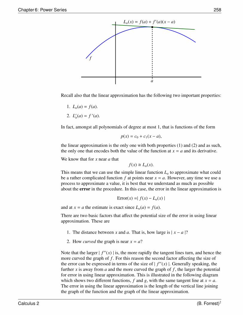
Chapter 6: Power Series 258
f
a
La(x) = f (a) + f ′(a)(x − a)
Recall also that the linear approximation has the following two important properties:
1. La(a) = f (a).
2. L′a(a) = f ′(a).
In fact, amongst all polynomials of degree at most 1, that is functions of the form
p(x) = c0 + c1(x − a),
the linear approximation is the only one with both properties (1) and (2) and as such,the only one that encodes both the value of the function at x = a and its derivative.
We know that for x near a thatf (x) � La(x).
This means that we can use the simple linear function La to approximate what couldbe a rather complicated function f at points near x = a. However, any time we use aprocess to approximate a value, it is best that we understand as much as possibleabout the error in the procedure. In this case, the error in the linear approximation is
Error(x) =| f (x) − La(x) |
and at x = a the estimate is exact since La(a) = f (a).
There are two basic factors that affect the potential size of the error in using linearapproximation. These are
1. The distance between x and a. That is, how large is | x − a |?
2. How curved the graph is near x = a?
Note that the larger | f ′′(x) | is, the more rapidly the tangent lines turn, and hence themore curved the graph of f . For this reason the second factor affecting the size ofthe error can be expressed in terms of the size of | f ′′(x) |. Generally speaking, thefurther x is away from a and the more curved the graph of f , the larger the potentialfor error in using linear approximation. This is illustrated in the following diagramwhich shows two different functions, f and g, with the same tangent line at x = a.The error in using the linear approximation is the length of the vertical line joiningthe graph of the function and the graph of the linear approximation.
Calculus 2 (B. Forrest)2
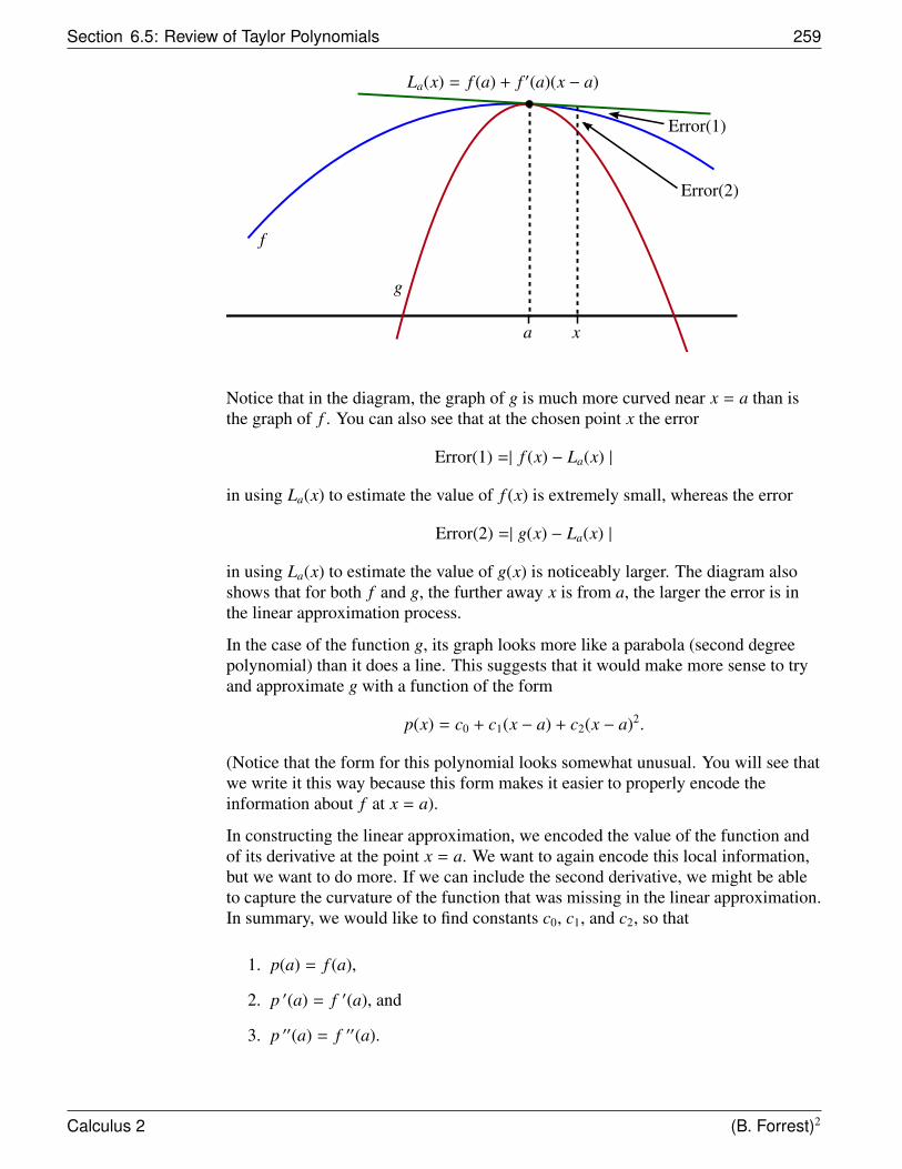
Section 6.5: Review of Taylor Polynomials 259
g
a x
Error(1)
Error(2)
f
La(x) = f (a) + f ′(a)(x − a)
Notice that in the diagram, the graph of g is much more curved near x = a than isthe graph of f . You can also see that at the chosen point x the error
Error(1) =| f (x) − La(x) |
in using La(x) to estimate the value of f (x) is extremely small, whereas the error
Error(2) =| g(x) − La(x) |
in using La(x) to estimate the value of g(x) is noticeably larger. The diagram alsoshows that for both f and g, the further away x is from a, the larger the error is inthe linear approximation process.
In the case of the function g, its graph looks more like a parabola (second degreepolynomial) than it does a line. This suggests that it would make more sense to tryand approximate g with a function of the form
p(x) = c0 + c1(x − a) + c2(x − a)2.
(Notice that the form for this polynomial looks somewhat unusual. You will see thatwe write it this way because this form makes it easier to properly encode theinformation about f at x = a).
In constructing the linear approximation, we encoded the value of the function andof its derivative at the point x = a. We want to again encode this local information,but we want to do more. If we can include the second derivative, we might be ableto capture the curvature of the function that was missing in the linear approximation.In summary, we would like to find constants c0, c1, and c2, so that
1. p(a) = f (a),
2. p ′(a) = f ′(a), and
3. p ′′(a) = f ′′(a).
Calculus 2 (B. Forrest)2
Chapter 6: Power Series 260
It may not seem immediately obvious that we can find such constants. However, thistask is actually not too difficult. For example, if we want p(a) = f (a), then by notingthat
p(a) = c0 + c1(a − a) + c2(a − a)2 = c0
we immediately know that we should let c0 = f (a).
We can use the standard rules of differentiation to show that
p ′(x) = c1 + 2c2(x − a).
In order that p ′(a) = f ′(a), we have
f ′(a) = p ′(a) = c1 + 2c2(a − a) = c1.
Finally, sincep ′′(x) = 2c2
for all x, if we let c2 =f ′′(a)
2 , we have
p ′′(a) = 2c2 = 2(f ′′(a)
2) = f ′′(a)
exactly as required. This shows that if
p(x) = f (a) + f ′(a)(x − a) +f ′′(a)
2(x − a)2,
then p is the unique polynomial of degree 2 or less such that
1. p(a) = f (a),
2. p ′(a) = f ′(a), and
3. p ′′(a) = f ′′(a).
The polynomial p is called the second degree Taylor polynomial for f centered atx = a. We denote this Taylor polynomial by T2,a.
EXAMPLE 13 Let f (x) = cos(x). Then,
f (0) = cos(0) = 1, and f ′(0) = − sin(0) = 0,
andf ′′(0) = − cos(0) = −1.
It follows that
L0(x) = f (0) + f ′(0)(x − 0) = 1 + 0(x − 0) = 1
Calculus 2 (B. Forrest)2
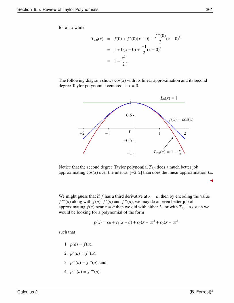
Section 6.5: Review of Taylor Polynomials 261
for all x while
T2,0(x) = f (0) + f ′(0)(x − 0) +f ′′(0)
2(x − 0)2
= 1 + 0(x − 0) +−12
(x − 0)2
= 1 −x2
2.
The following diagram shows cos(x) with its linear approximation and its seconddegree Taylor polynomial centered at x = 0.
L0(x) = 1
f (x) = cos(x)
T2,0(x) = 1 − x2
2
−2 −1 0
−0.5
−1
0.5
1
1 2
Notice that the second degree Taylor polynomial T2,0 does a much better jobapproximating cos(x) over the interval [−2, 2] than does the linear approximation L0.
We might guess that if f has a third derivative at x = a, then by encoding the valuef ′′′(a) along with f (a), f ′(a) and f ′′(a), we may do an even better job ofapproximating f (x) near x = a than we did with either La or with T2,a. As such wewould be looking for a polynomial of the form
p(x) = c0 + c1(x − a) + c2(x − a)2 + c3(x − a)3
such that
1. p(a) = f (a),
2. p ′(a) = f ′(a),
3. p ′′(a) = f ′′(a), and
4. p ′′′(a) = f ′′′(a).
Calculus 2 (B. Forrest)2
Chapter 6: Power Series 262
To find such a p, we follow the same steps that we outlined before. We wantp(a) = f (a), but p(a) = c0 + c1(a − a) + c2(a − a)2 + c3(a − a)3 = c0, so we can letc0 = f (a).
Differentiating p we get
p ′(x) = c1 + 2c2(x − a) + 3c3(x − a)2
so thatp ′(a) = c1 + 2c2(a − a) + 3c3(a − a)2 = c1.
Therefore, if we let c1 = f ′(a) as before, then we will get p ′(a) = f ′(a).
Differentiating p ′ gives us
p ′′(x) = 2c2 + 3(2)c3(x − a).
Therefore,p ′′(a) = 2c2 + 3(2)c3(a − a) = 2c2.
Now if we let c2 =f ′′(a)
2 , we get
p ′′(a) = f ′′(a).
Finally, observe that
p ′′′(x) = 3(2)c3 = 3(2)(1)c3 = 3!c3
for all x, so if we requirep ′′′(a) = 3!c3 = f ′′′(a),
then we need only let c3 =f ′′′(a)
3! .
It follows that if
p(x) = f (a) + f ′(a)(x − a) +f ′′(a)
2(x − a)2 +
f ′′′(a)3!
(x − a)3,
then
1. p(a) = f (a),
2. p ′(a) = f ′(a),
3. p ′′(a) = f ′′(a), and
4. p ′′′(a) = f ′′′(a).
In this case, we call p the third degree Taylor polynomial centered at x = a anddenote it by T3,a.
Given a function f , we could also write
T0,a(x) = f (a)
Calculus 2 (B. Forrest)2
Section 6.5: Review of Taylor Polynomials 263
andT1,a(x) = La(x) = f (a) + f ′(a)(x − a)
and call these polynomials the zero-th degree and the first degree Taylorpolynomials of f centered at x = a, respectively.
Observe that using the convention where 0! = 1! = 1 and (x − a)0 = 1, we have thefollowing:
T0,a(x) =f (a)0!
(x − a)0
T1,a(x) =f (a)0!
(x − a)0 +f ′(a)
1!(x − a)1
T2,a(x) =f (a)0!
(x − a)0 +f ′(a)
1!(x − a)1 +
f ′′(a)2!
(x − a)2
T3,a(x) =f (a)0!
(x − a)0 +f ′(a)
1!(x − a)1 +
f ′′(a)2!
(x − a)2 +f ′′′(a)
3!(x − a)3.
Recall that f (k)(a) denotes the k-th derivative of f at x = a. By convention,f (0)(x) = f (x). Then using summation notation, we have
T0,a(x) =
0∑k=0
f (k)(a)k!
(x − a)k
T1,a(x) =
1∑k=0
f (k)(a)k!
(x − a)k
T2,a(x) =
2∑k=0
f (k)(a)k!
(x − a)k
and
T3,a(x) =
3∑k=0
f (k)(a)k!
(x − a)k.
This leads us to the following definition:
DEFINITION Taylor Polynomials
Assume that f is n-times differentiable at x = a. The n-th degree Taylor polynomialfor f centered at x = a is the polynomial
Tn,a(x) =
n∑k=0
f (k)(a)k!
(x − a)k
= f (a) + f ′(a)(x − a) +f ′′(a)
2!(x − a)2 + · · · +
f (n)(a)n!
(x − a)n
Calculus 2 (B. Forrest)2
Chapter 6: Power Series 264
NOTE
A remarkable property about Tn,a is that for any k between 0 and n,
T (k)n,a(a) = f (k)(a).
That is, Tn,a encodes not only the value of f (x) at x = a but all of its first nderivatives as well. Moreover, this is the only polynomial of degree n or less thatdoes so!
EXAMPLE 14 Find all of the Taylor polynomials up to degree 5 for the function f (x) = cos(x) withcenter x = 0.
We have already seen that f (0) = cos(0) = 1, f ′(0) = − sin(0) = 0, andf ′′(0) = − cos(0) = −1. It follows that
T0,0(x) = 1,
andT1,0(x) = L0(x) = 1 + 0(x − 0) = 1
for all x, while
T2,0(x) = 1 + 0(x − 0) +−12!
(x − 0)2 = 1 −x2
2.
Since f ′′′(x) = sin(x), f (4)(x) = cos(x), and f (5)(x) = − sin(x), we getf ′′′(0) = sin(0) = 0, f (4)(0) = cos(0) = 1 and f (5)(0) = − sin(0) = 0. Hence,
T3,0(x) = 1 + 0(x − 0) +−12!
(x − 0)2 +03!
(x − 0)3
= 1 −x2
2= T2,0(x)
We also have that
T4,0(x) = 1 + 0(x − 0) +−12!
(x − 0)2 +03!
(x − 0)3 +14!
(x − 0)4
= 1 −x2
2+
x4
24
and
T5,0(x) = 1 + 0(x − 0) +−12!
(x − 0)2 +03!
(x − 0)3 +14!
(x − 0)4 +05!
(x − 0)5
= 1 −x2
2+
x4
24= T4,0(x)
Calculus 2 (B. Forrest)2
Section 6.5: Review of Taylor Polynomials 265
An important observation to make is that not all of these polynomials are distinct. Infact, T0,0(x) = T1,0(x), T2,0(x) = T3,0(x), and T4,0(x) = T5,0(x). In general, thisequality of different order Taylor polynomials happens when one of the derivativesis 0 at x = a. (In this example at x = 0.) This can be seen by observing that for any n
Tn+1,a(x) = Tn,a(x) +f (n+1)(a)(n + 1)!
(x − a)n+1
so if f (n+1)(a) = 0, we get Tn+1,a(x) = Tn,a(x).
The following diagram shows cos(x) and its Taylor polynomials up to degree 5. Youwill notice that there are only four distinct graphs.
f (x) = cos(x)
T2,0(x) = T3,0(x) = 1 − x2
2
T4,0(x) = T5,0(x) = 1 − x2
2 + x4
24
T0,0(x) = T1,0(x) = 1
−2 −10
−0.5
−1
0.5
1
1 2
In the next example, we will calculate the Taylor Polynomials for f (x) = sin(x).
EXAMPLE 15 Find all of the Taylor polynomials up to degree 5 for the function f (x) = sin(x) withcenter x = 0.
We can see that f (0) = sin(0) = 0, f ′(0) = cos(0) = 1, f ′′(0) = − sin(0) = 0,f ′′′(0) = − cos(0) = −1, f (4)(0) = sin(0) = 0, and f (5)(0) = cos(0) = 1. It followsthat
T0,0(x) = 0,
andT1,0(x) = L0(x) = 0 + 1(x − 0) = x
and
T2,0(x) = 0 + 1(x − 0) +02!
(x − 0)2
= x= T1,0(x).
Calculus 2 (B. Forrest)2
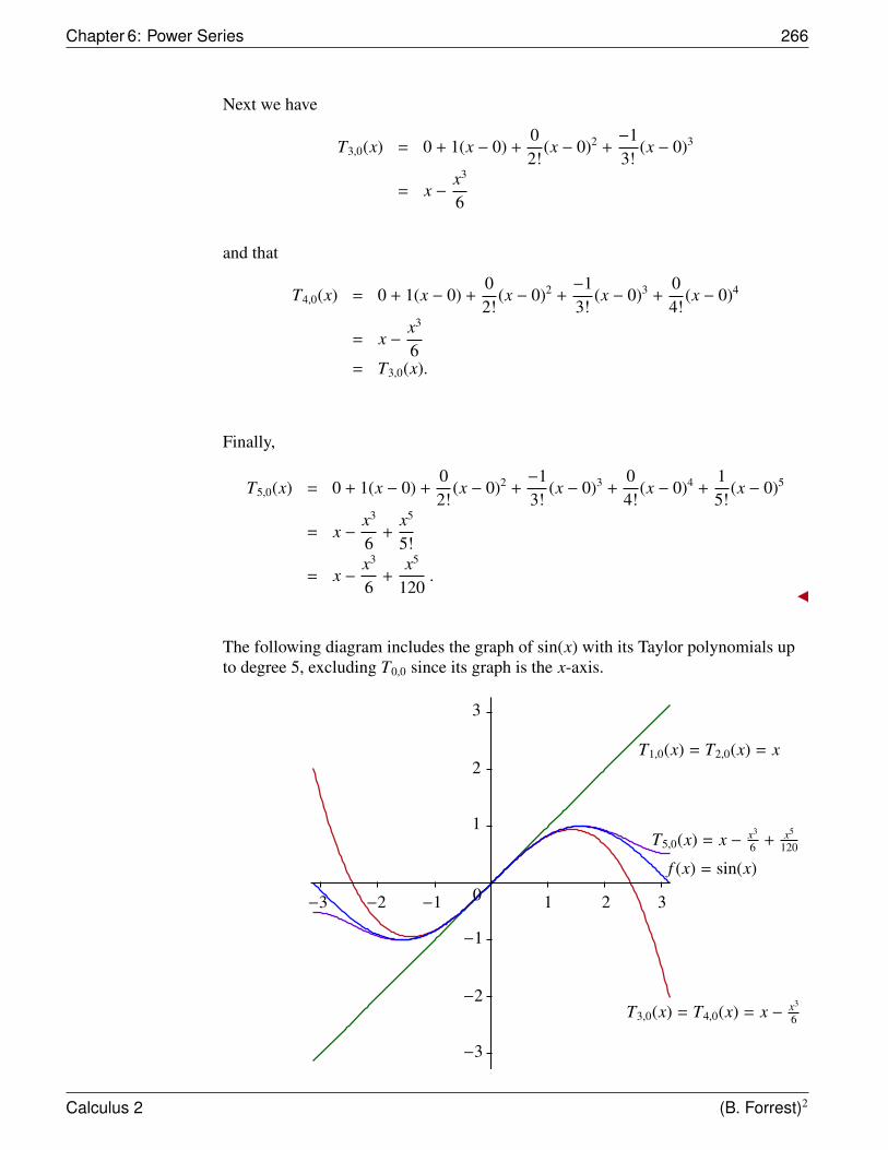
Chapter 6: Power Series 266
Next we have
T3,0(x) = 0 + 1(x − 0) +02!
(x − 0)2 +−13!
(x − 0)3
= x −x3
6
and that
T4,0(x) = 0 + 1(x − 0) +02!
(x − 0)2 +−13!
(x − 0)3 +04!
(x − 0)4
= x −x3
6= T3,0(x).
Finally,
T5,0(x) = 0 + 1(x − 0) +02!
(x − 0)2 +−13!
(x − 0)3 +04!
(x − 0)4 +15!
(x − 0)5
= x −x3
6+
x5
5!
= x −x3
6+
x5
120.
The following diagram includes the graph of sin(x) with its Taylor polynomials upto degree 5, excluding T0,0 since its graph is the x-axis.
T1,0(x) = T2,0(x) = x
T3,0(x) = T4,0(x) = x − x3
6
T5,0(x) = x − x3
6 + x5
120
f (x) = sin(x)
−2 −1 0 1 2−3 3
1
2
3
−3
−2
−1
Calculus 2 (B. Forrest)2
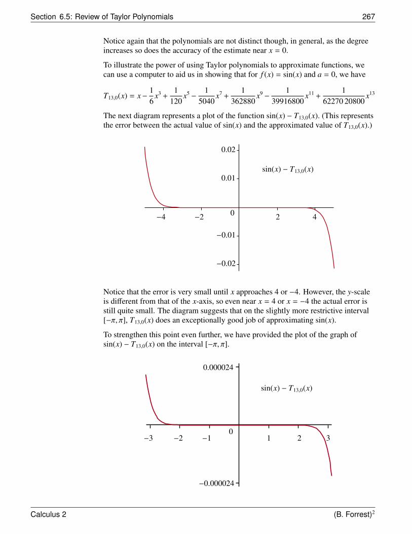
Section 6.5: Review of Taylor Polynomials 267
Notice again that the polynomials are not distinct though, in general, as the degreeincreases so does the accuracy of the estimate near x = 0.
To illustrate the power of using Taylor polynomials to approximate functions, wecan use a computer to aid us in showing that for f (x) = sin(x) and a = 0, we have
T13,0(x) = x−16
x3 +1
120x5 −
15040
x7 +1
362880x9 −
139916800
x11 +1
62270 20800x13
The next diagram represents a plot of the function sin(x) − T13,0(x). (This representsthe error between the actual value of sin(x) and the approximated value of T13,0(x).)
sin(x) − T13,0(x)
0.02
0.01
−0.01
−0.02
0 2 4−2−4
Notice that the error is very small until x approaches 4 or −4. However, the y-scaleis different from that of the x-axis, so even near x = 4 or x = −4 the actual error isstill quite small. The diagram suggests that on the slightly more restrictive interval[−π, π], T13,0(x) does an exceptionally good job of approximating sin(x).
To strengthen this point even further, we have provided the plot of the graph ofsin(x) − T13,0(x) on the interval [−π, π].
sin(x) − T13,0(x)
−0.000024
0.000024
−3 −2 −10
1 2 3
Calculus 2 (B. Forrest)2
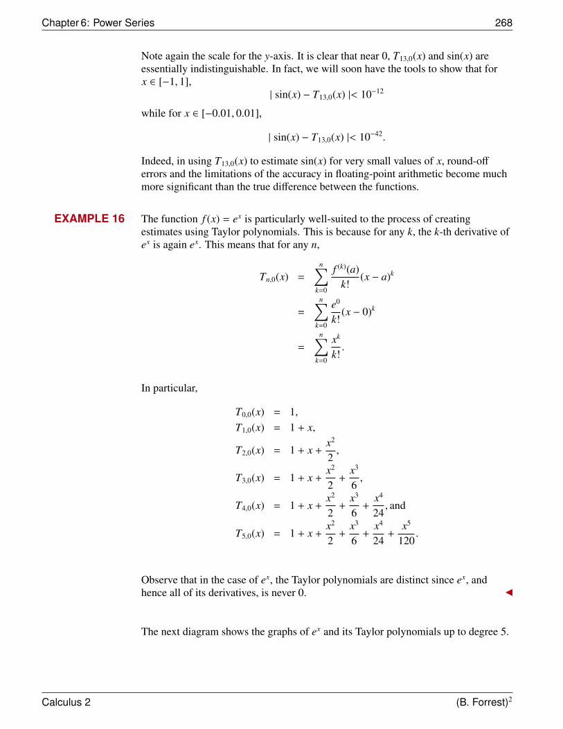
Chapter 6: Power Series 268
Note again the scale for the y-axis. It is clear that near 0, T13,0(x) and sin(x) areessentially indistinguishable. In fact, we will soon have the tools to show that forx ∈ [−1, 1],
| sin(x) − T13,0(x) |< 10−12
while for x ∈ [−0.01, 0.01],
| sin(x) − T13,0(x) |< 10−42.
Indeed, in using T13,0(x) to estimate sin(x) for very small values of x, round-off
errors and the limitations of the accuracy in floating-point arithmetic become muchmore significant than the true difference between the functions.
EXAMPLE 16 The function f (x) = ex is particularly well-suited to the process of creatingestimates using Taylor polynomials. This is because for any k, the k-th derivative ofex is again ex. This means that for any n,
Tn,0(x) =
n∑k=0
f (k)(a)k!
(x − a)k
=
n∑k=0
e0
k!(x − 0)k
=
n∑k=0
xk
k!.
In particular,
T0,0(x) = 1,T1,0(x) = 1 + x,
T2,0(x) = 1 + x +x2
2,
T3,0(x) = 1 + x +x2
2+
x3
6,
T4,0(x) = 1 + x +x2
2+
x3
6+
x4
24, and
T5,0(x) = 1 + x +x2
2+
x3
6+
x4
24+
x5
120.
Observe that in the case of ex, the Taylor polynomials are distinct since ex, andhence all of its derivatives, is never 0.
The next diagram shows the graphs of ex and its Taylor polynomials up to degree 5.
Calculus 2 (B. Forrest)2
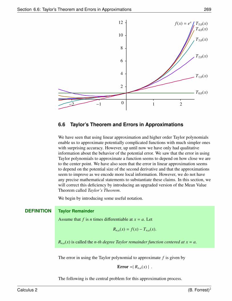
Section 6.6: Taylor’s Theorem and Errors in Approximations 269
f (x) = ex
T0,0(x)
T1,0(x)
T2,0(x)
T3,0(x)
T4,0(x)T5,0(x)
−2 −1 0 1 2
12
10
8
6
4
2
6.6 Taylor’s Theorem and Errors in Approximations
We have seen that using linear approximation and higher order Taylor polynomialsenable us to approximate potentially complicated functions with much simpler oneswith surprising accuracy. However, up until now we have only had qualitativeinformation about the behavior of the potential error. We saw that the error in usingTaylor polynomials to approximate a function seems to depend on how close we areto the center point. We have also seen that the error in linear approximation seemsto depend on the potential size of the second derivative and that the approximationsseem to improve as we encode more local information. However, we do not haveany precise mathematical statements to substantiate these claims. In this section, wewill correct this deficiency by introducing an upgraded version of the Mean ValueTheorem called Taylor’s Theorem.
We begin by introducing some useful notation.
DEFINITION Taylor Remainder
Assume that f is n times differentiable at x = a. Let
Rn,a(x) = f (x) − Tn,a(x).
Rn,a(x) is called the n-th degree Taylor remainder function centered at x = a.
The error in using the Taylor polynomial to approximate f is given by
Error =| Rn,a(x) | .
The following is the central problem for this approximation process.
Calculus 2 (B. Forrest)2
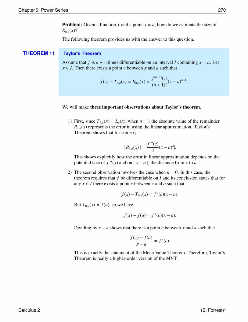
Chapter 6: Power Series 270
Problem: Given a function f and a point x = a, how do we estimate the size ofRn,a(x)?
The following theorem provides us with the answer to this question.
THEOREM 11 Taylor’s Theorem
Assume that f is n + 1-times differentiable on an interval I containing x = a. Letx ∈ I. Then there exists a point c between x and a such that
f (x) − Tn,a(x) = Rn,a(x) =f (n+1)(c)(n + 1)!
(x − a)n+1.
We will make three important observations about Taylor’s theorem.
1) First, since T1,a(x) = La(x), when n = 1 the absolute value of the remainderR1,a(x) represents the error in using the linear approximation. Taylor’sTheorem shows that for some c,
| R1,a(x) |= |f ′′(c)
2(x − a)2|.
This shows explicitly how the error in linear approximation depends on thepotential size of f ′′(x) and on | x − a |, the distance from x to a.
2) The second observation involves the case when n = 0. In this case, thetheorem requires that f be differentiable on I and its conclusion states that forany x ∈ I there exists a point c between x and a such that
f (x) − T0,a(x) = f ′(c)(x − a).
But T0,a(x) = f (a), so we have
f (x) − f (a) = f ′(c)(x − a).
Dividing by x − a shows that there is a point c between x and a such that
f (x) − f (a)x − a
= f ′(c).
This is exactly the statement of the Mean Value Theorem. Therefore, Taylor’sTheorem is really a higher-order version of the MVT.
Calculus 2 (B. Forrest)2
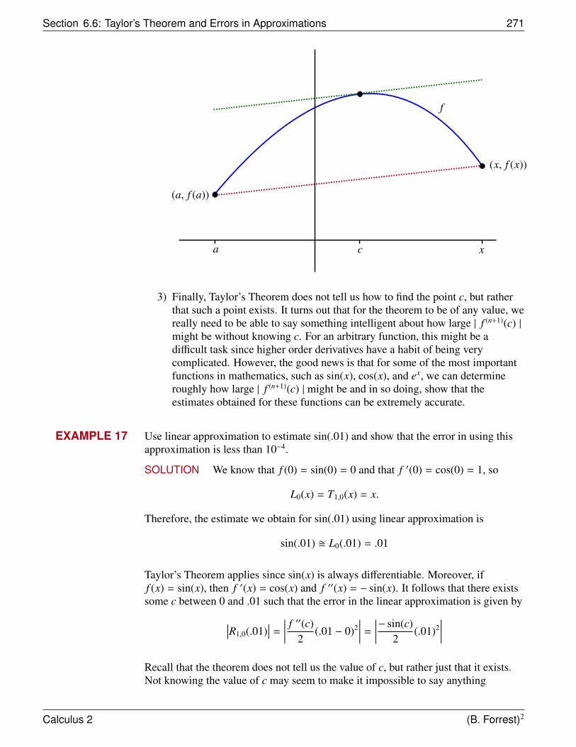
Section 6.6: Taylor’s Theorem and Errors in Approximations 271
a c x
(a, f (a))
(x, f (x))
f
3) Finally, Taylor’s Theorem does not tell us how to find the point c, but ratherthat such a point exists. It turns out that for the theorem to be of any value, wereally need to be able to say something intelligent about how large | f (n+1)(c) |might be without knowing c. For an arbitrary function, this might be adifficult task since higher order derivatives have a habit of being verycomplicated. However, the good news is that for some of the most importantfunctions in mathematics, such as sin(x), cos(x), and ex, we can determineroughly how large | f (n+1)(c) | might be and in so doing, show that theestimates obtained for these functions can be extremely accurate.
EXAMPLE 17 Use linear approximation to estimate sin(.01) and show that the error in using thisapproximation is less than 10−4.
SOLUTION We know that f (0) = sin(0) = 0 and that f ′(0) = cos(0) = 1, so
L0(x) = T1,0(x) = x.
Therefore, the estimate we obtain for sin(.01) using linear approximation is
sin(.01) � L0(.01) = .01
Taylor’s Theorem applies since sin(x) is always differentiable. Moreover, iff (x) = sin(x), then f ′(x) = cos(x) and f ′′(x) = − sin(x). It follows that there existssome c between 0 and .01 such that the error in the linear approximation is given by∣∣∣R1,0(.01)
∣∣∣ =
∣∣∣∣∣ f ′′(c)2
(.01 − 0)2∣∣∣∣∣ =
∣∣∣∣∣− sin(c)2
(.01)2∣∣∣∣∣
Recall that the theorem does not tell us the value of c, but rather just that it exists.Not knowing the value of c may seem to make it impossible to say anything
Calculus 2 (B. Forrest)2
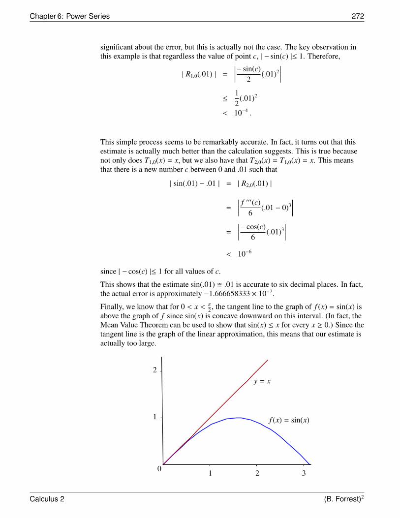
Chapter 6: Power Series 272
significant about the error, but this is actually not the case. The key observation inthis example is that regardless the value of point c, | − sin(c) |≤ 1. Therefore,
| R1,0(.01) | =
∣∣∣∣∣− sin(c)2
(.01)2∣∣∣∣∣
≤12
(.01)2
< 10−4 .
This simple process seems to be remarkably accurate. In fact, it turns out that thisestimate is actually much better than the calculation suggests. This is true becausenot only does T1,0(x) = x, but we also have that T2,0(x) = T1,0(x) = x. This meansthat there is a new number c between 0 and .01 such that
| sin(.01) − .01 | = | R2,0(.01) |
=
∣∣∣∣∣ f ′′′(c)6
(.01 − 0)3∣∣∣∣∣
=
∣∣∣∣∣− cos(c)6
(.01)3∣∣∣∣∣
< 10−6
since | − cos(c) |≤ 1 for all values of c.
This shows that the estimate sin(.01) � .01 is accurate to six decimal places. In fact,the actual error is approximately −1.666658333 × 10⁻⁷.
Finally, we know that for 0 < x < π2 , the tangent line to the graph of f (x) = sin(x) is
above the graph of f since sin(x) is concave downward on this interval. (In fact, theMean Value Theorem can be used to show that sin(x) ≤ x for every x ≥ 0.) Since thetangent line is the graph of the linear approximation, this means that our estimate isactually too large.
y = x
f (x) = sin(x)
1 2 30
1
2
Calculus 2 (B. Forrest)2
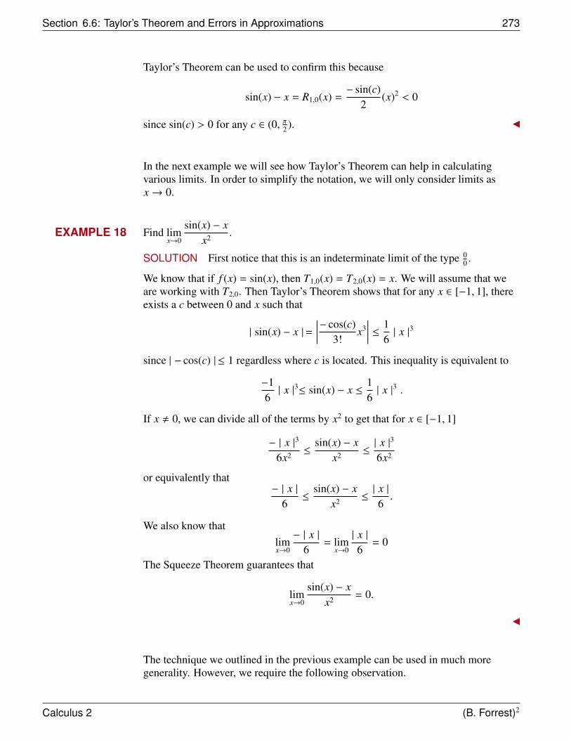
Section 6.6: Taylor’s Theorem and Errors in Approximations 273
Taylor’s Theorem can be used to confirm this because
sin(x) − x = R1,0(x) =− sin(c)
2(x)2 < 0
since sin(c) > 0 for any c ∈ (0, π2 ).
In the next example we will see how Taylor’s Theorem can help in calculatingvarious limits. In order to simplify the notation, we will only consider limits asx→ 0.
EXAMPLE 18 Find limx→0
sin(x) − xx2 .
SOLUTION First notice that this is an indeterminate limit of the type 00 .
We know that if f (x) = sin(x), then T1,0(x) = T2,0(x) = x. We will assume that weare working with T2,0. Then Taylor’s Theorem shows that for any x ∈ [−1, 1], thereexists a c between 0 and x such that
| sin(x) − x |=∣∣∣∣∣− cos(c)
3!x3
∣∣∣∣∣ ≤ 16| x |3
since | − cos(c) | ≤ 1 regardless where c is located. This inequality is equivalent to
−16| x |3≤ sin(x) − x ≤
16| x |3 .
If x , 0, we can divide all of the terms by x2 to get that for x ∈ [−1, 1]
− | x |3
6x2 ≤sin(x) − x
x2 ≤| x |3
6x2
or equivalently that− | x |
6≤
sin(x) − xx2 ≤
| x |6.
We also know thatlimx→0
− | x |6
= limx→0
| x |6
= 0
The Squeeze Theorem guarantees that
limx→0
sin(x) − xx2 = 0.
The technique we outlined in the previous example can be used in much moregenerality. However, we require the following observation.
Calculus 2 (B. Forrest)2
Chapter 6: Power Series 274
Suppose that f (k+1) is a continuous function on [−1, 1]. Then so is the function
g(x) =
∣∣∣∣∣∣ f (k+1)(x)(k + 1)!
∣∣∣∣∣∣ .The Extreme Value Theorem tells us that g has a maximum on [−1, 1]. Therefore,there is an M such that ∣∣∣∣∣∣ f (k+1)(x)
(k + 1)!
∣∣∣∣∣∣ ≤ M
for all x ∈ [−1, 1].
Let x ∈ [−1, 1]. Taylor’s Theorem assures us that there is a c between x and 0 suchthat
| Rk,0(x) |=
∣∣∣∣∣∣ f (k+1)(c)(k + 1)!
xk+1
∣∣∣∣∣∣ .Therefore,
| f (x) − Tk,0(x) | = | Rk,0(x) |
=
∣∣∣∣∣∣ f (k+1)(c)(k + 1)!
xk+1
∣∣∣∣∣∣≤ M | x |k+1
since c is also in [−1, 1].
It follows that−M | x |k+1≤ f (x) − Tk,0(x) ≤ M | x |k+1 .
We summarize this technique as follows:
THEOREM 12 Taylor’s Approximation Theorem I
Assume that f (k+1) is continuous on [−1, 1]. Then there exists a constant M > 0 suchthat
| f (x) − Tk,0(x) |≤ M | x |k+1
or equivalently that
−M | x |k+1≤ f (x) − Tk,0(x) ≤ M | x |k+1
for each x ∈ [−1, 1].
This theorem is very helpful in calculating many limits.
Calculus 2 (B. Forrest)2
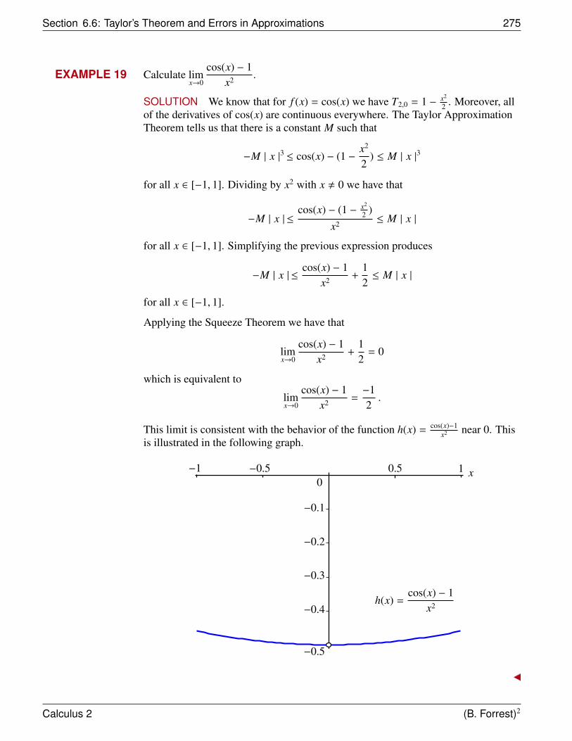
Section 6.6: Taylor’s Theorem and Errors in Approximations 275
EXAMPLE 19 Calculate limx→0
cos(x) − 1x2 .
SOLUTION We know that for f (x) = cos(x) we have T2,0 = 1 − x2
2 . Moreover, allof the derivatives of cos(x) are continuous everywhere. The Taylor ApproximationTheorem tells us that there is a constant M such that
−M | x |3 ≤ cos(x) − (1 −x2
2) ≤ M | x |3
for all x ∈ [−1, 1]. Dividing by x2 with x , 0 we have that
−M | x | ≤cos(x) − (1 − x2
2 )x2 ≤ M | x |
for all x ∈ [−1, 1]. Simplifying the previous expression produces
−M | x | ≤cos(x) − 1
x2 +12≤ M | x |
for all x ∈ [−1, 1].
Applying the Squeeze Theorem we have that
limx→0
cos(x) − 1x2 +
12
= 0
which is equivalent to
limx→0
cos(x) − 1x2 =
−12.
This limit is consistent with the behavior of the function h(x) =cos(x)−1
x2 near 0. Thisis illustrated in the following graph.
h(x) =cos(x) − 1
x2
x−1 −0.5 0.5 10
−0.1
−0.2
−0.3
−0.4
−0.5
Calculus 2 (B. Forrest)2
Chapter 6: Power Series 276
The previous limit can actually be calculated quite easily using L’Hopital’s Rule. Asan exercise, you should try to verify the answer using this rule. The next examplewould require much more work using L’Hopital’s Rule. It is provided to show youhow powerful Taylor’s Theorem can be for finding limits.
EXAMPLE 20 Find limx→0
ex42 − cos(x2)
x4 .
SOLUTION This is an indeterminate limit of type 00 . We know from Taylor’s
Approximation Theorem that we can find a constant M1 such that for any u ∈ [−1, 1]
−M1u2 ≤ eu − (1 + u) ≤ M1u2
since 1 + u is the first degree Taylor polynomial of eu. Now if x ∈ [−1, 1], thenu = x4
2 ∈ [−1, 1]. In fact, u ∈ [0, 12 ]. It follows that if x ∈ [−1, 1] and we substitute
u = x4
2 , then we get−M1x8
4≤ e
x42 − (1 +
x4
2) ≤
M1x8
4.
We also can show that there exists a constant M2 such that for any v ∈ [−1, 1]
−M2v4 ≤ cos(v) − (1 −v2
2) ≤ M2v4
since 1 − v2
2 is the third degree Taylor polynomial for cos(v).
If x ∈ [−1, 1] then so is x2. If we let v = x2, then we see that
−M2x8 ≤ cos(x2) − (1 −x4
2) ≤ M2x8 .
The next step is to multiply each term in the previous inequality by −1 to get
−M2x8 ≤ (1 −x4
2) − cos(x2) ≤ M2x8.
(Remember, multiplying by a negative number reverses the inequality.)
Now add the two inequalities together:
−(M1
4+ M2)x8 ≤ e
x42 − (1 +
x4
2) + (1 −
x4
2) − cos(x2) ≤ (
M1
4+ M2)x8 .
If we let M = M14 + M2 and simplify, this inequality becomes
−Mx8 ≤ ex42 − cos(x2) − x4 ≤ Mx8
for all x ∈ [−1, 1]. Dividing by x4 gives us that
−Mx4 ≤e
x42 − cos(x2)
x4 − 1 ≤ Mx4 .
Calculus 2 (B. Forrest)2
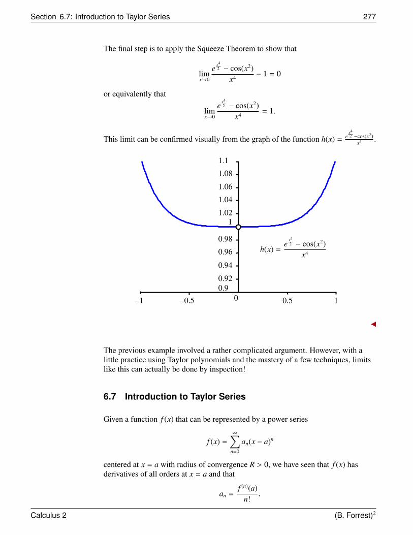
Section 6.7: Introduction to Taylor Series 277
The final step is to apply the Squeeze Theorem to show that
limx→0
ex42 − cos(x2)
x4 − 1 = 0
or equivalently that
limx→0
ex42 − cos(x2)
x4 = 1.
This limit can be confirmed visually from the graph of the function h(x) =e
x42 −cos(x2)
x4 .
h(x) =e
x42 − cos(x2)
x4
−1 −0.5 0 0.5 1
0.90.92
0.94
0.96
0.98
11.02
1.04
1.06
1.08
1.1
The previous example involved a rather complicated argument. However, with alittle practice using Taylor polynomials and the mastery of a few techniques, limitslike this can actually be done by inspection!
6.7 Introduction to Taylor Series
Given a function f (x) that can be represented by a power series
f (x) =
∞∑n=0
an(x − a)n
centered at x = a with radius of convergence R > 0, we have seen that f (x) hasderivatives of all orders at x = a and that
an =f (n)(a)
n!.
Calculus 2 (B. Forrest)2
Chapter 6: Power Series 278
In fact,
f (x) =
∞∑n=0
f (n)(a)n!
(x − a)n.
If we assume that a function f has derivatives of all orders at a ∈ R then this seriescan certainly be constructed.
DEFINITION Taylor Series
Assume that f has derivatives of all orders at a ∈ R. The series∞∑
n=0
f (n)(a)n! (x − a)n is
called the Taylor series for f centered at x = a.
We write
f (x) ∼∞∑
n=0
f (n)(a)n!
(x − a)n.
In the special case where a = 0, the series is referred to as the Maclaurin series forf .
Remark:
Up until now, we have started with a function that was represented by a power serieson its interval of convergence. In this case, the series that represents the functionmust be the Taylor Series.
However, suppose that f is any function for which f (n)(a) exists for each n. Then wecan build the power series
∞∑n=0
f (n)(a)n!
(x − a)n.
However, we do not know the following:
1) For which values of x does the series
∞∑n=0
f (n)(a)n!
(x − a)n
converge?
2) If the series converges at x0, is it true that
f (x0) =
∞∑n=0
f (n)(a)n!
(x0 − a)n ?
These two questions essentially ask whether a function f can be fully reconstructedfrom the data set consisting of the values the derivatives of all order at a point a ∈ R.
Calculus 2 (B. Forrest)2
Section 6.7: Introduction to Taylor Series 279
The answer to the first question can be answered by using the method developed forfinding the interval of convergence of a power series.
The second problem seems intuitively like it should be true at any point where theseries converges. However, a closer look reveals why this may not be true.Essentially we are trying to rebuild a function over an interval that could very wellbe the entire Real line by using only the information provided by the function at onesingle point. In this respect, it seems that using only information about ex at x = 0 toget
ex =
∞∑n=0
xn
n!
and as such to completely reproduce the function for all values of x seems quiteremarkable and indeed it is! To further illustrate why ex is such a remarkablefunction in this regard, consider the following example.
EXAMPLE 21 Consider the function g which is obtained by modifying f (x) = ex outside theinterval [−1, 1]:
g(x) =
1e if x < −1
ex if − 1 ≤ x ≤ 1
e if x > 1
On the interval [−1, 1], g(x) behaves exactly like ex. In particular, g(0) = e0 = 1 andg(n)(0) = e0 = 1 for every n. This means that the Taylor series centered at x = 0 forg(x) is
∞∑n=0
xn
n!
which is exactly the same Taylor Series for ex. We already know that this seriesconverges for all x ∈ R and that
ex =
∞∑n=0
xn
n!.
This means that the Taylor series for g centered at x = 0 also converges for all x ∈ Rand in particular at x = 2. However at x = 2, g(2) = e while
∞∑n=0
2n
n!= e2 , g(2).
Hence, this is an example of a function g with the property that its Taylor Seriesconverges at a point x0 but
g(x0) ,∞∑
n=0
g(n)(a)n!
(x0 − a)n.
Calculus 2 (B. Forrest)2
Chapter 6: Power Series 280
EXAMPLE 22 Find the Taylor series centered at x = 0 for f (x) = cos(x) and g(x) = sin(x).
We have that
f ′(x) = − sin(x) =⇒ f ′(0) = − sin(0) = 0f ′′(x) = − cos(x) =⇒ f ′′(0) = − cos(0) = −1f ′′′(x) = sin(x) =⇒ f ′′′(0) = sin(0) = 0f (4)(x) = cos(x) =⇒ f (4)(0) = cos(0) = 1f (5)(x) = − sin(x) =⇒ f (5)(0) = − sin(0) = 0f (6)(x) = − cos(x) =⇒ f (6)(0) = − cos(0) = −1f (7)(x) = sin(x) =⇒ f (7)(0) = sin(0) = 0f (8)(x) = cos(x) =⇒ f (8)(0) = cos(0) = 1
...
with the cycle repeating itself every four derivatives. Therefore
f (4k)(x) = cos(x) =⇒ f (4k)(0) = cos(0) = 1f (4k+1)(x) = − sin(x) =⇒ f (4k+1)(0) = − sin(0) = 0f (4k+2)(x) = − cos(x) =⇒ f (4k+2)(0) = − cos(0) = −1f (4k+3)(x) = sin(x) =⇒ f (4k+3)(0) = sin(0) = 0
Hence,cos(x) ∼
∞∑n=0
f (n)(0)n!
xn
= 1 +0x1!
+−1x2
2!+
0x3
3!+
1x4
4!+ · · ·
= 1 −x2
2!+
x4
4!−
x6
6!+ · · ·
=
∞∑k=0
(−1)k x2k
(2k)!
A similar calculation shows that
sin(x) ∼ x −x3
3!+
x5
5!−
x7
7!+ · · ·
=
∞∑k=0
(−1)k x2k+1
(2k + 1)!
The problems that remain is to determine if
cos(x) =
∞∑k=0
(−1)k x2k
(2k)!
and if
sin(x) =
∞∑k=0
(−1)k x2k+1
(2k + 1)!.
Calculus 2 (B. Forrest)2
Section 6.8: Convergence of Taylor Series 281
To answer these questions we will need to use Taylor’s Theorem.
6.8 Convergence of Taylor Series
In this section we return to a question that we asked earlier.
Question: Given a function f that is infinitely differentiable at x = a, is f equal toits Taylor Series? That is, does
f (x) =
∞∑n=0
f (n)(a)n!
(x − a)n
for any x at which the Taylor Series converges?
Unfortunately, we saw that this need not be true even if the Taylor Series convergeseverywhere. Taylor’s Theorem gives us a means to show that for many importantfunctions this equality does hold. To see why this is the case, note that if we fix anx0, then
Tk,a(x0) =
k∑n=0
f (n)(a)n!
(x0 − a)n
is not only the k-th partial sum of the Taylor Series for f centered at x = a, but it isalso the k-th degree Taylor polynomial. As such, Taylor’s Theorem shows that
| f (x0) − Tk,a(x0) |=| Rk,a(x0) | .
If we can show thatlimk→∞
Rk,a(x0) = 0
then
f (x) = limk→∞
Tk,a(x0) =
∞∑n=0
f (n)(a)n!
(x − a)n.
Therefore, f (x) agrees with its Taylor series precisely when the Taylor remainders
Rk,a(x)→ 0
as k goes to∞.
Remark: Before we present the next example we need to recall the following limitwhich we previously established as a consequence of the Ratio Test.
Let x0 ∈ R. Then
limk→∞
M | x0 |k
k!= 0.
Calculus 2 (B. Forrest)2
Chapter 6: Power Series 282
EXAMPLE 23 Let f (x) = cos(x) and a = 0. Let x0 be any point in R. Taylor’s Theorem shows thatfor each k there exists a point ck between 0 and x0 such that
| Rk,a(x0) |=
∣∣∣∣∣∣ f (k+1)(ck)(k + 1)!
xk+10
∣∣∣∣∣∣We have seen that if f (x) = cos(x), then f ′(x) = − sin(x), f ′′(x) = − cos(x),f ′′′(x) = sin(x) and f (4)(x) = cos(x). Since the fourth derivative is again cos(x), the5-th, 6-th, 7-th and 8-th derivative will be, respectively, f (5)(x) = − sin(x),f (6)(x) = − cos(x), f (7)(x) = sin(x) and f (8)(x) = cos(x). This pattern will berepeated for the 9-th, 10-th, 11-th and 12-th derivatives, and then for every group offour derivatives thereafter. In fact, what we have just shown is that if f (x) = cos(x),then for any k
f (k)(x) =
cos(x) if k = 4 j
− sin(x) if k = 4 j + 1
− cos(x) if k = 4 j + 2
sin(x) if k = 4 j + 3
where j = 0, 1, 2, · · · . However, this means that regardless the value of k or where ck
is, we will have
| f (k+1)(ck) |≤ 1.
It follows immediately that
∣∣∣Rk,a(x0)∣∣∣ =
∣∣∣∣∣∣ f (k+1)(ck)(k + 1)!
xk+10
∣∣∣∣∣∣ ≤ | x0 |k+1
(k + 1)!.
However, we know that limk→∞
|x0 |k
k! = 0, so the Squeeze Theorem shows that
limk→∞
Rk,a(x0) = 0.
Therefore, since x0 was chosen at random, for f (x) = cos(x) and any x ∈ R, we have
f (x) =
∞∑n=0
f (n)(0)n!
xn.
In particular, for any x ∈ R
cos(x) =
∞∑k=0
(−1)k x2k
2k!.
Calculus 2 (B. Forrest)2
Section 6.8: Convergence of Taylor Series 283
A similar argument applies to sin(x) as it did for cos(x) to show that for any x ∈ R,sin(x) agrees with the value of its Taylor series. That is,
sin(x) =
∞∑k=0
(−1)k x2k+1
(2k + 1)!.
Remark: Notice that in each of the previous examples that if either f (x) = cos(x) orf (x) = sin(x), then the function f had the property that for any k = 0, 1, 2, 3, . . . andfor each x ∈ R, then ∣∣∣ f (k)(x)
∣∣∣ ≤ 1.
The fact that we can find a simultaneous uniform bound for the size of all of thederivatives of f over all of R was the key to showing that both cos(x) and sin(x)agree with their Taylor series. In fact, these two examples suggest the followingvery useful theorem.
THEOREM 13 Convergence Theorem for Taylor Series
Assume that f (x) has derivatives of all orders on an interval I containing x = a.Assume also that there exists an M such that
| f (k)(x) | ≤ M
for all k and for all x ∈ I. Then
f (x) =
∞∑n=0
f (n)(a)n!
(x − a)n
for all x ∈ I.
PROOF
We know that Tk,a(x) is the k-th partial sum of the Taylor series centered at x = a.We also know that the Taylor series converges at x = a and that
∞∑n=0
f (n)(a)n!
(a − a)n = f (a) + 0 + 0 + 0 + · · · = f (a)
so we only need to show the theorem holds for x0 ∈ I with x0 , a.
Choose x0 ∈ I with x0 , a. Let k ∈ N ∪ {0}. Then Taylor’s Theorem tells us thatthere exists a c between a and x0 so that
| f (x0) − Tk,a(x0)| =| f (k+1)(c)|(k + 1)!
|x0 − a|k+1 .
Calculus 2 (B. Forrest)2
Chapter 6: Power Series 284
But since| f (k+1)(c) | ≤ M
we have that
0 ≤ | f (x0) − Tk,a(x0)| ≤ M ·|x0 − a|k+1
(k + 1)!.
Since
limk→∞
M ·|x0 − a|k+1
(k + 1)!= M · lim
k→∞
|x0 − a|k+1
(k + 1)!= 0
the Squeeze Theorem shows that
limk→∞| f (x0) − Tk,a(x0)| = 0
and hence that
f (x0) = limk→∞
Tk,a(x0) =
∞∑n=0
f (n)(a)n!
(x0 − a)n
for all x0 ∈ I.
We showed using term-by-term differentiation of power series that
ex =
∞∑n=0
f (n)(0)n!
(x)n =
∞∑n=0
xn
n!.
We can now provide a different proof of this important result.
EXAMPLE 24 Let f (x) = ex and let a = 0. Let I = [−B, B]. We know that for each k, f (k)(x) = ex.Moreover, since ex is increasing,
0 < e−B ≤ ex ≤ eB
for all x ∈ [−B, B]. This means that if M = eB, then for all x ∈ [−B, B] and all k, wehave
| f (k)(x) |= ex ≤ eB = M.
All of the conditions of the Convergence Theorem for Taylor Series are satisfied. Itfollows that for any x ∈ [−B, B],
ex =
∞∑n=0
f (n)(0)n!
(x)n =
∞∑n=0
xn
n!.
Finally, we see that this would work regardless of what B we choose. However,given any x ∈ R, if we pick a B such that | x |< B, then x ∈ [−B, B]. This means thatfor this x
Calculus 2 (B. Forrest)2
Section 6.9: Binomial Series 285
ex =
∞∑n=0
xn
n!.
Hence for every x ∈ R, the equality
ex =
∞∑n=0
xn
n!
holds.
6.9 Binomial Series
Consider the following version of the Binomial Theorem:
THEOREM 14 Binomial Theorem
Let a ∈ R and n ∈ N. Then for each x ∈ R we have that
(a + x)n =
n∑k=0
(nk
)an−kxk
where (nk
)=
n!k!(n − k)!
.
In particular, when a = 1 we have
(1 + x)n = 1 +
n∑k=1
n(n − 1)(n − 2) · · · (n − k + 1)k!
xk.
Remark: Consider the expression
n(n − 1)(n − 2) · · · (n − k + 1)k!
.
Typically we are only concerned with the case where k ∈ {0, 1, 2, . . . , n}. But theexpression actually makes sense for any k ∈ N ∪ {0}. If k > n, then one of the termsin the expression
n(n − 1)(n − 2) · · · (n − k + 1)
will be 0 and son(n − 1)(n − 2) · · · (n − k + 1)
k!= 0.
Calculus 2 (B. Forrest)2
Chapter 6: Power Series 286
Consequently,
(1 + x)n = 1 +
n∑k=1
n(n − 1)(n − 2) · · · (n − k + 1)k!
xk
= 1 +
∞∑k=1
n(n − 1)(n − 2) · · · (n − k + 1)k!
xk
This leaves us to make the rather strange observation that the polynomial function(1 + x)n is actually represented by the power series
1 +
∞∑k=1
n(n − 1)(n − 2) · · · (n − k + 1)k!
xk
In other words, 1 +∞∑
k=1
n(n−1)(n−2)···(n−k+1)k! xk is the Taylor Series centered at x = 0 for
the function (1 + x)n.
By itself the observation above does not tell us anything new about the function(1 + x)n. However it does give us an important clue towards answering the followingquestion.
Question: Suppose that α ∈ R. Is there an analog of the Binomial Theorem for thefunction
(1 + x)α?
To answer this question, one strategy would be to mimic what happens with theclassical Binomial Theorem. We begin by defining the generalized binomialcoefficients and the generalized binomial series.
DEFINITION Generalized Binomial Coefficients and Binomial Series
Let α ∈ R and let k ∈ {0, 1, 2, 3, . . .}. Then we define the generalized binomialcoefficient (
α
k
)=α(α − 1)(α − 2) · · · (α − k + 1)
k!
if k , 0 and (α
0
)= 1.
We also define the generalized binomial series for α to be the power series
1 +
∞∑k=1
α(α − 1)(α − 2) · · · (α − k + 1)k!
xk =
∞∑k=0
(α
k
)xk.
Remark: The first problem is to find the radius of convergence for the generalizedbinomial series. To do this let bk =|
(αk
)|. Then a straight-forward calculation shows
that if k ≥ 1bk+1
bk=| α − k |
k + 1.
Calculus 2 (B. Forrest)2
Section 6.9: Binomial Series 287
It follows thatlimk→∞
bk+1
bk= lim
k→∞
| α − k |k + 1
= 1.
This tells us that the radius of convergence for the binomial series is 1. In particular,the series converges absolutely on (−1, 1).
Next we must determine if
(1 + x)α = 1 +
∞∑k=1
α(α − 1)(α − 2) · · · (α − k + 1)k!
xk =
∞∑k=0
(α
k
)xk ?
To see why this is true we start with the following calculation whichshows that if k ≥ 1, then(
α
k + 1
)(k + 1) +
(α
k
)k =
α(α − 1) · · · (α − k + 1)k!
(α − k)
+α(α − 1) · · · (α − k + 1)
k!(k)
=α(α − 1) · · · (α − k + 1)
k!(α)
= α
(α
k
)
Next let
f (x) = 1 +
∞∑k=1
α(α − 1)(α − 2) · · · (α − k + 1)k!
xk =
∞∑k=0
(α
k
)xk
for each x ∈ (−1, 1). We claim that
f ′(x) + x f ′(x) = α f (x)
for each x ∈ (−1, 1). To see why this is true we use term-by-term differentiation toget that
f ′(x) + x f ′(x) =
∞∑k=1
(α
k
)kxk−1 +
∞∑k=1
(α
k
)kxk
=
(α
1
)+
∞∑k=2
(α
k
)kxk−1 +
∞∑k=1
(α
k
)kxk
= α +
∞∑k=1
(α
k + 1
)(k + 1)xk +
∞∑k=1
(α
k
)kxk
= α +
∞∑k=1
((α
k + 1
)(k + 1) +
(α
k
)k)xk
Calculus 2 (B. Forrest)2
Chapter 6: Power Series 288
But if k ≥ 1 we have (α
k + 1
)(k + 1) +
(α
k
)k = α
(α
k
).
It follows that
f ′(x) + x f ′(x) = α + α
∞∑k=1
(α
k
)xk
= α
∞∑k=0
(α
k
)xk
= α f (x)
as claimed.
Next letg(x) =
f (x)(1 + x)α
.
Then g is differentiable on (−1, 1) with
g ′(x) =f ′(x)(1 + x)α − α f (x)(1 + x)α−1
(1 + x)2α
=f ′(x)(1 + x)α − (1 + x) f ′(x)(1 + x)α−1
(1 + x)2α
=f ′(x)(1 + x)α − f ′(x)(1 + x)α
(1 + x)2α
= 0
since α f (x) = (1 + x) f ′(x).
Since g ′(x) = 0 for all x ∈ (−1, 1), g(x) is constant on this interval. However,
g(0) = f (0) = 1.
Therefore, g(x) = 1 for all x ∈ (−1, 1). It follows that
f (x) = (1 + x)α
for all x ∈ (−1, 1).
THEOREM 15 Generalized Binomial Theorem
Let α ∈ R. Then for each x ∈ (−1, 1) we have that
(1 + x)α = 1 +
∞∑k=1
α(α − 1)(α − 2) · · · (α − k + 1)k!
xk =
∞∑k=0
(α
k
)xk.
Calculus 2 (B. Forrest)2
Section 6.10: Binomial Series 289
EXAMPLE 25 Use the Generalized Binomial Theorem to find a power series representationfor (1 + x)−2.
The Generalized Binomial Theorem shows that
(1 + x)−2 =
∞∑k=0
(−2k
)xk.
For k ≥ 1, (−2k
)=
(−2)(−2 − 1) · · · (−2 − k + 1)k!
= (−1)k(k + 1).
It is also true that (−20
)= 1 = (−1)0(0 + 1).
Therefore,
(1 + x)−2 =
∞∑k=0
(−1)k(k + 1)xk
=
∞∑k=1
(−1)k−1kxk−1
We can also use term-by-term differentiation to verify the previous calculation. Firstbegin with
11 − u
=
∞∑k=0
uk
for all u ∈ (−1, 1). Differentiating both sides gives us
1(1 − u)2 =
∞∑k=1
kuk−1
for all u ∈ (−1, 1).
Finally, if we let u = −x, we have
1(1 + x)2 =
∞∑k=1
k(−x)k−1 =
∞∑k=1
(−1)k−1kxk−1
for all x ∈ (−1, 1).
Calculus 2 (B. Forrest)2
Chapter 6: Power Series 290
6.10 Additional Examples and Applications of Taylor Series
In this section we will present some further examples of functions that arerepresentable by their Taylor series and see what this tells us about these functions.
EXAMPLE 26 Find a power series representation for f (x) = arctan(x) and determine the intervalon which the representation is valid.
We begin with the observation that ddx (arctan(x)) = 1
1+x2 . Therefore, if we can find apower series representation for 1
1+x2 , we can use the integration techniques to find arepresentation for arctan(x).
We know that for any u ∈ (−1, 1),
11 − u
=
∞∑n=0
un.
Let x ∈ (−1, 1). If we let u = −x2, then u ∈ (−1, 1). It follows that
11 + x2 =
11 − (−x2)
=
∞∑n=0
(−x2)n
=
∞∑n=0
(−1)nx2n
Since arctan(x) is an antiderivative of 11+x2 , the Integration of Power Series Theorem
shows that there exists a constant C such that
arctan(x) = C +
∞∑n=0
∫(−1)nx2n dx
= C +
∞∑n=0
(−1)n x2n+1
2n + 1
To find C, note that arctan(0) = 0, so
0 = arctan(0)
= C +
∞∑n=0
(−1)n 02n+1
2n + 1
= C
Calculus 2 (B. Forrest)2
Section 6.10: Additional Examples and Applications of Taylor Series 291
Therefore, we have shown that if x ∈ (−1, 1)
arctan(x) =
∞∑n=0
(−1)n x2n+1
2n + 1.
The radius of convergence of this series is 1. At x = 1, the series becomes
∞∑n=0
(−1)n 12n + 1
which converges by the Alternating Series Test.
When x = −1, the series is
∞∑n=0
(−1)n (−1)2n+1
2n + 1=
∞∑n=0
(−1)3n+1 12n + 1
.
Since
(−1)3n+1 =
{1 if n is odd−1 if n is even
the series is the same as∞∑
n=0
(−1)n+1 12n + 1
which also converges by the Alternating Series Test.
Therefore, the Continuity Theorem for Power Series shows that
arctan(x) =
∞∑n=0
(−1)n x2n+1
2n + 1
for all x ∈ [−1, 1].
This last statement has an interesting application. We get that
π
4= arctan(1)
=
∞∑n=0
(−1)n 12n + 1
Multiplying both sides of this equation by 4 gives
π = 4(1 −13
+15−
17
+19− · · · )
= 4 −43
+45−
47
+49− · · ·
Calculus 2 (B. Forrest)2
Chapter 6: Power Series 292
Note: This series representation for arctan(x) is called the Gregory’s series after theScottish mathematician of the same name. The famous series expansion for π whichwe derived from Gregory’s series is called Leibniz’s formula for π.
EXAMPLE 27 (i) Find the Taylor series centered at x = 0 for the integral function
F(x) =
∫ x
0cos(t2) dt.
(ii) Find F(9)(0) and F(16)(0).
(iii) Estimate∫ 0.1
0cos(t2) dt with an error of less than 1
106 .
SOLUTIONS
(i) For any u ∈ R,
cos(u) =
∞∑n=0
(−1)n u2n
(2n)!.
Let u = t2 to get that for any t ∈ R,
cos(t2) =
∞∑n=0
(−1)n (t2)2n
(2n)!=
∞∑n=0
(−1)n t4n
(2n)!.
The Integration Theorem for Power Series gives us that
F(x) =
∫ x
0cos(t2) dt
=
∫ x
0
∞∑n=0
(−1)n t4n
(2n)!dt
=
∞∑n=0
∫ x
0(−1)n t4n
(2n)!dt
=
∞∑n=0
[(−1)n t4n+1
(4n + 1)(2n)!
∣∣∣∣∣∣x0
]=
∞∑n=0
(−1)n x4n+1
(4n + 1)(2n)!
This is valid for any x ∈ R. Moreover, by the Uniqueness Theorem for Power SeriesRepresentations, this must be the Taylor series centered at x = 0 for F.
(ii) To find F(9)(0), we recall that if
F(x) =
∞∑k=0
akxk
Calculus 2 (B. Forrest)2
Section 6.10: Additional Examples and Applications of Taylor Series 293
then
a9 =F(9)(0)
9!.
This tells us that to find F(9)(0) we must first identify the coefficient of x9 in
∞∑n=0
(−1)n x4n+1
(4n + 1)(2n)!.
Notice for x9, we let n = 2. The coefficient is then
(−1)2(1
(4(2) + 1)(2(2))!) =
19(4!)
Therefore,
a9 =1
9(4!).
Finally, this means
F(9)(0) = 9!a9
=9!
9(4!)= 5 · 6 · 7 · 8= 1680
Next, to find F(16)(0) we look for the coefficient of x16 in the Taylor series for F(x).However, this time there is no n such that x4n+1 = x16. This means that a16 = 0 andhence that
F(16)(0) = 0.
(iii) Since
F(x) =
∞∑n=0
(−1)n x4n+1
(4n + 1)(2n)!
we have ∫ 0.1
0cos(t2) dt = F(0.1) =
∞∑n=0
(−1)n (0.1)4n+1
(4n + 1)(2n)!.
This is an alternating series with
an =(0.1)4n+1
(4n + 1)(2n)!.
Moreover, we see that
a1 =(0.1)5
(5)(2)!=
1106
Calculus 2 (B. Forrest)2

Chapter 6: Power Series 294
and0∑
n=0
(−1)n (0.1)4n+1
(4n + 1)(2n)!=
(0.1)1
.
Using the error estimate in the Alternating Series Test we get that
∣∣∣∣∣∣∫ 0.1
0cos(t2) dt − 0.1
∣∣∣∣∣∣ < a1 =1
106 .
Suppose that we wanted to know the value of∫ 12
0
11 + x9 dx.
Since 11+x9 looks like a rather simple rational function, we might be tempted to use
partial fractions to try and calculate the integral exactly. At least theoretically, thisshould work. However, in practice, this would require us to factor the polynomial1 + x9 which would certainly require the aid of a sophisticated computer algebraprogram such as Maple. Even then, the answer that we would get would not be veryuseful. (Try it!)
Fortunately, we can use what we know about series to get an extremely accurateapproximation to this integral with surprisingly little effort.
EXAMPLE 28 Estimate∫ 1
2
01
1+x9 dx with an error of less than 10−12.
We know that for any −1 < u < 1,
11 − u
=
∞∑n=0
un.
If 0 ≤ x ≤ 12 , then −1 < −x9 < 1, so we can let u = −x9 to get
11 + x9 =
11 − (−x9)
=
∞∑n=0
(−1)nx9n
for all x ∈ [0, 12 ].
Calculus 2 (B. Forrest)2
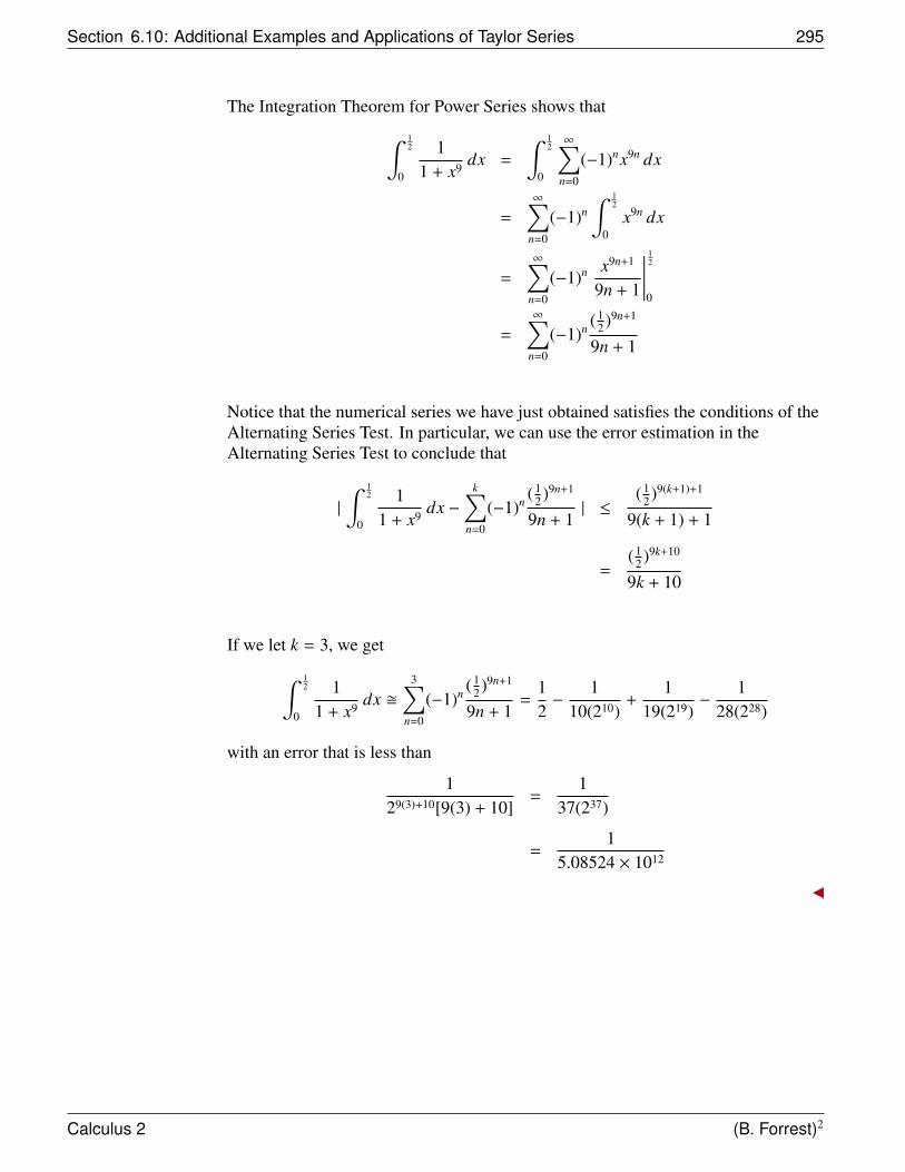
Section 6.10: Additional Examples and Applications of Taylor Series 295
The Integration Theorem for Power Series shows that∫ 12
0
11 + x9 dx =
∫ 12
0
∞∑n=0
(−1)nx9n dx
=
∞∑n=0
(−1)n∫ 1
2
0x9n dx
=
∞∑n=0
(−1)n x9n+1
9n + 1
∣∣∣∣∣∣12
0
=
∞∑n=0
(−1)n (12 )9n+1
9n + 1
Notice that the numerical series we have just obtained satisfies the conditions of theAlternating Series Test. In particular, we can use the error estimation in theAlternating Series Test to conclude that
|
∫ 12
0
11 + x9 dx −
k∑n=0
(−1)n (12 )9n+1
9n + 1| ≤
(12 )9(k+1)+1
9(k + 1) + 1
=( 1
2 )9k+10
9k + 10
If we let k = 3, we get∫ 12
0
11 + x9 dx �
3∑n=0
(−1)n ( 12 )9n+1
9n + 1=
12−
110(210)
+1
19(219)−
128(228)
with an error that is less than
129(3)+10[9(3) + 10]
=1
37(237)
=1
5.08524 × 10¹²
Calculus 2 (B. Forrest)2