MATH 112 1.2 Functions 09-09-05 - Ira A. Fulton College of ...vps/ET502WWW/TABLES-PDF/F.pdf · -...
22
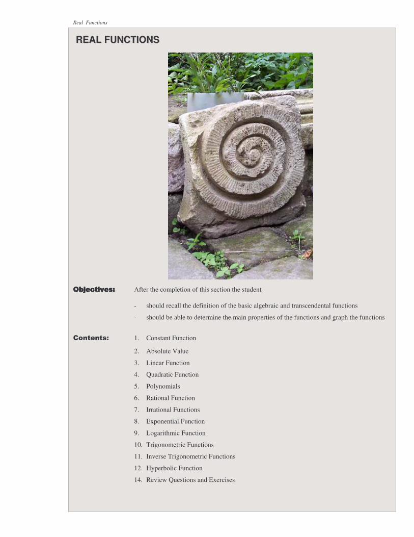
Real Functions REAL FUNCTIONS After the completion of this section the student - should recall the definition of the basic algebraic and transcendental functions - should be able to determine the main properties of the functions and graph the functions 1. Constant Function 2. Absolute Value 3. Linear Function 4. Quadratic Function 5. Polynomials 6. Rational Function 7. Irrational Functions 8. Exponential Function 9. Logarithmic Function 10. Trigonometric Functions 11. Inverse Trigonometric Functions 12. Hyperbolic Function 14. Review Questions and Exercises
Transcript of MATH 112 1.2 Functions 09-09-05 - Ira A. Fulton College of ...vps/ET502WWW/TABLES-PDF/F.pdf · -...
Real Functions
RREEAALL FFUUNNCCTTIIOONNSS ���� ���������������������������������������� After the completion of this section the student
- should recall the definition of the basic algebraic and transcendental functions
- should be able to determine the main properties of the functions and graph the functions
� ������ 1. Constant Function
2. Absolute Value
3. Linear Function
4. Quadratic Function
5. Polynomials
6. Rational Function
7. Irrational Functions
8. Exponential Function
9. Logarithmic Function
10. Trigonometric Functions
11. Inverse Trigonometric Functions
12. Hyperbolic Function
14. Review Questions and Exercises

Real Functions
( )f x x a= −
REAL FUNCTIONS A survey of elementary real-valued functions of real variable f : A ⊂ →� � with their definitions and main properties is presented. Functions can be given in explicit form
( )y f x= y 2x 3= +
in the implicit form ( )f x, y 0= 3y y 4x 0+ − =
or can be given parametrically ( )x f t=
( )y g t=
Functions can be also specified by their graph or given by a table of values. Functions are called algebraic if they are polynomials, roots or rational
functions, otherwise they are called transcendental functions (exponential, logarithmic, hyperbolic, trigonometric). The transcendental functions often can be defined by the infinite series.
Properties of the functions include: domain of definition, range of values, quadrant, periodicity, monotonicity, symmetry, asymptotes, characteristic particular values (zeros, poles, points of discontinuity, extremes, points of inflection).
1. CONSTANT FUNCTION: The constant function is defined by equation ( )f x c=
It assigns the same value c for all values of variable x ∈� . The constant function is a solution of differential equation
( )df x 0
dx=
Graphically, the constant function is represented by a horizontal straight line passes through the point ( )0,c . It is defined by equation y c= .
2. ABSOLUTE VALUE: The absolute value function ( )f x x= is defined as
x if x 0
x = -x if x<0
≥���
The other definition of the absolute value function uses the root of the square
2x = x
It defines the distance between the points 0 and x on the real line. Function is defined for all x ∈� . The function values are never negative, the range of values: 0 x≤ < ∞ .
Graph of the function ( )f x x= Shifting along the x-axis:
Properties: 1. x 0≥ x 0= only if x 0=
2. x x− = for all x ∈�
3. x y y x− = − for all x, y ∈�
4. x y x y⋅ = for all x, y ∈�
5. x y x y+ ≤ + for all x, y ∈� (triangle inequality)
( )f x c=
( )f x x=

Real Functions 3. LINEAR FUNCTION: A linear function is a function defined for all real numbers which describes a
straight line in the plane
( )f x ax b= +
It is given by a polynomial of degree one with the following forms of equation: 1) Slope-intercept equation:
y mx b= + m,b ∈�
m is called the slope and b is called the intercept of the function. The intercept b translates the function along the y-axis.
Increment of any points on the line: y
mx
∆∆
=
2) Line passes through the point ( )1 1x , y with the slope m :
( )1 1y m x x y= − +
3) Line passes through two fixed points ( )1 1x , y and ( )2 2x , y
( )2 11 1
2 1
y yy x x y
x x−
= − +−
The slope m defines the inclination of the line
2 1
2 1
y ym
x x−
=−
and the angle with the x-axis enclosed by the line
m tanϕ= 4) General linear equation:
Ax By C 0+ + = A,B,C ∈� 2 2A B 0+ >
4) Parametric equation of the line:
x t
y mt b
=�� = +�
t−∞ < < ∞
5) Differential equation of the line
( )df x m
dx=
The linear function is strictly increasing for m 0>
strictly decreasing for m 0<
a constant for m 0=

Real Functions Perpendicular lines If two non-vertical lines 1 1y m x b= + and 2 2y m x b= + are perpendicular, then
12
1m
m= −
Proof: 1 1
am tan
hφ= =
2 2 21
h 1 1m tan tan
a2 a mh
πφ φ� �= = − − = − = − = −� ��
4. QUADRATIC FUNCTION: Quadratic function is a function defined for all real numbers by the equation
2y ax bx c= + +
This equation can be reduced to the full square form:
2 2b b
y a x c2a 4a
� �= + + −� ��
The graph of the quadratic function is a parabola shifted to the left
by b
2a and up by
2bc
4a− .
The point 2b b
,c2a 4a
� �− −� ��
is called the vertex of the parabola.
For a 0> , concave up with a global minimum at b
x2a
= − ;
for a 0< , concave down with a global maximum at b
x2a
= − .
The parabola is symmetric with respect to vertical line b
x2a
= − .
The roots of quadratic equation 2ax bx c 0+ + = determine the points of intersection of the parabola with the x-axis:
2
1,2
b b 4ac b Dx
2a 2a− ± − − ±= =
If the discriminant 2D b 4ac 0≡ − > , then there are two intersections at
1,2
b Dx
2a− ±= . If the discriminant 2D b 4ac 0≡ − = , then there is the
intersection at b
x2a−= . If the discriminant 2D b 4ac 0≡ − < , then the parabola
has no intersections with the x-axis. Differential equation for the quadratic function:
( )2
2
df x ax
dx=
Power function The power function is defined all x ∈� by the equation
( ) nf x ax= n 0,1,2,3,...= a ∈� It is called the monomial function.
2 2b by a x c
2a 4a� �= + + −� ��

Real Functions 5. POLYNOMIALS: A linear combination of monoms of different powers forms the polynomial
function
( ) n n 1n n 1 1 0f x a x a x ... a x a−
−= + + + + 1 2 na ,a ,...,a ∈�
The highest power of the monoms, n , is called the degree of the polynomial.
1 2 na ,a ,...,a ∈� are the coefficients of the polynomial, and na 0≠ is called the leading coefficient. The polynomial function is defined for all real numbers x ∈� , and the range of the function depends on the special case of polynomial. For odd n , the range is ( )f x−∞ < < ∞ . In general, the polynomial function is not symmetric. But if the polynomial contains only even powers, then it has mirror symmetry about the y − axis. And if the polynomial contains only odd powers then it has point symmetry about the origin. The graph of the polynomial function can have at most n intersections with the x-axis (real zeros). If n is odd then it has at least one real zero. It also can have up to n 1− extremes and up to n 2− points of inflection. The linear polynomial 0x x− is a factor of the polynomial function ( )f x if and
only if 0x is a zero of the polynomial, i.e. ( )0f x 0= .
According to the Fundamental Theorem of Algebra, the polynomial function has exactly n zeros which can be complex or real, single or repeated. Because the polynomial function has only real coefficients, then the complex zeros appear in conjugate pairs. It means that the polynomial can be represented as a product of linear factors corresponding to real zeros and irreducible quadratic factors which correspond to complex zeros. For example, the cubic polynomial
( ) 3 2f x x 2x x 2= − + − has one real zero 1x 2= and two conjugate complex
zeros 2,3x i= ± . It can be factored in the following way
( ) ( )( )( ) ( )( )3 2 2f x x 2x x 2 x 2 x i x i x 2 x 1= − + − = − − + = − +
In general, the thn the polynomial is represented as a product of linear factors
( ) ( ) ( ) ( ) k1 2 ss sn 1 2 kf x a x x x x x x= − − −�
where ix is the real or complex zero of multiplicity is , and k is the total number of distinct zeros. Although the zeros of polynomial up to degree n 4= can be calculated analytically, in practice only for the quadratic polynomial the analytic formula is used:
21 1 2 0
1,22
a a 4a ax
2a
− ± −=
For polynomials of higher degree, in general, the numerical methods are used. In Maple, the polynomials can be factored with the following command:
> factor(x^5-x^4-x+1);
( ) + x 1 ( ) + x2 1 ( ) − x 1 2
The roots of the polynomial function can be found by
> solve(x^5-4*x^3+x^2+x+1=0.,x);
1. -2.087922659 − -0.2998974261 0.4402773912I + -0.2998974261 0.4402773912I, , , ,1.687717512
( ) 5 3 2f x x 4x x x 1= − + − +
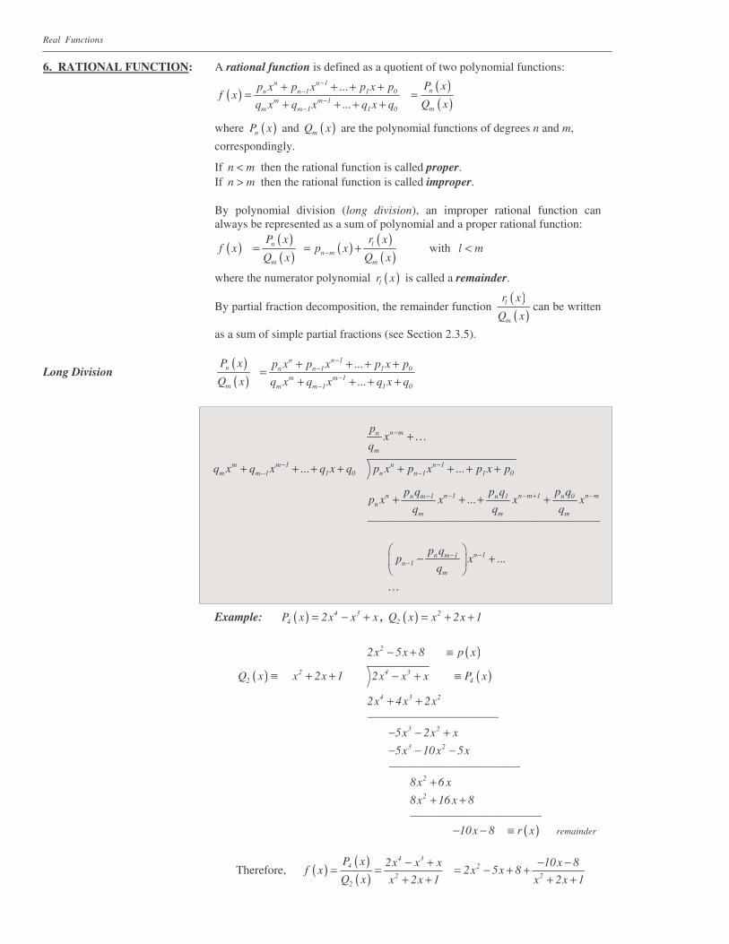
Real Functions 6. RATIONAL FUNCTION: A rational function is defined as a quotient of two polynomial functions:
( ) ( )( )
n n 1nn n 1 1 0
m m 1mm m 1 1 0
P xp x p x ... p x pf x
Q xq x q x ... q x q
−−
−−
+ + + += =
+ + + +
where ( )nP x and ( )mQ x are the polynomial functions of degrees n and m,
correspondingly.
If n m< then the rational function is called proper. If n m> then the rational function is called improper.
By polynomial division (long division), an improper rational function can always be represented as a sum of polynomial and a proper rational function:
( ) ( )( ) ( ) ( )
( )n l
n mm m
P x r xf x p x
Q x Q x−= = + with l m<
where the numerator polynomial ( )lr x is called a remainder.
By partial fraction decomposition, the remainder function ( )( )
l
m
r x
Q xcan be written
as a sum of simple partial fractions (see Section 2.3.5).
Long Division ( )( )
n
m
P x
Q x
n n 1n n 1 1 0
m m 1m m 1 1 0
p x p x ... p x p
q x q x ... q x q
−−
−−
+ + + +=
+ + + +
n mn
m
px
q− +�
m m 1m m 1 1 0q x q x ... q x q−
−+ + + + n n 1n n 1 1 0p x p x ... p x p−
−+ + + +
n n 1 n m 1 n mn m 1 n 1 n 0n
m m m
p q p q p qp x x ... x x
q q q− − + −−+ + + +
_______________________________________
n 1n m 1n 1
m
p qp x ...
q−−
−� �
− +� ��
� Example: ( ) 4 3
4P x 2x x x= − + , ( ) 22Q x x 2x 1= + +
( )22x 5x 8 p x− + ≡
( ) 22Q x x 2x 1≡ + + ( )4 3
42x x x P x− + ≡
4 3 22x 4x 2x+ + ______________________
3 25x 2x x− − + 3 25x 10x 5x− − − ______________________
28x 6 x+ 28x 16 x 8+ + ______________________
( )10x 8 r x− − ≡ remainder
Therefore, ( ) ( )( )
4 34 2
2 22
P x 2x x x 10x 8f x 2x 5x 8
Q x x 2x 1 x 2x 1− + − −= = = − + +
+ + + +

Real Functions
The long division together with the partial fraction decomposition of the remainder function can be performed with Maple by the following command: > convert((2*x^4-x^3+x)/(x^2+2*x+1),parfrac,x);
− + − + 2 x2 5 x 810 + x 1
2( ) + x 1 2
Graphing rational functions: The zeros of the denominator polynomial ( )mQ x determine the domain of
the rational function and the poles of its graph. The particular shape of the
graph, its extremes and points of inflection depend on the individual case.
The mirror symmetry of the graph about the y-axis occur in the cases when
both the denominator and the numerator polynomials have only even or
only the odd powers. The point symmetry of the graph about the origin
occur in the case when one of the polynomials has only even powers and
the other polynomial only odd powers.
Examples:
( )3
6 4
2x xf x
x x 1−=
− +
point symmetry
( )4 2
6 4
x 2x 1f x
x x 1− +=− +
mirror symmetry
( )3 2
6 2
3x 2x 1f x
3x 2x 1− +=+ +
no symmetry
( )( )( ) ( )
3 2 3 2
5 4 2 2
x 2x 1 x 2x 1f x
x x x 1 x 1 x 1 x 1
− + − += =− − + + − +
graph with
poles

Real Functions
7. IRRATIONAL FUNCTIONS: This is a wide class of functions which includes square root y x= and
cubic root 3y x= functions; root functions of integer order ny x= ,
n ∈� ; power functions with fractional exponents m ny x= , m,n ∈� or the
real exponent ry x= , r ∈� ; roots of polynomials and rational functions, etc. Consider some definitions of these functions:
Root function of integer order ( )1
n nf x x x= = , n ∈� , n 1> is defined
for x 0≥ as an inverse of the power function:
ny x= if ny x=
and for negative exponents
( )1
n n1
f x xx
−
= =
For odd n, the root function is defined also for negative x values as
( ) nf x x= − − , x 0<
Power function of fractional order ( ) m nf x x= , m,n ∈� is defined as
the thn root of the thm power
( ) nm n mf x x x= = with n 0> and m 0≠
The domain of the function depends on the particular values of m and n :
( ) ( )1m mm nnm 1
ln xln xln xn nx e e e= = = , then if m is even the domain is x 0≠ .
Power function of real order ( ) af x x= , a ∈� is defined for x 0> as
( ) a a ln xf x x e= =
( ) 2 5f x x=
( )f x xπ=
Rules for Radicals:
Let a,b and n,m , then∈ ∈��
n 1 1= n 0 0=
( )mnm n m na a a= =
n n na b ab⋅ =
nn
n
a abb
=
n mm n mna a a= =
( )nn a a=
n n x if n is evenx ,
x if n is odd
�= ��
x ∈�

Real Functions 8. EXPONENTIAL FUNCTION: Let b be a positive real number not equal to 1 , b , b 0, b 1∈ > ≠� . Then
the function
( ) xf x b=
is an exponential function with base b . If b e= , where e is a natural number defined as a limit
n
n
1e lim 1 2.71828
n→∞
� �= + ≈� ��
, then the function is called an exponential
function: ( ) xf x e=
The relationship between functions is established by the following equation:
( )x lnbx lnb x lnb xb e e e= = =
where lnb is a natural logarithm of b (see next section). An exponential function ( ) xf x e= can be defined for all real x in one of
the following ways: 1) Real power x of the number e:
{ }x r m ne inf e =e r=m n , r>x= ∈� where inf = infinum
2) Inverse of a natural logarithm function: xe y= if ln y x= , y 0> 3) As a limit
n
x
n
xe lim 1
n→∞
� �= +� ��
4) Power series (convergent for all real x)
k 2 3
x
k 0
x x xe 1 x ...
k ! 2 6
∞
== = + + + +
5) As the solution of the initial value problem
dy
ydx
= ( )y 0 1=
The general exponential function
( ) bx df x ca +=
Exponential Model The function ( ) kxf x ce , k 0= > models exponential growth and
( ) kxf x ce , k 0−= > models exponential decay.
Rules for exponents: for any a 0,b 0> > and for all x, y ∈� x y x ya a a +⋅ =
x
x yy
aa
a−=
( ) ( )y xx y xya a a= =
( )xx xa b ab⋅ =
xx
x
a abb� �= � ��
( ) xf x e=

Real Functions 9. LOGARITHMIC FUNCTION: Let b be a positive real number not equal to 1 : b , b 0, b 1∈ > ≠� .
Then the function
( ) bf x log x=
is a logarithm function with base b (general logarithm).
If b e= , where e is a natural number defined as a limit n
n
1e lim 1 2.71828
n→∞
� �= + ≈� ��
, then the function is called a natural
logarithm (usually, logarithm without stating the base means the natural logarithm): ( ) ef x log x ln x= =
The relationship between function is established by the following equation:
b
ln xlog x
lnb=
The logarithm function can be defined as inverse of the exponential function: by log x= if yb x= for all x 0>
y ln x= if ye x= for all x 0>
Rules of logarithms: For all real x 0> and y 0> :
b b blog xy log x log y= + ln xy ln x ln y= + product rule
b b b
xlog log x log y
y= −
xln ln x ln y
y= − quotient rule
yb blog x y log x= yln x y ln x= power rule
blog 1 0= ln1 0=
blog xb x= ln xe x=
xblog b x= xln e x=
blog b 1= lne 1=
b b
1log log x
x= −
1ln ln x
x= −
note! ( )b b blog x y log x log y+ ≠ + ( )ln x y ln x ln y+ ≠ + (typical mistake)
In pre-computer (pre-calculator) era, the logarithms were the main tool for performing arithmetic operations.
Conversion formulas: x x lnbb e= b
ln xlog x
lnb=
( )f x ln x=

Real Functions
Proof: start with by log x= � yx b= definition
� yln x lnb= take logarithm
� ln x y lnb= power rule
� ln x
ylnb
= solve for y
Exponential growth (decay) model kt0Q Q e±= where 0Q is the initial amount of substance at t 0=
1) if it is given 1Q the amount of substance at 1t t= , then
1kt1 0Q Q e= � 1kt1
0
Qe
Q= � 1
1 0
Q1k ln
t Q=
Then exponential model becomes:
tt111
101 0
tQQt lnln tQt Qkt 1
0 0 0 00
QQ Q e Q e Q e Q
Q
� �� �� ��
� �= = = = � �
�
2) Half-life time h is defined as the time needed for substance to be reduced by a half:
kh00
QQ e
2−= k 0>
Then kh1e
2−= � kh1
ln lne2
−=
� ln 2 kh− = −
� 1
k ln 2h
=
Then exponential model becomes:
t t
ln 2kt h h0 0 0Q Q e Q e Q 2
− −−= = =
3) Doubling time D is defined as the time needed for substance to be doubled:
kh0 02Q Q e= k 0>
Then kh2 e−= � kDln 2 lne=
� ln 2 kD=
� 1
k ln 2D
=
Then exponential model becomes:
t t
ln 2kt D D0 0 0Q Q e Q e Q 2= = =
kt0Q Q e−=
exponential decay model
kt0Q Q e=
exponential growth model

Real Functions 10. TRIGONOMETRIC FUNCTIONS: The trigonometric functions (also called the circular functions), in
calculus, are defined with the help of the unit circle (circle of radius 1 ). Consider a unit circle with a center placed at the origin of the Cartesian coordinates in the plane. Consider a point on the circle with the coordinates ( )x, y . The segment connecting the point with the origin
has the unit length. From the Pythagorean Theorem follows 2 2x y 1+ = This segment forms an angle with the x-axes counted positive in
counter-clock direction and negative in clock direction. The angles are measured in terms of radians, where 1 radian is a measure of the angle which corresponds to the arc of length 1 on the unit circle. No units are attached to the value of angles in radians. Denote the measure of angles by the variable t .
The points of intersection of the unit circle with coordinate axes
correspond to angles t 0= , t2π= (right angle), t π= (stright angle),
3t
2π= , and when we return to the first point, t 2π= (full angle). The
rotation of the point on the unit circle in the counter-clock direction defines the periodic values of angles corresponding to the same point on the unit circle
t n 2α π= + ⋅ where n is a number of full rotations
Then the set of all possible angles defined by the points on the unit circle is the set of real numbers t ∈� .
Functions sin t x= , cos t y= The basic trigonometric functions are defined for all t ∈� in the
following way:
sin t x= cos t y=
Because the same coordinates correspond to the angle after the full rotation, the introduced functions have the period p 2π= :
( )sin t 2 sin tπ+ = ( )cos t 2 cos tπ+ =
The range of both functions is between 1− and 1 .
The values of functions sin t and cos t for the key angles in the first quadrant can be easily determined from the right triangles are indicated in the following graph. They also can be plotted in the graph above the interval [ ]0, 2π yielding a curve which is a main element in
constructing the graph of both functions by flopping and reflections:
( )x, y
1
11−
1−
0
3π
4π
6π
32
22
12
12
22
32
2π
0
angle
3 2
2π
3π
2π
6π0
2 2
1 2
1
sin t
t

Real Functions These two graphs demonstrate that one of the functions can be obtained by shifting the other:
cos t sin t2π� �= +� �
� sin t cos t
2π� �= −� �
�
Table of the particular values:
0
6π
4π
3π
2π
23π
34π
56π
π
32π
2π
angle t
0�
30�
45�
60�
90�
120�
135�
150�
180�
270�
360�
sin t
0
12
22
3
2
1
32
2
2
12
0
1−
0
cos t
1
32
2
2
12
0
12
− 22
− 3
2−
1−
0
1
Sinusoidal Function ( ) cy = d+a sin bx c d a sin b x
b� � �− = + −� �� �� � �
2period =
bπ
Key point method for graphing the sinusoidal function (one period):
2π π 3
2π 2π2π− 3
2π− π−
2π− 0
1
1−
period = 2π
sin t
t
2π π 3
2π 2π2π− 3
2π−
π− 2π− 0
1
1−
period = 2π
cos t
t
2period =
bπ
c 2+
b bπc
b
d a+
d a−
damplitude
cphase shift =
b
a 0>

Real Functions
Other Trigonometric Functions: sin ttan t =
cos t cos t
cot t = sin t
1csc =
sin t 1
sec t = cos t
2π−
3π−
4π−
6π−
0 6
π
4π
3π
2π
angle t
90− �
60− �
45− �
30− �
0�
30�
45�
60�
90�
tant
−∞
3−
1−
33
− 0
33
1
3
∞
0
6π
4π
3π
2π
23π
34π
56π
π
angle t
0�
30�
45�
60�
90�
120�
135�
150�
180�
cot t
∞
3
1
33
− 0
33
−
1−
3− −∞
π2π
23π 3
4π 5
6π
6π
4π
3π0
2π−
3
1
1−
3−
32π
period = π
0
6π
4π
3π
2π ππ−
2π−
6π−
4π−
3π−
3−
3
1−
1
period = πy tant=
y cot t=

Real Functions
0
6π
4π
3π
2π
23π
34π
56π
π
32π
2π
angle t
0�
30�
45�
60�
90�
120�
135�
150�
180�
270�
360�
csc t
±∞
2
2
2 33
1
2 33
2 2
±∞
1−
±∞
sec t
1
2 33
2 2
±∞
2−
2−
2 33
−
1− ±∞
1
π
2π
2π
2π−
2π−
0
0
1
1
1−
1−
π
π
π−
π−
2π−
2π− 2π
2π32π
32π
32π−
t
t
sint
cos t
period = 2π
period = 2π
y csct=
y sect=
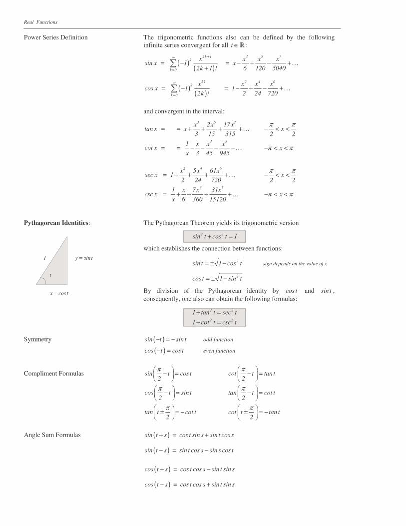
Real Functions Power Series Definition The trigonometric functions also can be defined by the following
infinite series convergent for all t ∈� :
( ) ( )2k 1 3 5 7
k
k 0
x x x xsin x 1 x
2k 1 ! 6 120 5040
+∞
== − = − + − +
+ �
( ) ( )2k 2 4 6
k
k 0
x x x xcos x 1 1
2k ! 2 24 720
∞
== − = − + − + �
and convergent in the interval:
3 5 7x 2x 17x
tan x x3 15 315
= = + + + +� x2 2π π− < <
3 51 x x x
cot x x 3 45 945
= = − − − −� xπ π− < <
2 4 6x 5x 61x
sec x 12 24 720
= + + + +� x2 2π π− < <
3 51 x 7x 31x
csc x x 6 360 15120
= + + + +� xπ π− < <
Pythagorean Identities: The Pythagorean Theorem yields its trigonometric version
2 2sin t cos t 1+ =
which establishes the connection between functions:
2sin t 1 cos t= ± − sign depends on the value of x
2cos t 1 sin t= ± −
By division of the Pythagorean identity by cos t and sin t , consequently, one also can obtain the following formulas:
2 21 tan t sec t+ = 2 21 cot t csc t+ = Symmetry ( )sin t sin t− = − odd function
( )cos t cos t− = even function
Compliment Formulas sin t cos t2π� �− =� ��
cot t tant2π� �− =� ��
cos t sin t2π� �− =� ��
tan t cot t2π� �− =� ��
tan t cot t2π� �± = −� �
� cot t tan t
2π� �± = −� �
�
Angle Sum Formulas ( )sin t s = cos t sin s sin t cos s+ +
( )sin t s = sin t cos s sin s cos t− −
( )cos t s = cos t cos s sin t sin s+ −
( )cos t s = cos t cos s sin t sin s− +
y sint=
x cos t=
1
t

Real Functions Double Angle Formulas sin 2t = 2 sin t cos t cos 2t 2 2= cos t sin t−
2= 2cos t 1−
2= 1 2 sin t−
2
2tanttan 2t
1 tan t=
−
Power Reducing Formulas 2 1 cos 2tcos t =
2+
2 1 cos 2tsin t =
2−
2 1 cos 2ttan t =
1 cos 2t−=
Half Angle Formulas t 1 cos t
sin2 2
−= ±
t 1 cos t
cos2 2
+= ±
t 1-cost sin t
tan 2 sint 1 cos t
= =+
Product-to-Sum ( ) ( )1sinu sinv cos u v cos u v
2= − − +� � �
( ) ( )1cos u cos v cos u v cos u v
2= − + +� � �
( ) ( )1sinu cos v sin u v sin u v
2= + + −� � �
( ) ( )1cos u sinv sin u v sin u v
2= + − −� � �
Sum-to-Product u v u v
sinu sin v 2 sin cos2 2+ −� � � �+ = � � � �
� �
u v u v
sinu sin v 2cos sin2 2+ −� � � �− = � � � �
� �
u v u v
cos u cos v 2cos cos2 2+ −� � � �+ = � � � �
� �
u v u v
cos u cos v 2 sin sin2 2+ −� � � �− = � � � �
� �
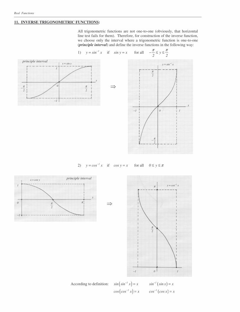
Real Functions 11. INVERSE TRIGONOMETRIC FUNCTIONS:
All trigonometric functions are not one-to-one (obviously, that horizontal line test fails for them). Therefore, for construction of the inverse function, we choose only the interval where a trigonometric function is one-to-one (principle interval) and define the inverse functions in the following way:
1) 1y sin x−= if sin y x= for all y2 2π π− ≤ ≤
2) 1y cos x−= if cos y x= for all 0 y π≤ ≤
According to definition: ( )1sin sin x x− = ( )1sin sin x x− =
( )1cos cos x x− = ( )1cos cos x x− =
101−
1y cos x−=
2π
π
2π−
0 11−
2π
1y sin x−=
x
x sin y=
2π−
2π0
1
1−
y
principle interval
2π π0
1
1−
x cos y=
y
principle interval
�
�

Real Functions 12. HYPERBOLIC FUNCTIONS: The hyperbolic functions are defined with the help of exponential functions:
x xe e
sinh x2
−−= ( )
2k 1 3 5 7
k 0
x x x x x
2k 1 ! 3! 5! 7 !
+∞
== = + + + +
+ �
x xe e
cosh x2
−+= ( )
2k 2 4 6
k 0
x x x x 1
2k ! 2! 4! 6 !
∞
== = + + + + �
Value at 0 : sinh0 0= cosh0 1= Symmetry: sinh( x ) sinh x− = − cosh( x ) cosh x− = Derivative: sinh x cosh x′ = cosh x sinh x′ =
Identities: 2 2cosh x sinh x 1− = Pythagorean Identity
xcosh x sinh x e+ = De Moivre’s formulas xcosh x sinh x e−− =
[ ]n nxcosh nx sinh nx cosh x sinh x e+ = + =
[ ]n nxcosh nx sinh nx cosh x sinh x e−− = − =
sinh x
cosh x
x0
1
Real Functions 14. REVIEW QUESTIONS: 1) By what properties the functions are characterized?
2) What are the domain and the range of the functions?
3) What functions are algebraic and functions are transcendental?
EXERCISES: 1) Sketch the graph of the break function defined with the help of the absolute
value function
( ) x xf x
2
+=
2) Sketch the graph of the functions: a) ( )f x 2x 3= − b) ( )f x 3x 5= − +
3) Sketch the graph of the functions:
a) ( ) 2f x log x= b) ( ) 3f x log 5x=
c) ( ) 0.5f x log x= d) ( ) 0.1f x log 2x=
e) ( ) ( )4f x log x 5= − f) ( ) 22f x log x=
g) ( ) ( )34f x log x 2= − h) ( ) ( )2
4f x log 2x 3= +
i) ( )x
2f x 1 e−
= + j) ( ) x 2f x 2 e −= +
k) ( )x
2f x 1 e−
= + l) ( )x
2f x 1 e−
= +
m) ( )23f x x= n) ( )
52f x x=
4) Prove the properties for the general power function:
a) a b a bx x x += b) ( )ba abx x=
5) Derive the trigonometric identities: a) 3sin 3x 3 sin x 4 sin x= − b) 3cos 3x 4 cos x 3cos x= −
c) 3 3 sin x sin3xsin x
4−= d) 3 3cos x cos 3x
cos x4+=
6) Evaluate: a) ( )1sin cos x− b) ( )1cos sin x−
c) ( )1sin cos 3x− d) ( )1cos sin 2x−
7) Sketch the graph of the functions:
a) ( )f x sin 2x4π� �= −� �
� b) ( ) ( )f x cos 4x π= − +
c) ( ) ( )f x = 3+2 sin 2x π− d) ( ) xf x = 5+2cos
2 4π� �−� �
�
e) ( )f x sin x cos x= f) ( ) 2f x 1 2 sin x= −
g) ( ) 2f x sin x= h) ( ) 2f x cos x=
i) ( )f x x sin x= j) ( )f x x cos x=
k) ( )f x tan 2x= l) ( ) xf x cot
2π� �= −� �
�
m) ( )f x sec 2x= n) ( ) xf x csc
2=

Real Functions
o) ( )f x sin x= p) ( ) xf x cos
2=
r) ( )f x sin 2x= s) ( ) xf x ln
2=
i) ( )f x x sin x= + j) ( )f x 2x ln x= +
8) a) Find an exponential function bxy ae= the graph of which passes two
fixed points ( )1,2 and ( )2,10 . Using properties of exponential and
logarithmic functions simplify the expression and sketch the graph.
b) Find an exponential function bxy ae= the graph of which passes two
fixed points ( )1,2 and ( )2,1 . Using properties of exponential and
logarithmic functions simplify the expression and sketch the graph.
9) Express the rational function as a sum of the polynomial and a proper rational function and sketch the graph:
a) ( )3 2
2
x 2x x 4f x
x 2x 1− + −=
+ − b) ( )
4 2
3 2
x 3x 2x 1f x
x 2x 1+ − +=
+ −
10) a) At any moment of time, the rate of production of a certain biological
substance is described by the exponential growth model ( ) kt0Q t Q e= .
If after 1 hour there is 2 lb of the substance and after 2 hours the amount is 8 lb , how much of the substance will be there after 3 hours of production?
b) At any moment of time, the rate of production of a certain biological substance is described by the exponential growth model ( ) kt
0Q t Q e= .
If after 1 hour there is 2 lb of the substance and after 2 hours the amount is 10 lb , how much of the substance was there initially?
c) At any moment of time, the rate of fission of a certain substance is described by the exponential decay model ( ) kt
0Q t Q e−= .
The half-life time is known to be 2 hours. If after 1 hour there is 10 lb of the substance, how much of the substance was there initially?
11) Sketch the graph of the functions:
a) ( ) ( ) ( )f x cosh 2x sinh 2x= − b) ( ) ( ) ( )f x sinh 2x cosh 2x= +
c) ( ) sinh xf x tanh x
cosh x= ≡ d) ( ) cosh x
f x coth xsinh x
= ≡
f) ( ) 1f x sech x
cosh x= ≡ g) ( ) 1
f x csch xsinh x
= ≡
12) Derive the identities:
a) 2 2cosh x sinh x 1− = b) 2 21 tanh x sech x− =
13) Find the inverse of the functions and sketch the graph of both of them:
a) ( ) x 1f x
2x 3+=+
b) ( ) 1f x
x 2=
+
c) ( )f x 2x 1= − d) ( ) 3f x x 1= +
f) ( ) xf x sin
2= g) ( )f x x 1= −

Real Functions
Novosibirsk State University