Matematica Aplicada I: Algebra Lineal y Ana´lisis …idbetan/CursoAplicada1-2017/...Chapter 1...
277
Matematica Aplicada I: ´ Algebra Lineal y An´ alisis Complejo Rodolfo M. Id Betan (Rolo) Por favor, reportar errores o comentarios a: [email protected] July 8, 2017
Transcript of Matematica Aplicada I: Algebra Lineal y Ana´lisis …idbetan/CursoAplicada1-2017/...Chapter 1...

Matematica Aplicada I:
Algebra Lineal y Analisis Complejo
Rodolfo M. Id Betan (Rolo)
Por favor, reportar errores o comentarios a:
July 8, 2017

Contents
1 Programa Analıtico 5
2 Sistemas de ecuaciones lineales 8
3 Matrices - Sub espacios vectoriales - Transformaciones lineales 143.1 Introduction . . . . . . . . . . . . . . . . . . . . . . . . . . . . . . 143.2 Matrix Operations . . . . . . . . . . . . . . . . . . . . . . . . . . 143.3 Matrix Algebra . . . . . . . . . . . . . . . . . . . . . . . . . . . . 183.4 The inverse of a Matrix . . . . . . . . . . . . . . . . . . . . . . . 223.5 The LU factorization . . . . . . . . . . . . . . . . . . . . . . . . . 28
3.5.1 LU factorization: . . . . . . . . . . . . . . . . . . . . . . . 293.5.2 An easy way to find LU factorization: . . . . . . . . . . . 313.5.3 The PTLU factorization . . . . . . . . . . . . . . . . . . . 31
3.6 Subspaces, Basis, Dimension, and Rank . . . . . . . . . . . . . . 333.6.1 Basis . . . . . . . . . . . . . . . . . . . . . . . . . . . . . . 353.6.2 Procedure to find the basis of a matrix. . . . . . . . . . . 35
3.7 Dimension and Rank . . . . . . . . . . . . . . . . . . . . . . . . . 373.8 Introduction to linear transformation . . . . . . . . . . . . . . . . 40
3.8.1 Composition of LT . . . . . . . . . . . . . . . . . . . . . . 433.8.2 Inverses of LT . . . . . . . . . . . . . . . . . . . . . . . . . 45
4 Autovalores y autovectores 474.1 Introduction . . . . . . . . . . . . . . . . . . . . . . . . . . . . . . 47
4.1.1 Determinants . . . . . . . . . . . . . . . . . . . . . . . . . 494.1.2 Determinants of n× n Matrices . . . . . . . . . . . . . . . 494.1.3 Properties of Determinants . . . . . . . . . . . . . . . . . 504.1.4 Determinants of Elementary Matrices . . . . . . . . . . . 514.1.5 Determinants and Matrix Operations . . . . . . . . . . . 514.1.6 Cramer’s Rule and the Adjoint . . . . . . . . . . . . . . . 52
4.2 Eigenvalues and Eigenvectors of n× n Matrices . . . . . . . . . . 534.3 Similarity and Diagonalization . . . . . . . . . . . . . . . . . . . 58
4.3.1 Similar Matrices . . . . . . . . . . . . . . . . . . . . . . . 584.3.2 Diagonalization . . . . . . . . . . . . . . . . . . . . . . . . 59
5 Ortogonalidad 655.1 Orthogonality in Rn . . . . . . . . . . . . . . . . . . . . . . . . . 65
5.1.1 Orthogonal and Orthonormal Sets of Vectors . . . . . . . 655.1.2 Orthogonal Matrices . . . . . . . . . . . . . . . . . . . . . 67
1

5.2 Orthogonal Complements and Orthogonal Projections . . . . . . 685.2.1 Orthogonal Complements . . . . . . . . . . . . . . . . . . 685.2.2 Orthogonal Projections . . . . . . . . . . . . . . . . . . . 72
5.3 The Gram-Schmidt Process and the QR Factorization . . . . . . 745.3.1 The Gram-Schmidt Process . . . . . . . . . . . . . . . . . 745.3.2 The QR Factorization . . . . . . . . . . . . . . . . . . . . 77
5.4 Orthogonal Diagonalization of Symmetric Matrices . . . . . . . . 795.5 Applications . . . . . . . . . . . . . . . . . . . . . . . . . . . . . . 81
5.5.1 Quadratic Forms . . . . . . . . . . . . . . . . . . . . . . . 815.5.2 Graphing Quadratic Equations . . . . . . . . . . . . . . . 83
6 Espacios vectoriales 856.1 Vector Spaces and Subspaces . . . . . . . . . . . . . . . . . . . . 85
6.1.1 Spanning Sets . . . . . . . . . . . . . . . . . . . . . . . . . 896.2 Linear Independence (LI), Basis, and Dimension . . . . . . . . . 89
6.2.1 Linear Independence (in finite spaces) . . . . . . . . . . . 906.2.2 Linear Independence (in infinite spaces) . . . . . . . . . . 916.2.3 Bases . . . . . . . . . . . . . . . . . . . . . . . . . . . . . 916.2.4 Coordinates . . . . . . . . . . . . . . . . . . . . . . . . . . 916.2.5 Dimension: . . . . . . . . . . . . . . . . . . . . . . . . . . 93
6.3 Change of Basis . . . . . . . . . . . . . . . . . . . . . . . . . . . . 966.3.1 Introduction . . . . . . . . . . . . . . . . . . . . . . . . . 966.3.2 Change-of-Basis Matrices . . . . . . . . . . . . . . . . . . 976.3.3 The Gauss-Jordan Method for Computing a Change-of-
Basis Matrix . . . . . . . . . . . . . . . . . . . . . . . . . 1016.4 Linear Transformations . . . . . . . . . . . . . . . . . . . . . . . 103
6.4.1 Properties of LT . . . . . . . . . . . . . . . . . . . . . . . 1046.4.2 Composition of LT . . . . . . . . . . . . . . . . . . . . . . 1056.4.3 Inverses of LT . . . . . . . . . . . . . . . . . . . . . . . . . 106
6.5 The Kernel and Range of a Linear Transformation . . . . . . . . 1076.5.1 One-to-One and Onto Linear Transformation . . . . . . . 1106.5.2 Isomorphisms of Vector Spaces . . . . . . . . . . . . . . . 112
6.6 The Matrix of a Linear Transformation . . . . . . . . . . . . . . 1126.6.1 Matrices of Composite and Inverse Linear Transformations 1166.6.2 Change of Basis and Similarity . . . . . . . . . . . . . . . 120
7 Distancia yAproximacion 1237.1 Introduction . . . . . . . . . . . . . . . . . . . . . . . . . . . . . . 1237.2 Inner Product Spaces . . . . . . . . . . . . . . . . . . . . . . . . . 123
7.2.1 Properties of Inner Products . . . . . . . . . . . . . . . . 1247.2.2 Length, Distance, and Orthogonality . . . . . . . . . . . . 1247.2.3 Orthogonal Projections and the Gram-Schmidt Process . 1257.2.4 The Cauchy-Schwarz and Triangle Inequalities . . . . . . 127
7.3 Vectors and Matrices with Complex Entries . . . . . . . . . . . . 1287.4 Geometric Inequalities and Optimization Problems . . . . . . . . 1317.5 Norms and Distance Functions . . . . . . . . . . . . . . . . . . . 132
7.5.1 Distance Functions . . . . . . . . . . . . . . . . . . . . . . 1327.5.2 Matrix Norms . . . . . . . . . . . . . . . . . . . . . . . . . 1337.5.3 The Condition Number of a Matrix . . . . . . . . . . . . 1347.5.4 The Convergence of Iterative Methods . . . . . . . . . . . 135
2
7.6 Least Squares Approximation . . . . . . . . . . . . . . . . . . . . 1357.6.1 Least Squares Approximation . . . . . . . . . . . . . . . . 1377.6.2 Least Squares via the QR Factorization . . . . . . . . . . 1377.6.3 Orthogonal Projection Revisited . . . . . . . . . . . . . . 1387.6.4 The Pseudoinverse of a Matrix . . . . . . . . . . . . . . . 138
7.7 The Singular Value Decomposition . . . . . . . . . . . . . . . . . 1397.7.1 The Singular Values of a Matrix . . . . . . . . . . . . . . 1397.7.2 The Singular Value Decomposition . . . . . . . . . . . . . 1407.7.3 Matrix Norms and the Condition Number . . . . . . . . . 1437.7.4 The pseudoinverse and Least Squares Approximation . . . 1437.7.5 The Fundamental Theorem of Invertible Matrices . . . . . 144
7.8 Applications . . . . . . . . . . . . . . . . . . . . . . . . . . . . . . 1457.8.1 Approximation of Functions . . . . . . . . . . . . . . . . . 145
8 Numeros complejos y plano complejo 1498.1 Introduction . . . . . . . . . . . . . . . . . . . . . . . . . . . . . . 1498.2 Complex Plane . . . . . . . . . . . . . . . . . . . . . . . . . . . . 1508.3 Polar Form of Complex Numbers . . . . . . . . . . . . . . . . . . 1518.4 Powers and Roots . . . . . . . . . . . . . . . . . . . . . . . . . . 1518.5 Set of Points in the Complex Plane . . . . . . . . . . . . . . . . . 152
9 Funciones complejas y mapeos 1549.1 Complex Functions . . . . . . . . . . . . . . . . . . . . . . . . . . 1549.2 Complex Functions as Mappings . . . . . . . . . . . . . . . . . . 1559.3 Linear Mappings . . . . . . . . . . . . . . . . . . . . . . . . . . . 157
9.3.1 Translations . . . . . . . . . . . . . . . . . . . . . . . . . . 1579.3.2 Rotation . . . . . . . . . . . . . . . . . . . . . . . . . . . . 1589.3.3 Magnifications . . . . . . . . . . . . . . . . . . . . . . . . 1589.3.4 Linear Mappings . . . . . . . . . . . . . . . . . . . . . . . 159
9.4 Special Power Functions . . . . . . . . . . . . . . . . . . . . . . . 1619.4.1 The function zn . . . . . . . . . . . . . . . . . . . . . . . 1619.4.2 The power function z1/n . . . . . . . . . . . . . . . . . . . 162
9.5 Reciprocal Function . . . . . . . . . . . . . . . . . . . . . . . . . 1659.6 Limits and Continuity . . . . . . . . . . . . . . . . . . . . . . . . 170
9.6.1 Limits . . . . . . . . . . . . . . . . . . . . . . . . . . . . . 1719.6.2 Continuity . . . . . . . . . . . . . . . . . . . . . . . . . . 173
10 Funciones analıticas 17710.1 Differentiability and Analyticity . . . . . . . . . . . . . . . . . . . 17710.2 Cauchy-Riemann Equations . . . . . . . . . . . . . . . . . . . . . 17910.3 Harmonic Functions . . . . . . . . . . . . . . . . . . . . . . . . . 180
11 Funciones elementales 18211.1 Exponential and Logarithmic Functions . . . . . . . . . . . . . . 182
11.1.1 Complex exponential function . . . . . . . . . . . . . . . . 18211.1.2 Complex Logarithmic Function . . . . . . . . . . . . . . . 184
11.2 Complex Powers . . . . . . . . . . . . . . . . . . . . . . . . . . . 18711.2.1 Trigonometric and Hyperbolic Functions . . . . . . . . . . 18811.2.2 Complex Hyperbolic Functions . . . . . . . . . . . . . . . 191
11.3 Inverse Trigonometric and Hyperbolic Functions . . . . . . . . . 192
3

12 Integracion en el plano complejo 19612.1 Real Integrals . . . . . . . . . . . . . . . . . . . . . . . . . . . . . 19612.2 Complex Integrals . . . . . . . . . . . . . . . . . . . . . . . . . . 19712.3 Cauchy-Goursat Theorem . . . . . . . . . . . . . . . . . . . . . . 20012.4 Cauchy’s Integral Formulas and their Consequences . . . . . . . . 208
12.4.1 Cauchy’s Two Integral Formulas . . . . . . . . . . . . . . 20812.4.2 Some Consequences of the Integral Formulas . . . . . . . 210
13 Series y residuos 21313.1 Sequences and Series . . . . . . . . . . . . . . . . . . . . . . . . . 21313.2 Taylor Series . . . . . . . . . . . . . . . . . . . . . . . . . . . . . 21713.3 Laurent Series . . . . . . . . . . . . . . . . . . . . . . . . . . . . . 22213.4 Zeros and Poles . . . . . . . . . . . . . . . . . . . . . . . . . . . . 22613.5 Residues and Residue Theorem . . . . . . . . . . . . . . . . . . . 22913.6 Some Consequences of the Residue Theorem . . . . . . . . . . . . 233
13.6.1 Evaluation of Real Trigonometric Integrals . . . . . . . . 23313.6.2 Evaluation of Real Improper Integrals . . . . . . . . . . . 23513.6.3 Integration along a Branch Cut . . . . . . . . . . . . . . . 24013.6.4 The Argument Principle and Rouche’s Theorem . . . . . 242
A Ejercicios: Sistemas de ecuaciones lineales 243
B Ejercicios: Matrices - Sub espacios vectoriales - Transforma-ciones lineales 248
C Ejercicios: Autovalores y autovectores 255
D Ejercicios: Ortogonalidad 259
E Ejercicios: Espacios vectoriales 265
F Ejercicios: Distancia yAproximacion 272
4
Chapter 1
Programa Analıtico
Matematica Aplicada I (F-311) es un materia de grado de a Licenciatura enFısica que se dicta en el primer semestre del tercer ano.
Destinatarios: Alumnos de la Licenciatura en Fısica que tengan regularizadao aprobada Analisis Matematico IV (F-221).
Cursado: ocho horas semanales.
Bibliografıa:
• Linear Algebra. A Modern Introduction [1]. David Poole. SecondEdition. Thomson. Australia, 2006.
• Algebra Lineal. Juan de Burgos Roman. McGraw-Hill.
• Introduction to Linear Algebra. Gilbert Strang (MIT). Wellesley.Cambridge Press.
• Complex Analysis with Applications [2]. Dennis G. Zill and PatrickD. Shanahan. Jones and Bartlett Publishers, 2003.
• Variable Compleja y Aplicaciones. R.V. Churchill y J.W. Brown.Universidad de Michigan. McGraw-Hill.
• Matematica avanzada para la Fısica. Manuel Balanzat. EUDEBA.
Programa analıtico
1. Sistemas de ecuaciones lineales.
• Introduccion a los sistemas de ecuaciones lineales. Metodos directospara resolver sistemas de ecuaciones lineales.
• Conjuntos generadores e independencia lineal. Metodos iterativospara la resolucion de sistemas de ecuaciones lineales.
2. Matrices y Espacios Vectoriales Rn.
5

• Definicion de matriz y algebra matricial. Matrices particionadas yrepresentacion matricial.
• Traspuesta de una matriz. Inversa de una matriz.
• Matrices elementales. La factorizacio LU.
• Subespacios, base, dimension y rango. Introduccion a las transfor-maciones lineales.
3. Autovalores y Autovectores.
• Autovalores y Autovectores: definiciones bsicas. Determinantes. Au-tovalores y autovalores de matrices nxn.
• Semejanza y diagonalizacion
4. Ortogonalidad.
• Ortogonalidad en Rn. Matrices ortogonales. Complemento ortogonaly proyecciones ortogonales.
• Elproceso de Gram-Schmidt y la factorizacion QR. Diagonalizacionortogonal d ematrices simetricas.
5. Espacios vectoriales generales.
• Espacios y subespacios vectoriales. Dependencia e independencialineal. Base y dimension.
• Cambio de bases. Transformaciones lineales. Inversa de una trans-formacion lineal.
• Nucleo e imagen de una transformacion lineal. Isomorfismo de espa-cios vectoriales.
• Matriz de una transformacion lineal. Cambio de bases y similaridad.
6. Distancia y aproximacion.
• Espacios vectoriales con producto interno. Vectores y matrices conentradas complejas (matrices hermitianas o hermıticas como gener-alizacion de las matrices simetricas y sus propiedades).
• Normas y funciones distancia. Aproximacion por mınimos cuadra-dos. La descomposicion de valor singular (compresion de imagenesdigitales).
7. Numeros complejos y el plano complejo.
• Numeros complejos: definicion y propiedades. El plano complejo yel concepto de infinito
8. Funciones complejas de variable compleja.
• Funcion compleja de variable compleja. Mapeo de regiones del planocomplejo.
• Funcion inversa. Funcion recıproca. Lımite y continuidad.
• Funciones multivaluadas. Ramas y rama principal.
6

9. Derivadas de funciones complejas.
• Definicion de derivada. Reglas de derivacion. Funciones analıticas.Funciones enteras. Puntos singulares.
• Ecuaciones de Cauchy-Riemann. Funciones armonicas y funcionesarmonicas conjugadas. Funciones elementales.
10. Integracion en el plano complejo .
• Integrales definidas. Integral de una funcioon compleja a lo largo deuna curva en el plano complejo. Dominios simplemente y multiplementeconexos.
• Teorema de Cauchy y Teorema de Cauchy-Gourzat. Integrales inde-pendientes del camino. Formulas integrales de Cauchy.
11. Sucesiones y series en el campo complejo .
• Sucesiones y series en el campo complejo. Criterios de convergenciay divergencia. Radio y cırculo de convergencia. Series de Taylor.
• Series de Laurent. Ceros y polos. Residuos. Teorema de Residuos deCauchy.
12. Aplicacion del Teorema de Residuos.
• Resolucion de integrales reales: integrales trigonometricas e inte-grales impropias.
• Integracion a lo largo de un branch cut (corte de rama).
7

Chapter 2
Sistemas de ecuacioneslineales
Credit: This notes are 100% from chapter 2 of the book entitled Linear Al-gebra. A Modern Introduction of David Poole (2006) [1].
Linear equation: a linear equation in the n variables x1, · · · , xn is an equa-tion that can be written in the form a1x1+ · · ·+anxn = b where the coefficientsa1, · · · , an and the constant term b are constants.
System of linear equations (SLE): a system of linear equations is a finiteset of linear equations, each with the same variables. A solution of a SLE is avector that is simultaneously a solution of each equation in the system.
Consistent and inconsistent: a SLE is called consistent if it has at leastone solution. A system with no solutions is called inconsistent. A SLE withreal coefficients has either (i) a unique solution (a consistent system), (ii) in-finitely many solutions (a consistent system) or (iii) no solution (an inconsistentsystem).
Equivalent: two SLE are called equivalent if they have the same solution set.The general approach to solving a SLE is to transform the given system into anequivalent one that is easier to solve.
Coefficients and augmented matrices: there are two important matricesassociated with a SLE. The coefficient matrix contains the coefficients of thevariables, and the augmented matrix is the coefficient matrix augmented by anextra column containing the constant terms.
Back substitution: is the procedure which consist to solve the SLE startingfrom the last equation and working backward when the SLE is given in the form
x− y − z = 2 (2.1)
y + 3z = 5 (2.2)
5z = 10 (2.3)
8

Next we turn to the general strategy for transforming a given system intoan equivalent one that can be solved easily by back substitution. What followis an example
x− y − z = 2 (2.4)
3x− 3y + 2z = 16 (2.5)
2x− y + z = 9 (2.6)
We built the extended or augmented matrix, i.e. the matrix of the SLEcoefficients and independent term,
1 −1 −1 23 −3 2 162 −1 1 9
(2.7)
First we eliminate x from the second and third equations: (i) we subtract thesecond line with 3 times the firs line: f2 − 3f1
1 −1 −1 20 0 5 102 −1 1 9
(2.8)
(ii)next we subtract third line with 2 times the first one: f3 − 2f1
1 −1 −1 20 0 5 100 1 3 5
(2.9)
(iii) next we interchange the second with the third equation f2 → f3
1 −1 −1 20 1 3 50 0 5 10
(2.10)
(iv) we are done. Now we write the SLE with the new coefficients and inde-pendent term. This is an equivalent SLE of the initial one and then they bothshare the same solution. The solution is obtained by back substitution.
x− y − z = 2 (2.11)
y + 3z = 5 (2.12)
5z = 10 (2.13)
Row echelon(escalon) form: In solving a linear system, it will no alwaysbe possible to reduce the coefficient matrix to triangular form. However, we canalways achieve a staircase pattern in the nonzero entries of the final matrix. Amatrix is row echelon form if it satisfies the following properties
• Any rows consisting entirely of zeros are at the bottom
• In each nonzero row, the first nonzero entry (called the leading entry) isin a column to the left of any leading entries below it.
If a matrix in row echelon form is actually the augmented matrix of a linearsystem, the system is quite easy to solve by back substitution alone.The row echelon form of a matrix is not unique (but they are all equivalents).
9

Elementary row operations: this is a procedure by which any matrix canbe reduced to a matrix in row echelon form. The allowed operations, calledelementary row operations, correspond to the operations that can be performedon a system of linear equations to transform it into an equivalent system. Theyare:
• Interchange two rows (Ri ↔ Rj).
• Multiply a row by a nonzero constant (kRi).
• Add a multiple of a row to another row (Ri + kRj).
Row reduction: the process of applying elementary row operations to bringa matrix into row echelon form, called row reduction, is used to reduce a matrixto echelon form.
Row equivalent: matrices A and B are row equivalent if there is a sequenceof elementary row operations that converts A into B.
Theorem 2.1: Matrices A and B are row equivalent if and only if they canbe reduced to the same row echelon form.Proof: If A and B are row equivalent, then further row operations will reduceB (and therefore A) to the (same) row echelon form.Conversely, if A and B have the same row echelon form R, then via elementaryrow operations, we can convert A into R and B into R. Reversing the lattersequence of operations, we can convert R into B, and therefore the sequenceA → R → B achieves the desired effect.
Gaussian elimination: when row reduction is applied to the augmented ma-trix of a SLE, we create an equivalent system that can be solved by back sub-stitution. The entire process is known as Gaussian elimination.
Rank: the rank (rank(A) of a matrix A is the number of nonzero rows in itsrow echelon form.
Theorem 2.2: The Rank Theorem Let A be the coefficient matrix of a SLEwith n variables. If the system is consistent, then number of free variables =n− rank(A)
• If n-rank(A)=0 there are no free variables and there is a unique solution.
• If rank(A)6= rank(A|b) the system is inconsistent, i.e. it has not solution.
Example
1 −1 2 31 2 −1 −30 2 −2 1
→
1 −1 2 30 1 −1 −20 0 0 5
Reduce row echelon: a modification of Gaussian elimination greatly sim-plifies the back substitution phase. This variant is known as Gauss-Jordanelimination, relies on reducing the augmented matrix even further. A matrix isin reduced row echelon form if:
10

• It is in row echelon form.
• The leading entry in each nonzero row is 1 (called a leading 1)
• Each column containing a leading 1 has zeros everywhere else.
Unlike the row echelon form, the reduced row echelon form of a matrix is unique.
Homogeneous systems: a system of linear equations is called homogeneousif the constant term in each equation is zero. A homogeneous system will haveeither a unique solution (namely, the zero, or trivial, solution) or infinitely manysolutions.
Theorem 2.3: If [A|0] is a homogeneous system of m linear equations with nvariables, where m < n, the the system has infinitely many solutions.Proof: Since the system has at least the zero solution, it is consistent. Alsorank(A)≤ m. Then by the rank theorem, we have
number of free variables = n− rank(A) ≥ n−m > 0 (2.14)
then, there is at least one free variable and, hence, infinitely many solutions.The theorem 2.3 says nothing about the case where m ≥ n. Exercise 44 asks
you to give examples to show that, in this case, there can be either a uniquesolution of infinitely many solutions.
Theorem 2.4: A system of linear equations with augmented matrix [A|b] isconsistent if and only if b is a linear combination of the column of A.
Span: If S = {v1, · · · , vk} is a set of vectors in Rn, the the set of all linearcombinations of v1, · · · , vk is called the span of v1, · · · , vk and is denoted byspan(v1, · · · , vk) or span(S)=Rn, then S is called a spanning set for Rn.
Example: R2 = span(v1, v2) with
v1 =
[
2−1
]
(2.15)
v2 =
[
13
]
(2.16)
We have to show that an arbitrary vector
[
ab
]
can be written as a linear
combination of v1 and v2, i.e. exist c1 and c2 such that c1
[
2−1
]
+ c2
[
13
]
=[
ab
]
for any a and b.
Built the augmented matrix and reduce to the equivalent echelon row and useback substitution to get the following values for c1 and c2
c1 =3a− b
7(2.17)
c2 =a+ 2b
7(2.18)
11

Linearly dependent (LD): A set of vectors v1, · · · , vk is linearly dependentif there are scalars c1, · · · , ck at least one of which is not zero, such that
c1 v1 ++ck vk = 0 (2.19)
Any set of vectors containing the zero vector is LD, since for if 0, v2, · · · , vm arein Rm, then we can find a nontrivial combination of the form c10 + c2v2 + · · ·+cmvm = 0 by setting c1 = 1 and c2 = · · · = cm = 0.
Linearly independent (LI): A set of vectors v1, · · · , vk that is not linearlydependent is called linearly independent.
Theorem 2.5: Vectors v1, · · · , vm in Rn are LD if and only if at least one ofthe vectors can be expressed as a linear combination of the others.Proof: If one of the vectors, let as say v1 is a linear combination of the others,then there are scalars c2, · · · , cm such that v1 = c2 v2+· · ·+cm vm. Rearranging,we obtain v1 − c2 v2 − · · · − cm vm = 0, which implies that v1, · · · , vm are LD,since at least one of the scalar (the coefficient c1 = 1 of v1) is nonzero.Conversely, suppose that v1, · · · , vm are LD. Then there are scalars c1, · · · , cm,not all zero, such that c1 v1 + c2 v2 + · · ·+ cm vm = 0. Suppose c1 6= 0. Then
c1 v1 = −c2 v2 − · · · − cm vm = 0 (2.20)
and we may Multiply both side by 1/c1 to obtain v1 as a linear combination ofthe others vectors:
v1 = −c2c1
v2 − · · · − cmc1
vm (2.21)
We have taken as a reference the vector v1 but this is valid for any other vectoras well.
Theorem 2.6: Let v1, · · · , vm be (column) vectors in Rn and let A be then×m matrix [v1, · · · , vm] with this vectors as its columns. Then v1, · · · , vm areLD if and only if the homogeneous linear system with augmented matrix [A|0as a nontrivial solution.Proof:v1, · · · , vm are LD if and only if there are scalars c1, · · · , cm, not all zero,such that c1v1+ · · ·+cmvm = 0. By the theorem 2.4, this is equivalent to saying
that the nonzero vector
c1...cm
is a solution of the system whose augmented
matrix is [v1, · · · , vm|0.
Theorem 2.7: Let v1, · · · , vm be (row) vectors in Rn and let A be the m×n
matrix
v1...vm
with this vectors as its rows. Then v1, · · · , vm are LD if and
only if the rank(A)< m.Proof: Assume that v1, · · · , vm are LD. Then theorem 2.2, at least one of thevectors can be written as a linear combination of the others. We relabel thevectors, if necessary, so that we can write vm = c1v1 + · · · + cm−1vm−1. Then
12

the elementary row operations Rm − c1R1, Rm − c2R2, · · · , Rm − cm−1Rm−1applied to A will create a zero row in row m. Thus, rank(A)< m.Conversely, assume that rank(A)< m. Then there is some sequence of rowoperations that will create a zero row. A successive substitution argumentanalogous to that used in Example 2.25 can be used to show that 0 is a nontriviallinear combination of v1, · · · , vm. Thus, v1, · · · , vm are LD.
Theorem 2.8: Any set of m vectors in Rn is LD if m > n.Proof: Assume that v1, · · · , vm be (column) vectors in Rn and A be then × m matrix [v1, · · · , vm] with these vectors as its columns. By Theorem 2.6v1, · · · , vm are LD if and only if the homogeneous linear system with augmentedmatrix [A|0] has a nontrivial solution. But, according to Theorem 2.6, this willalways be the case if A has more columns that rows; it is the case here, sincenumber of columns m is grater than numbers of rows n.
13

Chapter 3
Matrices - Sub espaciosvectoriales -Transformaciones lineales
Credit: This notes are 100% from chapter 3 of the book entitled Linear Al-gebra. A Modern Introduction of David Poole (2006) [1].
3.1 Introduction
We will use matrices to solve system of linear equations (SLE). Let us transformthe following SLE
x− y − z = 2 (3.1)
3x− 3y + 2z = 16 (3.2)
2x− y + z = 9 (3.3)
in matrix notation,
1 −1 −13 −3 22 −1 1
xyz
=
2169
(3.4)
These equation can be think as a certain type of function that act on vector,transforming them into other vectors. These matrix transformation will beginto play a key role in our study of linear algebra. We will review their algebraicproperties.
3.2 Matrix Operations
Matrix, size: a matrix is a rectangular array of numbers called the entries,of elements, of the matrix. The size of a matrix is a description of the numberof rows and columns it has. A matrix is called m × n if it has m rows and ncolumns. A 1×m matrix is called a row matrix, and an n× 1 matrix is calleda column matrix.
14

Some special matrices: If m = n A is called a square matrix. A squarematrix whose non diagonal entries are all zero is called a diagonal matrix. Adiagonal matrix, all of whose diagonal entries are the same is called a scalarmatrix. If the scalar on the diagonal is 1, the scalar matrix is called an identitymatrix. The n× n identity matrix is denoted by In.
Equal: tow matrices A and B are equal if they have the same size and iftheir corresponding entries are equal, i.e. if A = [aij ]m×n and B = [bij ]r×s,then A = B if and only if m = r and n = s and aij = bij for all i and j.
Sum: A = [aij ] and B = [bij ] are m× n matrices, their sum A + B is them× n matrix A + B = [aij ] + [bij ]. If A and B are not the same size, thenA+B is not defined.
Scalar multiple: If A is an m× n matrix and c is a scalar, then the scalarmultiple cA is the m× n matrix cA = c[aij ] = [caij ].
Difference: The matrix (−1)A is written as −A and called the negative ofA. If A and B are the same size, the A−B = A+ (−B).
Zero matrix: A matrix all of whose entries are zero is called zero matrixand denoted by O, and: (i)A +O = A = O +A, (ii) A−A = O = −A+A.
Product: If A is an m×n matrix and B is an n× r matrix, then the productC = AB is an m× r matrix. The (i, j) entry of the product is computed as
cij = ai1b1j + ai2b2j + · · ·+ ainbnj =
n∑
k=1
aikbkj (3.5)
SLE: Every linear system with m equations and n variables can be written inthe form
Ax = b (3.6)
with A a matrix m× n, x a vector of n× 1 and b a vector of m× 1.
Pick out a single row/column: Let A =
[
4 2 10 5 −1
]
the pre(post)-
multiplication with a versor gives a row(column) of A,
e2A = [0 1]
[
4 2 10 5 −1
]
= [0 5 − 1] (3.7)
Ae3 =
[
4 2 10 5 −1
]
001
=
[
1−1
]
(3.8)
15

Theorem 3.1: Let A be a matrix m× n, ei a standard unit vector of 1×m,and ej a standard unit vector of n× 1, then
a) eiA is the ith row of A and
b) Aej is the jth column of A.
Proof: Proof of [b] (the proof of [a] is left as and exercise). If the vectorsa1, · · · , an are the columns of A, then
Aej = 0a1 + 0a2 + · · ·+ 0aj−1 + 1aj + 0aj+1 + 0an = aj (3.9)
or
Aej =
a11 · · · a1j · · · a1na21 · · · a2j · · · a2n...
......
am1 · · · amj · · · amn
0...1...0
=
a1ja2j...
anj
(3.10)
Blocks: It will often be convenient to regard a matrix as being composed ofa number of smaller sub matrices. By introducing vertical and horizontal linesinto a matrix, we can partition it into blocks. Then the original matrix has asentries smaller matrices. Example
A =
1 0 0 2 −10 1 0 1 30 0 1 4 00 0 0 1 70 0 0 7 2
(3.11)
=
1 0 0 2 −10 1 0 1 30 0 1 4 00 0 0 1 70 0 0 7 2
(3.12)
=
[
I BO C
]
(3.13)
When matrices are being multiplied, there is often an advantage to be gainedby viewing them as partitioned matrices, since some of the sub matrices maybe the identity of the nil matrix.
Matrix-column representation: Suppose A is m × n and B is n × r, sothe product AB exist. Let us partition B in term of its columns vectors, asB = [b1| · · · |br] then
AB = A[b1| · · · |br] (3.14)
= [Ab1| · · · |Abr] (3.15)
16

Example,
A =
[
1 3 20 −1 1
]
(3.16)
B =
4 −11 23 0
(3.17)
then
AB = [Ab1|Ab2] (3.18)
=
[
13 52 −2
]
(3.19)
Linear combination: The matrix-column representation of AB allows us towrite each column of AB as a linear combination of the column of A with entriesfrom B as the coefficients. Example
Ab1 =
[
1 3 20 −1 1
]
413
(3.20)
= 4
[
10
]
+
[
3−1
]
+ 3
[
21
]
(3.21)
Row-matrix representation: similarly, if A is m × n and B is n× r, then
the product AB exist. If we partition A in terms of its row vectors, as
A1
A2
...Am
then,
AB =
A1
A2
...Am
B (3.22)
=
A1BA2B...
AmB
(3.23)
Outer product(column-row representation): If we partition the matrixA, m×n in columns and B, n× r is row, then the product AB exists and gives
A = [a1|a2| · · · |an] (3.24)
B =
B1
B2
...Bn
(3.25)
17

then
AB = [a1|a2| · · · |an]
B1
B2
...Bn
(3.26)
= a1B1 + a2B2 + · · ·+ anBn (3.27)
Each individual term in the above sum is a matrix, i.e. aiBi is the productof m× 1 and a 1× r matrix, thus aiBi is a m× r matrix. The product aiBi arecalled outer product, ant (3.26) is called the outer product expansion of AB.
Matrix powers: Let A be a matrix of dimension n× n, we define
• Ak = AA · · ·A (k-times)
• A0 = I
with the following properties
• ArAs = Ar+s
• (Ar)s = Ars
Transpose: the transpose of am×nmatrix A is the n×mmatrix AT obtainedby interchanging the rows and columns of A. That is, the ith column of AT isthe ith row of A for all i or (AT )ij = Aij for all i and j.
Scalar product: The dot product of two vectors u =
u1
...un
and v =
v1...vn
can be written in the form
u · v = u1v1 + · · ·+ unvn (3.28)
= [u1 · · · un]
v1...vn
(3.29)
= uT v (3.30)
Symmetric matrix: A square matrix A is symmetric if AT = A, that is, ifA is equal to its own transpose or Aij = Aji.
3.3 Matrix Algebra
Theorem 3.2: Algebraic properties of matrix addition and scalar multiplica-tion. Let A,B and C be matrices of the same size and let c and d be scalars.Then
18

a) A+B = B +A Commutativity
b) (A+B) + C = A+ (B + C) Associativity
c) A+O = A
d) A+ (−A) = O
e) c(A+B) = cA+ cB Distributivity
f) (c+ d)A = cA+ dA Distributivity
g) c(dA) = (cd)A
h) 1A = A
Linear combination: If A1, A2, · · · , Ak are matrices of the same size andc1, · · · , ck are scalars (called coefficients), we may form the linear combination
c1A1 + c2A2 + · · ·+ ckAk (3.31)
Example,
A1 =
[
0 1−1 0
]
A2 =
[
1 00 1
]
A3 =
[
1 11 1
]
(3.32)
are B and C linear combinations of A1, A2 and A3?, where
B =
[
1 42 1
]
(3.33)
C =
[
1 23 4
]
(3.34)
We write the linear combination c1A1 + c2A2 + c3A3, equal it to B and C.
For B we get
c1
[
0 1−1 0
]
+ c2
[
1 00 1
]
c3
[
1 11 1
]
=
[
1 42 1
]
(3.35)
then[
c2 + c3 c1 + c3−c1 + c3 c2 + c3
]
=
[
1 42 1
]
(3.36)
For which we built the system
c2 + c3 = 1 (3.37)
c1 + c3 = 4 (3.38)
−c1 + c3 = 2 (3.39)
c2 + c3 = 1 (3.40)
Next, we built the extended matrix and applied Gauss or Gauss-Jordan reduc-tion.
The solutions are
• For B: c1 = 1, c2 = −2, c3 = 3, i.e. B is the following linear combinationof Ai: A1 − 2A2 + 3A3 = B
• For C: C is not a LC since the system is inconsistent
19

Span: the span of the above matrices A1, A2 and A3 is given by all matrices
of the form
[
w xy z
]
such that,
c1A1 + c2A2 + c3A3 = c1
[
0 1−1 0
]
+ c2
[
1 00 1
]
c3
[
1 11 1
]
(3.41)
=
[
c2 + c3 c1 + c3−c1 + c3 c2 + c3
]
(3.42)
=
[
w xy z
]
(3.43)
which defined the following SE
c2 + c3 = w (3.44)
c1 + c3 = x (3.45)
−c1 + c3 = y (3.46)
c2 + c3 = z (3.47)
with the following extended matrix
0 1 1 w1 0 1 x−1 0 1 y0 1 1 z
(3.48)
The row reduction process gives
0 0 0 x−y2
0 1 0 −x+y2 + w
0 0 1 x+y2
0 0 0 w − z
(3.49)
the only restriction comes from the last column w = z, A1, A2, A3 expand all
matrices of the form
[
w xy w
]
with x, y, w arbitrary.
Using this information we could have been conclude that B is a linear combi-nation of A1, A2, A3 while C is not.
Linearly independent (LI): We say that matrices A1, A2, · · · , Ak of thesame size are LI if the only solution of the equation
c1A1 + c2A2 + · · ·+ ckAk = O (3.50)
is the trivial one: c1 = · · · = ck = 0.
Linearly dependent (LD): We say that matrices A1, A2, · · · , Ak of the samesize are LD if there are nontrivial coefficients c1, · · · , ck that satisfy
c1A1 + c2A2 + · · ·+ ckAk = O (3.51)
20

Example: determine whether the above matrices A1, A2, A3 are LI.
c1A1 + c2A2 + · · ·+ ckAk = O (3.52)
c1
[
0 1−1 0
]
+ c2
[
1 00 1
]
c3
[
1 11 1
]
=
[
0 00 0
]
(3.53)
we have to solve the homogeneous LS. From the previous calculations we have
0 0 0 00 1 0 00 0 1 00 0 0 0
(3.54)
then, c1 = c2 = c3 = 0, i.e. they are LI.
Multiplication: The multiplication is not commutative AB 6= BA (if B 6=A). Then (A + B)2 6= A2 + 2AB + B2 if A does not commute with B, i.e.AB 6= BA.If A2 = O does not implies A = O.
Theorem 3.3: Properties of Matrix multiplication. Let A,B and C be matri-ces (whose sizes are such that the indicated operations can be performed) andlet k be a scalar. Then
a) A(BC) = (AB)C Associativity
b) A(B + C) = AB +AC Left distributivity
c) (A+B)C = AC +BC Right distributivity
e) k(AB) = (kA)B = A(kB)
f) ImA = A = AIn if A is m× n Multiplicative identity
Theorem 3.4: Properties of the Transpose. Let A and B be matrices (whosesizes are such that the indicated operations can be performed) and let k be ascalar. Then
a) (AT )T = A
b) (A+B)T = AT +BT
c) (kA)T = k(AT )
d) (AB)T = BTAT
e) (Ar)T = (AT )r for all non negative integers r
Properties (b) and (d) can be generalized (assuming that the size of thematrices are such that all of the operations can be performed),
(A1 + · · ·+Ak)T = AT
1 + · · ·+ATk (3.55)
(A1 · · ·Ak)T = AT
k · · ·AT1 (3.56)
21

Theorem 3.5:
a) if A is a square matrix, then A+AT is a symmetric matrix
b) For any matrix A, AAT and ATA are symmetric matrices
Proof: We prove (a) and leave proving (b) as Exercise 34. Let us consider
(A+AT )T = AT + (AT )T = AT +A (3.57)
= A+AT (3.58)
we have used the properties of the transpose and the commutativity of matrixaddition. Thus A + AT is equal to its own transpose and so, by definition, issymmetric.
3.4 The inverse of a Matrix
Let us return to the matrix description of the SLE
Ax = b (3.59)
and let us look for ways to use matrix algebra to solve the system.If there would exist a matrix A′ such that A′A = I, then we could formally
get
Ax = b (3.60)
A′(Ax) = A′b (3.61)
x = A′b (3.62)
This A′ could be the inverse of A. In this section we will answer the followingtwo questions:
1. How can we know when a matrix has an inverse?
2. If a matrix does have an inverse, how can we find it?
Inverse: If A is an n× n matrix, an inverse of A is an n× n matrix A′ withthe property that AA′ = I and A′A = I where I = In is the n × n identitymatrix. If such an A′ exists, then A is called invertible. Even though we haveseen that matrix multiplication is not, in general, commutative, A′ (if it exists)must satisfy A′A = AA′.
Theorem 3.6: Unique inverse. If A is an invertible matrix, then its inverseis unique and it is denoted as A−1.Proof: Suppose that A has two inverses, say, A′ and A′′. Then
AA′ = I = A′A (3.63)
AA′′ = I = A′′A (3.64)
thus,A′ = A′I = A′(AA′′) = (A′A)A′′ = IA′′ = A′′ (3.65)
hence, A′ = A′′, and the inverse is unique.
22

Theorem 3.7: SLE solution. If A is an invertible n × n matrix, then theSLE given Ax = b has the unique solution x = A−1b for any b in Rn.Proof: We are asked to prove two things: that Ax = b has a solution and thatit has only one solution.Let us first verify that x = A−1b is a solution of Ax = b:
Ax = A(A−1b) = (AA−1)b = Ib (3.66)
= b (3.67)
In order to show that it is unique, let us suppose that there is another solutiony, then Ay = b. Working we have
A−1(Ay) = A−1b (3.68)
(A−1A)y = A−1b (3.69)
y = A−1b (3.70)
= x (3.71)
thus, y is the same solution as before, and therefore the solution is unique.
Theorem 3.8: Inverse of a matrix of dimension 2. If A =
[
a bc d
]
,
then A is invertible if ad− bc 6= 0, in which case
A−1 =1
ad− bc
[
d −b−c a
]
(3.72)
=1
detA
[
d −b−c a
]
(3.73)
Where the magnitude ad− bc = detA is called determinant of A. Then, a 2× 2matrix A is invertible if and only if detA 6= 0. If ad − bc = 0, then A is notinvertible.Proof: See demonstration in book, pag. 163, if needed.
Example: use the inverse of the coefficients matrix to solve the linear system
x+ 2y = 3 (3.74)
3x+ 4y = −2 (3.75)
The coefficient matrix is
[
1 23 4
]
whose inverse is
[
−2 132 − 1
2
]
then x = A−1b
gives
x =
[
−2 132 − 1
2
] [
3−2
]
(3.76)
=
[
−8112
]
(3.77)
(3.78)
23

Theorem 3.9: Properties of invertible matrices
a) If A is an invertible matrix, then A−1 is invertible and
(A−1)−1 = A (3.79)
b) If A is an invertible matrix and c is a nonzero scalar, then cA is an invertiblematrix and
(cA)−1 =1
cA−1 (3.80)
c) If A and B are invertible matrices of the same size, the AB is invertible and
(AB)−1 = B−1A−1 (3.81)
d) If A is an invertible matrix, the AT is invertible and
(AT )−1 = (A−1)T (3.82)
e) If A is an invertible matrix, then An is invertible for all non negative integersn and
(An)−1 = (A−1)n (3.83)
Proof: See book if needed, pag. 165 and forward.Property (c) generalizes to
(A1 · · ·An)−1 = A−1n · · ·A−11 (3.84)
Property (e) allows us to define negative integer powers of an invertiblematrix,
A−n = (A−1)n = (An)−1 (3.85)
Example: solve the following matrix equation for X assuming that the ma-trices involved are such that all of the indicated operations are defined:
A−1(BX)−1 = (A−1B3)2 (3.86)
The solution isX = B−4AB−3 (3.87)
Elementary matrix: An elementary matrix is any matrix that can be ob-tained by performing an elementary row operation (review row operations) onan identity matrix. Since there are three types of elementary row operations,there are three corresponding types of elementary matrices. The property of anelementary matrix is the following: let us assume that the elementary matrix Ewas obtained from the identity through the transformation R. The product ofE times any matrix A produces the same transformation R in the matrix A.
24

Examples:
E1 =
1 0 0 00 3 0 00 0 1 00 0 0 1
(3.88)
E2 =
0 0 1 00 1 0 01 0 0 00 0 0 1
(3.89)
and be the arbitrary matrix A
A =
a11 a12 a13a21 a22 a23a31 a32 a33a41 a42 a43
(3.90)
Then
E1A =
a11 a12 a133a21 3a22 3a23a31 a32 a33a41 a42 a43
(3.91)
and
E2A =
a31 a32 a33a21 a22 a23a11 a12 a13a41 a42 a43
(3.92)
Theorem 3.10: Let E be the elementary matrix obtained by performing anelementary row operation on In. If the same elementary row operation is per-formed on an n× n matrix A, the result is the same as the matrix EA.Comment 1: elementary matrices can provides some valuable insights into in-vertible matrices and the solution of systems of equations.Comment 2: as every elementary row operation can be reversed, every elemen-tary matrices is invertible.Comment 3: the inverse of and elementary matrix is another elementary ma-trix.Comment 4: the inverse of and elementary matrix is the elementary matrixwhich results from reversing the mathematical operation which gives origin tothe elementary matrix. Examples
Example 1: The elementary matrix E1
E1 =
1 0 00 0 10 1 0
(3.93)
corresponds to R2 ↔ R3, which ins undone by doing R2 ↔ R3 again. It alsocan be seen as the elementary matrix which reverse the original process, i.e.R3 ↔ R2 from the identity matrix. Thus, E−11 = E1 (check this by showingthat E2
1 = E1E1 = I).
25

Example 2: The elementary matrix E2
E2 =
1 0 0−2 1 00 0 1
(3.94)
corresponds to R2 → R2 − 2R1, which ins undone by doing the transformationR2 → R2 + 2R1 to the identity matrix
E−12 =
1 0 02 1 00 0 1
(3.95)
Thus, E2E−12 = I
1 0 0−2 1 00 0 1
1 0 02 1 00 0 1
=
1 0 00 1 00 0 1
(3.96)
Example 3: The elementary matrix E3
E3 =
1 0 00 −2 00 0 1
(3.97)
corresponds to R2 → −2R2, which ins undone by doing (from the identitymatrix) R2 → − 1
2R2, then
E−13 =
1 0 00 − 1
2 00 0 1
(3.98)
then
E3E−13 =
1 0 00 −2 00 0 1
1 0 00 − 1
2 00 0 1
=
1 0 00 1 00 0 1
(3.99)
Theorem 3.11: Each elementary matrix is invertible, and its inverse is anelementary matrix of the same type.
Theorem 3.12: The Fundamental theorem (FT) of invertible matrices.Version 1 of 5 This theorem gives a set of equivalent characterizations ofwhat it means for a matrix to be invertible. Let A be an n × n matrix. Thefollowing statements are equivalent:
a) A is invertible.
b) Ax = b has a unique solution for every b in Rn.
c) Ax = 0 has only the trivial solution.
d) The reduced row echelon form of A is In.
e) A is a product of elementary matrices.
Proof: See Ref. [1], pag. 171.
26

Example 3.19: Express A as product of elementary matrices, where
A =
[
2 31 3
]
(3.100)
Then,
A =
[
2 31 3
]
R1↔R2−−−−−→[
1 32 3
]
R2−2R1−−−−−→[
1 30 −3
]
R1+R2−−−−−→[
1 00 −3
]
− 13R2−−−−→
[
1 00 1
]
= I2 (3.101)
These transformation corresponds to the following elementary matrices
E1 =
[
0 11 0
]
E2 =
[
1 0−2 1
]
E3 =
[
1 10 1
]
E4 =
[
1 00 − 1
3
]
(3.102)
such thatE4E3E2E1A = I (3.103)
then
A = (E4E3E2E1)−1I (3.104)
= E−11 E−12 E−13 E−14 I (3.105)
(3.106)
- ejercicion: Demonstrate that the right hand side of the previous expressiongive A.This also shows that the inverse of A is
A−1 = E4E3E2E1 (3.107)
sinceE4E3E2E1A = I (3.108)
- ejercicio: Calculates the inverse.- ejercicio: comparar con la solucion obtenida por otro compa;ero y re-
sponeder (i) puede ser la descomposici’on diferente? (ii) puede ser la inversadiferente?
Comment 1: since the sequence of elementary row operations that transformA into I is not unique, neither is the representation of A as a product of ele-mentary matrices.Comment 2: despite the previous comment A−1 must be the same. Check thisstatement comparing with another elementary transformation.
Theorem 3.13: Let A be a square matrix. If B is a square matrix such thateither AB = I of BA = I, then A is invertible and B = A−1.Proof: Suppose BA = I. Consider the equation Ax = 0.First, let us left multiply by B, then, BAx = B0 then Ix = 0, i.e. the uniquesolution is x = 0. From the equivalence of (c) and (a) in the FundamentalTheorem (FT), A is invertible, which means that A−1 exist and satisfies AA−1 =I = A−1A.Second, let us right multiply BA = I by A−1, then BAA−1 = IA−1 ⇒ B =A−1.The proof in the case AB = I is propose as the Exercise 41.
27

Theorem 3.14: efficient method of computing inverses. Let A be asquare matrix. If a sequence of elementary row operations reduces A to I, thenthe same sequence of elementary row operations transform I into A−1.Proof: If A is row equivalent to I, then we can achieve the reduction byleft-multiplying by a sequence E1, · · · , Ek of elementary matrices. Therefore,Ek · · ·E1A = I. Setting B = Ek · · ·E1 gives BA = I. By Theorem 3.13, Ais invertible and A−1 = B. Now applying the same sequence of elementaryrow operations to I is equivalent to left-multiplying I by Ek · · ·E1 = B. ThenEk · · ·E1I = BI = B = A−1.Thus, I is transformed into A−1 by the same sequence of elementary row oper-ations, i.e. one can simultaneously transform A into I and I into A−1!!.
The Gauss-Jordan method for computing the inverse. We constructthe super-augmented matrix [A|I]. Theorem 3.14 shows that if A is row equiva-lent to I (which, by the FT (d)⇔(a), means that A is invertible), then elemen-tary row operations will yield [A|I] → [I|A−1]. If A cannot be reduced to I,then the FT guarantees us that A is not invertible.
Example 3.30: Find the inverse of A =
1 2 −12 2 41 3 −3
Starting from
[A|I] =
1 2 −1 1 0 02 2 4 0 1 01 3 −3 0 0 1
(3.109)
we should get
1 0 0 9 − 32 −5
0 1 0 −5 1 30 0 1 −2 1
2 1
= [I|A−1] (3.110)
Example 3.31: Verify that the following matrix is not invertibleA =
2 1 −4−4 −1 6−2 2 −2
We should get
1 2 −1 1 0 00 1 −3 2 1 00 0 0 −5 −3 1
(3.111)
3.5 The LU factorization
Matrix factorization is any representation of a matrix as a product of two ormore other matrices.
Example 3.33 Let A =
2 1 34 −1 3−2 5 5
28

Applies the following rows reductions,
A =
2 1 34 −1 3−2 5 5
R2−2R1;R3+R1−−−−−−−−−−→
2 1 30 −3 −30 6 8
R3+2R2−−−−−→
2 1 30 −3 −30 0 2
= U (3.112)
The three elementary matrices are
E1 =
1 0 0−2 1 00 0 1
E2 =
1 0 00 1 01 0 1
E3 =
1 0 00 1 00 2 1
(3.113)
HenceE3E2E1A = U ⇒ A = E−11 E−12 E−13 U (3.114)
with
E−11 =
1 0 02 1 00 0 1
E−12 =
1 0 00 1 0
−1 0 1
E−13 =
1 0 00 1 00 −2 1
(3.115)
then
A = E−11 E−12 E−13 U
=
1 0 02 1 0
−1 −2 1
U
= LU (3.116)
Then the matrix A can be factored as
A = LU (3.117)
with L the unit lower triangular matrix and U an upper triangular matrix.
3.5.1 LU factorization:
Let A be a square matrix. A factorization as A = LU , where L is unit lowertriangular and U is upper triangular, is called an LU factorization of A.Comment 1: In our previous example no row interchanges were needed in therow reduction of A.Comment 2: If a zero had appeared in a pivot position at any step, we wouldhave had to swap rows to get a nonzero pivot and the L would be no longerunit lower triangular.Comment 3: Inverses and products of unit lower triangular matrices are alsounit lower triangular (See Exercises 29 and 30).Comment 4: The notion of an LU factorization can be generalized to non squarematrices by requiring U to be a matrix in row echelon form. (See Exercises 13and 14.)Comment 5: Some books define and LU factorization of a square matrix A to beany factorization A = LU , were L is lower triangular and U is upper triangular.Notice that the ’unit’ condition over L was relaxed.
29

Theorem 3.15: If A is a square matrix that can be reduced to row echelonform without using any row interchanges, the A has an LU factorization.
Application: To see why the LU factorization is useful, consider a linearsystem Ax = b, where the coefficient matrix has an LU factorization A = LU .Then
Ax = b (3.118)
LUx = L(Ux) = b (3.119)
(3.120)
Let us define y = Ux then
• First we find y by solving Ly = b using forward substitution.
• Then we solve Ux = y for x using back substitution.
Each of these two linear systems is straightforward to solve because the coeffi-cient matrices L and U are both triangular.
Example: Solve the system Ax = b with A =
2 1 34 −1 3
−2 5 5
and b =
1−49
From example 3.116 we have
A = E−11 E−12 E−13 U
= LU
=
1 0 02 1 0
−1 −2 1
U (3.121)
then
L =
1 0 02 1 0
−1 −2 1
(3.122)
and Ly = b implies
y1 = 1 (3.123)
2y1 + y2 = −4 (3.124)
−y1 − 2y2 + y3 = 9 (3.125)
which give y1 = 1, y2 = −6, and y3 = −2.Then Ux = y implies
2x1 + x2 + 3x3 = 1 (3.126)
−3x2 − 3x3 = −6 (3.127)
2x3 = −2 (3.128)
which give x3 = −1, x2 = 3, and x1 = 12 .
30

3.5.2 An easy way to find LU factorization:
L can be computed directly from the row reduction process. This is validassuming that A can be reduced to row echelon form without using any rowinterchanges. Then the entire row reduction process can be done using onlyelementary row operations of the form Ri − kRf , where k is the multiplierfactor.In the example 3.116 we used the following elementary row operations:
R2 − 2R1 ⇒ k = 2 (3.129)
R3 +R1 ⇒ k = −1 (3.130)
R3 + 2R1 ⇒ k = −2 (3.131)
The unit triangular matrix L is build from the multiplier using the index i aslabeling the row and j the column,
R2 − 2R1 ⇒ k = 2 ⇒ L21 = 2 (3.132)
R3 +R1 ⇒ k = −1 ⇒ L31 = −1 (3.133)
R3 + 2R2 ⇒ k = −2 ⇒ L32 = −2 (3.134)
then
L =
1 0 02 1 0
−1 −2 1
(3.135)
Comment: in applying this method, it is important to note that the elemen-tary row operations Ri − kRj must be performed from top to bottom withineach column (using the diagonal entry as the pivot), and column by columnfrom left to right.
Example 3.35: Find (in class) the LU factorization ofA =
3 1 3 −46 4 8 −103 2 5 −1
−9 5 −2 −4
we should get L =
1 0 0 02 1 0 01 1
2 1 0−3 4 −1 1
U =
3 1 3 −40 2 2 −20 0 1 40 0 0 −4
Theorem 3.16: If A is an invertible matrix that has an LU factorization,then L and U are unique.Proof: See Ref. [1], pag. 184.
3.5.3 The P TLU factorization
If during the reduction we realize that row interchanges is necessary, we firstinterchange the rows in the original matrix and then we proceed to the factor-ization. If again, during the factorization it is found a new row interchange hasto be performed, we return to the already row-permuted matrix and performthe new row interchange. Then we restart the factorization. This has to be done
31

as many times is needed. Since the row interchange could be done in differentways, the PTLU will be not unique; however, one P ans been determined, Land U are unique.
Let us assume we have to make k permutation over the original matrix A
A′ = PkPk−1 · · ·P2P1A = PA (3.136)
and then we make the LU factorization to the resulting matrix A′
A′ = LU (3.137)
In order to get the factorization of A we need the inverse of P ,
PA = A′ = LU ⇒ A = P−1LU = PTLU (3.138)
where the following theorem have been used.
Theorem 3.17: If P is a permutation matrix, then P−1 = PT .Proof: See Ref. [1], pag. 185.
Definition: Let A be a square matrix. A factorization of A as A = PTLU ,where P is a permutation matrix, L is unit lower triangular, and U is uppertriangular, is called a PTLU factorization of A.
Example 3.36: Find the PTLU of A =
0 0 61 2 32 1 4
.
We will need two row interchanges: R1 ↔ R2 and R2 ↔ R3:
P = P2P1 (3.139)
=
1 0 00 0 10 1 0
0 1 01 0 00 0 1
(3.140)
=
0 1 00 0 11 0 0
(3.141)
then
PT =
0 0 11 0 00 1 0
(3.142)
The matrix to be factorized is
PA =
1 2 32 1 40 0 6
(3.143)
Making R2 − 2R1 we get U ,
PA →
1 2 30 −3 −20 0 6
= U (3.144)
32

and L comes from the multiplier of the single transformation, L21 = 2,
L =
1 0 02 1 00 0 1
(3.145)
Then, the factorization of A is given by A = PTLU with PT , L and U asgiven above,
A = PTLU =
0 0 11 0 00 1 0
1 0 02 1 00 0 1
1 2 30 −3 −20 0 6
(3.146)
Theorem 3.18: Every square matrix has a (non-unique) PTLU factorization.
3.6 Subspaces, Basis, Dimension, and Rank
Subspace of Rn: A subspace of Rn is any collection S of vectors in Rn suchthat
1. The zero vector 0 is in S
2. S is closed under addition, i.e., if u and v are in S, then u+ v is in S
3. S is closed under scalar multiplication, i.e. if u is in S and c is a scalar,the cu is in S.
Examples: every line and plane through the origin in R3 is a subspace of R3
: Let P be a plane through the origin with direction vectors v1 and v2. HenceP = span(v1, v2). The zero vector 0 is in P , since 0 = 0v1 + 0v2. Now let
u = a1v1 + a2v2 (3.147)
w = b1v1 + b2v2 (3.148)
(3.149)
be vectors in P . Then,
u+ w = (a1 + b1)v1 + (a2 + b2)v2 (3.150)
thus, u+ w is in P .Now let c be a scalar, then
cu = (ca1)v1 + (ca2)v2 (3.151)
thus, cu is in P .Then, P is a subspace of R3.
Comment: the fact that v1 and v2 are vectors in R3 played no role at all in theverification of the properties.
Theorem 3.19: Let v1, · · · , vk be vectors in Rn. Then span(v1, · · · , vk) is asubspace of Rn. We will refer to span(v1, · · · , vk) as the subspace spanned by(v1, · · · , vk).Proof: Idem previous demonstration.
33

Example 3.38: Let us see that the set of all vectors
xyz
with x = 3y and
a = −2y forms a subspace of R3.
We have
xyz
=
3yy
−2y
= y
31
−2
with y arbitrary and the vector
v =
31
−2
in R3. Then, by the theorem 3.19 the span(v) is a subspace of R3.
This subspace is formed by lines through the origin with direction v.
Definition: Let A be an m× n matrix
1. The row space of A is the subspace row(A) of Rn spanned by the rows ofA
2. The column space of A is the subspace col(A) of Rn spanned by thecolumns of A
Theorem 3.20: Let B be any matrix that is row equivalent to a matrix A.Then row(B)=row(A).Proof: The matrix A can be transformed into B by a sequence of row oper-ations. Then the row of B are linear combinations of the rows of A. Hence,linear combinations of the rows of B can be express as linear combinations ofthe rows of A, which implies that row(B) ⊆ row(A).By reversing these row operations transform B into A. Therefore, the aboveargument implies row(A) ⊆ row(B).Combining these two results, we have row(B) = row(A).
Theorem 3.21: Let A be an m× n matrix and let N be the set of solutionsof the homogeneous linear system Ax = 0 (with x n× 1 and 0 m× 1). Then Nis a subspace of Rn.Proof:(i) Since A0n = 0m, 0n is in N .(ii) Let u and v be in N , i.e. Au = 0 and Av = 0, then A(u+ v) = 0, i.e. u+ vis in N(iii) Finally, for any scalar c, we have A(cu) = 0, then cu is in N .From (i), (ii) and (iii) it follows that N is a subspace of Rn.
Null space: Let A be an m× n matrix. The null space of A is the subspaceof Rn consisting of solutions of the homogeneous linear system Ax = 0. It isdenoted by null(A).
Theorem 3.22: Let A be a matrix whose entries are real numbers. For anysystem of linear equations Ax = b, exactly one of the following is true:
a. There is no solutions
b. There is a unique solution
34
c. There are infinitely many solutions
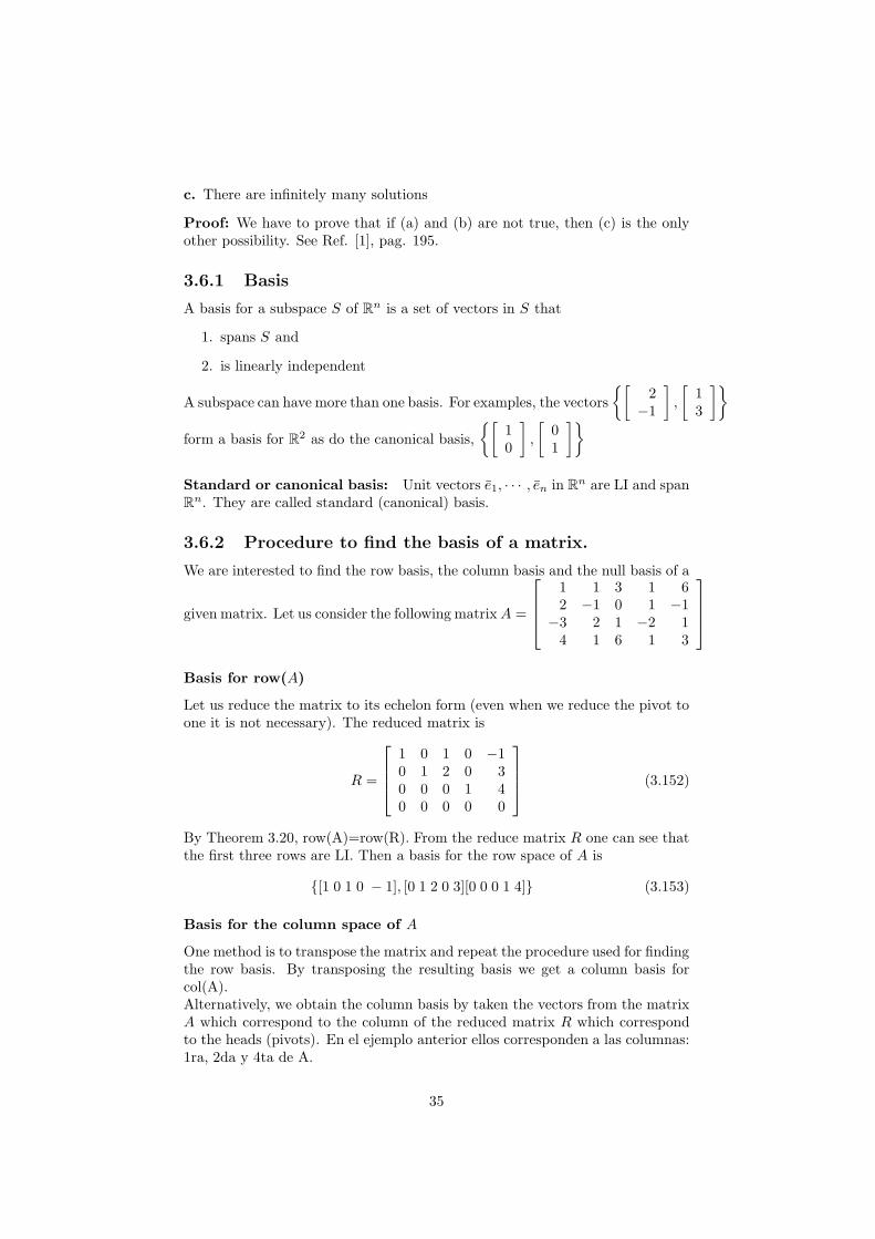
Proof: We have to prove that if (a) and (b) are not true, then (c) is the onlyother possibility. See Ref. [1], pag. 195.
3.6.1 Basis
A basis for a subspace S of Rn is a set of vectors in S that
1. spans S and
2. is linearly independent
A subspace can have more than one basis. For examples, the vectors
{[
2−1
]
,
[
13
]}
form a basis for R2 as do the canonical basis,
{[
10
]
,
[
01
]}
Standard or canonical basis: Unit vectors e1, · · · , en in Rn are LI and spanRn. They are called standard (canonical) basis.
3.6.2 Procedure to find the basis of a matrix.
We are interested to find the row basis, the column basis and the null basis of a
given matrix. Let us consider the following matrixA =
1 1 3 1 62 −1 0 1 −1
−3 2 1 −2 14 1 6 1 3
Basis for row(A)
Let us reduce the matrix to its echelon form (even when we reduce the pivot toone it is not necessary). The reduced matrix is
R =
1 0 1 0 −10 1 2 0 30 0 0 1 40 0 0 0 0
(3.152)
By Theorem 3.20, row(A)=row(R). From the reduce matrix R one can see thatthe first three rows are LI. Then a basis for the row space of A is
{[1 0 1 0 − 1], [0 1 2 0 3][0 0 0 1 4]} (3.153)
Basis for the column space of A
One method is to transpose the matrix and repeat the procedure used for findingthe row basis. By transposing the resulting basis we get a column basis forcol(A).Alternatively, we obtain the column basis by taken the vectors from the matrixA which correspond to the column of the reduced matrix R which correspondto the heads (pivots). En el ejemplo anterior ellos corresponden a las columnas:1ra, 2da y 4ta de A.
35

The justification of this procedure is as follows: considering the system Ax = 0,the reduction from A to R represents a dependence relation among the columnsof A. Since the elementary row operations do not affect the solution set, if A isrow equivalent to R, the columns of A have the same dependence relationshipsas the columns of R.Let as called ai the columns of A and ri the columns of R. By inspection wefind that
r3 = r1 + 2r2 (3.154)
r5 = −r1 + 3r2 + 4r4 (3.155)
From the previous argument the same relation exist for the columns of A (verifythis)
a3 = a1 + 2a2 (3.156)
a5 = −a1 + 3a2 + 4a4 (3.157)
and then the columns a1, a2, a4 form a basis for the col(A),
12
−34
,
1−121
,
11
−21
(3.158)
Notice that col(A) and col(R) do not expand the same space (see this byinspection). Then col(A)6=col(R) which implies that r1, r2, r4 can no be a basisfor col(A), i.e. elementary row operations change the column space.
Basis for the null space
We have to find the solution of the homogeneous system Ax = 0 from the
augmented matrix of A, [A|0] =
1 1 3 1 6 02 −1 0 1 −1 0
−3 2 1 −2 1 04 1 6 1 3 0
From the previous calculation we have
[R|0] =
1 0 1 0 −1 00 1 2 0 3 00 0 0 1 4 00 0 0 0 0 0
(3.159)
then,
x1 + x3 − x5 = 0 (3.160)
x2 + 2x3 + 3x5 = 0 (3.161)
x4 + 4x5 = 0 (3.162)
Since the leading 1s are in columns 1, 2 and 4, we solve for x1, x2 and x4. Letus renamed x3 = s and x5 = t, then,
x =
x1
x2
x3
x4
x5
= s
−1−2100
+ t
1−30
−41
(3.163)
36
Then, the vectors
−1−2100
,
1−30
−41
(3.164)
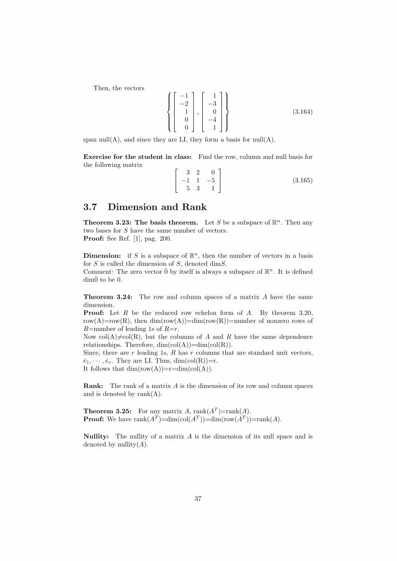
span null(A), and since they are LI, they form a basis for null(A).
Exercise for the student in class: Find the row, column and null basis forthe following matrix
3 2 0−1 1 −55 3 1
(3.165)
3.7 Dimension and Rank
Theorem 3.23: The basis theorem. Let S be a subspace of Rn. Then anytwo bases for S have the same number of vectors.Proof: See Ref. [1], pag. 200.
Dimension: if S is a subspace of Rn, then the number of vectors in a basisfor S is called the dimension of S, denoted dimS.Comment: The zero vector 0 by itself is always a subspace of Rn. It is defineddim0 to be 0.
Theorem 3.24: The row and column spaces of a matrix A have the samedimension.Proof: Let R be the reduced row echelon form of A. By theorem 3.20,row(A)=row(R), then dim(row(A))=dim(row(R))=number of nonzero rows ofR=number of leading 1s of R=r.Now col(A)6=col(R), but the columns of A and R have the same dependencerelationships. Therefore, dim(col(A))=dim(col(R)).Since, there are r leading 1s, R has r columns that are standard unit vectors,e1, · · · , er. They are LI. Thus, dim(col(R))=r.It follows that dim(row(A))=r=dim(col(A)).
Rank: The rank of a matrix A is the dimension of its row and column spacesand is denoted by rank(A).
Theorem 3.25: For any matrix A, rank(AT )=rank(A).Proof: We have rank(AT )=dim(col(AT ))=dim(row(AT ))=rank(A).
Nullity: The nullity of a matrix A is the dimension of its null space and isdenoted by nullity(A).
37
Theorem 3.26: Rank Theorem IfA is anm×nmatrix, then rank(A)+nullity(A)=n.This theorem rephrasing the Rank Theorem 2.2.Proof: LetR be the reduced row echelon form ofA, and suppose that rank(A)=r.Then R has r leading 1s, so there are r leading variables and n−r free variables inthe solution toAx = 0. Since dim(null(A))=n-r, we have rank(A)+nullity(A)=r+(n-r)=n.
Exercise for the student in class: (Example 3.51, pag. 283) Fin de nul-
lity of the matrices M , MT , N , and NT where M =
2 31 54 73 6
and N =
2 1 −2 −14 4 −3 11 7 1 8
Solution:
• rank(M)=2 ⇒ nullity(M)=2-rank(M)=0;
• rank(MT )=2 ⇒ nullity(MT )=4-rank(MT )=2;
• rank(N)=2 ⇒ nullity(N)=4-rank(N)=2;
• rank(NT )=2 ⇒ nullity(NT )=3-rank(NT )=1.
Theorem 3.27: Fundamental Theorem (FT) of Invertible Matrices.Version 2 of 5 . Let A be an n × n matrix. The following statements areequivalent:
From Version 1
a. A is invertible.
b. Ax = b has a unique solution for every b in Rn.
c. Ax = 0 has only the trivial solution.
d. The reduced row echelon form of A is In.
e. A is a product of elementary matrices.
New statements
f. rank(A)=n
g. nullity(A)=0
h. The column vectors of A are LI
i. The column vectors of A span Rn
j. The column vectors of A form a basis for Rn
k. The row vectors of A are LI
l. The row vectors of A span Rn
38

m. The row vectors of A form a basis for Rn
Proof: See Ref. [1], pag. 204.This theorem is a labor-saving device. Version 1 allowed us to cut in half the
work needed to check that two square matrices are inverses. It also simplifiesthe task of showing that certain sets of vectors are bases for Rn. Indeed, whenwe have a set of n vectors in Rn, that set will be a basis for Rn if either of thenecessary properties of linear independence or spanning set is true.
Example 3.52: Let us checks that the three following vectors from a basisfor R3
123
,
−101
,
497
(3.166)
From (f) or (j) of the FT, the vectors will form a basis if and only if a matrixwith these vectors as its columns (or rows) has rank 3. Making row reductionwe get
1 −1 42 0 93 1 7
→
1 −1 40 2 10 0 −7
(3.167)
then rank(A)=3. Then the original vectors for a basis for R3.
Theorem 3.28: Let A be an m× n matrix. Then
a. rank(ATA)=rank(A)
b. Then n× n matrix ATA is invertible if and only if rank(A)=n.
Proof:(a) Since (ATA) is n× n matrix, it has the same number of columns as A. TheRank Theorem states
rank(A) + nullity(A) = n = rank(ATA) + nullity(ATA) (3.168)
Hence, to show that rank(A)=rank(ATA), it is equivalent to show that
nullity(A) = nullity(ATA) (3.169)
We will do so by establishing that the null spaces of A and AT are the same.To this end, let x be in null(A) so that Ax = 0. Then ATAx = 0, thenxTATAx = xT 0 = 0. Then,
(Ax) · (Ax) = (Ax)T (Ax) = xTATAx = 0 (3.170)
and hence Ax = 0, by theorem 1.2(d). Therefore, x is in null(A), so null(A)=null(ATA),as required.
(b) By the FT, the n×nmatrixATA is invertible if and only if rank(ATA)=n.But, by (a) this is so if and only if rank(A)=n.
39

Theorem 3.29: Let S be a subspace of Rn and let B = {v1, · · · , vk} be abasis for S. For every vector v in S, there is exactly one way to write v as alinear combination of the basis vectors in B:
v = c1v1 + · · ·+ ckvk (3.171)
Proof: See Ref. [1], pag. 206.
Coordinates. Let S be a subspace of Rn and let B = {v1, · · · , vk} be a basisfor S. Let v be a vector in S, and write v = c1v1 + · · ·+ ckvk. Then c1, · · · , ckare called the coordinates of v with respect to B, and the column vector
[v]B =
c1...
ck
(3.172)
is called the coordinate vector of v with respect to B.
Example 3.53 Let E = {e1, e2, e3} be the standard basis for R3. The coordi-
nate vector of v =
274
with respect to the basis E is the same vector:
v =
274
=
200
+
070
+
004
= 2e1 + 7e2 + 4e3 (3.173)
Example 3.54 Let B = {v1, v2} be a basis for R3, where
v1 =
3−15
, v2 =
213
(3.174)
calculate the coordinate vector for the vector w =
0−51
From w = c1v1 + c2v2 we have from the first and second lines
3c1 + 2c2 = 0 (3.175)
−c1 + c2 = −5 (3.176)
then c2 = −3 and c1 = 2. The coordinate vector results [w]B =
[
2−3
]
3.8 Introduction to linear transformation
Matrices can be used to transform vectors, acting as a type of function of theform w = T v. Such matrix transformation leads to the concept of a lineartransformation. We are only interested in transformations that are compatiblewith the vector operations of addition and scalar multiplication.
40

Example: Let A =
1 02 −13 4
v =
[
xy
]
then, we can says that A trans-
form v in R2 into w in R3:
Av =
1 02 −13 4
[
xy
]
=
x2x− y3x+ 4y
= w (3.177)
We denote this transformation by TA, such that
TA
[
xy
]
=
x2x− y3x+ 4y
(3.178)
Transformation: More generally, a transformation (or mapping or function)T from Rn to Rm is a rule that assigns to each vector v in Rn a unique vectorT v in Rm.
Domain-Codomain: The domain of T is Rn, and the codomain of T is Rm.This is indicated by writing T : Rn → Rm.
Image: For a vector v in the domain of T , the vector T (v) in the codomainis called the image of v under (the action of) T .
Range: The set of all possible images T (v) is called the range of T .
Example: For the transformation TA
[
xy
]
=
x2x− y3x+ 4y
we have
• Domain: Rn
• Codomain: Rm
• Image of v: TA(v)
• Range: TA
[
xy
]
= x
123
+y
0−14
then, image is the plane span(v1, v2)=col(A),
i.e. the column space of A (dibujar diagrama) by v1 =
123
, v1 =
0−14
Linear Transformation (LT): A transformation T : Rn → Rm is called alinear transformation if
1. T (u+ v) = T (u) + T (v) for all u and v in Rn and
2. T (cv) = cT (v) for all v in Rn and all scalar c.
41
Example: Let us shows that the transformation TA
[
xy
]
=
x2x− y
3x+ 4y
is
a linear transformation.
Exercise for the student in class: Show that the previous transformationis linear using instead T (au+ bv) = aT (u) + bT (v).
Getting the matrix transformation from a transformation: From the
transformation T
[
xy
]
=
x2x− y
3x+ 4y
we can get a matrix which makes the
same job as the transformation:
T
[
xy
]
=
x2x− y
3x+ 4y
= x
123
+ y
0−14
=
1 02 −13 4
[
xy
]
(3.179)
then, T = TA, where A =
1 02 −13 4
Theorem 3.30: Let A be an m× n matrix. Then the matrix transformationTA : Rn → Rm defined by TA(x) = Ax, with x ∈ Rn is a linear transformation.Prof: Let u and v be vectors in R
n and let c be a scalar. Then
TA(u + v) = A(u+ v) = Au+Av = TAu+ TAv (3.180)
TA(cv) = A(cv) = cAv = cTA(v) (3.181)
Example: 90o counterclockwise rotation. Let R : R2 → R2 be the trans-
formation that rotates each point 90o counterclockwise about the origin (hacer
diagrama). Show that R is a LT: R
[
xy
]
=
[
−yx
]
. Its associate matrix is[
0 −11 0
]
, then R is a matrix transformation and from the Theorem 3.30 R is
a LT.
Exercise for the student in class: The transformation which transformeach point in R
2 into its reflection with respect to x axis (hacer diagrama) is
a LT: F
[
xy
]
=
[
x−y
]
. Its associate matrix is A =
[
1 00 −1
]
, then F is a
matrix transformation and from the Theorem 3.30 F is a LT.
Extracting a single column: Observe that if we multiply a matrix A bystandard basis vectors ei, we obtain the column i of the matrix A:
Ae1 =
a11 a12a21 a22a31 a32
[
10
]
=
a11a21a31
, Ae2 =
a12a22a32
(3.182)
42

Theorem 3.31: Standard matrix Let T : Rn → Rm be a LT. Then T is amatrix transformation (MT). More specifically, T = TA, where A is the m× nmatrix A = [T (e1)|T (e2)| · · · |T (en)].Proof: Let e1, · · · , en be the standard basis vectors in Rn and let x be a vectorin Rn. We can write x = x1e1 + · · ·+ xnen. Then
T (x) = x1T (e1) + · · ·+ xnT (en) (3.183)
because T is a LT. Each term T (ei) is a vector of dimension m. We can interpretthe above product as the product of a matrix with n columns T (ei), then
T (x) = x1T (e1) + · · ·+ xnT (en) (3.184)
= [T (e1)| · · · |T (en)]
x1
...xn
= Ax (3.185)
with A = [T (e1)| · · · |T (en)] a matrix of order m× n called standard matrix ofthe linear transformation T .
Example: Rotation. (Example 3.58, pags. 214-215) Let us build the stan-dard matrix for the rotation about the origin through an angle Rθ: Rθ : R2 →R2.First we apply the transformation to e1 and e2 (hacer diagrama de pag. 215):
Rθ(e1) = Rθ
[
10
]
=
[
cosθsinθ
]
(3.186)
Rθ(e2) = Rθ
[
01
]
=
[
−sinθcosθ
]
, (3.187)
then we build the matrix,
Rθ =
[
cosθ −sinθsinθ cosθ
]
(3.188)
Exercise for the student in class: Applied the rotation transformation tothe 90o counterclockwise rotation and compare with the previous result.
3.8.1 Composition of LT
If T : Rm → Rn and S : Rn → Rp are LT, then we may follow T by S to formthe composition of the two transformations, denoted S ◦T , where the codomainof T and the domain of S must match. The composite transformation S ◦ Tgoes from the domain of T to the codomain of S, S ◦ T : Rm → Rp, with(S ◦ T )(v) = S(T (v)).
Theorem 3.32: Let T : Rm → Rn and S : Rn → R
p be LT. Then S ◦ T :Rm → Rp is a LT with standard matrices given by the product of the standardmatrices of each transformation
[S ◦ T ] = [S][T ] (3.189)
43

where we used the notation [T ] for the standard matrix of the transformationT .Proof: Let [S] = A and [T ] = B with A of dimension p×n and B of dimensionn×m. If v is a vector in Rm, then (mostrar detalles de las dimensiones)
(S ◦T )(v) = S(T (v)) = S(Bv) = A(Bv) = (AB)v = [S][T ]v = [S ◦T ]v (3.190)
Example: (Example 3.60, pag. 218) Let us build the composite transforma-tion S ◦ T for T : R2 → R3 and S : R3 → R4, with
T
[
x1
x2
]
=
x1
2x1 − x2
3x1 + 4x2
(3.191)
S
y1y2y3
=
2y1 + y33y2 − y3y1 − y2
y1 + y2 + y3
(3.192)
We have that the standard matrices are
[T ] =
1 02 −13 4
(3.193)
[S] =
2 0 10 3 −11 −1 01 1 1
(3.194)
then
[S ◦ T ] = [S][T ] =
2 0 10 3 −11 −1 01 1 1
1 02 −13 4
=
5 43 −7
−1 16 3
(3.195)
Then,
(S ◦ T )[
x1
x2
]
=
5 43 −7
−1 16 3
[
x1
x2
]
(3.196)
=
5x1 + 4x2
3x1 − 7x2
−x1 + x2
6x1 + 3x2
(3.197)
Homework: Checks that [S ◦T ]x = S(T (x)). Notice that the left hand side isa matrix product, while the right h.s. are transformations (not matrix product)as defined in (3.191) and (3.192). Make explicit the dimensions in each step.
Lectura Sugerida: Section Robotics, pag. 224. (Explicar)
44

3.8.2 Inverses of LT
Consider the effect of a 90o counterclockwise rotation about the origin R90
followed by a 90o clockwise rotation about the origin R−90. This two trans-formations leave every point in R2 unchanged. Then, (R−90 ◦ R90)(v) = v forevery v in R2. It is also true (R90 ◦ R−90)(v) = v. Then (R−90 ◦ R90)(v) and(R90 ◦R−90) are identity transformation.
Identity transformation: An identity transformation In : Rn → Rn is thetransformation which satisfies In(v) = v for every v in R
n.
Inverse transformation: Let S and T be LT from Rn to Rn. Then S andT are inverse transformation is S ◦ T = In and T ◦ S = In.
Invertible transformation: Due to the symmetry of the definition of inversetransformation we will say that S is the inverse of T and T is the inverse of S.We will say that S and T are invertible.
Standard matrix of the identity transformation: If S and T are inversetransformations, then [S][T ] = [S ◦ T ] = [I] = I where I is the identity matrix.It is also true [T ][S] = [T ◦ S] = [I] = I.
Theorem 3.33: Let T : Rn → Rn be an invertible LT. Then its standardmatrix [T ] is an invertible matrix, and [T−1] = [T ]−1, where [T ]−1 means theinverse of the standard matrix of the transformation T !!.
Example 3.62: Let us find the standard matrix which rotates 60o clockwiseabout the origin from the previous calculated standard matrix Rθ which rotatescounterclockwise about the origin.From the previous example about the rotation transformation we have
[R60] =
[
cos(60) −sin(60)sin(60) cos(60)
]
=
[
12 −
√32√
32
12
]
(3.198)
then (review how to calculate the inverse of 2× 2 matrix)
[R−60] = [([R60])−1] =
[
12 −
√32√
32
12
]−1
=
[
12
√32
−√32
12
]
(3.199)
Homework: Check that [R−60] does what it is expected to do.
No inverse: From the Theorem of inversible matrices if the inverse of a matrixassociate to a transformation has no inverse, then the transformation has noinverse.
45

Exercise for the student in class: Show that the transformation whichprojects onto the x-axis is not invertible.
Solution: it standard matrix is
[
1 00 0
]
. Then rank of this matrix is less than
the number of columns, then, from the Theorem of invertible matrices it isnot invertible. From the inverse of two by two matrix we know that it is notinvertible because its determinant is nil.
46
Chapter 4
Autovalores y autovectores
Credit: This notes are 100% from chapter 4 of the book entitled Linear Al-gebra. A Modern Introduction of David Poole (2006) [1].
4.1 Introduction
For a square matrix A, we ask whether there exist nonzero vectors x such thatAx is just a scalar multiple of x. This is the eigenvalue problem, and it is oneof the most central problems in linear algebra. It has applications thoroughmathematics and in many other fields as well.
Eigenvalue: Let A be an n× n matrix. A scalar λ is called an eigenvalue ofA if there is a nonzero vector x such that Ax = λx. Such a vector x is calledan einvector of A corresponding to λ.
Geometric interpretation: In R2, the eigenvalue equation Ax = λx says
that the vectors Ax and x are parallel. Thus, x is an eigenvector of A if andonly if A transforms x into a parallel vector, i.e. TA(x) is parallel to x, whereTA is the matrix transformation (MT) corresponding to A.
Example: Let us calculate the eigenvalue of A =
[
3 11 3
]
associate to the
eigenvector x =
[
11
]
.
We compute Ax,
Ax =
[
3 11 3
] [
11
]
=
[
44
]
= 4x (4.1)
then λ = 4.
Example 4.2: Let us calculate the eigenvectors of A =
[
1 24 3
]
associate to
the eigenvalue λ = 5.From Ax = λx we have
(A− λI)x = (A− 5I)x = 0 (4.2)
47

This implies we have to compute the null space of the matrix A− 5I,[
1 24 3
]
− 5
[
1 00 1
]
=
[
−4 24 −2
]
→[
−4 2 04 −2 0
]
→[
1 − 12 0
0 0 0
]
(4.3)
then
x1 −1
2x2 = 0 (4.4)
0x1 + 0x2 = 0 (4.5)
Then, any vector of the form
[
t2t
]
is an eigenvector of A with eigenvalue λ = 5
with t in R.
Eigenspace: Let A be an n× n matrix and let λ be an eigenvalue of A. Thecollection of all eigenvectors corresponding to λ, together with the zero vector,is called the eigenspace of λ and is denoted by Eλ.
Example 1: In the previous example 4.2 the eigenspace is E5 = t
[
12
]
Example 2 Let us verifies that λ = 6 is an eigenvalue of A =
7 1 −2−3 3 62 2 2
and find a basis for its eigenspace.First we calculate the null space of A− 6I
A− 6I =
1 1 −2−3 −3 62 2 −4
→
1 1 −20 0 00 0 0
(4.6)
=⇒ x1 + x2 − 2x3 = 0 (4.7)
Then,
E6 =
−x2 + 2x3
x2
x3
=
x2
−110
+ x3
201
(4.8)
= span
−110
,
201
(4.9)
Calculation of eigenvalue for 2 × 2 matrices: How do we find the eigen-value and eigenvector of a matrix if we do not know any of them from the verybeginning?. The key is the observation that λ is an eigenvalue of A if and onlyif the null space of A−λI is nontrivial. For a two-by-two matrix we know fromsection 3.3 that A is invertible if and only if detA is nonzero. We also knowfrom the fundamental theorem (FT) of invertible matrices that a matrix has anontrivial null space if and only if it is noninvertible, hence, if and only if itsdeterminant is zero. Putting these facts together, we see that (for two by twomatrices at least) λ is an eigenvalue of A if and only if
det(A− λI) = 0 (4.10)
48

Application: Find all of the eigenvalues and the corresponding eigenvectos
of the matrix A =
[
3 11 3
]
• First we find the zeros of det(A− λI). They are λ1 = 4, λ2 = 2.
• Next we find the null space of the matrix A − λI separatelly for λ1 andλ2. They are E4 = span([1 1]T ) and E2 = span([−1 1]T ), respectively.
Exercise for the student in class: Find all of the eigenvalues and the
corresponding eigenvectos of the matrix A =
[
4 −12 1
]
Solution: Pending...
4.1.1 Determinants
Tema visto en Algebra II .For any square matrix A = [aij ] of order n, the determinant is the scalar
detA = |A| =n∑
j=1
(−1)j+1 a1j detA1j (4.11)
where Aij , called the (i, j)-minor of A, is the matrix obtained by deleting therow i and column j from A.
Example 4.8: By computing the determinant of A =
5 −3 21 0 22 −1 3
we get:
detA=5.
About the column expansion: The election of the first row is arbitrary.Any column can be use to expand the determinant. But is an even row is usedthen the sing must change consistently. For example, using the second columnthe definition change to
detA = |A| =n∑
j=1
(−1)j a2j detA2j (4.12)
Exercise for the student in class: Apply the above definition to the exam-ple 4.8.
4.1.2 Determinants of n× n Matrices
Cofactor: It is convenient to combine a minor with its plus or minus sign. Tothis end, we define the (i, j)-cofactor of A to be
Cij = (−)i+j detAij (4.13)
49

Theorem 4.1: The Laplace expansion Theorem. The previous definitionof the determinant were done in terms of row expansion. They are also validif we used instead column expansion: The determinant of an n × n matrixA = [aij ], where n ≥ 2, can be computed as (row expansion)
detA = |A| =n∑
j=1
aij Cij (4.14)
and also as (column expansion)
detA = |A| =n∑
i=1
aij Cij (4.15)
Proof: See Ref. [1], pag. 279 (see before the Lemmas from pag. 276.)
Theorem 4.2: The determinant of a triangular matrix is the product of theentries on its main diagonal: detA =
∑ni=1 aii.
Example 4.12: By computing the determinant of A =
2 −3 1 0 40 3 2 5 70 0 1 6 00 0 0 5 20 0 0 0 −1
using columns expansion (for example) we get: detA=-30. While the productof the diagonal give detA = 2× 3× 1× 5× (−1)=-30.
4.1.3 Properties of Determinants
Theorem 4.3: The most efficient way to compute determinants is to use rowreduction. This theorem summarizes the main properties needed in order toused row reduction effectively. Let A = [aij ] be square matrix.
a. If A has a zero row (column), then detA=0.
b. If B is obtained by interchanging two rows (columns) of A, then detB=-detA.
c. If A has two identical rows (columns), then detA=0.
d. If B is obtained by multiplying a row (column) of A by k, then detB=kdetA.
e. If A, B, and C are identical except that the ith row (column) of C is thesum of the ith rows (columns) of A and B, then detC=detA+detB.
f. If B is obtained by adding a multiple of one row (column) of A to anotherrow (column), then detB=detA.
Proof: See Ref. [1], page 269.
50

Example 4.13: Let us calculate the determinant of the matrices A and B,with
A =
2 3 −10 5 3
−4 −6 2
(4.16)
B =
0 2 −4 53 0 −3 62 4 5 75 −1 −3 1
(4.17)
We should get: detA=0 and detB=585.
4.1.4 Determinants of Elementary Matrices
Recalled that an elementary matrix results from performing an elementary rowoperation on an identity matrix. Setting A = In in Theorem 4.3 yields thefollowing theorem.
Theorem 4.4: Let E be an n× n elementary matrix.
a. If E results from interchanging two rows of In, then detE=-1.
b. If E results from multiplying one row of In by k, then detE=k.
c. If E results from adding a multiple of row of In to another row, then detE=1.
Proof: Since detIn=1, applying (b), (d), and (f) of Theorem 4.3 immediatelygives (a), (b), and (c), respectively.
Lemma 4.5: Since that multiplying a matrix B by an elementary matrix onthe left performs the corresponding elementary row operation of B. We canrephrase (b), (d), and (f) of Theorem 4.3 by det(EB)=(detE)(detB).
Theorem 4.6: A square matrix A is invertible if and only if detA 6= 0.Proof: Let A be an n × n matrix and let R be the reduced row echelon formof A, i.e. Er · · ·E1A = R. By taking determinant and applying Lemma 4.5, weget (detEr) · · · (detE1)(detA) = (detR). By Theorem 4.4, the determinantsdetEi are nonzero for all i = 1, · · · , r. Then, detA 6= 0 if and only if detR 6= 0.Now suppose that A is invertible. Then, by the FT of IM, R = In, so detR =1 6= 0. Hence, detA 6= 0 also.Conversely, if detA 6= 0, then detR 6= 0, then R cannot contain a zero row byTheorem 4.3.a. It follows that R must be In, so A is invertible, by the FT.
4.1.5 Determinants and Matrix Operations
This section is about to determine relationships between determinants and someof the basic matrix operations.
Theorem 4.7: If A is an n× n matrix, then
det(kA) = kn detA (4.18)
Proof: Exercise 44.
51

Theorem 4.8: If A and B are n× n matrices, then
det(AB) = (detA)(detB) (4.19)
Proof: See Ref. [1], pag. 272.
Theorem 4.9: If A is invertible, then
det(A−1) =1
detA(4.20)
Proof: See Ref. [1], pag. 273.
Theorem 4.10: For any square matrix A,
det(A) = detAT (4.21)
Proof: Since the rows of AT are the columns of A evaluating detAT by ex-panding along the first row is identical to evaluating detA by expanding alongits first column.
4.1.6 Cramer’s Rule and the Adjoint
The Cramer’s Rule gives a formula for describing the solution of certain systemsof n linear equations in n variables entirely in terms of determinants.
Theorem 4.11: Cramer’s Rule. Let A be an invertible n × n matrix andlet b be a vector in Rn. Then the unique solution x of the system Ax = b isgiven by
xi =det(Ai(b))
detA(4.22)
for i = 1, · · · , n and Ai(b) the matrix obtained by replacing the ith column ofA by b, i.e. Ai(b) = [a1 · · · ai−1 b ai+1 · · · an].Proof: See Ref. [1], pag. 274.
Example 4.16: Let us check that the solution of the following LSE
x1 + 2x2 = 2 (4.23)
−x1 + 4x2 = 1 (4.24)
is x1 = 1, x2 = 0.5, by using the Cramer’s Rule.
Theorem 4.12: Let A be an invertible n× n matrix. Then
A−1 =1
detAadjA (4.25)
where adjA the so called adjoint (or adjugate) matrix of A, defined as [Cji] =[Cij ]
T , with Cij the co-factors defined in (4.13).Proof: See Ref. [1], pag. 275.
52

Example 4.17 Calculates the inverse of the matrix A using the adjoint ma-
trix, with A =
1 2 −12 2 41 3 −3
Solution: the determinant is 2, the cofactors are
C11 = −18 (4.26)
C12 = 10 (4.27)
C13 = 4 (4.28)
C21 = 10 (4.29)
C22 = −2 (4.30)
C23 = −1 (4.31)
C31 = 10 (4.32)
C32 = −6 (4.33)
C33 = −2 (4.34)
then
A−1 =1
detAadjA =
1
2
−18 10 43 −2 −110 −6 −2
T
=
9 − 32 −5
−5 1 3−2 1
2 1
(4.35)
Compare this result with example 3.30
Lemma 4.13: Let A be an n× n matrix. Then
n∑
i=1
a1iC1i = detA =
n∑
i=1
ai1Ci1 (4.36)
Lemma 4.14: Let A be an n×nmatrix and letB be obtained by interchangingany two rows (columns) of A. Then
detB = −detA (4.37)
4.2 Eigenvalues and Eigenvectors of n × n Ma-trices
The eigenvalues of a square matrix A are precisely the solutions λ of the equation
det(A− λI) = 0 (4.38)
Characteristic polynomial/equation: When we expand det(A − λI), weget a polynomial in λ, called the characteristic polynomial of A. The equationdet(A− λI) = 0 is called the characteristic equation of A.
• If A is n× n, its characteristic polynomial will be of degree n.
• According to the Fundamental Theorem of Algebra (Theorem D.4 of theAppendix D of Ref. [1], pag. 668), a polynomial of degree n with real orcomplex coefficients has at most n distinct roots.
53
• Then an n× n matrix with real or complex entries has at most n distincteigenvalues.
Example 4.18: Find the eigenvalues and the corresponding eigenspaces of
the matrix A, with A =
0 1 00 0 12 −5 4
.
First we calculates the eigenvalues from det(A− λI). We should get
−λ3 + 4λ2 − 5λ+ 2 = 0 (4.39)
Using the Rational Roots Theorem (Theorem D.3 in page 665 in theAppendixD of Ref. [1]) we get λ1 = λ2 = 1 and λ3 = 2.
Some details about the Rational Roots Theorem: Let f(x) = anxn + · · · +
a1x+ a0 be a polynomial with integer coefficients and a/b be a rational numberwritten in lowest terms (???). If a/b is a zero of f(x), then a0 is a multiple ofa and an is a multiple of b. In our case we would have
2 = ka (4.40)
−1 = k′b (4.41)
the values for k and k′ which give a and b integers are k = 1, 2 and k′ = 1.Then the possible values of a which are multiples of a0 are a = ±2,±1. Whilefor b = ±1. Then, the possible roots of (4.39) of the form a/b are
a
b= ±2,±1 (4.42)
The next step is just try each one of the a/b possibility.
Second we find the eigenvectors by finding the null space of the matrix A−λiIfor each eigenvalue.
Using row reduction for λ = 1 we get
[A− I|0] =
−1 1 0 00 −1 1 02 −5 3 0
→
1 0 −1 00 1 −1 00 0 0 0
(4.43)
Then,x1 − x3 = 0x2 − x3 = 0
(4.44)
Then, the eigenvectors u for λ = 1 are
u =
ttt
(4.45)
with t in R.The eigenspase E1 is
E1 =
t
111
= span
111
(4.46)
54

Similarly for λ = 2 we get
[A− 2I|0] =
−2 1 0 00 −2 1 02 −5 2 0
→
1 0 − 14 0
0 1 − 12 0
0 0 0 0
(4.47)
Then,x1 − 1
4x3 = 0x2 − 1
2x3 = 0(4.48)
Then, the eigenvectors v for λ = 2 are
v =
14 t12 tt
(4.49)
with t in R.The eigenspase E3 is
E3 =
t
14121
= span
124
(4.50)
Algebraic multiplicity: The algebraic multiplicity of an eigenvalue is themultiplicity as a root of the characteristic equation. Thus, λ = 1 has algebraicmultiplicity 2 and λ = 2 has algebraic multiplicity 1: (λ − 1)2(λ− 2).
Geometric multiplicity: The geometric multiplicity of an eigenvalue λ isthe dimension of its eigenspace, i.e. dim(Eλ).
Exercise for the student in class (Example 4.19): Find all of the eigen-
values and the corresponding eigenvectors of the matrix A =
−1 0 13 0 −31 0 −1
.
Solution:
• λ1 = λ2 = 0, span
010
,
101
Notice that any linear combination of eigenvectors {v1, · · · , vk} of a giveneigenspace Eλ is also an eigenvector of the matrix A with the same eigen-value λ, since
Ax = A(c1v1 + · · ·+ ckvk) (4.51)
= c1Av1 + · · ·+ ckAvk (4.52)
= c1λv1 + · · ·+ ckλvk (4.53)
= λ(c1v1 + · · ·+ ckvk) (4.54)
Ax = λx (4.55)
• λ3 = −2, span
−131
55

In terms of the multiplicity we have
• The algebraic multiplicity of λ = 0 is 2 and its geometric multiplicity isalso 2.
• The algebraic multiplicity of λ = −2 is 1 and its geometric multiplicity isalso 1.
Theorem 4.15: The eigenvalues of a triangular matrix are the entries on itsmain diagonal.
Theorem 4.16: A square matrix A is invertible if and only if 0 is not aneigenvalue of A.Proof: Let A be a square matrix. By Theorem 4.6, A is invertible if and onlyif detA 6= 0. But detA 6= 0 is equivalent to det(A − 0I) 6= 0, which says that 0is not a root of the characteristic equation of A, i.e. 0 is not and eigenvalue ofA.
Theorem 4.17: Fundamental Theorem (FT) of Invertible Matrices.Version 3 of 5 Let A be an n × n matrix. The following statements areequivalent:
From Version 1
a. A is invertible.
b. Ax = b has a unique solution for every b in Rn.
c. Ax = 0 has only the trivial solution.
d. The reduced row echelon form of A is In.
e. A is a product of elementary matrices.
From Version 2
f. rank(A)=n
g. nullity(A)=0
h. The column vectors of A are LI
i. The column vectors of A span Rn
j. The column vectors of A form a basis for Rn
k. The row vectors of A are LI
l. The row vectors of A span Rn
m. The row vectors of A form a basis for Rn
New statements
n. detA 6= 0
o. 0 is not an eigenvalue of A
Proof: The equivalence (a)⇔(n) is Theorem 4.6. Theorem 4.16 proves (a)⇔(o).
56

Theorem 4.18: Let A be a square matrix with eigenvalue λ and correspondingeigenvector x.
a. For any positive integer n, λn is an eigenvalue of An with correspondingeigenvector x.
b. If A is invertible, the 1/λ is an eigenvalue of A−1 with corresponding eigen-vector x.
c. For any integer n (la diferencia con el punto (a) es que pedıa que n seapositivo), λn is an eigenvalue of An with corresponding eigenvector x.
Proof: See Ref. [1], pag. 293.
Application of the theorem 4.18: Calculate the action of A3 in the vector
u with, A =
[
0 12 1
]
and u =
[
51
]
.
The strategy consist in expanding the vector u in the basis (if it exist)generated by the eigenspaces of the eigenvalues of A.
Then, we first calculate the eigenvalues and get λ1 = −1 and λ2 = 2, with
eigenvectors v1 =
[
1−1
]
and v2 =
[
12
]
, respectively.
Next, we express the given vector u as linear combination of the eigenvectorsv1 and v2:
u = c1v1 + c2v2 (4.56)
which gives for the coefficients: c1 = 3 and c2 = 2.Finally, we apply the matrix A3 and use the fact that it is a linear operator
and that vi are eigenvectors of A,
A3u = A3(3v1) +A3(2v2) (4.57)
= 3λ31v1 + 2λ3
1v2 (4.58)
= 3(−1)3v1 + 2(2)3v2 (4.59)
= −3v1 + 16v2 (4.60)
= −3
[
1−1
]
+ 16
[
12
]
(4.61)
=
[
1335
]
(4.62)
This result should be the same that the one obtained by multiplying three timesthe matrix A with it self and the resulting matrix multiplied by the vector u.Check it!. You will need the explicit matrix A3 below.
Theorem 4.19: Suppose the n × n matrix A has eigenvectors v1, · · · , vmwith corresponding eigenvalues λ1, · · · , λm. If x is a vector in R
n that can beexpressed as a linear combination of these eigenvectors,
x = c1v1 + · · ·+ cmvm (4.63)
then, for any integer k,
Akx = c1λk1 v1 + · · ·+ cmλk
mvm (4.64)
57

Theorem 4.20: Let A be an n × n matrix and let λ1, · · · , λm be distincteigenvalues of A with corresponding eigenvectors v1, · · · , vm. Then v1, · · · , vmare LI.Proof: See Ref. [1], pag. 295.
4.3 Similarity and Diagonalization
Triangular and diagonal matrices expose their eigenvalues explicitly. We wishto relate a given matrix with its triangular or diagonal form. Since the Gausselimination does not preserve the eigenvalue of the matrix another procedure iscalled for. This is the goal of this section.
4.3.1 Similar Matrices
Let A and B be n × n matrices. We say that A is similar to B if there is aninvertible n× n matrix P such that
P−1AP = B (4.65)
and writeA ∼ B (4.66)
Remarks:
• If A ∼ B, we can write, equivalently, that A = PBP−1 or AP = PB.
• Similarity is a relation on square matrices.
• There is a direction (or order) implicit in the definition of similarity. Weshould not assume that A ∼ B implies B ∼ A (even when it is true) sinceit does not follow immediately from the definition.
• The matrix P depends on A and B.
• The matrix P is not unique for a given pair of similar matrices A andB. For example, if A = B = I then I ∼ I for any invertible matrix P ,because P−1IP = P−1P = I.
Theorem 4.21: Equivalence relation. Any relation satisfying the followingthree properties is called an equivalence relation. Let A, B and C be n × nmatrices,
a. A ∼ A
b. If A ∼ B, then B ∼ A.
c. If A ∼ B and B ∼ C, then A ∼ C.
Proof:
a. I−1AI = A
b. If A ∼ B, then P−1AP = B ⇒ A = PBP−1. Let us renamed Q = P−1,then Q−1BQ = A, so B ∼ A.
c. Exercise 30.
58

Theorem 4.22: Let A and B be n× n matrices with A ∼ B. Then
a. detA = detB
b. A is invertible if and only if B is invertible.
c. A and B have the same rank
d. A and B have the same characteristic polynomial.
e. A and B have the same eigenvalues.
Proof: See Ref. [1], pag. 299.
Remarks:
1. Two matrices may have properties (a) through (e) (and more) in commonand yet still not be similar.
2. Theorem 4.22 is most useful in showing that two matrices are not similar,since A and B cannot be similar if any of properties (a) through (e) fails.
Example of the remark 1: Be A =
[
1 00 1
]
and B =
[
1 10 1
]
:
a. detA = detB = 1
b. A and B both are invertible
c. rankA = rankB = 2
d. The characteristic polynomial of A and B is the same: (1− λ)2
e. The eigenvalues of A and B are the same: λ1 = λ2 = 1
But, P−1AP = P−1P (since A = I), then P−1AP = I 6= B for any invertiblematrix P .
Example of the remark 2: The following two matrices have the samedeterminant and rank but they have not the same characteristic polynomial.
A =
[
1 32 2
]
and B =
[
1 13 −1
]
:
• Characteristic polynomial of A: λ2 − 3λ− 4.
• Characteristic polynomial of B: λ2 − 4.
Check it!
4.3.2 Diagonalization
The best possible situation is when a square matrix is similar to a diagonalmatrix. Whether a matrix is diagonalizable is closely related to the eigenvaluesand eigenvectors of the matrix. This is the topic of this section.
An n×n matrix A is diagonalizable if there is a diagonal matrix D such thatA ∼ D, i.e. if there is an invertible n×n matrix P such that P−1AP = D. Theentries of the matrices D and P are related to the eigenvalues and eigenvectors,respectively of A.
59

Theorem 4.23: Let A be an n × n matrix. Then A is diagonalizable if andonly if A has n linearly independent eigenvectors.More precisely, there exist an invertible matrix P and a diagonal matrix D suchthat P−1AP = D is and only if the columns of P are n LI eigenvectors of Aand the diagonal entries of D are the eigenvalues of A corresponding to theeigenvectors in P in the same order.Proof: See Ref. [1], pag. 301.
Example 1 of the Theorem 4.23: The matrix A =
0 1 00 0 12 −5 4
has only
two LI eigenvectors (it was calculate previously, see Example 4.18). Therefore,A is not diagonalizable
Example 2 of the Theorem 4.23: The matrix A =
−1 0 13 0 −31 0 −1
has
three LI (check it!) eigenvectors (it was calculate previously, see example 4.19)with eigenvalues λ1 = λ2 = 0 and λ3 = −2:
p1 =
010
, p2 =
101
, p3 =
−131
(4.67)
If we take
P = [p1 p2 p3] =
0 1 −11 0 30 1 1
(4.68)
then P is invertible (find the inverse!). Furthermore,
P−1AP =
0 0 00 0 00 0 −2
=
λ1 0 00 λ2 00 0 λ3
= D (4.69)
About the order in P and D: The eigenvectors can be placed into thecolumns of P in any order. However, the eigenvalues will come up on thediagonal of D in the same order as their corresponding eigenvectors in P .
Theorem 4.24: Let A be an n × n matrix and let λ1, · · · , λk be distincteigenvalues of A. If Bi is a basis for the eigenspace Eλi , then B = B1 ∪ · · · ∪ Bk
is LI.Proff: See Ref. [1], pag. 303.
Example of Theorem 4.24: In the ’Example 2 of the Theorem 4.23’ abovewe were asked to demonstrate the independence of the three eigenvectors p1, p2, p3.It was unnecessarily since,
• p1, p2 is a basis for the eigenspace Eλ=0 and Eλ=0, then they are LI
• p3 is a basis for the eigenspace Eλ=−2
• Then, from Theorem 4.24 the vectors which result from the union of Eλ=0
and Eλ=−2 are LI.
60
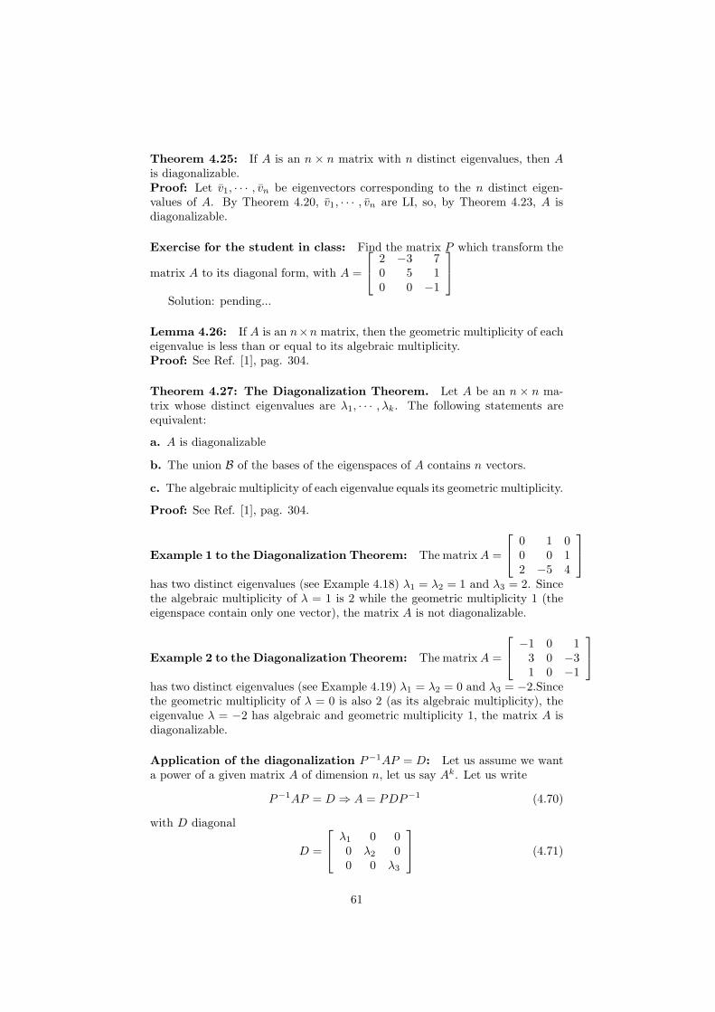
Theorem 4.25: If A is an n × n matrix with n distinct eigenvalues, then Ais diagonalizable.Proof: Let v1, · · · , vn be eigenvectors corresponding to the n distinct eigen-values of A. By Theorem 4.20, v1, · · · , vn are LI, so, by Theorem 4.23, A isdiagonalizable.
Exercise for the student in class: Find the matrix P which transform the
matrix A to its diagonal form, with A =
2 −3 70 5 10 0 −1
Solution: pending...
Lemma 4.26: If A is an n×n matrix, then the geometric multiplicity of eacheigenvalue is less than or equal to its algebraic multiplicity.Proof: See Ref. [1], pag. 304.
Theorem 4.27: The Diagonalization Theorem. Let A be an n× n ma-trix whose distinct eigenvalues are λ1, · · · , λk. The following statements areequivalent:
a. A is diagonalizable
b. The union B of the bases of the eigenspaces of A contains n vectors.
c. The algebraic multiplicity of each eigenvalue equals its geometric multiplicity.
Proof: See Ref. [1], pag. 304.
Example 1 to the Diagonalization Theorem: The matrixA =
0 1 00 0 12 −5 4
has two distinct eigenvalues (see Example 4.18) λ1 = λ2 = 1 and λ3 = 2. Sincethe algebraic multiplicity of λ = 1 is 2 while the geometric multiplicity 1 (theeigenspace contain only one vector), the matrix A is not diagonalizable.
Example 2 to the Diagonalization Theorem: The matrixA =
−1 0 13 0 −31 0 −1
has two distinct eigenvalues (see Example 4.19) λ1 = λ2 = 0 and λ3 = −2.Sincethe geometric multiplicity of λ = 0 is also 2 (as its algebraic multiplicity), theeigenvalue λ = −2 has algebraic and geometric multiplicity 1, the matrix A isdiagonalizable.
Application of the diagonalization P−1AP = D: Let us assume we wanta power of a given matrix A of dimension n, let us say Ak. Let us write
P−1AP = D ⇒ A = PDP−1 (4.70)
with D diagonal
D =
λ1 0 00 λ2 00 0 λ3
(4.71)
61

with λi the eigenvalues of A. Then
A2 = (PDP−1)2 = (PDP−1)(PDP−1) = PD2P−1 (4.72)
in general
Ak = PDkP−1 (4.73)
with
Dk =
λk1 0 00 λk
2 00 0 λk
3
(4.74)
Example: Calculates A3 where A =
[
0 12 1
]
From some previous calculation we know the eigenvalues and eigenvectors:
• λ1 = −1, v1 =
[
1−1
]
• λ2 = 2, v2 =
[
12
]
then
P = [v1 v2] =
[
1 1−1 2
]
(4.75)
and (using the Theorem for the inverse of a 2 by 2 matrix)
P−1 =
[
2 −11 1
]
(4.76)
and
D =
[
−1 00 2
]
(4.77)
The application of A3 = PD3P−1 gives,
A3 =
[
1 1−1 2
] [
(−1)3 00 (2)3
] [
2 −11 1
]
(4.78)
= (pending) (4.79)
Compare the result with the previous calculation of A3.
Application: exponential of a matrix. By analogy with the power series
expansion of ex = 1 + x+ x2
2! + · · · , let us define the exponential of a matrix Ain terms of powers of A,
eA = I +A+A2
2!+ · · · (4.80)
with A an square matrix. It can be shown (it is not demostrated in Ref. [1])that the series converges for any real matrix A.
62
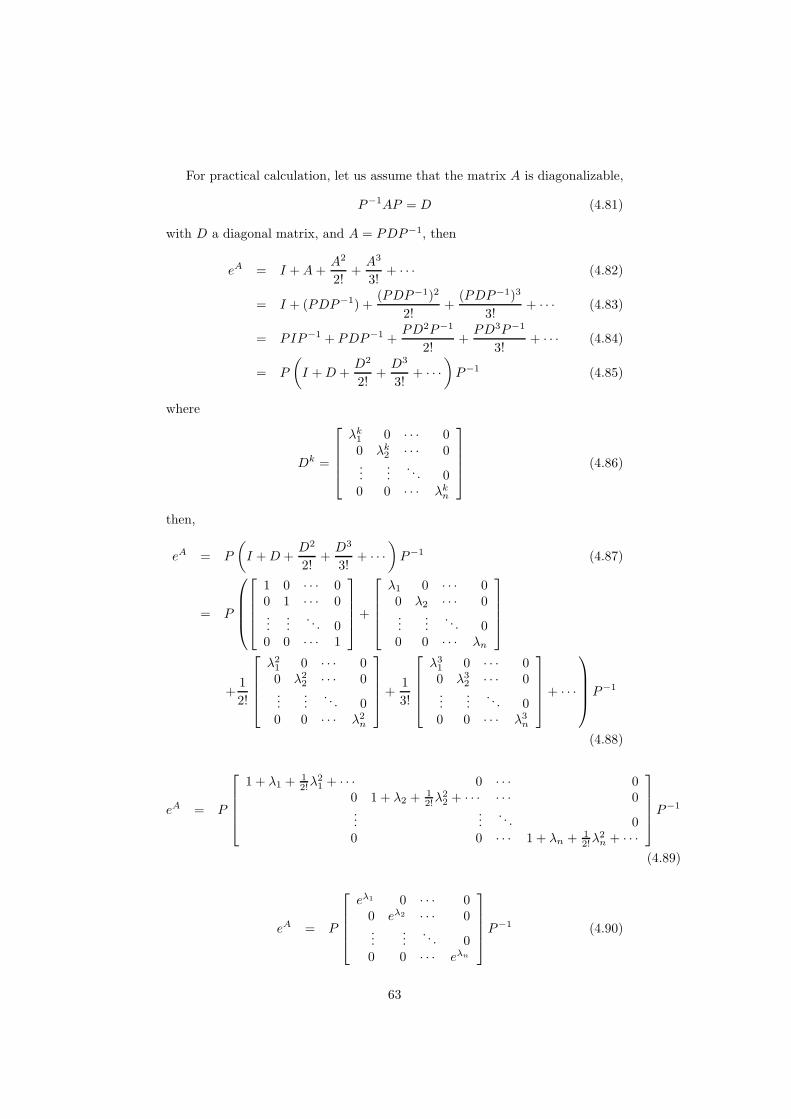
For practical calculation, let us assume that the matrix A is diagonalizable,
P−1AP = D (4.81)
with D a diagonal matrix, and A = PDP−1, then
eA = I +A+A2
2!+
A3
3!+ · · · (4.82)
= I + (PDP−1) +(PDP−1)2
2!+
(PDP−1)3
3!+ · · · (4.83)
= PIP−1 + PDP−1 +PD2P−1
2!+
PD3P−1
3!+ · · · (4.84)
= P
(
I +D +D2
2!+
D3
3!+ · · ·
)
P−1 (4.85)
where
Dk =
λk1 0 · · · 00 λk
2 · · · 0...
.... . . 0
0 0 · · · λkn
(4.86)
then,
eA = P
(
I +D +D2
2!+
D3
3!+ · · ·
)
P−1 (4.87)
= P
1 0 · · · 00 1 · · · 0...
.... . . 0
0 0 · · · 1
+
λ1 0 · · · 00 λ2 · · · 0...
.... . . 0
0 0 · · · λn
+1
2!
λ21 0 · · · 00 λ2
2 · · · 0...
.... . . 0
0 0 · · · λ2n
+1
3!
λ31 0 · · · 00 λ3
2 · · · 0...
.... . . 0
0 0 · · · λ3n
+ · · ·
P−1
(4.88)
eA = P
1 + λ1 +12!λ
21 + · · · 0 · · · 0
0 1 + λ2 +12!λ
22 + · · · · · · 0
......
. . . 00 0 · · · 1 + λn + 1
2!λ2n + · · ·
P−1
(4.89)
eA = P
eλ1 0 · · · 00 eλ2 · · · 0...
.... . . 0
0 0 · · · eλn
P−1 (4.90)
63

where λi are the eigenvalues of A and P is the matrix which has as columns theeigenvectors of A in the same order as the eigenvalues is the matrix D.
Computation of matrix exponential for nondiagonalizable matrices requiresthe Jordan normal form (???) of a matrix.
See, also page 343 in Ref. [1].
64

Chapter 5
Ortogonalidad
Credit: This notes are 100% from chapter 5 of the book entitled Linear Al-gebra. A Modern Introduction of David Poole (2006) [1].
5.1 Orthogonality in Rn
In this section, we will generalize the notion of orthogonality or vectors in Rn
from two vectors to sets of vectors. In doing so, we will see that two propertiesmake the standard basis {e1, · · · , en} of Rn easy to work with: (i) any twodistinct vectors in the set are orthogonal and (ii) each vector is a unit vector.
5.1.1 Orthogonal and Orthonormal Sets of Vectors
Orthogonal set: A set of vectors {v1, · · · , vn} in Rn is called orthogonal setif all pairs of distinct vectors in the set are orthogonal-that is, if
vi · vj = 0 (5.1)
whenever i 6= j, for i, j = 1, · · · , k.
Theorem 5.1 If {v1, · · · , vn} is an orthogonal set of nonzero vectors in Rn,then these vectors are LI.Proof: See Ref. [1], pag. 366.
Orthogonal basis: An orthogonal basis for a subspace W of Rn is a basis ofW that is an orthogonal set.
Example 5.3: Find an orthogonal basis for the subspace W of R3 given by
W =
xyz
: x− y + 2z = 0
(5.2)
A basis for W is given by
xyz
=
y − 2zyz
= y
110
+ z
−201
(5.3)
65

but, they are not orthogonal.Let us take one of them,
v =
110
(5.4)
an orthogonal vector w to v must verifies
v · w = vT w = [1 1 0]
xyz
= x+ y = 0 (5.5)
Since w must also belong to the plane W , it must verifies
x− y + 2z = 0 (5.6)
Solving the LSE
x+ y = 0 (5.7)
x− y + 2z = 0 (5.8)
we get y = −x, 2z = −x+ y = −2x ⇒ z = −x, then
w = t
1−1−1
(5.9)
with t in R. Finally,
v =
110
, and w =
1−1−1
(5.10)
form and orthogonal basis for the subspace W with dimension two.
Theorem 5.2: Let {v1, · · · , vk} be an orthogonal basis for a subspace W ofR
n and let w be any vector in W . Then the unique scalars c1, · · · , ck such that
w = c1v1 + · · ·+ ckvk (5.11)
are given by
ci =w · vivi · vi
(5.12)
for i = 1, · · · , k.Proof: Since {v1, · · · , vk} is a basis for W , we known from Theorem 3.29 thatthere are unique scalars c1, · · · , ck such that w = c1v1 + · · ·+ ckvk, then
w · vi = (c1v1 + · · ·+ ckvk) · vi (5.13)
since vj · vi = δjivi · vi results
w · vi = ci(vi · vi) ⇒ ci =w · vivi · vi
(5.14)
66

Orthonormal basis: A set of vectors in Rn is an orthonormal set if it is anorthogonal set of unit vectors. An orthonormal basis for a subspace W of Rn isa basis of W that is an orthonormal set.
Theorem 5.3: Let {q1, · · · , qk} be an orthonormal basis for a subspace W ofRn and let w be any vector in W . Then
w = (w · q1)q1 + · · ·+ (w · qk)qk (5.15)
and this representation is unique.
5.1.2 Orthogonal Matrices
In this section we will examine the properties of matrices whose columns forman orthonormal set.
Theorem 5.4: The columns of an m× n matrix Q form an orthonormal setif and only QTQ = In.Proof: We need to show that (QTQ)ij = δij . Let qi, denote the ith column ofQ. The (i, j) entry of QTQ is the dot product of the ith row of QT and the jthcolumn of Q: (QTQ)ij = qi · qj . Now the columns Q form and orthonormal setif qi · qj = δij = (QTQ)ij .
Orthogonal matrix: An n× n matrix Q whose columns form and orthonor-mal set is called an orthogonal matrix.
Theorem 5.5: A square matrix Q is orthogonal if and only if Q−1 = QT .Proof: By Theorem 5.4, Q is orthogonal if and only if QTQ = In. By Theorem3.13 this is true if and only if Q is invertible and Q−1 = QT .
Exercise for the student in class: Show that the following two matricesare orthogonal and find their inverses:
A =
0 1 00 0 11 0 0
B =
[
cosθ −sinθsinθ cosθ
]
(5.16)
Theorem 5.6: Let Q be an n × n matrix. The following statements areequivalent:
a. Q is orthogonal
b. ‖ Qx ‖=‖ x ‖ for every x in R
c. Qx ·Qy = x · y for every x and y in R
Proof: See Ref. [1], pag. 372.
Theorem 5.7: If Q is an orthogonal matrix, then its rows form an orthonor-mal set.Proof: From Theorem 5.5 Q−1 = QT . Therefore (QT )−1 = (Q−1)−1 = Q =(QT )T so QT is an orthogonal matrix. Thus, the columns of QT -which are therows of Q-form an orthogonal set.
67

Theorem 5.8: Let Q be an orthogonal matrix.
a. Q−1 is orthogonal
b. detQ = ±1
c. If λ is an eigenvalue of Q, the |λ| = 1.
d. If Q1 and Q2 are orthogonal n× n matrices, then so is Q1Q2
Proof: See Ref. [1], pag. 373.
5.2 Orthogonal Complements and Orthogonal
Projections
In this section we will generalize the concepts of normal vector to a plane andwill extend the concept of the projection of one vector onto another.
5.2.1 Orthogonal Complements
A normal vector n to a plane is orthogonal to every vector in that plane. If theplane passes through the origin, then it is a subspace of W of Rn, as is span(n).
Orthogonal Complement: LetW be a subspace of Rn. We say that a vectorv in Rn is orthogonal to W if v is orthogonal to every vector in W . The set ofall vectors that are orthogonal to W is called the orthogonal complement of W ,denoted W⊥,
W⊥ = {v in Rn : v · w = 0 in W} (5.17)
Theorem 5.9: Let W be a subspace of Rn.
a. W⊥ is a subspace of Rn.
b. (W⊥)⊥ = W
c. W ∩W⊥ = {0}
d. If W = span(w1, · · · , wk), then v is in W⊥ if and only if v · wi = 0 for alli = 1, · · · , k
Proof: See Ref. [1], pag. 376.
Theorem 5.10: Let A be an m×n matrix. Then the orthogonal complementof the row space of A is the null space of A
(row(A))⊥ = null(A) (5.18)
and the orthogonal complement of the column space of A is the null space ofAT
(col(A))⊥ = null(AT ) (5.19)
Proof: If x is a vector in Rn, then x is in (row(A))⊥ if and only if x is orthogonalto every row of A. But this is true if and only if Ax = 0, which is equivalent tox being in null(A). To show the second identity we replace A by AT and usethe fact that row(AT ) = col(A).
68

Exercise for the student in class(example 5.10): Consider the subspaceW of R5 spanned by w1, w2 and w3
w1 =
1−3505
, w2 =
−112
−23
, w3 =
0−14
−15
(5.20)
The subspace W is the same as the column space of A, with
A =
1 −1 0−3 1 −15 2 40 −2 −15 3 5
(5.21)
Using W⊥ = (col(A))⊥ = null(AT ), find a basis for W⊥.By reducing
[AT |0] =
1 −3 5 0 5 0−1 1 2 −2 3 00 −1 4 −1 5 0
→
1 0 0 3 4 00 1 0 1 3 00 0 1 0 2 0
(5.22)
then
x1 + 3x4 + 4x5 = 0 (5.23)
x2 + x4 + 3x5 = 0 (5.24)
x3 + 2x5 = 0 (5.25)
then
x =
−3x4 − 4x5
−x4 − 3x5
−2x5
x4
x5
= x4
−3−1010
+ x5
−4−3−201
(5.26)
Then, a basis for W⊥ is
−3−1010
,
−4−3−201
(5.27)
Fundamental subspaces: an m×n matrix A has four subspaces, which arecalled fundamental subspaces:
1. row(A)
2. null(A)
3. col(A)
4. null(AT )
The first two are orthogonal complements in Rn, and the last two are orthogonalcomplements in Rm
69

Transformation between subspaces of A: The m× n matrix A defines aLT from Rn into Rm whose range is col(A). This transformation sends null(A)to 0 in R
m.
Exercise for the student in class(example 5.9): Find the fundamentalsubspaces of the matrix A, with
A =
1 1 3 1 62 −1 0 1 −1
−3 2 1 −2 14 1 6 1 3
(5.28)
Basis for row(A)
By reducing the matrix to its echelon form we get
R =
1 0 1 0 −10 1 2 0 30 0 0 1 40 0 0 0 0
(5.29)
By Theorem 3.20, row(A)=row(R). From the reduce matrix R one can see thatthe first three rows are LI. Then a basis for the row space of A is
{[1 0 1 0 − 1], [0 1 2 0 3][0 0 0 1 4]} (5.30)
Basis for the col(A)
We obtain the column basis by selecting the vectors from the matrix A whichcorrespond to the column of the reduced matrix R which correspond to theheads (pivots). The justification of this procedure is as follows: considering thesystem Ax = 0, the reduction from A to R represents a dependence relationamong the columns of A. Since the elementary row operations do not affectthe solution set, if A is row equivalent to R, the columns of A have the samedependence relationships as the columns of R. Then the columns a1, a2, a4 froma basis for the col(A),
12
−34
,
1−121
,
11
−21
(5.31)
Basis for null(A)
We have to find the solution of the homogeneous system Ax = 0 from the
augmented matrix of A, [A|0] =
1 1 3 1 6 02 −1 0 1 −1 0
−3 2 1 −2 1 04 1 6 1 3 0
70

From the previous calculation we have
[R|0] =
1 0 1 0 −1 00 1 2 0 3 00 0 0 1 4 00 0 0 0 0 0
(5.32)
then,
x1 + x3 − x5 = 0 (5.33)
x2 + 2x3 + 3x5 = 0 (5.34)
x4 + 4x5 = 0 (5.35)
Since the leading 1s are in columns 1, 2 and 4, we solve for x1, x2 and x4. Letus renamed x3 = s and x5 = t, then,
x =
x1
x2
x3
x4
x5
= s
−1−2100
+ t
1−30
−41
(5.36)
Then, the following vectors form a basis for null(A)
−1−2100
,
1−30
−41
(5.37)
Basis for null(AT )
We have to find the solution of the homogeneous system AT x = 0 from theaugmented matrix of A,
[AT |0] =
1 2 −3 4 01 −1 2 1 03 0 1 6 01 1 −2 1 06 −1 1 3 0
→
1 0 0 1 00 1 0 6 00 0 1 3 00 0 0 0 00 0 0 0 0
(5.38)
then,
y1 + y4 = 0 (5.39)
y2 + 6y4 = 0 (5.40)
y3 + 3y4 = 0 (5.41)
then
y =
y1y2y3y4
=
−y4−6y4−3y4
y4
(5.42)
71

Then, the following vectors form a basis for null(AT )
−1−6−31
(5.43)
5.2.2 Orthogonal Projections
Let W be subspace of Rn and let {u1, · · · , uk} be an orthogonal basis for W .For any vector v in Rn, the orthogonal projection of v onto W is defined as
projW (v) =
(
u1 · vu1 · u1
)
u1 + · · ·+(
uk · vuk · uk
)
uk (5.44)
The component of v orthogonal to W is the vector
perpW (v) = v − projW (v) (5.45)
The projW (v) can be written in terms of projections onto single vectors, i.e.one-dimensional subspace, then
projW (v) = proju1(v) + · · ·+ projuk
(v) (5.46)
Geometric interpretation of Theorem 5.2: As a special case of the defi-nition of projW (v) we can give a geometric interpretation to the Theorem 5.2which states that if w is in the subspace W of Rn, which has orthogonal basis{v1, · · · , vk} then
w =
(
v1 · wv1 · v1
)
v1 + · · ·+(
vk · wvk · vk
)
vk (5.47)
= projv1(w) + · · ·+ projvk (w) (5.48)
Thus, w is decomposed into a sum of orthogonal projections onto mutuallyorthogonal one-dimensional subspaces of W .
Comment: The definition above seems to depend on the choice of orthogonalbasis; that is, a different basis {v′1, · · · , v′k} for W we would have a differentprojW (v) and perpW (v). This is not the case.
Exercise for the student in class: Let W be the plane in R3 with equation
x − y + 2z = 0 and let v =
3−12
. Find the orthogonal projection of v onto
W and the component of v orthogonal to W . (this is the same subspace as theExample 5.3)
Orthogonal projection of v onto W
• First we find two vectors which expand the subspace
xyz
=
y − 2zyz
= y
110
+ z
−201
(5.49)
72

Then, the two vectors are
v1 =
110
, v2 =
−201
(5.50)
Since, v1 and v2 are not orthogonal we take one of them and search oneorthogonal include in the plane.
• Next we search for a vector which is orthogonal to v1
0 = v1 · v3 = (v1)T v3 = [1 1 0]
xyz
⇒ x+ y = 0 (5.51)
• Next we make that the found vector belong to the plane x − y + 2z = 0by solving the system
x+ y = 0 (5.52)
x− y + 2z = 0 (5.53)
We get y = −x, 2z = −x+ y = −2x ⇒ z = −x, then
v3 =
1−1−1
(5.54)
In order to compare with Ref. [1] let us take
v3 =
−111
(5.55)
• Now that we have the orthonormal vectors v1 and v3 we project the vectorv in this orthogonal basis
proyW (v) =
(
v1 · vv1 · v1
)
v1 +
(
v3 · vv3 · v3
)
v3 (5.56)
with
v1 · v = 2 (5.57)
v3 · v = −2 (5.58)
v1 · v1 = 2 (5.59)
v3 · v3 = 3 (5.60)
then
proyW (v) =2
2v1 +
−2
3v3 (5.61)
proyW (v) =
110
− 2
3
−111
(5.62)
proyW (v) =
5/31/3−2/3
(5.63)
73

Component of v orthogonal to W
perpW (v) = v − proyW (v) =
3−12
−
5/31/3−2/3
=
4/3−4/38/3
(5.64)
Theorem 5.11: The Orthogonal Decomposition Theorem. Let W bea subspace of Rn and let v be a vector in Rn. Then there are unique vectors wand w⊥ in W⊥ such that
v = w + w⊥ (5.65)
Proof: See Ref. [1], pag. 381.
Example: from the previous example we have
v = w + w⊥ (5.66)
withw = projW (v) (5.67)
andw⊥ = perpW (v) (5.68)
By making the sum we get
w + w⊥ =
5/31/3−2/3
+
4/3−4/38/3
=
9/3−3/36/3
=
3−12
= v (5.69)
Theorem 5.13: If W is a subspace of Rn, then
dimW + dimW⊥ = n (5.70)
Proof: See Ref. [1], pag. 383.
5.3 The Gram-Schmidt Process and the QR Fac-
torization
In this section, we present a simple method for constructing an orthogonal/orthonormalbasis for any subspace of Rn.
5.3.1 The Gram-Schmidt Process
We want to find an orthonormal basis for a subspace W of Rn from an arbitrarybasis {x1, · · · , xk} of W .
74
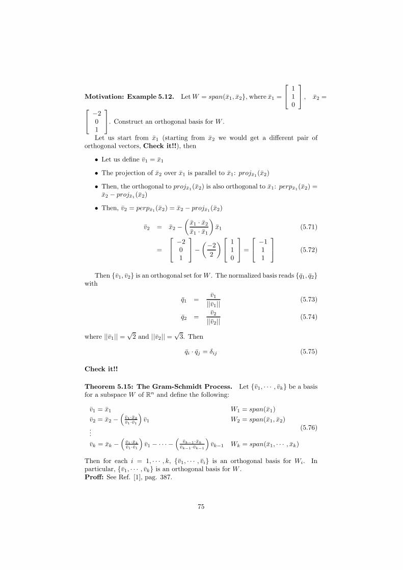
Motivation: Example 5.12. LetW = span(x1, x2}, where x1 =
110
, x2 =
−201
. Construct an orthogonal basis for W .
Let us start from x1 (starting from x2 we would get a different pair oforthogonal vectors, Check it!!), then
• Let us define v1 = x1
• The projection of x2 over x1 is parallel to x1: projx1(x2)
• Then, the orthogonal to projx1(x2) is also orthogonal to x1: perpx1
(x2) =x2 − projx1
(x2)
• Then, v2 = perpx1(x2) = x2 − projx1
(x2)
v2 = x2 −(
x1 · x2
x1 · x1
)
x1 (5.71)
=
−201
−(−2
2
)
110
=
−111
(5.72)
Then {v1, v2} is an orthogonal set forW . The normalized basis reads {q1, q2}with
q1 =v1
||v1||(5.73)
q2 =v2
||v2||(5.74)
where ||v1|| =√2 and ||v2|| =
√3. Then
qi · qj = δij (5.75)
Check it!!
Theorem 5.15: The Gram-Schmidt Process. Let {v1, · · · , vk} be a basisfor a subspace W of Rn and define the following:
v1 = x1 W1 = span(x1)
v2 = x2 −(
v1·x2
v1·v1
)
v1 W2 = span(x1, x2)
...
vk = xk −(
v1·xk
v1·v1
)
v1 − · · · −(
vk−1·xk
vk−1·vk−1
)
vk−1 Wk = span(x1, · · · , xk)
(5.76)
Then for each i = 1, · · · , k, {v1, · · · , vi} is an orthogonal basis for Wi. Inparticular, {v1, · · · , vk} is an orthogonal basis for W .Proff: See Ref. [1], pag. 387.
75

Comments related to Theorem 5.15
• Theorem states that every subspace of Rn has an orthogonal basis and itgives an algorithm for constructing such a basis.
• If we require an orthonormal basis we normalize the orthogonal vectorsproduced by the Gram-Schmidt Process. That is, for each i, we replacevi by the unit vector qi = vi/||vi||.
Exercise for the student in class (Example 5.13): Apply the Gram-Schmidt Process (starting from x1) to construct an orthonormal basis for thesubspace W = span(x1, x2, x3) of R
4, where
x1 =
1−1−11
, x2 =
2101
, x3 =
2212
(5.77)
Solution:
• First we must check that x1, x2, x3 are LI. In this case they are LI.
• If They are not, we through away any of LD vectors.
• Next we apply the GS procedure. We should get
v1 = x1 (5.78)
v2 = x2 −(
v1 · x2
v1 · v1
)
v1 =
3/23/21/21/2
(5.79)
Let us use a scale v′2 = 2v2
v3 = x3 −(
v1 · x3
v1 · v1
)
v1 −(
v′2 · x3
v′2 · v′2
)
v′2 =
−1/20
1/21
(5.80)
Let us use a scale v′3 = 2v3.Then, an orthogonal basis for W is {v1, v′2, v′3}.
76

• Finally we normalize the basis vectors. We should get
q1 =v1
||v1||=
1/2−1/2−1/21/2
(5.81)
q2 =v′2
||v′2||=
3√5/10
3√5/10√5/10√5/10
(5.82)
q3 =v′3
||v′3||=
−√6/60√6/6√6/3
(5.83)
5.3.2 The QR Factorization
If A is an m × n (m ≥ n) matrix with linearly independent columns ai, withi = 1, · · · , n, then applying the Gram-Schmidt Process to theses columns yieldsorthonormal vectors qi, with i = 1, · · · , n. From Theorem 5.15, for each i =1, · · · , n,
Wi = span(a1, · · · , ai) = span(q1, · · · , qi) (5.84)
Therefore, there are scalars r1i, · · · , rii such that
ai = r1iq1 + · · ·+ riiqi (5.85)
for each i = 1, · · · , n. That is,
a1 = r11q1 (5.86)
a2 = r12q1 + r22q2 (5.87)
... (5.88)
an = r1nq1 + · · ·+ rnnqn (5.89)
in matrix form it read,
A = [a1 · · · an] = [q1 · · · qn]
r11 r12 · · · r1n0 r22 · · · r2n...
.... . .
...0 0 · · · rnn
= QR (5.90)
where Q is a matrix m× n which has orthonormal columns
Q = [q1|q2| · · · |qn] (5.91)
and R is an invertible (see Exercise 23, pag. 392 in Ref. [1]) upper triangularmatrix n× n with non zero diagonal entries,
R =
r11 r12 · · · r1n0 r22 · · · r2n...
.... . .
...0 0 · · · rnn
(5.92)
77

Theorem 5.16: The QR Factorization. Let A be an m × n matrix withlinearly independent columns. Then A can be factored as A = QR, where Qis an m × n matrix with orthonormal columns and R is an invertible uppertriangular matrix.
Exercise for the student in class (Example 5.15): Find a QR factoriza-tion of
A =
1 2 2−1 1 2−1 0 11 1 2
(5.93)
Solution:
• First we identify the columns of A with vector
x1 =
1−1−11
, x2 =
2101
, x3 =
2212
(5.94)
• Next we check if the are LI
• Next we orthonormalized these vectors. I was done in the previous exam-ple:
q1 =v1
||v1||=
1/2−1/2−1/21/2
(5.95)
q2 =v′2
||v′2||=
3√5/10
3√5/10√5/10√5/10
(5.96)
q3 =v′3
||v′3||=
−√6/60√6/6√6/3
(5.97)
• Next, we build the matrix Q with these orthonormal vectors.
Q = [q1|q2|q3] (5.98)
=
1/2 3√5/10 −
√6/6
−1/2 3√5/10 0
−1/2√5/10
√6/6
1/2√5/10
√6/6
(5.99)
• Finally, we calculate the R matrix from
A = QR ⇒ QTA = R (5.100)
78

It should gives,
R =
2 1 1/2
0√5 3
√5/2
0 0√6/2
(5.101)
5.4 Orthogonal Diagonalization of Symmetric Ma-
trices
A square matrix with real entries will not necessarily have real eigenvalues. Wealso found that not all square matrices are diagonalizable. The situation changesdramatically if we restrict our attention to real symmetric matrices (A = AT ).
Orthogonally Diagonalizable Matrix: A square matrix A is orthogonallydiagonalizable if there exist an orthogonal matrix Q and a diagonal matrix Dsuch that QTAQ = D.
Theorem 5.17: If A is orthogonally diagonalizable, then A is symmetric.Proof: If A is orthogonally diagonalizable, then there exist an orthogonal ma-trix Q and a diagonal matrix D such that QTAQ = D. Since Q−1 = QT , wehave QTQ = I = QQT , so
QDQT = QQTAQQT = IAI = A (5.102)
But thenAT = (QDQT )T = QDQT = A ⇒ AT = A (5.103)
Theorem 5.18: If A is a real symmetric matrix, then the eigenvalues of Aare real.Proof: See Ref. [1], pag. 398.
Theorem 5.19: If A is a symmetric matrix, then any two eigenvectors corre-sponding to distinct eigenvalues of A are orthogonal.Proof: See Ref. [1], pag. 399.
Theorem 5.20: The (real) Spectral Theorem. Let A be an n × n realmatrix. Then A is symmetric if and only if it is orthogonally diagonalizable.Proof: See Ref. [1], pag. 399.
Exercise for the student in class (Example 5.18): Orthogonally diago-
nalize the matrix A =
1 1 11 2 11 1 2
Solution:
• First we calculate the eigenvalue from det(A−λI). We should get λ1 = 4and λ2 = 1
79

• Next we calculate the eigenvectors for each eigenvalue from the homoge-neous solution (A− λiI)v = 0, for i = 1, 2. We should get
E4 = span
111
(5.104)
E1 = span
−101
,
−110
(5.105)
• Since the two eigenvectors of λ = 1 are not orthogonal we apply theGram-Schmidt method starting from the first eigenvector. We should get
−1/21
−1/2
(5.106)
• Next we normalized the three orthogonal eigenvectors and build the or-thogonal matrix Q. We should get
Q =
1/√3 −1/
√2 −1/
√6
1/√3 0 2/
√6
1/√3 1/
√2 −1/
√6
(5.107)
• Finally we make the matrix products. We should get
QTAQ =
4 0 00 1 00 0 1
(5.108)
which is the usual matrix D build from the eigenvalues!.
Spectral Decomposition. The Spectral Theorem allows us to write a realsymmetric matrix A in the form
A = QDQT (5.109)
where Q is orthogonal form by the eigenvectors of A as columns and D isdiagonal form by the eigenvalues of A in the same order as the eigenvectors inQ,
A = QDQT (5.110)
= [q1 · · · qn]
λ1 · · · 0...
. . ....
0 · · · λn
qT1...
qTn
(5.111)
= [λ1q1 · · · λnqn]
qT1...
qTn
(5.112)
= λ1q1qT1 + · · ·+ λnqnq
Tn (5.113)
80

This is called the spectral decomposition of A. Each of the terms λiqiqTi is
a rank 1 matrix, by Exercise 56 in Section 3.5, and qiqTi is the matrix of the
projection onto the subspace spanned by qi. (See Exercise 25, pag. 405). Forthis reason, the spectral decomposition
A = λ1q1qT1 + · · ·+ λnqnq
Tn (5.114)
is sometimes referred to as the projection form of the Spectral Theorem.
Application: Example 5.20. Find a 2 × 2 matrix with eigenvalues λ1 = 3and λ2 = −2 and corresponding eigenvalues
v1 =
[
34
]
, v2 =
[
−43
]
(5.115)
Solution
• Firs we normalized the eigenvectors
q1 =
[
3/54/5
]
, q2 =
[
−4/53/5
]
(5.116)
• Next we compute qiqTi for i = 1, 2. We should get
q1qT1 =
[
9/25 12/2512/25 16/25
]
(5.117)
q2qT2 =
[
16/25 −12/25−12/25 9/25
]
(5.118)
• Finally we compute the matrix A in its spectral decomposition. We shouldget
A = λ1q1qT1 + λ2q2q
T2 (5.119)
=
[
−1/5 12/512/5 6/5
]
(5.120)
5.5 Applications
5.5.1 Quadratic Forms
A quadratic from is x, y (and z) is a sum of terms, each of which has totaldegree two in the variables, i.e. ax2 + by2(+cz2) + dxy(+exz + fyz) in 2 (or 3)variables.
Quadratic forms can be represented using matrices
ax2 + by2 + cxy = [x y]
[
a c/2c/2 b
] [
xy
]
(5.121)
and
ax2+by2+cz2+dxy+exz+fyz = [x y z]
a d/2 e/2d/2 b f/2e/2 f/2 c
xyz
(5.122)
81
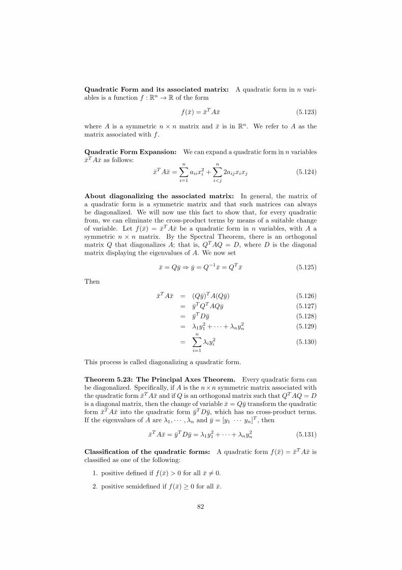
Quadratic Form and its associated matrix: A quadratic form in n vari-ables is a function f : Rn → R of the form
f(x) = xTAx (5.123)
where A is a symmetric n × n matrix and x is in Rn. We refer to A as thematrix associated with f .
Quadratic Form Expansion: We can expand a quadratic form in n variablesxTAx as follows:
xTAx =
n∑
i=1
aiix2i +
n∑
i<j
2aijxixj (5.124)
About diagonalizing the associated matrix: In general, the matrix ofa quadratic form is a symmetric matrix and that such matrices can alwaysbe diagonalized. We will now use this fact to show that, for every quadraticfrom, we can eliminate the cross-product terms by means of a suitable changeof variable. Let f(x) = xTAx be a quadratic form in n variables, with A asymmetric n × n matrix. By the Spectral Theorem, there is an orthogonalmatrix Q that diagonalizes A; that is, QTAQ = D, where D is the diagonalmatrix displaying the eigenvalues of A. We now set
x = Qy ⇒ y = Q−1x = QT x (5.125)
Then
xTAx = (Qy)TA(Qy) (5.126)
= yTQTAQy (5.127)
= yTDy (5.128)
= λ1y21 + · · ·+ λny
2n (5.129)
=
n∑
i=1
λiy2i (5.130)
This process is called diagonalizing a quadratic form.
Theorem 5.23: The Principal Axes Theorem. Every quadratic form canbe diagonalized. Specifically, if A is the n×n symmetric matrix associated withthe quadratic form xTAx and if Q is an orthogonal matrix such that QTAQ = Dis a diagonal matrix, then the change of variable x = Qy transform the quadraticform xTAx into the quadratic form yTDy, which has no cross-product terms.If the eigenvalues of A are λ1, · · · , λn and y = [y1 · · · yn]T , then
xTAx = yTDy = λ1y21 + · · ·+ λny
2n (5.131)
Classification of the quadratic forms: A quadratic form f(x) = xTAx isclassified as one of the following:
1. positive defined if f(x) > 0 for all x 6= 0.
2. positive semidefined if f(x) ≥ 0 for all x.
82
3. negative defined if f(x) < 0 for all x 6= 0.
4. negative semidefined if f(x) ≤ 0 for all x.
5. indefinite if f(x) takes on both positive and negative values.
Classification of symmetric matrices: A symmetric matrix A is calledpositive defined, positive semidefined, negative define, negative semidefined, orindefinite if the associated quadratic form f(x) = xTAx has the correspondingproperty.
Theorem 5.24: Let A be an n × n symmetric matrix. The quadratic formf(x) = xTAx is
a. positive definite if and only if all of the eigenvalues of A are positive.
b. positive semidefinite if and only if all of the eigenvalues of A are nonnegative.
c. negative definite if and only if all of the eigenvalues of A are negative.
d. negative semidefinite if and only if all of the eigenvalues of A are nonpositive.
e. indefinite if and only if A has both positive and negative eigenvalues.
Theorem 5.25: Let f(x) = xTAx be a quadratic form with associated n× nsymmetric matrix A. Let the eigenvalues of A be λ1 ≥ λ2 ≥ · · · ≥ λn. Thenthe following are true, subject to the constrain ||x|| = 1:
a. λ1 ≥ f(x) ≥ λn
b. The maximum value of f(x) is λ1, and it occurs when x is a unit eigenvectorcorresponding to λ1
c. The minimum value of f(x) is λn, and it occurs when x is a unit eigenvectorcorresponding to λn
5.5.2 Graphing Quadratic Equations
Conic sections
The general form of a quadratic equation in two variables is
ax2 + by2 + cxy + dx+ ey + f = 0 (5.132)
where at least one of a, b, and c is nonzero. The graphs of such quadraticequations are called conic sections. They can be obtain by taking cross sectionsof a double cone. The most important of the conic sections are the ellipses(with circles as a special case), hyperbolas, and parabolas. These are callednondegenerate conic. It is also possible for a cross section of a cone to resultin a single point, a straight line, or a pair of lines. These are called degenerateconics.
The graph of a nondegenerate conic is said to be in standard position relativeto the coordinate axes if its equation can be expressed in one of the followingforms:
83

• Ellipse of circle: x2
a2 + y2
b2 = 1; a, b > 0
• Hyperbola: x2
a2 − y2
b2 = 1; a, b > 0 or −x2
a2 + y2
b2 = 1; a, b > 0
• Parabola: y = ax2, a ≷ 0, x = ay2, a ≷ 0.
Other cases
• If a quadratic equation contains too many terms to be written in one ofthe above forms, the its graph is not in standard position. When thereare additional terms but no xy term, the graphs of the conic has beentranslated out of standard position. It can be identify by completing thesquares.
• If a quadratic equation contains a cross-product term, then it representsa conic that has been rotated.
Quadratic surface
The general form of a quadratic equation in three variables is
ax2 + by2 + cz2 + dxy + exz + fyz + gx+ hy + iz + j = 0 (5.133)
where at least one of a, b, · · · , f is nonzero. The graphs of such quadratic equa-tion is called a quadratic surface.
Some quadratic in standard position are
• Ellipsoid: x2
a2 + y2
b2 + z2
c2 = 1
• Hyperboloid: x2
a2 + y2
b2 − z2
c2 = 1
• Hyperboloid of two sheets: x2
a2 + y2
b2 − z2
c2 = −1
• Elliptic cone: z2 = x2
a2 + y2
b2
• Elliptic paraboloid: z = x2
a2 + y2
b2
• Hyperbolic paraboloid: z = x2
a2 − y2
b2
A quadratic graph that have been translated out of standard position canbe identify using the complete-the-squares method.
84

Chapter 6
Espacios vectoriales
Credit: This notes are 100% from chapter 6 of the book entitled Linear Al-gebra. A Modern Introduction of David Poole (2006) [1].
6.1 Vector Spaces and Subspaces
In this section we define generalized “vectors” that arise in a wide variety ofexamples.
Vector space: Let V be a set on which two operations, called addition andscalar (by scalar we will usually mean the real numbers) multiplication, havebeen defined. If u and v are in V , the sum of u and v is denoted by u+ v, andif c is a scalar, the scalar multiple of u by c is denoted by cu. If the followingaxioms hold for all u, v and w in V and for all scalars c and d, then V is calleda vector space and its elements are called vectors.
1. u+ v is in V . Closure under addition
2. u+ v=v + u. Commutativity
3. (u+ v) + w = u+ (v + w). Associativity
4. There exists and element 0 in V , called a zero vector, such that u+0 = u.
5. For each u in V , there is an element - u in V such that u+ (−u) = 0.
6. cu is in V . Closure under scalar multiplication
7. c(u+ v) = cu+ cv. Distributivity
8. (c+ d)u = cu+ du. Distributivity
9. c(du = (cd)u
10. 1u = u
85

Comments:
• By “scalar” we will usually mean the real numbers. In this case we referto V as a real vector space (or a vector space over the real numbers). It isalso possible for scalars to be complex numbers or to belong to Zp, wherep is prime. In these cases, V is called a complex vector space or a vectorspace over Zp, respectively.More generally, the scalar can be chosen from any number system in which,roughly speaking, we can add, subtract, multiply, and divide according tothe usual laws of arithmetic. In abstract algebra, such a number systemis called a field.
• The definition of a vector space does not specify what the set V consist of.Neither does it specify what the operations called “addition” and “scalarmultiplication” look like.
• The vector space is defined not only by the set V but also by the operationof addition, multiplication by scalar and the scalar field.
Examples:
• For any n ≥ 1, Rn is a vector space with the usual operations of additionsand scalar multiplication.
• The set of all 2× 3 matrices is a vector space with the usual operations ofmatrix addition and matrix scalar multiplication.
• The set of all m× n matrices Mmn is a vector space with the usual oper-ations of matrix addition and matrix scalar multiplication.
• Let P2 denote the set of all polynomials of degree 2 or less with realcoefficients: p(x) ∈ P2 with p(x) = a0 + a1x+ a2x
2.
• In general, for any n ≥ 0, the set Pn of all polynomials of degree less thanof equal to n, with real coefficients, is a vector space.
• The set P of all polynomials, with real coefficients, is a vector space.
• The set F denote the set of all real-valued functions defined on the realline. If f and g are two such functions and c is a scalar, then f + g andcf are defined by
(f + g)(x) = f(x) + g(x) (6.1)
and(cf)(x) = cf(x) (6.2)
is a vector space.
• The set F [a, b] denote the set of all real-valued functions defined on someclosed interval [a, b] of the real line is a vector space.
• The set Z of integers with the usual operations is not a vector space sinceit does not satisfied the axiom the closure under scalar multiplication, forexample: for 2 ∈ Z, 1
3 (2) /∈ Z.
86

• Let V = R2 with the usual definition of addition but the following defini-tion of scalar multiplication:
c
[
xy
]
=
[
cx0
]
(6.3)
is not a vector space since it fails the axiom 10,
1
[
xy
]
6=[
xy
]
(6.4)
Theorem 6.1: Let V be a vector space, u a vector in V , and c a scalar.
a. 0u = 0
b. c0 = 0
c. (−1)u = −u
d. If cu = 0, then c = 0 or u = 0
Proof: See Ref. [1], pag. 437.
Subtraction: We will write u− v for u+(−v), defining subtraction of vectors.
Linear combination: We will exploit the associativity property of additionto unambiguously write u+v+w for the sum of three vectors and, more generally,c1u1 + c2u2 + · · ·+ cnun for a linear combination of vectors.
Subspace: A subset W of a vector space V is called a subspace of V if W isitself a vector space with the same scalars, addition, and scalar multiplicationas V .
As in Rn, checking to see whether a subset W of a vector space V is asubspace of V involves testing only two of the ten vector space axioms.
Theorem 6.2: Let V be a vector space and let W be a nonempty subset ofV . Then W is a subspace of V if and only if the following conditions hold:
a. If u and v are in W , then u+ v is in W .
b. If u is in W and c is a scalar, then cu is in W
Proof: See Ref. [1], pag. 438.
Examples:
a. The set Pn of all polynomials with degree at most n is a subspace of thevector space P of all polynomials.
b. The symmetric n×n matrices form a subspace W of Mnn, where Mnn is theset of all n× n matrices with the usual operations of matrix addition andmatrix scalar multiplication: Let A and B be in W and let c be a scalar,then (a) (A+B)T = AT +BT = A+B and (b) (cA)T = cAT = cA.
87

c. Let C be the set of all continuous real-valued functions defined on R and letD be the set of all differentiable real-valued functions defined on R. Ithappens that C and D are subspaces of F , the vector space of all real-valued functions defined on R:From calculus, if f and g are continuous functions and c is a scalar, thenf + g and cf are also continuous. Hence, C is closed under addition andscalar multiplication and so is a subspace of F . If f and g are differentiable,then so are f + g and cf , (f + g)′ = f ′+ g′ and (cf)′ = c(f ′). So D is alsoclosed under addition and scalar multiplication, making it a subspace ofF .
Comment: It is a theorem of calculus that every differentiable function iscontinuous. Consequently, D is contained in C, i.e. D ⊂ C, making Da subspace of C. It is also the case that every polynomial function isdifferentiable, so P ⊂ D, and thus P a subspace of D. Then we have thefollowing hierarchy of subspaces of F : P ⊂ D ⊂ C ⊂ F .
d. If V is a vector space, then V is clearly a subspace of itself. The set {0},consisting of only the zero vector, is also a subspace of V , called the zerosubspace. This two subspaces are called trivial subspaces of V .
c. If W is a subspace of a vector space V , then (from Theorem 6.2) W containsthe zero vector {0} of V .
Comment to (c): The above observation is consistent with the fact that linesand planes are subspaces of R3 if and only if the contain the origin. Then,the requirement that every subspace must contain {0} is sometimes usefulin showing that a set is not a subspace.
Exercise for the student in class (Example 6.12): Let S be the set ofall functions that satisfy the differential equation f ′′ + f = 0. Show that S is asubspace of F . This is an example of homogeneous linear differential equation(the solution sets of such equations are always subspaces of F).Solution: It is nonempty, since the nil function satisfied the above differentialequation. We have to demonstrate that (c1f1 + c2f2)
′′ + (c1f1 + c2f2) = 0.
Exercise for the student in class (Example 6.15): Using the informationof then above ’Comment to (c)’ check if W is a subspace of M22, where W isthe set of all 2× 2 matrices of the form
[
a a+ 10 b
]
(6.5)
Exercise for the student in class (Example 6.16): Let W be the set ofall 2 × 2 matrices with determinant 0. Demonstrate that W is not a subspaceof M22. Help: used for testing the properties the matrices
A =
[
1 00 0
]
B =
[
0 00 1
]
(6.6)
88

6.1.1 Spanning Sets
If S = {v1, v2, · · · , vk} is a set of vectors in a vector space V , then the set ofall LC of v1, v2, · · · , vk is called the span of v1, v2, · · · , vk and is denoted byspan(v1, v2, · · · , vk) or span(S). If V = span(S), then S is called a spanningset for V and V is said to be spanned by S.
Exercise for the student in class (Example 6.18): Show that M23 =span(E11, E12, E13, E21, E22, E23), where
E11 =
[
1 0 00 0 0
]
E12 =
[
0 1 00 0 0
]
E13 =
[
0 0 10 0 0
]
(6.7)
E21 =
[
0 0 01 0 0
]
E22 =
[
0 0 00 1 0
]
E23 =
[
0 0 00 0 1
]
(6.8)
Help: you have to show that any 2 × 3 can be written as LC of the above sixmatrices.
Exercise for the student in class (Example 6.21):
a. In M22, found the span of the matrices A, B, and C (defined below)
b. Let X an arbitrary symmetric matrix (defined below), write it in term ofthe above matrices.
A =
[
1 11 0
]
B =
[
1 00 1
]
C =
[
0 11 0
]
(6.9)
X =
[
x yy z
]
(6.10)
Solution: [a] you should find that these matrices span the subspace of symmetricmatrices. [b] you should find that the coefficients in the expansion aA+bB+cCare a = x− z, b = z and c = −x+ y + z.
Theorem 6.3: Let v1, · · · , vk be vectors in a vector space V .
a. span(v1, · · · , vk) is subspace of V
b. span(v1, · · · , vk) is the smallest subspace of V that contains v1, · · · , vk.
Proof: See Ref. [1], pag. 445.
6.2 Linear Independence (LI), Basis, and Di-mension
This section extends the notion of LI, basis, and dimension to general vectorspaces. In most cases, the proof of the theorems carry over in Sections 2.3 and3.5 can be used replacing Rn by the vector space V .
89

6.2.1 Linear Independence (in finite spaces)
A set of vectors v1, · · · , vk in a vector space V is linearly dependent (LD) ifthere are scalars c1, · · · , ck, at least one of which is not zero, such that
c1 v1 + · · ·+ ck vk = 0 (6.11)
A set of vectors that is not LD is said to be linearly independent.
Comment: As in Rn, {v1, · · · , vk} is LI in a vector space V if and only if
c1 v1 + · · ·+ ck vk0 = 0 ⇒ ci = 0 (6.12)
for i = 1, · · · , k.
Example 6.25: Show that the set {1, x, x2, · · · , xn} is LI in Pn:Starting with
n∑
i=0
cixi = c0 + c1x+
n∑
i=2
cixi = 0 (6.13)
we set x = 0 which gives c0 = 0. Then we take the derivative and get
n∑
i=1
cii xi−1 = c1 + c2x+
n∑
i=3
cii xi−1 = 0 (6.14)
and setting again, x = 0, we get c1 = 0. By continuing this process we demon-strate that all ci = 0 and then the set {1, x, x2, · · · , xn} is LI.
Theorem 6.4 (alternative formulation of LD): A set of vectors {v1, · · · , vk}in a vector space V is LD if and only if at least one of the vectors can be ex-pressed as LC of the others.Proof: The proof is identical to that of Theorem 2.5.
Example 6.22: In P2, the set {f1(x), f2(x), f3(x)} where
f1(x) = 1 + x+ x2 (6.15)
f2(x) = 1− x+ 3x2 (6.16)
f3(x) = 1 + 3x− x2 (6.17)
is LD, since f3(x) = 2f1(x)− f2(x)
Exercise for the student in class (Example 6.26): In P2, determinewhether the set {f1(x), f2(x), f3(x)} is LI, where
f1(x) = 1 + x (6.18)
f2(x) = x+ x2 (6.19)
f3(x) = 1 + x2 (6.20)
Help: write c1f1(x) + c2f2(x) + c3f3(x) = 0 and search for the coefficients. Youshould get that is {f1(x), f2(x), f3(x)} is LI.
90
6.2.2 Linear Independence (in infinite spaces)
A set S of vectors in a vector space V is linearly dependent if it containsfinitely many LD vectors.A set of vectors that is not LD is said to be linearly independent.
Example 6.28: In P , shows that S = {1, x, x2, · · · } is LI:Suppose there is a finite subset T of S that is LD. Let xm be the highest powerof x in T and let xn be the lowest power of x in T . Then there are scalarscn, cn+1, · · · , cm = 0, not all zero, such that
m∑
i=n
ci xi = 0 (6.21)
By taking the derivatives we can show that all ci = 0 with i = n, · · · ,m, whichis a contradiction. Hence, S cannot contain finitely many linearly dependentvectors, so it is LI.
6.2.3 Bases
A subset B of a vector space V is a basis for V if
1. B spans V and
2. B is linearly independent
Examples:
• If ei is the ith column of the n× n matrix, the {e1, e2, · · · , en} is a basisfor Rn, called the standard basis for Rn.
• {1, x, x2, · · · , xn} is a basis for Pn, called the standard basis for Pn.
• The set E = {E11, · · · , E1n, E21, · · · , E2n, Em1, · · · , Emn} is a basis forMmn where the matrices Eij are as defined above. E is called the stan-dard basis for Mmn.
Example 6.32: Show that B = {1 + x, x+ x2, 1 + x2} is a basis for P2.Solution: It was already shown that B is LI. Next we must show that there arescalars c1, c2, and c3 such that a+ bx+ cx2 = c1(1+x)+ c2(x+x2)+ c3(1+x2).We built a linear system and show that the range of the matrix is 3 (not needto show only that the solution exist).
6.2.4 Coordinates
The most useful aspect of coordinate vectors is that they allow us to transferinformation form a general vector space to Rn, where we have the tools definesin Rn at our disposal.
Theorem 6.5: Let V be a vector space and let B be a basis for V . For everyvector v in V , there is exactly one way to write v as a LC of the basis vectorsin B.Proof: It is the same as the one of Theorem 3.29.
91

Unique representation: The converse of Theorem 6.5 is also true. That is,if B is a set of vectors in a vector space V with the property that every vectorin V can be written uniquely as a LC of the vectors in B, then B is a basis forV . In this sense, the unique representation property characterizes a basis.
Coordinates: Let B = {v1, · · · , vn} be a basis for a vector space V . Let vbe a vector in V , and write v = c1v1 + cnvn. Then c1, · · · , cn are called thecoordinates of v with respect to B, and the column vector
[v]B =
c1...cn
(6.22)
is called the coordinates vector of v with respect to B.
Example: The coordinate vector of a polynomial p(x) = a0+a1x+ · · ·+anxn
in Pn with respect to the standard basis B = {1, x, · · · , xn} is the vector
[p(x)]B =
a0a1...an
(6.23)
in Rn+1.
Example 6.35: Find the coordinate vectors [p(x)]Bi of p(x) = 2 − 3x + 5x2
with respect to the standard bases B1 = {1, x, x2} and B2 = {x2, x, 1}.
[p(x)]B1=
2−35
(6.24)
[p(x)]B2=
5−32
(6.25)
Exercise for the student in class (Example 6.36): Find the coordinatesvector [A]B of
A =
[
2 −14 3
]
(6.26)
with respect to the standard basis B = {E11, E12, E21, E11, E22} of M22.Solution: you should get:
[A]B =
2−143
(6.27)
92
Theorem 6.6: Let B = {v1, · · · , vn} be a basis for a vector space V . Let uand v be vectors in V and let c be scalar. Then
a. [u+ v]B = [u]B + [v]B
b. [cu]B = c[u]B
Proff: See Ref. [1], pag. 455.
Corollary to the Theorem 6.6: Coordinate vectors preserves lineal combi-nations:
[c1u1 + · · ·+ ckuk]B = c1[u1]B + · · ·+ ck[uk]B (6.28)
Theorem 6.7: Let B = {v1, · · · , vn} be a basis for a vector space V andlet {u1, · · · , uk} be vectors in V . Then {u1, · · · , uk} is LI in V if and only if{[u1]B, · · · , [uk]B} is LI in Rn.Prof ⇒: Assume that {u1, · · · , uk} is LI in V and let
c1[u1]B + · · ·+ ck[uk]B = 0 (6.29)
in Rn, with unknown ci.Using the property from the Corollary above we have
[c1u1 + · · ·+ ckuk]B = 0 (6.30)
this means that the coordinates of the vector c1u1 + · · ·+ ckuk with respect toB are all zero. Explicitly this implies
c1u1 + · · ·+ ckuk = 0v1 + · · ·+ 0vn = 0 (6.31)
Since we assume that {u1, · · · , uk} is LI, the above relation implies thatci = 0 for i = 1, · · · , k, so {[u1]B, · · · , [uk]B} is LI in R
n.The converse implication is left for the student (Exercise 32 in Ref. [1]).
Help: applies similar ideas used above.
Comment: Observe that, in the special case where ui = vi we have
vi = 0v1 + · · ·+ 1 vi + · · ·+ 0vn = 0 (6.32)
so[vi]B = ei (6.33)
and{[v1]B, · · · , [vn]B} = {[e1], · · · , [en]} (6.34)
6.2.5 Dimension:
Dimension is the number of vectors in a basis. Since a vector space can havemore that one basis, we need to show that this definition makes sense.
93

dimV V3 R3
2 Plane through 01 Line through 00 {0}
Theorem 6.8: Let B = {v1, · · · , vn} be a basis for a vector space V .
a. Any set of more than n vectors in V must be LD
b. Any set of fewer than n vectors in V cannot span V .
Proof: See Ref. [1], pag. 456.
The Basis Theorem (Theorem 6.9): If a vector space V has a basis withn vectors, then every basis for V has exactly n vectors.Proof: The proof of Theorem 3.23 also works here. See Ref. [1], pag. 457.
Definitions:
Finite-dimensional: A vector space V is called finite-dimensional if it has abasis consisting of finitely many vectors.
Dimension: The dimension of V , denoted by dimV , is the number of vectorsin a basis for V . The dimension of the zero vector space {0} is defined tobe zero.
Infinite-dimensional: A vector space that has no finite basis is called infinite-dimensional.
Example 6.38: Since the standard basis for Rn has n vectors, dimRn = n.In the case of R3:
• a one-dimensional subspace is span by a non-zero vector, i.e. a line throughthe origin,
• a two-dimensional subspace is spanned by its basis of two LI vectors, i.e.a plane through the origin
• any three LI vectors must span R3.
The subspaces of R3 are now completely classified according to dimension:
Examples:
• The standard basis for Pn contains n+ 1 vectors, so dimPn = n+ 1
• The standard basis for Mmn contains mn vectors, so dimMmn = mn.
• Both P and F are infinite-dimensional, since they each contain the infiniteLI set {1, x, x2, · · · }.
94

Exercise (Example 6.42): Find the dimension of the vector space W ofsymmetric 2× 2 matrices.A symmetric 2× 2 matrix has the form,
[
a11 a12a12 a22
]
= a11
[
1 00 0
]
+ a12
[
0 11 0
]
+ a22
[
0 00 1
]
(6.35)
so W is expanded by the set
S =
{[
1 00 0
]
,
[
0 11 0
]
,
[
0 00 1
]}
(6.36)
If S is LI, then it will be a basis for W . Setting
a
[
1 00 0
]
+ b
[
0 11 0
]
+ c
[
0 00 1
]
=
[
0 00 0
]
(6.37)
we geta = b = c = 0 (6.38)
Hence S is LI and dimW=3.
Comment: The dimension of a vector space V provides with much infor-mation about V and can greatly simplify the work needed in certain types ofcalculations, as the next few theorems and examples illustrate.
Theorem 6.10: Let V be a vector space with dimV =n. Then
a. Any LI set in V contains at most n vectors.
b. Any spanning set for V contains at least n vectors.
c. Any LI set of exactly n vectors in V is a basis for V .
d. Any spanning set for V consisting of exactly n vectors is a basis for V .
e. Any LI set in V can be extended to a basis for V .
f. Any spanning set for V can be reduced to a basis for V .
Proof: See Ref. [1], pag. 459.
Example 6.43: Let us see whether S is a basis for V for the following cases
a. V = P2 and S = {1 + x, 2− x+ x2, 3x− 2x2,−1 + 3x+ x2}.Solution: since dimP = 2+1 = 3 and S contains 4 vectors, S is LD, henceS is not, by Theorem 6.10(a), a basis for P2.
b. V = M22, S =
{[
1 01 1
]
,
[
0 −11 0
]
,
[
1 10 −1
]}
.
Solution: since dimM22 = 2 × 2 = 4 and S contains three vectors, Scannot, by Theorem 6.10(b), span M22. Hence, S is not a basis for M22.
c. V = P2 and S = {1 + x, x+ x2, 1 + x2}.Solution: since dimP = 2 + 1 = 3 and S contains 3 vectors, S will be abasis is they are LI or if it spans P2, by Theorem 6.10(c) or (d). It wasdemonstrated earlier that they are LI, do it again!. Therefore, S is abasis for P2.
95

Theorem 6.11: Let W be a subspace of a finite-dimensional vector space V .Then
a. W is finite-dimensional and dimW ≤dimV .
b. dimW=dimV if and only if W = V .
Proof: See Ref. [1], pag. 460.
6.3 Change of Basis
In many applications, a problem described using one coordinate system may besolved more easily by switching to a new coordinate system.
6.3.1 Introduction
From Theorem 3.29 we known: Let S be a subspace of Rn and let B ={v1, · · · , vk} be a basis for S. For every vector v in S, there is exactly oneway to write v as a linear combination of the basis vectors in B:
v = c1v1 + · · ·+ ckvk (6.39)
After this Theorem we defined coordinates: Let S be a subspace of Rn
and let B = {v1, · · · , vk} be a basis for S. Let v be a vector in S, and writev = c1v1 + · · · + ckvk. Then c1, · · · , ck are called the coordinates of v withrespect to B, and the column vector
[v]B =
c1...
ck
(6.40)
is called the coordinate vector of v with respect to B.Consider the following two different coordinate systems for R2,
• B = {u1, u2} u1 =
[
−12
]
, u2 =
[
2−1
]
• C = {v1, v2} v1 =
[
10
]
, v2 =
[
11
]
The vector r =
[
5−1
]
, can be written in terms of any of these two basis:
r = u1 + 3u2 (6.41)
r = 6v1 − v2 (6.42)
The coordinates of the vector r with respect to B and C are
[r]B =
[
13
]
(6.43)
[r]C =
[
6−1
]
(6.44)
96

We can find the coordinates of one basis in terms of the other with thefollowing procedures (see also Example 6.45). In this case we calculate thecoordinate in the basis C from the coordinates in the basis B by expanding thebasis vectors ui in the basis C,
r =
[
5−1
]
= u1 + 3u2 (6.45)
=
{
−3
[
10
]
+ 2
[
11
]}
+ 3
{
3
[
10
]
− 1
[
11
]}
(6.46)
= {−3v1 + 2v2}+ 3 {3v1 − 1v2} (6.47)
= 6v1 − v2 (6.48)
Hence, we recover the previous result
[r]C =
[
6−1
]
(6.49)
This procedure gives as a systematic way to transform the vector coordinatesfor a given vector from one basis to another by using a matrix transformation(see next section).
6.3.2 Change-of-Basis Matrices
Let us systematized the above procedure. From r = u1 + 3u2, we have
[r]C = [u1 + 3u2]C = [u1]C + 3 [u2]C (6.50)
by Theorem 6.6.Thus,
[r]C = [[u1]C [u2]C ]
[
13
]
(6.51)
The coordinates of ui in the basis C are,
u1 = −3v1 + 2v2 ⇒ [u1]C =
[
−32
]
(6.52)
u2 = 3v1 − v2 ⇒ [u2]C =
[
3−1
]
(6.53)
Then,
[r]C =
[
−3 32 −1
] [
13
]
(6.54)
= P [xB] (6.55)
where P is the matrix whose columns are [u1]C and [u2]C .Luego, si llamamos base vieja a la base B, y base nueva a la base C, la matriz
P transforma los coeficientes de un dado vector de la base vieja a la nueva. Deeste modo si el vector x en la base vieja se excribıa como x = u1 + 3u2, en lanueva se escribira x = c1v1 + c2v2 con
[
c1c2
]
= [r]C = P [xB] =
[
−3 32 −1
] [
13
]
=
[
6−1
]
esto es, x = 6v1 − v2.
97

Change of basis: Let B = {u1, · · · , un} and C = {v1, · · · , vn} be bases fora vector space V . The n× n matrix whose columns are the coordinate vectors[u1]C , · · · , [un]C of the vectors in B with respect to C is denoted by PC←B and iscalled the change-of-basis matrix from B to C. That is,
PC←B = [[u1]C [u2]C · · · [un]C ] (6.56)
Think of B as the “old” basis and C as the “new” basis. Then the columns ofPC←B are just the coordinate vectors obtained by writing the old basis vectorsin terms of the new ones.
Theorem 6.12: Let B = {u1, · · · , un} and C = {v1, · · · , vn} be bases for avector space V and let PC←B be the change-of-basis matrix from B to C. Then
a. PC←B[x]B = [x]C for all x in V .
b. PC←B is the unique matrix P with the property that P [x]B = [x]C for all xin V .
c. PC←B is invertible and (PC←B)−1 = PB←C .
Proof: See Ref. [1], pag. 469.
Comment: A change of basis is a transformation from Rn to itself thatswitches from one coordinate system to another. The transformation PC←Btakes [x]B as an input and returns [x]C as output. While PB←C is the other wayaround. See Fig. 6.1
Figure 6.1: (from Ref. [1])
Exercise (Example 6.46): Find the change-of-basis matrices PC←B andPB←C for the basis B = {1, x, x2} = {u1, u2, u3} and C = {1+x, x+x2, 1+x2} ={v1, v2, v3} of P2. Then find the coordinate vector of p(x) = 1 + 2x − x2 withrespect to C.
98
Solution: Changing to a standard basis is easy, so we start finding the transfor-mation PB←C . The coordinates vectors for C in terms of B are
v1 = 1+ x = u1 + u2 ⇒ [1 + x]B =
110
(6.57)
v2 = x+ x2 = u2 + u3 ⇒[
x+ x2]
B =
011
(6.58)
v3 = 1+ x2 = u1 + u3 ⇒[
x+ x2]
B =
101
(6.59)
Then
PB←C =
1 0 11 1 00 1 1
(6.60)
By direct calculation of the inverse of PB←C or by expressing the vectors inB as a linear combination of vectors in C, we should get (Try this last optionat home)
PC←B =
1/2 1/2 −1/2−1/2 1/2 1/21/2 −1/2 1/2
(6.61)
The coordinate vector of p(x) = 1+2x−x2 with respect to C can be obtainedby observing that the coordinate vector of p(x) with respect to B is
[p(x)]B =
12−1
(6.62)
and then change from one basis to the other using PC←B,
[p(x)]C = PC←B[p(x)]B (6.63)
=
1/2 1/2 −1/2−1/2 1/2 1/21/2 −1/2 1/2
12−1
(6.64)
=
1/2 + 1 + 1/2−1/2 + 1− 1/21/2− 1− 1/2
=
20−1
(6.65)
Exercise for the student in class (Example 6.47): In M22, let B be thebasis {E11, E21, E12, E22} with
E11 =
[
1 00 0
]
E21 =
[
0 00 1
]
E12 =
[
0 10 0
]
E22 =
[
0 00 1
]
and let be C be the basis {A,B,C,D} with
A =
[
1 00 0
]
B =
[
1 10 0
]
C =
[
1 11 0
]
D =
[
1 11 1
]
(6.66)
99

Find the change-of-basis matrix PC←B and verify that [X ]C = PC←B[X ]B for
X =
[
1 23 4
]
Solution: We need to express the matrices Eij in the basis C;
E11 =
[
1 00 0
]
=
[
1 00 0
]
= A ⇒ [E11]C =
1000
(6.67)
E21 =
[
0 01 0
]
=
[
1 11 0
]
−[
1 10 0
]
= C −B = −B + C ⇒ [E21]C =
0−110
E12 =
[
0 10 0
]
=
[
1 10 0
]
−[
1 00 0
]
= B −A = −A+B ⇒ [E12]C =
−1100
E22 =
[
0 00 1
]
=
[
1 11 1
]
−[
1 11 0
]
= D − C = −C +D ⇒ [E12]C =
00−11
The matrix which changes from basis B to C is
PC←B =
1 0 −1 00 −1 1 00 1 0 −10 0 0 1
(6.68)
Finally, verify that [X ]C = PC←B[X ]B for X =
[
1 23 4
]
The coordinate vector of X in the basis B is
X = 1E10 + 3E21 + 2E12 + 4E22 ⇒ [X ]B =
1324
(6.69)
Then,
PC←B[X ]B =
1 0 −1 00 −1 1 00 1 0 −10 0 0 1
1324
(6.70)
=
1 + 0− 2 + 00− 3 + 2 + 00 + 3 + 0− 40 + 0 + 0 + 4
=
−1−1−14
(6.71)
100

This implies that X expanded in the basis C should be given by
X = −1A− 1B − 1C + 4D (6.72)
Let us check this,
−1A− 1B − 1C + 4D = (−1)
[
1 00 0
]
+ (−1)
[
1 10 0
]
+ (−1)
[
1 11 0
]
+ 4
[
1 11 1
]
=
[
−1− 1− 1 + 4 0− 1− 1 + 40 + 0− 1 + 4 0 + 0 + 0 + 4
]
=
[
1 23 4
]
= X (6.73)
Then, it is true.
6.3.3 The Gauss-Jordan Method for Computing a Change-of-Basis Matrix
Finding the change-of-basis matrix to a standard basis is easy and can be doneby inspection. Finding the change-of-basis matrix from a standard basis isalmost as easy, but requires the calculation of a matrix inverse. From theexample 6.46 we have that we can find [p(x)]C from [p(x)]B and PB←C usingGaussian elimination, i.e. row reduction
[PB←C | [p(x)]B] →[
I | (PB←C)−1[p(x)]B]
= [I |PC←B[p(x)]B] = [I | [p(x)]C ]
We now look at a modification of the Gauss-Jordan method that can beused to find the change-of-basis matrix between two nonstandard bases, as inExample 6.47.
Suppose B = {u1, · · · , un} and C = {v1, · · · , vn} are bases for a vector spaceV and PC←B is the change-of-basis matrix from B to C. The ith column of P is
[ui]C =
[
p1i...pni
]
(6.74)
so ui = p1iv1 + · · ·+ pnivn. If E is any basis for V , then
[ui]E = [p1iv1 + · · ·+ pnivn]E = p1i[v1]E + · · ·+ pni[vn]E (6.75)
In matrix form,
[ui]E = [[v1]E · · · [vn]E ]
p1i...
pni
(6.76)
which we can solve by applying Gauss-Jordan elimination to the augmentedmatrix
[[v1]E · · · [vn]E | [ui]E ] (6.77)
There are n such systems of equations to be solved, one for each columnof PC←B but the coefficients matrix [[v1]E · · · [vn]E ] is the same in each case.
101

Hence, we can solve all the systems simultaneously by row reducing the n× 2naugmented matrix
[[v1]E · · · [vn]E | [u1]E ] · · · [un]E ] = [C |B] (6.78)
Since {v1, · · · , vn} is LI, so is {[v1]E · · · [vn]E}, by Theorem 6.7. Therefore,the matrix C whose columns are [v1]E · · · [vn]E has the n× n identity matrix Ifor its reduced row echelon form, by the Fundamental Theorem. If follows thatGauss-Jordan elimination will necessarily produce
[C |B] → [I |P ] (6.79)
whereP = PC←B (6.80)
The above prove the following theorem.
Theorem 6.13: B = {u1, · · · , un} and C = {v1, · · · , vn} be bases for a vectorspace V . Let B = [[u1]E ] · · · [un]E ] and C = [[v1]E · · · [vn]E ], where E is anybasis for V . Then row reduction applied to the n× 2n augmented matrix [C|B]produces
[C |B] → [I |PC←B] (6.81)
If E is a standard basis, this method is particularly easy to use, since in thatcase
B = PE←B (6.82)
and
C = PE←C (6.83)
Example 6.48 Rework Example 6.47 using Gauss-Jordan method.Solution:
B = PE←B =
1 0 0 00 0 1 00 1 0 00 0 0 1
(6.84)
and
C = PE←C =
1 1 1 10 1 1 10 0 1 10 0 0 1
(6.85)
Row reduction produces
[C |B] =
1 1 1 1 1 0 0 00 1 1 1 0 0 1 00 0 1 1 0 1 0 00 0 0 1 0 0 0 1
→
1 0 0 0 1 0 −1 00 1 0 0 0 −1 1 00 0 1 0 0 1 0 −10 0 0 1 0 0 0 1
= [I |PC←B] (6.86)
102

6.4 Linear Transformations
In this section we extend the concept of linear transformation between arbitraryvector spaces. Linear transformation was already introduced in section 3.6 inthe context of matrix transformations from Rn to Rn.
Linear Transformation (LT): A LT from a vector space V to a vector spaceW is a mapping T : V → W such that, for all u and v in V and for all scalars c,
1. T (u+ v) = T (u) + T (v)
2. T (cu) = cT (u)
This definition is equivalent to the requirement that T preserve all linearcombination, i.e. T : V → W is a LT if and only if
T (c1u1 + · · ·+ cnun) = c1T (u1) + · · ·+ cnT (un) (6.87)
for all ui in V and scalars ci with i = 1, · · · , n.
Examples of LT:
• Every matrix transformation is a LT, i.e., if A is an m × n matrix, thenTA : Rn → Rn defined by TA(x) = Ax, with x in Rn is a LT. Show it!!
• The transformation T : Mnn → Mnn defined by T (A) = AT is a LT.Show it!!
• The differential operator D : D → F defined by D(f) = f ′ is a LT. Showit!!
• The integration S : C[a, b] → R defined as S(f) =∫ b
a f(x)dx is a LT.Show it!!
Examples of non LT: Show them!!
1. T : M22 → R defined by T (A) = detA
2. T : R → R defined by T (x) = 2x
3. T : R → R defined by T (x) = x+ 1
Special transformations:
Zero transformation: For any vector spaces V and W , the transformationT0 : V → W that maps every vector V to the zero vector in W is calledzero transformation: T0(v) = 0 for all v in V .
Identity transformation: For any vector space V , the transformation I :V → V that maps every vector in V to itself is called the identity trans-formation: I(v) = v for all v in V .
103

6.4.1 Properties of LT
In chapter 3 of Ref. [1], all LT were matrix transformations, and their proper-ties were directly related to properties of the matrices involved. The followingTheorem is easy to demonstrate for matrices but it takes a bit more care forthe general case.
Theorem 6.14: Let T : V → W be a LT. Then
a. T (0) = 0
b. T (−v) = −T (v) for all v in V .
c. T (u− v) = T (u)− T (v) for all u and v in V .
Proff: See Ref. [1], pag. 479.
Comments:
• Property (a) can be useful in showing that certain transformation is notlinear. For example T (x) = 2x.
• Be warned, however, that there are lots of transformations that do mapthe zero vector to the zero vector but that are still no linear, for exampleT : M22 → R defined by T (A) = detA.
• The most important property of a LT T : V → W is that T is completelydetermined by its effect on a basis for V . The example below shows whatthis means.
Example 6.55: Suppose T is a LT from R2 to P2 such that
T
[
11
]
= 2− 3x+ x2
T
[
23
]
= 1− x2 (6.88)
Find
T
[
−12
]
(6.89)
Procedure:
1. First we expand each vector in the basis B form by the two LI vectors
B =
{[
11
]
,
[
23
]}
(6.90)
2. Then, we find the coefficients of the expansion
3. Finally we use the fact that T is linear.
104

Solution:[
−12
]
= c1
[
11
]
+ c2
[
23
]
⇒ c1 = −7, c2 = 3 (6.91)
then
T
[
−12
]
= −7T
[
11
]
+ 3T
[
23
]
= −7(2− 3x+ x2) + 3(1− x2) = −14 + 21x− 7x2 + 3− 3x2
= −11 + 21x− 10x2 (6.92)
Theorem 6.15: Let T : V → W be a LT and let B = {v1, · · · , vn} be aspanning set for V . Then T (B) = {T (v1), · · · , T (vn)} spans the range of T (seethe definition of range below).
Starts remenmbering from chapter (chapter 3 of Ref. [1]) LinearTransformation...
Transformation: More generally, a transformation (or mapping or function)T from Rn to Rm is a rule that assigns to each vector v in Rn a uniquevector T v in Rm.
Domain-Codomain: The domain of T is Rn, and the codomain of T is Rm.This is indicated by writing T : Rn → Rm.
Image: For a vector v in the domain of T , the vector T (v) in the codomain iscalled the image of v under (the action of) T .
Range: The set of all possible images T (v) is called the range of T .
...Ends remenmbering from chapter (chapter 3 of Ref. [1]) LinearTransformation
Proof: The range of T is the set of all vectors in W that are of the formT (v), where v is in V . Let T (v) be in the range of T . Since B spans V , thereare scalars c1, · · · , cn such that
v = c1v1 + · · ·+ cnvn (6.93)
Applying T and using the fact that it is a LT, we get
T (v) = c1T (v1) + · · ·+ cnT (vn) (6.94)
in other words, T (v) is in spans(T (B)), as required.
Comment to the Theorem 6.15: The Theorem 6.15 applies, in partivular,when B is a basis for V . It could be nice if T (B) would then be a basis for therange of T , but it is not always the case (see section 6.5 in Ref. [1].)
6.4.2 Composition of LT
If T : U → V and S : V → W are LT, then the composition of S with T is themapping S ◦ T , defined by
(S ◦ T )(u) = S(T (u)) (6.95)
where u is in U .
105

Example 6.56: Let T : R2 → P1 and S : P1 → P2 be the LT defined by
T
[
ab
]
= a+ (a+ b)x (6.96)
S(p(x)) = xp(x) (6.97)
find
(S ◦ T )[
3−2
]
(6.98)
We should get 3x+ x2.
Theorem 6.16: If T : U → V and S : V → W are LT, then S ◦ T : U → Wis a LT.Proof: Let u and v be in U and let C be a scalar. Then
(S ◦ T )(u+ v) = S(T (u+ v)) = S(T (u) + T (v)) = S(T (u)) + S(T (v) = (S ◦ T )(u) + (S ◦ T )(v)
and
(S ◦ T )(cu) = S(T (cu)) = S(cT (u)) = cS(T (u)) = c(S ◦ T )(u) (6.99)
6.4.3 Inverses of LT
A LT T : V → W is invertible if there is a LT T ′ : W → V such that
T ′ ◦ T = IV and T ◦ T ′ = IW (6.100)
In this case, T ′ is called an inverse for T .
Remarks:
• The domain V and codomain W of T do not have to be the same, as theydo in the case of invertible matrix transformations. However, we will seein the next section that V and W must be very closed related.
• The requirement that T ′ be linear could have been omitted from thisdefinition. For, as we will see in Theorem 6.24, it T ′ is any mapping fromW to V such that T ′ ◦ T = IV and T ◦ T ′ = IW , then T ′ is forced to belinear as well.
• If T ′ is an inverse for T , then the definition implies that T is a inverse forT ′. Hence, T ′ is invertible to.
Example 6.58: The mapping T : R2 → P1 and T ′ : P1 → R2 are inverses.Where
T
[
ab
]
= a+ (a+ b)x (6.101)
T ′(c+ dx) =
[
cd− c
]
(6.102)
106

Solution:Let us check that T ′ ◦ T = IR2
(T ′ ◦ T )[
ab
]
= T ′(
T
[
ab
])
= T ′(a+ (a+ b)x) =
[
a(a+ b)− a
]
=
[
ab
]
Next, we check that T ◦ T ′ = IP1
(T ◦ T ′)(c+ dx) = T (T ′(c+ dx)) = T
[
cd− c
]
= c+ (c+ (d− c))x = c+ dx
Theorem 6.17: If T is an invertible LT, then its inverse is unique and denotedby T−1.Proof: The proof is the same as that of Theorem 3.6 of Ref. [1], with productsof matrices replaced by compositions of LT (Exercise 31 in Ref. [1].)
Comments about the topic of the next two sections: In the next twosections, we will address the issue of determining when a given LT is invertibleand finding its inverse when it exists.
6.5 The Kernel and Range of a Linear Transfor-mation
This section extends the notion of null space and column space to the kerneland range of a LT.
Kernel: Let T : V → W be a LT. The kernel of T , denoted ker(T ), is the setof all vectors in V that are mapped by T to 0 in W . That is
ker(T ) = {v ∈ V : T (v) = 0} (6.103)
Range: The range of T , denoted range(T ), is the set of all vectors in W thatare images of vectors in V under T . That is,
range(T ) = {T (v) : v ∈ V } (6.104)
= {w ∈ W : w = T (v) for some v ∈ V } (6.105)
Example 6.59: Let A be anm×nmatrix and let T = TA be the correspondingmatrix transformation from Rn to Rm defined by T (v) = Av. Then
• the range of T is the column space of A (see Chapter 3 of Ref. [1].)
• the kernel of T is the null(A)
Exercise (Example 6.60): Find the kernel and range of the differential op-erator D : P3 → P2 defined by D(p(x)) = p′(x).Solution:
107
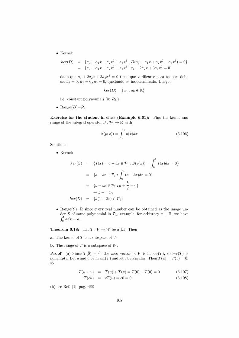
• Kernel:
ker(D) = {a0 + a1x+ a2x2 + a3x
3 : D(a0 + a1x+ a2x2 + a3x
3) = 0}= {a0 + a1x+ a2x
2 + a3x3 : a1 + 2a2x+ 3a3x
2 = 0}
dado que a1 + 2a2x + 3a3x2 = 0 tiene que verificarse para todo x, debe
ser a1 = 0, a2 = 0 , a3 = 0, quedando a0 indeterminado. Luego,
ker(D) = {a0 : a0 ∈ R}
i.e. constant polynomials (in P3.)
• Range(D)=P2
Exercise for the student in class (Example 6.61): Find the kernel andrange of the integral operator S : P1 → R with
S(p(x)) =
∫ 1
0
p(x)dx (6.106)
Solution:
• Kernel:
ker(S) = {f(x) = a+ bx ∈ P1 : S(p(x)) =
∫ 1
0
f(x)dx = 0}
= {a+ bx ∈ P1 :
∫ 1
0
(a+ bx)dx = 0}
= {a+ bx ∈ P1 : a+b
2= 0}
⇒ b = −2a
ker(D) = {a(1− 2x) ∈ P1}
• Range(S)=R since every real number can be obtained as the image un-der S of some polynomial in P1, example, for arbitrary a ∈ R, we have∫ 1
0adx = a.
Theorem 6.18: Let T : V → W be a LT. Then
a. The kernel of T is a subspace of V .
b. The range of T is a subspace of W .
Proof: (a) Since T (0) = 0, the zero vector of V is in ker(T ), so ker(T ) isnonempty. Let u and v be in ker(T ) and let c be a scalar. Then T (u) = T (v) = 0,so
T (u+ v) = T (u) + T (v) = T (0) + T (0) = 0 (6.107)
T (cu) = cT (u) = c0 = 0 (6.108)
(b) see Ref. [1], pag. 488
108

Definitions: Let T : V → W be a LT. Then
Rank: the rank of T is the dimension of the range of T , denoted by rank(T ).
Nullity: The nullity of T is the dimension of the kernel of T and is denoted bynullity(T ).
Example:
• If A is a matrix and T = TA is the matrix transformation defined byT (v) = Av, then the range and kernel of T are the column space and thenull space of A, respectively: rank(T)=rank(A) and nullity(T)=nullity(A)
• The rank and nullity of the LTD(p(x) = p′(x), D : P3 → P2 are: Since therange(D)=P2 (see above) we have rank(D)=dim P2=3. While the kernelof D is the set of all constant polynomials: ker(D)={a : a ∈ R} = {a · 1 :a ∈ R}, hence {1} is a basis for ker(D), son nullity(D)=dim(ker(D))=1.
• The rank and nullity of S : P1 → R with S(p(x)) =∫ 1
0p(x)dx are: since
range(S)=R, then rank(S)=dim(R)=1. The kernel ker(S)={a(1 − 2x) :a ∈ R} = span(1 − 2x), the 1 − 2x is a basis for ker(S). Therefor, nul-lity(S)=dim(ker(S))=1.
The Rank Theorem (Theorem 6.19): Let T : V → W be a LT from afinite-dimensional vector space V into a vector space W . Then
rank(T ) + nullity(T ) = dim(V ) (6.109)
Proof: See Ref. [1], pag. 490.
Examples: Using the information from the above examples we have
• D(p(x) = p′(x), D : P3 → P2
rank(D) + nullity(D) = 3 + 1 = 4 = dim(P3) (6.110)
• S : P1 → R with S(p(x)) =∫ 1
0 p(x)dx
rank(S) + nullity(S) = 1 + 1 = 2 = dim(P1) (6.111)
Exercise (Example 6.67): Find the rank and nullity of the LT T : P2 → P3
define by T (p(x)) = xp(x). (firs check that T is linear)Solution:
ker(T ) = {a+ bx+ cx2 ∈ P2 : T (a+ bx+ cx2) = 0}= {a+ bx+ cx2 : ax+ bx2 + cx3 = 0}
⇒ a = b = c = 0
ker(T ) = {0}
so we have nullity(T)=dim(ker(T))=0. The Rank Theorem implies that
rank(T ) = dim(P2)− nullity(T ) = 3− 0 = 3 (6.112)
109

Exercise for the student in class (Example 6.68): Let W be the vectorspace of all symmetric 2× 2 matrices. Define a LT T : W → P2 by (check thatit is linear)
T
[
a bb c
]
= (a− b) + (b− c)x+ (c− a)x2 (6.113)
Find the rank and nullity of T .Solution: we start calculating the nullity because it is easier that to calculatethe rank:
ker(T ) =
{[
a bb c
]
: T
[
a bb c
]
= 0
}
(6.114)
=
{[
a bb c
]
: (a− b) + (b− c)x+ (c− a)x2 = 0
}
(6.115)
⇒ (a− b) = 0, (b − c) = 0 (c− a) = 0 (6.116)
⇒ a = b, b = c c = a ⇒ a = b = c (6.117)
ker(T ) =
{[
a aa a
]}
= span
([
1 11 1
])
(6.118)
then nullity(T)=dim(ker(T))=1.Finally, from the Rank Theorem: rank(T)=dim W -nullity(T)=3-1=2.
6.5.1 One-to-One and Onto Linear Transformation
This section deals with the criteria for a LT to be invertible.
One-to-one transformation: A LT T : V → W is called one-to-one if Tmaps distinct vectors in V to distinct vectors in W another way to say is
• T : V → W is one-to-one if, for all u and v in V , u 6= v implies thatT (u) 6= T (v) or
• T : V → W is one-to-one if, for all u and v in V , T (u) = T (v) impliesthat u = v
Onto transformation: A LT T : V → W is called onto if range(T)=W.Another way to say it is: T : V → W is onto if, for all w in W , there is at leastone v in V such that w = T (v).
Examples: Let us consider T : R2 → R3 define by
T
[
xy
]
=
2xx− y0
(6.119)
one-to-one : It is one-to-one as we show below. Let
T
[
x1
y1
]
= T
[
x2
y2
]
(6.120)
110
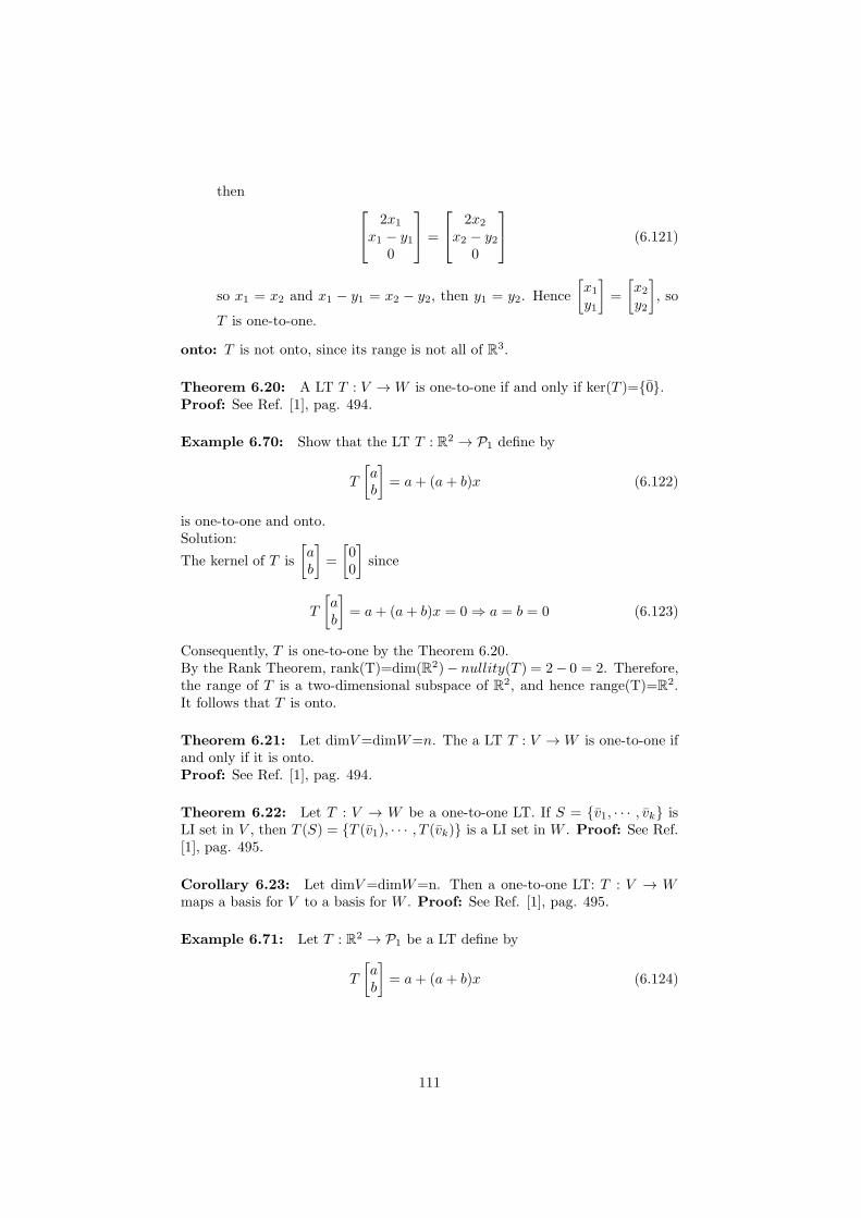
then
2x1
x1 − y10
=
2x2
x2 − y20
(6.121)
so x1 = x2 and x1 − y1 = x2 − y2, then y1 = y2. Hence
[
x1
y1
]
=
[
x2
y2
]
, so
T is one-to-one.
onto: T is not onto, since its range is not all of R3.
Theorem 6.20: A LT T : V → W is one-to-one if and only if ker(T )={0}.Proof: See Ref. [1], pag. 494.
Example 6.70: Show that the LT T : R2 → P1 define by
T
[
ab
]
= a+ (a+ b)x (6.122)
is one-to-one and onto.Solution:
The kernel of T is
[
ab
]
=
[
00
]
since
T
[
ab
]
= a+ (a+ b)x = 0 ⇒ a = b = 0 (6.123)
Consequently, T is one-to-one by the Theorem 6.20.By the Rank Theorem, rank(T)=dim(R2)− nullity(T ) = 2− 0 = 2. Therefore,the range of T is a two-dimensional subspace of R2, and hence range(T)=R2.It follows that T is onto.
Theorem 6.21: Let dimV=dimW=n. The a LT T : V → W is one-to-one ifand only if it is onto.Proof: See Ref. [1], pag. 494.
Theorem 6.22: Let T : V → W be a one-to-one LT. If S = {v1, · · · , vk} isLI set in V , then T (S) = {T (v1), · · · , T (vk)} is a LI set in W . Proof: See Ref.[1], pag. 495.
Corollary 6.23: Let dimV=dimW=n. Then a one-to-one LT: T : V → Wmaps a basis for V to a basis for W . Proof: See Ref. [1], pag. 495.
Example 6.71: Let T : R2 → P1 be a LT define by
T
[
ab
]
= a+ (a+ b)x (6.124)
111

Then, by Corollary 6.23, the standard basis E = {e1, e2} for R2 is mapped to abasis T (E) = {T (e1), T (e2)} of P1. We find that
T (e1) = T
[
10
]
= 1 + (1 + 0)x = 1 + x (6.125)
T (e2) = T
[
01
]
= 0 + (0 + 1)x = x (6.126)
(6.127)
It follows that {1 + x, x} is a basis for P1.
Theorem 6.24: A LT T : V → W is invertible if and only if it is one-to-oneand onto. Proof: See Ref. [1], pag. 496.
6.5.2 Isomorphisms of Vector Spaces
A LT T : V → W is called an isomorphisms if it is one-to-one and onto. If Vand W are two vector spaces such that there is an isomorphism from V to W ,then we say that V is isomorphic to W and write V ∼= W .
Examples: The following vector spaces are isomorphic each other:
• Pn and Rn (think about the definition of coordinates) (Example 6.72 inRef. [1], pag. 497)
• Mmn and Rmn (think about the definition of coordinates) (Example 6.73in Ref. [1], pag. 497)
The easiest way to check if two vector spaces are isomorphic is simply tocheck their dimensions (see the next theorem)
Theorem 6.25: Let V and W be two finite-dimensional vector spaces. ThenV is isomorphic to W if and only if dimV=dimW . Proof: See Ref. [1], pag.498.
Examples:
• Pn and Rn are no isomorphic since, dim(Pn)=n+1 6=dim(Rn)=n.
• The vector space of symmetric matricesM sym22 is isomorphic with R3, since
dim(M sym22 )=dim(R3)=3. (see above previous examples when we calculate
basis in order to determine the dimension of a basis and spaces)
6.6 The Matrix of a Linear Transformation
In this section it is shown that every LT between finite-dimensional vector spacescan be represented as a matrix transformation.Suppose that V is an n-dimensional vector space, W is an m-dimensional vectorspace, ant T : V → W is a LT. Let B and C be bases for V and W , respectively.Then the coordinate vector mapping R(v) = [v]B defines an isomorphism R :
112

V → Rn. At the same time, we have an isomorphism S : W → Rm givenby S(w) = [w]C , which allows us to associate the image T (v) with the vector[T (v)]C in R
m (see Fig. 6.2 Since R is an isomorphism, it is invertible, so we
Figure 6.2: (from Ref. [1])
may form the composite mapping
S ◦ T ◦R−1 : Rn → Rm (6.128)
which maps [v]B to [T (v)]C . Since this mapping goes from Rn to Rm, this is amatrix transformation.
We would like to find the m× n matrix A such that
A[v]B = (S ◦ T ◦R−1)[v]B (6.129)
= [T (v)]C (6.130)
Where the columns of A are the images of the standard basis vectors for Rn
under S ◦ T ◦R−1. But, if B = {v1, · · · , vn} is a basis for V , then
R(vi) = [vi]B (6.131)
=
0...
1...0
(6.132)
= ei (6.133)
soR−1(ei) = vi (6.134)
Therefore, the ith column of the matrix A we seek is given by
(S ◦ T ◦R−1)(ei) = S(T (R−1(ei))) (6.135)
= S(T (vi)) (6.136)
= [T (v)]C (6.137)
which is the coordinate vector of T (v) with respect to the basis C of W .
113

Theorem 6.26: Let V and W be two finite-dimensional vector spaces withbases B and C, respectively, where B = {v1, · · · , vn}. If T : V → W is a LT,then the m× n matrix A defined by
A = [[T (v1)]C | · · · |[T (vn)]C ] (6.138)
satisfies
A[v]B = [T (v)]C (6.139)
for every vector v in V .Where the matrix A is called matrix of T with respect to the bases B
and C. The relationship is illustrated in diagram of fig. 6.3 called commutativediagram,
Figure 6.3: Commutative diagram (from Ref. [1]).
Remarks:
• The matrix of a LT T with respect to bases B and C is sometimes denotedby [T ]C←B
• The matrix of a LT with respect to given basis is unique. That is, for everyvector v in V , there is only one matrix A whit the property specified byTheorem 6.26–namely, A[v]B = [T (v)]C
• The matrix [T ]C←B depends on the order of the vectors in the bases B andC (remember the exercises done earlier)
Exercise (Example 6.76): Let T : R3 → R2 be the LT defined by
T
xyz
=
[
x− 2yx+ y − 3z
]
(6.140)
and let B = {e1, e2, e3} and C = {e2, e1} be bases for R3 and R2, respectively.Find the matrix of T with respect to B and C and verify Theorem 6.26 for
v =
13−2
(6.141)
114

Solution:We want to built the matrix
A = [T ]C←B = [[T (v1)]C | · · · |[T (vn)]C ] (6.142)
For this end we need:
a. First calculate the images T (ei) of the vectors of the basis B
b. Then calculates the coefficient vectors of these images with respect to thebasis C of W
c. Finally, we built the matrix [[T (v1)]C | · · · |[T (vn)]C ]
[a.]
T (e1) =
[
11
]
T (e2) =
[
−21
]
T (e3) =
[
0−3
]
(6.143)
[b.] Be careful with the order of the basis vectors in C!
T (e1) =
[
11
]
=
[
01
]
+
[
10
]
(6.144)
⇒ [T (v1)]C =
[
11
]
(6.145)
T (e2) =
[
−21
]
=
[
01
]
− 2
[
10
]
(6.146)
⇒ [T (v2)]C =
[
1−2
]
(6.147)
T (e3) =
[
0−3
]
= −3
[
01
]
+ 0
[
10
]
(6.148)
⇒ [T (v3)]C =
[
−31
]
(6.149)
[c.]
A = [T ]C←B (6.150)
= [[T (v1)]C | · · · |[T (vn)]C ] (6.151)
=
[
1 1 −31 −2 0
]
(6.152)
In order to verified the Theorem we have to check that the matrix productA[v]B = [v]C . Then we have to calculate
c. The action of T on v and built it coordinate vector T (v) in the bases C
d. Calculate the product of the matrix A = [T ]C←B time the coordinates of thevector v in the basis B: A[v]B
e. Check that (c) and (d) give the same vector
115

[c.]
T (v) = T
13−2
(6.153)
=
[
−510
]
(6.154)
= 10
[
01
]
− 5
[
10
]
(6.155)
⇒ [v]C =
[
10−5
]
(6.156)
[d.]
v =
13−2
(6.157)
=
100
+ 3
010
− 2
001
(6.158)
⇒ [v]B =
13−2
(6.159)
Next,
[T ]C←B[v]B =
[
1 1 −31 −2 0
]
13−2
(6.160)
=
[
10−5
]
(6.161)
[e.] OK!
6.6.1 Matrices of Composite and Inverse Linear Transfor-mations
Theorem 6.27: Let U, V , and W be finite dimensional vector spaces withbases B, C, and D, respectively. Let T : U → V and S : V → W be LT. Then
[S ◦ T ]D←B = [S]D←C[T ]C←B (6.162)
Proof:See Ref. [1], pag. 508.
Example 6.81: Use matrix methods to compute
(S ◦ T )[
ab
]
(6.163)
116
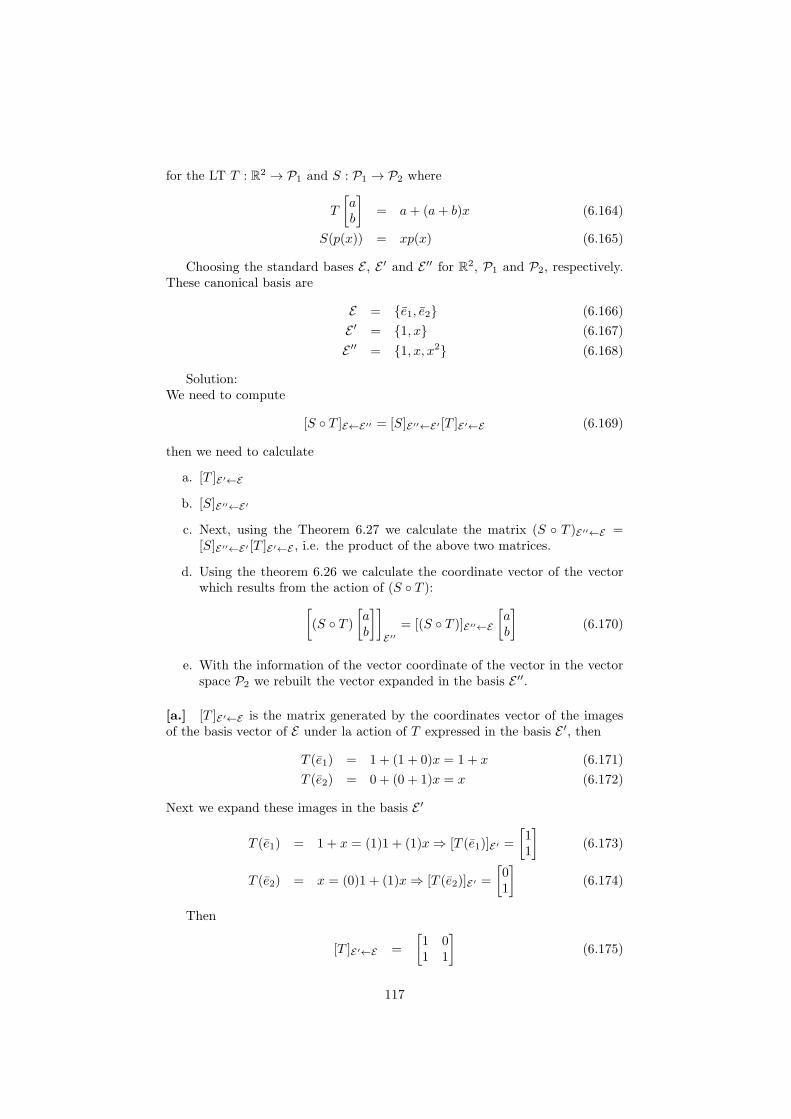
for the LT T : R2 → P1 and S : P1 → P2 where
T
[
ab
]
= a+ (a+ b)x (6.164)
S(p(x)) = xp(x) (6.165)
Choosing the standard bases E , E ′ and E ′′ for R2, P1 and P2, respectively.These canonical basis are
E = {e1, e2} (6.166)
E ′ = {1, x} (6.167)
E ′′ = {1, x, x2} (6.168)
Solution:We need to compute
[S ◦ T ]E←E′′ = [S]E′′←E′ [T ]E′←E (6.169)
then we need to calculate
a. [T ]E′←E
b. [S]E′′←E′
c. Next, using the Theorem 6.27 we calculate the matrix (S ◦ T )E′′←E =[S]E′′←E′ [T ]E′←E , i.e. the product of the above two matrices.
d. Using the theorem 6.26 we calculate the coordinate vector of the vectorwhich results from the action of (S ◦ T ):
[
(S ◦ T )[
ab
]]
E′′= [(S ◦ T )]E′′←E
[
ab
]
(6.170)
e. With the information of the vector coordinate of the vector in the vectorspace P2 we rebuilt the vector expanded in the basis E ′′.
[a.] [T ]E′←E is the matrix generated by the coordinates vector of the imagesof the basis vector of E under la action of T expressed in the basis E ′, then
T (e1) = 1 + (1 + 0)x = 1 + x (6.171)
T (e2) = 0 + (0 + 1)x = x (6.172)
Next we expand these images in the basis E ′
T (e1) = 1 + x = (1)1 + (1)x ⇒ [T (e1)]E′ =
[
11
]
(6.173)
T (e2) = x = (0)1 + (1)x ⇒ [T (e2)]E′ =
[
01
]
(6.174)
Then
[T ]E′←E =
[
1 01 1
]
(6.175)
117

[b.] [S]E′′←E′ is the matrix generated by the coordinates vector of the imaginesof the basis vector of E ′ under la action of S expressed in the basis E ′′, then
S(1) = x(1) = x (6.176)
S(x) = x(x) = x2 (6.177)
Next we expand these images in the basis E ′′
S(1) = x = (0)1 + (1)x+ (0)x2 (6.178)
⇒ [S(1)]E′′ =
010
(6.179)
S(x) = x2 = (0)1 + (0)x+ (1)x2 (6.180)
⇒ [S(x)]E′′ =
001
(6.181)
Then
[S]E′′←E′ =
0 01 00 1
(6.182)
[c.]
(S ◦ T )E′′←E = [S]E′′←E′ [T ]E′←E (6.183)
=
0 01 00 1
[
1 01 1
]
(6.184)
=
0 01 01 1
(6.185)
[d.]
[
(S ◦ T )[
ab
]]
E′′= [(S ◦ T )]E′′←E
[
ab
]
(6.186)
=
0 01 01 1
[
ab
]
(6.187)
=
0a
a+ b
(6.188)
[e.] In the basis
E ′′ = {1, x, x2} (6.189)
118

the vector (S ◦ T )v results,
(S ◦ T )v = (S ◦ T )[
ab
]
(6.190)
= (0)1 + (a)x + (a+ b)x2 (6.191)
= ax+ (a+ b)x2 (6.192)
which is the same result we obtained earlier in the Example 6.56.
Theorem 6.28: Let T : V → W be a LT between n-dimensional vectorspaces V and W and let B and C be bases for V and W , respectively. Then Tis invertible if and only if the matrix [T ]C←B is invertible. In this case,
([T ]C←B)−1
= [T−1]B←C (6.193)
Notice the change in the order of the basis!!Proof: See Ref. [1], pag. 509.
Example 6.82: In Example 6.70, the LT T : R2 → P1 defined by
T
[
ab
]
= a+ (a+ b)x (6.194)
was shown to be one-to-one and onto and hence invertible. Find T−1.Solution:In Example 6.81, we found the matrix of T with respect to the standard basesE and E ′ for R2 and P1, respectively, to be
[T ]E′←E =
[
1 01 1
]
(6.195)
By Theorem 6.28, it follows that the matrix of T−1 with respect to E ′ andE is
[T−1]E←E′ = ([T ]E′←E)−1
(6.196)
=
[
1 01 1
]−1(6.197)
=
[
1 0−1 1
]
(6.198)
By theorem 6.26,
[T−1(a+ bx)]E = [T−1]E←E′ [a+ bx]E′ (6.199)
=
[
1 0−1 1
] [
ab
]
(6.200)
=
[
ab− a
]
(6.201)
From this coordinate vector we can reconstruct the vector using the basis Eof R2
T−1(a+ bx) = ae1 + (b− a)e2 =
[
ab− a
]
(6.202)
Notice that even with the last two vector looks the same they have verydifferent mean, clarified it by yourself!
119

6.6.2 Change of Basis and Similarity
Theorem 6.29: Let V be a finite-dimensional vector space with bases B andC and let T : V → V be a LT. Then
[T ]C = (PB←C)−1[T ]BPB←C (6.203)
Notice that the matrix on the most right is the change-of-basis from C to B!!.Comentario: notar que esto no es el cambio de base del vector v dentro delmismo espacio V , sino como transforma las coordenadas del operador T en dosbases diferentes dentro del mismo espacio V !!!.
Example 6.84 This example is an application of the above Theorem. TheTheorem is used in order to find a basis with respect to which the matrix of LTis diagonal. Let T : R2 → R2 be defined by
T
[
xy
]
=
[
x+ 3y2x+ 2y
]
(6.204)
If possible, find a basis C for R2 such that the matrix of T with respect to C isdiagonal.Solution:
a. First we right the matrix T with respect to the canonical basis E of R2
b. Search for the eigenvalues and eigenvectors
c. Then we define a new basis with the eigenvectors
[a.] For this end, first we calculate the action of T on each vector of thecanonical basis and then we build the matrix [T ]E with the images as columns:
T (e1) = T
([
10
])
=
[
12
]
= (1)e1 + (2)e2 (6.205)
⇒ [T (e1)]E =
[
12
]
(6.206)
T (e2) = T
([
01
])
=
[
32
]
= (3)e1 + (2)e2 (6.207)
⇒ [T (e2)]E =
[
32
]
(6.208)
Then
[T ]E =
[
1 32 2
]
(6.209)
[b.] We search for the eigenvalues and the corresponding eigenvectors and gen-erates the diagonal matrix D and the P in the decomposition [T ]E = P−1DP .We should get
D =
[
4 00 −1
]
(6.210)
P =
[
1 31 −2
]
(6.211)
120

ThenP−1[T ]EP = D (6.212)
[d.] Now we defined a new basis C form by the columns of P , i.e. the eigen-vectors of [T ]E . This implies that P = PE←C , i.e. the change-of-basis matrixfrom C to E ,
PE←C =
[
1 31 −2
]
(6.213)
then
(PE←C)−1[T ]EPE←C = D (6.214)
[T ]C = D (6.215)
so, the matrix T with respect to the basis
C =
{[
11
]
,
[
3−2
]}
(6.216)
is diagonal!!
Diagonalizable Transformation: Let V be a finite-dimensional vector spaceand let T : V → V be a LT. Then T is called diagonalizable if there is a basisC for V such that the matrix [T ]C is a diagonal matrix.
Remark: It is not hard to show that if B is any basis for V , then T is diago-nalizable if and only if the matrix [T ]B is diagonalizable.
Theorem 4.17: Fundamental Theorem (FT) of Invertible Matrices.Version 4 of 5 Let A be an n× n matrix and let T : V → W be a LT whosematrix [T ]C←B with respect to bases B and C of V and W , respectively, is A.The following statements are equivalent:
From Version 1
a. A is invertible.
b. Ax = b has a unique solution for every b in Rn.
c. Ax = 0 has only the trivial solution.
d. The reduced row echelon form of A is In.
e. A is a product of elementary matrices.
From Version 2
f. rank(A)=n
g. nullity(A)=0
h. The column vectors of A are LI
i. The column vectors of A span Rn
121

j. The column vectors of A form a basis for Rn
k. The row vectors of A are LI
l. The row vectors of A span Rn
m. The row vectors of A form a basis for Rn
From Version 3
n. detA 6= 0
o. 0 is not an eigenvalue of A
New statements
p. T is invertible
q. T is one-to-one
r. T is onto
s. ker(T )={0}
t. range(T )=W
Proof: The equivalence (q)⇔(s) is Theorem 6.20, and (r)⇔(t) is the definitionof onto. Since A is n× n, we must have dimV=dimW=n. From Theorem 6.21and 6.24, we get (p)⇔(q)⇔(r). Finally, we connect the last five statements tothe others by Theorem 6.28, which implies that (a)⇔(p).
122

Chapter 7
Distancia yAproximacion
Credit: This notes are 100% from chapter 7 of the book entitled Linear Al-gebra. A Modern Introduction of David Poole (2006) [1].
7.1 Introduction
By allowing ourselves to think of “distance” in a more flexible way, we will havethe possibility of having a “distance” between polinomials, functions, matrices,and many other objects that arises in linear algebra.
7.2 Inner Product Spaces
Inner product: An inner product on a vector space V is an operation thatassigns to every pair of vectos u and v in V a real number 〈u, v〉 such that thefollowing properties hold for all vectors u and v, and w in V and all scalars c:
1. 〈u, v〉 = 〈v, u〉
2. 〈u, v + w〉 = 〈u, v〉+ 〈u, w〉
3. 〈cu, v〉 = c〈v, u〉
4. 〈u, u〉 ≥ 0 and 〈u, u〉 = 0 if and only if u = 0
Inner product space: A vector space with an inner product is called an(real) inner product space.
Example 7.1:
• Rn is an inner product space with 〈u, v〉 = u · v = uT v =∑n
i=1 uivi
• Rn is an inner product space with 〈u, v〉 =∑n
i=1 ωiuivi = uTWv whereW = diag(ωi), with ωi positive scalars. This is called weighted dot prod-uct.
• Let A be a symmetric, positive definite n× n matrix and u and v vectorsin Rn, the following defines an inner product: 〈u, v〉 = uTAv (Example7.3)
123

• In P2, let p(x) = a0+a1x+a2x2 and q(x) = b0+b1x+b2x
2. The followingproduct defines an inner product on P2: 〈p(x), q(x)〉 = a0b0 + a1b1 + a2b2(Example 7.4).
• Let f and g be in C[a, b], the vector space of all continuous functions onthe closed interval [a, b]. The following product defines an inner product
on C[a, b]: 〈f, g〉 =∫ b
af(x)g(x)dx (Example 7.5).
Exercise for the student in class (Example 7.2): Let u =
[
u1
u2
]
and
v =
[
v1v2
]
be two vector in R2. Show that
〈u, v〉 = 2u1v1 + 3u2v2 (7.1)
defines an inner product.
7.2.1 Properties of Inner Products
(Theorem 7.1) Let u, v, and w be vectors in an inner product space V and letc be a scalar,
a. 〈u + v, w〉 = 〈u, w〉+ 〈v, w〉
b. 〈u, cv〉 = c〈v, u〉
c. 〈u, 0〉 = 〈0, v〉 = 0
Proof: See Ref. [1], pag. 544.
7.2.2 Length, Distance, and Orthogonality
Let u and v be vectors in an inner product space V ,
Length-norm: The length or norm of v is ||v|| =√
〈v, v〉.
Distance: The distance between u and v is d(u, v)=||u− v||.
Orthogonal: u and v are orthogonal if 〈u, v〉 = 0.
Exercise for the student in class (Example 7.6): Let f and g be inC[0, 1], the vector space of all continuous functions on the closed interval [0, 1]
with the following inner product 〈f, g〉 =∫ 1
0 f(x)g(x)dx, with f(x) = x andg(x) = 3x− 2. Calculates
1. ||f ||
2. d(f, g)
3. 〈f, g〉
Solution:
124

1. Let us first calculate
〈f, f〉 =∫ 1
0
f2(x)dx =1
3(7.2)
then ||f || =√
〈f, f〉 = 1/√3.
2. Since d(f, g)=||f − g|| =√
〈(f − g), (f − g)〉
〈(f − g), (f − g)〉 =∫ 1
0
(f − g)2(x)dx =4
3(7.3)
then d(f, g)=2/√3.
3. Let us calculate 〈f, g〉
〈f, g〉 =∫ 1
0
f(x)g(x)dx = 0 (7.4)
Thus, f and g are orthogonal.
Pythagoras’ Theorem (Theorem 7.2): Let u and v be vectors in an innerproduct space V . Then u and v are orthogonal if and only if
||u+ v||2 = ||u||2 + ||v||2 (7.5)
Proof: In exercise 32 of Ref. [1] it is asked to prove
||u + v||2 = 〈u+ v, u+ v〉 = ||u||2 + 2〈u, v〉+ ||v||2 (7.6)
If follows immediately that ||u+ v||2 = ||u||2 + ||v||2 if and only if 〈u, v〉 = 0.
7.2.3 Orthogonal Projections and the Gram-Schmidt Pro-cess
Orthogonal set: an orthogonal set of vectors in an inner product space V isa set {v1, · · · , vk} of vectors from V such that 〈vi, vj〉 = 0, whenever vi 6= vj .
Orthonormal set: and orthonormal set of vectors is an orthogonal set of unitvectors.
Orthogonal basis: an orthogonal basis for a subspace W of V is just a basisfor W that is an orthogonal set.
Orthonormal basis: an orthonormal basis for a subspace W of V is a basisfor W that is an orthonormal set.
Remark: In Rn, the Gram-Schmidt Process(GSP) (Theorem 5.15 of Ref. [1])
shows that every subspace has an orthogonal basis. We can mimic the con-struction of the GSP to show that every finite-dimensional subspace of an innerproduct space has an orthogonal basis–all we need to do is replace the dotproduct by the more general inner product. See next example.
125

Construction of an orthogonal basis (Example 7.8): Construct an or-thogonal basis for P2 with respect to the inner product
〈f, g〉 =∫ 1
−1f(x)g(x)dx (7.7)
by applying the GSP to the basis {1, x, x2}. Solution:Let x1 = 1, x2 = x, and x3 = x2. We begin by setting v1 = x1 = 1. Next wecompute
〈v1, v1〉 =
∫ 1
−1dx = 2 (7.8)
〈v1, x2〉 =
∫ 1
−1xdx = 0 (7.9)
Then,
v2 = x2 −〈v1, x2〉〈v1, v1〉
v1 = x− 0
2(1) = x (7.10)
In order to find v3, we first compute
〈v1, x3〉 =
∫ 1
−1x2dx =
2
3(7.11)
〈v2, x3〉 =
∫ 1
−1x3dx = 0 (7.12)
〈v2, v2〉 =
∫ 1
−1x2dx =
2
3(7.13)
(7.14)
then,
v3 = x3 −〈v1, x3〉〈v1, v1〉
v1 −〈v2, x3〉〈v2, v2〉
v2 (7.15)
= x2 − 2/3
2(1)− 0
2/3(7.16)
= x2 − 1
3(7.17)
Then, {v1, v2, v3} is an orthogonal basis for P2 on the interval [−1, 1]. Thepolynomials
1, x, x2 − 1
3(7.18)
are the first three Legendre polynomials.
Orthogonal projection projW (v): We can define orthogonal projection projW (v)of a vector v onto a subspace W of an inner product space. If {u1, · · · , uk} isan orthogonal basis for W , then
projW (v) =〈u1, v〉〈u1, u1〉
u1 + · · ·+ 〈uk, v〉〈uk, uk〉
uk (7.19)
126
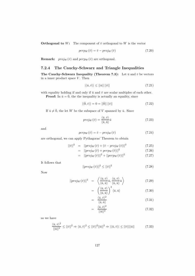
Orthogonal to W : The component of v orthogonal to W is the vector
perpW (v) = v − projW (v) (7.20)
Remark: projW (v) and perpW (v) are orthogonal.
7.2.4 The Cauchy-Schwarz and Triangle Inequalities
The Cauchy-Schwarz Inequality (Theorem 7.3): Let u and v be vectorsin a inner product space V . Then
|〈u, v〉| ≤ ||u|| ||v|| (7.21)
with equality holding if and only if u and v are scalar multiples of each other.Proof: In u = 0, the the inequality is actually an equality, since
|〈0, v〉| = 0 = ||0|| ||v|| (7.22)
If u 6= 0, the let W be the subspace of V spanned by u. Since
projW (v) =〈u, v〉〈u, u〉 u (7.23)
andperpW (v) = v − projW (v) (7.24)
are orthogonal, we can apply Pythagoras’ Theorem to obtain
||v||2 = ||projW (v) + (v − projW (v)||2 (7.25)
= ||projW (v) + perpW (v)||2 (7.26)
= ||projW (v)||2 + ||perpW (v)||2 (7.27)
It follows that||projW (v)||2 ≤ ||v||2 (7.28)
Now
||projW (v)||2 =
⟨ 〈u, v〉〈u, u〉 u,
〈u, v〉〈u, u〉 u
⟩
(7.29)
=
( 〈u, v〉〈u, u〉
)2
〈u, u〉 (7.30)
=〈u, v〉2〈u, u〉 (7.31)
=〈u, v〉2||u||2 (7.32)
so we have
〈u, v〉2||u||2 ≤ ||v||2 ⇒ 〈u, v〉2 ≤ ||v||2||u||2 ⇒ |〈u, v〉| ≤ ||v||||u|| (7.33)
127

Clearly |〈u, v〉| ≤ ||v||||u|| is an equality if and only if ||projW (v)||2 = ||v||2,and this is true if and only if perpW (v) = 0, equivalently
v = projW (v) =〈u, v〉〈u, u〉 u (7.34)
If this is so, then v is a scalar multiple of u. Consequently, if v = cu, then
perpW (v) = v − projW (v) (7.35)
= cu− 〈u, cu〉〈u, u〉 u (7.36)
= cu− c〈u, u〉〈u, u〉 u (7.37)
= 0 (7.38)
so equality holds in the Cauchy-Schwarz Inequality.
The Triangle Inequality (Theorem 7.4): Let u and v be vectors in aninner product space V . Then
||u+ v|| ≤ ||u||+ ||v|| (7.39)
Proof: We start the demostration with the following equality which is asked toproved in Exercise 32 in Ref. [1]
||u+ v||2 = ||u||2 + 2〈u, v〉+ ||v||2 (7.40)
≤ ||u||2 + 2|〈u, v〉|+ ||v||2 (7.41)
≤ ||u||2 + 2||u||||v||+ ||v||2 (7.42)
≤ (||u||+ ||v||)2 ⇒ ||u+ v|| ≤ ||u||+ ||v|| (7.43)
7.3 Vectors and Matrices with Complex Entries
Complex dot product: If u and v are vector in Cn, then the complex dotproduct of u and v is defined by
u · v = u∗1v1 + · · ·+ u∗nvn (7.44)
where u∗i is the complex conjugate of ui.
Norm: ||v|| =√v · v
Distance: d(u, v) = ||u− v||
Properties:
a1. u · v = (v · u)∗
a2. u · v = u+v where u+ is the conjugate transpose of u.
b. u · (v + w) = u · v + u · w
128

c. (cu) · v = c∗(u · v) and u · (cv) = c(u · v)d. u · u ≥ 0 and u · u = 0 if and only if u = 0
e. For matrices with complex entries, addition, multiplication by complex scalars,transpose, and matrix multiplication are all defined exactly as we did forreal matrices in Section 3.1 of Ref. [1], and the algebraic properties ofthese operations still hold (Section 3.2 of Ref. [1]).
f. The notion of inverse and determinant of a square complex matrix are likewisethe real case, and the techniques and properties all carry over the complexcase (Sections 3.3. and 4.2 of Ref. [1]).
However, the notion of transpose is not that useful in complex matrices.The following is an alternative useful definition when working with complexmatrices:
Conjugate Transpose: If A is a complex matrix, then the conjugate trans-pose of A is the matrix A+ defined by
A+ = (AT )∗ (7.45)
Properties of complex conjugate matrices:
a. (A∗)∗ = A
b. (cA)∗ = c∗A∗
c. (A+ B)∗ = A∗ +B∗
d. (AB)∗ = A∗B∗
Properties of complex transpose matrices:
a. (A+)+ = A
b. (cA)+ = c∗A+
c. (A+ B)+ = A+ +B+
d. (AB)+ = B+A+
The following definition is the complex generalization of real symmetric ma-trix.
Hermitian: A square complex matrix A is called Hermitian if A+ = A–thatis, if it is equal to its own conjugate transpose.
Properties of Hermitian matrices:
a. The diagonal entries of a Hermitian matrix are real
b. The eigenvalues of a Hermitian matrix are real numbers.
c. If A is Hermitian, then eigenvectors corresponding to distinct eigenvalues ofA are orthogonal.
If a square real matrix satisfies that Q−1 = QT then Q is orthogonal. Thenext definition give the analogue for complex matrices.
129

Unitary: A square complex matrix U is called unitary if U−1 = U+
Remark: In order to show that U is unitary you need only to show thatU+U = I.
The following statement are equivalent:
a. U is unitary
b. The columns of U form an orthonormal set in Cn with respect to the complexdot product.
c. The rows of U form an orthonormal set in Cn with respect to the complexdot product.
d. ||Ux|| = ||x|| for every x in Cn.
e. Ux · Uy = x · y for every x and y in Cn.
The following definition is the natural generalization of orthogonal diagonal-izability to complex matrices
Unitary Diagonalizable: A square matrix A is called unitary diagonalizableif there exist a unitary matrix U and a diagonal matrix D such that
U+AU = D (7.46)
where the columns of U must form an orthonormal basis in Cn consisting ofeigenvectors of A.
The following is the process to find U and D,
1. Compute the eigenvalues of A
2. Find a basis for each eigenspace
3. Ensure that each eigenspace basis consists of orthonormal vectors (usingthe Gram-Schmidt Process, with the complex dot product, if necessary)
4. Form the matrix U whose columns are the orthonormal eigenvectors justfound.
5. As a consequence of this construction the product U+AU will be a diagonalmatrix D whose diagonal entries are the eigenvalues of A arranged in theorder as the corresponding eigenvectors in the columns of U .
Remarks:
• Every Hermitian matrix is unitary diagonalizable. This is the ComplexSpectral Theorem.
• It turns that the inverse statement, i.e. every unitary diagonalizable ma-trix is Hermitian, is not true.
The charaterization of unitary diagonalizability is the following theorem (itis not demostrated in Ref. [1].
130
Unitarily Diagonalizable: A square complex matrix A is unitarily diago-nalizable if and only if
A+A = AA+ (7.47)
Normal matrix: A matrix A for which A+A = AA+ is called normal.
Skew(asimetrico)-Hermitian matrix: A matrix A for which A+ = −A iscalled skew-Hermitian.
Remark:
• Every Hermitian matrix, every unitary matrix, and every skew-Hermitianmatrix is normal. In the real case, this result refers to symmetric, orthog-onal, and skew-asymmetric matrices, respectively.
• If a square complex matrix is unitarily diagonalizable, then it is normal.
7.4 Geometric Inequalities and Optimization Prob-lems
Recall that the Cauchy-Schwarz Inequality in Rn states that for all vectors uand v,
|u · v| ≤ ||u|| ||v|| (7.48)
|n∑
i=1
xiyi| ≤
√
√
√
√
n∑
i=1
x2i
√
√
√
√
n∑
i=1
y2i (7.49)
⇒(
n∑
i=1
xiyi
)2
≤
√
√
√
√
n∑
i=1
x2i
2
√
√
√
√
n∑
i=1
y2i
2
(7.50)
Examples:
• √xy ≤ x+y
2 where√xy is the geometric mean and (x+ y)/2 is the arith-
metic mean or average.
• (∏n
i=1 xi)1n ≤
∑ni=1
xi
n
Definitions:
Quadratic Means:
√∑ni=1
x2i
n
Harmonic Mean: n∑ni=1
1xi
Relation between the different means:√
x2 + y2
2≥ x+ y
2≥ √
xy ≥ 21x + 1
y
(7.51)
131
7.5 Norms and Distance Functions
Norm: A norm on a vector space V is a mapping that associates with eachvector v a real number ||v||, called the norm of v, such that the following prop-erties are satisfied for all vector u and v and all scalars c:
1. ||v|| ≥ 0, and ||v|| = 0 if and only if v = 0
2. ||cv|| = c||v||
3. ||u+ v|| ≤ ||u||+ ||v||
Normed linear space: A vector space with a norm is called a normed linearspaced
Example:
scalar norm: An inner product space with norm ||v|| =√
〈v, v〉 defines a norm.
Sum norm or 1-norm: The sum norm ||v||s or ||v||1 of a vector v in Rn is thesum of the absolute values of its components. That is, if v = [v1, · · · , vn]T ,then ||v||s = |v1|+ · · ·+ |vn| is a norm.
Max norm or ∞ norm or uniform norm: The max norm ||v||m or ||v||∞of a vector in Rn is the largest number among the absolute values of itscomponents. That is, if v = [v1, · · · , vn]T , then ||v||m = max{|v1|, · · · , |vn|}is a norm.
In general, it is possible to define a norm ||v||p of a vector in Rn by ||v||p =(|v1|p + · · ·+ |vn|p)1/p for any real p ≥ 1. For
• p = 1, ||v||1 = ||v||s.• p = 2, ||v||2 =
√
|v1|2 + · · ·+ |vn|2. It is the familiar norm obtainfrom the dot product. This 2-norm of Euclidean norm, is often de-noted by ||v||E .
7.5.1 Distance Functions
For any norm, we can define a distance function:
d(u, v) = ||u− v|| (7.52)
Exercise for the student in class (Example 7.16): Compute the distanced(u, v) relative to
a. the Euclidean norm. You should get: 5.
b. the sum norm. You should get: 7.
c. the max norm. You should get: 4.
where uT = [3,−2] and vT = [−1, 1].
132

Properties of the distance function(Theorem 7.5): Let d be a distancefunction defined on a normed linear space V . The following properties hold forall vectors u, v, and w in V :
a. d(u, v)≥ 0, d(u, v)=0 if and only if u = v
b. d(u, v)=d(v, u)
c. d(u, w)≤d(u, v)+d(v, w)
Proof: See Ref. [1], pag. 564.
7.5.2 Matrix Norms
A matrix norm on Mnn is a mapping that associates with each n× n matrix Aa real number ||A||, called the norm of A, such that the following properties aresatisfied for all n× n matrices A and B and all scalars c,
1. ||A|| ≥ 0 and ||A|| = 0 if and only if A = O.
2. ||cA|| = c||A||3. ||A+B|| ≤ ||A||+ ||B||4. ||AB|| ≤ ||A||||B||
Compatible: A matrix norm on Mnn is said to be compatible with a vectornorm ||x|| on R
n if for all n× n matrices A and all vectors x in Rn, we have
||Ax|| ≤ ||A||||x|| (7.53)
Examples:
Frobenius norm: (Example 7.18) The Frobenius norm ||A||F of a matrix Ais obtained by stringing(desfibrar) out the entries of the matrix and thentaking the Euclidean norm,
||A||F =
√
√
√
√
n∑
i,j=1
a2ij (7.54)
Operator norm: (Theorem 7.6) If ||x|| is a vector norm on Rn, then ||A|| =max||x||=1||Ax|| defines a norm on Mnn that is compatible with the vectornorm that induces it. The following are three examples:
Sum norm: ||A||1 = max||x||s=1||Ax||sEuclidean norm: ||A||2 = max||x||E=1||Ax||EMax norm: ||A||∞ = max||x||m=1||Ax||m
Theorem 7.7: Let A be an n × n matrix with columns vectors ai and rowvectors Ai for i = 1, · · · , n,a. ||A||1 = maxj=1,··· ,n||aj ||s = maxj=1,··· ,n
∑ni=1 |aij | (notar que se suman las
columnas)
b. ||A||∞ = maxj=1,··· ,n||Aj ||s = maxi=1,··· ,n∑n
j=1 |aij | (notar que se sumanlas filas)
133

Example 7.19: Find ||A||1 and ||A||∞ using the Theorem 7.7 and the defini-tion ||A|| = max||x||=1||Ax|| for
A =
1 −3 24 −1 −2−5 1 3
(7.55)
• Using T. 7.7:
||A||1 = ||a1||s = |1|+ |4|+ | − 5| = 10 (7.56)
||A||∞ = ||A4||s = | − 5|+ |1|+ |3| = 9 (7.57)
• using the definition ||A|| = max||x||=1||Ax||:(i) For ||A||1 = max||x||s=1||Ax||s we see that the maximum value of 10 isachieved when we take x = e1, for then
||Ae1||s = ||a1||s = 10 = ||A||1 (7.58)
(ii) For ||A||∞ = max||x||m=1||Ax||m, if we take xT = [−1 1 1] we obtain
||Ax||m =
∥
∥
∥
∥
∥
∥
1 −3 24 −1 −2−5 1 3
−111
∥
∥
∥
∥
∥
∥
m
(7.59)
=
∥
∥
∥
∥
∥
∥
−2−79
∥
∥
∥
∥
∥
∥
m
= max{| − 2|, | − 7|, |9|} (7.60)
||Ax||m = 9 (7.61)
7.5.3 The Condition Number of a Matrix
Ill-Conditioned matrix: A matrix A is ill-conditioned if small changes inits entries can produce large changes in the solutions to Ax = b.
Well-Conditioned matrix: If small changes in the entries of a matrix Aproduce only small changes in the solutions to Ax = b, then A is called well-conditioned.
Ill-conditioned in terms of the norm: We can use matrix norms to give amore precise way of determining when a matrix is ill-conditioned. The inequality(see Ref. [1], pag. 571)
||∆x||||x′|| ≤ cod(A)
||∆A||||A|| (7.62)
gives an upper bound on how large the relative error in the solution can be interms of the relative error in the coefficient matrix. The larger the conditionnumber cond(A) = ||A−1||||A||, the more ill-conditioned the matrix, since thereis more “room” for the error to be large relative to the solution.
134

Remarks:
• The condition number
cond(A) = ||A−1||||A|| (7.63)
of a matrix depends on the choice of the norm. The most commonly usednorms are the operator norms ||A||1 and ||A||∞.
• For any norm, cond(A) ≥ 1.
• If the condition number is large relative to one compatible matrix norm,it will be large relative to any compatible matrix norm.
7.5.4 The Convergence of Iterative Methods
One of the most important uses of matrix norms is to establish the convergenceproperties of various iterative methods.
7.6 Least Squares Approximation
Best Approximation: If W is a subspace of a normed linear space V and ifv is a vector in V , then the best approximation to v in W is the vector v in Wsuch that
||v − v|| < ||v − w|| (7.64)
for every vector w in W different from v.
Remark: In R2 or R3, we are used to thinking of “shorter distance” as cor-responding to “perpendicular distance”. In algebraic terminology, “shorter dis-tance” relates to the notion of orthogonal projection, i.e. if W is a subspace ofRn and v is a vector in Rn, then we expect projW (v) to be the vector in W thatis closest to v, see Fig. 7.1.
Figure 7.1: (from Ref. [1])
135

The Best Approximation Theorem (Theorem 7.8): If W is a finite-dimensional subspace of an inner product space V and if v is a vector in V ,then projW (v) is the best approximation to v in W .Proof: Let w be a vector in W different from projW (v). Then projw(v) − wis also in W , so v − projW (v) = perpW (v) is orthogonal to projW (v) − w, byExercise 43 of Ref. [1] of Section 7.1. Pythagoras’s Theorem now implies that
||v − projW (v)||2 + ||projW (v)− w||2 = ||(v − projW (v)) + (projw(v)− w)||2
= ||v − w||2 (7.65)
as Fig. 7.1 illustrates. However, ||projW (v)− w||2 > 0, since w 6= projW (v), so
||v − projW (v)||2 < ||v − projW (v)||2 + ||projW (v)− w)||2 = ||v − w||2
⇒ ||v − projW (v)|| < ||v − w|| (7.66)
Remark: The Best Approximation Theorem gives us an alternative proof thatprojW (v) does not depend on the choice of the basis of W , since there can beonly one vector in W that is closest to v–namely projW (v).
Example 7.23: Let
u1 =
12−1
u2 =
5−21
v =
325
(7.67)
Find the best approximation to v in the plane W = span(u1, u2) and find theEuclidean distance from v to W .Solution:The vector in W which best approximate v is projW (v),
projW (v) =
(
u1 · vu1 · u1
)
u1 +
(
u2 · vu2 · u2
)
u2 (7.68)
=2
6
12−1
+16
30
5−21
=
3−2/51/5
(7.69)
The distance from v to W is the distance from v to the point is W closest to v.But this distance is just
||perpW (v)|| = ||v − projw(v)|| (7.70)
then
perpW (v) = v − projw(v) (7.71)
=
325
−
3−2/51/5
=
0−12/524/5
(7.72)
then distance from v to W is
||perpW (v)|| =√
02 + (−12/5)2 + (24/5)2 = 12√5/5 (7.73)
136

7.6.1 Least Squares Approximation
This section is about of finding a curve that “best fits” a set of data points.
Least Square Solution: If A is an m × n matrix and b is in Rm, a leastsquare solution of Ax = b is a vector x in Rn such that
||b−Ax|| ≤ ||b −Ax|| (7.74)
for all x in Rn.
The Least Squares Theorem (Theorem 7.9): Let A be an m× n matrixand let b be in Rm. Then Ax = b always has at least one least squares solutionx. Moreover,
a. x is a least squares solution of Ax = b if and only if x is a solution of thenormal equations ATAx = AT b.
b. A has LI columns if and only if ATA is invertible. In this case, the leastsquares solution of Ax = b is unique and is given by x = (ATA)−1AT b.
Proof: See Ref. [1], pag. 585.
7.6.2 Least Squares via the QR Factorization
If is often the case that the normal equations for a least squares problem are ill-conditioned. Therefore, a small numerical error in performing Gaussian elimina-tion will result in a late error in the least square solution. The QR factorizationof A yields a more reliable way of computing the least square approximation ofAx = b.
Theorem 7.10: Let A be an m × n matrix with LI columns and let b be inRm. If A = QR is a QR factorization of A (where Q is an m × n matrix withorthonormal columns and R is an invertible upper triangular matrix), then theunique least squares solution x of Ax = b is R−1QT b.Proof: Writing A = QR in ATAx = AT b we have
ATAx = AT b (7.75)
(QR)TQRx = (QR)T b (7.76)
RTQTQRx = RTQT b (7.77)
RTRx = RTQT b (7.78)
Rx = QT b (7.79)
x = R−1QT b (7.80)
(7.81)
where we used QTQ = I and the fact that RT is invertible because R is so.
Remark: Since R is upper triangular, in practice it is easier to solve Rx =QT b.
137

7.6.3 Orthogonal Projection Revisited
The least squares method give an alternative formulation for the orthogonalprojection of a vector onto a subspace on Rm.
Theorem 7.11: Let W be a subspace of Rm and let A be an m × n matrixwhose columns form a basis for W . If v is any vector in Rm, then the orthogonalprojection of v onto W is the vector
projW (v) = A(ATA)−1AT v (7.82)
The LT P : Rm → R
m that projects Rm onto W has A(ATA)−1AT as its
standard matrix.Proof: Given the way we have constructed A, its column space is W . Sincethe columns of A are LI, the Least Squares Theorem guarantees that there is aunique leas squares solution Ax = v given by
x = (ATA)−1AT v (7.83)
By equationAx = projcol(A)(b) (7.84)
and the above statement, we have
Ax = projW (b) (7.85)
ThereforeprojW (v) = A((ATA)−1AT v) = (A(ATA)−1AT )v (7.86)
as required.
Remark: Since the projection of a vector onto a subspace W is unique, thestandard matrix of this LT (as given by Theorem 7.11) cannot depend on thechoice of basis for W . That is, with a different basis for W , we have a differentmatrix A, but the matrix A(ATA)−1AT will be the same!!!.
7.6.4 The Pseudoinverse of a Matrix
If A is an n × n matrix with LI columns, then it is invertible, and the uniquesolution to Ax = b is x = A−1b. If m > n and A is m × n with LI columns,then Ax = b has no exact solution, but the best approximation is given bythe unique leas squares solution x = (ATA)−1AT b. The matrix (ATA)−1AT
therefore plays the role of an ”inverse of A“ in this situation.
Seudoinverse: If A is a matrix with LI columns, then the pseudoinverse ofA is the matrix A+ defined by
A+ = (ATA)−1AT (7.87)
138

Remarks:
• If the matrix A is m× n, then the pseudoinverse A+ is n×m.
• If A is m×n matrix with LI columns, the least squares solution of Ax = bis given by x = A+b.
• The standard matrix of the orthogonal projection P from Rm onto col(A)is [P ] = AA+
• If A is square, then A+ = A−1. In this case,
– the least square solution of Ax = b is the exact solution: x = A+b =A−1b = x.
– The projection matrix becomes [P ] = AA+ = A = A−1 = I
Properties of the seudoinverse (Theorem 7.12): Let A be a matrix withLI columns. Then the pseudoinverse A+ of A satisfies the following properties,called Penrose conditions for A:
a. AA+A = A
b. A+AA+ = A+
c. AA+ and A+A are symmetric.
Proof: See Ref. [1], pag. 595.
7.7 The Singular Value Decomposition
Remarks:
• We saw that every symmetric matrix A can be factored as A = PDPT ,where P is an orthogonal matrix and D is a diagonal matrix displayingthe eigenvalues for A.
• If A is not symmetric, such a factorization is not possible, but we maystill be able to factor a square matrix A as A = PDP−1, where D is asbefore but P is now simply an invertible matrix. (notar el cambio de PT
a P−1 para el caso de matrices no simetricas.)
• However, not every matrix is diagonalizable, but every matrix (symmetricof not, square or not) has a factorization of the form A = PDQT (calledsingular value decomposition), where P and Q are orthogonal and D is adiagonal matrix.
7.7.1 The Singular Values of a Matrix
For any m×n matrix A, the n× n matrix ATA is symmetric and hence can beorthogonally diagonalized, by the Spectral Theorem. Not only are the eigenvalueof ATA all real (Theorem 5.18 of Ref. [1]), they are all nonnegative: let λ bean eigenvalue of ATA with corresponding unit eigenvector v. Then
0 ≤ ||Av||2 = (Av) · (Av) = (Av)TAv = vTATAv (7.88)
= vTλv = λ(v · v) = λ||v||2 = λ (7.89)
It therefore makes sense to take (positive) square roots of these eigenvalues.
139

Singular Values: If A is an m × n matrix, the singular values of A are thesquare roots of the eigenvalues of ATA and are denoted by σ1, · · · , σn. It isconventional to arrange the singular values so that σ1 ≥ · · · ≥ σn.
Remark: Consider the eigenvectors of ATA for the matrix A of m×n. SinceATA is symmetric, we know that there is an orthonormal basis for Rn thatconsists of eigenvectors of ATA. Let {v1, · · · , vn} be such a basis correspondingto the eigenvalues of ATA, ordered so that λa ≥ · · · ≥ λn. We have
λi = ||Avi||2 ⇒ σi =√
λi = ||Avi|| (7.90)
i.e., the singular values of A are the lengths of the vectors Av1, · · · , Avn.
Geometrical interpretation: see Ref. [1], pag. 600.
7.7.2 The Singular Value Decomposition
We want to show that an m× n matrix A can be factored as
A = UΣV T (7.91)
where U is an m × m orthogonal matrix, V is an n × n orthogonal matrix,and Σ is and m× n ”diagonal“ matrix. If the nonzero singular values of A areσ1 ≥ · · · ≥ σr > 0 and σr+1 = · · · = σn = 0, then Σ will have the block form
Σ =
Drr Or,n−r
Om−r,r Om−r,n−r
(7.92)
where D is D = diag(σi) with i = 1, · · · , r and Okl is the zero matrix k × l.
About the matrix V: To construct the orthogonal matrix V , we first findan orthonormal basis {v1, · · · , vn} for Rn consisting of eigenvectors of the n×nsymmetric matrix ATA. Then
V = [v1 · · · vn] (7.93)
is an orthogonal n× n matrix.
About the matrix U: For the orthogonal matrix U , we first note that{Av1, · · · , Avn} is an orthogonal set of vectors in Rm: suppose that vi is theeigenvector of ATA corresponding to the eigenvalue λi, then, for i 6= j,
(Avi) · (Avj) = (Avi)TAvj (7.94)
= vTi ATAv; = vTi λj vj (7.95)
= λj vi · vj = 0 (7.96)
Next we used the fact thatσi = ||Avi|| (7.97)
140
and that the first r of these are nonzero. Therefore, we can normalizeAvi, · · · , Avrby setting
ui =1
σiAvi (7.98)
for i = 1, · · · , r, i.e. the set {u1, · · · , ur} is an orthonormal set in Rm. If ithappens that r < m we have to extend the set {u1, · · · , ur} to an orthonormalbasis {u1, · · · , um} form Rm.
Then we setU = [u1 · · · um] (7.99)
Checking: It remains to be shown that this factorization works, i.e. UΣV T =A. Since V T = V −1, this is equivalent to show that
AV = UΣ (7.100)
We know that Avi = σiui for i = 1, · · · , r and ||Avi = σi = 0 for i = r+1, · · · , n.Hence, Avi = 0 for i = r + 1, · · · , n.Therefore,
AV = A[v1 · · · vn] (7.101)
= [Av1 · · · Avn] (7.102)
= [Av1 · · · Avr 0 · · · 0] (7.103)
= [σ1u1 · · · σrur 0 · · · 0] (7.104)
= [u1 · · · um]
σ1 · · · 0...
. . ....
0 · · · σr
O
O O
(7.105)
= UΣ (7.106)
as required.The above proved the following theorem.
The Singular Value Decomposition(SVD) (Theorem 7.13): Let A beanm×nmatrix with singular values σ1 ≥ · · · ≥ σr > 0 and σr+1 = · · · = σn = 0.Then there exist and m×m orthogonal matrix U , and n×n orthogonal matrixV , and an m× n matrix Σ of the form
Σ =
Drr Or,n−r
Om−r,r Om−r,n−r
(7.107)
D =
σ1 · · · 0...
. . ....
0 · · · σr
(7.108)
such thatA = UΣV T (7.109)
141

Left and right eigenvectors: A factorization of A as in Theorem 7.13 iscalled a singular value decomposition of A. The columns of U are called leftsingular vectors of A, and the columns of V are called right singular vectorsof A. The matrices U and V are not uniquely determined by A, but Σ mustcontain the singular values of A.
The Outer Product Form of the SVD (Theorem 7.14): Let A be anm × n matrix with singular values σ1 ≥ · · · ≥ σr > 0 and σr+1 = σn = 0. Letu1, · · · , ur be left singular vectors and let v1, · · · , vr be right singular vectors ofA corresponding to these singular values. Then
A = σ1u1vT1 + · · ·+ σrur v
Tr (7.110)
Remark:
• The Theorem 7.13 generalizes the Spectral Theorem for positive definite,symmetric matrix.
• The Theorem 7.14 generalizes the spectral decomposition for positive def-inite, symmetric matrix
i.e., if A is a positive definite, symmetric matrix, then Theorems 7.13 and 7.14reduce to the spectral theorem and decomposition respectively.
The SVD of a matrix A contains much important information about A de-scribe in the following theorem:
Theorem 7.15 Let A = UΣV T be a singular value decomposition of an m×nmatrix A. Let σ1, · · · , σr be all the nonzero singular values of A. Then
a. The rank of A is r.
b. {u1, · · · , ur} is an orthonormal basis for col(A).
c. {ur+1, · · · , um} is an orthonormal basis for null(AT ).
d. {v1, · · · , vr} is an orthonormal basis for row(A).
e. {vr+1, · · · , vn} is an orthonormal basis for null(A).
Proof: See Ref. [1], pag. 606.
Theorem 7.16: Let A = UΣV T be a singular value decomposition of anm × n matrix A with rank r. Then the image of the unit sphere in Rn underthe matrix transformation that maps x to Ax is
a. the surface of an ellipsoid in Rm if r = n
b. a solid ellipsoid in Rm if r < n.
Proof: See Ref. [1], pag. 607.
142

Remark: We can describe the effect of an m×n matrix A on the unit spherein Rn in terms of the effect of each factor in its SVD, A = UΣV T , from rightto left (see Fig. 7.2):
1. Since V T is an orthogonal matrix, it maps the unit sphere to itself.
2. The m × n matrix Σ does two things: (i) the diagonal entries σr+1 =· · · = σn = 0 collapse n− r of the dimensions of the unit sphere, leavingan r-dimensional unit sphere, (ii) the nonzero diagonal entries σ1, · · · , σr
distort into an ellipsoid.
3. The orthogonal matrix U aligns the axes of this ellipsoid with the or-thonormal basis vectors {u1, · · · , ur} in Rm.
Figure 7.2: (from Ref. [1])
7.7.3 Matrix Norms and the Condition Number
Theorem 7.17: Let A be anm×nmatrix and let σ1, · · · , σr be all the nonzerosingular values of A. Then
||A||F =√
σ21 + · · ·+ σ2
r (7.111)
Remark:
• If A is and m × n matrix and Q is an m × m orthogonal matrix, then||QA||F = ||A||F
• ||A||2 = max||x||=1||Ax|| = σ1
• cond2(A) = |A−1||2||A||2 = σ1
σn
7.7.4 The pseudoinverse and Least Squares Approxima-tion
Moore-Penrose inverse (pseudoinverse): Let A = UΣV T be an SVD foran m× n matrix A, where
Σ =
[
D OO O
]
(7.112)
and D is an r × r diagonal matrix containing the nonzero singular values σ1 ≥· · · ≥ σr > 0 of A. The pseudoinverse or Moore-Penrose inverse of A is then×m matrix A+ defined by
A+ = V Σ+UT (7.113)
143
where Σ+ is the n×m matrix
Σ+ =
[
D−1 OO O
]
(7.114)
Theorem 7.18: The least squares problem Ax = b has a unique least squaressolution x of minimal length that is given by
x = A+b (7.115)
Remark: When A has LI columns, there is a unique least square solution xto Ax = b; that is, the normal equations ATAx = AT b have the unique solutionx = (ATA)−1AT b. When the columns of A are LD, then ATA is not invertible,so the normal equations have infinitely many solutions. In this case, we willask for the solution x of minimum length. The above Theorem 7.18 fulfill thisrequirement.
7.7.5 The Fundamental Theorem of Invertible Matrices
Here we complete the Fundamental Theorem using the information that thesingular value of a square matrix tell us when the matrix is invertible.
Theorem 7.19: Fundamental Theorem (FT) of Invertible Matrices.Version 5 of 5 Let A be an n× n matrix and let T : V → W be a LT whosematrix [T ]C←B with respect to bases B and C of V and W , respectively, is A.The following statements are equivalent:
From Version 1
a. A is invertible.
b. Ax = b has a unique solution for every b in Rn.
c. Ax = 0 has only the trivial solution.
d. The reduced row echelon form of A is In.
e. A is a product of elementary matrices.
From Version 2
f. rank(A)=n
g. nullity(A)=0
h. The column vectors of A are LI
i. The column vectors of A span Rn
j. The column vectors of A form a basis for Rn
k. The row vectors of A are LI
l. The row vectors of A span Rn
144

m. The row vectors of A form a basis for Rn
From Version 3
n. detA 6= 0
o. 0 is not an eigenvalue of A
From Version 4
p. T is invertible
q. T is one-to-one
r. T is onto
s. ker(T )={0}
t. range(T )=W
New statements
u. 0 is not a singular value of A
7.8 Applications
7.8.1 Approximation of Functions
Linear Approximation: Given a continuous function f on an interval [a, b]and a subspace W of C[a, b], find the function ”closest“ to f in W . The problemis analogous to the least squares fitting of data points, except now we haveinfinitely many data points. The Best Approximation Theorem give the answer.
The given function f lives in the vector space C[a, b] of continuous functionson the interval [a, b]. This is an inner product space, with inner product
〈f, g〉 =∫ b
a
f(x)g(x)dx (7.116)
If W is a finite-dimensional subspace of C[a, b], then the best approximation tof in W is given by the projection of f onto W , by Theorem 7.8. Furthermore,if {u1, · · · , uk} is an orthogonal basis for W, then
projW (f) =〈u1, f〉〈u1, u1〉
u1 + · · ·+ 〈uk, f〉〈uk, uk〉
uk (7.117)
Example 7.41: Find the best linear approximation to f(x) = ex on the in-terval [−1, 1].Solution:Linear functions are polynomials of degree 1, then we use the subspace W =
P1[−1, 1] of C[−1, 1] with the inner product 〈f, g〉 =∫ 1
−1 f(x)g(x)dx. A basisfor P1[−1, 1] is given by {1, x}. Since
〈1, x〉 =∫ 1
−1f(x)g(x)dx = 0 (7.118)
145

this is an orthogonal basis. Then the best approximation to f in W is (see Fig.7.3.)
g(x) = projW (ex) (7.119)
=〈1, ex〉〈1, 1〉 1 +
〈x, ex〉〈x, x〉 x (7.120)
=1
2(e − e−1) + 3e−1x (7.121)
≈ 1.18 + 1.10x (7.122)
Figure 7.3: (from Ref. [1])
The error is the one specified by the Best Approximation Theorem: thedistance ||f − g|| between f and g relative to the inner produc we are using:(the figure 0.23 was copied from Ref. [1], pag. 621)
||ex − [1
2(e − e−1) + 3e−1x]|| =
√
∫ 1
−1
[
ex − 1
2(e− e−1)− 3e−1x
]2
dx ≈ 0.23
(7.123)The root mean square error can be thought of as analogous to the area betweenthe graphs of f and g on the specified interval.
Exercise (Example 7.42): Find the best quadratic approximation to f(x) =ex on the interval [−1, 1].Solution:A quadratic form is a polynomial of the form g(x) = a + bx + cx2 in W =P2[−1, 1]. The standard basis {1, x, x2} is not orthogonal. Procedure
1. First we construct an orthogonal basis using the Gram-Schmidt Process.We should get {1, x, x2 − 1
3}.
146

2. We calculate each element on the expansion projW (ex). The first twoelement were already calculate in the previous example.
〈x2 − 1
3, ex〉 =
2
3(e − 7e−1) (7.124)
〈x2 − 1
3, x2 − 1
3〉 =
8
45(7.125)
3. We put all term together in projW (ex)
g(x) = projW (ex) (7.126)
=〈1, ex〉〈1, 1〉 1 +
〈x, ex〉〈x, x〉 x+
〈x2 − 13 , e
x〉〈x2 − 1
3 , x2 − 1
3 〉(x2 − 1
3) (7.127)
=1
2(e− e−1) + 3e−1x+
23 (e− 7e−1)
845
(x2 − 1
3) (7.128)
≈ 1.00 + 1.10x+ 0.54x2 (7.129)
See Fig. 7.4. The root mean square error gives ||ex − g(x)|| ≈ 0.04.
Figure 7.4: (from Ref. [1])
Trigonometric Polynomial A function of the form
p(x) = a0+a1 cosx+a2 cos 2x+· · ·+an cosnx+b1 sinx+b2 sin 2x+· · ·+bn sinnx(7.130)
is called a trigonometric polynomial of order n.
Trigonometric Expansion: Let us consider the vector space C[−π, π] withthe inner product
〈f, g〉 =∫ π
−πf(x)g(x)dx (7.131)
and the basis B = {1, cosx, · · · , cosnx, sinx, · · · , sinnx}. The best approxima-tion to a function f in C[−π, π] by a trigonometric polynomial of order n is
147
projW (f) given by
g(x) = projW (f) (7.132)
=〈1, f〉〈1, 1〉 1 +
〈cosx, f〉〈cos x, cosx〉 cosx+ · · ·+ 〈cosnx, f〉
〈cosnx, cosnx〉 cosnx
+〈sinx, f〉
〈sinx, sin x〉 sinx+ · · ·+ 〈sinnx, f〉〈sinnx, sinnx〉 sinnx
By defining the coefficients
a0 =〈1, f〉〈1, 1〉 =
〈1, f〉2π
(7.133)
ak =〈cos kx, f〉
〈cos kx, cos kx〉 =〈cos kx, f〉
π(7.134)
bk =〈sin kx, f〉
〈sin kx, sin kx〉 =〈sin kx, f〉
π(7.135)
where we have been used
〈cos kx, cos kx〉 =
∫ π
−πcos2 kxdx = π (7.136)
〈sin kx, sin kx〉 =
∫ π
−πsin2 kxdx = π (7.137)
〈1, 1〉 =
∫ π
−π12dx = 2π (7.138)
Then
g(x) = a0 + a1 cosx+ · · ·+ an cosnx+ b1 sinx+ · · ·+ bn sinnx
This approximation is called the nth-order Fourier approximation to f on[−π, π]. The coefficients a0, a1, · · · , an, b1, bn are called the Fourier coefficientsof f and are given explicitly by the definition of the inner product,
a0 =1
2π
∫ π
−πf(x)dx (7.139)
ak =1
π
∫ π
−πf(x) cos kxdx (7.140)
bk =1
π
∫ π
−πf(x) sin kxdx (7.141)
okular pag. 648
148

Chapter 8
Numeros complejos y planocomplejo
Credit: This notes are 100% from chapter 1 of the book entitled A FirstCourse in Complex Analysis with Applications of Dennis G. Zill and Patrick D.Shanahan (2003) [2].
In this chapter the complex numbers and some of their algebraic and geo-metric properties are introduced.
8.1 Introduction
Imaginary unit: We say that i is the imaginary unit and define it by theproperty i2 = −1
Complex number: A complex number is any number of the form z = a+ ibwhere a and b are real numbers and i is the imaginary unit.
Real and imaginary components: a is the real part of the complex numberz, while b is its imaginary part, with Re(z) = a and Im(z) = b.
Equality: Two complex numbers are equal if their corresponding real andimaginary parts are equal.
Set of complex numbers: The totality of complex numbers is denoted by thesymbol C. Since a ∈ R can be written as z = a + i0 we see that R is asubset of C.
Arithmetic Operations:
z1 + z2 = (a1 + a2) + i(b1 + b2) (8.1)
z1 − z2 = (a1 − a2) + i(b1 − b2) (8.2)
z1 · z2 = (a1a2 − b1b2) + i(b1a2 + a1b2) (8.3)
z1z2
=a1a2 + b1b2a22 + b22
+ ib1a2 − a1b2a22 + b22
(8.4)
149

Arithmetic Properties: Commutative laws:
z1 + z2 = z2 + z1 (8.5)
z1z2 = z2z1 (8.6)
Associative laws:
z1 + (z2 + z3) = (z1 + z2) + z3 (8.7)
z1(z2z3) = (z1z2)z3 (8.8)
Distributive law:
z1(z2 + z3) = z1z2 + z1z3 (8.9)
Zero and unit: The zero in the complex number system is the number 0 + i0and the unit is 1 + i0 denoted as 0 and 1, respectively.
Additive identity: The zero is the additive identity in the complex numbersystem, i.e. z + 0 = z.
Multiplicative identity: The unity is the multiplicative identity, i.e. z ·1 = z.
Complex conjugate: The complex conjugate of z = a + ib is defined as z =a− ib.
Additive inverse: The additive inverse of z = a + ib is −z = −a − ib, withz + (−z) = 0.
Multiplicative inverse or reciprocal: Every nonzero complex number z hasa multiplicative inverse z−1 or 1/z such that zz−1 = 1.
8.2 Complex Plane
A complex number z = x+ iy is uniquely determined by an ordered pair of realnumbers (x, y) in a coordinate plane, called complex plane or z-plane, with xthe real axis and y the imaginary axis.
Definitions:
Vector: a complex number z = x + iy can be viewed as a two-dimensionalposition vector.
Modulus or absolute value: the modulus or absolute value of a complexnumber z = x + iy, is the real number |z| =
√
x2 + y2, i.e. the distancefrom the origin to the point (x, y) and |z|2 = zz = x2 + y2.
Distance: The distance between two points z1 and z2 is |z| = |z2 − z1| =√
(x2 − x1)2 + (y2 − y1)2.
Triangle inequality: |z1+z2| ≤ |z1|+|z2|. From this inequality can be derivedthese others:
• |z1 + z2| ≥ |z1| − |z2|
150

• |z1 + z2| ≥ |(|z1| − |z2|)|• |z1 − z2| ≤ |z1|+ |z2|• |z1 − z2| ≥ |(|z1| − |z2|)|• |z1 + · · ·+ zn| ≤ |z1|+ · · ·+ |zn|
8.3 Polar Form of Complex Numbers
The complex number z = x+iy has its polar form of polar representation give byz = r(cos θ+ i sin θ) with r = |z| and θ a positive angle measure in radians fromthe positive real axis in counterclockwise direction. The parameter θ is calledargument of z and denoted by θ = arg(z), with cos θ = x/r and sin θ = y/r.An argument of a complex number z is not unique since cos θ and sin θ are 2π-periodic. In practice it is used tan θ = y/x to find θ, then if θ0 is an argumentof z, then the angles θ0 ± 2π, θ0 ± 4π, · · · are also arguments of z.
Principal Argument: The argument θ of a complex number that lies in theinterval −π < θ ≤ π is called the principal value of arg(z) or the principalargument of z, and noted as Arg(z), i.e. −π < Arg(z) ≤ π. In general, arg(z)and Arg(z) are related by arg(z) = Arg(z) + 2nπ, n = 0,±1, · · · .
Arithmetic Operations:
z1 + z2 = r1r2[cos(θ1 + θ2) + i sin(θ1 + θ2)] (8.10)z1z2
=r1r2
[cos(θ1 − θ2) + i sin(θ1 − θ2)] (8.11)
arg(z1z2) = arg(z1) + arg(z2) (8.12)
arg
(
z1z2
)
= arg(z1)− arg(z2) (8.13)
zn = rn(cosnθ + i sinnθ) for any integer n (8.14)
(cos θ + i sin θ)n = cosnθ + i sinnθ for any integer n (8.15)
Branch cut: If we take arg(z) from the interval (−π, π), the relationshipbetween a complex number z and its argument is single-valued. For this intervalthe negative real axis is analogous to a barrier that we agree not to cross; thetechnical name for this barrier is a branch cut. If we use (0, 2π), the branch cutis the positive real axis.
8.4 Powers and Roots
There are exactly n solutions of the equation wn = z = r(cos θ + i sin θ),
wk = n√r
[
cos
(
θ + 2kπ
n
)
+ i sin
(
θ + 2kπ
n
)]
(8.16)
All of them lie equally spaced 2π/n on a circle of radius n√r centered at the
origin in the complex plane, with k = 0, · · · , n− 1.
151

Principal nth Root: z1/n is n-valued, that is, it represents the set of n nthroots wk of z. The unique root of a complex number z (obtained by using theprincipal value of arg(z) with k = 0) is referred as the principal nth root of w.
Rational power: When m and n are positive integers with no common fac-tors, then we can define the rational power of z as zm/n, with (z1/n)m =(zm)1/n = zm/n.
8.5 Set of Points in the Complex Plane
Circle: The points z = x+ iy that satisfy the equation |z − z0| = ρ, ρ > 0, lieon a circle of radius ρ centered at the point z0.
Disk: The points z that satisfy the inequality |z − z0| ≤ ρ can be either onthe circle |z − z0| = ρ or within the circle. We say that the set of pointsdefined by |z − z0| ≤ ρ is a disk of radius ρ centered at z0.
Neighborhood: The points z that satisfy the strict inequality |z − z0| < ρ iscalled neighborhood of z0.
Deleted Neighborhood: The neighborhood of z0 that excludes z0, i.e. 0 <|z − z0| < ρ is called deleted neighborhood of z0.
Interior point and Open set: A point z0 is said to be interior point of a setS of the complex plane if there exist some neighborhood of z0 that liesentirely within S. If every point z of a set S is an interior point, then Sis said to be an open set.
Boundary point: If every neighborhood of a point z0 of a set S contains atleas one point of S and at least one point not in S, then z0 is said to bea boundary point of S.
Boundary of a set: The collection of boundary points of a set S is called theboundary of S.
Exterior point: A point z that is neither an interior point nor a boundarypoint of a set S is said to be an exterior point of S, i.e z0 is an exteriorpoint of a set S if there exists some neighborhood of z0 that contains nopoints of S.
Open circular annulus: The set of points satisfying the simultaneous in-equality ρ1 < |z − z0| < ρ2 is an open circular ring centered at z0, calledopen circular annulus.
Domain: If any pair of points z1 and z2 in a set S can be connected by apolygonal line that consists of a finite number of line segments joined endto end that lies entirely in the set, then the set S is said to be connected.An open connected set is called a domain.
Region: a region is a set of points in the complex plane with all, some, noneof its boundary points. Since an open set does not contains any boundarypoints, it is automatically a region.
152

Closed region: a region that contains all its boundary points is said to beclosed. The disk defined by |z − z0| ≤ ρ is an example of a closed region,it is called closed disk.
Open region: a neighborhood of a point z0 defined by |z − z0| < ρ is an openset or an open region, it is called open disk.
Punctured disk: a punctured disk is the region defined by 0 < |z− z0| ≤ ρ or0 < |z − z0| < ρ
Bounded Set: a set S in the complex plane is bounded if there exists a realnumber R > 0 such that |z| < R for every z in S.
Unbounded Set: a set is unbounded if it is not bounded.
Extended real-number system: is the set consisting of the real numbers Radjoined with ∞.
Extended complex-number system: We can associate a complex numberwith a point on a unit sphere called Riemmann sphere. By drawing a linefrom the number z = a + ib, written as (a, b, 0), in the complex plane to thenorth pole (0, 0, 1) of the sphere x2+y2+u2 = 1, we determined a unique point(x0, y0, u0) on a unit sphere. In this manner each complex number is identifiedwith a single point on the sphere. Because the point (0, 0, 1) corresponds tono number z in the plane, we correspond it with ∞. The system consisting ofC adjoined with the “ideal point” ∞ is called the extended complex-numbersystem. For a finite number z, we have z + ∞ = ∞ + z = ∞, and for z 6= 0,z · ∞ = ∞ · z = ∞. Moreover, for z 6= 0 we write z/0 = ∞ and for z 6= ∞,z/∞ = 0. Expressions such as ∞ −∞, ∞/∞, ∞0, and 1∞ cannot be given ameaningful definition and are called indetermined.
153

Chapter 9
Funciones complejas ymapeos
Credit: This notes are 100% from chapter 2 of the book entitled A FirstCourse in Complex Analysis with Applications of Dennis G. Zill and Patrick D.Shanahan (2003) [2].
In this chapter it is studied the functions from a set of complex numbers toanother set of complex numbers.
9.1 Complex Functions
A complex function or a complex-valued function of a complex variable is afunction f whose domain and range are subsets of the set C of complex numbers.
Real and Imaginary Parts of a Complex Function: If w = f(z) is acomplex function, then the image of a complex number z = x + iy under f isa complex number w = u + iv = f(x + iy) = u(x, y) + i v(x, y). The functionsu(x, y) and v(x, y) are called the real and imaginary parts of f , respectively.Example: f(z) = z2 − (2 + 1)z ⇒ u(x, y) = x2 − 2x + y − y2 and v(x, y) =2xy − x− 2y.
Comments:
• Every complex function is completely determined by the real functionsu(x, y) and v(x, y).
• Complex functions defined in terms of u(x, y) and v(x, y) can always beexpressed, if desired, in terms of operations on the symbols z and z.
Complex exponential function: This complex function is an example ofone that is defined by specifying its real and Imaginary parts, ez = ex cos y +iex sin y).
154

Exponential form of a complex number: the polar form of a nonzerocomplex number z = r(cos θ + i sin θ) can be written as z = reiθ , called theexponential form of the complex number z.
Properties:
• Notice that the exponential form is not unique since θ = arg(z) is notunique.
• e0 = 1
• ez1ez2 = ez1+z2
• ez1
ez2 = ez1−z2
• (ez1)n = enz1 for n = 0,±1,±2, · · ·
• The complex exponential function is periodic: ez+2πi = ez for all complexnumbers z.
Polar coordinates: Using the polar form of z = reiθ we can write the func-tion f(z) in its real and imaginary parts, f(z) = u(r, θ) + iv(r, θ). A complexfunction can be defined by specifying its real and imaginary parts in polar co-ordinates.
9.2 Complex Functions as Mappings
The graph (z, f(z)) of a complex function lies in four-dimensional space then, wecannot use graphs to study complex functions. Every complex function describesa correspondence between points in two copies of the complex plane. Specifically,the point z in the z-plane is associated with the unique point w = f(z) is thew-plane. We use the alternative term complex mapping in place of “complexfunction” when considering the function as this correspondence between pointsif the z-plane and points in the w-plane. The geometric representation of acomplex mapping w = f(z) consists of two figures: the first, a subset S ofpoints in the z-plane, and the second, the set S′ of the images of points in Sunder w = f(z) in the w-plane. Then, if the point z0 in the z-plane correspondsto the point w0 in the w-plane, that is, if w0 = f(z0), then we say that f mapsz0 onto w0 or, equivalently, that z0 is mapped onto w0 by f .
Image of S under f: If w = f(z) is a complex mapping and if S (pre-imageof S′) is a set of points in the z-plane, then we call the set of images of thepoints in S under f the image of S under f , and we denoted this set by thesymbol S′.
Exercise (Example 2): Find the image of the line x = 1 under the complexmapping w = z2 and represent the mapping graphically.Solution:Let C be the set of points on the vertical line x = 1, i.e z = 1 + iy, then
155
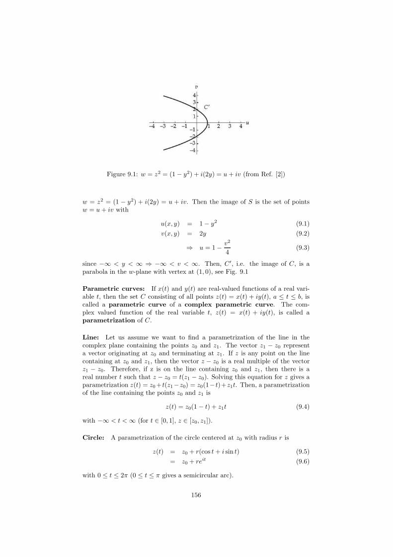
Figure 9.1: w = z2 = (1− y2) + i(2y) = u+ iv (from Ref. [2])
w = z2 = (1 − y2) + i(2y) = u + iv. Then the image of S is the set of pointsw = u+ iv with
u(x, y) = 1− y2 (9.1)
v(x, y) = 2y (9.2)
⇒ u = 1− v2
4(9.3)
since −∞ < y < ∞ ⇒ −∞ < v < ∞. Then, C′, i.e. the image of C, is aparabola in the w-plane with vertex at (1, 0), see Fig. 9.1
Parametric curves: If x(t) and y(t) are real-valued functions of a real vari-able t, then the set C consisting of all points z(t) = x(t) + iy(t), a ≤ t ≤ b, iscalled a parametric curve of a complex parametric curve. The com-plex valued function of the real variable t, z(t) = x(t) + iy(t), is called aparametrization of C.
Line: Let us assume we want to find a parametrization of the line in thecomplex plane containing the points z0 and z1. The vector z1 − z0 representa vector originating at z0 and terminating at z1. If z is any point on the linecontaining at z0 and z1, then the vector z − z0 is a real multiple of the vectorz1 − z0. Therefore, if z is on the line containing z0 and z1, then there is areal number t such that z − z0 = t(z1 − z0). Solving this equation for z gives aparametrization z(t) = z0+ t(z1−z0) = z0(1− t)+z1t. Then, a parametrizationof the line containing the points z0 and z1 is
z(t) = z0(1 − t) + z1t (9.4)
with −∞ < t < ∞ (for t ∈ [0, 1], z ∈ [z0, z1]).
Circle: A parametrization of the circle centered at z0 with radius r is
z(t) = z0 + r(cos t+ i sin t) (9.5)
= z0 + reit (9.6)
with 0 ≤ t ≤ 2π (0 ≤ t ≤ π gives a semicircular arc).
156

Image of a Parametric Curve under a Complex Mapping: If w = f(z)is a complex mapping and if C is a curve parametrized by z(t), a ≤ t ≤ b, then
w(t) = f(z(t)), (9.7)
with a ≤ t ≤ b is a parametrization of the image, C′ of C under w = f(z).
Example: Image of the semicircle center at zero of r = 2 contained in C underthe mapping w = z2.The points z ∈ C can be parametrized by z = 2eit with 0 ≤ t ≤ π, then, thepoints w ∈ C′ verify w(t) = (2eit)2 = 4e2it with 0 ≤ t ≤ π, i.e. a circle of radiusr′ = 4, since for s = 2t, w(s) = 4eis with 0 ≤ s ≤ 2π.
9.3 Linear Mappings
Every nonconstant complex linear mapping can be described as a compositionof three basic types of motions: a translation (T ), a rotation (R), and a magni-fication (M).
9.3.1 Translations
A complex linear function T (z) = z + b with b 6= 0, is called a translation. Thelinear mapping T (z) = z + b can be visualized in a single copy of the complexplane (single copy means that both, z and w = T (z) are graph in the samecomplex plane) as the process of translating the point z along the vector b withb = x0 + iy0 to the point T (z). Then, the mapping T (z) = z + b is also called atranslation by b. A translation does not change the shape or size of a figure inthe complex plane
Example: Find the image S′ of the square S with vertices
z1 = 1 + i (9.8)
z2 = 2 + i (9.9)
z3 = 2 + 2i (9.10)
z4 = 1 + 2i (9.11)
under the linear mapping T (z) = z + 2− i.Solution: From T (z) = z + 2− i = z + b with b = 2− i, we get that each pointon the square S will translate by the vector (2,−1) in the complex plane. Inparticular the vertices will be translate to
T (z1) = 3 (9.12)
T (z2) = 4 (9.13)
T (z3) = 4 + i (9.14)
T (z4) = 3 + i (9.15)
157

9.3.2 Rotation
A complex linear functionR(z) = az (9.16)
with |a| = 1 is called a rotation. Written in polar we get
R(z) = eiθreiφ = rei(θ+φ) (9.17)
Then, |R(z)| = r = |z| and arg(R(z)) = θ + φ = arg(z) + θ. Therefore, thelinear mapping R(z) = az can be visualized in a single copy of the complexplane as the process of rotating the point z counterclockwise through an angleof θ radians about the origin to the point R(z). If Arg(a) < 0, then the linearmapping R(z) = az can be visualized in a single copy of the complex plane asthe process of rotating points clockwise through an angle of θ radians about theorigin. For this reason the angle θ = Arg(a) is called an angle of rotation of R.
Example: Find the image of C, where C is the real axis y = 0 under thelinear mapping
R(z) = az =
(√2
2+
√2
2i
)
z
The modulus and principal argument of a are
|a| =
∣
∣
∣
∣
∣
√2
2+
√2
2i
∣
∣
∣
∣
∣
=2
4+
2
4= 1 (9.18)
Arg(a) = tan−1( √
22√22
)
= tan−1(1) =π
4(9.19)
9.3.3 Magnifications
A complex functionM(z) = az
with a > 0 (with a ∈ R) is called a magnification,
M(z) = az = (ax) + i(ay) (9.20)
= (ar)eiθ (9.21)
then
|M(z)| = |a||z| (9.22)
arg(M(z)) = arg(z) (9.23)
Thus, the linear mapping M(z) = az can be visualized in a single copy ofthe complex plane as the process of magnifying, for a > 1 the modulus of thepoint z by a factor of a to obtain the point M(z). The real number a is calledthe magnification factor of M . If 0 < a < 1, then the point M(z) is a timescloser to the origin than the point z. This special case of a magnification iscalled a contraction.
A magnification mapping will change the size of a figure but, it will notchange its basic shape.
158

Example: Image of the circle C given by |z| = 2 under the linear mappingM(z) = 3z.Solution: Each point in the image C′ will have modulus |M(z)| = |3z| = 6. Theimage points can have any argument since the points z in the circle C can haveany argument. Therefore, the image C′ is the circle |w| = 6 that is centered atthe origin and has radius 6.
9.3.4 Linear Mappings
A general linear mapping f(z) = az + b is a composition of a rotation, a mag-nification, and a translation.
Image of a Point under a Linear Mapping: Let us suppose that
f(z) = az + b = |a|(
a
|a|z)
+ b
is a complex linear function with a 6= 0 and z0 be a point in the complex plane.If the point w0 = f(z0) is plotted in the same copy of the complex plane as z0,then w0 is the point obtained by
1. the term a/|a| rotates z0 an angle Arg(a) about the origin,
2. the term |a| is a magnification with magnification factor |a|, and
3. the term b translates the result by b.
This description also describes the image of any set of points S. In particular,the image, S′, of a set S under f(z) = az + b is the set of points obtained byrotating S through Arg(a), magnifying by |a|, and then translating by b.
From f(z) = |a|(a/|a|)z + b we see that every nonconstant complex linearmapping is a composition of at most one rotation, one magnification, and onetranslation. Then, if a 6= 0 is a complex number, R(z) is a rotation throughArg(a), M(z) is a magnification by |a|, and T (z) is a translation by b, then thecomposition f(z) = (T ◦M ◦R)(z) = T (M(R(z))) is a complex linear function.
Since the composition of any finite number of linear functions is again alinear function, it follows that the composition of finitely many rotations, mag-nifications, and translations is a linear mapping.
A linear mapping f(z) = az+ b with a 6= 0 can distort the size of a figure inthe complex plane, but it preserve the basic shape of a figure.
The order of the composition is important (in some special cases the changingthe order does not change the mapping, see problems 27 and 28 in Ref. [2]).Example where the result change: consider the mapping f(z) = 2z + i, whichmagnifies by 2, then translates by i; so, f(0) = i. If we reverse the order ofcomposition, that is, if we translate by i, then magnify by 2 the effect is 0 mapsonto 2i!!.
A complex linear mapping can always be represented as a composition inmore than one way. The complex mapping f(z) = 2z + i, for example, can alsobe expressed as f(z) = 2(z + i/2).
159

Figure 9.2: Linear mapping f(z) = 4iz + 2 + 3i (from Ref. [2])
Example: Find the image of the rectangle with vertices
• −1 + i,
• 1 + i,
• 1 + 2i,
• −1 + 2i
under the linear mapping f(z) = 4iz + 2 + 3i.Solution 1: Let S be the rectangle with the above vertices and let S′ denote theimage of S under f . Because f is a linear mapping, our foregoing discussionimplies that S′ has the same shape as S. That is, S′ is also a rectangle withvertices
• f(−1 + i) = −2− i,
• f(1 + i) = −2 + 7i,
• f(1 + 2i) = −6 + 7i,
• f(−1 + 2i) = −6− i.
Solution 2: The linear mapping f can also be viewed as a composition of a
• rotation Arg(4i) = π/2
• magnification |4i| = 4
• translation 2 + 3i
see Fig. 9.2.
160

Figure 9.3: The mapping w = z2 (from Ref. [2])
9.4 Special Power Functions
A complex polynomial function is a function of the form p(z) = anzn +
an−1zn−1 + · · ·+ a1z + a0 where n is a positive integer and an, an−1, · · · , a1, a0are complex constants. In this section we study complex polynomials of theform f(z) = zn, n ≥ 2. The mappings w = zn, with n ≥ 2, do not preservethe basic shape of every figure in the complex plane. Associated to the functionzn, n ≥ 2, we also have the principal nth root function z1/n. The principal nthroot functions are inverse functions of the functions zn defined on a sufficientlyrestricted domain.
Power Functions A complex power function is a function of the form f(z) =zα where α is a complex constant. In this section we will restrict our attentionto special complex power functions of the form zn and z1/n where n ≥ 2 and nis an integer.
9.4.1 The function zn
The function z2: The values of f(z) = z2 are found using complex multipli-cation. For example, at z = 2−i, we get f(2−i) = (2−i)2 = (2−i)(2−i) = 3−4i.Understanding the complex mapping w = z2, requires a little more work.We begin by expressing this mapping in exponential notation by replacingthe symbol z with reiθ: w = z2 = (reiθ)2 = r2ei2θ. Then, |w| = r2 andarg(w) = 2θ = 2arg(z), see Fig. 9.3.
Mapping R+ by z2: The squaring function z2 maps a semicircle |z| = r,−π/2 ≤ arg(z) ≤ π/2, onto a circle |w| = r2, −π ≤ arg(w) ≤ π. Then, sincethe right half-plane Re(z) ≥ 0 consists of the collection of semicircles |z| = r,−π/2 ≤ arg(z) ≤ π/2, with r ∈ [0,∞), we have that the image of this half-planeconsists of the collection of circles |w| = r2 where r takes on any value in [0,∞).This implies that w = z2 maps the right half-plane Re(z) ≥ 0 onto the entirecomplex plane.
161

Mapping a triangle by z2: Let us find the image of the triangle S withvertices
• z1 = 0
• z2 = 1 + i
• z3 = 1− i
Solution: Let us denote S′ the image of S under w = z2. Each of the three sidesof S will be treated separately.
1. The side of z1− z2 lies on a ray emanating from the origin and making anangle of π/4 with the positive x-axis. The image of this segment must lieon a ray making an angle of 2(π/4) = π/2 with the positive u-axis. Sincethe module of the points on the edge containing 0 and 1+ i vary from 0 to2, the moduli of the images of these points vary from 02 = 0 to (
√2)2 = 2.
Thus, the image of z1 − z2 is a vertical line segment from 0 to 2i.
2. In a similar manner, the image of the side of S containing the verticesz1 = 0 and z3 = 1− i is a vertical line segment from 0 to −2i.
3. The remaining side of S contains the vertices z3 = 1 − i and z2 = 1 + iconsists of the set of points z = 1 + iy, −1 ≤ y ≤ 1. Because this sideis contained in the vertical line x = 1, it follows from a previous examplethat its image is a parabolic segment given by u = 1 − v2/4, −2 ≤ v ≤ 2or v = ±2
√1− u, 1 ≤ u ≤ 0.
The function zn, n > 2: If z and w = zn are plotted in the same copy of thecomplex plane, then this mapping can be visualized as the process of magnifyingor contracting the modulus r of z = reiθ to the modulus rn of w, and by rotatingz about the origin to increase an argument θ of z to an argument nθ of w,
w = zn = rneinθ
.
9.4.2 The power function z1/n
The n roots of a nonzero complex number
z = reiθ = r(cos θ + i sin θ)
are given by:
n√rei(θ+2kπ)/n = n
√r
(
cosθ + 2kπ
n+ i sin
θ + 2kπ
n
)
where k = 0, 1, 2, · · · , n− 1.
162

Principal Square Root Function z1/2: For n = 2, the two roots of anonzero complex number
√rei(θ+2kπ)/2 =
√r
(
cosθ + 2kπ
2+ i sin
θ + 2kπ
2
)
where k = 0, 1.This equation does not define a function because it assigns two complex
numbers (one for k = 0 and one for k = 1) to the complex number z. By settingθ = Arg(z) and k = 0 we can define a function that assigns to z the uniquesquare root called principal square root function, given by
z1/2 =√
|z|eiArg(z)/2
If we set θ = Arg(z) and replace z with reiθ in z1/2 =√
|z|eiArg(z)/2 we getz1/2 =
√reiθ/2.
Examples: The following are the principal square root z1/2 for
• z = 4 ⇒ z1/2 =√
|z|eiArg(z)/2 =√4ei0/2 = 2
• z = −2i ⇒ z1/2 =√
|z|eiArg(z)/2 =√2ei(−π/2)/2 =
√2e−iπ/4 = 1− i
• z = −1 + i ⇒ |z| =√2, tan θ = 1/(−1) = −1 ⇒ θ = 3π/4, then
z1/2 =√
|z|eiArg(z)/2 =√√
2ei(3π/4)/2 = 4√2ei3π/8
• z = i ⇒ i1/2 =√1ei(π/2)/2 = eiπ/4 =
√22 + i
√22 .
Inverse Function
One-to-one: A complex function f is one-to-one if each point w in the rangeof f is the image of a unique point z, called the pre-image of w, in the domainof f . That is, f is one-to-one if whenever f(z1) = f(z2), then z1 = z2. This saysthat a one-to-one complex function will not map distinct points in the z-planeonto the same point in the w-plane. If f is a one-to-one complex function, thenfor any point w in the range of f there is a unique pre-image in the z-plane,which we denote by f−1(w). This correspondence between a point w and itspre-image f−1(w) defines the inverse function of a one-to-one complex function.
Inverse Function: If f is a one-to-one complex function with domain A andrange B, then the inverse function of f , denoted by f−1, is the function withdomain B and range A defined by f−1(z) = w if f(w) = z.
Then, if a set S is mapped onto a set S′ by a one-to-one function f , thenf−1 maps S′ onto S. In other words, the complex mappings f and f−1 ’undo’each other. It also follows that if f has an inverse function, then f(f−1(z)) = zand f−1(f(z)) = z.
Example: inverse function of z2 Inverse Functions of zn, n ≥ 2 is not welldefined since it is not one-to-one. In order to see that this is so, consider thepoints z1 = reiθ and z2 = rei(θ+2π/n) with r 6= 0. Because n ≥ 2, the points z1and z2 are distinct but f(z1) = rneinθ and f(z2) = rnei(nθ+2π) = rneinθei2π =rneinθ = f(z1).
163

Figure 9.4: The principal square root function w = z1/2 (from Ref. [2])
For n = 2 the function f(z) = z2 is a one-to-one function on the set Adefined by −π/2 < Arg(z) ≤ π/2. It follows that this function has a well-defined inverse function f−1. This inverse function is the principal square rootfunction z1/2.
Remember: the principal argument Arg(z) of a complex number z lies −π <Arg(z) ≤ π
Let z = reiθ and f−1 = w = ρeiφ where θ = Arg(z) (−π < Arg(z) ≤ π)and φ = Arg(w). Since the range of f−1 = z1/2 is the domain of f = z2, then−π/2 < φ ≤ π/2 and ρ =
√r (ver figure 9.4), then
z1/2 =√reiθ/2 (9.24)
The Mapping w = z1/2 As a mapping, the function z2 squares the modulusof a point and doubles its argument. Because the principal square root functionz1/2 is an inverse function of z2, it follows that the mapping w = z1/2 takes thesquare root of the modulus of a point and halves its principal argument. Thatis, if w = z1/2, then we have |w| =
√
|z| and Arg(w) = 12Arg(z).
Principal nth Root Function
By modifying the argument given for the function f(z) = z2 is one-to-one onthe set defined by −π/2 < arg(z) ≤ π/2, it can be show that the complex powerfunction f(z) = zn, n > 2, is one-to-one on the set defined by
−π
n< arg(z) ≤ π
n(9.25)
The image of the set defined by above under the mapping w = zn is theentire complex plane C excluding w = 0. Therefore, there is a well-definedinverse function for f . Analogous to the case n = 2, this inverse function of zn
is called the principal nth root function z1/n. The domain of z1/n is the
164

set of all nonzero complex numbers, and the range of z1/n is the set of complexnumbers w satisfying −π/n < arg(z) ≤ π/n,
z1/n = n√
|z|eiArg(z)/n = n√
|z|eiθ/n (9.26)
with θ = Arg(z).
Multiple-Valued Functions
A nonzero complex number z has n distinct nth roots in the complex plane. Thismeans that the process of ”taking the nth root” of a complex number z does notdefine a complex function because it assigns a set of n complex numbers to thecomplex number z. These types of operations on complex numbers are examplesof multiple-valued functions. We will adopt the following functional notationfor multiple-valued functions: (i) when representing multiple-valued functionswith functional notation, we will use uppercase letters such as F (z) = z1/2
or G(z) = arg(z); (2) lower-case letters such as f and g will be reserved torepresent functions, for example, f(z) = z1/2 refers to the principal square rootfunction.
The visualization of multiple-to-one a complex mapping like z2 is the Rie-mann surface. See Fig. 9.5 (it seems that the cut in the Riemann surface isin R+ while the mapping has the cut at R−.)
9.5 Reciprocal Function
We define a complex rational function to be a function of the form f(z) =p(z)/q(z) where both p(z) and q(z) are complex polynomial functions. In thissection, we study the most basic complex rational function, the reciprocal func-tion 1/z, as a mapping of the complex plane. An important property of thereciprocal mapping is that it maps certain lines onto circles.
The function 1/z, whose domain is the set of all nonzero complex numbers,is called the reciprocal function,
w =1
z=
1
reiθ=
1
re−iθ (9.27)
therefore, the reciprocal function maps a point in the z-plane with polar coor-dinates (r, θ) onto a point in the w-plane with polar coordinates (1/r,−θ), seeFig. 9.6
Inversion in the Unit Circle The function
g(z) =1
reiθ
whose domain is the set of all nonzero complex numbers, is called inversion inthe unit circle.
We will describe this mapping by considering separately
1. the images of points on the unit circle,
2. the points outside the unit circle, and
165

Figure 9.5: Two mapping for w = z2 and a Riemann surface for the one-to-onevalued function f(z) = z2 (from Ref. [2])
166

Figure 9.6: The reciprocal mapping for w = 1/z (from Ref. [2]).
Figure 9.7: Inversion in the unit circle g(z) = 1r e
iθ (from Ref. [2]).
3. the points inside the unit circle.
(1) Consider first a point z on the unit circle. Since z = 1eiθ, then g(z) = eiθ =z. Therefore, each point on the unit circle is mapped onto itself by g.(2) If z is a nonzero complex number that does not lie on the unit circle, thenwe can write z as z = reiθ with r 6= 1. When r > 1 (z is outside of the unitcircle), we have that |g(z)| = 1/r < 1. So, the image under g of a point z outsidethe unit circle is a point inside the unit circle.(3) Conversely, if r < 1, then |g(z)| = 1/r > 1, and we conclude that if z isinside the unit circle, then its image under g is outside the unit circle.See Fig. 9.7
Complex Conjugation
The second complex mapping that is helpful for describing the reciprocal map-ping is a reflection across the real axis. Under this mapping the image of the
167

Figure 9.8: Reciprocal mapping of |z| = 2, 0 ≤ arg(z) ≤ π (from Ref. [2]).
point (x, y) is (x,−y), c(z) = z, called complex conjugation function,
c(z) = c(x+ iy) = x− iy (9.28)
c(z) = c(reiθ) = re−iθ (9.29)
Reciprocal Mapping
The reciprocal function f(z) = 1/z can be written as the composition of inver-sion in the unit circle and complex conjugation. Using the exponential formsc(z) = re−iθ and g(z) = eiθ/r of these functions we find that the compositionc ◦ g is given by:
c(g(z)) = c
(
1
reiθ)
=1
re−iθ
Then c(g(z)) = f(z) = 1/z. This implies that, as a mapping, the reciprocalfunction first inverts in the unit circle, then reflects across the real axis.
Image of a Point under the Reciprocal Mapping Let z0 be a nonzeropoint in the complex plane. If the point w0 = f(z0) = 1/z0 is plotted in thesame copy of the complex plane as z0, then w0 is the point obtained by: (i)inverting z0 in the unit circle, then, (ii) reflecting the result across the real axis.
Image of a semicircle: Let us find the image of the semicircle |z| = 2,0 ≤ arg(z) ≤ π under w = 1/z.Solution: the mapping is the semicircle |w| = 1/2, −π ≤ arg(w) ≤ 0. See Fig.9.8
Image of a line Let us find the image of the vertical line x = 1 under thereciprocal mapping w = 1/z.Solution: The vertical line x = 1 consists of the set of points z = 1 + iy,−∞ < y < ∞, then
w =1
1 + iy=
1
1 + y2− i
y
1 + y2= u+ iv ⇒ u2 − u+ v2 = 0 (9.30)
168

Figure 9.9: Reciprocal mapping of x = 1 (from Ref. [2]).
then,(
u− 1
2
)2
+ v2 =1
4(9.31)
with u 6= 0 since v = −yu. Figure 9.9 shows the mapping.Comments:
1) The above equation defines a circle centered at (1/2, 0) with radius 1/2. How-ever, because u 6= 0, the point (0, 0) is not in the image.2) Using the complex variable w = u + iv, we can describe this image by|w − 1/2| = 1/2, w 6= 0.3) The point (0, 0) is not included because there is no point on the line x = 1that actually maps onto 0. In order to obtain the entire circle as the imageof the line we must consider the reciprocal function defined on the extendedcomplex-number system.Remember: the extended complex-number system consists of all the points in thecomplex plane adjoined with the ideal point ∞4) Points in the extended complex plane that are near the ideal point ∞ corre-spond to points with extremely large modulus in the complex plane.
Reciprocal Function on the Extended Complex Plane: The reciprocalfunction on the extended complex plane is the function defined by:
f(z) =
1/z z 6= 0 or z 6= ∞∞ z = 00 z = ∞
(9.32)
Mapping Lines to Circles with w = 1/z The reciprocal function on theextended complex plane maps:
(i) the vertical line x = k with k 6= 0 onto the circle∣
∣
∣
∣
w − 1
2k
∣
∣
∣
∣
=
∣
∣
∣
∣
1
2k
∣
∣
∣
∣
(9.33)
169

Figure 9.10: Reciprocal mapping of vertical and horizontal lines (from Ref. [2]).
(ii) the horizontal line x = k with k 6= 0 onto the circle
∣
∣
∣
∣
w + i1
2k
∣
∣
∣
∣
=
∣
∣
∣
∣
1
2k
∣
∣
∣
∣
(9.34)
See Fig. 9.10.
Remarks: It is easy to verify that the reciprocal function f(z) = 1/z is one-to-one. Therefore, f has a well-defined inverse function f−1. We find a formulafor the inverse function f−1(z) by solving the equation z = f(w) for w. Clearly,this gives f−1(z) = 1/z . This observation extends our understanding of thecomplex mapping w = 1/z. For example, we have seen that the image of theline x = 1 under the reciprocal mapping is the circle |w − 1/2| = 1/2. Sincef−1(z) = 1/z = f(z) , it then follows that the image of the circle |z−1/2| = 1/2under the reciprocal mapping is the line u = 1. In a similar manner, we see thatthe circles |w− 1/(2k)| = |1/(2k)| and |w+ i/(2k)| = |1/(2k)| are mapped ontothe lines x = k and y = k, respectively.
9.6 Limits and Continuity
Remember: recall that limx→x0f(x) = L intuitively means that values f(x) of
the function f can be made arbitrarily close to the real number L if values of xare chosen sufficiently close to, but not equal to, the real number x0.The concept of a complex limit is similar to that of a real limit in the sensethat limz→z0 f(z) = L will mean that the values f(z) of the complex functionf can be made arbitrarily close the complex number L if values of z are chosensufficiently close to, but not equal to, the complex number z0.
In this section we will define the limit of a complex function, examine some ofits properties, and introduce the concept of continuity for functions of a complexvariable.
170
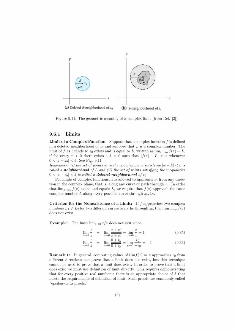
Figure 9.11: The geometric meaning of a complex limit (from Ref. [2]).
9.6.1 Limits
Limit of a Complex Function Suppose that a complex function f is definedin a deleted neighborhood of z0 and suppose that L is a complex number. Thelimit of f as z tends to z0 exists and is equal to L, written as limz→z0 f(z) = L,if for every ε > 0 there exists a δ > 0 such that |f(z) − L| < ε whenever0 < |z − z0| < δ. See Fig. 9.11Remember: (i) the set of points w in the complex plane satisfying |w−L| < ε iscalled a neighborhood of L and (ii) the set of points satisfying the inequalities0 < |z − z0| < δ is called a deleted neighborhood of z0
For limits of complex functions, z is allowed to approach z0 from any direc-tion in the complex plane, that is, along any curve or path through z0. In orderthat limz→z0 f(z) exists and equals L, we require that f(z) approach the samecomplex number L along every possible curve through z0, i.e.
Criterion for the Nonexistence of a Limit: If f approaches two complexnumbers L1 6= L2 for two different curves or paths through z0, then limz→z0 f(z)does not exist.
Example: The limit limz→0 z/z does not exit since,
limz→0
z
z= lim
z→0
x+ i0
x+ i0= lim
x→0
x
x= 1 (9.35)
limz→0
z
z= lim
z→0
0 + iy
0 + iy= lim
y→0
iy
−iy= −1 (9.36)
Remark 1: In general, computing values of limf(z) as z approaches z0 fromdifferent directions can prove that a limit does not exist, but this techniquecannot be used to prove that a limit does exist. In order to prove that a limitdoes exist we must use definition of limit directly. This requires demonstratingthat for every positive real number ε there is an appropriate choice of δ thatmeets the requirements of definition of limit. Such proofs are commonly called“epsilon-delta proofs.”
171

Remark 2: The definition of complex limits not provide a convenient methodfor computing limits. We will present a practical method for computing complexlimits shortly in a theorem. In addition to being a useful computational tool,this theorem also establishes an important connection between the complex limitof f(z) = u(x, y) + iv(x, y) and the real limits of the real-valued functions oftwo real variables u(x, y) and v(x, y).
Limit of the Real Function F (x, y): The limit of F as (x, y) tends to (x0, y0)exists and is equal to the real number L if for every ε > 0 there exists a δ > 0such that |F (x, y)− L| < ε whenever 0 <
√
(x− x0)2 + (y − y0)2 < δ.
Theorem (2.1): Real and Imaginary Parts of a Limit Suppose thatf(z) = u(x, y)+iv(x, y), z0 = x0+iy0, and L = u0+iv0. Then lim limz→z0 f(z) =L if and only if
lim(x,y)→(x0,y0)
u(x, y) = u0 (9.37)
and
lim(x,y)→(x0,y0)
v(x, y) = v0 (9.38)
Example Let us calculate the following limit: limz→1+i(z2 + 1).
Solution: let us start separating the real and imaginary parts of (z2 + 1)
ℜ(z2 + 1) = x2 − y2 (9.39)
ℑ(z2 + 1) = 2xy + 1 (9.40)
then
lim(x,y)→(1,1)
(x2 − y2) = 0 (9.41)
lim(x,y)→(1,1)
(2xy + 1) = 3 (9.42)
finallylim
z→1+i(z2 + 1) = i3 (9.43)
Theorem (2.2): Properties of complex limits Suppose that f and g arecomplex functions. If limz→z0 f(z) = L and limz→z0 g(z) = M , then
1. limz→z0 cf(z) = cL, with c a complex constant
2. limz→z0(f(z)± g(z)) = L±M
3. limz→z0 f(z)g(z) = LM
4. limz→z0f(z)g(z) = L
M , provided M 6= 0.
Exercises for the student in class: Calculates the following limits:
1. limz→i(3+i)z4−z2+2z
z+1 = 72 − i 12
2. limz→1+i√3z2−2z+4z−1−i
√3= i2
√3
172
9.6.2 Continuity
Continuity of a Complex Function
A complex function f is continuous at a point z0 if
limz→z0
f(z) = f(z0) (9.44)
Criteria for Continuity at a Point: A complex function f is continuous ata point z0 if each of the following three conditions hold:
1. limz→z0 f(z) exits,
2. f is defined at z0, and
3. limz→z0 f(z) = f(z0).
Discontinuous at z0 If a complex function f is not continuous at a point z0then we say that f is discontinuous at z0. For example, the function f(z) =1/(1 + z2) is discontinuous at z = i and z = −i.
Example: The principal square root function f(z) = z1/2 is discontinuous atthe point z0 = −1 since the limit from upper unit circle gives i while the limitfrom a lower unit circle gives −i.
Continuity in a set: A complex function f is continuous on a set S if f iscontinuous at z0 for each z0 in S. For example the function f(z) = z2 − iz + 2is continuous at any point z0 in the complex plane, while the function g(z) =1/(z2+1) is continuous on the set consisting of all complex z such that z 6= ±i.
Theorem (2.3): Real and Imaginary Parts of a Continuous FunctionSuppose that f(z) = u(x, y) + iv(x, y) and z0 = x0 + iy0. Then the complexfunction f is continuous at the point z0 if and only if both real functions u andv are continuous at the point (x0, y0).
Theorem (2.4): Properties of Continuous Functions: If f and g arecontinuous at the point z0 , then the following functions are continuous at thepoint z0:(i) cf , c a complex constant,(ii) f ± g,(iii) f · g, and(iv) f/g provided g(z0) 6= 0.(ii) and (iii) extend to any finite sum or finite product of continuous functions,respectively. We can use these facts to show that polynomials are continuousfunctions.
Theorem (2.5): Continuity of Polynomial Functions Polynomial func-tions are continuous on the entire complex plane C.
Since a rational function f(z) = p(z)/q(z) is quotient of the polynomialfunctions p and q, it follows from the above two Theorems that f is continuousat every point z0 for which q(z0) 6= 0. In other words, i.e. rational functionsare continuous on their domains.
173

Bounded functions
Continuous complex functions have many important properties that are analo-gous to properties of continuous real functions. For instance, recall that if a realfunction f is continuous on a closed interval I on the real line, then f is boundedon I. This means that there is a real number M > 0 such that |f(x)| ≤ M forall x in I. An analogous result for real functions F (x, y) states that if F (x, y)is continuous on a closed and bounded region R of the Cartesian plane, thenthere is a real number M > 0 such that |F (x, y)| ≤ M for all (x, y) in R, andwe say F is bounded on R.
Now suppose that the function f(z) = u(x, y) + iv(x, y) is defined on aclosed and bounded region R in the complex plane. We say that the complexf is bounded on R if there exists a real constant M > 0 such that |f(z)| < Mfor all z in R. If f is continuous on R, then Theorem 2.3 tells us that u and vare continuous real functions on R. It follows that the real function F (x, y) =√
[u(x, y)]2 + [v(x, y)]2 is also continuous on R since the square root functionis continuous. Because F is continuous on the closed and bounded region R,we conclude that F is bounded on R. That is, there is a real constant M > 0such that |F (x, y)| ≤ M for all (x, y) in R. However, since |f(z)| = F (x, y), wehave that |f(z)| ≤ M for all z in R. In other words, the complex function f isbounded on R. This establishes the following important property of continuouscomplex functions.
A Bounding Property If a complex function f is continuous on a closed andbounded region R, then f is bounded on R. That is, there is a real constantM > 0 such that |f(z)| ≤ M for all z in R.
While this result assures us that a bound M exists for f on R, it offersno practical approach to find it. One approach to find a bound is to use thetriangle inequality. Another approach to determine a bound is to use complexmappings.
Branches: We are usually interested in computing just one of the values of amultiple-valued function. For example, the function F (z) = z1/n assigns to theinput z the set of n roots of z. If we make a choice such that to keep only onefunction, for example we keep one of the roots of F (z) together with the conceptof continuity in mind, then we obtain a function that is called a branch of amultiple-valued function. In more rigorous terms, a branch of a multiple-valuedfunction F is a function f1 that is continuous on some domain and that assignsexactly one of the multiple-values of F to each point z in that domain. Thenotation for the branches will be lowercase letters with a numerical subscriptsuch as f1, f2, and so on.
About the domain of a branch: The requirement that a branch be con-tinuous means that the domain of a branch is different from the domain of themultiple-valued function. For example, the multiple-valued function F (z) =z1/2 is defined for all nonzero complex numbers z. Even though the principalsquare root function f(z) = z1/2 does assign exactly one value of F to each inputz, f is not a branch of F because f is not continuous at z0 = −1. In order to geta branch of F (z) = z1/2 we have to restrict the domain, i.e. f1(z) =
√reiθ/2,
with −π < θ < π; it is called the principal branch of F (z) = z1/2.
174

Figure 9.12: z = 1 is not a branch point (from Ref. [2])
Branch Cuts and Branch Points Although the multiple-valued functionF (z) = z1/2 is defined for all nonzero complex numbers C, the principal branchf1 is defined only on the domain |z| > 0, −π < arg(z) < π. In general, abranch cut for a branch f1 of a multiple-valued function F is a portion of acurve that is excluded from the domain of F so that f1 is continuous on theremaining points. Therefore, the nonpositive real axis is a branch cut for theprincipal branch f1 (defined above).
A different branch of F with the same branch cut is given by f2(z) = reiθ/2,π < θ < 3π. These branches are distinct because for, say, z = i we havef1(i) = 0.5
√2 + i0.5
√2, but f2(i) = −0.5
√2 − i0.5
√2. Notice that if we set
φ = θ − 2π, then the branch f2 =√rei(φ+2π)/2 = −√
reiφ/2, −π < φ < π, thenf2 = −f1.
Other branches of F (z) = z1/2 can be defined in a manner similar to theabove ones by using any ray emanating from the origin as a branch cut. Forexample, f3(z) = reiθ/2 , −3π/4 < θ < 5π/4, defines a branch of F (z) = z1/2.The branch cut for f3 is the ray arg(z) = −3π/4 together with the point z = 0.
It is not a coincidence that the point z = 0 is on the branch cut for f1, f2,and f3. The point z = 0 must be on the branch cut of every branch of themultiple-valued function F (z) = z1/2. In general, a point with the propertythat it is on the branch cut of every branch is called a branch point of F .
Alternatively, a branch point is a point z0 with the following property: Ifwe traverse any circle centered at z0 with sufficiently small radius starting at apoint z1, then the values of any branch do not return to the value at z1. Forexample, consider any branch of the multiple-valued function G(z) = arg(z). Atthe point, say, z0 = 1, if we traverse the small circle |z−1| = ε counterclockwisefrom the point z1 = 1− iε, then the values of the branch increase until we reachthe point 1 + iε; then the values of the branch decrease back down to the valueof the branch at z1 = 1− iε. See Figure 9.12. This means that the point z0 = 1is not a branch point.
On the other hand, suppose we repeat this process for the point z0 = 0. Forthe small circle |z| = ε, the values of the branch increase along the entire circle.
175
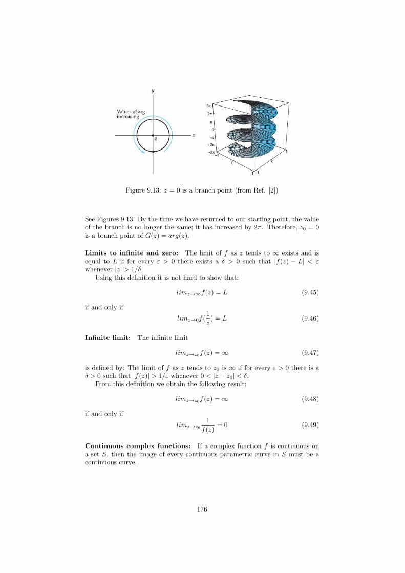
Figure 9.13: z = 0 is a branch point (from Ref. [2])
See Figures 9.13. By the time we have returned to our starting point, the valueof the branch is no longer the same; it has increased by 2π. Therefore, z0 = 0is a branch point of G(z) = arg(z).
Limits to infinite and zero: The limit of f as z tends to ∞ exists and isequal to L if for every ε > 0 there exists a δ > 0 such that |f(z) − L| < εwhenever |z| > 1/δ.
Using this definition it is not hard to show that:
limz→∞f(z) = L (9.45)
if and only if
limz→0f(1
z) = L (9.46)
Infinite limit: The infinite limit
limz→z0f(z) = ∞ (9.47)
is defined by: The limit of f as z tends to z0 is ∞ if for every ε > 0 there is aδ > 0 such that |f(z)| > 1/ε whenever 0 < |z − z0| < δ.
From this definition we obtain the following result:
limz→z0f(z) = ∞ (9.48)
if and only if
limz→z0
1
f(z)= 0 (9.49)
Continuous complex functions: If a complex function f is continuous ona set S, then the image of every continuous parametric curve in S must be acontinuous curve.
176

Chapter 10
Funciones analıticas
Credit: This notes are 100% from chapter 3 of the book entitled A FirstCourse in Complex Analysis with Applications of Dennis G. Zill and Patrick D.Shanahan (2003) [2].
10.1 Differentiability and Analyticity
Derivative of Complex Function Suppose the complex function f is de-fined in a neighborhood of a point z0. The derivative of f at z0, denoted byf ′(z0), is
f ′(z0) = lim∆z→0
f(z0 +∆z)− f(z0)
∆z(10.1)
provided this limit exists.If the above limit exists, then the function f is said to be differentiable at
z0.
Rules of Differentiation If f and g are differentiable at a point z, and c isa complex constant, then
Constant Rules: ddz c = 0 and d
dz cf(z) = cf ′(z)
Sum Rule: ddz [f(z)± g(z)] = f ′(z)± g′(z)
Product Rule: ddz [f(z)g(z)] = f(z)g′(z) + f ′(z)g(z)
Quotient Rule: ddz
[
f(z)g(z)
]
= f ′(z)g(z)−f(z)g′(z)[g(z)]2
Chain Rule: ddzf(g((z)) = f ′(g(z))g′(z)
Power Rule: ddzz
n = nzn−1
Power Rule for functions: ddz [g(z)]
n = n[g(z)]n−1g′(z)
The basic ’Power Rule’ does not apply to powers of the conjugate of z becausethe function f(z) = z is nowhere differentiable.
177

Analytic Functions
Analyticity at a Point A complex function w = f(z) is said to be analyticat a point z0 if f is differentiable at z0 and at every point in some neighborhoodof z0.
Analyticity at a point is not the same as differentiability at a point. Ana-lyticity at a point is a neighborhood property; in other words, analyticity is aproperty that is defined over an open set.
Analyticity in a domain A function f is analytic in a domain D if it isanalytic at every point in D.
Holomorphic or regular function A function f that is analytic throughouta domain D is called holomorphic or regular.
Entire Functions A function that is analytic at every point z in the complexplane is said to be an entire function. In view of differentiation we can concludethat polynomial functions are differentiable at every point z in the complex planeand rational functions are analytic throughout any domain D that contains nopoints at which the denominator is zero. The following theorem summarizesthese results.
Theorem (3.1): Polynomial and Rational Functions
i. A polynomial function p(z) = anzn + an−1zn−1 + · · ·+ a1z + a0, where n is
a nonnegative integer, is an entire function.
ii. A rational function f(z) = p(z)q(z) , where p and q are polynomial functions, is
analytic in any domain D that contains no point z0 for which q(z0) = 0.
Singular Points A point z at which a complex function w = f(z) fails tobe analytic is called a singular point of f . For example, the rational functionf(z) = 4z/(z2− 2z+2) is discontinuous at 1+ i and 1− i, f fails to be analyticat these points. Thus by (ii) of Theorem 3.1, f is not analytic in any domaincontaining one or both of these points.
Analyticity of Sum, Product, and Quotient If the functions f and gare analytic in a domain D then: the sum f(z) + g(z), difference f(z) − g(z),and product f(z)g(z) are analytic. The quotient f(z)/g(z) is analytic providedg(z) 6= 0 in D.
An Alternative Definition of f ′(z) Sometimes it is convenient to definethe derivative of a function f using
f ′(z0) = limz→z0
f(z)− f(z0)
z − z0(10.2)
As in real analysis, if a function f is differentiable at a point, the functionis necessarily continuous at the point.
178
Theorem (3.2): Differentiability Implies Continuity If f is differen-tiable at a point z0 in a domain D, then f is continuous at z0.
Of course the converse of Theorem 3.2 is not true; continuity of a function fat a point does not guarantee that f is differentiable at the point. It follows fromTheorem 2.3 that the simple function f(z) = x+ 4iy is continuous everywherebecause the real and imaginary parts of f , u(x, y) = x and v(x, y) = 4y arecontinuous at any point (x, y). Yet we saw in Example 3 in Ref. [2] thatf(z) = x+ 4iy is not differentiable at any point z.
As another consequence of differentiability, L’Hoopital’s rule for computinglimits of the indeterminate form 0/0, carries over to complex analysis.
Theorem (3.3) L’Hopital’s Rule Suppose f and g are functions that areanalytic at a point z0 and f(z0) = 0, g(z0) = 0, but g′(z0) 6= 0. Then
limz→z0
f(z)
g(z)=
f ′(z0)
g′(z0)(10.3)
10.2 Cauchy-Riemann Equations
A function f is analytic in a domain D if f is differentiable at all points inD. We shall now develop a test for analyticity of a complex function f(z) =u(x, y) + iv(x, y) that is based on partial derivatives of its real and imaginaryparts u and v.
Theorem (3.4): Cauchy-Riemann Equations Suppose f(z) = u(x, y) +iv(x, y) is differentiable at a point z = x+ iy. Then at z the first-order partialderivatives of u and v exist and satisfy the Cauchy-Riemann equations
∂u
∂x=
∂v
∂y(10.4)
∂u
∂y= −∂v
∂x(10.5)
Proof: see pages 152 and 153 of Ref. [2].If the Cauchy-Riemann equations are not satisfied at a point z, then f cannot
be differentiable at z. We have already seen in Example 3 of Section 3.1 of Ref.[2] that f(z) = x+ 4iy is not differentiable at any point z. If we identify u = xand v = 4y, then ∂u/∂x = 1, ∂v/∂y = 4, ∂u/∂y = 0, and ∂v/∂x = 0. In viewof ∂u/∂x = 1 6= ∂v/∂y = 4, f is nowhere differentiable.
Criterion for Non-analyticity If the Cauchy-Riemann equations are notsatisfied at every point z in a domain D, then the function f(z) = u(x, y) +iv(x, y) cannot be analytic in D.
Theorem (3.5): Criterion for Analyticity Suppose the real functionsu(x, y) and v(x, y) are continuous and have continuous first-order partial deriva-tives in a domain D. If u and v satisfy the Cauchy-Riemann equations at allpoints of D, then the complex function f(z) = u(x, y) + iv(x, y) is analytic inD.
Recall that analyticity implies differentiability but not conversely. Theorem3.5 has an analogue that gives the following criterion for differentiability.
179

Sufficient Conditions for Differentiability If the real functions u(x, y) andv(x, y) are continuous and have continuous first-order partial derivatives in someneighborhood of a point z, and if u and v satisfy the Cauchy-Riemann equationsat z, then the complex function f(z) = u(x, y) + iv(x, y) is differentiable at zand f(z) is given by
f ′(z) =∂u
∂x+ i
∂v
∂x(10.6)
=∂v
∂y− i
∂u
∂y(10.7)
The following theorem is a direct consequence of the Cauchy-Riemann equa-tions.
Theorem (3.6): Constant Functions Suppose the function f(z) = u(x, y)+iv(x, y) is analytic in a domain D.(i) If |f(z)| is constant in D, then so is f(z).(ii) If f ′(z) = 0 in D, then f(z) = c in D, where c is a constant.
Polar Coordinates
For f(z) = u(r, θ) + iv(r, θ) the Cauchy-Riemann equations become
∂u
∂r=
1
r
∂v
∂θ(10.8)
∂v
∂r= −1
r
∂u
∂θ(10.9)
The derivative of the function f(z) in polar coordinates reads,
f ′(z) = e−iθ(
∂u
∂r+ i
∂v
∂r
)
(10.10)
=1
re−iθ
(
∂v
∂θ− i
∂u
∂θ
)
(10.11)
About the exponential function f(z) = ez is differentiable everywhereand f ′(z) = f(z).
10.3 Harmonic Functions
In Section 5.5 of Ref. [2]) you shall see that when a complex function f(z) =u(x, y) + iv(x, y) is analytic at a point z, then all the derivatives of f :f ′(z), f ′′(z), f ′′′(z), · · · are also analytic at z. As a consequence of this remark-able fact, we can conclude that all partial derivatives of the real functions u(x, y)and v(x, y) are continuous at z. From the continuity of the partial derivatives wethen know that the second-order mixed partial derivatives are equal. This lastfact, coupled with the Cauchy-Riemann equations, will be used in this sectionto demonstrate that there is a connection between the real and imaginary partsof an analytic function f(z) = u(x, y) + iv(x, y) and the second-order partialdifferential equation
∂2φ
∂x2+
∂2φ
∂y2= 0 (10.12)
180

known as Laplace’s equation.
Harmonic Functions A real-valued function φ of two real variables x andy that has continuous first and second-order partial derivatives in a domain Dand satisfies Laplace’s equation is said to be harmonic in D.
Theorem (3.7): Harmonic Functions Suppose the complex function f(z) =u(x, y) + iv(x, y) is analytic in a domain D. Then the functions u(x, y) andv(x, y) are harmonic in D, i.e.
∂2u
∂x2+
∂2u
∂y2= 0 (10.13)
∂2v
∂x2+
∂2v
∂y2= 0 (10.14)
Harmonic Conjugate Functions We have just shown that if a functionf(z) = u(x, y) + iv(x, y) is analytic in a domain D, then its real and imaginaryparts u and v are necessarily harmonic in D. Now suppose u(x, y) is a given realfunction that is known to be harmonic in D. If it is possible to find another realharmonic function v(x, y) so that u and v satisfy the Cauchy-Riemann equa-tions throughout the domain D, then the function v(x, y) is called a harmonicconjugate of u(x, y). By combining the functions as u(x, y)+iv(x, y) we obtaina function that is analytic in D.
About the invariance of Laplace’s equation under mapping There isanother important connection between analytic functions and Laplace’s equa-tion. In applied mathematics it is often the case that we wish to solve Laplace’sequation ∇2φ in a domain D in the xy-plane, and for reasons that depend ina very fundamental manner on the shape of D, it simply may not be possibleto determine φ. But it may be possible to devise a special analytic mappingf(z) = u(x, y) + iv(x, y) or u = u(x, y), v = v(x, y), from the xy-plane to theuv-plane so that D′, the image of D, not only has a more convenient shape butthe function φ(x, y) that satisfies Laplace’s equation in D also satisfies Laplace’sequation in D′. We then solve Laplace’s equation in D′ (the solution Φ will bea function of u and v) and then return to the xy-plane and φ(x, y).
181
Chapter 11
Funciones elementales
Credit: This notes are 100% from chapter 4 of the book entitled A FirstCourse in Complex Analysis with Applications of Dennis G. Zill and Patrick D.Shanahan (2003) [2].
In this chapter we shall define and study a number of elementary complexanalytic functions. In particular, we will investigate the complex exponential,logarithmic, power, trigonometric, hyperbolic, inverse trigonometric, and in-verse hyperbolic functions. All of these functions will be shown to be analyticin a suitable domain and their derivatives will be found to agree with their realcounterparts. We will also examine how these functions act as mappings of thecomplex plane.
11.1 Exponential and Logarithmic Functions
11.1.1 Complex exponential function
It is defined asez = ex cos y + iex sin y (11.1)
Theorem (4.1): Analyticity of ez The exponential function ez is entireand its derivative is given by:
d
dzez = ez (11.2)
Modulus, Argument, and Conjugate Modulus and argument: From w =ez = ex cos y + iex sin y = r(cos θ + i sin θ) we have
|ez| = ex > 0 ⇒ ez 6= 0 for all complex z (11.3)
arg(ez) = y + 2nπ, n = 0,±1,±2, · · · (11.4)
Conjugate:
(ez) = ex cos y − iex sin y = ex cos(−y) + iex sin(−y) = ex−iy = ez (11.5)
182
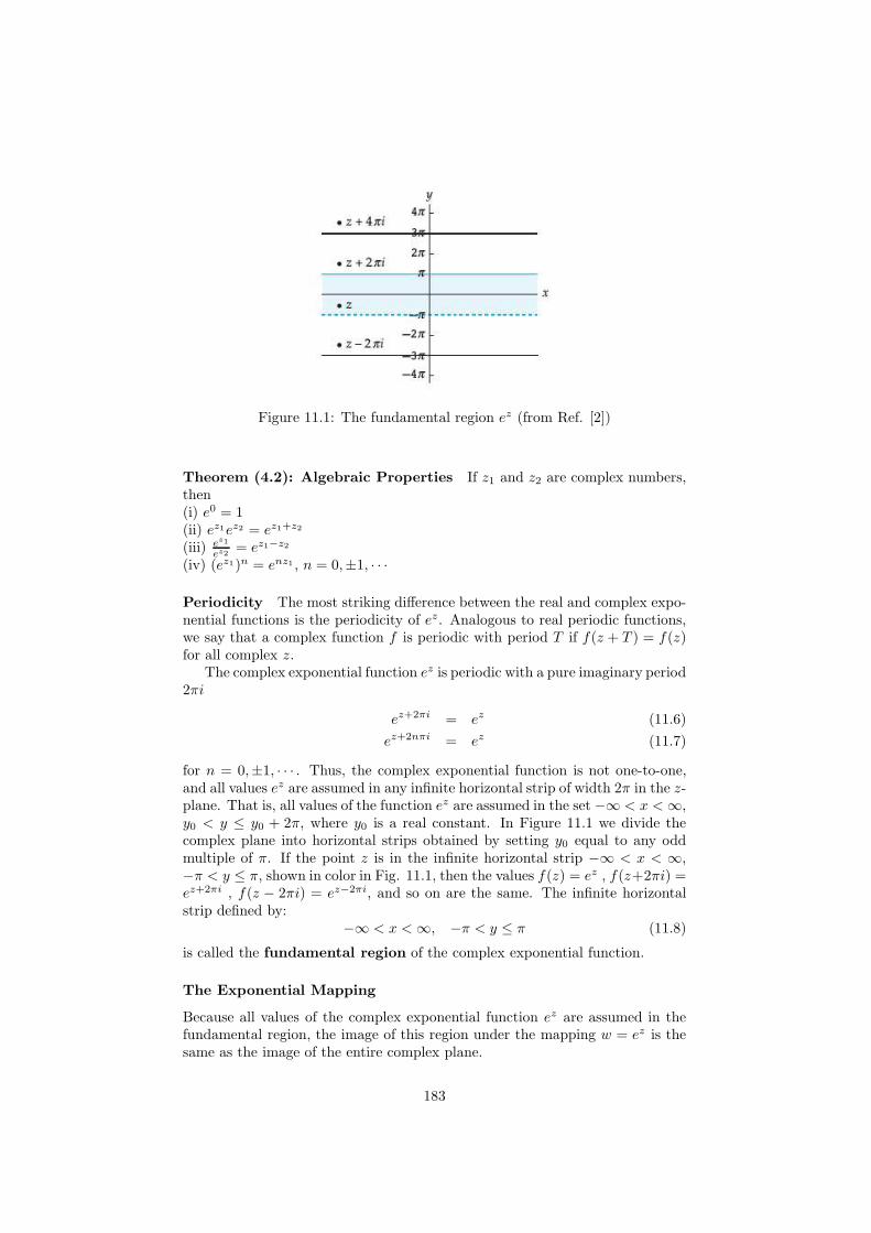
Figure 11.1: The fundamental region ez (from Ref. [2])
Theorem (4.2): Algebraic Properties If z1 and z2 are complex numbers,then(i) e0 = 1(ii) ez1ez2 = ez1+z2
(iii) ez1
ez2 = ez1−z2
(iv) (ez1)n = enz1 , n = 0,±1, · · ·
Periodicity The most striking difference between the real and complex expo-nential functions is the periodicity of ez. Analogous to real periodic functions,we say that a complex function f is periodic with period T if f(z + T ) = f(z)for all complex z.
The complex exponential function ez is periodic with a pure imaginary period2πi
ez+2πi = ez (11.6)
ez+2nπi = ez (11.7)
for n = 0,±1, · · · . Thus, the complex exponential function is not one-to-one,and all values ez are assumed in any infinite horizontal strip of width 2π in the z-plane. That is, all values of the function ez are assumed in the set −∞ < x < ∞,y0 < y ≤ y0 + 2π, where y0 is a real constant. In Figure 11.1 we divide thecomplex plane into horizontal strips obtained by setting y0 equal to any oddmultiple of π. If the point z is in the infinite horizontal strip −∞ < x < ∞,−π < y ≤ π, shown in color in Fig. 11.1, then the values f(z) = ez , f(z+2πi) =ez+2πi , f(z − 2πi) = ez−2πi, and so on are the same. The infinite horizontalstrip defined by:
−∞ < x < ∞, −π < y ≤ π (11.8)
is called the fundamental region of the complex exponential function.
The Exponential Mapping
Because all values of the complex exponential function ez are assumed in thefundamental region, the image of this region under the mapping w = ez is thesame as the image of the entire complex plane.
183

Figure 11.2: The image of the fundamental region under w = ez (from Ref. [2])
In order to determine the image of the fundamental region under w = ez, wenote that this region consists of the collection of vertical line segments z(t) = a+it, −π < t ≤ π, where a is any real number. Then, w(t) = ez(t) = ea+it = eaeit,−π < t ≤ π, where w(t) defines a circle centered at the origin with radiusea. Because a can be any real number, the radius ea of this circle can be anynonzero positive real number. Thus, the image of the fundamental region underthe exponential mapping consists of the collection of all circles centered at theorigin with nonzero radius. In other words, the image of the fundamental region−∞ < x < ∞, −π < y ≤ π, under w = ez is the set of all complex w withw 6= 0, or, equivalently, the set |w| > 0 (the point w = 0 is not in the range ofthe complex exponential function). See Fig. 11.2
There was nothing particularly special about using vertical line segmentsto determine the image of the fundamental region under w = ez. The imagecan also be found in the same manner by using, say, horizontal lines in thefundamental region.
Exponential Mapping Properties .(i) w = ez maps the fundamental region −∞ < x < ∞, −π < y ≤ π, onto theset |w| > 0.(ii) w = ez maps the vertical line segment x = a, −π < y ≤ π, onto the circle|w| = ea.(iii) w = ez maps the horizontal line y = b, −∞ < x < ∞, onto the rayarg(w) = b.
11.1.2 Complex Logarithmic Function
In complex analysis, the complex exponential function ez is not a one-to-onefunction on its domain C. To see why the equation ew = z has infinitely manysolutions, in general, suppose that w = u + iv is a solution of ew = z. Thenwe must have |ew| = |z| and arg(ew) = arg(z). It follows that eu = |z| and
184

v = arg(z), or, equivalently, u = ln |z| and v = arg(z). Therefore, if
ew = z ⇒ w = ln|z|+ iarg(z). (11.9)
Because there are infinitely many arguments of z, it gives infinitely many so-lutions w to the equation ew = z. The set of values given above defines amultiple-valued function w = G(z) which is called the complex logarithm ofz and denoted by lnz, that is,
ln z = ln |z|+ iarg(z) (11.10)
By switching to exponential notation z = reiθ we obtain the following alterna-tive description of the complex logarithm:
ln z = ln r + i(θ + 2nπ) (11.11)
with n = 0,±1,±2, · · · .The complex logarithm can be used to find all solutions to the exponential
equation ew = z when z is a nonzero complex number.
Examples: Find all complex solutions to each of the following equations:
1. ew = i
2. ew = 1 + i
3. ew = −2
Solution: For each equation ew = z, the set of solutions is given by w = ln z:
1. For z = i, we have |z| = 1 and arg(z) = π/2 + 2nπ. Thus, w = ln i =
ln 1 + i(π/2 + 2nπ) = (4n+1)π2 i, with n = 0,±1,±2, · · · .
2. For z = 1 + i, we have |z| =√2 and arg(z) = π/4 + 2nπ. Thus, w =
ln(1 + i) = ln√2 + i(π/4 + 2nπ), with n = 0,±1,±2, · · · .
3. For z = −2, we have |z| = 2 and arg(z) = π + 2nπ, thus w = ln(−2) =ln 2 + i(π + 2nπ), with n = 0,±1,±2, · · · .
Theorem (4.3): Algebraic Properties of ln z If z1 and z2 are nonzerocomplex numbers and n is an integer, then(i) ln(z1z2) = ln z1 + ln z2
(ii) ln(
z1z2
)
= ln z1 − ln z2
(iii) ln zn1 = n ln z1
185

Principal Value of a Complex Logarithm The complex function Lnzdefined by:
Lnz = ln |z|+ iArg(z) (11.12)
= ln r + iθ ,−π < θ ≤ π (11.13)
is called the principal value of the complex logarithm.It is important to note that the identities for the complex logarithm in
Theorem 4.3 are not necessarily satisfied by the principal value of the complexlogarithm. For example, it is not true that Ln(z1z2) = Lnz1 + Lnz2 for allcomplex numbers z1 and z2 (although it may be true for some complex numbers).
Lnz as an Inverse Function Because Lnz is one of the values of the com-plex logarithm ln z, it follows for z 6= 0 that, eLnz = z. This suggests thatthe logarithmic function Lnz is an inverse function of exponential function ez.Because the complex exponential function is not one-to-one on its domain, thisstatement is not completely accurate. The exponential function must first berestricted to the fundamental region on which it is one-to-one in order to havea well-defined inverse function, that is,
eLnz = z = x+ iy if −∞ < x < ∞ , −π < y ≤ π (11.14)
Lnz as an Inverse Function of ez If the complex exponential functionf(z) = ez is defined on the fundamental region −∞ < x < ∞, −π < y ≤ π,then f is one-to-one and the inverse function of f is the principal value of thecomplex logarithm f−1(z) = Lnz.
Analyticity The principal value of the complex logarithm Lnz is discontinu-ous at the point z = 0 since this function is not defined there. This function alsoturns out to be discontinuous at every point on the negative real axis. This isintuitively clear since the value of Lnz a point z near the negative x-axis in thesecond quadrant has imaginary part close to π, whereas the value of a nearbypoint in the third quadrant has imaginary part close to −π. The function Lnzis, however, continuous on the set consisting of the complex plane excluding thenonpositive real axis. Therefore Lnz is a continuous function on the domain|z| > 0, −π < arg(z) < π. Put another way, the function f1 (the principalbranch of ln z) defined by f1(z) = ln r+ iπ is continuous on the domain |z| > 0,−π < arg(z) < π for f1 where r = |z| and θ = arg(z). The nonpositive real axisis the branch cut and z = 0 is a branch point. The branch f1 is an analyticfunction on its domain.
Theorem (4.4): Analyticity of the Principal Branch of ln z The prin-cipal branch f1 of the complex logarithm defined by f1(z) = ln r + iπ is ananalytic function and its derivative is given by:
f ′1(z) =1
z(11.15)
Because f1(z) = Lnz for each point z in the domain |z| > 0, −π < arg(z) <π, it follows from Theorem 4.4 that Lnz is differentiable in this domain, and
186

that its derivative is given by f ′1. That is, |z| > 0, −π < arg(z) < π then:
d
dzLn(z) =
1
z(11.16)
Logarithmic Mapping The complex logarithmic mapping w = Lnz can beunderstood in terms of the exponential mapping w = ez since these functionsare inverses of each other. The following summarizes some of these properties.(i) w = Lnz maps the set |z| > 0 onto the region −∞ < u < ∞, −π < v ≤ π.(ii) w = Lnz maps the circle |z| = r onto the vertical line segment u = ln r,−π < v ≤ π.(iii) w = Lnz maps the ray arg(z) = θ onto the horizontal line v = θ, −∞ <u < ∞.
11.2 Complex Powers
If α is a complex number and z 6= 0, then the complex power zα is defined tobe:
zα = eα ln z (11.17)
In general, eα ln z gives an infinite set of values because the complex logarithmln z is multiple-valued. When n is an integer, however, the expression it is single-valued (in agreement with fact that zn is a function when n is an integer).
Examples: Find the values of the given complex power:(a) i2i
(b) (1 + i)i
Solution:(a) Since ln i = (4n+1)π
2 i then
i2i = e2i ln i = e−(4n+1)π (11.18)
(b) Since ln(1 + i) = 12 ln 2 +
(8n+1)π4 i then
(1 + i)i = ei ln(1+i) = e−(8n+1)π/4+i(ln 2)/2 (11.19)
Properties: .(i) zα1zα2 = zα1+α2
(ii) zα1
zα2= zα1−α2
(iii) (zα)n = znα
Principal Value of a Complex Power If α is a complex number and z 6= 0,then the function defined by:
zα = eαLnz (11.20)
is called the principal value of the complex power zα.
187

Analyticity In general, the principal value of a complex power zα = eαLnz isnot a continuous function on the complex plane because the function Lnz is notcontinuous on the complex plane. However, since the function eαz is continuouson the entire complex plane, and since the function Lnz is continuous on thedomain |z| > 0, −π < arg(z) < π, it follows that zα is continuous on the domain|z| > 0, −π < arg(z) < π. Using polar coordinates r = |z| and θ = arg(z) wehave found that the function defined by:
f1(z) = eα(ln r+iθ) (11.21)
−π < θ < π, is a branch of the multiple-valued function F (z) = zα = eα ln z.This particular branch is called the principal branch of the complex powerzα; its branch cut is the nonpositive real axis, and z = 0 is a branch point.
The branch f1 agrees with the principal value zα on the domain |z| > 0,−π < arg(z) < π. Consequently, the derivative of f1 can be found using thechain rule:
f ′1(z) =d
dzeαLnz = eαLnz d
dz(αLnz) = eαLnzα
z= zα
α
z= αzα−1
d
dzez
α
= αzα−1 (11.22)
Remarks: .(i) (zα1)α2 6= zα1α2 unless α2 is an integer.(ii) Some properties that do hold for complex powers do not hold for principalvalues of complex powers. For example, we can prove that (z1z2)
α = zα1 zα2 for
any nonzero complex numbers z1 and z2. However, this property does not holdfor principal values of these complex powers.
11.2.1 Trigonometric and Hyperbolic Functions
Complex Sine and Cosine Functions The complex sine and cosine func-tions are defined by:
sin z =eiz − e−iz
2i(11.23)
cos z =eiz + e−iz
2(11.24)
Analogous to real trigonometric functions, we next define the complex tan-gent, cotangent, secant, and cosecant functions using the complex sine andcosine:
tan z =sin z
cos zcot z =
cos z
sin z(11.25)
sec z =1
cos zcsc z =
1
sin z(11.26)
Trigonometric identities
sin(−z) = − sin z cos(−z) = cos z (11.27)
cos2 z + sin2 z = 1 (11.28)
sin(z1 ± z2) = sin z1 cos z2 ± cos z1 sin z2 (11.29)
cos(z1 ± z2) = cos z1 cos z2 ∓ sin z1 sin z2 (11.30)
188

Periodicity The complex sine and cosine are periodic functions with a realperiod of 2π
sin(z + 2π) = sin z (11.31)
cos(z + 2π) = cos z (11.32)
Example: Find all solutions to the equation sin z = 5.Solution: from
sin z =eiz − e−iz
2i= 5 (11.33)
we build a quadratic equation for eiz
e2iz − 10ieiz − 1 = 0 (11.34)
which gives
eiz = (5 ± 2√6)i (11.35)
then
z = −i ln(5 + 2√6)i =
(4n+ 1)π
2− i ln(5 + 2
√6) (11.36)
z = −i ln(5− 2√6)i =
(4n+ 1)π
2− i ln(5 − 2
√6) (11.37)
Modulus The modulus of a complex trigonometric function can also be help-ful in solving trigonometric equations. To find a formula in terms of x and y forthe modulus of the sine and cosine functions, we first express these functions interms of their real and imaginary parts.
sin z =eiz − e−iz
2i=
ei(x+iy) − e−i(x+iy)
2i(11.38)
=e−y(cosx+ i sinx)− ey(cosx− i sinx)
2i(11.39)
= sinxey + e−y
2+ i cosx
ey − e−y
2(11.40)
sin z = sinx cosh y + i cosx sinh y (11.41)
and
cos z = cosx cosh y − i sinx sinh y (11.42)
Then,
| sin z| =
√
sin2 x cosh2 y + cos2 x sinh2 y (11.43)
=
√
sin2 x+ sinh2 y (11.44)
| cos z| =
√
cos2 x+ sinh2 y (11.45)
where we have used sin2 +cos2 = 1.
189

Zeros It is a natural question to ask whether the complex sine and cosinefunctions have any additional zeros in the complex plane. One way to find thezero is by recognizing that a complex number is equal to 0 if and only if itsmodulus is 0. Thus, solving the equation sin z = 0 is equivalent to solving theequation | sin z| = 0, then
| sin z|2 = sin2 x+ sinh2 y = 0 (11.46)
Since sin2 x and sinh2 y are both nonnegative real numbers, this equation issatisfied if and only if sinx = 0 and sinh y = 0, that is, when x = nπ, n =0,±1,±2, · · · , y = 0. That is, the zeros of the complex sine function are thesame as the zeros of the real sine functions.
The only zeros of the complex cosine function are the real numbers z =(2n+ 1)π/2, n = 0,±1, · · · .
Analyticity The derivatives of the complex sine and cosine functions arefound using the chain rule, we get
d
dzsin z =
d
dz
(
eiz − e−iz
2i
)
=eiz + e−iz
2= cos z (11.47)
d
dzcos z = − sin z (11.48)
Since this derivative is defined for all complex z, sin z and cos z are an entirefunctions.
The derivatives of sin z and cos z can then be used to show that derivativesof all of the complex trigonometric functions are the same as derivatives of thereal trigonometric functions:
d
dzsin z = cos z (11.49)
d
dzcos z = − sin z (11.50)
d
dztan z = sec2 z (11.51)
d
dzcot z = − csc2 z (11.52)
d
dzsec z = sec z tan z (11.53)
d
dzcsc z = − csc z cot z (11.54)
The sine and cosine functions are entire, but the tangent and secant functionshave singularities at z = (2n+ 1)π/2 for n = 0,±1, · · · , whereas the cotangentand cosecant functions have singularities at z = nπ for n = 0,±1, · · · .
190

11.2.2 Complex Hyperbolic Functions
Complex Hyperbolic Sine and Cosine The complex hyperbolic sine andhyperbolic cosine functions are defined by:
sinh z =ez − e−z
2(11.55)
cosh z =ez + e−z
2(11.56)
The complex hyperbolic functions are periodic and have infinitely many zeros.The complex hyperbolic tangent, cotangent, secant, and cosecant are defined
in terms of sinh z and cosh z:
tanh z =sinh z
cosh zcoth z =
cosh z
sinh z(11.57)
sechz =1
cosh zcschz =
1
sinh z(11.58)
The hyperbolic sine and cosine functions are entire because the functions ez ande−z are entire.
From the chain rule we have:
d
dzsinh z = cosh z (11.59)
d
dzcosh z = sinh z (11.60)
d
dztanhz = sech2z (11.61)
d
dzcoth z = −csch2z (11.62)
d
dzsechz = −sechz tanh z (11.63)
d
dzcschz = −cschz coth z (11.64)
Relation to sine and cosine By replacing z with iz in the definition ofsinh z we have
sinh(iz) =eiz − e−iz
2= i sin z ⇒ sin(z) = −i sinh(iz) (11.65)
In a similar manner can be obtained others identities,
sin(z) = −i sinh(iz) (11.66)
cos(z) = cosh(iz) (11.67)
sinh(z) = −i sin(iz) (11.68)
cosh(z) = cos(iz) (11.69)
Relations between the other trigonometric and hyperbolic functions can nowbe derived from the above ones, for example,
tan(iz) = i tanh(z) (11.70)
191

We can also use above relations to derive hyperbolic identities from trigono-metric identities,
sinh(−z) = − sinh z cosh(−z) = cos z (11.71)
cosh2 z − sinh2 z = 1 (11.72)
sinh(z1 ± z2) = sinh z1 cosh z2 ± cosh z1 sinh z2 (11.73)
cosh(z1 ± z2) = cosh z1 cosh z2 ± sinh z1 sinh z2 (11.74)
11.3 Inverse Trigonometric and Hyperbolic Func-tions
The complex sine function is periodic with a real period of 2π. We also knownthat the sine function maps the complex plane onto the complex plane. Thesetwo properties imply that for any complex number z there exists infinitely manysolutions w to the equation sinw = z. Let us find an explicit formula for w
sinw = z =eiw − e−iw
2i⇒ ei2w − 2izeiw − 1 = 0 (11.75)
then
eiw = iz + (1− z2)1/2 (11.76)
where (1− z2)1/2 represents the two square roots of 1− z2.Finally, we solve for w using the complex logarithm:
w = −i ln[
iz + (1− z2)1/2]
(11.77)
Each value of w obtained from the above equation satisfies the equation sinw =z. Therefore, we call this multiple-valued function the inverse sine:
Inverse Sine The multiple-valued function sin−1 z defined by:
sin−1 z = arcsinz = −i ln[
iz + (1 − z2)1/2]
(11.78)
is called the inverse sine. The inverse sine is multiple-valued since it is definedin terms of the complex logarithm ln z. It is also worth repeating that theexpression (1− z2)1/2 represents the two square roots of 1− z2.
Example Find all values of sin−15.Solution: By setting z =
√5 we get,
sin−1√5 = −i ln
[
i√5 +
(
1− (√5)2)1/2
]
(11.79)
= −i ln[
i√5 + (−4)1/2
]
(11.80)
The two square roots (−4)1/2 of –4 are found to be ±2i, then
sin−1√5 = −i ln
[
i√5± 2i
]
= −i ln[
i(√
5± 2)]
(11.81)
192

Besides,
ln[
i(√
5± 2)]
= ln |(√
5± 2)
|+ i(
Arg[
i(√
5± 2)]
+ 2nπ)
(11.82)
= ln(√
5± 2)
+ i(π
2+ 2nπ
)
(11.83)
Let us noticing the following identity,
ln(√
5− 2)
= ln
[
(√5− 2)
√5 + 2√5 + 2
]
(11.84)
= ln
[
5− 4√5 + 2
]
(11.85)
= ln
[
1√5 + 2
]
(11.86)
= − ln(√
5 + 2)
(11.87)
which implies,
ln[
i(√
5± 2)]
= ± ln(√
5 + 2)
+ i(π
2+ 2nπ
)
(11.88)
Then,
sin−1√5 = −i ln
[
i(√
5± 2)]
(11.89)
= (−i)[
± ln(√
5 + 2)
+ i(π
2+ 2nπ
)]
(11.90)
= ∓i ln(√
5 + 2)
+(π
2+ 2nπ
)
(11.91)
=1 + 4n
2π ∓ i ln
(√5 + 2
)
(11.92)
Inverse cosine and inverse tangent
cos−1 z = −i ln[
z + i(1− z2)1/2]
(11.93)
tan−1 z =i
2ln
(
i+ z
i− z
)
(11.94)
Both the inverse cosine and inverse tangent are multiple-valued functions sincethey are defined in terms of the complex logarithm ln z.
Branches and Analyticity The inverse sine and inverse cosine are multiple-valued functions that can be made single-valued by specifying a single value ofthe square root to use for the expression (1 − z2)1/2 and a single value of thecomplex logarithm to use. The inverse tangent, on the other hand, can be madesingle-valued by just specifying a single value of ln z to use.
Example: We can define a function f that gives a value of the inverse sine byusing the principal square root and the principal value of the complex logarithm.
193

If, say, z =√5, then the principal square root of 1 − (
√5)2 = −4 is 2i, and
Ln(i√5 + 2i) = ln(
√5 + 2) + iπ/2, then
f(√5) =
π
2− i ln(
√5 + 2) (11.95)
Thus, we see that the value of the function f at z =√5 is the value of sin−1
√5
associated to n = 0 and the square root 2i in the example above.A branch of a multiple-valued inverse trigonometric function may be ob-
tained by choosing a branch of the square root function and a branch of thecomplex logarithm. Determining the domain of a branch defined in this mannercan be quite involved.
Derivatives of Branches sin−1 z, cos−1 z, and tan−1 z The following for-mulas for the derivatives hold only on the domains of these branches,
d
dzsin−1 z =
1
(1− z2)1/2(11.96)
d
dzcos−1 z =
−1
(1− z2)1/2(11.97)
d
dztan−1 z =
1
1 + z2(11.98)
Inverse Hyperbolic Functions The foregoing discussion of inverse trigono-metric functions can be repeated for hyperbolic functions. This leads to thedefinition of the inverse hyperbolic functions stated below. Once again theseinverses are defined in terms of the complex logarithm because the hyperbolicfunctions are defined in terms of the complex exponential.
Inverse Hyperbolic Sine, Cosine, and Tangent The multiple-valued func-tions sinh−1 z, cosh−1 z, and tanh−1 z, defined by:
sinh−1 z = ln[
z + (z2 + 1)1/2]
(11.99)
cosh−1 z = ln[
z + (z2 − 1)1/2]
(11.100)
tanh−1 z =1
2ln
(
1 + z
1− z
)
(11.101)
These expressions allow us to solve equations involving the complex hyperbolicfunctions. In particular, if w = sinh−1z, then sinhw = z.
Branches of the inverse hyperbolic functions are defined by choosing branchesof the square root and complex logarithm, or, in the case of the inverse hyper-bolic tangent, just choosing a branch of the complex logarithm. The derivativeof a branch can be found using implicit differentiation. The following resultgives formulas for the derivatives of branches of the inverse hyperbolic func-tions. In these formulas, the symbols sinh−1z, cosh−1z, and tanh−1z represent
194

branches of the corresponding inverse hyperbolic multiple-valued functions.
d
dzsinh−1 z =
1
(z2 + 1)1/2(11.102)
d
dzcosh−1 z =
1
(z2 − 1)1/2(11.103)
d
dztanh−1 z =
−1
z2 − 1(11.104)
195

Chapter 12
Integracion en el planocomplejo
Credit: This notes are 100% from chapter 5 of the book entitled A FirstCourse in Complex Analysis with Applications of Dennis G. Zill and Patrick D.Shanahan (2003) [2].
12.1 Real Integrals
Terminology Suppose a curve C in the plane is parametrized by a set ofequations x = x(t), y = y(t), a ≤ t ≤ b, where x(t) and y(t) are continuousreal functions. Let the initial and terminal points of C, that is, (x(a), y(a)) and(x(b), y(b)), be denoted by the symbols A and B, respectively. We say that:(i) C is a smooth curve if x′ and y′ are continuous on the closed interval [a, b]and not simultaneously zero on the open interval (a, b).(ii) C is a piecewise smooth curve if it consists of a finite number of smoothcurves C1, C2, · · · , Cn joined end to end, that is, the terminal point of one curveCk coinciding with the initial point of the next curve Ck+1.(iii) C is a simple curve if the curve C does not cross itself except possibly att = a and t = b.(iv) C is a closed curve if A = B.(v) C is a simple closed curve if the curve C does not cross itself and A = B;that is, C is simple and closed.
Method of Evaluation–C Defined Parametrically The line integrals canbe evaluated in two ways, depending on whether the curve C is defined by apair of parametric equations or by an explicit function. Either way, the basicidea is to convert a line integral to a definite integral in a single variable. If C issmooth curve parametrized by x = x(t), y = y(t), a ≤ t ≤ b, then replace x andy in the integral by the functions x(t) and y(t), and the appropriate differential
196

dx, dy, or ds by
dx = x′(t)dt (12.1)
dy = y′(t)dt (12.2)
ds =√
[x′(t)]2 + [y′(t)]2dt (12.3)
In this manner each of the line integrals becomes a definite integral in whichthe variable of integration is the parameter t. That is,
∫
C
G(x, y)dx =
∫ b
a
G(x(t), y(t))x′(t)dt (12.4)
∫
C
G(x, y)dy =
∫ b
a
G(x(t), y(t))y′(t)dt (12.5)
∫
C
G(x, y)ds =
∫ b
a
G(x(t), y(t))√
[x′(t)]2 + [y′(t)]2dt (12.6)
Method of Evaluation–C Defined by a Function If the path of inte-gration C is the graph of an explicit function y = f(x), a ≤ x ≤ b, then wecan use x as a parameter. In this situation, dy = f ′(x)dx, and the differentialds =
√
1 + [f ′(x)]2dx. Then,
∫
C
G(x, y)dx =
∫ b
a
G(x(t), f(x))dx (12.7)
∫
C
G(x, y)dy =
∫ b
a
G(x(t), f(x))f ′(x)dx (12.8)
∫
C
G(x, y)ds =
∫ b
a
G(x(t), f(x))√
1 + [f ′(x)]2dx (12.9)
A line integral along a piecewise smooth curve C is defined as the sum ofthe integrals over the various smooth curves whose union comprises C.
It is important to be aware that a line integral is independent of the parametriza-tion of the curve C, provided C is given the same orientation by all sets ofparametric equations defining the curve.
12.2 Complex Integrals
Curves Revisited Suppose the continuous real-valued functions x = x(t),y = y(t), a ≤ t ≤ b, are parametric equations of a curve C in the complex plane.If we use these equations as the real and imaginary parts in z = x + iy, wecan describe the points z on C by means of a complex-valued function of a realvariable t called a parametrization of C:
z(t) = x(t) + iy(t) (12.10)
with a ≤ t ≤ b. For example, the parametric equations x = cos t, y = sin t,0 ≤ t ≤ 2π, describe a unit circle centered at the origin. A parametrization ofthis circle is z(t) = cos t+ i sin t, or z(t) = eit, 0 ≤ t ≤ 2π.
The point z(a/b) = x(a/b) + iy(a/b) or A/B = (x(a/b), y(a/b)) is called theinitial/terminal point of C. z(t) = x(t)+ iy(t) could also be interpreted as a
197

two-dimensional vector function, with z(a) and z(b) being as position vectors.As t varies from t = a to t = b we can envision the curve C being traced out bythe moving arrowhead of z(t).
Contours The notions of curves in the complex plane that are smooth, piece-wise smooth, simple, closed, and simple closed are easily formulated in termsof the vector function z(t) = x(t) + iy(t). Suppose that its derivative is z′(t) =x′(t) + iy′(t). We say a curve C in the complex plane is smooth if z′(t) iscontinuous and never zero in the interval a ≤ t ≤ b. The vector z(t) is tan-gent to C at P . In other words, a smooth curve can have no sharp corners orcusps. A piecewise smooth curve C has a continuously turning tangent, ex-cept possibly at the points where the component smooth curves C1, C2, · · · , Cn
are joined together. A curve C in the complex plane is said to be a simple ifz(t1) 6= z(t2) for t1 6= t2 , except possibly for t = a and t = b. C is a closedcurve if z(a) = z(b). C is a simple closed curve if z(t1) 6= z(t2) for t1 6= t2and z(a) = z(b). In complex analysis, a piecewise smooth curve C is called acontour or path.
We define the positive direction/orientation on a contour C to be thedirection on the curve corresponding to increasing values of the parameter t. Inthe case of a simple closed curve C, the positive direction roughly correspondsto the counterclockwise direction. The negative direction is the directionopposite the positive direction.
Complex or Contour Integral An integral of a function f of a complexvariable z that is defined on a contour C is denoted by
∫
Cf(z)dz and is called
a complex or contour integral,
∫
C
f(z)dz = lim||P ||→0
n∑
k=1
f(z∗k)∆zk (12.11)
If the limit exists, then f is said to be integrable on C. The limit exists wheneverif f is continuous at all points on C and C is either smooth or piecewise smooth.Consequently we shall, hereafter, assume these conditions as a matter of course.Moreover, we will use the notation
∫
C f(z)dz to represent a complex integralaround a positively oriented closed curve.
By writing f = u + iv and ∆z = ∆x + i∆y we can write, in a short handnotation
∫
C
f(z)dz = lim∑
(u + iv)(∆x+ i∆y) (12.12)
= lim[
∑
(u∆x− v∆y) + i∑
(v∆x+ u∆y)]
(12.13)
The interpretation of the last line is
∫
C
f(z)dz =
∫
C
udx− vdy + i
∫
C
vdx+ udy (12.14)
If x = x(t), y = y(t), a ≤ t ≤ b are parametric equations of C, then
198

dx = x′(t)dt, dy = y′(t)dt, then
∫
C
udx− vdy + i
∫
C
vdx + udy =
∫ b
a
[u(x(t), y(t))x′(t)− v(x(t), y(t)) y′(t)]dt
+i
∫ b
a
[v(x(t), y(t))x′(t) + u(x(t), y(t)) y′(t)]dt (12.15)
If we use the complex-valued function z(t) = x(t)+ iy(t) to describe the contour
C, then Eq. (12.15) is the same as∫ b
a f(z(t)) z′(t)dt when the integrand
f(z(t)) z′(t) = [u(x(t), y(t)) + iv(x(t), y(t))][x′(t) + iy′(t)] (12.16)
is multiplied out and∫ b
a f(z(t))z(t)dt is expressed in terms of its real and imagi-nary parts. Thus we arrive at a practical means of evaluating a contour integral.
Evaluation of a Contour Integral If f is continuous on a smooth curve Cgiven by the parametrization z(t) = x(t) + iy(t), a ≤ t ≤ b, then
∫
C
f(z)dz =
∫ b
a
f(z(t)) z′(t) dt (12.17)
Example Evaluate the contour integral∫
Czdz, where C is given by x = 3t,
y = t2 , −1 ≤ t ≤ 4.Solution:z(t) = 3t+ it2, z′(t) = 3 + i2t and f(z(t)) = 3t− it2, then
∫
C
f(z)dz =
∫ b
a
f(z(t))z′(t)dt (12.18)
∫
C
zdz =
∫ b
a
(3t− it2)(3 + i2t)dt = 195 + i65 (12.19)
Example For some curves the real variable x itself can be used as the pa-rameter. For example, to evaluate
∫
C(8x2 − iy)dz on the line segment y = 5x,
0 ≤ x ≤ 2, we write z = x+ iy = x+ 5xi (i.e. y = 5x), dz = (1 + 5i)dx, then
∫
C
(8x2 − iy)dz =
∫ 2
0
(8x2 − i5x)(1 + 5i)dx =214
3+ i
290
3(12.20)
Properties(Theorem 5.2) Suppose the functions f and g are continuous ina domain D, and C is a smooth curve lying entirely in D. Then
(i)∫
C kf(z)dz = k∫
C f(z)dz, k a complex constant.
(ii)∫
C[f(z) + g(z)]dz =
∫
Cf(z)dz +
∫
Cg(z)dz.
(iii)∫
Cf(z)dz =
∫
C1f(z)dz+
∫
C2f(z)dz, where C consists of the smooth curves
C1 and C2 joined end to end.
199

(iv)∫
−C f(z)dz = −∫
C f(z)dz, where −C denotes the curve having the op-posite orientation of C.
All these four properties hold if C is a piecewise smooth curve in D.
Theorem (5.3): A Bounding Theorem or ML-inequality If f is contin-uous on a smooth curve C and if |f(z)| ≤ M for all z on C, then
|∫
C
f(z)dz| ≤ ML (12.21)
where L is the length of C , i.e. L =∫ b
a
√
[x′(t)]2 + [y′(t)]2dt =∫ b
a|z′(t)|dt,
where z′(t) = x′(t) + iy′(t).It follows that since f is continuous on the contour C, the bound M for the
values f(z) in Theorem 5.3 will always exist.
Example Find an upper bound for the absolute value of∮
C ez(z + 1)−1dzwhere C is the circle |z| = 4.Solution:The length L of the circle is 8π. Next, for all points z on the circle |z + 1| ≥|z| − 1 = 3. Thus
∣
∣
∣
∣
ez
z + 1
∣
∣
∣
∣
≤ |ez||z| − 1
=ex
3≤ e4
3(12.22)
where we used that on the circle |z| = 4 ⇒ maxx = 4, then
∣
∣
∣
∣
∫
C
f(z)dz
∣
∣
∣
∣
≤ ML =8πe4
3(12.23)
12.3 Cauchy-Goursat Theorem
In this section we shall concentrate on contour integrals, where the contour C isa simple closed curve with a positive (counterclockwise) orientation. Specifically,we shall see that when f is analytic in a special kind of domain D, the valueof the contour integral
∮
Cf(z)dz is the same for any simple closed curve C that
lies entirely within D.
Simply and Multiply Connected Domains A domain is an open con-nected set in the complex plane. We say that a domain D is simply connectedif every simple closed contour C lying entirely in D can be shrunk(encogido)to a point without leaving D. A simply connected domain has no “holes” init. The entire complex plane is an example of a simply connected domain; theannulus defined by 1 < |z| < 2 is not simply connected. A domain that is notsimply connected is called a multiply connected domain; that is, a multiplyconnected domain has “holes” in it.
In 1825 the French mathematician Louis-Augustin Cauchy proved one of themost important theorems in complex analysis:
200

Cauchy’s Theorem Suppose that a function f is analytic in a simply con-nected domain D and that f is continuous in D. Then for every simple closedcontour C in D,
∮
C
f(z)dz = 0 (12.24)
Proof: See pag. 257 in Ref. [2].In 1883 the French mathematician Edouard Goursat proved that the as-
sumption of continuity of f is not necessary to reach the conclusion of Cauchy’stheorem. The resulting modified version of Cauchy’s theorem is known todayas the Cauchy-Goursat theorem:
Theorem (5.4): Cauchy-Goursat Theorem Suppose that a function f isanalytic in a simply connected domain D. Then for every simple closed contourC in D,
∮
C
f(z)dz = 0 (12.25)
Proof: See Appendix II in Ref. [2].Since the interior of a simple closed contour is a simply connected domain,
the Cauchy-Goursat theorem can be stated in the slightly more practical man-ner:If f is analytic at all points within and on a simple closed contour C, then∮
Cf(z)dz = 0.
Example Using an arbitrary shaped contour C in the first quadrant calculates∮
C ezdz.Solution: The function f(z) = ez is entire and consequently is analytic at allpoints within and on the simple closed contour C. It follows that
∮
C ezdz = 0.The point in this example is that
∮
C ezdz = 0 for any simple closed contour inthe complex plane. Indeed, it follows that for any simple closed contour C andany entire function f that the integral is nil, for example
∮
C
sin zdz = 0 (12.26)
∮
C
cos zdz = 0 (12.27)
∮
C
n∑
k=0
akzkdz = 0 (12.28)
and so on.
Example Evaluate∮
Cdzz2 , where the contour C is the ellipse (x− 2)2 + 1
4 (y−5)2 = 1.Solution: The rational function f(z) = 1/z2 is analytic everywhere except atz = 0. But z = 0 is not a point interior to or on the simple closed ellipticalcontour C. Thus,
∮
Cdzz2 = 0.
201

Figure 12.1: Doubly connected domain D (from Ref. [2])
Principle of deformation of contours If f is analytic in a multiply con-nected domain D then we cannot conclude that
∮
C f(z)dz = 0 for every simpleclosed contour C in D. To begin, suppose that D is a doubly connected domain(i.e. a domain with a single “hole“) and C and C1 are simple closed contourssuch that C1 surrounds the “hole” in the domain and is interior to C (see Fig.12.1(a)). Suppose, also, that f is analytic on each contour and at each pointinterior to C but exterior to C1. By introducing the crosscut AB shown in Fig-ure 12.1(b), the region bounded between the curves is now simply connected.From (iv) of Theorem 5.2, the integral from A to B has the opposite value ofthe integral from B to A, then
0 =
∮
C
f(z)dz +
∫
AB
f(z)dz +
∫
−AB
f(z)dz +
∮
C1
f(z)dz
(aquı C se recorre en sentido antihorario y C1 en sentido horario)luego
∮
C
f(z)dz =
∮
C1
f(z)dz (12.29)
(aquı ambos, C y C1, se recorren en sentido antihorario)This result is sometimes called the principle of deformation of contours sincewe can think of the contour C1 as a continuous deformation of the contour C.Under this deformation of contours, the value of the integral does not change.The when can evaluate an integral over a complicated simple closed contour Cby replacing it with a contour C1 that is more convenient.
The next theorem summarizes the general result for a multiply connecteddomain with n “holes.”
Theorem (5.5): Cauchy-Goursat Theorem for Multiply ConnectedDomains Suppose C,C1, · · · , Cn are simple closed curves with a positive ori-entation such that C1, C2, · · · , Cn are interior to C but the regions interior toeach Ck , k = 1, 2, · · · , n, have no points in common. If f is analytic on each con-tour and at each point interior to C but exterior to all the Ck , k = 1, 2, · · · , n,then
∮
C
f(z)dz =n∑
k=1
∮
Ck
f(z)dz (12.30)
202

Example Evaluate∮
Cdzz−i , where C is a complicated contour which contains
z = i.Solution: we choose the more convenient circular contour C1 centered at z0 = iand radius r = 1, i.e. |z − i| = 1. It can be parametrized by z = i + eit,0 ≤ t ≤ 2π. Then
∮
C
dz
z − i=
∮
C1
dz
z − i=
∫ 2π
0
dz
eit=
∫ 2π
0
ieitdt
eit
= 2πi (12.31)
This result can be generalized: if z0 is any constant complex number interiorto any simple closed contour C, then for n an integer we have
∮
C
dz
(z − z0)n=
{
2πi n = 10 n 6= 1
(12.32)
The fact that this integral is zero when n 6= 1 follows only partially from theCauchy-Goursat theorem. When n is zero or a negative integer, then 1/(z −z0)
n is a polynomial and therefore entire. Theorem 5.4 then indicates that theintegral is zero.
Analyticity of the function f at all points within and on a simple closedcontour C is sufficient to guarantee that
∮
C f(z)dz = 0. However, the previousexample emphasizes that analyticity is not necessary.
Example Evaluate∮
C5z+7
z2+2z−3dz, where C is the circle |z − 2| = 2.Solution: The roots of the denominators are 1 and −3. The integrand failsat these roots. Of these two points, only z = 1 lies within the contour C.Separating the roots by partial fraction
5z + 7
z2 + 2z − 3=
3
z − 1+
2
z + 3(12.33)
we have∮
C
5z + 7
z2 + 2z − 3dz =
∮
C
3
z − 1dz +
∮
C
2
z + 3dz (12.34)
from the above calculation, the first integral gives 2πi, whereas the second gives0 by the Cauchy-Goursat theorem. Then
∮
C
5z + 7
z2 + 2z − 3dz = 3(2πi) + 2(0) = 6πi (12.35)
Example Evaluate∮
Cdz
z2+1 , where C is the circle |z| = 4.
Solution: In this case the denominator of the integrand factors as z2+1 = (z−i)(z+ i). Consequently, the integrand 1/(z2+1) is not analytic at z = ±i. Bothof these points lie within the contour C. Using partial fraction decompositiononce more, we have
∮
C
dz
z2 + 1=
∮
C
dz
2i(z − i)−∮
C
dz
2i(z + i)=
1
2i
∮
C
[
1
z − i− 1
z + i
]
dz
203
Next we surround the points z = i and z = −i by circular contours C1 and C2 ,respectively, that lie entirely within C. Specifically, the choice |z − i| = 1/2 forC1 and |z + i| = 1/2 for C2 will suffice. Then
∮
C
dz
z2 + 1=
1
2i
∮
C1
[
1
z − i− 1
z + i
]
dz +1
2i
∮
C2
[
1
z − i− 1
z + i
]
dz
=1
2i[2πi− 0] +
1
2i[0− 2πi] = 0 (12.36)
Remark Throughout the foregoing discussion we assumed that C was a simpleclosed contour. It can be shown that the Cauchy-Goursat theorem is valid forany closed contour C in a simply connected domain D.
There exist integrals∫
C Pdx+Qdy whose value depends only on the initialpoint A and terminal point B of the curve C, and not on C itself. In this casewe say that the line integral is independent of the path.
Independence of the Path Let z0 and z1 be points in a domain D. Acontour integral
∫
C f(z)dz is said to be independent of the path if its value isthe same for all contours C in D with initial point z0 and terminal point z1.
Theorem (5.6): Analyticity Implies Path Independence Suppose thata function f is analytic in a simply connected domain D and C is any contourin D. Then
∫
Cf(z)dz is independent of the path C. (See below...)
Suppose, as shown in Figure 12.2 that C and C1 are two contours lyingentirely in a simply connected domain D and both with initial point z0 andterminal point z1. If f is analytic in D, it follows from the Cauchy-Goursattheorem that
∫
C
f(z)dz +
∫
−C1
f(z)dz = 0 (12.37)
∫
C
f(z)dz =
∫
C1
f(z)dz (12.38)
A contour integral∫
Cf(z)dz that is independent of the path C is usually
written∫ z1z0
f(z)dz, where z0 and z1 are the initial and terminal points of C.
Example Evaluate∫
C 2zdz, where C is the contour shown in color in Figure12.3.Solution: Since the function f(z) = 2z is entire, we can, in view of Theorem5.6, replace the piecewise smooth path C by any convenient contour C1 joiningz0 = −1 and z1 = −1+i. Using the black contour in Fig. 12.3, then z = −1+iy,dz = idy, 0 ≤ y ≤ 1. Therefore,
∫
C
2zdz =
∫
C1
2zdz =
∫ 1
0
2(−1 + iy)(idy)
= −2i
∫ 1
0
dy − 2
∫ 1
0
ydy = [−2i]− 2[1
2] = −1− 2i
204

Figure 12.2: If f is analytic in D, integrals on C and C1 are equal (from Ref.[2]).
Figure 12.3: Alternative contour for the integral∫
C 2zdz (from Ref. [2]).
205

Antiderivative Suppose that a function f is continuous on a domain D. Ifthere exists a function F such that F ′(z) = f(z) for each z in D, then F iscalled an antiderivative of f . For example, the function F (z) = − cos z is anantiderivative of f(z) = sin z.
Indefinite integral The most general antiderivative, or indefinite integral, ofa function f(z) is written
∫
f(z)dz = F (z) + C, where F ′(z) = f(z) and C issome complex constant. For example,
∫
sin zdz = − cos z + C.Since an antiderivative F of a function f has a derivative at each point in a
domain D, it is necessarily analytic and hence continuous at each point in D.
Theorem (5.7): Fundamental Theorem for Contour Integrals Supposethat a function f is continuous on a domain D and F is an antiderivative of fin D. Then for any contour C in D with initial point z0 and terminal point z1,
∫
C
f(z)dz = F (z1)− F (z0) (12.39)
Example Calculate the integral∫
C2zdz with the same contour as in the pre-
vious example.Solution: Now since the f(z) = 2z is an entire function, it is continuous. More-over, F (z) = z2 is an antiderivative of f .
∫ −1+i
−12zdz = z2
∣
∣
−1+i
−1 = −1− 2i (12.40)
Example Evaluate∫
C cos zdz, where C is any contour with initial point z0 = 0and terminal point z1 = 2 + i.Solution: F (z) = sin z is an antiderivative of f(z) = cos z since F ′(z) = cos z =f(z). Therefore,
∫
C
cos zdz =
∫ 2+i
0
cos zdz = sin z|2+i0 = sin(2 + i) ≈ 1.4031− i0.4891 (12.41)
Some Conclusions We can draw several immediate conclusions from Theo-rem 5.7.(i) If the contour C is closed, then z0 = z1 and, consequently,
∫
C f(z)dz = 0.(ii) Since the value of
∫
Cf(z)dz depends only on the points z0 and z1 , this value
is the same for any contour C in D connecting these points, i.e. if a continuousfunction f has an antiderivative F in D, then
∫
C f(z)dz is independent of thepath.(iii) If f is continuous and
∫
C f(z)dz is independent of the path C in a domainD, then f has an antiderivative everywhere in D.
If f is an analytic function in a simply connected domain D, it is necessarilycontinuous throughout D. This fact, when put together with the results inTheorem 5.6 (iii), leads to a theorem which states that an analytic functionpossesses an analytic antiderivative.
206

Theorem (5.8): Existence of an Antiderivative Suppose that a functionf is analytic in a simply connected domain D. Then f has an antiderivative inD; that is, there exists a function F such that F ′(z) = f(z) for all z in D.
About the antiderivate of 1/z We saw for |z| > 0, −π < arg(z) < π, that1/z is the derivative of Lnz. This means that under some circumstances Lnzis an antiderivative of 1/z. But care must be exercised in using this result.For example, suppose D is the entire complex plane without the origin. Thefunction 1/z is analytic in this multiply connected domain. If C is any simpleclosed contour containing the origin, it does not follow that
∮
C dz/z = 0. In fact,from the result for
∮
c dz/(z− z0)n for n = 1 and z0 = 0, we have
∮
C dz/z = 2πi.In this case, Lnz is not an antiderivative of 1/z in D since Lnz is not analyticin D. Recall, Lnz fails to be analytic on the nonpositive real axis.
Example Evaluate∫
C 1/zdz, where C is a contour in the first quadrant start-ing at z0 = 3 and ending at z = 2i.Solution: Suppose that D is the simply connected domain defined by x > 0,y > 0, i.e. D is the first quadrant in the z-plane. In this case, Lnz is anantiderivative of 1/z since both these functions are analytic in D. Hence,
∫ 2i
3
1
zdz = Lnz|2i3 = Ln2i− Ln3 (12.42)
= (ln 2 + iπ
2) + (ln 3) ≈ −0.4055 + i1.5708 (12.43)
Example Evaluate∫
C1/z1/2dz, where C is the line segment between z0 = i
and z1 = 9.Solution: Throughout we take f1(z) = z1/2 to be the principal branch of thesquare root function. In the domain |z| > 0, −π < arg(z) < π, the functionf1(z) = 1/z1/2 = z−1/2 is analytic and possesses the antiderivative F (z) =2z1/2. Hence,
∫ 9
i
1
z1/2dz = 2z1/2
∣
∣
∣
9
i= 2
[
3−(√
2
2+ i
√2
2
)]
= (6 −√2)− i
√2 (12.44)
Remarks .(i) Integration by parts: Suppose f and g are analytic in a simply connecteddomain D. Then,
∫
f(z)g′(z)dz = f(z)g(z)−∫
g(z)f ′(z)dz (12.45)
(ii) In addition, if z0 and z1 are the initial and terminal points of a contour Clying entirely in D, then
∫ z1
z0
f(z)g′(z)dz = f(z)g(z)|z1z0 −∫ z1
z0
g(z)f ′(z)dz (12.46)
(iii) In complex analysis there is no complex counterpart to the mean-value
theorem∫ b
af(x)dx = f(c)(b− a) of real analysis, valid if f is continuous on the
closed interval [a, b], and c is a number in the open interval (a, b).
207

12.4 Cauchy’s Integral Formulas and their Con-
sequences
The most significant consequence of the Cauchy-Goursat theorem is the fol-lowing result: the value of a analytic function f at any point z0 in a simplyconnected domain can be represented by a contour integral.
After establishing this proposition we shall use it to further show that: ananalytic function f in a simply connected domain possesses derivatives of allorders.
12.4.1 Cauchy’s Two Integral Formulas
If f is analytic in a simply connected domain D and z0 is any point in D,the quotient f(z)/(z − z0) is not defined at z0 and hence is not analytic inD. Therefore, we cannot conclude that the integral of f(z)/(z − z0) around asimple closed contour C that contains z0 is zero by the Cauchy-Goursat theorem.Indeed, as we shall now see, the integral of f(z)/(z−z0) around C has the value2πif(z0). The first of two remarkable formulas is known simply as the Cauchyintegral formula.
Theorem (5.9): Cauchy’s Integral Formula Suppose that f is analytic ina simply connected domain D and C is any simple closed contour lying entirelywithin D. Then for any point z0 within C,
f(z0) =1
2πi
∮
C
f(z)
z − z0dz (12.47)
Proof: See pag. 273 in Ref. [2].Because the symbol z represents a point on the contour C, the integral
f(z0) =1
2πi
∮
C f(z)/(z − z0)dz indicates that the values of an analytic functionf at points z0 inside a simple closed contour C are determined by the values off on the contour C.
Cauchy’s integral formula can be used to evaluate contour integrals. Sincewe often work problems without a simply connected domain explicitly defined,a more practical restatement of Theorem 5.9 is:If f is analytic at all points within and on a single contour C, and z0 is anypoint interior to C, the f(z0) =
12πi
∮
Cf(z)/(z − z0)dz.
Example Evaluate∮
C(z2 − 4z + 4)/(z + i)dz, where C is the circle |z| = 2.
Solution: First, we identify f(z) = z2 − 4z + 4 and z0 = −i as a point withinthe circle C. Next, we observe that f is analytic at all points within and on thecontour C. Thus, by the Cauchy integral formula we obtain
∮
C
z2 − 4z + 4
z + idz = 2πif(−i) = π(−8 + i6) (12.48)
Example Evaluate∮
C z/(z2 + 9)dz, where C is the circle |z − 2i| = 4.Solution: The roots of denominator are 3i and −3i. We see that 3i is the only
208
point within the closed contour C at which the integrand fails to be analytic.Then,
∮
C
z
z2 + 9dz =
∮
C
z
(z − 3i)(z + 3i)dz =
∮
C
f(z)
z − 3idz (12.49)
with f(z) = z/(z + 3i), then∮
C
z
z2 + 9dz = 2πif(3i) = iπ (12.50)
We shall now build on Theorem 5.9 by using it to prove that the values of thederivatives f (n)(z0), n = 1, 2, 3, · · · of an analytic function are also given by anintegral formula. This second integral formula is known by the name Cauchy’sintegral formula for derivatives.
Theorem (5.10): Cauchy’s Integral Formula for Derivatives Supposethat f is analytic in a simply connected domain D and C is any simple closedcontour lying entirely within D. Then for any point z0 within C,
f (n)(z0) =n!
2πi
∮
C
f(z)
(z − z0)n+1dz (12.51)
Proof: The demostration for n = 1 is given in pag. 275 of Ref. [2].The Cauchy’s integral formula for derivatives can be used to evaluate inte-
grals.
Example Evaluate∮
C(z + 1)/(z4 + 2iz3)dz, where C is the circle |z| = 1.Solution: The integrand is not analytic at z = 0 and z = −2i, but only z = 0lies within the closed contour. By writing the integral as
∮
C
z + 1
z4 + 2iz3dz =
∮
C
z + 1
(z + 2i)(z − 0)3dz (12.52)
we can identify, z0 = 0, n = 2, and f(z) = (z + 1)/(z + 2i). Then, f ′′(z) =(2− 4i)/(z + 2i)3 and f ′′(0) = (2i− 1)/4i,
∮
C
z + 1
z4 + 2iz3dz =
2πi
2!f ′′(0) = −π
4+ i
π
2(12.53)
Example Evaluate∫
C(z3 + 3)/(z(z − i)2)dz, where C is shown in Fig. 12.4.
Solution: Although C is not a simple closed contour, we can think of it as theunion of two simple closed contours C1 and C2. Hence, we write
∫
C
z3 + 3
z(z − i)2dz =
∫
C1
z3 + 3
z(z − i)2dz +
∫
C2
z3 + 3
z(z − i)2dz (12.54)
= −∮
−C1
z3 + 3
z(z − i)2dz +
∮
C2
z3 + 3
z(z − i)2dz (12.55)
= −∮
−C1
f(z)
zdz +
∮
C2
g(z)
(z − i)2dz (12.56)
= −[2πif(0)] +2πi
1!g′(i) (12.57)
209

Figure 12.4: (from Ref. [2])
with
f(z) =z3 + 3
(z − i)2(12.58)
g(z) =z3 + 3
z(12.59)
g′(z) =2z3 − 3
z2(12.60)
and f(0) = −3, g′(i) = 3 + 2i, then
∫
C
z3 + 3
z(z − i)2dz = −6πi+ (−4π + 6πi) = −4π + i 12π (12.61)
12.4.2 Some Consequences of the Integral Formulas
Theorem (5.11): Derivative of an Analytic Function is Analytic Sup-pose that f is analytic in a simply connected domain D. Then f possessesderivatives of all orders at every point z in D. The derivatives f ′, f ′′, f ′′′, · · ·are analytic functions in D.
If a function f(z) = u(x, y) + iv(x, y) is analytic in a simply connecteddomain D, from
f ′(z) =∂u
∂x+ i
∂v
∂x=
∂v
∂y− i
∂u
∂y(12.62)
f ′′(z) =∂2u
∂x2+ i
∂2v
∂x2=
∂2v
∂y∂x− i
∂2u
∂y∂x(12.63)
=... (12.64)
we can also conclude that the real functions u and v have continuous partialderivatives of all orders at a point of analyticity.
Theorem (5.12): Cauchy’s Inequality Suppose that f is analytic in asimply connected domain D and C is a circle defined by |z − z0| = r that lies
210
entirely in D. If |f(z)| ≤ M for all points z on C, then
|f (n)(z0)| ≤n!M
rn(12.65)
Proof: Pag. 278 in Ref. [2]
Theorem 5.12 is then used to prove the next theorem. The gist(esencia) ofthe theorem is that an entire function f , one that is analytic for all z, cannotbe bounded unless f itself is a constant.
Theorem (5.13): Liouville’s Theorem The only bounded entire functionsare constants.Proof: See pag. 279 of Ref. [2].
Theorem (5.14): Fundamental Theorem of Algebra If p(z) is a non-constant polynomial, then the equation p(z) = 0 has at least one root.Proof: See pag. 279 of Ref. [2].
If p(z) is a nonconstant polynomial of degree n, then p(z) = 0 has exactly nroots (counting multiple roots). See Problem 29 in Exercises 5.5 of Ref. [2].
Morera’s Theorem gives a sufficient condition for analyticity. It is oftentaken to be the converse of the Cauchy-Goursat theorem.
Theorem (5.15): Morera’s Theorem If f is continuous in a simply con-nected domain D and if
∮
Cf(z)dz = 0 for every closed contour C in D, then f
is analytic in D.Proof: See pag. 280 of Ref. [2].
The next theorem tells us that |f(z)| assumes its maximum value at somepoint z on the boundary C.
Theorem (5.16): Maximum Modulus Theorem Suppose that f is ana-lytic and nonconstant on a closed region R bounded by a simple closed curveC. Then the modulus |f(z)| attains its maximum on C.
If the stipulation that f(z) 6= 0 for all z in R is added to the hypotheses ofTheorem 5.16, then the modulus |f(z)| also attains its minimum on C.
Example Find the maximum modulus of f(z) = 2z+5i on the closed circularregion defined by |z| ≤ 2.Solution: |z| = zz, then for z → 2z + i5 we get |f(z)| = 4|z2| + 20ℑ(z) + 25.Because f is a polynomial, it is analytic on the region defined by |z| ≤ 2. ByTheorem 5.16, max|z|≤2|2z +5i| occurs on the boundary |z| = 2. Therefore, on
|z| = 2, |2z + 5i| =√
41 + 20ℑ(z). This expression attains its maximum whenIm(z) attains its maximum on |z| = 2, namely, at the point z = 2i. Thus,max|z|≤2|2z + 5i| =
√81 = 9.
In this example, f(z) = 0 only at z = −i5/2 and that this point is outsidethe region defined by |z| ≤ 2. Hence we can conclude that |2z + 5i| attains
211

its minimum when Im(z) attains its minimum on |z| = 2 at z = −2i. Then,min|z|≤2|2z + 5i| =
√1 = 1.
212

Chapter 13
Series y residuos
Credit: This notes are 100% from chapter 6 of the book entitled A FirstCourse in Complex Analysis with Applications of Dennis G. Zill and Patrick D.Shanahan (2003) [2].
Cauchy’s integral formula for derivatives indicates that if a function f isanalytic at a point z0 , then it possesses derivatives of all orders at that point.As a consequence of this result we shall see that f can always be expanded in apower series centered at that point. On the other hand, if f fails to be analyticat z0, we may still be able to expand it in a different kind of series known as aLaurent series. The notion of Laurent series leads to the concept of a residue,and this, in turn, leads to yet another way of evaluating complex and, in someinstances, real integrals.
13.1 Sequences and Series
Sequences A sequence {zn} is a function whose domain is the set of positiveintegers and whose range is a subset of the complex numbers C. If limn→∞ zn =L, we say the sequence {zn} is convergent. In other words, {zn} converges tothe number L if for each positive real number ε an N can be found such that|zn − L| < ε whenever n > N . A sequence that is not convergent is said to bedivergent.
Example: The sequence { in+1
n } is convergent, limn→∞in+1
n = 0.
Theorem (6.1): Criterion for Convergence A sequence {zn} convergesto a complex number L = a+ ib if and only if ℜ(zn) converges to ℜ(L) = a andℑ(zn) converges to ℑ(L) = b.
213
Example Consider the sequence { 3+inn+i2n}
Solution: it converges since,
zn =3 + in
n+ i2n=
2n2 + 3n
5n2+ i
n2 − 6n
5n2(13.1)
ℜ(zn) → 2
5(13.2)
ℑ(zn) → 1
5(13.3)
as n → ∞.
Series An infinite series or series of complex numbers
∞∑
k=1
zk = z1 + z2 + · · ·+ zn + · · · (13.4)
is convergent if the sequence of partial sums {Sn}, where
Sn = z1 + z2 + · · ·+ zn (13.5)
converges. If Sn → L as n → ∞, we say that the series converges to L or thatthe sum of the series is L.
Geometric Series A geometric series is any series of the form
∞∑
k=1
azk−1 = a+ az + az2 + · · ·+ azn−1 + · · · (13.6)
the nth term of the sequence of partial sums is
Sn = a+ az + az2 + · · ·+ azn−1 (13.7)
When an infinite series is a geometric series, it is always possible to find aformula for Sn:
zSn = az + az2 + · · ·+ azn (13.8)
Sn − zSn = (az + az2 + · · ·+ azn)− (a+ az + az2 + · · ·+ azn−1)(13.9)
Sn(1 − z) = a− azn = a(1− zn) ⇒ Sn = a1− zn
1− z(13.10)
for n → ∞, zn → 0 whenever |z| < 1, then Sn → a/(1− z), then
a+ az + az2 + · · ·+ azn−1 + · · · = a
1− z(13.11)
A geometric series diverges when |z| ≥ 1.
Special Geometric Series .(i) For a = 1
1
1− z= 1 + z + z2 + z3 + · · · (13.12)
214
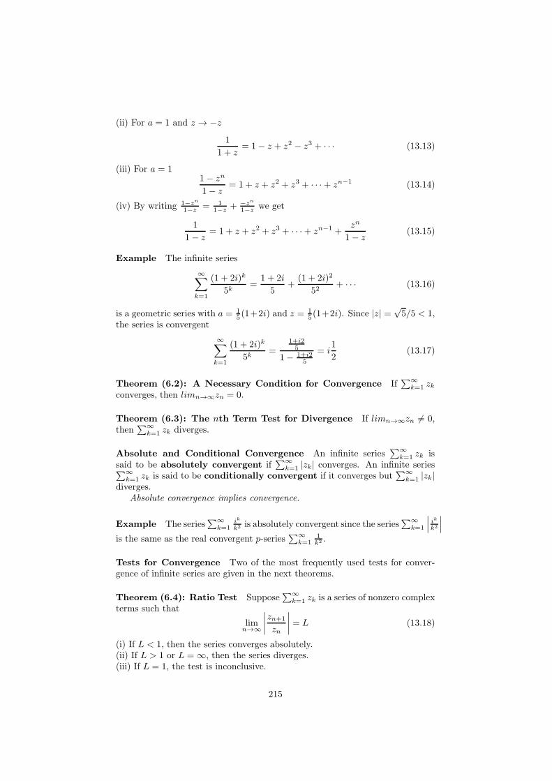
(ii) For a = 1 and z → −z
1
1 + z= 1− z + z2 − z3 + · · · (13.13)
(iii) For a = 11− zn
1− z= 1 + z + z2 + z3 + · · ·+ zn−1 (13.14)
(iv) By writing 1−zn
1−z = 11−z + −z
n
1−z we get
1
1− z= 1 + z + z2 + z3 + · · ·+ zn−1 +
zn
1− z(13.15)
Example The infinite series
∞∑
k=1
(1 + 2i)k
5k=
1 + 2i
5+
(1 + 2i)2
52+ · · · (13.16)
is a geometric series with a = 15 (1+2i) and z = 1
5 (1+2i). Since |z| =√5/5 < 1,
the series is convergent
∞∑
k=1
(1 + 2i)k
5k=
1+i25
1− 1+i25
= i1
2(13.17)
Theorem (6.2): A Necessary Condition for Convergence If∑∞
k=1 zkconverges, then limn→∞zn = 0.
Theorem (6.3): The nth Term Test for Divergence If limn→∞zn 6= 0,then
∑∞k=1 zk diverges.
Absolute and Conditional Convergence An infinite series∑∞
k=1 zk issaid to be absolutely convergent if
∑∞k=1 |zk| converges. An infinite series
∑∞k=1 zk is said to be conditionally convergent if it converges but
∑∞k=1 |zk|
diverges.Absolute convergence implies convergence.
Example The series∑∞
k=1ik
k2 is absolutely convergent since the series∑∞
k=1
∣
∣
∣
ik
k2
∣
∣
∣
is the same as the real convergent p-series∑∞
k=11k2 .
Tests for Convergence Two of the most frequently used tests for conver-gence of infinite series are given in the next theorems.
Theorem (6.4): Ratio Test Suppose∑∞
k=1 zk is a series of nonzero complexterms such that
limn→∞
∣
∣
∣
∣
zn+1
zn
∣
∣
∣
∣
= L (13.18)
(i) If L < 1, then the series converges absolutely.(ii) If L > 1 or L = ∞, then the series diverges.(iii) If L = 1, the test is inconclusive.
215

Theorem (6.5): Root Test Suppose∑∞
k=1 zk is a series of nonzero complexterms such that
limn→∞
n√
|zn| = L (13.19)
(i) If L < 1, then the series converges absolutely.(ii) If L > 1 or L = ∞, then the series diverges.(iii) If L = 1, the test is inconclusive.
Power Series The notion of a power series is important in the study of ana-lytic functions. An infinite series of the form
∞∑
k=1
ak(z − z0)k = a0 + a1(z − z0) + a2(z − z0)
2 + · · · (13.20)
where the coefficients ak are complex constants, is called a power series in z−z?0.It is said to be centered at z0, called the center of the series.
Circle of Convergence Every complex power series∑∞
k=0 ak(z − z0)k has
a radius of convergence and a circle of convergence, which is the circlecentered at z0 of largest radius R > 0 for which the series converges at everypoint within the circle |z − z0| = R. A power series converges absolutely at allpoints z within its circle of convergence, that is, for all z satisfying |z− z0| < R,and diverges at all points z exterior to the circle, that is, for all z satisfying|z − z0| > R. The radius of convergence can be:(i) R = 0 (in which case the serie converges only at its center z = z0 ),(ii) R a finite positive number (in which case the serie converges at all interiorpoints of the circle |z − z0| = R), or(iii) R = ∞ (in which case the serie converges for all z).A power series may converge at some, all, or at none of the points on the actualcircle of convergence.
Example Consider the power series∑∞
k=1zk+1
k . By the ratio test,
limn→∞
∣
∣
∣
∣
∣
zn+2
n+1
zn+1
n
∣
∣
∣
∣
∣
= limn→∞
n
n+ 1|z| = |z| (13.21)
Thus the series converges absolutely for |z| < 1. The circle of convergence is|z| = 1 and the radius of convergence is R = 1. On the circle of convergence|z| = 1, the series does not converge absolutely since
∑∞k=1
1k is the well-known
divergent harmonic series.For a power series
∑∞k=1 ak(z − z0)
k, the limit depends only on the coeffi-cients ak. Thus, if
(i) limn→∞∣
∣
∣
an+1
an
∣
∣
∣ = L 6= 0, the radius of convergence is R = 1/L. Esto es ası
porque para que la serie converja el cociente lim an+1|z−z0|n+1
an|z−z0|n = lim an+1
anR =
LR < 1.(ii) limn→∞
∣
∣
∣
an+1
an
∣
∣
∣ = 0, the radius of convergence is R = ∞
(iii) limn→∞∣
∣
∣
an+1
an
∣
∣
∣ = ∞, the radius of convergence is R = 0
Similar conclusions can be made for the root test.
216

Example Consider the power series∑∞
k=1(−1)k+1
k! (z− 1− i)k. With the iden-tification an = (−1)n+1/n! we have
limn→∞
∣
∣
∣
∣
∣
∣
(−1)n+2
(n+1)!
(−1)n+1
n!
∣
∣
∣
∣
∣
∣
= limn→∞
1
n+ 1= 0 (13.22)
Hence the radius of convergence is ∞; the power series with center z0 = 1 + iconverges absolutely for all z, that is, for |z − 1− i| < ∞.
Example Consider the power series∑∞
k=1
(
6k+12k+5
)k
(z − 2i)k. With an =(
6n+12n+5
)n
, the root test gives
limn→∞
n√
|an| = limn→∞
6n+ 1
2n+ 5= 3 (13.23)
Then, the radius of convergence of the series is R = 1/3. The circle of conver-gence is |z − 2i| = 1/3; the power series converges absolutely for |z − 2i| < 1/3.
The Arithmetic of Power Series Some facts
• A power series∑∞
k=0 ak(z − z0)k can be multiplied by a nonzero complex
constant c without affecting its convergence or divergence.
• A power series∑∞
k=0 ak(z − z0)k converges absolutely within its circle of
convergence. As a consequence, within the circle of convergence the termsof the series can be rearranged and the rearranged series has the same sumL as the original series.
• A power series∑∞
k=0 ak(z − z0)k and
∑∞k=0 bk(z − z0)
k can be added andsubtracted by adding or subtracting like terms. In symbols:
∞∑
k=0
ak(z − z0)k ±
∞∑
k=0
bk(z − z0)k =
∞∑
k=0
(ak ± bk)(z − z0)k (13.24)
If both series have the same nonzero radius R of convergence, the radiusof convergence of
∑∞k=0(ak ± bk)(z − z0)
k is R.
• Two power series can (with care) be multiplied and divided.
13.2 Taylor Series
Throughout the discussion in this section we will assume that a power serieshas either a positive or an infinite radius R of convergence.
Differentiation and Integration of Power Series The three theorems thatfollow indicate a function f that is defined by a power series is continuous,differentiable, and integrable within its circle of convergence.
217

Theorem (6.6): Continuity A power series∑∞
k=0 ak(z − z0)k represents a
continuous function f within its circle of convergence |z − z0| = R.
Theorem (6.7): Term-by-Term Differentiation A power series∑∞
k=0 ak(z−z0)
k can be differentiated term by term within its circle of convergence |z−z0| =R.
It follows as a corollary to Theorem 6.7 that a power series defines an in-finitely differentiable function within its circle of convergence and each differen-tiated series has the same radius of convergence R as the original power series.
Theorem (6.8): Term-by-Term Integration A power series∑∞
k=0 ak(z −z0)
k can be integrated term-by-term within its circle of convergence |z−z0| = R,for every contour C lying entirely within the circle of convergence.
The theorem states that
∫
C
∞∑
k=0
ak(z − z0)kdz =
∞∑
k=0
ak
∫
C
(z − z0)kdz (13.25)
whenever C lies in the interior of |z − z0| = R. Indefinite integration can alsobe carried out term by term:
∫ ∞∑
k=0
ak(z − z0)kdz =
∞∑
k=0
ak
∫
(z − z0)kdz =
∞∑
k=0
akk + 1
(z − z0)k+1 + constant
(13.26)The ratio test can be used to be prove that both
∞∑
k=0
ak(z − z0)k (13.27)
and ∞∑
k=0
akk + 1
(13.28)
have the same circle of convergence |z − z0| = R.
Taylor Series Suppose a power series represents a function f within |z−z0| =R, that is,
f(z) =
∞∑
k=0
ak(z−z0)k = a0+a1(z−z0)+a2(z−z0)
2+a3(z−z0)3+ · · · (13.29)
It follows from Theorem 6.7 that the derivatives of f are the series
f ′(z) =
∞∑
k=1
akk(z − z0)k−1 = a1 + 2a2(z − z0) + 3a3(z − z0)
2 + · · ·
f ′′(z) =
∞∑
k=2
akk(k − 1)(z − z0)k−2 = 2 · 1a2 + 3 · 2a3(z − z0) + · · ·
...
218

Since the power series f(z) =∑∞
k=0 ak(z− z0)k represents a differentiable func-
tion f within its circle of convergence |z − z0| = R, where R is either a positivenumber or infinity, we conclude that a power series represents an analytic func-tion within its circle of convergence. By evaluating the derivatives at z = z0 weget,
f(z0) = a0 (13.30)
f ′(z0) = 1!a1 (13.31)
f ′′(z0) = 2!a2 (13.32)
f ′′′(z0) = 3!a3 (13.33)
... (13.34)
In general,
an =f (n)(z0)
n!(13.35)
with n ≥ 0. Then
f(z) =∞∑
k=0
f (k)(z0)
k!(z − z0)
k (13.36)
This series is called the Taylor series for f centered at z0.
Maclaurin series It is the Taylor series for z0 = 0,
f(z) =
∞∑
k=0
f (k)(0)
k!zk (13.37)
Theorem (6.9): Taylor’s Theorem Let f be analytic within a domain Dand let z0 be a point in D. Then f has the series representation
f(z) =
∞∑
k=0
f (k)(z0)
k!(z − z0)
k (13.38)
valid for the largest circle C with center at z0 and radius R that lies entirelywithin D.Proof: See pag. 316 of Ref. [2].
We can find the radius of convergence of a Taylor series as the distance fromthe center z0 of the series to the nearest isolated singularity of f . Where, anisolated singularity is a point at which f fails to be analytic but is, nonetheless,analytic at all other points throughout some neighborhood of the point. Forexample, z = 5i is an isolated singularity of f(z) = 1/(z − 5i). If the functionf is entire, then the radius of convergence R = ∞.
219

Some Important Maclaurin Series
ez = 1 +z
1!+
z2
2!+ · · · =
∞∑
k=0
zk
k!(13.39)
sin z = z − z3
3!+
z5
5!− · · · =
∞∑
k=0
(−)kz2k+1
(2k + 1)!(13.40)
cos z = 1− z2
2!+
z4
4!− · · · =
∞∑
k=0
(−)kz2k
(2k)!(13.41)
Example Suppose the function f(z) = (3 − i)/(1 − i + z) is expanded in aTaylor series with center z0 = 4− 2i. What is its radius of convergence R ?Solution: Observe that the function is analytic at every point except at z =−1 + i, which is an isolated singularity of f . The distance from z = −1 + i toz0 = 4− 2i is
|z − z0| =√
(−1− 4)2 + (1− (−2))2 =√34 = R (13.42)
The power series expansion of a function, with center z0, is unique. On apractical level this means that a power series expansion of an analytic functionf centered at z0 , irrespective of the method used to obtain it, is the Taylorseries expansion of the function.
Example For example, we can obtain
cos z = 1− z2
2!+
z4
4!− · · · =
∞∑
k=0
(−)kz2k
(2k)!(13.43)
by simply differentiating
sin z = z − z3
3!+
z5
5!− · · · =
∞∑
k=0
(−)kz2k+1
(2k + 1)!(13.44)
term by term.
Example For example, the Maclaurin series for ez2
can be obtained by re-placing the symbol z in
ez = 1 +z
1!+
z2
2!+ · · · =
∞∑
k=0
zk
k!(13.45)
by z2,i.e.
ez2
= 1 +(z2)
1!+
(z2)2
2!+ · · · =
∞∑
k=0
(z2)k
k!(13.46)
= 1 +z2
1!+
z4
2!+ · · · =
∞∑
k=0
z2k
k!(13.47)
220

Example Find the Maclaurin expansion of f(z) = 1(1−z)2 .
Solution: From,1
1− z= 1 + z + z2 + z3 + · · · (13.48)
valid for |z| < 1, we differentiate both sides with respect to z to get
1
(1− z)2= 1 + 2z + 3z2 + · · · =
∞∑
k=1
kzk−1 (13.49)
Since we are using Theorem 6.7, the radius of convergence of the last powerseries is the same as the original series, R = 1.
Example We can often build on results such as the above one. For example,
if we want the Maclaurin expansion of f(z) = z3
(1−z)2 , we simply multiply the
above equation by z3:
z3
(1− z)2= z3 + 2z4 + 3z5 + · · · =
∞∑
k=1
kzk+2 (13.50)
Its radius of convergence is still R = 1.
Example Expand f(z) = 1/(1− z) in a Taylor series with center z0 = 2i.Solution: By using the geometric series we have
1
1− z=
1
1− z + 2i− 2i=
1
1− 2i− (z − 2i)(13.51)
=1
1− 2i
1
1− z−2i1−2i
(13.52)
Next, we use the power series by replacing z → z−2i1−2i ,
1
1− z=
1
1− 2i
1
1− z−2i1−2i
(13.53)
=1
1− 2i
[
1 +z − 2i
1− 2i+
(
z − 2i
1− 2i
)2
+z − 2i
1− 2i+
(
z − 2i
1− 2i
)3
+ · · ·]
(13.54)
=1
1− 2i+
z − 2i
(1− 2i)2+
(z − 2i)2
(1 − 2i)3+ · · · (13.55)
Because the distance from the center z0 = 2i to the nearest singularity z = 1 is√5, we conclude that the circle of convergence is |z − 2i| =
√5.
Remark As a consequence of Theorem 5.11, we know that an analytic func-tion f is infinitely differentiable. As a consequence of Theorem 6.9, we knowthat an analytic function f can always be expanded in a power series with anonzero radius R of convergence. In real analysis, a function f can be infinitelydifferentiable, but it may be impossible to represent it by a power series.
221

13.3 Laurent Series
If a complex function f fails to be analytic at a point z = z0, then this point issaid to be a singularity or singular point of the function. For example, thecomplex numbers z = ±2i are singularities of the function f(z) = z/(z2 + 4);the nonpositive x-axis and the branch point z = 0 are singular points of Lnz. Inthis section we will be concerned with a new kind of “power series” expansionof f about an isolated singularity z0.
Isolated Singularities Suppose that z = z0 is a singularity of a complexfunction f . The point z = z0 is said to be an isolated singularity of the function fif there exists some deleted neighborhood, or punctured open disk, 0 < |z−z0| <R of z0 throughout which f is analytic. For example, z = ±2i are isolatedsingularities of f(z) = z/(z2 + 4). On the other hand, the branch point z = 0is not an isolated singularity of Lnz. We say that a singular point z = z0of a function f is nonisolated if every neighborhood of z0 contains at leastone singularity of f other than z0. For example, the branch point z = 0 is anonisolated singularity of Lnz.
Series with negative powers If z = z0 is a singularity of a function f , thencertainly f cannot be expanded in a power series with z0 as its center. However,about an isolated singularity z = z0 , it is possible to represent f by a seriesinvolving both negative and nonnegative integer powers of z − z0,
f(z) = · · ·+ a−2(z − z0)2
+a−1
z − z0+ a0 + a1(z − z0) + a2(z − z0)
2 · · ·
=
∞∑
k=1
a−k(z − z0)−k +
∞∑
k=0
ak(z − z0)k (13.56)
The series with negative powers is called principal part and will converge for∣
∣
∣
1z−z0
∣
∣
∣ < r∗, i.e. |z − z0| > 1/r∗ = r. The part of nonnegative powers is called
the analytic part and will converge for |z− z0| < R. Then, the sum convergeswhen z is a point in an annular domains defined by r < |z − z0| < R.
Example The function f(z) = sin z/z4 is not analytic at the isolated singu-larity z = 0 and hence cannot be expanded in a Maclaurin series. Since sin z isan entire function with Maclaurin series given by,
sin z = z − z3
3!+
z5
5!− z7
7!+ · · · (13.57)
for |z| < ∞, we have
f(z) =sin z
z4=
1
z3− 1
3!z+
z
5!− z3
7!+ · · · (13.58)
The analytic part of this series converges for |z| < ∞. The principal part isvalid for |z| > 0. Thus, it converges for all z except at z = 0, i.e. 0 < |z| < ∞.
222

Figure 13.1: (From Ref. [2])
Theorem (6.10): Laurent’s Theorem Let f be analytic within the annulardomain D defined by r < |z − z0| < R. Then f has the series representation
f(z) =
∞∑
k=−∞ak(z − z0)
k (13.59)
valid for r < |z − z0| < R. The coefficients ak are given by
ak =1
2πi
∮
C
f(s)
(s− z0)k+1ds (13.60)
with k = 0,±1, · · · , where C is a simple closed curve that lies entirely within Dand has z0 in its interior. See Figure 13.1Proof: See pag. 327 in Ref. [2].
Regardless how a Laurent expansion of a function f is obtained in a specifiedannular domain it is the Laurent series; that is, the series we obtain is unique.
In the case when a−k = 0 for k = 1, 2, 3, · · · , the principal part of the Laurentseries is zero and it reduces to a Taylor series. Thus, a Laurent expansion canbe considered as a generalization of a Taylor series.
Example Expand f(z) = 1z(z−1) in a Laurent series valid for the following
annular domains:(a) 0 < |z| < 1(b) 1 < |z|(c) 0 < |z − 1| < 1(d) 1 < |z − 1|
(a) We expand the geometric series 1/(1− z) valid for |z| < 1,
f(z) = −1
z
1
1− z(13.61)
= −1
z[1 + z + z2 + z3 + · · · ] (13.62)
= −1
z− 1− z − z2 − · · · (13.63)
which converges for 0 < |z| < 1.
223

(b) To obtain a series that converges for 1 < |z|, we start by constructing aseries that converges for |1/z| < 1 ⇒ 1 < |z|,
f(z) =1
z21
1− 1z
(13.64)
=1
z2
[
1 +1
z+
1
z2+ · · ·
]
(13.65)
=1
z2+
1
z3+
1
z4+ · · · (13.66)
(c) We rewrite f(z) and proceed like in (a),
f(z) =1
(1− 1 + z)(z − 1)(13.67)
=1
z − 1
1
1 + (z − 1)(13.68)
=1
z − 1[1− (z − 1) + (z − 1)2 − (z − 1)3 + · · · ] (13.69)
=1
z − 1− 1 + (z − 1)− (z − 1)2 + · · · (13.70)
The requirement that z 6= 1 is equivalent to 0 < |z − 1|, and the geometricseries in brackets converges for |z − 1| < 1. Thus the last series converges for zsatisfying 0 < |z − 1| and |z − 1| < 1, that is, for 0 < |z − 1| < 1.
(d) Proceeding as in part (b), we write
f(z) =1
(z − 1)(1 + (z − 1))(13.71)
=1
(z − 1)21
1 + 1z−1
(13.72)
=1
(z − 1)2
[
1− 1
z − 1+
1
(z − 1)2− 1
(z − 1)3+ · · ·
]
(13.73)
=1
(z − 1)2− 1
(z − 1)3+
1
(z − 1)4− · · · (13.74)
Because the series within the brackets converges for |1/(z − 1)| < 1, the finalseries converges for 1 < |z − 1|.
Example Expand f(z) = 1(z−1)2(z−3) in a Laurent series valid for:
(a) 0 < |z − 1| < 2 and(b) 0 < |z − 3| < 2.Solution:
224

(a) We need to express z − 3 in terms of z − 1
f(z) =1
(z − 1)2(z − 3)(13.75)
=1
(z − 1)2
[
1
−2 + (z − 1)
]
(13.76)
=−1
2(z − 1)2
[
1
1− z−12
]
(13.77)
=−1
2(z − 1)2
[
1 +z − 1
2+
(
z − 1
2
)2
+
(
z − 1
2
)3
+ · · ·]
(13.78)
= − 1
2(z − 1)2− 1
4(z − 1)− 1
8− 1
16(z − 1)− · · · (13.79)
(b) To obtain powers of z − 3, we write z − 1 = 2 + (z − 3) and
f(z) =1
(z − 1)2(z − 3)(13.80)
=1
z − 3[2 + (z − 3)]−2 (13.81)
=1
4(z − 3)
[
1 +z − 3
2
]−2(13.82)
=1
4(z − 3)
[
1 +(−2)
1!
(
z − 3
2
)
+(−2)(−3)
2!
(
z − 3
2
)2
+ · · ·]
=1
4(z − 3)− 1
4+
3
16(z − 3)− 1
8(z − 3)2 + · · · (13.83)
where we have used the binomial series ((1 + z)α = 1 + αz + α(α−1)2! z2 +
α(α−1)(α−2)3! z3 + · · · valid for |z| < 1). The binomial expansion is valid for
|(z − 3)/2| < 1, i.e. |z − 3| < 2.
Example Expand f(z) = 8z+1z(1−z) in a Laurent series valid for 0 < |z| < 1.
Solution: by partial fractions we write
f(z) =8z + 1
z(1− z)(13.84)
=1
z+
9
1− z(13.85)
=1
z+ 9 + 9z + 9z2 + · · · (13.86)
the geometric series converges for |z| < 1, but due to the term 1/z, the resultingLaurent series is valid for 0 < |z| < 1.
Example Expand f(z) = e3/z in a Laurent series valid for 0 < |z| < ∞.Solution: For all finite |z| < ∞, is valid the expansion
ez = 1 + z +z2
2!+ · · · (13.87)
225

z = z0 Laurent series for 0 < |z − z0| < R
Removable singularity a0 + a1(z − z0) + a2(z − z0)2 + · · ·
Pole of order n a−n
(z−z0)n + · · ·+ a−1
z−z0 + a0 + a1(z − z0) + · · ·
Simple pole a−1
z−z0 + a0 + a1(z − z0) + · · ·
Essential singularity · · ·+ a2
(z−z0)−2 + a0 + a1(z − z0) + · · ·
We obtain the Laurent series f by simply replacing z → 3/z, for z 6= 0,
e3/z = 1 +3
z+
32
2!z2+ · · · (13.88)
valid for 0 < |z| < ∞.
13.4 Zeros and Poles
We will assign different names to the isolated singularity z = z0 according tothe number of terms in the principal part of the Laurent series.
Classification of Isolated Singular Points An isolated singular point z =z0 of a complex function f is given a classification depending on whether theprincipal part of its Laurent expansion contains zero, a finite number, or aninfinite number of terms.(i) Removable singularity: If the principal part is zero, that is, all the coef-ficients ak are zero, then z = z0 is called a removable singularity.(ii) Pole: If the principal part contains a finite number of nonzero terms, thenz = z0 is called a pole. If, in this case, the last nonzero coefficient is an , n ≤ 1,then we say that z = z0 is a pole of order n. If z = z0 is pole of order 1, thenthe principal part contains exactly one term with coefficient a1. A pole of order1 is commonly called a simple pole.(iii) Essential singularity: If the principal part contains an infinitely manynonzero terms, then z = z0 is called an essential singularity.See table 13.4
Removable Singularity In the series,
sin z
z= 1− z2
3!+
z4
5!− · · · (13.89)
that all the coefficients in the principal part of the Laurent series are zero. Hencez = 0 is a removable singularity of the function f(z) = (sin z)/z.
If a function f has a removable singularity at the point z = z0 , then wecan always supply an appropriate definition for the value of f(z0) so that f
226
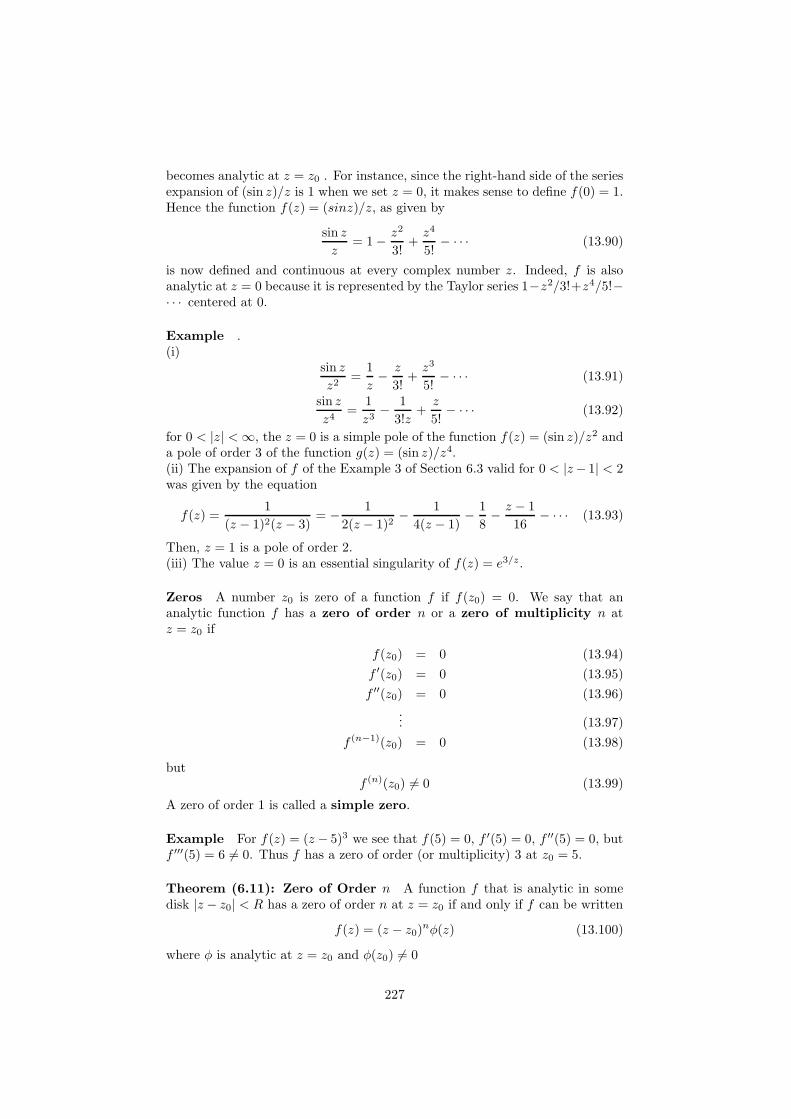
becomes analytic at z = z0 . For instance, since the right-hand side of the seriesexpansion of (sin z)/z is 1 when we set z = 0, it makes sense to define f(0) = 1.Hence the function f(z) = (sinz)/z, as given by
sin z
z= 1− z2
3!+
z4
5!− · · · (13.90)
is now defined and continuous at every complex number z. Indeed, f is alsoanalytic at z = 0 because it is represented by the Taylor series 1−z2/3!+z4/5!−· · · centered at 0.
Example .(i)
sin z
z2=
1
z− z
3!+
z3
5!− · · · (13.91)
sin z
z4=
1
z3− 1
3!z+
z
5!− · · · (13.92)
for 0 < |z| < ∞, the z = 0 is a simple pole of the function f(z) = (sin z)/z2 anda pole of order 3 of the function g(z) = (sin z)/z4.(ii) The expansion of f of the Example 3 of Section 6.3 valid for 0 < |z− 1| < 2was given by the equation
f(z) =1
(z − 1)2(z − 3)= − 1
2(z − 1)2− 1
4(z − 1)− 1
8− z − 1
16− · · · (13.93)
Then, z = 1 is a pole of order 2.(iii) The value z = 0 is an essential singularity of f(z) = e3/z.
Zeros A number z0 is zero of a function f if f(z0) = 0. We say that ananalytic function f has a zero of order n or a zero of multiplicity n atz = z0 if
f(z0) = 0 (13.94)
f ′(z0) = 0 (13.95)
f ′′(z0) = 0 (13.96)
... (13.97)
f (n−1)(z0) = 0 (13.98)
butf (n)(z0) 6= 0 (13.99)
A zero of order 1 is called a simple zero.
Example For f(z) = (z − 5)3 we see that f(5) = 0, f ′(5) = 0, f ′′(5) = 0, butf ′′′(5) = 6 6= 0. Thus f has a zero of order (or multiplicity) 3 at z0 = 5.
Theorem (6.11): Zero of Order n A function f that is analytic in somedisk |z − z0| < R has a zero of order n at z = z0 if and only if f can be written
f(z) = (z − z0)nφ(z) (13.100)
where φ is analytic at z = z0 and φ(z0) 6= 0
227

Example The analytic function f(z) = z sin z2 has a zero at z = 0. If wereplace z by z2 in the series expansion of sin z we get
f(z) = z sin z = z3 − z7
3!+
z11
5!− · · · (13.101)
= z3[1− z4
3!+
z8
5!− · · · ] (13.102)
= z3φ(z) (13.103)
with φ(0) = 1 6= 0, then z = 0 is a zero of f of order 3.
Theorem (6.12): Pole of Order n A function f analytic in a punctureddisk 0 < |z − z0| < R has a pole of order n at z = z0 if and only if f can bewritten
f(z) =φ(z)
(z − z0)n(13.104)
where φ is analytic at z = z0 and φ(z0) 6= 0.
More about zeros A zero z = z0 of an analytic function f is isolated in thesense that there exists some neighborhood of z0 for which f(z) 6= 0 at everypoint z in that neighborhood except at z = z0. As a consequence, if z0 is a zeroof a nontrivial analytic function f , then the function 1/f(z) has an isolatedsingularity at the point z = z0 .
Theorem (6.13): Pole of Order n If the functions g and h are analytic atz = z0 and h has a zero of order n at z = z0 and g(z0) 6= 0, then the functionf(z) = g(z)/h(z) has a pole of order n at z = z0.
Examples .(i) The rational function
f(z) =2z + 5
(z − 1)(z + 5)(z − 2)4(13.105)
shows that the denominator has zeros of order 1 at z = 1 and z = −5, and azero of order 4 at z = 2. Since the numerator is not zero at any of these points,it follows that f has simple poles at z = 1 and z = −5, and a pole of order 4 atz = 2.(ii) The value z = 0 is a zero of order 3 of z sin z2. Then, we conclude that thereciprocal function f(z) = 1/(z sin z2) has a pole of order 3 at z = 0.
Remarks .(i) From the preceding discussion, it should be intuitively clear that if a functionf has a pole at z = z0 , then |f(z)| → ∞ as z → z0 from any direction and wecan write limz→z0 f(z) = ∞.(ii ) A function f is meromorphic if it is analytic throughout a domain D,except possibly for poles in D. It can be proved that a meromorphic functioncan have at most a finite number of poles in D. For example, the rationalfunction f(z) = 1/(z2 + 1) is meromorphic in the complex plane.
228

13.5 Residues and Residue Theorem
Residue The coefficient a1 of 1/(z − z0) in the Laurent series is called theresidue of the function f at the isolated singularity z0, noted as a1 = Res(f(z), z0).
Examples .(i) z = 1 is a pole of order two of the function f(z) = 1
(z−1)2(z−3) . From
the Laurent series obtained above valid for the deleted neighborhood of z = 1defined by 0 < |z − 1| < 2,
f(z) =−1/2
(z − 1)2+
−1/4
z − 1− 1
8− z − 1
16− · · · ... (13.106)
we have Res(f(z), 1) = −1/4.(ii) z = 0 is an essential singularity of f(z) = e3/z. From its Laurent series
e3/z = 1 +3
z+
32
2!z2+ · · · (13.107)
valid for 0 < |z| < ∞, we get Res(f(z), 0) = 3.The following theorem gives a way to obtain the residues of a function f
without the necessity of expanding f in a Laurent series.
Theorem (6.14): Residue at a Simple Pole If f has a simple pole atz = z0 , then
Res(f(z), z0) = limz→z0
(z − z0)f(z) (13.108)
Prof: Since f has a simple pole at z = z0 , its Laurent expansion convergenton a punctured disk 0 < |z − z0| < R has the form
f(z) =a−1
z − z0+ a0 + a1(z − z0) + · · · (13.109)
where a1 6= 0. By multiplying both sides of this series by z−z0 and then takingthe limit as z → z0 we obtain the above relation.
Theorem (6.15): Residue at a Pole of Order n If f has a pole of ordern at z = z0 , then
Res(f(z), z0) =1
(n− 1)!limz→z0
dn−1
dzn−1(z − z0)
nf(z) (13.110)
Proof: See pag. 344 of Ref. [2].
Example The function f(z) = 1(z−1)2(z−3) has a simple pole at z = 3 and a
pole of order 2 at z = 1. Find the residues.Solution: Since z = 3 is a simple pole, we have:
Res(f(z), 3) = limz→3
(z − 3)f(z) = limz→3
1
(z − 1)2=
1
4(13.111)
229

For the pole of order 2, we have
Res(f(z), 1) =1
(2− 1)!limz→1
d2−1
dz2−1(z − 1)2f(z) (13.112)
= limz→1
d
dz(z − 1)2
1
(z − 1)2(z − 3)(13.113)
= limz→1
d
dz
1
(z − 3)(13.114)
= limz→1
−1
(z − 3)2=
−1
4(13.115)
When f is not a rational function, calculating residues by means of the abovelimits can sometimes be tedious. An alternative residue formula can be obtainif the function f can be written as a quotient f(z) = g(z)/h(z), where g and hare analytic at z = z0. If g(z0) 6= 0 and if the function h has a zero of order 1at z0, then f has a simple pole at z = z0 and
Res(f(z), z0) =g(z0)
h′(z0)(13.116)
Proof: Let us write the derivative of h
h′(z) = limz→z0
h(z)− h(z0)
z − z0= lim
z→z0
h(z)
z − z0(13.117)
by using the definition of residues and h(z0) = 0, we get
Res(f(z), z0) = limz→z0
(z − z0)f(z) (13.118)
= limz→z0
(z − z0)g(z)
h(z)(13.119)
= limz→z0
g(z)h(z)z−z0
(13.120)
= limz→z0
g(z)h(z)−h(z0)
z−z0
(13.121)
=g(z0)
h′(z0)(13.122)
Example The polynomial z4+1 can be factored as (z−z1)(z−z2)(z−z3)(z−z4), where z1 = eiπ/4 , z2 = e3iπ/4 , z3 = e5iπ/4, and z4 = e7iπ/4 are its fourdistinct roots. Then, the function f(z) = 1/(z4 + 1) has four simple poles. By
using Res(f(z), z0) =g(z0)h′(z0)
we get
Res(f(z), z1) =1
4z31=
1
4e−3iπ/4 = − 1
4√2− i
1
4√2
(13.123)
Res(f(z), z2) =1
4z32=
1
4e−9iπ/4 =
1
4√2− i
1
4√2
(13.124)
Res(f(z), z3) =1
4z33=
1
4e−15iπ/4 =
1
4√2+ i
1
4√2
(13.125)
Res(f(z), z4) =1
4z34=
1
4e−21iπ/4 = − 1
4√2+ i
1
4√2
(13.126)
230

Figure 13.2: n singular points within contour C (From Ref. [2])
Alternatively we can use the expression limz→z0(z − z0)f(z) for each, pole
Res(f(z), zi) = limz→zi
(z − zi)1
(z − z1)(z − z2)(z − z3)(z − z4)(13.127)
for example,
Res(f(z), z1) = limz→z1
(z − z1)1
(z − z1)(z − z2)(z − z3)(z − z4)
=1
(z − z2)(z − z3)(z − z4)
=1
(eiπ/4 − e3iπ/4)(eiπ/4 − e5iπ/4)(eiπ/4 − e7iπ/4)
and then, work out the above expression to reduce it to − 14√2− i 1
4√2.
Theorem (6.16): Cauchy’s Residue Theorem Let D be a simply con-nected domain and C a simple closed contour lying entirely within D. If afunction f is analytic on and within C, except at a finite number of isolatedsingular points z1, z2, · · · , zn within C, then
∮
C
f(z)dz = 2πi
n∑
k=1
Res(f(z), zk) (13.128)
Proof: Suppose C1, C2, · · · , Cn are circles centered at z1, z2, · · · , zn , respec-tively. Suppose further that each circle Ck has a radius rk small enough so thatC1, C2, · · · , Cn are mutually disjoint and are interior to the simple closed curveC, Fig. 13.2. We known from earlier develop that
∮
Ckf(z)dz = 2πiRes(f(z), zk),
and so by Theorem 5.5 we have
∮
C
f(z)dz =
n∑
k=1
∮
Ck
f(z)dz = 2πi
n∑
k=1
Res(f(z), zk) (13.129)
231

Example Evaluate∮
C1
(z−1)2(z−3)dz for the following two contours:
(i) a rectangle defined by x = 0, x = 4, y = −1, y = 1,(ii) the circle |z| = 2.Solution:(i) Since both z = 1 and z = 3 are poles within the rectangle we have
∮
C
1
(z − 1)2(z − 3)dz = 2πi[Res(f(z), 1) +Res(f(z), 3)] (13.130)
= 2πi
[−1
4+
1
4
]
= 0 (13.131)
(13.132)
(ii) Since only the pole z = 1 lies within the circle |z| = 2, we have
∮
C
1
(z − 1)2(z − 3)dz = 2πiRes(f(z), 1) (13.133)
= 2πi
(−1
4
)
= −iπ
2(13.134)
Example Evaluate∮
C2z+6z2+4dz where the contour C is the circle |z − i| = 2:
Solution: By factoring the denominator as z2 +4 = (z − 2i)(z +2i) we see thatthe integrand has simple poles at −2i and 2i. Because only 2i lies within thecontour C, we get
∮
C
2z + 6
z2 + 4dz = 2πiRes(f(z), 2i) (13.135)
= 2πi
(
3 + 2i
2i
)
= π(3 + i2) (13.136)
Example Evaluate∮
Cez
z4+5z3 dz where the contour C is the circle |z| = 2:
Solution: By factoring the denominator as z4 +5z3 = z3(z +5) we see that theintegrand has a pole of order 3 at z = 0 and a single pole at z = −5. But onlythe first one is inside C, then
∮
C
ez
z4 + 5z3dz = 2πiRes(f(z), 0) (13.137)
= 2πi1
2!limz→0
d2
dz2z3
ez
z4 + 5z3(13.138)
= πi limz→0
d2
dz2z3
ez
z3(z + 5)(13.139)
= πi limz→0
d2
dz2ez
(z + 5)(13.140)
= πi limz→0
(z2 + 8z + 17)ez
(z + 5)3(13.141)
= i17π
125(13.142)
232
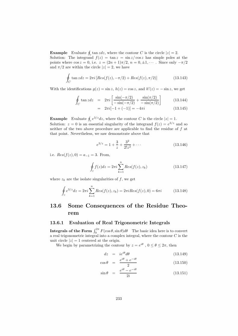
Example Evaluate∮
ctan zdz, where the contour C is the circle |z| = 2.
Solution: The integrand f(z) = tan z = sin z/ cosz has simple poles at thepoints where cos z = 0, i.e. z = (2n+ 1)π/2, n = 0,±1, · · · . Since only −π/2and π/2 are within the circle |z| = 2, we have
∮
C
tan zdz = 2πi [Res(f(z),−π/2) +Res(f(z), π/2)] (13.143)
With the identifications g(z) = sin z, h(z) = cos z, and h′(z) = − sin z, we get
∮
C
tan zdz = 2πi
[
sin(−π/2)
− sin(−π/2)+
sin(π/2)
− sin(π/2)
]
(13.144)
= 2πi[−1 + (−1)] = −4πi (13.145)
Example Evaluate∮
ce3/zdz, where the contour C is the circle |z| = 1.
Solution: z = 0 is an essential singularity of the integrand f(z) = e3/z and soneither of the two above procedure are applicable to find the residue of f atthat point. Nevertheless, we saw demonstrate above that
e3/z = 1 +3
z+
32
2!z2+ · · · (13.146)
i.e. Res(f(z), 0) = a−1 = 3. From,
∮
c
f(z)dz = 2πi
n∑
k=1
Res(f(z), zk) (13.147)
where zk are the isolate singularities of f , we get
∮
c
e3/zdz = 2πi
n∑
k=1
Res(f(z), zk) = 2πiRes(f(z), 0) = 6πi (13.148)
13.6 Some Consequences of the Residue Theo-
rem
13.6.1 Evaluation of Real Trigonometric Integrals
Integrals of the Form∫ 2π
0F (cos θ, sin θ)dθ The basic idea here is to convert
a real trigonometric integral into a complex integral, where the contour C is theunit circle |z| = 1 centered at the origin.
We begin by parametrizing the contour by z = eiθ , 0 ≤ θ ≤ 2π, then
dz = ieiθdθ (13.149)
cos θ =eiθ + e−iθ
2(13.150)
sin θ =eiθ − e−iθ
2i(13.151)
233

or
dθ =dz
iz(13.152)
cos θ =1
2(z + z−1) (13.153)
sin θ =1
2i(z − z−1) (13.154)
then∫ 2π
0
F (cos θ, sin θ)dθ →∮
C
F (1
2(z + z−1),
1
2i(z − z−1))
dz
iz(13.155)
where C is the unit circle |z| = 1.
Example Evaluate∫ 2π
01
(2+cos θ)2 dθ
Solution: using the above substitutions we get∮
C
1
[2 + 12 (z + z−1)]2
dz
iz=
∮
C
1
(2 + z2+12z )2
dz
iz(13.156)
=4
i
∮
C
z
(z2 + 4z + 1)2dz (13.157)
=4
i
∮
C
z
[(z − z1)(z − z2)]2dz (13.158)
with z1 = −2−√3 and z2 = −2 +
√3. Because only z2 is inside the unit circle
C, we have∮
C
1
[2 + 12 (z + z−1)]2
dz
iz=
4
i
∮
C
z
[(z − z1)(z − z2)]2dz (13.159)
=4
i
∮
C
z
(z − z1)2(z − z2)2dz (13.160)
=4
i2πiRes(f(z), z2) (13.161)
where
Res(f(z), z2) = limz→z2
d
dz(z − z2)
2f(z) (13.162)
= limz→z2
d
dz(z − z2)
2 z
(z − z1)2(z − z2)2(13.163)
= limz→z2
d
dz
z
(z − z1)2(13.164)
= limz→z2
−z − z1(z − z1)3
=1
6√3
(13.165)
then∮
C
1
[2 + 12 (z + z−1)]2
dz
iz=
4
i2πiRes(f(z), z2) (13.166)
=4
i2πi
1
6√3
(13.167)
=4π
3√3
(13.168)
234

and, finally,∫ 2π
0
1
(2 + cos θ)2dθ =
4π
3√3
(13.169)
13.6.2 Evaluation of Real Improper Integrals
Integrals of the Form∫∞−∞ f(x)dx Suppose y = f(x) is a real function that
is defined and continuous on the interval [0,∞) defined as∫ ∞
−∞f(x)dx =
∫ 0
−∞f(x)dx +
∫ ∞
0
f(x)dx = I1 + I2 (13.170)
with
I1 =
∫ ∞
0
f(x)dx = limR→∞
∫ R
0
f(x)dx (13.171)
I2 =
∫ 0
−∞f(x)dx = lim
R→−∞
∫ 0
−Rf(x)dx (13.172)
provided both integrals I1 and I2 are convergent. If either one, I1 or I2 , is diver-gent, then
∫∞−∞ f(x)dx is divergent. It is important to remember that the above
definition for the improper integral is not the same as limR→∞∫ R
−R f(x)dx.
For the integral∫∞−∞ f(x)dx to be convergent, the limits limR→∞
∫ R
0f(x)dx
and limR→−∞∫ 0
−R f(x)dx must exist independently of one another. But, in the
event that we know (a priori) that an improper integral∫∞−∞ f(x)dx converges,
we can then evaluate it by∫ ∞
−∞f(x)dx = lim
R→∞
∫ R
−Rf(x)dx (13.173)
On the other hand, the symmetric limit limR→∞∫ R
−R f(x)dx may exist even
though the improper integral∫∞−∞ f(x)dx is divergent.
The limit in
limR→∞
∫ R
−Rf(x)dx (13.174)
if it exists, is called the Cauchy principal value (P.V.) of the integral andis written
P.V.
∫ ∞
−∞f(x)dx = lim
R→∞
∫ R
−Rf(x)dx (13.175)
Cauchy Principal Value When an integral of form∫∞−∞ f(x)dx converges,
its Cauchy principal value is the same as the value of the integral. If the integraldiverges, it may still possess a Cauchy principal value.
About even functions Suppose f(x) is continuous on (−∞,∞) and is aneven function, that is, f(−x) = f(x). If the Cauchy principal value exists,
∫ ∞
0
f(x)dx =1
2P.V.
∫ ∞
−∞f(x)dx (13.176)
∫ ∞
−∞f(x)dx = P.V.
∫ ∞
−∞f(x)dx (13.177)
235

Figure 13.3: (From Ref. [2])
About evaluation of the improper integral To evaluate an integral∫∞−∞ f(x)dx, where the rational function f(x) = p(x)/q(x) is continuous on(−∞,∞), by residue theory we replace x by the complex variable z and integratethe complex function f over a closed contour C that consists of the interval[−R,R] on the real axis and a semicircle CR of radius large enough to encloseall the poles of f(z) = p(z)/q(z) in the upper half-plane Im(z) > 0, Fig. 13.3.By Theorem 6.16 we have
∮
C
f(z)dz =
∫
CR
f(z)dz +
∫ R
−Rf(x)dx (13.178)
= 2πin∑
k=1
Res(f(z), zk) (13.179)
where zk , k = 1, 2, · · · , n denotes poles in the upper half-plane. If we can showthat the integral
∫
CRf(z)dz → 0 as R → ∞, then we have
P.V.
∫ ∞
−∞f(x)dx = lim
R→∞
∫ R
−Rf(x)dx (13.180)
= 2πi
n∑
k=1
Res(f(z), zk) (13.181)
Example Evaluate the Cauchy principal value of∫∞−∞
1(x2+1)(x2+9)dx.
Solution: let us write
f(z) =1
(x2 + 1)(x2 + 9)=
1
(z − i)(z + i)(z − 3i)(z + 3i)(13.182)
we take C be the closed contour consisting of the interval [−R,R] on the x-axisand the semicircle CR of radius R > 3.
∮
C
f(z)dz =
∫ R
−Rf(z)dz +
∫
CR
f(z)dz = I1 + I2 (13.183)
= 2πi[Res(f(z), i) +Res(f(z), 3i)] = 2πi
(
1
16i− 1
48i
)
=π
12(13.184)
We now want to let R → ∞. Before doing this, we use the following inequalityvalid in the contour CR
|(z2 + 1)(z2 + 9)| ≥ ||z2| − 1| · ||z2| − 9| = (R2 − 1)(R2 − 9) (13.185)
236

Since the length L of the semicircle is πR, it follows from the ML-inequality,Theorem 5.3, that
|I2| =∣
∣
∣
∣
∫
CR
1
(z2 + 1)(z2 + 9)
∣
∣
∣
∣
≤ πR
(R2 − 1)(R2 − 9)(13.186)
Then, |I2| → 0 as R → ∞, and so
limR→∞
I2 = 0 (13.187)
(13.188)
and then,
limR→∞
I1 =π
12(13.189)
Finally,
limR→∞
∫ R
−R
1
(x2 + 1)(x2 + 9)dx = P.V.
∫ ∞
−∞
1
(x2 + 1)(x2 + 9)dx =
π
12(13.190)
Because the integrand f(z) is an even function, the existence of the Cauchyprincipal value implies that the original integral converges to π/12, i.e.
∫ ∞
−∞
1
(x2 + 1)(x2 + 9)dx =
π
12(13.191)
Sufficient conditions under which the contour integral along CR approacheszero as R → ∞ is always true are summarized in the next theorem.
Theorem (6.17): Behavior of Integral as R → ∞ Suppose f(z) =p(z)/q(z) is a rational function, where the degree of p(z) is n and the degree ofq(z) is m ≥ n + 2. If CR is a semicircular contour z = Reiθ , 0 ≤ θ ≤ π, then∫
CRf(z)dz → 0 as R → ∞.
Example Evaluate the Cauchy principal value of∫∞−∞
1x4+1dx.
Solution: The conditions given in Theorem 6.17 are satisfied. f(z) = 1/(z4+1)has simple poles in the upper half-plane at z1 = eπi/4 and z2 = e3πi/4, withresidues
Res(f(z), z1) = − 1
4√2− i
1
4√2
(13.192)
Res(f(z), z2) =1
4√2− i
1
4√2
(13.193)
then
PV
∫ ∞
−∞
1
x4 + 1dx = 2πi[Res(f(z), z1) +Res(f(z), z2)] =
π√2
(13.194)
Since the integrand f(z) is an even function, the original integral converges toπ/
√2, i.e.
∫ ∞
−∞
1
x4 + 1dx =
π√2
(13.195)
237

Fourier Integrals:∫∞−∞ f(x) cosαxdx and
∫∞−∞ f(x) sinαxdx Fourier inte-
grals appear as the real and imaginary parts in the improper integral∫∞−∞ f(x)eiαxdx.
We can write∫ ∞
−∞f(x)eiαxdx =
∫ ∞
−∞f(x) cosαxdx + i
∫ ∞
−∞f(x) sinαxdx (13.196)
whenever both integrals on the right-hand side of converge. Suppose f(x) =p(x)/q(x) is a rational function that is continuous on (−∞,∞). Then bothFourier integrals in can be evaluated at the same time by considering the com-plex integral
∫
C f(z)eiαzdz, where α > 0, and the contour C consists of theinterval [−R,R] on the real axis and a semicircular contour CR with radiuslarge enough to enclose the poles of f(z) in the upper-half plane.
The next theorem gives sufficient conditions under which the contour integralalong CR approaches zero as R → ∞.
Theorem (6.18): Behavior of Integral as R → ∞ Suppose f(z) =p(z)/q(z) is a rational function, where the degree of p(z) is n and the degree ofq(z) is m ≥ n + 2. If CR is a semicircular contour z = Reiθ , 0 ≥ θ ≥ π, andα > 0, then
∫
CRf(z)eiαzdz → 0 as R → ∞.
Example Evaluate the Cauchy principal value of∫∞0
x sin xx2+9 dx.
Solution: First we rewrite the integral∫ ∞
0
x sinx
x2 + 9dx =
1
2
∫ ∞
−∞
x sinx
x2 + 9dx (13.197)
With α = 1 we build∮
C
z
z2 + 9eizdz (13.198)
with C a semicircle in the upper complex plane. Using theorem 6.16∫
CR
z
z2 + 9eizdz +
∫ R
−R
x
x2 + 9eixdx = 2πiRes(f(z)eiz, 3i) (13.199)
where
Res(f(z)eiz, 3i) = Res(z
z2 + 9eiz, 3i) =
z
2zeiz∣
∣
∣
z=3i=
e−3
2(13.200)
The integral in the contour CR goes to zero, then
PV
∫ ∞
−∞
x
x2 + 9eixdx = 2πi
(
e−3
2
)
= iπ
e3(13.201)
Then,∫ ∞
−∞
x
x2 + 9eixdx =
∫ ∞
−∞
x cos x
x2 + 9dx+ i
∫ ∞
−∞
x sinx
x2 + 9dx = i
π
e3(13.202)
Equating real and imaginary parts we get
PV
∫ ∞
−∞
x cosx
x2 + 9dx = 0 (13.203)
PV
∫ ∞
−∞
x sinx
x2 + 9dx =
π
e3(13.204)
238

Figure 13.4: (From Ref. [2])
Finally, in view of the fact that the integrand is an even function, we obtain thevalue of the required integral,
∫ ∞
0
x sinx
x2 + 9dx =
1
2
∫ ∞
−∞
x sinx
x2 + 9dx =
π
2e3(13.205)
Indented Contours In the situation where f has poles on the real axis, wemust use an indented(mellado) contour as illustrated in Figure 13.4. Thesymbol Cr denotes a semicircular contour centered at z = c and oriented in thepositive direction. The next theorem is important to this discussion.
Theorem (6.19): Integral of functions with pole on the real axis Sup-pose f has a simple pole z = c on the real axis. If Cr is the contour defined byz = c+ reiθ , 0 ≤ θ ≤ π, then
limr→0
∫
Cr
f(z)dz = πiRes(f(z), c) (13.206)
Proof: See pag. 359 in Ref. [2]
Example Evaluate the Cauchy principal value of∫∞−∞
sin xx(x2−2x+2)dx.
Solution: Let us consider the contour integral
∮
C
eiz
z(z2 − 2z + 2)dx (13.207)
The function f(z) = eiz
z(z2−2z+2) has a pole at z = 0 and at z = 1+i in the upper
half-plane. The contour C, shown in Figure 13.5, is indented at the origin, then
∮
C
=
∫
CR
+
∫ −r
−R+
∫
−Cr
+
∫ R
r
= 2πiRes(f(z)eiz, 1 + i) (13.208)
By taking the limits R → ∞ and r → 0, it follows from Theorems 6.18 and 6.19that
PV
∫ ∞
−∞
eix
x(x2 − 2x+ 2)dx− πiRes(f(z)eiz, 0) = 2πiRes(f(z)eiz, 1 + i)
239

Figure 13.5: (From Ref. [2])
where
Res(f(z)eiz, 0) =1
2(13.209)
Res(f(z)eiz, 1 + i) = −e−1+i
4(1 + i) (13.210)
then
PV
∫ ∞
−∞
eix
x(x2 − 2x+ 2)dx = πi
1
2+ 2πi
(
−e−1+i
4(1 + i)
)
(13.211)
Using e−1+i = e−1(cos 1+ i sin 1) and equating real and imaginary parts, we get
PV
∫ ∞
−∞
cosx
x(x2 − 2x+ 2)dx =
π
2e−1(sin 1 + cos 1) (13.212)
PV
∫ ∞
−∞
sinx
x(x2 − 2x+ 2)dx =
π
2[1 + e−1(sin 1− cos 1)] (13.213)
13.6.3 Integration along a Branch Cut
Branch Point at z = 0 Here we examine integrals of the form∫∞0
f(x)dx,where the integrand f(x) is algebraic but when it is converted to a complexfunction, the resulting integrand f(z) has, in addition to poles, a nonisolatedsingularity at z = 0.
Example: Integration along a Branch Cut Evaluate∫∞0
1√x(x+1)
dx.
Solution: The above real integral is improper for two reasons: (i) an infinitediscontinuity at x = 0 and (ii) the infinite limit of integration. Moreover, it canbe argued from the facts that the integrand behaves like x−1/2 near the originand like x−3/2 as x → ∞, that the integral converges.
We form the integral∮
C
1
z1/2(z + 1)dz (13.214)
where C is the closed contour shown in Figure 13.6 consisting of four compo-nents. The integrand f(z) of the contour integral is single valued and analyticon and within C, except for the simple pole at z = −1 = eiπ. Hence we can
240

Figure 13.6: (From Ref. [2])
write∮
C
1
z1/2(z + 1)dz = 2πiRes(f(z),−1) (13.215)
∫
CR
+
∫
ED
+
∫
Cr
+
∫
AB
= 2πiRes(f(z),−1) (13.216)
(13.217)
with f(z) = 1z1/2(z+1)
. The segment AB coincides with the upper side of the
positive real axis for which θ = 0, z = xe0i; while, the segment ED coincideswith the lower side of the positive real axis for which θ = 2π, z = xe0+2πi, then
∫
ED
=
∫ r
R
(xe2πi)−1/2
xe2πi + 1(e2πidx) (13.218)
= −∫ r
R
x−1/2
x+ 1dx (13.219)
=
∫ R
r
x−1/2
x+ 1dx (13.220)
∫
AB
=
∫ R
r
(xe0i)−1/2
xe0i + 1(e0idx) (13.221)
=
∫ R
r
x−1/2
x+ 1dx (13.222)
Now with z = reiθ and z = Reiθ on Cr and CR , respectively, it can be shownthat
∫
Cr
→ 0 (13.223)
∫
CR
→ 0 (13.224)
241

as r → 0 and R → ∞, respectively. Then
limr→0,R→∞
[∫
CR
+
∫
ED
+
∫
Cr
+
∫
AB
]
= 2πiRes(f(z),−1) (13.225)
is the same as
2
∫ ∞
0
1√x(x+ 1)
dx = 2πiRes(f(z),−1) (13.226)
withRes(f(z),−1) = z−1/2
∣
∣
∣
z=eiπ= e−πi/2 = −i (13.227)
then∫ ∞
0
1√x(x+ 1)
dx = π (13.228)
13.6.4 The Argument Principle and Rouche’s Theorem
Argument Principle Unlike the foregoing discussion in which the focus wason the evaluation of real integrals, we next apply residue theory to the locationof zeros of an analytic function.
Theorem (6.20): Argument Principle Let C be a simple closed contourlying entirely within a domain D. Suppose f is analytic in D except at a finitenumber of poles inside C, and that f(z) 6= 0 on C. Then
1
2πi
∮
C
f ′(z)
f(z)dz = N0 −Np (13.229)
where N0 is the total number of zeros of f inside C and Np is the total numberof poles of f inside C. In determining N0 and Np , zeros and poles are countedaccording to their order or multiplicities.Proof: See pag. 363 in Ref. [2].
Theorem (6.21): Rouche’s Theorem Let C be a simple closed contourlying entirely within a domain D. Suppose f and g are analytic in D. If thestrict inequality |f(z)− g(z)| < |f(z)| holds for all z on C, then f and g havethe same number of zeros (counted according to their order or multiplicities)inside C.Proof: See pag. 365 in Ref. [2].
The Rouche’s Theorem is helpful in determining the number of zeros of ananalytic function (in a given region).
242

Appendix A
Ejercicios: Sistemas deecuaciones lineales
Credit: this notes are 100% from the book Linear Algebra. A Modern Intro-duction of David Poole (2006) [1].
Comentario: Los ejercicios son dados con el numero de ejemplo o ejercicioy la pagina del libro ”Linear Algebra. A Modern Introduction” de D. Poole delano 2006 [1]. Las soluciones de los ejercicios impares (en el conteo del libro)aparecen en el libro a partir de la pagina 571.
1) Resolver el sistema(Ejemplo 2.6, pag. 62, sol.: x=3, y=-1, z=2:)
x− y − z = 2
3x− 3y + 2z = 16
2x− y + z = 9
2) Encontrar el sistema de ecuaciones lineales que tiene por matriz aumentada(Ejercicio 31, pag. 64:)
0 1 1 11 −1 0 12 −1 1 1
(A.1)
3) Resolver los siguiente sistemas de ecuaciones(ejercicio 27, pag. 64, sol. x=1,y=1:)
x− y = 0
2x+ y = 3
(ejercicio 29, pag. 64, sol. x=4,y=-1:)
x+ 5y = −1
−x+ y = −5
2x+ 4y = 4
243

(ejercicio 31, pag. 64, no tiene sol.:)
x− y + 3z = 1
x− y = 1
2x− y + z = 1
(ejercicio 32, pag. 64:)
x1 − x2 + 3x4 + x5 = 2
x1 + x2 + 2x3 + x4 − x5 = 4
x2 + 2x4 + 3x5 = 0
4) Hacer un cambio de variables en el siguiente sistema y resolver.(ejercicio 43, pag. 65, sol. x=π/4, y=−π/6, z=π/3:)
tanx− 2 sin y = 2
tanx− sin y + cos z = 2
sin y − cos z = −1
5) Mediante reduccion por filas obtenga la matriz escalon y la matriz escalonreducida.(Ejercicio 9, pag. 83:)
0 0 10 1 11 1 1
(A.2)
(Ejercicio 11, pag. 83:)
3 55 −22 4
(A.3)
(Ejercicio 14, pag. 83:)
−2 −4 7−3 −6 101 2 −3
(A.4)
6) Mostrar que los siguientes pares de matrices son equivalentes(Ejercicio 17, pag. 83:)
A =
[
1 23 4
]
B =
[
3 −11 0
]
(A.5)
(Ejercicio 18, pag. 83:)
A =
2 0 −11 1 0−1 1 1
B =
3 1 −13 5 12 2 0
(A.6)
244
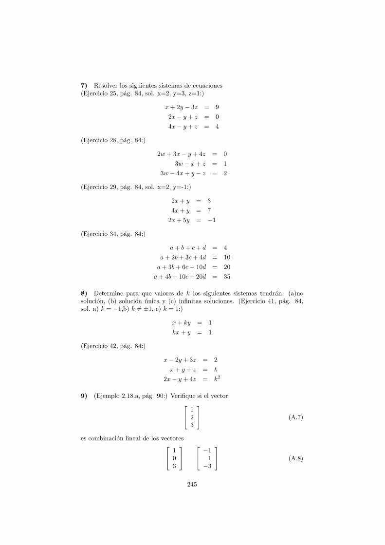
7) Resolver los siguientes sistemas de ecuaciones(Ejercicio 25, pag. 84, sol. x=2, y=3, z=1:)
x+ 2y − 3z = 9
2x− y + z = 0
4x− y + z = 4
(Ejercicio 28, pag. 84:)
2w + 3x− y + 4z = 0
3w − x+ z = 1
3w − 4x+ y − z = 2
(Ejercicio 29, pag. 84, sol. x=2, y=-1:)
2x+ y = 3
4x+ y = 7
2x+ 5y = −1
(Ejercicio 34, pag. 84:)
a+ b+ c+ d = 4
a+ 2b+ 3c+ 4d = 10
a+ 3b+ 6c+ 10d = 20
a+ 4b+ 10c+ 20d = 35
8) Determine para que valores de k los siguientes sistemas tendran: (a)nosolucion, (b) solucion unica y (c) infinitas soluciones. (Ejercicio 41, pag. 84,sol. a) k = −1,b) k 6= ±1, c) k = 1:)
x+ ky = 1
kx+ y = 1
(Ejercicio 42, pag. 84:)
x− 2y + 3z = 2
x+ y + z = k
2x− y + 4z = k2
9) (Ejemplo 2.18.a, pag. 90:) Verifique si el vector
123
(A.7)
es combinacion lineal de los vectores
103
−11
−3
(A.8)
245

(Ejemplo 2.18.b, pag. 90:) Verifique si el vector
234
(A.9)
es combinacion lineal de los vectores
103
−11
−3
(A.10)
10) Verifique si el vector v es combinacion lineal de los vectores u1 y u2.(Ejercicio 1, pag. 99, sol. sı:)
v =
[
12
]
u1 =
[
1−1
]
u2 =
[
2−1
]
(A.11)
(Ejercicio 3, pag. 99, sol. no:)
v =
123
u1 =
110
u2 =
011
(A.12)
(Ejercicio 4, pag. 99:)
v =
32
−1
u1 =
110
u2 =
011
(A.13)
11) Verifique si el vector b pertenece a la expandido de las columnas de lamatriz A.(Ejercicio 7, pag. 100, sol. sı:)
b =
[
56
]
A =
[
1 23 4
]
(A.14)
(Ejercicio 8, pag. 100, sol. sı:)
b =
101112
A =
1 2 34 5 67 8 9
(A.15)
12) Mostrar que los siguiente vectores expanden R2.(Ejercicio 9, pag. 100:)
[
11
] [
1−1
]
(A.16)
(Ejercicio 10, pag. 100:)[
3−2
] [
01
]
(A.17)
(Ejercicio 11, pag. 100:)
101
110
011
(A.18)
246

13) Ejercicio 21, pag. 100.
14) Revea el Ejemplo 2.23, pag. 96 para determinar si un conjunto de vectoresson linealmente independientes formando una combinacion lineal con ellos yresolviendo el sistema.
15) Utilizando el metodo del ejercicio (14) determinar si los siguientes vectoresson linealmente independientes.(Ejercicio 22 (pag. 100:)
2−13
144
(A.19)
(Ejercicio 24 (pag. 100:)
221
312
1−52
(A.20)
(Ejercicio 31 (pag. 100:)
3−11
−1
−131
−1
1131
−1−113
(A.21)
16) Revea el Ejemplo 2.25, pag. 98 para determinar si un conjunto de vectoresson linealmente independientes formando una matriz considerando a los vectorescomo vectores filas.
17) Utilizando el metodo del ejercicio (16) determinar si los siguientes vectoresdel ejercicio 15 son linealmente independientes.
247

Appendix B
Ejercicios: Matrices - Subespacios vectoriales -Transformaciones lineales
Credit: This notes are 100% from chapter 3 of the book entitled Linear Al-gebra. A Modern Introduction of David Poole (2006) [1].
Comentario: Cuando corresponda, los ejercicios son dados con el numero deejemplo o ejercicio y la pagina del libro ”Linear Algebra. A Modern Introduc-tion” de D. Poole del ano 2006 [1]. Las soluciones de los ejercicios impares (enel conteo del libro) aparecen en el libro a partir de la pagina 571.
— Seccion 3.1 —
1) Demostrar el teorema 3.1 de la pagina 142: (i) la premultiplicacion de unamatriz por el versor i-esimo da como resultado, la fila i-esima de la matriz. (ii)la posmultiplicacion de una matriz por el versor i-esimo da como resultado, lacolumna i-esima de la matriz.(Ejercicio 41, pag. 151:)
2) Calcular el producto de las matrices A y B utilizando matrices parti-cionadas.(Ejercicio 34, pag. 151:)
A =
1 0 0 10 1 0 20 0 1 30 0 0 4
B =
1 2 3 10 1 4 10 0 1 11 1 1 −1
— Seccion 3.2 —
248

3) Estudiar el ejemplo 3.16 de la pag. 153 para demostrar si las matrices B yC se pueden escribir como combinacion lineal de las matrices A1, A2 y A3
B =
[
1 42 1
]
C =
[
1 23 4
]
A1 =
[
0 1−1 0
]
A2 =
[
1 00 1
]
A3 =
[
1 11 1
]
4) Hallar si B es combinacion lineal de las matrices A1, A2 y A3
(Ejercicio 6, pag. 159:)
B =
[
2 3−4 2
]
A1 =
[
1 00 1
]
A2 =
[
0 −11 0
]
A3 =
[
1 10 1
]
5) Demostrar que dada la matriz A de orden m×n, las matrices AAT y ATAson simetricas.(Ejercicio 34, pag. 159:)
6) Determinar si las siguientes matrices son linealmente independientes.(Ejercicios 13, pag. 159:)
[
1 23 4
] [
4 32 1
]
(Ejercicio 14, pag. 159:)
[
1 11 1
] [
2 1−1 0
] [
1 24 3
]
— Seccion 3.3 —
7) Demostrar que si A′ y A′′ son ambas inversas de la matriz A, entoncesA′ = A′′.
8) Hallar X a partir de la ecuacion A−1(BX)−1 = (A−1B3)2 asumiendo quelas dimensiones de las matrices involucradas son tales que las operaciones indi-cadas en la ecuacion son posibles.(Ejemplo 3.26, pag. 167:)Sol.: X = B−4AB−3.
9) Revise los ejemplos 3.30 y 3.31 de las pags. 173-175 para calcular (si esposible), mediante la reduccion de Gauss-Jordan, la matriz inversa a partir dela matriz super ampliada.
249

10) Siguiendo el metodo del ejercicio (7) calcule, si es posible, la matricesinversas de(Ejercicios 52, pag. 177:)
2 3 01 −2 −12 0 −1
(Ejercicios 53, pag. 177:)
1 −1 23 1 22 3 −1
11) Calcule la matriz inversa de A descomponiendola en matrices elementales.(Ejemplo 3.29 , pag. 172:)
A =
[
2 31 3
]
Sol.:
A =
[
2 31 3
]
R1↔R2−−−−−→[
1 32 3
]
R2−2R1−−−−−→[
1 30 −3
]
R1+R2−−−−−→[
1 00 −3
]
− 13R2−−−−→
[
1 00 1
]
= I
Entonces,E4E3E2E1A = I ⇒ A−1 = E4E3E2E1
con
E1 =
[
0 11 0
]
E2 =
[
1 0−2 1
]
E3 =
[
1 10 1
]
E4 =
[
1 00 − 1
3
]
— Seccion 3.4 —
12) Repasar el ejemplo 3.33 de la pagina 178 para descomponer una dada ma-triz en el producto de dos matrices diagonales (recordar que la descomposicionLU funciona si no hay que hacer intercambio de filas!!).
13) Repasar el ejemplo 3.34 de la pagina 180 para resolver un SEL mediantela descompisicion LU
14) Resolver el SEL Ax = b usando la (dada) descomposicion LU.(Ejercicio 4, pag. 187:)
A =
2 −4 03 −1 4−1 2 2
=
1 0 03/2 1 0−1/2 0 1
2 −4 00 5 40 0 2
b =
20−5
250

15) Resolver el SEL Ax = b usando la (dada) descomposicion LU.(Ejercicio 6, pag. 187:)
A =
1 4 3 0−2 −5 −1 23 6 −3 −4−5 −8 9 9
=
1 0 0 0−2 1 0 03 −2 1 0−5 4 −2 1
1 4 3 00 3 5 20 0 −2 00 0 0 1
b =
1−3−10
16) Repasar el ejemplo 3.36 de la pagina 186 para resolver un SEL mediantela descompisicion LU cuando se hace necesario permutar filas.
17) Escribir la matriz A en termino de la factorizacion PTLU .(Ejercicio 24, pag. 188:)
0 0 1 2−1 1 3 20 2 1 11 1 −1 0
18) Resolver el SEL generado por la matriz A a partir de su descomposicionPTLU . Seguir los lineamientos aprendido en el ejercicio 13 (ejercicio 3.34, pag.180 del libro).(Ejercicio 27, pag. 188:)
A = PTLU =
0 1 −12 3 21 1 −1
=
0 1 01 0 00 0 1
1 0 00 1 01/2 −1/2 1
2 3 20 1 −10 0 −5/2
b =
115
— Seccion 3.5 —
19) Sea S el conjunto de vectores
[
xy
]
. Probar que S forma un subespacio de
R2 o dar un contraejemplo para mostrar que no lo es.(Ejercicio 1, pag. 207:)
x = 0
(Ejercicio 2, pag. 207:)x ≥ 0 , y ≥ 0
(Ejercicio 3, pag. 207:)y = 2x
(Ejercicio 4, pag. 207:)xy ≥ 0
la Resolver el SEL generado por la matriz A a partir de su descomposicionPTLU . Seguir los lineamientos aprendido en el ejercicio 13 (ejercicio 3.34, pag.180 del libro).(Ejercicio 27, pag. 188:)
251

20) Demostrar que toda recta en R3 que pasa por el origen es un subespaciode R3 .(Ejercicio 9, pag. 207:)
21) Revise el ejemplo 3.41 de la pag. 193 para la determinacion de si un dadovector columna o fila pertenece al espacio columna o fila, respectivamente, deuna dada matriz.
22) Siguiendo el procedimiento del ejercicio (21) determine si los vectores b yw pertencen a los espacion columna y fila, respectivamente de la matriz A.(Ejercicio 11, pag. 207:)
A =
[
1 0 −11 1 1
]
b =
[
32
]
w =[
−1 1 1]
(Ejercicio 12, pag. 207:)
A =
1 1 −30 2 11 −1 −4
b =
110
w =[
2 4 −5]
23) Hallar bases para el espacio generado por las filas y la columnas de lamatriz A y para el espacio nulo de A. Determinar el rango y la nulidad de A.Procedimiento para calcular bases
fila(A): reducir la matriz a su forma escalonada. A partir del teorema 3.20, setienen que las lıneas no nulas generan los vectores l.i.
col(A): Metodo 1: transponer la matriz y aplicar el procedimiento para file(A).Metodo 2: tomar las columnas de A que corresponden a los pivotes de lamatriz en su forma escalonada. Comentario: la dependencia lineal entrelas columnas se conserva en las operaciones, pero las correspondientescolumnas de la matriz reducida no expanden el mismo espacio.
null(A): A partir de la matriz reducida escribimos la matriz reducida am-pliada. Luego generamos el SEL y renombramos las variablers libres yescribimos el vector solucion. La base queda determinada por los vectoresque aparecen como los coeficientes de las variables libres.
(Ejercicio 17, pag. 208:)
A =
[
1 0 −11 1 1
]
(Ejercicio 19, pag. 208:)
A =
1 1 0 10 1 −1 10 1 −1 −1
252
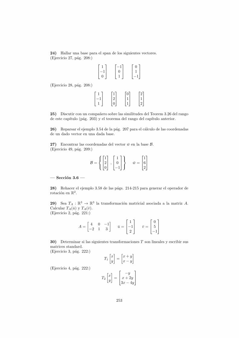
24) Hallar una base para el span de los siguientes vectores.(Ejercicio 27, pag. 208:)
1−10
−101
01−1
(Ejercicio 28, pag. 208:)
1−11
120
011
212
25) Discutir con un companero sobre las similitudes del Teorem 3.26 del rangode este capıtulo (pag. 203) y el teorema del rango del capıtulo anterior.
26) Reparsar el ejemplo 3.54 de la pag. 207 para el calculo de las coordenadasde un dado vector en una dada base.
27) Encontrar las coordenadas del vector w en la base B.(Ejercicio 49, pag. 209:)
B =
120
,
10−1
w =
162
— Seccion 3.6 —
28) Rehacer el ejemplo 3.58 de las pags. 214-215 para generar el operador derotacion en R2.
29) Sea TA : R3 → R3 la transformacion matricial asociada a la matriz A.Calcular TA(u) y TA(v).(Ejercicio 2, pag. 221:)
A =
[
4 0 −1−2 1 3
]
u =
1−12
v =
05−1
30) Determinar si las siguientes transformaciones T son lineales y escribir susmatrices standard.(Ejercicio 3, pag. 222:)
T1
[
xy
]
=
[
x+ yx− y
]
(Ejercicio 4, pag. 222:)
T2
[
xy
]
=
−yx+ 2y3x− 4y
253

(Ejercicio 5, pag. 222:)
T3
xyz
=
[
x− y + z2x+ y − 3z
]
(Ejercicio 6, pag. 222:)
T4
xyz
=
x+ zy + zx+ y
31) Rehacer el ejemplo 3.60 de la pag. 218 sobre la composicion de dos trans-formaciones lineales.
32) Verificar el teorema 3.32 sobre la composicion de TL y calcular la matrizde la composicion S ◦T por (i) sustitucion y (ii) haciendo el producto matricial.(Ejercicio 30 , pag. 223:)
T
[
xy
]
=
[
x− yx+ y
]
S
[
uv
]
=
[
2u−v
]
(Ejercicio 31 , pag. 223:)
T
[
xy
]
=
[
x+ 2y−3x+ y
]
S
[
uv
]
=
[
u+ 3vu− v
]
(Ejercicio 33 , pag. 223:)
T
xyz
=
[
x+ y − z2x− y + z
]
S
[
uv
]
=
[
4u− 2v−u+ v
]
254

Appendix C
Ejercicios: Autovalores yautovectores
Credit: This notes are 100% from chapter 4 of the book entitled Linear Al-gebra. A Modern Introduction of David Poole (2006) [1].
Comentario: Cuando corresponda, los ejercicios son dados con el numero deejemplo o ejercicio y la pagina del libro ”Linear Algebra. A Modern Introduc-tion” de D. Poole del ano 2006 [1]. Las soluciones de los ejercicios impares (enel conteo del libro) aparecen en el libro a partir de la pagina 571.
— Seccion: Introduccion a los autovalores y autovectores
1) Mostrar que v es un autovector de A y hallar su autovalores.(Ejercicio 1, pag. 259:)
A =
[
0 33 0
]
v =
[
11
]
(Ejercicio 2, pag. 259:)
A =
[
1 22 1
]
v =
[
3−3
]
(Ejercicio 6, pag. 259:)
A =
0 1 −11 1 11 2 0
v =
2−1−1
2) Encontrar los autovales de A y los correspondientes autoespacios. Dar lamultiplicidad algebraica y geometrica.(Ejercicio 23, pag. 261:)
A =
[
4 −12 1
]
(Ejercicio 24, pag. 261:)
A =
[
2 46 0
]
255

— Seccion: Determinantes
3) Calcular el determinante de A usando expansion en cofactores.(Ejercicio 1, pag. 280:)
A =
1 0 35 1 10 1 2
(Ejercicio 2, pag. 280:)
A =
0 1 −12 3 −2−1 3 0
4) Encontrar los valores de k para los cuales la matriz A es invertible.(Ejercicio 45, pag. 281:)
A =
k −k 30 k + 1 1k −8 k − 1
(Ejercicio 46, pag. 281:)
A =
k k 0k2 2 k0 k k
5) Utilizando la regla de Crammer resolver los siguientes SEL.(Ejercicio 57, pag. 282:)
x+ y = 1x− y = 2
(Ejercicio 58, pag. 282:)2x− y = 5x+ 3y = −1
(Ejercicio 60, pag. 282:)x+ y − z = 1x+ y + z = 2x− y = 3
— Seccion: Autovalores y autovectores de matrices de orden n
6) Calcular A20x en termino de los autovalores (λ1 = −1/3, λ2 = 1/3, λ3 = 1,) y autovectores de A.(Ejercicio 17, pag. 296:)
v1 =
100
v2 =
110
v3 =
111
x =
212
256

7) Calcular A10x en termino de los autovalores y autovectores de A.(Ejemplo 4.21, pag. 294:)
A =
[
0 12 1
]
— Seccion: Similaridad y diagonalizacion
8) Hallar si A es diagonalizable y en tal caso calcular las patrices D y P de ladescomposicion P−1AP = D(Ejercicio 9, pag. 307:)
A =
[
−3 4−1 1
]
(Ejercicio 11, pag. 307:)
A =
1 0 10 1 11 1 0
(Ejercicio 12, pag. 307:)
A =
1 0 02 2 13 0 1
9) Calcular las siguientes potencias de A utilizando la descomposicion A =PDP−1
(Ejercicio16, pag. 307:) Calcular A9
A =
[
−4 6−3 5
]
(Ejercicio17, pag. 307:) Calcular A10
A =
[
−1 61 0
]
(Ejercicio 22, pag. 307:) Calcular A−5
A =
2 0 11 1 11 0 2
10) Demostrar que las matrices A y B son similares, demostrando que A y Bson similares a la misma matriz diagonal. Calcular P tal que P−1AP = B(Ejercicio 36, pag. 307:)
A =
[
3 10 −1
]
B =
[
1 22 1
]
(Ejercicio 37, pag. 307:)
A =
[
5 −34 −2
]
B =
[
−1 1−6 4
]
257

(Ejercicio 38, pag. 307:)
A =
2 1 00 −2 10 0 1
B =
3 2 −51 2 −12 2 −4
258

Appendix D
Ejercicios: Ortogonalidad
Credit: This notes are 100% from chapter 5 of the book entitled Linear Al-gebra. A Modern Introduction of David Poole (2006) [1].
Comentario: Cuando corresponda, los ejercicios son dados con el numero deejemplo o ejercicio y la pagina del libro ”Linear Algebra. A Modern Introduc-tion” de D. Poole del ano 2006 [1]. Las soluciones de los ejercicios impares (enel conteo del libro) aparecen en el libro a partir de la pagina 571.
— Seccion: Ortogonalidad en Rn
1) Determinar si los siguientes conjunto de vectores son ortogonales.(Ejercicio 1, pag. 373:)
−312
241
1−12
(Ejercicio 2, pag. 373:)
42−5
−120
212
2) (i) Mostrar que los vectores vi forman una base orthonormal para R2 y R3.(ii) Calcular los coeficientes ci = w · vi/(vi · vi) de la expansion del vector w enla base de (i). (iii) Dar las coordenadas del vector w en la base (i).(Ejercicio 7, pag. 374:)
v1 =
[
4−2
]
v2 =
[
12
]
w =
[
1−3
]
(Ejercicio 8, pag. 374:)
v1 =
[
13
]
v2 =
[
−62
]
w =
[
11
]
259

(Ejercicio 10, pag. 374:)
v1 =
111
v2 =
1−10
v3 =
11−2
w =
123
3) (i) Mostrar si las siguiente matrices son ortogonales. (ii) Para las matricesortogonales, calcular su inversa.(Ejemplo 5.7, pag. 371:)
[
cos θ − sin θsin θ cos θ
]
(Ejercicio 16, pag. 374:)[
0 11 0
]
(Ejercicio 17, pag. 374:)[
1/√2 1/
√2
−1/√2 1/
√2
]
(Ejercicio 18, pag. 374:)
1/2 1/3 2/51/2 −1/3 2/5−1/2 0 4/5
4) Encontrar una base ortonormal del subespacion W de R3 dado por(Ejemplo 5.3, pag. 367:)
W =
xyz
: x− y + 2z = 0
— Seccion: Complemento ortogonal y proyeccion ortogonal
5) Sea W el plano en R3 definido por x− y+2z = 0. Encontrar la proyeccion
ortogonal de v sobre W .(Ejemplo 5.11, pag. 380:)
v =
3−12
6) (a) Calcular el complemento ortogonal W⊥ de W . (b) Dar una base paraW⊥.(Ejercicio 1, pag. 384:)
W =
{[
xy
]
: 2x− y = 0
}
(Ejercicio 2, pag. 384:)
W =
{[
xy
]
: 3x+ 4y = 0
}
260
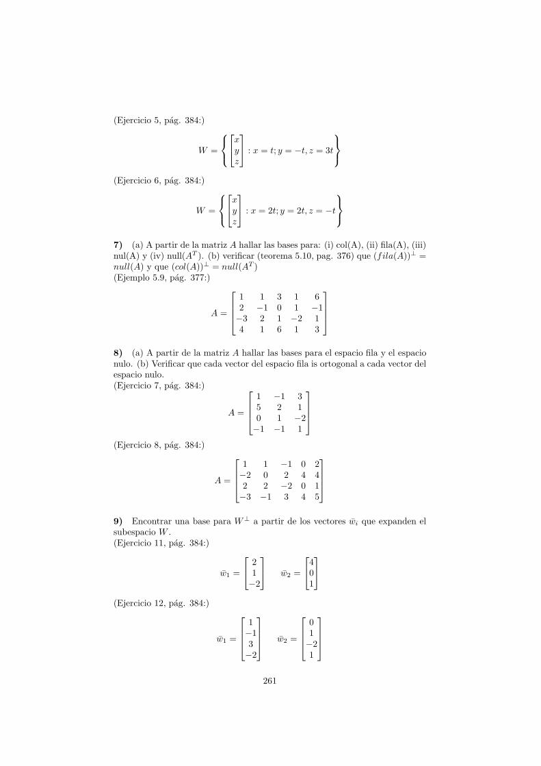
(Ejercicio 5, pag. 384:)
W =
xyz
: x = t; y = −t, z = 3t
(Ejercicio 6, pag. 384:)
W =
xyz
: x = 2t; y = 2t, z = −t
7) (a) A partir de la matriz A hallar las bases para: (i) col(A), (ii) fila(A), (iii)nul(A) y (iv) null(AT ). (b) verificar (teorema 5.10, pag. 376) que (fila(A))⊥ =null(A) y que (col(A))⊥ = null(AT )(Ejemplo 5.9, pag. 377:)
A =
1 1 3 1 62 −1 0 1 −1−3 2 1 −2 14 1 6 1 3
8) (a) A partir de la matriz A hallar las bases para el espacio fila y el espacionulo. (b) Verificar que cada vector del espacio fila is ortogonal a cada vector delespacio nulo.(Ejercicio 7, pag. 384:)
A =
1 −1 35 2 10 1 −2−1 −1 1
(Ejercicio 8, pag. 384:)
A =
1 1 −1 0 2−2 0 2 4 42 2 −2 0 1−3 −1 3 4 5
9) Encontrar una base para W⊥ a partir de los vectores wi que expanden elsubespacio W .(Ejercicio 11, pag. 384:)
w1 =
21−2
w2 =
401
(Ejercicio 12, pag. 384:)
w1 =
1−13−2
w2 =
01−21
261
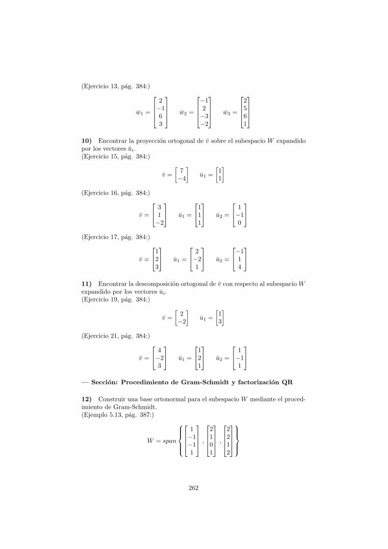
(Ejercicio 13, pag. 384:)
w1 =
2−163
w2 =
−12−3−2
w3 =
2561
10) Encontrar la proyeccion ortogonal de v sobre el subespacio W expandidopor los vectores ui.(Ejercicio 15, pag. 384:)
v =
[
7−4
]
u1 =
[
11
]
(Ejercicio 16, pag. 384:)
v =
31−2
u1 =
111
u2 =
1−10
(Ejercicio 17, pag. 384:)
v =
123
u1 =
2−21
u2 =
−114
11) Encontrar la descomposicion ortogonal de v con respecto al subespacio Wexpandido por los vectores ui.(Ejercicio 19, pag. 384:)
v =
[
2−2
]
u1 =
[
13
]
(Ejercicio 21, pag. 384:)
v =
4−23
u1 =
121
u2 =
1−11
— Seccion: Procedimiento de Gram-Schmidt y factorizacion QR
12) Construir una base ortonormal para el subespacio W mediante el proced-imiento de Gram-Schmidt.(Ejemplo 5.13, pag. 387:)
W = span
1−1−11
,
2101
,
2212
262

13) Utilizando el procedimiento de GS hallar una base orthonormal a partirde los siguientes vectores.(Ejercicio 1, pag. 391:)
x1 =
[
11
]
x2 =
[
12
]
(Ejercicio 3, pag. 391:)
x1 =
1−1−1
x2 =
033
x3 =
324
(Ejercicio 4, pag. 392:)
x1 =
111
x2 =
110
x3 =
100
14) Utilizando el procedimiento de GS hallar una base para R3 a partir x1 yx2.(Ejercicio 5, pag. 392:)
x1 =
110
x2 =
342
15) Encontrar la descomposicion ortogonal de v con respecto al subespacioformado por los vectores x1 y x2 del ejercicio (15).(Ejercicio 7, pag. 392:)
v =
4−43
16) Encontrar una base ortogonal para R3 que contenga al vector v. Ayuda:primero buscar una base arbitraria que contenga v y luego aplicar el metodo deGram-Schmidt (GS).(Ejemplo 5.14, pag. 389:)
v =
123
(Ejercicio 11, pag. 392:)
v =
315
— Seccion: Diagonalizacion ortogonal de matrices simetricas
263

17) Verificar que los autovectores correspondientes a distintos autovalores dela matriz A son ortogonales.(Ejemplo 5.17, pag. 399:)
A =
2 1 11 2 11 1 2
18) (a) Diagonalizar ortogonalmente la matriz A del ejercicio (17), esto es,generar una base ortonormal {qi} para cada autoespacio y construir la matrizQ ubicando los vectores qi en columnas. (b) Verifcar que QTAQ = D, conD = diag(λi) y λi los autovalores de A. (c) Ensayar la construccion de lamatriz Q ubicando los vectores en diferente orden y ver que cambios ocurren enla matriz D. (d) Construir la descomposicion espectral de A con los autovalesλi y los autovecto normalizados qi.(Ejemplos 5.18 y 5.19, pags. 401-403:)
19) (a) Diagonalizar ortogonalmente las siguientes matrices. (b) Calcular sudescomposicion espectral.(Ejercicio 1, pags. 404:)
A =
[
4 11 4
]
(Ejercicio 2, pags. 404:)
A =
[
−1 33 −1
]
20) Diagonalizar ortogonalmente las siguientes matrices.(Ejercicio 5, pags. 404:)
A =
5 0 00 1 30 3 1
(Ejercicio 6, pags. 404:)
A =
2 3 03 2 40 4 2
264

Appendix E
Ejercicios: Espaciosvectoriales
Credit: This notes are 100% from chapter 6 of the book entitled Linear Al-gebra. A Modern Introduction of David Poole (2006) [1].
Comentario: Cuando corresponda, los ejercicios son dados con el numero deejemplo o ejercicio y la pagina del libro ”Linear Algebra. A Modern Introduc-tion” de D. Poole del ano 2006 [1]. Las soluciones de los ejercicios impares (enel conteo del libro) aparecen en el libro a partir de la pagina 571.
Seccion: Espacios vectoriales y subespacios
1) (Ejemplo 6.12, pag. 439) Sea S el conjunto de todas las funciones que sat-isfacen la ecuacion diferencial f ′′+f = 0. Mostrar que S es un subespacio de F .
2) Determinar si los siguientes conjuntos forman un espacio vectorial. En casoque no lo sean list los axiomas que no verifican.(a) (Ejercicio 2, pag. 445) El conjunto de los vectores (x, y)T ∈ R2 con x ≥ 0,y ≥ 0 con las operaciones usuales de suma y producto.
(b) (Ejercicio 4, pag. 445) El conjunto de los vectores (x, y)T ∈ R2 con x ≥ ycon las operaciones usuales de suma y producto.
(c) (Ejercicio 6, pag. 445) El conjunto de los vectores (x, y)T ∈ R2 con elproducto usual y la suma definida como
[
x1
y1
]
+
[
x2
y2
]
=
[
x1 + x2 + 1y1 + y2 + 1
]
(E.1)
(d) (Ejercicio 6, pag. 445) El conjunto de los numeros racionales con lasoperaciones de suma y producto usual.
3) (Ejemplo 6.15, pag. 442) Utilizando el teorema 6.2, verificar si el conjunto
W es un subespacio de M22, donde W estformado por las matrices de la forma[
a a+ 10 b
]
(E.2)
265

4) (Ejercicio 24, pag. 446) Utilizando el teorema 6.2, verificar si W es unsubespacio de R3.
W =
ab
a+ b+ 1
(E.3)
5) (Ejercicio 34, pag. 446) Utilizando el teorema 6.2, verificar si W = {bx +cx2} es un subespacio de P2.
6) (Ejemplo 6.16, pag. 442) Verificar si el conjunto W formado por la matricesde orden dos con determinante nulo es un subespacio de M22.
7) (Ejemplo 6.18, pag. 443) Mostrar queM23 = span(E11, E12, E13, E21, E22, E23),donde Eij es la matriz con todos los elementos nulos excepto en la posicion ij.
8) (Ejemplo 6.21, pag. 444) (a) Mostrar que las matrices A, B y C expandeel subespacio de matrices simetricas. (b) Escribir la matriz X en termino de A,B y C y determinar los coeficientes de la combinacion lineal.
A =
[
1 11 0
]
B =
[
1 00 1
]
C =
[
0 11 0
]
X =
[
x yy z
]
9) (Ejercicio 46, pag. 446) Sea V un espacio vectorial con subespacios U y W .Provar que U ∩W es un subspacio de V .
10) (Ejercicio 47, pag. 446) Sea V un espacio vectorial con subespacios U yW . Dar un ejemplo con V = R2 para mostrar que U ∪ W no necesita ser unsubespacio de V .
Seccion: Dependencia lineal, base y dimension
11) (Ejemplo 6.25, pag. 448) Mostrar que el conjunto {1, x, x2, · · · , xn} eslinealmente independiente (LI) en Pn.
12) (Ejemplo 6.26, pag. 449) Verificar que el conjunto de funciones {f1(x), f2(x), f3(x)}de P2 son LI.
f1(x) = 1 + x f2(x) = x+ x2 f3(x) = 1 + x2
13) (Ejercicio 8, pag. 461) Verificar que el conjunto de funciones {2x, x −x2, 1 + x3, 2− x2 + x3} de P3 es LI.
14) (Ejercicio 15, pag. 461) Mostrar que f(x) y g(x) de C(1) son LI si suWronskiano W (x) es no nulo, con
W (x) =
∣
∣
∣
∣
f gf ′ g′
∣
∣
∣
∣
(E.4)
266

15) (Ejercicio 17, pag. 461) Sea {u, v, w} un conjunto LI en el espacio vectorialV . Para los siguientes dos conjuntos mostrar si son LI o dar un contraejemplosi no lo son.(a) {u+ v, v + w, u+ w}.(b) {u− v, v − w, u− w}.
16) (Ejercicio 19, pag. 461) Determinar si el conjunto B es una base de M22.
B =
{[
1 00 1
]
,
[
0 −11 0
]
,
[
1 11 1
]
,
[
1 11 −1
]}
17) (Ejemplo 6.36, pag. 454) Encontrar el vector coordenadas [A]B de lamatriz A en la base standard B = {E11, E12, E21, E11, E22} de M22.
A =
[
2 −14 3
]
18) (Ejercicio 27, pag. 461) Encontrar el vector coordenadas [A] con respectoa la base B.
A =
[
1 23 4
]
B =
{[
1 00 0
]
,
[
1 10 0
]
,
[
1 11 0
]
,
[
1 11 1
]}
19) (Ejercicio 28, pag. 461) Encontrar el vector coordenadas de p(x) = 2 −x+ 3x2 con respecto a la base B = {1 + x, 1− x, x2} de P2.
20) (Ejercicio 30, pag. 461) Sea B un conjunto de vectores de un espacio vec-torial V con la propiedad que cada vector en V puede ser escrito unıvocamentecomo una combinacion lineal de los vectores en B. Probar que B es una basepara V .
21) (Ejercicio 33, pag. 461) Sea {u1, · · · , um} un conjunto de vectores enun espacio vectorial V de dimension n y sea B una base para V . Sea S ={[u1]B, · · · , [um]B} el conjunto de vectores coordenadas de {u1, · · · , um} conrespecto a B. Probar que span(u1, · · · , um) = V si y solo si span(S) = Rn.
22) (Ejercicio 44, pag. 462) Probar que el espacio vectorial P es de dimensioninfinita. (Ayuda: suponer que tiene una base de dimension finita. Mostrar queexiste algun polinomio que no es una combinaci’on lineal de esa base.)
23) (Ejercicio 54, pag. 462) Sea S = {v1, · · · , vn} un conjunto LI en un espaciovectorial. Mostrar que si v es un vector en V que no esta en span(S), entoncesS′ = {v1, · · · , vn, v} es aun LI.
Seccion: Cambio de base
267

24) (Ejemplo 6.46, pag. 470) (a) Calcular la matriz cambio de base PC←B yPB←C para las bases B = {1, x, x2} = {u1, u2, u3} y C = {1+x, x+x2, 1+x2} ={v1, v2, v3} de P2. (b) Calcular el vector coordenada de p(x) = 1 + 2x− x2 conrespecto a C.
25) (Ejercicio 2, pag. 475) (a) Encontrar los vectores coordenadas [x]B y [x]Cde x con respecto a las bases B y C, respectivamente. (b) Calcular la matrizcambio de base PC←B. (c) Usar la respuesta de la parte (b) para calcular [x]C ,y compararla con la solucion en (a). (d) Hallar la matriz cambio de base PB←C .(e) Usar la solucion de las partes (c) y (d) para calcular [x]B, y comparar con(a).
x =
[
4−1
]
B =
{[
10
]
,
[
11
]}
C =
{[
01
]
,
[
23
]}
26) (Ejercicio 8, pag. 475) Repetir las consignas del ejercicio (25) para p(x) ∈P2.
p(x) = 4− 2x− x2 B = {x, 1 + x2, x+ x2} C = {1, x, x2}
27) (Ejemplo 6.47, pag. 471) (a) Hallar la matriz cambio de base PC←B.(b) Verificar que [X ]C = PC←B[X ]B. Donde B = {E11, E21, E12, E22} y C ={A,B,C,D}.
X =
[
1 23 4
]
A =
[
1 00 0
]
B =
[
1 10 0
]
C =
[
1 11 0
]
D =
[
1 11 1
]
28) (Ejemplo 6.48, pag. 474) Calcular la matriz cambio de base PB←C para lasbases del ejercicio (27) mediante la eliminacion de Gauss-Jordan de la matriz decoeficientes de ambas bases. Utilizar como base de referencia la base canonica.
29) (Ejercicio 21, pag. 476) Sean B, C y D bases para un espacio vectorial Vde dimension finita. Probar que PD←C PC←B = PD←B.
30) (Ejercicio 22, pag. 476) Sea V un espacio vectorial V de dimension ncon base B = {v1, · · · , vn}. Sea P una matriz invertible n × n y sea ui =p1iv1 + · · ·+ pnivn, con i = 1, · · · , n. Probar que C = {u1, · · · , un} es una basepara V y mostrar que P = PB←C .
Seccion: Transformaciones lineales (TL)
31) (Ejercicio 2) Determinar si T : M22 → M22 es una transformacion lineal.
T
[
a bc d
]
=
[
a+ b 00 c+ d
]
32) (Ejercicio 12) Determinar si T : F → R es una transformacion lineal:T (f) = f(c) con c un escalar fijo.
268

33) (Ejemplo 6.55, pag. 479) Hallar la imagen T (v) de la tranformacion T :R2 → P2 a partir de las imagenes de T (u1) y T (u2), donde B = {u1, u2}.
u1 =
[
11
]
u2 =
[
23
]
T (u1) = 2− 3x+ x2 T (u2) = 1− x2
34) (Ejercicio 14) Sea T : R2 → R3 una transformacion lineal tal que
T
[
10
]
=
12−1
T
[
01
]
=
304
hallar T
[
52
]
y T
[
ab
]
.
35) (Ejercicio 20) Mostrar que no existe ninguna TL T : R3 → P2 tal que
T
210
= 1 + x, T
302
= 2− x+ x2, T
06−8
= −2 + 2x2
36) (Ejercicio 22) Sea {v1, · · · , vn} una base para el espacio vectorial V y seaT : V → V sea un TL. Provar que si T (v1) = v1, · · · , T (vn) = vn, entonces Tes la transformacion identidad sobre V .
37) (Ejercicio 24) Sea v1, · · · , vn vectores en un espacio vectorial V y seaT : V → W una TL. Mostrar que {v1, · · · , vn} es LI en V si {T (v1), · · · , T (vn)}is LI en W .
38) (Ejemplo 6.56, pag. 481) Calcular (S ◦ T )v con T : R2 → P1 y S : P1 →P2.
T
[
ab
]
= a+ (a+ b)x, S(p(x)) = xp(x), v =[
3 −2]
39) (Ejercicio 28) Hallar (S ◦T ) y (T ◦S), donde S y T son TL, S : Pn → Pn
y T : Pn → Pn, con S(p(x)) = p(x+ 1) y T (p(x)) = xp′(x).
40) (Ejemplo 6.58, pag. 483) Verificar que las tranformaciones T : R2 → P1
y T ′ : P1 → R2 son inversas una de otra.
T
[
ab
]
= a+ (a+ b)x T ′(c+ dx) =
[
cd− c
]
41) (Ejercicio 30) Sea S : P1 → P1 definida por S(a+ bx) = (−4a+ b) + 2axy T : P1 → P1 definida por T (a + bx) = b/2 + (a + 2b)x. Verificar que S y Tson inversas.
42) (Ejercicio 32) Sea T : V → V una TL tal que T ◦ T = I. (a) Mostrar que{v, T (v)} is LD si y solo sı T (v) = ±v. (b) Dar un ejemplo con V = R2.
269

Seccion: Nucleo y rango de una TL
43) (Ejemplo 6.61, pag. 487) (a) Hallar el kernel y el rango del operadorintegral S : P1 → R. (b) Mostrar que ambos son subespacios. (c) Determinar lanulidad y el rango de S. (d) Verificar si rank(S)+nullity(S) = dim(V ), dondeV = P1.
S(p(x)) =
∫ 1
0
p(x)dx (E.5)
44) (Ejercicio 6) Encontrar bases para el nucleo y el rango de la TL T : M22 →R, con T (A) = tr(A). Determinar la nulidad y el rango y verificar el teoremadel rango.
45) (Ejemplo 6.68, pag. 491) (a) Hallar el rango y la nulidad de T , donde Wes el espacio vectorial de las matrices simetricas de orden dos, T : W → P2. (b)Mostrar que T es una TL.
T
[
a bb c
]
= (a− b) + (b− c)x+ (c− a)x2 (E.6)
46) (Ejercicio 10) Hallar o la nulidad o el rango de T : P2 → R2 y luego
utilizar el teorema del rango para hallar la/el otro, con T (p(x)) =
[
p(0)p(1)
]
.
47) (Ejercicio 14) Idem ejercicio (45) para T : M33 → M33, con T (A) =A−AT .
48) (Ejercicio 15) Determinar si la TL T : R2 → R2 is (a) uno a uno y (b)
onto, con T
[
xy
]
=
[
2x− yx+ 2y
]
.
49) (Ejercicio 18) Determinar si la TL del ejercicio (46) is (a) uno a uno y (b)onto.
50) (Ejercicio 22) Determinar si V = S3 (matrices simetricad de orden 3) yW = U3 (matrices triangular superior de orden 3) son isomorfos. Si lo son, darun isomorfismo especıfico T : V → W .
51) (Ejercicio 33) Sea S : V → W y T : U → V TL. (a) Probar que si S y Tson uno a uno, entonces, tambien lo es S ◦T . (b) Probar que si S y T son onto,entonces, tambien lo es S ◦ T .
Seccion: Matriz de una TL
52) (Ejercicio 2) Sea T : P1 → P1, con T (a+ bx) = b− ax, B = {1+x, 1−x},C = {1, x}, v = p(x) = 4 + 2x. (a) Encontrar la matriz [T ]C←B. (b) Verificar elteorema 6.26 para v calculando T (v) en forma directa y usando el teorema.
270

53) (Ejercicio 4) Sea T : P2 → P2, con T (p(x)) = p(x+2), B = {1, x+2, (x+2)2}, C = {1, x, x2}, v = p(x) = a+ bx+ cx2. (a) Encontrar la matriz [T ]C←B.(b) Verificar el teorema 6.26 para v calculando T (v) en forma directa y usandoel teorema.
54) (Ejemplo 6.76, pag. 503) Sea la TL T : R3 → R2 y sean B = {e1, e2, e3}y C = {e2, e1} bases de R3 y R2, respectivamente. (a) Hallar la matriz de T :A = [[T (v1)]C | · · · |[T (vn)]C ]. (b) Verificar A[v]B = [T (v)]C .
T
xyz
=
[
x− 2yx+ y − 3z
]
v =
13−2
55) (Ejemplo 6.81, pag. 508) Calcular por el metodo de las matrices (S ◦T )v,T : R2 → P1 y S : P1 → P2. Utilzar para cada espacio la base canonica de R
2,P1, y P2, respectivamente.
v =
[
ab
]
T v = a+ (a+ b)x S(p(x)) = xp(x)
56) (Ejercicio 22) Determinar si la TL T : P2 → P2, con T (p(x)) = p′(x),es invertible considerando su matriz con respecto a la base estandard. Si T esinvertible, usar el Teorema 6.28 y el metodo del ejemplo 6.82 para hallar T−1.
57) (Ejemplo 6.82, pag. 509) Calcular T−1 utilizando representacion matri-cial. Donde T : R2 → P1 es one-to-one y onto. Utilizar las bases canonicas paraR2 y P1.
T
[
ab
]
= a+ (a+ b)x (E.7)
58) (Ejercicios 40-42) Set T : V → W un TL entre espacios vectoriales finitos.Sea B y C bases para V y W respectivamente, y sea A = [T ]C←B. (a) Mostrarque null(T ) = null(A). (b) Mostrar que rango(T ) = rango(A). (c) Si V = Wy B = C, mostrar que T es diagonalizable si y solo si A es diagonalizable.
271

Appendix F
Ejercicios: DistanciayAproximacion
Credit: This notes are 100% from chapter 7 of the book entitled Linear Al-gebra. A Modern Introduction of David Poole (2006) [1].
Comentario: Cuando corresponda, los ejercicios son dados con el numero deejemplo o ejercicio y la pagina del libro ”Linear Algebra. A Modern Introduc-tion” de D. Poole del ano 2006 [1]. Las soluciones de los ejercicios impares (enel conteo del libro) aparecen en el libro a partir de la pagina 571.
Seccion: Espacios producto interno
1) (Ejercicio 1) Calcular: (a) 〈u, v〉, (b) ||u, c) d(u, v), y d) encontrar un vectorno nulo ortogonal a u.
u =
[
2−1
]
v =
[
34
]
2) (Ejercicios 5-9) Idem Ej. (1) para u = 2− 3x+ x2, v = 1− 3x2 utilizando
los productos internos (a) 〈u, v〉 =∑2i=0 aibi y (b) 〈u, v〉 =
∫ 1
0 u(x)v(x)dx.
3) (Ejercicios 13-15) Determinar para cada caso cual de los axiomas de pro-ducto interno no se verifica, con uT = (u1, u2), v
T = (v1, v2) ∈ R2.(a) 〈u, v〉 = u1v1.(b) 〈u, v〉 = u1v1 − u2v2 .(c) 〈u, v〉 = u1v2 + u2v1.
4) (Ejemplo 7.2, pag. 540) Mostrar que 〈u, v〉 = 2u1v1 + 3u2v2 define unproducto interno en R2.
5) (Ejemplo 7.6, pag. 544) Sea f(x) = x y g(x) = 3x − 2 dos vectores en
C[0, 1], con el siguiente producto interno 〈f, g〉 =∫ 1
0f(x)g(x)dx. Calcular: (a)
||f ||, (b) d(f, g) y (c) 〈f, g〉.
272

6) (Ejercicios 31-33) Probar las siguientes identidades:(a) 〈u+ v, u− v〉 = ||u||2 − ||v||2.(b) ||u+ v||2 = ||u||2 + 2〈u, v〉+ ||v||2.(c) ||u||2 + ||v||2 = 1
2 ||u+ v||2 + 12 ||u− v||2.
7) (Ejemplo 7.8, pag. 546) Utilizando el procedimiento de Gram-Schmidt,construir una base orthogonal para P2 (polinomios de Legendre hasta orden 2)
con respecto al siguiente producto interno: 〈f, g〉 =∫ 1
−1 f(x)g(x)dx.
8) (Ejercicios 37 y 38) Idem ejercicio (7) para la base B =
{[
10
]
,
[
11
]}
para
los siguientes productos internos:(a) 〈u, v〉 = 2u1v1 + 3u2v2.
(b) 〈u, v〉 = uTAv con A =
[
4 −2−2 7
]
.
Seccion: Normas y distancias de funciones
9) (Ejemplo 7.16, pag. 563) Calcular la distancia d(u, v) = ||u− v|| usando lassiguientes definiciones de norma: (a) Norma Euclideana, (b) Norms de suma y(c) Norma del maximo; para uT = [3,−2] y vT = [−1, 1].
10) (Ejercicios 1-3) Para el vector uT = (−1, 4,−5) calcular: (a) la normaEuclideana, (b) la norma suma y (c) la norma maxima. Para el mismo u yvT = (2,−2, 0) calcular la distancia d(u, v) en: (d) la norma Euclideana, (e) lanorma suma y (f) la norma maxima.
11) (Ejercicios 16) Probar que ||A|| = maxi,j{|aij |} define una norma enMnm.
12) (Ejemplo 7.19, pag. 569) Calcular ||A||1, ||A||∞ (Teorema 7.7) y ||A|| =max||x||=1||Ax||.
A =
1 −3 24 −1 −2−5 1 3
Seccion: Aproximacion por mınimos cuadrados
13) (Teorema 7.8, pag. 579) Demostrar que projW (v) es la mejor aproxi-macion de v ∈ V en W , donde W es un subespacio del espacio producto internoV . Remark: The Best Approximation Theorem gives us an alternative proofthat projW (v) does not depend on the choice of the basis of W , since there canbe only one vector in W that is closest to v–namely projW (v).
273

14) (Ejemplo 7.23, pag. 580) (a) Hallar la mejor aproximacion a v en el planoW = span{u1, u2}. (b) Calcular la distancia Euclideana de v a W .
u1 =
12−1
u2 =
5−21
v =
325
Seccion: Aplicaciones
15) (Ejemplo 7.44, pag. 624) Polinomio de Fourier de orden n. Consideremosel espacio vectorial C[−π, π] con el producto interno 〈f, g〉 =
∫ π
−π f(x)g(x)dx.SeaW un subespacio de C[−π, π] con base B = {1, cosx, · · · , cosnx, sinx, · · · , sinnx}.Calcular la mejor aproximacion a la funcion f ∈ C[−π, π] en W .
Solucion: La mejor aproximacion g(x) vendra dada por la proyeccion def(x) en el subespacio W :
g(x) = projW (f) (F.1)
=〈1, f〉〈1, 1〉 1 +
〈cosx, f〉〈cos x, cosx〉 cosx+ · · ·+ 〈cosnx, f〉
〈cosnx, cosnx〉 cosnx
+〈sinx, f〉
〈sinx, sin x〉 sinx+ · · ·+ 〈sinnx, f〉〈sinnx, sinnx〉 sinnx
Definamos los siguientes coeficientes
a0 =〈1, f〉〈1, 1〉 =
〈1, f〉2π
(F.2)
ak =〈cos kx, f〉
〈cos kx, cos kx〉 =〈cos kx, f〉
π(F.3)
bk =〈sin kx, f〉
〈sin kx, sin kx〉 =〈sin kx, f〉
π(F.4)
Para el calculo de los denominadores usamos
〈cos kx, cos kx〉 =
∫ π
−πcos2 kxdx = π (F.5)
〈sin kx, sin kx〉 =
∫ π
−πsin2 kxdx = π (F.6)
〈1, 1〉 =
∫ π
−π12dx = 2π (F.7)
Luego,
g(x) = a0 + a1 cosx+ · · ·+ an cosnx+ b1 sinx+ · · ·+ bn sinnx
Esta aproximacion es llamada aproximacion de Fourier de n-th orden de fen [−π, π]. Los coeficientes ai y bj se les llama coeficientes de Fourier de f y
274

quedan determinados por la definicion del producto interno
a0 =1
2π
∫ π
−πf(x)dx (F.8)
ak =1
π
∫ π
−πf(x) cos kxdx (F.9)
bk =1
π
∫ π
−πf(x) sin kxdx (F.10)
275

Bibliography
[1] David Poole, Linear Algebra. A Modern Introduction. Second Edition.Thomson. Australia. 2006.
[2] Dennis G. Zill and Patrick D. Shanahan. A First Course in Complex Anal-ysis with Applications. Jones and Bartlett Publishers. 2003.
276