Matching Pursuit Decomposition for EEG Analysis

Arindam DuttaDepartment of Electrical Engineering, Arizona State University

adutta7@asu.edu

Abstract

Matching Pursuit Algorithm is an adaptive decomposition technique that decomposes a

signal into a set of linear waveforms which can be used for feature extraction, wave parame-

ter estimation, EEG analysis etc. This paper explored Matching Pursuit decomposition using

Gaussian and GD power signal dictionaries to decompose/approximate EEG signals and extract

wave parameters. While the Gaussian dictionary is optimal to decompose symmetric signals, it

is shown that the GD power signal dictionary is able to decompose asymmetric signals, such as

EEG with artifacts.

1 Introduction

Electroencephalography (EEG) and magneto encephalography (MEG) can be used to examine

activity in the brain using a net of sensors placed over the scalp to measure electric potential

and magnetic field, respectively. Since its first recordings on human subject performed in 1929,

the EEG has become one of the most important diagnostic tools in clinical neurophysiology [8].

EEG recordings are achieved by placing electrodes of high conductivity in different locations of

the head. Measures of the electric potentials can be recorded between pairs of active electrodes

(bipolar recordings) or with respect to a supposed passive electrode called reference (monopolar

recordings). These measures are mainly performed on the surface of the scalp of the head. Modern

ERP studies that intend topographic analysis often employ 32 to 256 electrodes [6]. Location of

such electrodes is given in Figure 1.

EEG analysis had mostly relied on visual inspection which is rather very subjective and hardly

allows any statistical analysis or standardization. Due to this several methods were proposed

in order to quantify the information of the EEG. One of such method was the Fourier analysis.

1

Although the Fourier Transform allows a passage from domain to frequency domain, it does not

allow the combination of both the domains, in other words it does not provide the time localization

of the frequency components. That is why time-frequency analysis proved to be a better solution

for EEG analysis. One of the methods which is presented in this paper is the Matching pursuit

decomposition of the EEG signals using time-frequency dictionary.

Matching pursuit relies on the decomposition of signals into linear expansion of waveforms be-

longing to a very broad class of functions. These waveforms are adaptively matched to a dictionary

of known waveforms, so that proper analysis can be made based on it. The objective of this paper

is to explore the application of Matching Pursuit to decompose an approximate EEG signals using

two different dictionaries, the conventional Gabor (Gaussian) dictionary and GD power (signal with

power law group delay) dictionary.

Figure 1: EEG sensor locations (32), created using EEGLAB

2 Matching Pursuit Algorithm

Matching pursuits (MP) is a well known technique for sparse signal representation introduced

first by Mallat and Zhang [2]. MP is a greedy algorithm that finds linear approximations of

signals by iteratively projecting them over a redundant, possibly non-orthogonal set of signals

called dictionary. Since MP is a greedy algorithm, it may give a suboptimal approximation. It

decomposes any signal belonging to a Hilbert space H into a linear expansion of waveforms that

are selected from a redundant dictionary (or set of dictionaries) D of functions. These waveforms

are iteratively chosen to best match the signal structures, producing a sub-optimal expansion.

Vectors are selected one by one from the dictionary, while optimizing the signal approximation at

each step k.

2

Let D = {gγ}γ∈Γ be the dictionary of P > N × M with the properties cited above. This

dictionary includes N ×M independent vectors that dene a basis of the space RN×M of signals

with size N ×M . The Matching Pursuit algorithm begins by projecting the target function f on

a vector gγ0 ∈ D and computing the residue Rf .

f = 〈f, gγ0〉gγ0 +Rf, (2.1)

where Rf is the residual vector after approximating f in the direction of gγ0 . Since we impose

Rf to be orthogonal to gγ0 :

‖f‖2 = ‖f, gγ0‖2 + ‖Rf‖2, (2.2)

As we want to minimize ‖Rf‖2 = ‖f‖2‖f, gγ0‖2 we must choose gγ0 ∈ D such that ‖f, gγ0‖ is

maximum. In some cases, it is not computationally ecient to nd the solution given by the Matching

Pursuit algorithms, and a Matching Pursuit-suboptimal solution is computed instead:

|〈f, gγ0〉| ≥ α supγ∈Γ|〈f, gγ〉|, (2.3)

where α ∈ (0, 1] is an optimality factor (α = 1 means that we choose the optimal solution given

by the Matching Pursuit method).

Into the next step, Matching Pursuit subdecomposes iteratively the residue Rf by projecting it

on a vector of D that matches Rf at best. If we consider R0f = f and we suppose the n-th order

residue Rnf(n ≥ 0) has been computed, the next iteration will choose gγn ∈ D such that:

|〈Rnf, gγn〉| ≥ α supγ∈Γ|〈Rnf, gγ〉|, (2.4)

With this choice Rnf is projected onto gγn and decomposed as follows:

Rnf = 〈Rnf, gγn〉gγn +Rn+1f, (2.5)

where Rn+1f and gγn are orthogonal, so the quadratic module of the previous equation is:

3

‖Rnf‖2 = ‖Rnf, gγn‖2 + ‖Rn+1f‖2, (2.6)

From Equation 2.5, we can see that the decomposition of f is given by:

f =

N−1∑n=0

〈Rnf, gγn〉gγn +RNf, (2.7)

and with the same principle we can also deduce from Equation 2.6 that the module of the signal

f is:

‖f‖2 =N−1∑n=0

|〈Rnf, gγn〉|2 + ‖RNf‖2, (2.8)

where RNf converges exponentially to 0 when n tends to ∞

limx→∞

‖RNf‖ = 0; (2.9)

Hence

f =∞∑k=0

〈Rkf, gγk〉gγk , (2.10)

and

‖f‖2 =∞∑k=0

|〈Rkf, gγk〉|2, (2.11)

Thus the original vector f is decomposed into sum of the dictionary that matches best with the

residual at each stage. Also it can be seen that although the decomposition is non-linear, it follows

the energy conservation rule as if it was linear.

3 Time Frequency Decomposition

The time representation is usually the first description about a signal. The Fourier transform is

also a powerful tool which gives light to the spectral part of the signal. But it does give us any idea

about the time localization of the signal. Especially most of the real- world signals are time varying

signals whose frequency change with time. In that case neither representation is good enough to

4

get a detailed idea about the signal. That is why time-varying signals are best represented in the

time-frequency (TF) domain to obtain time-varying frequency information. In order to analyze

the time varying EEG signals effectively, the time and frequency domain characteristics must be

considered jointly. These joint time frequency representation gives light to both the time and the

frequency localization which can help us to analyze a signal properly. A number of time frequency

representations have been built such as the linear TFRs like Short time Fourier transform, Wavelet

transform, quadratic TFRs like Wigner distribution, Spectrogram etc. The matching pursuit a

TF based technique that decomposes a signal into highly localized TF atoms and can provide a

highly concentrated TFR. These atoms are the dilated, translated, and modulated versions of a

single basic function, for example Gaussian function. The matching pursuit decomposition (MPD)

algorithm iteratively selects the best atoms for the decomposition of the waveform based on their

orthogonal projections on the waveform. This is done by performing an exhaustive search over all

the atoms in the dictionary [1].

3.1 Gabor Matching Pursuit

In general any basis function can be used as a dictionary to decompose the required signal. But It

can be shown that the only signal that achieves the lower bound is the Gaussian signal,

x(t) = ce−αt2 ⇒ TxFx =

1

4π, (3.1)

where Tx and Fx are the duration and the bandwidth of the signal.

This implies that it is the most concentrated signal in the time frequency plane. This is why

Gaussian dictionary is chosen for optimal matching pursuit. In practice the Gaussian basis function

is dilated, translated and modulated to create a large array of dictionary. Let D = gγ(t), γ =

(s, u, ζ), be the dictioanry of all time-frequency atoms generated g(t), where (s, u, ζ) are the scaling

factor, translation is time and frequency shift respectively. The Gaussian atom belonging to the

dictionary is given by,

gγ(t) =1√sg(t− us

)ejζt, (3.2)

5

where,

g(t) = 214 eπt

2, (3.3)

Its Fourier transform is centred at the frequency ζ and localized over the frequency domain

proportional to 1s . The Wigner Distribution of a Gaussian atom is given as,

WDgγ (t, ω) = 2H(t− us

)F [s(ω − ζ)],where

H(t) = e−2πt2 , F (ω) = e−ω2

2π

(3.4)

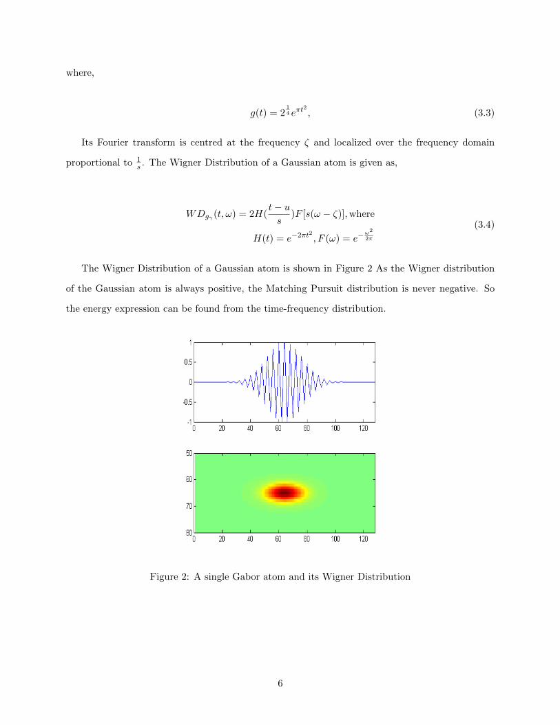
The Wigner Distribution of a Gaussian atom is shown in Figure 2 As the Wigner distribution

of the Gaussian atom is always positive, the Matching Pursuit distribution is never negative. So

the energy expression can be found from the time-frequency distribution.

Figure 2: A single Gabor atom and its Wigner Distribution

6

3.2 Simulation Results

In this section the Matching pursuit decomposition algorithm is implemented on the EEG dataset

created using EEGLAB with an array of Gabor atoms. The algorithm is given as follows,

Algorithm 1: How to write algorithms

input : EEG signal ”b” , Gabor dictionary ”D”

output: Residue R, Normalized energy of Residue E

initialization R=b; Iteration = 400; En= ||R||2;

for i=1:iteration do

→ Calculate the inner product (dot product) for each atom, P = 〈R,D〉;

→ Find D for which P is maximum (Dγi);

→ update Residue,R = R− αDγi , α = 〈R,Dγi〉;

→ update Energy, E = R×R′En ;

→ set i = i+1;

if E ≤ En then

break;

end

end

3.2.1 EEG dataset

The EEG dataset has been obtained from an experiment on reaction to visual stimulus. This is

provided with the EEGLAB toolbox [6]. In this experiment, there were two events, ”square” and

”rt”. The ”square” events are the appearances of a green colored square on the screen and ”rt” is

the reaction time of the subject. The square could be presented at five locations, but here we have

only considered presentation on the left. In this experiment, the subject covertly attended to the

selected location on the computer screen responded with a quick thumb button press only when

a square was presented. They were to ignore circles which were presented at the same time. To

reduce the amount of data required to download and process, this dataset contains only targets,

i.e. ”square” presented at the two visual field attended locations for a single subject.

Figure 1 shows the 32 sensor locations on the brain scalp. Figure 3 shows each sensor readings.

7

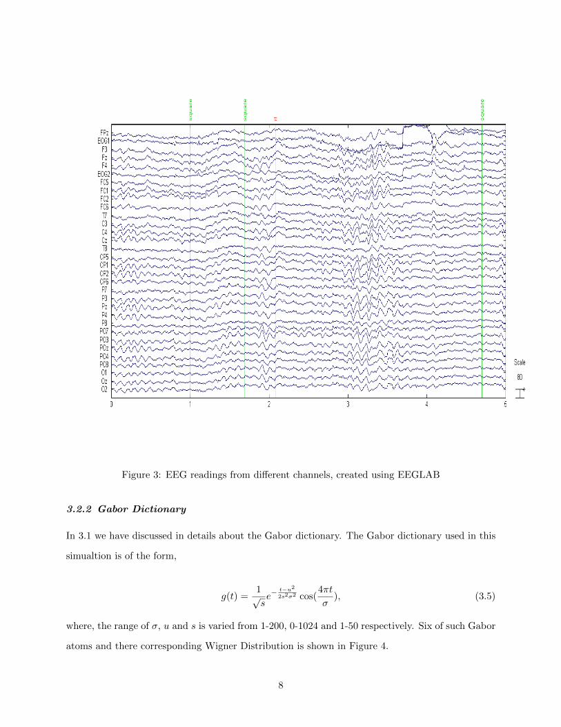
Figure 3: EEG readings from different channels, created using EEGLAB

3.2.2 Gabor Dictionary

In 3.1 we have discussed in details about the Gabor dictionary. The Gabor dictionary used in this

simualtion is of the form,

g(t) =1√se−

t−u22s2σ2 cos(

4πt

σ), (3.5)

where, the range of σ, u and s is varied from 1-200, 0-1024 and 1-50 respectively. Six of such Gabor

atoms and there corresponding Wigner Distribution is shown in Figure 4.

8

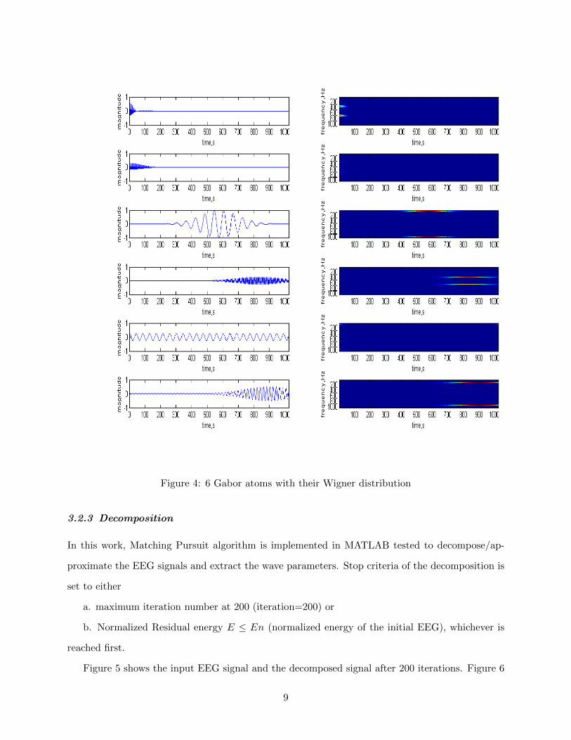
Figure 4: 6 Gabor atoms with their Wigner distribution

3.2.3 Decomposition

In this work, Matching Pursuit algorithm is implemented in MATLAB tested to decompose/ap-

proximate the EEG signals and extract the wave parameters. Stop criteria of the decomposition is

set to either

a. maximum iteration number at 200 (iteration=200) or

b. Normalized Residual energy E ≤ En (normalized energy of the initial EEG), whichever is

reached first.

Figure 5 shows the input EEG signal and the decomposed signal after 200 iterations. Figure 6

9

shows the first 5 gabor atoms that matches with the input EEG signal and the residue after 200

iterations.

Figure 5: Input EEG and residue after 200 iterations

3.2.4 Residual Energy

The residual energy E is defined as

E =

√√√√∑i

(b−N−1∑n=0

〈Rnb, gγn〉)2, (3.6)

Figure 7 shows the gradual reduction of energy of the residue with the increase in the number

of iterations.

3.3 Matching pursuit with Power law group delay signals

In this part dictionary atoms are created using signals with nonlinear group delay. Such signals

have dispersive group delays which are governed by a power law of some factor k. Analysis of these

signals with linear or bilinear TFRs, which belong to the Cohens class, is almost inadequate. These

signals are represented by the Power class (Affine class) quadratic time frequency representations

where these signals are well localized along their power law group delay functions. The general

10

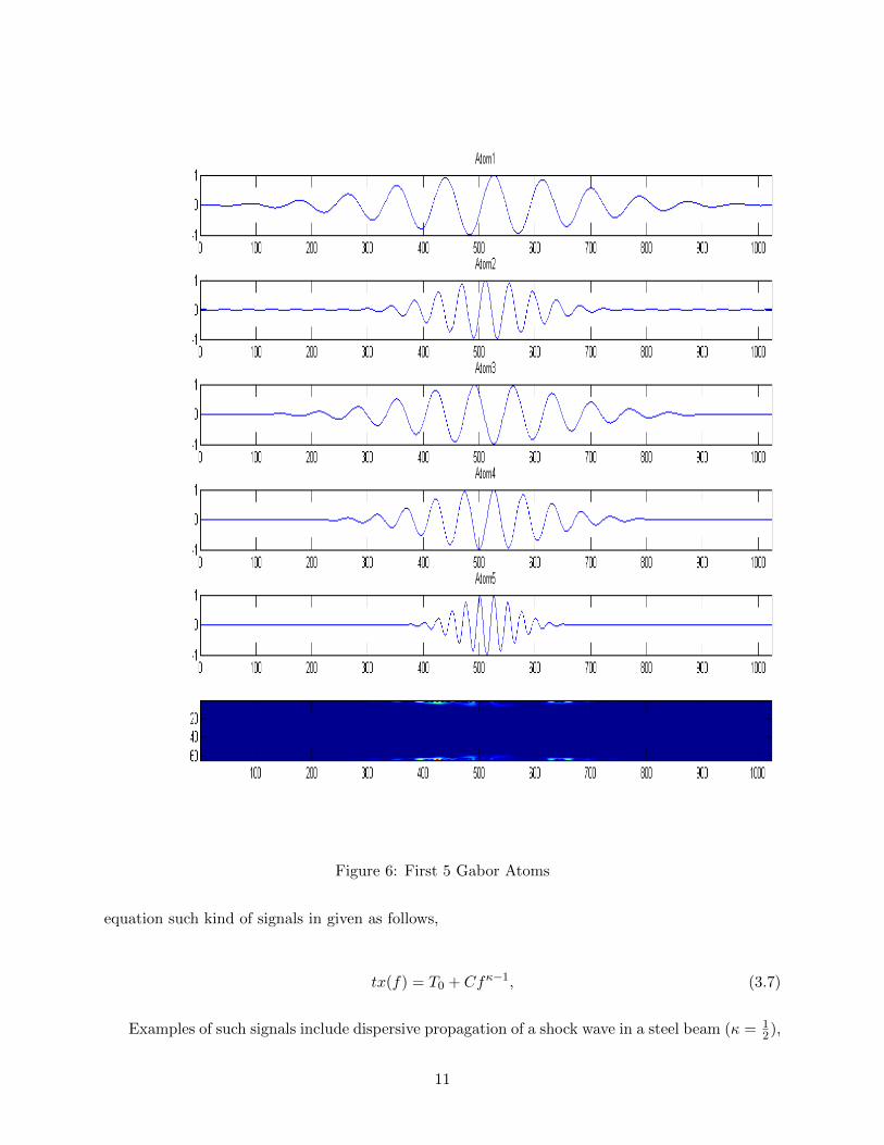
Figure 6: First 5 Gabor Atoms

equation such kind of signals in given as follows,

tx(f) = T0 + Cfκ−1, (3.7)

Examples of such signals include dispersive propagation of a shock wave in a steel beam (κ = 12),

11

Figure 7: Change in Energy of the Residue wth iteration

trans-ionospheric chirps measured by satellites (κ = −1), acoustical waves reflected from a spherical

shell immersed in water, waves propagating along a uniform distributed RC transmission lines

(κ = 12) [9]. These signals constitute the family of power impulses. Power impulses are defines in

the frequency domain as:

Iκc (f) =√|τκ(f)|ej2πcΛκ

ffr =

√(|κ|fr

)| ffr|κ−1

e−j2πcsgn(f)| f

fr|κ

(3.8)

with power group delay

τg(f) = cτκ(f) = c|κ|fr| ffr|κ−1

= cd

dfΛκ(

f

fr)withf ∈ R (3.9)

One of such atoms with its Bertrand distribution is given in Figure 8

12

Figure 8: Signal with power law group delay with its Bertrand distribution

3.4 Simulation Results

In this section Matching pursuit decomposition algorithm is implemented on the EEG dataset,

created by EEGLAB, with atoms of the above described signals. The algorithm is same as given

in section 3.2

3.4.1 EEG dataset

Same EEG dataset is taken as in section 3.2.1

3.4.2 Dictionary

The dictionary of atoms is created using the file gdpower.m from the tftb-0.2 toolbox. Equation

3.7 is used to create the dictionary by varying values of κ and C. Six of such atoms and their

corresponding Bertrand distribution is shown in Figure 9

13

Figure 9: 6 atoms with their Bertrand distribution

3.4.3 Decomposition

In this work, Matching Pursuit algorithm is implemented in MATLAB tested to decompose/ap-

proximate the EEG signals and extract the wave parameters. Stop criteria of the decomposition is

set to either

a. maximum iteration number at 200 (iteration=200) or

b. Normalized Residual energy E ≤ En (normalized energy of the initial EEG), whichever is

reached first.

Figure 10 shows the input EEG signal and the decomposed signal after 200 iterations. Figure

14

11 shows the first 5 gabor atoms that matches with the input EEG signal and the residue after 200

iterations.

Figure 10: Input EEG and residue after 200 iterations

3.4.4 Residual Energy

The energy of the residue is given as in equation 3.6. Figure 12 shows the gradual reduction of

energy of the residue with the increase in the number of iterations.

4 Conclusion

It can be said that an EEG signal as a whole conveys very limited knowledge about itself unless

some methods are used to extarct the features for a better study. From the above analysis it can

be said that the Matching Pursuit Algorithm provides one of the best ways to extarct significant

features about the EEG. A comparative study is done here between two different types of atoms

used as the dictionary, one with the conventional Gabor dictionary and the other with a dictionary

of signals with nonlinear group delay. It can be seen that though Gaussian atoms provide an

optimal matching pursuit, the nonlinear group delay signal also provides an optimal solution in

this case. Moreover if we see the final Residues in both the cases, it can be seen that the Signal is

more decomposed in the latter case that the former. So the latter provides a good result even if

the signal family is a bit complicated.

15

Figure 11: First 5 Atoms that matched the Residue

References

[1] F. Hlawatsch and G. F. Boudreaux-Bartels, “Linear and quadratic time-frequency representa-

tions,” IEEE Signal Processing Magazine, vol. 9, no. 2, pp. 21-67, 1992.

16

Figure 12: Change in Energy of the Residue wth iteration

[2] S. Mallat and Z. Zhang, ”Matching Pursuits with Time-Frequency Dictionaries”, IEEE trans-

actions on Signal Processing, vol. 41, no. 12, December 1993

[3] Alex Maurer, Miao Lifeng,J.J. Zhang, N. Kovvali, A. Papandreou-Suppappola, C. Chakrabarti,

”EEG/MEG artifact suppression for improved neural activity estimation”, Signals, Systems

and Computers (ASILOMAR), pp. 1646 - 1650, 2012

[4] S. Das, I. Kyriakides, A. Chattopadhyay and A. Papandreou-Suppappola, ”Monte Carlo Match-

ing Pursuit Decomposition Method for Damage Quantification in Composite Structures” Jour-

nal of Intelligent Material Systems and Structures 2009, November 2008

[5] P. J. Durka and K. J. Blinowska,Analysis of EEG Transients by Means of Matching Pursuit,

Annals of Biomedical Engineering, Vol. 23, pp. 608-611, 1995

17

[6] A. Delorme and S. Makeig. (2012, March) EEGLAB tutorial outline chapter 1: Loading

data in EEGLAB. [Online]. Available: http:/sccn.ucsd.edu/wiki/Chapter 01: Loading Data

in EEGLAB

[7] Time Frequency toolbox (tftb-2.0), [Online], Available: http:/tftb.nongnu.org

[8] J. C. Mosher, R. M. Leahy, and P. S. Lewis, EEG and MEG: Forward solutions for inverse

methods,” IEEE Transactions in Biomedical Engineering”, vol. 146, pp. 245-259, March 1999.

[9] Antonia Papandreaou- Suppappola, Time-Frequency Processing: tutorial on principles and

practice, [Book] Applications in Time-Frequency Signal Processing

18

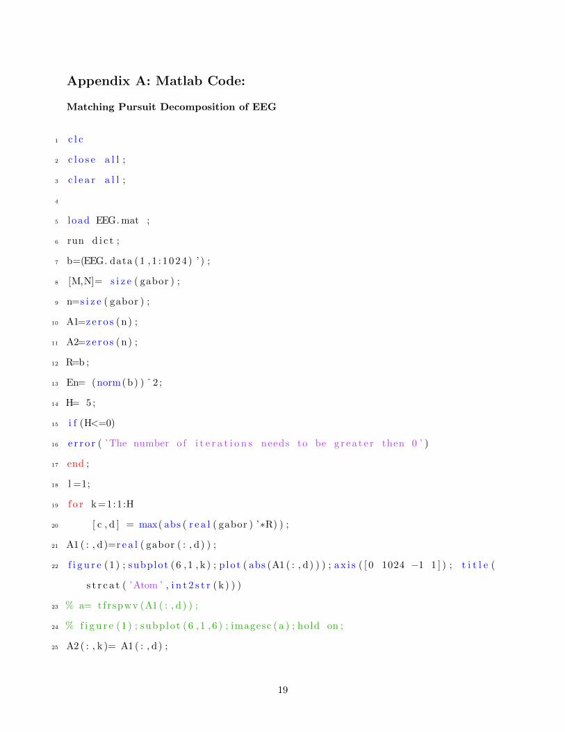
Appendix A: Matlab Code:

Matching Pursuit Decomposition of EEG

1 c l c

2 c l o s e a l l ;

3 c l e a r a l l ;

4

5 load EEG. mat ;

6 run d i c t ;

7 b=(EEG. data ( 1 , 1 : 10 2 4 ) ’ ) ;

8 [M,N]= s i z e ( gabor ) ;

9 n=s i z e ( gabor ) ;

10 A1=ze ro s (n) ;

11 A2=ze ro s (n) ;

12 R=b ;

13 En= (norm(b) ) ˆ2 ;

14 H= 5 ;

15 i f (H<=0)

16 e r r o r ( ’The number o f i t e r a t i o n s needs to be g r e a t e r then 0 ’ )

17 end ;

18 l =1;

19 f o r k =1:1 :H

20 [ c , d ] = max( abs ( r e a l ( gabor ) ’∗R) ) ;

21 A1 ( : , d )=r e a l ( gabor ( : , d ) ) ;

22 f i g u r e (1 ) ; subplot (6 , 1 , k ) ; p l o t ( abs (A1 ( : , d ) ) ) ; a x i s ( [ 0 1024 −1 1 ] ) ; t i t l e (

s t r c a t ( ’Atom ’ , i n t 2 s t r ( k ) ) )

23 % a= tfrspwv (A1 ( : , d ) ) ;

24 % f i g u r e (1 ) ; subplot ( 6 , 1 , 6 ) ; imagesc ( a ) ; hold on ;

25 A2 ( : , k )= A1 ( : , d ) ;

19

26

27 f i g u r e (2 ) ; subplot ( 3 , 1 , 2 ) ; p l o t (A2) ;

28 a= abs ( t f r b e r t (A2 ( : , k ) ) ) ;

29 f i g u r e (1 ) ; subplot ( 6 , 1 , 6 ) ; imagesc ( a ) ;

30 gabor ( : , d ) =0;

31 y = A1\b ;

32 R = b − A1∗y ;

33 f i g u r e (3 ) ; subplot ( 3 , 1 , 3 ) ; p l o t (R) ; a x i s ( [ 0 1024 −100 1 0 0 ] ) ;

34 E( l )= (R’∗R) /En ;

35 f i g u r e (2 ) ; p l o t (E) ; t i t l e ( ’ Energy o f the Residue ’ ) ; x l a b e l ( ’ i t e r a t i o n s ’ )

; y l a b e l ( ’ Energy ’ ) ;

36 l=l +1;

37 % i f (E<= En∗0 . 2 )

38 % break

39 % end

40 % m=input ( ’Do you want to continue , Y/N : ’ , ’ s ’ ) ;

41 % i f m==’N’

42 % break

43 % end

44 end

45 a= abs ( t f r b e r t (A2 ( : , k ) ) ) ;

46 f i g u r e (1 ) ; subplot ( 6 , 1 , 6 ) ; imagesc ( a ) ;

Gabor Dictionary

1 % c l c

2 % c l e a r a l l

3 % c l o s e a l l

4

5 t = (0 : 102 3 ) ’ ;

6 j =1;

20

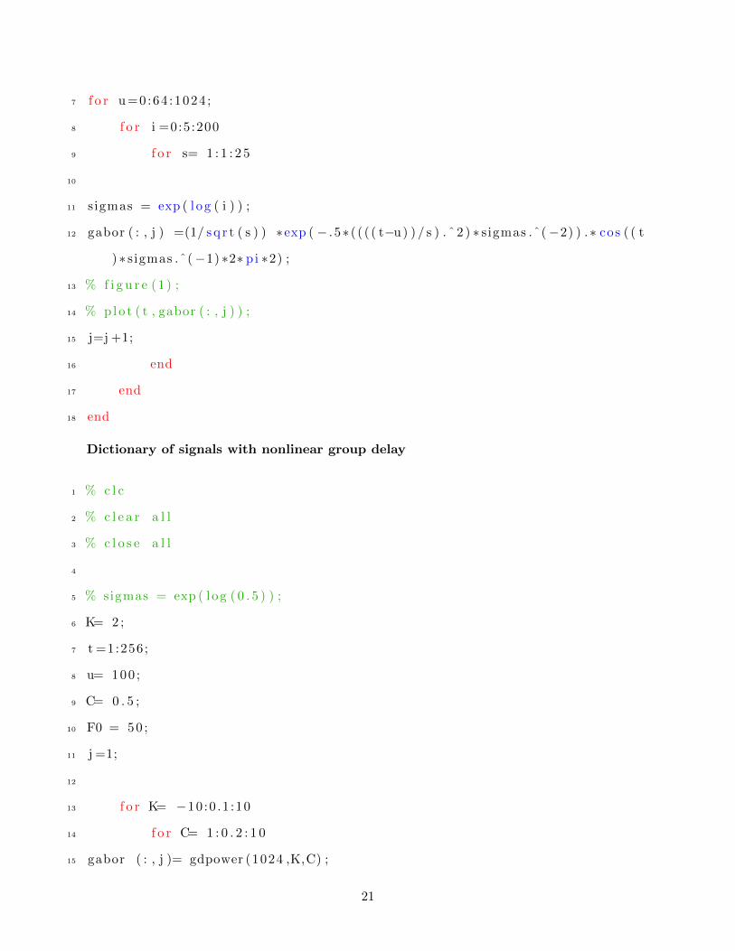
7 f o r u =0:64 :1024 ;

8 f o r i =0:5:200

9 f o r s= 1 : 1 : 2 5

10

11 sigmas = exp ( l og ( i ) ) ;

12 gabor ( : , j ) =(1/ s q r t ( s ) ) ∗exp ( − . 5∗ ( ( ( ( t−u) ) / s ) . ˆ 2 ) ∗ sigmas .ˆ(−2) ) .∗ cos ( ( t

) ∗ sigmas .ˆ(−1) ∗2∗ pi ∗2) ;

13 % f i g u r e (1 ) ;

14 % plo t ( t , gabor ( : , j ) ) ;

15 j=j +1;

16 end

17 end

18 end

Dictionary of signals with nonlinear group delay

1 % c l c

2 % c l e a r a l l

3 % c l o s e a l l

4

5 % sigmas = exp ( log ( 0 . 5 ) ) ;

6 K= 2 ;

7 t =1:256;

8 u= 100 ;

9 C= 0 . 5 ;

10 F0 = 50 ;

11 j =1;

12

13 f o r K= −10:0 .1 :10

14 f o r C= 1 : 0 . 2 : 1 0

15 gabor ( : , j )= gdpower (1024 ,K,C) ;

21

16 j=j +1;

17 end

18 end

19

20 % gabor =(1/ s q r t ( s ) ) ∗exp ( − . 5∗ ( ( ( ( ( t−u) ) ) / s ) . ˆ 2 ) ∗ sigmas .ˆ(−2) ) .∗ cos ( ( t )

∗ sigmas .ˆ(−1) ∗2∗ pi ∗2) ;

21

22 % f i g u r e , p l o t ( r e a l ( gabor ) ) ;

23 % f i g u r e , t f rwv ( r e a l ( gabor ) ) ;

22