MATCHING INVENTORY REPLENISHMENT by RANDALL A. …
236
MATCHING INVENTORY REPLENISHMENT HEURISTICS TO DEMAND PATTERNS: A COST/BENEFIT APPROACH by RANDALL A. NAPIER Presented to the Faculty of the Graduate School of The University of Texas at Arlington in Partial Fulfillment of the Requirements for the Degree of DOCTOR OF PHILOSOPHY THE UNIVERSITY OF TEXAS AT ARLINGTON December 2012
Transcript of MATCHING INVENTORY REPLENISHMENT by RANDALL A. …

MATCHING INVENTORY REPLENISHMENT
HEURISTICS TO DEMAND PATTERNS:
A COST/BENEFIT APPROACH
by
RANDALL A. NAPIER
Presented to the Faculty of the Graduate School of
The University of Texas at Arlington in Partial Fulfillment
of the Requirements
for the Degree of
DOCTOR OF PHILOSOPHY
THE UNIVERSITY OF TEXAS AT ARLINGTON
December 2012

Copyright © by Randall A. Napier 2012
All Rights Reserved

iii
ACKNOWLEDGEMENTS
First off, I would like to express my extreme appreciation for the mentoring and
guidance that Dr. Greg Frazier has provided. From my first visit to the UTA campus after being
accepted as a doctoral student, through an early seminar that introduced me to the nuts and
bolts of scholarly research, and as my primary academic advisor he has been extremely
generous with his time. He has always been positive and encouraging—while ready to firmly
but gently say “No!” when that’s what is needed.
I would also like to recognize the help and support of other UTA faculty members during
the dissertation process, and across my journey through the graduate program. Dr. Edmund
Prater told me early on that every PhD student hits the wall at some point, and he was there to
help get me back on track when I did. Dr. Mary Whiteside taught me that learning is not always
linear, and I certainly found that to be true of dissertation research. Dr. Martin Taylor served as
my minor field advisor, and has always been available when I needed him during the
dissertation process.
Friends and family also stepped up to support me in the challenges of advanced
graduate study. My business partner, Russ Flowers, was patient and forgiving when my
academic pursuits inevitably drew time and energy away from our consulting practice. My
children and my stepson—Benjamin, Mary, and Mitchaell—have moved past the Pokemon,
Beany Baby, and garage band phases to become fully functional, low-maintenance young
adults. And my wife, Connie Napier, continues to bring out the best in me in every facet of our
life together.
Thanks to all for enabling me to live the dream!
November 13, 2012

iv
ABSTRACT
MATCHING INVENTORY REPLENISHMENT
HEURISTICS TO DEMAND PATTERNS:
A COST/BENEFIT APPROACH
Randall A. Napier, PhD
The University of Texas at Arlington, 2012
Supervising Professor: Gregory Frazier
Behavioral research indicates that bounded rationality and resource constraints support
the use of “fast and frugal heuristics” that intentionally exclude some available information from
decision models. Inventory replenishment decisions must be made quickly and efficiently, and
as such are a promising realm for the use of fast and frugal heuristics. This research includes a
simulation study to identify significant relationships among heuristics and demand patterns,
yielding inferences regarding the advantages of selecting replenishment models to match
demand patterns. Findings from the simulation are validated against three years of actual
usage data for 278 independent demand items from a single industrial company. The research
also develops a process-driven analytical framework for identifying best-fit demand patterns for
independent demand items. The final section of the study presents a cost/benefit analysis that
recognizes the differential costs of implementing and managing alternative replenishment
models, and offers inferences regarding the use of simple heuristics in lieu of more data-
intensive models for inventory replenishment decisions.
v
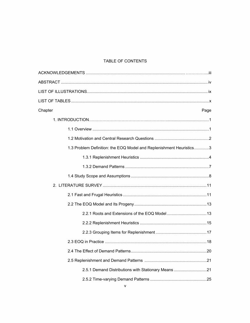
TABLE OF CONTENTS
ACKNOWLEDGEMENTS ........................................................................................ ……………..iii ABSTRACT .................................................................................................................................. iv LIST OF ILLUSTRATIONS........................................................................................................... ix LIST OF TABLES .......................................................................................................................... x Chapter Page
1. INTRODUCTION……………………………………..………..….................................... .1
1.1 Overview ...................................................................................................... .1
1.2 Motivation and Central Research Questions ............................................... .2
1.3 Problem Definition: the EOQ Model and Replenishment Heuristics ............. 3
1.3.1 Replenishment Heuristics ............................................................. 4
1.3.2 Demand Patterns .......................................................................... 7 1.4 Study Scope and Assumptions ..................................................................... 8
2. LITERATURE SURVEY ............................................................................................ 11
2.1 Fast and Frugal Heuristics .......................................................................... 11 2.2 The EOQ Model and Its Progeny ................................................................ 13
2.2.1 Roots and Extensions of the EOQ Model ................................... 13 2.2.2 Replenishment Heuristics ........................................................... 15 2.2.3 Grouping Items for Replenishment ............................................. 17
2.3 EOQ in Practice .......................................................................................... 18
2.4 The Effect of Demand Patterns ................................................................... 20
2.5 Replenishment and Demand Patterns ....................................................... 21
2.5.1 Demand Distributions with Stationary Means ............................. 21 2.5.2 Time-varying Demand Patterns .................................................. 25

vi
2.5.3 Uncertain Demand ...................................................................... 25
2.6 Alternative Research Methodologies .......................................................... 26
2.7 Gap Analysis ............................................................................................... 28
3. METHODOLOGY ...................................................................................................... 31
3.1 Methodology Overview ................................................................................ 31
3.2 Simulation .................................................................................................... 31
3.2.1 Experimental Design and Software Selection ............................. 31 3.2.2 Model Definition: Assumptions, Issues and Iterations ................ 32 3.2.3 Model Verification ........................................................................ 50 3.2.4 Model Execution and Evaluation of Results................................ 52
3.3 Empirical Validation ..................................................................................... 53 3.4 Item-Demand Pattern Fitting Implementation Study ................................... 60 3.5 Cost/Benefit Analysis .................................................................................. 61
4. SIMULATION ............................................................................................................ 62
4.1 Simulation: Overview .................................................................................. 62
4.2 Simulation Results: Inventory System Cost for All Items ............................ 62
4.3 t-Tests for Equal Means: Same Demand / Alternative Models ................... 65 4.4 t-Tests for Equal Means: Same Model / Alternative Demand ..................... 70 4.5 Factor Level Analysis: Cost, Demand, and Lead Time ............................... 77 4.6 Inferences from the Simulation Study ......................................................... 78
5. EMPIRICAL VALIDATION ........................................................................................ 82
5.1 Empirical Validation: Overview .................................................................... 82
5.2 Validation Results: Inventory System Cost for All Items ............................. 83
5.3 t-Tests for Equal Means: Alternative Models .............................................. 87 5.4 Inferences from the Empirical Validation .................................................... 88
vii
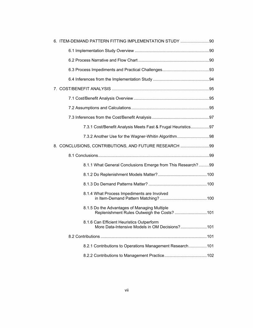
6. ITEM-DEMAND PATTERN FITTING IMPLEMENTATION STUDY ......................... 90
6.1 Implementation Study Overview ................................................................. 90
6.2 Process Narrative and Flow Chart .............................................................. 90 6.3 Process Impediments and Practical Challenges ......................................... 93 6.4 Inferences from the Implementation Study ................................................. 94
7. COST/BENEFIT ANALYSIS ..................................................................................... 95
7.1 Cost/Benefit Analysis Overview .................................................................. 95
7.2 Assumptions and Calculations .................................................................... 95 7.3 Inferences from the Cost/Benefit Analysis .................................................. 97
7.3.1 Cost/Benefit Analysis Meets Fast & Frugal Heuristics ................ 97
7.3.2 Another Use for the Wagner-Whitin Algorithm ............................ 98
8. CONCLUSIONS, CONTRIBUTIONS, AND FUTURE RESEARCH ......................... 99
8.1 Conclusions ................................................................................................. 99
8.1.1 What General Conclusions Emerge from This Research? ......... 99 8.1.2 Do Replenishment Models Matter? ........................................... 100 8.1.3 Do Demand Patterns Matter? ................................................... 100 8.1.4 What Process Impediments are Involved in Item-Demand Pattern Matching? ......................................... 100 8.1.5 Do the Advantages of Managing Multiple Replenishment Rules Outweigh the Costs? ............................ 101 8.1.6 Can Efficient Heuristics Outperform More Data-Intensive Models in OM Decisions? ....................... 101
8.2 Contributions ............................................................................................. 101
8.2.1 Contributions to Operations Management Research ................ 101
8.2.2 Contributions to Management Practice ..................................... 102

viii
8.3 Limitations and Future Research .............................................................. 103
8.3.1 Limitations of This Research ..................................................... 103 8.3.2 Future Research Directions ...................................................... 104 8.3.3 A Parting Thought ..................................................................... 106
APPENDIX A. HISTORICAL DEMAND DATA AND SUMMARY STATISTICS ..................................................................................................... 107 B. INVENTORY ITEMS AND ATTRIBUTES USED IN SIMULATION STUDY...................................................................................................... 152 C. PARAMETER VALUES FOR DEMAND PATTERN SIMULATIONS ................................................................................................... 154 D. SAMPLE SCREEN PRINTS FROM SIMULATION MODELS .............................................. 160
E. T-TEST SAMPLE OUTPUT: SAME DEMAND PATTERN / ALTERNATIVE REPLENISHMENT MODELS ..................................................................... 172 F. T-TEST SAMPLE OUTPUT: SAME REPLENISHMENT MODEL / ALTERNATIVE DEMAND PATTERNS ................................................................ 179 G. INVENTORY SYSTEM COST AT FACTOR LEVELS OF COST, DEMAND, AND LEAD TIME .............................................................................. 186 H. SAMPLE REGRESSION REPORTS AND STACKED TIME SERIES PLOTS FROM VALIDATION STUDY .................................................................... 190 I. SAMPLE SCREEN PRINTS FROM VALIDATION STUDY ................................................... 203 J. T-TEST OUTPUT: VALIDATION STUDY ALTERNATIVE REPLENISHMENT MODELS .............................................................................................. 206 REFERENCES .......................................................................................................................... 216 BIOGRAPHICAL INFORMATION ............................................................................................. 224

ix
LIST OF ILLUSTRATIONS
Figure Page 3.1 Screen Print of Silver-Meal Heuristic Lot Sizing Calculation ............................................................................................................. 39 3.2 Screen Print of Wagner-Whitin Inventory System Cost Model ................................................................................................................ 40 3.3 Screen Print of Lot Size Comparison .................................................................................... 41 3.4 Lot Size Comparison – Cost and Demand Levels: Normal Demand / Low Variability .............................................................................. 42 3.5 Screen Print of Simulated Demand Worksheet: Normal Demand / Low Variability ....................................................................... 45 3.6 Time Series Plot: Seasonal with Trend Demand / Low Variability........................................................................................................ 46 3.7 Simulated Demand Histogram: Normal Demand / Low Variability ........................................................................................... 51 3.8 Screen Print of Nested Audit/Verification Cells ..................................................................... 52 3.9 Screen Print of Simulation Data Summary Worksheet ......................................................... 52 3.10 Screen Print of Crystal Ball Demand Fit Utility .................................................................... 54 3.11 Time Series Plot with Trend Line ........................................................................................ 55 3.12 Stacked Time Series Plot .................................................................................................... 56 3.13 Screen Print of Empirical Validation: (R, s, S) EOQ Model .............................................................................................................. 59 6.1 Process Flow Chart: Item-Demand Pattern Fitting ............................................................... 92

x
LIST OF TABLES
Table Page 1.1 Inventory Replenishment Model Comparison ......................................................................... 4
1.2 Demand Pattern Categories .................................................................................................... 8
3.1 EOQ Simulation Study / Assumptions for Low-Variability Cases ....................................................................................................... 34 3.2 EOQ Simulation Study / (R, s, S) EOQ Model Lot-Sizing Calculations ................................................................................................ 36 3.3 EOQ Simulation Study / EOQ Range Model Lot-Sizing Calculations ................................................................................................ 37 3.4 EOQ Simulation Study / Normal and Poisson Distribution Parameter Values .................................................................................. 43 3.5 EOQ Simulation Study / Gamma and Erlang-C Distribution Parameter Values ................................................................................ 44 3.6 Empirical Validation Study / Assumptions for Inventory System Cost Calculations ................................................................................. 58 4.1 EOQ Simulation Study / Total Inventory System Cost Comparison ....................................................................................... 63 4.2 EOQ Simulation Study / Total Inventory System Cost Comparison: Penalty Multiple vs. Wagner-Whitin Algorithm.................................................. 64 4.3 EOQ Simulation Study / t-Test Results: Total System Costs / Same Demand / Alternative Replenishment Models Time-Varying Demand / Low-Variability Cases ..................................................................... 66 4.4 EOQ Simulation Study / t-Test Results: Total System Costs / Same Demand / Alternative Replenishment Models Stationary Mean Demand / Low-Variability Cases ................................................................. 67 4.5 EOQ Simulation Study / t-Test Results: Total System Costs / Same Demand / Alternative Replenishment Models Time-Varying Demand / High-Variability Cases ..................................................................... 68

xi
4.6 EOQ Simulation Study / t-Test Results: Total System Costs / Same Demand / Alternative Replenishment Models Stationary Mean Demand / High-Variability Cases ................................................................ 69 4.7 EOQ Simulation Study / t-Test Results: Total System Costs / Same Model / Alternative Demand Patterns (R, s, S) EOQ Model / Low-Variability Cases ........................................................................ 71 4.8 EOQ Simulation Study / t-Test Results: Total System Costs / Same Model / Alternative Demand Patterns EOQ Range Model / Low-Variability Cases ........................................................................... 72 4.9 EOQ Simulation Study / t-Test Results: Total System Costs / Same Model / Alternative Demand Patterns Silver-Meal Heuristic / Low-Variability Cases......................................................................... 73 4.10 EOQ Simulation Study / t-Test Results: Total System Costs / Same Model / Alternative Demand Patterns (R, s, S) EOQ Model / High-Variability Cases ........................................................................ 74 4.11 EOQ Simulation Study / t-Test Results: Total System Costs / Same Model / Alternative Demand Patterns EOQ Range Model / High-Variability Cases .......................................................................... 75 4.12 EOQ Simulation Study / t-Test Results: Total System Costs / Same Model / Alternative Demand Patterns Silver-Meal Heuristic / High-Variability Cases ........................................................................ 76 4.13 EOQ Simulation Study—Summary of Results: Same Demand / Different Models ........................................................................ 79 4.14 EOQ Simulation Study—Summary of Results: Same Model / Different Demand Patterns ........................................................... 80 5.1 Empirical Validation / Total Inventory System Cost: Optimized Match of Models to Demand Patterns .................................................................. 83 5.2 Empirical Validation / Total Inventory System Cost Penalty vs. Optimal Model by Variability Level ...................................................................... 85 5.3 Empirical Validation / Total Inventory System Cost Penalty Multiple vs. Wagner-Whitin Algorithm ....................................................................... 86
xii
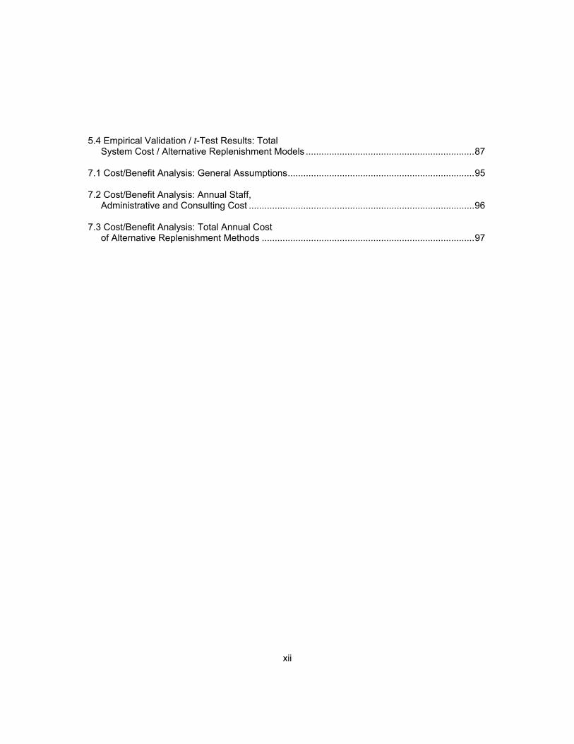
5.4 Empirical Validation / t-Test Results: Total System Cost / Alternative Replenishment Models ................................................................. 87 7.1 Cost/Benefit Analysis: General Assumptions ........................................................................ 95 7.2 Cost/Benefit Analysis: Annual Staff, Administrative and Consulting Cost ....................................................................................... 96 7.3 Cost/Benefit Analysis: Total Annual Cost of Alternative Replenishment Methods .................................................................................. 97

1
CHAPTER 1
INTRODUCTION
1.1 Overview
Behavioral research indicates that bounded rationality and resource constraints support
the use of “fast and frugal heuristics” that intentionally exclude some available information from
decision processes. Inventory replenishment decisions must be made quickly and efficiently,
and as such are a promising realm for the use of fast and frugal heuristics.
Peer-reviewed literature in Operations Management (OM) and related disciplines has
focused extensively on the Economic Order Quantity (EOQ) model, and on EOQ-based
heuristics for the replenishment of independent demand inventory items. The typical paper
examines a specific variant or extension of the EOQ model, or proposes and tests a single
heuristic with hypothetical data and simulation. Most papers address the single-item
replenishment problem, and ignore practical issues such as the need to use different lot-sizing
rules for different item categories.
This research develops and analyzes a process for matching inventory replenishment
heuristics to categories of inventory items with different demand patterns. The methodology
involves (a) running a simulation study to identify significant relationships among inventory
replenishment heuristics and demand patterns, (b) using actual data on multiple years of
demand for 278 independent demand items from a single industrial company to validate the
results of the simulation study, (c) designing an implementation process for fitting items to
demand patterns, and (d) a cost/benefit analysis to evaluate the tradeoffs involved in applying
different replenishment models in a multi-item inventory environment.
The remainder of this document is organized as follows. The remaining parts of
Chapter 1 discuss the study motivation and research questions, define the underlying business

2
problem, and establish the scope of this study. Chapter 2 presents a survey of relevant
literature with a focus on gap analysis, and Chapter 3 details the methodology applied in the
different phases of this research. Chapter 4 presents results and findings from the simulation
study; Chapter 5 discusses validation of the simulation results with empirical data drawn from
an industrial company. Chapter 6 applies lessons learned from the simulation and validation to
design an implementation process for matching inventory items to demand patterns. Chapter 7
uses assumptions drawn from the company that provided the empirical data, along with results
from prior phases of this research, to analyze the cost/benefit tradeoffs of using alternative
replenishment models. Section 8 presents concluding remarks, discusses contributions of this
research, and identifies promising areas for future research.
1.2 Motivation and Central Research Questions
Notwithstanding the availability of material requirements planning (MRP) techniques,
many industrial companies continue to use EOQ-based reorder point models and related
heuristics to replenish purchased independent demand inventory items. The combined effect of
the following factors leads many manufacturing and distribution companies to use reorder point
models:
The company handles a large number of purchased independent demand items.
The company chooses not to allocate staff time to item-level demand forecasting.
Absent item-level forecasting, MRP is not useful for items with purchasing lead times
that exceed customer-required lead times.
In selecting reorder point models, efficient maintenance and ease of application is
preferred for the same reasons that lead companies to avoid item-level demand forecasting.
Many companies therefore apply a one-rule-fits-all approach to reorder point replenishment.
Even companies that apply sophisticated variants of the EOQ model simplistically apply
formulas based on the assumption that probabilistic demand adheres to the normal probability
distribution.
3
Similarly, most research on EOQ model variations and heuristics devotes little or no
consideration to demand distributions and demand patterns other than the normal distribution.
This gives rise to the central research questions presented below. The first two research
questions pertain to matching replenishment rules to demand patterns, while the others address
related issues.
(1) Do replenishment models matter? In other words, does the choice of replenishment
models significantly affect inventory system performance?
(2) Do demand patterns matter? In other words, for a given replenishment model will
different demand patterns yield significantly different inventory system performance?
(3) What process impediments are involved in item-demand pattern matching?
(4) Do the advantages of alternative replenishment rules outweigh the costs?
(5) Can efficient heuristics outperform more data-intensive models in OM decisions?
As the literature survey indicates, the most common use of EOQ-based reorder point
models involves recognizing demand variability, but assuming that periodic demand is normally
distributed. Actual demand for individual items may well follow (a) a time-varying demand
pattern, or (b) a non-normal distribution with a stationary mean. With that in mind, a formal
EOQ model that assumes normally-distributed demand for all items represents a heuristic (rule
of thumb) rather than the application of a purpose-built model. Under that view, even the formal
EOQ-based reorder point model as it is used in practice can be evaluated under the fast and
frugal heuristics paradigm.
1.3 Problem Definition: the EOQ Model and Replenishment Heuristics
Replenishment models and demand patterns have been selected for inclusion in this
study pursuant to the results of the literature survey. The selection process was designed to
recognize widely-used replenishment heuristics, and frequently-encountered and researched
demand patterns, while appropriately limiting the scope of this exploratory study. The four
selected replenishment models and seven selected demand patterns are discussed below.

4
1.3.1 Replenishment Heuristics
The four replenishment models investigated, which are overviewed in the Literature
Summary, are:
Wagner-Whitin Algorithm Baseline for cost-performance evaluation
EOQ Model (R, s, S) Lowest cost EOQ model (assume normality)
EOQ Range Model Most promising/administratively efficient heuristic
Silver-Meal Heuristic Widely used and researched EOQ-based heuristic
The assumptions underlying these four replenishment models are compared in Table
1.1, and the rationale for including each model is discussed below.
The Wagner-Whitin Algorithm is included in the study only to provide a baseline for
measuring the cost-efficiency of the three alternative replenishment heuristics under stochastic
Wagner-Whitin Algorithm Deterministic Choose the sequence of period-quantity replenishment lots that minimizes holding costs plus ordering costs for a defined planning period.
Defines the mathematically optimal replenishment strategy for variable but deterministic demand. Used here to calculate best-possible inventory system cost after-the-fact. This provides a baseline for cost-performance evaluation of heuristics.
(R, s, S) EOQ Model Stochastic/Normal Periodic review; use basic EOQ model to calculate the difference between reorder point and order-up-to target; set reorder point to average demand during lead time plus safety stock; use normal probability distribution to calculate safety stock.
This EOQ model variant is widely used in practice; periodic demand is assumed to be normally distributed. This is evaluated as a heuristic method here due to the exclusion of alternative demand pattern information from lot size calculation.
EOQ Range Model Stochastic Periodic review; calculate indifference points for holding cost plus ordering cost for period replenishment quantity based on annual spend of individual items. Assume same safety stock level as (R, s, S) EOQ model.
This lot sizing heuristic is less calculation-intensive than the (R, s, S) EOQ model and may offer comparable inventory system cost performance with lower administrative and staffing costs.
Silver-Meal Heuristic Deterministic Periodic review; calculate integer-period replenishment quantity that most nearly equalizes holding cost and ordering cost for each item. Assume same safety stock level as (R, s, S) EOQ model.
This widely-used and researched method is simple to calculate (frugal); it may perform nearly as well as the (R, s, S) EOQ model while entailing lower administrative & staffing costs.
Table 1.1Inventory Replenishment Model Comparison
DemandAssumption Decision Rule Role in Current Study

5
demand. As noted in the literature survey, the Wagner-Whitin algorithm defines the
mathematically optimal cost-minimization scenario for inventory replenishment when demand is
deterministic (i.e., known with certainty in advance). The deterministic demand requirement
makes this algorithm infeasible in the no-forecast scenario that is assumed in this study, but the
Wagner-Whitin method can be applied after the fact to calculate the lowest possible inventory
system cost that could have been achieved. This calculation is applied to simulated and actual
demand to yield the optimal baseline against which the results of the three heuristics can be
measured to calculate a penalty cost multiple.
The (R, s, S) EOQ reorder point model is treated as a heuristic in this study because it
is commonly calculated and applied in practice with the assumption that periodic demand is
normally distributed—when in fact this is not always the case. Viewed in that light, the
intentional exclusion of information regarding actual demand patterns makes the application of
the (R, s, S) model consistent with the Gigerenzer et al. (1999) definition of a heuristic. The
specific (R, s, S) version of the EOQ model is chosen for the study because (a) it is recognized
as the EOQ-based reorder point model that will yield the lowest inventory system cost when
demand is normally distributed, while (b) requiring more calculation and administrative intensity
than true heuristic methods such as the Range EOQ model and the Silver-Meal Heuristic.
The Range EOQ model, as defined with the notation used by Silver, Pyke and Peterson
(1998), involves assigning inventory items to fixed-duration replenishment classes based on the
annual amount spent to acquire each item. Items with a large annual spend are ordered more
frequently, and a formula is used to calculate the end points of the ranges (annual spend
indifference points). The formula for calculating the indifference points is presented below.
Let
A = the fixed cost of processing one replenishment order
v = the unit variable (purchase) cost of an item
r = the carrying cost per year of holding $1 of item variable cost in inventory

6
D = the annual demand of an item, in units
T1, T2 , . . . Tn = the number of months of supply to be ordered at one time
Dv(indifference) = the annual spend indifference point between Tn and Tn+1
for number of months of supply
Then, the annual spend indifference points for period-duration replenishment quantities
can be calculated as
Dv(indifference) = (288A) ÷ (T1T2)r
When this heuristic is used, a larger number of alternative values of Tn will reduce the
resulting cost penalty while increasing the administrative complexity involved in using this
method. Fractional values of Tn can be used to determine period-duration replenishment
quantities.
The Silver-Meal Heuristic is an EOQ-based rule for minimizing the total of relevant
costs (ordering cost plus holding cost) for each replenishment cycle (Silver and Meal 1973).
Assuming that a replenishment order is received at the start of Period 1 and contains a quantity
sufficient to meet requirements through the end of period T, the value of T that minimizes per-
period inventory system costs defined by the following expression is used to establish the
period-duration replenishment quantity for an item:
(Setup cost + Total carrying cost to end of period T) ÷ T
The assumptions underlying the Silver-Meal heuristic make it necessary to use an
integer number for the replenishment duration T (Silver et al. 1998). In practice, the selected
period value of T will represent the period immediately before the period average of total
inventory system cost increases for the first time. In fast and frugal heuristics research (e.g.,
Gigerenzer et al. 1999, citing Hey 1982, 1987) this is known as a “one-bounce rule,” which
involves checking values as long as they move in a particular direction (the search rule) and
selecting the last value before the direction reverses (the stopping rule and decision rule).

7
As noted in the literature survey, the Silver-Meal Heuristic is chosen for inclusion in the
current study because it is widely used and understood, and because it offers reduced
calculation intensity when compared to the (R, s, S) EOQ model under stochastic demand.
1.3.2 Demand Patterns
The choice of demand patterns for this study was shaped by an interest in considering
(a) demand distributions with stationary means as well as (b) time-varying demand patterns.
Four stationary-mean distributions and three time-varying demand patterns were chosen.
The four stationary-mean distributions to be investigated are discussed in the literature
survey. These are:
Normal distribution Widely assumed in practice
Poisson distribution Most frequently researched non-normal distribution
Gamma distribution Frequently researched distribution; parameter flexibility
Erlang-C distribution Special form of the gamma distribution
The three time-varying demand patterns to be investigated are also discussed in the
literature survey. Chosen because they are frequently encountered in practice, these are:
Seasonal demand
Trend demand
Seasonal demand with trend
Each demand pattern is used in one high-variability category and one low-variability
category in the simulation study, and in the empirical validation study. The variability categories
are based on a cutoff value for the coefficient of variation. The validation study also recognizes
an “other” demand pattern group, which is used for all items with demand patterns that do not
properly fit into one of the six designated patterns. Items with demand patterns designated as
“other” are also assigned to high-variability and low-variability categories. The demand pattern
categories used in the study are summarized in Table 1.2.

8
1.4 Study Scope and Assumptions
This research addresses a specific problem involving the replenishment of a large
number of purchased inventory items that are subject to independent demand. This problem is
relevant to many make-to-order manufacturers, and also to many distribution companies. In
order to define and focus the study, the following assumptions are applied:
1. No forecasting for individual items: The desire to avoid forecasting demand for a
large number of purchased independent demand items is a primary motivation for companies to
use reorder point replenishment methods.
X = Used in SimulationY = Used in Empirical Validation
Time-Varying Patterns:
1. Seasonal X Y X Y
2. Trend X Y X Y
3. Seasonal with Trend X Y X Y
Stationary-Mean Distributions:
4. Normal X Y X Y
5. Poisson X Y N/A
6. Gamma X Y X Y
7. Erlang-C X Y X Y
Other Demand Patterns:
8. Other Y Y
Table 1.2
Demand Pattern Categories
Low Variability (A) High Variability B)

9
2. MRP logic is not applicable: When vendor lead time plus internal processing time
exceeds the fulfillment cycle time the customer is willing to accept, MRP logic cannot be applied
without individual forecasts for independent demand items.
3. Stochastic periodic demand: Periodic demand for each purchased independent
demand item is assumed to be probabilistic (stochastic). Demand that is constant and known in
advance (deterministic) is one of the baseline assumptions of the classic EOQ model, but this
assumption is relaxed here to reflect empirical reality.
4. No constraints on lot size: It is assumed for simplicity that lot sizes calculated by
each of the replenishment models do not require modification to meet quantity restrictions such
as case quantities, pallet quantities, or full truckloads. This is consistent with one of the
assumptions of the classic EOQ model, and this assumption implies that no joint costing is
involved in any item replenishment decision or inventory system cost calculation.
5. Relevant inventory system costs: Relevant costs for comparing the cost-minimization
performance of different replenishment models include inventory holding costs, order
processing costs, and stockout costs. The classic EOQ model assumes that stockouts or
backorder situations do not exist, but stockouts will occur under stochastic demand. A cost per
stockout occurrence is calculated as a function of both the order processing cost and variable
unit cost of each item. Stockout costs are included in the evaluation of inventory system costs
in the simulation study, and in validating the simulation results with actual data.
6. Independent replenishment decisions: It is assumed that replenishment decisions for
each item are independent of replenishment decisions for any other item. This reflects the
characterization of items included in the study as purchased independent demand items, and is
consistent with one of the assumptions of the classic EOQ model.
7. Deterministic lead time: Vendor lead time is assumed to be consistent and
predictable enough to be treated as deterministic. This assumption isolates the effect of

10
stochastic demand with different demand patterns on inventory system costs, and is consistent
with one of the baseline assumptions of the classic EOQ model.
8. Stockouts for individual inventory items create backorders that are satisfied on a first
come, first served basis as soon as additional units of the item are delivered.
9. Stable pricing for purchased items: Stable purchase prices are assumed for each of
the independent demand items over the period considered in the study. This assumption
eliminates the effect of price variability on the simulation results, and isolates the effect of
different demand patterns on inventory system costs.
10. Historical usage data represent demand: The empirical data set used to validate the
simulation study reflects actual usage for the slate of independent demand items. The company
that provided the data did not track stockouts, product substitutions, or lost orders during the
relevant three-year period, so actual demand history (including unmet demand) is not available.
The subject company tended to carry excess inventory for most of the independent demand
items over the relevant period, so it is unlikely that actual stockout experience would materially
affect the study results.
11. Administrative and staffing costs differ among replenishment models: It is assumed
that different administrative and staffing costs would be associated with different levels of data
maintenance, professional judgment, and calculation-intensity of the different replenishment
models studied. These differences are quantified, based on the simulation results and using
information on staff time and costs from the company that provided the empirical usage data, to
estimate relevant cost differences among the replenishment models. These estimated costs
are compared against the calculated benefits of alternative replenishment methods in the cost-
benefit analysis.

11
CHAPTER 2
LITERATURE SURVEY The literature survey presented in this chapter is organized as follows. Section 2.1
summarizes relevant literature dealing with fast and frugal heuristics. Section 2.2 traces the
history of the EOQ model, identifies foundation literature underlying widely-used EOQ-based
replenishment heuristics, and summarizes papers dealing with the grouping of inventory items
for replenishment. Section 2.3 examines published work dealing with the prevalence of the
EOQ model in practice. Section 2.4 discusses research that addresses the significance of
demand assumptions on replenishment models, and Section 2.5 examines replenishment
research involving demand distributions with stationary means and demand patterns that vary
over time. Section 2.6 details different research methodologies that have been used to study
EOQ-based inventory replenishment. Section 2.7 presents a gap analysis that identifies
potential research contributions of the current study.
2.1 Fast and Frugal Heuristics
The fast and frugal heuristics paradigm for decision making under uncertainty was
developed in the field of behavioral psychology by Gigerenzer and his colleagues (e.g.,
Gigerenzer and Goldstein 1996; Gigerenzer, Todd, and The ABC Group 1999; Todd and
Gigerenzer 2001). This approach has been applied widely in other fields, but it is evident that
the fast and frugal heuristics approach has not yet been embraced by Operations Management
researchers. Research relevant to the current study is summarized below.
The fast and frugal heuristics approach recognizes that bounded rationality, along with
limited availability of time and other resources, leads to reliance on simple decision rules
(heuristics) rather than detailed analysis of all available information (Gigerenzer et al. 1999).
Heuristics can be applied very effectively if they are ecologically rational, which means that they
12
recognize useful elements (cues) of the decision process at hand (Todd and Gigerenzer 2001).
As demonstrated by Hoffrage and Reimer (2004), simple heuristics can be nearly as effective
as comprehensive data-based models (such as regression analysis) in explanatory contexts,
and can outperform comprehensive models in predictive contexts under certain circumstances.
Fast and frugal heuristics can yield better predictive results than more detailed decision models
when linear models overfit correlations between variables, where small data sets are in play, or
where out-of-range predictions are necessary (Hoffrage and Reimer 2004).
Decision making research typically assumes that more information will yield better
decisions, but fast and frugal heuristics research recognizes that the intentional omission of
available information from a decision process may be rational (Gigerenzer et al. 1999; Hoffrage
and Reimer 2004). According to Hoffrage and Reimer (2004), fast and frugal heuristics are
most useful when decisions must be made under time pressure (fast), and when additional
information is costly (frugal).
Experimental research in behavioral psychology tends to support the validity of fast and
frugal heuristics. Bröder and Schiffer (2006) conduct a laboratory experiment leading to the
conclusion that higher information processing requirements tend to increase reliance on simple
decision heuristics. Bryant (2007) taught experimental subjects to visually classify situations
involving potential mid-air collisions, and varied conditions to test the subjects’ reliance on
information-intensive classification methods vs. fast and frugal heuristics. That study led to the
inference that complex decision models did not outperform the heuristics, although no single
heuristic emerged as dominant. Newell, Weston, and Shanks (2003) conduct a laboratory
experiment in which students are given access to categories of information and asked to select
competing stocks for a hypothetical investment portfolio. There the majority of participants
opted for simple heuristics, although only about one-third applied the specific search, stop, and
decision rules proposed by Gigerenzer et al. (1999).

13
Published research in other fields supports the potential extension of the fast and frugal
heuristics approach to OM and related fields. Elwyn, Edwards, Eccles, and Rovner (2001)
address patient decisions in health care, and conclude that fast and frugal heuristics are more
promising than decision tree analysis in that context. Dhami and Ayton (2001) conduct survey
research on bail decisions by magistrates in the United Kingdom, and find that simple heuristics
outperform legal guidelines in predicting the outcome of bail decisions. More recently,
Goldstein and Gigerenzer (2009) use data from field studies in sports, marketing, and
criminology to demonstrate the superior predictive power of fast and frugal heuristics over linear
models in specific settings.
2.2 The EOQ Model and Its Progeny
2.2.1 Roots and Extensions of the EOQ Model
It can be argued that every inventory replenishment decision implicitly involves striking
a balance between the cost of processing transactions (ordering cost) and the cost of holding
inventory (holding cost). The economic order quantity (EOQ) model was originally expressed in
mathematical terms and presented by Harris (1913). The EOQ model was widely adopted in
practice and studied by management scientists throughout the twentieth century, but the roots
of the EOQ model as presented by Harris were obscured until the original paper was
rediscovered by Erlenkotter (1989, 1990). References to Harris’ work were traced by
Erlenkotter through books by Raymond (1931) and Whitin (1953), but these works cited a later
compilation for which Harris authored one chapter (Erlenkotter, 1989). In the wake of its
rediscovery, the original Harris paper was republished (Harris, 1990).
The Harris (1913) paper is significant not only for presenting a model that has been
conceptually useful and widely applied, but also for its frank assessment of the model’s
unrealistic assumptions. Another significant contribution of the 1913 paper is Harris’ recognition
that the EOQ model is robust with regard to cost penalties under small deviations from the
mathematically optimal EOQ value. The perception that small deviations from the calculated

14
EOQ are insignificant has assumed the status of conventional wisdom among scholars and
practitioners. This may explain, at least partially, the relative scarcity of research on the effect
of alternative demand patterns on the cost performance of inventory replenishment models.
Modern extensions of the classical EOQ model include reorder point replenishment
systems that relax the rigid assumptions of the original model by recognizing variable demand
and variable lead time. These models are widely accepted (e.g., Meredith and Shafer 2007;
Krajewski, Ritzman and Malhotra 2010) and in practice are applied most frequently in
connection with the assumption that demand during lead time is normally distributed (Silver et
al. 1998). These systems are commonly distinguished depending on whether inventory levels
are monitored continuously or periodically reviewed to determine if replenishment orders should
be placed, and what the replenishment quantity should be. The notation and definitions that
follow are drawn from Silver et al. (1998).
The Continuous Order-Point, Order Quantity (s, Q) System: This involves continuous
review of the inventory position at the individual item level. If the inventory position falls to or
below the reorder point (s), an order of the fixed quantity (Q) is placed. As with each of the
replenishment models discussed here, the definition of inventory position includes quantities on
order as well as on-hand quantities to avoid redundant orders.
The Continuous Order-Point, Order-Up-To-Level (s, S) system: Under this continuous
review system, an order is generated whenever the inventory position falls to or below the
reorder point level (s). In this case the size of the order will tend to vary, depending on the
difference between the inventory position and the order-up-to-level (S). This is the common
definition of a min-max replenishment system.
The Periodic Order-Up-To-Level (R, S) System: Under this periodic review system, an
order is placed at each time interval (R) with a quantity equal to the difference between the
order-up-to-level (S) and the current inventory position. This system is regarded as simple to

15
administer, and the periodic review property facilitates the coordination of replenishment orders
for related items.
The Periodic Order-Point, Order-Up-To-Level (R, s, S) System: This periodic review
system essentially combines the properties of the (s, S) and (R, S) systems. Here the inventory
position is checked at each time interval (R) and an order is placed only if the inventory level is
at or below the reorder point (s). When an order is needed, the quantity of the order is equal to
the difference between the order-up-to-level (S) and the current inventory position. As
explained by Silver et al. (citing Scarf 1960), the (R, s, S) system tends to produce the lowest
total inventory system cost but involves more calculation intensity than the other three reorder
point systems.
2.2.2 Replenishment Heuristics
This section discusses research that applies EOQ-based principles to those frequently-
encountered situations where the rigid assumptions of the classic EOQ model must be relaxed,
and where the large number of items being managed makes simplification desirable. This
includes heuristic replenishment rules that are relatively simple to apply. The body of research
in these areas is extensive, but the focus here is limited to widely-accepted replenishment
models that were considered for inclusion in the current study. An overview of each
replenishment heuristic is presented here, with more detailed formulations presented in the
methodology section for the models included in this study.
The Wagner-Whitin Algorithm is an economic lot sizing technique that generates a
mathematically optimal least-cost replenishment solution for a defined series of time periods; it
assumes time-varying deterministic demand and a specified end to the planning horizon. This
algorithm was originally presented in Wagner and Whitin (1958). The original paper was later
republished some forty-six years later (Wagner and Whitin 2004) along with a reflective
commentary by one of the authors (Wagner 2004). Like the classic EOQ model, the Wagner-
Whitin method involves minimizing the total of ordering costs and holding costs. Also like the

16
classic EOQ model, rigid assumptions (deterministic demand and a fixed end-date) minimize
the usefulness of the Wagner-Whitin method in practice. The Wagner-Whitin Algorithm is
considered for use in the current study as a retroactive baseline measure of the optimal
inventory system cost that would result if actual demand had been known in advance (and was
therefore deterministic). The operationalization of the Wagner-Whitin Algorithm used in this
study is based on the explanation of the technique in Silver et al. (1998).
The EOQ Range Model is a technique for reducing the calculation-intensity required to
use EOQ-based lot sizing rules over a large number of inventory items with common ordering
costs and percentage holding costs. The technique involves using a specific number of periods
of supply as the order quantity for each item within a range of annual spending amounts
(quantity × unit cost). Items with a large annual spend are ordered more frequently, and a
formula is used to calculate the end points of the ranges (annual spend indifference points).
The technique is based on the work of Crouch and Oglesby (1978), Chakravarty (1981),
Donaldson (1981), and Goyal and Chakravarty (1982). The technique is given the name used
here by Patterson (1982), although the Patterson model is designed to establish percentage
cost penalty limits for a range of variability around a single EOQ value. The EOQ Range Model
is presented with an implementation framework in Silver et al. (1998). The attractive simplicity
of the EOQ Range Model, compared to the volume of calculations required to use the formal
EOQ model for a large number of items, played a prominent role in the conceptualization of this
study.
The Silver-Meal Heuristic is an EOQ-based rule for minimizing the total of relevant
costs (ordering cost plus holding cost) for each replenishment period (Silver and Meal 1973).
Like the classical EOQ formula, the Silver-Meal Heuristic is based on the assumption of
deterministic demand but can be applied in practice to stochastic demand situations. The
Silver-Meal approach involves selecting a replenishment quantity that will meet demand for an
integer number of periods such that the average cost per period is minimized (Silver et al.

17
1998). The rule is applied by calculating total ordering plus holding costs for each n-period
replenishment quantity, and ordering the quantity for the first period n where total costs for (n+1)
periods would exceed total costs for n periods. If demand is assumed to be constant from
period to period, the Silver-Meal Heuristic would yield equal-quantity replenishment orders in
each series of n periods. The Silver-Meal Heuristic is considered for use in the current study
because it is widely researched and understood (Silver et al. 1998), and because it offers
reduced calculation intensity when compared to the formal EOQ model under stochastic
demand.
The Part-Period Balancing Criterion is another technique for selecting an individual
replenishment quantity for an integer number of periods. Introduced by DeMatteis (1968), this
technique involves selecting the integer number of periods of demand n that minimizes the
difference between ordering costs and carrying costs. As such, it is evident that the
replenishment quantity calculated under the Part-Period method would equal the calculated
EOQ when the EOQ exactly equals demand for an integer number of periods. On the other
hand, the Part-Period result would be sub-optimal when compared to the EOQ method in all
other cases. As noted by Silver et al. (1998), the Part-Period Balancing Criterion is more
calculation-intensive than the Silver-Meal Heuristic but does not generally outperform the Silver-
Meal technique for selecting integer-period replenishment quantities.
2.2.3 Grouping Items for Replenishment
Despite the evident advantages of categorizing inventory items for replenishment
planning purposes, published research on such categorization is rare (Boylan, Syntetos, and
Karakostas 2008). It has been noted that the grouping of items for replenishment planning in
practice is often idiosyncratic or arbitrary (Syntetos, Boylan, and Croston 2005). Research
dealing with categorization is summarized in the paragraphs that follow.
The most typical approach to grouping inventory items for replenishment planning
purposes, in practice and in published research, involves using operational attributes of the

18
items for classification purposes. Kim (1995) discusses the challenges involved in grouping
items, and develops a complex rule for multi-item grouping that relies on neural network
modeling. Gupta (2004) offers a conceptual four-dimensional framework yielding a total of 256
item categories; this paper recognizes demand patterns (“consumption pattern”) as one of the
classification dimensions but considers only the variability of demand as opposed to different
(non-normal) distributions or time-varying patterns. Cohen and Ernst (1988) present an iterative
model for determining the optimal number of replenishment groups for a given number of
criteria, but assume that operations-related attributes other than demand patterns would serve
as primary determinants of any resulting cost advantage. Lenard and Roy (1995) propose a
multi-criteria grouping model that is designed to streamline multiple aspects of inventory
management and, as such, does not emphasize differing demand patterns. Stone (1980) offers
a grouping strategy that considers on-hand quantities, periodic usage quantities, and standard
cost but does not differentiate items by demand pattern.
OM researchers who consider demand patterns for grouping inventory items tend to do
so for forecasting purposes rather than for the execution of replenishment models. For
example, Chen and Ebrahimpour (1997) develop a time-series forecasting model that
recognizes seasonal demand for a single class of items. Bradford and Sugrue (1997) present a
method for forecasting aggregate demand for class “C” inventory items that is based on the
Poisson distribution. Neither of these papers considers the use of demand patterns for
developing reorder point replenishment rules. Boylan et al. (2008) develop a categorization
method that uses a group-forecasting procedure to arrive at a value for annual demand in
calculating reorder point parameters, but applying this procedure would negate the objective of
avoiding detailed forecasts in the current study.
2.3 EOQ in Practice
The use of EOQ-based replenishment models is widespread in practice and has been
studied frequently in OM and related fields. The articles cited below do not exhaustively cover

19
peer-reviewed research on the practical use of EOQ-based techniques; they are selected to
affirm that EOQ logic is widely used, and that consideration of demand patterns other than the
normal distribution is rare in practice.
A useful practitioner article on the use of EOQ techniques is presented by Cannon and
Crandall (2004); these authors note that EOQ continues to enjoy widespread use in practice
and observe that the technique often performs better than expected in spite of operating
environments that deviate significantly from the rigid assumptions of the classic EOQ model.
Woolsey (1975) recognizes the prevalence of EOQ models in practice, and discusses
behavioral reasons for continued reliance on EOQ models. A more recent paper that discusses
reasons for choosing specific inventory management approaches is presented by Wallin,
Ragtusanatham, and Rabinovich (2006).
Tunc, Kilic, Tarim, and Eksioglu (2011) affirm that EOQ models in practice often
assume that demand is stationary; these authors then demonstrate cost penalty calculations,
and present algorithms to address non-stationary demand. An alternative view is presented by
McLaughlin, Vastag, and Whybark (1994), who discuss situations leading to ineffective
application of EOQ models in practice; these authors attribute such problems to organizational
factors rather than faulty assumptions regarding demand patterns. Syntelos, Boylan, and
Croston (2005) study the categorization of items for EOQ-based replenishment in practice, note
that such categorizations are often arbitrary, and propose the use of demand-based criteria for
replenishment grouping.
Other published articles illustrate the use of EOQ techniques to recognize resource
limitations or bounded rationality. Braglia and Gabbrielli (2001) offer a single site case study of
a manufacturing company, and note that EOQ techniques are used due to limitations on the
applicability of MRP in the particular environment. Buxey (2006) exemplifies the recent shift of
focus from single-echelon to multiple-echelon inventory replenishment problems; that author

20
considers the supplier viewpoint as well as that of the focal firm, but applies classic EOQ
analysis to the lot sizing problem without considering the effect of alternative demand patterns.
2.4 The Effect of Demand Patterns
Although the effect of alternative demand patterns on inventory system cost is a
generally under-researched area, substantial support exists for the proposition that demand
patterns matter. As noted previously, Tunc et al. (2011) observe that EOQ models often
assume stationary demand due to the computational complexity involved in recognizing other
demand patterns. These authors demonstrate cost penalty calculations for non-stationary
demand, and find that cost penalties increase as demand variability increases. McLaughlin,
Vastag, and Whybark (1994) discuss flaws in techniques used to simulate demand patterns,
and note that simulation results often differ from service levels achieved in practice.
Lau and Wang (1987) present numeric examples to show that significant error can
result when inventory decisions ignore alternative demand distributions. Similarly, Mentzer and
Krishnan (1985) use simulation to show that the assumption of normality can lead to incorrect
estimates of service levels when demand actually follows an alternative pattern. This view is
reinforced by Cattani, Jacobs, and Schoenfelder (2011), who study multi-echelon data from a
consumer products manufacturer and observe that inconsistencies between assumed demand
and actual demand can impede system performance.
Phillippakis (1970) uses historical data to study inventory system cost with EOQ
techniques for items with variable demand; this author concludes that EOQ-based rules are not
well-suited to variable demand items. Ritchie and Tsado (1986) use hypothetical data to study
the use of EOQ models for items with linear increasing demand, and find that the failure of EOQ
techniques to recognize changing demand levels could be problematic. Azoury (1985)
investigates a Bayesian approach to inventory replenishment with the demand distribution
unknown, and finds that the optimality of an inventory replenishment policy depends on the
underlying demand distribution.

21
More recent articles offer other insight on the relevance of demand patterns to inventory
replenishment decisions. Chen and Plambeck (2008) show that higher inventory levels are
necessary to avoid losing visibility of demand that would be unmet and unobserved due to
stockouts. Bijulal, Venkateswaran, and Hemachandra (2011) conduct a simulation study and
conclude that inventory system costs and service levels are sensitive to varying demand
parameters. Janssen, Strijbosch, and Brekelmans (2009) conduct a simulation study and
determine that inventory system performance can be improved by refining the specification of
demand assumptions.
2.5 Replenishment and Demand Patterns
This subsection addresses research that considers the effect of alternative demand
patterns on inventory replenishment. This analysis covers demand distributions with stationary
means, time-varying demand patterns, and uncertain demand.
2.5.1 Demand Distributions with Stationary Means
Published research on the effect of demand distributions with stationary means is
addressed below. These papers are categorized by the specific demand distributions they
consider. Other than the normal distribution, the most frequently considered demand
distributions are the Poisson distribution and the gamma distribution. A relatively small number
of papers examine the effect of multiple distributions in a single study, and papers that consider
other distributions and take novel research approaches are also discussed.
As with research on inventory replenishment in general, papers dealing with the
Poisson distribution deal primarily with the single-item replenishment problem rather than multi-
item inventory management. Some of these papers present replenishment algorithms tailored
to Poisson demand, but evidence of widespread acceptance in practice is scarce for any of
these special-purpose algorithms.
Bishop (1972) uses the Poisson distribution to simulate non-normal demand and test
alternative replenishment models for Poisson-distributed demand. Single-item replenishment

22
models or algorithms for compound Poisson replenishment are developed by Katircioglu (1996);
Matheus and Gelders (2000); Ohno and Ishigaki (2001), and Bijvank and Johansen (2012).
Other papers investigate the replenishment of Poisson-distributed items with different
levels of demand variability or lead time variability. Silver, Ho, and Deemer (1971) model
demand with Poisson arrivals and geometrically distributed quantities. Song, Zhang, Hou, and
Wang (2010) study the effects of shorter and less-variable lead times with compound Poisson
demand items. Babai, Jemai, and Dallery (2011) model and compare inventory system
performance for fast- and slow-moving items with compound Poisson demand.
Papers on variants of the Poisson distribution generally have not considered demand
patterns other than the normal distribution within a single study. An exception is Nenes,
Panagiotidou, and Tagaras (2010); that study considers multiple items with demand modeled by
the Poisson and gamma distributions.
Along with the discrete Poisson distribution, the continuous gamma distribution has
been frequently considered in research that recognizes the effect of demand distributions on
inventory system performance. As is the case with studies on the Poisson distribution, papers
addressing the gamma distribution deal primarily with the single-item replenishment problem
rather than multi-item inventory management. Some of these papers present replenishment
algorithms tailored to gamma-distributed demand, but evidence of widespread acceptance in
practice is scarce for any of these special-purpose algorithms.
Some researchers have focused primarily on the nature of the gamma distribution and
its potential usefulness in practice. Snyder (1984) advocates the use of the gamma distribution
to model inventory replenishment problems due to the inherent flexibility and simplicity of the
gamma distribution, which can be modeled with only two or three parameters. Keaton (1995)
compares the gamma distribution to the Poisson for modeling demand, and expresses a
preference for the gamma distribution due to its simplicity. Tyworth, Guo, and Ganeshan (1996)
also advocate the use of the gamma distribution to simulate item demand, but note that
23
developing an optimization model for gamma-distributed demand is computationally difficult.
Moors and Strijbosch (2002) model the performance of an (R, s, S) replenishment system with
gamma-distributed demand, and Yeh (1997) develops a replenishment algorithm for a gamma
demand pattern.
The Erlang-C distribution is a form of the gamma distribution that has not been widely
considered in OM research, but is regarded as useful for modeling resource consumption in
other disciplines. Leven and Segerstedt (2004) consider the performance of an inventory
control system with the Erlang demand distribution, but do so with forecasting rather than using
reorder point logic in lieu of item-specific forecasts.
After the Poisson and gamma distributions, the stationary mean distribution that
appears to have been examined most frequently in OM is the uniform distribution. Naddor
(1975b) models the application of heuristic decision rules to demand that follows the uniform
distribution. Bookbinder and Heath (1988) consider the uniform distribution along with the
normal distribution in a multi-echelon simulation of distribution requirements planning (DRP)
logic. Ren (2010) and Wang (2010), respectively, apply simulation and mathematical modeling
in studies that consider the normal and uniform distributions. Wanke (2010) frames the single-
item replenishment problem in terms of a new product, and presents a replenishment algorithm
based on the uniform distribution.
Other peer-reviewed papers examine the effect of stationary mean distributions on
inventory system costs. A few of these are noteworthy for considering multiple demand
distributions in a single study; others consider less-frequently studied distributions or apply
novel research approaches.
Van Ness and Stevenson (1983) observe that the normal and Poisson distributions are
used most frequently to calculate lot sizes and safety stock levels, and propose the use of
mathematical modeling rather than simulation to calculate probabilities from empirical demand
data. Iglehart (1964) considers the effect of exponential and range distributions of demand on

24
inventory system performance. A sampling-based algorithm for estimating demand from
empirical data, without assuming a specific demand distribution, is developed by Levi, Roundy,
and Schmoys (2007).
Some researchers have studied inventory system performance with compound Poisson
demand. This assumes that instances of demand (“arrivals”) follow the Poisson distribution, but
that the quantities demanded for any arrival follow some other stationary-mean distribution.
Mizoroki (1981) considers a single-item (s, S) reorder point model with compound Poisson
demand. Boylan and Johnston (1996) focus on mean to variance relationships for compound
Poisson demand. Park (2005) applies compound distribution analysis to estimate demand
during lead time, and finds that compound distribution analysis is less accurate for items with
short lead times.
Others consider demand distributions that have rarely been investigated. Strijbosch and
Moors (2006) study an (R, S) replenishment model with the normal distribution modified to
exclude negative values. Kumaran and Achary (1996) study inventory system performance
under the generalized lambda distribution, which is a four-parameter distribution that can
recognize variability of lead time as well as variability of periodic demand. Walker (1993)
applies the triangle distribution to the single-item, single-period replenishment problem.
The relatively few studies that have investigated inventory system performance with
multiple non-normal demand distributions are distinguishable from the current study. Speh and
Wagenheim (1978) consider the normal, Poisson, and exponential distributions but find that
variability of lead time is more significant than variability of periodic demand. Ha (1989)
develops an algorithm for Pearson or Weibull demand, but does not validate this algorithm with
empirical data. Similarly, Hayya, Bagchi, and Ramasesh (2011) simulate demand under the
Poisson, exponential, and gamma distributions but do not test the simulation results with
empirical data.

25
2.5.2 Time-varying Demand Patterns
The inventory management effects of time-varying demand patterns have been studied
less frequently than the effects of stationary-mean distributions. As is true of papers on
stationary mean distributions, most studies on time-varying demand patterns focus on the
single-item replenishment problem and/or present single-purpose algorithms.
Some papers consider trending demand in the absence of seasonality. Chakravorty
(1992) considers level demand and increasing trend demand in the context of a multi-echelon
distribution requirements planning (DRP) environment, and concludes that inventory turns are
affected by the demand pattern. Yang and Rand (1993); Giri, Jalan, and Chaudhuri (2003); and
Rau and OuYang (2007) develop special purpose heuristics and algorithms for demand with a
linear upward trend.
Other papers recognize seasonal demand patterns in the absence of an underlying
trend. You (2005) presents an optimal replenishment model for seasonal demand, but assumes
that demand is deterministic. Mandal and Mahanty (1990) propose the use of variable reorder
points based on a three-month seasonal average.
Papers on inventory management that recognize seasonal demand with an underlying
trend are relatively rare. Reyman (1989) derives a time series model for trending demand with
seasonality, and Zhang (2004) examines demand evolution with a moving average model.
Beardslee (2007) examines the inventory replenishment problem in the context of a large spare
parts inventory; that paper considers seasonal and trending demand patterns but does not
consider seasonal demand combined with an underlying trend.
2.5.3 Uncertain Demand
Some researchers in OM and related fields address the inventory replenishment
problem in terms of demand patterns that are unknown or uncertain. These papers typically
focus on the single-item replenishment problem and offer special-purpose replenishment
algorithms. Naddor (1975a) proposes replenishment rules that are independent of a demand

26
distribution specification, but these rules are designed to apply only to items for which the
probability of zero demand in any period is significant. Azoury (1985) develops an inventory
replenishment model for demand that is dynamic. Bulinskaya (1990) presents an optimization
algorithm for demand that is asymptotic, while Song and Zipkin (1993) offer algorithms for
fluctuating demand. Strijbosch and Heuts (1993) use nonparametric methods to estimate the
distribution of lead time demand, and find that cost differences can affect inventory system
performance.
Some papers investigate various dimensions of inventory system performance when
demand is random or chaotic. Brill and Chaouch (1995) conduct a sensitivity analysis on the
expected value of total inventory cost with randomly varying demand. Roundy and Muckstadt
(2000) examine the effect of random demand on a base stock inventory replenishment policy.
Wang, Wee, Gao, and Chung (2005) develop a replenishment algorithm for demand that is
chaotic. Akcay, Biller and Tayur (2011) present an approach for determining the optimal
inventory target with limited demand information.
Recent research devoted specifically to the replenishment problem for spare parts
considers items for which demand is sporadic, meaning that demand is zero for many periods.
Li and Ryan (2011) propose an adaptive replenishment heuristic for spare parts. Demand that
is unknown and sporadic is addressed via an optimization model based on the Kaplan-Meier
estimator by Huh, Levi, Rusmevichientong, and Orlin (2011).
2.6 Alternative Research Methodologies
Various research methodologies have been applied to the study of EOQ-based
inventory replenishment. Papers discussed below are categorized as literature survey/historical
analyses, simulation studies, mathematical modeling papers, case studies, and novel or cross-
disciplinary studies.
Historical analyses of EOQ-based research provide a useful point of departure,
although these papers are relatively scarce compared to the amount of research that exists on

27
replenishment models. Zanakis, Evans, and Vazacopoulos (1989) survey 442 published
articles on inventory heuristics in sixteen years preceding 1989, identify historical patterns, and
suggest directions for future research. Fu (2002) surveys articles on the use of simulation for
inventory system optimization, and distinguishes research streams on deterministic vs.
stochastic processes. Khouja and Goyal (2008) conduct a survey on research devoted to the
joint replenishment problem; these authors observe that research activity in this area has
diminished, but note that interest in new variants of this problem is significant. Williams and
Tokar (2008) summarize research on inventory management that has been published in
logistics journals, and Glock (2012) surveys literature on multi-echelon joint replenishment
models and identifies promising avenues for related research.
Simulation studies have contributed significantly to the body of research on inventory
replenishment, although some simulation research lacks empirical validation. Bishop (1972)
uses simulation to identify the effects of alternative inventory control policies. Bookbinder and
Heath (1988) use simulation to study a multi-echelon DRP system, and Ren (2010) uses
simulation to test the robustness assumption of the EOQ model in practice. Hayya et al. (2011)
use simulation to study the performance of a base stock inventory model
Some papers evaluate the use of simulation from a methodology perspective. Alstrom
and Madsen (1992) advocate the use of simulation to study inventory systems, and present one
specific model. Olhager and Persson (2006) discuss the use of simulation in production and
inventory research in general terms, and find that the technique is useful for process-related
learning and process design. Bijulal et al. (2011) discuss simulation from a conceptual
perspective, and apply simulation to identify inventory system parameter effects.
Many papers cited elsewhere in this literature survey offer mathematical models for
inventory replenishment. Some modeling papers make contributions in this area but diverge
from the research patterns discussed previously. Roundy and Muckstadt (2000) address the
question of variability in terms of the coefficient of variation, and use a breakpoint value of 2.0 to

28
distinguish high vs. low variability of periodic demand. Zinn and Charnes (2005) compare EOQ-
based replenishment to just-in-time (JIT) inventory management, and conclude that lower order
processing costs favor the JIT approach. Minner (2009) studies the capacity-limited multi-
product lot sizing problem, compares alternative replenishment heuristics to a goal-
programming optimized solution, and finds that an iterative heuristic performs reasonably well in
comparison to the optimized solution.
The economic significance and implementation challenges of inventory management
make the practical application of EOQ-based techniques a promising area for case studies.
Nonetheless, true case studies in this area—as opposed to papers that refer to the use of
empirical data to test a model as a case study—are relatively rare. Zomerdijk and de Vries
(2003) advocate the case study method to understand inventory control problems in context,
and apply the case method to the redesign of inventory control procedures in an African aviation
organization. Garcia-Flores, Wang, and Burgess (2003) present a case study involving the
development of inventory replenishment rules in a small U.K. chemical company, and identify
some of the practical issues involved in identifying demand patterns for specific items. Nenes et
al. (2010) detail the development of inventory replenishment rules for multiple items with
sporadic and intermittent demand in a Greek distribution company.
Two papers published in recent years apply principles rooted in the physical sciences to
inventory replenishment. Tsou and Kao (2008) present and test a multi-objective inventory
control metaheuristic that is based on the principles underlying electromagnetism. Lisboa
(2010) develops an inventory replenishment model that is based on the principles of fluid
dynamics. These two papers offer interesting possibilities, although evidence of significant
follow-on research and practical application of these principles has yet to emerge.
2.7 Gap Analysis
This study makes contributions that are distinguishable from any prior work in OM. As
noted above, the fast and frugal heuristics research paradigm has yet to be embraced by OM

29
researchers. Also as noted, most published papers dealing with reorder point logic focus on the
single-item replenishment problem, and apply EOQ logic to varying special situations. The
relatively few papers that address multiple-item replenishment are focused on manufacturing
capacity issues, joint-setup costs, or other special situations that do not apply to the purchased-
item scenario that is the focus of the current study.
Additionally, most published papers on inventory replenishment assume normally
distributed demand without considering the effect of other demand distributions. Papers dealing
with multiple-item replenishment may address the need to group items for replenishment
purposes, but use characteristics other than underlying demand patterns to test this. Other
papers examine reorder point replenishment with different demand scenarios, but do so to test
a newly-developed replenishment model that is applicable only to a specific demand situation.
The few papers that do consider multiple replenishment models and demand patterns in a
single study have addressed single-mean demand patterns but not time-varying demand
patterns, or vice-versa, without considering both types of demand variability. It is typical for
studies on replenishment methods to evaluate models in terms of inventory system costs, but
the literature review has turned up no studies that compare the relevant administrative and
staffing costs associated with different models. In addition, few papers dealing with EOQ and
related replenishment models address implementation issues.
Based on the literature gap analysis summarized above, opportunities to extend the
body of research on reorder point replenishment for purchased independent demand items exist
with regard to:
Extending application of the fast and frugal heuristics paradigm in OM;
Considering the effect of non-normal demand patterns on inventory system costs;
Using demand patterns rather than physical or administrative characteristics to group
inventory items for replenishment purposes;

30
Studying the performance of multiple heuristics with non-normal stationary-mean
distributions and time-varying demand patterns in a single study;
Developing an implementation framework to apply best practices for matching
replenishment heuristics to demand patterns in a multi-item environment; and
Comparing the benefits of alternative replenishment models against the relevant
differential costs to achieve a full cost/benefit analysis.

31
CHAPTER 3
METHODOLOGY
3.1 Methodology Overview
Methodologies applied in different phases of this research were conceptualized in
advance and adapted as the study unfolded. One section of this chapter details the
methodology underlying each phase of the study. Section 3.2 presents the methodology for the
simulation study. Section 3.3 details the methodology applied in the empirical validation study.
Section 3.4 discusses the methodology of the demand-pattern fitting implementation study, and
Section 3.5 sets out the methodology used in the cost/benefit analysis.
3.2 Simulation
3.2.1 Experimental Design and Software Selection
At this point it is useful to note that application of the simulation methodology to
evaluate decision rules is supported by published research in OM and related fields (e.g., Bijulal
et al. 2011; Cattani et al. 2011; Hayya et al. 2011; Strijbosch & Moors 2005; Mandal & Mahanty
1990; Bookbinder & Heath 1988), and also by the fast & frugal heuristics research stream
(Hoffrage & Reimer 2004, Gigerenzer et al. 1999). Design of the simulation study is consistent
with the principles outlined by Law and Kelton (2000), with the empirical validation phase
discussed in a separate chapter from the simulation study.
Here the design of the proposed simulation study includes factors with various numbers
of levels as shown below:
Factor Levels
Replenishment models (including Wagner-Whitin baseline) 4
Demand patterns (4 stationery-mean, 3 time-varying) 7
Levels of variability for each demand pattern 2
32
This yields a total of (4 × 7 × 2) or 56 simulations. Each simulation includes 1,000
iterations, and uses a hypothetical set of 36 inventory items with different item cost, usage, and
lead time profiles. The Oracle Crystal Ball® software package is used to generate simulated
demand for one year (52 weekly periods) for each item/distribution pattern combination, and the
resulting inventory system costs are tabulated in Microsoft Excel®.
Output from the simulation study includes an absolute estimate of inventory system cost
(holding cost + order processing cost + stockout cost), and a percentage comparison of the cost
under each replenishment model to the optimal result that would be achieved under the
Wagner-Whitin model if actual demand could be determined in advance. This output is used to
conduct t-tests tests of statistical significance for the differences in estimated inventory system
costs. The t-tests are conducted in the NCSS® statistical software package. The t-test results
are used to support inferences regarding the potential usefulness of alternative replenishment
rules with different underlying demand patterns.
Most of the effort devoted to the simulation study was spent in (a) developing the model
to calculate the Wagner-Whitin system costs under deterministic demand through 52 weekly
periods, and (b) developing the model that works through 19 data tables with baseline
assumptions and simulated weekly demand values for the 36 independent demand inventory
items. Each model was used for the 1,000 iterations under each replenishment rule for each
demand pattern case. With seven demand patterns and a low- and high-variability scenario
tested for each demand pattern, fourteen separate Excel spreadsheet models were coded and
used in the simulation study.
3.2.2 Model Definition: Assumptions, Issues and Iterations
Each model was initially developed as a prototype with four time periods. The
prototype was used to pilot-test the calculations and optimize the layout of the multiple
worksheets that comprise each model. The lot size calculation for each stochastic-demand
replenishment model is consistent with the relevant formula presented in Silver et al. (1998) as

33
discussed above, and the same (normal-demand based) safety stock calculation is used for
each replenishment model in order to isolate the effect of the lot-sizing decision on inventory
system costs. Safety stock is not applicable under the Wagner-Whitin algorithm due to the
limiting assumption of deterministic demand.
The simulation study is meant to be broadly applicable to multi-item independent
demand inventory replenishment, but it was necessary to analyze the empirical demand data
and use some underlying characteristics of that data set to select relevant parameters for the
simulation. The starting point was three years of actual usage data on 402 independent
demand items. After eliminating (a) items that were not active for the entire three-year period,
and (b) items with minimal demand that would be ordered on an as-needed basis, 278 items
remained. Sample means and standard deviations of weekly demand for the entire three-year
period were calculated, and these values were used to calculate the coefficient of variation (cv)
for each item. The coefficient of variation measures the variability of the values in a data set in
relation to their mean, and is calculated by dividing the standard deviation of the observations
by their mean (Keller 2005). If s represents the sample standard deviation and ̅ represents the
mean of the sample, then
cv ̅
The 278 actual demand items were sorted by coefficient of variation value in ascending
order, and that sequencing was used in the empirical validation study. The arithmetic average
cv values were calculated separately for the 139 of 278 items with the lowest demand
variability, and for the 139 items with the highest demand variability. These values came in
close to 1.50 for the items with the lowest variability and 4.00 for those with the highest
variability, and these were chosen as the target cv values for the low-variability and high-
variability cases in the simulation, respectively. Historical data on the 278 inventory items,
along with summary statistics including the coefficient of variation, are shown in Appendix A.

34
With the simulation case assumptions established for the two levels of demand
variability, the assumptions for other variables and factor levels were determined and added to
the simulation model. The list of inventory items used in the simulation and the associated
values for cost, demand, and lead time for each item are presented in Appendix B. The
calculation assumptions used in the simulation model for all of the low-variability cases are
summarized in Table 3.1.
The assumptions used in the high-variability cases are identical to those displayed in
Table 3.1 except that the coefficient of variation value is 4.00 for the high-variability cases.
The assumptions were adapted as needed for the low- and high-variability cases for
each of the 7 demand patterns studied. This yielded 14 self-contained simulation models, each
of which included the following components:
Lot size calculations
Lot size comparison among the different replenishment models

35
Simulated demand
Wagner-Whitin inventory system costs
(R, s, S) EOQ inventory system costs
EOQ Range Model inventory system costs
Silver-Meal Heuristic inventory system costs
Inventory system cost and summary statistics for all models
With the general assumptions established, a safety stock and lot sizing calculation was
conducted for each of the 14 simulation cases (7 demand patterns x 2 variability levels). The
safety stock and lot size calculation for the (R, s, S) EOQ model in the Normal Demand/Low
Variability case is shown in Table 3.2. These calculations were performed for each of the
replenishment models in each of the 14 simulation cases, and the formulas used are consistent
with those presented in Silver et al. (1998).

1
36

37
The lot size calculation for the EOQ Range model is simpler but significantly different
from the lot size calculation for the (R, s, S) EOQ model. As explained in Subsection1.3.1, the
formula
Dv(indifference) = (288A) ÷ (T1T2)r
is used to calculate the indifference points for the number of periods of demand that define the
order quantity for individual items based on the expected annual spend of each item. The
indifference point calculations for the EOQ Range period order quantities are shown in Table
3.3.
Calculated Indifference Points:
Time period Indifference POQ Valuevalues Point (# of Periods to Order)
T1 vs. T2 $90,000 POQ = 1 Week if $90,000 ≤ Dv 1
T2 vs. T3 $30,000 POQ = 2 Weeks if $30,000 ≤ Dv ≤ $90,000 2
T3 vs. T4 $15,000 POQ = 3 Weeks if $15,000 ≤ Dv ≤ $30,000 3
T4 vs. T6 $7,500 POQ = 4 Weeks if $7,500 ≤ Dv ≤ $15,000 4
T6 vs. T8 $3,750 POQ = 6 Weeks if $3,750 ≤ Dv ≤ $7,500 6
T8 vs. T13 $1,731 POQ = 8 Weeks if $1,731 ≤ Dv ≤ $3,750 8
T13 vs. T26 $533 POQ = 13 Weeks if $533 ≤ Dv ≤ $1,731 13
T26 vs. T52 $133 POQ = 26 Weeks if $133 ≤ Dv ≤ $533 26
T52 $0 POQ = 52 Weeks if Dv ≤ $133 52
Lookup Table for Period Order Quantities:
Per calculated indifference poi Threshhold POQValue of Dv Value (Weeks)
0 52133 26533 13
1,731 83,750 67,500 4
15,000 330,000 290,000 1
Period Order Quantity (POQ) Rule
Table 3.3EOQ Simulation Study
EOQ Range Model Lot Sizing Calculations

38
The Indifference Point formula is used to calculate the values in the Indifference Point
column. The lot sizing calculation in the EOQ Range Model simulation compares the product of
(52 x the average weekly demand) with the values in the lookup table to determine the reorder
quantity for each simulated item.
The lot size calculation for the Silver-Meal heuristic is the simplest among the three
stochastic replenishment models included in this study. The criterion at issue is the average
inventory system cost per period. The heuristic inherently assumes that average periodic
demand is constant, and defines the period-duration replenishment quantity for an item by
searching for the value of the number of periods T that minimizes the value of the expression
(Setup cost + Total carrying cost to end of period T) ÷ T
As such, the only values needed to calculate the period order quantity under the Silver-
Meal Heuristic are the average periodic demand, the order processing cost, and the periodic
inventory holding cost per unit. This calculation is performed in the simulation model by
calculating the cumulative inventory system cost per period for each item. This assumes that
an order is placed in Period 1, and conditional formatting is used to identify the last period
before the average inventory system cost per period would increase—which implies that it
would be optimal to place a new order to meet requirements for the next and subsequent
period. A screen print of the Silver-Meal Heuristic lot sizing calculation is shown in Figure 3.1.

39
Figure 3.1 Silver-Meal Heuristic Lot Sizing Calculation
With the lot sizes, safety stock, reorder point, and order-up to levels established for the
stochastic demand replenishment models it was necessary to develop a model capable of
calculating the minimum inventory system cost for a 52-week planning horizon with
deterministic demand under the Wagner-Whitin algorithm. This is possible with a path-
dependent spreadsheet model that tests each successive period to determine whether the
minimum cumulative inventory system cost results from (a) placing a new order, or (b) adding
the new period’s demand to the last order that was placed. The minimum cumulative cost at the
end of the planning horizon defines the optimal (lowest) Wagner-Whitin inventory system cost.
This model was developed, tested, and copied 36 times into a single Excel worksheet
with formulas linked to other worksheets in the overall model for each demand/variability case.
That allows the new set of simulated demand values for each successive iteration to be applied
to the Wagner-Whitin calculation model, with the results automatically captured along with other
statistics for that iteration. Screen prints that illustrate the assumptions and results of the
Wagner-Whitin calculation for a single item is shown in Figure 3.2.

40
Figure 3.2 Screen Print of Wagner-Whitin Inventory Cost Model
With the lot sizing calculations and Wagner-Whitin model development complete, it was
necessary to review the results of the lot sizing calculations for accuracy and reasonableness.
A worksheet was created within each of the 14 simulation models to support a visual review and
comparison of the calculated lot size, reorder point, and order-up to values for each of the 36
inventory items in the simulation. Figure 3.3 shows a screen print of the Lot Size Comparison

41
worksheet for the Normal Demand / Low Variability case. It is evident in this case, as was true
in virtually all cases, that the lot sizes for the (R, s, S) EOQ model and the Silver-Meal heuristic
are close in magnitude, but that the lot sizes for the EOQ Range model differ from those for the
other two models.
Figure 3.3 Screen Print of Lot Size Comparison
Lot sizes were also compared for the simulation items grouped by the three cost levels
and the three levels of demand variability. This was done to verify that the different levels of
cost and demand had plausible effects on the lot size calculations. The different levels of item
lead time are not considered in this analysis because the different lead times affect the safety
stock requirement but not the lot size. The factor-level lot size comparison for the Normal
Demand/Low Variability case is shown in Figure 3.4. For all factor levels, it is apparent that the
(R, s, S) EOQ and Silver-Meal lot sizes are similar while the Range EOQ lot sizes differ from
those for the other two models.

42
Figure 3.4 Lot Size Comparison
Normal Demand / Low Variability
With the lot size calculations verified, the next step was to create the worksheet that
would simulate demand according to the relevant stationary-mean probability distribution or
time-varying demand pattern for each demand pattern/variability case. The same basic
worksheet structure was adapted to recognize the relevant parameters for each distribution or
pattern. One row was assigned to each of the 36 simulation items, and columns were
established for the parameter values and for the 52 weekly time periods for which demand was
simulated.
For the stationary mean cases, Crystal Ball probability distribution formulas are nested
in each weekly demand cell, and these formulas reference the parameter values for the item.
Each weekly demand cell is recalculated when any value is changed in the worksheet, and this
capability is used to generate and capture values for each iteration of the simulation.
Parameter values for each of the stationary mean distributions used in the study were
determined with the interactive Distribution Gallery utility in the Crystal Ball software. To the
extent possible, the parameters of each relevant distribution were set to yield the target value
for mean weekly demand while generating a coefficient of variation equal to 1.50 for the low-
0
50
100
150
200
250
300
350
400
450
C1D1 C2D1 C3D1 C1D2 C2D2 C3D2 C1D3 C2D3 C3D3
Lot Size(Units)
Item Cost & Demand Levels
(R, s, S) EOQ Model
Range EOQ Model
Silver‐Meal Heuristic

43
variability cases and 4.00 for the high-variability cases. The parameter values for the normal
and Poisson distributions are shown in Table 3.4. Screen prints of the Distribution Gallery
values for the non-normal stationary mean distributions are shown in Appendix C.
Simulated demand formulas for the normal distribution were modified to show a
minimum demand value of zero in any given week, as the presence of a standard deviation in
excess of the mean would otherwise generate a large number of negative demand values. This
treatment is consistent with the approach applied in Strijbosch and Moors (2006). The Poisson
distribution presents a problem in terms of targeting different levels of variability, as the single-
parameter character of the Poisson makes it impossible to target the weekly mean demand
level and simultaneously alter the resulting variability. This phenomenon is addressed in the
Normal Distribution Parameter Values:
4A Low Variability cv = 1.50
Mean Weekly Demand = 1
Mean Weekly Demand = 10
Mean Weekly Demand = 20
4B High Variability cv = 4.0
Mean Weekly Demand = 1
Mean Weekly Demand = 10
Mean Weekly Demand = 20
Poisson Distribution Parameter Values:
5A Low Variability
Mean Weekly Demand = 1
Mean Weekly Demand = 10
Mean Weekly Demand = 20
Table 3.4
EOQ Simulation Study
Normal and Poisson Distribution Parameter Values
20.00 0.2236
1.00 1.0000
10.00 0.3162
20.00 80.00
λ Memo: cv Value
1.00 4.00
10.00 40.00
1.00 1.50
10.00 15.00
20.00 30.00
Mean Standard Deviation
Mean Standard Deviation

44
study by treating the Poisson demand distribution as a low-variability case, and excluding the
Poisson from the slate of high-variability cases in the study.
Parameter values for the gamma and Erlang-C distributions are shown in Table 3.5.
The gamma distribution has three parameters: Location, Scale, and Shape. Setting the
Location parameter to 0 precludes the generation of negative demand values. From there the
Scale and Shape parameters are selected to yield the targeted weekly demand value as the
mean and the target value for the coefficient of variation. The Erlang-C distribution is a special
variation of the gamma distribution that can have only integer values as its Shape parameter.
This made only two Shape parameter values feasible for this study in order to yield the target
values for mean weekly demand; these Shape values are 1.0 and 2.0. These values were used
Gamma Distribution Parameter Values:
Low Variability cv = 1.5
Mean Weekly Demand = 1 0.00 2.25 0.4450
Mean Weekly Demand = 10 0.00 22.48 0.4450
Mean Weekly Demand = 20 0.00 44.95 0.4450
High Variability cv = 4.0
Mean Weekly Demand = 1 0.00 16.00 0.0625
Mean Weekly Demand = 10 0.00 160.00 0.0625
Mean Weekly Demand = 20 0.00 320.00 0.0625
7A Low Variability cv = 0.7071
Mean Weekly Demand = 1 0.00 0.50 2.0
Mean Weekly Demand = 10 0.00 5.00 2.0
Mean Weekly Demand = 20 0.00 10.00 2.0
7B High Variability cv = 1.0
Mean Weekly Demand = 1 0.00 1.00 1.0
Mean Weekly Demand = 10 0.00 10.00 1.0
Mean Weekly Demand = 20 0.00 20.00 1.0
Table 3.5
EOQ Simulation Study
Gamma and Erlang-C Distribution Parameter Values
Location Scale Shape
Location Scale Shape
Location Scale Shape
Erlang-C Distribution Parameter Values:
Location Scale Shape

45
and assigned to the low-variability and high-variability cases accordingly—in spite of large
differences between the resulting coefficient of variation values and the target cv values for low-
and high-variability.
After working through the issues and assumptions discussed above, the relevant
parameter values for stationary-mean cases were used to create the 36-item weekly demand
values for each of the stationary-mean cases. A screen print of the demand simulation
worksheet for the normal demand/low variability case is shown in Figure 3.5.
Figure 3.5
Screen Print of Simulated Demand Worksheet Normal Demand / Low Variability
For the time-varying demand cases, the simulation calculation was more complex. A
basic worksheet structure was created to calculate level, trend, and seasonal demand as
separate elements of total demand. This calculation is based on the formula for the
multiplicative seasonal-trend model provided by Silver et al. (1998) as follows:
xt = (a + bt)Ft + εt
Where
a = a level
b = a linear trend factor

46
Ft = a seasonal coefficient or index value for period t
εt = the period error term, which is an independent random variable with a mean of 0 and a constant variance .
The worksheet template for time-varying demand simulation includes the ability to
create trend, seasonal, or seasonal with trend models by varying the values of the parameter
values. For example, an Ft value of 1 for all periods yields a pure trend model. The time-
varying demand pattern simulation for each case computes an additive estimate of demand for
the period based on the relevant values of a, b, and Ft, and then adds a value for εt that is
randomly generated based on the assumed coefficient of variability value: 1.50 for the low-
variability cases, and 4.00 for the high-variability cases. The simulated error term is
recalculated when any value in the worksheet changes, and this capability is used to generate
and capture values for each iteration of the simulation. Simulated demand values for each of
the time-varying demand cases were plotted, and the plots were visually evaluated for
conformance to the relevant demand pattern for each demand factor level. The time series plot
for seasonal with trend demand, low variability, and high-level demand is shown in Figure 3.6.
Figure 3.6 Time Series Plot:
Seasonal with Trend Demand / Low Variability
0
5
10
15
20
25
30
35
40
0 10 20 30 40 50
Week
Case 3A Seasonal Trend/Low VariabilitySample Demand (d) = 20

47
Screen prints illustrating the flow of data through the demand simulation worksheets are
presented in Appendix D.
With calculations in place for reorder point settings and simulated demand, it is
appropriate to consider the model that works through the inventory consumption and
replenishment logic for each of the 52 weekly periods for the 36 simulation items to generate
inventory system cost and other values. As noted above, this involves working through 19
tables in a single worksheet for each of the inventory replenishment models in each of the 14
demand pattern/variability models. The system cost worksheets are substantially identical for
each model, with formulas used to import the appropriate reorder point parameters and
simulated periodic demand values from the other worksheets. The 19 tables, and relevant
information on the function performed by each, are described below.
1. Beginning On-Hand Quantity (Units): This contains the opening quantity on hand for
each week. An assumption is needed in Week 1 to initialize the simulation; the assumption
used is that the opening quantity for each item is equal to the reorder point for the item. That
quantity is equal to demand during the relevant protection interval plus the calculated safety
stock. This means that an order will be placed as soon as possible for each item, but no item is
subject to an unusual risk of a stockout.
2. Replenishment Quantity Received: This contains units received against previously-
generated replenishment orders. No receipts are allowed for the number of weeks equal to the
replenishment lead time for an item at the start of the simulation. As an example, the first
replenishment quantity received for an item with a four-week lead time would arrive in Week 5
for the order that is generated in Week 1.
3. Total Quantity Available: This represents the number of units of each item available
to meet demand in the current week. This value is the sum of the beginning on-hand quantity
and the replenishment quantity received during the current week.
48
4. Simulated Weekly Demand (Units): Formulas are used to bring the simulated weekly
demand values from the Simulated Demand worksheet into this table.
5. Ending On-Hand Quantity for Reorder Point Test and Stockout Calculations (Units):
This is an interim measure of the inventory position before new replenishment orders are
generated in the current week. It is calculated by subtracting the simulated weekly demand
from the total quantity available.
6. Ending On-Hand Quantity Net of Stockouts--Positive Quantities Only (Units): This
table replaces any stockout values from Table 5 with zeros. The values in this table are used to
calculate inventory holding cost by item for each week, and the negative quantities must be
suppressed in order to avoid the generation of negative values for inventory holding cost.
7. Prior Open Replenishment Order Quantity Less Current Receipts (Units): The values
in this table are used to calculate the current inventory position in determining whether a new
replenishment order is to be generated in the current week.
8. Inventory Position for Reorder Point Test (Units): The values in this table are
measured against the reorder point value for each item to determine whether a new
replenishment order is generated in the current week. This calculation uses the ending on-hand
quantity from Table 5 (which recognizes backorders by including negative quantities) plus the
open replenishment order quantities calculated in Table 7.
9. Reorder Point (s) in Units: This table uses formulas to import the reorder point value
from the Lot Size Calculations worksheet. These values are repeated for all 52 weeks for each
simulation item, primarily for consistency in the documentation and to facilitate verification of the
matrix algebra used in the overall flow of calculations within the simulation model.
10. Reorder Point Test (1 = Order; 0 = No Order): This table is used to generate a value
of 1 or 0 depending on the whether the value for each week in Table 8 is less than or equal to
the reorder point value from Table 9. Given the assumption that a periodic replenishment
model is in use with a period of two weeks between replenishment assessments for all items,

49
the even-numbered weeks are “blocked out” in this table so that the reorder point test is
conducted bi-weekly.
11. Order Up To Target (S) Units: Using logic similar to that applied in Table 9, this
table uses formulas to import the order up to target value from the Lot Size Calculations
worksheet.
12. Order Quantity (Units): This table multiples the 1 or 0 value from Table 10 by the
difference between the inventory position in Table 8 and the order up to target in Table 11. If
the value from Table 10 is a one, a new replenishment order is generated with a quantity equal
to the difference between the order up to target and the inventory position.
13. Ending Open Replenishment Order Quantity (Units): The values in this table are
calculated by adding the current week’s new order quantity from Table 12 to the prior open
order quantity net of current week receipts from Table 7. This table is used to provide beginning
open replenishment order quantities for the subsequent week in Table 7.
14. Ending Inventory Cost (v x Ending On Hand Quantity): The values in this table are
calculated by multiplying the ending on-hand quantities excluding stockouts from Table 6 by the
variable purchase cost of each item. This value is needed to calculate the inventory carrying
cost.
15. Ordering Cost: This table calculates the cost of processing each replenishment
order. The values are calculated by multiplying the fixed cost per order from the Lot Size
Calculations worksheet by the 1 or 0 values from Table 10.
16. Inventory Holding Cost: This table calculates the inventory holding cost. The values
are calculated by multiplying the Ending Inventory Cost from Table 14 by the calculated
inventory holding cost per $/period from the Lot Size Calculations worksheet.
17. Inventory Stockout Cost: This table calculates the stockout cost for each item and
weekly period. If the ending on-hand quantity from Table 5 is less than zero, the assumed fixed

50
and variable stockout cost values from the Lot Size Calculations spreadsheet are used to
calculate an inventory stockout cost for that item and period.
18. Total Inventory System Cost: This table summarizes the ordering cost, holding cost,
and stockout cost values from Tables 15, 16, and 17 to show total inventory system cost by item
and period.
19. Inventory System Performance Statistics: This table draws values from other tables
in the same worksheet to calculate inventory system cost and other values by item, by period,
and in the aggregate for all 36 simulation items. These values are refreshed for all
replenishment models anytime a change is made in the worksheet, and these summary values
are captured in the Simulation Results worksheet for each demand/variability case.
Each demand/variability model has a Simulation Results worksheet that uses formulas
to capture inventory system costs and other potentially useful statistics for each iteration of the
simulation. A stored procedure (“macro”) is used to expeditiously generate each new iteration
of the simulation, copy the resulting summary values into a static table, and then repeat these
steps until summary values for 1,000 iterations have been recorded.
3.2.3 Model Verification
As detailed in Law and Kelton (2000), two separate processes are involved in reviewing
a simulation model to ensure that it accurately represents the system or process that is being
modeled. These processes are (a) verification, which involves reviewing the model to ensure
that the calculations work as intended; and (b) validation, which involves comparing output from
the simulation to actual results from the system or process to determine that the simulation
accurately represents or predicts the real-world process. Verification of the simulation model is
discussed in the paragraphs that follow, while validation of the simulation results is addressed in
Chapter 4 and Chapter 5.

51
Verification of the various sub-models that comprise the simulation model for each of
the 14 demand pattern/variability categories was undertaken as a continuous process as each
model was developed and replicated. Four general approaches to verification were applied:
review and manual reperformance of calculations; visual inspection of scatterplots, bar charts,
and histograms for logical patterns and consistency among subsets of calculated data; nested
audit verifications to confirm that mathematical relationships that should exist are actually in
effect; and evaluation of summary output values for logical patterns and consistency.
The review and reperformance of calculations was done routinely after each new
calculation was added or adapted, and as changes to the formulas and assumptions were
applied. Examples of visual inspection of scatterplots and bar charts are presented in the
preceding subsection. An example of a histogram of simulated demand values in the Poisson
demand case is shown in Figure 3.7.
Figure 3.7 Sample Histogram Poisson Demand
Mean Weekly Demand = 1
Nested audit verifications are used in locations where formulas are intended to import
data values from another worksheet, and control totals for the source data series and the
imported values should agree. Conditional formatting is used to generate a visual signal when,
for whatever reason, these totals fail to agree. An example of two adjacent verification cells,
0
5
10
15
20
25
0 1 2 3 4 5 More

52
with one of them intentionally subjected to a disparity of values that should agree, is shown in
Figure 3.8.
Figure 3.8 Screen Print of Nested Audit/Verification Cells
3.2.4 Model Execution and Evaluation of Results
With the simulation model developed, adapted to all 14 demand pattern/variability
cases, and duly verified, the stored procedure was used to generate inventory system cost
values and other summary data for 1,000 iterations in each case. A screen print of the
worksheet used to capture the iteration values and calculated the summary statistics for the
Normal Demand/Low Variability case is shown in Figure 3.9.
Figure 3.9 Screen Print of Simulation Data Summary Worksheet
The simulation summary data for inventory system costs were tabulated for comparison
and analysis. In addition, the 1,000 observation sets of total inventory system cost values for

53
the alternative replenishment model and demand pattern combinations were evaluated for
statistical significance of the difference between sample means using two-sample t-tests in the
NCSS software.
The specific t-test evaluation procedure relied upon in this study is the Aspin-Welch
Unequal-Variance test. This test is regarded as appropriate for comparing sample means when
the underlying populations may be non-normal and may have unequal variances (Sawilowsky
2002, citing Welch 1947). As explained in Hintze (2007), the null and alternative hypotheses in
the NCSS output for the Aspin-Welch t-test cases are:
Two-tail test: : − = 0 : − ≠ 0
Left-tail test: : − = 0 : − < 0
Right-tail test: : − = 0 : − > 0
Analysis of summary data from the simulation study, including evaluation of the
statistical significance of differences in the mean inventory system cost results for alternative
combinations of replenishment models and demand patterns, is presented in Chapter 4.
3.3 Empirical Validation
The empirical validation study serves two purposes. The first is to validate the results
of the simulation study with actual data, which is regarded as an important part of the simulation
study methodology prescribed by Law and Kelton (2000). The second purpose is the use of
archival data to identify and understand the practical challenges of classifying independent
demand items by demand pattern for replenishment management. The methodology and
processes used in the empirical validation study are described in this section. The results of the
validation study are presented and analyzed in Chapter 5.
The first step in the empirical validation study was to analyze Year 1 and Year 2
demand for each of the 278 actual demand items with the Crystal Ball Demand Fit function to
identify the best stationary demand pattern in terms of the Chi-Square goodness of fit statistic.
The Chi-Square statistic is widely used to measure how well a given data set fits a particular

54
model (Keller 2005, Hintze 2007). The Crystal Ball Demand Fit function was executed
separately for each of the 278 items, and the following values were recorded for each item:
best-fit distribution, Chi-Square value, probability value, and the item-specific parameter values
for the identified best-fit distribution. A screen print showing the Crystal Ball Demand Fit
analysis is presented in Figure 3.10.
Figure 3.10
Screen Print of Crystal Ball Demand Fit Utility (Line 83)
Distributions like the Geometric distribution or the Negative Binomial distribution that
are used to measure variables such as trials between successes are deemed not applicable to
the current study and are disregarded. In some cases the best fit was one of the four stationary
demand distributions used in the simulation study. In other cases some other distribution
emerged as the “winner.” Items for which a non-study distribution is the best fit, or for which no
distribution is identified as a fit, were placed in the “other” demand pattern category.
In addition to the stationary-mean demand analysis described above, Year 1 and Year
2 demand for each of the 278 items was used to calculate parameter values for the three time-
varying demand patterns used in the study: seasonal, trend, and seasonal with trend. This

55
required calculating the seasonal index for the seasonal case as a proportion above or below
the average value for each season, doing a regression analysis to identify the intercept and
slope values for the trend case, and combining seasonal and trend components of demand for
the seasonal with trend case. For the sake of consistency, Year 1 and 2 weekly demand values
were grouped and analyzed in terms of 13 equal-length periods of four weeks each. This step
was taken to prevent random variability from obscuring seasonal patterns in each 52-week time
series.
The NCSS statistical software package was used to run the regression analysis that
identified the y-intercept and slope values for the demand trend for each item. These values
were recorded and the NCSS regression report, which included a time series plot with trend
line, was saved. A screen print of time series plot for one item is shown in Figure 3.11. The
coding scheme used to name the variables uses the character “X” followed by the digits of the
line number assigned to the individual inventory item in the empirical validation model.
Figure 3.11 Time Series Plot with Trend Line
NCSS was also used to prepare a stacked time series plot of Year 1 and Year 2
demand for each item. Each stacked time series plot was visually evaluated for evidence of
seasonality. The visual impression with regard to seasonality was recorded for each item, and
these plots were saved for verification. A screen print of the stacked time series plot for one
item is shown in Figure 3.12.

56
Figure 3.12 Stacked Time Series Plot
With two base years of demand data in hand, a 13-period Year 3 demand forecast was
calculated for each of the 278 items using four methods:
(a) the best-fit stationary demand pattern, using the Crystal ball distribution formula for
that pattern and the previously-identified parameter values for that
distribution/item combination. If an item was placed in the “other” demand
pattern category and Crystal Ball did not identify any demand distribution as
being a fit for the item, the normal distribution with the appropriate mean and
standard deviation values were used to generate the stationary-mean demand
forecast for that item.
(b) seasonal demand, using the seasonal index values identified above.
(c) trend demand, using the intercept and slope values identified above.
(d) seasonal with trend demand, using the seasonal index values around the trend line
as discussed above.
For each of the 278 items, each of the four 13-period forecasts was compared against
actual Year 3 demand to calculate two relevant forecast accuracy metrics. These metrics are
the cumulative forecast error (CFE) and the mean absolute deviation (MAD). The MAD is
regarded as a useful measure of forecast accuracy because it measures the precision of each

57
observation without offsetting positive vs. negative differences (Krajewski et al. 2010). For each
item, the forecast method for Year 3 demand yielding the best value for forecast accuracy
(lowest MAD) was chosen as the best-fit demand pattern for that item.
With the best-fit demand pattern identified for each item, each item was assigned to
one of the relevant cases: a high-variability and low-variability case for each of the four
stationary demand patterns, the three time-varying demand patterns, and the “other” demand
pattern category. The previously-calculated coefficient of variation values were used to assign
items to the high- or low-variability cases, with the cutoff value of the coefficient of variation set
at 2.00. This is the approximate median value among the 278 items, and it is also consistent
with the variability cutoff applied by Roundy and Muckstadt (2000).
Independently of the assignment of items to cases, the same inventory system cost
analysis used in the simulation study was applied to each of the 278 items for the 52 weeks of
actual demand in Year 3. That required adapting and replicating a single-case model used in
the simulation study for use with the 278 actual items rather than 36 simulation items.
The general assumptions used in the inventory system cost calculation are similar, but
not identical to, the assumptions used in the simulation study. The general assumptions used in
the empirical validation study are summarized in Table 3.6.

58
Comparison of Table 3.6 against the assumptions used in the simulation study, as
shown in Table 3.1, reveals some structural differences in the assumptions for the validation
study. Actual purchase costs, actual demand data, and actual standard deviations are used in
the empirical validation study. And the empirical validation study assumes that all items have
an identical lead time of 8 weeks. This assumption is used due to a limitation in the actual data,
as the company that provided the data did not accurately track vendor lead times throughout the
three-year period from which the data were drawn.
Following the basic data flow of the simulation study, this yields a model with the
following components:
Lot size calculations
Lot size comparison among the different replenishment models
Actual Year 3 demand
Wagner-Whitin inventory system costs
(R, s, S) EOQ inventory system costs

59
EOQ Range Model inventory system costs
Silver-Meal Heuristic inventory system costs
Inventory system cost and summary statistics for Year 3 actual demand
Each of the three inventory system cost worksheets in the empirical validation study
executed the same set of 19 tabular calculations that were used to calculate inventory system
costs in the simulation study. A screen print of the inventory system cost summary table for the
(R, s, S) EOQ model is shown in Figure 3.13.
Figure 3.13
Screen Print of Empirical Validation: (R, s, S) EOQ Model
This inventory system cost analysis was run only once for the single year of actual
demand for each item. In other words, this part of the study was not a simulation with multiple
iterations. The validation study is designed to estimate the inventory system cost result that
would actually have occurred in Year 3 if techniques identified in the simulation study had been
applied.
The inventory system cost and summary data from the validation study were tabulated
for comparison and analysis. In addition, the 278 inventory system cost observations for the
three alternative replenishment models were tested to evaluate the statistical significance of the
differences among sample means using two-sample t-tests in the NCSS software. As was true

60
in the simulation study, the specific t-test evaluation procedure relied upon in the empirical
validation study is the Aspin-Welch Unequal-Variance test.
Inventory system cost as calculated for Year 3 for all 278 items was analyzed to
evaluate the overall system cost performance for each of the heuristics, and for consistency of
the results of individual heuristic/demand category pairings with the results of the simulation
study. For each heuristic/demand category pairing, and for application of each heuristic to all
items, an absolute inventory system cost value and a percentage cost penalty against the
optimal replenishment model for that category was calculated.
The procedures followed and time required to fit actual demand data to stationary-mean
distributions and time-varying demand patterns were logged. This information was used in the
item-demand pattern fitting implementation study. The actual inventory system cost results
from this analysis were used in the cost/benefit study involving the differential staff and
administrative costs of using the different inventory replenishment models. The inventory
system cost value for each replenishment method is used to calculate the benefits (inventory
system cost difference) of the alternative replenishment methods in the cost/benefit analysis.
Analysis of summary data from the empirical validation study, including evaluation of
the statistical significance of differences in the inventory system cost for the alternative
replenishment models, is presented in Chapter 5.
3.4 Item-Demand Pattern Fitting Implementation Study
The item-demand pattern fitting implementation study incorporates findings from the
simulation study and the empirical validation study. This includes a discussion of inferences
drawn and lessons learned from other parts of this research as they affect implementation
issues. It also includes a process narrative and flow chart that identifies and explains the
sequence of steps followed to assign individual items to demand pattern categories. The
results of the item-demand pattern fitting study are presented in Chapter 6.

61
3.5 Cost/Benefit Analysis
The cost/benefit analysis incorporates findings from the simulation process, the
empirical validation, and the demand-pattern fitting implementation study. The a priori
expectation was that a more calculation-intensive reorder point model, such as the (R, s, S)
EOQ model that assumes normality, might yield lower inventory system costs than a more
frugal heuristic like the EOQ Range Model or the Silver-Meal Heuristic. The cost/benefit
analysis is included in this research to determine whether the lower staff, administrative and
consulting cost of a frugal heuristic might offset the incremental benefits of the more precise but
more costly and complex model.
The cost/benefit analysis considers a multi-item replenishment environment similar in
size and scope to the industrial company that provided actual demand data for the study.
Based on cost and staffing information from that company, and additional specified
assumptions, the relevant annual costs of managing and administering the alternative
replenishment models are estimated and compared. Constraints such as the availability of in-
house quantitative expertise are considered to distinguish activities that could be performed by
in-house staff vs. work performed by outside consultants. The results are used to draw
inferences regarding the economic viability of a more precise but more costly and complex
replenishment system as opposed to a less precise but more frugal heuristic.
The assumptions, calculations, and results of the cost/benefit analysis are presented in
Chapter 7, which includes analysis and discussion of the results.

62
CHAPTER 4
SIMULATION
4.1 Simulation: Overview
Output from the simulation study includes an average value of the inventory system
cost (holding cost + order processing cost + stockout cost) that would be result (a) under the
Wagner-Whitin model if actual demand could be determined in advance, (b) under the (R, s, S)
EOQ replenishment model for all items, (c) under the EOQ Range model for all items, and (d)
under the Silver-Meal Heuristic for all items. These four estimates are provided for each of the
fourteen demand pattern/variability scenarios, following the methodology detailed in Chapter 3.
This output was used to conduct t-tests tests of statistical significance for the differences in
estimated inventory system costs in the NCSS statistical software package.
The results of the simulation study are presented and analyzed below. Section 4.2
provides an overview of the simulation results and addresses verification of the simulation
model. Section 4.3 analyzes the results of the simulation in terms of the use of alternative
models for a given demand pattern. Section 4.4 takes an alternate perspective, analyzing
simulation results in terms of the effect of alternative demand patterns given the use of a single
replenishment model. Section 4.5 analyzes the inventory system cost results at the different
factor levels of item cost, periodic demand, and lead time. Section 4.6 offers inferences that
can be drawn from the simulation study.
4.2 Simulation Results: Inventory System Cost for All Items
A summary of average inventory system cost resulting from the simulation for different
replenishment models and demand patterns is presented in Table 4.1.

63
It is useful to consider Table 4.1 in two dimensions. Horizontal analysis offers a
comparison of inventory system costs that result from using different replenishment models for
a given demand pattern and variability level. Vertical analysis offers a comparison of inventory
system costs that result from different demand patterns and variability levels given the use of a
single replenishment model.
One relationship that emerges from horizontal analysis is the fact that normally-
distributed demand (Case 4A and 4B) yields the lowest inventory system cost for a given level
of variability regardless of which replenishment model is used. This finding tends to reinforce
the validity of the simulation model: given that each of the stochastic-demand replenishment
models is based on a relaxed version of the classic EOQ model that assumes normally-
distributed demand, we would expect each of those models to perform best in terms of
minimizing inventory system cost when demand is, in fact, normally distributed.
Conducting a vertical analysis at the level of low- vs. high-variability cases reveals that
inventory system costs are higher for the high-variability case than for the low-variability case
for every stochastic model and demand pattern combination. This is intuitively plausible, as the
Wagner-Whitin (R, s, S) EOQ Range Silver-MealCase # Algorithm EOQ Model Model Heuristic
1A Seasonal Low Variability 34,286 156,527 x 171,197 156,9752A Trend Low Variability 34,379 159,663 x 173,386 159,9373A Seasonal w/ Trend Low Variability 34,476 159,452 x 173,436 159,7854A Normal Low Variability 30,632 143,498 x 150,780 143,5225A Poisson Low Variability 33,702 156,001 x 168,178 156,8056A Gamma Low Variability 25,770 170,959 177,958 170,860 x7A Erlang-C Low Variability 31,271 156,957 165,291 156,839 x
1B Seasonal High Variability 33,093 305,970 316,581 305,967 x2B Trend High Variability 33,160 308,741 x 318,619 308,7523B Seasonal w/ Trend High Variability 33,242 308,734 x 318,855 308,7844B Normal High Variability 32,817 257,686 x 272,107 257,9155B Poisson N/A6B Gamma High Variability 14,938 457,040 x 463,118 457,0527B Erlang-C High Variability 29,178 308,594 313,668 308,431 x
x = Lowest inventory system cost among the three replenishment models for each simulated demand case.
EOQ Simulation StudyTotal Inventory System Cost Comparison
Table 4.1
Description
Total Inventory System Cost

64
high-variability cases involve higher safety stock and more stockout exposure than the related
low-variability cases. This is consistent with the findings of Tunc et al. (2011), and is further
evidence in favor of the validity of the simulation model.
Vertical analysis at the individual demand pattern/model level indicates that, among the
three replenishment models considered, the (R, s, S) EOQ model yields the best result under
most demand scenarios. It is also evident that the Silver-Meal Heuristic performs nearly as well
as the (R, s, S) EOQ model in most cases and even yields slightly lower inventory system costs
in some scenarios. The EOQ Range model, regarded at the outset of the study as a promising
frugal heuristic due to its simplicity, finishes a distant third for all of the demand scenarios.
Vertical analysis of Table 4.1 also indicates that the inventory system cost for the
deterministic Wagner-Whitin algorithm is far below the cost of any stochastic replenishment
model for the same demand case. This is further evidence in favor of the validity of the
simulation model. We would expect the Wagner-Whitin inventory system cost to be significantly
lower because neither the costs of holding safety stock (not needed for deterministic demand)
nor any stockout costs are present under the Wagner-Whitin paradigm. Table 4.2 compares the
calculated system cost penalty multiple against the optimal Wagner-Whitin cost for each
demand simulation case.
(R, s, S) EOQ Range Silver-MealCase # EOQ Model Model Heuristic
1A Seasonal Low Variability 4.57 x 4.99 4.582A Trend Low Variability 4.64 x 5.04 4.653A Seasonal w/ Trend Low Variability 4.62 x 5.03 4.634A Normal Low Variability 4.68 x 4.92 4.695A Poisson Low Variability 4.63 x 4.99 4.656A Gamma Low Variability 6.63 y 6.91 6.63 y7A Erlang-C Low Variability 5.02 y 5.29 5.02 y
1B Seasonal High Variability 9.25 y 9.57 9.25 y2B Trend High Variability 9.31 y 9.61 9.31 y3B Seasonal w/ Trend High Variability 9.29 y 9.59 9.29 y4B Normal High Variability 7.85 x 8.29 7.865B Poisson N/A6B Gamma High Variability 30.60 y 31.00 30.60 y7B Erlang-C High Variability 10.58 10.75 10.57 x
x = Lowest inventory system cost penalty multiple vs. Wagner-Whitin algorithm for each simulated case.y = Tie among two models for lowest system cost penalty multiple vs. W-W rounded to two decimal places.
Table 4.2EOQ Simulation Study
Total Inventory System Cost Comparison: Penalty Multiple vs. Wagner-Whitin Algorithm
Description
System Cost Penalty Multiple vs. Wagner-Whitin

65
A review of Table 4.2 indicates that the (R, s, S) EOQ model offers the best overall
performance as measured by the Wagner-Whitin cost penalty multiple. It is evident, however,
that rounding the cost penalty multiple to two decimal places brings about a virtual tie between
the (R, s, S) EOQ model and the Silver-Meal Heuristic for many demand cases. The inventory
system cost differences between these two models are measured and tested for statistical
significance in the next section.
4.3 t-Tests for Equal Means: Same Demand / Alternative Models
This section considers the horizontal analysis of inventory system costs from Table 4.1
in statistical terms. Absolute and percentage differences between the inventory system cost
results for different replenishment models under each demand scenario are calculated, and two-
sample t-tests are used to evaluate the significance of the differences among the sample
means. In other words, this section addresses the question, “Do replenishment rules matter?”
As noted in Chapter 2, the two-way t-tests conducted in NCSS to identify the statistical
significance of the different inventory system cost results rely on the Aspin-Welch test, which
allows for non-normality and unequal variances among the samples that are compared. The
calculated differences and t-test results are displayed in separate tables for the time-varying
demand/low variability cases, the stationary-mean demand/low variability cases, the time-
varying demand/high variability cases, and the stationary-mean demand/high variability cases.
In each comparison, the differences are evaluated for both statistical significance and
managerial importance. Samples of NCSS output for the two-sample t-tests conducted for the
horizontal analysis are presented in Appendix E.
Statistical significance is evaluated at the α = .05 level, while managerial importance is
deemed to exist if the difference among models or demand patterns is greater than 5% of the
baseline inventory system cost measure. The baseline inventory cost measure for the
horizontal analysis is the inventory system cost that would result under the best-performing
stochastic (R, s, S) EOQ model.

66
Results for the time-varying demand/low variability cases are presented in Table 4.3.
As Table 4.3 indicates, all of the differences among the sample means for inventory
system cost are statistically significant for the low-variability, time-varying demand cases. But in
terms of managerial importance, the result is different. We see that the differences against the
(R, s, S) EOQ inventory system costs are important (greater than 5%) for the EOQ Range
Model but not for the Silver-Meal Heuristic. In absolute terms, the difference is less than $1,000
against an inventory system cost of more than $156,000, or 0.2% to 0.3%, for the Silver-Meal
Heuristic.
Total Inventory Reject H0 Reject H0Case Demand Model System Cost t-Value Probability at 0.05 t-Value Probability at 0.05
1A-1 Seasonal (R, s, S) EOQ 156,527 -362.7515 0.000000 Yes -362.7515 0.000000 Yes1A-2 Seasonal EOQ Range 171,197
Difference (14,670) -9.4%
1A-1 Seasonal (R, s, S) EOQ 156,527 -11.9449 0.000000 Yes -11.9449 0.000000 Yes1A-3 Seasonal Silver-Meal 156,975
Difference (448) -0.3%
1A-2 Seasonal EOQ Range 171,197 353.6762 0.000000 Yes 353.6762 0.000000 Yes1A-3 Seasonal Silver-Meal 156,975
Difference 14,222 8.3%
2A-1 Trend (R, s, S) EOQ 159,663 -356.89 0.000000 Yes -356.89 0.000000 Yes2A-2 Trend EOQ Range 173,386
Difference (13,723) -8.6%
2A-1 Trend (R, s, S) EOQ 159,663 -7.5738 0.000000 Yes -7.5738 0.000000 Yes2A-3 Trend Silver-Meal 159,937
Difference (274) -0.2%
2A-2 Trend EOQ Range 173,386 349.3433 0.000000 Yes 349.3433 0.000000 Yes2A-3 Trend Silver-Meal 159,937
Difference 13,449 7.8%
3A-1 Seasonal w/ Trend (R, s, S) EOQ 159,452 -360.4624 0.000000 Yes -360.4624 0.000000 Yes3A-2 Seasonal w/ Trend EOQ Range 173,436
Difference (13,984) -8.8%
3A-1 Seasonal w/ Trend (R, s, S) EOQ 159,452 -9.1079 0.000000 Yes -9.1079 0.000000 Yes3A-3 Seasonal w/ Trend Silver-Meal 159,785
Difference (333) -0.2%
3A-2 Seasonal w/ Trend EOQ Range 173,436 356.3639 0.000000 Yes 356.3639 0.000000 Yes3A-3 Seasonal w/ Trend Silver-Meal 159,785
Difference 13,651 7.9%
2-Tail t -Test Directional t -Test
Table 4.3EOQ Simulation Study
t -Test Results: Total System Costs / Same Demand / Alternative Replenishment ModelsTime-Varying Demand - Low Variability Cases
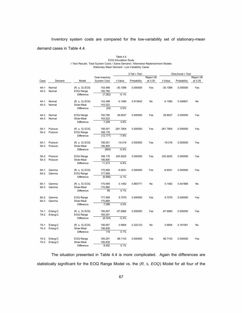
67
Inventory system costs are compared for the low-variability set of stationary-mean
demand cases in Table 4.4.
The situation presented in Table 4.4 is more complicated. Again the differences are
statistically significant for the EOQ Range Model vs. the (R, s, EOQ) Model for all four of the
Total Inventory Reject H0 Reject H0Case Demand Model System Cost t-Value Probability at 0.05 t-Value Probability at 0.05
4A-1 Normal (R, s, S) EOQ 143,498 -30.1089 0.000000 Yes -30.1089 0.000000 Yes4A-2 Normal EOQ Range 150,780
Difference (7,282) -5.1%
4A-1 Normal (R, s, S) EOQ 143,498 -0.1085 0.913642 No -0.1085 0.456821 No4A-3 Normal Silver-Meal 143,522
Difference (24) 0.0%
4A-2 Normal EOQ Range 150,780 29.8527 0.000000 Yes 29.8527 0.000000 Yes4A-3 Normal Silver-Meal 143,522
Difference 7,258 4.8%
5A-1 Poisson (R, s, S) EOQ 156,001 -261.7804 0.000000 Yes -261.7804 0.000000 Yes5A-2 Poisson EOQ Range 168,178
Difference (12,177) -7.8%
5A-1 Poisson (R, s, S) EOQ 156,001 -19.018 0.000000 Yes -19.018 0.000000 Yes5A-3 Poisson Silver-Meal 156,805
Difference (804) -0.5%
5A-2 Poisson EOQ Range 168,178 245.9202 0.000000 Yes 245.9202 0.000000 Yes5A-3 Poisson Silver-Meal 156,805
Difference 11,373 6.8%
6A-1 Gamma (R, s, S) EOQ 170,959 -9.6031 0.000000 Yes -9.6031 0.000000 Yes6A-2 Gamma EOQ Range 177,958
Difference (6,999) -4.1%
6A-1 Gamma (R, s, S) EOQ 170,959 0.1462 0.883771 No 0.1462 0.441885 No6A-3 Gamma Silver-Meal 170,860
Difference 99 0.1%
6A-2 Gamma EOQ Range 177,958 9.7079 0.000000 Yes 9.7079 0.000000 Yes6A-3 Gamma Silver-Meal 170,860
Difference 7,098 4.0%
7A-1 Erlang-C (R, s, S) EOQ 156,957 -67.6965 0.000000 Yes -67.6965 0.000000 Yes7A-2 Erlang-C EOQ Range 165,291
Difference (8,334) -5.3%
7A-1 Erlang-C (R, s, S) EOQ 156,957 0.9904 0.322123 No 0.9904 0.161061 No7A-3 Erlang-C Silver-Meal 156,839
Difference 118 0.1%
7A-2 Erlang-C EOQ Range 165,291 68.7143 0.000000 Yes 68.7143 0.000000 Yes7A-3 Erlang-C Silver-Meal 156,839
Difference 8,452 5.1%
Table 4.4EOQ Simulation Study
t -Test Results: Total System Costs / Same Demand / Alternative Replenishment ModelsStationary Mean Demand - Low Variability Cases
2-Tail t -Test Directional t -Test

68
stationary-mean demand patterns. But the Silver-Meal Heuristic yields inventory system cost
results that are significantly different from (R, s, S) EOQ results only in the case of Poisson
demand. For the other three demand patterns, Silver-Meal results are so close to the (R, s, S)
EOQ results that the difference is not statistically significant at the α = .05 level. When we
consider managerial importance, the differences for the EOQ Range Model exceed the 5%
threshold vs. the (R, s, S) EOQ for normal, Poisson, and Erlang-C demand, and comes in at
4.1% for the gamma distribution case. But the differences for the Silver-Meal Heuristic are not
important for any demand pattern, again falling below $1,000 in each case and ranging from
0.0% to 0.5%.
The inventory system costs for the high-variability cases with time-varying demand are
compared in Table 4.5.
Total Inventory Reject H0 Reject H0Case Demand Model System Cost t-Value Probability at 0.05 t-Value Probability at 0.05
1B-1 Seasonal (R, s, S) EOQ 305,970 -114.9492 0.000000 Yes -114.9492 0.000000 Yes1B-2 Seasonal EOQ Range 316,581
Difference (10,611) -3.5%
1B-1 Seasonal (R, s, S) EOQ 305,970 0.0242 0.980668 No 0.0242 0.490334 No1B-3 Seasonal Silver-Meal 305,967
Difference 3 0.0%
1B-2 Seasonal EOQ Range 316,581 114.9004 0.000000 Yes 114.9004 0.000000 Yes1B-3 Seasonal Silver-Meal 305,967
Difference 10,614 3.4%
2B-1 Trend (R, s, S) EOQ 308,741 -112.4839 0.000000 Yes -112.4839 0.000000 Yes2B-2 Trend EOQ Range 318,619
Difference (9,878) -3.2%
2B-1 Trend (R, s, S) EOQ 308,741 -0.1325 0.894632 No -0.1325 0.447316 No2B-3 Trend Silver-Meal 308,752
Difference (11) 0.0%
2B-2 Trend EOQ Range 318,619 112.1832 0.000000 Yes 112.1832 0.000000 Yes2B-3 Trend Silver-Meal 308,752
Difference 9,867 3.1%
3B-1 Seasonal w/ Trend (R, s, S) EOQ 308,734 -113.92 0.000000 Yes -113.92 0.000000 Yes3B-2 Seasonal w/ Trend EOQ Range 318,855
Difference (10,121) -3.3%
3B-1 Seasonal w/ Trend (R, s, S) EOQ 308,734 -0.574 0.566025 No -0.574 0.283012 No3B-3 Seasonal w/ Trend Silver-Meal 308,784
Difference (50) 0.0%
3B-2 Seasonal w/ Trend EOQ Range 318,855 113.4949 0.000000 Yes 113.4949 0.000000 Yes3B-3 Seasonal w/ Trend Silver-Meal 308,784
Difference 10,071 3.2%
Table 4.5EOQ Simulation Study
t -Test Results: Total System Costs / Same Demand / Alternative Replenishment ModelsTime-Varying Demand - High Variability Cases
2-Tail t -Test Directional t -Test
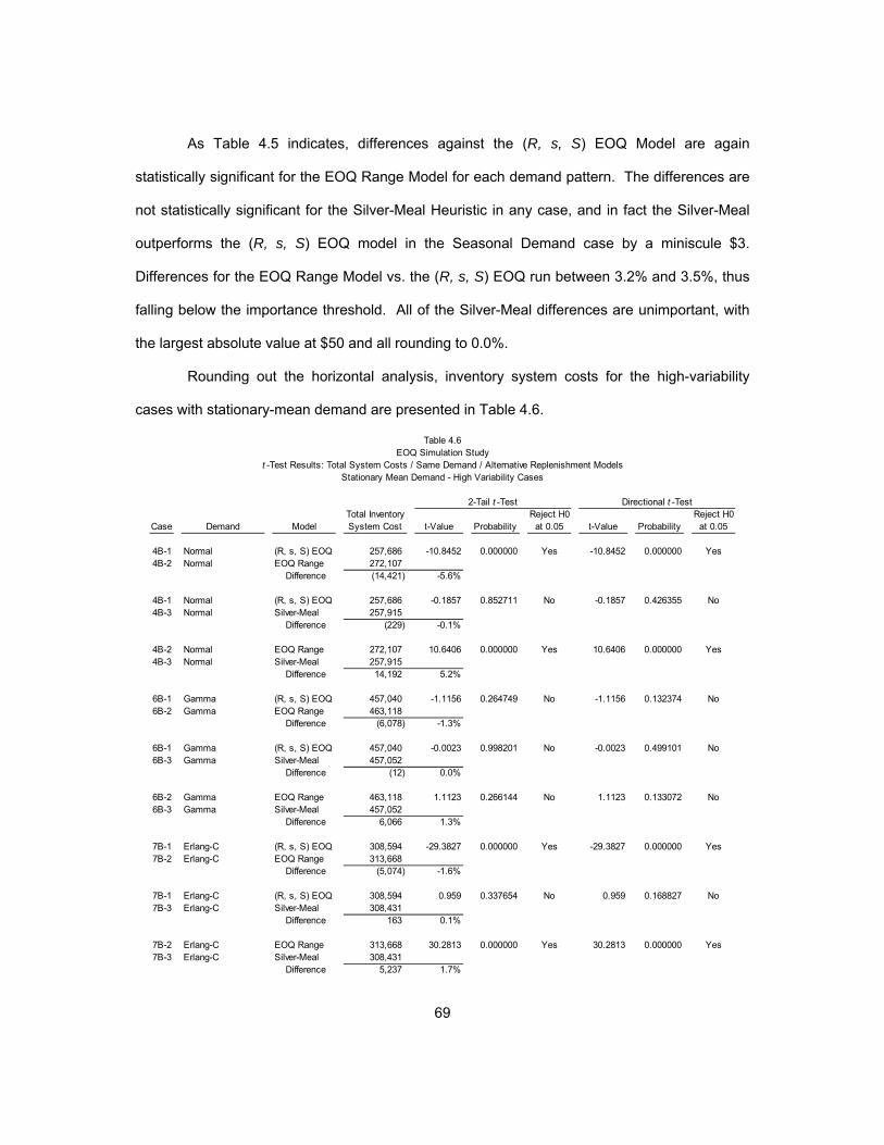
69
As Table 4.5 indicates, differences against the (R, s, S) EOQ Model are again
statistically significant for the EOQ Range Model for each demand pattern. The differences are
not statistically significant for the Silver-Meal Heuristic in any case, and in fact the Silver-Meal
outperforms the (R, s, S) EOQ model in the Seasonal Demand case by a miniscule $3.
Differences for the EOQ Range Model vs. the (R, s, S) EOQ run between 3.2% and 3.5%, thus
falling below the importance threshold. All of the Silver-Meal differences are unimportant, with
the largest absolute value at $50 and all rounding to 0.0%.
Rounding out the horizontal analysis, inventory system costs for the high-variability
cases with stationary-mean demand are presented in Table 4.6.
Total Inventory Reject H0 Reject H0Case Demand Model System Cost t-Value Probability at 0.05 t-Value Probability at 0.05
4B-1 Normal (R, s, S) EOQ 257,686 -10.8452 0.000000 Yes -10.8452 0.000000 Yes4B-2 Normal EOQ Range 272,107
Difference (14,421) -5.6%
4B-1 Normal (R, s, S) EOQ 257,686 -0.1857 0.852711 No -0.1857 0.426355 No4B-3 Normal Silver-Meal 257,915
Difference (229) -0.1%
4B-2 Normal EOQ Range 272,107 10.6406 0.000000 Yes 10.6406 0.000000 Yes4B-3 Normal Silver-Meal 257,915
Difference 14,192 5.2%
6B-1 Gamma (R, s, S) EOQ 457,040 -1.1156 0.264749 No -1.1156 0.132374 No6B-2 Gamma EOQ Range 463,118
Difference (6,078) -1.3%
6B-1 Gamma (R, s, S) EOQ 457,040 -0.0023 0.998201 No -0.0023 0.499101 No6B-3 Gamma Silver-Meal 457,052
Difference (12) 0.0%
6B-2 Gamma EOQ Range 463,118 1.1123 0.266144 No 1.1123 0.133072 No6B-3 Gamma Silver-Meal 457,052
Difference 6,066 1.3%
7B-1 Erlang-C (R, s, S) EOQ 308,594 -29.3827 0.000000 Yes -29.3827 0.000000 Yes7B-2 Erlang-C EOQ Range 313,668
Difference (5,074) -1.6%
7B-1 Erlang-C (R, s, S) EOQ 308,594 0.959 0.337654 No 0.959 0.168827 No7B-3 Erlang-C Silver-Meal 308,431
Difference 163 0.1%
7B-2 Erlang-C EOQ Range 313,668 30.2813 0.000000 Yes 30.2813 0.000000 Yes7B-3 Erlang-C Silver-Meal 308,431
Difference 5,237 1.7%
Table 4.6EOQ Simulation Study
t -Test Results: Total System Costs / Same Demand / Alternative Replenishment ModelsStationary Mean Demand - High Variability Cases
2-Tail t -Test Directional t -Test

70
Table 4.6 indicates that differences between the EOQ Range Model and the (R, s, S)
EOQ Model are statistically significant for the normal and Erlang-C distributions but not for the
gamma distribution. The differences against the (R, s, S) EOQ are not significant for the Silver-
Meal Heuristic under any of the three demand scenarios. In terms of managerial importance,
the EOQ Range differences exceed the threshold for importance at 5.6% for the normal
distribution, but are only 1.3% for the gamma distribution and 1.6% for the Erlang-C distribution.
The Silver-Meal differences are again unimportant for all three demand patterns, with
percentage differences at 0.0% or 0.1% for each pattern.
The horizontal analysis is reviewed from an aggregate perspective at the end of this
chapter. In general, differences between the EOQ Range Model and the (R, s, S) EOQ Model
are significantly different at the α = .05 level in most cases, and these differences are
managerially important in some but not all cases. Differences between the Silver-Meal Heuristic
and the (R, s, S) EOQ Model are so small as to be statistically insignificant and managerially
unimportant in most cases.
4.4 t-Tests for Equal Means: Same Model / Alternative Demand
This section considers the vertical analysis of inventory system costs from Table 4.1 in
statistical terms. Absolute and percentage differences between the inventory system cost
results for different demand patterns under each stochastic replenishment model are calculated,
and two-sample t-tests are used to evaluate the significances of the differences among the
sample means. In other words, this section addresses the question, “Do demand patterns
matter?”
The calculated differences and t-test results are displayed in three separate tables for
the (R, s, S) EOQ Model, the EOQ Range Model, and the Silver-Meal Heuristic for the low-
variability demand cases, and in three other tables for high-variability demand cases. For
purposes of the vertical analysis, the normal distribution inventory system cost is treated as the
baseline, and the calculated inventory system cost for each demand pattern under the same

71
replenishment model is compared to the result for the normal distribution. In each comparison,
the differences are evaluated for both statistical significance and managerial importance.
Samples of the NCSS output for the t-tests used in the vertical analysis are provided in
Appendix F.
Inventory system cost results are compared for the (R, s, S) EOQ Model with low
demand variability in Table 4.7.
This set of comparisons shows that differences from inventory system costs under
normal demand are statistically significant at the α = .05 level for every demand pattern
considered. These differences are all managerially important, ranging from 8.7% for Poisson
demand to 19.1% for gamma-distributed demand.
Inventory system cost results are compared for the EOQ Range Model with low
demand variability in Table 4.8.
Total Inventory Reject H0 Reject H0Case Demand Model System Cost t-Value Probability at 0.05 t-Value Probability at 0.05
4A Normal (R, s, S) EOQ 143,498 -82.5257 0.000000 Yes -82.5257 0.000000 Yes1A Seasonal (R, s, S) EOQ 156,527
Difference (13,029) -9.1%
4A Normal (R, s, S) EOQ 143,498 -102.5066 0.000000 Yes -102.5066 0.000000 Yes2A Trend (R, s, S) EOQ 159,663
Difference (16,165) -11.3%
4A Normal (R, s, S) EOQ 143,498 -101.1044 0.000000 Yes -101.1044 0.000000 Yes3A Seasonal w/ Trend (R, s, S) EOQ 159,452
Difference (15,954) -11.1%
4A Normal (R, s, S) EOQ 143,498 -78.8883 0.000000 Yes -78.8883 0.000000 Yes5A Poisson (R, s, S) EOQ 156,001
Difference (12,503) -8.7%
4A Normal (R, s, S) EOQ 143,498 -54.5576 0.000000 Yes -54.5576 0.000000 Yes6A Gamma (R, s, S) EOQ 170,959
Difference (27,461) -19.1%
4A Normal (R, s, S) EOQ 143,498 -75.96 0.000000 Yes -75.96 0.000000 Yes7A Erlang-C (R, s, S) EOQ 156,957
Difference (13,459) -9.4%
2-Tail t -Test Directional t -Test
Table 4.7EOQ Simulation Study
t -Test Results: Total System Costs / Same Model / Alternative Demand Patterns(R, s, S) EOQ Model / Low Variability Cases

72
When the EOQ Range Model is applied across the full set of low-variability demand
patterns, the inventory system cost difference from the cost result under normal demand is
statistically significant for all demand patterns. These differences are all managerially
important, running from 9.6% for the Erlang-C distribution to 18.0% for the gamma distribution.
It is evident that these differences are larger in percentage terms than the differences observed
for the (R, s, S) EOQ Model with low variability.
Inventory system cost results are compared for the Silver-Meal Heuristic with low
demand variability in Table 4.9.
Total Inventory Reject H0 Reject H0Case Demand Model System Cost t-Value Probability at 0.05 t-Value Probability at 0.05
4A Normal EOQ Range 150,780 -108.7935 0.000000 Yes -108.7935 0.000000 Yes1A Seasonal EOQ Range 171,197
Difference (20,417) -13.5%
4A Normal EOQ Range 150,780 -120.6291 0.000000 Yes -120.6291 0.000000 Yes2A Trend EOQ Range 173,368
Difference (22,588) -15.0%
4A Normal EOQ Range 150,780 -120.9076 0.000000 Yes -120.9076 0.000000 Yes3A Seasonal w/ Trend EOQ Range 173,436
Difference (22,656) -15.0%
4A Normal EOQ Range 150,780 -92.2693 0.000000 Yes -92.2693 0.000000 Yes5A Poisson EOQ Range 168,178
Difference (17,398) -11.5%
4A Normal EOQ Range 150,780 -46.8617 0.000000 Yes -46.8617 0.000000 Yes6A Gamma EOQ Range 177,958
Difference (27,178) -18.0%
4A Normal EOQ Range 150,780 -70.5829 0.000000 Yes -70.5829 0.000000 Yes7A Erlang-C EOQ Range 165,291
Difference (14,511) -9.6%
Table 4.8EOQ Simulation Study
t -Test Results: Total System Costs / Same Model / Alternative Demand PatternsEOQ Range Model / Low Variability Cases
2-Tail t -Test Directional t -Test
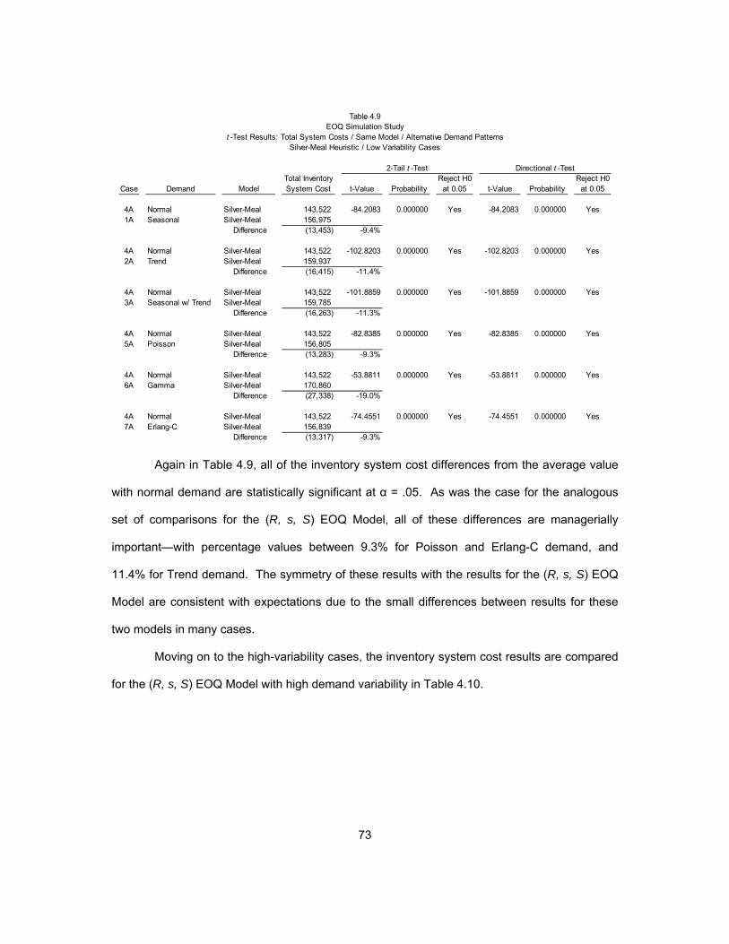
73
Again in Table 4.9, all of the inventory system cost differences from the average value
with normal demand are statistically significant at α = .05. As was the case for the analogous
set of comparisons for the (R, s, S) EOQ Model, all of these differences are managerially
important—with percentage values between 9.3% for Poisson and Erlang-C demand, and
11.4% for Trend demand. The symmetry of these results with the results for the (R, s, S) EOQ
Model are consistent with expectations due to the small differences between results for these
two models in many cases.
Moving on to the high-variability cases, the inventory system cost results are compared
for the (R, s, S) EOQ Model with high demand variability in Table 4.10.
Total Inventory Reject H0 Reject H0Case Demand Model System Cost t-Value Probability at 0.05 t-Value Probability at 0.05
4A Normal Silver-Meal 143,522 -84.2083 0.000000 Yes -84.2083 0.000000 Yes1A Seasonal Silver-Meal 156,975
Difference (13,453) -9.4%
4A Normal Silver-Meal 143,522 -102.8203 0.000000 Yes -102.8203 0.000000 Yes2A Trend Silver-Meal 159,937
Difference (16,415) -11.4%
4A Normal Silver-Meal 143,522 -101.8859 0.000000 Yes -101.8859 0.000000 Yes3A Seasonal w/ Trend Silver-Meal 159,785
Difference (16,263) -11.3%
4A Normal Silver-Meal 143,522 -82.8385 0.000000 Yes -82.8385 0.000000 Yes5A Poisson Silver-Meal 156,805
Difference (13,283) -9.3%
4A Normal Silver-Meal 143,522 -53.8811 0.000000 Yes -53.8811 0.000000 Yes6A Gamma Silver-Meal 170,860
Difference (27,338) -19.0%
4A Normal Silver-Meal 143,522 -74.4551 0.000000 Yes -74.4551 0.000000 Yes7A Erlang-C Silver-Meal 156,839
Difference (13,317) -9.3%
Table 4.9EOQ Simulation Study
t -Test Results: Total System Costs / Same Model / Alternative Demand PatternsSilver-Meal Heuristic / Low Variability Cases
2-Tail t -Test Directional t -Test

74
Table 4.10 shows that differences from inventory system costs under normal demand
are statistically significant at the α = .05 level with the (R, s, S) EOQ Model for every demand
pattern considered. These differences are all managerially important, ranging from 18.7% for
Seasonal demand to 77.4% for gamma-distributed demand. Comparing these results to the
results in Table 4.7 for the (R, s, S) EOQ Model under low demand variability indicates that the
differences are larger in absolute and relative terms for the set of high-variability cases.
Inventory system cost results are compared for the EOQ Range Model with high
demand variability in Table 4.11.
Total Inventory Reject H0 Reject H0Case Demand Model System Cost t-Value Probability at 0.05 t-Value Probability at 0.05
4B Normal (R, s, S) EOQ 257,686 -55.2765 0.000000 Yes -55.2765 0.000000 Yes1B Seasonal (R, s, S) EOQ 305,970
Difference (48,284) -18.7%
4B Normal (R, s, S) EOQ 257,686 -58.4625 0.000000 Yes -58.4625 0.000000 Yes2B Trend (R, s, S) EOQ 308,741
Difference (51,055) -19.8%
4B Normal (R, s, S) EOQ 257,686 -58.4469 0.000000 Yes -58.4469 0.000000 Yes3B Seasonal w/ Trend (R, s, S) EOQ 308,734
Difference (51,048) -19.8%
4B Normal (R, s, S) EOQ 257,686 -51.3405 0.000000 Yes -51.3405 0.000000 Yes6B Gamma (R, s, S) EOQ 457,040
Difference (199,354) -77.4%
4B Normal (R, s, S) EOQ 257,686 -57.8844 0.000000 Yes -57.8844 0.000000 Yes7B Erlang-C (R, s, S) EOQ 308,954
Difference (51,268) -19.9%
Table 4.10EOQ Simulation Study
t -Test Results: Total System Costs / Same Model / Alternative Demand Patterns(R, s, S) EOQ Model / High Variability Cases
2-Tail t -Test Directional t -Test

75
Applying the EOQ Range Model across all of the high-variability demand patterns yields
inventory system cost differences from the cost result under normal demand that are
statistically significant for all demand patterns. These differences are all managerially important
to a large extent, running from 15.3% for the Erlang-C distribution to 70.2% for the gamma
distribution. As was true with the (R, s, S) EOQ model, these differences are larger in absolute
and percentage terms than the differences observed for the EOQ Range Model with low
variability.
Inventory system cost results are compared for the Silver-Meal Heuristic with high
demand variability in Table 4.12.
Total Inventory Reject H0 Reject H0Case Demand Model System Cost t-Value Probability at 0.05 t-Value Probability at 0.05
4B Normal EOQ Range 272,107 -44.1745 0.000000 Yes -44.1745 0.000000 Yes1B Seasonal EOQ Range 316,581
Difference (44,474) -16.3%
4B Normal EOQ Range 272,107 -46.21 0.000000 Yes -46.21 0.000000 Yes2B Trend EOQ Range 318,619
Difference (46,512) -17.1%
4B Normal EOQ Range 272,107 -46.4445 0.000000 Yes -46.4445 0.000000 Yes3B Seasonal w/ Trend EOQ Range 318,855
Difference (46,748) -17.2%
4B Normal EOQ Range 272,107 -47.2034 0.000000 Yes -47.2034 0.000000 Yes6B Gamma EOQ Range 463,118
Difference (191,011) -70.2%
4B Normal EOQ Range 272,107 -41.0628 0.000000 Yes -41.0628 0.000000 Yes7B Erlang-C EOQ Range 313,668
Difference (41,561) -15.3%
Table 4.11EOQ Simulation Study
t -Test Results: Total System Costs / Same Model / Alternative Demand PatternsEOQ Range Model / High Variability Cases
2-Tail t -Test Directional t -Test

76
In Table 4.12, all of the inventory system cost differences from the average value with
normal demand are statistically significant at α = .05. All of these differences are managerially
important—with percentage values between 18.6% for Seasonal demand, and 77.2% for
gamma-distributed demand. As with the other high-variability cases, the differences from
baseline inventory system costs are larger with high-variability demand patterns than with the
low-variability patterns under the Silver-Meal Heuristic. We also see that inventory system cost
results and differences are very similar between the (R, s, S) EOQ Model and the Silver-Meal
Heuristic.
The vertical analysis is discussed from an aggregate perspective in the Section 4.6. In
general, differences in inventory system cost under normal demand vs. the other demand
patterns are significantly different at the α = .05 level and managerially important in all cases.
This is true at both low- and high-variability demand levels.
Total Inventory Reject H0 Reject H0Case Demand Model System Cost t-Value Probability at 0.05 t-Value Probability at 0.05
4B Normal Silver-Meal 257,915 -54.6315 0.000000 Yes -54.6315 0.000000 Yes1B Seasonal Silver-Meal 305,967
Difference (48,052) -18.6%
4B Normal Silver-Meal 257,915 -57.8099 0.000000 Yes -57.8099 0.000000 Yes2B Trend Silver-Meal 308,752
Difference (50,837) -19.7%
4B Normal Silver-Meal 257,915 -57.84 0.000000 Yes -57.84 0.000000 Yes3B Seasonal w/ Trend Silver-Meal 308,784
Difference (50,869) -19.7%
4B Normal Silver-Meal 257,915 -51.1727 0.000000 Yes -51.1727 0.000000 Yes6B Gamma Silver-Meal 457,052
Difference (199,137) -77.2%
4B Normal Silver-Meal 257,915 -57.0443 0.000000 Yes -57.0443 0.000000 Yes7B Erlang-C Silver-Meal 308,431
Difference (50,516) -19.6%
Table 4.12EOQ Simulation Study
t -Test Results: Total System Costs / Same Model / Alternative Demand PatternsSilver-Meal Heuristic / High Variability Cases
2-Tail t -Test Directional t -Test

77
4.5 Factor Level Analysis: Cost, Demand, and Lead Time
Tables comparing the inventory system cost results for the different factor levels of
cost, demand, and lead time are presented in Appendix G. As discussed in the Methodology
section, the simulation featured a balanced design with three levels of item cost, three levels of
periodic demand, and four levels of lead time. These results are summarized below, with
primary emphasis on implications for verification of the simulation model.
In terms of the two levels of variability, higher inventory system costs are calculated for
higher levels of variability for all of the factor levels, models, and demand patterns considered.
This is consistent with the findings of Tunc et al. (2011), and serves to support the validity of the
simulation model.
As noted above, the normal distribution yields the lowest total inventory system cost of
any demand distribution for each of the three stochastic-demand replenishment models
considered in the simulation study. This relationship holds for most of the factor levels, with the
exception of the lowest level of item cost (v = $7.50), and the lowest level of weekly unit
demand ( ̅ = 1). The Poisson distribution yields the lowest total inventory system cost under
the (R, s, S) EOQ model for the lowest level of item cost, and the gamma and Erlang-C
distributions yield lower inventory system costs than the normal distribution with the EOQ
Range Model or the Silver-Meal Heuristic for the lowest level of item cost and the lowest level of
weekly unit demand.
Inventory system costs are lower in all cases for items at the lowest levels of item cost
and weekly demand, so this relationship does not invalidate the results with regard to aggregate
inventory system costs. But this relationship does raise a caveat regarding the generalizability
of results from the simulation study to multi-item inventory environments that are heavily tilted
toward low-cost or low levels of periodic demand.
When we consider the horizontal analysis of the application of different models for the
same demand pattern the same overall relationships observed at the aggregate level are in

78
place at all of the factor levels. Inventory system cost results are lowest overall for the (R, s, S)
EOQ Model, with the calculated results for the Silver-Meal Heuristic very close to the (R, s, S)
EOQ results in most cases. The EOQ Range Model generally yields higher inventory system
cost, although that model tends to perform better relative to the other models for items at the
highest level of item cost (v = $750.00). This provides evidence that the EOQ Range Model
could perform better relative to the other models in multi-item inventory environments that are
weighted toward items with purchase costs that are high relative to order processing costs.
In terms of the vertical analysis of applying a single model to different demand patterns
within a variability level, the relationships that emerge at the factor level are consistent with the
aggregate-level relationships. The inventory costs that result from applying a given model to
alternative demand patterns will differ, although the absolute magnitude of these differences will
be smaller for lower levels of items cost or periodic demand.
As a whole, the factor-level analysis of inventory system cost supports the validity of
the simulation model while revealing some factor-level distinctions that may be relevant in
inventory environments that are unbalanced with regard to the range of item costs and demand
levels that are present.
4.6 Inferences from the Simulation Study
In looking at results from the simulation study, it is useful to begin with inferences
regarding the validity of the simulation model that can be drawn from an overview of inventory
system cost results for the different replenishment models, demand patterns and demand
variability levels as shown in Table 4.1. The validity of the simulation model is supported by the
fact that inventory system costs are lowest when demand is normally distributed—regardless of
which replenishment model is used, and across both levels of demand variability. This is
explained by the fact that the three stochastic-demand models used in the study are all based
on a relaxed version of the classic EOQ model that assumes normally-distributed demand.

79
The validity of the simulation model is also supported by the observation that inventory
system costs are higher for high-variability demand cases than for the related low-variability
demand case for all demand patterns, which is consistent with the findings in Tunc et al. (2011).
Validity is also supported by the fact that inventory system costs are much higher for all of the
stochastic replenishment models than for the deterministic Wagner-Whitin Algorithm under
every demand scenario. Further evidence that will be useful in evaluating the simulation model
will be presented in the empirical validation study in Chapter 5.
It is helpful to recap the horizontal analysis of results from alternative models with the
same demand pattern, and the vertical analysis of results from alternative demand patterns with
the same model. A summary of results from the horizontal analysis is shown in Table 4.13.
For purposes of the horizontal analysis, the (R, s, S) EOQ Model, which provides the
best overall inventory system cost performance against the stochastic-demand replenishment
models considered, is treated as the baseline for comparison. Comparing the performance of
the EOQ Range Model to the (R, s, S) EOQ Model indicates that the inventory system cost
differences are both statistically significant at the α = .05 level, and managerially important with
percentage differences greater than 5%, in nearly all cases. We can infer that the (R, s, S)
% Significant Important % Significant ImportantCase Demand Pattern Variability Penalty at .05? (> 5%) ? Penalty at .05? (> 5%) ?
1A Seasonal Low 9.4% Yes Yes 0.3% Yes No2A Trend Low 8.6% Yes Yes 0.2% Yes No3A Seasonal w/ Trend Low 8.8% Yes Yes 0.2% Yes No4A Normal Low 5.1% Yes Yes 0.0% No No5A Poisson Low 7.8% Yes Yes 0.5% Yes No6A Gamma Low 4.1% Yes No 0.1% No No7A Erlang-C Low 5.3% Yes Yes 0.1% No No
1B Seasonal High 3.5% Yes No 0.0% No No2B Trend High 3.2% Yes No 0.0% No No3B Seasonal w/ Trend High 3.3% Yes No 0.0% No No4B Normal High 5.6% Yes Yes 0.1% No No5B Poisson N/A6B Gamma High 1.3% No No 0.0% No No7B Erlang-C High 1.6% Yes No 0.1% No No
EOQ Range vs. (R, s, S) EOQ Silver-Meal vs. (R, s, S) EOQ
Table 4.13EOQ Simulation Study
Summary of Results: Same Demand / Different Models

80
EOQ Model generally outperforms the EOQ Range Model with regard to inventory system cost
given the assumptions used in the simulation.
On the other hand, comparing the performance of the Silver-Meal Heuristic against the
(R, s, S) EOQ Model indicates that the inventory system cost differences are statistically
significant at the α = .05 level for only some of the low-variability demand scenarios. These
differences are small in absolute and percentage terms in all cases, and are not managerially
important in any case, with these percentage differences never exceeding 0.5%. We can infer
that the (R, s, S) EOQ Model does not significantly outperform the Silver-Meal Heuristic with
regard to inventory system cost given the assumptions used in the simulation.
A summary of results from the vertical analysis is shown in Table 4.14.
For purposes of the vertical analysis, normally distributed demand—which provides the
best overall inventory system cost result across all stochastic models for a given level of
demand variability, is treated as the baseline for comparison. Comparing the performance of
each model across the range of demand patterns studied indicates that the inventory system
cost differences are both statistically significant at the α = .05 level and managerially important,
with percentage differences greater than 5%, in nearly all cases. We can infer that the cost
performance of any of the replenishment models considered will be affected significantly if the
Significant ImportantModel Variability % Penalty at .05? (> 5%) ?
(R, s, S) EOQ Model Low 8.7%-11.3% Yes YesEOQ Range Model Low 9.6%-18% Yes YesSilver-Meal Heuristic Low 9.3%-11.4% Yes Yes
(R, s, S) EOQ Model High 18.7%-77.4% Yes YesEOQ Range Model High 15.3%-77.2% Yes YesSilver-Meal Heuristic High 18.6%-77.2% Yes Yes
Table 4.14EOQ Simulation Study
Summary of Results: Same Model / Different Demand Patterns
Differences vs. Normal Demand

81
actual demand pattern encountered is different from the demand pattern that is expected. This
inference would be valid under the set of assumptions used in the simulation. The identified
relationships might not apply to inventory environments containing a slate of items that are
weighted differently with regard to item costs and periodic demand in comparison to the
balanced representation of the different factor levels assumed in this simulation study.
The inferences developed in this section can be offered to answer the two relevant
research questions in the affirmative: replenishment models matter, and demand patterns
matter. With these inferences grounded in the assumptions used in the simulation, it is
appropriate to gather further evidence regarding the validity of the model and the
generalizability of simulation results. That purpose is served by the empirical validation study,
which is presented in Chapter 5.

82
CHAPTER 5
EMPIRICAL VALIDATION
5.1 Empirical Validation: Overview
As detailed in Section 3.3, inventory system costs for each of the four models were
compared and analyzed across the 278 actual inventory items after the items had been
assigned to the different demand pattern categories. Output from the empirical validation study
includes the total Year 3 inventory system cost (holding cost + order processing cost + stockout
cost) that would be result (a) under the Wagner-Whitin model if actual demand could be
determined in advance, (b) under the (R, s, S) EOQ replenishment model for all items, (c) under
the EOQ Range model for all items, and (d) under the Silver-Meal Heuristic for all items. These
four estimates are broken down by the demand pattern/variability scenarios, following the
methodology detailed in Chapter 3. This output was used to conduct t-tests tests of statistical
significance for the differences in estimated inventory system costs in the NCSS statistical
software package.
Samples of regression reports and stacked time series plots used in the validation
study are presented in Appendix H. Sample screen prints from the model used to calculate
inventory system costs for the validation study are shown in Appendix I, and screen prints of the
t-test output used in the validation study are presented in Appendix J.
The results of the empirical validation study are detailed and analyzed below. Section
5.2 provides an overview of the validation results, and discusses these results with respect to
the simulation model. Section 5.3 presents the results of t-tests that compare the inventory
system cost results for the alternative models as applied to actual Year 3 demand. Section 5.4
offers inferences that can be drawn from the empirical validation study.

83
5.2 Validation Results: Inventory System Cost for All Items
A summary of inventory system cost results for Year 3 for all items, broken into demand
pattern categories and showing the number of items assigned to each demand pattern
category, is shown in Table 5.1.
One relationship that becomes evident immediately is the lack of symmetry in the
breakdown of the 278 items by demand category. This does not bear on the validity of the
simulation model, as no attempt was made to weight the items in the simulation study to
represent the distribution of the actual items by demand pattern.
Over half of the 278 items are assigned to the Trend demand pattern category,
including 110 of the low-variability items and 46 of the high-variability items. Summing items in
the Seasonal, Trend, and Seasonal with Trend categories at both levels of demand variability
indicates that 215 or 77.3% of the actual inventory items have time-varying demand patterns.
This can be attributed to the fact that the company that provided the historical demand data
Wagner-Whitin (R, s, S) EOQ Range Silver-Meal OptimizedCase # # of Items Algorithm EOQ Model Model Heuristic Model-Demand
1A Seasonal Low Variability 2 220 386 674 358 x 3582A Trend Low Variability 110 45,465 156,816 x 238,112 163,489 156,8163A Seasonal w/ Trend Low Variability 9 3,611 8,828 x 10,494 8,846 8,8284A Normal Low Variability 1 161 229 362 223 x 2235A Poisson Low Variability 23 5,252 40,473 37,777 x 40,019 37,7776A Gamma Low Variability 0 N/A N/A N/A N/A N/A7A Erlang-C Low Variability 0 N/A N/A N/A N/A N/A8A Other Distributions Low Variability 10 1,503 7,155 x 8,988 8,533 7,155
Subtotal: Low Variability 155 56,211 213,887 x 296,408 221,467 211,157
1B Seasonal High Variability 31 4,707 25,334 x 33,297 28,612 25,3342B Trend High Variability 46 8,627 104,548 x 133,966 114,890 104,5483B Seasonal w/ Trend High Variability 17 4,085 22,815 x 32,260 23,815 22,8154B Normal High Variability 2 526 988 x 2,536 1,033 9885B Poisson N/A 0 N/A N/A N/A N/A N/A6B Gamma High Variability 0 N/A N/A N/A N/A N/A7B Erlang-C High Variability 0 N/A N/A N/A N/A N/A8B Other Distributions High Variability 27 5,017 52,798 x 64,330 56,155 52,798
Subtotal: High Variability 123 22,962 206,483 x 266,390 224,505 206,483
Total: All Items 278 79,173 420,370 x 562,797 445,973 417,640
x = Lowest inventory system cost among the three replenishment models for each demand pattern group.
Description
Total Inventory System Cost
Table 5.1Empirical Validation Study
Total Inventory System Cost: Optimized Match of Models to Demand Patterns

84
experienced significant increases in business activity during the three years for which the
historical data were provided.
Turning to the stationary-mean demand patterns, 23 or 8.3% of the items are assigned
to the Poisson demand category. Only 3 or 1.1% of the 278 items have demand that is
normally distributed, which is surprising given the widespread assumption of normally-
distributed demand in practice. None of the 278 items had the gamma or Erlang-C distribution
identified as its best-fit distribution.
Among the 37 items or 13.3% of the total items assigned to the Other demand
category, 36 are assigned to the discrete uniform distribution and one item is assigned to the
Weibull distribution.
Continuing with the total system cost analysis presented in Table 5.1, the reliance on a
single actual demand stream in the validation study precludes a vertical analysis of the effect of
a given replenishment model on alternative demand patterns. But it is possible to apply a
horizontal analysis to consider the effect of applying the alternative stochastic-demand
replenishment models to the given demand stream. A visual scan of Table 5.1 reveals the
same pattern identified in the simulation study: the inventory system cost results for the (R, s, S)
EOQ Model are the lowest resulting for any single model in most demand categories and
overall.
As was true in the simulation study, Silver-Meal Heuristic results are close to those for
the (R, s, S) EOQ in most cases and in total, and the EOQ Range Model generally finishes a
distant third. An exception occurs for Poisson demand, for which the EOQ Range Model yields
the lowest inventory system cost. This can be attributed to the small sample size, with only 23
items assigned to the Poisson category.
The absolute and percentage differences among inventory system cost results will be
evaluated further in Section 5.3. Meanwhile, an analysis of the relative cost performance of

85
each replenishment model for each demand pattern category represented in the actual data is
presented in Table 5.2.
Overall, the results of the empirical validation study are consistent with the results of the
simulation study. Again it is evident that the absolute cost penalty against the optimal
replenishment model is higher for high-variability items than it is for low-variability items in most
cases. The (R, s, S) EOQ model performs better than the EOQ Range model or the Silver-Meal
Heuristic across the full set of items, but the absolute cost advantage over the Silver-Meal
Heuristic is small relative to the total of inventory system costs across all items.
It is also helpful to evaluate the inventory system cost penalty multiple against the
optimal Wagner-Whitin inventory system cost. This analysis is provided in Table 5.3.
# of (R, s, S) EOQ Range Silver-Meal (R, s, S) EOQ Range Silver-MealCase # Items EOQ Model Model Heuristic EOQ Model Model Heuristic
1A Seasonal Low Variability 2 28 317 0 7.8% 88.7% 0.0%1B Seasonal High Variability 31 0 7,963 3,278 0.0% 31.4% 12.9%
2A Trend Low Variability 110 0 81,296 6,673 0.0% 51.8% 4.3%2B Trend High Variability 46 0 29,418 10,342 0.0% 28.1% 9.9%
3A Seasonal w/ Trend Low Variability 9 0 1,666 18 0.0% 18.9% 0.2%3B Seasonal w/ Trend High Variability 17 0 9,444 999 0.0% 41.4% 4.4%
4A Normal Low Variability 1 6 139 0 2.7% 62.4% 0.0%4B Normal High Variability 2 0 1,548 46 0.0% 156.7% 4.7%
5A Poisson Low Variability 23 2,696 0 2,242 7.1% 0.0% 5.9%5B Poisson N/A 0 N/A N/A N/A N/A N/A N/A
6A Gamma Low Variability 0 N/A N/A N/A N/A N/A N/A6B Gamma High Variability 0 N/A N/A N/A N/A N/A N/A
7A Erlang-C Low Variability 0 N/A N/A N/A N/A N/A N/A7B Erlang-C High Variability 0 N/A N/A N/A N/A N/A N/A
8A Other Distributions Low Variability 10 0 1,833 1,378 0.0% 25.6% 19.3%8B Other Distributions High Variability 27 0 11,533 3,357 0.0% 21.8% 6.4%
Total: All Items 278 2,730 145,157 28,333 0.6% 34.5% 6.7%
Table 5.2Empirical Validation Study
Total Inventory System Cost Penalty vs. Optimal Model by Variability Level
Absolute $ Cost Penalty vs. Optimal Model Percentage Cost Penalty vs. Optimal Mode
Description

86
The pattern observed here is consistent with the pattern that is evident in Table 4.2 for
the simulation study. The system cost penalty against the deterministic Wagner-Whitin
Algorithm is larger for items with high demand variability than for items with low variability.
The Wagner-Whitin penalty multiple offers another opportunity to compare the
validation study results with the results of the simulation study. The Wagner-Whitin penalty
multiple calculated for all items for Year 3 under the (R, s, S) EOQ Model stands at 5.3 for the
278 items the validation study. This result can be compared to the Wagner-Whitin penalty
multiple for the (R, s, S) EOQ Model with different demand patterns in the simulation study in
Table 4.2. We can exclude the gamma and Erlang-C multiples in Table 4.2 from consideration,
(R, s, S) EOQ Range Silver-MealCase # # of Items EOQ Model Model Heuristic
1A Seasonal Low Variability 2 1.8 3.1 1.6 x2A Trend Low Variability 110 3.4 x 5.2 3.63A Seasonal w/ Trend Low Variability 9 2.4 x 2.9 2.54A Normal Low Variability 1 1.4 y 2.3 1.4 y5A Poisson Low Variability 23 7.7 7.2 x 7.66A Gamma Low Variability 0 N/A N/A N/A7A Erlang-C Low Variability 0 N/A N/A N/A8A Other Distributions Low Variability 10 4.8 x 6.0 5.7
Subtotal: Low Variability 155 3.8 x 5.3 3.9
1B Seasonal High Variability 31 5.4 x 7.1 6.12B Trend High Variability 46 12.1 x 15.5 13.33B Seasonal w/ Trend High Variability 17 5.6 x 7.9 5.84B Normal High Variability 2 1.9 x 4.8 2.05B Poisson N/A 0 N/A N/A N/A6B Gamma High Variability 0 N/A N/A N/A7B Erlang-C High Variability 0 N/A N/A N/A8B Other Distributions High Variability 27 10.5 x 12.8 11.2
Subtotal: High Variability 123 9.0 x 11.6 9.8
Total: All Items 278 5.3 x 7.1 5.6
x = Lowest inventory system cost-multiple vs. Wagner-Whitin algorithm for actual demand pattern group.y = Tie among two models for lowest system cost penalty multiple vs. W-W rounded to two decimal places.
Table 5.3Empirical Validation Study
Total Inventory System Cost Comparison: Penalty Multiple vs. Wagner-Whitin Algorithm
System Cost Multiple vs. Wagner-Whitin
Description

87
as none of the items in the validation study adhere to these distributions. The aggregate value
of 5.3 for the Wagner-Whitin penalty multiple in the validation study lies in the range between
the low-variability and high-variability demand categories for the (R, s, S) EOQ Model in Table
4.2. This consistency is evidence that supports the validity of the simulation model.
The inventory system cost differences among the stochastic-demand replenishment
models are measured and tested for statistical significance in the next section.
5.3 t-Tests for Equal Means: Alternative Models
Inventory system costs for the third year of actual demand for the 278 items as
computed under the three competing replenishment models were subjected to t-tests in NCSS
to evaluate the statistical significance of the calculated differences. The t-test results are
summarized in Table 5.4.
The t-tests fail to reject the null hypothesis of equal means for all models. This can be
attributed to the fact that the sample was based on a single calculation for the third year of
actual demand, as compared to the 1,000 replications used in t-tests for the simulation results.
In terms of the magnitude of the calculated differences in inventory system costs, it is evident
that the 33.9% difference between the cost under the (R, s, S) EOQ Model and the EOQ Range
model would be managerially important. The total inventory system cost difference between the
Total Inventory Reject H0 Reject H0Model System Cost t-Value Probability at 0.05 t-Value Probability at 0.05
(R, s, S) EOQ 420,370 -1.0784 0.281323 No -1.0784 0.140661 NoEOQ Range 562,797 Difference (142,427) -33.9%
(R, s, S) EOQ 420,370 -0.2117 0.832458 No -0.2117 0.416229 NoSilver-Meal 445,973 Difference (25,603) -6.1%
EOQ Range 562,797 0.8841 0.377057 No 0.8841 0.188528 NoSilver-Meal 445,973 Difference 116,824 20.8%
Table 5.4Empirical Validation Study
t -Test Results: Total Inventory System Cost / Alternative Replenishment Models
2-Tail t -Test Directional t -Test

88
(R, s, S) EOQ Model and the Silver-Meal Heuristic stands at 6.1%, or just above the 5%
threshold used in this study for managerial importance.
Notwithstanding the failure to reject the hypothesis of equal means among the inventory
system costs calculated with the three replenishment models, we might consider the cost
differences as managerially relevant to the extent that they are consistent with the simulation—
and assuming that the simulation model is valid. The light that the validation study sheds on the
simulation model is discussed in the next section.
5.4 Inferences from the Empirical Validation
As noted in section 3.3, the empirical validation study serves two purposes. The first is
to validate the results of the simulation study with actual data. The second purpose is the use
of archival data to identify and understand the practical challenges of classifying independent
demand items by demand pattern for replenishment management. Inferences regarding
validation of the simulation model are discussed below. Process issues involved in classifying
items by demand pattern, as identified during the execution of the validation study, are
addressed in Chapter 6.
When the results of the validation study are compared to the results of the simulation
study, four relationships that tend to support the validity of the simulation model emerge:
1. Inventory system cost performance of different replenishment models: The (R, s, S)
EOQ model yielded the lowest inventory system cost in the simulation study and the empirical
validation study, with the Silver-Meal Heuristic performing nearly as well in both studies.
2. Penalty vs. optimal model is higher for high-variability patterns and items: Items with
high-variability were associated with higher levels of inventory system cost penalties against the
optimal stochastic replenishment model in both the simulation study and the empirical validation
study.
3. The Wagner-Whitin penalty multiple is higher for high-variability patterns and items:
This pattern is observed in both the simulation study and the empirical validation study.

89
4. The Wagner-Whitin penalty multiple value range is consistent: The inventory system
cost penalty multiple against the Wagner-Whitin algorithm for the full slate of 278 items falls
within the range of values calculated for different demand patterns and variability levels in the
simulation study.
One finding that emerges from the empirical validation study is the revelation that the
demand patterns actually observed in a multi-item inventory environment may not be consistent
with the patterns that are presumed to exist, or with the patterns that are most frequently
researched in peer-reviewed literature. The company that provided the empirical data has
traditionally based its replenishment rules on the assumption that periodic demand is normally
distributed—but the validation study indicated that only three out of 278 independent demand
items had demand that fit the normal distribution during the three years studied. Trend demand,
which is researched frequently in forecasting literature, and Poisson demand were present
among the items studied, but none of the 278 items was found to follow a gamma-distributed or
Erlang-C demand pattern.
Allowing for the fact that the simulation model was not designed to specifically reflect
the mix of item cost, demand, and lead time that was present in the historical demand data, it
can be argued that the simulation model is valid, and that inferences drawn from the simulation
study can be applied to operating environments similar to that of the company that provided the
historical demand data. These findings are applied to the demand-pattern fitting implementation
study in Chapter 6, and to the cost/benefit analysis in Chapter 7.

90
CHAPTER 6
ITEM-DEMAND PATTERN FITTING IMPLEMENTATION STUDY
6.1 Implementation Study Overview
To the extent that using different replenishment rules for independent demand inventory
items with different demand patterns is desirable, it becomes necessary to design and follow a
consistent process for fitting inventory items to demand patterns. Identifying relevant demand
patterns can also be useful for other inventory management decisions.
From that point, it becomes necessary to work through the effects of market complexity,
multiple-item obfuscation, and random demand variability to design an efficient process. The
process defined below is based on the steps followed and lessons learned during the empirical
validation study. The process developed during the research is adapted to provide a replicable
set of steps that can be followed for independent demand items in any operating environment.
As other researchers have observed, practicing managers rarely apply the full range of
quantitative inventory management techniques that are available (McLaughlin et al. 1994). This
chapter addresses the following research question: What process impediments are involved in
item-demand pattern matching?
6.2 Process Narrative and Flow Chart
The defined process for fitting items to demand patterns is explained in a step-by-step
narrative, and supported by a process flow chart. The narrative assumes that at least three
years of item-specific historical demand data are available, and that this time series demand
information can be used to assign items to demand pattern groups for the upcoming target year.
As noted above in the Methodology section, the Crystal Ball software Fit Distribution function
was used in the current study—but any statistical software package with the ability to fit time
series data to probability distributions or forecast models can be used in this process. This
91
process recognizes the possibility that a given time series may be associated with a stationary
mean probability distribution, a time-varying demand pattern, or both. The process narrative
follows.
1. Analyze multiple years of historical demand for each of the independent demand
items with the statistical software package to identify the best stationary demand pattern in
terms of the Chi-Square goodness of fit statistic. For each independent demand item, record
the identified best-fit demand pattern and the parameter values for the actual demand data
series. The year prior to the target year (Year T-1) would be excluded from this analysis.
2. In addition to the stationary demand analysis described in step 1 above, use
historical demand data prior to Year T-1 for each independent demand item to calculate
parameter values for relevant time-varying demand patterns such as seasonal, trend, and
seasonal with trend demand. This will involve calculating the seasonal index for the seasonal
case, doing a regression analysis to identify the intercept and slope values for the trend case,
and calculating a seasonal index for variability around the trend line for the seasonal with trend
case. For the sake of consistency, each year can be analyzed in terms of 13 equal-length
periods of four weeks each. This eliminates the need to address issues like 4-week vs. 5-week
calendar months.
3. For each independent demand item, calculate a 13-period demand forecast for the
Year T-1 with each of the following four methods:
the best-fit stationary demand pattern, using the previously-identified parameter
values for the distribution/item combination.
seasonal demand, using the seasonal index values identified in step 2.
trend demand, using the intercept and slope values identified in step 2.
seasonal with trend demand, using the seasonal index values around the trend line
as identified in step 2.

92
4. For each independent demand item, compare each of the four annual forecasts
against actual Year T-1 demand to calculate two relevant forecast accuracy metrics. These
metrics will be the cumulative forecast error (CFE) value and the mean absolute deviation
(MAD). Offsetting positive and negative values via the CFE may be preferable for purposes of
optimizing inventory system costs if upward or downward bias exists for the item-specific
forecast.
5. For each independent demand item, the forecast method for Year T-1 demand that
yields the best value for forecast accuracy (lowest CFE or lowest MAD) will be chosen as the
best-fit demand pattern for that item.
The process flow chart for the item-demand fitting process is presented in Figure 6.1.
Figure 6.1 Process Flow Chart
Item-Demand Pattern Fitting

93
6.3 Process Impediments and Practical Challenges
This brings the discussion back to the research question. What process impediments
are involved in item-demand pattern matching? Information gained during the execution of the
empirical validation study provides some insight. Possible reasons for the rarity of item-demand
pattern matching include resource limitations, perceived cost/benefit relationships, and inertia.
Resource limitations come into play when practicing managers would like access to
more information for inventory management, but are unable or unwilling to commit the
necessary resources. The item-demand pattern matching on 278 items in the empirical
validation study required 100 hours. Limited staff, lack of necessary expertise among the staff,
limited budgets for consulting services, and the lack of specialized software or training in the
specialized functions of existing software could all come into play. And this limitation is not
confined to small- and medium-sized business settings. These resource limitations exist in the
company that provided the actual demand data for this research, and that company is a
subsidiary of one of the fifty largest U.S.-based manufacturing companies.
Perceived cost/benefit relationships may also prevent the adoption of item-demand
pattern fitting. As noted in Chapter 1, it is widely understood that the EOQ model is robust in
terms of small cost penalties for deviations from the optimal target. It is also possible that
experienced supply chain and financial professionals have intuitively recognized that the cost of
diligently matching items to demand patterns may exceed the resulting benefits—which may be
true in many cases. In this regard, these decision makers may have already applied a fast and
frugal heuristic.
Inertia is another possible explanation for the rarity of item-demand pattern fitting. The
practice is not followed in any given company because that company has never done this, and
as far as anyone knows their competitors have never done it either. Such inertia may result
from the historical absence of a well-defined process for matching items to demand patterns—a
gap that could be filled by the defined implementation process offered here.

94
Exploratory research to better understand the value of item-demand pattern matching is
mentioned as a possibility in the concluding section of this paper. As this point it is appropriate
to review the inferences that can be drawn from the item-demand fitting implementation study.
6.4 Inferences from the Implementation Study
The process presented above defines an implementation process for analyzing a large
number of independent demand items to identify the best-fit demand pattern for each item. It is
possible that the presence of a well-defined five-step process for item-demand pattern
matching, like the one presented here, could serve to remove one of the aforementioned
impediments.
As the results of the cost/benefit analysis will indicate, matching replenishment rules to
items by demand distribution may not be cost-effective in many situations. Nonetheless, this
framework is defined and offered here because some enterprises may find the use of different
replenishment rules to be advantageous. In addition, identifying relevant demand patterns may
be useful for other inventory management decisions.

95
CHAPTER 7
COST/BENEFIT ANALYSIS
7.1 Cost/Benefit Analysis Overview
The approach applied here begins with inventory system costs calculated via the
alternative replenishment models for the various demand categories in the empirical validation
study. The relative cost advantage of matching replenishment rules to different demand
categories or using the (R, s, S) EOQ model for all items can be regarded as “benefits” for this
analysis. The differential cost of implementing and managing each replenishment model are
then applied to compare the benefits of each model after recognizing the differential costs.
This chapter addresses the following research questions: Do the advantages of
alternative replenishment rules outweigh the costs? And, can efficient heuristics outperform
more data-intensive models in OM decisions?
7.2 Assumptions and Calculations
The general assumptions used in the cost/benefit analysis are presented in Table 7.1.
Match ModelGeneral (R, s, S) EOQ Range Silver-Meal to Demand
Assumptions EOQ Model Model Heuristic Pattern
Year 3 Inventory System Cost per Validation $420,370 y $562,797 $445,973 $417,640 x
Average Annual Salary-Procurement Professional $120,000
Regular Full-Time Work Hours per Year 2,000
Salary Cost per Hour-Procurement Professional $60.00
Benefit Cost as % of Salary 40.0%
Overhead as % of Annual Salary 30.0%
Total Benefit & Overhead as % of Annual Salary 70.0%
Salary, Benefits & Overhead Full Cost per Hour $102.00
Average Consulting Cost/Hour Incl Travel $200.00
x = Lowest inventory system cost (holding cost + order processing cost + stockout cost) of among all replenishment methods.y = Lowest inventory system cost of any single replenishment model as applied to all all items.
Description
Table 7.1Cost/Benefit AnalysisGeneral Assumptions

96
The estimated differential staff, administrative, and consulting costs associated with
implementing and managing the alternative replenishment methods are developed in Table 7.2.
These estimates are based on information gathered from the company that provided
the actual demand data, and on actual time logged in classifying items by demand pattern in the
empirical validation study. It is assumed for purposes of the cost/benefit analysis that
application of either of the more frugal heuristics—the EOQ Range Model or the Silver-Meal
Match Model(R, s, S) EOQ Range Silver-Meal to Demand
EOQ Model Model Heuristic Pattern
Staff Professional Hours for:
Annual Review and Update of Model Values 60 2 2 64
Periodic/Interim Update of Model Values 40 0 0 40
Managing Consulting Support Services 20 2 2 24
Total Annual Staff Professional Hours 120 4 4 128
Consulting Hours for:
Developing/Updating replenishment software 40 2 2 44
Annual retrofit study of demand patterns 0 0 0 100
Business intelligence/Data extraction 20 0 0 20
Ongoing support services 40 2 2 44
Total Annual Consulting Hours 100 4 4 208
Annual Staff, Admin & Consulting Cost:
Staff hours at full rate of $102.00 $12,240 $408 $408 $13,056
Consulting hours at full rate of $200.00 20,000 800 800 41,600
Total Annual Staff, Admin & Consulting Cost $32,240 $1,208 $1,208 $54,656
Table 7.2Cost/Benefit Analysis
Annual Staff, Administrative, and Consulting Cost
Description

97
Heuristic—would entail the use of a base stock inventory policy or an efficient heuristic for
establishing safety stock levels.
The total annual costs (inventory system cost plus differential staff, administrative, and
consulting cost) of the alternative replenishment methods are compared in Table 7.3.
7.3 Inferences from the Cost/Benefit Analysis
7.3.1 Cost/Benefit Analysis Meets Fast and Frugal Heuristics
The results of the simulation study and the empirical validation study are consistent in
indicating that the more calculation-intensive (R, s, S) EOQ model yields the lowest inventory
system cost when applied to the full slate of independent demand items. As the validation study
indicates, a small reduction in inventory system cost could be achieved by using different
replenishment models for items with certain demand patterns. But this aspect of the research,
like most peer-reviewed research on inventory replenishment, considers only inventory system
cost without addressing the differential costs of implementing and managing alternative models.
The cost/benefit analysis yields an interesting result. Under the assumptions applied
here, the inventory system cost advantage (holding cost + order processing cost + stockout
cost) of the more calculation-intensive replenishment methods is fully offset by the lower
implementation cost of the more frugal Silver-Meal Heuristic. This result may not be
generalizable to all multiple-item inventory replenishment situations, but it does confirm the
Match Model(R, s, S) EOQ Range Silver-Meal to Demand
EOQ Model Model Heuristic Pattern
Year 3 Inventory System Cost per Validation $420,370 y $562,797 $445,973 $417,640 x
Annual Staff, Admin & Consulting Cost 32,240 1,208 1,208 54,656
Total Annual Cost of Replenishment Method $452,610 $564,005 $447,181 z $472,296
x = Lowest inventory system cost (holding cost + order processing cost + stockout cost) of among all methods.y = Lowest inventory system cost of any single replenishment model as applied to all all items.z = Lowest total annual cost (inventory system cost + differential staff, admin, & consulting) among alternative methods.
Table 7.3Cost/Benefit Analysis
Total Annual Cost of Alternative Replenishment Methods
Description

98
potential usefulness of the fast and frugal heuristics paradigm for inventory management
replenishment decisions.
So, under the assumptions applied here, the incremental benefits of managing
alternative replenishment rules are not cost-justified. And in this example the more frugal
heuristic outperforms the more data-intensive (R, s, S) EOQ Model.
7.3.2 Another Use for the Wagner-Whitin Algorithm
Another useful observation that emerges from the cost/benefit analysis involves the
comparison of all-inclusive inventory system and implementation costs under stochastic
demand to the optimal inventory system costs that could be achieved under deterministic
demand via the Wagner-Whitin model. The difference between these two annual cost totals
could be used to measure the potential benefits of implementing process changes that would
enable a manufacturing company to move from a make-to-stock (MTS) inventory flow to a
make-to-order (MTO) process.
This cost difference represents the amount of annual cost that could be incurred to (a)
compensate vendors for shorter lead times, and (b) implement manufacturing cycle time
reductions that, taken together, would make it possible to respond only to firm customer orders
in making inventory replenishment decisions. Shortening the enterprise response time in this
way would enable management to respond only to known demand for inventory replenishment.
This would essentially turn stochastic demand into deterministic demand, making it possible to
follow the Wagner-Whitin algorithm for inventory replenishment decisions.

99
CHAPTER 8
CONCLUSIONS, CONTRIBUTIONS, AND FUTURE RESEARCH
8.1 Conclusions
The analysis presented above indicates that this paper answers the key research
questions—in some cases confirming the a priori expectations, and in other cases refuting
them. It is useful here to summarize conclusions that flow from this research. This summary
begins with general conclusions, and moves on to the central research questions.
8.1.1 What General Conclusions Emerge from This Research?
This research demonstrates the feasibility of using simulation techniques to understand
the effect of alternative replenishment rules in a multi-item inventory environment for purchased
independent demand items. The research involves the application of various techniques to
verify the model, and includes the validation of the simulation model with empirical data.
The empirical validation study illustrates a situation where the demand patterns actually
observed in a single operating environment are not consistent with the demand patterns that are
presumed to exist, or with the patterns that are most frequently researched in peer-reviewed
literature. The company that provided the empirical data had traditionally based its
replenishment rules on the assumption that demand is normally distributed—but the validation
study showed that only 3 of the 278 independent demand items studied had demand that fit the
normal distribution. Many of the frequently-researched demand patterns were not represented
at all in actual data over the three years studied.
This research included the development of a method for applying the Wagner-Whitin
Algorithm to a large number of independent demand items. The Wagner-Whitin Algorithm is not
widely used in practice because it is limited to deterministic demand situations. But direct
engagement with the Wagner-Whitin Algorithm led to the identification of a potential new use for

100
the calculation of optimal inventory system costs with this method. The difference between
actual inventory system cost under stochastic demand and the optimal Wagner-Whitin inventory
system cost could be used to measure the potential benefits of process changes that would
enable a manufacturing company to move from a make-to-stock inventory flow to a make-to-
order model. Shortened cycle times would essentially turn stochastic demand into deterministic
demand, making it possible to apply the Wagner-Whitin Algorithm to inventory replenishment
decisions.
8.1.2 Do Replenishment Models Matter?
Horizontal analysis of results from the simulation study indicate that replenishment
models matter in terms of yielding different inventory system costs for a given demand pattern.
The identified differences are statistically significant at the α = .05 level, but in practical terms
may lack managerial importance. In other words, these differences may be too small to alter
management decisions or practices in some cases.
8.1.3 Do Demand Patterns Matter?
Vertical analysis of results from the simulation study indicate that the cost performance
of any of the replenishment models considered will be affected significantly if the demand
pattern that is actually encountered is different from the demand pattern that is expected. One
limitation of the current study, which is also discussed below, is related to the fact that all of the
stochastic-demand replenishment models studied assume that demand is normally distributed.
8.1.4 What Process Impediments Are Involved in Item-Demand Pattern Matching?
Fitting demand patterns to individual items was time-consuming but showed limited
potential to affect total inventory system cost because the optimal replenishment model
considered in this study—the (R, s, S) EOQ Model—tended to yield the lowest inventory system
cost for all of the demand patterns studied. Process impediments identified included limited
resources, limited expertise, and inertia. The development and presentation of a 5-step process
for matching inventory items to demand patterns is offered to address these impediments.

101
8.1.5 Do the Advantages of Managing Multiple Replenishment Rules Outweigh the Costs?
The cost/benefit analysis became a total cost analysis with consideration of differential
staff, administrative, and consulting expenses associated with using the different models or
matching of models to demand pattern groups. For the one year studied, matching models to
demand patterns or using the (R, s, S) EOQ model would be optimal if only inventory system
costs (benefits) are considered. But after recognizing implementation costs, the lower cost of
the Silver-Meal Heuristic could make this the optimal model choice. So, under the assumptions
used in the cost/benefit analysis, the differential costs of managing multiple replenishment rules
would not be justified.
8.1.6 Can Efficient Heuristics Outperform More Data-Intensive Models in OM Decisions?
Returning to the fast and frugal heuristics paradigm as an overarching framework for
this research, the cost/benefit analysis identifies a situation where the use of a fast and frugal
heuristic (the Silver-Meal Heuristic) offers better overall results than matching items to
replenishment rules, or to relying on the more complete but more calculation-intensive (R, s, S)
EOQ Model. This provides evidence that efficient heuristics can outperform more data-
intensive models for operations management decisions.
8.2 Contributions
8.2.1 Contributions to Operations Management Research
The proposed study extends existing OM research, and also offers potential
contributions to management practice. Contributions to OM research are discussed below,
while contributions to management practice are discussed in the next subsection.
This study offers an early extension of the fast and frugal heuristics research paradigm
to OM. The finding that a simple heuristic can outperform more calculation-intensive decision
models for multi-item inventory replenishment suggests that the fast and frugal research
paradigm can be useful elsewhere in the field.

102
Use of the Wagner-Whitin algorithm with actual demand to quantify the optimal system
cost result for multiple items is a novel approach. This study demonstrates a practical approach
to quantification of the optimal Wagner-Whitin inventory system cost for multiple items. The
study also offers the difference between the inventory system costs under existing
replenishment rules and the Wagner-Whitin system cost as a measure of the potential benefit of
implementing process changes to move from a make-to-stock inventory flow to a make-to-order
inventory flow.
Use of demand patterns rather than other characteristics to group items for
replenishment planning purposes is a novel approach. The simulation study presented in this
paper indicates that matching inventory replenishment rules to items with different demand
patterns may offer benefits that are statistically significant but not large enough to justify the use
of different replenishment models for items with different demand patterns. But this technique
could be useful in some situations.
Applying differential staff, administrative, and consulting costs to the inventory system
costs resulting from the implementation and management of different replenishment models for
cost/benefit analysis is a novel approach. The cost/benefit analysis presented in this study
indicates that the less calculation-intensive and therefore more frugal Silver-Meal Heuristic may
not outperform the (R, s, S) EOQ model when only inventory system costs (holding cost + order
processing cost + stockout cost) are considered. But when the lower implementation costs of
the Silver-Meal model are recognized, the more frugal heuristic wins.
8.2.2 Contributions to Management Practice
Potential contributions of this research to management practice are discussed below.
This research reflects the replenishment management challenges faced by practicing
managers in that it considers multiple replenishment models, and both stationary-mean and
time-varying demand patterns, in a single study. Study results reinforce the perception that
EOQ-based lot sizing rules are robust and effective even when demand variability is great, and

103
when demand patterns do not even remotely resemble the normal distribution in a multi-item
environment.
The definition and demonstration of an implementation process for identifying the best-
fit demand patterns for individual inventory items in a multi-item environment represents a
useful extension of the OM body of knowledge. This process addresses some of the
impediments that prevent the widespread adoption of item-demand pattern fitting, and can be
used for decisions regarding the management of individual items even when matching different
replenishment rules to demand patterns is not appropriate.
The finding, under the assumptions used in this study, that greater implementation
costs offset the benefits of managing multiple replenishment rules for independent demand
items with long lead times and highly variable demand is significant. This encourages the use
of frugal heuristics in lieu of more data-intensive methods by practicing managers.
8.3 Limitations and Future Research
8.3.1 Limitations of This Research
This research is subject to some limitations that are useful to recognize. Some
limitations pertain to the assumptions applied here, which may limit the generalizability of the
conclusions. Another limitation pertains to the choice of replenishment models for inclusion in
the study.
The assumptions used in the simulation study and in the validation study are valid for a
manufacturing or distribution company that manages a large number of independent demand
items. The assumptions applied here include specified values and limits for the variability of
periodic demand, and levels of item cost, periodic demand, and lead time. As the results of the
empirical validation study indicate, the simulation results are valid for a multi-item inventory with
similar parameter values. While the relationships and inferences developed here are intended
to be broadly applicable, it would be useful to replicate this study with different values assigned

104
to these assumptions rather than extrapolating outside the range of the assumption values used
in this research to specific inventory management environments.
Another limitation pertaining to the simulation assumptions deals with the values
assigned to inventory ordering cost, holding cost, and stockout cost. The values used in the
simulation are consistent with the ordering cost and holding cost values actually used by the
company that provided the actual demand data, but these values have not been consistently
reviewed and updated by the company. This situation is not unusual, but it could limit the
generalizability of the findings. Again the best way to apply the results of this study to
enterprises that use different values for ordering cost and holding cost would be to replicate the
study with company-specific values.
The limitation dealing with the choice of replenishment models is relevant with regard to
the results of the vertical analysis of inventory system cost results for a given replenishment
model under different demand patterns. The vertical analysis indicated that different demand
patterns could yield inventory system costs that are both statistically significant and
managerially important. But all three of the stochastic-demand replenishment models
considered in this research are based on the EOQ model. Therefore no combination of non-
EOQ models and demand patterns was tested to compete against an EOQ-based model. This
occurred because the focus of the research was replenishment rules known to be widely-used
in practice, but it leaves the possibility of matching a demand pattern-specific lot sizing rule for,
say, trend demand against an EOQ rule untested.
The limitations discussed above are recognized below in the discussion of potential
extensions of this research.
8.3.2 Future Research Directions
This research could be extended to situations involving different demand patterns and
levels of demand variability. Different factor levels of item cost, periodic demand, and lead time
105
could also be studied. Studies of this type would need to be relevant to a specific industrial
setting, and would need to be validated with actual demand data.
This research could also be extended by comparing the performance of demand
pattern-specific replenishment models and lot sizing rules against the EOQ-based models.
These alternative replenishment models are presented from time to time in peer-reviewed
journals, but are not widely used in practice. Replicating this research with pattern-specific
replenishment rules could identify situations where matching replenishment rules to demand
patterns would be cost-effective.
It would be helpful to address the uncertainty surrounding assumed values for order
processing costs and inventory holding cost. These variables are treated in a cursory way in
many accounting, finance, and operations management textbooks, but peer-reviewed research
on how these variables are or should be quantified is rare. Research to solidify these
underlying assumptions would enhance the validity of simulation studies that seek to identify the
effect of replenishment models and demand patterns on inventory system costs. Multiple
research approaches would be needed to address these variables. Case studies, action
research, archival data studies, and survey research could all be useful.
The simulation approach used in this research could be applied to estimate the
inventory system cost/benefit advantages of reducing vendor lead times. Cost differentials
could include fees for more frequent deliveries, higher transportation costs for more rapid
delivery, higher prices paid to domestic vs. overseas vendors, etc. A related extension of the
techniques applied here would involve the extension of the simulation to multi-echelon inventory
management processes, as advocated by Cattani et al. (2011).
In addition, simulation studies can be applied to other OM problems involving the
possibility that heuristic decision rules could outperform more detailed and data-intensive
quantitative models. As noted previously, (e.g., Gigerenzer at al. 1999) simulation has been
identified and applied as a useful technique for evaluating heuristics.
106
8.3.3 A Parting Thought
Speaking generally of future directions, this research provides evidence that significant
opportunities exist to use simulation and other quantitative tools to improve inventory
management practice—not to push the limits of bounded rationality, but rather to identify fast
and frugal heuristics that can be used to optimize business processes within the manageable
limits of that rationality.

107
APPENDIX A
HISTORICAL DEMAND DATA AND SUMMARY STATISTICS

108

109

110

111

112

113

114
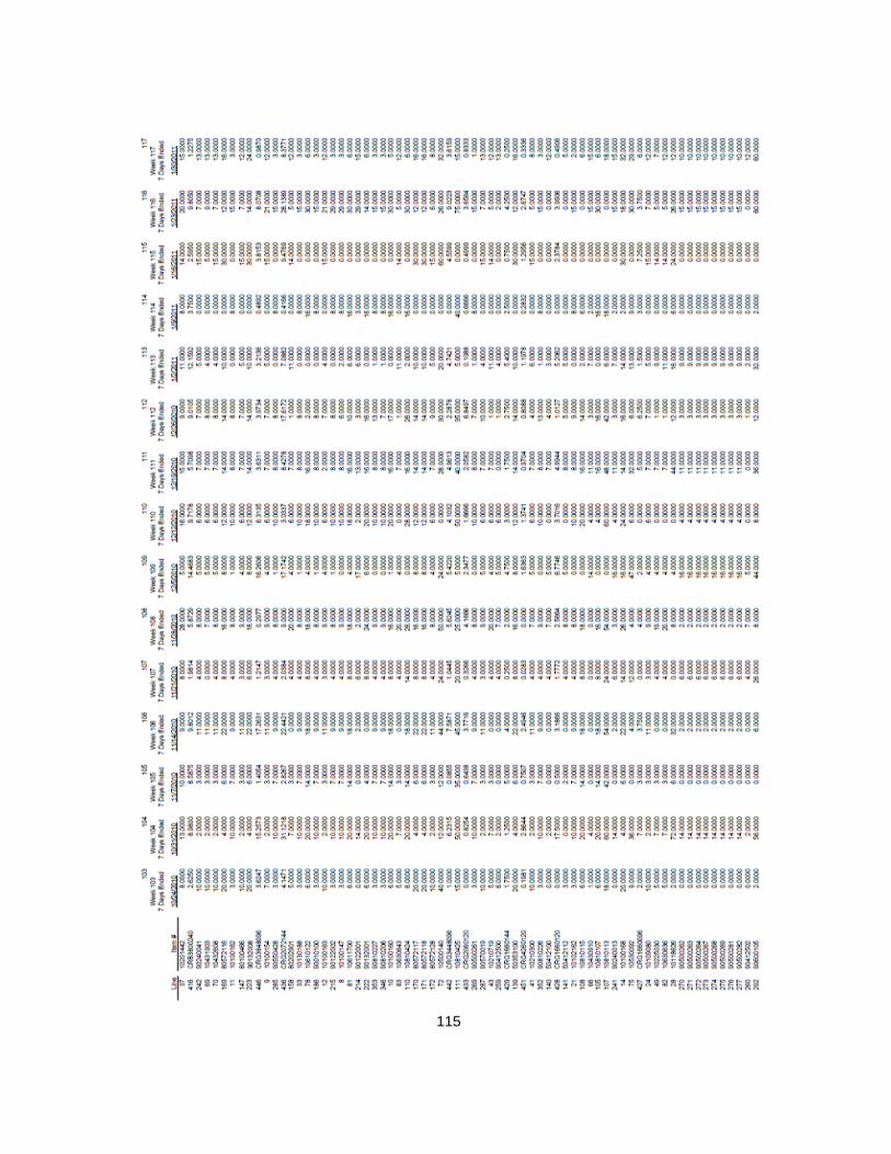
115

116

117

118

119
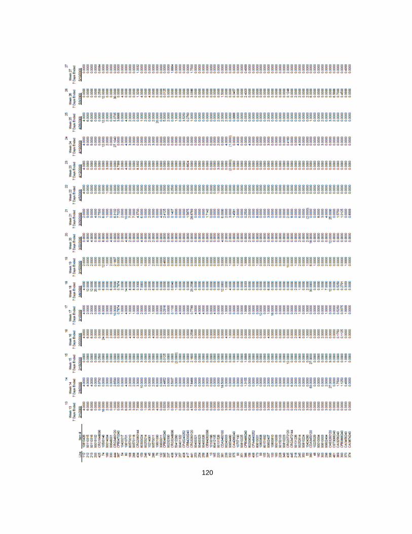
120

121

122

123

124

125

126
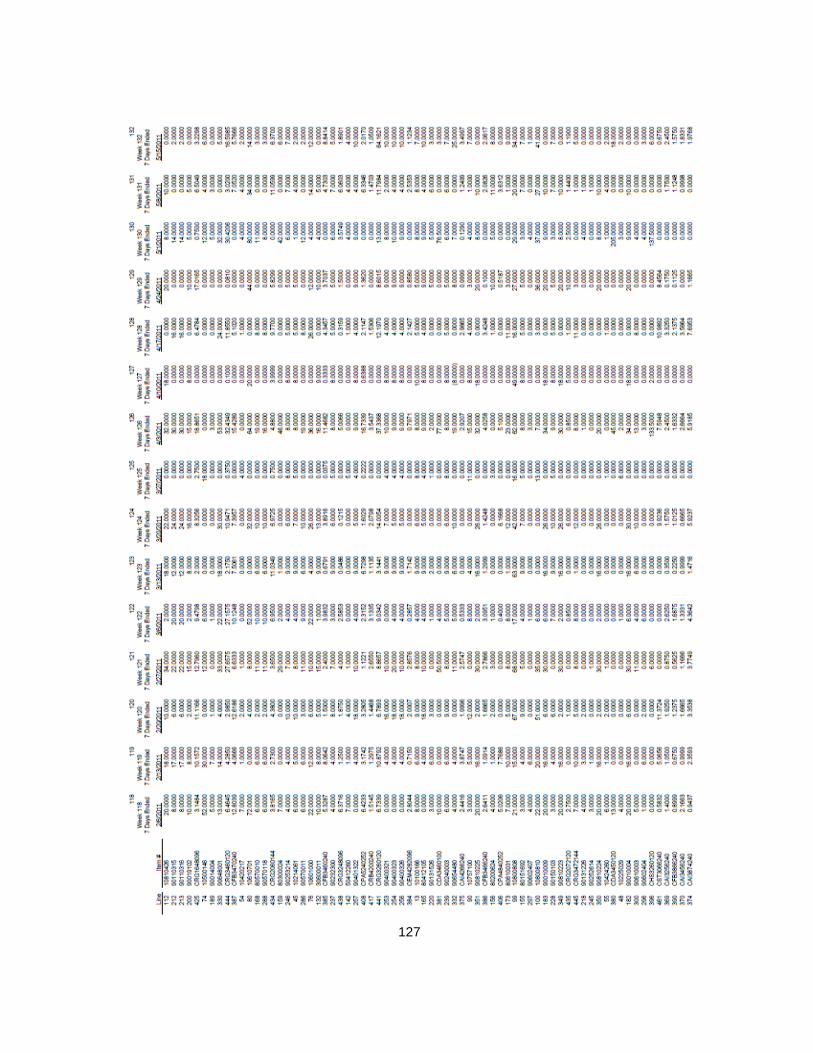
127

128

129

130
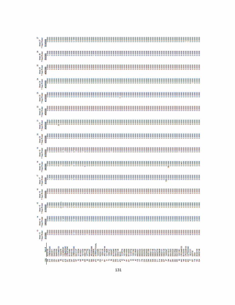
131

132

133

134

135

136

137

138

139

140

141

142

143

144

145

146

147

148

149

150

151

152
APPENDIX B
INVENTORY ITEMS AND ATTRIBUTES USED IN SUMULATION STUDY

Sequence Item Cost Weekly Unit Annual Unit Lead Time# Item # (v ) Demand (d̅) Demand (D ) Weeks (L )
1 C1D1L1 $7.50 1 52 42 C2D1L1 $75.00 1 52 43 C3D1L1 $750.00 1 52 4
4 C1D1L2 $7.50 1 52 65 C2D1L2 $75.00 1 52 66 C3D1L2 $750.00 1 52 6
7 C1D1L3 $7.50 1 52 88 C2D1L3 $75.00 1 52 89 C3D1L3 $750.00 1 52 8
10 C1D1L4 $7.50 1 52 1011 C2D1L4 $75.00 1 52 1012 C3D1L4 $750.00 1 52 10
13 C1D2L1 $7.50 10 520 414 C2D2L1 $75.00 10 520 415 C3D2L1 $750.00 10 520 4
16 C1D2L2 $7.50 10 520 617 C2D2L2 $75.00 10 520 618 C3D2L2 $750.00 10 520 6
19 C1D2L3 $7.50 10 520 820 C2D2L3 $75.00 10 520 821 C3D2L3 $750.00 10 520 8
22 C1D2L4 $7.50 10 520 1023 C2D2L4 $75.00 10 520 1024 C3D2L4 $750.00 10 520 10
25 C1D3L1 $7.50 20 1,040 426 C2D3L1 $75.00 20 1,040 427 C3D3L1 $750.00 20 1,040 4
28 C1D3L2 $7.50 20 1,040 629 C2D3L2 $75.00 20 1,040 630 C3D3L2 $750.00 20 1,040 6
31 C1D3L3 $7.50 20 1,040 832 C2D3L3 $75.00 20 1,040 833 C3D3L3 $750.00 20 1,040 8
34 C1D3L4 $7.50 20 1,040 1035 C2D3L4 $75.00 20 1,040 1036 C3D3L4 $750.00 20 1,040 10
EOQ Simulation StudyInventory Items and Attributes Used in Simulation Study
153

154
APPENDIX C
PARAMETER VALUES FOR DEMAND PATTERN SIMULATION
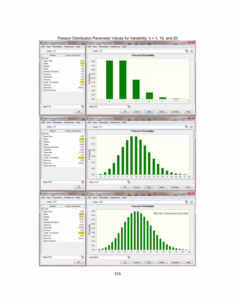
155
Poisson Distribution Parameter Values for Variability: λ = 1, 10, and 20

156
Gamma Distribution Parameter Values for Variability: Coefficient of Variation = 1.5

157
Gamma Distribution Parameter Values for Variability: Coefficient of Variation = 4.0

158
Erlang-C Parameter Values for Variability: Coefficient of Variation = 0.7071

159
Erlang-C Parameter Values for Variability: Coefficient of Variation = 1.0

160
APPENDIX D
SAMPLE SCREEN PRINTS FROM SIMULATION MODELS

161
Sample Screen Prints from Simulation Models
Simulated Demand Table: Trend Demand
Simulated Demand Table: Poisson Demand

162
Sample Screen Prints from Simulation Models (Continued)
(R, s, S) EOQ Inventory System Cost Table 1: Normal Demand/Low Variability
(R, s, S) EOQ Inventory System Cost Table 2: Normal Demand/Low Variability

163
Sample Screen Prints from Simulation Models (Continued) (R, s, S) EOQ Inventory System Cost Table 3: Normal Demand/Low Variability
(R, s, S) EOQ Inventory System Cost Table 4: Normal Demand/Low Variability
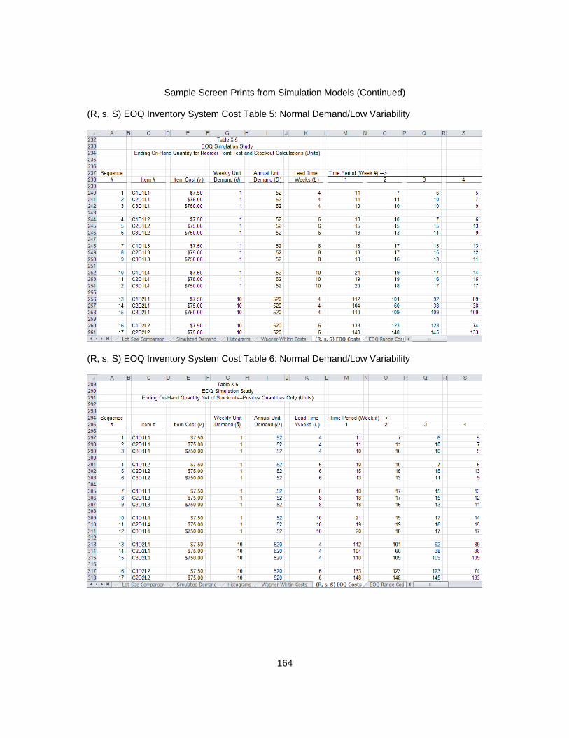
164
Sample Screen Prints from Simulation Models (Continued) (R, s, S) EOQ Inventory System Cost Table 5: Normal Demand/Low Variability
(R, s, S) EOQ Inventory System Cost Table 6: Normal Demand/Low Variability

165
Sample Screen Prints from Simulation Models (Continued) (R, s, S) EOQ Inventory System Cost Table 7: Normal Demand/Low Variability
(R, s, S) EOQ Inventory System Cost Table 8: Normal Demand/Low Variability

166
Sample Screen Prints from Simulation Models (Continued) (R, s, S) EOQ Inventory System Cost Table 9: Normal Demand/Low Variability
(R, s, S) EOQ Inventory System Cost Table 10: Normal Demand/Low Variability

167
Sample Screen Prints from Simulation Models (Continued) (R, s, S) EOQ Inventory System Cost Table 11: Normal Demand/Low Variability
(R, s, S) EOQ Inventory System Cost Table 12: Normal Demand/Low Variability

168
Sample Screen Prints from Simulation Models (Continued) (R, s, S) EOQ Inventory System Cost Table 13: Normal Demand/Low Variability
(R, s, S) EOQ Inventory System Cost Table 14: Normal Demand/Low Variability

169
Sample Screen Prints from Simulation Models (Continued) (R, s, S) EOQ Inventory System Cost Table 15: Normal Demand/Low Variability
(R, s, S) EOQ Inventory System Cost Table 16: Normal Demand/Low Variability

170
Sample Screen Prints from Simulation Models (Continued) (R, s, S) EOQ Inventory System Cost Table 17: Normal Demand/Low Variability
(R, s, S) EOQ Inventory System Cost Table 18: Normal Demand/Low Variability

171
Sample Screen Prints from Simulation Models (Continued) (R, s, S) EOQ Inventory System Cost Table 19: Normal Demand/Low Variability

172
APPENDIX E
T-TEST SAMPLE OUTPUT: SAME DEMAND PATTERN / ALTERNATIVE REPLENISHMENT MODELS

173

174

175

176

177

178

179
APPENDIX F
T-TEST SAMPLE OUTPUT: SAME REPLENISHMENT MODEL / ALTERNATIVE DEMAND PATTERNS

180

181

182

183

184
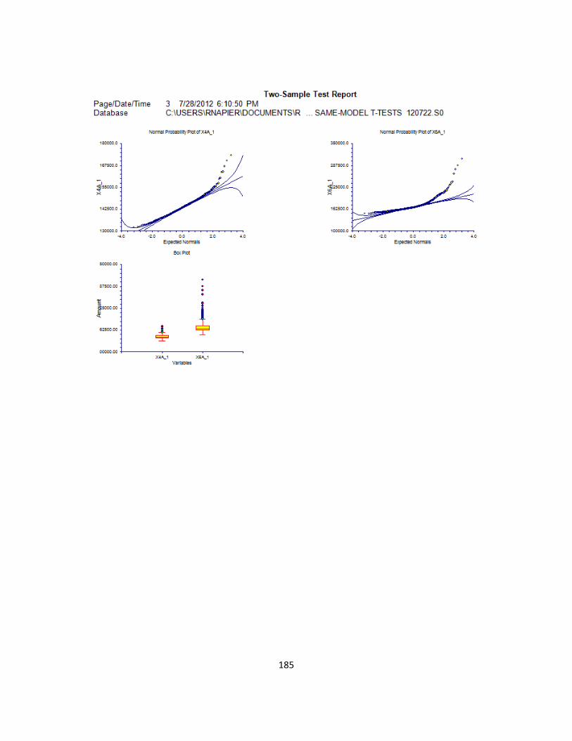
185

186
APPENDIX G
INVENTORY SYSTEM COST AT FACTOR LEVELS OF COST, DEMAND, AND LEAD TIME

187

188

189

190
APPENDIX H
SAMPLE REGRESSION REPORTS AND STACKED TIME SERIES PLOTS FROM
VALIDATION STUDY

191

192

193

194

195

196

197

198

199

200
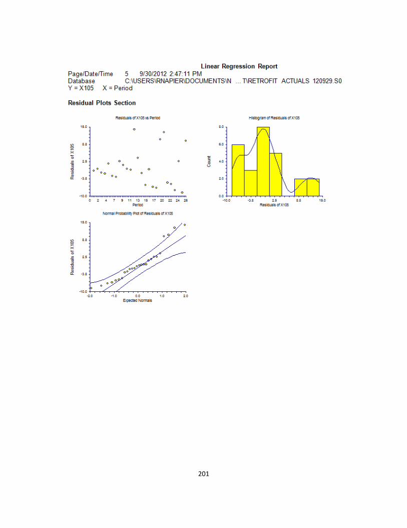
201

202

203
APPENDIX I
SAMPLE SCREEN PRINTS FROM VALIDATION STUDY

204
Sample Screen Prints from Validation Study
Lot Size Calculation: (R, s, S) EOQ Model
Assignment to Demand Classes Based on Mean Absolute Deviation

205
Sample Screen Prints from Validation Study (Continued) Inventory System Cost Calculation: (R, s, S) EOQ Model, Table 1

206
APPENDIX J
T-TEST OUTPUT: VALIDATION STUDY ALTERNATIVE REPLENISHMENT MODELS

207

208

209

210

211

212

213

214

215
216
REFERENCES
Akcay, A., B. Biller, S. Tayur. (2011). "Improved inventory targets in the presence of limited historical demand data." Manufacturing & Service Operations Management 13(3): 297-309. Alstrøm, P., P. Madsen. (1992). "Simulation of inventory control systems." International Journal of Production Economics 26(1-3): 125-134. Azoury, K. S. (1985). "Bayes solution to dynamic inventory models under unknown demand distribution." Management Science 31(9): 1150-1160. Babai, M. Z., Z. Jemai, Y. Dallery. (2011). "Analysis of order-up-to-level inventory systems with compound Poisson demand." European Journal of Operational Research 210(3): 552-558. Beardslee, E. (2007). Dynamic optimization of service part inventory control policy through applied data mining and simulation. PhD dissertation. Norman, Oklahoma; University of Oklahoma. Bijulal, D., J. Venkateswaran, N. Hemachandra. (2011). "Service levels, system cost and stability of production–inventory control systems." International Journal of Production Research 49(23): 7085-7105. Bijvank, M., S. G. Johansen. (2012). "Periodic review lost-sales inventory models with compound Poisson demand and constant lead times of any length." European Journal of Operational Research 220(1): 106-114. Bishop Jr., J. L. (1972). A comparative evaluation of optimal inventory control policies. PhD dissertation. Urbana, Illinois; University of Illinois. Bookbinder, J. H., D. B. Heath. (1988). "Replenishment analysis in distribution requirements planning." Decision Sciences 19(3): 477-489. Boylan, J. E., F. R. Johnston. (1996). "Variance laws for inventory management." International Journal of Production Economics 45(1-3): 343-352. Boylan, J. E., A. A. Syntetos, G. C. Karakostas. (2008). "Classification for forecasting and stock control: a case study." Journal of the Operational Research Society 59(4): 473-481. Bradford, J. W. and P. K. Sugrue. (1997). "Estimating the demand pattern for C category items." Journal of the Operational Research Society 48(5): 530. Braglia, M., R. Gabbrielli. (2001). "A genetic approach for setting parameters of reorder point systems." International Journal of Logistics: Research & Applications 4(3): 345-358. Brill, P. H., B. A. Chaouch. (1995). "An EOQ model with random variations in demand." Management Science 41(5): 927-936.

217
Bröder, A., S. Schiffer. (2006). "Stimulus format and working memory in fast and frugal strategy selection." Journal of Behavioral Decision Making 19(4): 361-380. Bryant, D. J. (2007). "Classifying simulated air threats with fast and frugal heuristics." Journal of Behavioral Decision Making 20(1): 37-64. Bulinskaya, E. V. (1990). "Inventory control in case of unknown demand distribution." Engineering Costs & Production Economics 19(1-3): 301-306. Buxey, G. (2006). "Reconstructing inventory management theory." International Journal of Operations & Production Management 26(9): 996-1012. Cannon, A. R., R. E. Crandall. (2004). "The way things never were." APICS--The Performance Advantage 14(1): 32-35. Cattani, K. D., F. R. Jacobs, J. Schoenfelder. (2011). "Common inventory modeling assumptions that fall short: arborescent networks, Poisson demand, and single-echelon approximations." Journal of Operations Management 29(5): 488-499. Chakravarty, A. K. (1981). "Multi-item inventory aggregation into groups." Journal of the Operational Research Society 32(1): 19-26. Chakravorty, S. S. (1992). A simulation study of the performance of a multi-echelon production-distribution system with feedback and feedforward controls. PhD dissertation. Athens, Georgia; University of Georgia. Chen, L., E. L. Plambeck. (2008). "Dynamic inventory management with learning about the demand distribution and substitution probability." Manufacturing & Service Operations Management 10(2): 236-256. Chen, S. K., M. Ebrahimpour. (1991). "Demand forecasting for a jewelry packaging company: pattern identification and assessment." International Journal of Production Economics 22(3): 203-209. Cohen, M. A., R. Ernst. (1988). "Multi-item classification and generic inventory stock control policies." Production & Inventory Management Journal 29(3): 6-8. Crouch, R., S. Oglesby. (1978). "Optimization of a few lot sizes to cover a range of requirements." Journal of the Operational Research Society 29(9): 897-904. DeMatteis, J. J. (1968). "An economic lot-sizing technique, I: the part-period algorithm." IBM Systems Journal 7(1): 30-38. Dhami, M. K., P. Ayton. (2001). "Bailing and jailing the fast and frugal way." Journal of Behavioral Decision Making 14(2): 141-168. Donaldson, W. A. (1981). "Grouping inventory items by review period." Journal of the Operational Research Society 32(12): 1075-1076. Elwyn, G., A. Edwards, M. Eccles, D. Rovner. (2001). "Decision analysis in patient care." Lancet 358 571-574.

218
Erlenkotter, D. (1989). "An early classic misplaced: Ford W. Harris's economic order quantity model of 1915." Management Science 35(7): 898-900. Erlenkotter, D. (1990). "Ford Whitman Harris and the economic order quantity model." Operations Research 38(6): 937-946. Fu, M. C. (2002). "Optimization for simulation: theory vs. practice." INFORMS Journal on Computing 14(3): 192-215. Garcia-Flores, R., X. Z. Wang, T. F. Burgess. (2003). "Tuning inventory policy parameters in a small chemical company." Journal of the Operational Research Society 54(4): 350. Gigerenzer, G., D. G. Goldstein. (1996). Reasoning the fast and frugal way: models of bounded rationality. Psychological Review 103, 650–669. Gigerenzer, G., P. M. Todd, and The ABC Group. (1999). Simple Heuristics That Make Us Smart. New York, Oxford University Press. Giri, B. C., A. K. Jalan, K. S. Chaudhuri. (2003). "Economic order quantity model with Weibull deterioration distribution, shortage and ramp-type demand." International Journal of Systems Science 34(4): 237. Glock, C. H. (2012). "The joint economic lot size problem: a review." International Journal of Production Economics 135(2): 671-686. Goldstein, D. G., G. Gigerenzer. (2009). "Fast and frugal forecasting." International Journal of Forecasting 25(4): 760-772. Goyal, S. K., A. K. Chakravarty. (1984). "Two heuristic methods for grouping inventory items." Engineering Costs & Production Economics 8(3): 211-214. Gupta, H. D. (2004). "Four-dimensional unified inventory control." Journal of Management Research (09725814) 4(3): 171-174. Ha, H.-S. (1989). "Toward an inventory control system under non-normal demand and lead-time uncertainty." Journal of Business Logistics 10(1): 88-103. Harris, F. W. (1913). "How many parts to make at once." Factory, the Magazine of Management 10(2): 135-136, 152. Harris, F. W. (1990). "How many parts to make at once." Operations Research 38(6): 947-950. Hayya, J. C., U. Bagchi, R. Ramasesh. (2011). "Cost relationships in stochastic inventory systems: a simulation study of the (S, S−1, t=1) model." International Journal of Production Economics 130(2): 196-202. Hey, J. D. (1982). “Search for rules for search.” Journal of Economic Behavior and Organization 3: 65-81. Hey, J. D. (1987). “Still searching.” Journal of Economic Behavior and Organization 8: 137-144. Hintze, J. (2007). NCSS Help System. Kaysville, Utah; NCSS, LLC.

219
Hoffrage, U., T. Reimer. (2004). "Models of bounded rationality: the approach of fast and frugal heuristics." Management Revue 15(4): 437-459. Huh, W. T., R. Levi, P. Rusmevichientong, J. B. Orlin. (2011). "Adaptive data-driven inventory control with censored demand based on Kaplan-Meier estimator." Operations Research 59(4): 929-941. Iglehart, D. L. (1964). "The dynamic inventory problem with unknown demand distribution." Management Science 10(3): 429-440. Janssen, E., L. Strijbosch, R. Brekelmans. (2009). "Assessing the effects of using demand parameters estimates in inventory control and improving the performance using a correction function." International Journal of Production Economics 118(1): 34-42. Katircioglu, K. (1996). Essays in inventory control. PhD dissertation. Calgary, Alberta, Canada; University of Calgary. Keaton, M. (1995). "Using the gamma distribution to model demand when lead time is random." Journal of Business Logistics 16(1): 107-131. Keller, G. (2005). Statistics for Management and Economics (Seventh Edition). Mason, Ohio; Thompson South-Western. Khouja, M., S. Goyal. (2008). "A review of the joint replenishment problem literature: 1989–2005." European Journal of Operational Research 186(1): 1-16. Kim, S. (1995). Multi-criteria numerous-item inventory grouping (MNIG): by integrating hierarchical heuristics and neural networks. PhD dissertation. Tuscaloosa, Alabama; University of Alabama. Krajewski, L. J., L. P. Ritzman, M. K. Malhotra. (2010). Operations Management: Processes and Supply Chains (Ninth Edition). Upper Saddle River, New Jersey; Prentice Hall. Kumaran, M., K. K. Achary. (1996). "On approximating lead time demand distributions using the generalised lambda-type distribution." Journal of the Operational Research Society 47(3): 395. Lau, H.-S., M.-C. Wang. (1987). "Estimating the lead-time demand distribution when the daily demand is non-normal and autocorrelated." European Journal of Operational Research 29(1): 60-69. Law, A. M., W. D. Kelton. (2000). Simulation Modeling & Analysis. New York, NY, McGraw-Hill, Inc. Lenard, J. D., B. Roy. (1995). "Multi-item inventory control: a multicriteria view." European Journal of Operational Research 87(3): 685-692. Levén, E., A. Segerstedt. (2004). "Inventory control with a modified Croston procedure and Erlang distribution." International Journal of Production Economics 90(3): 361-367. Levi, R., R. O. Roundy, D. B. Shmoys. (2007). "Provably near-optimal sampling-based policies for stochastic inventory control models." Mathematics of Operations Research 32(4): 821-839.
220
Li, R., J. K. Ryan. (2011). "A Bayesian inventory model using real-time condition monitoring information." Production & Operations Management 20(5): 754-771. Lisboa, J. (2010). "Inventory management-non-classical views, edited by M.Y. Jaber." International Journal of Production Research 48(18): 5539-5540. Mandal, P., B. Mahanty. (1990). "Decomposition of demand and optimisation for a perpetual inventory system." International Journal of Operations & Production Management 10(7): 47-56. Matheus, P., L. Gelders. (2000). "The (R, Q) inventory policy subject to a compound Poisson demand pattern." International Journal of Production Economics 68(3): 307-317. McLaughlin, C. P., G. Vastag, D. G. Whybark. (1994). "Statistical inventory control in theory and practice." International Journal of Production Economics 35: 161-169. Mentzer, J. T., R. Krishnan (1985). "The effect of the assumption of normality on inventory control/customer service." Journal of Business Logistics 6(1): 101. Meredith, J. R., S. M. Shafer. (2007). Operations Management for MBA's, Third Edition. Hoboken, New Jersey; John Wiley & Sons, Inc. Minner, S. (2009). "A comparison of simple heuristics for multi-product dynamic demand lot-sizing with limited warehouse capacity." International Journal of Production Economics 118(1): 305-310. Mizoroki, Y. (1981). Analysis of lumpy demand and its application to inventory control systems. PhD dissertation. Chicago, Illinois; Illinois Institute of Technology. Moors, J. J. A., L. W. G. Strijbosch. (2002). "Exact fill rates for (R, s, S) inventory control with gamma distributed demand." Journal of the Operational Research Society 53(11): 1268-1274. Naddor, E. (1975a). "Optimal heuristic decisions for the s, S inventory policy." Management Science 21(9): 1071-1072. Naddor, E. (1975b). "Optimal and heuristic decisions in single and multi-item inventory systems." Management Science 21(11): 1234-1249. Nenes, G., S. Panagiotidou, G. Tagaras. (2010). "Inventory management of multiple items with irregular demand: a case study." European Journal of Operational Research 205(2): 313-324. Newell, B. R., N. J. Weston, D. R. Shanks. (2003). "Empirical tests of a fast-and-frugal heuristic: not everyone ‘takes-the-best’." Organizational Behavior & Human Decision Processes 91(1): 82-96. Ohno, K., T. Ishigaki. (2001). "A multi-item continuous review inventory system with compound Poisson demands." Mathematical Methods of Operations Research 53(1): 147. Olhager, J., F. Persson. (2006). "Simulating production and inventory control systems: a learning approach to operational excellence." Production Planning & Control 17(2): 113-127. Park, C. (2007). "An analysis of the lead time demand distribution derivation in stochastic inventory systems." International Journal of Production Economics 105(1): 263-272.

221
Patterson, M. C. (1982). "An EOQ range model." Journal of Purchasing & Materials Management 18(3): 26-29. Philippakis, A. S. (1970). "The cost of using EOQ with variable demand items." Journal of Purchasing 6(4): 65-73. Rau, H., B.-C. OuYang. (2007). "A general and optimal approach for three inventory models with a linear trend in demand." Computers & Industrial Engineering 52(4): 521-532. Raymond, F. E. Quantity and Economy in Manufacture, McGraw-Hill, New York, 1931. Ren, L. (2010). "The robustness of the basic EOQ." International Business & Economics Research Journal 9(12): 17-22. Reyman, G. (1989). "State reduction in a dependent demand inventory model given by a time series." European Journal of Operational Research 41(2): 174-180. Ritchie, E., A. Tsado. (1986). "The penalties of using the EOQ: a comparison of lot-sizing rules for linear increasing demand." Production & Inventory Management 27(1): 12-18. Roundy, R. O., J. A. Muckstadt. (2000). "Heuristic computation of periodic-review base stock inventory policies." Management Science 46(1): 104. Sawilowsky, S. S. (2002). "Fermat, Schubert, Einstein, and Behrens-Fisher: the probable difference between two means when [variances are unequal] " Journal of Modern Applied Statistical Methods 1(1): 461-472. Scarf, H. (1960). “The Optimality of (s,S) policies in the dynamic inventory problem.” In K. J. Arrow, S. Karlin, and P. Suppes (Eds.), Mathematical Methods in the Social Sciences (Chapter 13). Stanford, California; Stanford University Press. Silver, E. A., C.-M. Ho, R. Deemer. (1971). "Cost-minimizing inventory control of items having a special type of demand pattern." INFOR 9(3): 198-219. Silver, E. A., H. A. Meal. (1973). "A heuristic for selecting lot size requirements for the case of a deterministic time varying demand rate and discrete opportunities for replenishment." Production & Inventory Management 14(2): 64-74. Silver, E. A., D. F. Pyke, Peterson, R. (1998). Inventory Management and Production Planning and Scheduling. New York; John Wiley & Sons, Inc. Snyder, R. D. (1984). "Inventory control with the gamma probability distribution." European Journal of Operational Research 17(3): 373-381. Song, J.-S., H. Zhang, Y. Hou, M. Wang. (2010). "The effect of lead time and demand uncertainties in (r, q) inventory systems." Operations Research 58(1): 68-80. Song, J.-S., P. Zipkin. (1993). "Inventory control in a fluctuating demand environment." Operations Research 41(2): 351.

222
Speh, T. W., G. D. Wagenheim. (1978). "Demand and lead-time uncertainty: the impacts on physical distribution performance and management." Journal of Business Logistics 1(1): 95-113. Stone, P. A. (1980). "Use of part groups to improve inventory planning and control." Production & Inventory Management 21(4): 95-105. Strijbosch, L. W. G., R. M. J. Heuts. (1992). "Modeling (s, Q) inventory systems: parametric versus non-parametric approximations for the lead time demand distribution." European Journal of Operational Research 63(1): 86-101. Strijbosch, L. W. G., J. J. A. Moors. (2006). "Modified normal demand distributions in (R, S)-inventory control." European Journal of Operational Research 172(1): 201-212. Syntetos, A. A., J. E. Boylan, J. D. Croston. (2005). "On the categorization of demand patterns." Journal of the Operational Research Society 56(5): 495-503. Todd, P. M., G. Gigerenzer. (2001). "Putting naturalistic decision making into the adaptive toolbox." Journal of Behavioral Decision Making 14(5): 381-383. Tsou, C. S., C. H. Kao. (2008). "Multi-objective inventory control using electromagnetism-like meta-heuristic." International Journal of Production Research 46(14): 3859-3874. Tunc, H., O. A. Kilic, S. A. Tarim, B. Eksioglu. (2011). "The cost of using stationary inventory policies when demand is non-stationary." Omega 39(4): 410-415. Tyworth, J. E., Y. Guo, R. Ganeshan. (1996). "Inventory control under gamma demand and random lead time." Journal of Business Logistics 17(1): 291-304. Van Ness, P. D., W. J. Stevenson. (1983). "Reorder point models with discrete probability distributions." Decision Sciences 14(3): 363-369. Wagner, H. M. (2004). "Comments on "Dynamic version of the economic lot size model"." Management Science 50: 1775-1777. Wagner, H. M., T. M. Whitin. (1958). "Dynamic version of the economic lot size model." Management Science 5(1): 89-96. Wagner, H. M., T. M. Whitin. (2004). "Dynamic version of the economic lot size model." Management Science 50(12): 1770-1774. Walker, J. (1993). "The single-period inventory problem with triangular demand distribution." Journal of the Operational Research Society 44(7): 725. Wallin, C., M. J. Rungtusanatham, E. Rabinovich. (2006). "What is the "right" inventory management approach for a purchased item?" International Journal of Operations & Production Management 26(1): 50-68. Wang, C.-H. (2010). "Some remarks on an optimal order quantity and reorder point when supply and demand are uncertain." Computers & Industrial Engineering 58(4): 809-813.

223
Wang, K.-J., H.-M. Wee, S.-F. Gao, S.-L. Chung. (2005). "Production and inventory control with chaotic demands." Omega 33(2): 97-106. Wanke, P. F. (2008). "The uniform distribution as a first practical approach to new product inventory management." International Journal of Production Economics 114(2): 811-819. Whitin, T. M. (1953) The Theory of Inventory Management. Princeton, New Jersey; Princeton University Press. Welch, B. L. (1947). "The generalization of Student’s problem when several different population variances are involved." Biometrika 34(1): 28-35. Williams, B. D., T. Tokar. (2008). "A review of inventory management research in major logistics journals: themes and future directions." International Journal of Logistics Management 19(2): 212-232. Woolsey, G. (1975). "On doing good things and dumb things in production & inventory control." Interfaces 5(3): 65-67. Yang, J., G. K. Rand. (1993). "An analytic eclectic heuristic for replenishment with linear increasing demand." International Journal of Production Economics 32(2): 261-266. Yeh, Q.-J. (1997). "A practical implementation of gamma distribution to the reordering decision of an inventory control problem." Production & Inventory Management Journal 38(1): 51-57. You, P. S. (2005). "Optimal replenishment policy for product with season pattern demand." Operations Research Letters 33(1): 90-96. Zanakis, S. H., J. R. Evans, A. A. Vazacopoulos. (1989). "Heuristic methods and applications: A categorized survey." European Journal of Operational Research 43(1): 88-110. Zhang, X. (2004). "Evolution of ARMA demand in supply chains." Manufacturing & Service Operations Management 6(2): 195-198. Zinn, W., J. M. Charnes (2005). "A comparison of the economic order quantity and quick response inventory replenishment methods." Journal of Business Logistics 26(2): 119-141. Zomerdijk, L. G., J. de Vries (2003). "An organizational perspective on inventory control: theory and a case study." International Journal of Production Economics 81/82: 173.
224
BIOGRAPHICAL INFORMATION
Before entering graduate study at The University of Texas at Arlington, Randall A.
Napier earned a B.A. in Economics from Northwestern University, an M.S. in Accounting from
Florida International University, and a J.D. from the University of Houston Law Center. He is
qualified as a Certified Public Accountant, and has earned the Certified Fellow in Production
and Inventory Management (CFPIM) designation from APICS, the Association for Operations
Management. His research interests focus on the use of quantitative tools and techniques to
understand and improve business processes.