MASTER’S THESIS - Welcome to the Cartography M.Sc....

MASTER’S THESIS

Persistence of Physical Patterns of a Mountain Landscape-

Detection and Map Representation.

CARLOS ERNESTO VÁZQUEZ ARIAS

Matrikel Nr. 3837376

Supervisor: Dr. Nikolas Prechtel

Institute for Cartography, Technische Universität Dresden

Dresden, October 2013

II

CONFIRMATION OF AUTHORSHIP

Herewith I declare that I am the sole author of the thesis named “Persistence of Physical

Patterns of a Mountain Landscape- Detection and Map Representation” which has been

submitted to the study commission of geosciences today. I have fully referenced the ideas and

work of others, whether published or un-published. Literal or analogous citations are clearly

marked as such.

Carlos Ernesto Vázquez Arias

Dresden, October 2013

III

Task of Master Thesis

Course of Studies: International Master Course in Cartography

Name of Graduand: Carlos Ernesto Vázquez Arias

Topic: Persistence of Physical Patterns of a Mountain Landscape- Detection and Map Repre-

sentation

Goals of this study

Scope / Previous Results: The work is based on a long-term project „Ecological GIS for the

Russian Altai“. From extensive previous work and partly from external sources a fully struc-

tured topographic database is now available (data set termed "ALTAI 1000"). It consists of

vector- and raster data. Cartographic visualisations have been generated in a traditional ana-

logue form (map prints) and as a WebGIS (http://kartographie.geo.tu-dresden.de/altai/). Of

particular relevance for the topic are the following thematic layers: land use/land cover,

catchments, and relief.

Motivation: Operational satellite observations (like from the MODIS-sensor) allow a moder-

ate resolution observation of various physical surface parameters on a daily basis, and can be

downloaded in an already value-added form (in terms of spatial reference and observation

targets). Snow cover, surface temperature, vegetation indices, and other parameters are, at

first, very interesting ecological parameters or indicators as such, and, secondly, highly varia-

ble due to meteorological and seasonal environmental conditions. However, a characterisa-

tion of landscape units aims at a detection of typical patterns. “Typical” refers to a temporally

persistent status, expressed as a systematic medium- to long-term deviation from a standard

behaviour of the adjoining landscape units. One day, on the other hand, is only a snapshot,

and necessarily of a limited relevance to the characterisation of a spatial unit. Simple exam-

ple: A steep south-facing slope in the alpine zone of a mid-latitude mountain range may be

IV

most of the time dryer, warmer, and less snow-covered then its north-facing counterpart. This

is, however, definitely not detectable on every single day.

Objective: The task has a clearly defined spatial reference, which is given by the existing

ALTAI-1000 GIS data. The objective is to statistically exploit selected standard MODIS

products characterising a set of physical surface parameters (compare above). From a time

series (for feasibility a lower resolution then one day might be envisaged, also a spatial com-

pression might be sensible) a temporal feature space shall be generated. A clever data reduc-

tion into indicative subsets of the original data is one major task of the project. The input pa-

rameters are then normalised to show the spatial deviation from a mean status. This normal-

ised feature space shall then be analysed for temporally and spatially persistent patterns. The

statistical processing shall make use of powerful open-source programming environments

such as “R”. A generic approach, which allows an easy transfer to other regions is strongly

recommended. The resulting and statistically proved patterns will finally be transformed into

GIS-vector layers for display. These results shall be integrated into the existing WebGIS-

solution, in order to give easy access for the interested public.

Deliverables: The written document has to be delivered in two copies. The complete thesis

plus all relevant data have to be added to the written document through an attached portable

data storage media (CD, DVD, etc.) The contents of the digital media should be structured in

a way,that an easy continuation of work will be facilitated. The results should furthermore be

presented on a A0 poster using a poster template which is available through the institute’s

homepage.

Tutors: Dr. Nikolas Prechtel (TU Dresden)

Delivered: May 15, 2013

To be Filed: November 1, 2013

Prof. Dr. Manfred Buchroithner Dr. Nikolas Prechtel

Board of Examiners Tutor

V

Abstract

The monitoring of complex environments such as mountain landscapes, where it is difficult

to measure physical parameters in situ due to their inherent conditions, continues to be a ma-

jor interest of the environmental research agenda. Remotely sensed data represents one of the

solutions to this concern. The present study is based on the Ecological GIS for the Russian

Altai (ALTAI-1000 GIS) which is one of the most comprehensive remote area mountain GIS

worldwide. The main goal of the present study is to continue with the integration of this GIS,

working on the characterization of landscape units through physical surface parameters gen-

erated by operational satellite observations. This characterization requires the detection of

persistent patterns in space and time which is one of the main goals of geospatial analysis.

Statistical analyses were performed in selected standard MODIS products (Normalized Dif-

ference Vegetation Index and Land Surface Temperature) with time coverage of 12 years

(2001-2012). The study added value to both datasets by producing a consistent series of sta-

tistics which enables comparisons to be made across space and time. In order to perform this,

tests were developed using R language for statistical computing and other open source tools.

Time series were extracted and anomaly maps for the specific variables were generated. The

identification of general trends and the definition of a generic approach to analyze raster data

sets of time-dependent variables were some of the most important tasks. The results show the

capabilities of map algebra to generate valuable information and both weaknesses and

strengths of the selected open source solutions to perform geospatial analysis.

Keywords: Altai, Mountain landscapes, persistent patterns, Map Algebra, MODIS, Normal-

ized Difference Vegetation Index, Land Surface Temperature

VI

Kurzfassung

Die Beobachtung komplexer Umgebungen wie Gebirgslandschaften, in denen es aufgrund

der ihnen inhärenten Gegebenheiten schwierig ist, physikalische Messungen in situ

vorzunehmen, ist für die Umweltwissenschaften weiterhin von großem Interesse. Durch

Fernerkundung gewonnene Daten stellen eine der Lösungen für dieses Problem dar. Die

vorliegende Studie basiert auf dem ökologischen Geoinformationssystem für das russische

Altai (ALTAI-1000 GIS), einem der umfangreichsten Gebirgslandschafts-GIS weltweit. Das

vornehmliche Ziel dieser Studie ist es, die Integration des GIS durch Charakterisierung von

Landschaftseinheiten anhand von physikalischen Oberflächeneigenschaften, die mit Hilfe

von Satellitenbeobachtung gewonnen worden sind, fortzusetzen. Diese Charakterisierung

erfordet es, persistente Muster in Raum und Zeit zu erkennen, was eine der wesentlichen

Anwendungen graphischer Analysewerkzeuge für Geodaten ist. Statistische Analysen

wurden in ausgewählten MODIS-Produkten (normalisierter differenzierter Vegetationsindex

und Landoberflächentemperatur) für eine Zeitspanne von 12 Jahren (2001-2012)

durchgeführt. In dieser Studie wurden beide Datensätze durch das Erzeugen einer

konsistenten Datenreihe angereichert, wodurch Vergleiche bezogen auf Raum und Zeit

ermöglicht werden. Hierzu wurden Tests in der Statistiksoftware R und anderen Open-

Source-Tools entwickelt. Es wurden Zeitreihen extrahiert und Anomalie-Karten für die

jeweiligen Variabeln erzeugt. Die Identifikation allgemeiner Trends und die Definition eines

generischen Ansatzes für die Analyse von Rasterdaten zeitabhängiger Variabeln gehörten zu

den wichtigsten Aufgaben. Die Ergebnisse demonstrieren die Möglichkeiten, durch

geographische Algebra wertvolle Informationen zu gewinnen, und die Stärke von

existierenden Open-Source-Lösungen in der Durchführung graphischer Analysen von

Geodaten.

Keywords: Altai, Gebirgslandschaften, persistente Muster, geographische Algebra, MODIS,

normalisierter differenzierter Vegetationsindex, Landoberflächentemperatur.

VII

On Exactitude in Science

. . . In that Empire, the Art of Cartography attained such Perfection that the map of a single

Province occupied the entirety of a City, and the map of the Empire, the entirety of a Prov-

ince. In time, those Unconscionable Maps no longer satisfied, and the Cartographers Guilds

struck a Map of the Empire whose size was that of the Empire, and which coincided point for

point with it. The following Generations, who were not so fond of the Study of Cartography

as their Forebears had been, saw that that vast Map was Useless, and not without some Piti-

lessness was it, that they delivered it up to the Inclemencies of Sun and Winters. In the De-

serts of the West, still today, there are Tattered Ruins of that Map, inhabited by Animals and

Beggars; in all the Land there is no other Relic of the Disciplines of Geography.

Suarez Miranda. Viajes de varones prudentes, Libro IV, Cap. XLV, Lerida, 1658

From Jorge Luis Borges, Collected Fictions, Translated by Andrew Hurley

Copyright Penguin 1999.

VIII

Acknowledgments

I would like to express my gratitude to all people that supported and encouraged me to con-

clude this Master’s thesis. First, I would like thank my supervisor, Dr. Nikolas Prechtel for all

his patience and advice always full of knowledge during the last months.

It was a pleasure to have met the staff from the International Master of Science in Cartog-

raphy in Munich, Vienna and Dresden. I really appreciate the help that I always received

from our coordinator Stefan Peters and the support from the Professors Georg Gartner and

Manfred Buchroithner. I really appreciate the opportunity to be part of the first intake of this

Master Program. I also want to thank all my classmates who, from now on, I can call not only

colleagues but friends.

My studies were made partly possible by the financial support I received from the Govern-

ment of Jalisco, Mexico, through the Instituto Jalisciense de la Juventud.

Also, I want to thank my family, my mother, Martha and Enrique who, despite the distance,

always supported me in all respects. This couldn’t be achieved without them.

This thesis is especially dedicated to Rea who I met during this journey and I am very glad to

say that she is now part of my life.

IX

List of Abbreviations DEM Digital Elevation Model

DOY Day of Year

EOS End of Season

EROS Earth Resources Observation and Science

ESA European Space Agency

ESRI Environmental Systems Research Institute

GeoVITe Geodata Visualization & Interactive Training Environment

GIS Geographic Information System

HDF Hierarchical Data Format

HEG HDF EOS-to-GeoTiff Tool

IQR Inter Quartile Range

LI Large Integral

LOS Length of Season

LPDAAC Land Processes Distributed Archive Center

LST Land Surface Temperature

MOD13A2 Short name for NDVI 16-Days-1km resolution product

MOD11A1 Short name for LST- daily-1km resolution product

MOD11A2 Short name LST 8-days-1km resolution product

MODIS Moderate Resolution Imaging Spectroradiometer

MRT MODIS Reprojection Tool

NASA National Aeronautics and Space Administration

NDVI Normalized Difference Vegetation Index

QA Quality Assurance

QC Quality Control

RMSE Root Mean Square Error

SDS Scientific Data Set

SI Small Integral

SOS Start of Season

SITS Satellite Imagery Time Series

USGS U.S. Geological Survey

UTM Universal Transverse Mercator

X

List of Figures

Figure 1.1 Ecological zonation for a polar site and hypothetical zonation after climate

change................................................................................................................................. 6

Figure 2.1 Location of the Altai Republic.......................................................................... 9

Figure 2.2. MODIS Tiling System...................................................................................... 13

Figure 2.3 Elevation map of Altai Republic........................................................................ 19

Figure 2.4 Land cover map of Altai Republic..................................................................... 20

Figure 2.5 General Remote sensing-based approach........................................................... 21

Figure 2.6. Location of the Altai Republic in relation to MODIS tiles............................... 22

Figure 2.7 The snapshot approach........................................................................................ 27

Figure 2.8 Equation to calculate standardized anomaly....................................................... 29

Figure 2.9 General workflow of the software TIMESAT..................................................... 31

Figure 2.10 Seasonality Parameters in TIMESAT................................................................. 31

Figure 2.11 The Gaussian function....................................................................................... 33

Figure 2.12 Effect of parameter changes on the local functions.......................................... 34

Figure 2.13 Logistic function............................................................................................... 34

Figure 2.14 TIMESAT Graphical User Interface................................................................. 35

Figure 2.15 Creating the settings file in TIMESAT............................................................... 36

Figure 2.16 Spatial distribution of significant land cover types in Altai Republic................ 39

Figure 2.17 General workflow of the study......................................................................... 40

Figure 2.18 Majority Filter principle in ArcGIS................................................................ 41

Figure 3.1 Basic statistics of NDVI in Altai Republic.......................................................... 42

Figure 3.2 Standardized NDVI Anomaly in Altai Republic 2001-2012 ........................... 43

Figure 3.3 Season anomaly of NDVI in Altai Republic 2001-2012..................................... 44

Figure 3.4 Average start of growing season (DOY) in Altai Republic 2001-2012............... 45

Figure 3.5 Average end of the growing season (DOY) in Altai Republic 2001-2012.......... 45

Figure 3.6. Average Length of Season (DOY) in Altai Republic 2001-2012....................... 46

Figure 3.7 Average of Large Integral in Altai Republic 2001-2012..................................... 46

Figure 3.8 Large and Small Integrals.................................................................................... 47

Figure 3.9 Trends in Annual Maximum NDVI-Altai Republic 2001-2012.......................... 48

Figure 3.10 Trend in mean NDVI in Altai Republic 2001-2012........................................... 48

XI

Figure 3.11 Anomalies in Large Integral in Altai Republic 2001-2012............................... 49

Figure 3.12 Relationship Large Integral-Elevation in Altai Republic.................................. 50

Figure 3.13 Map of the residuals of the linear regression model Large Integral~Elevation.. 51

Figure 3.14 New map of Large Integral with elevation correction...................................... 51

Figure 3.15 Relationship Small Integral-Elevation in Altai Republic................................ 52

Figure 3.16 Map of the residuals of the linear regression model Small Integral~Elevation. 53

Figure 3.17 New map of Small Integral with elevation correction..................................... 53

Figure 3.18 LST Basic statistics.......................................................................................... 54

Figure 3.19 Standardized LST Anomaly in Altai Republic 2001-2012............................ 54

Figure 3.20 NDVI- LST relationships for selected land cover types................................. 56

Figure 3.21 Start of Season in Altai Republic 2001-2012.................................................. 59

Figure 3.22 End of season in Altai Republic 2001-2012................................................... 60

Figure 3.23 Length of season in Altai Republic 2001-2012............................................. 60

Figure 3.24 Large Integral in Altai Republic 2001-2012.................................................. 61

Figure 3.25 Small Integral in Altai Republic 2001-2012.................................................. 61

List of Tables

Table 2.1 MODIS Characteristiscs........................................................................... 11

Table 2.2 MODA132 Data Set Characteristics......................................................... 15

Table 2.3 Science Data Sets of MOD13A2 product ................................................ 16

Table 2.4 MODA112 Data set Characteristics......................................................... 17

Table 2.5 The SDSs in the MOD11A2 product....................................................... 18

Table 2.6 MOD13A2 Pixel Reliability...................................................................... 23

Table 2.7. Bit flags defined for the SDS QC_day in

MOD11A2 gridded in Sinusoidal projection ........................................................... 24

Table 2.8 The QC_ layer values for Altai Republic and their meaning..................... 25

Table 2.9 NDVI 2001-2012 raster brick characteristics in R.................................... 28

Table 2.10 LST 2001-2012 raster brick characteristics in R..................................... 28

Table 2.11 Phenology metrics in TIMESAT............................................................. 32

Table 2.12 Land cover types in GlobCover 2009 V2.3............................................. 38

Table 2.13 Significant land cover types for the study area....................................... 38

Table 3.1 Summary statistics for selected land cover types..................................... 55

Persistence of Physical Patterns of a Mountain Landscape.


Contents

Confirmation of autorship..................................................................................... II

Task of Master’s Thesis......................................................................................... III

Abstract................................................................................................................... V

Kurzfassung........................................................................................................... VI

Acknowledgments................................................................................................. VIII

List of Abbreviations............................................................................................. IX

List of Figures........................................................................................................ X

List of Tables.......................................................................................................... XI

Introduction.......................................................................................................... 1

Objectives ………………………………………………………......................... 2

Thesis structure……………………………………………………..................... 3

1. Background………………………………………………………………...… 4

1.1Persistent patterns and regionalization............................................. 4

1.2 Why Mountain Landscapes?...............………………………......... 5

1.3 The Technique: Map Algebra ……………………………………. 7

2. Materials and Methods……………………………………………………… 8

2.1 Study Area......................................................................................... 8

2.2 Data……………………..................................................................... 11

2.2.1 MODIS Data.........................……………………............. 11

2.3 Description of parameters................................................................ 14

2.3.1 Normalized Difference Vegetation Index…...…............. 14

2.3.2 Land Surface Temperature.............................................. 16

2.4.Digital Elevation Model....................................................... 19

2.5 Land cover data.................................................................... 20

2.6. Method…………………………………………………………....... 21

2.6.1 Data preprocessing………………………………………. 21

2.6.1.1 Download and pre-processing of MODIS data............ 21

2.6.1.2 Quality Assurance…………………….......................... 23

2.6.2 NDVI and LST Statistical Analysis……………….......... 27

2.6.2.1 Extracting Phenology Metrics………………................ 30

2.6.2.2 Comparing NDVI and LST spatial distribution........... 38

2.6.3 Transformation of patterns to ESRI shapefiles................ 41

3. Results………………………………………………………………………..... 42

4. Discussion……………………............................................................................ 62

5. Conclusions………………………………………………………..................... 64

6. References.......................................................................................................... 66

7. Appendix A....................................................................................................... 70

1

Persistence of Physical Patterns of a Mountain Landscape-


Introduction

The monitoring of complex environments such as mountain landscapes, where it is difficult

to measure certain physical parameters in situ due to their inherent conditions, continues to be

a major interest in the environmental research agenda (Neteler, 2010). Remotely sensed data

represents one of the solutions to this concern.

The sensors that are available produce everyday thousands of data which could be useful for

many purposes. However, this amount of data is useless without the proper methodology to

acquire insight from it. For this reason, the geospatial data mining, analysis and afterwards

the visualization of this data appear among the main challenges of cartography. The integra-

tion of time into cartographic modeling has been also a subject that continues to be part of the

scientific community agenda (Peuquet, 2005). The detection of typical patterns in space and

time is one of the ways to acquire useful information from remotely sensed data.

Regarding this concern, on the last decades, the interest in the study of satellite imagery time

series (SITS) has increased due to the need to explore both the spatial and temporal patterns

of physical and biological components of the landscape. Since one single snapshot is not suf-

ficient to understand the landscape complexity, it is essential to use time series to analyze

dynamic systems. The present study focuses on the Altai Republic as case study and its

framework is the Ecological Geographic Information System (GIS) for the Russian Altai

which is one of the most comprehensive remote area mountain GIS worldwide (Prechtel et al.

2003). The main goal of the present study is to continue with the integration of this GIS,

working on the characterization of landscape units through the detection of persistent spatio-

temporal patterns from selected physical surface parameters.

2

Objectives

The objective of this study is using remotely sensed time-series data derived from MODIS, to

characterize spatial units through the identification of spatial patterns of selected physical

parameters (NDVI and LST) in the Altai Republic, Russia. Regarding this main objective,

specific objectives arise, which are:

1) To statistically analyze remotely sensed LST and NDVI products.

2) To analyze the spatial variation of NDVI and LST.

3) To detect persistent patterns through the production of anomaly maps.

4) To examine the relationships between phenology metrics and LST spatial distribution.

3

Thesis Structure

The study is divided in three main parts. Part A includes the theoretical background and con-

ceptual framework that was used to develop this study. It basically contains three main topics

and serves as a literature review in areas related to this work. These topics include:

a) Persistent patterns and regionalization

b) The importance of mountain landscapes

c) A short introduction to the concept of map algebra, which is the main principle for

processing the datasets in this study.

Part B, includes a full description of the data and methods developed in this study. In section

2.1 a description of the study area from a geographical point of view is presented. It begins

with a description of the general mountain landscape and then it focusses on previous re-

search in the Altai Republic and the environmental importance of this region. On section 2.2

and 2.3 a description of MODIS and the physical parameters of interest are described. In

section 2.4, stepping into the experimental task, a description of the method and the statistical

analysis that were developed are presented. Section 2.4.1 presents a full description of how

the parameters of interest were obtained and pre-processed. Later, in section 2.4.2, the meth-

od and the tools used to perform the analysis are presented. The last part C is divided in three

sections. In Section 3 the results as an analysis of the main findings obtained in this research

are presented. Section 4, presents a discussion about the main results. Finally, in Section 5,

conclusions, limitations of this study and possible further developments are presented.

4

1. Background

1.1 Persistent Patterns and regionalization

The term of persistent pattern is frequently found in literature related to atmospheric sciences

(Kysely, 2008). There is a large tradition on mapping anomalies of selected physical parame-

ters in the scientific arena and as good examples come mainly from climatology. Exactly

from this discipline is where the idea of developing this thesis started, we wanted to use simi-

lar methods that those used in climatology to depict anomalies but translate them to repre-

sent, persistent anomalies in the landscape related to the measurements that satellite images

can provide. Our starting point and inspiration were the studies from Ekhart (1950) and Fliri

(1970), having the Alps as study site.

As Turner (1990) pointed out, a large number of ecological questions need the study of large

regions and the understanding of spatial patterns. Here we talk about persistent anomaly pat-

terns in both space and time. To detect anomalies, it is needed a comparison of the activity at

a particular time with the expected activity based on behavioral patterns in the whole period,

and classify an event as anomalous if it differs significantly from the expected activity. Our

goal is to identify any anomalous regional event and through this identification perform a

regionalization based on the anomalies of selected physical parameters.

The process of subdiving the earth’s surface into regions, that have a certain degree of uni-

formity has a large tradition in physical geography. Physico-geographical regionalization can

be defined as a special kind of classification of natural spatial units, and as a method of iden-

tifying the distinctive features of individual parts. In the case of mountain areas, altitudinal

zonality is the major criterion in physico-geographical regionalization. This regionalization

serves as an important basis for the assessment of natural conditions and resources.

5

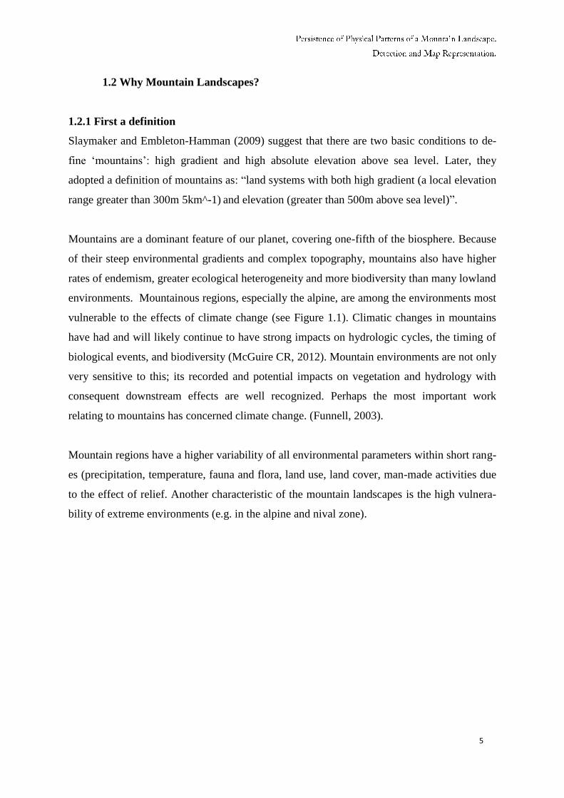
1.2 Why Mountain Landscapes?

1.2.1 First a definition

Slaymaker and Embleton-Hamman (2009) suggest that there are two basic conditions to de-

fine ‘mountains’: high gradient and high absolute elevation above sea level. Later, they

adopted a definition of mountains as: “land systems with both high gradient (a local elevation

range greater than 300m 5km^-1) and elevation (greater than 500m above sea level)”.

Mountains are a dominant feature of our planet, covering one-fifth of the biosphere. Because

of their steep environmental gradients and complex topography, mountains also have higher

rates of endemism, greater ecological heterogeneity and more biodiversity than many lowland

environments. Mountainous regions, especially the alpine, are among the environments most

vulnerable to the effects of climate change (see Figure 1.1). Climatic changes in mountains

have had and will likely continue to have strong impacts on hydrologic cycles, the timing of

biological events, and biodiversity (McGuire CR, 2012). Mountain environments are not only

very sensitive to this; its recorded and potential impacts on vegetation and hydrology with

consequent downstream effects are well recognized. Perhaps the most important work

relating to mountains has concerned climate change. (Funnell, 2003).

Mountain regions have a higher variability of all environmental parameters within short rang-

es (precipitation, temperature, fauna and flora, land use, land cover, man-made activities due

to the effect of relief. Another characteristic of the mountain landscapes is the high vulnera-

bility of extreme environments (e.g. in the alpine and nival zone).

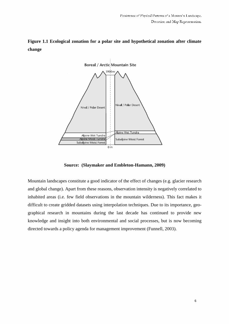
6

Figure 1.1 Ecological zonation for a polar site and hypothetical zonation after climate

change

Source: (Slaymaker and Embleton-Hamann, 2009)

Mountain landscapes constitute a good indicator of the effect of changes (e.g. glacier research

and global change). Apart from these reasons, observation intensity is negatively correlated to

inhabited areas (i.e. few field observations in the mountain wilderness). This fact makes it

difficult to create gridded datasets using interpolation techniques. Due to its importance, geo-

graphical research in mountains during the last decade has continued to provide new

knowledge and insight into both environmental and social processes, but is now becoming

directed towards a policy agenda for management improvement (Funnell, 2003).

7

1.3 The technique: Map Algebra

1.3.1 Raster data

As described by the platform GeoVITe (Geodata Visualization & Interactive Training Envi-

ronment ,ETH Zurich, 2010) raster data represents geographic data by discretizing it equally-

spaced and by quantizing each raster cell. A raster cell is most of the times a square, but

could theoretically be another regular polygon that is able to fully cover an image area with-

out leaving holes in the covered region, e.g. a triangle, hexagon or rectangle. A raster cell is

often also referred to as a pixel (picture element). A pixel can hold data values within the

specified possible range or color depth of a raster image or raster geodata set. This data value

can represent a color or gray value, depth or height, measurements or any other thematic val-

ue, such as an index to a landcover class. Raster cells are usually organized in a matrix (rows

and columns).

1.3.2 Map Algebra-The concept

The concept of map algebra was first introduced by Dana Tomlin and Joseph Berry in the

1970’s. Map Algebra principle is based on the cell by cell combination of raster layers with

each raster cell location representing a certain value. According to this principle, raster layers

can be combined from very simple to complex operations making it possible to analyze large

datasets.

8

2. Materials and Methods

2.1 Study Area.

The Altai Republic is located in central Eurasia. The territory of the Altai Republic is 92902

square km, that is 0.55 % of the whole territory of the Russian Federation. The territory

contains: agricultural lands - 19%, forests - 47%, water space - 0.9% and other lands - 33.1%

(Official portal Altai Republic, 2013). This territory changes from lowlands to highlands,

which causes a complexity in natural and economic spheres within it. The landscape of the

Altai Republic represents a continuity shared with three other countries - Mongolia, China

and Kazakhstan, as well as with three areas of Russia - Altai Territory, Tuva Republic and

Kemerovo region. Despite this description, this study has been developed in the polygon of

the Altai Republic (see Figure 2.1) used in the Altai GIS 1000 which provides an exact

spatial setting for the task. This setting is constituted by mountainous terrain in the south of

Siberia with highly variable relief and climate conditions.

The Altai Mountains in southern Siberia form a major mountain range, with the total area

covering 1,600,000 ha and representing the most complete sequence of altitudinal vegetation

zones in Siberia, from steppe, forest-steppe, mixed forest, sub-alpine vegetation, to alpine

vegetation. Because of its great importance, the Russian sector was inscribed on the World

Heritage List under natural criteria in 1998 (UNESCO, 2009). The region experiences a con-

tinental climate characterized by cold, dry winters and warm locally moist summers, con-

trolled primarily through the influence of the Siberian High and Asia-Pacific monsoon sys-

tems (Loader, et al. 2010). Much of this region, especially on the northern (Russian) part,

continues to be pristine, and the access to it remains difficult. Its position on the border of

four countries could be the reason for the slow development, although mining is spread in

some areas (W. Fund, 2012).

9

Figure 2.1 Location of the Altai Republic

Source: http://kartographie.geo.tu-dresden.de/altai and www.naturalearthdata.com

http://kartographie.geo.tu-dresden.de/altai

http://www.naturalearthdata.com/

10

This region is therefore of great interest from an Earth system science perspective. Regarding

the Altai Republic as a study area for scientific purposes, the literature focuses mainly in ge-

netic, ethnic, anthropological or demographical characteristics of the region. Also historical

geology investigations have been developed in those areas. All this research, suggest the spe-

cial characteristics of Altai, which isolation makes it interesting for those scientific disci-

plines. Some studies related to the physical environment in Altai must be emphasized for

example the studies regarding the glaciers in Altai environment in the Russian Altai Moun-

tains(Aizen, 1997).Also, it should be pointed out, similar studies to the presented here where

the spatial variability of physical parameters in this study are were investigated (Kerchove,

et.al 2013). The Altai republic represents a border area, thus, it is an area of great geopoliti-

cal importance and it is necessary to give it attention, but not only because of this but because

the biological diversity and environmental functions it has, make it a region of great im-

portance for the whole world.

11

2.2 Data

2.2.1 MODIS Data

In this section, the general characteristics of the MODIS data are presented, including the

spatial organization of the data, the naming system, the storage format and the metadata.

As, Hengl (2009) points out, NASA’s MODIS (or Moderate Resolution Imaging Spectrora-

diometer) is possibly one of the richest sources of remote-sensing data for monitoring of en-

vironmental dynamics. This is due to the following reasons:

It has global coverage; it has a relatively high temporal resolution, coverage (1–2 days); it is

open-access, a significant work has been done to filter the original raw images for clouds and

artifacts; a variety of complete MODIS products such as composite 15–day and monthly im-

ages is available at three resolutions: 250 m, 500 m and 1 km. (Hengl, 2009).

According to the Land Processes Distributed Archive Center (LPDAAC, 2013), MODIS is a

key instrument aboard the Terra and Aqua satellites. Terra passes from north to south across

the equator in the morning, while Aqua passes south to north in the afternoon. Terra MODIS

and Aqua MODIS captures the entire Earth's surface every 1 to 2 days, acquiring data in 36

spectral bands. MODIS data are distributed by the LPDAAC, located at U.S. Geological

Survey (USGS) Earth Resources Observation and Science (EROS) Center.

Table 2.1 MODIS Characteristiscs

Orbit: 705 km, 10:30 a.m. descending node (Terra) or 1:30 p.m. ascending node (Aqua), sun-

synchronous, near-polar, circular

Scan Rate: 20.3 rpm, cross track

Swath Dimesions: 2330 km (cross track) by 10 km (along track at nadir)

Telescope: 17.78 cm diam. off-axis, afocal (collimated), with intermediate field stop

Size: 1.0 x 1.6 x 1.0 m

Weight: 228.7 kg

Power: 162.5 W (single orbit average)

Data Rate: 10.6 Mbps (peak daytime); 6.1 Mbps (orbital average)

Quantization: 12 bits

Spatia Resolution: 250 m (bands 1-2)

500 m (bands 3-7)

1000 m (bands 8-36)

http://aqua.nasa.gov/

12

2.2.2 MODIS Naming Conventions

MODIS file names, have a naming convention which gives useful information regarding the

specific product. In this study we included images from LST and NDVI parameters for 8 days

and 16 days respectively, with a spatial resolution of 1km each of them.

In the following example, the filename for LST 8-day 1km spatial resolution for a section of

the study area is disaggregated as follows:

MOD11A2.A2002033.h23v04.005.2007121022621.hdf indicates:

MOD11A2 - Product Short Name

. A2002033 - Julian Date of Acquisition (A-YYYYDDD)

. h23v04 - Tile Identifier (horizontalXXverticalYY)

.005 - Collection Version

. 2007121022621 - Julian Date of Production (YYYYDDDHHMMSS)

.hdf - Data Format (HDF-EOS)

2.2.3 MODIS Temporal and Spatial Resolution

The high level MODIS Land products are produced at various temporal resolutions, based on

the instruments' orbital cycle. The following time resolutions exist in the generation of

MODIS Land products:

Daily, 8-Day, 16-Day, Monthly, Quarterly, Yearly

Additionaly, the MODIS instruments acquire data in three native spatial resolutions:

Bands 1–2 - 250-meter



13

Specifically, the high level MODIS Land Products distributed are produced at four nominal

spatial resolutions: 250-meter, 500-meter, 1000-meter, and 5600-meter (0.05 degrees).

2.2.4 MODIS Sinusoidal Tiling System

The tiles presented in Figure 2.2 are 10 degrees by 10 degrees at the equator. The tile coordi-

nate system starts at (0,0) (horizontal tile number, vertical tile number) in the upper left cor-

ner and proceeds right (horizontal) and downward (vertical). The tile in the bottom right cor-

ner is (35,17).

Figure 2.2. MODIS Tiling System

Source: modis.gsfc.nasa.gov

2.2.5 MODIS Processing Levels.

Level-2: derived geophysical variables at the same resolution and location as level-1

source data (swath products)

Level-2G: level-2 data mapped on a uniform space-time grid scale (Sinusoidal)

Level-3: gridded variables in derived spatial and/or temporal resolutions

14

Level-4: model output or results from analyses of lower-level data

2.3 Description of Parameters

2.3.1. Vegetation Indices 16-Day L3 Global 1km (MOD13A2)

Although there are several vegetation indices, one of the most used is the Normalized

Difference Vegetation Index (NDVI). NDVI values range from +1.0 to -1.0. The NDVI is

used to measure vegetation conditions and biomass production from multispectral satellite

data. NDVI is calculated as follows:

NDVI = (Channel 2 - Channel 1) / (Channel 2 + Channel 1)

The principle in NDVI is that Channel 1 is in the red-light region of the electromagnetic spec-

trum where chlorophyll absorbs considerable amount of sunlight, whereas Channel 2 is in the

near-infrared region of the spectrum where a plant's spongy mesophyll leaf structure reflects

considerable light. As a result, it is possible to identify healthy vegetation with low red-light

reflectance and high near-infrared reflectance with high NDVI values. Positive NDVI values

indicate green vegetation while NDVI values near zero and negative indicate non-vegetated

areas such as barren surfaces (rock and soil) and water, snow, ice, and clouds. (USGS, 2013)

Vegetation indices are mainly used for global monitoring of plant conditions and are used in

for identifying land cover and land cover changes. These results could be useful for modeling

global biogeochemical and hydrologic processes and global and regional climate. NDVI

values can be averaged over time to establish "normal" growing conditions in a region for a

given time of year.(NASA, 2013)

Further analysis can then characterize the health of vegetation in that place relative to the

norm. When analyzed through time, NDVI can reveal where vegetation is thriving and where

it is under stress, as well as changes in vegetation due to human activities such as

deforestation, natural disturbances such as wild fires, or changes in plants’ phenological

stage. Sparse vegetation such as shrubs and grasslands or senescing crops may result in

moderate NDVI values (approximately 0.2 to 0.5). High NDVI values (approximately 0.6 to

15

0.9) correspond to dense vegetation such as that found in temperate and tropical forests or

crops at their peak growth stage.

Global MODIS vegetation indices are designed to provide consistent spatial and temporal

comparisons of vegetation conditions. Blue, red, and near-infrared reflectances, centered at

469-nanometers, 645-nanometers, and 858-nanometers, respectively, are used to determine

the MODIS daily vegetation indices. Global MOD13A2 data are provided every 16 days at

1-kilometer spatial resolution as a gridded level-3 product in the Sinusoidal projection.

(USGS,2013)

Table 2.2 MOD13A2 Data Set Characteristics

Temporal Coverage February 24, 2000 -

Area ~10 x 10 lat/long

File Size ~1–22 MB

Projection Sinusoidal

Data Format HDF-EOS

Dimensions 1200 x 1200 rows/columns

Resolution 1 kilometer

Science Data Sets (SDS HDF Layers) 12


16

Table 2.3 Science Data Sets of MOD13A2 product

Source: Solano et al., 2010

2.3.2 Land Surface Temperature & Emissivity 8-Day L3 Global 1km (MOD11A2)

Land Surface Temperature is the result of the interaction of energy between the Earth's sur-

face and the atmosphere. Land surface temperature is one of the key parameters in the phys-

ics of the land-surface processes, and can be used as a good indicator of the Earth's green-

house effect. Generally, the lower the LST, the more energy the surface reflects, while the

higher LSTs are, the more energy and heat is absorbed by the Earth’s systems. On land, soil

and canopy temperature are among the main determinants of the rate of growth of vegetation,

and they also govern when growing seasons start and end. LST can be used in many different

applications, starting with agriculture, for classifying land surface types applications and epi-

demiology. Deserts tend to have very high LSTs, forests and plant-covered lands have more

moderate temperatures, and permafrost lands have much colder temperatures. (MODIS Web-

site)

This knowledge, combined with seasonal change patterns, allows the creation of land cover

maps that can be used by different fields of geoscientists and urban planners, since it is re-

quired for a wide variety of climate, hydrological, ecological, and biogeochemical studies.

17

LST also has a significant impact on hydrologic processes, such as evapotranspiration and

snow/ice melt. When LSTs rise, snow and ice melt, can evaporate, and contribute to fill bod-

ies of water. (MODIS Website)

The MODIS global Land Surface Temperature (LST) and Emissivity 8-day data are com-

posed from the daily 1-kilometer LST product (MOD11A1) and stored on a 1-km Sinusoidal

grid as the average values of clear-sky LSTs during an 8-day period. Version-5 MODIS/Terra

Land Surface Temperature/Emissivity products are validated to Stage 2, which means that

their accuracy has been assessed over a widely distributed set of locations and time periods

via several ground-truth and validation efforts.

According to Wan (2007) the eight-day compositing period (MODA11A2) was chosen be-

cause twice of such period is the exact ground track repeat period of the Terra platform. LST

over eight days is the averaged LSTs of the MOD11A1 product over eight days. For the

MOD11A2 product a simple average method is used in the current algorithm.

Table 2.4 MODA112 Data set Characteristics

Temporal Coverage March 5, 2000 -

Area ~1100 x 1100 km

File Size ~5 MB compressed

Projection Sinusoidal

Data Format HDF-EOS

Dimensions 1200 x 1200 rows/columns

Resolution 1 kilometer (0.93-km)

Science Data Sets (SDS HDF Layers) 12


18

Table 2.5 Science Data Sets in the MOD11A2 product.

Source: Wan, 2007

19

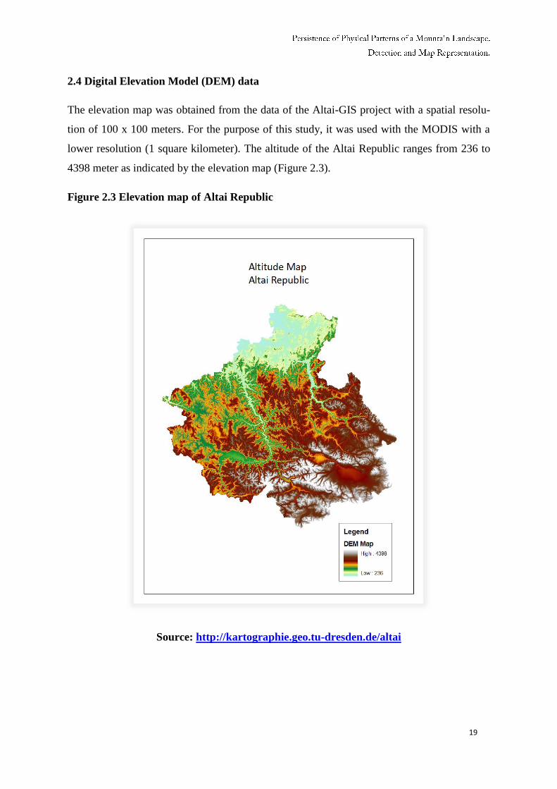
2.4 Digital Elevation Model (DEM) data

The elevation map was obtained from the data of the Altai-GIS project with a spatial resolu-

tion of 100 x 100 meters. For the purpose of this study, it was used with the MODIS with a

lower resolution (1 square kilometer). The altitude of the Altai Republic ranges from 236 to

4398 meter as indicated by the elevation map (Figure 2.3).

Figure 2.3 Elevation map of Altai Republic

Source: http://kartographie.geo.tu-dresden.de/altai

http://kartographie.geo.tu-dresden.de/altai

20

2.5 Land cover map

Figure 2.4 Land cover map of Altai Republic

Source: http://due.esrin.esa.int/globcover/

http://due.esrin.esa.int/globcover/

21

2.6 Method

2.6.1 Data pre-processing

As mentioned before, satellite imagery constitutes one of the most important sources of in-

formation for cartography and the steps to get insight from this data represent one of the most

important concerns. Figure 2.5 depicts a general overview of the process to retrieve infor-

mation from remote sensing. However, a further process is needed to complete the goal of

retrieval of meaningful information. This process will be complete only with the extraction of

significant patterns to arrive to a generalized level where processes can be understood region-

ally instead of having pixel-based random phenomena. This is the main objective of the pre-

sent study.

Figure 2.5 General Remote sensing-based approach

Source: (ITC,2004)

2.6.1.1 Download and preprocessing of MODIS data

There are different ways to perform the MODIS data download and preprocessing. One can

simply enter the MODIS website (modis.gsfc.nasa.gov/ ) and access the data pool where it is

possible to download the MODIS products either via http or by direct search. Grid data are

originally obtained in equal-area Sinusoidal projection (SIN) and delivered in Hierarchical

Data Format (HDF) which cannot be used for processing in the designed language R.

22

HDF is the standard data format for all NASA(National Aeronautics and Spaces Administra-

tion) Earth Observing System (EOS) data products; a multi-object file format developed by

the HDF Group. (National Snow and Ice Data Center, 2013)

For the reformat process, the Data Pool HDF EOS-to-GeoTiff (HEG) Tool is one of the op-

tions. Another option is to use the script ModisDownload.R developed by Babak Naimi. It is

an R function which gives the possibility to download, mosaic, and reproject the MODIS

images (See http://r-gis.net/?q=ModisDownload, for more information).

Regarding the Vegetation Indices, there exists a freely available data service platform (web-

application) for executing pre-processing operations of archived MODIS vegetation indices

time series on request (Vuolo, 2012).

Taking into account all these options, the MODIS package in R has been preferred since it

gives the simplest and straight-forward solution for downloading, re-projecting and mosaick-

ing of the satellite images. After specifying the extent of the output, the Modis Reprojection

Tool (MRT), which should be previously installed (see Land Processes DAAC, 2008) is

called and performs all the operations needed in an automatic way.

In this case the extent is the bounding box that completely contains the Altai Republic poly-

gon from the Altai GIS 1000 (Prechtel, et al 2003).

As general steps, first we define the extreme coordinates of the study area as a list in R:

Altai <- (list (xmax= 83.917152, xmin= 89.864043, ymin= 48.90463, ymax= 52.669577))

Later on, the user can define the time range and define the Scientific Data Sets (SDS) to

download. In the following example only the LST_Day_1km and Quality data layer are

downloaded:

runMrt (product="MOD11A2", begin="2001-01-01", end="2013-01-01",

SDSstring="11", extent=Altai, outProj="UTM", mosaic=TRUE, save=TRUE )

In the working directory, the HDF files are saved in folders according to the image date. In

this case the Altai republic is completely contained by the tiles h23v03 and h23v04 (see Fig-

ure 2.6) so a mosaicking process is needed. In a different folder, the processed product is

saved containing the image mosaic re-projected to the desired projection. As a note, the year

2000 was excluded from the analysis in order to consider only years with full data coverage.

http://r-gis.net/?q=ModisDownload

23

Figure 2.6. Location of the Altai Republic in relation to MODIS tiles


2.6.1.2 Quality Assurance

Clouds and other atmospheric artifacts, may occlude some pixels or even the whole satellite

image, this implies a significant problem for continuous monitoring. For this reason, the low

quality pixels of each LST and NDVI image were marked in an accompanying quality assur-

ance (QA) layer. Regarding the NDVI dataset, a quality layer has been included in the

MOD13A2, called “pixel reliability”. This layer contains values describing overall pixel

quality (see Table 2.6).

Table 2.6 MOD13A2 Pixel Reliability.

Rank Key Summary QA Description

-1 Fill/No Data Not Processed

0 Good Data Use with confidence

1 Marginal data Useful, but look at other QA information

2 Snow/Ice Target covered with snow/ice

3 Cloudy Target not visible, covered with cloud

Source: Solano et al., 2010.

24

A mask was created according to the values described in the Quality Assessment tutorials and

NDVI/LST User’s Guide. All grid cells with unuseful QC bits were set to NA. Later using

the mask() function in R, these values were filtered. Bits that are NA in LST and NDVI

rasters will be NA in the destination rasters (“Good_LST, Good_NDVI”). If a pixel is not NA

in the mask and has a value, then the value of the source (LST_Day, NDVI) is written into

the destination.

For the LST products, the quality layer that represents values of 0-255 was used. Following

the technique proposed by Neteler (2010). Pixels with certain labels indicated in the QA bit-

map layer were rejected: “clouds”, “other error”, “cirrus cloud”, “missing pixel”, “poor quali-

ty”, “Average emissivity error >0.04”, “LST error 2K−3K”, and “LST error >3K” See Table

(2.7) for more details. The images are originally produced in Kelvin.

Table 2.7. Bit flags defined for the SDS QC_day in MOD11A2 gridded in Sinusoidal projection

Source: Wan, 2007

25

Interpreting QC (Quality Control) Bits and applying the mask

For the purpose of interpreting the QC layer values, the LST user’s guide was consulted. The

values were converted to integers and then to big endian which is the format used in the HDF

files. For example to interpret the value of 33, in R:

QC_value33<-as.integer(intToBits(33)[1:8])

Little Endian: 1 0 0 0 0 1 0 0 = 33 2^0 + 2^5

QC_value33<-as.integer(intToBits(33)[8:1])

Big Endian: 0 0 1 0 0 0 0 1= 33 2^5 + 2^0

This bit order has the first two bits as 01 which indicates that the pixel is produced, but that

other information should be checked. The least significant bit is on the right. The following

values were found for the QC layer: 0,2,17,33,65,81,97,129,145,161.

Table 2.8 The QC_ layer values for Altai Republic and their meaning.

Source: author modified from Neteler (2010)

Bit position 7 6 5 4 3 2 1 0

Integer 128 64 32 16 8 4 2 1 Key

0 0 0 0 0 0 0 0 0 Good Quality, average LST <=1k

2 0 0 0 0 0 0 1 0 Not Produced, due to cloud effects

17 0 0 0 1 0 0 0 1LST produced, good quality, Average emissivity

error <= 0.02

21 0 0 0 1 0 1 0 1LST produced, other quality, Average emissivity

error <= 0.02

33 0 0 1 0 0 0 0 1 LST produced,Average emissivity error <= 0.04


error <= 0.01, Average LST error <= 2K



97 0 1 1 0 0 0 0 1LST produced, other quality,Average emissivity

error <= 0.04, average LST error <= 2K





161 1 0 1 0 0 0 0 1LST produced,,Average emissivity error <= 0.04,

Average LST error <= 3K

26

As a note, the numbers marked with green represent the accepted values and the marked with

red, the values that were rejected according to the method proposed by Neteler (2010).

Removing the outliers

To detect the outliers the following formulas were applied (see Appendix A for the complete

function in R).

First quartile – (1.5 * IQR) = lower boundary outliers

Third quartile + (1.5 *IQR) = upper boundary outliers

IQR (Interquartile Range)= First quartile subtracted from the third Quartile

General steps

Finally, as summary, the following preprocessing steps are required to obtain usable NDVI

and LST maps from MOD13A2 and MOD11A2 respectively into R:

A) Re-projection from SIN to a commonly used projection (e.g., UTM)

B) Application of the quality layers

C) In the case of NDVI, multiplication by scale factor of 0.0001 to get the range from

-1.0 to +1.0

D) In the case of LST, multiplication by scale factor of 0.02 and then setting of all values

equal to zero, to NA. If needed, conversion of Kelvin values to Celsius by subtracting 273.15

from each cell.

E) For NDVI, elimination of pixels with value outside of the expected range. For LST,

remove outliers on both sides either negative or positive.

27

2.6.2 NDVI and LST Statistical Analysis

The statistical analysis was performed in raster layers of the specific time-dependent varia-

bles. As Figure 2.7 shows, each layer represents the state of a specific variable in time.

Figure 2.7 The snapshot approach

Source: (Peuquet, 2005)

After downloading and preprocessing, the function brick was used in order to read the fil-

tered, multilayer raster dataset in R. According to the documentation of the raster package

(Hijmans, 2013) a RasterBrick is a multi-layer raster object. RasterBricks are typically creat-

ed from a multi-layer (band) file; but they can also exist entirely in memory. It shares similar

characteristics to a RasterStack (that can be created with the function “stack”), but processing

time should be shorter when using a RasterBrick. The general characteristics of the bricks

generated for the study area, for the period 2001-2012 are shown below:

28

Table 2.9 NDVI 2001-2012 raster brick characteristics in R

> NDVI2001_2012

class RasterBrick

dimensions 453, 471, 213363, 276 (nrow, ncol, ncell, nlayers)

resolution 926.6254, 926.6254 (x, y)

extent 274097.2, 710537.8, 5420214, 5839976 (xmin, xmax, ymin, ymax)

coord. Ref: +proj=utm +zone=45 +datum=WGS84 +units=m +ellps=WGS84

Table 2.10 LST 2001-2012 raster brick characteristics in R

>LST 2001_2012

class RasterBrick

dimensions 453, 471, 213363, 552 (nrow, ncol, ncell, nlayers)

resolution 926.6254, 926.6254 (x, y)

extent 274097.2, 710537.8, 5420214, 5839976 (xmin, xmax, ymin, ymax)

coord. Ref: +proj=utm +zone=45 +datum=WGS84 +units=m +ellps=WGS84

The NDVI and LST time series were analyzed in different ways. The analysis is described

below, in a step by step way.

First, the basic statistics for the period where computed. This was performed in order to give

a general overview of the data.

• The mean of the NDVI and LST values between start and end date

• The maximum of the NDVI and LST values between start and end date

• The minimum of the NDVI and LST values between start and end date

• The standard deviation of the NDVI and LST values between start and end date

29

Second, the standardized anomaly proposed by Wilks (1995) was computed for the NDVI

and LST products. The standardized anomaly, z, is computed by subtracting the mean of the

raw data x, and dividing by the corresponding standard deviation (See Figure 2.8). As ex-

plained by Wilks, the idea behind the standardized anomaly is to try to remove the influences

of location and spread from the data. The physical units of the original data cancel, for this

reason standardized anomalies are always dimensionless quantities. The result is a rescaling

of the data to the percent variation from the average. Mapped data expressed in this form

enables you to easily identify “statistically unusual” areas, for example +100% locates areas

that are one standard deviation above the typical value; -100% locates areas that are one

standard deviation below.

Figure 2.8 Equation to calculate standardized anomaly

Source: (Wilks, 1995)

Other methods to compute anomalies were performed for comparison, following the method

proposed by Frelat and Bertran (2012). Because we are talking about vegetation indices, the

seasonal anomaly was computed. For each year, the mean of the NDVI is computed for the

given period. Then, the global average over the year is calculated for this period. Anomaly

maps, with this procedure, are computed from the difference between the annual mean of the

growing season and the global average. If the difference is positive, it indicates that the sea-

son was “greener" than usual. In contrast, if it is negative, the season was “drier” than nor-

mal.

30

For NDVI, additional computations were performed. First, using the package greenbrown in

R (Forkel et al., 2013) the main trends in the spatial setting were calculated using the built-in

functions. Temporal trends and trend breakpoints on the multi-temporal raster data were

computed. Later, a classification of the trend analysis into significant positive and negative

trends was performed. For LST, some temperature-related indicators as suggested by Neteler

(2010) were computed as well.

2.6.2.2 Extracting Phenology metrics

According to Buers (2009) the range of methods for extracting phenology metrics can be

divided into four main categories: threshold, derivative, smoothing algorithms, and model fit.

The simplest and most frequently applied method determines Start of Season (SOS) and End

of Season (EOS) based on threshold values. The SOS is determined as the day of the year

(DOY) that the NDVI crosses a given threshold in upward direction; likewise, the EOS is

determined as the DOY that the NDVI crosses the same threshold in downward direction.

Phenology metrics were calculated using different open source approaches available by

experimenting with the threshold method. First of all, the software TIMESAT was used to

calculate some of the most significant. TIMESAT was developed for estimating growing

seasons from satellite time-series, as well as for computing phenological metrics from the

data (Jönsson and Eklundh 2002, 2003, 2004, Eklundh and Jönsson 2003). TIMESAT fits

smooth mathematical functions to time-series of noisy satellite data, and later extracts key

phenological metrics (See Figure 2.9). Figure 2.10 shows a diagram with the main indicators

of phenology. For a full description of this parameters see Table (2.11). To visualize the

spatial variability of the phenology metrics, different NDVI metrics were mapped. Beginning

and end of the growing season, length of the season, large and small integrals were extracted

for each image pixel.

31

Figure 2.9 General workflow of the software TIMESAT

Source: Eklundh, L. and Jönsson, P., 2011

Figure 2.10 Seasonality Parameters in TIMESAT


32

In Figure 2.10, points (a) and (b) represent, respectively, start and end of the season. Points

(c) and (d) give the 80% level. Point e gives the largest value. Point (f) mark the seasonal

amplitude and (g) give the seasonal length. Finally, (h) and (i) are integrals showing the cu-

mulative effect of vegetation during the season.

Table 2.11 Phenology metrics in TIMESAT

Seasonality parameter Definition

time for the start of the season time for which the left edge has increased to a user de-

fined level (often a certain of the seasonal amplitude)

measured from the left minimum level.

time for the end of the season time for which the right edge has decreased to a user

defined level measured from the right minimum level

length of the season time from the start to the end of the season.

base level given as the average of the left and right minimum val-

ues

time for the mid of the season computed as the mean value of the times for which, re-

spectively, the left edge has increased to the 80 % level

and the right edge has decreased to the 80 % level.

largest data value for the fitted

function during the season

may occur at a different time compared with 5

seasonal amplitude difference between the maximum value and the base

level.

rate of increase at the beginning

of the season

calculated as the ratio of the difference between the left

20 % and 80 % levels and the corresponding time differ-

ence

rate of decrease at the end of

the season

calculated as the absolute value of the ratio of the differ-

ence between the right 20 % and 80 % levels and the

corresponding time difference. The rate of decrease is

thus given as a positive quantity

large seasonal integral integral of the function describing the season from the

season start to the season end.

small seasonal integral integral of the difference between the function describ-

ing the season and the base level from season start to

season end.


33

In the next lines, a description of the workflow followed in TIMESAT is presented. First, the

different curves were fitted for comparison in the TIMESAT Graphical User Interface (see

Figure 2.14). Also different threshold values were selected to visualize the differences. The

choices for data plotting control the display of the current time-series. When selecting Gauss-

ian, Double Logistic or Savitzky-Golay, the fitted data are displayed along with the original

data, and seasonality parameters are shown in the window seasonality data. Different sources

were consulted in order to choose the best fit. In the following lines a brief description of the

fitting functions is presented, this section was taken from the TIMESAT Software’s Manual.

Savitzky-Golay

One way of smoothing data and suppressing disturbances is to use a filter, and replace each

data value yi, i = 1, . . . ,N by a linear combination of nearby values in a window. In the sim-

plest case, referred to as a moving average, the weights are cj = 1/(2n + 1), and the data value

yi is replaced by the average of the values in the window. The moving average method pre-

serves the area and mean position of a seasonal peak, but alters both the width and height.

The latter properties can be preserved by approximating the underlying data value, not by the

average in the window, but with the value obtained from a least-squares fit to a polynomial.

For each data value yi, i = 1, 2, . . . ,N we fit a quadratic polynomial f(t) = c1 +c2t+c3t2 to all

2n+1 points in the moving window and replace the value yi with the value of the polynomial

at position ti. The procedure above is commonly referred to as a Savitzky-Golay filter (Press

et al. 1994).

Gaussian function

Figure 2.11 The Gaussian function

Source: Eklundh, L. and Jönsson, P., (2011)

34

For this function x1 determines the position of the maximum or minimum with respect to the

independent time variable t, while x2 and x3 determine the width and flatness (kurtosis) of

the right function half. Similarly, x4 and x5 determine the width and flatness of the left half.

The effects of varying the parameters x2, x5 are shown in Figure (2.12).

Figure 2.12 Effect of parameter changes on the local functions

Source: Eklundh, L. and Jönsson, P., (2011)

In (a) the parameter x2, which determines the width of the right function half, has been de-

creased (solid line) and increased (dashed line) compared to the value of the left half. In (b)

the parameter x3, which determines the flatness of the right function half, has been decreased

(solid line) and increased (dashed line) compared to the value of the left half.

Double logistic functions

Figure 2.13 Logistic function

Source : Eklundh, L. and Jönsson, P., (2011)

35

x1 determines the position of the left inflection point while x2 gives the rate of change. Simi-

larly x3 determines the position of the right inflection point while x4 gives the rate of change

at this point. Also for this function the parameters are restricted in range to ensure a smooth

shape. As mentioned by Beck et al. (2006), “Many of the algorithms used for vegetation

monitoring are ill-suited for boreal regions. These algorithms rely on second-order Fourier

series which cannot represent short growing seasons well, especially when the increase and

decrease in NDVI in spring and autumn occur abruptly. In this case, the fitted Fourier series

tends to overestimate the duration of the growing season”. Later on that same research a dou-

ble logistic function was proposed to describe NDVI time series. So “Double logistic” was

chosen as a smoothing function for calculating the seasonality parameters. NDVI spikes larg-

er than two times the standard deviation of the median values were eliminated.

Figure 2.14 TIMESAT Graphical User Interface

36

As can be seen from Figure 2.14, the periodic character of the series is captured reasonably

well by this fitted function. In our experience, it was worth experimenting with several differ-

ent combinations of fitted functions offered by the software, in order to find a satisfactory

estimate of the seasonal component. TIMESAT gives the possibly to use different fitted mod-

els to enhance our understanding of the mechanism generating the time series. TIMESAT

reads and writes raw, or flat, binary files. 8-bit unsigned integer, 16-bit signed integer or 32-

bit signed real data are the formats supported. After creating a settings file (see Figure 2.15),

the seasonality parameters were calculated for each year and exported in 16-bit signed integer

format.

Figure 2.15 Creating the settings file in TIMESAT

After processing in TIMESAT, the images were exported to R where an average for the

2001-2012 period of the seasonality parameters were mapped to visualize the spatial distribu-

tion.

37

Elevation correction

As Gommes (2013) suggests, physical variables undergo systematic changes with elevation.

For this reason, in order to eliminate the influence of altitude which was obvious in our anal-

ysis, scatterplots of altitude versus the most significant phenology metrics (large and small

integrals) were analyzed and a linear regression model was fitted for each one. Later a new

raster with the residuals of the function was computed. The residual data of the simple linear

regression model is the difference between the observed data of the dependent variable y and

the fitted values ŷ (Residual = y- ˆy).

Model Formulae in R

response variable~explanatory variable(s)

where the tilde symbol ~ means ‘is modelled as a function of’. A a simple linear regression of

y on x in R should be written as:

y~x

A simplified approach was used based on (Courault, 1999). A constant coefficient obtained

from the relationship between the different phenology metrics and elevation was extended to

transform the values to an ‘equivalent at sea level’. In order to evaluate the presented correc-

tion methods, root mean square error (RMSE) as statistical accuracy measure was used.

38

2.6.2.2 Comparing NDVI AND LST spatial distribution

Using the Global Land Cover information from the European Space Agency (ESA), the rela-

tionships between NDVI and LST in the growing season were investigated. (see table 2.12

for more information on the land cover types). This part of the analysis focused mainly on

land cover related to forests and other natural land cover types. Crops, water bodies, urban

areas and other less significant land cover types for the study area were discarded.

Table 2.12 Land cover types in GlobCover 2009 V2.3

Source: http://due.esrin.esa.int/globcover/

Table 2.13 Significant land cover types for the study area

LAND COVER TYPE

CODE

DESCRIPTION No. of

pixels

50 Closed (>40%) broadleaved deciduous forest (>5m) 281753

90 Open (15-40%) needleleaved deciduous or evergreen forest (>5m) 192961

100 Closed to open (>15%) mixed broadleaved and needle leaved forest (>5m) 163298

150 Sparse (<15%) vegetation 145336

70 Closed (>40%) needle leaved evergreen forest (>5m) 139457 139457

200 Bare areas 120253

Value Label

11 Post-flooding or irrigated croplands (or aquatic)

14 Rainfed croplands

20 Mosaic cropland (50-70%) / vegetation (grassland/shrubland/forest) (20-50%)

30 Mosaic vegetation (grassland/shrubland/forest) (50-70%) / cropland (20-50%)

40 Closed to open (>15%) broadleaved evergreen or semi-deciduous forest (>5m)

50 Closed (>40%) broadleaved deciduous forest (>5m)

60 Open (15-40%) broadleaved deciduous forest/woodland (>5m)

70 Closed (>40%) needleleaved evergreen forest (>5m)

90 Open (15-40%) needleleaved deciduous or evergreen forest (>5m)

100 Closed to open (>15%) mixed broadleaved and needleleaved forest (>5m)

110 Mosaic forest or shrubland (50-70%) / grassland (20-50%)

120 Mosaic grassland (50-70%) / forest or shrubland (20-50%)

130 Closed to open (>15%) (broadleaved or needleleaved, evergreen or deciduous) shrubland (<5m)

140 Closed to open (>15%) herbaceous vegetation (grassland, savannas or lichens/mosses)

150 Sparse (<15%) vegetation

160 Closed to open (>15%) broadleaved forest regularly flooded (semi-permanently or temporarily) - Fresh or brackish water

170 Closed (>40%) broadleaved forest or shrubland permanently flooded - Saline or brackish water

180 Closed to open (>15%) grassland or woody vegetation on regularly flooded or waterlogged soil - Fresh, brackish or saline water

190 Artificial surfaces and associated areas (Urban areas >50%)

200 Bare areas

210 Water bodies

220 Permanent snow and ice

230 No data (burnt areas, clouds,…)


39

Figure 2.16 Spatial distribution of significant land cover types in Altai Republic

40

Later, to complement this analysis, selected values from points that were representative of the

different land cover types were extracted. The time series were plotted and the main features

were examined. To give a brief overview of the whole process, a flow diagram was created to

improve the understanding of the different steps that were carried out. These general steps

can then be followed in similar case studies (See Figure 2.17).

Figure 2.17 General workflow of the study

41

2.6.3 Transformation of patterns to ESRI shapefiles for integration in the Altai GIS

As a final task, some of the final raster results from the analysis were in a first moment re-

classified and then converted to polylines and polygons. Using as inspiration the research of

Erckhart and Fliri where this thesis idea started (see section 2),the generalization analysis

tools in ArcGIS 9.3 were used in order to clean up small data in the raster layers or generalize

the data to get rid of unnecessary detail for a more general representation.

The generalization tools were useful to identify significant areas and automate the assignment

of more reliable values to the cells that make up the areas. In this final step, the following

procedure was followed:

First, the tool Majority Filter was used to replace the cells in the raster layers based on the

majority of their contiguous neighboring cells. A kernel filter of eight nearest neighbors (a 3-

by-3 window) was selected to the present cell. Later a Boundary clean was applied. These

results will be available as shapefiles in the Altai Web GIS for the interested public.

Figure 2.18 Majority Filter principle in ArcGIS

Source: ESRI, 2013

42

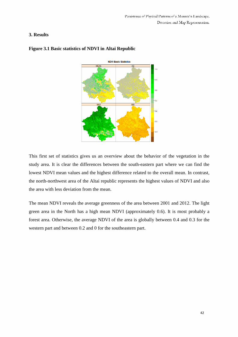
3. Results

Figure 3.1 Basic statistics of NDVI in Altai Republic

This first set of statistics gives us an overview about the behavior of the vegetation in the

study area. It is clear the differences between the south-eastern part where we can find the

lowest NDVI mean values and the highest difference related to the overall mean. In contrast,

the north-northwest area of the Altai republic represents the highest values of NDVI and also

the area with less deviation from the mean.

The mean NDVI reveals the average greenness of the area between 2001 and 2012. The light

green area in the North has a high mean NDVI (approximately 0.6). It is most probably a

forest area. Otherwise, the average NDVI of the area is globally between 0.4 and 0.3 for the

western part and between 0.2 and 0 for the southeastern part.

43

Figure 3.2 Standardized NDVI Anomaly in Altai Republic 2001-2012

Talking about the Standardized NDVI Anomaly, it is also clear that the highest anomalies

both positive (2005, 2006, 2012) and negative (2001, 2008, 2009) are focused mainly in the

southeastern part of the study region. In a global view of the region, the attention should be

directed towards the years 2009 as a negative anomaly (i.e. a drier season with about 20 to

40% less) for almost the entire region and also 2007 as a positive anomaly (a greener season)

for most of the study area.

44

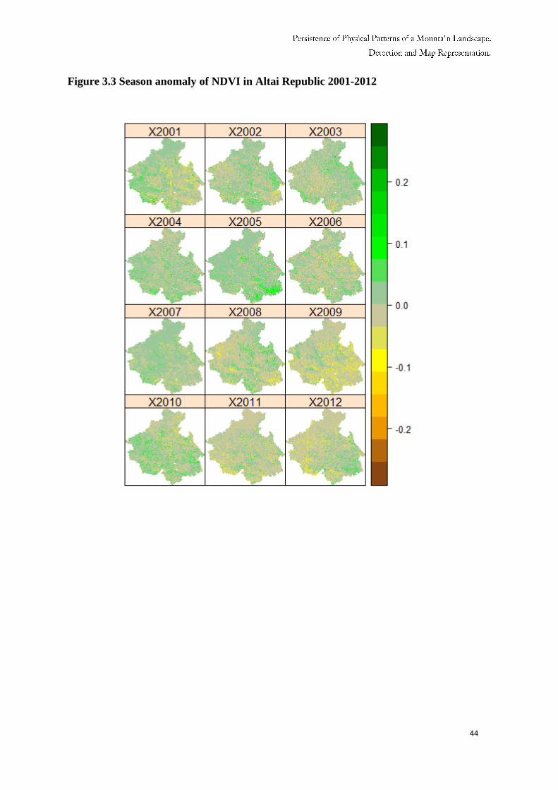
Figure 3.3 Season anomaly of NDVI in Altai Republic 2001-2012

45

Figure 3.4 Average start of growing season (DOY) in Altai Republic 2001-2012

Figure 3.5 Average end of the growing season (DOY) in Altai Republic 2001-2012

46

Figure 3.6. Average Length of Season (DOY) in Altai Republic 2001-2012

Figure 3.7 Average of Large Integral in Altai Republic 2001-2012

47

According to (van Leeuwen, et al. 2010), the small Integral (SI), given by the area of the re-

gion between the fitted function and the average of StartNDVI and EndNDVI values, called

the BaseNDVI, represents the seasonally active vegetation. The Large Integral(LI), given by

the area between the fitted function and the zero NDVI value bounded by the Startt and Endt,

represents the total vegetation stand and is a proxy for vegetation production (see Figure 3.8).

Figure 3.8 Large and Small Integrals

Source: (Van Leeuwen, et al., 2010)

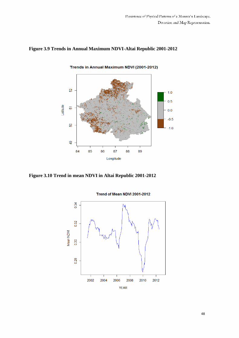
48

Figure 3.9 Trends in Annual Maximum NDVI-Altai Republic 2001-2012

Figure 3.10 Trend in mean NDVI in Altai Republic 2001-2012

49

Figures 3.10 shows the mean trend for the Altai Republic for the given period. The main

features are both an increase in the mean NDVI in the years around 2005-2007 and a

significant decrease in the years 2008 to 2010. This graph has comparable results to both

standardized anomalies (Figure 3.2) and seasonal anomalies(Figure 3.3) for the given period.

Figure 3.11 Anomalies in Large Integral in Altai Republic 2001-2012

50

Figure 3.12 Relationship Large Integral-Elevation in Altai Republic

Figure 3.12, shows the relation between large integral and elevation in the study area. The

linear regression model describes a decrease of 0.27 in the value of the integral per 100

meter. This value was applied and a new large integral map was generated.

Here is a summary of the linear model calculated in R:

lm(formula = getValues(LARGEINTEGRALMEAN) ~ getValues(DEM), na.action =

na.exclude)

R-squared: 0.5172

coefficients (model)

(Intercept) x

11.151471355 -0.002717677

51

Figure 3.13 Map of the residuals of the linear regression model Large

Integral~Elevation

Figure 3.14 New map of Large Integral with elevation correction

52

Figure 3.15

Figure 3.15, shows the relation between small integral and elevation in the study area. The

linear regression model describes a decrease of 0.17 in the value of the integral per 100

meter. This value was applied and a new small integral map was generated

Here is a summary of the linear model calculated in R:

lm(formula = getValues(SMALLINTEGRALMEAN) ~ getValues(DEM), na.action =

na.exclude)

R-squared: 0.4309

coefficients (model)

(Intercept) (x)

8.257705151 -0.001731454

53

Figure 3.16 Map of the residuals of the linear regression model Small

Integral~Elevation

Figure 3.17 New map of Small Integral with elevation correction

54

Results for LST

Figure 3.18 LST Basic statistics

Figure 3.19 Standardized LST Anomaly in Altai Republic 2001-2012

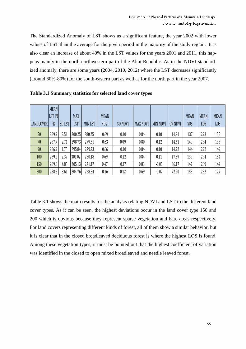
55

The Standardized Anomaly of LST shows as a significant feature, the year 2002 with lower

values of LST than the average for the given period in the majority of the study region. It is

also clear an increase of about 40% in the LST values for the years 2001 and 2011, this hap-

pens mainly in the north-northwestern part of the Altai Republic. As in the NDVI standard-

ized anomaly, there are some years (2004, 2010, 2012) where the LST decreases significantly

(around 60%-80%) for the south-eastern part as well as for the north part in the year 2007.

Table 3.1 Summary statistics for selected land cover types

Table 3.1 shows the main results for the analysis relating NDVI and LST to the different land

cover types. As it can be seen, the highest deviations occur in the land cover type 150 and

200 which is obvious because they represent sparse vegetation and bare areas respectively.

For land covers representing different kinds of forest, all of them show a similar behavior, but

it is clear that in the closed broadleaved deciduous forest is where the highest LOS is found.

Among these vegetation types, it must be pointed out that the highest coefficient of variation

was identified in the closed to open mixed broadleaved and needle leaved forest.

LANDCOVER

MEAN

LST IN

°K SD LST

MAX

LST MIN LST

MEAN

NDVI SD NDVI MAX NDVI MIN NDVI CV NDVI

MEAN

SOS

MEAN

EOS

MEAN

LOS

50 289.9 2.51 300.25 280.25 0.69 0.10 0.84 0.10 14.94 137 293 155

70 287.7 2.71 298.73 279.61 0.63 0.09 0.80 0.12 14.61 149 284 135

90 286.9 1.75 295.84 279.73 0.66 0.10 0.84 0.10 14.72 144 292 149

100 289.0 2.37 301.02 280.18 0.69 0.12 0.84 0.11 17.59 139 294 154

150 289.0 4.85 305.13 271.17 0.47 0.17 0.83 -0.05 36.17 147 289 142

200 288.8 8.61 304.76 268.54 0.16 0.12 0.69 -0.07 72.20 155 282 127

56

Results in NDVI-LST relationships

Figure 3.20 NDVI- LST RELATIONSHIPS FOR SELECTED LAND COVER TYPES IN

THE GROWING SEASON PERIOD (APRIL-SEPTEMBER) FOR 2001-2012

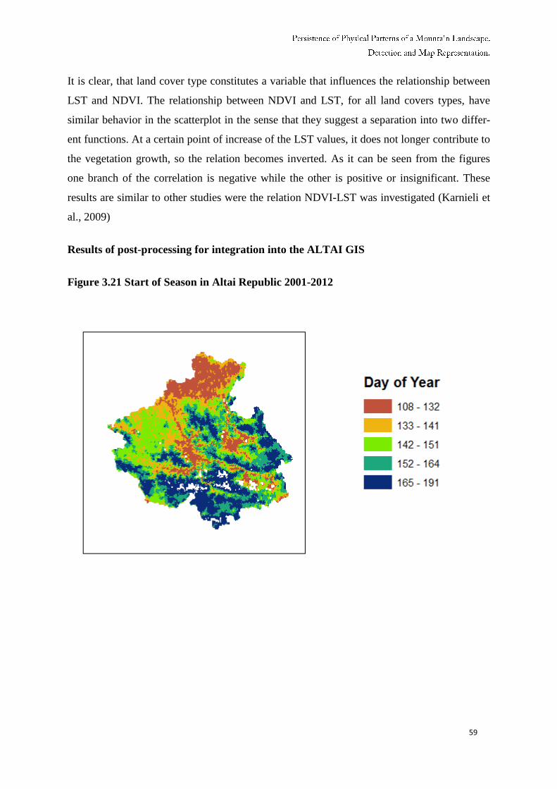
59

It is clear, that land cover type constitutes a variable that influences the relationship between

LST and NDVI. The relationship between NDVI and LST, for all land covers types, have

similar behavior in the scatterplot in the sense that they suggest a separation into two differ-

ent functions. At a certain point of increase of the LST values, it does not longer contribute to

the vegetation growth, so the relation becomes inverted. As it can be seen from the figures

one branch of the correlation is negative while the other is positive or insignificant. These

results are similar to other studies were the relation NDVI-LST was investigated (Karnieli et

al., 2009)

Results of post-processing for integration into the ALTAI GIS

Figure 3.21 Start of Season in Altai Republic 2001-2012

60

Figure 3.22 End of season in Altai Republic 2001-2012

Figure 3.23 Length of season in Altai Republic 2001-2012

61

Figure 3.24 Large Integral in Altai Republic 2001-2012

Figure 3.25 Small Integral in Altai Republic 2001-2012

62

4. Discussion

About NDVI and LST statistical analysis

The coefficient of variation proved to be more useful than the standard deviation to detect

variability of the parameters when comparing different land cover types (see Table 3.1).This

is because the standard deviation can only be understood in the context of the mean of the

data. In contrast, the value of the coefficient of variation is independent of the unit in which

the measurement has been taken, so it can be compared among variables.

Figure 3.8 shows the general trend for the selected time period. In general, it shows mainly a

significant negative trend on the northern and southwestern part of the study area. Positive

trends appear randomly on the study area and could be considered as not significant. Howev-

er, in a further analysis it was notices that these results could be not satisfactory because the

NDVI maximum values are not a very trust parameter. Therefore an analysis of the trend re-

lated to the integrals of NDVI was performed as well.

About the phenology metrics

In this study, maps of the beginning, the end and the length of the growing season and large

integral as means over the years 2001–2012 are presented. The results show just by visual

analysis a strong relationship between altitude (Fig. X) and phenology metrics. It can be said

that as altitude increases the start of season appears later and also the EOS appears earlier. If

we compare the map of SOS and EOS, using the same palette it is almost the same depiction

but with an inversed ramp of colors. This simple visual analysis can be corroborated by a

regression analysis of each of the seasonality raster layers and the independent variable

(DEM). These results coincide to those of similar research in Europe (Rötzer & Chmielewski,

2001).

As it is discussed by Buers (2009), in high latitude biomes, the greatest temporal increase in

the NDVI, which some methods use to indicate start of the season, is often due to snow melt

(Reed et al.1994, Delbart et al. 2005). The EOS metric, on the other hand, can be fooled by

an extended period of cloudiness that yields low NDVI, instead of actual senescence. We

were interested in the extent to which the variation in the response variable, in this case the

63

NDVI metrics are associated with the variation of the explanatory variables (e.g. altitude,

latitude, longitude).

Figure 3.4 presents a map showing the dates for SOS estimated from NDVI data averaged

over the years 2001–2012. As it was expected, the patterns depend strongly on altitude and

reveal how the date of SOS decreases from northwest to southeast from the beginning of

April to early July. The growing season starts in most land cover types of Altai Republic be-

tween 15 of April (Land cover type 50) and 15 of May.

The general trend is that in mountainous regions such as the Altai Mountains, great differ-

ences in the phenology metrics can be seen: the growing season starts much later in the

mountains compared to the areas where altitude was lower (northern part of Altai Republic).

The latest data of SOS June is observed in the land cover type 200 which represents bare are-

as. As the length of the growing season mainly depends on the beginning, almost the same

trend was found for LOS as SOS. The longest growing seasons, with over 200 days, can be

found in the northern part of Altai. In large parts of the Altai Republic, except for the moun-

tainous regions, the growing season lasts between 120 and 220 days. Shorter growing sea-

sons, with less than 130 days, are calculated for high altitudes as well as for nearly all the

south and south-eastern part.

In section 3, time series from MODIS dataset were extracted to compare the results with

those of selected land cover types. The 12-years long time series allow the study of trend in

phenology over understand the dynamics of mountain environments. The NDVI time series

can reveal the impact of climate change on ecosystems and their variability. The phenological

metrics, calculated in TIMESAT can be used as a diagnostic of ecosystem response to global

change. The results in SOS, EOS and LOS could represent valuable information for climate

change studies. In maps of standardized and seasonal anomalies, showed in the results, inter-

esting patterns appear even if at a first glance the information provided seems to be simply

calculated. The average of the large integral over the period 2001-2012 gives information

about the greenness of the region. As, explained in section, the spatial distribution of NDVI

and LST is linked with the land cover.

64

5. Conclusions

Large scale timeseries NDVI and LST images can be applied in conjunction with traditional

methods for monitoring environmental conditions and changes across time and space.

Especially, they are useful where there is lack of in situ measurements of vegetation and

climate conditions in complex terrain areas where there is no possibility to perform

traditional geostatistical interpolations. With the use of free available time series satellite

images provided by sensors like MODIS, this problem can be partly solved.

The present study analyzed both LST and NDVI time series (2001-2012) to characterize

long-term variability and trends in the Altai Republic region. The basic statistics (maximum,

minimum, average, and standard deviation were computed. Yearly standardized, seasonal and

maximum anomaly for both parameters were used to assess the vegetation and land surface

temperature variability during the given period. A comparison of the different methods

proved to enrich the analysis.

Another aim of the study was the evaluation of the correlation between LST and NDVI.

Therefore, both parameters were compared for the period of study in different ways. Using

land cover information as a base, the relationship between both parameters was assessed. The

comparison between the LST and NDVI values for the 2001-2012 period reveal a strong

variability across the Altai Republic. It can be said that vegetation greenness is highly

variable in space and time within the study area and its relationship with LST has different

results according to the spatial setting (land cover).

5.1 Data processing and visualization

Most of the data processing steps including import, statistical analysis, GIS operations and

map representation were performed in R and are explained in detail in the Appendix A.

Operations in R can be combined with the help of R packages, so that the complete process

can be put in a single script and adopted to perform similar case studies. It could be good for

publishing to export the result to external GIS packages or graphical design software for

improving the aesthetics of the maps. During the processing, due to the large datasets ( 276

layers for NDVI and 552 LST), the script had to be be adapted for good performance because

the computational effort compromises the system’s memory.

65

5.2 Limitations of the study and recommendations

Although remote sensing data can be interpreted and processed without other information, it

should be said that the best results could be obtained by linking remote sensing measurements

to in situ measurements and observations. Highly accurate anomaly maps can be derived

from this combination process. Future persistent patterns studies need to consider this in or-

der to better evaluate trend changes in both NDVI and LST, because one of the main prob-

lems of this study was the validation of the results. The only possible solution was to com-

pare the results with other studies performed in similar spatial settings and environmental

conditions and with the values extracted from points. Other geographical factors, which were

not included in this analysis, could have made the research significantly richer.

As general remarks, it is recommended for environmental studies to use time series instead of

single snapshots as in traditional GIS to account for the parameters variability. This study

was almost fully developed using open source tools which prove the power and potential that

these initiatives have for research in geosciences. Despite R resources are scattered and there-

fore difficult to find and to compare, it is possible to find answers to questions in this plat-

form through the mailing lists and papers from the contributors of the huge community this

represents. Some complementary tasks were produced, as showed before, in TIMESAT

which is also non-commercial software. However, some of the final tasks were done in ESRI

ArcGIS because it represented an easier solution to the problem of regionalization. Addition-

al efforts have to be made to allow these freeware tools to fully compete with the commercial

solutions, especially in an era where nobody can deny that scientific research is almost com-

pletely driven by corporation’s needs, an issue that puts into a debate the real function science

should have in our society.

66

6. References:

Aizen, V. B., E. M. Aizen. (1997). Regional Hydrological Response to Climate Change and

Global Warming. Kluwer Academic Publ.

Beck, P., Atzberger, C., Høgda, K. A., Johansen, B., & Skidmore, A. K. (2006). Improved

monitoring of vegetation dynamics at very high latitudes: A new method using MODIS

NDVI. Remote Sensing of Environment, 100(3), 321-334.

Beurs de M., K. and Geoffrey M. Henebry.(2010) Spatio-Temporal Statistical Methods for

Modelling Land Surface Phenology. Chapter 9. In Phenological Research. Methods for Envi-

ronmental and Climate Change Analysis. Hudson, Irene L.; Keatley, Marie R. (Eds.)

Courault, D., and Monestiez, P. (2009).Spatial interpolation of air temperature according to

atmospheric circulation patterns in southeast France. Int. J. Climatol. 19: 365–378 (1999)

Eklundh, L. and Jönsson, P., (2011), Timesat 3.1 Software Manual, Lund University, Swe-

den. http://www.nateko.lu.se/personal/Lars.Eklundh/TIMESAT/timesat.html.

Erkhart.E.(1950), Das Temperaturfeld der Alpen und seine Jahresperiode. Geografiska An-

naler © Swedish Society for Anthropology and Geography. Vol. 32, 1950

Fliri, F. (1970): Probleme und Methoden einer gesamtalpinen Klimatographie. - Jb. geogr.

Ges. Bern II : 113-127.

Fund,W.(2012). Altai alpine meadow and tundra. Retrieved from

http://www.eoearth.org/view/article/150001. Accessed July 2013

Funnel D. and Price, M. (2003). Mountain geography: a review The Geographical Journal,

Vol.169 , No. 3, pp. 183–190

Gommes, R. (2013) Mountain climates. Agrometeorology Group.Environment and Natural

Resources Service.Research, Extension and Training Division.Sustainable Development De-

partment. Retrieved from http://www.fao.org/nr/climpag/pub/EN0701_en.asp

Karnieli,A, Agam,N., Pinker, R.T., Anderson, M., M.L. Imhoff, G.G. Gutman, N. Panov, A.

Goldberg, (2010) “Use Of NDVI And Land Surface Temperature For Drought Assessment:

MeritsAnd Limitations”, Journal Of Climate Volume: 23, Issue: 3,Pages: 618-633.

Hengl, Tomislav.(2009) A practical guide to geostatistical mapping. Amsterdam. Retrieved

from: http://spatial-analyst.net/book/system/files/Hengl_2009_GEOSTATe2c1w.pdf

International Institute for Geo-information Science and Earth Observation. (2004). Principles

of Remote Sensing.Norman Kerle, Lucas L. F. Janssen and Gerrit C. Huurneman (eds.) (ITC

Educational Textbook Series; 2) Third edition.

http://www.nateko.lu.se/personal/Lars.Eklundh/TIMESAT/timesat.html.

http://www.eoearth.org/view/article/150001.%20Accessed%20July%202013

http://www.fao.org/nr/climpag/pub/EN0701_en.asp

http://spatial-analyst.net/book/system/files/Hengl_2009_GEOSTATe2c1w.pdf

67

Jönsson P.and Eklundh, L.(2002) “Seasonality Extraction by Function Fitting to Time-Series

of Satellite Sensor Data,” IEEE Transactions on Geoscience and Remote Sensing, vol. 40, no.

8, pp. 1824–1832.

Jönsson, P. and Eklundh, L., (2002), Seasonality extraction and noise removal by function

fitting to time-series of satellite sensor data, IEEE Transactions of Geoscience and Remote

Sensing, 40, No 8, 1824 – 1832.

Jönsson, P. and Eklundh, L., (2004), Timesat - a program for analyzing time-series of satellite

sensor data, Computers and Geosciences, 30, 833 – 845

Kerchove Van de R. , Lhermitteb, S., Veraverbekea,S., Goossens, R.(2013) Spatio-temporal

variability in remotely sensed land surface temperature, and its relationship with physio-

graphic variables in the Russian Altay Mountains. International Journal of Applied Earth Ob-

servation and Geoinformation 20, 4–19.

Kysely, J. and Huth R. (2008). Relationships of surface air temperature anomalies over

Europe to persistence of atmospheric circulation patterns conducive to heat waves Adv. Ge-

osci., 14, 243–249,www.adv-geosci.net/14/243/2008/.

McGuire CR, Nufio CR, Bowers MD, Guralnick RP (2012) Elevation-Dependent Tempera-

ture Trends in the Rocky Mountain Front Range: Changes over a 56- and 20-Year Record.

PLoS ONE 7(9): e44370. doi:10.1371/journal.pone.0044370

Land Processes DAAC. (2008). MODIS Reprojection Tool User’s Manual. USGS Earth Re-

sources Observation and Science (EROS) Center

Loader, N.J., Helle, G., Los, S.O., Lehmkuhl F., and G.H. Schleser,G.H 2010) Twentieth-

century summer temperature variability in the southern Altai Mountains: A carbon and oxy-

gen isotope study of tree-rings. The Holocene 2010 20: 1149 originally published online 13

July 2010

NASA(2013). http://earthobservatory.nasa.gov/Features/MeasuringVegetation

Neteler, M. (2010) Estimating Daily Land Surface Temperatures in Mountainous Environ-

ments by Reconstructed MODIS LST Data. Remote Sens. 2010, 2, 333-351.

Peuquet, D.J. (2005) Time in GIS and geographical databases Chapter 8. In: Geographical

Information Systems and Science (Second Edition) (Paul A. Longley, Michael F. Goodchild,

David J. Maguire, and David W. Rhind).

Prechtel, N. & Buchroithner, M.F. (2003): Establishing an Environmental GIS for Mountain

Regions: The Altai Example. In: Proceedings of the Workshop "GIS Ostrava 2003" (January,

26-29), CD-publication, 11.

Rötzer, T. & Chmielewski, F.-M. (2001) Phenological maps of Europe. Climate Research,

18, 249–257.

http://earthobservatory.nasa.gov/Features/MeasuringVegetation

68

Solano, R; Didan, K, Jacobson, A.,and Huete, A. MODIS Vegetation Index User ’s Guide

(MOD13 Series) Version 2.00, May 2010 (Collection 5). Accessed June 2013

http://vip.arizona.edu/documents/MODIS/MODIS_VI_UsersGuide_01_2012.pdf

Slaymaker,O., Embleton-Hamann,C. (2009) Mountains. Chapter 2.In Geomorphology and

Global Environmental Change. Slaymaker,O., Spencer,T., Embleton-Hamann,C.(Eds).

Cambridge University Press, United Kingdom.

Turner, M. (1990). Spatial and temporal analysis of landscape patterns. Spatial Landscape

Ecology vol. 4 no. 1pp 21-30 (1990) SPB Academic Publishing by The Hague

Wan, Z. (2007) MODIS Land Surface Temperature Products Users' Guide

www.icess.ucsb.edu/modis/LstUsrGuide/MODIS_LST_products_Users_guide.pdf

UNESCO. (2009) Case Studies on Climate change and World Heritage

Accessed on August 2013:

http://whc.unesco.org/uploads/activities/documents/activity-43-9.pdf

Vuolo F.;Mattiuzzi, M.; Klisch, A.; Atzberger, C; (2012) .Data service platform for MODIS

NDVI time series pre-processing at BOKU Vienna: current status and future perspectives.

Proc. SPIE 8538, Earth Resources and Environmental Remote Sensing/GIS Applications III,

85380A (October 25, 2012); doi:10.1117/12.974857.

Wilks, D.S., (1995). Statistical Methods in the Atmospheric Sciences, First. ed. Academic

Press, Inc.

Van Leeuwen , Jennifer E. Davison , Grant M. Casady and Stuart E. Marsh Phenological

Characterization of Desert Sky Island Vegetation Communities with Remotely Sensed and

Climate Time Series Data. Remote Sens. 2010, 2, 388-415; doi:10.3390/rs2020388

R packages:

Frelat, R and Gerard, B. (2012). ndvits: NDVI Time series extraction and analysis.

R package version 1.0.1.

http://CRAN.R-project.org/package=ndvits

Matteo Mattiuzzi, Jan Verbesselt, Forrest Stevens, Steven Mosher, Tomislav Hengl, Anja

Klisch, Bradley Evans and Agustin Lobo (2013). MODIS: MODIS download and processing

package. Processing functionalities for (multi-temporal) MODIS grid data.

R package version 0.8-07/r386.

http://R-Forge.R-project.org/projects/modis/

Robert J. Hijmans (2013). raster: raster: Geographic data analysis and modeling.

R package version 2.1-49.

http://CRAN.R-project.org/package=raster

http://vip.arizona.edu/documents/MODIS/MODIS_VI_UsersGuide_01_2012.pdf

http://www.icess.ucsb.edu/modis/LstUsrGuide/MODIS_LST_products_Users_guide.pdf

http://whc.unesco.org/uploads/activities/documents/activity-43-9.pdf

http://proceedings.spiedigitallibrary.org/proceeding.aspx?articleid=1387480

http://cran.r-project.org/package=ndvits

http://r-forge.r-project.org/projects/modis/

http://cran.r-project.org/package=raster

69

Oscar Perpinan Lamigueiro and Robert Hijmans (2013). rasterVis: Visualization methods

for the raster package.

R package version 0.21.

http://CRAN.R-project.org/package=rasterVis

Matthias Forkel, Nuno Carvalhais, Jan Verbesselt, Miguel D. Mahecha, Christopher Neigh

and Markus Reichstein (2013). Trend Change Detection in NDVI Time Series: Effects of

Inter-Annual Variability and Methodology. Remote Sensing, 5(5), 2113-2144.

Websites:

MODIS Website modis.gsfc.nasa.gov

USGS, (2013) http://ivm.cr.usgs.gov/whatndvi.php

Website of Altai GIS 1000 http://kartographie.geo.tu-dresden.de/altai/

GeoVITe-Geodata Structures and Data Models

https://geodata.ethz.ch/geovite/ -Version September 2010

GlobCover 2009 (Global Land Cover Map) RELEASED on 21st December 2010


http://nsidc.org/data/hdfeos/


Natural Earth Datahttp://www.naturalearthdata.com

Oficial Portal of the Altai Republic http://eng.altai-republic.ru/

http://cran.r-project.org/package=rasterVis

http://ivm.cr.usgs.gov/whatndvi.php

http://kartographie.geo.tu-dresden.de/altai/

https://geodata.ethz.ch/geovite/


http://nsidc.org/data/hdfeos/


http://www.naturalearthdata.com/

http://eng.altai-republic.ru/

70

7. Appendix A-Code used in R

Download and reprojection of MODIS Products

# setting the working directory:

setwd ('C:/modis')

library(MODIS)

# Important settings on MODIS package

#Set MRT (MODIS Reprojection Tool ) and GDAL (Geospatial Data Abstraction Li-

brary) with these options:

Use MODIS:::checkTools() to detect them automatically

MODIS options (save=TRUE)

library(SSOAP)

#Tiles of Altai: h23v04 and h23v03

#Specifying the extent of Altai

AltaiRepublic = list (xmax= -215484.484400, xmin=203097.390600, ymin= 595477.500000,

ymax=6195918.500000 )

# For NDVI 16 Day 1km resolution (MOD13A2)

runMrt(product="MOD13A2", begin="2001-01-01", end="2012-12-31", SDSstring="1",

extent=Altai, outProj="UTM", mosaic=TRUE, save=TRUE)

#For LST 8 day 1km resolution (MODA112)

71

runMrt(product="MOD11A2", begin="2001-01-01", end="2012-12-31", SDSstring="1",

extent=Altai, outProj="UTM", mosaic=TRUE, save=TRUE)

#Preprocessing for NDVI

NDVI2001_2012<- dir(pattern=glob2rx("MOD13A2.*.*.1_km_16_days_NDVI.tif"))

QA<- dir(pattern=glob2rx("MOD13A2.*.*.1_km_16_days_pixel_reliability.tif"))

NDVI2001_2012=stack(NDVI2001_2012)

QA=stack(QA)

setNA <- function(x, na.rm = T){x[(x==2)|(x==3)|(x==255)] <- NA; return(x)}

#Create mask

NDVIMASK <- stackApply (QA, fun = set.NA, indices = 1:nlayers(QA))

#Apply mask

NDVI2001_2012=mask(NDVI2001_2012,NDVIMASK)

#Apply scale factor

NDVI2001_2012=NDVI2001_2012*.0001

# Export NDVI raster stack as separated files in 32-bit real for processing in TIMESAT

export_NDVI=unstack(NDVI2001_2012)

output_NDVI <- paste(seq_along(export_NDVI), ".grd",sep="")

for(i in seq_along(d2)){writeRaster(export_NDVI[[i]], file=output_NDVI[i],

datatype=”FLT4S”)}

#Preprocessing for LST

72

LST <- dir(pattern=glob2rx("MOD11A2.**.**.LST_Day_1km.tif"))

LST=stack(LST)

#Removing outliers

outliers=function(x,na.rm = TRUE, ...) {

IQR= (quantile(x, probs=c(.75), na.rm = na.rm, ...))-(quantile(x, probs=c(.25), na.rm =

na.rm, ...))

IQR=as.numeric(IQR)

Q1=(quantile(x, probs=c(.25), na.rm = TRUE))

Q3=(quantile(x, probs=c(.75), na.rm = TRUE))

H <- 1.5 *IQR

QLOWER=Q1-H

QUPPER=Q3+H

x[x < as.numeric(QLOWER)] <- NA

x[x > as.numeric(QUPPER)] <- NA

x

}

#Scale factor and conversion from Kelvin to Celsius

(stackLST*0.02)-273.15

Mask the images with the boundary of Altai Republic

library(maptools)

#Loading the shapefile in R

Altai_shp<-readShapePoly("Altai.shp")

# Getting the spatial extent of the shapefile

e <- extent(Altai)

73

# Reading the raster to crop

NDVI<- raster(NDVI)

# Cropping the raster to the shapefile spatial extent

NDVI.crop <- crop(NDVI, e, snap="out")

# Create dummy raster with a spatial extension equal to the cropped raster

crop <- setValues(NDVI.crop, NA)

# Rasterize the boundaries, with NA outside the polygon boundaries

Altai <- rasterize (Altai_shp, crop)

# Putting NA values in all the raster cells outside the shapefile boundaries

NDVI.masked <- mask(x=NDVI.crop, mask=Altai)

#Statistical analysis

#Basic statistics

LST2001_2012MEAN=calc(LST2001_2012,mean)

LST2001_2012SD=cacl(LST2001_2012,sd)

LST2001_2012MAX=calc(LST2001_2012,max)

LST2001_2012MIN=calc(LST2001_2012,min)

LST2001_2012CV=calc(LST2001_2012,cv)

#Calculate Standardized Anomaly for each year

LSTAnomYear=(LSTyear1Mean-LST2001_2012Mean)/(LST2001_2012sd)*100

74

#Calculate Maximum Anomaly

LSTMAXANOM2001=LSTMAX-LSTMEANMAX

#NDVI GROWING SEASON

NDVI_GROWING=subset(NDVIyearX,8:18)

#LST GROWING SEASON

LST_GROWING=subset(LST_yearX,16:36)

#Mapping and data visualization

#Display the palettes available in package RColorbrewer

display.brewer.all()

#Choose a palette and create your own palette

mypalette<-brewer.pal(7,"Spectral")

#plotting

plot (LST, col=mypalette)

#raster to ESRI shapefile

LST <- rasterToPolygons(LST, dissolve=TRUE)

MASTER’S THESIS - Welcome to the Cartography M.Sc....

Documents

Transcript of MASTER’S THESIS - Welcome to the Cartography M.Sc....