Master of Science in Product and System Design

Submission date: 11th June 2019

Supervisor: Henry Piehl, NTNU

Co-Supervisor: Jagan Gorle, Parker Hannifin

Norwegian University of Science and Technology

Department of Ocean operations and Civil engineering

Ålesund, Norway

Master’s Degree Thesis

IP501909 MSc Thesis, discipline-oriented master

Numerical analysis of water absorption from

hydraulic oil flow using cellulose porous media

Mohammed Fazin Kareem Palikandy Meethal /10008

Mandatory statement

Each student is responsible for complying with rules and regulations that relate to examinations

and to academic work in general. The purpose of the mandatory statement is to make students

aware of their responsibility and the consequences of cheating. Failure to complete the

statement does not excuse students from their responsibility.

Please complete the mandatory statement by placing a mark in each box for statements 1-6

below.

1. I/we hereby declare that my/our paper/assignment is my/our own

work and that I/we have not used other sources or received other

help that is mentioned in the paper/assignment.

☒

2. I/we hereby declare that this paper

1. Has not been used in any other exam at another

department/university/university college

2. Is not referring to the work of others without acknowledgment

3. Is not referring to my/our previous work without

acknowledgment

4. Has acknowledged all sources of literature in the text and in the

list of references

5. Is not a copy, duplicate or transcript of other work

Mark each

box:

1. ☒

2. ☒

3. ☒

4. ☒

5. ☒

3.

I am/we are aware that any breach of the above will be considered as

cheating, and may result in annulment of the examination and

exclusion from all universities and university colleges in Norway for

up to one year, according to the Act relating to Norwegian

Universities and University Colleges, section 4-7 and 4-8 and

Examination regulations at NTNU.

☒

4. I am/we are aware that all papers/assignments may be checked for

plagiarism by a software assisted plagiarism check.

☒

5. I am/we are aware that The Norwegian University of Science and

Technology (NTNU) will handle all cases of suspected cheating

according to prevailing guidelines.

☒

6. I/we are aware of the University’s rules and regulations for using

sources paragraph 30.

☒

Publication agreement

ECTS credits: 30

Supervisor: Henry Piehl

Co-Supervisor: Jagan Gorle

Agreement on electronic publication of the master thesis

Author(s) have the copyright to the thesis, including the exclusive right to publish the document

(The Copyright Act §2).

All thesis fulfilling the requirements will be registered and published in Brage HiÅ, with the

approval of the author(s).

Thesis with a confidentiality agreement will not be published

I/we hereby give NTNU the right to, free of

charge make the thesis available for electronic publication: ☒yes ☐ no

Is there an agreement of confidentiality? ☐ yes ☒ no

(A supplementary confidentiality agreement must be filled in)

- If yes: Can the thesis be online published when

the period of confidentiality is expired? ☐ yes ☐ no

Date: 11.06.2019

MASTER THESIS 2019

FOR

STUD.TECHN. Mohammed Fazin Kareem Palikandy Meethal

Numerical analysis of water absorption from hydraulic oil

flow using cellulose porous media

Background and Objective

Parker Hannifin,-a Fortune 250 Company, is a global leader in motion and control technologies

for the applications in the fields of aerospace, climate control, electromechanics, filtration, fluid

& gas handling, hydraulics, process control, and sealing and shielding. The Hydraulic and

Industrial Process Filtration Division EMEA develops manufactures and delivers the products

and solutions for fluid filtration and condition monitoring to serve the markets of marine, power

generation, and mobile hydraulic machines.

The porous medium of the mechanical filter, called filter element, is usually made up of

multiple layers of different materials for an effective filtration/separation process. The foreign

matter in the hydraulic oil causes major problems such as component wear, reduced system

efficiency and operational life.

This thesis work focuses on the liquid (water) contaminant and its separation from the oil using

a commercial filter’s media pack. The filter element contains different layers including the

cellulose-based porous medium, non-woven layers, and supporting meshes. Water is absorbed

by the cellulose layers while the oil passes through. The aim of this project is to gain insights

into water absorption and its mechanics using computations and experiments. Computational

Fluid Dynamics (CFD) models of flow through porous media are developed and validated

using the Multipass (ISO 16889) measurements. Water absorption of the chosen porous media

tests on a tailor-made test rig, and a pertinent numerical model is developed to examine the

motion of the water droplets through randomly generated fibers of porous material using

Discrete Phase Model. These CFD models can help in determining the pressure drop across the

filtering media and the phase-separation efficiency which can be used in improving the fiber

orientation, thickness, material of the media used in water absorption.

The following tasks are to be considered:

1. Literature study on water separation methods, multiphase flows, porous media, Discrete

Phase Model (DPM)

2. Experiments for pressure drop measurements and water absorption tests

3. 3D random fiber generation

4. CFD modeling for estimating the pressure drop across a porous domain, and water

absorption by microstructural porous media

The master thesis shall comprise of 30 credits. The thesis shall be written as a research report

with Introduction, literature review, methodology, conclusions, references, table of contents,

etc. To ease the evaluation of the thesis, the references of the corresponding texts, tables, and

figures are to be clearly stated. The results are to be thoroughly treated, presented in clearly

arranged tables and/or graphs and discussed in detail.

The thesis is carried out at Parker’s R&D lab in Urjala, Finland and hence the candidate as to

abide by the terms of the company and, keep in frequent contact with the academic supervisor

for the progress of his thesis work.

The report shall be submitted online in INSPERA according to the standard procedures to the

Department of Ocean operations and Civil engineering within 11th June 2019.

Supervisor: Henry Piehl, Academic Supervisor, NTNU

Mohammed Fazin Kareem Palikandy Meethal

Candidate Signature

Preface

The thesis was written as part of my Master Science degree program in Product and System

design at NTNU (Norwegian University of Science and Technology), Ålesund, Norway, during

Spring 2019 under the supervision of Dr-Ing. Henry Piehl in the Department of Ocean

operations and Civil engineering and also, under the co-supervision of Dr. Jagan Gorle,

Principal R&D Engineer at the Hydraulic and Industrial Process Filtration Division of Parker

Hannifin in Urjala, Finland

I would like to acknowledge the support, patience, and guidance of the following people

without whom, the thesis would not have been completed. Firstly, I would like to thank my

thesis supervisor Dr-Ing. Henry Piehl and my course coordinator Prof. Henrique M. Gaspar

for their support throughout the course. Their guidance has navigated me effortlessly to the

thesis completion.

I would like to express my respect and gratitude to my co-supervisor Dr. Jagan Gorle,

Principal R&D Engineer at Parker Hannifin, for giving me an opportunity to do the thesis in

their lab and sharing his ideas, information, and assistance throughout my research period. His

motivation, help, and support are the reasons for having the work on track and completing the

thesis in time.

I would also like to acknowledge, Mr. V.M Heiskanen, Ms. Satu Nissi and Mr. Martin

Majas for their useful inputs and helping me in conducting the experiments at Parker’s R&D

Lab. The lively environment and encouragement in the lab have a stress-free worktime.

Last but not least, I would like to thank my parents, siblings, and friends for their support and

continuous encouragement throughout my studies at NTNU.

Mohammed Fazin Kareem Palikandy Meethal

Ålesund, 11th June 2019

Abstract

Filtration is a part of the wider concept of contamination control. Contaminants in the hydraulic

oil can be in the form of solids, liquids, and gas. Particularly, water in oil can cause major

problems in a given hydraulic system such as corrosion and wear of components which would

not only deteriorate the efficiency of the system but also lead to extensive maintenance. The

type of material used in order to filter water out of the hydraulic oil has to be considered. A

filter media is made up of cellulose fibrous media with numerous pores. Due to its property of

affinity towards water, the majority of water molecules gets absorbed by its fibrous elements

and allowing the oil to pass through it. The filtration efficiency is a function of fluid flow,

temperature, operation, and calibration of feed systems.

In this thesis a numerical model to estimate the pressure drop over a porous domain is

developed. The model is validated using the standard multipass experiment. The CFD model

is further developed with 3D random fiber distribution in the porous zone that is used in

separating the water in hydraulic oil flows. The developed fibers are distributed over a domain

which is equivalent to the overall dimension of the filter media. Ansys fluent’s Discrete Phase

Model is used in order to study the water absorption in filter media. The resulting simulation

is validated with the water absorption test experiment. The pressure drop and efficiency of the

filter media estimated can be used for studying filters properties, type, layer consideration and

fiber orientation required for different industrial water absorption applications.

Table of Contents

ABSTRACT ......................................................................................................... 7

1 INTRODUCTION ........................................................................................ 1

1.1 BACKGROUND ............................................................................................................. 1

1.2 PARKER’S DUPLEX FILTER FOR WATER SEPARATION FROM HYDRAULIC OIL ............... 1

1.3 PROBLEM DEFINITION ................................................................................................. 2

1.3.1 Water is highly reactive..................................................................................................... 3

1.3.2 Symptoms of water contamination are explained below ................................................... 4

1.4 OBJECTIVE .................................................................................................................. 6

1.5 SCOPE ......................................................................................................................... 7

1.6 CONCLUSION ............................................................................................................... 8

2 LITERATURE REVIEW ............................................................................ 9

2.1 INTRODUCTION ........................................................................................................... 9

2.2 POROUS MEDIA ........................................................................................................... 9

2.2.1 Porosity ........................................................................................................................... 10

2.2.2 Permeability .................................................................................................................... 10

2.3 WATER SEPARATION CONCEPTS ................................................................................ 11

2.3.1 Coalescence ..................................................................................................................... 11

2.3.2 Absorption ....................................................................................................................... 12

2.4 WATER ABSORPTION THROUGH CELLULOSE MEDIA ................................................. 13

2.5 DARCY AND FORCHHEIMER LAW .............................................................................. 13

2.6 COMPUTATIONAL FLUID DYNAMICS (CFD) .............................................................. 14

2.6.1 Multiphase flow .............................................................................................................. 16

2.7 RESEARCH METHODS ................................................................................................ 18

2.7.1 Computational methods................................................................................................... 18

2.7.2 Turbulence modeling ...................................................................................................... 22

2.7.3 Fluent solver .................................................................................................................... 23

2.7.4 Experimental methods ..................................................................................................... 23

2.8 CONCLUSIONS ........................................................................................................... 25

3 METHODOLOGY ..................................................................................... 27

3.1 INTRODUCTION ......................................................................................................... 27

3.2 PRESSURE DROP TESTS USING MULTIPASS METHOD .................................................. 29

3.2.1 Test 1: Pleated element ................................................................................................... 31

3.2.2 Test 2: Flat sheet ............................................................................................................. 33

3.3 TEST BENCH FOR WATER ABSORPTION FROM HYDRAULIC FLOWS.............................. 34

3.4 COMPUTATIONAL FRAMEWORK ................................................................................ 36

3.4.1 Case 1: Model without Fibers ......................................................................................... 37

3.4.2 Case 2: Model with Fibers .............................................................................................. 43

3.5 CONCLUSION ............................................................................................................. 50

4 RESULTS AND DISCUSSIONS .............................................................. 51

4.1 PRESSURE DROP FOR FLAT SHEET AND PLEATED ELEMENT FROM MULTIPASS TEST .. 51

4.2 FLAT SHEET ANALYSIS USING CFD (CFD MODEL WITHOUT FIBERS) ........................ 52

4.3 EXPERIMENT VS NUMERICAL SIMULATION OF FLAT SHEET ....................................... 56

4.4 PRESSURE DROP FROM THE WATER ABSORPTION TEST .............................................. 56

4.5 PRESSURE DROP ESTIMATION USING CFD MODEL WITH FIBERS ................................ 57

4.6 EXPERIMENT VS NUMERICAL SIMULATION OF MODEL WITH FIBERS .......................... 59

4.7 WATER REMOVAL EFFICIENCY .................................................................................. 60

4.8 LIMITATION OF THE MODEL....................................................................................... 61

5 CONCLUSION ........................................................................................... 62

6 FUTURE WORK ....................................................................................... 63

7 REFERENCES ........................................................................................... 64

APPENDIX A: ................................................................................................... 66

APPENDIX B .................................................................................................... 68

APPENDIX C .................................................................................................... 71

List of Figures

Figure1. 1: Duplex Filter (left), and the water absorption filter element (right) ....................... 2

Figure1. 2: Water reacts chemically with the fluid and system components ............................. 4

Figure1. 3: Water changes the viscosity of an oil base fluid (Parker Corporation, 2019) ......... 5

Figure1. 4: Scope of the thesis ................................................................................................... 8

Figure 2. 1: Two droplets going to collide (Left) and Droplets forming a thin film after a

finite time (Right) .................................................................................................................... 12

Figure 2. 2: Process of water absorption by a cellulose fiber .................................................. 12

Figure 2. 3: Flow regimes in porous media (Skjetne & Auriault, 1999) ................................. 13

Figure 2. 4: Overview of the modeling approaches (Tsuji, 2008) ........................................... 16

Figure 2. 5: Droplet distribution defining an initial spatial distribution of particle streams

(Fluent, 2019) ........................................................................................................................... 20

Figure 2. 6: Reflect Boundary condition in fluent for discrete phase (Fluent, 2019) .............. 21

Figure 2. 7: Trap Boundary condition in Fluent for discrete phase (Fluent, 2019) ................. 21

Figure 2. 8: Escape Boundary condition in Fluent for discrete phase (Fluent, 2019) ............. 22

Figure 3. 1: Detailed methodology .......................................................................................... 28

Figure 3. 2: Schematic diagram of Multipass test bench ......................................................... 29

Figure 3. 3: Multipass test bench ............................................................................................. 30

Figure 3. 4: Layers in the filter element ................................................................................... 31

Figure 3. 5: Housing used for Pleated element in the test rig .................................................. 32

Figure 3. 6: Flat sheet and its layer orientation used for pressure drop test ............................ 33

Figure 3. 7: Housing used for flat sheet in the test bench ........................................................ 33

Figure 3. 8: Schematic diagram of the experimental system of water absorption test ............ 35

Figure 3. 9: Schematic of the general CFD setup. ................................................................... 36

Figure 3. 10: Pleated media stretched to the flat sheet and the size considered for CFD

modeling .................................................................................................................................. 37

Figure 3. 11: CFD model ......................................................................................................... 38

Figure 3. 12: Mesh model for CFD model without fibers ....................................................... 39

Figure 3. 13: Inlet and Outlet boundary condition ................................................................... 40

Figure 3. 14: Symmetry boundary condition ........................................................................... 40

Figure 3. 15: Interior boundary condition ................................................................................ 40

Figure 3. 16: Porous cell zone.................................................................................................. 41

Figure 3. 17: Flowchart for generating 3D random fibers ....................................................... 45

Figure 3. 18: Random fibers developed in the porous zone .................................................... 46

Figure 3. 19: Mesh generated for fiber model ......................................................................... 48

Figure 3. 20: Element edges with curvature normal angle. ..................................................... 48

Figure 3. 21: Fibers set with ‘TRAP’ Boundary condition ...................................................... 49

Figure 4. 1: Pressure drop vs Velocity for Flat and Pleated Element ...................................... 52

Figure 4. 2: Equation from the experimental result of Flat sheet ............................................ 53

Figure 4. 3: Pressure drop when velocity is 0.00296 m/s ........................................................ 54

Figure 4. 4: : Pressure drop when velocity is 0.00591 m/s ...................................................... 55

Figure 4. 5: Pressure drop when velocity is 0.00887 m/s ....................................................... 55

Figure 4. 6: Experimental vs CFD with 5% error for flat sheet ............................................... 56

Figure 4. 7: Pressure drop vs velocity from the experiment .................................................... 57

Figure 4. 8: Pressure drop-Oil and water simulation for velocity of 0.0001773 m/s .............. 58

Figure 4. 9:Pressure drop-Oil and water simulation for velocity of 0.0001773 m/s ............... 58

Figure 4. 10: Pressure drop-Oil and water simulation for the velocity of 0.000709 m/s......... 58

Figure 4. 11: Experimental and CFD results ........................................................................... 59

Figure 4. 12: Discrete phase concentration on the fibers ......................................................... 61

List of Tables

Table 1. 1: Specification of the selected duplex filter ............................................................... 2

Table 2. 1: Capture efficiency Vs Beta ratio for any particle size (X) .................................... 25

Table 3. 1: Specification of Multipass test............................................................................... 30

Table 3. 2: Media layer specifications ..................................................................................... 31

Table 3. 3: Test matrix for the pleated element ....................................................................... 32

Table 3. 4: Test matrix ............................................................................................................. 34

Table 3. 5: Instruments and its specifications from manufacturers ......................................... 35

Table 3. 6: Study matrix........................................................................................................... 36

Table 3. 7: Oil Specification .................................................................................................... 42

Table 3. 8: Simulations ............................................................................................................ 42

Table 3. 9: Domain details ....................................................................................................... 44

Table 3. 10: Fiber details ......................................................................................................... 44

Table 3. 11: Mesh quality for the Model ................................................................................. 47

Table 3. 12: Simulations- Case 2 CFD model with fibers ....................................................... 50

Table 4. 1: Pressure drop for Flat sheet ................................................................................... 51

Table 4. 2: Pressure drop for Pleated Element ......................................................................... 51

Table 4. 3: Viscous resistance coefficients .............................................................................. 54

Table 4. 4: Pressure drop for Flat sheet from simulation ......................................................... 55

Table 4. 5: Pressure drop from the water absorption test ........................................................ 56

Table 4. 6: Viscous resistance coefficient................................................................................ 57

Table 4. 7: Pressure drop from CFD simulation with fibers .................................................... 59

Table 4. 8: Experimental and Simulation results of water absorption test .............................. 60

1

1 Introduction

1.1 Background

Filtration is a part of the wider concept of contamination control. Any contamination in the

working fluid interferes with the intended functions of a fluid or the associated fluid system

component. Contaminants may be in the form of solids, liquids or gas. The mechanical

filtration is a process where the foreign matter is separated from the working fluid by means of

a porous material. A mechanical filter is often used to separate the particulate matter from the

pressurized liquid or gaseous flow. Here, the filtration happens through a porous material. On

the other hand, coalescers or absorbers are used to separate the liquid contamination from the

working liquid flows and gaseous flows. Amount of water contamination present in the oils

usually defines the type of filtration method; smaller the water in volume, absorption is the

method to use and coalescing if otherwise. The limit of the water contamination to choose a

specific filtration method is, however, application dependent.

A perfect working fluid without contamination is practically impossible to achieve. Even

before the system is first commissioned, it contains considerable contaminant particles left over

from the manufacturing process, assembly and transportation. The hydraulic fluid used in the

system also contains several pre-existing contaminants. Numerous sources of contamination

bring a variety of particulate content such as dust, water, and wear particles into the working

fluid which damage the system components including cylinders, seals, valves, pumps, etc. over

the time. As a result, the overall performance of the system decreases and ultimately it can

lead to catastrophic failure. As reported by Gorle (2019), more than 90% of the failures of

hydraulic systems are due to the presence of foreign matter in the hydraulic oil. Replacement

of damaged mechanical components is not only expensive but also adversely impacts the

operation or production life cycle. In many modern production environments, the combination

of extended operating periods and fast cycle times tend to increase the risk of hydraulic fluid

contamination (Hannifin, Parker, 2010)

1.2 Parker’s Duplex filter for water separation from hydraulic oil

The duplex filters of Parker, shown in Figure 1.1 are mainly used to separate the water

contamination from the industrial lube oil systems and medium pressure hydraulic systems as

well as fuel systems of the diesel engines. The filter unit has two bowls wherein the filtration

2

and servicing exclusively happen in either of them so that an uninterrupted filtration process is

possible. The maximum allowable flow rate is 80 l/min. The porous medium of the filter

element is made of cellulose media. Other specifications of the filter are furnished in Table 1.1.

Figure1. 1: Duplex Filter (left), and the water absorption filter element (right)

SPECIFICATION

Duplex Filter Valves can be changed with

the open center position

Maximum Operating Pressure 30 bar

Operating Temperature [-20°C …+160°C]

Weight 15 Kg

Nominal Flowrate (30 Cst) 80 l/min

Table 1. 1: Specification of the selected duplex filter

1.3 Problem Definition

Almost every engineering practice has an action of filtration. Filtration plays a significant role

in ensuring the right cleanliness of the hydraulic oil in numerous applications such as hydraulic

controls which would possibly halt without it. As a worldwide business fragment, filtration is

assessed to reach USD 110.82 billion by 2024 and to develop at a compound yearly

development rate of 6.50% from 2018 to 2024 (Abetz, 2018). This filtration market remains

underneath the consumer’s radar in light of the fact that their purchase is generally not filters.

What the consumers buy are the beverages that have been filtered; they buy automobiles and

3

mobile machines that contains dozens of filters. Also, in medical injections to jet engines, the

filters are an auxiliary, but very important component of the whole system. Filters in vehicles

upgrade the eco-friendliness and clean the cabin air. Filtration and separation solutions in the

industrial processes have thus a direct influence on the economy.

Achieving acceptable cleanliness levels in today’s machinery has been an active research area.

Several research institutes like IFTS (Institut de la Filtration et des Techniques séparatives)

have focused on successful capture and removal of water contaminants from the hydraulic oil

flows. Ideally, the filtration of water contamination from hydraulic oil should not interrupt the

oil flow and create no energy loss as the flow passes through the filter media. A finer media

pack for the filter element can guarantee a better filtration quality but leads to increased

pressure drop at the same time. To this end, a trade-off between the system design which is

easy and economical to develop and efficiency that meets the oil cleanliness requirement

should be realized.

Water as a contaminant is present in most hydraulic systems in noticeable concentrations due

to its affinity towards the other liquids. The usual locations which promote the water

contamination in hydraulic systems are typically the air breathers, heat exchangers, worn seals,

and new oil. The hydroscopic nature of hydraulic oils causes them to pick up the water particles

from humid air. In enough quantity, these water particles produce undesirable effects in a

system designed for other fluids. The severity depends on the degree of water dissolution,

entrainment, and emulsification of the hydraulic oil. Below the saturation level, water will be

completely dissolved in the other liquids and the range of saturation is between 100 to 1000

parts per million (0.001% to 0.1%) at room temperature. The saturation is higher at room

temperature. Water becomes entrained above the saturation level, which means that it takes the

form of relatively large droplets. This is also called as free-water. Sometimes these droplets

come together and then drop (precipitate) to the bottom of the host fluid.

1.3.1 Water is highly reactive

Water reacts chemically with fluids and additives to interfere with their functions. This shortens

fluid life and produces by-products which are harmful. In enough quantity, water can result in

undesirable mechanical effects such as changes in viscosity, loss of lubrication and poor system

response.

Without fluid analysis or control measures, water content probably will increase to the point

where these and other symptoms begin to appear.

4

Figure1. 2: Water reacts chemically with the fluid and system components

(Source: chemistry.stackexchange.com)

1.3.2 Symptoms of water contamination are explained below

1.3.2.1 System response:

When the concentration of water reaches 1% or 2%, the hydraulic system response is affected.

Water will shift the viscosity of the fluid which changes the operating characteristics of the

system. When the influx is swift, poor system response could be the first indication that there

is the presence of water.

Cavitation is another problem of water in the fluid. Since the vapor pressure of water is higher

than the hydrocarbon liquids, even small amounts in the solution can cause cavitation in pumps

and other components. This occurs when water vaporizes in the low-pressure areas of the

components, such as the suction side of the pump. Vapor bubbles collapse on metal surfaces in

these areas and fatigue damage results. The characteristics of sounds can also be noticed.

Water’s reaction to antiwear additives and oxidation inhibitors can produce solid precipitates.

Or the water may act as an adhesive to cause small particles to clump together in a larger mass.

These sticky solids may slow down values spools or cause them to stick in one position or

another. Also, they may plug component orifices. In either case, the result could be an erratic

operation or complete system failure.

5

Figure1. 3: Water changes the viscosity of an oil base fluid (Parker Corporation, 2019)

1.3.2.2 Evidence of fluid reactions

Due to churning or other mixing action, undissolved (free) water may be emulsified into very

fine droplets suspended in oil. This could make mineral base oils appear cloudy or milky.

Sometimes, entrained air can give a similar appearance, but discrete bubbles are usually visible

when there is a presence of air.

If free water is present and the system operates at temperatures below 32°F, ice crystals will

form. The ice crystals can plug component orifices and clearance spaces. In a hydraulic system,

this will cause slow and erratic response. In a lubrication system, these crystals can stop the

flow of lubrication through metering valves.

1.3.2.3 Chemical reactions

Combined with high operating temperature (above 140°F), water reacts and destroys zinc type

antiwear additives. For instance, Zinc dithiophosphate (ZDDO) is a boundary lubricant that

reduces wear in high-pressure pumps, gears, and bearings. When this additive is depleted,

abrasive wear accelerates rapidly. This will show up as a premature component failure and

other wear mechanisms.

An inspection of failed components can point to another type of water damage. Aluminum and

zinc alloys may have a whitish oxide coating. Bearing and gear surfaces may show signs of

pitting. These are the signs of corrosion damage. The water presence will shorten the long life

expectancy of bearing. Apart from corrosion, water will contribute to shorter component life

6

by lowering viscosity, which reduced the thickness of the fluids lubricating film. When the film

drops below a critical thickness, wear increases rapidly.

1.3.2.4 Microbial growth

Prolonged water contamination can eventually lead to the growth of microbes in the system.

These microbes can include algae, bacteria, fungi, and yeast. A foul odor, the appearance of

slime and sediment in the reservoir, and the darkening of fluid may be the signs of microbial

growth. If the microbial growth is severe, the viscosity of the fluid may increase dramatically.

Unfortunately, by the time these symptoms appear, system components and the fluid may have

been severely damaged which could lead to major overhaul or replacement of the system.

1.3.2.5 Rapid plugging of filters

As we have seen water creates reaction products and increase wear particles in a fluid. This

places a heavy load on system filters. When properly selected, particle filters will remove these

harmful by-products. But the filters will get quickly become plugged, resulting in frequent

replacement of the element.

The above reasons and factors clearly state that water in oil can be very destructive in nature

and therefore, there is a need in completely removing the water, which is almost impossible.

But there is always new techniques and material of media developed for efficient removal of

these water droplets. The main goal of the project is to evaluate how these water droplets are

absorbed by the filter media using the Discrete Phase Model (DPM) in Ansys and validate with

the experimental results.

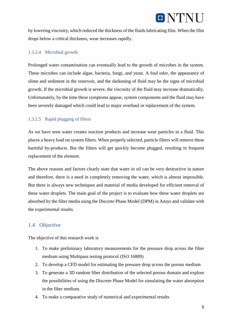
1.4 Objective

The objective of this research work is

1. To make preliminary laboratory measurements for the pressure drop across the filter

medium using Multipass testing protocol (ISO 16889)

2. To develop a CFD model for estimating the pressure drop across the porous medium

3. To generate a 3D random fiber distribution of the selected porous domain and explore

the possibilities of using the Discrete Phase Model for simulating the water absorption

in the fiber medium.

4. To make a comparative study of numerical and experimental results

7

1.5 Scope

This thesis work is an applied research work based on the requirement of the industry and

addresses how CFD can be used to improve the water filtration in hydraulic oil. Out of different

water separation/filtration techniques, this research is limited only to absorption method using

a multi-layered cellulose media. The work considered the experimental measurements of

pressure drop across the filter medium to generate the flow resistance coefficients of porous

material using the Darcy-Forchheimer equation, which are then used to define the material

properties in the CFD simulations. While the numerical modeling of media pack in the form of

flat sheet is validated using the laboratory measurements, the full-scale pleated filter is not

modeled in this work due to time constraints. However, a correction factor based on the

measurements of flat sheet vs pleated filter is used to extend the numerical findings of flat sheet

filter media to the pleated filter.

The attempt of generating the multiphase flow through a microstructural porous media is made

in this study. To reduce the complexity of the investigation, only X fibers are created in the

geometry model. However, the effective porosity of the modeled medium is consistent with

the real product. Also, the number of water particles injected into the domain is limited to

approximately 1500 to reduce the CPU effort. The validation experiments considered only the

steady state inflow conditions, which is not the reality in industrial applications. The scope of

this work is pictorially presented in Figure 1.4. These numerical models can be further

improved, and the knowledge can be of help in enhancing the porous properties of the medium.

8

Figure1. 4: Scope of the thesis

1.6 Conclusion

In this thesis, the focus is on liquid-liquid separation, where the water is filtered out from the

hydraulic oil flow. Water can be in dissolved, undissolved (free) or entrained in an oil.

Depending on the form of waters presence in the oil, there are different water removal methods

such has settling, centrifuging, coalescing, vaccum distillation, adsorption, and absorption.

This chapter presented the introductory remarks of the project including the problem definition,

objectives, and scope of this work. The project focuses on the water absorbing property of the

fiber media, where a huge knowledge is available a wide range of application possibility. The

next chapter will make a literature survey on the porous flows and phase separation, which is

critical for developing an acceptable research methodology.

9

2 Literature Review

2.1 Introduction

This chapter will focus on the topics that can be utilized in developing a methodology to carry

out the thesis. Section 2.2 gives an overview of how a porous media is used in filtration

applications and its properties like porosity and permeability. Section 2.3 explains different

water separations concepts such as coalescence and absorption process which are important in

understanding the physics of water droplets in fluid flows. The dynamics of fluid inside a

porous structure is given by Darcy-Forchheimer law. The literature focuses on how this law

can be utilized in determining the flows through porous media. The law is further used in fluid

flow equations for developing a numerical model. The simulation is carried out with the help

of Ansys Fluent and is detailed in section 2.6 respectively. There are many standard

experiments developed to study the porous medium, but section 2.7.4 will focus on two

experiments that can be used in validating the CFD model.

2.2 Porous media

Porous media are encountered everywhere in our daily life, technology and nature. Some dense

rocks and some plastics, virtually all solid and semi-solid materials are ‘porous’ in varying

degrees. For a material to be porous it should exhibit the following properties:

1. The material must contain pores or voids, free of solids, imbedded in a solid or semi-solid

matrix.

2. It is permeable to a variety of fluids, i.e. the fluid should be able to penetrate through one

face of material and emerge on the other side of the material.

Porous materials have become critical in engineering and technological advancements. In

hydrology, it relates to water movement in earth and sand structure and petroleum engineering

which is mainly concerned with petroleum and natural gas exploration and production (Perm

Inc, 2018). Another major application of porous materials is filtration. As the name filtration

means the process used to separate solids from liquids or gases using a filter medium that allows

the fluid to pass through them but not the solid. Here the filter medium is one which functions

like a porous medium.

10

2.2.1 Porosity

Porosity also called as a void fraction, is a measure of empty spaces in the material. It is given

by

Porosity = 𝑉𝑜𝑙𝑢𝑚𝑒 𝑜𝑓 𝑣𝑜𝑖𝑑 𝑠𝑝𝑎𝑐𝑒

𝑇𝑜𝑡𝑎𝑙 𝑣𝑜𝑙𝑢𝑚𝑒

The resistance to the flow through the filter medium depends on the effective pore size. An

ideal medium is characterized by a mass of holes divided by the thinnest possible wall, thus

presenting the maximum open area through which the fluid flows. In practice, these holes

account for an only a small part of the surface. The exact proportion depends on the properties

of the raw material from which the porous medium is made (Purchas & Sutherland, 2011).

Therefore, care should be taken before choosing a medium for specific industrial operation,

because it may affect the capital and operating costs. The actual resistance to flow is a

combination of the porosity and permeability of the medium

2.2.2 Permeability

Permeability is the measure of material’s ability to allow the fluids to flow through it. The

permeability of a filter medium is a vital measure of its capability of filtration. It is usually

determined through the experimental investigation of pressure drop across the medium at

different flow rates. There are several expressions for the permeability of the filter media.

Constant thickness presumption is more commonly used when the porous medium is treated as

a flat sheet than characterizing the medium by its permeability coefficient. Air and water are

the two fluids that are mostly used in the assessment of permeability. The technique employed,

and data generated vary by two extremes; one is using a fixed rate of flow and observing the

corresponding differential pressure and the other is using a fixed pressure and observing the

time required for the flow of the specified volume of fluid. (Purchas & Sutherland, 2011)

The empirical expression for the permeability quantifies the flow rate per unit area under

defined differential pressure. The permeability coefficient of the medium 𝐾𝑝 is defined by the

Darcy equation, which reads

𝑃

𝐿=

𝑄𝜇

𝐴𝐾𝑝

11

where P is the differential pressure in Pa, L is the depth or thickness of the medium in m, Q is

the volumetric rate of flow in m3/s, 𝜇 is the kinematic viscosity in Ns/m2, A is the area in m2,

𝐾𝑝 is the permeability expressed in m2

2.3 Water separation concepts

A dispersion consists of two immiscible liquids, where the dispersed phase exists as droplets

in the continuous phase. In the case of water in oil, as concerned in this project, oil is the

continuous phase and water is the dispersed phase. An appropriate way of removing water from

the oil is usually chosen by the type of problems the contamination is causing. This is due to

the fact that the problem may be related to the water concentration and which determines the

suitability of the separation or filtration method. This section presents the popular methods –

coalescence and absorption of water from the oils.

2.3.1 Coalescence

Multiphase flows are associated with a multitude of interactions, which involve a collision

between the droplets and particles. When two or more droplets collide or in contact with each

other for a long time, the coalescence phenomena take place. A study on the dynamics of drop

coalescence has been revealed that the impact condition decides whether the drop will either

coalesce with another droplet or splash (Fedorchenko & Bang Wang, 2004). It can either form

a complete coalescence with a secondary droplet or may even form partial coalescence. Also,

the drop can bounce off or float on the liquid surface (Yong;Park;Hu;& Leal, 2001). On the

other hand, every collision does not lead to coalescence. When a drop comes in contact with

the surface of the same fluid, it floats on the interface for a finite time until the thin layer of the

surrounding fluid between the two interfaces drains out (Deka;Biswas;Chakraborty;& Dalal,

2019). The coalescence phenomena of two droplets are shown in Figure 2.1 where the thin film

is formed after a finite time.

12

Figure 2. 1: Two droplets going to collide (Left) and Droplets forming a thin film after a

finite time (Right)

2.3.2 Absorption

Absorption is a physical and chemical phenomenon in which atoms, molecules or ions enter a

bulk phase, either liquid or solid material. In this process, the molecules are taken up by volume

by a liquid (absorbent, solvent).

In the context of filtration, filter medium absorbs the liquid contaminant. Absorption filter

media creates a process wherein the porous material draws the contaminant and retains it until

it gets saturated. Figure 2.2 demonstrates how a single fiber absorbs the water molecules in a

filter media.

Figure 2. 2: Process of water absorption by a cellulose fiber

13

2.4 Water Absorption through Cellulose media

Cellulose is one of the popular porous materials. The hydrophilic fibers of the medium are

capable of absorbing the water particles and the pores will allow the oil through flow through

it. The pores of the medium trap the water and hold them 100 to 1000 times their weight in

water, and will allow the oil to pass through them. Absorption of water causes the fibers of the

cellulose paper to swell and the space between the adjacent fibers to reduce, this will cause the

restriction of the flow and rise in the pressure drop across the medium.

2.5 Darcy and Forchheimer law

Flow regimes are classified by the dimensionless quantity called Reynolds number (Re), which

is defined as

𝑅𝑒 =𝜌𝑣𝑙

𝜇

where 𝜌 is the fluid density (kg/m3), 𝑣 is the fluid velocity (m/s), 𝑙 is the characteristics length

(m) and 𝜇 is the fluid viscosity (Pa s).

Refer to Figure 2.3 the flow regimes in porous media are classified as lower Re to higher Re

(Skjetne & Auriault, 1999).

Figure 2. 3: Flow regimes in porous media (Skjetne & Auriault, 1999)

1=Darcy

2=weak inertia

3=Forchheimer (strong inertia)

4=transition from Forchheimer to turbulence

5=Turbulence

14

Darcy (Darcy, 1856) developed a one-dimensional empirical model for laminar flow through

porous media at low flowrates (Re < 1). The pressure gradient and the flow rate have a linear

relationship and it assumes that the viscous forces dominates the inertial forces in the porous

medium. Therefore, the inertial forces can be neglected. Darcy’s equation is given below:

−∇𝑝 =𝜇

𝛼 𝑣

Where 𝑣 is the velocity of the fluid in a porous media, 𝛼 is the permeability of the porous

medium, 𝜇 is the dynamic viscosity of the fluid, ∇𝑝 is the pressure drop in the flow direction.

The law is a standard approach to describe single-phase flow in microscopically disordered and

macroscopically homogenous porous media (Costa, 1999). This law is only valid for flows

with low Reynolds number, such as laminar flows.

Forchheimer equation is a phenomenological approach. It was seen that Darcy’s law deviates

for Re numbers of around 10. For turbulent flows in porous media, both the viscous and inertial

effects cause more non-linear behavior which has to be considered. Forchheimer then added a

term in Darcy’s equation in order to account for this non-linearity. This equation which he

developed is accepted as an extension to Darcy’s equation for higher flow rates. As the flow

rate (Reynolds number) increases, the pressure drop transforms from Darcy regime to

Forchheimer (strong inertia) regime. Therefore, we have

−∇𝑝 =𝜇

𝛼 𝑣 + 𝛽𝜌𝑣2

Where 𝛽 is the inertial resistance(coefficient) or non-Darcy flow coefficient or Forchheimer

coefficient (1/m) and 1

𝛼 is the viscous resistance coefficient.

This viscous resistance coefficient and inertial resistance coefficient are added as a momentum

source term to the standard fluid flow equations during the simulation for a porous media.

2.6 Computational Fluid Dynamics (CFD)

Computational Fluid dynamics (CFD) is used to analyze systems involving fluid dynamics,

heat transfer and various other related phenomena by numerical calculations. It has larger

applications in both industrial and non-industrial applications. In this thesis, Ansys fluent is

used for simulation.

15

Generally, a flow can be described by solving the three consecutive equations:

• Conversation of mass

• Conservation of momentum

• Conservation of energy

For incompressible flows, the equations for conservation of mass and momentum are referred

to as Navier-Stokes equation which is partial differential equations (PDEs) and difficult to

solve analytically. A discretization method that approximates the PDEs with a system of

algebraic equations is applied and solved numerically on a computer. These algebraic equations

are then solved for small domains in space and time. The numerical solution of the flow consists

of a solution in these discretized locations. The accuracy of the solution is very much dependent

on the discretization method used.

The CFD simulation has many advantages in engineering analysis. It is a useful tool to analyze

the flow characteristics when experiments are very costly. But, we need to understand that the

CFD simulations are an approximation of real experiments and should not be considered as a

substitute for experiments, but rather it should be complimentary to experiments.

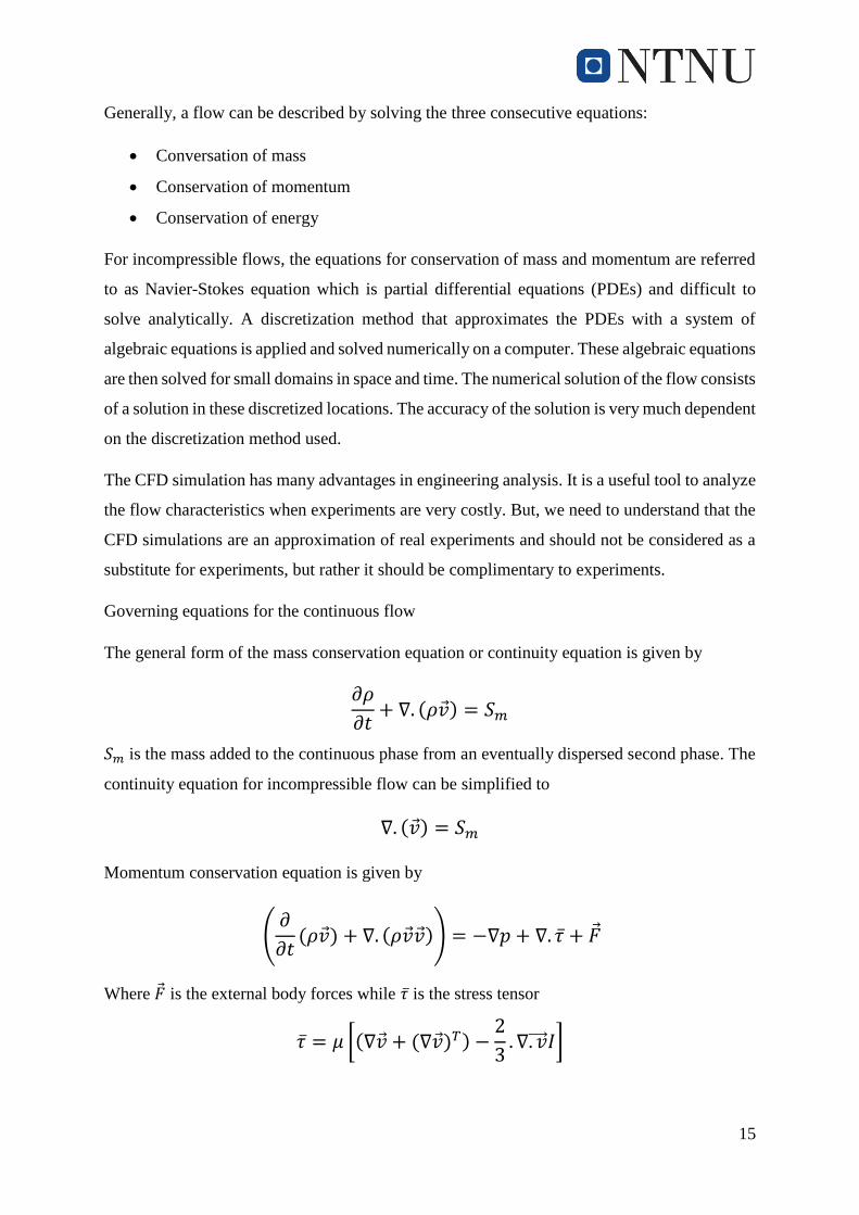
Governing equations for the continuous flow

The general form of the mass conservation equation or continuity equation is given by

𝜕𝜌

𝜕𝑡+ ∇. (𝜌�⃗�) = 𝑆𝑚

𝑆𝑚 is the mass added to the continuous phase from an eventually dispersed second phase. The

continuity equation for incompressible flow can be simplified to

∇. (�⃗�) = 𝑆𝑚

Momentum conservation equation is given by

(𝜕

𝜕𝑡(𝜌�⃗�) + ∇. (𝜌�⃗��⃗�)) = −∇𝑝 + ∇. 𝜏̅ + �⃗�

Where �⃗� is the external body forces while 𝜏̅ is the stress tensor

𝜏̅ = 𝜇 [(∇�⃗� + (∇�⃗�)𝑇) −2

3. ∇. 𝑣⃗⃗⃗⃗ 𝐼]

16

The energy equation can be expressed as:

𝜕(𝑇)

𝜕𝑡+ ∇. (�⃗�𝑇) = ∇(𝛼∇𝑇) +

1

𝜌𝑐𝑣

(𝜏̅. ∇). �⃗�

Here, 𝛼 =𝑘

𝜌𝑐𝑣 is the thermal diffusivity. The energy equation for incompressible flow is

decoupled from Navier Stokes equations. This means that the mass conversation and

momentum conservation equation are solved first for 𝑣 ⃗⃗⃗ ⃗ 𝑎𝑛𝑑 𝑝 and then for energy equation

for T.

2.6.1 Multiphase flow

The flows in nature can be of a mixture of phases that are gas-liquid, gas-solid, liquid-solid or

liquid-liquid flows or also can be a more complex with a mixture of three phases as gas-liquid-

solid flows. In our case, the focus is on two phases that is liquid-liquid phase flows, where oil

is considered as the continuous phase and water is a secondary phase. The secondary phase

volume fraction is low, for this different model are considered below and an appropriate one

which is most equivalent to the case is considered.

There are two basic methods for multiphase phase flow simulation.

1. Eulerian-Eulerian Approach

2. Eulerian-Lagrangian approach

Figure 2. 4: Overview of the modeling approaches (Tsuji, 2008)

17

2.6.1.1 Eulerian Approach

In this approach, different phases are treated mathematically as interpenetrating continua and

are based on the fact that space can only be occupied by a single phase at any one time i.e. total

volume fraction of all the phases are equal to 1. There are several variations in this method

which are listed below.

2.6.1.1.1 VOLUME OF FLUID MODEL

It is a method studied and developed by (Hirt and Nicholas, 1981) and it is a used to model two

or more immiscible fluids by solving a single set of momentum equation and tracking the volume

fraction of each of the fluids throughout the domain.

2.6.1.1.2 MIXTURE MODEL

The mixture model is like VOF model, uses a single fluid approach. But it differs from VOF in

two aspects that is the mixture model allows the interpenetrating of phases, therefore, the volume

fraction for two phases in a control volume can be equal to any volume between 0 and 1. The

mixture model allows the phases to move at different velocities using the concept of slip

velocities. Here, one momentum equation is solved for the n-phases during transportation.

2.6.1.1.3 EULERIAN MODEL

It allows modeling of multiple, yet separate phases. This model, the number of secondary phases

is limited only by memory and convergence behavior. Any number of secondary phases can be

modeled provided there is enough memory is available. In this model ‘N’ momentum equation

is solved for the n-phases during transportation. This model is used when the volume fraction of

the secondary phase is more than 10%.

2.6.1.2 Eulerian-Lagrangian Approach- Discrete Phase model

In this approach, the oil is considered as continuous phase whereas the secondary phase that is

the water liquid is tracked as a discrete particle using the application of Newton’s laws of

motion. In this project, we will look into the Eulerian-Lagrangian approach based on the fact

that the volume fraction of water droplets in oil is less than 10 % and there is limited interaction

with continuous flow. When the volume is low, the force balance for each particle is solved

individually and computational power has to be made. The trajectories of the particles/water

droplets are computed in the Lagrangian reference frame.

18

The force balance on a single particle derived from Newton’s law:

ⅆ𝑣𝑝⃗⃗⃗⃗⃗

𝑑𝑡= 𝐹𝐷(𝑣𝑐⃗⃗ ⃗⃗ − 𝑣𝑝⃗⃗⃗⃗⃗) +

𝑔(𝜌𝑝 − 𝜌)

𝜌𝑝+ 𝐹𝑖

𝐹𝐷 is the drag force which is the function of relative velocity

𝐹𝐷 =18𝜇𝐶𝐷𝑅𝑒𝑟𝑒𝑙

𝜌𝑝𝑑𝑝224

The drag coefficient 𝐶𝐷 can be considered to be a single most important force acting on the

discrete phase. Water droplets attain a spherical shape due to surface tension, and for spherical

particles, the Morsi and Alexander drag law (Morsi & Alexander, 2006) is considered. This

drag law is as follows

𝐶𝐷 = 𝑎1 +𝑎2

𝑅𝑒𝑟𝑒𝑙+

𝑎3

𝑅𝑒𝑟𝑒𝑙2

In the above equations, 𝑣𝑐⃗⃗ ⃗⃗ the velocity of the continuous fluid phase, 𝑣𝑝⃗⃗⃗⃗⃗ 𝑡ℎ𝑒 velocity of the

particle, 𝜇 is the molecular viscosity of the fluid, 𝜌 is the density of fluid, 𝜌𝑝 is the density of

the particle, 𝑑𝑝 is the diameter of the particle, 𝑔(𝜌𝑝−𝜌)

𝜌𝑝 is the gravity force, 𝑅𝑒𝑟𝑒𝑙 is the relative

Reynolds number, defined by:

𝑅𝑒𝑟𝑒𝑙 =𝜌𝑑𝑝(𝑣𝑝 − 𝑣𝑐)

𝜇

The force balance equation also includes additional forces, called 𝐹𝑖. The additional forces are

important in certain times among these are Virtual mass force, which is the force required to

accelerate the fluid surrounding the particle and another is the additional force that exits

because of the pressure gradient in the fluid. Both forces are important when 𝜌 > 𝜌𝑝 . The

additional forces can also include Saffman lift force, Brownian motion, Collision, Break up.

2.7 Research methods

2.7.1 Computational methods

Ansys fluent has a CFD tool can be used to simulate the pressure drop and also analyze the

water absorption process. Since both these characteristics are essential in the present work, an

insight is given for different models.

19

2.7.1.1 Porous modeling in the fluent

Fluent has inbuilt porous media conditions that can be used for a variety of single and

multiphase problems. This condition can be utilized for packed beds, filter papers, perforated

plates, flow distributions and tube tanks (Fluent, 2019). This model is activated only for the

cell zones in which a porous media model is applied and the pressure loss in the flow is

determined by the addition of momentum source term in standard fluid flow equation. The

viscous resistance coefficient and inertial resistance coefficient are considered based on the Re

number. If the viscous forces are dominant, then we neglect the inertial resistance coefficient.

In fluent this resistance coefficient are defined using a cartesian coordinate system where it

defines two direction vectors for 3D and then specify the viscous and/or viscous resistance

coefficient in each direction.

In 3D there are three possible categories of coefficients:

• For isotropic material, the resistance coefficients in all directions are the same and

hence the same values are set in each direction. For example sponge

• When the resistance coefficient in two directions are the same and third direction is

different. Here the values are to be set accordingly for each direction. For example, if a

porous region consists cylindrical straws with small holes in them which are positioned

parallel to the flow direction, the flow would easily pass through the straws, but the

flow in the remaining two directions (through the small holes) would be very little.

• The third possibility is that the coefficients are different in all three direction

These values can be calculated from the experimental data that is available in the form of

pressure drop against velocity through the porous region.

Another important factor that is to be included is the porosity. That is usually in the range of 0

to 1 in fluent. The porosity 𝛾 is the volume fraction of the fluid within the porous region (that

is, the open volume fraction of the medium). The value of 1 describes that the medium is

completely open (no effect of the solid medium). Different material has different porosities

which are to be determined set during the simulation.

2.7.1.2 Discrete Phase modeling (DPM)

The discrete phase model (DPM) in fluent can be used in solving the multiphase problem which

allows simulating a discrete second phase in a Lagrangian frame of reference. This secondary

20

phase consists of the spherical or non-spherical particle (which may be taken as bubbles or

droplets) dispersed in a continuous phase. Fluent has the ability to compute the trajectories of

these discrete phase entities as well as heat and mass transfer to/from them. It can also include

coupling between the phases and its impact on both the discrete phase trajectories and the

continuous phase.

2.7.1.2.1 INJECTION OF PARTICLE OR WATER DROPLETS IN DPM

Water droplets are can be injected into the flow based on the initial conditions of the water

droplet properties. The properties of the water droplets usually include position (x, y, z

coordinates of the particle), velocities (u, v, w) of the particle, the diameter of the particle, the

temperature of the particle and mass flow rate of particle steam that will follow the trajectory

of the individual droplet.

The injections can be from a single point, group or from a surface. Fluent provides a variety of

injection type which can be incorporated based on the desired injections.

Figure 2. 5: Droplet distribution defining an initial spatial distribution of particle streams

(Fluent, 2019)

2.7.1.2.2 BOUNDARY CONDITIONS IN DPM

The fluent’s DPM boundary condition is important in modeling the water absorption process.

Generally, when the particles reach the physical boundary eg: a wall or inlet boundary, fluent

determines the fate of the trajectory at the boundary based on applied discrete phase boundary

condition. These boundary conditions can be defined separately for each zone in the fluent

model.

21

Types of boundary conditions are:

1. Reflect- Rebounds the particle off the boundary by a change in momentum which is

defined by the coefficient of restitution. The normal coefficient of restitution defines

the amount of momentum in the direction normal to the wall that is retained by the

particle after the collision with the boundary (Fluent, 2019).

𝑒𝑛 =𝑣2,𝑛

𝑣1,𝑛

Where, 𝑣𝑛 are the particle velocity normal to the wall and the subscripts 1 and 2 refer

to before and after the collision, respectively.

Figure 2. 6: Reflect Boundary condition in fluent for discrete phase (Fluent, 2019)

2. Trap- This condition terminates the trajectory calculations and records the fate of the

particle as ‘trapped’. This can be utilized in water absorption of cellulose fiber. The

mass of water droplets deposited can be easily determined on the fibers and can be

utilized for studying the distribution, material, and diameter of fibers in the cellulose

media.

Figure 2. 7: Trap Boundary condition in Fluent for discrete phase (Fluent, 2019)

22

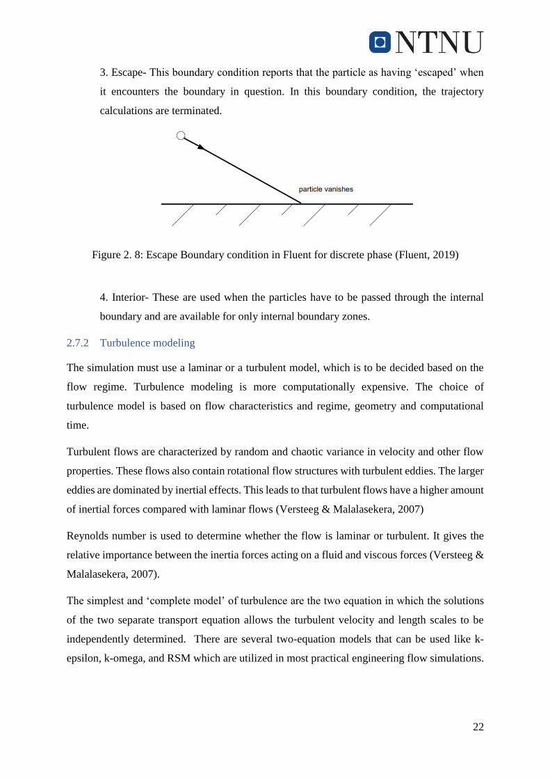
3. Escape- This boundary condition reports that the particle as having ‘escaped’ when

it encounters the boundary in question. In this boundary condition, the trajectory

calculations are terminated.

Figure 2. 8: Escape Boundary condition in Fluent for discrete phase (Fluent, 2019)

4. Interior- These are used when the particles have to be passed through the internal

boundary and are available for only internal boundary zones.

2.7.2 Turbulence modeling

The simulation must use a laminar or a turbulent model, which is to be decided based on the

flow regime. Turbulence modeling is more computationally expensive. The choice of

turbulence model is based on flow characteristics and regime, geometry and computational

time.

Turbulent flows are characterized by random and chaotic variance in velocity and other flow

properties. These flows also contain rotational flow structures with turbulent eddies. The larger

eddies are dominated by inertial effects. This leads to that turbulent flows have a higher amount

of inertial forces compared with laminar flows (Versteeg & Malalasekera, 2007)

Reynolds number is used to determine whether the flow is laminar or turbulent. It gives the

relative importance between the inertia forces acting on a fluid and viscous forces (Versteeg &

Malalasekera, 2007).

The simplest and ‘complete model’ of turbulence are the two equation in which the solutions

of the two separate transport equation allows the turbulent velocity and length scales to be

independently determined. There are several two-equation models that can be used like k-

epsilon, k-omega, and RSM which are utilized in most practical engineering flow simulations.

23

2.7.3 Fluent solver

The phase coupled SIMPLE algorithm can be used to couple the pressure and velocity

equations in our model. The SIMPLE algorithm uses a relationship between velocity and

pressure corrections to enforce mass conservation and to obtain the pressure field. Also, the

discretization methods approximate the differential equations that are solved by the computer.

In order to obtain numerical solutions for governing equations, discretization methods are

implemented. The accuracy of the solution is dependent on the discretization.

First order and second order upwind schemes are the recommended discretization schemes.

The practical difference between these two is the truncation error, which is the difference

between the exact equations and the discretized equations. The truncation error is reduced in a

second order scheme because more cells faces are taken into interpolation. The accuracy is,

therefore, higher for second order scheme than for a first-order scheme, which may also

introduce a high level of diffusion. For this simulation, the discretization of momentum,

turbulent kinetic energy, and specific dissipation rate was done using the second order upwind

method.

Under-relaxation factors are used to control the update of computed variables at each iteration

(Fluent, 2019). This will assist in stabilizing the convergence. If any unstable behavior occurs,

the under-relaxation factors can be reduced.

2.7.4 Experimental methods

2.7.4.1 Single pass and Multi-pass test method

Any porous material or filter elements when developed is tested for its efficiency and

contaminant holding capacity and, in the meantime, not increasing the pressure drop. There are

many efficiency tests that were developed, but there are two tests which are commonly used in

industries, which are the single pass and multiple pass test (ISO, 2008). One simulates the

single pass system and another test the circulating fluid system. In a single pass test, a fluid

volume with a known amount of standard contaminants passes through the test elements only

once. Fluid particle counters determine contamination concentration upstream and downstream

of the element for various particle sizes.

The other test is the Multipass Test Procedure-ISO 16889, where the filtration industry uses it

to evaluate the filter element performance. In this test, the test procedures simulate what

24

happens to a fluid circulating a system. This test creates a realistic mathematical model for

circulating filtration systems. Also, it creates data set for filter elements that can give the

contaminant removal efficiency, contamination holding capacity and differential pressure

rating for any kind of filter being tested. The data set can be used to compare filter elements,

new filter material or media layers and filter housing design. Such comparisons are helpful in

making product selections and thus making designers select cost-effective filter media for their

systems.

Both the tests are to be set with some standard variables and changing these variables can

change the test results for any given element. The standard variables are given below:

• Temperature/viscosity,

• Upstream contamination concentration

• Flow rate and density

• System volume and mass of contamination passed through the filter

• The differential pressure across the element at which the test is ended

The data obtained can be used to calculate the filtration beta ratios. Filtration ratios can be used

to express the fraction of the particles getting through the element and is calculated as described

below.

Beta(X) = No of particle ≥𝑠𝑖𝑧𝑒 (𝑋)upstream

No of particle ≥𝑠𝑖𝑧𝑒 (𝑋)downstream

The table 2.1 illustrates the Beta ratio for any particle size and its corresponding efficiency.

This table can be used for any particle size, and the diameter of the particle in micrometers

would replace the ‘X’ in Beta (X).

Beta (X) Efficiency %

1.0 0.00

1.5 33.33

2.0 50.00

4.0 75.00

10.0 90.00

20.0 95.00

50.0 98.00

75.0 98.67

25

100.0 99.00

200.0 99.50

1000.0 99.90

5000.0 99.98

Table 2. 1: Capture efficiency Vs Beta ratio for any particle size (X)

2.7.4.2 Water absorption test

There are no widely accepted tests methods that are recognized or published by the standard-

setting organization for testing the water removal elements. Testing labs usually use Single

pass and Multipass test methods for water absorption to test and rate the water removal

elements. Thus, the manufacturers are free to establish and develop their own test methods.

Most of the laboratories use the Karl Fischer titration method to measure the water content in

the fluid.

A known quantity of water is fed into the system at a known flow rate using a peristaltic pump.

The water-laden fluid is pumped through a test filter using a gear pump followed by a

centrifugal pump to emulsify the water into the oil. The differential pressure is monitored and

the filtered fluid is returned to the reservoir.

Capacity and Efficiency can be calculated using the below formula:

Capacity C = 𝑾𝒇𝒆𝒅 − 𝑾𝒓𝒆𝒎𝒂𝒊𝒏𝒊𝒏𝒈

Efficiency % = 𝑾𝑪𝒂𝒑𝒕𝒖𝒓𝒆𝒅

𝑾𝒇𝒆𝒅 X 100 %

Where C is the Capacity

E is the Efficiency

𝑊𝑓𝑒𝑑= Mass or Volume of water feed

𝑊𝑟𝑒𝑚𝑎𝑖𝑛𝑖𝑛𝑔= Mass or volume of water remaining

𝑊𝑐𝑎𝑝𝑡𝑢𝑟𝑒𝑑= Mass or volume of water absorbed

2.8 Conclusions

It is evident that porosity and permeability are the two main factors that characterize a porous

medium. The one-dimensional empirical model for laminar flow through porous media by

26

Darcy is used in developing the numerical model. The necessary inputs to the model can be

calculated from experiments and thus helping in validation of the numerical results.

Computational Fluid Dynamics has the capabilities to estimate the pressure drop and amount

of water deposited on the fibers of the filter media. Ansys Fluent is used for this purpose, where

Darcy’s law is added to the standard fluid flow equation that results in pressure variations for

the considered cell zones and DPM model is used in simulating the water absorption process.

From the above literature study, a research methodology is developed that is used in estimating

the pressure drop and water absorption for the considered filter element.

27

3 Methodology

3.1 Introduction

The methodology is developed based on the literature study of various experiments and fluid

flows relating to the porous medium. There are two experiments which are to be conducted,

one is the pressure drop test by Multipass method and other is the water absorption test. The

experiments are conducted at Parker’s R&D lab. The first experiment measures the pressure

drop and other experiment measures the water content absorbed for the considered filter media.

The experiments are detailed in section 3.2 and 3.3 respectively. CFD models were generated

based on the media used in the filter element. Two models were developed that are illustrated

in sections 3.4.1 and 3.4.2 respectively. Figure 3.2 shows the detailed methodology flowchart

adopted in the project.

28

Figure 3. 1: Detailed methodology

29

3.2 Pressure drop tests using Multipass method

The multipass test is used for providing the information of differential pressure across the

element. A Schematic diagram of the experimental system is shown in figure 3.2.

In this project, the test is used for measuring the pressure drop for flat sheet and pleated

element. There is no information or data related to contamination removal efficiency or

contamination holding capacity as the contaminants are not added. It will only focus on the oil

flow through the flat sheet and pleated element which results in differential pressure for

different flow rates. From this experiment, a correction factor is determined that is used in

calculating the viscous resistance coefficient. This coefficient is used in porous modeling

during CFD simulation. Figure 3.3 and Table 3.1 shows the Multipass test bench and its

specifications.

Figure 3. 2: Schematic diagram of Multipass test bench

30

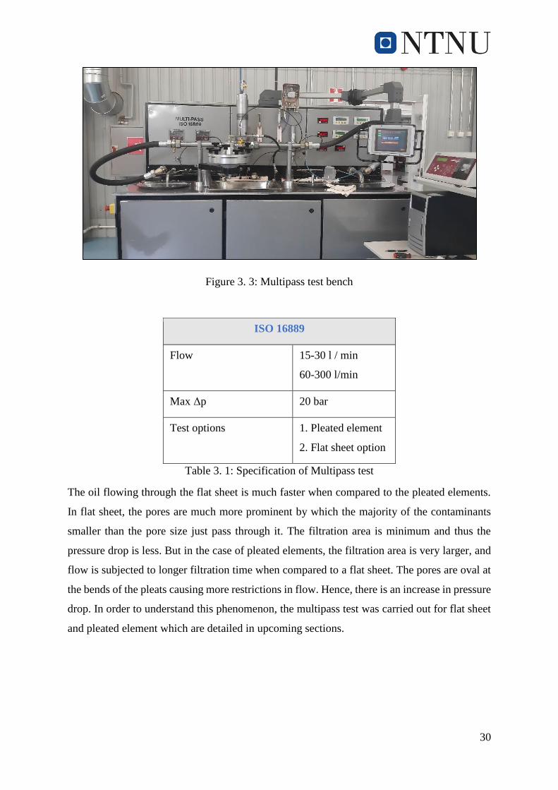
Figure 3. 3: Multipass test bench

ISO 16889

Flow 15-30 l / min

60-300 l/min

Max Δp 20 bar

Test options 1. Pleated element

2. Flat sheet option

Table 3. 1: Specification of Multipass test

The oil flowing through the flat sheet is much faster when compared to the pleated elements.

In flat sheet, the pores are much more prominent by which the majority of the contaminants

smaller than the pore size just pass through it. The filtration area is minimum and thus the

pressure drop is less. But in the case of pleated elements, the filtration area is very larger, and

flow is subjected to longer filtration time when compared to a flat sheet. The pores are oval at

the bends of the pleats causing more restrictions in flow. Hence, there is an increase in pressure

drop. In order to understand this phenomenon, the multipass test was carried out for flat sheet

and pleated element which are detailed in upcoming sections.

31

3.2.1 Test 1: Pleated element

Pleated element in hydraulic fluid flow system provides a greater surface area and has a greater

capacity to capture and retain particles. The design of pleat numbers and pleats height in the

unit length greatly impacts the pressure drop in the filtration process (Hai Ming Fu, 2014).

The pleated element is a water absorbing type of filter element that is used inside the DF2145

filter. It consists of 57 pleats with an effective height of 317 mm. The pleated media is

composed of six layers of media which are shown in Figure 3.4 and its specification is shown

in Table 3.2.

Figure 3. 4: Layers in the filter element

Fiber orientation Type Thickness in mm

Layer 1 Glass fiber 0.24

Layer 2 Cellulose fiber media 1.3

Layer 3 Cellulose fiber media 1.3

Layer 4 Solid filtering 0.46

Layer 5 Non-woven 0.24

Layer 6 Metal mesh 0.1778

Total thickness 3.7178

Table 3. 2: Media layer specifications

32

The experiment is conducted to estimate the pressure drop occurring due to the oil flow through

the pleated element. The experiment is started by maintaining the temperature of the oil at 40°C

whose viscosity is found to be 15 Cst. The pump used to circulate the oil is set in such a way

that the desired flow rates are obtained, refer to Table 3.3. The experiment is repeated for 5

times, so there is consistency in the reading and the average pressure drop is taken into

consideration. The results are compared with the flat sheet values that are detailed in section

4.1. Figure 3.5 shows the housing used for the pleated element.

Figure 3. 5: Housing used for Pleated element in the test rig

Flowrate

l/min

Viscosity

Cst

Density

𝑘𝑔/𝑚3

Temperature

°C

Operating

pressure

Pa

50 15 870 40 500000

100 15 870 40 500000

150 15 870 40 500000

Table 3. 3: Test matrix for the pleated element

33

3.2.2 Test 2: Flat sheet

The flat sheet is cut from the actual pleated element. The pleats are straightened and made flat.

It contains the exact six layers that are used in the pleated element whose function is to capture

the contaminants like dust, metals, water droplets, etc. The flat sheet containing the six layers

is cut exactly in 0,189 m in diameter and placed on the testing rig. Figure 3.6 and Figure 3.7

shows the flat sheet and housing used for flat sheet in the test bench.

Figure 3. 6: Flat sheet and its layer orientation used for pressure drop test

Figure 3. 7: Housing used for flat sheet in the test bench

The pressure drop from the flat sheet is comparatively less when compared with the pleated

element which is determined using the experiment. The experimental condition is not changed,

and the oil temperature and viscosity are maintained at 40°c and at 15 Cst. The maximum

pressure drop for a flat sheet of area 0.0282 m2 is less than 5 bars, therefore, the flow rates are

34

reduced in this case. The experiment is repeated for 5 times, so there is consistency in the

reading and the average pressure drop is taken into consideration. The results are compared

with the pleated element values that are detailed in section 4.1. Table 3.4 shows the test matrix

for the flat sheet media.

Flowrate

l/min

Viscosity

Cst

Density

𝑘𝑔/𝑚3

Temperature

°C

Operating

pressure

Pa

5 15 870 40 500000

10 15 870 40 500000

15 15 870 40 500000

Table 3. 4: Test matrix

3.3 Test bench for water absorption from hydraulic flows

Water absorption test is used to determine the water absorbing properties of a filter element.

This setup is specially designed and used when water is a major contaminant in the hydraulic

oil flow. The experiment will yield pressure drop, water absorption capacity, time and

efficiency of filter media. The results are used for comparison and selection of the type of water

absorber, media layer specification for specific water absorption operation.

This test setup was built in house at Parker’s R&D lab and is based on the multi-pass

arrangement. The setup contains a free circuit and a test circuit. In the free circuit, oil is in

continuous circulation in the system and the test circuit is where the filter element is placed for

testing. The reservoir tank stores and supplies the oil in the system. The setup also contains a

small water tank to supply water into the oil. A temperature sensor is used to record the

temperature of the oil. Pressure, water content and flow measurements are also noted by the

system for continuous monitoring. Water content in an oil is measured using an Oilan water

analyzer device that instantaneously shows the changes in the lubrication oil’s water content.

A Schematic diagram of the experimental system is shown in Figure 3.8. Table 3.5 shows the

instruments and its uncertainty from the manufacturers.

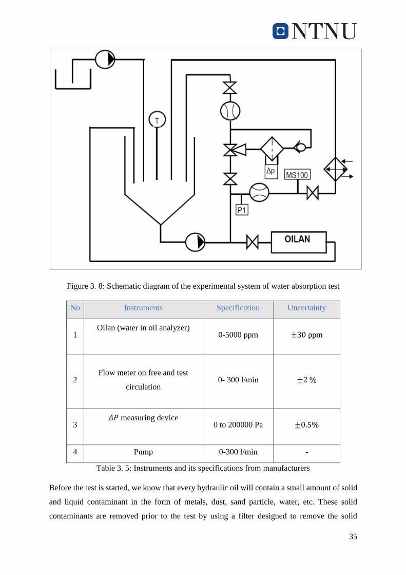
35

Figure 3. 8: Schematic diagram of the experimental system of water absorption test

No Instruments Specification Uncertainty

1 Oilan (water in oil analyzer)

0-5000 ppm ±30 ppm

2 Flow meter on free and test

circulation 0- 300 l/min ±2 %

3 𝛥𝑃 measuring device

0 to 200000 Pa ±0.5%

4 Pump 0-300 l/min -

Table 3. 5: Instruments and its specifications from manufacturers

Before the test is started, we know that every hydraulic oil will contain a small amount of solid

and liquid contaminant in the form of metals, dust, sand particle, water, etc. These solid

contaminants are removed prior to the test by using a filter designed to remove the solid

36

particles. When maximum particles are removed, the setup is changed to test circuit. This is

done so the solid particles will not influence the pressure drop during the water absorption

process.

The test is started by adding 200 ml (0.2 kg) of water into 20-liter oil reservoir tank (volume

of water in oil is 0.01%) and allowing it to mix for about 30 minutes. The test circuit is then

opened were oil and water start flowing through the water absorbing filter element. The filter

element starts absorb the waters molecules and reduce the water content in the oil. The

experiment is monitored until there is no further drop in water content in the system. The test

is carried out for different flow rates and corresponding pressure drop and water content values

are noted. Table 3.6 shows the study matrix of the experiment.

Flowrate

l/min

Viscosity

Ns/𝑚2

Density

𝑘𝑔/𝑚3

Temperature

°C

Initial water content

ml

Operating

pressure

Pa

5 0.02784 870 40 200 500000

10 0.02784 870 40 200 500000

20 0.02784 870 40 200 500000

Table 3. 6: Study matrix

3.4 Computational framework

CFD is a well-established tool which can be utilized to study the water absorption in a cellulose

porous media. Firstly, the necessary domain or CAD required to simulate the pressure drop

across a porous media is created using Ansys workbench. The model is further developed with

random fibers that are distributed over its porous zone. The model is then discretized with

appropriate element size and the necessary boundary conditions, physics models are set. The

study does not include any temperature effects; thus the energy equation is not considered. The

mass and momentum equations are then solved using pressure-based solver using SIMPLE

algorithm. A schematic of the general setup is shown in Figure 3.9.

Figure 3. 9: Schematic of the general CFD setup.

Geometry

•Computer Aided Design

Meshing

•Flow geometry is divided into cell

Physics

•Flow and Boundary conditions are setup

Solve

•Flow equations are solved

Post-Processing

•Assessment of flow variables

37

There are two cases which are detailed in the upcoming sections, one is the flow of only oil

through a porous domain which gives a pressure drop and is validated with the pressure drop

test using Multipass method. The second case involves the development of fibers in the porous

domain with a thickness equal to the cellulose water absorber media which is validated using

the water absorption test.

3.4.1 Case 1: Model without Fibers

3.4.1.1 Geometry

The filter contains six layers of media whose thicknesses are equal to 3.717 mm and the overall

length and slighting width of the water absorber media is as shown in Figure 3.10. To make

simulation much easier and faster, only 1/50th of its length and width is considered.

Figure 3. 10: Pleated media stretched to the flat sheet and the size considered for CFD

modeling

The rectangular model of 29.64 mm X 6.34 mm with the overall domain length of 10.717 mm

is created and the model contains three fluid zones that are inlet zone, porous zone and outlet

zone which are of 3 separate bodies, refer Figure 3.11. The six layers of the media which are

3.717 mm in thickness is considered as a single layer with a porosity of 0.9 (from the datasheet

of the material manufacturer) and is represented as a porous zone in the model. This is done as

the model is only used for getting the pressure drop across the porous media with different flow

rates of oil only. The simulation does not include any water absorption phenomenon.

38

The three bodies inlet, porous and outlet have a contact region between each other. These

contact regions are important while carrying out a 1D simplification of porous media model

available for cell zones, which acts as a porous jump type wall condition. But in our case, it is

a 3D model, where the cells are considered as porous zone, and the inlet and outlet face of the

porous zone is considered as interior faces of the zones.

To eliminate the contact region and defining the inlet and the outlet faces of the porous zone

as interior, the geometry containing 3 bodies is formed as one part. Ansys workbench is used

in order to carry out the modeling.

Figure 3. 11: CFD model

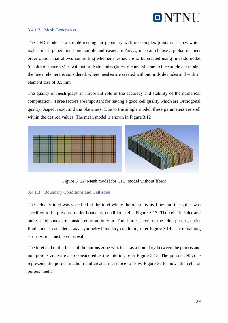
39

3.4.1.2 Mesh Generation

The CFD model is a simple rectangular geometry with no complex joints or shapes which

makes mesh generation quite simple and easier. In Ansys, one can choose a global element

order option that allows controlling whether meshes are to be created using midside nodes

(quadratic elements) or without midside nodes (linear elements). Due to the simple 3D model,

the linear element is considered, where meshes are created without midside nodes and with an

element size of 0.5 mm.

The quality of mesh plays an important role in the accuracy and stability of the numerical

computation. Three factors are important for having a good cell quality which are Orthogonal

quality, Aspect ratio, and the Skewness. Due to the simple model, these parameters are well

within the desired values. The mesh model is shown in Figure 3.12

Figure 3. 12: Mesh model for CFD model without fibers

3.4.1.3 Boundary Conditions and Cell zone

The velocity inlet was specified at the inlet where the oil starts its flow and the outlet was

specified to be pressure outlet boundary condition, refer Figure 3.13. The cells in inlet and

outlet fluid zones are considered as an interior. The shortest faces of the inlet, porous, outlet

fluid zone is considered as a symmetry boundary condition, refer Figure 3.14. The remaining

surfaces are considered as walls.

The inlet and outlet faces of the porous zone which act as a boundary between the porous and

non-porous zone are also considered as the interior, refer Figure 3.15. The porous cell zone

represents the porous medium and creates resistance to flow. Figure 3.16 shows the cells of

porous media.

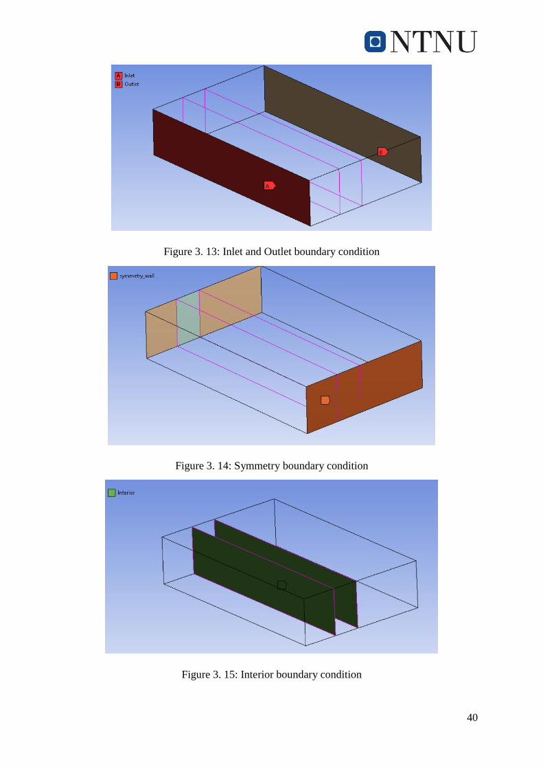
40

Figure 3. 13: Inlet and Outlet boundary condition

Figure 3. 14: Symmetry boundary condition

Figure 3. 15: Interior boundary condition

41

Figure 3. 16: Porous cell zone

3.4.1.4 Turbulence model

The simulation is performed using Ansys Fluent, and it is solved for transient state condition.

The model involves a single-phase flow, where oil flows through a rectangular domain

containing the media with porosity 0.9. In our case, the flow in the inlet and outlet sections is

turbulent and hence, standard k-epsilon with standard fall function model is chosen.

3.4.1.5 Porous condition

The flow through the porous media is considered to be laminar and is characterized by viscous

loss coefficients in the direction of flow that is y-direction. For this, Fluent’s porous media

model was enabled. The media is considered to be impermeable in the remaining two directions

i.e. x and z-direction, whose values of viscous resistance coefficients are four orders of

magnitude higher than in the y-direction. The viscous resistance coefficient and direction are

calculated from the experimental data that is available in the form of pressure against velocity

through the porous media which is determined from pressure drop test using Multipass method.

The pressure drop vs velocity is plotted to create a trendline, through these points an equation

is generated. The equation is now compared with the Darcy equation, from which the viscous

resistance coefficients are determined. Section 4.2 details the estimation of the viscous

resistance coefficients.

42

3.4.1.6 Oil Specifications

Fluid considered is standard Mobile DTE 25 from Exxon Mobil. It finds its application in many

hydraulics systems. Fluent library contains most of the standard fluids used for simulation. But

in our case, new fluid is created using the property of the oil which is listed in Table 3.7.

Type Mobil DTE 24

ISO VG30

Density,

Kg/m3 870

Viscosity, Cst 30

Table 3. 7: Oil Specification

3.4.1.7 Solver Setting

The phase coupled SIMPLE algorithm is used to couple the pressure and velocity equations in

our model. In this case, there is no particle or water injection. The second order upwind spatial

discretization method is chosen for momentum and turbulent equations in order to achieve a

fully converged solution of the flow field. The default values of under-relaxation factors are

chosen. The simulation is then initialized from the inlet and the model is run for a number of

time steps until a converged solution is obtained. The results are discussed in section 4.2 and

are compared with the experimental data.

The CFD model is simulated for 3 different flow rates, refer to Table 3.8

Parameters Simulation 1 Simulation 2 Simulation 3

Fluid Velocity, m/s 0.00295 0.00591 0.00886

Porosity 0.9 0.9 0.9

Fluid viscosity, Cst 30 30 30

Fluid density, kg/m3 870 870 870

Operating pressure, Pa 500000 500000 500000

Table 3. 8: Simulations

43

3.4.2 Case 2: Model with Fibers

3.4.2.1 Random fiber generation

The cellulose porous media is made of fibers that absorb water and retain it up to 10 to 100

times the weight of the water. Hydraulic oil with water passes through these fibers, where water

is absorbed and allowing the oil to flow through them. But in order to simulate water absorption

process, fibers have to be developed. These fibers can vary in length, diameter and also how

well they are packed together in a media. The porosity and permeability can also be varied and

the developed fibers can help us in determining the type of cellulose media for a different type

of water absorption applications. To reduce the complexity of the investigation, only X fibers

are created in the geometry model. However, the effective porosity of the modeled medium is

consistent with the real product.

Figure 3.17 shows a flow chart for the generation of these fibers. Firstly, a domain with length

(Dx), height (Dy) and thickness (Dz) is created with fibers start points and endpoints spread

along x, y, z directions respectively. Table 3.9 shows the domain dimensions based on media

size. Since, the fibers are randomly distributed, therefore, we use the rand () function in Excel

to create the start points 𝑥𝑖 , 𝑦𝑖, 𝑧𝑖 and endpoints 𝑥𝑗 , 𝑦𝑗 , 𝑧𝑗 of fibers. Table 3.10 shows the fiber

details. The endpoints are multiplied with the length of the fiber, which will help in creating

fibers of constant length. The number of fibers is generated based on the porosity required

which in our case is 0.9.

The number of fibers taken determines the porosity, which is calculated as shown below. The

number of fibers taken is 16 in order to attain 0.9 porosity.

Porosity = 𝑉𝑜𝑙𝑢𝑚𝑒 𝑜𝑓 𝑣𝑜𝑖𝑑 𝑠𝑝𝑎𝑐𝑒

𝑇𝑜𝑡𝑎𝑙 𝑣𝑜𝑙𝑢𝑚𝑒

Total Volume is the volume of the domain where the fibers are distributed.

Volume of void space= Volume of the domain (total volume)-Volume of number of fibers

44

Length of domain, Dx (media length) 29.64 mm

Height of domain, Dy (media height) 6.34 mm

Thickness of domain, Dz (media thickness) 2.6 mm

Volume of domain (Total Volume) 488.58 𝑚𝑚3

Table 3. 9: Domain details

Length of each fiber, Lf 15 mm

Diameter of each fiber, df 0.5 mm

Area of each fiber, Af 0.196 𝑚𝑚2

Volume of each fiber 2.94 𝑚𝑚3

Volume of 16 fiber 47.12 𝑚𝑚3

Table 3. 10: Fiber details

From the above table,

Volume of void space= 441.5 𝑚𝑚3

Therefore, Porosity = 441.5

488.58 =0.9

45

Figure 3. 17: Flowchart for generating 3D random fibers

3.4.2.2 Modeling Random fibers

Once the start points and end points are generated, the next step is to read the file .csv file and

develop the fibers in Ansys by assigning the diameter. The inlet zone is created with the exact

dimensions mentioned in section 3.4.1.1. The outlet zone is reduced in length to make the

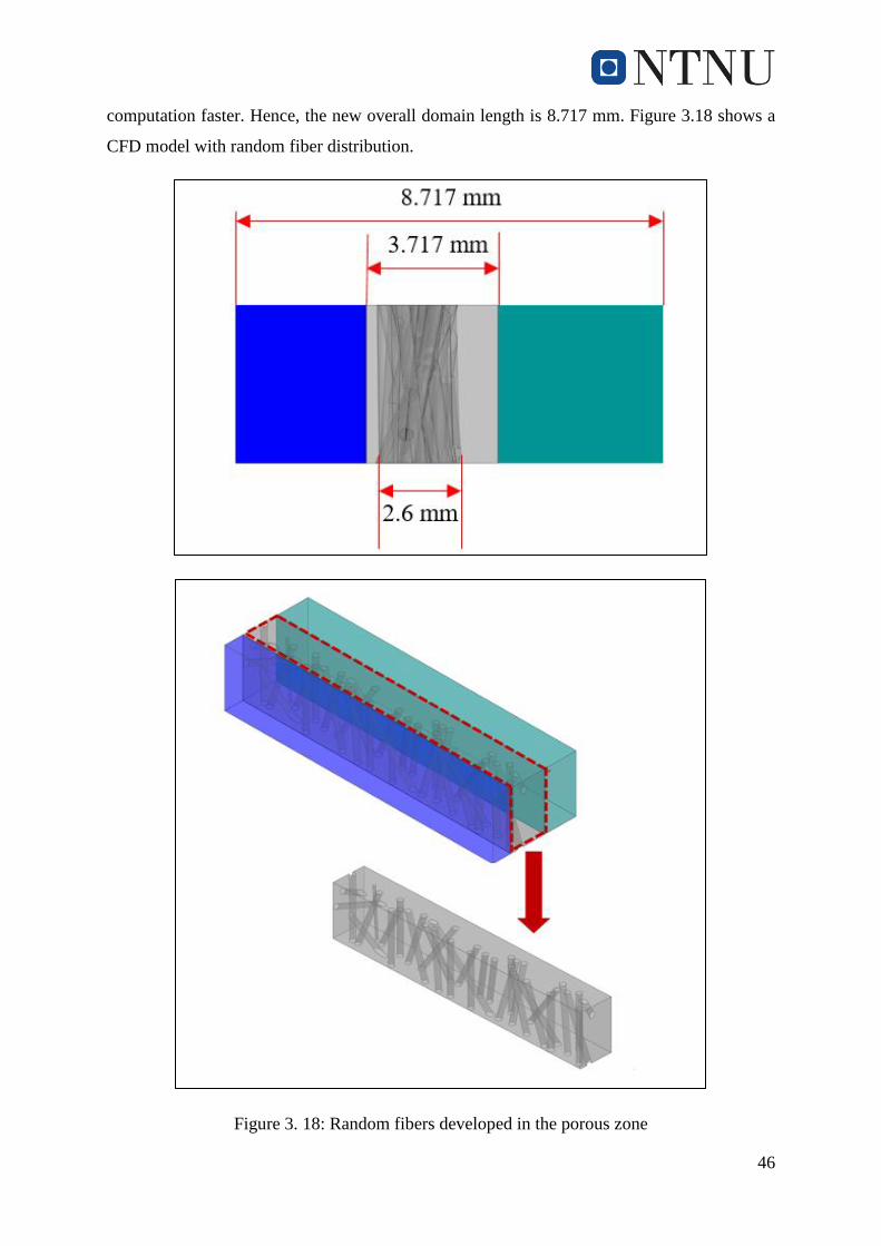
46

computation faster. Hence, the new overall domain length is 8.717 mm. Figure 3.18 shows a

CFD model with random fiber distribution.

Figure 3. 18: Random fibers developed in the porous zone

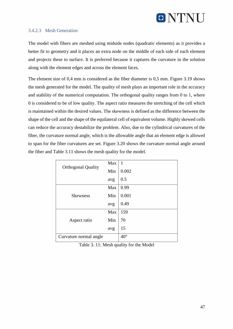
47

3.4.2.3 Mesh Generation

The model with fibers are meshed using midside nodes (quadratic elements) as it provides a

better fit to geometry and it places an extra node on the middle of each side of each element

and projects these to surface. It is preferred because it captures the curvature in the solution

along with the element edges and across the element faces.

The element size of 0,4 mm is considered as the fiber diameter is 0,5 mm. Figure 3.19 shows

the mesh generated for the model. The quality of mesh plays an important role in the accuracy

and stability of the numerical computation. The orthogonal quality ranges from 0 to 1, where

0 is considered to be of low quality. The aspect ratio measures the stretching of the cell which

is maintained within the desired values. The skewness is defined as the difference between the

shape of the cell and the shape of the equilateral cell of equivalent volume. Highly skewed cells

can reduce the accuracy destabilize the problem. Also, due to the cylindrical curvatures of the

fiber, the curvature normal angle, which is the allowable angle that an element edge is allowed

to span for the fiber curvatures are set. Figure 3.20 shows the curvature normal angle around

the fiber and Table 3.11 shows the mesh quality for the model.

Orthogonal Quality

Max

Min

avg

1

0.002

0.5

Skewness

Max

Min

avg

0.99

0.001

0.49

Aspect ratio

Max

Min

avg

159

70

15

Curvature normal angle 40°

Table 3. 11: Mesh quality for the Model

48

Figure 3. 19: Mesh generated for fiber model

Figure 3. 20: Element edges with curvature normal angle.

3.4.2.4 Simulation Setup

In order to simulate water in oil flow, the DPM model is activated. The model is run for steady

state condition. But the particle or the droplet trajectories can be advanced in time in the

simulation for each iteration of the continuous phase. This is done by checking the Unsteady

particle tracking option in Fluent. Here, the particles will be advanced by the particle flow time

step.

49

The K-epsilon with standard wall functions is used for turbulence modeling. The porous model

is activated for the cells of the porous zone and porosity of 0.9 is set. The viscous resistance

coefficient with the correction factor is determined from the pressure drop vs velocity plot of

experimental data. The boundary condition remains the same for the model as mentioned in

section 3.4.1.3, but with an addition of fibers which is set as ‘Trap’ boundary condition for the

droplet to get trapped during the flow. Trapped water droplets depict the water absorbed by the

fibers. This trap condition is only available using Discrete phase model in fluent which makes

it distinct from various other models and thus estimating the number of water droplets

deposited on the fibers. Figure 3.22 shows the fibers which are set with ‘TRAP’ boundray

conditon.

Figure 3. 21: Fibers set with ‘TRAP’ Boundary condition

The volume of water in oil is very less, which is 0.01%. The droplets are injected from the inlet

surface of the model that releases particle stream from each facet of the surface. The mesh

model contains about 1360 mesh facet on the inlet surface. The droplets are made to inject

normal to the face of the surface. The number of droplets is usually injected as parcels. The

concept of parcels is that each parcel contains a number of droplets which makes computational

time, memory and cost of computation very less.

The initial parameters such as start time and end time, type of droplet, droplet velocity, droplet

diameter are also defined. These initial parameters provide the starting values for all the

dependent discrete phase variables that describe the instantaneous conditions of individual

droplets. Table 3.12 shows the simulations carried out for three different velocities for the

model.

50

Continuous Phase – oil

Simulation 1 Simulation 2 Simulation 3

Oil velocity, m/s 0.0001773 0.000354 0.000709

Oil density, kg/m3 870 870 870

Oil viscosity, Cst 30 30 30

Operating pressure, Pa 500000 500000 500000

Discrete phase-water droplets

Velocity, m/s 0.0001773 0.000354 0.000709

Diamter of the droplet, mm 1e-5 1e-5 1e-5

Start of injection, s 0.2 0.2 0.2

End of injection, s 0.2 0.3 0.3

Density, kg/s 998 998 998

Total Flow rate. kg/s 0.000143 0.000143 0.000143

Table 3. 12: Simulations- Case 2 CFD model with fibers

3.5 Conclusion

The experiments were performed, and pressure drop measurements were recorded with the

least errors. The experiments were able to yield many factors that can be utilized in developing

the filter. But, it is limited to estimating the pressure drop and water content in oil. The tests

are carried out for three flow rates that yielded corresponding pressure drop values which

discussed in the next chapter.

The CFD model is developed considering the porous layers and its function. Each layer has its

importance, but only the layer which absorbs water is developed with fibers, other layers are

considered within the porous zone with a porosity of 0.9. Only X number of fiber were

generated, but the porosity is in consistent with the considered product. This is done in order

to make the simulation simple and faster. The CFD modelsare simulated with the same inputs

used in the experiments. The porous and DPM model in Ansys Fluent was successfully

implemented in determining the pressure drop and water content for the considered filter

element. The results are detailed in the next chapter.

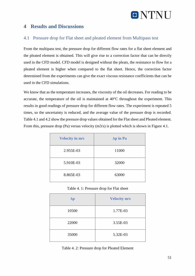
51

4 Results and Discussions

4.1 Pressure drop for Flat sheet and pleated element from Multipass test

From the multipass test, the pressure drop for different flow rates for a flat sheet element and

the pleated element is obtained. This will give rise to a correction factor that can be directly

used in the CFD model. CFD model is designed without the pleats, the resistance to flow for a

pleated element is higher when compared to the flat sheet. Hence, the correction factor

determined from the experiments can give the exact viscous resistance coefficients that can be

used in the CFD simulations.

We know that as the temperature increases, the viscosity of the oil decreases. For reading to be

accurate, the temperature of the oil is maintained at 40°C throughout the experiment. This

results in good readings of pressure drop for different flow rates. The experiment is repeated 5

times, so the uncertainty is reduced, and the average value of the pressure drop is recorded.

Table 4.1 and 4.2 show the pressure drop values obtained for the Flat sheet and Pleated element.

From this, pressure drop (Pa) versus velocity (m3/s) is plotted which is shown in Figure 4.1.

Velocity in m/s Δp in Pa

2.955E-03 11000

5.910E-03 32000

8.865E-03 63000

Table 4. 1: Pressure drop for Flat sheet

Δp Velocity m/s

10500 1.77E-03

22000 3.55E-03

35000 5.32E-03

Table 4. 2: Pressure drop for Pleated Element

52

Figure 4. 1: Pressure drop vs Velocity for Flat and Pleated Element

From the above plot, the slope of the curves yields the correction factor. The viscous resistance

is different for flat sheet and pleated element. This correction factor is used in determining the

exact viscous resistance coefficient for a flat sheet. The resulting viscous resistance coefficient

is used in the case 2 CFD model for attaining a good validation with the experimental results.

Correction factor, CF = 𝑆𝑙𝑜𝑝𝑒 𝑜𝑓 𝑃𝑙𝑒𝑎𝑡𝑒𝑑 𝐸𝑙𝑒𝑚𝑒𝑛𝑡

𝑆𝑙𝑜𝑝𝑒 𝑜𝑓 𝐹𝑙𝑎𝑡 𝑆ℎ𝑒𝑒𝑡

Correction Factor, CFD = 0.78

4.2 Flat sheet Analysis using CFD (CFD model without fibers)

The aim of the simulation work is to study the pressure drop occurring due to the porous

medium in the domain. Before the simulation is started, the viscous resistance coefficients must

be calculated from the pressure drop experiment for a flat sheet. From table 4.1, the pressure

drop against velocity through the porous component is extrapolated to determine the viscous

coefficients for the porous media.

The pressure drop vs velocity is plotted to create a trendline, through these points an equation

is generated. The equation is now compared with the Darcy equation, from which the viscous

resistance coefficients are determined.

0

10000

20000

30000

40000

50000

60000

70000

0 0,002 0,004 0,006 0,008 0,01

Dp

in

Pa

Velocity in m/s

Flat Sheet vs Pleated Element

Flat Sheet

Pleated Element

53

Figure 4. 2: Equation from the experimental result of Flat sheet

The plot from Figure 4.2, yields the following equation:

∆𝑝 = 6393342.86 𝑣

Where ∆𝑝 is the pressure drop in Pa and 𝑣 is the velocity in m/s

The above equation is compared with the Darcy equation as the flow is laminar through porous

media (Re<1).

∇𝑝 =𝜇

𝛼 𝑣

By comparing the above equations, the viscous resistance coefficient, 1

𝛼 is found to be to

8.19e+06 1

𝑚2 . The flow is through a 3D porous domain and is considered to be laminar,

therefore, it is characterized by viscous loss coefficients in the direction of flow which in the

present case is in the positive y-direction. The media is impermeable in the remaining two

directions i.e. x and z-direction, whose values of viscous resistance coefficients are four orders

of magnitude higher than in the y-direction. The table below gives the viscous resistance

coefficient in x, y, z directions.

∆𝑝= 6 393 342,86𝑣

0

10000

20000

30000

40000

50000

60000

70000

0 0,001 0,002 0,003 0,004 0,005 0,006 0,007 0,008 0,009 0,01

Dp

in P

a

Velocity m/s

Equation from experimental data

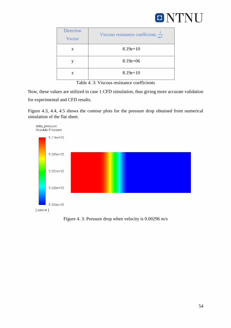
54

Direction

Vector Viscous resistance coefficient,

1

𝑚2

x 8.19e+10

y 8.19e+06

z 8.19e+10

Table 4. 3: Viscous resistance coefficients

Now, these values are utilized in case 1 CFD simulation, thus giving more accurate validation

for experimental and CFD results.

Figure 4.3, 4.4, 4.5 shows the contour plots for the pressure drop obtained from numerical

simulation of the flat sheet.

Figure 4. 3: Pressure drop when velocity is 0.00296 m/s

55

Figure 4. 4: : Pressure drop when velocity is 0.00591 m/s

Figure 4. 5: Pressure drop when velocity is 0.00887 m/s

Pressure drop in Pa Velocity in m/s

11486 2.955E-03

33112 5.910E-03

65171 8.865E-03

Table 4. 4: Pressure drop for Flat sheet from simulation

56

4.3 Experiment vs Numerical simulation of Flat sheet

From Table 4.1 and 4.4, it is seen that the values of pressure drop obtained from numerical

simulation lies within 5 % error margin of experimental pressure drop values. The results

obtained are very well in accordance with each other, the model forms a good basis for

developing the model further with 3D random fibers in the porous zone and simulate the water

absorption process. Figure 4.6 shows the pressure drop plot of experimental vs CFD results.

Figure 4. 6: Experimental vs CFD with 5% error for flat sheet

4.4 Pressure drop from the water absorption test

The water absorption test carried on the pleated filter element yielded the pressure drop which

is presented in Table 4.5. The experimental data is extrapolated to find the viscous resistance

coefficient.

Velocity in m/s Pressure drop in Pa

0.0001773 20000

0.000354 53000

0.000709 85000

Table 4. 5: Pressure drop from the water absorption test

0

10000

20000

30000

40000

50000

60000

70000

0 0,002 0,004 0,006 0,008 0,01

Dp

in P

a

Velocity in m/s

Exp vs CFD -Flat Sheet with 5 % error

Exp

CFD

57

Figure 4. 7: Pressure drop vs velocity from the experiment

The plot from Figure 4.7, yields the following equation,

∆𝑝 = 123408172.46 𝑣

The above equation is compared with the Darcy equation. The correction factor is also

incorporated in the viscous loss terms and we have the new viscous resistance coefficient with

a correction factor, refer Table 4.6.

Direction

Vector Viscous resistance coefficient,

1

𝑚2

x 1.44e+12

y 1.44e+08

z 1.44e+12

Table 4. 6: Viscous resistance coefficient

4.5 Pressure drop estimation using CFD model with fibers

The CFD model with fibers is solved for steady state condition. The values from table 4.6 are

utilized in CFD simulation. The oil is considered as continuous phase and water as discrete

phase. The volume of water in oil is 0.01% therefore, the water molecules are not causing a

∆𝑝= 1E+08 𝑣

0

10000

20000

30000

40000

50000

60000

70000

80000

90000

100000

0 0,0002 0,0004 0,0006 0,0008

Dp

in P

a

Velocity m/s

Equation from experimental data

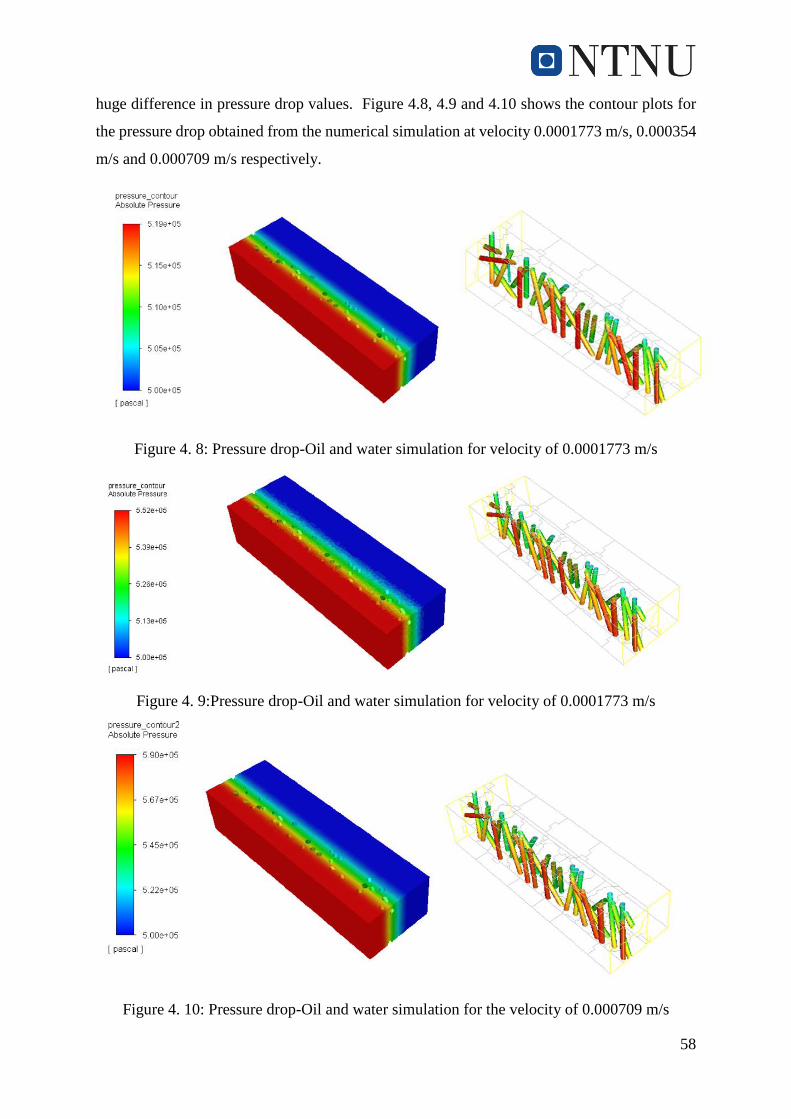
58

huge difference in pressure drop values. Figure 4.8, 4.9 and 4.10 shows the contour plots for

the pressure drop obtained from the numerical simulation at velocity 0.0001773 m/s, 0.000354

m/s and 0.000709 m/s respectively.

Figure 4. 8: Pressure drop-Oil and water simulation for velocity of 0.0001773 m/s

Figure 4. 9:Pressure drop-Oil and water simulation for velocity of 0.0001773 m/s

Figure 4. 10: Pressure drop-Oil and water simulation for the velocity of 0.000709 m/s

59

Velocity in m/s Pressure drop in Pa

0.0001773 19500

0.000354 52500

0.000709 90000

Table 4. 7: Pressure drop from CFD simulation with fibers

4.6 Experiment vs Numerical simulation of model with fibers

From Table 4.5 and 4.7, it is seen that the values of pressure drop obtained from numerical

simulation lies within 5 % error margin of experimental pressure drop values. The results

obtained are very well in accordance with each other but increasing for higher velocities. This

indicates that the inertia forces are arising which are to be considered while simulating for high

velocity flows. Figure 4.6 shows the pressure drop plot of experimental vs CFD results.

Figure 4. 11: Experimental and CFD results

0

10000

20000

30000

40000

50000

60000

70000

80000

90000

100000

0 0,0002 0,0004 0,0006 0,0008

Dp

in P

a

Velocity m/s

Experimental vs CFD- with 5 % error

Experiment

CFD

60

4.7 Water removal efficiency

The experiment was added with 200 ml of water in 20- liters of the oil reservoir tank. The water

content was monitored at regular intervals of time. But in the present case, only the initial and

final water content values are considered. When the flow rates increase, the water retention

capacity of the filter element reduces. Filters are very efficient at low flow rates, as filter paper

is in a long time in contact with water droplets. But due to the limitation of the numerical

model, its compared with only single set of experimental values. The experimental and

simulation results are given in the table 4.8. The capacity and efficiency are calculated using

the formula,

Capacity C = 𝑾𝒇𝒆𝒅 − 𝑾𝒓𝒆𝒎𝒂𝒊𝒏𝒊𝒏𝒈

Efficiency % = 𝑾𝑪𝒂𝒑𝒕𝒖𝒓𝒆𝒅

𝑾𝒇𝒆𝒅 X 100 %

The amount of water droplet injected is equivalent to the number of mesh facet on the inlet

surface of the CFD model, which in our case is 1360. Ansys fluent injects 1360 particle streams

with total mass flow rate of 0.000143 kg/s that will follow the trajectory of the individual

particle/droplet. From the simulations, the fibers were able to trap 900 particle streams during

the flow which is equivalent to 0.159 kg of water deposited on the fibers. Table 4.8 shows the

capacity and efficiency of filter medium from experimental and numerical simulations. Figure

4.12 shows the mass concentration of water droplets on the fibers.

Methods Velocity

m/s

Water fed

𝑾𝒇𝒆𝒅

ml

Water

remaining

𝑾𝒓𝒆𝒎𝒂𝒊𝒏𝒊𝒏𝒈

ml

Water

captured

𝑾𝑪𝒂𝒑𝒕𝒖𝒓𝒆𝒅

ml

Capacity

C

ml

Efficiency

%

Experiment 0.0001773 200 20 180 180 90

CFD 0.0001773 200 40.1 159.85 159.85 80

Table 4. 8: Experimental and Simulation results of water absorption test

61

Figure 4. 12: Discrete phase concentration on the fibers

4.8 Limitation of the model

The CFD model with fiber only shows, the amount of water trapped and how the random fibers

are oriented. The fibers generated can take up any amount of water molecules without any

limit. But in actual cellulose porous media, these fibers have some limits in absorbing the water

and when they absorb water they tend to expand thereby reducing the pore size in the media.

This increases the pressure drop and after a certain point the filter element has to be changed.

The water retention property of the media also decreases when it has captured some of the

water molecules. Also, as the velocity increases the water absorbing ability of the cellulose

porous media reduces, this is because the water molecules has to be in contact with cellulose

media for a longer time. The longer the water molecules are in contact, the better the efficiency.

All these characteristics of a media are which the CFD model cannot include in its simulation.

But what the model can simulate is the stochastic collision-coalescence, breakup during the

flow and also its interaction with the continuous phase. The model can be further developed

for turbulent flows in porous domain by considering the inertial effects. The water properties

such as diameter, velocity can also changed based on requirements. Though there are

limitations, it can be further developed for studying the oil water separation process.

62

5 Conclusion

The preliminary objective was to carry out a pressure drop test across a porous medium using

a standard Multipass arrangement. The data from the test was fed into the model in order to

validate the data predicted by the computational model. The data considered during the

experiments were also used in the numerical model, therefore there is much consistency in the

results. The estimated pressure drop for flat sheets from simulations was compared with

experimental data and was found to be within 5% deviation from the experimental values. The

model thus formed a good base for further improvements and thereby introducing fibers into

the porous media.

In present work, a full-scale model of the pleated element was not developed, but a correction

factor based on the measurements of flat sheet vs pleated filter is used to extend the numerical

findings of flat sheet filter media to the pleated filter. The flat sheet model is now developed

with fibers in porous domain to simulate the water absorption process. The main aim was to

separate the water droplets from hydraulic oil flows using these generated fibers. These fibers

are randomly distributed in cellulose porous media. The 3D random fiber distribution in the

porous model was achieved using rand() function is excel, that created start and endpoints of

the fibers. The points were read into Ansys and thus an effective porous model consistent to

the real product was obtained. The goal for developing these fibers was to absorb and trap water

molecules which was successfully implemented by using the Discrete Phase model in Fluent.

The pressure drop and water removal efficiency was found to be in accordance with the

experimental data. Due to time constraints, water removal efficiency by the numerical model

is validated with only single set of experimental data and for steady state inflow conditions.

Therefore, there is a need for further simulations which can improve the model significantly.

The next section gives useful insights for carrying out further simulations which can be

included in investigation of water absorption process of the porous media.

63

6 Future work

The thesis developed just gives the overview and basic structure for simulating the water

absorption process. The model can be further developed by considering the following

recommendations for future studies.

• The numerical model does not include temperature effects in its simulation. At high

temperatures the viscosity changes and water molecules can evaporate, hence a user

defined function can be used to include these effects.

• In the present case, the water droplet is of constant diameter. But in actual hydraulic oil

flows, the droplet can be of different sizes. The variations in droplet diameters can be

achieved by using Rosin-Rammler distribution in Fluent.

• The numerical model can be included with Coalescence, Break up modelling in oil

flows. The droplets can coalesce or split into multiple droplets based on the impact

conditions. This physics model can be included in further developments of the model

but can be expensive due to increased computational time.

• The fibre distribution in the porous domain can be varied based on porosity. The fiber

diameter considered in the study is quite large, which can be reduced to make the model

realistic as possible. The smaller the diameter of fiber, the smaller should be the grid

size.

• The project involves two phase flows, where oil is considered to be continuous phase

and water as discrete phase. The hydraulic oil usually consists of solids, liquids and

gaseous contaminants. Further improvements can be made by introducing, three phase

or multiple phases in oil flows thereby predicting more accurate pressure drop and

particle interactions.

• The model is only for low Reynolds number where viscous forces are dominated.

Hence, there is further scope in including inertia forces to analyse and simulate the

model at high velocities.

• Generally, the permeability and resistance coefficients increase with time which is

common phenomena in filtration process. The model can include this effect by running

for transient inflow conditions.

64

7 References

Abetz, S. (2018, 08 09). Filtech. (K. Journal, Interviewer) From Kohan textile journal:

http://kohantextilejournal.com/filtech-largest-filtration-show-world-wide/

Costa, U. (1999). The role of inertia on fluid flow through disordered porous media. 420-424.

Darcy, H. (1856). Fontaines publiques de la ville de Dijon. Librairie des Corps Imperiaux

des Ponts et Chaussees et des Mines. Paris.

Deka, H., Biswas, G., Chakraborty, S., & Dalal, A. (2019). Coalescence dynamics of unequal

sized drops. Physics of fluid.

Fedorchenko, A., & Bang Wang, A. (2004). On some common features of drop impact on

liquid surfaces. Physics of Fluids 16, 1349-1365.

Fischer, K. (1935). New method for the dimensional analysis of the water content of liquids

and solid bodies. WILEY-VCH Verlag GmbH & Co.

Fluent, A. (2019). Ansys Fluent theory guide. From Ansys :

https://support.ansys.com/portal/site/AnsysCustomerPortal

Hai Ming Fu, Y. F. (2014, June). Experiment and Simulation on Pressure Drop of Pleated Air

Filters. Advanced Materials Research (Volume 960-961).

Haider, A., & Levenspiel, O. (1989). Drag coefficient and terminal velocity of spherical and

nonspherical particles. Power Technology, 63-70.

Hannifin, Parker. (2010, July 19). Filtration separation. Retrieved from Filtsep:

https://www.filtsep.com/filter%20media/features/hydraulic-fluids-controlling-

contamination-in/

ISO. (2008). Hydraulic fluid power -- Filters -- Multi-pass method for evaluating filtration

performance of a filter element.

Morsi, S., & Alexander, A. (2006). An investigation of particle trajectories in two-phase flow

systems. Journal of Fluid Mechanics, 193-208.

Parker Corporation. (2019, May 15). From parker.com: https://www.parker.com

Perm Inc. (2018, June 25). Fundamentals of Fluid Flow in Porous Media. From Perm Inc

TIPM Laboratory: http://perminc.com/resources/fundamentals-of-fluid-flow-in-

porous-media/chapter-1-introduction/

Prince, M., & Blanch, H. (1990). Bubble Coalescence and Break-Up in Air Sparged Bubble

Columns. AIChE Journal 36, 1485-1499.

Purchas, D., & Sutherland, K. (2011). Handbook of Filter media. Elsevier Advanced

Technology.

Skjetne, E., & Auriault, J. (1999). High-Velocity Laminar and Turbulent Flow in Porous

Media. Transport in Porous media, 131-147.

65

Tsuji, T. (2008). Multi-scale structure of clustering particles. World Conference of Particle

techology (WCPT5) (pp. 115-125). Orlando: Elsevier.

Versteeg, H., & Malalasekera, W. (2007). An introcution to Computational Fluid Dynamics:

The Finite Volume Method. Harlow: Pearson Education Limited.

Wright , J. (2008, January). Understanding Filter Efficiency and Beta Ratios. From

Machinery Lubrication: https://www.machinerylubrication.com

Yong, H., Park, C., Hu, Y., & Leal, L. (2001). The coalescence of two equal-sized drops in a

two-dimensional linear flow. Physics of Fluids, 1087-1106.

66

Appendix A:

General Settings used in Fluent for simulation: Case 1

Category Sub

category 1

Subcategory 2 Choice /Value Choice

/Value

GENERAL Solver Type

Velocity-

Formulation

Time

Gravity

Pressure based

Absolute

Transient

Gravitational

acceleration

x=0 m/𝑠2

y=0 m/𝑠2

z=0 m/𝑠2

OPERATING

CONDITIONS

Pressure Operating

Reference pressure

500000 Pa

x=0, y=0, z=0

MODEL Energy OFF

Viscous K-epsilon model

Near-wall

treatment

Model Constants

Standard

Standard wall functions

Default values for all

constants

Radiation OFF

MATERIAL Fluid Oil

Density

Viscosity

870 Kg/𝑚3

0.02784 Kg/ms

CELL ZONE Laminar Zone ON

Porous Zone ON

Viscous Resistance x= 8.19e+10 1/𝑚2

y= 8.19e+6 1/𝑚2

z=8.19e+10 1/𝑚2

Porosity 0.9

BOUNDARY

CONDITION

Inlet Velocity inlet Velocity magnitude

Turbulent Intensity

Hydraulic diameter

0.00295 m/s

5%

0.01547 m

Outlet Pressure outlet Gauge pressure 0 Pa

67

Backflow Turbulent

Intensity

5%

Backflow Hydraulic

diameter

0.01547 m

Internal Part Interior Default

Wall

Side Walls

Wall

Symmetry

Default

Default

SOLUTION

METHODS

Pressure-

Velocity

Coupling

Scheme SIMPLE

Spatial

Discretization

Gradient

Pressure

Momentum

Turb. Kinetic

energy

Turb. Diss. rate

Transient

Formulation

Least Square cell based

Second order

Second order upwind

Second order upwind

Second order upwind

First order implicit

Under

Relaxation

Factors

Pressure

Density

Body Force

Momentum

Turb. Kinetic

energy

Turb. Diss. Rate

Turbulent viscosity

0.3

1

1

0.7

0.8

0.4

1

Run

Calculation

Time Step Size (s)

Number of Time

Steps

Max Iteration/Time

Step

0.01

5000

30

Table A. 1: General settings in fluent for CFD model without fibers

68

Appendix B

General Settings used in Fluent for simulation: Case 2

Category Sub

category 1

Subcategory 2 Choice /Value Choice /Value

GENERAL Solver Type

Velocity-Formulation

Time

Gravity

Pressure based

Absolute

Steady

Gravitational

acceleration

x=0 m/𝑠2

y=0 m/𝑠2

z=0 m/𝑠2

OPERATING

CONDITIONS

Pressure Operating Reference

Pressure

500000 Pa

x=0, y=0, z=0

MODEL Energy OFF

Viscous K-epsilon model

Near-wall treatment

Model Constants

Standard

Standard wall functions

Default values for all

constants

Discrete Phase ON (See table B.1.1)

Radiation OFF

MATERIAL Fluid Oil

Density

Viscosity

870 Kg/𝑚3

0.02784 Kg/ms

Inert Particle Water Particle

Density

998 Kg/𝑚3

CELL ZONE Laminar Zone ON

Porous Zone ON

Viscous Resistance x= 1.44e+12 1/𝑚2

y= 1.44e+08 1/𝑚2

z=1.44e+12 1/𝑚2

Porosity 0.9

69

BOUNDARY

CONDITION

Inlet Velocity inlet Velocity magnitude

Turbulent Intensity

Hydraulic diameter

Discrete phase BC type

0.0001773 m/s

5%

0.01547 m

Reflect

Outlet Pressure outlet Gauge pressure

Backflow Turb. Intensity

Backflow Hydraulic

diameter

Discrete phase BC type

0 Pa

5%

0.01547 m

Escape

Internal Part Interior Default

Wall

Side Walls

Wall

Symmetry

Default

Default

Discrete phase BC type

Reflect

Fibers Wall Default

Discrete phase BC type

‘TRAP’

SOLUTION

METHODS

Pressure-

Velocity

Coupling

Scheme SIMPLE

Spatial

Discretization

Gradient

Pressure

Momentum

Turb. Kinetic energy

Turb. Diss. rate

Transient Formulation

Least-Square cell based

Second order

Second order upwind

Second order upwind

Second order upwind

First order implicit

Under

Relaxation

Factors

Pressure

Density

Body Force

Momentum

Turb. Kinetic energy

Turb. Diss. Rate

Turbulent viscosity

0.3

1

1

0.3

0.4

0.4

0.8

70

Run

Calculation

Number of Iteration 5000

Table B. 1: General settings in fluent for the CFD model with fibers

Category Sub

category 1

Sub category 2 Choice /Value

DISCRETE

PHASE

MODEL

Interaction Interaction with the continuous

phase

Update DPM sources very flow

iteration

Number of Continuous Phase

Iterations per DPM Iteration

ON

OFF

10

Particle Treatment Unsteady particle tracking

Particle time step

Number of time steps

ON

0.1

1

Tracking Parameters

Number of Maximum steps

Step Length Factor

9e+15

300

Numerics Tracking Options

Tracking scheme

Default values

Default values

Injections ON (See table B.1.2)

Table B.1. 1: Settings used in fluent for Discrete phase model

71

Category Sub category 1 Choice/ Value

INJECTION TYPE Surface

RELEASE FROM

SURFACE

Inlet

PARTICLE TYPE Inert

Material

Diameter distribution

Water liquid

Uniform

POINT PROPERTIES Diameter

Start time

End time

Velocity magnitude

Total flow rate

Inject from face normal direction

1e-05 m

0.2

0.3

0.0001773 m/s

0.000143 kg/s

ON

PHYSICAL MODEL Drag parameters Spherical drag law

Table B.1. 2: Settings for injection used in the DPM in fluent

Appendix C

The animated video of simple model of discrete phase getting trapped by the fibers is included

during the submission. File name’ Simple model demonstrating the DPM model’