Master’s Thesis Industrial Engineering Mobility and ...
38
Master’s Thesis Industrial Engineering Mobility and environment improvement of signalized networks through Vehicle-to-Infrastructure (V2I) communications Author: Gerard Aguilar Ubiergo Escola Tècnica Superior d’Enginyeria Industrial de Barcelona Universitat Politècnica de Catalunya 08028 Barcelona, Spain E-mail address: [email protected] Director / corresponding author: Wen-Long Jin Institute of Transportation Studies Department of Civil and Environmental Engineering University of California Irvine, CA 92697, United States Tel.: +1 949 824 1672; fax: +1 949 824 8385 E-mail address: [email protected] Spring 2014
Transcript of Master’s Thesis Industrial Engineering Mobility and ...
Master’s Thesis Industrial Engineering
Mobility and environment improvement of signalized networks through Vehicle-to-Infrastructure (V2I) communications
Author: Gerard Aguilar Ubiergo Escola Tècnica Superior d’Enginyeria Industrial de Barcelona Universitat Politècnica de Catalunya 08028 Barcelona, Spain E-mail address: [email protected]
Director / corresponding author:
Wen-Long Jin Institute of Transportation Studies Department of Civil and Environmental Engineering University of California Irvine, CA 92697, United States Tel.: +1 949 824 1672; fax: +1 949 824 8385 E-mail address: [email protected]
Spring 2014

G. Aguilar, W.-L. Jin
2
ABSTRACT
Traffic signals, even though crucial for safe operations of busy intersections, are one of the
leading causes of travel delays in urban settings, as well as the reason why billions of gallons of fuel are burned each year by idling engines, releasing tons of unnecessary toxic pollutants to the atmosphere. Recent advances in cellular networks and dedicated short-range communications make Vehicle-to-Infrastructure (V2I) communications a reality, as individual cars and traffic signals can now be equipped with numerous communication and computing devices. In this thesis, an initial comprehensive literature search is carried out on topics related to traffic flow models, connected vehicles, eco-driving, traffic signal timing, and the application of connected vehicle technologies in improving the operation of signalized networks. Then a car-following model and an emission model are combined to simulate the behavior of vehicles at signalized intersections and calculate traffic delays in queues, vehicle emissions and fuel consumption. Next, a strategy to provide mobility and environment improvements in signalized networks is presented. In this strategy, the control variable is the advisory speed limit, which is designed to smooth vehicles’ speed profiles taking advantage of Vehicle-to-Intersection communication. Finally, the performance of the control system is studied depending on market penetration rate and traffic conditions, as well as communication, positioning and network characteristics. In particular, savings of around 15% in user delays and around 8% in fuel consumption and CO2 emissions are demonstrated.
Keywords: Vehicle-to-Infrastructure communication, advisory speed limit, intersection efficiency, market penetration rate, communication delay

G. Aguilar, W.-L. Jin
3
TABLE OF CONTENTS
ABSTRACT ................................................................................................................................ 2
TABLE OF CONTENTS ............................................................................................................. 3
1. INTRODUCTION ................................................................................................................ 4
1.1. Eco-Driving and Eco-Routing ...................................................................................... 4
1.2. Reservation-Based Control ......................................................................................... 5
1.3. Advisory Speed Limit Fundamentals ........................................................................... 5
2. SIMULATION TESTBED .................................................................................................... 8
2.1. Vehicle Behavior Model ............................................................................................... 9
2.2. Traffic Lights .............................................................................................................. 12
2.3. VT-Micro Emission Model ......................................................................................... 13
2.4. Vehicle-to-Infrastructure (V2I) Communication and Positioning Settings ................ 14
3. ADVISORY SPEED LIMIT (ASL) OPERATION ............................................................... 15
3.1. Control Algorithms ..................................................................................................... 15
3.2. Feedback Control System ......................................................................................... 17
4. ADVISORY SPEED LIMIT (ASL) ON ISOLATED INTERSECTIONS ............................. 18
4.1. Influence of the Market Penetration Rate and the Communication Network ........... 19
4.2. Influence of the Location Accuracy ........................................................................... 20
4.3. Influence of Traffic Congestion.................................................................................. 23
5. ADVISORY SPEED LIMIT (ASL) ON LOOP INTERSECTIONS ..................................... 24
5.1. Influence of the Market Penetration Rate and the Communication Network ........... 25
5.2. Influence of the Location Accuracy ........................................................................... 27
5.3. Influence of Traffic Congestion.................................................................................. 29
6. INFLUENCE OF THE CAR-FOLLOWING MODEL ......................................................... 31
6.1. Intelligent Driver Model (IDM) with Bounded Acceleration ....................................... 31
6.2. Corrected Optimal Velocity Model (OVM) ................................................................. 32
6.3. Results Comparison .................................................................................................. 32
7. CONCLUSIONS ................................................................................................................ 35
8. FUTURE DIRECTIONS .................................................................................................... 36
REFERENCES ......................................................................................................................... 37

G. Aguilar, W.-L. Jin
4
1. INTRODUCTION
Traffic Optimization are the methods by which time stopped in road traffic (particularly, at
traffic signals) is reduced. Texas Transportation Institute estimates travel delays of between 12–67 hours of delay per person per year relating to congestion on the streets [1], hence Traffic Optimization becomes a significant aspect of operations. The goal of this project is to take advantage of Vehicle-to-Infrastructure (V2I) communication capabilities to reduce stopping delays (user time), as well as to minimize the vast amount of fuel wasted by stationary vehicles [1] (energy consumption) and its environmental impact (emissions). An intelligent transportation system is developed, in which equipped vehicles are advised on a particular speed limit to avoid stops and smoothen its speed profile. This green driving strategy will be referred from now on as Advisory Speed Limit (ASL).
The project will start by modeling and
optimizing the simplest case, with single signalized intersections and single-lane roads. However, in real world, a route involves driving through multiple signals. Thus, as the project advances, operation in multiple traffic signals will need to be collectively synchronized in order to be effective in a real-life situation.
First, the most relevant work found on
intersection efficiency and environmental impact optimization is commented in order to better understand the ASL fundamentals explained after that.
1.1. Eco-Driving and Eco-Routing
Interesting research on eco-vehicle speed control at signalized intersections using V2I communication has been carried out at Virginia Polytechnic Institute and State University and at Virginia Tech Transportation Institute [3].
The conception behind this field of study is that, as researchers at the Laboratory of Energy
and the Environment at the Massachusetts Institute of Technology (MIT) reported, approximately 7 percent of a vehicle’s energy is lost due to braking [4]. Consequently, reducing braking was assumed a direct fuel savings strategy that gave result in driving practices known as eco-driving that assist drivers in achieving smoother speed fluctuations.
Having a smoother speed profile during driving is transformed into several research
subjects pertaining to energy and emissions savings. Eco-driving and eco-routing were two types of driving system improvements found in a comprehensive literature search. Eco-driving involves driving in an eco-friendly style (avoiding abrupt speed changes in driving and maintaining a constant velocity around the fuel-optimal velocity have been associated with improved fuel economy and emission reductions by various fuel consumption models [5,6]), and eco-routing implicates selecting the route that will consume the least energy and generate minimum emission levels.
If a driver is informed of the upcoming signal status, the speed of the vehicle can be
regulated accordingly to avoid hard braking or accelerating, thereby reducing energy consumption and pollutant emissions. As with Virginia Polytechnic Institute and State University and Virginia Tech Transportation Institute research on the topic, the ASL control system uses advanced notification of signal status to adjust the speed of vehicles to produce delay, fuel and emission savings.
Fig. 1: Traffic jam at an intersection [2]

G. Aguilar, W.-L. Jin
5
In their research, the lowest throttle level downstream was found to be a fuel efficient technique. However, it should be noticed that lower acceleration after an intersection affects its discharge rate and thus could reduce the road’s flow rate. In this thesis, following vehicles are taken into account so a compromise solution that does not adversely affect the approach capacity has to be found.
The differences between the mentioned literature and this particular research are primarily
four. First of all, this thesis compares cellular networks with dedicated short-range communication (DSRC) networks, as the idea is to have this system working due to a smartphone application. The delay in cellular networks may be larger, but the distance from which the intersection is aware of the vehicle also increases. Second, another difference are the objectives, as this research does not only focus on fuel efficiency and emissions but also on stopping time and delay optimization. Third, eco-driving wants to control the speed profile and this research just controls ASL indications. And finally, as previously mentioned, vehicle-to-vehicle interaction is taken into account by using a car-following model that make the system closer to implementation, as well as more complex.
1.2. Reservation-Based Control
The idea from Kurt Dresner and Peter Stone, called reservation-based control [7,8,9], consists on computer programs (called “driver agents”) controlling completely autonomous vehicles. The driver agents communicate with the intersection manager before arriving at the crossing and attempt to reserve blocks of space-time in the intersection. The reservation request may include parameters such as time and velocity of arrival, as well as vehicle characteristics like size together with acceleration and deceleration specifications.
To establish whether or not a petition can be met, the reservation manager simulates the
course of the vehicle across the intersection, which it divides into a grid of square tiles. At each time step of the simulation, the system determines which tiles will need to be reserved for the arriving vehicle. If throughout the simulation no required tile is occupied by another vehicle (from previous reservations), the manager grants the reservation and books the combination of space-time tiles for this vehicle. This decision process is called the intersection control policy (which does not need to be understood by the driver agent), and determines whether or not it is safe for a vehicle to make its journey through the intersection.
If the policy considers a request to be safe, the intersection manager answers back to the
driver agent pointing out that the reservation has been accepted and including any additional restrictions the driver must comply with in order to guarantee the safety of the crossing. Otherwise, if the request is not considered safe, the intersection manager sends a message indicating that the reservation request has been rejected, possibly including the reasons for the denial or responding with an alternative reservation. No vehicle is allowed to enter the intersection without a reservation, and even with a reservation, the driver agent may only lead the vehicle into the junction according to the parameters and restrictions associated with the reservation.
While the reservation-based control seems to be an effective way to maximize intersection
efficiency in a future filled with fully autonomous vehicles, the focus of the current research is to obtain a more short term solution based on today’s average vehicles and smartphones by advising human drivers on a particular speed limit.
1.3. Advisory Speed Limit Fundamentals
The fundamentals behind ASL ideas are easy to understand with the help of the adjoining figure. A “normal” or non-equipped vehicle would maintain a high velocity to arrive earlier at the intersection and remain idle until the traffic light turns green (see trajectory 1). Instead, equipped vehicles would slow down to a speed that would let them arrive at the intersection

G. Aguilar, W.-L. Jin
6
when the traffic lights and the intersection capacity allow them to enter (see trajectory 2), maintaining a smoother speed profile that could lead to a series of advantages. Theoretically, this could result in less emissions released to the environment, less money spent on gas and fewer delays (t2<t1) due to entering the downstream road at a higher speed and increasing the approach capacity.
In this thesis, the benefits of advising the drivers on this particular speed limit calculated by
algorithms are analyzed, all within the framework of feedback control systems. In these systems, vehicles are still manually driven, the control variable is an advisory speed limit for each equipped vehicle, and the control objective is to reduce delays, air pollutant emissions and fuel consumption in stop-and-go traffic at signalized intersections.
The figure in the following page is useful to understand the work behind this thesis from an
upper level, providing a global vision of the Advisory Speed Limit system. With the data collected by the loop detectors at the start and the end of the upstream road,
as well as the information provided by the traffic signals, the control algorithms are able to anticipate the expected arrival time of each vehicle at the intersection, tike. With this value and the position and speed of the vehicle (xk and vk respectively) sent over V2I communication, the ‘ASL Equation’ provides an individual advisory speed limit (vk
ASL) for each equipped car to follow. At last, a car-following model is used to compute the acceleration of the vehicles at each time step, and therefore the position and speed too.
In this study, Gipps’ model is the main car-following model used to describe vehicles’
movements, and the Virginia Tech Microscopic Energy and Emission Model (VT-Micro) is used to calculate vehicle emissions and fuel consumption. With simulations, the impacts of several parameters on the performance of the explained green driving strategies are examined, namely market penetration rates (MPRs), traffic congestion levels, communication characteristics (communication delay and transmission range) and location accuracy, as well as the influence of the car-following model itself.
Fig. 2: ASL fundamentals chart

G. Aguilar, W.-L. Jin
7
Fig. 3: Feedback control system of an Advisory Speed Limit strategy
The rest of the thesis is organized as follows. In the next section, the operation of the
simulator is described (its variables and parameters, the car behavior and emission models used, the traffic lights and the Vehicle-to-Infrastructure communication characteristics). In section 3, ASL operation and its control algorithms are detailed. In sections 4 and 5, the obtained results in two different road configurations (isolated or open intersections, and loop or closed intersections) are shown. After that, the effects of the car-following model in the results are analyzed. Then, in section 7, the conclusions are stated and finally, in section 8, some future research topics are discussed.
𝑡𝑖𝑗𝑒 Loop
Detectors
Traffic
Lights
Control
Algorithms
𝑡𝑖𝑖𝑒 𝑣
𝑖
𝐴𝑆𝐿s 𝑥
𝑖
Car-
Following
Model
ASL
Equation
equipped vehicle i
𝑣𝑖
𝑣𝑗
𝐴𝑆𝐿s 𝑥
𝑗
Car-
Following
Model
ASL
Equation
equipped vehicle j
𝑣𝑗
𝑥𝑚
Car-
Following
Model
non-equipped vehicle m
𝑥𝑛 Car-
Following
Model
non-equipped vehicle n
…
…

G. Aguilar, W.-L. Jin
8
2. SIMULATION TESTBED
A custom simulator has been developed using MATLAB® software. Its main properties are
explained below. Both upstream and downstream roads are incorporated as fuel, emissions and delay downstream depend on the upstream behavior.
Fig. 4: Schematic representation of the simulation testbed
The following parameters and variables are used to carry out the computer simulations:
Table 1: General parameters used in the simulator
Parameter Description Value
𝑣𝑓 free flow speed / speed limit at which vehicles wish to travel 12.5 m/s
∆𝑡 time step between iteration computations 0.1 s
𝑠 service rate, intersection capacity 1800 v/h
𝐿1 length of the upstream road (Road 1) 495 m
𝐿𝑖𝑛𝑡 length of intersection 10 m
𝐿2 length of the downstream road (Road 2) 495 m
𝑛𝑐 number of cars arriving at Road 1 per simulation run 100
𝑡𝑙𝑔 instant when the last green light turned on (it is updated every cycle) 0 s
𝑡𝑎𝑔 seconds after a green light that a car can enter intersection 1 s
𝑡𝑏𝑟 seconds before a red light that a car can enter intersection 1 s
Table 2: Car and drivers’ parameters used in the simulator
Parameter Description Value
𝑎𝑏𝑟 absolute value of the desired maximum braking deceleration 4 m/s2
𝑎𝑓𝑤 desired maximum forward acceleration 3 m/s2
𝑠𝑗 jam spacing (spacing between stopped cars) 7.1 m
𝜏 drivers time of reaction 1.6 s
𝑇 car-following model sensitivity coefficient 1.2 s
𝑗𝑚𝑎𝑥 maximum jerk 20 m/s3
Table 3: Main variables used in the simulator
Variable Description Restrictions
𝑥𝑘(𝑡) position of vehicle 𝑘 at time 𝑡 [m] 𝑘 = 1, … , 𝑛𝑐; 𝑡 ≥0
𝑣𝑘(𝑡) speed of vehicle 𝑘 at time 𝑡 [m/s] 𝑘 = 1, … , 𝑛𝑐; 𝑡 ≥0
𝑎𝑘(𝑡) acceleration of vehicle 𝑘 at time 𝑡 [m/s2] 𝑘 = 1, … , 𝑛𝑐; 𝑡 ≥0
𝑡𝑎𝑘 arrival time of vehicle 𝑘 at the upstream road [s] 𝑘 = 1, … , 𝑛𝑐 𝑡𝑖𝑘 arrival time of vehicle 𝑘 at the intersection entrance [s] 𝑘 = 1, … , 𝑛𝑐
𝑡𝑑𝑘 departure time of vehicle 𝑘 from the system [s] 𝑘 = 1, … , 𝑛𝑐
𝑡𝑤𝑘 waiting time of vehicle 𝑘 due to congestion [s] 𝑘 = 1, … , 𝑛𝑐

G. Aguilar, W.-L. Jin
9
Given the difficulty in measuring the delays, the waiting time is defined as the extra amount of time needed to fulfill the drive compared to the time it would take to travel the roads at its speed limit, and it is obtained using the following formulation:
𝑡𝑤𝑘 = 𝑡𝑑𝑘 – 𝑡𝑎𝑘 – 𝐿1 + 𝐿𝑖𝑛𝑡 + 𝐿2
𝑣𝑓 (1)
2.1. Vehicle Behavior Model
Uniform acceleration equations and time-iteration correspondence equation are pertinent.
To consider network properties, the speed is bounded between zero (stopped car) and 𝑣𝑓
(speed limit).
𝑥𝑘(𝑡 + ∆t) = 𝑚𝑎𝑥 {𝑥𝑘(𝑡), 𝑚𝑖𝑛 {𝑥𝑘(𝑡) + 𝑣𝑓 · ∆t, 𝑥𝑘(𝑡) + 𝑣𝑘(𝑡) · ∆t +𝑎𝑘(𝑡) · ∆t2
2}} (2)
𝑣𝑘(𝑡 + ∆t) = 𝑚𝑎𝑥 {0, 𝑚𝑖𝑛{𝑣𝑓, 𝑣𝑘(𝑡) + 𝑎𝑘(𝑡) · ∆t}} (3)
𝑡 = ∆t · (𝑖𝑡𝑒𝑟𝑎𝑡𝑖𝑜𝑛 − 1) (4)
In order to apply these equations, 𝑎𝑘(𝑡) must be decided. The behavior (acceleration) of
the cars is modeled depending on two different situations, explained below: - Following car, when there are other vehicles in front (between them and the intersection
entrance). This vehicles’ behavior, as well as with cars on downstream roads, is simulated using Gipps’ car-following model.
- Leading car on upstream road, when there are no other vehicles between this car and the intersection entrance. As there is only one lane and no overtaking, this will be the next vehicle of that road to enter the intersection. Its behavior depends on the traffic lights and other intersection parameters.
2.1.1. Gipps’ Car-Following Model with Bounded Acceleration
The behavior of the following cars does not depend on the color of the traffic lights. On a
single-lane road, the acceleration of these vehicles at any given time is just a function of the speed of the car in front, the speed of the follower and the distance between them. Note that no overtaking is considered.
To take into account the dynamic characteristics of the vehicles, Gipps’ model with bounded
acceleration is employed. In this model, the vehicle acceleration cannot be greater than 𝑎𝑓𝑤
and the deceleration cannot be inferior than −𝑎𝑏𝑟.
Fig. 5: A car following scenario
The model used consists of two parts: free-flow and congested traffic. Gipps defines the model by a set of limitations [10]. The following vehicle is limited by two
constraints: that it will not exceed its driver’s desired speed and its free acceleration should first increase with speed as engine torque increases then decrease to zero as the desired

G. Aguilar, W.-L. Jin
10
speed is reached. This defines the free-flow component of the model which, by definition,
cannot be greater than 𝑎𝑓𝑤:
𝑎𝑘𝑓𝑟𝑒𝑒−𝑓𝑙𝑜𝑤
(𝑡) = 2.5 · 𝑎𝑓𝑤 · (1 −𝑣𝑘(𝑡)
𝑣𝑓) · √0.025 +
𝑣𝑘(𝑡)
𝑣𝑓 (5)
This part of the model alone is useless in the current case due to the presence of signals
and traffic so another constraint, braking, had to be added to the model. This second part of the model takes into account the different speeds in leading and following vehicles, and it is given by:
𝑎𝑘𝑐𝑜𝑛𝑔𝑒𝑠𝑡𝑒𝑑
(𝑡) = 1
𝑇· [
1
𝜏· (𝑥𝑘−1(𝑡) − 𝑥𝑘(𝑡) − 𝑠𝑗 +
𝑣𝑘−1(𝑡)2
2 · 𝑎𝑏𝑟−
𝑣𝑘(𝑡)2
2 · 𝑎𝑏𝑟) − 𝑣𝑘(𝑡)] (6)
Finally, the whole Gipps’ model with bounded acceleration is given by:
𝑎𝑘(𝑡) = 𝑚𝑎𝑥 {−𝑎𝑏𝑟, 𝑚𝑖𝑛{𝑎𝑘𝑓𝑟𝑒𝑒−𝑓𝑙𝑜𝑤
(𝑡), 𝑎𝑘𝑐𝑜𝑛𝑔𝑒𝑠𝑡𝑒𝑑
(𝑡)}} (7)
On the downstream road (Road 2), vehicles are only subject to the described car-following
model, without the additional constraints related to the presence of traffic signals.
2.1.2. Leading Car Behavior The behavior of the first car on the upstream road, the leading car, depends on the color of
the traffic light (green, yellow or red) a period of time equal to the time of reaction (𝜏) before the current iteration. Vehicles will only enter the intersection if the service rate and the traffic lights allow them to do it safely.
If the green light was on, the vehicle will maintain the optimal acceleration so as to enter
the intersection in the next possible instant (that is at least 3600/s seconds after the last car
entered, 𝑡𝑙𝑒𝑓𝑡 seconds after the current time). Acceleration is bounded between – 𝑎𝑏𝑟
and 𝑎𝑘𝑓𝑟𝑒𝑒−𝑓𝑙𝑜𝑤
(𝑡).
(Algorithm 1)
1 𝑡𝑙𝑒𝑓𝑡 = 𝑚𝑎𝑥 {0+, 𝑡𝑖𝑘−1 +3600
𝑠− 𝑡}
2 𝑎𝑘(𝑡) = 𝑚𝑎𝑥 {−𝑎𝑏𝑟, 𝑚𝑖𝑛 {𝑎𝑘𝑓𝑟𝑒𝑒−𝑓𝑙𝑜𝑤
(𝑡),(𝐿1−𝑥𝑘(𝑡)−𝑣𝑘(𝑡)·𝑡𝑙𝑒𝑓𝑡)·2
𝑡𝑙𝑒𝑓𝑡2 }}
If at that time the red light was on, the vehicle will stop at a specified position, which is
defined as 𝑠𝑗/2 meters before the intersection entrance. Braking is imposed using the
deceleration part of the car-following model imagining that the car in front is stopped, 𝑣𝑘−1(𝑡) =0, at a location 𝑥𝑘−1(𝑡) = 𝐿1 + 𝑠𝑗/2. An extra condition (lines 2-4) has been added in order to
make sure the desired maximum braking is achieved if needed. Acceleration is bounded
between – 𝑎𝑏𝑟 and 𝑎𝑘𝑓𝑟𝑒𝑒−𝑓𝑙𝑜𝑤
(𝑡), as if the car is still far from the intersection the car-following
model dictates that it will accelerate, just like it would be logical to happen in real life.
(Algorithm 2)
1 𝑎𝑘(𝑡) = 𝑚𝑎𝑥 {−𝑎𝑏𝑟, 𝑚𝑖𝑛 {𝑎𝑘𝑓𝑟𝑒𝑒−𝑓𝑙𝑜𝑤
(𝑡),1
𝑇· [
1
𝜏· (𝐿1 −
𝑠𝑗
2− 𝑥𝑘(𝑡) −
𝑣𝑘(𝑡)2)
2·𝑎𝑏𝑟) − 𝑣𝑘(𝑡)]}}
2 if 𝑥𝑘(𝑡) +𝑣𝑘(𝑡)2
2·𝑎𝑏𝑟≥ 𝐿1 +
𝑠𝑗
2
3 𝑎𝑘(𝑡) = −𝑎𝑏𝑟 4 end

G. Aguilar, W.-L. Jin
11
If the yellow light was on, the driver will have to decide whether the time available until the
next red light (𝑡𝑠𝑡𝑜𝑝) is enough to enter the intersection respecting its service rate (being 𝑡𝑙𝑒𝑓𝑡
the time that the car should still remain in the upstream road to respect the intersection capacity). Decisions are made according to the following criteria:
- If, at its current speed, the vehicle is able to enter the intersection at least 𝑡𝑏𝑟 seconds before the red light (and the intersection is clear), the vehicle will maintain the optimal acceleration so as to do so (same behavior as a green light).
- Else, if the vehicle is not able to enter the intersection at least 𝑡𝑏𝑟 seconds before the red light or the intersection service rate does not allow more vehicles in that period of time, the car will stop 𝑠𝑗/2 meters before the intersection entrance (same behavior as a
red light).
(Algorithm 3)
1 𝑡𝑠𝑡𝑜𝑝 = 𝑡𝑙𝑔 + 𝐺𝐿𝑃 + 𝑌𝐿𝑃 − 𝑡
2 𝑡𝑙𝑒𝑓𝑡 = 𝑚𝑎𝑥 {0, 𝑡𝑖𝑘−1 + 3600
𝑠 − 𝑡}
3 if (𝐿1 −𝑥𝑘(𝑡)
𝑣𝑘(𝑡)< 𝑡𝑠𝑡𝑜𝑝 − 𝑡𝑏𝑟) · (𝑡𝑠𝑡𝑜𝑝 − 𝑡𝑏𝑟 ≥ 𝑡𝑙𝑒𝑓𝑡)
4 𝐴𝑙𝑔𝑜𝑟𝑖𝑡ℎ𝑚 1 5 else 6 𝐴𝑙𝑔𝑜𝑟𝑖𝑡ℎ𝑚 2 7 end
2.1.3. Arrival Speed
In order to avoid car crashes in the model and obtain a more realistic simulation, the arrival
speed of the vehicles at the simulator is a function of the position and speed of the car in front. With the correct formulation, the cars enter the simulator at slower speeds in congested environments and at faster speeds in less saturated conditions. 𝐿𝑏𝑟 is defined as the necessary
distance to stop from the speed limit 𝑣𝑓 to zero with a uniform acceleration of – 𝑎𝑏𝑟. Its
mathematical expression is:
𝐿𝑏𝑟 = 𝑣𝑓
2
2 · 𝑎𝑏𝑟 (8)
If, at the arrival time, the vehicle in front is within the distance needed to perform a safety complete stop, its arrival speed may be reduced by the following safety expression:
𝑣𝑘(𝑡) = 𝑚𝑖𝑛 {𝑣𝑓, 𝑚𝑎𝑥 {𝑣𝑘−1(𝑡), 𝑣𝑓 ·𝑥𝑘−1(𝑡) − 𝑥𝑘(𝑡)
𝐿𝑏𝑟 + 𝑠𝑗}} (9)
2.1.4. Jerk
With the purpose of creating a more objective simulator, the vehicles’ maximum jerk (rate
of change of acceleration or derivative of acceleration with respect to time) is limited. This way, the acceleration changes between two close iterations cannot be greater than a set value. Once the acceleration at a specific time step is calculated, the next statement ensures that the maximum jerk limitation is respected.
𝑎𝑘(𝑡) = 𝑚𝑎𝑥{𝑎(𝑘, 𝑡 − ∆t) − 𝑗𝑚𝑎𝑥 · ∆𝑡, 𝑚𝑖𝑛{𝑎𝑘(𝑡), 𝑎𝑘(𝑡 − ∆t) + 𝑗𝑚𝑎𝑥 · ∆𝑡}} (10)

G. Aguilar, W.-L. Jin
12
2.2. Traffic Lights
A typical three-aspect traffic light system is selected (see adjacent figure). Note that an “all
red” phase is also considered, as it is now a safety standard to turn the lights red in all directions, for a brief time, to clear any remaining traffic in the intersection. It is also interesting to notice how the red phase (excluding the “all red” lapse) corresponds to the time allocated to green, yellow and “all red” phases on the perpendicular approach.
Green Yellow “All red” Red
Fig. 6: Traffic light cycle representation
The traffic lights simulated follow a pre-timed cycle, that is, with fixed phases’ times. A fixed
cycle time of 60 seconds is allocated equally to each one of the two intersection approaches, so that each approach has the following periods assigned to their phases:
Table 4: Pre-timed traffic lights parameters used in simulation
Parameter Description Value
𝐺𝐿𝑃 Green light time per traffic light cycle 23 s
𝑌𝐿𝑃 Yellow light time per traffic light cycle 5 s
𝑅𝐿𝑃 Red light time per traffic light cycle (includes red and “all red” phases) 32 s
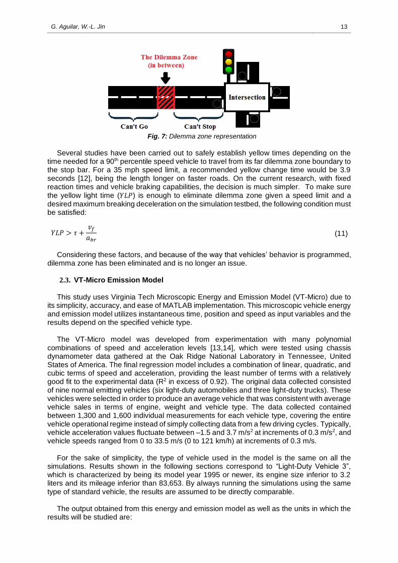
2.2.1. Dilemma Zone
Due to the network and drivers characteristics, dilemma zone must be considered when
choosing the duration of the yellow light. The yellow indication is designed to warn drivers approaching an intersection that the signal is about to turn red. The length of the yellow light should be enough for the approaching drivers to either safely stop before the intersection, or continue clear through the intersection before the traffic light turns red [11].
An inadequate yellow extension will either prevent the drivers from safely stopping their
vehicles before the intersection entrance or force them to enter the crossing on a red light. None of these options is admissible when designing signal timing.
The following scheme exemplifies what happens when a vehicle approaching an
intersection faces a yellow light. Drivers who are in the zone marked as "Can't Go" when the traffic light turns yellow know they are too far back and will not be able to reach the intersection before the light turns red. Hence, they must stop. On the other hand, drivers who are in the "Can't Stop" zone are too close to the intersection to stop safely: they must proceed before the red light. But when the yellow time is inadequate, there is range between both zones (generally called the “dilemma zone”) where the driver can neither proceed safely, nor stop safely. The duration of a yellow light in an appropriately timed signal must be enough for drivers to avoid the impossible election presented by the dilemma zone.
G. Aguilar, W.-L. Jin
13
Fig. 7: Dilemma zone representation
Several studies have been carried out to safely establish yellow times depending on the
time needed for a 90th percentile speed vehicle to travel from its far dilemma zone boundary to the stop bar. For a 35 mph speed limit, a recommended yellow change time would be 3.9 seconds [12], being the length longer on faster roads. On the current research, with fixed reaction times and vehicle braking capabilities, the decision is much simpler. To make sure the yellow light time (𝑌𝐿𝑃) is enough to eliminate dilemma zone given a speed limit and a desired maximum breaking deceleration on the simulation testbed, the following condition must be satisfied:
𝑌𝐿𝑃 > 𝜏 +𝑣𝑓
𝑎𝑏𝑟 (11)
Considering these factors, and because of the way that vehicles’ behavior is programmed,
dilemma zone has been eliminated and is no longer an issue. 2.3. VT-Micro Emission Model
This study uses Virginia Tech Microscopic Energy and Emission Model (VT-Micro) due to
its simplicity, accuracy, and ease of MATLAB implementation. This microscopic vehicle energy and emission model utilizes instantaneous time, position and speed as input variables and the results depend on the specified vehicle type.
The VT-Micro model was developed from experimentation with many polynomial
combinations of speed and acceleration levels [13,14], which were tested using chassis dynamometer data gathered at the Oak Ridge National Laboratory in Tennessee, United States of America. The final regression model includes a combination of linear, quadratic, and cubic terms of speed and acceleration, providing the least number of terms with a relatively good fit to the experimental data (R2 in excess of 0.92). The original data collected consisted of nine normal emitting vehicles (six light-duty automobiles and three light-duty trucks). These vehicles were selected in order to produce an average vehicle that was consistent with average vehicle sales in terms of engine, weight and vehicle type. The data collected contained between 1,300 and 1,600 individual measurements for each vehicle type, covering the entire vehicle operational regime instead of simply collecting data from a few driving cycles. Typically, vehicle acceleration values fluctuate between –1.5 and 3.7 m/s2 at increments of 0.3 m/s2, and vehicle speeds ranged from 0 to 33.5 m/s (0 to 121 km/h) at increments of 0.3 m/s.
For the sake of simplicity, the type of vehicle used in the model is the same on all the
simulations. Results shown in the following sections correspond to “Light-Duty Vehicle 3”, which is characterized by being its model year 1995 or newer, its engine size inferior to 3.2 liters and its mileage inferior than 83,653. By always running the simulations using the same type of standard vehicle, the results are assumed to be directly comparable.
The output obtained from this energy and emission model as well as the units in which the
results will be studied are:
G. Aguilar, W.-L. Jin
14
- Average HC emission (mg/km) - Average CO emission (mg/km) - Average NOx emission (mg/km) - Average CO2 emission (g/km) - Average fuel economy (l/100km)
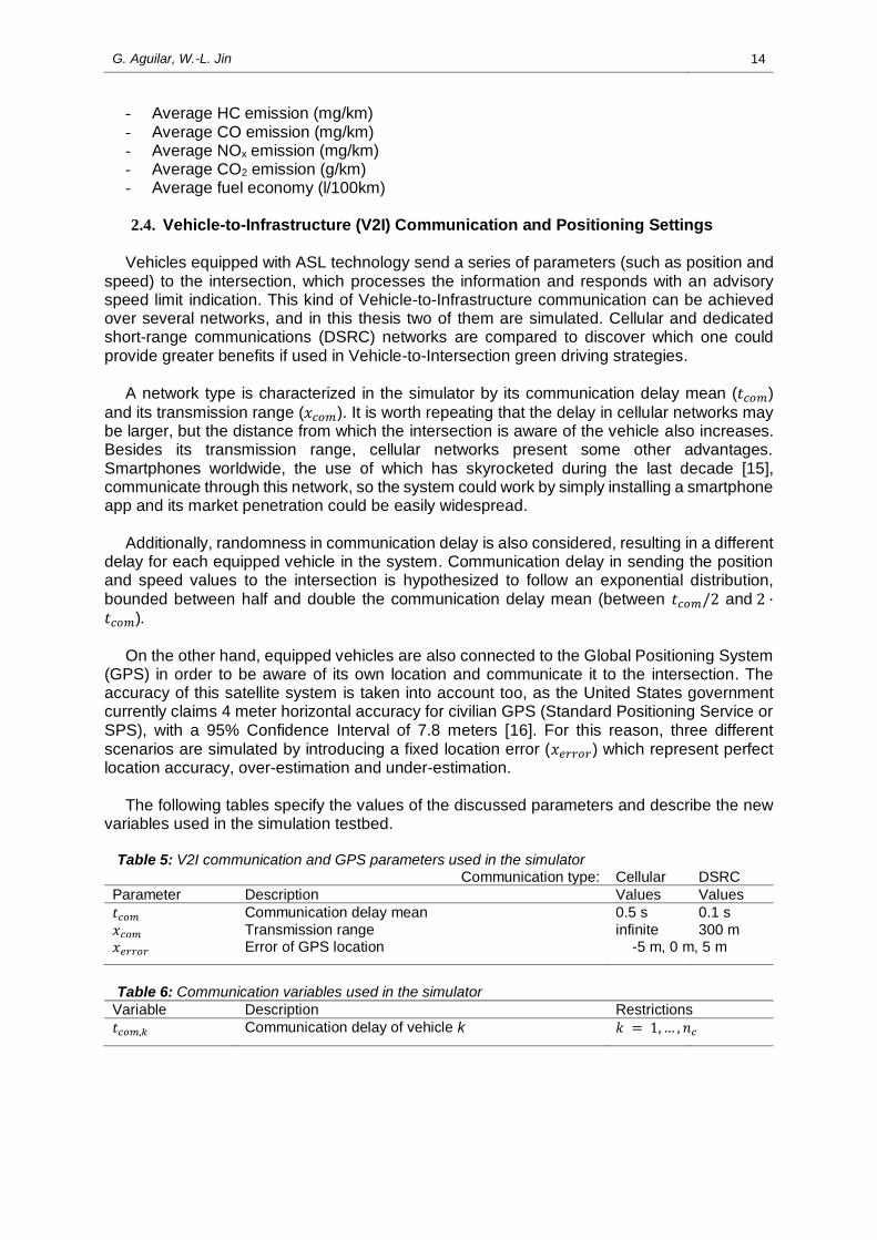
2.4. Vehicle-to-Infrastructure (V2I) Communication and Positioning Settings
Vehicles equipped with ASL technology send a series of parameters (such as position and
speed) to the intersection, which processes the information and responds with an advisory speed limit indication. This kind of Vehicle-to-Infrastructure communication can be achieved over several networks, and in this thesis two of them are simulated. Cellular and dedicated short-range communications (DSRC) networks are compared to discover which one could provide greater benefits if used in Vehicle-to-Intersection green driving strategies.
A network type is characterized in the simulator by its communication delay mean (𝑡𝑐𝑜𝑚)
and its transmission range (𝑥𝑐𝑜𝑚). It is worth repeating that the delay in cellular networks may be larger, but the distance from which the intersection is aware of the vehicle also increases. Besides its transmission range, cellular networks present some other advantages. Smartphones worldwide, the use of which has skyrocketed during the last decade [15], communicate through this network, so the system could work by simply installing a smartphone app and its market penetration could be easily widespread.
Additionally, randomness in communication delay is also considered, resulting in a different
delay for each equipped vehicle in the system. Communication delay in sending the position and speed values to the intersection is hypothesized to follow an exponential distribution, bounded between half and double the communication delay mean (between 𝑡𝑐𝑜𝑚/2 and 2 ·𝑡𝑐𝑜𝑚).
On the other hand, equipped vehicles are also connected to the Global Positioning System
(GPS) in order to be aware of its own location and communicate it to the intersection. The accuracy of this satellite system is taken into account too, as the United States government currently claims 4 meter horizontal accuracy for civilian GPS (Standard Positioning Service or SPS), with a 95% Confidence Interval of 7.8 meters [16]. For this reason, three different scenarios are simulated by introducing a fixed location error (𝑥𝑒𝑟𝑟𝑜𝑟) which represent perfect location accuracy, over-estimation and under-estimation.
The following tables specify the values of the discussed parameters and describe the new
variables used in the simulation testbed.
Table 5: V2I communication and GPS parameters used in the simulator Communication type: Cellular DSRC
Parameter Description Values Values
𝑡𝑐𝑜𝑚 Communication delay mean 0.5 s 0.1 s
𝑥𝑐𝑜𝑚 Transmission range infinite 300 m
𝑥𝑒𝑟𝑟𝑜𝑟 Error of GPS location -5 m, 0 m, 5 m
Table 6: Communication variables used in the simulator
Variable Description Restrictions
𝑡𝑐𝑜𝑚,𝑘 Communication delay of vehicle k 𝑘 = 1, … , 𝑛𝑐
G. Aguilar, W.-L. Jin
15
3. ADVISORY SPEED LIMIT (ASL) OPERATION
In the ASL control strategies that are studied in this thesis, vehicles are still manually driven.
Thus, a vehicle’s speed cannot be directly controlled, but instead an individual advisory speed limit is provided to each driver of the equipped vehicles. Therefore, non-equipped vehicles’ movements are still described by Gipps’ car-following model and the previous algorithms explained on Section 2, but for vehicles with V2I communication, the acceleration part of the
model is modified by replacing the speed limit, 𝑣𝑓, by the advisory speed limit, 𝑣𝑘𝐴𝑆𝐿(𝑡), which
is time-dependent. Consequently, the movement of vehicles that follow ASL indications and that are close enough to the intersection is described by:
𝑎𝑘(𝑡) = 𝑚𝑎𝑥 {−𝑎𝑏𝑟, 𝑚𝑖𝑛 { 2.5 · 𝑎𝑓𝑤 · (1 −𝑣𝑘(𝑡)
𝑣𝑘𝐴𝑆𝐿(𝑡)
) · √0.025 +𝑣𝑘(𝑡)
𝑣𝑘𝐴𝑆𝐿(𝑡)
, 𝑎𝑘𝑐𝑜𝑛𝑔𝑒𝑠𝑡𝑒𝑑(𝑡)}} (12)
Note how V2I-equipped vehicles’ movements have nothing to do with the color of the traffic
light, as ASL indications already make sure that the vehicles arrive at the intersection with green or yellow lights and enough time to cross it.
But what would happen if ASL indications were incorrect, for example due to GPS
inaccuracies? Human drivers are still handling the vehicles, so they are expected to brake if they feel the system is putting them in unsafe situations. Imagine a car is driving at the speed limit towards a signalized intersection with the red light on. Even though the system says it is safe to proceed at that speed because the traffic lights are soon going to turn green, the driver would be expected to gently brake to stop at a safe location if it was needed to. This kind of reaction is programmed in the simulator using a variation of algorithms 2 and 3 in equipped vehicles.
3.1. Control Algorithms
To calculate at which time instant a car is expected to enter the intersection (𝑡𝑖𝑘
𝑒), the
following algorithm is executed every time a new vehicle enters the upstream road. Basically, the control system expects the vehicles to enter the intersection at their first possible chance, taking into account three factors: the speed limit, the intersection service rate and the traffic lights.
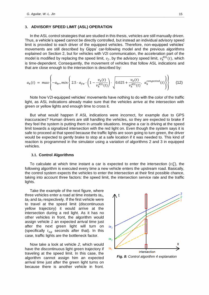
Take the example of the next figure, where
three vehicles enter a road at time instants ta1, ta2 and ta3 respectively. If the first vehicle were
to travel at the speed limit (discontinuous yellow trajectory) it would arrive at the intersection during a red light. As it has no other vehicles in front, the algorithm would assign vehicle 1 an expected arrival time just after the next green light will turn on (specifically 𝑡𝑎𝑔 seconds after that). In this
case, traffic lights are the bottleneck factor. Now take a look at vehicle 2, which would
have the discontinuous light green trajectory if traveling at the speed limit. In this case, the algorithm cannot assign him an expected arrival time just after the green light turns on because there is another vehicle in front.
Fig. 8: Control algorithm 4 explanation
G. Aguilar, W.-L. Jin
16
Therefore, intersection service rate is the limiting factor and vehicle 2 would be assigned an
expected arrival time 3600/𝑠 seconds after vehicle 1. Finally, see how vehicle 3 is able to enter the intersection travelling at the speed limit while
also respecting the intersection capacity and the traffic lights. Speed limit would be the deciding factor in this third occurrence.
This thought process has been programmed as follows:
(Algorithm 4)
1 𝑡𝑖𝑘𝑒 = 𝑚𝑎𝑥 {𝑡𝑎𝑘 +
𝐿1
𝑣𝑓, 𝑡𝑖𝑘−1
𝑒 + 3600
𝑠, 𝑡𝑙𝑔 + 𝑡𝑎𝑔}
2 if 𝑡𝑖𝑘𝑒 > 𝑡𝑙𝑔 + 𝐺𝐿𝑃 + 𝑌𝐿𝑃 − 𝑡𝑏𝑟
3 𝑛 = 1 4 while 𝑡𝑖𝑘
𝑒 > 𝑡𝑙𝑔 + 𝑛 · (𝐺𝐿𝑃 + 𝑌𝐿𝑃 + 𝑅𝐿𝑃) + 𝐺𝐿𝑃 + 𝑌𝐿𝑃 − 𝑡𝑏𝑟
5 𝑛 = 𝑛 + 1 6 end 7 𝑡𝑖𝑘
𝑒 = 𝑡𝑙𝑔 + 𝑛 · (𝐺𝐿𝑃 + 𝑌𝐿𝑃 + 𝑅𝐿𝑃) + 𝑡𝑎𝑔
8 end
Note that the arrival time of all the vehicles at the upstream road, even if they do not have
V2I communication capabilities, must be known in order to more accurately calculate the expected arrival times at the intersection. For this reason, inductive loops need to be set at the start of the upstream road.
Several things can happen meanwhile a vehicle is on the road that can make its expected
arrival time change its value, the main reason for this being the presence of non-equipped vehicles and its less predictable behavior. When this happens, the control system needs to be prepared to update the expected arrival time values and modify the indications given to equipped vehicles.
Notice that if inductive loops are also placed at the intersection entrance it would be possible
to calculate the number of cars between the intersection and any given vehicle on the upstream road. Hence, with inductive loops present at both the start and the end of the upstream road, the next confirmation algorithm will be executed before sending any advisory speed limit indication. It first ensures service rate compatibility with previously updated values, being 𝑐𝑘(𝑡)
the number of cars between vehicle 𝑘 and the intersection entrance at time 𝑡, and later verifies that the newly assigned expected arrival times are in accordance with the traffic light signals.
Basically, the function of this algorithm is to update the values of expected arrival times at
the intersection (𝑡𝑖𝑘𝑒) whenever there is a change, until they take the real value (𝑡𝑖𝑘) when a
vehicle has already entered the crossing. It can be especially useful if the traffic lights change its cycle lengths, or if the loop detectors alert the system that a vehicle is running behind schedule, potentially affecting all the following vehicles.
Imagine, for example, that a vehicle is expected to enter the intersection 5 seconds from
now, but thanks to the loop detectors it is possible to know that it still has three vehicles in front. With a service rate of 1800 vehicles/hour, the first part of the algorithm (lines 1-3) update its expected arrival to 3·3600/1800 = 6 seconds from now, and the second part (lines 4-11) makes sure that this newly assigned expected arrival time respects the future traffic light indications, assigning the vehicle to the next green cycle if necessary.

G. Aguilar, W.-L. Jin
17
(Algorithm 5)
1 for 𝑟 = 1: 𝑐𝑘(𝑡)
2 𝑡𝑖𝑘𝑒 = 𝑚𝑎𝑥 {𝑡𝑖𝑘
𝑒, 𝑡𝑖𝑘−𝑟𝑒 + 𝑟 ·
3600
𝑠}
3 end 4 if 𝑡 ≤ 𝑡𝑙𝑔 + 𝐺𝐿𝑃 + 𝑌𝐿𝑃 − 𝑡𝑏𝑟
5 𝑡𝑖𝑘𝑒 = 𝑚𝑎𝑥 {𝑡𝑖𝑘
𝑒, 𝑡 + 𝑐𝑘(𝑡) ·3600
𝑠}
6 if 𝑡𝑖𝑘𝑒 > 𝑡𝑙𝑔 + 𝐺𝐿𝑃 + 𝑌𝐿𝑃 − 𝑡𝑏𝑟
7 𝑡𝑖𝑘𝑒 = 𝑚𝑎𝑥{𝑡𝑖𝑘
𝑒 , 𝑡𝑙𝑔 + 𝐺𝐿𝑃 + 𝑌𝐿𝑃 + 𝑅𝐿𝑃 + 𝑡𝑎𝑔}
8 end 9 else
10 𝑡𝑖𝑘𝑒 = 𝑚𝑎𝑥 {𝑡𝑖𝑘
𝑒 , 𝑡𝑙𝑔 + 𝐺𝐿𝑃 + 𝑌𝐿𝑃 + 𝑅𝐿𝑃 + 𝑡𝑎𝑔 + 𝑐𝑘(𝑡) ·3600
𝑠}
11 end
Note how the system needs to gather information from both the traffic lights and the
inductive loops in order to more precisely calculate the expected vehicle arrival times at the intersection. Traffic lights must share the instant when the last green light turned on as well as the length of all the phases for that particular approach. On the other hand, inductive loops will need to be placed at the start and the end of the upstream road for the system to be aware of the instants of car arrival and departures from the upstream road, therefore being possible to calculate the number of cars in front of a given vehicle (between the vehicle and the intersection entrance).
3.2. Feedback Control System
With the updated value of expected arrival time at the intersection (𝑡𝑖𝑘
𝑒), the Advisory Speed
Limit control system is able to define at which speed should the car go to enter the intersection
at its expected time. This speed (𝑣𝑘𝐴𝑆𝐿) is the necessary one to travel the distance from the last
known location to the intersection entrance with the time left until the expected arrival time. As explained, the intersection entrance is located at 𝑥 = 𝐿1. Moreover, the last known
location is the location of the car a period of time equal to the communication delay ago,
𝑥𝑘(𝑡 − 𝑡𝑐𝑜𝑚,𝑘); plus the location error introduced by GPS inaccuracies, 𝑥𝑒𝑟𝑟𝑜𝑟. But since within
a given communication type the network delay mean is known (𝑡𝑐𝑜𝑚), the system is able to approximate the true location multiplying this network delay mean by the last known speed, 𝑣𝑘(𝑡 − 𝑡𝑐𝑜𝑚,𝑘).
This approximation is more accurate when the communication delay of the vehicle involved
is closer to the network delay mean, when the network delay is as low as possible and when in that period of time the vehicle has not changed its speed. However, GPS-introduced location error is not known and therefore not corrected.
Finally, the time left until the expected arrival time at the intersection is defined as 𝑡𝑑𝑘
𝑒 − 𝑡,
and the ‘ASL Equation’ is defined as:
𝑣𝑘𝐴𝑆𝐿(𝑡) =
𝐿1 − [𝑥𝑘(𝑡 − 𝑡𝑐𝑜𝑚,𝑘) + 𝑥𝑒𝑟𝑟𝑜𝑟 + 𝑣𝑘(𝑡 − 𝑡𝑐𝑜𝑚,𝑘) · 𝑡𝑐𝑜𝑚]
𝑡𝑖𝑘𝑒 − 𝑡
(13)
This speed modifies the car behavioral model replacing the speed limit in the acceleration
part of Gipps’ model, as seen in Equation 12.

G. Aguilar, W.-L. Jin
18
4. ADVISORY SPEED LIMIT (ASL) ON ISOLATED INTERSECTIONS
As already explained, the ASL control system uses advanced notification of signal status to
inform drivers on an optimum speed in order to produce delay, emission and fuel savings by avoiding hard-braking and hard-acceleration maneuvers.
In this study, the influence of several parameters in the performance of ASL technology are
analyzed. These parameters are: market penetration rate of the system, traffic congestion level, communication network type (which affects the communication delay and the transmission range) and GPS accuracy.
In regards to the market penetration rates (MPR’s), a few values are tested, so that in each
scenario a different percentage of vehicles are equipped. Theoretically, even though only a small amount of the cars followed ASL indications, all the vehicles following them would also profit from this technology as they would smoothen their speed profile too. The market penetration rates simulated are 0%, 25%, 50%, 75% and 100%, and they state the probability that a randomly generated vehicle is equipped with ASL technology or not.
Fig. 9: Schematic representation of an isolated intersection
On an isolated intersection, vehicle arrivals are random. Traffic congestion levels are
characterized by their mean time between car arrivals (𝜆), which is hypothesized and programmed to follow an exponential distribution inferiorly bounded by ℎ𝑚𝑖𝑛. A mean of 𝜆 = 4
seconds is used to represent dense traffic situations whereas 𝜆 = 8 seconds is used for low traffic conditions. An intermediate situation of 𝜆 = 6 seconds is also simulated to characterize a medium level of traffic congestion. Therefore, the next equation is used to determine the arrival times of the vehicles at the upstream road:
𝑡𝑎𝑘 = 𝑡𝑎𝑘−1 + 𝑚𝑎𝑥{ℎ𝑚𝑖𝑛, 𝑟𝑎𝑛𝑑𝑜𝑚_𝑒𝑥𝑝𝑜𝑛𝑒𝑛𝑡𝑖𝑎𝑙(𝜆)} (14)
Table 7: Market penetration and congestion level parameters used in the isolated intersection simulation
Parameter Description Values
𝑀𝑃𝑅 market penetration rate 0%, 25%, 50%, 75%, 100%
𝜆 mean time between vehicle arrivals 4 s, 6 s, 8 s
ℎ𝑚𝑖𝑛 minimum arrival headway (minimum time between arrivals)
0.5 s
All the possible parameter combinations are run in the simulator on a single-lane road with
only through movements permitted. Only one approach of the intersection is considered, as with the signal allocation and the network characteristics described all the approaches happen to be identical. Besides the already mentioned hypothesis, a few other are considered and are stated below:
- Roads and intersection are initially empty (no vehicles)

G. Aguilar, W.-L. Jin
19
- All the vehicles are generated at the start of Road 1 and they exit the system at the end of Road 2 (no vehicles enter or exit the road in any other way than the stipulated, i.e. no parking or turning). Therefore, isolated intersections are open systems in the sense that vehicles get out after finishing their journey.
For each combination of market penetration rate (5 rates), mean time between arrivals (3
levels of congestion), communication network (cellular vs. DSRC) and GPS location error (3 values), 200 simulations are executed, obtaining the following average results.
4.1. Influence of the Market Penetration Rate and the Communication Network
The next graphs show the average results sorted by MPR percentage, for all the traffic congestion levels simulated and error-less GPS characteristics, depending on the communication network. The first and second row of graphs represent, respectively, the average waiting time (in seconds) and the average fuel economy (in liters/100km) of the vehicles and their 95% Confidence Intervals (CI). The third row show the average pollutant emissions.
(a)
(b)
Fig. 10: Waiting time (error-less GPS) on (a) cellular networks or (b) DSRC networks
(a)
(b)
Fig. 11: Fuel economy (error-less GPS) on (a) cellular networks or (b) DSRC networks
0
20
40
60
80
0% 25% 50% 75% 100%Avera
ge w
ait a
nd 9
5%
CI (s
)
MPR
Cellular networks
0
20
40
60
80
0% 25% 50% 75% 100%Avera
ge w
ait a
nd 9
5%
CI (s
)
MPR
DSRC networks
0
2
4
6
8
10
12
0% 25% 50% 75% 100%
Avera
ge fuel econom
y and 9
5%
CI
(l/1
00km
)
MPR
Cellular networks
0
2
4
6
8
10
12
0% 25% 50% 75% 100%
Avera
ge fuel econom
y and 9
5%
CI
(l/1
00km
)
MPR
DSRC networks

G. Aguilar, W.-L. Jin
20
(a)
(b)
Fig. 12: Average emission levels (error-less GPS) on (a) cellular networks or (b) DSRC networks
In the previous figures it can be seen how as the market penetration rate increases so the
benefits do, but it is not clear whether results are different depending on the network characteristics. For this reason, numerical results are presented below and will be the standard method for comparing results in this thesis from now on. The following table shows the improvements over 0% MPR on both networks (to clarify, negative values found in tables mean that a particular output has decreased):
Table 8: Improvements over 0% MPR with both cellular and DSRC networks (error-less GPS)
Cellular networks DSRC networks
MPR 25% 50% 75% 100% 25% 50% 75% 100%
Average Wait -5,1% -8,1% -10,2% -14,6% 0,0% -4,8% -9,4% -10,8%
Average HC -1,5% -1,9% -2,1% -2,6% -0,5% -0,9% -1,1% -1,1%
Average CO 0,0% 0,1% 0,1% -0,3% 0,7% 0,6% 0,6% 0,7%
Average NOx -5,9% -7,8% -8,2% -9,1% -3,3% -4,3% -4,7% -4,8%
Average CO2 -4,7% -6,2% -6,8% -8,0% -2,7% -4,2% -5,0% -5,3%
Average Fuel Economy -4,6% -6,2% -6,7% -7,9% -2,7% -4,1% -5,0% -5,3%
Numerical results show that the implementation of the Advisory Speed Limit could report
improvements of over 14% on vehicles average waiting time, almost 8% on average fuel economy and up to 9% on some pollutant emissions. Improvements are appreciably better if Vehicle-to-Infrastructure communication is carried out over cellular networks instead of DSRC.
4.2. Influence of the Location Accuracy
Previous results show that cellular networks perform better than DSRC with error-less GPS
characteristics. In this section, the influence of under-estimation and over-estimation in the GPS location is analyzed, as it is of common awareness that current GPS technology may introduce location errors. The next graphs and table show the average results for all the traffic congestion levels simulated sorted by market penetration rate, for under-estimated GPS location, depending on the communication type:
0
50
100
150
200
250
300
350
400
0% 50% 100%MPR
Cellular networks
Avg HC(mg/km)
Avg CO(mg/km)
Avg NOx(mg/km)
Avg CO2(g/km) 0
50
100
150
200
250
300
350
400
0% 50% 100%MPR
DSRC networks
Avg HC(mg/km)
Avg CO(mg/km)
Avg NOx(mg/km)
Avg CO2(g/km)
G. Aguilar, W.-L. Jin
21
(a)
(b)
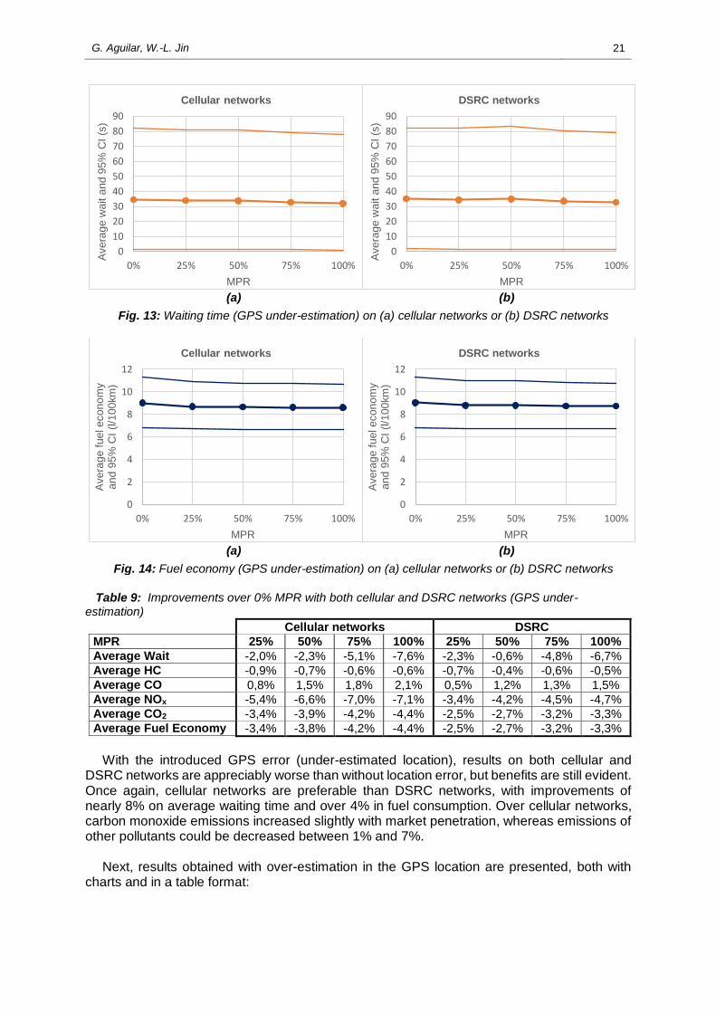
Fig. 13: Waiting time (GPS under-estimation) on (a) cellular networks or (b) DSRC networks
(a)
(b)
Fig. 14: Fuel economy (GPS under-estimation) on (a) cellular networks or (b) DSRC networks
Table 9: Improvements over 0% MPR with both cellular and DSRC networks (GPS under-
estimation)
Cellular networks DSRC
MPR 25% 50% 75% 100% 25% 50% 75% 100%
Average Wait -2,0% -2,3% -5,1% -7,6% -2,3% -0,6% -4,8% -6,7%
Average HC -0,9% -0,7% -0,6% -0,6% -0,7% -0,4% -0,6% -0,5%
Average CO 0,8% 1,5% 1,8% 2,1% 0,5% 1,2% 1,3% 1,5%
Average NOx -5,4% -6,6% -7,0% -7,1% -3,4% -4,2% -4,5% -4,7%
Average CO2 -3,4% -3,9% -4,2% -4,4% -2,5% -2,7% -3,2% -3,3%
Average Fuel Economy -3,4% -3,8% -4,2% -4,4% -2,5% -2,7% -3,2% -3,3%
With the introduced GPS error (under-estimated location), results on both cellular and
DSRC networks are appreciably worse than without location error, but benefits are still evident. Once again, cellular networks are preferable than DSRC networks, with improvements of nearly 8% on average waiting time and over 4% in fuel consumption. Over cellular networks, carbon monoxide emissions increased slightly with market penetration, whereas emissions of other pollutants could be decreased between 1% and 7%.
Next, results obtained with over-estimation in the GPS location are presented, both with
charts and in a table format:
0
10
20
30
40
50
60
70
80
90
0% 25% 50% 75% 100%
Ave
rag
e w
ait a
nd
95
% C
I (s
)
MPR
Cellular networks
0
10
20
30
40
50
60
70
80
90
0% 25% 50% 75% 100%
Ave
rag
e w
ait a
nd
95
% C
I (s
)
MPR
DSRC networks
0
2
4
6
8
10
12
0% 25% 50% 75% 100%
Avera
ge fuel econom
y and 9
5%
CI
(l/1
00km
)
MPR
Cellular networks
0
2
4
6
8
10
12
0% 25% 50% 75% 100%
Avera
ge fuel econom
y and 9
5%
CI
(l/1
00km
)
MPR
DSRC networks

G. Aguilar, W.-L. Jin
22
(a)
(b)
Fig. 15: Waiting time (GPS over-estimation) on (a) cellular networks or (b) DSRC networks
(a)
(b)
Fig. 16: Fuel economy (GPS over-estimation) on (a) cellular networks or (b) DSRC networks
Table 10: Improvements over 0% MPR with both cellular and DSRC networks (GPS over-
estimation)
Cellular networks DSRC
MPR 25% 50% 75% 100% 25% 50% 75% 100%
Average Wait 11,7% 28,7% 48,2% 85,1% 12,3% 27,9% 51,1% 96,1%
Average HC -0,3% 1,1% 3,0% 6,8% 0,0% 1,1% 3,3% 7,8%
Average CO 1,4% 3,2% 5,3% 9,3% 1,2% 2,6% 5,0% 9,6%
Average NOx -6,5% -8,2% -8,7% -7,8% -4,2% -5,5% -5,6% -4,2%
Average CO2 -2,9% -1,7% 0,7% 6,0% -2,0% -1,0% 1,9% 8,2%
Average Fuel Economy -2,9% -1,6% 0,8% 6,1% -2,0% -0,9% 1,9% 8,2%
It is surprising how average waiting times are extremely sensitive to over-estimation in the
location (increasing particularly on intense traffic levels) and how, in general, the benefits of ASL strategies are completely cancelled. Pollutant emissions, as well as fuel consumption, increased between 6% and 10%, except for NOx emissions, which were the only to decrease in this scenario. Again, DSRC networks performed worse than cellular networks.
To understand the underlying reasons behind this results, individual simulations were
observed. Under-estimating vehicles’ location resulted in the system believing that drivers were further to the intersection than they really were, so higher speed indications were given. When equipped vehicles adjusted their speed to follow ASL indications, they found that they arrived earlier than expected to the intersection. The first vehicle of each platoon arrived at the intersection when the light was still red, so the driver had to start breaking before he could react to the light turning green. In consequence, all the vehicles could still enter the intersection during their expected green light cycle, but less smooth speed profiles were achieved (which is known to increase fuel consumption and emissions).
0
50
100
150
0% 25% 50% 75% 100%Ave
rag
e w
ait a
nd
95
% C
I (s
)
MPR
Cellular networks
0
50
100
150
0% 25% 50% 75% 100%Ave
rag
e w
ait a
nd
95
% C
I (s
)
MPR
DSRC networks
0
2
4
6
8
10
12
14
0% 25% 50% 75% 100%
Avera
ge fuel e
co
no
my
and 9
5%
CI
(l/1
00
km
)
MPR
Cellular networks
0
2
4
6
8
10
12
14
0% 25% 50% 75% 100%
Avera
ge fuel e
co
no
my
and 9
5%
CI
(l/1
00
km
)
MPR
DSRC networks

G. Aguilar, W.-L. Jin
23
On the other hand, over-estimated locations resulted in the system thinking that vehicles
were closer to the intersection than they really were, therefore sending slower ASL indications. This led to vehicles arriving late at the intersection and having to stop at red lights waiting for the next green cycle, when they could have easily passed the intersection if they had arrived a few seconds earlier. Basically, over-estimating the location resulted in a decrease of the effective green time.
In conclusion, the influence of location error cannot be neglected as the system has proven
to be very sensitive to over-estimation, even though perhaps this could be compensated by purposely introducing under-estimation error in the programming.
4.3. Influence of Traffic Congestion
As expected, simulations have far different results if sorted by mean time between arrivals,
being higher the delays, fuel consumption and emissions while the traffic got denser, as shown below:
(a)
(b)
Fig. 17: (a) Waiting time or (b) fuel economy sorted by mean time between arrivals on cellular networks (error-less GPS)
Finally, if the improvements over 0% MPR with the different traffic congestion levels
simulated are compared, it is noticeable how ASL control can provide superior improvements in waiting time (-16%) with intermediate traffic density (regardless of the communication network). However, greater improvements in fuel consumption and emissions are possible with dense traffic (10% decrease in fuel consumption, and between 2% and 13% on pollutant emissions, much more than in low traffic conditions). The exact obtained numbers on cellular networks and error-less GPS location are:
Table 11: Improvements over 0% MPR for different traffic densities (cellular networks, error-less
GPS)
(in %) Low traffic Intermediate traffic Dense traffic
MPR 25% 50% 75% 100% 25% 50% 75% 100% 25% 50% 75% 100%
Average Wait -1,6 -5,1 -8,3 -13,1 -4,8 -7,0 -9,6 -16,3 -6,1 -9,2 -11,0 -14,5
Average HC 0,0 -0,1 -0,2 -0,5 -1,0 -1,2 -1,4 -2,0 -3,2 -4,0 -4,3 -5,0
Average CO 1,0 1,5 1,7 1,7 0,3 0,7 0,8 0,4 -1,0 -1,5 -1,9 -2,5
Average NOx -3,1 -4,6 -5,6 -6,2 -5,1 -6,8 -7,7 -8,4 -9,3 -11,6 -11,0 -12,3
Average CO2 -2,6 -4,0 -4,8 -5,7 -4,2 -5,5 -6,3 -7,5 -6,6 -8,5 -8,7 -10,1
Avg. Fuel Economy -2,6 -3,9 -4,8 -5,6 -4,2 -5,4 -6,2 -7,4 -6,6 -8,5 -8,6 -10,0
0
20
40
60
80
100
120
140
160
4 5 6 7 8
Avera
ge w
ait a
nd 9
5%
CI (s
)
λ
Cellular networks
0
2
4
6
8
10
12
14
4 5 6 7 8
Ave
rage
fu
el e
con
om
yan
d 9
5% C
I (l/
100k
m)
λ
Cellular networks

G. Aguilar, W.-L. Jin
24
5. ADVISORY SPEED LIMIT (ASL) ON LOOP INTERSECTIONS
To test the improvements that the Advisory Speed Limit control could provide in an
intersection located inside a city’s network grid, a minor modification of the previous case is programmed. To achieve this scenario, the road configuration has been changed into a loop or ring road, which is a closed system in the sense that every vehicle that leaves the downstream road finds itself another time on the upstream road leading to the same intersection. With this configuration it is possible to take into account queue spillback implications if the number of vehicles on the road is large enough. On this occasion, vehicle arrivals at the intersection are not random but instead depend on the green cycle of the previous intersection, which is also signalized.
Fig. 18: Schematic representation of a loop intersection
It is known that even with the new road configuration the simulation does not depict a real
road network, as in this particular study all the intersections are exactly the same (same road lengths, no offset between green cycles, etc.) and there are no turns (no vehicles leaving or arriving), but the purpose of this study is just to provide a first approximation to the implications of non-arbitrary arrivals and see if the Advisory Speed Limit system would be able to achieve benefits.
Within this closed system, all the runway is considered “upstream road”. This means that if
the transmission range is large enough, a vehicle starts receiving ASL indications for the next intersection just after leaving the current one. In the simulator, this is equivalent to:
Table 12: General parameters used in the loop intersection simulation
Parameter Description Value
𝐿1 length of the upstream road (Road 1) 990 m
𝐿𝑖𝑛𝑡 length of intersection 10 m
𝐿2 length of the downstream road 0 m
As in the previous study, the ASL control system informs drivers on an optimum speed in
order to produce delay, emission and fuel savings by avoiding hard-braking and hard-acceleration handling. Also, the influence of several parameters in the performance of ASL technology is analyzed. These parameters, as in the previous section, are: market penetration rate (MPR) of the technology, traffic congestion level, communication network type (which affects the communication delay and the transmission range) and GPS accuracy.
Again, several values of market penetration rates are tested, so that in each scenario a
different percentage of vehicles lie equipped. The market penetration rates that are going to be simulated are the same as in the preceding section (0%, 25%, 50%, 75% and 100%), and they state the probability that a randomly generated vehicle is equipped with ASL technology or not.
G. Aguilar, W.-L. Jin
25
A significant difference between this study and the isolated intersection study is in the way
to define traffic congestion levels. In this case, instead of using the mean time between arrivals to characterize the congestion level, another indicator is employed: the number of cars on the track (𝐶𝑂𝑇), which is directly related to the car density. In this case, 𝐶𝑂𝑇 is equivalent to the
car density expressed in vehicles/km, as the length of the loop is defined as 𝐿1 + 𝐿𝑖𝑛𝑡 + 𝐿2 = 1.000 𝑚. A value of 𝐶𝑂𝑇 = 24 is utilized to represent dense traffic situations whereas 𝐶𝑂𝑇 = 12 is used to depict low traffic conditions. An intermediate situation of 𝐶𝑂𝑇 = 18 is also simulated to characterize a medium level of traffic congestion.
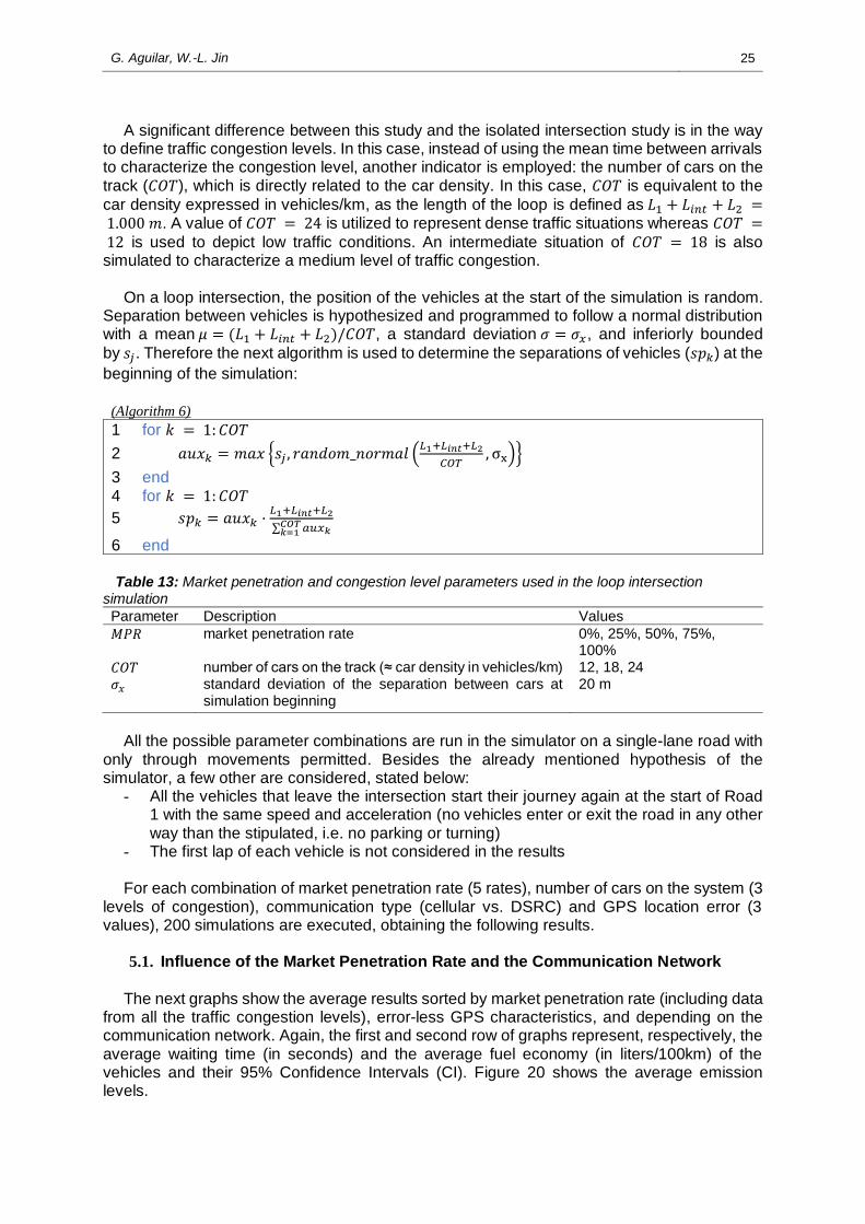
On a loop intersection, the position of the vehicles at the start of the simulation is random.
Separation between vehicles is hypothesized and programmed to follow a normal distribution with a mean 𝜇 = (𝐿1 + 𝐿𝑖𝑛𝑡 + 𝐿2)/𝐶𝑂𝑇, a standard deviation 𝜎 = 𝜎𝑥, and inferiorly bounded
by 𝑠𝑗. Therefore the next algorithm is used to determine the separations of vehicles (𝑠𝑝𝑘) at the
beginning of the simulation:
(Algorithm 6)
1 for 𝑘 = 1: 𝐶𝑂𝑇
2 𝑎𝑢𝑥𝑘 = 𝑚𝑎𝑥 {𝑠𝑗 , 𝑟𝑎𝑛𝑑𝑜𝑚_𝑛𝑜𝑟𝑚𝑎𝑙 (𝐿1+𝐿𝑖𝑛𝑡+𝐿2
𝐶𝑂𝑇, σx)}
3 end 4 for 𝑘 = 1: 𝐶𝑂𝑇
5 𝑠𝑝𝑘 = 𝑎𝑢𝑥𝑘 ·𝐿1+𝐿𝑖𝑛𝑡+𝐿2
∑ 𝑎𝑢𝑥𝑘𝐶𝑂𝑇𝑘=1
6 end
Table 13: Market penetration and congestion level parameters used in the loop intersection
simulation
Parameter Description Values
𝑀𝑃𝑅 market penetration rate 0%, 25%, 50%, 75%, 100%
𝐶𝑂𝑇 number of cars on the track (≈ car density in vehicles/km) 12, 18, 24
𝜎𝑥 standard deviation of the separation between cars at simulation beginning
20 m
All the possible parameter combinations are run in the simulator on a single-lane road with
only through movements permitted. Besides the already mentioned hypothesis of the simulator, a few other are considered, stated below:
- All the vehicles that leave the intersection start their journey again at the start of Road 1 with the same speed and acceleration (no vehicles enter or exit the road in any other way than the stipulated, i.e. no parking or turning)
- The first lap of each vehicle is not considered in the results
For each combination of market penetration rate (5 rates), number of cars on the system (3 levels of congestion), communication type (cellular vs. DSRC) and GPS location error (3 values), 200 simulations are executed, obtaining the following results.
5.1. Influence of the Market Penetration Rate and the Communication Network
The next graphs show the average results sorted by market penetration rate (including data
from all the traffic congestion levels), error-less GPS characteristics, and depending on the communication network. Again, the first and second row of graphs represent, respectively, the average waiting time (in seconds) and the average fuel economy (in liters/100km) of the vehicles and their 95% Confidence Intervals (CI). Figure 20 shows the average emission levels.

G. Aguilar, W.-L. Jin
26
(a)
(b)
Fig. 19: Waiting time (error-less GPS) on (a) cellular networks or (b) DSRC networks
(a)
(b)
Fig. 20: Fuel economy (error-less GPS) on (a) cellular networks or (b) DSRC networks
(a)
(b)
Fig. 21: Fuel economy (error-less GPS) on (a) cellular networks or (b) DSRC networks
In the previous figures it is seen how as the market penetration rate increases so do the improvement in results, but the numerical results presented in the following table make it easier to see the potential benefits in both mobility and environment over the 0% MPR “initial” situation (again, negative values mean that a particular output has decreased):
0
5
10
15
20
25
30
35
40
45
0% 25% 50% 75% 100%
Ave
rag
e w
ait a
nd
95
% C
I (s
)
MPR
Cellular networks
0
5
10
15
20
25
30
35
40
45
0% 25% 50% 75% 100%
Ave
rag
e w
ait a
nd
95
% C
I (s
)
MPR
DSRC networks
0
2
4
6
8
10
0% 25% 50% 75% 100%
Avera
ge fuel econom
yand 9
5%
CI
(l/1
00km
)
MPR
Cellular networks
0
2
4
6
8
10
0% 25% 50% 75% 100%
Avera
ge fuel econom
yand 9
5%
CI
(l/1
00km
)
MPR
DSRC networks
0
50
100
150
200
250
300
350
400
0% 50% 100%
MPR
Cellular networks
Avg HC(mg/km)
Avg CO(mg/km)
Avg NOx(mg/km)
Avg CO2(g/km)
0
50
100
150
200
250
300
350
400
0% 50% 100%
MPR
DSRC networks
Avg HC(mg/km)
Avg CO(mg/km)
Avg NOx(mg/km)
Avg CO2(g/km)

G. Aguilar, W.-L. Jin
27
Table 14: Cellular vs. DSRC networks improvements over 0% MPR (error-less GPS)
Cellular networks DSRC networks
MPR 25% 50% 75% 100% 25% 50% 75% 100%
Average Wait -3,7% -8,1% -13,7% -18,8% -3,6% -7,9% -13,6% -19,4%
Average HC -0,4% -1,1% -1,8% -2,5% 0,0% -0,3% -0,8% -1,4%
Average CO 2,6% 2,9% 2,4% 1,8% 1,3% 1,3% 1,0% 0,5%
Average NOx -9,3% -12,0% -13,2% -13,7% -3,5% -4,6% -5,0% -5,2%
Average CO2 -4,4% -6,4% -8,0% -9,2% -2,2% -3,5% -4,7% -5,7%
Average Fuel Economy -4,4% -6,4% -8,0% -9,1% -2,2% -3,5% -4,7% -5,7%
With the loop configuration, simulation results show that the implementation of Advisory
Speed Limit control could report improvements of around 19% on vehicles average waiting time and 9% on average fuel economy. Average carbon monoxide emissions seem to increase slightly, whereas emissions of other pollutants can be decreased between 2% and 14%. Improvements on waiting times are marginally better if V2I communication is carried out over DSRC networks, while over cellular networks it is possible to get much better fuel economy and emissions.
To further compare the advantages of using one kind of communication network over the
other, the adjoining surface chart is exhibited. The graph shows the benefits of running Advisory Speed Limit communications over cellular networks instead of over DSRC networks on average fuel economy (as it is also very closely related to pollutant emissions), sorting at the same time by market penetration rate and by number of cars in the system (traffic congestion level).
Fig. 22: Fuel consumption savings using cellular networks over DSRC (error-less GPS)
The chart evidences how cellular networks can provide higher fuel consumption savings
than DSRC networks, being the difference greater also when market penetration rate increases and traffic congestion level diminishes. The maximum difference in results (around 4% difference in fuel consumption) is therefore located on high MPR and low COT.
On the contrary, DSRC networks are able to provide lower waiting times than cellular
networks with dense traffic and high market penetration rates (almost 5% better). 5.2. Influence of the Location Accuracy
After seeing how both networks perform with error-less GPS characteristics, the influence
of under-estimating and over-estimating the GPS location is treated below. The next graphs and table show the averages for all the traffic congestion levels simulated sorted by market penetration rate, for under-estimated GPS location, depending on the communication network:
12
18
240%
1%
2%
3%
4%
5%
0%25%
50%75%
100%
COT
MPR
Differences in output (%)
0%-1% 1%-2% 2%-3% 3%-4% 4%-5%

G. Aguilar, W.-L. Jin
28
(a)
(b)
Fig. 23: Waiting time (GPS under-estimation) on (a) cellular networks or (b) DSRC networks
(a)
(b)
Fig. 24: Fuel economy (GPS under-estimation) on (a) cellular networks or (b) DSRC networks
Table 15: Cellular vs. DSRC networks improvements over 0% MPR (GPS under-estimation)
Cellular networks DSRC
MPR 25% 50% 75% 100% 25% 50% 75% 100%
Average Wait -2,3% -4,2% -6,3% -8,1% -0,1% -0,2% -0,2% -0,4%
Average HC 0,0% -0,1% -0,2% -0,3% 0,2% 0,4% 0,5% 0,5%
Average CO 3,1% 3,9% 4,2% 4,3% 1,6% 2,3% 2,7% 2,8%
Average NOx -9,2% -11,7% -12,6% -13,0% -3,6% -4,8% -5,3% -5,5%
Average CO2 -3,7% -4,9% -5,5% -6,0% -1,1% -1,5% -1,6% -1,6%
Average Fuel Economy -3,7% -4,8% -5,5% -5,9% -1,1% -1,5% -1,6% -1,6%
With the introduced GPS error (under-estimated location), results on both cellular and
DSRC networks are appreciably worse than before, but in this case cellular networks clearly outperform DSRC networks on the results, with improvements of over 8% on average waiting time (vs. no improvement on DSRC networks) and almost 6% in fuel consumption. Over this network, carbon monoxide emissions increase slightly with market penetration, whereas emissions of other pollutants can be decreased by as much as 13%.
Simulation results with over-estimation in the GPS location are displayed below, both with
charts and in a table format:
0
10
20
30
40
0% 25% 50% 75% 100%Ave
rag
e w
ait a
nd
95
% C
I (s
)
MPR
Cellular networks
0
10
20
30
40
0% 25% 50% 75% 100%Ave
rag
e w
ait a
nd
95
% C
I (s
)
MPR
DSRC networks
0
2
4
6
8
10
0% 25% 50% 75% 100%
Avera
ge fuel econ
om
yand 9
5%
CI
(l/1
00km
)
MPR
Cellular networks
0
2
4
6
8
10
0% 25% 50% 75% 100%
Avera
ge fuel econ
om
yand 9
5%
CI
(l/1
00km
)
MPR
DSRC networks

G. Aguilar, W.-L. Jin
29
(a)
(b)
Fig. 25: Waiting time (GPS over-estimation) on (a) cellular networks or (b) DSRC networks
(a)
(b)
Fig. 26: Fuel economy (GPS over-estimation) on (a) cellular networks or (b) DSRC networks
Table 16: Cellular vs. DSRC networks improvements over 0% MPR (GPS over-estimation)
Cellular networks DSRC
MPR 25% 50% 75% 100% 25% 50% 75% 100%
Average Wait 6,9% 18,0% 31,2% 47,1% 8,9% 21,1% 32,9% 49,3%
Average HC 0,1% 0,4% 0,8% 1,4% 0,7% 1,4% 2,4% 3,9%
Average CO 3,4% 4,7% 5,5% 6,2% 1,9% 3,2% 4,4% 6,0%
Average NOx -10,1% -13,9% -16,1% -17,5% -3,9% -5,7% -6,2% -6,0%
Average CO2 -3,5% -3,8% -3,3% -2,1% -0,9% -0,3% 1,0% 3,0%
Average Fuel Economy -3,4% -3,8% -3,2% -2,1% -0,9% -0,3% 1,0% 3,0%
It is noticeable how average waiting times are also very sensitive to over-estimation in the
location (even though less than in isolated intersections). Again, cellular networks performed better than DSRC networks, providing over 2% improvements in fuel economy and carbon dioxide emissions, and over 17% decline in nitrogen oxides. On the other hand, hydrocarbon and carbon monoxide emissions increased between 1% and 6% with over-estimated GPS location.
The reasons for this behavior with under-estimated and over-estimated location are the
same than with the previous road configuration, and are explained in Section 4. 5.3. Influence of Traffic Congestion
As expected, simulations have far different results if sorted by car density, being higher the
delays, fuel consumption and emissions while the traffic got denser, as shown below:
0
10
20
30
40
50
60
0% 25% 50% 75% 100%Ave
rag
e w
ait a
nd
95
% C
I (s
)
MPR
Cellular networks
0
10
20
30
40
50
60
0% 25% 50% 75% 100%Ave
rag
e w
ait a
nd
95
% C
I (s
)
MPR
DSRC networks
0
2
4
6
8
10
0% 25% 50% 75% 100%
Avera
ge fuel e
co
no
my
and 9
5%
CI
(l/1
00
km
)
MPR
Cellular networks
0
2
4
6
8
10
0% 25% 50% 75% 100%
Avera
ge fuel e
co
no
my
and 9
5%
CI
(l/1
00
km
)
MPR
DSRC networks

G. Aguilar, W.-L. Jin
30
(a)
(b)
Fig. 27: (a) Waiting time or (b) fuel economy sorted by number of cars on the track on cellular networks (error-less GPS)
Finally, if the improvements over 0% MPR for each traffic congestion level simulated are
compared, it is noticeable how ASL control can provide superior improvements in waiting time (over 26% fall) with low traffic density (regardless of the communication network). However, greater improvements in fuel consumption and emissions are possible with dense traffic (almost 10% decline in fuel consumption, and between 0% and 16% on pollutant emissions). The exact obtained numbers on cellular networks and error-less GPS location are:
Table 17: Cellular network improvements over 0% MPR for different traffic congestion levels, on
error-less GPS
(in %) Low traffic Intermediate traffic Dense traffic
MPR 25% 50% 75% 100% 25% 50% 75% 100% 25% 50% 75% 100%
Average Wait -7,9 -13,1 -21,1 -26,4 -3,0 -7,0 -10,6 -15,4 -1,8 -5,9 -11,6 -16,7
Average HC -0,4 -0,9 -1,6 -2,1 -0,1 -0,5 -1,1 -1,6 -0,8 -1,7 -2,7 -3,6
Average CO 2,1 2,3 2,0 1,6 3,1 3,8 3,6 3,2 2,6 2,5 1,7 0,8
Average NOx -7,3 -9,4 -10,6 -11,0 -9,0 -12,1 -13,2 -13,6 -11,5 -14,4 -15,6 -16,3
Average CO2 -4,6 -6,4 -8,3 -9,4 -4,2 -6,3 -7,5 -8,6 -4,5 -6,6 -8,3 -9,7
Avg. Fuel Econ. -4,6 -6,4 -8,2 -9,3 -4,1 -6,2 -7,4 -8,5 -4,5 -6,5 -8,2 -9,6
0
10
20
30
40
50
12 18 24Ave
rag
e w
ait a
nd
95
% C
I (s
)
COT
Cellular networks
0
2
4
6
8
10
12 18 24
Ave
rag
e fu
el e
co
no
my
an
d 9
5%
CI
(l/1
00
km
)
COT
DSRC networks

G. Aguilar, W.-L. Jin
31
6. INFLUENCE OF THE CAR-FOLLOWING MODEL
In previous sections, it has been proven that Advisory Speed Limit (ASL) strategies can
provide benefits in a different array of situations. In this chapter, three car-following models are compared to see if the results are sensitive to the car behavioral model. Gipps’ model results are compared with results of both Intelligent Driver Model (IDM) and a corrected version of Optimal Velocity Model (OVM), on an isolated intersection configuration, with ASL indications over cellular networks and error-less GPS.
First of all, the two newly mentioned models and their characteristics are discussed. Next,
the obtained results are compared. The same market penetration rates and traffic congestion levels as in Section 4 are simulated with IDM and OVM, executing 200 simulations for each parameter combination.
6.1. Intelligent Driver Model (IDM) with Bounded Acceleration
Again, the behavior of the following cars does not depend on the color of the traffic lights.
On a single-lane road, the acceleration of these vehicles at any given time is just a function of the speed of the vehicle immediately ahead, the speed of the follower itself and the distance between them. Note that no overtaking is considered. In this model, the vehicle acceleration cannot be greater than 𝑎𝑓𝑤 and the deceleration cannot be inferior than −𝑎𝑏𝑟.
Intelligent Driver Model equations [17] read as follows:
𝑎𝑘(𝑡) = 𝑚𝑎𝑥 {−𝑎𝑏𝑟, 𝑎𝑓𝑤 · [1 − (𝑣𝑘(𝑡)
𝑣𝑓)
𝛿
− (𝑠𝑘
∗(𝑡)
𝑥𝑘−1(𝑡) − 𝑥𝑘(𝑡))
2
]} (15)
Where:
𝑠𝑘∗(𝑡) = 𝑠𝑗 + 𝑚𝑎𝑥 {0, 𝑣𝑘(𝑡) · 𝑇ℎ +
𝑣𝑘(𝑡) · [𝑣𝑘(𝑡) − 𝑣𝑘−1(𝑡)]
2 · √𝑎𝑓𝑤 · 𝑎𝑏𝑟
} (16)
The acceleration is divided into a "desired" acceleration 𝑎𝑓𝑤 · [1 − (𝑣𝑘(𝑡)/𝑣𝑓)𝛿
] on a free
road, and a braking deceleration induced by the preceding vehicle. The acceleration on a free
road decreases from the initial acceleration 𝑎𝑓𝑤 to zero while the automobile’s velocity
approaches the specified speed limit, defined as 𝑣𝑓 for non-equipped vehicles and as 𝑣𝑘𝐴𝑆𝐿(𝑡)
for vehicles with V2I communication. The braking term is based on a comparison between the "desired dynamical distance" 𝑠∗,
and the actual gap to the front vehicle. If the actual spacing is approximately equal to 𝑠∗, then the breaking deceleration part of the model essentially compensates the free acceleration part, so the resulting acceleration is nearly zero. Therefore, 𝑠∗ corresponds to the gap when
following other vehicles in steadily flowing traffic. In addition, 𝑠∗ augments dynamically when approaching slower vehicles and decreases when the vehicle in front is advancing faster. As a consequence, the imposed braking deceleration increases with decreasing distance to the front vehicle (drivers want to maintain a certain safety distance), increasing own speed (the safety distance lengthens) or increasing speed difference to the front vehicle (when approximating the forward vehicle at a too high rate, a dangerous situation may take place).
The model parameters values used in the simulations are:
G. Aguilar, W.-L. Jin
32
Table 18: Intelligent Driver Model (IDM) parameters used in the simulation
Parameter Description Value
𝑇ℎ safe time headway 1.5 s
𝛿 acceleration exponent 4
6.2. Corrected Optimal Velocity Model (OVM)
The concept of this microscopic traffic flow model is, as a matter of fact, quite simple: each driver tries to achieve an optimal velocity based on the distance to the preceding vehicle. This was an alternative possibility explored recently in car-following models. The formulation is based on the assumption that the desired speed depends on the distance headway with the
previous vehicle, being 𝑣𝑜𝑝𝑡 the optimal velocity 18,19,20:
𝑣𝑘𝑜𝑝𝑡
(𝑡) = 𝑚𝑖𝑛 {𝑣𝑓, 𝑚𝑎𝑥 {0,𝑥𝑘−1(𝑡) − 𝑥𝑘(𝑡) − 𝑠𝑗
𝜏}} (17)
Therefore the acceleration for the Optimal Velocity Model with bounded acceleration is
given by:
𝑎𝑘(𝑡) = 𝑚𝑎𝑥 {−𝑎𝑏𝑟 , 𝑚𝑖𝑛 {𝑎𝑓𝑤, (1
𝑇) · (𝑣𝑘
𝑜𝑝𝑡(𝑡) − 𝑣𝑘(𝑡))}} (18)
Nevertheless, the presence of traffic lights and stopped traffic suppose that the previous
equations are not enough to ensure that the vehicles brake properly, resulting in car crashes or vehicles skipping red lights. A correction to the model is added to guarantee that the appropriate safety distance is respected, even though the desired maximum braking deceleration can sometimes be surpassed:
𝑥𝑘(𝑡 + ∆𝑡) ≤ 𝑥𝑘−1(𝑡) − 𝑠𝑗 −1
2· 𝑎𝑏𝑟 · (∆𝑡 − √
2 · [𝑥𝑘−1(𝑡) − 𝑠𝑗 − 𝑥𝑘(𝑡)]
𝑎𝑏𝑟) (19)
6.3. Results Comparison
The first row of graphs show the average waiting time and its 95% Confidence Interval (CI), the second row the average fuel economy and its 95% CI, and the third row contains the average emission levels (average data for all the traffic congestion levels simulated). On the left part of each row there are the results utilizing Gipps’ car-following model (previously shown in Section 4), while on the center and the right part there are the results obtained utilizing IDM and OVM car-following models, respectively.

G. Aguilar, W.-L. Jin
33
(a)
(b) (c)
Fig. 28: Waiting time with (a) Gipps, (b) IDM or (c) OVM car-following models
(a)
(b) (c)
Fig. 29: Fuel economy with (a) Gipps, (b) IDM or (c) OVM car-following models
(a)
(b) (c)
Fig. 30: Emissions with (a) Gipps, (b) IDM or (c) OVM car-following models
Although the previous figures show that results are far different depending on the car-
following model used (for example, with the Intelligent Driver Model waiting times can be over 80% higher, while fuel and emissions can be over 10% higher than with Gipps’ model), there are also some similarities. The next table shows the improvements over 0% MPR with all three models:
0
20
40
60
80
100
120
140
0% 25% 50% 75% 100%
Ave
rag
e w
ait a
nd
95
% C
I (s
)
MPR
Gipps
0
20
40
60
80
100
120
140
0% 25% 50% 75% 100%
MPR
IDM
0
20
40
60
80
100
120
140
0% 25% 50% 75% 100%
MPR
OVM
0
2
4
6
8
10
12
14
0% 25% 50% 75% 100%
Avera
ge fuel econom
y and 9
5%
CI
(l/1
00km
)
MPR
Gipps
0
2
4
6
8
10
12
14
0% 25% 50% 75% 100%
MPR
IDM
0
2
4
6
8
10
12
14
0% 25% 50% 75% 100%
MPR
OVM
0
100
200
300
400
0% 50% 100%MPR
Gipps
0
100
200
300
400
0% 50% 100%MPR
IDM
0
100
200
300
400
0% 50% 100%MPR
OVM
Avg HC(mg/km)
Avg CO(mg/km)
Avg NOx(mg/km)
Avg CO2(g/km)
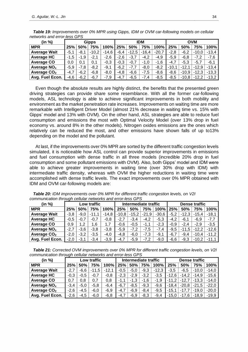
G. Aguilar, W.-L. Jin
34
Table 19: Improvements over 0% MPR using Gipps, IDM or OVM car-following models on cellular networks and error-less GPS
(in %) Gipps IDM OVM
MPR 25% 50% 75% 100% 25% 50% 75% 100% 25% 50% 75% 100%
Average Wait -5,1 -8,1 -10,2 -14,6 -6,4 -12,5 -16,4 -20,7 -2,8 -6,2 -10,0 -13,4
Average HC -1,5 -1,9 -2,1 -2,6 -2,6 -3,7 -4,2 -4,9 -5,9 -6,8 -7,2 -7,6
Average CO 0,0 0,1 0,1 -0,3 -0,3 -0,7 -1,0 -1,6 -4,7 -5,3 -5,7 -6,1
Average NOx -5,9 -7,8 -8,2 -9,1 -6,2 -7,7 -8,0 -8,2 -10,1 -12,1 -12,9 -13,4
Average CO2 -4,7 -6,2 -6,8 -8,0 -4,8 -6,6 -7,5 -8,6 -8,6 -10,9 -12,3 -13,3
Avg. Fuel Econ. -4,6 -6,2 -6,7 -7,9 -4,7 -6,5 -7,4 -8,5 -8,5 -10,8 -12,2 -13,2
Even though the absolute results are highly distinct, the benefits that the presented green
driving strategies can provide share some resemblance. With all the former car-following models, ASL technology is able to achieve significant improvements in both mobility and environment as the market penetration rate increases. Improvements on waiting time are more remarkable with Intelligent Driver Model (almost 21% decrease in waiting time vs. 15% with Gipps’ model and 13% with OVM). On the other hand, ASL strategies are able to reduce fuel consumption and emissions the most with Optimal Velocity Model (over 13% drop in fuel economy vs. around 8% in the other models). Nitrogen oxides emissions are the ones which relatively can be reduced the most, and other emissions have shown falls of up to13% depending on the model and the pollutant.
At last, if the improvements over 0% MPR are sorted by the different traffic congestion levels simulated, it is noticeable how ASL control can provide superior improvements in emissions and fuel consumption with dense traffic in all three models (incredible 20% drop in fuel consumption and some pollutant emissions with OVM). Also, both Gipps’ model and IDM were able to achieve greater improvements in waiting time (over 30% drop with IDM) with intermediate traffic density, whereas with OVM the higher reductions in waiting time were accomplished with dense traffic levels. The exact improvements over 0% MPR obtained with IDM and OVM car-following models are:
Table 20: IDM improvements over 0% MPR for different traffic congestion levels, on V2I
communication through cellular networks and error-less GPS
(in %) Low traffic Intermediate traffic Dense traffic
MPR 25% 50% 75% 100% 25% 50% 75% 100% 25% 50% 75% 100%
Average Wait -3,8 -9,0 -11,1 -14,8 -10,8 -15,2 -21,9 -30,6 -5,2 -12,3 -15,4 -18,1
Average HC -0,5 -0,7 -0,7 -0,8 -2,7 -3,4 -4,2 -5,3 -4,2 -6,1 -6,9 -7,7
Average CO 0,9 1,2 1,6 1,7 -0,6 -0,5 -1,1 -2,3 -0,9 -2,4 -2,9 -3,5
Average NOx -2,7 -3,6 -3,8 -3,8 -5,9 -7,2 -7,5 -7,4 -9,5 -11,5 -12,2 -12,6
Average CO2 -2,0 -3,2 -3,5 -4,0 -4,8 -6,0 -7,3 -9,1 -6,7 -9,4 -10,4 -11,2
Avg. Fuel Econ. -2,0 -3,1 -3,4 -3,9 -4,7 -5,9 -7,2 -9,0 -6,6 -9,3 -10,2 -11,1
Table 21: Corrected OVM improvements over 0% MPR for different traffic congestion levels, on V2I
communication through cellular networks and error-less GPS
(in %) Low traffic Intermediate traffic Dense traffic
MPR 25% 50% 75% 100% 25% 50% 75% 100% 25% 50% 75% 100%
Average Wait -2,7 -6,6 -11,5 -12,1 -0,5 -5,0 -9,3 -12,3 -3,5 -6,5 -10,0 -14,0
Average HC -0,3 -0,5 -0,7 -0,8 -2,3 -2,9 -3,2 -3,5 -12,6 -14,2 -14,9 -15,6
Average CO 0,7 0,8 0,7 0,8 -1,1 -1,3 -1,6 -1,9 -11,2 -12,7 -13,3 -14,0
Average NOx -3,4 -5,0 -5,8 -6,4 -6,7 -8,5 -9,3 -9,6 -18,4 -20,8 -21,5 -22,0
Average CO2 -2,6 -4,5 -6,0 -6,9 -4,7 -6,9 -8,4 -9,5 -15,1 -17,7 -19,0 -20,0
Avg. Fuel Econ. -2,6 -4,5 -6,0 -6,8 -4,7 -6,9 -8,3 -9,4 -15,0 -17,6 -18,9 -19,9

G. Aguilar, W.-L. Jin
35
7. CONCLUSIONS
In this thesis, the Advisory Speed Limit (ASL) control strategies based on Vehicle-to-
Infrastructure communication were studied to smooth vehicle trajectories in stop-and-go traffic. The problem was formulated with the feedback control theory, in which improvements in delays, fuel economy and emissions were first studied in an isolated intersection and then in a loop intersection. Control algorithms for the calculus of ASL indications were proposed, and the effects of several parameters in the results were analyzed, namely market penetration rate, traffic congestion level, communication network and location accuracy, as well as the car-following model itself.
Through simulations, the effectiveness of this control strategy was demonstrated in multiple
scenarios, concluding that high market penetration rates will make possible to achieve remarkable improvements in average delay, fuel economy and emissions, and that this is certainly an encouraging alternative for individuals in the near future. In particular, it was found that the system would perform better over cellular networks than over DSRC networks (therefore being more important a higher transmission range than a lower delay), with the added benefit of the system being able to work thanks to a smartphone application solely, without implying general modifications in the vehicle.
Also, it was seen how average waiting times are very sensitive to location over-estimation
with the designed strategy, and that this perhaps could be resolved by purposely introducing a fixed under-estimation error in the vehicles’ location, even though sacrificing greater improvements in fuel economy and pollutant emissions. At last, it was observed that improvements can be obtained either on isolated or non-isolated intersections, and using diverse car-following models.

G. Aguilar, W.-L. Jin
36
8. FUTURE DIRECTIONS
After discussing the influence of each of the studied parameters on ASL control strategies,
it would be interesting to extend the current study in several other directions. A list of proposed future work is:
- Field-test the effectiveness of ASL strategies in real life to verify the results - Results have been encouraging enough to at least consider this kind of strategies in
the future, therefore being important to know the improvements at even lower market penetration rates (probably between 1% and 10%) to observe short term benefits
- Even though the implementation of ASL technology could provide benefits, would it be possible to obtain the goals of this project (reduce vehicle stopping time, fuel consumption and emissions) by just changing the state of the traffic lights and the duration of its phases (Signal Timing Change –STC- control)?
- Consider large networks (see figure below), adding the possibility to perform right and left turns, or even multi-lane roads
Fig. 31: Network grid
- Placing initial inductive loops on each road would help to know how many vehicles are on the road and therefore improve ASL indications, but it would require a lot of infrastructural change and resources. It would be interesting to know how would the system perform without knowing the exact number of vehicles on the road (non-equipped vehicles would appear “invisible” to the system). A simple modification of some of the ASL operation algorithms could provide an answer to this discussion, which will probably be studied in the future
- Vehicle-to-Infrastructure (V2I) communication has proven successful in managing intersection traffic by reducing delays, emissions and fuel consumption. Would Vehicle-to-Vehicle (V2V) communication be able to outperform or complement V2I communication on the scenarios studied in this thesis?
- The benefits of ASL control in intersections with a cycle length of 60 seconds has been studied, but most certainly the cycle length could impact the results. Future study could consider the effects of different cycle lengths or even non pre-timed (actuated) traffic lights
- Study similar strategies for autonomous vehicles (smaller reaction times) - Discuss GPS delay implications (take into account that the position of the GPS updates
every 1s approximately)

G. Aguilar, W.-L. Jin
37
REFERENCES
[1] D. Schrank, B. Eisele, and T. Lomax. “National Congestion Tables”. Urban Mobility Report, 2012, pp. 24-27. [2] Oran Viriyincy. “1st Avenue Traffic”. Flickr, 2009. https://www.flickr.com/photos/viriyincy/. Accessed June 20, 2014. [3] H. A. Rakha, R. K. Kamalanathsharma and K. Ahn. “AERIS: Eco-Vehicle Speed Control at Signalized Intersections Using I2V Communication”. Publication FHWA-JPO-12-063. FHWA, U.S. Department of Transportation, 2012. [4] A. Bandivadekar, K. Bodek, L. Cheah, C. Evans, T. Groode, J. Heywood, E. Kasseris, M. Kromer, and M. Weiss. “On the road in 2035: Reducing transportation’s petroleum consumption and GHG emissions”, 2008. [5] H. A. Rakha, K. Ahn, K. Moran, B. Saerens, and E. V. D. Bulck. “Virginia Tech Comprehensive Power-Based Fuel Consumption Model: Model development and testing”. Transportation Research Part D: Transport and Environment, Vol. 16, 2011, pp. 492-503. [6] K. Ahn, H. Rakha, A. Trani, and M. Van Aerde, “Estimating vehicle fuel consumption and emissions based on instantaneous speed and acceleration levels”. Journal of Transportation Engineering, Vol. 128, 2002, pp. 182-190. [7] K. Dresner and P. Stone. “Multiagent Traffic Management: A Reservation-Based Intersection Control Mechanism”. The Third International Joint Conference on Autonomous Agents and Multiagent Systems, 2004, pp. 530–537. [8] K. Dresner and P. Stone. “Multiagent Traffic Management: An Improved Intersection Control Mechanism”. The Fourth International Joint Conference on Autonomous Agents and Multiagent Systems, 2005, pp. 471-477. [9] K. Dresner and P. Stone. “A Multiagent Approach to Autonomous Intersection Management”. Journal of Artificial Intelligence Research, Vol. 31, 2008, pp. 591–656. [10] P. Gipps. “A behavioural car-following model for computer simulation”. Transportation Research Part B: Methodological, Vol. 15, 1981, pp. 105–111. [11] Office of the Majority Leader, U.S. House of Representatives. “The Red Light Running Crisis. Is it Intentional?”, 2001. http://www.motorists.org/red-light-cameras/armeyreport.pdf. Accessed April 17, 2014. [12] D. Maas. Sacramento County, Department of Transportation. “Dilemma Zone Elimination”, 2008. http://www.ite.org/meetings/2008AM/Session%2047_Doug%20Maas.pdf. Accessed May 5, 2014. [13] H. Rakha, K. Ahn, and A. Trani. “Development of VT-Micro Model for Estimating Hot Stabilized Light Duty Vehicle and Truck Emissions”. Transportation Research Part D: Transport and Environment, Vol. 9, 2004, pp. 49-74. [14] K. Ahn, H. Rakha, A. Trani, and M. Van Aerde. “Estimating vehicle fuel consumption and emissions based on instantaneous speed and acceleration levels”. Journal of Transportation Engineering, Vol. 128, 2002, pp. 182-190.
G. Aguilar, W.-L. Jin
38
[15] J. Heggestuen. “One In Every 5 People In The World Own A Smartphone, One In Every 17 Own A Tablet”. Business Insider, 2013. http://www.businessinsider.com/smartphone-and-tablet-penetration-2013-10. Accessed June 10, 2014. [16] U.S. Government and the National Coordination Office for Space-Based Positioning, Navigation, and Timing (PNT). “GPS Accuracy”, 2014. http://www.gps.gov/systems/gps/performance/accuracy/. Accessed June 1, 2014. [17] M. Treiber, A. Hennecke and D. Helbing. “Congested Traffic States in Empirical Observations and Microscopic Simulations”. Physical Review E, Vol. 62, 2000, pp. 1805-1824. [18] M. Bando, K. Hasebe, A. Nakayama, A. Shibata, Y. Sugiyama. “Structural Stability of Congestion in Traffic Dynamics”. Japan Journal of Industrial and Applied Mathematics, Vol. 11, 1994, pp. 203-223. [19] M. Bando, K. Hasebe, A. Nakayama, A. Shibata, Y. Sugiyama. “Dynamical model of traffic congestion and numerical simulation”. Physics Review E, Vol. 51, 1995, pp. 1035-1042. [20] M. Bando, K. Hasebe, A. Nakayama, A. Shibata, Y. Sugiyama. “Phenomenological Study of Dynamical Model of Traffic Flow”. Journal of Physique I (France), Vol. 5, 1995, pp. 1389-1400.