MASTERARBEIT

Titel der Masterarbeit

„Transfer Pricing and Strategic Delegation“

Verfasser

Patrick-Philipp Valda, Bakk. rer. soc. oec.

angestrebter akademischer Grad

Master of Science (MSc)

Wien, 2013 Studienkennzahl lt. Studienblatt: A 066 915 Studienrichtung lt. Studienblatt: Masterstudium Betriebswirtschaft Betreuer / Betreuerin: Univ.-Prof. Dr. Thomas Pfeiffer

I

Foreword

I want to express my gratitude to the people who supported me during the time I’ve been

writing this thesis. First and foremost Dipl.-Ing. Dr. Clemens Löffler, who guided me when I

lost track and gave me very valuable input during every occasion we met. Of course, Univ.-

Prof. Dr. Thomas Pfeiffer with his vast understanding of the topic was very helpful since he

understood to question those questions which I haven’t asked myself and needed to be

answered more thoroughly.

A major force that led to the successful completion of this thesis has been the sum of

supportive actions undertaken by my friends and family who believed in me, my abilities and

my willingness to complete it, even if I had doubts sometimes. Thank you!

Declaration on Oath

Herewith I affirm that I have written the master’s thesis “Transfer Pricing and Strategic

Delegation” entirely on my own and have not used outside sources without declaration in the

text. Any concepts or quotations applicable to these sources are clearly attributed to them.

This diploma thesis has not been submitted in the same or substantially similar version, not

even in part, to any other authority for grading and has not been published elsewhere.

Signature, Date:

(Patrick-Philipp Valda, Bakk. rer. soc. oec.)

II

Table of Content

Foreword ..................................................................................................................................... I

Declaration on Oath .................................................................................................................... I

Table of Content .........................................................................................................................II

List of Tables ............................................................................................................................ III

List of Figures .......................................................................................................................... III

Abbreviations ........................................................................................................................... IV

1 Introduction and Motivation ............................................................................................... 1

2 Theory of Transfer Prices ................................................................................................... 2

2.1 Types of Transfer Prices .............................................................................................. 9

2.2 The Coordination Problem ........................................................................................ 10

2.3 Strategic Function of Transfer Pricing ...................................................................... 13

3 Game-Theoretical Background ......................................................................................... 17

4 Basic Setup of Arya and Mittendorf ................................................................................. 19

4.1 Input ........................................................................................................................... 21

4.2 Cost-Based Transfer Price ......................................................................................... 23

4.3 Market-Based Transfer Price ..................................................................................... 26

5 Modified Setup .................................................................................................................. 30

5.1 Case of One Competitor on the Intermediate Market ................................................ 32

5.1.1 Input ................................................................................................................... 33

5.1.2 Calculation and On the Fly Interpretation .......................................................... 35

5.1.3 Comparison with Results of Arya/Mittendorf .................................................... 39

5.2 Standardized Case: Multiple Competitors on the Intermediate Market .................... 44

5.2.1 Input ................................................................................................................... 45

5.2.2 Output and Interpretation ................................................................................... 47

6 Conclusion ........................................................................................................................ 53

III

7 Works Cited ...................................................................................................................... 55

8 Appendix ........................................................................................................................... 57

8.1 Proof of Calculation for a variable Number of Competitors ..................................... 57

8.2 Split Up Profit Function ............................................................................................ 63

8.3 Differential Analysis for One- and Multiple Competitors ......................................... 64

9 Summary ........................................................................................................................... 71

10 Zusammenfassung ......................................................................................................... 71

11 Curriculum Vitae ........................................................................................................... 72

List of Tables

Table 1: Timeline of actions set by the actors of the company 1 ............................................. 21

Table 2: Timeline of actions set by the actors of the company AB ......................................... 32

Table 3: Arya/Mittendorf’s simplified results versus the modified model’s results ................ 40

List of Figures

Figure 1: Visualization of the Setup by Arya/Mittendorf ........................................................ 20

Figure 2: Visualization of the Modified Model with one Competitor ..................................... 33

Figure 3: Visualization of the Modified Model with ( ∈ ℕ) Competitors ........................ 45

Figure 4: change to according to (48) ..................................................................... 48

Figure 5: change to ...................................................................................................... 49

Figure 6: responds unexpectedly to .......................................................................... 50

Figure 7: Slope of transfer price ............................................................................................... 51

Figure 8: Profit functions’ responses to ............................................................................... 52

Figure 9: Plot of (A38) ........................................................................................................... 67

Figure 10: Plot of (A41) ........................................................................................................... 68

IV

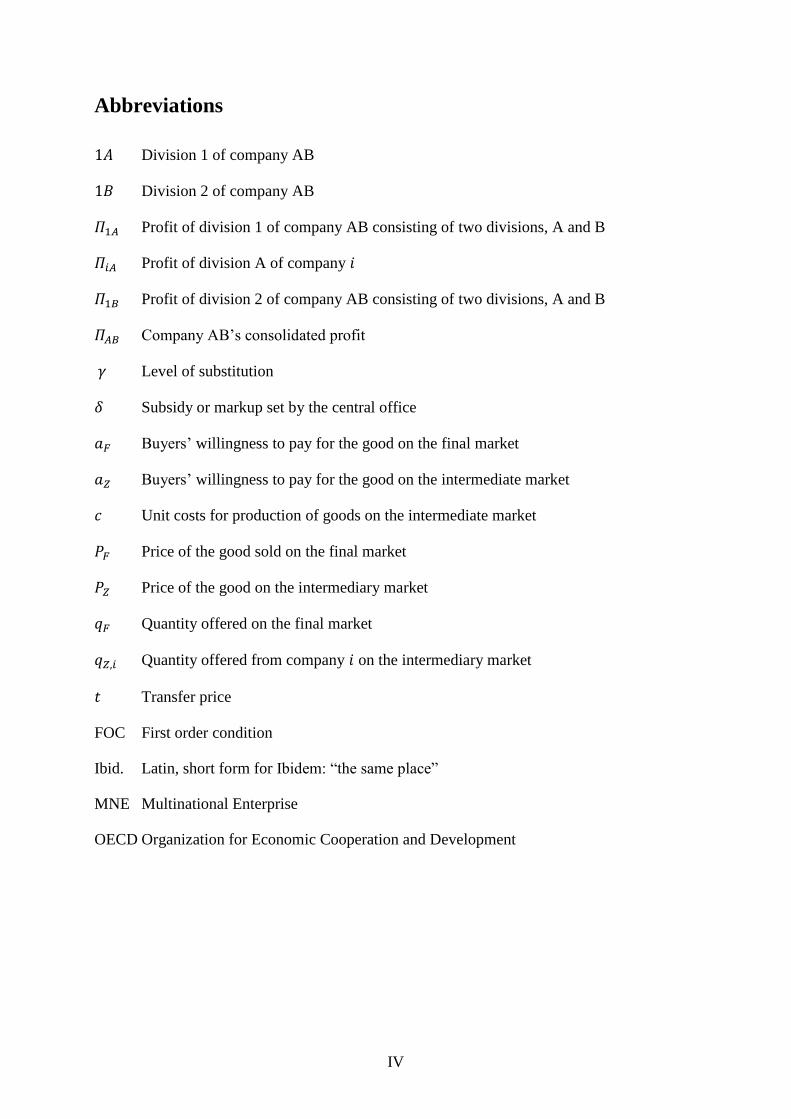
Abbreviations

Division 1 of company AB

Division 2 of company AB

Profit of division 1 of company AB consisting of two divisions, A and B

Profit of division A of company

Profit of division 2 of company AB consisting of two divisions, A and B

Company AB’s consolidated profit

Level of substitution

Subsidy or markup set by the central office

Buyers’ willingness to pay for the good on the final market

Buyers’ willingness to pay for the good on the intermediate market

Unit costs for production of goods on the intermediate market

Price of the good sold on the final market

Price of the good on the intermediary market

Quantity offered on the final market

Quantity offered from company on the intermediary market

Transfer price

FOC First order condition

Ibid. Latin, short form for Ibidem: “the same place”

MNE Multinational Enterprise

OECD Organization for Economic Cooperation and Development

1

1 Introduction and Motivation

As transfer pricing has become a topic of increasing importance due to numerable reasons, the

topic has also received more attention from scientific sources over the years. Transfer pricing

theory is an essential part of making a partitioned company with more than one independently

acting division an effective construction. After all, if there are no synergies and ways to

efficiently use these synergies, then there are no reasons for companies’ divisions to be

economically related in the first place. Instead, they probably would be better off being

independent units competing with each other on the open market, relying on the popular

“invisible hand” by Adam Smith, to maximize efficiency. The effects and objectives of

transfer pricing strategies can be manifold. The topics of tax avoidance and the maximization

of consolidated profits through strategically thought-through transfer pricing probably are the

most familiar applications coming to one’s mind. Another very important purpose of transfer

pricing strategies is mitigating coordination problems which arise in segregated companies.

The core of this thesis will be the focus on extending and modifying the model described in a

working paper published by Anil Arya and Brian Mittendorf in 2008 titled “Pricing Internal

Trade to get a Leg up on External Rivals” which deals with internal transaction pricing and its

strategic effects. Arya/Mittendorf focus on a model composed of a parent firm that offers an

“intermediate” good on an intermediate market where it faces Cournot competition from a

second firm and a subsidiary that uses this “intermediate” good to produce a final good for a

final good market where it enjoys monopoly power. The parent division in the model of

Arya/Mittendorf tries to maximize consolidated profit whereas the subsidiary maximizes its

own profit. Therefore, the parent can influence the transfer price either indirectly by adjusting

its output to the intermediate market since the transfer price is derived from the price on the

market which is affected by supply or directly via an internal subsidy. Then, the authors

examine among others the effects of the transfer price strategy on the competitor as well as

the internal effect under market based transfer pricing as well as cost based transfer pricing.

In contrast to the model of Arya/Mittendorf, in this thesis the model has been modified in a

way that the “parent”, which then will be regarded as a simple division of the company, no

longer tries to maximize consolidated profit but rather pays attention to its own gains. The

subsidiary, as in the model of Arya/Mittendorf, still maximizes its own profit on the final

good market. Another difference is the introduction of a third party in the organization,

namely the “central office”, which then tries to maximize consolidated company profits using

2

its power of being able to set the value of a subsidization/markup factor. This introduction of

the central office is the main difference between the models of Arya/Mittendorf and the one

proposed in this thesis. Cost based transfer prices will be excluded from the analysis in the

modified model since the focus will be laid on the effect of a market based transfer price.

Differences between the relevant results of Arya/Mittendorf and the modified model in this

thesis will be highlighted.

After this first introduction and analysis of the modified model’s results the model will be

further altered to move away from the proposition of a duopoly on the intermediate market.

The modified model will be standardized to portrait the competition of competitors on the

intermediate market to examine the influence of increasing competition on the actions of the

decision making units within the company. Interestingly, the model does not react as planned

under the postulated assumptions.

Besides focusing on these models and their results, the thesis will give an overview of the

importance of transfer pricing in today’s business world.

2 Theory of Transfer Prices

Simply spoken, transfer prices are needed for intra-company accounting purposes to evaluate

intra-company goods and services, which are transferred from one division to another

division.

Transfer pricing theory is a field of study with a history that reaches back more than half a

century, see, for example, publications by Stone (1956) or Paul W. Cook (1955). According

to these publications, the upcoming interest on transfer pricing theory was strongly related to

the increasing decentralization of companies. That is consequential, as decentralization of

companies into several divisions leaves the central offices’ managers with the question of

how to make the divisions’ executives manage their division in the shareholders’ best interest

(i.e. to maximize consolidated profit) and still be able to enjoy the opportunities provided by

having several internal divisions working independently in conjunction with the arm’s length

principle.

Although the topic has already been picked up decades ago, the initial problem of setting

internal transfer prices between the divisions of a company is still subject to intense research.

Since transfer prices are also a subject to conflicts of objectives, the perfect solution might

very well remain a theoretical concept and in the real world decision-makers could be forced

3

to be content with the approach of converging to the theoretically best possible result. The

topic of transfer pricing is also closely related to the problem of setting suitable incentives to

maximize profits. Since multidivisional companies seek to evaluate their divisions, they will

want to enforce certain managerial structures on them, organizing them for instance as profit

centers, which then are evaluated according to their profits. These profits however are

influenced by the transfer pricing strategies enforced by the central office. This setup thereby

bares risks of leaving one of the parties unsatisfied and could even have a share in proving

compensation-schemes useless if divisional managers feel they are restricted in optimizing the

outcomes of their performance figures by what they feel are unjustly set transfer prices.

(Stone, 1956)

In any case, divisional performance measurement is an important topic of its own. On the one

hand, separately measuring divisional performances increases incentives for these divisions to

perform well. This decreases the problematic issue of divisional managements that profit

largely from consolidated companies results without contributing as positively as they could,

also called the “free rider problem”. On the other hand, divisional performance measuring can

lead to the exact opposite, namely increasing divisional profit by sacrificing the whole

companies’ profits. (Zimmerman, 1997)

Zimmerman (1997) does also give a very neat and intuitive example of how performance

measurement and transfer pricing act in concert. The example gives an idea about the depth of

the topic. Zimmerman describes a scenario of a Casino divided in three divisions. Two of

them are achieving a negative performance according to Economic Value Added (EVA).

However, the third division, the “Gaming” division, is highly profitable. Regarded separately,

the two unprofitable divisions should be disposed of or restructured, but that wouldn’t pay

any respect to the synergies which in this case exist. The two divisions’ services are highly

relevant to the success of the third division. There is obviously a need for internal

compensation, otherwise the managers of the unprofitable division will most likely choose to

become profitable on their own and thereby undermine the great results of the consolidated

company. In this case however, there’s not even an open market for their services. So, what

kind of transfer price should be introduced? There is no definitive answer to that question.

Zimmerman points out that accounting for synergies is often unprofitable and this example

gives a first impression of the difficulties of transfer pricing. (Zimmerman, 1997, p. 99ff)

When it comes to intercompany transactions, the transfer pricing strategy has to be fine-tuned

with the divisional performance measures. Assume, for instance, the application of a market

4

based transfer pricing strategy on a cost center. In this theoretical example the division would

then be judged by its costs which would depend on the market price, on which it would in

most cases not have any influence at all. Divisional management should only be judged by

measures they can influence. Transfer pricing choices for cost centers have to be related to

cost. But again, the situation is not so easy to be assessed since it’s not obvious what kind of

cost should be contemplated for evaluation. Actual cost would lead to an incentive of the

producing division’s management to act careless since the buying division would be the one

to suffer from exuberating costs. The appliance of standard cost however solves the problem

by leaving any variances, positive or negative, in the selling division. That leads to a fair

transfer price from which the consolidated company profits as the selling division tries to

control its cost. (Fabozzi, Drake, & Polimeni, 2008, p. 406f)

There are several types of transfer prices known in literature and practice. Ewert and

Wagenhofer (2005, p. 585) roughly separate them into market based transfer prices, cost

based transfer prices and negotiated transfer prices. Coenenberg (2003, p. 526) refers to

Riebel/Paudtke/Zscherlich (1973, p. 29ff) who are more exact and divide transfer prices into 9

categories, which include differentiations according to the manner of occurence, material and

time-wise orientation, cost-figures, length of validity, consistency, diversity, multi-part

features and complementary transfer price types. Since this itemization may be exact it is

rather cryptical which supposedly leads Coenenberg (2003, p. 527ff) to focus on highlighting

the most important transfer prices which are closely related to the description summarized in

Ewert and Wagenhofer (2005, p. 585) mentioned before, namely the market-based transfer

prices, cost-based transfer prices and miscellaneous transfer prices, which include for instance

negotiated transfer prices.

The importance of transfer pricing can also be conceived by having a glance at the latest

global transfer pricing tax authority survey published by Ernst & Young. It tells a story of just

how much effort governments around the world have started to put into monitoring

companies‘ internal transfer prices and their effects on tax burdens. (Ernst & Young, 2012)

However, any of the big four accounting companies has transfer pricing on their agenda and

does their own copious studies in this field.

The OECD also publishes „Transfer Pricing Guidelines for Multinational Enterprises and Tax

Administrations“ which affects multinational companies addresses not only governmental

interests like taxes, but also taxpayers interests like avoiding double taxation.

5

According to the global transfer pricing survey of Ernst & Young (2010), the awareness of

managers to the importance of transfer pricing has been increasing during the last years.

Although levels have been decreasing since the peak of awareness in 2005, only 5% of

managers take the transfer pricing topic as “not very important” or “not at all important”.

Ernst & Young account the decrease in concern about transfer pricing to the fact that

managers nowadays feel more in control about the topic. This is comprehensible since in

2010 a striking 86% of parent company respondents have indicated their transfer pricing

policies have been examined by tax authorities, up from 52% in 2007, so dealing with transfer

pricing policies has become a vital part of the overall managerial responsibility. Another

interesting finding of the study is that there’s an ongoing shift from transactional methods of

transfer pricing to profit-based methods (Comparable profit method/Transactional net margin

method), which are preferred by tax authorities. (Ernst & Young, 2010, p. 6ff)

At the time of writing this thesis the most recent case of transfer pricing violation involves the

finish company Nokia, which may have violated transfer pricing norms in India. Nokia’s local

subsidiary allegedly has transferred profits to its headquarters and there have been intra-

company transactions of software without meeting all legal requirements. Beside from RS

3.000 crore for tax violations Nokia will probably have to pay RS 10.000 crore for transfer

pricing issues. This would equal about 1.4 billion Euros for disobeying transfer pricing rules.

Even if allegations would be alleviated, this is just the latest example of how much effect

transfer pricing rules could possibly have on multinational companies. (The Economic Times,

2013)1

Another hint concerning the importance of transfer pricing decisions can be deduced from a

legal point of view. Since about 60 to 70 percent of worldwide trade happens within

companies and tax-regulations vary from country to country, multinational companies tend to

use transfer pricing strategies to minimize tax burden. (Sheppard, 2012)

Reducing tax burden is however not the only strategic effect of transfer prices. As described

in the paper of Arya/Mittendorf and also in this thesis, transfer pricing strategy affects

divisions’ as well as competitors’ behavior and therefore has to be set with care to prevent

unwanted signaling.

1 Exchange rate from the website of the ECB on February 6

th 2013, EUR 1 = INR 71.8490;

1 crore equals

6

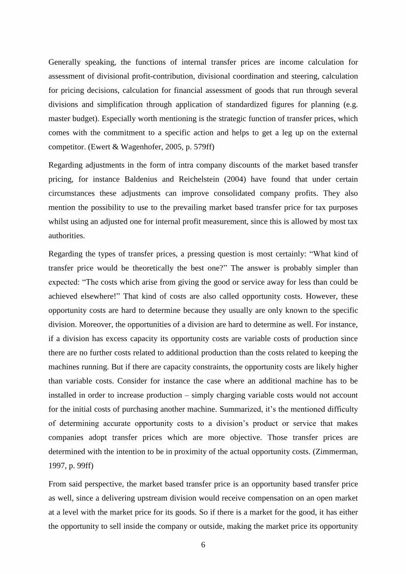
Generally speaking, the functions of internal transfer prices are income calculation for

assessment of divisional profit-contribution, divisional coordination and steering, calculation

for pricing decisions, calculation for financial assessment of goods that run through several

divisions and simplification through application of standardized figures for planning (e.g.

master budget). Especially worth mentioning is the strategic function of transfer prices, which

comes with the commitment to a specific action and helps to get a leg up on the external

competitor. (Ewert & Wagenhofer, 2005, p. 579ff)

Regarding adjustments in the form of intra company discounts of the market based transfer

pricing, for instance Baldenius and Reichelstein (2004) have found that under certain

circumstances these adjustments can improve consolidated company profits. They also

mention the possibility to use to the prevailing market based transfer price for tax purposes

whilst using an adjusted one for internal profit measurement, since this is allowed by most tax

authorities.

Regarding the types of transfer prices, a pressing question is most certainly: “What kind of

transfer price would be theoretically the best one?” The answer is probably simpler than

expected: “The costs which arise from giving the good or service away for less than could be

achieved elsewhere!” That kind of costs are also called opportunity costs. However, these

opportunity costs are hard to determine because they usually are only known to the specific

division. Moreover, the opportunities of a division are hard to determine as well. For instance,

if a division has excess capacity its opportunity costs are variable costs of production since

there are no further costs related to additional production than the costs related to keeping the

machines running. But if there are capacity constraints, the opportunity costs are likely higher

than variable costs. Consider for instance the case where an additional machine has to be

installed in order to increase production – simply charging variable costs would not account

for the initial costs of purchasing another machine. Summarized, it’s the mentioned difficulty

of determining accurate opportunity costs to a division’s product or service that makes

companies adopt transfer prices which are more objective. Those transfer prices are

determined with the intention to be in proximity of the actual opportunity costs. (Zimmerman,

1997, p. 99ff)

From said perspective, the market based transfer price is an opportunity based transfer price

as well, since a delivering upstream division would receive compensation on an open market

at a level with the market price for its goods. So if there is a market for the good, it has either

the opportunity to sell inside the company or outside, making the market price its opportunity

7

costs. On the topic of transfer prices’ effectiveness for instance Loeffler and Pfeiffer (2011)

have written a paper which gives insight about the specifications transfer prices should have

in various settings and how market conditions affect the suitability of certain types of transfer

prices. Hirshleifer (1956) has famously shown that in theory without capacity constraints

marginal costs of the selling division are the optimal transfer price under a specific set of

assumptions. This means that the consolidated company’s optimum is maximized as long as

the transfer price equals marginal costs (i.e. costs which arise from producing one additional

unit). Under these circumstances, a firm would increase its output until marginal revenue

would equal marginal costs and the production of one additional unit would result in a

decreasing profit. Although this seems a relatively easy transfer pricing rule to solving the

coordination problem which results from decentralized decision-making, it’s not applicable to

reality, as will be explained in chapter 2.2.

Hirshleifer has also pointed out that in a competitive market, the transfer price should be

equal to the market price. The firm then would be a price taker and would not be able to

influence the price. If the price on the market is higher than marginal costs of production, this

would lead to a higher output of the company since it would increase production until

marginal revenue (which would be determined by a predetermined market price) meets

marginal costs of production. Moreover, the central office would be indifferent about a

separation of the companies’ divisions since the selling division would be indifferent between

selling to the market or the purchasing division as the purchasing division would be

indifferent between buying from the market or the selling division.

Multinational enterprises (MNE) often are constraint by regulators to use transfer prices tied

to the “arm’s length principle”. This is a terminus one will certainly stumble across when

dealing with the topic of transfer pricing. Governments need to ensure that multinational

enterprises with several divisions don’t evade tax burdens by artificially shifting profits out of

their jurisdiction. However, taxpaying multinationals need to make sure to avoid falling under

double taxation which can arise when divisions operate in countries which are not at odds

concerning arm’s lengths pricing method. Therefore, the Organization for Economic Co-

operation and Development (OECD) publishes “Transfer Pricing Guidelines for Multinational

Enterprises and Tax Administrations” which can be found on the OECD website and be read

for free or downloaded by subscribers. Therein the arm’s length transfer principle is referred

to as:

8

“…the international transfer pricing standard that OECD member countries have agreed

should be used for tax purposes by MNE groups and tax administrations.” (Organisation for

Economic Co-operation and Development (OECD), 2010, p. 33)

“Arm’s length transfer pricing” relates to the requirement that intra-company compensation is

based on levels of value conform to those that would have been applied if the transaction

would have been conducted between unrelated parties. This sounds reasonably simple.

However, there is a set of rules defining not only the amount of compensation but also the

manner of transaction (e.g. one-time payment versus stream of payments).

PricewaterhouseCoopers (2012) for instance provide an international transfer pricing report

that gives an overview of this set of rules. Even though the OECD currently states the arm’s-

length principle as a fair and reliable basis for choosing transfer pricing, they are well aware

of criticism concerning the arm’s length principle.

“The arm’s length principle is viewed by some as inherently flawed because the separate

entity approach may not always account for the economies of scale and interrelation of

diverse activities created by integrated businesses.” (Organisation for Economic Co-operation

and Development (OECD), 2010, p. 34)

They then even discuss an alternative approach called “Global formulary apportionment” that

would use a predetermined formula to allocate a segregated multinational company’s profits

amongst its divisions. The main concern appears to be problems arising from double taxation

as international coordination and consensus regarding the formula in question would be

needed. (Organisation for Economic Co-operation and Development (OECD), 2010, p. 37f)

Picturing all the regulations regarding the excessively detailed reports from OECD,

PricewaterhouseCoopers, Ernst & Young, etc., it is interesting that Arya and Mittendorf note

that these regulatory constraints can even be advantageous instead of harming for

multinationals since they provide strategic opportunities on intermediate good markets. These

advantages result from credible competitive posturing, i.e. making the competitors believe the

company is more committed to achieving a target than its competition. (Arya & Mittendorf,

2008, p. 711)

To provide executives with an overview of the transfer pricing jumble, accounting companies

like Ernst & Young or the formerly mentioned PricewaterhouseCoopers on their part publish

guides, for instance the “Transfer pricing global reference guide” by Ernst & Young. “The

guide outlines basic information for the covered jurisdictions regarding their transfer pricing

9

tax laws, regulations and rulings, Organization for Economic Co-operation and Development

(OECD) guidelines treatment, priorities and pricing methods, penalties, the potential for relief

from penalties, documentation requirements and deadlines, statute of limitations, required

disclosures, audit risk and opportunities for advance pricing agreements (APAs).” (Ernst &

Young, 2010)

Transfer pricing strategies can also be a means to mitigate intra-company coordination

problems. In the modified model this coordination problem will play a role since the sales

decision is not made from a centralized perspective.

2.1 Types of Transfer Prices

According to the OECD guidelines, the appropriate transfer price is chosen with respect to the

availability of reliable information and the degree of comparability between controlled and

uncontrolled transactions as there is no transfer price suitable for all circumstances.

(Organisation for Economic Co-operation and Development (OECD), 2010, p. 59)

Correspondent to OECD (2010), to apply the arm’s length principle, traditional transaction

methods compile the following types:

Comparable uncontrolled price method, which compares the prices of goods and

services of a controlled transaction to those of an uncontrolled transaction happening

on the market.

The resale price method, that takes the price for which a product has been effectively

sold (resale price) by an associated division to an outside company and then

determines the transfer price by calculating backwards, deducting a profit margin and

selling costs from that resale price.

Cost plus method, that begins with the costs that actually occur at the selling division

and then adds a markup. The determination of the costs thereby raises questions since

there are several types of costs suitable for internal cost allocation.

The transactional profit methods may be used under certain conditions to approximate arm’s

length conditions. The idea is that profits arising from controlled transactions are examined

and regarded as indicators whether the transactions differ from those made by independent

companies. They comprise two methods:

Transactional net margin method, which examines the net margin in a controlled

environment by comparing it to an appropriate base (e.g. cost, sales, assets…). This

10

net margin is compared to the net margin achieved by unrelated companies operating

in the same field of work.

Transactional profit split method that divides the combined intra-company profits of

related divisions in a way that unassociated, independent companies would agree on.

This method is especially interesting, if the individual divisions are closely interrelated

and the contribution to the profit of the transaction is not easily determinable. This

method suggests examining unrelated companies on the market to get an idea about

the profit allocation. (Organisation for Economic Co-operation and Development

(OECD), 2010, p. 63ff)

A more general means of classification is the division of transfer prices into market-based

transfer prices, cost-based transfer prices and negotiated transfer prices.

2.2 The Coordination Problem

Successfully guided companies require attention on various aspects of coordination.

According to Ewert and Wagenhofer (2005), factual reasons for coordination are a result of

problems arising from:

Limited resources, which have to be allocated efficiently across companies’ divisions.

Interdependencies across divisions – in order to achieve the best possible result,

divisions have to coordinate their actions. Think about two divisions in a company,

one producing printer and the other printer cartridges.

Stochastic correlation of measures executed by intra-company divisions. Think about

several, yet to be executed, measures depending on rising/falling market prices of a

specific commodity.

Possible interrelations concerning assessments of performances if the subjective

assessment method is dependent on the characteristic of other variables. This problem

arises from the characteristics of the utility function applied. For instance, if due to a

utility function the outcomes of projects with 2 stages (year 1, year 2) have to be

assessed and the outcome at stage 1 does not interfere with the choices for stage 2,

there are no interdependencies. However, if outcome 2 depends on outcome 1, a need

for coordination arises.

Beside the factual reasons for coordination are also personnel reasons for coordination. The

need for coordination scales among other factors with the size of the company and the

11

quantity of decision-making-units or persons involved in the process. Information usually is

not distributed evenly across all of these decision-makers. More likely there will be

asymmetries in the distribution of information which arise due to the delegation of tasks in a

company and are hardly avoidable. Theoretical solutions like simply requesting divisional

managers to pass their superior information on to the top management is unrealistic as

conflicts of interest hinder divisional managers to do so. (Ewert & Wagenhofer, 2005, p.

402ff)

For the sake of achieving a greater good, all the players on a football field must work

together. They combine forces and it’s not unusual that the youth, the impulsive manner and

the arrogance of some players are hard to control by the teams coach. Especially as some of

these players, usually the ones, who score the most goals, shine brighter than others.

The football team example mirrors an integrated company quite well in some respect. Take

for instance a vertically integrated company with two profit centers, which are accountable for

both costs and revenues, as profits equal revenues minus costs. Even if one of the two

divisions had the possibility to assist its intra-company team member in a way that overall

profitability could be increased to a higher level than could be achieved by simply adding up

the results of both divisions, it would still seem as if the supported division performed better

and the supporting division performed worse.

Hirshleifer (1956) graphically presents a model where division A produces an intermediate

product which is processed by division B to be sold to a final monopolistic market. There is

no market for the intermediate product. The divisions decide on their own upon their output

and the question is how the transfer price has to be set to maximize consolidated profit.

Hirshleifer concludes that the optimal transfer price is the producing division’s marginal costs

but remarks the following:

“The full solution involves one of the divisions presenting to the other its supply schedule (or

demand schedule, as the case may be) as a function of the transfer price. The second division

then establishes its output and the transfer price by a rule which leads to the optimum

solution specified above for the firm as a whole.” (Hirshleifer, 1956, p. 183)

Without this information about the supply schedule, the result is not optimal.

Let’s look at an example of the coordination problem based on the model proposed by

Hirshleifer (1956) and portrayed by Ewert and Wagenhofer (2005, p. 598ff).

Consider a company with two divisions, whereas the cost functions of division A and B are:

12

and

The price sales function for the product on the end market – there is no intermediate market –

is:

)

The consolidated company would determine its profit ( ) by maximizing its profit function

with respect to the quantity:

) ) ) )

[ ) ) )]

This yields a consolidated profit ( ) of 57 and an optimal output ( ) of 6 units. Now

consider a decentralization of decision-making regarding the output of the divisions. What

transfer price should the central office enforce to make the divisional managers choose their

output in line with the superior target of maximizing consolidated profit? There is exactly one

transfer price that suits this objective, namely the marginal costs of the selling division in the

optimum. The divisional profits now are dependent on an intra-company transfer price ( ):

) and ) )

If the central office enforces a transfer price ( ) of the marginal costs in the optimum (

) of the selling division, that is:

[ ] [ ]

If , then division A wants to sell

[ )] [ )] and again

And division B wants to sell:

[ ) )] [ ) )]

and again

13

Therefore, both companies want to produce the quantity that maximizes consolidated profit

( is again 57). The imposition of any other transfer price has the effect that the allocation

of profits would be either advantageous for the buying division, if the transfer price would be

smaller, or advantageous for the selling division, if the transfer price would be higher.

However, if the transfer price would be any higher than 12, the buying division would not

want to produce the optimal quantity of 6 in the first place, since its profit would be

maximized at a lower quantity as its marginal costs would intersect with its marginal revenue

earlier. The same principle applies for the selling division, with the difference that it would

want to produce a lower quantity than 6 if the transfer price would be lower than 12 as its

profit would be maximized already at that lower quantity.

Stated the above example, it just looks like the coordination problem has been solved

although it really hasn’t. Remember that the central office has to fix the transfer price at

exactly to maximize the consolidated profit in a decentralized setup. This bears the

question how the central office is able to determine this optimal transfer price in the first

place. In order to know the optimal transfer price, the central office would have to solve the

decision problem and could thereby decide the optimal output on its own, rendering the

divisional managers useless. This thereby is a problem of circularity as decentralized

decision-making under a predetermined transfer price by the central office solves a pseudo

problem. (Ewert & Wagenhofer, 2005, p. 600)

2.3 Strategic Function of Transfer Pricing

Under observable transfer pricing and price competition Robert F. Göx (2000) shows the

effects of strategic transfer pricing in a model. The model depicts two companies in price

competition. He portrays a case where an outperformance can be achieved if not the central

offices decide upon the price directly but the companies employ divisional managers and

profit from decentralization. The outcome for both companies in competition is higher than

under centralized management. Göx (2000) shows, that the competitors’ transfer prices affect

the pricing decision of each company, whereby the marginal costs curves shift upward,

resulting in a lower output to the market with higher prices. Thereby, the outcome drifts

closer to a cartel solution. Both competitors benefit as the consolidated profits of both

companies exceed the profit achieved by price decisions undertaken directly by the central

offices. The higher output can only be achieved in the decentralized setting, since the

divisional managers can credible commit to setting a transfer price above marginal costs as

14

the divisions are structured as profit centers. Considering a centralized solution, the

companies could not credible commit to set transfer prices above marginal cost as the

intermediate product costs would be an exogenous parameter for the consolidated companies

profit function. In a centralized setting, the Nash equilibrium would require setting the price

of the intermediate good to marginal cost. (Göx, 2000, p. 332ff)

As it is more intuitive to reproduce, the effect of strategic transfer prices shall be explained in

an example on the basis of Ewert and Wagenhofer (2005) who took the work of Robert F.

Göx, “Strategische Transferpreispolitik im Dyopol” (1999) as foundation. Therefore, consider

two companies in price competition. Unit costs are equal in both companies with and

the level of product substitution is . The customers’ willingness to pay is

. The prices they achieve on the market are denoted . Their inverse price-sales

functions are:

and

Their profits functions of company 1 and 2 ( , ) are:

) ) )

) ) )

Maximizing these profit functions with respect to respectively yields the optimal price

for each company, since the solution fulfills the profit maximizing condition that marginal

revenue equals marginal cost.

[ ) ] [ ] [ ] [ ]

[ ] [ ]

The first order condition of the profit functions with respect to the prices yields the following

reaction curves:

) and

)

Inserting one curve in the other and solving for the prices results in:

15

This is the equilibrium price and the Bertrand-Nash equilibrium. Inserting these prices into

the price-sales function results in the optimal profit for both companies under centralized

management:

))

)

Now let’s assume that each company decentralizes its pricing decision to a manger of a profit

center. The central office decides upon the transfer price ( ) which is publicly observable.

Profit of the profit centers are now:

) ) )

) ) )

Again, after maximizing profits with respect to the prices and intersecting the reaction curves,

both managers decide to choose the following prices:

) )

Profits of the consolidated companies differ from the profits of the profit centers, since the

transfer price does not express actual cost but is in this case merely an instrument for steering:

) (

) ) (

) (

)

) (

) ) (

) (

)

To determine the optimal transfer price from the consolidated companies’ perspectives, that

are the perspectives of the central offices, the above portrayed profits of the companies have

to be differentiated with respect to the transfer price.

)

)

Optimal transfer price ( ) is:

16

) )

) )

As the transfer price ( ) is actually higher than unit costs ( ), the introduction of a transfer

price results in a strategic effect. Now, the profit is:

) ) )

Comparing the consolidated profit under a transfer pricing strategy with the consolidated

profit without strategic transfer pricing, it’s evident that the profit under strategic transfer

pricing is higher for every level of product substitution, as long as there is even the slightest

difference in products. ( ):

( ) ) )

) )

The reason for this advantageous effect for both companies on the market is due to the

increase of selling prices by the managers in the new equilibrium. The higher the level of

similarity of the products the two companies produce ( ), the more pronounced this effect

becomes. Price-competition with two competitors would already lead to a scenario of perfect

competition, where no profit above economic cost of production could be achieved. This

favorable solution is only applicable under decentralized decision-making because if the

central offices would directly decide upon the market prices, the two companies would not

have the possibility to credible choose a higher market price in the equilibrium. Only if the

central offices of the companies enforce a publicly observable transfer price which cannot be

altered after being made publicly observable, whereas the optimal transfer price is higher than

the actual unit costs, a higher market price is credible. Both managers enforce a higher market

price by their own will, as, from their perspective, this higher market price yields the optimal

result with respect to the competing manager’s market price (i.e. they take each other’s

actions in consideration by regarding the reaction curves). If it were not for the managers, the

company choosing a higher market price than the equilibrium market price would offer its

competitor the possibility to increase profits at its own expense. (Ewert & Wagenhofer, 2005,

p. 634f) (Pfähler & Wiese, 2006, p. 125ff)

17

3 Game-Theoretical Background

The necessary mathematical skills to understand and follow the model, which will soon be

presented, are not on a breathtaking level. However, it is of use to have a basic knowledge

about game theory, since multilateral interests are in the focus of the analysis. The few

concepts that will be necessary to understand the model shall be highlighted briefly.

The following model and its modification will be based on competition in quantities and not

competition in prices. This is not imperative; the model could also be transformed and

interpreted in an environment of price competition. The decision, if one assumes competition

in quantities or prices, depends essentially on the expectation about the long-term action

parameter, if it’s rather the price or quantity. An oil producing company cannot set prices

since it takes quite some time to extract and deliver oil via freighter, thereby its action

parameter will be the quantity produced. The action parameter for an operator of a gas station

on the other hand is the price. This separation is important since it leads to different models

which are applicable: The Bertrand model in the case of price competition or the Cournot

model in the case of competition in quantities. Which one of these models is more appropriate

depends largely on the market position a company finds itself in (e.g. industry, retailer), as

stated in the above example. One important difference is that in the Bertrand competition,

even a market with just two competitors, a duopoly, is enough to make both competitors offer

their goods for just marginal costs which is the result of a market with perfect competition.

This means, the companies would not make any profits on their goods and are just about able

to cover their economic costs (Bertrand paradox). This is not the case in a market in Cournot

competition. (Pfähler & Wiese, 2006, pp. 67ff, 125ff)

Consider a company that operates on a market and faces one competitor. It has to decide upon

the quantity it sells on this market, taking its competitor’s output into equation. Its competitor

deals with the exact same thoughts. Mathematically speaking, this is the reaction curve, which

shows the possible action alternatives whilst taking the behavior of the competitors into

consideration.

)

) (Pfähler & Wiese, 2006, p. 128)

The argument of the maximum determines all the possible quantities on the quantity-curve

from company 1 ( ), where company 1’s profit ( ) is maximized with respect to the

competitor’s output ( ). These quantities are deduced by maximizing the profit of company

18

1 with respect to its own quantity ( ). At the same time, company 2 determines its own

reaction function.

)

)

These reaction functions likewise yield the best possible outcome for both companies, taking

each other’s actions into account. The reaction curves have a negative slope since the increase

of output of one company makes the market price shrink. Thus it’s profitable for the other

company to decrease its output as marginal revenue still needs to equal marginal cost to

maximize profits and marginal revenue just decreased in said situation. The Cournot model

assumes that both actors simultaneously determine their outputs. Thus, strictly speaking, they

have to know about each other’s organization and costs. Stackelberg (1934) for instance dealt

critically with the issue that Cournot-competitors choose their quantity simultaneously and

proposed sequential competition of quantities. Thereby he showed that the Stackelberg leader,

that is the market participant who determines his output first, has a strategically advantageous

position and can thereby achieve a higher output compared to the Stackelberg follower and

the actors in a Cournot competition. However, this requires that the Stackelberg follower is

aware of the quantity that the leader proposes. Availability of information thereby is critical.

(Pfähler & Wiese, 2006, pp. 125ff, 140ff)

Another aspect to successfully understanding the following model and its modification is the

process of backward induction, or backward solving. By using this process, it is possible to

examine if a solution to a multiparty and multilevel problem is in a subgame perfect

equilibrium. This is the case if the whole problem or game is in a Nash-Equilibrium and every

subgame of the multilevel game is in a Nash-Equilibrium, too. A Nash-Equilibrium is

achieved in a game if all parties have decided upon a strategy, which they unilaterally don’t

want to change or adjust. If no party sees an advantage by changing its strategy, the game is in

a Nash-Equilibrium. Keep in mind though that this doesn’t necessarily mean the solution is

Pareto efficient. Pareto efficiency goes one step further and would express a situation where

no player could be made better off without making another player worse off. (Pfähler &

Wiese, 2006, p. 28ff)

Related to the reaction curves, the Nash-Equilibrium is determined by intersecting both

reaction curves. The thereby determined equilibrium tells the involved market participants

about the quantity they need to produce in order to maximize their profit while accounting for

the actions of each other. In this situation, the market participants share the interest to increase

19

the customers’ willingness to pay on their mutual market. This could for instance be achieved

by jointly realized marketing campaigns. Another mutual interest is to decrease cost, which

could be achieved by amplified efforts of lobbying or agreements related to the negotiations

with labor unions. (Ibid, p. 129ff)

4 Basic Setup of Arya and Mittendorf

Arya and Mittendorf focus in their paper titled “Pricing Internal Trade to Get a Leg up on

External Rivals” (2008) on the influence of transfer pricing on competitors behavior. They

highlight cost based transfer pricing as well as market based transfer pricing in multiple

model configurations. For this thesis, one configuration under market based transfer pricing is

of particular interest. According to the results of Arya/Mittendorf, the competitor can be

forced to cede market share through a credible, aggressive signal via market based transfer

pricing. A vital function of this kind of transfer pricing next to tax compliance and shifting tax

burdens thereby can be competitive posturing. Considering this competitive role, a market

based transfer price might even be considered when the market in question is thin. Usually,

internal coordination is problematic due to the subsidiaries interest to procure a less than

optimal quantity of goods from the upstream division unless the transfer price is equal to

marginal costs. This proves costly in the final market but useful in the intermediate market

since the parent, that oversees the profit of the consolidated company, has an incentive to

reduce costs for the subsidiary’s procurement and thereby also reduce the intermediate

product’s market price. This of course puts Cournot competitors under pressure as the parent

aggressively pushes to decrease the market price and, having the subsidiary’s procurement at

the back of its mind, has credible incentive for its course of action. (Arya & Mittendorf, 2008,

p. 709ff)

In order to show the strategic effect a transfer price can have on competitors’ behavior,

Arya/Mittendorf introduce a simple model as follows: A parent and a subsidiary form the

components of a vertically integrated company. The parent produces an input good for the

subsidiary, the intermediate good, and additionally competes on an intermediate market with

one competitor in Cournot-competition. The subsidiary enjoys monopoly power on the final

good market. Figure 1 illustrates the setup:

20

Figure 1: Visualization of the Setup by Arya/Mittendorf

(Source: Own figure)

In this setting, with market-based transfer prices, the parent has incentives to drive down the

market price for the intermediate good to increase internal procurement of the subsidiary. This

is because the subsidiary will increase its procurement when it has to pay a smaller transfer

price to the parent for the input good. This transfer price depends on the market price, which

is called market based transfer price for that reason. The result is an aggressive behavior of

the parent resulting in a softened response from its competitor. This means that the parent has

not only a primary incentive to maximize its own profits but also a secondary incentive to

increase the willingness of the subsidiary to procure more in order to sell more goods on the

monopoly market, which is highly profitable. Thereby the parent maximizes its own profits as

well as the profits of the subsidiary and thus the consolidated company. To manage

distortions – which in this case are purposefully introduced for competitive advantages – and

balance the effects of market-based transfer pricing on the profits of both divisions, the firm

uses intra company discounts which are set by the parent. These intra company discounts are

basically an additional mechanism for the parent to steer the value of the transfer price and

thereby the amount the subsidiary procures. (Ibid.)

To make the setup of Arya/Mittendorf comparable to the modified model, which will be

proposed later on in this thesis, we shall have a closer look at the basic conditions and the

main results of Arya/Mittendorf. The following terms and equations are taken directly from

their above mentioned paper, with the only difference being the denotation of the variables in

order to simplify comparison later on as nomenclature will already be known and similar.

21

Important Assumptions:

∈ ) Conversion costs

Arya/Mittendorf make the assumptions that marginal unit costs exceed 0 and the customers’

willingness to pay both on the intermediate market ( ) and on the final market ( ) exceed

costs . Moreover, they introduce a substitution factor which can have any value between 0,

inferring total dissimilarity of the product the company in focus produces compared to the

products of its competitor, and 1, inferring total similarity. Hereby it has to be clarified that

this substitution factor will later on, in the modified model, be neglected for simplicity. More

specifically, it will be set to the value of 1. This simplification results formulas which depict

the case that the products of the consolidated company and its competitors are equal in every

manner.

Table 1: Timeline of actions set by the actors of the company 1

T=0 T=1 T=2

Company 1 specifies publicly

observable transfer pricing

strategy

Company 1 and 2 compete in

the intermediate market

The subsidiary of company 1

(=1B) decides upon its

quantity on the final good

market

Source: own figure based on “Figure 1. Timeline of Events in the Base Model” (Arya & Mittendorf, 2008, p.

714)

To have a strategic effect (i.e. express credible commitment on the intermediate market

through transfer pricing strategy), the transfer price has to be publicly observable by

competitors and unchangeable after adoption. (Arya & Mittendorf, 2008, p. 719)

4.1 Input

) (1)

The price on the final market ( ) is dependent on the willingness of the customers to pay for

a final good ( ) and only the quantity which the subsidiary sells on the final good market

( ), since it operates in a monopoly in Arya/Mittendorf’s base setting.

22

) whereas and (2)

In the model of Arya/Mittendorf, the price on the intermediate market is different for

company 1 and company 2, since their products are not equal except for the case where the

level product substitution is 1 ( ). If the customers’ willingness to pay on the

intermediate market ( ) increases, the price does so as well. It decreases simply if

aggregated supply is increased by the competing companies. However, the substitution-factor

determines the magnitude of the effect this increase in the competitor’s supply has on the

intermediate market price that the company in focus can achieve.

) (3)

The transfer price ( ) links the two divisions of the multi-divisional company in focus. It is

simply the price that the upstream division of the company receives for delivering its goods to

the downstream division, which is responsible for the further steps in the manufacturing

process. In this case the transfer price is a market-based transfer price. This means the opinion

of the market ( ) is consulted when it comes to the question about the value of the good on

the intermediate market and then adjusted by the parent by applying an intra-company

discount or markup ( ) to optimize consolidated profit.

) (4)

The subsidiary’s revenue ( ) depends on the price on the final market ( ) times the

quantity ( ) sold on the final market. According to the changes in demand and supply the

price reacts to the subsidiaries output. This can be seen by looking at the equation depicting

the price on the final market ( ). Then the costs, in this case the costs for the subsidiary are

equal to the transfer price times the quantity it procures, are subtracted. This is due to a

simplification introduced by Arya/Mittendorf: They set conversion costs to zero. Thereby any

additional costs of production arising from further process done by the subsidiary to finish the

product are neglected. One input good procured by the subsidiary from the parent is turned

directly into one final good, which the subsidiary then sells on the final market for the price

achievable there ( ).

23

( )

) ( ) (5)

The parent’s revenues ( ) are increased by either a higher price on the intermediate market

( ) or a higher quantity sold on the intermediate market ( ). That however affects the

price on the intermediate market negatively since that price is dependent on the output of the

parent and its single competitor on the intermediate market. Additionally, the parent receives

revenues as a result of the procurement by the subsidiary. The amount of these revenues

depends on the level of the transfer price ( ) which depends on the intermediate market price

( ) and the level of subsidization/markup ( ) by the parent. Finally, deducting the cost of

production for the quantity sold on the intermediate market by the parent and those sold to the

subsidiary, leads to the profit of the parent ( ).

) ( ) ( ) (6)

By substituting for the intermediate market price ( ) and the price on the final good market

( ), the sum of the two divisional profits ( ) results in consolidated profit ( ). This

eliminates the transfer price ( ) since the profit and costs of the quantity transferred stays

within the company. In the consolidated company, one division’s receivables are the others

division’s liabilities.

At last, the counterpart of the parent is the standalone division of the competing company.

The competitor only consists of this division and thus doesn’t have to manage any intra-

company transactions. Of course, it thereby has no possibility to profit from the adaption of a

transfer pricing policy. Its profit is:

) (7)

4.2 Cost-Based Transfer Price

First, Arya and Mittendorf introduce their model with a cost-based transfer price in order to

later on provide a comparison between the efficiency of cost-based transfer prices versus

market-based transfer prices in their proposed model.

Using backward induction, transfer pricing policy shall now be considered under the objective

to maximize consolidated firm profit.

24

Irrespective of the transfer price ( ), the subsidiary’s objective is to maximize its profit ( )

on the final good market. Inserting the term for the price on the final good market ( ) (1)

into the equation for division 2’s profit ( ) (4) yields:

[ ) ] (8)

The first order condition (FOC) yields the optimal quantity in dependency of the transfer price

( ):

(9)

The optimal quantity for the subsidiary therefore increases with the willingness to pay ( ) on

the final good market and decreases (increases) with an increasing (decreasing) value of the

transfer price ( ).

The next step in the backward induction concerns the parent division that maximizes

consolidated profit ( ) (6) with respect to the intermediate quantity ( ).

[ ) ( ) ( )] (10)

FOC then yields:

) (11)

This is the optimal quantity the parent should sell on the intermediate market ( ) in

dependency of the quantity which the competing company decides to sell ( ). The other

variables are all exogenous.

Meanwhile, the second company, the competitor to our company in focus, also seeks to

maximize its profits on the intermediate market according to its quantity ( ) in

consideration of the quantity its competitor unloads ( ). According to its profit function

( ) (7) the following function has to be differentiated:

[( ) ] (12)

FOC yields:

25

) (13)

This, in contrast to (11), is the situation from the competitor’s point of view. It will adjust its

output ( ) in dependency of the quantity company 1 ( ) puts out on the intermediate

market.

As explained in chapter 3 (Game-Theoretical Background), both companies will decide at the

same point in time what quantity to sell and therefore need to anticipate each other’s action.

Equations (11) and (13) therefore are called reaction curves. Since both companies decide

simultaneously upon their output, they don’t know about the competitors output at the

decision’s point in time. They rather decide upon the expected quantity of the competitor.

After inserting (13) in (11), and the other way round, and solving for the quantity , we end

up with the Cournot quantities which define the Cournot equilibrium. Unilateral

improvements of the profits are not possible in this environment. This equilibrium therefore

describes a situation in which both companies have maximized their profits in consideration

of the competitor’s output. (Pfähler & Wiese, 2006, p. 128f)

Cournot quantities:

(14)

To reach optimal profit under cost-based transfer pricing, optimal quantities (14) and

(9) are inserted into the profit function of the consolidate company (6).

Optimal profit is:

[

] [

)

)

] (15)

The two terms stand for the intermediate market and the final good market and show that

there is no interconnection between the two. The left term in the squared brackets stands for

the intermediate market, the right one in the second pair of squared brackets for the final good

market. As long as the transfer price ( ) exceeds marginal costs ( ), there is still room for

profit-optimization until the transfer price equals marginal cost ( ). This yields to

equation (16). (Arya & Mittendorf, 2008, p. 714f)

26

[

] [

)

] (16)

4.3 Market-Based Transfer Price

Next, the same model will be regarded under market-based transfer pricing. Remember, the

transfer price is defined in equation (3) as ). As in equation (9), the subsidiary

maximizes its profit on the final good market, taking the newly defined transfer price as well

the price on the intermediate market ( ) into account. The optimal output for the subsidiary

under market-based transfer price is:

)

( )

(17)

Larger internal discounts ( ) increase the output to the final good market and thus also the

demand of the subsidiary, since conversion costs are assumed to be zero. Now, in contrast to

the cost-based transfer pricing method, the intermediate good market and the final good

market are linked together! The market price on the intermediate good market ( ) is

dependent on the quantity of goods ( and ) supplied to the market. then

influences the quantity which the subsidiary sells on the final market ( ) via the transfer

price ( ).

The parent takes this into account as it solves the exact same equation (10) as in the cost-

based transfer pricing case, but with a different quantity on the final market ( ), as in

equation (17):

[ ) ( ) ( )] (10) from chapter 4.2

Inserting (17) for the FOC yields:

) ) (18)

The optimum quantity on the intermediate market ( ) now looks similar to the one depicted

in (11) from chapter 4.2, but is not only dependent on the output of the competitor ( ) but

also the subsidy or markup ( ). If the markup increases (decreases) it becomes less (more)

attractive for the parent to sell to the intermediate market.

27

The competitor solves again for (12), the differences also being hidden within the quantities:

[( ) ] (12) from chapter 4.2

Again, FOC is:

) (13) from chapter 4.2

Inserting (13) in (18), and the other way round, plus solving for both quantities ( and )

results again in the – compared to the cost-based ones quite different – Cournot quantities:

[ ][ ]

[ ][ ]

(19)

Now, both quantities offered on the intermediate market ( , ) depend on the subsidy or

markup ( ) which the parent of company 1 introduces! Interestingly, company 1 decides to

offer less if the subsidy/markup increases and company 2 offers more. Since the quantity of

company 1 in (19) exceeds its cost-based cousin in (14) in the case that that there’s no subsidy

provided by the central office ( , i.e. transfer price is similar to the market price), the

parent can act more aggressively using a market-based transfer price. This comes as with the

Cournot quantities in the cost-based scenario, the subsidiary doesn’t procure enough to

operate in the monopoly optimum on the final market since the costs for procurement would

be above marginal cost. Thanks to the link between the markets through the transfer price,

which is now market based, the parent tries to actively lower the transfer price to increase

procurement of its subsidiary. The first way to do so is increasing its output to the

intermediate market, which according to (2) lowers the market price ( ) and thereby the

transfer price ( ) seen in (3). This credible commitment to increase output on the intermediate

market decreases the output of the competitor. The second way to improve procurement of the

subsidiary is to increase the subsidy ( ). However, this action comes with the undesired

drawback that company 2 increases and company 1 decreases its output, as can be seen in

(19). Therefore it remains to be seen which level of subsidy is optimal to achieve the wanted

strategic effect without compromising the output of company 1 to the intermediate market and

thereby increasing the transfer price again! By plugging the optimal quantities and

28

from (17) and (19) into the equation of consolidated profit (6) and differentiating it with

respect to the subsidy ( ), we end up with the optimal subsidy, i.e. the difference between the

market price and the internal transfer price. (Arya & Mittendorf, 2008, p. 716)

Arya and Mittendorf use caret (e.g. ) to display market-based equilibriums and tilde (e.g.

) to display cost-based equilibriums.

The optimal subsidy ( ) is:

[ ][ ]

[ ] (20)

This optimal subsidy is now plugged into the Cournot-quantities from division A ( ) and

division B ( ) depicted in (19) to determine the optimal quantities from the central offices

point of view under market-based transfer pricing:

[ ][ ]

[ ] (21)

This is the optimal quantity on the final market under market-based transfer pricing ( ) in

relation to the optimal quantity on the final market under cost-based transfer pricing ( ).

Under the assumptions of Arya/Mittendorf, the quantity on the final market is always higher

with cost-based transfer prices, since transfer prices exceeding marginal cost lead to

restrictions in procurement by the purchasing division (1B). If the products are absolutely

diverse (i.e. ), the quantities are equal. If products would be absolutely unrelated in

every aspect, the companies would not be competing in the same market and there would not

be effects of cannibalization. This effect is expressed in the equation for the market price (2)

in this model.

[ ]

[ ][ ] (22)

Contrarian to the quantity on the final market ( ) in (21), the company sells more units on

the intermediate market ( ) under market-based transfer pricing, again with the exceptional

case when products are absolutely diverse.

29

[ ]

[ ][ ] (23)

Company 2 on the other hand loses share on the intermediate market compared to cost-based

transfer pricing.

To reach the term for the optimal transfer price under market-based transfer pricing, the

optimal quantities ( and ) need to be plugged into the equation of the market price in

(2), which then has to be inserted into the equation of the transfer price (3). Finally, the

optimal subsidy ( ) from (20) needs to be applied to equation (3) as well, which results in:

) )

(24)

From (20) Arya and Mittendorf deduce that regardless of the level of substitution ( ) between

the companies’ products, the subsidy ( ) is positive. Thus, the subsidiary can procure its input

goods cheaper inside the company than on the open market but still has to pay more than

marginal cost, which they deduce from (24). Arya/Mittendorf conclude that intra-company

subsidy is used to provide the subsidiary an incentive to procure more than it would under

unadjusted market-based transfer pricing, but still less than with marginal cost. The upside is

that the parent can send a credible signal of commitment to its competitor which results in

competitive posturing on the intermediate market. When the products become more similar

(i.e. increases), intra company subsidy decreases. One reason for this development is a

general decrease in the market price which goes along with increased competition on the

intermediate market. From (2) and common sense it’s inferable that products converging in

similarity decrease the price on the market. Interestingly, the reasoning doesn’t stop there.

From (24) we know that with increasing the transfer price ( ) diverges from marginal cost

( ). As long as the competitors’ products are absolutely different (i.e. ) transfer price

should be the same as in the cost-based model ( ) where markets are not linked. With a

convergence of the products the transfer price ( ) rises and the market price ( ) falls.

Besides however, the quantity on the intermediate market offered by company 1 ( ) rises

according to (22). In favor of showing its teeth to its competitor, company 1 sacrifices profit

on the final good market for profit and an aggressive signal on the intermediate market.

Arya/Mittendorf note, that with the fitting subsidization ( ) there is a benefit irrespective of

the level of similarity ( ).

30

At last, they compare the profit under market-based transfer pricing ( ) relative to profit

under cost-based transfer pricing ( ):

[ ]

[ ] [ ] (25)

It is apparent that regardless of the level of product difference ( ) the profit with market-based

transfer pricing exceeds profit with cost-based transfer pricing. As increases, the advantage

of market-based transfer pricing advances. Summed up, via market-based transfer pricing the

company enhances its output on the intermediate market by credibly committing to mitigate

the problem of undersupply in the final good market. In this model, the market price, which is

the basis for the transfer price, is dependent on the output of two companies. The results show

that the company with an upstream and a downstream division can convince its competitor on

the intermediate market that it needs to put out more units as this will boost procurement by

the downstream division. The subsidy ( ) balances the effect to maximize consolidated

company profit under any level of substitution ( ). (Arya & Mittendorf, 2008, p. 718)

Subsequently, Arya and Mittendorf expand their model to represent symmetric competition,

i.e. two companies competing on both markets, intermediate good market and final good

market. They find that in that changed setting both companies would introduce market-based

transfer pricing as a disadvantage in profits would occur for the company which adopts cost-

based transfer pricing. Moreover, from their model, it seems that both firms would want to

use the credible commitment pictured above to increase market share. This seems like

disadvantageous for both firms as they just increase competition. However, Arya/Mittendorf

point out even more harmful results can be deduced from their model, if the companies could

not link markets via market-based transfer pricing. (Arya & Mittendorf, 2008, p. 725)

5 Modified Setup

In this chapter we will look at a modified model that is related to the one of Arya/Mittendorf.

This will lead to a configuration that is in a way more related to the actual circumstances of

reality, in other ways however it is simplified to keep it neat and focused. Now the question is

how things change when the supplying division (1A) doesn’t have intrinsic motivation, like

the parent in the model of Arya/Mittendorf, to support the purchasing division (1B). The

simple fact in the matter is that an intra-company support is desirable to make the 1B procure

more from 1A since 1B will restrict procurement the more the transfer price ( ) diverges from

31

marginal cost ( ). In the basic model of Arya/Mittendorf the strategic effect of transfer pricing

is examined. Now, next to the strategic effect a coordination problem needs to be overcome.

In this modified model the focus now lies on a company with two rather self-involved

decision-making units and one unit which tries to interconnect these units and their productive

efficiency: These units shall be tagged as follows: Central office, upstream division 1A and

downstream division 1B. Division 1A and 1B are related by internal transactions. 1A

produces a good which it delivers to the intermediate market on the one hand and to 1A on the

other. Doing this, 1A faces Cournot-competition from A competitors, which themselves are

not subject to in-depth analysis and do not operate within a segmented company.

resembles the special case where only one competitor offers its goods on the intermediate

market. Thus, this is the most interesting case for comparison with the results of

Arya/Mittendorf and will be dealt with before the second case, which then resembles a multi-

competitor situation on the intermediate market where and ∈ ℕ. Division 1B

internally receives a good from 1A and it has, as in the Paper of Arya/Mittendorf, no access to

the external intermediate market. This assumption makes more sense in the model of

Arya/Mittendorf since they account for differences between the products of 1A and 2A (see

the substitution factor in their model). Those differences in products will be neglected in the

comparison as well as in the forthcoming calculations for simplicity.

The intermediate good is produced at unit costs , . However, this assumption will later

on be alleviated to for the comparison of results. Otherwise the terms would be

unnecessarily hard to interpret, without much added value. Like in the basic model of

Arya/Mittendorf it will be assumed that without loss of generality conversion costs of one

intermediary product to one final product are zero. Customers’ willingness to pay is likewise

assumed to be larger than the costs on both intermediate and final market .

To calculate the results, backwards induction is used. Starting point is the profit maximization

of 1B, following by the profit of 1A in conjunction with 2A respectively A. In the last step

of the calculation, when the profits of all other parties are maximized, the optimal

subsidy/markup factor ( ) is determined. Of course in reality the time line of actions is as

follows:

32

Table 2: Timeline of actions set by the actors of the company AB

T=0 T=1 T=2

Central office determines

subsidy/markup ( ), the

transfer pricing policy is

publicly observable

1A maximizes profit

according to its quantity

( ) under consideration of

2A’s actions

1B maximizes profit with

respect to its quantity ( )

(Source: own table)

It’s important to mention that the central office knows about the goals of 1A and 1B as does

1A know about 1B’s objective, which is the maximization of their profit according to their

profit functions. The main difference to the Model of Arya/Mittendorf is the observation of a

divergence in interests of party 1A. It can either choose to make more profits on the

intermediary market by pushing its sales there or it tries to use its market power to increase

the transfer price which it receives from 1B by decreasing its sales on the intermediary

market. The central office on the other hand wants to maximize consolidated profit by

introducing a subsidization/markup. In the setting of Arya/Mittendorf the power of

influencing the market price ( ) by increasing or decreasing output and setting the

subsidy/markup ( ) was combined in one division, which they called the “parent”. This

division is now segregated into the central office and 1A, which makes the subsidy/markup

( ) a much more important tool for maximizing consolidated profit.

5.1 Case of One Competitor on the Intermediate Market

The modified model’s visualization for the case of one competitor is depicted in Figure 2:

Visualization of the Modified Model with one Competitor. The model’s calculations will be

reviewed on the following pages. Then, the outcome will be subject to an in-depth analysis

with the outcomes of Arya/Mittendorf under some simplifications.

33

Figure 2: Visualization of the Modified Model with one Competitor

(Source: Own figure)

5.1.1 Input

The demand function for the intermediate product is

), (26)

where denotes the price on the intermediate market for the good 1A produces, denotes

the customers’ willingness to pay on the intermediate market and respectively

denotes the quantity which 1A and 2A intend to sell on the intermediate market. Compared to

Arya/Mittendorf, there is no price for each of the competing companies on the intermediary

market ( ) but one price for both of them ( ). This is due to the assumed lack of product

differentiation.

The demand function on the final good market is exactly similar to the one in chapter 4.1:

), (1) from chapter 4.1

denotes the price on the final market, denotes the customers willingness to pay on the

final market and denotes the quantity that 1B chooses to sell on the final market.

Unlike in the setting of Arya/Mittendorf pictured in chapter 4, division 1A no longer tries to

maximize consolidated profit, taking into account both intermediate and final good markets.

Now, in this model, 1A is as egocentric as 1B. Hence, both of them try to maximize their own

profits without bearing any shortcomings on the consolidated level in mind. There is however

a third player in the game that tries to maximize consolidated profits. This is the central

office, which overlooks the overall business activity and tries to maximize both divisions

34

aggregated profits. In order to calculate the optimal profit from the central office’s point of

view, three steps can be distinguished through backwards-induction. Again, backwards

induction stands for the process of calculating the optimal outcome by starting at the level of

the calculation, where no interdependencies exist, then working your way backwards until the

level is reached, where all the other optimal outcomes have to be considered. At first, division

1B’s maximal profit

(4) from chapter 4.1

is determined with respect to the quantity on the final market . The equation stays the same

as the one already introduced in chapter 4.1.

The equation of the transfer ( ) price slightly changes due to the simplification of the now

neglected level of product substitution, now accounting for just one price on the intermediate

market since there’s the same unique product offered by two companies ( ):

) ( ) (27)

The factor therein determines the subsidy/markup set by the central office to steer the

transfer price and thereby influence the behavior of division 1A and 1B. Secondly, 1A’s

maximal profit, taking (26) into consideration,

( ) ) ( ) (28)

is determined according to the quantity it sells on the intermediary market ( ).

Simultaneously the output of its competitor 2A on the intermediate market has to be

considered ( ). This is achieved by determining the intersection of the reaction curves of

both 1A’s and 2A’s demand curves. It is of special interest to mention that 1A not only

influences its profit directly by determining the optimal amount of goods ( ) it is going to

sell on the intermediate market, but also through the not so obvious effect of its decision of

quantity of sales ( ) on the intermediate market price ( ). Thereby it has an opportunity to

influence the transfer price ( ) it receives from 1B. In the model of Arya/Mittendorf, the

parent (=1A+CO) didn’t abuse the opportunity to increase the transfer price to achieve a

higher profit itself since it maximized for consolidated profit. Now however, 1A doesn’t care

about the sake of 1B and the central office is left with the opportunistic behavior of 1A and

35

needs to make sure that 1B serves the monopoly market well enough since it’s highly

profitable, even if 1A increases the transfer price far above marginal costs.

Profits of the consolidated company are the sum of (4) and (28):

( )

( ) ) ( ) (29)

The profits achieved on the intermediate market (market price times quantity sold: ),

plus the profits achieved on the final good market ( ) minus total cost of production

( )) of these goods equal the consolidated company’s profits. The transfer price ( )

does not directly appear in this equation. However, it influences consolidated profits by

influencing its constituent variables.

The competitor on the intermediate market (2A) has the following profit function that

resembles equation (7) in chapter 4.1 without accounting for product differentiation:

) (30)

5.1.2 Calculation and On the Fly Interpretation

At first, according to backward induction we have to consider the optimal result from the

downstream division ( ) which like in chapter 4 has to decide upon its optimal output to the

final market ( ). Therefore we reach the same equation, however not accounting for

product substitution ( ) anymore:

[ ) ]

( )

(17)

Next, we have to construct the two reaction curves for the optimal quantities of division 1A

and 2A and deduce the Cournot-Nash equilibrium:

[( ) ( )] (31)

Substituting transfer price ( ) for (27) and the quantity on the final market ( ) for (17), FOC

yields to the reaction curve that depicts the quantity that 1A sells on the intermediate market

with considering the output of 2A:

36

) (32)

2A simultaneously maximizes its output:

[( ) ] (33)

FOC yields the second reaction curve that similarly shows the quantity that sells on the

intermediate market with considering the output of 1A:

) (34)

Intersecting these curves (i.e. plugging (34) in (32) and solving for as well as plugging

(32) in (34) and solving for ) we get the optimal quantities in a Cournot-equilibrium of 1A

and 2A:

)

) (35)

Again, as in chapter 4.3 the quantities offered on the intermediate market by 1A and 2A

depend on the subsidy or markup ( ) introduced by the central office (not the parent!). If the

central office decides to increase subsidy so that division 1B can procure closer to marginal

costs and thereby skim the monopoly market more efficiently, division 1A will decrease its

output on the intermediate market. As can be seen in the equations in (19), an increase in

subsidy by the central office results in

in output on the intermediate market ( ) and is

not completely balanced by the increase of the output on the intermediate market by the

competitor 2A which increases its output by just

. According to (26) that results in a higher

market price ( ) and thereby a higher market-based transfer price ( ). Thus, the central office

has to decide upon the subsidy/markup ( ) with care to improve overall company results. In

this matter the willingness to pay-ratio ( ) plays huge role since the profit from the final

market has to make up for the missed share on the intermediate market. The question is how

profitable the monopoly is compared to the intermediate market. Moreover, the quantities on

the intermediate market in comparison to the results from Arya/Mittendorf in (19) not only

37

depend on the willingness to pay on the intermediate market ( ) but also the willingness to

pay on the final market ( ). Mathematically the reason for this change is in the

differentiation of division 1A’s profit with respect to the quantity it sells on the intermediate

market ( ) in equation (31). The logical reasoning is that 1A decides to sell less on the

intermediate market as increases, since an increase of would naturally lead to an

increase of from 1B (and thereby increased procurement from 1A) and as a result 1A could

achieve a higher profit by simply pushing higher the market price and thereby the transfer

price, and vice versa.

Now, as both individual divisions of company 1 have maximized their profits according to

their quantities, the central office adds the profit functions of the two parties up and

maximizes consolidated profits with respect to the subsidy/markup ( ) which it is empowered

to determine for strategic steering. The FOC of (29) in conjunction with optimal (17),

and (35) results in (for a more voluminous presentation of the equation please refer to

formula (A18) in the appendix and account for ):

[( ) ) ( )]

)

(36)

The optimal subsidy/markup ( ) increases more with the willingness to pay on the

intermediate market ( ) than it decreases with the willingness to pay on the final market

( ). For instance consider the case when costs , then as long as

, will be

a subsidy. If

, the transfer price will be exactly the market price. For

, we

would have a markup over the market price on the transfer price. Thus, the central office will

decide upon the profitability of the markets and the costs whether it introduces a markup or

subsidy and thus steers the transfer price so that either 1A or 1B will profit.

The optimal subsidy/markup ( ) is then taken and plugged into optimal quantities from the

divisions’ 1A and 1B point of view, displayed in equations (17) and (35). The results are the

optimal quantities with respect to the central offices influence on the transfer price.

Based on the basic equation for the quantity on the final market (17) the optimal quantity on

the final market ( ) from the central offices point of view is expressed. The basic

38

equation needs to be updated with the Cournot quantities and (35). Then, optimal

subsidy/markup in (36) is inserted and the result is:

( )

)

(37)

Since the value of the transfer price ( ) influences procurement of division 2A (see equation

(17)), it depends on both the willingness to pay on the intermediate as the final market ( ,

). All things being equal, if rises, the intermediate market price ( ) rises. Thus, transfer

price ( ) rises and that makes procurement for 2A less interesting. On the other hand, if the

rises, the price on the final market ( ) increases and 2A will increase its output.

)

)

(38)

1A increases distribution to the intermediate market with and decreases it with , 2A

increases its output to the final market with both, and . The reasoning is already outlined

above, next to equation (35). By subtracting from we can interpret whether a

strategic effect of the transfer pricing policy is achieved, like in the model of Arya/Mittendorf.

) (39)

Assuming for simplicity that then if

(but

since that would render

in (37) negative) there is still a strategic effect of transfer pricing as in the equilibrium,

division 1A of company AB decides to sell more units than its competitor 2A on the

intermediate market. This helps again to increase the procurement of 1B. The willingness to

pay on the intermediate market ( ) has to be relatively high to the willingness to pay on the

final market ( ) in order to make it attractive for division 1A to increase its output to the

intermediate market, to stimulate procurement.

By plugging the optimal quantities ( , ) and optimal subsidy/markup ( ) into

the transfer price equation in (27) we arrive at the optimal transfer price:

39

) (40)

The optimal transfer price ( ) increases with the willingness to pay on the final market ( )

and half as much for every increase on the intermediate market ( ). In the Arya/Mittendorf

model, without a coordination problem, there isn’t even an involved in the related

equation, see (24). Here however, the does act a part in the transfer price, since it already

influences , and .

Finally, by applying all the optimal outcomes so far to the equation the consolidated

company’s profit (29) we arrive at optimal consolidated profit ( ):

) ) (41)

5.1.3 Comparison with Results of Arya/Mittendorf

Finally we reach the second most interesting part of this thesis: The results of

Arya/Mittendorf from chapter 4.3 will be compared with those of the modified model of

chapter 5.1.2.

Let’s have a look at a brief summary concerning the differences of the two models:

Arya/Mittendorf present a “two-step model” where the parent has to balance the

effects of achieving a higher transfer price by producing less on the one hand and

producing more for the intermediate market to lower transfer price and to put pressure

on its competitor on the other hand. This is a problem of strategic delegation. The

parent does so by maximizing its profit function according to amount of goods sold on

the intermediate market, then inserting this quantity and the optimal output of the

subsidiary on the final market into consolidated profits and maximizing this to

subsidy/markup factor ( ). In contrast to the modified model’s division 1A (which

produces the same good for the intermediate market and the subsidiary as the parent),

the parent does take the subsidiaries profit into account when maximizing its profits

with respect to the intermediate good! The subsidiary will procure less the more the

transfer price is above marginal cost, which lessens its profits.

The modified model introduces a “third step” since divisions 1B and 1A maximize

their profit without taking each other’s interests into account. 1B still maximizes its

profit with respect to its output, but in contrast to the basic model Arya/Mittendorf

40

portrayed, 1A does so as well. The central office then tries to get the optimum out of

the situation by imposing a subsidy/markup. This is the third step in this model that

separates the results compared to those of Arya/Mittendorf.

To compare the results, they need to be adjusted to reach a mutual foundation.

Arya/Mittendorf have established the assumptions that costs and product substitution

parameter ∈ ). For simplicity, these assumptions will be loosened to and

and thereby facilitate the formulas of Arya/Mittendorf accordingly. This step simplifies

comparison without compromising the core message; otherwise the terms would be too

excessive. This means that we are comparing the models for the special case that the

production of one marginal unit costs nothing (imaginable would be a setting affected by a

high ratio of fixed costs, e.g. software development if distribution costs are neglected) and

total substitution, which is assumed for simplicity and seldom encountered in reality

(thinkable could be the case of Coca-Cola and Pepsi, which mostly differentiate their products

by means of brand image). Of course, the comparison is drawn for the case of one competitor

on the intermediate market ( ), since this is the case which Arya/Mittendorf computed.

This gives us the following table of results to analyze:

Table 3: Arya/Mittendorf’s simplified results versus the modified model’s results

Figure Arya/Mittendorf (X) Modified Model (Y) Divergence (X-Y)

(

)

)

)

)

)

)

)

)

)

)

)

)

) )

41

)

)

) )

)

)

(Own figure)

To avoid negative quantities it’s a necessary condition to mind the restrictions

derived from the equations depicted in the column of the modified model (Y) in the rows

and !

At first glance it’s eye-catching that in the Arya/Mittendorf model, where the parent

aggregates the modified models central office plus the first division, the quantities on the final

and intermediate market ( respectively ) are bigger which can be derived from the

positive divergence. In the case of the quantity on the intermediate market ( ), this depends

however on the ratio of the willingness to pay on the final market to the willingness to pay on

the intermediate market ( respectively ). Should the willingness to pay on the

intermediate market ( ) be more than

, the quantity sold on the intermediate market

( ) in the model of Arya/Mittendorf becomes less than in the modified one. On the other

hand, the quantity sold on the intermediate market by the competitor ( ) is less in the

Arya/Mittendorf configuration unless the willingness to pay on the intermediate market ( )

is again

. It seems that this, as expected, means that the company dealing with the

coordination problem in the modified setup is in worse condition of putting pressure on its

competitor than the company not dealing with the coordination problem. This result coincides

with the intuition, that the better result in a segregated company is achieved when the

divisions acknowledge that they are members of the same team.

There’s another urging question: Why don’t the quantity on the intermediate and final market

( , ) and the subsidy/markup ( ) in the Arya/Mittendorf configuration depend on both,

willingness to pay on the intermediate and final market ( , ), like in the modified model?

Thinking through the interrelations of the modified model, the result comes intuitively:

Division 1A will increase its output ( ) with the willingness to pay on the intermediate

market ( ) since, all other things kept equal, a higher willingness to pay on the intermediate

42

market ( ) increases the intermediate market price ( ) and 1A will yield a higher profit

( ). 1A will however decrease its output ( ) the more profitable the final market

becomes in order to increase its profits by increasing the market price ( ) through the

mechanics of supply and demand. In these models, as there are only two companies sharing

the intermediate market, each of the companies has substantial market power to influence the

market price. 1A seeks to increase market price ( ) if the final market is reasonably

profitable relative to the intermediate market in order to increase the market-based transfer

price ( ). Thereby, 1A maximizes its profits through division 2A’s increased willingness to

procure, since willingness to pay on the monopoly ( ) has driven the price on the final good

market ( ) and thereby the quantity 2A wants to sell to that market ( ) increases. 1A’s

profit function depends on the transfer price ( ) times the quantity 2A procures ( ), which

gives 1A the said incentive to restrict sales to the intermediate market if the final market is

relatively profitable.

The mathematical explanation is that in the Arya/Mittendorf configuration, the parent

maximizes consolidated profit (see equation (6), there is no transfer price in the equation!)

and in the modified model, 1A maximizes its own profit (see equation (28), there is a transfer

price!). The outcome is that the parent takes the subsidiaries maximized profit as given and

doesn’t try to increase its own profit by pushing the price on the intermediary market. In

contrast, that’s exactly what 1A does, since it accounts for the transfer price it receives from

1B. To be more specific, the parent does also influence the output on the intermediary market,

but for a different ulterior motive: It wants to decrease the market price to stimulate

procurement of the subsidiary. Therefore this results in an aggressive, competitive posturing.

Arya/Mittendorf show in their paper that, compared to cost-based transfer pricing, the parent

does in fact increase its amount to the intermediary market in a setting with market-based

transfer pricing! They conclude that if the usual Cournot quantities were chosen, the

subsidiary would restrict procurement below the monopoly optimum, because in a Cournot-

equilibrium, prices are well above marginal costs. The parent does react to this undesirable

circumstance and increases its output on the intermediate market ( ) to bring the market

price nearer to marginal cost. This additional supply is also the reason for a softened response

by the rival – its output decreases compared to cost based transfer pricing! (Arya &

Mittendorf, 2008, p. 716)

In contrast, division 1A adjusts its output directly to boost its own profit from the transfer

price. The higher the willingness to pay on the final market, the less it will produce since it

43

becomes more and more lucrative to decrease the market price in order to increase the transfer

price. 1A simply does not see the big picture and therefore does not care that the monopoly

situation would make it very profitable for 1B to produce at the monopoly optimum. Thus,

there is no competitive posturing without team spirit.

Let’s have a look at subsidy/markup ( ) and the transfer price ( ), which is the intermediate

market price ( ) less the subsidy/markup ( ). The divergence in the subsidy/markup-terms

turns out to be always positive since the willingness to pay on the markets is assumed to be

positive. This goes hand in hand with the suspicion that there might be a higher incentive for

the parent, which combines the central office and the first division, compared to a separated

central office/first division to support the second division with its dealings on the monopoly

market. The divergence in transfer price terms is always negative, meaning the modified

model’s transfer price is always higher. This can be interpreted as the results of the division

1A’s interest to increase the transfer price in order to achieve a higher profit. In the modified

model the central office has to interfere more cautiously, effectively setting a lower subsidy

which then yields a higher transfer price. This results in decreases procurement from 2A and

thus diverges from an optimal situation.

In the Arya/Mittendorf configuration, subsidy ( ) is positively dependent only on the

willingness to pay on the intermediate market ( ). This is because an increase in also

increases the intermediate market price ( ) (42) and therefore reduces division 1B’s

procurement. To counterbalance this effect, the parent increases the subsidy ( ). In the

modified model, the subsidy/markup ( ) increases with and decreases with willingness to

pay on the final market ( ). If the willingness to pay on the intermediary market ( )

increases, the price on the intermediate market ( ) (42) will increase and the transfer price

( ) (A4) will increase as a result. Thus, 1B will restrict procurement and produce far below

the monopoly optimum. The central office therefore increases the subsidy ( ) to increase 1B’s

procurement again.

Subsequently, the subsidiaries profit ( ) in the Arya/Mittendorf model is considerably larger

than in the modified model, unless, according to the equations, willingness to pay on the

intermediate market ( ) would more than around 8.46 times willingness to pay on the final

market ( ) – which is restricted as we would see a negative quantity on the final market ( ).

Hence, the subsidiaries profit (=1B) always performs better in a setting without a coordination

problem.

44

According to the equations, the parents profit ( ) is less in the Arya/Mittendorf

configuration if not willingness to pay on the intermediate market ( ) would be about 7.75

bigger times than willingness to pay on the final market ( ). This is also impossible due to

restrictions, as we would again see a negative quantity on the final market ( ). Thus, division

1A outperforms in a setting with the coordination problem, of course at the expense of

division 1B.

In the end, the consolidated profit of the Arya/Mittendorf model exceeds the one of the

modified configuration, unless

√ ), which is about 8.22 times and

again impossible according to the restrictions. The conclusion is that the profit in a setting

without the coordination problem exceeds the profit in a setting that suffers from that problem

for all possible multiples of the willingness to pay-factors ( , ).

5.2 Standardized Case: Multiple Competitors on the Intermediate Market

This alteration of the modified model is visualized in Figure 3: Visualization of the Modified

Model with ( ∈ ℕ) Competitors. The model’s outputs will be reviewed on the following

pages. The full calculation of the outcomes can be found in the appendix and is left out here

since the process is a more complicated iteration of the one already explained in chapter 5.1.2.

After explaining the alterations concerning the input, the outcomes interpretation then will

highlight an issue that puts even the theoretical applicability of the model in a multi-

competitor environment in question.

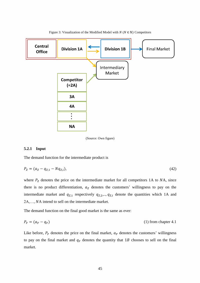
45

Figure 3: Visualization of the Modified Model with ( ∈ ℕ) Competitors

(Source: Own figure)

5.2.1 Input

The demand function for the intermediate product is

), (42)

where denotes the price on the intermediate market for all competitors 1A to A, since

there is no product differentiation, denotes the customers’ willingness to pay on the

intermediate market and respectively ,.., denote the quantities which 1A and

2A,…, A intend to sell on the intermediate market.

The demand function on the final good market is the same as ever:

) (1) from chapter 4.1

Like before, denotes the price on the final market, denotes the customers’ willingness

to pay on the final market and denotes the quantity that chooses to sell on the final

market.

46

The transfer price ( ) does change slightly with the newly introduced change in the equation

of the market price ( ) that account for multiple competitors:

) ( ) (43)

Division ’s profit function still is the same as in (4) from chapter 4.1, but also varies with

the number of competitors on the intermediate market ( ) through the transfer price ( ):

) (( ) ) (44)

Division 1A’s maximal profit is also still the same. However, keep in mind that all equations

which depend either directly on the market price for the intermediate good ( ) or indirectly

through transfer price ( ) change in a way so they are now influenced by the number of

competitors on the intermediate market ( ). Therefore the profit of division 1A is:

( )

) (( ) ) ( ) (45)

By having a glance at the number of competitors in the equation ( ), it’s already easily

deducible that division 1A’s profit will decrease with increasing competition both directly

through the part of the profit achieved on the intermediate market and indirectly by a decrease

in the market-based transfer price ( ). Also keep in mind that the coordination problem should

start to evaporate as competition on the intermediate market becomes fiercer as every

competitor increasingly becomes a price taker. In reality this would be the case for

homogenous goods which suits the model as we assumed goods are indeed homogenous. In

an environment characterized by perfect competition, it would not make a difference if the

company operates as one unit or is divided into subdivisions under market-based transfer

pricing.

( )

) ) ( ) (46)

The consolidated profit ( ) also decreases with the number of competitors on the

intermediate market.

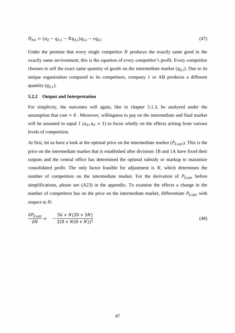
47

) (47)

Under the premise that every single competitor produces the exactly same good in the

exactly same environment, this is the equation of every competitor’s profit. Every competitor

chooses to sell the exact same quantity of goods on the intermediate market ( ). Due to its

unique organization compared to its competitors, company 1 or AB produces a different

quantity ( ).

5.2.2 Output and Interpretation

For simplicity, the outcomes will again, like in chapter 5.1.3, be analyzed under the

assumption that cost . Moreover, willingness to pay on the intermediate and final market

will be assumed to equal 1 ( ) to focus wholly on the effects arising from various

levels of competition.

At first, let us have a look at the optimal price on the intermediate market ( ). This is the

price on the intermediate market that is established after divisions 1B and 1A have fixed their

outputs and the central office has determined the optimal subsidy or markup to maximize

consolidated profit. The only factor feasible for adjustment is , which determines the

number of competitors on the intermediate market. For the derivation of before

simplifications, please see (A23) in the appendix. To examine the effects a change in the

number of competitors has on the price on the intermediate market, differentiate with

respect to :

)

)) (48)

48

Figure 4: change to according to (48)

(Source: Own figure)

With rising competition, the

price on the intermediate

market shrinks and converges

towards zero. The more

competitors enter the

intermediate market, the slower

the pace of the decline in price.

Even though theory and model

comply at this point, keep the

marker at in mind.

In a duopoly-setting (one competitor: ) on the intermediate market, the slope of

is

, which tells us that a marginal increase (decrease) in decreases (increases) the

intermediate market price by

. As can be seen from the graphic, the step from 1 competitor

to 5 has a more pronounced effect than from 5 to 10. The numerator of equation (48)

increases slower with the number of competitors ( ) than the denominator and thereby the

FOC converges against zero with . The consequent and intuitive assertion is that eventually

a higher number of does not anymore decrease the market price since it will equal marginal

cost in the end. We’d end up in a market with perfect competition. So far, intuition and model

comply.

Next, it is of interest how the central office acts under increasing competition. Does the

management enforce a subsidy to facilitate procurement for division 1B with a higher number

of competitors, or will we see a markup on the transfer price instead?

)

)) (49)

The differentiation of the optimal subsidy/markup ( ) from (A19) tells us how the

subsidy/markup reacts to a change in the number of competitors on the intermediate market.

When we apply numbers from 1 until 10 to , we will see that the slope is negative until

. That means for every number of competitors smaller than 6, an additional competitor

will push the central office to reduce the subsidy. In fact, the equation also tells us that at

0 5 10 15 20 25 300.15

0.10

0.05

0.00

0.05

Number of Competitors N

Pri

ceon

the

Inte

rmed

iate

Mar

ket

PZ

49

the slope is maximized and then the curve runs towards to zero. The central office

seemingly decides to reduce the subsidy with an increase in until and then increases

subsidy again. How does that make sense?

To find an answer to this unsettling outcome, we should have a glance at the original equation

of the subsidiary factor, (A19). After inserting and the equation is:

)) (50)

Plotting this we see the following, rather unexpected outcome:

Figure 5: change to

(Source: Own figure)

The graph shows very straight-

forward that competition from

a second competitor on the

intermediate market ( )

drives the central office to

impose a markup instead of a

subsidy.

This result gives us a first reasonably strong suspicion to question the model’s validity, since

the interpretation of that outcome goes as follows: Ceteris paribus, the central office

introduces a markup when 1A faces competition from at least 2 competitors. The central

offices motive is to support 1A with its distribution of goods on the intermediate market. The

reason why the central office considers this supportive action a necessity lies in the actions of

1A. As we shall see in a moment, 1A decides to quit offering its products on the intermediate

market up to a level where, according to a model, its output even is negative (i.e. it would

start “neutralizing” goods on the intermediate market) in order to increase the transfer price

by pushing the market price to increase its profits. This is of course utter nonsense and a result

of missing restrictions.

1.0 1.2 1.4 1.6 1.8 2.00.10

0.05

0.00

0.05

0.10

Number of Competitors N

Sub

sidy

Mar

kup

50

This hypothetical outcome would of course not be in the interest of consolidated profit

maximization since the consolidated profit increases when 1A also sells on the intermediate

market. Therefore the central office would try to prevent this trend by imposing a negative

subsidy, which is a markup.

To prove this point and to show where exactly things start to go wrong and restrictions should

be introduced, a look at the optimal output of division 1A (A22) is helpful. Simplified

according to the assumptions mentioned above it is:

)

)) (51)

Figure 6: responds unexpectedly to

(Source: Own figure)

At the central offices optimal

subsidy ( ), 1A relatively

quickly decides that already

with 5 ( ) competitors it

doesn’t want to compete on the

intermediate market at all.

According to the model, 1A

then would offer “negative

quantities”.

Mathematically, the reason for this outcome is the definition of the intermediate market price

equation in (1) respectively (42). Without restrictions it enables 1A to counter a decreasing

market price by “neutralizing enemy production”.

Summed up we have to enforce restrictions for the model before the number of competitors

on the intermediate market hits 5 ( ). The easiest way to do so is to cut the model at

. By double-checking if any other quantity or optimal outcome yields unreasonable

results it is revealed that indeed division 1A is the weak point in the design of the model,

given the assumptions made.

By reason of the interrelations, the unexpected outcomes continue: Since 1A is increasingly

reluctant to compete on the intermediate market due to the possibility to maximize its profits

via internal trade, it pushes the central office towards a policy involving a markup, instead of

1 2 3 4 50.2

0.1

0.0

0.1

0.2

0.3

Number of Competitors N

Qua

ntit

yon

the

Inte

rmed

iate

Mar

ket

q Z,1

51

a subsidy. As seen in Figure 5, with the subsidy already is not a subsidy anymore but a

markup. 1B therefore has to pay a higher price than the market price and consequently 1A is

rewarded by the central office with a subsidy for selling its goods to the intermediate market.

Under the assumptions, a generalization could be that the division, which is exposed to a

contested market, should be the one to be subsidize, not the division that enjoys monopoly

power. On the other hand this is a problem of the model since goods are supposed to be equal

according to the simplification. Technically speaking, with absolute substitutability, 1B has

no reason to procure from 1A, as it also could procure from any other competitor on the

intermediate market. Thus, 1A would not have the power to increase its profits on at 1B’s

expense via the transfer price in the first place, since 1B would not be forced to procure from

1A.

At rounded up competitors 1A “offers” a negative quantity. This means

is the definite point where the model doesn’t make sense anymore and a restriction has

to be introduced!

To get an aggregated perspective of the effect that the number of competitors has on the

transfer price, let’s have a look at the plot. According to optimal transfer price (A25):

)

)) (52)

Figure 7: Slope of transfer price

(Source: Own figure)

According to the graph, the

transfer price increases until

and falls thereafter.

This result is merely

interesting to understand the

model, since per definition

∈ ℕ. It’s obvious that

even before a second

competitor enters the

market, the model proposes

a decreasing transfer price.

We now know that the transfer price decreases as the second competitor enters the

intermediate market.

1.0 1.5 2.0 2.5 3.0 3.5 4.0

0.02

0.01

0.00

0.01

0.02

0.03

Numberof Competitors N

t N

52

At last we want to have a look at the profit functions of 1B (A26), 1A (A27) and the

consolidated company AB (A28) (again, simplified for the assumptions mentioned above) and

how they react to changes in competition. They are plotted in one diagram which shows

results fitting the interpretation above. According to the findings related to intermediate

market competition, is already cut before .

Figure 8: Profit functions’ responses to

(Source: Own figure)

1B, 1A and the consolidated

profit AB in one plot. 1B’s

profit actually rises slightly with

whereas the profit of 1A

declines with . AB simply is

the sum of both curves and

shows that increasing

competition decreases overall

profit.

The obvious question to be raised here is: What’s the reason for 1B’s increase in profit with

rising competition on the intermediate market? Remember that increased competition drives

down the market price for the intermediate good. The market price is linked to the company’s

internal transfer price. 1B competes in a monopoly, making its profit dependent on the price it

has to pay 1A for the input good, which is lessened with higher competition since this, as

mentioned, drives down intermediate market price. The development of 1A’s curve on the

other hand is self-explanatory. Rising competition on the intermediate market drives down its

profits as a logical conclusion of supply and demand, which is expressed equation (42). The

consolidated company’s profit curve is simply the sum of the two divisional profits curves as

the consolidated profit equals the profit of division 1A plus the profit of division 1B. It shows

a decrease in overall profits with increasing competition on the intermediate market. The

difference in profits arising from one additional competitor is more pronounced from the first

to the second competitor compared to the third to the forth since 1B profits from increased

competition on the intermediate market and 1A profits from the markup imposed by the

central office as soon as equals an artificial “1.2 competitors”.

53

To determine whether there is still a strategic effect on the intermediate market, the quantities

of company AB’s division 1A ( , see (A22)) and the quantity of its competitors, A

( , see (A21)), shall be compared.

) )

)) (53)

For simplicity, assume cost . Then, a strategic effect exists if ))

)

what means the intermediate market, i.e. the customers’ willingness to pay ( ), has

to be more attractive as more competitors ( ) enter that intermediate market.2 Also, if the

final market ( ) becomes more attractive in relation to the intermediate market, 1A’s

willingness to produce more units for the intermediate market and thereby affect 1B’s level of

procurement positively, decreases. This is because 1A tries to maximize its profits from 1B’s

gains on the final market.

6 Conclusion

The modified model proves not to be perfectly extendable to depict multi-competition on the

intermediate market under the assumptions made. Attention is raised from the analysis of the

effect that an increasing number of competitors on the intermediate market leads to supportive

actions from the central office to help division 1A instead of division 1B. This alone is

interesting but doesn’t make the models results invalid. Especially illuminative in showing

that the model needs to be restricted is the insight that division 1A’s output on the

intermediate market eventually becomes negative (51). To make any sense of the proposed

model, strict restrictions have to be applied. The modified model has to be cut at 4

competitors as division 1A of the vertically integrated company AB otherwise shows

illegitimate behavior. Another means of restricting the model in order to achieve sensible

outcomes would be to introduce the restriction which however would lead to a

division 1A that’s not producing anything as soon as the fifth competitor enters the market

under the assumptions made.

The most interesting difference between the outcome of Arya/Mittendorf and the alterations

in the modified model is that the parent in the model of Arya/Mittendorf, which basically

2

))

according to non-negativity restriction resulting from (A20)

54

resembles a combination of division 1A and the central office in the modified model, seeks to

drive down market price ( ) to enable its subsidiary (=1B), which is the same division in

both configurations, to procure more. The reason for this is to be found in the absence of the

coordination problem as the parent does account for consolidated profits. The parent is in

competition with another competitor on the intermediate market but the subsidiary enjoys

monopoly power including the price advantage. Therefore the parent intelligently uses the

transfer price for competitive posturing since it has an incentive to make a profit on the

intermediate market but another incentive to make the subsidiary procure more. Thus the

parent chooses to sell more units on the intermediate market than it would have usually done

without a promisingly profitable subsidiary that’s enjoying monopoly power and is

contributing to consolidating profit.

Splitting the parent into two profit centers (1A and 1B) and a central office, that seeks to

mitigate the arising coordination problem inside the vertically integrated company, bears a

wholly different outcome. The division 1A has an incentive to drive up the market price to

make transfer price ( ) move up. Therefore it uses its market power in a duopoly by selling

less of its goods on the intermediate market. Even with just one competitor on the

intermediate market, the strategic effect vanishes due to a lack of credible commitment since

division 1A acts egocentric. In an attempt to optimize the consolidated result, the central

office tries to mitigate the coordination problem.

In the case of multiple ( ) competitors on the intermediate market, the model’s outcomes

demand scrutiny. The expectation with higher competition on the intermediate market (i.e.

increasing ) would be that by converging to perfect competition, the coordination problem

should disappear without any intervention at all. After all, division 1A does incrementally

lose market power with rising competition on the intermediate market. Without restricting the

model however, 1A restricts production of the intermediate product and relies on a markup

introduced by the central office to stimulate production of 1A again.

Another interesting question for further research would definitely be, if it’s that easy to get a

leg on upon external rivals if you’re not acting in a duopoly and you have no market power in

a more appropriate setting under more appropriate assumptions. Then, the model could be

incrementally extended to depict variable levels of product diversity and eventually

competition on the final market.

55

7 Works Cited

Arya, A., & Mittendorf, B. (2008). Pricing Internal Trade to Get a Leg up on External Rivals.

Journal of Economics & Management Strategy, pp. 709-731.

Baldenius, T., & Reichelstein, S. (2004). External and Internal Pricing in Multidivisional

Firms. Research Paper Series. Stanford Graduate School of Business.

Coenenberg, A. G. (2003). Kostenrechnung und Kostenanalyse. Schäffer-Poeschel.

Ernst & Young. (2010). 2010 Global Transfer Pricing Survey. Ernst & Young.

Ernst & Young. (2012). Ernst & Young. Retrieved November 12, 2012, from

http://www.ey.com/Publication/vwLUAssets/2012-Global-TP-Tax-Authority-

Survey/$FILE/2012-Global-TP-Tax-Authority-Survey.pdf

Ewert, R., & Wagenhofer, A. (2005). Interne Unternehmensrechnung (6. ed.). Berlin:

Springer.

Fabozzi, F. J., Drake, P. P., & Polimeni, R. S. (2008). The Complete CFO Handbook: From

Accounting to Accountability. New Jersey: John Wiley & Sons.

Göx, R. F. (2000, September). Strategic Transfer Pricing, Absorption Costing, and

Observability. Management Accounting Research, Vol 11, pp. 327-348.

Hirshleifer, J. (1956, July). On the Economics of Transfer Pricing. The Journal of Business,

pp. 172-184.

Loeffler, C., & Pfeiffer, T. (2011). Market- versus cost-based transfer pricing, intra-company

coordination and competitive behavior on the intermediate market. Vienna: University

of Vienna.

Organisation for Economic Co-operation and Development (OECD). (2010). Transfer Pricing

Guidelines for Multinational Enterprises and Tax Administrations. OECD.

Paul W. Cook, J. (1955). Decentralization and the Transfer-Price Problem. The Journal of

Business, pp. 87-94.

Pfähler, W., & Wiese, H. (2006). Unternehmensstrategien im Wettbewerb. Berlin: Springer.

PricewaterhouseCoopers. (2012). International transfer pricing 2012.

PricewaterhouseCoopers. Retrieved from PricewaterhouseCoopers:

http://download.pwc.com/ie/pubs/2012_international_transfer_pricing.pdf

56

Riebel, P., Paudtke, H., & Zscherlich, W. (1973). Verrechnungspreise für Zwischenprodukte.

Westdeutscher Verlag.

Sheppard, L. (2012, August). tax justice network. Retrieved November 11, 2012, from

http://www.taxjustice.net/cms/front_content.php?idcat=139

Stone, W. E. (1956). Intracompany Pricing. The Accounting Review, pp. 625-627.

The Economic Times. (2013, February 6). Retrieved from

http://articles.economictimes.indiatimes.com/2013-01-31/news/36659178_1_income-

tax-department-nokia-india-income-tax

Zimmerman, J. L. (1997). EVA and Divisional Performance Measurement: Capture Synergies

and Other Issues. Journal of Applied Corporate Finance, pp. 98-109.

57

8 Appendix

8.1 Proof of Calculation for a variable Number of Competitors

The demand function for the intermediate product is:

( ) (A1)

The demand function for the final good market is:

), (A2)

Division 1B’s profit function is:

(A3)

The transfer price is defined as:

) (A4)

Division 1A’s profit function is:

) (A5)

Inserting (A1), (A2), (A4) in (A3), we end up with:

) (( ) ) (A6)

1B’s profit depends on the price of the good sold on the intermediate market ( ). This price

is influenced by the quantity 1A, 2A… A, ∈ ℕ determine to offer. The denotation of the

competitor’s amount on the intermediary market shall be , whereas the index ).

denotes every competitor’s quantity on the intermediary market. More specific, if

equals 1, there is just one competitor on the intermediate market (see the case in chapter 5.1)

which makes equal to 2, denoting the quantity that the first competitor of the company with

divisions 1A and 1B, let’s call it “company AB”, offers on the intermediary market ( ). If

equals 2, then is 3 and denotes the amount both the first and the second competitor of

company AB simultaneously choose to offer on the intermediate market. Their amounts are

the same due to the assumption of symmetry in organization, unit cost and product

58

characteristics – see (A9) for further details. The subsidy/markup ( ) increases 1B’s profit if

the central office sets an internal discount ( is positive) and decreases it, if it sets an internal

markup ( is negative) to the price obtainable on the intermediate market.

According to microeconomic theory, the optimal output is reached when marginal revenue

(MR) equals marginal cost (MC). In other words, until one additional marginal unit’s revenue

exceeds its costs, it shall be produced.

[ ) ] [(( ) ) ] (A7)

Thereby maximizing 1B’s profit (A6) with respect to yields the FOC:

( )

) (A8)

This is the optimal quantity according to 1B. It increases with an internal discount ( ) and

decreases with the price of the good on the intermediate market ( ) which is influenced by

the number of competitors ( ) and the quantities ( ) they offer to the market.

On the second level, the optimal quantities for division 1A and every competitor A on the

intermediary market are determined. All the participants on the market take each other’s

intentions into account and thereby form a Nash-Cournot-Equilibrium.

Generally speaking, without taking the symmetry/equality assumption into account yet, the

profit of every competitor on the market is depicted as:

∑

) (A9)

FOC yields:

∑

) (A10)

At this point, the symmetry assumption is introduced: Assuming that all the competitors

choose to offer exactly the same quantity under equal circumstances, mainly offering identical

products ( ), having equal costs per unit ( ) and equal internal organization, this formula

can be adjusted for simplification. Mark that company AB does not offer the same quantity as

59

the others on the internal market. This comes due to internal strategic and coordination

processes related to the transfer price that affects the segregated company with two divisions

and decentralized decision-making. Thereby the quantity it offers ( ) differs from all the

others companies.

( ) ) (A11)

The quantity of competitor equals the willingness to pay on the intermediate market ( )

less the quantity all other competitors ( ) with one division (A) that effectively choose to

offer the same quantity ( ) less the quantity that division A of the vertically integrated

company AB decides to offer ( ).

Simplified this equates to:

(A12)

At the same time, 1A maximizes its profit according to its output on the intermediary market

( ), taking the optimal quantity on the final market ( ) into equation. Inserting (A8), (A4),

(A1) in (A5) results in:

( )

(( ) ) (

( ))

( (

( )))

(A13)

The FOC then yields the optimal quantity for 1A under consideration of 1B’s optimal quantity

on the final market:

) (A14)

Now, that we have calculated the optimal quantities of both 1A and the individual optimum of

each and every one of its competitors on the intermediary market, a Nash-Cournot-

Equilibrium can be achieved by intersecting the two relation curves (A12) and (A14).

Nash-Cournot-Equilibrium determined according to these equations then is:

60

) (A15)

) ) )

) (A16)

It is of interest that not only reacts positively on the willingness to pay on the

intermediary market ( ) but decreases with the willingness to pay on the final market ( ).

When the willingness to pay on the final market shrinks, 1A wants to decrease its output on

the intermediary market, too. This is due to the decreased unit sales to 1B when willingness to

pay on the final market shrinks. 1A tries to counter this development with an increased

transfer price. 1A itself can influence the transfer price by reducing its amount sold on the

intermediary market, thus decreasing the intermediate market price ( ). Of course, from the

central office’s point of view that might not be a preferred intervention.

Finally, on the third level of backward induction, the optimal quantities of 1A and 1B have to

be taken into account to determinate the optimal subsidy/markup ( ), fixed by the central

office. Thereafter, the optimal can be utilized to compute the optimal profit of the

consolidated company from the central office’s point of view.

In order to calculate optimal subsidy/markup ( ), the consolidated profit has to be depicted

and all optimal quantities have to be inserted into the equation. Consolidated profit simply is

1A’s profit depicted in (A5) added up with 1B’s profit, depicted in (A3), thereby eliminating

transfer prices in the formula.

) (A17)

Replacing (A1) and (A2) and inserting optimized terms of (A8), (A15) and

(A16) into the equation of consolidated profit yields (A18)

61

) ) )

))

)))

) ) )

))

) ) )

))

) ) )

))

))))))

) ) )

))

))))))

) ) )

))

)))))

(A18)

FOC with respect to and then solved for determines the optimal subsidy/markup ( ):

) ) )

)) (A19)

In order to calculate the optimal consolidated profit it’s necessary to calculate the optimal

quantities from the central office’s point of view and insert those into the consolidated profit

equation.

First, take 1B’s optimal (A8). Inserting (A1) in the first step, continuing with the

Nash-Cournot-Equilibrium optima’s (A15) and (A16) and finally inserting the

optimal (A19) results in the optimal quantity on the final market from the central office’s

point of view in dependency on the number of competitors on the intermediary market ( ):

)) ))

))

(A20)

62

Optimal values for the quantities, which divisions A and 1A offer on the intermediary

market, are calculated by inserting optimal subsidy/markup (A19) into the respective

terms (A15) and ( ):

) ) )

))

(A21)

) ) ) ) )

)) (A22)

The optimal price on the intermediary market ( ) is calculated by taking the original

intermediate market price equation (A1) and replacing the quantities with the terms in (A21)

and (A22). The optimal price on the final market is expressed similarly by taking expression

(A2) and replacing the quantity with the optimum depicted in ( ):

) ) ) )

)) (A23)

)) ))

)) (A24)

Optimum transfer price results from inserting (A21) and (A22) into the original transfer price

formula (A4):

)) )

) (A25)

Finally, the optimal profits of 1A and 1B as well as consolidated profit can be depicted.

Therefore the original formula for 1B’s profit (A3) is merged with the optimal (A24),

(A20) and (A25). 1A’s optimal profit equation is expressed by taking the original

equation (A5) and applying (A23), ( ), (A25) as well as (A20) to it.

)) )) )

)) (A26)

63

( )) ))) )

)) ))) ))

) )) ) ))

(A27)

Profit 1A (A27) and 1B (A26) added up equals consolidated profit:

)) )) ))

) )) ))

(A28)

The competitors’ profits after the central office sets the subsidy/markup is expressed by

applying (A21) and (A23) to the following general profit function of the

competitors:

(A29)

Simplified, this yields:

) ) ) )

))

) )

(A30)

8.2 Split Up Profit Function

To examine which terms of the model’s outcomes are of particular interest for a differential

and graphical analysis, a closer look at the profit function is informative. A full breakdown of

the profit function looks like (A31).

(A31)

64

In this massive term all the (inter-)dependencies are depicted and the general steps of

calculation for competitors basically recapitulated. However, some of them are unnecessary

regarding the analysis since includes and . The terms in green can be itemized to:

(A32)

Now let’s have a closer look on how to further simplify this term. At first, with the terms ( )

and (A8) we have defined that:

(A33)

In order to reach outcome (A14) it must be true that:

(A34)

Given the knowledge about (A32), (A33) and (A34), the terms of interest for further analysis,

as the profit function of AB is concerned, can be reduced to the following ones:

(A35)

By looking closely at (A35) it appears there are essentially four major terms, which are

separated by pluses. This fragmentation will serve to distinct the terms during the analysis.

Another point worth mentioning is that the parts of terms marked in orange resemble each

other.

8.3 Differential Analysis for One- and Multiple Competitors

To analyze the outcome of the model and to get a grip on the interrelations it is helpful to look

at the meaningful differentials. Therefore, the outcomes will be analyzed for the case that 1A

is in competition with one competitor and competitors on the intermediate market. For that

reason will be applied to the general formulas expressed at the beginning of the

appendix.

65

Effect of a change in 1A’s quantity on the intermediate market ( ) on 1B’s

profit ( )

According to (A35), (A6) is differentiated with respect to :

) (

))) (A36)

) (

))) (A37)

1B’s profit on the final market grows (shrinks) as the amount which 1A chooses to sell

on the intermediate market increases (decreases). The reason for this development is to be

found in the inverse influence of the units sold on the intermediate market ( and ) on

the price on the intermediate market ( ) as can be seen in (A1). Disregarding the

subsidy/markup ( ), the price on the intermediate market ( ) eventually affects the transfer

price ( ) (A4) unidirectional: If 1A increases its output ( ) on the intermediate market, the

price on this market ( ) sinks and the transfer price ( ) is reduced as well. As the transfer

price ( ) is regarded as cost-factor by 1B, its profit ( ) increases as the transfer price

decreases.

The difference for multiple competitors lies in the equation of the amount that 1B offer on the

final market ( ), which now is also dependent on the number of competitors ( ). Quantity

on the final market ( ) is increased with a higher subsidy ( ) from the central office, a higher

willingness of the customers on the final market to pay and is decreased with the cost of

the input good on the intermediate market (A1), which is exactly the part of the equation

that now depends on the number of competitors on the intermediate market. It is observable

that with more competitors on the intermediate market, 1A’s effect via is decreased and

the slope

decreases. For every additional unit sold on the intermediate market by 1A, the

increase in 1B’s profit then is ) ). In other words, 1B’s marginal

revenue decreases with because the influence of 1A’s output on the price on the

intermediate market decreases as there are more opportunities for buyers to choose from.

Effect of the change in subsidy/markup ( ) on 1A’s quantity ( ) on the

intermediate market

(A16) is differentiated with respect to

66

(A38)

)

(A39)

For one competitor on the intermediate market (A38), this outcome tells us that in the case of

an increase (decrease) of the subsidy/markup by 1, the quantity sold on the intermediate

market by 1A decreases (increases) by half of that. A higher decreases the transfer price ( )

(A4). That is not in the favor of division 1A as it is striving for the highest possible profit,

which, not accounting for changes in 1B’s output ( ), comes with the highest possible

transfer price that it receives from 1B. At this point, 1A itself has a possibility to influence the

transfer price indirectly. This connection becomes more tangible by closely examining the

definition of the market price ( ) in equation (A1) in conjunction with the equation of the

transfer price (A4). The price on the intermediate good market is dependent on the change of

the quantity 1A chooses to sell, as well as on the quantity its competitor chooses to sell or

choose to sell, as more competitors enter the market. The intermediate market price ( )

increases as 1A decreases the quantity it offers on the intermediate market ( ). This decline

in consequence influences to rise, which then raises the transfer price which is to 1A’s

liking. A higher subsidy thus has two mentionable effects on the transfer price. Firstly, it

decreases the transfer price directly. Secondly however, it increases the transfer price through

the implicitly consequential action of 1A. According to this result, the central office has to

cautiously balance these effects to maximize consolidated profit because the indirect effect

backfires on the company’s performance.

With an increasing number of players ( ) on the intermediate market 1A’s influence

decreases. With a sufficiently high , no party would be able to influence the market price

and we would be in perfect competition. Since the model is restricted at as it is, this is

not depicted in the following plot.

67

Figure 9: Plot of (A38)

(Source: Own figure)

This plot shows the effect of

the markup/subsidy ( ) on

1A’s quantity ( ). With

increasing competition ( )

the effect of the subsidy

becomes smaller, the central

office’s action have

decreasing effects.

Effect of a change in the competitors’ ( , ) quantities on AB’s

profit( )

) (A40)

) (A41)

The result in a duopoly ( ) tells, that an increase (decrease) of the competitor’s quantity

( ) on the intermediate good market by 1 decreases (increases) consolidated profit of AB

by . This is logical since an increase (decrease) of the competitors quantity decreases

(increases) market price, which decreases (increases) AB’s profit.

1.0 1.5 2.0 2.5 3.0 3.5 4.00.75

0.70

0.65

0.60

0.55

0.50

0.45

Number of Competitors N

q Z,1

68

Figure 10: Plot of (A41)

(Source: Own figure)

The plot shows increasing effect of the competitors’ quantities on the intermediate market as

the number of competitors increase. This is comprehensible since each additional competitor

takes another share in the market. The effect is also dependent on division 1A’s interest in the

intermediate market. If its output is relatively high, sharing with additional competition hurts

more than if its output is relatively low.

Effect of a change in the subsidy/markup factor on the quantity of 2A

(A42)

(A43)

If the subsidy factor increases by one unit, the quantity that competitor 2A offers on the

intermediary market increases by

(A42). This is because 1A reduces its quantity on the

intermediate market with increasing subsidy in order to push the market price and

thereby indirectly raise the transfer price it receives from 1B for the intermediate good.

Using the subsidy factor, the central office is able to slightly influence the degree of

competition on the intermediate market.

With an increasing number of competitors on the intermediate market, the effect of a change

in the subsidy factor on A’s quantity becomes less pronounced. The central office

69

influences the quantity of 1A’s competitors in way that each of them increases (decreases)

their by

with every unit of increased (decreased) subsidy ( ).

Effect of a change in 1B’s quantity on 1A’s profit

(A44)

(A45)

The effect is exactly the transfer price (A4) minus cost , see (A44). If 1B’s quantity on the

final market ( ) increases, the profit of 1A ( ) increases as well. When 1B increases its

output by one unit, the profit of 1A increases exactly by the amount of money that 1B initially

paid 1A to receive one input unit to produce that unit for the final market. This is due to the

conversion rate being set at 1. Transfer price (A4) is always positive with the single

exception if market price is equal to marginal cost which we defined as zero in a

sufficiently competitive market. Then the transfer price would also be zero.

With increasing competition the effect of a change in 1B’s quantity on 1A’s profit lessens, as

to be seen in (A45). It converges to zero with an evolving perfect market. This is because

eventually market price will equal marginal cost.

Effect of a change in subsidy/markup on 1B’s quantity

(A46)

The optimal quantity on the final good market deduced with respect to subsidy factor is

, see

(A46). If the subsidy increases (decreases) by one unit, the amount on the final good market

increases (decreases) by half that. The relation between the two figures is the transfer price

which decreases (increases) when the subsidy/markup factor increases (decreases). 1B will

want to procure more input goods when prices are low to maximize its profit. In this case, the

effect doesn’t scale with the number of competitors on the intermediate market ( ).

Effect of a change in 2A’s quantity on 1B’s quantity

(A47)

70

(A48)

According to (A48) the result is

which tells that an increasing (decreasing) output of 2A on

the intermediate market increases the output of 1B on the final good market . The two

amounts are related by the market price which in turn affects the transfer price (A4). If

the intermediate market price decreases (increases) because of an increased (decreased) output

of 2A, the transfer price ceteris paribus (i.e. given an unchanged subsidy/markup ( )) will

decrease (increase). A decreased (increased) transfer price then will boost (reduce) 1B’s

procurement.

With increasing competition on the intermediate market the increase in on the final market

picks up momentum. Again this is closely related to the diminishing effect of increased

competition on the intermediate market price which inversely affects transfer price (A4).

Basically, consolidated AB can shift its focus from intermediate market to the final good

market with monopoly-prices.

71

9 Summary

This thesis gives an introduction to (market-based) transfer prices and highlights interrelations

which are linked to transfer pricing policies. A strategic effect of transfer pricing and the

delegation problem are highlighted. On the basis of a paper published by Arya and Mittendorf

(2008), a basic model of a vertically integrated company is introduced. After examining the

results of Arya and Mittendorf (2008) a modified model is portrayed to show the changes in

the effect of the transfer pricing policy in comparison with the basic model. Further on, the

modified model is extended to portray an intermediate market that converges to full

competition. The rather unexpected outcome is again presented and the problems arising from

the assumptions are examined. It is observed that strategic effects of transfer pricing requires

credible commitment and an additional coordination problem in the modified model

compromises corporate efficiency.

10 Zusammenfassung

Diese Arbeit gibt eine Einführung zu (marktbasierten) Transferpreisen und zeigt in Folge

unternehmensinterne Zusammenhänge auf, die mit der Transferpreis-Thematik in Verbindung

stehen. Auf Basis eines Arbeitspapiers, das von Arya und Mittendorf (2008) publiziert wurde,

wird das Basismodell von Arya und Mittendorf vorgestellt. Nach der Analyse der Ergebnisse

von Arya und Mittendorf (2008) wird ein modifiziertes Modell präsentiert und es werden im

Vergleich zum Basismodell Veränderungen beleuchtet, die die Transferpreispolitik betreffen.

Darauffolgend wird das modifizierte Modell so angepasst, dass es einen Zwischenmarkt

abbildet, der in Richtung eines perfekten Wettbewerbs konvergiert. Daraus und aus den

gewählten Annahmen resultieren allerdings unerwartete Probleme, die dann beleuchtet

werden. Im Ergebnis scheint auf, dass durch ein zusätzliches Koordinationsproblem im

modifizierten Modell der Gewinn im Vergleich zum Basismodell vermindert wird.

72

11 Curriculum Vitae

PERSÖNLICHE DATEN

Patrick-Philipp Valda, Bakk.rer.soc.oec.

Patrick.Valda@gmail.com

Geburtsdatum: 02.09.1987

Staatsbürgerschaft: Österreich

STUDIUM

10/2006 – 01/2010 Universität Wien

Studium der Betriebswirtschaftslehre

Schwerpunkte: Management und Wirtschaftsrecht

Thema der ersten Bakkalaureatsarbeit: “Unternehmensanalyse der OMV AG”

Thema der zweiten Bakkalaureatsarbeit: “Einstellung zu wirtschaftspolitischen

Maßnahmen”

Abschluss: Bakk.rer.soc.oec. (Bakkalaureus der Sozial- und

Wirtschaftswissenschaften)

03/2010 – 02/2013 Universität Wien

Studium der Betriebswirtschaftslehre

Schwerpunkte: Controlling, Investments

Thema der Master-Thesis: Das Verhalten von Anlegern und Fundamentalanalyse

Angestrebter Abschluss: Master of Science (MSc)

PRAKTIKA

07/2011 – 09/2011 Praktikum bei Gaotime Information Co., Ltd als Marktanalyst

07/2008 – 08/2008 Praktikum in der Qualitätssicherung bei der Volksbank Vorarlberg e. Gen

Mitarbeit bei der Umsetzung des Projektes Basel II, Säule 1

SCHULBILDUNG

1002 - 2006 Bundesoberstufenrealgymnasium Dornbirn-Schoren mit Schwerpunkt Informatik

1998 - 2002 Bundesrealgymnasium Dornbirn-Schoren

1994 - 1998 Volksschule in Hohenems-Herrenried

PERSÖNLICHE FÄHIGKEITEN

Sprachen

Deutsch: Muttersprache

Englisch: B2/C1

Französisch: A2

Chinesisch: A1/A2