Market Reforms at the Zero Lower Boundfaculty.washington.edu/ghiro/CDFGZLBMACFINROBODS... ·...

Market Reforms at the Zero Lower Bound

Matteo Cacciatore1, Romain Duval2,

Giuseppe Fiori3, and Fabio Ghironi4

1: HEC Montréal and NBER

2: International Monetary Fund

3: North Carolina State University

4: University of Washington, CEPR, and NBER

MACFINROBODS

Third Consortium Scientific Workshop

Como, November 17, 2016

“During the global financial crisis and ensuing Great Recession, economists at policy-

making institutions had little choice but to augment macroeconomic models with ad-hoc

assumptions and adjustments in order to provide analysis and advice for policy makers.

The MACFINROBODS consortium aims to move policy-focused macroeconomic modelling

beyond this approach.”

http://www.macfinrobods.eu, VISION

Motivation

• Labor and product market reforms are at the heart of the structural reform agenda advocatedby many to boost performance of several advanced economies, notably in Europe andJapan.

• The theoretical case has been laid out by extensive literature that highlights long-term gains.

• No consensus on short-term impact, and even less on whether short-run effects depend onstate of business cycle and how reforms interact with monetary (and fiscal) policy.

1

Motivation, Continued

• A central issue in the current economic environment involves the consequences of structuralreforms when central banks face binding constraints on monetary policy easing, such as theso-called zero lower bound (ZLB) on nominal interest rates.

• At the heart of the debate lies the question whether reforms have important deflationaryeffects.

• As argued by Eggertsson (2010), in a liquidity trap, expectation of deflation increases realinterest rates, thus depressing current demand further.

• Building on this insight, Eggertsson, Ferrero, and Raffo (2014, EFR) argue that structuralreforms can have costly contractionary effects when monetary policy is constrained by theZLB, since reforms fuel expectations of prolonged deflation.

2

Motivation, Continued

• Importantly, the analysis in EFR—and in several other papers that followed their approach—models market reforms as exogenous reductions in price and wage markups.

• This implies that reforms are automatically deflationary (and also that they depreciate theterms of trade and improve the external balance).

• However, from an empirical perspective, market regulation affects the incentives to createand destroy product and jobs by acting on barriers to entry and labor market legislation.

• Price and wage markup dynamics are endogenous outcomes of market reforms.

• The goal of this paper is to address the consequences of primitive changes in marketregulation (rather than exogenous markup cuts) when the economy is in a deep recessionthat has triggered the ZLB on nominal interest rates.

3

Strategy

• Two-country, multi-sector model of a monetary union with endogenous producer entry andsearch and matching market frictions in the labor market.

– Bilbiie, Ghironi, and Melitz (2012) and Ghironi and Melitz (2005).

– Mortensen and Pissarides (1994) and den Haan, Ramey, and Watson (2000).

• Sticky prices and monetary policy, subject to ZLB constraint.

• We calibrate the model with parameter values from literature and to match features of macrodata for euro area.

4

Strategy, Continued

• Then study dynamic response to:

1. product market reform: reduction in regulatory costs of entry in non-tradable sector;– Focus on non-tradable sector to explore idea that deregulation of profession/servicesectors should propagate as cost-reduction throughout economy.

– Different from Cacciatore, Duval, Fiori, and Ghironi (2015), Cacciatore and Fiori (2016),and Cacciatore, Fiori, and Ghironi (2015, 2016).

2. labor market reform: decline in firing costs or decline in generosity of unemploymentbenefits.

• Two alternative scenarios: Reforms are either implemented in normal times, assumingthat the economy is at the steady state, or in the aftermath of a large adverse shock thatdepresses the economy and pushes monetary policy to the ZLB.

5

Results

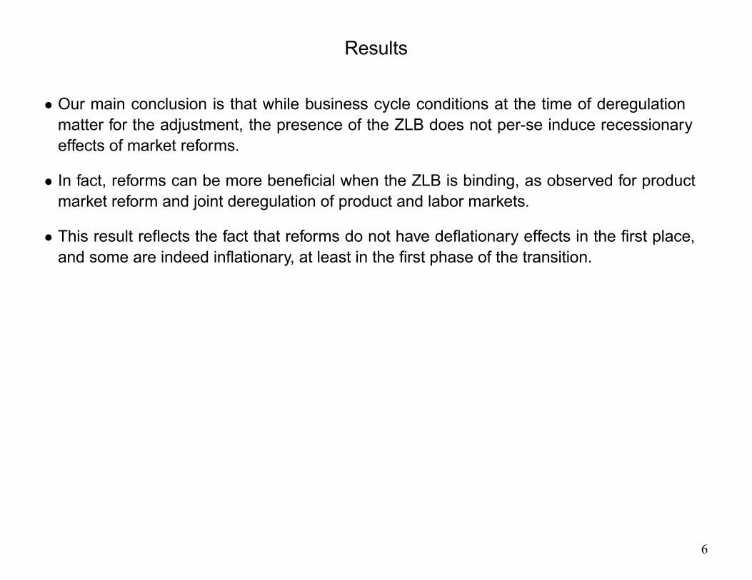
• Our main conclusion is that while business cycle conditions at the time of deregulationmatter for the adjustment, the presence of the ZLB does not per-se induce recessionaryeffects of market reforms.

• In fact, reforms can be more beneficial when the ZLB is binding, as observed for productmarket reform and joint deregulation of product and labor markets.

• This result reflects the fact that reforms do not have deflationary effects in the first place,and some are indeed inflationary, at least in the first phase of the transition.

6

Results, Continued

Intuition• Consider first a reduction in barriers to producer entry.

• While such reform reduces price markups over time as a larger number of products resultsin higher substitutability, the downward pressure on prices is initially more than offset by twoinflationary forces.

1. Lower entry barriers trigger entry of new producers, which increases demand for factors ofproduction and thereby marginal costs.

2. Incumbent producers lay off less productive workers in response to increased competition.– Since remaining workers have higher wages on average, marginal labor costs rise.

• The latter effect also explains why lower firing costs—which induce firms to lay off lessproductive workers—are not deflationary either, even though layoffs reduce aggregatedemand all else equal.

• Finally, while unemployment benefit cuts have a negative impact on wages and aggregatedemand by weakening workers’ outside option in the wage bargaining process, thisdeflationary effect is offset by the positive general equilibrium impact of the reform on labordemand, which increases wages other things equal.

7

Results, Continued

• Our results (and those in Cacciatore, Duval, Fiori, and Ghironi, 2016) highlight thatprevailing business cycle conditions and not constraints on monetary policy represent thekey dimension to consider when evaluating the short- to medium-run effects of marketreforms.

• Moreover, contrary to the conventional view that emerges from reduced-form modelingof reforms as exogenous markup cuts, there is no simple across-the-board relationshipbetween market reforms and the behavior of the real marginal costs.

• This is because reforms affect both supply and demand in complex ways, and themicroeconomic underpinnings of the analysis are crucial to understand them.

8

Related Literature

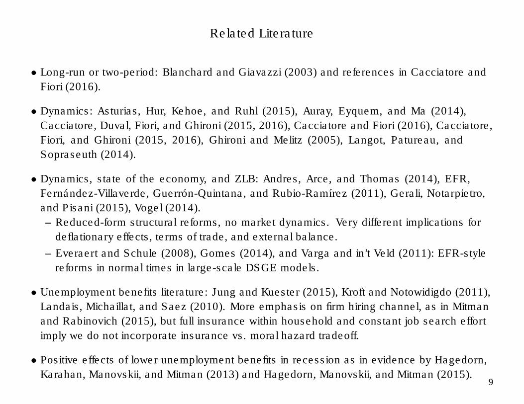
• Long-run or two-period: Blanchard and Giavazzi (2003) and references in Cacciatore and

Fiori (2016).

• Dynamics: Asturias, Hur, Kehoe, and Ruhl (2015), Auray, Eyquem, and Ma (2014),

Cacciatore, Duval, Fiori, and Ghironi (2015, 2016), Cacciatore and Fiori (2016), Cacciatore,

Fiori, and Ghironi (2015, 2016), Ghironi and Melitz (2005), Langot, Patureau, and

Sopraseuth (2014).

• Dynamics, state of the economy, and ZLB: Andres, Arce, and Thomas (2014), EFR,

Fernández-Villaverde, Guerrón-Quintana, and Rubio-Ramírez (2011), Gerali, Notarpietro,

and Pisani (2015), Vogel (2014).

– Reduced-form structural reforms, no market dynamics. Very different implications for

deflationary effects, terms of trade, and external balance.

– Everaert and Schule (2008), Gomes (2014), and Varga and in’t Veld (2011): EFR-style

reforms in normal times in large-scale DSGE models.

• Unemployment benefits literature: Jung and Kuester (2015), Kroft and Notowidigdo (2011),

Landais, Michaillat, and Saez (2010). More emphasis on firm hiring channel, as in Mitman

and Rabinovich (2015), but full insurance within household and constant job search effort

imply we do not incorporate insurance vs. moral hazard tradeoff.

• Positive effects of lower unemployment benefits in recession as in evidence by Hagedorn,

Karahan, Manovskii, and Mitman (2013) and Hagedorn, Manovskii, and Mitman (2015).9

The Model: Household Preferences

• Monetary union of two countries, Home and Foreign.

• Cashless economy (Woodford, 2003).

• Representative home household maximizes:

" ∞X=

−¡ −

−1¢

1−

1−#

where ≡ discount factor and ≡ habit, both between 0 and 1; 0.

• ≡ household consumption:

≡ + (1− )

– ≡ mass of employed workers,– ≡ home production,– ≡ basket of domestic and imported consumption sub-bundles.

10

The Model: Household Preferences, Continued

• The consumption basket aggregates a bundle of domestic and imported traded goods, , and a bundle of non-tradable goods,

:

=

∙(1− )

1

¡

¢−1 +

1

¡

¢−1

¸ −1

• Tradable consumption:

=

∙(1− )

1

¡

¢−1 +

1

¡ ∗

¢−1

¸ −1

• Home bias in tradable preferences.

11

The Model: Household Preferences, Continued

• Endogenous number of non-tradable product varieties available to consumers ():Ω ∈ Ω.

• Aggregator takes a translog form (Feenstra, 2003).

• Unit expenditure function on basket given by:

ln =

1

2

µ1

− 1

¶+1

Z∈Ω

ln () +

2

Z∈Ω

Z0∈Ω

ln () (ln ()− ln (0))0

where 0 ≡ price elasticity of spending share on individual good, ≡ total number ofproducts available at time , ≡ mass of Ω, and () ≡ nominal price of good ∈ Ω

• Property of translog preferences (in the symmetric equilibrium):

≡ − ln

ln¡

¢ = 1 +

12

The Model: Production

• Vertically integrated production sectors.

• Upstream sector: perfectly competitive firms use capital and labor to produce a non-tradableintermediate input

.

– Search and matching frictions in labor market.

• Downstream sectors:

– Monopolistically competitive firms use to produce differentiated non-tradable varieties.

– Perfectly competitive firms combine and differentiated non-tradable products to

produce homogeneous tradable good.

– Production structure consistent with Boeri at al. (2005):

· Service industries key supplier of the manufacturing sector.

13

The Model: Intermediate Input Producers

• Firms post vacancies, , to hire new workers, incurring real cost .

• Unemployed workers, , search for jobs.

• Aggregate matching technology: =

1− .

• Probability of filling a vacancy: ≡; probability of becoming employed: ≡.

14

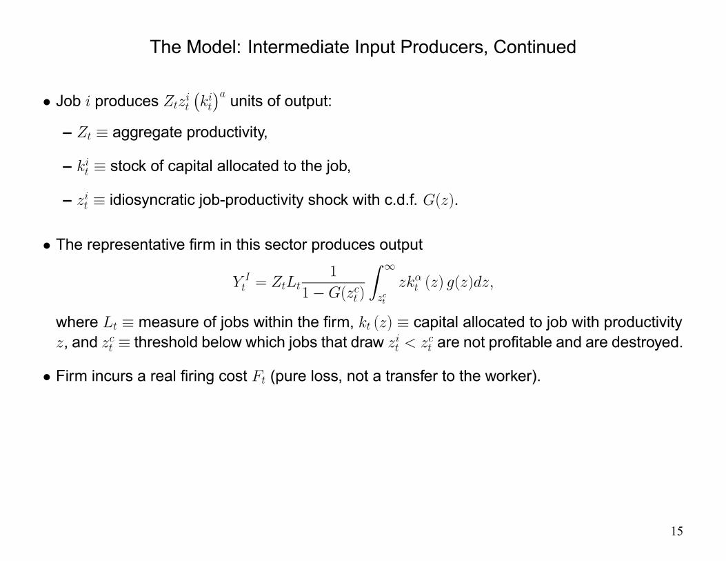
The Model: Intermediate Input Producers, Continued

• Job produces

¡¢ units of output:

– ≡ aggregate productivity,

– ≡ stock of capital allocated to the job,

– ≡ idiosyncratic job-productivity shock with c.d.f. ().

• The representative firm in this sector produces output

=

1

1−( )

Z ∞

() ()

where ≡ measure of jobs within the firm, () ≡ capital allocated to job with productivity, and ≡ threshold below which jobs that draw are not profitable and are destroyed.

• Firm incurs a real firing cost (pure loss, not a transfer to the worker).

15


• Perfect mobility of capital rented in competitive market implies that production can berewritten as:

=

1−

where:

– ≡h

11−( )

R∞

1(1−)()i1−

(weighted) average job productivity,

– = , where ≡R∞

() () [1− ( )]

– See Cacciatore and Fiori (2016) for more details.

16


• Producers chooses (, , , ) to maximize PDV of profits.

• Period profits, :

≡

1− − − − −( ) (1− ) (−1 + −1−1)

where:

– ≡ price in units of consumption,

– ≡R∞

()() [1− ( )] (weighted) average wage,

– ≡ rental rate of capital,

– ≡ probability of exogenous job separation.

• Constraint: The law of motion of employment:

= (1− ) (1− ( )) (−1 + −1−1)

17


Job Creation•

= (1− )

½+1

∙(1− (+1))

µ(1− )+1

+1

+1− +1 +

+1

¶− (+1)+1

¸¾

– ≡ − ≡ stochastic discount factor of Home households, who areassumed to own firms, where:

≡¡ −

−1¢− −

h¡+1 −

¢−i

• Marginal cost of posting vacancy = marginal benefit:

– With probability , vacancy is filled; two events possible:

– Either the new recruit fired in period + 1, and firm will pay firing cost, or match willsurvive job destruction, generating value for firm.

– Marginal benefit of filled vacancy includes expected discounted savings on futurevacancy posting, plus average profits generated by match.

18


Job Destruction

(1− )

µ

¶ 11−

− ( ) +

= −

• Value to firm of job with productivity must be equal to zero:

– Contribution of match to current and expected future profits = firm outside option—firingthe worker, paying .

– When unprofitable jobs are terminated, firm loses current and expected profits it wouldhave earned had it kept the laid-off workers.

– But firm benefits from job destruction in the form of improved distribution of jobproductivities.

Capital

=

19


Wage Bargaining• Individual Nash bargaining: worker’s exogenous bargaining weight .

• Firm’s outside option: firing the worker and posting a new vacancy.

• Worker’s outside option: unemployment benefit from the government, , and homeproduction, .

• In equilibrium:

() =

"(1− )

µ

¶ 11−

+ + − (1− ) (1− )+1+1

#+(1− ) ( + )

20

The Model: Non-Tradable Output Producers

• Continuum of symmetric monopolistically competitive producers.

– Endogenous number of producers: .

• Producer faces demand:

() = ln

µ

()

¶

()

where

ln ≡ (1) + (1)

Z∈Ω

ln ()

is maximum price that producer can charge while still having a positive market share.

• Period profit:

() =

µ ()

−

¶ ()−

Γ ()

• Price setting is subject to quadratic adjustment costs as in Rotemberg (1982): Γ () ≡¡ ()

¢2 ()

() 2, ≥ 0, () ≡

¡ ()

−1 ()

¢− 1,

21

The Model: Non-Tradable Output Producers, Continued

• Optimal price setting (and symmetry across producers):

=

¡ − 1

¢Ξ

• Pro-competitive effect of entry: ≡ 1 + .

• Sticky prices imply:

Ξ ≡ 1−

2

¡¢2+

− 1

½¡ + 1

¢ − (1− )

∙+1

¡+1 + 1

¢+1

+1+1

+1

¸¾

22


Entry• Sunk entry cost: ≡ + in units of final consumption.

– ≡ red tape,

– ≡ technological entry cost.

• Exogenous exit shock with probability at the end of each period.

23


• Entry decision: =

where

=

" ∞X=+1

(1− )−

#

and ≡¡ −

¢ = period firm profit (symmetric equilibrium).

• Number of producers (time to build):

= (1− )(−1 +−1)

where ≡ number of entrants.

24

The Model: Tradable Output Producers

• Production function: =

¡

¢ ¡

¢1−

where:

– ≡ intermediate input,

– ≡ non-tradable goods used in tradable good production.

25

The Model: Tradable Output Producers, Continued

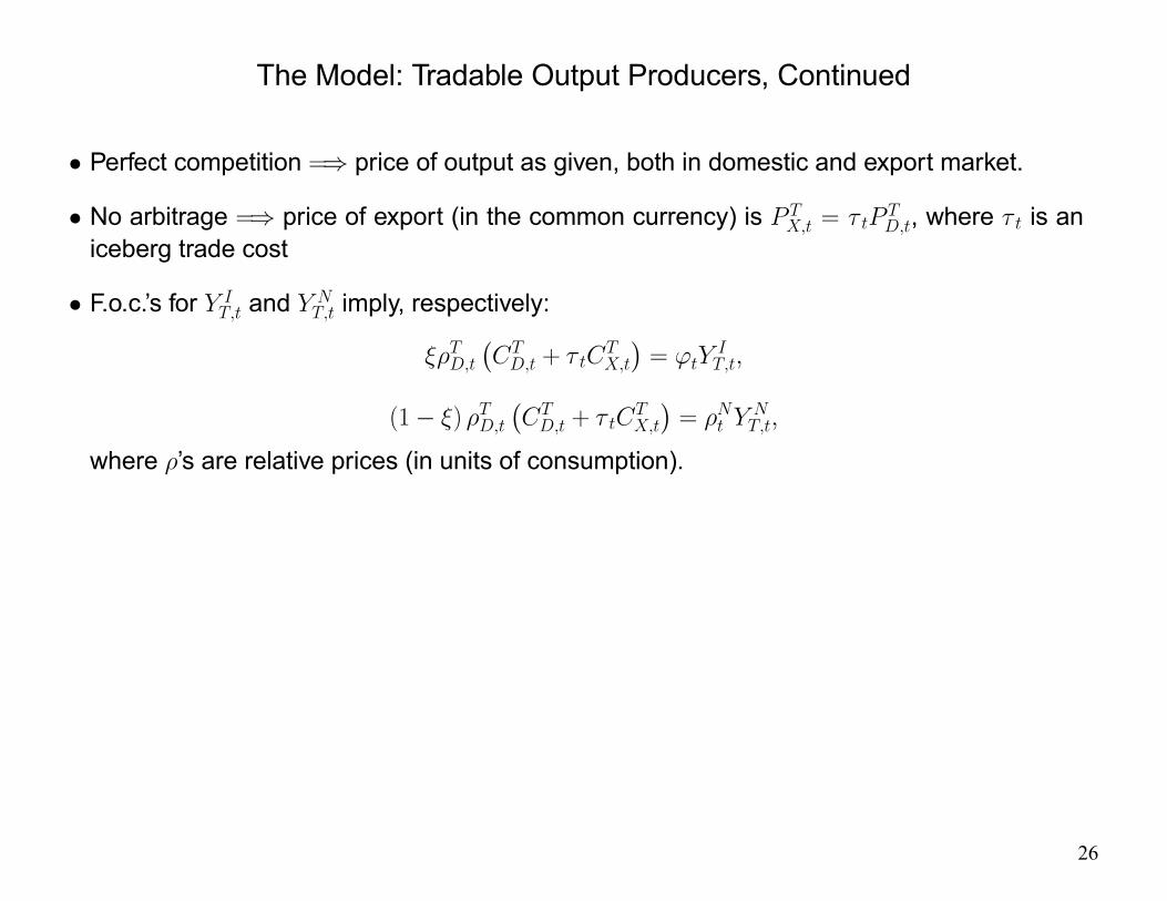
• Perfect competition =⇒ price of output as given, both in domestic and export market.

• No arbitrage =⇒ price of export (in the common currency) is =

, where is an

iceberg trade cost

• F.o.c.’s for and

imply, respectively:

¡ +

¢=

(1− )

¡ +

¢=

where ’s are relative prices (in units of consumption).

26

Household’s Intertemporal Choices

• Owns capital stock, rented competitively to intermediate input producers, and invests in twofinancial assets:

– shares in mutual fund of non–tradable-output firms,

– non-contingent, internationally traded bond denominated in units of currency.

• Stock market investment is the mechanism through which household savings are madeavailable to prospective entrants to cover entry costs.

27

Household’s Intertemporal Choices, Continued

• Convex investment adjustment costs and variable capital utilization (set by household):

– Effective capital rented to firms, = , where ≡ utilization rate.

– Increases in utilization imply faster depreciation: ≡ κ1+ (1 + ).

· Greenwood, Hercowitz, and Huffman (1988), Burnside and Eichenbaum (1996).

• Law of motion of physical capital:

+1 = (1− ) +

"1−

2

µ

−1− 1¶2#

28


• Euler equation for capital accumulation:

=

©+1

£+1+1 + (1− +1) +1

¤ª

where ≡ shadow value of capital (in units of consumption)

• F.o.c. for investment :

−1 =

"1−

2

µ

−1− 1¶2−

µ

−1− 1¶µ

−1

¶#

++1

"+1

µ+1

− 1¶µ

+1

¶2#

• F.o.c. for capital utilization :

= κ1+

29


• Euler equation for share holdings:

= (1− )

£+1

¡+1 + +1

¢¤

– ≡ real price of a share (claim to future profits).

• Euler equations for bond holdings:

1 + +1 + Λ = (1 + +1)

µ+1

1 + +1

¶

– ≡ scale parameter in cost of adjusting bond holdings (2+12),

– ≡ nominal interest rate on bond holdings between − 1 and , set by the central bankat − 1,

– ≡ Home CPI inflation rate, (−1)− 1,

– Λ ≡ risk-premium shock that affects demand for (nominally) risk-free assets, (1)with i.i.d. Normal innovations.

· As in Smets and Wouters (2007) and subsequent literature, Λ appended to bondEuler equation to generate liquidity trap.

· For our exercise, we assume Λ = Λ∗ in each period.

30

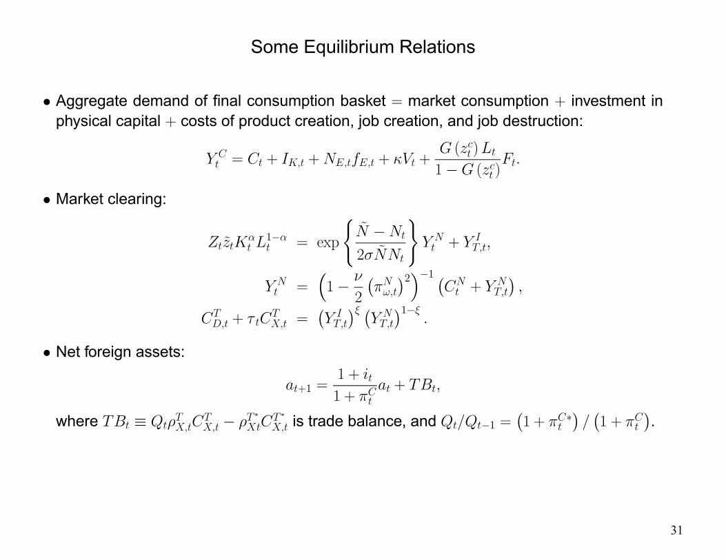
Some Equilibrium Relations

• Aggregate demand of final consumption basket = market consumption + investment inphysical capital + costs of product creation, job creation, and job destruction:

= + + + +

( )

1− ( )

• Market clearing:

1− = exp

( −

2

) +

=

³1−

2

¡¢2´−1 ¡

+

¢

+

=

¡

¢ ¡

¢1−

• Net foreign assets:

+1 =1 + 1 +

+

where ≡

−

∗

∗

is trade balance, and −1 =¡1 + ∗

¢¡1 +

¢.

31

Monetary Policy

• We take explicitly into account the possibility that the nominal interest rate cannot fall belowsome lower bound , so that in each period +1 > .

• Therefore, the nominal interest rate set by the central bank of our model monetary unionsatisfies:

1 + +1 = max

½1 + (1 + )

h(1 + )

¡1 +

¢ ¡

¢ i1−¾

– ≡

∗1− is the data-consistent, union-wide CPI inflation, and

≡

∗1− is

the data-consistent, union-wide GDP gap.

– Data-consistent = purged of pure variety effect.

32

TABLE 2: CALIBRATION

Variety elasticity σ = 0.34 Unemployment benefit b = 0.33

Risk aversion γ = 1 Firing costs F = 0.06

Discount factor β = 0.99 Matching function elasticity ε = 0.5

EOS, home and foreign goods φT = 1.5 Home bias 1− αT = 0.6

EOS, tradables and non-tradables φN = 0.5 Share of non-tradables consumption αN = 0.80

Share of non-tradables in manufacturing ξ = 0.6 Bond adjustment cost ψ = 0.0025

Technological entry cost fT = 0.73 Workers’ bargaining power η = 0.5

Regulation entry cost fR = 1.09 Home production hP = 0.6

Plant exit δ = 0.004 Matching efficiency χ = 0.45

Investment adjustment costs ν = 0.16 Vacancy cost k = 0.11

Capital depreciation rate δK = 0.025 Exogenous separation rate λ = 0.036

Capital share α = 0.33 Lognormal shape σzi = 0.14

Capital utilization, scale κ = 0.035 Lognormal log-scale µzi = 0

Consumption habits hC = 0.6 Capital utilization, convexity ς = 0.41

Interest Rate Smoothing %ι = 0.87 Inflation Response %π = 1.93

GDP Gap Response %i = 0.075 Zero lower bound izlb = 0.01

Market Reforms

• Permanent change in product and labor market policy parameters (in one country or both).

• Product market reform: reduction of red tape entry costs, .

• Labor market reform:

– reduction of firing costs, ,

– reduction of unemployment benefit replacement rate, (the replacement rate).

• Reform size: from average levels in the euro area to corresponding U.S. level.

• We contrast deregulation in normal times vs. recession that causes the nominal interestrate to reach the ZLB.

33

Liquidity Trap!

• Assume the risk-premium shock is realized at time 0.

• We calibrate the size of the shock to reproduce the peak-to-trough decline of euro-areaoutput of about 4 percent following the collapse of Lehman Brothers in September 2008.

• We set the persistence of the shock such that, in the absence of market reforms, the ZLB isbinding for approximately two years.

34

Liquidity Trap! Continued

• Exogenous reduction in Λ lowers the marginal cost of saving in the risk-free bond, therebyincreasing the incentive to save through this vehicle rather than via capital accumulation orproduct creation.

• As households demand more bonds, consumption, investment in physical capital, andproducer entry fall.

• In turn, lower aggregate demand results in lower production in both tradable and non-tradable sectors, and higher unemployment.

• The central bank immediately cuts the nominal interest rate to the ZLB and keeps thisaccommodative stance for 8 quarters.

• As the shock slowly reverts back, the central bank smoothly increases the policy rate towardits long-run value.

• Consumption, output, and GDP recover.

35

Market Reforms at the Zero Lower Bound

• We assume that at quarter 0 both Home and Foreign are hit by the symmetric risk-premiumshock described above.

• At quarter 1, there is a permanent change in regulation.

• As before, we consider a permanent reduction in barriers to entry, firing costs, andunemployment benefits, and we treat this policy shock as unanticipated.

• We construct the net effect of deregulating markets in a recession as the difference betweenthe impulse responses following deregulation and the impulse responses following therisk-premium shock in the absence of market reform.

36

Figure 1. Top panel : recession (continuos lines) versus recession followed by product market reform (dashedlines); Bottom panel : net effect of product market reform in normal times (continuos lines), in a recessionwith binding ZLB (dashed lines), and in a recession where the interest rate is allowed to violate the ZLB(dotted lines). Responses show percentage deviations from the initial steady state. Unemployment is indeviations from the initial steady state.

Figure 2. Top panel : recession (continuos lines) versus recession followed by firing cost reform (dashed lines);Bottom panel : net effect of firing cost reform in normal times (continuos lines), in a recession with bindingZLB (dashed lines), and in a recession where the interest rate is allowed to violate the ZLB (dotted lines).Responses show percentage deviations from the initial steady state. Unemployment is in deviations from theinitial steady state.

Figure 3. Top panel : recession (continuos lines) versus recession followed by unemployment benefit reform(dashed lines); Bottom panel : net effect of unemployment benefit reform in normal times (continuos lines),in a recession with binding ZLB (dashed lines), and in a recession where the interest rate is allowed to violatethe ZLB (dotted lines). Responses show percentage deviations from the initial steady state. Unemploymentis in deviations from the initial steady state.

Figure 4. Top panel : recession (continuos lines) versus recession followed by joint product and labor marketreform (dashed lines); Bottom panel : net effect of joint product and labor market reform in normal times(continuos lines), in a recession with binding ZLB (dashed lines), and in a recession where the interest rateis allowed to violate the ZLB (dotted lines). Responses show percentage deviations from the initial steadystate. Unemployment is in deviations from the initial steady state.

Conclusions

• We developed a model with micro-level product and labor market dynamics to study theconsequences of product and labor market reforms and their interaction with monetarypolicy when the latter is constrained by the ZLB

• Micro matters! Conclusions are quite different from the implications of reduced-formmodeling of structural reforms as exogenous markup cuts.

• The ZLB should not be taken as reason to delay structural reforms.

37

Market Reforms at the Zero Lower Boundfaculty.washington.edu/ghiro/CDFGZLBMACFINROBODS... ·...

Documents

Transcript of Market Reforms at the Zero Lower Boundfaculty.washington.edu/ghiro/CDFGZLBMACFINROBODS... ·...