
Mardie Project - Bitterns Outfall Dispersion Modelling
60
Mardie Project Bitterns Outfall Modelling Report 14 April 2020 | 12979.101.R5.Rev0
Transcript of Mardie Project - Bitterns Outfall Dispersion Modelling
Mardie Project Bitterns Outfall Modelling Report
14 April 2020 | 12979.101.R5.Rev0
Mardie Project Bitterns Outfall Modelling Report
© 2020 Baird Australia Pty Ltd as Trustee for the Baird Australia Unit Trust (Baird) All Rights Reserved. Copyright in the whole and every part of this document, including any data sets or outputs that accompany this report, belongs to Baird and may not be used, sold, transferred, copied or reproduced in whole or in part in any manner or form or in or on any media to any person without the prior written consent of Baird.
This document was prepared by Baird Australia Pty Ltd as Trustee for the Baird Australia Unit Trust for BCI Minerals. The outputs from this document are designated only for application to the intended purpose, as specified in the document, and should not be used for any other site or project. The material in it reflects the judgment of Baird in light of the information available to them at the time of preparation. Any use that a Third Party makes of this document, or any reliance on decisions to be made based on it, are the responsibility of such Third Parties. Baird accepts no responsibility for damages, if any, suffered by any Third Party as a result of decisions made or actions based on this document.
12979.101.R5.Rev0 Commercial in Confidence Page i
Prepared for: Prepared by:
BCI Minerals Level 1 15 Rheola Street West Perth, WA, 6005
Baird Australia Pty Ltd as Trustee for the Baird Australia Unit Trust ACN 161 683 889 | ABN 92 798 128 010 For further information, please contact Jim Churchill at +61 8 6255 5080 [email protected] www.baird.com
12979.101.R5.Rev0 Z:\Shared With Me\QMS\2020\Reports_2020\12979.101.R5.Rev0_Mardie Project_BitternsOutfallReport.docx
Rev Date Status Comments Prepared Reviewed Approved
A 12/03/2020 Draft Issued For Client Review RW DT JC
B 19/03/2020 Draft Issued For Client Review RW DT DT
0 14/04/2020 Final Issued For Release JC DT JC
Mardie Project Bitterns Outfall Modelling Report
12979.101.R5.Rev0 Commercial in Confidence Page ii
Executive Summary The Mardie Project is a greenfields high-quality salt project proposed in the Pilbara region of Western Australia. Baird Australia Pty Limited (Baird) have been engaged by Mardie Minerals, a wholly owned subsidiary of BCI Minerals Limited (BCIM) to develop a hydrodynamic modelling program to support the environmental approvals process to assess: • Modelling of dredge plumes to inform the preparation of a Dredging and Spoil Disposal Management
Plan (DSDMP); and • Modelling of mixing and dilution of bitterns discharge into the marine environment to inform the
preparation of a Environmental Quality Plan (EQP).
Investigation into the dispersal of the high salinity bitterns to be produced as part of the Mardie Project has led to identification of an optimised discharge configuration and regime. The bitterns are to be discharged through a diffuser at the far end of the Project’s trestle jetty, following 5:1 dilution with seawater to bring the bitterns’ salinity closer to that of the receiving environment. A diffuser arrangement of 20 ports spaced 10.5m apart, with an aperture of 0.13m, has been selected for the project.
Following identification of this diffuser arrangement, investigation into the expected dispersal of the diluted bitterns plume within the marine environment was carried out through modelling of the nearfield and far-field mixing zones. Environmental Quality Criteria (EQC) zones are assigned at 250 m from the diffuser location (High LEP) and at 70 m from the diffuser location (Moderate LEP). The target requirements defined by the WET test species protection levels at 99% level (0.24% Bitterns) for the High LEP and 90% species protection level (0.38% Bitterns) at the Moderate LEP boundary.
The modelling of the bitterns discharge has determined the number of dilutions achieved at the boundaries of the ecological protection (LEP) to ensure these can meet the level of ecological protection of the waters surrounding the mixing zone. The model system has been developed with two parts: a far-field model (Delft3D) based on the validated hydrodynamic model (Baird 2020) and a nearfield model (CORMIX) which specifically model the turbulent mixing zone immediately surrounding the diffuser. Comparison of nearfield and farfield modelling regimes show that the nearfield extent is consistently in the range of 20 m to 100 m in the absence of near seabed stratification. The most significant reasons for the difference between the CORMIX (nearfield) and Delft3D (farfield) model is that CORMIX does not account for the vertical stratification that occurs within the dredged navigation area and does not account for the effect of bitterns accumulation over time in this area. Overall, CORMIX provides an assessment of the ‘best possible’ mixing under given discrete hydrodynamic conditions, and Delft3D gives a more conservative, and ultimately more realistic view of the mixing with the complete seabed bathymetry, variable tides and currents, and continuous discharge of bitterns into the receiving waters.
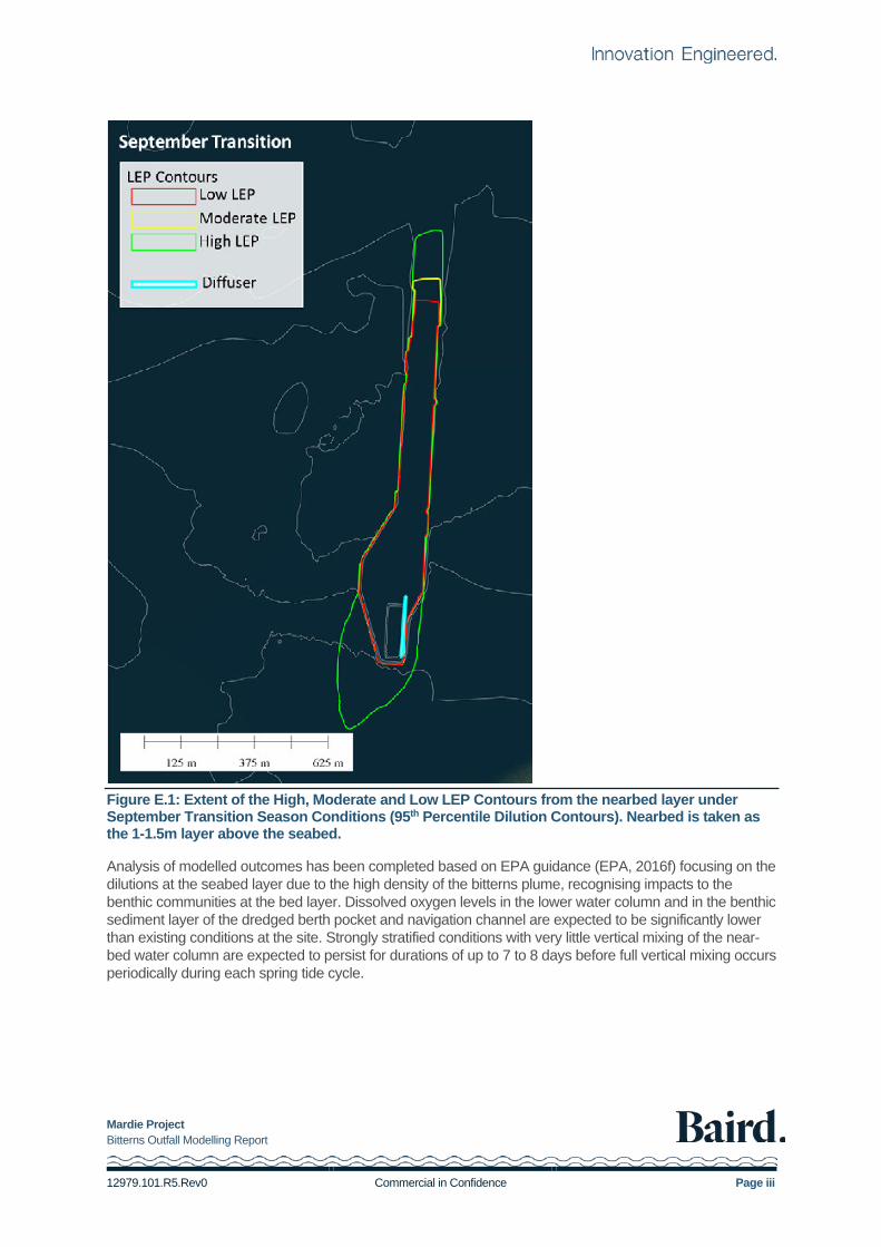
As a result of the stratification that occurs in the dredged area, the Environmental Quality Criteria (EQC) zones extend across the dredged area and the Low, Medium and High LEP extend north along the navigation channel. The boundary of the High LEP extends a short distance south west across the unaltered seabed surrounding the development area and diffuser, with the Moderate and Low LEP boundaries both confined to the dredged channel area. The critical case identified during the modelling, i.e. the case with the largest LEP contour extents, is the September Transition Season, taking the LEP analysis from the nearbed layer representing the water column 1 m to 1.5 m above the seabed. The LEP contour extents modelled during this case are shown in Figure E.1.
Mardie Project Bitterns Outfall Modelling Report
12979.101.R5.Rev0 Commercial in Confidence Page iii
Figure E.1: Extent of the High, Moderate and Low LEP Contours from the nearbed layer under September Transition Season Conditions (95th Percentile Dilution Contours). Nearbed is taken as the 1-1.5m layer above the seabed.
Analysis of modelled outcomes has been completed based on EPA guidance (EPA, 2016f) focusing on the dilutions at the seabed layer due to the high density of the bitterns plume, recognising impacts to the benthic communities at the bed layer. Dissolved oxygen levels in the lower water column and in the benthic sediment layer of the dredged berth pocket and navigation channel are expected to be significantly lower than existing conditions at the site. Strongly stratified conditions with very little vertical mixing of the near-bed water column are expected to persist for durations of up to 7 to 8 days before full vertical mixing occurs periodically during each spring tide cycle.
Mardie Project Bitterns Outfall Modelling Report
12979.101.R5.Rev0 Commercial in Confidence Page iv
Table of Contents
1. Introduction ............................................................................................................................. 1
1.1 Background 1
1.2 Project Overview 1
1.3 Bitterns Outfall Modelling Scope 2
2. Background Information ........................................................................................................ 4
2.1 Key Reports 4
2.1.1 Site Specific Reports Prepared for the Mardie Project 4
2.1.2 Key EPA Documents 4
2.1.3 Other Policy and Guidance 4
2.2 Measured Data Sources 5
3. Environmental Quality Criteria .............................................................................................. 7
3.1 Outfall Process and Assessment of Environmental Quality 7
3.2 WET Testing 7
3.3 Environmental Quality Criteria 7
4. Model Setup ............................................................................................................................. 8
4.1 Model System 8
4.1.1 Nearfield Model 8
4.1.2 Far-field Model – Sigma Layer 3D mode 8
4.1.3 Far-field Model – Z Layer 3D Model 11
4.2 Determination of the Discharge Requirements in the Model 13
4.2.1 Scenario Modelling – Far-field Model 13
4.2.2 Discharge Calculations 14
4.3 Model Settings for Nearfield Modelling – CORMIX 15
4.3.1 Diffuser Design 15
4.4 Model Settings for Farfield Modelling – Delft3D 18
5. Modelling Outcomes ........................................................................................................... 19
Mardie Project Bitterns Outfall Modelling Report
12979.101.R5.Rev0 Commercial in Confidence Page v
5.1 CORMIX results 19
5.2 Comparison of Near field and Far-field Model Results 20
5.3 Far-field Model Results 21
5.3.1 Comparison of Sigma Layer to Z-Layer 3D modes 21
5.3.2 Stratification within the Dredged Navigation Area 23
5.3.3 Recirculation of Saline Water in wider Coastal Waters 26
5.3.4 Stratification and Dissolved Oxygen Implications 28
5.3.5 Seasonal Results 28
5.4 Analysis Method – Calculation of Dilution Rates for LEP Boundaries 32
5.5 Far-field Model Outcomes Compared to Target Dilution 33
6. Conclusions ......................................................................................................................... 47
7. References ............................................................................................................................ 49
Data Files for LEP Zones
Tables Table 2.1: Measured Data Summary .................................................................................................................5
Table 3.1: Environmental Quality Criteria based on Level of Species Protection (O2Marine2019b) ..............7
Table 4.1: Delft Model setup summary (adopted from Baird, 2020) .............................................................. 10
Table 4.2: Delft Model setup summary ........................................................................................................... 13
Table 4.3: Bitterns outfall diffuser required flow rate calculation .................................................................... 14
Table 4.4: Model Settings – Far field Model ................................................................................................... 14
Table 4.5: CORMIX model setup summary ................................................................................................... 15
Table 5.1: Nearfield and Far-field Models Comparison of Modelled Dilution Rate at edge of Nearfield ...... 20
Table 5.2: Vertical stratification for locations in the dredged navigation area ............................................... 24
Mardie Project Bitterns Outfall Modelling Report
12979.101.R5.Rev0 Commercial in Confidence Page vi
Figures Figure E.1: Extent of the High, Moderate and Low LEP Contours from the nearbed layer under September Transition Season Conditions (95th Percentile Dilution Contours). Nearbed is taken as the 1-1.5m layer above the seabed. ............................................................................................................................................. iii
Figure 2.1: Measured Data Locations ................................................................................................................6
Figure 4.1: Local Hydrodynamic Model - Domain Decomposition Grid setup .................................................8
Figure 4.2: Bathymetry Grid for Local Scale Model (Datum mMSL Mardie 2018) ..........................................9
Figure 4.3: Bathymetry Grid – Developed Case Port Precinct (Datum mMSL Mardie 2018) ...................... 10
Figure 4.4: Local Hydrodynamic Model - Domain Decomposition Grid setup .............................................. 12
Figure 4.5: Bathymetry Grid for Local Scale Model (Datum mMSL Mardie 2018) ....................................... 12
Figure 4.6: Sensitivity analysis of number of ports and spacing of ports on dilution rates............................ 15
Figure 4.7: Diffuser geometry as modelled in CORMIX ................................................................................. 16
Figure 4.8: CORMIX 3D Plume result for the adopted 20 port diffuser design for 50th percentile currents, shown as the full plume (top) and as a mesh (bottom) to demonstrate the mixing from the entire length of the diffuser ....................................................................................................................................................... 17
Figure 5.1: CORMIX 2D Plume result for Diffuser Design ............................................................................. 19
Figure 5.2: Salinity levels modelled at 3 points outside of the dredged channel and one point within the dredged channel using the sigma layer model mode and Z-layer model mode. .......................................... 22
Figure 5.3: Location of the points corresponding to the timeseries presented above in Figure 5.2 ............. 23
Figure 5.4: Vertical salinity profiles from within the berth pocket (top) and along the channel (bottom) with a 200m diffuser outputting at a level elevated within the water column ........................................................... 25
Figure 5.5: Locations of salinity timeseries data ............................................................................................. 26
Figure 5.6: Salinity timeseries plots from the sigma layer model outer grids in Dry Season ........................ 27
Figure 5.7: Salinity timeseries plots from the sigma layer model outer grids in Wet Season ....................... 27
Figure 5.8: Plots showing the extent of the plume from the high density bitterns outfall during the Wet seasonal scenario, showing a fully flushed channel during spring tides (top left and bottom) and a stratified channel during neap tides (top right) .............................................................................................................. 30
Figure 5.9: Plots showing the extent of the plume from the high density bitterns outfall during the Dry seasonal scenario, showing a fully flushed channel during spring tides (top right) and a stratified channel during neap tides (top left and bottom) ........................................................................................................... 30
Mardie Project Bitterns Outfall Modelling Report
12979.101.R5.Rev0 Commercial in Confidence Page vii
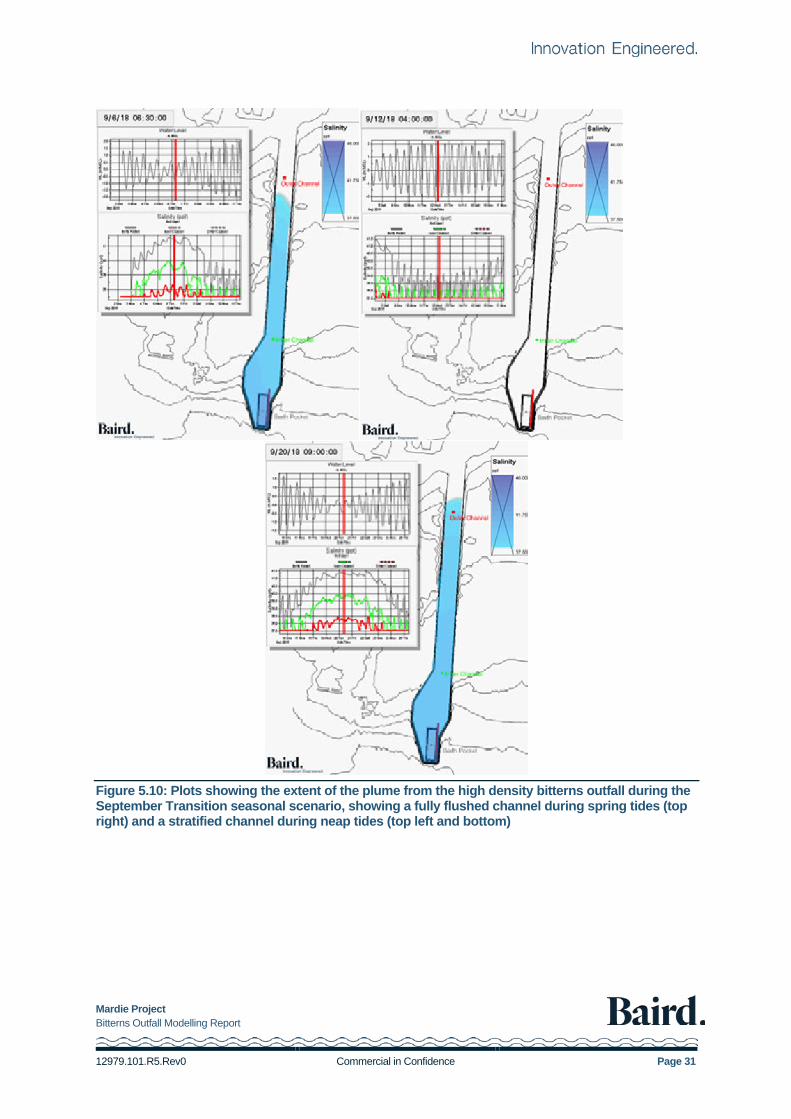
Figure 5.10: Plots showing the extent of the plume from the high density bitterns outfall during the September Transition seasonal scenario, showing a fully flushed channel during spring tides (top right) and a stratified channel during neap tides (top left and bottom) ........................................................................... 31
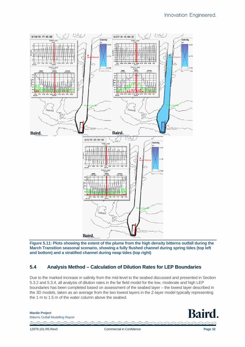
Figure 5.11: Plots showing the extent of the plume from the high density bitterns outfall during the March Transition seasonal scenario, showing a fully flushed channel during spring tides (top left and bottom) and a stratified channel during neap tides (top right) ............................................................................................ 32
Figure 5.12: Extent of the High, Moderate and Low LEP Contours from the nearbed layer under Dry Season Conditions (95th Percentile Dilution Contours). Nearbed is taken as the 1-1.5m layer above the seabed. ............................................................................................................................................................ 35
Figure 5.13: Extent of the High, Moderate and Low LEP Contours from the nearbed layer under Wet Season Conditions (95th Percentile Dilution Contours). Nearbed is taken as the 1-1.5m layer above the seabed. ............................................................................................................................................................ 36
Figure 5.14: Extent of the High, Moderate and Low LEP Contours from the nearbed layer under March Transition Season Conditions (95th Percentile Dilution Contours). Nearbed is taken as the 1-1.5m layer above the seabed. ........................................................................................................................................... 37
Figure 5.15: Extent of the High, Moderate and Low LEP Contours from the nearbed layer under September Transition Season Conditions (95th Percentile Dilution Contours). Nearbed is taken as the 1-1.5m layer above the seabed. ........................................................................................................................................... 38
Figure 5.16: Extent of the High, Moderate and Low LEP Contours under a depth averaged scenario and under Dry Season Conditions (95th Percentile Dilution Contours) ................................................................. 39
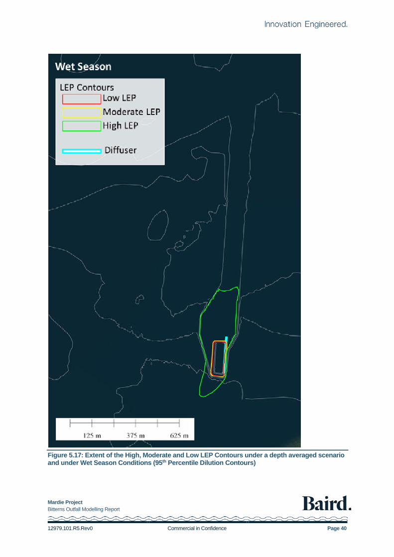
Figure 5.17: Extent of the High, Moderate and Low LEP Contours under a depth averaged scenario and under Wet Season Conditions (95th Percentile Dilution Contours) ................................................................ 40
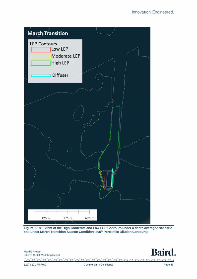
Figure 5.18: Extent of the High, Moderate and Low LEP Contours under a depth averaged scenario and under March Transition Season Conditions (95th Percentile Dilution Contours) ........................................... 41
Figure 5.19: Extent of the High, Moderate and Low LEP Contours under a depth averaged scenario and under September Transition Season Conditions (95th Percentile Dilution Contours) ................................... 42
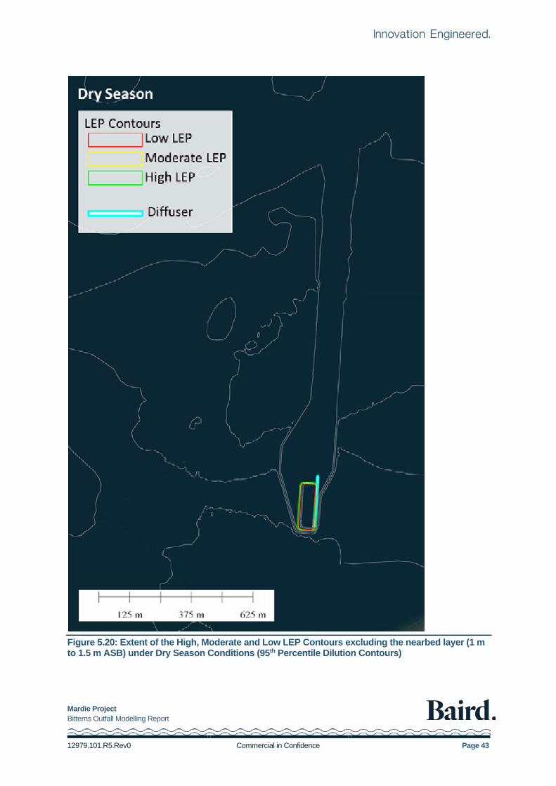
Figure 5.20: Extent of the High, Moderate and Low LEP Contours excluding the nearbed layer (1 m to 1.5 m ASB) under Dry Season Conditions (95th Percentile Dilution Contours) ................................................... 43
Figure 5.21: Extent of the High, Moderate and Low LEP Contours excluding the nearbed layer (1 m to 1.5 m ASB), under Wet Season Conditions (95th Percentile Dilution Contours) ................................................. 44
Figure 5.22: Extent of the High, Moderate and Low LEP Contours excluding the nearbed layer (1 m to 1.5 m ASB), under March Transition Season Conditions (95th Percentile Dilution Contours) ............................ 45
Figure 5.23: Extent of the High, Moderate and Low LEP Contours excluding the nearbed layer (1 m to 1.5 m ASB), under September Transition Season Conditions (95th Percentile Dilution Contours) .................... 46

Mardie Project Bitterns Outfall Modelling Report
12979.101.R5.Rev0 Commercial in Confidence Page 1
1. Introduction
1.1 Background
The Mardie Project is a greenfields high-quality salt project proposed in the Pilbara region of Western Australia. Baird Australia Pty Limited (Baird) have been engaged by Mardie Minerals, a wholly owned subsidiary of BCI Minerals Limited (BCIM) to develop a hydrodynamic modelling program to support the environmental approvals process to assess: • Modelling of dredge plumes to inform the preparation of a Dredging and Spoil Disposal Management
Plan (DSDMP); and • Modelling of mixing and dilution of bitterns discharge into the marine environment to inform the
preparation of a Environmental Quality Plan (EQP).
The following report presents the setup and modelling of the bitterns discharged into the marine environment. The modelling has adopted the calibrated 2D/3D hydrodynamic model presented in Baird (2020). The report also presents concept design parameters for the outlet diffuser which is required to meet the requirements of the EQP. The calibrated model presented in this report has been adopted in the subsequent dredge plume and bitterns dilutions studies.
Details on the Mardie Project and Baird’s scope of engagement are presented in the following sections.
1.2 Project Overview
The proposal is a solar salt project that utilises seawater and evaporation to produce raw salts as a feedstock for dedicated processing facilities that will produce a high purity salt, industrial grade fertiliser products, and other commercial by-products. Production rates of 4.0 Million tonnes per annum (Mtpa) of salt (NaCl), 100 kilo tonnes per annum (ktpa) of Sulphate of Potash (SoP), and up to 300 ktpa of other salt products are being targeted, sourced from a 150 Gigalitre per annum (GLpa) seawater intake. To meet this production, the following infrastructure will be developed: • Seawater intake, pump station and pipeline; • Concentrator ponds; • Drainage channels; • Crystalliser ponds; • Trestle jetty and transhipment berth/channel; • Bitterns disposal pipeline and diffuser; • Processing facilities and stockpiles; • Administration buildings; • Accommodation village; • Access / haul roads; • Desalination plant for freshwater production, with brine discharged to the evaporation ponds; and • Associated infrastructure such as power supply, communications, workshop, laydown, landfill facility,
sewage treatment plant, etc.
Seawater for the process will be pumped from a large tidal creek into the concentrator ponds. All pumps will be screened and operated accordingly to minimise entrapment of marine fauna and any reductions in water levels in the tidal creek.
Mardie Project Bitterns Outfall Modelling Report
12979.101.R5.Rev0 Commercial in Confidence Page 2
Concentrator and crystalliser ponds will be developed behind low permeability walls engineered from local clays and soils and rock armoured to protect against erosion. The height of the walls varies across the project and is matched to the flood risk for the area.
Potable water will be required for the production plants and the village. The water supply will be sourced from a desalination plant which will provide the water required to support the Project. The high salinity output from the plant will be directed to a concentrator pond with the corresponding salinity.
A trestle jetty will be constructed to convey salt (NaCl) from the salt production stockpile to the transhipment berth pocket. The jetty will traverse the intertidal zone for approximately 3.6 km before extending into the ocean for a further 2.4 km. The jetty will minimise impediment of coastal water or sediment movement, thus ensuring disturbance to coastal processes is minimal.
Dredging of up to 800,000 m3 will be required to ensure sufficient depth for the transhipper berth pocket at the end of the trestle jetty, as well as along a 4.5 km long channel out to deeper water. The dredge spoil is inert and will be transported to shore for use within the development.
The production process will produce a high-salinity bittern that, prior to its discharge through a diffuser at the far end of the trestle jetty, will be diluted with seawater to bring its salinity closer to that of the receiving environment.
The Project was referred to DWER – EPA Services and the Level of Assessment (LOA) was set at Public Environmental Review (PER). The EPA determined on 13 June 2018 that there were seven preliminary key environmental factors related to the Project, with Benthic Communities and Habitat (BCH) and Marine Environmental Quality (MEQ) being relevant to this Scope of Works (SOW). BCI are currently finalising the Environmental Review Document (ERD) with the DWER and DoTEE, with potential BCH and MEQ impacts and risks associated with the SOW being: • 3.6GL/a of Bitterns disposal (salinity) at discharge location; • Localised reduction in water quality around the bitterns outfall location; • Direct disturbance / removal of benthic communities and habitat; • Direct loss and degradation of marine fauna habitat; • Marine fauna injury or fatality as a result of vessel strike or contact with dredge equipment; • Changes to water quality due to subtidal dredging, including increased sedimentation resulting in
settlement on, and smothering of, habitat.
Baird has been engaged by BCIM to deliver a numerical modelling study which will provide the basis to support the environmental approvals for the Mardie project.
1.3 Bitterns Outfall Modelling Scope
Baird was also engaged by Mardie Minerals to assess the bitterns discharge and plume dispersal at the discharge location. The established hydrodynamic model and validation, as outlined in the Hydrodynamic Modelling Report (Baird, 2020), was utilised in conjunction with an appropriate model for representing mixing within the nearfield mixing zone around the bitterns outfall; CORMIX, a data-driven rule-based expert system commonly used to represent the complex mixing zone conditions within the nearfield region of outfall facilities, has been used in this case.
The tasks undertaken for the bitterns outfall modelling, and detailed in Baird’s initial scope for Mardie Minerals, are as follows: 1. Establishment and validation of the Hydrodynamic model, as outlined in Baird’s Hydrodynamic
Modelling Report – see Baird (2020). 2. Outfall Options Assessment:
Mardie Project Bitterns Outfall Modelling Report
12979.101.R5.Rev0 Commercial in Confidence Page 3
• An Options Assessment for the outfall design has been completed to determine the optimal / preferred alternative that will be adopted in the modelling study. Outfall options were developed in consultation with Mardie Minerals and include a diffuser to achieve the initial mixing requirements. The analysis examined the plume dispersal under ‘Worst Case’ hydrodynamic scenarios and the testing of four different outfall design cases using far field 2D Modelling and CORMIX Near Field 3D modelling.
3. 3D Bitterns discharge modelling (‘far-field’ modelling) has been completed as follows: • For the preferred option, full process (3D) modelling of bitterns discharge examining plume
dispersion under the four seasonal environmental conditions • Outputs have been prepared in suitable format to support the environmental approvals process -
Spatial mapping, exceedance thresholds based on EQC 4. Plume stability assessment (nearfield):
• CORMIX modelling undertaken of the outlet to investigate the stability of the plume in the immediate area around the outfall location (10m-130m).
• CORMIX results have been integrated with the far-field modelling to establish a full picture of the bitterns dispersal.
Mardie Project Bitterns Outfall Modelling Report
12979.101.R5.Rev0 Commercial in Confidence Page 4
2. Background Information
2.1 Key Reports The background reports referenced in the development of the hydrodynamic model and application in the Bitterns Outfall modelling program are outlined in this section.
2.1.1 Site Specific Reports Prepared for the Mardie Project • O2Marine (2018). Mardie Project Progress Report #1 for Metocean Data Collection, REPORT No.:
R1800106, ISSUE DATE: 22 Oct 2018. • O2Marine (2019a). Mardie Project Progress Report for Metocean Data Collection, R1800132 ISSUE
DATE: 15th January 2019. • O2Marine (2019b). Mardie Project Whole Effluent Toxicity Assessment, R190054 ISSUE DATE: 20th
May 2019, Prepared for Mardie Minerals Limited • EGS Survey (2019). Mardie Salt Project Geophysical Survey - BCI Minerals SURVEY REPORT, EGS
PROJECT REF: AU025918, Prepared for O2Marine 21 January 2019. • RPS (2017). Mardie Salt Project, Preliminary Storm Surge Study, Prepared for BCI. • Surrich and EGS (2019), Detailed Bathymetry data provided by the Mardie project ,
Surrich_EGS_Datasets_Merged_Mardie_Creek_MGAZ50_1m_Shoal_Final_GRIDDED_DepthPos_AHD.
2.1.2 Key EPA Documents • EPA (2016a) Statement of Environmental Principles, Factors and Objectives, EPA, Western Australia. • EPA (2016b) Environmental Impact Assessment (Part IV Divisions 1 and 2) Administrative
Procedures 2016. • EPA (2018a) Environmental Impact Assessment (Part IV Divisions 1 and 2) Procedures Manual, EPA,
Western Australia. • EPA, (2016c) Environmental Factor Guideline – Marine Environmental Quality, EPA, Western
Australia. • EPA, (2016d) Environmental Factor Guideline – Benthic Communities and habitat, EPA, Western
Australia. • EPA, (2016e) Environmental Factor Guideline – Marine Fauna, EPA, Western Australia. • EPA, (2018b) Instructions on how to prepare Environmental Protection Act Part IV Environmental
Management Plans. • EPA, (2016f) Technical Guidance – Protecting the Quality of Western Australia’s Marine Environment,
EPA, Western Australia. • EPA, (2016g) Technical Guidance - Environmental Impact Assessment of Marine Dredging
Proposals, EPA, Western Australia.
2.1.3 Other Policy and Guidance • DoE, (2006) Pilbara Coastal Water Quality Consultation Outcomes – Environmental Values and
Environmental Quality Objectives, Department of Environment (DoE), Government of Western Australia, Marine Series Report No. 1.
• ANZECC & ARMCANZ (2000) Australian and New Zealand Guidelines for Fresh and Marine Water Quality (Australian and New Zealand Environment and Conservation Council (ANZECC) & Agriculture and Resource Management Council of Australia and New Zealand (ARMCANZ).
Mardie Project Bitterns Outfall Modelling Report
12979.101.R5.Rev0 Commercial in Confidence Page 5
2.2 Measured Data Sources
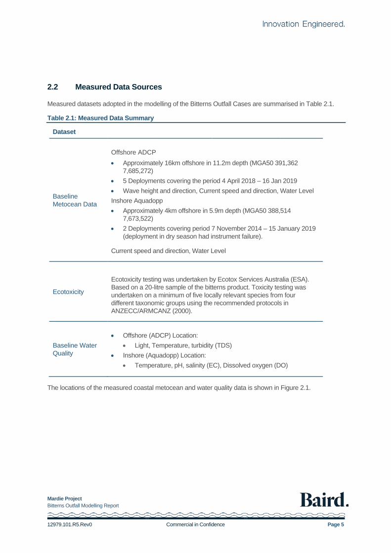
Measured datasets adopted in the modelling of the Bitterns Outfall Cases are summarised in Table 2.1.
Table 2.1: Measured Data Summary
Dataset
Baseline Metocean Data
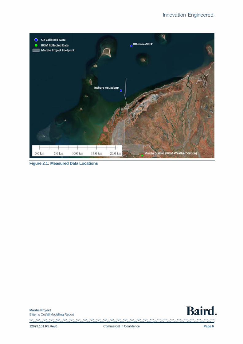
Offshore ADCP • Approximately 16km offshore in 11.2m depth (MGA50 391,362
7,685,272) • 5 Deployments covering the period 4 April 2018 – 16 Jan 2019 • Wave height and direction, Current speed and direction, Water Level Inshore Aquadopp • Approximately 4km offshore in 5.9m depth (MGA50 388,514
7,673,522) • 2 Deployments covering period 7 November 2014 – 15 January 2019
(deployment in dry season had instrument failure).
Current speed and direction, Water Level
Ecotoxicity
Ecotoxicity testing was undertaken by Ecotox Services Australia (ESA). Based on a 20-litre sample of the bitterns product. Toxicity testing was undertaken on a minimum of five locally relevant species from four different taxonomic groups using the recommended protocols in ANZECC/ARMCANZ (2000).
Baseline Water Quality
• Offshore (ADCP) Location: • Light, Temperature, turbidity (TDS)
• Inshore (Aquadopp) Location: • Temperature, pH, salinity (EC), Dissolved oxygen (DO)
The locations of the measured coastal metocean and water quality data is shown in Figure 2.1.
Mardie Project Bitterns Outfall Modelling Report
12979.101.R5.Rev0 Commercial in Confidence Page 6
Figure 2.1: Measured Data Locations
Mardie Project Bitterns Outfall Modelling Report
12979.101.R5.Rev0 Commercial in Confidence Page 7
3. Environmental Quality Criteria
3.1 Outfall Process and Assessment of Environmental Quality
The Mardie project production process will produce a high-salinity bittern that, prior to its discharge through a diffuser at the far end of the trestle jetty, will be diluted with seawater to bring its salinity closer to that of the receiving environment.
In accordance with the Environmental Assessment Guideline for Protecting the Quality of Western Australia’s Marine Environment (EPA, 2015), the predicted concentrations of constituents at the point of discharge will be compared to Environmental Quality Criteria (EQC) defined within the Environmental Quality Plan (EQP), which are likely to be default trigger values derived from ANZECC/ARMCANZ (2000) or more robust and locally relevant values using baseline data from suitable un-impacted reference sites.
The modelling of the bitterns discharge will determine the number of dilutions achieved at the boundaries of the ecological protection (LEP) under the modelled regime, thereby demonstrating that the level of ecological protection required in the waters surrounding the mixing zone can be achieved. The model system has been developed with two parts: a far-field model based on the validated hydrodynamic model (Baird 2019) and a nearfield model (CORMIX) which specifically model the turbulent mixing zone immediately surrounding the diffuser (refer Section 4).
3.2 WET Testing
Whole effluent toxicity (WET) testing to determine and describe the toxic effects of the bitterns’ discharge and predict the number of dilutions required to meet the different levels of ecological protection surrounding the outfall was undertaken by Ecotox Services Australia (Eco Tox 2019). A sample of bitterns was produced, and testing included tropical species from a range of trophic levels (primary producer, herbivore and carnivore) and development stages, using both acute and chronic tests for toxicity. The analysis from the Ecotoxicity testing reported the raw bitterns product had a salinity of 325ppt.
3.3 Environmental Quality Criteria
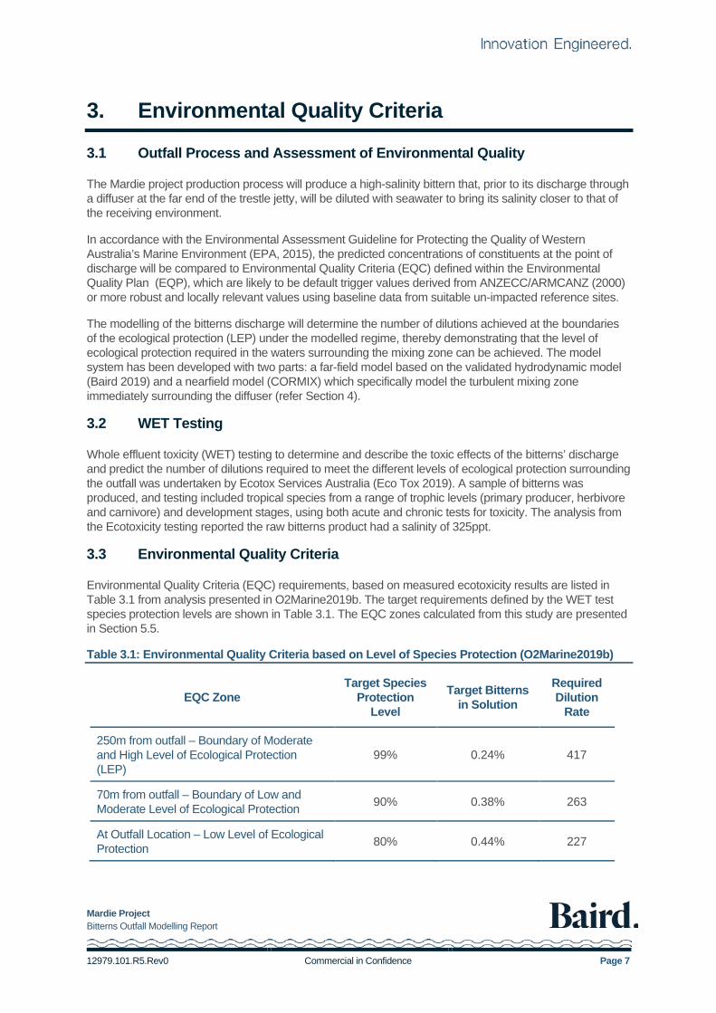
Environmental Quality Criteria (EQC) requirements, based on measured ecotoxicity results are listed in Table 3.1 from analysis presented in O2Marine2019b. The target requirements defined by the WET test species protection levels are shown in Table 3.1. The EQC zones calculated from this study are presented in Section 5.5.
Table 3.1: Environmental Quality Criteria based on Level of Species Protection (O2Marine2019b)
EQC Zone Target Species
Protection Level
Target Bitterns in Solution
Required Dilution
Rate
250m from outfall – Boundary of Moderate and High Level of Ecological Protection (LEP)
99% 0.24% 417
70m from outfall – Boundary of Low and Moderate Level of Ecological Protection 90% 0.38% 263
At Outfall Location – Low Level of Ecological Protection 80% 0.44% 227
Mardie Project Bitterns Outfall Modelling Report
12979.101.R5.Rev0 Commercial in Confidence Page 8
4. Model Setup
4.1 Model System
The bitterns outfall modelling has been completed using a nearfield and far-field modelling approach
4.1.1 Nearfield Model
To model the bitterns plume dispersion in the immediate vicinity of the outfall location, the CORMIX model has been applied. CORMIX is a rules based expert system used to provide mixing zone analysis for a range of discharges into bodies of water, with particular emphasis on the geometry and dilution characteristics of plumes defining the nearfield mixing zone (Doneker et al 2007). In this case, CORMIX has been used solely to define the characteristics of the nearfield mixing zone dominated by the buoyancy and mass flux of the jet discharging from the bitterns diffuser outfall. CORMIX has the ability to describe the smaller scale fluid motions in this zone where strong initial mixing occurs as a result of the significant buoyancy difference between the diffuser jet and the receiving environment, as well as mixing created by the momentum of the diffuser jet.
4.1.2 Far-field Model – Sigma Layer 3D mode
Description of the wider hydrodynamics influencing the advection and dispersion of the bitterns requires a model capable of incorporating metocean parameters including tides and winds. The hydrodynamic model developed for the Mardie Project (Baird 2019) has used the Delft3D modelling system (Deltares 2018). Delft3D is an integrated modelling suite, which simulates two-dimensional (in either the horizontal or a vertical plane) and three-dimensional flow, sediment transport and morphology, waves, water quality, and ecology and can handle the interactions between these processes.
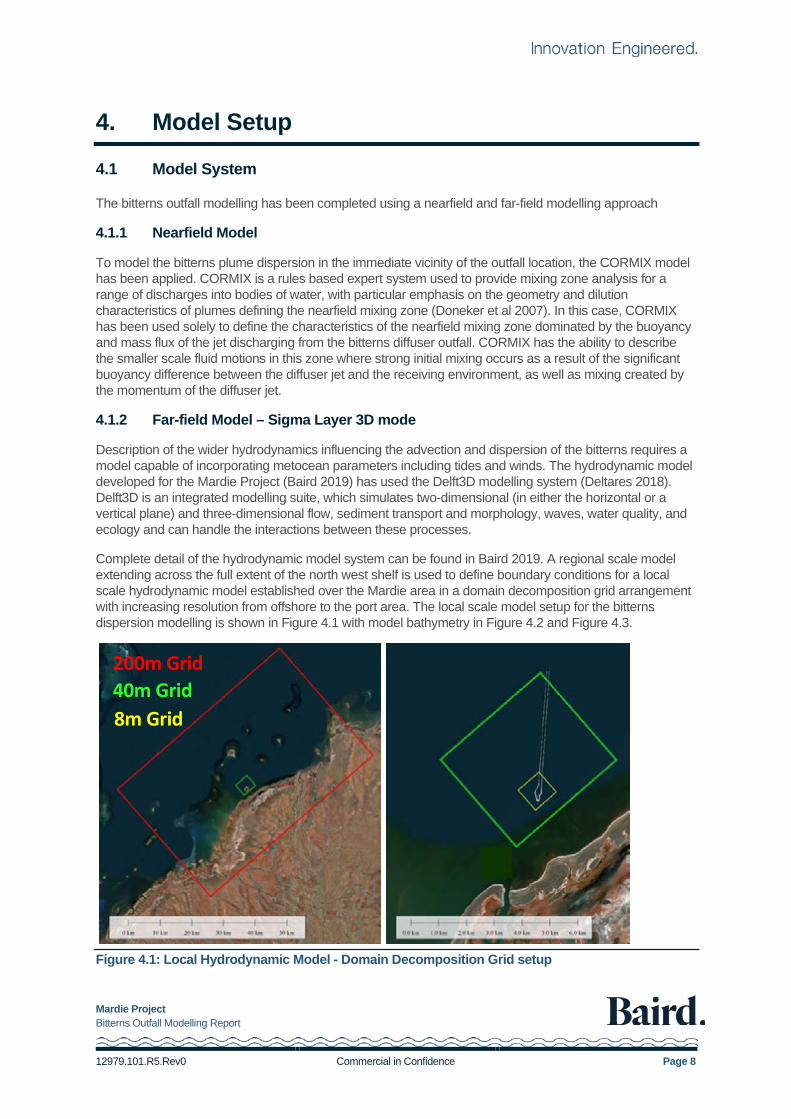
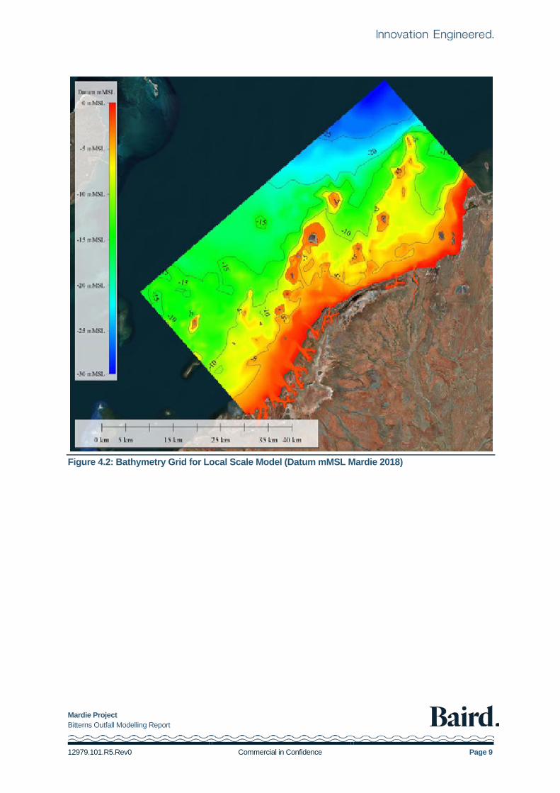
Complete detail of the hydrodynamic model system can be found in Baird 2019. A regional scale model extending across the full extent of the north west shelf is used to define boundary conditions for a local scale hydrodynamic model established over the Mardie area in a domain decomposition grid arrangement with increasing resolution from offshore to the port area. The local scale model setup for the bitterns dispersion modelling is shown in Figure 4.1 with model bathymetry in Figure 4.2 and Figure 4.3.
Figure 4.1: Local Hydrodynamic Model - Domain Decomposition Grid setup
200m Grid 40m Grid 8m Grid
Mardie Project Bitterns Outfall Modelling Report
12979.101.R5.Rev0 Commercial in Confidence Page 9
Figure 4.2: Bathymetry Grid for Local Scale Model (Datum mMSL Mardie 2018)
Mardie Project Bitterns Outfall Modelling Report
12979.101.R5.Rev0 Commercial in Confidence Page 10
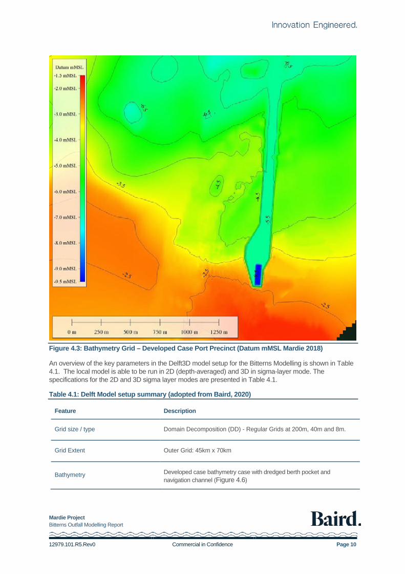
Figure 4.3: Bathymetry Grid – Developed Case Port Precinct (Datum mMSL Mardie 2018)
An overview of the key parameters in the Delft3D model setup for the Bitterns Modelling is shown in Table 4.1. The local model is able to be run in 2D (depth-averaged) and 3D in sigma-layer mode. The specifications for the 2D and 3D sigma layer modes are presented in Table 4.1.
Table 4.1: Delft Model setup summary (adopted from Baird, 2020)
Feature Description
Grid size / type Domain Decomposition (DD) - Regular Grids at 200m, 40m and 8m.
Grid Extent Outer Grid: 45km x 70km
Bathymetry Developed case bathymetry case with dredged berth pocket and navigation channel (Figure 4.6)
Mardie Project Bitterns Outfall Modelling Report
12979.101.R5.Rev0 Commercial in Confidence Page 11
Feature Description
3D sigma layer model 5-vertical sigma layers with layer thicknesses of 20% all the way through the water column.
Vertical Datum Mean Sea Level (m MSL) which is approximately Australian Height Datum (AHD)
Horizontal eddy diffusivity coefficient Across the DDGrids 200m / 40m / 8m: 25 / 5 / 1 m2/s
Horizontal eddy viscosity coefficient Across the DDGrids 200m / 40m / 8m: 25 / 5 / 1 m2/s
Vertical eddy viscosity / diffusivity k-ε turbulence closure model
Time step (2D model) 0.25 mins (15 secs)
Time step (3D z-layer) 0.1 mins (6 secs)
Time step (3D sigma-layer) 0.25 mins (15 secs)
Bed friction Chezy 55m1/2/s
4.1.3 Far-field Model – Z Layer 3D Model
Following 3D modelling carried out using the sigma layer mode model, further modelling using the Z layer mode was required to verify the vertical mixing created by the density gradients created by the high-density bitterns product released at the outfall sinking into a dredged berth pocket and channel where bed shear stresses are low. The Delft3D Z-Layer model is model computationally demanding than the sigma-layer model and is also subject to more stringent stability criteria in the numerical solution. It was not feasible to couple a high resolution Z-layer model which had sufficient resolution for the dredge area into the overall model domain described in Section 4.1.2. To address this limitation, a mid-field model was developed, with an 8 m model grid resolution that obtained boundary conditions over the natural (undredged) seabed from the model described in Section 4.1.2. Due to the nature of Delft 3D’s Z layer 3D model mode, the full domain decomposition grid used for the sigma layer modelling was not able to be used, and a single grid domain was used to run the model in Z layer mode.
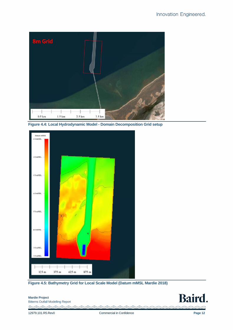
The larger local scale domain decomposition model was used to define boundary conditions for the smaller local scale hydrodynamic Z layer model. The local scale Z layer model setup for the bitterns dispersion modelling is shown in Figure 4.4 with model bathymetry in Figure 4.5.
Mardie Project Bitterns Outfall Modelling Report
12979.101.R5.Rev0 Commercial in Confidence Page 12
Figure 4.4: Local Hydrodynamic Model - Domain Decomposition Grid setup
Figure 4.5: Bathymetry Grid for Local Scale Model (Datum mMSL Mardie 2018)
8m Grid
Mardie Project Bitterns Outfall Modelling Report
12979.101.R5.Rev0 Commercial in Confidence Page 13
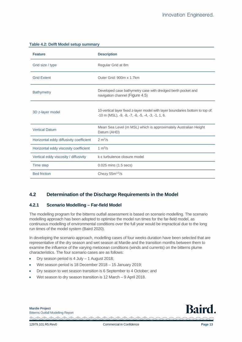
Table 4.2: Delft Model setup summary
Feature Description
Grid size / type Regular Grid at 8m
Grid Extent Outer Grid: 900m x 1.7km
Bathymetry Developed case bathymetry case with dredged berth pocket and navigation channel (Figure 4.5)
3D z-layer model 10-vertical layer fixed z-layer model with layer boundaries bottom to top of: -10 m (MSL), -9, -8, -7, -6, -5, -4, -3, -1, 1, 6.
Vertical Datum Mean Sea Level (m MSL) which is approximately Australian Height Datum (AHD)
Horizontal eddy diffusivity coefficient 2 m2/s
Horizontal eddy viscosity coefficient 1 m2/s
Vertical eddy viscosity / diffusivity k-ε turbulence closure model
Time step 0.025 mins (1.5 secs)
Bed friction Chezy 55m1/2/s
4.2 Determination of the Discharge Requirements in the Model
4.2.1 Scenario Modelling – Far-field Model
The modelling program for the bitterns outfall assessment is based on scenario modelling. The scenario modelling approach has been adopted to optimise the model run times for the far-field model, as continuous modelling of environmental conditions over the full year would be impractical due to the long run times of the model system (Baird 2020).
In developing the scenario approach, modelling cases of four weeks duration have been selected that are representative of the dry season and wet season at Mardie and the transition months between them to examine the influence of the varying metocean conditions (winds and currents) on the bitterns plume characteristics. The four scenario cases are as follows: • Dry season period is 4 July – 1 August 2018; • Wet season period is 18 December 2018 – 15 January 2019; • Dry season to wet season transition is 6 September to 4 October; and • Wet season to dry season transition is 12 March – 9 April 2018.
Mardie Project Bitterns Outfall Modelling Report
12979.101.R5.Rev0 Commercial in Confidence Page 14
4.2.2 Discharge Calculations
The initial discharge objective of Mardie Minerals set the required annual diluted bitterns discharge rate based on a 1:1 dilution (1-part bitterns / 1-part seawater). Modelling commenced to assess this approach against the EQC under a range of assumptions: • The analysis from the Ecotoxicity testing reported the raw bitterns product had a salinity of 325ppt and
this was adopted in the initial series of dispersion modelling calculations; • Background salinity consistent with the median value from measured data at the Mardie location was
applied in the scenario models for the respective periods the models were run; • For each model case the time series discharge of salinity was schematised as an input to the 3D
model (sigma layer model in Delft3D). The volume was discharged into the lower levels of the water column, based on the height of the diffuser and the density of the plume.
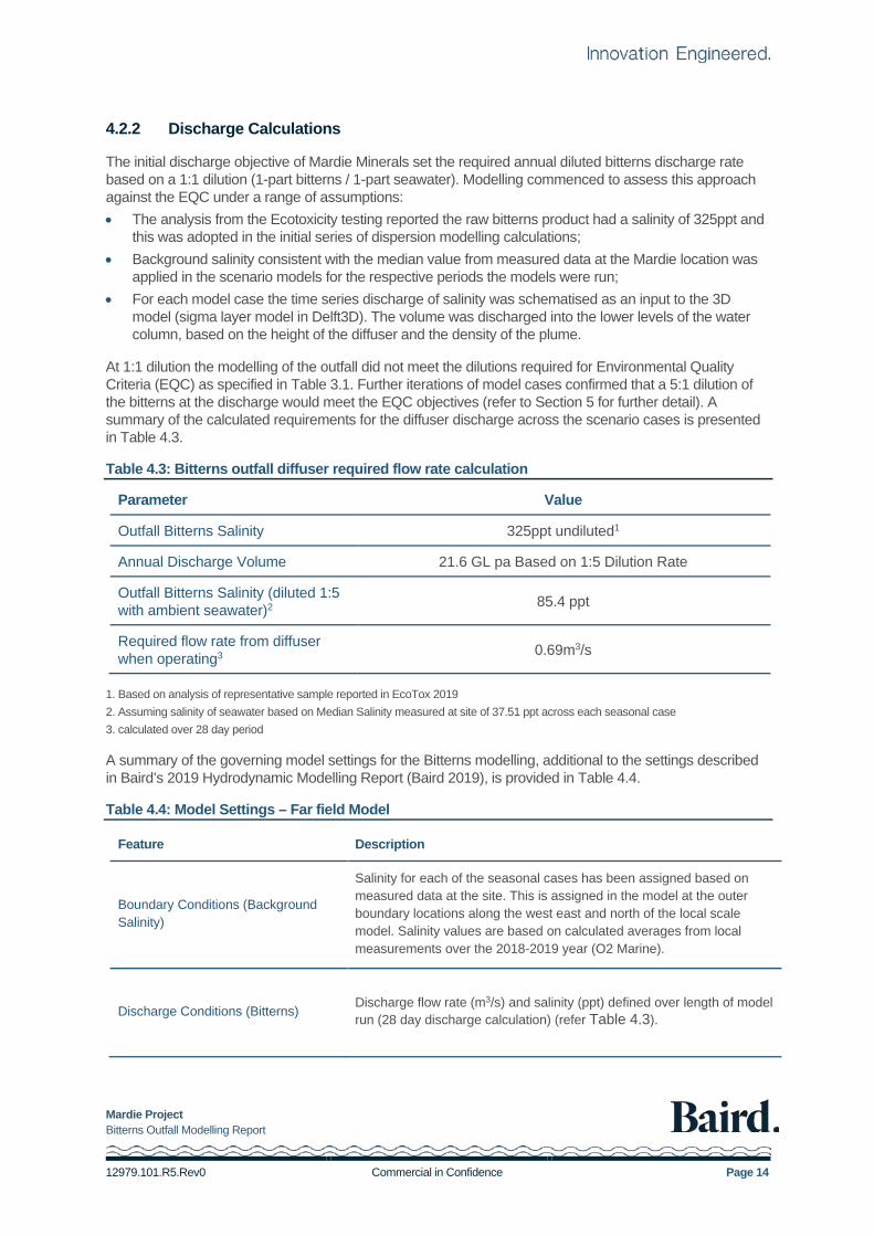
At 1:1 dilution the modelling of the outfall did not meet the dilutions required for Environmental Quality Criteria (EQC) as specified in Table 3.1. Further iterations of model cases confirmed that a 5:1 dilution of the bitterns at the discharge would meet the EQC objectives (refer to Section 5 for further detail). A summary of the calculated requirements for the diffuser discharge across the scenario cases is presented in Table 4.3.
Table 4.3: Bitterns outfall diffuser required flow rate calculation
Parameter Value
Outfall Bitterns Salinity 325ppt undiluted1
Annual Discharge Volume 21.6 GL pa Based on 1:5 Dilution Rate
Outfall Bitterns Salinity (diluted 1:5 with ambient seawater)2 85.4 ppt
Required flow rate from diffuser when operating3 0.69m3/s
1. Based on analysis of representative sample reported in EcoTox 2019 2. Assuming salinity of seawater based on Median Salinity measured at site of 37.51 ppt across each seasonal case 3. calculated over 28 day period
A summary of the governing model settings for the Bitterns modelling, additional to the settings described in Baird’s 2019 Hydrodynamic Modelling Report (Baird 2019), is provided in Table 4.4.
Table 4.4: Model Settings – Far field Model
Feature Description
Boundary Conditions (Background Salinity)
Salinity for each of the seasonal cases has been assigned based on measured data at the site. This is assigned in the model at the outer boundary locations along the west east and north of the local scale model. Salinity values are based on calculated averages from local measurements over the 2018-2019 year (O2 Marine).
Discharge Conditions (Bitterns) Discharge flow rate (m3/s) and salinity (ppt) defined over length of model run (28 day discharge calculation) (refer Table 4.3).
Mardie Project Bitterns Outfall Modelling Report
12979.101.R5.Rev0 Commercial in Confidence Page 15
4.3 Model Settings for Nearfield Modelling – CORMIX
4.3.1 Diffuser Design
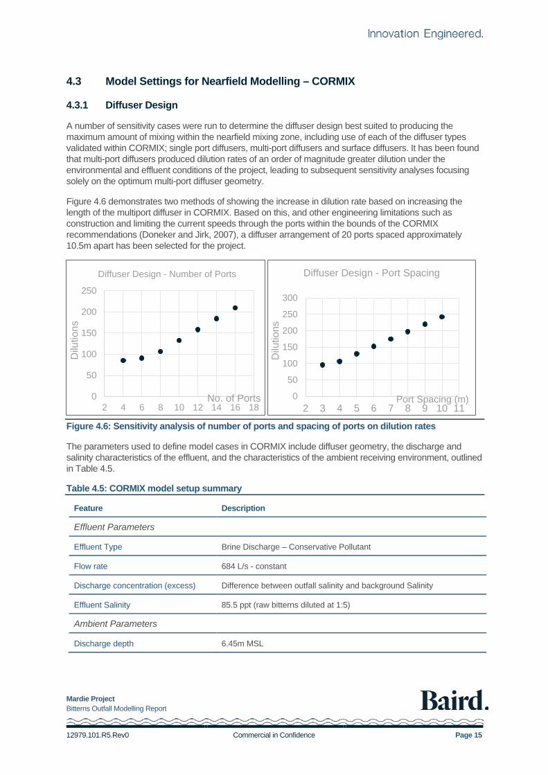
A number of sensitivity cases were run to determine the diffuser design best suited to producing the maximum amount of mixing within the nearfield mixing zone, including use of each of the diffuser types validated within CORMIX; single port diffusers, multi-port diffusers and surface diffusers. It has been found that multi-port diffusers produced dilution rates of an order of magnitude greater dilution under the environmental and effluent conditions of the project, leading to subsequent sensitivity analyses focusing solely on the optimum multi-port diffuser geometry.
Figure 4.6 demonstrates two methods of showing the increase in dilution rate based on increasing the length of the multiport diffuser in CORMIX. Based on this, and other engineering limitations such as construction and limiting the current speeds through the ports within the bounds of the CORMIX recommendations (Doneker and Jirk, 2007), a diffuser arrangement of 20 ports spaced approximately 10.5m apart has been selected for the project.
Figure 4.6: Sensitivity analysis of number of ports and spacing of ports on dilution rates
The parameters used to define model cases in CORMIX include diffuser geometry, the discharge and salinity characteristics of the effluent, and the characteristics of the ambient receiving environment, outlined in Table 4.5.
Table 4.5: CORMIX model setup summary
Feature Description
Effluent Parameters
Effluent Type Brine Discharge – Conservative Pollutant
Flow rate 684 L/s - constant
Discharge concentration (excess) Difference between outfall salinity and background Salinity
Effluent Salinity 85.5 ppt (raw bitterns diluted at 1:5)
Ambient Parameters
Discharge depth 6.45m MSL
0
50
100
150
200
250
2 4 6 8 10 12 14 16 18
Dilu
tions
No. of Ports
Diffuser Design - Number of Ports
0
50
100
150
200
250
300
2 3 4 5 6 7 8 9 10 11
Dilu
tions
Port Spacing (m)
Diffuser Design - Port Spacing
Mardie Project Bitterns Outfall Modelling Report
12979.101.R5.Rev0 Commercial in Confidence Page 16
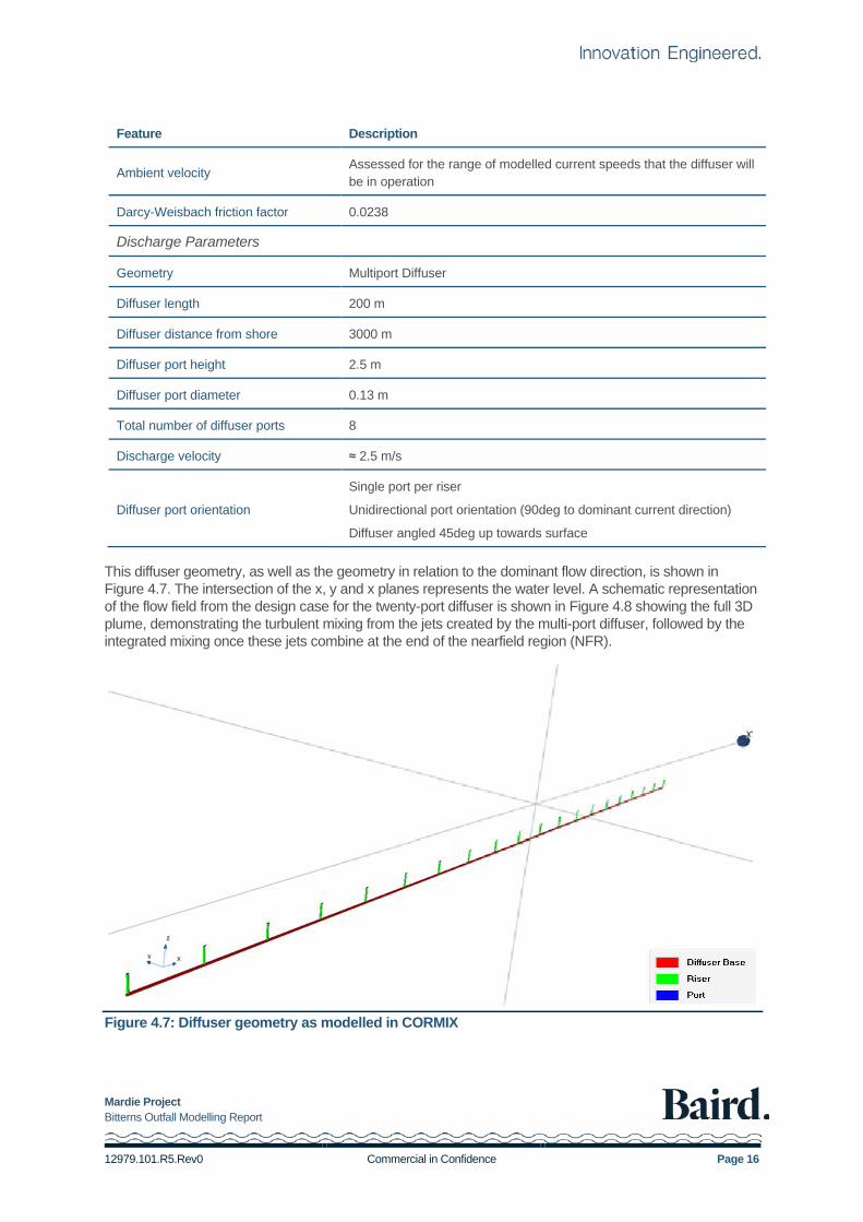
Feature Description
Ambient velocity Assessed for the range of modelled current speeds that the diffuser will be in operation
Darcy-Weisbach friction factor 0.0238
Discharge Parameters
Geometry Multiport Diffuser
Diffuser length 200 m
Diffuser distance from shore 3000 m
Diffuser port height 2.5 m
Diffuser port diameter 0.13 m
Total number of diffuser ports 8
Discharge velocity ≈ 2.5 m/s
Diffuser port orientation
Single port per riser
Unidirectional port orientation (90deg to dominant current direction)
Diffuser angled 45deg up towards surface
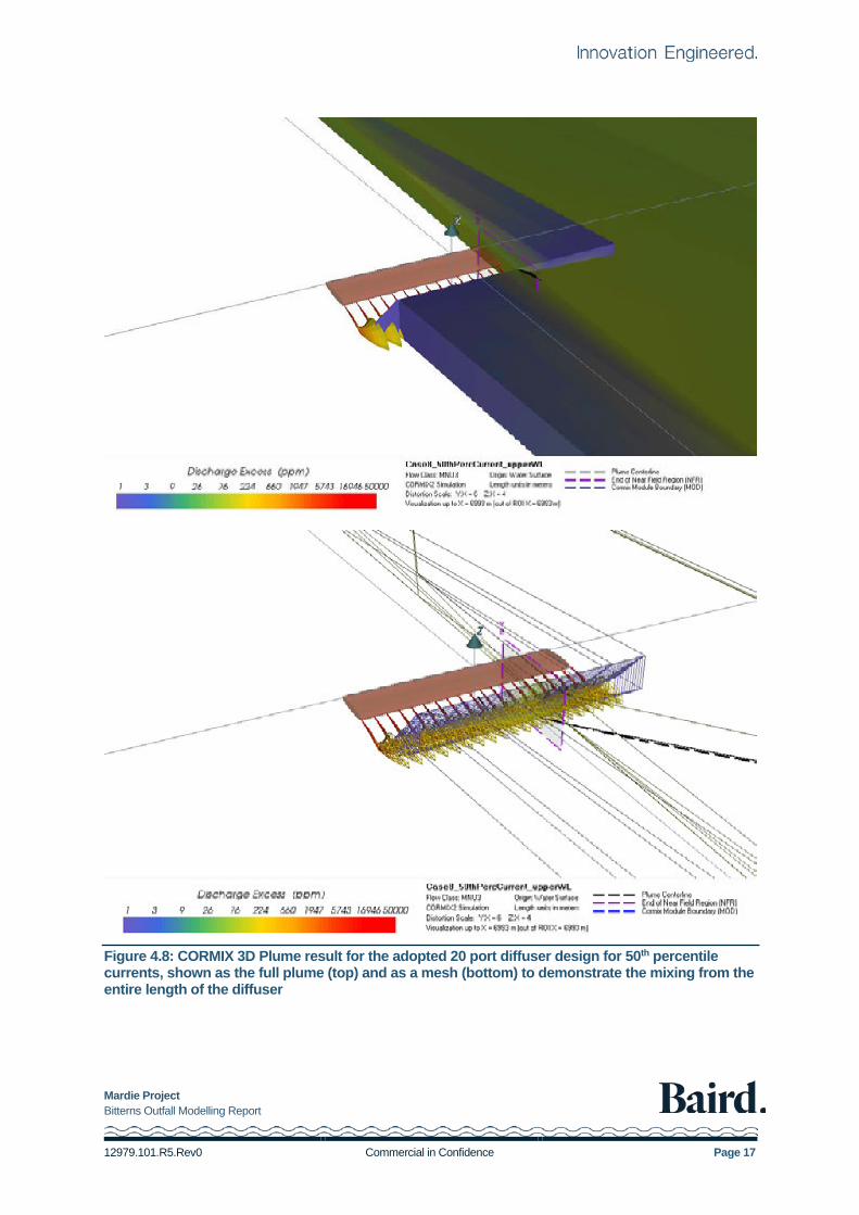
This diffuser geometry, as well as the geometry in relation to the dominant flow direction, is shown in Figure 4.7. The intersection of the x, y and x planes represents the water level. A schematic representation of the flow field from the design case for the twenty-port diffuser is shown in Figure 4.8 showing the full 3D plume, demonstrating the turbulent mixing from the jets created by the multi-port diffuser, followed by the integrated mixing once these jets combine at the end of the nearfield region (NFR).
Figure 4.7: Diffuser geometry as modelled in CORMIX
Mardie Project Bitterns Outfall Modelling Report
12979.101.R5.Rev0 Commercial in Confidence Page 17
Figure 4.8: CORMIX 3D Plume result for the adopted 20 port diffuser design for 50th percentile currents, shown as the full plume (top) and as a mesh (bottom) to demonstrate the mixing from the entire length of the diffuser
Mardie Project Bitterns Outfall Modelling Report
12979.101.R5.Rev0 Commercial in Confidence Page 18
4.4 Model Settings for Farfield Modelling – Delft3D
The input of the bitterns release to the far-field Delft3D model has been schematised to approximate the discharge from the diffuser jets which disperse the plume into the upper to middle layers of the water column in the near field (refer Figure 4.8). The grid size of the Delft3d model is 8m and the diffuser flows have been divided and dispersed through 25 input cells representative of the diffuser length in the model. Velocity is not specified as a model input for Delft3D, however tidal velocity in the hydrodynamic model immediately directs the discharge in the ebb tide current direction at time of release. Over the length scale of the nearfield mixing region (discussed in the next section) the input discharge immediately proceeds to dilute in the receiving waters and sink to the lower levels as a dense plume.
Mardie Project Bitterns Outfall Modelling Report
12979.101.R5.Rev0 Commercial in Confidence Page 19
5. Modelling Outcomes
5.1 CORMIX results
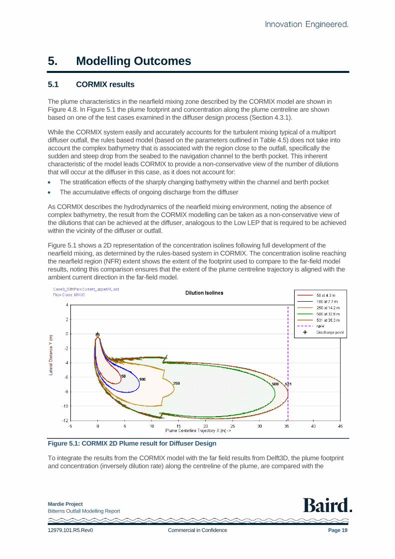
The plume characteristics in the nearfield mixing zone described by the CORMIX model are shown in Figure 4.8. In Figure 5.1 the plume footprint and concentration along the plume centreline are shown based on one of the test cases examined in the diffuser design process (Section 4.3.1).
While the CORMIX system easily and accurately accounts for the turbulent mixing typical of a multiport diffuser outfall, the rules based model (based on the parameters outlined in Table 4.5) does not take into account the complex bathymetry that is associated with the region close to the outfall, specifically the sudden and steep drop from the seabed to the navigation channel to the berth pocket. This inherent characteristic of the model leads CORMIX to provide a non-conservative view of the number of dilutions that will occur at the diffuser in this case, as it does not account for: • The stratification effects of the sharply changing bathymetry within the channel and berth pocket • The accumulative effects of ongoing discharge from the diffuser
As CORMIX describes the hydrodynamics of the nearfield mixing environment, noting the absence of complex bathymetry, the result from the CORMIX modelling can be taken as a non-conservative view of the dilutions that can be achieved at the diffuser, analogous to the Low LEP that is required to be achieved within the vicinity of the diffuser or outfall.
Figure 5.1 shows a 2D representation of the concentration isolines following full development of the nearfield mixing, as determined by the rules-based system in CORMIX. The concentration isoline reaching the nearfield region (NFR) extent shows the extent of the footprint used to compare to the far-field model results, noting this comparison ensures that the extent of the plume centreline trajectory is aligned with the ambient current direction in the far-field model.
Figure 5.1: CORMIX 2D Plume result for Diffuser Design
To integrate the results from the CORMIX model with the far field results from Delft3D, the plume footprint and concentration (inversely dilution rate) along the centreline of the plume, are compared with the
Mardie Project Bitterns Outfall Modelling Report
12979.101.R5.Rev0 Commercial in Confidence Page 20
concentrations at the extent of the CORMIX nearfield plume footprint from the far field model, at a point in time in the far-field model where the same hydrodynamic conditions are met.
5.2 Comparison of Near field and Far-field Model Results
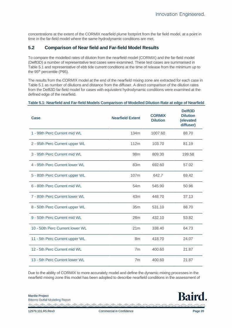
To compare the modelled rates of dilution from the nearfield model (CORMIX) and the far-field model (Delft3D) a number of representative test cases were examined. These test cases are summarised in Table 5.1 and representative of ebb tide current conditions at the time of release from the minimum up to the 95th percentile (P95).
The results from the CORMIX model at the end of the nearfield mixing zone are extracted for each case in Table 5.1 as number of dilutions and distance from the diffuser. A direct comparison of the dilution rates from the Delft3D far-field model for cases with equivalent hydrodynamic conditions were examined at the defined edge of the nearfield.
Table 5.1: Nearfield and Far-field Models Comparison of Modelled Dilution Rate at edge of Nearfield
Case Nearfield Extent CORMIX Dilution
Delft3D Dilution
(elevated diffuser)
1 - 99th Perc Current mid WL 134m 1007.60 88.70
2 - 95th Perc Current upper WL 112m 103.70 81.19
3 - 95th Perc Current mid WL 98m 809.30 199.58
4 - 95th Perc Current lower WL 83m 692.60 57.02
5 - 80th Perc Current upper WL 107m 642.7 69.42
6 - 80th Perc Current mid WL 54m 545.90 50.96
7 - 80th Perc Current lower WL 43m 448.70 37.13
8 - 50th Perc Current upper WL 35m 531.10 88.70
9 - 50th Perc Current mid WL 28m 432.10 53.82
10 - 50th Perc Current lower WL 21m 338.40 64.73
11 - 5th Perc Current upper WL 8m 418.70 24.07
12 - 5th Perc Current mid WL 7m 400.60 21.87
13 - 5th Perc Current lower WL 7m 400.60 21.87
Due to the ability of CORMIX to more accurately model and define the dynamic mixing processes in the nearfield mixing zone this model has been adopted to describe nearfield conditions in the assessment of
Mardie Project Bitterns Outfall Modelling Report
12979.101.R5.Rev0 Commercial in Confidence Page 21
the EQC for the Low LEP. The target rate of dilutions in the Low ecological protection (Low LEP) for the 80% Species protection level is 227 dilutions (Table 3.1). Based on the CORMIX cases presented in Table 5.1, this is achieved within a 10 m nearfield extent of the diffuser.
The results in Table 5.1 indicate that the Delft3D model is more conservative in the calculation of the achieved dilution rates between the region between the nearfield and far-field where the EQC boundaries are defined and explicitly models the reduction in effective mixing that occurs as a result of stratification within the dredged channel. Each of the CORMIX dilutions noted in Table 5.1 represent the dilutions achieved directly after releasing the bitterns into the receiving environment (i.e. the receiving environment is always at ambient salinity concentration), whereas the Delft3D dilutions are those that are achieved at times in the Delft3D runs where the ambient salinity maybe altered from the background concentration due to prior bitterns discharge. These times are distributed throughout the Delft3D run, with some directly after release of the bitterns, but most occurring well after the first release or towards the end of the run, when the receiving environment has been affected by the bitterns product that has already been released the background salinity is generally raised. CORMIX does not consider the accumulation of higher salinity water over time in the dredged basin and channel, whereas the Delft3D Z-layer model does.
Noting these limitations, and those mentioned in Section 5.1, it can be said that CORMIX provides the ‘best possible’ mixing under given discrete hydrodynamic conditions, and Delft3D gives a more conservative and likely more realistic view of the mixing under conditions with the complete seabed bathymetry, variable water levels and currents, and continuous discharge of bitterns into the receiving waters.
In light of this, a best case estimate of the low LEP region could be taken from the CORMIX results; however, Delft3D provides a more realistic description of the low LEP due the reduction of mixing efficiency that occurs as a stratified nearbed layer develops in the dredged area. The low LEP region has been defined from the Delft3D model results presented in Section 5.5.
5.3 Far-field Model Results
5.3.1 Comparison of Sigma Layer to Z-Layer 3D modes
The 3D model grid layer regimes available in Delft3D-FLOW and that were considered in this study are: • Sigma-layer grid where the vertical layer thickness varies with the depth of water and the number of
active layers is constant; and • Z-layer grid where the vertical layer thickness is fixed across the grid and the number of active layers
varies with the depth of water.
Following completion of modelling in the sigma layer 3D model mode, further investigation into the effects of density driven currents and mixing was carried out using the Z-layer 3D mode. The Z-layer model minimises the occurrence of errors in the approximation of horizontal density gradients in areas of steep bottom topography, therefore providing greater confidence that the mixing produced by the model is more closely simulating the actual mixing that would occur at the outfall (Deltares 2014). The relatively steep batters of the dredge channel and berth pocket create the requirement to resolve the currents and mixing using the Z-layer model within the vicinity of the dredged area.
Comparison of the two model modes show that outside of the dredge area the two models are simulating a similar mixing outcome, and that a significant difference can be seen within the dredged channel. Figure 5.2 shows the similarity in salinity levels over time at locations outside of the dredged channel, and the significantly difference mixing that occurs within the dredged channel, demonstrating the necessity in using the Z-layer model when considering the mixing regime within the dredged channel. It should be noted that the Z-layer model boundaries as indicated in Figure 4.4 had a fixed salinity boundary condition of 37.5 ppt and as a result of the relatively small domain of that model, there are frequent periods where the salinity at the three undredged locations (NE, NW, SE) are equal to the boundary salinity. The sigma layer model includes the whole model extent as defined in Figure 4.1 and salinities in the mid-field are slightly elevated

Mardie Project Bitterns Outfall Modelling Report
12979.101.R5.Rev0 Commercial in Confidence Page 22
by 0.2 to 0.3 ppt above the current background level as a result of the ongoing bitterns discharge into the model.
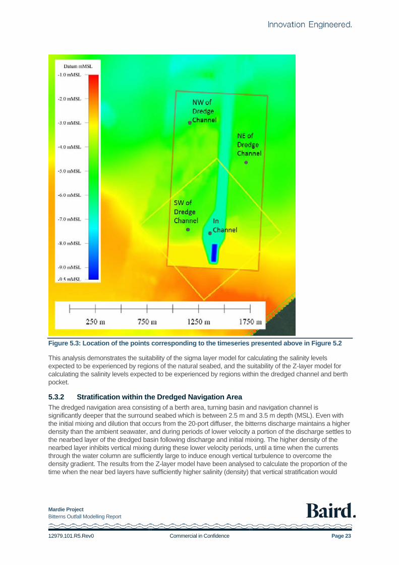
Figure 5.2: Salinity levels modelled at 3 points outside of the dredged channel and one point within the dredged channel using the sigma layer model mode and Z-layer model mode.
The timeseries plots in Figure 5.2 are taken from the points mapped in Figure 5.3, showing their position within the Z-layer grid (red rectangular grid) and sigma layer grids (yellow square grid and outer green square grid).
Mardie Project Bitterns Outfall Modelling Report
12979.101.R5.Rev0 Commercial in Confidence Page 23
Figure 5.3: Location of the points corresponding to the timeseries presented above in Figure 5.2
This analysis demonstrates the suitability of the sigma layer model for calculating the salinity levels expected to be experienced by regions of the natural seabed, and the suitability of the Z-layer model for calculating the salinity levels expected to be experienced by regions within the dredged channel and berth pocket.
5.3.2 Stratification within the Dredged Navigation Area The dredged navigation area consisting of a berth area, turning basin and navigation channel is significantly deeper that the surround seabed which is between 2.5 m and 3.5 m depth (MSL). Even with the initial mixing and dilution that occurs from the 20-port diffuser, the bitterns discharge maintains a higher density than the ambient seawater, and during periods of lower velocity a portion of the discharge settles to the nearbed layer of the dredged basin following discharge and initial mixing. The higher density of the nearbed layer inhibits vertical mixing during these lower velocity periods, until a time when the currents through the water column are sufficiently large to induce enough vertical turbulence to overcome the density gradient. The results from the Z-layer model have been analysed to calculate the proportion of the time when the near bed layers have sufficiently higher salinity (density) that vertical stratification would
Mardie Project Bitterns Outfall Modelling Report
12979.101.R5.Rev0 Commercial in Confidence Page 24
occur. In the assessment of the model results, a threshold of the nearbed salinity being more that 0.5 ppt higher than the layers above was specified as threshold for when stratification would likely occur.
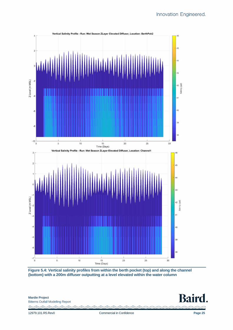
Table 5.2 provides an overview of the periods of time that 5 points within the dredged channel and berth pocket are unstratified (as a percentage of the full run and in continuous unbroken time periods) and stratified (in full unbroken time periods). Comparison of these stratification statistics demonstrates that elevating the diffuser within the water column provides significantly more ability for the dense plume to be mixed within the water column.
Table 5.2: Vertical stratification for locations in the dredged navigation area
Period of time
unstratified across whole run (%)
Longest continuous time
spent unstratified (hours)
Longest continuous time spent stratified
(hours)
shortest continuous time spent stratified
(hours)
200m Diffuser elevated within water column
BerthPok2 8.2% 3.5 186.8 10
Channel 1 34.5% 10.3 112 1
Channel 2 51.1% 11.3 86.5 1
Channel 3 68.5% 24.2 72.8 0.7
Channel 4 79.4% 196.8 23.8 0.7 A graphical timeseries representation of the potential stratification in the berth pocket (top plot) and along the channel (bottom plot) is presented in Figure 5.4. Periods when dark blue extends down to the seabed denote periods when the water is unstratified, and conversely, periods when the lower layers of the represented water column are lighter blue is when stratification is likely. This stratification breaks down periodically in the spring tides across the entirety of the model domain, but the berth pocket, turning basin and southern section of the channel remain stratified throughout the whole neap tide cycle.
Mardie Project Bitterns Outfall Modelling Report
12979.101.R5.Rev0 Commercial in Confidence Page 25
Figure 5.4: Vertical salinity profiles from within the berth pocket (top) and along the channel (bottom) with a 200m diffuser outputting at a level elevated within the water column
Mardie Project Bitterns Outfall Modelling Report
12979.101.R5.Rev0 Commercial in Confidence Page 26
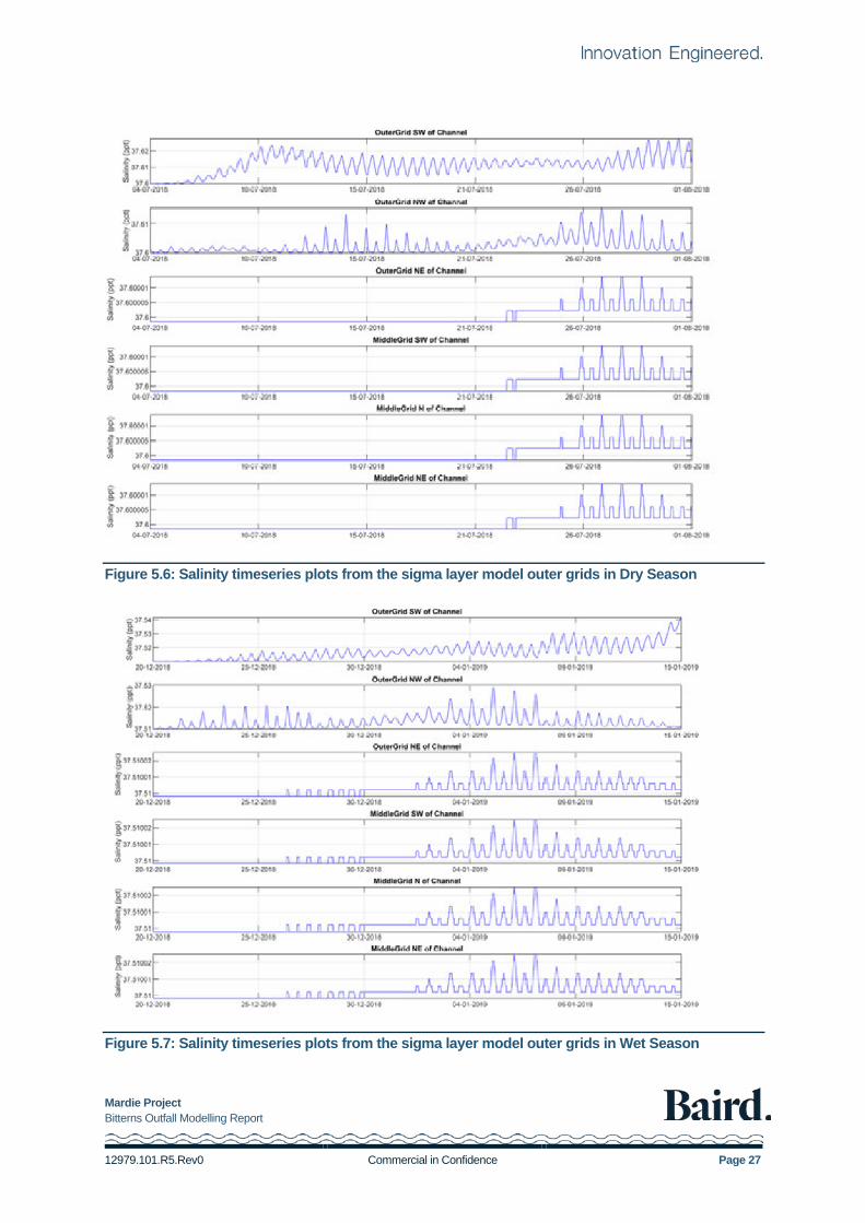
5.3.3 Recirculation of Saline Water in wider Coastal Waters
As the sigma layer model has been seen to provide similar mixing in regions of natural seabed, it has been used to determine if the high saline outfall plume is leading to continuously increasing salinity levels within the model, with specific focus on regions outside of the bounds of the Z-layer model.
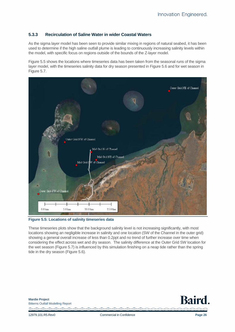
Figure 5.5 shows the locations where timeseries data has been taken from the seasonal runs of the sigma layer model, with the timeseries salinity data for dry season presented in Figure 5.6 and for wet season in Figure 5.7.
Figure 5.5: Locations of salinity timeseries data
These timeseries plots show that the background salinity level is not increasing significantly, with most locations showing an negligible increase in salinity and one location (SW of the Channel in the outer grid) showing a general overall increase of less than 0.2ppt and no trend of further increase over time when considering the effect across wet and dry season. The salinity difference at the Outer Grid SW location for the wet season (Figure 5.7) is influenced by this simulation finishing on a neap tide rather than the spring tide in the dry season (Figure 5.6).
Mardie Project Bitterns Outfall Modelling Report
12979.101.R5.Rev0 Commercial in Confidence Page 27
Figure 5.6: Salinity timeseries plots from the sigma layer model outer grids in Dry Season
Figure 5.7: Salinity timeseries plots from the sigma layer model outer grids in Wet Season
Mardie Project Bitterns Outfall Modelling Report
12979.101.R5.Rev0 Commercial in Confidence Page 28
5.3.4 Stratification and Dissolved Oxygen Implications
The vertical stratification that occurs in the dredged navigation areas as presented in Section 5.3.2 will likely impact on dissolved oxygen levels within the lower water column of this area. The larger scale modelling of the bitterns plume outside the navigation channel indicates that vertical stratification is unlikely to occur, and that prevailing currents, waves and shallow water depths are sufficient to maintain a well-mixed vertical water column.
Based on the model results presented in Table 5.2, the water column is likely to be stratified 90% to 95% of the time in the berth pocket, and between 20% to 65% of the time along the channel. It is expected that dissolved oxygen levels near the seabed in the berth pocket to be significantly reduced and expected to be within the range of 2 – 6 mg/L. During each spring tide cycle, the model results are indicating that full vertical mixing occurs, and dissolved oxygen levels should recover towards background ambient conditions. In summary: • Stratified conditions will occur for continuous durations of up to:
• 24-hours in the outer channel; and • 8-days in berth pocket.
• Well mixed (unstratified conditions will occur for continuous durations of up to: • 8-days in the outer channel; and • 3.5-hours in the berth pocket.
In the longer term, the continuation of the low dissolved oxygen levels in the water column will depend on the sediment response to the reduced dissolved oxygen in the water and ongoing organic sediment loads to the seabed of the dredged area. In the absence of ongoing sedimentation of fine organic sediments, the oxygen consumption capacity of the seabed sediments may reduce as the sediments become anoxic.
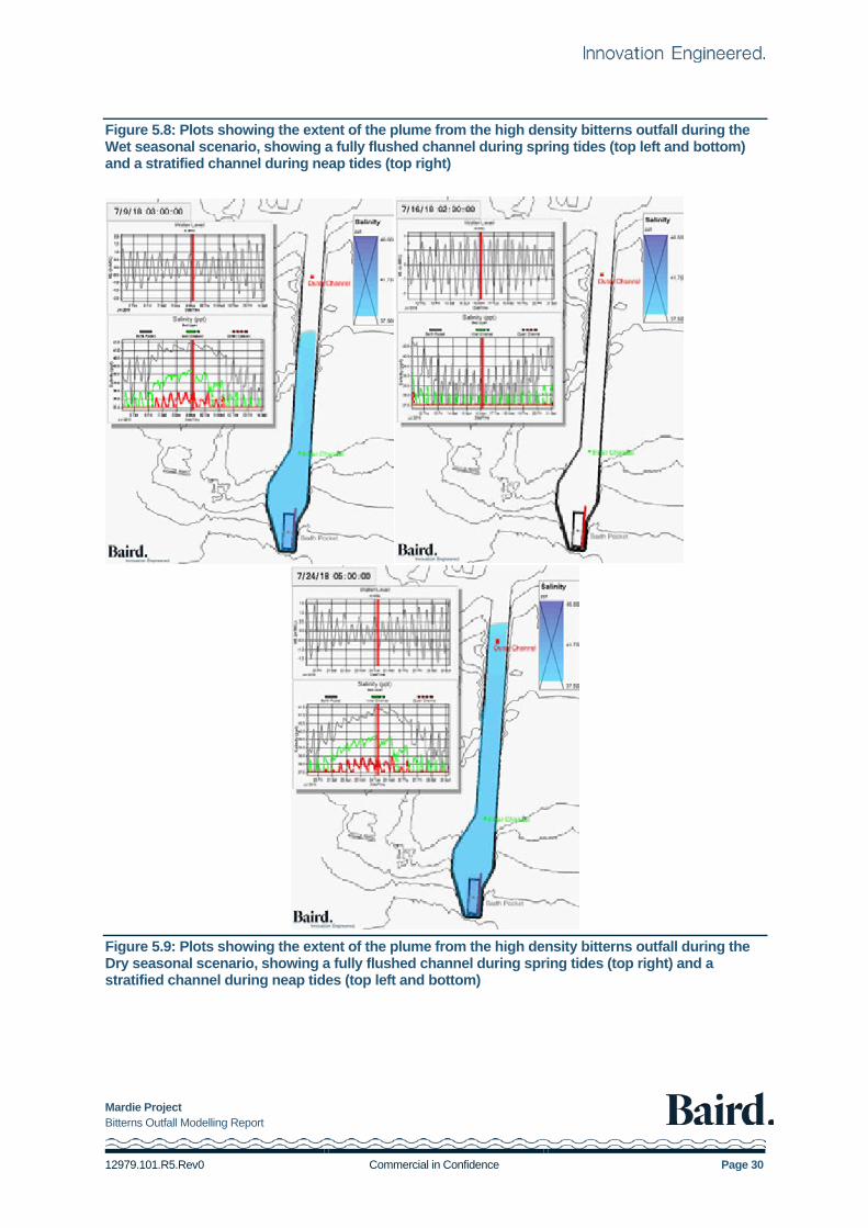
5.3.5 Seasonal Results
Following selection of the best diffuser length and arrangement, each of the seasonal scenarios outlined in Section 4.2.1 were run with constant output from the chosen diffuser arrangement. As noted previously, the 50th percentile salinity level for each seasonal scenario, taken from the data measured between March 2018 and September 2019, was found to be the same, therefore the major difference between scenarios is from the effects of differing tides and winds.
Figure 5.8, Figure 5.9, Figure 5.10, Figure 5.11 present spatial plots of the near seabed salinity at differ phases of the spring-neap tide cycle for the 4 seasonal periods modelled. The near seabed layer typically represents the 1 m to 1.5m of the water column immediately above the seabed. Each of the runs demonstrates the ability for the entire channel to flush during spring tides, and the periods of stratification that occur during neap tides.
Mardie Project Bitterns Outfall Modelling Report
12979.101.R5.Rev0 Commercial in Confidence Page 29
Mardie Project Bitterns Outfall Modelling Report
12979.101.R5.Rev0 Commercial in Confidence Page 30
Figure 5.8: Plots showing the extent of the plume from the high density bitterns outfall during the Wet seasonal scenario, showing a fully flushed channel during spring tides (top left and bottom) and a stratified channel during neap tides (top right)
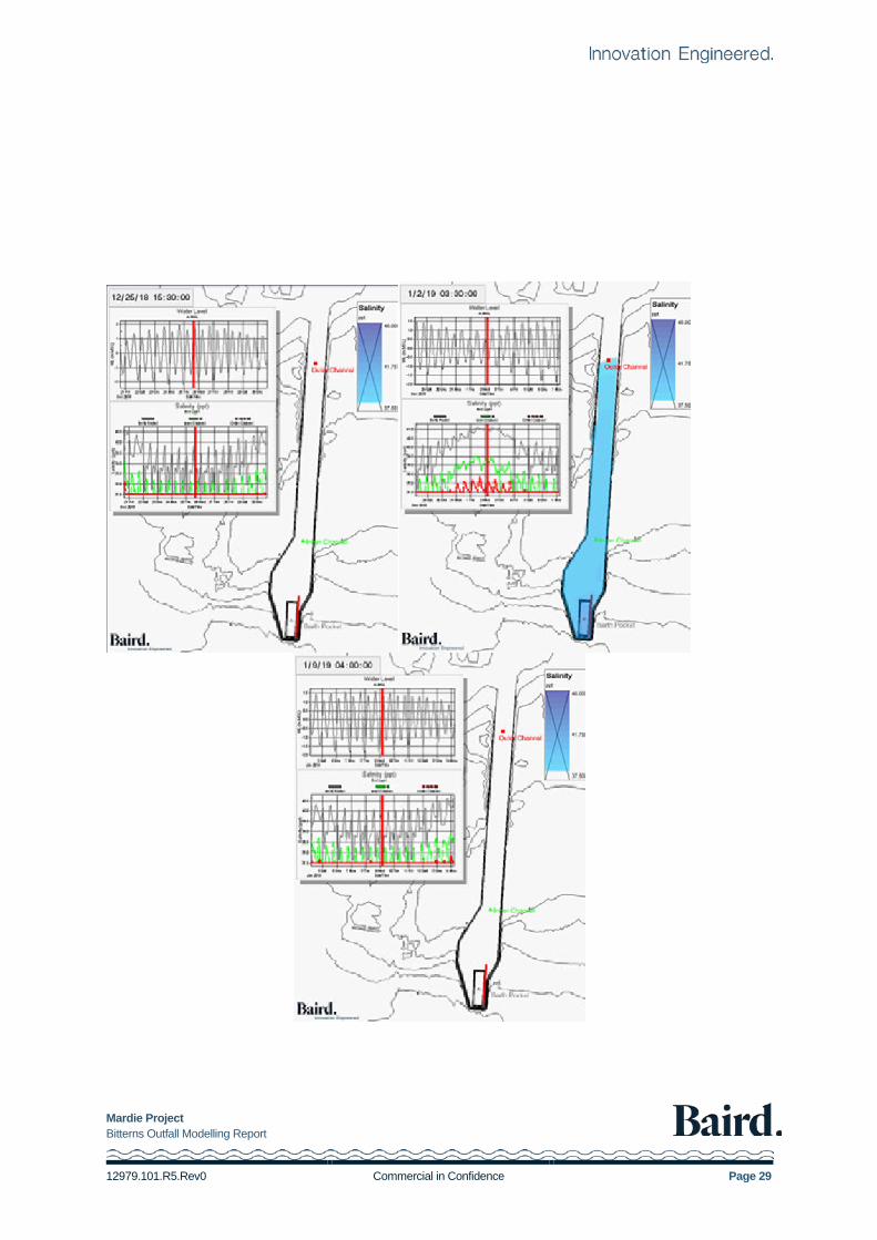
Figure 5.9: Plots showing the extent of the plume from the high density bitterns outfall during the Dry seasonal scenario, showing a fully flushed channel during spring tides (top right) and a stratified channel during neap tides (top left and bottom)
Mardie Project Bitterns Outfall Modelling Report
12979.101.R5.Rev0 Commercial in Confidence Page 31
Figure 5.10: Plots showing the extent of the plume from the high density bitterns outfall during the September Transition seasonal scenario, showing a fully flushed channel during spring tides (top right) and a stratified channel during neap tides (top left and bottom)
Mardie Project Bitterns Outfall Modelling Report
12979.101.R5.Rev0 Commercial in Confidence Page 32
Figure 5.11: Plots showing the extent of the plume from the high density bitterns outfall during the March Transition seasonal scenario, showing a fully flushed channel during spring tides (top left and bottom) and a stratified channel during neap tides (top right)
5.4 Analysis Method – Calculation of Dilution Rates for LEP Boundaries
Due to the marked increase in salinity from the mid-level to the seabed discussed and presented in Section 5.3.2 and 5.3.4, all analysis of dilution rates in the far field model for the low, moderate and high LEP boundaries has been completed based on assessment of the seabed layer – the lowest layer described in the 3D models, taken as an average from the two lowest layers in the Z-layer model typically representing the 1 m to 1.5 m of the water column above the seabed.
Mardie Project Bitterns Outfall Modelling Report
12979.101.R5.Rev0 Commercial in Confidence Page 33
The analysis of the model results was completed as follows: 1. For each scenario case (wet, dry, transition season) the model records the salinity value (ppt) in every
grid cell across the model on a timestep of 30 minutes. Over the 1-month simulation there are approximately 1300 model result grids.
2. The result grids are analysed using a MATLAB based analysis algorithm to determine the 95th percentile salinity value in each respective grid cell across the month-long model duration.
3. The calculated 95th percentile salinity value is converted to dilutions based on the background model salinity (baseline value).
It should be noted that the final dilution contours are a statistical composite of the analysis across the entire month-long simulation period and do not represent a single point in time.
5.5 Far-field Model Outcomes Compared to Target Dilution
The far field model results have been analysed to determine the dilution rates achieved at the boundary of the Low, Moderate and High LEP. The analysis of the model results has been completed based on the recommended approach in EPA (2016f), with analysis of the 95th percentile of the time series values modelled for salinity across the full spatial grid completed for each of the scenario modelling cases (method detailed in Section 5.4).
As noted in Section 4.2.2, the initial discharge objective of Mardie Minerals was to discharge the raw bitterns based on a 1:1 dilution (1-part bitterns / 1-part seawater). Modelling commenced to assess this approach against the EQC (90% and 99% species protection level) which determined the outfall regime did not meet the dilutions required. Further iterations of pre-dilution of the raw bitterns product from the diffuser in the model led to a 5 to 1 dilution of the bitterns being adopted. The model scenario cases were completed with the pre-treated bitterns discharge (i.e. 5 parts seawater:1-part raw bitterns).
Model outcomes are analysed in this section to determine the modelled dilution rate around the diffuser based on the diluted bitterns product. The target requirements defined by the WET test species protection levels from Table 3.1 are: • 80% species protection level = 227 dilutions • 90% species protection level = 263 dilutions • 99% species protection level = 417 dilutions
The Low, Moderate and High LEP’s have previously been defined as having to be reached at the outfall (Low LEP), within 70m of the outfall (Moderate LEP) and within 250m of the outfall (High LEP); modelling carried out during this study have shown that even with dilution of the raw bitterns at a ratio of 1:5 with seawater, these dilutions cannot be achieved within the distances stipulated when taking the dilution contours occurring in the nearbed layer. The LEP contour extents modelled are presented in Figure 5.12 to Figure 5.15 for this nearbed layer (1 m to 1.5 m above seabed) layer. The greatest dilution is achieved in the Wet Season (Figure 5.13), while the least dilution occurs in the September Transition Season (Figure 5.15), and this has been adopted as the scenario for the reported LEP’s. It should be noted that although the LEP’s cannot be achieved within the required distances, the moderate and low LEP contour boundaries are confined to the channel and berth pocket and do not spill over into any undisturbed areas of the surrounding seabed, while the High LEP contour boundary covers a small region of the undredged natural seabed surrounding the navigation channel in each seasonal case.
Further analysis of the LEP contours have been carried out from a depth averaged approach, with these LEP contours presented in Figure 5.16 to Figure 5.19. A further set of analyses excluding the near seabed layer have been completed to assess the mixing for the mid and upper layers of the water column and those LEP contours are presented in Figure 5.20 to Figure 5.23. For the depth-averaged and upper layer analyses, the critical scenario for the largest LEP extents is the September Transition season (Figure 5.19 and Figure 5.23).

Mardie Project Bitterns Outfall Modelling Report
12979.101.R5.Rev0 Commercial in Confidence Page 34
Appendix A presents the data files prepared by Baird to define the Moderate and High LEP boundaries, and an extended set of data files containing High, Moderate and Low LEP boundaries, as well as contours between the 70% to 10% species protection levels. The Moderate and High LEP boundaries files (Nearbed Layer Moderate/High LEPs in Appendix A) have been provided to BCIM and O2 Marine, and the extended set of data files (Nearbed Layer LEPs – Extended Set, Depth Averaged Layer LEPs – Extended Set and Depth Averaged Layer LEPs – Extended Set in Appendix A) have been provided to O2 Marine for the preparation of the Environmental Quality Plan for the bitterns discharge.

Mardie Project Bitterns Outfall Modelling Report
12979.101.R5.Rev0 Commercial in Confidence Page 35
Figure 5.12: Extent of the High, Moderate and Low LEP Contours from the nearbed layer under Dry Season Conditions (95th Percentile Dilution Contours). Nearbed is taken as the 1-1.5m layer above the seabed.

Mardie Project Bitterns Outfall Modelling Report
12979.101.R5.Rev0 Commercial in Confidence Page 36
Figure 5.13: Extent of the High, Moderate and Low LEP Contours from the nearbed layer under Wet Season Conditions (95th Percentile Dilution Contours). Nearbed is taken as the 1-1.5m layer above the seabed.

Mardie Project Bitterns Outfall Modelling Report
12979.101.R5.Rev0 Commercial in Confidence Page 37
Figure 5.14: Extent of the High, Moderate and Low LEP Contours from the nearbed layer under March Transition Season Conditions (95th Percentile Dilution Contours). Nearbed is taken as the 1-1.5m layer above the seabed.

Mardie Project Bitterns Outfall Modelling Report
12979.101.R5.Rev0 Commercial in Confidence Page 38
Figure 5.15: Extent of the High, Moderate and Low LEP Contours from the nearbed layer under September Transition Season Conditions (95th Percentile Dilution Contours). Nearbed is taken as the 1-1.5m layer above the seabed.

Mardie Project Bitterns Outfall Modelling Report
12979.101.R5.Rev0 Commercial in Confidence Page 39
Figure 5.16: Extent of the High, Moderate and Low LEP Contours under a depth averaged scenario and under Dry Season Conditions (95th Percentile Dilution Contours)
Mardie Project Bitterns Outfall Modelling Report
12979.101.R5.Rev0 Commercial in Confidence Page 40
Figure 5.17: Extent of the High, Moderate and Low LEP Contours under a depth averaged scenario and under Wet Season Conditions (95th Percentile Dilution Contours)
Mardie Project Bitterns Outfall Modelling Report
12979.101.R5.Rev0 Commercial in Confidence Page 41
Figure 5.18: Extent of the High, Moderate and Low LEP Contours under a depth averaged scenario and under March Transition Season Conditions (95th Percentile Dilution Contours)

Mardie Project Bitterns Outfall Modelling Report
12979.101.R5.Rev0 Commercial in Confidence Page 42
Figure 5.19: Extent of the High, Moderate and Low LEP Contours under a depth averaged scenario and under September Transition Season Conditions (95th Percentile Dilution Contours)
Mardie Project Bitterns Outfall Modelling Report
12979.101.R5.Rev0 Commercial in Confidence Page 43
Figure 5.20: Extent of the High, Moderate and Low LEP Contours excluding the nearbed layer (1 m to 1.5 m ASB) under Dry Season Conditions (95th Percentile Dilution Contours)

Mardie Project Bitterns Outfall Modelling Report
12979.101.R5.Rev0 Commercial in Confidence Page 44
Figure 5.21: Extent of the High, Moderate and Low LEP Contours excluding the nearbed layer (1 m to 1.5 m ASB), under Wet Season Conditions (95th Percentile Dilution Contours)

Mardie Project Bitterns Outfall Modelling Report
12979.101.R5.Rev0 Commercial in Confidence Page 45
Figure 5.22: Extent of the High, Moderate and Low LEP Contours excluding the nearbed layer (1 m to 1.5 m ASB), under March Transition Season Conditions (95th Percentile Dilution Contours)

Mardie Project Bitterns Outfall Modelling Report
12979.101.R5.Rev0 Commercial in Confidence Page 46
Figure 5.23: Extent of the High, Moderate and Low LEP Contours excluding the nearbed layer (1 m to 1.5 m ASB), under September Transition Season Conditions (95th Percentile Dilution Contours)
Mardie Project Bitterns Outfall Modelling Report
12979.101.R5.Rev0 Commercial in Confidence Page 47
6. Conclusions The Mardie Project is a greenfields high-quality salt project proposed in the Pilbara region of Western Australia. Baird Australia Pty Limited (Baird) have been engaged by Mardie Minerals, a wholly owned subsidiary of BCI Minerals Limited (BCIM) to develop a hydrodynamic modelling program to support the environmental approvals process to assess: • Modelling of dredge plumes to inform the preparation of a Dredging and Spoil Disposal Management
Plan (DSDMP); and • Modelling of mixing and dilution of bitterns discharge into the marine environment to inform the
preparation of a Environmental Quality Plan (EQP).
The modelling of the bitterns discharge has determined the number of dilutions achieved at the boundaries of the ecological protection (LEP) to ensure these can meet the level of ecological protection of the waters surrounding the mixing zone. The model system has been developed with two parts: a far-field model based on the validated hydrodynamic model (Baird 2020) and a nearfield model (CORMIX) which specifically model the turbulent mixing zone immediately surrounding the diffuser (refer Section 4).
Investigation into the dispersal of the high salinity bitterns to be produced as part of the Mardie Project has led to identification of an optimised discharge configuration and regime. The bitterns are to be discharged through a diffuser at the far end of the Project’s trestle jetty, following dilution with seawater to bring the bitterns’ salinity closer to that of the receiving environment; a diffuser arrangement of 20 ports spaced approximately 10.5m apart, with an aperture of 0.13m, has been selected for the project.
Following identification of this diffuser arrangement, investigation into the expected dispersal of the diluted bitterns plume within the marine environment was carried out through modelling of the nearfield and far-field mixing zones using a nearfield model (CORMIX) and a far-field model (Delft3D). The nearfield model outcomes have been compared against the far-field model results examining dilution rates from the near field and far-field model for cases with equivalent hydrodynamic conditions at the defined edge of the nearfield. The nearfield modelling shows that the nearfield extent is consistently in the range of 20 m to 100 m in the absence of near seabed stratification. Overall, the far-field model is reporting a more conservative outcome of dilution rate compared with the nearfield model with CORMIX achieving generally higher horizontal mixing compared with the Delft3D model at the edge of the nearfield extent. The most significant reasons for the difference between the CORMIX (nearfield) and far-field model is that CORMIX does not account for the vertical stratification that occurs within the dredged navigation area and does not account for the effect of bitterns accumulation over time in the near seabed layer which reduces overall mixing efficiency. Noting these limitations, it can be said that CORMIX provides the ‘best possible’ mixing under given discrete hydrodynamic conditions, and Delft3D gives a more conservative and likely realistic view of the mixing that occurs as a result of the variable seabed bathymetry (including dredging), variation in water level and currents and continuous discharge of bitterns into the receiving waters.
The general mixing conditions for the undredged seabed area surrounding the diffuser are dominated by tidal currents, and the water column is generally well mixed across each seasonal case, with the bitterns concentration reducing significantly within 20 to 100 m of the diffuser.
As a result of the stratification that occurs in the dredged area, the Environmental Quality Criteria (EQC) zones extend across the dredged area and the Low, Medium and High LEP extend north along the navigation channel. The target requirements defined by the WET test species protection levels at 99% level (0.24% Bitterns) for the High LEP and 90% species protection level (0.38% Bitterns) at the Moderate LEP boundary. The boundary of the High LEP extends a short distance south west across the undredged seabed surrounding the development area and diffuser, with the Moderate and Low LEP boundaries based on the near seabed salinity extends throughout most of the dredged channel area.
Analysis of modelled outcomes has been completed based on EPA guidance (EPA, 2016f) focusing on the dilutions at the seabed layer due to the high density of the bitterns plume, recognising impacts to the

Mardie Project Bitterns Outfall Modelling Report
12979.101.R5.Rev0 Commercial in Confidence Page 48
benthic communities at the bed layer. Dissolved oxygen levels in the lower water column and in the benthic sediment layer of the dredged berth pocket and navigation channel are expected to be significantly lower than existing conditions at the site. Strongly stratified conditions with very little vertical mixing of the near-bed water column are expected to persist for durations of up to 7 to 8 days in the berth pocket before full vertical mixing occurs periodically during each spring tide cycle.
Mardie Project Bitterns Outfall Modelling Report
12979.101.R5.Rev0 Commercial in Confidence Page 49
7. References ANZECC & ARMCANZ (2000). Australian and New Zealand Guidelines for Fresh and Marine Water Quality (Australian and New Zealand Environment and Conservation Council (ANZECC) & Agriculture and Resource Management Council of Australia and New Zealand (ARMCANZ).
Baird (2020). Mardie Project – Hydrodynamic Modelling Report. Prepared for BCI Minerals. Ref 12979.101.R1.Rev2.
BCIM (2018). MARDIE PROJECT Pre-Feasibility Study, May 2018.
Deltares (2014). Delft3D-FLOW: Simulation of multi-dimensional hydrodynamic flows and transport phenomena, including sediments. User Manual. Hydro-Morphodynamics. Version: 3.15.32923
DoE (2006). Pilbara Coastal Water Quality Consultation Outcomes – Environmental Values and Environmental Quality Objectives, Department of Environment (DoE), Government of Western Australia, Marine Series Report No. 1;
Doneker, R.L. and G.H. Jirka (2007). CORMIX User Manual: A Hydrodynamic Mixing Zone Model and Decision Support System for Pollutant Discharges into Surface Waters", EPA-823-K-07-001.
Survey - BCI Minerals SURVEY REPORT, EGS PROJECT REF: AU025918, Prepared for O2Marine 21 January 2019
EcoTox Services Australia. 2019. Toxicity Assessment of a Bitterns Brine Sample. Report: TR1791/1
EPA (2016a). Statement of Environmental Principles, Factors and Objectives, EPA, Western Australia;
EPA (2016b). Environmental Impact Assessment (Part IV Divisions 1 and 2) Administrative Procedures 2016;
EPA (2018a). Environmental Impact Assessment (Part IV Divisions 1 and 2) Procedures Manual, EPA, Western Australia;
EPA, (2016c). Environmental Factor Guideline – Marine Environmental Quality, EPA, Western Australia;
EPA, (2016d). Environmental Factor Guideline – Benthic Communities and habitat, EPA, Western Australia;
EPA, (2016e). Environmental Factor Guideline – Marine Fauna, EPA, Western Australia;
EPA, 2018b). Instructions on how to prepare Environmental Protection Act Part IV Environmental Management Plans.
EPA, (2016f). Technical Guidance – Protecting the Quality of Western Australia’s Marine Environment, EPA, Western Australia; and
EPA, (2016g). Technical Guidance - Environmental Impact Assessment of Marine Dredging Proposals, EPA, Western Australia.
O2Marine (2018). Mardie Project Progress Report #1 for Metocean Data Collection, REPORT No.: R1800106, ISSUE DATE: 22 Oct 2018, Prepared for BCIM
O2Marine (2019a). Mardie Project Progress Report for Metocean Data Collection, R1800132 ISSUE DATE: 15th January 2019, Prepared for BCIM

Mardie Project Bitterns Outfall Modelling Report
12979.101.R5.Rev0 Commercial in Confidence Page 50
O2Marine (2019b). Mardie Project Whole Effluent Toxicity Assessment, R190054 ISSUE DATE: 20th May 2019, Prepared for Mardie Minerals Limited
RPS (2017), MARDIE SALT PROJECT, PRELIMINARY STORM SURGE STUDY, Prepared for BCIM.
Sun.C, Shimizu.K, Symonds.G, (2016). Numerical modelling of dredge plumes: a review, CSIRO Oceans and Atmosphere Flagship, Perth, Western Australia, Western Australian Marine Science Institution, Perth, Western Australia, Australia.
Surrich and EGS (2019), Detailed Bathymetry data provided by the Mardie project , Surrich_EGS_Datasets_Merged_Mardie_Creek_MGAZ50_1m_Shoal_Final_GRIDDED_DepthPos_AHD.
Mardie Project Bitterns Outfall Modelling Report
12979.101.R5.Rev0 Commercial in Confidence Appendix A
Data Files for LEP Zones
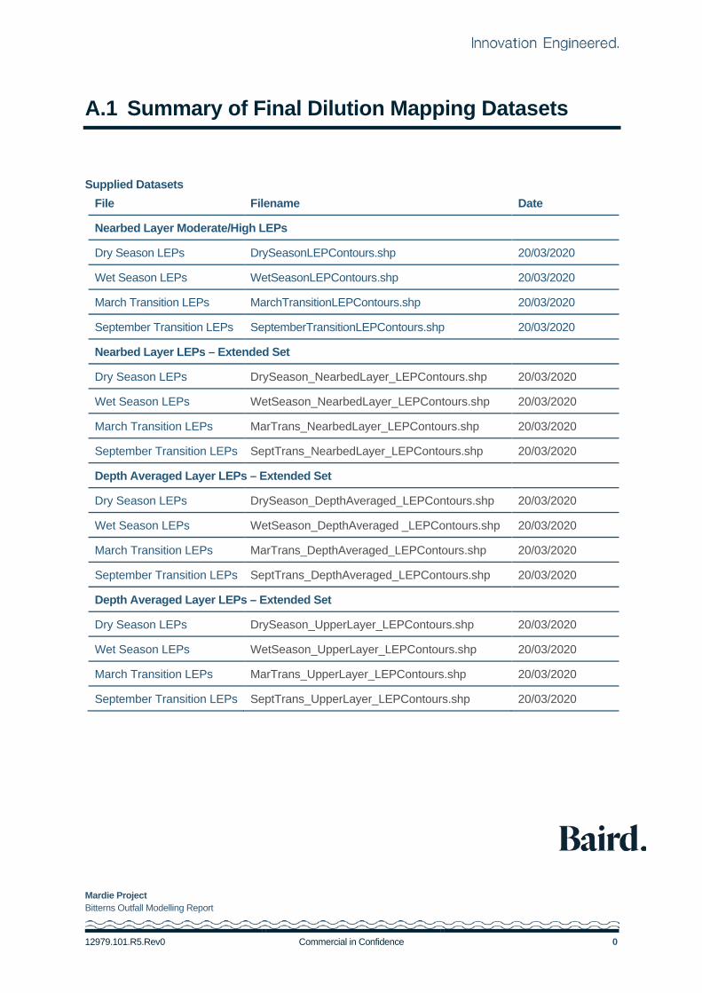
Mardie Project Bitterns Outfall Modelling Report
12979.101.R5.Rev0 Commercial in Confidence 0
A.1 Summary of Final Dilution Mapping Datasets
Supplied Datasets File Filename Date
Nearbed Layer Moderate/High LEPs
Dry Season LEPs DrySeasonLEPContours.shp 20/03/2020
Wet Season LEPs WetSeasonLEPContours.shp 20/03/2020
March Transition LEPs MarchTransitionLEPContours.shp 20/03/2020
September Transition LEPs SeptemberTransitionLEPContours.shp 20/03/2020
Nearbed Layer LEPs – Extended Set
Dry Season LEPs DrySeason_NearbedLayer_LEPContours.shp 20/03/2020
Wet Season LEPs WetSeason_NearbedLayer_LEPContours.shp 20/03/2020
March Transition LEPs MarTrans_NearbedLayer_LEPContours.shp 20/03/2020
September Transition LEPs SeptTrans_NearbedLayer_LEPContours.shp 20/03/2020
Depth Averaged Layer LEPs – Extended Set
Dry Season LEPs DrySeason_DepthAveraged_LEPContours.shp 20/03/2020
Wet Season LEPs WetSeason_DepthAveraged _LEPContours.shp 20/03/2020
March Transition LEPs MarTrans_DepthAveraged_LEPContours.shp 20/03/2020
September Transition LEPs SeptTrans_DepthAveraged_LEPContours.shp 20/03/2020
Depth Averaged Layer LEPs – Extended Set
Dry Season LEPs DrySeason_UpperLayer_LEPContours.shp 20/03/2020
Wet Season LEPs WetSeason_UpperLayer_LEPContours.shp 20/03/2020
March Transition LEPs MarTrans_UpperLayer_LEPContours.shp 20/03/2020
September Transition LEPs SeptTrans_UpperLayer_LEPContours.shp 20/03/2020