http://wrap.warwick.ac.uk/

Original citation: Miller, Marcus, 1941-, Zhang, Lei, Dr. and Li, Han Hao (2011) When bigger isn’t better : bailouts and bank behaviour. Working Paper. Coventry, UK: Department of Economics, University of Warwick. (CAGE Online Working Paper Series). Permanent WRAP url: http://wrap.warwick.ac.uk/57671 Copyright and reuse: The Warwick Research Archive Portal (WRAP) makes this work of researchers of the University of Warwick available open access under the following conditions. Copyright © and all moral rights to the version of the paper presented here belong to the individual author(s) and/or other copyright owners. To the extent reasonable and practicable the material made available in WRAP has been checked for eligibility before being made available. Copies of full items can be used for personal research or study, educational, or not-for-profit purposes without prior permission or charge. Provided that the authors, title and full bibliographic details are credited, a hyperlink and/or URL is given for the original metadata page and the content is not changed in any way. A note on versions: The version presented here is a working paper or pre-print that may be later published elsewhere. If a published version is known of, the above WRAP url will contain details on finding it. For more information, please contact the WRAP Team at: publicatons@warwick.ac.uk

WORKING PAPER SERIES

Centre for Competitive Advantage in the Global Economy

Department of Economics

November 2011 No.66

When bigger isn’t better: bailouts and bank behaviour

Marcus Miller, Lei Zhang, and Han Hao Li University of Warwick

1

When bigger isn’t better: bailouts and bank behaviour1

Marcus Miller, Lei Zhang, and Han Hao Li

University of Warwick

November 2011

Abstract

Lending retail deposits to SMEs and household borrowers may be the traditional role of

commercial banks: but banking in Britain has been transformed by increasing consolidation

and by the lure of high returns available from wholesale Investment activities. With

appropriate changes to the baseline model of commercial banking in Allen and Gale (2007),

we show how market power enables banks to collect „seigniorage‟; and how „tail risk‟

investment allows losses to be shifted onto the taxpayer.

In principle, the high franchise values associated with market power assist regulatory capital

requirements to check risk-taking. But when big banks act strategically, bailout expectations

can undermine these disciplining devices: and the taxpayer ends up „on the hook‟ - as in the

recent crisis. That structural change is needed to prevent a repeat seems clear from the

Vickers report, which proposes to protect the taxpayer by a „ring fence‟ separating

commercial and investment banking.

Key Words: Money and banking, Seigniorage, Risk-taking, Bailouts, Regulation

JEL Classification: E41 E58 G21 G28

1 We would like to acknowledge the benefit of discussions with Sayantan Ghosal, Peter Hammond, John Kay,

Frederic Schlosser and Jonathan Thomas and comments from seminar participants at the Universities of Heriot-

Watt, York and Warwick, the Royal Economic Society Conference and the Bank of England, especially

Henrique Basso, Michael McMahon, David Miles, Udara Peiris and Paul Youdell. For research support, we are

grateful to Antonia Maier funded by ESRC/CAGE. All errors are ours.

Corresponding author: marcus.miller@warwick.ac.uk

2

‘Expansion in the variety of intermediaries and financial transactions has major

benefits…[But] it has potential downsides … to do with incentives’. Rajan (2005)

Introduction

With the adoption of Inflation Targeting, monetary policy in the UK came to consist

essentially in setting the discount rate, without any special attention to monetary aggregates.

The shift of focus from monitoring developments in money and banking to policy rules for

interest rates was reflected in the widespread adoption of DSGE models by Central Banks --

with Taylor rules used to determine interest rates and the assumption of efficient markets

used to justify „light touch‟ regulation. The granting of operational independence in setting

interest rates to the Bank of England in 1997 was, indeed, accompanied by a transfer of

responsibility for Financial Stability to the FSA – a newly created agency that ipso facto

lacked practical experience .

In fact, the combined forces of increased globalization and reduced regulation led to

extraordinary developments in UK banking- an unprecedented increase in the size and

profitability of banking relative to GDP, (see charts in Appendix A, based on Haldane et al,

2010), with a pronounced degree of market concentration (see ICB, 2010, p.9). Although, at

the time, it seemed that this headlong expansion was achieved without any great increase in

risk, it ended in severe liquidity runs and solvency crises with two mortgage banks being

nationalised and major two universal banks rescued with substantial capital support from the

Treasury.

Chastened by this episode, macroeconomists are busy adding financial frictions to their

models. For banking, too, there is surely a case for retooling. The account of banking to be

found in Allen and Gale‟s widely acclaimed monograph Understanding Financial Crisis

published in 2007, for example, is of small, competitive, utility banks. In this paper,

therefore, starting with this traditional model of competitive banking as a baseline, we first

add the concentration of market power -- and draw out the consequence that banks will

collect the seigniorage attached to monopoly in money creation. Next we add the taking on of

3

risk associated with wholesale and investment banking2 and why this may not be apparent if

it is „tail risk‟. Then we turn to an issue emphasized by Andy Haldane, Director of Financial

Stability at the Bank of England, namely the shift in strategic power that has taken place as

banks have grown so large in size and complexity that the state is forced to bail them out with

taxpayers money -- an issue tackled in the Final Report of the Independent Commission on

Banking (2011) in terms of „getting the taxpayer off the hook‟.

Two informational paradigms

Before embarking on detailed analysis, an important issue to be confronted is whether the

players in the industry were aware of the severe risk of insolvency to which the banks were

exposed, or not. Were they as unaware of the trouble in store as those outside the industry –

the politicians, for example, happy to see such success for enterprise in Britain and the taxes

it was yielding; or the regulators, willing to let the industry run on a loose leash with „light

touch‟ regulation; or depositors, amazed at the salaries paid by the rapidly expanding

investment arms of previously staid commercial banks, but confident that their money

remained in safe hands?

Two contrasting informational paradigms may be considered. The first, that of asymmetric

information3, where banks were aware of risk but outsiders were not, is the perspective taken

by Hellman et al. (2000) in analysing regulations to check excessive risk-taking („gambling‟)

by those managing bank portfolios; and by Rajan (2005), whose assessment of the powerful

incentives for taking on tail risk is widely regarded as a prescient early-warning of the crisis

to come4. It is also the view taken subsequently by Paul Wooley in The Future of Finance

(2010, Chapter Three).

The second paradigm, what de la Torre and Ize (2011) call one of collective cognition, is

where neither principal nor agent is aware of the downside risks associated with new

2 Involving the provision of finance to other financial institutions and large corporations, assisting governments

and large corporations in raising equity and debt finance, advising on M&A, acting as counterparty to client

trades, etc see ICB (2010, p.45). 3 with the associated principal/agent problem of how to design incentives to promote the objectives of the

principal even though the agent is better informed. 4 It was the approach used, more broadly, to warn of the risks of corporate looting in an earlier paper by Akerlof

and Romer (1993).

4

investment strategies5. This is the perspective taken by Gennaioli et al. (2011), for example,

in their paper on “Neglected risks, financial innovation, and financial fragility”.

Though the policy implications may differ, the two approaches are close to being

observationally equivalent: risks are taken which lead to insolvency -- and possibly to

emergency rescue packages for failing financial firms. Nor does asking the players help: even

if there is asymmetric access to information, the agent may choose to neglect some factors ex

ante and and/or to feign ignorance ex post.

Recognising that the distribution of information is endogenous might help to discriminate

between these two approaches, however, as in the discussion of distorted incentives by Rajan

(2005). One of these distortions is:

„the incentive to take risk that is concealed from investors – since risk and return

are related, the manager then looks as if he outperforms peers given the risk he

takes. Typically, the kinds of risks that can be concealed most easily, given the

requirement of periodic reporting, are risks that generate severe adverse

consequences with small probability but, in return, offer generous compensation

the rest of the time. These risks are known as tail risks.‟ Rajan (2005, p. 316)

A simple example, from Rajan (2010, pp. 138-9), is of a financial manager, with a safe

security on the balance sheet, who posts returns that include the premiums on an out-of-the-

money put – conveniently left off balance sheet. The overall return on such a portfolio will be

elevated because of the risk involved – but this will not be apparent for some time (because it

is „in the tail‟) and, as a contingent liability, can be left off balance sheet. So the investor can

collect what is effectively the risk premium as a bonus, leaving the firm badly exposed as and

when the downside appears6. The names of the trading strategies that were being used also

suggest an ex ante awareness of risk: they include, apparently:

IBG (I‟ll Be Gone if it doesn‟t work), and in Chicago, the O‟Hare Option (buy a ticket

departing from O‟Hare International Airport: if the strategy fails, use it; if the strategy

succeeds, tear up the ticket and return to the office). That such strategies were common

enough in the industry as to have names suggests that not all traders were oblivious of

the risks they were taking. Rajan (2010, p.139).

5 In the words of Charles Goodhart at the Herriot Watt Conference: „The depositors didn‟t know, the regulators didn‟t know; the banks themselves did not know [of the risks inherent in expanding their portfolios]‟. 6 Foster and Young (2011) demonstrate further that the use of financial derivatives to reshape portfolio returns

makes it almost impossible to discriminate the true alpha investor from a mimic on the basis of realised returns

for an extended period of time.

5

In these circumstances, we have opted for the principal/agent paradigm in the analysis of the

banking crisis that follows7, grafting the „gambling‟ model of Hellman et al. (2000) onto the

base-line model of Allen and Gale (2007), modified to include seigniorage and risk as

discussed above. But it is important that proposed reform measures be robust to the choice of

paradigm.

Strategic balance of banks and the state

To the extent that seigniorage increases the „franchise‟ value of banking, so, it might be

reasoned, monopoly power will help to check excessive risk-taking, and complement

official regulation in the form of required capital and real time monitoring. But this ignores

the strategic threat that large banks can pose for society in terms of negative externalities

that will ensue if they are not rescued after risky gambles that fail -- as can be seen in terms

of a game where the banks have first-mover advantage. In this setting, a universal bank

realises correctly that, given the threat of economic disruption that would follow from

liquidation, a bail out after a gamble that fails is a subgame perfect response for the

regulator. As the monopoly bank is insured against risk, it has the incentive to gamble.

To promote prudent behaviour when banks possess significant strategic power, structural

reform to shift the balance between large banks and the regulatory authorities is surely

required. A key issue with regard to the recommendations of ICB in particular is whether

the proposal to ring-fence retail banking – with the associated ban on many risky strategies

– will shift strategic power back to the regulator so that bank resolution is a credible threat.

The model used in this paper is admittedly stylised and compact; and there is, of course,

an extensive literature on the market structure of the financial sector from the

perspective of industrial organisation, succinctly summarised in Allen and Gale (2000)

and Freixas and Rochet (2008), for example. Recent research has used network theory

to analyse the structure of banking system, focusing on how inter-bank connectivity

affects the transmission of systemic risk. Gai and Kapadia (2010a) and May and

Arinaminpathy (2010), for example, study the stability of the banking system using

random graphs and find that it is typically “robust-yet-fragile” (robust to the failures of

periphery banks but fragile in respect of failure by central players). Our „moral hazard‟

7 When we come to discuss regulatory responses, however, we will consider the extent to which the measures

proposed are robust – i.e. will work even if the problem is one of „collective cognition‟.

6

approach suggests that concentration may arise for strategic reasons; and we investigate

how concentration may impact on banks‟ incentives to behave prudently, focusing for

convenience on the case of monopoly.

The paper is organised as follows. Section 1 reviews the traditional model of

competitive banking and modifies it to allow for market concentration. In Section 2 we

analyse the equilibrium when „tail risk‟ investment opportunities are available to a

monopoly bank with an information advantage; and investigate how far the franchise

value and/or loss-absorbing capital can ensure prudent behaviour. Section 3 extends the

analysis to look at the strategic factors that arise when banking is highly concentrated

and economic externalities come into play. Section 4 looks at implications for banking

reform -- the ICB proposals in particular. Section 5 concludes.

1. Utility Banking: competition and concentration

To fix ideas, we first use the standard three-date model with „early and late‟ consumers

(depositors) to see how market concentration affects bank profitability. This is done by

comparing the optimal „take it or leave it‟ deposit contract offered by a monopoly bank with

the competitive equivalent.

Following Bryant (1980), Diamond and Dybvig (1983), and Allen and Gale (2007), each

round has three dates, . There are two assets available to the bank, short and long,

all associated with constant return to scale technology. The short asset – representing

accessible storage – lasts only one period, and converts one unit of good today into one unit

tomorrow. The long asset – representing illiquid but productive investment – takes two

periods to mature, and converts one unit invested at t = 0 into units at t = 2 later. There

is a continuum of ex ante identical depositors with measure 1, each endowed with one unit of

good at . At , the types of depositors are known, a fraction of them

being early consumers who derive utility from consumption only at ; and fraction

being late consumers who derive utility from consumption at .

The ex ante utility of depositors is

(1)

7

where and are consumptions for early and late consumers, while is strictly

increasing and strictly concave.

Assume that depositors have an outside option which gives a minimum utility of . 8

For depositors to participate in banking, the utility from the deposit contract offered should

be at least at the level of this outside option,

. (3)

The other incentive constraint is that the banking contract should be able to separate early and

late consumers (so late consumers have no incentive to withdraw earlier), so

. (4)

Returns from short and long assets are used to finance early and late consumptions as follows

(5)

and

. (6)

The sequence of events is such that at , a bank offers a contract in exchange for

the depositor‟s endowment. At , the types of the depositors are realised: and, if they are

the early consumers, they receive . At , the late consumers receive consumption .

1.1 The competitive case

The competitive banking solution is illustrated in Figure 1, where the horizontal axis

represents consumption in date 1 and the vertical the consumption at date 2, and the

indifference curves represent expected utility of the average depositor. The participation

constraint on banking outcomes is indicated by the downward sloping convex curve passing

through the point labelled Market Equilibrium: so feasible deposit contracts are

restricted to consumption points in the convex set defined by (3). The downward sloping

straight line passing through the Market Equilibrium indicates the resource constraint

8 Specifically potential depositors can, after the realisation of types, exchange their endowments with each other

for early and late consumption goods in capital markets to ensure that See Allen and Gale (2007, pp. 60-64) for discussion of such a market equilibrium.

8

applying to banking equilibria. Bank profitability is zero on (but positive on , i.e. when

the line is shifted to the left).

The competitive contract is illustrated at point A in the figure, where the indifference curve

(iso-EU) is tangent to the zero profit line ( ). For risk aversion greater than 1, it can be seen

that .

In the standard model of competitive banking discussed above, the capital structure may be

varied without any implications for the asset side of the balance sheet: and Diamond and

Dybvig‟s (1983) model of debt-financed banking was promptly complemented by Jacklin‟s

(1987) version of pure equity banking. The Modigliani and Miller Theorem applies because

of the assumptions of perfect competition, full information and no risk.9

9 Where the bank is fully equity financed, with the shareholders paid dividends in each period, the cost of capital

is where is the per share dividend paid to all shareholders in period i, i.e., the cost of capital is the second period dividend per unit invested – corrected for the interim dividend paid out in period 1. With

perfect competition and no risk, this will match the return on capital, R.

B

A

Market

equilibrium

Competitive

banking

Iso-EU

Inter-temporal

efficiency

condition

Monopoly

banking

Participation constraint

S

N

Figure 1. Competitive and monopoly banking

9

1.2 Monopoly banking and the ‘seignorage’ on money creation

„It is well known that financial intermediaries can extract rents by exploiting monopoly

power through some combination of market share, collusion and barrier to entry‟ (Woolley,

2010, p.124). This can be accommodated in the traditional banking model without much

difficulty by allowing for positive profits, as in Chang and Velasco (2001). Here we

explicitly consider the case of monopoly: in addition to being analytically tractable, this has

the implication that any failure will be „systemic‟.

A risk-neutral monopoly bank is assumed to maximise its undiscounted, one round, profits

by choosing a suitable deposit contract and investment in short asset, , i.e

, (7)

The first two terms from the profit function are returns from the short and long assets

respectively, and the last two terms represent early and late consumption. The optimal deposit

contract is determined when the monopoly bank maximises its profits in (7) subject to

constraints (3)-(6).

Since the short asset earns lower returns, the bank will have incentive to minimise its holding

of x. This implies that (5) must always be binding, i.e.

(5‟)

Replacing x using (5‟), the above problem can be rewritten as

(7‟)

subject to

(6‟)

plus (3) and (4).

The outcome with monopoly can be characterised as follows:

10

Proposition 1:

The optimal monopoly banking contract satisfies the first order condition for inter-

temporal efficiency, , and the participation constraint,

. This contract exists if and only if

. (8)

and it must satisfy .

Proof: The existence condition is trivial because otherwise the feasible set is empty. When

(8) is given by a strict inequality, constraint (6‟) is not binding while (3) binds. In this case,

the first order condition is given by , which implies since and the

utility function is strictly concave. QED

Thus the monopoly bank uses its market power to deny depositors any of the welfare gains

available to risk pooling. This monopoly solution is shown at point B in Figure 1. Profit

maximisation subject to the participation constraint is achieved when the profit function is

tangent to the indifference curve of the depositor‟s ex ante utility function,

.

As regards the distribution of monopoly profits, we assume that these accrue to a limited

number of shareholders. Thus, while all members of the population have the same unit

endowment of goods, a small fraction of the population, , are also entitled to share in

the profits of the monopoly bank.

The final outcome, as shown in the figure, is one of inter-temporal efficiency but income

inequality. The majority of the population will expect to achieve the utility associated with no

banking, being constrained to consume at point B on the participation constraint.

Shareholders, however, will expect to consume an additional amount which takes them to

point S, which is the sum of the contract offered by the monopoly bank and their entitlement

as shareholders. See Appendix B for brief discussion of how this may affect the Gini

coefficient.

11

2. Banking with ‘tail risk’

In discussing its extraordinary expansion of the US banks just before the financial crisis,

Reinhart and Rogoff (2009, p.210) comment:

The size of the US financial sector more than doubled, from an average of 4% of GDP

in the mid-1970s to almost 8% of GDP by 2007… Leaders in the financial sector

argued that in fact their high returns were the result of innovation and genuine value-

added products, and they tended to grossly understate the latent risks their firms were

undertaking10

.

For analytical convenience, in what follows we leave the real productivity gains generated

by the financial sector to one side, and focus on the profit to be made due to distorted

incentives to shift risks into the tail.

As in Hellman et al. (2000), we assume that the bank exploits the asymmetry of information

to invest in a risky asset with mean return , whose true prospects for high and low returns

are private information to the bank. These prospects – to be realised in – are denoted

and respectively, with probabilities and and we only consider

the case where is a mean-preserving-spread11

of , i.e., . Because of

the information asymmetry, the downside possibility is not known to the depositors who treat

the prospect of high returns as safe – the sweet fruits of innovative financial engineering. As

these high, and seemingly safe, returns are not available outside banks, there is no shift to the

outside option.

2.1 ‘Tail risk’ in a Monopoly bank

We assume there is concentration in banking and focus especially on a monopoly bank which

offers the non-risky contract to consumers. Its expected profits are then

(13)

10 That the value added from the banking system may be overestimated in the absence of tail risk has been

documented in Colangelo and Inklaar (2010). Wang et al. (2009) suggest a way to measure properly the

contribution of the banking sector in a general equilibrium setting. 11Hellman et al. (2000) use the word gamble to describe the taking-on of the tail risk with lower mean return.

Note that, we use the term gamble below even when there is no lowering of expected return. Our results would

remain the same even if the expected return for taking risky investment is lower than the safe return.

12

where the term represents the realised profits in the high state,

and represents the realised profits in the low state. Note

that if , the bank will not be able to fulfil its contract to late

consumers, and will be insolvent. What happens in this case is not apparent to the depositors

ex ante, however: the low-probability financial crisis will be unanticipated.

To find the optimal deposit contract, one maximises (13) subject to (4) and (5‟). Note that

here we cannot impose constraint (7‟), even in expected terms, because it is possible that the

bank is protected by limited liability – and might even be bailed out by the government in the

low state, as discussed further below.

The optimal deposit contract is summarised in the following proposition, which covers two

cases, only the first being relevant here:

Proposition 2:

(1) If the bank uses the risky technology, and if , then the

optimal contract is a solution to and .

(2) If , the optimal deposit contract is the same as that in

Proposition 1.

Proof: See Appendix C.

It is worth noting that the gambling bank will offer a deposit contract with dated

consumptions further apart than for a bank that does not gamble. The optimal deposit contract

with a gambling monopoly is shown in Figure 2, using the same axes as in Figure 1. As long

as the gamble succeeds, the effective returns for the long asset will apparently have increased

to , so the iso-profit functions show a clockwise rotation (see and ) and the efficiency

locus also shifts as if there has been a positive productivity shock. But as discussed above

there is no change in the outside option, so the deposit contract shifts along the original

participation constraint. Consequently, the optimal deposit contract offered by the gambling

bank is at B‟‟ where the iso-profit function is tangent to the binding participation constraint

(2). Compared with the contract without gambling, date 1 consumption falls and date 2

consumption increases. As long as the gamble succeeds, so bank profits, ( ), will rise

13

sharply, as is suggested by the point S representing consumption of owner-managers of the

monopoly bank.

2.2 Franchise values and capital buffers as checks on gambling

Hellmann, Murdock and Stiglitz (2000) consider two regulatory restraints on gambling

behaviour: either to impose minimum capital requirements and/or to limit deposit rates so as

to allow banks to make excess profits (as with Regulation Q in the U.S.) – subject to the loss

of the bank licence if the bank fails in either case.

As Bhattacharya (1982) points out, however, the threat of losing its franchise could alone

inhibit gambling by a financial institution; and Allen and Gale (2000, p. 269) note that „the

incentive for banks to take risks in their investments … is reduced the greater the degree of

concentration and the higher the level of profits‟.12

Before looking at regulatory intervention,

consider the possibility of self-regulation via franchise values.

Self-regulation: franchise value without capital requirements

Will monopoly profits suffice to check gambling without regulation? To compute the

franchise value of the monopoly, we consider a repeated game with infinite number of

possible rounds. Each round has three dates, and the bank exchanges its deposit contract with

consumers at the beginning of each round. There is no discounting within the round but the

discount factor between two consecutive rounds is . If the bank does not gamble,

its capitalised profits are given by the following value function:

(14)

In the context of the model we are using, this quantity is the “seigniorage” accruing to the

monopoly bank by virtue of its right to create money. Is this seigniorage large enough such

that its loss will prevent gambling?

If the bank gambles, the value function is:

(15)

12 Boyd and De Nicolo (2005) have, however, argued that monopoly behavior which generates franchise values

may also have adverse selection effect as loan rates increase and loan quality deteriorates.

14

This means that the gambling bank can capture current-round profits and future discounted

profits if the gamble succeeds. But if the gamble fails, losses are taken over by the

government and shareholders lose the franchise.

Simplifying (15) yields,

. (16)

To remove the incentive for the bank to gamble, we have to ensure that

. (17)

Using (14) and (16), one can rewrite (17) as

(18)

where the left hand side indicates the one round gain from gambling, and the right hand side

represents the ex ante cost of gambling: the probability of failed gamble, , times the

franchise value, . This „no-gambling-condition‟ is similar to that in Hellmann, Murdock

and Stiglitz (2000).We may characterise the boundary of the no-gambling-constraint, NGC,

(where (18) holds as an equality, the specific form is given in Appendix C) in terms of ,

and .

Proposition 3:

(1) Given , the boundary of the no-gambling-constraint, , is downward sloping

in .

(2) An increase in will result in a upward shift of the boundary .

Proof: See Appendix C.

The boundary of the no-gambling-condition is shown labelled NGC in Figure 2, where the

horizontal axis indicates the higher returns for the gambling asset in good state and the

vertical the probability of gambling success. For the distribution of returns on risky

investment lying below the NGC boundary, the bank will invest prudently; while for the area

above the NGC boundary, the bank will take on excessive risks.

15

The dotted curve, FYM, in Figure 2 indicates the mimicking strategy of Foster and Young

(2011), which replicates the safe pay-off with mean-preserving risky investments such that

, where is set to zero and is chosen to reflect the targeted alpha

investor. For the parameters used in Table 1 below, FYM lies above the NGC, so the bank

will gamble, as shown at point A for example, where the alpha target is achieved by

taking on tail risk13

(see the entry for and ). This may be countered by

imposing capital requirement, k, as discussed in the next Section.

The essential features of the boundary of no-gambling constraint given in Proposition 3 are

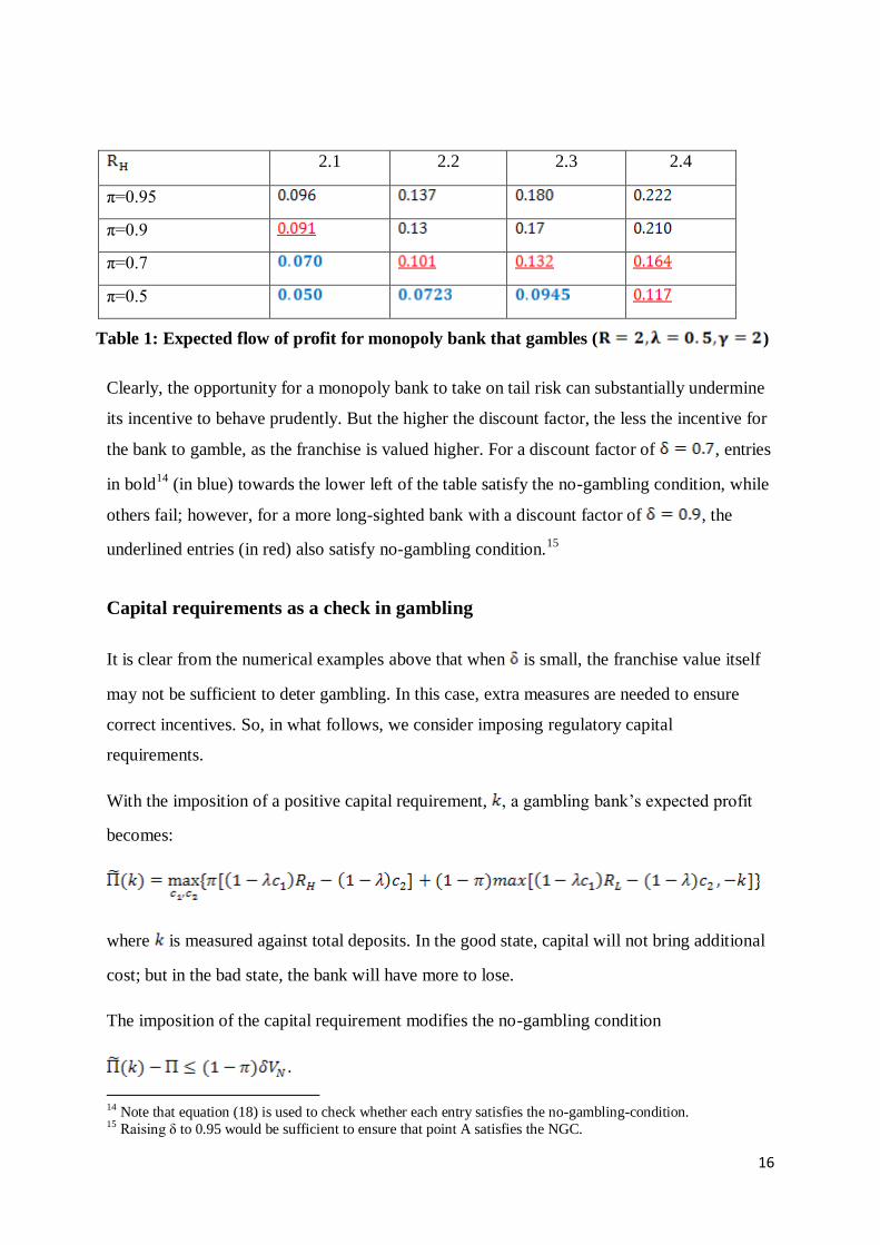
illustrated by the numerical example in Table 1, where . For these

parameter values, the monopoly bank makes a seignoirage profit of 0.057, measured in date 2

consumption. (Given , this implies that almost 3 percent of the endowment will be

transferred from the depositors to the shareholders even without taking on tail risk.) Entries in

the table indicate how profits may be boosted by risk-taking for various values of and .

13 Using standard definition for tail risk, the lower threshold for tail risk is in our binominal model with mean preserving spread, as shown by the dashed horizontal line in the figure.

Taking on ‘tail risk’ Gambling

Figure 2. No-gambling-condition (NGC) and the mimicking constraint

16

2.1 2.2 2.3 2.4

π=0.95

π=0.9

π=0.7

π=0.5

Table 1: Expected flow of profit for monopoly bank that gambles ( )

Clearly, the opportunity for a monopoly bank to take on tail risk can substantially undermine

its incentive to behave prudently. But the higher the discount factor, the less the incentive for

the bank to gamble, as the franchise is valued higher. For a discount factor of , entries

in bold14

(in blue) towards the lower left of the table satisfy the no-gambling condition, while

others fail; however, for a more long-sighted bank with a discount factor of , the

underlined entries (in red) also satisfy no-gambling condition.15

Capital requirements as a check in gambling

It is clear from the numerical examples above that when is small, the franchise value itself

may not be sufficient to deter gambling. In this case, extra measures are needed to ensure

correct incentives. So, in what follows, we consider imposing regulatory capital

requirements.

With the imposition of a positive capital requirement, , a gambling bank‟s expected profit

becomes:

where is measured against total deposits. In the good state, capital will not bring additional

cost; but in the bad state, the bank will have more to lose.

The imposition of the capital requirement modifies the no-gambling condition

.

14 Note that equation (18) is used to check whether each entry satisfies the no-gambling-condition. 15 Raising δ to 0.95 would be sufficient to ensure that point A satisfies the NGC.

17

Note that has no effect on the optimal deposit contract offered by the gambling bank, and

has no effect on and , so the no-gambling-condition above can be rewritten as

. (18‟)

It is clear that in checking gambling is a perfect substitute for the franchise value .

Since is increasing in and , the imposition of the capital requirement shifts the no-

gambling boundary, NGC, in Figure 2, upward, reducing the incentive to gamble for any

given and .

It is worth bearing in mind, however, that the efficacy of regulatory capital will also be

limited by outside options. Securitisation may be one of these: if regulatory burden on banks

becomes excessive, securitisation may be a form of „regulatory arbitrage‟, helping to move

the business of banking off-balance sheet. In Appendix D we look ex-ante monitoring – the

loss of franchise value in particular – an important complement to the ex-post measures

considered above.

3. Concentration, strategic behaviour and the U-shaped No-

Gambling Boundary

A further key element not yet considered is the role of negative externalities, what de la Torre

and Ize (2011) refer to as collective action problem. If the banking sector is highly

concentrated, the failure of one bank is likely to spread to the whole sector, generating

systemic risk; so, to prevent a wholesale banking collapse – with all the externalities that will

involve -- the government may see no alternative but to bailout the failing bank.16

Seeing

itself as “too big to fail” can greatly undermine a bank‟s incentive to invest prudently , as

Haldane and Alessandri (2009) point out in a paper with the suggestive title “Banking on the

State”.

Here too there is a choice of informational paradigms – the view that these are issues of

which agents are unaware (precisely because they are externalities) and the view that they

16 As the then Chancellor reports: “The risk of one bank collapsing and taking all the others with it was acute. I

suppose it could have been tried, but I would not have wanted to be responsible for the economic and social

catastrophe that might follow.” (Darling, 2011, p142)

18

simply chose to keep quiet. Again one might want to look at the incentives to find things out.

An interesting case in point arose when the FSA sought to establish why big financial firms

operating in the City of London only looked at minor shocks when conducting stress tests.

The public officials asked the bankers why their firms had failed to explore the

possibility of a real blow-up. Was it a result of disaster myopia, or a failure to

appreciate the dangers of contagion? No, one of the attendees replied. It was nothing

like that. The problem was that risk departments didn‟t have any incentive to simulate

genuine disasters. If such an awful eventuality materialized, the simulators would likely

lose their bonuses and possibly their jobs. And, in any case, the authorities would step

in and rescue the bank. Cassidy (2009, p.317)

As Rajan (2010, p. 151) notes, the same logic may apply even for small firms if traders

believe that the risky strategies are being so widely used that there will be official

intervention when collectively they fail:

But as enough banks imitated the innovators and took on similar risks, and as it

became common wisdom among market participants that the market would be

supported in the event of a crisis, there would have been strong incentives to

load up on tail risks, even if such activity became visible. Rajan (2010, p.151).

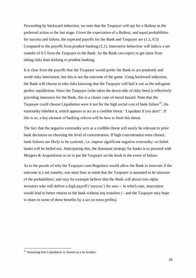
3.1 Bailout as the sub-game perfect equilibrium

Before discussing in detail how the no-gambling-condition might be modified in the presence

of “too big to fail” policy, consider the strategic elements involved with the aid of a simple

two-player game between the banking industry – represented by a monopoly bank -- and the

state – represented by the taxpayer.17

In the extensive game shown in Figure 3 we focus on a big bank with substantial franchise

value.18

The players are a Bank and the Taxpayer – assumed also to be a Depositor. It is the

Bank that moves first, choosing either to pursue traditional Prudent banking or to experiment

with Innovative behaviour, where for simplicity we ignore capital requirements. The figures

in parentheses indicate the notional payoffs to the Bank and Taxpayer-cum-Depositor. Note

that, in order to see whether the Bank is able to profit from risk per se (as argued by Sinn for

example), Innovative behaviour is taken to involve a mean preserving widening of the spread

of returns on the portfolio of the Bank. We also assume that there is asymmetric information

17 This is a heroic simplification, of course, as in practice protecting the interests of the taxpayer is delegated to

a troika of agencies, the Bank of England, Treasury and the FSA. 18 Prior to this game being played, banks as a group will have chosen whether or not to concentrate as is

discussed further below.

19

about probabilities of Success or Failure, with the Bank knowing the probabilities (π and 1-π,

respectively) but not the Taxpayer. (Appendix E is a more realistic case with payoffs

calculated for a dynamic game using parameter values based on Sinn (2010).)

If the Bank chooses to act Prudent, the safe return of 2 is split equally between Bank and the

Taxpayer. But if it chooses to innovate the payoffs depend on Nature and the response to

failure. Nature moves next, awarding Success or Failure to the innovation with equal

probability, the former generating attractive returns of 4 (with the depositor getting 1 and the

rest going to the bank) the latter yielding nothing. It is now the Taxpayers turn; action is only

called for if the Bank fails, however, and there is a choice of closure (Liquidation) or granting

a Bailout. In the latter case, with payoffs shown as (0,0), the depositor is bailed out by the

Taxpayer, at zero net gain; and the Bank gets nothing either. If the Bank goes into

Liquidation, however, (as for Lehman Brothers) it also loses its franchise, f; and, in addition,

there is a large negative externality for the Taxpayer in the form of economic disruption, x.

Figure 3. Moral hazard as the Taxpayer underwrites risky behaviour

Bank

1

Prudent

Failure

(-f,- x)

(3,1)

(1,1)

,,0

Innovative

Success

Taxpayer

Nature

Nature

(0,1-b=0)

Liquidation Bailout

20

Proceeding by backward induction, we note that the Taxpayer will opt for a Bailout as the

preferred action at the last stage. Given the expectation of a Bailout, and equal probabilities

for success and failure, the expected payoffs for the Bank and Taxpayer are (1.5, 0.5)

Compared to the payoffs from prudent banking (1,1). Innovative behaviour will induce a net

transfer of 0.5 from the Taxpayer to the Bank. So the Bank can expect to get more from

taking risks than sticking to prudent banking.

It is clear from the payoffs that the Taxpayer would prefer the Bank to act prudently and

avoid risky innovation, but this is not the outcome of the game. Using backward induction,

the Bank will choose to take risks knowing that the Taxpayer will bail it out as the sub-game

perfect equilibrium. Since the Taxpayer (who takes the down-side of risky bets) is effectively

providing insurance for the Bank, this is a classic case of moral hazard. Note that the

Taxpayer could choose Liquidation were it not for the high social cost of bank failure19

, the

externality labelled x, which appears to act as a credible threat: „Liquidate if you dare!‟. If

this is so, a key element of banking reform will be how to limit this threat.

The fact that the negative externality acts as a credible threat will surely be relevant to prior

bank decisions on choosing the level of concentration. If high concentration were chosen,

bank failures are likely to be systemic, i.e. impose significant negative externality: so failed

banks will be bailed out. Anticipating this, the dominant strategy for banks is to proceed with

Mergers & Acquisitions so as to put the Taxpayer on the hook in the event of failure.

As to the puzzle of why the Taxpayer-cum-Regulator would allow the Bank to innovate if the

outcome is a net transfer, one must bear in mind that the Taxpayer is assumed to be unaware

of the probabilities; and may for example believe that the Bank will attract true alpha

investors who will deliver a high payoff („success‟) for sure -- in which case, innovation

would lead to better returns to the bank without any transfers (– and the Taxpayer may hope

to share in some of these benefits by a tax on extra profits).

19 Assuming that Liquidation is chosen as a tie breaker.

21

3.2 Concentration and U-shaped No Gambling Boundary

Can these strategic features be incorporated within the framework developed in Section 2? In

what follows, we analyse how given concentration can affect bank‟s incentives; then we

discuss the strategic incentives for choosing high concentration.

For analytical simplicity, let the degree of concentration, ( ) be defined by the

fraction of the monopoly franchise value , , that is obtained if a bank plays safe or is bailed

out after a failed gamble. To model “too big to fail” policy, TBTF, let the probability the

government will come to the bank‟s rescue, , increase with , with

and . The rationale for specifying the bailout policy in this way is as follows: when

the degree of concentration is low, no bank is “too big to fail”, so the failure of a bank is less

likely to have systemic effect; when the degree of concentration increases, any bank failure is

more likely to be systemic, so the probability of attracting bailout increases. The TBTF policy

used here specifies that if the bank gambles and fails, it may be bailed out by the government

which will honour all deposit contracts. In this case, the bank loses its equity buffer but its

franchise is not revoked.

With a given degree of concentration, the bank‟s profit if it plays safe is a fraction of that

under monopoly, so the deposit contract offered by these safe banks will be a scaled-up

version of that offered by the non-gambling monopoly (though each bank makes less profits

per unit of deposit).

For the gambling bank under market concentration, , its expected profit, assuming

, is given by

(19)

where the probability of losing capital for the gambling banks is . Note that the

optimal deposit contract with market concentration of , if they exist, would be the same as

that of a gambling monopoly.

22

Given the capital requirements and the TBTF policy specified above, the no-gambling

condition is then modified to

, (20)

where represents franchise value under full monopoly and the franchise value with

market concentration of and the failed gambling bank will be bailed out with probability .

To summarise the results for the no-gambling boundary (above which banks will not gamble)

in and space for some given and :

Proposition 4:

(i) For , the no-gambling boundary is downward sloping in beta and k space.

(ii) For , the no-gambling boundary is U-shaped in and space.

(iii)Increasing shift the U-shaped no-gambling boundary upwards.

Proof: See Appendix C.

The significance of Proposition 4 (iii) is that if the bailout is restricted to banks with less

attractive gambles (i.e., low and/or low ) the U-shaped no-gambling boundary will be

much less pronounced, as we discuss further below.

23

The above framework may be used in a heuristic discussion of options for the reform of the

UK banking system, distinguishing in particular between reforms related to structure of bank

balance sheets (the degree of leverage, for example) and those related to markets (such as

the degree of concentration). For this purpose, we use Figure 4, with market concentration, ,

on the horizontal axis (acting as a proxy for franchise value, assuming that high concentration

implies high franchise value), and minimum capital requirement, k, on the vertical axis (to

represent variations in bank leverage).

The no gambling boundary, defining the shaded area of Prudential Banking, is the U-shaped

schedule LNR in the figure. The downward slope LN reflects the trade-off between bank‟s

profitability (franchise value) and the official capital requirement in terms of prudential

behaviour: as banking becomes more competitive and franchise values fall, so the minimum

capital requirement will need to be raised to ensure prudence, for any given degree of tail

Required

Capital

Excess

Risk-taking

Concentration TBTF

Figure 4. How bailouts increase the risk of imprudent banking

L

R

N

UK

Excess

Risk-taking

Prudent Banking

24

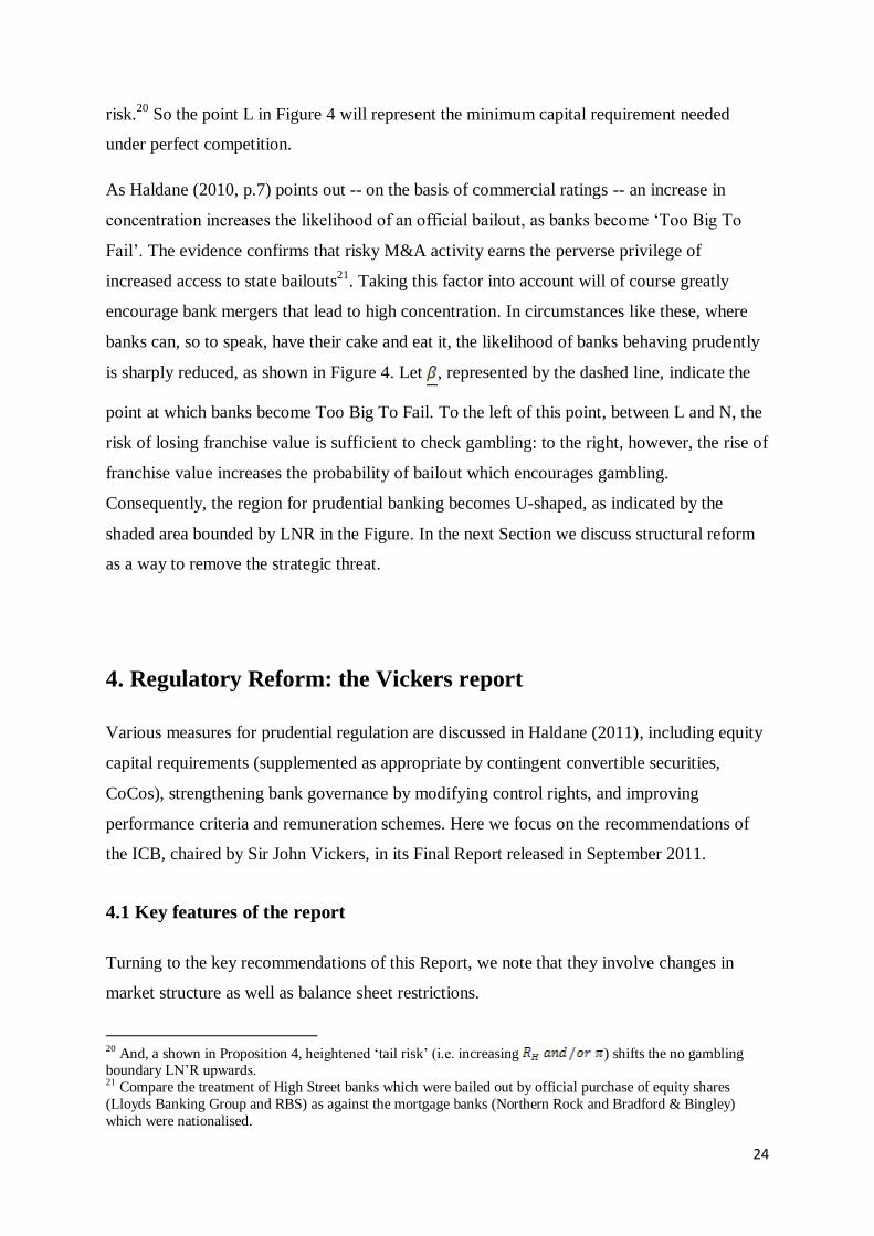
risk.20

So the point L in Figure 4 will represent the minimum capital requirement needed

under perfect competition.

As Haldane (2010, p.7) points out -- on the basis of commercial ratings -- an increase in

concentration increases the likelihood of an official bailout, as banks become „Too Big To

Fail‟. The evidence confirms that risky M&A activity earns the perverse privilege of

increased access to state bailouts21

. Taking this factor into account will of course greatly

encourage bank mergers that lead to high concentration. In circumstances like these, where

banks can, so to speak, have their cake and eat it, the likelihood of banks behaving prudently

is sharply reduced, as shown in Figure 4. Let , represented by the dashed line, indicate the

point at which banks become Too Big To Fail. To the left of this point, between L and N, the

risk of losing franchise value is sufficient to check gambling: to the right, however, the rise of

franchise value increases the probability of bailout which encourages gambling.

Consequently, the region for prudential banking becomes U-shaped, as indicated by the

shaded area bounded by LNR in the Figure. In the next Section we discuss structural reform

as a way to remove the strategic threat.

4. Regulatory Reform: the Vickers report

Various measures for prudential regulation are discussed in Haldane (2011), including equity

capital requirements (supplemented as appropriate by contingent convertible securities,

CoCos), strengthening bank governance by modifying control rights, and improving

performance criteria and remuneration schemes. Here we focus on the recommendations of

the ICB, chaired by Sir John Vickers, in its Final Report released in September 2011.

4.1 Key features of the report

Turning to the key recommendations of this Report, we note that they involve changes in

market structure as well as balance sheet restrictions.

20 And, a shown in Proposition 4, heightened „tail risk‟ (i.e. increasing ) shifts the no gambling boundary LN‟R upwards. 21 Compare the treatment of High Street banks which were bailed out by official purchase of equity shares

(Lloyds Banking Group and RBS) as against the mortgage banks (Northern Rock and Bradford & Bingley)

which were nationalised.

25

Structural separation is recommended in the form of a „retail ring-fence‟ designed to isolate

and contain banking activities where the continuous provision of service is vital to the

economy and a bank‟s customers so as to ensure that such provision is protected from

incidental activities and that it can be maintained in the event of bank failure without

government solvency support. „In essence, ring-fenced banks would take retail deposits,

provide payments services and supply credit to households and businesses.‟ ICB (2011, para.

3.1) These services are divided into those which are mandated (involving about 18% of assets

as of end 2010); are permitted (another 18%); and those which are prohibited (about 64%).

Ring-fenced banks will thus be banned from a very considerable range of activities currently

conducted by universal banks. Depending on how much of the second category are taken

inside the fence, „the ring fence might include between a sixth and a third of the total assets

of the UK banking sector of over £6 trillion.‟‟ ICB (2011, para. 3.40). (As banks inside the

fence can stay linked with those outside, subject to arms length and other restrictions,

however, this is not the complete separation mandated by the Glass-Steagall Act in the USA.)

In addition several steps are recommended in order to increase competition on the High Street

– increased transparency of costs and transferability of accounts, in particular.

Balance sheet requirements involve substantial loss-absorbing capacity in the form of equity

and bonds so as to avoid claims on the taxpayer following bank insolvency. Specifically, the

Commission recommends that „large UK ring-fenced banks (and the biggest UK Globally

Significant Banks) be required to hold primary loss-absorbing capacity of at least 17% of

RWAs which can be increased to a further buffer of up to 3% of RWAs for a bank to the

extent that its supervisor has doubts about its resolvability‟, ICB (2010, para. 4.118).

This loss absorbing capacity can be split between equity and bail-in bonds, where the equity-

to-RWAs ratio is at least 10% for ring-fenced banks with 3% or more of UK GDP in RWAs

(falling to 7% for those with RWAs of 1% of UK GDP), ICB (2010, para. 4.132-134).

As regards monitoring and transparency, issues discussed in Appendix C, the Commission

notes that: “[a] ring-fence of this kind would also have the benefit that ring-fence banks

would be more straightforward than some existing banking structures and thus easier to

manage, monitor and regulate.” (ICB, 2010, para 3.4)

26

4.2 Getting the taxpayer off the hook: bailout no longer guaranteed

How can ring-fencing change the strategic relation between the state and banks? With

reference to the game tree in Figure 3, the fundamental requirement is that the severe

externalities triggered by unpremeditated bank closure be removed i.e. the payoff to the

Taxpayer in the case of liquidation be changed from -x to zero22

. The means to this end

include (a) improved ex ante monitoring of risk-taking; (b) a great reduction of risks that may

be taken; (c) substantially increased loss-absorbing capacity on the part of the bank to cover

what risk remains, and (d) better resolution procedures should the retail bank need to be

reconstituted.

Heuristically, this strategy can be illustrated with reference to Figure 5, referring only to

banks within the ring-fence, where some of the measures should act to expand the region of

“Prudential Banking” (beyond that in the earlier Figure 4, indicated here by the dashed U-

shape); others to shift the locus of a ring-fenced bank into this enlarged area.23

22 Assuming that in the event of a tie the taxpayer will prefer liquidation to bail-out. 23 As access to more exotic gambles was found to shift the U-shaped frontier upwards according to Proposition 5, so the prohibition of many risky assets – two thirds of the current portfolio of UK banks, in fact – should

have the reverse effect, as indicated by the shift from L to L‟ in the No Gambling frontier. Improved monitoring

- backed by a threat of losing one‟s licence if caught – should further reduce the region of excess risk by making

the frontier slope down more steeply from L‟. Steps to move the locus for ring-fenced banks towards Prudential

Banking include both the decisive increase in the level of capital required for the operation of a ring-fenced

bank and steps to increase competition among High Street banks, see the arrow pointing NW in the figure.

27

The various regulatory changes indicated in the Figure– together with arrangements such as

„Living Wills‟ for prompt resolution – are, according to the ICB Final Report, designed to get

the taxpayer „off the hook‟ of bailing out universal banks in trouble.

The stated purpose of retail „ring-fencing‟ is to get such banks back to the business of taking

retail deposits, and supplying credit and liquidity to households and businesses. Thus the

proposed reforms would:

put the UK banking system of 2019 on an altogether different basis from that of 2007.

In many respects, however, it would be restorative of what went before in the recent

past – better capitalised, less leveraged banking more focussed on the needs of savers

and borrowers in the domestic economy. ICB (2011, p.18)

We have analysed the Vickers Report from the perspective of asymmetric information. Are

the proposals still appropriate if there are problems of „collective cognition‟? Perhaps the

emphasis on ex ante monitoring -- and especially the outright banning of products that appear

risky -- could be seen as a step away from the Anglo-Saxon principle of common law (where

Required

Capital

Prudent Banking

Concentration

Figure 5. Checking risk-taking in ‘ring-fenced’ banks

L′ R′

Ring-

fenced

Bank

Higher capital

requirements

and more

competition

Reduced

incentive

to Bailout

Excess Risk-taking

Risk Prohibition

& Monitoring

Excess Risk-taking

L

R

28

products are permitted unless found to be dangerous ) towards the Roman law principle (that

products are banned unless shown to be safe). In this case, as with new medicines, society

may be protected by shifting the burden of proof onto the innovator -- with some loss of

efficiency but gains in stability.

5. Conclusion: back to banking basics

There clearly is a dangerous propensity for banks to take on excessive risks in the current

regulatory environment: as Vickers (2011, p.2) remarks: “One of the roles of financial

institutions and markets is efficiently to manage risks. Their failure to do so – and indeed to

amplify rather than absorb shocks from the economy at large – has been spectacular.”

Financial innovations, such as securitisation and Credit Default Swaps, have increased the

ease with which banks can take risky assets onto their balance sheets while satisfying the

regulatory norms set by Basel. There are clear private incentives for High Street banks to

expand into investment banking, raising their balance sheets well beyond the needs of

households and SME borrowers and shifting risk onto depositors and/or the taxpayer by

greatly increased leverage. But the social cost of interrupting the nationwide provision of

payments services and credit supply associated with bank failures means that banks that

combine retail and wholesale activities will be rescued by the government, a threat to the

economy that effectively puts tax-payers on the hook to underwrite the risks taken by large

universal banks.

Nor has the incidence of crisis itself changed these incentives, apparently. As Diane Coyle

(2011), a former member of the UK Competition Commission, noted as bank profitability

recovered in 2010-11 despite a still-fragile economy: „The truth is that banks are again doing

well out of banking, but businesses and consumers are not... Bonuses are back... they are a

measure of monopoly rents in the business, it does not take great talent to make a profit by

taking excessive risk, safe from effective competition and sure of a bailout if needed.‟

As a contribution to the debate on problems besetting modern banking in Britain, we began

with a simple model of retail banking and showed how, behind the veil of asymmetric

information, the incentive to take on risk can easily exceed the threat of losing the franchise –

especially if the probability of losing the franchised is reduced by the prospect of an official

29

bailout. As the prudential benefits of increased concentration are progressively offset by the

prospect of rescue, the „prudential frontier‟ relating capital requirements to concentration

becomes U–shaped.

This framework – of concentrated banking with asymmetric information – is used to discuss

the impact of regulatory reforms involving changes to market structure, balance sheet

restrictions and the efficacy of monitoring. Considering the reforms advocated by the ICB in

their Final Report in particular, we note that they are designed to offset excess risk-taking and

promote competition, i.e. to eliminate the very features that we have added to the basic

banking model to capture current distortions! But they go further.

A key aim of Mrs Thatcher‟s industrial policy was to reduce the threat to the provision of

goods and services posed by strikes in the public sector – the confrontation with coal miners

being a decisive case in point. An important – perhaps the most important – aspect of the

„ring-fence‟ proposal viewed as industrial policy is how – by reducing the threat of abrupt

contagious closure on the part of retail banks – it aims to change the strategic balance

between banking and the state.

30

References:

Allen, F. and Gale, D. (2000), Comparing Financial Systems, Cambridge, MA: MIT Press.

Allen, F. and Gale, D. (2007), Understanding Financial Crises, New York: Oxford

University Press.

Akerlof, G. and Romer, P. (1993): Looting: The Economic Underworld of Bankruptcy for

Profit. Brookings Papers on Economic Activity, vol. 24(2), pages 1-74.

Bhattacharya, S. (1982) "Aspects of Monetary and Banking Theory and Moral Hazard."

Journal of Finance, May, 37(2), pp. 371-84.

Boyd, J. and De Nicolo, G. (2005), „The theory of bank risk taking and competition

revisited‟, The Journal of Finance, vol. LX No. 3.

Bryant, J. (1980). “A Model of Reserves, Bank Runs, and Deposit Insurance,”

Journal of Banking and Finance 4, 335-344.

Cassidy, J. (2009), How Markets Fail: the Logic of Economic Calamities. London: Allen

Lane.

Chang, R. and Velasco, A. (2001) "A Model of Financial Crises In Emerging Markets," The

Quarterly Journal of Economics, vol. 116(2), pages 489-517, May.

Colangelo, A. and Inklaar, R. (2010). “Banking sector output measurement in the Euro area -

a modified approach”. ECB working paper 1204.

Coyle, D. (2011) „Merlin deal will not fix flawed banks‟, published in FT 8th Feb 2011.

Darling, A. (2011), Back from the Brink, London: Atlantic Books.

De la Torre, Augusto and Alain Ize, (2011), “Containing Systemic Risk: Paradigm-Based

Perspectives on Regulatory Reform”, World Bank Policy Research Working Paper, 5523.

Diamond, D.W. and Dybvig, P.H. (1983), „Bank runs, deposit insurance, and liquidity‟,

Journal of Political Economy, 91 (June): 401–19.

31

Foster D. P. and Young, P., (2011) "Gaming Performance Fees by Portfolio Managers‟ The

Quarterly Journal of Economics, forthcoming.

Freixas, X. and Rochet J-C., (2008), Microeconomics of Banking, MIT Press.

Gai, P. and Kapadia, S., (2010), “Contagion in Financial Networks”, Bank of England

Working Paper No. 383.

Gennaioli, N., A. Shleifer and R. Vishny, (2011), “Neglected risks, financial innovation, and

financial fragility”, Journal of Financial Economics 125, forthcoming.

Haldane, A. (2010), „The $100 billion question‟, Institute of Regulation & Risk, North Asia

(IRRNA), Hong Kong, March 2010.

Haldane, A. and Alessandri P. (2009), „Banking on the state‟, Available at:

http://www.bankofengland.co.uk/publications/speeches/2009/speech409.pdf

Haldane, A., Brennan, S. and Madouros, V., (2010), „What is the Contribution of the

Financial Sector: Miracle or Mirage?‟ The Future of Finance: the LSE report, Chapter 2.

London: LSE.

Haldane, A. G. and May, R. M, (2011), “Systemic risk in banking ecosystems”, Nature 469,

351–355.

Hellmann, T. F., Murdock K. C. and Stiglitz J. E., (2000). "Liberalization, Moral Hazard in

Banking, and Prudential Regulation: Are Capital Requirements Enough?" American

Economic Review, American Economic Association, vol. 90(1), pages 147-165, March.

Independent Commission on Banking (2010), „Issues Paper, Call for Evidence,‟ London:

ICB.

Independent Commission on Banking (2011), Final Report:Recommendations, London: ICB.

Jacklin, C.J. (1987) „Demand Deposits, Trading Restrictions and Risk Sharing.‟ In E.C

Prescott and N. Wallace (eds), Contractual Arrangements for Intertemporal Trade, 26-47,

Minneapolis: University of Minnesota Press.

Kuvshinov, D. (2011), “The optimal capital requirement for UK banks: a moral hazard

perspective”, MSc Dissertation, Department of Economics, University of Warwick.

32

May, R. M. and Arinaminpathy, N. (2010), “Systemic risk: the dynamics of model banking

systems”. J. R. Soc. Interface 7, 823–838.

Rajan, R. G., (2005), „Has Financial Development Made the World Riskier?‟ Proceedings of

the Jackson Hole Conference organised by Kanas City Fed.

Rajan, R. G., (2010), Fault Lines, Princeton NJ: Princeton University Press.

Reinhart, C. and K. Rogoff, (2009), This Time It’s Different: Eight Centuries of Financial

Folly. Princeton: Princeton University Press, 2009

Wang, J.C, S. Basu, and J.G. Fernald (2009). “A General Equilibrium Asset-Pricing

Approach to the Measurement of Nominal and Real Bank Output”. In W.E. Diewert, J.S.

Greenlees, and C.R. Hulten (Eds.) Price Index Concepts and Measurement. NBER Studies

in Income and Wealth, Volume 70.

Woolley, P., (2010), „Why are financial markets so inefficient and exploitative – and a

suggested remedy‟, Future of finance: The LSE Report. London: LSE.

33

Appendices

Appendix A Salient features of banking in Britain

Two salient characteristics of UK banking are that the key players are universal banks24

and

that the industry is concentrated, „especially in the retail and commercial sector, where the

top six banks account for 88% of retail deposits‟ ICB (2010, p.9). Two other striking features

are the rapid expansion of balance sheets prior to the crisis; and the increase in measured

value added, especially in profits. As can be seen from Chart A1, banking assets doubled

relative to GDP since 1990, rising to more than five times annual GDP – which represents a

10-fold increase above the long run historical average of around 50%.

Chart A1: UK banking sector as % of GDP.

Note: The definition of UK banking sector assets used in the series is broader after 1966,

but using a narrower definition throughout gives the same profile.

Source: Haldane et al (2010, p.84)

24 i.e., they combine both categories of banking - retail & commercial and wholesale & investment.

34

Evidence of the sharp rise in the measured contribution of banking to national income in the

run-up to the financial crisis is provided by Haldane et al. (2010), where it is reported that,

using conventional measures of value added:

In 2007, financial intermediation accounted for more than 8% of total GVA, compared

with 5% in 1970. The gross operating surpluses of financial intermediaries show an

even more dramatic trend. Between 1948 and 1978, intermediation accounted on

average for around 1.5% of whole economy profits. By 2008, that ratio had risen

tenfold to about 15% (See Chart A2).

Chart A2: Gross operating surplus of UK private financial corporations (% of

total)

Source: Haldane et al (2010, p.68)

Perhaps the most extraordinary feature, however, is that the recent rapid expansion of balance

sheets and profitability was accompanied by an apparent reduction in the riskiness of bank

portfolios. As shown in Chart A3, the doubling of leverage from the late 1990s until just

before the crisis was accompanied by a halving of the fraction of risk-weighted assets. Thus –

despite the efforts of the Basel Committee to ensure banks were adequately capitalised -- for

the period 2005-2008, leverage was around 40 for UK banks on average, and considerably

higher for some.

35

Chart A3: Leverage and risk-taking in UK banks.

Source: Haldane et al (2010, p.89)

Ex-post, the sliver of equity turned out to be far too slender to absorb the risks actually being

taken. In the event, official support for the financial sector running to 74 % of GDP

(including capital injections of more than 5% of GDP) had to be supplied to prevent banking

collapse25

.

25

See Haldane and Alessandri (2009, Annex, Table 1) who also describe various profit-making strategies -

including taking on tail risk - that contributed to these losses and may have been induced by expectations of

state support.

36

Appendix B. Gambling and Gini Coefficient: Miracle and Mirage?

It is evident that in this simplified model, bank concentration will lead to an increase in the

Gini coefficient compared with competitive banking: and this effect will become much more

pronounced with gambling. This is illustrated by the stylised Lorenz curves in Figure A1,

where σ represents the fraction of the population owning shares in the all-deposit bank. If ω

represents the consumption bundle available to depositors under monopoly banking, and

ω(1+μ) is the consumption available to the depositors who are also shareholders enjoying the

monopoly premium, μ, then and the Gini coefficient26

turns out to be

. When the bank gambles, the premium paid to owner-managers will of

course rise, say to , shifting the Lorenz curve to in the figure.

In discussing whether the contribution of financial sector is „Miracle or Mirage‟, Haldane et

al. (2010, pp. 79-80) report that the share of financial intermediation in employment in UK is

around 4%, and that:

the measured „productivity miracle‟ in finance …has been reflected in the returns to

both labour and capital, if not in the quantity of these factors employed. For labour,

financial intermediation is at the top of the table, with the weekly earnings roughly

double the whole economy median. This differential widened during this century,

roughly mirroring the accumulation of leverage within the financial sector.

Using the above formula, a doubling of consumption opportunities for those in finance would

add about 4% to the Gini coefficient, i.e. about half the rise in Gini coefficient for the UK

from 1986 when the Big Bang took place, to just before the crisis in 2007. (Focusing more

narrowly on Investment Banking, however, the Financial Times reports compensation

running at 6 times the median income in both US and UK.27

26 i.e. the area OLP divided by O1P in the diagram. 27 FT, Feb 17th, 2011, „Banker‟s pay: time for deep cuts.‟

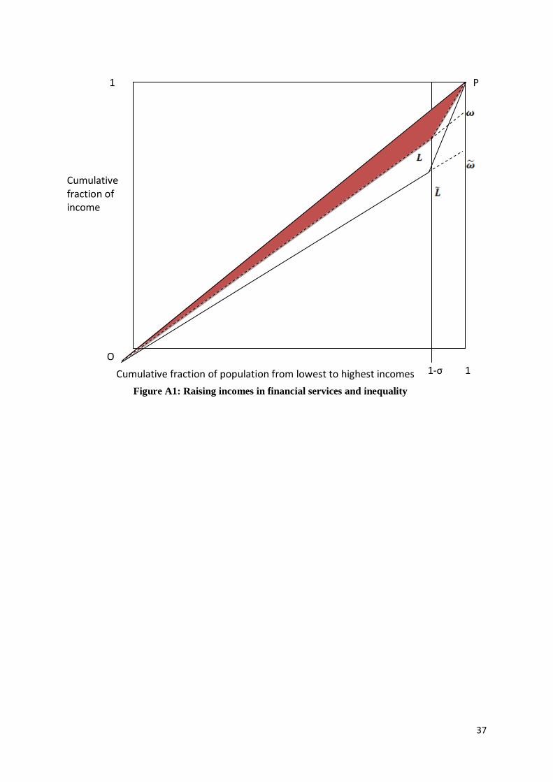
37

Cumulative fraction of income

Cumulative fraction of population from lowest to highest incomes 1-σ 1

1

Figure A1: Raising incomes in financial services and inequality

O

P

38

Appendix C. Proof of Propositions

Proof of Proposition 3

If is low enough, the bank cannot honour the contract to the late consumers in the low

state (the late consumption in this case is honoured by the insuring agency). So the bank‟s

profits are given by . This changes the first order condition to

. Together with the binding participation constraint, one can then determine the

optimal contract as in the second part of Proposition 4. (Since case (2) has the same deposit

contract as that under certainty and no default from the bank, we use case (1) to represent

gambling.)

If is large, the bank can honour the contract to the late consumers in either state. So the

optimal contract satisfies the first order condition . With the

binding participation constraint the same as in Proposition 1, the optimal contract must be the

same.

Proof of Proposition 4

Given the monopoly bank will gamble, it is best for it to choose the deposit contract

specified in Proposition (4). In this case, to ensure that the bank will gamble, condition (18)

becomes

. (B1)

Similarly, given the monopoly bank will not gamble, it is best for it to choose the deposit

contract specified in Proposition (3.1). To ensure that the bank will not gamble,

condition (18) becomes

. (B2)

For some given parameters of , and , it is always possible to have

39

. (B3)

If (B3) is satisfied, then both (B1) and (B2) are true as

and . So for the set of parameter values

such that (B3) holds, the monopoly bank may choose either to gamble or to play safe.

Now we show that in and space, for a given delta, the boundary specified in (B3) lies

below the boundary where (B2) holds as an equality and above the boundary where (B1)

holds as an equality. To simplify comparison, we fix the value for . Then, we can select the

appropriate value for such that (B3) holds. In this case, (B2) is satisfied. To ensure (B2)

holds as an equality, we have to increase the value of . Since , the

which ensures that (B2) is an equality must be greater than or equal to the for which (B3)

holds. So the boundary of (B3) lies below the boundary where (B2) is an equality. Similarly,

one can show that (B3) also lies above the boundary where (B1) is an equality.

In and space, multiplicity of equilibria occurs in the area bounded by the boundaries of

(B1) and (B2). So the sufficient condition to ensure no gambling is to choose the parameters

of and such that they lie below the boundary of (B1). In what follows, we characterise

the general properties of this boundary.

(1) Rewrite the no-gambling condition as

. (B4)

Note that the contract offered by the gambling bank, , must satisfy the first order

condition

, (B5)

and the binding participation constraint

. (B6)

So, it is clear that , and . This implies .

Using (B5) and (B6), one can show that

40

(B7)

Applying the envelope theorem, one obtains,

, (B8)

and

. (B9)

Differentiating the no-gambling condition (B4) with respect to and yields

(B10)

Since both terms before and are positive, the no-gambling condition must slope

downward in and space.

Finally, note that if and , then (B4) holds. So the no-gambling boundary starts

from in the and space and goes asymptotically towards the axis.

(2) An increase in increases the coefficient of the second term in (B4), . To

maintain equality, has to increase for a fixed . Note that all no-gambling boundaries start

from , so an increase in swivels the no-gambling boundary upwards in the and

space.

Proof of Proposition 5

As is shown in the proof of Proposition 5 above, it is sufficient to specify the no-gambling

condition (20) as

, (B10)

where is the optimal deposit contract offered by the gambling bank.

41

For , , so (B10) can be rewritten as

(B11)

Note that the deposit contract is unaffected by either or , so to keep (B11) as an

equality, a reduction in must be compensated by an appropriate increase in . This

generates the downward sloping section of the no-gambling condition in and space.

For , we rewrite (B10) as

. (B12)

Since the left hand side is independent of and , maintaining (B12) as an equality requires

the right hand side to be a constant. Differentiating the right hand side with respect to or ,

one can obtain the slope of the no-gambling condition as

. (B13)

It is clear from (B13) that the numerator is negative if and positive if . So the

no-gambling condition is U-shaped.

42

Appendix D. Real-Time Monitoring

For the case discussed above, the regulatory capital required to deter gambling can be

substantial, even for moderate gambles (see rows 1 and 3 in Table 2 below). One way to

reduce the capital charge is to introduce real-time monitoring. Real-time monitoring will be

characterised by a given probability of detecting gambling before it fails; and an associated

punishment. For simplicity, we assume that the probability of detection is q and the

punishment is the loss of franchise. (Later, we discuss the effect of other punishments.) In

this case, the value function of the gambling bank becomes

or

Note that introducing real-time monitoring simply scales down the profits of a gambling

bank, so the functional form of deposit contracts offered by the gambling bank are

unchanged.

Applying the no-gambling-condition and re-arranging yields

(18‟‟)

Given capital requirements, imposing real-time monitoring reduces gambling profits and so

decreases the incentive to gamble. By comparing (18‟‟) with (18‟), it is clear that the net

effect is “as if” there is an increase in franchise value. So, in terms of Figure 2, introducing

real-time monitoring further shifts the no-gambling-condition upwards in and space.

Using the no-gambling-condition (18‟‟), one can obtain the minimum capital requirements as:

43

To gauge quantitative significance of real-time monitoring of this form, we compare

minimum capital requirements (measured in terms of deposits) for the mimicking strategy,

, both under perfect competition and under monopoly. Results are summarised in

Table 2 where , , , and . For returns under prudent

investment, we choose as in Allen and Gale (2007), as in Foster and Young

(2011) and an intermediate case where .

Regime R = 2 R= 1.5 R = 1.04

Monopoly without

monitoring

0.315 0.550 0.528

Monopoly with

monitoring

0 0.209 0.522

Perfect competition

0.854 0.693 0.528

Table 2: Minimum capital requirements under different regimes

The first row in Table 2 indicates that, without monitoring, decreasing safe returns, R,

increases the minimum prudential capital requirement. This is because smaller R implies a

smaller franchise value, so capital requirements have to be increased to offset this and

preserve proper incentives. The second row shows that the effect of introducing real-time

monitoring depends crucially on the franchise value. When this is high (R=2), a moderate

probability of detecting the gamble (30%) can substantially reduce the minimum capital

requirement.28

When the franchise value is low (R=1.04), the effect on the minimum capital

requirement is minimal.

The third row illustrates minimum capital requirements under perfect competition: as R

decreases, gambling by using mimicking strategy becomes less attractive, so minimum

capital requirements decline. Note first that, for any given R, the minimum capital

requirements under perfect competition are generally greater than those under monopoly.

This is because there is no franchise value under perfect competition; so the gap between

28

Similar results are found elsewhere. Thus, in a careful calibration of the Hellmann, Murdock and Stiglitz

(2000) model, Kuvshinov (2011) shows that real time monitoring can reduce minimum capital adequacy ratio

from around 40% to 20%.

44

them shrinks as the franchise value decreases. Note also that, because of the specific form of

the punishment used above, real-time monitoring has no effect on minimum capital

requirements under perfect competition.

The numerical examples illustrate how the effectiveness of our form of the real-time

monitoring depends on the level of franchise values: becoming ineffective when the franchise

value is low (either because of high degree of competition or low returns on prudent

investment). One way to overcome this would be to impose an alternative (or additional)

sanction in the form of fixed fine, for example, the loss of regulatory capital in the case where

capital requirements are in force. By combining these two forms of sanction, real-time

monitoring could be effective regardless of the level of franchise value. In Kuvshinov (2011),

for example, the assumption that a competitive bank that is gambling will lose all of its equity

capital if caught has the dramatic effect of halving the risk weighted capital requirement even

if the chance of being detected is only 10%.

These numerical exercises are, however, subject to a major qualification: they take no

account of bank bailouts, so they exaggerate the prudential benefits of concentration.

45

Appendix E. Bailout and the incentive to take on tail risk: a numerical

illustration

As our framework assumes monopoly profits even when investing in the prudent asset, the

deposit rate r is set below the prudent rate α. The parameters are as in Hellmann et al (2000)

with values based on Sinn (2010).

Prudent Rate α=1.05 Success return on risky asset γ=1.066

Downside of gamble β=0.91 Probability of failing gamble π=0.9

Discount factor δ=0.9 Capital holdings of bank k=5

Deposit rate r=1.04

Payoffs (Bank, Taxpayer)

Bank

1

Prudent

Failure

(-5, -x)

Bailout: (2.8+δVB =20.98, 3.8)

Liquidation: (2.8+δVL =12.37, 3.8)

(1.2+δVN=12, 3.8)

Innovative

Success

Taxpayer

Nature

Nature

(-5+ δVB=14.09, -4 + b=0)

where b=4

Liquidation Bailout

Expected Payoff for the shareholder:

Bailout: 0.9*(2.8+δVB)+0.1*(-5+ δVB)=20.9> 12

Liquidation: 0.9*(2.8 δVL)+0.1*(-5)=10.63< 12

46

The profits of a monopoly (concentrated) bank are given by

Profits:

Profit of investment in the prudent return: ПN=1.2

Profits of investment in risky return: ПG=2.8

Payoffs and Expected Values:

Prudent:

Payoff and expected value to bank if it invests in the prudent investment:

EV=1.2+δVN=12

Bailout:

Payoff to the bank if it invests in the risky return and assumes to be bailed out (success):

2.8+δVB=20.98

Payoff to the bank if it invests in the risky return and assumes to be bailed out (failure):

-k+δVB=14.09

The expected value for the bank of the gamble assuming it will be bailed out becomes

20.29.

Liquidation:

Payoff to the bank if it invests in the risky return and assumes liquidation (success):

2.8+δVL=12.36

Payoff to the bank if it invests in the risky return and assumes to be bailed out (failure):

-k =-5

The expected value for the bank of the gamble assuming it will be bailed out becomes

10.63.

It becomes clear that if the bank knows it will be bailed out, risky innovation is preferred, otherwise it

will invest prudently assuming liquidation is the tie breaker for the Taxpayer.

Note

47

and VB>VN>VL.