1

FEAR AND MARKET FAILURE: GLOBAL IMBALANCES AND “SELF- INSURANCE”

Marcus Miller and Lei Zhang

CSGR Working Paper No. 216/07

December 2006

2

Fear and Market Failure: Global Imbalances and “Self-insurance” Marcus Miller1 and Lei Zhang2 CSGR Working Paper 216/07 December 2006 Abstract: Two key issues are examined in an integrated framework: the emergence of global imbalances and the precautionary motive for accumulating reserves. Standard models of general equilibrium would predict modest current account surpluses in the emerging markets if they face higher risk than the US itself. But, with pronounced Loss Aversion in emerging markets, their precautionary savings can generate substantial ‘global imbalances’, especially if there is an inefficient supply of global ‘insurance’. A combination of fear and market failure generates imbalances as a general equilibrium outcome. In principle, lower real interest rates will ensure aggregate demand equals supply at a global level: but disequilibrium may result if the required real interest rate is negative. A precautionary savings glut appears to us to be a temporary phenomenon, however, destined for correction as and when adequate reserve levels are achieved. If the process of correction is triggered by ‘Sudden Stop’ on capital flows to the US, might this not lead to “hard landing” that is forecast by several leading macroeconomists? When precautionary saving is combined with financial panic, history offers no guarantee of full employment. Keywords: Stochastic dynamic general equilibrium, loss aversion, liquidity trap JEL Classification: D51, D52, E12, E13, E21, E44, F32. Acknowledgements: The paper has benefited from feedback at seminars in Birkbeck College, in the Universities of Warwick, Manchester and York, and at the IADB. We thank in particular David Backus, Jonathan Cave, Jayasri Dutta, Sayantan Ghosal, Chris Meissner, Adam Posen, Herakles Polemarchakis, Neil Rankin, Romain Raciere and Joseph Stiglitz for their comments. We are especially indebted to John Driffill, director of the ESRC World Economics and Finance Programme, for his encouragement and support, though we remain responsible for errors. The authors gratefully acknowledge the research assistance of Parul Gupta and the financial support of the ESRC, under Grant No. RES-051-27-0125 for Marcus Miller, and for Lei Zhang under Grant No. RES-156-25-0032. Contact Details: Centre for the Study of Globalisation and Regionalisation (CSGR) Warwick University CV4 7AL Coventry (UK) Marcus.Miller@warwick.ac.uk

1 Department of Economics, University of Warwick, and CEPR. 2 Department of Economics, University of Warwick.

3

FEAR AND MARKET FAILURE: GLOBAL IMBALANCES AND “SELF-INSURANCE”

Non Technical Summary

Are the present current account imbalances – including notably a US external deficit

now running at 7% of its national output – part of the normal ebb and flow of trade

and finance; or are there special factors at work? Is laissez faire the appropriate

policy or is there a case for policy coordination? It depends who you ask.

According to Nouriel Roubini, looking for factors to account for current global

imbalances is rather like solving a ‘whodunnit’: and the two most plausible culprits

turn out to be the US and Asia. He notes, for example, that from 2000 to 2004 US

fiscal policy showed a large swing into deficit of almost 6% of GDP. But matters

have, he argues, changed since 2005: the US fiscal deficit has shrunk somewhat but

the external deficit continues to widen. The ‘global savings glut’ identified by Mr

Bernanke, allied with weak investment in East Asia following the crisis experience of

1997/8 are named as key factors.

A very different perspective is offered by David Backus and co-authors, however.

They bridle at the use of the term global imbalances; and by the same token they

reject the idea of looking for special factors or ‘culprits’ associated with them. What

we observe, they suggest, is business-as-usual: for this no special explanation (nor

any policy initiatives) are required.

To investigate how plausible it is that standard optimising behaviour explains what

we observe – and, if not, what special factors need to be introduced - we employ a

simple global model of trade and finance which incorporates elements of higher risk

faced in emerging markets.

What we find is that an orthodox general equilibrium approach fails to produce

significant imbalances, in part because of assuming that efficient competitive asset

markets spread risk globally. To this extent, we must part company from Backus and

co-authors. But things change when we go further to introduce unorthodox features

into the model: then, the general equilibrium approach does produce imbalances.

4

What are these factors? We refer to them in summary fashion as fear and market

failure. The former refers to the scarring effects that the East Asia crisis has had on

countries in the region; for which the concept of Loss Aversion is introduced in

modelling aggregate demand by emerging markets. The latter refers to the absence

of efficient means to spread the risk.

Even when countries are profoundly loss averse - determined to avoid the downside

consumption shocks of the recent past – we find that efficient asset markets can, in

principle, provide the necessary assurance without a savings glut. It is when

appropriate insurance is not available that fearful consumers self-insure through

saving, and global imbalances begin to emerge. Our approach is one in which we

integrate the precautionary motive for accumulating reserves into a model of global

imbalances.

Joseph Stiglitz remarks that “The East Asian countries that constitute the class of ’97

– the countries that learned the lessons of instability the hard way in the crises that

began in that year – have boosted their reserves in part because they wanted to

make sure that they won’t need to borrow from the IMF again. Others, who saw their

neighbours suffer, came to the same conclusion – it is imperative to have enough

reserves to withstand the worst of the world’s economic vicissitudes.” A combination

of fear and market failure generates this scenario as a general equilibrium outcome.

The effect of precautionary behaviour in depressing real interest rates (and possibly

employment) is, however, checked by the US acting as ‘consumer-of-last-resort’. But

there are risks for the global economy. In the immediate short run, interest rates

might hit a floor – the so-called Liquidity Trap – where the consumer of last resort

fails to match precautionary savings, and global demand falls below supply. This is

especially true if those outside the US are no longer willing to accumulate US debt

and the US is faced with a ‘Sudden Stop’ in its deficit financing

Over the longer run, we have effectively assumed that demand in Emerging Markets

will rise strongly when adequate reserve levels have been achieved. But this may

well be excessively optimistic – posing similar issues of adjusting demand in the

longer term. The simplifying assumption of only one good conceals the need for

exchange rate changes to accompany this adjustment – as described by Obstfeld

and Rogoff – and the need to avoid exchange rate “overshooting” along the way.

5

Roubini sees an important role for the IMF in this process of adjustment. This may

well prove to be true. But it will surely involve a substantial change from the current

situation, where the behaviour of emerging markets reflects considerable fear and

mistrust of global financial markets – and a loss of confidence in the IMF. As Martin

Wolf has observed: “the failure to create stable net flows of capital from the rich world

to the poor one is arguably the greatest failure of the second age of globalisation”.

6

Introduction

Current forecasts of global growth may be benign, but they pose interesting puzzles.

If growth is expected to proceed at a healthy rate, why are real interest rates so low

(Greenspan’s conundrum)? If the current account US deficit proves unsustainable,

how is it to adjust? Will this be assisted by policy coordination3, as for the dollar in the

1980s: or can it be left to market forces? Before developing a simple global model to

show how low real interest rates around the world and high savings outside the USA

may be explained by attitudes towards risk, we briefly outline some influential but

contrasting views currently in circulation4.

Bretton Woods 2; ‘Charles River’ reactions; and ‘Dark matter’

To understand current events some argue that one needs to look back fifty years to

the creation of the Bretton Woods system of fixed-but-adjustable exchange rates.

Then, after WW II was over, the major economies of Europe pegged against the US

dollar at exchange rates low enough to permit export-led recovery and a

reconstitution of reserves. Now, in the 21st century, it is not recovery from war but

emergence from relative poverty that dictates the choice of regime; and the currency

that is effectively pegged against the dollar is the Chinese remnimbi in what Dooley

et al. (2004) call a revived Bretton Woods (hereafter BW2).

In their eyes, a policy of export-led growth, giving jobs to the millions who are leaving

the land to seek jobs in manufacturing, makes good sense for China, now and for

some time to come. And China is willing to hold the US securities that are financing

the counterpart US deficits, a ready store of liquidity available to head off virulent

financial panic of the type that swept East Asia in 1997/8. (If that was like bank run,

as Jeffrey Sachs suggested at the time, China is now enabled to act as a regional

lender-of-last-resort, and it is in fact party to regional swap arrangements to boost

confidence, Kohlscheen and Taylor, 2006).

Support for the viability of BW2 has been provided by Richard Cooper of Harvard

University, a close observer of the Chinese scene, who argues that the investing

domestic savings in dollars makes good sense for a country plagued with insecurity

3 As argued recently by the Governor of the Bank of England (King, 2006). 4 A more comprehensive list is to be found in Roubini (2006).

7

of property rights. This view effectively attributes to the US an ‘exorbitant privilege’

akin to monopoly in the issue of money as a liquid store of value: so the US is

exporting security of ownership in exchange for cheap manufactures of goods.

Cooper’s view has been provided with intriguing theoretical underpinning in a recent

paper whose first author is at nearby MIT. Caballero et al. (2006) specify an infinite

horizon OLG model of global demand and supply, where one group of countries is

restricted in its ability to capitalise on future earnings. They show how this reduces

the group’s effective wealth in global capital markets, lowering world interest rates

and redistributing consumption towards countries that are not so restricted.

Conditional on the existence of such capital market constraints, the constellation of

low real rates and ‘global imbalances’ is an equilibrium phenomenon. The idea that

agents whose budget constraints reflect current income rather than expected future

flows will restrict their consumption accordingly may sound rather Keynesian; but, on

their analysis, the restriction leads to lower interest rates not unemployment.

Rather than shackles that may hobble Asian economies, Hausmann and

Sturzenegger (2005) appeal to the quasi-monopoly power of the US to explain the

viability of the current regime5. The country may be running deficits as conventionally

measured, but this is offset, they argue, by the acquisition of assets that are

improperly accounted for. The missing elements, so-called dark matter, reflect quasi–

rents in three areas: in the issuance of money in the form of dollar bills (seigniorage);

in the provision of secure assets for a risky world; and in the supply of

entrepreneurial know-how (adding ‘goodwill’ to US FDI).

5 An analysis that may find support in Meissner and Taylor (2006).

8

The Transfer Problem; the Peso Problem; and the Risk of Recession

The sanguine view of a revived and relatively durable BW2 has been subjected to

persistent and detailed criticism from academics, market watchers and think tanks,

many located in the US itself. What then of those who see cracks in the edifice, signs

of the demise of a regime created by peradventure and sustained by US deficits

which would merit severe downgrades for any other sovereign borrower?

Obstfeld and Rogoff (2005), for example, judge the pattern of global imbalances to

be unsustainable. To calibrate the adjustments needed to correct for this they appeal

to an earlier historical episode – the transfer of resources from Germany to the Allies

after WWI. Since the US is absorbing more than it produces (pace Hausmann and

Sturzenegger), this will have shifted the real exchange rate, with the terms of trade

moving in favour of US exports and the price of non-traded goods in the US rising

relative to foreign counterparts. As and when the US curbs its absorption, the real

exchange rate must adjust to reflect the shift of global demand. This may require a

thirty percent devaluation of the dollar (a weighted average of a 10% shift in the

terms of trade and 40% shift in the relative price of non-traded goods, very

approximately).

Their timely treatment is, however, subject to two criticisms. First, the model is static

so it has little to say about the global interest rates. It is an account of general

equilibrium in a global endowment economy, with inter-temporal issues left to one

side: the US deficit continues until, at some unspecified date, capital markets cry halt

and the dollar falls to secure the appropriate reallocation of consumption. Second, in

the process of adjustment it is assumed that national income constraints mimic those

of a “transfer” problem; but it is far from clear why unilateral action by the US to

reduce absorption will lead to expanded absorption elsewhere, especially if the

trigger for the US adjustment is a Sudden Stop in capital flows to the world’s largest

economy.

Assuming that the end of BW2 will involve a significant dollar devaluation, this should

surely have implications for the global pattern of interest rates. Indeed, as Jim

Hanson has pointed out6, it implies existence of a ‘peso problem’. If people expect a

30% dollar devaluation at some random time, then US assets should offer a 6 In his contribution to the conference on “Global Imbalances and Risk Management Has the center become the periphery?”, Madrid May 2006.

9

devaluation premium. A peso problem in emerging market economies pushes their

interest rates above the US rate: in this case, however, it is the rest of the world that

adjusts. Given that the US sets rates, other countries have to pump in liquidity to

lower theirs. This offers an alternative explanation for low rates to the capital

constrained view of Caballero et al. (2006); and a prediction for US/ non-US

differentials that does not exist in their model.

Nouriel Roubini and Brad Setser have expressed persistent doubts as to how long

current imbalances can be sustained, Roubini(2006), Setser (2006). Their scepticism

is shared by Fred Bergsten and his colleagues at the IIE who have been calling for a

dollar devaluation for some time, Bergsten and Williamson (2004). Their calculation

of a multilateral adjustment of exchange rates implicitly rejects the view taken in

some quarters that ‘the Euro is no part of the problem, so it is no part of the solution’.

Insofar as these calculations assume no collapse of global demand they may like

Obstfeld and Rogoff be assuming effective ‘transfers’ (or they may be assuming

successful monetary stabilisation of world demand). Martin Wolf is perhaps the most

widely-read proponent of the view that substantial rebalancing of global demand and

adjustment of exchange rates is necessary for sustainability.

It is a matter of history that the transfers mandated by the victorious allies after WWI

were followed not by smooth economic adjustment but by falling demand and,

ultimately, by the Great Depression. This may well be the historical precedent that

prompts the warnings of possible disaster made by Barry Eichengreen, an expert on

the Gold Standard and its collapse. He and Yung Park of Seoul University outline a

scenario where a Sudden Stop in the lending to the US leads to a collapse in the

dollar with rising interest rates to prevent overshooting (and an accompanying

collapse of asset prices, especially housing): and the combination of rising rates and

falling demand in the US leads to deficient demand at a global level (Eichengreen

and Park, 2006).

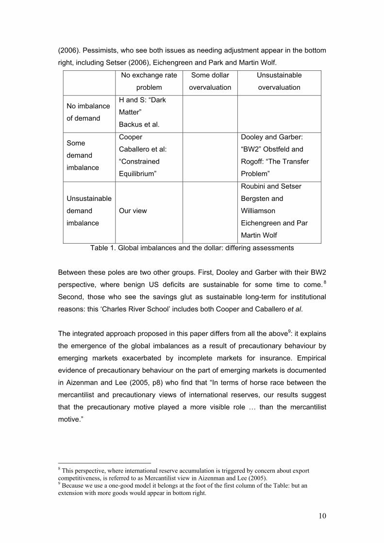
Table 1 provides a brief summary of these views, classified by whether the need to

adjust the pattern of global demand and/ or the need to adjust the dollar exchange

rate is seen as a major problem. 7 Outright optimism, which sees neither as a

problem, appears in the upper left right corner, represented by Hausmann and

Sturzenegger - for whom Dark Matter dispels all doubts – and by Backus et al.

7 For an alternative summary, listing ten causes of current imbalances, see Roubini (2006).

10

(2006). Pessimists, who see both issues as needing adjustment appear in the bottom

right, including Setser (2006), Eichengreen and Park and Martin Wolf.

No exchange rate

problem

Some dollar

overvaluation

Unsustainable

overvaluation

No imbalance

of demand

H and S: “Dark

Matter”

Backus et al.

Some

demand

imbalance

Cooper

Caballero et al:

“Constrained

Equilibrium”

Dooley and Garber:

“BW2” Obstfeld and

Rogoff: “The Transfer

Problem”

Unsustainable

demand

imbalance

Our view

Roubini and Setser

Bergsten and

Williamson

Eichengreen and Par

Martin Wolf

Table 1. Global imbalances and the dollar: differing assessments

Between these poles are two other groups. First, Dooley and Garber with their BW2

perspective, where benign US deficits are sustainable for some time to come. 8

Second, those who see the savings glut as sustainable long-term for institutional

reasons: this ‘Charles River School’ includes both Cooper and Caballero et al.

The integrated approach proposed in this paper differs from all the above9: it explains

the emergence of the global imbalances as a result of precautionary behaviour by

emerging markets exacerbated by incomplete markets for insurance. Empirical

evidence of precautionary behaviour on the part of emerging markets is documented

in Aizenman and Lee (2005, p8) who find that “In terms of horse race between the

mercantilist and precautionary views of international reserves, our results suggest

that the precautionary motive played a more visible role … than the mercantilist

motive.”

8 This perspective, where international reserve accumulation is triggered by concern about export competitiveness, is referred to as Mercantilist view in Aizenman and Lee (2005). 9 Because we use a one-good model it belongs at the foot of the first column of the Table: but an extension with more goods would appear in bottom right.

11

The paper is structured as follows. Using the Fisherian inter-temporal approach,

Section 2 briefly looks at the savings when there is no uncertainty. Section 3

develops the benchmark model of general equilibrium with uncertainty where risk in

the emerging markets (henceforth referred to as ‘EM’) is shared with the US without

substantial surpluses or deficits. Section 4 introduces loss aversion and

precautionary saving. In the absence of complete markets, substantial risk can lead

to substantial imbalances and negative real interest rates. Interestingly, the absence

of insurance allows us to use Fisher’s approach to characterise a global equilibrium

of fear and market failure. Section 5 discusses whether strategic factors may account

for the limitation of insurance markets. Section 6 discusses sustainability and the

temporary nature of the precautionary savings. Section 7 considers the possible

emergence of Keynesian equilibrium due to a Liquidity Trap and/ or a ‘Sudden Stop’

in capital flows. Section 8 concludes that a savings glut could lead to deficient world

demand if it is combined with financial panic that prevents the US from acting as

“consumer of last resort”.

2. External Imbalances and Irving Fisher

Irving Fisher viewed savings and investment decisions from the perspective of

optimising consumption over time 10 : and applying this perspective to countries

involved in international trade has led to the now-popular inter-temporal approach to

the balance of payments. As Obstfeld and Rogoff (1996, Chapter 1) express it,

“Much of the macroeconomic action in an open economy is connected with its inter-

temporal trade, which is measured by the current account of the balance of

payments”.

Before introducing our general equilibrium approach, which includes risk as well, we

sketch three variants of the neo-Fisherian perspective that bear on the current

debate. First that current account imbalances may reflect international differences in

growth rates, as suggested by Backus et al. (2006); second that, with no growth

differentials, imbalances may reflect capital market constraints, as in Caballero et al.

(2005); a third, closely-related possibility is that behaviour may be reflecting insecure

10 As, in a full employment context, did Keynes and Ramsey (1928).

12

property rights in the EM, the Cooper hypothesis. These can be illustrated simply as

in Figure 1.

Figure 1. Fisher diagram: differentials in growth, wealth constraint and pessimism

First let the endowment of the US be at point A and that of EM at A’, the former

exhibiting high growth and the latter no growth. Given identical tastes, these growth

differentials provide incentives for inter-temporal trade. The US can smooth

consumption by consuming EM saving at interest rates lying between the pure rate of

time-preference shown at A’ and the much high rate of inter-temporal substitution at

point A (where the slope of the indifference curve also reflects the high growth rate).

The equilibrium trade vectors are shown by A’B and AC and both countries end up

consuming on the same ray from the origin. We believe this captures the spirit of the

“business-as-usual” global equilibrium perspective of Backus et al. (though it is

admittedly something of a caricature as growth differentials are taken as exogenous).

Next assume by contrast that both countries have identical endowments at point A.

While the US consumes with the appropriate inter-temporal budget constraint, let the

EM be constrained to lower budget line passing through A’ as might be the case if

capital markets fail to take due account of future endowments. The consumption and

savings in period 1 will be precisely the same as for the case of growth differentials.

Could this represent the capital-constrained perspective of Caballero et al? (Probably

not, because it would not be sensible for the EM to save knowing that it is about to

receive the same endowment as the US!)

A

A’

B

C

C1, Y1

C2, Y2

13

But what if consumers in the EM are not sure that they will secure the extra output-

because of ill-defined property rights, as Cooper says is true in China? Then they

might act ‘as if’ their expectations of the growth in the EM were unduly pessimistic –

as if they expected output in EM to be stationary, for example. In which case, despite

the fact that both countries have identical endowments at point A, insecure

ownership might lead to the same high savings in EM and low global interest rates as

predicted Backus et al.

These inter-temporal accounts are essentially deterministic: would a stochastic

specification have something more to offer? This is what we explore next, first with

standard (logarithmic) preferences and then with the introduction of loss aversion.

With the addition of market failure, we find that loss aversion generates a constrained

equilibrium rather similar to that of Cabbellero et al. and Cooper.

3. General Equilibrium with Complete Markets

To incorporate risk, we use a simplified dynamic stochastic general equilibrium

(DSGE) model in the tradition of Mas-Colell et al (1995) and Obstfeld and Rogoff

(1996). This stylised one good model has two time periods, two states of nature and

two countries – the US and EM; and we use the asterisk suffix ‘*’ to denote EM. The

framework is similar to that used earlier to study global finance and the US New

Economy in Miller et al (2005, 2006), though the endowment pattern reflects the

traditional situation where the US invests in risky assets and supplies safety and

security in exchange (Hausmann and Sturzenegger, 2005).

Rather than postulating growth differentials, with low growth for the EM accounting

for low world real interest rates and large US deficits, we assume identical expected

growth but differential risk. Specifically growth prospects in EM have greater volatility

than for the US, modelled by adding a mean-preserving spread. Though this does

not have a great impact in a standard general equilibrium framework, results change

when downside risk is aggravated by a form of Loss Aversion. (The utility of

consumption in period 2 which lies below that reached in the previous period is

sharply discounted.) In a stochastic environment, the resulting risk sensitivity can

lead the EM to acquire substantial insurance; and to act ‘as if’ it underestimates the

mathematical expectation of growth.

14

When the relevant insurance is not available (or the provision is not credible), the EM

can always ‘self-insure’ – saving instead of swapping financial promises. So the

desire to limit downside risk can make the EM act ‘as if’ it has very low time

preference as we show in numerical outcomes below. Combining inadequate

insurance with Loss Aversion provides a ready explanation for low interest rates, the

US deficit and high EM savings.

To put this in context, consider the case of China. After what happened to many East

Asian countries in 1997/811, it is clear that interruptions to trend growth are perfectly

possible: and the rampant Chinese Dragon may be no more immune to shocks than

were the Asian Tigers. In the words of Peter Nolan (2004, pp48-49):

Today, the Chinese economy is growing fast, but the lesson from

the past, especially the Asian Financial Crisis, is that perceptions

can change overnight. China is today the last remaining large

‘Growth story’ in the world; it already has a huge ‘bubble’ of FDI,

with the largest FDI inflows of any economy in the world… It is easy

to imagine how the bubble might burst, and the flow of capital be

reversed, with huge potential de-stabilizing consequences for the

economy and society. There would then be a full-blown ‘Chinese

Financial Crisis’. A central goal of policy must be to avoid such an

outcome. [Italics added]

If there is concern that consumption on the downside should not fall relative to past

levels, China can of course seek insurance by selling FDI and buying US government

bonds: and it can also seek to self-insure by acquiring US bonds via the current

account. If, for any reason, the first option is limited, then self-insurance will be seen

as the only way to avoid an unappealing prospect – the prospect, perhaps, of

humiliation like that suffered by its near neighbour South Korea in 1997/1998 when it

had to go cap in hand to the IMF and G7 and sacrifice sovereignty to get the financial

support it needed in the crisis.12

11 when, in the crisis, trend growth rates effectively changed sign. 12 Stiglitz (2006, p248) comments “The East Asian countries that constitute the class of ’97 – the countries that learned the lessons of instability the hard way in the crises that began in that year – have boosted their reserves in part because they wanted to make sure that they won’t need to borrow from the IMF again. Others, who saw their neighbours suffer, came to the same conclusion – it is imperative to have enough reserves to withstand the worst of the world’s economic vicissitudes.”

15

These considerations may suggest that strategic factors play a role that is not

captured in the competitive framework we use here13– that some sort of insurance

market game may be in process. This is discussed briefly in section 4 below.

3.1 The Benchmark Case

The pattern of endowments assumed is indicated in Table 2. Both blocs are endowed

with one unit at time one. In expected terms each bloc grows at the rate g , say three

percent. In the absence of uncertainty each bloc would consume its endowment and,

with log utility, real interest rates would equal growth rate plus the pure rate of time

preference. If the latter were, say, 1.5 percent, this would imply the global real

interest rates of 4.5%.

With uncertainty, consider the case where future endowments for EM can take one of

two values: high and low, with a standard deviation of σ around the mean rate of

growth. (For convenience, each of the two outcomes is treated equi-probable; and in

simulationsσ varies between 3 to 12 %. But the assumption of symmetry for the

shocks to EM growth is made for expositional convenience. The main results are

independent of the shape of the probability distribution, as is noted below.)

USA EM

High (with

probability π )

Low (with

probability π−1 )

Period 1 11 =Y 1*1 =Y 1*

1 =Y

Period 2 gYY +== 1)2()1( 22 σ++= gY 1)1(*2 σ−+= gY 1)2(*

2

Table 2. The pattern of endowments

To study the pattern of savings and world real interest rates, we first present

benchmark results where the complete set of Arrow-Debreu securities can be traded.

Later we look at how these results may change if the set of securities is restricted or

preferences modified. To simplify the exposition of the benchmark results, we

assume representative consumers in both countries share identical preferences.

Home country’s lifetime utility is given by

13 We are grateful to Sayantan Ghosal for this observation. It carries the implication that the model of ‘unrelentingly competitive’ Incomplete General Equilibrium with default studied by Dubey et al (2005) is not really appropriate here.

16

))]2(ln()1())1(ln([)ln())(,( 22121 CCCCCU ππβ −++=⋅ (1)

where β is time preference, 1C and )(2 ⋅C are period 1 and period 2 consumption

respectively. The budget constraint of US is given by

WYqYqYCqCqC ≡++=++ )2()2()1()1()2()2()1()1( 221221 (2)

where 0)( >sq ( 2,1=s ) are Arrow prices measured in period 1 sure consumption,

and W is the present value of US’s total wealth.

Given Arrow prices, US’s optimal consumption implied by its first order conditions are

simply

β+=

11WC . (3)

12 )1()1( C

qC βπ

= (4)

12 )2()1()2( C

qC πβ −

= (5)

Those for EM follow the same forms.

Applying equilibrium conditions, that total consumption in each period and state

equals the corresponding total endowment, determines the equilibrium Arrow prices

and real interest rates as follows:

)1(/)1( 21WW YYq πβ= (6)

)2(/)1()2( 21WW YYq βπ−= (7)

)1/(1)( rsqs

+=∑ (8)

where superscript W indicates world endowment. The pattern of consumption is

obtained by substituting (6) and (7) into (3), (4) and (5).

With the endowments specified in Table 2, EM has an incentive to save in period 1.

This is evident from a comparison of EM wealth relative to US wealth. Note that

17

WqqWW <−−= )))1()2(((* σ

where σ is the standard deviation of the EM endowment and )1()2( qq > .

Because EM wealth is relatively lower, so is consumption, i.e.

1**

1 )1/()1/( CWWC =+<+= ββ . So EM saves, matched by a US current account

deficit. Clearly the more volatile is EM’s endowment is in period 2 (i.e. the greater is

σ ), the higher will be its period 1 savings. But with log utility and efficient provision of

‘insurance’, the savings effects are distinctly modest, as will be seen in Table 3.

High state EM

US

Contract Curve

Endowment Point A

Low state

-σ

g

Mean income for EM

Y*1

E BInsurance

Saving

+σ

Figure 2. Endowments and trading opportunities in Period 2 – the Edgeworth Box

How securities markets provide this insurance is indicated graphically in Figure 2, an

Edgeworth box diagram as in Mas-Colell et al (p.593, 1995) describing allocations in

period 2. Outcomes for the high payoff state are on the horizontal and for the low

payoff state on the vertical, and utility for the EM is measured from the lower left

corner and that for US from the upper right. Identical probability assessments and

utility functions imply that the contract curve is the diagonal in the figure.14 The

autarky endowment point is at A, where for the US – identical endowments in both

states – this lies on the 45-degree line measured from the upper right corner. For the

EM, however, disparity in the endowment between the two states means that it lies to

14 The assumption of identical utility is more restrictive than Mas-Colell et al (p.693, 1995) where the contract curve is non-linear.

18

the right of the 45-degree line drawn from the bottom left corner. Ignoring the effect of

the first period savings on reallocating entitlements (as they are so small, see Table

3), general equilibrium consumption is shown at point E (on the contract curve).

How much does aggregate risk affect global interest rates and current account

imbalances? Not very much, if we use parameter values of 985.0=β , 2/1=π , and

endowments from Table 2, where average growth is 3% in both blocs.

3σ = 12σ =

US deficit 0.01 0.2 Benchmark

Real interest rate 4.5% 4.2%

US deficit 0.02 0.34 Bonds-only

Real interest rate 4.5% 3.9%

US deficit 0.01 1.2 LA with

complete

markets

Real interest rate 4.5% 3.5%

US deficit 0.02 4.6 LA with

bonds-only Real interest rate 4.5% -4.3%

Table 3. US deficits and the world real interest rates: 4 cases.

Note: LA refers to Loss Aversion. US deficits are measured as percentage of period

1 GDP. All simulations assume equi-probable states; but, for the case of LA and

bonds only, the results are in fact independent of state probabilities.

From lines 2 and 3 for the Benchmark case in Table 3, it is evident that stochastic

endowments for the EM do lead to some lowering of world interest rates and some

increase in the US deficit as the theory predicts: but with log preferences the

quantitative effects are very small. Increasing the standard deviation from 3% to

12%, for example, only increases the US deficit by one fifth of a percentage point of

GDP; and it shaves a mere 30 basis points off the world interest rate.

19

High state EM

US

Contract Curve

Endowment Point A

Low state

E

B

FDIBonds

1 2/q q

Figure 3: Buying insurance: a swap of GDP-Bonds.

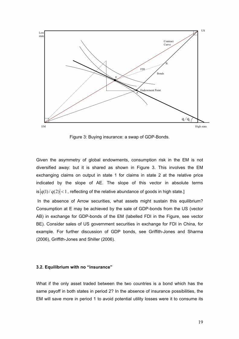
Given the asymmetry of global endowments, consumption risk in the EM is not

diversified away: but it is shared as shown in Figure 3. This involves the EM

exchanging claims on output in state 1 for claims in state 2 at the relative price

indicated by the slope of AE. The slope of this vector in absolute terms

is (1) / (2) 1q q < , reflecting of the relative abundance of goods in high state.]

In the absence of Arrow securities, what assets might sustain this equilibrium?

Consumption at E may be achieved by the sale of GDP-bonds from the US (vector

AB) in exchange for GDP-bonds of the EM (labelled FDI in the Figure, see vector

BE). Consider sales of US government securities in exchange for FDI in China, for

example. For further discussion of GDP bonds, see Griffith-Jones and Sharma

(2006), Griffith-Jones and Shiller (2006).

3.2. Equilibrium with no “insurance”

What if the only asset traded between the two countries is a bond which has the

same payoff in both states in period 2? In the absence of insurance possibilities, the

EM will save more in period 1 to avoid potential utility losses were it to consume its

20

unequal endowments in period 2, and the extra savings will bring down the global

rate of interest. This can be shown as follows.

Denote S the first period saving by US (the amount of bonds purchased), its optimal

level is determined by the solution to the following problem:

))]}2(ln()1())1(ln([){ln( 221 CCCMaxS ππβ −++ (8a)

subject to

SYC −= 11 (8b)

SrYC )1()1()1( 22 ++= (8c)

SrYC )1()2()2( 22 ++= (8d)

where )1( r+ is the gross real interest rates.

As 222 )2()1( YYY == , the optimal saving implies the period 1 consumption

⎟⎠⎞

⎜⎝⎛

++

+=

rYYC

111 2

11 β (8e)

One can solve for a similar problem for EM to yield its period 1 consumption

)1(2)1(42

1*1 β

ςβξξ+

+−+−−= YC (9)

where

1*

2*

2*

2*

2 )1()]1()1()2([)2()1( YrYYYY +−−+++= βππβξ

)]1()1()2([)1()2()1( *2

*21

*2

*2 YYYrYY ππβς −++−=

Imposing equilibrium condition

1*11 2YCC =+

yields the following fixed point condition for real interest rates

0)1(11 1

22

12 =++⎟

⎠⎞

⎜⎝⎛ −+

+⎟⎠⎞

⎜⎝⎛ −+

ςββξβ Yr

YYr

Y (10)

Equations (9) and (10) are used to generate numerical results in lines 4 and 5 for the

Bonds-only case in Table 3.

EM saving as percentage of GDP (and the US deficit) is twice as large as in the

Benchmark case, but it still remains very small even when standard deviation of the

21

shock to its endowment rises to 12%. With log utility, therefore, eliminating insurance

does not predict a savings glut in the EM. (The effect of increasing risk on the world

interest rate is more pronounced: it falls by 60 basis points, to less than 4%, when

the standard deviation increases from 3 to 12%.)

4. Global Equilibrium with Loss Aversion

4.1. Loss aversion with a complete set of Arrow securities

In this section, we modify the preferences of the EM by incorporating two elements

from Prospect Theory (Kahneman and Tversky, 1979): namely, reference

dependence and loss aversion. We assume that consumption achieved in the

previous period acts as a reference in the current period, so the measurement of

utility depends on whether there is a “loss” or a “gain” in current consumption relative

to this reference. To capture loss aversion, we assume that, close to the reference

point, the increase in utility of a unit “gain” in current consumption (relative to the

reference) is much smaller than the decrease in utility of a unit “loss” in current

consumption.

Specifically, let the utility of state i consumption be defined as

⎩⎨⎧

<≥

= *1

*2

*1

*2

*1

*2

*1

*2*

2 )()/)(ln()()/)(ln(

))((CiCifCiC

CiCifCiCiCu

λ (11)

where 1>λ indicates the degree of loss aversion. (Note that the utility measure

becomes negative for consumption below reference level.)

To make the following treatment tractable, we consider a limiting case of loss

aversion, namely, +∞→λ . Under this simplification which implies extreme disutility

of any contraction of consumption, (11) is equivalent to imposing the constraint that *1

*2 )( CiC ≥ (12)

The procedure used here, of imposing the constraint that next period’s consumption

in any state of the world should not fall below consumption in the current period,

could also be viewed as an extreme form of habit formation as widely used in

macroeconomic models. Chari, Kehoe and McGrattan (2002), in their attempts to

22

determine whether sticky prices can lead to volatile and persistent real exchange rate

movements, for example, assume in one experiment that the utility from consumption

depends not on current consumption but its level relative to a fraction of last period’s

aggregate consumption. A similar formulation has also been used by Campbell and

Cochrane (1999), Carroll, Overland, and Weil (2000), Ravn, Schmitt-Grohe, and

Uribe (2004). As Carroll et al show, with this form of habit-persistence in

consumption, higher growth may lead to higher saving.

In what follows, we show that loss aversion can also increase savings, but only if

consumption would otherwise have fallen below the reference trigger. With complete

contingent securities, US optimal consumption is derived in the same way as in

Section 2.1. But EM’s optimal consumptions are solutions to the following problem:

))]}2(ln()1())1(ln([){ln( *2

*2

*1)(, *

2*1

CCCMaxiCC

ππβ −++ (13)

subject to the budget constraint **

2*

2*

1*2

*2

*1 )2()2()1()1()2()2()1()1( WYqYqYCqCqC LALALALA ≡++=++ (14)

and (12).

How does loss aversion in EM change the equilibrium prices and allocation? We

summarise these results in the following propositions.

Proposition 1. If 2gσ ≤ , equilibrium prices and allocation are the same as those in

Section 2.1.

Proof: See Appendix A.

Note that with complete Arrow securities, both countries can share risks. This risk-

sharing means that both countries consume more or less equal proportions of the

aggregate state endowment. So if the standard deviation of EM endowment in period

2 is small, EM is effectively insured against low consumption in the bad state.

Therefore, no additional saving is required.

23

E-σ

Y*1=C*1

High stateEM

USLow State

Contract Curve

Endowment PointA

+σ

E-σ

Y*1=C*1

High stateEM

USLow State

Contract Curve

Endowment PointA

+σ

Figure 4a. Unchanged equilibrium when the loss aversion constraint fails to bind

Proposition 1 is illustrated in Figure 4a, where point E represents optimal

consumption allocation with loss aversion. The loss aversion constraint is

represented the L-shaped lined emanating from the point * *1 1Y C= , and all EM

consumption allocations to the north-east of this point satisfy the constraint. As point

E lies on the contract curve north-east of point * *1 1Y C= , the loss aversion constraint

is not binding; and equilibrium in Figure 4a is identical to that in Figure 3. When risk

increases, however, equilibrium can change as indicated in the following proposition.

Proposition 2. For the endowment structure given in Table 2, if 2gσ > , then

(1) )1()1( qq LA > and )2()2( qq LA > ;

(2) )1(/)2()1(/)2( qqqq LALA > ;

(3) rr LA < ;

(4) *1

*1 )( CLAC ≤ .

(5) * * * *2 2 2 2(2, ) / (1, ) (2) / (1)C LA C LA C C>

Proof: See Appendix B.

Results in Proposition 2 are quite intuitive. If the standard deviation of period 2 EM

endowment is large, simple risk sharing is not sufficient to ensure that the

consumption in the bad state remains above the reference level for the EM country.

24

So loss aversion increases EM’s demand for insurance in period 2. As this raises the

relative price )1(/)2( LALA qq , EM also increases savings as a substitute for high cost

insurance. (Note that period 1 savings for EM not only act as a substitute for

insurance but also reduce the reference consumption in period 2, making the

constraint less likely to bind.) Proposition 2(5) implies that consumption allocation in

period 2 when loss aversion constraint is binding lies above the contract curve

associated with no loss aversion.

Suppose we allow EM to have a different parameters for time preference, 'β , and

the subjective probability parameter, 'π , while keeping those of US as before, can

we replicate the outcomes in Proposition 2 without evoking the assumption of loss

aversion? The results for this “as if” exercise are given in the following proposition.

Proposition 3. For a set of parameters }',';,{ πβπβ (and given restriction on

endowments as in Proposition 2) to replicate the equilibrium results in Proposition 2,

it is sufficient that

(1) πβπβ

βππ <++

+=

)2()1())2(1(' LA

LA

qq

(2) βπβ

βπββ >−+

++=

)1(1)2()1('

LAq

Proof: See Appendix C.

Proposition 3 indicates that the effects of introducing loss aversion on the part of the

EM will (when the constraint is binding) be to increase its perceived pessimism

( ππ <' ) and to make it more forward-looking ( ββ >' ).

How loss aversion can impact on global equilibrium is illustrated using Figure 4b, the

Edgeworth box used earlier. As before, points A and E represent EM’s second period

endowment and consumption allocation in the absence of loss aversion. With large

enough σ , however, the loss aversion constraint becomes binding and EM will

increase its first period savings (Proposition 2(4)), moving its second period effective

endowment from A (along the 45 degree line) to B. The binding of the loss aversion

constraint will also change relative Arrow prices (Proposition 2(2)), making EM’s

period 2 budget constraint flatter (see line BE’). The intersection of the budget line

25

BE’ with the loss aversion constraint * *

2 1( )C L C= defines the new equilibrium E’ which

lies above the contract curve due to Proposition 2(5). From A, a combination of

savings and an asset swap of US bonds for FDI allows for consumption at point E’

satisfying the loss aversion constraint.

Figure 4b: Savings and insurance with Loss Aversion; it’s ‘as if’ time preference has

fallen and pessimism has increased in EM.

As indicated in Proposition 3, this new equilibrium may also be replicated without loss

aversion if EM has lower time preference (higher β ) and greater pessimism (lower

π ). As can be seen in Figure 4b, the increase in pessimism in the EM, calibrated by

a fall in ππ /' , has two effects: first it makes the contract curve concave, and second

it changes the relative Arrow prices which makes EM’s budget constraint flatter. The

decrease in the time preference, calibrated by the increase in ββ /' , has the effect of

increasing EM’s savings and so shifting its second period effective endowments from

A to B. The intersection of the budget constraint BE’ with the modified contract curve

defines the equilibrium.

The quantitative significance of loss aversion on real interest rates and savings is

indicated in lines 6 and 7 for the third case considered in Table 3. With the standard

deviation of up to 6%, the constraint is not binding, so the real interest rates and

savings are the same as in the benchmark case. But the effect of loss aversion

becomes apparent when the standard deviation increases to 12%: this generates a

H igh EM

US

Old Contract Curve

A

Low State

BE

E’

New Contract Curve

BondsFDI

B’

σ C2*(L)=C1*

M

C1*

gY1*

26

substantial increase in the EM savings and a marked fall in the global interest rates.

As a consequence, the US deficit rises by 1% of GDP as a 0.7% fall of the real

interest rates encourages US consumption.

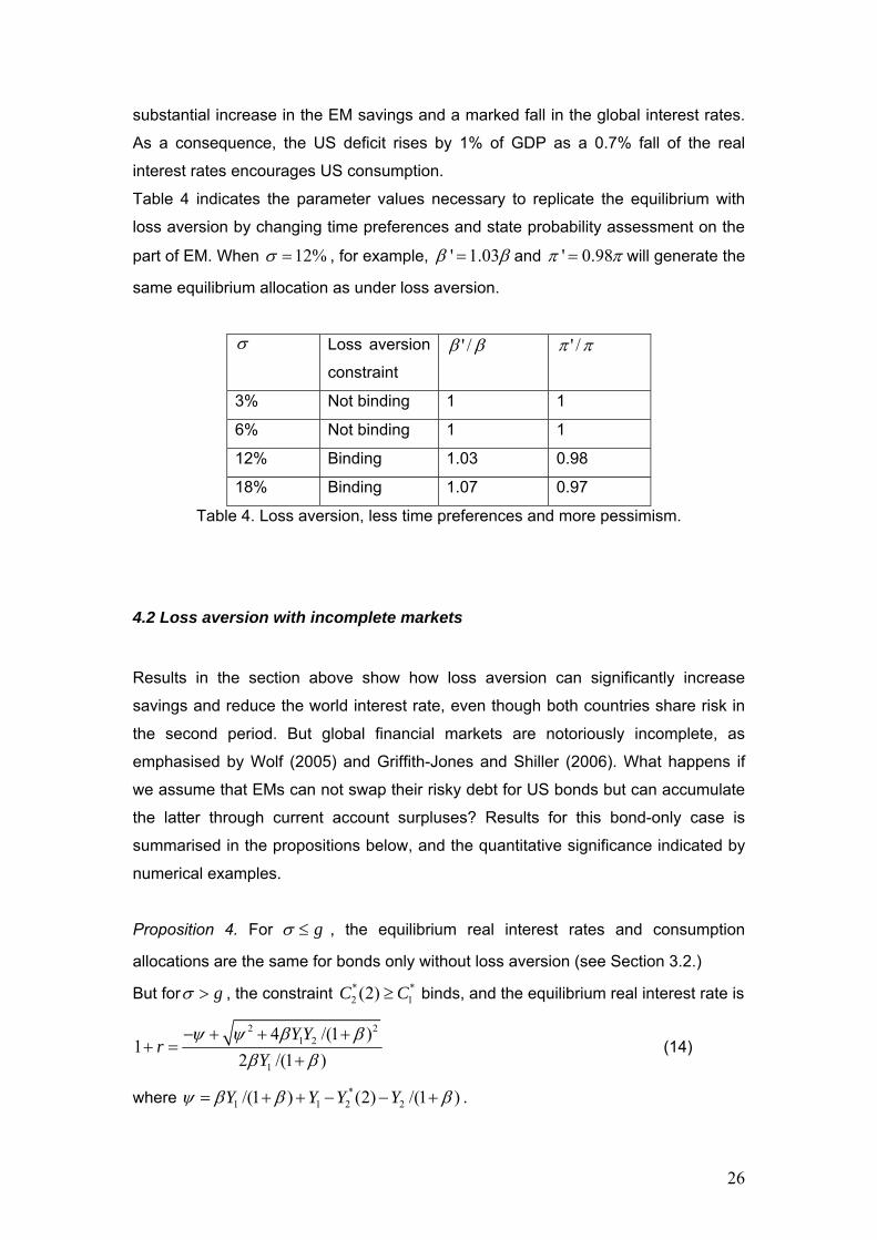
Table 4 indicates the parameter values necessary to replicate the equilibrium with

loss aversion by changing time preferences and state probability assessment on the

part of EM. When 12%σ = , for example, ' 1.03β β= and ' 0.98π π= will generate the

same equilibrium allocation as under loss aversion.

σ Loss aversion

constraint ββ /' ππ /'

3% Not binding 1 1

6% Not binding 1 1

12% Binding 1.03 0.98

18% Binding 1.07 0.97

Table 4. Loss aversion, less time preferences and more pessimism.

4.2 Loss aversion with incomplete markets

Results in the section above show how loss aversion can significantly increase

savings and reduce the world interest rate, even though both countries share risk in

the second period. But global financial markets are notoriously incomplete, as

emphasised by Wolf (2005) and Griffith-Jones and Shiller (2006). What happens if

we assume that EMs can not swap their risky debt for US bonds but can accumulate

the latter through current account surpluses? Results for this bond-only case is

summarised in the propositions below, and the quantitative significance indicated by

numerical examples.

Proposition 4. For gσ ≤ , the equilibrium real interest rates and consumption

allocations are the same for bonds only without loss aversion (see Section 3.2.)

But for gσ > , the constraint * *2 1(2)C C≥ binds, and the equilibrium real interest rate is

2 21 2

1

4 /(1 )1

2 /(1 )YY

rY

ψ ψ β ββ β

− + + ++ =

+ (14)

where *1 1 2 2/(1 ) (2) /(1 )Y Y Y Yψ β β β= + + − − + .

27

The consumption allocation for EM is given by * * *2 2 1 2(1) (1) (1 )( (2)) /(2 )C Y r Y Y r= + + − + (15)

* * *2 1 1 2(2) [(1 ) (2)] /(2 )C C r Y Y r= = + + + (16)

and the consumption allocation for US can be obtained simply by using the market

clearing conditions.

Proof: For gσ ≤ , one can show that * *2 1(2)C C≥ , so real interest rates and

consumption allocation in Section 3.2 still constitute the equilibrium solution.

For gσ > , however, solutions in Section 3.2 violate the constraint * *2 1(2)C C≥ .

Imposing binding constraint yields the optimal consumption for EM as in (15) and

(16). The optimal consumption for US, derived in the same way as in Section 3.2,

gives

21 1

11 1 1

Y WC Yrβ β

⎛ ⎞= + ≡⎜ ⎟+ + +⎝ ⎠ (17)

2 2(1 )(1) (2)1

r WC C ββ

+= =

+ (18)

Using market clearing condition 1*11 2YCC =+ one arrives at the equilibrium real

interest rates represented by (14). Using (14), one can back out the equilibrium

consumption for both US and EM.

Two implications of the above proposition are worth noting. First that, with bonds

only, the loss aversion constraint * *2 1(2)C C= binds for a smaller σ than is the case

when Arrow securities can be traded. This is because the removal of state-contingent

securities means that risk can not be shared at a global level, so EM has to self-

insure by increasing savings even for a moderateσ . Second that, when the loss

aversion constraint is binding, the global real interest rate is determined

independently of state probabilities.

28

Figure 5. Loss Aversion and Precautionary Saving

In state space form, equilibrium with fear and market failure is shown in Figure 5.

Note that due to incomplete markets, there is no asset swap of GDP-bonds: instead,

to acquire US bonds, EM is forced to self-insure by saving in period 1. The effective

endowment position in period 2 shifts from A to B where the vector AB includes the

interest rate on savings. How this interest rate is determined can be seen in the

following Fisher diagram.

As before, the horizontal axis measures endowments and consumption in period 1,

and the vertical outcomes in period 2. Point A describes the income in both periods

for US and the hyperbola AF represents US offer curve15. (Point A also indicates first

period income and average second period endowments for EM.) For any given

interest rate, the intersection of the appropriate US budget constraint AA’ and the

offer curve AF determines the optimal inter-temporal consumption allocation of the

US (at point A’) and the US current account deficit.

15 The parametric representations of the US offer curve is given by the US inter-temporal budget constraint and the proportionality condition, 2 1/ (1 )C C r β= + , implied by its first order conditions. Replacing the real interest rates in one of the equations using the other gives the US offer curve.

High state EM

US

Asset swap(insurance)

Contract Curve

Endowment Point A

Savings in Bonds

σ

σ

Low state

E

g Y1*

C*1

Savings in Bonds

A

C*2(L)= C*1

M

B

29

First periodPrecautionary Savings

C2*(L)

Y2*(L)

Y2*(H)

Second period

AY2

Y1

g

A’

L’

L

H’

H

“Consumer of Last Resort”

C1* C1 1+r1+r

EM USBudget Constraints

Loss Aversion Constraint - EM

F

US Offer Curve

First periodPrecautionary Savings

C2*(L)

Y2*(L)

Y2*(H)

Second period

AY2

Y1

g

A’

L’

L

H’

H

“Consumer of Last Resort”

C1* C1 1+r1+r

EM USBudget Constraints

Loss Aversion Constraint - EM

F

US Offer Curve

Figure 6: Global Equilibrium: Precautionary Saving and “the consumer of last resort”

Turning to the EM, when the constraint is binding its inter-temporal budget constraint, * * *1 2 1 2( ) /(1 ) ( ) /(1 )C C L r Y Y L r+ + = + + , is represented by the downward sloping line

passing through low state endowment L. To satisfy the constraint, consumption in the

first period and in the low state in the second period must lie on the 45-degree line

OC. The intersection of the budget line LL’ and this 45-degree line determines the

EM precautionary savings, indicated by the horizontal distance *1 1C Y . As σ increases,

and point L moves downwards, precautionary savings will go up.

How is the world interest rate to be determined? For markets to clear in period 1, the

real interest rate has to fall sufficiently so that extra consumption by the US balances

precautionary savings by the emerging markets. In Martin Wolf’s words, the US has

to act as the global ‘consumer of last resort’ (Wolf, 2006). Diagrammatically, the real

interest rate must be chosen such that vector of excess consumption AA’ is equal

and opposite to the precautionary savings vector LL’, as in Figure 6. It is clear from

the figure that an increase in σ would result in an increase in the EM’s savings. To

ensure that this is matched by the US deficit, the budget line AA’ has to rotate anti-

clock-wise, reducing real interest rates.

30

Three observations are clear from the Figure. First, that as L’ is on a budget line

which lies below the usual Fisherian inter-temporal budget constraint, loss aversion

can apparently generate outcomes observationally equivalent to the lack of

capitalisation postulated by Caballero et al (2006) and the contrarian view of Cooper

(2005).

The second that the predictions for savings and global interest rates in period 1 do

not depend on the state probabilities. Figure 6 illustrates the global equilibrium for the

case where high and low states are equi-probable: so the US trading vector AA’ is

balanced by the equally weighted EM’s trading vectors LL’ and HH’. Consequently,

when high state is realised in period 2, this model predicts a massive increase in the

EM’s state consumption (given by point H’). But this unrealistic prediction can easily

be modified without changing savings behaviour. Consider for example, the case of

asymmetric shocks where there is low probability of a large negative shock and a

high probability of a small positive shock, see Jeanne and Ranciere (2006).

To keep the mean-preserving feature of the EM’s second period state endowments,

requires 2 2 2( ) (1 )( )H LY Y Yπ σ π σ+ + − − = or 1

H Lπσ σ

π−

= , where Hσ is the shock

in the high state and Lσ that in the low state. By fixing Lσ at the same level as that

in Figure 6, one can choose π close to 1 to make Hσ arbitrarily small. This would

yield the same equilibrium savings as drawn in Figure 6, but reduce EM’s high state

consumption substantially. This is because savings and the interest rate do not

depend on how likely the low state is but on how bad it is.

The third observation is that, given expectations of a large negative shock,

equilibrium real interest rates can be negative. In terms of the figure, this will occur

when the point A’ on the US offer curve required to match these savings is

sufficiently far to the right that the budget line has an absolute slope less than unity.

The algebraic condition for negative real rates is as follows:

Proposition 5. Given the endowment structure specified in Table 2, the real interest

rate 0r ≤ for (2 2 ) /(1 ) [2 /(1 ) 1]gσ β β β≥ − + + + + .

31

Proof: From (14), imposing the condition 0r ≤ , one obtains the parameter restriction

given in the above proposition.

This is illustrated numerically in the last two lines of Table 3, where for σ=12%

savings reaches 4.6% and the equilibrium real interest rate fall to -4.3%16.

The relationship between real interest rates and risk for parameters of our

benchmark model is illustrated in more detail in Figure 7 where the horizontal axis

measures the negative shock to EM’s period 2 endowment and the equilibrium real

interest rates is plotted on the vertical axis. When the loss aversion constraint is not

binding real interest rates decrease very slowly with increasing σ; but when the loss

aversion constraint is binding the real interest rates fall sharply as risk increases.

From Proposition 5, the critical level of σ beyond which the real interest turns

negative turns out to be about 7.5% for the parameters used here.

2 4 6 8 10 12Sigma

-4

-2

2

4

Interest Rate

Figure 7. Real interest rates and risk: numerical results.

Possible ramifications of negative real interest rates are discussed below. Here we

summarise the results of the earlier calibrations in a new table, where the effect of

fear is captured by moving from orthodox preferences to loss aversion and that of

market failure by restricting the set of Arrow securities. As can be seen from Column

1, fear does cause some increase in global imbalances but not a great deal; similarly

from row 1 we see that market failure also increases global imbalances, but only

16 Note that in their paper on the optimal level of international reserves for emerging market countries, Jeanne and Ranciere (2005) assume a crisis output cost of 10% in their benchmark calibration.

32

marginally. It is when fear and market failure combine that global imbalances become

significant and real interest rates can turn negative.

Arrow-Debreu Incomplete Markets

Orthodox

preferences

Δ deficit/GDP Δ interest rate

+0.2

-0.3

+0.3

-0.6

Loss Aversion in

EM

Δ deficit/GDP Δ interest rate

+1.2

-1.4

+4.6

-8.8

Table 4. The effect of increasing risk (from benchmark of σ = 3 to σ=12)

Note: For Jeanne and Ranciere (2006) σ of 10% might lead to imbalances of about

5%.

5. Strategic considerations

All the calculations reported above assume competitive equilibrium even when the

set of assets is incomplete. But, as Dooley and Garber (2005) point out, the big

players in asset markets are governments who can manipulate supply. Furthermore,

Meissner and Taylor have shown how Britain in the years 1870–1913 and US in

years 1981 – 2003 have been able to enjoy a “privilege” in the form of higher yields

earned on external assets than paid on external liabilities – worth about 0.5% of GDP

per annum in both cases. Could this, in the terminology of Hausmann and

Sturzenegger (2005), be the “dark matter” which allows the US to sustain substantial

portfolio imbalance? Maybe so, but Meissner and Taylor warn that such monopoly

power is a fading asset: the privilege is much higher in earlier years than later.17

Could one modify the competitive equilibrium by allowing for monopoly power on the

part of the US? Instead of supplying safe asset on a competitive basis, US could, for

example, select the utility maximising point on the demand for safe asset from the

EM: or could it act as a dynamic monopolist?18 As indicated by Table below this

17The gradual disappearance of the privilege is examined in Thamotheram, 2006. 18 Supplying dollars at high prices as the RoW accumulates reserves, with a dollar devaluation when reserve stock reaches equilibrium, see Section 7.2 below.

33

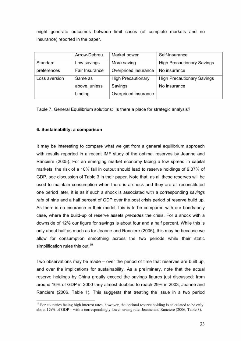
might generate outcomes between limit cases (of complete markets and no

insurance) reported in the paper.

Arrow-Debreu Market power Self-insurance

Standard

preferences

Low savings

Fair Insurance

More saving

Overpriced insurance

High Precautionary Savings

No insurance

Loss aversion Same as

above, unless

binding

High Precautionary

Savings

Overpriced insurance

High Precautionary Savings

No insurance

Table 7. General Equilibrium solutions: Is there a place for strategic analysis?

6. Sustainability: a comparison

It may be interesting to compare what we get from a general equilibrium approach

with results reported in a recent IMF study of the optimal reserves by Jeanne and

Ranciere (2005). For an emerging market economy facing a low spread in capital

markets, the risk of a 10% fall in output should lead to reserve holdings of 9.37% of

GDP, see discussion of Table 3 in their paper. Note that, as all these reserves will be

used to maintain consumption when there is a shock and they are all reconstituted

one period later, it is as if such a shock is associated with a corresponding savings

rate of nine and a half percent of GDP over the post crisis period of reserve build up.

As there is no insurance in their model, this is to be compared with our bonds-only

case, where the build-up of reserve assets precedes the crisis. For a shock with a

downside of 12% our figure for savings is about four and a half percent. While this is

only about half as much as for Jeanne and Ranciere (2006), this may be because we

allow for consumption smoothing across the two periods while their static

simplification rules this out.19

Two observations may be made – over the period of time that reserves are built up,

and over the implications for sustainability. As a preliminary, note that the actual

reserve holdings by China greatly exceed the savings figures just discussed: from

around 16% of GDP in 2000 they almost doubled to reach 29% in 2003, Jeanne and

Ranciere (2006, Table 1). This suggests that treating the issue in a two period

19 For countries facing high interest rates, however, the optimal reserve holding is calculated to be only about 1½% of GDP – with a correspondingly lower saving rate, Jeanne and Ranciere (2006, Table 3).

34

context (as the IMF study and we do) is too restrictive. The level of reserves may be

built up over a period of two or three years – and it can be expanded by assets

swaps as well as external surpluses, as the case with insurance has shown.

The second observation is that the reserve build-up is essentially a transitional

phenomenon: once reserves have reached their desired level, there is no need for

high precautionary savings 20 . This has profound implications: high savings, low

interest rate outcomes we have studied are not to be thought of as steady-state

equilibria, but as temporary phenomena. Putting it more bluntly, the precautionary

approach implies that the current pattern of imbalances is not sustainable. What this

might mean for global equilibrium is considered in Section 7.2.

7. The possibility of Keynesian equilibria

7.1 The Liquidity Trap

No matter that EM saving rises sharply as perceived risk increases, markets will clear

so long as the real interest rate is free to adjust. That is the message of the

calculations at the end of Section 4: and it seems to suggest that the model we

propose, like that of Caballero et al., is one of full employment equilibrium, loss

aversion or no.

It was found, however, that market-clearing interest rates have to be negative for

substantial risk (σ > 7.5%). What if there is a zero lower bound on the real interest

rate? This will imply that the US deficit is less than high savings in the EM in these

circumstances: in other words, global demand will fall short of global supply at full

employment levels of income.

When might such a bound be relevant? Consider a world with fixed nominal prices

and a zero lower bound on the nominal interest rate: in such a world, real rates can

be lowered by cutting nominal rates, but they cannot go below zero. (Nor would

adding price flexibility help, unless prices are expected to rise.) The case of Japan,

where the collapse of the Nikkei in the early 1990s was followed by a decade or more

20 We can show this in the GE context by changing the initial holding of bonds by the RoW, which play the same role as reserves as in the analysis of Jeanne and Ranciere (2006).

35

of inadequate demand with sticky prices and near zero nominal rates, may serve to

illustrate.

If one was to impose an exogenous zero bound on the real rates, how is the model to

be solved? One will have to make assumptions of what happens when markets do

not clear: that supply contracts until global demand and supply balance, for example.

Assuming that EM savings were proportional to its first period income, then a

contraction of EM income is sufficient to cut EM savings to match the US full

employment deficit would equate demand and supply. This is, in fact, something like

what happened after the East Asian crisis when countries in the region went into

sharp recession and the US acted as the ‘consumer of last resort’. But if income in

both countries can be treated as endogenous, there will be many other equilibria, as

there are two variables and only one constraint21.

Rather than pursuing this thought experiment much further, it is better to

acknowledge that one is re-examining issues at the heart of the debate between

Keynes and the Classics. Faced with a rise of savings, Classical economists argued

that interest rates would fall as needed to equate savings and investment (and

preserve full employment). Keynes objected that interest rates would be subject to a

lower bound (set by the Liquidity Trap) and, for this reason, income would become

endogenous, falling until savings matched investment. The Japanese experience has

led to a resurgence of interest in Keynesian equilibria, most notably in the 1998

Brookings Paper by Paul Krugman subtitled “Japan’s Slump and the Return of the

Liquidity Trap”.

7.2 A ‘Sudden Stop’?

Given robust expectations of growth, current real interest rates are surprisingly low;

but the world is not in a liquidity trap. Nevertheless, the pattern of global imbalances

has given economists cause for concern. Does the global model sustain such

concern or not? First, we conclude that a pattern of global imbalances where high

savings in the EM is matched by corresponding US deficits is essentially a

transitional phenomenon. So some adjustment will have to come.

21 It may be tempting, for this reason to aggregate across the two regions and treat the world as a closed economy.

36

When reserve positions are adequate, there will be no need for additional

precautionary saving, and EM should consume more and the US less. In addition,

however, relative prices may need to adjust. This is spelled out in detail in Obstfeld

and Rogoff (2005), for example, who argue that the price of US non-traded goods will

have to fall sharply relative to EM non-traded goods, and the relative price of US

traded goods will also have to fall. Given the objective of keeping the aggregate price

indices constant in each block, they calculate that this translates into a decline of

about 30% in the dollar. In their view, moreover, the perception that the situation is

not sustainable and that adjustment requires a fall in the dollar leaves the US

vulnerable to a Sudden Stop in capital flows.

No adjustment of relative prices is necessary in our one good model: but what if,

nonetheless, there a Sudden Stop were to occur constraining the US to balance its

current account? This would of course prevent the US from acting as ‘consumer of

last resort’, and require the EM to achieve balance on its own. If there is a

precautionary demand for savings outside the US – and particularly if there is limited

access to insurance markets – an excess supply of global savings will emerge. But,

in a world of low inflation and low nominal rates, the Classical argument that the

implied shortage of global demand can be remedied by an appropriate lowering of

interest rates lacks conviction. We have seen that a Liquidity Trap could, in principle,

prevent this adjustment even where the US is free to act as ‘consumer of last resort’:

how can it be relied to work in circumstances when the US consumption is checked

by financial panic?

8. Conclusion

A model of global equilibrium where countries outside the US face higher risk than

the US itself can lead to current account surpluses in the EM. If it is driven by Loss

Aversion, such precautionary savings can cause substantial ‘global imbalances’,

particularly if there is an inefficient supply of global insurance. In principle, this simply

requires lower real interest rates to ensure that aggregate demand equals supply at

the global level (though the required real interest may turn out to be negative). A

situation with low interest rates and high savings outside the US thus appears to be

an efficient global equilibrium: but is it sustainable?

37

A precautionary savings glut appears to us to be a temporary phenomenon, destined

for correction as and when adequate reserve levels are achieved. In a realistic

setting with differentiated traded and non-traded goods, this correction will also

require a substantial change in relative prices. So expectations of adjustment may

lead to a pre-emptive Sudden Stop in capital flows to the US, as Obstfeld and Rogoff

have suggested.

If the process of correction is triggered by panic, could it not lead to the inefficient

outcomes that concern macroeconomists such as Eichengreen and Park, Roubini

and Setser, and Martin Wolf? The unprecedented savings levels recorded in East

Asia since 1997/8 financial crises and the prolonged failure of Japan to escape from

a Liquidity Trap would then appear as early warning signals: and the failure to effect

a smooth transfer after the first World War, leading as it did to a Liquidity Trap and

the emergence of Keynesian under-employment economics, as a precedent that

should not be ignored. Blithe trust in market forces may be misplaced. When

precautionary savings is combined with financial panic, history offers no guarantee of

full employment.

38

References Aizenman, Joshua and Jaewoo Lee (2005), “International Reserves: Precautionary vs. Mercantilist Views, Theory and Evidence”, IMF Working Paper, WP/05/198. Bailey, A., S. Millard and S. Wells. (2001). “Capital Flows and Exchange Rates.” Bank of England Quarterly Bulletin, Autumn: 310-318. Backus, D; B Routledge, and SE Zin (2004), “Exotic Preferences for Macroeconomists”, NBER Working Paper 10597, June. Backus, David; Espen Henriksen; Frederic Lambert; and, Chris Telmer (2006), “Current Account Fact and Fiction,” Working paper, New York University. Bergsten, Fred and John Williamson (Eds) (2004) Dollar Adjustment: How Far? Against What? IIE:Washington DC. Buiter, W. (2006), “Dark Matter or Cold Fusion?”, Global Economics Paper No: 136, Goldman Sachs. See also: http://www.nber.org/~wbuiter/dark.pdf Caballero, Ricardo Emmanuel Farhi and Pierre-Olivier Gourinchas (2006), "An Equilibrium Model of "Global Imbalances" and Low Interest Rates", MIT Department of Economics, Working paper: 06-02 Campbell, John Y. and John H. Cochrane (1999), “By Force of Habit: A Consumption-Based Explanation of Aggregate Stock Market Behaviour,” Journal of Political Economy, vol. 107 no 2, 205-251. Carroll, Christopher D., Jody Overland, and David N. Weil (2000), “Saving and Growth with Habit Formation,” American Economic Review, vol. 90 no 3, 341-355. Chari, V. V., Patrick J. Kehoe, and Ellen McGrattan (2002), “Can Sticky Price Models Generate Volatile and Persistent Real Exchange Rates?” Review of Economic Studies, vol. 69 no 3, 533-563 Cooper, Richard (2005), “Living with Global Imbalances: A Contrarian View”, Policy Briefs in International Economics, IIE. November. Dooley, Michael, David Folkerts-Landau and Peter Garber (2004) "The revived Bretton Woods system," International Journal of Finance & Economics, vol. 9(4), pages 307-313. Dooley, Michael and Peter Garber, (2005) "The cosmic risk: an essay on global imbalances and treasuries," Proceedings, Federal Reserve Bank of San Francisco, issue Feb. Driffill, J. and A. and Snell (2003), "What moves OECD real interest rates?", Journal of Money, Credit and Banking, vol. 35 no 3, 375 - 402. Eichengreen, Barry and Yung Park (2006) “Global Imbalances: Implications for Emerging Asia and Latin America”. Presented at “Global Imbalances and Risk Management Has the center become the periphery?”, Madrid, May.

39

Gourinchas, P. and H. and Rey (2006), “From World Banker to World Venture Capitalist: US External Adjustment and the Exorbitant Privilege”, In Richard Clarida, ed., G7 Current Account Imbalances: Sustainability and Adjustment, University of Chicago Press, forthcoming. Griffith-Jones, Stephany and Krishnan, Sharma (2006) “GDP-Indexed Bonds: Making it Happen”. DESA Working Paper No. 21, Department of Economic and Social Affairs. Griffith-Jones, Stephany and Robert Shiller (2006), “A bond that insures against instability”, Financial Times, July 10th. Hanson, James (2006) “Global Imbalances: Resolving the US Peso Problem” Presented at “Global Imbalances and Risk Management: Has the center become the periphery?”, Madrid, May.

Hausmann, R. and F. Sturzenegger. 2005. “Global imbalances or bad accounting? The missing dark matter in the wealth of nations.” Mimeo, Harvard University.

Jeanne, Olivier and Romain Ranciere (2006) “The Optimal Level of International Reserves for Emerging Market Economies: Formulas and Applications”, Mimeo IMF Kahneman, D., & Tversky, A. (1979) “Prospect theory: An analysis of decision under risk”. Econometrica, 47, 263-291. King, Mervyn (2006), “Reform of the International Monetary Fund”, speech at the Indian Council for Research on International Economic Relations (ICRIER) in New Delhi, India. 20 February. Kohlscheen, Emanuel and Mark Taylor (2006) “International Liquidity Swaps: Is the Chiang Mai Initiative Efficiently Pooling Reserves?” Mimeo University of Warwick Krugman, Paul (1998) “It’s Baaak:Japan’s Slump and the Return of the Liquidity Trap” Brookings Paer s on Economic activity, No.2, pp 137-205.

Lane, P. R. and G. M. Milesi-Ferretti (2004), “Financial globalization and exchange rates.” CEPR DP: No. 4745.

Meissner, Christopher and Alan Taylor (2006), “Losing our Marbles in the New Century? The Great Rebalancing in Historical Perspective” Mimeo, Cambridge.

Miller, Marcus, Olli Castren and Lei Zhang (2005), “Capital flows and the US ‘New Economy’: consumption smoothing and risk exposure”. ECB Working Paper No. 459 (March).

Miller, Marcus, Olli Castren and Lei Zhang (2006), “Irrational Exuberance” and Capital Flows for the US New Economy: A Simple Global Model, mimeo, University of Warwick. (Forthcoming in International Journal of Finance & Economics.) Nolan, Peter (2004), China at the Crossroads, Oxford: Polity Obstfeld, M. and K. Rogoff (2005), Foundations of international macroeconomics, Cambridge MA: MIT Press

40

Obstfeld, M. and K. Rogoff (2005), “Global Current Account Imbalances and Exchange Rate Adjustments”, Brookings Papers on Economic Activity. Ravn, Morten, Stephanie Schmitt-Grohe and Martin Uribe (2004), “Deep Habits”, CEPR Discussion Paper 4269. Roubini, Nouriel (2006), “Mind the gap”, Global Economy and International Finance. See http://www.rgemonitor.com/blog/roubini/. Setser, Brad (2006) “Bretton Woods 2: Is it Sustainable?” Paper presented at “Global Imbalances and Risk Management Has the center become the periphery?”, Madrid, May. Stiglitz, Joseph (2006), Making globalization work, Penguin: London. Thamotheram, Craig (2006) “Sustainability of global imbalances”. MSc dissertation, University of Warwick Wolf, Martin (2005), “Will Globalisation Survive?”, World Economics, 6(4), pp.1-10. Wolf, Martin (2006), “Fixing Global Finance”, SAIS Lecture series, March 28-30.

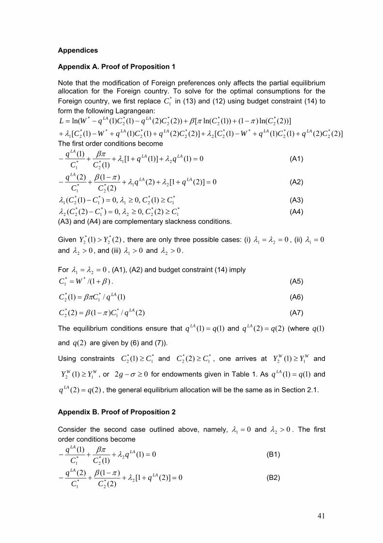
41

Appendices Appendix A. Proof of Proposition 1 Note that the modification of Foreign preferences only affects the partial equilibrium allocation for the Foreign country. To solve for the optimal consumptions for the Foreign country, we first replace *

1C in (13) and (12) using budget constraint (14) to form the following Lagrangean:

)]2()2()1()1()1([)]2()2()1()1()1([

))]2(ln()1())1(ln([))2()2()1()1(ln(*2

*2

**22

*2

*2

**21

*2

*2

*2

*2

*

CqCqWCCqCqWC

CCCqCqWLLALALALA

LALA

++−+++−+

−++−−=

λλ

ππβ

The first order conditions become

0)1()]1(1[)1(

)1(21*

2*1

=++++− LALALA

qqCC

q λλβπ (A1)

0)]2(1[)2()2()1()2(

21*2

*1

=+++−

+− LALALA

qqCC

q λλπβ (A2)

*1

*21

*1

*21 )1(,0,0))1(( CCCC ≥≥=− λλ (A3)

*1

*22

*1

*22 )2(,0,0))2(( CCCC ≥≥=− λλ (A4)

(A3) and (A4) are complementary slackness conditions. Given )2()1( *

2*

2 YY > , there are only three possible cases: (i) 021 == λλ , (ii) 01 =λ and 02 >λ , and (iii) 01 >λ and 02 >λ . For 021 == λλ , (A1), (A2) and budget constraint (14) imply

)1/(**1 β+=WC . (A5)

)1(/)1( *1

*2

LAqCC βπ= (A6)

)2(/)1()2( *1

*2

LAqCC πβ −= (A7)

The equilibrium conditions ensure that )1()1( qq LA = and )2()2( qq LA = (where )1(q

and )2(q are given by (6) and (7)).

Using constraints *1

*2 )1( CC ≥ and *

1*2 )2( CC ≥ , one arrives at WW YY 12 )1( ≥ and

WW YY 12 )1( ≥ , or 02 ≥−σg for endowments given in Table 1. As )1()1( qq LA = and

)2()2( qq LA = , the general equilibrium allocation will be the same as in Section 2.1.

Appendix B. Proof of Proposition 2 Consider the second case outlined above, namely, 01 =λ and 02 >λ . The first order conditions become

0)1()1(

)1(2*

2*1

=++− LALA

qCC

q λβπ (B1)

0)]2(1[)2()1()2(

2*2

*1

=++−

+− LALA

qCC

q λπβ (B2)

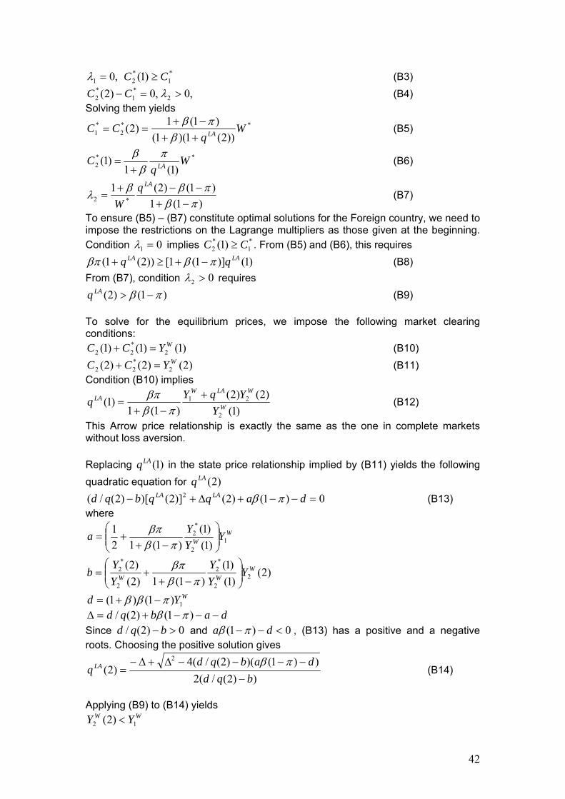
42

*1

*21 )1(,0 CC ≥=λ (B3)

,0,0)2( 2*1

*2 >=− λCC (B4)

Solving them yields **

2*1 ))2(1)(1(

)1(1)2( Wq

CC LA++−+

==β

πβ (B5)

**2 )1(1

)1( Wq

C LA

πβ

β+

= (B6)

)1(1)1()2(1

*2 πβπββλ

−+−−+

=LAq

W (B7)

To ensure (B5) – (B7) constitute optimal solutions for the Foreign country, we need to impose the restrictions on the Lagrange multipliers as those given at the beginning. Condition 01 =λ implies *

1*2 )1( CC ≥ . From (B5) and (B6), this requires

)1()]1(1[))2(1( LALA qq πββπ −+≥+ (B8) From (B7), condition 02 >λ requires

)1()2( πβ −>LAq (B9) To solve for the equilibrium prices, we impose the following market clearing conditions:

)1()1()1( 2*22

WYCC =+ (B10) )2()2()2( 2

*22

WYCC =+ (B11) Condition (B10) implies

)1()2()2(

)1(1)1(

2

21W

WLAWLA

YYqYq +

−+=

πββπ

(B12)

This Arrow price relationship is exactly the same as the one in complete markets without loss aversion. Replacing )1(LAq in the state price relationship implied by (B11) yields the following quadratic equation for )2(LAq

0)1()2()]2()[)2(/( 2 =−−+Δ+− daqqbqd LALA πβ (B13) where

WW Y

YY

a 12

*2

)1()1(

)1(121

⎟⎟⎠

⎞⎜⎜⎝

⎛−+

+=πβ

βπ

)2()1()1(

)1(1)2()2(

22

*2

2

*2 W

WW YYY

YY

b ⎟⎟⎠

⎞⎜⎜⎝

⎛−+

+=πβ

βπ

WYd 1)1()1( πββ −+= dabqd −−−+=Δ )1()2(/ πβ

Since 0)2(/ >− bqd and 0)1( <−− da πβ , (B13) has a positive and a negative roots. Choosing the positive solution gives

))2(/(2))1()()2(/(4

)2(2

bqddabqd

q LA

−−−−−Δ+Δ−

=πβ

(B14)

Applying (B9) to (B14) yields

WW YY 12 )2( <

43

or 02 <−σg (B15)

With (B15) and assumptions made in Table 1 ( WW YY 12 )1( > ), (B8) is satisfied. So (B15) is the parameter restriction used in Proposition 2. Rearranging (B13), one can show

)1)2(/)2())(2(1())1()2())(2(( −+=−−+ qqqdqbqa LALALALA πβ (B16) As a , b , d and )2(LAq are all positive, with 0)1()2( >−− πβLAq implied by (B15), (B16) can hold if and only if

01)2(/)2( >−qq LA So )2()2( qq LA > . Since (B12) is the Arrow price relationship in complete markets without loss aversion, so if )2()2( qq LA = , (B12) must imply )1()1( qq LA = . As )1(LAq varies positively with

)2(LAq in (B12), )2()2( qq LA > implies )1()1( qq LA > . To see how relative prices )1(/)2( LALA qq must increase in the presence of loss aversion, we rearrange (B12) to

yield

)2()1()2(

)1()1()1(1

21

2W

LA

LA

LA

WW Y

qq

qYY +=

−+βπ

πβ

As )1()1( qq LA > , the above equation implies )1(/)2()1(/)2( qqqq LALA > . The effect of loss aversion on the equilibrium real interest rates is straightforward to gauge. Because )2()2( qq LA > and )1()1( qq LA > , so

)2()1(11

)2()1(11

qqr

qqr LALA

LA

+=+<

+=+ .

To show (5) in Proposition 2, note that from (B5), (B6), (4)—(7), one has

* *2 2* *2 2

(2, ) (2) 1 (1 ) (1) (2)/(1, ) (1) 1 (2) (1)

LA

LA

C LA C q qC LA C q q

β πβπ

+ −=

+

Replacing the relative prices (2) / (1)LA LAq q using (B12), one can show that the right hand side of the above equation is strictly greater than 1. Appendix C. Proof of Proposition 3. With parameters }','{ πβ for the Foreign country, the optimal consumption without loss aversion gives arise the following set of first order conditions:

)'1/(**1 β+=WC . (C1)

)]1()'1/[('')1( **2

LAqWC βπβ += (C2)

)]2()'1/[()'1(')2( **2

LAqWC βπβ +−= (C3)

Equating (C1) and (B5) gives

)1(1)2()1('πβ

βπββ−+

++=

LAq (C4)

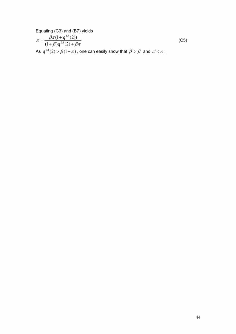
44

Equating (C3) and (B7) yields

βπββππ

+++

=)2()1(

))2(1(' LA

LA

qq

(C5)

As )1()2( πβ −>LAq , one can easily show that ββ >' and ππ <' .

45

CSGR Working Paper Series 190/06, January Marcus Miller, Javier Garcia-Fronti and Lei Zhang

Contractionary devaluation and credit crunch: Analysing Argentina. 191/06, January Wyn Grant

Why It Won’t Be Like This All The Time: the Shift from Duopoly to Oligopoly in Agricultural Trade

192.06, January Michael Keating Global best practice(s) and electricity sector reform in Uganda 193/06 February Natalie Chen, Paola Conconi and Carlo Perroni Does migration empower married women? 194/06 February Emanuel Kohlscheen

Why are there serial defaulters? Quasi-experimental evidence from constitutions.

195/06 March Torsten Strulik

Knowledge politics in the field of global finance? The emergence of a cognitive approach in banking supervision

196/06 March Mark Beeson and Hidetaka Yoshimatsu Asia’s Odd Men Out: Australia, Japan, and the Politics of Regionalism 197/06 March Javier Garcia Fronti and Lei Zhang Political Instability and the Peso Problem 198/06 March Hidetaka YOSHIMATSU Collective Action Problems and Regional Integration in ASEAN 199/06 March Eddy Lee and Marco Vivarelli The Social Impact of Globalisation in the Developing Countries. 200/06 April Jan Aart Scholte Political Parties and Global Democracy 201/06 April Peter Newell

Civil society participation in trade policy-making in Latin America: The Case of the Environmental Movement

202/06 April Marcus Miller and Dania Thomas Sovereign Debt Restructuring: The Judge, the Vultures and Creditor Rights 203/06 April Fondo Sikod

Globalisation and Rural Development in Africa: The Case of the Chad-Cameroon Oil Pipeline.

204/06 April Gilles Quentel

The Translation of a Crucial Political Speech: G.W.Bush’ State of the Union Address 2003 in Le Monde

205/06 April Paola Robotti

Arbitrage and Short Selling: A Political Economy Approach

206/06 May T.Huw Edwards Measuring Global and Regional Trade Integration in terms of Concentration of Access

46

207/06 May Dilip K. Das

Development, Developing Economies and the Doha Round of Multilateral Trade Negotiations

208/06 May Alla Glinchikova

A New Challenge for Civic National Integration: A Perspective from Russia. 209/06 June Celine Tan

Who’s ‘Free Riding’? A Critique of the World Bank’s Approach to Non-Concessional Borrowing in Low-Income Countries

210/06 September Richard Higgott

International Political Economy (IPE) and the Demand for Political Philosophy in an Era of Globalisation

211/06 October Peter Waterman

Union Organisations, Social Movements and the Augean Stables of Global Governance

212/06 October Peter Waterman and Kyle Pope The Bamako Appeal of Samir Amin: A Post-Modern Janus? 213/06 October Marcus Miller, Javier García-Fronti and Lei Zhang Supply Shocks and Currency Crises: The Policy Dilemma Reconsidered 214/06 December Gianluca Grimalda Which Relation between Globalisation and Individual Propensity to Co-Operate? Some Preliminary Results from an Experimental Investigation 215/07 January Kui-Wai Li, Iris A.J. Pang and Michael C.M. Ng Can Performance of Indigenous Factors Influence Growth and Globalisation? 216/06 December Marcus Miller and Lei Zhang Fear and Market Failure: Global Imbalances and “Self-insurance”

Centre for the Study of Globalisation and Regionalisation University of Warwick

Coventry CV4 7AL, UK

Tel: +44 (0)24 7657 2533 Fax: +44 (0)24 7657 2548

Email: csgr@warwick.ac.uk Web address: http://www.csgr.org