
MARCO VARGAS CORREIA - Páginas pessoais estáticasuserweb.fct.unl.pt/~pb/resources/phd_mvc.pdf ·...
235
MARCO VARGAS CORREIA MODERN TECHNIQUES FOR CONSTRAINT SOLVING THE CASPER EXPERIENCE Dissertação apresentada para obtenção do Grau de Doutor em Engenharia Informática, pela Universidade Nova de Lisboa, Faculdade de Ciências e Tecnologia. UNIÃO EUROPEIA Fundo Social Europeu LISBOA 2010
Transcript of MARCO VARGAS CORREIA - Páginas pessoais estáticasuserweb.fct.unl.pt/~pb/resources/phd_mvc.pdf ·...

MARCO VARGAS CORREIA
MODERN TECHNIQUES FOR CONSTRAINT SOLVINGTHE CASPER EXPERIENCE
Dissertação apresentada para obtenção doGrau de Doutor em Engenharia Informática,pela Universidade Nova de Lisboa, Faculdadede Ciências e Tecnologia.
UNIÃO EUROPEIAFundo Social Europeu
LISBOA2010

ii

Acknowledgments
First I would like to thank Pedro Barahona, the supervisor of this work. Besides his valuablescientific advice, his general optimism kept me motivated throughout the long, and some-times convoluted, years of my PhD. Additionally, he managed to find financial support for myparticipation on international conferences, workshops, and summer schools, and even for theextension of my grant for an extra year and an half. This was essential to keep me focused onthe scientific work, and ultimately responsible for the existence of this dissertation.
Designing, developing, and maintaining a constraint solver requires a lot of effort. I havebeen lucky to count on the help and advice of colleagues contributing directly or indirectly tothe design and implementation of CASPER, to whom I am truly indebted:
Francisco Azevedo introduced me to constraint solving over set variables, and was the firstto point out the potential of incremental propagation. The set constraint solver integratingthe work presented in this dissertation is based on his own solver CARDINAL, which he hasthoroughly explained to me.
Jorge Cruz was very helpful for clarifying many issues about real valued arithmetic, andpropagation of constraints over real valued variables in general. The adoption of CaSPER asan optional development platform for his lectures boosted the development of the module forreal valued constraint solving.
Olivier Perriquet was directly involved in porting the PSICO library to CASPER, an applica-tion of constraint programming to solve protein folding problems.
Ruben Viegas developed a module for constraint programming over graph variables, whicheventually led to a joint research on new representations for the domains of set domain vari-ables. Working with Ruben was a pleasure and very rewarding. His work marks an importantmilestone in the development of CaSPER - the first contributed domain reasoning module.
Sérgio Silva has contributed a parser for the MINIZINC language that motivated an improveddesign of the general solver interface to other programming languages.
Several people have used the presented work for their own research or education. Manytimes they had to cope with bugs, lack of documentation, and an ever evolving architecture.Although this was naturally not easy for them, they were always very patient and helped im-proving my work in many ways. I’m very grateful to João Borges, Everardo Barcenas, JeanChristoph Jung, David Buezas, and the students of the “Search and Optimization” and “Con-straints on Continuous Domains” courses.
I would like to thank to my colleagues at CENTRIA for all the informal discussions and
iii

mostly for being a constant source of encouragement and motivation. I specially thank Ar-mando Fernandes and Cecilia Gomes for their concern and advice on the time schedule andcontents of this dissertation.
A significant part of the material presented in this dissertation is based on the formalismdeveloped by Guido Tack. I am very grateful to him for his willingness to answer my questionson some aspects of his approach, and for his valuable comments on the work presented inchapters 6 and 7.
Finally I thank my family and friends for all the emotional support and for being a motiva-tion in the quest for success. This dissertation is dedicated to them.
iv

No idea is so antiquated that it was notonce modern; no idea is so modern thatit will not someday be antiquated.
Ellen Glasgow
v

vi

Sumário
A programação por restrições é um modelo adequado à resolução de problemas combinato-riais com aplicação a problemas industriais e académicos importantes. Ela é realizada comrecurso a um resolvedor de restrições, um programa de computador que tenta encontrar umasolução para o problema, i.e. uma atribuição de valores a todas as variáveis que satisfaça todasas restrições.
Esta dissertação descreve um conjunto de técnicas utilizadas na implementação de um re-solvedor de restrições. Estas técnicas tornam um resolvedor de restrições mais extensível eeficiente, duas propriedades que dificilmente são integradas em geral, e em particular em re-solvedores de restrições. Mais especificamente, esta dissertação debruça-se sobre dois proble-mas principais: propagação incremental genérica, e propagação de restrições decomponíveisarbitrárias. Para ambos os problemas apresentamos um conjunto de técnicas que são origi-nais, correctas, e que se orientam no sentido de tornar a plataforma mais eficiente, extensível,ou ambos.
A matéria apresentada nesta dissertação surgiu da resolução dos problemas encontradosno desenho e implementação de um resolvedor de restrições genérico. O resolvedor CASPER(Constraint Solving Platform for Engineering and Research) não serve apenas de protótipo in-tegrando todas as técnicas apresentadas, mas é também a plataforma experimental comumaos vários modelos teóricos discutidos. Para além do trabalho relacionado com o desenho eimplementação de um resolvedor de restrições, esta dissertação apresenta também a primeiraaplicação bem sucedida da plataforma na abordagem de um problema importante em aberto,nomeadamente a caracterização de heurísticas que direccionem a pesquisa rapidamente parauma solução.
vii

viii
Abstract
Constraint programming is a well known paradigm for addressing combinatorial problemswhich has enjoyed considerable success for solving many relevant industrial and academicproblems. In the heart constraint programming lies the constraint solver, a computer programwhich attempt to find a solution to the problem, i.e. an assignment of all the variables in theproblem such that all the constraints are satisfied.
This dissertation describes a set of techniques to be used in the implementation of a con-straint solver. These techniques aim at making a constraint solver more extensible and effi-cient, two properties which are hard to integrate in general, and in particular within a con-straint solver. Specifically, this dissertation addresses two major problems: generic incremen-tal propagation and propagation of arbitrary decomposable constraints. For both problems wepresent a set of techniques which are novel, correct, and directly concerned with extensibilityand efficiency.
All the material in this dissertation emerged from our work in designing and implementinga generic constraint solver. The CASPER (Constraint Solving Platform for Engineering andResearch) solver does not only act as a proof-of-concept for the presented techniques, butalso served as the common test platform for the many discussed theoretically models. Besidesthe work related to the design and implementation of a constraint solver, this dissertationsalso presents the first successful application of the resulting platform for addressing an openresearch problem, namely finding good heuristics for efficiently directing search towards asolution.
ix

x

Contents
1. Introduction 11.1. Constraint reasoning . . . . . . . . . . . . . . . . . . . . . . . . . . . . . . . . . . . . 11.2. This dissertation . . . . . . . . . . . . . . . . . . . . . . . . . . . . . . . . . . . . . . 3
1.2.1. Motivation . . . . . . . . . . . . . . . . . . . . . . . . . . . . . . . . . . . . . . 31.2.2. Contributions . . . . . . . . . . . . . . . . . . . . . . . . . . . . . . . . . . . . 41.2.3. Overview . . . . . . . . . . . . . . . . . . . . . . . . . . . . . . . . . . . . . . . 6
2. Constraint Programming 92.1. Concepts and notation . . . . . . . . . . . . . . . . . . . . . . . . . . . . . . . . . . . 9
2.1.1. Constraint Satisfaction Problems . . . . . . . . . . . . . . . . . . . . . . . . . 92.1.2. Tuples and tuple sets . . . . . . . . . . . . . . . . . . . . . . . . . . . . . . . . 102.1.3. Domain approximations . . . . . . . . . . . . . . . . . . . . . . . . . . . . . . 112.1.4. Domains . . . . . . . . . . . . . . . . . . . . . . . . . . . . . . . . . . . . . . . 12
2.2. Operational model . . . . . . . . . . . . . . . . . . . . . . . . . . . . . . . . . . . . . 142.2.1. Propagation . . . . . . . . . . . . . . . . . . . . . . . . . . . . . . . . . . . . . 142.2.2. Search . . . . . . . . . . . . . . . . . . . . . . . . . . . . . . . . . . . . . . . . 19
2.3. Summary . . . . . . . . . . . . . . . . . . . . . . . . . . . . . . . . . . . . . . . . . . . 22
I. Incremental Propagation 23
3. Architecture of a Constraint Solver 253.1. Propagation kernel . . . . . . . . . . . . . . . . . . . . . . . . . . . . . . . . . . . . . 25
3.1.1. Propagation loop . . . . . . . . . . . . . . . . . . . . . . . . . . . . . . . . . . 253.1.2. Subscribing propagators . . . . . . . . . . . . . . . . . . . . . . . . . . . . . . 263.1.3. Event driven propagation . . . . . . . . . . . . . . . . . . . . . . . . . . . . . 273.1.4. Signaling fixpoint . . . . . . . . . . . . . . . . . . . . . . . . . . . . . . . . . . 283.1.5. Subsumption . . . . . . . . . . . . . . . . . . . . . . . . . . . . . . . . . . . . 303.1.6. Scheduling . . . . . . . . . . . . . . . . . . . . . . . . . . . . . . . . . . . . . . 30
3.2. State manager . . . . . . . . . . . . . . . . . . . . . . . . . . . . . . . . . . . . . . . . 313.2.1. Algorithms for maintaining state . . . . . . . . . . . . . . . . . . . . . . . . . 323.2.2. Reversible data structures . . . . . . . . . . . . . . . . . . . . . . . . . . . . . 343.2.3. Memory pools . . . . . . . . . . . . . . . . . . . . . . . . . . . . . . . . . . . . 36
xi

Contents
3.3. Other components . . . . . . . . . . . . . . . . . . . . . . . . . . . . . . . . . . . . . 37
3.3.1. Constraint library . . . . . . . . . . . . . . . . . . . . . . . . . . . . . . . . . . 37
3.3.2. Domain modules . . . . . . . . . . . . . . . . . . . . . . . . . . . . . . . . . . 38
3.3.3. Interfaces . . . . . . . . . . . . . . . . . . . . . . . . . . . . . . . . . . . . . . 38
3.4. Summary . . . . . . . . . . . . . . . . . . . . . . . . . . . . . . . . . . . . . . . . . . . 39
4. A Propagation Kernel for Incremental Propagation 414.1. Propagator and variable centered propagation . . . . . . . . . . . . . . . . . . . . . 41
4.1.1. Incremental propagation . . . . . . . . . . . . . . . . . . . . . . . . . . . . . 44
4.1.2. Improving propagation with events . . . . . . . . . . . . . . . . . . . . . . . 46
4.1.3. Improving propagation with priorities . . . . . . . . . . . . . . . . . . . . . 47
4.2. The NOTIFY-EXECUTE algorithm . . . . . . . . . . . . . . . . . . . . . . . . . . . . . 48
4.3. An object-oriented implementation . . . . . . . . . . . . . . . . . . . . . . . . . . . 51
4.3.1. Dependency lists . . . . . . . . . . . . . . . . . . . . . . . . . . . . . . . . . . 53
4.3.2. Performance . . . . . . . . . . . . . . . . . . . . . . . . . . . . . . . . . . . . . 53
4.4. Experiments . . . . . . . . . . . . . . . . . . . . . . . . . . . . . . . . . . . . . . . . . 54
4.4.1. Models . . . . . . . . . . . . . . . . . . . . . . . . . . . . . . . . . . . . . . . . 54
4.4.2. Benchmarks . . . . . . . . . . . . . . . . . . . . . . . . . . . . . . . . . . . . . 55
4.4.3. Setup . . . . . . . . . . . . . . . . . . . . . . . . . . . . . . . . . . . . . . . . . 55
4.5. Discussion . . . . . . . . . . . . . . . . . . . . . . . . . . . . . . . . . . . . . . . . . . 56
4.6. Summary . . . . . . . . . . . . . . . . . . . . . . . . . . . . . . . . . . . . . . . . . . . 56
5. Incremental Propagation of Set Constraints 595.1. Set constraint solving . . . . . . . . . . . . . . . . . . . . . . . . . . . . . . . . . . . . 59
5.1.1. Set domain variables . . . . . . . . . . . . . . . . . . . . . . . . . . . . . . . . 60
5.1.2. Set constraints . . . . . . . . . . . . . . . . . . . . . . . . . . . . . . . . . . . . 60
5.2. Domain primitives . . . . . . . . . . . . . . . . . . . . . . . . . . . . . . . . . . . . . 61
5.3. Incremental propagation . . . . . . . . . . . . . . . . . . . . . . . . . . . . . . . . . 63
5.4. Implementation . . . . . . . . . . . . . . . . . . . . . . . . . . . . . . . . . . . . . . . 65
5.4.1. Propagator-based deltas . . . . . . . . . . . . . . . . . . . . . . . . . . . . . . 65
5.4.2. Variable-based deltas . . . . . . . . . . . . . . . . . . . . . . . . . . . . . . . 67
5.4.3. Optimizations . . . . . . . . . . . . . . . . . . . . . . . . . . . . . . . . . . . . 68
5.5. Experiments . . . . . . . . . . . . . . . . . . . . . . . . . . . . . . . . . . . . . . . . . 71
5.5.1. Models . . . . . . . . . . . . . . . . . . . . . . . . . . . . . . . . . . . . . . . . 71
5.5.2. Problems . . . . . . . . . . . . . . . . . . . . . . . . . . . . . . . . . . . . . . . 71
5.5.3. Setup . . . . . . . . . . . . . . . . . . . . . . . . . . . . . . . . . . . . . . . . . 73
5.6. Discussion . . . . . . . . . . . . . . . . . . . . . . . . . . . . . . . . . . . . . . . . . . 73
5.7. Summary . . . . . . . . . . . . . . . . . . . . . . . . . . . . . . . . . . . . . . . . . . . 74
xii

Contents
II. Efficient Propagation of Arbitrary Decomposable Constraints 77
6. Propagation of Decomposable Constraints 796.1. Decomposable constraints . . . . . . . . . . . . . . . . . . . . . . . . . . . . . . . . 79
6.1.1. Functional composition . . . . . . . . . . . . . . . . . . . . . . . . . . . . . . 806.2. Views . . . . . . . . . . . . . . . . . . . . . . . . . . . . . . . . . . . . . . . . . . . . . 816.3. View-based propagation . . . . . . . . . . . . . . . . . . . . . . . . . . . . . . . . . . 83
6.3.1. Constraint checkers . . . . . . . . . . . . . . . . . . . . . . . . . . . . . . . . 836.3.2. Propagators . . . . . . . . . . . . . . . . . . . . . . . . . . . . . . . . . . . . . 84
6.4. Views over decomposable constraints . . . . . . . . . . . . . . . . . . . . . . . . . . 846.4.1. Composition of views . . . . . . . . . . . . . . . . . . . . . . . . . . . . . . . 856.4.2. Checking and propagating decomposable constraints . . . . . . . . . . . . 87
6.5. Conclusion . . . . . . . . . . . . . . . . . . . . . . . . . . . . . . . . . . . . . . . . . . 88
7. Incomplete View-Based Propagation 917.1. ΦΨ-complete propagators . . . . . . . . . . . . . . . . . . . . . . . . . . . . . . . . 917.2. View models . . . . . . . . . . . . . . . . . . . . . . . . . . . . . . . . . . . . . . . . . 92
7.2.1. Soundness . . . . . . . . . . . . . . . . . . . . . . . . . . . . . . . . . . . . . . 937.2.2. Completeness . . . . . . . . . . . . . . . . . . . . . . . . . . . . . . . . . . . . 937.2.3. Idempotency . . . . . . . . . . . . . . . . . . . . . . . . . . . . . . . . . . . . 957.2.4. Efficiency . . . . . . . . . . . . . . . . . . . . . . . . . . . . . . . . . . . . . . . 96
7.3. Finding stronger models . . . . . . . . . . . . . . . . . . . . . . . . . . . . . . . . . . 977.3.1. Trivially stronger models . . . . . . . . . . . . . . . . . . . . . . . . . . . . . 977.3.2. Relaxing the problem . . . . . . . . . . . . . . . . . . . . . . . . . . . . . . . . 997.3.3. Computing an upper bound . . . . . . . . . . . . . . . . . . . . . . . . . . . 997.3.4. Rule databases . . . . . . . . . . . . . . . . . . . . . . . . . . . . . . . . . . . 1007.3.5. Multiple views . . . . . . . . . . . . . . . . . . . . . . . . . . . . . . . . . . . . 1027.3.6. Idempotency . . . . . . . . . . . . . . . . . . . . . . . . . . . . . . . . . . . . 1037.3.7. Complexity and optimizations . . . . . . . . . . . . . . . . . . . . . . . . . . 104
7.4. Experiments . . . . . . . . . . . . . . . . . . . . . . . . . . . . . . . . . . . . . . . . . 1057.5. Incomplete constraint checkers . . . . . . . . . . . . . . . . . . . . . . . . . . . . . 1077.6. Summary . . . . . . . . . . . . . . . . . . . . . . . . . . . . . . . . . . . . . . . . . . . 107
8. Type Parametric Compilation of Box View Models 1118.1. Box view models . . . . . . . . . . . . . . . . . . . . . . . . . . . . . . . . . . . . . . 1118.2. View objects . . . . . . . . . . . . . . . . . . . . . . . . . . . . . . . . . . . . . . . . . 114
8.2.1. Typed constraints . . . . . . . . . . . . . . . . . . . . . . . . . . . . . . . . . . 1148.2.2. Box view objects . . . . . . . . . . . . . . . . . . . . . . . . . . . . . . . . . . 114
8.3. View object stores . . . . . . . . . . . . . . . . . . . . . . . . . . . . . . . . . . . . . . 1158.3.1. Subtype polymorphic stores . . . . . . . . . . . . . . . . . . . . . . . . . . . 115
xiii

Contents
8.3.2. Parametric polymorphic stores . . . . . . . . . . . . . . . . . . . . . . . . . . 1168.4. Auxiliary variables . . . . . . . . . . . . . . . . . . . . . . . . . . . . . . . . . . . . . 1178.5. Compilation . . . . . . . . . . . . . . . . . . . . . . . . . . . . . . . . . . . . . . . . . 117
8.5.1. Subtype polymorphic views . . . . . . . . . . . . . . . . . . . . . . . . . . . . 1188.5.2. Parametric polymorphic views . . . . . . . . . . . . . . . . . . . . . . . . . . 1198.5.3. Auxiliary variables . . . . . . . . . . . . . . . . . . . . . . . . . . . . . . . . . 120
8.6. Model comparison . . . . . . . . . . . . . . . . . . . . . . . . . . . . . . . . . . . . . 1218.6.1. Memory . . . . . . . . . . . . . . . . . . . . . . . . . . . . . . . . . . . . . . . 1218.6.2. Runtime . . . . . . . . . . . . . . . . . . . . . . . . . . . . . . . . . . . . . . . 1228.6.3. Propagation . . . . . . . . . . . . . . . . . . . . . . . . . . . . . . . . . . . . . 123
8.7. Beyond arithmetic expressions . . . . . . . . . . . . . . . . . . . . . . . . . . . . . . 1258.7.1. Casting operator . . . . . . . . . . . . . . . . . . . . . . . . . . . . . . . . . . 1258.7.2. Array access operator . . . . . . . . . . . . . . . . . . . . . . . . . . . . . . . 1258.7.3. Iterated expressions . . . . . . . . . . . . . . . . . . . . . . . . . . . . . . . . 126
8.8. Summary . . . . . . . . . . . . . . . . . . . . . . . . . . . . . . . . . . . . . . . . . . . 126
9. Implementation and Experiments 1299.1. View models in Logic Programming . . . . . . . . . . . . . . . . . . . . . . . . . . . 1299.2. View models in strongly typed programming languages . . . . . . . . . . . . . . . 130
9.2.1. Subtype polymorphism . . . . . . . . . . . . . . . . . . . . . . . . . . . . . . 1309.2.2. Parametric polymorphism . . . . . . . . . . . . . . . . . . . . . . . . . . . . 1319.2.3. Advantages of subtype polymorphic views . . . . . . . . . . . . . . . . . . . 133
9.3. Experiments . . . . . . . . . . . . . . . . . . . . . . . . . . . . . . . . . . . . . . . . . 1339.3.1. Models . . . . . . . . . . . . . . . . . . . . . . . . . . . . . . . . . . . . . . . . 1339.3.2. Problems . . . . . . . . . . . . . . . . . . . . . . . . . . . . . . . . . . . . . . . 1349.3.3. Setup . . . . . . . . . . . . . . . . . . . . . . . . . . . . . . . . . . . . . . . . . 139
9.4. Discussion . . . . . . . . . . . . . . . . . . . . . . . . . . . . . . . . . . . . . . . . . . 1399.4.1. Auxiliary variables Vs Type parametric views . . . . . . . . . . . . . . . . . . 1399.4.2. Type parametric views Vs Subtype polymorphic views . . . . . . . . . . . . 1409.4.3. Caching type parametric views . . . . . . . . . . . . . . . . . . . . . . . . . . 1419.4.4. Competitiveness . . . . . . . . . . . . . . . . . . . . . . . . . . . . . . . . . . 142
9.5. Summary . . . . . . . . . . . . . . . . . . . . . . . . . . . . . . . . . . . . . . . . . . . 142
III. Applications 145
10.On the Integration of Singleton Consistencies and Look-Ahead Heuristics 14710.1.Singleton consistencies . . . . . . . . . . . . . . . . . . . . . . . . . . . . . . . . . . 14810.2.Informed decision making . . . . . . . . . . . . . . . . . . . . . . . . . . . . . . . . . 14910.3.Experiments . . . . . . . . . . . . . . . . . . . . . . . . . . . . . . . . . . . . . . . . . 152
xiv

Contents
10.3.1. Heuristics . . . . . . . . . . . . . . . . . . . . . . . . . . . . . . . . . . . . . . 15310.3.2. Strategies . . . . . . . . . . . . . . . . . . . . . . . . . . . . . . . . . . . . . . . 15310.3.3. Problems . . . . . . . . . . . . . . . . . . . . . . . . . . . . . . . . . . . . . . . 154
10.4.Discussion . . . . . . . . . . . . . . . . . . . . . . . . . . . . . . . . . . . . . . . . . . 15610.5.Summary . . . . . . . . . . . . . . . . . . . . . . . . . . . . . . . . . . . . . . . . . . . 159
11.Overview of the CaSPER* Constraint Solvers 16111.1.The third international CSP solver competition . . . . . . . . . . . . . . . . . . . . 16111.2.Propagation . . . . . . . . . . . . . . . . . . . . . . . . . . . . . . . . . . . . . . . . . 162
11.2.1. Predicates . . . . . . . . . . . . . . . . . . . . . . . . . . . . . . . . . . . . . . 16211.2.2. Global constraints . . . . . . . . . . . . . . . . . . . . . . . . . . . . . . . . . 162
11.3.Symmetry breaking . . . . . . . . . . . . . . . . . . . . . . . . . . . . . . . . . . . . . 16311.4.Search . . . . . . . . . . . . . . . . . . . . . . . . . . . . . . . . . . . . . . . . . . . . . 164
11.4.1. Heuristics . . . . . . . . . . . . . . . . . . . . . . . . . . . . . . . . . . . . . . 16411.4.2. Sampling . . . . . . . . . . . . . . . . . . . . . . . . . . . . . . . . . . . . . . . 16411.4.3. SAC . . . . . . . . . . . . . . . . . . . . . . . . . . . . . . . . . . . . . . . . . . 16511.4.4. Restarts . . . . . . . . . . . . . . . . . . . . . . . . . . . . . . . . . . . . . . . . 165
11.5.Experimental evaluation . . . . . . . . . . . . . . . . . . . . . . . . . . . . . . . . . . 16511.6.Conclusion . . . . . . . . . . . . . . . . . . . . . . . . . . . . . . . . . . . . . . . . . . 166
12.Conclusions 16912.1.Summary of main contributions . . . . . . . . . . . . . . . . . . . . . . . . . . . . . 16912.2.Future work . . . . . . . . . . . . . . . . . . . . . . . . . . . . . . . . . . . . . . . . . 170
Bibliography 171
A. Proofs 185A.1. Proofs of chapter 6 . . . . . . . . . . . . . . . . . . . . . . . . . . . . . . . . . . . . . 185A.2. Proofs of chapter 7 . . . . . . . . . . . . . . . . . . . . . . . . . . . . . . . . . . . . . 189A.3. Proofs of chapter 8 . . . . . . . . . . . . . . . . . . . . . . . . . . . . . . . . . . . . . 192
B. Tables 195B.1. Tables of chapter 4 . . . . . . . . . . . . . . . . . . . . . . . . . . . . . . . . . . . . . 195B.2. Tables of chapter 5 . . . . . . . . . . . . . . . . . . . . . . . . . . . . . . . . . . . . . 198
B.2.1. Social golfers . . . . . . . . . . . . . . . . . . . . . . . . . . . . . . . . . . . . 198B.2.2. Hamming codes . . . . . . . . . . . . . . . . . . . . . . . . . . . . . . . . . . . 199B.2.3. Balanced partition . . . . . . . . . . . . . . . . . . . . . . . . . . . . . . . . . 200B.2.4. Metabolic pathways . . . . . . . . . . . . . . . . . . . . . . . . . . . . . . . . 200B.2.5. Winner determination problem . . . . . . . . . . . . . . . . . . . . . . . . . 201
B.3. Tables of chapter 9 . . . . . . . . . . . . . . . . . . . . . . . . . . . . . . . . . . . . . 202B.3.1. Systems of linear equations . . . . . . . . . . . . . . . . . . . . . . . . . . . . 202
xv

Contents
B.3.2. Systems of nonlinear equations . . . . . . . . . . . . . . . . . . . . . . . . . 203B.3.3. Social golfers . . . . . . . . . . . . . . . . . . . . . . . . . . . . . . . . . . . . 205B.3.4. Golomb ruler . . . . . . . . . . . . . . . . . . . . . . . . . . . . . . . . . . . . 206B.3.5. Low autocorrelation binary sequences . . . . . . . . . . . . . . . . . . . . . 207B.3.6. Fixed-length error correcting codes . . . . . . . . . . . . . . . . . . . . . . . 208
B.4. Tables of chapter 11 . . . . . . . . . . . . . . . . . . . . . . . . . . . . . . . . . . . . . 210
xvi

List of Figures
1.1. Magic square found in Albrecht Dürer’s engraving Melancholia (1514). . . . . . . 21.2. Constraint program (in C++ using CaSPER) for finding a magic square. . . . . . . 2
2.1. Domain taxonomy . . . . . . . . . . . . . . . . . . . . . . . . . . . . . . . . . . . . . 132.2. Partially filled magic square of order 4: without any filtering (a); where some in-
consistent values were filtered (b,c); with no inconsistent values (d). . . . . . . . . 142.3. Taxonomy of constraint propagation strength. Each arrow specifies a strictly
stronger than relation between two consistencies (see example 2.39). . . . . . . . 182.4. Partial search tree obtained by GenerateAndTest on the magic square problem. 202.5. Partial search tree obtained by SOLVE on the magic square problem while main-
taining local domain consistency. . . . . . . . . . . . . . . . . . . . . . . . . . . . . 22
3.1. A possible search tree for the CSP described in example 3.11. Search decisionsare underlined. . . . . . . . . . . . . . . . . . . . . . . . . . . . . . . . . . . . . . . . 32
3.2. Contents of the stack used by the copying method for handling state. . . . . . . . 323.3. Contents of the stack used by the trailing method for handling state. . . . . . . . . 333.4. Contents of the queue used by the recomputation method for handling state. . . 343.5. Reversible single-linked list. Memory addresses of the values and pointers com-
posing the data structure are shown below each cell. . . . . . . . . . . . . . . . . . 35
4.1. Example of a CSP with variables x1, x2, x3, and propagators π1, . . . ,π4. . . . . . . . 444.2. Suspension list . . . . . . . . . . . . . . . . . . . . . . . . . . . . . . . . . . . . . . . 53
5.1. a) Powerset lattice for {a,b,c}, with set inclusion as partial order. b) Lattice cor-responding to the set domain [{b} , {a,b,c}]. . . . . . . . . . . . . . . . . . . . . . . 60
5.2. ∆GLBx1
and ∆LUBx1
delta sets and associated iterators after each propagation duringthe computation of fixpoint for the problem described in example 5.14. . . . . . . 69
5.3. Updating the POSS set and storing the corresponding delta using a list splice op-eration assuming a doubly linked list representation. . . . . . . . . . . . . . . . . . 70
6.1. Computations involved in the composition of views described in example 6.30. . 866.2. Application of the view-based propagator for the composed constraint described
in example 6.36. . . . . . . . . . . . . . . . . . . . . . . . . . . . . . . . . . . . . . . . 87
xvii
List of Figures
7.1. View model lattice. . . . . . . . . . . . . . . . . . . . . . . . . . . . . . . . . . . . . . 99
8.1. An unbalanced expression syntax tree. The internal nodes n1 . . .nn−1 representoperators and leafs l1 . . . ln represent variables. . . . . . . . . . . . . . . . . . . . . . 121
9.1. Number of solutions per second when enumerating all solutions of a CSP with agiven number of variables (in the xx axis), domain of size 8, and no constraints. . 143
10.1.Number of problems solved (yy axis) after a given time period (xx axis). Thegraphs show the results obtained for, from left to right, the graph coloring in-stances, the random instances, and latin square instances. . . . . . . . . . . . . . 156
10.2.Difference between the number of problems solved when using the LA heuris-tic and when using the DOM+MIN heuristic (yy axis) after a given time period(xx axis). The graphs show the results obtained for, from left to right, the graphcoloring instances, the random instances, and latin square instances. . . . . . . . 157
10.3.Number of problems solved when using several strategies (yy axis) after a giventime period (xx axis). The graphs show the results obtained for, from left to right,the graph coloring instances, the random instances, and latin square instances. . 158
10.4.Search space size during solving of a typical instance in each problem. . . . . . . 158
xviii

List of Tables
4.1. Geometric mean, standard deviation, minimum and maximum of ratios of prop-agation times when solving the set of benchmarks using implementations of themodels described above. . . . . . . . . . . . . . . . . . . . . . . . . . . . . . . . . . . 57
5.1. Worst-case runtime for set domain primitives when performing non-incrementalpropagation. . . . . . . . . . . . . . . . . . . . . . . . . . . . . . . . . . . . . . . . . . 62
5.2. Worst-case runtime for set domain primitives when performing incremental prop-agation. . . . . . . . . . . . . . . . . . . . . . . . . . . . . . . . . . . . . . . . . . . . . 70
5.3. Geometric mean, standard deviation, minimum and maximum of ratios of run-time for solving the first set of benchmarks described above using the presentedimplementations of incremental propagation, compared to non-incremental prop-agation. . . . . . . . . . . . . . . . . . . . . . . . . . . . . . . . . . . . . . . . . . . . . 74
5.4. Geometric mean, standard deviation, minimum and maximum of ratios of run-time for solving the second set of benchmarks (graph problems) using the vari-able delta implementation of incremental propagation, compared to propagatordeltas. . . . . . . . . . . . . . . . . . . . . . . . . . . . . . . . . . . . . . . . . . . . . . 74
7.1. Constraint propagator completeness. . . . . . . . . . . . . . . . . . . . . . . . . . . 927.2. Strength of the view model m for a set of arithmetic constraints. . . . . . . . . . . 106
8.1. Cost of accessing and updating an arbitrary expression represented by each ofthe described models. . . . . . . . . . . . . . . . . . . . . . . . . . . . . . . . . . . . 123
9.1. Geometric mean, standard deviation, minimum and maximum of the ratios de-fined by the runtime of best performing model using views over the runtime ofthe best performing model using auxiliary variables, on all benchmarks. . . . . . 140
9.2. Geometric mean, standard deviation, minimum and maximum of the ratios de-fined by the number of fails of the best performing solver using views over thenumber of fails of the best performing solver using auxiliary variables, on all in-stances of each problem where the number of fails differ. . . . . . . . . . . . . . . 140
9.3. Geometric mean, standard deviation, minimum and maximum of the ratios de-fined by the runtime of the solver implementing the PVIEWS model over the run-time of the solver implementing the SVIEWS model, on all benchmarks. . . . . . . 141
xix

List of Tables
9.4. Geometric mean, standard deviation, minimum and maximum of the ratios de-fined by the runtime of the solver implementing the PVIEWS model over the run-time of the solver implementing the CPVIEWS model, on all benchmarks. . . . . 141
9.5. Geometric mean, standard deviation, minimum and maximum of the ratios de-fined by the runtime of the CaSPER solver implementing the VARS+GLOBAL modelover the runtime of the Gecode solver implementing the VARS+GLOBAL model,on all benchmarks. . . . . . . . . . . . . . . . . . . . . . . . . . . . . . . . . . . . . . 142
9.6. Geometric mean, standard deviation, minimum and maximum of the ratios de-fined by the runtime of the CaSPER solver implementing the PVIEWS model overthe runtime of the Gecode solver implementing the VARS+GLOBAL model, on allbenchmarks. . . . . . . . . . . . . . . . . . . . . . . . . . . . . . . . . . . . . . . . . . 143
10.1.Results for finding the first solution to latin-15 with a selected strategy. . . . . . . 159
11.1.Global constraint propagators used in solvers. . . . . . . . . . . . . . . . . . . . . . 16211.2.Summary of features in each solver. . . . . . . . . . . . . . . . . . . . . . . . . . . . 166
B.1. Number of global constraints of each kind present in each benchmark . . . . . . 195B.2. Propagation time (seconds) for solving each benchmark using each model (table
1/2) . . . . . . . . . . . . . . . . . . . . . . . . . . . . . . . . . . . . . . . . . . . . . . 196B.3. Propagation time (seconds) for solving each benchmark using each model (table
2/2) . . . . . . . . . . . . . . . . . . . . . . . . . . . . . . . . . . . . . . . . . . . . . . 197B.4. Social golfers: 5w-5g-4s (v=25,c/v=11.2,f=25421) . . . . . . . . . . . . . . . . . . . 198B.5. Social golfers: 6w-5g-3s (v=30,c/v=13.6,f=1582670) . . . . . . . . . . . . . . . . . . 198B.6. Social golfers: 11w-11g-2s (v=121,c/v=55.4,f=10803) . . . . . . . . . . . . . . . . . 198B.7. Hamming codes: 20s-15l-8d (v=42,c/v=10,f=7774) . . . . . . . . . . . . . . . . . . 199B.8. Hamming codes: 10s-20l-9d (v=22,c/v=5,f=59137) . . . . . . . . . . . . . . . . . . 199B.9. Hamming codes: 40s-15l-6d (v=82,c/v=15.1,f=27002) . . . . . . . . . . . . . . . . . 199B.10.Balanced partition: 150v-70s-162m (v=212,c/v=11.7,f=48525) . . . . . . . . . . . 200B.11.Balanced partition: 170v-80s-182m (v=242,c/v=13.4,f=54573) . . . . . . . . . . . 200B.12.Balanced partition: 190v-90s-202m (v=272,c/v=15,f=57424) . . . . . . . . . . . . . 200B.13.Metabolic pathways: g250_croes_ecoli_glyco (f=916) . . . . . . . . . . . . . . . . . 200B.14.Metabolic pathways: g500_croes_ecoli_glyco (f=2865) . . . . . . . . . . . . . . . . 201B.15.Metabolic pathways: g1000_croes_scerev_heme (f=2466) . . . . . . . . . . . . . . 201B.16.Metabolic pathways: g1500_croes_ecoli_glyco (f=4056) . . . . . . . . . . . . . . . 201B.17.Winner determination problem: 200 (f=1550) . . . . . . . . . . . . . . . . . . . . . 201B.18.Winner determination problem: 300 (f=2924) . . . . . . . . . . . . . . . . . . . . . 201B.19.Winner determination problem: 400 (f=6693) . . . . . . . . . . . . . . . . . . . . . 202B.20.Winner determination problem: 500 (f=16213) . . . . . . . . . . . . . . . . . . . . . 202B.21.Linear 20var-7vals-7cons-4arity-6s (SAT) (S=56.15) . . . . . . . . . . . . . . . . . . 202
xx

List of Tables
B.22.Linear 20var-30val-6cons-8arity-2s (UNSAT) (S=98.14) . . . . . . . . . . . . . . . 202B.23.Linear 40var-7val-12cons-20arity-3s (UNSAT) (S=112.29) . . . . . . . . . . . . . . 203B.24.Linear 40var-7val-10cons-40arity-3s (UNSAT) (S=112.29) . . . . . . . . . . . . . . 203B.25.NonLinear 20var-20val-10cons-4term-2fact-2s (SAT) (S=86.44) . . . . . . . . . . . 203B.26.NonLinear 50var-10val-19cons-4term-2fact-1s (SAT) (S=166.1) . . . . . . . . . . . 204B.27.NonLinear 50var-10val-28cons-4term-3fact-1s (UNSAT) (S=166.1) . . . . . . . . 204B.28.NonLinear 50var-5val-20cons-4term-3fact-1s (UNSAT) (S=116.1) . . . . . . . . . 204B.29.NonLinear 50var-6val-26cons-4term-4fact-1s (UNSAT) (S=129.25) . . . . . . . . 205B.30.NonLinear 60var-4val-24cons-4term-4fact-5s (UNSAT) (S=120) . . . . . . . . . . . 205B.31.Social golfers: 5week-5group-4size (S=432.19) . . . . . . . . . . . . . . . . . . . . . 205B.32.Social golfers: 6week,5group,3size (S=351.62) . . . . . . . . . . . . . . . . . . . . . 206B.33.Social golfers: 4week,7group,7size (S=1100.48) . . . . . . . . . . . . . . . . . . . . 206B.34.Golomb ruler: 10 (S=58.07) . . . . . . . . . . . . . . . . . . . . . . . . . . . . . . . . 206B.35.Golomb ruler: 11 (S=68.09) . . . . . . . . . . . . . . . . . . . . . . . . . . . . . . . . 207B.36.Golomb ruler: 12 (S=76.91) . . . . . . . . . . . . . . . . . . . . . . . . . . . . . . . . 207B.37.Low autocorrelation binary sequences: 22 (S=22) . . . . . . . . . . . . . . . . . . . 207B.38.Low autocorrelation binary sequences: 24 (S=25) . . . . . . . . . . . . . . . . . . . 208B.39.Fixed-length error correcting codes: 2-20-32-10-hamming (S=640) . . . . . . . . 208B.40.Fixed-length error correcting codes: 3-15-35-11-hamming (S=525) . . . . . . . . . 208B.41.Fixed-length error correcting codes: 2-20-32-10-lee (S=640) . . . . . . . . . . . . . 209B.42.Fixed-length error correcting codes: 3-15-35-10-lee (S=525) . . . . . . . . . . . . . 209B.43.CPAI’08 competition results (n-ary intension constraints category) . . . . . . . . 210B.44.CPAI’08 competition results (global constraints category) . . . . . . . . . . . . . . 211
xxi

List of Tables
xxii

List of Algorithms
1. GenerateAndTest(d ,C ) . . . . . . . . . . . . . . . . . . . . . . . . . . . . . . . . . . . 192. Solve(d ,C ) . . . . . . . . . . . . . . . . . . . . . . . . . . . . . . . . . . . . . . . . . . . 21
3. Propagate1(d ,C ) . . . . . . . . . . . . . . . . . . . . . . . . . . . . . . . . . . . . . . . 264. Propagate2(d ,P ) . . . . . . . . . . . . . . . . . . . . . . . . . . . . . . . . . . . . . . . 275. Propagate3(d ,P ) . . . . . . . . . . . . . . . . . . . . . . . . . . . . . . . . . . . . . . . 29
6. PropagatePC(d ,P ) . . . . . . . . . . . . . . . . . . . . . . . . . . . . . . . . . . . . . . 427. PropagateVC(d ,V ) . . . . . . . . . . . . . . . . . . . . . . . . . . . . . . . . . . . . . . 438. PropagatePCEvents(d ,E) . . . . . . . . . . . . . . . . . . . . . . . . . . . . . . . . . . 479. PropagateVCEvents(d ,E) . . . . . . . . . . . . . . . . . . . . . . . . . . . . . . . . . . 4810. Execute(d) . . . . . . . . . . . . . . . . . . . . . . . . . . . . . . . . . . . . . . . . . . . 4911. Notify(e) . . . . . . . . . . . . . . . . . . . . . . . . . . . . . . . . . . . . . . . . . . . . 5012. Notify(e) . . . . . . . . . . . . . . . . . . . . . . . . . . . . . . . . . . . . . . . . . . . . 5113. Method νi .Call() . . . . . . . . . . . . . . . . . . . . . . . . . . . . . . . . . . . . . . . 52
14. FindUb(m) . . . . . . . . . . . . . . . . . . . . . . . . . . . . . . . . . . . . . . . . . . 100
15. SCθ(d ,X ,C ) . . . . . . . . . . . . . . . . . . . . . . . . . . . . . . . . . . . . . . . . . . 14916. RSCθ(d ,X ,C ) . . . . . . . . . . . . . . . . . . . . . . . . . . . . . . . . . . . . . . . . . 14917. SReviseθ(x,d ,C ) . . . . . . . . . . . . . . . . . . . . . . . . . . . . . . . . . . . . . . . . 15018. SReviseInfoθ(x,d ,C ,INFO) . . . . . . . . . . . . . . . . . . . . . . . . . . . . . . . . . . 15119. Solveθ(d ,C ,INFO) . . . . . . . . . . . . . . . . . . . . . . . . . . . . . . . . . . . . . . . 152
20. Search strategy sampling . . . . . . . . . . . . . . . . . . . . . . . . . . . . . . . . . . 165
xxiii

List of Algorithms
xxiv

Chapter 1.
Introduction
1.1. Constraint reasoning
Constraint reasoning may be introduced with a simple example. Consider the following wellknown combinatorial object:
Definition 1.1 (Magic Square). An order n magic square is a n×n matrix containing the num-bers 1 to n2, where each row, column, and main diagonal equal the same sum (the magicconstant).
Magic squares were known to Chinese mathematicians as early as 650 BC. They were oftenregarded as objects with magical properties connected to diverse fields such as astronomy,mythology and music [Swaney 2000]. Figure 1.1 shows one of the earliest known squares, partof Albrecht Dürer’s engraving Melancholia.
Problems involving magic square range from completing an empty or partial filled magicsquare, or counting the number of magic squares with a given order or other mathemati-cal properties. Solving these problems presents various interesting challenges: while fillingan empty magic square may be accomplished in polynomial time, completing a partial filledsquare is NP-complete, and finding the exact number of squares with some dimension is #P-complete.
The combinatorial structure inherent to this puzzle together with its simple declarative de-scription makes it an optimal candidate for a constraint programming solving approach. Fig-ure 1.2 shows a constraint program which finds a magic square where the numbers 15 and 14(the date of the engraving) are already placed as in Dürer’s original. The program embodiesthe following outstanding features of this technology:
Completeness Constraint programs provide completeness guarantees. This contrasts withother combinatorial solving methods, such as tabu search or genetic algorithms, which do notexplore the solution space exhaustively. Consequently, these methods are not adequate for anumber of problems, e.g. proving that there is no square having a given sequence of numbers,or counting the number of squares of a given order.
1

Chapter 1. Introduction
Figure 1.1.: Magic square found in Albrecht Dürer’s engraving Melancholia (1514).
1 void magic ( Int n) {2 const Int k = n* (n*n+ 1 ) / 2 . 0 ;3 Solver solver ;4 DomVarArray<Int ,2 > square ( solver , n , n, 1 ,n*n ) ;5 solver . post ( d i s t i n c t ( square ) ) ;6 MutVar<Int > i ( solver ) ;7 for ( Int j = 0 ; j < n ; j ++) {8 solver . post (sum( a l l ( i , range ( 1 ,n) , square [ i ] [ j ] ) ) == k ) ;9 solver . post (sum( a l l ( i , range ( 1 ,n) , square [ j ] [ i ] ) ) == k ) ;
10 }11 solver . post (sum( a l l ( i , range ( 1 ,n) , square [ i ] [ i ] ) ) == k ) ;12 solver . post (sum( a l l ( i , range ( 1 ,n) , square [ i ] [ n−i −1])) == k ) ;13 solver . post ( square [3][1]==15 and square [ 3 ] [ 2 ] = = 1 4 ) ;14 i f ( solver . solve ( l ab el ( square ) ) )15 cout << square << endl ;16 }
Figure 1.2.: Constraint program (in C++ using CaSPER) for finding a magic square.
2
1.2. This dissertation
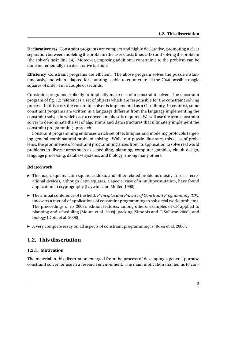
Declarativeness Constraint programs are compact and highly declarative, promoting a clearseparation between modeling the problem (the user’s task: lines 2-13) and solving the problem(the solver’s task: line 14). Moreover, imposing additional constraints to the problem can bedone incrementally in a declarative fashion.
Efficiency Constraint programs are efficient. The above program solves the puzzle instan-taneously, and when adapted for counting is able to enumerate all the 7040 possible magicsquares of order 4 in a couple of seconds.
Constraint programs explicitly or implicitly make use of a constraint solver. The constraintprogram of fig. 1.2 references a set of objects which are responsible for the constraint solvingprocess. In this case, the constraint solver is implemented as a C++ library. In contrast, someconstraint programs are written in a language different from the language implementing theconstraint solver, in which case a conversion phase is required. We will use the term constraintsolver to denominate the set of algorithms and data structures that ultimately implement theconstraint programming approach.
Constraint programming embraces a rich set of techniques and modeling protocols target-ing general combinatorial problem solving. While our puzzle illustrates this class of prob-lems, the prominence of constraint programming arises from its application to solve real worldproblems in diverse areas such as scheduling, planning, computer graphics, circuit design,language processing, database systems, and biology, among many others.
Related work
Ï The magic square, Latin square, sudoku, and other related problems mostly arise as recre-ational devices, although Latin squares, a special case of a multipermutation, have foundapplication in cryptography [Laywine and Mullen 1998].
Ï The annual conference of the field, Principles and Practice of Constraint Programming (CP),uncovers a myriad of applications of constraint programming to solve real world problems.The proceedings of its 2008’s edition features, among others, examples of CP applied toplanning and scheduling [Moura et al. 2008], packing [Simonis and O’Sullivan 2008], andbiology [Dotu et al. 2008].
Ï A very complete essay on all aspects of constraint programming is [Rossi et al. 2006].
1.2. This dissertation
1.2.1. Motivation
The material in this dissertation emerged from the process of developing a general purposeconstraint solver for use in a research environment. The main motivation that led us to con-
3

Chapter 1. Introduction
sider this endeavor was the lack of a constraint solver which was both competitive, extensible,open-source, and written in a popular, preferably object-oriented, programming language. Wefound these are necessary attributes for a constraint solver aiming to be a general constraintsolving research platform.
Achieving the optimal balance between efficiency and extensibility is challenging for anylarge software project in general, and in particular for a constraint solver. Our hypothesis wasthat one does not necessarily sacrifices the other if the solver is based on a solid architecture,specifically designed with these concerns in mind.
1.2.2. Contributions
Committing ourselves to this project presented us with many interesting problems. Many ofthem have been solved by others, often in different ways, since practical constraint solvershave been around since the 80’s. However, until very recently the constraint programmingcomunity has partially disregarded implementation aspects. The architecture and design de-cisions used in most of these solvers is thus many times not fully described, discussed, or jus-tified. Therefore, for many problems we had to find our own solution given that the solutionsfound by others were either (a) not published, (b) jeopardized efficiency or extensibility, or (c)did not fit well with the rest of our architecture.
Presenting, explaining and evaluating all decisions behind the design of a constraint solverwould be an enormous task, and perhaps not very interesting since many of these decisionscondition each other. Instead, we have deliberately chosen to present what we believe are themost interesting and original ideas in our solver, hoping that they may be useful to others aswell. Additionally, we also included our work on look-ahead search heuristics, which is thefirst application of our solver fulfilling its purpose: to be a research platform on constraintprogramming.
The four major contributions of this dissertation may thus be summarized as follows:
Techniques for incremental propagation We introduce a framework for integrating incremen-tal propagation in a general purpose constraint solver. The contribution is twofold: a gener-alized propagation algorithm assisting domain agnostic incremental propagation, and its ap-plication for incremental propagation of finite set constraints, showing how the frameworkefficiently supports domain specific models of incremental propagation.
Efficient propagation of decomposable constraints We extend the theoretical model of Tack[2009] for the case of propagation of arbitrary decomposable constraints involving multiplevariables. We prove that the generalized propagation model is correct, and provide an algo-rithm for approximating its completeness guarantees. We show how arbitrary decomposableconstraints may be automatically compiled and efficiently propagated using this model for aspecial class of propagation algorithms.
4

1.2. This dissertation
Look-ahead heuristics We present a family of variable and value search heuristics based onlook-ahead information, i.e. information collected while performing a limited amount of searchand propagation. In particular, we describe how to integrate these heuristics with propagationalgorithms achieving a specific form of consistency, namely singleton consistency, adding anegligible performance overhead to the global algorithm. We show that the resulting combi-nation compares favorably with other popular heuristics in a number of standard benchmarks.
CaSPER We developed a new constraint solver implementing the techniques discussed in thisdissertation. The solver was designed with efficiency, simplicity and extensibility as primaryconcerns, aiming to fulfill the need of a flexible platform for research on constraint program-ming. Its flexibility and competitive performance is attested throughout this dissertation, ei-ther when used for implementing and evaluating the specific techniques discussed, but alsowhen compared globally with other state-of-the-art solvers.
Most of the material in this dissertation has appeared on the following publications, althoughwith a different, less uniform presentation.
Marco Correia, Pedro Barahona, and Francisco Azevedo (2005). CaSPER: A ProgrammingEnvironment for Development and Integration of Constraint Solvers. Workshop on ConstraintProgramming Beyond Finite Integer Domains, BeyondFD’05 (proceedings).
Marco Correia and Pedro Barahona (2006). Overview of an Open Constraint Library. ERCIMWorkshop on Constraint Solving and Constraint Logic Programming, CSCLP’06 (proceedings),pp. 159–168.
Marco Correia and Pedro Barahona (2007). On the integration of singleton consistency andlook-ahead heuristics. Recent Advances in Constraints, volume 3010 of Lecture Notes in Artifi-cial Intelligence, pp 62–75. Springer.
Marco Correia and Pedro Barahona (2008). On the Efficiency of Impact Based Heuristics.Principles and Practice of Constraint Programming, CP’08 (proceedings), volume 5202 of Lec-ture Notes in Computer Science, pp. 608–612. Springer.
Ruben Duarte Viegas, Marco Correia, Pedro Barahona, and Francisco Azevedo (2008). Us-ing Indexed Finite Set Variables for Set Bounds Propagation. Ibero-American Conference onArtificial Intelligence, IBERAMIA’08, volume 5290 of Lecture Notes in Artificial Intelligence, pp.73–82. Springer.
Marco Correia and Pedro Barahona (2009). Type parametric compilation of algebraic con-straints. Progress in Artificial Intelligence, volume 5816 of Lecture Notes in Artificial Intelligence,pp. 201–212. Springer.
5
Chapter 1. Introduction
1.2.3. Overview
This dissertation is organized as follows.
Chapter 2 Presents the conceptual and operation models behind constraint solving and in-troduces the formalism used throughout this dissertation.
The first part covers incremental propagation, and is composed of chapters 3-5:
Chapter 3 Summarizes the major design decisions and techniques used in state-of-the-artconstraint solvers, in particular its main constraint propagation algorithm, commonly usedtechniques for maintaining state, and other less frequently discussed, nevertheless importantarchitectural elements. The chapter provides the necessary background for the first part of thedissertation.
Chapter 4 Describes two standard propagation models, namely variable and propagator cen-tered and discusses a set of commonly used optimizations. Shows that, when compared tovariable centered algorithms, the use of a propagator centered algorithm is advantageous in anumber of aspects, including performance. Introduces a new generalized propagator centeredmodel which brings to propagator centered models a feature originally unique to variable cen-tered models - support for incremental propagation.
Chapter 5 Shows that incremental propagation can be more efficient than non-incrementalpropagation, in particular for constraints over set domains. Describes and compares two dis-tinct models for maintaining the information required by incremental propagators for con-straints over sets. Provides an efficient implementation of these models that takes advantageof the generic incremental propagation kernel introduced in the previous chapter.
The second part of the dissertation focuses on propagation of decomposable constraints, andis composed of chapters 6-9:
Chapter 6 Presents the formal model used for representing propagators over arbitrary decom-posable constraints, which is used extensively throughout the second part of the dissertation.Extends the notation introduced in [Tack 2009] to accommodate constraints involving an arbi-trary number of variables. Additionally, shows how sound and complete propagators may beobtained for this type of constraints.
Chapter 7 Considers the case of incomplete propagation of decomposable constraints by ex-tending the material presented in the previous chapter and moving closer to a practical im-plementation. Formalizes sound and incomplete propagators, and presents an algorithm thatprovides an approximation to the problem of deciding the completeness of the propagatorsobtained from this model.
6

1.2. This dissertation
Chapter 8 Details a realization of the theoretical model introduced in the previous chaptersfor obtaining propagators with specific type of completeness. Shows how these propagatorsmay be efficiently compiled for arbitrary decomposable constraints. Performs a theoreticalcomparison of the compilation and propagation algorithms with other algorithms for prop-agating arbitrary decomposable constraints, in particular the popular method based on theintroduction of auxiliary variables and propagators.
Chapter 9 Describes the implementation of the compilation and propagation algorithms fordecomposable constraints discussed in the previous chapter. Performs a set of experimentsfor evaluating the performance of such implementations.
The third part of the dissertation aims at evaluating the CaSPER solver as a general researchplatform and consists of chapters 10-11:
Chapter 10 Describes a set of search heuristics which explore look-ahead information. Showshow to efficiently integrate these heuristics with strong consistency propagation algorithms.Evaluates the performance of the solver in a number of benchmarks using these and otherpopular search heuristics.
Chapter 11 Compares the performance of CaSPER with other state-of-the-art constraint solversthat competed on the third international CSP solver competition.
7

Chapter 1. Introduction
8

Chapter 2.
Constraint Programming
This chapter will introduce several important concepts used in constraint programming, andprovide an overview of the two major actors of the constraint solving process, namely con-straint propagation and search. Simultaneously, it will present the notation and formal modelused throughout this dissertation for describing many aspects of constraint solving.
2.1. Concepts and notation
2.1.1. Constraint Satisfaction Problems
A constraint satisfaction problem (CSP) is traditionally defined by a set of variables modelingthe unknowns of the problem, a set of domains which define the possible values the variablesmay take, and a set of constraints that express the relations between variables. Before we for-malize CSPs, let us detail these concepts.
Definition 2.1 (Assignment). An assignment a is a mapping ℘ (X ) → ℘ (V ) from variables tovalues. A total assignment maps every variable in X to some value, while a partial assignmentinvolves only a subset of X . We represent an assignment using a set of expressions of the formx 7−→ v , meaning that variable x ∈ X takes value v ∈V .
Definition 2.2 (Constraint). A constraint c describes a set of (partial) assignments specifyingthe possible assignments to a set of variables in the problem. We may represent a constraintby extension by providing the full set of allowed assignments, or by intension in which casewe will write the constraint expression in square brackets. A partial assignment a is consistentwith some constraint c if a belongs to the set of assignments allowed by c.
Example 2.3 (Assignment,Constraint). The assignment a1 = {x1 7−→ 1, x2 7−→ 3} assigns 1 tovariable x1 and 3 to variable x2. The assignment a2 = {x1 7−→ 2, x2 7−→ 3} assigns 2 to variable x1
and 3 to variable x2. The constraint c = {{x1 7−→ 2, x2 7−→ 1} , {x1 7−→ 1}} may also be representedas c = [(x1 = 2∧x2 = 1)∨x1 = 1]. The assignment a1 is consistent with the constraint c, whilethe assignment a2 is not.
9

Chapter 2. Constraint Programming
In theory, variables and constraints are sufficient to model a CSP, since constraints may beused to specify all the domains of the variables in the problem. However, most textbook defi-nitions of CSPs explicitly specify an initial set of values for the variables in the problem, whichwill be refered to as variable domains.
Definition 2.4 (Variable domain). A variable domain dD ⊆D represents the set of allowed val-ues for some variable. Common variable domains are dZ for integer variables, d2Z for integerset variables, and dR for real-valued variables. When D is omitted we assume dZ.
We may now define constraint satisfaction problems.
Definition 2.5 (CSP). A Constraint Satisfaction Problem is a triple ⟨X ,D,C⟩ where X is a finiteset of variables, D is a finite set of variable domains, and C is a finite set of constraints. Wewill denote by D (x) the domain of some variable x ∈ X . Similarly, we will refer to the set ofconstraints involving some variable x ∈ X as C (x). The set of variables in some constraintc ∈C may be selected with X (c).
The task of solving a CSP consists of finding a solution, i.e. one total assignment which isconsistent with all constraints in the problem, or proving that no such assignment exists.
Example 2.6 (Magic square as a CSP). We can easily formalize the problem of filling a n-ordermagic square, introduced in the previous section. The CSP consists of n2 integer variables,one for each cell. Each variable xi , j ∈ X represents the unknown figure corresponding to thecell at position
(i , j
)in the square, where 1 ≤ i ≤ n, 1 ≤ j ≤ n, and have the initial domain
D(xi , j
) = {1, . . . ,n2
}. This corresponds to line 4 in the program of figure 1.2 on page 2. Let
k = n(n2 +1
)/2 denote the magic constant. The CSP’s constraint set C is composed of the
following constraints:∧x,y∈X
[x 6= y
]all cells take distinct values (line 5)∧
1≤i≤n
∑1≤ j≤n
[xi , j = k
]the sum of cells in the same row equals k (line 8)∧
1≤i≤n
∑1≤ j≤n
[x j ,i = k
]the sum of cells in the same column equals k (line 9)
{∑1≤i≤n
[xi ,i = k
]∑1≤i≤n
[xi ,n−i = k
] the sum of cells in the main diagonals equals k (lines 11,12)
2.1.2. Tuples and tuple sets
Tuples and sets of tuples are central concepts in constraint programming and in this disser-tation in particular. They are used to model constraints, and will form the basis for definingdomains (not to be confused with variable domains described earlier). We will use the follow-ing notation when referring to tuples and tuple sets.
10

2.1. Concepts and notation
Definition 2.7 (Tuple). An n-tuple is a sequence of n elements, denoted by angle brackets. Wemake no restriction on the type of elements in a tuple, but tuples of integers will be most oftenused. Tuples will be refered by using bold lowercase letters, optionally denoting the number ofelements in superscript.
Definition 2.8 (Element projection). We will write t j to refer to the j -th element of tuple t, inwhich case we consider tuples as 1-based arrays. Similarly, we extend the notation to allowmultiple selection, writing t J =
⟨t j
⟩j∈J to specify the tuple of elements at positions given by set
J .
Example 2.9 (Tuple, Element projection). Considering t3 = ⟨2,3,1⟩, a 3-tuple, we have t2 = ⟨3⟩(or simply t2 = 3), and t{1,3} = ⟨2,1⟩.Definition 2.10 (Tuple set). A tuple set Sn ⊆ Zn is a set of n-tuples, also referred to as table.When needed, we will refer to the size of the tuple set, the number of tuples, as |Sn |.Definition 2.11 (Tuple projection). Let proj j (Sn) = {
t j : t ∈ Sn}
the projection operator. We
generalize the operator for projections over a set of indexes, projJ (Sn) = {t J : t ∈ Sn
}.
Example 2.12 (Tuple set, Tuple projection). S3 = {⟨1,2,3⟩ ,⟨3,1,2⟩} is a 3-tuple set, with size∣∣S3∣∣= 2. Then proj2
(S3
)= {⟨2⟩ ,⟨1⟩} and proj{2,3}
(S3
)= {⟨2,3⟩ ,⟨1,2⟩}.
Definition 2.13 (Assignments as tuples). Throughout this dissertation we will implicitely usetuples to represent assignments. A given assignment {x1 7→ v1, . . . , xn 7→ vn} may be representedby an n-tuple tn = ⟨v1, . . . , vn⟩. If an assignment ti is a partial assignment, i.e. covers only asubset X ′ of X , then the size i of the tuple equals the number of variables in X ′, that is i = ∣∣X ′∣∣.Definition 2.14 (Constraints as tuple sets). We may also represent constraints as tuple sets.The notation con(c) specifies the set of tuples corresponding to the partial assignments al-lowed by the constraint. It is assumed that the set of partial assignments allowed by the con-straint affects the same set of variables. This does not restrict the expressiveness of the notationsince any partial assignment may be extended to cover more variables by taking the Cartesianproduct of the allowed values in the domains of the remaining variables.
Example 2.15. Let D (x1) = {1,2}, and D (x2) = {1,2,3}. The assignment a = {x1 7−→ 1, x2 7−→ 3}may be respresented as a = ⟨1,3⟩. Let c be a constraint defined as c = {{x1 7−→ 2, x2 7−→ 1} , {x1 7−→ 1}}.Then con(c) = {⟨2,1⟩ ,⟨1,1⟩ ,⟨1,2⟩ ,⟨1,3⟩}. The fact that the assignment a is consistent with theconstraint c is equivalent to the expression a ∈ con(c).
2.1.3. Domain approximations
Before we define domains, let us introduce two important tuple set operators, which will bereferred to as domain approximations.
11

Chapter 2. Constraint Programming
Definition 2.16 (Cartesian approximation). The Cartesian approximation VSnWδ of a tuple setSn ⊆Zn is the smallest Cartesian product which contains Sn , that is:
VSnWδ = proj1
(Sn)× . . .×projn
(Sn)
Definition 2.17 (Box approximation). Given an ordered set S ⊆ D, let conv(S) be the convexset of S, i.e.
convD (S) = {z ∈D : min(S) ≤ z ≤ max(S)}
The box approximation VSnWβ(D) of a tuple set Sn ⊆ Dn is the smallest n-dimensional boxcontaining Sn , that is:
VSnWβ(D) = convD
(proj1
(Sn))× . . .×convD
(projn
(Sn))
Whenever D is omitted we will be referring to the integer box approximation operator, i.e.V·Wβ(Z).
We introduce one more operator, the identity operator, which will be used mostly for sim-plifying notation:
Definition 2.18 (Identity approximation). The identity operator V·Wϕ transforms a tuple set initself, i.e. VSnWϕ = Sn .
Let Sn ,Sn1 ,Sn
2 ⊆Zn be arbitrary n-tuple sets and Φ ∈ {ϕ,δ,β
}. We note the following proper-
ties of these operators:
Property 2.19 (Idempotence). The V·WΦ operator is idempotent, i.e. VSnWΦ = VVSnWΦWΦ.
Property 2.20 (Monotonicity). The V·WΦ operator is monotonic, i.e. Sn1 ⊆ Sn
2 =⇒ VSn1 WΦ ⊆
VSn2 WΦ.
Property 2.21. The V·WΦ operator is closed under intersection, i.e. VSn1 WΦ∩VSn
2 WΦ = VVSn1 WΦ∩
VSn2 WΦWΦ.
These domain approximation operators will be used extensively to specify particular typesof tuple sets called domains.
2.1.4. Domains
Definition 2.22 (Φ-domain). Let Sn be an arbitrary n-tuple set and Φ ∈ {ϕ,δ,β
}. We call Sn a
Φ-domain if and only if Sn = VSnWΦ.
Domains will be used for multiple purposes. First we note that, by definition, any tuple setis a ϕ-domain. For any CSP ⟨X ,D,C⟩ we can also observe the following: The set D of variable
12

2.1. Concepts and notation
−domains
−domains
−domains
Figure 2.1.: Domain taxonomy
domains is a δ-domain capturing the initial set of variable assignments. For any constraintc ∈ C , con(c) is a domain specifying the possible assignments to X (c), and the conjunctionof all constraints con(
∧c∈C c) in the problem is also a domain specifying the solutions to the
problem.The following concepts define a partial order on domains.
Definition 2.23. A domain Sn1 ⊆ Zn is stronger than a domain Sn
2 ⊆ Zn (or equivalently Sn2 is
weaker than Sn1 ), if and only if Sn
1 ⊆ Sn2 . Sn
1 is strictly stronger than Sn2 (or equivalently Sn
2 isstrictly weaker than Sn
1 ) if and only if Sn1 ⊂ Sn
2 .
The following lemma shows how the previously defined approximations are ordered for agiven tuple set.
Lemma 2.24. Let Sn ⊆Zn be an arbitrary tuple set. Then,
Sn = VSnWϕ ⊆ VSnWδ ⊆ VSnWβ
Note that this contrasts with the relation between all possible Φ-domains with Φ ∈ {ϕ,δ,β
},
as depicted in figure 2.1.
Related work
Ï The classic view of CSP’s was initially developed by Montanari [1974] and Mackworth [1977a].The formalization described above extends their work by accommodating intensional con-straints (initially constraints were exclusively given by extension), and broadening the no-tion of domain to include not only the traditional Cartesian domains, but also box domainsand any arbitrary tuple set.
Ï The Cartesian approximation was defined in [Ball et al. 2003], while box approximation isdefined in [Benhamou 1995]. Domain approximations in the context of constraint program-
13

Chapter 2. Constraint Programming
15 14
Σ=34
1..161..16
1..16 1..16
1..16
1..16
1..16
1..16
1..161..16
1..16
1..16
1..16
1..16
(a)
15 14
Σ=34
1..161..16
1..16 1..16
1..16
1..16
1..16
1..161..16
1..16
1..16
1..16
1..4 1..4
(b)
1..13,16
1..13,16
1..13,16
1..13,16
1..13,16
1..13,16
1..13,16
1..13,16
1..13,16
1..13,16
1..13,16
1..13,16
15 141..4 1..4
Σ=34(c)
5,6,8..12
5..9,11,12
5,6,8..12
5..9,11,12
15 14
1..4 1..4
Σ=34
1..4
5..12
5..12
5..12
5..12
1..4
13,16 13,16
(d)
Figure 2.2.: Partially filled magic square of order 4: without any filtering (a); where some incon-sistent values were filtered (b,c); with no inconsistent values (d).
ming were further refined by Benhamou [1996], and Maher [2002], and reconciled with theclassical notions of consistency in [Tack 2009].
2.2. Operational model
Solving constraint satisfaction problems involves two main ingredients: propagation and search.Propagation infers sets of assignments which are not solutions to the problem and excludesthem from the current domain. Search finds assignments which are possible within the currentdomain. The solving process consists of interleaving the execution of these two procedures,exploring the problem search space exhaustively until a solution is found.
2.2.1. Propagation
Let us revisit the magic square problem introduced earlier:
Example 2.25 (Magic Square filtering). Imagine Dürer’s task of finding a magic square withthe figures 14 and 15 already placed. He probably began by writing an empty square, whereall values are possible in all cells except in those which are already assigned (similar to thesquare of fig. 2.2 a). Soon he must have realized that some values were impossible in somecells, namely in the two inferior corners, which must add to 5 (fig. 2.2 b), and in all remainingcells, which cannot take 14 nor 15 since they are already placed (fig. 2.2 c).
The inference process just described is called constraint propagation, or constraint filtering.By removing figures that cannot be part of a magic square, Dürer was discarding an exponen-tial number of inconsistent assignments. With some time and patience, he could have gonefurther and removed all inconsistent values from the initial problem, ending with the partialmagic square shown in fig. 2.2 (d).
14

2.2. Operational model
The amount of filtering performed on a CSP is related to a property known as consistency.Before we give the classical definition of consistency regarding CSPs, let us first focus on con-sistencies of an arbitrary δ-domain with respect to a single constraint, which basically tell ushow well the domain approximates the constraint.
Definition 2.26 (Domain consistency). A δ-domain Sn is domain consistent for a constraintc ∈C if and only if Sn ⊆ Vcon(c)∩VSnWδWδ.
Definition 2.27 (Bounds(Z) consistency). A δ-domain Sn is bounds(Z) consistent for a con-straint c ∈C if and only if Sn ⊆ Vcon(c)∩VSnWβWβ.
Definition 2.28 (Bounds(R) consistency). A δ-domain Sn is bounds(R) consistent for a con-straint c ∈C if and only if Sn ⊆ Vcon(cR)∩VSnWβ(R)Wβ(R).
Definition 2.29 (Bounds(D) consistency). A δ-domain Sn is bounds(D) consistent for a con-straint c ∈C if and only if Sn ⊆ Vcon(c)∩VSnWδWβ.
Definition 2.30 (Range consistency). A δ-domain Sn is range consistent for a constraint c ∈Cif and only if Sn ⊆ Vcon(c)∩VSnWβWδ.
The above concepts define different consistencies by requiring that all members of the do-main lie within some neighborhood of the constraint. Intuitively, for a given consistency theinner approximation operator V·W tell us which solutions to the constraint are taken into con-sideration, while the outer V·W defines the set of non-solutions which are acceptable.
Example 2.31 (Consistency). Consider the sum constraint c (corresponding to the bottom rowof the magic square in fig. 2.2), and the tuple set S4 = {1,2,4}× {15}× {14}× {1,2,3,4}. The setof solutions that domain and bounds(D) consistency must approximate is con(c)∩VSnWδ ={⟨1,15,14,4⟩ ,⟨2,15,14,3⟩ ,⟨4,15,14,1⟩}. Since Vcon(c)∩VSnWδWδ = {1,2,4}×{15}×{14}×{1,3,4} ⊂S4, then S4 is not domain consistent to constraint c. Similarly, since Vcon(c) ∩ VSnWδWβ ={1,2,3,4}× {15}× {14}× {1,2,3,4} ⊃ S4, then S4 is bounds(D) consistent to constraint c.
The notion of consistency applies naturally to a given set of constraints and domain of a CSP,in which case it may be referred to as local consistency or global consistency of the constraintnetwork as explained below.
Definition 2.32 (Local consistency). A CSP ⟨X ,D,C⟩ is locally domain consistent (respectivelylocally bounds(Z), bounds(R), bounds(D), or range consistent), if and only if D is domain con-sistent (respectively bounds(Z), bounds(R), bounds(D), or range consistent) for every con-straint c ∈C .
Definition 2.33 (Global consistency). A CSP ⟨X ,D,C⟩ is globally domain consistent (respec-tively globally bounds(Z), bounds(R), bounds(D), or range consistent), if and only if D is do-main consistent (respectively bounds(Z), bounds(R), bounds(D), or range consistent) for theconstraint
∧c∈C c.
15

Chapter 2. Constraint Programming
Example 2.34 (Consistency of a CSP). The CSP corresponding to the magic square of figure 2.2(b) is locally bounds(Z) and bounds(D) consistent, but not domain nor range consistent. Thesquare shown in (c) is locally domain consistent (and consequently also locally bounds(Z),bounds(R), bounds(D), and range consistent). The square shown in (d) is globally domainconsistent.
The computational cost of achieving local and global consistency on a given CSP depends onthe constraint network structure, on the semantics of the constraints involved, and on the sizeof the domains. Achieving global consistency is usually intractable except for CSPs with a veryspecific network structure, but polynomial time algorithms exist that achieve local consistencyfor a number of important constraints. Perhaps because it is easier to reason with independentconstraints rather than with their conjunction, constraint propagation has been traditionallyimplemented in modular, independent components called propagators, which achieve someform of local consistency on specific constraints.
Definition 2.35 (Propagator). A propagator (or filter) implementing a constraint c ∈ C is afunction πc :℘ (Zn) →℘ (Zn) which is contracting, i.e. πc (Sn) ⊆ Sn for any tuple set Sn ⊆Zn . Apropagator is sound if and only if it never removes tuples which are allowed by the associatedconstraint, i.e. con(c)∩Sn ⊆πc (Sn) for any tuple set Sn ⊆Zn .
Traditionally, propagators were also required to be monotonic, i.e. πc(Sn
1
) ⊆ πc(Sn
2
)if Sn
1 ⊆Sn
2 , and idempotent, i.e. πc (πc (Sn)) = πc (Sn), however these additional restrictions are notmandatory in modern constraint solvers, as shown in Tack [2009]. Throughout this disserta-tion we will consider propagators to be monotonic and non-idempotent unless stated other-wise. Moreover, we will use the following notation concerning idempotency.
Definition 2.36 (Idempotent propagator). Let πc be a propagator for a constraint c ∈ C . Letπ?c represent the iterated function π?c = πc ◦ . . . ◦πc such that πc
(π?c (x)
) = π?c (x). Propagatorπc is an idempotent propagator for Sn if and only if πc (Sn) = π?c (Sn). In such case we also saythat πc (Sn) is a fixpoint for πc , or equivalently that πc is at fixpoint for πc (Sn). Propagator πc isan idempotent propagator if and only if πc (Sn) is a fixpoint for πc for any Sn ⊆Zn . Finally, weremark that we always have πc (Sn) ⊂ Sn unless Sn is a fixpoint for πc . This is a consequence ofπc being deterministic, and is independent of the idempotency of πc .
The contracting condition alone sets a very loose upper bound on the output of a propa-gator. Many functions meet these requirements without performing any useful filtering, asfor example the identity function. Useful propagators are complete with respect to some do-main, which translates to achieving some consistency on the constraint associated with thepropagator. According with our previous definitions of consistency, we now enumerate thecorresponding completeness guarantees provided by propagators.
16
2.2. Operational model
Definition 2.37 (Domain completeness). A propagator πc implementing constraint c ∈ C isdomain complete if and only if π?c (Sn) is domain consistent for the constraint c, for any δ-domain Sn . In such case we say the propagator achieves domain consistency for the constraintc.
Definition 2.38 (Bounds completeness). A propagator πc implementing constraint c ∈ C isbounds(Z) (respectively bounds(R), bounds(D), or range) complete if and only if π?c (Sn) isbounds(Z) (respectively bounds(R), bounds(D), or range) consistent for the constraint c, forany δ-domain Sn .
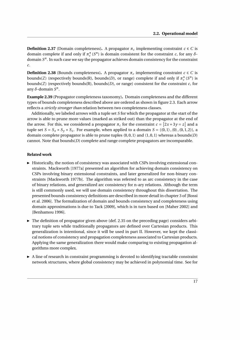
Example 2.39 (Propagator completeness taxonomy). Domain completeness and the differenttypes of bounds completeness described above are ordered as shown in figure 2.3. Each arrowreflects a strictly stronger than relation between two completeness classes.
Additionally, we labeled arrows with a tuple set S for which the propagator at the start of thearrow is able to prune more values (marked as striked out) than the propagator at the end ofthe arrow. For this, we considered a propagator πc for the constraint c = [
2x +3y = z]
and atuple set S = Sx × Sy × Sz . For example, when applied to a domain S = {⟨0,1⟩ ,⟨0⟩ ,⟨0,1,2⟩}, adomain complete propagator is able to prune tuples ⟨0,0,1⟩ and ⟨1,0,1⟩ whereas a bounds(D)cannot. Note that bounds(D) complete and range complete propagators are incomparable.
Related work
Ï Historically, the notion of consistency was associated with CSPs involving extensional con-straints. Mackworth [1977a] presented an algorithm for achieving domain consistency onCSPs involving binary extensional constraints, and later generalized for non-binary con-straints [Mackworth 1977b]. The algorithm was referred to as arc consistency in the caseof binary relations, and generalized arc consistency for n-ary relations. Although the termis still commonly used, we will use domain consistency throughout this dissertation. Thepresented bounds consistency definitions are described in more detail in chapter 3 of [Rossiet al. 2006]. The formalization of domain and bounds consistency and completeness usingdomain approximations is due to Tack [2009], which is in turn based on [Maher 2002] and[Benhamou 1996].
Ï The definition of propagator given above (def. 2.35 on the preceding page) considers arbi-trary tuple sets while traditionally propagators are defined over Cartesian products. Thisgeneralization is intentional, since it will be used in part II. However, we kept the classi-cal notions of consistency and propagation completeness associated to Cartesian products.Applying the same generalization there would make comparing to existing propagation al-gorithms more complex.
Ï A line of research in constraint programming is devoted to identifying tractable constraintnetwork structures, where global consistency may be achieved in polynomial time. See for
17

Chapter 2. Constraint Programming
domain
bounds(D)
bounds(Z)
bounds(R)
range
Sx = {0,1}Sy = {0}
Sz = {0,1/,2}
Sx = {0,1/}
Sy = {0,1}Sz = {0,3}
Sx = {0,1/}
Sy = {0,1}Sz = {0,3}
Sx = {0}Sy = {0,1}
Sz = {0,2/,3}
Sx = {0,1}Sy = {0,1}
Sz = {1/,2,3}
Sx = {0}Sy = {0,1}
Sz = {0,1/,3}
Sx = {0,1/}
Sy = {0,1}Sz = {0,3}
Figure 2.3.: Taxonomy of constraint propagation strength. Each arrow specifies a strictlystronger than relation between two consistencies (see example 2.39).
18

2.2. Operational model
Function GenerateAndTest(d ,C)Input: A domain d and a set of constraints COutput: A subset S ⊆ d satisfying all constraints in C , i.e. S ⊆ con(c) : ∀c ∈Cif d =; then1
return ;2
if |d | = 1∧∀c ∈C ,d ⊆ con(c) then3
return {d}4
⟨d1,d2⟩← Branch(d)5
return GenerateAndTest(d1,C) ∪ GenerateAndTest(d2,C)6
example chapter 7 of [Rossi et al. 2006]. For a complete characterization of tractable CSPsfor 2-element and 3-element domains see [Schaefer 1978; Bulatov 2006].
Ï A number of polynomial algorithms have been identified that achieve domain or boundsconsistency in a number of useful constraints. A notable example is the constraint thatenforces all variables to take distinct values (used in the magic square example) for which analgorithm exists that achieves domain consistency in time O
(n2.5
)by Régin [1994], another
achieving bounds(Z) on time O(n logn
)by Puget [1998], and a range complete propagator
which runs in time O(n2
)by Leconte [1996]. Algorithms achieving bounds(D) consistency
are rarely found in practice.
Ï Consistencies stronger than domain consistency have been proposed, namely path consis-tency [Montanari 1974], and k-consistency [Freuder 1978]. These consistencies approxi-mate constraints using domains stronger than δ-domains, whose representation requiresexponential space, and are disregarded in most constraint solvers.
2.2.2. Search
Generate and test is a brute force method that generates all possible combinations of valuesand then selects those that satisfy all constraints in the problem. The method is easily imple-mented using recursion (function GenerateAndTest).
Line 1 tests for the case where an empty domain is passed to the function, which triviallyhas no solutions. Line 3 tests if the current domain if it is singleton, i.e. all variables are instan-tiated, and satisfy all constraints in the problem. Otherwise, line 5 calls a function Branch thatsplits the domain d in two smaller domains d1, d2, such that d = d1 ∪d2, and line 6 calls thefunction recursively on each of these domains.
Figure 2.4 shows a trace, or search tree, of the algorithm applied to the magic square prob-lem. The leftmost square represents the initial domain, and the direct children of each squareare the domains resulting from the Branch function.
19

Chapter 2. Constraint Programming
15 14
1..16 1..16 1..16
1..16
1..16
1..16
1..16
1..161..16
1..161..16
1..16
1..16
1..16
15 14
2..16 1..16 1..16
1..16
1..16
1..16
1..16
1..161..16
1..161..16
1..16
1..16
1..16
14
1..16 1..16
1..16
1..16
1..16
1..16
1..161..16
1..161..16
1..16
1..16
1..16
15
1
14
1..16
1..16
1..16
1..16
1..16
1..161..16
1..161..16
1..16
1..16
1..16
15
1 1
15 14
1..16 1..16
1..16
1..16
1..16
1..16
1..161..16
1..161..16
1..16
1..16
1..162
x1,3 = 1
x1,3 6= 1
x1,2 = 1
x1,2 6= 1
...
...
...
...
x1,2 6= 1
x1,1 6= 2
x1,1 = 2
x1,2 = 1
...
...x1,1 6= 1
x1,1 = 1
Figure 2.4.: Partial search tree obtained by GenerateAndTest on the magic square problem.
The GenerateAndTest algorithm may generate an exponential number of domains that donot contain any solution. An example is the topmost square in fig. 2.4 that corresponds to anon-singleton domain which does not contain any solutions since the same value is used inthe first two cells of the first row. An improved version of this algorithm is given by functionSolve.
The difference is the inclusion of a call to the Propagate function, which filters inconsis-tent values from the input domain, as discussed in the previous section. The search tree of theSolve algorithm now depends on the consistency achieved by constraint propagation. For ex-ample, if Propagate enforces local domain consistency on this problem, we obtain the partialsearch tree shown in figure 2.5, where each square corresponds to the domain obtained afterpropagation (line 1). Note that all the upper children which cannot lead to any solution areimmediately rejected, hence the algorithm avoids exploring an exponential number of nodes.
The Solve algorithm is complete for any CSP - given enough time it will find a solution orprove that no solution exists, which is in fact one of the most appealing aspects of the con-straint programming approach. Additionally, it is also space efficient since only one child ofeach node must be in memory at all times, and the depth of the search tree is bounded by thenumber of variables and values in their domains. Unfortunately, the time efficiency of this al-gorithm greatly depends on the way the search tree is explored, i.e. on the order in which thechild nodes of a given node are visited (line 7). A number of heuristics have been proposed that
20

2.2. Operational model
Function Solve(d ,C)Input: A domain d and a set of constraints COutput: A subset S ⊆ d satisfying all constraints in C , i.e. S ⊆ con(c) : ∀c ∈Cd ← Propagate(d ,C)1
if d =; then2
return ;3
if |d | = 1∧∀c ∈C ,d ⊆ con(c) then4
return {d}5
⟨d1,d2⟩← Branch(d)6
return Solve(d1,C) ∪ Solve(d2,C)7
try to direct search towards the solution, with some success for many combinatorial problems.However, the algorithm will, in the worst case, explore the full search tree before finding thesolution or proving that it does not exist.
Although other complete search algorithms exist, they are essentially variations of the Solvealgorithm. Therefore, in this dissertation we will assume that search is performed using thisalgorithm.
Related work
Ï The Solve algorithm is also known as backtracking. Other popular complete algorithmsthat may be used with constraint propagation are backmarking, forward checking, back-jumping, among others [Dechter 2003].
Ï Most search heuristics are correlated with either a first-fail or a best-promise policy [Har-alick and Elliott 1980]. First-fail consists in trying first the domains which are more likelyto contain no solutions. While it seems contradictory, this will make the search algoritmvisit smaller search paths first, which increases the number of search paths visited for agiven amount of time. Best-promise does the opposite, it visits first the domains that aremore likely to contain solutions. First-fail heuristics are usually connected with the selec-tion of the next variable to enumerate: the variable with smaller domain, more constraintsattached [Bessère and Régin 1996], more constraints to instantiated variables, and varia-tions [Brélaz 1979; Boussemart et al. 2004]. Best-promise is usually connected to the choiceof value to enumerate, and is often obtained by integrating some knowledge about the struc-ture of the problem [Geelen 1992].
21

Chapter 2. Constraint Programming
1..13,16
1..13,16
1..13,16
1..13,16
1..13,16
1..13,16
1..13,16
1..13,16
1..13,16
1..13,16
1..13,16
1..13,16
14151..4 1..4
1..13,16
1..13,16
1..13,16
1..13,16
1..13,16
1..13,16
1..13,16
1..13,16
1..13,16
1..13,16
1..13,16
2..13,16
14151..4 1..4
1..12,16
1..12,16
1..12,16
1..12,16
1..12,16
1..12,16
1..12,16
1..12,16
1..12,16
1..12,16
1..12,16
14151..4 1..4
13
14151..4 1..4
16 1..13 1..13 4..13
1..13 1..13 4..13 4..13
1..13 4..13 1..13 4..13
x1,1 6= 1
x1,1 = 1
x1,1 = 13
x1,1 6= 13
x1,1 6= 2
x1,1 = 3
x1,1 6= 3
x1,1 = 2
...
...
...
Figure 2.5.: Partial search tree obtained by SOLVE on the magic square problem while main-taining local domain consistency.
2.3. Summary
This chapter presented the necessary notation for formalizing constraint satisfaction problemsand the constraint solving process. We have seen that constraint propagation operates ontuple sets, and how their approximations may be used to characterize the completeness ofpropagation algorithms. Finally, we introduced the main algorithm of a constraint solver thatintegrates constraint propagation with a general brute-force search algorithm.
22
Part I.
Incremental Propagation
23


Chapter 3.
Architecture of a Constraint Solver
This chapter will describe a number of important techniques and decisions behind the designand implementation of a modern constraint solver. It will focus on two main components:a propagation kernel implementing generalized constraint propagation (§3.1), and the statemanager, responsible for maintaining the state of all elements of a constraint solver synchro-nized with the search procedure (§3.2). Additionally, this chapter will present other importantstructural resources of constraint solvers, such as the support for domain specific reasoning,global constraints, and language interfaces (§3.3). Whenever possible, we will provide point-ers to state-of-the-art constraint solvers which advertise the use of a particular method. In thissame spirit, this chapter will also perform a global overview of CaSPER, the constraint solverused for implementing and evaluating all the techniques described in this dissertation.
3.1. Propagation kernel
The propagation kernel forms the core of a constraint solver. Because propagation takes thelargest share of time spent on solving a given problem, designing a propagation kernel involvesdecisions that affect the global performance of a constraint solver.
3.1.1. Propagation loop
Most constraint solvers do not maintain a specific type of consistency in particular, but in-stead achieve an hybrid form of local consistency. They associate one or more propagatorswith specific strengths with each constraint of the problem, and combine their propagationby repeatedly executing propagators until a fixpoint is achieved. The existence of a fixpoint,hence the termination of the algorithm, is guaranteed since propagators are contracting anddomains are finite, as we have observed in the previous chapter. A very simple implementationof this algorithm is given by function Propagate1.
This algorithm and its variants will be thoroughly revised in the next chapter.
25

Chapter 3. Architecture of a Constraint Solver
Function Propagate1(d ,C)Input: A domain d and a set of constraints COutput: A subset of d consistent with Cwhile ¬ fixpoint do1
fixpoint ← true2
foreach c ∈C do3
t ← d4
d ←πc (d)5
if d ⊂ t then6
fixpoint ← false7
8
9
return d10
3.1.2. Subscribing propagators
Most constraints typically involve a small subset of variables in the problem. For a given con-straint c ∈ C , its associated propagator πc reasons exclusively with X (c) instead of the full setof variables X . Consequently, changes to the domains of the variables in X \ X (c) are alwaysignored by πc - the propagator πc needs to be executed only when the domains of variablesin X (c) are updated. Algorithm Propagate1 does not take this observation into account, andsimply executes all propagators associated with all constraints in the problem, and that is, ofcourse, very inefficient.
Example 3.1. Consider a CSP with variables x1, . . . , xn , domains D (xi ) = {1, . . . ,b}, 1 ≤ i ≤ n,and a set of constraints C = c1, . . . ,cn where x1, x2 ∉ X (ci ), 1 ≤ i ≤ n −2, and cn−1 = [x1 > x2],cn = [x1 < x2]. Note that this CSP does not have any solutions. Calling Propagate1 on this CSPdetects inconsistency after O (nb) propagator executions (line 5), but only O (2b) propagatorexecutions are effective, i.e. not idempotent.
To mitigate this problem, constraint solvers maintain a queue of pending propagators, thatis, a set of propagators that can effectively prune the current domain. This is implementedby subscribing propagators to their relevant variables, so that updating a variable’s domaincan trigger the addition of all subscribed propagators to the pending queue, or in other words,schedule the propagators for execution. Let us formalize the set of propagators subscribed tovariable x:
Definition 3.2. For a given variable x ∈ X let PROPS (x) =⋃c∈C (x)πc .
Selecting which propagators must be scheduled requires a mechanism for identifying theset of variables whose domain changes from a given fixpoint to another.
26

3.1. Propagation kernel
Function Propagate2(d ,P)Input: A domain d and a set of propagators P implementing constraints COutput: A subset of d consistent with the constraints in Cwhile P 6= ; do1
πc ← SelectPropagator(P)2
P ← P \ {πc }3
d ′ ←πc (d)4
P ← P ∪⋃x∈VARS(d ,d ′) PROPS (x)5
d ← d ′6
return d7
Definition 3.3 (Prunned variables). Let d n1 , d n
2 , where d n2 ⊆ d n
1 denote two different domainsof a given CSP involving n variables. Let VARS
(d n
1 ,d n2
)⊆ X be defined as follows
VARS(d n
1 ,d n2
)= {xi ∈ X : d n
2 (xi ) ⊂ d n1 (xi )
}The optimization is integrated in the Propagate1 function by modifying the inner loop
(lines 3-8) to iterate over the queue of pending propagators instead of the full set of propa-gators, as shown by function Propagate2. Line 2 selects one propagator from the queue ofpending propagators P , line 3 removes the propagator from the queue, and line 4 executes thepropagator. Line 5 adds to the queue P all propagators subscribed to the domains which wereupdated. The mutual fixpoint of all propagators is implied by an empty queue P .
3.1.3. Event driven propagation
Determining the exact set of propagators whose execution will prune a given domain is notstraightforward. Variable subscription, described above, is often too conservative in the sensethat it may still schedule propagators that are at fixpoint for the current domain.
Example 3.4. Consider again the previous example, but where the set of constraints is now C =c1, . . . ,cn where ci = [x1 +x2 6= xi+2], 1 ≤ i ≤ n −2, and cn−1 = [x1 > x2], cn = [x1 < x2]. Note thatexecuting propagators πci , 1 ≤ i ≤ n −2, does not prune any domain whenever |D (xi )| > 1 forall i . Consequently, calling Propagate2 still requires O (nb) propagator executions to detectinconsistency on this CSP, even if only O (2b) propagator executions are effective.
In fact, determining if a propagator can prune a given domain is co-NP-complete in gen-eral. Fortunately, an approximation that is less conservative than variable subscription butstill efficient to implement can be devised using events.
In an event driven solver, propagators are subscribed to events representing propagation
27

Chapter 3. Architecture of a Constraint Solver
conditions. For example, propagators reasoning with integer domain variables usually sub-scribe to one of the following events:
¦ DOM (xi ) : the domain of variable xi has been updated
¦ BND (xi ) : the bounds of the domain of variable xi have been updated
¦ VAL (xi ) : variable xi has become instantiated
Updating the domain of a variable triggers the corresponding events, adding subscribed prop-agators to the pending queue.
Example 3.5. In an event driven solver, a propagator for a constraint ci = [x1 +x2 6= xi+2] wouldsubscribe to VAL (x1), VAL (x2), and VAL (xi+2), since propagation of this constraint requires thateither xi+2 or both x1 and x2 are instantiated. Likewise, propagators for cn−1 = [x1 > x2], andcn = [x1 < x2] would subscribe to BND (x1) and BND (x2), since propagation for this constraintreasons exclusively with the bounds of the domains.
Note that even event driven solvers may still schedule propagators which are at fixpoint forthe current domain. An example is the propagator for a constraint ci , described above. In thiscase, the propagator may be executed needlessly because the exact propagation condition, i.e.(VAL (x1)∧ VAL (x2))∨VAL (xi+2), cannot be expressed as a disjunction of events. In chapter 4 wepropose an alternative propagation model that may be used to circumvent this problem.
Finally, we remark that during search, propagators may cancel or alter the set of eventswhich they are subscribed to. An example is the propagator for an n-ary boolean disjunction.
Example 3.6. Consider a propagator for the constraint c = [∨
i∈1...n xi ], where n is an integergreater than two. This constraint is usually propagated using the watched literal scheme origi-nally introduced for SAT solving [Gent et al. 2006b]. The propagator initially subscribes to twoarbitrary non-ground variables xi , x j , more specifically to VAL (xi ), and VAL
(x j
). When any of
these events occur, the algorithm cancels the subscription to the event, searches for anothernon-ground variable xk where k 6= i and k 6= j , and subscribes to VAL (xk ). It repeats this pro-cedure until there are no more non-ground variables to replace the last instantiated variable,say xi , which mean that x j must be set to true.
Most modern constraint solvers use events to optimize propagation, as will be detailed inthe next chapter.
3.1.4. Signaling fixpoint
Another inefficiency of both versions of the Propagate function given above arises from theway fixpoint is detected. The presented approach assumes that a propagator is not at fix-point if its last execution was able to prune the current domain. While this is a safe way to
28

3.1. Propagation kernel
Function Propagate3(d ,P)Input: A domain d and a set of propagators P implementing constraints COutput: A subset of d consistent with the constraints in Cwhile P 6= ; do1
πc ← SelectPropagator(P)2 ⟨d ′, fixpoint ⟩←πc (d)3
P ← P ∪⋃x∈VARS(d ,d ′) PROPS (x) \ {πc }4
if ¬ fixpoint then5
P ← P ∪ {πc }6
d ← d ′7
return d8
detect fixpoint, it implies that a propagator that updates the domains of its own set of sub-scribed variables is always scheduled one additional time after achieving its fixpoint. A solu-tion to this problem is to force propagators to report whether they are currently at fixpoint. Thepseudocode for the algorithm integrating this optimization is given by function Propagate3.This function assumes that when the execution of πc does not change any domain it returnsfixpoint= true.
A constraint solver may have to handle propagators that are idempotent for any domain,and propagators that are idempotent for some domains.
Example 3.7. Consider a propagator for the constraint a = [x1 ≥ x2], where x1, x2, are integerdomain variables, defined as follows,
πa (d) ={
d (x1) ← d (x1) \ {−∞ . . .bd (x2)c−1}
d (x2) ← d (x2) \ {dd (x1)e+1. . .+∞}
It easy to see that πa (d) is sound and a fixpoint for πa for any domain d , i.e. the propagatoris an idempotent propagator (def. 2.36 on page 16). Now, consider a similar propagator πb forthe constraint b = [x2 ≥ x1], and a propagator for c = [x1 = x2] defined as,
πc (d) = πb (πa (d))
Although πc is sound, it is no longer an idempotent propagator, as witnessed when settingd1 = {v : v is odd}, and d2 = {v : v is even}.
The above example shows propagators which are idempotent for any domain, πa , πb , and apropagator πc which may or may not be at fixpoint after execution. An optimized constraintsolver could schedule πa and πb to a dedicated queue of idempotent propagators, but for πc
it has no other option than to query its idempotency status after every execution and proceed
29
Chapter 3. Architecture of a Constraint Solver
accordingly.Since the time spent on redundant propagator executions seems not to be significantly
larger than the time spent in computing the idempotency status (see [Schulte and Stuckey2004]), this optimization is not used in most constraint solvers. As far as we know, Gecode[Gecode 2010] is the only constraint solver implementing fixpoint signaling [Tack 2009].
3.1.5. Subsumption
Another common optimization used by most constraint solvers explores a relation betweenconstraints and domains called entailment. The goal is the same as before: to avoid schedulingpropagators unnecessarily.
Definition 3.8 (Entailnment,Subsumption). A constraint c is said to be entailed for a domaind if and only if d ⊆ con(c). A propagator πc for a constraint c is said to be subsumed for adomain d if and only if πc
(d ′)= d ′ for any d ′ ⊆ d .
A propagator which is subsumed for d cannot contribute to any further pruning and there-fore should never be scheduled again. Subsumed propagators can therefore be canceled. Can-celing does the opposite of subscribing - it unsubscribes the propagators of all previously sub-scribed events, so that they may not be scheduled again.
Example 3.9. Consider a constraint c = [x < y
]and a domain d = {1,2}× {3,4}. Then c is en-
tailed for d , and a bounds(Z) complete propagator πc is subsumed for d .
Modern constraint solvers typically cancel subsumed propagators. In CaSPER, cancellationis optional, i.e. is not integrated in the propagation kernel, but instead is left to the specificpropagator implementation. This allows each propagator to choose to cancel itself if the effortspent in checking subsumption compensates the extra redundant executions.
3.1.6. Scheduling
We have not discussed so far the order in which propagators are executed. The Propagate3function is non-deterministic assuming that SelectPropagator selects an arbitrary propaga-tor from the propagation queue. However, the order in which propagators are executed affectsthe number of executions and consequently the runtime required until the mutual fixpoint isachieved.
Example 3.10. Consider a CSP with variables x, y , and z, and domains D (x) = {−n . . .1}, D(y)=
D (z) = {1 . . .n}, where n is an arbitrary large number, and the constraints c1 = [x ≥ y
]and
c2 = [x + y = z
]. Consider also domain complete propagators for both constraints. Propagat-
ing πc1 only requires updating the bounds of the domains of x and y , which may be done inO (1) time. Propagating πc2 costs O
(n3
)since all values in the domains of x, y , and z must
30

3.2. State manager
be considered. Therefore, executing πc2 and then πc1 takes O(n3
). However, if πc1 is executed
first, the domains of x and y are pruned to D (x) = D(y)= {1} in O (1), which can lower the cost
of executing πc2 to O (1) since variables x and y are instantiated. Hence, in this case the totalcost of executing both propagators is O (1).
The above example suggests an heuristic for scheduling propagators: those with a lower costshould be executed first than those with higher cost. The rationale is that executing cheaperpropagators first may prune the current domain thus simplifying the task of costly propaga-tors.
Most modern constraint solvers employ priority based filter scheduling policies for schedul-ing their propagators. SICStus Prolog [Carlsson et al. 1997] uses two priority levels where in-dexicals have higher priority and global constraints have lower priority. Gecode and CaSPERuse ten priority levels based on estimated cost of execution. Eclipse Prolog [ECLiPSe 2010]supports twelve priority levels, but its finite domains solver uses only two. Choco [Laburtheand the OCRE project team 2008] uses cost and event based scheduling with seven prioritylevels.
Ï Entailment information may be obtained for special cases of indexical constraints, as shownin [Carlson et al. 1994].
Ï Cost based filter scheduling and an experimental comparison of different filter schedulingpolicies is detailed in [Schulte and Stuckey 2004].
3.2. State manager
Propagation eliminates inconsistent values from the domains. However, since propagationmust be complemented by some form of non-deterministic search, any update to the currentdomain is tentative and thus may have to be undone. In fact, not only variable domains, butthe state of propagators, their internal data structures and subsumption status, may have to berestored later due to a wrong guess in the search procedure. In practice, even good heuristicsimply a large number of wrong decisions, which makes state handling a central element in aconstraint solver.
Example 3.11. Consider a CSP with variables x, y , and z, domains D (x) = D(y)= {0,1}, D (z) =
{0 . . .3}, and constraints c1 =[2x + y = z
], c2 = [x 6= z], and c3 =
[y 6= z
]. Figure 3.1 shows a pos-
sible search tree for this problem. Each numbered node represents a state while arcs denotesearch decisions. Arcs are labeled with a tentative assignment, inside boxes, and the result ofpropagating the assignment. The two leftmost leaves are not solutions to the problem since zcannot be equal to x or y (constraints c2 and c3). Both children of node 3 satisfy all the con-straints and therefore are solutions to the problem.
31

Chapter 3. Architecture of a Constraint Solver
1
2
× ×
3
p p
x = 0⇒ D(z) = {0,1}
y = 0⇒ D(z) = {}
y = 1⇒ D(z) = {}
x = 1⇒ D(z) = {2,3}
y = 0⇒ z = 2
y = 1⇒ z = 3
Figure 3.1.: A possible search tree for the CSP described in example 3.11. Search decisions areunderlined.
D(x) = {0,1}D(y) = {0,1}
D(z) = {0 . . .3}
(a) at state 1
D(x) = {0,1}D(y) = {0,1}
D(z) = {0 . . .3}
D(x) = {0}D(y) = {0,1}D(z) = {0,1}
(b) at state 2
D(x) = {0,1}D(y) = {0,1}
D(z) = {0 . . .3}
D(x) = {1}D(y) = {0,1}D(z) = {2,3}
(c) at state 3
Figure 3.2.: Contents of the stack used by the copying method for handling state.
3.2.1. Algorithms for maintaining state
There are three popular methods for handling state of a constraint solver: copying, trailing,and recomputation. Copying saves the current state before each search decision, by pushingall stateful data to a stack. In case the search decision leads to a dead end, the current statemay be restored by copying back all data from the top of the stack. Search then proceeds bycommitting to a different decision.
Example 3.12. Figure 3.2 shows the contents of the stack used by the copying method whilesolving the CSP of the previous example. The contents of all domains are pushed to the stackat the initial state (fig. 3.2 a), and again after the first search decision and propagation (fig. 3.2b). After assigning y = 0 and propagating the solver finds an inconsistency, and restores state2 from the top of the stack. Then it assigns y = 1, propagates, again finds an inconsistency andbacktracks to state 1. This is done by poping state 2 from the stack and restoring state 1 fromthe top of the stack (fig. 3.2 a). It then assigns x = 1, propagates, and pushes state 3 to the stack(fig. 3.2 c). Finally, it assigns y = 0, propagates, and finds a solution.
32

3.2. State manager
1 ∉ D(x)2,3 ∉ D(z)
(a) at state 2
1 ∉ D(x)2,3 ∉ D(z)
1 ∉ D(y)0,1 ∉ D(z)
(b) at first failed state
0 ∉ D(x)0,1 ∉ D(z)
(c) at state 3
Figure 3.3.: Contents of the stack used by the trailing method for handling state.
While copying backups all stateful data before any modifications, trailing stores only thedata that is going to be modified. Since most of the times is hard to know beforehand whichdata is going to be updated, trailing must be embedded in any procedure that changes statefuldata. Any update operation must therefore check whether the data that is going to change isalready saved to the stack, and if not it must push it. On backtrack the solver transverses thelist of saved data (the trail) on the top of the stack and restores it.
Example 3.13. The stack used by trailing on the CSP of example 3.11 is shown in figure 3.3.Unlike the stack used in copying, the trailing stack is initially empty. All the domain updatesthat are a consequence of the first search decision and propagation, leading state 1 to state 2,are then pushed to stack (fig. 3.3 a). When the solver finds the first inconsistency, the contentsof the stack are as shown in fig. 3.3 b). It then restores state 2 by undoing the updates on thetop of the stack and poping the top trail, leaving the stack as shown in (fig. 3.3 a). When thesecond inconsistency is found, the solver restores state 1 by undoing the contents of both trailsin the stack, and emptying it. The contents of the stack at state 3 are shown in (fig. 3.3 c).
Unlike copying or trailing, recomputation does not store the full current state to memory,but instead only keeps track of the search decisions that lead to the current state. For restoringa given state, recomputation resets the original domains and other stateful data and repeatsall operations since the beginning of the search procedure leading to the state to be restored.
Example 3.14. Recomputation uses a queue for recording the original domains, and the searchdecisions leading to the current state. Figure 3.4 a) shows the initial state of the queue holdingthe original domains. At state 2 the search decision x = 0 is at the end of the queue (fig. 3.4b). Then, y = 0 is added and the solver finds the first inconsistency (fig. 3.4 c). For restoringstate 2, the solver first resets the domains from the backup stored in the first position of thequeue, and then propagates all the assignments in the queue except the last (y = 0). The solveris now on state 2 again, with the queue as shown in (fig. 3.4 b), and thus search may proceed toexplore the right branch.
The above methods for handling state may be categorized by expectation. Copying andtrailing always backup the current state anticipating that it will be proven inconsistent and will
33

Chapter 3. Architecture of a Constraint Solver
D(x) = {0,1}D(y) = {0,1}
D(z) = {0 . . .3}
(a) at state 1
D(x) = {0,1}D(y) = {0,1}
D(z) = {0 . . .3}
x = 0
(b) at state 2
D(x) = {0,1}D(y) = {0,1}
D(z) = {0 . . .3}
x = 0
y = 0
(c) at first failed state
Figure 3.4.: Contents of the queue used by the recomputation method for handling state.
have to be restored: both are pessimistic. Copying is still more pessimistic than trailing since itassumes that everything will change before finding an inconsistency, hence it is more efficientto push the full state to memory beforehand. Unlike copying or trailing, recomputation neverstores the current state hoping that it contains a solution and thus will not have to be restored- it is optimistic.
Trailing sacrifices modularity due to the fact that all operations and data structures mustbe reversible, i.e. must be synchronized with the trail. On the other hand, both copying andrecomputation are non-intrusive - an existing data structure or algorithm does not need tobe modified for integration in a constraint solver handling state using any of these methods.We will detail a simple framework for efficient and correct implementations of reversible datastructures maintained with trailing in the next section.
Trailing has been widely adopted by most constraint solvers, namely CaSPER, ILOG Solver[ILOG 2003a], Choco, Minion [Gent et al. 2006a], and Prolog based solvers in detriment ofcopying or recomputation, showing a robust expectation balance in different kinds of searchtrees. One notable exception is Gecode which uses an hybrid approach combining copyingand recomputation. Choco allows the user to select whether to use copying or trailing formaintaining state.
3.2.2. Reversible data structures
Solvers that use trailing for managing state typically provide a library of reversible data struc-tures, i.e. data structures which automatically record all updates on the trail and thus are ableto restore their previous state when required. A common framework for a clean implementa-tion of these data structures builds on the concept of a backtrackable or reversible pointer.From the client’s point of view, a reversible pointer is essentially a standard pointer whichkeeps a record of the addresses it was pointing to in any previous choice point, so that theycan be restored on demand.
34

3.2. State manager
1
@1 @2
6
@3 @4
(a) At state 0
1
@1 @2
5
@5 @6
6
@3 @4
(b) At state 1
1
@1 @2
6
@3 @4
(c) At state 2
Figure 3.5.: Reversible single-linked list. Memory addresses of the values and pointers com-posing the data structure are shown below each cell.
Implementing a reversible pointer is straightforward - for any update of the reversible pointera tuple composed of two standard pointers is stored in the trail: the address of the pointervariable, and the address of the location the pointer was pointing to before the update. Re-versible pointers allows a complex reversible data structure to be implemented just like thecorresponding non-reversible data structure, the only difference is that reversible pointers areused instead of standard pointers.
Example 3.15. Figure 3.5 shows a reversible single linked list, initially in state 0. Consider thatthe solver creates a choice point and inserts value 5 in the list, leaving the structure at state 1.For trailing this operation, the tuple t1 = ⟨2,3⟩ is pushed in the trail, representing the update ofa pointer at memory address 2 previously pointing to a memory location with address 3. Then,assume it creates another choice point and removes value 5 from the list, leading to state 2.This last operation triggers the insertion of a tuple t2 = ⟨2,5⟩ in the trail reflecting the updateof the same pointer (at memory address 2) previously pointing to a location with address 5.If the solver later backtracks one step and needs to undo the last operation then knowing t2 isenough to restore the list back to state 1, just by copying the old value 5 to the memory locationat address 2.
Using reversible pointers is also an efficient method of implementing most reversible datastructures. For example, each element insertion or removal in the above list requires four con-stant time copy operations, two for saving and two when restoring. In fact, in the particularcase of lists, inserting or removing a contiguous range of elements also takes a constant num-ber of trail operations, since only the pointers connecting the first and last cells in the rangehave to be trailed. Additionally, this trailing method works very well with lists that must bekept sorted, as those used for maintaining variable domains, since the same cells are restoredto the same positions.
The technique just described may be optimized to make the number of save and restoreoperations depend only on the number of choicepoints, and not on the number of updates tothe data structure (see related work below). However, even the basic version described above ismuch more efficient than, for example, a method that keeps track of which elements have beeninserted or removed, which would take linear time for restoring a single update to a sorted list.
Most Prolog engines provide a library of reversible structures. Eclipse Prolog for exampleprovides reversible lists, trees, ordered sets, hash tables, among others. Reversible structures
35

Chapter 3. Architecture of a Constraint Solver
are also available in Choco, referred to as backtrackable structures. In CaSPER the concept ofreversible pointer is generalized to any type, providing the user with a myriad of truly transpar-ent reversible data types, of which reversible pointers are a special case. The implementationexplores parametric polymorphism so that the type of the basic data type is not abstracted,which is useful for the compiler, and in particular the optimizer. CaSPER additionally providesa library of several reversible structures, such as stacks, lists, arrays, matrices, sets, maps, andtuples among others. ILOG Solver also provides reversible pointers and some plain reversibledata types such as reversible integers or booleans whose implementation seems to be basedon subtype polymorphism.
3.2.3. Memory pools
The speculative nature of depth search algorithms makes memory management a crucial ele-ment in a constraint solver. Most constraints solvers implement an elaborated memory man-ager that essentially provides fast allocation and deallocation of free memory with a confinedscope of existence. There are at least two good reasons to explicitly limit the lifetime of allo-cated memory. Firstly, it frees the programmer from the difficult task of keeping track of allallocated memory - memory will be automatically reclaimed by the memory manager whenits period of existence is over. Secondly, it allows optimizing the number of calls required to re-quest and release memory to the operating system since in many cases the provided memorywill be used for data structures which share the same scope of existence. Memory with specificlifetime is usually associated with a dedicated memory pool.
A memory manager of a constraint solver may implement several memory pools, but it cer-tainly provides a pool of backtrackable memory, i.e. memory which is available from the cur-rent choice point node to the leaf of the current search path. This kind of memory is useful forstoring variables and propagators added during search, maintaining the incremental state ofa propagator, and in general for any data which only exists below the current choice point. Wewill not detail an implementation of a backtrackable memory pool, but we note that it typicallyallows constant time allocation of new memory, and constant time deallocation of all memoryallocated on the same choice point.
Example 3.16. In the previous example we implicitly assumed that the described single-linkedlist is allocated on backatrable memory. This means that erasing value 5 does not frees thememory locations at addresses 3 and 4, which would be the natural thing to do with a standardlist. Storing the cell holding value 5 in backtrackable memory is essential to allow it to be safelyrestored just by resetting the values of the pointers, as explained above. The memory is onlyeffectively freed when the solver backtracks to state 0, i.e. before the choice point where cellholding value 5 was created.
Other memory pools may exist in a constraint solver, all with the same goal: simplified andefficient deallocation of memory. Gecode additionally maintains a pool for storing equally-
36

3.3. Other components
sized blocks of memory, and a pool for temporary storage. Minion has backtrackable and non-backtrackable memory pools, and even stores some data structures across different memorypools. For example, the storage of domain of binary domain variables or contiguous inter-val variables is split in two: one part stored in backtrackable memory and another in non-backtrackable memory [Gent et al. 2006a]. CaSPER additionally provides a pool for memorywhich is a available exclusively for the current choice point, which is useful for storing tempo-rary data used for computing the current fixpoint.
Related work
Ï For a detailed comparison of trailing methods versus copying and recomputation see [Reis-chuk et al. 2009].
Ï The Warren’s Abstract Machine [Aït-Kaci 1991] pioneered the presented techniques for main-taining state on a trailing based system, namely reversible pointers and memory pools.
Ï Memory pools described above may be seen as dedicated garbage collectors (see e.g. [Jonesand Lins 1996]). However, they are much simpler than general purpose garbage collectorsand also much more efficient for the task since they are tightly coupled with the solver’sexecution model.
3.3. Other components
In the previous sections we have described the elements that form the core of a constraintsolver. In this section we will discuss the remaining aspects of a constraint solver, which areorthogonal to the core architecture, and usually integrated in a modular, extensible way.
3.3.1. Constraint library
One of the most appealing aspects of a constraint solver is the span of supported constraintssince it reflects its ability to deal to specific applications efficiently. The global constraint cat-alog [Beldiceanu et al. 2010] currently lists 348 global constraints, for which several practi-cal propagation algorithms often exist. Creating, debugging and maintaining propagators forsuch a large number of constraints is a daunting task, considering that implementing an ef-ficient propagator for many global constraints is not straightforward. This makes the set ofsupported constraints one of the most valuable resources of a constraint solver.
Most, if not all constraint solvers either allow adding propagators for existing constraints, orfor new constraints, or more frequently both. The propagation algorithm given in section 3.1promotes this extensibility by establishing a clear separation between the propagation loop,and the propagator task - the propagation kernel is blind with respect to the specific constraintbeing propagated or the algorithm used for the propagation. However, the constraint kernel
37

Chapter 3. Architecture of a Constraint Solver
may provide services for simplifying the task of designing new propagators. Reversible struc-tures and dedicated memory pools, introduced above, are one example. In the next chapter wewill detail a kernel service that reports the set of changes in the domain of variables betweentwo consecutive executions of a given propagator, which can be very useful for designing prop-agators.
All constraint solvers mentioned above provide propagators for a large number of constraints.Compared with the remaining solvers, Choco and CaSPER offer a smaller set of specialized do-main consistent propagators. In these solvers, constraints for which no specialized propagatorexist are compiled to an extensional representation and propagated using a more general butless efficient algorithm. CaSPER additionally implements a technique for achieving boundsconsistency on arbitrary constraints, behaving as if specialized propagators were available,described in the second part of this dissertation.
3.3.2. Domain modules
Constraint solving has historically addressed integer domain problems, and more recently, setdomain problems. A number of representations and algorithms for reasoning with other do-mains have also been proposed, namely for addressing multiset problems [Walsh 2003], graphproblems [Viegas 2008], real-valued problems [Benhamou 1995], or for specific applicationssuch as protein folding [Krippahl and Barahona 2002]. Support for integrating domain-specificreasoning is therefore an imperative design condition for a general purpose constraint solver,perhaps as important as the ability to integrate new constraint propagators. General purposeconstraint solvers are Choco and ILOG Solver, supporting integer, set, and real-valued domainvariables, Gecode, handling integer and set domain variables, and Prolog based solvers suchas SICStus, Eclipse, and B-Prolog which additionally provide support for graph, tree, and ratio-nal domain variables. CaSPER fully supports integer and set domain variables, and providesexperimental support for real-valued, graph and coordinate domain variables.
There are also a number of constraint solvers designed for addressing specific domainsor special kind of constraints. These solvers are often significantly different than the afore-mentioned general purpose solvers. Examples are SAT solvers that address problems involv-ing boolean variables, or solvers which work exclusively with finite domain variables, suchas MDDC-Solv [Zhou 2009], Abscon [Merchez et al. 2001], CSP4J [Julien Vion 2007], or Sugar[Tamura et al. 2009], among others. These solvers often apply specialized techniques such ascompilation of constraints to extensional representation or SAT.
3.3.3. Interfaces
Constraint programs are conceptually highly declarative - the user declares the constraints andvariables of the problem, and the solver finds a satisfiable assignment. In practice, however,the user often has to provide specific instructions to the solving process for obtaining a so-
38

3.4. Summary
lution in reasonable time. A common solver interface gives the user control over the model,the propagation and search algorithms used for solving the problem. This is the case of Pro-log based constraint solvers, Choco, Gecode and CaSPER. Notable exceptions are Minion, andrecent versions of ILOG Solver, which provide self-parametrized propagation and search algo-rithms, thus following the black-box approach [Puget 2004].
Recent efforts have been made to establish interfaces for constraint solvers. The JAVA Con-straint API is a JAVA interface for constraint solving [ACP 2010]. Numberjack interfaces con-straint solvers from the Python language [Hebrard et al. 2010]. XCSP defines a XML based prob-lem specification format, useful for interchanging problems between different solvers [Rousseland Lecoutre 2009]. Minizinc is also a problem specification language, but additionally allowsparametrizing the propagation and search algorithms, although currently only in a limitedform [Nethercote et al. 2007]. Many constraint solvers are now able to solve constraint prob-lems written in XCSP and Minizinc. CaSPER currently fully supports the former, and offerspartial support for the latter, as described in [Silva 2010].
3.4. Summary
This chapter presented an overview of the architecture and techniques used in state-of-the-art constraint solvers. The first part covered a generalized propagation kernel, optimized usingvariable and event subscription, fixpoint reasoning, subsumption checking, and filter schedul-ing. Then we have introduced the most popular algorithms for maintaining the state of a con-straint solver, namely trailing, copying, and recomputation. We have also described the useof reversible data structures and memory pools, two important techniques for making statemanaging efficient and transparent. Finally, we have mentioned other important componentsof a constraint solver, in particular extensible support for new propagators, specific domainreasoning, and standard interfaces.
39

Chapter 3. Architecture of a Constraint Solver
40
Chapter 4.
A Propagation Kernel for IncrementalPropagation
This chapter will discuss a central component of a constraint solver - the propagation engine.It will describe two models for scheduling propagators, namely variable and propagator cen-tered architectures, highlight their inherent advantages and disadvantages, and show how tointegrate standard optimizations such as events or priorities on both models (§4.1). It will beshown that the propagator centered model is theoretically more efficient than the variable cen-tered model. Then we will present a modified propagation centered algorithm that integratesa feature originally exclusive of the variable centered model - support for incremental prop-agation (§4.2). The implementation of this algorithm in an object-oriented environment willbe discussed in §4.3. Finally, we will present a set of experiments performed for comparingseveral propagator and event scheduling policies using the new propagator-centered modeland the variable-centered model (§4.4), and discuss the results obtained providing empiricalevidence of the superiority of the former (§4.5).
4.1. Propagator and variable centered propagation
The following concept allows us to analyze and compare fixpoint computations.
Definition 4.1 (Propagation sequence). A propagation sequence describes the domains andpropagator executions involved in the computation of a fixpoint. The sequence consists on aseries of nodes d1, . . . ,dn representing domains, and labeled arrows representing propagatorexecutions. There is a labeled arrow from a domain di to domain d j , denoted di →
πd j , if and
only if the execution of propagator π filtered domain di to domain d j during the computationof the fixpoint. Although propagation is non-deterministic, we will assume a deterministicimplementation on one processor, which consequently allow us to represent propagation se-quences of the form
d1 →π1
. . . →πt
dn
41

Chapter 4. A Propagation Kernel for Incremental Propagation
Function PropagatePC(d ,P)Input: A domain d and a set of propagators P implementing constraints COutput: A subset of d consistent with the constraints in Cwhile P 6= ; do1
πc ← SelectPropagator(P)2
P ← P \ {πc }3
d ′ ←πc (d)4
P ← P ∪⋃x∈VARS(d ,d ′) PROPS (x)5
d ← d ′6
return d7
Function PropagatePC, introduced in the last chapter, implements what is commonly re-ferred to as propagator centered propagation, due to its main data structure: a queue of prop-agators.
Example 4.2. Consider a CSP with variables x1, x2, x3, with domains D (x1) = D (x2) = D (x3) ={1,2,3}, and the constraints a = [x2 6= 3], b = [x1 ≤ x2], and c = [DISTINCT (x1, x2, x3)]. Invok-ing the function PropagatePC with P = {πa}, assuming that SelectPropagator follows aFIFO policy, and all propagators are domain complete, produces the following propagationsequence,
d1 →πa
d2 →πb
d3 →πc
d4
(→πb
d4 →πc
d4
)A trace of the execution of algorithm PropagatePC for this example is shown below, whereeach row shows the state of the contents of the data structures at line 1,
0 d1 (x1) = {1,2,3} d1 (x2) = {1,2,3} d1 (x3) = {1,2,3} P = {πa}1 d2 (x1) = {1,2,3} d2 (x2) = {1,2} d2 (x3) = {1,2,3} P = {πb ,πc }2 d3 (x1) = {1,2} d3 (x2) = {1,2} d3 (x3) = {1,2,3} P = {πc ,πb}3 d4 (x1) = {1,2} d4 (x2) = {1,2} d4 (x3) = {3} P = {πb ,πc }4 P = {πc }5 P = {}
Note that the second execution of πb and πc (iterations 4 and 5) is redundant and could beavoided using the techniques for signaling fixpoint discussed in the previous chapter.
Some constraint solvers take a distinct approach, denoted variable centered propagation.This algorithm maintains a queue V of variables whose domain has changed and executes allpropagators subscribed for each variable x ∈ V in turn until there are no more changes in thedomains (function PropagateVC).
Example 4.3. Consider again the CSP of the previous example. Invoking function PropagateVC
42

4.1. Propagator and variable centered propagation
Function PropagateVC(d ,V )Input: A domain d and a set of variables V ⊆ XOutput: A subset of d consistent with all constraints in Cwhile V 6= ; do1
x ← SelectVariable(V )2
V ←V \ {x}3
P ← PROPS (x)4
while P 6= ; do5
πc ← SelectPropagator(P)6
P ← P \ {πc }7
d ′ ←πc (d)8
V ←V ∪ VARS(d ,d ′)9
d ← d ′10
11
return d12
with V = {x2}, assuming that both SelectVariable and SelectPropagator follow a FIFO pol-icy is described by the following propagation sequence,
d1 →πa
d2 →πb
d3 →πc
d4
(→πa
d4 →πb
d4 →πc
d4 →πb
d4 →πc
d4 →πc
d4
)A trace of the execution of algorithm PropagateVC for this example is shown below, whereeach row shows the contents of the data structures at line 5,
0 d1 (x1) = {1,2,3} d1 (x2) = {1,2,3} d1 (x3) = {1,2,3} x = x2,V =;,P = {πa ,πb ,πc }1 d2 (x1) = {1,2,3} d2 (x2) = {1,2} d2 (x3) = {1,2,3} x = x2,V = {x2} ,P = {πb ,πc }2 d3 (x1) = {1,2} d3 (x2) = {1,2} d3 (x3) = {1,2,3} x = x2,V = {x2, x1} ,P = {πc }3 d4 (x1) = {1,2} d4 (x2) = {1,2} d4 (x3) = {3} x = x2,V = {x2, x1, x3} ,P =;4 x = x2,V = {x1, x3} ,P = {πa ,πb ,πc }5 x = x2,V = {x1, x3} ,P = {πb ,πc }6 x = x2,V = {x1, x3} ,P = {πc }7 x = x2,V = {x1, x3} ,P =;8 x = x1,V = {x3} ,P = {πb ,πc }9 x = x1,V = {x3} ,P = {πc }10 x = x1,V = {x3} ,P =;11 x = x3,V =;,P = {πc }12 x = x3,V =;,P =;
43

Chapter 4. A Propagation Kernel for Incremental Propagation
x1
x2
x3
π1 π2
π3 π4
Figure 4.1.: Example of a CSP with variables x1, x2, x3, and propagators π1, . . . ,π4.
As seen in the above example, variable centered propagation may lead to more propagatorexecutions compared to propagator centered propagation. This is due to the fact that prop-agator centered propagation will never schedule a propagator if the propagator is already inthe queue, which might not be true for variable centered propagation. The problem can per-haps be best explained using the graph of figure 4.1, which shows a possible structure forpropagating a CSP. Each variable is represented as a node in the graph, and an arc betweentwo nodes represents a propagator implementing some constraint between the correspondingvariables. Assume that each propagator can modify the domains of both associated variablesand is awaken each time the domain of any of its variables changes.
Consider applying variable centered propagation to propagate this CSP. If the domain ofvariable x2 is updated, all propagators π1 . . .π4 are added to the queue P . Now, imagine thatπ1 is executed and changes variable x1. Then propagator π2 will be scheduled for executionwhen variable x1 is processed even if it is already on the current propagation queue. The orderin which propagators are scheduled does not solve this problem - if π2 was executed first, π1
would then be executed twice. The number of extra executions of variable centered propaga-tion compared with propagator centered propagation could be estimated based on the num-ber of loops in the constraint graph of the problem: in the example CSP, there are always twopropagators which are executed twice each time variable x2 changes.
We note that signaling fixpoint would allow both methods to achieve fixpoint using the samenumber of propagator executions. As discussed previously, this method is untractable in gen-eral, but for some constraints it is straightforward to determine fixpoint. For example, itera-tions 4-7 of the previous example could be easily avoided since the propagator for the con-straint a = [x2 6= 3] is idempotent.
4.1.1. Incremental propagation
A popular algorithm for achieving domain consistency on the DISTINCT constraint of the pre-vious example is given in [Régin 1994]. The algorithm incrementally maintains a data structurewhich is a function of the domains of the variables involved in the constraint. For every exe-cution of the propagator, this data structure must be updated to reflect the current domain,which may have changed since the last execution due to the execution of other propagators.
44

4.1. Propagator and variable centered propagation
There are two options for performing this update, either the current data structure is discardedand rebuilt from the current domain, or the current data structure is updated by integrating thechanges occurred on the domains since the last execution of the propagator, referred through-out this dissertation as domain delta. Apparently the best method to apply is constraint spe-cific or perhaps domain specific, but for some situations using domain deltas may improvepropagation significantly, as we will see in the next chapter.
An approximation for providing the domain delta to incremental propagators is simply toinform the propagator which variable has triggered propagation. The propagator for the DIS-TINCT constraint, for example, may use this information to optimize the update of its internaldata structure since it knows which variable domain changed. Variable centered propagationnaturally integrates this kind of incremental propagation simply by changing line 8 of functionPropagateVC to d ′ ←πc (d , x), where x is the variable that triggered propagation (line 2). Sincethe propagator is executed once for every variable domain that has changed, its internal datastructure will eventually reflect the current domain.
Example 4.4. Consider again the previous example, where πb is designed to perform incre-mental propagation as explained above. The propagation sequence when applying incremen-tal variable centered propagation is as follows,
d1 →πa
d2 →πb
d3
(→πc
d3 →πa
d3 →πb
d3 →πc
d3 →πb
d3
)→πc
d4
(→πc
d4
)
0 d1 (x1) = {1,2,3} d1 (x2) = {1,2,3} d1 (x3) = {1,2,3} x = x2,V =;,P = {πa ,πb ,πc }1 d2 (x1) = {1,2,3} d2 (x2) = {1,2} d2 (x3) = {1,2,3} x = x2,V = {x2} ,P = {πb ,πc }2 d3 (x1) = {1,2} d3 (x2) = {1,2} d3 (x3) = {1,2,3} x = x2,V = {x2, x1} ,P = {πc }3 x = x2,V = {x2, x1} ,P =;4 x = x2,V = {x1} ,P = {πa ,πb ,πc }5 x = x2,V = {x1} ,P = {πb ,πc }6 x = x2,V = {x1} ,P = {πc }7 x = x2,V = {x1} ,P =;8 x = x1,V =;,P = {πb ,πc }9 x = x1,V =;,P = {πc }10 d4 (x1) = {1,2} d4 (x2) = {1,2} d4 (x3) = {3} x = x1,V = {x3} ,P =;11 x = x3,V =;,P = {πc }12 x = x3,V =;,P =;
Note that the first and second executions of πc (iterations 3 and 7) do not prune the domain.This is because the algorithm for propagating πc is not fully aware of the current domain - itonly knows that x2 has changed, but not x1. Only on its third execution (iteration 10), πc isinformed about the update of the domain of x1, and is finally able to prune the domain of x3.
45

Chapter 4. A Propagation Kernel for Incremental Propagation
This shows that using variable centered propagation for incremental propagation may lead toa different propagation sequence compared to non-incremental variable centered propaga-tion. While the fact that an extra number of propagations may be required to synchronize theinternal state of the incremental propagators with the current domain may suggest that addingincrementality to variable centered propagation leads to more propagator executions, we can-not confirm that this is always the case due to the complex nature of fixpoint computations (inour example they take the same number of executions).
We also remark that integrating incremental propagation with propagator centered prop-agation is not as simple as with variable centered propagation, since the information aboutwhich variable triggered the propagator execution is not directly available. Later on, we willsee how to address this problem. Before that, let us show how the two approaches may beimproved using events and priority queues.
4.1.2. Improving propagation with events
Both propagator and variable centered propagation may be improved using events to signalspecific propagator conditions. Events have been informally introduced in the previous chap-ter. Let us now formalize them.
Definition 4.5. Let d1 (x), and d2 (x) be two domains of a variable x ∈ X , such that d2 (x) ⊆d1 (x). The set of events produced by the update of d1 (x) to d2 (x) is defined by
events(d1 (x) ,d2 (x)) = dom(d1 (x) ,d2 (x))∪bnd(d1 (x) ,d2 (x))∪val(d1 (x) ,d2 (x))
where
dom(d1 (x) ,d2 (x)) ={
{DOM(x)} ⇐ d1 (x) ⊃ d2 (x)
{} otherwise
bnd(d1 (x) ,d2 (x)) ={
{BND(x)} ⇐dd1 (x)e > dd2 (x)e∨bd1 (x)c < bd2 (x)c{} otherwise
val(d1 (x) ,d2 (x)) ={
{VAL(x)} ⇐|d1 (x)| > 1∧|d2 (x)| = 1
{} otherwise
Similar to the VARS(d ,d ′) function which captures the set of variables whose domain has
changed from d to domain d ′, we introduce the EVENTS(d ,d ′) function used for obtaining the
set of events that describe the update of domain d to domain d ′.
Definition 4.6. Let d1, d2 be two domains of the same CSP such that d1 ⊆ d2. Then
EVENTS (d1,d2) = ⋃x∈X
events(d1 (x) ,d2 (x))
46

4.1. Propagator and variable centered propagation
Function PropagatePCEvents(d ,E)Input: A domain d and a set of events EOutput: A subset of d consistent with the constraints in CP ←⋃
e∈E PROPS (e)1
while P 6= ; do2
πc ← SelectPropagator(P)3
P ← P \ {πc }4
d ′ ←πc (d)5
P ← P ∪⋃e∈EVENTS(d ,d ′) PROPS (e)6
d ← d ′7
return d8
Since propagators are now associated with events instead of variables, we naturally extendthe function PROPS (e) to provide us the set of propagators associated with event e.
Function PropagatePCEvents corresponds to an event based implementation of propaga-tor centered propagation. The algorithm now accepts a set E of events signaling domain mod-ifications since its last execution and uses the EVENTS function (line 6) which always inserts aset of propagators in the P queue which is a subset of those that would be inserted with theprevious version.
Function PropagateVCEvents applies the same optimization to variable centered propa-gation. Compared with the basic version described earlier (function PropagateVC) there aresome changes to note. First the algorithm now traverses a queue E of events, instead of aqueue of variables - the algorithm is now performing event centered propagation. Again theoptimization comes from the selection of propagators to execute (line 5) which will be moreaccurate than with the basic version. Compared with event based propagator centered prop-agation (function PropagatePCEvents), this algorithm may perform even more redundantexecutions, since the probability that a propagator may be scheduled twice is increased. Fi-nally, we remark that incremental propagation may still be integrated easily, since the eventthat triggered propagation is available, describes an update of a single domain, and may beprovided to the propagator to execute as before.
4.1.3. Improving propagation with priorities
As mentioned earlier, a propagator may be scheduled for execution using distinct policies. Forthe above algorithms, propagator scheduling may be controlled by modifying the semanticsof SelectPropagator in functions PropagatePC and PropagatePCEvents, SelectVariableand SelectPropagator in function PropagateVC, and SelectEvent and SelectPropagatorin function PropagateVCEvents. As mentioned earlier, popular propagator scheduling poli-cies are FIFO or cost based scheduling, but these are mainly suited for propagator centered
47

Chapter 4. A Propagation Kernel for Incremental Propagation
Function PropagateVCEvents(d ,E)Input: A domain d and a set of events EOutput: A subset of d consistent with all constraints in CP ←;1
while E 6= ; do2
e ← SelectEvent(E)3
E ← E \ {e}4
P ← PROPS (e)5
while P 6= ; do6
πc ← SelectPropagator(P)7
P ← P \ {πc }8
d ′ ←πc (d)9
E ← E ∪ EVENTS(d ,d ′)10
d ← d ′11
12
return d13
propagation since scheduling propagators for variable or event centered propagation is af-fected also by the order in which variables or events are processed. Cost based scheduling forevent centered propagation, for example, only affects the queue of propagators of the event be-ing processed (line 7 of function PropagateVCEvents) which may potentially compromise itsperformance compared with propagator based scheduling which always maintains all pend-ing propagators ordered by its cost. On the other hand, variable and event centered propaga-tion offer other opportunities for scheduling - we may choose to first process variables whichare more constrained or events which correspond to stronger propagation conditions. We willperform an empirical comparison of propagator scheduling using the presented algorithms insection 4.5.
4.2. The NOTIFY-EXECUTE algorithm
We have seen that propagator centered propagation does not directly allow incremental prop-agation. To specifically address this problem we designed a new propagation algorithm sup-porting incremental propagation which is still propagator centered, thus avoiding all the prob-lems inherent to variable or event centered propagation pointed out previously.
The algorithm assumes a global queue P and is composed of two interleaved tasks, EXE-CUTE and NOTIFY, which break propagator execution from propagator scheduling. The exe-cute phase (function Execute) processes all pending propagators, thus emptying the queue P .It is very similar to the basic propagator-centered algorithm given by function PropagatePC,
48

4.2. The NOTIFY-EXECUTE algorithm
Function Execute(d)Data: P and ’failed’ are global variablesInput: A domain dOutput: A subset of d consistent with the constraints in Cwhile P 6= ;∧¬failed do1
πc ← SelectPropagator(P)2
P ← P \ {πc }3
d ←πc (d)4
return d5
except in that it does not insert propagators into the queue. This is done in the notify phase(procedure Notify) which basically processes an event corresponding to a domain updateand informs all propagators attached to that event that they should update their internal state.Additionally, this phase is responsible for inserting pending propagators into the queue P .
For this model to work, a call to the Notify procedure must be made after every atomicdomain update. What consists an atomic domain update is domain specific - for integer andset domains we have chosen to consider the removal of contiguous subset of values as a do-main update1. This allows propagators to obtain exact information about the current domainand update their internal state incrementally. It also allows delta domains to be maintained inconstant space since only the description of the last atomic update is required at any moment.Further details about delta domains will be given in the next chapter.
The NotifyPropagator function called from line 2 of the Notify procedure is thereforepropagator specific, and returns one of fail, schedule, or ignore. The fail condition is re-turned when the propagator discovers inconsistency while updating its internal state, whichis not uncommon, and allows the solver to backtrack immediately. The ignore condition issignaled if the propagator finds that it is idempotent for the current domain, which may alsooccur when updating its state. This avoids redundant executions of the propagator which can-not be captured by events. Otherwise, the schedule condition is returned to specify that thepropagator must be executed. Note that idempotent propagators may still return scheduleimplying one redundant execution but otherwise not compromising the integrity of the sys-tem - this is required since finding if a propagator is idempotent may be as costly as alreadydiscussed.
Priority scheduling may be integrated in this algorithm in two different ways. Propagatorsmay be scheduled by modifying the SelectPropagator function called from line 2 of func-tion Execute. For example, FIFO based scheduling would always return the first propagatorin the queue, and cost based filter scheduling would always return the propagator with lowest
1By contiguous subset of values we mean values which are contiguous in the set, e.g. {1,3} is a contiguous subsetof {1,3,5}.
49
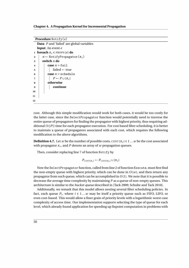
Chapter 4. A Propagation Kernel for Incremental Propagation
Procedure Notify(e)Data: P and ’failed’ are global variablesInput: An event eforeach πc ∈ PROPS (e) do1
n ← NotifyPropagator(πc)2
switch n do3
case n = fail4
failed ← true5
case n = schedule6
P ← P ∪ {πc }7
otherwise8
continue9
10
11
12
cost. Although this simple modification would work for both cases, it would be too costly forthe latter case, since the SelectPropagator function would potentially need to traverse theentire queue of propagators for finding the propagator with highest priority, thus requiring ad-ditional O (|P |) time for each propagator execution. For cost based filter scheduling, it is betterto maintain a queue of propagators associated with each cost, which requires the followingmodification to the above algorithms.
Definition 4.7. Let w be the number of possible costs, COST (πc ) ∈ 1. . . w be the cost associatedwith propagator πc , and P denote an array of w propagation queues.
Then, consider replacing line 7 of function Notify by
PCOST(πc ) ← PCOST(πc ) ∪ {πc }
Now the SelectPropagator function, called from line 2 of function Execute, must first findthe non-empty queue with highest priority, which can be done in O (w), and then return anypropagator from such queue, which can be accomplished in O (1). We note that it is possible todecrease the average time complexity by maintaining P as a queue of non-empty queues. Thisarchitecture is similar to the bucket-queue described in [Tack 2009; Schulte and Tack 2010].
Additionally, we remark that this model allows nesting several filter scheduling policies. Infact, each queue Pi , where i ∈ 1. . . w may be itself a priority queue such as FIFO, LIFO, oreven cost-based. This would allow a finer grain of priority levels with a logarithmic worst casecomplexity of access time. Our implementation supports selecting the type of queue for eachlevel, which already found application for speeding up fixpoint computation in problems with
50

4.3. An object-oriented implementation
Procedure Notify(e)Data: ’failed’ is a global variableInput: An event eforeach ν ∈ NOTIFIABLES (e) do1
n ← ν.Call2
if n = fail then3
failed ← true4
return5
6
7
a particular constraint structure [Jung 2008]. However, we did not yet performed a detailedanalysis on the effect of changing priorities at this level in general.
The NOTIFY-EXECUTE algorithm also provides opportunity for event scheduling. This maybe accomplished by ordering the events and corresponding calls to the Notify function foreach domain update.
4.3. An object-oriented implementation
Our implementation of the NOTIFY-EXECUTE algorithm does not follow the model presentedabove literally, but instead takes advantage of the object-oriented paradigm for achieving moreflexibility. The most important concept in this setting is the notifiable object, which generalizesand extends the function NotifyPropagator presented above by additionally maintaining astate, which is not possible using a simple function.
Definition 4.8 (Notifiable). A notifiableν is a function object (see e.g. [Kühne 1997]) exposing asingle method called Call. The method takes no arguments, and returns either ok, or failed,to signal if the solver should proceed or backtrack, respectively.
In practice, constructors for notifiable objects are given a set of objects required by the spe-cific notifiable, in particular but not necessarily, an associated propagator. Once notifiable ob-jects become part of the architecture, some modifications to procedure Notify are required,as shown on the current page.
The first visible modification is that now notifiables are associated with events, in the sameway propagators were associated with events in the previous version - the NOTIFIABLES(e)function in the code returns the set of notifiables associated with event e. This allows sev-eral notifiables to be associated with a single propagator, which is very useful as will be shownshortly. The main Notify function is now blind with respect to propagators, it only calls noti-fiable objects, and therefore it is no longer responsible for adding propagators to the queue P .
51

Chapter 4. A Propagation Kernel for Incremental Propagation
Method νi .Call()Preconditions: xi is instantiatedInput: An event eπc .S.PUSH (i )1
P ← P ∪ {πc }2
return ok3
The task of scheduling propagators is now delegated to the notifiable objects, which thereforemust have access to P . Let us illustrate with a practical example.
Example 4.9. Consider the global constraint c = [DISTINCT(x)]. Designing a propagator forachieving node consistency for c is trivial for the case |x| = 2 - the propagator waits until oneof the variables is instantiated and then removes its corresponding value from the domain ofthe other variable. When |x| = n and n is an arbitrary number greater than 2, then usuallya set of n (n −1)/2 binary DISTINCT propagators are posted between each pair of variables toenforce the constraint. Achieving the fixpoint of this set of propagators takes O
(n2
)propagator
executions, thus the overall time complexity is O(n2
)assuming each execution takes constant
time.Another solution is to design a global node-consistent propagator for c which, although hav-
ing the same overall complexity and achieving the same pruning than the previous decompo-sition, may decrease the number of executions to O (n), one for each variable that gets instan-tiated. This may be significant since operations in the propagation queue have an associated,albeit small cost. Note that for maintaining the overall complexity we need that each executionof the global propagator takes at most O (n).
A naïve, non-incremental, implementation of this propagator would, on each execution,search for the variables that became ground since the last execution and then prune theirvalues from the domains of the remaining variables. Since each execution of the propaga-tor would take O
(n2
)time, this solution is not admissible. A more efficient version of this
propagator requires an internal state that is updated incrementally. It works as follows.In the propagator πc we maintain a stack S of the indexes of the variables that became
ground since the last execution of the propagator. An execution of this propagator simply popseach index i from S and removes value xi from the domains of the remaining variables. Sinceeach variable can become instantiated only once, the number of executions of this propagatoris bounded by O (n), and thus the overall time complexity will be O
(n2
). In order to maintain
the stack S we need a set N of n notifiable objects, one for each variable, where each notifiableobject νi ∈ N is subscribed to VAL(xi ), and has local variables P , πc , and i , passed as argumentsto its constructor. Then, the Call method of each notifiable νi is as shown on this page.
Note that there are other subtleties for maintaining state in the previous example, such asthe effect of a possible backtrack before the propagator is executed, but after its internal state is
52

4.3. An object-oriented implementation
d(xi )
VAL
BND
DOM
ν1 ν2 ν3
ν4 ν5
ν6 ν7 ν8 ν9
Figure 4.2.: Suspension list
updated. In practice this can be handled straightforwardly by using reversible data structures,as explained in the previous chapter.
4.3.1. Dependency lists
We did not yet addressed how to implement function NOTIFIABLES(e), which returns the setof notifiables subscribed to a specific event e. The common solution to this problem is to usedependency lists, also called suspension lists. This data structure essentially associates a queueof notifiables with each variable and event type, as shown in fig. 4.2. The object representingthe domain of each variable xi maintains three lists of notifiables (in case of a finite integerdomain), one for each event type. Any method performing an update on the domain maytherefore directly access the list of relevant notifiables in constant time. The implementationof the suspension lists may be more complex depending on the type of events allowed by thesystem, and on the kind of operations allowed. A doubly linked queue, as shown in the figure,makes it possible to insert and remove notifiables in constant time, which is mandatory forsystems with support for subscribing and canceling propagators, as described in the previouschapter.
Note that the figure presents a simplified representation of a finite domain object - in prac-tice it also maintains other data structures, e.g. for storing the current domain.
An interesting feature of this architecture is that it allows propagators to be subscribed tocomplex propagation conditions, which are otherwise not captured by basic event subscrip-tion, as illustrated in example 3.5 on page 28. With this propagation model, notifiables havethe last word for avoiding the scheduling of idempotent propagators. This means that prop-agation conditions are no longer restricted to disjunctions of events, but may be expressedusing an arbitrarily complex function.
4.3.2. Performance
An important feature of the NOTIFY-EXECUTE algorithm is that it only adds a negligible timeand memory overhead to the standard propagator-centered model when there are no incre-mental propagators involved. In the non-incremental propagation-centered algorithm (func-tion PropagatePCEvents), for each raised event it is necessary to add the set of relevant prop-
53

Chapter 4. A Propagation Kernel for Incremental Propagation
agators to the queue, which takes linear time on the number of propagators subscribed to thatevent. Likewise, in the NOTIFY-EXECUTE algorithm, for each event it is necessary to call allrelevant notifiables. When no incremental propagators are involved, then the suspension listholds exactly one notifiable for each propagator subscribed to that event, whose task is simplyto add the corresponding propagator to the queue. Therefore, for each notifiable the incre-mental model only performs one extra virtual call, and stores one extra pointer, comparedwith the non-incremental model.
When incremental propagators are involved, then the incremental propagation algorithmmay be significantly more costly since a call for each notifiable may not only schedule the as-sociated propagator, but also perform extra operations for updating the propagator’s internalstate, as seen in the previous example. This means that incremental propagators must be usedwisely - a good balance must be achieved between the effort spent to maintain the propagator’sinternal state and the effort saved by exploring that state. The good news is that the NOTIFY-EXECUTE algorithm itself does not favour any of these methods in particular and allows mixingboth incremental and non-incremental propagators. The choice of which propagation modelto use is ultimately left to the designer of each propagator.
4.4. Experiments
In this section we perform an empirical evaluation of the previous described models. Sincewe are interested in propagation algorithms with support for incremental propagation, we willconsider only the algorithm for event-centered propagation (function PropagateVCEvents)and the NOTIFY-EXECUTE algorithm introduced in the previous section. Recall that the formeris essentially an improved version of the variable centered propagation algorithm, while thelatter is a propagator centered propagation algorithm modified to support incremental prop-agation.
Besides directly comparing these two algorithms, the selected set of experiments also as-sesses the impact that different priority scheduling policies have on the global algorithm. Morespecifically, we will compare the following models.
4.4.1. Models
EC,EV:COST,PR:COST This model implements the event centered propagation algorithm(function PropagateVCEvents) using a cost based policy for scheduling both eventsand propagators. The cost of each event is associated with the event type: VAL eventswere given the highest priority, 0, BND events, 1, and DOM events the lowest priority, 2.The hypothesis is that events which signal stronger propagation conditions should beprocessed first since it should lead to more effective pruning. In this model propagatorsare scheduled also using their cost, which is associated with its worst-case performancetime.
54

4.4. Experiments
NE,EV:COST,PR:COST This model represents the notify-execute propagation algorithm givenin the previous section. Propagators and events were scheduled based on their cost, as inthe previous model. Note that in this particular model the impact of scheduling eventsaffects only the order of execution of filters having the same cost.
EC,EV:COST,PR:FIFO Same as EC,EV:COST,PR:COST but scheduling filters using a simpleFIFO policy, which means that the impact of scheduling events (using their cost) is in-creased.
NE,EV:COST,PR:FIFO Like the previous model, but implemented with the notify-executealgorithm.
EC,EV:ANTICOST,PR:COST Same as EC,EV:COST,PR:COST but scheduling events using theinverse cost function, i.e. DOM events are given the highest priority and VAL events thelowest.
NE,EV:ANTICOST,PR:COST Like the previous model, but implemented with the notify-executealgorithm.
EC,EV:ANTICOST,PR:FIFO Same as EC,EV:COST,PR:FIFO but with inverse cost event schedul-ing.
NE,EV:ANTICOST,PR:FIFO Like the previous model, but implemented with the notify-executealgorithm.
4.4.2. Benchmarks
For testing the above models we used the XCSP benchmark database, used for the CSP solvercompetitions, and available from [Lecoutre 2010]. From the full set of benchmarks we se-lected the subset of benchmarks involving global constraints, since this is the kind of problemswhere scheduling propagators plays an important role. Then, we further restricted this subsetto those that were solved in more than 0.2 seconds and less than 120 seconds by the fastestalgorithm, resulting in a benchmark set involving a total of 72 benchmarks. The set of globalconstraints expressible in XCSP is currently limited to the WEIGHTEDSUM, DISTINCT, ELEMENT,and CUMULATIVE constraints. Table B.1 in the appendix enumerates these benchmarks andspecifies the number of global constraints of each kind present in each benchmark.
4.4.3. Setup
The code for all experiments was compiled with the gcc-4.4.3 C++ compiler and executed onan Intel Core 2 Duo @ 2.20GHz, using Linux-2.6.32.9. All algorithms were implemented in
55

Chapter 4. A Propagation Kernel for Incremental Propagation
CaSPER, revision 583. Each benchmark was repeated until the standard deviation of the prop-agation time was below 2% of the average propagation time, and then the minimum prop-agation time was used. Propagation time accumulates the CPU time used while executingpropagators.
4.5. Discussion
The results of the experiments described above, shown in tables B.2 and B.3 in the appendix,and summarized in table 4.1, provide the ground for the following conclusions.
Scheduling filters based on cost is more efficient than using a simple FIFO policy when prop-agating with the notify-execute algorithm. In this case, propagation time using cost basedscheduling takes 86% on average of the propagation time if using FIFO scheduling, and forsome benchmarks it can be as low as 31% (see first row of table 4.1). On the other hand, event-centered propagation does not benefit from this optimization in general - the average propa-gation time using cost based scheduling takes 99% of the average propagation time using FIFO(second row of the same table).
The second conclusion is that scheduling events plays an important role for event-centeredpropagation - scheduling events using their cost reduces propagation time to 80% of the prop-agation time spent when scheduling events using the inverse of their cost, and is not sensible tothe order filters are scheduled (third and fourth row). Symmetrically, scheduling events doesnot affect performance of the notify-execute algorithm, since the average propagation timewhen solving using cost based event scheduling is approximately the same propagation timewhen solving using the anticost based event scheduling, independently of the filter schedulingpolicy used (fifth and sixth rows).
Therefore, we may conclude that filter scheduling policies only affect the performance of thenotify-execute algorithm, and event scheduling policies only affect the performance of event-centered propagation.
Finally, when comparing NE,EV:COST,PR:COST and EC,EV:COST,PR:COST, which are the bestmodels using the notify-execute or the event-centered algorithm respectively, we observe thatthe notify-execute is much more efficient, which was expected due to the limitations of event-centered propagation described previously. On average, the solver implementing the notify-execute algorithm performs propagation in 15% of the time used by the solver implementingevent-centered propagation, and was consistently better across all benchmarks, sometimestwo orders of magnitude faster (see last row of the table).
4.6. Summary
In this chapter we have introduced a propagator-centered algorithm supporting incremen-tal propagation. We have seen that this algorithm compares favorably, both theoretically and
56

4.6. Summary
mean stddev min max
NE,EV:COST,PR:COST / NE,EV:COST,PR:FIFO 0.86 1.28 0.31 1.17EC,EV:COST,PR:COST / EC,EV:COST,PR:FIFO 0.99 1.06 0.83 1.17
EC,EV:COST,PR:FIFO / EC,EV:ANTICOST,PR:FIFO 0.81 1.42 0.2 1.29EC,EV:COST,PR:COST / EC,EV:ANTICOST,PR:COST 0.8 1.42 0.2 1.04NE,EV:COST,PR:FIFO / NE,EV:ANTICOST,PR:FIFO 0.99 1.03 0.91 1.03NE,EV:COST,PR:COST / NE,EV:ANTICOST,PR:COST 1 1.02 0.95 1.04
NE,EV:COST,PR:COST / EC,EV:COST,PR:COST 0.15 3.06 0.01 0.86
Table 4.1.: Geometric mean, standard deviation, minimum and maximum of ratios of prop-agation times when solving the set of benchmarks using implementations of themodels described above.
experimentally, with variable-centered propagation algorithms, which are the traditional ap-proach for incremental propagation. We have also shown how event and filter cost based prior-ities interact with both models, in particular that scheduling events does not affect propagatorcentered algorithms.
Related work
Ï The distinction between variable and propagator centered propagation is made several timesin the literature, see for example [Schulte and Tack 2010; Tack 2009; Lagerkvist 2008], but wecould not find an experimental comparison of these models.
Ï We are not sure about the propagation model used in ILOG Solver. Puget and Leconte[1995] mention it is based on AC-5 [Deville and Hentenryck 1991], which would suggest anevent-centered propagation algorithm. We know it allows incremental propagation throughdemons, which are similar to notifiables described above.
Ï The Choco solver [Laburthe and the OCRE project team 2008] allows both event-centered,propagator-centered and the hybridization of both types of propagation. For each domainupdate, the solver inserts the triggered events in a cost-based priority queue. Later the eventqueue is processed and propagators associated with that event are added to the propaga-tion priority queue. Events with higher priority are raised immediately, adding the cor-responding propagators to the propagation queue, and thus making the solver behave aspropagator-centered. Otherwise the events are sorted according to their cost, much like asdiscussed above for event-centered propagation, but using a different cost map - VAL<DOM<BND,where VAL has the highest priority. We could not find if this solver supports incrementalpropagation.
57

Chapter 4. A Propagation Kernel for Incremental Propagation
Ï Schulte and Stuckey [2008] perform an extensive analysis of a constraint propagation en-gine. In particular, they discuss propagator-centered propagation, with all the optimiza-tions described above, namely events, priorities, and other mentioned in the previous chap-ter, such as checking for subsumption and fixpoint. They do not compare with variable-centered nor event-centered propagation, and do not show how their algorithm may beadapted for incremental propagation. Additionally, they also do not consider event schedul-ing policies.
Ï Tack [2009] presents a formal analysis of the Gecode constraint programming system, apropagator-centered solver. His work describes an efficient implementation of the opti-mizations mentioned in [Schulte and Stuckey 2008]. It discusses variable-centered sys-tems and highlights some of its advantages and disadvantages compared with propagation-centered systems. It does not perform an empirical comparison of these systems, does notconsider event scheduling policies, and does not discuss support for incremental propaga-tion.
Ï Incremental propagation for the Gecode propagator-centered solver is described in [Lagerkvistand Schulte 2007]. The presented algorithm is similar to the NOTIFY-EXECUTE algorithm,where the execution of a notifiable is replaced by the execution of an advisor, which essen-tially performs the same task. However, there are significant differences between the twoalgorithms. Firstly, in our case notifiables are associated with events, whether advisors areassociated with variables. Additionally, advisors require a log of the update, that is, infor-mation of which variable changed and how it changed. In our case, the information aboutwhich variable has changed may be retrieved by subscribing several specific notifiables toeach variable, as shown in section 4.3. Perhaps the most important difference is that thecontract between domain updates and notifiables is different from the contract betweendomain updates and advisors. In our case, notifiables are executed for each atomic update,and have access to exact delta information. In contrast, advisors are executed less often, forcomplex kind of updates for which the corresponding deltas are often too costly to repre-sent, and thus are approximated.
58

Chapter 5.
Incremental Propagation of Set Constraints
In this chapter we will analyze incremental propagation of constraints involving set domainvariables. It will be shown that exploring incrementality in such constraints can lead to moreefficient propagators (§5.3), and present two distinct solutions for maintaining the informa-tion essential to an incremental propagator - the list of what has changed since last propaga-tion, i.e. the domain deltas (§5.4). The first solution stores the domain deltas in each propaga-tor, while the second maintains them in a shared data structure associated with each variabledomain. We will show both theoretically and experimentally that the second solution is moreefficient and more robust (§5.5-5.6).
5.1. Set constraint solving
Many interesting combinatorial problems involve finding sets of elements satisfying a numberof set relations.
Example 5.1 (Steiner triples). Let n, t be two positive integers such that t = n (n −1)/6. TheSteiner triples problem consists in finding t triples of elements chosen from 1.. .n such thatany pair of triples share at most one element. A solution for n = 7, t = 7, is for example{{1,2,3} , {1,4,5} , {1,6,7} , {2,4,6} , {2,5,7} , {3,4,7} , {3,5,6}}.
Set problems may be naturally modeled using set variables and set constraints.
Example 5.2 (Steiner triples as a CSP). Let x1 . . . xt be set variables with domain 21...n , i.e. thepowerset of the set 1. . .n. The following constraints model the Steiner triples problem:
[#xi = 3] ,∀i ∈ 1. . . t (each set is a triple)[#(xi ∩x j
)≤ 1]
,∀i , j : 1 ≤ i < j ≤ t (any pair of triples share at most one element)
Constraint solvers with set abstraction facilities have been developed to address these prob-lems using search and propagation, fully integrated within the constraint programming paradigm[Gervet 1994; Azevedo 2007].
59

Chapter 5. Incremental Propagation of Set Constraints
{a,b,c}
{a,b}
{a}
{}
{a,c} {b,c}
{b} {c}
(a)
{a,b,c}
{a,b} {b,c}
{b}
(b)
Figure 5.1.: a) Powerset lattice for {a,b,c}, with set inclusion as partial order. b) Lattice corre-sponding to the set domain [{b} , {a,b,c}].
5.1.1. Set domain variables
Most set constraint solvers maintain the domain of set domain variables as an interval d = [l ,u]where l , u, are known sets ordered by set inclusion, representing the greatest lower bound,GLB, and least upper bound, LUB, of d , respectively. Set intervals define a lattice of sets. Figure5.1 a) illustrates the powerset lattice for the set domain {a,b,c}, where a line connecting set S1
to underneath set S2 means S2 ⊂ S1.
The two bounds (GLB and LUB) define a set interval (e.g.[{b} , {a,b,c}]) which is the domainof a set variable x, meaning that x is one of the sets defined by its interval (lattice); all othersets are excluded from its domain. Thus, b is definitely an element of x, while a and c are theonly other possible elements. Hence x may be instantiated to one of the sets in the lattice offig. 5.1 b).
Some set solvers, notably CARDINAL [Azevedo 2007], also explicitly maintain the cardinalityof the set variable. This allows for extra inference when propagating set constraints, which hasproven very efficient in a number of benchmarks. A set domain therefore consists of a set in-terval and an integer domain representing the cardinality allowed for the set. For example theset domain [{b} , {a,b,c}] : [1 . . .2] may be instantiated to {b}, {a,b}, or {b,c}, but not to {a,b,c}since its cardinality must be at most 2.
5.1.2. Set constraints
Set constraint solvers have specialized propagators for a number of useful constraints and op-erations over set variables. Examples of common relations are set membership (i ∈ x), setinclusion (x1 ⊆ x2), equality (x1 = x2), distinctness (x1 6= x2), and disjointness (x1 ∩ x2 = ;).Set operations includes set intersection (x1 ∩ x2), set union (x1 ∪ x2), set difference (x1 \ x2),and symmetric difference (x1
ax2). Additionally, a number of constraint involving sets of
set variables, commonly referred to as global constraints, are usually available in a set solver.
60

5.2. Domain primitives
These include the alldisjoint, alldistinct, or partition constraints, among others. Finally, someset solvers also implement propagators for a number of constraints over integer set variableswhich occur often in practice, such as minimum or maximum element in a set (resp. min(x),max(x)), or the sum of all elements in a set (
∑i : i ∈ x).
Propagators typically explore a small set of primitives for updating the domain of the vari-ables involved in the constraint. In the case of set domain variables there are three main op-erations: insert elements in the domain, remove elements from the domain, and update thecardinality of the domain.
Example 5.3 (Propagator for set inclusion). Let GLB(x), and LUB(x), denote respectively thegreatest lower bound and least upper bound of the domain of the set variable x. The followingset of operations propagates the constraint x1 ⊆ x2 where x1 and x2 are set variables:
GLB (x2) ← GLB (x2)∪GLB (x1)
LUB (x1) ← LUB (x1)∩ LUB (x2)
d#x1e ← min(d#x1e ,d#x2e)
b#x2c ← max(b#x1c ,b#x2c)
The last two operations update the cardinalities of the sets and correspond to propagatingan inequality constraint over the pair of integer domain variables representing the cardinalitiesof the sets: #x1 ≤ #x2. Inference on the cardinality of the sets will always be accomplishedthrough propagation of integer constraints, and thus will not be described in this chapter.
Example 5.4. Let x1, x2, be two set domain variables with domains D (x1) = [{a,b} , {a,b,c}] :[2 . . .3], D (x2) = [{b} , {a,b}] : [1 . . .2]. Enforcing the constraint x1 ⊆ x2 by applying the opera-tions described above instantiates the variables to x1 = x2 = {a,b}.
5.2. Domain primitives
The operations required for propagating the set inclusion constraint are rather straightfor-ward. Other constraints such as set intersection or set union often require a larger set of opera-tions, see [Azevedo 2007] for a comprehensive description. Nevertheless, for all set constraints,propagation is performed by a set of updates to the GLB, LUB, and cardinalities of the involvedvariables, as shown above for the set inclusion constraint. Let us formalize these operations.
Definition 5.5 (Set domain primitives). Let x be a set variable, and R denote a set of values,possibly with just one element. We will consider two atomic operations for updating the do-main of set domain variables, defined as follows
INSERTINGLB (x,R) = {GLB (x) ← GLB (x)∪R}
REMOVEFROMLUB (x,R) = {LUB (x) ← LUB (x) \ R}
61

Chapter 5. Incremental Propagation of Set Constraints
primitive cost
INSERTINGLB (x,R) O (|GLB (x)|+ |R|)REMOVEFROMLUB (x,R) O (|POSS (x)|+ |R|)
INSERTINGLB? (x,R) O (|LUB (x)|)REMOVEFROMLUB? (x,R) O (|LUB (x)|)
Table 5.1.: Worst-case runtime for set domain primitives when performing non-incrementalpropagation.
We note that the above operations are not safe. There is an implicit relation between a set’sGLB and LUB due to the lattice structure of the domain described above: GLB (x) ⊆ LUB (x). Allupdates on the domain GLB or LUB must fail if this constraint is not satisfied. For making thisexplicit we redefine the above set of primitives which return a boolean indicating the successstatus of the operation.
Definition 5.6 (Safe set domain primitives). Let x and R be defined as above and r be a booleanvalue indicating the return status of the operation, and
INSERTINGLB? (x,R) = {r ← R ⊆ LUB (x) ; INSERTINGLB (x,R)}
REMOVEFROMLUB? (x,R) = {r ← (R ∩GLB (x) = 0) ; REMOVEFROMLUB (x,R)}
Example 5.7. The propagator for the set inclusion constraint c = [x1 ⊆ x2] given in example 5.3may be expressed using the above primitives,
πc =INSERTINGLB? (x2, GLB (x1))
∧REMOVEFROMLUB? (x1, LUB (x1) \ LUB (x2))
There are a number of important optimizations that we should remark. Firstly, we note thatπc does not always call both primitives, but instead only call those for which R has changedsince last execution. Most set solvers use events, as discussed in chapter 3, that implementthis optimization. Secondly, for efficiency reasons, set solvers do not explicitly maintain boththe GLB and LUB sets of a set domain variable. Instead, they maintain the GLB and the POSS set,where for a given set variable x, POSS (x) = LUB(x) \ GLB (x), representing the set of values thatcan be possibly added to GLB(x).
Assuming this representation, that both the GLB and POSS sets of a set domain variable,which are totally ordered, are maintained in a sorted data structure, and that R is a sortedset, then the runtime cost of the set domain primitives is given by table 5.1.
62

5.3. Incremental propagation
5.3. Incremental propagation
Constraint propagation is accomplished by executing propagators until a fixpoint is reached.Recall that a specific propagator may therefore be executed multiple times during the samefixpoint computation. For helping us in the detailed analysis of incremental propagation overset constraints, let us refine the previously introduced notation.
Definition 5.8 (Propagation sequence). A propagation sequence describes the domains andpropagator executions involved in the computation of a fixpoint. The sequence consists on aseries of nodes d1, . . . ,dn representing domains, and labeled arrows representing propagatorexecutions. There is a labeled arrow from a domain di to domain d j , denoted di →
πtd j , if and
only if the t ’th execution of propagator π filtered domain di to domain d j during the compu-tation of the fixpoint. Although propagation is non-deterministic, we will assume a determin-istic implementation on one processor, which consequently allow us to represent propagationsequences of the form
d1 →π1
. . . →πt
dn
Example 5.9. Consider set variables x1, x2, with domains D (x1) = D (x2) = [1 . . .n,1 . . .m],where m > n +1. Consider also the constraints a = [x1 ⊆ x2], b = [n +1 ∈ x1] and c = [m ∉ x2].Let us assume the following sequence of propagations until a fixpoint is reached:
d1 →π1
a
d2 →π1
b
d3 →π2
a
d4 →π1
c
d5 →π3
a
d6
d1 (x1) = [1 . . .n,1 . . .m] d1 (x2) = [1 . . .n,1 . . .m]d2 (x1) = d1 (x1) d2 (x2) = d1 (x2)d3 (x1) = [1 . . .n +1,1. . .m] d3 (x2) = d2 (x2)d4 (x1) = d3 (x1) d4 (x2) = [1 . . .n +1,1. . .m]d5 (x1) = d4 (x1) d5 (x2) = [1 . . .n +1,1. . .m −1]d6 (x1) = [1 . . .n +1,1. . .m −1] d6 (x2) = d5 (x2)
Definition 5.10. Let GLB<πt (x) (resp. LUB<πt (x)) denote the GLB (resp. LUB) of x immediatelybefore the t ’th execution of π. Similarly, let GLB>πt (x) (resp. LUB>πt (x)) denote the GLB (resp.LUB) of x immediately after the t ’th execution of π. For instance, in the example above we haveGLB<π2
a(x1) = 1. . .n +1 and LUB>π3
a(x2) = 1. . .m −1.
According to the propagation rules for the constraint a = [x1 ⊆ x2] given in the previous sec-tion, the set of primitives involved in the several executions of πa in the propagation sequence
63

Chapter 5. Incremental Propagation of Set Constraints
of the above example are
πia = INSERTINGLB?
(x2, GLB<πi
a(x1)
)∧ REMOVEFROMLUB?
(x1, LUB<πi
a(x1) \ LUB<πi
a(x2)
)Although the above propagation is correct, the involved operations are somewhat redundant.For example all elements in GLB<π2
a(x1) except one have already been inserted in GLB (x2) by
π1a when π2
a is executed. Similarly, all elements in LUB<π3a
(x1) \ LUB<π3a
(x2) except one werealready removed from LUB (x1) by π1
a when π3a is executed. In fact, π2
a and π3a could have been
simplified to
π2a = INSERTINGLB? (x2, {n +1}) (5.1)
π3a = REMOVEFROMLUB? (x1, {m}) (5.2)
In this case, the set R to insert or remove from the domain is computed from the set of domainupdates since the last execution of the propagator, hence the term incremental propagation.Let us formalize this concept.
Definition 5.11 (Set domain deltas). The GLB delta for a variable x with respect to the i ’thexecution of a propagator π, written ∆GLB
x
(πi
), is the set of values inserted in GLB(x) since the
execution πi−1. Similarly, the LUB delta for a variable x with respect to the i ’th execution of apropagator π, written ∆LUB
x
(πi
), is the set of values removed from LUB(x) since the execution
πi−1. Formally,
∆GLBx
(πi
)= GLB<πi (x) \ GLB>πi−1 (x)
∆LUBx
(πi
)= LUB>πi−1 (x) \ LUB<πi (x)
Example 5.12. An incremental propagator for the set inclusion constraint a = [x1 ⊆ x2] maybe defined as
πia =INSERTINGLB?
(x2,∆GLB
x1
(πi
a
))∧REMOVEFROMLUB?
(x1,∆LUB
x2
(πi
a
))Using this propagator for computing the fixpoint of example 5.9 would perform exactly theincremental operations shown in eq. 5.1 and 5.2,
π2a = INSERTINGLB?
(x2,∆GLB
x1
(π2
a
))= INSERTINGLB? (x2, {n +1})
π3a = REMOVEFROMLUB?
(x1,∆LUB
x2
(π3
a
))= REMOVEFROMLUB? (x1, {m})
64

5.4. Implementation
Note that these operations are still linear in the worst case (see table 5.1), which makes in-cremental propagation advantageous only if
∣∣∆GLBx
∣∣ and∣∣∆LUB
x
∣∣ are small on average. It turnsout that this occurs frequently in practice, as we will see later.
5.4. Implementation
Incremental propagators require access to the set of updates to the domains of the associatedvariables since their last execution - the domain deltas. In this section we investigate two so-lutions for making this information available to propagators, with distinct efficiency tradeoffs.
5.4.1. Propagator-based deltas
For each incremental propagatorπc and variable x in their associated constraint c we explicitlymaintain the delta sets ∆GLB
x
(πi+1
c
)and ∆LUB
x
(πi+1
c
), where i corresponds to the last execution
of propagator πc .
Definition 5.13. Let G (x) and L (x) denote the set of delta sets associated with variable x, andG (πc ) and L (πc ) denote the set of delta sets associated with propagator πc , i.e.
G (x) = {∆GLB
x
(πi+1
c
): ∀πc
}G (πc ) = {
∆GLBx
(πi
c
): ∀x ∈ X
}L (x) = {
∆LUBx
(πi+1
c
): ∀πc
}L (πc ) = {
∆LUBx
(πi
c
): ∀x ∈ X
}During search and propagation the solver maintains all delta sets by implementing the fol-
lowing operations:
• Each domain update of a variable x is stored in all relevant delta sets:
INSERTINGLB(x,R) ⇒ ∆←∆∪ (R ∩ POSS(x)) ,∀∆ ∈G (x) (5.3)
REMOVEFROMLUB(x,R) ⇒ ∆←∆∪ (R ∩ POSS(x)) ,∀∆ ∈ L (x) (5.4)
• All delta sets associated with a propagator are cleared after its execution or when thesolver backtracks:
∆←; ,∀∆ ∈G (πc ) (5.5)
∆←; ,∀∆ ∈ L (πc ) (5.6)
Example 5.14. Consider set variables x1, x2, x3, with domains D (x1) = D (x2) = D (x3) = [{} , {1,2}].Consider also the constraints a = [1 ∈ x1], b = [2 ∉ x1], and the relation x1 = x2 = x3 enforcedwith a set of binary constraints c = [x1 ⊆ x2], d = [x2 ⊆ x1], e = [x1 ⊆ x3], and f = [x3 ⊆ x1]. Letus assume that the propagators for the constraint x1 = x2 = x3 have been executed once and
65

Chapter 5. Incremental Propagation of Set Constraints
thus are at fixpoint. Then, consider that constraints a, and b, are added to constraint store,triggering the following sequence of propagations until the fixpoint is reached:
d1 →π1
a
d2 →π1
b
d3 →π2
c
d4 →π2
d
d5 →π2
e
d6 →π2
f
d7
d1 (x1) = [{} , {1,2}] d1 (x2) = [{} , {1,2}] d1 (x3) = [{} , {1,2}]π1
a : d2 (x1) = [{1} , {1,2}] d2 (x2) = d1 (x2) d2 (x3) = d1 (x3)π1
b : d3 (x1) = {1} d3 (x2) = d2 (x2) d3 (x3) = d2 (x3)π2
c : d4 (x1) = d3 (x1) d4 (x2) = [{1} , {1,2}] d4 (x3) = d3 (x3)π2
d : d5 (x1) = d4 (x1) d5 (x2) = {1} d5 (x3) = d4 (x3)π2
e : d6 (x1) = d5 (x1) d6 (x2) = d5 (x2) d6 (x3) = [{1} , {1,2}]π2
f : d7 (x1) = d6 (x1) d7 (x2) = d6 (x2) d7 (x3) = {1}
There are 12 delta sets involved in the incremental propagation of the previous example: ∆GLBxi
(π j
)and ∆LUB
xi
(π j
)for all i ∈ 1. . .3 and j ∈ {
c,d ,e, f}. They are maintained according to the rules
given above as follows:
π1a : ∆GLB
x1(πc ) =∆GLB
x1(πe ) = {1} (rule 5.3)
π1b : ∆LUB
x1(πd ) =∆LUB
x1
(π f
)= {2} (rule 5.4)π2
c : ∆GLBx2
(πd ) = {1} (rule 5.3)∆GLB
x1(πc ) =∆LUB
x2(πc ) =; (rule 5.5)
π2d : ∆LUB
x2(πc ) = {2} (rule 5.4)
∆GLBx2
(πd ) =∆LUBx1
(πd ) =; (rules 5.5,5.6)π2
e : ∆GLBx3
(π f
)= {1} (rule 5.3)∆GLB
x1(πe ) =∆LUB
x3(πe ) =; (rule 5.5)
π2f : ∆LUB
x3(πe ) = {2} (rule 5.4)
∆GLBx3
(π f
)=∆LUBx1
(π f
)=; (rules 5.5,5.6)
In our implementation we represent each delta set with a stack. This allows the operationsdescribed by eqs. 5.3 and 5.4, to be performed in O (R) and those described by eqs. 5.5 and5.6 in O (1). However, since propagation may update domains in an arbitrary order, a stackassociated with a specific delta set is not necessarily sorted. Unfortunately, sorted delta setsare required for a linear runtime cost of the insert and remove operations, as we have seen inthe previous section. This means that, in our implementation, incremental propagation for setsolving has a higher worst-case runtime cost compared to non-incremental propagation. Wewill return to this matter later.
66

5.4. Implementation
5.4.2. Variable-based deltas
An incremental propagator must access the set of changes on the domains of their associatedvariables since its own last execution. The propagator-based solution described above solvesthis problem by storing a copy of each domain update in all relevant propagators. This meansthat for each update R of a domain of a variable x participating in n constraints, there arepotentially n copies of R stored in n delta sets. The variable-based solution avoids this prob-lem by storing only one copy of the domain update in a shared location (the variable’s domain).Propagators are then given access to their own relevant set of updates by a sophisticated mech-anism based on iterators.
Definition 5.15 (Shared FIFO data structure). A shared FIFO data structure Q is any FIFO datastructure with additional support for the following primitives: BEGIN (Q) which returns an it-erator, i.e. a pointer, to the a special element called BEGIN, END (Q) which returns a pointer tothe last element in the queue, and TAIL (Q, i ) which returns the queue of elements of Q startingafter the element pointed by i , and ending in END (Q) .
For every variable x in the problem we have a pair of shared FIFO data structures: ∆GLBx ,
associated with the set of updates to GLB (x), and ∆LUBx , associated with the set of updates to
LUB (x). For any incremental propagatorπc and relevant variable x, we define a pair of iteratorsto ∆GLB
x , ∆LUBx , denoted I GLB
x (πc ) and I LUBx (πc ) respectively. The delta sets and the iterators are
maintained during search and propagation by applying the following operations:
• Each domain update of a variable x is stored in all relevant delta sets:
INSERTINGLB(x,R) ⇒ PUSHBACK(∆GLB
x ,R ∩ POSS(x))
(5.7)
REMOVEFROMLUB(x,R) ⇒ PUSHBACK(∆LUB
x ,R ∩ POSS(x))
(5.8)
• All delta sets are cleared after each fixpoint computation, or when the solver backtracks:
∆GLBx ← {BEGIN} ,∀x ∈ X (5.9)
∆LUBx ← {BEGIN} ,∀x ∈ X (5.10)
• All iterators associated with a propagator πc are assigned to the BEGIN position when thesolver backtracks, and before the initial propagation:
I GLBx (πc ) ← BEGIN
(∆GLB
x
),∀x ∈ X (c) (5.11)
I LUBx (πc ) ← BEGIN
(∆LUB
x
),∀x ∈ X (c) (5.12)
A propagator πc may obtain the delta set of a variable x at any moment during propagationusing TAIL
(∆GLB
x , I GLBx (πc )
)or TAIL
(∆LUB
x , I LUBx (πc )
). In practice the delta set is obtained by iter-
ating Ix (πc ) throughout the queue - it defines the set of deltas of x already processed by the
67

Chapter 5. Incremental Propagation of Set Constraints
propagator πc . Usually, when the propagator exits Ix (πc ) is pointing to the last element in thequeue, but this not required by the model.
Computing the fixpoint of example 5.14 involving the set of operations described above isshown in figure 5.2.
All the above operations may be performed in time O (1). Compared to the previous ap-proach, the variable-based solution is more efficient in memory and runtime: the propagator-based approach takes runtime and memory O (n |R|) for each domain update, where R is theset of elements inserted or removed from the domain and n is the number of propagatorsinvolving the variable being updated, while the variable-based approach takes runtime andmemory O (|R|). However, accessing the (sorted) delta set is still O
(|R| log(|R|)) since the queueobtained by the TAIL primitive is not sorted, similarly to what happens with the previous ap-proach.
Finally, we remark that the propagator-based solution still has an advantage over the presentapproach. If no incremental propagators are used for solving a given problem then no time isspent in saving deltas: it follows a pay-per-use philosophy. On the other hand, the variable-based solution always stores one copy of any domain update, regardless of the existence orabsence of propagators which will effectively make use of this information. Particularly for setsolving there is no real disadvantage on the present solution since the vast majority of propa-gators are (or can be made) incremental, however for integer domains, the propagator basedsolution is perhaps preferable.
5.4.3. Optimizations
Both approaches can be made more efficient by exploring the fact that a domain update in-volving a contiguous subset may be performed in constant time.
Definition 5.16 (Contiguous subset). Let S = {e1, . . . ,en} be a totally ordered set, e1 < e2 < . . . <en . A contiguous subset C of S is a totally ordered set such that for any element e in min(C ) ≤e ≤ max(C ), e is in S if and only if e is in C . For example {2,5} is a contiguous subset of {1,2,5,7},while {2,7} is not.
Let C be a contiguous subset of POSS (x). One should recall that both INSERTINGLB(x,C ) andREMOVEFROMLUB(x,C ) must remove C from POSS (x). If the POSS set of set domain variablesis stored in a data structure for which list splicing takes constant time, e.g. a doubly linked list,storing the domain delta corresponding to the update can be achieved in constant time (seefig. 5.3).
Instead of storing the individual elements being removed, both approaches may store listsof contiguous subsets. Consider a domain update involving a non-contiguous subset R ofPOSS (x), and let c denote the minimum number of contiguous subsets of POSS (x) that cover R.Then, this optimization allow us to decrease the runtime and memory cost involved in storing
68

5.4. Implementation
∆GLBx1
∆LUBx1
π1a
{1}BEGIN
I GLBx1
(πc )I GLB
x1(πe )
BEGIN
I LUBx1
(πd )I LUB
x1
(π f
)
π1b
{1}BEGIN
I GLBx1
(πc )I GLB
x1(πe )
{2}BEGIN
I LUBx1
(πd )I LUB
x1
(π f
)
π2c
{1}BEGIN
I GLBx1
(πe ) I GLBx1
(πc )
{2}BEGIN
I LUBx1
(πd )I LUB
x1
(π f
)
π2d
{1}BEGIN
I GLBx1
(πe ) I GLBx1
(πc )
{2}BEGIN
I LUBx1
(π f
)I LUB
x1(πd )
π2e
{1}BEGIN
I GLBx1
(πc )I GLB
x1(πe )
{2}BEGIN
I LUBx1
(π f
)I LUB
x1(πd )
π2f
{1}BEGIN
I GLBx1
(πc )I GLB
x1(πe )
{2}BEGIN
I LUBx1
(πd )I LUB
x1
(π f
)Figure 5.2.: ∆GLB
x1and∆LUB
x1delta sets and associated iterators after each propagation during the
computation of fixpoint for the problem described in example 5.14.
69

Chapter 5. Incremental Propagation of Set Constraints
Initial POSS (x):
1 2 5 7 end
POSS (x) after INSERTINGLB (x,C ) or REMOVEFROMLUB (x,C ) with C = {2,5}:
1 7 end
∆GLBx or ∆LUB
x :
2 5 end
Figure 5.3.: Updating the POSS set and storing the corresponding delta using a list splice oper-ation assuming a doubly linked list representation.
primitive cost incremental pre-sorting cost incremental contiguous
INSERTINGLB (x,R) O(|GLB (x)|+ |R| log(|R|)) O (c |GLB (x)|)
REMOVEFROMLUB (x,R) O(|POSS (x)|+ |R| log(|R|)) O (c |POSS (x)|)
INSERTINGLB? (x,R) O(|LUB (x)|+ |R| log(|R|)) O (c |LUB (x)|)
REMOVEFROMLUB? (x,R) O(|LUB (x)|+ |R| log(|R|)) O (c |LUB (x)|)
Table 5.2.: Worst-case runtime for set domain primitives when performing incremental prop-agation.
deltas to O (cn) and O (c) when using the propagator and variable based approach respectively,where n is the number of propagators involving x.
Since any contiguous subset of a totally ordered set is also totally ordered, we may use thisoptimization for mitigating the problem of the unsorted delta set already mentioned. Forthis, we replace any call to INSERTINGLB(x,R) or REMOVEFROMLUB(x,R) where R is a non-contiguous subset of POSS (x) to a set of c calls to INSERTINGLB(x,Ci ) or REMOVEFROMLUB(x,Ci )where Ci is the i ’th contiguous subset of POSS (x) covering R. The cost of the primitive updateoperations becomes as shown in table 5.2.
Note that this table cannot be directly compared with table 5.1 since domain update prim-itives are called with different parameter R in both cases. However, the cost of incrementalpropagation using these optimizations is asymptotically worst than the cost of non-incrementalpropagation since it depends on c while non-incremental propagation does not. However, inpractice c is very small, typically 1, as we will see in the next section.
70
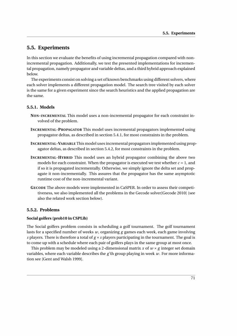
5.5. Experiments
5.5. Experiments
In this section we evaluate the benefits of using incremental propagation compared with non-incremental propagation. Additionally, we test the presented implementations for incremen-tal propagation, namely propagator and variable deltas, and a third hybrid approach explainedbelow.
The experiments consist on solving a set of known benchmarks using different solvers, whereeach solver implements a different propagation model. The search tree visited by each solveris the same for a given experiment since the search heuristics and the applied propagation arethe same.
5.5.1. Models
NON-INCREMENTAL This model uses a non-incremental propagator for each constraint in-volved of the problem.
INCREMENTAL-PROPAGATOR This model uses incremental propagators implemented usingpropagator deltas, as described in section 5.4.1, for most constraints in the problem.
INCREMENTAL-VARIABLE This model uses incremental propagators implemented using prop-agator deltas, as described in section 5.4.2, for most constraints in the problem.
INCREMENTAL-HYBRID This model uses an hybrid propagator combining the above twomodels for each constraint. When the propagator is executed we test whether c = 1, andif so it is propagated incrementally. Otherwise, we simply ignore the delta set and prop-agate it non-incrementally. This assures that the propagator has the same asymptoticruntime cost of the non-incremental variant.
GECODE The above models were implemented in CaSPER. In order to assess their competi-tiveness, we also implemented all the problems in the Gecode solver[Gecode 2010] (seealso the related work section below).
5.5.2. Problems
Social golfers (prob10 in CSPLib)
The Social golfers problem consists in scheduling a golf tournament. The golf tournamentlasts for a specified number of weeks w , organizing g games each week, each game involvings players. There is therefore a total of g × s players participating in the tournament. The goal isto come up with a schedule where each pair of golfers plays in the same group at most once.
This problem may be modeled using a 2-dimensional matrix x of w × g integer set domainvariables, where each variable describes the g ’th group playing in week w . For more informa-tion see [Gent and Walsh 1999].
71

Chapter 5. Incremental Propagation of Set Constraints
Hamming codes
This is a particular case of the Fixed-length error correcting codes (problem 36 in CSPLib). Theproblem involves generating a set of binary strings which satisfy a pairwise minimum distance.Each instance is defined by a tuple ⟨n, l ,d⟩ where n is the number of strings, l is the stringlength, and d is the minimum distance allowed between any two strings. For measuring thedistance between two strings the Hamming distance is used.
This problem may be implemented using two arrays a, b, of n integer set variables each.Each integer set variable ai denotes the set of positions set to 0 in the string i . Conversely, theset variable bi denotes the set of positions set to 1 in the string i . They are related through thefollowing set of constraints:
∀1≤i≤n PARTITION(ai ,bi )
Then, the following constraint ensures that each string is at least d bits apart from any otherstring:
∀1≤i< j≤n∣∣ai ∩b j
∣∣+ ∣∣bi ∩a j∣∣≥ d
Balanced partition
The balanced partition problem consists in finding a partition of the set of values 1. . . v throughthe sets S1, . . . ,Sn which minimizes m, where
m = max1≤i≤n
( ∑j∈Si
j
)
For the decision version of this problem the value m is given and the goal is to find the corre-sponding partition. This problem has a direct model using n set domain variables correspond-ing to S1, . . . ,Sn constrained by a PARTITION constraint.
Metabolic pathways
The metabolic pathways problem consists in searching for a particular path in a graph repre-senting a metabolic network. Metabolic networks are biochemical networks which encode in-formation about molecular compounds and reactions which transform these molecules intosubstrates and products. This problem was modeled in GRASPER, a graph-based constraintsolver built on top of the set solver available in CASPER. Both the problem, the model, and thegraph-based solver are detailed in [Viegas 2008; Viegas and Azevedo 2007].
Winner determination problem
In a combinatorial auction, the auctioneer makes available a set M = 1. . .m of items and thereis a set K = 1. . .k of bidders participating in the auction. A set of bids B = 1. . .b is submitted
72

5.6. Discussion
by the bidders, where each bid corresponds to a subset of M . Let pi be the price agreed to payfor the items of bid i , and G j the set of bids contemplating item j . The winner determinationproblem consists in labeling each bid as winning (xi = 1) or losing (xi = 0) so as to maximizethe auctioneer’s revenue given that no item can belong to more than one winning bid:
max∑i∈B
pi xi s.t.∀ j∈M∑
i∈G j
xi ≤ 1
Like the previous benchmark, this problem was modeled in GRASPER. The specific model andfurther details are given in [Viegas 2008].
5.5.3. Setup
The code for all experiments was compiled with the gcc-4.4.3 C++ compiler and executed onan Intel Core 2 Duo @ 2.20GHz, using Linux-2.6.32.9. The versions of the CaSPER and Gecodesolvers were the most recently available at the moment, respectively revision 583 and version3.3.1. Each benchmark was repeated until the standard deviation of the runtime was below 2%of the average time, and then the minimum runtime was used.
5.6. Discussion
The runtimes obtained for all the experiments are detailed in section B.2 (in the appendix).Each table shows the number of domain updates, average size of domain update, the time andnumber of propagations for solving the benchmark. Additionally, for each instance we showthe number of variables involved in the problem (v), the ratio constraints/variable (c/v) andnumber of fails (f).
The runtimes for solving the first three benchmarks are summarized in table 5.3. The tableprovides some statistical measures concerning the ratio of the runtime using the correspond-ing implementation over the runtime using an implementation with non-incremental propa-gation. For example, solving a problem performing incremental propagation using propagatordeltas takes on (geometric) average 88% of the time spent solving the same problem with non-incremental propagation.
The table shows that incremental propagation using variable deltas is better on average thanany other method, although only slightly better than incremental propagation using propaga-tor deltas. Additionally, it is always better than non-incremental propagation, and also themost robust alternative. The hybrid approach does not pay off in practice probably due to theoverhead involved in selecting the best approach at every propagation. Finally, the last rowshows that all tested solvers implemented in CaSPER slightly outperform the Gecode solver.
The results concerning the last two benchmarks are summarized in table 5.4. The tableprovides a statistical analysis on the ratio of the solver runtime using incremental propaga-
73

Chapter 5. Incremental Propagation of Set Constraints
mean stddev min max
INCREMENTAL-PROPAGATOR 0.88 1.14 0.67 1.07INCREMENTAL-VARIABLE 0.83 1.12 0.66 0.96INCREMENTAL-HYBRID 0.93 1.14 0.73 1.15
GECODE 1.14 1.13 0.91 1.33
Table 5.3.: Geometric mean, standard deviation, minimum and maximum of ratios of run-time for solving the first set of benchmarks described above using the presentedimplementations of incremental propagation, compared to non-incremental prop-agation.
mean stddev min max
INCREMENTAL-VARIABLE 0.7 1.27 0.46 0.91
Table 5.4.: Geometric mean, standard deviation, minimum and maximum of ratios of runtimefor solving the second set of benchmarks (graph problems) using the variable deltaimplementation of incremental propagation, compared to propagator deltas.
tion based on variable deltas over the solver runtime using incremental propagation based onpropagator deltas. In these benchmarks using variable deltas instead of propagator deltas forimplementing incremental propagation has a greater impact on runtime compared with thefirst three benchmarks (about 13% better on average). This discrepancy is probably due tothe fact that some graph constraints used involve an exponential number of set propagators,which is the case where using variable deltas is more efficient.
5.7. Summary
We have seen that incremental propagation can make constraint involving set domain vari-ables significantly more efficient. Incremental propagation requires knowing the set of changesbetween propagator executions, for which we have introduced two distinct techniques: prop-agator and variable based deltas. We have shown that the latter is theoretically more efficientin both time and memory, and that it performs slightly better in practice on problems involv-ing set domain variables. Additionally, on problems involving graph domain variables it canachieve an improvement on runtime of about 30% on average compared to propagator baseddeltas.
74

5.7. Summary
Related work
Ï The set solver used in the experiments is based on and extends the Cardinal set solver[Azevedo 2007]. This set solver is implemented in Eclipse prolog [ECLiPSe 2010] and doesnot support incremental propagation.
Ï We have focused exclusively on propagators achieving bounds consistency for set constraints.Domain consistent propagators for set constraints have been introduced in [Lagoon andStuckey 2004]. These propagators maintain a compacted extensional representation of theset of possible values (which are themselves sets) for each set domain variable. An incre-mental domain consistent propagator for a constraint involving set variables would requireaccess to a number of domain updates which is exponential on the set cardinality, insteadof linear as in the case of incremental bounds consistent propagators. Therefore, we believethat our method would not be easily adapted for domain complete propagators.
Ï In this chapter we presented incremental propagation for constraints involving set domainvariables. CaSPER also provides incremental propagators for constraints over integer do-main variables, but they are implemented differently due to the following two facts. Firstly,most propagators involving integer domain variables have a very efficient non-incrementalimplementation, specifically those for arithmetic constraints achieving bounds consistency.Secondly, incremental domain consistent propagators such as the alldifferent, extensionalor regular constraint propagators, achieve their incrementality by querying and modify-ing its internal state according to the specific domain update, as illustrated in the previouschapter. Therefore, the information about most domain updates is not used and maintain-ing it in delta sets would often be a waste of time. The current implementation associatesa demon to each propagator which is able to access and update the internal state of incre-mental propagators. For those propagators which require the full delta information, thespecific demon may store it in a data structure which is local to the propagator, similar towhat is done with propagator based deltas. This technique is not new, it is used for examplein Choco [Choco 2010], ILOG Solver [ILOG 2003b], and Minion [Gent et al. 2006b].
Ï Incremental propagation in Gecode solver is implemented through an abstraction calledAdvisor [Lagerkvist and Schulte 2007; Lagerkvist 2008]. Advisors are associated with prop-agators and besides providing delta information can be used to alter the internal state ofeach propagator, similar to the incremental propagators involving integer domain variablesavailable in CaSPER explained above. We did not found a detailed description of the advi-sors used on propagators for simple set constraints but their implementation should mapto propagator based deltas.
Ï Throughout this chapter we assumed a set domain representation based on a doubly linkedlist. This is indeed the most common implementation, but others are possible. For exam-ple in [Viegas et al. 2008] we introduced an hash set representation of the domain of a set
75

Chapter 5. Incremental Propagation of Set Constraints
domain variable. This representation has interesting advantages, namely O (1) inserts andupdates, but disallows the optimization which explores updates of contiguous sets of valuesdescribed in section 5.4.3.
76

Part II.
Efficient Propagation of ArbitraryDecomposable Constraints
77

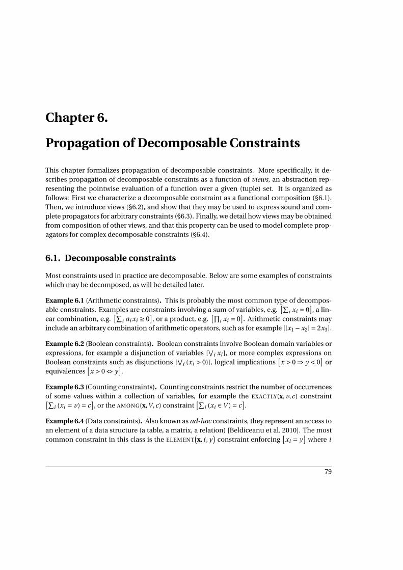
Chapter 6.
Propagation of Decomposable Constraints
This chapter formalizes propagation of decomposable constraints. More specifically, it de-scribes propagation of decomposable constraints as a function of views, an abstraction rep-resenting the pointwise evaluation of a function over a given (tuple) set. It is organized asfollows: First we characterize a decomposable constraint as a functional composition (§6.1).Then, we introduce views (§6.2), and show that they may be used to express sound and com-plete propagators for arbitrary constraints (§6.3). Finally, we detail how views may be obtainedfrom composition of other views, and that this property can be used to model complete prop-agators for complex decomposable constraints (§6.4).
6.1. Decomposable constraints
Most constraints used in practice are decomposable. Below are some examples of constraintswhich may be decomposed, as will be detailed later.
Example 6.1 (Arithmetic constraints). This is probably the most common type of decompos-able constraints. Examples are constraints involving a sum of variables, e.g.
[∑i xi = 0
], a lin-
ear combination, e.g.[∑
i ai xi ≥ 0], or a product, e.g.
[∏i xi = 0
]. Arithmetic constraints may
include an arbitrary combination of arithmetic operators, such as for example [|x1 −x2| = 2x3].
Example 6.2 (Boolean constraints). Boolean constraints involve Boolean domain variables orexpressions, for example a disjunction of variables [
∨i xi ], or more complex expressions on
Boolean constraints such as disjunctions [∨
i (xi > 0)], logical implications[x > 0 ⇒ y < 0
]or
equivalences[x > 0 ⇔ y
].
Example 6.3 (Counting constraints). Counting constraints restrict the number of occurrencesof some values within a collection of variables, for example the EXACTLY(x, v,c) constraint[∑
i (xi = v) = c], or the AMONG(x,V ,c) constraint
[∑i (xi ∈V ) = c
].
Example 6.4 (Data constraints). Also known as ad-hoc constraints, they represent an access toan element of a data structure (a table, a matrix, a relation) [Beldiceanu et al. 2010]. The mostcommon constraint in this class is the ELEMENT
(x, i , y
)constraint enforcing
[xi = y
]where i
79

Chapter 6. Propagation of Decomposable Constraints
is a variable. Decomposable constraints involving this constraint are for example[xi ≥ y
]or[
xi −x j ≥ 0].
6.1.1. Functional composition
We propose to express decomposable constraints as a composition of functions. For this pur-pose we will make extensive use of functions that evaluate to tuples, i.e. f : Zn → Zk wherek ≥ 1, together with the operations (and conventions):
Definition 6.5 (Functional composition). Functional composition is denoted by operator ◦ asusual:
(f ◦ g
)(x) = f
(g (x)
).
Definition 6.6 (Cartesian product of functions). Cartesian product of functions is denoted byoperator × as follows:
(f × g
)(x) = ⟨
f (x) , g (x)⟩
. If x is a tuple we may write(f × g
)(x1, . . . , xn) = ⟨
f (x1, . . . , xn) , g (x1, . . . , xn)⟩
These operators may of course be combined thus providing a very effective way to repre-sent decomposable constraints. To exercise this terminology, we will exemplify with a possibledecomposition of some of the constraints given above. In the following examples let x, y rep-resent variables, a a constant, and pi (x) = xi the projection operator.
Example 6.7 (Equality constraint). Let constraint ceq (x) = [x1 = x2] be the binary constraintstating that variable x1 and x2 must take the same value. A unary equality constraint ceqc (x, a) =[x = a] may be obtained by ceqc =
[ceq ◦
(p1 × fa
)], where fa (x) = a.
Example 6.8 (Sum constraint). Let f (x) = x1 + x2. A sum of three variables is represented byf ◦ (
f ×p3). The generalization to a sum of n variables is defined as
g = f ◦ (f ×p3
)◦ (f ×p3 ×p4
)◦ . . .◦ (f ×p3 ×p4 × . . .×pn
)Therefore we may decompose a constraint for a sum of n variables csum0 (xn) = [∑n
i xi = 0]
ascsum0 =
[ceq0 ◦ g
], where ceq0 (x) = ceqc (x,0) defined in the previous example.
Example 6.9 (Linear constraint). A linear constraint clin0 (an ,xn) = [∑ni=1 ai xi = 0
]may be com-
posed as follows. Let f1, . . . , fn :Zn →Z, where fi (xn) = ai xi . Then, clin0 =[csum0 ◦
(f1 × . . .× fn
)],
where csum0 is defined in the previous example.
Example 6.10 (Arbitrary arithmetic constraint). Let f (x) = x1 − x2, g (x) = |x|, h (x) = 2x. Thearithmetic constraint c
(x3
)= [|x1 −x2| = 2x3] may be represented as
c = [ceq ◦
((g ◦ f ◦ (
p1 ×p2))× (
h ◦p3))]
80
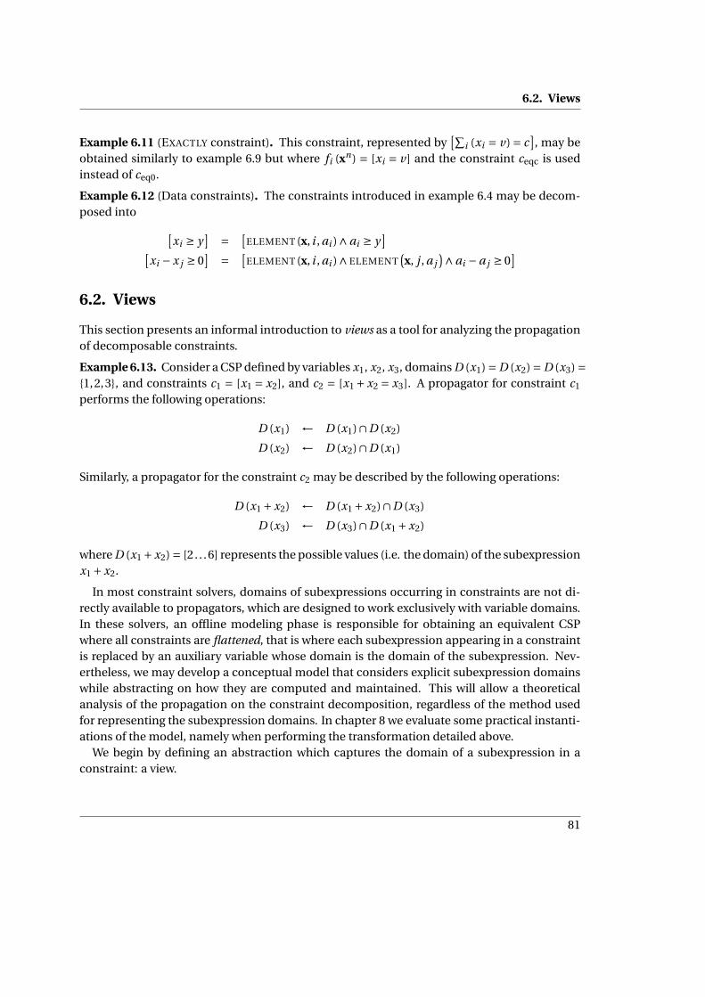
6.2. Views
Example 6.11 (EXACTLY constraint). This constraint, represented by[∑
i (xi = v) = c], may be
obtained similarly to example 6.9 but where fi (xn) = [xi = v] and the constraint ceqc is usedinstead of ceq0.
Example 6.12 (Data constraints). The constraints introduced in example 6.4 may be decom-posed into [
xi ≥ y] = [
ELEMENT (x, i , ai )∧ai ≥ y][
xi −x j ≥ 0] = [
ELEMENT (x, i , ai )∧ ELEMENT(x, j , a j
)∧ai −a j ≥ 0]
6.2. Views
This section presents an informal introduction to views as a tool for analyzing the propagationof decomposable constraints.
Example 6.13. Consider a CSP defined by variables x1, x2, x3, domains D (x1) = D (x2) = D (x3) ={1,2,3}, and constraints c1 = [x1 = x2], and c2 = [x1 +x2 = x3]. A propagator for constraint c1
performs the following operations:
D (x1) ← D (x1)∩D (x2)
D (x2) ← D (x2)∩D (x1)
Similarly, a propagator for the constraint c2 may be described by the following operations:
D (x1 +x2) ← D (x1 +x2)∩D (x3)
D (x3) ← D (x3)∩D (x1 +x2)
where D (x1 +x2) = [2 . . .6] represents the possible values (i.e. the domain) of the subexpressionx1 +x2.
In most constraint solvers, domains of subexpressions occurring in constraints are not di-rectly available to propagators, which are designed to work exclusively with variable domains.In these solvers, an offline modeling phase is responsible for obtaining an equivalent CSPwhere all constraints are flattened, that is where each subexpression appearing in a constraintis replaced by an auxiliary variable whose domain is the domain of the subexpression. Nev-ertheless, we may develop a conceptual model that considers explicit subexpression domainswhile abstracting on how they are computed and maintained. This will allow a theoreticalanalysis of the propagation on the constraint decomposition, regardless of the method usedfor representing the subexpression domains. In chapter 8 we evaluate some practical instanti-ations of the model, namely when performing the transformation detailed above.
We begin by defining an abstraction which captures the domain of a subexpression in aconstraint: a view.
81

Chapter 6. Propagation of Decomposable Constraints
Definition 6.14 (View). A view over a function f :Zn →Zk is a tupleϕ=⟨ϕ+
f ,ϕ−f
⟩of two func-
tions, the image function ϕ+f : ℘ (Zn) → ℘
(Zk
), and the object function ϕ−
f : ℘(Zk
) → ℘ (Zn),defined as
ϕ+f
(Sn) =
{f(xn) ∈Zk : xn ∈ Sn
},∀Sn ⊆Zn
ϕ−f
(Sk
)=
{xn ∈Zn : f
(xn) ∈ Sk
},∀Sk ⊆Zk
A viewϕ f is therefore defined by considering the pointwise application of f over a given set.The image function computes a set of images of f , that is the set resulting from applying f toall the points in the given set. The object function does the inverse transformation, it computesthe set of objects of f for which its image is in the given set.
Example 6.15. Applying a view over function f (x) = x +1 to a random set:
ϕ+f ({1,2,3}) = {2,3,4}
ϕ−f ({2,3,4}) = {1,2,3}
As discussed earlier, propagating a constraint may require consulting and updating the do-main of a subexpression. A view over the subexpression defines these operations:
Example 6.16. Consider a view ϕg over function g(x, y
)= x + y , and the CSP of example 6.13on the preceding page. Function ϕ+
g may be used to compute the subexpression domainD (x1 +x2) from the variable domains D (x1) and D (x2), while function ϕ−
g may be used tospecify the set of values for the variables x1, x2 that satisfy constraint c2.
ϕ+g (D (x1)×D (x2)) = [2 . . .6]
ϕ−g (D (x3)) = {⟨
x, y⟩ ∈Z2 : x + y ∈ {1,2,3}
}Propagation consists in removing inconsistent values from the domain of the variables. In
this sense, the computation of ϕ−f , i.e. the set of consistent assignments, will always precede
an intersection with the original domain to guarantee that the propagation is contracting. Thefollowing definition captures exactly that.
Definition 6.17 (Contracting object function). Let Sn ∈Zn , Sk ∈Zk , be two arbitrary tuple setsand f :Zn →Zk an arbitrary function. Then,
ϕ f
(Sk ,Sn
)=ϕ−
f
(Sk
)∩Sn
Example 6.18. The result of evaluating and updating the domain D (x1 +x2), as defined in the
82

6.3. View-based propagation
previous example, may be formalized using views as follows:
ϕ+g (D (x1)×D (x2)) = [2 . . .6]
ϕg (D (x3) ,D (x1)×D (x2)) = {⟨1,1⟩ ,⟨1,2⟩ ,⟨2,1⟩}
6.3. View-based propagation
A constraint may be seen as a Boolean function c : Zn → {0,1}, mapping allowed tuples (i.e.tuples satisfying the constraint) to 1 and forbidden tuples to 0. In this sense, views may repre-sent not only subexpression domains, but the domains of the constraints as well. Let us thenformally explore the relation among views, constraint domains, and the most common opera-tions occurring in the process of constraint solving: checking and propagating constraints.
6.3.1. Constraint checkers
A constraint checker decides if the constraint c is satisfied (or entailed), or unsatisfied (resp.disentailed) for some tuple set. Constraint checkers are used in practice for many purposes,such as implementing reification [Hentenryck and Deville 1993], optimizing constraint prop-agation by detecting subsumed propagators [Schulte and Stuckey 2004], or as part of weakersearch algorithms which do not require propagation, e.g. pure backtracking.
Definition 6.19 (Constraint checker). A constraint checker is a monotonic functionχc :℘ (Zn) →℘ ({0,1}). The constraint checker is sound if and only if
con(c)∩Sn 6= ;⇒ 1 ∈χc(Sn)∧
con(c)∩Sn 6= Sn ⇒ 0 ∈χc(Sn)
and complete if and only if
con(c)∩Sn 6= ;⇐ 1 ∈χc(Sn)∧
con(c)∩Sn 6= Sn ⇐ 0 ∈χc(Sn)
Example 6.20 (Constraint checker). Consider set S = {⟨2,2⟩ ,⟨3,3⟩} and constraints c1 =[x = y
],
c2 =[x 6= y
]. Thenχc1 is sound iff 1 ∈χc1 (S) and complete iffχc1 (S) = {1}. Similarly, χc2 is sound
iff 0 ∈χc2 (S) and complete iff χc2 (S) = {0}.
Constraint checkers may be obtained directly using the image view function.
Definition 6.21 (View-based constraint checker). A view-based constraint checker for a con-straint c ∈C is a function χc :℘ (Zn) →℘ ({0,1}) such that χc (Sn) =ϕ+
c (Sn).
83

Chapter 6. Propagation of Decomposable Constraints
The following proposition states that view based constraint checkers are sound and com-plete constraint checkers.
Proposition 6.22. A view-based constraint checker χc is a sound and complete constraint checker.
6.3.2. Propagators
We have previously defined propagators (def. 2.35 on page 16) implementing a constraint c ∈Cas a function πc :℘ (Zn) →℘ (Zn) having the following properties:
• con(c)∩Sn ⊆πc (Sn) (soundness)
• πc (Sn) ⊆ Sn (contraction)
A propagator πc which satisfies these conditions and also π?c (Sn) = con(c)∩Sn corresponds tothe strongest propagator for the constraint c - the propagator that, at fixpoint, is able to removeall tuples not satisfying the constraint. Let us represent such propagator using views.
Definition 6.23 (View-based propagator). A view-based complete propagator (or filter) imple-menting a constraint c ∈C is a function πc :℘ (Zn) →℘ (Zn) such that
π?c(Sn)=ϕ−
c ({1})∩Sn = ϕc({1} ,Sn)
This definition supports the following proposition.
Proposition 6.24. A view-based complete propagator for a constraint c is a sound and completepropagator for c.
6.4. Views over decomposable constraints
In the previous section we have shown how constraint checkers and propagators map to theirview-based counterparts when the constraint is represented as a single view. This does not yetbring any practical advantages in terms of modularity or code reuse - an arbitrary constraintwould still require a specific view for that constraint, as it requires a specific propagator. How-ever, when the constraint is decomposable, a view over the constraint may be obtained fromcomposition of other views. First we present some properties of views:
Property 6.25 (Distributivity). Views distribute over set union and with set intersection. LetSn
1 , Sn2 be two arbitrary sets and ⊕∈ {∪,∩},
ϕ+f
(Sn
1 ⊕Sn2
) = ϕ+f
(Sn
1
)⊕ϕ+f
(Sn
2
)ϕ−
f
(Sn
1 ⊕Sn2
) = ϕ−f
(Sn
1
)⊕ϕ−f
(Sn
2
)
84

6.4. Views over decomposable constraints
Property 6.26 (Monotonicity). ϕ+f and ϕ−
f are monotonic for any arbitrary function f .
Property 6.27 (Identity). Let Sn ⊆ Zn , Sk ⊆ Zk , and f : Zn → Zk an arbitrary function. Thefollowing equivalences are true,
Sn ⊆ ϕ− ◦ϕ+ (Sn)
Sn = ϕ(ϕ+ (
Sn),Sn)=ϕ− ◦ϕ+ (
Sn)∩Sn
Sk = ϕ+ ◦ϕ−(Sk
)
6.4.1. Composition of views
Views may be composed either vertically using functional composition, or horizontally usingthe Cartesian product of functions. A view over a composition of functions is equivalent to thecomposition of views over the individual functions:
Proposition 6.28. Let Si ⊆ Zi , Sk ⊆ Zk denote arbitrary tuple sets, f : Z j → Zk , g : Zi → Z j
arbitrary functions (possibly composition of functions). Then,
ϕ+f ◦g
(Si
)= ϕ+
f ◦ϕ+g
(Si
)ϕ−
f ◦g
(Sk
)= ϕ−
g ◦ϕ−f
(Sk
)Corollary 6.29. Let Si ⊆ Zi , Sk ⊆ Zk denote arbitrary tuple sets, f : Z j → Zk , g : Zi → Z j arbi-trary functions (possibly Cartesian product of functions). Then,
ϕ f ◦g
(Sk ,Si
)= ϕg
(ϕ f
(Sk ,ϕ+
g
(Si
)),Si
)Example 6.30 (Composition of views). Consider expression
∣∣x − y∣∣ expressed as a functional
composition f ◦g , where g (x1, x2) = x1−x2, and f (x) = |x|. Let S2 = {⟨2,2⟩ ,⟨1,3⟩}, and S1 = {2}.Thenϕ+
f ◦g (Sn) may be obtained byϕ+f ◦ϕ+
g
(Si
)=ϕ+f ({0,−2}) = {0,2}. The above corollary allow
us to compute ϕ f ◦g(S1,S2
)as
ϕ f ◦g(S1,S2) = ϕg
(ϕ f
(S1,ϕ+
g
(S2)) ,S2
)= ϕg
(ϕ f
(S1, {0,−2}
),S2)
= ϕg({−2} ,S2)
= {⟨1,3⟩}
Figure 6.1 illustrates these operations.
85

Chapter 6. Propagation of Decomposable Constraints
fg
S2 ϕ+g (S2)
ϕ−f ◦g (S1) ⊆Z2
S1
0
2
ϕ−f (S1)
−22
⟨2,2⟩⟨1,3⟩
. . .
0
ϕ f ◦g (S2)ϕ f (S1,ϕ+g (S2))
ϕ f ◦g (S1,S2)
Figure 6.1.: Computations involved in the composition of views described in example 6.30.
Although a view over a Cartesian product of functions is not generally equivalent to theCartesian product of views, it may still be obtained from the concatenation of views over theindividual functions. Let us then define the concatenation operator between ordered sets.
Definition 6.31. The concatenation of two tuples tn , uk , is defined as,
tn ∥ uk = ⟨t1, . . . , tn ,u1, . . . ,uk⟩
Let Sn ⊆Zn and Sk ⊆Zk be two arbitrary ordered tuple sets with the same size, i.e. |Sn | = ∣∣Sk∣∣.
Let sni denote the i ’th tuple of Sn . Then Sn concatenated with Sk , written Sn ∥ Sk , is defined as
Sn ∥ Sk ={
sni ∥ sk
i : 1 ≤ i ≤ ∣∣Sn∣∣}
Proposition 6.32. Let Sn ⊆Zn denote an arbitrary tuple set, and f , g , arbitrary functions (pos-sibly composition of functions). Then,
ϕ+f ×g
(Sn) = ϕ+
f
(Sn) ∥ϕ+
g
(Sn)
ϕ−f ×g
(Sn) = ϕ−
f
(Sn) ∥ϕ−
g
(Sn)
Example 6.33 (View over Cartesian product of functions). Consider set S2 = {⟨1,1⟩ ,⟨1,2⟩} andfunctions f (x1, x2) = x1+x2, g (x1, x2) = x1−x2. The view image functionϕ+
f ×g may be obtainedby
ϕ+f ×g
(S2) = ϕ+
f
(S2) ∥ϕ+
g
(S2)
= {⟨2⟩ ,⟨3⟩} ∥ {⟨0⟩ ,⟨−1⟩}= {⟨2,0⟩ ,⟨3,−1⟩}
86

6.4. Views over decomposable constraints
... ...
⟨9,6⟩
cf ×p3
⟨3,3⟩
S3 πc (ϕ+f ×p3
(S3)) ϕ+f ×p3
(S3)
ϕ−c ({1})
⟨4,5,6⟩⟨1,2,3⟩
0
1
ϕ−c◦( f ×p3)({1}) ⊆Z3
Figure 6.2.: Application of the view-based propagator for the composed constraint describedin example 6.36.
6.4.2. Checking and propagating decomposable constraints
Constraint checkers and propagators for composed constraints may be obtained by exploringcomposition of views introduced in the previous section and the fact that constraint checkersand propagators may be defined using views over their associated constraints.
Proposition 6.34. A view-based constraint checker for the constraint c ◦ f may be obtained by
χc◦ f(Sn)=ϕ+
c ◦ϕ+f
(Sn)
Proposition 6.35. A complete view-based propagator for the constraint c ◦ f may be obtainedby
πc◦ f(Sn)= ϕ f
(π?c
(ϕ+
f
(Sn))
,Sn)
In this case πc◦ f (Sn) is also idempotent, i.e. πc◦ f (Sn) = π?c◦ f (Sn).
Example 6.36. Consider the view-based propagator for the constraint c◦( f ×p3)= [x1 +x2 = x3]
obtained by the above formula, where c = [x1 = x2], f (x) = x1 + x2. Let S3 = {⟨1,2,3⟩ ,⟨4,5,6⟩}.Function ϕ+
f ×p3applies the addition and identity operations to the original set, ϕ+
f ×p3
(S3
) ={⟨3,3⟩ ,⟨9,6⟩}. The resulting set is filtered by propagator πc ({⟨3,3⟩ ,⟨9,6⟩}) = {⟨3,3⟩}, and trans-formed back into ϕ f ×p3 ({⟨3,3⟩} , {⟨1,2,3⟩ ,⟨4,5,6⟩}) = {⟨1,2,3⟩}. Figure 6.2 illustrates these oper-ations.
The above proposition defines a complete idempotent view-based propagator πc◦ f froma composition of views with an idempotent propagator πc . It turns out that if we relax thecondition of idempotency of πc we may still obtain a complete view-based propagator.
Proposition 6.37. A complete constraint propagator (not necessarily idempotent) for the con-straint c ◦ f may be obtained by
πc◦ f(Sn)= ϕ f
(πc
(ϕ+
f
(Sn))
,Sn)
87

Chapter 6. Propagation of Decomposable Constraints
6.5. Conclusion
We have seen how views may be used to obtain sound and complete propagators and con-straint checkers for decomposable constraints. Moreover, we have shown that a view over adecomposable constraint may be modeled by a composition of views. In chapter 8 we explorethis property to define a repository of views over primitive expressions and a method that in-stantiates a view-based propagator for any decomposable constraint. In the next chapter wewill focus on an important issue not yet addressed: the efficiency of view-based propagation.
Related work
Ï Hentenryck et al. [1992]; Carlson [1995] introduced indexicals as a tool for creating propa-gators for arithmetic constraints. An indexical roughly correspond to the image functionϕ+
in the sense that it computes the domain of an expression. However, unlike views indexicalsdo not define the inverse transformation ϕ− and therefore are less powerful - representinga decomposable constraint using indexicals requires the additional definition of the projec-tion of the object function for each variable in the constraint.
Ï Constrained expressions [ILOG 2003a] are apparently similar to views. We are not aware of aformalization of these, but the implementation of propagators using constraint expressionsshare some similarities to the implementation of view-based propagators, as we will seelater.
Ï The idea of defining view-based propagators for arbitrary constraints is incipient in [Cor-reia et al. 2005] and [Schulte and Tack 2005]. The former presents a general overview of aconstraint solver incorporating type polymorphism and its application for creating propa-gators from arbitrary expressions. The latter coins the term view (we originally called thempolymorphic constraints), and describes how it can be used for creating generic propagatorimplementations, that is, propagators which can be reused for different constraints.
Ï Rina Dechter [Rossi et al. 2006] approaches decomposition of constraints from a differentperspective. There, the full constraint network is taken into consideration in order to obtaingeneric global propagation algorithms with theoretical performance guarantees. The prop-agation is still time or space exponential but depends exclusively on specific graph-basedparameters of the graph describing the constraint network. In contrast, we focus on the de-composition of a single constraint into simpler constraints for which specific propagationalgorithms are applied independently. Our decomposition does not provide performanceguarantees for the global search algorithm.
Ï The problem of creating propagators for arbitrary expressions has been approached in adifferent way using knowledge compilation techniques [Gent et al. 2007; Cheng and Yap2008]. These methods create a compact extensional representation of the set of solutions
88

6.5. Conclusion
to the constraint and apply a general propagation algorithm which filters tuples not foundin this set. The propagation algorithm completely discards the semantics of the expression,contrasting to our approach that exploits them. It is therefore most used for constraintswithout any particular semantics, such as databases. Applying these algorithms for arith-metic expressions is possible, and not so inefficient in practice concerning runtime whenexpressions have small domains. However even the most compact extensional represen-tation is exponential in the number of variables, which makes the method unpractical formost arithmetic constraints.
Ï The formalization presented above is due to Tack [2009], but has been adapted and ex-tended in several ways to accommodate views over functions involving multiple variables.Firstly, we associate views with (sub)expressions, while in its original formalization viewsare associated with variables. Secondly, views were originally required to be over injectivefunctions, a condition we found too restrictive (in particular it excludes most multiple vari-able functions) and consequently discarded in our formalization. We have also introducedthe Cartesian product of functions to express multiple variable views, the contracting objectfunction ϕ f to guarantee that view-based propagators are contracting (which is always thecase if f is injective), and view-based constraint checkers which were not contemplated inthe original formalization.
89

Chapter 6. Propagation of Decomposable Constraints
90

Chapter 7.
Incomplete View-Based Propagation
In the previous chapter we have seen how to obtain complete view-based propagators for ar-bitrary constraints. Unfortunately, complete propagation algorithms for most constraints areintractable, and therefore such propagators have limited, or no practical application. Mostpractical propagators are incomplete, in the sense that they only filter a subset of the inconsis-tent values for a given constraint and domain. In this chapter we will see how sound incom-plete propagators may be obtained from a composition of views with the domain approxima-tion operators introduced in chapter 2 (§7.1). Then, it will be shown that the strength of theresulting propagator is a function of these approximations and consequently that propagatorswith various completeness guarantees may be obtained from views (§7.2). Furthermore, wewill present an algorithm for comparing the strength of two (incomplete) view-based propa-gators (§7.3). For this we use a rewriting system that maps any view-based propagator into alattice of consistencies that includes the well-known cases of domain consistency as well asthe different forms of bounds consistency. This algorithm allows us to select the most efficientview-based propagator for a certain consistency type. We evaluate its adequacy on section 7.4.
7.1. ΦΨ-complete propagators
As seen in chapter 2, filtering algorithms are categorized by the consistency they are able toenforce on a constraint network - propagators which find and remove more inconsistent val-ues are usually more expensive in terms of memory, time, or both. Practical propagators areincomplete to some degree, that is, they only guarantee that their output is stronger than someupper bound. Let us recall the definition of propagator completeness.
Definition 7.1 (ΦΨ-completeness). Let Sn be an arbitrary δ-domain, c ∈ C an arbitrary con-straint, and Φ,Ψ ∈ {
ϕ,δ,β}. A propagator πc is ΦΨ-complete, denoted as πΦΨc , if and only if
π?c(Sn)⊆ Vcon(c)∩VSnWΦWΨ∩Sn
We have already introduced some common completeness classes, namely domain, range,bounds(D), bounds(Z), and bounds(R). All these classes except the latter map to instantiationsof the above parametrized expression as summarized in table 7.1.
91

Chapter 7. Incomplete View-Based Propagation
Upper bound Propagator strength ΦΨ-completenessVcon(c)∩VSnWδWδ∩Sn domain complete δδ-completeVcon(c)∩VSnWδWβ∩Sn bounds(D) complete δβ-completeVcon(c)∩VSnWβWδ∩Sn range complete βδ-completeVcon(c)∩VSnWβWβ∩Sn bounds(Z) complete ββ-complete
Table 7.1.: Constraint propagator completeness.
7.2. View models
View models provide an approximation to complete view based propagation as introduced inthe previous chapter.
Definition 7.2 (View approximations). Let f :Zn →Zk be an arbitrary function, Sn an arbitrarytuple set, and Φ,Ψ ∈ {
ϕ,δ,β}. We define view functions that are always input a given domain
type, and that are always relaxed to a certain domain type, and denote them as follows:
Φ+f →Ψ
= Vϕ+f
(VSnWΦ
)WΨ
→ΦΨ−
f = Vϕ−f
(VSnWΦ
)WΨ
→ΦΨ f = Vϕ f
(VSkWΦ,Sn
)WΨ
We define an arbitrary approximation for a view-based propagator πc◦ f , called a view modelfor c ◦ f , by applying domain approximations to the result of every operation involved in acomplete view-based propagator defined in the previous chapter,
πc◦ f(Sn) = ϕ f
(π?c ◦ϕ+
f
(Sn)
,Sn)
Specifically, since both the input and output of the view functions ϕ+f and ϕ f may be approx-
imated, and we may use a ΦΨ-complete propagator for c instead of a complete propagator, aview model has at least six approximation operators involved,
⟨Φ1, . . . ,Φ6⟩c◦ f = Vϕ f
(VπΦ3Φ4?
c
(Vϕ+
f
(VSnWΦ1
)WΦ2
)WΦ5 ,VSnWΦ1
)WΦ6 ∩Sn
which is more conveniently represented using the notation introduced by definition 7.2:
⟨Φ1, . . . ,Φ6⟩c◦ f = Φ+1 f →Φ2
πΦ3Φ4?c →
Φ5
Φ6 f
Additionally, a view model is parametrized by two extra approximation operators guaran-teeing that the input and output tuple sets of the full propagator have a known domain type.
92

7.2. View models
This takes into account the fact that common propagators work with specific domain types(e.g. δ-domains) and not arbitrary tuple sets. Let us then formalize view models.
Definition 7.3 (View model). LetΦ0, . . . ,Φ7 ∈{ϕ,δ,β
}be a set of approximation operators. Any
instance of the following functional composition is called a view model for the constraint c ◦ f ,
⟨Φ0, . . . ,Φ7⟩c◦ f = →Φ0
Φ+1 f →Φ2
πΦ3Φ4?c →
Φ5
Φ6 f →Φ7
The operational semantics of a view model should be clear: given aΦ0-domain Sn , the prop-agator first applies the approximated image function Φ+
1 f →Φ2
, then the idempotent propagator
πΦ3Φ4?c for the constraint c and finally function →
Φ5
Φ6 f whose result is intersected with Sn and
relaxed to a Φ7-domain.
Example 7.4. Consider the constraint c ◦ f = [2x +3y = z
]composed from constraint c =[
x = y]
and function f(x, y, z
)= ⟨2x +3y, z
⟩. Let S = {0,1}×{0,1}×{0,3}, and m be a view model
for c ◦ f defined as follows,
m = →δδ+f →
ϕπββ?c →
ϕβ f →
δ
Propagating m involves the following computations,
Vϕ+f
(VSWδ
)Wϕ = {0,2,3,5}× {0,3}
πββ?c ({0,2,3,5}× {0,3}) = {0,2,3}× {0,3}
Vϕ f(V{0,2,3}× {0,3}Wϕ,S
)Wβ∩S = {0,1}× {0,1}× {0,3}
leading to no filtering.
7.2.1. Soundness
A view model is a relaxation of a complete view-based propagator. Since complete view-basedpropagators are sound propagators then view models must also be sound propagators.
Proposition 7.5. Let Φ0, . . . ,Φ7 ∈{ϕ,δ,β
}be a set of approximation operators. Any view model
⟨Φ0, . . . ,Φ7⟩c◦ f is a sound propagator for c ◦ f .
7.2.2. Completeness
Deciding completeness of an arbitrary view model is not trivial. However, the completeness ofa specific set of view models can be easily mapped to one of the completeness classes intro-duced in section 7.1. Let us first focus on view models belonging to this set, called ΦΨ viewmodels.
93

Chapter 7. Incomplete View-Based Propagation
Definition 7.6 (ΦΨ view model). Let Φ,Ψ ∈ {ϕ,δ,β
}. A ΦΨ view model for a constraint c ◦ f is
any view model m such that
m = Vϕ f
(π?c ◦ϕ+
f
(VSnWΦ
),VSnWΦ
)WΨ∩Sn
= →δΦ+
f →ϕπϕϕ?c →
ϕΨ f →
δ
In other words, aΦΨ view model is a model for propagating δ-domains which only approx-imates the input of the image view function and the output of the object view function. Whena view model is aΦΨ view model, then its completeness is given by the following proposition.
Proposition 7.7. A ΦΨ view model for a constraint c ◦ f is a ΦΨ-complete propagator for c ◦ f .Moreover, it is also an idempotent propagator, i.e.
→δΦ+
f →ϕπϕϕ?c →
ϕΨ f →
δ= πΦΨc◦ f = πΦΨ?c◦ f
Example 7.8. Consider the constraint and tuple set S from the previous example and the fol-lowing view model,
n = →δδ+f →
ϕπϕϕ?c →
ϕβ f →
δ
Propagating n involves the following computations,
Vϕ+f
(VSWδ
)Wϕ = {0,2,3,5}× {0,3}
πϕϕ?c ({0,2,3,5}× {0,3}) = {0,3}× {0,3}
Vϕ f(V{0,3}× {0,3}Wϕ,S
)Wβ∩S = {0}× {0,1}× {0,3}
This view model is δβ-complete (it is one of the examples illustrating the propagator strengthtaxonomy given in fig. 2.3 on page 18), unlike the view model of the previous example sincen (S) ⊂ m (S).
By definition, a ΦΨ view model for a constraint c ◦ f uses an idempotent propagator forc. The idempotency of the propagator for c is a sufficient condition for guaranteeing ΦΨ-completeness of a ΦΨ view model for c ◦ f . The following definition relaxes the idempotencycondition.
Definition 7.9 (ΦΨ relaxed view model). Let Φ,Ψ ∈ {ϕ,δ,β
}. A ΦΨ relaxed view model for a
constraint c ◦ f is any view model m such that
m = Vϕ f
(πc ◦ϕ+
f
(VSnWΦ
),VSnWΦ
)WΨ∩Sn
= →δΦ+
f →ϕπϕϕc →
ϕΨ f →
δ
94

7.2. View models
AΦΨ relaxed view model for c ◦ f may or may not beΦΨ-complete, according to the follow-ing proposition.
Proposition 7.10. Let S be an arbitrary tuple set and m aΦΨ relaxed view model for c◦ f . Thenm isΦΨ-complete if and only if any pruning achieved by the propagator for c is preserved by allinvolved view functions and approximations, formally
πc
(ϕ+
f
(VSWΦ
)) ⊇ ϕ+f
(Vm? (S)WΦ
)Example 7.11. Consider the constraint c ◦ f = [x ≥ 4] where c = [x ≥ 4] and f (x) = x. Addition-ally, let πc be a non-idempotent propagator defined as follows:
πc (S) = {x ∈ S : x ≥ 4∨x < max(S \ [4. . .∞])}
To see that propagator πc is sound and complete consider for example S = [1 . . .4]. Thenπc (S) = {1,2,4}, πc ◦πc (S) = {1,4} and πc ◦πc ◦πc (S) =π?c (S) = {4}.
Let p be a ββ view model and q a ββ relaxed view model for the constraint c ◦ f obtainedrespectively from π?c and πc :
p (S) = Vϕ f
(π?c ◦ϕ+
f
(VSWβ
),VSWβ
)Wβ∩S
q (S) = Vϕ f
(πc ◦ϕ+
f
(VSWβ
),VSWβ
)Wβ∩S
Propagator p is bounds(Z) complete by proposition 7.7, and infers p (S) = {4}. Propagator q isnot bounds(Z) complete by proposition 7.10:
πc
(ϕ+
f
(VSWβ
))+ ϕ+
f
(Vπββ?c◦ f (S)Wβ
){1,2,4} + [1 . . .4]
In particular it does not do any filtering for S, i.e. q (S) = S.
Finally we remark that soundness of ΦΨ view models is not affected by idempotency sincefor any Sn ⊆Zn ,
Vϕ f
(π?c ◦ϕ+
f
(VSnWΦ
),VSnWΦ
)WΨ∩Sn ⊆ Vϕ f
(πc ◦ϕ+
f
(VSnWΦ
),VSnWΦ
)WΨ∩Sn
7.2.3. Idempotency
Let us go back to non-relaxed view models, that is view models which use an idempotent prop-agator for c. Proposition 7.7 tells us that any ΦΨ view model for c ◦ f that uses an idempotentpropagator πc is also idempotent. Unfortunately, this is not true for a general view model forc ◦ f .
95

Chapter 7. Incomplete View-Based Propagation
Proposition 7.12. Let m = ⟨Φ0, . . . ,Φ7⟩ be a (non-relaxed) view model for an arbitrary constraintc ◦ f , and S an arbitrary Φ0-domain. Then m may be not idempotent for S.
This can be shown by the following example.
Example 7.13. Let c ◦ f = [2x1 = 2x2 +1], where f (x1, x2) = ⟨2x1,2x2 +1⟩, and c = [x1 = x2].Consider the δ-domain S = [1 . . .4]×[1 . . .4] and the following view model for propagating c ◦ f ,
m = →δβ+
f →βπββ?c →
ββ f →
δ
Applying m once gives us m (S) = [2 . . .4]× [1 . . .3] which is not a fixpoint for m (the constraintis unsatisfiable and m is able to prove it at fixpoint).
Knowing whether a propagator is idempotent for a given domain may be used to optimizepropagator execution scheduling, as seen in chapter 3. Therefore a propagator scheduler thattakes into account idempotency of a view model for a constraint c ◦ f by querying the idem-potency of the propagator for c is safe but may loose propagation - it could possibly fail toreexecute a non-idempotent view model.
7.2.4. Efficiency
We have not yet addressed the efficiency of view-based propagation. In general, computingand representing views over many interesting functions is intractable in time and space. How-ever, when the input or output (or both) sets of a view have some special structure, computingand representing views is polynomial, as is the case for many useful views.
Example 7.14 (Tractable view functions). Let f (xn) = Σni=1xi . The runtime cost of comput-
ing ϕ+f (Sn) for an arbitrary tuple set Sn ⊆Zn , and the space cost for representing ϕ f (c,Sn) for
some constant are exponential in n. However, the cost of computing ϕ+f
(VSnWβ
)and repre-
senting Vϕ f(c,VSnWβ
)Wβ is linear in n.
The fact that some view-based propagators are more efficient than others is not surprisingsince the same is true for ordinary (i.e. non-view-based) propagators. Given that the set ofview models is a superset of ΦΨ-complete propagators, view models indeed provide an extradegree of freedom for achieving a tradeoff between completeness and efficiency. Additionally,the declarative definition of a view model may expose a performance bottleneck which maybe avoided by using an alternative view approximation.
Example 7.15. A bounds(Z) complete propagator for the constraint x1+x2 = x3 may be repre-sented by the following view model,
→δβ+
f →ϕπϕϕ?c →
ϕβ−
f →δ
96

7.3. Finding stronger models
where c (x) = [x1 = x2], f (x) = ⟨x1 +x2, x3⟩. It turns out that it may also be obtained by analternative view model, which makes use of a much more efficient propagator for c,
→δβ+
f →βπββ?c →
ββ−
f →δ
The fact that both models are equivalent is easy to see in this case. Although propagator πββc
is not equivalent to πϕϕc in general, the equivalence stands when the input domain is already aβ-domain. This is the case here since the output of β+
f →ϕ
is always a β-domain, that is,
β+f →ϕ
= β+f →β
The above example shows a view model which happens to be aΦΨ view model, henceΦΨ-complete. However, example 7.4 has shown us that view models are not ΦΨ-complete in gen-eral. The problem of quantifying the strength of a view model, or decide if a given model isstronger than another is not trivial for many view models. The next section addresses thisproblem.
7.3. Finding stronger models
Both the problem of comparing view models and the problem of quantifying the strength ofa given view model m may be addressed by a procedure which finds the sets Lm , Um , of viewmodels stronger and weaker than m:
Lm = {b : b ¹ m}
Um = {b : m ¹ b}
Then, comparing two view models m1, m2, may be accomplished by testing m1 ∈ Lm2 , m1 ∈Um2 or vice-versa. The problem of quantifying the strength of a view model m may be re-duced to this problem by comparing m with a ΦΨ view model, which as we have seen areΦΨ-complete propagators. While finding stronger view models is not straightforward in gen-eral, a large number of models stronger than a given view model may be easily found.
7.3.1. Trivially stronger models
Definition 7.16. Given two arbitrary functions f , g :℘ (Zn) →℘(Zk
), f is stronger than g , writ-
ten f ¹ g , if and only if f (Sn) ⊆ g (Sn) for any domain Sn ⊆Zn .
Proposition 7.17. Let f1, . . . , fk , g :℘ (Zn) →℘ (Zn) be arbitrary monotonic functions. Then for
97

Chapter 7. Incomplete View-Based Propagation
any 1 ≤ i ≤ j ≤ k,
fi ◦ . . .◦ f j ¹ g ⇒ f1 ◦ . . .◦ fk ¹ f1 ◦ . . .◦ fi−1 ◦ g ◦ f j+1 ◦ . . .◦ fk
A view model is by definition a functional composition involving only monotonic functionsand operators: ϕ+, ϕ−, π, V·WΦ, and ∩. A consequence of the above proposition is that we willobtain a stronger view model if we replace any subset of these functions by a stronger subset.We will use this result in two ways. Firstly, to establish a natural partial ordering among viewmodels.
Corollary 7.18. For any constraint c, function f , and approximation operators Φ1, . . . ,Φk , andΘ,
Φi ¹Θ⇒⟨Φ1, . . . ,Φn⟩ ¹ ⟨Φ1, . . . ,Φi−1,Θ,Φi+1, . . . ,Φn⟩Recall that approximation operators are totally ordered: ϕ¹ δ¹β (see lemma 2.24). There-
fore for a given view model we may obtain a set of trivially stronger (resp. weaker) models justby replacing approximation operators by stronger (resp. weaker) approximation operators.
Definition 7.19. Let m1 = ⟨Φ1, . . . ,Φ8⟩, m2 = ⟨Θ1, . . . ,Θ8⟩ be two view models. m1 is triviallystronger than m2, written m1 ¹T m2, if and only if Φi ¹Θi , 1 ≤ i ≤ 8. Additionally, we will de-note the set of trivially stronger (resp. weaker) models of a given model m by bmcT = {
b : b ¹T m}
(resp. dmeT = {b : m ¹T b
}).
The trivially stronger relation orders all possible view models for a constraint in a lattice,shown in figure 7.1.
Proposition 7.20. The set of view models for a constraint ordered by the trivially stronger rela-tion is a bounded lattice where >= ⟨
β,β, . . . ,β⟩
and ⊥= ⟨ϕ,ϕ, . . . ,ϕ
⟩.
Example 7.21. The ββ-complete propagator for the constraint [x1 +x2 = x3] of example 7.15is trivially stronger than the presented alternative view model but the converse is not true, thatis
→δβ+
f →ϕπϕϕ?c →
ϕβ−
f →δ
¹T →δβ+
f →βπββ?c →
ββ−
f →δ
→δβ+
f →ϕπϕϕ?c →
ϕβ−
f →δ
�T →δβ+
f →βπββ?c →
ββ−
f →δ
This means that the model in the left hand side of the equation may be reached in the latticefrom the node corresponding to the model in the right hand side by moving downwards intothe trivially stronger lattice (or vice-versa). However, for this specific constraint we have
→δβ+
f →ϕπϕϕ?c →
ϕβ−
f →δ
º →δβ+
f →βπββ?c →
ββ−
f →δ
which is not captured in the lattice since it is not a trivially stronger relation.
98

7.3. Finding stronger models
⟨β,β,β,β, . . . ,β⟩ =>
⟨δ,β,β,β, . . . ,β⟩
⟨δ,δ,β,β, . . . ,β⟩
⟨β,δ,β,β, . . . ,β⟩
⟨ϕ,ϕ,ϕ,ϕ, . . . ,ϕ⟩ =⊥
⟨δ,ϕ,ϕ,ϕ, . . . ,ϕ⟩
⟨δ,δ,ϕ,ϕ, . . . ,ϕ⟩
⟨ϕ,δ,ϕ,ϕ, . . . ,ϕ⟩
Weaker
Stronger
Figure 7.1.: View model lattice.
7.3.2. Relaxing the problem
For a given view model m we are interested in the sets of view models stronger and weaker thanm. We will present a procedure that does not compute Lm , Um exactly, but instead provides anapproximation.
Definition 7.22 (Approximation bound). Let m be an arbitrary view model. Then the approxi-mated lower bound of m, Lm , is a set of view models where b ∈ Lm ⇒ b ¹ m. The approximatedupper bound of m, Um is similarly defined as b ∈ Um ⇒ b º m.
The sets Lm = {⊥} and Um = {>} are trivial bounds for any view model, but are of coursetoo loose. A procedure which finds tighter upper bounds for view models of many useful con-straints is detailed in the following section. The algorithm for computing the lower bound isanalogous.
7.3.3. Computing an upper bound
Function FindUb takes as input a view model m for a constraint c◦ f and returns a set of modelsUm . The method makes use of a rule database Rc◦ f .
Definition 7.23 (Rule database). A rule database Rc◦ f for a constraint c◦ f is a set of rules whereeach rule ⟨m1,m2⟩ ∈ Rc◦ f is a tuple representing a non-trivial order relation between two viewmodels, that is m1 ¹ m2 although m1�T m2. The rule database is sound iff ⟨m1,m2⟩ ∈ Rc◦ f ⇒m1 ¹ m2. It is complete iff m1 ¹ m2 ⇒ HASPATH
(Rc◦ f ,m1,m2
)for any non-trivial order relation
99

Chapter 7. Incomplete View-Based Propagation
Function FindUb(m)Data: Rc◦ f is a rule database for the constraint c ◦ fInput: A view model m for the constraint c ◦ fOutput: A set of view models Um for the constraint c ◦ fU ←dmeT1
repeat2
changed ← false3
foreach ⟨m1,m2⟩ ∈ Rc◦ f do4
if m1 ∈U then5
U ←U ∪dm2eT6
changed ← true7
8
9
until ¬changed10
return U11
m1 ¹ m2, where HASPATH is defined as
HASPATH(Rc◦ f ,m1,m2
) ⇔ m1 = m2
∨ ∃mi : m1 ¹T mi ∧HASPATH(Rc◦ f ,mi ,m2
)∨ ∃mi : ⟨m1,mi ⟩ ∈ Rc◦ f ∧HASPATH
(Rc◦ f ,mi ,m2
)The algorithm computes the transitive closure of the given set of rules Rc◦ f unioned with the
set of trivial rules. It performs a breadth first search from the node representing the given viewmodel, traversing the lattice of models downwards (i.e. in the stronger than direction), untilthere are no more applicable rules in the database. The algorithm is basically an exhaustiverule rewriting procedure, for which the following is easy to see.
Proposition 7.24. Algorithm FindUb is sound if the rules database Rc◦ f is sound. It is completeif the rules database Rc◦ f is complete.
7.3.4. Rule databases
Algorithm FindUb requires a database of rules Rc◦ f which is specific to the constraint c ◦ f .Creating a rule database for any constraint is of course unpractical. Instead we create ruledatabases for primitive constraints Rc and expressions R f and use them to obtain Rc◦ f .
Definition 7.25 (Constraint rule database). Let c be an arbitrary constraint and Rc be a con-straint rule database for c. Then each rule ⟨m1,m2⟩ ∈ Rc specifies a non-trivial order relationbetween two propagators for c, m1 =→
Φ1
πΦ2Φ3c →
Φ4
and m2 =→Θ1
πΘ2Θ3c →
Θ4
.
100

7.3. Finding stronger models
Integrating a constraint rule database in a rule database is straightforward due to the follow-ing corollary to proposition 7.17,
Corollary 7.26. For any constraint c, function f , and approximation operators Φi ,Θi ,
→Φ3
πΦ4Φ5c →
Φ6
¹ →Θ3
πΘ4Θ5c →
Θ6
⇒→Φ1
Φ+2 f →Φ3
πΦ4Φ5c →
Φ6
Φ−7 f →Φ8
¹ →Φ1
Φ+2 f →Θ3
πΘ4Θ5c →
Θ6
Φ−7 f →Φ8
Definition 7.27 (Function rule database). Let f be an arbitrary function and R f be a functionrule database for f . Then each rule ⟨m1,m2⟩ ∈ R f specifies a non-trivial order relation be-tween two view models, m1 = ⟨Φ1, . . . ,Φ8⟩x◦ f and m2 = ⟨Θ1, . . . ,Θ8⟩x◦ f , where x is an arbitraryconstraint.
Note that a function rule database abstracts the semantics of the constraint used with theview - rules must be applicable to any constraint. For obtaining a tight upper bound, the al-gorithm benefits from the specificity of the rules, which is increased when the function andconstraint rule databases for the given view model are combined.
Proposition 7.28. Let Rc be a constraint rule database for a constraint c, R f a function ruledatabase for a function f , let
R+c = {⟨t1, t2⟩ :
t1 = ⟨Φ1,Φ2,m1,Φ3,Φ4⟩ , t2 = ⟨Φ1,Φ2,m2,Φ3,Φ4⟩ ,
Φ1, . . . ,Φ4 ∈{ϕ,β,δ
},
⟨m1,m2⟩ ∈ Rc }
Then Rc◦ f = R+c ∪R f is a sound rule database for the constraint c ◦ f .
Example 7.29. Consider the constraint c◦ f = [ax1 ≥ x2], where c = [x1 ≥ x2] and f (x) = ⟨ax1, x2⟩,and a is a positive constant. Let Rc be a rule database for c defined as follows:
Rc =
→βπββ?c →
β¹ →
βπβδ?c →
β(rule 1)
→βπβδ?c →
β¹ →
βπβδ?c →
δ(rule 2)
→δπβδ?c →
δ¹ →
δπβϕ?c →
δ(rule 3)
The first rule states that a ββ complete propagator for c achieves the same pruning that aβδ-complete propagator for c when its input is a β-domain and its output is stored as a β-
domain. The second rule specifies that the output of πβδ?c (S) when S is a β-domain is always a
101

Chapter 7. Incomplete View-Based Propagation
β-domain. The third rule states that a βδ (range)-complete propagator for c achieves the samepruning that a βϕ-complete propagator for c.
Let R f be a rule database for f defined as follows:
R f =→δβ+
f →βπββ?→
ββ−
f →δ
¹ →δδ+f →
βπββ?→
βδ−f →
δ(rule 1)
→δδ+f →
βπβδ?→
δδ−f →
δ¹ →
δδ+f →
δπβδ?→
δδ−f →
δ(rule 2)
→δδ+f →
δπβϕ?→
δδ−f →
δ¹ →
δδ+f →
ϕπϕϕ?→
ϕδ−f →
δ(rule 3)
The first rule specifies that if the output of the image view function and the input of the ob-ject view function are β-domains then the input of the image view function and the output ofthe object view function may be relaxed to β-domains with no loss of representation. The sec-ond rule states that when using a πβδ? propagator then the output of the image view functionfor f may be relaxed to a β-domain with no loss of representation. The third rule specifies thata domain complete propagator for πx◦ f for any constraint x achieves the same pruning that aview model using a βϕ-complete propagator for x.
Now consider the following model m for propagating c ◦ f ,
m =→δβ+
f →βπββ?c →
ββ−
f →δ
Finding the transitive closure of this model under the combined set of rules Rc◦ f proves thatm is a domain complete propagator for c ◦ f . A possible trace of the algorithm is the following,
m =→δβ+
f →βπββ?c →
ββ−
f →δ
=→δδ+f →
βπββ?c →
βδ−f →
δ(from rule 1 in R f )
=→δδ+f →
βπβδ?c →
δδ−f →
δ(from rules 1 and 2 in R+
c )
=→δδ+f →
δπβδ?c →
δδ−f →
δ(from rule 2 in R f )
=→δδ+f →
δπβϕ?c →
δδ−f →
δ(from rule 3 in R+
c )
=→δδ+f →
ϕπϕϕ?c →
ϕδ−f →
δ(from rule 3 in R f )
=πδδ?c◦ f (prop. 7.7)
7.3.5. Multiple views
As seen in the previous chapter, view-based propagators for composed constraints may beobtained by exploring composition of views. In such cases, the corresponding view models
102

7.3. Finding stronger models
will use multiple views, contrasting with the single view models we have been considering sofar.
Definition 7.30. Let f , g be arbitrary functions, and c a constraint. A view model for the con-straint c ◦ f ◦ g is characterized by the following functional composition,
⟨Φ1, . . . ,Φ12⟩ = →Φ1
Φ+2g →
Φ3
Φ+4 f →Φ5
πΦ6Φ7c →
Φ8
Φ−9 f →
Φ10
Φ−11g →
Φ12
The previous algorithm has therefore to be adapted for handling view models parametrizedby a variable number of approximation operators. This may be accomplished for any con-straint c ◦ f ◦ g using an adequate rule database Rc◦ f ◦g . We will not provide the counterpart ofproposition 7.28 for this case, but instead remark that it basically explores the following lemmato map view models involving multiple views to the simpler case presented previously.
Lemma 7.31. Let f , g be arbitrary functions and c a constraint. Then,
→Φ1
Φ+2g →
Φ3
Φ+4 f →ϕ π
ϕϕ?c →
ϕΦ−
5 f →Φ6
Φ−7g →
Φ8=→Φ1
Φ+2g →
Φ3
πΦ4Φ5?c◦ f →
Φ6
Φ−7g →
Φ8
7.3.6. Idempotency
The method for comparing propagation strength of view models described above does notthem to be idempotent. Constraint rule databases are integrated through corollary 7.26 whichdoes not require idempotency. In fact, constraint rule databases for idempotent view modelsof a constraint c are a superset of constraint rule databases for non-idempotent view modelsfor c, since
→Φ1
πΦ2Φ3c →
Φ4
¹ →Θ1
πΘ2Θ3c →
Θ4
⇒→Φ1
πΦ2Φ3?c →
Φ4
¹ →Θ1
πΘ2Θ3?c →
Θ4
The same occurs with function rule databases given that
→Φ1
Φ+2g →
Φ3
πΦ4Φ5
c◦ f →Φ6
Φ−7g →
Φ8
¹ →Θ1
Θ+2g →
Θ3
πΘ4Θ5
c◦ f →Θ6
Θ−7g →
Θ8
⇒→Φ1
Φ+2g →
Φ3
πΦ4Φ5?c◦ f →
Φ6
Φ−7g →
Φ8
¹ →Θ1
Θ+2g →
Θ3
πΘ4Θ5?c◦ f →
Θ6
Θ−7g →
Θ8
This means that, by using rule databases that consider non-idempotent propagators exclu-sively, we are sure that the algorithm is correct for the case where such propagators are exe-
103

Chapter 7. Incomplete View-Based Propagation
cuted until fixpoint. However, rule databases that are specific to idempotent propagators maybe used to improve the approximations obtained for models that are indeed idempotent, inparticular for view models with multiple views since corollary 7.31 requires idempotency. Thisis a consequence of the direct relation between specificity of rules and inference inherent torule rewriting algorithms.
Integrating idempotency information in our algorithm is a matter of selecting specific rules(i.e. for idempotent or non-idempotent propagators) according to the model we are testing.This assumes of course that there is a way to know the idempotency of the model. In fact thismay not be a problem, either because it is known beforehand as with auxiliary variables viewmodels (more on this later), or because it may be inferred (see section 7.2.3).
Finally, we recall that ΦΨ-completeness of a view model for a constraint c ◦ f is guaranteedby requiring propagator for c to be idempotent. Therefore, for proving ΦΨ-completeness of aview model that uses a non-idempotent propagator for c the rule database must contain somerules comparing idempotent with non-idempotent propagators. Although this is possible intheory, in our experiments we opted to use view models based on idempotent propagatorsexclusively.
7.3.7. Complexity and optimizations
Let n be the number of functions in a given view model⟨Φ1, . . . ,Φ4(n+1)
⟩c◦ f1◦...◦ fn . The algo-rithm FindUb may explore an exponential number of models, more specifically O
(34(n+1)
).
However, since practical constraints usually involve a small n, this is seldom a problem inpractice. For constraints with large n we may use an incremental version of the algorithmwhich first computes the upper bound for ⟨Φ1, . . . ,Φ8⟩c◦ f1 , uses proposition 7.7 to select thestrongerΦΨ-complete propagator πΦΨc◦ f in that set, and then repeat the process iteratively from(c ◦ f1
)◦ f2 to(c ◦ f1 ◦ . . .
)◦ fn . In this case the algorithm will loose in completeness, but the run-time complexity decreases to O
(n38
).
The lattice structure of trivial order relations also provides opportunities for optimization.The algorithm may maintain only the non-trivially stronger models of the upper bound, that is⌊U
⌋Tinstead of the full set U . This may be done by replacing line 2 by U ← {m}, the condition
in line 6 by m1 ∈ dUeT and line 7 by a routine which stores the model m2 in bUcT only if m2
is not already a member, in which case it first removes dm2eT from bUcT . We remark that inthis case the rule rewriting algorithm may still explore an exponential number of models in theworst scenario, but the performance of the algorithm for the average case is increased.
Regarding the space complexity we note that although proposition 7.28 has shown how tocompute Rc◦ f from a union of explicit sets R+
c , and R f , this was intended for making the de-scription of the algorithm more clear, and that an implementation of the FindUb algorithmdoes not require the existence of a pre-computed Rc◦ f (not even R+
c ), but instead infers thecombined rules dynamically from Rc and R f . In such case, the space complexity is in O
(n ×316
)
104

7.4. Experiments
since there are n rule databases each having a quadratic number of rules. We may still decreasethis number by optimizing the size of the rule databases, which also plays a role on the algo-rithm runtime. Small rule databases may be obtained using the transitive reduction of all rules,which may be computed offline, in polynomial time [Aho et al. 1972].
7.4. Experiments
There are two important applications for the algorithm described above, both of them centralin the modeling phase of a constraint program. On one hand we may use it to approximate thecompleteness guarantees of a given view model for a specific constraint. This information ishelpful for reasoning globally about the constraint program and make an informed and con-certed decision on the selection of propagators for the constraints in the problem. In this casewe have an arbitrary view model m = ⟨Φ1, . . . ,Φn⟩c , and test if aΦΨ-complete propagator πΦΨc
belongs to FindUb(m), FindLb(m), or both.
On the other hand, we may already have decided upon a specific strength for a given con-straint propagator, but wish to select the most efficient view model that implements it. Thisproblem is the inverse of the former: we are given a ΦΨ-complete propagator m = πΦΨc andthen select the most efficient view model ⟨Φ1, . . . ,Φn⟩c from FindUb(m).
For evaluating our algorithm, we simulated an instance of the first scenario. Specifically,we have a view model m for a constraint c ◦ f1 ◦ . . . ◦ f2 consisting of only β approximation
operators except the initial and final approximation, that is m = ⟨δ,β,β, . . .β,δ
⟩c◦ f1◦...◦ f2 , andwish to know the strength of the resulting propagator. This problem occurs often in practicesince these ββ view approximations are very efficient to compute.
We have generated propagator rule databases for c = [x = y
], and c = [
x ≤ y], and view rule
databases for the functions f (x) = ax, f (x) = |x|, f(x, y
)= x+y , and f(x, y
)= x×y , where x, yare variables and a,b are constants. The algorithm was then tested in a number of arithmeticconstraints created by composition of these functions.
Table 7.2 shows the results. For each function we show the obtained upper bound (actuallyonly the trivially stronger models) and their intersection with the obtained lower bound, which
was⌈
Lm⌉T = {bounds(Z)} for all constraints. Set Em = Um ∩ Lm represents the set of view
models known to be equivalent to the given model. In the last column we show the differencebetween the exact set of equivalent models and the set of equivalent models computed by ouralgorithm. An empty set in this column means that the algorithm was exact.
Recall that a > represents the weakest view model in the lattice. We have found a numberof view models which are strictly stronger than > and strictly weaker than bounds(Z) whichwe did not classify (see the last row in the table). The propagator strength of those modelsshould be bounds(R), a class strictly weaker than bounds(Z), however we are still unsure howthis class maps into the view model lattice.
105

Chapter 7. Incomplete View-Based Propagation
bUm c T
Em
Em
\E
m
ax=
ca
x≥y
{ do
main
}{b
ou
nd
s(Z),b
ou
nd
s(D),ran
ge,do
main }
{}{}x+
y≥z
x+y=
c
{range,b
ou
nd
s(D) }
{bo
un
ds(Z
),bo
un
ds(D
),range }
{ do
main
}{}
∑n>
2i=
1x
i ≥z
∑n>
2i=
1x
i =c
{range }
{range,b
ou
nd
s(Z) }
{ do
main
,bo
un
ds(D
)}{}
ax=
ya
x+b
y=c
ax+
by≥
z{ b
ou
nd
s(D)}
{ bo
un
ds(D
),bo
un
ds(Z
)}{}{}
{do
main
,range }
∑ni=
1x
i =z
x×y=
cx×
y≥z
{ bo
un
ds(Z
)}{ b
ou
nd
s(Z)}
{}{}{ b
ou
nd
s(D)}
∏ni=
1x
i =z
∏n>
2i=
1x
i =c
∑ni=
1a
i xi =
z∏
n>2
i=1
xi ≥
z
{ >}
{}
{}{}{}{ b
ou
nd
s(Z),b
ou
nd
s(D)}
Table
7.2.:Strength
ofth
eview
mo
delm
for
aseto
farithm
eticco
nstrain
ts.
106

7.5. Incomplete constraint checkers
7.5. Incomplete constraint checkers
Like propagators, constraint checkers may also be approximated. View models for constraintcheckers are reasonably simpler than view models for propagators since constraint checkersmay are defined exclusively using the image view function ϕ+. We may define an incompleteconstraint checker by approximating its input or output:
Definition 7.32 (Incomplete constraint checker). Let Φ1,Φ2 ∈ {ϕ,δ,β
}. An incomplete con-
straint checker for the constraint c is defined as
⟨Φ1,Φ2⟩c = Vϕ+ (VSWΦ1
)WΦ2
Proposition 7.33. Let Φ1,Φ2 ∈ {ϕ,δ,β
}and c be an arbitrary constraint. An incomplete con-
straint checker ⟨Φ1,Φ2⟩c is a sound constraint checker for c.
Additionally, we may rank constraint checkers according to its completeness similarly towhat was done with incomplete constraint propagators. Likewise, an incomplete constraintchecker for a functional composition may be created by combining the constraint checkers forthe individual functions, and its overall completeness may be assessed by an adapted versionof the rule rewriting algorithm described above.
7.6. Summary
In this chapter we have characterized view models as a tool for defining incomplete propa-gators with different strength. For assessing the strength of a view model we have presenteda rule rewriting algorithm that maps the model into a lattice of consistencies including thewell-known cases of domain consistency as well as the different forms of bounds consistency.The algorithm may be used to select the most efficient view-based propagator for a certainconsistency type or to inform the consistency achieved by some predefined model.
An implementation of the algorithm and the rule databases for the experiments in this chap-ter may be obtained from the author upon request.
Related work
Ï Yuanlin and Yap [2000] present an analysis on the complexity of propagating some arith-metic constraints. In particular, they show that a bounds complete propagation algorithmis also domain complete when the constraints are linear.
Ï In [Apt and Zoeteweij 2003] the decomposition of arithmetic expressions using idempotentpropagators is presented formally. The propagation complexity is analyzed for differentdecomposition models, although the focus is on symbolic manipulation of expressions, inparticular replacing common subexpressions and factorizing.
107

Chapter 7. Incomplete View-Based Propagation
Ï A related problem is to compare the strength of two different sets of propagators in a givenCSP. This problem was approached in Schulte and Stuckey [2005] which presented an algo-rithm that detects when two sets of propagators are equivalent, in particular bounds anddomain complete propagators. The algorithm performs a different, although related anal-ysis, and provides exact results for cases where our algorithm does not, specifically con-straints involving inequalities. There are other significant differences, namely that no dis-tinction is made among several bounds complete classes, and that it works with propaga-tors, and not arbitrary view models.
Ï Schulte and Tack [2008] provide a set of conditions which guarantees the strength of a view-based propagator, which is the problem we address in section 7.3. In their work, the strengthof a view model is computed as a function of two properties of the involved views, namelyinjectivity and surjectivity, and the strength of the propagator being derived. These proper-ties essentially guarantee that a known set of equivalent models exists for the functions ϕ+
f ,ϕ−
f and π f individually. It is then proved that when these models exist the obtained viewmodel is a propagator with a certain strength. The simplicity of this method is appealing,but it has some limitations. Firstly, f is required to be an injective function, which excludesmany interesting functions for which efficient view models have been found, namely func-tions involving multiple variables (see examples in section 6.1). Secondly, the method is lesscommitted to the semantics of the involved functions and consequently is less exact in gen-eral. It cannot show for example that the view model for the constraint [ax = z] mentionedin table 7.2 is a bounds(Z) propagator. Finally, our algorithm may be used to order viewmodels that are not (equivalent to) ΦΨ-propagators, and that is not possible using theirmethod.
Future work
The fact that we are using a blind, brute force algorithm for approximating the strength of aview model suggests several developments:
. Compare models which use different functions. It has been shown that symbolic manip-ulation such as factorizing improves propagation in some constraints [Apt and Zoeteweij2003]. It would be interesting to see if we can adapt our algorithm to order different repre-sentations of the same constraint.
. Create rule databases for specific non-idempotent propagators. In our experiments we usedrule databases solely for idempotent propagators. However, as discussed in section 7.3.6,non-idempotent propagators may be integrated as well using specific rules.
. Improve the treatment of inequalities by considering open β-operators, i.e. box domainswhich are not finite. These operators fit nicely in the operator hierarchy since they are
108

7.6. Summary
weaker than β-operators, and would allow for more expressive rules and therefore providestronger inference in general, and in particular for view models involving inequalities.
109

Chapter 7. Incomplete View-Based Propagation
110

Chapter 8.
Type Parametric Compilation of Box ViewModels
This chapter details an efficient realization of formerly described view models. More specifi-cally, it presents a set of algorithms for propagating a view model consisting exclusively of boxapproximations, and shows how to apply them for an arbitrary decomposable constraint. Theset of algorithms described cover the classical propagation scheme for decomposable con-straints based on the introduction of auxiliary variables, and also two frameworks based onan abstraction called a view object. We show that the kind of algorithm used for propagating aview model is deeply connected with its compilation scheme.
The chapter is organized as follows: we first discuss a class of view models which are inher-ently very efficient to compute, namely box view models (§8.1). Then we introduce box viewobjects, explain how they naturally map to box view models (§8.2), and discuss the connectionbetween practical implementations of view objects and the kind of polymorphism availablein the subjacent programming language (§8.3). Section 8.4 shows that view models may alsobe implemented using auxiliary variables and extra propagators. Then, we describe a com-pilation algorithm for each of the presented methods for propagating view models (§8.5) andprovide a theoretical comparison of these methods (§8.6). Finally, we discuss views over usefulnon-arithmetic expressions (§8.7).
8.1. Box view models
Bounds(Z) propagators are widely used in constraint programs. Consider the following exam-ple.
Example 8.1. Let c = [x1 ≥ x2] and S2 an arbitrary δ-domain. A bounds(Z) propagator for cmay be defined as follows
πββc (S) = Vcon(c)∩VSWβWβ∩S
= ([⌊proj2 (S)
⌋. . .
⌈proj1 (S)
⌉]× [⌊proj2 (S)
⌋. . .
⌈proj1 (S)
⌉])∩S
111

Chapter 8. Type Parametric Compilation of Box View Models
The fact that the above bounds(Z) propagator is defined exclusively from operations involv-ing the lower and upper bounds of the input set makes it very efficient to compute. In general,computing view operations involving box approximations is also efficient: β-domains may bestored in constant space since the domain is fully characterized by its lower and upper bound,and computing views which are applied and relaxed to β-domains takes constant time formost functions.
Example 8.2. Let f (x) = |x| and S1,S2 ⊆ Z two arbitrary sets, and assume bS2c ≥ 0. Considerthe problem of computing the view functions Vϕ+
f
(VS1Wβ
)Wβ and Vϕ f
(VS2Wβ,VS1Wβ
)Wβ. Re-
call that, by definition,
Vϕ+f
(VS1Wβ
)Wβ = V
{|x| : x ∈ VS1Wβ
}Wβ
Vϕ f
(VS2Wβ,VS1Wβ
)Wβ = V
{x : |x| ∈ VS2Wβ∧x ∈ VS1Wβ
}Wβ
This definition may suggest that evaluating these functions would take linear time, but in factthey may be computed in constant time assuming that finding the minimum and maximumof sets S1, S2 takes constant time (i.e. the sets are ordered):
Vϕ+f
(VS1Wβ
)Wβ =
[bS1c . . .dS1e] ⇐bS1c > 0
[−dS1e . . .−bS1c] ⇐dS1e < 0
[0. . .max(−bS1c ,dS1e)] otherwise
Vϕ f
(VS2Wβ,VS1Wβ
)Wβ =
[max(bS2c ,bS1c) . . .min(dS2e ,dS1e)] ⇐bS1c > 0
[max(−dS2e ,bS1c) . . .min(−bS2c ,dS1e)] ⇐dS1e < 0
[max(−dS2e ,bS1c) . . .min(dS2e ,dS1e)] otherwise
Before we proceed to analyzing the efficiency of view models, let us make the following ob-servation concerning notation. In this chapter we will focus on tuple sets which are at leastδ-domains. This allows us to express formulas like the above, which are based on the nota-tion introduced in the previous chapter, with a more convenient notation which is also morecommon within constraint programming.
Example 8.3. Let D be the set of Cartesian product of variable domains in a CSP ⟨X ,D,C⟩ asdefined in chapter 2. A bounds(Z) propagator for c = [x1 ≥ x2], x1, x2 ∈ X , may be defined asfollows
πββc (D) = ([⌊
proj2 (D)⌋
. . .⌈
proj1 (D)⌉]× [⌊
proj2 (D)⌋
. . .⌈
proj1 (D)⌉])∩D
= ([bD (x2)c . . .dD (x1)e]× [bD (x2)c . . .dD (x1)e])∩D
112

8.1. Box view models
Given that the output of the above propagator is also a Cartesian product, i.e.
πββc (D) = proj1
(πββc (D)
)×proj2
(πββc (D)
)we may express the propagator as
proj1
(πββc (D)
)= [bD (x2)c . . .dD (x1)e]∩D (x1)
proj2
(πββc (D)
)= [bD (x2)c . . .dD (x1)e]∩D (x2)
or more commonly,
πββc (D) =
{D (x1) ← [bD (x2)c . . .dD (x1)e]∩D (x1)
D (x2) ← [bD (x2)c . . .dD (x1)e]∩D (x2)
Since bounds(Z) propagators and view box approximations are efficient to compute, it is notsurprising that view models resulting from the combination of these propagators and views arealso efficient.
Example 8.4. Let c ◦ f = [|x1| ≥ x2] where f (x1, x2) = ⟨|x1| , x2⟩, and c = [x1 ≥ x2]. The viewmodel
→δβ+
f →βπββ?c →
ββ f →
δ
may be defined based on the πββc propagator and view operations presented above:
D (x1) ← D (x1)∩
[bD (x2)c . . .dD (x1)e] ⇐bD (x1)c > 0
[bD (x1)c . . .−bD (x2)c] ⇐dD (x1)e < 0
D (x1) otherwise
D (x2) ← D (x2)∩
[bD (x2)c . . .dD (x1)e] ⇐bD (x1)c > 0
[bD (x2)c . . .−bD (x1)c] ⇐dD (x1)e < 0
[bD (x2)c . . .max(−bD (x1)c ,dD (x1)e)] otherwise
In this chapter we focus on the process of compiling efficient box view models like the abovefrom the necessary views and propagators.
Definition 8.5 (Box view model). A box view model is a view model consisting exclusively ofbox approximation operators, formally
→δβ+
f →βπββ?c →
ββ f →
δ
113

Chapter 8. Type Parametric Compilation of Box View Models
8.2. View objects
To help us formalize view model implementations it is useful to think of views and domainvariables as objects exposing a known interface. Note however that this does not imply anobject oriented architecture for practical use of views, as it will be shown in the next chapter.
8.2.1. Typed constraints
Let us begin by introducing a type-aware representation of constraints and expressions. Specif-ically, we will express constraints as sentences of a first-order language L (Σ, X ) involving astandard set of arithmetic and logical operators Σ, and domain variables X . The type of a vari-able occurring in a constraint is made explicit by a suffix : type after the reference to the vari-able. Making the type of the operands explicit allow us to specify constraints between objectsof different types unambiguously.
Domain variables are objects of type dvar and their interface simply exposes the lower andupper bounds of the variable’s domain. We assume throughout this chapter that accessing andupdating these bounds takes constant time.
Example 8.6. The constraint c ◦ f of the previous example applied to the set of domain vari-ables D may be represented by the following typed constraint e ∈L (Σ, X ),
e = [|x1 : dvar| ≥ x2 : dvar]
Note that the function c ◦ f of the previous example uniquely maps to the above typed con-straint e ∈L (Σ, X ) when applied to D .
8.2.2. Box view objects
A box view object implements the operations Vϕ+f
(VS1Wβ
)Wβ and Vϕ f
(VS2Wβ,VS1Wβ
)Wβ over
a specific expression e ∈ L (Σ, X ). We assume that both the function f and the δ-domain S1
may be determined from e as in the previous example.
Box view objects are of type bnd, and have the following interface,
bnd :
{GETMIN : func [→ l ] , GETMAX : func [→ u] ,
UPDMIN : func [l →] , UPDMAX : func [u →]
}(8.1)
The GETMIN and GETMAX functions computeϕ+ and the UPDMIN and UPDMAX are used to
114

8.3. View object stores
update ϕ, specifically
GETMIN : l ←⌊Vϕ+
f
(VS1Wβ
)Wβ
⌋GETMAX : u ←
⌈Vϕ+
f
(VS1Wβ
)Wβ
⌉UPDMIN (l ) : S1 ← S1 ∩Vϕ f
([l . . .+∞] ,VS1Wβ
)Wβ
UPDMAX (u) : S1 ← S1 ∩Vϕ f
([−∞ . . .u] ,VS1Wβ
)Wβ
Note that the parameter l , b of the UPDMIN and UPDMAX functions are respectively the lowerand upper bounds of VS2Wβ.
Example 8.7. A box view object over a domain variable x ∈ X is defined by the following set ofmethods
bnd [x : dvar] =
GETMIN = {r ←bD (x)c}
GETMAX = {r ←dD (x)e}
UPDMIN = {D (x) ← D (x) \ [−∞ . . . i −1]}
UPDMAX = {D (x) ← D (x) \ [i +1. . .+∞]}
8.3. View object stores
A view object provides a known interface to a specific expression e ∈L (Σ, X ). The set of viewobjects over expressions of a given language is called a view object store.
Definition 8.8 (View store). A view store λ⟨L ⟩ is an indexed collection of objects which pro-vide a common interface (a view) to each element of the language L being viewed. We callλ⟨L ⟩ a view store λ over L , and λ [e] the view object for the expression e ∈L .
A box view store over the language of typed constraints defined previously is convenientlydenoted bnd⟨L ⟩. View stores indexing other kinds of view objects, i.e. views combined withother approximations, could be defined in the same way.
Given that one may create infinitely many expressions from most useful languages, in par-ticular from our language L , defining a view object for each possible expression is clearly in-feasible. We now turn to this problem and present two solutions with a different compromiseregarding efficiency as we will see later.
8.3.1. Subtype polymorphic stores
A possible solution explores the fact that each view object has a known interface, describedabove by eq. 8.1. As long as the interface defines the necessary operations, the true identity of
115

Chapter 8. Type Parametric Compilation of Box View Models
the object may be abstracted away. This approach, called subtype polymorphism, is a classicalsolution to the problem of allowing values of different data types to be handled using a uniforminterface.
Subtype polymorphic view stores are defined over a subset L ′ of language L supporting afinite number of expressions. Specifically, finite view stores define view objects over domainvariables and operations involving other view objects, formally
L ′ = {x : dvar}∪ ⋃⊕∈Σ
x : bnd⊕ y : bnd
Example 8.9. The following is the definition of a bnd view object over the addition of two bndobjects:
bnd[x : bnd+ y : bnd
]:
GETMIN ={r ← x.GETMIN ()+ y.GETMIN ()
}GETMAX ={
r ← x.GETMAX ()+ y.GETMAX ()}
UPDMIN ={
x.UPDMIN(i − y.GETMAX ()
)y.UPDMIN (i −x.GETMAX ())
}
UPDMAX ={
x.UPDMAX(i − y.GETMIN ()
)y.UPDMAX (i −x.GETMIN ())
}
Since a subtype polymorphic view store indexes a limited set of expressions, the problem ofobtaining the view object corresponding to an expression e ∈ L such that e ∉ L ′ remains tobe solved. This problem will be addressed later when we focus on compilation of expressions.
8.3.2. Parametric polymorphic stores
Another possible solution is to design a store that indexes generic view objects, that is viewobjects whose definition does not depend on the actual type of the associated expression. Thisdesign idiom is commonly referred to as parametric polymorphism [Reynolds 1974]. Let usformalize expressions involving generic types.
Definition 8.10 (Expression template). An expression template is an expression t ∈ L(Σ, X ′)
where X ′ is the set of domain variables X augmented with term variables (denoted by upper-case letters). It represents the largest language subset L t ⊆ L where for all i ∈ L t , i may beobtained from t by instantiating the term variables.
Unlike subtype polymorphic stores, parametric polymorphic stores are based on two impor-tant requirements: Firstly, view objects may be associated with partially defined expressions,i.e. expression templates, instead of concrete expressions e ∈L . Secondly, references to viewstores may appear in the definition of view objects. By providing view objects for a carefulselection of expression templates, we may obtain a view object for any expression e ∈L .
116

8.4. Auxiliary variables
Example 8.11. The following is the definition of a bnd view object for the addition of twogeneric expressions:
bnd [X+Y] =
GETMIN = {r ← bnd [X ] .GETMIN ()+bnd [Y ] .GETMIN ()}
GETMAX = {r ← bnd [X ] .GETMAX ()+bnd [Y ] .GETMAX ()}
UPDMIN ={
bnd [X ] .UPDMIN (i −bnd [Y ] .GETMAX ())
bnd [Y ] .UPDMIN (i −bnd [X ] .GETMAX ())
}
UPDMAX ={
bnd [X ] .UPDMAX (i −bnd [Y ] .GETMIN ())
bnd [Y ] .UPDMAX (i −bnd [X ] .GETMIN ())
}
8.4. Auxiliary variables
The classical solution for creating propagators for arbitrary constraints does not make use ofview objects at all. Instead, it consists in introducing a propagator and an auxiliary variablefor each subexpression of the input expression. The propagator is responsible for channelingmodifications in the auxiliary variable’s domain to the domains of the variables in the subex-pression and vice-versa.
Proposition 8.12. Any box view model may be enforced by a set of propagators and a set ofauxiliary domain variables.
8.5. Compilation
We now detail the process of generating a propagator or set of propagators for a given arbitraryconstraint. The compilation process will be defined declaratively by means of action rules:
Definition 8.13 (Action Rule, Rule repository). An action rule associated with a language L
takes the form
t
e
a1
...
an
and defines the rewriting of any input expression i ∈L t (i.e. matched by the template expres-sion t ) into output expression e ∈ L , performing actions a1, . . . , an (the rule actions) as a sideeffect. A rule repository R(L ) is a collection of action rules associated with language L .
Rule repositories will be used to perform derivations of expressions.
117

Chapter 8. Type Parametric Compilation of Box View Models
Definition 8.14 (Derivation). A derivation (written R [e]) denotes the output of applying themost specific rule in the repository R matching e. A rule r1 ≡ t1
e1is more specific than a rule
r2 ≡ t2e2
if L t1 ⊂L t2 . For simplification, we will assume that there is no ambiguity for selectingthe most specific rule for a given expression. In practice this can be enforced by adding extrarules to the repository.
8.5.1. Subtype polymorphic views
Compiling an arbitrary expression to subtype polymorphic view objects recursively rewritesan expression bottom-up, starting with higher precedence subexpressions. The introductionof an auxiliary variable is replaced by the introduction of a box view object, which means thatall view object definitions may safely assume that all operands are x : bnd objects.
The compilation algorithm is fully described by the following rule repository:
RBND =
∀⊕∈Σ
X ⊕Y
z : bnd
[z ← newbnd [RBND [X ]⊕RBND [Y ]]
]x : dvar
z : bnd
[z ← newbnd [x : dvar]
]The above repository is incomplete: extra rules should be added for handling expressions witharity other than two, and creating bound objects from literals. We intentionally exclude theserules throughout this section for the sake of simplicity - they may be included straightforwardlywithout loss of correctness.
The decomposition process for an arbitrary constraint e ∈ L is triggered by the addition ofthe following propagator to the constraint store
π [X ] = {RBND [X ] .UPDMIN (true)} (8.2)
Propagator π [e] instantiates the view for the constraint e and propagates it by setting itsvalue to true.
Example 8.15. The compilation of the constraint [a ×b + c ≤ d ] using repository RBND yieldsthe following derivation:
118

8.5. Compilation
a : dvar×b : dvar+ c : dvar≤ d : dvar
v1 : bnd× v2 : bnd+ c : dvar≤ d : bnd
v3 : bnd+ v4 : bnd≤ v6 : bnd
v5 : bnd≤ v6 : bnd
v7 : bnd
v1 ← newbnd [a : dvar]v2 ← newbnd [b : dvar]
v3 ← newbnd [v1 : bnd× v2 : bnd]v4 ← newbnd [c : dvar]
v5 ← newbnd [v3 : bnd+ v4 : bnd]v6 ← newbnd [d : dvar]
v7 ← newbnd [v5 : bnd≤ v6 : bnd] ,π= {v7.UPDMIN (true)}
postπ
8.5.2. Parametric polymorphic views
The decomposition model described above assume the existence of a finite indexed collectionof views. Replacing subexpressions by view objects guarantees the existence of a view for eachgenerated subexpression. Compiling an expression to parametric polymorphic view objectscan be done simply by a top-down recursive instantiation of view objects, triggered by instan-tiating the view for the full expression:
π [X ] = {bnd [X ] .UPDMIN (true)} (8.3)
Given that now the full expression is known to the view (i.e. operands are not abstractionslike before), it is easy to design an algorithm which, for a specific instantiation, replaces allfunction calls with the corresponding definitions.
Example 8.16. Simplification of the GETMIN function of the bnd view over the a+b+c expres-sion:
bnd [a : dvar+b : dvar+ c : dvar] .GETMIN == {r ← bnd [a : dvar+b : dvar] .GETMIN ()+bnd [c : dvar] .GETMIN ()} == {r ← bnd [a : dvar] .GETMIN ()+bnd [b : dvar] .GETMIN ()+bD (c)c} =
= {r ←bD (a)c+bD (b)c+bD (c)c}
In the present context, views are used very much like macros, effectively allowing creatingspecific propagators for arbitrary expressions which do not make use of function calls at exe-cution.
Example 8.17. The compilation of the constraint [a +b + c = d ] using repository RBND yields
119

Chapter 8. Type Parametric Compilation of Box View Models
the following propagator:
π=
D (d) ← D (d) \ [−∞ . . .bD (a)c+bD (b)c+bD (c)c−1]
D (d) ← D (d) \ [dD (a)e+dD (b)e+dD (c)e+1. . .+∞]
D (a) ← D (a) \ [dD (d)e−bD (b)c−bD (c)c+1. . .+∞]
etc.
8.5.3. Auxiliary variables
The compilation process for the auxiliary variables model recursively rewrites an expressionbottom-up, starting with higher precedence subexpressions, similarly to what is done for sub-type polymorphic views. It is defined by the following repository:
RAUX (π) =
∨⊕∈Σ
X ⊕Y
z : dvar
[z ← newdvar,
postπ [RAUX [X ]⊕RAUX [Y ] = z]
]x : dvar
x : dvar[]
The decomposition process for an arbitrary constraint e ∈ L is triggered by the addition ofthe following propagator to the constraint store:
π [RAUX [e] = true] (8.4)
Note that in this decomposition process auxiliary variables are introduced for any subexpres-sion, possibly using reification in the case of logical or comparison subexpressions.
Example 8.18. The compilation of the constraint [a ×b + c ≤ d ] using repository RAUX yieldsthe following derivation:
a : dvar×b : dvar+ c : dvar≤ d : dvar
t3 : dvar+ c : dvar≤ d : dvar
t2 : dvar≤ d : dvar
t1 : dvar
t1 ← newdvart2 ← newdvart3 ← newdvar
postπ [a : dvar×b : dvar= t3 : dvar]postπ [t3 : dvar+ c : dvar= t2 : dvar]postπ [(t2 : dvar≤ d : dvar) = t1 : dvar]
postπ [t1 : dvar= true]
This method requires a predefined repository of propagators for basic expressions involv-
ing domain variables, more specifically it assumes the existence of a collection of propagatorsπ
⟨L ′⟩ indexed by expressions of a bounded language L ′ ⊂L , typically defined as
120

8.6. Model comparison
nn−1
n2
n1
l1 l2
l3
ln
Figure 8.1.: An unbalanced expression syntax tree. The internal nodes n1 . . .nn−1 represent op-erators and leafs l1 . . . ln represent variables.
L ′ = ⋃⊕∈Σ
x : dvar⊕ y : dvar= z : dvar
Since rules in RAUX may only generate x : dvar expressions, created propagators will alwayshave x : dvar operands, i.e. RAUX (π) [e] only requires propagators in π
⟨L ′⟩, for any e ∈L .
Assuming a method like hashing is used to index elements of the rule and propagator repos-itories, the runtime cost of the compilation algorithm RAUX for an arbitrary constraint is linearon the number of binary operators in the constraint.
8.6. Model comparison
The adoption of views avoids introducing auxiliary variables and propagators for every subex-pression. Conceptually, a view object over an expression serves the same purpose as the aux-iliary variable introduced for that expression: to expose its domain. However, the presentedmodels differ in many ways. We will refer to the decomposition model using auxiliary vari-ables as VARS, subtype polymorphic view as SVIEWS, and parametric polymorphic views asPVIEWS.
For the memory and runtime analysis below we will consider an arithmetic constraint in-volving n variables with uniform domain size d , with an unbalanced syntax tree, i.e. whereeach operator in the expression involves at least one variable. Figure 8.1 shows a fragment ofthe expression syntax tree.
8.6.1. Memory
A view object can be designed to expose just the subset of the expression’s domain which is re-quired for the view’s client (e.g. the bounds of the expression). In contrast, a variable maintainsthe full domain of the expression, possibly containing regions which will always be ignored forpropagation. For an expression containing n −1 operators such the expression in fig. 8.1, the
121
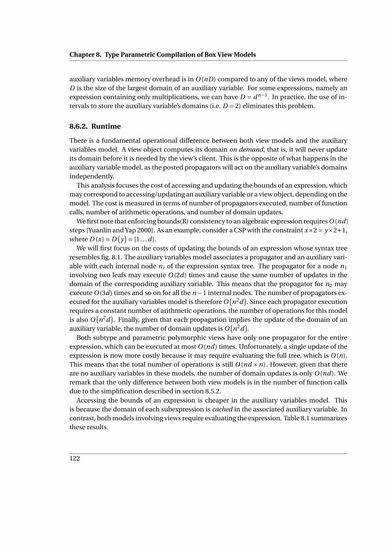
Chapter 8. Type Parametric Compilation of Box View Models
auxiliary variables memory overhead is in O (nD) compared to any of the views model, whereD is the size of the largest domain of an auxiliary variable. For some expressions, namely anexpression containing only multiplications, we can have D = d n−1. In practice, the use of in-tervals to store the auxiliary variable’s domains (i.e. D = 2) eliminates this problem.
8.6.2. Runtime
There is a fundamental operational difference between both view models and the auxiliaryvariables model. A view object computes its domain on demand, that is, it will never updateits domain before it is needed by the view’s client. This is the opposite of what happens in theauxiliary variable model, as the posted propagators will act on the auxiliary variable’s domainsindependently.
This analysis focuses the cost of accessing and updating the bounds of an expression, whichmay correspond to accessing/updating an auxiliary variable or a view object, depending on themodel. The cost is measured in terms of number of propagators executed, number of functioncalls, number of arithmetic operations, and number of domain updates.
We first note that enforcing bounds(R) consistency to an algebraic expression requires O (nd)steps [Yuanlin and Yap 2000]. As an example, consider a CSP with the constraint x×2 = y×2+1,where D (x) = D
(y)= [1 . . .d ].
We will first focus on the costs of updating the bounds of an expression whose syntax treeresembles fig. 8.1. The auxiliary variables model associates a propagator and an auxiliary vari-able with each internal node ni of the expression syntax tree. The propagator for a node n1
involving two leafs may execute O (2d) times and cause the same number of updates in thedomain of the corresponding auxiliary variable. This means that the propagator for n2 mayexecute O (3d) times and so on for all the n −1 internal nodes. The number of propagators ex-ecuted for the auxiliary variables model is therefore O
(n2d
). Since each propagator execution
requires a constant number of arithmetic operations, the number of operations for this modelis also O
(n2d
). Finally, given that each propagation implies the update of the domain of an
auxiliary variable, the number of domain updates is O(n2d
).
Both subtype and parametric polymorphic views have only one propagator for the entireexpression, which can be executed at most O (nd) times. Unfortunately, a single update of theexpression is now more costly because it may require evaluating the full tree, which is O (n).This means that the total number of operations is still O (nd ×n) . However, given that thereare no auxiliary variables in these models, the number of domain updates is only O (nd). Weremark that the only difference between both view models is in the number of function callsdue to the simplification described in section 8.5.2.
Accessing the bounds of an expression is cheaper in the auxiliary variables model. Thisis because the domain of each subexpression is cached in the associated auxiliary variable. Incontrast, both models involving views require evaluating the expression. Table 8.1 summarizesthese results.
122
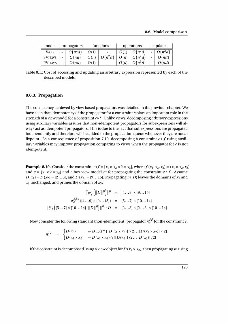
8.6. Model comparison
model propagators functions operations updates
VARS - O(n2d
)O (1) - O (1) O
(n2d
)- O
(n2d
)SVIEWS - O (nd) O (n) O
(n2d
)O (n) O
(n2d
)- O (nd)
PVIEWS - O (nd) O (1) - O (n) O(n2d
)- O (nd)
Table 8.1.: Cost of accessing and updating an arbitrary expression represented by each of thedescribed models.
8.6.3. Propagation
The consistency achieved by view based propagators was detailed in the previous chapter. Wehave seen that idempotency of the propagator for a constraint c plays an important role in thestrength of a view model for a constraint c◦ f . Unlike views, decomposing arbitrary expressionsusing auxiliary variables assures that non-idempotent propagators for subexpressions will al-ways act as idempotent propagators. This is due to the fact that subexpressions are propagatedindependently and therefore will be added to the propagation queue whenever they are not atfixpoint. As a consequence of proposition 7.10, decomposing a constraint c ◦ f using auxil-iary variables may improve propagation comparing to views when the propagator for c is notidempotent.
Example 8.19. Consider the constraint c◦ f = [x1 ×x2 ×2 = x3], where f (x1, x2, x3) = ⟨x1 ×x2, x3⟩and c = [x1 ×2 = x2] and a box view model m for propagating the constraint c ◦ f . AssumeD (x1) = D (x2) = [2 . . .3], and D (x3) = [9 . . .15]. Propagating m (D) leaves the domains of x1 andx2 unchanged, and prunes the domain of x3:
Vϕ+f
(VDWβ
)Wβ = [4 . . .9]× [9 . . .15]
πββ?c ([4 . . .9]× [9 . . .15]) = [5 . . .7]× [10. . .14]
Vϕ f
([5 . . .7]× [10. . .14] ,VDWβ
)Wβ∩D = [2 . . .3]× [2 . . .3]× [10. . .14]
Now consider the following standard (non-idempotent) propagator πββc for the constraint c:
πββc =
{D (x3) ← D (x3)∩ [bD (x1 ×x2)c×2. . .dD (x1 ×x2)e×2]
D (x1 ×x2) ← D (x1 ×x2)∩ [bD (x3)c/2. . .dD (x3)e/2]
If the constraint is decomposed using a view object for D (x1 ×x2), then propagating m using
123

Chapter 8. Type Parametric Compilation of Box View Models
the above propagator gives:
Vϕ+f
(VDWβ
)Wβ = [4 . . .9]× [9 . . .15]
πββc ([4 . . .9]× [9 . . .15]) = [5 . . .7]× [9 . . .15]
Vϕ f
([5 . . .7]× [10. . .14] ,VDWβ
)Wβ∩D = [2 . . .3]× [2 . . .3]× [9 . . .15]
Since the domains of the variables did not change, the propagator is at fixpoint. If the con-straint is decomposed using an auxiliary variable to represent D (x1 ×x2), then the propaga-
tion engine would reexecute πββc since the domain of the auxiliary variable has changed. Thiswould then cause m to be also reexecuted and infer D (x3) = [10. . .14] as when using an idem-potent propagator for c.
The above example may suggest that a decomposition of constraint c ◦ f using views wouldbe equivalent to using auxiliary variables if view models simply allow the propagator πc to rununtil fixpoint. However, converting non-idempotent propagators to idempotent propagatorsrequires also that the changes made by πc are persistent from one execution to another, whichis always true when πc involves domain variables exclusively, but might not be the case whenπc is applied to view objects. In fact, updating the domain of an auxiliary variable may be seenas a permanent operation - the domain effectively remembers the update. The same is notalways true when updating view objects since they are not strictly monotonic in general, thatis
S1 ⊂ S2; Vϕ(VS1Wβ,VSWβ
)Wβ∩S ⊂ Vϕ
(VS2Wβ,VSWβ
)Wβ∩S
Example 8.20. Consider again the previous example, but now assume that we use a view
model that runs propagator πββc until fixpoint. The first execution of the view model wouldcompute
D (x3) ← D (x3)∩ [bD (x1 ×x2)c×2. . .dD (x1 ×x2)e×2] = [10. . .14]
D (x1 ×x2) ← D (x1 ×x2)∩ [bD (x3)c/2. . .dD (x3)e/2] = [5 . . .7]
However, when D (x1 ×x2) is associated with a view object, evaluating D (x1 ×x2) after the sec-ond update above would still yield D (x1 ×x2) = [4 . . .9], i.e. the update is not persistent. Thereason for this is that the interval [5 . . .7] cannot be obtained by the product of a unique pair of
integer intervals representing D (x1) and D (x2). Therefore, reexecutingπββc would not performany further pruning.
As we have discussed earlier, decompositions using auxiliary variables cache the domains ofsubexpressions across executions of the involved propagators. In contrast, the domain repre-sented by box view objects is not maintained but recomputed in every propagation. A possiblesolution to the above problem would be to cache the domains of the box view objects when
124

8.7. Beyond arithmetic expressions
the update cannot be expressed by pruning the domains of the variables involved in the corre-sponding subexpression. This solution is a compromise between recomputing and cachingthe domain of subexpressions and guarantees that decomposition based on views has thesame strength as when using auxiliary variables even when using non-idempotent propaga-tors. While caching domains introduces performance penalties as discussed above, we wouldstill expect this solution to be more efficient than the auxiliary variable decomposition sincedomains would be cached much less frequently. In our experiments we found out that theamount of extra propagation earned when using auxiliary variables does not compensate theoverall inefficiencies of the variable decomposition model, as will be shown in the followingchapter.
8.7. Beyond arithmetic expressions
Although we have mostly focused on views over arithmetic expressions, views are also effectivefor accessing and updating other kind of expressions, namely the following.
8.7.1. Casting operator
Casting provides a type-safe mechanism to access or update polymorphic data types. A verycommon situation in Constraint Programming is treating Boolean variables as integer vari-ables or vice-versa, as shown in the following example.
Example 8.21 (Casting). Consider again the EXACTLY(x, v,c) constraint which constrains thenumber of occurrences of a given value in a collection of variables, i.e.
[∑i (xi = v) = c
]. The
expression in parenthesis is a Boolean expression, while the sum is treating it like a numeric ex-pression, where tr ue corresponds to 1 and f al se to 0. This is known as type casting. Defininga box view object over casting expressions allows a solver to integrate these kind of expressionsin an efficient, type-safe manner.
8.7.2. Array access operator
The ELEMENT(x, i , v) constraint is used to access a position in an array of domain variablesby constraining the element i of the array x to be equal to v . By forcing the xi variable toequal variable v , using this constraint may introduce a superfluous variable in a number ofconstraints, for example
[xi > y
]which is typically decomposed as
[ELEMENT (x, i , v)∧ v > y
].
In contrast, a box view object over a xi expression maintains the bounds of the variable atposition i , and does not introduce an extra variable.
125
Chapter 8. Type Parametric Compilation of Box View Models
8.7.3. Iterated expressions
Sometimes we may want to aggregate n subexpressions in some global expression, and n isnot known at compile time. For example in the Golomb ruler problem (see [Gent and Walsh1999]), the constraint
c = [DISTINCT
(xi −x j : 1 < i < j < m
)]enforces all pairwise differences to be distinct. Since m is typically given at runtime, the num-ber of differences (m × (m −1)/2) is not known when compiling the program, and thereforewe cannot state the constraint by enumerating all subexpressions literally. Even if we could, itwould not be very convenient either since m can be arbitrarily large.
When decomposing using auxiliary variables or subtype polymorphic views, an auxiliaryvariable (resp. a subtype polymorphic view object) is created for each difference at runtime,and the DISTINCT constraint is posted on these variables (resp. sview objects),
c = ∧1<i< j<m
[ai j = xi −x j
]∧ [DISTINCT(a)]
However, for compiling constraints to type parametric view objects the compiler must visitthe full expression top-down at compile time, as explained above. We must therefore find acompact and readable description of a repeating occurrence of a subexpression. Based onthe concept of aggregator [Hentenryck et al. 2000; Hentenryck and Michel 2005], we solvedthis problem using the ALL(I ,S,d ,e) expression which represents an array where each positionholds the expression e instantiated when each variable in I is assigned to a value of the set Sand the condition d is satisfied.
Example 8.22 (ALL expression). The constraint c may be represented as follows, where i , j arevariables taking values in {1, . . . ,m}, satisfying i < j ,
c = [DISTINCT
(ALL
({i , j
}, {1, . . . ,m} , i < j , xi −x j
))]For this to work we defined view objects over iterated expressions, that is, expressions that
depend on the value of the iterated variables i , j . In this particular case, view objects overiterated expressions are able to save a quadratic number of variables and still benefit from theefficiency of type parametric view objects.
8.8. Summary
This chapter introduced subtype and parametric polymorphic box view objects for efficientpropagation of box view models for arbitrary decomposable constraints. We have established
126

8.8. Summary
a formal relation between decompositions using view objects and auxiliary variables. Specifi-cally, we have shown under which circumstances using view objects or auxiliary variables forpropagating a given view model lead to the same search space. We have also seen how tocompile a propagation algorithm using a set of view objects or a set of propagators and aux-iliary variables from an arbitrary constraint. Moreover, we have presented two variants of thepropagation algorithm based on view objects, which suggest distinct implementations in poly-morphic programming languages. In the next chapter we will see that this difference has asignificant impact on performance.
Related work
There is a significant amount of work related to the material in this chapter, but since it is avail-able mostly in the form of computer program implementations, we have chosen to discuss itin the end of the next chapter.
Future work
. We have intentionally restricted the instantiation of view models to view models consistingonly of box approximations. This was partially because view objects may be implementedefficiently as discussed, but also because presenting an implementation of a generic viewmodel would make the exposition much more complex. In fact, other view models may bepropagated using a similar approach. The resulting propagators are correct, but creatingefficient corresponding view objects is much more challenging in general. As an example,consider designing a domain view object, that is an object which computes
Vϕ+f
(VS1Wδ
)Wδ
S1 ← S1 ∩Vϕ f(VS2Wδ,VS1Wδ
)Wδ
A domain view object must be able to compute δ-domains, which cannot be done in con-stant time for most functions f as it is the case for β-domains. In fact, the above operationsrequire time exponential in the arity of f , which renders domain view objects unpracticalfor most functions. It was found that for specific classes of functions, namely injective func-tions, computing δ-domain objects may be done in linear time [Tack 2009]. As future workit would be interesting to see if incrementality (discussed in part I of this dissertation) couldbe used to improve the runtime cost of computing domain view objects.
. Providing a domain view (or evenϕ-view) object over a compact extensional representationof the domain of the view is another possible development. Compact representations of ar-bitrary tuple sets have been successfully used for propagating extensional constraints [Gentet al. 2007; Cheng and Yap 2008]. Since such representations are exponential in the worstcase, using views over subexpressions could be a way to achieve a finer space-time tradeoff.
127

Chapter 8. Type Parametric Compilation of Box View Models
128

Chapter 9.
Implementation and Experiments
This chapter is divided in two parts. The first provides some details on how view objects pre-sented previously may be implemented, either in a logic programming setting (§9.1) or in astrongly typed imperative language (§9.2). The second part evaluates decomposition methodsexperimentally, summarizing the tested models and benchmarks (§9.3), and discussing theresults obtained (§9.4).
9.1. View models in Logic Programming
Propagators for box view models may be implemented straightforwardly in Prolog. A viewobject for a given function f is defined by a set of predicates, one for each method, of theform METHOD
(f ,b
)where b is either an input or output parameter depending on the method.
Prolog’s unification mechanism allows a literal implementation of parametric polymorphicview stores with respect to the previously described conceptual model. The rule repository isthe Prolog predicate store, and rewriting rules are simply stated as Prolog predicates.
Example 9.1. Partial implementation of bnd [x : dvar], bnd [X +Y ], and π [X ] in (eclipse) Pro-log:
% bnd[X+Y ]bnd_getmin (X+Y , R):− bnd_getmin (X , R1 ) ,
bnd_getmin (Y , R2 ) ,R i s R1+R2 .
bnd_updmin(X+Y , I ):− bnd_getmax (X ,MX) ,bnd_getmax (Y ,MY) ,IX i s I−MY, IY i s I−MX,bnd_updmin(X , IX ) ,bnd_updmin(Y , IY ) .
% bnd[ x : dvar ]bnd_getmin (X , R):− get_min (X , R ) .bnd_updmin(X , I ):− X #>= I .
129
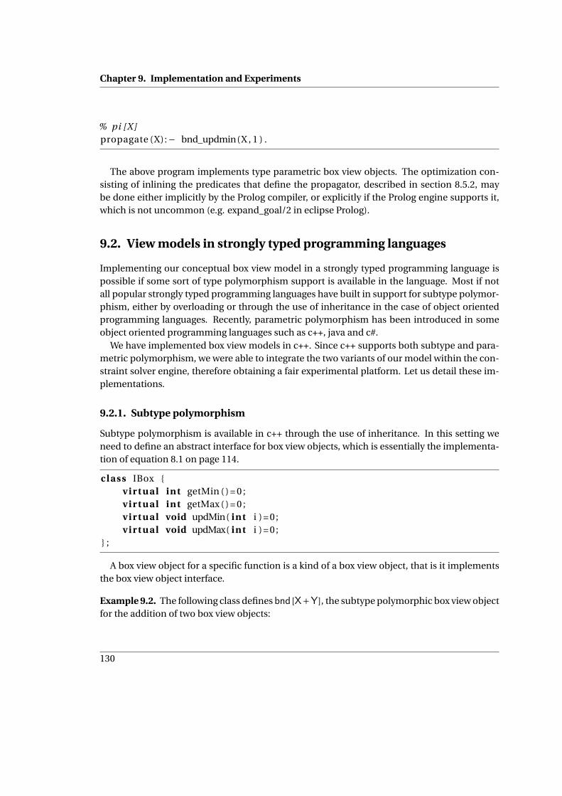
Chapter 9. Implementation and Experiments
% pi [X]propagate (X):− bnd_updmin(X , 1 ) .
The above program implements type parametric box view objects. The optimization con-sisting of inlining the predicates that define the propagator, described in section 8.5.2, maybe done either implicitly by the Prolog compiler, or explicitly if the Prolog engine supports it,which is not uncommon (e.g. expand_goal/2 in eclipse Prolog).
9.2. View models in strongly typed programming languages
Implementing our conceptual box view model in a strongly typed programming language ispossible if some sort of type polymorphism support is available in the language. Most if notall popular strongly typed programming languages have built in support for subtype polymor-phism, either by overloading or through the use of inheritance in the case of object orientedprogramming languages. Recently, parametric polymorphism has been introduced in someobject oriented programming languages such as c++, java and c#.
We have implemented box view models in c++. Since c++ supports both subtype and para-metric polymorphism, we were able to integrate the two variants of our model within the con-straint solver engine, therefore obtaining a fair experimental platform. Let us detail these im-plementations.
9.2.1. Subtype polymorphism
Subtype polymorphism is available in c++ through the use of inheritance. In this setting weneed to define an abstract interface for box view objects, which is essentially the implementa-tion of equation 8.1 on page 114.
class IBox {v i r t u a l int getMin ( ) = 0 ;v i r t u a l int getMax ( ) = 0 ;v i r t u a l void updMin( int i ) = 0 ;v i r t u a l void updMax( int i ) = 0 ;
} ;
A box view object for a specific function is a kind of a box view object, that is it implementsthe box view object interface.
Example 9.2. The following class defines bnd [X+Y], the subtype polymorphic box view objectfor the addition of two box view objects:
130

9.2. View models in strongly typed programming languages
class Add2 : IBox {Add2( IBox * x , IBox * y ) : x ( * x ) , y ( * y ) { }v i r t u a l int getMin ( ) { return x . getMin ( ) + y . getMin ( ) ; }v i r t u a l int getMax ( ) { return x . getMax ( ) + y . getMax ( ) ; }v i r t u a l void updMin( int i ){ x . updMin( i−y . getMax ( ) ) ; y . updMin( i−x . getMax ( ) ) ; }v i r t u a l void updMax( int i ){ x .updMax( i−y . getMin ( ) ) ; y .updMax( i−x . getMin ( ) ) ; }IBox& x ;IBox& y ;
} ;
Compiling a given constraint into subtype polymorphic box view objects is straightforwardsince in c++ expressions are evaluated bottom-up. Below are set of convenience functionswhich may be used to create subtype polymorphic view box objects for a binary addition.
IBox * add ( IBox * x , IBox * y ){ return new Add2( x , y ) ; }
IBox * operator +( IBox * x , IBox * y ){ return new Add2( x , y ) ; }
The user may then create box view objects for arbitrary expressions in C++ using a cleansyntax:
DomVar a , b , c ;a+b* c ;add ( a , mul(b , c ) ) ;
9.2.2. Parametric polymorphism
The fact that the c++ compiler evaluates expressions bottom-up makes the implementation ofparametric polymorphic view objects slightly more complex, since as we have seen in the pre-vious chapter, need to be compiled top-down. The solution we propose breaks the compilationalgorithm in two phases. The first phase creates a syntactic representation of the expression,called a type parametric relation object, using the natural bottom-up evaluation order intrin-sic in the language. Type parametric relations captures the data and the type of the objects andoperations involved in the constraint. After the full constraint is compiled, we use the obtainedrelation object for instantiating the required view objects.
131

Chapter 9. Implementation and Experiments
We will use templates for defining type parametric relations, since this is the language mech-anism available in c++ to support type parametric polymorphism. The following template de-fines generic binary relations, where “Op” is a type describing the operator, and “X” and “Y”are types of the operands.
template<class Op, class X , class Y>class Rel2 {
Rel2 (X x , Y y ) : x ( x ) , y ( y ) { }X x ;Y y ;
} ;
Since any expression may be transformed to a relation object with a unique type, we cancreate view objects over arbitrary expressions by defining templates over relation objects.
Example 9.3. The following template defines bnd [X+Y], the parametric polymorphic boxview object for the addition of two arbitrary objects:
template<class X , class Y>class Box<Rel2<Add, X , Y> > {
Box ( Rel2<Add, X , Y> r ) : x ( r . x ) , y ( r . y ) { }int getMin ( ) { return x . getMin ( ) + y . getMin ( ) ; }int getMax ( ) { return x . getMax ( ) + y . getMax ( ) ; }void updMin( int i ){ x . updMin( i−y . getMax ( ) ) ; y . updMin( i−x . getMax ( ) ) ; }void updMax( int i ){ x .updMax( i−y . getMin ( ) ) ; y .updMax( i−x . getMin ( ) ) ; }Box<X> x ;Box<Y> y ;
} ;
Parametric relation objects are created by a set of convenience functions, such as:
template<class X , class Y>Rel2<Add, X , Y> add (X x , Y y ){ return Rel2<Add, X , Y>(x , y ) ; }
template<class X , class Y>Rel2<Add, X , Y> operator +(X x , Y y ){ return Rel2<Add, X , Y>(x , y ) ; }
132

9.3. Experiments
Note that the above functions only create the relation object for the expression, and not thecorresponding view object. Creating the view object is accomplished by providing the relationobject to the following function:
template<class T>Box<T> box (T t ){ return Box<T>( t ) ; }
The following code instantiates two parametric box view objects for an expression using theabove constructs.
DomVar a , b , c ;box ( a+b* c ) ;box (add( a , mul(b , c ) ) ) ;
9.2.3. Advantages of subtype polymorphic views
We have seen in section 8.6.3 that propagators using type parametric view objects are theo-retically more efficient than those using subtype polymorphic view objects, by assuming thatthe compiler is able to eliminate function calls. This is often the case when the constraint isstated directly in a strongly typed programming language supporting type parametricity andthe code is compiled with a modern compiler. However, this may not be possible if the expres-sion is given as input by the user at runtime, for example if the solver is embedded in an inter-preter. In this case the expression was obviously not known when compiling the interpreter,and therefore there is no opportunity for compile time optimizations. We remark however thattype parametric views may still be useful in this scenario for defining a set of propagators for alimited number of expressions, which may be enough for domain specific interpreters.
9.3. Experiments
In this section we evaluate the performance of previously described decomposition methodson a set of benchmarks. Specifically we are interested in comparing the following models.
9.3.1. Models
VARS This is the classical method for decomposing constraints into primitive propagatorsintroducing one auxiliary variable for each subexpression, as discussed in section 8.4 onpage 117.
VARS+GLOBAL This model is similar to the previous but uses global constraints for loweringthe number of auxiliary variables. Only a subset of problems support this decompositionin which case we will specifically mention which global constraints are used.
133

Chapter 9. Implementation and Experiments
PVIEWS The model that implements the decomposition based on parametric polymorphicview objects, the central topic in the previous chapter.
SVIEWS The decomposition based on subtype polymorphic view objects described in theprevious chapter.
CPVIEWS This model is equivalent to the pviews model except that the computations ofthe view objects are cached in order to guarantee the same propagation as when usingauxiliary variables. This was discussed in section 8.6.3 on page 123.
VIEWS+GLOBAL Like the VARS+GLOBAL model, this model uses a combination of some typeof views and a global constraint propagator.
All the above decomposition models were implemented in CaSPER. Additionally, we also im-plemented the first two in Gecode [Gecode 2010] as an external reference, denoted GECODE-VARS and GECODE-VARS+GLOBAL respectively.
9.3.2. Problems
The set of benchmarks covers a total of 22 instances from 6 different problems. Before wepresent them in detail, we should make a few general considerations.
For each given instance we used the same labeling heuristics (or no heuristics at all) fortesting the above models. This means that, for each instance, the solvers resulting from theimplementation of the above models explore exactly the same search space, unless the de-compositions have different propagation strength, which may occur as we have already seen.
In the following exposition we will mostly focus on the decomposable constraints for whichour models apply. When describing the model, we may choose to ignore other necessary,redundant, or symmetry breaking constraints that we used in our implementations. Thesewere kept constant across all implementations of the above models for each benchmark andtherefore do not influence the conclusions. For additional information, we provide referencesto detailed descriptions of the problems in the online constraint programming benchmarkdatabase CSPLib [Gent and Walsh 1999]. The source code for all the solvers may be obtainedfrom the author upon request.
Systems of linear equations
This experiment consists in solving a system of linear equations. Linear equations are usuallyintegrated in Constraint Programming using a specific global constraint propagator. The goalof the experiment is therefore to assess the overhead of decomposing expressions using thepresented models compared to a decomposition which uses a special purpose algorithm, i.e.a global constraint.
134

9.3. Experiments
Each system of linear equations is described by a tuple ⟨n,d ,c, a, s|u⟩ where n is the numberof variables in the problem, d is the uniform domain size, c is the number of linear equa-tions, a is the number of terms in each equation, and the last term denotes if the problem is(s)atisfiable or (u)nsatisfiable. Each problem is defined by
c∧i=1
∑v∈p(i )
v = t
where p (i ) is a function returning a combination of a variables for the equation i , selected ran-domly from the full set of C n
a possible combinations. The independent term t in each equationwas selected randomly with a uniform probability from the interval [a . . . a ×d ]. Different ran-dom seeds were experimented in order to generate difficult instances.
The a-ary sum constraints were decomposed using binary sums implementing a subset ofthe previously described models, namely VARS, SVIEWS, and PVIEWS. Model VARS+GLOBAL
used global constraint propagators for the a-ary sums.
Systems of nonlinear equations
The second experiment considers systems of nonlinear equations. These problems arise oftenin practice, and since the decomposition to special purpose propagators is not so direct as inprevious case, it provides a realistic opportunity to apply the previously discussed models.
A system of nonlinear equations is described by a tuple ⟨n,d ,c, a1, a2, s|u⟩ where a1 is thenumber of terms in each equation, each term is composed of a product of a2 factors, and allremaining variables have the same meaning as before. Each system of nonlinear equations isformally defined as:
c∧i=1
a1∑j=1
∏v∈p(i , j)
v = t
where p(i , j
)is a function returning a combination of a2 variables for the term j of equation
i , selected randomly from the full set of C na2
possible combinations.The tested models consist on the decomposition into binary sums and products using aux-
iliary variables exclusively (VARS) and using view models (SVIEWS, PVIEWS, and CPVIEWS).We also tested two models where each product is decomposed using either auxiliary variablesor views, projected to a variable xi , and a sum propagator is used to enforce
∑a1i=1 xi for each
equation (VARS+GLOBAL and PVIEWS+GLOBAL respectively).
Social golfers (prob10 in CSPLib)
The Social golfers problem consists in scheduling a golf tournament. The golf tournamentlasts for a specified number of weeks w , organizing g games each week, each game involving
135

Chapter 9. Implementation and Experiments
s players. There is therefore a total of g × s players participating in the tournament. The goal isto come up with a schedule where each pair of golfers plays in the same group at most once.
This problem may be solved efficiently in Constraint Programming using a 3-dimensionalmatrix x of w ×g × s integer domain variables, where each variable identifies a golf player. Fortwo groups of players G1, G2, the MEETONCE constraint ensures that any pair of players in onegroup does not meet in the other group,
MEETONCE (G1,G2) =[ ∑
x∈G1,y∈G1
(x = y
)≤ 1
]
This constraint is then used to impose that each pair of players meets at most once during theentire tournament,∧
1≤wi<w j≤wMEETONCE
({xwi ,gi ,si : 1 ≤ gi ≤ g ,1 ≤ si ≤ s
},{
xw j ,g j ,s j : 1 ≤ g j ≤ g ,1 ≤ s j ≤ s})
We tested a subset of our models for propagating the MEETONCE constraint, namely PVIEWS+GLOBAL,SVIEWS+GLOBAL, CPVIEWS+GLOBAL, and VARS+GLOBAL. View based models implement theMEETONCE constraint using the above expression directly, using a global propagator for thesum constraint. This constraint translates almost literally to CaSPER,
MEETONCE (G1,G2) = [SUM
(ALL
(x ∈G1, y ∈G2, x = y
))≤ 1]
The VARS+GLOBAL model implements the traditional decomposition using a set b of s2 aux-iliary boolean domain variables,
MEETONCE (G1,G2) = ∧x∈G1,y∈G2
[bi =
(x = y
)](9.1)
∧[
s2∑i=1
bi ≤ 1
](9.2)
In this case we used the (reified) equality propagator for each equation in the conjunction ofeq. 9.1, and a sum global propagator for equation 9.2.
Golomb ruler (prob6 in CSPLib)
A Golomb ruler of m marks and length xm is a set of m integers,
0 = x1 < x2 < . . . < xm
such that the m(m − 1)/2 differences xi − x j , 1 ≤ j < i ≤ m are distinct. The Golomb rulerproblem is an optimization problem, where the goal is to find the smallest possible Golomb
136
9.3. Experiments
ruler with a given number of marks.This problem makes use of a constraint of the form
DISTINCT({
xi −x j : 1 ≤ j < i ≤ m})
enforcing that the pairwise differences xi − x j are all distinct. The classical decomposition forthis constraint (VARS+GLOBAL) introduces one auxiliary variable for each pairwise difference,and makes use of the alldiff [ref] global propagator for the DISTINCT constraint,∧
1≤i< j≤m[ai , j = xi −x j
]∧ [DISTINCT (a)]
Using views avoids introducing the set of auxiliary variables a. Instead, the constraint isused directly as follows,
DISTINCT(
ALL(1 ≤ i ≤ m,1 ≤ j ≤ m, j < i , xi −x j
))In our benchmarks we solved the decision version of this problem, i.e. we provided the size
of the ruler xm as a parameter of the problem, and asked for the ruler satisfying the constraints.
Low autocorrelation binary sequences (prob5 in CSPLib)
The goal is to construct a binary sequence S = x1, . . . , xn of length n, where D (xi ) = {−1,1},1 ≤ i ≤ n, that minimizes the autocorrelations between bits, i.e. that minimizes the followingexpression,
m =n−1∑i=1
(n−i−1∑
j=1x j ×x j+i+1
)2
(9.3)
The VARS+GLOBAL model decomposes the above expression using three sets of auxiliary vari-ables a, b, and c, and sum constraints as follows,∧n−1
i=1
∧n−i−1j=1
[x j ×x j+i+1 = ai , j
]∧n−1
i=1
[n−i−1∑
j=1ai , j = bi
]∧n−1
i=1
[b2
i = ci]
∧[
m =n−1∑i=1
ci
]
In this experiment we implemented three variants of the PVIEWS model. The PVIEWS-PARTIAL1 model implements the following decomposition which is just slightly more compact
137

Chapter 9. Implementation and Experiments
than the above,
∧n−1i=1
[n−i−1∑
j=1x j ×x j+i+1 = bi
]∧n−1
i=1
[b2
i = ci]
∧[
m =n−1∑i=1
ci
]
The PVIEWS-PARTIAL2 model further decreases the number of auxiliary variables,
∧n−1i=1
[n−i−1∑
j=1x j ×x j+i+1 = bi
]
∧[
m =n−1∑i=1
b2i
]
Finally, the PVIEWS, SVIEWS and CPVIEWS model implements expression 9.3 directly, withoutintroducing any auxiliary variable.
Fixed-length error correcting codes (prob36 in CSPLib)
This problem involves generating a set of strings from a given alphabet which satisfy a pairwiseminimum distance. Each instance is defined by a tuple ⟨a,n, l ,d⟩ where a is the alphabetsize, n is the number of strings, l is the string length, and d is the minimum distance allowedbetween any two strings. For measuring the distance between two strings we have used theHamming distance on two instances and the Lee distance on the other two. For two arbitrarystrings x, y of length l , these measures are defined as follows,
HAMMING(x, y
) =l∑
i=1
(xi 6= yi
)LEE
(x, y
) =l∑
i=1min
(∣∣xi − yi∣∣ , a − ∣∣xi − yi
∣∣) (9.4)
This problem was modeled by a matrix x of n×l integer domain variables, where each variablexi , j can take a value in 1. . . a corresponding to the symbol of string i in position j . Then,distance constraints are imposed between each pair of strings,∧
1≤i1<i2≤nDISTANCE
({xi1, j : 1 ≤ j ≤ l
},{
xi2, j : 1 ≤ j ≤ l})≥ d
138

9.4. Discussion
The VARS+GLOBAL model decomposes distance constraints using auxiliary variables and sumconstraints. Note that in the case of the Lee distance, a total of 4l auxiliary variables are in-troduced for each distance constraint. The SVIEWS, PVIEWS, and CPVIEWS models implementboth distance functions without any extra variables.
9.3.3. Setup
The code for the first two experiments was compiled with the gcc-4.2.4 C++ compiler, whilethe remaining experiments were compiled with gcc-4.4.3. All experiments were executed onan Intel Core 2 Duo @ 2.20GHz, using Linux-2.6.31.6. The versions of the CaSPER and Gecodesolvers were the most recently available, respectively revision 548 and version 3.3.1. Eachbenchmark was repeated until the standard deviation of the runtime was below 2% of the av-erage time, and then the minimum runtime was used.
9.4. Discussion
The results of all benchmarks are detailed in appendix B.3 from which we drawn the followingconclusions.
9.4.1. Auxiliary variables Vs Type parametric views
Table 9.1 compares the runtime of the best model using auxiliary variables, i.e. either VARS
or VARS+GLOBAL, with the runtime of the best model that uses type parametric views, i.e. ei-ther PVIEWS or PVIEWS+GLOBAL. View objects do not intend to be a replacement for globalconstraint propagators, and therefore this table shows how much the runtime of a constraintprogram may be improved when using the best available tools.
Before we take a global view on the results in this table, let us focus on the special case of thebenchmark involving systems of linear equations. We recall that this benchmark should notbe considered as part of a realistic application of views or auxiliary variables since it may bemodeled using a global constraint propagator exclusively. However, modeling the global sumconstraint using using type parametric views over binary sums was only 7% worst on average,which is nevertheless remarkable.
For all other benchmarks, using type parametric views instead of auxiliary variables wasconsistently better, approximately twice as fast on (geometric) average, and always more than25% faster. An interesting particular case are the two instances of the “Fixed length errorcorrecting codes” problem using the Lee distance. These instances are in fact the only forwhich decomposing using auxiliary variables could be recommended. This is because thereis a subexpression which occurs twice in the expression, and therefore can be represented bythe same auxiliary variable (see equation 9.4), possibly leading to a smaller search tree. Even
139

Chapter 9. Implementation and Experiments
mean stddev min max
Systems of linear equations 1.07 1.15 0.91 1.21Systems of nonlinear equations 0.42 1.08 0.36 0.46
Social golfers 0.62 1.09 0.59 0.69Golomb ruler 0.74 1.02 0.73 0.75
Low autocorrelation binary sequences 0.35 1.02 0.35 0.36Fixed-length error correcting codes 0.44 1.38 0.28 0.57
All 0.56 1.51 0.28 1.21All except linear 0.49 1.34 0.28 0.75
Table 9.1.: Geometric mean, standard deviation, minimum and maximum of the ratios definedby the runtime of best performing model using views over the runtime of the bestperforming model using auxiliary variables, on all benchmarks.
mean stddev min max
Systems of nonlinear equations 1.06 1.08 1.01 1.16Golomb ruler 1.00 1.00 1.00 1.01
Fixed-length error correcting codes 1.20 1.00 1.20 1.20
All 1.06 1.08 1.00 1.20
Table 9.2.: Geometric mean, standard deviation, minimum and maximum of the ratios definedby the number of fails of the best performing solver using views over the number offails of the best performing solver using auxiliary variables, on all instances of eachproblem where the number of fails differ.
without this optimization, the solver using type parametric views was more than twice as faston average on these instances.
Regarding propagation, even if using auxiliary variables may sometimes lead to smallersearch trees, the difference was not so significant in our experiments. In fact, for those in-stances where using auxiliary variables increases propagation strength compared to views, thediscrepancy in the number of fails was only of 6% on average, and never more than 20% (table9.2). On the other hand, the number of propagations using auxiliary variables is on averagean order of magnitude greater than when using views, which partially explains the superiorperformance of type parametric view models (shown in the appendix).
9.4.2. Type parametric views Vs Subtype polymorphic views
Recall from section 8.6.2 on page 122 that solvers using type parametric view objects are able toavoid a linear number of function calls for each access or update due to code inlining optimiza-
140

9.4. Discussion
mean stddev min max
Systems of linear equations 0.57 1.63 0.33 0.96Systems of nonlinear equations 0.83 1.07 0.77 0.93
Social golfers 0.77 1.05 0.73 0.81Golomb ruler 0.89 1.03 0.87 0.91
Low autocorrelation binary sequences 0.41 1.02 0.41 0.42Fixed-length error correcting codes 0.55 1.43 0.4 0.77
All 0.67 1.4 0.33 0.96
Table 9.3.: Geometric mean, standard deviation, minimum and maximum of the ratios definedby the runtime of the solver implementing the PVIEWS model over the runtime ofthe solver implementing the SVIEWS model, on all benchmarks.
mean stddev min max
Systems of nonlinear equations 0.57 1.13 0.46 0.65Social golfers 0.6 1.06 0.56 0.63Golomb ruler 0.83 1.03 0.8 0.85
Low autocorrelation binary sequences 0.82 1 0.82 0.82Fixed-length error correcting codes 0.57 1.44 0.33 0.72
All 0.64 1.27 0.33 0.85
Table 9.4.: Geometric mean, standard deviation, minimum and maximum of the ratios definedby the runtime of the solver implementing the PVIEWS model over the runtime ofthe solver implementing the CPVIEWS model, on all benchmarks.
tions. Table 9.3 shows how this optimization improves performance in practice, in particularfor problems involving a large number of subexpressions where it can be 66% times faster.
9.4.3. Caching type parametric views
Caching type parametric views is a way to overcome the loss of propagation strength in someproblems compared to the decomposition based on auxiliary variables. In our experiments,cached parametric view objects increased runtimes considerably, even if exploring a smallersearch space. Table 9.4 summarizes the results.
As we have seen in table 9.2, the search space visited by type parametric views is not muchlarger than when performing caching, which certainly influences these results. Note that cachingtype parametric views is still more efficient than using auxiliary variables (15% better on aver-age).
141

Chapter 9. Implementation and Experiments
mean stddev min max
Systems of linear equations 1.32 1.22 0.99 1.54Systems of nonlinear equations 1.42 1.12 1.2 1.63
Social golfers 1.43 1.28 1.15 1.86Golomb ruler 1.59 1.13 1.38 1.71
Low autocorrelation binary sequences 1.45 1.01 1.44 1.46Fixed-length error correcting codes 0.19 1.93 0.09 0.33
All 0.99 2.34 0.09 1.86All except fixed-length error correcting codes 1.43 1.16 0.99 1.86
Table 9.5.: Geometric mean, standard deviation, minimum and maximum of the ratios definedby the runtime of the CaSPER solver implementing the VARS+GLOBAL model overthe runtime of the Gecode solver implementing the VARS+GLOBAL model, on allbenchmarks.
9.4.4. Competitiveness
Modeling decomposable constraints using type parametric views makes CaSPER competitivewith the state-of-the-art Gecode solver. This may be seen by comparing the results presentedin table 9.5 with table 9.6. In the first table we compare the runtimes obtained by running thesame model on both solvers, i.e. VARS+GLOBAL and GECODE-VARS+GLOBAL. The second ta-ble compares the PVIEWS model against GECODE-VARS+GLOBAL, which are the best modelsthat can be implemented in both platforms using the available modeling primitives. WhileCaSPER is worse in all but one problem when using auxiliary variables and global propagators,it becomes very competitive when using type parametric views. We believe that the discrep-ancy observed in the “Fixed length error correcting codes” benchmark is related to aspects ofthe architecture of both solvers which are orthogonal to the tested models, in particular theperformance of labeling which seems to vary with the number of variables in Gecode, whileremaining approximately constant in CaSPER (see figure 9.1).
9.5. Summary
We have seen how box view objects may be implemented using several language paradigms,with a focus on strongly typed languages, namely c++. Decomposition models based on aux-iliary variables, subtype polymorphic views, and type parametric views were implemented fora number of well known benchmarks, and the results were discussed. We observed that typeparametric views are clearly more efficient than models resulting from the other decompo-sition/compilation methods for all benchmarks. Moreover, we have seen that this techniqueimproves the performance of CaSPER to the point of being competitive with Gecode, which is
142

9.5. Summary
mean stddev min max
Systems of linear equations 1.42 1.3 0.98 1.78Systems of nonlinear equations 0.59 1.12 0.5 0.68
Social golfers 0.89 1.28 0.67 1.1Golomb ruler 1.18 1.15 1 1.29
Low autocorrelation binary sequences 0.51 1.03 0.5 0.52Fixed-length error correcting codes 0.08 2.47 0.03 0.19
All 0.55 2.87 0.03 1.78All except fixed-length error correcting codes 0.85 1.54 0.5 1.78
Table 9.6.: Geometric mean, standard deviation, minimum and maximum of the ratios definedby the runtime of the CaSPER solver implementing the PVIEWS model over the run-time of the Gecode solver implementing the VARS+GLOBAL model, on all bench-marks.
Sheet3
Page 1
10 20 40 80 160 320 640 1280
0
1
2
3
4
5
6
7
8
9
10
Labeling runtime
caspergecode
#variables
#so
lutio
ns/
sec o
nd
(x1
0^-
5)
Figure 9.1.: Number of solutions per second when enumerating all solutions of a CSP with agiven number of variables (in the xx axis), domain of size 8, and no constraints.
143

Chapter 9. Implementation and Experiments
regarded as one of the most efficient solvers available.
Related work
Ï Most popular Prolog systems [SICStus 2006; ECLiPSe 2010; GNUProlog 2008] automaticallydecompose constraints over arbitrary arithmetic expressions using auxiliary variables. Theuse of indexicals and goal expanded constraints [SICStus 2006] is advised as a way to avoidintroducing auxiliary variables. We are not aware of a published description of the imple-mentation of the propagator achieved in this case, but we suspect it should be comparableto subtype polymorphic views model, since Prolog, being an untyped interpreted language,should not support type parametric polymorphism. Given the simplicity of the Prolog im-plementation of this model (see section 9.1) it is unfortunate that it requires special featuresof the language and is not transparent to the user.
Ï ILog Solver is well known constraint solver written in C++ supporting posting constraintsover arbitrary expressions. It processes an expression bottom-up by converting its subex-pressions to constrained expressions [ILOG 2003a], which are exactly subtype polymorphicview objects.
Ï Choco solver [Choco 2010] is a constraint solver written in Java which also allows postingconstraints over arbitrary expressions. In this system the user may ask the solver to eitherdecompose the expression using the auxiliary variables model, or to compile the expressionto an extensional representation.
Ï Gecode solver [Gecode 2010] is a very efficient constraint solver written in C++. At the timeof this writing, Gecode does not support constraints over arbitrary expressions. Instead, itrequires the user to provide the decomposition by means of auxiliary variables. However,this solver makes an extensive use of views very much as we describe in section 8.5.2. Themain difference is that in Gecode, views are available as an extension mechanism for de-signing new propagators explicitly. That is, unlike our model, there is no automatic processfor instantiating the required views for a given arbitrary expression. For more informationsee [Schulte and Tack 2005].
144

Part III.
Applications
145

Chapter 10.
On the Integration of Singleton Consistenciesand Look-Ahead Heuristics
Complete constraint programming solvers have their efficiency dependent on two comple-mentary components, propagation and search. Constraint propagation is a key componentin constraint solving, eliminating values from the domains of the variables with polynomialalgorithms. When propagation is effective, such algorithms reduce the search space by somecombinatorial (i.e exponential) factor, with a polynomial cost. The other component, search,aims at finding solutions in the remaining search space, and is usually driven by heuristicsboth for selecting the variable to enumerate and the value that is chosen first.
Typically, these components are independent. In particular, heuristics take into accountsome features of the remaining search space, and some structure of the problem to take de-cisions. Clearly, the more information there is, the more likely it is to get a good (informed)heuristics. In many search problems addressed in Artificial Intelligence, additional informa-tion is often obtained by performing a limited amount of look-ahead, and assessing the stateof search some steps ahead. For example in two players games, like chess or checkers, ratherthan considering the current state of the board to decide the move to make, a number of movesby both players can be simulated, such that board configurations with a more advanced phaseof the game (thus better informed) can be taken into consideration.
Although better solver performances can be achieved by improving any of the two compo-nents (propagation and search) they are seldom, if ever, integrated. The main reason for thislies in that typical propagation procedures, such as maintenance of local bounds or domainconsistency, are basically local filtering algorithms. Recently, a lot of attention has been givento a class of algorithms which analyze look-ahead what-if scenarios: what would happen ifa variable x takes some value v? Such look-ahead analysis (typically done by subsequentlymaintaining some local consistency on the constraint network) may detect that value v is notpart of any solution, and eliminate it from the domain of variable x. This is the purpose of thedifferent variants of Singleton Consistency [Debruyne and Bessière 1997; Barták and Erben2004; Bessière and Debruyne 2005; Lecoutre and Cardon 2005].
In this chapter we propose to go one step further of the above approaches. On the one hand,by recognizing that SAC propagation is not very cost-effective [Prosser et al. 2000], we propose
147

Chapter 10. On the Integration of Singleton Consistencies and Look-Ahead Heuristics
to restrict it to those variables more likely to be chosen by the variable selection heuristics(§10.1). More specifically, we assume that there are often many variables that can be selectedand for which no good criteria exists to discriminate them. This is the case with the first-fail(FF) heuristics, where often there are many variables with 2 values, all connected to the samenumber of other variables (as is the case with complete graphs). Hence the information gainobtained from SAC propagation is used to break the ties between the pre-selected variables.
On the other hand, we attempt to better exploit the information made available by the looka-head procedure, and use it not only to filter values but also to guide search. We thus investigatethe possibility of integrating Singleton Consistency propagation procedures with variable andvalue selection heuristics (§10.2), and analyze the speedups obtained in a number of bench-mark problems (§10.3-10.4).
10.1. Singleton consistencies
Let us consider a CSP P = ⟨X ,D,C⟩ where X is the set of variables, D is the Cartesian productof the variables domains, and C is the set of constraints (see def. 2.5 on page 10). Let n be thenumber of variables in P , i.e. n = |X |.
Definition 10.1 (Singleton θ-consistency). Let d be δ-domain such that d ⊆ D , and d |xi=a bethe domain obtained by setting d (xi ) = {a}, i.e.
d |xi=a = d (x1)× . . .×d (xi−1)× {a}×d (xi+1)× . . .×d (xn)
Additionally, let d |θx=a be the subdomain d |θx=a ⊆ d |x=a which is θ-consistent for all con-straints c ∈ C . A domain d is singleton θ-consistent (SC), iff for any value a ∈ d (x) of everyvariable x ∈ X , d |θx=a is not empty.
Cost-effective singleton consistencies are singleton arc-consistency (SAC) [Debruyne andBessière 1997] and singleton generalized arc-consistency (SGAC) [Prosser et al. 2000].
To achieve SC in a CSP, procedure SC [Debruyne and Bessière 1997] instantiates each vari-able to each of its possible values in order to prune those that (after some form of propagation)lead to a domain wipe out (function SC).
Once some (inconsistent) value is removed, then there is a chance that a value in a previ-ously revised variable has become inconsistent, and therefore SC must check these variablesagain. This can happen at most ns times, where n is the number of variables, and s the sizeof the largest domain, hence SC time complexity is in O(n2s2Θ), Θ being the time complexityof the algorithm that achieves θ-consistency on the constraint network. Variants of this al-gorithm with the same pruning power but yielding distinct space-time complexity trade-offshave been proposed [Barták and Erben 2004; Bessière and Debruyne 2004, 2005; Lecoutre andCardon 2005]. A related algorithm that considers each variable only once (function RSC), has
148

10.2. Informed decision making
Function SCθ(d ,X ,C)Input: A domain d , a set of variables X , and a set of constraints COutput: A domain d ′ ⊆ d which is singleton consistent with Crepeat1
modified ← false2
foreach x ∈ X do3 ⟨d ,modified′⟩← SReviseθ(x,d ,C)4
modified = modified ∨ modified′5
if d (x) =; then6
return ;7
8
9
until ¬ modified10
return d11
Function RSCθ(d ,X ,C)Input: A domain d , a set of variables X , and a set of constraints COutput: A domain d ′ ⊆ d which is restricted singleton consistent with Cforeach x ∈ X do1
⟨d ,modified⟩← SReviseθ(x,d ,C)2
if d (x) =; then3
return ;4
5
return d6
better runtime complexity O(nsΘ), but achieves a weaker consistency, is called restricted sin-gleton consistency (RSC) [Prosser et al. 2000].
Note that both algorithms use function SRevise which prunes the domain of a single vari-able by trying all of its possible instantiations.
10.2. Informed decision making
Another possible trade-off between run-time complexity and pruning power is to enforce sin-gleton consistency on a subset of variables S ⊆ X . We identified two possible goals which con-dition the selection of S : filtering and decision making. From a filtering perspective, S shouldbe the smallest subset where (restricted) singleton consistency can actually prune values, andalthough this is not known a priori, approximations are possible by exploring incrementality
149

Chapter 10. On the Integration of Singleton Consistencies and Look-Ahead Heuristics
Function SReviseθ(x,d ,C)Input: A variable x, domain d , and a set of constraints COutput: A domain d ′ ⊆ d where d |θx=a ∀a ∈ d (x) is θ-consistent with Cmodified ← false1
foreach a ∈ d (x) do2
if Propagateθ(d ,C ∪ [x = a]) =; then3
d (x) ← d (x) \ a4
modified ← true5
6
return ⟨d ,modified⟩7
and value support [Barták and Erben 2004; Bessière and Debruyne 2005]. On the other hand, Smay be selected for improving the decision making process, in particular of variable selectionheuristics that are based on the cardinality of the current domains. In this case, the pruningresulting from enforcing singleton consistency is used as a mechanism to break ties both inthe selection of variable and in the choice of the value to enumerate.
Observing the general preference for variable heuristics which select smallest domains first,we propose defining S as the set of variables whose domain cardinality is below a given thresh-old t .
Definition 10.2. Let X≤t be the subset of variables in X having domains with cardinality lessor equal to t , i.e.
X≤t = {xi ∈ X : |d (x1)| ≤ t }
We denote by RSC≤t (d , X ,C ) and SC≤t (d , X ,C ), respectively, the algorithms RSC(d , X≤t ,C ) andSC(d , X≤t ,C ).
A further step in integrating singleton consistencies with search heuristics is to explore in-formation regarding the subproblems that are generated each time a value is tested for con-sistency. We propose a class of look-ahead heuristics (LA) for any CSP which reason over thenumber of solutions in the current domain d ⊆ D , given by a function σ (d), collected whileenforcing singleton consistency. Although there is no known polynomial algorithm for com-puting σ (finding the number of solutions of a CSP is a #P-complete problem), there exists anumber of naive as well as more sophisticated approximation functions [Gent et al. 1996; Kasket al. 2004]. We conjecture that by estimating the size of the solution space for each possible
instantiation, i.e. σ(
d |θx=a
), there is an opportunity for making more informed decisions that
will exhibit both better first-failness and best-promise behavior. Moreover, the class of ap-proximations of σ presented below are easy to compute, do not add complexity to the cost ofgenerating the subproblems, and only requires a slight modification of the SRevise function.
150

10.2. Informed decision making
Function SReviseInfoθ(x,d ,C ,INFO)Input: A variable x, domain d , a set of constraints C , and a reference to the INFO data
strucureOutput: A domain d ′ ⊆ d where d |θx=a ∀a ∈ d (x) is θ-consistent with Cmodified ← false1
foreach a ∈ d (x) do2
b ←Propagateθ(d ,C ∪ [x = a])3
INFO [x, a] ← CollectInfo(b,C)4
if b =; then5
d (x) ← d (x) \ a6
modified ← true7
8
return ⟨d ,modified⟩9
The SReviseInfo function stores in a table, denoted INFO, relevant information to the spe-cific subproblem being considered in each loop iteration. In our case, INFO is an estimation
of the subproblem solution space, more formally INFO [x, a] =σ′(
d |θx=a
)where σ′ ≈σ. The ta-
ble is initialized before singleton consistency enforcement, computed after propagation, andhanded to the SelectVariable and SelectValue functions as shown in function Solve.
There are several possible definitions for these functions associated with how they integratethe collected information. Regarding the selection of variable, we identified two FF heuristicswhich are cheap and easy to compute:
VAR1 (d) = argminx∈X
( ∑a∈d(x)
σ′(
d |θx=a
))
VAR2 (d) = argminx∈X
(max
a∈d(x)σ′
(d |θx=a
))Informally, VAR1 gives preference for the variable with a smaller sum of the number of solu-
tions for every possible instantiation, while VAR2 selects the variable whose instantiation withmaximum number of solutions is the minimum among all variables. For the selection of valuefor some variable x ∈ X , a possible BP heuristic is
VAL1 (d , x) = arg maxa∈d(x)
(σ′
(d |θx=a
))which simply prefers the instantiation that prunes less solutions from the remaining searchspace.
Functions VAR1 and VAL1 correspond to the minimize promise variable heuristic and maxi-
151

Chapter 10. On the Integration of Singleton Consistencies and Look-Ahead Heuristics
Function Solveθ(d ,C ,INFO)Input: A domain d , and a set of constraints COutput: A set of solutions in d satisfying all constraints in CINFO ←;1
d ← SCθ(d ,C , INFO)2
if d =; then3
return ;4
if |d | = 1∧∀c ∈C ,d ⊆ con(c) then5
return d6
x ←SelectVariable(X , INFO)7
a ←SelectValue(x, INFO)8
return Solveθ(d ,C ∪ [x = a])∪Solveθ(d ,C ∪ [x 6= a])9
mize promise value heuristic defined in [Geelen 1992]. Note that we do not claim these are thebest options for the estimation of the search space or the number of solutions. We have simplyadopted them for simplicity and for testing the concept (more discussion on section 10.5).
10.3. Experiments
A theoretical analysis on the adequacy of these heuristics as FF or BP candidates is needed,but hard to accomplish. Alternatively, in this section we attempt to give some empirical evi-dence of the quality of these heuristics by presenting the results of using them combined withconstraint propagation and backtracking search on a set of typical CSP benchmarks.
More specifically, the set of experiments presented in this section intend to answer the fol-lowing three questions:
• Does performing any restricted form of singleton consistency improves the overall solv-ing process compared with performing full singleton consistency? In this case we areinterested in assessing the possible advantages of using a faster but less complete prop-agation algorithm, indepentently of the search heuristic used.
• When solving a problem using (restricted) singleton consistent propagation, does inte-grating lookahead information in the search heuristic present any advantage comparedto using a search heuristic which discards this information?
• How does performing (restricted) singleton consistency and using the look-ahead in-formation to guide search compares with not performing such costly propagation andusing other good heuristics which do not require look-ahead information.
152

10.3. Experiments
10.3.1. Heuristics
LA This heuristic implement the proposed functions VAR1 and VAL1. As a first attempt atmeasuring its potential, a simple measure was used for estimating the number of solu-tions in a given domain d :
σ′ (d) =∑
x∈Xlog2 (|d(x)|)
which informally expresses that the number of solutions is correlated to the size of thesubproblem search space1. Although this is a very rough estimate, we are assumingthat it could nevertheless provide valuable information to compare alternatives (see sec-tion 10.5).
DOM+value This heuristic selects the variable with less values in its domain, and assigns itthe value selected by the value heuristic value. The value heuristic value can be eitherMIN, which corresponds to selecting the minimum possible value in the domain of theselected variable, or MC that selects the value which minimizes the number of conflictswith the variables connected to the selected variable by some constraint.
DOM/WDEG+value This heuristic selects the variable with the smallest ratio between thenumber of values in its domain and the sum of the weighted degrees of all the con-straints it participates. The weighted degree of a constraint is the the number of times ithas been proven unsatisfiable since the begining of the search process (see [Boussemartet al. 2004]). The value selection is guided by value as described above.
IMPACTS The impact of an assignment x 7→ a is defined as,
Ix 7→a (d) =σ′
(d |θx=a
)−σ′
(d |θx=a
)σ′
(d |θx=a
)averaged over all domains d since the begining of search. This heuristic selects the vari-able and value with largest impact (see [Refalo 2004]).
10.3.2. Strategies
heuristic On every choice point uses heuristic without any kind of singleton consistency en-forcement to make the decision on which variable/value to select, where heuristic is oneof the heuristics defined in the previous section.
SC+heuristic On every choice point first achieves singleton consistency and then uses heuris-tic to make the decision on which variable/value to select.
1We use the logarithm since the size of search space can be a very large number.
153

Chapter 10. On the Integration of Singleton Consistencies and Look-Ahead Heuristics
RSC+heuristic On every choice point first achieves restricted singleton consistency and thenuses heuristic to make the decision on which variable/value to select.
SC2+heuristic On every choice point first achieves singleton consistency further restrictedto variables with only two values in its domain, i.e. SC≤2(X ,C ) as discussed previously,and then uses heuristic to make the decision on which variable/value to select.
RSC2+heuristic On every choice point first achieves restricted singleton consistency furtherrestricted to variables with only two values in its domain, i.e. RSC≤2(X ,C ) as discussedpreviously, and then uses heuristic to make the decision on which variable/value to se-lect.
10.3.3. Problems
Graph Coloring
Graph coloring consists of trying to assign n colors to m nodes of a given graph such that nopair of connected nodes have the same color. In this section we evaluate the performance ofthe presented heuristics in two sets of 100 instances of 10-colorable graphs, respectively with50 and 55 nodes, generated using Joseph Culberson’s k-colorable graph generator [Culberson2010].
A CSP for solving the graph coloring problem was modeled by using variables to representeach node and values to define its color. Difference binary constraints were posted for everypair of connected nodes.
The average degree of a node in the graph d , i.e. the probability that each node is connectedto every other node, has been used for describing the phase transition in graph coloring prob-lems [Cheeseman et al. 1991]. In this experiment we started by determining empirically thephase transition to be near d = 0.6, and then generated 100 random instances varying d uni-formly in the range [0.5. . .0.7].
Random CSPs
Randomly generated CSPs have been widely used experimentally, for instance to compare dif-ferent solution algorithms. In this section we evaluate the look-ahead heuristics on severalrandom n-ary CSPs. These problems were generated using model C [Gent et al. 2001] general-ized to n-ary CSPs, that is, each instance is defined by a 5-tuple
⟨n,d , a, p1, p2
⟩, where n is the
number of variables, d is the uniform size of the domains, a is the uniform constraint arity, p1
is the density of the constraint graph, and p2 the looseness of the constraints.These tests evaluate the performance of the several heuristics in a set of random instances
near the phase transition. For this task we used the constrainedness measure κ [Gent et al.1996] for the case where all constraints have the same looseness and all domains have the
154

10.3. Experiments
same size:
κ= −|C | log2
(p2
)n log2 d
where |C | is the number of n-ary constraints.
We started by fixing n, d and a, and then computed 100 values for p2 uniformly in the range[0.1. . .0.8]. For each of these values, a value of p1 was used such that κ= 0.95 (problems in thephase transition have typically κ≈ 1). The value of p1, given by
p1 =−κn log2 d
log2 p2× a! (n −a)!
n!
is computed from the first formula and by noting that p1 is the fraction of constraints over allpossible constraints in the constraint graph, i.e.
p1 = |C | a! (n −a)!
n!
Solutions were stored as positive table constraints and a domain complete propagator im-plementing GAC-Schema [Bessière and Régin 1997] was used for filtering.
Partial Latin Squares
Latin squares is a well known benchmark which combines randomness and structure, alreadyintroduced in chapter 2. Recall that the problem consists in placing the elements 1. . .n in an ×n grid, such that each element occurs exactly once on the same row or column. A partialLatin squares (or quasigroup completion) problem is a Latin squares problem with a numberof preassigned cells, and the goal is to complete the puzzle.
The problem was modeled using the direct encoding, i.e. using an all-different constraint forevery row and column, propagated using a domain complete propagator. The dual encodingmodel, as proposed in [Dotu et al. 2003], was also considered but never improved over the di-rect model on the presented instances. The value selection heuristic used in conjunction withthe dom variable selection heuristic, denoted as mc (minimum-conflicts), selects the valuewhich occurs less in the same row and column of the variable to instantiate. This is reportedto be the best known value selection heuristic for this problem [Dotu et al. 2003].
We generated 200 instances of a satisfiable partial Latin squares of a given size, with approx-imately one third of cells preassigned, using lsencode-v1.1 [Kautz et al. 2001], a widely usedrandom quasigroup completion problem generator.
155

Chapter 10. On the Integration of Singleton Consistencies and Look-Ahead Heuristics
10
15
20
25
30
0 50 100 150 200 250 300
sc+dom+minrsc+dom+minsc2+dom+min
rsc2+dom+min 50
55
60
65
70
75
80
85
90
0 100 200 300 400 500 600
sc+dom+minrsc+dom+minsc2+dom+min
rsc2+dom+min 140
150
160
170
180
190
200
0 100 200 300 400 500 600 700 800 900
sc+dom+mcrsc+dom+mcsc2+dom+mc
rsc2+dom+mc
Figure 10.1.: Number of problems solved (yy axis) after a given time period (xx axis). Thegraphs show the results obtained for, from left to right, the graph coloring in-stances, the random instances, and latin square instances.
10.4. Discussion
In the following experiments all times are given in seconds, and represent the time neededfor finding the first solution. The first set of experiments try to answer the two first questionspresented in the previous section. These experiments considered the graph coloring instanceswith n = 50 nodes, the random instances with n = 50, d = 5 and a = 3, and the latin squareproblem instances of size n = 30. The experiments involving graph coloring and random in-stances were performed on a Pentium4, 3.4GHz with 1Gb RAM, while the experiments involv-ing latin square instances were performed on a Pentium4, 1.7GHz with 512Mb RAM. Timeoutswere set to 300, 600 and 900 seconds for the graph coloring, random and latin squares in-stances respectively. These experiments were implemented in CaSPER, revision 157.
Figure 10.1 compares the results obtained for solving the benchmarks described above whenachieving some form of (restricted) singleton consistency, but using an heuristic that does notmake use of look-ahead information to guide the search (we used DOM+MIN on the graph andrandom instances, and DOM+MC on the latin square instances). Note that this experimentonly considers using singleton consistency for improving propagation.
We can observe that restricting singleton consistency to subsets of variables with a small do-main size has an impact on performance, but it is not clear if it is positive in general - it is posi-tive on the random and latin square instances, and negative on the graph instances. However,using restricted singleton consistency was consistently better than full singleton consistencyacross all instances, which confirms the results of [Prosser et al. 2000].
In figure 10.2 we assess the advantage of using look-ahead information to guide search in thecase this information is available for free, that is as a consequence of the enforcement of someform of singleton consistency. For this we compare the performance of the solver using theLA heuristic with the performance of the solver using either DOM+MIN or DOM+MC as in the
156

10.4. Discussion
-6
-4
-2
0
2
4
6
8
0 50 100 150 200 250 300 350
scrscsc2
rsc2
-5
0
5
10
15
20
25
30
0 100 200 300 400 500 600
scrscsc2
rsc2
-80
-60
-40
-20
0
20
40
60
80
0 100 200 300 400 500 600 700 800 900
scrscsc2
rsc2
Figure 10.2.: Difference between the number of problems solved when using the LA heuris-tic and when using the DOM+MIN heuristic (yy axis) after a given time period (xxaxis). The graphs show the results obtained for, from left to right, the graph color-ing instances, the random instances, and latin square instances.
previous experiment, when both solvers already maintain some form of singleton consistency.
The figure shows that using look-ahead information to guide search when this informationis available at no extra cost is significatively advantegeous on all instances except on those ofthe graph coloring problem, where it did not make much difference. We can also observe thatthis is true independently of the form of singleton consistency enforced, although the combi-nation with some forms of singleton consistency seem to perform better on some problems.Finally, we note that the fact that the curves tend to zero with time is a consequence of thesmaller number of hard problems compared with the number of easy problems (heavy tailedbehaviour).
The second set of experiments address the third question presented in the previous section.These experiments considered the graph coloring instances with n = 65 nodes, the randominstances with n = 50, d = 5 and a = 4, and the latin square problem instances of size n = 35.Experiments were performed on a Pentium4, 1.7GHz with 512Mb RAM. Timeout was set to1800 seconds for any instance. These experiments were implemented in CaSPER, revision 333.
In these experiments we compared the performance of a solver implementing some formof singleton consistency and using the collected information to guide search with the perfor-mance of a solver implementing other good heuristic which does not required lookahead in-formation.
The results (fig. 10.3) show that there is no clear winner across all problems. As possiblyexpected, for problems where propagation achieves less pruning, impact based heuristics areless effective. This is the case of both the random and the graph coloring problems, as illus-trated in fig. 10.4, that shows, in log scale, the reduction of the size of the search space, sub-sequent to each enumeration. In random problems the propagation is poor given the lack ofstructure of the problem.
157

Chapter 10. On the Integration of Singleton Consistencies and Look-Ahead Heuristics
40
60
80
100
120
140
160
180
200
0 200 400 600 800 1000 1200 1400 1600 1800
dom/wdeg+minimpacts+min
rsc2+la 40
60
80
100
120
140
160
180
200
0 200 400 600 800 1000 1200 1400 1600 1800
dom/wdeg+minimpacts+min
rsc2+la 40
60
80
100
120
140
160
180
200
0 200 400 600 800 1000 1200 1400 1600 1800
dom/wdeg+minimpacts+min
rsc2+la
Figure 10.3.: Number of problems solved when using several strategies (yy axis) after a giventime period (xx axis). The graphs show the results obtained for, from left to right,the graph coloring instances, the random instances, and latin square instances.
0
100
200
300
400
500
600
700
0 5 10 15 20 25 30
latingraph
random
Figure 10.4.: Search space size during solving of a typical instance in each problem.
158

10.5. Summary
strategy #timeouts avgfails stddevfails avgtime stddevtime
dom/wdeg 2 63549 422439 13.7 94.6la 42 8022 30312 208.3 366.4
Table 10.1.: Results for finding the first solution to latin-15 with a selected strategy.
The networks for the graph coloring problem exhibit some locality, and propagation mostlyaffect variables in the same cluster of the variable being assigned, with limited propagationto variables far away in the network. Apparently, the dom/wdeg heuristics, by reasoning atconstraint level, is able to "infer" such locality and take advantage of it for variable selection.
In contrast, in the latin square instances modeled by means of all different global constraintslocality is not so marked (two variables often share the same constraint, if in the same row orcolumn, or are separated by two constraints, one row and one column, and seldom by morethan that, when both row and column pivot elements are already ground). Moreover, gen-eralized arc consistency propagation virtually affects all variables after variable enumeration.The greater impact achieved in these problems, together with the lack of locality to be ex-ploited by a constraint centered impact heuristic such as dom/wdeg, makes variable centeredimpact heuristics more adequate in this problem. We tried both heuristics in a set of smallerlatin square instances modelled with pairwise distinct constraints while maintaining (single-ton) node consistency and observed a different ranking, which confirms our thesis (see table10.1).
10.5. Summary
This chapter presented an approach that incorporates look ahead information for directingbacktracking search, and suggested that this could be largely done at no extra cost by takingadvantage of the work already performed by singleton consistency enforcing algorithms. Wedescribed how such a framework could extend existing SC and RSC algorithms by requiringonly minimal modifications. Additionally, a less expensive form of SC was revisited, and a newone proposed which involves revising only a subset of variables. Finally, empirical tests withtwo common benchmarks and with randomly generated CSPs showed promising results oninstances near the phase transition.
Related work
Ï The impact heuristic introduced by Refalo [2004] suggests improving the variable selectionheuristic based on the impact each variable assignment has on the future search space size.In their paper the use of a specific look-ahead procedure for measuring this impact is re-garded as costly, and depreciated in favor of a method that accumulates this information
159

Chapter 10. On the Integration of Singleton Consistencies and Look-Ahead Heuristics
across distinct search branches and/or search iterations (restarts). Their results show thatthe method eventually converges to a good variable ordering (the value selection heuristicis not considered).
Ï In [Kask et al. 2004], belief updating techniques are used to estimate the likelihood of a valuebelonging to some solution. These likelihoods are then used to improve the value selectionheuristic and as propagation: if it decreases to zero, the value is discarded from the domain.However, the integration of this kind of propagation with common local propagation algo-rithms is not explored in that paper.
Future work
. As discussed in the previous section, tests which use singleton consistency on a subset ofvariables defined by its cardinality were not consistently better or worse than the others,but may be very beneficial sometimes. We think this deserves more investigation, namelytesting with more structured problems, and using a distinct selection criteria (other thandomain cardinality).
. Improving the FF and BP measures. Look-ahead heuristics presented above use rather naiveestimation of number of solutions for a given subproblem compared to, for example, the κmeasure introduced in [Gent et al. 1996], or the probabilistic inference methods describedin [Kask et al. 2004]. The κ measure, for example, takes into account the individual tight-ness of each constraint and the global density of the constraint graph. Their work showsstrong evidence for best performance of this measure compared with standard FF heuris-tics, but also point out that the complexity of its computation may lead to suboptimal resultsin general CSP solving (the results reported are when using forward-checking). Given thatwe perform a stronger form of propagation and have look-ahead information available, thecost for computing κ may be worth while.
. Include the use of faster singleton consistency enforcing algorithms [Barták and Erben 2004;Bessière and Debruyne 2005], which should be orthogonal to the results presented here, andthe use of constructive disjunction during the maintenance of SC, by pruning values fromthe domains of a variable that does not appear in the state of the problem for all values ofanother variable.
160
Chapter 11.
Overview of the CaSPER* Constraint Solvers
This chapter describes the casperzito and casperzao constraint solvers submitted to the thirdinternational CSP solver competition. These solvers are based on the CaSPER solver, the con-straint solver integrating the techniques presented throughout this dissertation. Addition-ally, they implement automatic symmetry detection and symmetry breaking, the lookaheadheuristics described in the previous chapter, and search strategy sampling. The structure ofthe chapter is as follows. We first describe the competition purpose, scope, and rules (§11.1),and then focus on the techniques integrated on solvers submitted to the competition, namelyconcerning propagation (§11.2), symmetry breaking (§11.3), and search (§11.4). Finally, wepresent and discuss the results obtained (§11.5).
11.1. The third international CSP solver competition
The goal of this competition is to help identifying successful techniques in constraint solvingby comparing solvers in the same environment presented with a large set of benchmarks. Thethird edition of the competition happened in 2008 and the results were presented during theCP’2008 conference. The rules of the competition are as follows.
Instances are represented in XCSP 2.1, a XML based format of CSP instances, for which allsolvers must provide a parser (see [Roussel and Lecoutre 2009]). Solvers may compete in sev-eral categories:
2-ARY-EXT only binary constraints defined in extension
2-ARY-INT only binary constraints (some of them being defined by a predicate)
N-ARY-EXT some n-ary constraints (all constraints defined in extension)
N-ARY-INT some n-ary constraints and some constraints defined by a predicate
GLOBAL some global constraints
The categories 2-ARY-EXT and N-ARY-EXT allows defining positive and negative table con-straints, i.e. enforce that the values of a given sequence of variables either belong or do not
161

Chapter 11. Overview of the CaSPER* Constraint Solvers
constraint value bounds domain
positive table no no [Bessière and Régin1997; Gent et al. 2007] (a)
negative table custom (b) no custom (b)distinct custom [Lopez-ortiz et al. 2003] [Régin 1994]element no custom custom
linear no [Yuanlin and Yap 2000] nocumulative no [Beldiceanu and
Carlsson 2002; Mercierand Hentenryck 2008]
no
Table 11.1.: Global constraint propagators used in solvers.
belong to a given table. The set of predicates in 2-ARY-INT and N-ARY-INT allows definingarithmetic and logical expressions, and the available set of global constraints in GLOBAL isrestricted to CUMULATIVE, DISTINCT, WEIGHTEDSUM, and ELEMENT.
A solver is given an amount of time (30 minutes) and memory (900MB), and one CPU foreach benchmark. The solver must decide if the problem is satisfiable or unsatisfiable. In theformer case it must also present a satisfiable solution to the problem. A solver giving a wronganswer is disqualified from that category. The ranking of the solvers is based on the number ofsolved instances.
11.2. Propagation
11.2.1. Predicates
Except for global constraints (see below), arithmetic predicates used in the competition areenforced in CaSPER using bounds consistency. In many benchmarks used in the competi-tion, predicates are conjoined together in larger predicates, and we found that decomposingthem was sometimes penalizing performance. To solve this problem, we translated these con-junctions of predicates to positive or negative table constraints (whichever is smaller) by solv-ing the corresponding subproblems before search, and enforced domain consistency on theseconstraints during search. We only did this in zao, since we were not sure this was a good idea.
11.2.2. Global constraints
Table 11.1 describes the propagators used for the global constraints in the competition.For the domain consistency propagator for positive table constraints (a) we used the first
algorithm [Bessière and Régin 1997] on zito and the new trie-based propagator of [Gent et al.
162

11.3. Symmetry breaking
2007] in zao. While the latter exhibited better results in our tests, we still found the first moreefficient for small arity constraints.
The most popular algorithm for propagating the negative table constraint (b) seems to bethe two watched literal scheme introduced for SAT, which achieves value (node) consistency.In [Bessière and Régin 1997], a domain consistency algorithm for this constraint that makesheavy use of hashing for checking disallowed tuples was presented. We have extended thework of [Gent et al. 2007] which focus on positive table constraints to handle negative tableconstraints as well. While we also base our idea in the trie data structure, this is in fact a com-pletely different propagator which has the advantage of performing much cheaper tests com-pared to the hashing proposal. For the competition we used the value consistency propagatorfor negative table constraints in zito and our new trie-based propagator in zao.
11.3. Symmetry breaking
We mostly followed the ideas of Puget [2005] for automatic symmetry detection using compu-tational group theory and [Aloul et al. 2006; Puget 2005] for symmetry breaking. The basic ideaof the detection process is to translate the given CSP to a graph which expresses the symmetriesassociated with each constraint. The automorphism group of this graph defines the set of sym-metries in the original CSP. Puget shows how to translate some common global constraints, e.g.the alldifferent constraint. Extending the idea for the predicates and global constraints used inthe competition is straightforward. Additionally, both solvers perform a small amount of sym-bolic computation in order to circumvent some situations where the symmetries in the CSPwould be hidden by the formulation. Although the detection process is able to identify bothvariable and value symmetries, we just focused on the first kind1.
Since the number of detected variable symmetries is quite large for most problems, we fol-lowed the method of Aloul et al. [2006] for breaking symmetries, that is we restrict to the vari-able symmetries present on the generators of the symmetry group (also referred as the GENclass in [Puget 2005]), and added a number of lexicographic ordering constraints [Carlsson andBeldiceanu 2002] before starting search. This is a popular technique known as static symmetrybreaking (SSB) [Puget 1993]. Moreover, both solvers do some effort to identify symmetries insets of variables known to be all different, in which case we break symmetries by enforcing atotal ordering.
It is known that SSB may potentially make the task of solving a satisfiable problem harder,since it can prune the solutions that would be found first by the search heuristics. In our pre-liminary tests we also tried breaking symmetries using the dynamic lex method [Puget 2006]which does not have this drawback. Despite performing slightly better, this method requiresa fixed value selection ordering, which we found too restrictive for our exploration strategiesdescribed in the next section.
1We adapted the code from saucy, a graph automorphism generator [Darga et al. 2004].
163
Chapter 11. Overview of the CaSPER* Constraint Solvers
11.4. Search
11.4.1. Heuristics
It is well known that variable and value selection heuristics play a crucial goal for guidingsearch towards a solution, or for proving that no solution exists. Recently, the dom/wdeg [Bousse-mart et al. 2004] heuristic has been given a lot of attention, although we have found that im-pact based heuristics [Refalo 2004] perform better for some problems, as seen in the previouschapter. For the competition we considered a portfolio composed of the dom/wdeg and impactvariable heuristics for the zito solver, and also the lookahead variable heuristic (as describedin the previous chapter) for the zao solver.
While there has been recent work aiming at informed value selection heuristics [Hsu et al.2007], the most popular is probably the min-conflicts which selects the value having less con-flicts with the values of other variables. Other common value selection heuristics select thevalues in increasing ordering (min), or just randomly (rand). Unfortunately, for the compe-tition we didn’t have time to implement anything more sophisticated than the min and randvalue selection ordering.
11.4.2. Sampling
In order to choose which variable-value heuristic combination is finally used for solving agiven instance, we introduced a sampling phase in the solving process (alg. 20). We evaluateeach strategy based on the criteria of first-failness and best-promise [Haralick and Elliott 1980;Geelen 1992]. Roughly, first-failness is the ability of the heuristic to easily find short refutationsfor large regions of the search tree that contain no solutions, while best-promise characterizesthe potential to guide search quickly towards a solution. Typical search strategies combinethese two components, usually by associating first-failness with the variable selection heuris-tic, and best-promise with the value selection heuristic.
Informally, our sampling phase works by performing several time bounded search runs(restarts) with each possible strategy while collecting information regarding its behavior. Thetime slice is increased geometrically from one run to the next in order to provide a basis forprojecting the behavior of the strategy on a real (time unbounded) search run. After each runwe compute an approximation of the ratio of the explored search space by analyzing the visitedsearch tree, and store this information in F . After the sampling process, we compute from F anestimate of the first-failness and best-promise coefficients for each variable and value heuris-tic and select the best combination. Although the approximation makes a strong assumptionthat the search tree is uniformly balanced, our preliminary tests revealed that most of the timesthis method selects the best heuristics, specially when the choice of heuristic is crucial.
164

11.5. Experimental evaluation
Algorithm 20: Search strategy sampling
Input: A set S of possible exploration strategies, initial and final time slice Ti ,T f , andgeometric ratio r
Output: One of SAT,UNSAT or ⟨UNKNOWN,F ⟩F ← {}1
foreach s ∈S do2
t ← Ti3
while t ≤ T f do4
f ← search(s,t ) /* Search with strategy s, timeout at t. */5
if f=SAT or f=UNSAT then6
return f7
e ← ratioOfExploredSearchSpace()8
F ← F ∪⟨s, t ,e⟩9
t ← t × r10
11
return ⟨UNKNOWN,F ⟩12
11.4.3. SAC
Enforcing singleton arc consistency on a constraint network is a popular pruning technique[Debruyne and Bessière 1997], although its time complexity can be limiting. For the com-petition, both solvers enforce a time bounded SAC on the first propagation only. However,given that RSAC [Prosser et al. 2000], a restricted form of SAC, is achieved while evaluating thelookahead heuristic (only on zao), then it may happen that RSAC is always enforced on someinstances if it is selected by the method described in the previous section.
11.4.4. Restarts
For exploring the search tree we employed depth first search with time bounded restarts. Com-pleteness is guaranteed by increasing the time allowed for each restart. We used 2.5 as thegeometric ratio.
11.5. Experimental evaluation
Currently CaSPER does not implement any learning techniques, smart backjumping methods,constraint network analysis and (de)composition, or specialized data structures for CSPs givenin extension (apart from table constraints). We think that these are required to be competitivein all categories except the GLB category, and perhaps on the set of instances from the INT andNINT categories that are too large to convert to extensional form. Unfortunately, there was a
165

Chapter 11. Overview of the CaSPER* Constraint Solvers
zito zao
static symmetry breaking yes yespredicate tabling no yes
lookahead var heuristic no yesheuristic sampling yes yes
GAC for negative table no yes
Table 11.2.: Summary of features in each solver.
bug in the propagator achieving bounds consistency for the constraint[mod(x, y) = z
]which
caused both solvers to be disqualified from the INT category. We will therefore focus on theGLB and NINT categories exclusively.
Table 11.2 summarizes the distribution of the previously discussed features among bothsolvers.
The results of the CPAI’08 solver competition for the NINT and GLB categories are given intables B.43 and B.44 in the appendix, and also in the website of the competition [CPAI08 2008].In the n-ary intension constraints category, zao was the third best solver out of 18 contestants,ranked after the two versions of the portfolio solver cpHydra. In the global constraints category,zito and zao were ranked in the 6th an 7th positions respectively out of 17 contestants, loosingto cpHydra, Sugar (a SAT solver), and Mistral.
Finally, we would like to point out that zito and zao were the two best solvers for the subsetof UNSAT problems in both categories. This supports our believe that the absence of a smartvalue ordering heuristic, which is mostly important for proving satisfiability, was a key factorfor not obtaining even better overall results.
11.6. Conclusion
This paper describes the casperzito and casperzao constraint solvers as submitted to the thirdinternational solver competition. These solvers are small instantiations of the CaSPER librarywhich aims to provide a comprehensive environment for doing applied research in constraintprogramming.
After a brief description of the propagation model, we focused on the less standard featureswhich were added specifically to the competition, such as automatic symmetry detection andsymmetry breaking, or are product of our own research, such as search strategy sampling, andimpact based search. Finally, we have made a global analysis of the results from the competi-tion, which shows a good overall performance of both solvers.
166

11.6. Conclusion
Future work
. At the propagation level, a careful analysis on the best propagator to use for a given con-straint when there is more than one choice is missing. A propagator for positive table con-straints, for example, may be implemented based on a table [Bessière and Régin 1997], atrie [Gent et al. 2007], or a multivalued decision diagram [Cheng and Yap 2008], with dis-tinct average runtime expectation. An online or offline sampling strategy could perhapsprovide some insight on the best propagator for a specific constraint.
. The symmetry breaking framework could be made more dynamic and complete and ex-tended to value symmetries as well. Search would certainly benefit from ideas such as learn-ing from restarts [Lecoutre et al. 2007], conflict-based static value ordering [Mehta and vanDongen 2005] and better integration of our own work on lookahead heuristics.
167

Chapter 11. Overview of the CaSPER* Constraint Solvers
168

Chapter 12.
Conclusions
This dissertation covered a number of techniques for improving the implementation of con-straint solving. In general it shows that achieving a good compromise between flexibility andefficiency is feasible within a constraint solver, a large and relatively complex system. In par-ticular, it presented the following contributions.
12.1. Summary of main contributions
We have described a constraint propagation kernel supporting different models of incremen-tal propagation. We have seen that incremental propagation may be more efficient than non-incremental propagation for a number of constraints, in particular constraints over set domainvariables. The support for incremental propagation adds an overhead to the propagation ker-nel which is a function of the model used for incremental propagation. Since this overhead isclose to zero when no incremental propagators are used, this architecture actually implementsa pay-per-use philosophy, allowing the designer of each propagator to perform an uncommit-ted choice of the best propagation model for each specific case. We believe this design booststhe flexibility of a constraint solver.
We have introduced views over multiple variables, which generalizes the model of Tack[2009]. The new model allows to derive efficient propagation algorithms for many more de-composable constraints, in particular arithmetic constraints. We have seen that the general-ized model is sound and that its completeness may be approximated using a rule rewritinginference process. We have introduced an automatic compilation method of arbitrary decom-posable constraints into box view models based on parametric polymorphic objects, yieldingvery efficient propagation algorithms. We remark that the top-down approach followed by thecompilation algorithm does not bound subexpressions to specific propagation algorithms, asis usual in most constraint solvers. Instead it allows any propagation algorithm to be associ-ated with an arbitrary decomposable constraint as a whole, which we consider a very impor-tant feature of a flexible constraint solver.
169

Chapter 12. Conclusions
We performed a number of experiments with non-standard heuristics and propagation al-gorithms, which eventually allowed us to contribute with a new general constraint solvingmethod that explores a fruitful combination of search heuristics integrating lookahead infor-mation and singleton consistency propagation algorithms. This work greatly benefited fromthe flexibility of our solver, which allowed us to easily obtain a sound and competitive imple-mentation of the algorithms.
We contributed CaSPER, a highly efficient and flexible constraint solver, which is now a valu-able resource for advanced research on constraint programming. The correctness, efficiencyand flexibility of the solver are witnessed by the results obtained from the large number of ex-periments done with the platform, either when integrating all the techniques described above,or as a participant of third international solver competition.
12.2. Future work
Future work which extends the material presented in this dissertation as been pointed out atthe end of each corresponding chapter. Here we mention work which we intend to perform inthe near future for improving our solver in general and unrelated ways.
. The recent trend consisting of introducing CPU’s with multiple cores for increasing process-ing power has made exploring parallelism one major concern for any time critical computerprogram. Parallelizing a sequential program raises a number of important problems, muchof them related to the concurrent access to shared resources such as memory, which are nottrivially solved in general. However, the particular exploratory nature of constraint solvingmakes parallelization less hard to implement. A simple technique, which is being adoptedby several constraint solvers such as Gecode [Chu et al. 2009], is to create several copies ofthe constraint program, and synchronize them in a way that they explore different parts ofthe search tree. Integrating this method in CaSPER should not be too hard and is orthogonalto any of the presented techniques.
. We intend to further develop our preliminary work on real valued reasoning. The propaga-tors for constraints over real valued variables are based on box view models, and are verysimilar to the corresponding propagators for integer domain variables. Although propaga-tion of real valued variables takes into account other concerns, such as safe rounding-offoperations, in our solver we were able to use the same infrastructure for propagating boxview models for real and integer valued variables. This gave us a comprehensible set ofpropagators for constraints over real-valued variables, almost for free. We intend to furtherdevelop this model by integrating algorithms which are specific to the propagation of con-straints over real valued variables, such as the Newton method among others [Benhamou1995].
170

Bibliography
ACP (2010). Standardization of Constraint Programming. The Internet.http://4c110.ucc.ie/cpstandards/.Cited on page 39.
Afred V. Aho, Michael R. Garey, and Jeffrey D. Ullman (1972). The Transitive Reduction of aDirected Graph. SIAM Journal on Computing, volume 1(2):131–137, SIAM.Cited on page 105.
Hassan Aït-Kaci (1991). Warren’s Abstract Machine: A Tutorial Reconstruction. MIT Press.Cited on page 37.
Fadi A. Aloul, Karem A. Sakallah, and Igor L. Markov (2006). Efficient Symmetry Breaking forBoolean Satisfiability. IEEE Transactions on Computers, volume 55(5):549–558, IEEE Com-puter Society.Cited on page 163.
Krzysztof R. Apt and Peter Zoeteweij (2003). A Comparative Study of Arithmetic Constraintson Integer Intervals. ERCIM workshop on Constraint Solving and Constraint Logic Program-ming, CSCLP’03 (proceedings), volume 3010 of Lecture Notes in Artificial Intelligence, pp.1–24. Springer.Cited on pages 107 and 108.
Francisco Azevedo (2007). Cardinal: A Finite Sets Constraint Solver. Constraints journal, vol-ume 12(1):93–129, Springer.Cited on pages 59, 60, 61, and 75.
Thomas Ball, Andreas Podelski, and Sriram K. Rajamani (2003). Boolean and Cartesian ab-straction for model checking C programs. International Journal on Software Tools for Tech-nology Transfer (STTT), volume 5(1):49–58, Springer.Cited on page 13.
Roman Barták and Radek Erben (2004). A New Algorithm for Singleton Arc Consistency.Florida Artificial Intelligence Research Society Conference, FLAIRS’04 (proceedings). AAAIPress.Cited on pages 147, 148, 150, and 160.
171

Bibliography
Nicolas Beldiceanu and Mats Carlsson (2002). A New Multi-resource cumulatives Constraintwith Negative Heights. Principles and Practice of Constraint Programming, CP’02 (proceed-ings), volume 2470 of Lecture Notes in Computer Science, pp. 63–79. Springer.Cited on page 162.
Nicolas Beldiceanu, Mats Carlsson, and Jean-Xavier Rampon (2010). Global Constraint Cat-alog. The Internet.http://www.emn.fr/x-info/sdemasse/gccat/index.html.Cited on pages 37 and 79.
Frédéric Benhamou (1995). Interval constraint logic programming. Constraint programming:basics and trends (proceedings), volume 910 of Lecture Notes in Computer Science, pp. 1–21.Springer.Cited on pages 13, 38, and 170.
Frédéric Benhamou (1996). Heterogeneous Constraint Solving. Algebraic and Logic Program-ming, ALP’96 (proceedings), volume 1139 of Lecture Notes in Computer Science, pp. 62–76.Springer-Verlag.Cited on pages 14 and 17.
Christian Bessère and Jean-Charles Régin (1996). MAC and combined heuristics: Two reasonsto forsake FC (and CBJ?) on hard problems. Principles and Practice of Constraint Program-ming, CP’96 (proceedings), volume 1118 of Lecture Notes in Computer Science, pp. 61–75.Springer.Cited on page 21.
Christian Bessière and Romuald Debruyne (2004). Theoretical analysis of singleton arc con-sistency. ECAI’04 workshop on Modelling and Solving Problems with Constraints (proceed-ings), pp. 20–29.Cited on page 148.
Christian Bessière and Romuald Debruyne (2005). Optimal and suboptimal singleton arcconsistency algorithms. International Joint Conference on Artificial Intelligence, IJCAI’05(proceedings), pp. 54–59. Morgan Kaufmann Publishers, Inc.Cited on pages 147, 148, 150, and 160.
Christian Bessière and Jean-Charles Régin (1997). Arc Consistency for General ConstraintNetworks: Preliminary Results. Iternational Joint Conference on Artificial Intelligence, IJ-CAI’97 (proceedings), pp. 398–404. Morgan Kaufmann Publishers, Inc.Cited on pages 155, 162, 163, and 167.
Frédéric Boussemart, Fred Hemery, Christophe Lecoutre, and Lakhdar Sais (2004). BoostingSystematic Search by Weighting Constraints. European Conference on Artificial Intelligence,
172

Bibliography
ECAI’04 (proceedings), pp. 146–150. IOS Press.Cited on pages 21, 153, and 164.
Daniel Brélaz (1979). New methods to color the vertices of a graph. Communications of theACM, volume 22(4):251–256, ACM.Cited on page 21.
Andrei A. Bulatov (2006). A dichotomy theorem for constraint satisfaction problems on a 3-element set. Journal of the ACM, volume 53(1):66–120, ACM.Cited on page 19.
Björn Carlson (1995). Compiling and executing finite domain constraints. Ph.D. thesis, Upp-sala University.Cited on page 88.
Björn Carlson, Mats Carlsson, and Daniel Diaz (1994). Entailment of Finite Domain Con-straints. International Conference on Logic Programming, ICLP’94 (proceedings), pp. 339–353. MIT Press.Cited on page 31.
Mats Carlsson and Nicolas Beldiceanu (2002). Revisiting the Lexicographic Ordering Con-straint. Research Report T2002-17, Swedish Institute of Computer Science.Cited on page 163.
Mats Carlsson, Greger Ottosson, and Björn Carlson (1997). An Open-Ended Finite Do-main Constraint Solver. Programming Languages: Implementations, Logics, and Programs,PLILP’97 (proceedings), volume 1292 of Lecture Notes in Computer Science, pp. 191–206.Springer.Cited on page 31.
Peter Cheeseman, Bob Kanefsky, and William M. Taylor (1991). Where the Really Hard Prob-lems Are. International Joint Conference on Artificial Intelligence, IJCAI’91 (proceedings), pp.331–340. Morgan Kaufmann Publishers, Inc.Cited on page 154.
Kenil C. K. Cheng and Roland H. C. Yap (2008). Maintaining Generalized Arc Consistency onAd Hoc r-Ary Constraints. Principles and Practice of Constraint Programming, CP’08 (pro-ceedings), volume 5202 of Lecture Notes in Computer Science, pp. 509–523. Springer.Cited on pages 88, 127, and 167.
Choco (2010). Choco constraint programming system. The Internet.http://www.emn.fr/x-info/choco-solver/doku.php?id=.Cited on pages 75 and 144.
173

Bibliography
Geoffrey Chu, Christian Schulte, and Peter J. Stuckey (2009). Confidence-based Work Steal-ing in Parallel Constraint Programming. Principles and Practice of Constraint Program-ming, CP’09 (proceedings), volume 5732 of Lecture Notes in Computer Science, pp. 226–241.Springer.Cited on page 170.
Marco Correia, Pedro Barahona, and Francisco Azevedo (2005). CaSPER: A Programming En-vironment for Development and Integration of Constraint Solvers. Workshop on ConstraintProgramming Beyond Finite Integer Domains, BeyondFD’05 (proceedings).Cited on page 88.
CPAI08 (2008). Third International CSP Solver Competition. The Internet.http://cpai.ucc.ie/08/.Cited on page 166.
Joseph Culberson (2010). Graph Coloring Resources. The Internet.http://web.cs.ualberta.ca/~joe/Coloring/Generators/generate.html.Cited on page 154.
Paul T. Darga, Mark H. Liffiton, Karem A. Sakallah, and Igor L. Markov (2004). Exploitingstructure in symmetry detection for CNF. Design Automation Conference, DAC’04 (proceed-ings), Annual ACM IEEE Design Automation Conference, pp. 530–534. ACM.Cited on page 163.
Romuald Debruyne and Christian Bessière (1997). Some Practicable Filtering Techniques forthe Constraint Satisfaction Problem. International Joint Conference on Artificial Intelligence,IJCAI’97 (proceedings), pp. 412–417. Morgan Kaufmann Publishers, Inc.Cited on pages 147, 148, and 165.
Rina Dechter (2003). Constraint Processing. Morgan Kaufmann.Cited on page 21.
Yves Deville and Pascal Van Hentenryck (1991). An efficient arc consistency algorithm fora class of CSP problems. International Joint Conference on Artificial Intelligence, IJCAI’91(proceedings), pp. 325–330. Morgan Kaufmann Publishers, Inc.Cited on page 57.
Dotu, del Val, and Cebrian (2003). Redundant Modeling for the QuasiGroup Completion Prob-lem. Principles and Practice of Constraint Programming, CP’03 (proceedings), volume 2833of Lecture Notes in Computer Science. Springer.Cited on page 155.
174

Bibliography
Ivan Dotu, Manuel Cebrián, Pascal Van Hentenryck, and Peter Clote (2008). Protein Struc-ture Prediction with Large Neighborhood Constraint Programming Search. Principles andPractice of Constraint Programming, CP’08 (proceedings), volume 5202 of Lecture Notes inComputer Science, pp. 82–96. Springer.Cited on page 3.
ECLiPSe (2010). ECLiPSe Prolog. The Internet.http://www.eclipse-clp.org/.Cited on pages 31, 75, and 144.
Eugene C. Freuder (1978). Synthesizing constraint expressions. Communications of the ACM,volume 21:958–966, ACM.Cited on page 19.
Gecode (2010). Gecode: Generic Constraint Development Environment. The Internet.http://www.gecode.org.Cited on pages 30, 71, 134, and 144.
Pieter Andreas Geelen (1992). Dual viewpoint heuristics for binary constraint satisfactionproblems. European Conference on Artificial Intelligence, ECAI’92 (proceedings), pp. 31–35.John Wiley & Sons, Inc.Cited on pages 21, 152, and 164.
I. P. Gent, E. MacIntyre, P. Prosser, and T. Walsh (1996). The Constrainedness of Search. Con-ference on Artificial Intelligence, AAAI’96 (proceedings), volume 1, pp. 246–252. AAAI Press.Cited on pages 150, 154, and 160.
Ian P. Gent, Christopher Jefferson, and Ian Miguel (2006a). Minion: A fast scalable constraintsolver. European Conference on Artificial Intelligence, ECAI’06 (proceedings), pp. 98–102.IOS Press.Cited on pages 34 and 37.
Ian P. Gent, Christopher Jefferson, and Ian Miguel (2006b). Watched Literals for ConstraintPropagation in Minion. Principles and Practice of Constraint Programming, CP’06 (proceed-ings), volume 4204 of Lecture Notes in Computer Science, pp. 182–197. Springer.Cited on pages 28 and 75.
Ian P. Gent, Christopher Jefferson, Ian Miguel, and Peter Nightingale (2007). Data Structuresfor Generalised Arc Consistency for Extensional Constraints. Conference on Artificial Intelli-gence, AAAI’07 (proceedings), pp. 191–197. AAAI Press.Cited on pages 88, 127, 162, 163, and 167.
175

Bibliography
Ian P. Gent, E. MacIntyre, P. Prosser, Barbara M. Smith, and Toby Walsh (2001). RandomConstraint Satisfaction: Flaws and Structure. Constraints, volume 6(4):345–372, Springer.Cited on page 154.
Ian P. Gent and Toby Walsh (1999). CSPLib: a benchmark library for constraints. Technicalreport, APES-09-1999.http://www.csplib.org/.Cited on pages 71, 126, and 134.
Carmen Gervet (1994). Conjunto: Constraint Propagation over Set Constraints with Finite SetDomain Variables. International Conference on Logic Programming, ICLP’94 (proceedings),p. 733. MIT Press.Cited on page 59.
GNUProlog (2008). GNU Prolog. The Internet.http://www.gprolog.org/.Cited on page 144.
Robert M. Haralick and G. L. Elliott (1980). Increasing tree search efficiency for constraintsatisfaction problems. Artificial Intelligence, volume 14:263–313, Elsevier.Cited on pages 21 and 164.
Emmanuel Hebrard, Eoin O’Mahony, and Barry O’Sullivan (2010). Constraint Programmingand Combinatorial Optimisation in Numberjack. Integration of AI and OR Techniques inConstraint Programming for Combinatorial Optimization Problems, volume 6140 of LectureNotes in Computer Science, pp. 181–185. Springer.Cited on page 39.
Pascal Van Hentenryck and Yves Deville (1993). The cardinality operator: a new logical con-nective for constraint logic programming. Constraint logic programming: selected research,pp. 383–403, MIT Press.Cited on page 83.
Pascal Van Hentenryck and Laurent Michel (2005). Constraint-Based Local Search. The MITPress.Cited on page 126.
Pascal Van Hentenryck, Perron, and Jean-François Puget (2000). Search and Strategies inOPL. ACMTCL: ACM Transactions on Computational Logic, volume 1, ACM.Cited on page 126.
Pascal Van Hentenryck, Vijay Saraswat, and Yves Deville (1992). Constraint Processing incc(FD). Technical report, Brown University.Cited on page 88.
176

Bibliography
Eric I. Hsu, Matthew Kitching, Fahiem Bacchus, and Sheila A. McIlraith (2007). Using Expec-tation Maximization to Find Likely Assignments for Solving CSP’s. Conference on ArtificialIntelligence, AAAI’07 (proceedings), pp. 224–230. AAAI Press.Cited on page 164.
ILOG (2003a). ILOG Solver 6.0 Reference Manual. ILOG s.a.http://www.ilog.com.Cited on pages 34, 88, and 144.
ILOG (2003b). ILOG Solver 6.0 User’s Manual. ILOG s.a.http://www.ilog.com.Cited on page 75.
Richard Jones and Rafael D. Lins (1996). Garbage Collection: Algorithms for Automatic Dy-namic Memory Management. Wiley.Cited on page 37.
Julien Vion (2007). Hybridation de prouveurs CSP et apprentissage. Journées Francophones dela Programmation avec Contraintes, JFPC’07 (proceedings), pp. 159–168.Cited on page 38.
Jean Christoph Jung (2008). Value Orderings Based on Solution Counting. Master’s thesis,Faculdade de Ciências e Tecnologia, Universidade Nova de Lisboa.Cited on page 51.
Kalev Kask, Rina Dechter, and Vibhav Gogate (2004). New Look-Ahead Schemes for Con-straint Satisfaction. Artificial Intelligence and Mathematics, AMAI’04 (proceedings).http://rutcor.rutgers.edu/~amai/aimath04/AcceptedPapers/Kask-aimath04.pdf.Cited on pages 150 and 160.
Kautz, Ruan, Achlioptas, Gomes, Selman, and Stickel (2001). Balance and Filtering in Struc-tured Satisfiable Problems. International Joint Conference on Artificial Intelligence, IJCAI’01(proceedings). Morgan Kaufmann Publishers, Inc.Cited on page 155.
Ludwig Krippahl and Pedro Barahona (2002). PSICO: Solving Protein Structures with Con-straint Programming and Optimization. Constraints, volume 7(3-4):317–331, Kluwer Aca-demic Publishers.Cited on page 38.
Thomas Kühne (1997). The Function Object Pattern. C++ Report, volume 9(9).Cited on page 51.
177

Bibliography
François Laburthe and the OCRE project team (2008). CHOCO: implementing a CP kernel.Proceedings of TRICS: Techniques for implementing constraint programming systems, a post-conference workshop of CP2000 (proceedings).Cited on pages 31 and 57.
Mikael Z. Lagerkvist (2008). Techniques for Efficient Constraint Propagation. Master’s thesis,Royal Institute of Technology.Cited on pages 57 and 75.
Mikael Z. Lagerkvist and Christian Schulte (2007). Advisors for Incremental Propagation.Principles and Practice of Constraint Programming, CP’07 (proceedings), volume 4741 ofLecture Notes in Computer Science, pp. 409–422. Springer.Cited on pages 58 and 75.
Vitaly Lagoon and Peter J. Stuckey (2004). Set Domain Propagation Using ROBDDs. Principlesand Practice of Constraint Programming, CP’04 (proceedings), volume 3258 of Lecture Notesin Computer Science, pp. 347–361. Springer.Cited on page 75.
Charles F. Laywine and Gary L. Mullen (1998). Discrete Mathematics Using Latin Squares.Wiley-IEEE.Cited on page 3.
Michel Leconte (1996). A bounds based reduction scheme for constraints of difference. Inter-national Workshop on Constraint-Based reasoning (proceedings), pp. 19–28.Cited on page 19.
Christophe Lecoutre (2010). XCSP benchmarks. The Internet.http://www.cril.univ-artois.fr/~lecoutre/benchmarks.html.Cited on page 55.
Christophe Lecoutre and Stéphane Cardon (2005). A Greedy Approach to Establish SingletonArc Consistency. International Joint Conference on Artificial Intelligence, IJCAI’05 (proceed-ings), pp. 199–204. Morgan Kaufmann Publishers, Inc.Cited on pages 147 and 148.
Christophe Lecoutre, Lakhdar Sais, Sebastien Tabary, and Vincent Vidal (2007). Recordingand Minimizing Nogoods from Restarts. Journal on Satisfiability, Boolean Modeling andComputation(JSAT), volume 1:147–167.Cited on page 167.
Ro Lopez-ortiz, Claude guy Quimper, John Tromp, and Peter Van Beek (2003). A fast andsimple algorithm for bounds consistency of the alldifferent constraint. International Joint
178

Bibliography
Conference on Artificial Intelligence, IJCAI’03 (proceedings), pp. 245–250. Morgan KaufmannPublishers, Inc.Cited on page 162.
Alan K. Mackworth (1977a). Consistency in Networks of Relations. Artificial Intelligence, vol-ume 8(1):99–118, Elsevier.Cited on pages 13 and 17.
Alan K. Mackworth (1977b). On Reading Sketch Maps. International Joint Conference on Arti-ficial Intelligence, IJCAI’77 (proceedings), pp. 598–606. Morgan Kaufmann Publishers, Inc.Cited on page 17.
Michael J. Maher (2002). Propagation Completeness of Reactive Constraints. InternationalConference on Logic Programming, ICLP’02 (proceedings), volume 2401 of Lecture Notes inComputer Science, pp. 148–162. Springer.Cited on pages 14 and 17.
Deepak Mehta and Mark R. C. van Dongen (2005). Static Value Ordering Heuristics for Con-straint Satisfaction Problems. Second International Workshop on Constraint PropagationAnd Implementation (proceedings), pp. 49–62.Cited on page 167.
Sylvain Merchez, Christophe Lecoutre, and Frederic Boussemart (2001). AbsCon: A Pro-totype to Solve CSPs with Abstraction. Principles and Practice of Constraint Program-ming, CP’01 (proceedings), volume 2239 of Lecture Notes in Computer Science, pp. 730–744.Springer.Cited on page 38.
Luc Mercier and Pascal Van Hentenryck (2008). Edge Finding for Cumulative Scheduling.Informs journal on computing, volume 20.Cited on page 162.
Ugo Montanari (1974). Networks of constraints: Fundamental properties and applications topicture processing. Information Science, volume 7:95–132.Cited on pages 13 and 19.
Arnaldo V. Moura, Cid C. Souza, Andre A. Cire, and Tony M. Lopes (2008). Planning andScheduling the Operation of a Very Large Oil Pipeline Network. Principles and Practice ofConstraint Programming, CP’08 (proceedings), volume 5202 of Lecture Notes on ComputerScience, pp. 36–51. Springer.Cited on page 3.
179

Bibliography
Nicholas Nethercote, Peter J. Stuckey, Ralph Becket, Sebastian Brand, Gregory J. Duck, andGuido Tack (2007). MiniZinc: Towards a Standard CP Modelling Language. Principles andPractice of Constraint Programming, CP’07 (proceedings), volume 4741 of Lecture Notes inComputer Science, pp. 529–543. Springer.Cited on page 39.
Patrick Prosser, Kostas Stergiou, and Toby Walsh (2000). Singleton Consistencies. Principlesand Practice of Constraint Programming, CP’00 (proceedings), volume 1894 of Lecture Notesin Computer Science, pp. 353–368. Springer.Cited on pages 147, 148, 149, 156, and 165.
Jean-François Puget (1993). On the Satisfiability of Symmetrical Constrained SatisfactionProblems. ISMIS ’93: Proceedings of the 7th International Symposium on Methodologies forIntelligent Systems (proceedings), pp. 350–361. Springer-Verlag, London, UK.Cited on page 163.
Jean-François Puget (1998). A fast algorithm for the bound consistency of alldiff constraints.Conference on Artificial Intelligence, AAAI’98 (proceedings), pp. 359–366. AAAI Press, MenloPark, CA, USA.Cited on page 19.
Jean-François Puget (2004). Constraint Programming Next Challenge: Simplicity of Use. Prin-ciples and Practice of Constraint Programming, CP’04 (proceedings), volume 3258 of LectureNotes in Computer Science, pp. 5–8. Springer.Cited on page 39.
Jean-François Puget (2005). Breaking symmetries in all different problems. International JointConference on Artificial Intelligence, IJCAI’05 (proceedings), pp. 272–277. Morgan KaufmannPublishers, Inc.Cited on page 163.
Jean-François Puget (2006). Dynamic Lex Constraints. Principles and Practice of ConstraintProgramming, CP’06 (proceedings), volume 4204 of Lecture Notes in Computer Science, pp.453–467. Springer.Cited on page 163.
Jean-François Puget and Michel Leconte (1995). Beyond the Glass Box: Constraints as Ob-jects. International Logic Programming Symposium, ILPS’95 (proceedings), pp. 513–527.MIT Press.Cited on page 57.
Philippe Refalo (2004). Impact-Based Search Strategies for Constraint Programming. Princi-ples and Practice of Constraint Programming, CP’04 (proceedings), volume 3258 of Lecture
180

Bibliography
Notes in Computer Science, pp. 557–571. Springer.Cited on pages 153, 159, and 164.
Jean-Charles Régin (1994). A Filtering Algorithm for Constraints of Difference in CSPs. Con-ference on Artificial Intelligence, AAAI’94 (proceedings), pp. 362–367. AAAI Press.Cited on pages 19, 44, and 162.
Raphael M. Reischuk, Christian Schulte, Peter J. Stuckey, and Guido Tack (2009). Maintain-ing State in Propagation Solvers. Principles and Practice of Constraint Programming, CP’09(proceedings), volume 5732 of Lecture Notes in Computer Science, pp. 692–706. Springer.Cited on page 37.
John Reynolds (1974). Towards a theory of type structure. Programming Symposium, vol-ume 19 of Lecture Notes in Computer Science, pp. 408–425. Springer.Cited on page 116.
Francesca Rossi, Peter Van Beek, and Toby Walsh (eds.) (2006). Handbook of Constraint Pro-gramming. Foundations of Artificial Intelligence. Elsevier Science.Cited on pages 3, 17, 19, and 88.
Olivier Roussel and Christophe Lecoutre (2009). XML Representation of Constraint Networks:Format XCSP 2.1. CoRR, volume abs/0902.2362.Cited on pages 39 and 161.
Thomas J. Schaefer (1978). The complexity of satisfiability problems. Symposium on Theoryof Computing, STOC’78 (proceedings), pp. 216–226. ACM.Cited on page 19.
Christian Schulte and Peter J. Stuckey (2004). Speeding Up Constraint Propagation. Principlesand Practice of Constraint Programming, CP’04 (proceedings), volume 3258 of Lecture Noteson Computer Science, pp. 619–633. Springer.Cited on pages 30, 31, and 83.
Christian Schulte and Peter J. Stuckey (2005). When do bounds and domain propagationlead to the same search space? ACM Transactions on Programming Languages and Systems(TOPLAS), volume 27(3):388–425, ACM.Cited on page 108.
Christian Schulte and Peter J. Stuckey (2008). Efficient Constraint Propagation Engines.Transactions on Programming Languages and Systems, volume 31(1):2:1–2:43, ACM.Cited on pages 57 and 58.
181

Bibliography
Christian Schulte and Guido Tack (2005). Views and Iterators for Generic Constraint Imple-mentations. Recent Advances in Constraints (proceedings), volume 3978 of Lecture Notes inComputer Science, pp. 118–132. Springer.Cited on pages 88 and 144.
Christian Schulte and Guido Tack (2008). Perfect Derived Propagators. Principles and Practiceof Constraint Programming, CP’08 (proceedings), volume 5202 of Lecture Notes on ComputerScience. Springer.Cited on page 108.
Christian Schulte and Guido Tack (2010). Implementing Efficient Propagation Control.TRICS: Techniques foR Implementing Constraint programming Systems, a conference work-shop of CP 2010 (proceedings). St Andrews, UK.Cited on pages 50 and 57.
SICStus (2006). SICStus Prolog 3.12 User’s Manual, 3.12 edition.http://www.sics.se/sicstus/.Cited on page 144.
Sérgio Silva (2010). Interfacing the CaSPER Constraint Solver. Technical report, Faculdade deCiências e Tecnologia / Universidade Nova de Lisboa.Cited on page 39.
Helmut Simonis and Barry O’Sullivan (2008). Search Strategies for Rectangle Packing. Princi-ples and Practice of Constraint Programming, CP ’08 (proceedings), volume 5202 of LectureNotes on Computer Science, pp. 52–66. Springer.Cited on page 3.
Mark Swaney (2000). History of Magic Squares. The Internet.http://www.ismaili.net/mirrors/Ikhwan_08/magic_squares.html.Cited on page 1.
Guido Tack (2009). Constraint Propagation – Models, Techniques, Implementation. Doctoraldissertation, Saarland University.Cited on pages 4, 6, 14, 16, 17, 30, 50, 57, 58, 89, 127, and 169.
Naoyuki Tamura, Akiko Taga, Satoshi Kitagawa, and Mutsunori Banbara (2009). Compilingfinite linear CSP into SAT. Constraints, volume 14:254–272, Springer.Cited on page 38.
Ruben Viegas and Francisco Azevedo (2007). GRASPER: A Framework for Graph CSPs. Work-shop on Constraint Modelling and Reformulation, ModRef ’07 (proceedings).Cited on page 72.
182

Bibliography
Ruben Duarte Viegas (2008). Constraint Solving over Finite Graphs. Master’s thesis, Faculdadede Ciências e Tecnologia, Universidade Nova de Lisboa.Cited on pages 38, 72, and 73.
Ruben Duarte Viegas, Marco Correia, Pedro Barahona, and Francisco Azevedo (2008). UsingIndexed Finite Set Variables for Set Bounds Propagation. IBERAMIA 2008 (proceedings),volume 5290 of Lecture Notes in Artificial Intelligence, pp. 73–82. Springer.Cited on page 75.
Toby Walsh (2003). Consistency and Propagation with Multiset constraints: A formal view-point. Principles and Practice of Constraint Programming, CP’03 (proceedings), volume 2833of Lecture Notes in Computer Science, pp. 724–738. Springer.Cited on page 38.
Zhang Yuanlin and Roland H. C. Yap (2000). Arc Consistency on n -ary Monotonic and LinearConstraints. Principles and Practice of Constraint Programming, CP’00 (proceedings), vol-ume 1894 of Lecture Notes in Computer Science, pp. 470–483. Springer.Cited on pages 107, 122, and 162.
Neng-Fa Zhou (2009). Encoding Table Constraints in CLP(FD) Based on Pair-Wise AC. LogicProgramming, volume 5649 of Lecture Notes in Computer Science, pp. 402–416. Springer.Cited on page 38.
183

Bibliography
184

Appendix A.
Proofs
A.1. Proofs of chapter 6
Proposition 6.22. A view-based constraint checker χc is a sound and complete constraint checker.
Proof. We want to prove that
con(c)∩Sn 6= ;⇔ 1 ∈ χc(Sn)∧
con(c)∩Sn 6= Sn ⇔ 0 ∈ χc(Sn)
Recall that, by definition, χc (Sn) =ϕ+c (Sn). For the first equivalence we note that:
con(c)∩Sn 6= ;⇔∃sn ∈ Sn : sn ∈ con(c)
⇔∃t ∈ϕ+c
(Sn)
: t = c(sn)
,sn ∈ con(c) (def. 6.14)
⇔ 1 ∈ϕ+c
(Sn)
The proof for the second equivalence is analogous:
con(c)∩Sn 6= Sn ⇔∃sn ∈ Sn : sn ∉ con(c)
⇔∃t ∈ϕ+c
(Sn)
: t = c(sn)
,sn ∉ con(c) (def. 6.14)
⇔ 0 ∈ϕ+c
(Sn)
Proposition 6.24. A view-based complete propagator for a constraint c is a sound and completepropagator for c.
Proof. By def 6.14 ϕ−c ({1}) = con(c) , therefore
π?c(Sn)=ϕ−
c ({1})∩Sn = con(c)∩Sn =π?c(Sn)
185

Appendix A. Proofs
Property 6.26. ϕ+f and ϕ−
f are monotonic for any arbitrary function f .
Proof. This can be shown for ϕ+f as follows (the proof for ϕ−
f is analogous): Assuming Sn1 ⊆ Sn
2 ,
and rewriting it as Sn2 = Sn
1 ∪Sn3 where Sn
3 ∈Zn (possibly the empty set), we have
ϕ+f
(Sn
1
)⊆ϕ+f
(Sn
2
)ϕ+
f
(Sn
1
)⊆ϕ+f
(Sn
1 ∪Sn3
)ϕ+
f
(Sn
1
)⊆ϕ+f
(Sn
1
)∪ϕ+f
(Sn
3
)(prop. 6.25)
which is always true.
Proposition 6.28. Let Si ⊆ Zi , Sk ⊆ Zk denote arbitrary tuple sets, f : Z j → Zk , g : Zi → Z j
arbitrary functions (possibly composition of functions). Then,
ϕ+f ◦g
(Si
)= ϕ+
f ◦ϕ+g
(Si
)ϕ−
f ◦g
(Sk
)= ϕ−
g ◦ϕ−f
(Sk
)
Proof.
ϕ+f ◦g
(Si
)=
{f ◦ g
(si
): si ∈ Si
}=
={
f(t j
): t j = g
(si
),si ∈ Si
}=
={
f(t j
): t j ∈ϕ+
g
(Si
)}=
= ϕ+f ◦ϕ+
g
(Si
)
ϕ−f ◦g
(Sk
)=
{si : f ◦ g
(si
)∈ Sk
}=
={
si : g(si
)= t j , f
(t j
)∈ Sk
}=
={
si : g(si
)∈ϕ−
f
(Sk
)}=
= ϕ−g ◦ϕ−
f
(Sk
)
Corollary 6.29. Let Si ⊆ Zi , Sk ⊆ Zk denote arbitrary tuple sets, f : Z j → Zk , g : Zi → Z j arbi-
186

A.1. Proofs of chapter 6
trary functions (possibly Cartesian product of functions). Then,
ϕ−f ◦g
(Sk ,Si
)= ϕ−
g
(ϕ−
f
(Sk ,ϕ+
g
(Si
)),Si
)
Proof.
ϕ−f ◦g
(Sk ,Si
)=ϕ−
f ◦g
(Sk
)∩Si = (def. 6.17)
=ϕ−g ◦ϕ−
f
(Sk
)∩Si = (lem. 6.28)
Since Si =ϕ−g ◦ϕ+
g
(Si
)∩Si by property 6.27,
ϕ−g ◦ϕ−
f
(Sk
)∩Si =ϕ−
g ◦ϕ−f
(Sk
)∩ϕ−
g ◦ϕ+g
(Si
)∩Si = (prop. 6.27)
=ϕ−g
(ϕ−
f
(Sk
)∩ϕ+
g
(Si
))∩Si = (prop. 6.25)
=ϕ−g
(ϕ−
f
(Sk ,ϕ+
g
(Si
)),Si
)(def. 6.17)
Proposition 6.34. A view-based constraint checker for the constraint c ◦ f may be obtained by
χc◦ f(Sn)=ϕ+
c ◦ϕ+f
(Sn)
Proof. For any arbitrary Sn ⊆Zn :
χc◦ f(Sn)=ϕ+
c◦ f
(Sn)
(def. 6.21)
=ϕ+c ◦ϕ+
f
(Sn)
(def. 6.28)
Proposition 6.35. A complete view-based propagator for the constraint c ◦ f may be obtained by
πc◦ f(Sn)= ϕ f
(π?c
(ϕ+
f
(Sn))
,Sn)
In this case πc◦ f (Sn) is also idempotent, i.e. πc◦ f (Sn) = π?c◦ f (Sn).
187

Appendix A. Proofs
Proof. We only need to prove that πc◦ f (Sn) =π?c◦ f (Sn) for any arbitrary Sn ⊆Zn :
π?c◦ f
(Sn)= ϕc◦ f
({1} ,Sn)
(def. 6.23)
= ϕ−f
(ϕ−
c
({1} ,ϕ+
f
(Sn))
,Sn)
(def. 6.29)
= ϕ−f
(π?c
(ϕ+
f
(Sn))
,Sn)
(def. 6.23)
= πc◦ f(Sn)
Lemma A.1. Let πc and πd be two arbitrary propagators for constraints c, d, and S an arbitrarytuple set. Then, π?d
(π?c (S)
)=π?c (S) if and only if π?c (S) ⊆π?d (S).
Proof. By definition π?c (S) = con(c)∩S, and therefore
π?d(π?c (S)
) = con(d)∩π?c (S)
= con(d)∩con(c)∩S
= π?d (S)∩π?c (S)
The lemma then follows from the fact that A∩B = A ⇔ A ⊆ B for any sets A,B .
Proposition 6.37. A complete constraint propagator (not necessarily idempotent) for the con-straint c ◦ f may be obtained by
πc◦ f(Sn)= ϕ f
(πc
(ϕ+
f
(Sn))
,Sn)
Proof. Let us denote the above propagator by p, and the idempotent propagator πc◦ f given byproposition 6.35 by q (note that therefore q = q?) . Now we have to show that propagator qand propagator p have the same fixpoint for every Sn , i.e.
q?(Sn) = p?
(Sn)
Case 1. We will prove p? (Sn) ⊆ q? (Sn) by proving the equivalent relation q?(p? (Sn)
) =p? (Sn) given by lemma A.1. We know that q?
(p? (Sn)
) ⊆ p? (Sn) since propagators are con-tracting. To prove the converse let Sn be an arbitrary tupe set Sn ⊆Zn and F n ⊆ Sn the fixpointof p (Sn), i.e.
F n = p?(Sn)= p?
(F n)= p
(F n)
188

A.2. Proofs of chapter 7
Assume that p? (Sn)* q?(p? (Sn)
). Then,
F n * q?(F n)⇔∃t n ∈ F n : t n ∉ q?
(F n)
⇔∃t n ∈ F n : t n ∉ ϕ f
(π?c
(ϕ+
f
(F n))
,F n)
(cor. 6.35)
⇔∃t n ∈ F n : t n ∉ϕ−f ◦π?c ◦ϕ+
f
(F n)
⇔∃t n ∈ F n : t k ∉ϕ−f ◦πi
c ◦ . . .◦π2c ◦π1
c ◦ϕ+f
(F n)
⇔∃t n ∈ F n : t k ∉ϕ−f ◦πi
c ◦ . . .◦π2c ◦ϕ+
f ◦ϕ−f ◦π1
c ◦ϕ+f
(F n)
⇔∃t n ∈ F n : t k ∉ϕ−f ◦πi
c ◦ . . .◦π2c ◦ϕ+
f ◦ ϕ f
(π1
c ◦ϕ+f
(F n)
,F n)
(pty. 6.27)
⇔∃t n ∈ F n : t k ∉ϕ−f ◦πi
c ◦ . . .◦π2c ◦ϕ+
f ◦p(F n)
⇔∃t n ∈ F n : t k ∉ϕ−f ◦πi
c ◦ . . .◦π2c ◦ϕ+
f
(F n)
⇔∃t n ∈ F n : t k ∉ F n
⇔⊥
Case 2. This case proves q? (Sn) ⊆ p? (Sn). The proof is analogous to case 1.The proposition follows from the union of the above cases.
A.2. Proofs of chapter 7
Proposition 7.5. Let Φ1, . . . ,Φ8 ∈{ϕ,δ,β
}be a set of approximation operators. Any view model
⟨Φ1, . . . ,Φ8⟩c◦ f is a sound propagator for c ◦ f .
Proof. Let us write the view model corresponding to a complete view-based propagator forc ◦ f :
πc◦ f =⟨ϕ, . . . ,ϕ
⟩c◦ f =→ϕϕ+
f →ϕπϕϕc →
ϕϕ f →
ϕ
Since all operations involved in a view model are monotonic, replacing any ϕ operator in theabove expression by a weaker operator results in a weaker expression, that is⟨
ϕ, . . . ,ϕ⟩c◦ f ⊆ ⟨Φ1, . . . ,Φ8⟩c◦ f
and since πc◦ f is sound (by proposition 6.37) so must be ⟨Φ1, . . . ,Φ8⟩c◦ f .
Proposition 7.7. A ΦΨ view model for a constraint c ◦ f is a ΦΨ-complete propagator for c ◦ f .Moreover, it is also an idempotent propagator.
Proof. Let m be a ΦΨ view model for the constraint c ◦ f . We only need to show that m (Sn) =
189

Appendix A. Proofs
πΦΨ?c◦ f (Sn) for any arbitrary Sn ⊆Zn :
πΦΨ?c◦ f
(Sn)= Vcon
(c ◦ f
)∩VSnWΦWΨ∩Sn (def. 7.1)
= Vϕc◦ f({1} ,VSnWΦ
)WΨ∩Sn (def. 6.23)
= Vϕ f
(ϕc
({1} ,ϕ+
f
(VSnWΦ
)),VSnWΦ
)WΨ∩Sn (def. 6.29)
= Vϕ f
(π?c ◦ϕ+
f
(VSnWΦ
),VSnWΦ
)WΨ∩Sn (def. 6.23)
= m(Sn)
Proposition 7.10. Let S be an arbitrary tuple set and m aΦΨ relaxed view model for c ◦ f . Thenm is ΦΨ-complete if and only if any prunning achieved by the propagator for c is preserved byall involved view functions and approximations, formally
πc
(ϕ+
f
(VSWΦ
)) ⊇ ϕ+f
(Vm? (S)WΦ
)
Proof. By proposition 7.7, the above propagator m is ΦΨ-complete iff
m? ⊆ Vϕ f
(π?c ◦ϕ+
f
(VSWΦ
),VSWΦ
)WΨ∩S
Therefore, we have to prove
m? (S) ⊆ Vϕ f
(π?c ◦ϕ+
f
(VSWΦ
),VSWΦ
)WΨ∩S (A.1)
⇔πc
(ϕ+
f
(VSWΦ
)) ⊇ ϕ+f
(Vm? (S)WΦ
)(A.2)
Case 1: Proof that eq. A.1 implies eq. A.2:
m? (S) ⊆ Vϕ f
(π?c ◦ϕ+
f
(VSWΦ
),VSWΦ
)WΨ∩S
⇒Vm? (S)WΦ ⊆ VVϕ f
(π?c ◦ϕ+
f
(VSWΦ
),VSWΦ
)WΨ∩SWΦ
⇒ϕ+f
(Vm? (S)WΦ
)⊆ϕ+f
(VVϕ f
(π?c ◦ϕ+
f
(VSWΦ
),VSWΦ
)WΨ∩SWΦ
)⇒ϕ+
f
(Vm? (S)WΦ
)⊆ϕ+f
(VSWΦ
)
190

A.2. Proofs of chapter 7
Case 2: Proof that eq. A.2 implies eq. A.1:
ϕ+f
(Vm? (S)WΦ
)⊆πc
(ϕ+
f
(VSWΦ
))⇒πc
(ϕ+
f
(Vm? (S)WΦ
))⊆πc
(πc
(ϕ+
f
(VSWΦ
)))⇒πc
(ϕ+
f
(Vm? (S)WΦ
))⊆π?c (ϕ+
f
(VSWΦ
))⇒ϕ f
(πc
(ϕ+
f
(Vm? (S)WΦ
)),S
)⊆ ϕ f
(π?c
(ϕ+
f
(VSWΦ
)),S
)⇒Vϕ f
(πc
(ϕ+
f
(Vm? (S)WΦ
)),S
)WΨ∩S ⊆ Vϕ f
(π?c
(ϕ+
f
(VSWΦ
)),S
)WΨ∩S
⇒m(m? (S)
)⊆ Vϕ f
(π?c
(ϕ+
f
(VSWΦ
)),S
)WΨ∩S
⇒m? (S) ⊆ Vϕ f
(π?c
(ϕ+
f
(VSWΦ
)),S
)WΨ∩S
Proposition 7.20. The set of view models for a constraint ordered by the trivially stronger rela-tion is a bounded lattice where >= ⟨
β,β, . . . ,β⟩
and ⊥= ⟨ϕ,ϕ, . . . ,ϕ
⟩.
Proof. For any two approximation operators Φ,Ψ ∈ {ϕ,δ,β
}, let
min(Φ,Ψ) ={Φ ⇐Φ¹ΨΨ ⇐Ψ¹Φ
max(Φ,Ψ) ={Φ ⇐Ψ¹ΦΨ ⇐Φ¹Ψ
Let v1 = ⟨Φ1, . . . ,Φn⟩, v2 = ⟨Ψ1, . . . ,Ψn⟩ be two arbitrary view models, and
v1 ∧ v2 = ⟨min(Φ1,Ψ1) , . . . ,min(Φn ,Ψn)⟩v1 ∨ v2 = ⟨max(Φ1,Ψ1) , . . . ,max(Φn ,Ψn)⟩
The trivially stronger relation (def. 7.19) partially orders the set of view models for a con-straint. The poset is a lattice because for any two view models v1, v2, we can always find twounique models l = v1 ∧ v2 and u = v1 ∨ v2. Since the number of approximation operators isfixed the lattice has exactly 3n nodes, and is bounded above and below by >= ⟨
β,β, . . . ,β⟩
and⊥= ⟨
ϕ,ϕ, . . . ,ϕ⟩
.
191

Appendix A. Proofs
Lemma 7.31. Let f , g be arbitrary functions and c a constraint. Then,
→Φ1
Φ+2g →
Φ3
Φ+4 f →ϕ π
ϕϕ?c →
ϕΦ−
5 f →Φ6
Φ−7g →
Φ8=→Φ1
Φ+2g →
Φ3
πΦ4Φ5?c◦ f →
Φ6
Φ−7g →
Φ8
Proof. We note that (see the proof of proposition 7.7),
πΦΨ?c◦ f = Φ+f →ϕπϕϕ?c →
ϕΨ−
f
and therefore
πΦ4Φ5?c◦ f = Φ+
4 f →ϕ πϕϕ?c →
ϕΦ−
5 f
→Φ1
Φ+2g →
Φ3
πΦ4Φ5?c◦ f →
Φ6
Φ−7g →
Φ8
=→Φ1
Φ+2g →
Φ3
Φ+4 f →ϕ π
ϕϕ?c →
ϕΦ−
5 f →Φ6
Φ−7g →
Φ8
(cor. 7.26)
Proposition 7.33. Let Φ1,Φ2 ∈ {ϕ,δ,β
}and c be an arbitrary constraint. An incomplete con-
straint checker ⟨Φ1,Φ2⟩c is a sound constraint checker for c.
Proof. Since by definition χc (S) = ϕ+c (S) is a sound constraint checker and we have ϕ+
c (S) ⊆Vϕ+
c
(VSWΦ1
)WΦ2 then ⟨Φ1,Φ2⟩c must be sound.
A.3. Proofs of chapter 8
Lemma A.2. Let Sn ,Sk be two arbitrary δ-domains, f :Zn →Zk a Cartesian product of k n-aryfunctions, and Φ,Ψ ∈ {
δ,β}. Let N = 1. . .n, K = n +1. . .n +k, and c = [
f (xN ) = xK]. Then,
Vϕ+f
(VSnWΦ
)∩VSkWΦWΨ∩Sk = projK ◦πΦΨ?c
(Sn ×Sk
)Vϕ f
(VSkWΦ,VSnWΦ
)WΨ∩Sn = projN ◦πΦΨ?c
(Sn ×Sk
)Proof. Let t = n+k and S t = Sn ×Sk . Additionally, we will explore the decomposition c = e ◦g ,
192
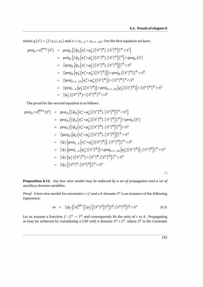
A.3. Proofs of chapter 8
where g(x t
)= ⟨f (xN ) , xK
⟩and e = [x1...k = xk+1...2k ]. For the first equation we have,
projK ◦πΦΨ?c
(S t ) = projK
(Vϕg
(π?e ◦ϕ+
g
(VS tWΦ
),VS tWΦ
)WΨ∩S t
)= projK
(Vϕg
(π?e ◦ϕ+
g
(VS tWΦ
),VS tWΦ
)WΨ
)∩projK
(S t )
= VprojK
(ϕg
(π?e ◦ϕ+
g
(VS tWΦ
),VS tWΦ
))WΨ∩Sk
= VprojK
(ϕ−
g
(π?e ◦ϕ+
g
(VS tWΦ
)))∩projK
(VS tWΦ
)WΨ∩Sk
= Vprojk+1...2k
(π?e ◦ϕ+
g
(VS tWΦ
))∩VSkWΦWΨ∩Sk
= Vproj1...k
(ϕ+
g
(VS tWΦ
))∩projk+1...2k
(ϕ+
g
(VS tWΦ
))∩VSkWΦWΨ∩Sk
= Vϕ+f
(VSnWΦ
)∩VSkWΦWΨ∩Sk
The proof for the second equation is as follows.
projN ◦πΦΨ?c
(S t ) = projN
(Vϕg
(π?e ◦ϕ+
g
(VS tWΦ
),VS tWΦ
)WΨ∩S t
)= projN
(Vϕg
(π?e ◦ϕ+
g
(VS tWΦ
),VS tWΦ
)WΨ
)∩projN
(S t )
= projN
(Vϕg
(π?e ◦ϕ+
g
(VS tWΦ
),VS tWΦ
)WΨ
)∩Sn
= VprojN
(ϕg
(π?e ◦ϕ+
g
(VS tWΦ
),VS tWΦ
))WΨ∩Sn
= Vϕ f
(proj1...k
(π?e ◦ϕ+
g
(VS tWΦ
)),VSnWΦ
)WΨ∩Sn
= Vϕ f
(proj1...k
(ϕ+
g
(VS tWΦ
))∩projk+1...2k
(ϕ+
g
(VS tWΦ
)),VSnWΦ
)WΨ∩Sn
= Vϕ f
(ϕ+
f
(VS tWΦ
)∩VSkWΦ,VSnWΦ)WΨ∩Sn
= Vϕ f
(VSkWΦ,VSnWΦ
)WΨ∩Sn
Proposition 8.12. Any box view model may be enforced by a set of propagators and a set ofauxiliary domain variables.
Proof. A box view model for constraint c ◦ f and a δ-domain Sn is an instance of the followingexpression:
m = Vϕ f
(Vπββ?c
(Vϕ+
f
(VSnWβ
)Wβ
)Wβ,VSnWβ
)Wβ∩Sn (A.3)
Let us assume a function f : Zn → Zk and consequently fix the arity of c to k. Propagatingm may be achieved by considering a CSP with a domain Sn × Sk , where Sk is the Cartesian
193

Appendix A. Proofs
product of the domains of k new domain variables. The auxiliary variable’s domain must besufficiently large, specifically such that Vϕ+
f
(VSnWβ
)Wβ ⊆ Sk , and consequently
Vϕ+f
(VSnWβ
)Wβ = Vϕ+
f
(VSnWβ
)∩VSkWβWβ∩Sk
Then, using the above lemma one may rewrite equation A.3 using propagators πββ?c , and πββ?dwhere d = [
f (x1...n) = xn+1...n+k].
194

Appendix B.
Tables
B.1. Tables of chapter 4
benchmark #wsum #distinct #element #cumulative benchmark #wsum #distinct #element #cumulative
quasigroup3-7.xml 14 49 bibd-31-31-6-6-1_glb.xml 527quasigroup4-7.xml 14 49 bibd-25-30-6-5-1_glb.xml 355quasigroup6-7.xml 14 97 bibd-7-210-60-2-10_glb.xml 238quasigroup7-7.xml 14 97 bibd-14-26-13-7-6_glb.xml 131squares-10-10.xml 45 2 bibd-19-57-9-3-1_glb.xml 247squares-11-11.xml 55 2 bibd-15-35-7-3-1_glb.xml 155
squares-9-9.xml 36 2 bibd-8-56-21-3-6_glb.xml 92bibd-6-60-30-3-12_glb.xml 81 patat-02-comp-17.xml 300bibd-6-50-25-3-10_glb.xml 71 patat-08-comp-10.xml 904bibd-7-42-18-3-6_glb.xml 70 patat-08-comp-15.xml 486bibd-7-49-21-3-7_glb.xml 77 patat-08-comp-8.xml 490bibd-8-42-21-4-9_glb.xml 78 latinSquare-dg-6_all.xml 24bibd-8-28-14-4-6_glb.xml 64 queens2.xml 3
bibd-8-56-28-4-12_glb.xml 92 cabinet-5561.xml 7 98bibd-9-48-16-3-4_glb.xml 93 cabinet-5562.xml 7 98
rcpsp20-06.xml 3 cabinet-5563.xml 7 98rcpsp20-10.xml 3 cabinet-5564.xml 7 98rcpsp20-18.xml 3 cabinet-5565.xml 7 98rcpsp20-19.xml 3 cabinet-5566.xml 7 98
bibd-11-55-15-3-3_glb.xml 121 cabinet-5567.xml 7 98bibd-10-60-18-3-4_glb.xml 115 cabinet-5568.xml 7 98bibd-13-78-18-3-3_glb.xml 169 cabinet-5569.xml 7 98bibd-12-44-11-3-2_glb.xml 122 cabinet-5570.xml 7 98bibd-13-52-12-3-2_glb.xml 143 cabinet-5571.xml 7 98
magicSquare-8_glb.xml 18 1 cabinet-5572.xml 7 98magicSquare-7_glb.xml 16 1 cabinet-5573.xml 7 98magicSquare-9_glb.xml 20 1 cabinet-5574.xml 7 98magicSquare-6_glb.xml 14 1 cabinet-5575.xml 7 98
bibd-13-26-8-4-2_glb.xml 117 cabinet-5576.xml 7 98bibd-11-22-10-5-4_glb.xml 88 cabinet-5577.xml 7 98bibd-12-22-11-6-5_glb.xml 100 cabinet-5578.xml 7 98bibd-16-24-9-6-3_glb.xml 160 cabinet-5579.xml 7 98bibd-19-19-9-9-4_glb.xml 209 cabinet-5580.xml 7 98bibd-21-21-5-5-1_glb.xml 252 costasArray-13.xml 11
bibd-15-70-14-3-2_glb.xml 190 costasArray-14.xml 12bibd-16-80-15-3-2_glb.xml 216 costasArray-15.xml 13
Table B.1.: Number of global constraints of each kind present in each benchmark
195

Appendix B. Tables
algorithm propagator-centered event-centeredevent policy cost FIFO cost FIFOfilter policy cost FIFO cost FIFO cost FIFO cost FIFO
quasigroup3-7.xml 30.55 43.83 31.34 47.02 472.59 455.16 2322.28 2275.57quasigroup4-7.xml 28.63 41.91 30.18 45.69 470.21 469.29 2194.11 2217.49quasigroup6-7.xml 1.11 1.54 1.15 1.67 28.67 29.07 100.09 101.77quasigroup7-7.xml 8.66 12.09 8.96 13.16 202.88 209.24 737.07 756.63squares-10-10.xml 14.47 47.3 14.24 47.39 114.34 128.24 114.51 126.78squares-11-11.xml 0.63 0.8 0.61 0.79 1.68 1.91 1.68 1.91
squares-9-9.xml 0.99 0.98 0.98 0.97 1.94 2.2 1.96 2.17bibd-6-60-30-3-12_glb.xml 1.86 1.77 1.84 1.75 46.32 47.27 44.44 47.04bibd-6-50-25-3-10_glb.xml 0.41 0.41 0.41 0.4 9.34 9.55 9.36 9.63bibd-7-42-18-3-6_glb.xml 3.47 3.34 3.45 3.28 47.65 46.4 48.11 47.53bibd-7-49-21-3-7_glb.xml 25.13 25.2 24.93 24.95 516.81 549.29 509.87 547.62bibd-8-42-21-4-9_glb.xml 0.52 0.51 0.52 0.5 9.02 8.72 8.91 8.77bibd-8-28-14-4-6_glb.xml 0.4 0.38 0.4 0.37 4.65 4.63 4.62 4.61
bibd-8-56-28-4-12_glb.xml 0.5 0.48 0.5 0.48 12.73 13.08 12.8 13.19bibd-9-48-16-3-4_glb.xml 19.18 18.06 19.3 17.88 361.73 367.75 361.59 365.39
rcpsp20-06.xml 21.1 42.08 21.05 41.98 86.18 101.04 85.44 102.69rcpsp20-10.xml 1.13 1.95 1.13 1.95 4.29 4.96 4.28 4.91rcpsp20-18.xml 30.51 58.9 30.55 58.78 124.26 146.21 124.29 145.59rcpsp20-19.xml 0.78 1.42 0.79 1.41 3.71 4.15 3.65 4.11
bibd-11-55-15-3-3_glb.xml 0.28 0.28 0.28 0.28 8.26 8.27 8.17 8.26bibd-10-60-18-3-4_glb.xml 0.67 0.65 0.68 0.66 17.99 18.37 18.02 18.36bibd-13-78-18-3-3_glb.xml 0.92 0.88 0.92 0.9 38.17 38.5 38.38 39.05bibd-12-44-11-3-2_glb.xml 0.51 0.48 0.52 0.48 10.34 10.7 10.32 10.68bibd-13-52-12-3-2_glb.xml 0.16 0.16 0.16 0.16 4.65 4.78 4.64 4.78
magicSquare-8_glb.xml 1.63 2.38 1.58 2.52 2.35 2.81 3.2 3.17magicSquare-7_glb.xml 43.86 62.9 43.86 65.6 81.41 81.94 94.94 94.98magicSquare-9_glb.xml 11.63 18.08 11.42 19 22.46 22.07 25.89 25.72magicSquare-6_glb.xml 1.08 1.53 1.08 1.61 1.92 1.92 2.29 2.29
bibd-13-26-8-4-2_glb.xml 0.16 0.16 0.16 0.15 1.83 1.87 1.83 1.44bibd-11-22-10-5-4_glb.xml 2.52 2.39 2.51 2.36 22.18 22.63 22.03 22.34bibd-12-22-11-6-5_glb.xml 0.32 0.3 0.32 0.29 2.95 2.94 2.96 2.92bibd-16-24-9-6-3_glb.xml 0.73 0.68 0.72 0.69 6.93 7.07 6.93 6.92bibd-19-19-9-9-4_glb.xml 0.46 0.39 0.46 0.39 3.42 3.32 3.4 3.3bibd-21-21-5-5-1_glb.xml 0.04 0.05 0.04 0.05 0.35 0.3 0.39 0.37
bibd-15-70-14-3-2_glb.xml 3.3 3.23 3.39 3.26 103.82 105.89 103.85 105.9bibd-16-80-15-3-2_glb.xml 0.93 0.93 0.93 0.93 40.1 40.4 39.62 40.62
Table B.2.: Propagation time (seconds) for solving each benchmark using each model (table1/2)
196

B.1. Tables of chapter 4
algorithm propagator-centered event-centeredevent policy cost FIFO cost FIFOfilter policy cost FIFO cost FIFO cost FIFO cost FIFO
bibd-31-31-6-6-1_glb.xml 0.14 0.15 0.14 0.14 1.8 1.79 1.81 1.8bibd-25-30-6-5-1_glb.xml 0.41 0.41 0.41 0.41 5.47 5.36 5.46 5.37
bibd-7-210-60-2-10_glb.xml 0.19 0.19 0.19 0.2 32.43 31.28 32.47 32.35bibd-14-26-13-7-6_glb.xml 43.05 40.24 42.14 40.25 443.59 446.59 444.1 449.1bibd-19-57-9-3-1_glb.xml 0.24 0.25 0.23 0.25 7.3 7.59 7.32 7.5bibd-15-35-7-3-1_glb.xml 0.07 0.07 0.07 0.08 1.22 1.25 1.23 1.24bibd-8-56-21-3-6_glb.xml 8.98 8.1 9.05 8.09 184.62 185.28 186.44 185.6
patat-02-comp-17.xml 3.17 3.52 3.21 3.72 4.25 4.45 7.77 7.55patat-08-comp-10.xml 1.98 2.12 1.91 2.22 2.52 2.52 4.97 4.92patat-08-comp-15.xml 19.62 26.43 19.38 26.01 23.87 23.11 49.99 49.24patat-08-comp-8.xml 0.91 1.02 0.9 1.04 1.23 1.23 1.96 1.94
latinSquare-dg-6_all.xml 0.96 1.1 0.96 1.13 1.11 1.09 1.8 1.79queens2.xml 1.6 3.99 1.61 4.41 2.41 2.37 4.72 4.6
cabinet-5561.xml 14.7 15.76 14.37 15.45 55.69 53.59 69.2 67.25cabinet-5562.xml 14.68 15.64 14.43 15.46 55.7 53.78 68.63 68.43cabinet-5563.xml 14.55 15.81 14.42 15.49 55.94 53.97 68.99 66.92cabinet-5564.xml 14.56 15.77 14.47 15.45 54.58 53.12 69.17 67.82cabinet-5565.xml 14.6 15.73 14.49 15.45 55.79 53.84 69.55 67.29cabinet-5566.xml 14.6 15.72 14.47 15.52 55.1 53.89 69.15 66.96cabinet-5567.xml 14.61 15.76 14.49 15.42 55.27 53 69.03 67.11cabinet-5568.xml 14.59 15.72 14.43 15.35 55.3 53.45 69.38 67.21cabinet-5569.xml 14.62 15.7 14.46 15.46 55.64 53.54 69.56 67.22cabinet-5570.xml 14.61 15.68 14.44 15.43 55.25 53.42 69.21 68.16cabinet-5571.xml 14.62 15.85 14.47 15.68 55.44 53.5 69.53 67.3cabinet-5572.xml 14.67 15.78 14.53 15.47 55.57 53.58 69.17 67.19cabinet-5573.xml 14.75 15.84 14.54 15.5 55.13 53.68 69.23 67.16cabinet-5574.xml 14.68 15.9 14.58 15.56 55.14 53.13 69.73 67.5cabinet-5575.xml 14.72 15.97 14.54 15.52 56.18 53.63 69.24 67.08cabinet-5576.xml 14.98 16.11 14.76 15.78 56.67 54.6 71.3 68.46cabinet-5577.xml 14.98 16.11 14.73 15.78 56.95 54.67 70.51 68.41cabinet-5578.xml 15.06 16.1 14.71 15.75 56.93 54.73 70.46 68.68cabinet-5579.xml 14.91 16.14 14.79 15.91 57.01 54.16 70.42 68.64cabinet-5580.xml 14.94 16.21 14.71 15.76 57.03 54.59 71.06 68.4
costasArray-13.xml 1.96 2.91 1.95 3 2.53 2.51 3.61 3.59costasArray-14.xml 1.86 2.88 1.86 2.99 2.37 2.35 3.49 3.44costasArray-15.xml 10.28 16.52 10.14 17.15 13.25 13.18 20.09 19.75
Table B.3.: Propagation time (seconds) for solving each benchmark using each model (table2/2)
197

Appendix B. Tables
B.2. Tables of chapter 5
B.2.1. Social golfers
#updates avg-update time #props
NON-INCREMENTAL 8.65E+6 6.37E-1 2.72 8,970,454INCREMENTAL-PROPAGATOR 6.01E+6 6.06E-1 2.64 8,970,454
INCREMENTAL-VARIABLE 6.01E+6 6.07E-1 2.44 8,970,454INCREMENTAL-HYBRID 5.42E+6 6.05E-1 2.94 8,970,454
GECODE N/A N/A 2.92 3,734,251
Table B.4.: Social golfers: 5w-5g-4s (v=25,c/v=11.2,f=25421)
#updates avg-update time #props
NON-INCREMENTAL 6.85E+8 5.64E-1 307 740,977,445INCREMENTAL-PROPAGATOR 4.70E+8 6.49E-1 298 740,977,445
INCREMENTAL-VARIABLE 4.70E+8 6.49E-1 282.65 740,977,445INCREMENTAL-HYBRID 4.24E+8 6.42E-1 303.62 740,977,445
GECODE N/A N/A 304 319,631,533
Table B.5.: Social golfers: 6w-5g-3s (v=30,c/v=13.6,f=1582670)
#updates avg-update time #props
NON-INCREMENTAL 1.25E+7 5.36E-1 5.36 13,597,902INCREMENTAL-PROPAGATOR 8.17E+6 5.64E-1 5.75 13,597,902
INCREMENTAL-VARIABLE 8.17E+6 5.64E-1 5.13 13,597,902INCREMENTAL-HYBRID 8.00E+6 5.61E-1 6.14 13,597,902
GECODE N/A N/A 6.65 6,265,389
Table B.6.: Social golfers: 11w-11g-2s (v=121,c/v=55.4,f=10803)
198

B.2. Tables of chapter 5
B.2.2. Hamming codes
#updates avg-update time #props
NON-INCREMENTAL 2.14E+6 1.48E+0 1.04 4,130,735INCREMENTAL-PROPAGATOR 1.52E+6 6.20E-1 0.88 4,138,480
INCREMENTAL-VARIABLE 1.52E+6 6.20E-1 0.83 4,138,480INCREMENTAL-HYBRID 1.37E+6 8.93E-1 0.9 4,138,480
GECODE N/A N/A 1.38 1,918,498
Table B.7.: Hamming codes: 20s-15l-8d (v=42,c/v=10,f=7774)
#updates avg-update time #props
NON-INCREMENTAL 8.34E+6 3.19E+0 5.66 16,769,450INCREMENTAL-PROPAGATOR 5.61E+6 7.33E-1 3.78 16,775,413
INCREMENTAL-VARIABLE 5.61E+6 7.33E-1 3.73 16,775,413INCREMENTAL-HYBRID 5.37E+6 1.11E+0 4.12 16,775,413
GECODE N/A N/A 5.16 6,420,351
Table B.8.: Hamming codes: 10s-20l-9d (v=22,c/v=5,f=59137)
#updates avg-update time #props
NON-INCREMENTAL 1.81E+7 1.88E+0 12.39 37,788,547INCREMENTAL-PROPAGATOR 1.40E+7 5.84E-1 10.12 37,857,135
INCREMENTAL-VARIABLE 1.40E+7 5.84E-1 9.46 37,857,135INCREMENTAL-HYBRID 1.23E+7 1.08E+0 10.97 37,857,135
GECODE N/A N/A 15.02 14,005,989
Table B.9.: Hamming codes: 40s-15l-6d (v=82,c/v=15.1,f=27002)
199

Appendix B. Tables
B.2.3. Balanced partition
#updates avg-update time #props
NON-INCREMENTAL 1.74E+6 5.34E+0 3.06 11,810,152INCREMENTAL-PROPAGATOR 2.06E+6 5.28E-1 2.77 11,810,152
INCREMENTAL-VARIABLE 2.06E+6 5.27E-1 2.68 11,810,192INCREMENTAL-HYBRID 1.02E+6 1.61E+0 2.86 11,810,152
GECODE N/A N/A 3.57 5,361,471
Table B.10.: Balanced partition: 150v-70s-162m (v=212,c/v=11.7,f=48525)
#updates avg-update time #props
NON-INCREMENTAL 2.01E+6 6.06E+0 3.86 14,504,618INCREMENTAL-PROPAGATOR 2.50E+6 5.41E-1 3.41 14,504,618
INCREMENTAL-VARIABLE 2.50E+6 5.40E-1 3.29 14,504,658INCREMENTAL-HYBRID 1.17E+6 1.75E+0 3.29 14,504,618
GECODE N/A N/A 4.64 6,598,932
Table B.11.: Balanced partition: 170v-80s-182m (v=242,c/v=13.4,f=54573)
#updates avg-update time #props
NON-INCREMENTAL 2.17E+6 6.77E+0 4.66 16,572,703INCREMENTAL-PROPAGATOR 2.82E+6 5.52E-1 3.94 16,572,703
INCREMENTAL-VARIABLE 2.82E+6 5.51E-1 3.81 16,572,743INCREMENTAL-HYBRID 1.26E+6 1.88E+0 4.4 16,572,703
GECODE N/A N/A 5.6 7,481,239
Table B.12.: Balanced partition: 190v-90s-202m (v=272,c/v=15,f=57424)
B.2.4. Metabolic pathways
time #props
INCREMENTAL-PROPAGATOR 0.9 1,030,438INCREMENTAL-VARIABLE 0.74 1,268,920
Table B.13.: Metabolic pathways: g250_croes_ecoli_glyco (f=916)
200

B.2. Tables of chapter 5
time #props
INCREMENTAL-PROPAGATOR 10.3 7,163,926INCREMENTAL-VARIABLE 9.38 20,681,066
Table B.14.: Metabolic pathways: g500_croes_ecoli_glyco (f=2865)
time #props
INCREMENTAL-PROPAGATOR 52.6 4,517,381INCREMENTAL-VARIABLE 24.1 4,584,786
Table B.15.: Metabolic pathways: g1000_croes_scerev_heme (f=2466)
time #props
INCREMENTAL-PROPAGATOR 171 15,657,341INCREMENTAL-VARIABLE 88.1 60,006,142
Table B.16.: Metabolic pathways: g1500_croes_ecoli_glyco (f=4056)
B.2.5. Winner determination problem
time #props
INCREMENTAL-PROPAGATOR 2.82 37,014INCREMENTAL-VARIABLE 2.17 35,693
Table B.17.: Winner determination problem: 200 (f=1550)
time #props
INCREMENTAL-PROPAGATOR 13.4 69,030INCREMENTAL-VARIABLE 9.92 66,536
Table B.18.: Winner determination problem: 300 (f=2924)
201

Appendix B. Tables
time #props
INCREMENTAL-PROPAGATOR 39 160,878INCREMENTAL-VARIABLE 29.5 155,775
Table B.19.: Winner determination problem: 400 (f=6693)
time #props
INCREMENTAL-PROPAGATOR 80.4 393,580INCREMENTAL-VARIABLE 61.7 381,869
Table B.20.: Winner determination problem: 500 (f=16213)
B.3. Tables of chapter 9
B.3.1. Systems of linear equations
#vars #vars/const time #fails #props
VARS 41 7 19.3 11,983,390 1.14E+7VARS+GLOBAL 20 4 18.2 11,983,390 5.72E+6
PVIEWS 20 4 18.1 11,983,390 5.72E+6SVIEWS 20 4 18.9 11,983,390 5.72E+6
GECODE-VARS 41 7 19.9 11,983,390 8.75E+6GECODE-VARS+GLOBAL 20 4 18.4 11,983,390 2.90E+6
Table B.21.: Linear 20var-7vals-7cons-4arity-6s (SAT) (S=56.15)
#vars #vars/const time #fails #props
VARS 62 15 142 6,444,629 5.97E+8VARS+GLOBAL 20 8 46.7 6,444,629 7.01E+7
PVIEWS 20 8 42.3 6,444,629 7.41E+7SVIEWS 20 8 57 6,444,629 7.41E+7
GECODE-VARS 62 15 155 6,444,629 9.56E+8GECODE-VARS+GLOBAL 20 8 30.36 6,444,629 6.62E+7
Table B.22.: Linear 20var-30val-6cons-8arity-2s (UNSAT) (S=98.14)
202

B.3. Tables of chapter 9
#vars #vars/const time #fails #props
VARS 508 39 134 1,515,353 5.25E+8VARS+GLOBAL 40 20 21.4 1,515,353 1.81E+7
PVIEWS 40 20 25.8 1,515,353 1.81E+7SVIEWS 40 20 58.4 1,515,353 1.81E+7
GECODE-VARS 508 39 163 1,515,353 9.21E+8GECODE-VARS+GLOBAL 40 20 15.6 1,515,353 2.07E+7
Table B.23.: Linear 40var-7val-12cons-20arity-3s (UNSAT) (S=112.29)
#vars #vars/const time #fails #props
VARS 988 79 144 700,752 6.17E+8VARS+GLOBAL 40 40 16.8 700,752 1.00E+7
PVIEWS 40 40 20.3 700,752 1.00E+7SVIEWS 40 40 62 700,752 1.00E+7
GECODE-VARS 988 79 168 700,752 1.07E+9GECODE-VARS+GLOBAL 40 40 11.4 700,752 1.54E+7
Table B.24.: Linear 40var-7val-10cons-40arity-3s (UNSAT) (S=112.29)
B.3.2. Systems of nonlinear equations
#vars #vars/const time #fails #props
VARS 90 15 53.1 651,189 1.89E+8VARS+GLOBAL 60 12 46.9 651,189 1.24E+8
PVIEWS 20 8 19.6 651,189 2.40E+7SVIEWS 20 8 21 651,189 2.40E+7
CPVIEWS 20 8 31.5 651,189 6.79E+7PVIEWS+GLOBAL 20 8 25 651,189 2.40E+7
GECODE-VARS 90 15 40.3 651,189 2.67E+8GECODE-VARS+GLOBAL 60 12 28.7 651,189 1.72E+8
Table B.25.: NonLinear 20var-20val-10cons-4term-2fact-2s (SAT) (S=86.44)
203

Appendix B. Tables
#vars #vars/const time #fails #props
VARS 183 15 136 1,451,881 4.79E+8VARS+GLOBAL 126 12 119 1,451,881 3.10E+8
PVIEWS 50 8 48 1,451,881 5.70E+7SVIEWS 50 8 56.4 1,451,881 5.70E+7
CPVIEWS 50 8 73.7 1,451,881 1.58E+8PVIEWS+GLOBAL 50 8 60.5 1,451,881 5.70E+7
GECODE-VARS 183 15 105.8 1,451,881 6.34E+8GECODE-VARS+GLOBAL 126 12 74.15 1,451,881 4.10E+8
Table B.26.: NonLinear 50var-10val-19cons-4term-2fact-1s (SAT) (S=166.1)
#vars #vars/const time #fails #props
VARS 358 23 93 514,680 2.90E+8VARS+GLOBAL 134 15 86.7 514,680 2.23E+8
PVIEWS 50 12 38 596,669 2.79E+7SVIEWS 50 12 47.4 596,669 2.79E+7
CPVIEWS 50 12 63.4 514,680 1.18E+8PVIEWS+GLOBAL 50 12 43.9 596,669 2.79E+7
GECODE-VARS 358 23 71.3 514,680 3.95E+8GECODE-VARS+GLOBAL 134 15 64.4 514,680 3.67E+8
Table B.27.: NonLinear 50var-10val-28cons-4term-3fact-1s (UNSAT) (S=166.1)
#vars #vars/const time #fails #props
VARS 270 23 51.2 342,311 1.60E+8VARS+GLOBAL 110 15 46.8 342,311 1.20E+8
PVIEWS 50 12 16.9 346,762 1.18E+7SVIEWS 50 12 20.4 346,762 1.18E+7
CPVIEWS 50 12 29.4 342,311 5.37E+7PVIEWS+GLOBAL 50 12 19 346,762 1.18E+7
GECODE-VARS 270 23 39.1 342,311 2.20E+8GECODE-VARS+GLOBAL 110 15 33.5 342,311 1.88E+8
Table B.28.: NonLinear 50var-5val-20cons-4term-3fact-1s (UNSAT) (S=116.1)
204

B.3. Tables of chapter 9
#vars #vars/const time #fails #props
VARS 440 31 68.6 282,476 2.12E+8VARS+GLOBAL 362 28 65.3 282,476 1.75E+8
PVIEWS 50 16 27.6 287,138 1.30E+7SVIEWS 50 16 35.8 287,138 1.30E+7
CPVIEWS 50 16 59.9 282,476 8.67E+7PVIEWS+GLOBAL 50 16 28 287,138 1.30E+7
GECODE-VARS 440 31 51.7 282,476 2.92E+8GECODE-VARS+GLOBAL 362 28 47.3 282,476 2.72E+8
Table B.29.: NonLinear 50var-6val-26cons-4term-4fact-1s (UNSAT) (S=129.25)
#vars #vars/const time #fails #props
VARS 420 31 1.34 7,742 4.18E+6VARS+GLOBAL 348 28 1.27 7,742 3.39E+6
PVIEWS 60 16 0.58 7,742 2.68E+5SVIEWS 60 16 0.75 7,742 2.68E+5
CPVIEWS 60 16 1.1 7,742 1.59E+6PVIEWS+GLOBAL 60 16 0.59 7,742 2.68E+5
GECODE-VARS 420 31 1.13 7,743 5.68E+6GECODE-VARS+GLOBAL 348 28 1.06 7,742 5.47E+6
Table B.30.: NonLinear 60var-4val-24cons-4term-4fact-5s (UNSAT) (S=120)
B.3.3. Social golfers
#vars #vars/const time #fails #props
VARS+GLOBAL 4100 48 0.89 5,035 3.47E+6
PVIEWS+GLOBAL 100 32 0.6 5,035 5.06E+5SVIEWS+GLOBAL 100 32 0.82 5,035 5.06E+5
CPVIEWS+GLOBAL 100 32 1.07 5,035 4.23E+6
GECODE-VARS+GLOBAL 4100 48 0.89 5,035 3.47E+6
Table B.31.: Social golfers: 5week-5group-4size (S=432.19)
205

Appendix B. Tables
#vars #vars/const time #fails #props
VARS+GLOBAL 3465 27 9.88 33,969 4.25E+7
PVIEWS+GLOBAL 90 18 5.84 33,969 6.24E+6SVIEWS+GLOBAL 90 18 7.66 33,969 6.24E+6
CPVIEWS+GLOBAL 90 18 9.74 33,969 3.72E+7
GECODE-VARS+GLOBAL 3465 27 5.31 33,969 2.81E+7
Table B.32.: Social golfers: 6week,5group,3size (S=351.62)
#vars #vars/const time #fails #props
VARS+GLOBAL 14602 147 38.2 120,110 1.50E+8
PVIEWS+GLOBAL 196 98 26.2 120,110 1.74E+7SVIEWS+GLOBAL 196 98 32.4 120,110 1.74E+7
CPVIEWS+GLOBAL 196 147 41.4 120,110 1.40E+8
GECODE-VARS+GLOBAL 14602 147 27.9 120,110 7.05E+7
Table B.33.: Social golfers: 4week,7group,7size (S=1100.48)
B.3.4. Golomb ruler
#vars #vars/const time #fails #props
VARS+GLOBAL 55 55 0.11 1,703 3.77E+5
PVIEWS+GLOBAL 10 10 0.08 1,707 5.07E+4SVIEWS+GLOBAL 10 10 0.09 1,707 5.07E+4
CPVIEWS+GLOBAL 10 10 0.1 1,703 2.24E+5
GECODE-VARS+GLOBAL 55 55 0.08 1,707 3.36E+5
Table B.34.: Golomb ruler: 10 (S=58.07)
206

B.3. Tables of chapter 9
#vars #vars/const time #fails #props
VARS+GLOBAL 66 66 0.63 7,007 2.12E+6
PVIEWS+GLOBAL 11 11 0.47 7,063 2.41E+5SVIEWS+GLOBAL 11 11 0.52 7,063 2.41E+5
CPVIEWS+GLOBAL 11 11 0.56 7,007 1.23E+6
GECODE-VARS+GLOBAL 66 66 0.37 7,012 1.59E+6
Table B.35.: Golomb ruler: 11 (S=68.09)
#vars #vars/const time #fails #props
VARS+GLOBAL 78 78 36.58 283,156 1.16E+8
PVIEWS+GLOBAL 12 12 27.6 284,301 1.19E+7SVIEWS+GLOBAL 12 12 30.7 284,301 1.19E+7
CPVIEWS+GLOBAL 12 12 32.4 283,156 6.73E+7
GECODE-VARS+GLOBAL 78 78 21.4 283,162 1.00E+8
Table B.36.: Golomb ruler: 12 (S=76.91)
B.3.5. Low autocorrelation binary sequences
#vars #vars/const time #fails #props
VARS+GLOBAL 296 296 17.6 214,151 5.15E+7
PVIEWS-PARTIAL-1 65 65 13.8 214,151 2.61E+7PVIEWS-PARTIAL-2 44 44 10.6 214,151 1.34E+7
PVIEWS+GLOBAL 23 23 6.13 214,151 2.18E+6SVIEWS+GLOBAL 23 23 14.6 214,151 2.18E+6
CPVIEWS+GLOBAL 23 23 7.51 214,151 8.97E+6
GECODE-VARS+GLOBAL 296 296 12.22 214,151 6.63E+7
Table B.37.: Low autocorrelation binary sequences: 22 (S=22)
207

Appendix B. Tables
#vars #vars/const time #fails #props
VARS+GLOBAL 347 347 65.5 724,517 1.88E+8
PVIEWS-PARTIAL-1 71 71 49.9 724,517 9.11E+7PVIEWS-PARTIAL-1 48 48 39.1 724,517 4.83E+7
PVIEWS+GLOBAL 25 25 23.4 724,517 7.38E+6SVIEWS+GLOBAL 25 25 57.2 724,517 7.38E+6
CPVIEWS+GLOBAL 25 25 28.5 724,517 3.24E+7
GECODE-VARS+GLOBAL 347 347 44.73 724,517 2.46E+8
Table B.38.: Low autocorrelation binary sequences: 24 (S=25)
B.3.6. Fixed-length error correcting codes
#vars #vars/const time #fails #props
VARS+GLOBAL 6721 52 17.8 240,475 4.93E+7
PVIEWS+GLOBAL 641 20 9.25 240,475 1.25E+7SVIEWS+GLOBAL 641 20 12.7 240,475 1.25E+7
CPVIEWS+GLOBAL 641 20 12.9 240,475 4.10E+7
GECODE-VARS+GLOBAL 6721 52 53.5 240,475 2.41E+7
Table B.39.: Fixed-length error correcting codes: 2-20-32-10-hamming (S=640)
#vars #vars/const time #fails #props
VARS+GLOBAL 4201 50 7.96 153,207 2.46E+7
PVIEWS+GLOBAL 526 15 4.56 153,207 7.24E+6SVIEWS+GLOBAL 526 15 5.89 153,207 7.24E+6
CPVIEWS+GLOBAL 526 15 6.51 153,207 2.09E+7
GECODE-VARS+GLOBAL 4201 50 24.57 153,207 1.84E+7
Table B.40.: Fixed-length error correcting codes: 3-15-35-11-hamming (S=525)
208

B.3. Tables of chapter 9
#vars #vars/const time #fails #props
VARS+GLOBAL 24961 148 35.1 240,475 1.71E+8
PVIEWS+GLOBAL 641 20 9.74 240,475 6.46E+6SVIEWS+GLOBAL 641 20 23.8 240,475 6.46E+6
CPVIEWS+GLOBAL 641 20 29.4 240,475 2.09E+8
GECODE-VARS+GLOBAL 24961 148 292 240,475 1.48E+8
Table B.41.: Fixed-length error correcting codes: 2-20-32-10-lee (S=640)
#vars #vars/const time #fails #props
VARS+GLOBAL 15226 155 76.6 1,066,081 3.82E+8
PVIEWS+GLOBAL 526 15 34.5 1,283,612 2.86E+7SVIEWS+GLOBAL 526 15 86.5 1,283,612 2.86E+7
CPVIEWS+GLOBAL 526 15 55.7 1,066,081 3.65E+8
GECODE-VARS+GLOBAL 15226 155 807 1,066,081 3.29E+8
Table B.42.: Fixed-length error correcting codes: 3-15-35-10-lee (S=525)
209

Appendix B. Tables
B.4. Tables of chapter 11
Rank Solver Version Number ofsolved
instances
% of VBS CumulatedCPU timeon solvedinstances
AverageCPU timeper solvedinstance
Virtual Best Solver (VBS) 660 100% 20689.09 31.351 cpHydra k_10 569 86% 31124.32 54.702 cpHydra k_40 569 86% 49899.25 87.703 casper zao 562 85% 31205.61 55.534 Mistral-prime 1.313 560 85% 17929.82 32.025 MDG-probe 2008-06-27 560 85% 20146.70 35.986 casper zito 555 84% 31629.81 56.997 Mistral-option 1.314 554 84% 43364.56 78.288 MDG-noprobe 2008-06-27 530 80% 18115.71 34.189 choco2_impwdeg 2008-06-26 518 78% 25745.10 49.70
10 Abscon 112v4 ESAC 488 74% 36101.57 73.9811 Abscon 112v4 AC 486 74% 25860.43 53.2112 Sugar v1.13+minisat 486 74% 29306.62 60.3013 Sugar v1.13+picosat 481 73% 26580.81 55.2614 bpsolver 2008-06-27 459 70% 77397.38 168.6215 Concrete + CPS4J 2008-05-30 456 69% 91862.96 201.4516 Concrete + CSP4J - Tabu Engine 2008-05-30 199 30% 36056.08 181.1917 SAT4J CSP 2008-06-13 174 26% 19628.31 112.8118 Concrete + CSP4J - WMC Engine 2008-05-30 174 26% 23628.78 135.80
Table B.43.: CPAI’08 competition results (n-ary intension constraints category)
210

B.4. Tables of chapter 11
Rank Solver Version Number ofsolved
instances
% of VBS CumulatedCPU timeon solvedinstances
AverageCPU timeper solvedinstance
Virtual Best Solver (VBS) 501 100% 12233.86 24.421 Sugar v1.13+picosat 424 85% 23575.77 55.602 cpHydra k_40 420 84% 80832.22 192.463 cpHydra k_10 419 84% 33879.89 80.864 Sugar v1.13+minisat 405 81% 30617.59 75.605 Mistral-prime 1.313 403 80% 22849.50 56.706 casper zito 397 79% 32937.25 82.977 casper zao 390 78% 24804.15 63.608 Mistral-option 1.314 383 76% 37615.36 98.219 choco2_dwdeg 2008-06-26 358 71% 26103.18 72.91
10 MDG-noprobe 2008-06-27 353 70% 16548.16 46.8811 choco2_impwdeg 2008-06-26 347 69% 28393.77 81.8312 bpsolver 2008-06-27 347 69% 48728.37 140.4313 MDG-probe 2008-06-27 337 67% 17668.90 52.4314 Minion/Tailor 2008-07-04 216 43% 14889.77 68.9315 Abscon 112v4 AC 184 37% 31394.49 170.6216 Abscon 112v4 ESAC 173 35% 33623.73 194.3617 SAT4J CSP 2008-06-13 63 13% 8092.34 128.45
Table B.44.: CPAI’08 competition results (global constraints category)
211