1

Centrality measures for graphons: Accountingfor uncertainty in networks

Marco Avella-Medina, Francesca Parise, Michael T. Schaub, and Santiago Segarra, Member, IEEE

Abstract—As relational datasets modeled as graphs keep increasing in size and their data-acquisition is permeated by uncertainty,graph-based analysis techniques can become computationally and conceptually challenging. In particular, node centrality measures relyon the assumption that the graph is perfectly known — a premise not necessarily fulfilled for large, uncertain networks. Accordingly,centrality measures may fail to faithfully extract the importance of nodes in the presence of uncertainty. To mitigate these problems, wesuggest a statistical approach based on graphon theory: we introduce formal definitions of centrality measures for graphons and establishtheir connections to classical graph centrality measures. A key advantage of this approach is that centrality measures defined at themodeling level of graphons are inherently robust to stochastic variations of specific graph realizations. Using the theory of linear integraloperators, we define degree, eigenvector, Katz and PageRank centrality functions for graphons and establish concentration inequalitiesdemonstrating that graphon centrality functions arise naturally as limits of their counterparts defined on sequences of graphs ofincreasing size. The same concentration inequalities also provide high-probability bounds between the graphon centrality functions andthe centrality measures on any sampled graph, thereby establishing a measure of uncertainty of the measured centrality score.

Index Terms—Random graph theory, Networks, Graphons, Centrality measures, Stochastic block model

F

1 INTRODUCTION

MANY biological [1], social [2], and economic [3] systemscan be better understood when interpreted as net-

works, comprising a large number of individual componentsthat interact with each other to generate a global behavior.These networks can be aptly formalized by graphs, inwhich nodes denote individual entities, and edges representpairwise interactions between those nodes. Consequently,a surge of studies concerning the modeling, analysis, anddesign of networks have appeared in the literature, usinggraphs as modeling devices.

A fundamental task in network analysis is to identifysalient features in the underlying system, such as key nodesor agents in the network. To identify such important agents,researchers have developed centrality measures in variouscontexts [4], [5], [6], [7], [8], each of them capturing differentaspects of node importance. Prominent examples for the util-ity of centrality measures include the celebrated PageRankalgorithm [9], [10], employed in the search of relevant sites onthe web, as well as the identification of influential agents insocial networks to facilitate viral marketing campaigns [11].

A crucial assumption for the applicability of these cen-trality measures is that the observation of the underlyingnetwork is complete and noise free. However, for many sys-

Authors are ordered alphabetically. All authors contributed equally. M. Avella-Medina is with the Department of Statistics, Columbia University. F. Pariseis with the Laboratory for Information and Decision Systems, MIT. M.Schaub is with the Institute for Data, Systems, and Society, MIT andwith the Department of Engineering Science, University of Oxford, UK. S.Segarra is with the Department of Electrical and Computer Engineering,Rice University. Emails: marco.avella@columbia.edu, {parisef,mschaub}@mit.edu, segarra@rice.edu. Funding: This work wassupported by the Swiss National Science Foundation grants P2EGP1 168962,P300P1 177746 (M. Avella-Medina) and P2EZP2 168812, P300P2 177805(F. Parise); the European Union’s Horizon 2020 research and innovationprogramme under the Marie Sklodowska-Curie grant agreement No 702410(M. Schaub); the Spanish MINECO TEC2013-41604-R and the MIT IDSSSeed Fund Program (S. Segarra).

tems we might be unable to extract a complete and accurategraph-based representation, e.g., due to computational ormeasurement constraints, errors in the observed data, orbecause the network itself might be changing over time. Forsuch reasons, some recent approaches have considered theissue of robustness of centrality measures [12], [13], [14],[15] and general network features [16], as well as theircomputation in dynamic graphs [17], [18], [19]. The closestwork to ours is [20], where convergence results are derivedfor eigenvector and Katz centralities in the context of randomgraphs generated from a stochastic block model.

As the size of the analyzed systems continues to grow,traditional tools for network analysis have been pushed totheir limit. For example, systems such as the world wideweb, the brain, or social networks can consist of billions ofinterconnected agents, leading to computational challengesand the irremediable emergence of uncertainty in the obser-vations. In this context, graphons have been suggested as analternative framework to analyze large networks [21], [22].While graphons have been initially studied as limiting objectsof large graphs [23], [24], [25], they also provide a rich non-parametric modeling tool for networks of any size [26], [27],[28], [29]. In particular, graphons encapsulate a broad classof network models including the stochastic block model [30],[31], random dot-product graphs [32], the infinite relationalmodel [33], and others [34]. A testament of the practicalityof graphons is their use in applied disciplines such as signalprocessing [35], collaborative learning [36], and control [37].

In this work we aim at harnessing the additional flexibilityprovided by the graphon framework to suggest a statisticalapproach to agents’ centralities that inherently accounts fornetwork uncertainty, as detailed next.

arX

iv:1

707.

0935

0v4

[cs

.SI]

28

Nov

201

8

2

1.1 Motivation

Most existing applications of network centrality measuresfollow the paradigm in Fig. 1a: a specific graph — such as asocial network with friendship connections — is observed,and conclusions about the importance of each agent are thendrawn based on this graph, e.g., which individuals havemore friends or which have the most influential connections.Mathematically, these notions of importance are encapsulatedin a centrality measure that ranks the nodes according tothe observed network structure. For instance, the idea thatimportance derives from having the most friends is capturedby degree centrality. Since the centrality of any node iscomputed solely from the network structure [4], [5], [6],[7], [8], a crucial assumption hidden in this analysis is thatthe empirically observed network captures all the data wecare about.

However, in many instances in which centrality measuresare employed, this assumption is arguably not fulfilled:we typically do not observe the complete network at once.Further, even those parts we observe contain measurementerrors, such as false positive or false negative links, and otherforms of uncertainty. The key question is therefore how toidentify crucial nodes via network-based centrality measureswithout having access to an accurate depiction of the ‘true’latent network.

One answer to this problem is to adopt a statisticalinference-based viewpoint towards centrality measures, byassuming that the observed graph is a specific realizationof an underlying stochastic generative process; see Fig. 1b.In this work, in particular, we use graphons to model suchunderlying generative process, because they provide a richnon-parametric statistical framework. Further, it has beenrecently shown that graphons can be efficiently estimatedfrom one (or multiple) noisy graph observations [28], [38].Our main contribution is to show that, based on the inferredgraphon, one can compute a latent centrality profile of thenodes that we term graphon centrality function. This graphoncentrality may be seen as a fundamental measure of nodeimportance, irrespective of the specific realization of thegraph at hand. This leads to a robust estimate of the centralityprofiles of all nodes in the network. In fact, we providehigh-probability bounds between the distance of such latentgraphon centrality functions and the centrality profiles inany realized network, in terms of the network size.

To illustrate the dichotomy of the standard approachtowards centrality and the one outlined here, let us considerthe graphon in Fig. 1c. Graphons will be formally defined inSection 2.2, but the fundamental feature is that it defines arandom graph model from where graphs of any pre-specifiedsize can be obtained. If we generate one of these graphs with100 nodes, we can apply the procedure in Fig. 1a to obtaina centrality value for each agent, as shown in the red curvein Fig. 1c. In the standard paradigm we would then sortthe centrality values to find the most central nodes, whichin this case would correspond to the node marked as v1 inFig. 1c. On the other hand, if we have access to the generativegraphon model (or an estimate thereof), then we can computethe continuous graphon centrality function and compare thedeviations from it in the specific graph realization; see blueand red curves in Fig. 1c.

Fig. 1: Schematic — Network centrality analysis. (a) Classical centralityanalysis computes a centrality measure purely based on the observednetwork. (b) If networks are subject to uncertainty, we may adopt astatistical perspective on centrality, by positing that the observed networkis but one realization of a true, unobserved latent model. Inference ofthe model then would lead to a centrality estimate that accounts for theuncertainty in the data in a well-defined manner. (c) Illustrative example.Left: A network of 100 nodes is generated according to a graphon modelwith a well-defined increasing connectivity pattern. Right: This graphonmodel defines a latent (expected) centrality for each node (blue curve).The centralities of a single realization of the model (red curve) will ingeneral not be equivalent to the latent centrality, but deviate from it.Estimating the graphon-based centrality thus allows us to decomposethe observed centrality into an expected centrality score (blue), and afluctuation that is due to randomness.

The result is that while v1 is the most central node in thespecific graph realization (see red curve), we would expect itto be less central within the model-based framework sincethe two nodes to its right have higher latent centrality (seeblue curve). Stated differently, in this specific realization, v1

benefited from the random effects in terms of its centrality.If another random graph is drawn from the same graphonmodel, the rank of v1 might change, e.g., node v1 mightbecome less central. Based on a centrality analysis akin toFig. 1a, we would conclude that the centrality of this nodedecreased relative to other agents in the network. However,this difference is exclusively due to random variations andthus not statistically significant. The approach outlined inFig. 1b and, in particular, centrality measures defined ongraphons thus provide a statistical framework to analyzecentralities in the presence of uncertainty, shielding us frommaking the wrong conclusion about the change in centralityof node v1 if the network is subject to uncertainty.

3

A prerequisite to apply the perspective outlined aboveis to have a consistent theory of centrality measures forgraphons, with well-defined limiting behaviors and well-understood convergence rates. Such a theory is developed inthis paper, as we detail in the next section.

1.2 Contributions and article structure

Our contributions are listed below.1) We develop a theoretical framework and definitions forcentrality measures on graphons. Specifically, using theexisting spectral theory of linear integral operators, wedefine the degree, eigenvector, Katz and PageRank centralityfunctions (see Definition 3).2) We discuss and illustrate three different analytical ap-proaches to compute such centrality functions (see Section 4).3) We derive concentration inequalities showing that ournewly defined graphon centrality functions are naturallimiting objects of centrality measures for finite graphs. Theseconcentration inequalities improve the current state of theart and constitute the main technical results of this paper(see Theorems 1 and 2).4) We illustrate how such bounds can be used to quantifythe distance between the latent graphon centrality functionand the centrality measures of finite graphs sampled fromthe graphon.

The remainder of the article is structured as follows. InSection 2 we review preliminaries regarding graphs, graphcentralities, and graphons. Subsequently, in Section 3 werecall the definition of the graphon operator and use itto introduce centrality measures for graphons. Section 4discusses how centrality measures for graphons can becomputed using different strategies, and provides somedetailed numerical examples. Thereafter, in Section 5, wederive our main convergence results. Section 6 providesconcluding remarks. Appendix A contains proofs omittedin the paper. Appendix B provided in the supplementarymaterial presents some auxiliary results and discussions.

Notation: The entries of a matrix X and a (column) vectorx are denoted by Xij and xi, respectively; however, in somecases [X]ij and [x]i are used for clarity. The notation T

stands for transpose. diag(x) is a diagonal matrix whose ithdiagonal entry is xi. dxe denotes the ceiling function thatreturns the smallest integer larger than or equal to x. Sets arerepresented by calligraphic capital letters, and 1B(·) denotesthe indicator function over the set B. 0, 1, ei, and I refer tothe all-zero vector, the all-one vector, the i-th canonical basisvector, and the identity matrix, respectively. The symbols v,ϕ, and λ are reserved for eigenvectors, eigenfunctions, andeigenvalues, respectively. Additional notation is provided atthe beginning of Section 3.

2 PRELIMINARIES

In Section 2.1 we introduce basic graph-theoretic conceptsas well as the notion of node centrality measures for finitegraphs, emphasizing the four measures studied throughoutthe paper. A brief introduction to graphons and their relationto random graph models is given in Section 2.2.

2.1 Graphs and centrality measuresAn undirected and unweighted graph G = (V, E) consists ofa set V of N nodes or vertices and an edge set E of unorderedpairs of elements in V . An alternative representation of such agraph is through its adjacency matrix A ∈ {0, 1}N×N , whereAij = Aji = 1 if (i, j) ∈ E and Aij = 0 otherwise. In thispaper we consider simple graphs (i.e., without self-loops), sothat Aii = 0 for all i.

Node centrality is a measure of the importance of a nodewithin a graph. This importance is not based on the intrinsicnature of each node, but rather on the location that thenodes occupy within the graph. More formally, a centralitymeasure assigns a nonnegative centrality value to every nodesuch that the higher the value, the more central the nodeis. The centrality ranking imposed on the node set V is ingeneral more relevant than the absolute centrality values.Here, we focus on four centrality measures, namely, thedegree, eigenvector, Katz and PageRank centrality measuresoverviewed next; see [8] for further details.

Degree centrality is a local measure of the importance ofa node within a graph. The degree centrality cdi of a node iis given by the number of nodes connected to i, that is,

cd := A1, (1)

where the vector cd collects the values of cdi for all i ∈ V .Eigenvector centrality, just as degree centrality, depends

on the neighborhood of each node. However, the centralitymeasure cei of a given node i does not depend only onthe number of neighbors, but also on how important thoseneighbors are. This recursive definition leads to an equationof the form Ace = λce, i.e., the vector of centralities ce isan eigenvector of A. Since A is symmetric, its eigenvaluesare real and can be ordered as λ1 ≥ λ2 ≥ . . . ≥ λN . Theeigenvector centrality ce is then defined as the principaleigenvector v1, associated with λ1:

ce :=√N v1. (2)

For connected graphs, the Perron-Frobenius theorem guaran-tees that λ1 is a simple eigenvalue, and that there is a uniqueassociated (normalized) eigenvector v1 with positive realentries. As will become apparent later, the

√N normalization

introduced in (2) facilitates the comparison of the eigenvectorcentrality on a graph to the corresponding centrality measuredefined on a graphon.

Katz centrality measures the importance of a node basedon the number of immediate neighbors in the graph as wellas the number of two-hop neighbors, three-hop neighbors,and so on. The effect of nodes further away is discountedat each step by a factor α > 0. Accordingly, the vector ofcentralities is computed as ck

α = 1+ (αA)11+ (αA)21+ . . .,where we add the number of k-hop neighbors weightedby αk. By choosing α such that 0 < α < 1/λ1(A), theabove series converges and we can write the Katz centralitycompactly as

ckα := (I− αA)−11. (3)

Notice that if α is close to zero, the relative weight givento neighbors further away decreases fast, and ck

α is drivenmainly by the one-hop neighbors just like degree centrality. Incontrast, if α is close to 1/λ1(A), the solution to (3) is almosta scaled version of ce. Intuitively, for intermediate values of

4

α, Katz centrality captures a hybrid notion of importance bycombining elements from degree and eigenvector centralities.We remark that Katz centrality is sometimes defined as ck

α−1.Since a constant shift does not alter the centrality ranking,we here use formula (3). We also note that Katz centrality issometimes referred to as Bonacich centrality in the literature.

PageRank measures the importance of a node in a recur-sive way based on the importance of the neighboring nodes(weighted by their degree). Mathematically, the PageRankcentrality of node is given by

cpβ := (1− β)(I− βAD−1)−11, (4)

where 0 < β < 1 and D is the diagonal matrix of the degreesof the nodes. Note that the above formula corresponds tothe stationary distribution of a random ‘surfer’ on a graph,who follows the links on the graph with probability β andwith probability (1 − β) jumps (‘teleports’) to a uniformlyat random selected node in the graph. See [10] for furtherdetails on PageRank.

2.2 GraphonsA graphon is the limit of a convergent sequence of graphs ofincreasing size, that preserves certain desirable features ofthe graphs contained in the sequence [21], [22], [23], [24], [25],[39], [40], [41]. Formally, a graphon is a measurable functionW : [0, 1]2 → [0, 1] that is symmetric W (x, y) = W (y, x).Intuitively, one can interpret the value W (x, y) as the proba-bility of existence of an edge between x and y. However, the‘nodes’ x and y no longer take values in a finite node set asin classical finite graphs but rather in the continuous interval[0, 1]. Based on this intuition, graphons also provide a naturalway of generating random graphs [39], [42], as introduced inthe seminal paper [23] under the name W -random graphs.In this paper we will make use of the following model, inwhich the symmetric adjacency matrix S(N) ∈ {0, 1}N×N ofa simple random graph of sizeN constructed from a graphonis such that for all i, j ∈ {1, . . . , N}

Pr[S(N)ij = 1|ui, uj ] = κNW (ui, uj), (5)

where ui and uj are latent variables selected uniformly atrandom from [0, 1], and κN is a constant regulating thesparsity of the graph (see also Definition 7)1

This means that, when conditioned on the latent variables(u1, u2, . . . , uN ), the off-diagonal entries of the symmetricmatrix S(N) are independent Bernoulli random variableswith success probability given by κNW . In this sense, whenκN = 1, the constant graphon W (x, y) = p gives riseto Erdos-Renyi random graphs with edge probability p.Analogously, a piece-wise constant graphon gives rise tostochastic block models [30], [31]; for more details see Section4.1. Interestingly, it can be shown that the distributionof any simple exchangeable random graph [34], [39] ischaracterized by a function W as discussed above [39],[47], [48]. Finally, observe that for any measure preserv-ing map π : [0, 1] → [0, 1], the graphons W (x, y) and

1. Throughout this paper we adopt the terminology of sparse graphsfor graphs generated following (5) with parameter κN → 0 andNκN →∞ as N →∞, even though this does not imply a bounded degree. Thisterminology is consistent with common usage in the literature [43], [44],[45]. Note also that [46] proposed an interesting graph limit frameworkfor graph sequences with bounded degree.

Wπ(x, y) := W (π(x), π(y)) define the same probabilitydistribution on random graphs. A precise characterizationof the equivalence classes of graphons defining the sameprobability distribution can be found in [22, Ch. 10].

3 EXTENDING CENTRALITIES TO GRAPHONS

In order to introduce centrality measures for graphons wefirst introduce a linear integral operator associated with agraphon and recall its spectral properties. From here on, wedenote by L2([0, 1]) the Hilbert function space with innerproduct 〈f1, f2〉 :=

∫ 10 f1(x)f2(x)dx for f1, f2 ∈ L2([0, 1]),

and norm ‖f1‖ :=√〈f1, f1〉. The elements of L2([0, 1]) are

the equivalence classes of Lebesgue integrable functionsf : [0, 1] → R, that is, we identify two functions f andg with each other if they differ only on a set of measurezero (i.e., f ≡ g ⇔ ‖f − g‖ = 0). 1[0,1] is the identityfunction in L2([0, 1]). We use blackboard bold symbols (suchas L) to denote linear operators acting on L2([0, 1]), withthe exception of N and R that denote the sets of natural andreal numbers. The induced (operator) norm is defined as|||L||| := supf∈L2([0,1]) s.t. ‖f‖=1 ‖Lf‖.

3.1 The graphon integral operator and its properties

Following [22], we introduce a linear operator that is funda-mental to derive the notions of centrality for graphons.

Definition 1 (Graphon operator). For a given graphon W , wedefine the associated graphon operator W as the linear integraloperator W : L2([0, 1])→ L2([0, 1])

f(y)→ (Wf)(x) =

∫ 1

0W (x, y)f(y)dy.

From an operator theory perspective, the graphon W isthe integral kernel of the linear operator W. Given the keyimportance of W, we review its spectral properties in thenext definition and lemma.

Definition 2 (Eigenvalues and eigenfunctions). A complexnumber λ is an eigenvalue of W if there exists a nonzero functionϕ ∈ L2([0, 1]), called the eigenfunction, such that

(Wϕ)(x) = λϕ(x). (6)

It follows from the above definition that the eigenfunc-tions are only defined up to a rescaling parameter. Hence,from now on we assume all eigenfunctions are normalizedsuch that ‖ϕ‖ = 1.

We next recall some known properties of the graphonoperator.

Lemma 1. The graphon operator W has the following properties.1) W is self-adjoint, bounded, and continuous.2) W is diagonalizable. Specifically, W has countably many eigen-values, all of which are real and can be ordered as λ1 ≥ λ2 ≥ λ3 ≥. . .. Moreover, there exists an orthonormal basis for L2([0, 1])of eigenfunctions {ϕi}∞i=1. That is, (Wϕi)(x) = λiϕi(x),〈ϕi, ϕj〉 = δi,j for all i, j and any function f ∈ L2([0, 1])can be decomposed as f(x) =

∑∞i=1〈f, ϕi〉ϕi(x). Consequently,

(Wf)(x) =∞∑i=1

λi〈f, ϕi〉ϕi(x).

5

If the set of nonzero eigenvalues is infinite, then 0 is its uniqueaccumulation point.3) Let Wk denote k consecutive applications of the operator W.Then, for any k ∈ N,

(Wkf)(x) =∞∑i=1

λki 〈f, ϕi〉ϕi(x).

4) The maximum eigenvalue λ1 is positive and there exists anassociated eigenfunction ϕ1 which is positive, that is, ϕ1(x) > 0for all x ∈ [0, 1]. Moreover, λ1 = |||W|||.

Points 1 to 3 of the lemma above can be found in [24],while part 4) follows from the Krein-Rutman theorem [49,Theorem 19.2], upon noticing that the graphon operator Wis positive with respect to the cone K defined by the set ofnonnegative functions in L2([0, 1]).

3.2 Definitions of centrality measures for graphons

We define centrality measures for graphons based on thegraphon operator introduced in the previous section. Thesedefinitions closely parallel the construction of centralitymeasures in finite graphs; see Section 2.1. The main differenceis that the linear operator defining the respective centralitiesis an infinite dimensional operator, rather than a finitedimensional matrix.

Definition 3 (Centrality measures for graphons). Given agraphon W and its associated operator W, we define the followingcentrality functions:

1) Degree centrality: We define cd : [0, 1]→ R+ as

cd(x) := (W1[0,1])(x) =∫ 10 W (x, y)dy. (7)

2) Eigenvector centrality: For W with a simple largesteigenvalue λ1, let ϕ1 (‖ϕ1‖ = 1) be the associated positive eigen-function. The eigenvector centrality function ce : [0, 1] → R+

isce(x) := ϕ1(x). (8)

3) Katz centrality: Consider the operator Mα where(Mαf)(x) := f(x) − α(Wf)(x). For any 0 < α < 1/|||W|||,we define the Katz centrality function ckα : [0, 1]→ R+ as

ckα(x) :=(M−1α 1[0,1]

)(x). (9)

4) PageRank centrality: Consider the operator

(Lβf)(x) = f(x)− β∫ 1

0W (x, y)f(y)(cd(y))†dy,

where (cd(y))† = (cd(y))−1 if cd(y) 6= 0 and (cd(y))† = 0 ifcd(y) = 0. For any 0 < β < 1, we define cpr

β : [0, 1]→ R+ as

cprβ (x) := (1− β)(L−1

β 1[0,1])(x). (10)

Note that cd(y) =∫ 10 W (y, z)dz = 0 implies W (x, y) = 0

almost everywhere.

Remark 1. The Katz centrality function is well defined, sincefor 0 < α < 1/|||W||| the operator Mα is invertible [50, Theorem2.2]. Moreover, denoting the identity operator by I, it follows thatMα = I− αW. Hence, by using a Neumann series representation

and the properties of the higher order powers of W we obtain theequivalent representation

(M−1α f)(x) = ((I− αW)−1f)(x) =

∑∞k=0 α

k(Wkf)(x)

= f(x) +∑∞k=1 α

k∑∞i=1 λ

ki 〈ϕi, f〉ϕi(x)

= f(x) +∑∞i=1

αλi1−αλi 〈ϕi, f〉ϕi(x),

where we used that |λi| < |||W||| for all i. Using an analogousseries representation it can be shown that PageRank is well defined.Note also that eigenvector centrality is well-defined by Lemma 1,part 4).

Since a graphon describes the limit of an infinite dimen-sional graph, there is a subtle difference in the semantics ofthe centrality measure compared to the finite graph setting.Specifically, in the classical setting the network consists of afinite number of nodes and thus for a graph of N nodes weobtain an N -dimensional vector with one centrality valueper node. In the graphon setting, we may think of each realx ∈ [0, 1] as corresponding to one of infinitely many nodes,and thus the centrality measure is described by a function.

4 COMPUTING CENTRALITIES ON GRAPHONS

We illustrate how to compute centrality measures forgraphons by studying three examples in detail. The graphonswe consider are ordered by increasing complexity of theirrespective eigenspaces and by the generality of the methodsused in the computation of the centralities.

4.1 Stochastic block model graphonsWe consider a class of piecewise constant graphons thatmay be seen as the equivalent of a stochastic block model(SBM). Such graphons play an important role in practice, asthey enable us to approximate more complicated graphonsin a ‘stepwise’ fashion. This approximation idea has beenexploited to estimate graphons from finite data [28], [51],[52]. In fact, optimal statistical rates of convergence can beachieved over smooth graphon classes [45], [53]. The SBMgraphon is defined as follows

WSBM(x, y) :=m∑i=1

m∑j=1

Pij1Bi(x)1Bj (y), (11)

where Pij ∈ [0, 1], Pij = Pji, ∪mi=1Bi = [0, 1] and Bi∩Bj = ∅for i 6= j. We define the following m dimensional vector ofindicator functions

1(x) := [1B1(x), . . . , 1Bm(x)]T , (12)

enabling us to compactly rewrite the graphon in (11) as

WSBM(x, y) = 1(x)TP1(y). (13)

We also define the following auxiliary matrices.

Definition 4. Let us define the effective measure matrix QSBM ∈Rm×m and the effective connectivity matrix ESBM ∈ Rm×m forSBM graphons as follows

QSBM :=

∫ 1

01(x)1(x)Tdx, ESBM := PQSBM. (14)

Notice that QSBM is a diagonal matrix with entriescollecting the sizes of each block. Similarly, the matrix ESBM

6

a b c d e

Fig. 2: Illustrative example of a graphon with stochastic block model structure. (a) Graphon WSBM with block model structure as described in the text.(b-d) Degree, eigenvector, Katz, and PageRank centralities for the graphon depicted in (a).

is obtained by weighting the probabilities in P by the sizesof the different blocks. Hence, the effective connectivity fromblock Bi to two blocks Bj and Bk may be equal even if thelatter block Bk has twice the size (Qkk = 2Qjj), provided thatit has half the probability of edge appearance (2Pik = Pij).Notice also that the matrix ESBM need not be symmetric. Aswill be seen in Section 4.2, the definitions in (14) are specificexamples of more general constructions.

The following lemma relates the spectral properties ofESBM to those of the operator WSBM induced by WSBM. Wedo not prove this lemma since it is a special case of Lemma 3,introduced in Section 4.2 and shown in Appendix A.

Lemma 2. Let λi and vi denote the eigenvalues and eigenvectorsof ESBM in (14), respectively. Then, all the nonzero eigenvaluesof WSBM are given by λi and the associated eigenfunctions are ofthe form ϕi(x) = 1(x)Tvi.

Using the result above, we can compute the centralitymeasures for stochastic block model graphons based on theeffective connectivity matrix.

Proposition 1 (Centrality measures for SBM graphons). Letλi and vi denote the eigenvalues and eigenvectors of ESBM

in (14), respectively, and define the diagonal matrix DE :=diag(ESBM1). The centrality functions cd, ce, ckα, and cpr

β ofthe graphon WSBM can be computed as follows

cd(x) = 1(x)TESBM1, ce(x) =

1(x)Tv1√

v1TQSBMv1

, (15)

ckα(x) = 1(x)T

(I− αESBM)−11,

cprβ (x) = (1− β)1(x)T (I− βESBMD−1

E )−11.

We next illustrate this result with an example. Its proof isgiven in Appendix A.

4.1.1 Example of a stochastic block model graphon

Consider the stochastic block model graphonWSBM depictedin Fig. 2-(a), with corresponding symmetric matrix P [cf. (11)]as in (16). Let us define the vector of indicator functionsspecific to this graphon 1(x) := [1B1(x), . . . , 1B5(x)]T ,where the blocks coincide with those in Fig. 2-(a), that is,B1 = [0, 0.1), B2 = [0.1, 0.4), B3 = [0.4, 0.6), B4 = [0.6, 0.9),and B5 = [0.9, 1]. To apply Proposition 1 we need to computethe effective measure and effective connectivity matrices

[cf. (14)], which for our example are given by

QSBM =diag

0.10.30.20.30.1

, P=

1 1 1 0 01 0.5 0 0 01 0 0.25 0 10 0 0 0.5 10 0 1 1 1

, (16a)

ESBM =

0.1 0.3 0.2 0 00.1 0.15 0 0 00.1 0 0.05 0 0.10 0 0 0.15 0.10 0 0.2 0.3 0.1

. (16b)

The principal eigenvector of ESBM is given by v1 ≈[0.59, 0.28, 0.38, 0.28, 0.59]T . Furthermore, from (15) we cancompute the graphon centrality functions to obtain

cd(x) = 1(x)T [0.6, 0.25, 0.25, 0.25, 0.6]T ,

ce(x) ≈ 1(x)T [1.56, 0.72, 0.99, 0.72, 1.56]T ,

ckα(x) ≈{1(x)T [1.36, 1.15, 1.16, 1.15, 1.36]T if α = 0.5,

1(x)T [2.86, 1.84, 2.01, 1.84, 2.86]T if α = 1.5,

cpr0.85(x) ≈ 1(x)T [1.77, 0.82, 0.78, 0.82, 1.77]T ,

where for illustration purposes we have evaluated the Katzcentrality for two specific choices of α, and we have setβ = 0.85 for the PageRank centrality. These four centralityfunctions are depicted in Fig. 2(b)-(e).

Note that these functions are piecewise constant accord-ing to the block partition {Bi}mi=1. Moreover, as expectedfrom the functional form of WSBM in Fig. 2-(a), blocks B1

and B5 are the most central as measured by any of the fourstudied centralities. Regarding the remaining three blocks,degree centrality deems them as equally important whereaseigenvector centrality considers B3 to be more important thanB2 and B4. To understand this discrepancy, notice that in anyfinite realization of the graphon WSBM, most of the edgesfrom a node in block B3 will go to nodes in B1 and B5, whichare the most central ones. On the other hand, for nodes inblocks B2 and B4, most of the edges will be contained withintheir own block. Hence, even though nodes correspondingto blocks B2, B3, and B4 have the same expected numberof neighbors – thus, same degree centrality – the neighborsof nodes in B3 tend to be more central, entailing a highereigenvector centrality. As expected, an intermediate situationoccurs with Katz centrality, whose form is closer to degreecentrality for lower values of α (cf. α = 0.5) and closer toeigenvector centrality for larger values of this parameter (cf.

7

a b c d e

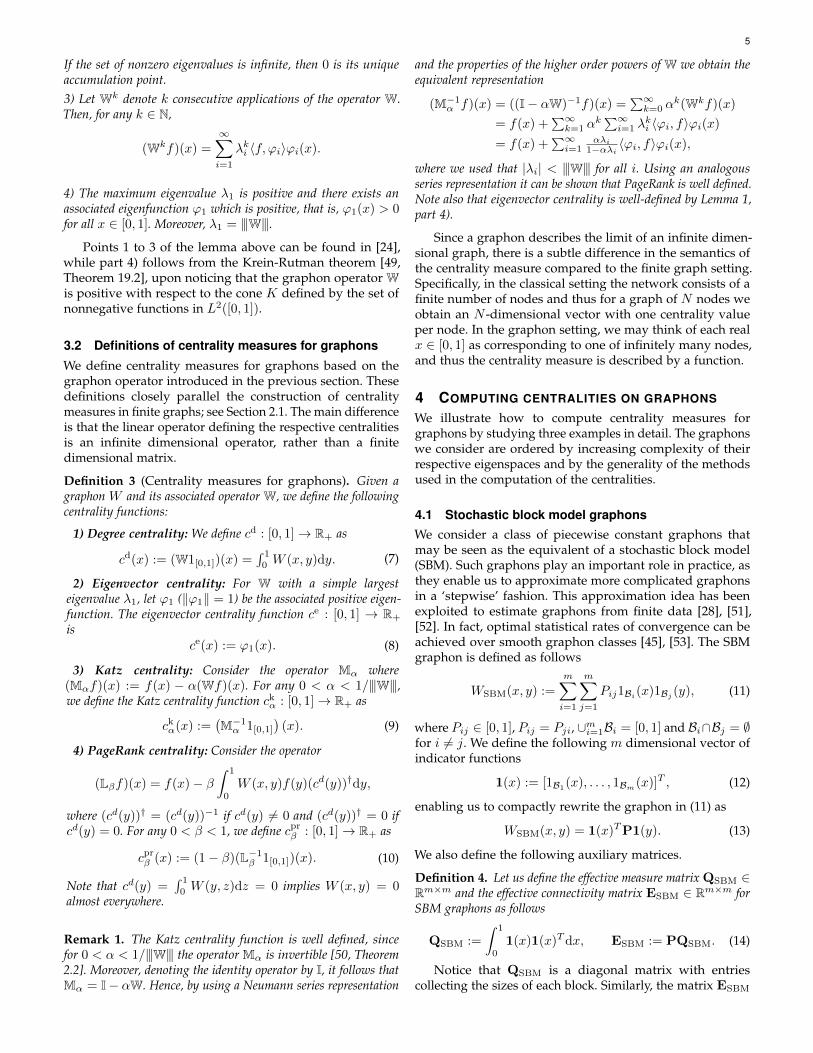
Fig. 3: Illustrative example of a graphon with finite rank. (a) The graphon WFR = (x2 + y2)/2 is decomposable into a finite number of components,inducing a finite-rank graphon operator. (b-d) Degree, eigenvector, Katz, and PageRank centralities for the graphon depicted in (a).

α = 1.5). For the case of PageRank, on the other hand, blockB3 is deemed as less central than B2 and B4. This can beattributed to the larger size of these latter blocks. Indeed, theclassical PageRank centrality measure is partially driven bysize [10].

4.2 Finite-rank graphonsWe now consider a class of finite-rank (FR) graphons that canbe written as a finite sum of products of integrable functions.Specifically, we consider graphons of the form

WFR(x, y) :=m∑i=1

gi(x)hi(y) = g(x)Th(y), (17)

where m ∈ N and we have defined the vectors of functionsg(x) = [g1(x), . . . , gm(x)]T and h(y) = [h1(y), . . . , hm(y)]T .Observe that g(x) and h(y) must be chosen so that WFR issymmetric, and WFR(x, y) ∈ [0, 1] for all (x, y) ∈ [0, 1]2.Based on g(x) and h(y) we can define the generalizations ofQSBM and ESBM introduced in Section 4.1, for this class offinite-rank graphons.

Definition 5. The effective measure matrix Q and the effectiveconnectivity matrix E for a finite-rank graphon WFR as definedin (17) are given by

Q :=

∫ 1

0g(x)g(x)Tdx, E :=

∫ 1

0h(x)g(x)Tdx. (18)

The stochastic block model graphon operator introducedin (11) is a special case of the class of operators in (17). Moreprecisely, we recover the SBM graphon by choosing gi(x) =1Bi(x) and hi(y) =

∑mj=1 Pij1Bj (y) for i = 1, . . . ,m. The

matrices defined in (14) are recovered when specializingDefinition 5 to this choice of gi(x) and hi(y). We may nowrelate the eigenfunctions of the FR graphon with the spectralproperties of E, as explained in the following lemma.

Lemma 3. Let λi and vi denote the eigenvalues and eigenvectorsof E in (18), respectively. Then, all the nonzero eigenvalues ofWFR, the operator associated with (17), are given by λi and theassociated eigenfunctions are of the form ϕi(x) = g(x)Tvi.

Lemma 3 is proven in Appendix A and shows that thegraphon in (17) is of finite rank since it has at most mnon-zero eigenvalues. Notice that Lemma 2 follows fromLemma 3 when specializing the finite rank operator to theSBM case as explained after Definition 5. Moreover, wecan leverage the result in Lemma 3 to find closed-formexpressions for the centrality functions of FR graphons. Towrite these expressions compactly, we define the vectors of

integrated functions g :=∫ 10 g(y)dy and h :=

∫ 10 h(y)dy, as

well as the following normalized versions of h and E

hnor =

∫ 1

0

h(y)

gTh(y)dy, Enor =

∫ 1

0

h(y)g(y)T

gTh(y)dy. (19)

With this notation in place, we can establish the followingresult, which is proven in Appendix A.

Proposition 2 (Centrality measures for FR graphons). Letv1 be the principal eigenvector of E in (18). Then, the centralityfunctions cd, ce, ckα, and cpr

β of the graphon WFR can be computedas follows

cd(x) =g(x)Th, ce(x) =g(x)Tv1√v1TQv1

, (20)

ckα(x) = 1 + αg(x)T (I− αE)−1

h,

cprβ (x) = (1− β)(1 + βg(x)T (I− βEnor)

−1hnor).

In the next subsection we illustrate the use of Proposi-tion 2 for the computation of graphon centralities.

4.2.1 Example of a finite-rank graphonConsider the FR graphon given by

WFR(x, y) = (x2 + y2)/2,

and illustrated in Fig. 3-(a). Notice that this FR graphoncan be written in the canonical form (17) by defining thevectors g(x) = [x2, 1/2]T and h(y) = [1/2, y2]T . From (18)we then compute the relevant matrices Q and E, as well asthe relevant normalized quantities, to obtain

Q =

[1/5 1/61/6 1/4

], E =

[1/6 1/41/5 1/6

], g =

[1/31/2

],

h =

[1/21/3

], hnor ≈

[1.810.79

], Enor ≈

[0.40 0.910.40 0.40

].

A simple computation reveals that the principal eigenvectorof E is v1 = [

√10/3, 2

√2/3]T . We now leverage the result

in Proposition 2 to obtain

cd(x) = [x2, 1/2]

[1/21/3

]=x2

2+

1

6,

ce(x) =3

2

√3

3 +√

5[x2, 1/2]

[√10/3

2√

2/3

]≈1.07x2 + 0.54,

ckα(x) = [x2, 1/2]

([1 00 1

]−α

[1/6 1/41/5 1/6

])−1

α

[1/21/3

]+1

≈ 10.19x2 + 5.44,

cpr0.85(x) ≈ 1.31x2 + 0.56,

8

0 0.5 1x

0

0.05

0.1

0.15

cd

a b c d e

Fig. 4: Illustrative example of a general smooth graphon. (a) The graphon WG induces an operator that has countably infinite number of nonzeroeigenvalues and corresponding eigenfunctions. (b-d) Degree, eigenvector, Katz, and PageRank centralities for the graphon depicted in (a).

where we have set β = 0.85 in the PageRank centrality. More-over, we have evaluated the Katz centrality for α = 0.9/λ1,where λ1 is the largest eigenvalue of E. The four centralityfunctions are depicted in Fig. 3-(b) through (e). As anticipatedfrom the form of WFR, there is a simple monotonicity in thecentrality ranking for all the measures considered. Moreprecisely, highest centrality values are located close to 1 inthe interval [0, 1], whereas low centralities are localized closeto 0. Unlike in the example of the stochastic block model inSection 4.1.1, all centralities here have the same functionalform of a quadratic term with a constant offset.

4.3 General smooth graphonsIn general, a graphon W need not induce a finite-rankoperator as in the preceding Sections 4.1 and 4.2. How-ever, as shown in Lemma 1, a graphon always inducesa diagonalizable operator with countably many nonzeroeigenvalues. In most cases, obtaining the degree centralityfunction is immediate since it entails the computation ofan integral [cf. (7)]. On the other hand, for eigenvector,Katz, and PageRank centralities that depend on the spectraldecomposition of W, there is no universal technique available.Nonetheless, a procedure that has shown to be useful inpractice to obtain the eigenfunctions ϕ and correspondingeigenvalues λ of smooth graphons is to solve a set ofdifferential equations obtained by successive differentiation,when possible, of the eigenfunction equation in (6), that is,by considering

dk

dxk

∫ 1

0W (x, y)ϕ(y)dy = λ

dkϕ(x)

dxk, (21)

for k ∈ N. In the following section we illustrate this techniqueon a specific smooth graphon that does not belong to thefinite-rank class.

4.3.1 Example of a general smooth graphonConsider the graphon WG depicted in Fig. 4-(a) and with thefollowing functional form

WG(x, y) = min(x, y)[1−max(x, y)].

Specializing the differential equations in (21) for graphonWG we obtain

dk

dxk

[(1− x)

∫ x

0yϕ(y)dy+x

∫ 1

x(1− y)ϕ(y)dy

]=λ

dkϕ(x)

dxk.

(22)First notice that without differentiating (i.e. for k = 0) wecan determine the boundary conditions ϕ(0) = ϕ(1) = 0.

Moreover, by computing the second derivatives in (22), weobtain that −ϕ(x) = λϕ′′(x). From the solution of thisdifferential equation subject to the boundary conditionsit follows that the eigenvalues and eigenfunctions of theoperator WG are

λn =1

π2n2and ϕn(x) =

√2 sin(nπx) for n ∈ N. (23)

Notice that WG has an infinite — but countable —number of nonzero eigenvalues, with an accumulation pointat zero. Thus, WG cannot be written in the canonical form forfinite-rank graphons (17). Nevertheless, having obtained theeigenfunctions we can still compute the centrality measuresfor WG. For degree centrality, a simple integration gives us

cd(x) = (1− x)

∫ x

0y dy + x

∫ 1

x(1− y) dy =

x(1− x)

2.

From (23) it follows that the principal eigenfunction isachieved when n = 1. Thus, the eigenvector centralityfunction [cf. (8)] is given by

ce(x) =√

2 sin(πx).

Finally, for the Katz centrality we leverage Remark 1 and theeigenfunction expressions in (23) to obtain

ckα(x) = 1 +∞∑k=1

αk∞∑n=1

(1

n2π2

)k 1− (−1)n

πn2 sin(nπx)

= 1 +∞∑n=1

2α

n2π2 − α1− (−1)n

πnsin(nπx),

which is guaranteed to converge as long as α < 1/λ1 = π2.We plot these three centrality functions in Fig. 4-(b) through(d), where we selected α = 0.9π2 for the Katz centrality.Also, in Fig. 4-(e) we plot an approximation to the PageRankcentrality function cpr

β obtained by solving numerically theintegral in its definition. According to all centralities, themost important nodes within this graphon are those locatedin the center of the interval [0, 1], in line with our intuition.Likewise, nodes at the boundary have low centrality values.Note that while the ranking according to all centralityfunctions is consistent, unlike in the example in Section 4.2.1,here there are some subtle differences in the functionalforms. In particular, degree centrality is again a quadraticfunction whereas the eigenvector and Katz centralities are ofsinusoidal form.

9

5 CONVERGENCE OF CENTRALITY MEASURES

In this section we derive concentration inequalities relatingthe newly defined graphon centrality functions with standardcentrality measures. To this end, we start by noting thatwhile graphon centralities are functions, standard centralitymeasures are vectors. To be able to compare such objects, wefirst show that there is a one to one relation between any finitegraph with adjacency matrix A and a suitably constructedstochastic block model graphon WSBM|A. Consequently, anycentrality measure of A is in one to one relation with thecorresponding centrality function of WSBM|A. To this end, foreach N ∈ N, we define a partition of [0, 1] into the intervalsBNi , where BNi = [(i− 1)/N, i/N) for i = 1, . . . , N − 1, andBNN = [(N − 1)/N, 1]. We denote the associated indicator-function vector by 1N (x) := [1BN1 (x), . . . , 1BNN (x)]T , consis-tently with (12).

Lemma 4. For any adjacency matrix A ∈ {0, 1}N×N define thecorresponding stochastic block model graphon as

WSBM|A(x, y) =N∑i=1

N∑j=1

Aij1BNi (x)1BNj (x).

Then the centrality function cN (x) corresponding to the graphonWSBM|A is given by

cN (x) = 1N (x)TcA.

where cA is the centrality measures of the graph with rescaledadjacency matrix 1

NA.

Proof. The graphon WSBM|A has the stochastic block modelstructure described in Section 4.1, with N uniform blocks. Byselecting m = N and Bi = BNi for each i ∈ {1, . . . , N},we obtain QSBM = 1

N I. Consequently, the formulas inProposition 1 simplify as given in the statement of thislemma.

Remark 2. Note that the scaling factor 1N does not affect the

centrality rankings of the nodes in A, but only the magnitude ofthe centrality measures. This re-scaling is needed to avoid divergingcentrality measures for graphs of increasing size. Observe furtherthat cN (x) is the piecewise-constant function corresponding to thevector cA. We finally remark that graphons of the type WSBM|Ahave appeared before in the literature using a different notation [24].

By using the previous lemma, we can compare centralitiesof graphons and graphs by working in the function space.Using this equivalence, we demonstrate that the previouslydefined graphon centrality functions are not only definedanalogously to the centrality measures on finite graphs, butalso emerge as the limit of those centrality measures for asequence of graphs of increasing size. Stated differently, justlike the graphon provides an appropriate limiting object fora growing sequence of finite graphs, the graphon centralityfunctions can be seen as the appropriate limiting objects ofthe finite centrality measures as the size of the graphs tendsto infinity. In this sense, the centralities presented here maybe seen as a proper generalization of the finite setting, justlike a graphon provides a generalized framework for finitegraphs. Most importantly, we show that the distance (in L2

norm) between the graphon centrality function and the step-wise constant function associated with the centrality vector

of any graph sampled from the graphon can be bounded,with high probability, in terms of the sampled graph size N .

Definition 6 (Sampled graphon). Given a graphon W and asize N ∈ N fix the latent variables {ui}Ni=1 by choosing either:

- ‘deterministic latent variables’: ui = iN .

- ‘stochastic latent variables’: ui = U(i) where U(i) is the i-thorder statistic of N random samples from Unif [0, 1].

Utilizing such latent variables construct

- the ‘probability’ matrix P(N) ∈ [0, 1]N×N

P(N)ij := W (ui, uj) for all i, j ∈ {1, . . . , N}.

- the sampled graphon

WN (x, y) :=∑Ni=1

∑Nj=1 P

(N)ij 1BNi (x)1BNj (y).

- the operator WN of the sampled graphon

(WNf)(x) :=∑Nj=1 P

(N)ij

∫BNj

f(y)dy for any x ∈ BNi

The sampled graphon WN obtained when working withdeterministic latent variables can intuitively be seen as anapproximation of the graphon W by using a stochasticblock model graphon with N blocks, as the one describedin Section 4.1, and is useful to study graphon centralityfunctions as limit of graph centrality measures. On the otherhand, the sampled graphon WN obtained when workingwith stochastic latent variables is useful as an intermediatestep to analyze the relation between the graphon centralityfunction and the centrality measure of graphs sampled fromthe graphon according to the following procedure.

Definition 7 (Sampled graph). Given the ‘probability’ matrixP(N) of a sampled graphon we define

- the sampled matrix S(N) ∈ {0, 1}N×N as the adjacency matrixof a symmetric (random) graph obtained by taking N isolatedvertices i ∈ {1, . . . , N}, and adding undirected edges betweenvertices i and j at random with probability κNP

(N)ij for all i > j.

Note that E[S(N)] = κNP(N).- the associated (random) linear operator

(SNf)(x) :=∑Nj=1 S

(N)ij

∫BNj

f(y)dy for any x ∈ BNi , (24)

and its associated (random) graphon:

SN (x, y) = 1N (x)TS(N)1N (y). (25)

In general, we denote the centrality functions associatedwith the sampled graphon operator WN by cN (x) whereasthe centrality functions associated with the operator κ−1

N SNare denoted by cN (x). Note that thanks to Lemma 4 suchcentrality functions are in one to one correspondence with thecentrality measures of the finite graphs P(N) and κ−1

N S(N),respectively. Consequently, studying the relation betweenc(x), cN (x) and cN (x) allows us to relate the graphon central-ity function with the centrality measure of graphs sampledfrom the graphon. We note that previous works on graphlimit theory imply the convergence of WN and κ−1

N SN to thegraphon operator W [22], [25], [54]. Intuitively, convergence

10

of cN (x) and cN (x) to c(x) then follows from continuity ofspectral properties of the graphon operator. In the following,we make this argument precise and more importantly weprovide a more refined analysis by establishing sharp ratesof convergence of the sampled graphs, under the followingsmoothness assumption on W . A more detailed discussionof related convergence results can be found in Appendix B(see supplementary material).

Assumption 1 (Piecewise Lipschitz graphon). There existsa constant L and a sequence of non-overlapping intervals Ik =[αk−1, αk) defined by 0 = α0 < · · · < αK+1 = 1, for a (finite)K ∈ N, such that for any k, l, any set Ikl = Ik × Il and pairs(x, y) ∈ Ikl, (x′, y′) ∈ Ikl we have that

|W (x, y)−W (x′, y′)| ≤ L(|x− x′|+ |y − y′|).

This assumption has also been used in the context ofgraphon estimation [28], [53] and is typically fulfilled formost of the graphons of interest.

Theorem 1 (Convergence of graphon operators). For agraphon fulfilling Assumption 1, it holds with probability1− δ′ that:

|||WN −W||| := sup‖f‖=1

‖WNf −Wf‖

≤ 2√

(L2 −K2)d2N +KdN =: ρ(N),

(26)where δ′ = 0 and dN = 1

N in the case of determinis-tic latent variables and δ′ = δ ∈ (Ne−N/5, e−1) anddN := 1

N +√

8 log(N/δ)(N+1) in the case of stochastic latent

variables. Moreover, if N is large enough, as specified inLemma 5, then with probability at least 1− δ − δ′

∣∣∣∣∣∣κ−1N SN −W

∣∣∣∣∣∣ ≤√

4κ−1N log(2N/δ)

N+ ρ(N). (27)

In particular, if κN = 1Nτ with τ ∈ [0, 1), then:

limN→∞

∣∣∣∣∣∣κ−1N SN −W

∣∣∣∣∣∣ = 0, almost surely. (28)

Remark 3. To control the error induced by the random sampling,we derive a concentration inequality for uniform order statistics,as reported next, that can be of independent interest. As this resultis not central to the discussion of our paper, we relegate its proofto Appendix B. In addition, we make use of a lower bound on themaximum expected degree as reported in Lemma 5 and proven inAppendix B.

Proposition 3. LetU(i) be the order statistics ofN points sampledfrom a standard uniform distribution. Suppose that N ≥ 20 andδ ∈ (Ne−N/5, e−1). With probability at least 1− δ∣∣∣U(i) −

i

N + 1

∣∣∣ ≤√8 log(N/δ)

(N + 1)for all i.

Lemma 5. If N is such that

2dN < ∆(α)MIN := min

k∈{1,...,K+1}(αk − αk−1), (29a)

1

Nlog

(2N

δ

)+ dN (2K + 3L) < Cd := max

xcd(x) (29b)

Fig. 5: Schematic for the sets AN and AcN in the case of stochastic

latent variables for K = 1, threshold α1 and 4 Lipschitz blocks. The ploton the left shows the original graphon W (x, y), the 4 Lipschitz blocksand some representative latent variables. The plot on the right showsthe sampled graphon WN (x, y) which is a piecewise constant graphonwith uniform square blocks of side 1

N. The 1

N-grid is illustrated in gray.

The constant value in each block BNi × BNj corresponds to the valuein the original graph sampled at the point (ui, uj) (as illustrated by thearrows). The set BNi × BNi in the bottom left is an example where allthe points (x, y) ∈ BNi × BNi belong to the same Lipschitz block astheir corresponding sample, which is (ui, ui), so that BNi × BNi = Siiand therein |D(x, y)| ≤ 2LdN . The set BNk × B

Nl instead is one of

the problematic ones since part of its points (cyan) belong to the sameLipschitz block as (uk, ul) and are thus in Skl but part of its points(red) do not and therefore belong to Ac

N . Note that by construction withprobability 1− δ′ all such problematic points are contained in the set DN

(which is illustrated in light red). This figure also illustrates that in generalDN is a strict superset of Ac

N (hence the bound in (30) is conservative).

then CdN := maxi(∑Nj=1 P

(N)ij ) ≥ 4

9 log( 2Nδ ).

Proof of Theorem 1:We prove the three statements sequentially.

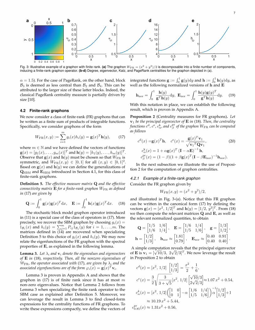
Proof of (26). First of all note that by definition, for any(x, y) ∈ BNi × BNj it holds WN (x, y) = W (ui, uj), but it isnot necessarily true that (ui, uj) ∈ BNi × BNj . Let us defineki, kj ∈ {1, . . . ,K + 1} such that the point (ui, uj) belongsto the Lipschitz block Ikikj , as defined in Assumption 1 andillustrated in Fig. 5. We define as Sij the subset of points inBNi × BNj that belong to the same Lipschitz block Ikikj as(ui, uj). Mathematically,

Sij = {(x, y) ∈ BNi ×BNj | (ui, uj)∈ Ikikj and (x, y)∈ Ikikj}.

In the following, we partition the set [0, 1]2 into the setAN := ∪ijSij and its complement AcN := [0, 1]2\AN . Inwords, AN is the set of points, for which (x, y) and itscorresponding sample (ui, uj) belong to the same Lipschitzblock. We now prove that, with probability 1− δ′, AcN hasarea

Area(AcN ) ≤ Area(DN ) = 4KdN − 4K2d2N . (30)

To prove the above, we define the set DN by constructinga stripe of width 2dN centered at each discontinuity of thegraphon, as specified in Assumption 1. This guaranteesthat any point in [0, 1]2\DN has distance more than dNcomponent-wise from a discontinuity.

Note that in the case of deterministic latent variables forany i ∈ {1, . . . , N} and any x ∈ BNi it holds by constructionthat |x− ui| = |x− i

N | ≤ dN = 1N and similarly |y − uj | ≤

dN . In the case of stochastic latent variables, Proposition 3guarantees that with probability at least 1− δ for any i, j ∈{1, . . . , N} and any x ∈ BNi , y ∈ BNj it holds |x − ui| =

11

|x−U(i)| ≤ dN , |y−uj | ≤ dN . In both cases, with probability1 − δ′, all the points in [0, 1]2\DN are less than dN closeto their sample (ui, uj) and more than dN far from anydiscontinuity (component-wise) hence they surely belong toAN .

Consequently, with probability 1 − δ′ we have AcN ⊆DN . Each stripe in DN has width 2dN , length 1, and thereare 2K stripes in total. Formula (30) is then immediate bynoticing that multiplying 2dN times 2K counts twice the K2

intersections between horizontal and vertical stripes.Consider now any f ∈ L2([0, 1]) such that ‖f‖ = 1. Let

D(x, y) := WN (x, y)−W (x, y) and note that |D(x, y)| ≤ 1.Then we get

‖WNf −Wf‖2 =∫ 10 (WNf −Wf)2(x)dx

=∫ 10

(∫ 10 D(x, y)f(y)dy

)2dx

≤∫ 10

(∫ 10 D(x, y)2dy

)(∫ 10 f

2(y)dy)

dx (31)

=∫ 10

(∫ 10 D(x, y)2dy

)‖f‖2dx =

∫ 10

∫ 10 D(x, y)2dydx

=∫∫AN D(x, y)2dydx+

∫∫AcN

D(x, y)2dydx. (32)

Expression (31) follows from the Cauchy-Schwarz inequality;we used ‖f‖ = 1 and, in the last equation, we split theinterval [0, 1]2 into the sets AN and AcN , as described aboveand illustrated in Fig. 5.

We can now bound both terms in (32). For the first term,note that for all the points (x, y) in AN the correspondingsample (ui, uj) belongs to the same Lipschitz block and isat most dN apart (component-wise). Consequently, for thesepoints |D(x, y)| ≤ 2LdN . Overall, we get∫∫

AN D(x, y)2dydx ≤ 4L2d2N

∫∫AN 1 dy dx ≤ 4L2d2

N .

For the second term in (32), we use (30) and the fact that|D(x, y)| ≤ 1 to get∫∫

AcND(x, y)2dydx ≤

∫∫AcN

1 dy dx = Area(AcN ).

Substituting these two terms into (32) yields

‖WNf −Wf‖2 ≤ (4L2d2N + 4KdN − 4K2d2

N ).

Since this bound holds for all functions f with unit norm,we recover (26).

Proof of (27). From the triangle inequality we get that∣∣∣∣∣∣κ−1N SN −W

∣∣∣∣∣∣ ≤ ∣∣∣∣∣∣κ−1N SN −WN

∣∣∣∣∣∣+ |||WN −W|||. (33)

We have already bounded the second term on the righthand side of (33), so we now concentrate on the first term.

The operator κ−1N SN −WN can be seen as the graphon

operator of an SBM graphon with matrix κ−1N S(N) − P(N).

By Lemma 2 we then have that its eigenvalues coincide withthe eigenvalues of the corresponding ESBM matrix which is1N (κ−1

N S(N) −P(N)) since in this case QSBM = 1N IN (given

that all the intervals BNi have length 1N ).2 Consequently,∣∣∣∣∣∣κ−1

N SN −WN

∣∣∣∣∣∣ = λmax(κ−1N SN −WN )

=1

Nλmax(κ−1

N S(N) −P(N)) =1

N‖κ−1

N S(N) −P(N)‖.

2. Note that Lemma 2 is formulated for graphon operators (i.e. linearintegral operators with nonnegative kernels). An identical proof showsthat the result holds also if the kernel assumes negative values.

Hence, to bound the norm of the difference between arandom SBM graphon operator κ−1

N SN based on the graphonκ−1N S = κ−1

N 1(x)TS(N)1(y), with S(N)ij = Ber(κNP

(N)ij ),

and its expectation WN defined via the graphon WN =1(x)TP(N)1(y), we can employ matrix concentration in-equalities. Specifically, we use [55, Theorem 1] in order tobound the deviations of ‖S(N) − κNP(N)‖.

By Lemma 5, for N large enough, the maximum expecteddegree κNC

dN := κN maxi(

∑Nj=1 P

(N)ij ) of the random

graph represented by S(N) grows at least as 49κN log( 2N

δ ).Consequently, all the conditions of [55, Theorem 1] are metand we get that with probability 1− δ − δ′∣∣∣∣∣∣κ−1

N SN −WN

∣∣∣∣∣∣ =κ−1N

N‖S(N) − κNP(N)‖

≤ κ−1N

N

√4κNCdN log(2N/δ) ≤

√4κ−1

N log(2N/δ)

N,

where we used that CdN ≤ N since each element in P(N)

belongs to [0, 1].Proof of (28). We finally show that (27) implies almost sure

convergence. We start by restating (27) as

Pr[∣∣∣∣∣∣κ−1

N SN −W∣∣∣∣∣∣ ≤√ 4κ−1

N log(2N/δ)

N + ρ(N)

]≥ 1− 2δ.

(34)Further, pick any γ > 0 and define the infinite sequence ofevents

EN :={∣∣∣∣∣∣κ−1

N SN −W∣∣∣∣∣∣ ≥ γ + ρ(N)

},

for each N ≥ 1. From (34) it follows that Pr [EN ] ≤4N exp

(−κNNγ2/4

). Consequently, if κN = 1

Nτ withτ ∈ [0, 1), then:∑∞

N=1 Pr [EN ] ≤ 4∑∞N=1Nexp

(−κNNγ2

4

)<∞

and by the Borel-Cantelli lemma there exists a positive inte-ger Nγ such that for all N ≥ Nγ , the complement of EN , i.e.,∣∣∣∣∣∣κ−1

N SN −W∣∣∣∣∣∣ ≤ γ + ρ(N), holds almost surely. To see that∣∣∣∣∣∣κ−1

N SN −W∣∣∣∣∣∣ → 0 almost surely we follow the ensuing

argument. For any given deterministic sequence {aN}∞N=1

the fact that for each γ > 0 there is a positive integer Nγ suchthat for allN ≥ Nγ , |aN | ≤ γ+ρ(N) implies that aN → 0. Infact for all ε > 0, if we set γ = ε/2 and Nε := max{Nγ , Nρ}(where Nρ is the smallest N such that ρ(N) ≤ ε/2) then weget that for all N > Nε,

∣∣∣∣∣∣κ−1N SN −W

∣∣∣∣∣∣ ≤ ε. Hence, we canconclude that

∣∣∣∣∣∣κ−1N SN −W

∣∣∣∣∣∣→ 0 almost surely. �The previous theorem provides us with convergence rates

for the graphon operators. Based on these we are able toshow a similar convergence result for centrality measures ofgraphons with a simple dominant eigenvalue.

Assumption 2 (Simple dominant eigenvalue). Let the eigen-values of W be ordered such that λ1 ≥ λ2 ≥ λ3 ≥ . . . and assumethat λ1 > λ2.

We note that in most empirical studies degeneracy of thedominant eigenvalue is not observed, justifying the aboveassumption. A noteworthy exception in which a non-uniquedominant eigenvalue may arise is if the graph consists ofmultiple components. In this case, however, one can treateach component separately.

12

For the proof in case of PageRank we will make thefollowing additional assumption on the graphon.

Assumption 3 (Minimal degree assumption). There existsη > 0 such that W (x, y) ≥ η for all x, y ∈ [0, 1].

Note that while this assumption is not fulfilled, e.g., fora SBM graphon with a block of zero connection probability,it can be further relaxed to accommodate such cases as well.However, to simplify the proof and avoid additional technicaldetails, we invoke Assumption 3 in the following theorem.

Theorem 2. (Convergence of centrality measures) Thefollowing statements hold:

1) For any N > 1, the centrality functions cN (x) andcN (x) corresponding to the operators WN and κ−1

N SN ,respectively, are in one to one relation with the centralitymeasures cP (N) ∈ RN , cS(N) ∈ RN of the graphs withrescaled adjacency matrices P(N) := 1

NP(N) and S(N) :=1

NκNS(N), via the formulaa

cN (x) = 1N (x)TcP (N) , cN (x) = 1N (x)

TcS(N) .

2) Under Assumptions 1, 2 and (for PageRank) 3, and Nsufficiently large, with probability at least 1− δ′

‖cN − c‖ ≤ Cρ(N)

for some constant C and ρ(N), δ′ defined as in Theorem 1.3) Under Assumptions 1, 2 and (for PageRank) 3, and N

sufficiently large, with probability at least 1− 2δ

‖cN − c‖ ≤ C ′(√

4κ−1N log(2N/δ)

N + ρ(N)

),

for some constant C ′.4) Under Assumptions 1, 2 and (for PageRank) 3, if κN =1Nτ with τ ∈ [0, 1), then:

limN→∞

‖cN − c‖ = 0, almost surely.

a. Note that P(N), S(N) belong to RN×N≥0 as opposed to

{0, 1}N×N . Nonetheless, the definitions of centrality measuresgiven in Section 2.1 can be extended to the continuous intervalcase in a straightforward manner.

Proof. 1) Follows immediately from Lemma 4 since WN andκ−1N SN are the operators of the graphons corresponding to

P(N) and κ−1N S(N), respectively.

2) We showed in Theorem 1 that, under Assumption 1,|||WN −W||| ≤ ρ(N) with probability 1− δ′. This fact can beexploited to prove convergence of the centrality measurescN to c. All the subsequent statements hold with probability1− δ′.

For degree centrality: cN (x) = (WN1[0,1])(x) and c(x) =(W1[0,1])(x). Since ‖1[0,1]‖ = 1 we get

‖cN −c‖ = ‖(WN −W)1[0,1]‖ ≤ |||WN −W||| ≤ ρ(N). (35)

For eigenvector centrality: Let {λk, ϕk}k≥1,{λ(N)

k , ϕ(N)k }k≥1 be the ordered eigenvalues

and eigenfunctions of W and WN , respec-tively. Note that |λ(N)

1 − λ1| ≤ ρ(N) since

λ(N)1 = |||WN ||| ≤ |||W|||+ |||WN −W||| ≤ λ1 + ρ(N) andλ1 = |||W||| ≤ |||WN||| + |||WN −W||| ≤ λ

(N)1 + ρ(N).

Furthermore, since by Assumption 2 we have that λ1 > λ2,there exists a large enough N such that for all N > N itholds that λ(N)

1 > λ2 and |λ1 − λ2| > |λ(N)1 − λ1|. Therefore,

by Lemma 8 in Appendix B, we obtain

‖ϕ(N)1 − ϕ1‖ ≤

√2 |||WN −W|||

|λ1 − λ2| − |λ(N)1 − λ1|

. (36)

From the facts that λ1 6= λ2 (by Assumption 2), |λ(N)1 −λ1| ≤

ρ(N), and |||WN −W||| ≤ ρ(N), it follows that (36) impliesthat for N > N

‖ϕ(N)1 − ϕ1‖ ≤

√2ρ(N)

|λ1 − λ2| − ρ(N)= O

(ρ(N)

). (37)

For Katz centrality: Take any value of α < 1/|||W|||, sothat Mα = I − αW is invertible and c(x) =

(M−1α 1[0,1]

)(x)

is well defined. Since |||WN −W||| → 0 as N → ∞, thereexists Nα > 0 such that α < 1/|||WN ||| for all N > Nα. Thisimplies that for anyN > Nα, [MN ]α := I−αWN is invertibleand cN (x) =

([MN ]−1

α 1[0,1]

)(x) is well defined. Note that

|||WN −W||| ≤ ρ(N) implies |||[MN ]α −Mα||| = O(ρ(N)).We now prove that∣∣∣∣∣∣[MN ]−1

α −M−1α

∣∣∣∣∣∣ = O(ρ(N)

). (38)

To this end, note that L2([0, 1]) is a Hilbert space, the inverseoperator M−1

α is bounded and for N large enough it holds|||[MN ]α −Mα||| < 1/

∣∣∣∣∣∣M−1α

∣∣∣∣∣∣, since |||[MN ]α −Mα||| → 0. Itthen follows by [56, Theorem 2.3.5 ] with L := Mα,M :=[MN ]α that

∣∣∣∣∣∣[MN ]−1α −M−1

α

∣∣∣∣∣∣ ≤ ∣∣∣∣∣∣M−1α

∣∣∣∣∣∣2|||[MN ]α −Mα|||1−∣∣∣∣∣∣M−1

α

∣∣∣∣∣∣|||[MN ]α −Mα|||=O(ρ(N)),

thus proving (38). Finally, since ‖1[0,1]‖ = 1,

‖cN − c‖ = ‖[MN ]−1α 1[0,1] −M−1

α 1[0,1]‖≤∣∣∣∣∣∣[MN ]−1

α −M−1α

∣∣∣∣∣∣ = O(ρ(N)

).

For PageRank centrality: Consider β ∈ (0, 1) such thatLβ is invertible and cpr(x) is well defined. Similar to theargument used to show (38) in the proof for Katz centrality,it suffices to show that |||[LN ]β − Lβ ||| = O(ρ(N)). To showthis note that under Assumption 3 it holds

cd(x) =

∫ 1

0W (x, y)dy ≥ η,

cdN (x) =

∫ 1

0WN (x, y)dy ≥ η.

(39)

Hence (cd(x))† = (cd(x))−1 ≤ 1η and (cd

N (x))† =

(cdN (x))−1 ≤ 1

η . For any f ∈ L2([0, 1]) such that ‖f‖ = 1,

‖[LN ]βf − Lβf‖ = β ‖WN

(f · (cd

N )−1)−W

(f · (cd)−1

)‖

≤β‖(WN −W)(f ·(cd)−1

)‖+β‖WN

(f ·(cd

N )−1− f ·(cd)−1)‖

≤ β |||WN −W|||‖(cd)−1‖+ β|||WN |||‖(cdN )−1−(cd)−1‖

≤ βρ(N)‖(cd)−1‖+ 2β|||W|||‖(cdN )−1 − (cd)−1‖, (40)

where we used that for N large enough |||WN ||| ≤ 2|||W|||. In(40), the notation (cd)−1 is used to denote the function that

13

takes values (cd(x))−1 and similarly for (cdN )−1. Observe

that equation (39) implies

‖(cd)−1‖ ≤ 1

η(41)

and

‖(cdN )−1 − (cd)−1‖2 =

∫ 1

0

((cdN (y))−1 − (cd(y))−1

)2dy

=

∫ 1

0

(cdN (y)− cd(y)

cdN (y)cd(y)

)2

dy ≤ 1

η4‖cdN − cd‖2. (42)

Combining (35), (40), (41) and (42) yields the desired result

‖[LN ]βf − Lβf‖ ≤β

η

[1 +

2

η|||W|||

]ρ(N) = O(ρ(N)).

(43)3) It suffices to mimic the argument made above for

‖cN − c‖ adapting it for the case ‖cN − c‖ by making use of(27). The proof is omitted to avoid redundancy.

4) By Theorem 1 we have that∣∣∣∣∣∣κ−1

N SN −W∣∣∣∣∣∣ → 0 al-

most surely. This means that the set of realizations {SN}∞N=1

of {SN}∞N=1 for which |||κ−1N SN −W||| → 0 has probability

one. For each of these realizations it can be proven (exactlyas in part 2)3 that

limN→∞

‖cN − c‖ = 0,

where cN (x) is the deterministic sequence of centrality mea-sures associated with the realization {SN}∞N=1. Consequently,Pr[limN→∞ ‖cN − c‖ = 0] = 1 and limN→∞ ‖cN − c‖ = 0almost surely.

To sum up, Theorem 2 shows that, on the one hand, thecentrality functions of the finite-rank operators WN andκ−1N SN can be computed by simple interpolation of the

centrality vectors of the corresponding finite-size graphs withadjacency matrices P(N) and κ−1

N S(N) (suitably rescaled). Onthe other hand, such centrality functions cN (x) and cN (x)become better approximations of the centrality functionc(x) of the graphon W as N increases. As alluded above,the importance of this result derives from the fact that itestablishes that the centrality functions here introduced arethe appropriate limits of the finite centrality measures, thusvalidating the presented framework. We finally note thatas immediate corollary of the previous theorem we get thefollowing robustness result for the centrality measures ofdifferent realizations.

Corollary 1. Consider two graphs SN1 and SN2 sampled froma graphon W satisfying Assumptions 1 and 2. Assume withoutloss of generality that N1 ≤ N2 and let cS(Ni) ∈ RN be thecentrality of the graphs with rescaled adjacency matrices S(Ni) :=

1NiκNi

S(Ni), for i ∈ {1, 2}. Then for N sufficiently large, withprobability at least 1− 4δ∥∥∥1N1(x)

TcS(N1) − 1N2(x)

TcS(N2)

∥∥∥≤ 2C ′

√4κ−1N1

log(2N1/δ)

N1+ ρ(N1)

3. In part 2(b) the rate of convergence of WN to W was used.

Nonetheless, the same statement holds under the less stringent condition|||WN −W||| → 0, since this is sufficient to prove that λ(N)

1 → λ1.

3

a b

c

Fig. 6: Convergence of the eigenvector centrality function for the FRgraphon in section 4.2.1. (a-b) Eigenvector centrality functions computedfrom a sampled graphon with deterministic latent variables (black; onerealization shown in cyan for visualization purposes) and the eigenvectorcentrality function of the continuous graphon (blue). The examples showncorrespond to a resolution of (a) N = 68 grid points, and (b) N = 489grid points. In each case 20 realizations were drawn from the discretizedgraphon P(N). (c) Convergence of the error ‖cN − c‖ as a function ofthe number of grid points N , corresponding to the number of nodes in thesampled graph. For each point we plot the sample mean ± one standarddeviation.

for some constant C ′ and ρ(N), δ defined as in Theorem 1.

To check our analytical results, we performed numericalexperiments as illustrated in Figs. 6 and 7. In Fig. 6, weconsider again the finite-rank graphon from our example inSection 4.2.1 and assess the convergence of the eigenvectorcentrality function ce

N from the sampled networks (withdeterministic latent variables and κN = 1), to the trueunderlying graphon centrality measure ce. As this graphon issmooth we have K = 0, i.e., there is only a single Lipschitzblock, and we observe a smooth decay of the error whenincreasing the number of grid points N , corresponding tothe number of nodes in the sampled graph.

For the stochastic block model graphon WSBM from ourexample in Section 4.1.1, however, we have K = 4 and thus25 Lipschitz blocks, which are delimited by discontinuousjumps in the value of the graphon. The effect of thesejumps is clearly noticeable when assessing the convergenceof the centrality measures, as illustrated in Fig. 7 for theexample of Katz centrality. If the deterministic samplinggrid of the discretized graphon WN is aligned with thestructure of the stochastic block model WSBM, there is nomismatch introduced by the sampling procedure and thusthe approximation error of the centrality measure cN issmaller (also in the sampled version cN ). Stated differently, ifthe 1

N -grid is exactly aligned with the Lipschitz blocks of theunderlying graphon, we are effectively in a situation in whichthe area AcN is zero, which is analogous to the case of K = 0(see Fig. 5). In contrast, if there is a misalignment between theLipschitz blocks and the 1

N -grid, then additional errors are

14

30

0.2

0.4

0.6

a b

c

alignedmismatch

Fig. 7: Convergence of the Katz centrality function for the SBM graphonin section 4.1.1. (a-b) Katz centrality functions computed from a sampledgraphon with deterministic latent variables (black; one realization shownin cyan for visualization purposes) and the Katz centrality function ofthe continuous graphon (blue). The examples shown correspond to aresolution of (a) N = 58 grid points, and (b) N = 960 grid points. Ineach case 20 realizations were drawn from the discretized graphon P(N).(c) Convergence of the error ‖cN − c‖ as a function of the number of gridpoints N , corresponding to the number of nodes in the sampled graph.For each point we plot the sample mean ± one standard deviation. Forvisualization purposes we connect the data-points (red) in which the gridapproximation was aligned with the piece-wise constant changes of theSBM (i.e. each grid point is within one Lipschitz block of the SBM graphon– c.f. Fig. 5). For this graphon, this happens for all N that are divisibleby 10. Likewise, we connected those data points where there was amismatch between the sampling grid and the SBM graphon structure(blue).

introduced leading to an overall slower convergence, whichis consistent with our results above.

6 DISCUSSION AND FUTURE WORK

In many applications of centrality-based network analysis,the system of interest is subject to uncertainty. In this context,a desirable trait for a centrality measure is that the relativeimportance of agents should be impervious to randomfluctuations contained in a particular realization of a network.In this paper, we formalized this intuition by extending thenotion of centrality to graphons. More precisely, we proposeda departure from the traditional concept of centrality mea-sures applied to deterministic graphs in favor of a graphon-based, probabilistic interpretation of centralities. Thus, we1) introduced suitable definitions of centrality measures forgraphons, 2) showed how such measures can be computedfor specific classes of graphons, 3) proved that the standardcentrality measures defined for graphs of finite size convergeto our newly defined graphon centralities, and 4) bound thedistance between graphon centrality function and centralitymeasures over sampled graphs.

The results presented here constitute a first step towardsa systematic analysis of centralities in graphons and severalquestions remain unanswered. In particular, we see two main

challenges that need to be addressed to widen the scope ofapplications of our methods. First, in most practical scenariosthe graphon will need to be estimated from (finite) data. Thevalidity (error terms) of the centrality scores will accordinglybe contingent on the errors made in this estimation [28],[53]. It would therefore be very interesting to explore how tobest levarage existing graphon estimation results in order toestimate our proposed graphon centrality functions. Second,the parameter κN allows for the analysis of sparse networksas introduced in [26], [27], [43], [44], [45] but not for networkswith asymptotically bounded degrees [46]. An extension ofour results to the analysis of networks with finite degrees isthus of future interest.

Additionally, there are a number of other generalizationsthat are worth investigating.

First, the generalization of centralities for graphonsbeyond the four cases studied in this paper. In particular,the extension to centralities that do not rely directly onspectral graph properties, such as closeness and betweennesscentralities, appears to be a challenging task. Indeed, asuitable notion of path for infinite-size networks needs to bedefined first and bounds on the possible fluctuations of sucha notion of path would need to be derived. Enriching theclass of graphon centrality measures would also contributeto the characterization of the relative robustness of certainclasses of centralities, which would allow us to better assesstheir utility for the analysis of uncertain networks in practice.

Second, the identification of classes of graphons (othersthan the ones here discussed) for which explicit and efficientformulas of the centrality functions can be derived.

Third, the determination of whether the convergencerates provided in Theorem 2 are also optimal. A relatedquestion in this context is to derive convergence results forthe exact ordering of the nodes. This is in particular relevantfor applications where we would like to know by how muchthe ranking of an individual node might have changed as aresult of the uncertainty of the network. One possible avenueto tackle this kind of question would be to start investigating`∞-norm bounds [57] for centralities, which enable us tocontrol the maximal fluctations of each individual entry ofthe centrality measures.

Finally, the extension of the centrality definitions from reg-ular graphons to more complex objects, such as asymmetricnetworks or time-varying graphons [58], [59].

APPENDIX A : OMITTED PROOFS

Proof of Proposition 1

Proof. This proof is a consequence of Proposition 2. We noticethat we can specialize the formula therein to the case of blockstochastic models to obtain the relations: h = ESBM1,Q =QSBM,E = ESBM,Enorm = ESBMD−1

E ,hnor = ESBMD−1E 1. To

see that these equivalencies are true one can check that, forinstance:

[hnor]i =∑mj=1

Pij [QSBM]jj∑mk=1[QSBM]kkPkj

=∑mj=1

Pij [QSBM]jj∑mk=1[QSBM]kkPjk

=∑mj=1

[ESBM]ij[DE]jj

=∑mj=1[ESBMD−1

E ]ij .

15

From the above equivalences, the formulas for cd(x), ce(x)follow immediately. For ckα(x) we obtain

ckα(x) = 1 + α1(x)T (∑∞

k=0 αkEkSBM

)ESBM1

= 1 + 1(x)T (∑∞

k=1 αkEkSBM

)1

= 1(x)T (∑∞

k=0 αkEkSBM

)1 = 1(x)

T(1− αESBM)

−11.

Finally, cprβ (x) can be proven similarly.

Proof of Lemma 3Proof. Assume that v is an eigenvector of E such that Ev =λv with λ 6= 0. We now show that this implies that ϕ(x) =∑mj=1 vjgj(x) is an eigenfunction of W with eigenvalue λ.

From an explicit computation of (Wϕ)(x) we have that

(Wϕ)(x) =∑mi=1 gi(x)

∫ 10 hi(y)

∑mj=1 vjgj(y)dy

=∑mi=1 gi(x)

∑mj=1 vj

∫ 10 hi(y)gj(y)dy.

Recalling the definition of E from (18), it follows that

(Wϕ)(x)=∑mi=1 gi(x)

∑mj=1 vjEij=

∑mi=1 gi(x)λvi=λϕ(x),

where we used the fact that v is an eigenvector of E for thesecond equality.

In order to show the converse statement, let us assumethat ϕ is an eigenfunction of W with associated eigenvalueλ 6= 0. Then, we may write that

(Wϕ)(x) =∑mi=1 gi(x)

∫ 10 hi(y)ϕ(y)dy = λϕ(x),

from where it follows that

ϕ(x)=λ−1∑mi=1 gi(x)

∫ 10 hi(y)ϕ(y)dy=

∑mi=1 gi(x)vi, (44)

where we have implicitly defined vi := λ−1∫ 10 hi(y)ϕ(y)dy.

Substituting (44) into this definition yields, for all i =1, . . . ,m,

λvi =∫ 10 hi(y)

∑mj=1 gj(y)vjdy =

∑mj=1 vjEij = [Ev]i.

By writing the above equality in vector form we get thatEv = λv, thus completing the proof.

Proof of Proposition 2Proof. The proof for degree centrality follows readily from (7),i.e. cd(x) =

∫ 10 g(x)Th(y)dy = g(x)T

∫ 10 h(y)dy = g(x)Th.

Based on Lemma 3, for ce it is sufficient to prove that ‖ce‖ =1. To this end, note that

‖ce‖2 = 1v1TQv1

∫ 10 (g(x)Tv1)2dx

= 1v1TQv1

∫ 10 (vT1 g(x))(g(x)Tv1)dx

= 1v1TQv1

vT1∫ 10 g(x)g(x)Tdxv1 = v1

TQv1

v1TQv1

= 1.

For Katz centrality, we first prove by induction that

(WkFRf)(x) =

∫ 10 g(x)TEk−1h(y)f(y)dy, (45)

for all finite-rank operators WFR. The equality holds triviallyfor k = 1. Now suppose that it holds for k − 1, we can thencompute

(WkFRf)(x) = (WFRWk−1

FR f)(x)

=∫ 10 g(x)Th(z)

∫ 10 g(z)TEk−2h(y)f(y) dy dz

=∫ 10 g(x)T

(∫ 10 h(z)g(z)T dz

)Ek−2h(y)f(y) dy

=∫ 10 g(x)TEk−1h(y)f(y) dy,

where we used Definition 5 for the last equality. We leverage(45) to compute ckα using the expression in Remark 1,

ckα(x) = 1 +∑∞k=1 α

k(Wk1[0,1])(x)

= 1 +∑∞k=1 α

k∫ 10 g(x)TEk−1h(y)dy

= 1 +∑∞k=1 α

kg(x)TEk−1h = 1 + α∑∞k=0 α

kg(x)TEkh

=1+αg(x)T(∑∞

k=0 αkEk

)h=1+αg(x)T(I− αE)

−1h,

as we wanted to show.Finally, the methodology to prove the result for PageRank

is similar to the one used for Katz, thus we sketch the proofto avoid redundancy. First, we recall the definition of G fromthe proof of Proposition 1 and use induction to show that forevery finite-rank graphon (Gk1[0,1])(x) = g(x)TEk−1

nor hnor

for all integer k ≥ 1. We then compute the inverse in thedefinition of PageRank (10) via an infinite sum as done abovefor Katz but using the derived expression for (Gk1[0,1])(x).

REFERENCES

[1] D. Bu, Y. Zhao, L. Cai, H. Xue, X. Zhu, H. Lu, J. Zhang, S. Sun,L. Ling, and N. Zhang, “Topological structure analysis of theprotein–protein interaction network in budding yeast,” Nucleicacids research, vol. 31, no. 9, pp. 2443–2450, 2003.

[2] J. Kleinberg, “Authoritative sources in a hyperlinked environment,”J. ACM, vol. 46, no. 5, pp. 604–632, Sep. 1999.

[3] A. Garas, P. Argyrakis, C. Rozenblat, M. Tomassini, and S. Havlin,“Worldwide spreading of economic crisis,” New Journal of Physics,vol. 12, no. 11, p. 113043, 2010.

[4] N. E. Friedkin, “Theoretical foundations for centrality measures,”American Journal of Sociology, vol. 96, no. 6, pp. 1478–1504, 1991.

[5] L. C. Freeman, “A set of measures of centrality based on between-ness,” Sociometry, pp. 35–41, 1977.

[6] ——, “Centrality in social networks conceptual clarification,” SocialNetworks, vol. 1, no. 3, pp. 215–239, 1978.

[7] P. Bonacich, “Power and centrality: A family of measures,” Americanjournal of sociology, vol. 92, no. 5, pp. 1170–1182, 1987.

[8] S. P. Borgatti and M. G. Everett, “A graph-theoretic perspective oncentrality,” Social Networks, vol. 28, no. 4, pp. 466–484, 2006.

[9] L. Page, S. Brin, R. Motwani, and T. Winograd, “The pagerankcitation ranking: Bringing order to the web.” Stanford InfoLab,Technical Report 1999-66, November 1999.

[10] D. F. Gleich, “Pagerank beyond the web,” SIAM Review, vol. 57,no. 3, pp. 321–363, 2015.

[11] D. Kempe, J. Kleinberg, and E. Tardos, “Maximizing the spreadof influence through a social network,” in Proceedings of theInternational Conference on Knowledge Discovery and Data Mining(KDD), 2003, pp. 137–146.

[12] E. Costenbader and T. W. Valente, “The stability of centralitymeasures when networks are sampled,” Social Networks, vol. 25,no. 4, pp. 283–307, 2003.

[13] S. P. Borgatti, K. M. Carley, and D. Krackhardt, “On the robustnessof centrality measures under conditions of imperfect data,” SocialNetworks, vol. 28, no. 2, pp. 124–136, 2006.

[14] M. Benzi and C. Klymko, “On the limiting behavior of parameter-dependent network centrality measures,” SIAM Journal on MatrixAnalysis and Applications, vol. 36, no. 2, pp. 686–706, 2015.

[15] S. Segarra and A. Ribeiro, “Stability and continuity of centralitymeasures in weighted graphs,” IEEE Transactions on Signal Process-ing, vol. 64, no. 3, pp. 543–555, Feb 2016.

[16] P. Balachandran, E. Airoldi, and E. Kolaczyk, “Inference of networksummary statistics through network denoising,” arXiv preprintarXiv:1310.0423, 2013.

[17] K. Lerman, R. Ghosh, and J. H. Kang, “Centrality metric fordynamic networks,” in Proceedings of the Workshop on Mining andLearning with Graphs (MLG), 2010, pp. 70–77.

[18] R. K. Pan and J. Saramaki, “Path lengths, correlations, and centralityin temporal networks,” Physical Review E, vol. 84, no. 1, p. 016105,2011.

16

[19] P. Grindrod and D. J. Higham, “A matrix iteration for dynamicnetwork summaries,” SIAM Review, vol. 55, no. 1, pp. 118–128,2013.

[20] K. Dasaratha, “Distributions of centrality on networks,” arXivpreprint arXiv:1709.10402, 2017.

[21] C. Borgs and J. T. Chayes, “Graphons: A nonparametric methodto model, estimate, and design algorithms for massive networks,”arXiv:1706.01143, 2017.

[22] L. Lovasz, Large Networks and Graph Limits. American Mathemati-cal Society Providence, 2012, vol. 60.

[23] L. Lovasz and B. Szegedy, “Limits of dense graph sequences,”Journal of Combinatorial Theory, Series B, vol. 96, no. 6, pp. 933–957,2006.

[24] C. Borgs, J. T. Chayes, L. Lovasz, V. T. Sos, and K. Vesztergombi,“Convergent sequences of dense graphs I: Subgraph frequencies,metric properties and testing,” Advances in Mathematics, vol. 219,no. 6, pp. 1801–1851, 2008.

[25] ——, “Convergent sequences of dense graphs II: Multiway cutsand statistical physics,” Annals of Mathematics, vol. 176, no. 1, pp.151–219, 2012.

[26] P. J. Bickel and A. Chen, “A nonparametric view of network modelsand Newman–Girvan and other modularities,” Proceedings of theNational Academy of Sciences, vol. 106, no. 50, pp. 21 068–21 073, 2009.

[27] P. J. Bickel, A. Chen, and E. Levina, “The method of moments anddegree distributions for network models,” The Annals of Statistics,vol. 39, no. 5, pp. 2280–2301, 2011.

[28] E. M. Airoldi, T. B. Costa, and S. H. Chan, “Stochastic blockmodelapproximation of a graphon: Theory and consistent estimation,” inAdvances in Neural Information Processing Systems, 2013, pp. 692–700.

[29] J. Yang, C. Han, and E. Airoldi, “Nonparametric estimation andtesting of exchangeable graph models,” in Artificial Intelligence andStatistics, 2014, pp. 1060–1067.

[30] P. W. Holland, K. B. Laskey, and S. Leinhardt, “Stochastic block-models: First steps,” Social Networks, vol. 5, no. 2, pp. 109–137,1983.

[31] T. A. Snijders and K. Nowicki, “Estimation and prediction forstochastic blockmodels for graphs with latent block structure,”Journal of Classification, vol. 14, no. 1, pp. 75–100, 1997.

[32] S. J. Young and E. R. Scheinerman, “Random dot product graphmodels for social networks,” in International Workshop on Algorithmsand Models for the Web-Graph. Springer, 2007, pp. 138–149.

[33] C. Kemp, J. B. Tenenbaum, T. L. Griffiths, T. Yamada, and N. Ueda,“Learning systems of concepts with an infinite relational model,” inProceedings of the National Conference on Artificial Intelligence (AAAI),2006, pp. 381–388.

[34] A. Goldenberg, A. X. Zheng, S. E. Fienberg, E. M. Airoldi et al., “Asurvey of statistical network models,” Foundations and Trends inMachine Learning, vol. 2, no. 2, pp. 129–233, 2010.

[35] M. W. Morency and G. Leus, “Signal processing on kernel-basedrandom graphs,” in Proceedings of the European Signal ProcessingConference (EUSIPCO), Kos island, Greece, 2017.

[36] C. E. Lee and D. Shah, “Unifying framework for crowd-sourcingvia graphon estimation,” arXiv preprint arXiv:1703.08085, 2017.

[37] S. Gao and P. E. Caines, “The control of arbitrary size networksof linear systems via graphon limits: An initial investigation,” in2017 IEEE 56th Annual Conference on Decision and Control (CDC),Dec 2017, pp. 1052–1057.

[38] Y. Zhang, E. Levina, and J. Zhu, “Estimating network edgeprobabilities by neighbourhood smoothing,” Biometrika, vol. 104,no. 4, pp. 771–783, 2017.

[39] P. Orbanz and D. M. Roy, “Bayesian models of graphs, arraysand other exchangeable random structures,” IEEE Transactions onPattern Analysis and Machine Intelligence, vol. 37, no. 2, pp. 437–461,2015.

[40] C. Borgs, J. Chayes, and L. Lovasz, “Moments of two-variablefunctions and the uniqueness of graph limits,” Geometric AndFunctional Analysis, vol. 19, no. 6, pp. 1597–1619, 2010.

[41] L. Lovasz and B. Szegedy, “The automorphism group of a graphon,”Journal of Algebra, vol. 421, pp. 136–166, 2015.

[42] P. Diaconis and S. Janson, “Graph limits and exchangeable randomgraphs,” arXiv preprint arXiv:0712.2749, 2007.

[43] C. Borgs, J. Chayes, and A. Smith, “Private graphon estimation forsparse graphs,” in Advances in Neural Information Processing Systems,2015, pp. 1369–1377.

[44] C. Gao, Y. Lu, Z. Ma, and H. Zhou, “Optimal estimation andcompletion of matrices with biclustering structures,” The Journal ofMachine Learning Research, vol. 17, no. 1, pp. 5602–5630, 2016.

[45] O. Klopp, A. Tsybakov, and N. Verzelen, “Oracle inequalities fornetwork models and sparse graphon estimation,” The Annals ofStatistics, vol. 45, no. 1, pp. 316–354, 2017.

[46] V. Veitch and D. M. Roy, “The class of random graphs arising fromexchangeable random measures,” arXiv preprint arXiv:1512.03099,2015.

[47] D. J. Aldous, “Representations for partially exchangeable arrays ofrandom variables,” Journal of Multivariate Analysis, vol. 11, no. 4,pp. 581–598, 1981.

[48] D. N. Hoover, “Relations on probability spaces and arrays ofrandom variables,” Preprint, Institute for Advanced Study, Princeton,NJ, vol. 2, 1979.

[49] K. Deimling, Nonlinear Functional Analysis. Dover publications,1985.

[50] P. H. Bezandry and T. Diagana, Almost Periodic Stochastic Processes.Springer Science & Business Media, 2011.

[51] P. Latouche and S. Robin, “Variational Bayes model averaging forgraphon functions and motif frequencies inference in W-graphmodels,” Statistics and Computing, vol. 26, no. 6, pp. 1173–1185, Nov2016.

[52] P. J. Wolfe and S. C. Olhede, “Nonparametric graphon estimation,”arXiv preprint arXiv:1309.5936, 2013.

[53] C. Gao, Y. Lu, and H. H. Zhou, “Rate-optimal graphon estimation,”The Annals of Statistics, vol. 43, no. 6, pp. 2624–2652, 2015.

[54] B. Szegedy, “Limits of kernel operators and the spectral regularitylemma,” European Journal of Combinatorics, vol. 32, no. 7, pp. 1156–1167, 2011.

[55] F. Chung and M. Radcliffe, “On the spectra of general randomgraphs,” the electronic journal of combinatorics, vol. 18, no. 1, p. 215,2011.

[56] K. Atkinson and W. Han, Theoretical Numerical Analysis: A FunctionalAnalysis Framework. Springer, 2009, vol. 39.

[57] J. Fan, W. Wang, and Y. Zhong, “An l-infinity eigenvector pertur-bation bound and its application to robust covariance estimation,”arXiv preprint arXiv:1603.03516, 2016.

[58] H. Crane, “Dynamic random networks and their graph limits,” TheAnnals of Applied Probability, vol. 26, no. 2, pp. 691–721, 2016.

[59] M. Pensky, “Dynamic network models and graphon estimation,”arXiv preprint arXiv:1607.00673, 2016.

[60] R. M. Dudley, Real Analysis and Probability. Cambridge UniversityPress, 2002, vol. 74.

[61] S. Janson, Graphons, cut norm and distance, couplings and rearrange-ments. NYJM Monographs, 2013.

[62] C. Davis and W. M. Kahan, “The rotation of eigenvectors by aperturbation,” SIAM Journal on Numerical Analysis, vol. 7, no. 1, pp.1–46, 1970.

[63] M. Avella-Medina, F. Parise, M. T. Schaub, and S. Segarra, “Central-ity measures for graphons: Accounting for uncertainty in networks,”arXiv preprint arXiv:1707.09350v3, 2018.

[64] S. Boucheron and M. Thomas, “Concentration inequalities for orderstatistics,” Electronic Communications in Probability, vol. 17, 2012.

[65] L. Devroye, Non-Uniform Random Variate Generation. Springer-Verlag, New York, 1986.

[66] J. B. Conway, A Course In Functional Analysis. Springer Science &Business Media, 1997, vol. 96.

[67] F. Sauvigny, Partial Differential Equations 2: Functional AnalyticMethods. Springer Science & Business Media, 2012.

Marco Avella-Medina holds a B.A. degree inEconomics (2009), a M.Sc. degree in Statistics(2011) and a Ph.D. in Statistics (2016) from theUniversity of Geneva, Switzerland. From August2016 to June 2018 he was a postdoctoral re-searcher with the Statistics and Data ScienceCenter, and the Sloan School of Management atthe Massachusetts Institute of Technology. SinceJuly 2018, he is an Assistant Professor in theDepartment of Statistics at Columbia University.His research interests include robust statistics,

high-dimensional statistics and statistical machine learning.

17

Francesca Parise was born in Verona, Italy, in1988. She received the B.Sc. and M.Sc. de-grees (cum Laude) in Information and Automa-tion Engineering from the University of Padova,Italy, in 2010 and 2012, respectively. She con-ducted her master thesis research at ImperialCollege London, UK, in 2012. She graduatedfrom the Galilean School of Excellence, Univer-sity of Padova, Italy, in 2013. She defended herPhD at the Automatic Control Laboratory, ETHZurich, Switzerland in 2016 and she is currently

a Postdoctoral researcher at the Laboratory for Information and DecisionSystems, M.I.T., USA. Her research focuses on identification, analysisand control of complex systems, with application to distributed multi-agentnetworks, game theory and systems biology.

Michael T. Schaub obtained a B.Sc. in ElectricalEngineering and Information Technology fromETH Zurich (2009), an M.Sc. in Biomedical En-gineering (2010) from Imperial College London,and a Ph.D. in Applied Mathematics (2014) fromImperial College. After a Postdoctoral stay at theUniversite catholique de Louvain and the Univer-sity of Namur (Belgium), he has been a Postdoc-toral Researcher at the Institute of Data, Systemsand Society (IDSS) at the Massachusetts Instituteof Technology since November 2016. Presently,

he is a Marie-Sklodowska Curie Fellow at IDSS and the Department ofEngineering Science, University of Oxford, UK. He is broadly interestedin interdisciplinary applications of applied mathematics in engineering,social and biological systems. His research interest include in particularnetwork theory, data science, machine learning, and dynamical systems.

Santiago Segarra (M’16) received the B.Sc. de-gree in industrial engineering with highest honors(Valedictorian) from the Instituto Tecnologico deBuenos Aires (ITBA), Argentina, in 2011, theM.Sc. in electrical engineering from the Universityof Pennsylvania (Penn), Philadelphia, in 2014and the Ph.D. degree in electrical and systemsengineering from Penn in 2016. From September2016 to June 2018 he was a postdoctoral re-search associate with the Institute for Data, Sys-tems, and Society at the Massachusetts Institute

of Technology. Since July 2018, Dr. Segarra is an Assistant Professor inthe Department of Electrical and Computer Engineering at Rice University.His research interests include network theory, data analysis, machinelearning, and graph signal processing. Dr. Segarra received the ITBA’s2011 Best Undergraduate Thesis Award in industrial engineering, the2011 Outstanding Graduate Award granted by the National Academyof Engineering of Argentina, the 2017 Penn’s Joseph and RosalineWolf Award for Best Doctoral Dissertation in electrical and systemsengineering as well as four best conference paper awards.

18

APPENDIX B: ADDITIONAL RESULTS

Invariance of centrality measures under permutationsJust as the topology of a graph is invariant with respectto relabelings or permutations of its nodes, graphons aredefined only up to measure preserving transformations.We show in the next lemma that the linear operator Wπ

associated with any such ‘permutation’ π (formalized via ameasure preserving transformation) of a graphon W sharesthe same eigenvalues of W and ‘permuted’ eigenfunctions.

Lemma 6. Consider the graphon Wπ(x, y) := W (π(x), π(y))obtained by transformingW using the measure preserving functionπ : [0, 1]→ [0, 1]. Let W and Wπ be the associated linear integraloperators. If (λ, ϕ) is an eigenvalue-eigenfunction pair of W, then(λ, ϕ ◦ π) is an eigenvalue-eigenfunction pair of Wπ .

Proof. From a direct computation we obtain that

(Wπ(ϕ ◦ π))(x) =∫ 10 W

π(x, y)ϕ(π(y))dy

=∫ 10 W (π(x), π(y))ϕ(π(y))dy =

∫ 10 W (π(x), y)ϕ(y)dy

= (Wϕ)(π(x)) = λϕ(π(x)).

The third equality uses the fact that π is a measure preservingtransformation and the ergodic theorem [60, Ch. 8].

Lemma 6 complements the discussion at the end ofSection 2.2 by showing the effect of measure preservingtransformations on the spectral properties of the graphon.

Discussion on related graphon convergence resultsWe introduce some additional definitions in order to compareour work with previous results on graphon convergence. Inparticular, let us start by introducing the cut norm whichis typically used for the statement of graphon convergenceresults. For a graphon W in the graphon space W , the cutnorm is denoted by ‖W‖� and is defined as

‖W‖� := supU,V

∣∣∣∣ ∫U

∫VW (x, y)dxdy

∣∣∣∣,where U and V are measurable subsets of [0, 1]. The cutmetric between two graphons W,W ′ ∈ W is

d�(W,W ′) := infφ∈Π[0,1]

‖Wφ −W ′‖�,

where Wφ(x, y) := W (φ(x, ), φ(y)) and Π[0,1] is the class ofmeasure preserving permutations φ : [0, 1] 7→ [0, 1]. Intu-itively, the function φ performs a node relabeling to find thebest match between W and W ′. Because of such relabeling,d�(W,W ′) is not a well defined metric inW since we mighthave that d�(W,W ′) = 0 even if W 6= W ′. To avoid sucha problem, we define the space W as the space where weidentify graphons up to measure preserving transformations,so that d� is a well defined metric in W . It can be shownthat the metric space (W,d�) is complete [22]. The followinglemma is instrumental for our comparison to previous work,as it establishes the equivalence between the Lp,q norms andthe cut norm. Recall that for any p, q ≥ 1, the Lp,q operatornorm is defined as |||W|||p,q := supf∈Lp,‖f‖p=1 ‖Wf‖q .

Lemma 7. [61] For any W ∈W and all p, 1 ∈ [1,∞]

‖W‖� ≤ |||W |||p,q ≤√

2(4‖W‖�)min(1−1/p,1/q).

In particular, for p = q = 2 we get

|W‖� ≤ |||W||| ≤√

8‖W‖�.

It follows from Lemma 7 that convergence of the graphonoperator can be deduced from previous works establishinggraphon convergence in cut norm. For example one can usethe results of [25], [54] combined with Lemma 7 to easilyconclude that the graphon operator converges in operatornorm. However taking this approach one typically doesnot obtain rates of convergence of the sampled graph’soperator to the graphon operator. A convergence rate isinstead provided in [22, Lemma 10.16] for general graphons.We next show that, for graphons satisfying Assumption 1with K = 0, the result in [22, Lemma 10.16] leads to a slowerrate of convergence than the one provided in Theorem 1.More precisely, combining [22, Lemma 10.16] and Lemma 7,we get that with probability at least 1−exp(− N

2 logN ) it holds

|||SN −W||| ≤√

176/(logN)1/4. (46)

By defining δ = exp(− N2 logN ), the bound provided in Eq.

(27) (for κN = 1 and K = 0) leads to

|||SN −W||| ≤ O(

1/(logN)1/2), (47)

thus proving faster convergence. Finally, we note that thebounds provided in Theorem 1 are not only tighter butalso more flexible. In fact, by introducing the parameter δwe establish a trade off between sharper error bounds andthe probability that such bounds hold, as typically done inconcentration inequality results.

A useful variant of the Davis-Kahan theorem

The following technical lemma is used to prove the conver-gence of the eigenvector centrality for graphons and is aconsequence of the Davis-Kahan sin θ theorem for compactoperators in Hilbert space [62].

Lemma 8. Consider two linear integral operators L and L,with ordered eigenvalues {λk}k≥1, {λk}k≥1. Let ϕ1, ϕ1 be theeigenfunctions associated with the dominant eigenvalues λ1 and λ1

(normalized to norm one) and suppose that |λ1−λ2| > |λ1−λ1|.Then

‖ϕ1 − ϕ1‖ ≤√

2|||L−L||||λ1−λ2|−|λ1−λ1|

. (48)

The proof can be found in [63].

Concentration of uniform order statistics

The goal of this subsection is to derive a uniform deviationbound for order statistics sampled from a standard uniformdistribution, as detailed in Proposition 3 in the main text. Thisresult is required in the proof of Theorem 1. Although it isintuitive to expect subgaussian deviations for uniform orderstatistics, we could not find the desired statement explicitlyin the literature and believe it could be of interest on its ownright. From a technical point of view, the key ingredient inour argument is to use the exponential Efron-Stein inequalityderived in [64].

Let U1, . . . , UN ∼ Unif(0, 1) and define their correspon-dent order statistics U(1) ≤ U(2) ≤ · · · ≤ U(N) and spacings

19

∆i = U(i) − U(i−1) for i = 1, . . . , N + 1 with the conventionU(i) = 0 and U(N+1) = 1. It is shown in [65] that

- Each U(i) is distributed according to Beta(i,N + 1 − i)and thus has mean i

N+1 ;

- The joint survival function of the spacings is

P(∆1 > s1, . . . ,∆N+1 > sN+1

)=

(1−

N+1∑i=1

si

)N+

.

Consequently the spacings are identically (but not indepen-dently) distributed with cumulative distribution F∆(s) =1− (1− s)N and marginal density f∆(s) = N(1− s)N−1.

The following lemma is a key intermediate step in thederivation of concentration inequalities for order statisticsdrawn from a uniform distribution.

Lemma 9. For any λ ≥ 0 it holds

logEeλ|U(i)−EU(i)| ≤ λN2E[∆i(e

λ∆i − 1)].

Proof. We show this result by first proving

(a) logEeλ(U(i)−EU(i)) ≤ λN−i+12 E[∆i(e

λ∆i − 1)];(b) logEeλ(EU(i)−U(i)) ≤ λ i2E[∆i(e

λ∆i − 1)].

To this end, note that the hazard rate of a uniform distributionis increasing since it has the form h(x) = 1

1−x . Thereforeapplying Theorem 2.9 of [64] shows (a). Note that therein theresult is proven only for i ≥ N/2 + 1 (equivalently in thenotation of [64] k := N +1− i ≤ N/2) but such condition oni is never used in the proof. Indeed, in order to prove claim(2.1) of Theorem 2.9 in [64] one only needs to show that

Ent[eλX(k) ] ≤ kE[eλX(k+1)ψ(λ(X(k) −X(k+1)))] (49)

for 1 ≤ k ≤ N , where Ent[Y ] = E[Y log Y ] − E[Y ] logE[Y ]is the entropy of a non-negative random variable Y . Thisfollows easily from the arguments of Proposition 2.3 in [64].Note that the authors only consider k := N + 1− i ≤ N/2in this proposition because for k > N/2 the bound can beimproved.

Let us now turn to the proof of (b). Note that the betadistribution is reflection symmetric i.e. if X ∼ Beta(α, β)then 1 − X ∼ Beta(β, α) for α, β > 0. Therefore U(i) ∼1 − U(N−i+1) and EU(i) − U(i) ∼ U(N−i+1) − EU(N−i+1).Hence by (a) we have that

logEeλ(EU(i)−U(i)) = logEeλ(U(N−i+1)−EU(N−i+1))

≤ λN−(N−i+1)+12 E[∆N−i+1(eλ∆N−k+1 − 1)]

= λ i2E[∆i(eλ∆i − 1)],

where in the last step we used the fact that the spacings∆1, . . . ,∆N have the same marginal distribution. Finally, thestatement of the lemma is an immediate consequence of (a)and (b).

Lemma 10. Suppose that N > 5 and δi ∈ (e−N/5, e−1) then,for i = 1, . . . , N , with probability at least 1− δi∣∣∣U(i) −

i

N + 1

∣∣∣ ≤√8 log(1/δi)

(N + 1).

Proof. We note that by Chernoff’s inequality

P(∣∣∣U(i) −

i

N + 1

∣∣∣ > t)≤ E[eλ|U(i)− i

N+1 |]

eλt(50)

and from Lemma 9 we see that

E[eλ|U(i)− iN+1 |] ≤ eλN2 E[∆i(e

λ∆i−1)]. (51)

From the marginal density of the spacings we get

E[∆ki ]=N

∫ 1

0(si)

k(1−si)N−1dsi=NB(k+1, N)=k!N !

(N + k)!,

where we used the definition of the beta function B(x, y) =∫ 10 t

x−1(1− t)y−1dt = (x−1)!(y−1)!(x+y−1)! for integers x, y. Then

E[∆i(eλ∆i − 1)] = E[∆i(

∑∞k=0

(λ∆i)k

k! − 1)]

=∑∞k=1

λk

k! E[∆k+1i ] =

∑∞k=1

λk(k+1)N !(N+k+1)!

≤∑∞k=1

λk(k+1)N !Nk(N+1)N !

= 1N+1

∑∞k=1

(λN

)k(k + 1)

= 1N+1

[∑∞k=0

(λN

)k(k + 1)− 1

]= 1

N+1

[1

(1− λN )2 − 1

]= 1

N+1

[1−(1− λ

N )2

(1− λN )2

]= 1

N+1

[1−1−( λN )2+2 λN

(1− λN )2

]= λ

N(N+1)

[2− λ

N

(1− λN )2

](52)

where we used∑∞k=0 α

k(k + 1) = 1(1−α)2 (obtained by

differentiating the geometric sum for λN < 1). If we set

λ < 0.35N then

E[∆i(eλ∆i − 1)] ≤ 4λ

N(N + 1)

since y < 7−√

49−328 ≈ 0.36 implies

[2−y

(1−y)2

]< 4. Combin-

ing (50), (51) and (52) yields

P(∣∣∣U(i) −

i

N + 1

∣∣∣ > t)≤ e

2λ2

N+1 e−λt.

Minimizing over λ leads to the choice λ = t(N+1)4 and thus

P(∣∣∣U(i) −

i

N + 1

∣∣∣ > t)≤ exp

(− t2(N + 1)

8

).

The proof is concluded if we select t =√

8 log(1/δi)(N+1) . Note

that for this choice

λ=t(N + 1)

4=

√8 log(1/δi)

(N + 1)

(N + 1)

4=

√log(1/δi)(N + 1)

2.

We need to verify that λ < 0.35N or equivalently that2(0.35)2N2 − log(1/δi)N − log(1/δi) > 0. A sufficient

condition is N >log(1/δi)+

√log(1/δi)2+8 log(1/δi)(0.35)2

4(0.35)2 =: N .

Note that N <1+√

1+8(0.35)2

4(0.35)2 log(1/δi) < 5 log(1/δi), sincelog(1/δi) > 1 for δi < e−1. Hence a simpler sufficientcondition is N > 5 log(1/δi).

Proof of Proposition 3:

From Lemma 10 we known that for each i = 1, . . . , Nif we set δi = δ

N then with probability at least 1 − δN

20

it holds Gi :=∣∣∣U(i) − i

N+1

∣∣∣ ≤ √8 log(N/δ)

(N+1) =: t. It then

follows from the union bound that P(⋂

1≤i≤N{Gi ≤ t})

=(1 − P

(⋃1≤i≤N{Gi > t}

))≥ 1 −

∑Ni=1 P

(Gi > t

)≥

1−∑Ni=1

δN = 1− δ.

Proof of Lemma 5: A lower bound on the maximumexpected degree

Using the definition of WN and the reverse triangle inequal-ity yields

1

NCdN =

1

Nmaxi

N∑j=1

P(N)ij

=1

Nmaxi

N∑j=1

W (ui, uj)

= maxx∈[0,1]

(∫ 1

0WN (x, y)dy

)≥ maxx∈CcN

(∫ 1

0WN (x, y)dy

)≥ maxx∈CcN

(∫ 1

0W (x, y)dy −

∫ 1

0|D(x, y)|dy

), (53)

where CN := {x ∈ [0, 1] | ∃k ∈ {1, . . . ,K} s.t. |x − αk| ≤dN} is the subset of points in [0, 1] that are up to dN close toa discontinuity. Note that for any x ∈ CcN , with probability1− δ′ (see part 1 of Theorem 1)∫ 1

0|D(x, y)|dy =

∫CcN

|D(x, y)|dy +

∫CN

|D(x, y)|dy

≤ 2LdN + Area(CN ) = 2LdN + 2KdN .

Substituting in (53) we get

1

NCdN ≥ max

x∈CcN

(∫ 1

0W (x, y)dy

)− 2(L+K)dN .

Finally, note that Assumption 1 implies that the degreecd(x) is piece-wise Lipschitz continuous, that is, for anyk ∈ {1, . . . ,K + 1} and any x, x′ ∈ Ik it holds |cd(x) −cd(x′)| ≤ L|x− x′|. If ∆

(α)MIN > 2dN this implies that

| maxx∈CcN

(∫ 1

0W (x, y)dy

)− Cd| ≤ LdN ,

since there must be at least one point in CcN which belongs tothe same Lipschitz block as argmax cd(x) and has distancedN from it. Overall, we have proven

CdN ≥ NCd −N(3L+ 2K)dN ≥ log(

2Nδ

)≥ 4

9 log(

2Nδ

).

APPENDIX C: MATHEMATICAL BACKGROUND

For completeness, we provide a self-contained review ofthe mathematical tools required in the proofs of our results.The subsection on bounded linear operators is a condensedoverview of concepts detailed in, e.g., [49], [66], [67]. Thesubsection on perturbation theory introduces concepts neces-sary for a formal statement of the sin θ theorem of [62] in thecase of compact operators.

Bounded linear operators in Hilbert space

Let us start by introducing some basic notions regardinglinear operators in metric spaces.

Definition 8. Let X , Y be normed linear spaces and let L : X →Y be a linear operator.

(a) L is continuous at a point f ∈ X if fn → f in X impliesLfn → Lf in Y .(b) L is continuous if it is continuous at every point, i.e. iffn → f in X implies Lfn → Lf in Y for every f .(c) L is bounded if there exists a finite M ≥ 0 such that, for allf ∈ X ,

‖Lf‖ ≤M‖f‖.

Note that ‖Lf‖ is the norm of Lf in Y , while ‖f‖ is the norm off in X .(d) The operator norm of L is |||L||| := sup‖f‖=1 ‖Lf‖.(e) We let B(X ,Y) denote the set of all bounded linear operatorsmapping X into Y , that is

B(X ,Y) = {L : X → Y| L is bounded and linear}.

If X = Y we write B(X ) = B(X ,X )

The following Proposition shows that (a), (b) and (c) areequivalent.

Proposition 4. Let L : X → Y be a linear operator. Then thefollowing conditions are equivalent.

(a) L is continuous at every point of X .(b) L is continuous at 0 ∈ X .(c) ‖Lf‖ is bounded on the unit ball {f ∈ X ; ‖f‖ ≤ 1}.

Let us now focus on linear operators acting on Hilbertspaces.

Proposition 5. (Adjoint) Let L ∈ B(X ,Y), where X and Y areHilbert spaces. Then there exists a unique bounded linear mapL∗ : Y → X such that

〈Lx, y〉 = 〈x,L∗y〉 for all x ∈ X , y ∈ Y.

Definition 9. Let X be a Hilbert space and L ∈ B(X ).

(a) L is self-adjoint if L = L∗ i.e. 〈Lx, y〉 = 〈x,Ly〉 for allx, y ∈ X .(b) L is compact if it maps the unit ball in X to a set with compactclosure.

We are now ready to state the spectral theorem forcompact operators.

Theorem 1. (Spectral theorem, [67, Theorem 2, Chapter 8 §7])Let the L : X → X be a compact self-adjoint operator on theHilbert space X satisfying L 6= 0. Then we have a finite orcountably infinite system of orthonormal elements {ϕk}k≥1 in Xsuch that

(a) The elements ϕk are eigenfunctions associated with theeigenvalues λk ∈ R, i.e.

Lϕk = λkϕk, k = 1, 2, . . .

21

If the set of nonzero eigenvalues is infinite, then 0 is the uniqueaccumulation point.(b) The operator L has the representation

L =∑k≥1

λkϕkϕ∗k i.e. Lf =

∑k≥1

λk〈ϕk, f〉ϕk for all f ∈ X .

The following useful result shows that linear integraloperators are compact.

Proposition 6. ( [66, Chapter 2, Proposition 4.7]) If K ∈L2([0, 1]2), then (Kf)(x) =

∫ 10 K(x, y)f(y)dy is a compact

operator.

We conclude this subsection with a generalization ofthe Perron-Frobenius theorem to linear operators in Hilbertspace. Let us first introduce some additional notions usedin the statement of the result. A closed convex set K ⊂ X iscalled a cone if λK ⊂ K for all λ ≥ 0 and K ∩ (−K) = {0}.If the set {u− v : u, v ∈ K} is dense in X , then K is called atotal cone.

Theorem 2. (Krein-Rutman theorem, [49, Theorem 19.2]) LetX be a Hilbert space, K ⊂ X a total cone and L : X → X acompact linear operator that is positive (i.e. L(K) ⊂ K) withpositive spectral radius r(L). Then r(L) is an eigenvalue with aneigenvector ϕ ∈ K \ {0} : Lϕ = r(L)ϕ.

Perturbation theory for compact self-adjoint operatorsThe natural definition of the angle between two nonzerovectors ϕ and ϕ in a Hilbert space X is the number

Θ(ϕ, ϕ) = cos−1

( 〈ϕ, ϕ〉‖ϕ‖‖ϕ‖

). (54)

Note that the above concept is well defined because ofCauchy-Schwartz inequality. Consider now the two sub-spaces spanned by the two nonzero vectors ϕ and ϕ, thatis [ϕ] := ϕϕ∗X and [ϕ] := ϕϕ∗X . One can extend (54) todefine an angle between the two subspaces [ϕ] and [ϕ] as

Θ([ϕ], [ϕ]) := infu,v

{Θ(u, v);u ∈ [ϕ], v ∈ [ϕ]

}.

More generally, one can extend this definition of angle tosubspaces spanned by eigenfunctions. This will be partic-ularly useful in situations where we are interested in acompact self-adjoint operator L but we only have access to amodified operator L = L+H. Indeed, in this case one way tomeasure how close these operators are is to measure the anglebetween subspaces spanned by their eigenfunctions. Let usintroduce some notation in order to formalize this. We writethe subspace (eigenspace) spanned by the eigenfunctions{ϕk}mk=1 of L by [E0] := [ϕ1 ϕ2 . . . ϕm]. We denotethe projector of [E0] by P0 = E0E∗0 =

∑mk=1 ϕkϕ

∗k and its

complementary projector by P1 = E1E∗1. Now any vectorx ∈ X can be written as

x =(E0 E1

)(x0

x1

)= E0x0 + E1x1,

where x0 = E∗0x and x1 = E∗1x. We therefore say that x

is represented by(x0

x1

). The corresponding notation for an

operator L : X → X is

L =(E0 E1

)(L0 00 L1

)(E∗0E∗1

)= E0L0E∗0 + E1L1E∗1,

where LE0 = E0L0 and LE1 = E1L1. Similarly, we canconsider the eigenspace [F0] spanned by the eigenfunctions{ϕk}mk=1 of L + H and write

L = L + H = F0L0F∗0 + F1L1F∗1.

The problem of measuring the closeness between theeigenspaces [E0] = P0X and [F0] = P0X can betackled by looking at the angle between these sub-spaces. To do so, we can define a diagonal operatorΘ0 using the principal angles between E0 and F0, i.e.,(cos−1(s1) . . . cos−1(sm)

)where s1 ≥ · · · ≥ sm are

the singular values of E∗0F0, or equivalently the square-root of the nonzero eigenvalues of E∗0F0F∗0E0. Then, writ-ing S := diag

(cos−1(s1) . . . cos−1(sm)

), we can define

Θ0 = Θ(E0,F0) as

Θ0 = cos−1(S) i.e. Θ0f =∑mk=1 cos−1(sk)〈φk, f〉φk

for all f ∈ X and any basis {φ}∞k=1. We are now ready tostate the Davis-Kahan sin θ theorem.

Theorem 3. (Davis-Kahan sin θ theorem [62]) Let L and L =L + H be two self-adjoint operators acting on the Hilbert spaceX such that L = E0L0E∗0 + E1L1E∗1 and L + H = F0L0F∗0 +F1L1F∗1 with [E0,E1] and [F0,F1] orthogonal. If the eigenvaluesof L0 are contained in an interval (a, b), and the eigenvalues of L1

are excluded from the interval (a− δ, b+ δ) for some δ > 0, then

‖ sin Θ(E0,F0)‖ = ‖F∗1E0‖ ≤‖F∗1HE0‖

δ

for any unitarily invariant operator norm ‖ · ‖.

Note that the above theorem holds even for non-compactoperators. Indeed, one might consider more general orthogo-nal subspaces defined through their projectors, which in turnmight not be written as countable sums of the product of theelements of an orthogonal basis [62].