Management criteria for lake ecosystems applied to case ...

Lakes & Reservoirs: Research and Management

2003

8

: 141–155

Management criteria for lake ecosystems applied to case studies of changes in nutrient loading and

climate change

Lars Håkanson,

1*

Alexander Ostapenia,

2

Arkady Parparov,

3

K. David Hambright

4

and Viktor V. Boulion

5

1

Institute of Earth Sciences, Uppsala University, Uppsala, Sweden,

2

Laboratory of Hydroecology, Belarus State University, Minsk, Belarus,

3

Israel Oceanographic and Limnological Research, Kinneret Limnological Laboratory, Migdal, Israel,

4

University of Oklahoma Biological Station, Kingston, Oklahoma, USA, and

5

Laboratory of Freshwater Hydrobiology, Zoological Institute of Russian Academy of Sciences, St Petersburg, Russia

Abstract

The aim of this paper is twofold: to present and discuss practically useful management criteria from different perspectives oflake management (fishery, recreation, conservation, monitoring of water quality and use of water for irrigation and drinking),and to put these criteria into the context of a holistic lake ecosystem model, LakeWeb, which accounts for production,biomasses, predation and abiotic/biotic feedbacks related to nine key functional groups of organisms constituting the lakeecosystem. These are phytoplankton, benthic algae, macrophytes, bacterioplankton, herbivorous zooplankton, predatoryzooplankton, zoobenthos, prey fish and predatory fish. The LakeWeb model also includes a mass-balance model forphosphorus and calculates bio-uptake and retention of phosphorus in these groups of organisms. It also includes submodelsfor the depth of the photic zone and lake temperature. The LakeWeb model is driven by few and readily accessible drivingvariables and it has been extensively tested and shown to capture fundamental lake foodweb interactions very well, whichshould lend credibility to the scenarios discussed in this paper regarding the conditions in Lake Batorino, Belarus. TheLakeWeb model offers a tool to address important, often very complex, scientific problems in a realistic manner. The firstscenario describes the changes after 1990 when there was a drastic reduction in the use of fertilizers in agriculture becauseof political changes and the corresponding changes in lake characteristics and foodweb structures utilizing the given manage-ment criteria. The second scenario describes, for comparative purposes, the probable alterations in the lake foodweb relatedto global climatic changes; in this case, warming and increased temperature variations. This study indicates that there areseveral similarities between eutrophication and increases in temperatures, which are discussed in this paper along with themechanistic reasons related to such changes by using a set of general management criteria.

Key words

climate change, criteria, eutrophication, holistic approach, lake management, management model.

INTRODUCTION AND AIM

It is logical and understandable that people responsible forfisheries, monitoring and control of water quality, conserv-ation, preservation of biological diversity and recreationuse different criteria to manage lake systems. The basicpurpose of this paper is to present a set of criteria for lakeresources management and to apply these criteria toimportant management problems (changes in nutrient

loading and temperature regime), and to get realisticexpectations (both positive and negative) of the outcome.The recently developed LakeWeb model (Håkanson &Boulion 2002) will be used as a tool to reach these objec-tives. To carry out these analyses using traditional methodswith extensive field work in a given lake would be verydemanding. A short description of the LakeWeb model willbe presented below.

The LakeWeb model

The results presented here come from a comprehensivelake model, LakeWeb (Håkanson & Boulion 2002; Fig. 1).The primary aim of the LakeWeb model is not to give good

*Corresponding author.

Email: [email protected]

Accepted for publication 30 April 2003

142 L. Håkanson

et al.

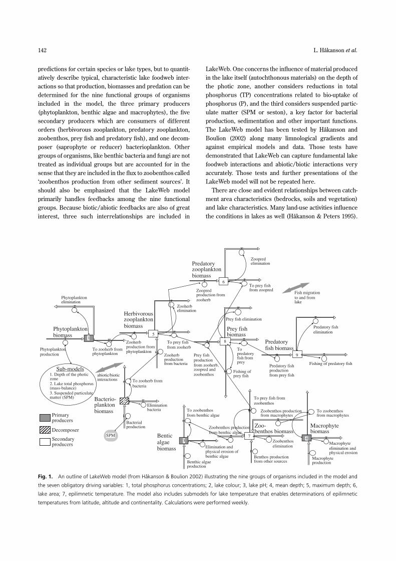
predictions for certain species or lake types, but to quantit-atively describe typical, characteristic lake foodweb inter-actions so that production, biomasses and predation can bedetermined for the nine functional groups of organismsincluded in the model, the three primary producers(phytoplankton, benthic algae and macrophytes), the fivesecondary producers which are consumers of differentorders (herbivorous zooplankton, predatory zooplankton,zoobenthos, prey fish and predatory fish), and one decom-poser (saprophyte or reducer) bacterioplankton. Othergroups of organisms, like benthic bacteria and fungi are nottreated as individual groups but are accounted for in thesense that they are included in the flux to zoobenthos called‘zoobenthos production from other sediment sources’. Itshould also be emphasized that the LakeWeb modelprimarily handles feedbacks among the nine functionalgroups. Because biotic/abiotic feedbacks are also of greatinterest, three such interrelationships are included in

LakeWeb. One concerns the influence of material producedin the lake itself (autochthonous materials) on the depth ofthe photic zone, another considers reductions in totalphosphorus (TP) concentrations related to bio-uptake ofphosphorus (P), and the third considers suspended partic-ulate matter (SPM or seston), a key factor for bacterialproduction, sedimentation and other important functions.The LakeWeb model has been tested by Håkanson andBoulion (2002) along many limnological gradients andagainst empirical models and data. Those tests havedemonstrated that LakeWeb can capture fundamental lakefoodweb interactions and abiotic/biotic interactions veryaccurately. Those tests and further presentations of theLakeWeb model will not be repeated here.

There are close and evident relationships between catch-ment area characteristics (bedrocks, soils and vegetation)and lake characteristics. Many land-use activities influencethe conditions in lakes as well (Håkanson & Peters 1995).

Fig. 1.

An outline of LakeWeb model (from Håkanson & Boulion 2002) illustrating the nine groups of organisms included in the model and

the seven obligatory driving variables: 1, total phosphorus concentrations; 2, lake colour; 3, lake pH; 4, mean depth; 5, maximum depth; 6,

lake area; 7, epilimnetic temperature. The model also includes submodels for lake temperature that enables determinations of epilimnetic

temperatures from latitude, altitude and continentality. Calculations were performed weekly.

Holistic lake management criteria 143

We will provide one scenario on such matters. It deals withalterations in the use of fertilizers in agriculture and howthis influences the transport of P to a lake, the lake concen-tration of P, and the corresponding probable changes in thelake ecosystem structure. We will address how long it takesfor changes in tributary TP concentrations to cause alter-ations in the lake foodweb, whether there are positive andnegative aspects of changes in nutrient loading, and whatcriteria can be applied to answer such questions.

The other scenario concerns climate change, or ratherchanges in mean epilimnetic temperatures and/or incre-ased variations in lake temperature. The LakeWeb modelwill be used to quantify such changes for key functionalorganisms and lake foodweb structures.

At the outset, it must be clearly stressed that thesescenarios will discuss important issues which have beenextensively studied and are covered by numerous public-ations. The aim here is not to make literature compilationson eutrophication or on possible changes to lake eco-systems related to climate changes (Vollenweider &Kerekes 1980; OECD 1982; Reckhow & Chapra 1983;Wetzel & Likens 1990; Håkanson & Peters 1995; Wetzel

2001; Kalff 2002). We will only give very brief literaturecompilations introducing each scenario.

TARGET VARIABLES FOR LAKE MANAGEMENT

A critical area for environmental protection is the develop-ment and implementation of general criteria for the deline-ation of environmental problems. Formal tools are neededto establish what everybody intuitively understands, that allenvironmental disturbances are not of the same size. Fromthe perspective of the ecosystem scale, relatively littleresearch has been devoted to the important but complexproblem of developing scientific criteria to distinguishbetween large and small, real and imaginary problemsrelated to factors which cause alterations in limnologicalstate variables and ecosystem structures.

Ecosystem indices

In environmental management, it is important not to usepersonal viewpoints as criteria to rank threats as a basis foraction, but to try to develop and use more general andobjective approaches. There is a growing awareness thatmuch better individual indicators of environmental healthare necessary because they alone could provide a rationalstructure for decision-making in the environmentalsciences (Bromberg 1990; OECD 1991). An index (anaggregated measure) is generally distinguished from anindicator (a single variable), and an ecosystem (a singleinstance, like a lake) from an ecosystem type (the summa-tion of several or many ecosystems). This section discussesvery briefly one type of environmental index, PER (thePotential Ecosystem Risk number; Håkanson 1999 for morebackground information on PER analysis) in order to illus-trate the following scenario which discusses changes innutrient

loading,

and

to

put

lake

eutrophication

into

awider context concerning chemical threats to aquatic eco-systems. PER is a general, holistic index calculated fromthe geographical extent and duration of a defined change ofan ecosystem effect variable. Certainly, the complexitiesinvolved in establishing simple, practical and meaningfulecological indices sometimes seem insurmountable. Still,the

benefits

of

even

crude

indices

are

so

great

that

theyare well worth pursuing. So long as one can clearly stateone’s criteria, theories and evidence in these complicatedmatters, then these components can be discussed, testedand improved. A frame of reference is required to assessthe status of the environment. Since 1987, many countrieshave accepted ‘sustainable management’ as a goal forenvironmental and economic policy. The term wasintroduced in the final report of the Commission forEnvironment and Development (the Brundtland Com-

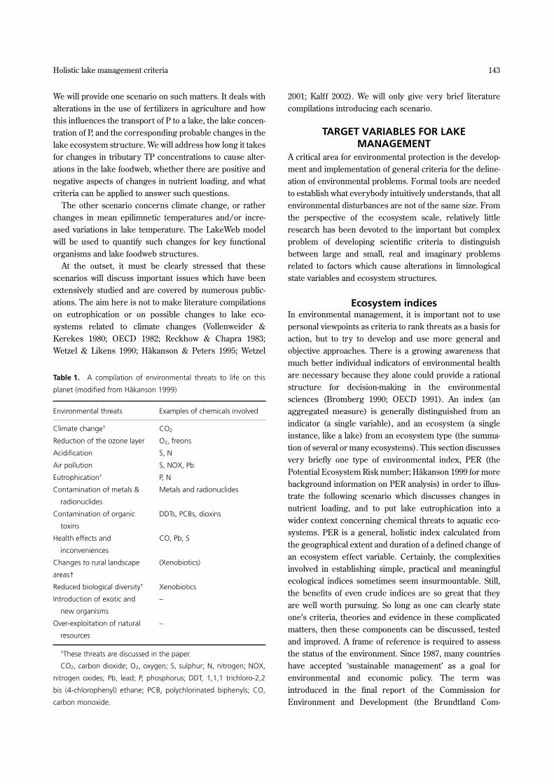
Table 1.

A compilation of environmental threats to life on this

planet (modified from Håkanson 1999)

Environmental threats Examples of chemicals involved

Climate change

†

CO

2

Reduction of the ozone layer O

2

, freons

Acidification S, N

Air pollution S, NOX, Pb

Eutrophication

†

P, N

Contamination of metals &

radionuclides

Metals and radionuclides

Contamination of organic

toxins

DDTs, PCBs, dioxins

Health effects and

inconveniences

CO, Pb, S

Changes to rural landscape

areas†

(Xenobiotics)

Reduced biological diversity

†

Xenobiotics

Introduction of exotic and

new organisms

–

Over-exploitation of natural

resources

–

†

These threats are discussed in the paper.

CO

2

, carbon dioxide; O

2

, oxygen; S, sulphur; N, nitrogen; NOX,

nitrogen oxides; Pb, lead; P, phosphorus; DDT, 1,1,1 trichloro-2,2

bis (4-chlorophenyl) ethane; PCB, polychlorinated biphenyls; CO,

carbon monoxide.

144 L. Håkanson

et al.

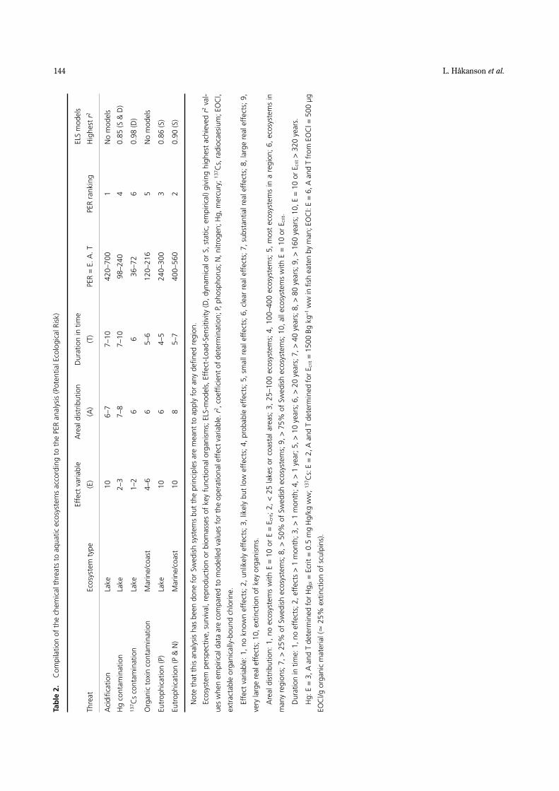
Tab

le 2

.

Com

pila

tion

of t

he c

hem

ical

thr

eats

to

aqua

tic e

cosy

stem

s ac

cord

ing

to t

he P

ER a

naly

sis

(Pot

entia

l Eco

logi

cal R

isk)

Thre

atEc

osys

tem

typ

e

Effe

ct v

aria

ble

(E)

Are

al d

istr

ibut

ion

(A)

Dur

atio

n in

tim

e

(T)

PER

= E

. A. T

PER

rank

ing

ELS

mod

els

Hig

hest

r

2

Aci

dific

atio

nLa

ke10

6–7

7–10

420–

700

1N

o m

odel

s

Hg

cont

amin

atio

nLa

ke2–

37–

87–

1098

–240

40.

85 (S

& D

)

137

Cs

cont

amin

atio

nLa

ke1–

26

636

–72

60.

98 (D

)

Org

anic

tox

in c

onta

min

atio

nM

arin

e/co

ast

4–6

65–

612

0–21

65

No

mod

els

Eutr

ophi

catio

n (P

)La

ke10

64–

524

0–30

03

0.86

(S)

Eutr

ophi

catio

n (P

& N

)M

arin

e/co

ast

108

5–7

400–

560

20.

90 (S

)

Not

e th

at t

his

anal

ysis

has

bee

n do

ne f

or S

wed

ish

syst

ems

but

the

prin

cipl

es a

re m

eant

to

appl

y fo

r an

y de

fined

reg

ion.

Ecos

yste

m p

ersp

ectiv

e, s

urvi

val,

repr

oduc

tion

or b

iom

asse

s of

key

fun

ctio

nal o

rgan

ism

s; E

LS-m

odel

s, E

ffec

t-Lo

ad-S

ensi

tivity

(D,

dyna

mic

al o

r S,

sta

tic, e

mpi

rical

) giv

ing

high

est

achi

eved

r

2

val

-

ues

whe

n em

piric

al d

ata

are

com

pare

d to

mod

elle

d va

lues

for

the

ope

ratio

nal e

ffec

t va

riabl

e.

r

2

, coe

ffici

ent

of d

eter

min

atio

n; P

, pho

spho

rus;

N, n

itrog

en; H

g, m

ercu

ry;

137

Cs,

rad

ioca

esiu

m; E

OC

l,

extr

acta

ble

orga

nica

lly-b

ound

chl

orin

e.

Effe

ct v

aria

ble:

1, n

o kn

own

effe

cts;

2, u

nlik

ely

effe

cts;

3, l

ikel

y bu

t lo

w e

ffec

ts; 4

, pro

babl

e ef

fect

s; 5

, sm

all r

eal e

ffec

ts; 6

, cle

ar r

eal e

ffec

ts; 7

, sub

stan

tial r

eal e

ffec

ts; 8

, lar

ge r

eal e

ffec

ts; 9

,

very

larg

e re

al e

ffec

ts; 1

0, e

xtin

ctio

n of

key

org

anis

ms.

Are

al d

istr

ibut

ion:

1,

no e

cosy

stem

s w

ith E

= 1

0 or

E =

E

crit

; 2,

< 2

5 la

kes

or c

oast

al a

reas

; 3,

25–

100

ecos

yste

ms;

4,

100–

400

ecos

yste

ms;

5,

mos

t ec

osys

tem

s in

a r

egio

n; 6

, ec

osys

tem

s in

man

y re

gion

s; 7

, > 2

5% o

f Sw

edis

h ec

osys

tem

s; 8

, > 5

0% o

f Sw

edis

h ec

osys

tem

s; 9

, > 7

5% o

f Sw

edis

h ec

osys

tem

s; 1

0, a

ll ec

osys

tem

s w

ith E

= 1

0 or

E

crit

.

Dur

atio

n in

tim

e: 1

, no

effe

cts;

2, e

ffec

ts >

1 m

onth

; 3, >

1 m

onth

; 4, >

1 y

ear;

5, >

10

year

s; 6

, > 2

0 ye

ars;

7, >

40

year

s; 8

, > 8

0 ye

ars;

9, >

160

yea

rs; 1

0, E

= 1

0 or

E

crit

> 3

20 y

ears

.

Hg:

E =

3, A

and

T d

eter

min

ed f

or H

g

pi

= E

crit

= 0

.5 m

g H

g/kg

ww

;

137

Cs:

E =

2, A

and

T d

eter

min

ed f

or E

crit

= 1

500

Bg k

g

–

1

ww

in fi

sh e

aten

by

man

; EO

Cl:

E =

6, A

and

T f

rom

EO

Cl =

500

µg

EOC

l/g o

rgan

ic m

ater

ial (

�

25%

ext

inct

ion

of s

culp

ins)

.


mission). However, this phrase is empty unless it is definedin terms of operationally measurable properties, desiredgoals and relevant data. There are alternatives to choosingthe ecosystem as the basis for environmental typology(O’Neill

et al

. 1982; Cairns & Pratt 1987). There is,however, a clear international trend towards considerationof the health of the different ecosystems (Bailey

et al

.1985).

Table 1 gives a compilation of all major threats to life onplanet

Earth.

Ten

of

these

12

threats

involve

chemicals.A set of ecological effect variables is expected to reflectsuch threats and the extent to which they affect the eco-system. Note the difference between biological effects forindividual animals or organs and ecological effects forentire ecosystems. According to Håkanson & Peters(1995), practically useful, operational effect variablesshould be:1. Measurable, preferably simply and inexpensively.2. Clearly interpretable and predictable by validated

quantitative models.3. Internationally applicable.4. Relevant for the given environmental threat.5. Representative for the given ecosystem.

Ideally, environmental effect variables should be compre-hensible without expert knowledge. In fact, one reason todevelop such measures is so that politicians and the generalpublic can understand the present condition and futurechanges in the environment.

The

creation

of

an

ecosystem

index

requires

aggre-gation of information. For example, if the indices for allecosystems in a region are averaged, this figure is then aregional ecosystem index. A still higher level of aggre-gation is obtained if one sums (or averages) the regionalindices for each ecosystem type (for lakes, forests andagricultural land) into a single regional or national environ-mental state index. Such an aggregated index wouldcomplement the picture of the country’s economic develop-ment given by the gross national product. An importantstep in delineating environmental problems is to identifythe effects associated with various perturbations. If weselect the example of different heavy metals in freshwaters, one might assume that the mercury (Hg) problemshould have high priority in many countries, but one shouldask what criteria allow us to make this ranking? Can the Hgproblem in fresh waters be compared with other national,regional and local environmental problems? Probably, wewill never know enough to have scientifically unassailablecriteria for delineating all environmental disturbances, butwe may be able to group disturbances into classes ofdifferent priority. It would be of great value if we could, atleast, establish a number of priority classes and accurately

explain the criteria of classification. Naturally, when usingan analysis on the ecosystem level (for example, for entirelakes), it is not possible to explain many phenomena thatoccur on the individual, organ or cell levels. For example,in the PER analysis, one follows a specific scheme ofaddressing questions. For each problem (for example,acidification, eutrophication or contamination) questionsare first asked about:1. The effect variable (E).2. The geographical or areal extent (A) of the effect

variable.3. The temporal extent, or duration (T) of the effect

variable.

The effect variable

In this system (see Table 2), the E value should vary from1 (no effect) to 10. E = 10 means that a given threat in a realecosystem (not in the laboratory or in model simulationsusing higher concentrations than the maximum valuesrecorded in real ecosystems) has caused a total change(100% reduction) in abundance of a defined key functionalorganism in at least one ecosystem. The grading from 1–10is given in Table 2. The PER systems can be seen as ananalogy to the well-known and practically useful Richterscale for quantifying seismic events. Note that an eco-system is an entire lake or a whole, defined coastal areawhere a certain set of key functional groups prevail. Theboundaries of a lake constitute the natural limitations forthe lake as an ecosystem in this context. However, a verylarge lake (> 300 km

2

) might have to be divided into partswhere different key functional groups dominate. Forexample, a large shallow bay might have to be separatedfrom the open water area. It is often more difficult to definethe limitation for other types of ecosystems with open and/or diffuse boundaries, like forests, rivers and coastal areas.When E < 10, it is important to seek an operationalguideline value for E (E

crit

, which can be, for example, aguideline concentration of a toxin in fish) for the determin-ations of the areal and temporal extent. The motivation forsuch E

crit

values is very important because it relates to thepractical applicability of the method.

The geographical or areal extent of the effect variable

The classes are given in Table 2. Note that the selectedregion for environmental management in the examplesgiven in Table 2 is the country of Sweden, but this partic-ular selection has very little to do with the basic principlesof the overall PER analysis. These principles are meant to

146 L. Håkanson

et al.

be generally applicable for any country, defined region orecosystem type.

The temporal extent, or duration, of the problem

These classes are given in Table 2. In the PER approach,where chemicals are assessed at the ecosystem level, the Eor the E

crit

value can also be determined by means ofspecific ecotoxicological or physiological tests (Boudou &Ribeyre 1989a,b; Gottofrey 1990; Wicklund 1990; Burton1992; International Council on Metals and the Environment1995). The PER value depends on defined and measuredecological effects for given ecosystems; for example, E1 inlake X, E2 in lake Y. PER increases when the E valueincreases reflecting the amount of virulence of a givencontaminant load, but PER also depends on both the arealextent and the duration in time. The greater the arealdistribution, the higher the PER value (then a given E1appears in many lakes in a region) and the longer the effectlasts, the higher the PER value (then the given E1 lasts forN years in lake X).

The complicated nature of ecosystems makes it verydifficult indeed to carry out causal, mechanistic analysesconcerning the quantitative linkages between a giventhreat (like increased nutrient loading) and variablesexpressing ecosystem effects. Mathematical modelling is

the only tool that allows quantitative dynamical (time-dependent) predictions. This means that it is very impor-tant to define operational management targets and to applya structured analysis in order to model such target vari-ables. This is, we would argue, the main benefit of theLakeWeb model – that it can be an important tool for suchstructured analyses. One objective of this paper is todemonstrate this point.

An important aspect of the information in Table 2 is thestructure to ask questions and analyse the threats. Thisstructure is meant to be simple and useful for most types ofthreats and for most types of ecosystems. The basic idea isto use the PER criteria to minimize the element of sub-jectivity and maximize the element of objectivity in thesevery complicated matters where expert judgement isimportant and full ‘objectivity’ can never be obtained. Theidea is to have a general scientific framework for manage-ment to rank different threats so that time and effort can bedirected to the large problems. According to the PERcriteria, one can note that acidification is the largestchemical

threat

to

Swedish

aquatic

ecosystems,

followedby coastal and lake eutrophication, and Hg contaminationof lakes. So, these results have motivated the selection ofthe following scenarios. The smallest problem in the surveygiven in Table 2 is the radiocaesium (

137

Cs) contaminationfollowing

the

Chernobyl

accident

of

1986

because

thereare no established, or even likely, effects on aquatic eco-

Table 3.

Compilation of general operational targets for lake management

Basic management objectives Target variables (y

i

) Fundamental abiotic variables (x

i

)

Conservation, water quality, Algal volume Suspended particulate matter

drinking water, irrigation Secchi depth TP concentration

Bacterioplankton biomass Lake pH

Chlorophyll

a

concentration

(Number of coliform bacteria)

†

Lake morphometry (area, volume, mean depth,

maximum depth)

Catchment characteristics (size, precipitation,

latitude)

Recreation Algal volume

(angling, swimming etc.) Secchi depth

Maximum phytoplankton biomass

Chlorophyll

a

concentration

Macrophyte cover or biomass

Bacterioplankton biomass

(Cyanobacteria biomass)

†

Fishery (professional Fish biomass (predatory fish biomass)

fishing and aquaculture) (Toxic substances in fish e.g.

137

Cs, Hg)

†

(Target fish species biomass)†

†

Important variables not yet included in the LakeWeb model.

TP, total phosphate,

137

Cs, radiocaesium; Hg, mercury.


systems from this threat in Swedish lakes. The arealdistribution of the

137

Cs problem concerns not the entirecountry but certain regions, and the duration of theproblem could be seen in terms of a few decades ratherthan centuries.

The result of the PER ranking, that is, the overall rankingof these major threats under the given presuppositions, isgiven in Table 2. Acidification of freshwater ecosystems(PER = 420–700, depending on how the areal distribution isdefined and calculated) > eutrophication of coastal eco-systems (PER = 400–560) > eutrophication of freshwaterecosystems (PER = 240–300) > Hg contamination of lakes(PER = 98–240) > contamination of organic toxins in theBaltic Sea (PER = 120–220) >

137

Cs contamination of lakes(PER = 36–72).

Note again that the PER approach can be used not justfor Swedish aquatic ecosystems, but for most types ofecosystems in most regions. The proposed approach

provides a general scientific structure for ‘environmentaldiagnosis’ where important elements are: (i) definition ofecosystem; (ii) definition of operational effect variablesrelated to the defined threat; (iii) effect-load-sensitivityanalysis; (iv) integration (or summation) of E or E

crit

overimpact area; and (v) integration (or summation) of E or E

crit

over impact time.

OPERATIONAL VARIABLES FOR LAKE MANAGEMENT

Table 3 gives a compilation of results from a project(Håkanson

et al

. 2000) which had the following goals:1. To

develop

a system of water quality indicesaccording to specific requirements of different waterusers.

2. To establish normal values (corresponding tonatural, reference conditions) of the chosen set ofindices.

Table 4. Operational ranges for ‘critical’ and ‘alarm’ levels in lake management

Variables Critical Alarm

Abiotic limnological state variables

pH change > 1 pH = 5.5 or pH = 9.5

Colour > 50 (mg Pt L–1) change > 2 change > 3

Colour < 50 (mg Pt L–1) change > 2.5 change > 3.5

Total P (µg L–1) change > 1.5 change > 2.5

Standard operational lake management variables

Secchi depth (m) change > 1.5 change > 2.5

Algal volume (mm3 L–1) 5.0 10.0

Chlorophyll a concentration (mg m–3) change > 1.5 change > 2.5

Biomasses (kg ww) of key functional groups of organisms

Phytoplankton change > 1.5 change > 2.5

Bacterioplankton change > 2 change > 3

Benthic algae change > 2 change > 3

Macrophytes change > 1.5 change > 2.5

Zoobenthos change > 2 change > 3

Herbivorous zooplankton change > 1.5 change > 2.5

Predatory zooplankton change > 1.5 change > 2.5

Prey fish change > 1.5 change > 2.5

Predatory fish change > 1.5 change > 2.5

Special lake management variables

Hg content in fish eaten by humans (mg kg–1 ww) 0.5 1.0

Macrophyte cover (%) change > 1.15 change > 1.3

In these environmental consequence analyses, one could use the following system to compare changes in the management target

variables. All changes refer to mean values for the growing season, and not to variations in weekly values. Note that this is not an attempt to

define guideline values or to set management limits. It is meant as an example and the given values for the ‘critical’ limits and the ‘alarm’

limits are meant as reference values indicating the ‘state of alert’ when there is a change in any of the given variables. Also note that this is

not based on individual species, but on functional groups of organisms.

P, phosphorus; Hg, mercury.

148 L. Håkanson et al.

3. To estimate the environmental sensitivity and stabilityof the studied lakes by applying mathematical modelsof fluxes for SPM and P.

Table 3 lists biotic and abiotic target variables for threedifferent categories of water users, that is, from threemanagement perspectives:

The first perspective involves conservation of the lakeecosystem at some steady state allowing efficient use ofwater resources for domestic water supply, irrigation,fisheries etc. Evidently, different users might havedifferent demands on ‘water quality’, different criteria todefine water quality and setting management targets.Fundamental abiotic variables for this category of users areSPM, lake TP concentration, lake pH, as well as data onlake and catchment characteristics. Key biotic variablesinclude algal volume (biomass per volume unit), Secchidepth and bacterioplankton biomass. All these variables areimportant and included in the LakeWeb model. There arealso, of course, important target variables which are notincluded in the present version of the LakeWeb model,such as number of coliform bacteria.

The second perspective is recreation, with a focus onsuitable conditions for angling, swimming, etc. Targetbiotic variables are algal volume, Secchi depth (waterclarity), maximum (rather than mean) phytoplankton bio-mass, chlorophyll a (Chl a) concentration (a simple andoften used operational variable for primary production andwater quality), macrophyte cover (regulating access to theshoreline for recreation), bacterioplankton biomass andnumber of cyanobacteria (blue-greens, which can causedamage to animals and humans), and bacterioplanktonbiomass. All these variables are included in the LakeWebmodel.

The third perspective, fishery, has a focus on biomassand production of ‘attractive’ species of fish with lowconcentrations of toxic substances (such as Hg and 137Cs;see Table 2). In the present version of the LakeWeb model,the purpose is not to predict defined species of fish but‘prey’ fish and ‘predatory’ fish, that is, two fundamentalfunctional groups of fish.

In the following scenarios, we will focus on water qualitychanges in the main target variables for lake managementlisted in Table 3 and how these changes relate to changesin nutrient loading.

For lake management, it is also important to:1. Develop simple but practically useful lake ecosystem

indices as a function of ratios between actual andnormal (ideal) values for biomasses of selected keyfunctional organisms or abiotic targets like SPMconcentration, Secchi depth and TP concentration.

2. Define permissible ranges (lower and upper values) forall target variables. This is done to minimize risks

related to changes in ecosystem structure and bio-diversity.

3. Keep an open dialogue between scientists, policymakers, administrators and the general public basedon facts and reason (rather than feelings and emotionswhich are ingredients in many ‘environmental’ debatesand discussions).

However, it has been beyond the scope of this work todevelop and test such ecosystem or water quality indices,although there are several interesting approaches on thesematters (Hambright et al. 2002). In the following environ-mental consequence analyses, we will use the target vari-ables for lake management listed in Table 3, and the‘permissible’ ranges given in Table 4.

ABIOTIC LAKE MANAGEMENT VARIABLESLake pH

If the mean lake pH is changed (for example, due to acidrain) from a given initial value (generally in the range from6–8) to either of the ‘critical threshold values’ of 5.5 or 9.5(Henrikson & Brodin 1992), this should be a signal thatthere will likely be a major change in the structure of thelake foodweb, and that at least one group of the mostsensitive key functional organisms might be significantlychanged. Using the PER analysis, one could then set the Evalue to 10. So, this is a signal for ‘alarm’. A less strongwarning that a given change in lake pH would be likely toinfluence the survival, reproduction and biomass of keyfunctional organisms would be if the mean, characteristiclake pH value is changed by one pH unit from the initial(normal, reference) value. This is then a ‘critical’ change.Note that the terms ‘critical’ and ‘alarm’ are meant to bemeaningful in communications between scientists, journal-ists, the general public and environmental politicians. Thegiven limits should be based on expert judgement. Theselimits could then always be criticized and altered by newdata and results.

ColourIf the mean, characteristic initial lake colour value is higherthan 50 mg Pt L–1, and if there is a change from such a givenvalue by a factor of 2, this might be regarded as a criticalchange (Håkanson & Peters 1995). A change by a factor of3 might be regarded as a signal for alarm. If the mean,characteristic initial lake colour value is lower than50 mg Pt L–1, and if there is a change by a factor of 2.5, thismight be regarded as critical, and a change by a factor of 3could be regarded as a signal for alarm.

PhosphorusIf the mean initial TP concentration is changed by naturalor anthropogenic reasons from a given value by a factor of


1.5, this might be regarded as critical while a change by afactor of 2.5 might be regarded as a signal for alarm. Thesefactors are meant to be simple and realistic values relatedto the trophic level categories presented by Håkanson andBoulion (2002).

We will also use three standard operational lake manage-ment variables.

Secchi depthNote that Secchi depth and SPM include both biotic andabiotic components; for example, living and dead phyto-plankton. If the mean Secchi depth is changed from a givenvalue by a factor of 1.5, this might be regarded as a criticalchange while a change by a factor of 2.5 might be regardedas a signal for alarm (Håkanson & Boulion 2002).

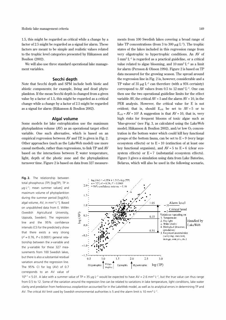
Algal volumeSome models for lake eutrophication use the maximumphytoplankton volume (AV) as an operational target effectvariable. One such alternative, which is based on anempirical regression between AV and TP, is given in Fig. 2.Other approaches (such as the LakeWeb model) use morecausal methods, rather than regressions, to link TP and AVbased on the interactions between P, water temperature,light, depth of the photic zone and the phytoplanktonturnover time. Figure 2 is based on data from 327 measure-

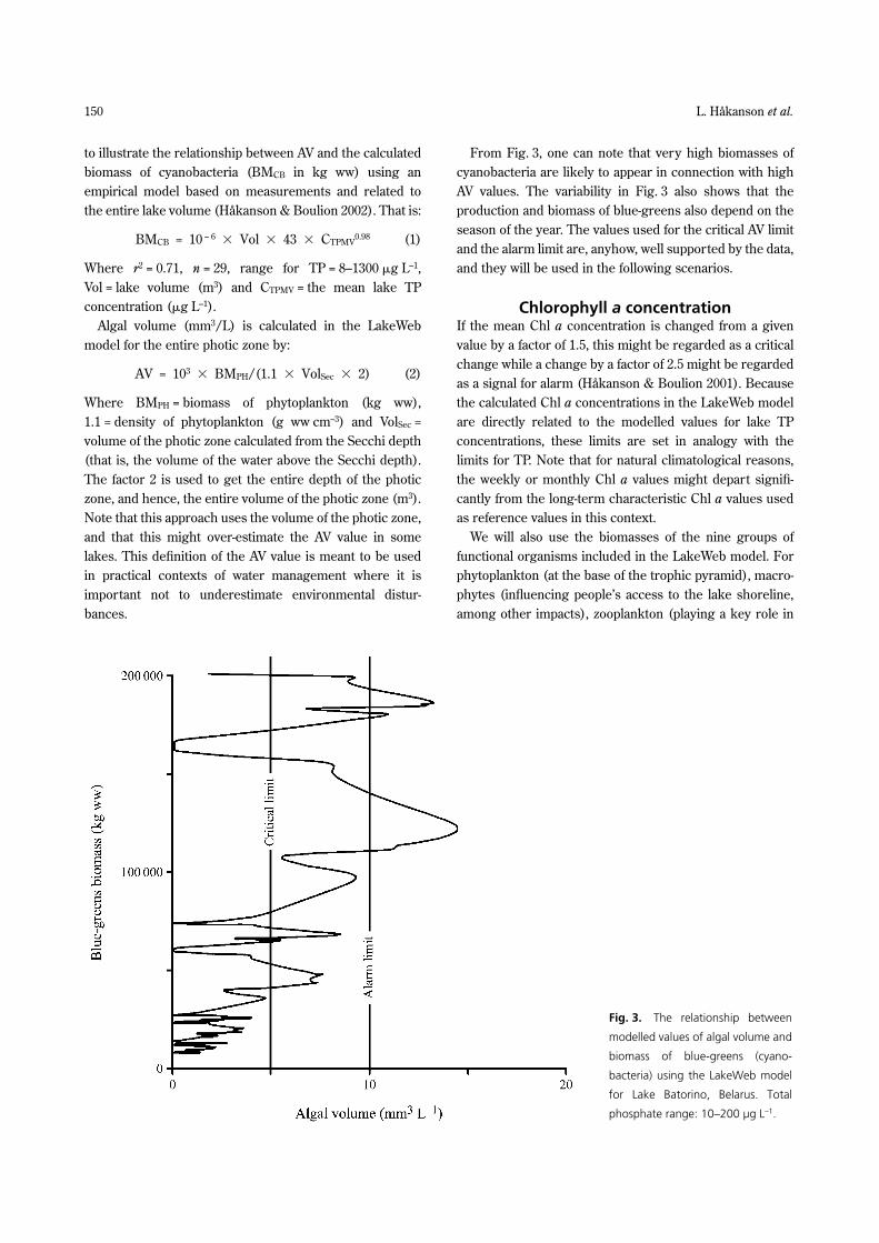
ments from 100 Swedish lakes covering a broad range oflake TP concentrations (from 3 to 300 �g L–1). The trophicstates of the lakes included in this regression range fromvery oligotrophic to hypertrophic conditions. An AV of5 mm3 L–1 is regarded as a practical guideline, or a criticalvalue related to algae blooming, and 10 mm3 L–1 as a limitfor alarm (Persson & Olsson 1994). Figure 2 is based on TPdata measured for the growing season. The spread aroundthe regression line in Fig. 2 is, however, considerable and aTP value of 35 �g L–1 can therefore (with a 95% certainty)correspond to AV values from 0.5 to 12 mm3 L–1. One canthen use the two operational guideline limits for the effectvariable AV, the critical AV = 5 and the alarm AV = 10, in thePER analysis. However, the critical value for E is notevident; that is, should Ecrit be set to AV = 5 or toEcrit = AV = 10? A suggestion is that AV = 10, that is, veryhigh risks for frequent blooms of toxic algae such as‘blue-greens’ (see Fig. 3, as calculated using the LakeWebmodel; Håkanson & Boulion 2002), and/or low O2 concen-tration in the bottom water which could kill key functionalgroups of the bottom fauna, can be set to E = 9 (very largeecosystem effects) or to E = 10 (extinction of at least onekey functional organism), and AV = 5 to E = 6 (clear eco-system effects) or E = 7 (substantial ecosystem effects).Figure 3 gives a simulation using data from Lake Batorino,Belarus, which will also be used in the following scenario,

Fig. 2. The relationship between

total phosphorus (TP) [log(TP); TP in

µg L–1; mean summer values] and

maximum volume of phytoplankton

during the summer period [log(AV);

algal volume, AV, in mm3 L–1]. Based

on unpublished data from E. Willén

(Swedish Agricultural University,

Uppsala, Sweden). The regression

line and the 95% confidence

intervals (CI) for the predicted y show

that there exists a very strong

(r2 = 0.76, P < 0.0001) general rela-

tionship between the x-variable and

the y-variable for these 327 mea-

surements from 100 Swedish lakes,

but there is also a substantial residual

variation around the regression line.

The 95% CI for log (AV) of 0.7

corresponds to an AV value of

100.7 = 5.01. A lake with a summer value of TP = 35 µg L–1 would be expected to have AV = 2.6 mm3 L–1, but the true value can thus range

from 0.5 to 12. Some of the variation around the regression line can be related to variations in lake temperature, light conditions, lake water

clarity and predation from herbivorous zooplankton accounted for in the LakeWeb model, as well as to analytical errors in determining TP and

AV. The critical AV limit used by Swedish environmental authorities is 5 and the alarm limit is 10 mm3 L–1.


to illustrate the relationship between AV and the calculatedbiomass of cyanobacteria (BMCB in kg ww) using anempirical model based on measurements and related tothe entire lake volume (Håkanson & Boulion 2002). That is:

BMCB = 10 – 6 � Vol � 43 � CTPMV0.98 (1)

Where r2 = 0.71, n = 29, range for TP = 8–1300 �g L–1,Vol = lake volume (m3) and CTPMV = the mean lake TPconcentration (�g L–1).

Algal volume (mm3/L) is calculated in the LakeWebmodel for the entire photic zone by:

AV = 103 � BMPH/(1.1 � VolSec � 2) (2)

Where BMPH = biomass of phytoplankton (kg ww),1.1 = density of phytoplankton (g ww cm–3) and VolSec =volume of the photic zone calculated from the Secchi depth(that is, the volume of the water above the Secchi depth).The factor 2 is used to get the entire depth of the photiczone, and hence, the entire volume of the photic zone (m3).Note that this approach uses the volume of the photic zone,and that this might over-estimate the AV value in somelakes. This definition of the AV value is meant to be usedin practical contexts of water management where it isimportant not to underestimate environmental distur-bances.

From Fig. 3, one can note that very high biomasses ofcyanobacteria are likely to appear in connection with highAV values. The variability in Fig. 3 also shows that theproduction and biomass of blue-greens also depend on theseason of the year. The values used for the critical AV limitand the alarm limit are, anyhow, well supported by the data,and they will be used in the following scenarios.

Chlorophyll a concentrationIf the mean Chl a concentration is changed from a givenvalue by a factor of 1.5, this might be regarded as a criticalchange while a change by a factor of 2.5 might be regardedas a signal for alarm (Håkanson & Boulion 2001). Becausethe calculated Chl a concentrations in the LakeWeb modelare directly related to the modelled values for lake TPconcentrations, these limits are set in analogy with thelimits for TP. Note that for natural climatological reasons,the weekly or monthly Chl a values might depart signifi-cantly from the long-term characteristic Chl a values usedas reference values in this context.

We will also use the biomasses of the nine groups offunctional organisms included in the LakeWeb model. Forphytoplankton (at the base of the trophic pyramid), macro-phytes (influencing people’s access to the lake shoreline,among other impacts), zooplankton (playing a key role in

Fig. 3. The relationship between

modelled values of algal volume and

biomass of blue-greens (cyano-

bacteria) using the LakeWeb model

for Lake Batorino, Belarus. Total

phosphate range: 10–200 µg L–1.


the lake foodweb) and fish (at the top of the lake nutrientpyramid), one can use the same management limits tocompare changes. So, if these biomasses are changed froma given mean value by a factor of 1.5, this can be regardedas a critical change while a change by a factor of 2.5 canbe regarded as a signal for alarm. For bacterioplankton,benthic algae and zoobenthos, we suggest that one can useslightly different criteria to compare changes. If the meansummer biomasses are changed from a given value by afactor of 2, this can be regarded as a critical change while achange by a factor of 3 can be regarded as a signal foralarm.

In the following scenario, we will also use a special lakemanagement variable, the macrophyte cover (in percent-age of the lake area). If the long-term characteristic macro-phyte cover is changed from a given value by a factor of1.15, this might be regarded as a critical change while achange by a factor of 1.3 might be regarded as a signal foralarm. Note that dramatic changes in macrophyte cover canoccur due to ice movement during winter and spring, andsuch natural changes are not included in this definition.

In other contexts of lake management, one can use otherspecial variables like Hg concentration in fish (see Table 4),water salinity and number of coliform bacteria.

PRACTICAL SCENARIOSScenario 1: Changes in agriculture and

oligotrophication, Lake Batorino, BelarusThe following two case studies concern Lake Batorino,Belarus (see Table 5). The aim is to model the changes inthe lake foodweb related to the drastic and sudden changesin agricultural land use practices in 1990. The next scenarioon changes in temperature will use the same lake to getcomparability with this scenario.

The presuppositions for the oligotrophication scenarioare given in Fig. 4(a), curve 1, illustrating the suddenchange in tributary TP concentration at week 521 inJanuary 1990 (week 1 is the first week of 1980 so thesimulation covers a period of 20 years). There are reliableempirical data for this scenario giving mean characteristicannual values, first for the period 1980–1989 and thenfrom 1990 to 1999, for lake TP concentrations (curve 3 inFig. 4(a)), Chl a (curve 2 in Fig. 4(b)) and Secchi depth(curve marked in Fig. 4(c)). The question regarding whichtributary TP concentrations would give the best correlationwith the empirical data on TP, Chl a and Secchi depth isaddressed next.

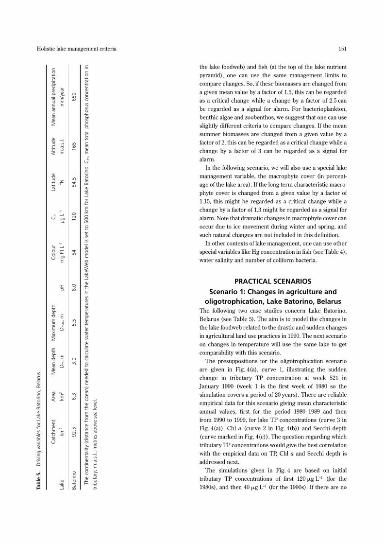
The simulations given in Fig. 4 are based on initialtributary TP concentrations of first 120 �g L–1 (for the1980s), and then 40 �g L–1 (for the 1990s). If there are noTa

ble

5.

Driv

ing

varia

bles

for

Lak

e Ba

torin

o, B

elar

us

Lake

Cat

chm

ent

km2

Are

a

km2

Mea

n de

pth

Dm, m

Max

imum

dep

th

Dm

ax, m

pH

Col

our

mg

Pt L

–1

Cin

µg L

–1

Latit

ude

�N

Alti

tude

m.a

.s.l.

Mea

n an

nual

pre

cipi

tatio

n

mm

/yea

r

Bato

rino

92.5

6.3

3.0

5.5

8.0

5412

054

.516

565

0

The

cont

inen

talit

y (d

ista

nce

from

the

oce

an)

need

ed t

o ca

lcul

ate

wat

er t

empe

ratu

res

in t

he L

akeW

eb m

odel

is s

et t

o 50

0 km

for

Lak

e Ba

torin

o. C

in,

mea

n to

tal p

hosp

horu

s co

ncen

trat

ion

in

trib

utar

y; m

.a.s

.l., m

etre

s ab

ove

sea

leve

l.


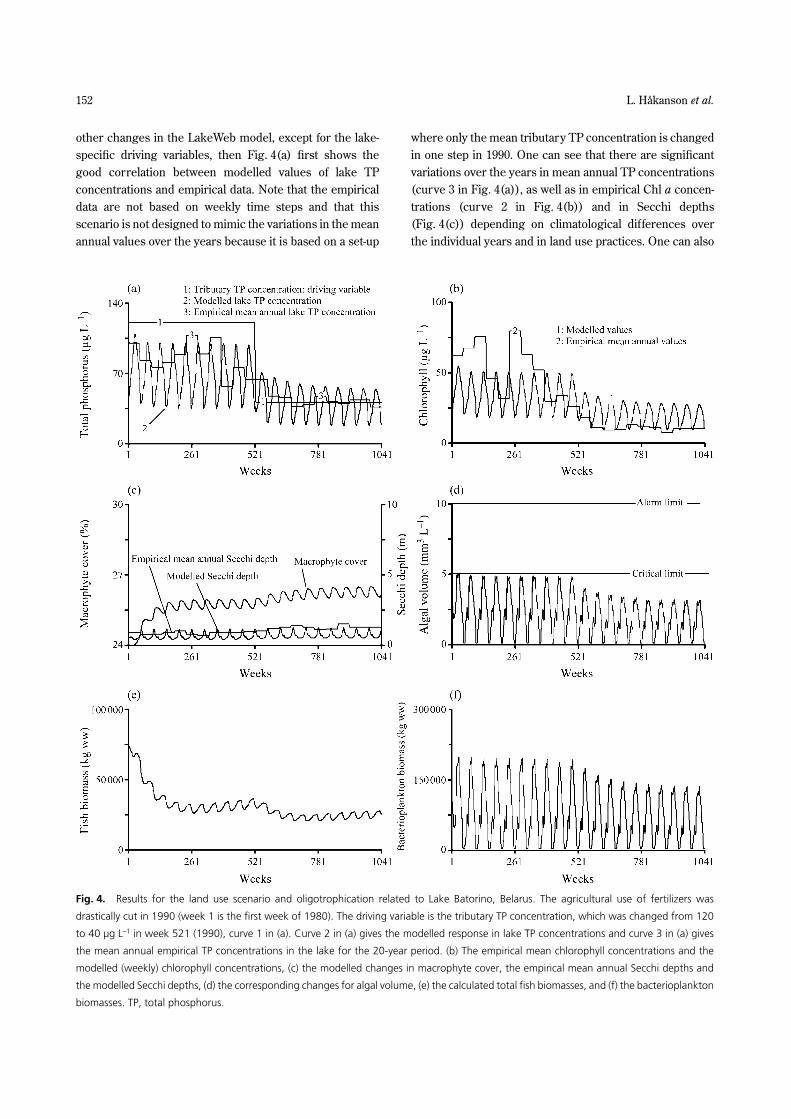
other changes in the LakeWeb model, except for the lake-specific driving variables, then Fig. 4(a) first shows thegood correlation between modelled values of lake TPconcentrations and empirical data. Note that the empiricaldata are not based on weekly time steps and that thisscenario is not designed to mimic the variations in the meanannual values over the years because it is based on a set-up

where only the mean tributary TP concentration is changedin one step in 1990. One can see that there are significantvariations over the years in mean annual TP concentrations(curve 3 in Fig. 4(a)), as well as in empirical Chl a concen-trations (curve 2 in Fig. 4(b)) and in Secchi depths(Fig. 4(c)) depending on climatological differences overthe individual years and in land use practices. One can also

Fig. 4. Results for the land use scenario and oligotrophication related to Lake Batorino, Belarus. The agricultural use of fertilizers was

drastically cut in 1990 (week 1 is the first week of 1980). The driving variable is the tributary TP concentration, which was changed from 120

to 40 µg L–1 in week 521 (1990), curve 1 in (a). Curve 2 in (a) gives the modelled response in lake TP concentrations and curve 3 in (a) gives

the mean annual empirical TP concentrations in the lake for the 20-year period. (b) The empirical mean chlorophyll concentrations and the

modelled (weekly) chlorophyll concentrations, (c) the modelled changes in macrophyte cover, the empirical mean annual Secchi depths and

the modelled Secchi depths, (d) the corresponding changes for algal volume, (e) the calculated total fish biomasses, and (f) the bacterioplankton

biomasses. TP, total phosphorus.


note the good overall correlation between the modelledvalues and the empirical data, not just for TP, but also forChl a and Secchi depth. So, the main conclusion is that thismodelling set-up will capture the essential elements of thelake oligotrophication process in this lake.

Then, one can ask about the changes for fundamentallake management variables, like macrophyte cover, algalvolume, fish biomass and bacterioplankton biomass. Lakemanagers responsible for recreation would like the macro-phyte cover to be as small as possible so that the people

visiting the lake for recreational purposes can more easilyaccess the shoreline and beaches. Managers responsiblefor leisure time and professional fishing would like the fishbiomass to be high. Few persons would like the biomass ofbacterioplankton to be high, except maybe scientists inter-ested in feeding behaviour of herbivorous zooplankton.

From Fig. 4(c), one can note that the oligotrophicationwould be likely to cause an increase in macrophyte cover(by 1–2%), the algal volume would go down from valuesaround the critical limit to values clearly below the critical

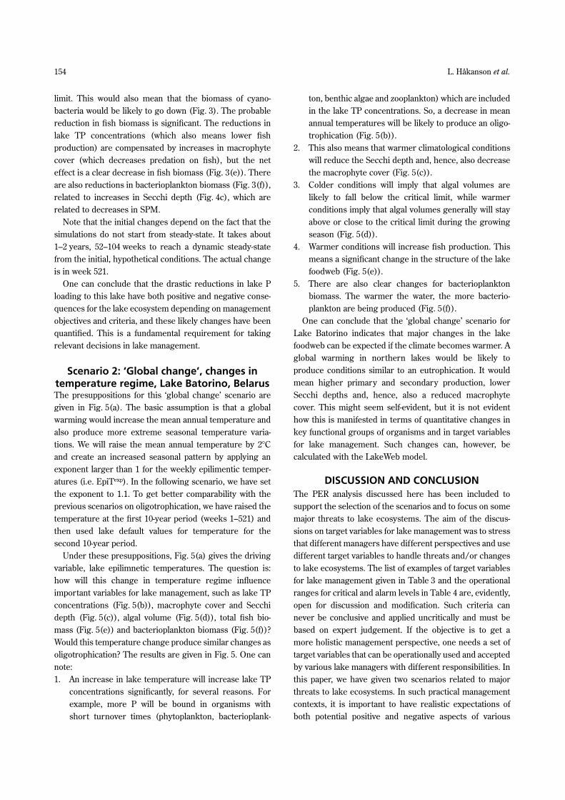
Fig. 5. Results for the ‘global change’ scenario related lake temperature changes in Lake Batorino, Belarus. The driving variable is the

epilimnetic temperature, as given by (a). The mean annual epilimnetic temperature was raised by 2�C and the range in the weekly epilimnetic

temperatures (EpiT) was increased by the exponent 1.1 (EpiT1.1). (b) The modelled changes in lake TP concentrations, (c) the calculated changes

in macrophyte cover and Secchi depth, (d) the corresponding changes for algal volume, (e) the calculated changes in predatory fish biomass,

and (f) the modelled changes in bacterioplankton biomass. TP, total phosphorus.


limit. This would also mean that the biomass of cyano-bacteria would be likely to go down (Fig. 3). The probablereduction in fish biomass is significant. The reductions inlake TP concentrations (which also means lower fishproduction) are compensated by increases in macrophytecover (which decreases predation on fish), but the neteffect is a clear decrease in fish biomass (Fig. 3(e)). Thereare also reductions in bacterioplankton biomass (Fig. 3(f)),related to increases in Secchi depth (Fig. 4c), which arerelated to decreases in SPM.

Note that the initial changes depend on the fact that thesimulations do not start from steady-state. It takes about1–2 years, 52–104 weeks to reach a dynamic steady-statefrom the initial, hypothetical conditions. The actual changeis in week 521.

One can conclude that the drastic reductions in lake Ploading to this lake have both positive and negative conse-quences for the lake ecosystem depending on managementobjectives and criteria, and these likely changes have beenquantified. This is a fundamental requirement for takingrelevant decisions in lake management.

Scenario 2: ‘Global change’, changes in temperature regime, Lake Batorino, BelarusThe presuppositions for this ‘global change’ scenario aregiven in Fig. 5(a). The basic assumption is that a globalwarming would increase the mean annual temperature andalso produce more extreme seasonal temperature varia-tions. We will raise the mean annual temperature by 2�Cand create an increased seasonal pattern by applying anexponent larger than 1 for the weekly epilimentic temper-atures (i.e. EpiTexp). In the following scenario, we have setthe exponent to 1.1. To get better comparability with theprevious scenarios on oligotrophication, we have raised thetemperature at the first 10-year period (weeks 1–521) andthen used lake default values for temperature for thesecond 10-year period.

Under these presuppositions, Fig. 5(a) gives the drivingvariable, lake epilimnetic temperatures. The question is:how will this change in temperature regime influenceimportant variables for lake management, such as lake TPconcentrations (Fig. 5(b)), macrophyte cover and Secchidepth (Fig. 5(c)), algal volume (Fig. 5(d)), total fish bio-mass (Fig. 5(e)) and bacterioplankton biomass (Fig. 5(f))?Would this temperature change produce similar changes asoligotrophication? The results are given in Fig. 5. One cannote:1. An increase in lake temperature will increase lake TP

concentrations significantly, for several reasons. Forexample, more P will be bound in organisms withshort turnover times (phytoplankton, bacterioplank-

ton, benthic algae and zooplankton) which are includedin the lake TP concentrations. So, a decrease in meanannual temperatures will be likely to produce an oligo-trophication (Fig. 5(b)).

2. This also means that warmer climatological conditionswill reduce the Secchi depth and, hence, also decreasethe macrophyte cover (Fig. 5(c)).

3. Colder conditions will imply that algal volumes arelikely to fall below the critical limit, while warmerconditions imply that algal volumes generally will stayabove or close to the critical limit during the growingseason (Fig. 5(d)).

4. Warmer conditions will increase fish production. Thismeans a significant change in the structure of the lakefoodweb (Fig. 5(e)).

5. There are also clear changes for bacterioplanktonbiomass. The warmer the water, the more bacterio-plankton are being produced (Fig. 5(f)).

One can conclude that the ‘global change’ scenario forLake Batorino indicates that major changes in the lakefoodweb can be expected if the climate becomes warmer. Aglobal warming in northern lakes would be likely toproduce conditions similar to an eutrophication. It wouldmean higher primary and secondary production, lowerSecchi depths and, hence, also a reduced macrophytecover. This might seem self-evident, but it is not evidenthow this is manifested in terms of quantitative changes inkey functional groups of organisms and in target variablesfor lake management. Such changes can, however, becalculated with the LakeWeb model.

DISCUSSION AND CONCLUSIONThe PER analysis discussed here has been included tosupport the selection of the scenarios and to focus on somemajor threats to lake ecosystems. The aim of the discus-sions on target variables for lake management was to stressthat different managers have different perspectives and usedifferent target variables to handle threats and/or changesto lake ecosystems. The list of examples of target variablesfor lake management given in Table 3 and the operationalranges for critical and alarm levels in Table 4 are, evidently,open for discussion and modification. Such criteria cannever be conclusive and applied uncritically and must bebased on expert judgement. If the objective is to get amore holistic management perspective, one needs a set oftarget variables that can be operationally used and acceptedby various lake managers with different responsibilities. Inthis paper, we have given two scenarios related to majorthreats to lake ecosystems. In such practical managementcontexts, it is important to have realistic expectations ofboth potential positive and negative aspects of various


potential actions. It is also important to be able to compareconsequences of such actions to natural causes for vari-ability. We have demonstrated by these case studies howthe LakeWeb model can be used in practice for suchsimulations. Evidently, we have not addressed and dis-cussed all aspects of lake eutrophication, oligotrophicationand land use changes, but we have tried to illustrate thegreat potential that the LakeWeb model offers for suchenvironmental consequence analyses. We also hope that wehave demonstrated the great future possibilities of usingthe LakeWeb model in other situations, such as for rivers,big lakes and coastal bays. Many of the tested features inthe LakeWeb model are general and can be used withrelative ease in other contexts.

ACKNOWLEDGEMENTSThese studies were carried out partly with support of theRussian Foundation for Basic Research (Project 00-15-97825) and Biodiversity Grant, and partly within the frame-work of an INTAS project – ‘Development of a system ofwater quality indices for lakes as a tool for management’.We would also like to thank Tatiana Zukova for all datarelated to the Belarus lake.

REFERENCESBailey R. G., Zoltan S. & Wiken E. B. (1985) Ecological

regionalization in Canada and the United States.Geoforum 16, 265–75.

Boudou A. & Ribeyre F. (1989a) Aquatic Ecotoxicology,Vol. 1. CBC Press, Boca Raton.

Boudou A. & Ribeyre F. (1989b) Aquatic Ecotoxicology,Vol. 2. CBC Press, Boca Raton.

Bromberg S. (1990) Identifying ecological indicators: Anenvironmental monitoring and assessment program.J. Air Waste Manage. Assoc. 40, 976–87.

Burton G. A. Jr (ed.). (1992) Sediment Toxicity Assessment.Lewis, Boca Raton.

Cairns J. Jr & Pratt J. R. (1987) Ecotoxicological effectindices: a rapidly evolving system. Wat. Sci. Techn 19,1–12.

Gottofrey J. (1990) The disposition of cadmium, nickel,mercury and methylmercury in fish and effects of lipo-philic metal chelation. Unpublished Thesis. SwedishAgricultural University, Uppsala.

Håkanson L. (1999) Water Pollution – Methods and Criteriato Rank, Model and Remediate Chemical Threats toAquatic Ecosystems. Backhuys Publishers, Leiden.

Håkanson L. & Boulion V. V. (2001) Regularities in primaryproduction, Secchi depth and fish yield and a new sys-tem to define trophic and humic state indices for aquaticecosystems. Internat. Rev. Hydrobiol. 86, 23–62.

Håkanson L. & Boulion V. V. (2002) The Lake Foodweb –Modelling Predation and Abiotic/Biotic Interactions.Backhuys Publishers, Leiden.

Håkanson L., Parparov A., Ostapenia A. & Boulion V. V.(2000) Development of a system of water quality as atool for management. Final report to INTAS. Depart-ment of Earth Science, Uppsala University, Uppsala,Sweden. No. 2000–11–07.

Håkanson L. & Peters R. H. (1995) Predictive Limnology.Methods for Predictive Modelling. SPB AcademicPublishing, Amsterdam.

Hambright K. D., Parparov A. & Berman T. (2003) Indicesof water quality for sustainable management andconservation of an arid region lake, Lake Kinneret(Sea of Galileee). Israel. Aquat. Conserv. Mar. Freshwat.Ecosyst. (in press).

Henrikson L. & Brodin Y. W. (eds). (1992) Liming ofAcidified Surface Waters. A Swedish Synthesis. Springer-Verlag, Berlin.

International Council on Metals and the Environment(1995) Persistence, bioaccumulation and toxicity ofmetals and metal compounds. Parametrix.

Kalff J. (2002) Limnology. Prentice Hall, New Jersey.O’Neill R. V., Gardner R. H., Barnthouse L. W., Suter

G. W., Hildebrand S. G. & Gehrs C. W. (1982) Eco-system risk analysis: a new methodology. Environ. Tox.Chem. 1, 167–77.

OECD (1982) Eutrophication of Waters. Monitoring,Assessment and Control. OECD, Paris.

OECD (1991) Environmental Indicators. OECD, Paris.Persson G. & Olsson H. (1994) Eutrofiering I Svenska

Sjöar Och Vattendrag – Tillstånd, Utveckling, OrsakOch Verkan. Swedish Environmental ProtectionAgency, Stockholm. No. 4147.

Reckhow K. H. & Chapra S. C. (1983) EngineeringApproaches to Lake Management, Vol. 1. Butterworth,Woburn, MS, USA.

Vollenweider R. A. & Kerekes J. (1980) OECD cooperativeprogramme for monitoring of inland waters. Eutrophic-ation control. Synthesis Report. OECD, Paris.

Wetzel R. G. (2001) Limnology. Academic Press, London.Wetzel R. G. & Likens G. E. (1990) Limnological Analyses.

Springer, Heidelberg.Wicklund A. (1990) Metabolism of cadmium and zinc in

fish. Unpublished Thesis. Uppsala University, Sweden.

Management criteria for lake ecosystems applied to case ...

Documents

Transcript of Management criteria for lake ecosystems applied to case ...