Magnetism and AC Fundamentals

MODULE 2 EE100 Basics of Electrical Engineering

of 15

MAGNETIC CIRCUITS

Magnet is a material which has the property of attracting iron pieces. This property is called

magnetism.

When a magnet is suspended freely, it will align itself in the north-south direction of earth. The

tip of the magnet pointing north is called north pole and the tip pointing the south is called the

south pole of the magnet.

Magnetic Field : It is the region around a magnet within which the influence of the

magnet can be experienced.

Magnetic Lines of Force : These are the imaginary lines surrounding the magnet which

represent the magnetic field. The lines of force always flown from North pole to South

pole of the magnet.

Magnetic Flux (ϕ) : The total number of magnetic lines of force existing in a particulat

magnetic field is called magnetic flux. The unit of flux is Weber (Wb).

1 Weber = 108 lines of force.

Magnetic Flux Density (B) : It is defined as the flux per unit area.

B = ϕ

𝑎 ; Unit : Wb/m2 or Tesla (T)

Magnetic Field Strength (H) : The force experienced by a unit north pole when placed

at any point in magnetic field is known as Magnetic field strength at that point.

H = Ampere Turns

Length=

N I

𝑙 ; Unit = AT/m


of 15

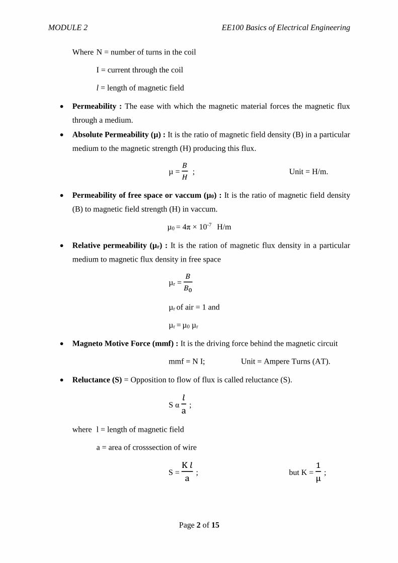
Where N = number of turns in the coil

I = current through the coil

l = length of magnetic field

Permeability : The ease with which the magnetic material forces the magnetic flux

through a medium.

Absolute Permeability (µ) : It is the ratio of magnetic field density (B) in a particular

medium to the magnetic strength (H) producing this flux.

µ = 𝐵

𝐻 ; Unit = H/m.

Permeability of free space or vaccum (µ0) : It is the ratio of magnetic field density

(B) to magnetic field strength (H) in vaccum.

µ0 = 4π × 10-7 H/m

Relative permeability (µr) : It is the ration of magnetic flux density in a particular

medium to magnetic flux density in free space

µr = 𝐵

𝐵0

µr of air = 1 and

µr = µ0 µr

Magneto Motive Force (mmf) : It is the driving force behind the magnetic circuit

mmf = N I; Unit = Ampere Turns (AT).

Reluctance (S) = Opposition to flow of flux is called reluctance (S).

S α 𝑙

a ;

where l = length of magnetic field

a = area of crosssection of wire

S = K 𝑙

a ; but K =

1

µ ;


of 15

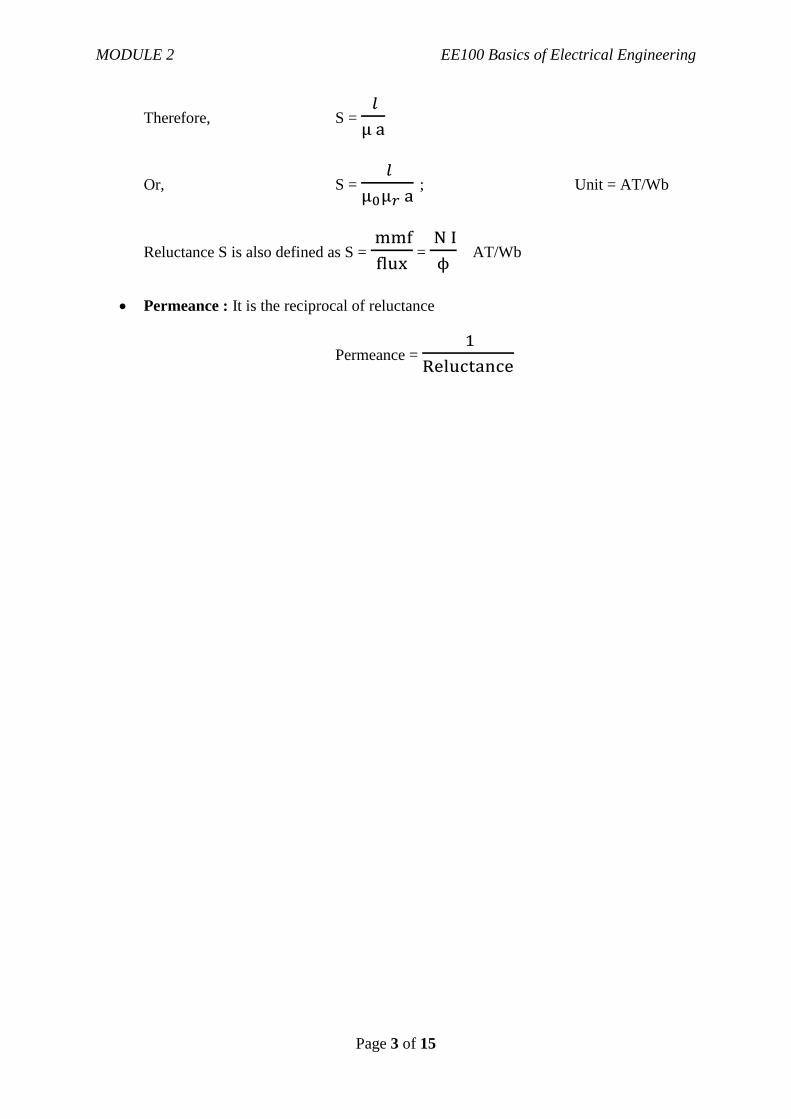
Therefore, S = 𝑙

µ a

Or, S = 𝑙

µ0µ𝑟 a ; Unit = AT/Wb

Reluctance S is also defined as S = mmf

flux =

N I

ϕ AT/Wb

Permeance : It is the reciprocal of reluctance

Permeance = 1

Reluctance


of 15

ELECTROMAGNETIC INDUCTION

FARADAYS LAWS OF ELECTROMAGNETIC INDUCTION

Michael Faraday, a British Scientist as stated 2 laws related to electromagnetic induction.

Faraday’s First Law of Electromagnetic Induction:

“Whenever the flux linking with a coil changes, an EMF is induced in the coil”

Faraday’s Second Law of Electromagnetic Induction :

“The magnitude of induced EMF is directly proportional to rate of change of flux

linkages”

e = dϕ

dt

Where, e = induced EMF in the coil

Φ = flux linking with the coil.

If the coil has N turns, then

e = N dϕ

dt

Lenz’s Law :

“The direction of induced EMF is such that it always opposes the cause”

By considering the effect due to Lenz’s Law, we can write induced EMF as

e = -N dϕ

dt

NATURE OF INDUCED EMF

Depending upon the nature of inducing EMF, the induced EMF is classified into two :

Dynamically Induced EMF and Statically Induced EMF.

Dynamically Induced EMF

Here the EMF is induced by moving the flux with respect to the coil or by moving the

coil with respect to flux. In either way there involves the physical movement of coil or

the flux.

Magnitude of Dynamically Induced EMF


of 15

Consider a conductor of length l moving perpendicular to a magnetic field with flux density

B with a velocity of v m/s.

Let the conductor moves a very small distance of dx in a small time dt.

The area, A covered by the conductor = l . dx

Flux dϕ in the area A = flux density × area

i.e dϕ = B.l.dx

Induced EMF, e = dϕ

dt =

B.𝑙.dx

dt but

dx

dt = velocity, v

Therefore, e = B.l.v Unit = volts V

If the motion is not perpendicular i.e the motion is at an angle θ from the vertical plane, the

induced EMF is given by

e = B.l.v sin θ Volts

Statically Induced EMF

If the EMF is induced without the physical movement of coil or magnet, then it is called

statically induced EMF.

Consider an electromagnet as shown below.

If the current in the coil is reversed, the direction of magnetic field also gets reversed.

Thus by periodically changing the direction of current, the flux can also be changed.

This periodically changing flux is linked with the same coil and generates an EMF in

the coil. This is called self induced EMF.

In other words “EMF induced in a coil due to change in its own flux linked with it is

called self indued EMF”.

Self Inductance

The direction of self induced EMF is such that it always oppose the cause producing it.

Here the cause is change in direction of current. So self inductance can be defined as

“the property of the coil to oppose any change in current through it”.

Self induced EMF is given by e = -N dϕ

dt


of 15

ϕ = ϕ

I × I

therefore, dϕ

dt =

ϕ

I ×

dI

dt

So, self induced EMF, e = -N ϕ

I dI

dt

Here N ϕ

I = L;

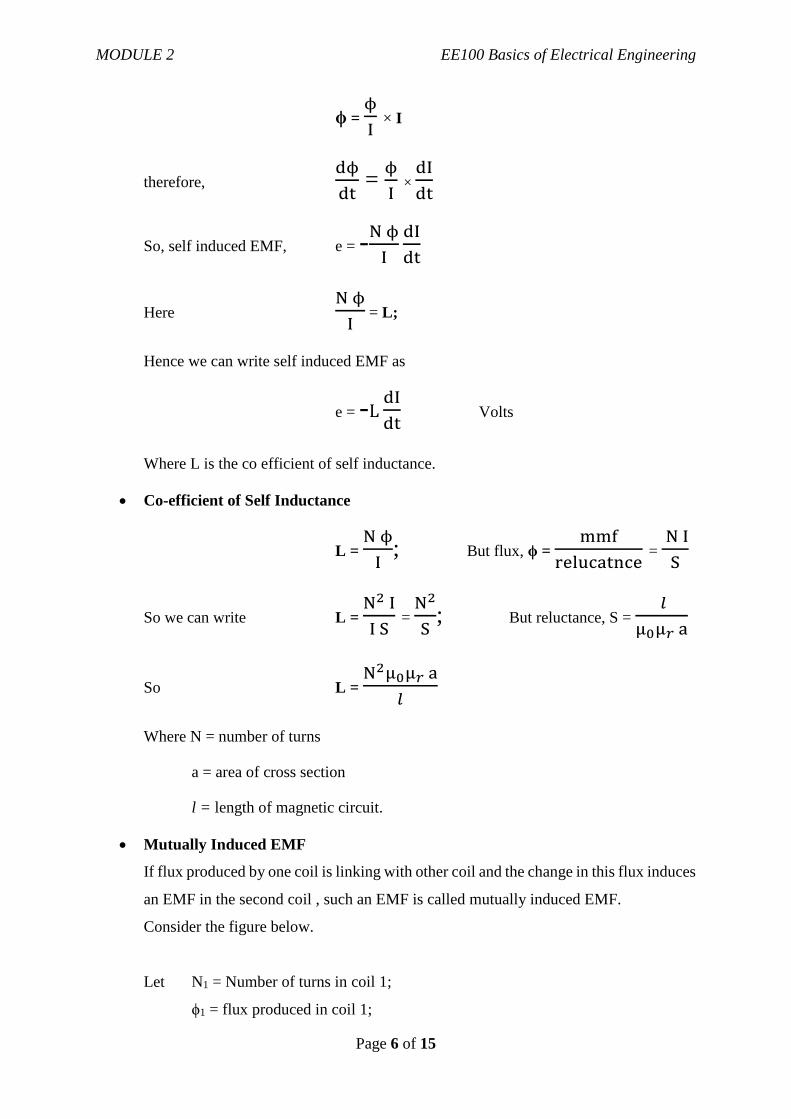
Hence we can write self induced EMF as

e = -L dI

dt Volts

Where L is the co efficient of self inductance.

Co-efficient of Self Inductance

L = N ϕ

I; But flux, ϕ =

mmf

relucatnce =

N I

S

So we can write L = N2 I

I S =

N2

S; But reluctance, S =

𝑙

µ0µ𝑟 a

So L = N2µ0µ𝑟 a

𝑙

Where N = number of turns

a = area of cross section

l = length of magnetic circuit.

Mutually Induced EMF

If flux produced by one coil is linking with other coil and the change in this flux induces

an EMF in the second coil , such an EMF is called mutually induced EMF.

Consider the figure below.

Let N1 = Number of turns in coil 1;

ϕ1 = flux produced in coil 1;


of 15

I1 = current flowing through coil 1

N2 = Number of turns in coil 2;

Φ2 = flux linking with coil 2;

I2 = current induced in coil 2

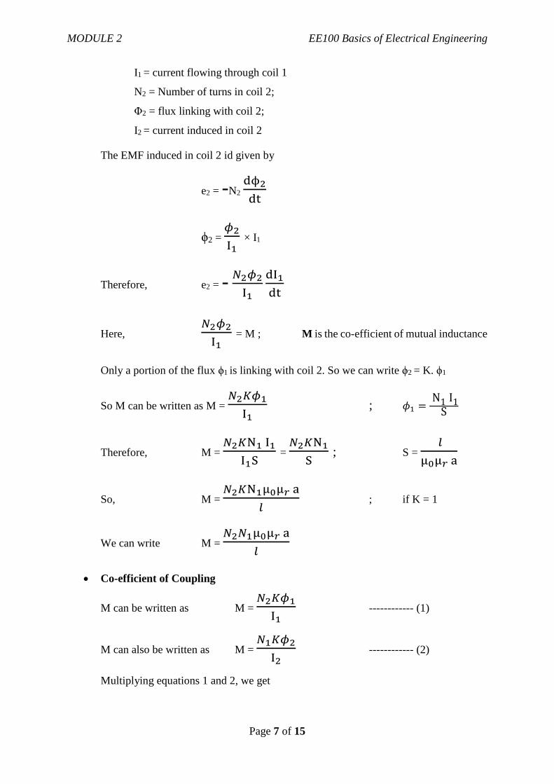
The EMF induced in coil 2 id given by

e2 = -N2 dϕ2

dt

ϕ2 = 𝜙2

I1 × I1

Therefore, e2 = - 𝑁2𝜙2

I1 dI1

dt

Here, 𝑁2𝜙2

I1 = M ; M is the co-efficient of mutual inductance

Only a portion of the flux ϕ1 is linking with coil 2. So we can write ϕ2 = K. ϕ1

So M can be written as M = 𝑁2𝐾𝜙1

I1 ; 𝜙1 =

N1 I1S

Therefore, M = 𝑁2𝐾N1 I1

I1S =

𝑁2𝐾N1

S ; S =

𝑙

µ0µ𝑟 a

So, M = 𝑁2𝐾N1µ0µ𝑟 a

𝑙 ; if K = 1

We can write M = 𝑁2𝑁1µ0µ𝑟 a

𝑙

Co-efficient of Coupling

M can be written as M = 𝑁2𝐾𝜙1

I1 ------------ (1)

M can also be written as M = 𝑁1𝐾𝜙2

I2 ------------ (2)

Multiplying equations 1 and 2, we get


of 15

M2 =

𝑁2𝐾𝜙1 𝑁1𝐾𝜙2

I1I2

i.e M2 =

𝐾𝑁1𝜙1 . 𝐾𝑁2𝜙2

I1 . I2

in the above equation put N1 ϕ1

I1 = L1 and

N2 ϕ2

I2 = L2

i.e M2 = K2 L1.L2

or M = 𝐾√L1L2

i.e K = M

√L1L2


of 15

AC FUNDAMENTALS

INTRODUCTION

In Direct Current (DC), the magnitude is constant and direction remains same with

respect to time. Whereas in an Alternating Current (AC), the current changes both its

magnitude and direction periodically.

GENERATION OF AC VOLTAGE

The machine used to produce electricity is called generators. The generator which produce ac

voltages is called alternators. The working principle behind working of alternators is Faradays

Laws of Electromagnetic Induction. The figure below shows the simple diagram of an

alternator.

It consist of two permanent magnets, north and south. A single turn coil is placed in between

the magnets. The coil is connected to a resistor through slip rings and brushes. As the coil is


of 15

rotated, coil cuts the magnetic field lines. This results in generation of alternating EMF as stated

by faradays law.

The induced EMF is given by e = B l v sinθ

Different instants during the generation of alternating EMF is shown below.

INSTANT – 1 (θ = 0)

At this instant the coil is along the horizontal axis. The velocity of the coil is parallel to the field

as shown in figure. So the angle θ = 0O and sin 0 = 0. So during this instant the induced EMF is zero.

INSTANT – 2 (θ < 90)

At this instant the coil is rotated by an angle θ. During this instant the induced EMF generated

in the coil whose magnitude is proportional to v sin θ which is increasing. That is during this instant

the induced EMF gradually increases from zero to maximum value.


of 15

INSTANT – 3 (θ = 90)

At this instant the coil is rotated by an angle 90. Since sin 90 = 1, the magnitude of the EMF

generated is maximum.

Induced EMF, e = B l v

INSTANT – 4 (θ > 90)

At this instant the coil is rotated by an angle θ which is greater than 90. During this instant

the magnitude of induced EMF is proportional to the value v sinθ which is decreasing. That is during

this instant the induced EMF gradually decreases from maximum value to zero.

INSTANT – 5 (θ =180)

At this instant the coil has rotated over an angle of 180o and is along the horizontal axis. The

velocity of the coil is parallel to the field. Here sin 180 = 0. So during this instant the induced EMF is

zero.


of 15

INSTANT – 6 (θ > 180)

At this instant the coil is rotated by an angle θ greater than 180. During this instant the induced

EMF generated in the coil whose magnitude is proportional to v sin θ which is negative and

increasing in negative direction. That is during this instant the induced EMF increasing in

negative direction.

The waveform for all the 6 instants is shown below.


of 15

STANDARD TERMS RELATED TO ALTERNATING QUANTITY

Before further analysis of alternating quantity, it is necessary to be familiar with the

different terms and different parameters of the alternating quantity. For this, consider the

waveform of one cycle of alternating EMF shown in figure 2d.

Instantaneous Value

Since the magnitude of an alternating current varies with time as shown in figure 3, the

value of the current at a particular instant is called instantaneous value. In the figure, e1 and e2

are the instantaneous value of alternating emf at instants t1 and t2 respectively.

Waveform

The graph of instantaneous values of an alternating quantity plotted against time is

called its waveform.

Cycle

A set of positive and negative half cycles of an alternating quantity is called a cycle.

One cycle = 360o or 2π radians.

Time Period

Time taken by an alternating quantity to complete on cycle is called its time period. It

is denoted by T seconds.

Frequency

It is the number of cycles of alternating quantity in one second. It is denoted by f and it

is measured in cycles/second, which is also known as Hertz (Hz). Frequency can be also stated

as reciprocal of time period.


of 15

f = 𝟏

𝑻 Hz

Amplitude

The maximum value attained by the alternating quantity during positive or negative

half cycle is called amplitude. The amplitude of voltage is denoted by Em and amplitude of

current is denoted by Im.

Angular Frequency

It is the frequency expressed in electrical radians per second. Since one cycle of

alternating quantity corresponds to 2π radians, the angular frequency can be expressed as (2π×

cycles/sec). It is denoted by ω and its unit is radians/second.

ω = 2πf rad/sec

or

ω = 𝟐𝛑

𝑻 rad/sec

Equation For Instantaneous Voltage And Current

If the amplitude of voltage and amplitude of current of an AC supply with angular

frequency ω are Em and Im, then the instantaneous values of voltage and current can be given

as

e = Em sin(ωt)

i = Im sin(ωt)

RMS Value or Effective Value

The rms value or effective value of an alternating current is given by that steady

current (DC) which, when flowing through a given circuit for a given time, produces same

amount of heat as produced by alternating current, which when flowing through the same

circuit for the same time.

All the values of magnitudes of alternating quantities are expressed in rms values. The

standard value of 230V and 415V are rms values of alternating voltage.

All the ammeters and voltmeters measure the rms value of the current and voltage.

RMS value = 𝟏

√𝟐 [Maximum Value]

Irms = 𝑰𝒎

√𝟐


of 15

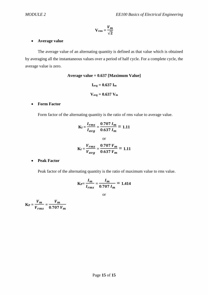
Vrms = 𝑽𝒎

√𝟐

Average value

The average value of an alternating quantity is defined as that value which is obtained

by averaging all the instantaneous values over a period of half cycle. For a complete cycle, the

average value is zero.

Average value = 0.637 [Maximum Value]

Iavg = 0.637 Im

Vavg = 0.637 Vm

Form Factor

Form factor of the alternating quantity is the ratio of rms value to average value.

Kf = 𝑰𝒓𝒎𝒔

𝑰𝒂𝒗𝒈 =

𝟎.𝟕𝟎𝟕 𝑰𝒎

𝟎.𝟔𝟑𝟕 𝑰𝒎 = 1.11

or

Kf = 𝑽𝒓𝒎𝒔

𝑽𝒂𝒗𝒈 =

𝟎.𝟕𝟎𝟕 𝑽𝒎

𝟎.𝟔𝟑𝟕 𝑽𝒎 = 1.11

Peak Factor

Peak factor of the alternating quantity is the ratio of maximum value to rms value.

KP= 𝑰𝒎

𝑰𝒓𝒎𝒔 =

𝑰𝒎

𝟎.𝟕𝟎𝟕 𝑰𝒎 = 1.414

or

KP = 𝑽𝒎

𝑽𝒓𝒎𝒔 =

𝑽𝒎

𝟎.𝟕𝟎𝟕 𝑽𝒎

Magnetism and AC Fundamentals

Education

Transcript of Magnetism and AC Fundamentals