
MAE 577 PROJECT 2 FEM ANALYSIS OF POWER SCREW
39
MAE 577 PROJECT 2 FEM ANALYSIS OF POWER SCREW By, SUMIT TRIPATHI
Transcript of MAE 577 PROJECT 2 FEM ANALYSIS OF POWER SCREW

MAE 577 PROJECT 2
FEM ANALYSIS OF POWER SCREW
By,
SUMIT TRIPATHI
Project Statement
MAE 477/577
Feb. 2, 2009
Project #2
Finite Element Problem
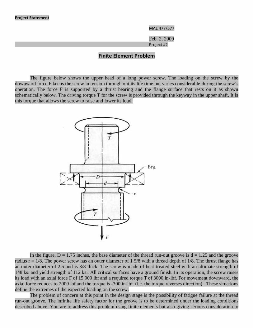
The figure below shows the upper head of a long power screw. The loading on the screw by the
downward force F keeps the screw in tension through out its life time but varies considerable during the screw’s
operation. The force F is supported by a thrust bearing and the flange surface that rests on it as shown
schematically below. The driving torque T for the screw is provided through the keyway in the upper shaft. It is
this torque that allows the screw to raise and lower its load.
In the figure, D = 1.75 inches, the base diameter of the thread run-out groove is d = 1.25 and the groove
radius r = 1/8. The power screw has an outer diameter of 1 5/8 with a thread depth of 1/8. The thrust flange has
an outer diameter of 2.5 and is 3/8 thick. The screw is made of heat treated steel with an ultimate strength of
148 ksi and yield strength of 112 ksi. All critical surfaces have a ground finish. In its operation, the screw raises
its load with an axial force F of 15,000 lbf and a required torque T of 3000 in-lbf. For movement downward, the
axial force reduces to 2000 lbf and the torque is -300 in-lbf (i.e. the torque reverses direction). These situations
define the extremes of the expected loading on the screw.
The problem of concern at this point in the design stage is the possibility of fatigue failure at the thread
run-out groove. The infinite life safety factor for the groove is to be determined under the loading conditions
described above. You are to address this problem using finite elements but also giving serious consideration to
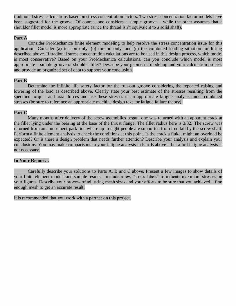
traditional stress calculations based on stress concentration factors. Two stress concentration factor models have
been suggested for the groove. Of course, one considers a simple groove – while the other assumes that a
shoulder fillet model is more appropriate (since the thread isn’t equivalent to a solid shaft).
Part A
Consider ProMechanica finite element modeling to help resolve the stress concentration issue for this
application. Consider (a) tension only, (b) torsion only, and (c) the combined loading situation for lifting
described above. If tradional stress concentration calculations are to be used in this design process, which model
is most conservative? Based on your ProMechanica calculations, can you conclude which model is most
appropriate – simple groove or shoulder fillet? Describe your geometric modeling and your calculation process
and provide an organized set of data to support your conclusion.
Part B
Determine the infinite life safety factor for the run-out groove considering the repeated raising and
lowering of the load as described above. Clearly state your best estimate of the stresses resulting from the
specified torques and axial forces and use these stresses in an appropriate fatigue analysis under combined
stresses (be sure to reference an appropriate machine design text for fatigue failure theory).
Part C
Many months after delivery of the screw assemblies began, one was returned with an apparent crack at
the fillet lying under the bearing at the base of the thrust flange. The fillet radius here is 3/32. The screw was
returned from an amusement park ride where up to eight people are supported from free fall by the screw shaft.
Perform a finite element analysis to check the conditions at this point. Is the crack a fluke, might an overload be
expected? Or is there a design problem that needs further attention? Describe your analysis and explain your
conclusions. You may make comparisons to your fatigue analysis in Part B above – but a full fatigue analysis is
not necessary.
In Your Report…
Carefully describe your solutions to Parts A, B and C above. Present a few images to show details of
your finite element models and sample results – include a few “stress labels” to indicate maximum stresses on
your figures. Describe your process of adjusting mesh sizes and your efforts to be sure that you achieved a fine
enough mesh to get an accurate result.
It is recommended that you work with a partner on this project.

Model Assumption
We have assumed that the groove starts from the base of thread, since the groove cannot end at the thread edge
(provided that the thread is through-out the length of the power screw). With this assumption we have calculated base
diameter of the thread run out groove to be d=1.125 in, instead of 1.25 in.
in
sidebothondepthgrooveThesidebothondepthThreadThepowerscrewofDiaOuterThed
125.1
)(8
2)(
8
2)(
8
51
We have neglected any strength contribution due to threads. Hence the diameter of shaft is taken as base diameter of
thread. Hence diameter of power shaft for FEM analysis = 1.375 in
in
sidebothondepthThreadThepowerscrewofDiaOuterTheD
375.1
)(8
2)(
8
51
Material : Steel
poison's ratio =0.27
Young's modulus =2.9e+07psi
Yield strength: 112 ksi
Ultimate Strength: 148 ksi

Model Design and Constraint Set:
The FEM Analysis involves generation of hundreds of small element and calculations involved for those elements, which
costs lot of computation time. To avoid unnecessary computation time we have to carefully select our model design.
My approach:
First we are going to study the actual design with minimal mesh size so that we will have fair idea about the location of
stress concentrations.
The following figure displays that the shaft flange, which is supported on the bearing is constrained at bottom surface of
it in all 6 degrees of freedom. The tensile load of 15000lbf is applied at the bottom surface of the shaft. The FEM analysis
accomplished by Pro Mechanica shows that the stress generation in all the volume that above top of the shaft flange is
insignificant. Hence we will cut off this volume in subsequent study.
The motor is attached to top shaft with key. My assumption is that the motion is constrained my motor (only for
analysis, because for every action of motor there will be equal and opposite reaction by shaft). Without loss of
generality we can constrain the top of the flange in modifies model to study stress generation in groove.
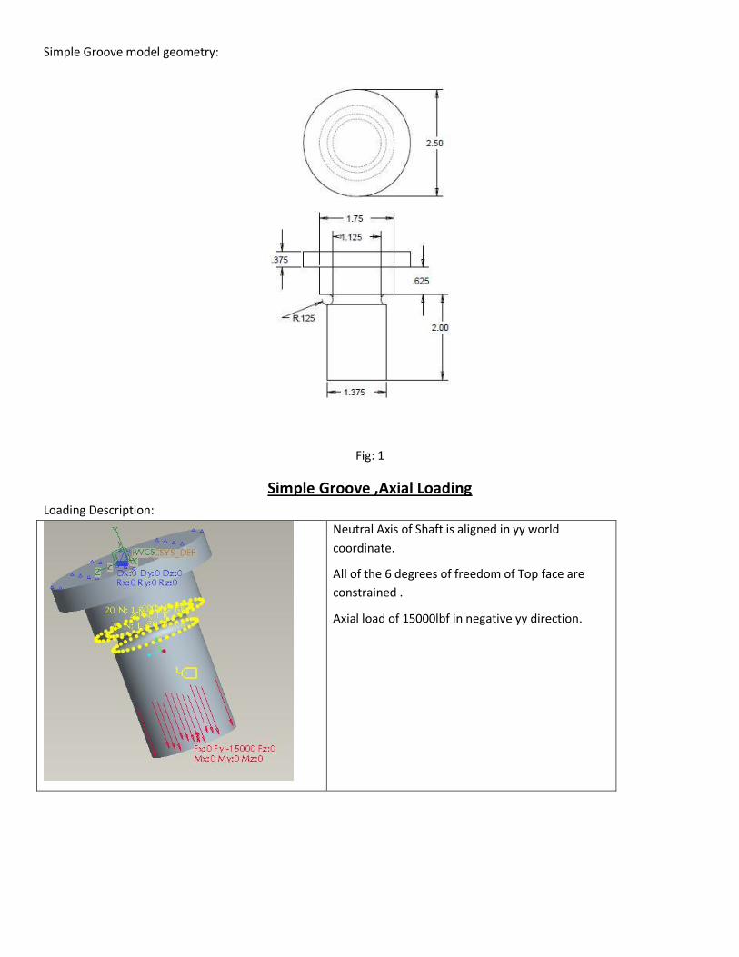
Simple Groove model geometry:
Fig: 1
Simple Groove ,Axial Loading
Loading Description:
Neutral Axis of Shaft is aligned in yy world
coordinate.
All of the 6 degrees of freedom of Top face are
constrained .
Axial load of 15000lbf in negative yy direction.

Mesh Geometry:
Mesh refinement is implemented by changing the allowable angles between the edges, number of nodes on the edges
and maximum edge turn angle.
H1
Points: 73 Edges: 324
Faces: 439 Elements: 187
H2
Points: 335 Edges: 1751
Faces: 2614 Elements: 1197
H3
Points: 724 Edges: 3981
Faces: 6104 Elements: 2846
FEM solutions might be less reliable, if the elements
involved in FEM computations are too stiff, i.e. the
angle between the edges of the element. This happens
because of difficulty in fitting the polynomial over sharp
corners of elements.
My Approach in Mechanica:
Increase the minimum allowable angle between edges
so that better polynomial curve fitting is achieved. This
process in effect increases the number of elements to
mesh volume. We did this in conjunction with reduction
in aspect ratio and increment of manual nodes.
Why not reduce only Aspect ratio?
Reducing only maximum allowed aspect ratio and
leaving the minimum allowable angle b/w edges as
default (5 Degree), will not serve the purpose. Still there
may be some adjacent elements having maximum
aspect ratio reached and leaving the angle between
the edges somewhat steep.
Initial Mesh H1: Default setting in pro Mechanica, i.e.
Allowable angles:
Edge Max=175 degree, Edge min=5degree
Face max=175 degree Face min=5degree
Max Aspect Ratio=30 Max Edge Turn=95 degree
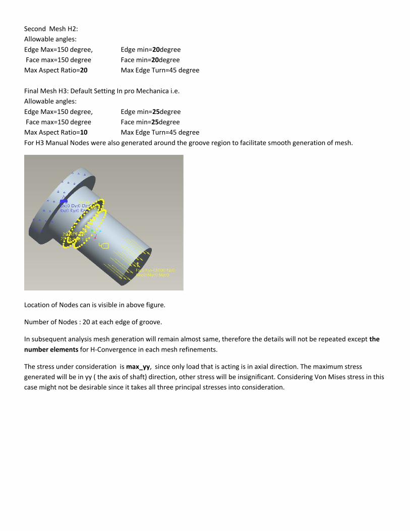
Second Mesh H2:
Allowable angles:
Edge Max=150 degree, Edge min=20degree
Face max=150 degree Face min=20degree
Max Aspect Ratio=20 Max Edge Turn=45 degree
Final Mesh H3: Default Setting In pro Mechanica i.e.
Allowable angles:
Edge Max=150 degree, Edge min=25degree
Face max=150 degree Face min=25degree
Max Aspect Ratio=10 Max Edge Turn=45 degree
For H3 Manual Nodes were also generated around the groove region to facilitate smooth generation of mesh.
Location of Nodes can is visible in above figure.
Number of Nodes : 20 at each edge of groove.
In subsequent analysis mesh generation will remain almost same, therefore the details will not be repeated except the
number elements for H-Convergence in each mesh refinements.
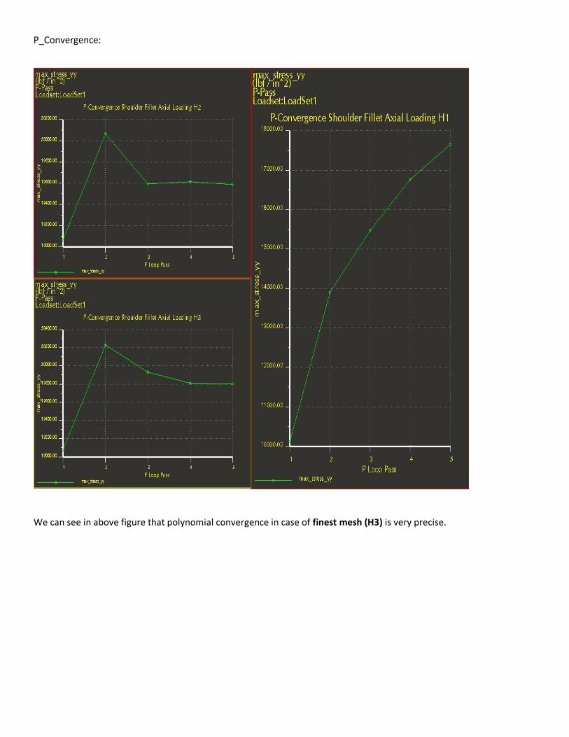
The stress under consideration is max_yy, since only load that is acting is in axial direction. The maximum stress
generated will be in yy ( the axis of shaft) direction, other stress will be insignificant. Considering Von Mises stress in this
case might not be desirable since it takes all three principal stresses into consideration.

P_Convergence:
We can see in above figure that polynomial convergence in case of finest mesh (H3) is very precise.
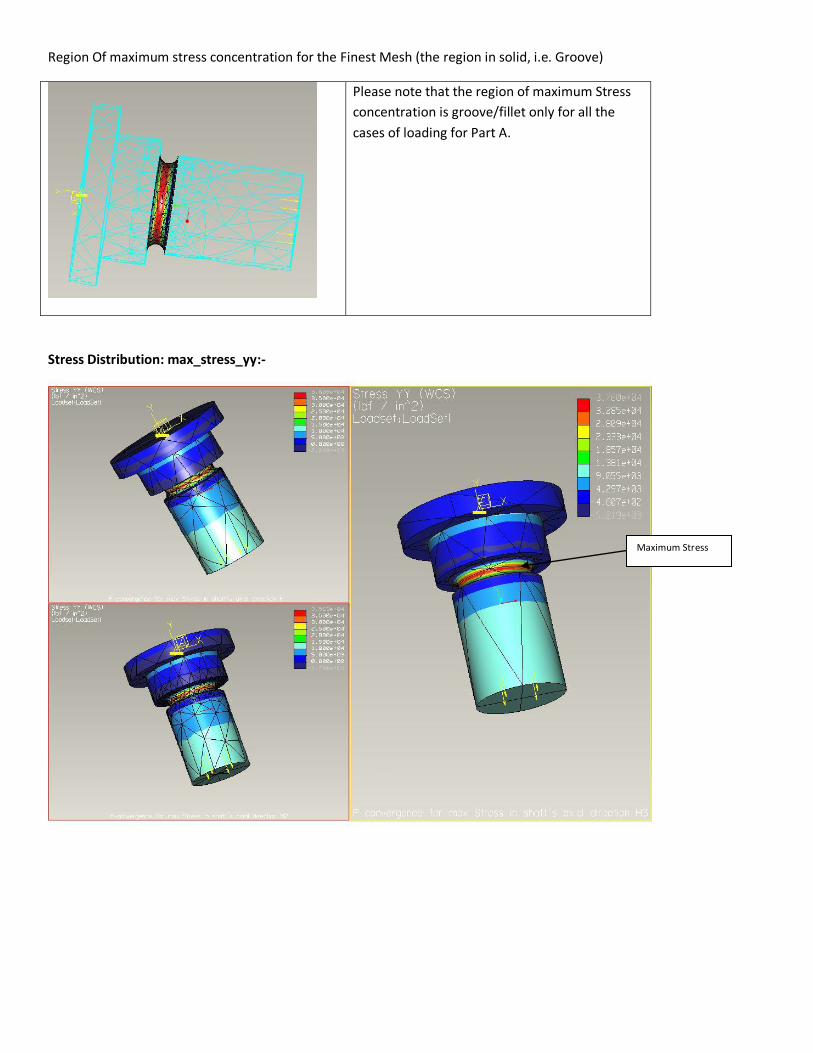
Region Of maximum stress concentration for the Finest Mesh (the region in solid, i.e. Groove)
Please note that the region of maximum Stress
concentration is groove/fillet only for all the
cases of loading for Part A.
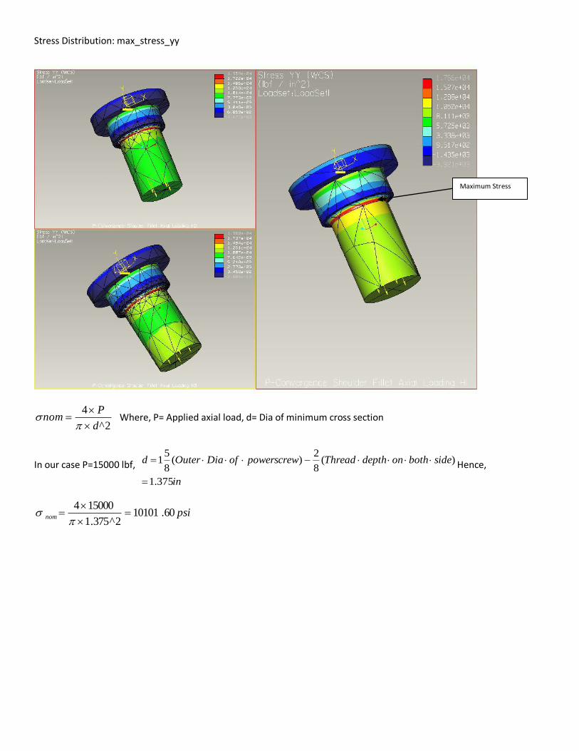
Stress Distribution: max_stress_yy:-
Maximum Stress

Nominal Stress=2^
4
d
Pnom
Where, P= Applied axial load, d= Dia of minimum cross section
In our case P=15000 lbf,
in
sidebothondepthgroovesidebothondepthThreadpowerscrewofDiaOuterd
125.1
)(8
2)(
8
2)(
8
51
Hence,
psinom 24.150902^125.1
150004
H – Convergence:
The exact solution based on FEM solutions of the 3 finest meshes is carried out by Lagrangian Interpolating polynomial,
which gives as exact solution as
21
21
2
2)^(
nn
nn
n
nexact
, Where ‘n’ is subscript for the finest mesh and ‘n-1’ and ‘n-2’ are previous two
meshes.:
%Convergence= 100X( exact - fem )/ exact
Stress concentration factor based on FEM computation Stress concentration
factor based on” R. E.
Peterson Stress
concentration Hand
Book” , Chart 2.19
Simple Groove Maximum Stress Convergence, Axial Loading
No of
Elements
Max Stress in axial
direction(yy) psi
%Convergence
187.00 36882.84 5.34
1197.00 36089.57 3.08
2846.00 35632.57 1.77
Exact Solution
35011.49 Nominal
Stress 15090.24
2.3201
11.0125.1
125.0
d
r
Ref fig:1
22.1125.1
375.1
d
D
From chart 2.19
Kt = 2.3
100
Sex
SfeSex
Stress Nominal
Stress MaximumFactorion Concentrat Stress

Simple Groove ,Torsion Loading
Loading Description:
Neutral Axis of Shaft is aligned in yy world coordinate.
All of the 6 degrees of freedom of Top face are
constrained .
Torsion load of 3000 lbf-in in tangential direction as
shown.
Force applied is force per unit area
psihdd
T27.577
75.16875.26875.0
3000
)2/(2)2/(
For torsion load maximum principal stress magnitude is considered, since principal stresses are the eigenvalues of the
stress matrix it will include shear forces in all directions for each Mesh Element.
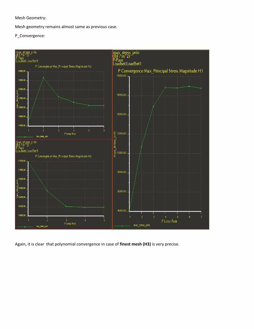
Mesh Geometry:
Mesh geometry remains almost same as previous case.
P_Convergence:
Again, it is clear that polynomial convergence in case of finest mesh (H3) is very precise.

Stress Distribution: max_stress_prin
J
cTnom
Where, T= 3000 lbf-in,
c= distance of extreme fiber of minimum cross section from neutral axis = 1.125/2 =d/2
32
4^dJ
in
sidebothondepthgroovesidebothondepthThreadpowerscrewofDiaOuterd
125.1
)(8
2)(
8
2)(
8
51
Hence,
psid
T
J
cTnom 84.10730
3^125.1
300016
3^
16
Maximum Stress

H – Convergence:
The exact solution based on FEM solutions of the 3 finest meshes is carried out by Lagrangian Interpolating polynomial,
which gives as exact solution as
21
21
2
2)^(
nnn
nnn
exact
, Where ‘n’ is the finest mesh and ‘n-1’ and ‘n-2’ are previous two meshes.:
Stress concentration factor based on FEM computation Stress concentration
factor based on” R. E.
Peterson Stress
concentration Hand
Book” , Chart 2.47
Simple Groove Maximum Stress Convergence,Torsional Loading
No of
Elements
Max Principal Stress
Magnitude
%Convergence
147 16784.64 3.76
1210 16258.63 0.51
1752 16187.53 0.07
Exact Solution
16176.42 Nominal
Stress 10730.84
1.5075
11.0125.1
125.0
d
rRef
fig:1
22.1125.1
375.1
d
D
From Chart 2.47
Kts = 1.55
Clearly Kts is smaller
than Kt(2.3), which
implies that stress
concentration is higher
in tensile loading in our
case.
100
Sex
SfeSex
Stress Nominal
Stress MaximumFactorion Concentrat Stress

Simple Groove ,Combined Loading
Loading Description:
Please refer previous definitions of axial and
torsion loading, both are acting simultaneously.
Von mises stress is considered here, as it combines all the shear and tensile stress with the calculation of principal stress
, the eigen values of matrix of shear and normal stresses
2
2)^32(2)^32(2)^21(
vm , as we can see that Vm stress average out the principal stresses,
it is considered to be the best stress distribution in case of combined loading.
Please refer to H- Convergence table for number of elements. The initial mesh geometry is almost same.

P_Convergence: (Von mises stress is considered over here)

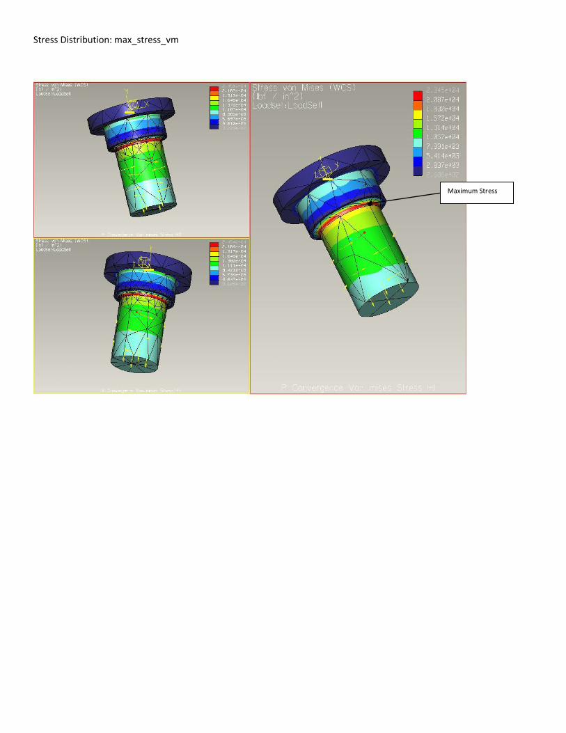
Stress Distribution: max_stress_vm
Maximum Stress
H – Convergence:
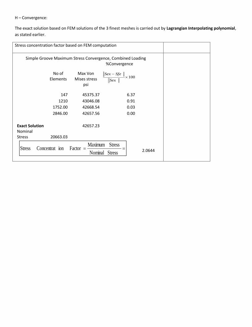
The exact solution based on FEM solutions of the 3 finest meshes is carried out by Lagrangian Interpolating polynomial,
as stated earlier.
Stress concentration factor based on FEM computation
Simple Groove Maximum Stress Convergence, Combined Loading
No of
Elements
Max Von Mises stress
psi
%Convergence
147 45375.37 6.37
1210 43046.08 0.91
1752.00 42668.54 0.03
2846.00 42657.56 0.00
Exact Solution
42657.23 Nominal
Stress 20663.03
2.0644
100
Sex
SfeSex
Stress Nominal
Stress MaximumFactorion Concentrat Stress

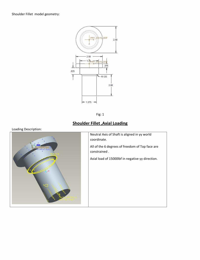
Shoulder Fillet model geometry:
Fig: 1
Shoulder Fillet ,Axial Loading
Loading Description:
Neutral Axis of Shaft is aligned in yy world
coordinate.
All of the 6 degrees of freedom of Top face are
constrained .
Axial load of 15000lbf in negative yy direction.
P_Convergence:
We can see in above figure that polynomial convergence in case of finest mesh (H3) is very precise.
Stress Distribution: max_stress_yy
2^
4
d
Pnom
Where, P= Applied axial load, d= Dia of minimum cross section
In our case P=15000 lbf,
in
sidebothondepthThreadpowerscrewofDiaOuterd
375.1
)(8
2)(
8
51
Hence,
psinom 60.101012^375.1
150004
Maximum Stress

H – Convergence:
The exact solution based on FEM solutions of the 3 finest meshes is carried out by Lagrangian Interpolating polynomial,
Stress concentration factor based on FEM computation Stress concentration
factor based on” Richard
M. Phelan fig-6-14
Shoulder Fillet, Maximum Stress Convergence,Axial Loading
No of
Elements
Max Stress in axial
direction(yy)
%Convergence
206 17656.85 10.96
1034 19585.74 1.23
2219 19802.49 0.14
Exact Solution
19829.93 Nominal
Stress 10101.60
1.9630
09.0375.1
125.0
d
rRef
fig:1
27.1375.1
75.1
d
D
Kt = 1.8
Clearly Kt in case of
shoulder fillet is much
smaller than simple
groobe(2.3), the stress
concentration is less for
fillet, which implies that
fillet design is better.
100
Sex
SfeSex
Stress Nominal
Stress MaximumFactorion Concentrat Stress
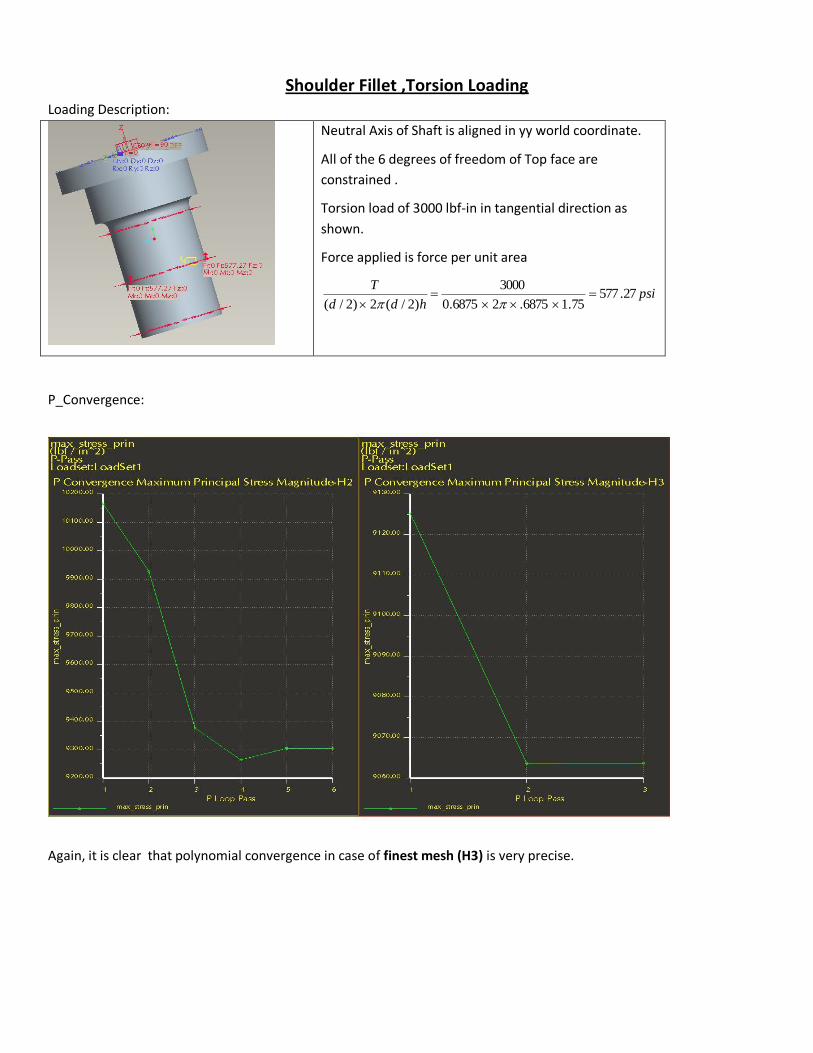
Shoulder Fillet ,Torsion Loading
Loading Description:
Neutral Axis of Shaft is aligned in yy world coordinate.
All of the 6 degrees of freedom of Top face are
constrained .
Torsion load of 3000 lbf-in in tangential direction as
shown.
Force applied is force per unit area
psihdd
T27.577
75.16875.26875.0
3000
)2/(2)2/(
P_Convergence:
Again, it is clear that polynomial convergence in case of finest mesh (H3) is very precise.

Stress Distribution: max_stress_prin
J
cTnom
Where, T= 3000 lbf-in,
c= distance of extreme fiber of minimum cross section from neutral axis = 1.375/2 =d/2
32
4^dJ
in
sidebothondepthThreadpowerscrewofDiaOuterd
375.1
)(8
2)(
8
51
Hence,
psid
T
J
cTnom 37.5877
3^375.1
300016
3^
16
Maximum Stress

H – Convergence:
The exact solution based on FEM solutions of the 3 finest meshes is carried out by Lagrangian Interpolating polynomial,
which gives as exact solution as
21
21
2
2)^(
nnn
nnn
exact
, Where ‘n’ is the finest mesh and ‘n-1’ and ‘n-2’ are previous two meshes.:
Stress concentration factor based on FEM computation Stress concentration
factor based on
Richard M. Phelan fig
– 6-17
Shoulder Fillet, Maximum Stress Convergence,Torsional Loading
No of
Elements
Max Principal Stress
Magnitude
%Convergence
206 9319.64 3.41
1034 9137.89 1.39
2602 9063.65 0.57
Exact Solution
9012.38 Nominal
Stress 5877.37
1.5334
11.0125.1
125.0
d
rRef
fig:1
22.1125.1
375.1
d
D
Kts = 1.45
100
Sex
SfeSex
Stress Nominal
Stress MaximumFactorion Concentrat Stress
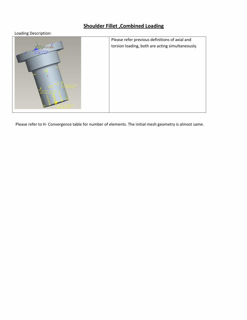
Shoulder Fillet ,Combined Loading
Loading Description:
Please refer previous definitions of axial and
torsion loading, both are acting simultaneously.
Please refer to H- Convergence table for number of elements. The initial mesh geometry is almost same.

P_Convergence: (Von mises stress is considered here, as it combines all the shear and tensile stress with the calculation
of principal stress , the eigen values of matrix of shear and normal stresses )
Stress Distribution: max_stress_vm
Maximum Stress

H – Convergence:
The exact solution based on FEM solutions of the 3 finest meshes is carried out by Lagrangian Interpolating polynomial,
Stress concentration factor based on FEM computation
Shoulder Fillet Maximum Stress Convergence,Combined Loading
No of
Elements
Maximum Von Mises Stress
psi
%Convergence
206 23451.72 4.45
1034 24508.23 0.15
1394.00 24542.68 0.00
Exact Solution
24543.84 Nominal
Stress 12800.00
1.9175
100
Sex
SfeSex
Stress Nominal
Stress MaximumFactorion Concentrat Stress

Conclusion:
Refinement of mesh by increasing minimum allowable angle between edges gives more accurate result as
compared to reduction of only aspect ratio.
Defining manual nodes at appropriate locations smooths out mesh, giving more reliable results.
Stress concentration in tensile loading is higher than torsion loading.
Stress concentration for shoulder fillet is much less than simple groove.
Shoulder fillet model is more appropriate for the type of loading stated in the problem.
PRAT B
PART B:
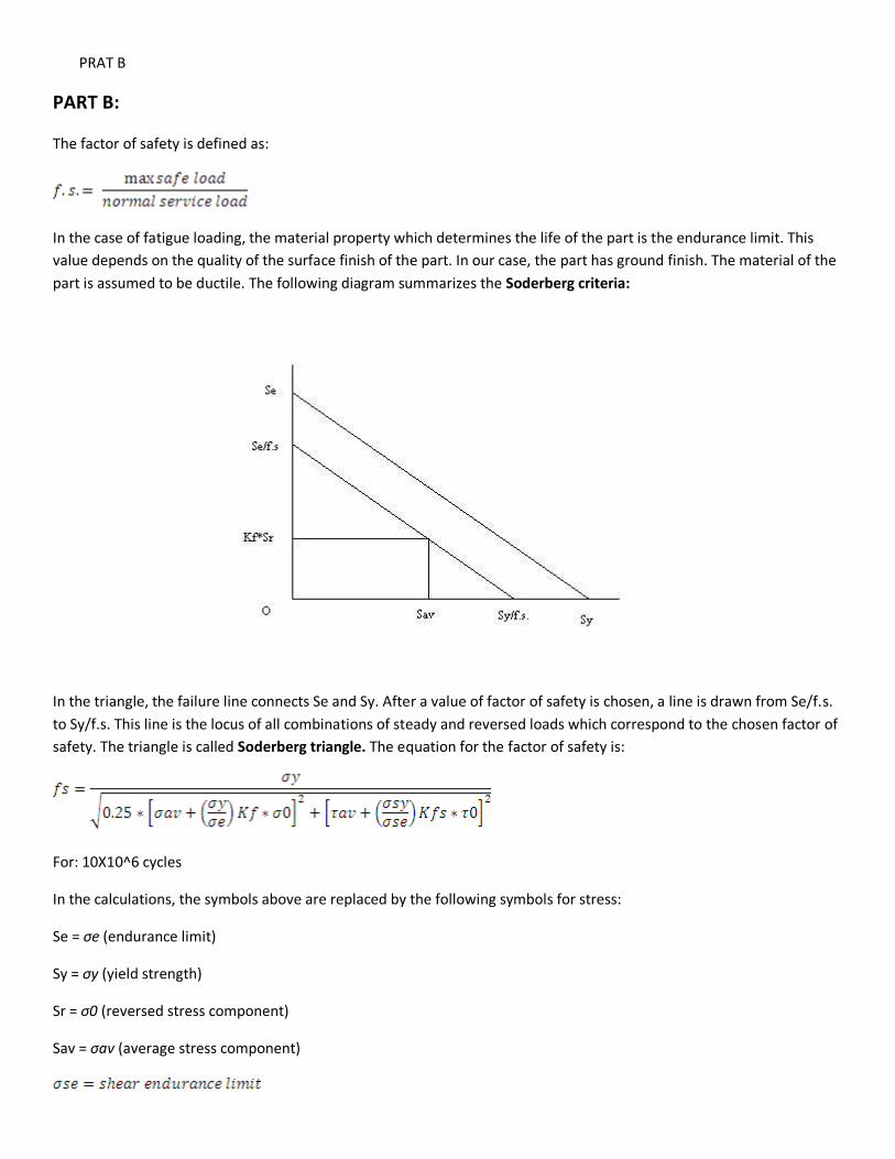
The factor of safety is defined as:
In the case of fatigue loading, the material property which determines the life of the part is the endurance limit. This
value depends on the quality of the surface finish of the part. In our case, the part has ground finish. The material of the
part is assumed to be ductile. The following diagram summarizes the Soderberg criteria:
In the triangle, the failure line connects Se and Sy. After a value of factor of safety is chosen, a line is drawn from Se/f.s.
to Sy/f.s. This line is the locus of all combinations of steady and reversed loads which correspond to the chosen factor of
safety. The triangle is called Soderberg triangle. The equation for the factor of safety is:
For: 10X10^6 cycles
In the calculations, the symbols above are replaced by the following symbols for stress:
Se = σe (endurance limit)
Sy = σy (yield strength)
Sr = σ0 (reversed stress component)
Sav = σav (average stress component)
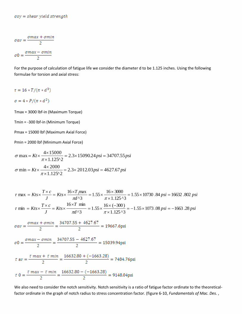
For the purpose of calculation of fatigue life we consider the diameter d to be 1.125 inches. Using the following
formulae for torsion and axial stress:
Tmax = 3000 lbf-in (Maximum Torque)
Tmin = -300 lbf-in (Minimum Torque)
Pmax = 15000 lbf (Maximum Axial Force)
Pmin = 2000 lbf (Minimum Axial Force)
psipsid
TKts
J
cTKts
psipsid
TKts
J
cTKts
28.166308.107355.13^125.1
)300(1655.1
3^
min16min
802.1663284.1073055.13^125.1
30001655.1
3^
max16max 1
We also need to consider the notch sensitivity. Notch sensitivity is a ratio of fatigue factor ordinate to the theoretical-
factor ordinate in the graph of notch radius to stress concentration factor. (figure 6-10, Fundamentals of Mac. Des. ,
psipsiKt
psipsiKt
67.462703.20123.22^125.1
20004min
55.3470724.150903.22^125.1
150004max
Phelan).
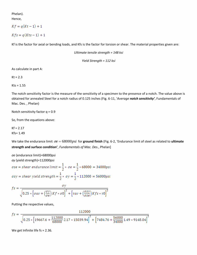
Hence,
Kf is the factor for axial or bending loads, and Kfs is the factor for torsion or shear. The material properties given are:
Ultimate tensile strength = 148 ksi
Yield Strength = 112 ksi
As calculate in part A:
Kt = 2.3
Kts = 1.55
The notch sensitivity factor is the measure of the sensitivity of a specimen to the presence of a notch. The value above is
obtained for annealed Steel for a notch radius of 0.125 inches (Fig. 6-11, ‘Average notch sensitivity’, Fundamentals of
Mac. Des. , Phelan)
Notch sensitivity factor q = 0.9
So, from the equations above:
Kf = 2.17
Kfs= 1.49
We take the endurance limit psie 68000 for ground finish (Fig. 6-2, ‘Endurance limit of steel as related to ultimate
strength and surface condition’, Fundamentals of Mac. Des., Phelan]
σe (endurance limit)=68000psi
σy (yield strength)=112000psi
Putting the respective values,
We get Infinite life fs = 2.36.
Part C:
My design is based on the stress concentration of thread run out groove. All the analysis done in part A reflects that the
maximum stress is in the region of groove.
There one more region, the flange fillet, which is to be addressed, since we have sudden change in cross section at
meeting section of shaft and flange. Although the fillet is provided to take care of the change in cross section, the radius
of fillet is of much importance while considering stress concentration.
Since the flange is resting on the thrust bearing , we have to constrain the bottom surface of the flange to study the
effect of stress concentration in flange fillet.
Loading : Torsion 3000lbf-in, Tensile Load: 15000lbf
Mesh Generation for Part_C
Final Mesh:
Points: 323
Edges: 1730
Faces: 2614
Elements: 1206
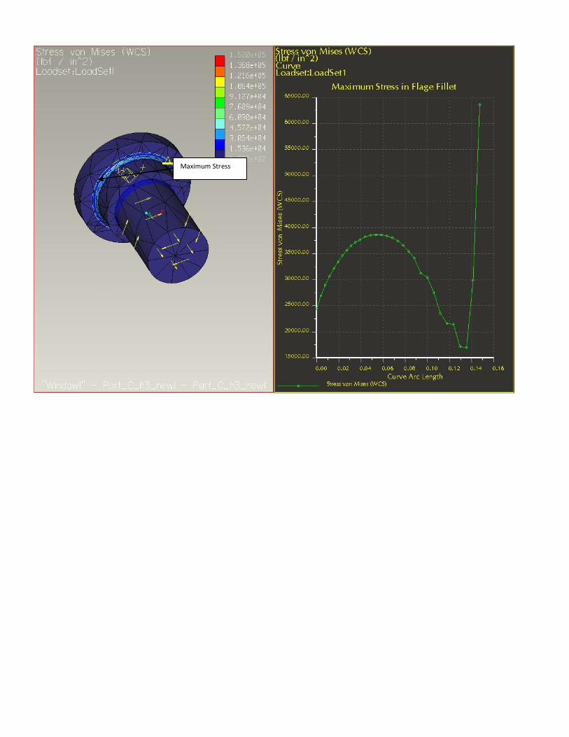
Maximum Stress

From above figure it is evident that Stress at outer edge of the fillet is very high.
Let us refine the mesh little further
Points: 502
Edges: 2766
Faces: 4237
Elements: 1972
Max Von Mises Stress=59009.7psi . This value is very high as comparison to max von mises stress in case of simple
groove combined loading, which was 42657 psi.
383.142657
7.59009
max
max
groovesimple
filletflange
The infinite life safety factor is calculated based on the groove design. However, the stress generation at outer periphery
of the flange fillet is 1.383 times greater.
The infinite life safety factor is 2.36, which leads to allowable maximum stress to 2.36*42657=100670.52psi. The max
stress in flange fillet is well within the range. It appears that “ filletflangemax ” might not cause the crack.
However, we have to keep in mind that the shaft is subjected to alternating loading. The F.S calculation is considered for
10X10^6 cycles. Since filletflangemax is higher flange will not sustain the loading for 10X10^6 cycles.

Hence there might be two cases:
Case 1 : Shaft running time < < 10X10^6 cycles (Very less than 10X10^6 cycles)
The crack might have appeared because of mishandling or overloading of the shaft.
Case 1 : Shaft running time close to 10X10^6 cycles
The crack might is appeared due to wrong design.


![Mandeep Singh MAE[577] Project 01](https://static.fdocuments.in/doc/165x107/577d2e581a28ab4e1eaec4c7/mandeep-singh-mae577-project-01.jpg)


