Macro Paper JN

8/6/2019 Macro Paper JN

http://slidepdf.com/reader/full/macro-paper-jn 1/33

Testing the importance of monetary variables in explaining the dynamics of

inflationary process in a Small Developing Country : New Evidence from

Burundi based on a Vector Error Correction Modeling Approach

by

Jean NDENZAKO

Economist, The World Bank

Burundi Country Office

P.O. BOX 2637

Bujumbura

A paper presented at the Symposium on

“Les défis de la planification du CSLP et les perspectives pour le renforcement descapacités d’analyse, de programmation et de suivi des réformes économiques et

sociales »

Bujumbura, 26 au 27 septembre 2002



Testing the importance of monetary variables in explaining the dynamics of

inflationary process in a Small Developing Country : New Evidence fromBurundi based on a Vector Error Correction Modeling Approach

Jean NDENZAKO1

Economist, The World Bank Burundi Country Office

Bujumbura-Burundi

Abstract

This paper examines the importance of monetary variables ( money and exchange rate) in theinflationary process within the Burundian economy for the period 1970-1998. The results of both co-integration and error correction confirmed that there is a long run equilibrium relationship between

prices, money , exchange rate and income. In line with the monetarist thesis, the findings

demonstrate that, in the long run, inflation is positively related to money supply and the exchangerate while it is negatively related to real income. More specifically, using M1 as explanatoryvariable in the inflation equation, we found that in the long run, a one percent increase in M1 wouldraise inflation by 0.76 percent, a one percent depreciation of the BIF on the parallel markets wouldraise inflation by 0.28 percent and a one percent increase in real income would reduce inflation by0.64 percent. Using M2 as explanatory variable in the inflation equation, a one percent increase inM2 would raise inflation by 0.72 percent, a one percent depreciation of the BIF in the parallelmarkets would raise inflation by 0.25 percent while a one percent increase in income would reduceinflation by 0.86 percent.The existence of a long run equilibrium relationship among money , price, exchange rate and incomeappears to be supported by annual data for Burundi for 1970-1998. An important finding from thedynamic models presented is that the error correction terms are statistically significant.

JEL Classification: O11, E17, C52Key Words: Monetary variables, Inflation, Vector Error Correction, Co-integration,

Causality

1. Introduction

Over the last decade, the Burundian economy has been subjected to a number

of major adverse external shocks. The protracted internal conflict that erupted in 1993

has dramatically affected the performance of the economy which in the pre-crisis

periods recorded sustainable growth rates estimated at over 4 percent per annum

between 1980-1991.

1 E-mail address: [email protected]. .

The findings , interpretations and conclusions expressed in this paper are entirely those of the author

and do not necessarily represent the views of the World Bank , its Executive Directors , or the

countries they represent. I would like to thank participants in the symposium, for their valuable

comments and suggestions. All remaining errors are my sole responsibility.

2



The stagnant economy was accompanied by rapidly rising inflation and the

deterioration of the balance of payment and accumulation of arrears. The sharp

deterioration of the current account was largely attributed to negative terms of trade

shocks and falling coffee production, which accounts for over 90 percent of export

revenues. Indeed, the coffee prices in the world market established at US$346 cents

per kilogram in 1980 fell to US$137 in 2001.

Coffee production which averaged 45,000 tons in the pre-crisis period fell to

18,000 tons in 2001. The imbalances in the economy were also policy driven,

resulting from the controls on the allocation of credit and foreign exchange, intensive

exchange and trade restrictions, distortions in the pricing system including exchange

rates, interest rates and domestic energy prices in an environment of inadequate

demand management.

This has induced inefficiency in the allocation of resources, rendered the

economy less competitive and wakened its capacity to respond to external shocks .

All these factors have led to chronic inflation peaking at 31 percent in 1997 after five

consecutive years of double digits. As a result, the objectives of monetary policy have

been mainly concerned with maintenance of adequate foreign exchange reserves and

price stability. The country has adopted a system of fixed exchange rate regime under

which the Burundian Franc is pegged to a basket of currencies of its major trading partners.

Greater concern with price stability in the past seemed to have influenced the

exchange rate policy, the overvalued exchange rate has helped to insulate the

domestic economy from imported inflation. The awareness that any deviation from

the real exchange rate due to difference between domestic and overseas inflation rates

hurts the competitiveness of exports, has recently forced policy makers to think in

terms flexibility in manipulating the exchange rates. The needs to determine the

relationship between inflation and money growth and exchange rate derives thus from

strongly held domestic views that inflation in Burundi has often been triggered by

monetary factors, especially the devaluation of the Burundi Franc.

The present study attempts to explain the dynamics of the inflationary process in

Burundi employing “ the monetarist framework ” over the period 1970 through 1998.

3



The paper is organized as follows: Section 2 provides a brief literature review, section

3 describes the monetarist model which is employed in this paper. Section 4 presents

the data and the methodology used in the study. Section 5 is devoted to an analysis of

the empirical results. Finally, the paper is concluded with section 6 which summarizes

the main policy implications.

2. Literature Review

In the literature, three competing approaches have been advanced especially during

the sixties and seventies, to explain the process of inflation and to propose appropriate

remedial policies, both for developed and developing economies.

There are four major explanations of inflation. The first approach, known as

the fiscal-quasi fiscal approach considers that inflation is a result of large public

sector deficits that need to be financed through money creation. The second approach,

known as the “ Monetarist approach ” advocates a close connection between the rate

of inflation and the growth rate of money supply per unit of output. The third

approach put emphasis on the balance of payments aspect since exchange rate

depreciation induces either higher import prices or increases inflationary expectationswhich are often accommodated and bring about inflation. The fourth, the

“ structuralist approach ” advocates that inflation is explained by “ structural factors ”

through inter alia accelerated wage indexation mechanisms which boost production

costs.2

Among the various competing approaches, the monetarist explanation of

inflation has received considerable attention over the last decades. Among developing

countries, the evidence for the monetarist approach to inflation is derived largely

from Latin American Countries which have had higher rates of inflation. While the

monetarist approach to inflation is powerful, it may not however be a viable guide for

2 A detailed discussion of these theories can be found in Frisch, H. (1983), “ Theories of Inflation ”,Cambridge University Press, Cambridge, Mass. and Canavese, A. J.(1982), “ The stucturalistExplanation in the Theory of Inflation ” ,World Development , 10 (7) July and Kirkpatrick, C. And

Nixon F.I (1986), “ Inflation in Less Developed Countries ” in N. Gemmell (ed.), Survey inDevelopment Economics. Basil Blackwell, London, 423-453 among others.

4



policy formulation in moderate inflation cases as it has been shown for a group of

Asian Countries 3

Although data on prices in Burundi as well as in most developing countries

must be treated with caution because of limitation in coverage and price controls, the

available information suggests that Burundi has experienced high variability of

inflation pressure during the past three decades or so.

As shown in Table 1, the annual inflation rate, as measured by changes in

official consumer price index averaged 11.68 percent during 1971-1982, 7.79 percent

during 1983-1994 and reached a peak of 31.7 in 1997. The growth rate of broad

money averaged 18.92 percent during 1971-1982, 10.41 percent during 1983-1994.

The growth rate of narrow money almost followed the same trend. Moreover, a close

examination of the trend of price increases indicates that the main shocks to the

inflationary process occurred in 1978 and 1993.

Table 1. Inflation and monetary growth in Burundi (percent changes)

Variables 1971-19824 1983-19945 1995 1996 1997 1998Inflation 11.68 7.79 19.38 26.37 31.09 12.55Parallel exchange rate BIF/US $ 1.72 12.35 -13.28 9.01 34.37 23.65 Narrow money 16.99 10.71 6.48 8.48 9.73 1.34Broad money 18.92 10.41 4.12 15.88 6.65 0.21

Source: Calculated from International Financial Statistics and Central Bank of

Burundi, Monthly Bulletin, various issues, 1970-1998,

3. A Simple monetarist model of inflation determination in Burundi

According to the monetarist approach to inflation , the causal relationship of

changes in the price level to changes in the money stock, real income and cost of

holding money runs from money to prices and output. Any persistent increase in

3 Saini, K.G., (1982) “ The Monetarist Explanation of Inflation: The Experience of Six Asian

Countries ”, World Development , Vol.10, N°10, p.871.4 Annual average5 Annual average

5



money relative to output is a sufficient condition for inflation. The magnitude and

length of inflation depend on the magnitude and persistence of money growth.

The occurrence of inflation is “ independent ” to the level of employment in

the economy. It is the increasing growth rate of money which yields uniformly

inflationary pressure. An exogenous ( policy-controllable) money supply is the

presumption made in virtually all monetarist studies of inflation within the single

equation framework, for all developed and developing countries.6

A single-equation fairly widely used monetarist model of the determinants of

inflation is derived from the simple transformation of the conventional demand-for

-money function ( a stable function of real income and cost of holding money

balances) of the form :

M=PYα C β (1)

α>0 and β<0 where M is the nominal stock of money (currency +demand deposits), P

is the price level, Y is the real income and C is the expected cost of holding real

money balances. This specification assumes that the price equation and the demand-for-money function underlying it represents a long run relationship.

Transforming in logarithms, equation (1) may be written as follows:

ln M=ln P+α lnY+ β lnC (2)

Thus, since β <0, we can write

lnP=lnM-α lnY+β ln C (3)

6 The most often used monetarist analysis is that of Friedman and is based on Traditional QuantityTheory of Money and is expounded in its Restatement. It advocates that excessive monetaryexpansion by the authorities is the predetermined source of inflation and that inflation is always andeverywhere a monetary phenomenon. More precisely, the proponents of the Monetarist Approach to

Inflation have argued that inflation , as a process of continuous rise in the price level, can be produced solely through expanding the money stock at a faster rate than the real money demanded inthe economy.

6



where αand β are constants and all other variables are as mentioned above.

As far as the opportunity cost variable is concerned, the interest rate would

ordinarily be included, but the recorded interest rate in Burundi changed very

infrequently during the period of our study and appears to have little empirical

relevance. For this study, interest rates have therefore been omitted since in

Burundi ,interest rates are controlled and administered by the government. The

interest rate remains however the appropriate opportunity variable in financially

developed economies although the question of which interest rate should be used

remains debatable .

A general consensus has emerged that in developing economies, expected

inflation is the relevant measure of the opportunity cost of holding money and the

empirical measure of the expected rate of inflation, assuming inflationary

expectations are static, can be assumed to be determined by the inflation rate in the

previous period; i.e. πet= ∆Pt-1

Recent empirical findings on this issue for many developing countries have

indeed found inflation to be an important determinant of the demand for money andsuggest that the expected rate of inflation can be approximated by a very recent

lagged rate of inflation [2] . In fact, it has been shown elsewhere [Ndenzako (1998a ,

1998b)] that inflation is statistically significant in reducing the real money balances in

Burundi and can be considered as an opportunity cost variable for the demand for real

money balances. Therefore, the expected rate of inflation is employed here as the

relevant measure of opportunity cost of holding money.

The monetarist thesis is that inflation is always and everywhere a monetary

phenomenon. Thus the current rate of inflation is expected to vary, ceteris paribus,

positively in relation to the rate of change of money supply and negatively with

respect to the rate of change of real income. Coefficients of the money growth

variable should sum to one, as should those of the income variable. Most of the

widely used monetarist models include the effect on the inflation rate of the change in

the cost of holding money, with the coefficient expected to bear a positive sign.

7



In a study by Canetti and Greene (1992)7 on a group of 10 african countries,

both cross-section and times series regressions indicated that models of inflation

based solely on monetary expansion and real income growth (which is related

negatively to the inflation rate) leave sizable portions of the inflationary process

unexplained.

As a matter of fact, Agénor (1989) examining trends in inflation in four

african countries, has identified an important role for parallel market exchange rates,

as compared to official rates and monetary expansion in explaining both the

decomposition of the forecast error variance of inflation rates and in estimating the

response of the inflation rate to unit shocks to each of these variables. This variable is

not of course one over which policy makers have a direct influence.

Rather, it is determined by, among other factors, anticipated devaluation and

actual and projected rates of monetary growth. Accordingly, the parallel market

exchange rate is investigated below as a potential additional explanatory variable.

It is also widely believed in developing countries that a major source of

inflation in them has been the behavior of the prices of imported goods. Theconsumer price inflation is expected to vary, ceteris paribus, positively to growth of

import prices. The import- price augmented inflation equation may be interpreted as

follows. Inflation in an economy may be decomposed into two independent parts, one

entirely dependent upon domestic developments and the other on external factors.

Under this reasoning, the domestic component of inflation is fully accounted for by

movements in money, income, and the expectations variables. The second part of

inflation is then entirely due to the behavior of import prices.

Finally, the government taxation’s policy may also affect the inflation rate. In

order to finance expenditure programs, the Burundian government has relied on

indirect taxes which have represented 71% of total government revenue for the period

1970 -19988. The incidence of these taxes depends on the value of the demand and

7 Canetti (E.) and Greene (J.), “ Monetary Growth and Exchange Rate Depreciation as Causes of Inflation in African Countries: An Empirical Analysis ”, Journal of African Finance and EconomicDevelopment, Spring 1992, p.43.

8 J. NDENZAKO, “ Economie souterraine, Evasion Fiscale et Elasticité du Système FiscalBurundais ”, Revue de l’Institut de Développement Economique du Burundi (RIDEC) , vol.4, N°2,Septembre1999.

8



supply price elasticities but, in general, one would expect that the continuous

increases in indirect taxes would affect the rate of inflation.

In this paper, we have not considered both explicit effect of prices of imported goods

and tax rate changes. The exclusion of these variable may impart a specification error

to our results but we expect that this will have a non significant effect on the standard

errors of our estimate. If we hypothesize that prices of imported goods and tax rates

changes have positive effects on the inflation rate, then their mean effect can be

captured in a positive constant term.9

Based on the underling assumptions discussed above, the long run inflation equation

can be written as: lnP=lnM-α lnY +δ ln e +β ln C (4)

The following a priori assumptions can be made regarding the signs of the

explanatory variables:

Pt / Mt>0 ; Pt / Yt < 0 ; Pt / et>0 ; where P is the consumer price

index, Y is real income, M is a monetary aggregate either M1 or M2, e is the

parallel market exchange rate and C is a measure of inflationary expectations.

Where an increase in the nominal stock of money and the BIF/US dollar parallel

exchange rate leads to an increase in prices in period t, while an increase in real

income leads to a fall in prices.

4. DATA AND METHODOLOGY.

In order to analyze the short-run dynamics and long-run relationships among money

growth, exchange rate depreciation and inflation, this study makes use of Vector

Autoregression ( VAR) and Vector Error Correction ( VEC) specifications. VARs

are appropriate for cases where the aim is to examine the channels through which a

number of variables interact potentially. Spurious a priori constraints are not imposed

in these models. As unrestricted VARs do not impose co-integration on its variables,

a VEC model needs to be set up if the variables are known to be non-stationary and

co-integrated.9 See Rao Potluri and Roger L.Miller, Applied Econometrics, Dehli: Printice Hall, 1971, p.6

9



The present study covers the period 1970 through 1998 on the basis of annual

data. The choice of period is solely based on the availability of data. All times series

on Money Stock (M1and M2) , Consumer Price Index (CPI) and Gross National

Product (Yt) are collected from the “ International Financial Statistics ” published by

the IMF and the Central Bank of Burundi Monthly Bulletin. Data on the BIF/US

dollar parallel exchange rate are collected from Pick’s Currency Year Book The

variables used in the estimating model are defined as:

M1= demand deposits at commercial banks plus currency in circulation (narrow

definition of money).

M2 = M1 plus time and savings deposits. (broad definition of money)

P = Consumer price index ( 1987=100)

Yt = Measured Real Income, obtained from GDP at constant prices of 1987, as

reported in the national accounts. It is derived by deflating nominal GDP by the

consumer price index

et = The BIF/US dollar parallel exchange rate.

10



Table 2: Summary statistics of the Model variables ( All variables represent annual

average growth rates over the period 1970-1998.)

Variable Mean Standard

deviation

Maximum Minimum JB

Statistic10

y 0.29 10.61 18.4 -33.67 11.28 p 10.6 7.46 31.13 1.75 6.94m1 11.43 13.65 44.14 -14.07 0.97m2 12.02 11.43 34.13 -3.65 1.88e 6.38 16.29 36.95 -25.87 0.77

As table 2 shows, inflation has grown at almost the same rate (10.61 percent) of

growth as different monetary aggregates ( 11.43 percent for the M1 aggregate and

12.02 percent for the M2 monetary aggregate). The variability in the growth of prices

as measured by their standard deviation has been almost two times smaller than that

of M1 and the parallel market exchange rate and one and a half time that of M2 and

real output.

5. EMPIRICAL RESULTS.

This paper adopts a times series approach to the development of a monetarist

approach to inflation for Burundi and analyze the short-run dynamic structure of the

inflationary process by avoiding at the same time spurious results encountered in

recent studies based on non-stationary data series11. Following the work of Engle and

Granger (1987), we begin by testing the existence of a co-integrating relationship

among the variables in equation 3.

If the variables are co-integrated, then a stable long-run relationship can be

estimated using standard ordinary least squares (OLS) techniques.

5.1. Unit Root Tests

10 The Jarque-Bera statistic is given by2

412

6)3( −+

− k sk T where T =number of observations,

k=0 for an ordinary series, S=Skewness, and K=Kurtosis. Under the null hypothesis of normality, theJB statistic has a Chi-square distribution with two degrees of freedom. The relevant critical values at

the 1%, 5%, and 10% levels are, respectively, 9.21, 5.99, and 4.61.11 The only existing work that we are aware of are students’ papers written at The University of Burundi.

11



A necessary but not sufficient condition for co-integration is that all series should

have the same order of integration. Prior to testing for co-integration, we investigate

the properties of integration of each variable by applying a battery of unit roots

procedures.

Testing for co-integration, or more specifically, testing the lack of co-

integration among a set of variables necessitates a test of the presence of unit roots of

individual series using among others the Augmented Dickey-Fuller (ADF) test

derived from the following auxiliary regression:

0ω + 1

ω (time) + 2

ω Xt-1+ ∑=

−

p

i

it x

3

iω ∆Xt-i+ ε t

12 (5)

where ∆ is the first difference of the variable tested, t denotes the deterministic time

trend,

∆Xt are lagged first differences to purge serial correlation in the errors, 1ω

, 2ω , i

ω

and ε are the parameters to be estimated. Since variables following different

stationary processes cannot be co-integrated, testing for stationarity allows one to

determine if a model follows a Differenced Stationary Process (DSP) or a Trend

Stationary Process (TSP) ( Harris, 1995, Tzouvelekas, 2001). X follows a DSP

process if 1ω

≠ 0

and 2ω ≠ 0

. When 1ω = 0 and 2

ω ≠ 0, then x follows a TSP

process and x is stationary when 1ω =0 and 2

ω ≠ 0.

The null and alternative hypotheses for a unit root in Xt are:

H 0 : = 0 H1

< 0

To perform the test we proceed by successive sequences. First we calculate the ADF

test for the sample period with and without a deterministic trend. If the reported ADF

t –statistics with and without and without a trend are substantially different, then we

include a time trend in the auxiliary regression equation.

Table 3: Unit Root Tests

12 Operationally, it has been suggested by Engle and Yoo that the choice for p should be based uponsome information criterion such as the Akaike information criterion (AIC). In the parlance of unitroot tests, when p is chosen as zero, this test is referred to as the Dickey-Fuller test (DF) andotherwise this test is referred to as the augmented Dickey-Fuller (ADF) test. Since these tests areconducted upon the residuals from a least squares regression, the critical values for the statisticsgenerated by Fuller (1976) are not applicable, but the relevant critical values for the DF and ADF

tests may be found in Engle and Granger (1987) for the bivariate case and in Engle and Yoo (1987)for the 3, 4 and 5 variable cases

12



Augmented Dickey-Fuller Phillips - PerronVariables µ τ

τ τ Z ( µ τ ) Z( τ τ )

p -0.325 -1.887 -0.791 -1.490

∆ p -3.081 -3.052 -3.591 -3.592

y -1.527 -0.661 -2.074 - 1.289

∆y -3.516 -4.174 -5.821 -6.324e -1.437 -1.306 -1.940 -1.522

∆e -3.514 -4.185 -6.083 -7.461m1 -1.837 -1.274 -1.841 -1.589

∆m1 3.475 -3.948 -6.820 -7.455m2 -2.026 -0.596 -2.003 -0.675

∆m2 -3.083 -4.123 -5.214 -5.765

Notes:

All variables are in logarithms. ADF and PP refers Augmented Dickey-Fuller, and

Phillips-Perron stationarity tests. The variables are defined in section 3. MacKinnon

critical value: for non-trended variables; and for trended variables.

µ τ without trend in DGP ; τ τ with trend in DGP

Critical values at the 5% level are -3.083 , –3.594 , -2.975 and -3.586 for µ τ , τ τ ,

Z ( µ τ ) and Z( τ τ ) tests respectively.

Tests for higher orders of integration were also applied using the procedure outlined

by Dickey and Pantula (1987) and confirmed, as with other tests that were applied,

that [ p, m, e] were difference stationary time series processes ( as opposed to trend).

These results corroborate Nelson and Plosser’s findings that most macroeconomic

series are difference stationary processes.

Given that all variables share the same properties of integration, we can

proceed to test for the presence of co-integration in the vector [p,m,e] by using

Johansen and Juselius’s (1988) multivariate MLE procedure.

5.2. Co-integration analysis and vector error correction modeling

Co-integration indicates the presence or absence of Granger causality but does

not indicate the direction of causality. The direction of Granger causality ( or

temporal) can be detected through the vector error correction model derived from the

long-run co-integrating vectors.

If we assume that there may exist co-movements between exchange rates,money growth and prices and that they will trend together, by the Granger

13



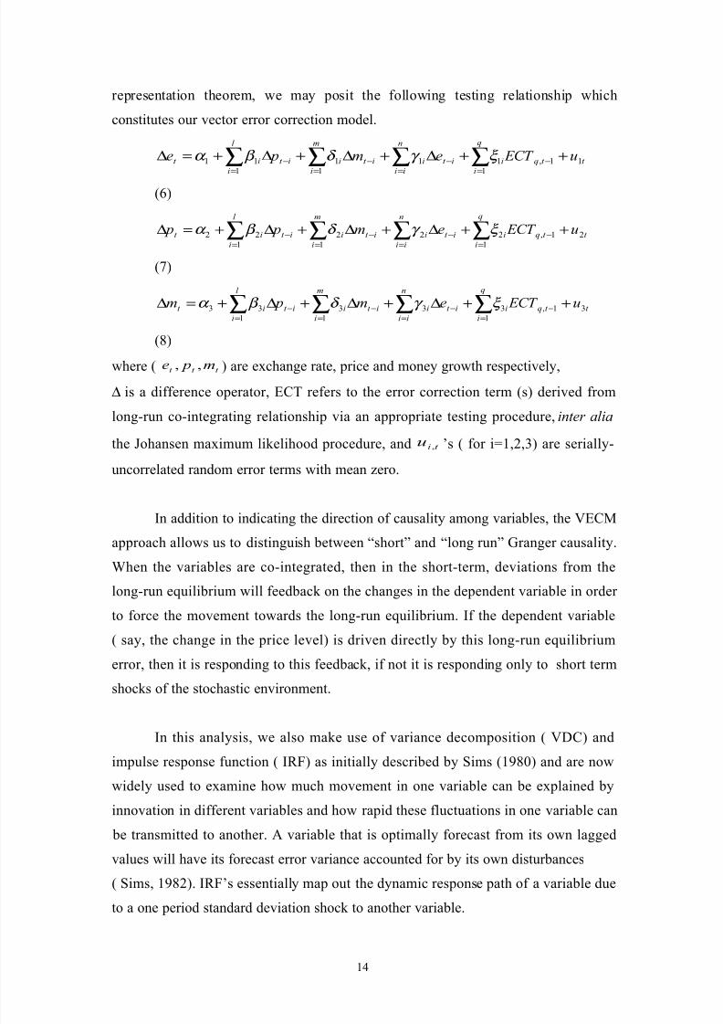
representation theorem, we may posit the following testing relationship which

constitutes our vector error correction model.

t t q

q

i

iit

n

ii

iit

m

i

iit

l

i

it u ECT em pe 11,

1

11

1

1

1

11++∆+∆+∆+=∆

−

=

−

=

−

=

−

=

∑∑∑∑ ξ γ δ β α

(6)

t t q

q

i

iit

n

ii

iit

m

i

iit

l

i

it u ECT em p p21,

1

22

1

2

1

22++∆+∆+∆+=∆

−

=

−

=

−

=

−

=

∑∑∑∑ ξ γ δ β α

(7)

t t q

q

i

iit

n

ii

iit

m

i

iit

l

i

it u ECT em pm31,

1

33

1

3

1

33 ++∆+∆+∆+=∆ −

=

−

=

−

=

−

=

∑∑∑∑ ξ γ δ β α

(8)

where ( t t t m pe ,, ) are exchange rate, price and money growth respectively,

∆ is a difference operator, ECT refers to the error correction term (s) derived from

long-run co-integrating relationship via an appropriate testing procedure, inter alia

the Johansen maximum likelihood procedure, and t iu

, ’s ( for i=1,2,3) are serially-

uncorrelated random error terms with mean zero.

In addition to indicating the direction of causality among variables, the VECM

approach allows us to distinguish between “short” and “long run” Granger causality.

When the variables are co-integrated, then in the short-term, deviations from the

long-run equilibrium will feedback on the changes in the dependent variable in order

to force the movement towards the long-run equilibrium. If the dependent variable

( say, the change in the price level) is driven directly by this long-run equilibrium

error, then it is responding to this feedback, if not it is responding only to short term

shocks of the stochastic environment.

In this analysis, we also make use of variance decomposition ( VDC) and

impulse response function ( IRF) as initially described by Sims (1980) and are now

widely used to examine how much movement in one variable can be explained by

innovation in different variables and how rapid these fluctuations in one variable can

be transmitted to another. A variable that is optimally forecast from its own lagged

values will have its forecast error variance accounted for by its own disturbances

( Sims, 1982). IRF’s essentially map out the dynamic response path of a variable due

to a one period standard deviation shock to another variable.

14



There are also a number of tests that can be used for testing co-integration.

These can be grouped into residual-based approach and the maximum likelihood

approach.

The residual-based approach, proposed by Engle and Granger (1987), relies

on the premise that if a set of variables is co-integrated of order (1,1) then the residual

from the co-integrating regression should be I(0).

Thus, co-integration could be tested by subjecting the co-integration residuals

to the DF, ADF , CRDW, or the Phillips-Perron tests.13 The Engle -Granger method

consists a two step procedure. First estimate the equation:

Yt=βXt+ut (9)

by OLS and test for stationarity of the residuals. Second, if this is not rejected

estimate the Error Correction Model (ECM).:

∆Yt=α0 + α1∆Xt+ α2 (Yt-1 -βXt-1) + ε t (10)

and replacing β by its previously computed OLS estimate.

One problem about the Engle-Granger procedure concerns its first step,

namely the variables Yt and Xt are non-stationary. Hence the use of OLS is

inappropriate and the resulting OLS estimate are inconsistent.

The Engle-Granger two step procedure was first adopted to determine any co-

integrating relationship between the dependent variables and independent variables.

Different co-integrating relationships were experimented with. The residuals of such

static regression equations were then computed and tested for the existence of co-

integration using the Dickey-Fuller (DF), the Augmented Dickey-Fuller (ADF) and

Sargan-Bhargava Durbin Watson Tests for Co-integration (SBDW)14. From the

results of various tests15, we could not reject the null hypothesis that the residuals are

non – stationary.

The model performed well in terms of explaining the price level as a function

of money, real income and the parallel exchange rate. The empirical results indicate

13 See Engle R.F and B.S Yoo (1987). “ Forecasting and Testing in Co-integrated Systems ”, Journalof Econometrics, 35:143-59. Operationally, it has been suggested by Engle and Yoo that the choice

14 Sargan J.D. and Bhargava, A. (1983), “ Testing Residuals from Least Regression for BeingGenerated by the Gaussian Random Walk ” Econometrica, 51, Jan, 153-174.15Results are available and may be obtained from the author by request

15



that there is a long-run equilibrium relationship between the above mentioned

variables . Moreover, the findings show that, in the long-run, inflation is positively

related to money supply and the BIF/US dollar parallel exchange rate, while it is

negatively related to real income.

We also employ the Johansen-Juselius (1990) analysis to determine the

existence of a long-run relationship between prices, money, real income and the

BIF/US dollar parallel exchange rate as the Engle-Granger two steps procedures may

not appropriate for a multivariate case where if co-integration exists, it will not be

unique as there are several equilibrium relationships linking n (>2) variables. We will

also test certain restrictions suggested by economic theory such as size of the

estimated elasticities.

In fact, if some variables are hypothesized to be linked by some theoretical

relationship, they should not diverge from each other in the long-run. Although such

variables may drift apart in the short-run, they converge toward equilibrium in the

long-run thanks to disequilibrium forces.

16



Table 4a

Johansen Co-integration λ-max Test among y, m1, e and p

o H A H Intercept only Intercept and Time Trend

r = 0 r = 1 42.62** 50.77**r=1 r = 2 17.89 21.29*

r = 2 r = 3 11.23 15.31

r = 3 r = 4 0.31 8.69

**, * denote significance level at 99.0 % and 95 % respectively

Table 4b

Johansen Co-integration Trace Test among y, m1, e and p


r = 0 r > 0 72.06** 96.08**

r ≤1 r > 1 29.44 45.30*

r ≤ 2 r > 2 11.54 24.01

r ≤ 3 r > 3 0.31 8.69


17



Table 5a

Johansen Co-integration λ-max Test among y, m2, e and p


r = 0 r = 1 34.21* 37.47*

r=1 r = 2 19.34 27.34

r = 2 r = 3 11.54 14.07

r = 3 r = 4 0.52 6.58


Table 5b

Johansen Co-integration Trace Test among y, m2, e and p


r = 0 r > 0 65.62** 83.18**

r ≤1 r > 1 31.41* 48.70**

r ≤ 2 r > 2 12.06 21.36

r ≤ 3 r > 3 0.52 6.58


Co-integration results showed that in the long-run a 1 percent increase in M1

will raise inflation by 0.78 percent, while a 1 percent depreciation of the BIF will

increase inflation by 0.26 percent. On the other hand, a 1 percent increase in real

income will reduce inflation by 0.66 percent. Table 4 and 5 report the results of the

co-integration test on the specification that uses the logarithms of the price level,

real income and the parallel exchange rate and money aggregates M1 and M2

respectively. Likelihood ratio test statistics suggest that there are at most one co-

integrating vector at 5% significance level for the system using M1 and M2 as

explanatory variables.

The optimal lag length was selected by minimizing the Akaike FPE criterion. Critical

values are sourced from MacKinnon (1991).

18



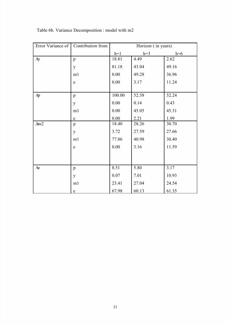
5.3. Variance decompositions

The result of VECM indicates the exogeneity or endogeneity of a variable in

the system and the direction of Granger causality within the sample period. However

it does not provide us with the dynamic properties of the system. The analysis of the

dynamic interactions among the variable in the post sample period is conducted

through variance decomposition ( VDCs) and impulse response functions ( IRFs) .

The variance decomposition of the six years forecast errors are presented in Tables 6a

for model with m1 and 6b for model with m2. Since the results of VDC may be

sensitive to the ordering of the variables, three different orderings were set up to

ensure that the monetary variables both precede and follow the other two variables.

However, the results from different orderings showed no significant differences, and

therefore only the results of the first ordering ( ∆y, ∆ p, ∆m1/m2, ∆e) was focused to

summarize the findings. The results fro the VDC are found to be consistent with that

of the causality tests. M1 and M2 respectively account for 11% and 45% of the

variation in the forecast of the price level.

19



Table 6a. Variance Decomposition : model with m1

Error Variance of Contribution from Horizon ( in years)

h=1 h=3 h=6

∆y p

y

m1

e

57.27

42.75

0.00

0.00

32.08

48.96

0.36

18.23

54.37

29.66

1.14

15.30

∆ p p

y

m1

e

100.00

0.00

0.00

0.00

89.81

1.73

5.72

2.72

86.23

0.96

11.43

1.36∆m1 p

y

m1

e

20.66

1.34

77.98

0.00

10.53

20.01

65.50

3.95

6.52

18.22

68.24

7.01

∆e p

y

m1

e

5.80

42.09

2.46

49.63

8.93

25.29

34.84

30.91

12.52

11.74

61.99

13.73

20



Table 6b. Variance Decomposition : model with m2

Error Variance of Contribution from Horizon ( in years)

h=1 h=3 h=6

∆y p

y

m1

e

18.81

81.18

0.00

0.00

4.49

43.04

49.28

3.17

2.62

49.16

36.96

11.24

∆ p p

y

m1

e

100.00

0.00

0.00

0.00

52.58

0.14

45.05

2.21

52.24

0.43

45.31

1.99

∆m2 p

y

m1

e

18.40

3.72

77.86

0.00

28.26

27.59

40.98

3.16

30.70

27.66

30.40

11.59

∆e p

y

m1

e

8.51

0.07

23.41

67.98

5.80

7.01

27.04

60.13

3.17

10.93

24.54

61.35

21



5.4. Impulse Response Functions

The impulse response functions ( IRFs), presented in Figures1 and 2 illustrate

ten years response of the endogenous variables to an initial shock of one standard

deviation in M1, M2,M3 and P. In general the IRFs appear to be consistent with the

results obtained from the VECM and VCD discussed above.

Figure 1: Impulse responses of output, prices, parallel market exchange rate and

narrow money

-.04

.00

.04

.08

.12

.16

1 2 3 4 5 6 7 8 9 10

LCPI

LGDPR

LM1

LPRATE

Response of LCPI to Cholesky

One S.D. Innovations

-.16

-.12

-.08

-.04

.00

.04

.08

.12

1 2 3 4 5 6 7 8 9 10

LCPI

LGDPR

LM1

LPRATE

Response of LGDPR to Cholesky


-.04

.00

.04

.08

.12

.16

1 2 3 4 5 6 7 8 9 10

LCPI

LGDPR

LM1

LPRATE

Response of LM1 to Cholesky


-.20

-.16

-.12

-.08

-.04

.00

.04

.08

.12

1 2 3 4 5 6 7 8 9 10

LCPI

LGDPR

LM1

LPRATE

Response of LPRATE to Cholesky


22



Figure 2: Impulse responses of output, prices, parallel market exchange rate and

broad money ( m2)

-.04

.00

.04

.08

.12

.16

1 2 3 4 5 6 7 8 9 10

LCPI

LGDPR

LM2

LPRATE

Response of LCPI to CholeskyOne S.D. Innovations

-.08

-.04

.00

.04

.08

1 2 3 4 5 6 7 8 9 10

LCPI

LGDPR

LM2

LPRATE

Response of LGDPR to CholeskyOne S.D. Innovations

-.04

-.02

.00

.02

.04

.06

.08

.10

1 2 3 4 5 6 7 8 9 10

LCPI

LGDPR

LM2

LPRATE

Response of LM2 to Cholesky


-.08

-.04

.00

.04

.08

.12

.16

1 2 3 4 5 6 7 8 9 10

LCPI

LGDPR

LM2

LPRATE

Response of LPRATE to Cholesky


Tables 6a report the Granger-causality results based on VECM for model with m1.

The optimal lag structure was determined using the criterion of minimum Akaike’s

Final Prediction Error (FPE) The F-statistics of the independent variables indicate

that there is a unidirectional causality running from p to y, m1to y, p to m1, and a bi-

directional feedback running from p to e and from m1 to e.

23



Table 7a: Granger Temporal causality results based on Vector Error-Correction

Model ( VECM- Uniform lag length): Model with M1

∆y

F-stat

∆ p

F-stat

∆m1

F-stat

∆e

F-stat

ECT(-1)

t-stat

∆y - 5.24*** 6.05** 13.42* -3.59*∆ p 0.96 - 2.01 2.41 0.56

∆m1 2.52*** 5.83 - 2.31 -035∆e 1.48 2.88 2.72 - 1.60*** Notes: The F-statistics tests the joint significance of the lagged values of the independent variables,

and t-statistics tests the significance of the error correction term ( ECT) . Diagnostic tests ( not

reported) conducted for residual autocorrelation are found to be satisfactory. The asterisks indicate

the following levels of significance * 1%, ** 5% and ***10% level.

Tables 7a report the Granger-causality results based on VECM for model with m2.

The F-statistics of the independent variables indicate that there is bi-directional

feedback running p to m , p to e and p to y.

Table 7b: Granger Temporal causality results on vector error-correction model

( VECM): Model with M2 ( F-stat.)

∆y

F-stat

∆ p

F-stat

∆m2

F-stat

∆e

F-stat

ECT(-1)

t-stat

∆y - 2.85 0.66 1.01 4.87*∆ p 2.74 - 0.70 0.58 -3.51*

∆m1 7.83** 0.24 - 0.15 1.56***∆e 24.55* 11.75* 0.29 - 0.23 Notes : As in Table 6a.

Second in order to investigate the short-run dynamics, we turn to the estimates of the

error correction model, which is formulated as:

∆Pt= α0 +i

n

=∑0 (α1i ∆Mt-i +α2i ∆yt-i +α3i∆et-i ) + i

n

=∑1 α4i ∆Pt-i ) + α5ECt-i + vt (11)

24



where ∆ represents the first difference operator, ECt the error correction term, and v t a

disturbance term, and the lag length n is determined by Hendry’s General -to-

Specific-Modeling ( HGSM) strategy. We include two lags on each term and

eliminate the lags whose coefficients are not statistically significant. Longer lag

specification was not possible due to the relatively short length of our sample and the

low frequency of the data. Equation (8) was used to estimate the short run model,

with the most parsimonious formulation of the model presented below, based on a

simplification search of n=2:

An error correction model (ECM) capturing the relationship between inflation, money

and parallel market exchange rate yielded the following results:

25



Table 8. Forecasting Models of Inflation using different monetary aggregates

(Dependent Variable pt, Sample: 1972 1998)

Regressors Model 1 with

Narrow Money

Model 2 with

Broad MoneyC 0.017

[0.975]

-0.007

[-0.424]

∆(m) t 0.289

[4.253]

0.320

[4.224]

∆(e) t 0.152

[2.942]

0.127

[2.993]

∆(y) t -0.304

[-4.086]

-0.450

[-7.003]

∆(p) 1−t 0.419

[3.835]

0.446

[5.149]

∆(m) 1−t 0.153

[2.435]

∆(p+m-y) t -0.572

[-5.631]

0.819

[-5.870]

R 2 0.778 0.848

Adj. R 2 0.725 0.803S.E. Regression 0.039 0.033

Table 8 summarizes the final version of each of the models estimated from

1970 to1998. The model was estimated using standard OLS estimation techniques on

annual data for the period 1970-1998. The t-values are beneath beside each

coefficient ; p-values are in brackets beneath each coefficient. R 2 and SEE are

respectively the multiple correlation coefficient adjusted for degrees of freedom and

the standard error of estimate. It performed well in terms of the expected signs of the

explanatory variables and in terms of its explanatory power, with an adjusted

coefficient of determination value of 0.725 for the model with M1 as explanatory

variable and 0.803 for the model with M2 as explanatory variable.

Moreover, when the error correction model was fitted against historical

inflation data, it performed well in terms of tracking the cyclical nature of price

movements in Burundi ( Figure 1 and 2). The estimation results indicate that the predictions obtained by the monetary aggregate M2 are better than those obtained

26



when M1 is used as the explanatory variable. This suggests that M2 may provide a

more appropriate guide to predict prices.

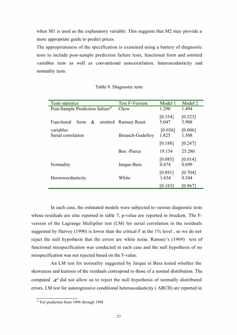
The appropriateness of the specification is examined using a battery of diagnostic

tests to include post-sample prediction failure tests, functional form and omitted

variables tests as well as conventional autocorrelation, heteroscedasticity and

normality tests.

Table 9. Diagnostic tests

Tests statistics Test F-Version Model 1 Model 2Post-Sample Prediction failure16 Chow 1.290

[0.354]

1.494

[0.323]Functional form & omitted

variables

Ramsey Reset 5.047

[0.036]

5.908

[0.006]Serial correlation Breusch-Godefrey

Box -Pierce

1.825

[0.188]

19.154

[0.085]

1.508

[0.247]

25.280

[0.014] Normality Jarque-Bera 0.474

[0.891]

0.699

[0.704]Hereroscedasticity White 1.634

[0.183]

0.344

[0.967]

In each case, the estimated models were subjected to various diagnostic tests

whose residuals are also reported in table 7, p-value are reported in brackets. The F-

version of the Lagrange Multiplier test (LM) for serial correlation in the residuals

suggested by Harvey (1990) is lower than the critical F at the 1% level , so we do not

reject the null hypothesis that the errors are white noise. Ramsey’s (1969) test of

functional misspecification was conducted in each case and the null hypothesis of no

misspecification was not rejected based on the F-value.

An LM test for normality suggested by Jarque et Bera tested whether the

skeweness and kurtosis of the residuals correspond to those of a normal distribution. The

computed 2 χ did not allow us to reject the null hypothesis of normally distributed

errors. LM test for autoregressive conditional heteroscedasticity ( ARCH) are reported in

16 For prediction from 1996 through 1998

27



the F –form. ). The form of serial correlation, or more general forms of autocorrelation,

was rejected based on the Breusch-Godfrey and Box-Pierce Q statistic.

Figure 3: Actual and fitted inflation using M1 as explanatory variable, 1970-1998

[First difference log (CPI)]

-0.10

-0.05

0.00

0.05

0.10

0.0

0.1

0.2

0.3

0.4

72 74 76 78 80 82 84 86 88 90 92 94 96 98

Residual Actual Fitted

28



Figure 4: Actual and fitted inflation using M2 as explanatory variable, 1970-1998

[First difference log (CPI)]

-0.06

-0.04

-0.02

0.00

0.02

0.04

0.06 0.0

0.1

0.2

0.3

0.4

72 74 76 78 80 82 84 86 88 90 92 94 96 98

Residual Actual Fitted

Moreover, the estimated error correction model was found to be stable over

the period studied based on the Chow breakpoint test.

Two years were selected for the Chow F-test as possible breakpoints ( 1986,

1993 ) representing years of pronounced structural reforms or exogenous shocks. The

CUSUM recursive residuals test also confirmed the structural stability of the model.Figure 3 plots the CUSUM cumulative recursive residuals, with deviations inside the

5 percent critical line implying structural stability.

Figure 5: Cusum recursive residuals test

CUSUM recursive residuals

Model 1

CUSUM recursive residuals

Model 2

-0.10

-0.05

0.00

0.05

0.10

78 80 82 84 86 88 90 92 94 96 98

Recursive Residuals ± 2 S.E.

-0.10

-0.05

0.00

0.05

0.10

80 82 84 86 88 90 92 94 96 98

Recursive Residuals ± 2 S.E.

6. Conclusion and Policy Implications

29



This paper examines the importance of monetary variables ( money and

exchange rate) in the inflationary process within the Burundian economy for the

period 1970-1998. The results of both co-integration and error correction confirmed

that there is a long run equilibrium relationship between prices, money , exchange

rate and income. In line with the monetarist thesis, the findings demonstrate that, in

the long run inflation is positively related to money supply and the exchange rate

while it is negatively related to real income. More specifically, using M1 as the

explanatory variable in the inflation equation, we found that in the long run, a one

percent increase in M1 would raise inflation by 0.76 percent , a one percent

depreciation of the BIF on the parallel markets would raise inflation by 0.28 percent

and a one percent increase in real income would reduce inflation by 0.64 percent.

Using M2 as explanatory variable in the inflation equation, a one percent increase in

M2 would raise inflation by 0.72 percent, a one percent depreciation of the BIF in the

parallel markets would raise inflation by 0.25 percent while a one percent increase in

income would reduce inflation by 0.86 percent.

The existence of a long run equilibrium relationship among money , price,

exchange rate and income appears to be supported by annual data for Burundi for

1970-1998. According to the theory of co-integration, the estimated co-integratingresidual should appear as the error correction term in a dynamic VEC model. An

important finding from the dynamic models presented is that the error correction

terms are statistically significant.

Not only all the regressors in the VEC models significant but also the

diagnostic tests conducted show that there is no evidence of any problems of serial

correlation, heteroscedasticity, non-normal errors, parameter instability or predictive

inaccuracy when the data are split at 1986 and 1993. Additionally, the CUSUM and

CUSUMSQ statistics are consistently in the center of their 5% bounds, while the

recursive coefficients of the regressors display no sudden variations as more data is

added, indicating that the estimated equations are highly stable and shows no signs of

underlying misspecification.

The empirical findings from the error correction models showed that short –

run money elasticities, (0.289 for M1 and 0.320 for M2) are considerably smaller in

30



magnitude than the relevant long-run estimates. The short adjustment effect is –0.57

for model with M1 and 0.82 for model with M2. The empirical findings from the

error correction models showed that inflation adjusts to its equilibrium value rapidly,

that is almost 60 percent per annum for the model with M1 and 82 percent for the

model with M2.

Work on inflation in Burundi is still embryonic. Our hope is that this study

will set a stage for more quantitative research on inflation in Burundi. Further

refinement of the analysis developed here, notably by using longer series could yields

stronger results. Additional analysis is also needed to examine the factors which

determine increases in individual components of the consumer price index and the

revenue-raising possibility of inflation, through the “inflation tax”.

31



Bibliography

Akhtar, M.A., (1980) .“ Recent experience with monetary growth and inflation in

Germany, Japan and the United States ”, Journal of Post-Keynesian Economics, Vol.

II, N°4 (Summer ), pp.585-592.

Argy, V., “ Structural inflation in developing countries ”, Oxford Economic Papers,

Vol.22, N°.1, New Series (March), pp-73-85.

Bomberger, W.A. and G.E.Makinen, (1979). “ Some further tests of the Haberger

inflation model using quarterly data ”, Economic Development and Cultural Change,

Vol.27, N° 4 (July), pp. 629-644.

Canavese, A. J.(1982), “The structuralist explanation in the Theory of Inflation ”,

World Development , 10 (7) July .

Canetti, E. and J. Greene, “Monetary growth and exchange rate depreciation as causes

of Inflation in African Countries: An empirical Analysis” Journal of African Finance

and Economic Development, Spring , p.37-62

Chandavarkar, (1977). A.G., “ Monetization of developing economies ”, IMF Staff

Papers, Vol. XXIV, N°. 3, (November ), pp.665-751.

Frisch, H. (1983), “ Theories of Inflation ”, Cambridge University Press, Cambridge,

Mass.Granger, C.W.J. « Developments in the Study of Co-integrated Variables : An

Overview”, Oxford Bulletin of Economics and Statistics, Vol. 48 ( August 19860,

pp201.12.

Karnosky, M. (1979). “ The link between money and prices , 1971-76 ”, Federal

Reserve Bank of St.Louis Review, 58(6), June.

Khan, M. (1980), Monetary shocks and the dynamics of inflation ”, IMF Staff Papers,

27(2), June.

MacKinnon, James, (1991), “Critical Values for Co-integration Tests”, in Long-run

Economic Relationships: Readings in Co-integration, ed. By Robert F. Engle and

Clive W.J. Granger

( Oxford University Press).

Montiel, P . (1989). “ Empirical Analysis of High-Inflation Episodes in Argentina,

Brazil and Israel”, IMF Staff Papers 36 (3), pp.527-49.

32



Kirkpatrick, C. And Nixon F.I (1986), “ Inflation in Less Developed Countries ” in

Gemmell N.(ed.), Survey in Development Economics. Basil Blackwell, London, 423-

453 .

Ndenzako, J. « Does the monetary model provides a reasonable explanation of the

dynamics of inflationary process in Burundi”, Revue de l’Institut de Développement

Economique du Burundi , RIDEC , 4(1), March 2000, p.84-111.

Ndenzako, J. “ Economie Souterraine, Evasion Fiscale et Elasticité du Système Fiscal

Burundais », Revue de l’Institut de Développement Economique du Burundi ,

RIDEC , 3(2), Sept. 1999.

Ndenzako, J. “ The Stability of the Burundian Demand for Money Function : Some

Further Results», Revue de l’Institut de Développement Economique du Burundi ,

RIDEC , 3(2), Sept. 1998, p.297-319.

Ndenzako, J. “ The Demand for Money in Burundi : Some Preliminary Results»,

Revue de l’Institut de Développement Economique du Burundi , RIDEC , 2(1),

March, 1998, p.178-195.

Nikolic, N. (2000), “Money Growth-Inflation Relationship in Postcommunist

Russia”, Journal of Comparative Economics, vol. 58, 17-29.

Nugent, J.B., and C.Glezakos, (1979). “ A model of inflation and expectations in

Latin America ”, Journal of Development Economics, Vol. 6 , pp.431-446.Rogers, J.H. and P. Wang, (1995). “Output, Inflation and Stabilization in a Small

Open Economy: Evidence from Mexico”, Journal of Development Economics, 46 (2),

pp.1-37.

Ross, K. (1998), “Post Stabilization Inflation Dynamics in Slovenia”, International

Monetary Fund Working Paper, WP/98/27.

Otani, I. , “ Inflation in an open economy ”, IMF Staff Papers, Vol. XXII, N°3.

(November 1975), pp.750-774

Saini, K.G., (1982) “ The Monetarist Explanation of Inflation: The Experience of Six

Asian Countries ”, World Development , Vol.10, N°10, p.871.

Sheehey, E.J., (1980), “ Money, Income and Prices in Latin America ”, An Empirical

Note ”, Journal of Development Economics, 7(3), September.

Vogel, R.C., (1974) “ The dynamics of inflation in Latin America ”, American

Economic Review, Vol.64, N°1. (March ), pp.102-114.

Macro Paper JN

Documents

Transcript of Macro Paper JN