Machine Translation ofMorphologically Rich Languages

Using Deep Neural Networks

Peyman PassbanB.Eng., M.Sc.

A dissertation submitted in fulfillment of the requirements for the award of

Doctor of Philosophy (Ph.D.)

to the

Dublin City UniversitySchool of Computing

Supervisors:Prof. Qun LiuProf. Andy Way

January 2018

I hereby certify that this material, which I now submit for assessment on theprogramme of study leading to the award of Ph.D. is entirely my own work, thatI have exercised reasonable care to ensure that the work is original, and does notto the best of my knowledge breach any law of copyright, and has not been takenfrom the work of others save and to the extent that such work has been cited andacknowledged within the text of my work.

Signed:

(Candidate) ID No.: 13212218

Date:

Contents

Abbreviations xv

Abstract xvi

Acknowledgements xvii

1 Introduction 1

1.1 Research Questions . . . . . . . . . . . . . . . . . . . . . . . . . . . . 3

1.2 Thesis Structure . . . . . . . . . . . . . . . . . . . . . . . . . . . . . 4

1.3 Contributions . . . . . . . . . . . . . . . . . . . . . . . . . . . . . . . 6

1.4 Publication . . . . . . . . . . . . . . . . . . . . . . . . . . . . . . . . 7

2 Fundamental Concepts 9

2.1 An Introduction to Morphology . . . . . . . . . . . . . . . . . . . . . 9

2.1.1 Morphological Complexity . . . . . . . . . . . . . . . . . . . . 13

2.2 Statistical Machine Translation . . . . . . . . . . . . . . . . . . . . . 17

2.3 SMT for MRLs . . . . . . . . . . . . . . . . . . . . . . . . . . . . . . 20

2.3.1 Incorporating Morphological Information at Decoding Time

(Type 1) . . . . . . . . . . . . . . . . . . . . . . . . . . . . . . 21

2.3.2 Multi-Step Translation (Type 2) . . . . . . . . . . . . . . . . 24

2.3.3 Morphological Processing for Translation (Type 3) . . . . . . 30

2.4 Deep Neural Networks . . . . . . . . . . . . . . . . . . . . . . . . . . 31

2.4.1 Feed Forward Neural Models . . . . . . . . . . . . . . . . . . 34

2.4.2 Recurrent Neural Models . . . . . . . . . . . . . . . . . . . . 35

i

2.4.3 Convolutional Neural Models . . . . . . . . . . . . . . . . . . 36

2.4.4 Training Neural Networks . . . . . . . . . . . . . . . . . . . . 39

2.4.5 Sequence Modeling with DNNs . . . . . . . . . . . . . . . . . 40

2.5 Summary . . . . . . . . . . . . . . . . . . . . . . . . . . . . . . . . . 42

3 Learning Compositional Embeddings for MRLs 46

3.1 Embedding Learning . . . . . . . . . . . . . . . . . . . . . . . . . . . 49

3.1.1 Subword-level Information for Embeddings . . . . . . . . . . . 50

3.2 Learning Morphology-Aware Embeddings . . . . . . . . . . . . . . . . 52

3.2.1 Network Architecture . . . . . . . . . . . . . . . . . . . . . . 54

3.2.2 Word Embeddings . . . . . . . . . . . . . . . . . . . . . . . . 57

3.3 Experimental Results . . . . . . . . . . . . . . . . . . . . . . . . . . . 58

3.4 Further Investigation of Experimental Results . . . . . . . . . . . . . 61

3.4.1 POS and Morphology Tagging Experiments . . . . . . . . . . 61

3.4.2 Impact of Using Different Architectures . . . . . . . . . . . . 64

3.4.3 Analytical Study . . . . . . . . . . . . . . . . . . . . . . . . . 67

3.5 Summary . . . . . . . . . . . . . . . . . . . . . . . . . . . . . . . . . 68

4 Morpheme Segmentation for Neural Language Modeling 69

4.1 Background . . . . . . . . . . . . . . . . . . . . . . . . . . . . . . . . 72

4.1.1 Related Work . . . . . . . . . . . . . . . . . . . . . . . . . . . 74

4.2 Morpheme Segmentation . . . . . . . . . . . . . . . . . . . . . . . . . 77

4.3 Count-based Segmentation for MCWs . . . . . . . . . . . . . . . . . . 79

4.3.1 Model A: Greedy Selection . . . . . . . . . . . . . . . . . . . 81

4.3.2 Model B: Adaptive Thresholding . . . . . . . . . . . . . . . . 84

4.3.3 Model C: Mutual Information-based Selection . . . . . . . . . 85

4.3.4 Model D: Dynamic Programming-based Segmentation . . . . 86

4.3.5 Segmentation Quality . . . . . . . . . . . . . . . . . . . . . . 92

4.4 Network Architecture . . . . . . . . . . . . . . . . . . . . . . . . . . . 96

4.5 Experimental Results . . . . . . . . . . . . . . . . . . . . . . . . . . . 100

ii

4.5.1 Discussion . . . . . . . . . . . . . . . . . . . . . . . . . . . . . 103

4.5.2 Neural Language Modeling for SMT . . . . . . . . . . . . . . 106

4.6 Summary . . . . . . . . . . . . . . . . . . . . . . . . . . . . . . . . . 107

5 Boosting SMT via NN-Generated Features 109

5.1 Incorporating Embeddings into Phrase Tables . . . . . . . . . . . . . 110

5.1.1 Background . . . . . . . . . . . . . . . . . . . . . . . . . . . . 111

5.1.2 Proposed Model . . . . . . . . . . . . . . . . . . . . . . . . . 113

5.1.3 Experimental Results . . . . . . . . . . . . . . . . . . . . . . . 121

5.2 Further Investigation of Neural Features . . . . . . . . . . . . . . . . 122

5.2.1 Capturing Semantic Relations . . . . . . . . . . . . . . . . . . 123

5.2.2 Using Semantic Features for Other Languages . . . . . . . . . 124

5.2.3 Using Morphology-Aware Embeddings in SMT . . . . . . . . . 125

5.2.4 Training Bilingual Embeddings Using Convolutional Neural

Networks . . . . . . . . . . . . . . . . . . . . . . . . . . . . . 127

5.2.5 Human Evaluation . . . . . . . . . . . . . . . . . . . . . . . . 130

5.3 Summary . . . . . . . . . . . . . . . . . . . . . . . . . . . . . . . . . 132

6 Morpheme Segmentation for Neural Machine Translation 134

6.1 Neural Machine Translation (NMT) . . . . . . . . . . . . . . . . . . . 135

6.2 Literature Review . . . . . . . . . . . . . . . . . . . . . . . . . . . . . 139

6.2.1 Main Models in NMT . . . . . . . . . . . . . . . . . . . . . . 140

6.2.2 Multi-Task Multilingual NMT Models . . . . . . . . . . . . . 144

6.2.3 Effective Training Techniques for Deep Neural Models . . . . 146

6.2.4 Hybrid Statistical and Neural Models . . . . . . . . . . . . . . 147

6.3 Improving NMT for MRLs with Subword Units . . . . . . . . . . . . 148

6.3.1 Experimental Study . . . . . . . . . . . . . . . . . . . . . . . 151

6.4 Summary . . . . . . . . . . . . . . . . . . . . . . . . . . . . . . . . . 156

7 Double-Channel NMT Models for Translating from MRLs 158

iii

7.1 Proposed Architecture . . . . . . . . . . . . . . . . . . . . . . . . . . 162

7.2 Experimental Study . . . . . . . . . . . . . . . . . . . . . . . . . . . 165

7.3 Conclusion . . . . . . . . . . . . . . . . . . . . . . . . . . . . . . . . . 172

8 Conclusions and Future Study 173

Bibliography 181

iv

List of Figures

2.1 Where morphology lies in linguistics (Uí Dhonnchadha, 2002). . . . . 10

2.2 Arabic patterns and the letter substitution system. The first line

shows two Arabic patterns and the second line, words in those pat-

terns. As the figure depicts, in this case فـ (1), ـعـ or عـ (2) and ل (3)

which are the reserved letters of the pattern (act as placeholders) are

substituted by ك (1), ت (2) and ب (3), respectively. . . . . . . . . . . 13

2.3 Qualitative categorization of morphologically complex languages. . . 16

2.4 Vocabulary size vs. MT performance. The figure shows how mor-

phological complexity can affect the final performance. The x axis

shows the vocabulary size and the y axis is the BLEU score. . . . . . 16

2.5 Phrase-level translation. The figure tries to illustrate complex word

alignments. The Farsi word āz is aligned to (nothing) the Null token. 18

2.6 The high-level architecture of the factored translation model (Koehn

and Hoang, 2007). . . . . . . . . . . . . . . . . . . . . . . . . . . . . 23

2.7 The model proposed by Lee (2004) for translating complex Arabic

words. The model decides to either keep segmented morphemes or

delete them. . . . . . . . . . . . . . . . . . . . . . . . . . . . . . . . . 25

2.8 Data preparation for Arabic MT proposed in El Kholy and Habash

(2012) . . . . . . . . . . . . . . . . . . . . . . . . . . . . . . . . . . . 26

2.9 Compound merging in German, based on the model proposed in Cap

et al. (2014). . . . . . . . . . . . . . . . . . . . . . . . . . . . . . . . 29

2.10 Architecture of a simple neuron to model the logical OR function. . . 32

v

2.11 Distributed function approximation using DNNs (Bengio, 2009). . . . 33

2.12 Visualizing the process of data-distribution learning via NNs. The

figure shows which node learns which part of the distribution. . . . . 33

2.13 Unrolling an RNN over time. . . . . . . . . . . . . . . . . . . . . . . 36

2.14 The convolution operation in CNNs. . . . . . . . . . . . . . . . . . . 38

3.1 The cubic and matrix data structures for the input string [w0 w1

w2 w3 w4]. Lemma, prefix and suffix embeddings for each word is

referred to by Li, Pi and Si, respectively, andWi indicates the surface-

form embedding. n = 3, m = 1 and the target word is w3. The

first 3 columns include the related embeddings for w0 to w2 and the

fourth column includes the embedding for w4. We emphasize that the

data structure on the right-hand side is used by previous embedding

models and our model benefits from the cube on the left-hand side. . 53

3.2 Network Architecture. . . . . . . . . . . . . . . . . . . . . . . . . . . . 57

3.3 Comparison of the convergence speed between Word2Vec and our

model for the POS-tagging task. The x axis shows the iteration

number and the y axis is the error rate. . . . . . . . . . . . . . . . . . 64

4.1 The network on the left-hand side is the character-level architecture

(Kim et al., 2016). word2 is segmented into characters and different

filters with different widths are applied to construct the word-level

representation. The network on the right-hand side is the morpheme-

level architecture (Botha and Blunsom, 2014). Subunit embeddings

are linearly summed with the surface-form embedding to build the

final representation for each word (Ci). . . . . . . . . . . . . . . . . . 76

vi

4.2 The process of segmenting ‘prdrãmdtrynhã’. main for each node is

its offspring in the middle. The nodes before and after main are L-

string and R-string, respectively. Dotted and solid lines indicate the

character-level and morpheme-level decompositions. Final states are

illustrated with double lines. . . . . . . . . . . . . . . . . . . . . . . 83

4.3 Different segmentation boundaries for the Turkish word ‘hakkinizdakiler’

meaning ‘things about you’. Different paths yield different segmen-

tations for this word. . . . . . . . . . . . . . . . . . . . . . . . . . . . 87

4.4 Morpheme segmentation with Model D. . . . . . . . . . . . . . . . . 92

4.5 Different segmentations provided by Byte-pair and Model D. We use

superscripts to make a connection among words, their translation

and segmented forms. ‚ shows the segmentation boundary. bpe-xK

means the Byte-pair model trained to extract x thousands different

symbols. Turkish Seq. is the given Turkish sentence and Translation

is the English counterpart of the Turkish sentence. . . . . . . . . . . 95

4.6 The figure depicts the third time step when processing the input

string s=[... wi´2 wi´1 wi wi+1 ...]. The complex Farsi word is de-

composed into blocks. Different filters (shown by different colors) are

applied over blocks to extract different (n-gram) features. The vec-

tor generated by the filters is processed by a highway and an LSTM

module to make the prediction, which is the next word wi+1. At each

time step, the filters are only applied to the current word. . . . . . . 99

4.7 Impact of different θ values on PPL and |M|. . . . . . . . . . . . . . 105

vii

5.1 The figure shows the structure of a German-to-English phrase table where

the first constituent at each line is a German phrase which is separated

by ||| from its English translation. The following 4 scores after the En-

glish phrase are default bilingual scores extracted from training corpora.

These scores show how phrases are semantically related to each other. The

decoder selects the best phrase pair at each step based on these scores. . . 110

5.2 S, T , and B indicate the source, target, and bilingual corpora, respec-

tively. The SMT model generates the phrase table and bilingual lexicon

using S and T (shown in the middle). The bilingual corpus consists of

6 different sections of 1) all source sentences (Sentences), 2) all source

phrases (Phrases), 3) all target sentences (Sentencet), 4) all target phrases

(Phraset), 5) all phrase pairs (Phrases-Phraset) and 6) all bilingual lexi-

cons (Words-Wordt). . . . . . . . . . . . . . . . . . . . . . . . . . . . . 114

5.3 sp, tp, sm and tm stand for source phrase, target phrase, source

match and target match, respectively. The embedding size for all

types of embedding is the same. The source/target-side embedding

could belong to a source/target word, phrase, or sentence. The labels

on the links indicate the Cosine similarity between two embeddings

which is mapped to the range [0,1]. . . . . . . . . . . . . . . . . . . . 117

5.4 Network architecture. The input document is S = w1 w2 w3 w4

w5 w6 and the target word is w3. In the backward pass document

embeddings for w1, w2, w4 to w6, and Ds are updated. . . . . . . . . 120

5.5 Word alignments provided by a PBSMT engine for a given (s, t) ex-

ample. ‘him’ is selected as the target word so ‘him’ and its transla-

tions are excluded from the input tensor. . . . . . . . . . . . . . . . 128

5.6 Human evaluation results on EnÑFa translation. . . . . . . . . . . . 132

viii

6.1 A high-level view of the encoder-decoder architecture. The direction

of arrows show the impact of each unit on other units. The infor-

mation flow from st to ht starts when all input symbols have been

processed. . . . . . . . . . . . . . . . . . . . . . . . . . . . . . . . . 137

6.2 The network on the right-hand side depicts the basic encoder-decoder

model which summarizes all input hidden states into a single vector.

The network on the left-hand side is an encoder-decoder model with

attention which defines a weight for each of the input hidden states.

αti indicates the weight assigned to the i-th input state to make the

prediction of the t-th target symbol. . . . . . . . . . . . . . . . . . . 139

7.1 A comparison between the simple and double-attentive attention

models. It should be noted that the figure only shows connections

associated with the attention module. . . . . . . . . . . . . . . . . . . 165

ix

List of Tables

2.1 Examples of MCWs in agglutinative languages. Morphemes are se-

quentially added to change the form, meaning, and syntactic role of

the word. The bold-faced morpheme is the stem. . . . . . . . . . . . 11

2.2 Summary of SMT models for MRLs. Models are sorted in chrono-

logical order. . . . . . . . . . . . . . . . . . . . . . . . . . . . . . . . 45

3.1 Results for the word-similarity task. Numbers indicate Spearman’s

rank correlation coefficient (ρ ˆ 100) between similarity scores as-

signed by different neural networks and human annotators. . . . . . . 60

3.2 Results for the POS-tagging experiment. Numbers indicate the accu-

racy of the neural POS tagger. According to word-level paired t-test

with p ă 0.05, our results are significantly better than other models. . 63

3.3 Results for the morphology-tagging experiment. Numbers indicate

the accuracy of the neural tagger. According to word-level paired

t-test with p ă 0.05, our results are significantly better than other

models. . . . . . . . . . . . . . . . . . . . . . . . . . . . . . . . . . . 64

3.4 Impact of different subword-combination models on the word-similarity

task. . . . . . . . . . . . . . . . . . . . . . . . . . . . . . . . . . . . . 65

3.5 The top-10 most similar embeddings to the Farsi verb ‘krdn’ meaning

‘doing’. Similarity is the Cosine distance between ‘krdn’ and the

retrieved verb. . . . . . . . . . . . . . . . . . . . . . . . . . . . . . . . 67

x

4.1 Results reported from state-of-the-art NLMs on PTB. PPL refers to

perplexity which is a standard to evaluate LMs (lower is better). The

table only reports the best performance achieved by the models. . . . 75

4.2 Different segmentations with different levels of granularity for the

input sequence ‘thisisasimplepreprocessingstep’. We emphasize that

this is a quite complex example which is never faced in the training

phase. We used this example to show that the granularity level in

our models can vary from the sentence level (to separate words) to

the character level (to extract characters). Model Broot generates

the same results as Model Bdiv. . . . . . . . . . . . . . . . . . . . . 93

4.3 Results for the morpheme segmentation task. Model Bdiv and Model

Broot performed equally in this task so we showed both of them with

Model B. . . . . . . . . . . . . . . . . . . . . . . . . . . . . . . . . . 94

4.4 Statistics of datasets. T , V , C and M indicate the number of tokens,

word vocabulary size, character vocabulary size, and the number of

different blocks for each language, respectively. θ is the frequency

threshold andm is the break-point threshold. The subscript indicates

to which model the parameter belongs. . . . . . . . . . . . . . . . . . 101

4.5 Perplexity scores for different MRLs (lower is better). . . . . . . . . . 101

4.6 Experimental results for large datasets. mc is the extrenal parameter

of Model C. dp stands for dynamic programming and indicates the

tokens extracted via Model D. . . . . . . . . . . . . . . . . . . . . . . 104

4.7 Boosting n-gram-based LMs with NLMs. Improvements (Imp.) are

statistically significant according to the results of paired bootstrap

re-sampling with p = 0.05 for 1000 samples (Koehn, 2004b) . . . . . . 107

5.1 Context vectors for different input documents. wt (the word to

be predicted) is better and m = 5 (context). Italics are in Farsi

(transliterated forms). . . . . . . . . . . . . . . . . . . . . . . . . . . 119

xi

5.2 Impact of the proposed features over the En–Cz engine. . . . . . . . . 121

5.3 Impact of the proposed features over the En–Fa engine. . . . . . . . . 122

5.4 The top-10 most similar vectors for the given English query. Recall

that the retrieved vectors could belong to words, phrases or sentences

in either English or Farsi as well as word or phrase pairs. The items

that were originally in Farsi have been translated into English, and

are indicated with italics. . . . . . . . . . . . . . . . . . . . . . . . . 124

5.5 For training the French and German engines we randomly selected

2M sentences from the Europral collection. The phrase table for

the extended system is enriched with our novel sp2tp feature. Im-

provements in the last row are statistically significant according to

the results of paired bootstrap re-sampling with p = 0.05 for 1000

samples (Koehn, 2004b). . . . . . . . . . . . . . . . . . . . . . . . . . 125

5.6 Results for factored translation models enhanced with morphology-

aware embeddings. Improvements in the last row are statistically

significant according to the results of paired bootstrap re-sampling

with p = 0.05 for 1000 samples. . . . . . . . . . . . . . . . . . . . . . 126

5.7 Baseline is a PBSMT model. Extended is a system enriched with

the sp2tp feature where the neural model is initialized with random

values. Extended+ is a type of Extended where the neural model is

initialized with morphology-aware embeddings. Imp shows the dif-

ference between Baseline and Extended+ and indicates the impact of

using morphology-aware embeddings. Improvements in the last row

are statistically significant according to the results of paired boot-

strap re-sampling with p = 0.05 for 1000 samples. . . . . . . . . . . . 127

xii

5.8 Experimental results on the En–Fa pair. The feed-forward model

shows an SMT engine enriched with the sp2tp feature. The convo-

lutional model is the same engine where embeddings were generated

with the convolutional network. Improvements are statistically sig-

nificant according to the results of paired bootstrap re-sampling with

p = 0.05 for 1000 samples. . . . . . . . . . . . . . . . . . . . . . . . . 129

5.9 Translation results from different models. Differences between refer-

ence and candidate translations are underlined and missing transla-

tions are shown within parenthesis. sBLEU indicates the sentence-

level BLEU score. . . . . . . . . . . . . . . . . . . . . . . . . . . . . . 131

5.10 Average fluency and adequacy scores for 100 translations. Base and

Ext show the baseline and extended systems, respectively. . . . . . . . 131

6.1 Sent. shows the number of parallel sentences in the corpus. Token

and Type indicate the number of words and unique words, respec-

tively. dp is the number of unique tokens generated by Model D and

mr is the number of unique tokens generated by Morfessor. . . . . . . 152

6.2 bp, char, and dp show the Byte-pair, character-level and dynamic programming-

based encodings. The bold-faced number in each category is the best

BLEU score. The second and third columns show the data format for

the encoder and decoder. C2/50K means the model keeps the 50K most

frequent words and segments the remainder into bigrams. De, En, Ru,

and Tr stand for German, English, Russian, and Turkish, respectively. *

indicates that the original work did not provide the result for that specific

experiment and the result belongs to our implementation of that architec-

ture. . . . . . . . . . . . . . . . . . . . . . . . . . . . . . . . . . . . . 153

xiii

6.3 Impact of different morpheme-segmentation schemes. w is the word’s

surface form and char is the character. mr, bp, and dp show the

unique tokens generated by Morfessor, Byte-pair and Model D. Num-

bers are BLEU scores for EnglishÑGerman. . . . . . . . . . . . . . . 155

7.1 En, De and Ru stand for English, German and Russian, respectively.

Sentence is the number of parallel sentences in the corpus. Token is

the number of words. Type shows the number of unique words. Stem,

Prefix, Suffix and Affix show the number of unique stems, prefixes,

suffixes and affix tokens in the corpus. char shows the number of

unique letters. dp shows the number of tokens generated by Model

D (Section 4.3.4). . . . . . . . . . . . . . . . . . . . . . . . . . . . . . 166

7.2 Source and Target indicate the data type for the encoder and de-

coder, respectively. ς is the stem, pre is the prefix and suf is the

suffix. τ is the affix token. bp, dp, and char show the Byte-pair,

dynamic programming-based, and character-level encodings, respec-

tively. The bold-faced score is the best score for the direction and

the score with * shows the best performance reported by other ex-

isting models. According to paired bootstrap re-sampling (Koehn,

2004b) with p = 0.05, the bold-faced number is significantly better

than the score with *. Brackets show different channels and the +

mark indicates the summation, e.g. [ς]1 [pre+suf]2 means the first

channel takes a stem at each step and the second channel takes the

summation of the prefix and suffix of the associated stem. . . . . . . 168

7.3 Experimental results for TurkishÑEnglish. char, bp, and dp show

the character, Model D, and Byte-pair tokens. ς, pre, and suf are the

stem, prefix, and suffix, respectively. . . . . . . . . . . . . . . . . . . 171

xiv

Abbreviations

Abbreviation Full Term

Ar ArabicBLEU Bilingual Evaluation UnderstudyCh ChineseCNN Convolutional Neural NetworkCRF Conditional Random FieldCz CzechDe GermanDNN Deep Neural NetworkEM Expectation-MaximizationEn EnglishEs EstonianFa FarsiFi FinnishFr FrenchFTM Factored Translation ModelGr GreekHe HebrewHSMX Hierarchical SoftmaxHu HungarianLM Language ModelLSTM Long Short-Term MemoryMCW Morphologically Complex WordMRL Morphologically Rich LanguageMT Machine TranslationNLM Neural Language ModelNLP Natural Language ProcessingNMT Neural Machine TranslationNN Neural NetworkOOV Out Of VocabularyPBSMT Phrase-based Statistical Machine TranslationPOS Part Of SpeechReLU Rectified Linear UnitRu RussianSGD Stochastic Gradient DescentSMT Statistical Machine TranslationTr TurkishTTR Type Token Ratio

xv

Machine Translation of Morphologically RichLanguages Using Deep Neural Networks

Peyman Passban

AbstractThis thesis addresses some of the challenges of translating morphologically rich lan-guages (MRLs). Words in MRLs have more complex structures than those in otherlanguages, so that a word can be viewed as a hierarchical structure with severalinternal subunits. Accordingly, word-based models in which words are treated asatomic units are not suitable for this set of languages. As a commonly used andeffective solution, morphological decomposition is applied to segment words intoatomic and meaning-preserving units, but this raises other types of problems someof which we study here. We mainly use neural networks (NNs) to perform machinetranslation (MT) in our research and study their different properties. However,our research is not limited to neural models alone as we also consider some of thedifficulties of conventional MT methods.

First we try to model morphologically complex words (MCWs) and provide bet-ter word-level representations. Words are symbolic concepts which are representednumerically in order to be used in NNs. Our first goal is to tackle this problem andfind the best representation for MCWs. In the next step we focus on language mod-eling (LM) and work at the sentence level. We propose new morpheme-segmentationmodels by which we fine-tune existing LMs for MRLs. In this part of our researchwe try to find the most efficient neural language model for MRLs. After providingword- and sentence-level neural information in the first two steps, we try to use suchinformation to enhance the translation quality in the statistical machine translation(SMT) pipeline using several different models. Accordingly, the main goal in thispart is to find methods by which deep neural networks (DNNs) can improve SMT.

One of the main interests of the thesis is to study neural machine translation(NMT) engines from different perspectives, and fine-tune them to work with MRLs.In the last step we target this problem and perform end-to-end sequence model-ing via NN-based models. NMT engines have recently improved significantly andperform as well as state-of-the-art systems, but still have serious problems withmorphologically complex constituents. This shortcoming of NMT is studied in twoseparate chapters in the thesis, where in one chapter we investigate the impact ofdifferent non-linguistic morpheme-segmentation models on the NMT pipeline, andin the other one we benefit from a linguistically motivated morphological analyzerand propose a novel neural architecture particularly for translating from MRLs.Our overall goal for this part of the research is to find the most suitable neuralarchitecture to translate MRLs.

We evaluated our models on different MRLs such as Czech, Farsi, German, Rus-sian, and Turkish, and observed significant improvements. The main goal targetedin this research was to incorporate morphological information into MT and definearchitectures which are able to model the complex nature of MRLs. The resultsobtained from our experimental studies confirm that we were able to achieve ourgoal.

xvi

Acknowledgments

I would like to express my special appreciation and thanks to my great supervisors

Professor Qun Liu and Professor Andy Way. I was very lucky to have tremendous

supervisors like you.

I would like to thank Qun for his continued patience when I started working

on machine translation and I was new to the field. He helped me understand the

fundamentals of machine translation and shared his great research ideas with me. I

appreciate his support and thank him for everything he did for me.

I would like to thank Andy. He is more than a simple supervisor. He is the most

supportive person I have ever seen in my academic life. He always tries to train his

students as successful researchers. I have learned so much from him, and his advice

on research as well as on my career and life have been priceless. This thesis would

definitely not have been prepared without Qun and Andy’s help.

I would also like to thank my committee members, Professor Alexander Fraser,

Dr Suzanne Little, and Dr Alistair Sutherland. I want to thank you for letting my

defence be an enjoyable moment, and for your brilliant comments and suggestions.

I would like to thank all ADAPT members and specially my DCU colleagues. It has

been a great experience to work with such professional and supportive people. I also

thank the Irish centre for high-end computing (ICHEC) for providing resources and

computational infra-structures for Irish researchers. Deep learning was impossible

without your GPUs.

Last but not least, I would like to thank my family. Words cannot express how

grateful I am to my mother, father, and sister. I would also like to thank all of my

friends in our lab who supported me and helped me with my research.

xvii

Chapter 1

Introduction

The main goal of this thesis is to explore neural architectures which can be used

independently for machine translation (MT) purposes, as end-to-end purely neural

translation engines, or can be embedded as complementary modules into existing

translation models in order to boost their performance. Therefore, the thesis is

mainly about the application of neural networks (NNs) in MT. Along with the main

direction of the thesis we also focus on issues related to the translation of morpho-

logically rich languages (MRLs). We are interested in investigating the impact of

morphological information on neural MT models.

Without considering the translation approach (neural or statistical), MT can

be viewed as a loop consisting of three steps in which i) a source constituent is

detected, ii) required information including syntactic, semantic, and other types of

information related to the constituent is collected and iii) finally, it is transfered to

a target form which is the end of the translation process for that constituent. By

“constituent” we mean a translation unit which can vary from a single character to a

chunk of text (phrase), i.e. in IBM models (Brown et al., 1993) the translation unit

is the word, whereas existing phrase-based statistical machine translation (PBSMT)

models (Koehn et al., 2003) consider the phrase as the translation unit. There are

also models (Luong et al., 2010; Eyigöz et al., 2013) in which the translation units

are defined based on subword units (characters or morphemes). The last approach

1

is more common in neural systems rather than non-neural counterparts. Both con-

ventional and neural approaches are extensively discussed in the next chapters.

The selection of the translation unit directly affects the whole pipeline as all steps

have to be customized accordingly. In word- or phrase-based models the first step

segments a source sequence into words, and if required, phrases are extracted. At

the second step, statistical information (word co-occurrences etc.) is retrieved from

a pre-trained model. For syntax-based models the procedure is almost the same

with a single difference where the constituent is a syntax rule (instead of a word or

phrase). In these paradigms word-level information is further targeted. The last step

generates word- or phrase-level translations. In subword-based models these steps

are quite different where in the first step we separate morphemes (subunits) instead

of words. The second step relies more on subword-level information rather than

statistical and syntactic information, and the third step requires a post-translation

phase to merge subword-level translations.

Words in MRLs have more complex structures compared to those in non-MRLs,

so that a word can be viewed as a hierarchical structure with several internal sub-

units. The Farsi1 word ‘ānqlāb1.y2.tryn3.hā4.yšān5.nd6’ meaning ‘they4 are6 the3

most3 revolutionary1,2 group4,5’ is a good example of such structures (see Table 2.1

for more details). Each subunit can carry a meaning and/or have a syntactic role.

Therefore, it intuitively seems that word-based models in which words are treated as

atomic units are not suitable for this set of languages, and intra-word dependencies

within morphologically complex words (MCWs) should be extracted. As a com-

monly used and effective solution, morphological decomposition is applied to break

up words into atomic and meaning-preserving units to reveal such dependencies, but

this raises other types of problems. Our goal in this thesis is to investigate these

problems.

According to the aforementioned issues discussed so far, the thesis tries to address1We use the DIN transliteration standard to show the Farsi alphabets; https://en.wikipedia.

org/wiki/Persian_alphabet.

2

problems such as: why and where morphological segmentation is required in MT,

the optimal representation for MCWs, which of the character-level or morpheme-

level segmentation yields a better performance in translating MRLs, what happens

if a linguistically-precise morphological analyzer is not available, how morphological

information can be used in SMT and neural MT (NMT), and what is the impact of

such information.

1.1 Research Questions

In this research we follow specific goals which define our research questions. As

previously mentioned, we work with NNs in which both the input and output should

be numerical vectors. Accordingly, before designing any MT model, characters,

morphemes, and words, as inputs and outputs in our case should be efficiently

encoded into a numerical vector space. This process is called ‘embedding learning’

(Mikolov et al., 2013a). Word embeddings preserve syntactic and semantic relations

as well as contextual information. In addition to these types of information we wish

to highlight morphological dependencies in our embeddings, which is the focus of

our first research question (RQ1). Clearly, in RQ1 we try to answer this question:

What is the best representation for MCWs? The model proposed for this research

question is expected to provide a flexible framework to take morphologically complex

structures with several subunits as its input and provide the surface-form embedding

as well as subunit embeddings for the input and its internal constituents.

At the next step, we look beyond word-level modeling and focus on sequence

modeling. The main challenge here is to model morphologically complex constituents

at the sequence level. Language modeling by nature is a hard problem. It becomes

more severe when the vocabulary is diverse and the out-of-vocabulary (OOV) word

rate is high, a phenomenon frequently encountered in MRLs. We specifically try

to solve problems related to rare and unknown words in language modeling, which

are covered by the second research question (RQ2). In RQ2, our goal is to answer

3

this question: What is the most effective neural language model (NLM) for MRLs?

The model proposed for this research question is expected to receive a sequence

of subword units as its input and model the sequence better than other word-,

morpheme-, and character-level counterparts. Segmenting words into subunits is

also another responsibility defined in this part of the research.

To answer the third research question (RQ3), we study methods by which we

could incorporate NN-generated information into the conventional SMT pipeline. In

RQ3 we try to enhance the quality of SMT models using results from the previous

research questions. Similarly, in this part we focus on MRLs. However, our models

are not only limited to this set of languages. RQ3 mainly answers this question:

How do/can deep neural networks (DNNs) improve SMT? The framework proposed

in this research question is expected to take an existing SMT engine as the input

and enrich its different modules with neural features.

The fourth and last research question (RQ4) targets NMT models for MRLs. We

try to perform an end-to-end translation in purely neural settings. Existing neural

architectures are not suitable for MRLs, as they do not consider morphological units

as separate units. Accordingly, we propose several compatible neural architectures,

and the main goal is to answer this question: How can we (fine-)tune NMT models for

translating MRLs? Neural architectures proposed for this part of the research should

be able to accept different types of inputs, provide high-quality representations for

them, and generate the final translation better than other models. They should also

be able to embed morphological information into different modules of the neural

architecture.

1.2 Thesis Structure

The thesis is organized in three main parts. The first part, including Chapter 1

and Chapter 2, explains the structure of the thesis along with fundamental concepts

which we require to explain and expand our ideas. The second part covers the

4

core research and answers our research questions in Chapters 3 to 7. The last part

explains how this research contributes to our field and concludes the thesis with

some avenues for future work in Chapter 8. More detailed information about each

chapter is as follows:

• Chapter 1 explains the skeleton of the thesis along with the achievements and

contributions.

• Chapter 2 provides basic concepts which we need to express the core ideas of

the thesis. Since the thesis is about MRLs, DNNs, and their application in

MT, first we have an introduction to problems related to morphology. After-

wards, we explain the fundamentals of SMT. We also discuss different neural

architectures. Apart from these introductory topics, Chapter 2 reviews the

related literature. For the purpose of clarity, modularity, and consistency, we

only review SMT models in this chapter. All other chapters start with an

introductory section followed by a background section including the literature

review and continue with other subjects.

• Chapter 3 explains the problem of embedding learning and reviews related

models. It proposes a new embedding model for MCWs and discusses an

attempt to incorporate morphological information into word embeddings.

• Chapter 4 is about neural language modeling for MRLs. It discusses differ-

ent models for decomposing MCWs and proposes count-based and statistical

models in this regard. In this chapter, we not only propose a novel NLM but

also using our models, we manipulate n-gram-based language models (LMs)

to provide better translations.

• Chapter 5 studies the use of NN-generated features in SMT. We use the find-

ings of the previous research questions to improve SMT quality. We boost fac-

tored translation models and enrich the phrase table using word and phrase

5

embeddings. Methods in Chapter 5 are language-independent, so while we

focus on MRLs in our experiments they can be applied to any language.

• Chapter 6 discusses end-to-end neural architectures for sequence modeling

and translation. In our models we try to capture morphological complexities

both on source and target sides, where we use better morpheme segmentation

models and design neural models particularly for MRLs.

• Chapter 7 manipulates the neural architecture and proposes an NMT engine

which is designed particularly for translating from MRLs. This chapter in-

troduces our new NMT engine with a double-channel encoder and double-

attentive decoder.

• Chapter 8 concludes the thesis and explains our plans for future work. We

summarize the thesis in this chapter and provide a roadmap which declares

the goals achieved so far and including some questions which should be solved

in the future.

1.3 Contributions

The summary of the main contributions of the thesis is as follows:

• Developing a bilingual corpus of „600K English–Farsi sentences.

• Developing a state-of-the-art neural part-of-speech (POS) tagger for Farsi.

• Incorporating morphological information into word embeddings (RQ1).

• Mitigating the OOV word problem in embedding learning and language mod-

eling (RQ1 and RQ2).

• Proposing an unsupervised segmentation model for MCWs (RQ2).

• Developing a state-of-the-art NLM for MRLs (RQ2).

6

• Learning bilingual and mixed embeddings (RQ3).

• Enriching SMT phrase tables using word and phrase embeddings (RQ3).

• Proposing compatible NMT models for MRLs (RQ4).

• Discovering an optimal morpheme segmentation scheme for NMT (RQ4).

1.4 Publication

Publications which are directly related to the research conducted in this thesis in-

clude:

• Passban, P., Hokamp, C., and Liu, Q. (2015a). Bilingual distributed phrase

representations for statistical machine translation. In Proceedings of MT Sum-

mit XV, pages 310–318, Miami, Florida, USA.

• Passban, P., Way, A., and Liu, Q. (2015b). Benchmarking SMT perfor-

mance for Farsi using the TEP++ corpus. In Proceedings of The 18th Annual

Conference of the European Association for Machine Translation (EAMT),

pages 82–89, Antalya, Turkey.

• Passban, P., Hokamp, C., Way, A., and Liu, Q. (2016a). Improving phrase-

based SMT using cross-granularity embedding similarity. Baltic Journal of

Modern Computing, 4(2):129–140.

• Passban, P., Liu, Q., and Way, A. (2016b). Boosting neural POS tagger

for Farsi using morphological information. ACM Transactions on Asian and

Low-Resource Language Information Processing (TALLIP), 16(1):4:1–4:15.

• Passban, P., Liu, Q., and Way, A. (2016c). Enriching phrase tables for

statistical machine translation using mixed embeddings. In Proceedings of

The 26th International Conference on Computational Linguistics (COLING),

pages 2582–2591, Osaka, Japan.

7

• Passban, P., Liu, Q., and Way, A. (2017a). Providing morphological infor-

mation for SMT using neural networks. The Prague Bulletin of Mathematical

Linguistics, 108:271–282, Prague, Czech Republic.

• Passban, P., Liu, Q., and Way, A. (2017b). Translating low-resource lan-

guages by vocabulary adaptation from close counterparts. ACM Transactions

on Asian and Low-Resource Language Information Processing (TALLIP), In

press.

8

Chapter 2

Fundamental Concepts

Since our research questions are deeply related to MRLs and morphological informa-

tion, we begin with an introduction to morphology. We review morphology-related

problems along with different morphological operations (see Section 2.1). We dis-

cuss why a language is labeled as “morphologically complex” or “isolating” (Pirkola,

2001) (see Section 2.1.1). In this thesis morphological and NN-generated informa-

tion is intended to serve SMT models, so first we need to understand the framework

itself. Accordingly, we explain the SMT framework. After providing this prerequi-

site knowledge we review SMT models which have been proposed particularly for

MRLs. Apart from SMT, another key concept of the thesis is (D)NNs, so the last

part of this chapter (see Section 2.4) reviews the fundamentals of NNs including

different architectures.

2.1 An Introduction to Morphology

Morphology is the field of studying ways by which words are built up from smaller

fundamental units, morphemes (Jurafsky and Martin, 2009). Morphology lies be-

tween phonology and syntax in linguistics. Figure 2.1 illustrates the relation of

morphology with other linguistic fields (Uí Dhonnchadha, 2002). Morphemes are

fundamental units in morphology which are categorized into five main classes of

9

stems, prefixes, suffixes, infixes, and circumfixes. Each morpheme is a meaning-

bearing unit which is not further decomposable (they are atomic units). They may

have syntactic roles as well as semantic roles.

Phonetics Phonology Morphology Syntax Semantics Pragmatics

Morphophonology Morphosyntax

Sound Grammar Meaning

Figure 2.1: Where morphology lies in linguistics (Uí Dhonnchadha, 2002).

A prefix precedes a stem, e.g. pre in pre process is a prefix. A suffix appears

after a stem, e.g. dom is a suffix in free dom . An infix is an affix inserted inside

a word stem. This affix type is not very common in English but in languages such

as Arabic, most morphological (and even semantic and syntactic) transformations

are carried out via infixes, e.g. the Arabic1 verb ـهد ـ ـت اجـ (ij t ahada) meaning ‘he

worked hard’ is a transformation derived from جهد (jahada) meaning ‘he strove’.

The infix (t) ت in the middle of the verb acts as a comparative and also slightly

changes the meaning. A circumfix is a more complicated constituent which occurs

in languages such as Czech, Dutch, and German. It has two parts, one residing at

the beginning of words and the other at the end. For example in German, the past

participle of some verbs is formed by adding ‘ge’ to the beginning of the stem and

‘t’ to the end; so the past participle of the verb ‘sagen’ meaning ‘say’ is ge sag t

(Jurafsky and Martin, 2009).

As previously mentioned, a morpheme is the smallest unit of words, and each

word can be viewed as a morpheme or a combination of different morphemes. The

stem can exist independently and it is hence called a free morpheme, but other1We provide the transliterated form of Arabic words within parenthesis along with the original

form. To encode Arabic words we use the standard Buckwalter transliteration; https://en.

wikipedia.org/wiki/Buckwalter_transliteration.

10

affixes are always attached to stems, so they are referred to as bounded morphemes.

Morphologically simple languages like English does not tend to combine more than

four or five morphemes, whereas morphologically complex languages can easily have

nine or ten morphemes in a word. This phenomenon is very common in agglutinative

languages such as Farsi or Turkish. Table 2.1 shows examples for this case.

Word TranslationTurkish:terbiye good mannersterbiye+siz rudeterbiye+siz+lik rudenessterbiye+siz+lik+leri their rudenessterbiye+siz+lik+leri+nden from their rudenessterbiye+siz+lik+leri+nden+mis it was because of their rudenessFarsi:drāmd incomepr+drāmd wealthypr+drāmd+tar more wealthypr+drāmd+tar+in the most wealthypr+drāmd+tar+in+hā the most wealthy peoplepr+drāmd+tar+in+hā+yshān the most wealthy group of thempr+drāmd+tar+in+hā+yshān+nd they are the most wealthy group of them

Table 2.1: Examples of MCWs in agglutinative languages. Morphemes are sequen-tially added to change the form, meaning, and syntactic role of the word. Thebold-faced morpheme is the stem.

Table 2.1 shows that in agglutinative languages, as a subset of MRLs, morphemes

can be easily stacked to construct complex structures. This feature is a simple

indication that MCWs are multi-layer and hierarchical structures and cannot be

treated as atomic units.

Word formation or affixation is a process whereby different morphemes and af-

fixes are combined together. There are four general ways of inflection, derivation,

compounding, and cliticization to combine different morphemes (morphological op-

erations). In inflection the word’s appearance is changed depending on the context.

Usually the new inflected word stays in the same grammatical class to which the

original word belongs, i.e. both ‘work’ and its inflected form work ed are English

11

verbs. In derivation a new word is formed on the basis of an existing word, e.g.

happy and happi ness . It can be said that the idea behind both inflection and

derivation is similar in a way that they produce a new constituent with a distinctive

difference where the constituent produced by inflection is a new word form whereas

derivation produces a grammatical variant of the base word.

Compounding is the process of combining multiple word stems to yield a new

structure with a new meaning, e.g with+out Ñ without. This phenomenon is very

common in Farsi. Cliticization is less common than other types in which a stem is

combined with a clitic to form a new word. A clitic is a syntactic morpheme which

acts like a word but is reduced in form and attached to another word, such as ve in

I’ ve .

The affixation operations reviewed so far are known as concatenative. There

is another group of morphological operations called non-concatenative, which has a

more complex affixation system. One of the well-known members of this group is the

templatic or root-and-pattern morphology (Beesley, 1998; Soudi et al., 2007), which

is commonly used in Semitic languages such as Arabic. There are different patterns

or templates acting as placeholders in Arabic. Root letters reside in specific positions

within patterns and new words are derived from pattern-specific combinations which

fuse root letters with other morphemes. Fusions are not simple and linear. Root

and affix characters are combined in interleaved forms.

A pattern can be viewed as a morphological system which takes root and mor-

pheme letters as its inputs and combines them in an exclusive way so that the

position of each character, their relation with each other, agreements and all defor-

mations are controlled by the pattern. It generates a new syntactically correct and

meaningful word. For example, let us suppose the root letters are ك (k), ت (t) and

ب (b). If these letters occur in the ـل عـ فـ ا 2 (faa-il) template, the new word would

be ـب تـ كـ ا (kaatib) meaning ‘writer’, but if they are processed by the ـل ـعـ فـ(fa-ala) template the result would be ـب ـتـ كـ (kataba) meaning ‘he wrote’. As can

2The original form without boxes is .فاعـل

12

be seen, templates influence a word’s semantic and syntactic roles. In this system,

the first letter of the root always resides in the فـ (f) position, the second letter in the

ـعـ (no equivalent in English)3 position and the last letter in the ل (l) position. Our

examples also obey this substitution rule where ,1فـ 2ـعـ and 3ل are substituted by

,1ك 2ت and ,3ب respectively. Figure 2.2 shows this procedure. These two instances

illustrate only a simple transformation model, but there are more complex forms in

other Arabic templates.

ل عــــــ لفـ فــــــ اعـــــ ـــــ

ک ب تــــــ ب ــــــ اتـــــ کـــــ

Z

X

X

X

X

Y

Y

Y Z

Z

Z

f1a-2al3a

k1at2ab3a Y

f1aa-2il3

k1aat2ib3

Figure 2.2: Arabic patterns and the letter substitution system. The first line showstwo Arabic patterns and the second line, words in those patterns. As the figuredepicts, in this case فـ (1), ـعـ or عـ (2) and ل (3) which are the reserved letters of thepattern (act as placeholders) are substituted by ك (1), ت (2) and ب (3), respectively.

2.1.1 Morphological Complexity

In this section we explain several qualitative and quantitative criteria which enable

us to measure the morphological complexity of languages. All natural languages have

their own morphological system. Some languages have complex word-formation rules

and some others are more straightforward. In this section we try to define a border

to separate languages which are referred to as MRLs from other simpler languages.

First we explain two quantitative criteria to this end.

The first criterion is based on Kolmogorov complexity (Vitányi and Li, 2000;

McWhorter, 2001). The Kolmogorov complexity of a string is the length of the3It is a consonantal sound which is pronounced similar to the æ sound but they are not really

the same.

13

shortest computer program (or any computational system) which can generate the

string as its output. The idea that an object with a more complex structure than

others takes longer to be described is what Kolmogorov complexity aims to formalize.

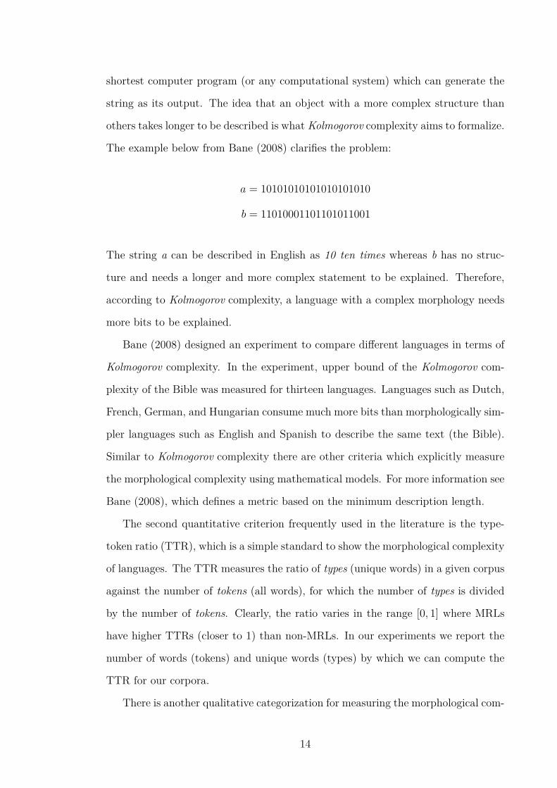
The example below from Bane (2008) clarifies the problem:

a = 10101010101010101010

b = 11010001101101011001

The string a can be described in English as 10 ten times whereas b has no struc-

ture and needs a longer and more complex statement to be explained. Therefore,

according to Kolmogorov complexity, a language with a complex morphology needs

more bits to be explained.

Bane (2008) designed an experiment to compare different languages in terms of

Kolmogorov complexity. In the experiment, upper bound of the Kolmogorov com-

plexity of the Bible was measured for thirteen languages. Languages such as Dutch,

French, German, and Hungarian consume much more bits than morphologically sim-

pler languages such as English and Spanish to describe the same text (the Bible).

Similar to Kolmogorov complexity there are other criteria which explicitly measure

the morphological complexity using mathematical models. For more information see

Bane (2008), which defines a metric based on the minimum description length.

The second quantitative criterion frequently used in the literature is the type-

token ratio (TTR), which is a simple standard to show the morphological complexity

of languages. The TTR measures the ratio of types (unique words) in a given corpus

against the number of tokens (all words), for which the number of types is divided

by the number of tokens. Clearly, the ratio varies in the range [0, 1] where MRLs

have higher TTRs (closer to 1) than non-MRLs. In our experiments we report the

number of words (tokens) and unique words (types) by which we can compute the

TTR for our corpora.

There is another qualitative categorization for measuring the morphological com-

14

plexity, which labels natural languages as analytic or synthetic (Pirkola, 2001). An

analytic language is a type of language with a very low morpheme-per-word ratio.

Bulgarian is a good example for this category (Rehm and Uszkoreit, 2012). There

is also a specific subtype of this category called isolating, which has similar proper-

ties but simpler morphological structures. This category could be considered as an

extreme case of analytic languages, where each word contains a single morpheme.

Mandarin Chinese is a good example for this category.

A synthetic language is a language with a high morpheme-per-word ratio. The

morphological richness in this category is more than the analytic category. Most

Indo-European languages are from this family. Synthetic languages can be divided

into two groups of agglutinative and fusional (or inflectional).

An agglutinative language is a type of synthetic language with a morphology

system that primarily uses agglutination. In the agglutinative combination, atomic

morphemes are sequentially added to the stem and the forms of the morphemes do

not change after the combination. They collocate with each other to construct the

final word, where each unit has its own syntactic role. Turkish is a good example

for this category (Kuribayashi, 2013).

A fusional language is a language in which one form of a morpheme can simul-

taneously encode several meanings. These languages may have a large number of

morphemes in each word, but morpheme boundaries are difficult to identify as they

are fused together. Germanic and Romance languages are in this category. The

opposite of a highly fusional language is a highly agglutinative language.4 Figure

2.3 shows the relations between these different groups. This classification also gives

us clues about the complexity of languages. In our experiments we select languages

which do not belong to the isolating group.

In this section (Section 2.1) we tried to briefly review the problem of morphology.

For more linguistic details see De Groot (2008), Delahunty and Garvey (2010), and4We introduced a hierarchy for different groups but it should be noted that there are no clear-cut

boundaries among these categories.

15

MRLs

analytic

fusional agglutinative isolating

synthetic

Figure 2.3: Qualitative categorization of morphologically complex languages.

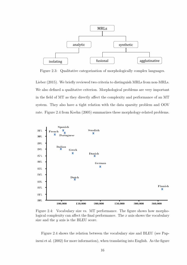
Lieber (2015). We briefly reviewed two criteria to distinguish MRLs from non-MRLs.

We also defined a qualitative criterion. Morphological problems are very important

in the field of MT as they directly affect the complexity and performance of an MT

system. They also have a tight relation with the data sparsity problem and OOV

rate. Figure 2.4 from Koehn (2005) summarizes these morphology-related problems.

Dutch

German

Danish

Swedish Spanish

French

Portuguese

Italian Greek

Finnish

100,000 150,000 200,000 250,000 300,000 360,000 20%

21%

22%

23%

24%

25%

26%

27%

28%

29%

30%

31%

Figure 2.4: Vocabulary size vs. MT performance. The figure shows how morpho-logical complexity can affect the final performance. The x axis shows the vocabularysize and the y axis is the BLEU score.

Figure 2.4 shows the relation between the vocabulary size and BLEU (see Pap-

ineni et al. (2002) for more information), when translating into English. As the figure

16

shows, the vocabulary diversity which is a direct consequence of the rich morphology

affects MT performance. Motivated by such issues and based on our investigations,

we recognized that to address the problem of morphology, language such as Farsi

(Fa), German (De), and Turkish (Tr) are suitable for our experimental studies (see

Chapter 6 for the reason), so we evaluate our models and report their results on

these languages. We also have some experiments on other languages such as Czech

(Cz) and Russian (Ru). In the next chapters we give more detailed information on

statistics of our corpora and their morphological specifications.

2.2 Statistical Machine Translation

We are interested in SMT (Och and Ney, 2000; Lopez, 2008; Koehn, 2009) and

specifically PBSMT (Zens et al., 2002; Koehn et al., 2003) in this thesis. PBSMT

is an extension to previously-proposed word-based models (Brown et al., 1993), in

which translation is performed at the phrase level. The whole PBSMT pipeline

can be summarized in three general steps of word alignment, phrase extraction and

decoding.

In the first step of the PBSMT pipeline,5 alignments between source and target

words are identified. Each word is mapped to its counterpart(s) on the opposite (tar-

get) side. This process is performed by the well-known Expectation-Maximization

(EM) algorithm (Dempster et al., 1977). EM is an unsupervised algorithm which

starts from random estimations for word alignments (the expectation or E step) and

tries to rectify and improve approximations (the maximization or M step) over iter-

ations. For more detailed information and examples on word alignment see Brown

et al. (1993) and Koehn (2009). The EM algorithm for word alignment was imple-

mented in the GIZA++ toolkit (Och and Ney, 2003) 6 which is frequently used by

different models.

A word may not be the best candidate as the smallest unit of translation. Some-5Data preprocessing is not considered as a PBSMT submodule.6http://www.fjoch.com/giza-training-of-statistical-translation-models.html.

17

times one word on the source side is translated into more than one word on the target

side, or vice versa (Koehn, 2009), so word-based models do not perform well in such

cases. Figure 2.5 illustrates this problem where an English sentence is translated

into Farsi. As the figure shows, any word-level model would have serious problems

he enjoyed the party last night

āu āz mhmāny dyšb lẕt brd

Figure 2.5: Phrase-level translation. The figure tries to illustrate complex wordalignments. The Farsi word āz is aligned to (nothing) the Null token.

with this example. Blocks of consecutive words are translated altogether, not word

by word. Motivated by such difficulties, the phrase-based (phrase-level) translation

model was proposed (Zens et al., 2002; Koehn et al., 2003). In this type of transla-

tion the goal is to segment sentences into phrases7 and find a set of target phrases

which maximizes the translation probability of a target translation given a source

sentence. This problem is formulated as in (2.1):

ebest = argmaxe

p(e|f) (2.1)

where e and f are the target and source sentences, respectively. Applying the Bayes’

rule, the translation direction can be inverted, as in (2.2):

ebest = argmaxe

p(f|e)pLM(e) (2.2)

where pLM(e) incorporates the impact of a language model. As a very basic descrip-

tion, a language model measures how fluent the generated translation is. Chapter

4 extensively discusses language modeling. The PBSMT model works at the phrase

level so in order to generate the translation sentences are decomposed into phrases,7Phrases are not necessarily linguistic phrases in this approach, which means any set of consec-

utive words can be considered as a phrase.

18

as in (2.3):

p(f I1 |eI1) =

Iź

i=1

ϕ(fi|ei)d(starti ´ endi ´ 1) (2.3)

where the foreign sentence f is broken up into I phrases fi, ϕ is the phrase-translation

probability function which is based on word alignments. For more information on

the phrase-translation probability and the relation of source and target phrases see

Figure 5.1 and Koehn (2009). d(.) indicates the reordering function. In translation

results some phrases may occur in wrong positions, which the reordering function

penalizes wrong word orders.

In PBSMT, a source sentence is segmented into many phrases and each source

phrase can have several target translations, which the best one should be selected

according to the source sentence and context. Clearly, this is a search problem

where we should find the best source phrase (segmentation) at each step, find the

best counterpart on the target side, and generate the final sentence-level translation.

The decoder is responsible for this process in which many syntactic, semantic, and

reordering features are involved to show how phrases are tightly related to each

other. These features help the decoder search and find the best match. In SMT, the

decoding process is modeled via the log-linear framework (Och, 2003), where we can

define unlimited number of features for each phrase pair. In Chapter 5, we define 6

new features in order to generate better translations. The decoder is implemented

via well-known search models such as beam search (Koehn, 2004a) by which the best

match is searched for a given source phrase.

In Section 2.2, we briefly reviewed the SMT pipeline in which (given a parallel

corpus) translationally equivalent words are aligned to each other and phrases are

extracted based on word alignments. Then the decoder takes a source sentence as

the input, considers all possible phrases in the sentence and finds the best match for

each source phrase. Matches are connected to each other in a way that generates

a fluent target sentence. In the next section we review models which fine-tune this

pipeline in order to make it more compatible for MRLs.

19

2.3 SMT for MRLs

In the previous sections we studied the problem of morphology and its relevance

to our research. Similarly, we explained SMT and related topics which can help us

elaborate our research. In this section we try to review various SMT approaches that

are suitable for translating MRLs. All techniques proposed to tackle the problem

of morphology are extensions to existing SMT models. However, there are a few

instances which tried to address the same problem in the NMT framework, which

we postpone their investigation to Chapter 6, where a basic knowledge of NMT is

provided, and then we study the incorporation of morphological information.

There are three general approaches to translating MRLs. The first approach ma-

nipulates the decoding process and directly incorporates morphological information

for translation (Type 1). The second approach does not change the decoder but

performs translation in multiple steps (Type 2). For translating from MRLs, first a

MCW is transformed into a simpler form and then translation is performed using

these basic forms. In such models MT engines do not have to deal with complex

structures. In translating into MRLs the direction is reversed, so that a simple word

is enriched step-by-step to reach the final complex form. In this approach additional

complementary tools such as classifiers and stemmers are used. The third approach

can be viewed as a subclass of the second approach, in which neither the decoding

nor the translation process is manipulated, but the source-side data is preprocessed

to change MCWs into more suitable forms for MT engines (Type 3). Similarly,

post-translation processing is also carried out to transform translations into more

accurate forms. All pre/post-processing steps are performed outside the decoding

phase. The third approach is the easiest solution compared to the others. We review

different examples for all of these approaches in the following section.

20

2.3.1 Incorporating Morphological Information at Decoding

Time (Type 1)

A factored translation model (Koehn and Hoang, 2007), which is an extension to

PBSMT, is the most suitable example for incorporating any additional annotation,

including morphological information, at decoding time. The main problem with

PBSMT is that it translates text phrases without any explicit use of linguistic infor-

mation, which seems beneficial for a fluent translation. In factored models each word

is extended by a set of annotations, so a word in this framework is not only a token,

but a vector of factors. For example a simple word in PBSMT can be represented

by a vector of word (surface form), lemma, POS tag, word class, morphological in-

formation. Clearly, the new representation is richer than that of the word’s surface

form. As the main focus in factored models is on word-level enrichments, clearly it

addresses the problem of morphology which fits our case.

Let us have a closer look at the model. In word-based or phrase-based approaches

each word is treated independently, i.e. ‘studies’ has no relation to ‘studied’. If only

one of them was seen during training, translation of the other one would be hard

(or even impossible) for any MT engine, even though they come from the same

root. Translation knowledge of their shared stem, along with extra morphological

information, could help us translate both of them (and even all derivative forms of

the stem). This property not only provides solutions for this sort of morphological

issues but also addresses the data sparsity problem at the same time. A factored

translation model follows a similar approach and performs better than other word-

based models for MRLs (see Section 5.2.3).

Translation in factored models is generally broken up into two translation and

one generation steps. A source lemma is translated into a target lemma. Morpholog-

ical and POS factors are translated into target forms and the final form is generated

based on the lemma and other factors. Factored models follow the same imple-

mentation framework as the phrase-based model. In these models the translation

21

step operates at the phrase level whereas generation steps are word-level operators.

The pipeline is illustrated step-by-step to translate the German word Häuser into

English. We use the same example reported in Koehn and Hoang (2007):

• Factored representation: (surface form: Häuser), (lemma: Haus), (POS:

NN), (count: plural), (case: nominative)

• Translation (mapping lemmas): Haus Ñ house|home|building|shell

• Translation (mapping morphology): NN|plural-nominative-neutral Ñ NN|plural,

NN|singular

• Generation (generating surface forms):

– house|NN|plural Ñ houses

– house|NN|singular Ñ house

– home|NN|plural Ñ homes

Multiple choices can generate multiple surface forms which result in phrase ex-

pansions. Training is performed similar to the basic phrase-based model. Word

phrases are extracted with standard models. Factors are also treated as words

whose phrases are extracted in the same way as surface forms. Generation distribu-

tions are estimated on the output side only, i.e. word alignments play no role here.

The generation model is learned on a word-for-word basis. Obviously, a factored

model is a combination of several components which can be easily integrated into

the log-linear translation model. A simple form of the entire pipeline is illustrated

in Figure 2.6

The factored translation model is the most well-known model which explicitly

addresses the morphology problem in SMT. We are able to boost this approach by

our morphology-aware word embeddings. We provide more detailed information on

our model in Chapter 5. Apart from the factored model we wish to review two other

models which study the same problem with different approaches.

22

Input Output

word

lemma

POS

morphology

word

lemma

POS

morphology

Figure 2.6: The high-level architecture of the factored translation model (Koehnand Hoang, 2007).

Dyer (2007) proposed a model for translating from MRLs. The goal is to capture

source-side complexities. The system is based on a hierarchical phrase-based model

(Chiang, 2007) and evaluated on CzechÑEnglish. The main intuition behind the

model is to extend the noisy channel metaphor, where the new model is referred to

as the noisier channel. It suggests that an English source signal is a distorted variant

of a morphologically neutral French signal. In the noisy channel model, the French

signal is known as a noise-free signal whereas the noisier channel assumes the French

signal is noisy, as it is a result of another distortion applied by a morphological

process to the original source signal. This part of the distortion can be modeled

separately apart from the main noisy channel.

In order to implement the noisier channel, first lemma forms of Czech words

are extracted. Corpora consisting of truncated forms are also generated, using a

length limit of 6. This means that for all words, the first 6 characters only are taken

into account and the rest is discarded. Hierarchical grammar rules are induced

based on surface, lemmatized, and truncated forms. These three grammars are

combined together for use by a hierarchical phrase-based decoder, such that the

model’s performance was improved by 10%.

Williams and Koehn (2011) proposed another model to manipulate the decoder

in order to translate into MRLs. The model is an extension to a string-to-tree model

by which unification-based constraints were added to the target side of the model.

23

The main idea is to penalize implausible hypotheses during search. They applied

the model to EnglishÑGerman and were able to improve performance over the

baseline model. The aforementioned three models are examples for incorporating

morphological information into the decoding phase; see Table 2.2 on page 44 for the

summary of similar models

2.3.2 Multi-Step Translation (Type 2)

A dominant amount of research in SMT for MRLs belongs to models which we call

multi-step translation models. In these models, additional tools such as morpholog-

ical analyzers are usually deployed to decompose complex words. Such models are

designed based on decomposed constituents to translate from/into those units, not

complex surface forms. Therefore, there is at least one additional mid-translation

phase to balance the morphological symmetry between source and target sides. Clas-

sifiers are also commonly used in these models whereby complex surface forms are

induced using simpler forms (such as lemmas) together with contextual information

provided for the classifier.

The models of Lee (2004) and Goldwater and McClosky (2005) are well-known

instances of multi-step models. Lee (2004) proposed a technique to balance the

morphological and syntactic symmetry between source and target languages. The

model was evaluated on Arabic as the rich side. First, words are segmented into

prefix(es)-stem-suffix(es) sequences. Both sides of the training corpora are also

annotated with POS tags. Because of the segmentation phase, each word is unpacked

to multiple morphemes, some of which contribute to translation but others playing

no role. Lee (2004) proposed a technique to identify which morphemes should be

deleted (as they have no role), which ones should be merged and which ones should

be treated as independent constituents, during translation. This issue is illustrated

in Figure 2.7, which depicts the process of translating part of an English sentence

“Sudan: alert in the red sea to face build-up of the oppositions in Eritrea” into an

Arabic sentence “AlswdAn: AstnfAr fy AlbHr AlAHmr lmwAjhp H$wd llmEArDp

24

the red sea to face

AlbHr AlAHmr lmwAjhp

Al bHr Al AHmr l mwAjh p

the red sea to face

Al bHr AHmr l mwAjhp

the red sea to face

1

2

3

Figure 2.7: The model proposed by Lee (2004) for translating complex Arabicwords. The model decides to either keep segmented morphemes or delete them.

dAxl ArytryA”.

After segmenting Arabic words (Block 2), ‘AlAHmr’ is changed to ‘Al’ + ‘AHmr’

and ‘lmwAjhp’ to ‘l’ + ‘mwAjh’ + ‘p’. The algorithm proposed in this work identifies

that ‘Al’ from ‘AlAHmr’ is redundant and has no role in translation, so it is deleted.

‘l’ from ‘lmwAjhp’ carries a meaning so it should be treated as an independent unit

in this context, and ‘p’ from ‘lmwAjhp’ should be merged with ‘mwAjh’, as it can

only contribute to the translation phases in that form. The algorithm of Lee (2004)

calculates some probabilities based on POS tags and the co-occurrence of words and

morphemes, and decides to keep, merge or delete morphemes.

Goldwater and McClosky (2005) proposed another model but the main intuition

is the same as Lee (2004). For sparse datasets and MRLs, estimating word-to-word

alignment probabilities is hard, as in such cases most words occur at most a handful

of times. This problem becomes more severe as the morphological richness increases.

Motivated by this problem, Goldwater and McClosky (2005) proposed a new model

and applied it to Czech. They decompose words into morphemes to reduce the data

25

sparseness. In Czech, a lot of information resides in bounded morphemes (see Section

2.1), which is encoded as function words in English. To model this phenomenon, they

enriched decomposed morphemes by adding extra annotations. This is performed to

mitigate the information loss during lemmatization. By this technique they changed

complex Czech words to simple units with some extra guiding information. These

units are easy to handle, and were able to considerably improve their SMT engine.

Another model was proposed by El Kholy and Habash (2012) to address morpho-

logical problems in Arabic. They focused on the three most common morphological

problems in Arabic MT, which according to automatic and human evaluations on

MT outputs are gender, number, and the determiner clitic. Similar to all other

methods they also proposed word segmentation, but this raised other serious prob-

lems. Tokenized words should be de-tokenized on the target side, but because of the

fusional and non-concatenative morphology of Arabic, the de-tokenization process

could be just as challenging as translation itself. It also requires much orthographic

and morphological processing (El Kholy and Habash, 2010). To cope with the prob-

lem they carried out translation in multiple steps and used classifiers. First an SMT

engine is trained to translate from English words and POS tags into tokenized Ara-

bic lemmas plus zero or more morphological features. Figure 2.8 illustrates the data

format for this module. They used lemmas (not stems), as this makes translation

models tighter. This is a notable simplification because a lemma in Arabic can have

two stems on average.

EngWord#POS

Saddam#NN hussein#NN ’s#POS half-brother#NN refuses#VBZ to#TO return#VB to#TO iraq#NN

Âax#det γayor#0 šaqiyq#det li+#na Sad~Am#0 Husayon#0 rafaD#0 ςawodah#det Ᾰilaý#na ςirAq#det

ArabLem#Det

Figure 2.8: Data preparation for Arabic MT proposed in El Kholy and Habash(2012)

They did not use factored models nor was the decoding procedure changed, but

they only changed the data format. English words and Arabic lemmas were enriched

26

by POS and morphological tags, respectively. They trained a PBSMT model on this

data format. For the next step they predicted the morphological class of translated

words, using the conditional random field (CRF) toolkit (Lafferty et al., 2001). They

trained a CRF model using Arabic information (Figure 2.8), word alignments, and

English words. After predicting the morphological tag of all the words, the next step

is morphology generation. Another SMT engine either a factored or phrase-based

mode is trained which takes lemmas and morphology tags and translates them into

inflected word forms.

Minkov et al. (2007) and Toutanova et al. (2008) proposed models for translating

into Arabic and Russian. The goal is to predict inflected word forms. They collect a

rich set of syntactic and morphological information from source and target sentences.

First an MT engine is run to generate translations. Each word is converted into its

stem form, then a correct inflected form of the word is predicted based on context

and stem information. A maximum entropy Markov model was used in their research

which is trained using Equation (2.4):

P (y|x) =n

ź

t=1

p(yt|yt´1, yt´2, xt) (2.4)

As can be seen, the model is a second-order Markov model, where yt´1 and yt´2 are

previously-generated outputs and xt denotes the context at position t.

Chahuneau et al. (2013) used the same mechanism to translate into Russian,

Hebrew and Swahili. First, a discriminative model is trained to predict inflections

of target words from rich source-side annotations. They also used their model to

generate artificial word- and phrase-level translations, which are referred to as syn-

thetic phrases. In their model, the input is an English sentence e together with any

available linguistic analysis of the sentence. The output f is composed of a sequence

of stems and a morphological inflection pattern for each stem. The whole process is

27

modeled by Equation (2.5):

p(f |e, i) =ÿ

σ‹µ=f

p(σ|ei)loomoon

st.g.

ˆ p(µ|σ, e, i)loooomoooon

inf.g.

(2.5)

The st.g. part models generating a stem σ and the inf.g. part models its inflected

form µ in the position i. The model assumes that there is a deterministic function

that maps stems and morphological inflections to target surface forms. This function

is denoted by the σ ‹ µ = f notation. p(.) values are collected from training cor-

pora based on source context and morphological feature vectors. For more detailed

information see Chahuneau et al. (2013).

The baseline system in their model is a hierarchical phrase-based model which by

default generates grammars for a training data. They have a mechanism to extend

this grammar. First, they train a PBSMT model on a parallel corpus and perform

translation. Afterwards, surface forms are replaced with their stems. By use of the

probabilistic model explained in Equation (2.5), new inflected forms are generated

for stems. This step generates synthetic phrases whose quality is evaluated with the

log-probability of the main translation model. High-quality phrases are added to

the main model to extend the grammar and provide better translations.8

German is another MRL for which a considerable amount of MT research work is

available. Koehn and Knight (2003) proposed a way for compound splitting. Com-

pounds are created by joining existing words together. Modeling the compounding

operation has a significant impact on MT quality as it reduces the amount of OOVs.

First, they split a compound word into all possible subunits. A valid subunit is a

constituent which exists as a free morpheme (see Section 2.1) in training corpora.

There could be several segmentations for each word, so the most frequent candidate

is selected based on a specific count function.

Cap et al. (2014) also focused on compounding for German. The approach has

two steps. First to balance the degree of morphological complexity between source8The source code for this project is available at: https://github.com/eschling/morphogen.

28

and target languages, compounds are split and words are lemmatized. To make the

splitting phase more accurate, parsing and POS tagging information is also explored.

Translation is performed where separated units should be merged thereafter, to make

correct compounds. This process is illustrated in Figure 2.9.

hausboote (“house boats”) haus<+NN><Neut><Sg> + boot<+NN><Neut><Pl> → haus<NN> + boot <+NN><Neut><Pl> (merged) haus<NN> + boot <+NN><Neut><Acc><Pl> → hausbooten (inflected)

Figure 2.9: Compound merging in German, based on the model proposed in Capet al. (2014).

Figure 2.9 shows a data structure generated by the first phase. Compounds are

merged together. Merged forms are not necessarily correct so another process is

applied to make the final inflected forms. For merging and inflection-generation, a

CRF model and SMOR (Schmid et al., 2004), a rule-based word formation model,

is used.

SMT solutions for handling the rich morphology problem in German are not

limited to these models alone. For example, Fraser (2009) and Fritzinger and Fraser

(2010) addressed compounding. Fraser et al. (2012) performed translation in two

steps: English word Ñ German stems and additional markups Ñ German words.

Along with Arabic, Czech and German, some other morphology-aware SMT

models have been proposed which study Turkish. In this language, syntax and mor-

phology has a tight relation. Yeniterzi and Oflazer (2010) trained a factored model

to enhance Turkish MT quality. The model relies on syntactic analysis of English.

Source words are enriched with dependency and POS annotations. Then morpho-

logical tags for the Turkish side are produced. Unlike other models, complex Turkish

words are not decomposed in this approach. Because of the nature of Turkish, word

alignments between English and Turkish words are sparse, as many English words

have no counterparts (i.e. they are mapped to nothing) on the Turkish side. By

use of dependency links, unaligned words are attached to words with alignments.

For example, in translating ‘On their economic relations’ into Turkish, there is no

29

alignment for ‘On’ and ‘their’, so ‘On’ and ‘their’ are attached to ‘relations’, as

there are dependency links from these words to ‘relations’, and ‘relations’ has an

alignment link to a Turkish word. Some new rules were defined for the dependency

parser to generate such merged links.

El-Kahlout and Oflazer (2010) proposed another model for Turkish which seg-

ments MCWs and benefits from English POS tags. They also used a morpheme-

aware language model to re-rank n-best lists generated by the decoder.

Research for MT of MRLs is not limited to the languages reviewed so far. Similar

to El-Kahlout and Oflazer (2010), Virpioja et al. (2007) used a morpheme-aware lan-

guage model for translating Nordic languages. Clifton and Sarkar (2011) proposed a

model for Finnish. Words are segmented using Morfessor (Creutz and Lagus, 2002)

and Paramor (Monson et al., 2008), and then a post-processing morpheme predic-

tion system is set up to generate the final translation. This approach uses a CRF

model similar to that of Toutanova et al. (2008). Fishel and Kirik (2010) trained

a factored model for Estonian. Avramidis and Koehn (2008) extended a PBSMT

model by syntactic and semantic annotations for the English-to-Greek and -Czech

directions. For a summary of these models, see Section 2.5.

2.3.3 Morphological Processing for Translation (Type 3)

The task of preprocessing (and normalization) is very language-dependent and is

usually defined based on morphological and syntactic properties of languages. Habash

and Sadat (2006) proposed a preprocessing scheme for Arabic. Singh and Habash

(2012) performed the same for Hebrew. They compared two rule-based and unsu-

pervised models and were able to improve over the baseline model by +3.5 BLEU

points. Rasooli et al. (2013) defined orthographic and morphological processing rules

for a Farsi-to-English model. We also addressed the same problem in our research

(Passban et al., 2015).

Mehdizadeh Seraj et al. (2015) did not change the decoding process, nor did

they perform any preprocessing. They used a multilingual paraphrase database and

30

translated OOVs. They applied their model to ArabicÑEnglish and achieved an

improvement of +1.3 BLEU score over the baseline model. There are many other

models which fall into this group. For a summary of such models, see Section 2.5.

2.4 Deep Neural Networks

Theoretical results demonstrate that we require deep architectures in order to learn

complicated functions (Bengio, 2009). A deep architecture is a composition of many

simple computational units, such as in NNs with many hidden layers and neurons.

In this section we discuss the fundamentals of DNNs and explain the necessity of

transforming NNs to DNNs. A large set of parameters are involved in DNNs that

should be optimized to produce desirable outputs. Clearly, this is a challenging

optimization task which makes the training of DNNs more complicated. In this

section we review issues regarding such problems and study potential solutions.

Any machine-learning technique scaled for big data and complex problems can

be claimed as deep. The common feature of all these models is that they consist

of a massive number of computational units, which makes them suitable for large-

scale settings. Although deep learning is not limited to a specific group of models,

almost all successful solutions have been implemented by NNs. NNs are distributed

computational models inspired by the human brain. They are distributed because

an input signal is processed by many interconnected computational processing units

(neurons). Neurons are located in layers and sequentially connected to each other

via weights. Weights show the connection strength between nodes. Each node is

a simple mathematical function. There should be a cost function for each NN in

order to compute errors. An input is passed through various layers and produces

an output. The prediction error is computed with respect to the output and back-

propagated to the network to update weights (network parameters). The final goal is

to find an optimal configuration of weights. After reaching the optimal configuration,

the network is ready to process any random input in order to map it to the output

31

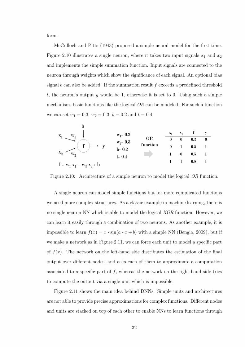
form.

McCulloch and Pitts (1943) proposed a simple neural model for the first time.

Figure 2.10 illustrates a single neuron, where it takes two input signals x1 and x2

and implements the simple summation function. Input signals are connected to the

neuron through weights which show the significance of each signal. An optional bias

signal b can also be added. If the summation result f exceeds a predefined threshold

t, the neuron’s output y would be 1, otherwise it is set to 0. Using such a simple

mechanism, basic functions like the logical OR can be modeled. For such a function

we can set w1 = 0.3, w2 = 0.3, b = 0.2 and t = 0.4.

x1

x2

f y

w1

w2

f = w1 x1 + w2 x2 + b

b

0 0 0.2 0

0 1 0.5 1

1 0 0.5 1

1 1 0.8 1

w1= 0.3 w2= 0.3 b= 0.2 t= 0.4

OR function

x1 f x1 y

Figure 2.10: Architecture of a simple neuron to model the logical OR function.

A single neuron can model simple functions but for more complicated functions

we need more complex structures. As a classic example in machine learning, there is

no single-neuron NN which is able to model the logical XOR function. However, we

can learn it easily through a combination of two neurons. As another example, it is

impossible to learn f(x) = x ˚ sin(a ˚ x+ b) with a simple NN (Bengio, 2009), but if

we make a network as in Figure 2.11, we can force each unit to model a specific part

of f(x). The network on the left-hand side distributes the estimation of the final

output over different nodes, and asks each of them to approximate a computation

associated to a specific part of f , whereas the network on the right-hand side tries

to compute the output via a single unit which is impossible.

Figure 2.11 shows the main idea behind DNNs. Simple units and architectures

are not able to provide precise approximations for complex functions. Different nodes

and units are stacked on top of each other to enable NNs to learn functions through

32

inputs x a b sin ⊕ ⊛

⊛ Output

inputs x a b

f(x)=x*sin(a*x+b) Output

3 2 Figure 2.11: Distributed function approximation using DNNs (Bengio, 2009).

a multi-step and distributional procedure. To learn a complex data distribution, the

network’s architecture and a training algorithm manage the learning procedure, and

distribute the function approximation over different nodes. Figure 2.12 visualizes9

an NN which tries to learn a real-world classification problem over a complex data

distribution.

D

x1

x2

n1

n2

n3

n4

D’

Dl n1 n2 n3 n4

+ + + =

Figure 2.12: Visualizing the process of data-distribution learning via NNs. Thefigure shows which node learns which part of the distribution.

The NN in Figure 2.12 tries to learn the distribution D. D1 is an approximation

learned by the NN for the real distribution. The figure also illustrates the nodes

(magnified) in the first layer to show which node learns which part of the distribution.

A single node in the first layer is not solely able to learn D, but a combination of

nodes can provide an acceptable approximation. Dl is a distribution learned by the9We use the tool developed by Daniel Smilkov and Shan Carter; http://playground.

tensorflow.org/.

33

nodes n1 to n4.

We now understand the necessity of designing DNNs. In order to have precise

approximations, we need to stack several layers one on top of another. In the

next section we discuss how to connect layers together and explain different neural

architectures. For more information on the fundamentals of deep learning, see Arel

et al. (2010), Bengio et al. (2013) and Schmidhuber (2015).

2.4.1 Feed Forward Neural Models

Multi-layer feed-forward (MLF) models are the most popular NN types applied to

a wide range of problems. An MLF consists of multiple neurons which reside within

layers. The first layer is known as the “input layer” and the last layer is the “output

layer”. There could be one to many internal layers between the input and output

layers which are called “hidden layers”. A single-layer network (one hidden layer)

can only solve linearly-separable problems, so multiple layers are connected to each

other to empower the network. Each computational neuron in layers is a non-linear

mathematical function. Tanh, Sigmoid (Karlik and Olgac, 2011), Rectified Linear

Unit (ReLU) (Nair and Hinton, 2010), Leaky ReLU (He et al., 2015) and Maxout

(Goodfellow et al., 2013) are some commonly used functions.

Neurons are connected through weights. There may or may not be a connection

between a random pair of neurons. Weights are multiplied by input signals and

linearly summed together. An optional bias value could also be added to summation

results. This computation is formulated as in (2.6):

y = f(Wx+ b)

yi =ÿ

j

f(wjxj + bi)(2.6)

where y represents the h-th layer, a vector with n neurons. Each of those neurons

are referred to by yi; i P [1, n]. x is the (h-1)-th layer with m neurons. m is

not necessarily equal to n. W P Rmˆn is a weight matrix which maps x to y and

34

b P Rn is a bias vector. An MLF is an NN which sequentially connects layers to

each other. In theory, a two-layer MLF is mathematically able to approximate any

function (Hornik et al., 1989), but it rarely appears in practice.10 For more detailed

information on MLFs, see Bebis and Georgiopoulos (1994).

2.4.2 Recurrent Neural Models

In some cases the input has a constant form which can be modeled using predefined

structures. For example, the character recognition task falls in this group, as inputs

are images with constant dimensions. If we represent each character with a 28 ˆ 28

matrix of black and white pixels, there is always a structure with 28 ˆ 28 = 784

elements at the input layer. For such cases MLFs are the best alternatives, but all

problems cannot be straightforwardly modeled in this way. In most cases the input

has a temporal, dynamic or sequential structure, e.g time series, words or sentences

are sequential structures, which means the length of the inputs varies from one

instance to another. Accordingly, we do not have a constant structure for the whole

data set and MLFs are not able to model these phenomena.

To tackle this problem, recurrent neural networks (RNNs) have been proposed.

An RNN is an MLF with at least one feed-back connection, which means there is a

loop or recurrency connection over one (or more than one) hidden layer. The loop

adds the last state or the output of the hidden layer to its input. This is simply

formulated as in (2.7):ht =fh(Wi:hxt +Wh:hht´1)

yt =fo(Wh:oht)

(2.7)

where x P Rn is an input vector and Wi:h P Rnˆd is a weight matrix which connects

the input layer to the hidden layer. Recurrency is applied through the Wh:h P Rdˆd

matrix. ht P Rd and ht´1 indicate the hidden states at the time steps t and t ´ 1,

respectively. The hidden layer is connected to the next layer y P Rm through10http://neuralnetworksanddeeplearning.com/chap4.html.

35

Wh:o P Rdˆm. fh and fo are non-linear functions which are applied to the input and

output of the hidden layer. This architecture is not exactly different from MLFs,

but rather a simple extension. Any recurrent network can be converted into an MLF

by unfolding over time, so RNNs by nature inherit all mathematical properties of

MLFs. An example of an unrolled version of an RNN and the recurrency mechanism

is illustrated in Figure 2.13.

xt

Wi:h

Wh:o

Wh:h

yt

ht

xt-1

Wi:h

Wh:o Wh:h

yt-1

ht-1

xt

Wi:h

Wh:o Wh:h

yt

ht

xt+1

Wi:h

Wh:o

yt+1

ht+1

Unfolding

Figure 2.13: Unrolling an RNN over time.

The loop mechanism enables RNNs to accept variable-length sequences as their

inputs. Furthermore, at each time step t a summary of all preceding elements before

xt resides in hidden states. Clearly, this mechanism is very useful for NLP tasks,

which we will discuss in the next chapters. Simple RNNs are not powerful enough to

summarize complex structures and capture their properties. They also have prob-

lems in remembering long-distance dependencies. To mitigate these shortcomings,

extended RNNs with memory units (Hochreiter and Schmidhuber, 1997; Sukhbaatar

et al., 2015) have been proposed which we also use in our research (see Chapter 4).

2.4.3 Convolutional Neural Models

Convolutional models implement the mathematical convolution operation. Convolu-

tion is a process on two signals, the input and filter (or kernel), produces an output.

The output is typically viewed as a modified version of the input, or a non-linear

combination of the input and filter. The convolution function is formulated as in

(2.8):

yn = x b f =+8ÿ

i=´8

xifn´i (2.8)

36

where all x, f and y are one-dimensional signals and y has m elements (1 ď n ď m).

The model assumes that the output signal is a deformed version of the input in the

presence of a filter. The filter is applied to highlight and extract specific features of

the input. This is the main intuition behind the convolution operation.

Convolutional neural networks (CNNs) are usually explored for complex data

structures such as RGB images or natural language sentences. An RGB image is a

result of a non-linear (fusional) integration of different complex pixels. A natural

language sentence has a similar structure as it combines words and characters in

a way that is dictated by syntactic and morphological rules. These fundamental

units (pixels, words etc.) are complex because they carry and combine information

from different sources. In RGB images all red, green and blue sources are involved

in a pixel, or in sentences, words are affected by different morphological, syntactic,

semantic and contextual restrictions (different sources of information).

In order to extract information existing in such complex structures, a hierarchi-

cal and fusional architecture is required. The architecture should be able to take

simple elements (RGB signals or characters) and fuse them to construct basic units

(colourful pixels or words). Then it should have a hierarchical mechanism to in-

tegrate such basic units to construct the final output (images or sentences). The

forward or generation pass is a bottom-up procedure going from very basic elements

toward a complex result, and the backward or decomposition path is a top-down

procedure which crunches a complex constituent into subunits, and reveals infor-

mation concealed at each hierarchy. CNNs by their very nature provide such a

mechanism.

The computation explained in Equation (2.8) can be extended for 2D or 3D

settings, and applied to different tasks such as image processing (Krizhevsky et al.,

2012) or sentence modeling (Kalchbrenner et al., 2014). In such CNNs, it is assumed

that the state ht is a complex version of the state ht´1. Accordingly, elements in ht

have more complex structures than those of ht´1. This can be viewed as a procedure

in which several elements in a layer contribute to make a high(er)-level element in

37

the following layer(s). The procedure is gradually and continuously applied layer-by-

layer to reach the final output. The convolution operation is usually followed by a

pooling operation, so that the main transformation is applied to an input signal, and

then a pooling operation is used to select average, minimum, or maximum values

from the convolution’s output. Pooling is carried out to attenuate the impact of

noise and select high-grade signals.

The process of gradually reaching a high-level description of an RGB image by

use of a CNN is illustrated in Figure 2.14. The input data is a set of 2D matrices

(an input with several channels). A 2D convolution function is applied to different

regions (red and green windows) of the input to make new forms (red and green

cells). Applying the convolution function and the filter to all regions generates a

convolved signal which encodes information with a more dense structure. Based on

the type of the filter some important properties of the input are also highlighted

in the convolved signal. Finally, a pooling operation is applied (e.g. a 2-by-2 max-

pooling function).

convolution pooling

Figure 2.14: The convolution operation in CNNs.

These operations are successively applied to extract high(er)-level representations

and reach the final output in the end. The final output could be a word which

describes the class of the input image, or any description about it. This pipeline is

not exclusive for RGB images, i.e. a natural language sentence can be represented by

a cube or a matrix at the input layer (see Chapter 3). Then a convolution operation

is applied. At each layer a new representation of the sentence is generated, and

38

based on the task for which the NN is trained, some features of the sentence are

highlighted. For example in the sentence compression task, redundant words are

truncated as the sentence is passed through layers. In Chapter 3, CNNs are used

for similar (NLP) tasks.

2.4.4 Training Neural Networks

This section explains how to train an NN and find optimal values for network param-

eters (weights, biases etc.) with respect to a given task (Li Deng, 2014; Goodfellow

et al., 2016). To train NNs, we use a well-known principle in machine learning known

as empirical risk minimization (Vapnik, 1991), whereby we convert the problem of

training NNs into an optimization problem, as shown in (2.9):

argminθ

1

T

ÿ

t

ℓ(f(x(t); θ), y(t)) + λΩ(θ) (2.9)

The parameter set θ should be optimized in a way which the NN approximates the

function f(.) with the minimum cost according to the loss function ℓ. x(t) is the

t-th training example whose class label is y(t). The term added to the end of the

equation is a regularizer to penalize certain values of θ.

To optimize Equation (2.9), gradient-based methods such as the stochastic gra-

dient descent (SGD) algorithm are used (Bottou, 2010). Algorithm 1 shows how

SGD functions. In this algorithm values are updated after processing each example.

Training happens through Steps 5 and 6. In NN training, the number of iterations

is controlled by the epoch size which one epoch is the same to one iteration over all

training examples. To apply the SGD algorithm we need to define the loss function

ℓ, a procedure to compute gradients of network parameters and a regularizer. It

is also important to correctly initialize parameters, as it directly affects the NN’s

performance.

Suppose an NN is trained for a classification task, so we expect the NN to give

an estimation of the class c to which a given input x belongs: f(x)c = p(y = c|x).

39

Algorithm 1 Stochastic Gradient Descent (SGD)1: procedure SGD2: initialize θ; Ź θ ” W (1), b(1), ...,W (L+1), b(L+1)u

3: Ź L: the number of hidden layers4: for N iterations:5: for each training example (x(t), y(t)):6: ∆ = -∇θℓ(f(x

(t); θ), y(t)) ´ λ∇θΩ(θ)7: θ Ð θ + α∇

The goal is to maximize the probability of finding the correct class label y(t) given

x(t). Using the negative log-likelihood criterion the maximization problem can be

converted to a problem for minimizing the negative of the function, which gives us

(2.10):

ℓ(f(x), y) = ´ log f(x)y (2.10)

where y is the true class and f(x)y is the y-th element of the output layer which

indicates an estimation of x belonging to that class. Optimizing (maximizing or

minimizing) a mathematical function is equal to optimizing the logarithm of the

same function as the logarithm is a monotonically increasing function. It also sim-

plifies the computation drastically, as the logarithm function is an easily-derivable

function. The loss function defined in this way is referred to as cross entropy, which

is commonly used in many neural models such as our embedding learning models in

Chapter 3.

2.4.5 Sequence Modeling with DNNs

Sequences are the key concepts of this thesis. A word/sentence could be seen as

a variable-length sequence of characters/words for which we require specific archi-

tectures. The training procedure explained so far is suitable for MLFs and shallow

NNs which consist of a limited number of layers. However, there is a serious dif-

ficulty with all gradient-based models when they are used to train deep networks

for variable-length inputs. In deep architectures, each parameter receives an update

proportional to the NN error with respect to its current value. Gradient values

usually vary in the range (−1, 1) or [0, 1), and the back-propagation step computes

40

gradients by the chain rule. This means that for nodes which reside in front layers,

these small values are multiplied n times to compute gradients. Clearly, after several

steps the gradient (error signal) decreases exponentially by the order of n, and the

front layers are trained very slowly. Accordingly, the gradient cannot affect such

layers as much as we expect. This shortcoming causes an incomplete training and

is known as the “vanishing gradient” problem.

This phenomenon is very common in RNNs, because each RNN can be viewed

as a very deep NN when it is unfolded. To cope with this problem, long short-

term memory (LSTM) networks (Hochreiter and Schmidhuber, 1997) were proposed.

In LSTMs, layers are equipped with memory units which mitigate the gradient

vanishing problem. Chapter 4 discusses LSTMs in more detail.

Similar to the vanishing problem, the “gradient explosion” is another issue in

training DNNs. If the gradient value is a big number, after n times multiplication it

grows exponentially which makes the NN unstable. The gradient explosion problem

is the opposite point of the vanishing problem. To control the explosion, gradient

values which exceed a predefined threshold are clipped. This simple solution was

proposed by Mikolov (2010) for the first time. To understand the difficulties of

training DNNs and RNNs, see Pascanu et al. (2013).

Although (efficient) training of RNNs is quite challenging, they are still the best

candidates for NLP tasks. The loop-form architecture of RNNs enables us to handle

variable-length sequences, and techniques proposed for dealing the vanishing and

explosion problems help us train high-quality networks, therefore, it is possible to

model sequences via RNNs. Sequences could be modeled in either monolingual or

multilingual settings, and we have both in this thesis. In the monolingual setting

we train the NN using sentences for language-modeling purposes. In this setting the

NN is fed by a sequence and the output of the network is i) the best word from the

same language (the language of the sequence) which can appear as the next word,

and ii) the probability of such a sequence occurring in the language. Basically, a

language model scores the fluency of the input sequence and in some cases tries to

41

complete it by predicting subsequent words.

In the multilingual setting we have a similar architecture where the input se-

quence is from a source language and output words (to be predicted) from a target

language. Words from the other language are interpreted as translations of source

words, and the model which follows this architecture is known as the neural trans-

lation engine. To implement such models (language modeling and translation) we

could have a very similar neural architecture, in which words (or any other unit such

as characters, morphemes etc.) are consumed sequentially, one after another. At

each time step the hidden state of the network is updated by an input word and

includes a summary of the entire input sequence. After consuming the last word,

the hidden state is an internal representation for the whole sequence. This mech-

anism could be easily implemented by an RNN which is referred to as the encoder

RNN. We need a mechanism to decompose the encoded sequence and decode it

into our desired output. In language modeling the output should be the next word

and in translation the translation of an input word. We place a classifier on top of

the encoder to sample from a vocabulary to predict the best output. The classifier

could also be an RNN. This architecture is applied to almost all sequence-modeling

problems including language modeling and translation. These topics are extensively

discussed in Chapters 4, 6, and 7.

2.5 Summary

In this chapter we explained the fundamental concepts of our research as essential

prerequisites of the thesis. First we addressed the problem of morphology. We

described the problem itself and defined some criteria to distinguish MRLs from

non-MRLs. Then we explained the SMT pipeline. In Section 2.3, we summarized

some of the most important models which addressed the problem of morphology

in SMT. We categorized these models into three classes. The first group incorpo-

rates morphological information at decoding time and manipulates the decoding

42

process. The second class performs multi-step translation, using external tools such

as morphological analyzers and classifiers. Models in this group try to balance the

morphological complexity between source and target languages. The main idea be-

hind these models is to gradually translate words from a simple source form into

a complex target form or vice versa. The third group provides an easier solution

compared to the others, which proposes text-processing models to change MCWs

to simpler forms. A summary of all models reviewed in this chapter is shown in

Table 2.2. Finally, we studied DNNs. We explained what a DNN is, what types of

architectures it might have and how it is trained. Chapter 2 provided prerequisites

for our research questions. In the next chapter we study our first research question

and explain how we can train morphology-aware word embeddings.

43

# System Lang. Summary

1 Koehn and Knight (2003) De–En Models word compounding in German.

2 Lee (2004) En–Ar Proposes an algorithm which decides to keep, merge or

delete morphemes after segmentation, before aligning to

English words.

3 Goldwater and McClosky (2005) Cz–En Enriches morphemes with additional information and ap-

plies word truncating.

4 Habash and Sadat (2006) Ar–En Preprocessing.

5 Dyer (2007) Cz–En The noisier channel: an extension to the hierarchical PB-

SMT model. Combines different grammars to decode com-

plex source languages.

6 Koehn and Hoang (2007) En–De

En–Cz

En–Es

En–Ch

De–En

Ch–En

Factored translation models.

7-

8

Minkov et al. (2007) and

Toutanova et al. (2008)

En–Ar

En–Ru

a) An SMT model translates English. b) MT outputs are

stemmed. c) Inflected forms are generated by use of a

2nd-order Markov model.

9 Virpioja et al. (2007) Nordic SMT with morpheme-aware language models.

10 Avramidis and Koehn (2008) En–Gr

En–Cz

A phrase based model extended by syntactic and semantic

tags.

11 El-Kahlout and Oflazer (2010) En–Tr Word segmentation for Turkish along with a morpheme-

aware language model to re-rank translation results.

12 Fishel and Kirik (2010) Es–En A Factored translation model. Word segmentation with

Morfessor.

13 Fritzinger and Fraser (2010) En–De Models word compounding in German.

14 Yeniterzi and Oflazer (2010) En–Tr Uses dependency annotations to enhance a factored trans-

lation model.

15 Clifton and Sarkar (2011) En–Fi A two-step model which segments words using Morfessor

and Paramor and generates morphological information by

a CRF model.

16 Williams and Koehn (2011) En–De An extension to the string-to-tree model by applying

unification-based constrains on the target side.

17 El Kholy and Habash (2012) En–Ar Multi-step translation: a) Translates English words into

Arabic lemmas. b) Predicts morphology tags of Arabic

words with a CRF classifier. c) Translates tags and lem-

mas into inflected Arabic forms.

18 Fraser et al. (2012) En–De Translates English words to German stems, enriches data

with additional morphology markups and translates stems

into German words.

44

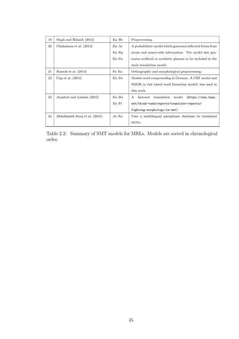
19 Singh and Habash (2012) En–He Preprocessing.

20 Chahuneau et al. (2013) En–Ar

En–Ru

En–Sw

A probabilistic model which generates inflected forms from

stems and source-side information. The model also gen-

erates artificial or synthetic phrases to be included in the

main translation model.

21 Rasooli et al. (2013) Fa–En Orthographic and morphological preprocessing.

22 Cap et al. (2014) En–De Models word compounding in German. A CRF model and

SMOR (a rule based word formation model) was used in

this work.

23 Aranberi and Labaka (2015) En–Hu

En–Fi

A factored translation model (https://www.taus.

net/think-tank/reports/translate-reports/

fighting-morphology-in-smt).

24 Mehdizadeh Seraj et al. (2015) Ar–En Uses a multilingual paraphrase database to translated

OOVs.

Table 2.2: Summary of SMT models for MRLs. Models are sorted in chronologicalorder.

45

Chapter 3

Learning Compositional

Embeddings for MRLs

In the last chapter we studied the importance of morphology, provided prerequisite

knowledge to explore our research questions, and reviewed SMT models for MRLs.

In this chapter we focus on our first research question and introduce models by

which we can incorporate morphological information into word embeddings.

Word embeddings are real-valued word representations in an n-dimensional fea-

ture space. Recent work has shown that these distributed representations can pre-

serve meanings, as well as semantic and syntactic dependencies. However, existing

word-embedding models have some deficiencies, especially with regard to MRLs. In

most popular models, each word is treated as an atomic unit which is not suitable

for complex words. In MRLs words can be viewed as hierarchical structures which

contain meaning-preserving internal subunits (morphemes). In this chapter, we pro-

pose a novel architecture designed to model intra-word relations. Through various

experiments we show that the proposed model performs better than other existing

models for complex structures.

Word embeddings have recently become ubiquitous in NLP tasks (Collobert

et al., 2011). They are an efficient means of transferring knowledge from large

datasets into task-specific models which may have very limited training data (Mikolov

46

et al., 2013b). Historically, the concept of distributed representations for symbolic

linguistic units was introduced by the vector space model of Salton et al. (1975), and

expanded by techniques such as latent semantic analysis (Deerwester et al., 1990),

latent Dirichlet allocation (Blei et al., 2003), and random indexing (Sahlgren, 2005).

Recently, NNs have become the established state-of-the-art for creating dis-

tributed representations of characters, words, sentences, and documents. Hinton

(1984) proposed an NN-based embedding model for the first time. This work in-

troduced the idea of a “shared learning space”, where embeddings themselves are

also trainable parameters of the model. In this chapter, we discuss a CNN designed

to generate better representations of MCWs. Complex words are decomposable

structures which are particularly common in languages that rely heavily upon ag-

glutination (see Table 2.1). According to previous findings, not only the inter-word

dependencies and contextual information (Huang et al., 2012; Mikolov et al., 2013a)

but also the intra-word dependencies (Luong et al., 2013) affect word embeddings,

so our proposed model takes both types of information into account.

The main problem with existing word-based models (Mikolov et al., 2013a; Pen-

nington et al., 2014) is their deficiency in modeling rare words. Our CNN composes

word embeddings from subunit embeddings and tries to solve this problem. For

example, ‘distinctness’ and ‘unconcerned’ are very rare, occurring only 141 and 340

times in Wikipedia documents (Luong et al., 2013), even though their corresponding

stems ‘distinct’ and ‘concern’ are very frequent (35323 and 26080, respectively). In

such cases word-based models generate poor word representations, whereas better

surface-form embeddings can be generated by combining subunit (stem and affixes)

embeddings. The problem becomes more serious for words which were never ob-

served during training. Our model is able to produce embeddings for unseen words

by composing the representations of their morphological subunits.

Motivated by the aforementioned challenges, we develop a new CNN which ex-

plicitly targets some of the problems of morphology and learns more representative

embeddings. The way we fuse together different types of information to make em-

47

beddings is quite novel. We also apply a 3D convolution function and propose a

new cubic data structure as the CNN input. The input cube encompasses infor-

mation for internal subunits of context words. By proposing our architecture we

try to address shortcomings of existing embedding-learning models. The way our

architecture differs from others, along with our motivations and contributions, can

be summarizes as follows:

• Usually, RNNs are the most preferred neural models when working with tex-

tual data, but we propose a CNN-based solution. The baseline model (Luong

et al., 2013) in our experiments benefits from a very powerful RNN-based de-

sign and introduces the recursive architecture to train word embeddings (see

Section 3.1 for more details). Experimental results show that our model is

able to surpass their RNN-based architecture with better results.

• In existing models, the word’s embedding is generated using information from

its adjacent words. In our architecture, we use a cubic data structure which

provides information about adjacent words, their stems, prefixes, and suffixes.

The architecture assumes that any subword unit of a word can be affected

by any other subword unit of other neighbouring words, e.g. in other existing

models we cannot provide the stem of a word with information about the stem,

prefixes, or suffixes of other words, whereas in our model the stem, prefixes,

and suffixes of each word are affected by stems, prefixes, and suffixes of other

words.

• Although including subword (morpheme) information is very important to

have high-quality and morphology-aware embeddings, the way such informa-

tion is used (and combined) is crucial. Information carried by such units can

be less useful (or even useless) when they are processed by a weak combination

model. Existing models simply sum or concatenate subword embeddings to

construct the surface-from embedding, which is not the best way. Here in this

chapter, we discuss different methods by which subword embeddings can be

48

combined, and argue that the proposed convolutional method is a better way

to combine subword embeddings.

In the next sections we will review the fundamentals of the embedding-learning

task, together with our proposed architecture and experimental studies.

3.1 Embedding Learning

Several early models such as Bengio et al. (2003) utilized word embeddings but did

not address the embedding-learning task itself (as an independent problem). They

also did not directly use morphological information in embeddings. In Bengio et al.

(2003); Botha and Blunsom (2014); Dos Santos and Zadrozny (2014); Kim et al.

(2016), embeddings are trained with respect to a specific task. Therefore, trained

embeddings are only useful for the specific experimental settings and training con-

texts. There is only a limited amount of work which has addressed embedding train-

ing as an independent problem. A very successful example is Word2Vec1 (Mikolov

et al., 2013a) which almost all other work has followed this unsupervised approach.

The main intuition behind our model is also the same, but the internal operation of

the model enables representations to directly benefit from morphological informa-

tion.

Word2Vec is a simple feed-forward model in which a target random word of

an input sequence is selected to be predicted by use of its surrounding context.

Embeddings are updated with respect to error values of the prediction phase. More

formally, the network tries to compute P (wi|C) where wi is the target word and C

indicates its context. In the simplest scenario the context C is a preceding word

just before the target word and the network includes one hidden layer h with the

weight matrices Wi:h P R|input|ˆd and Wh:o P Rdˆ|V|, where V is the vocabulary set

and d is the size of h (hidden layer). The probability of each word given its context

is estimated via Softmax, which is a scalar function which maps values of its input1https://code.google.com/p/word2vec/.

49

vector into the range [0, 1], so that new values could be interpreted as probabilities.

Softmax is formulated as in (3.1):

P (wt = j|C) =exp(ht.w

j + bj)ř

j1PV exp(ht.wj1 + bj1)(3.1)

where wj is the j-th column of Wh:o and bj is a bias term. The input of Softmax is

ht P Rd and its output is v P R|V|. The j-th cell of v is interpreted as the probability

of selecting the j-th word from V as the target word. Based on Softmax values the

word with the highest probability is selected and the error is computed accordingly.

Error values are back-propagated to the NN in order to update network parameters.

Word embeddings are part of those parameters which are updated too.

3.1.1 Subword-level Information for Embeddings

As previously mentioned, MCWs are structures with internal dependencies. Cur-

rent models treat words as atomic units, and are thus unable to benefit from the

compositional nature of MCWs. An MCW can be viewed as an ordered sequence of

morphemes, so methods developed for sequences of words are a promising avenue

of investigation. Luong et al. (2013) used a recursive sentence-modeling network

(Socher et al., 2011) to model MCWs. While the original model works over words

they adapted the model to work at the morpheme level in order to generate word

embeddings.

Based on their definition, embeddings of MCWs are gradually built up from their

morphemic representations (Luong et al., 2013). First, they segment words where

each word is changed to a prefix(es)-stem-suffix(es) sequence. There is a specific em-

bedding for each subunit. Then they sequentially combine the embedding of each

subunit with that of the following one, and continue this process until reaching the

final embedding, which is the surface form. We use the example studied in their

paper to clarify the procedure. In order to build the embedding for the word ‘unfor-

tunately’, the embeddings of ‘un’ and ‘fortunate’ are combined. The new internal

50

embedding generated by this combination is supposed to represent ‘unfortunate’.

At the next step, the internal embedding is combined with the embedding of ‘ly’ to

generate the surface-form embedding.

The combination to generate an internal embedding based on two subword units

is carried out through a transformation (weight) matrix, where the concatenated

embedding of subwords is multiplied by the matrix, i.e. the combination is based

on a dot product. The model of Luong et al. (2013) seems to be appropriate for

processing variable-length words and sentences, as it relies on a recurrent/recursive

architecture. The model is able to generate better results compared to other existing

models, which is our baseline for all experiments.

Another idea to extract subword information is to work at the character level. In

the models of Dos Santos and Zadrozny (2014) or Kim et al. (2016), words are broken

up into characters. A convolutional layer is established over character embeddings

to create word-level embeddings. They applied this method to POS-tagging and

language-modeling tasks, respectively. According to their results, working at the

character level is a better alternative to model MCWs.

Approaches based on morpheme-level representations find a middle-ground solu-

tion between word- and character-level modelings. According to experimental results

from Cotterell and Schütze (2015), words with close embeddings in the feature space

share morphological subunits. Botha and Blunsom (2014) incorporated morphology

embeddings in the language-modeling task and studied the impact of subword em-

beddings. In our research, unlike previous models (Qiu et al., 2014) we explicitly

use morphological information within the embedding task rather than within other

downstream tasks. Therefore, our setting is different from language-modeling (and

other similar) settings. However, the problem of incorporating subword information

is also investigated in the fields of language modeling and machine translation in

Chapters 5 and 6.

51

3.2 Learning Morphology-Aware Embeddings

Our model uses CNNs to produce compositional embeddings. CNNs are suitable

models when the input data has a complex structure (such as 3-channel RGB images

or natural language sentences). Convolution is a mathematical operation on an input

(variable, vector, multi-dimensional tensor etc.) and a filter2 (with the same shape

of the input but not necessarily the same size), producing an output that is typically

viewed as a modified version of the input or a non-linear combination of the input

and filter. We believe that the combinatorial pipeline enabled by CNNs is well suited

to model MCWs.

An MCW can be viewed as a convolutional result of its subunits. In the ex-

isting convolutional embedding models (Kalchbrenner et al., 2014; Dos Santos and

Zadrozny, 2014), an input sentence/word with n words/characters is represented

by a 2D tensor I P Rdˆn in which the i-th column indicates the embedding (E) of

the corresponding word/character si: E(si) = I[:, i] P Rd, where d is the embedding

size, and [:, i] indicates all possible rows and the i-th column in the matrix I. A

convolutional function over I fuses all columns together. A limitation of these mod-

els is that using a matrix-form input captures only contextual information, losing

information conveyed by the subword units.

In our model we wish to capture subword, word-level, and context-level informa-

tion in a single representation. We thus extend the 2D input to a 3D representation,

which also includes subword representations. We propose a cubic data structure (3D

tensor). The cubic input Ic is made up of lemma (L), prefix (P) and suffix (S) planes:

Ic P R3ˆ(n+m)ˆd. Each plane is a 2D tensor with the shape dˆ(n+m). In the lemma

plane L the i-th column represents the embedding of the i-th word’s lemma which is

surrounded by the lemma embeddings of other words. With the same structure, P

and S planes include n+m embeddings belonging to the affixes of (context) words.

In the embedding task, the target word is not included in the (matrix-form) input.2The filter is sometimes referred to as the kernel in the literature.

52

Accordingly, we do not have lemma, suffix and prefix embeddings of the target word

in the input cube. In our setting n and m indicate the number of preceding and

following words before and after the target word, respectively. Figure 3.1 illustrates

an example of an input cube.

n m

L1

P1

S1

d

n m

d

W1

Figure 3.1: The cubic and matrix data structures for the input string [w0 w1 w2 w3

w4]. Lemma, prefix and suffix embeddings for each word is referred to by Li, Pi andSi, respectively, and Wi indicates the surface-form embedding. n = 3, m = 1 andthe target word is w3. The first 3 columns include the related embeddings for w0 tow2 and the fourth column includes the embedding for w4. We emphasize that thedata structure on the right-hand side is used by previous embedding models and ourmodel benefits from the cube on the left-hand side.

The network takes the cube as its input and convolves the planes with a specific

multi-plane convolution function. In our case we incorporate contextual as well as

intra-word information. Similar to the matrix-form input we have information about

the target word’s context. Moreover, by use of the lemma and affix planes we have

access to subword-level information. Our cubic/multi-plane convolution module

applies a series of convolution operations where each operation is a 3D extension of

the standard 2D convolution function. The entire process can be formulated as in

Equation (3.2). The convolution module takes a multi-plane data structure (in our

case 3-plane) and generates another data structure with one or more planes, as in

(3.2):

Op,i,jc =

|P |ÿ

l=1

wFÿ

s=1

hFÿ

t=1

F p,l,s,tc ˆ I l,(i´1)+s,(j´1)+t

c (3.2)

where Ic, Oc and Fc are the input, output and filter, respectively. Since in our

53

setting the input, output and filter are all cubic data structures, they are shown

with the ‘c’ subscript. Oc could have one to many planes which are referred to by

the ‘p’ superscript. Each plane within Oc is a 2D tensor whose values are accessible

through the (i, j) coordinates, i.e. Op,i,jc shows the value of the i-th row and the

j-th column in the p-th plane of the multi-plane output Oc. l is the plane index and

|P | shows the number of input planes. In our setting both Ic and Fc are 3-plane

structures so |P | = 3. wF and hF are the width and height of each plane in the

filter. Finally, the (s, t) tuple shows the coordinates of each plane in the filter Fc.

The first superscript of filter (p) says to which plane in Oc the filter belongs. In our

setting Ic P R(m+n)ˆd (see Figure 3.1).

3.2.1 Network Architecture

Our network is proposed in order to learn embeddings for MCWs. To this end:

i) first we take a cubic data structure as the input which includes embeddings for

lemmas and affixes of n preceding and m following words around the target word;

ii) we apply the 3D convolution function over the cube to combine its elements;

iii) then apply other mathematical functions and transformations (such as non-

linearity) to the convolution result and reshape it into a vector; and iv) at the end,

the final vector is passed to a Softmax layer in order to predict the target word. To

implement such a pipeline we propose the following architecture.

The first layer of our architecture is a lookup table which includes embeddings

for lemmas, suffixes, and prefixes. The lookup table is treated as a matrix of network

parameters whose values are updated during training. From each sentence in the

training set, one word is randomly selected as the target word. During training, we

process sentences multiple times and different words are selected as the target word.

All words from the training sentence are decomposed into subunits (each word is

decomposed into 1 lemma, 1 prefix and 1 suffix). Based on the selected target word,

corresponding lemma and affix embeddings for context words are retrieved from the

lookup table and placed in the cube. In our implementation, we use a window of

54

10 words around the target word, namely n=m=5. This means that if the target

word is the fifth word in a sentence, the first plane of the input cube includes prefix

embeddings for wordi where 0 ď i ď 10 & i ‰ 5. Similarly, the second and the third

planes include suffix and lemma embeddings for the same set of context words. n

and m are hyperparameters of the model, both of which we set both m and n to

5 to make our work comparable to others (see Section 3.3 for more details). The

look-up table is a matrix with |V | rows and d columns, where V is the vocabulary

set and d is the embedding size (see Section 3.3 for more details).

In the second layer the multi-plane convolution function is applied. The input

data is a 3-plane cube which the convolution module changes to a more dense struc-

ture with 6 planes, i.e. the input instance at each step with the shape 3ˆ(n+m)ˆd

is transformed to a data structure with 6 ˆ wout ˆ dout dimensions, where wout =

t(m+n)´wF

2u and dout = t

(d)´hF

2u. In our setting wF = hF = 5. We empirically

recognized these numbers to be the best trade-off between the training time and

the network accuracy. We also apply max-pooling to the 6-plane convolution re-

sult, where each plane is segmented into 2 ˆ 2 windows whose maximum values are

selected (one maximum value from each of those 4-cell windows).

The next layer applies non-linearity, where we transform each cell of the 6-

plane data structure with rectifier units. For the purpose of generalization and

preventing over-fitting, we also placed a dropout layer with p = 0.3 after the non-

linear layer. Srivastava et al. (2014) extensively discussed the advantages of using

rectifier+dropout layers. Up to this layer we have a data structure with several

planes. We unfold the planes and reshape them all into a single vector. The vector

is passed through another rectifier+dropout layer and is mapped to a 200-dimensional

vector.

All cells of the final vector are processed by a hierarchical Softmax (HSMX)

function to produce the probability distribution over classes (words). Softmax is

a very expensive function in terms of time and space complexities. To deal with

this problem, we used HSMX (Morin and Bengio, 2005) which first finds the correct

55

word cluster and then looks for the correct word within the cluster. Similar to Kim

et al. (2016), we pick the number of clusters K = r?Vs and randomly split V into

mutually exclusive and collectively exhaustive subsets V1, ...,VK of (approximately)

equal size. HSMX in our setting is formulated as in (3.3):

P (wt = j|C) =exp(ht.w

k + bk)řK

k1=1 exp(ht.wk1 + bk1)ˆ

exp(ht.wjk + ajk)

ř

j1PVkexp(ht.w

j1

k + aj1

k )(3.3)

where similar to the regular Softmax function (Equation (3.1)), wt is the target

word, C is the context (in our case the cube) and ht is the output of the last layer

just before HSMX. The first term is the probability of picking the cluster k and

the second is the probability of selecting the word j given the cluster k. With the

regular Softmax layer the network processes 2, 500, 000 tokens in „9 hours whereas

with HSMX it is reduced to „1.5 hours (both on GPUs).

The network is trained using SGD and back-propagation (Rumelhart et al.,

1988). All parameters of the model are randomly initialized over a uniform dis-

tribution in the range [´0.1, 0.1]. Filters, weights, bias values and embeddings are

all network parameters which are tuned during training. The lemma/affix embed-

ding size for the English experiment is 50 (see Section 3.3) and 200 for the other

experiments. We use the negative log likelihood criterion to compute the cost. More

formally, we wish to maximize the average log-probability in our network, as in (3.4):

1

J

Jÿ

j=1

log p(wj|Cij) (3.4)

where J shows the number of all words in a training corpus, and wj is the target

word whose context information is represented by the cube Cij. One wj can have

different context cubes which is shown with the i superscripts. Figure 3.2 shows the

network architecture.

56

Li

Lookup table

Pi

Si

3D Convolution

+ Max-pooling

Non-linearity +

Dropout +

Reshaping

Non-linearity +

Dropout +

Resizing

V1

…

V2

Vk

Hierarchical Softmax

Vo

cab

ula

ry

Target word

Figure 3.2: Network Architecture.

3.2.2 Word Embeddings

In our pipeline each word is decomposed into 3 subunits whose embeddings are

trained via the CNN proposed in the last section. Since subunit embeddings are

part of the neural architecture and involved in the prediction phase (forward pass),

they are directly updated through the error back-propagation pass. After training

we have high-quality lemma and affix embeddings which preserve information about

themselves and lemmas and affixes of other context words. However, our final goal

is to have high-quality embeddings for surface forms, not subunits. In order to

generate surface-form embeddings we propose four simple models:

• Model A: in this model the word’s surface-form embedding is generated

through the concatenation of its subunit embeddings, namely Wi = Pi.Li.Si,

where Wi indicates the surface-form embedding for wi and Pi, Li and Si are

prefix, lemma, and suffix embeddings available through the lookup table.

• Model B: in this model we add another plane to the input cube. In the new

data structure the fourth plane includes surface-form embeddings, e.g. the i-th

column of the first, second, third, and fourth planes includes Pi, Si, Li and Wi,

respectively. With this technique we directly train surface-form embeddings

using the proposed architecture.

• Model C: in this model we sum subunit embeddings to generate the word

embedding, which means Wi = Pi + Li + Si.

• Model D: this model is an extension to the previous model, in which we use

a weighted summation of subunit embeddings to generate the surface-form

57

embedding, namely Wi = α ˆ Pi + β ˆ Li + γ ˆ Si, where α, β and γ are

weights and show the contribution/impact of each subunit. Weight values can

be estimated as in (3.5):

α =c(prewi

)

c(all); β =

c(lemwi)

c(all); γ =

c(sufwi)

c(all)(3.5)

where c(.) counts the number of the occurrence of each subunits, i.e. c(lemwi)

is the number of words whose lemma is lemwi. c(all) is equal to c(prewi

) +

c(lemwi) + c(sufwi

). With this type of modeling, word embeddings are gener-

ated based on their subunits where the impact of each subunit is taken into ac-

count, so that if a word has a rare prefix its impact is attenuated in the surface-

form embedding and the surface-form embedding relies more on its lemma or

suffix. For example, in the surface-form embedding of ‘infra+structure+s’, it

is better to focus more on ‘structure’ and ‘s’ which frequently occur in English

words (as a lemma and suffix), rather than ‘infra’ which is not a very frequent

prefix.

3.3 Experimental Results

Although some prior work addressed the morphological representations in various

language-processing tasks (Botha and Blunsom, 2014; Dos Santos and Zadrozny,

2014; Cotterell and Schütze, 2015; Kim et al., 2016), only Luong et al. (2013) studied

this problem for the word-embedding task and is the work most related to ours.

We compare our work to that of Luong et al. (2013) (see Table 3.1) to evaluate

the quality of our embeddings, and to make the work comparable we use the same

training set, embedding size, context-window size, test sets, and evaluation methods.

The most common way of intrinsically evaluating the quality of word-embedding

models is to estimate the correlation between their scores and human judgments

on similar word pairs. For this purposes one of the most frequently used datasets

58

is Wordsim353 (Finkelstein et al., 2001).3 The collection includes 353 word pairs

accompanied with human-assigned similarity judgments. We evaluate our model on

Wordsim353. Luong et al. (2013) developed a new dataset of rare words (RareWord).4

The set includes 2034 word pairs with a similar structure to Wordsim353 (both are

English datasets). The surface-form of rare words is not frequently seen in training

corpora, but other forms (in a different tense or lemma form etc.) might occur fre-

quently. If an embedding model could capture subword-level information, it should

have better performance on such a dataset. We evaluated our model on this dataset

too.

As a training set we use the April 2010 snapshot of the Wikipedia5 corpus (Shaoul

and Westbury, 2010), which was tokenized and lowercased in a pre-processing step.

The baseline model also uses the same training set. In Luong et al. (2013), word

embeddings were initialized by the HSMN embeddings (Huang et al., 2012). HSMN

includes embeddings for 138, 218 unique words, covering all words from RareWord

and 419 words from Wordsim353 (419 out of 439 unique words). In our experiment

we use the same vocabulary set along with those uncovered words from Wordsim353,

which are not included in HSMN.

In the training corpus we keep all those paragraphs which include at least one

of the vocabulary words and exclude other paragraphs. We replace all numbers

with “NUM” and words not in the vocabulary with “UNK”. After preprocessing,

the final training corpus includes 15, 469, 077 paragraphs and 919, 646, 155 words.

Using the training corpus, lemma and affix embeddings of the vocabulary set are

trained. Afterwards, we explore the techniques discussed in Section 3.2.2 to generate

surface-form embeddings.

As previously mentioned, Wordsim353 and RareWord include word pairs where

their semantic similarity is indicated with a human-assigned number. For each pair,

we retrieve the embeddings of the words (of the pair) and estimate their distance3http://www.cs.technion.ac.il/~gabr/resources/data/wordsim353/4http://stanford.edu/~lmthang/morphoNLM/5http://www.psych.ualberta.ca/~westburylab

59

using the Cosine similarity, which is a number in the range [´1, 1]. First we map the

number to the range [0, 1] and then using Spearman’s rank correlation, we compare

the generated number with the human judgment. The model whose results have

a better correlations with human-assigned numbers is a better model. Table 3.1

summarizes the results obtained by Luong et al. (2013) and our embeddings.

Embeddings Wordsim353 RareWordHSMN (Huang et al., 2012) 62.58 1.97+stem (Luong et al., 2013) 62.58 3.40+cimRNN (Luong et al., 2013) 62.81 14.85+csmRNN (Luong et al., 2013) 64.58 22.31Model A 62.22 17.93Model B 66.16 24.01Model C 64.93 23.93Model D 65.43 26.92

Table 3.1: Results for the word-similarity task. Numbers indicate Spearman’s rankcorrelation coefficient (ρˆ100) between similarity scores assigned by different neuralnetworks and human annotators.

The first pair of numbers in Table 3.1 shows the correlation of the HSMN em-

beddings with human judgments. +stem is the case when unknown words are rep-

resented by their stem embeddings. Luong et al. (2013) proposed two models of

cimRNN and csmRNN. The first model tries to optimize embeddings using a recur-

sive neural network. By use of the recursive model they tried to capture intra-word

(morpheme-level) information. In the second model, cimRNN was used within a

language model. The motivation behind the second model (csmRNN) is to capture

contextual information along with intra-word information. The last four rows show

our models which yield better results than the recursive model.

Our results consistently improve on previously reported numbers, especially for

RareWord. There could be two possible reasons: i) in the model of Luong et al.

(2013), the network has a reference embedding table. Embeddings for each word

are generated and the error is computed based on the distance between reference

and generated embeddings. The network tries to make new embeddings as close as

possible to the reference embeddings. This form of learning degrades the impact of

60

morpheme-level information, as reference embeddings are provided by word-based

methods such as Collobert et al. (2011) or Huang et al. (2012). Although cim-

RNN tries to learn morpheme-level information, by comparing its results to refer-

ence embeddings it (implicitly) forces the network to learn word-level embeddings;

and ii) to the best of our knowledge, for the first time Botha and Blunsom (2014)

combined subword-level information by linearly summing the corresponding embed-

dings. However, other models such as Luong et al. (2013) and Kim et al. (2016)

have argued that a simple linear combination might not be ideal, and they instead

proposed convolutional and recursive approaches. The recursive model is also a

variation of summation over morpheme embeddings but not as simple as the model

of Botha and Blunsom (2014). In our proposed model we have different types of

subword-level information. They are all combined together through a convolutional

process, which enables the network to have multi-granular information about its

input. Perhaps this type of fusion works better than other models (linear, recursive,

etc.). These discrepancies (i and ii) between the models could be the source of

the different results achieved. In the next section we describe more experiments to

investigate the proposed model from other perspectives.

3.4 Further Investigation of Experimental Results

In this section we try to address some issues regarding the network architecture and

embeddings in order to extensively analyze the proposed pipeline.

3.4.1 POS and Morphology Tagging Experiments

Since English is not considered as an MRL, in addition to the English experiment we

designed another experiment on Farsi and German. We evaluate our embeddings in

the POS-tagging task. For this experiment we use a simplified version of our neural

POS tagger (Passban et al., 2016a), which is a multi-layer perceptron with 4 layers.

The first layer is the input layer and includes word embeddings. The second and

61

third layers are tanh layers with 300 and 200 units, respectively. The fourth layer is

a Softmax layer to compute class probabilities over POS tags. For this experiment,

the embedding size is 200 and word embeddings are produced by Model D.

We run the neural POS tagger with two different settings. In one setting the

network input is the word embedding ([Wi]), and in the other one we enrich the

input by adding the embedding of one preceding word ([Wi´1,Wi]). We estimate

the accuracy of the neural POS tagger when it is initialized by our own, Word2Vec

and GloVe6 (Pennington et al., 2014) embeddings. To train embeddings and the

POS tagger for Farsi we used the UPC7 corpus (Seraji, 2015), which is a collection

of 2, 704, 028 words, with 66, 629 unique words, 59, 865 unique lemmas, 368 unique

prefixes, and 1096 unique suffixes. To segment Farsi words we used our in-house

morphological analyzer which is a rule-based model. We used the first 2 million

words for training, the next 200, 000 words for tuning and the next 200, 000 words

for testing. The tagset size for UPC is 31.

For German we used the first part of the DEWAC 1.3 corpus from the WaCKy8

collection (Baroni et al., 2009). To segment German words we used the NLTK

lemmatizer.9 We selected the same number of words for the training, tuning and

test sets. The German corpus includes 53 POS tags, 2, 232, 913 words, 185, 895

unique words, 136, 876 unique lemmas, 11 prefixes, and 153 unique suffixes. The

results for the POS-tagging task are reported in Table 3.2.

According to the results from Table 3.2, GloVe’s performance is well below that

of the other models. Our model works better than Word2Vec for both languages.10

We believe that this is because our embeddings preserve subword-level (morpho-

logical) information and boost tagging performance. We train morphology-aware

embeddings which were able to enhance the performance of the neural POS tagger.6http://nlp.stanford.edu/projects/glove/.7UPC is a commonly used dataset in this field which is available at: http://stp.lingfil.uu.

se/~mojgan/UPC.html.8http://wacky.sslmit.unibo.it/doku.php?id=start.9http://www.nltk.org/api/nltk.stem.html?highlight=lemmatizer

10We do not have access to the source of other embedding models to train on Farsi and German.

62

Input GloVe Word2Vec Model D

Farsi [Wi] 90.09 93.28 96.11[Wi´1,Wi] 92.65 93.65 96.64

German [Wi] 81.20 86.22 87.74[Wi´1,Wi] 81.84 87.20 88.64

Table 3.2: Results for the POS-tagging experiment. Numbers indicate the accuracyof the neural POS tagger. According to word-level paired t-test with p ă 0.05, ourresults are significantly better than other models.

Clearly, the main reason behind proposing our new architecture is to obtain

high-quality word embeddings, and both the word-similarity and POS-tagging ex-

periments confirm that our model could be an appropriate alternative in this regard.

We report some additional results from the model to further support this claim. Fig-

ure 3.3 illustrates the behaviour of our tagger during the training phase. The x axis

shows the first 200 training iterations, and the y axis is the error rate (100 - accu-

racy). We see that when the tagger is internalized with our embeddings (blue), it

quickly converges to the final result (after almost 220 iterations), whereas almost 600

iterations are required to reach the same point with Word2Vec embeddings (red).

This indicates that our embeddings provide richer information for the tagger. Fur-

thermore, for the first iteration the initial error rate is about 45 for Word2Vec while

this number is 33 for ours. The initial error rate also confirms that our embed-

dings (by nature) are more representative than those of Word2Vec, as even without

fine-tuning the embeddings with respect to the POS-tagging task, they are able to

provide acceptable representations.

Since we learn morphological information about words, we are interested in es-

timating the impact of embeddings on the morphology-tagging task too. We used

the same setting, embeddings and network as in the POS-tagging task. Given the

input data, we try to tag its morphology class. The tag for each word is defined as

the combination of its affixes, “prefix+suffix”. The Farsi and German corpora have

1818 and 154 morphology tags, respectively. Results for the morphology-tagging

task are reported in Table 3.3.

63

0 30 60 90 120 150 180 2100

10

20

30

40

50

Our ModelWord2Vec

Figure 3.3: Comparison of the convergence speed between Word2Vec and our modelfor the POS-tagging task. The x axis shows the iteration number and the y axis isthe error rate.

The trend in Table 3.3 is similar to the results of the POS-tagging task where

we significantly outperform other models. As expected, our embeddings were able

to predict the morphological tags more precisely because of their awareness of mor-

phological information. The large number of classes in Farsi makes the classification

process much harder but our model still provides acceptable performance. Accord-

ing to word-level paired t-test with p ă 0.05, when the both POS and morphology

taggers are initialized using our embeddings, results are significantly better than

when embeddings are initialized by Word2Vec.

Input GloVe Word2Vec Model D

Farsi [Wi] 72.53 74.01 74.76[Wi´1,Wi] 72.82 74.08 75.00

German [Wi] 79.00 83.38 85.29[Wi´1,Wi] 79.48 83.75 86.01

Table 3.3: Results for the morphology-tagging experiment. Numbers indicate theaccuracy of the neural tagger. According to word-level paired t-test with p ă 0.05,our results are significantly better than other models.

3.4.2 Impact of Using Different Architectures

The proposed network has a complex architecture whose parameters can directly

affect its final performance. There are also other alternatives such as the segmen-

64

tation scheme which play the same role. In this section we try to show the impact

of each module. We have a cubic data structure and a convolution function in our

network. The idea behind proposing such a model is to provide a richer represen-

tation of words. We believe that the convolutional module preserves and combines

subword-level information better than other models, so we compared it to other

simpler combination models. Table 3.4 summarizes the results of this comparison.

Numbers in the table indicate Spearman’s rank correlation coefficient between sim-

ilarity scores assigned by different neural architectures and human annotators. We

evaluated the models on the RareWord dataset.

Embeddings Concat Sum W-sum Model DRareWord 15.11 18.31 19.44 26.92

Table 3.4: Impact of different subword-combination models on the word-similaritytask.

The first column (Concat) belongs to a simple feed-forward architecture in which

words are segmented into affixes and lemmas. In the forward pass, context words

are represented by a concatenation of their subunit embeddings. Accordingly, this

model can be viewed as an extension to the CBOW setting of Word2Vec, where for

each context word the concatenation of subunit embeddings is used instead of the

surface-form embedding. Concat does not include any convolutional module, so it is

quite different from Model A. In Model A, subunit embeddings are trained through

a convolutional process and concatenated outside of the NN, after the completion

of training, whereas in Concat subunit embeddings are directly retrieved from the

lookup table, concatenated and consumed in the forward pass.

Sum has the same architecture as Concat with only one difference. In order to

make the surface-form embedding in Sum, word and subunit embeddings are linearly

combined together, i.e. for each context word the surface-form embedding is equal

to Pi+Li+Si+Wi. A variation of this architecture was used in Botha and Blunsom

(2014) for modeling which has a different setting with embedding learning but the

main idea is the same.

65

W-sum is an extension to Sum where each component has a dedicated weight.

The weight values are learnable network parameters and set during training, so

the surface-form embedding in this model is generated by w1iPi + w2

iLi + w3iSi +

w4iWi. Results obtained by different architectures demonstrate that involving the

convolutional process in the learning pipeline boosts the final performance.

In the proposed architecture we use a 3-plane cube which is mapped to a 6-plane

structure. This number is a trade-off between complexity and accuracy. Mapping

the 3-plane cube to more dense structures provides better correlations but (almost)

doubles the training time. The correlation obtained with our model for the word-

similarity task on RareWord is 26.92 (Table 3.1) whereas if we map the same cube

to a 7-plane structure, the final correlation will be 27.04. The improvement from

26.92 to 27.04 is negligible but the difference in the training time is significant.

In our model words are segmented into three different subunits of prefix, lemma

and suffix. We use the NLTK toolkit to lemmatize English words.11 What remains

before the lemma is considered as a prefix and what comes after the lemma is consid-

ered as a suffix. With this type of segmentation we always have 3 planes in the input

cube which provides the best performance. We studied another alternative architec-

ture, where we decomposed words using Morfessor12 (Smit et al., 2014). Each word

may have one to many (more than 3) subunits. Accordingly, we enlarged the cube

to a multi-plane structure. Since different words could be segmented into different

number of subunits and it is not possible to have a dynamic number of planes in

the neural architecture, the number of the input planes should be controlled, so we

used a 6-plane structure instead of the cubic input. Words which have fewer than 6

subunits are padded with “Null” and for those which consist of more than 6 subunits

we consider the first 5 subunits as separate subunits and the rest of them as a single

unit. Therefore, for all cases we have 6 units (which means 6 planes). However,

using more than 3 subunits did not help at all and only delayed the training phase.11We emphasize that we lemmatize words instead of stemming.12http://morfessor.readthedocs.io/en/latest/

66

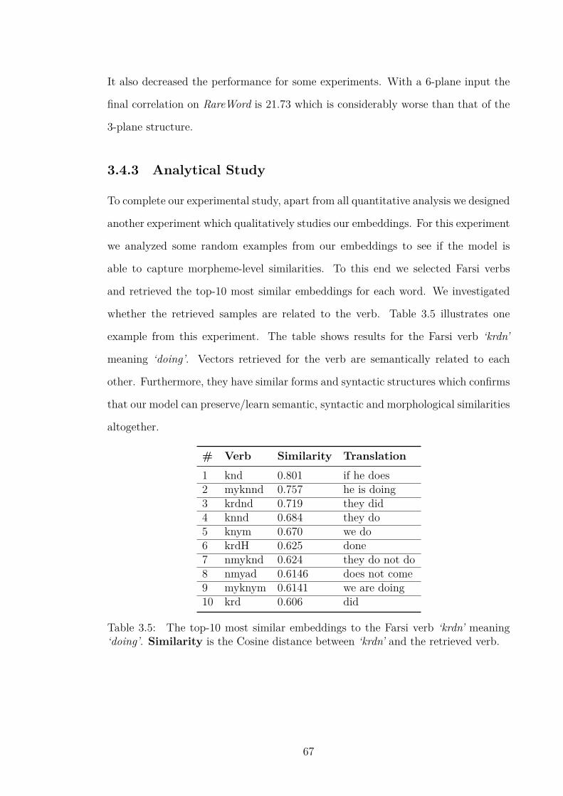
It also decreased the performance for some experiments. With a 6-plane input the

final correlation on RareWord is 21.73 which is considerably worse than that of the

3-plane structure.

3.4.3 Analytical Study

To complete our experimental study, apart from all quantitative analysis we designed

another experiment which qualitatively studies our embeddings. For this experiment

we analyzed some random examples from our embeddings to see if the model is

able to capture morpheme-level similarities. To this end we selected Farsi verbs

and retrieved the top-10 most similar embeddings for each word. We investigated

whether the retrieved samples are related to the verb. Table 3.5 illustrates one

example from this experiment. The table shows results for the Farsi verb ‘krdn’

meaning ‘doing’. Vectors retrieved for the verb are semantically related to each

other. Furthermore, they have similar forms and syntactic structures which confirms

that our model can preserve/learn semantic, syntactic and morphological similarities

altogether.

# Verb Similarity Translation1 knd 0.801 if he does2 myknnd 0.757 he is doing3 krdnd 0.719 they did4 knnd 0.684 they do5 knym 0.670 we do6 krdH 0.625 done7 nmyknd 0.624 they do not do8 nmyad 0.6146 does not come9 myknym 0.6141 we are doing10 krd 0.606 did

Table 3.5: The top-10 most similar embeddings to the Farsi verb ‘krdn’ meaning‘doing’. Similarity is the Cosine distance between ‘krdn’ and the retrieved verb.

67

3.5 Summary

In this chapter we discussed a new word-embedding model which is able to explic-

itly capture morphological information. Our approach decomposes surface forms

into smaller units and trains embeddings for them; then a word-level embedding is

generated by combination of such subunit embeddings. Results reported from the

proposed model confirm that it outperforms systems which do not take morpholog-

ical information into account. On the word-similarity task, for both common and

rare words, we perform better than the state-of-the-art recursive model. Moreover,

we applied the proposed model to Farsi and German POS tagging, to further eval-

uate our morphology-aware embeddings. For the tagging tasks our model clearly

outperforms word-level models. Via the architecture discussed in this chapter we

are able to efficiently model MCWs. Our morphology-aware embeddings are also

used in the next chapter to improve translation quality.

68

Chapter 4

Morpheme Segmentation for

Neural Language Modeling

In the last chapter we introduced our models to learn morphology-ware word embed-

dings. In this chapter we look beyond word-level modeling and work at the sentence

level, which is referred to as language modeling in the field of NLP. Recently, neural

language models (NLMs) have appeared as powerful alternatives to conventional n-

gram models. They perform efficiently in most cases but still have serious problems

with MRLs. Words are treated as atomic units in existing word-level NLMs, which

is not suitable for MRLs as words are complex structures in this set of languages

and should be processed at the subword level. Morpheme-level and character-level

NLMs have been proposed to address this issue. In this chapter, we further explore

this problem by tuning the state-of-the-art character-level model (Kim et al., 2016)

in order to propose better language-modeling alternatives. We also propose data-

driven and count-based morpheme segmentation1 models to process MCWs, prior to

being used by NLMs. Through the segmentation process, MCWs are decomposed

into different sets of consecutive characters. Our proposed models benefit from the1In NLP, word segmentation is usually known as a process in which words are separated from

each other but here we tend to segment words into their subunits, so we use the term morpheme

segmentation. In our models, morphemes are not necessarily linguistic morphemes and could be

any set of consecutive characters.

69

advantages of both character-level and morpheme-level decompositions. We eval-

uated our models on English and four MRLs, namely Czech, Farsi, German, and

Russian, and observed significant improvements for all experiments.

In this chapter the main goal is to propose data-driven techniques to extract

basic units of languages. A set of basic units is a set by which all constituents

of the language can be modeled (represented). A particular language could have

several basic sets with different levels of granularities. Using this definition, a set

of unique words (vocabulary) can be considered as the set of basic units, because

each word is a basic element in itself. With the same logic, a set of stems and all

possible affixes plays the same role, as stems and affixes are basic units and can be

combined to generate new linguistically correct constituents. However, there is a key

difference between these two sets. The first set includes thousands (or even millions)

of surface forms and all new constituents generated via the set are only limited to

that. Therefore, it is not possible to model unseen forms (which do not exist in the

set or include unseen subunits), whereas the second set is able to partially mitigate

this problem as the chance of modeling an unseen constituent via a combination of

stems and affixes is very high. Another advantage of the second set compared to the

first one is its size. The size of a set including all stems and affixes is considerably

smaller than the size of the vocabulary set, which enables us to model much more

constituents via a much smaller set.

The alphabet is the third alternative which can be considered as the set of basic

units for any language. All possible constituents in a language can be generated via a

combination of letters. This third set has the smallest size and the finest granularity,

that is able to thoroughly solve the problem of generating unseen words. Modeling

constituents via the alphabet set looks a promising avenue of investigation, and

thus recent models have been designed based on characters. Character-level models

receive a sequence of characters as the input and try to extract meaningful relations

between characters. Models proposed based on this idea are successful and have

shown impressive results. However, there are still unanswered questions related to

70

these models, some of which we address in the next sections.

Morpheme-level NLMs (see Section 4.1) feed the neural architecture with sub-

word units instead of words. In contrast, character-level models are designed based

on the assumption that the subword-level representation may not be the best (machine-

understandable) input form, so they prefer to receive a sequence of characters as the

input and extract the relation between subunits by themselves. In this approach

characters are supposed to be basic units of the language, which is a correct as-

sumption but it complicates the problem. Characters are neutral units, namely any

character can collocate with any other character with no constraint. This much flex-

ibility can entail serious problems for neural models. Moreover, treating words and

sentences as sequences of characters drastically increases the computational com-

plexity. One sentence includes a limited number of words and neural models are

able to handle this much complexity without difficulty, but when the same sentence

is decomposed into characters it is changed to a very long sequence with hundreds

of units, so modeling such a long sequence and remembering the relation between

units is quite challenging or even impossible.

Considering these issues, we propose segmentation models which are able to

control the level of granularity of the segmentation scheme. The granularity provided

by word-level (and sometimes morpheme-level) models is too coarse for MCWs, and

the granularity of the character-level model could be too fine. We are not sure

as to which yields the best performance, because there are different results based

on different architectures. We believe that to answer this question we should have

different segmentation models with tunable granularity levels, where we can search

for and decide what the best granularity level is. In this research, we tried to design

such models, where the granularity level is tunable and lies in between the word-

level and character-level segmentations. Detailed information of the models and

their justification are discussed in the next sections.

Since our approach changes words into more understandable forms for NLMs, it

outperforms word- and morpheme-level models. It is also able to partially address

71

the shortcomings of character-level NLMs, as it decomposes words into blocks blocks

(sets of consecutive characters) which are bigger than characters, which means that

the final generated sequence is not very long. Shorter sequences are easier to process

for neural models. Furthermore, in our case the search space becomes smaller and

more tractable. In the character-level model the history is based on a chain of

characters and the next character could be any other character, but in our model

the history is constructed based on a sequence of morphemes which conveys a specific

meaning with a specific structure and expects a particular token in the following

step(s). To benefit from the advantages of our approach we should find the best level

of granularity for representing words in the context of language modeling which is

the main contribution of this research.

4.1 Background

Language modeling is the process of assigning a probability to a given sequence of

words. An LM measures how likely a sequence of words is to occur in a text. It

addresses the fluency feature of the given sequence, so that a sequence with a good

word order has a higher probability. The most popular types of LMs are count-based

or n-gram models which function based on the Markov chain assumption. In such

models the probability of a sequence is computed by the conditional probabilities of

words given their history, as in (4.1):

P (S) = P (w1, ..., wm) =m

ź

i=1

P (wi|wi´11 ) (4.1)

where S is the given sequence of length m. The model conditions the probability

of each word over a chain of preceding words. Since computing the probability over

the entire chain is not computationally feasible, it is usually limited to a bounded

set of n most recent words, as in (4.2):

P (wi|wi´11 ) » P (wi|w

i´1i´n+1) (4.2)

72

The assumption states that the probability of a word is affected by its n preceding

words. Obviously, a long history is preferable but such an assumption is made in

practice because of computational restrictions and limited data resources. These

models are known as n-gram models and the limited-history problem is the main

disadvantage of these models.

NLMs (Alexandrescu and Kirchhoff, 2006; Mikolov et al., 2011; Botha and Blun-

som, 2014; Kim et al., 2016) have been proposed to solve the limited-history problem.

Generally in NLMs, embeddings of input words (words of an input sequence) are

combined to make an internal representation of the whole sequence. At the output

layer the next word (in the chain) is predicted given the input/internal represen-

tation and the conditional word probabilities, and the probability of the sequence

is computed accordingly. The work by Bengio et al. (2003) is the main basis for

all other NLMs and follows this architecture. Although this model performs better

than analogous n-gram models, it also suffers from the limited history as it considers

only the last n words in the prediction phase. To extend the history from n words

to the entire sequence Mikolov et al. (2010) proposed a recurrent architecture.

NLMs are able to solve the limited-history problem (through the recurrency fea-

ture) but both neural and n-gram models have fundamental problems with large

vocabularies and out-of-vocabularies (OOVs) phenomena which are commonly en-

countered in MRLs. To address this issue, subword-level models have been proposed

(Sutskever et al., 2011). The most impactful NLMs which explicitly address the rich

morphology problem are the morpheme-level log-bilinear (MLBL) and character-

level (CLM) models, proposed by Botha and Blunsom (2014) and Kim et al. (2016),

respectively. Our NLM relies extensively on these models with a similar architec-

ture to CLM. Botha and Blunsom (2014) extended the well-known log-bilinear LM

(Mnih and Hinton, 2007) for MRLs. It benefits from morpheme-level and word-

level information as the surface-form and subunit embeddings are linearly combined

to build the word representation. The model is able to achieve better performance

compared to existing word-level NLMs. CLM uses character-level information. Each

73

word is decomposed into characters and they are combined via a convolutional pro-

cess. Results reported from CLM indicate that such an architecture could be an

appropriate model for MRLs (see Section 4.4 for more details). In this chapter we

also address the same problem and try to find an optimal segmentation for MCWs.

Experimental results demonstrate that the proposed segmentation model enables

our NLM to perform better than the state-of-the-art morpheme-level (Botha and

Blunsom, 2014) and character-level (Kim et al., 2016) NLMs. The impact of the

proposed model is more tangible for languages with rich morphology.

4.1.1 Related Work

Language modeling is a well-studied problem with broad applications in different

fields such as speech processing, machine translation and information retrieval, and

covers numerous languages and architectures. In this section we review conventional

and neural LMs which either have the same concerns as we do or which efficiently

utilize neural architectures for language-modeling purposes.

To address the rich-morphology problem, the class-based approach (Brown et al.,

1992) was proposed. Bisazza and Monz (2014) reviewed the application of this ap-

proach for language modelling. The main idea behind class-based models is to group

words with the same distribution into equivalent classes and estimate class proba-

bilities instead of word probabilities. Since LMs work with word classes, they are no

longer sensitive to morphological variations and surface forms, which might allow the

rich-morphology problem to be mitigated. Factored (Bilmes and Kirchhoff, 2003)

and maximum entropy models (Shin et al., 2013) are other approaches which are

suitable for MRLs. Instead of working with surface forms, each word is represented

by a set of factors over which the word conditional probabilities are computed. A

factor can be any function or annotation which provides extra information about

the word itself, and its behaviour, semantic, grammatical role and context.

A group of NLMs achieved state-of-the-art results because of their optimal neural

architecture. Pascanu et al. (2014) studied the behaviour of deep recurrent neural

74

networks (RNNs) in language modeling. RNNs are the best alternatives in this re-

gard, since their recurrent (iterative) nature allows them to read the entire sequence

and preserve its features within hidden layers. Pascanu et al. (2014) tried several

deep and complex architectures to obtain the best result (see Table 4.1). Zaremba

et al. (2014) proposed a deep long short-term memory (LSTM) RNN. Simple RNNs

usually perform better than feed-forward models for sequences but they still have

problems to model long-distance dependencies. The vanishing gradient problem is

another common issue of simple RNNs (Pascanu et al., 2013). LSTM units were

proposed to solve these problems (Hochreiter and Schmidhuber, 1997). LSTMs work

as memory units which are able to memorize longer dependencies (see Section 4.4

for more details). Wang et al. (2015) designed a convolutional architecture for their

LM. Our model is also a convolution network combined with an LSTM RNN. Zhang

et al. (2015) proposed an encoding model to encode the input sequence into a fixed-

length vector and developed a feed-forward architecture to work over the vector.

These models and their performance on the English Penn Treebank (PTB) (Marcus

et al., 1993) are summarized in Table 4.1. PTB is a standard dataset on which all

LMs are evaluated in order to make them comparable.

Model PTB PPLDeepRNN (Pascanu et al., 2014) 107.5DeepLSTM (Zaremba et al., 2014) 78.4genCNN (Wang et al., 2015) 116.4FOFE (Zhang et al., 2015) 108.0CLM (Kim et al., 2016) 78.9

Table 4.1: Results reported from state-of-the-art NLMs on PTB. PPL refers toperplexity which is a standard to evaluate LMs (lower is better). The table onlyreports the best performance achieved by the models.

There are NLMs that were proposed particularly for MRLs such as factored

NLMs. Factored models have neural versions where the intuition behind them is

the same as non-neural models. Each word is represented by embeddings of its

factors instead of the surface-form embedding (Alexandrescu and Kirchhoff, 2006).

There are two main models, namely MLBL (Botha and Blunsom, 2014) and CLM

75

(Kim et al., 2016), which are known to be the most impactful NLMs for MRLs and

explicitly address the problem of rich-morphology problem. Figure 4.1 illustrates

their architecture.

word1 stem1

word2 stem2 suff2

word3 stem3 suff3 word1 word2 word3 …

Figure 4.1: The network on the left-hand side is the character-level architecture(Kim et al., 2016). word2 is segmented into characters and different filters withdifferent widths are applied to construct the word-level representation. The networkon the right-hand side is the morpheme-level architecture (Botha and Blunsom,2014). Subunit embeddings are linearly summed with the surface-form embeddingto build the final representation for each word (Ci).

Our NLM relies extensively on these models with a similar architecture to CLM.

As previously mentioned, Botha and Blunsom (2014) extended the well-known log-

bilinear LM (Mnih and Hinton, 2007). The original log-bilinear model is perhaps

the simplest neural language model. The model is a feed-forward network where the

probability of predicting the next word wi in the chain is estimated by linearly com-

bining the representations of the context words w0 to wi´1. In the model extended

by Botha and Blunsom (2014), each word is represented by the combination of its

surface-form and subword embeddings. The combination was quite successful and

surpassed all word-based models. Unlike MLBL, CLM works at the character-level

where character embeddings are learnable network parameters which are updated

during training. They are combined via a convolutional layer and passed through a

highway layer to make the word representation. CLM showed promising results for

MRLs. Its performance on PTB2 is also reported in Table 4.1.2PTB results are not available for Botha and Blunsom (2014).

76

4.2 Morpheme Segmentation

Sequence segmentation has recently become very important for many NLP tasks

such as POS tagging, language modeling and translation (Botha and Blunsom, 2014;

Dos Santos and Zadrozny, 2014; Chung et al., 2016; Costa-jussà and Fonollosa, 2016;

Kim et al., 2016; Luong and Manning, 2016). One of the main problems with neural

models is their inability to handle large vocabularies and complex words. More-

over, their performance drops considerably in the presence of OOVs. Morpheme

segmentation is usually applied as a solution but it raises other types of problems.

For morpheme-level segmentation, a precise morphological analyzer have to be pro-

vided as segmentation errors can directly affect the final performance. However, it

is not always possible to have such a high-quality analyzer. Morfessor (Smit et al.,

2014), an unsupervised model, is commonly used for this purpose, e.g. MLBL uses

Morfessor to decompose MCWs.

Recently, character-level segmentation has been proposed which usually provides

better results than morpheme-level methods. However, it is debatable as to which

of them (morpheme-level or character-level) provides the optimal segmentation. Ac-

cording to discussions (Botha and Blunsom, 2014; Sennrich et al., 2016b), the gain

achieved by morpheme-level neural models is mainly because of the segmentation

scheme rather than the neural architecture. However, this is not very clear as far

as character-level models are concerned, as they usually explore quite complex and

deep networks, and different alternatives might affect the performance. For example,

Ling et al. (2015) applied character-level segmentation, developed a quite complex

architecture and used pre-trained models but could not achieve comparable results

to state-of-the-art models, whereas Chung et al. (2016) applied the same segmenta-

tion model with better performance than previously reported work. Accordingly, it

is still questionable which model mainly affects the final performance: the segmen-

tation model or the neural architecture. It should also be mentioned that the model

of Chung et al. (2016) benefits from a mixed segmentation scheme. Chung et al.

77

(2016) have morpheme-level segmentations in the encoder of their neural translation

engine and a character-level segmentation in the decoder.

We believe that character-level segmentation does not provide an optimal repre-

sentation. CLM reported state-of-the-art results but for Russian which has a very

rich morphology, Kim et al. (2016) (Table 5) shows that the morpheme-level model

still works better. A similar situation was also reported in Vylomova et al. (2016)

where morpheme-level segmentations outperform character-level models for some

MRLs. Characters are not meaning-bearing units. They can appear in every word

regardless of its semantics, structure and context. There are many words which share

the exact or similar set of characters but have quite different meanings, e.g. ‘salt’

and ‘last’ or ‘except’ and ‘expect’. Character subunits do not preserve any specific

information. Furthermore, the surface form is completely destroyed when a word

is decomposed into characters. The surface form preserves a significant amount of

important information. Therefore, we believe that words should not be completely

decomposed into characters. However, we do not want to imply that character-level

information is not useful at all.

Results reported from different experimental studies related to morpheme seg-

mentation issues demonstrate that:

• Morpheme segmentation is not always required. It is only applied to languages

that have limited resources and a high OOV rate, in order to mitigate the data

sparsity problem. If enough data is available a model based on surface forms

(words without any segmentation) could be the best solution. Dos Santos

and Zadrozny (2014) report POS-tagging results where a word-level model

works better than a character-level counterpart. Note also that the word-

based model of Zaremba et al. (2014) has the best perplexity score on the

PTB dataset among all other morpheme- and character-level models.

• From a linguistic perspective, a precise morphological analyzer can provide the

best segmentation. However, finding such a tool can be impossible for some

78

languages.

• For situations where we do not have access to such a precise analyzer, character-

level models are the best and even the only solution.

• According to experimental results, for a particular set of languages, morpheme-

level models work better and for some of them character-level models provide

better performance, so it is not very clear which one is a good solution to deal

with MRLs.

Motivated by the aforementioned issues, in our research we try to find a middle-

ground solution that benefits from the advantages of all existing approaches. If we

capture the strengths of both paradigms we may obtain better results. To this end

we propose novel count-based segmentation models which combine both character-

level and morpheme-level models.

4.3 Count-based Segmentation for MCWs

Experimental results demonstrate that models which rely on word- and morpheme-

level segmentations perform well in the presence of enough data and preprocessing

tools, but it is not always feasible to guarantee this. Character-level models could be

considered as backup solutions for such situations, as they are not dependent on tools

and data as much as other models. However, character-level models require powerful

neural architectures. In such models the main goal is to connect related characters to

each other via a neural computation (not through segmentation), which is carried out

through convolutional modules. Usually, such convolutional computations are quite

costly, e.g. in the model of Kim et al. (2016) about 500 convolution operations are

applied to each word in the first layer, and then the result is sent to other following

layers. Such a convolutional process is a complementary process to prepare the input

for neural language modeling which imposes significant overheads, i.e. for the same

task (in the best case) the character-level model should have at least one layer more

79

than other counterparts.

Regarding the aforementioned issues we can conclude that the granularity level

of the input dictates the network architecture and affects the computational com-

plexity. Accordingly, we can debate important questions that: “Do we really need

a complex model to work at the character level?” or “Is the granularity provided

by the character-level segmentation optimal?” Although the set of characters of a

language is the minimal set and is able to model all possible constituents, we be-

lieve that it is not the optimal set. Existing state-of-the-art NLMs are designed to

work with character inputs, but it seems there is an easier way to solve the problem

with simpler models and different levels of granularity. Instead of asking the neural

architecture to decipher the relation among characters via complex convolutional

structures, we can explicitly solve the segmentation problem via a non-neural model

prior to performing language modeling, and feed the network with better segmented

units. We hope that by making the input data slightly more complex than that of

the character-level input, we will be able to mitigate the complexity of the neural

computation/architecture.

To study our hypothesis we compare and evaluate different segmentation schemes.

Existing segmentation models such as Morfessor (Smit et al., 2014) or the Byte-pair

model (Sennrich et al., 2016b) do not provide different/tunable granularity levels.

Morfessor is an unsupervised segmentation model which tries to extract linguis-

tically correct morphemes. The level of granularity provided by this model is in

between the word level and the character level, but it is not tunable. Byte-pair is a

similar model which processes words to extract frequent subunits. It relies on statis-

tical information and does not pay attention to linguistic rules. It takes a training

corpus and merges the most frequent character n-grams together. Through merging,

it generates a number of new tokens/blocks, the number of which should not exceed

a user-defined upper bound. The level of granularity of this model is almost the

same as Morfessor. These two models do not completely satisfy our needs to study

the hypothesis, so we propose new segmentation models with tunable granularity

80

levels. However, together with our models we also study Byte-pair and Morfessor.

The next sections explain our models.

4.3.1 Model A: Greedy Selection

In the first proposed model we use bigger subunits (blocks) than characters. The

proposed segmentation model takes a string (word) as its input and finds the longest

and frequent substring within its input. A frequent substring is a substring which

occurs at least θ times in a training corpus, where θ is a parameter of the model. We

refer to the longest and frequent substring as main. If there is any other substring

before and after main, the segmentation function is applied to them too. Clearly this

is a recursive pipeline to find the longest and frequent substring at each step. At the

end, if there exists some remainder that are not frequent, they are all decomposed

into characters. The pseudo-code of the model is illustrated in Algorithm 2.

Algorithm 2 CountSegmentation (InputS, Start, End, θ)1: procedure CountSegmentation2: Ź Start: index of the first character of InputS.3: Ź End: index of the last character of InputS4: (main,index) = find(InputS)5: Ź main: the longest & frequent substring within InputS.

6: Ź index: index of the main’s first character.

7: if main != null then8: Store main9: L = length(main)10: CountSegmentation(InputS,Start,index-1,θ)11: CountSegmentation(InputS,index+L,End,θ)12: else13: decompose all reminders into characters

The process is an optimization problem to find segmentation boundaries which

try to jointly maximize the length and frequency criteria. For a given input string

with a length L, there can be Lˆ(L+1)2

character n-grams, e.g. for the sequence

S=abcd with L = 4, the list of character n-grams is equal to a, b, c, d, ab, bc,

cd, abc, bcd, abcd. Among character n-grams some of them are frequent based on

statistics of the training corpus. At each step of the segmentation process, we select

81

an n-gram which is frequent and has the longest length compared to other frequent

alternatives.

In the character-level decomposition, the idea is to segment strings into their

basic subunits which are characters (the alphabet set of the corpus). Then by using

of different neural architectures, an attempt is made to reveal the relation between

related characters (Kim et al., 2016). This is a bottom-up approach, going from a

character-level representation to a morpheme- and word-level representation. The

intuition behind our model is partly the same with some distinctive differences.

We believe that the set of basic elements of each corpus is not only limited to

its characters. If a set of consecutive characters occurs frequently, then it could

be considered as a basic element. Accordingly, we introduce new atomic blocks

(instead of just characters) which include one or more characters, and all words can

be transformed/decomposed through these blocks.

To clarify the process we use a dummy example. For a given sequence s=‘aabcxy’

with two frequent substrings ‘ab’ and ‘xy’, the word-level segmentation keeps s as

it is and the character-level model blindly maps s to ‘a.a.b.c.x.y’ regardless of any

other criterion. In contrast, according to the count-based segmentation model, if

there are frequent substrings in s, they could be substantial units for other strings

and should be treated as atomic units, similar to characters, in which case the final

segmentation should be ‘a.ab.c.xy’. Clearly, in ‘ab’ all of ‘a’, ‘b’ and ‘ab’ substrings

are frequent but as ‘ab’ has the longest length, it is selected from that part of s.

We also have a real-world example for this procedure. Figure 4.2 shows the

count-based segmentation process for a complex Farsi word which was taken from

our training corpus. The input word is ‘prdrãmdtrynhã’ meaning ‘the people with

the highest salary’. Based on statistics of the Farsi training corpus (see Section 4.5),

the longest and most frequent substring is ‘ãmd’ which is a 3-gram constituent.

This means that there is no frequent n-gram with n ą 3 and ‘ãmd’ has the highest

frequency among all other 3-grams. ‘ãmd’ is separated and the segmentation model

is applied to its preceding (L-string) and following substrings (R-string). Each

82

substring is considered as a new input for the model which has a dedicated main,

L-string and R-string. The model is recursively applied until all frequent substrings

–‘ãmd’, ‘dr’, ‘tr’ and ‘hã’– are separated. There are still two substrings remaining,

namely ‘pr’ and ‘yn’. These two substrings are not considered as frequent in our

setting, so they are decomposed into characters. The final decomposition result by

the proposed model is: ‘prdrãmdtrynhã’ ñ ‘p.r.dr.ãmd.tr.y.n.hã’.

Figure 4.2: The process of segmenting ‘prdrãmdtrynhã’. main for each node is itsoffspring in the middle. The nodes before and after main are L-string and R-string,respectively. Dotted and solid lines indicate the character-level and morpheme-leveldecompositions. Final states are illustrated with double lines.

The segmentation model benefits from the advantages of the word-level, morpheme-

level and character-level models. If the input string’s surface-form is frequent, the

model does not decompose it and uses the original form. If it is considered as a rare

sequence, it is decomposed into characters, and if the string is neither frequent nor

rare it is segmented into sets of characters. There might be one or more charac-

ters in each set which means that the model uses a hybrid segmentation (as in the

aforementioned Farsi example).

In Model A and all other models the frequency of a subunit is computed using the

training corpus (not the lexicon/vocabulary), in which we consider all occurrences of

the subunit. We do not cross word boundaries for collecting frequency information,

i.e. words are separated from each other (space-to-space), segmented into all possible

character n-grams and the number of occurrences is counted for each n-gram.

83

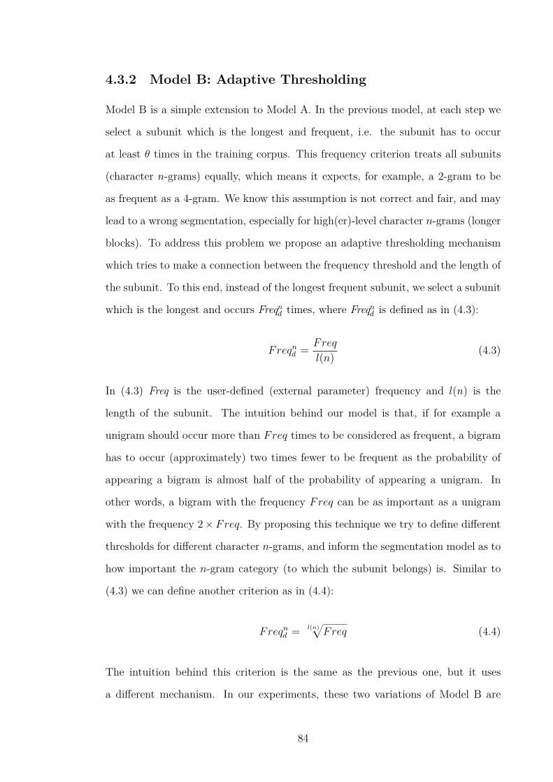
4.3.2 Model B: Adaptive Thresholding

Model B is a simple extension to Model A. In the previous model, at each step we

select a subunit which is the longest and frequent, i.e. the subunit has to occur

at least θ times in the training corpus. This frequency criterion treats all subunits

(character n-grams) equally, which means it expects, for example, a 2-gram to be

as frequent as a 4-gram. We know this assumption is not correct and fair, and may

lead to a wrong segmentation, especially for high(er)-level character n-grams (longer

blocks). To address this problem we propose an adaptive thresholding mechanism

which tries to make a connection between the frequency threshold and the length of

the subunit. To this end, instead of the longest frequent subunit, we select a subunit

which is the longest and occurs Freqnd times, where Freqnd is defined as in (4.3):

Freqnd =Freq

l(n)(4.3)

In (4.3) Freq is the user-defined (external parameter) frequency and l(n) is the

length of the subunit. The intuition behind our model is that, if for example a

unigram should occur more than Freq times to be considered as frequent, a bigram

has to occur (approximately) two times fewer to be frequent as the probability of

appearing a bigram is almost half of the probability of appearing a unigram. In

other words, a bigram with the frequency Freq can be as important as a unigram

with the frequency 2ˆFreq. By proposing this technique we try to define different

thresholds for different character n-grams, and inform the segmentation model as to

how important the n-gram category (to which the subunit belongs) is. Similar to

(4.3) we can define another criterion as in (4.4):

Freqnd =l(n)a

Freq (4.4)

The intuition behind this criterion is the same as the previous one, but it uses

a different mechanism. In our experiments, these two variations of Model B are

84

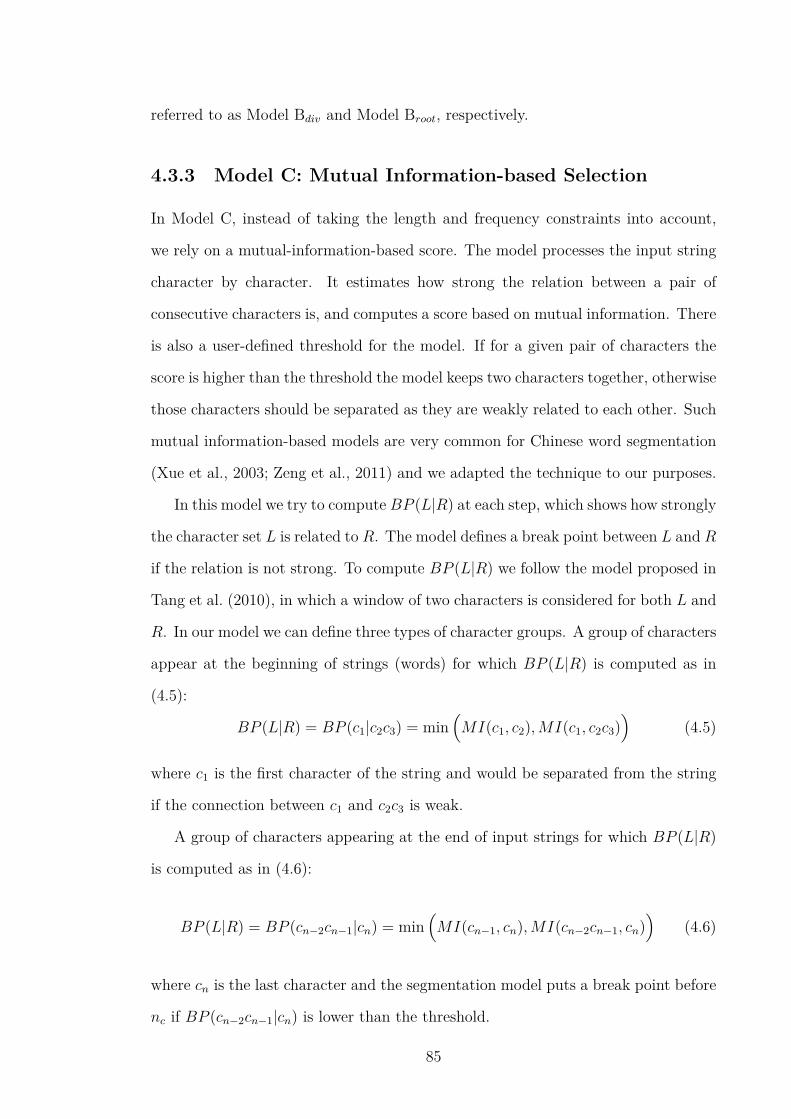
referred to as Model Bdiv and Model Broot, respectively.

4.3.3 Model C: Mutual Information-based Selection

In Model C, instead of taking the length and frequency constraints into account,

we rely on a mutual-information-based score. The model processes the input string

character by character. It estimates how strong the relation between a pair of

consecutive characters is, and computes a score based on mutual information. There

is also a user-defined threshold for the model. If for a given pair of characters the

score is higher than the threshold the model keeps two characters together, otherwise

those characters should be separated as they are weakly related to each other. Such

mutual information-based models are very common for Chinese word segmentation

(Xue et al., 2003; Zeng et al., 2011) and we adapted the technique to our purposes.

In this model we try to compute BP (L|R) at each step, which shows how strongly

the character set L is related to R. The model defines a break point between L and R

if the relation is not strong. To compute BP (L|R) we follow the model proposed in

Tang et al. (2010), in which a window of two characters is considered for both L and

R. In our model we can define three types of character groups. A group of characters

appear at the beginning of strings (words) for which BP (L|R) is computed as in

(4.5):

BP (L|R) = BP (c1|c2c3) = min(MI(c1, c2),MI(c1, c2c3)

)(4.5)

where c1 is the first character of the string and would be separated from the string

if the connection between c1 and c2c3 is weak.

A group of characters appearing at the end of input strings for which BP (L|R)

is computed as in (4.6):

BP (L|R) = BP (cn´2cn´1|cn) = min(MI(cn´1, cn),MI(cn´2cn´1, cn)

)(4.6)

where cn is the last character and the segmentation model puts a break point before

nc if BP (cn´2cn´1|cn) is lower than the threshold.

85

For those characters which neither appear at the beginning nor the end of strings

(middle characters), BP (L|R) is computed as in (4.7):

BP (L|R) = BP (ci´2ci´1|cici+1) = min(MI(ci´1, ci),

MI(ci´2ci´1, ci),

MI(ci´1, cici+1)

MI(ci´2ci´1, cici+1))

(4.7)

If the connection between ci´2ci´1 and cici+1 is weak, the model puts a break point

between ci´1 and ci. MI is a score defined based on mutual information and is

computed as in (4.8):

MI(x, y) = logfrq(xy)

Ng

frq(x)Ng

frq(y)Ng

(4.8)

where x and y can be any random character n-gram. frq(x) is a function which

counts how many times x appears in the training corpus. Ng shows the number of

all character n-grams which has an equal length to the parameter of frq, e.g. in

frq(cici+1), Ng is the total number of bigrams or for frq(ci´2ci´1cici+1), Ng shows

the number of all 4-grams.

4.3.4 Model D: Dynamic Programming-based Segmentation

Models A to C introduce morpheme segmentation models with tunable levels of

granularity. They help us feed neural models (NLMs or NMT engines) with multi-

granular subword units, but they have a serious problem, namely their dependency

on the external parameter (θ or m). Other similar models such as Byte-pair or

Morfessor also suffer from the same shortcoming. Their performance is highly in-

fluenced by the external parameter and they can only help us provide our desirable

result when the external parameter is set to an optimal value. Finding such a value

is usually performed in an empirical manner which can be quite costly (or even

impossible) for (very) deep neural models. Therefore, apart from these parameter-

86

dependent techniques, we need to have a model which has no external parameter.

Model D employs principles of dynamic programming and provides such a solution.

The morpheme segmentation problem is an optimization problem, where a se-

quence can be viewed as a container of character n-grams and the task of segmen-

tation is to find the best boundaries between such n-grams. There could be several

segmentation patterns for a single sequence, where the best segmentation is defined

based on the evaluation metric we consider for the task. For example, to provide

a linguistically correct segmentation we expect the model to separate stems from

syntactic affixes (valid affixes which exist in the language), or in Byte-pair we try

to set boundaries in a way which generates up to S unique symbols for the entire

corpus (S is a predefine vocabulary size). Figure 4.3 illustrates an example of a

Turkish sequence (word) with different segmentation boundaries to elaborate this

issue.

i n

in

i z

ini

ni iz

niz

iniz

da

nizda

ki

daki

le r

ler

kiler

Figure 4.3: Different segmentation boundaries for the Turkish word ‘hakkinizdakiler’meaning ‘things about you’. Different paths yield different segmentations for thisword.

As Figure 4.3 shows, we can have several segmentation patterns for the Turk-

ish word ‘hakkinizdakiler’ meaning ‘things about you’ such as ‘hakk.in.i.z.da.ki.ler’,

‘hakk.i.niz.da.ki.ler’, ‘hakk.i.nizda.ki.ler’ etc., as ‘i’, ‘in’, ‘ini’, ‘niz’, ‘nizda’, ‘da’,

‘daki’, ‘ki’, ‘kiler’, ‘le’, and ‘ler’ are all valid suffixes in Turkish (hakk is the stem).

Different segmentation models provide different patterns based on different criteria.

If the model prioritizes linguistic aspects, probably the best segmentation would be

87

‘hakk.in.iz.daki.ler’, but if it considers the frequency feature together with linguistic

constraints the final segmentation would be ‘hakk.i.n.i.z.da.ki.le.r’. Therefore, the

problem is an optimization problem and different results can be obtained based on

different constraints.

As we do not have access to a precise morphological analyzer for all languages,

we try to benefit from statistical techniques to find a suboptimal segmentation. It

should also be noted that nothing forces us to find linguistically correct segmenta-

tions. Existing (NLP) models are flexible/powerful enough to work with different

segmentation schemes and the only prerequisite is that they work with a limited set

of basic units. With this assumption, we try to discover such a set of basic units. In

our model we consider two constraints, namely length and frequency. We wish to

find (disjunctive) boundaries between sets of characters which maximize both con-

straints at the same time. If we only consider the length constraint then all words

(or sequences in general) would stay in their original form and the model would give

the surface form as its output. Similarly, if we only take the frequency constraint

into account we would not obtain the best result as the model will decompose words

purely into characters. We try to make a balance between these two paradigms and

obtain a better segmentation scheme. We mentioned that it could be challenging

to assign an optimal value to these parameters, so we propose a model to set them

automatically.

If a unit frequently occurs in a corpus, there is a chance for the unit to be a basic

element of the language. However, we should define a prescriptive criterion for this

situation. We know that all frequent units are not basic or they could be basic (such

as characters) but not useful for our purposes. Since a frequency threshold labels

a unit as frequent or infrequent, finding an appropriate threshold is a critical issue.

A mechanism should be defined to recognize the threshold value but it can make

the segmentation model fragile, as its performance would totally rely on a single

parameter which is very context-dependent. A wrong threshold could lead to wrong

segmentations. Another important issue about the threshold is that when it is set

88

to a particular value such as θ all units with frequencies higher than θ are considered

as frequent and, all other units with lower frequencies even with very close values

to θ (such as θ-1) are neglected. Accordingly, even in the presence of an optimal

threshold it is a very strict constraint to treat units based on a single value.

As far as problems caused by frequency-based models are concerned, it is not

an appropriate idea to set a global threshold value and we can decide to select

(or skip) a unit based on its context and adjacent units. Furthermore, it seems

that another complementary constraint should be included too, namely the length

of units. Similar to the frequency threshold we cannot have a global value for this

criterion. We do not know how many characters are enough to make an atomic block

and we cannot set a predefined value. Any set of characters with any random length

could be a basic block. So, apart from finding a dynamic and context-dependent

frequency value for each subunit, the segmentation algorithm should also be able to

find dynamic boundaries.

According to the discussion so far, it is not possible to separate subunits based

on predefined global length and frequency constraints and the model should set

dynamic values at each step. We propose a model in this regard. More formally,

given two m-tuples of positive numbers ă v1, v2, ..., vm ą and ă l1, l2, ..., lm ą, and

L ą 0, we wish to determine the subset A Ď t1, 2, ...,mu that maximizes (4.9a),

subject to (4.9b):

ÿ

aPA

va (4.9a)

ÿ

aPA

la = L (4.9b)

An input sequence (word) with the length L can include up to M sub n-grams where

M = Lˆ(L+1)2

and 1 ď n ď L. The a subscript in Equation (4.9) indicates the index

for each of these sub n-grams. The final goal is to select a subset of such n-grams

(finding A) which satisfies all constraints. la indicates the length of the a-th n-gram

and va is its value in the training corpus. A simple example can hopefully clarify the

89

problem. The set of all possible sub n-grams extracted from the word ‘the’ is t1, h2,

e3, th4, he5, the6 (L = 3 so there are 3ˆ42

sub n-grams). Our model tries to find a

subset of these n-grams which maximizes the optimization constraints so that their

combination gives us the original word ‘the’. Patterns such as ‘t.he’ (A = t1, 4u) or

‘the’ (A = t6u) could be possible alternatives as results of the segmentation process,

but a pattern such as ‘t.th.e’ (A = t1, 4, 3u) is wrong, as this violates the length

constraint and does not generate the original surface form.

In order to solve the problem formulated by equation (4.9), we need to define

la and va. It is clear that what the length value la is for each n-gram. For va, a

simple estimation could be the frequency of each n-gram, as because it shows the

importance (value) of the n-gram. However, with this simple estimation characters

would have much higher values than others, which means the final result would be

the same as (or very similar to) the character-level segmentation. This is not our

desirable result so we approximate the value of each character n-gram va with (4.10):

imp(n) ˆ freq(na) (4.10)

where freq(na) shows the frequency of the a-th n-gram in the entire training corpus

and imp(n) indicates the impact/importance of that n-gram category (to which na

belongs), i.e. imp(n) tries to make a balance between length and frequency. Clearly

the frequency of a single character (unigram) is much higher than other n-grams, but

we know that there is only a limited number of unigrams in the corpus. There could

be up to 500 unique unigrams in a corpus but each of them could occur millions of

times. Accordingly, unigrams are important in terms of frequency but the category

to which they belong is not very popular/important in the corpus. Similarly the

number of bigrams is considerably fewer than trigrams but the frequency of each

bi-gram is much higher than trigrams. There should be a mechanism that shows

how frequently a character n-gram occurs and how important the n-gram category

is among others. To this end we define imp(n) which shows the portion of a specific

90

n-gram category among all other n-grams which might be estimated as in (4.11):

imp(n) =count(n)

řNn1=1 count(n

1)(4.11)

where count(n) enumerates how many n-grams exist in the corpus and N indicates

the length of the longest n-gram possible in the corpus.

Our segmentation model is defined based on these criteria. In order to implement

our model we propose a dynamic programming-based solution. To select the best

subset of all items (character n-grams) for the input sequence, at each step we

iteratively add a new item to an existing subset which is the optimal set up to that

step. The new item is selected in a way where the combination of a new item and

the existing set is another optimal set with one more member. We can compute

the value of the obtained segmentation at the i-th step (the total value of the items

selected up to the i-th step) with V (i, L) as in (4.12):

V (i, L) =

$

’

’

’

’

’

’

&

’

’

’

’

’

’

%

0 if i = 1

V (i ´ 1, L) if li ą L

max(V (i ´ 1, L), vi + V (i ´ 1, L ´ li)

)otherwise

(4.12)

The model starts with an empty set and by the model explained in (4.12) adds a

single item to the set. This procedure continues until the optimal set of subunits (A)

is reached. We select items which satisfy our constraints and make a segmentation

pattern for a given word. Figure 4.4 illustrates the python code for Equation (4.12).

Word() is a function which takes two inputs and segments the word. The first input

is a set of tuples which provides all possible character n-grams of the word (to be

segmented) and their values, and the second one is the length of the word. For exam-

ple, when we segment the word ‘the’, the set of all character n-grams and their values

would be similar to items=(‘t’,vt),(‘h’,vh),(‘e’,ve),(‘th’,vth),(‘he’,vhe),(‘the’,vthe) and

the length L is 3.

91

Figure 4.4: Morpheme segmentation with Model D.

4.3.5 Segmentation Quality

There are user-defined external parameters –the frequency threshold or θ in Model A

and Model B, and the BP threshold or m in Model C– which define the granularity

level of segmentations and directly affect the final output. Table 4.2 illustrates the

impact of these parameters.

As the table shows, the external parameters define segmentation boundaries.

In the given example the input is a long sequence of characters, including several

words joined to one another, and the model is expected to find the correct boundaries

between words. However, in our experiments we never have such an input as the

input is always a word. We use this (artificial) example to show that the granularity

level of our models could vary from a sentence to a character. It should also be noted

that if the results provided in the table are not precise enough, the reason is because

i) our models are designed to segment words (in order to extract basic subunits)

not sentences, and also ii) the given input is quite complex as it is a long sequence

with meaningful subunits. The collocation of characters from different words can

mislead the segmentation model.

Our segmentation models are proposed in order to find the optimal basic set

that maximizes the performance of our neural language model, but it is also inter-

92

Model Parameter Output

Model Aθ = 10, 000 th.is.is.as.i.m.p.le.pr.e.pr.o.ce.ss.ing.st.e.pθ = 5, 000 th.is.is.as.im.pl.ep.re.pro.c.ess.ing.st.epθ = 1, 000 this.is.as.imp.le.pre.pro.ces.sing.ste.pθ = 500 this.is.asi.mple.pre.pro.cess.ings.te.pθ = 100 this.isa.simpl.epre.process.ings.tep

Model Bdiv

θ = 10, 000 thi.si.sa.si.mp.le.pre.pro.c.ess.ing.ste.pθ = 5, 000 this.is.as.im.ple.pre.pro.ces.sing.ste.pθ = 1, 000 this.is.asi.mple.pre.process.ings.te.pθ = 500 this.isa.simpl.epre.process.ings.tepθ = 100 this.isa.simple.pre.processing.step

Model Cm = ´1 this.is.a.s.i.mple.p.rep.r.ocessings.t.epm = ´2 this.is.a.s.i.mple.p.reprocessings.tepm = ´3 this.is.as.i.mple.p.reprocessings.tepm = ´10 this.is.as.i.mple.p.reprocessingstepm = ´20 thisisasimplepreprocessingstep

Table 4.2: Different segmentations with different levels of granularity for the inputsequence ‘thisisasimplepreprocessingstep’. We emphasize that this is a quite complexexample which is never faced in the training phase. We used this example to showthat the granularity level in our models can vary from the sentence level (to separatewords) to the character level (to extract characters). Model Broot generates thesame results as Model Bdiv.

esting to see how precisely they can perform when they are studied as independent

modules. However, we emphasize that our goal is not to find linguistically correct

morpheme segmentations, and the main goal targeted here is being able to control

the level of granularity of intra-word segmentations, which is not provided by ex-

isting morpheme- and character-level models. In order to evaluate our models we

use the dataset provided by Morpho Challenge 2010,3 a shared task on morpheme

segmentation. We use the English and Turkish datasets in our evaluation. Our

models are trained on the training set to learn the statistics of words and character

n-grams. Then we fine-tune them using the development set to find the best values

of the external parameters. Finally, we apply them to the test set to see how they

segment unseen words. For both English and Turkish we combined the original3http://morpho.aalto.fi/events/morphochallenge2010/datasets.shtml.

93

training and development sets which gives us more than 1500 manually annotated

samples. We select the first 900 instances for training, the next 300 instances as the

development set and the remaining 300 instances as the test set.4 The results for

this experiment are reported in Table 4.3.

Language Model Correct Incorrect

EnglishMorfessor 47% 53%Model A 26% 74%Model B 33% 67%Model C 39% 61%

TurkishMorfessor 29% 71%Model A 20% 80%Model B 27% 73%Model C 34% 66%

Table 4.3: Results for the morpheme segmentation task. Model Bdiv and ModelBroot performed equally in this task so we showed both of them with Model B.

As the table shows, despite not being proposed for the morpheme segmentation

task, our models are able to produce comparable results to Morfessor which is a

powerful and well-known model in the field. As all models including Morfessor (the

version we use) are unsupervised models and the annotated dataset provided by the

shared task is quite small, we use additional corpora to enrich our training sets. For

the English set we used PTB and for the Turkish dataset we used the Turkish part

of the corpus of news articles in the Balkan languages (Tiedemann, 2009).5

Apart from Models A to C, we also studied Model D and Byte-pair. These models

are not supposed to extract syntactically correct morphemes. They are count-based

models which try to find the optimal set of basic units with statistical rules, so it

is not a meaningful comparison to evaluate these models in the previous morpheme

segmentation scenario. Moreover, there is no intrinsic evaluation for these models

as they are only evaluated extrinsically in neural language modeling or translation

tasks. However, we can provide some examples from these segmentation models and4The test set is not available through the link of the shared task and we had to combine and

separate the dataset in this way to produce a test set for our experiment.5http://opus.lingfil.uu.se/SETIMES2.php

94

qualitatively evaluate their performance.

Figure 4.5 illustrates examples of these models when Turkish sequences are seg-

mented. Turkish is a highly agglutinative language so we can easily show segmen-

tation boundaries for Turkish words.

Figure 4.5: Different segmentations provided by Byte-pair and Model D. We usesuperscripts to make a connection among words, their translation and segmentedforms. ‚ shows the segmentation boundary. bpe-xK means the Byte-pair modeltrained to extract x thousands different symbols. Turkish Seq. is the given Turkishsentence and Translation is the English counterpart of the Turkish sentence.

As the figure shows our model provides a considerably better segmentation. In

the first example e is separated from the first and second words, which shows two im-

portant properties of our model: i) first, the model provides a hybrid character-level

and morpheme-level segmentation; ii) second, it tries to learn meaningful relations

among subunits through the training phase and separate based on the context and

adjacent subunits. There are several e characters in the sequence but the model

separates only those of the first and second words. The reason for this is because

those specific characters play the role of a suffix in those words and they are not

simple characters. Although the model does not benefit from linguistic knowledge,

through the dynamic segmentation process it learns the constructive role of sub-

units. Selecting the e characters from the first and second words and not separating

those of the other words could confirm this issue. Similar properties can be seen for

other words, e.g. the segmented form of the fifth word in the first example is very

95

close to segmentations generated by models which rely on linguistic databases.

The segmentation scheme provided by bpe-5K is closer to ours but such a seg-

mentation is generated when all words of our training corpus are mapped to only

5K unique symbols. Such a drastic simplification never happens in practice, as in

neural models we usually map the input vocabulary to (about) 30K (or 35, 40, 50)

Byte-pair tokens. This means that to achieve an acceptable segmentation (similar

to ours) the Byte-pair model should be run with a very specific setting (which is

then not fair to compare with other models). For normal settings reported in the

table such as 30K or 50K, the Byte-pair model does not perform well. For these

cases it does not change surface forms, which means Byte-pair manipulates only a

limited number of words and does not efficiently change the corpus. In some cases it

has even negative affects over words, e.g. in the first example for bpe-50K the fourth

and fifth words are combined together, which not only does not solve the problem

but also makes the corpus harder to translate (it destroyed the original corpus).

4.4 Network Architecture

We segment input words to convert them into sequences of basic units, then they are

sent to our NLM. The proposed network architecture is slightly different from CLM

in the input layer, but other basic parts are almost the same. The network includes

5 main modules. The input sequence S = w1, ..., wm is processed word by word.

Each word is decomposed into different character blocks. For a given word wi the

segmentation result is Bi = tb1i , ..., bliu where bji indicates the j-th block of wi which

can be a single character or a set of consecutive characters. From a lookup table,

embeddings for blocks (bji ; 1 ď j ď l) are retrieved. The lookup table is basically a

weight matrix which contains embeddings. It is part of the neural architecture whose

values are updated during training. Clearly in our case the lookup table includes

block embeddings (which is different from that of CLM). Embeddings retrieved from

the table are combined together which yields a matrix-form data structure. For wi,

96

the matrix-form data structure is Ci P Reˆl, where the j-th column cji P Re indicates

the embedding of bji and e is the morpheme embedding size. Ci is padded with ‘Null’

columns to handle the variable length of different words.

Ci is a numerical representation for wi which preserves different types of informa-

tion including n-gram information. To extract such information, several convolution

functions are applied with different filters. This model was explored for the first time

for language modeling by Kim et al. (2016). In our convolution module we follow

the same model. For each Ci the convolution module provides a vector fCi, as in

(4.13):

fCi[k] = σ((Ci[:][k : k + w ´ 1] f F ) + a) (4.13)

where F P Reˆw is a filter of width wF , a is a bias value, σ is a non-linear function,

Ci[:][k : k+w ´ 1] indicates the k-to-(k+w ´ 1)-th columns of Ci, and f is the 2D

convolution operation. After applying the convolution function the maximum value

of fCiis selected, as in (4.14):

yi = maxk

fCi[k] (4.14)

The idea behind these computations is to capture the most important and

strongest (the maximum value) feature for a given filter. Each filter provides spe-

cific n-gram information where the size of n-gram corresponds to the filter width.

In CLM, different filters are scrolled over characters to capture different types of

information and connect related characters to each other. In the proposed segmen-

tation model, since we have a hybrid segmentation scheme, we already connected

related characters to each other (they appear as sets of consecutive characters in

blocks). Frequent character sequences are not decomposed and stay together. This

means that instead of finding relations through convolutional computations, we ex-

plicitly provide this type of information via our segmentations. The convolutional

computation can be interpreted as a complementary process in our case.

As previously mentioned, different filters with different sizes are applied, so with

97

m filters F1, ..., Fm the convolution module’s output is yi = [yi1, ..., yim] which is a

new representation for the word wi. Word representations (vectors) are passed to a

highway layer (Srivastava et al., 2015). In the highway network one additional affine

transformation is applied to obtain a better set of features. Equation (4.15) shows

the difference between the simple (4.15a) and highway (4.15b) connections:

y = g(Wx+ b) (4.15a)

y = t d g(WHx+ bH) + (1 ´ t) d x (4.15b)

where g() is a nonlinearity, t = σ(Wtx+ bt) is called the transform gate, and (1´ t)

is called the carry gate. The depth of neural networks has a direct impact on

their performance but as the depth grows training becomes more difficult. Highway

networks are effective models which provide deep but easily-trainable networks.

The fourth and main module of the NLM is an LSTM module which is fed by

the output of the highway module at each time step. LSTM units are the best alter-

natives for sequence modeling as they are able to model long-distance dependencies

and mitigate the vanishing gradient problem. In our setting, an LSTM unit takes

yt (LSTM input), ht´1 (previous hidden state) and mt´1 (previous memory vector)

as its input and produces ht and mt via the calculations in (4.16):

it = σ(Wiyt + Uiht´1 + bi)

ft = σ(Wfyt + Ufht´1 + bf )

ot = σ(Woyt + Uoht´1 + bo)

gt = tanh(Wgyt + Ught´1 + bg)

mt = ft d mt´1 + it d gt

ht = ot d tanh(mt)

(4.16)

where it, ft and ot indicate the input, forget and output gates, respectively. σ(.) is

an element-wise sigmoid function and Wρ, Uρ and bρ, ρ P ti, f, o, gu, are all network

98

parameters. For more information about the application of LSTMs in sequence

modeling, see Sutskever et al. (2014), Zaremba et al. (2014) and Kim et al. (2016).

At the end, we have a selection module which is implemented by a softmax function.

The output generated by the LSTM module is a representation of the input sequence

which is considered as history (see Equation 4.1). The goal in the prediction module

is to predict the most likely word from a target vocabulary with respect to history.

We follow the same training procedure as CLM to train our network (training

algorithm, parameter initialization etc). The learning criterion for the network is

the negative log-likelihood (NLL) of the input sequence S, as in 4.17:

NLL = ´

mÿ

t=1

logP (wt|wt´11 ) (4.17)

where the conditional word probability is a value generated by a softmax module.

The whole architecture of our NLM is illustrated in Figure 4.6.

p r d r ā m d t r y n h ā 𝑤𝑖−1 𝑤𝑖+1 𝑤𝑖−2 … …

Filters

𝑤𝑖+1

Highway

LSTM

Figure 4.6: The figure depicts the third time step when processing the input strings=[... wi´2 wi´1 wi wi+1 ...]. The complex Farsi word is decomposed into blocks.Different filters (shown by different colors) are applied over blocks to extract different(n-gram) features. The vector generated by the filters is processed by a highwayand an LSTM module to make the prediction, which is the next word wi+1. At eachtime step, the filters are only applied to the current word.

In our setting the batch size is 25 (25 sentences in each batch), the sequence

99

length is 30 and we train the network for 22 epochs. In the input module we set the

morpheme-embedding size e to 30 and word embedding-size to 200. As our filters,

we used 6 sets of filters with width [1, 2, 3, 4, 5, 6] of size [25, 50, 75, 100, 125, 150].

All these values are determined based on our empirical studies and the information

provided in Kim et al. (2016). We use ReLU to apply non-linearity within the

highway module which is a one-layer network. For regularization we placed two

dropout layers (Hinton et al., 2012) before and after the LSTM module with p = 0.4

for each. The LSTM module includes two hidden layers of size 300. We refer to this

configuration as the default configuration in Section 4.5.

4.5 Experimental Results

We compare our models to other four different models of MLBL, CharCLM, Word-

CLM, and MorphCLM. MLBL is the model proposed by Botha and Blunsom (2014).

CharCLM is the character-level neural language model (CLM) with the default con-

figuration. WordCLM and MorphCLM are variations of CLM where the first one

takes surface-form embeddings as the input without any prepossessing and segmen-

tation, and the second one linearly combines the word’s surface-form embedding

with morpheme embeddings. Morphemes for MorphCLM are provided by Morfes-

sor.

We evaluate the model on Czech (Cz), English (En), Farsi (Fa), German (De)

and Russian (Ru). Since our model is an extension to CLM, in order to make our

work comparable, we use the same datasets (test, validation and training sets) as

CLM and MLBL. We add Farsi as a new dataset to our experiments. To the best

of our knowledge, this is the first time that an NLM has been evaluated on this

language. We use the Farsi side of the TEP++ corpus (Passban et al., 2015) which

is a collection of ∼600K parallel English–Farsi sentences, to train the Farsi model.

Table 4.4 provides some statistics about our training corpora, and the optimal value

for the external parameter. Model D has no external parameter and learns to extract

100

subunits automatically.

Lang. T V C MA θA MBdivθBdiv

MBroot θBroot MC mC MD

Czech (Cz) 1m 46k 101 3,481 500 1,528 5k 1,284 10 670 1 1,636German (De) 1m 37k 74 2,522 700 1,701 5k 1,143 10 914 1 2,949English (En) 1m 10k 51 1,655 700 1,569 3k 1,066 10 582 1 1,070Farsi (Fa) 1m 37k 55 1,460 500 889 3k 945 10 543 1.5 1,431Russian (Ru) 1m 63k 62 1,079 2k 756 10k 1,505 10 829 1 2,987

Table 4.4: Statistics of datasets. T , V , C and M indicate the number of tokens,word vocabulary size, character vocabulary size, and the number of different blocksfor each language, respectively. θ is the frequency threshold andm is the break-pointthreshold. The subscript indicates to which model the parameter belongs.

As is standard, we use perplexity (PPL) to measure the quality of NLMs. The

perplexity of a given sequence S with n words is computed by exp(NLLn

) (NLL was

defined in Section 4.4). According to our experiments, the perplexity of the proposed

model (Model C as the best model) on PTB is 91 whereas CharCLM obtained 103.

We emphasize that these numbers are based on the default configuration. Our

model’s performance is comparable (slightly better) to that of CharCLM on PTB,

but as English is not usually considered to be an MRL, it is not the main interest

of this research. We perform other experiments on some MRLs, the results of which

are reported in Table 4.5.

System LanguageCzech (Cz) German (De) Farsi (Fa) Russian (Ru)

WordCLM 503 305 - 352WordCLMbp 341 239 113 230WordCLMdp 330 231 107 215MLBL 465 296 - 304MorphCLM 414 278 - 290MorphCLMbp 500 291 175 330MorphCLMdp 460 264 175 330CharCLM 385 239 128 259CLMA 365 230 110 243CLMBdiv

365 230 105 220CLMBroot 362 230 110 230CLMC 340 223 105 233

Table 4.5: Perplexity scores for different MRLs (lower is better).

In Table 4.5, WordCLM is the CLM of Kim et al. (2016) where each word is

101

represented by the surface-form embedding, which is directly sent to the highway

module (no convolutional process). This model is a surface-form-based model which

works with thousands of tokens (e.g. 63K for Russian, as in Table 4.4). Clearly, this

large number of tokens makes the modeling process challenging. WordCLMbp and

WordCLMdp have the same architecture as WordCLM where instead of words

they work with Byte-pair (bp) and Model D (dp) tokens, respectively. The perplexity

scores for these two models are significantly better than the word-based model, and

compete with those of character-based models. We were expecting such good results

as the number of unique tokens is significantly decreases in these models (e.g. from

36K to 2,987 for Russian). The neural model used for this task is quite powerful

which is able to provide precise predictions when it works with a limited set of

tokens.

MLBL is the model of Botha and Blunsom (2014). In MorphCLM, each

word is represented by the summation of surface-form and subword embeddings,

and the neural architecture is the same as the previous one, which means there

is no convolutional module. Subword embeddings are linearly combined and the

final embedding is sent to the highway module. In this model subword units are

separated by Morfessor. We also introduce two extensions for this architecture,

namely MorphCLMbp and MorphCLMdp. In the first and second extensions

subwords are segmented via Byte-pair and Model D, respectively. Results for these

extensions are not as well as other results, and this did not surprise us as Byte-pair

and Model D are not supposed to generate linguistically correct morphemes and

we do not expect to obtain a high-quality embedding for a word when we combine

the embeddings of its bp or dp subunits. In our experiments, to make our results

comparable we extract the same number of tokens for both Model D and Byte-pair.

Finally, the last 5 rows show CLM and our models with the default configuration

where input sequences are processed by the character-level and our segmentation

models, respectively. As the table shows, because the set of basic units extracted

via Models A to C is (supposed to be) better than the set of characters our NLMs

102

perform better than CharCLM.

In Section 4.3, we debated two important questions: “Do we really need a com-

plex model to work at the character level?” and “Is the granularity provided by the

character-level segmentation optimal?” Table 4.5 fully addressed these two questions.

For Czech and Russian which are morphologically complex languages, a simple NLM

working with dp tokens is able to generate better results than more complicated

subword-based models. This shows that in the presence of high-quality segmenta-

tions we do not need to explore complicated neural models (we will further discuss

the impact of effective segmentations in Section 6.3.1.1). Moreover, the character-

based model performs better when it is fed with our basic units (not characters).

This confirms that the simple character-based segmentation scheme does not provide

the optimal granularity.

4.5.1 Discussion

In this section we try to address two different properties to analyze the model from

different perspectives. The first issue that we wish to discuss is the size of training

corpora. Recently, Józefowicz et al. (2016) trained huge neural networks with dif-

ferent architectures for language modeling. They trained deep models on very large

corpora (on the one billion word benchmark6 (Chelba et al., 2013)) using massive

hardware resources (the best performance was reported from a model trained over

32 Tesla K40 GPUs for 3 weeks). According to their comparisons, the architecture

proposed by Kim et al. (2016) provides state-of-the-art results. As our model is

an extension to that architecture, it is supposed to perform better, but it cannot

be claimed without evaluating the model in practice. In large-scale experimental

settings the model might behave differently. We cannot afford the setting and re-

sources described in Józefowicz et al. (2016) but we are able to design a comparable

experiment. To evaluate the performance of our (best) models in the presence of

large vocabularies, we use two large Farsi and German corpora. Information about6http://www.statmt.org/lm-benchmark/.

103

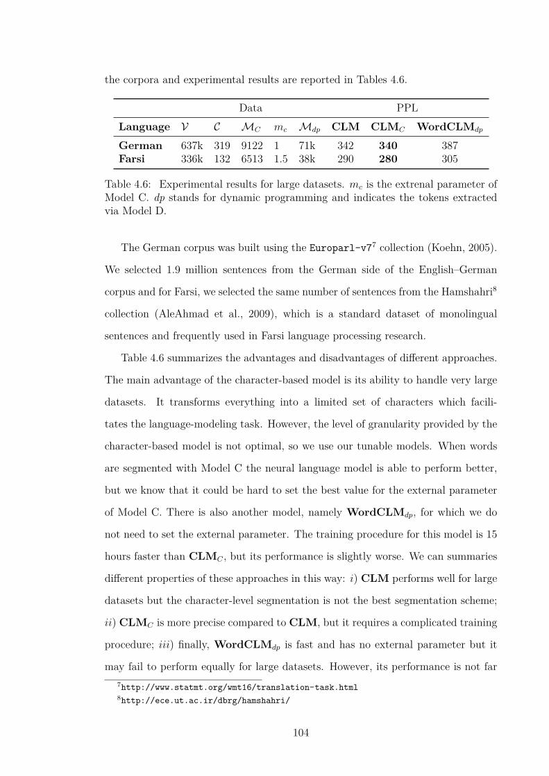
the corpora and experimental results are reported in Tables 4.6.

Data PPLLanguage V C MC mc Mdp CLM CLMC WordCLMdp

German 637k 319 9122 1 71k 342 340 387Farsi 336k 132 6513 1.5 38k 290 280 305

Table 4.6: Experimental results for large datasets. mc is the extrenal parameter ofModel C. dp stands for dynamic programming and indicates the tokens extractedvia Model D.

The German corpus was built using the Europarl-v77 collection (Koehn, 2005).

We selected 1.9 million sentences from the German side of the English–German

corpus and for Farsi, we selected the same number of sentences from the Hamshahri8

collection (AleAhmad et al., 2009), which is a standard dataset of monolingual

sentences and frequently used in Farsi language processing research.

Table 4.6 summarizes the advantages and disadvantages of different approaches.

The main advantage of the character-based model is its ability to handle very large

datasets. It transforms everything into a limited set of characters which facili-

tates the language-modeling task. However, the level of granularity provided by the

character-based model is not optimal, so we use our tunable models. When words

are segmented with Model C the neural language model is able to perform better,

but we know that it could be hard to set the best value for the external parameter

of Model C. There is also another model, namely WordCLMdp, for which we do

not need to set the external parameter. The training procedure for this model is 15

hours faster than CLMC , but its performance is slightly worse. We can summaries

different properties of these approaches in this way: i) CLM performs well for large

datasets but the character-level segmentation is not the best segmentation scheme;

ii) CLMC is more precise compared to CLM, but it requires a complicated training

procedure; iii) finally, WordCLMdp is fast and has no external parameter but it

may fail to perform equally for large datasets. However, its performance is not far7http://www.statmt.org/wmt16/translation-task.html8http://ece.ut.ac.ir/dbrg/hamshahri/

104

50 500 1,000 1,500 2,800

110

115

120

125

130

|M|

Perplexity

Figure 4.7: Impact of different θ values on PPL and |M|.

from that of CLMC .

The second issue which can be discussed is the segmentation scheme itself. As

previously mentioned, we think that the improvement gained by character-level

models is not only because of the segmentation model. As an example in CLM, the

highway module directly affects word representations. Kim et al. (2016) extensively

discussed this matter and provided several examples. We believe that the strength

of our model relies heavily on the chosen segmentation technique, rather than the

neural architecture. Our performance does not rely on highway layers as much as

CLM, as if we add/remove a layer to/from the highway module in the default con-

figuration (in Model C), the final perplexity would stay almost unchanged, whereas

if we do the same with CharCLM (add one extra layer or remove a layer from the

highway module), its performance fluctuates (perplexity changes) by 10 to 20 points.

Therefore, our segmentation scheme by its very nature is able to provide richer and

more representative information.

In our models the final output is highly influenced by the external parameters (θ

and m), so that it is necessary to find their best value to obtain the optimal output.

However, with some random values such as m = 1 or θ = 500, our models can

provide comparable results to state-of-the-art models. We designed an experiment

to show how these parameters affect the number of blocks and the model’s perfor-

105

mance. In our experiment we studied Model A (on Farsi) with different θ values.

As Figure 4.7 shows, the best perplexity score achieved by the model is 110 where

θ = 500, which generates a basic set of 1460 blocks. This means that by the given

frequency threshold, all existing words in the corpus can be encoded by 1460 atomic

units. When the threshold is increased the model starts to react similarly to CLM,

because the basic units become smaller so that the basic set becomes closer to the

alphabet set. For example with θ = 10, 000, the basic set includes 124 blocks and

the perplexity is 120. We can see the opposite trend when the θ value is decreased.

When the threshold is set to a value smaller than 500 the basic set is not optimal

any more and it downgrades the performance of the NLM, because with smaller

θ values the chance of selecting longer blocks is higher and the basic set becomes

too sparse., e.g. with θ = 200 the size of the basic set is 2795 which results in a

perplexity score of 112, which is worse than 110. As the value of θ decreases this

negative trend continues up to θ = 100, and after this threshold the quality of the

model drops drastically.

4.5.2 Neural Language Modeling for SMT

All issues discussed so far are purely related to language modeling. Language models

are frequently used in different fields such as MT. In this section we show the ap-

plication of language modeling in SMT and explain how the proposed NLM enables

us to provide better translations. To this end we designed a simple experiment,

where we manipulate the n-gram language model with our NLM which means we

do not change anything but the n-gram scores. The n-gram-based language model

includes n-grams and their associated scores. We recompute those scores with our

NLM models. Results for this experiment are shown in Table 4.7.

In this experiment we trained different SMT engines to translate from English

(En) into German (De) and vice versa. To train the En–De engines we used the

WMT-15 datasets.9 For the training set we randomly selected 2M sentences. Our9http://www.statmt.org/wmt15/translation-task.html.

106

NLM EnÑDe Imp. DeÑEn Imp.Baseline 15.25 0 20.13 0WordCLM 15.78 +0.53 20.44 +0.31WordCLMdp 16.27 +1.02 20.72 +0.59WordCLMbp 16.24 +0.99 20.72 +0.59MorphCLM 15.85 +0.60 20.83 +0.70CharCLM 15.89 +0.64 20.85 +0.72CLMA 16.18 +0.93 20.96 +0.83CLMBdiv

16.15 +0.90 20.84 +0.71CLMBroot 16.11 +0.86 20.92 +0.79CLMC 16.20 +0.95 20.90 +0.77

Table 4.7: Boosting n-gram-based LMs with NLMs. Improvements (Imp.) arestatistically significant according to the results of paired bootstrap re-sampling withp = 0.05 for 1000 samples (Koehn, 2004b)

models were evaluated on newstest-2015 and tuned using newstest-2013. We

trained them using Moses (Koehn et al., 2007) with the default configuration, tuned

via MERT (Och, 2003) and evaluated using BLEU (Papineni et al., 2002).

In Table 4.7, Baseline shows the baseline systems which are phrase-based SMT

models. For our baseline models we trained 5-gram language models on the mono-

lingual parts of the bilingual corpora using SRILM (Stolcke, 2002). Other settings

indicate enhanced models for the baseline systems where n-gram counts are re-

computed using different NLMs. Imp is the difference between the baseline score

and the score obtained after embedding the NLM, which shows the impact of the

NLM. As the table shows using the NLM instead of/along with the n-gram-based

LM considerably improves the quality of both the directions.

4.6 Summary

In this chapter we proposed an extension to the state-of-the-art character-level NLM.

We did not drastically change the neural architecture but developed new segmen-

tation models to decompose morphologically complex words. Our proposed models

are simple and unsupervised models. The models learn the segmentation scheme

from a training corpus. The granularity provided by the models falls in between

107

character-level and morpheme-level models. They define a new set of basic units

(alphabet) for the given corpus. Through the training phase, they learn to connect

a set of related and consecutive characters to one another to construct new blocks.

The proposed neural language-modeling pipeline outperforms existing models for

all of our experiments. We studied our models from different perspectives and dis-

cussed the impact of the external parameters. Following this, we used our NLM

in the SMT pipeline. In our future work we plan to focus more on the generation

aspect of our neural language model.

108

Chapter 5

Boosting SMT via NN-Generated

Features

In this chapter we benefit from neural features generated by our NNs (reported in

Chapters 3 and 4) to boost SMT models. First we introduce a general pipeline to

incorporate word and phrase embeddings into SMT. By use of embeddings, not only

is the SMT model informed with syntactic and semantic (similarity) information,

but also we define different word-, phrase-, and sentence-level features to provide

better translations. We show how to use monolingual and bilingual embeddings.

Accordingly, training embeddings in the SMT context, especially bilingual embed-

dings, is one of the key contributions of the chapter. Our pipeline is investigated

from different perspectives through different experiments. We evaluated our mod-

els by translating between English (En) and Czech (Cz), Farsi (Fa), French (Fr),

and German (De) and observed significant improvements for all language pairs. The

main goal targeted in this chapter is to introduce a pipeline by which neural features

can be incorporated into the SMT pipeline, so models in this chapter are not only

limited to MRLs and can be applied to any language. However, as we are interested

in this set of languages, we designed our experiments based on MRLs and improved

our models via morphological information, which were reported in Section 5.2.3.

109

5.1 Incorporating Embeddings into Phrase Tables

The process of PBSMT can be interpreted as a search problem for the best target-

side match for a given input sentence where the score at each step of exploration

is formulated as a log-linear model (Koehn, 2009). For each candidate phrase, the

set of features is combined with a set of learned weights to find the best target

counterpart of the provided source sentence. Because an exhaustive search of the

entire candidate space is not computationally feasible, the space is typically pruned

via some heuristics, such as using beam search (see Chapter 2). The discrimina-

tive log-linear model allows the incorporation of arbitrary context-dependent and

context-independent features. Thus, features such as those in Och and Ney (2002)

or Chiang et al. (2009) can be combined to improve translation performance. The

standard baseline bilingual features (in the phrase table) included in Moses (Koehn

et al., 2007) by default are: the phrase translation probability ϕ(e|f), inverse phrase

translation probability ϕ(f |e), direct lexical weighting lex(e|f), and inverse lexical

weighting lex(f |e).1 The structure of the phrase table is illustrated in Figure 5.1.

Figure 5.1: The figure shows the structure of a German-to-English phrase table wherethe first constituent at each line is a German phrase which is separated by ||| from itsEnglish translation. The following 4 scores after the English phrase are default bilingualscores extracted from training corpora. These scores show how phrases are semanticallyrelated to each other. The decoder selects the best phrase pair at each step based on thesescores.

1Although the features contributed by the language model component are as important as the

bilingual features, we do not address them in Chapter 5, since they traditionally only make use

of the monolingual target language context, and we are concerned with incorporating bilingual

semantic knowledge.

110

The scores in the phrase table (see Figure 5.1) are computed directly from the

co-occurrence of aligned phrases in the training corpora. A large body of recent

work evaluates the hypothesis that co-occurrence information alone cannot capture

contextual information as well as the semantic relations among phrases (see Section

5.1.1). Therefore, many techniques have been proposed to enrich the feature list with

semantic information. In our model, we define six new features for this purpose. All

of our features indicate the semantic relatedness (similarity) of source and target

phrases. Our features leverage contextual information which is lost by the traditional

phrase extraction operations. Specifically, on both sides (source and target) we look

for any type of constituents including phrases, sentences, or even words which can

fortify the semantic information about phrase pairs.

Our main contributions in this model are threefold: i) we define new similarity

features and embed them into PBSMT to enhance the translation quality; ii) in order

to define the new features we train bilingual phrase and sentence embeddings using

an NN. Embeddings are trained in a joint distributed feature space which not only

preserves monolingual similarity and syntactic information but also represents cross-

lingual relations; and iii) we indirectly incorporate external contextual information

using the neural features. We search in the source and target spaces and retrieve

the closest constituent to the phrase pair in our bilingual embedding space.

5.1.1 Background

Several models such as He et al. (2008); Liu et al. (2008); Shen et al. (2009) studied

the use of contextual information in SMT. The idea is to go beyond the phrase level

and enhance the phrase representation by taking surrounding phrases into account.

This line of research is referred as discourse SMT (Hardmeier, 2014; Meyer, 2014).

Because NNs can provide distributed representations for words and phrases, they

are ideally suited to the task of comparing semantic similarity. Unsupervised models

such as Word2Vec or Paragraph Vectors (Le and Mikolov, 2014) have shown that

distributional information is often enough to learn high-quality word and sentence

111

embeddings.

A large body of recent work has evaluated the use of embeddings in MT. A

successful use-case was reported in Mikolov et al. (2013b), where they separately

project words of source and target languages into embeddings, then try to find a

transformation function to map the source embedding space into the target space.

The transformation function was approximated using a small set of word pairs ex-

tracted using an unsupervised alignment model trained with a parallel corpus. This

approach allows the construction of a word-level translation engine via a very large

amount of monolingual data and only a small number of bilingual word pairs. The

cross-lingual transformation mechanism allows the engine to search for translations

of OOVs by consulting a monolingual index which contains words that were not

observed in the parallel training data. The work by Martinez Garcia et al. (2014) is

another model that follows the same paradigm. However, MT is more than word-

level translation.

In Martínez et al. (2015), word embeddings were used in document-level MT to

disambiguate the word selection. Tran et al. (2014) used bilingual word embeddings

to compute the semantic similarity of phrases. To extend the application of text

embedding beyond single words, Gao et al. (2013) proposed learning embeddings

for source and target phrases by training a network to maximize the sentence-level

BLEU score. Costa-jussa et al. (2014) worked at the sentence-level and incorpo-

rated the source-side information into the decoding phase by finding the similarities

between phrases and source embeddings. Some other models re-scored the phrase

table (Alkhouli et al., 2014) or generated new phrase pairs in order to address the

OOV word problem (Zhao et al., 2015).

Our network makes use of some ideas from existing models, but also extends the

information available to the embedding model. We train embeddings in the joint

space using both source- and target-side information simultaneously, using a model

which is similar to that of Devlin et al. (2014). Similar to Gao et al. (2013), we make

embeddings for phrases and sentences and add their similarity as feature functions

112

to the SMT model.

5.1.2 Proposed Model

Our proposed model is explained in two main parts. Section 5.1.2.1 shows what the

data format is for our model, as we need to generate a special training corpus to train

our model. This section also studies our similarity features. Section 5.1.2.2 explains

the neural architecture and how the architecture enables us to train document-level2

and bilingual embeddings. Our training model provides unique embeddings for all

words, phrases, and sentences in the training corpus. In our case, embeddings are

distributed structures which are supposed to provide bilingual and contextual in-

formation. Such information is quite useful for any SMT engine whereby we enrich

the phrase table. The extended phrase table in our model includes 6 scores (fea-

tures) additional to those 4 default scores, which convey similarity and contextual

information.

5.1.2.1 Training Bilingual Embeddings

In order to train our bilingual embeddings, we start by creating a large bilingual

corpus. Each line of the corpus may include:

• a source or target sentence,

• a source or target phrase,

• a concatenation of a phrase pair (source and target phrases which are each

other’s translation),

• a tuple of source and target words (each other’s translation).

Sentences of the bilingual corpus are taken from our SMT training corpora. Ac-

cordingly, phrases and words are from the phrase tables and lexicons, generated by2In the literature document is a term which is used for any chunk of a text such as characters,

words, phrases, sentences, and paragraphs.

113

the alignment model and phrase extraction heuristic used by the SMT model. This

means that the bilingual corpus is a very large corpus with 2 ˚ |c| + 3 ˚ |pt| + |bl|

lines where |c| indicates the number of source/target sentences, |pt| is the size of the

phrase table and |bl| is the size of the bilingual lexicon. |c| is multiplied by 2 because

we have |c| source sentences (one sentence per line) and |c| target sentences. Simi-

larly, |pt| is multiplied by 3 as there are |pt| source phrases, |pt| target phrases and

|pt| concatenated phrases (paired). The structure of the bilingual training corpus is

illustrated in Figure 5.2. 𝑆𝑒𝑛𝑡𝑒𝑛𝑐𝑒1𝑠 𝑆𝑒𝑛𝑡𝑒𝑛𝑐𝑒2𝑠 …

S

𝑆𝑒𝑛𝑡𝑒𝑛𝑐𝑒1𝑡 𝑆𝑒𝑛𝑡𝑒𝑛𝑐𝑒2𝑡 …

T

𝑃ℎ𝑟𝑎𝑠𝑒1𝑠 ||| 𝑃ℎ𝑟𝑎𝑠𝑒1𝑡 ||| … 𝑃ℎ𝑟𝑎𝑠𝑒2𝑠 ||| 𝑃ℎ𝑟𝑎𝑠𝑒2𝑡 ||| … … < 𝑊𝑜𝑟𝑑1𝑠 , 𝑊𝑜𝑟𝑑1𝑡 > < 𝑊𝑜𝑟𝑑2𝑠 , 𝑊𝑜𝑟𝑑2𝑡 >

𝑆𝑒𝑛𝑡𝑒𝑛𝑐𝑒𝑠 𝑃ℎ𝑟𝑎𝑠𝑒𝑠 𝑆𝑒𝑛𝑡𝑒𝑛𝑐𝑒𝑡 𝑃ℎ𝑟𝑎𝑠𝑒𝑡 𝑃ℎ𝑟𝑎𝑠𝑒𝑠 𝑃ℎ𝑟𝑎𝑠𝑒𝑡 𝑊𝑜𝑟𝑑𝑠 𝑊𝑜𝑟𝑑𝑡 B

Figure 5.2: S, T , and B indicate the source, target, and bilingual corpora, respectively.The SMT model generates the phrase table and bilingual lexicon using S and T (shown inthe middle). The bilingual corpus consists of 6 different sections of 1) all source sentences(Sentences), 2) all source phrases (Phrases), 3) all target sentences (Sentencet), 4) alltarget phrases (Phraset), 5) all phrase pairs (Phrases-Phraset) and 6) all bilingual lexicons(Words-Wordt).

By use of the concatenated phrases and bilingual tuples we try to score the

quality of both sides of the phrase pair, by connecting phrases with other phrases

in the same language, and with their counterparts in the other language. The next

section discusses how the network benefits from this bilingual property.

In our model we have an embedding matrix whose rows represent the bilingual

corpus, namely each line of the bilingual training corpus has a dedicated vector (row)

in the embedding matrix. During training these vectors are updated to obtain high-

quality embeddings. After training, we would have a unique embedding for each

word, phrase, and sentence in each language (source and target). We use such

114

embeddings (Section 5.1.2.2 explains how we train embeddings) to extract phrase-

level and contextual information to enrich the phrase table.

As mentioned, the model trains a dedicated embedding for each phrase in the

phrase table. Such an embedding is used in the phrase table with the hope that

it will provide semantic information about the phrase itself. Since our embeddings

are bilingual, the phrase embedding is also able to provide semantic information

about the target side and the target phrase. This property is definitely useful to

guide the decoder. Apart from phrase-level embeddings we can use other word

and sentence embeddings to fortify existing phrase-level information and provide

contextual information.

In order to enrich the phrase table with our bilingual embeddings, first we com-

pute the semantic similarity between source and target phrases in phrase pairs. The

similarity shows how phrases are semantically related to each other. The Cosine

measure is used to compute the similarity, as in (5.1):

similarity(Es, Et) =Es.Et

||Es|| ˆ ||Et||(5.1)

where Es and Et indicate embeddings for the given source and target phrases, re-

spectively. We map Cosine scores into the range [0, 1]. This can be interpreted as

a probability indicating the semantic relatedness of the source and target phrases.

The similarity between the source phrase and target phrase is the first feature and

is referred as sp2tp. Apart from this score, we compute five more scores for each

phrase pair.

Among source-side embeddings (word, phrase, or sentence embeddings) we search

for the closest match to the source phrase. The closest match has the minimum dis-

tance to the source phrase. There might be a word, phrase, or sentence on the

source side which can enhance the source phrase representation and facilitate its

translation. We use the source-phrase embedding as it is supposed to enrich the

phrase table by proving semantic information about the source phrase, but noth-

115

ing limits us to work at the phrase level so we can provide further information by

using embeddings of other source-side documents. Although other source-side em-

beddings might not be directly related to the source phrase, as they are distributed

representations they can carry relevant information to the source phrase and/or

provide contextual information. If the closest match retrieved for the source phrase

belongs to a sentence, that might be the sentence from which the source phrase

was extracted. Clearly taking that sentence into account would provide contextual

information for the given phrase. If the closest match belongs to a phrase, that is

probably a paraphrased form of the original phrase (or a translationaly equivalent

phrase), and if the closest match belongs to a word, that is probably a keyword

which conveys the main meaning of the phrase (see Figure 5.3 and Table 5.1 for

more clarification). We compute the similarity of the closest source match to the

source phrase which is referred to as sp2sm in our setting. This is another feature

that we extract for our model.

We also look for the closest match of the source phrase on the target side. As we

jointly learn embeddings, structures that are each other’s translation should have

close embeddings. We find the closest match to the source phrase among target-side

embeddings as there might be some target-side contextual information which can

be useful for the decoder. We compute the similarity of the closest target match to

the source phrase, which is labeled as sp2tm. We compute the same similarities for

the target phrase, namely the similarity of the target phrase with the closest target

match (tp2tm) and the closest source match (tp2sm). The source and target matches

may preserve other types of semantic similarity as they are the most representative

constituents for the given phrase pair on the source and target sides. Therefore

we compute the similarity between the source match and target match (the sm2tm

feature). All new features are added to the phrase table and used in the tuning

phase to optimize the translation model. Figure 5.3 tries to clarify the relationship

between different matches and phrases.

116

sm2tm

tp2tm sp2sm

sp2tp

source phrase

source embeddings

target phrase

target embeddings

Figure 5.3: sp, tp, sm and tm stand for source phrase, target phrase, source matchand target match, respectively. The embedding size for all types of embedding isthe same. The source/target-side embedding could belong to a source/target word,phrase, or sentence. The labels on the links indicate the Cosine similarity betweentwo embeddings which is mapped to the range [0,1].

5.1.2.2 Training Document Embeddings

We have explained how to build the bilingual corpus and compute semantic features.

Now we discuss the network architecture to train bilingual embeddings. Our network

is an extension of Devlin et al. (2014) and Le and Mikolov (2014). In those methods,

documents (words, phrases, sentences and any other chunks of text) are treated as

atomic units in order to learn embeddings in the same semantic space as that used

for the individual words in the model. The model includes an embedding for each

document which in our case may be a monolingual sentence, a monolingual phrase,

a bilingual phrase pair, or a bilingual word pair. During training, at each iteration

a random target word (wt) is selected from the input document to be predicted at

the output layer by using the context and document embeddings (typical Word2Vec

approach). The context embedding is made by averaging embeddings of adjacent

words around the target word. Word and document embeddings are updated during

training until the cost is minimized. The model learns an embedding space in which

constituents with similar distributional tendencies are close to each other. More

formally, given a sequence of Si = w1, w2, ..., wn the objective is to maximize the log

117

probability of the target word given the context and document vector, as in (5.2):

1

n

nÿ

j=1

log p(wtj|C

wt

i , Di) (5.2)

where wtj P Si is randomly selected at each iteration. Di is the document embedding

for Si and Cwt indicates the context embedding which is the mean of embeddings

for m preceding and m following words around the target word wt.

As previously mentioned, Si could be a monolingual sentence (one line from

Sentences or Sentencet in Figure 5.2) or phrase (one line from Phrases or Phraset in

Figure 5.2), in which wt and adjacent words are from the same language. In other

words, the context includes m words before and m words after the target word. Si

also could be a concatenation of source and target phrases (one line from Phrases-

Phraset in Figure 5.2). In that case context words are selected from both languages,

i.e. m words from the source (the side from which wt is selected) and m words

from the target side. Finally, Si could be a pair of source and target words (one

line from Words-Wordt in Figure 5.2) where Cwt is made using the target word’s

translation. The word on one side is used to predict the word on the opposite side.

In the proposed model, m is the upper bound.

Table 5.1 illustrates some examples of the context window. The examples are se-

lected from the English–Farsi bilingual corpus (see Section 5.1.3). In C1 the context

window includes 2 words before better and 2 words after. In this case the target

word and all other context words are from the same language (indicated by the ‘s’

subscript). In the second example the input document is a concatenation of English

and Farsi phrases, so C2 includes m (or fewer) words from each side (indicated with

different subscripts). In the final example the input document is a word tuple where

the target word’s translation is considered as its context.

As shown in Huang et al. (2012), word vectors can be affected by the word’s

surrounding as well as by the global structure of a text. Each unique word has a

specific vector representation and clearly similar words in the same language should

118

D1 know him better than anyoneCbetter

1 [know, him, than, anyone]sD2 know him better than anyone . āv rā bhtr āz hrks myšnāsyCbetter

2 [know, him, than, anyone]s + [āv, rā, bhtr, āz, hrks]tD3 better . bhtrCbetter

3 [bhtr]t

Table 5.1: Context vectors for different input documents. wt (the word to bepredicted) is better and m = 5 (context). Italics are in Farsi (transliterated forms).

have similar vectors (Mikolov et al., 2013a). By means of the bilingual training cor-

pus and our proposed architecture, we tried to expand the monolingual similarities

to the bilingual setting, resulting in an embedding space which contains both lan-

guages. Words that are direct translations of each other should have similar/close

embeddings in our model. As the corpus contains tuples of ă wordL1 , wordL2 ą, em-

beddings for words which tend to be translations of one another are trained jointly.

Phrasal units are also connected together by the same process. Since the bigger

blocks encompass embeddings for words and phrasal units, they should also have

representations which are similar to representations of their constituents.

In our neural architecture we have a multi-layer feed-forward network. In the

input layer we have an embedding matrix. Each row in the matrix is dedicated

to one specific line in the bilingual corpus. During training embeddings are tuned

and updated. The network has only one hidden layer. The input for the Softmax

layer is h = W (Cwt

i ‚ Di) + b, where W is a weight matrix between the input layer

and the hidden layer, b is a bias vector and ‚ indicates the concatenation function.

The output of Softmax, V P R|V|, is the distribution probability over classes which

are words in our setting. The j-th cell in V is interpreted as the probability of

selecting the j-th word from the target vocabulary V as the target word. Based

on Softmax values the word with the highest probability is selected and the error

is computed accordingly. The network parameters are optimized using stochastic

gradient descent and back-propagation (Rumelhart et al., 1988). All parameters of

the model are randomly initialized over a uniform distribution in the range [-0.1,0.1].

119

Weight matrices, bias values and word embeddings are all network parameters which

are tuned during training. Figure 5.4 illustrates the whole pipeline.

1𝑛∑

w2

w4

w5

w6

w1

Ds

Csw3

h

Target Vocab.

w3

Figure 5.4: Network architecture. The input document is S = w1 w2 w3 w4 w5 w6

and the target word is w3. In the backward pass document embeddings for w1, w2,w4 to w6, and Ds are updated.

To enrich the phrase table properly, we need to have high-quality embeddings

which preserve contextual information. The neural architecture proposed here is one

of the well-known models which has been evaluated for many tasks (Devlin et al.,

2014; Le and Mikolov, 2014), so it can guaranty that we would have high-quality

embeddings. Moreover, our bilingual corpus also helps us train high-quality embed-

dings. It is large enough to cover almost all words and all co-occurrences. There are

millions of words in the bilingual corpus which is sufficient to reach an acceptable

quality for word embeddings. Accordingly, sentences and phrase embeddings would

also have the same quality as they are based on those (millions of) words. It should

be also noted that we do not only rely on words to train phrase and sentence embed-

dings, as we have a sufficient number of training instances for them too. We usually

have millions of parallel sentences in MT corpora which are included in the bilingual

corpus. Phrase tables generated using such parallel corpora are also quite large, e.g.

there are more than 30 million phrase pairs in one of our German–English phrase

tables. All these numbers ensure us that we can rely on our model and corpus for

training high-quality embeddings. The next section explains our experimental study

and shows the impact of our embeddings.

120

5.1.3 Experimental Results

We evaluated our new features on two language pairs: English–Czech and English–

Farsi. Both Czech and Farsi are morphologically rich languages; therefore, trans-

lation to/from these languages can be more difficult than it is for languages where

words tend to be discrete semantic units. Farsi is also a low-resource language, so

we are interested in working with these pairs. For the En–Cz and En–Fa pairs we

used the Europarl (Koehn, 2005) corpus and TEP++ corpus (Passban et al., 2015),

respectively. We randomly selected 1K sentences for testing and 2K for tuning, and

the rest of the corpus for training. The baseline system is a PBSMT engine built

using Moses (Koehn et al., 2007). We used MERT (Och, 2003) for tuning. In the

experiments we trained 5-gram language models on the monolingual parts of the

bilingual corpora using SRILM (Stolcke, 2002). We used BLEU (Papineni et al.,

2002) as the evaluation metric.

We added our features to the phrase table and tuned the translation models.

Tables 5.2 and 5.3 show the impact of each feature. The embedding size for these

experiments is 200. We also estimated the translation quality in the presence of the

all features (we run MERT for each row of the tables). Bold numbers are statistically

significant according to the results of paired bootstrap re-sampling with p = 0.05 for

1000 samples (Koehn, 2004b). Arrows indicate whether the new features increased

or decreased the quality over the baseline.

Feature En–Cz ÒÓ Cz–En ÒÓ

Baseline 28.35 0.00 39.63 0.00sp2tp 28.72 0.37 Ò 40.34 0.71 Ò

sp2sm 28.30 0.05 Ó 39.76 0.13 Ò

sp2tm 28.52 0.17 Ò 39.79 0.16 Ò

tp2tm 28.00 0.35 Ó 39.68 0.05 Ò

tp2sm 28.94 0.59Ò 39.81 0.18 Ò

sm2tm 28.36 0.01 Ò 39.99 0.36 Ò

All 29.01 0.66 Ò 40.24 0.61 Ò

Table 5.2: Impact of the proposed features over the En–Cz engine.

Results reported in Tables 5.2 and 5.3 show that the new features are useful and

121

Feature En–Fa ÒÓ Fa–En ÒÓ

Baseline 21.03 0.00 29.21 0.00sp2tp 21.46 0.43 Ò 29.71 0.50 Ò

sp2sm 21.32 0.29 Ò 29.74 0.53 Ò

sp2tm 21.40 0.37 Ò 29.56 0.35 Ò

tp2tm 20.40 0.63 Ó 29.56 0.35 Ò

tp2sm 21.93 0.90 Ò 29.26 0.05 Ò

sm2tm 21.18 0.15 Ò 30.08 0.87 Ò

All 21.84 0.81 Ò 30.26 1.05 Ò

Table 5.3: Impact of the proposed features over the En–Fa engine.

positively affect the translation quality. Some of the features such as sp2tp are always

helpful regardless of the translation direction and language pair, so this feature is

the most important of our feature. The sm2tm feature always works effectively in

translating into English and the tp2sm feature is effective when translating from

English. In the presence of all features results are significantly better than the

baseline system in all cases. Some of the features are not as strong as the others

(tp2tm) and some of them behave differently based on the language (sp2tm). With

these feature we (partly) incorporate contextual information by use of multi-granular

similarities among embeddings.

5.2 Further Investigation of Neural Features

We introduced a framework to leverage word embedding in the SMT pipeline. In

this section we study the framework from different perspectives. First we study how

powerful the proposed model is to capture semantic relations. We provide examples

from embeddings to highlight this property. Afterwards we study whether the model

is applicable to other languages. We do not necessarily need to train bilingual

embeddings, so this implies we explain a model to use monolingual embeddings as

well as morphology-aware embeddings to boost (phrase-based and factored) SMT

models. In a separate section we discuss the neural architecture and show that the

proposed feed-forward architecture can be substituted with a better convolutional

122

model. Finally, we take a look at the performance and quality issues. Our enhanced

SMTmodel improves the quality in terms of the automatic evaluation metric, BLEU,

but we wish to determine that the model actually changes translations, so we perform

human evaluations to verify this.

5.2.1 Capturing Semantic Relations

Numbers reported in Section 5.1.3 indicate that the proposed method and features

result in a significant enhancement of translation quality, but it cannot be decisively

claimed that they are always helpful for all languages and settings. Accordingly, we

tried to study the impact of features not only quantitatively but also qualitatively.

Based on our investigation, the new features seem to help the model determine

the quality of a phrase pair. As an example for the English phrase “but I’m your

teammate” in the phrase table, the corresponding Farsi target phrase is “āmā mn hm

tymyt hstm” which is the exact translation of the source phrase. The closest match

in the source side is “we played together” and in the target side is “Ben mn ānjā

bāzy krdm” (meaning “I played in that team”). These retrieved matches indicate that

we retrive something related and useful in our model which can help the decoder

generate better translations.

Note also that by comparing the outputs we noticed that before adding our

features, the word “your” in the English phrase was not translated. In translation

into Farsi, possessives are sometimes not translated as the verb implicitly shows

them, but the best translation is a translation including possessives. After adding

our features, the translation of “your” did appear in the output. In terms of linguistic

issues this is an important achievement in Farsi translation as it is very hard to solve

this problem by automatic translation models alone, and the fact that our solution

(at least) addressed and slightly mitigated the problem is encouraging.

The proposed model is expected to learn cross-lingual similarities along with

monolingual relations. To study this feature Table 5.4 illustrates how the proposed

model can capture cross-lingual relations. It can also model similarities in different

123

Query sadness1 ăapprehension, nervousą2 emotion3 ăill,sicką

4 pain5 ămoney,moneyą

6 benignity7 ămay he was punished,punished harshlyą

8 is really gonna hurt9 i know tom ’ s dying10 ăbitter,angryą

Table 5.4: The top-10 most similar vectors for the given English query. Recall thatthe retrieved vectors could belong to words, phrases or sentences in either Englishor Farsi as well as word or phrase pairs. The items that were originally in Farsi havebeen translated into English, and are indicated with italics.

granularities. It has word-level, phrase-level and sentence-level similarities. Re-

trieved instances are semantically related to the given queries.

5.2.2 Using Semantic Features for Other Languages

We reported our results on the Cz–En and Fa–En pairs. As we wanted to focus on

a language that has been not studied extensively, we chose Farsi. As Farsi is a low-

resource and complex language, improving its quality is an important achievement.

There exist many parallel corpora, systems, techniques and tools for well-studied

languages, so (small) enhancements such as the proposed model in this chapter might

not be so useful and interesting, as words, phrase tables or other components such

as language models etc. for such languages are already rich enough to provide high-

quality translations and do not necessarily need additional features. Along with Farsi

we also tried to study the impact of our model on Czech as another morphologically

complex language. Results were quite successful for both languages but to give a

better understanding of the model and provide more experimental studies, we also

applied our model to two well-studied languages, French and German.

For French and German we used the same experimental setting as that of Farsi

and Czech (Europral Corpus, Moses, SRILM, MERT etc.). Since the most important

124

System En–Fr Fr–En En–De De–EnBaseline 29.21 27.31 15.25 20.13Extended 29.92 27.95 15.56 20.64Improvement +0.71 +0.64 +0.31 +0.51

Table 5.5: For training the French and German engines we randomly selected 2Msentences from the Europral collection. The phrase table for the extended system isenriched with our novel sp2tp feature. Improvements in the last row are statisticallysignificant according to the results of paired bootstrap re-sampling with p = 0.05for 1000 samples (Koehn, 2004b).

feature is sp2tp, we report our experiments only on this feature. Table 5.5 shows the

results. Similar to the previous experiments, our model is also able to improve the

En–De and En–Fr engines. Improvements for French are more tangible than those

of German which could be because of the closer similarity of French and English.

It is usually claimed that these two languages are close to each other and, as sp2tp

tries to extract semantic relations, it performs well on this pair.

5.2.3 Using Morphology-Aware Embeddings in SMT

We use word embeddings to improve the translation quality. In our experiments we

applied our techniques to complex languages such as Farsi and German. We also

have a model to train high-quality embeddings for such languages (see Chapter 3). It

intuitively seems that if we use our morphology-aware embeddings we might obtain

better results. To this end we designed two experiments. In the first experiment

we use monolingual embeddings (as they are) in factored translation models, and in

the second experiment we turn our embeddings to bilingual forms.

We discussed the factored translation model (see Section 2.3.1) and explained

that they use a set of factors to represent words. In our experiments designed for

Farsi and German, we use embeddings to define new factors. We have three factors of

lemma, POS tag and morphology tag for each word. To lemmatize words we used our

in-house morphological analyzer for Farsi and NLTK for English and German. We

used our neural model (Passban et al., 2016a) for tagging. Using morphology-aware

125

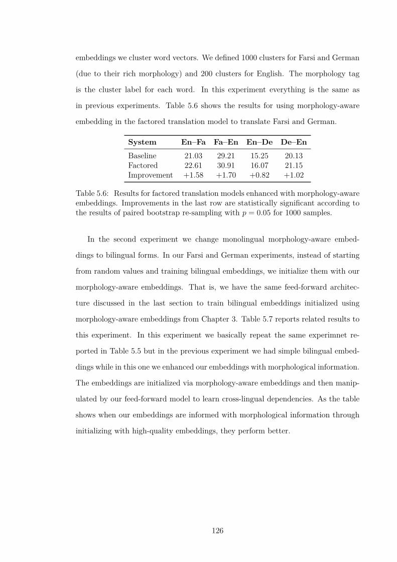
embeddings we cluster word vectors. We defined 1000 clusters for Farsi and German

(due to their rich morphology) and 200 clusters for English. The morphology tag

is the cluster label for each word. In this experiment everything is the same as

in previous experiments. Table 5.6 shows the results for using morphology-aware

embedding in the factored translation model to translate Farsi and German.

System En–Fa Fa–En En–De De–EnBaseline 21.03 29.21 15.25 20.13Factored 22.61 30.91 16.07 21.15Improvement +1.58 +1.70 +0.82 +1.02

Table 5.6: Results for factored translation models enhanced with morphology-awareembeddings. Improvements in the last row are statistically significant according tothe results of paired bootstrap re-sampling with p = 0.05 for 1000 samples.

In the second experiment we change monolingual morphology-aware embed-

dings to bilingual forms. In our Farsi and German experiments, instead of starting

from random values and training bilingual embeddings, we initialize them with our

morphology-aware embeddings. That is, we have the same feed-forward architec-

ture discussed in the last section to train bilingual embeddings initialized using

morphology-aware embeddings from Chapter 3. Table 5.7 reports related results to

this experiment. In this experiment we basically repeat the same experimnet re-

ported in Table 5.5 but in the previous experiment we had simple bilingual embed-

dings while in this one we enhanced our embeddings with morphological information.

The embeddings are initialized via morphology-aware embeddings and then manip-

ulated by our feed-forward model to learn cross-lingual dependencies. As the table

shows when our embeddings are informed with morphological information through

initializing with high-quality embeddings, they perform better.

126

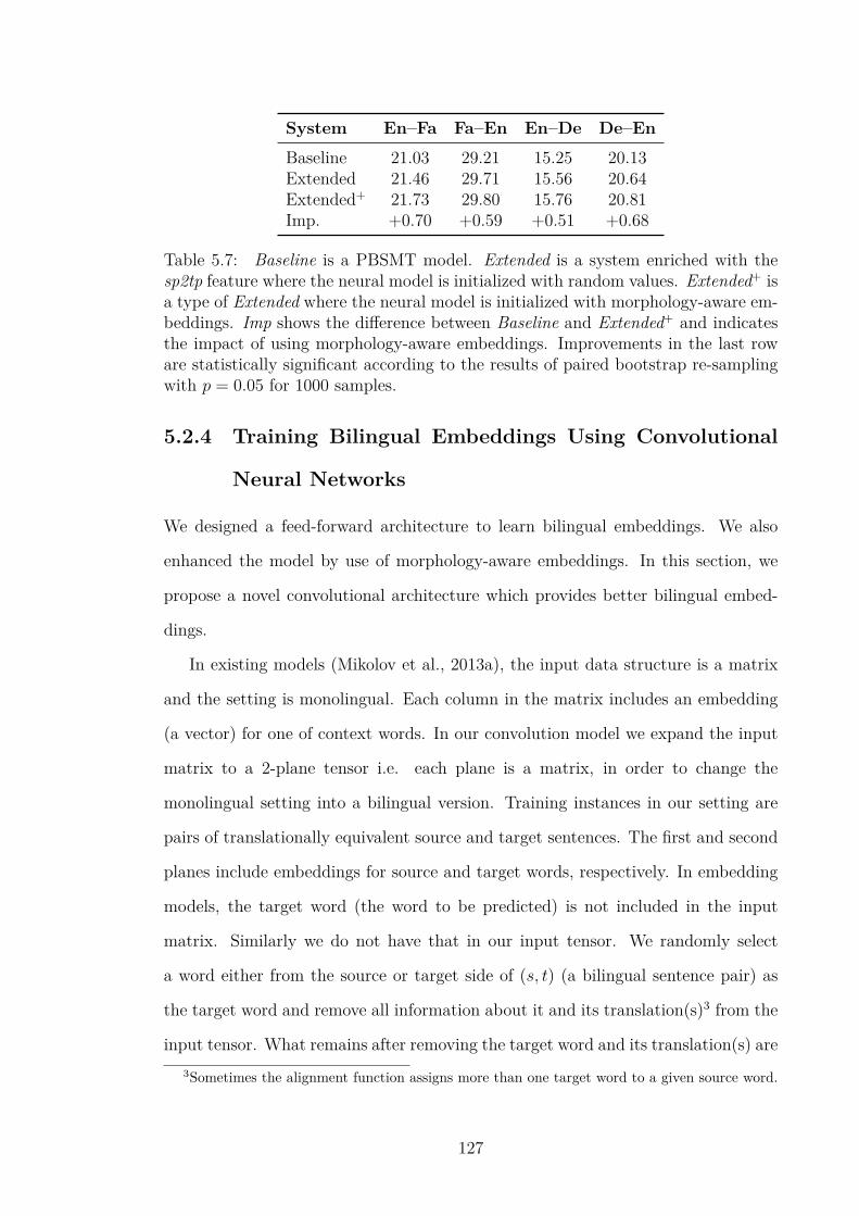
System En–Fa Fa–En En–De De–EnBaseline 21.03 29.21 15.25 20.13Extended 21.46 29.71 15.56 20.64Extended+ 21.73 29.80 15.76 20.81Imp. +0.70 +0.59 +0.51 +0.68

Table 5.7: Baseline is a PBSMT model. Extended is a system enriched with thesp2tp feature where the neural model is initialized with random values. Extended+ isa type of Extended where the neural model is initialized with morphology-aware em-beddings. Imp shows the difference between Baseline and Extended+ and indicatesthe impact of using morphology-aware embeddings. Improvements in the last roware statistically significant according to the results of paired bootstrap re-samplingwith p = 0.05 for 1000 samples.

5.2.4 Training Bilingual Embeddings Using Convolutional

Neural Networks

We designed a feed-forward architecture to learn bilingual embeddings. We also

enhanced the model by use of morphology-aware embeddings. In this section, we

propose a novel convolutional architecture which provides better bilingual embed-

dings.

In existing models (Mikolov et al., 2013a), the input data structure is a matrix

and the setting is monolingual. Each column in the matrix includes an embedding

(a vector) for one of context words. In our convolution model we expand the input

matrix to a 2-plane tensor i.e. each plane is a matrix, in order to change the

monolingual setting into a bilingual version. Training instances in our setting are

pairs of translationally equivalent source and target sentences. The first and second

planes include embeddings for source and target words, respectively. In embedding

models, the target word (the word to be predicted) is not included in the input

matrix. Similarly we do not have that in our input tensor. We randomly select

a word either from the source or target side of (s, t) (a bilingual sentence pair) as

the target word and remove all information about it and its translation(s)3 from the

input tensor. What remains after removing the target word and its translation(s) are3Sometimes the alignment function assigns more than one target word to a given source word.

127

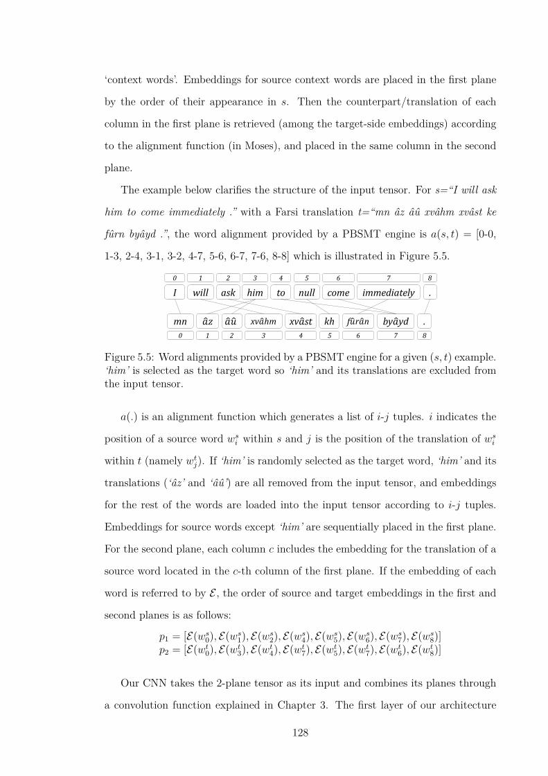
‘context words’. Embeddings for source context words are placed in the first plane

by the order of their appearance in s. Then the counterpart/translation of each

column in the first plane is retrieved (among the target-side embeddings) according

to the alignment function (in Moses), and placed in the same column in the second

plane.

The example below clarifies the structure of the input tensor. For s=“I will ask

him to come immediately .” with a Farsi translation t=“mn âz âû xvâhm xvâst ke

fûrn byâyd .”, the word alignment provided by a PBSMT engine is a(s, t) = [0-0,

1-3, 2-4, 3-1, 3-2, 4-7, 5-6, 6-7, 7-6, 8-8] which is illustrated in Figure 5.5.

I will ask him to null come immediately . 0 1 2 3 4 5 6 7 8

mn 𝑎 z 𝑎 𝑢 xv𝑎 hm kh f𝑢 r𝑎 n . xv𝑎 st by𝑎 yd 0 1 2 3 4 5 6 7 8

Figure 5.5: Word alignments provided by a PBSMT engine for a given (s, t) example.‘him’ is selected as the target word so ‘him’ and its translations are excluded fromthe input tensor.

a(.) is an alignment function which generates a list of i-j tuples. i indicates the

position of a source word wsi within s and j is the position of the translation of ws

i

within t (namely wtj). If ‘him’ is randomly selected as the target word, ‘him’ and its

translations (‘âz’ and ‘âû’) are all removed from the input tensor, and embeddings

for the rest of the words are loaded into the input tensor according to i-j tuples.

Embeddings for source words except ‘him’ are sequentially placed in the first plane.

For the second plane, each column c includes the embedding for the translation of a

source word located in the c-th column of the first plane. If the embedding of each

word is referred to by E , the order of source and target embeddings in the first and

second planes is as follows:

p1 = [E(ws0), E(ws

1), E(ws2), E(ws

4), E(ws5), E(ws

6), E(ws7), E(ws

8)]p2 = [E(wt

0), E(wt3), E(wt

4), E(wt7), E(wt

5), E(wt7), E(wt

6), E(wt8)]

Our CNN takes the 2-plane tensor as its input and combines its planes through

a convolution function explained in Chapter 3. The first layer of our architecture

128

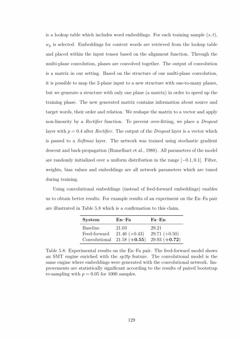
is a lookup table which includes word embeddings. For each training sample (s, t),

wp is selected. Embeddings for context words are retrieved from the lookup table

and placed within the input tensor based on the alignment function. Through the

multi-plane convolution, planes are convolved together. The output of convolution

is a matrix in our setting. Based on the structure of our multi-plane convolution,

it is possible to map the 2-plane input to a new structure with one-to-many planes,

but we generate a structure with only one plane (a matrix) in order to speed up the

training phase. The new generated matrix contains information about source and

target words, their order and relation. We reshape the matrix to a vector and apply

non-linearity by a Rectifier function. To prevent over-fitting, we place a Dropout

layer with p = 0.4 after Rectifier. The output of the Dropout layer is a vector which

is passed to a Softmax layer. The network was trained using stochastic gradient

descent and back-propagation (Rumelhart et al., 1988). All parameters of the model

are randomly initialized over a uniform distribution in the range [´0.1, 0.1]. Filter,

weights, bias values and embeddings are all network parameters which are tuned

during training.

Using convolutional embeddings (instead of feed-forward embeddings) enables

us to obtain better results. For example results of an experiment on the En–Fa pair

are illustrated in Table 5.8 which is a confirmation to this claim.

System En–Fa Fa–EnBaseline 21.03 29.21Feed-forward 21.46 (+0.43) 29.71 (+0.50)Convolutional 21.58 (+0.55) 29.93 (+0.72)

Table 5.8: Experimental results on the En–Fa pair. The feed-forward model showsan SMT engine enriched with the sp2tp feature. The convolutional model is thesame engine where embeddings were generated with the convolutional network. Im-provements are statistically significant according to the results of paired bootstrapre-sampling with p = 0.05 for 1000 samples.

129

5.2.5 Human Evaluation

After training our SMT models, we encountered instances which show that our new

features drastically change translations, so in addition to quantitative evaluations,

we looked at the output of our engines to confirm that the proposed pipeline affects

the translation process in a particular way. Table 5.9 compares translations between

the baseline SMT system and the enriched model via the sp2tp feature. Based on

our analysis, the new feature positively affects word selection. Extended translations

include better words than baseline translations. Furthermore, translations provided

by the extended models have better grammatical structures. They are also seman-

tically close(r) to the reference translations. The second and third examples are a

clear indication of these issues. For the third example, in spite of a very low BLEU

score the translation provided by the extended engine is a perfect translation.

If we compare the baseline and reference translations in the Farsi example, there

is almost nothing shared between these two translations, whereas in the extended

translation we see that almost all words are identical to those of the reference. In the

extended translation, مجموعه meaning ‘collection’ is redundant based on the reference

sentence while this is a perfect word should exist in the translation but the reference

does not include it. The other differences with the reference are تو meaning ‘you’ and

میاید meaning ‘will come back’. The Farsi word برمیگرده meaning ‘will be back’ in the

reference translation is substituted by میاید in the extended translation which is not

wrong, as these two words can be used interchangeably in Farsi, but BLEU is not

able to recognize these linguistic similarities and the human evaluation is the best

way to capture and study such phenomena. Similarly, the missing word تو in the

extended translation is not problematic at all as the verb in Farsi by its very nature

provides the pronoun information. Accordingly, تو is ineducable from the verb itself

and its absence does not make the translation wrong or even less fluent.

In order to complete the evaluation process, we asked a native Farsi speaker to

evaluate our results from the perspectives of fluency and adequacy. We prepared

a list of 100 sentences, randomly selected from translations of the extended model.

130

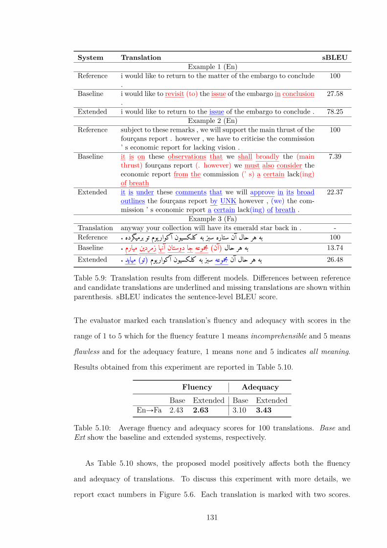
System Translation sBLEUExample 1 (En)

Reference i would like to return to the matter of the embargo to conclude.

100

Baseline i would like to revisit (to) the issue of the embargo in conclusion.

27.58

Extended i would like to return to the issue of the embargo to conclude . 78.25Example 2 (En)

Reference subject to these remarks , we will support the main thrust of thefourçans report . however , we have to criticise the commission’ s economic report for lacking vision .

100

Baseline it is on these observations that we shall broadly the (mainthrust) fourçans report (. however) we must also consider theeconomic report from the commission (’ s) a certain lack(ing)of breath

7.39

Extended it is under these comments that we will approve in its broadoutlines the fourçans report by UNK however , (we) the com-mission ’ s economic report a certain lack(ing) of breath .

22.37

Example 3 (Fa)Translation anyway your collection will have its emerald star back in . -Reference . برمیگرده تو یوم آكوار كلـكسیون به سبز ستاره آن حال هر به 100Baseline . میارم زمردین آنها دوستان جا مجموعه (آن) حال هر به 13.74Extended . میاید (تو) یوم آكوار كلـكسیون به سبز مجموعه آن حال هر به 26.48

Table 5.9: Translation results from different models. Differences between referenceand candidate translations are underlined and missing translations are shown withinparenthesis. sBLEU indicates the sentence-level BLEU score.

The evaluator marked each translation’s fluency and adequacy with scores in the

range of 1 to 5 which for the fluency feature 1 means incomprehensible and 5 means

flawless and for the adequacy feature, 1 means none and 5 indicates all meaning.

Results obtained from this experiment are reported in Table 5.10.

Fluency AdequacyBase Extended Base Extended

EnÑFa 2.43 2.63 3.10 3.43

Table 5.10: Average fluency and adequacy scores for 100 translations. Base andExt show the baseline and extended systems, respectively.

As Table 5.10 shows, the proposed model positively affects both the fluency

and adequacy of translations. To discuss this experiment with more details, we

report exact numbers in Figure 5.6. Each translation is marked with two scores.

131

Clearly, there are 100 fluency and 100 adequacy scores for the evaluation set. Results

can be interpreted from different perspectives, some of which we briefly mention

below. For the baseline model, the fluency rate of 38% of translations is 3, but this

percentage is raised to 45% in the extended model. 27% of the baseline translations

are disfluent (scale 2) but in the extended model this is reduced to 19%. For the

adequacy feature the condition is even better. Translations which could not properly

convey the meaning are changed to translations which are more acceptable for our

evaluators. The number of bad translations is reduced in the extended model and

correspondingly, the number of high-quality translations is increased.

Figure 5.6: Human evaluation results on EnÑFa translation.

5.3 Summary

In this chapter we introduced a framework to train bilingual embeddings and pro-

posed techniques to incorporate such features into the SMT model. Our bilingual

embeddings preserve semantic and syntactic information as well as cross-lingual

similarities. Using bilingual embeddings we extract different word-, phrase- and

sentence-level features for the SMT model which yield significant improvements.

We also noted that it is not necessary to have bilingual embeddings. We boosted

factored translation model through monolingual but morphology-aware embeddings.

In another experiment we tried to enrich embeddings with morphological informa-

132

tion which was also a successful model. The architecture of the embedding-learning

network is the key concept in training. We tuned the convolutional function ex-

plored in Chapter 3 for the task of embedding training and generated better results

than the feed-forward model. Finally, to conform that our techniques effectively

help the SMT model and not only improve the BLEU score, we performed human

evaluation and analyzed our results.

In the next chapter we will introduce a completely different paradigm for MT

which is known as neural machine translation (NMT). NMT models are end-to-end

purely neural models which do not follow the statistical pipeline but have their own

architecture. We explain the framework and introduce our models which propose

more compatible architectures for translating MRLs.

133

Chapter 6

Morpheme Segmentation for

Neural Machine Translation

In the last chapter we studied SMT and methods by which we can incorporate

morphological and neural information into SMT. In this chapter1 we try to address

the same problem with neural models. Recently, NN-based models have become

increasingly popular in different NLP fields including MT. NMT models have been

proposed as successful alternatives for conventional statistical models, which not

only boost existing systems and enhance their quality but also introduce new re-

search lines to further enrich the field. NMT provides a framework that enables us

to incorporate different types of annotations and external knowledge much better

than the existing log-linear model. The whole translation process is based on mil-

lions of different features that are learned in supervised and unsupervised manners.

Accordingly, there is no need for feature engineering and everything is performed

(semi-)automatically, which is the main difference between neural and log-linear ap-

proaches. In the log-linear model (see Chapter 2), different features are defined a

prior for the system, whereas the neural engine starts from a random setting for

features and gradually optimizes to reach the optimal configuration.1In this chapter we frequently refer to Models A to D which we mean the segmentation models

proposed in Chapter 4.

134

In this chapter we attempt to provide a comprehensive analysis of NMT models.

We introduce the framework and review the literature to summarize existing models

in this area. Then, we propose methods which are particularly designed for trans-

lating MRLs. We perform our experiments on German, Russian, and Turkish. We

select these languages for specific reasons. German has a complex morphology which

includes almost all morphological behaviour (fusional structures, agglutinative struc-

tures, compounds etc.). Furthermore, all well-known models have an experimental

analysis on German which makes it an important language for our comparative ex-

periments. Russian has a fusional morphology which is suitable to study the strength

of character-based models. Finally, Turkish is a highly agglutinative language by

which we can study the impact of our morpheme-segmentation models.

6.1 Neural Machine Translation (NMT)

NMT is not a new research field as its history goes back to almost twenty years

ago when Forcada and Ñeco (1997) proposed the encoder-decoder framework for

the first time. In that work a simple neural framework was proposed for basic

translation using finite state automata. In the proposed architecture the source

side is encoded into a numerical representation and outputs are sampled from the

encoded source input. The model was very basic with a limited number of neurons.

Forcada and Ñeco (1997) posited that the encoder-decoder framework is potentially

a very powerful alternative for sequence-modeling tasks but the strength of the model

could not be investigated at the time because of the lack of computational resources.

Recently, several models (Schwenk et al., 2006; Kalchbrenner and Blunsom, 2013;

Cho et al., 2014b; Sutskever et al., 2014) were proposed based on the same framework

that could efficiently benefit from that architecture to perform MT and language

modeling.

The intuition behind all these models is the same with slight differences that

we discuss here. As the model in Cho et al. (2014b) directly addresses the encoder-

135

decoder framework, we discuss the model in detail. The model consists of two RNNs.

One RNN encodes the source side into a fixed-length representation. By the encod-

ing, an internal representation of the sequence (sequence-level embedding) is pro-

duced. The other RNN is fed with source-side information to decode a sequence of

target symbols. Both the encoder and decoder modules are trained jointly to maxi-

mize the conditional probability of the target sequence given a source sequence. This

framework has the potential of being used as an independent end-to-end translation

engine as well as being embedded into conventional MT pipelines. Furthermore, it

is able to perform any sequence-to-sequence mappings such as parsing (Luong et al.,

2015a; Konstas et al., 2017), POS tagging (Ma and Hovy, 2016), caption generation

(Laokulrat et al., 2016) etc.

More formally, the model can be described as follows. For a given input sequence

x = x1, ..., xn, at each time step t, the encoder’s hidden state is updated as in (6.1):

st = f(st´1, xt) (6.1)

where f(.) applies non-linearity and st´1 is the previous state. The encoder consumes

all input symbols until the end of the sequence is arrived at. The last hidden state

hn is a summary of all previous states and represents x. Then the model freezes

the encoder and switches to decoding mode. The hidden state of the decoder is

initialized with the input representation, i.e. the decoder is informed about the

source sequence. In NMT, this information is referred to as context (c). At each

time step t, the decoder’s hidden state ht is updated conditioned on the previous

state ht´1, the last generated target symbol yt´1 and c, as formulated in (6.2):

ht = f(ht´1, yt´1, c) (6.2)

To sample the next target symbol both ht and c are used. The decoder needs to

136

compute a probabilistic value over the target vocabulary, as in (6.3):

P (yt|yt´1, yt´2, ..., y1, c) = g(ht, yt´1, c) (6.3)

where g(.) is a function like Softmax which generates valid values in the range [0,1].

Clearly the next target word is selected based on a history which is provided by ht.

These steps explain the most basic model for NMT, but there are more sophisticated

alternatives, such as using the beam search algorithm for decoding (Sutskever et al.,

2014) or more complex recurrent models (Chung et al., 2016).

Simple RNNs are not able to remember long-distance dependencies. In order to

address this shortcoming, RNNs have been equipped with memory units. Hochre-

iter and Schmidhuber (1997) proposed long short-term memory (LSTM) networks

to this end. Cho et al. (2014b) also proposed a variation of LSTMs called gated

recurrent unit (GRU), which is a simplified model with an almost equivalent com-

putational power. These models are frequently used in NMT. A high-level view of

the framework is illustrated in Figure 6.1.

𝑥1

𝑥2

𝑥3

𝑥𝑇 …

𝑦1

𝑦2

𝑦3

𝑦𝑇′ …

Encoder Decoder

Figure 6.1: A high-level view of the encoder-decoder architecture. The direction ofarrows show the impact of each unit on other units. The information flow from stto ht starts when all input symbols have been processed.

The basic encoder-decoder model suffers from a serious problem, whereby an

input sequence is squashed into a fixed-length representation and the decoder has

to sample everything based on the representation. Bahdanau et al. (2014) demon-

strated that this is a bottleneck for NMT, especially when the input sequence is

long or has a complex structure. The other problem with the basic architecture is

137

that the contribution of all source words is equal, because they (all) are summarized

into one vector. However, this rarely happens in practice. In real-world scenarios,

each target word is affected by a specific set of source words, not all of them at

once. To cope with this problem the attention mechanism was proposed (Bahdanau

et al., 2014), by which the decoder searches different parts of the input sequence to

find the most relevant words for the prediction phase. The model thus establishes

a soft alignment module over words. We know that c is computed by a nonlinear

computation applied to all encoder hidden states, as in (6.4):

c = f(ts1, ..., snu) (6.4)

where in the simplest scenario c = sn. In attention-based models c is dynamically

defined for each state of the decoder, which gives us (6.5):

p(yi|y1, ..., yi´1,x) = g(hi, yi´1, ci) (6.5)

Each state has its own context vector which is exclusively defined for yi. ci is a

weighted summation over all encoder states, so that lower (or zero) weights are

assigned to irrelevant words and the impact of relevant words is maximized by

assigning higher weights. This mechanism can be formulated as in (6.6):

ci =n

ÿ

j=1

αijsj (6.6)

where α denotes the weight assigned to each state, as in (6.7):

αij = align(sj, hi´1) =exp (eij)

ř Txk=1 exp (eik)

eij = a(sj, hi´1)

(6.7)

e(.) denotes an alignment model and scores the relevance of source words to the

i-th target symbol. a(.) is a combinatorial function that can be modeled through a

138

simple feed-forward connection, as in (6.8):

a(hi´1, sj) = v⊺a tanh(Wahi´1 + Uasj) (6.8)

va (vector), Wa and Ua (matrices) are all network parameters. The difference be-

tween the basic encoder-decoder model and its extension with an attention mecha-

nism is illustrated in Figure 6.2.

𝑥1 𝑥2 𝑥3 𝑥𝑇

𝑦𝑡 𝛼1𝑡 𝛼2𝑡 𝛼𝑇

𝑡 𝛼2𝑡

𝑥1 𝑥2 𝑥3 𝑥𝑇

𝑦𝑡 𝑐 𝑐𝑡

Figure 6.2: The network on the right-hand side depicts the basic encoder-decodermodel which summarizes all input hidden states into a single vector. The networkon the left-hand side is an encoder-decoder model with attention which defines aweight for each of the input hidden states. αt

i indicates the weight assigned to thei-th input state to make the prediction of the t-th target symbol.

In all encoder-decoder models and their attention-based extensions, network pa-

rameters are jointly learned during training to maximize the translation probability

of a target sequence given a source sequence, for all training instances, as in (6.8):

maxθ

1

M

Mÿ

m=1

log(ym|xm) (6.9)

where θ is a set of network parameters and M indicates the size of the training set.

6.2 Literature Review

In this section we try to cover NMT models which showed promising results and

introduced successful solutions/architectures. Models are discussed in four main

sections. Section 6.2.1 introduces the problem, reviews the main/basic architecture,

139

studies models and techniques which can boost the basic architecture, and explains

models which addressed different aspects of the translation problem such as incorpo-

rating monolingual features into the NMT pipeline or the impact of morphological

information. Section 6.2.2 explains how flexible and powerful the NMT architecture

is, which can be used for other NLP tasks such as image/video caption generation

or multi-modal MT. It also reviews some multi-purpose networks in order to train

a single neural model to learn multiple NLP tasks. Section 6.2.3 studies potential

problems we can face when training deep neural models. As we know, NMT engines

are very deep models and it is quite challenging to find an optimal configuration for

a deep model with millions of parameters. This section addresses this problem and

introduces simple techniques to train effective and efficient NMT engines. Finally,

Section 6.2.4 reviews hybrid models which benefit from neural techniques to improve

existing SMT models.

6.2.1 Main Models in NMT

As previously mentioned, the main idea of using NNs for modeling sequences started

with Forcada and Ñeco (1997), where a very simple network with a handful of

neurons was used in this regard. The paradigm was successful in theory but it

failed in practice, due mainly to the limitation of computational resources available

at the time. The research in the field has not stopped as NNs are now one of the

main computational models in artificial intelligence (and MT). Accordingly, other

similar models such as Bengio et al. (2003) and Schwenk (2010) were proposed to

address the MT problem. They were able to achieve some promising results, but

neural models were never considered as serious alternatives for machine translation,

language modeling, and other similar tasks at that time. With the appearance

of new technologies and powerful computational tools/models, the field started to

change, to a point where neural models have become the best solutions for many

problems.

140

Kalchbrenner and Blunsom (2013) proposed a novel NN-based translation model

with better perplexity than conventional and statistical models. The model used

a convolutional architecture. Auli et al. (2013) proposed a similar but recurrent

model for language modeling and translation. They used the same model to re-rank

sequences to boost the performance of existing non-neural models. These networks

are comparable to state-of-the-art statistical models. However, for the first time

Cho et al. (2014b) proposed a model with a pure neural architecture that was able

to outperform statistical models. The intuition behind the model is extensively

explained in Cho et al. (2014a). They discussed different perspectives of the model

and discussed what such a model can learn.

Although the model by Cho et al. (2014b) could outperform other models, it

had some serious problems which have now been solved. One of the main problems

was the attention problem (discussed in the last section). Bahdanau et al. (2014)

mitigated the problem by proposing an attention mechanism. The basic attention

mechanism is a simple summation over all source-side hidden states. Using such a

mechanism provides a very dense and complex representation which makes the de-

coding of the target string very hard and inaccurate. Luong et al. (2015c) proposed

a more effective attention method whereby an appropriate position (instead of con-

sidering all states) is identified within the source sequence. The intuition is that the

target state hi is mostly affected by a specific source symbol and a limited set of

context words around it. Instead of assigning weights to all states, a limited subset

of them are selected. The correct (most appropriate) position pi is set according to

(6.10):

pi = S.σ(v⊺p tanh(Wphi)

)(6.10)

where S indicates the source-sentence length and vp and Wp are network parameters

to set up the pi value. The sigmoid function σ(.) fluctuates in the range [0, 1] so

its multiplication with S gives a position in the range [0,S]. Wp acts as a mapper

which takes the current state of the decoder hi and predicts the most relevant source

141

position. By use of pi, attention weights are defined as in (6.11):

αij = align(hi, sj) exp(

´(j ´ pi)

2

2ω2

)(6.11)

In Equation (6.11), the decoder always focuses on a fixed-dimensional window of

2ω + 1 states with spi at the centre (ω states before and ω states after spi). This

effective approach to attention significantly improved the model.

The network in Cho et al. (2014b) is based on gated units. Gated recurrent units

extend simple RNNs with memory units but they are not as powerful as LSTMs.

Motivated by such a shortcoming, Sutskever et al. (2014) proposed another model

based on LSTM units. This work is one of the most important models in the field

of NMT as it inspired many other models.

The models by Bahdanau et al. (2014); Cho et al. (2014b); Sutskever et al.

(2014) are known as the base models of NMT. Researchers started to propose new

architectures and extensions to make these models as powerful as possible. A large

body of recent work studied the open vocabulary problem, as NMT models have

serious problems with large vocabularies and OOVs. When the size of vocabulary

grows to even modest size, neural models fail to provide acceptable translations.

Jean et al. (2015) changed the neural architecture for target word prediction and

proposed an efficient way of computation to handle large sets of vocabularies. The

technique is very similar to negative sampling (Goldberg and Levy, 2014). For the

same problem, Luong et al. (2015d) proposed a post-editing phase on translation

results to substitute unknown words with their translations. This is a very simple

technique but showed promising improvements over the baseline model. Luong and

Manning (2016) manipulated the encoder to achieve the open vocabulary setting.

The model benefits from a hybrid representation. Words that are known are treated

as they are, but for OOVs, a word-level representation (embedding) is changed

to a character-level representation. Any unknown word is represented as a set of

character embeddings. This model is not only useful for OOVs but can also be used

142

for MCWs.

In order to handle MCWs at the encoder side, Sennrich et al. (2016b) decom-

poses words using the Byte-pair segmentation scheme. The Byte-pair model is a

simple form of data compression in which the most frequent pair of consecutive

bytes (characters) of a corpus are combined together to make a new atomic symbol.

This is a simple but efficient count-based model. Sennrich et al. (2016b) does not

change the neural architecture but only manipulates words through a preprocessing

step. Unlike this model, Costa-jussà and Fonollosa (2016) drastically changed the

neural architecture, with words decomposed into characters. Character embeddings

are combined through a convolutional function to construct the word-level repre-

sentation. An RNN module is placed on top of the convolutional layer to connect

words to each other, in order to provide the source-side representation. Costa-jussà

and Fonollosa (2016) applied the neural architecture proposed by Kim et al. (2016)

to NMT.

Monolingual features are as important as bilingual features in MT. Language

models are the main source of monolingual knowledge for SMT models which help

provide more fluent translations, but NMT models do not directly benefit from such

useful information. Vaswani et al. (2013) and Gülçehre et al. (2015) proposed mod-

els to embed language models into NMT systems. There are two main approaches

in this regard. In one approach NLMs are used to re-rank MT outputs. In the other

approach different techniques are proposed to add the language-modeling compo-

nent as an additional source of information together with the decoder. For example,

to generate a target translation, a sequence is selected which maximizes both the

translation and language-modeling scores. The score from the decoder shows how

good the translation result is in terms of adequacy, and the score from the language

model shows how fluent it is. This architecture could be interpreted as an inter-

polation of a decoder and a language model which are jointly trained to make the

final prediction. Sennrich et al. (2016a) proposed a slightly different pipeline to use

monolingual features. They generate some artificial (synthetic) sentences to enrich

143

the training dataset. They also back-translate target sentences to make the parallel

corpus as rich as possible and train an NMT system on a very large parallel corpus.

NMT models work based on millions of parameters which are learned by the

network through training. They enable the neural architecture to find the best

translation but have no clue about the syntactic and/or semantic structure of lan-

guages. It could be quite useful if we feed neural models with such information.

A small number of research papers have proposed models to enrich the existing

set of (numerical) features by explicitly defining complementary linguistic features.

Sennrich and Haddow (2016) implemented a factor-based model in the neural frame-

work. Each word is represented by a set of factors, and a concatenation of all factors

is considered as the source-sentence representation. Li et al. (2016) address another

linguistic point, by incorporating a named-entity recognition module which sepa-

rates name entities from other constituents. Names are translated separately (or

kept unchanged) from other parts of the sentence and the new sentence is manipu-

lated by the NMT model. Considering this linguistic feature enabled the system to

provide more precise and fluent results. There are a limited number of papers which

explicitly incorporate linguistic knowledge into the neural pipeline. Clearly, neural

models require linguistic information but how this should be incorporated efficiently

and how such information should be embedded is still an open question.

6.2.2 Multi-Task Multilingual NMT Models

NMT models have been proposed for MT purposes, but they can be considered

as general-purpose models for other sequence-learning tasks. Luong et al. (2015b)

use a single DNN for multi-task sequence-to-sequence learning. They have multiple

inputs and multiple outputs. They designed the network for many-to-one and one-

to-many settings, e.g. the network is fed with an English sentence whose POS

annotations, parsing labels, and translations are generated at the output. This is

a one-to-many task. In the many-to-one setting they use several encoders and one

decoder. For example, on the source side a German sequence along with an image

144

representation of the sentence is provided to the network to generate the target

(English) translation. This work elaborates a very important aspect of DNNs. Since

everything relies on numerical values (network parameters), there is no restriction

on input/output signals and any type of data (text, image, video etc) could be

manipulated using the same neural model. In one-to-many settings, different types

of outputs can be generated using a single source-side representation and this is

possible only in neural models. In non-neural models, each task requires a specific

solution and architecture, as the data type is different. Similarly, in neural models

as everything is changed into numerical forms, different inputs with different data

types can be combined together.

The idea of using multiple encoders/decoders in a single network and training

them jointly is an interesting idea that makes sequence-learning models very flexible

to perform quite complex tasks. The auxiliary encoder/decoder channel(s) makes

sequence representations richer which yields better results. Firat et al. (2016a)

used the same idea for multi-way multi-lingual NMT. The model includes multiple

encoders and multiple decoders which are jointly trained together. Each encoder-

decoder pair is responsible for translating a particular source language into a par-

ticular target language, but the key feature of the model is the use of multilingual

information. Since all encoders and decoders are trained together, the encoder for

a specific language pair has information about other languages. This architecture

can be considered as a multi-source translation engine which uses several languages

to translate into a specific target language. The other important advantage of the

model is sharing parameters among different translation paths. For example, to

translate L1 and L2 into L3 and L4, we have to train four (all possibilities) different

NMT models, which means four encoders, four decoders, four attention mechanisms

etc. with millions of parameters. In this pipeline we only need to have two encoders

and two decoders and other parameters and modules such as the attention compo-

nent and most of the weight parameters could be shared across languages. This is

a significant achievement in terms of time and computational complexities.

145

The multi-path translation framework builds the source-side representation by

combining information from different source channels (languages), where one of the

source languages is the main one and other additional languages are incorporated

to enrich its representation as much as possible. This architecture looks suitable for

translating low-resource languages. A language with a small amount of data could

rely on other source languages, or –in the ideal case, as all encoders are sharing some

parameters– the source-side representation could be generated completely based on

other languages without using the low-resource language at all. Firat et al. (2016b)

and Johnson et al. (2016) developed zero-resource and zero-shot models in this

regard. These models target languages for which (no or) only a small amount of

parallel sentences are available. They use NMT models in two ways. In the first

setting pivoting is applied. To translate from L1 into L2 a pivot language Lp is used,

which means L1 is translated into Lp first, and L2 translations are generated from Lp

sentences. In the second scenario, first L1 is mapped into a rich-resource language,

for which there is a large amount of parallel sentences between that language and

L1. Afterwards, using the many-to-one architecture, a small number of L1 sentences

are added to the result of the first phase to make the final translation pass.

In sum, we have covered several aspects of NMT models. We described how re-

cent research papers tried to address the (linguistic) complexity problem by propos-

ing different word-segmentation schemes and attention mechanisms. They also pro-

vided solutions to incorporate linguistic information and performed other sequence-

learning tasks. Some models targeted the data scarcity problem and tried to tune

models for low-resource languages.

6.2.3 Effective Training Techniques for Deep Neural Models

All NMT models suffer from a serious problem. DNNs are quite expensive models

which require several weeks to be trained, and compared to existing statistical mod-

els they are considerably slower at run time. Motivated by such problems Kim and

Rush (2016) and See et al. (2016) have proposed more efficient models. In the first

146

solution (Kim and Rush, 2016) a high-quality model is trained. The model is a large

but precise translation model which consists of millions of parameters and takes a

long time to be trained. After making the main model, a child model is trained

based on it. The child model does not deal with the task itself nor the parameters.

It only tries to imitate the behaviour of the main model. Accordingly, the child

model is a small model which tries to learn a simple classification task, namely to

make consistent predictions with those of the main model. The main model has

to capture different types of morphological, syntactic, and semantic complexities of

a source language and translate them into a target language. The parameter set

(weights, biases etc.) in the main model preserves information about languages, but

the child model has just a limited number of parameters which represent properties

of the main model. The child model can be seen as a sub-model which learns only

one (or some limited) aspect of the problem and all it has to do is to imitate the

main model regardless of the translation task and its complexities.

The second solution (See et al., 2016) uses a simpler idea. The goal of training

NNs is to find optimal weight values and connections, which means we do not

necessarily need precise values so that a rough estimation might be enough to reach

the network configuration. In the model of See et al. (2016), useless weights and

connections are pruned using a threshold. Furthermore, weights are represented

with fewer floating points, with weights rounded to the nearest value. This simple

technique is able to reduce the number of parameters by up to 40%.

6.2.4 Hybrid Statistical and Neural Models

Nowadays NMT engines are state-of-the-art models but this does not mean that the

SMT approach is redundant as SMT models still perform well for many settings.

There is also a new research line which tries to mix the two approaches. The

SMT pipeline involves different components (see Chapter 2). Some research papers

have proposed models to replace or boost each of these components with neural

alternatives. For example, Duh et al. (2013) use NNs to select better sentences to

147

train high-quality SMT engines. Yang et al. (2013) and Tamura et al. (2014) used

neural models instead of the EM-based model to perform word alignment. Li et al.

(2014) designed a neural reordering function. Hybrid (NMT+SMT) models are not

limited to these examples and we mentioned here only some of the most important

instances.

6.3 Improving NMT for MRLs with Subword Units

The main interest of this section is to focus on dealing with morphologically complex

structures in NMT, by segmenting them into more machine-understandable units

via different morpheme-segmentation models. Complex structures could reside on

both source and target sides. One way to cope with this problem is to manipulate

training corpora via morpheme segmentation models (as we do in this section). In

this approach we do not need to treat source and target sides differently, as source,

target, or both sides can be morphologically rich and the segmentation model is able

to handle these different settings. The other way to deal with this problem is to fine-

tune neural architectures in order to adapt them to work with MRLs. Character-

based decoding (Chung et al., 2016) is an example of this approach, in which a

target word is generated character by character instead of sampling the surface

form. Comparisons between character-based and other decoders demonstrate that

character-based decoding performs considerably better, and it can be considered as

a potential solution when we translate into MRLs. However, we still have problems

when translating from MRLs. There are models (Costa-jussà and Fonollosa, 2016;

Lee et al., 2016) which have been proposed particularly for translating from MRLs,

but they do not explicitly address the problem. They are character-based models

that only empower the encoder-decoder model with convolutional modules with the

hope that the new model will be able to provide better results in the presence of

complex inputs, but they do not benefit from useful morphological information. This

gap persuades us to propose a better model for translating from MRLs which is the

148

topic of Chapter 7.

In this chapter we apply our segmentation models to reduce the morphological

complexity for NMT. We also compare our models to existing state-of-the-art mod-

els. Our focus in this chapter is on translating into MRLs. However, we also provide

experimental results for other settings. More specifically, we want to compare com-

plex character-based decoders to simple neural models that work with subunits, and

find out whether we can surpass those complex architectures with simpler coun-

terparts. In the next chapter we will demonstrate that segmentation alone is not

enough when we translate from MRLs, so we will propose a novel NMT architecture

in this regard.

Although NMT has recently achieved impressive results and become the first

alternative to produce state-of-the-art MT translations, it still has serious problems

with OOVs and rare words. It also fails in the presence of large vocabularies. It has

been discussed earlier that these phenomena are commonly encountered in MRLs,

which makes their translation so challenging. Morpheme segmentation is the most

common solution proposed in this regard. When MCWs are decomposed into simple

units, NMT engines no longer need to work with complicated surface forms, which

boosts their functionality. However, using segmentation models also raises other

types of problems.

There are different methods to extract subword units from MCWs. A group of

segmentation models relies on linguistic knowledge and tends to extract linguistic

morphemes, such as Morfessor (Smit et al., 2014). The main problem with this

category is the difficulty of developing such models. A morphological analyzer for a

particular language may not always be available. Moreover, existing models which

work for a handful of languages do not perform very precisely, as the task of mor-

pheme segmentation is quite challenging.

There is another group of models which performs at the character level, and

breaks up words into characters. We demonstrated earlier (see Section 4.2) that for

character-level segmentation we need complex neural architectures. This expensive

149

requirement makes the translation process even more complicated. Character-level

segmentation also increases the length of the sequence. We know that neural mod-

els have serious problems with long sequences, so we only prefer character-level

segmentation where there is no alternative.

Finally, there is a third group of models which leverages statistical information

and segments words based on frequency information. We introduced examples of

these models in Section 4.3. The Byte-pair model (Sennrich et al., 2016b) also

belongs to this category. These models do not require linguistic knowledge which

reduces the cost of developing such models and makes them more popular. However,

optimizing these models for the specific task at hand could be difficult. For example,

the Byte-pair model performs differently when vocabulary size varies, or different

results are obtained when the external parameter of our segmentation model is

changed. In some (small) neural models it is possible to find the best value of

the external parameter empirically, by setting a random value to the parameter,

evaluating the network’s performance, and updating the parameter with respect to

the network’s performance. We carried out a similar process in Section 4.5 as it

takes a limited time to retrain an NLM, but it is too expensive to do the same for

NMT as the same process (retraining) can take at least three weeks for any NMT

engine.

As far as NMT models are concerned, we preferably need segmentation models

that are fast and have no (or a minimum number of) external parameters. This was

the main reason we proposed our dynamic programming-based model (Model D) in

Section 4.3.4. We applied the model to the problem of neural language modeling,

but because of its specific properties it can also serve the NMT field. In the next

section we explore different segmentation models and compare different settings for

translating into MRLs.

150

6.3.1 Experimental Study

In order to make our work comparable with other existing models we tried to use

a similar architecture. Our NMT engine is a four-layer encoder-decoder model with

attention. We trained the model using SGD and Adam (Kingma and Ba, 2015). The

model is trained until the BLEU score (Papineni et al., 2002) on the validation set

stops improving. The gradient norm is clipped with the threshold 1.0. All weights

in our network are initialized from a uniform distribution [´0.01, 0.01]. The beam

size is 12 and the mini-batch size is 50. We have bidirectional GRUs at the input

layer followed by another unidirectional GRU layer. The encoder includes these two

layers. The decoder consists of two unidirectional GRU layers. The GRU layer size

is 1024 and all tokens are represented with 512-dimensional embeddings.

We use German and Russian in our experiments as all existing models proposed

for this task have studied these languages. Moreover, these two languages include

morphologically complex constituents which make them appropriate for our exper-

imental study. To train our models we use the standard WMT-15 datasets.2 We

use newstest-2013 for the development sets and newstest-2015 for testing our

models. In addition to these languages we also provide experimental results for

Turkish, which is a highly agglutinative language and can clearly reflect the impact

of different segmentation models. As our English–Turkish training corpus we use

the OpenSubtitle2016 collection (Lison and Tiedemann, 2016)3 from which we ran-

domly select 4M sentences for the training set and 3K for each of the development

and test sets. Table 6.1 reports some statistics about our corpora.

As the table shows, our segmentation model is able to map very large vocabu-

lary sets into smaller sets with a reasonable number of tokens. The simplification

provided by our segmentation model considerably mitigates the complexity of the

problem and boosts NMT engines. In order to process large datasets in NMT, it

is very common to keep frequent words unchanged and substitute infrequent words2http://www.statmt.org/wmt15/translation-task.html3http://opus.lingfil.uu.se/OpenSubtitles2016.php.

151

Corpus De–En Ru–En Tr–EnGerman English Russian English Turkish English

Sent. 4.2M 2.1M 4.0MToken 96,406,624 103,905,690 39,819,227 44,026,780 17,915,076 24,875,286Type 390,726 268,133 317,859 181,600 178,672 108,699dp 54,370 19,777 45,375 13,569 10,097 5,255mr 36,488 27,612 27,266 21,142 13,831 18,691

Table 6.1: Sent. shows the number of parallel sentences in the corpus. Tokenand Type indicate the number of words and unique words, respectively. dp is thenumber of unique tokens generated by Model D and mr is the number of uniquetokens generated by Morfessor.

with a specific token such as UNK. This process would change the surface form of

a significant number of words, which obviously affects translation quality. Accord-

ingly, for these situations models such as ours could be the best alternative, as it

changes nothing and preserves all information.

6.3.1.1 Experimental Results

We studied all recent models that we are aware of which provide experimental results

for German and Russian, and compare them to our models. We also report some

experimental results on Turkish. Results obtained from our models and other state-

of-the-art models are reported in Table 6.2.

There are 4 systems reported for EnglishÑGerman in Table 6.2. The model of

Chung et al. (2016) is an encoder-decoder model with a character-level decoder. It

takes sequences of bp tokens as its input and samples either a character or a bp

token at each times step. The model is quite powerful and introduced the effective

implementation of character-based decoding for the first time.

The other model belonging to Firat et al. (2016a) is known as the multi-way

multilingual NMT model. It benefits from multilingual information for translating

a language pair. In this model many languages contribute to the building of a

representation of the source sentence which is then translated into a particular target

sentence. The model has several encoders and several decoders.

152

Model Source Target Direction BLEU

EnÑ

MR

L

Chung et al. (2016) bp bp

EnÑDe

20.47Chung et al. (2016) bp char 21.33Firat et al. (2016a) bp bp 20.59Sennrich et al. (2016b) C2/50K C2/50K 22.8Our model dp dp 23.41Chung et al. (2016) bp bp

EnÑRu

25.30Chung et al. (2016) bp char 26.00Firat et al. (2016a) bp bp 19.39Sennrich et al. (2016b) C2/50K C2/50K 20.90Our model dp dp 24.71Chung et al. (2016)* bp char

EnÑTr18.01

Our model bp bp 16.76Our model dp dp 21.05

MR

LÑE

n

Costa-jussà and Fonollosa (2016) word word

DeÑEn

18.83Costa-jussà and Fonollosa (2016) char word 21.40Firat et al. (2016a) bp bp 24.00Lee et al. (2016) bp char 25.27Lee et al. (2016) bp char 25.83Our model dp dp 27.13Firat et al. (2016a) bp bp

RuÑEn

22.40Lee et al. (2016) bp char 22.83Lee et al. (2016) char char 22.73Our model dp dp 23.07Chung et al. (2016)* bp char

TrÑEn23.11

Our model bp bp 23.17Our model dp dp 23.46

Table 6.2: bp, char, and dp show the Byte-pair, character-level and dynamicprogramming-based encodings. The bold-faced number in each category is the best BLEUscore. The second and third columns show the data format for the encoder and decoder.C2/50K means the model keeps the 50K most frequent words and segments the remain-der into bigrams. De, En, Ru, and Tr stand for German, English, Russian, and Turkish,respectively. * indicates that the original work did not provide the result for that specificexperiment and the result belongs to our implementation of that architecture.

The third system for EnglishÑGerman is the model of Sennrich et al. (2016a),

which proposed the Byte-pair model. The paper reports different improvements

over the baseline model using different Byte-pair settings but the best performance

is achieved when the 50K most frequent words are selected and the reminder is seg-

mented into bigrams (C2/50K). This shows that a simple technique can outperform

Byte-pair and provide better results. Byte-pair suffers from some problems as it is

an unsupervised model which only takes the frequency criterion into account. How-

153

ever, we do not mean that Byte-pair is not useful as it served has NMT models very

well.

The last row in the EnglishÑGerman section illustrates our model which is able

to outperform all other models. It shows that we do not necessarily need complicated

neural architectures such as those of the multi-way multilingual or character-based

models, and in the presence of a good segmentation model such as ours or Byte-

pair we are able to provide comparable or even better results with much simpler

architectures.

For the EnglishÑRussian setting there is no new model (apart from the afore-

mentioned ones). For this setting the best performance is obtained by the model of

Chung et al. (2016), which is not unsurprising. Russian is a fusional language with

morphologically rich structures and it is very challenging to apply segmentation

models for this language, so character-based decoding could be the best alternative

when translating into Russian. However, our model also provides a close result to

the best model with the basic encoder-decoder architecture.

For EnglishÑTurkish we compare four models. For the first two systems we

reimplemented the character-based decoder of Chung et al. (2016). For the last two

systems we used our own model with bp and dp tokens. The number of bp and dp

tokens are the same. Results from this part demonstrate that our simple model

outperforms the complex character-based model due to the effective segmentation

technique used in our model. It also shows that for the same neural architecture,

tokens generated by our segmentation model are more useful than those of Byte-pair.

Apart from the EnÑMRL(De|Ru|Tr) setting, we also report experimental results

for the opposite direction, namely MRLÑEn. The table reports results from the

model of Costa-jussà and Fonollosa (2016) for the DeÑEn direction. The model has

a complex architecture where there is deep a convolutional module at the first layer

to capture source-side complexities, which makes the model suitable for translating

from MRLs. This complicated architecture is also unable to compete with our simple

architecture enriched with high-quality morpheme segmentations. For the other two

154

languages (Russian and Turkish) we can see a similar trend which means that dp

tokens are able to positively affect the translation of the MRLÑEn direction similar

to the previous direction.

Table 6.2 shows that our simple model with the dpÑdp setting provides the best

(or very close to the best) BLEU score for all experiments. We believe that our

segmentation model serves the NMT pipeline well, but it should also be interesting

to see the impact of other models and see how different segmentation schemes work

with each other. To this end, we designed another experiment whose results are

summarized in Table 6.3.

Targetw mr bp dp char

Sour

ce

w 20.60 20.79 20.77 20.75 20.77mr 17.93 19.12 19.01 18.94 19.03bp 21.00 21.45 23.19 22.91 23.33dp 21.13 21.47 23.01 23.41 23.40

char 19.87 22.71 23.18 23.27 23.21

Table 6.3: Impact of different morpheme-segmentation schemes. w is the word’ssurface form and char is the character. mr, bp, and dp show the unique tokensgenerated by Morfessor, Byte-pair and Model D. Numbers are BLEU scores forEnglishÑGerman.

In Table 6.3, for charÑchar we use the fully character-based model of Lee et al.

(2016), for Ñchar we use the model of Chung et al. (2016), and for the remaining

settings we use our own neural model. Results in this table belong to our own

implementations of the aforementioned architectures. As the table shows, the best

score is obtained for dpÑdp. The table shows a similar trend to that of Table 6.2 and

confirms that with a better segmentation model our simple encoder-decoder model

is able to provide comparable results to those of more complex neural models. Our

segmentation model not only provides high-quality results but also improves the

quality of other architectures when it is used with other segmentation models.

The most important properties of the different segmentation models illustrated

in Table 6.3 can be summarized as follows:

155

• When translating into an MRL, it is better to work with a character-based

decoder or sample from dp tokens.

• Except for the mr-based decoder, all other decoders provide their best results

when the encoder works with dp tokens.

• For the w-, mr-, and bp-based encoder, character-level decoding is the best

alternative.

• For the char- and dp-based encoders, the dp-based decoder is the best alter-

native.

Apart from these segmentation models we also proposed three other models in

Chapter 4, namely Models A to C. As previously mentioned, it is quite hard to find

the optimal value for the external parameter of these models when they are used

in NMT settings, and this was our main motivation to propose Model D. However,

we selected the best model of Models A to C (which is Model C) and fine-tuned it

for the EnglishÑGerman translation task. The best BLEU score obtained for this

experiment was 22.17 when both sides are segmented with Model C which is 1.24

BLEU points lower than that of Model D.

6.4 Summary

This chapter provides useful information about NMT models and their behaviour

with regard to MRLs. This chapter directly addresses problems that negatively

influence the performance of neural models when they work with MRLs. The chapter

started with the fundamentals of the NMT field. We explained that the encoder-

decoder architecture dominates other models. We provided detailed information

about the architecture and discussed how it maps a source language into a target

language. The introductory section was followed by another section which reviewed

existing NMT models. We studied models which introduced novel techniques and/or

156

boosted other existing models. We also introduced models which are useful for

translating MRLs.

Together with reviewing other models, we also studied the segmentation problem

for NMT and tried to find the best segmentation scheme for this task. We compared

our simple NMT model to more complex counterparts and showed that we do not

necessarily need to have such complicated neural architectures, and in the presence

of an effective segmentation model we are able to obtain state-of-the-art results.

Our findings in the next section show that a good segmentation model alone is not

enough, and in order to obtain the best performance we need to redesign the neural

architecture to take the maximum advantage of morphological information.

157

Chapter 7

Double-Channel NMT Models for

Translating from MRLs

In the last chapter we discussed neural settings which are useful for translating

MRLs. In this chapter we propose an NMT architecture which is particularly de-

signed to deal with morphological complexities on the source side. In this scenario

the source language is an MRL that is translated into English, so the neural model

and specifically the encoder should be able to handle morphologically complex in-

puts. We have already noted that treating an MCW as an atomic unit is not suitable,

as it consists of several meaning-bearing subunits. It should also be noted that those

units not only preserve semantic information, but they also have syntactic roles. It

is very hard (or even impossible) to benefit from (all) subunit information within an

MCW when it is treated as a single word. It also complicates the neural computation

as it forces the network to learn all those intra-word relations by itself. To address

these problems, existing NMT models explore word-segmentation techniques.

When processing an MRL via morpheme-segmentation models, we should pay at-

tention to a very important issue. Complex constituents can be segmented based on

either linguistically motivated or non-linguistic criteria. We explored non-linguistic

(count-based) morpheme-segmentation models in Chapter 6, but in this chapter

we use morphological analyzers which segment words into meaningful and linguis-

158

tically correct units, as opposed to random subunits. The morphological analyzer

used in this chapter separates the stem from other syntactic affixes, but those used

in Chapter 6 segment words without linguistic knowledge and treat all subword

units equally. Clearly, the stem and affixes provide us with useful information by

which we can boost the NMT engine. Such a useful segmentation scheme enables

us to redesign the neural architecture in order to take the maximum advantages of

morphological information. Accordingly, we propose a new architecture to better

understand the nature of the input MRL and explore morphological information in

a better way. In our design we have two different encoders to process stems and

affixes separately. This double-channel mechanism is the main contribution of this

chapter.

In subword-based NMT models words are segmented into their subunits. This

approach, by its very nature seems a promising solution, as it changes the sparse

surface-form-based vocabulary set into a much smaller set of fundamental units, e.g.

Morfessor employs linguistic criteria and segments words into stems and affixes.

The size of a set including stems and affixes is considerably smaller than that of

the vocabulary set (see Table 7.1), especially for MRLs in which several words can

be derived from a single stem. This solution not only mitigates the complexity but

also addresses the OOV problem, as the chance of facing an unknown surface form

is much higher than the chance of facing an unknown stem and/or affix.

Together with models which rely on linguistic criteria there are other types of

unsupervised, data-driven, or statistical models which do not necessarily obey lin-

guistic rules but segment words using frequency features. The Byte-pair model or

our models in Chapter 4 are examples of them. Both linguistically motivated and

statistical approaches suffer from various problems which can be summarized as

follows:

• When a sequence of words is segmented into subwords, the length of the

sequence is increased which can downgrade the accuracy of the sequence-

modeling process. Neural models are very sensitive to the length of the input

159

sequence.

• At this stage the segmentation process (in NMT) is somewhat random in which

we change the surface form of words, decrease the size of the vocabulary set

and gain better results. However, from a linguistic point of view, it is still

questionable how and why segmentation models improve the quality. We are

still not sure which segmentation scheme yields the best result.

• It should also be discussed what the best or most compatible neural archi-

tecture is when words are segmented into subunits. Existing subword-level

models benefit from the basic (original) encoder-decoder architecture, where

an encoder reads subunits one after another and feeds the decoder, but we

believe that there should be a better way to benefit from morphological or

subword information, as the existing architecture is not designed to work at

the subword level.

Character-level models perform differently from subword-level models and seg-

ment words into characters, not subwords (or morphemes). All the aforementioned

problems discussed for subword-level models also apply to this approach. Moreover,

processing the input with the basic encoder-decoder model when it is a long sequence

of characters does not provide acceptable results, which means character-level mod-

els must have their own architecture. They usually use a convolutional module at

the input layer to read characters, extract their relations and build the word-level

representation. This convolutional computation could be quite costly, e.g. in one

of their models Lee et al. (2016), use 200 convolutional filters of width 1 along with

200 filters of width 2, 250 filters of width 3, and continue up to a filter size of 300

with width 8. This much computation is carried out only in one layer, so in addition

they have max-pooling layers followed by 4 highway layers and then the recurrent

encoder-decoder architecture. As can be seen this is quite a complex architecture

which is determined by the type of the input data (a sequence of characters). Such

a network includes millions of parameters and it is challenging to reach the best

160

configuration in training.

In the last paragraphs we reviewed existing approaches to facing the problem

of rich morphology on the source side and explained their potential disadvantages.

However, we do not mean that these models are not useful, as they are state-of-the-

art models and produce high-quality translations. The main issue we are trying to

point out here is that existing architectures either the character-based or the simple

encoder-decoder one is not the best alternative to work at the subword level. It

seems there are techniques to further benefit from subword units, using simpler and

more compatible architectures.

Motivated by the aforementioned problems, we propose an NMT architecture

with a double-source encoder and double-attentive decoder. Our model takes its in-

puts from two different channels: one channel which is referred to as the main chan-

nel sends stem information (main input), and the other one (the auxiliary channel)

sends affix information. If the input is w0, w1, ..., wn for the (original) encoder-

decoder model, our proposed architecture takes two sequences of ς0, ς1, ..., ςn and

τ0, τ1, ..., τn through the main and auxiliary channels, respectively, where wi shows

the surface form of a word whose stem is ςi, and affix information associated with

wi is provided by τi. In our setting the affix token τi is the combination of a word’s

suffixes and prefixes (see Section 7.2 for more details).

The new neural architecture is based on a hypothesis which assumes the core

semantic unit is the stem. The translation generated on the target side could appear

in different surface forms but it should convey the core meaning dictated by source-

side stems. Therefore, to generate a translation the minimum requirement is stem

information. Designing/defining the translation process based on stems simplifies

the problem drastically, because we no longer need to work with complex surface

forms as inputs. The sentence representation generated based on stems provides

the decoder with high-level source-side information. It could also steer the decoder

toward potentially correct words (gisting), but the decoder needs more than this to

generate precise translations. Accordingly, stem information is accompanied with

161

auxiliary information supplied by the affix channel.

There are two main reasons why we model the problem in this way (two input

channels), which are the main contributions of this work. We can have different

words on the target side (morphologically naive) which are all translations of a

single stem. The reason they differ from one another and appear in different forms

is because the source-side stem collocates with different affixes. By having different

input channels we can model these combinations to help the decoder with word

formation/selection. This is the first reason behind our design. Furthermore, the

neural model (embedding-learning model, NLM, NMTmodel etc.) is not totally able

to extract all information preserved in MCWs when it works with surface forms, so

we can simplify the process by explicitly showing subword units (instead of surface

forms) to the network. This is the second reason we process stems and affixes

separately. This double-source model requires its own specific neural architecture

which is elaborated in the next section.

7.1 Proposed Architecture

In our architecture, given an input sequence w1, w2, ..., wn, words are segmented

into their stems (ς) and affix tokens (τ). Regarding the structure of the input data,

our encoder should process two tokens (stem and affix) instead of one (word) at

each time step. Accordingly, the neural architecture should be adapted to the new

data structure. To this end, we equipped our encoder with two GRU networks

(RNNs with GRUs). The stem RNN reads stems one after another to update its

hidden state, and the other one (affix RNN) reads affix tokens. The process can be

formulated as in (7.1):st = f(st´1, ςt)

at = f(at´1, τt)

(7.1)

where st and at are the hidden states of the stem and affix RNNs, respectively, at

time step t.

162

Clearly the length of the stem and affix sequences are equal (each stem has a

dedicated affix token), so we have an equal number of time steps for both RNNs.

When the final time step is reached, i.e. all stems and affixes have been consumed,

we have sn and an which represent the summary of the stem and affix sequences,

respectively. The decoder should be informed about source-side information to start

sampling/generation. To this end, in the original encoder-decoder model we simply

initialize the first hidden state of the decoder with the last hidden state of the

encoder. However, the simple initialization method is not applicable in our case as

the encoder generates two representation vectors. Therefore, to feed the decoder

with source-side information, we place a fully-connected layer with a transformation

matrix between the encoder and decoder by which both of the source vectors are

mapped to the first hidden state of the decoder, as in (7.2):

h0 = tanh(Wςτ [sn ‚ an]

)(7.2)

where the decoder is initialized with h0, tanh applies non-linearity,Wςτ P R(|sn|+|an|)ˆ|h0|

is the transformation matrix and ‚ indicates the concatenation operation.

At each time step the decoder samples a token from the target vocabulary. In the

simple encoder-decoder model (see Equation (6.5)), the decoder makes the prediction

based on its hidden state ht, the last predicted token yt´1 and a dedicated context

vector ct. The context vector is exclusively defined for each time step using all

source-side hidden states and the last hidden state of the decoder (Equations (6.6)

and (6.7)). In our case we have two sets of source-side hidden states and the decoder

pays attention to both instead of one. Equation (7.3) shows this structure:

yt = g(ht, yt´1, cςt , cτ

t ) (7.3)

where the next target token is predicted based on the last predicted token yt´1, the

decoder’s hidden state ht and two context vectors. Our decoder benefits from a

double-attentive mechanism instead of the simple attention model; cςt is the stem-

163

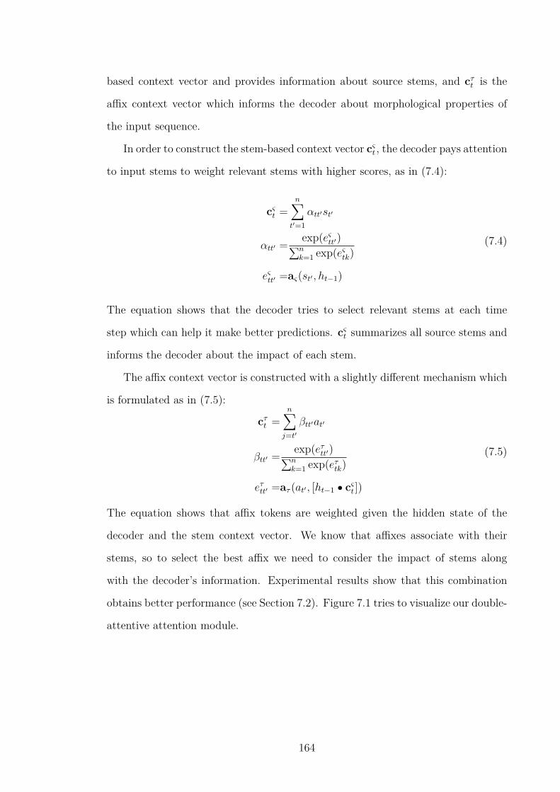
based context vector and provides information about source stems, and cτt is the

affix context vector which informs the decoder about morphological properties of

the input sequence.

In order to construct the stem-based context vector cςt , the decoder pays attention

to input stems to weight relevant stems with higher scores, as in (7.4):

cςt =

nÿ

t1=1

αtt1st1

αtt1 =exp(eςtt1)

řnk=1 exp(eςtk)

eςtt1 =aς(st1 , ht´1)

(7.4)

The equation shows that the decoder tries to select relevant stems at each time

step which can help it make better predictions. cςt summarizes all source stems and

informs the decoder about the impact of each stem.

The affix context vector is constructed with a slightly different mechanism which

is formulated as in (7.5):

cτt =

nÿ

j=t1

βtt1at1

βtt1 =exp(eτtt1)

řnk=1 exp(eτtk)

eτtt1 =aτ (at1 , [ht´1 ‚ cςt ])

(7.5)

The equation shows that affix tokens are weighted given the hidden state of the

decoder and the stem context vector. We know that affixes associate with their

stems, so to select the best affix we need to consider the impact of stems along

with the decoder’s information. Experimental results show that this combination

obtains better performance (see Section 7.2). Figure 7.1 tries to visualize our double-

attentive attention module.

164

st+1 st

attention

h

h

h

h ht-1 ht

st+1 st

attentions

h

h

h

h ht-1 ht

at+1 at

h

h

attentiona

ct

𝑐𝑡𝑠

𝑐𝑡𝑎

(a) This figure shows the original attention mechanism where the source side encoderconsumes one word at each time step and updates its hidden state st. The decoderconstructs the context vector ct based on the decoder’s previous hidden state and allsource-side hidden states. The context vector is used along with the (current) hiddenstate ht to generate the output.

st+1 st

attention

h

h

h

h ht-1 ht

st+1 st

attentions

h

h

h

h ht-1 ht

at+1 at

h

h

attentiona

ct

𝑐𝑡𝑠

𝑐𝑡𝑎

(b) This figure shows the double-source encoder, where the stem RNN takes one stem ateach time step and updates st, and the affix RNN updates at after consuming the t-thaffix token. The stem-based context vector is generated by attentionς . The affix-basedcontext vector is constructed using information provided by all of the affix-RNN’s hiddenstates, the decoder’s previous hidden state and the stem context vector.

Figure 7.1: A comparison between the simple and double-attentive attention mod-els. It should be noted that the figure only shows connections associated with theattention module.

7.2 Experimental Study

Our NMT model is a GRU-based encoder-decoder model. On the encoder side we

have two RNNs, one for stems and the other for affix tokens. Both RNNs include

two GRU layers where the first layer is a bidirectional layer and the second layer is

a unidirectional layer. Stems and affix tokens are represented with 512-dimensional

embeddings. The encoder is connected to the decoder through the affine connec-

tion described in Equation (7.2). On the decoder side, we have the double-attentive

attention module and two GRU layers. The GRU size for both of the encoder

and decoder is 1024. Since experimental studies demonstrated that character-based

165

decoding yields better translations, our decoder works at the character level. More-

over, as the main goal in this chapter is to show the impact of our proposed encoder,

we prefer to keep the target side constant for all models and compare the impact of

different encoding techniques. However, we also provide a few examples from mod-

els with different decoding techniques. Similar to input tokens, target tokens are

also represented with 512-dimensional embeddings. The network was trained using

stochastic gradient descent with Adam (Kingma and Ba, 2015). The mini-batch size

is 80, the beam search width is 20, and the norm of the gradient is clipped with the

threshold 1.0.

Our models are trained to translate from German and Russian into English. We

used the WMT-15 datasets, where the German–English corpus includes 4.5M parallel

sentences and the size of the Russian–English corpus is 2.1M. The newstest-2013

and newstest-2015 datasets are used as the development and test sets, respectively.

We selected these datasets to make our work comparable with existing models. As

we are interested in translating from MRLs, we pre-process the training corpora to

segment words and extract stems and affixes. Table 7.1 provides related statistics

for our training copora.

English–German English–RussianEn De En Ru

Sentence 4.2M 2.1MToken 103, 692, 553 96, 235, 845 43, 944, 989 39, 694, 475Type 103, 574 143, 329 70, 376 119, 258Stem 21, 223 26, 301 15, 964 19, 557Affix 13, 410 24, 054 9, 320 17, 542Prefix 3, 104 5, 208 2, 959 3, 324Suffix 3, 285 4, 974 2, 219 3, 460char 355 302 360 323dp 19,777 54,370 13,569 45,357

Table 7.1: En, De and Ru stand for English, German and Russian, respectively.Sentence is the number of parallel sentences in the corpus. Token is the number ofwords. Type shows the number of unique words. Stem, Prefix, Suffix and Affix showthe number of unique stems, prefixes, suffixes and affix tokens in the corpus. charshows the number of unique letters. dp shows the number of tokens generated byModel D (Section 4.3.4).

166

The table shows different statistics about the training corpora along with the

number of affixes for each corpus. We segment input words with Morfessor. The

longest subunit is selected as the stem. What appears before the stem is the prefix

and what follows the stem is considered as the suffix. A word may have none (null),

one or many prefixes and suffixes, by which their combination construct the affix

token in our implementation.

It is clear what the stem RNN takes as its input at each time step. The encoder

has an embedding table for stems. Each row of the table is a unique vector represent-

ing a particular stem. The encoder processes the main sequence (stem sequence),

retrieves the related embedding for each stem and sends that to the stem RNN. We

can have the same mechanism for prefixes and suffixes, which means the encoder

has separate suffix and prefix embedding tables. It retrieves associated prefix and

suffix embeddings for each word, combines them (vector summation) and sends the

combined vector to the affix RNN. This architecture is referred to as the pre-suf

extension of the proposed model in our experiments. If a word has more than one

prefix/suffix the encoder retrieves all of them, and if it has none the encoder uses a

null embedding.

In the pre-suf extension, what the affix RNN receives as its input is a vec-

tor which has some information about morphological properties of the associated

stem (word). We believe that the encoder and affix RNN could be provided with

richer information, so we propose the affix extensions. In these extensions we

combine all prefixes and suffixes to generate the new affix token, e.g if wordi =

prefix1i +stemi+suffix1i +suffix2i , the affix token τi would be prefix1i +suffix1i +suffix2i .

The embedding of the new affix token is different from the summation of the em-

beddings of the prefix and suffix and introduces a new token. In the affix extensions,

apart from the stem-embedding table the encoder has a dedicated embedding table

for affix tokens. Therefore, the affix RNN at each time step takes an affix token

instead of the summation of prefixes and suffixes. Table 7.1 shows the number of

unique affix tokens for each corpus.

167

The embedding of the affix token defined for each word is a new unit which

preserves information about: i) morphological properties of its related word, ii)

morphological properties of other words appearing in the sentence, and iii) the

collocation and order of different prefixes and suffixes, at the word and sentence

level. It seems that the simple combination of prefix and suffix embeddings in the

pre-suf extension cannot preserve this amount of information, as the role of each

suffix/prefix is clear, but in this extension, we can expect the neural network to

learn such useful information through the training phase (and store it in the affix-

embedding table).

Model Source Target DeÑEn RuÑEnBaseline ς+pre+suf char 22.11 22.79

Costa-jussà and Fonollosa (2016) word word 18.83 -char word 21.40 -

Firat et al. (2016a) bp bp 24.00 22.40

Lee et al. (2016) bp char 25.27 22.83*char char 25.83* 22.73

Our modeldp-model dp dp 27.13 23.07dp-model dp char 26.79 22.81pre-suf [ς]1 [pre+suf]2 char 26.11 22.95affix-cςcτ [ς]1 [τ ]2 char 26.74 23.44affix-cτ [ς]1 [τ ]2 char 26.29 23.40

Table 7.2: Source and Target indicate the data type for the encoder and decoder,respectively. ς is the stem, pre is the prefix and suf is the suffix. τ is the affix token.bp, dp, and char show the Byte-pair, dynamic programming-based, and character-level encodings, respectively. The bold-faced score is the best score for the directionand the score with * shows the best performance reported by other existing models.According to paired bootstrap re-sampling (Koehn, 2004b) with p = 0.05, the bold-faced number is significantly better than the score with *. Brackets show differentchannels and the + mark indicates the summation, e.g. [ς]1 [pre+suf]2 means thefirst channel takes a stem at each step and the second channel takes the summationof the prefix and suffix of the associated stem.

Results obtained from our experiments are reported in Table 7.2. The first row of

the table reports results from an encoder-decoder model where the decoder works at

the character level and uses the architecture proposed by Chung et al. (2016). The

first row can be considered as a baseline for all other models reported in the table, as

168

it does not use any complicated neural architecture. For each word it simply sums

stem, prefix, and suffix embeddings together and sends the summed vector as the

word representation to the GRU-based encoder. Although the model is quite simple,

it is able to generate comparable results to other complex architectures. This fact

reinforces our claim that existing neural architectures are not suitable to work at

the subword level. If we find a better way to provide the neural model with subword

information, we will be able to improve translation quality still further.

The second row shows the model proposed by Costa-jussà and Fonollosa (2016)

in which a complicated convolutional module is used to model the relation between

characters and build the word-level representation. The simple baseline model per-

forms better than this model. The third row belongs to Firat et al. (2016a) which is

a multi-way multilingual NMT model. The fourth row shows a fully character-level

model (Lee et al., 2016) where both the encoder and decoder work at the character

level. As previously discussed this model has quite a complicated architecture.

The last block shows 5 variations of our model. dp-model is an encoder-decoder

NMT engine with single source channel. Both the source and target sides for this

model are segmented using our dynamic programming-based model (Model D). This

model is also reported with another setting where the encoder consumes dp tokens

and the decoder samples a character at each time step.

In the pre-suf model the encoder has two GRU RNNs, one for stems and the

other for prefixes and suffixes. At each time step, the stem RNN takes one stem

embedding. On the other channel the affix RNN takes an embedding which is the

summation of the prefix and suffix embeddings of the word whose stem is processed

by the stem RNN at the same time step.

The pre-suf model has two input channels and benefits from the double-attentive

attention mechanism. This new architecture enables the pre-suf model to perform

better than the very complicated fully character-based model. This is an indica-

tion that the character-level representation does not necessarily provide the best

representation, and our model is able to perform better as its architecture is more

169

compatible with the nature of MRLs. The impact of the compatible neural archi-

tecture becomes more important when we compare the baseline and pre-suf models.

The input format is exactly the same for both, but the baseline model simply sums

stem, prefix and suffix embeddings and sends them to the original encoder, whereas

our model has two different channels to process stem and prefix/suffix information.

It shows that our proposed architecture is able to process morphological information

better than the baseline model.

The affix-cςcτ variation is the best model among our double-channel models,

where we have stem tokens and affix tokens. As previously discussed, assigning a

unique embedding to the combination of prefixes and suffixes instead of summing

their embeddings generates better results and provides richer information.

The third and last variation, affix-cτ , shows the impact of our architecture on

the decoder side. As we modeled in Equation (7.5), attention weights assigned to

the affix-RNN’s hidden states are computed based on the decoder’s hidden state

and the stem context vector. As affix tokens provide complementary information

to stem information, the affix context vector should be aware of the content of the

stem context vector, so we proposed the model explained in Equation (7.5). If we

only consider the decoder’s information to compute affix weights, the equation will

be revised as in (7.6):

cτt =

nÿ

j=t1

βtt1at1

βtt1 =exp(eτtt1)

řnk=1 exp(eτtk)

eτtt1 =aτ (at1 , ht´1)

(7.6)

In the affix-cςcτ version, the energy between the decoder’s (t-1)-th state and the

affix-RNN’s t1-th state was computed by eτtt1 = aτ (at1 , [ht´1‚cςt ]), whereas this version

simplifies the computation by estimating eτtt1 with aτ (at1 , ht´1). The model described

in Equation (7.6) is implemented in the affix-cτ extension. Results obtained from

this extension show that, although the architecture is also successful compared to

other exiting models, its performance is worse than the model which (additionally)

170

involves the stem context vector to compute affix weights.

For GermanÑEnglish, the best BLEU score is obtained when our model has a

single encoder channel and works with dp units. However, this does not mean that

the double-source encoder is not effective; rather, that these two models study the

same problem from different perspectives. One model tries to handle morphological

complexity by segmenting complex structure into basic units, and the other approach

adapts the neural architecture to benefit from morphological information. Although

having a good segmentation model could be quite useful, it is not enough alone

to address all problems. Results from the RussianÑEnglish supports this claim.

For this direction the character-based (Costa-jussà and Fonollosa, 2016; Lee et al.,

2016) or subword-based (dp-model, Baseline, and Firat et al. (2016a)) models should

perform well, as they all benefit from segmentation techniques which can reduce the

complexity of Russian, but the best score remained with double-channel model. In

addition to the Russian experiment, we also have results when we translate from

Turkish. We observed similar properties for this language too. Table 7.3 summarizes

results from the Turkish experiment.

Model Source Target BLEUBaseline ς+pre+suf char 22.98char-model bp char 23.11char-model dp char 23.27dp-model bp bp 23.17dp-model dp dp 23.46affix-cςcτ [ς]1 [τ ]2 char 23.81

Table 7.3: Experimental results for TurkishÑEnglish. char, bp, and dp show thecharacter, Model D, and Byte-pair tokens. ς, pre, and suf are the stem, prefix, andsuffix, respectively.

Our Turkish models are trained using the same dataset as in Section 6.3.1, and

the number of bp and dp are the same. In Table 7.3 the baseline model uses a

character-based decoder. It linearly sums the stem, prefix, and suffix embeddings

for each word to build its surface-form embedding on the encoder side, which could

be a good alternative when translating from MRLs. char-model has the same neural

171

architecture as the baseline, but it consumes bp or and dp tokens. Each token

is treated as a single independent unit, which means subunit tokens of a word

are not summed to build the surface-form representation. dp-model is our model

from Chapter 6. The last row in the table is our best double-encoder model which

obtained the best BLEU score. Similar to the Russian experiment, for this language

the morpheme-segmentation model is also unable to help the neural architecture

achieve the best BLEU score, while Turkish is a highly agglutinative language and

the segmentation-based solution should have worked perfectly for it.

According to the Russian and Turkish experiments, we can conclude that the best

performance is achieved when the neural architecture is able to (better) understand

the nature of its inputs and outputs, which means that we may have to redesign the

neural architecture accordingly. Although morpheme segmentation is quite useful

for NMT, it is not the best solution to cope with difficulties of translating (from)

MRLs.

7.3 Conclusion

In this chapter we focused on morphological complexities on the source side and tried

to equip the encoder to handle complex inputs. The proposed model includes two

separate channels to consume stems and affix tokens. In our experiments, we showed

that this double-input encoder seems to be a suitable architecture when translating

from MRLs. Since the encoder has two input channels it generates two source-

side representations. Accordingly, the decoder had to be fine-tuned to handle the

extra representation vector. To this end, we designed a double-attentive attention

mechanism to control the information flow in both channels. Our model generates

better results and seems able to better inform the neural model with morphological

information, compared to other existing models.

172

Chapter 8

Conclusions and Future Study

The research conducted in this thesis addresses the problem of morphology in the

context of MT. Statistical and neural approaches to MT suffer from serious short-

comings, which almost all explicitly or implicitly involve morphology. OOVs are

commonly encountered in translating morphologically rich languages. Moreover,

according to recent research (Bentivogli et al., 2016; Tu et al., 2016; Toral and

Sánchez-Cartagena, 2017), a considerable amount of wrong translations belong to

the categories of ‘missing words’ and ‘wrong surface forms’, which can be related

to the problem of morphology. Clearly, the second one is a direct consequence of

the problem of morphology. The first one is also related as MT models do not de-

compose MCWs during translation, which leads to wrong results. Since an MCW

preserves more information and subunits than a simple non-MCW, all subunits are

not completely translated and some target words are missed in the target translation.

In order to address these problems, we decided to study the problem of morphol-

ogy and its impact on MT models. First we explained what morphology is and how

it helps us construct new words. Chapter 2 covers introductory and fundamental

concepts. We reviewed several important models in the field of SMT, which in some

way incorporate morphological information into the translation pipeline. Models are

divided into three main categories. One approach does not change the translation

architecture but preprocesses the training corpora, decomposing morphologically

173

complex structures into simpler and atomic units. For this approach, it should be

discussed that what happens if there is no (precise) morphological analyzer for a

language.

The other approach manipulates the decoding procedure by directly exploring

morphological criteria. The decoder is extended with additional morphological in-

formation and the word selection is controlled by such constrains.

The last approach tries to make a morphological symmetry between the complex

and simple(er) sides. First, words are lemmatized and then translation is performed

based on simplified units. Finally, translations generated by such a model are pro-

cessed through an additional step, in which classifiers are used to gather contextual

information in order to detect the correct surface form of each word. Classifiers

essentially take the simplified form of a word and generate the correct inflected or

morphologically complex form.

Along with SMT-related topics, one important part of Chapter 2 relates to

DNNs. In this thesis the main platform to perform MT is NNs. We reviewed

the fundamentals of deep learning. The procedure for training a neural network was

explained and we introduced a number of well-known neural architectures. Both

Chapter 1 and Chapter 2 provide background knowledge about the research carried

out in the thesis, but the core research is explained in Chapters 3 to 6. Each chap-

ter studies a dedicated research question which is introduced at the beginning of

the chapter. The history of the research question and related models are discussed

thereafter. The last part of each chapter covers the problem itself and a potential

solution.

Chapter 3 introduces an embedding-learning model for MCWs. In order to trans-

late languages via NNs, we should be able to encode characters, words, and other

constituents into numerical forms. In this regard, the best solution is to use doc-

ument embeddings, but existing embeddings such as those of Word2Vec or GloVe

are not compatible with our datasets. Since our corpora include MCWs, such word-

based models fail to provide representative embeddings, as they are not able to go

174

deeper and extract intra-word relations. They function based on the surface form of

words, which is clearly not the ideal choice for our setting. In order to mitigate this

shortcoming we propose a new CNN-based model, which includes a multi-channel

data structure as its input. Each channel consists of a specific type of information

representing a particular aspect of the word. In experiments designed in Chapter

3, the input includes three channels of prefix, stem, and suffix, which means we try

to train embeddings for subword units. The cubic data structure preserves infor-

mation about words and subunits, as well as information about context words and

their subunits. Feeding a network with this amount of information helps the model

provide better connections among words and train better embeddings.

We designed a specific 3D convolution function to process the proposed data

structure. Our model is not the first embedding-learning network which benefits

from subword-level information, but because of i) the way we represent words and ii)

the convolution technique, we are able to better benefit from subword information.

In Chapter 3 we evaluated the impact of different techniques to combine subunit

vectors. The experiment confirmed that the 3D technique outperforms other models.

The only concern about the model is that it has a complex architecture, so that when

it is plugged into a high(er)-level model such as an NLM or NMT engine, it could

make the whole pipeline complex and delay the entire procedure. Neural models

by their very nature are already complex enough, so we do not want to make them

more complicated. Accordingly, in future work we plan to find a better way to

combine this technique with other models. Except for this shortcoming, we believe

that the model provides a very efficient framework, not only for word-embedding

tasks but also for other NLP tasks, e.g. the flexibility provided by the proposed

cubic data structure enabled us to use the same NN for our MT purposes. Instead

of representing subunits in the cube, we stored translationally equivalent words in

different channels and trained bilingual embeddings (Passban et al., 2016b).

Chapter 4 looks beyond word-level modeling. Word embeddings are generated by

the technique proposed in Chapter 3, but we need more than word-level information.

175

In this chapter we study the language-modeling problem to work at the sequence

level. Simply put, the main responsibility of a language model is to predict the best

word given a history of its preceding words, which is a quite challenging task. There

could be different alternatives for a given history and the model should select the

best one based on the context. The problem becomes even harder in the presence of

morphologically complex structures. If we decompose an MCW, we might be able

to obtain a more informative history. Accordingly, state-of-the-art models work at

both morpheme and character levels. First, subunit information is combined to

provide the word-level representation, then words are consumed one after another

to make the final history. Although morpheme-based models outperform word-

level models which the reason is clear, they cannot compete with character-based

counterparts. We believe that there are two main reasons for this: i) almost all

character-level models are quite complex and utilize powerful neural modules such

as CNNs with hundreds of filters, highway layers etc. Therefore, it is not very clear

whether the main gain comes from the network architecture, or the representation

form; and ii) morpheme-level models combine subword-level information with a

simple linear summation or concatenation function. This type of combination may

not be powerful enough to reveal the relations between morphemes. As we showed

in Chapter 3, an efficient combination technique can yield quite different results.

It does not (intuitively) seem appropriate to consider a single character as the

atomic unit of a language, as characters can appear in every word regardless of its

syntactic and semantic role. They give no information about the word to which

they belong, but morphemes can easily provide such information. Accordingly, we

think that there should be a middle-ground solution which takes advantages of both

approaches. One solution is to manipulate morpheme-based models with a better

combination technique, e.g. replacing a simple summation function with our 3D

convolution function, which we leave for future work. The other solution which

was proposed in Chapter 4 is to push character-level models toward morpheme-level

models. Words should not be completely decomposed into characters. Existing

176

models separate all characters, and then combine them via a convolutional process

to make a connection among them. We follow the same approach but not via neural

computations. Before training an NLM, we make a hybrid segmentation of words

by use of our technique. If there is a set of consecutive characters that frequently

appear together, they may try to build up a bigger block and we think that they

should stay together. Accordingly, we extract frequent character n-grams within

words, keep them as they are, and separate the remainder into characters. Using

this technique, we are able to better model languages. At the end of the segmentation

procedure we have a set of atomic symbols which include characters and n-grams.

The segmentation models in Chapter 4 enable us to achieve better performance,

but clearly they are sub-optimal as they rely on a threshold (or other external

parameters) to extract frequent blocks. Finding an optimal value for the threshold

is crucial for our models. For these versions of our models we compare different

settings in our experiments and empirically set the threshold value. Motivated by

these problems we also proposed another model which has no external parameter.

Both paradigms have their own advantages and disadvantages, which we summarized

in Chapter 4. In our future work we are interested in finding a model which benefits

from the advantages of both approaches (tunable level of granularity with no external

parameter). The second plan for future work is to use our NLM in SMT/NMT

models. We evaluated the impact of incorporating NLM signals in the SMT pipeline

and improved the translation engine, but we re-scored probabilities of the n-gram-

based LM with our neural model. This is not the best way to use the NLM, so in

future work we will try to find a solution to incorporate neural scores at decoding

time.

Chapter 5 is complementary to the preceding, which trains word and sentence

embeddings. All these neural features can be used in the SMT pipeline to boost

translation engines. In Chapter 5, first we proposed a framework to train bilin-

gual embeddings; MT is a bilingual setting so we need more than monolingual

embeddings. The proposed architecture is a feed-forward neural model which is an

177

extension to Devlin et al. (2014) and Le and Mikolov (2014). By means of such

a model we train bilingual word-level, phrase-level and sentence-level embeddings,

and define different feature functions to show the relatedness of bilingual words and

phrases to one another. We also try to capture contextual information. Incorporat-

ing such neural features results in better BLEU scores, but we support our results

with qualitative evaluations through different experiments. This chapter also shows

that there could be better architectures than a feed-forward model. The architecture

is substituted with a convolutional counterpart which gives even better results. One

of the important achievements of the chapter is that we do not necessarily need to

train bilingual embeddings in order to boost SMT models, as we introduced a way

to benefit from monolingual embeddings to enrich the decoder.

Chapter 6 tries to propose neural models to translate MRLs. It complements

Chapter 4, as similar to that chapter we perform sequence modeling, but the main

difference is that the models in this chapter are designed for multilingual settings.

It is hard to train a deep neural model to work with millions of parallel sentences,

so models have to be efficient, effective, and fast enough. We also show the impact

of morphological information, despite the fact that this makes the problem even

harder. In this chapter we explained the established NMT framework, namely the

encoder-decoder model. Then we fine-tuned the model to work for MRLs. In our

models, we studied the impact of different segmentation schemes and recognized the

best setting for working with MRLs. Our dynamic programming-based segmentation

model performed very well for our NMT engines and obtained the best result.

In Chapter 7, we proposed a model to translate from MRLs. In this model the

neural model takes two input tokens at each time step. One input represents the

stem and the other one represents morphological information of the word to which

the stem belongs. The main idea behind this separative design is to reduce the com-

plexity on the source side. Since the encoder generates two different representations

at each step, the decoder should be customized accordingly. The original decoder

takes one input, whereas ours has two inputs. The decoder also has two attention

178

modules to select the most relevant information from both channels. This model

was proposed for translating from MRLs. Experimental results demonstrate that

compared to other existing models ours has a more compatible architecture with the

complex nature of MRLs.

In Chapters 6 and 7, we proposed different models to study NMT of MRLs from

different perspectives and addressed different shortcomings in the field. There are

different languages in terms of the morphological categorization which we provided

in Chapter 2 (see Figure 2.3). We are interested in fusional and agglutinative types

of languages in this thesis. In fusional languages morphemes are combined in a very

complex way and there is no clear boundary between them. Moreover, the surface

form of morphemes can be changed after the combination. Accordingly, preprocess-

ing MCWs and analysing them from a morphological point of view might not be

the best solution if we want to provide high-quality translations for such structures.

Instead, we should find neural models which are able to take MCWs and handle their

complexity themselves. Considering all word-, morpheme-, and character-level NMT

models, it seems that character-based models could be better alternatives compared

to others. The convolutional transformation applied to characters in character-based

models can partially simulate the word formation procedure in fusional languages.

We are not able to exactly model the process but we can expect the neural model

to learn it automatically. The multi-filter convolutional process is the only existing

model to deal with this sort of complexity in fusional languages, but it could be

boosted or even replaced with other techniques which is one of our future plans.

In contrast to fusional languages, there are agglutinative types in which mor-

phemes are clearly separable from each other. For this key reason we can easily

rely on morpheme segmentation and morpheme-based neural models for this set

of languages, so in our research we evaluated our segmentation model (Model D)

on preprocessing the training corpus and obtained significant improvements. We

also proposed the double-channel encoding model to work at the morpheme level. It

seems that we do not necessarily require complex character-based models for aggluti-

179

native languages and simple techniques for manipulating and processing morphemes

can lead to better results.

We believe that Chapters 6 and 7 provided useful information on NMT of MRLs

and studied the problem from different perspectives. There is still room for further

investigation which we leave for future work. For our future work in the field of

NMT, we target four main goals: i) we are interested in designing a model which is

able to translate from an MRL into another MRL. When both source and target sides

are complex, a simple encoder-decoder model will fail to provide fluent translations,

so we will try to find architectures to control complexities of both sides; ii) we are

planning to work on the decoding side and constrain the decoder with morphological

information, as we think it can boost the quality when we translate into MRLs; iii)

we plan to apply the sequence-to-sequence model used for MT tasks in Chapters 6

and 7 to other NLP tasks such as parsing, POS tagging, morphological segmentation

etc; finally iv) we tend to train neural models for low-resource languages. We

know that deep-learning-based models are data-hungry models and need a massive

amount of resources to provide acceptable results. Our plan is to train small and

efficient neural models with affordable resources and datasets. We already started

this research path by developing a model for translating Azeri (Passban et al., 2017),

and plan to further expand our models.

In Chapter 8 we tried to summarize all other chapters. We explained the core

idea of each chapter and discussed what questions the chapter tried to solve. We

reviewed the proposed solutions and enumerated their shortcomings (and also their

advantages). For each chapter we mentioned that what questions were solved and

what questions remained unanswered. We addressed some complimentary ideas for

our future work. In this thesis, we believe that we could contribute to our field as

we collected data and provided a bilingual corpus, and designed and implemented

different NLP tools such as a morphological analyzer and POS tagger. Our solutions

introduced new models for embedding learning, language modeling, and machine

translation. We also enhanced the NMT framework to work better for MRLs.

180

Bibliography

AleAhmad, A., Amiri, H., Darrudi, E., Rahgozar, M., and Oroumchian, F. (2009).Hamshahri: A standard Persian text collection. Knowledge-Based Systems,22(5):382–387.

Alexandrescu, A. and Kirchhoff, K. (2006). Factored neural language models. InProceedings of the Human Language Technology Conference of the NAACL, Com-panion Volume: Short Papers, pages 1–4, New York, USA.

Alkhouli, T., Guta, A., and Ney, H. (2014). Vector space models for phrase-basedmachine translation. In Proceedings of SSST-8, Eighth Workshop on Syntax,Semantics and Structure in Statistical Translation, pages 1–10, Doha, Qatar.

Arel, I., Rose, D. C., and Karnowski, T. P. (2010). Deep machine learning: anew frontier in artificial intelligence research. IEEE Computational IntelligenceMagazine, 5(4):13–18.

Auli, M., Galley, M., Quirk, C., and Zweig, G. (2013). Joint language and translationmodeling with recurrent neural networks. In Proceedings of the 2013 Conferenceon Empirical Methods in Natural Language Processing, pages 1044–1054, Seattle,Washington, USA.

Avramidis, E. and Koehn, P. (2008). Enriching morphologically poor languages forstatistical machine translation. In the 46th Annual Meeting of the Association forComputational Linguistics, pages 763–770, Columbus, Ohio, USA.

Bahdanau, D., Cho, K., and Bengio, Y. (2014). Neural machine translation by jointlylearning to align and translate. In Proceedings of the International Conference onLearning Representations, Banff, Canada.

Bane, M. (2008). Quantifying and measuring morphological complexity. In Pro-ceedings of the 26th west coast conference on formal linguistics, pages 69–76,University of California, Berkeley, USA.

181

Baroni, M., Bernardini, S., Ferraresi, A., and Zanchetta, E. (2009). The wackywide web: a collection of very large linguistically processed web-crawled corpora.Language resources and evaluation, 43(3):209–226.

Bebis, G. and Georgiopoulos, M. (1994). Feed-forward neural networks. IEEEPotentials, 13(4):27–31.

Beesley, K. R. (1998). Arabic morphology using only finite-state operations. InProceedings of the Workshop on Computational Approaches to Semitic languages,pages 50–57, Montreal, Canada.

Bengio, Y. (2009). Learning deep architectures for ai. Foundations and trends® inMachine Learning, 2(1):1–127.

Bengio, Y., Courville, A., and Vincent, P. (2013). Representation learning: Areview and new perspectives. IEEE transactions on pattern analysis and machineintelligence, 35(8):1798–1828.

Bengio, Y., Ducharme, R., Vincent, P., and Jauvin, C. (2003). A neural probabilisticlanguage model. Journal of machine learning research, 3:1137–1155.

Bentivogli, L., Bisazza, A., Cettolo, M., and Federico, M. (2016). Neural versusphrase-based machine translation quality: a case study. In Proceedings of the2016 Conference on Empirical Methods in Natural Language Processing, pages257–267, Austin, Texas.

Bilmes, J. A. and Kirchhoff, K. (2003). Factored language models and generalizedparallel backoff. In Proceedings of the 2003 Conference of the North AmericanChapter of the Association for Computational Linguistics on Human LanguageTechnology: companion volume of the Proceedings of HLT-NAACL 2003–shortpapers-Volume 2, pages 4–6, Edmonton, Canada.

Bisazza, A. and Monz, C. (2014). Class-based language modeling for translating intomorphologically rich languages. In Proceedings of the 25th Annual Conference onComputational Linguistics (COLING), pages 1918–1927, Dublin, Ireland.

Blei, D. M., Ng, A. Y., and Jordan, M. I. (2003). Latent dirichlet allocation. Journalof machine learning research, 3:993–1022.

Botha, J. A. and Blunsom, P. (2014). Compositional morphology for word represen-tations and language modelling. In The 3st International Conference on MachineLearning (ICML), pages 1899–1907, Beijing, China.

182

Bottou, L. (2010). Large-scale machine learning with stochastic gradient descent.In Proceedings of 19th International Conference on Computational Statistics(COMPSTAT’2010), pages 177–186, Paris France.

Brown, P. F., Della Pietra, V. J., Della Pietra, S. A., and Mercer, R. L. (1993). Themathematics of statistical machine translation: parameter estimation. Computa-tional Linguistics, 19(2):263–311.

Brown, P. F., deSouza, P. V., Mercer, R. L., Della Pietra, V. J., and Lai, J. C.(1992). Class-based n-gram models of natural language. Computationl Linguistics,18(4):467–479.

Cap, F., Fraser, A. M., Weller, M., and Cahill, A. (2014). How to produce unseenteddy bears: Improved morphological processing of compounds in SMT. In Pro-ceedings of the 14th Conference of the European Chapter of the Association forComputational Linguistics (EACL), pages 579–587, Gothenburg, Sweden.

Chahuneau, V., Schlinger, E., Smith, N. A., and Dyer, C. (2013). Translatinginto morphologically rich languages with synthetic phrases. In Proceedings ofConference on Empirical Methods in Natural Language Processing (EMNLP),pages 677–1687, Melbourne, Australia.

Chelba, C., Mikolov, T., Schuster, M., Ge, Q., Brants, T., and Koehn, P. (2013). Onebillion word benchmark for measuring progress in statistical language modeling.CoRR, abs/1312.3005.

Chiang, D. (2007). Hierarchical phrase-based translation. Computational Linguis-tics, 33(2):201–228.

Chiang, D., Knight, K., and Wang, W. (2009). 11,001 new features for statisti-cal machine translation. In Proceedings of Human Language Technologies: The2009 Annual Conference of the North American Chapter of the Association forComputational Linguistics, pages 218–226, Boulder, Colorado.

Cho, K., van Merrienboer, B., Bahdanau, D., and Bengio, Y. (2014a). On theproperties of neural machine translation: Encoder-decoder approaches. CoRR,abs/1409.1259.

Cho, K., van Merrienboer, B., Gulcehre, C., Bahdanau, D., Bougares, F., Schwenk,H., and Bengio, Y. (2014b). Learning phrase representations using rnn encoder–decoder for statistical machine translation. In Proceedings of the 2014 Conferenceon Empirical Methods in Natural Language Processing (EMNLP), pages 1724–1734, Doha, Qatar.

183

Chung, J., Cho, K., and Bengio, Y. (2016). A character-level decoder withoutexplicit segmentation for neural machine translation. In Proceedings of the 54thAnnual Meeting of the Association for Computational Linguistics (Volume 1: LongPapers), pages 1693–1703, Berlin, Germany.

Clifton, A. and Sarkar, A. (2011). Combining morpheme-based machine transla-tion with post-processing morpheme prediction. In Proceedings of the 49th An-nual Meeting of the Association for Computational Linguistics: Human LanguageTechnologies-Volume 1, pages 32–42, Portland, Oregon, USA.

Collobert, R., Weston, J., Bottou, L., Karlen, M., Kavukcuoglu, K., and Kuksa, P.(2011). Natural language processing (almost) from scratch. Journal of MachineLearning Research, 12:2493–2537.

Costa-jussa, M., Gupta, P., Rosso, P., and Banchs, R. (2014). English-to-Hindisystem description for wmt 2014: Deep sourcecontext features for moses. InProceedings of the Ninth Workshop on Statistical Machine Translation, pages 79–83, Baltimore, Maryland, USA.

Costa-jussà, M. R. and Fonollosa, J. A. R. (2016). Character-based neural ma-chine translation. In Proceedings of the 54th Annual Meeting of the Associationfor Computational Linguistics (Volume 2: Short Papers), pages 357–361, Berlin,Germany.

Cotterell, R. and Schütze, H. (2015). Morphological word-embeddings. In Proceed-ings of the 2015 Conference of the North American Chapter of the Associationfor Computational Linguistics: Human Language Technologies, pages 1287–1292,Denver, Colorado.

Creutz, M. and Lagus, K. (2002). Unsupervised discovery of morphemes. In Proceed-ings of the ACL-02 workshop on Morphological and Phonological Learning-Volume6, pages 21–30, Philadephia, Pennsylvania, USA.

De Groot, C. (2008). Morphological complexity as a parameter of linguistic typology.John Benjamins Publishing Co.

Deerwester, S., Dumais, S. T., Furnas, G. W., Landauer, T. K., and Harshman, R.(1990). Indexing by latent semantic analysis. Journal of the American society forinformation science, 41(6):391.

Delahunty, G. P. and Garvey, J. J. (2010). The English language: from sound tosense. WAC Clearinghouse.

184

Dempster, A. P., Laird, N. M., and Rubin, D. B. (1977). Maximum likelihood fromincomplete data via the EM algorithm. Journal of the Royal Statistical Society.Series B (methodological), pages 1–38.

Devlin, J., Zbib, R., Huang, Z., Lamar, T., Schwartz, R. M., and Makhoul, J. (2014).Fast and robust neural network joint models for statistical machine translation.In The 52nd Annual Meeting of the Association for Computational Linguistics,pages 1370–1380, Baltimore, USA.

Dos Santos, C. N. and Zadrozny, B. (2014). Learning character-level representationsfor part-of-speech tagging. In Proceedings of the 31st International Conference onMachine Learning (ICML), pages 1818–1826, Beijing, China.

Duchi, J., Hazan, E., and Singer, Y. (2011). Adaptive subgradient methods for onlinelearning and stochastic optimization. Journal of Machine Learning Research,12:2121–2159.

Duh, K., Neubig, G., Sudoh, K., and Tsukada, H. (2013). Adaptation data selectionusing neural language models: Experiments in machine translation. In Proceed-ings of the 51st Annual Meeting of the Association for Computational Linguistics(Volume 2: Short Papers), pages 678–683, Sofia, Bulgaria.

Dyer, C. J. (2007). The noisier channel: translation from morphologically com-plex languages. In Proceedings of the Second Workshop on Statistical MachineTranslation, pages 207–211, Prague, Czech Republic.

El-Kahlout, I. D. and Oflazer, K. (2010). Exploiting morphology and local word re-ordering in English-to-Turkish phrase-based statistical machine translation. IEEETransactions on Audio, Speech, and Language Processing, 18(6):1313–1322.

El Kholy, A. and Habash, N. (2010). Techniques for Arabic morphological detok-enization and orthographic denormalization. In Proceedings of the Workshop onLanguage Resources and Human Language Technology for Semitic Languages inthe Language Resources and Evaluation Conference (LREC), pages 45–51, Val-letta, Malta.

El Kholy, A. and Habash, N. (2012). Translate, predict or generate: Modeling richmorphology in statistical machine translation. In Proceedings of the 16th AnnualConference of the European Association for Machine Translation (EAMT), pages27–34, Trento, Italy.

Eyigöz, E., Gildea, D., and Oflazer, K. (2013). Simultaneous word-morpheme align-ment for statistical machine translation. In Proceedings of the 2013 Conference

185

of the North American Chapter of the Association for Computational Linguistics,pages 32–40, Atlanta, Georgia.

Finkelstein, L., Gabrilovich, E., Matias, Y., Rivlin, E., Solan, Z., Wolfman, G.,and Ruppin, E. (2001). Placing search in context: The concept revisited. InProceedings of the 10th international conference on World Wide Web, pages 406–414, Hong Kong,.

Firat, O., Cho, K., and Bengio, Y. (2016a). Multi-way, multilingual neural ma-chine translation with a shared attention mechanism. In Proceedings of the 2016Conference of the North American Chapter of the Association for ComputationalLinguistics: Human Language Technologies, pages 866–875, San Diego, California.

Firat, O., Sankaran, B., Al-Onaizan, Y., Yarman Vural, F. T., and Cho, K. (2016b).Zero-resource translation with multi-lingual neural machine translation. In Pro-ceedings of the 2016 Conference on Empirical Methods in Natural Language Pro-cessing, pages 268–277, Austin, Texas.

Fishel, M. and Kirik, H. (2010). Linguistically motivated unsupervised segmentationfor machine translation. In Chair), N. C. C., Choukri, K., Maegaard, B., Mari-ani, J., Odijk, J., Piperidis, S., Rosner, M., and Tapias, D., editors, Proceedingsof the Seventh conference on International Language Resources and Evaluation(LREC’10), Valletta, Malta. European Language Resources Association (ELRA).

Forcada, M. L. and Ñeco, R. P. (1997). Recursive hetero-associative memories fortranslation. In Proceedings of the International Work-Conference on ArtificialNeural Networks, pages 453–462, Lanzarote, Canary Islands, Spain. Springer.

Fraser, A. (2009). Experiments in morphosyntactic processing for translating toand from German. In Proceedings of the Fourth Workshop on Statistical MachineTranslation, pages 115–119, Athens, Greece.

Fraser, A., Weller, M., Cahill, A., and Cap, F. (2012). Modeling inflection and word-formation in SMT. In Proceedings of the 13th Conference of the European Chapterof the Association for Computational Linguistics, pages 664–674, Avignon, France.

Fritzinger, F. and Fraser, A. (2010). How to avoid burning ducks: Combininglinguistic analysis and corpus statistics for German compound processing. InProceedings of the Joint Fifth Workshop on Statistical Machine Translation andMetricsMATR, pages 224–234, Uppsala, Sweden.

Gao, J., He, X., Yih, W., and Deng, L. (2013). Learning semantic representationsfor the phrase translation model. CoRR, abs/1312.0482.

186

Goldberg, Y. and Levy, O. (2014). Word2Vec explained: deriving Mikolov et al.’snegative-sampling word-embedding method. CoRR, abs/1402.3722.

Goldwater, S. and McClosky, D. (2005). Improving statistical mt through morpho-logical analysis. In Proceedings of the Conference on Human Language Technologyand Empirical Methods in Natural Language Processing, pages 676–683, Vancou-ver, Canada.

Goodfellow, I., Bengio, Y., and Courville, A. (2016). Deep Learning. MIT Press.http://www.deeplearningbook.org.

Goodfellow, I. J., Warde-Farley, D., Mirza, M., Courville, A. C., and Bengio, Y.(2013). Maxout networks. In The 30th International Conference on MachineLearning (ICML), volume 28, pages 1319–1327, Atlanta, Georgia, USA.

Gülçehre, Ç., Firat, O., Xu, K., Cho, K., Barrault, L., Lin, H., Bougares, F.,Schwenk, H., and Bengio, Y. (2015). On using monolingual corpora in neuralmachine translation. CoRR, abs/1503.03535.

Habash, N. and Sadat, F. (2006). Arabic preprocessing schemes for statistical ma-chine translation. In Proceedings of the Human Language Technology Conferenceof the NAACL, Companion Volume: Short Papers, pages 49–52, New York, USA.

Hardmeier, C. (2014). Discourse in statistical machine translation. PhD thesis, ActaUniversitatis Upsaliensis, Uppsala, Sweden.

He, K., Zhang, X., Ren, S., and Sun, J. (2015). Delving deep into rectifiers: Sur-passing human-level performance on imagenet classification. In Proceedings of theIEEE International Conference on Computer Vision, pages 1026–1034, Santiago,Chile.

He, Z., Liu, Q., and Lin, S. (2008). Improving statistical machine translation usinglexicalized rule selection. In Proceedings of the 22nd International Conferenceon Computational Linguistics - Volume 1, COLING, pages 321–328, Manchester,United Kingdom.

Hinton, G. E. (1984). Distributed representations. Technical report, Carnegie MellonUniversity.

Hinton, G. E., Srivastava, N., Krizhevsky, A., Sutskever, I., and Salakhutdinov,R. (2012). Improving neural networks by preventing co-adaptation of featuredetectors. CoRR, abs/1207.0580.

187

Hochreiter, S. and Schmidhuber, J. (1997). Long short-term memory. Neural Com-putation, 9(8):1735–1780.

Hornik, K., Stinchcombe, M., and White, H. (1989). Multilayer feedforward net-works are universal approximators. Neural networks, 2(5):359–366.

Huang, E. H., Socher, R., Manning, C. D., and Ng, A. Y. (2012). Improving wordrepresentations via global context and multiple word prototypes. In Proceedings ofthe 50th Annual Meeting of the Association for Computational Linguistics: LongPapers-Volume 1, pages 873–882, Jeju, Republic of Korea.

Jean, S., Cho, K., Memisevic, R., and Bengio, Y. (2015). On using very largetarget vocabulary for neural machine translation. In Proceedings of the 53rdAnnual Meeting of the Association for Computational Linguistics and the 7thInternational Joint Conference on Natural Language Processing (Volume 1: LongPapers), pages 1–10, Beijing, China.

Johnson, M., Schuster, M., Le, Q. V., Krikun, M., Wu, Y., Chen, Z., Thorat,N., Viégas, F. B., Wattenberg, M., Corrado, G., Hughes, M., and Dean, J.(2016). Google’s multilingual neural machine translation system: Enabling zero-shot translation. CoRR, abs/1611.04558.

Józefowicz, R., Vinyals, O., Schuster, M., Shazeer, N., and Wu, Y. (2016). Exploringthe limits of language modeling. CoRR, abs/1602.02410.

Jurafsky, D. and Martin, J. (2009). Speech and Language Processing: An Intro-duction to Natural Language Processing, Computational Linguistics, and SpeechRecognition. Prentice Hall Series in Artifi. Pearson Prentice Hall.

Kalchbrenner, N. and Blunsom, P. (2013). Recurrent continuous translation models.In Proceedings of the 2013 Conference on Empirical Methods in Natural LanguageProcessing, pages 1700–1709, Seattle, Washington, USA.

Kalchbrenner, N., Grefenstette, E., and Blunsom, P. (2014). A convolutional neuralnetwork for modelling sentences. In Proceedings of the 52nd Annual Meeting ofthe Association for Computational Linguistics (Volume 1: Long Papers), pages655–665, Baltimore, Maryland.

Karlik, B. and Olgac, A. V. (2011). Performance analysis of various activation func-tions in generalized MLP architectures of neural networks. International Journalof Artificial Intelligence and Expert Systems, 1(4):111–122.

188

Kim, Y., Jernite, Y., Sontag, D., and Rush, A. M. (2016). Character-aware neurallanguage models. In Proceedings of the Thirtieth AAAI Conference on ArtificialIntelligence (AAAI-16), pages 2741–2749, Phoenix, Arizona, USA.

Kim, Y. and Rush, A. M. (2016). Sequence-level knowledge distillation. In Proceed-ings of the 2016 Conference on Empirical Methods in Natural Language Processing,pages 1317–1327, Austin, Texas.

Kingma, D. and Ba, J. (2015). Adam: A method for stochastic optimization. InInternational Conference on Learning Representations (ICLR), San Diego, USA.

Koehn, P. (2004a). Pharaoh: a beam search decoder for phrase-based statisticalmachine translation models. In Proceeding of the Conference of the Associationfor Machine Translation in the Americas, pages 115–124.

Koehn, P. (2004b). Statistical significance tests for machine translation evaluation.In Lin, D. and Wu, D., editors, Proceedings of EMNLP 2004, pages 388–395,Barcelona, Spain.

Koehn, P. (2005). Europarl: A parallel corpus for statistical machine translation. InProceedings of the 10th Machine Translation Summit (MT Summit X), volume 5,pages 79–86, Phuket, Thailand.

Koehn, P. (2009). Statistical machine translation. Cambridge University Press.

Koehn, P. and Hoang, H. (2007). Factored translation models. In Conference onEmpirical Methods in Natural Language Processing Conference on ComputationalNatural Language Learning (EMNLP-CoNLL), pages 868–876, Prague, Czech Re-public.

Koehn, P., Hoang, H., Birch, A., Callison-Burch, C., Federico, M., Bertoldi, N.,Cowan, B., Shen, W., Moran, C., Zens, R., Dyer, C., Bojar, O., Constantin, A.,and Herbst, E. (2007). Moses: Open source toolkit for statistical machine trans-lation. In Proceedings of the 45th Annual Meeting of the Association for Com-putational Linguistics Companion Volume Proceedings of the Demo and PosterSessions, pages 177–180, Prague, Czech Republic.

Koehn, P. and Knight, K. (2003). Empirical methods for compound splitting. InProceedings of the 10th Conference on European Chapter of the Association forComputational Linguistics (EACL), pages 187–193, Budapest, Hungary.

189

Koehn, P., Och, F. J., and Marcu, D. (2003). Statistical phrase-based translation.In Proceedings of the 2003 Conference of the North American Chapter of the As-sociation for Computational Linguistics on Human Language Technology-Volume1, pages 48–54, Edmonton, Canada.

Konstas, I., Iyer, S., Yatskar, M., Choi, Y., and Zettlemoyer, L. (2017). Neuralamr: Sequence-to-sequence models for parsing and generation. In Proceedingsof the 55th Annual Meeting of the Association for Computational Linguistics,Vancouver, Canada.

Krizhevsky, A., Sutskever, I., and Hinton, G. E. (2012). Imagenet classification withdeep convolutional neural networks. In Advances in neural information processingsystems, pages 1097–1105, California, USA.

Kuribayashi, Y. (2013). Transitivity in Turkish—a study of valence orientation—.Asian and African Languages and Linguistics, 7:39–52.

Lafferty, J., McCallum, A., and Pereira, F. (2001). Conditional random fields:Probabilistic models for segmenting and labeling sequence data. In Proceedingsof the eighteenth international conference on machine learning, ICML, volume 1,pages 282–289, New York, NY, USA.

Laokulrat, N., Phan, S., Nishida, N., Shu, R., Ehara, Y., Okazaki, N., Miyao,Y., and Nakayama, H. (2016). Generating video description using sequence-to-sequence model with temporal attention. In Proceedings of COLING 2016, the26th International Conference on Computational Linguistics, pages 44–52, Osaka,Japan.

Le, Q. V. and Mikolov, T. (2014). Distributed representations of sentences anddocuments. CoRR, abs/1405.4053.

LeCun, Y. A., Bottou, L., Orr, G. B., and Müller, K.-R. (2012). Efficient backprop-agation. In Neural networks: Tricks of the trade, pages 9–48. Springer. Berlin,Heidelberg.

Lee, J., Cho, K., and Hofmann, T. (2016). Fully character-level neural machinetranslation without explicit segmentation. CoRR, abs/1610.03017.

Lee, Y.-S. (2004). Morphological analysis for statistical machine translation. InProceedings of the Human Language Technology conference/North American chap-ter of the Association for Computational Linguistics, pages 57–60, Boston, Mas-sachusetts, USA.

190

Li, P., Liu, Y., Sun, M., Izuha, T., and Zhang, D. (2014). A neural reorderingmodel for phrase-based translation. In Proceedings of COLING 2014, the 25thInternational Conference on Computational Linguistics: Technical Papers, pages1897–1907, Dublin, Ireland.

Li, X., Zhang, J., and Zong, C. (2016). Neural name translation improves neuralmachine translation. CoRR, abs/1607.01856.

Li Deng, D. Y. (2014). Deep learning: Methods and applications. Technical report,Microsoft Research.

Lieber, R. (2015). Introducing Morphology. Cambridge University Press.

Ling, W., Trancoso, I., Dyer, C., and Black, A. W. (2015). Character-based neuralmachine translation. CoRR, abs/1511.04586.

Lison, P. and Tiedemann, J. (2016). Opensubtitles2016: Extracting large parallelcorpora from movie and tv subtitles. In Proceedings of the 10th International Con-ference on Language Resources and Evaluation, pages 923–929, Portorož, Slovenia.

Liu, Q., He, Z., Liu, Y., and Lin, S. (2008). Maximum entropy based rule selectionmodel for syntax-based statistical machine translation. In Proceedings of theConference on Empirical Methods in Natural Language Processing (EMNLP),pages 89–97, Honolulu, Hawaii.

Lopez, A. (2008). Statistical machine translation. ACM Computing Survey.,40(3):8:1–8:49.

Luong, M., Le, Q. V., Sutskever, I., Vinyals, O., and Kaiser, L. (2015a). Multi-tasksequence to sequence learning. CoRR, abs/1511.06114.

Luong, M.-T., Le, Q. V., Sutskever, I., Vinyals, O., and Kaiser, L. (2015b). Multi-task sequence to sequence learning. In Proceedings of the 4th International Con-ference on Learning Representations, San Juan, Puerto Rico.

Luong, M.-T. and Manning, C. D. (2016). Achieving open vocabulary neural ma-chine translation with hybrid word-character models. In Proceedings of the 54thAnnual Meeting of the Association for Computational Linguistics (Volume 1: LongPapers), pages 1054–1063, Berlin, Germany.

Luong, M.-T., Nakov, P., and Kan, M.-Y. (2010). A hybrid morpheme-word repre-sentation for machine translation of morphologically rich languages. In Proceed-ings of the 2010 Conference on Empirical Methods in Natural Language Processing,pages 148–157, Cambridge, MA.

191

Luong, T., Pham, H., and Manning, C. D. (2015c). Effective approaches toattention-based neural machine translation. In Proceedings of the 2015 Con-ference on Empirical Methods in Natural Language Processing, pages 1412–1421,Lisbon, Portugal.

Luong, T., Socher, R., and Manning, C. (2013). Better word representations withrecursive neural networks for morphology. In Proceedings of the Seventeenth Con-ference on Computational Natural Language Learning, pages 104–113, Sofia, Bul-garia.

Luong, T., Sutskever, I., Le, Q., Vinyals, O., and Zaremba, W. (2015d). Addressingthe rare word problem in neural machine translation. In Proceedings of the 53rdAnnual Meeting of the Association for Computational Linguistics and the 7thInternational Joint Conference on Natural Language Processing (Volume 1: LongPapers), pages 11–19, Beijing, China.

Ma, X. and Hovy, E. (2016). End-to-end sequence labeling via bi-directional lstm-cnns-crf. In Proceedings of the 54th Annual Meeting of the Association for Compu-tational Linguistics (Volume 1: Long Papers), pages 1064–1074, Berlin, Germany.

Marcus, M. P., Marcinkiewicz, M. A., and Santorini, B. (1993). Building a largeannotated corpus of english: The penn treebank. Computational linguistics,19(2):313–330.

Martínez, E., España Bonet, C., Márquez Villodre, L., et al. (2015). Document-levelmachine translation with word vector models. In Proceedings of the 18th AnnualConference of the European Association for Machine Translation (EAMT), pages59–66, Antalya, Turkey.

Martinez Garcia, E., Tiedemann, J., España Bonet, C., and Màrquez, L. (2014).Word’s vector representations meet machine translation. In Proceedings of SSST-8, Eighth Workshop on Syntax, Semantics and Structure in Statistical Translation,pages 132–134, Doha, Qatar.

McCulloch, W. S. and Pitts, W. (1943). A logical calculus of the ideas immanentin nervous activity. The bulletin of mathematical biophysics, 5(4):115–133.

McWhorter, J. (2001). The world’s simplest grammars are creole grammars. Lin-guistic typology, 5(2/3):125–166.

Mehdizadeh Seraj, R., Siahbani, M., and Sarkar, A. (2015). Improving statisticalmachine translation with a multilingual paraphrase database. In Proceedings of

192

the 2015 Conference on Empirical Methods in Natural Language Processing, pages1379–1390, Lisbon, Portugal.

Meyer, T. (2014). Discourse-level features for statistical machine translation. PhDthesis, École Polytechnique Fédérale de Lausanne, Lausanne, Switzerland.

Mikolov, T. (2010). Statistical Language Models based on Neural Networks. PhDthesis, Brno University of Technology, Brno, Czech Republic.

Mikolov, T., Chen, K., Corrado, G., and Dean, J. (2013a). Efficient estimation ofword representations in vector space. CoRR, abs/1301.3781.

Mikolov, T., Karafiát, M., Burget, L., Cernockỳ, J., and Khudanpur, S. (2010).Recurrent neural network based language model. In The 11th Annual Conferenceof the International Speech Communication Association (INTERSPEECH), pages1045–1048, Makuhari, Japan.

Mikolov, T., Kombrink, S., Burget, L., Černockỳ, J. H., and Khudanpur, S. (2011).Extensions of recurrent neural network language model. In Acoustics, Speechand Signal Processing (ICASSP), 2011 IEEE International Conference on, pages5528–5531, Prague, Czech Republic.

Mikolov, T., Le, Q. V., and Sutskever, I. (2013b). Exploiting similarities amonglanguages for machine translation. CoRR, abs/1309.4168.

Minkov, E., Toutanova, K., and Suzuki, H. (2007). Generating complex morphol-ogy for machine translation. In The 45th Annual Meeting of the Association forComputational Linguistics(ACL), pages 128–135, Prague, Czech Republic.

Mnih, A. and Hinton, G. (2007). Three new graphical models for statistical lan-guage modelling. In Proceedings of the 24th international conference on MachineLearning, pages 641–648, Oregon, USA.

Monson, C., Carbonell, J., Lavie, A., and Levin, L. (2008). Paramor and mor-pho challenge 2008. In Workshop of the Cross-Language Evaluation Forum forEuropean Languages, pages 967–974, Aarhus, Denmark.

Morin, F. and Bengio, Y. (2005). Hierarchical probabilistic neural network lan-guage model. In Proceedings of the Tenth International Workshop on ArtificialIntelligence and Statistics, pages 246–252, Savannah, Barbados.

Nair, V. and Hinton, G. E. (2010). Rectified linear units improve restricted boltz-mann machines. In Proceedings of the 27th International Conference on MachineLearning (ICML-10), pages 807–814, Haifa, Israel.

193

Och, F. J. (2003). Minimum error rate training in statistical machine translation.In Proceedings of the 41st Annual Meeting on Association for ComputationalLinguistics - Volume 1, pages 160–167, Sapporo, Japan.

Och, F. J. and Ney, H. (2000). Statistical machine translation. In Proceedings of theEuropean Association for Machine Translation (EAMT) Workshop, pages 39–46,Ljubljana, Slovenia.

Och, F. J. and Ney, H. (2002). Discriminative training and maximum entropy mod-els for statistical machine translation. In Proceedings of the 40th Annual Meetingon Association for Computational Linguistics, pages 295–302, Philadelphia, Penn-sylvania.

Och, F. J. and Ney, H. (2003). A systematic comparison of various statistical align-ment models. Computational Linguistics, 29(1):19–51.

Papineni, K., Roukos, S., Ward, T., and Zhu, W.-J. (2002). BLEU: a method forautomatic evaluation of machine translation. In Proceedings of the 40th annualmeeting on association for computational linguistics, pages 311–318, Pennsylvania,PA., USA.

Pascanu, R., Gulcehre, C., Cho, K., and Bengio, Y. (2014). How to constructdeep recurrent neural networks. In The International Conference on LearningRepresentations (ICLR), pages 1–4, Banff, Alberta, Canada.

Pascanu, R., Mikolov, T., and Bengio, Y. (2013). On the difficulty of trainingrecurrent neural networks. In The 30th International Conference on MachineLearning (ICML 2013), volume 28, pages 1310–1318, Atlanta, Georgia, USA.

Passban, P., Liu, Q., and Way, A. (2016a). Boosting neural POS tagger for Farsiusing morphological information. ACM Transactions on Asian and Low-ResourceLanguage Information Processing (TALLIP), 16(1):4:1–4:15.

Passban, P., Liu, Q., and Way, A. (2016b). Enriching phrase tables for statisticalmachine translation using mixed embeddings. In The 26th International Confer-ence on Computational Linguistics (COLING), pages 2582–2591, Osaka, Japan.

Passban, P., Liu, Q., and Way, A. (2017). Translating low-resource languages byvocabulary adaptation from close counterparts. ACM Transactions on Asian andLow-Resource Language Information Processing (TALLIP), In press.

Passban, P., Way, A., and Liu, Q. (2015). Benchmarking SMT performance forFarsi using the TEP++ corpus. In The 18th Annual Conference of the EuropeanAssociation for Machine Translation (EAMT), pages 82–89, Antalya, Turkey.

194

Pennington, J., Socher, R., and Manning, C. (2014). Glove: Global vectors for wordrepresentation. In Proceedings of the 2014 Conference on Empirical Methods inNatural Language Processing (EMNLP), pages 1532–1543, Doha, Qatar.

Pirkola, A. (2001). Morphological typology of languages for IR. Journal of Docu-mentation, 57(3):330–348.

Qiu, S., Cui, Q., Bian, J., Gao, B., and Liu, T.-Y. (2014). Co-learning of wordrepresentations and morpheme representations. In Proceedings of the the 25thInternational Conference on Computational Linguistics (COLING), pages 141–150, Dublin, Ireland.

Rasooli, M. S., El Kholy, A., and Habash, N. (2013). Orthographic and morpho-logical processing for Persian-to-English statistical machine translation. In Inter-national Joint Conference on Natural Language Processing (IJCNLP), Nagoya,Japan.

Rehm, G. and Uszkoreit, H. (2012). The Bulgarian language in the European infor-mation society. The Bulgarian Language in the Digital Age, pages 50–57.

Rojas, R. (2013). Neural networks: a systematic introduction. Springer Science &Business Media.

Rumelhart, D. E., Hinton, G. E., and Williams, R. J. (1988). Learning representa-tions by back-propagating errors. Cognitive modeling, 5(3).

Sahlgren, M. (2005). An introduction to random indexing. In Methods and ap-plications of semantic indexing workshop at the 7th international conference onterminology and knowledge engineering (TKE), volume 5, pages 1–9, Copenhagen,Denmark.

Salton, G., Wong, A., and Yang, C.-S. (1975). A vector space model for automaticindexing. Communications of the ACM, 18(11):613–620.

Schmid, H., Fitschen, A., and Heid, U. (2004). Smor: A german computationalmorphology covering derivation, composition and inflection. In Proceedings of the4th Conference on Language Resources and Evaluation (LREC), page 1263–1266,Lisbon, Portugal.

Schmidhuber, J. (2015). Deep learning in neural networks: An overview. NeuralNetworks, 61:85–117.

Schwenk, H. (2010). Continuous-space language models for statistical machine trans-lation. The Prague Bulletin of Mathematical Linguistics, 93:137–146.

195

Schwenk, H., Dchelotte, D., and Gauvain, J.-L. (2006). Continuous space languagemodels for statistical machine translation. In Proceedings of the COLING/ACLconference, pages 723–730, Sydney, Australia.

See, A., Luong, M., and Manning, C. D. (2016). Compression of neural machinetranslation models via pruning. CoRR, abs/1606.09274.

Sennrich, R. and Haddow, B. (2016). Linguistic input features improve neural ma-chine translation. In Proceedings of the First Conference on Machine Translation,pages 83–91, Berlin, Germany.

Sennrich, R., Haddow, B., and Birch, A. (2016a). Improving neural machine trans-lation models with monolingual data. In Proceedings of the 54th Annual Meetingof the Association for Computational Linguistics (Volume 1: Long Papers), pages86–96, Berlin, Germany.

Sennrich, R., Haddow, B., and Birch, A. (2016b). Neural machine translation ofrare words with subword units. In Proceedings of the 54th Annual Meeting ofthe Association for Computational Linguistics (Volume 1: Long Papers), pages1715–1725, Berlin, Germany.

Seraji, M. (2015). Morphosyntactic Corpora and Tools for Persian. PhD thesis,Department of Linguistics and Philology, Uppsala University, Uppsala, Sweden.

Shaoul, C. and Westbury, C. (2010). The Westbury Lab Wikipedia Corpu. Technicalreport, Edmonton, AB.

Shen, L., Xu, J., Zhang, B., Matsoukas, S., and Weischedel, R. (2009). Effectiveuse of linguistic and contextual information for statistical machine translation. InProceedings of the 2009 Conference on Empirical Methods in Natural LanguageProcessing: Volume 1, pages 72–80, Singapore.

Shin, E., Stüker, S., Kilgour, K., Fügen, C., and Waibel, A. (2013). Maximumentropy language modeling for Russian ASR. In Proceedings of the InternationalWorkshop for Spoken Language Translation (IWSLT 2013), Heidelberg, Germany.

Singh, N. and Habash, N. (2012). Hebrew morphological preprocessing for statisti-cal machine translation. In Proceedings of the 16th Conference of the EuropeanAssociation for Machine Translation (EAMT), pages 43–50, Trento, Italy.

Smit, P., Virpioja, S., Grönroos, S.-A., and Kurimo, M. (2014). Morfessor 2.0:Toolkit for statistical morphological segmentation. In Proceedings of the Demon-strations at the 14th Conference of the European Chapter of the Association forComputational Linguistics, pages 21–24, Gothenburg, Sweden.

196

Socher, R., Lin, C. C., Manning, C., and Ng, A. Y. (2011). Parsing natural scenesand natural language with recursive neural networks. In Proceedings of the 28thinternational conference on machine learning (ICML-11), pages 129–136, NewYork, NY, USA.

Soudi, A., Neumann, G., and Van den Bosch, A. (2007). Arabic computationalmorphology: knowledge-based and empirical methods. In Arabic ComputationalMorphology, pages 3–14. Springer.

Srivastava, N., Hinton, G. E., Krizhevsky, A., Sutskever, I., and Salakhutdinov,R. (2014). Dropout: a simple way to prevent neural networks from overfitting.Journal of Machine Learning Research, 15(1):1929–1958.

Srivastava, R. K., Greff, K., and Schmidhuber, J. (2015). Highway networks. InProceedings of the ICML Deep Learning Workshop, Lille, France.

Stolcke, A. (2002). SRILM - an extensible language modeling toolkit. In 7th Interna-tional Conference on Spoken Language Processing, ICSLP2002 - INTERSPEECH,Denver, Colorado, USA.

Sukhbaatar, S., Szlam, A., Weston, J., and Fergus, R. (2015). End-to-end memorynetworks. In Advances in Neural Information Processing Systems 28 (NIPS 2015),pages 2440–2448, Montreal, Canada.

Sutskever, I., Martens, J., and Hinton, G. E. (2011). Generating text with recurrentneural networks. In Proceedings of the 28th International Conference on MachineLearning (ICML-11), pages 1017–1024, New York, NY, USA.

Sutskever, I., Vinyals, O., and Le, Q. V. (2014). Sequence to sequence learningwith neural networks. In Ghahramani, Z., Welling, M., Cortes, C., Lawrence,N. D., and Weinberger, K. Q., editors, Proceedings of the Confrence on Advancesin Neural Information Processing Systems (NIPS), pages 3104–3112. Montreal,Canada.

Tamura, A., Watanabe, T., and Sumita, E. (2014). Recurrent neural networksfor word alignment model. In Proceedings of the 52nd Annual Meeting of theAssociation for Computational Linguistics (Volume 1: Long Papers), pages 1470–1480, Baltimore, Maryland.

Tang, L.-X., Geva, S., Trotman, A., and Xu, Y. (2010). A boundary-oriented Chi-nese segmentation method using n-gram mutual information. In Proceedings ofCIPS-SIGHAN Joint Conference on Chinese Language Processing, pages 234–239,Beijing, China.

197

Tiedemann, J. (2009). News from OPUS - A collection of multilingual parallelcorpora with tools and interfaces. In Recent Advances in Natural Language Pro-cessing, volume V, pages 237–248, Borovets, Bulgaria.

Toral, A. and Sánchez-Cartagena, V. M. (2017). A multifaceted evaluation of neuralversus phrase-based machine translation for 9 language directions. In Proceedingsof the 15th Conference of the European Chapter of the Association for Computa-tional Linguistics: Volume 1, Long Papers, pages 1063–1073, Valencia, Spain.

Toutanova, K., Suzuki, H., and Ruopp, A. (2008). Applying morphology generationmodels to machine translation. In The 46th Annual Meetings of the Associationfor Computational Linguistics, pages 514–522, Columbus, Ohio.

Tran, K. M., Bisazza, A., and Monz, C. (2014). Word translation prediction formorphologically rich languages with bilingual neural networks. In Proceedingsof the 2014 Conference on Empirical Methods in Natural Language Processing(EMNLP), pages 1676–1688, Doha, Qatar.

Tu, Z., Lu, Z., Liu, Y., Liu, X., and Li, H. (2016). Coverage-based neural machinetranslation. CoRR, abs/1601.04811.

Uí Dhonnchadha, E. (2002). An analyzer and generator for irish for irish inflectionalmorphology using finite-state transducers. Master’s thesis, Dublin City University,Dublin, Ireland.

Vapnik, V. (1991). Principles of risk minimization for learning theory. In Advancesin Neural Information Processing Systems, pages 831–838, San Francisco, USA.

Vaswani, A., Zhao, Y., Fossum, V., and Chiang, D. (2013). Decoding with large-scale neural language models improves translation. In Proceedings of the 2013Conference on Empirical Methods in Natural Language Processing, pages 1387–1392, Seattle, Washington, USA.

Virpioja, S., Väyrynen, J. J., Creutz, M., and Sadeniemi, M. (2007). Morphology-aware statistical machine translation based on morphs induced in an unsuper-vised manner. In Proceedings of Machine Translation Summit XI, pages 491–498,Copenhagen, Denmark.

Vitányi, P. M. and Li, M. (2000). Minimum description length induction, bayesian-ism, and kolmogorov complexity. IEEE Transactions on information theory,46(2):446–464.

198

Vylomova, E., Cohn, T., He, X., and Haffari, G. (2016). Word representationmodels for morphologically rich languages in neural machine translation. CoRR,abs/1606.04217.

Wang, M., Lu, Z., Li, H., Jiang, W., and Liu, Q. (2015). gencnn: A convolutionalarchitecture for word sequence prediction. CoRR, abs/1503.05034.

Williams, P. and Koehn, P. (2011). Agreement constraints for statistical machinetranslation into german. In Proceedings of the Sixth Workshop on StatisticalMachine Translation, pages 217–226, Edinburgh, UK.

Xue, N. et al. (2003). Chinese word segmentation as character tagging. Computa-tional Linguistics and Chinese Language Processing, 8(1):29–48.

Yang, N., Liu, S., Li, M., Zhou, M., and Yu, N. (2013). Word alignment modelingwith context dependent deep neural network. In Proceedings of the 51st An-nual Meeting of the Association for Computational Linguistics (Volume 1: LongPapers), pages 166–175, Sofia, Bulgaria.

Yeniterzi, R. and Oflazer, K. (2010). Syntax-to-morphology mapping in factoredphrase-based statistical machine translation from English to Turkish. In Proceed-ings of the 48th Annual Meeting of the Association for Computational Linguistics,pages 454–464, Uppsala, Sweden.

Zaremba, W., Sutskever, I., and Vinyals, O. (2014). Recurrent neural networkregularization. CoRR, abs/1409.2329.

Zeiler, M. D. (2012). Adadelta: an adaptive learning rate method. arXiv preprintarXiv:1212.5701.

Zeng, D., Wei, D., Chau, M., and Wang, F. (2011). Domain-specific Chinese wordsegmentation using suffix tree and mutual information. Information Systems Fron-tiers, 13(1):115–125.

Zens, R., Och, F. J., and Ney, H. (2002). Phrase-based statistical machine trans-lation. In Proceedings of the 18th Annual Conference on Artificial Intelligence,pages 18–32, Edmonton, Canada.

Zhang, S., Jiang, H., Xu, M., Hou, J., and Dai, L. (2015). A fixed-size encod-ing method for variable-length sequences with its application to neural networklanguage models. CoRR, abs/1505.01504.

Zhao, K., Hassan, H., and Auli, M. (2015). Learning translation models from mono-lingual continuous representations. In Proceedings of the 2015 Conference of the

199

North American Chapter of the Association for Computational Linguistics: Hu-man Language Technologies, pages 1527–1536, Denver, Colorado.

200