Machine-learning approaches for the empirical Schrödinger ...

Technical ReportNumber 958

Computer Laboratory

UCAM-CL-TR-958ISSN 1476-2986

Machine-learning approaches for theempirical Schrodinger bridge problem

Francisco Vargas

June 2021

15 JJ Thomson AvenueCambridge CB3 0FDUnited Kingdomphone +44 1223 763500

https://www.cl.cam.ac.uk/

© 2021 Francisco Vargas

This technical report is based on a dissertation submitted 24June 2020 by the author for the degree of Master ofPhilosophy (Advanced Computer Science) to the Universityof Cambridge, Girton College.

Technical reports published by the University of CambridgeComputer Laboratory are freely available via the Internet:

https://www.cl.cam.ac.uk/techreports/

ISSN 1476-2986

Abstract

The Schrodinger bridge problem is concerned with finding the most likely stochastic evo-lution between two probability distributions given a prior/reference stochastic evolution.This problem was posed by Schrodinger (1931, 1932) and solved to a large extent. Prob-lems of this kind, whilst not popular in the machine learning community, have directapplications such as domain adaptation, hypothesis testing, semantic similarity, and oth-ers.

Thus, the focus of this thesis is to carry out a preliminary study on computational ap-proaches for estimating the Schrodinger bridge between two distributions, when thesedistributions are available (or can be available) through samples, as most problems inmachine learning are.

Due to the mathematical nature of the problem, this manuscript is also concerned withrestating and re-deriving theorems and results that seem to be considered communalknowledge within the mathematical community or hidden in type-written textbooks be-hind paywalls. Part of the aim of this thesis is to make the mathematical machinerybehind these approaches more accessible to a broader audience.

3

Acknowledgements

This work was first submitted on the 24 June 2020 in partial fulfilment of the regulationsfor the M.Phil in Advanced Computer Science.

I would like to thank my supervisor, Professor Neil Lawrence, for his guidance through-out this project and for providing extensive feedback for this manuscript. I would liketo thank my second supervisor, Professor Austen Lamacraft, for his in-depth tutoring onstochastic differential equations and his assistance in some of the mathematical aspectsof this work.

I would like to thank my parents Julio and Ligia and to my brother Arturo for theireternal support in my education.

I would like to thank Ramona Comanescu, for her support throughout this whole projectand the challenging times during lockdown. Finally, I would like to thank Neil Lawrence,Thomas Burger, Ramona Comanescu, Paul Scherer and Kamen Brestnichki for helpingwith the proofreading of this manuscript.

4

Contents

1 Introduction 13

2 Mathematical Preliminaries 172.1 Probability Space Formalism . . . . . . . . . . . . . . . . . . . . . . . . . . 17

2.1.1 Lebesgue–Stieltjes Integral . . . . . . . . . . . . . . . . . . . . . . . 192.2 Stochastic Process Formalism . . . . . . . . . . . . . . . . . . . . . . . . . 20

2.2.1 Wiener Process . . . . . . . . . . . . . . . . . . . . . . . . . . . . . 212.2.2 Stochastic Integrals . . . . . . . . . . . . . . . . . . . . . . . . . . . 212.2.3 Ito Processes and SDEs . . . . . . . . . . . . . . . . . . . . . . . . 23

2.3 Radon-Nikodym Derivative . . . . . . . . . . . . . . . . . . . . . . . . . . . 242.3.1 Disintegration Theorem and Conditional Measures . . . . . . . . . . 252.3.2 RN Derivative of Ito Processes . . . . . . . . . . . . . . . . . . . . . 27

2.4 Summary . . . . . . . . . . . . . . . . . . . . . . . . . . . . . . . . . . . . 29

3 The Schrodinger Bridge Problem 313.1 Rare Events and Maximum Entropy . . . . . . . . . . . . . . . . . . . . . 313.2 Dynamic Formulation . . . . . . . . . . . . . . . . . . . . . . . . . . . . . . 32

3.2.1 As a Stochastic Control Problem . . . . . . . . . . . . . . . . . . . 333.3 Static Formulation . . . . . . . . . . . . . . . . . . . . . . . . . . . . . . . 34

3.3.1 As an Entropy-Regularised Optimal Transport Problem . . . . . . . 363.3.2 The Schrodinger System . . . . . . . . . . . . . . . . . . . . . . . . 37

3.4 Half Bridges . . . . . . . . . . . . . . . . . . . . . . . . . . . . . . . . . . . 383.5 Summary . . . . . . . . . . . . . . . . . . . . . . . . . . . . . . . . . . . . 40

4 Iterative Proportional Fitting Procedure 434.1 Fortet’s Algorithm . . . . . . . . . . . . . . . . . . . . . . . . . . . . . . . 434.2 Kullback’s IPFP . . . . . . . . . . . . . . . . . . . . . . . . . . . . . . . . 464.3 Generalised IPFP . . . . . . . . . . . . . . . . . . . . . . . . . . . . . . . . 46

5 Related Problems 495.1 Continuous-Time Stochastic Flows . . . . . . . . . . . . . . . . . . . . . . 495.2 Domain Adaptation and Generative Adversarial Networks (GANs) . . . . . 50

5.2.1 Short Introduction to Domain Adaptation with GANs . . . . . . . 505.2.2 Connection to IPFP . . . . . . . . . . . . . . . . . . . . . . . . . . 51

5.3 Summary . . . . . . . . . . . . . . . . . . . . . . . . . . . . . . . . . . . . 54

6 Empirical Schrodinger Bridges 576.1 Maximum Likelihood Approach (Pavon et al., 2018) . . . . . . . . . . . . . 58

6.1.1 Importance Sampling Approach by Pavon et al. (2018) . . . . . . . 596.1.2 Alternative Formulation as an Unnormalised Likelihood Problem . . 60

5

6.2 Direct Half-Bridge-Drift Estimation with Gaussian Processes . . . . . . . . 616.2.1 Fitting the Drift from Samples . . . . . . . . . . . . . . . . . . . . . 62

6.3 Stochastic Control Approach . . . . . . . . . . . . . . . . . . . . . . . . . . 666.3.1 Forward and Backward Diffusions . . . . . . . . . . . . . . . . . . . 676.3.2 Numerical Implementation . . . . . . . . . . . . . . . . . . . . . . . 706.3.3 Mode Collapse in Reverse KL . . . . . . . . . . . . . . . . . . . . . 73

6.4 Conceptual Comparison of Approaches . . . . . . . . . . . . . . . . . . . . 736.5 Summary . . . . . . . . . . . . . . . . . . . . . . . . . . . . . . . . . . . . 75

7 Experiments 777.1 Method by Pavon et al. (2018) . . . . . . . . . . . . . . . . . . . . . . . . . 78

7.1.1 Unimodal Experiments . . . . . . . . . . . . . . . . . . . . . . . . . 787.1.2 Multimodal Experiments . . . . . . . . . . . . . . . . . . . . . . . . 807.1.3 Extracting the Optimal Drift . . . . . . . . . . . . . . . . . . . . . 81

7.2 Our Approach - Direct Drift Estimation (DDE) . . . . . . . . . . . . . . . 827.2.1 1D Toy Experiments . . . . . . . . . . . . . . . . . . . . . . . . . . 827.2.2 2D Toy Experiments . . . . . . . . . . . . . . . . . . . . . . . . . . 85

7.3 Stochastic Control (SC) Approach . . . . . . . . . . . . . . . . . . . . . . . 917.3.1 Unimodal Experiments . . . . . . . . . . . . . . . . . . . . . . . . . 947.3.2 Multimodal Experiments . . . . . . . . . . . . . . . . . . . . . . . . 95

7.4 Comparison of Methods . . . . . . . . . . . . . . . . . . . . . . . . . . . . 101

8 Discussion 1038.1 Summary of Contributions . . . . . . . . . . . . . . . . . . . . . . . . . . . 1048.2 Further Work . . . . . . . . . . . . . . . . . . . . . . . . . . . . . . . . . . 104

A Analysis of Simple Gaussian Like Parametrisation 107A.1 Unimodal Parametrisation . . . . . . . . . . . . . . . . . . . . . . . . . . . 107A.2 Mixture of Exponentiated Quadratics . . . . . . . . . . . . . . . . . . . . . 109

6

List of Figures

1.1 Intuitive Illustration of the Schrodinger Bridge. . . . . . . . . . . . . . . . 15

2.1 This diagram shows that it is possible to construct a conditional measureto calculate the “size” of the green rectangle (whose height tends to 0),however, under the joint measure, such volume evaluates to 0. The Dis-integration Theorem provides us with the construction of such conditionalmeasure. . . . . . . . . . . . . . . . . . . . . . . . . . . . . . . . . . . . . . 26

4.1 Illustration of the iterative proportional fitting procedure, inspired andadapted from Figure 1 in Bernton et al. (2019). The red line representsvalid Ito-process posteriors with the terminal constraint P ∈ D(·, π1), andthe blue represents valid Ito-process posteriors with the initial constraintQ ∈ D(π0, ·). The illustration shows the alternation between the forwardand backward steps, until the joint-bridge solution is reached where bothconstraints are met. Note the sheet represents the space of all valid Itoprocesses in the interval [0, 1]. By valid we mean Ito processes driven bythe prior of the form dx(t) = bt + γdβ(t). . . . . . . . . . . . . . . . . . . 47

4.2 Genealogy of IPFP-based algorithms for solving the Schrodinger bridgeproblem. “?” symbolises an area without much prior research. . . . . . . . 48

6.1 Iteration i for the drift-based approximation to g-IPFP. In each iteration,we draw samples from the process in the direction that incorporates theconstraint as an initial value, and we learn the drift which simulates thesame path measure in the opposite direction to the sampling. With each

iteration pP∗i0 and p

Q∗i1 get closer to π0 and π1 respectively. . . . . . . . . . . 64

6.2 Figure 1 from Zhang et al. (2019): Fitting a Gaussian to a mixture ofGaussians (black) by minimizing the forward KL (red) and the reverse KL(blue). . . . . . . . . . . . . . . . . . . . . . . . . . . . . . . . . . . . . . . 73

7.1 Schrodinger Bridge results using the method by Pavon et al. (2018) onunimodal Gaussian 1D data. We included the potentials since it was helpfulto illustrate how they compensate each other. . . . . . . . . . . . . . . . . 78

7.2 Schrodinger Bridge results using the method by Pavon et al. (2018) onunimodal Gaussian 1D data and different variances. . . . . . . . . . . . . 79

7.3 Likelihood per epoch for the method by Pavon et al. (2018) applied tounimodal Gaussian 1D data with different variances. . . . . . . . . . . . . 80

7.4 Schrodinger Bridge results using the method by Pavon et al. (2018) onunimodal to bimodal Gaussian 1D data. This example illustrates the Diracdelta collapse of the marginals. . . . . . . . . . . . . . . . . . . . . . . . . 81

7.5 Schrodinger Bridge results using the method by Pavon et al. (2018) onunimodal to bimodal Gaussian 1D data. . . . . . . . . . . . . . . . . . . . 82

7

7.6 Extracted drift from optimal potentials. Marginals highlighted in red forvisibility. . . . . . . . . . . . . . . . . . . . . . . . . . . . . . . . . . . . . 83

7.7 Loss per epoch for fitted unimodal Schrodinger (SB) using the DDE method. 847.8 Fitted SB trajectories using the DDE approach on unimodal to unimodal

1D data. . . . . . . . . . . . . . . . . . . . . . . . . . . . . . . . . . . . . 857.9 Fitted SB marginals using the DDE approach on unimodal to unimodal

1D data. . . . . . . . . . . . . . . . . . . . . . . . . . . . . . . . . . . . . 857.10 Fitted SB trajectories using the DDE method on the unimodal to bimodal

1D dataset. . . . . . . . . . . . . . . . . . . . . . . . . . . . . . . . . . . . 867.11 Fitted SB marginals using the DDE method on the unimodal to bimodal

1D dataset. . . . . . . . . . . . . . . . . . . . . . . . . . . . . . . . . . . . 867.12 Fitted SB trajectories for unimodal to trimodal data using DDE, success-

fully fitting three modes. . . . . . . . . . . . . . . . . . . . . . . . . . . . 877.13 Fitted SB trajectories for unimodal to trimodal data using DDE. . . . . . 877.14 Fitted SB trajectories using the DDE method for unimodal to trimodal

data. . . . . . . . . . . . . . . . . . . . . . . . . . . . . . . . . . . . . . . 887.15 Fitted SB marginals using the DDE method for unimodal to trimodal data. 897.16 2D histograms for the fitted SB marginals using the DDE method for uni-

modal to trimodal data. On the left we show the true empirical distribu-tion and on the right we show the empirical distribution learned by ourSchrodinger bridge mapping. . . . . . . . . . . . . . . . . . . . . . . . . . . 89

7.17 Fitted SB trajectories using the DDE method for unimodal to circles data.We can observe the nice and clear concentric circles trajectories arising inthe learned bridge. . . . . . . . . . . . . . . . . . . . . . . . . . . . . . . . 90

7.18 Fitted SB Boundary distributions using the DDE method on unimodal tocircles data. . . . . . . . . . . . . . . . . . . . . . . . . . . . . . . . . . . . 90

7.19 2D histograms for the fitted SB marginals using the DDE method for uni-modal to circles data. . . . . . . . . . . . . . . . . . . . . . . . . . . . . . . 91

7.20 Fitted SB trajectories using the DDE method for unimodal to moons data. 927.21 Fitted SB Boundary distributions using the DDE method for unimodal to

moons data. . . . . . . . . . . . . . . . . . . . . . . . . . . . . . . . . . . . 927.22 2D histograms for the fitted SB marginals using the DDE method for uni-

modal to moons data. . . . . . . . . . . . . . . . . . . . . . . . . . . . . . 937.23 Loss per epoch for fitted unimodal SB using tanh activation, single layer

and 200 hidden units for SC approach. . . . . . . . . . . . . . . . . . . . . 937.24 Fitted SB trajectories using the SC method with tanh activations, single

layer and 200 hidden units, fitted on the unimodal dataset. Note that thetrajectories seem much smoother than the ones induced by the direct driftapproach. This is mostly a visual effect due to the scale of the y axis beingmuch higher. In other words you will see less noise if you zoom out. . . . . 94

7.25 Fitted SB boundary distributions using the SC method with tanh activa-tions, single layer and 200 hidden units. . . . . . . . . . . . . . . . . . . . 95

7.26 Fitted SB trajectories using ReLu activation, 3 hidden layers of 20 hiddenunits each . . . . . . . . . . . . . . . . . . . . . . . . . . . . . . . . . . . . 96

7.27 Fitted SB boundary distributions using the SC method with ReLu activa-tions, 3 hidden layers of 20 hidden units each. . . . . . . . . . . . . . . . . 96

7.28 Additional bimodal experiment - Fitted SB trajectories using the SC methodwith ReLu activations, 3 hidden layers of 20 hidden units each. . . . . . . . 97

7.29 Fitted SB trajectories using the SC method with tanh activations, 3 hiddenlayers of 20 hidden units each. . . . . . . . . . . . . . . . . . . . . . . . . . 97

8

7.30 Fitted SB boundary distributions using the SC method with tanh activa-tions, 3 hidden layers of 20 hidden units each. . . . . . . . . . . . . . . . . 98

7.31 Fitted SB trajectories using hard-tanh activation, 2 hidden layers and 200hidden units per layer. . . . . . . . . . . . . . . . . . . . . . . . . . . . . . 99

7.32 Fitted SB boundary distributions using the SC method with hard-tanhactivations, 2 hidden layers and 200 hidden units per layer. . . . . . . . . . 99

7.33 Mode collapse example, using the SC method with tanh activations, 3hidden layers 20 hidden units each. . . . . . . . . . . . . . . . . . . . . . . 100

9

List of Tables

6.1 Challenges faced by methods. A check mark indicates the method over-comes the respective pitfall. . . . . . . . . . . . . . . . . . . . . . . . . . . 74

7.1 Scenarios that each algorithm is able to overcome. The checkmark indicatesthe method can overcome this task/challenge, whilst a cross indicates it isnot able to do so. The exclamation mark indicates in some cases it was ableto solve this milestone. The underscores indicates a lack of experiments forthe relevant milestone-method pair. . . . . . . . . . . . . . . . . . . . . . . 100

7.2 Kolmogorov-Smirnov test results on learned boundary distribution. Thesignificance level is set at α = 0.05. All methods use γ = 1 with theexception of the method in Pavon et al. (2018) for which we had to useγ = 100 for the Unimodal experiment. . . . . . . . . . . . . . . . . . . . . 101

11

Chapter 1

Introduction

The motion of small particles in a fluid and the value of financial instruments as a function

of time have an interesting intersection. These two processes have a large number of

underlying factors (e.g. physical forces) that impact their trajectories and constantly

change as a function of time. This constant stream of varying forces causes the trajectory

of these systems to seem random and makes it infeasible to model with non-probabilistic

approaches.

What we call Brownian motion today is a random process. It is one of the simplest physical

models used to describe the motion of small particles in a fluid. The earliest mathemat-

ical formulations of this process date back to Einstein (1905), where the diffusion-based

formulation of Brownian motion was used to describe the motion of pollen particles in

a fluid. Many day-to-day processes have an element of Brownian motion within them,

thus Brownian motion has become a fundamental mathematical tool when describing the

motion of stochastic temporal processes.

A class of Brownian-motion-driven processes that is of particular interest to many areas

of applied science is the drift-augmented Brownian motion. In simple terms, this family

of processes can be split into two components: a Brownian-motion-driven term and a

drift which provides a directional drive to the system, much like a driving force. A

particular example process that is popular in the machine learning and computational

neuroscience communities is the Ornstein–Uhlenbeck (OU) process (Doob, 1942). The

OU-process is used to model particles undergoing Brownian motion that are subject to

friction represented by the drift term. An interesting remark is that the discrete-time

analogue of the OU-process is the auto-regressive process of order 1 – AR(1).

This project is concerned with a specific event regarding Brownian-motion-driven pro-

cesses proposed by Schrodinger (Schrodinger, 1931, 1932). The event postulates a group

of particles undergoing Brownian motion in Rd, where we observe their position distri-

butions π0(x) at time 0, and then π1(y) at time 1. Then, consider the case where π1(y)

13

differs significantly from the distribution predicted by Brownian motion, that is

π1(y) 6=∫p(x, 0,y, 1)π0(x)dx,

where p(x, 0,y, 1) = p(y1|x0) represents the transition density under the Brownian mo-

tion. The transition density is the probability of transitioning from x at time 0 to y at

time 1. We can model this event as if the particles at time 0 were transported to time 1

in an unlikely manner (a rare event). Out of the many unlikely ways in which this event

could have happened, the Schrodinger bridge tells us which one is the most likely. This

question turns out to be equivalent to finding a drift-augmented Brownian motion that

satisfies the observed distributions and is as close to Brownian motion as possible in an

information-theoretic sense.

Rephrasing this in a more machine-learning setting, the Schrodinger bridge is concerned

with finding the most likely stochastic process that evolves a distribution π0(x) to another

distribution π1(y), and is in line with a pre-specified Brownian-motion prior.

From an application viewpoint, the Schrodinger bridge provides us with a theoretically-

grounded mechanism for mapping between two distributions. When those distributions

are only available through samples, we effectively have a classical, unsupervised domain-

adaptation problem, as illustrated in Figure 1.1. Furthermore, the Schrodinger bridge

also provides us with the probability of this stochastic evolution, thus allowing us to

compare two datasets/distributions which can be useful for hypothesis testing (Gretton

et al., 2012; Ramdas et al., 2017) and semantic similarity (Vargas et al., 2019).

In this project, we explore machine-learning-based approaches to estimating the Schrodinger

bridge between two distributions that are available through samples.

14

Figure 1.1: Intuitive Illustration of the Schrodinger Bridge.

15

Chapter 2

Mathematical Preliminaries

The goal of this chapter is to introduce mathematical notation, concepts and lemmas

that we will use throughout this thesis. Whilst many of these lemmas are omitted or

taken for granted in the stochastic process literature, we found that some of them were

not directly accessible when searched for and not taught in graduate-level measure– and

probability-theory courses (Salamon, 2019; Viaclovsky, 2003; Andres, 2019). Therefore,

it will be useful to restate and rederive some of these results, in order to make the theory

behind Schrodinger bridges more accessible to the computational sciences.

Due to limitations of the Riemann integral, we will be briefly covering a measure-theoretic

introduction to probability in order to have the background required to introduce the

Lebesgue–Stieltjes integral, which we will be using to express some of the expectations in

this thesis. Furthermore, we will also be providing a sketch proof of standard results for

decompositions of the Radon-Nikodym derivative which we will employ in decomposing

the Kullback–Leibler (KL) divergence.

2.1 Probability Space Formalism

For many of the technical derivations in the methodology we will study, a basic notion

of measure and integration is required, thus we will refresh concepts such as σ-algebra,

probability measures, measurable functions and the Lebesgue–Stieltjes integral, without

going into unnecessary technical detail.

Definition 2.1.1. A probability space is defined as a 3-element tuple (Ω,F ,P), where:

• Ω is the sample space, i.e. the set of possible outcomes. For example, for a coin toss

Ω = Head,Tails.

• The σ-algebra F ⊆ 2Ω represents the set of events we may want to consider. Con-

tinuing the coin toss example, we may have Ω = ∅,Head,Tails, Head,Tails.

• A probability measure P : F → [0, 1] is a function which assigns a number in [0, 1] to

17

any event (set) in the σ-algebra F . The function P has the following requirements:

– σ-additive, which means that if⋃∞i=0Ai ∈ F and Aj ∩ Aj = ∅, i 6= j, then

P (⋃∞i=0Ai) =

∑∞i=0 P(Ai).

– P(Ω) = 1, which we can read as the sample space summing up to (integrating)

to 1. Without this condition P would be a regular measure.

Note that we want to be able to measure (assign a probability to) each set in F rather

than 2Ω, since the latter is not always possible. In other words, one can construct sets that

cannot be measured (or can only be measured by the trivial measure λ(A) = 0, ∀A ⊆ Ω,

which is not a probability measure). Thus, we require F to only contain measurable sets

and this is what a σ-algebra guarantees.

Definition 2.1.2. A σ-algebra F ⊆ 2Ω is a collection of sets satisfying the property:

• F contains Ω: Ω ∈ F .

• F is closed under complements: if A ∈ F , then Ω \ A ∈ F .

• F is closed under countable union: if Ai ∈ F ∀i, then⋃iAi ∈ F .

Note we use the notation B(Rd) for the Borel σ-algebra of Rd, which we can think of as

the canonical σ-algebra for Rd – it is the most compact representation of all measurable

sets in Rd. This notation can also be extended for subsets of Rd and more generally to

any topological space.

Definition 2.1.3. For a probability space (Ω,F ,P), a real-valued random variable (vec-

tor) x(ω) is a function x : Ω→ Rd, requiring that x(ω) is a measurable function, meaning

that the pre-image of x(ω) lies within the σ-algebra F :

x−1(B) = ω : x(ω) ∈ B ∈ F , ∀B ∈ B(Rd).

The above formalism of the random variable allows us to assign a numerical representation

to outcomes in Ω. The clear advantage is that we can now ask questions such as what is

the probability that x is contained within a set B ⊆ Rd:

P(x(ω) ∈ B) = P(ω : x(ω) ∈ B),

and if we consider the more familiar 1D example, we recover the cumulative distribution

function (CDF):

P(x(ω) ≤ r) = P(ω : x(ω) ≤ r).

The random-variable formalism provides us with a more clear connection between the

probability measure P and the familiar CDF. For simplicity in some cases, we may drop

18

the argument ω from the random variable notation (e.g. x ∼ N (0, I)).

2.1.1 Lebesgue–Stieltjes Integral

Here we offer a pragmatic introduction to the Lebesgue–Stieltjes integral, in the context

of a probability space. For a more technical introduction, we point the reader to advanced

probability theory or measure and integration courses (Salamon, 2019; Viaclovsky, 2003;

Andres, 2019).

Definition 2.1.4. For a probability measure space (Ω,F ,P), a measurable function f :

Ω→ R and A ∈ F , the Lebesgue–Stieltjes integral∫A

f(x)dP(x) (2.1)

is a Lebesgue integral with respect to the probability measure P.

Whilst we have not yet introduced a precise definition for the Lebesgue integral, we will

now illustrate some of its properties that give us a grasp of this seemingly new notation.

Expectations in our probability space can be written as

EP[f(x)] =

∫Ω

f(x)dP(x). (2.2)

Let 1(x ∈ A) be the indicator function for set A, then

EP[1(x ∈ A)] =

∫Ω

1(x ∈ A)dP(x) =

∫A

dP(x) = P(A). (2.3)

The above result is a useful example, since it shows how a distribution (probability mea-

sure) is defined in terms of the integral. This is effectively the definition of a cumulative

density function. When our distribution P admits a probability density function (PDF)

p(x), we have the following:∫Ω

f(x)dP(x) =

∫Ω

f(x)p(x)dλ(x), (2.4)

where λ is the Lesbesgue measure, and we can think of it as the characteristic measure

for Rd. For many purposes, we can interpret∫

Ωf(x)p(x)dλ(x) as the regular Riemann

integral and in many cases authors (Williams & Rasmussen, 2006) use∫

Ωf(x)p(x)dx

notationally when the integral is with respect to the Lebesgue measure.

An important takeaway is that, whilst connecting the Lebesgue integral to the standard

Riemann integral gives us a useful conceptual connection, it is not always something that

can be done. As we will soon see, many random processes do not admit a PDF. In

order to be able to compute expectations with respect to these processes, we must adopt

the Lebesgue-Stieltjes integral, which is well-defined in these settings, while the standard

19

Riemann integral is not.

2.2 Stochastic Process Formalism

Informally, a stochastic process is a time-dependent random variable x(t). In other words,

it is a random variable whose distribution at any point in time Pt(x(t) < r) is itself a

function of time.

Definition 2.2.1. Given probability space (Ω,F ,P), a stochastic process is a collection

of random variables x(ω, t) : Ω×T → R indexed by T (T = R+ when representing time),

which can be written as

x(ω, t) : t ∈ T.

We will adopt the notation x(t). More commonly in the statistics community, the notation

Xt is used to emphasise that T is an index set.

Stochastic processes are not necessarily limited to temporal processes like the examples

we have given so far. In fact, one of the most popular stochastic processes in machine

learning, the Gaussian process (GP) for regression, was initially devised for a spatial

application known as Kriging. In this thesis, we will focus on the temporal case where

T = R+. Furthermore, we will also restrict ourselves to causal processes1 in that x(t)

only depends on the present and the past. In order to formalise this notion of causality,

we require the concept of a filtration:

Definition 2.2.2. A filtration F = (Ft)i∈T on probability space (Ω,F ,P) is a sequence

of indexed sub-σ-algebras of F :

Fs ⊆ Ft ⊆ F ,∀s ≤ t.

We then call the space (Ω,F ,F,P) an F-filtered probability space.

At a high level, the construction in Definition 2.2.2 simply creates an indexed sequence

of events (Ft)i∈T , which now allows us to define processes that only depend on the past

and present:

Definition 2.2.3. A stochastic process x is Ft-adapted if x(t) is Ft-measurable:

ω : x(ω, t) ∈ B ∈ Ft ,∀t ∈ T, ∀B ∈ B(Rd).

1Causal in the engineering and physics sense, e.g. causal Green’s function.

20

2.2.1 Wiener Process

We will provide the definition of a causal Wiener process (Ft-adapted), since it is the type

of processes that we will be working with. More generally, Wiener processes do not have

to be Ft-adapted.

Definition 2.2.4. An Ft-adapted Wiener process (Brownian motion) is a stochastic pro-

cess β(t) with the following properties:

• β(0) = 0,

• β(t)− β(s) ⊥⊥ Fs, ∀s < t (independent increments),

• β(t)− β(s) ∼ N (0, (t− s)Id), ∀s < t,

• β(t) is continuous in t.

A simpler way of looking at the above definition is to examine what the joint PDF is for

a set of observations β(t1), ...,β(tn) under this process:

p(β(t1), ...,β(tn)) =n−1∏i=1

N(β(tn+1)

∣∣β(tn), (tn+1 − tn)Id).

From here, we can see that N(β(tn+1)

∣∣β(tn), (tn+1 − tn)Id), meaning the transition is

given by a random increment from β(tn), i.e.

β(tn+1) = β(tn) +√

(tn+1 − tn)z, z ∼ N (0, Id).

Additionally it follows that the Wiener process is also a Gaussian process, more specifically

a Gaussian-Markov process parametrised by mean and covariance functions

m(t) = 0, k(t, s) = Id min(t, s).

2.2.2 Stochastic Integrals

Stochastic integrals are the integrals induced by a stochastic process. Let’s first consider

the simplest type of stochastic integral, that is∫ b

a

x(t)dt, (2.5)

where x(ω, t) : Ω × T → Rd is a Ft-adapted stochastic process. This type of integral

appears in machine learning, for example through latent-force models (Alvarez et al.,

2009, 2013), where the integrand x(t) is a Gaussian process. The notation in Equation 2.5,

whilst compact, may initially seem confusing to the reader, as x(t) is not a deterministic

function and can effectively take on different values at each time step t.

21

To clarify the above, we can express Equation 2.5 in more detail:∫ b

a

x(ω, t)dt, ∀ω.

We basically fix ω (i.e. consider a single-sampled random function) and the resulting

integral should exist for all ω. Now we can define the above integral as a Riemann sum:

∫ b

a

x(ω, t)dt = limn→∞

n−1∑i=1

x(ω, t∗i )(ti+1 − ti),

where t1 = a <t2 < . . . < tn = b, t∗i ∈ [ti, ti+1]

and the convergence of the limit is defined in the mean-square sense:

limn→∞

E

∣∣∣∣∣∣∣∣∣∣n−1∑i=1

x(ω, t∗i )(ti+1 − ti)−∫ b

a

x(ω, t)

∣∣∣∣∣∣∣∣∣∣2 = 0.

Now it remains to discover when the above limit exists:

Theorem 1. If a stochastic process x(t) has continuous mean and covariance functions

m(t) = E[x(t)], k(t, s) = Cov(x(t),x(s)), then the limit∫ ba

x(ω, t)dt exists.

If Theorem 1 holds true, then analysing the resulting stochastic process produced by∫ ba

x(ω, t)dt can be quite simple. For example, in Alvarez et al. (2009), it was sufficient

to compute expectations and covariances of the above integral to fully characterise the

resulting process.

Ito Integral

considerring integrals with respect to Brownian motion is more difficult:∫ b

a

x(t)dβ(t). (2.6)

First thing to note is that this takes the form of a Stieltjes integral with respect to

another function β(t) (which in this case is a random function), rather than the domain

of integration t. Naively defining this integral as before is problematic, since the limit is

no longer well-defined (unique) for this case:

∫ b

a

x(t)dβ(t) = limn→∞

n−1∑i=0

x(t∗i )(β(ti+1)− β(ti)). (2.7)

For the above limit to exist, we require that the function β(ω, t) has a bounded total

variation in t, which does not happen, since Brownian-motion paths do not have bounded

22

total variation. However, if we fix the choice t∗i = ti, so that

∫ b

a

x(t)dβ(t) = limn→∞

n−1∑i=0

x(ti)(β(ti+1)− β(ti)), (2.8)

it can be shown that this limit will converge in the mean-square sense. The above integral

is known as the Ito integral.

2.2.3 Ito Processes and SDEs

For the purpose of this work, Ito processes will be our definition of stochastic differential

equations (SDEs) and we will use both terms to refer to the same object.

Definition 2.2.5. For Ft-adapted stochastic processes b(t) and σ(t), an Ito process x(t)

is defined as

x(t) = x(0) +

∫ t

0

b(s)ds+

∫ t

0

σ(s)dβ(s). (2.9)

Equation 2.9 is often notationally simplified to

dx(t) = b(t)dt+ σ(t)dβ(t). (2.10)

The process b(t) is often referred to as the drift, and σ(t) as the volatility. The notation

in Equation 2.10 is what we typically refer to as a stochastic differential equation, since

if we “divide” both sides by dt we obtain

dx(t)

dt= b(t) + σ(t)ε(t),

where ε(t) ∼ N (0, δ(k−s)Id) is white noise, and is regarded as the derivative of Brownian

motion (in some sense). Note that the above representation is purely notational, since

most stochastic processes are not differentiable (e.g. Brownian motion). Note that SDEs

describe the dynamical evolution of a random variable in time, and thus, one may want

to ask what the probability density of such random variable is. For Ito processes of the

form

dx(t) = b(x(t), t)dt+ σ(x(t), t)dβ(t), (2.11)

where b : Rd × R+ → Rd and σ : Rd × R+ → Rd×d are deterministic functions that

parametrise the drift and volatility respectively, we can define a partial differential equa-

tion (PDE), that describes the evolution of the PDF as a function of time (Sarkka &

Solin, 2019):

Definition 2.2.6. For an Ito process following the form of Equation 2.11, the Fokker-

23

Planck (FPK) equation has the form

∂tp(x, t) = −∇ · p(x, t)b(x(t), t) +1

2

∑ij

∂2xixj

[σ(x(t), t)σ(x(t), t)>]ij, (2.12)

where p(x, t) is the probability density function of the solution of the SDE equation.

The FPK equation provides us with an alternative representation for the solution of SDEs,

via a PDE whose solution describes a PDF. The above result is intuitive: given that the

SDE describes the dynamic evolution of a random variable, then we should be able to

describe the PDF for said random variable at a given point in time, and it seems natural

that said PDF can be described with a differential equation. For more rigorous details of

the derivation of the FPK equation see Sarkka & Solin (2019).

Ito’s Rule

At a high level, Ito’s rule is the equivalent to the change-of-variables rule for integration.

We will not be going into much technical detail explaining how to arrive to this rule, but

we will be restating it here since it is used in some of our results.

Theorem 2. (Ito’s rule) Assume that x(t) is an Ito process and consider an arbitrary

scalar function f(x(t), t) of the process. Then, the Ito SDE for f is given by

df = ∂tfdt+∑i

∂xifdxi +1

2

∑ij

∂2xixj

fdxidxj, (2.13)

provided that the required partial derivatives exist.

Proof. See Øksendal (2003).

Note that the above is very similar to the standard change-of-variables formula, apart

from an extra quadratic term. For more intuition behind this result, see Sarkka & Solin

(2019, Chapter 4).

Euler-Mayurama Discretisation

A particular tool, useful when deriving and interpreting Ito processes, is considering their

time discretisations. The Euler-Mayurama (EM) discretisation will be the method we use

throughout this work to sample trajectories, in order to compute expectations and other

quantities.

2.3 Radon-Nikodym Derivative

As hinted earlier, we will require the Radon-Nikodym (RN) derivative in order to compute

the KL divergence between two stochastic processes. We introduce the RN derivative in

24

Algorithm 1: Euler-Mayurama Discretisation

input: [t0, t], p(x(t0)), ∆t, dx(t) = b(x(t), t) + σ(x(t), t)dβ(t)1 Divide the interval[t0, t] into steps of size ∆t: t0, t0 + ∆t, . . . , t0 + k∆t, . . . , t2 x(t0) ∼ p(x(t0))3 for each step k do4 ∆β(tk) ∼ N (0,∆tId)5 x(tk+1) = x(tk) + b(x(tk), tk)∆t+ σ(x(tk), tk)∆β(tk)

6 end7 return x(tk)k

this section, as well as certain properties required later.

The RN theorem allows us to write a probability measure in terms of an integral with

respect to another probability measure.

Theorem 3. (Radon-Nikodym theorem) Given probability measures P and Q, defined on

the measurable space (Ω,F), there exists a measurable function dPdQ : Ω→ [0,∞), and for

any set A ⊆ F :

P(A) =

∫A

dPdQ

(x)dQ(x), (2.14)

where the function dPdQ(x) is known as the RN-derivative.

A direct consequence of this result is∫A

f(x)dP(x) =

∫A

f(x)dPdQ

(x)dQ(x).

The change of measure above is analogous to the trick employed when we do importance

sampling (Martino et al., 2017). The RN derivative is effectively the same as the impor-

tance sample weights, and it in fact reduces to a ratio of PDFs for the case when the

PDFs of the respective distributions are available.

2.3.1 Disintegration Theorem and Conditional Measures

In this section, we will present the Disintegration Theorem in the context of probability

measures, which serves as the extension of the product rule to measures that do not admit

the traditional product rule. The product rule is an essential rule in machine learning:

for example, it is used in factorising the posterior in Bayesian inference (Bayes, 1763).

We will use this theorem to present a derivation for the RN-derivative equivalent of the

product rule.

Theorem 4. (Disintegration Theorem for continuous probability measures):

For a probability space (Z,B(Z),P), where Z is a product space: Z = Zx × Zy and

25

Figure 2.1: This diagram shows that it is possible to construct a conditional measure tocalculate the “size” of the green rectangle (whose height tends to 0), however, under thejoint measure, such volume evaluates to 0. The Disintegration Theorem provides us withthe construction of such conditional measure.

• Zx ⊆ Rd, Zy ⊆ Rd′,

• πi : Z → Zi is a measurable function known as the canonical projection operator

(i.e. πx(zx, zy) = zx and π−1x (zx) = y|πx(zx) = z),

there exists a measure Py|x(·|x), such that∫Zx×Zy

f(x,y)dP(y) =

∫Zx

∫Zy

f(x,y)dPy|x(y|x)dP(π−1(x)), (2.15)

where Px(·) = P(π−1(·)) is a probability measure, typically referred to as a pullback mea-

sure, and corresponds to the marginal distribution.

A direct consequence of the above instance of the disintegration theorem is, with f(x,y) =

1Ax×Ay(x,y),

P(Ax × Ay) =

∫Ax

P(Ay|x)dPx(x). (2.16)

We can see that, in the context of probability measures, the above is effectively analogous

to the product rule.

We now have the required ingredients to show the following:

Lemma 1. (RN-derivative product rule) Given two probability measures defined on the

26

same product space, (Zx×Zy,B(Zx×Zy),P) and (Zx×Zy,B(Zx×Zy),Q), the Radon–Nikodym

derivative dPdQ(x,y) can be decomposed as

dPdQ

(x,y) =dPy|xdQy|x

(y)dPxdQx

(x). (2.17)

Proof. Starting from

P(Ax × Ay) =

∫Ax

P(Ay|x)dPx(x),

we apply the Radon-Nikodym theorem to P(Ay|x) and then to Px:

P(Ax × Ay) =

∫Ax

∫Ay

dPy|xdQy|x

(y)dQy|x(y)dPx(x)

=

∫Ax

(∫Ay

dPy|xdQy|x

(y)dQy|x(y)

)dPxdQx

(x)dQx(x)

=

∫Ax

∫Ay

dPxdQx

(x)dPy|xdQy|x

(y)dQy|x(y)dQx(x).

Now, via the disintegration we have that∫Ax×Ay

dPxdQx

(x)dPy|xdQy|x

(y)dQ(x,y) =

∫Ax

∫Ay

dPxdQx

(x)dPy|xdQy|x

(y)dQy|x(y)dQx(x).

Thus, we conclude that

P(Ax × Ay) =

∫Ax×Ay

dPxdQx

(x)dPy|xdQy|x

(y)dQ(x,y),

which, via the Radon-Nikodym theorem, implies

dPdQ

(x,y) =dPy|xdQy|x

(y)dPxdQx

(x).

The above result is used across a variety of different texts in stochastic processes, nonethe-

less it has proven difficult to find an original source for it and its derivation. We searched

through a variety of graduate courses and books on measure and integration and could

not find this result, either stated or derived, thus we decided it would be instructive to

provide a sketch proof for it, since we will be using it multiple times.

2.3.2 RN Derivative of Ito Processes

As hinted earlier, Ito processes do not admit a PDF, since they are not absolutely contin-

uous with respect to the Lebesgue measure. However, some Ito processes are absolutely

27

continuous with respect to one another, and thus we are able to compute their RN deriva-

tives, useful for calculating the KL divergence between the two processes. First, we must

introduce the following notation:

Definition 2.3.1. (Path measure) For an Ito process of the form

dx(t) = b(t) + σ(t)dβ(t),

defined in [0, T ], we call P the path measure of the above process, with outcome space

Ω = C([0, T ],Rd), if the distribution P describes a weak solution to the above SDE2.

In short, the path measure represents the probability measure associated to the stochastic

process specified by the SDE. For example, Wγ is the Wiener measure and represents the

path measure of a Wiener process with volatility√γ (i.e. dx(t) =

√γdβ(t)). For a more

formal introduction to path measures, we require the notion of a path integral. We point

the reader to Sarkka & Solin (2019); Øksendal (2003) for a more thorough introduction.

We can now present the following theorem (Sarkka & Solin, 2019):

Theorem 5. (Sarkka & Solin, 2019) Given two Ito processes with the same constant

volatility:

dx(t) = b1(t) + σβ(t), x = x0,

dy(t) = b2(t) + σβ(t), y = x0,

the RN derivative of their respective path measures P,Q is given by

dPdQ

(·) = exp

(− 1

2σ2

∫ t

0

||b1(s)− b2(s)||2ds+1

σ2

∫ t

0

(b1(s)− b2(s))>dβ(s)

), (2.18)

where the type signature of this RN derivative is dPdQ : C(T,Rd) → R. For example, if

b1(s) = b1(x(s), s) and b2(s) = b2(x(s), s) we can write

dPdQ

(x(t)) = exp

(− 1

2σ2

∫ t

0

||b1(x(s), s)− b2(x(s), s)||2ds

+1

σ2

∫ t

0

(b1(x(s), s)− b2(x(s), s)

)>dβ(s)

).

Note that, in the case where we take the RN derivative with respect to Brownian motion

2Weak solution is a terminology for a solution of an SDE, that does not take into account an initialvalue problem and has the freedom of specifying its probability space.

28

(i.e. b2(t) = 0, σ = 1), we have the following expression:

dPdW

(·) = exp

(−1

2

∫ t

0

||b1(s)||2ds+

∫ t

0

b1(s)>dβ(s)

), (2.19)

which is popularly referred to as Girsanov’s theorem, as it is one of the main elements in

said theorem.

2.4 Summary

So far, we have introduced a set of self-contained mathematical definitions and results. We

have briefly motivated the need for these results and some potentially familiar applications

to make them more accessible. Now, we will briefly go over the concepts introduced in

this chapter and why we will be needing them:

• We have introduced probability measures and defined integration with respect to

these measures (i.e. the Lebesgue–Stieltjes integral). We require these formalisms in

order to write expectations with respect to stochastic processes which do not admit

a formulation as a Riemann integral.

• We have introduced Brownian motion, path measures and stochastic integrals, which

are the core tools needed for representing and manipulating SDEs (Ito processes).

SDEs are the main object of study in this thesis and a basic understanding is required

to follow some of the algorithms and proofs.

• We have provided a sketch proof of a theorem that allows us to decompose the RN

derivative (change of measure ratio) of two probability measures analogous to the

product rule of probability. We will be using this to decompose and extremise the

KL divergence between two SDEs.

• We have presented how to compute the RN derivative between two SDEs, required

when computing the KL divergence between SDEs.

29

Chapter 3

The Schrodinger Bridge Problem

As originally posed by Schrodinger (1931, 1932), the Schrodinger bridge consists of finding

a posterior stochastic evolution between two distributions, that is optimally close to a

Brownian-motion prior in a KL sense:

Q = arg minQ∈D(π0,π1)

DKL

(Q∣∣∣∣W) , (3.1)

where D(π0, π1) represents the set of path measures with marginals π0 and π1 and:

DKL

(Q∣∣∣∣W) = EQ

[lndQdW

]. (3.2)

To the eye of a probabilistic modeller, this objective may be initially quite confusing,

mainly because it is minimising the KL divergence between a “posterior” distribution Qand a “prior” distribution W, which does not match the usual variational inference objec-

tives that arise from minimising an evidence lower bound (Yang, 2017). In order to give

a sound interpretation to the objective in Equation 3.1, we will look into the Schrodinger

Bridge’s formulation as a rare event, and additionally comment on the maximum-entropy-

like nature of the objective.

3.1 Rare Events and Maximum Entropy

Let our sample space be the space of random functions with the unit interval as pre-image

C([0, 1],Rd), meaning a sample represents a function of the form x : [0, 1] :→ Rd. We

now take a set of i.i.d samples xi(t)Ni=1 following standard Brownian motion defined on

C([0, 1],Rd). The empirical distribution for xi(t)Ni=1 is defined by

W(A) =1

N

N∑i=1

1 (xi(t) ∈ A) , A ∈ B(Rd)[0,1]. (3.3)

31

We then might want to find the probability that the empirical distribution prescribes

marginals π0, π1 which cannot be attained by Brownian motion:

P(W ∈ D(π0, π1)

). (3.4)

It turns out that a result from the theory of large deviations (Sanov’s theorem) allows us

to compute an asymptotic expression for such probability (Leonard, 2012):

P(W ∈ D(π0, π1)

)∼ exp

(−N inf

Q∈D(π0,π1)DKL

(Q∣∣∣∣W)) . (3.5)

For a more technically thorough introduction, please check Leonard (2013). Note that

the exponent for the probability in Equation 3.5 extremises the KL divergence, follow-

ing the principle of minimum discrimination information by Kullback (1997), which is a

generalisation of Edwin Jaynes’ maximum entropy principle (Jaynes, 1957, 2003) to con-

tinuous distributions. Note one can observe the connection between maximising entropy

and minimising KL divergence by considering the discrete setting, where minimising KL

divergence with respect to a uniform reference distribution is equivalent to maximising

entropy. In simple words, we are selecting a distribution Q, subject to the marginal

constraints, that is as close as possible to given prior knowledge W.

We can see how the extremisation in the exponent of Equation 3.5 may be a difficult prob-

lem numerically, since it involves two boundary-value constraints, which cannot both be

enforced without introducing computational overhead. For example, using the approach

of Lagrange multipliers will turn the problem into one of finding a saddle point, rather

than the minimisation for which our current tools are better suited.

3.2 Dynamic Formulation

The dynamic formulation of the Schrodinger bridge follows directly from the exponent

in the maximum-entropy formulation. The dynamic version of the Schrodinger bridge is

written in terms of path measures, that describe the stochastic dynamics defined over the

unit interval.

Definition 3.2.1. (Dynamic Schrodinger problem) The dynamic Schrodinger problem is

given by

infQ∈D(π0,π1)

DKL

(Q∣∣∣∣Wγ

), (3.6)

where Q ∈ D(π0, π1) is a path measure with prescribed marginals of π0, π1 at times 0, 1,

and Wγ is the Wiener measure with volatility γ (see Definition 2.3.1).

32

3.2.1 As a Stochastic Control Problem

This formulation of the Schrodinger bridge problem is characterised in terms of extrem-

ising a mean-squared-error-styled objective with respect to the drift that describes the

SDE for Q. This formulation will allow us to naturally enforce one of the boundary value

constraints as an initial value, which will be helpful in the design of an iterative procedure

for solving the Schrodinger bridge problem.

The two results presented below are from Pavon & Wakolbinger (1991). For pedagogical

reasons, we provide a proof sketch of these two results.

We can represent Q as a distribution which evolves according to the solution of an SDE

of the form

dx(t) = b+(t)dt+√γβ+(t).

Lemma 2. (Pavon & Wakolbinger, 1991) The KL divergence between Q and Wγ can be

decomposed as

DKL

(Q∣∣∣∣Wγ

)= DKL(pQ0 ||pW

γ

0 ) + EQ

[∫ 1

0

1

2γ

∣∣∣∣b+(t)∣∣∣∣2dt] . (3.7)

We use the notation pXt for the marginal induced by path measure X at time t. We refer

to this expression (Equation 3.7) as the stochastic control formulation of the Schrodinger

bridge problem.

Proof. Via the Disintegration Theorem and Theorem 1, we can condition on the endpoint

and re-write the RN derivative as

dQdWγ

=pQ0pW

γ

0

dQ(0,1]

dWγ(0,1]

(·|x(0) = x) ,

where the disintegration Q(0,1] (·|x(0) = x) is a solution to dx(t) = b+t dt+

√γβ+(t). Then,

by Theorem 5, we can express the RN derivative in terms of the drift b+t :

dQdWγ

=pQ0pW

γ

0

exp

(∫ 1

0

1

2γ

∣∣∣∣b+(t)∣∣∣∣2dt) .

Substituting the above back into the KL divergence completes the result for Theorem

3.7.

We can equivalently express Q as the solution to a reverse time diffusion:

dx(t) = b−(t)dt+√γβ−(t), (3.8)

33

where x(t) is adapted to the reverse filtration (F−i )i∈T , that is F−t ⊆ F−s , s ≤ t1, and

b+(t)− b−(t) = γ∇xp(x(t), t), (3.9)

where p(x(t), t) is the solution to the FPK equation. The above is typically known as

Nelson’s duality equation and it relates the forward drift to the dual backward drift

(Nelson, 1967).

Using reverse diffusion, Pavon & Wakolbinger (1991) decompose the KL divergence as

done with the forward diffusion:

Lemma 3. (Pavon & Wakolbinger, 1991) The KL divergence between Q and Wγ can be

decomposed as

DKL

(Q∣∣∣∣Wγ

)= DKL(pQ1 ||pW

γ

1 ) + EQ

[∫ 1

0

1

2γ

∣∣∣∣b−(t)∣∣∣∣2dt] . (3.10)

Using the drift-based formulations defined above, Pavon & Wakolbinger (1991) derive

alternate (yet equivalent) objectives for the Schrodinger Bridge problem:

• Forward Objective:

minQ∈D(π0,π1)

DKL

(Q∣∣∣∣Wγ

)= min

b+∈BEQ

[∫ 1

0

1

2γ

∣∣∣∣b+(t)∣∣∣∣2dt] ,

s.t. dx(t) = b+(t)dt+√γβ+(t), x(0) ∼ π0, x(1) ∼ π1. (3.11)

• Backward Objective:

minQ∈D(π0,π1)

DKL

(Q∣∣∣∣Wγ

)= min

b−∈BEQ

[∫ 1

0

1

2γ

∣∣∣∣b−(t)∣∣∣∣2dt] ,

s.t. dx(t) = b−(t)dt+√γβ−(t), x(1) ∼ π1, x(0) ∼ π0. (3.12)

Where B represents the space of admissible control signals or equivalently the space of

valid drifts. Notice that the conditioning carried out by the disintegration theorem allows

us to remove one of the boundary constraints and integrate it as an initial value problem

to the objective. This result inspired us the most in the design of an iterative algorithm

for solving the Schrodinger bridge numerically.

3.3 Static Formulation

Definition 3.3.1. (Static Schrodinger Problem) The static Schrodinger bridge consists in

finding the joint distribution q(x,y) ∈ D(π0(x), π1(y)) which is closest to the Brownian-

1This simply means x(t) is only aware about the future.

34

motion prior subject to marginal constraints, that is

infq(x,y)

DKL(q(x,y)||pWγ

(x,y))

s.t. π0(x) =

∫q(x,y)dy, π1(y) =

∫q(x,y)dx. (3.13)

We will now derive this result from the dynamic version. Most surveys and papers on the

Schrodinger bridge include some form of this derivation, however they skip several steps

which might make it inaccessible.

Theorem 6. (Follmer, 1988) The dynamic Schrodinger bridge is solved by

Q∗(·) =

∫Wγ (·|x,y) q∗(x,y)dxdy, (3.14)

where q∗ is the optimal density that solves the static bridge

q∗(x,y) = arg infq(x,y)

DKL(q(x,y)||pWγ

(x,y)),

s.t. π0(x) =

∫q(x,y)dy, π1(y) =

∫q(x,y)dx,

and

Wγ (·|x,y) = Wγ(0,1) (·|x(0) = x,x(1) = y)

is the conditional (disintegration) of the Wiener measure about its endpoints.

Proof. Firstly, we decompose the KL divergence over path measures DKL

(Q∣∣∣∣W) using

Lemma 1, and conditioning on the endpoints x(0),x(1) we can re-express the RN deriva-

tive as

dQdWγ

=q(x,y)

pWγ (x,y)

dQ(0,1)

dWγ(0,1)

(·|x(0) = x,x(1) = y) . (3.15)

Let Q(0,1)(·|x(0) = x,x(1) = y) = Q(·|x,y). Substituting the above decomposition back

into the KL divergence and marginalising where possible, we arrive at

DKL

(Q∣∣∣∣Wγ

)=DKL

(q(x,y)

∣∣∣∣pWγ

(x.y))

+ EQ

[dQdWγ

(·|x,y)

]=DKL

(q(x,y)

∣∣∣∣pWγ

(x.y))

+ Eq(x,y)

[DKL

(Q(·|x,y)

∣∣∣∣Wγ(·|x,y))].

(3.16)

Notice that the conditional Q(0,1)(·|x(0) = x,x(1) = y) is not affected by the boundary

constraints, thus we can set Q(·|x,y) = Wγ (·|x,y), making the second term 0, and

leaving us with the static bridge. It then suffices to reverse the disintegration theorem in

35

order to build up Q∗ from q∗ and Q∗(·|x,y), completing the proof.

The earliest references we found for the above result are given by Follmer (1988), where

the decomposition of the KL divergence for two diffusions (Equation 3.16) is provided.

However, we were not able to find a good reference for Lemma 1 and thus we have provided

an instructive derivation for it.

3.3.1 As an Entropy-Regularised Optimal Transport Problem

The optimal transport problem in its intuitive form is concerned with the transportation of

a distribution into another distribution, subject to cost c(x,y). In its discrete histogram-

based formulation, it is referred to as the earth mover’s distance (EMD) (Levina & Bickel,

2001), since it can be illustrated as moving dirt between two piles of earth. One of the

early applications of EMD was in comparing grey-scale images for the development of an

image retrieval system.

Definition 3.3.2. Formally, the optimal transport problem is given by the following

objective:

infQ∈D(π0,π1)

∫c(x,y)dQ(x,y),

and if Q is absolutely continuous w.r.t. to the Lebesgue measure, we can express the above

as

infQ∈D(π0,π1)

∫ ∫c(x,y)q(x,y)dxdy.

Furthermore, when c(x,y) = ||x−y||2, the above resembles the square of the Wasserstein

distance W22 (π0, π1).

Here, we will present and discuss a very well-studied (Mikami & Thieullen, 2008; Leonard,

2012, 2013; Carlier et al., 2017) connection between the static bridge and the Wasserstein

distance. For the Wiener process Wγ prior, we have

pWγ

(x,y) = pWγ

0 (x)N (y|x, γId), (3.17)

and the term ∫q(x,y) ln pW

γ

0 (x)dxdy =

∫π0(x) ln pW

γ

0 (x)dx

does not depend on q (due to the constraints). Substituting the above into Equation 3.13,

36

we arrive at

infq∈D(π0,π1)

∫ ∫−||x− y||

2

2γq(x,y)dxdy +

∫ ∫q(x,y) ln q(x,y)dxdy,

= infq∈D(π0,π1)

∫ ∫−||x− y||

2

2q(x,y)dxdy − γH (q(x,y)) , (3.18)

which is an entropy-regularised optimal mass transport problem (OMT) (Villani, 2003)

with a quadratic cost function. Furthermore, as the volatility/noise of the Brownian-

motion prior goes to 0 (γ ↓ 0), the above quantity converges to W22 (π0, π1) (squared

Wasserstein distance in an L2 metric space).

3.3.2 The Schrodinger System

Following Pavon et al. (2018), the Lagrangian of Equation 3.13 is given by

L(q, λ, µ) = DKL(q(x,y)||pWγ

(x,y))

+

∫λ(x)

(∫q(x,y)dy − π0(x)

)dx

+

∫µ(y)

(∫q(x,y)dx− π1(y)

)dy. (3.19)

Let pWγ(x,y) = pW

γ

0 (x)pWγ(y|x), where pW

γ

0 (x) is the marginal prior, which we are free

to set, and pWγ(y|x) = N (y|x, γId) is the transition density of the prior. Then, we set

the functional derivative δLδq(x,y)

to 0 and obtain

1 + ln q(x,y)− ln pWγ

(y|x)− ln pWγ

0 (x) + λ(x) + µ(y) = 0.

Rearranging, we get

q∗(x,y) = exp(ln pW

γ

0 (x)− λ(x)− 1)pW

γ

(y|x) exp (−µ(y)) ,

which we can re-express in terms of the auxiliary potentials φ0(x), φ1(y):

q∗(x,y) = φ0(x)pWγ

(y|x)φ1(y),

satisfying

φ0(x)

∫φ1(y)pW

γ

(y|x)dy = π0(x),

φ1(y)

∫φ0(x)pW

γ

(y|x)dx = π1(y),

37

where we re-label the terms with the integrals to

φ0(x) =

∫φ1(y)pW

γ

(y|x)dy,

φ1(y) =

∫φ0(x)pW

γ

(y|x)dx.

Putting it all together, the following linear functional system is known as the Schrodinger

system:

φ0(x)φ1(x) = π0(x),

φ1(x)φ1(y) = π1(y). (3.20)

We obtain the distribution π∗t (z) (solution to the FPK equation for the optimal Q∗):

π∗t (z) = φt(z)φt(z), (3.21)

where

φt(z) =

∫φ1(y(1))pW

γ

(y(1)|z(t))dy(1),

φt(z) =

∫φ0(x(0))pW

γ

(z(t)|x(0))dx(0).

Note that, by Proposition 3.3 of Pavon & Wakolbinger (1991), the optimal control sig-

nal/drift b+t can be recovered from the solution of the Schrodinger system:

b+t = γ∇ lnφt(x(t)). (3.22)

The Schrodinger system is an equivalent formulation to the static Schrodinger problem in

terms of the potential functions. It is by no means a method or an algorithm for solving

the problem. One can solve the system in closed form, when the integrals in Equation

3.20 admit a simple solution, by guessing for the potentials in a similar way to how we

formulate an ansatz for simple differential equations.

3.4 Half Bridges

Having only one boundary constraint simplifies the original problem, since it becomes

trivial to enforce such constraint numerically. In this section, we will study in more detail

such single-constraint problems and illustrate why exactly this is a simpler problem. This

construction will be of use, since it will constitute part of the steps in the final algorithms

for solving the full bridge problem.

The half-bridge problem, as presented in Pavon et al. (2018), is a simpler variant of the

full Schrodinger bridge with only one boundary constraint.

38

Definition 3.4.1. The forward half bridge is given by

Q∗ = infQ∈D(π0,·)

DKL(Q||Wγ). (3.23)

Theorem 7. The forward half bridge admits the following solution:

Q∗(A0 × A(0,1]

)=

∫A0×A(0,1]

dπ0

dpWγ

0

dWγ. (3.24)

Proof. Via the disintegration theorem, we have the following decomposition of KL:

DKL(Q||Wγ) = DKL(pQ0 ||pW0 ) + Ep [DKL(Q(·|x)||Wγ(·|x))] .

Thus, via matching terms accordingly, we can construct Q∗ by setting Q(·|x) = Wγ(·|x)

and matching the constraints:

Q∗(A0 × A(0,1]

)=

∫A0×A(0,1]

Wγ(A(0,1]|x)dπ0(x), (3.25)

Q∗ =

∫A0

dπ0

dpWγ

0

(x)Wγ(·|x)dpWγ

0 (x)

=

∫A0×A(0,1]

dπ0

dpW0(x)dWγ. (3.26)

Definition 3.4.2. The backward half bridge is given by

P∗ = infP∈D(·,π1)

DKL(P||Wγ). (3.27)

Theorem 8. The backward half bridge admits the following solution:

P∗(A[0,1) × A1

)=

∫A[0,1)×A1

dπ1

dpWγ

1

dWγ. (3.28)

Proof. Same as Theorem 7.

Note how the main difference between the full and half bridges is that the half bridge

admits a closed-form solution in terms of known quantities. Similarly to the full bridge,

the half bridges admit a static formulation:

39

Definition 3.4.3. The static forward bridge is given by the following objective:

infq(x,y)

DKL(q(x,y)||pWγ

(x,y)),

s.t. π0(x) =

∫q(x,y)dy. (3.29)

Theorem 9. The static forward bridge admits the following solution:

q∗(x,y) = pWγ (x,y)π0(x)

pWγ (x). (3.30)

Proof. See Pavon et al. (2018) for the solution of the backward half bridge. Proof is simple

and easy to adapt to the forward bridge.

Definition 3.4.4. The static backward bridge is given by the following objective:

infp(x,y)

DKL(p(x,y)||pWγ

(x,y)),

s.t. π1(y) =

∫p(x,y)dx. (3.31)

Theorem 10. The static backward bridge admits the following solution:

p∗(x,y) = pWγ (x,y)π1(y)

pWγ (y). (3.32)

Proof. See Pavon et al. (2018).

Half bridges are a significantly easier problem than full bridges. Not only do they admit

“closed-form” solutions in some sense, they also allow removing constraints by incorporat-

ing them as an initial value problem. Going forward, we will see how to build an iterative

scheme for solving the full bridge that makes use of solving half bridge sub-problems at

each iteration.

3.5 Summary

In this chapter, we have introduced the dynamic and static formulations of the Schrodinger

bridge problem, together with the following equivalent formulations:

• A stochastic control formulation that parametrises the dynamic bridge in terms of

a drift and allows to incorporate a boundary constraint as an initial value problem.

• A system of functions known as the Schrodinger system, parametrised in terms of

potentials. The solution of this system solves the static Schrodinger bridge.

40

We will be using these alternate formulations in the design of numerical algorithms for

solving the Schrodinger bridge problem.

41

Chapter 4

Iterative Proportional Fitting

Procedure

So far we have introduced the Schrodinger bridge problem as well as its simpler half

bridge variant. We have also introduced the Schrodinger system and loosely hinted at a

potential iterative solution, but we have not yet presented a full solution and discussed

its guarantees/properties.

In this chapter, we will study an algorithmic framework known as the Iterative Propor-

tional Fitting Procedure (IPFP) (Csiszar, 1975; Kullback, 1968; Ruschendorf et al., 1995;

Cramer, 2000) and describe its usage for solving the Schrodinger bridge. Furthermore,

we will formalise a previously made observation that connects Fortet’s Iterative scheme

(Fortet, 1940) for solving the Schrodinger system with the more general IPFP.

4.1 Fortet’s Algorithm

Let us start by introducing Fortet’s algorithm, which is maybe the oldest algorithm with

a proof of convergence (Fortet, 1940) for solving the Schrodinger system.

Modern adaptations for the proof of convergence for Algorithm 2 can be found in (Essid

& Pavon, 2019; Chen et al., 2016), however, these proofs are beyond the scope of this

thesis. Let us now provide an intuition behind each step in the algorithm:

• φ(i)0 (x) := π0(x)

φ(i)0 (x)

: enforces the marginal/boundary constraint at time 0. That is, it

enforces that the product of the factors/potentials matches the marginal distribution

π0.

• φ(i)1 (y) :=

∫p(y|x)φ

(i)0 (x)dx : Now that we have the factors φ

(i)0 (x)φ

(i)0 (x) :=

π0(x) for the marginal at t = 0, we transport/transition them to the marginal

at time t = 1 by marginalising the current estimate of the joint posterior π1(y) =

φ1(y)∫p(y|x)φ

(i)0 (x)dx.

43

Algorithm 2: Fortet’s Iterative Procedure

input: π0(x), π1(y), p(y|x)

1 Initialise φ(0)0 (x) such that φ

(0)0 (x) << π0(x)

2 repeat

3 φ(i)0 (x) := π0(x)

φ(i)0 (x)

4 φ(i)1 (y) :=

∫p(y|x)φ

(i)0 (x)dx

5 φ(i)1 (y) := π1(y)

φ(i)1 (y)

6 φ(i+1)0 (x) :=

∫p(y|x)φ

(i)1 (y)dy

7 i := i+ 1

8 until convergence;

9 return φ(i)0 (x), φ

(i)1 (y)

• φ(i)1 (y) := π1(y)

φ(i)1 (y)

: As with t = 0, we enforce the marginal/boundary constraint such

that φ(i)1 (y)φ

(i)1 (y) := π1(y).

• φ(i+1)0 (x) :=

∫p(y|x)φ

(i)1 (y)dy: Now that we have enforced the constraint for t = 1,

we marginalise our current estimate of the joint to move from y to x and repeat.

The potential at time t = 0 is initialised with the prior marginal. Then, we iterate the

Schrodinger system until reaching a fixed point. The marginal constraints are satisfied

by alternating between the t = 0 and t = 1 marginals. This leads us to the following

observation:

Observation 1. Fortet’s algorithm starting at t = 1, rather than t = 0, is equivalent to

sequentially alternating between solving forward and backward static half bridges.

Algorithm 3: Alternating half bridges (Kullback (1968) IPFP)

input: π0(x), π1(y), p(y|x)1 Initialise:2 pW

γ

1 (y) such that pWγ

1 (y) << π1(y)3 q∗0(x,y) := pW

γ(x,y)

4 i = 05 repeat6 i := i+ 17 p∗i (x,y) = infp(x,y)∈D(·,π1) DKL(p(x,y)||p∗i−1(x,y))8 q∗i (x,y) = infq(x,y)∈D(π0,·) DKL(q(x,y)||p∗i (x,y))

9 until convergence;10 return q∗i (x,y), p∗i(x,y)

Proof. Consider the first two iterations of Algorithm 3:

Using Theorem 10, the solution to the backward half bridge

infp(x,y)∈D(·,π1)

DKL(p(x,y)||pWγ

(x,y))

44

is

p∗0(x,y) = pWγ

0 (x)pWγ

(y|x)π1(y)

pWγ

1 (y). (4.1)

We set up the following forward bridge:

arg infq0(x,y)∈D(π0,·)

DKL(q0(x,y)||p∗0(x,y)), (4.2)

which, following Theorem 3.29, can be solved by

q∗0(x,y) = p∗0(x,y)π0(x)

p∗0(x)(4.3)

= pWγ

(y|x)π1(y)

pWγ

1 (y)

π0(x)∫pWγ (y|x) π1(y)

pWγ

1 (y)dy. (4.4)

If we proceed to the second iteration of this procedure, the backward bridge step will yield

p∗1(x,y) = q∗0(x,y)pW

γ

1 (y)∫pW

γ(y|x)π0(x)∫

pWγ (y|x) π1(y)

pWγ

1 (y)dydx︸︷︷︸

φ1(y)

, (4.5)

and the forward step:

q1∗(x,y) = p∗1(x,y)

∫pW

γ(y|x) π1(y)

pWγ

1 (y)dy∫

pWγ (y|x)π1(y)φ1(y)

dy. (4.6)

Re-labeling, we get

φ0(y) = pWγ

1 (y), (4.7)

φi0(x) =

∫pW

γ

(y|x)π1(y)

φi(y)dy, (4.8)

and we can make an inductive argument on i for the following inductive hypothesis1:

φi+1(y) =

∫pW

γ(y|x)π0(x)∫

pWγ (y|x)π1(y)φi(y)

dydx, (4.9)

p∗i (x,y) = q∗i−1(x,y)φi−1(y)

φi(y), (4.10)

1Some simple term-cancellation steps have been omitted to reduce verbosity.

45

qi∗(x,y) = p∗i (x,y)φi−1

0 (x)

φi0(x). (4.11)

We can see that the recurrence in Equation 4.9 is the exact same set of steps performed

by Fortet’s algorithm, if we were to reverse the time order or start Fortet’s algorithm at

step 5 and consider the first steps as an initialisation of φ0(y).

Whilst in hindsight the above observation may seem simple, we regard it as a contribution,

as we have not observed a formal argument made towards this connection. As we will see

in the following sections, Observation 1 establishes a link between Fortet’s algorithm and

algorithms derived from the iterative proportional fitting procedure.

4.2 Kullback’s IPFP

The original iterative proportional fitting procedure (IPFP) consists of estimating a nor-

malised contingency table (discrete joint distribution) given prescribed marginals, via

some form of information-discrimination/maximum-entropy principle. However, we are

interested in the continuous variant of IPFP, which dates back to Kullback (Kullback,

1968).

What we call in this section Kullback’s IPFP is in fact Algorithm 3, which we have

introduced via its formal connection to Fortet’s algorithm. The first complete proof of

convergence to Algorithm 3 was provided in Ruschendorf et al. (1995), using information-

geometric arguments from Csiszar (1975).

4.3 Generalised IPFP

We call generalised iterative proportional fitting procedure (g-IPFP) the extension of

the continuous IPFP, initially proposed by Kullback to a more general setting over path

measures, as presented in Cramer (2000); Bernton et al. (2019). The method is identical

to the regular IPFP, only that it re-states the problem in terms of probability measures.

Algorithm 4: g-IPFP (Cramer, 2000)

input: π0(x), π1(y),Wγ

1 Initialise:2 Q∗0 = Wγ

3 i = 04 repeat5 i := i+ 16 P∗i = infP∈D(·,π1) DKL(P||Q∗i−1)7 Q∗i = infQ∈D(π0,·) DKL(Q||P∗i )8 until convergence;9 return Q∗i ,P∗i

46

Figure 4.1: Illustration of the iterative proportional fitting procedure, inspired andadapted from Figure 1 in Bernton et al. (2019). The red line represents valid Ito-processposteriors with the terminal constraint P ∈ D(·, π1), and the blue represents valid Ito-process posteriors with the initial constraint Q ∈ D(π0, ·). The illustration shows thealternation between the forward and backward steps, until the joint-bridge solution isreached where both constraints are met. Note the sheet represents the space of all validIto processes in the interval [0, 1]. By valid we mean Ito processes driven by the prior ofthe form dx(t) = bt + γdβ(t).

Using Theorems 7 and 8, steps 6 and 7 of Algorithm 4 can be expressed in “closed form”

in terms of known quantities:

P∗i(A[0,1) × A1

)=

∫A[0,1)×A1

dπ1

dpQ∗i−1

1

dQ∗i−1, (4.12)

Q∗i(A0 × A(0,1]

)=

∫A0×A(0,1]

dπ0

dpP∗i0

dP∗i . (4.13)

An important thing to note about the above solutions is that while these quantities are

written in terms of components that we “know”, such components are themselves not

available in closed form and require some form of approximation scheme (e.g. Monte

47

Carlo integration) in order to be computed.

Via the disintegration theorem, we can reduce g-IPFP to the standard IPFP, by not-

ing that Q∗i (·|x,y) = P∗i (·|x,y) = W(·|x,y) remains invariant across iterations, thus

we highlight that more than being an algorithm, g-IPFP serves as a framework for the

development and design of algorithms aimed at solving the Schrodinger Bridge.

The proof from Ruschendorf et al. (1995) extends naturally to g-IPFP, as mentioned

in Bernton et al. (2019). Furthermore, Bernton et al. (2019) provide additional results

regarding the convergence rate of g-IPFP.

Figure 4.2: Genealogy of IPFP-based algorithms for solving the Schrodinger bridge prob-lem. “?” symbolises an area without much prior research.

48

Chapter 5

Related Problems

We have presented the Schrodinger bridge, as well as an algorithmic framework for solving

it. In this chapter, we will compare the Schrodinger bridge and IPFP to two different

methodologies employed in machine learning for mapping between distributions.

5.1 Continuous-Time Stochastic Flows

Imagine that, as a probabilistic modeller, you were given the problem of mapping from

one distribution to another. One of the simplest ways of approaching such task is to

specify a generative process of the form

x ∼ π0,

y = Tθ(x),

where Tθ(x) is a stochastic mapping (i.e. Tθ(x) = fθ(x) + ε). Then, to learn the mapping

Tθ(x), we maximise the marginal likelihood for a set of observations yi ∼ π1:

arg maxθ

∏i

p(yi) = arg maxθ

∏i

∫pθ(yi|x)dπ0(x).

We can take a further step and model the relationship between the two distributions using

an SDE:

x(0) ∼ π0,

dx(t) = bθ(x(t), t) +√γdβ(t),

y = fθ(x(1)).

In other words: y is generated by the solutions to an SDE with initial distribution π0. We

can also interpret the above as the latent object living in path space (i.e. C([0, 1],Rd)),

as we have no observations for the trajectories, but only observations of its initial and

49

terminal distributions. Similarly to the latent-variable-model example, we aim to max-

imise an estimate of the marginal likelihood under this generative process. Variants of

this approach are explored by (Lahdesmaki & Kaski; Tzen & Raginsky, 2019) as ways of

having infinitely-deep neural networks and Gaussian processes.

It is clear that this approach is different to the Schrodinger bridge. Firstly, the generative

process requires the observation of pairs xi,yi in order to estimate the marginal likelihood.

Secondly, the Schrodinger bridge is based on the principle of maximum entropy (Jaynes,

1957), whilst this generative approach is based on maximising a marginal likelihood (ML-

II). However, they share the similarity of exploiting stochastic dynamics to relate source

and target distributions. Additionally, both have similar notions of prior and posterior

dynamics.

5.2 Domain Adaptation and Generative Adversarial

Networks (GANs)

In this section, we will motivate and provide some formal arguments towards the following

observation:

Observation 2. Each half-bridge objective in the IPFP algorithm is equivalent to a GAN-

like objective with a corresponding cycle-consistency term, up to a regularisation term.

5.2.1 Short Introduction to Domain Adaptation with GANs

The goal of a GAN (Goodfellow et al., 2014) is to fit a generative model of the form

x ∼ π0,

y = fθ(x),

in the setting where we can sample from π0(x) and π1(y) tractably. The above model

induces likelihood pθ(y|x) and marginal pθ(y), however the marginal is never computed

explicitly and, thus, sometimes fitting GANs is referred to as fitting implicit generative

models (Mohamed & Lakshminarayanan, 2016).

Using our notation, the GAN-fitting procedure (Goodfellow et al., 2014) takes the follow-

ing form:

• (Discriminator loss) Estimating the surrogate to later be fitted by model pθ(y):

β∗ = arg minβ

(αEπ1(y)[− lnDβ(y)] + (1− α)Epθ(y)[− ln(1−Dβ(y))]

).

50

• (Generative loss) Fitting model pθ(y) on the estimated surrogate:

θ∗ = arg minθ−Epθ(y)

[ln(Dβ∗(y))

].

In practice, the generator step (Goodfellow et al., 2014) typically minimises−Epθ(y) [ln(D(y))],

which according to Goodfellow et al. (2014) is equivalent to maximising Epθ(y) [ln(1−D(y))].

The task of domain adaptation in GANs is finding a mapping between two distributions

π0, π1 that have been observed empirically. This has applications in image and language

translation (Zhu et al., 2017; Lample et al., 2017). Typically, in domain adaptation with

GANs, the following two processes are fitted in parallel:

x ∼ π0, y ∼ π1,

y = fθ(x), x = gφ(y).

An interesting variation of GANs, used for domain adaptation and known as Cycle-GAN,

adds an extra term to the generative loss, called the cycle-consistency loss:

Ex∼π0

[∣∣∣∣∣∣x− gφ (fθ(x))∣∣∣∣∣∣2]+ Ey∼π1

[∣∣∣∣∣∣y − fθ (gφ(y))∣∣∣∣∣∣2] .

This additional autoencoder loss encourages the transformations from one dataset to

another to be inverses of each other. In the next section, we will show how the cycle-

consistency term arises naturally from the Schrodinger bridge problem.

5.2.2 Connection to IPFP

Starting from the static Schrodinger bridge:

arg minq(x,y)∈D(π0,π1)

−∫q(x,y) ln pW

γ

(x,y)dxdy +

∫q(x,y) ln q(x,y)dxdy,

we consider the backward step in IPFP for the i-th iteration

arg infp(x,y)∈D(π1)

−∫p(x,y) ln qi−1(x,y)dxdy +

∫p(x,y) ln p(x,y)dxdy.

We can enforce this constraint using the product rule p(x,y) = pφ(x|y)π1(y), and

parametrise pφ(x|y) with a powerful estimator:

arg minφ−∫pφ(x|y)π1(y) ln qi−1(x,y)dxdy+

∫pφ(x|y)π1(y) ln pφ(x|y)π1(y)dxdy,

arg minφ

−∫pφ(x|y)π1(y) ln qi−1(x,y)dxdy +

∫pφ(x|y)π1(y) ln qφ(x|y)dxdy.

51

Following our selected parametrisation, when we pass the first iteration, the product rule

yields qi−1(x,y) = qi−1θ (y|x)π0(x), which results in

arg minθ−∫pφ(x|y)π1(y) ln qi−1

θ (x|y)dxdy −∫pφ(x|y)π1(y) lnπ0(x)dxdy

+

∫pφ(x|y)π1(y) ln pφ(x|y)dxdy.

Simplifying further, we get

arg minφ−Epφ(x|y)π1(y)

[ln qi−1

θ (y|x)]− Epφ(x) [lnπ0(x)]−H (pφ(x|y)π1(y)) .

Sampling from pφ(x|y)π1(y) can be achieved via ancestral sampling and we can parametrise

pφ(x|y) = N (x|µφ(y), σ2φ(y)) following Kingma & Welling (2013) such that it is easy to

sample x conditioned on y. However, we have introduced some bias by parametrising

pφ(x|y) with a class of distributions.

Backward step:

arg minφ−Epφ(x|y)π1(y)

[ln qi−1

θ (y|x)]− Epφ(x) [lnπ0(x)]−H (pφ(x|y)π1(y)) .

Forward step:

arg minθ−Eqθ(y|x)π0(x)

[ln piφ(x|y)

]− Eqθ(y) [lnπ1(y)]−H (qθ(y|x)π0(x)) .

We note that the above objectives are very similar to the Cycle-GAN (Zhu et al., 2017)

objective, which gives us a link to a wide variety of successful empirical methods.

Observation 3. Using our proposed parametrisation, we can see that the term

Eqiθ(y|x)π0(x)

[ln piφ(x|y)

]∝ Eπ0(x)N (ε|0,Id)

[− 1

2σ2x

∣∣∣∣∣∣x− µφ (µθ(x) + σyε)∣∣∣∣∣∣2] ,

matches the corresponding cycle-consistency loss terms in Cycle-GAN (Zhu et al., 2017)

in the σy ↓ 0 limit.

Proof. For simplicity, let’s make the variance function independent of the input σ2θ(x) =

σ2xId :

Eqθ(y|x)π0(x)

[ln piφ(x|y)

]∝ Eqθ(y|x)π0(x)

[− 1

2σ2x

||x− µφ(y))||2].

52

Applying the reparametrisation trick (Kingma & Welling, 2013) to pθ(y|x)π0(x), we get

x ∼ π0(x),

y = µθ(x) + σyε ε ∼ N (0, Id).

We can rewrite the cross-term loss as

Eqθ(y|x)π0(x)

[ln piφ(x|y)

]∝ Eπ0(x)N (ε|0,Id)

[− 1

2σ2x

∣∣∣∣∣∣x− µφ (µθ(x) + σyε)∣∣∣∣∣∣2] ,

where − 12σ2x

∣∣∣∣∣∣x−µφ (µθ(x) + σyε)∣∣∣∣∣∣2 takes the same autoencoder (AE) form as the cycle-

consistency loss in Cycle-GAN, with some added noise (they are related asymptotically

in the zero-noise limit, just like VAEs and AEs).

For notational simplicity, we have treated the σi terms as constants in the above deriva-

tions. Adapting the above argument to their non-constant counterparts is simple and

does not add much to Observation 3.

Now, we will focus on the connection between the remaining half bridge terms and the

GAN generative loss:

Observation 4. Up to optimisation constants and for the optimal discriminator D∗ for a

generator qθ(y|x) as defined in (Goodfellow et al., 2014; Mohamed & Lakshminarayanan,

2016), we have the following:

−Eqθ(y) [lnπ1(y)] ∝ −Eqθ(y) [ln(D∗(y))]− Eqθ(y) [ln (qθ(y) + π1(y))] .

In short, we can express the cross-entropy between our parametrised model and the em-

pirical distribution in terms of the optimal discriminator D∗ and a further term (which is

one of the terms in the Jensen-Shannon Divergence (JSD)).

Proof. Using the ratio expression from Mohamed & Lakshminarayanan (2016):

lnD∗(y) = ln

(π1(y)p(c = 1)

p(y)

)= ln

(π1(y)p(c = 1)

p(c = 1)p(y|c = 1) + p(c = 0)p(y|c = 0)

)= ln

(π1(y)α

απ1(y) + (1− α)pθ(y)

)∝ ln (π1(y))− ln (απ1(y) + (1− α)pθ(y)) .

53

Considering the case where α = 12,

lnD∗(y) ∝ ln (π1(y))− ln (qθ(y) + π1(y)) ,

thus

Eqθ(y) [lnD∗(y)] ∝ Eqθ(y) [ln (π1(y))]− Eqθ(y) [ln (qθ(y) + π1(y))] . (5.1)

The above observation holds true for an optimal classifier D∗ that can perfectly distin-

guish samples from πθ(y) and π1(y). Mohamed & Lakshminarayanan (2016) offer further

motivations. Therefore, up to a term, IPFP trains two GANs until convergence, going

forward and backward in turn.

We explore the terms that differ between our loss and the GAN loss. Removing constants,

the terms are

Eqθ(y|x)π0(x) [ln qθ(y|x)] vs Eqθ(y) [ln (qθ(y) + π1(y))] . (5.2)

The term Hθ(y|x) = Eqθ(y|x)π0(x) [ln qθ(y|x)] is a conditional entropy, whilst the term

Eqθ(y) [ln (qθ(y) + π1(y))] is one of the terms in the Jensen-Shannon divergence. This is

the main difference between GANs and a single forward (or backward) pass of IPFP

on the Schrodinger bridge problem, but both prevent the delta collapse of the reverse

cross-entropy.

Note than under this parametrisation, the term Hθ(y|x) can be obtained in closed form

(Eπ0(x)[lnσθ(x)]), and has the clear interpretation of maximising the variance/spread of

our mapping.

The above results raise an interesting question: is it possible to train GANs for domain

adaptation by alternating half-bridge-styled GAN iterations until convergence as some

form of approximate IPFP? The additional term difference from the half bridges removes

the theoretical support from this proposed heuristic. Nonetheless, there might still be a

deeper relationship that we may have missed between the two.

5.3 Summary

In this chapter we have:

• Highlighted the differences between the Schrodinger bridge problem and learning a

stochastic flow between two distributions via maximum likelihood,

• Shown the similarities between GANs for domain adaptation and solving a single

54

half bridge sub-iteration in IPFP.

55

Chapter 6

Empirical Schrodinger Bridges

Having introduced, motivated and discussed the Schrodinger bridge problem, we will move

onto the core section of this thesis, where we propose and discuss numerical implementa-

tions of it. We call the empirical Schrodinger bridge the setting of the Schrodinger bridge

problem where the marginal/boundary distributions are only available via samples (i.e.

their empirical distribution):

π0(x) =1

N

∑i

δ(x− xi), π1(y) =1

M

∑j

δ(y − yj),

xi ∼ π0, yj ∼ π1. (6.1)

Note that Pavon et al. (2018) refer to this problem as the data-driven Schrodinger bridge.

We will discuss different algorithms derived from the g-IPFP framework for solving the

Schrodinger bridge in this setting. As this is a fairly new problem of interest in the

applied/numerical setting, there is not much accessible and validated prior work available.

We will only comment on the work of Pavon et al. (2018) and omit a discussion of Bernton

et al. (2019), we reserve this for future work.

Our core contributions in this chapter are:

• The rephrasing of the method by Pavon et al. (2018) as an unnormalised likelihood

estimation problem, which allows a connection to alternative methods within the

machine-learning and applied-statistics communities.

• The proposal of two novel numerical algorithms for solving the empirical Schrodinger

bridge problem.

57

6.1 Maximum Likelihood Approach (Pavon et al.,

2018)

The approach proposed in Pavon et al. (2018) is an adaptation of Fortet’s algorithm

(Algorithm 2) to the empirical setting, and is based on the following unstated observation:

Observation 5. Steps 3 and 5 of Algorithm 2:

φ(i)0 (x) :=

π0(x)

φ(i)0 (x)

, (6.2)

φ(i)1 (y) :=

π1(y)

φ(i)1 (y)

(6.3)

can equivalently be stated as a free-form, cross-entropy minimisation problem over the

space of probability distributions H:

φ(i)0 (x) = arg sup

φ0(x)∈HEπ0(x)

[ln φ0(x)φ

(i)0 (x)

], (6.4)

φ(i)1 (y) = arg sup

φ1(y)∈HEπ1(y)

[lnφ1(y)φ

(i)1 (y)

]. (6.5)

Proof. Equation 6.2 implies the following:

DKL

(π0(x)||φ(i)

0 (x)φ(i)0 (x)

)= 0, (6.6)

which can be restated as

φ(i)0 (x) = arg inf

φ0(x)∈HDKL

(π0(x)||φ0(x)φ

(i)0 (x)

). (6.7)

By removing the constant-entropy term, we arrive at

φ(i)0 (x) = arg inf

φ0(x)∈H−Eπ0(x)

[ln φ0(x)φ

(i)0 (x)

].

A similar argument follows for Equation 6.3.

Note that Equation 6.6 motivates the use of other probability metrics/divergences, pro-

vided they share the same property of being minimised when their arguments are equal.

Following Observation 5, the essence of the method in Pavon et al. (2018) is parametrising

φ0(x), φ1(y) with a parametric family of positive functions and minimising an empirical

58

estimate of Equation 6.4:

β∗i = arg maxβ

1

M

∑s

ln φ0(xs; β)φ(i)0 (xs), xs ∼ π0(x),

s.t.

∫φ0(x; β)φ

(i)0 (x)dx = 1, (6.8)

and

β∗i = arg maxβ

1

N

∑s

lnφ1(ys; β)φ(i)1 (ys), ys ∼ π1(y),

s.t.

∫φ1(y; β)φ

(i)1 (y)dy = 1. (6.9)

Furthermore, via the method of Lagrange multipliers, Pavon et al. (2018) show that the

above two objectives can be reduced to

β∗i = arg maxβ

1

M

∑s

ln φ0(xs; β)φ(i)0 (xs)−

∫φ0(x; β)φ

(i)0 (x)dx, xs ∼ π0(x),

and

β∗i = arg maxβ

1

N

∑s

lnφ1(ys; β)φ(i)1 (ys)−

∫φ1(y; β)φ

(i)1 (y)dy, ys ∼ π1(y).

Now, all that is left to numerically carry out this approximate variant of Fortet’s algorithm

is to estimate the propagation terms φ(i)0 (xs), φ

(i)1 (ys) and compute the constraint terms∫

φ1(y; β)φ(i)1 (y)dy,

∫φ0(x; β)φ

(i)0 (x)dx, which depend on a non-trivial multidimensional

integral.

6.1.1 Importance Sampling Approach by Pavon et al. (2018)

Estimating the terms φ(i)0 (xs), φ

(i)1 (ys) can be done through sampling the prior, either

directly, in the case of Brownian motion, or via the EM discretisation for more complex

Ito-process priors. Pavon et al. (2018) only estimate the term φ(i)0 (xs):

φ(i)0 (xs) =

∫P (y|xs)φ(i)

1 (y; β)dy

≈ 1

M

∑l

φ(i)1 (yls; β) yls ∼ P (y|xs), (6.10)

as we require only one of the propagations in order to compute the normalising constraints∫φ1(y; β)φ

(i)1 (y)dy,

∫φ0(x; β)φ

(i)0 (x)dx, since both integrals are equal to each other.

59

Pavon et al. (2018) note that the integrals arising from the constraint can be decomposed

in the following convenient order:∫φ0(x; β)φ

(i)0 (x)dx =

=

∫φ0(x; β)

∫P (y|xs)φ(i)

1 (x; β)dydx, (6.11)∫φ1(y; β)φ

(i)1 (y)dy =

=

∫φ0(x; β)

∫P (y|xs)φ(i)

1 (x; β)dydx. (6.12)

Now, all that is required is estimating the outer integrals with respect to dx, as we have

already provided a Monte Carlo estimate for the dy integral in Equation 6.10. In order

to estimate the outer integrals, Pavon et al. (2018) propose to use importance sampling:∫φ0(x; β)

∫P (y|xs)φ(i)

1 (x; β)dydx =

=

∫π0(x)

φ0(x; β)∫P (y|xs)φ(i)

1 (x; β)dy

π0(x)dx

≈ 1

MN

∑lk

φ0(xk; β)φ(i)1 (ylk; β)

π0(xk), ylk ∼ P (y|xk), xk ∼ π0(x), (6.13)

where the authors of Pavon et al. (2018) recommend setting π0(x) to a density estimator

of π0(x), since the integrand φ0(x; β)φ(i)0 (x) will converge to a density estimator for π0(x)

as we iterate Fortet’s algorithm. However, in the early iterations of Fortet’s algorithm

there is no particular advantage in using this heuristic to initialise the importance sampler.

Furthermore, this naive importance sampling scheme does not focus on sampling in areas

where the integrand has mass (i.e. near its modes for example). Finally, due to the curse

of dimensionality, vanilla importance samplers will not scale to high dimensions.

6.1.2 Alternative Formulation as an Unnormalised Likelihood

Problem

Rather than enforcing the normalization constraint via a method of Lagrange multipliers,

we can enforce it via the following reparametrisation:

β∗i = arg maxβ

1

M

∑s

lnφ0(xs; β)φ

(i)0 (xs)∫

φ0(x; β)φ(i)0 (x)dx

, xs ∼ π0(x),

and

β∗i = arg maxβ

1

N

∑s

lnφ1(ys; β)φ

(i)1 (ys)∫

φ1(y; β)φ(i)1 (y)dy

, ys ∼ π1(y),

60

turning the problem into estimating and fitting an unnormalised likelihood (Gutmann &

Hyvarinen, 2010). This formulation opens the door to estimation techniques alternate to

maximum likelihood, such as noise-contrastive estimation (Gutmann & Hyvarinen, 2010).

A natural follow-up arising from this setup is to parametrise the potentials with (mixtures

of) Gaussian distributions. This parametrisation would lead to closed-form expressions

for the partition function and, intuitively, mixtures of Gaussians seem flexible enough to

fit arbitrary distributions. However, we found that these parametrisations are not flex-

ible enough to fit most distributions. This can be explained by looking at how Fortet’s

algorithm requires one potential to be the reciprocal of the other times the marginal,

which in many cases can lead to having one potential being log-concave, whilst the other

is log-convex. This does not hold true for Gaussian potentials. Further details are found

in Appendix A.

6.2 Direct Half-Bridge-Drift Estimation with Gaus-

sian Processes

We now present a novel approach to approximately solving the empirical Schrodinger

bridge problem by exploiting the “closed-form” expressions of the half bridge problem.

Thus, rather than parametrising the measures in the half bridge and solving the optimi-

sation numerically, we seek to directly approximate the measure that extremises the half

bridge objective. We do this by using Gaussian processes (Williams & Rasmussen, 2006)

to estimate the drift of the trajectories sampled from the optimal half bridge measure.

We start from the following observation, which, in short, tells us how to sample from the

optimal half bridge distribution:

Observation 6. We can parametrise a measure Q with its drift as the solution to the

following SDEs:

dx±(t) = b±(t) +√γdβ±(t),

x(0) ∼ pQ0 , x(1) ∼ pQ1 .

Then, we can sample from the solution to the following half bridges:

P∗− = arg infP∈D(·,π1)

DKL(P||Q),

P∗+ = arg infP∈D(π0,·)

DKL(P||Q),

61

via simulating trajectories (e.g. using the EM method) following the SDEs

dx−(t) = b−(t) +√γdβ−(t), x(1) ∼ π1,

dx+(t) = b+(t) +√γdβ+(t), x(0) ∼ π0.

Paths sampled from the above SDEs will be distributed according to P∗− and P∗+ respec-

tively.

Proof. (Sketch) W.l.o.g., the disintegration Q(·|x(0)) follows the dynamics dx+(t) =

b+(t) +√γdβ+(t). Since the optimal half bridge’s disintegration is given by P+(·|x(0)) =

Q(·|x(0)), its dynamics also follow dx+(t) = b+(t) +√γdβ+(t). What is left is to attach

the constraint via x(0) ∼ π0(x(0)).

This is simply enforcing the constraints via the product rule (Disintegration Theorem)

and then matching the remainder of the unconstrained interval with the disintegration

for the reference distribution Q, following Theorems 7 and 8.

Intuitively, we are performing a cut-and-paste-styled operation by cutting the dynamics

of the shortened (unconstrained) time interval and pasting the constraint to it at the

corresponding boundary.

6.2.1 Fitting the Drift from Samples

Once we have sampled trajectories from the half bridge solutions(x+n (tk)

)Tk=0

Nn=0

,(x−m(tl)

)Tl=0

Mm=0

, (6.14)

we apply the methodology from (Ruttor et al., 2013; Batz et al., 2018), in order to infer

the optimal half bridge drifts. Note that the method by Ruttor et al. (2013) is specified

for inferring the drift from a single sampled trajectory. We adapt this method to work

for multiple sampled trajectories.

Using the Euler-Mayurama discretisations, we know that the discretised transition prob-

abilities follow a Gaussian distribution.

For the backward samples, we wish to infer the forward drift:

p((x+n (tk)

)Tk=0

∣∣∣b+Pi(·, ·)

)∝

T∏k=0

exp

(− 1

2∆t||x+

n (tk)− x+n (tk −∆t)−∆tb+

Pi

(x−n (tl −∆t), tk −∆t

)||2),

62

and, conversely for forward samples, we wish to infer the backward drift:

p((x−m(tl)

)Tl=0

∣∣∣b−Qi(·, ·)) ∝T∏l=0

exp

(− 1

2∆t||x−m(tl −∆t)− x−m(tl) + ∆tb−Qi

(x−m(tl −∆t), tl −∆t

)||2).

Placing Gaussian-process priors on the drift functions b−Qi ∼ GP and b+Pi ∼ GP , we arrive

at the following multioutput GP regression problems:

x−n (tk)− x−n (tk −∆t)

∆t= b+

Pi

(x−n (tk −∆t), tk −∆t

)+γ1/2

∆tε,

x−m(tl −∆t)− x−m(tl)

∆t= −b−Qi

(x−m(tl −∆t), tl −∆t

)+γ1/2

∆tε,

where ε ∼ N (0, Id). Following (Ruttor et al., 2013; Batz et al., 2018), we assume the

dimensions of the drift function are independent (equivalent to imposing a block-diagonal

kernel matrix on a multi-output GP) and thus we fit a separate GP for each dimension,

yielding the following predictive mean per dimension d of the drift:

[b+Pi(x, t)]d = vec

(k+d (x⊕ t)

)> (K+

d +γ

∆tIMT

)−1

vec(Y +d ), (6.15)

[b−Qi(x, t)]d = vec(k−d (x⊕ t)

)> (K−d +

γ

∆tINT)−1

vec(Y −d ), (6.16)

where

[K+d ]m·T+l,m′·T+l′ = [K+

d ]mm′ll′ , [K+d ]n·T+k,n′·T+k′ = [K+

d ]nn′kk′ ,

[K+d ]mm′ll′ = Kd

(x−m(tl −∆t)⊕ (tl −∆t),x−m′(tl′ −∆t)⊕ (tl′ −∆t)

),

[K−d ]nn′kk′ = Kd

(x+n (tk)⊕ tk,x+

n′(tk′)⊕ tk′),

[k+d (x⊕ t)]lm = Kd(x⊕ t,x−m(tl −∆t)⊕ (tl −∆t)),

[k−d (x⊕ t)]kn = Kd(x⊕ t,x−n (tk)⊕ (tk)),

[Y +d ]lm =

[x−m(tl)− x−m(tl −∆t)

∆t

]d

, [Y −d ]kn =

[x+n (tk −∆t)− x+

n (tk)

∆t

]d

,

⊕ is the concatenation operator, vec is the standard vectorisation operator,

63

Figure 6.1: Iteration i for the drift-based approximation to g-IPFP. In each iteration, we draw samples from the process in the direction thatincorporates the constraint as an initial value, and we learn the drift which simulates the same path measure in the opposite direction to the

sampling. With each iteration pP∗i0 and p

Q∗i1 get closer to π0 and π1 respectively.

64

and Kd : Rd+1 × Rd+1 → R is a valid kernel function. In practice, we are not making use

of the predictive variances1. Instead, we simply use the predictive mean as an estimate

of the drift and subsequently use that estimate to perform the EM method.

We now have the relevant ingredients to carry out this flavour of approximate g-IPFP

specified in Algorithm 5, where the SDESolve(− b−Qi−1

, γ, π1,∆t,M)

routine generates

M trajectories using the Euler-Mayurama method.

Note that we can use Equations 3.7 and 3.10, which allow us to easily compute an estimate

of the Schrodinger bridge using the current estimates of the optimal drifts.

Algorithm 5: Approximate g-IPFP with Gaussian processes (GP)

input: π0(x), π1(y),Wγ

1 Initialise:2 i := 03 Q∗0 := Wγ

4 Obtain or estimate backward drift of prior:5 b−Q0

(x, t) := ObtainBackwardDrift(Q∗0)

6 repeat7 i := i+ 1

8

(x−m(tl)

)Tl=0

Mm=0

:= SDESolve(− b−Qi−1

, γ, π1,∆t,M)

9 b+Pi := GPDriftFit

((x−m(tl)

)Tl=0

Mm=0

, γ, forward=True)

10

(x+n (tk)

)Tk=0

Nn=0

:= SDESolve(b+Pi , γ, π0,∆t, N

)11 b−Qi :=GPDriftFit

((x+n (tk)

)Tk=0

Nn=0

, γ, forward=False)

12 until convergence;13 return b−Qi , b

+Pi

Sampling a Reverse-Time Diffusion

A quick note to the reader is that the sign multiplying the drift in line 8 of Algorithm

5 may seem arbitrary. However, we can motivate it by regarding an Ito process as the

continuous-time limit of discrete-time Markov chains.

We want to consider the case where both backward and forward transitions obey the same

joint probability law, that is

p+(xt+∆t|xt)pt(xt) = p−(xt|xt+∆t)pt+ε(xt+∆t), (6.17)

where pt(·) is the marginal distribution at time t and p+(·|·), p−(·|·) respectively are

1We are effectively simply doing kernel ridge regression.

65

Gaussians of the form

p+(xt+∆t|xt) =1

2π∆texp

(− 1

2∆t

[xt+∆t − (xt + b+(xt, t)∆t)

]2),

p−(xt|xt+∆t) =1

2π∆texp

(− 1

2∆t

[xt −

(xt+∆t − b−(xt+∆t, t+ ∆t)∆t

)]2).

Taking logs on both sides of Equation 6.17 and preserving a linear order in ∆t gives

(b+(xt, t)− b−(xt+∆t, t+ ∆t)(xt+∆t − xt) = ln pt+∆t(xt+∆t)− ln pt(xt),

which, in the continuous-time limit, arrives to our chosen flavour2 of Nelson’s duality

formula (Nelson, 1967):

b+(xt, t)− b−(xt, t) = ∇ ln p(xt, t).

6.3 Stochastic Control Approach

We would like to carry out a variant of g-IPFP that is based on the stochastic control

formulations of the half bridge problems. Using a slight adaptation to Lemma 3, we can

rewrite the half bridge steps of g-IPFP as:

• Backward half bridge (time-reversed dynamics):

b−Pi(t) = minb−∈B

EP

[∫ 1

0

1

2γ

∣∣∣∣b−(t)− b−Qi−1(t),∣∣∣∣2dt] ,

s.t. dx(t) = b−(t)dt+√γdβ−(t), x(1) ∼ π1. (6.18)

• Forward half bridge:

b+Qi(t) = min

b+∈BEQ

[∫ 1

0

1

2γ

∣∣∣∣b+(t)− b+Pi(t)

∣∣∣∣2dt] ,s.t. dx(t) = b+(t)dt+

√γdβ+(t), x(0) ∼ π0. (6.19)

The dual drifts can be obtained using Nelson’s duality equations:

b−Qi−1(t) = b+

Qi−1(t)− γ∇xp

Qi−1(x(t), t),

b+Pi(t) = b−Pi(t) + γ∇xp

Pi(x(t), t).

We express the dynamical evolution of P in the backward half bridge as a time-reversed

process (Pavon & Wakolbinger, 1991; Nelson, 1967), such that the terminal distribution

2Different authors (e.g. Nagasawa (2012)) parametrise the duality formula with different signs, in turnchanging the sign of the EM discretisation.

66

constraint x(1) ∼ π1 becomes an initial value problem in reversed time, which is something

we know how to sample from.

In theory, we now have all the elements required to carry out g-IPFP under this control

formulation. However, the dual drifts require the logarithmic gradient of the solution to

their respective Fokker-Plank equations (i.e. ∇xpPi(x(t), t), ∇xp

Qi−1(x(t), t)). Estimating

pPi(x(t), t) or pQi−1(x(t), t) is very costly, since we will also need to evaluate such estima-

tions for every point in the interval [0, 1] that we use to estimate the integral∫ 1

0. . . dt.

6.3.1 Forward and Backward Diffusions

As mentioned, Equations 6.19 and 6.18 exhibit the computational challenge of estimating

pX(x(t), t). In order to overcome this, we derive alternate expressions for Equations 6.19

and 6.18 that do not involve FPK solution terms inside the time integral.

Proposition 1. The forward half bridge (setting γ = 1 for simplicity):

b+Qi(t) = min

b−Q∈BEQ

[∫ 1

0

1

2

∣∣∣∣b+Q(t)− b+

Pi(t)∣∣∣∣2dt] ,

s.t. dx(t) = b+Q(t)dt+ β+(t), x(0) ∼ π0

can be expressed as3:

b+Qi(t) = min

b−∈B−2EpQ1 [lnπ1] + EQ

[∫ 1

0

(1

2||b+

Q(t)− b−Pi(t)||2 −∇ · b−Pi(t)

)],

s.t. dx(t) = b+Q(t)dt+ β+(t), x(0) ∼ π0. (6.20)

Proof. We abbreviate terms of the form pX(x(t), t) with pXt and bX±(t), using bX

± for com-

pactness. We express the KL in terms of backward drifts (known result):

DKL(Q||Pi) = DKL(pQ0 ||pPi0 ) +

1

2EQ

[∫ 1

0

||b+Q − b+

Pi ||2dt

]. (6.21)

Using Nelson’s duality formula bPi+ (t) = bPi

− (t) +∇ ln pt:

DKL(Q||Pi) = DKL(pQ0 ||pPi0 ) +

1

2EQ

[∫ 1

0

||b+Q − b−Pi −∇ ln pPit ||2dt

]. (6.22)

Expanding:

DKL(Q||Pi) = DKL(pQ0 ||pPi0 )+

1

2EQ

[∫ 1

0

(||b+

Q − b−Pi ||2 − 2∇ ln pPit · (b+

Q − b−Pi) +∇ ln pPit2)dt

].

3We thank Professor Austen Lamacraft for providing the first sketch of this proof, which we havereviewed in detail and iterated on.

67

Using the chain rule for the second derivative ∆ ln p = − (∇p)2p2

+ ∆pp

:

DKL(Q||Pi) = DKL(pQ0 ||pPi0 )+

1

2EQ

[∫ 1

0

(||b+

Q − b−Pi ||2− 2∇ ln pPit ·(b+

Q − b−Pi)−∆ ln pPi+∇pPipPi

)dt

].

Using Ito’s rule, we can show the following:

EQ[ln pPi1 − ln pPi0

]= EQ

[∫dt

(b+Q · ∇ ln pPit +

1

2∆ ln pPit

)],

EQ

[∫dt(bQ

+ · ∇ ln pPit)]

= EQ

[ln pPi1 − ln pPi0 −

∫dt

(1

2∆ ln pPit

)].

The above step is derived using Ito’s formula:

d ln pPit = b+Q · ∇ ln pPit dt+

1

2∆ ln pPit dt+∇ ln pPit · dβ+(t),

which implies (taking expectations on both sides w.r.t. Q and then dividing by dt. See

Equation 5.13, Theorem 5.4 from Sarkka & Solin (2019)):

∂tEQ[ln pPit ] = EQ

[b+Q · ∇ ln pPit +

1

2∆ ln pPit

].

Integrating both sides from 0 to 1 (and applying Fubini) gives the result.

Substituting this back into the KL (the Laplacians cancel out):

DKL(Q||Pi) =EQ

[− ln

pPi1

pQ0

]+

1

2EQ

[∫ 1

0

(||b+

Q − b−Pi ||2 + 2∇ ln pPit · b−Pi +

∆pPi

pPi

)dt

].

Since pPit obeys the Fokker-Planck equation (this is the case for diagonal covariance Ito-

Processes, otherwise we would have cross terms from the Hessian, see Equation 13.4 in

Nelson (1967)4):

−∂tpPit =1

2∆pPit +∇ · (bPi

− pPit ).

Using the product rule:

−∂tpPit =1

2∆pPit + pPit ∇ · (bPi− ) + b−Pi · ∇p

Pit ,

−∂tpPit − pPit ∇ · b−Pi =1

2∆pPit + b−Pi · ∇p

Pit .

4more generally we have ±∂tpPit = 1

2∆pPit ∓∇ · (b

Pi± pPi

t )

68

Dividing both sides by pPit :

−∂t ln pPit −∇ · b−Pi =1

2

∆pPitpPit

+ b−Pi · ∇ ln pPit .

Substituting back into the KL we have:

DKL(Q||Pi) = EQ

[− ln

pPi1

2

pQ0 pPi0

]+

1

2EQ

[∫ 1

0

(||b+

Q − b−Pi||2 − 2∇ · b−Pi

)dt

],

We are only interested in terms that depend on b+Q for the optimisation. Using that

pPi1 = π1, which follows as a constraint from the previous iteration, we arrive at:

DKL(Q||Pi) ∝ −2EpQ1 [lnπ1] + EQ

[∫ 1

0

(1

2||b+

Q − b−Pi ||2 −∇ · b−Pi

)dt

]. (6.23)

Following the same steps as above, we derive the equivalent result for the backward bridge.

Proposition 2. The backward half bridge:

b−Pi(t) = minb−P ∈B

EQ

[∫ 1

0

1

2

∣∣∣∣b−P (t)− b−Qi−1(t)∣∣∣∣2dt] ,

s.t. dx(t) = b−P (t)dt+ β−(t), x(1) ∼ π1,

can be expressed as:

b+Pi(t) = min

b−P ∈B−2EpP0 [ln π0] + EP

[∫ 1

0

(1

2||b−P (t)− b+

Qi−1(t)||2 +∇ · b+

Qi−1(t)

)],

s.t. dx(t) = b−P (t)dt+ β−(t), x(1) ∼ π1. (6.24)

We now have all the ingredients to carry out g-IPFP using the newly derived half bridge

formulations:

• Backward step:

b+Pi(t) = min

b−P ∈B−2EpP0 [lnπ0] + EP

[∫ 1

0

(1

2||b−P (t)− b+

Qi−1(t)||2 +∇ · b+

Qi−1(t)

)],

s.t. dx(t) = b−P (t)dt+√γβ−(t), x(1) ∼ π1.

69

• Forward step:

b+Qi(t) = min

b+∈B−2EpQ1 [ln π1] + EQ

[∫ 1

0

(1

2||b+

Q(t)− b−Pi(t)||2 −∇ · b−Pi(t)

)],

s.t. dx(t) = b+Q(t)dt+

√γβ+(t), x(0) ∼ π0.

Here, b+Q0(t) is initialised in accordance to the prior (such that Q0 = Wγ), which in the

case of Brownian Wγ motion is zero, that is b+Q0

(t) = 0.

We highlight that the newly derived objective has an interpretable decomposition:

cross entropy/data fit︷︸︸︷−2EpP0 [lnπ0] +

path error︷︸︸︷EP

[∫ 1

0

(1

2||b−P (t)− b+

Qi−1(t)||2 +∇ · b+

Qi−1(t)

)].

The cross entropy/data fit term acts as a density estimator encouraging the drift to

match its end point distribution, in this case π0. Meanwhile, the path error term enforces

the duality of the drifts, as well as making the process akin to the reference prior in the

KL sense.

Note that the new terms left to estimate that may seem nontrivial are the cross entropy

terms EpQ1 [lnπ1] and EpP0 [lnπ0]. We will later discuss how to estimate the cross entropy

of two distribution that are only available through samples.

6.3.2 Numerical Implementation

The objectives we have just derived are in general not solvable in closed form for the

optimal drift, thus we will require three main approximations:

• A parametrisation of the drift such that we can optimise the objectives approxi-

mately using gradient based methods.

• A Monte Carlo approximation to the path integrals arising from the expectations.

• We need to be able to estimate the cross entropy terms as discussed previously.

We proceed to discuss these approximations in more detail.

Numerical Optimization (Differentiable Parametrisation)

In order to optimise the control based variants of the half bridge objectives, we need

to parametrise the drift as a differentiable function 5. We parametrise the forward and

5We could alternatively parametrise the space of admissible control signals B as a functional space(i.e. an RKHS (Alvarez et al., 2012)) in which we may be able to carry out minimisation of the halfbridges in closed form.

70

backward drift with neural networks:

b+Q(t) := b+

φ (x(t), t),

b−P (t) := b−θ (x(t), t). (6.25)

Rather than optimising over B, the optimisations are carried out in terms of the param-

eters θ and φ respectively. This will also help in the next step, which is estimating the

expectations and integrals in the half bridge objective.

We refer to the path measures induced under this parametrisation as Pθ and Qφ respec-

tively.

Numerical Integration (Path Error Term)

We can sample from Qφ and Pθ, whilst enabling the single boundary constraints using

the Euler-Mayurama method:

• Forward SDE discretisation for Qφ:

xt+∆t = xt + b+φ (xt, t) +

√γε, x0 ∼ π0, ε ∼ N (0, Id).

• Backward SDE discretisation for Pθ:

xt = xt+∆t − b−φ (xt, t) +√γε, x1 ∼ π1, ε ∼ N (0, Id).

Once we have sampled batches of trajectories(x+i (tk)

)Tk=0

Nn=0

and(x−j (tl)

)Tl=0

Mm=0

,

we can proceed to estimate the path error term in the objective using the Monte Carlo

method:

• Backward path error term

EP

[∫ 1

0

(1

2||b−P (x(t), t)− b+

Qi−1(x(t), t)||2 +∇ · b+

Qi−1(x(t), t)

)]≈

∆t

M

∑m,l

(1

2||b−φ (x−m(tl), tl)− b+

θ (x−m(tl), tl)||2 +∇ · b+θ (x−m(tl), tl)

). (6.26)

• Forward path error term

EQ

[∫ 1

0

(1

2||b+

Q(x−(t), t)− b−Pi(x, t)||2 −∇ · b−Pi(x, t)

)]≈

∆t

N

∑n,k

(1

2||b+

θ (x+n (tk), tk)− b−φ (x+

n (tk), tk)||2 −∇ · b−φ (x+n (tk), tk)

). (6.27)

71

Cross-entropy Boundary Terms

The densities inside the cross-entropy terms are π0, π1, which we only have access to via

samples. Thus, we can not apply the standard Monte Carlo method as we can not evaluate

the integrands π0, π1 at the Monte Carlo samples.

Therefore, we are required to use some form of density estimation for the boundary

distributions π0, π1, in order to compute a Monte Carlo estimator for the cross entropy

boundary terms. The two approximations we consider are non parametric approximations

using Kernel Density Estimation and K-Nearest Neighbours.

We need to estimate:

EπP0[lnπ0] ≈ 1

M

M∑m

ln π0(x−m(1)),

EπQ1[lnπ1] ≈ 1

N

N∑n

ln π1(x+n (0)),

where πi is a KDE based approximation of πi:

π0(x) =1

N

N∑n

kHx(x− xn),

π1(y) =1

M

M∑m

kHy(y − ym),

where kH is a smooth function called a kernel. In our case, we use the Squared Exponential

kernel:

kH(x− x′) = (2π)d/2|H|−1/2 exp

(−1

2||x− x′||2H−1

),

where the bandwidth matrix H is set using Silverman’s rule (Silverman, 1986):

Hij =

(

4d+2

) 2d+4 N

−2d+4σ2

i if i = j,

0 otherwise,(6.28)

where N is the number of data points used in the KDE estimate. Alternatively, for

estimating the densities non-parametrically one can use a K-nearest neighbours basis

(Veksler, 2013):

π0(x) ∝ Rk(x, xn)−d

π1(y) ∝ Rk(y, ym)−d,

where Rk(x, xi) is the distance to the kth nearest neighbour of x in xi. Approximating

72

Figure 6.2: Figure 1 from Zhang et al. (2019): Fitting a Gaussian to a mixture of Gaus-sians (black) by minimizing the forward KL (red) and the reverse KL (blue).

the density with a KNN basis is the core ingredient for approximating entropy in Singh

& Poczos (2016).

6.3.3 Mode Collapse in Reverse KL

The forward KL (e.g. Maximum Likelihood) arg minQDKL(P||Q) blows up when P tries

to assign 0 to regions where Q has mass. The reverse KL (i.e arg minQ DKL(Q||P)) can

be prone to mode collapse (Zhang et al., 2019). The issue arises from the expectations

and minimisations both being taken with respect to Q. Thus we can set the measure Qto 0 for regions where P has mass without incurring in an additional penalty since this

zeroes out the cost over that region.

As put succinctly in Lawrence (2001):

”In other words, when the approximating distribution is not well matched to the true

posterior, the former case is likely to produce a very implausible inference. The latter

case will only produce plausible inference, in legal terms it would find the truth, nothing

but the truth, but not the whole truth.”

Meaning that the reverse KL provides us with the truth (it is precise), yet it does not

provide us with the whole truth (i.e. has low recall).

6.4 Conceptual Comparison of Approaches

In this section we briefly define and contrast some of the points of failure of each method

based on conceptual observations prior to any experimentation.

• Copes with Mode Collapse: This occurs when the optimisation procedure is not

penalised for missing a particular mode in the boundary distributions. As a result,

73

Table 6.1: Challenges faced by methods. A check mark indicates the method overcomesthe respective pitfall.

MethodCopes with No Handles Scales well No ExplicitMode Auxiliary Distant in N,M DensityCollapse Sampling Support and ∆t Estimation

Pavon et al. (2018) 3 7 7 3 7

Drift Estimation 3 3 7 7 3

Stochastic Control 7 3 3 3 7

the method is prone to missing modes and is unable to map between distributions

with a signficant difference in the numbers of modes.

• No Auxiliary Sampling: This is concerned with computing integrals with auxil-

iary distributions (e.g. importance sampling) as done in the method by Pavon et al.

(2018).

• Handles Distant Support: This issue is concerned with being unable to generate

samples that are in the empirical support of π1 when evolving from π0 (and vice-

versa). This problem is due to the reference process not being able to transport

samples from one marginal to areas where there is mass in the other marginal. As

a result, this will not give any initial signal to the IPFP algorithm and in lay terms

it will not kick off the feedback-loop that refines the constraints in turn.

• Scales well in N,M and ∆t: By this we mean that the method scales well in the

number of data-points, a problem with most non-parametric kernel methods that

are O((NM∆t)2) in memory and O((NM∆t)3) in computation. Note that there

are techniques to overcome this (e.g. sparse variational approaches (Van der Wilk,

2019)).

• No Explicit Density Estimation: This applies to methods that require solving

an explicit density estimation task at each g-IPFP iteration. Whilst not a major

downside, Pavon et al. (2018) mentions that density estimation in high dimensions

may be both difficult and inaccurate, resulting in poor g-IPFP iterations.

We believe that mode collapse and auxiliary sampling are the most impact-full issues

when numerically solving the empirical bridge, since there are mitigations for the other

issues. We could not find any successful heuristics to improve mode collapse. For auxiliary

sampling based approaches as in Pavon et al. (2018), it becomes very difficult to scale

them to high dimensions. In particular, one needs to design an approach that is aware of

where the mass in the integrand resides, as in Osborne et al. (2012). This is where our

proposed methods have the biggest advantage.

The problem of missing the support of the boundary distributions can be addressed by re-

scaling the data (i.e. standardise) so that it is at a scale where the Brownian motion prior

74

can cover the support of the boundaries when going from one to the other. Alternatively,

increasing the value of γ will also achieve this. See Table 6.1 for a conceptual comparison

between the studied methods in this thesis.

6.5 Summary

In this section we studied and proposed different approaches for numerically solving the

Schrodinger bridge problem. Since the algorithms used for solving the Schrodinger bridge

are derived from the g-IPFP framework, much of the focus in this chapter is placed on

how to solve the half bridges numerically, given these are the inner steps of the g-IPFP

based algorithms.

• Presented the method by Pavon et al. (2018) for solving the Schrodinger system via

a maximum likelihood variant of Fortet’s. This method proposes representing the

potentials in the Schrodinger system as parametric functions and enforces the steps

in Fortet’s algorithm using maximum likelihood.

• Introduced a novel direct drift estimation based approach using Gaussian processes.

This method proposes to approximate the optimal half bridge path measures directly

by fitting a dual drift to trajectories sampled from the optimal half bridge path

measure. We use the method by Ruttor et al. (2013) in order to fit the drift of an

SDE observed through samples.

• Introduced a novel approach for solving the dynamic half bridges numerically using

the stochastic control formulation of the half bridges. In this approach we represent

the drift as a parametric function and numerically minimise the half bridge objective

with respect to the drifts parameters.

• Presented a conceptual comparison of the 3 discussed approaches , discussing their

strengths and weakness.

75

Chapter 7

Experiments

In this section we explore the performance of our methods for the empirical Schrodinger

bridge on toy 1D and 2D datasets. We limit to toy data which we can visually evaluate,

due to the early nature of the approaches. This helps gainining a practical understanding

of their mechanics and limitations before handling real world data.

Our experiments can be grouped into the following tasks:

• Unimodal to Unimodal Tests: In these experiments we evaluate the ability

of the algorithms to transition from simple unimodal Gaussian distributions with

different means and variances. This is one of the simplest tests and serves as the

most basic sanity check for each method.

• Unimodal to Multimodal Tests: Some of the methods might suffer from mode

collapse. In order to evaluate the ability of a method to fit multimodal boundaries,

we set up a simple test of mapping from a unimodal distribution to a multimodal

one.

• Non-Gaussian Distributions Tests: Here we explore the tasks for mapping from

a unimodal Gaussian to a complex non-Gaussian distribution, such as the moons

and circles datasets (Pedregosa et al., 2011). Due to time constraints, we only

explored this test with the direct drift estimation approach.

Finally, we select two toy datasets (one unimodal to unimodal and one unimodal to

bimodal) which all methods managed to fit visually, and construct a hypothesis test for

comparing the methods against each other in a more statistically sound framework. We

have open-sourced the code for the experiments and algorithms 1.

1For our proposed approach the experiments can be found at https://github.com/

franciscovargas/GP_Sinkhorn. For the experiments with the method by Pavon et al. (2018) the note-books can be found at https://github.com/AforAnonyMeta/DataDrivenSchrodingerBridge/tree/

master/notebooks

77

Figure 7.1: Schrodinger Bridge results using the method by Pavon et al. (2018) on uni-modal Gaussian 1D data. We included the potentials since it was helpful to illustrate howthey compensate each other.

7.1 Method by Pavon et al. (2018)

We found Pavon et al. (2018) to be extremely sensitive to the value of γ in the prior Wγ:

for most values of γ < 5, the method worked poorly and the boundary distributions would

collapse to Dirac delta distributions. In order to overcome this issue, we had to experiment

with large values of γ. Alternatively, we found that another heuristic to overcome this

issue was to standardise the data. This led us to understand that the issue was due to

not being able to cover the support of the boundary distributions when sampling from

the transition density of Wγ.

We set γ = 1000 in all the following experiments, unless stated otherwise. We determined

this value to be stable enough for us to explore the method. We used 400 Monte Carlo

samples for each of the expectations approximated. A single hidden layer neural network

(LeCun et al., 2015) with ReLu activations (Glorot et al., 2011) and 500 hidden units is

used to parametrise the potentials across all experiments. We used Glorot initialisation

(Glorot & Bengio, 2010) to initialize the weights and the optimizer was Adagrad (Duchi

et al., 2011). Each example was trained for an outer loop of 250 epochs with 150 inner

epochs for the MLE sub-iterations.

7.1.1 Unimodal Experiments

In this section, we explore transitioning in between normal distributions with different

means and variances. We also illustrate how the method fails for small values of γ and

78

Figure 7.2: Schrodinger Bridge results using the method by Pavon et al. (2018) on uni-modal Gaussian 1D data and different variances.

correctly diagnose a cause, in addition to proposing heuristics to overcome this issue.

Different Means, Same Variances

In this experiment, we explore the following generative process for the marginals:

π0(x)= N (x; 5, 1)

π1(y)= N (y;−2, 1).

Results can be found in Figure 7.1, where we visually observe a good fit of the boundary

distributions. This experiment serves mostly as a sanity check and to tune γ to a value

where the method is stable.

Different Means and Variances

We generated a 1D toy dataset using the following process:

π0(x)= N (x; 0, 9)

π1(y)= N (y; 20, 0.52).

Results can be found in Figure 7.2, where we observe a good fit for π0, yet visually

not such a good fit for π1. Furthermore, the Lagrange constraint integral converged to

approximately 0.6 rather than 1, meaning the distribution was not normalised via this

approximate Lagrange multipliers based approach. From Figure 7.3 it is not clear if the

79

Figure 7.3: Likelihood per epoch for the method by Pavon et al. (2018) applied to uni-modal Gaussian 1D data with different variances.

method fully converged.

Delta Collapse

In this section we explore how the method in Pavon et al. (2018) fails for small values

of γ. In this case we use the different means, same variance dataset and set γ = 1. We

observed similar behaviour up to γ = 10 and it was not until γ = 100 that results became

stable. In order to save time and avoid having to tweak γ per experiment, we choose an

overly conservative value of γ = 1000 which we used for all experiments in this section.

As shown in Figure 7.4, the learned marginal distributions have effectively collapsed into

a Dirac delta function. We believe this happens due to the transition probability not

being able to hit points in the support of π0 when mapping from π1 (and vice-versa). The

empirical proof backing this is the fact that this only happens for low values of γ and that

standardising the data or considering toy examples whose modes lie in the unit cube fixes

this issue. We note that in Pavon et al. (2018) they use a value of γ = 2 and furthermore

the only 2 examples they have are distributions centered very close to 0, all with means

< 3, which is where we observe the cutoff happens empirically.

7.1.2 Multimodal Experiments

Unfortunately, we were unable to obtain sensible results for trimodal data with distinct

modes, thus we focused solely on bimodal data where we managed to get this method

working.

π0(x)= N (x; 0, 1)

π1(y)=1

2N (y; 20, 0.52) +

1

2N (y;−20, 0.52).

80

Figure 7.4: Schrodinger Bridge results using the method by Pavon et al. (2018) on uni-modal to bimodal Gaussian 1D data. This example illustrates the Dirac delta collapse ofthe marginals.

As shown in Figure 7.5, the method correctly identifies the modes and in the case of π1

it correctly identifies the variance. However, for π0 we can see that the method fits some

slightly broader variances than those of the target.

7.1.3 Extracting the Optimal Drift

Using Proposition 3.3 of Pavon & Wakolbinger (1991), we extract the optimal control

signal/drift b+t from the potentials fitted in Figure 7.5 by Pavon et al. (2018)’s method

using:

b+t = γ∇ lnφ∗t (x(t)).

We then generate trajectories using the EM method in order to visualise samples from the

fitted path measure. Results can be seen in Figure 7.6. Whilst the trajectories successfully

split and manage to match the modes, they do not match the variances of the fitted

potentials from Figure 7.5. This suggests that although the method from Pavon et al.

(2018) may seem to solve the static bridge and provide some reasonable approximation

for the potentials in the Schrodinger system, we are not able to recover a good estimate of

the drift from these fitted potentials. This might be due to the inaccuracies arising from

the importance sampling used in the method generating an overall poor estimate of the

logarithmic derivative. We do note that the method by Pavon et al. (2018) does seem to

provide reasonable estimates to the solution of the FPK equation and thus one can still

81

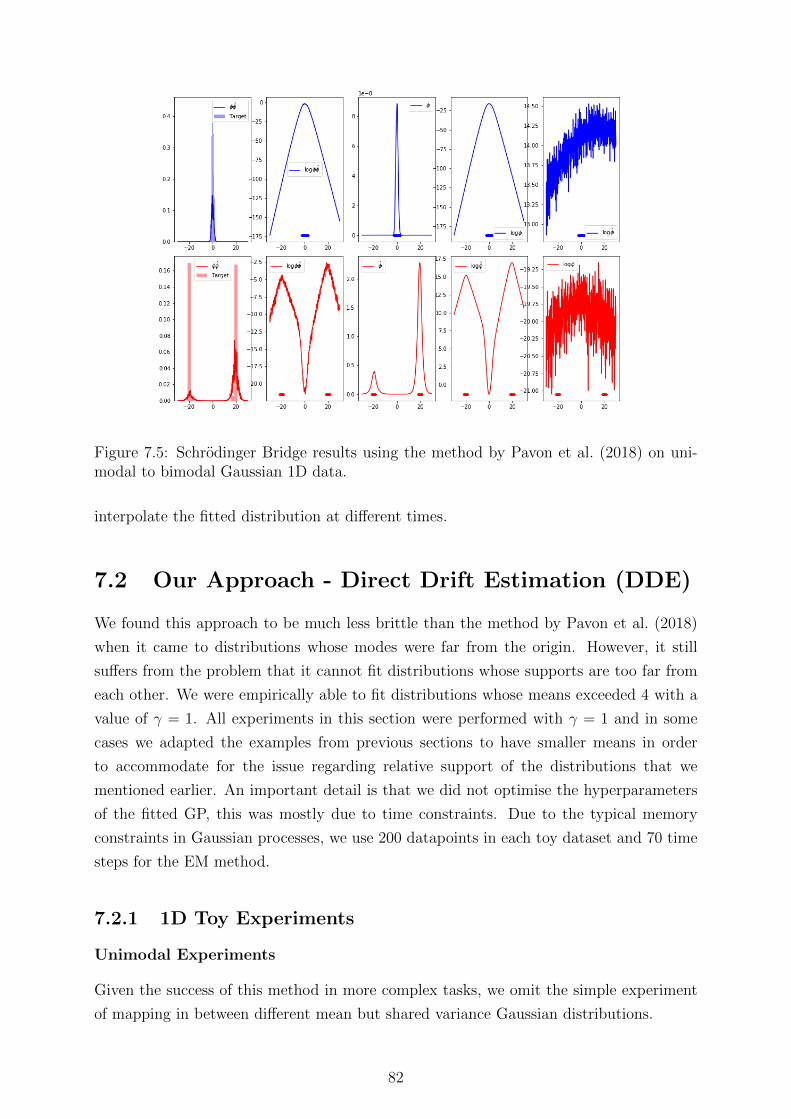
Figure 7.5: Schrodinger Bridge results using the method by Pavon et al. (2018) on uni-modal to bimodal Gaussian 1D data.

interpolate the fitted distribution at different times.

7.2 Our Approach - Direct Drift Estimation (DDE)

We found this approach to be much less brittle than the method by Pavon et al. (2018)

when it came to distributions whose modes were far from the origin. However, it still

suffers from the problem that it cannot fit distributions whose supports are too far from

each other. We were empirically able to fit distributions whose means exceeded 4 with a

value of γ = 1. All experiments in this section were performed with γ = 1 and in some

cases we adapted the examples from previous sections to have smaller means in order

to accommodate for the issue regarding relative support of the distributions that we

mentioned earlier. An important detail is that we did not optimise the hyperparameters

of the fitted GP, this was mostly due to time constraints. Due to the typical memory

constraints in Gaussian processes, we use 200 datapoints in each toy dataset and 70 time

steps for the EM method.

7.2.1 1D Toy Experiments

Unimodal Experiments

Given the success of this method in more complex tasks, we omit the simple experiment

of mapping in between different mean but shared variance Gaussian distributions.

82

Figure 7.6: Extracted drift from optimal potentials. Marginals highlighted in red forvisibility.

Different Means and Variances

We generate this dataset following:

π0(x)= N (x; 0, 1)

π1(y)= N (y; 4, 0.12).

We can observe from Figure 7.8 that the trajectories match the correct evolution of the

means and the variances. Inspecting Figure 7.9, we can observe a minor struggle in

matching the 0.1 variance for which our approach seems to estimate a slightly higher

variance. Overall we can observe a good fit.

Multimodal Experiments

We experiment with mapping in between unimodal and multimodal distributions. We

empirically find that this is the only method that can robustly cope with more than 2

modes.

Unimodal to Bimodal

83

Figure 7.7: Loss per epoch for fitted unimodal Schrodinger (SB) using the DDE method.

We follow the generative following generative process for generating the toy data:

π0(x)= N (x; 0, 1)

π1(y)=1

2N (y; 1.8, 0.62)+

1

2N (y;−1.9, 0.62).

Results can be found in Figures 7.11 and 7.10. We observe mostly a good fit for the

unimodal boundary and for the bimodal boundary with the exception of 3 outliers that

were transported to an area that should have close to 0 probability mass. We found that

these outliers occurred outside of the Schrodinger bridge context and rather due to the

method by Ruttor et al. (2013) (used for fitting the drift of SDEs) struggling in matching

low variances at the boundaries. It is possible that optimising the GPs hyperparameters

may also improve on this.

Unimodal to Trimodal

We generate the 1D toy dataset following the following distribution:

π0(x)= N (x; 0, 1)

π1(y)=1

3N (y; 5, 0.52)+

1

3N (y; 2, 0.52) +

1

3N (y;−5, 0.52).

We can observe from Figures 7.12, 7.13 that the boundaries distributions are matched

nicely both in variance and mean. Furthermore, the trajectories look sound: they have

some reminiscence of Brownian motion, follow nice simple paths, and look dual to each

other. We also observe that for the two modes that are close to each other there are two

outliers in low probability areas.

84

Figure 7.8: Fitted SB trajectories using the DDE approach on unimodal to unimodal 1Ddata.

7.2.2 2D Toy Experiments

Given the success of the DDE method in going beyond splitting two modes, we decided

to experiment further and go into 2-dimensions. Due to time constraints, we chose not to

carry out 2-dimensional experiments for the method in Pavon et al. (2018), furthermore

we were unable to get their method to split beyond 2 modes.

Figure 7.9: Fitted SB marginals using the DDE approach on unimodal to unimodal 1Ddata.

85

Figure 7.10: Fitted SB trajectories using the DDE method on the unimodal to bimodal1D dataset.

Figure 7.11: Fitted SB marginals using the DDE method on the unimodal to bimodal 1Ddataset.

86

Figure 7.12: Fitted SB trajectories for unimodal to trimodal data using DDE, successfullyfitting three modes.

Trimodal Experiment

In this section we consider the 2D extension of the trimodal experiment. We use the

following distributions to generate our toy examples:

π0(x)= N

(x;−

(0.1

0.1

), 0.192 I2

)

π1(y)=1

3N

(y;−

(3.3

0.1

), 0.112I2

)+

1

3N

(y;

(3.5

3.5

), 0.112I2

)+

1

3N

(y;

(0.7

0.7

), 0.112I2

).

Figure 7.13: Fitted SB trajectories for unimodal to trimodal data using DDE.

87

Figure 7.14: Fitted SB trajectories using the DDE method for unimodal to trimodal data.

In Figure 7.14 we can see how the trajectories successfully split and merge into 3 modes.

In Figure 7.15 we observe that the marginal constraints are enforced to a reasonable

amount, matching means quite well, yet struggling partly with the variance of the low

variance boundaries.

Circles Dataset

We used the circles dataset (Pedregosa et al., 2011) which consists of two concentric

circles. In this task we consider mapping from a standardised unimodal Gaussian to the

Circles data.

π0(x)= N (x; 0, I2)

π1(y)= GenerateCircles(factor=0.3, radius=3.5, noise=0.03).

The radius and factor (distance between circles) were picked so the data was still within

a close proximity to the origin, whilst making the circles distinct.

We can see from Figure 7.17 that some very structured inner circle-like trajectories are

formed going forward and backward with a dual like pattern. Furthermore, from Figures

7.18, 7.19 we can observe a good fit in terms of structure, but the fits of our method are

slightly more dispersed, with higher variance. We noticed this could be improved by using

more training data and tweaking the GP hyper-parameters. Further experiments should

be carried out to diagnose and solve this issue.

88

Figure 7.15: Fitted SB marginals using the DDE method for unimodal to trimodal data.

Figure 7.16: 2D histograms for the fitted SB marginals using the DDE method for uni-modal to trimodal data. On the left we show the true empirical distribution and on theright we show the empirical distribution learned by our Schrodinger bridge mapping.

89

Figure 7.17: Fitted SB trajectories using the DDE method for unimodal to circles data.We can observe the nice and clear concentric circles trajectories arising in the learnedbridge.

Figure 7.18: Fitted SB Boundary distributions using the DDE method on unimodal tocircles data.

90

Figure 7.19: 2D histograms for the fitted SB marginals using the DDE method for uni-modal to circles data.

Moons Dataset

We use the moons dataset from Pedregosa et al. (2011), generated by the following pro-

cedure:

π0(x)= N (x; 0, I2)

π1(y)= GenerateMoons(scale x=1.8, scale y=3.8, noise=0.03).

Similar to the circles dataset, the scales were picked to give a nice visual scale and a clear

separation between the moons, making the task as simple as possible given that we were

still in an exploratory stage.

We observe that the DDS method struggles with the moons dataset in Figures 7.22, 7.21.

However, it still manages to capture most of the structure in the marginals, except for

the higher variances. As with the other experiments, the trajectories (Figure 7.20) have

a dual like nature.

7.3 Stochastic Control (SC) Approach

Throughout this section we employ neural networks (LeCun et al., 2015) to parametrise

the drifts in Equation 6.25 and experiment with 3 different types of activations: Tanh,

Hard Tanh, ReLu. We varied layer widths and depths in order to obtain good results,

without careful regard for overfitting, since, as mentioned, we are merely exploring the

capacities and faults of the approaches. Across all experiments we initialise the weights of

the neural networks using Glorot initialisation (Glorot & Bengio, 2010) and we used the

Adagrad optimiser (Duchi et al., 2011). Due to the KNN based approach to computing

91

Figure 7.20: Fitted SB trajectories using the DDE method for unimodal to moons data.

Figure 7.21: Fitted SB Boundary distributions using the DDE method for unimodal tomoons data.

92

Figure 7.22: 2D histograms for the fitted SB marginals using the DDE method for uni-modal to moons data.

Figure 7.23: Loss per epoch for fitted unimodal SB using tanh activation, single layer and200 hidden units for SC approach.

93

Figure 7.24: Fitted SB trajectories using the SC method with tanh activations, singlelayer and 200 hidden units, fitted on the unimodal dataset. Note that the trajectoriesseem much smoother than the ones induced by the direct drift approach. This is mostlya visual effect due to the scale of the y axis being much higher. In other words you willsee less noise if you zoom out.

cross entropy being unstable, we used the KDE based approach across all experiments.

This method allowed using bigger datasets than the previous two methods, thus we used

900 datapoints in each toy dataset, 100 time steps for the EM method and a batch size

of 900 (only one batch) for the optimiser.

7.3.1 Unimodal Experiments

For the unimodal experiments we focus on mapping between normal distributions with

different means and variances.

Small to Big Variance

Data was generated using:

π0(x)= N (x; 0, 3)

π1(y)= N (y; 6, 0.12)

For these particular experiments, we found very little differences among the trajectories

learned by different activations. Results can be found in Figures 7.25 and 7.24, where we

can see a good fit for the marginal with low variance, but a worse fit for the high variance

distribution where the variance is matched but the mode is not.

94

Figure 7.25: Fitted SB boundary distributions using the SC method with tanh activations,single layer and 200 hidden units.

7.3.2 Multimodal Experiments

In this section we followed the generative process:

π0(x)= N (x; 0, 1)

π1(y)=1

2N (y; 20, 0.62)+

1

2N (y;−20, 0.62).

We parametrised the drifts with 3 hidden layers, each having 20 hidden units, with the

exception of the final experiment and best performing model for which we used 2 hidden

layers, each with 200 units. In general, we found that increasing the number of units and

layers made the optimisation process more unstable and typically required reducing the

initial step size for the optimiser. These experiments are used for investigating how the

stochastic control based approach can handle mode collapse.

ReLu

For these experiments, we use the rectified linear-unit (ReLu) (Glorot et al., 2011). We

show results of a further experiment with larger means to illustrate the shape of the

trajectories induced by this activation. As shown in Figures 7.26 and 7.28, the learned

trajectories are more curved (almost parabolic like) than the trajectories induced by tanh

based activations. We also observe that whilst being on the right track to matching the

means, it fails to match the variance of the bimodal marginals. One positive aspect is

that the curves do have a dual like nature.

Tanh

Here we use the hyperbolic-tangent (Tanh) as the activation function. We also experi-

mented with similar smooth activations and obtained similar results. We observe from

Figures 7.29 and 7.30 that the method roughly matches the means, with a clear dual

95

Figure 7.26: Fitted SB trajectories using ReLu activation, 3 hidden layers of 20 hiddenunits each

Figure 7.27: Fitted SB boundary distributions using the SC method with ReLu activa-tions, 3 hidden layers of 20 hidden units each.

96

Figure 7.28: Additional bimodal experiment - Fitted SB trajectories using the SC methodwith ReLu activations, 3 hidden layers of 20 hidden units each.

Figure 7.29: Fitted SB trajectories using the SC method with tanh activations, 3 hiddenlayers of 20 hidden units each.

97

Figure 7.30: Fitted SB boundary distributions using the SC method with tanh activations,3 hidden layers of 20 hidden units each.

nature between the trajectories. However, a strange spike forms where the two modes try

to merge. This spike has a much sharper variance than the actual marginal and seems

to be an issue the tanh (and sigmoid and hard-tanh) based activations experience when

merging modes. Increasing the number of hidden units improved this effect, however it

did not remove it completely.

Hard Tanh

The hard tanh activation is given by:

σ(x) = max(−1,min(1, x)),

and it is a piecewise analogue of the tanh function, similar to what the step function is

to the logistic sigmoid. We found this function was the most stable when optimising and

were able to obtain better results with both deeper and wider networks than with the

other activations which became unstable with increased depth and width.

As shown in Figures 7.31 and 7.32, the trajectories and results are similar to when using

a tanh activation function, however the spike caused when the trajectories merge was

less prominent. We believe that increasing the parameters of the network led to this im-

provement. Unfortunately, we were unable to improve on this issue further. We explored

several other activations, with hard-tanh giving the best results when it came to splitting.

An interesting empirical observation is that increasing the depth of the network helped

with being able to split modes (which requires learning a piecewise drift), while increasing

the width helped with being able to learn mappings from distributions with very different

variances. It is possible that learning drifts that are dual to each other, close to Brownian

98

Figure 7.31: Fitted SB trajectories using hard-tanh activation, 2 hidden layers and 200hidden units per layer.

Figure 7.32: Fitted SB boundary distributions using the SC method with hard-tanhactivations, 2 hidden layers and 200 hidden units per layer.

99

Figure 7.33: Mode collapse example, using the SC method with tanh activations, 3 hiddenlayers 20 hidden units each.

motion (close to 0) and match the boundary distributions is a very challenging task and

thus reaches the maximum capacity of the neural network architectures we explored.

Mode Collapse

As mentioned earlier, due to minimising the reverse KL numerically, this method is in

theory prone to mode collapse. In practice, mode collapse did occur fairly often, especially

when the marginals were not symmetrically positioned relative to each other.

Table 7.1: Scenarios that each algorithm is able to overcome. The checkmark indicatesthe method can overcome this task/challenge, whilst a cross indicates it is not able to doso. The exclamation mark indicates in some cases it was able to solve this milestone. Theunderscores indicates a lack of experiments for the relevant milestone-method pair.

Method2 Mode 3 Mode Non Small Works DistantSplit Split Gaussian variance at γ = 1 π0, π1

π0, π1

Pavon et al. (2018) 3 7 7 7 7

Drift Estimation 3 3 3 7 3 7

Stochastic Control ! 7 7 3 3

100

Table 7.2: Kolmogorov-Smirnov test results on learned boundary distribution. The sig-nificance level is set at α = 0.05. All methods use γ = 1 with the exception of the methodin Pavon et al. (2018) for which we had to use γ = 100 for the Unimodal experiment.

MethodUnimodal Bimodal

π0 π1 π0 π1

D200 p-value D200 p-value D200 p-value D200 p-value

Pavon et. al. (2018) 0.150 0.221 0.195 0.001 0.115 0.142 0.110 0.178Direct Drift 0.070 0.713 0.190 0.001 0.110 0.178 0.125 0.088Stochastic Control 0.070 0.713 0.805 < 10−3 0.360 < 10−3 0.500 10−3

7.4 Comparison of Methods

First, we summarize our findings, highlighting the empirical capacities of the three ap-

proaches we trialed. A summary of the results can be found in Table 7.1. The main

practical milestones considered when evaluating the methods are:

• 2 Modes: Being able to split into 2 modes and merge into 1.

• 3 Modes: Being able to split into 3 modes and merge into one.

• Non-Gaussian π0, π1: Being able to handle non-Gaussian boundary distributions

(moons and circles datasets).

• Small Variance: Being able to match a boundary distribution that has a numeri-

cally small variance (e.g. tending towards a point mass).

• Works at γ = 1: Being able to work for a volatility of γ = 1. We consider it

working if it handles at least a radius of 4 between the two distributions, meaning

the mode that is most distant to the unimodal distribution has a magnitude of 4.

The only method failing this milestone was the method by Pavon et al. (2018) since

the method effectively only worked for γ = 1 when the support of the data was

within the unit cube.

• Distant π0, π1: This is effectively the same milestone as above, however we do

not limit the radius to 3. It tests how well the models work when the distributions

are very far apart from each other. We found that the method by Pavon et al.

(2018) and our direct drift estimation approach did not work well in this scenario

and required either increasing γ or standardising the data.

Inspecting the summary of findings reported Table 7.1, we can observe that the most

robust method is the direct drift estimation approach using GPs. We will now carry out

a comparative experiment with a sound hypothesis test set a priori.

101

Comparative Results

In order to carry out a more quantitative comparison of the methods, we select two of

the toy datasets that all methods seem to be able to fit:

π0(x)= N (x; 0, 1)

π1(y)= N (y; 4, 0.12),

and

π0(x)= N (x; 0, 1)

π1(y)=1

2N (y; 1.8, 0.62)+

1

2N (y;−1.9, 0.62).

We then perform a Kolmogorov-Smirnov (Kolmogorov-Smirnov et al., 1933) test where

the null hypothesis is that the learned marginals from our methods are equal. We set

the significance level to its usual setting α = 0.05, meaning that if we observe a p-value

≤ 0.05, we reject the null hypothesis that the two distributions are equal. We present

results in Table 7.2, displaying both the Kolmogorov test statistic as a goodness of fit

measure (the lower the better) across methods and the estimated p-value for the test. We

reject the null-hypothesis three times for the stochastic control based method meaning

that it had the lowest performance across all methods. We also observe that overall the

Direct Drift method and the method by Pavon et al. (2018) are fairly on-par for these

two datasets.

102

Chapter 8

Discussion

Schrodinger bridges have broad applications in physical sciences, but only recently have

they sparked interest in the machine learning community. In this work we have aimed to

bridge this gap, firstly by trying to present an extensive yet accessible background to the

problem, producing proofs for select known results whose original resource we could not

find. We have highlighted some of its known connections to the more popular Wasserstein

distance and thus we have suggested its potential application in machine learning as a way

of comparing distributions. Furthermore, we explored the connection between IPFP and

generative adversarial networks, motivating the potential application of using Schrodinger

bridges for the task of domain adaptation.

We have learned and illustrated how challenging it is to develop a numerical algorithm for

solving the Schrodinger bridge. Part of this challenge comes from having to deal with more

than one boundary condition. This is where the g-IPFP framework comes in, allowing us

to alternate between sub-problems (half bridges) with only one boundary condition until

convergence. However, empirically solving these half bridges proved challenging, since

they presented harder variants of typical challenges that arise in machine learning, such

as numerical integration and density estimation.

We proposed two methods for solving the empirical setting of the Schrodinger bridge and

explored them through simple 1D and 2D simulations which allowed us to visually and

extensively evaluate the properties of the proposed methods. We compared against the

recently proposed method by Pavon et al. (2018) and showed competitive performance

across two toy datasets, whilst being more robust to values of γ than the method of (Pavon

et al., 2018). In addition, our method was uniquely able to successfully fit a unimodal to

trimodal experiment.

At the core of the direct drift estimation approach, we have successfully transformed a

complex mathematical problem arising from the physical sciences into a classical machine

learning task (regression).

103

8.1 Summary of Contributions

The key contributions of this thesis are:

• Provided a thorough and accessible introduction to the problem, with motivational

examples closer to machine learning as well as intuitive proof sketches for steps that

are skipped in the available literature.

• Structured the existing IPFP algorithmic framework and provided formal connec-

tions between existing methods, highlighting that they are within the IPFP frame-

work.

• Turned the iterative procedure for solving the Schrodinger bridge into a classical

machine learning task at each iteration (i.e. regression). This contribution makes

the problem much more accessible to the machine learning community.

• Proposed, implemented and evaluated two new working methods that use common

methodology from machine learning. The newly proposed methods overcome some

of the conceptual issues in Pavon et al. (2018) (e.g. importance sampling not scaling

to high dimensions, instability for low values of γ).

• Using thorough experimentation, we uncovered many of the breaking points of differ-

ent methods (e.g. mode collapse, sampling between distant boundary distributions),

including ours. This is work that was missing from Pavon et al. (2018) and Bernton

et al. (2019), thus we provided a holistic view of the methods, helpful for porting

the algorithms to practical applications.

8.2 Further Work

Whilst we introduced and evaluated to a great extent the first successful machine learning

based approach for solving the Schrodinger bridge, there are still areas of exploration left

to pursue further:

• Our best performing method is based on Gaussian processes, which will not scale

well to large datasets. Ruttor et al. (2013) further propose a sparse expectation

maximisation based algorithm for inferring the drift of SDEs which we did not ex-

plore. This could potentially make the DDE method scalable enough for optimising

the GP hyperparameters, which we were unable to do due to speed limitations.

• We found that the method by Ruttor et al. (2013) had difficulties in learning drifts

whose end point distribution was very sharp (low variance). Optimising the hyper-

parameters may fix this issue.

• Explore the learning of the drift using a method that is not based on Gaussian

processes.

104

• Some of the unimodal examples admit closed form solutions for the full bridge. We

should use this as a ground truth and compute the relative path error to the closed

form drift in order to evaluate the methods.

• The direct half bridge drift estimation method we proposed can be adapted to

the static Schrodinger bridge. This would be an interesting avenue of research,

potentially reducing the computational complexity of the approach.

• We should explore our methods on real world data. One possible task is 2-sample

hypothesis tests as in Gretton et al. (2012), where we would use our approach to

compare datasets to each other.

• Explore and compare our proposed method with the method in Bernton et al. (2019).

105

Appendix A

Analysis of Simple Gaussian LikeParametrisation

This appendix illustrates the challenges in parametrising the MLE based objectives pro-posed in Pavon et al. (2018), such that the partition function can be computed in closedform. Ultimately, we were unable to come up with a parametrisation that had a closedform partition function and was flexible enough to solve the half bridge for multimodaldistributions.

A.1 Unimodal Parametrisation

Following the reparametrisation introduced in Section 6.1.2, we consider the case ofparametrising the potentials with unimodal Gaussians. This allows for further analy-sis of the method, since both the normalisation and the updates can be attained in closedform.

Firstly, we offer the counterexample that valid Gaussian like parametrisations for thepotentials cannot solve the bridge even for unimodal Gaussian marginals:

Proposition 3. If we parametrise the potentials as:

φ0(x; β) = N (x|µx,Σx), (A.1)

φ1(y; β) = N (y|µy,Σy), (A.2)

and try to solve the empirical bridge for the marginals:

π0(x) = Z−1x N (x, 0, 1),

π1(y) = Z−1y N (y, 0, 102),

then the MLE based approximation of Fortet’s in Pavon et al. (2018) will not meet themarginal constraints.

Proof. Assuming a prior Wγ. Propagating:

φ0(x; β) = Z−1x N (x|µy,Σy + γId),

φ1(y; β) = Z−1y N (y|µx,Σx + γId).

107

Then:

φ0(x; β)φ0(x; β) = N(x∣∣∣(Σ−1

x + (Σy + γId)−1)−1(

Σ−1x µx + (Σy + γId)−1µy)

),(

Σ−1x + (Σy + γId)−1

)−1).

Via MLE (holding y-parameters constant) we have:(Σ−1x + (Σy + γId)−1

)−1= Sx.

Yielding update

Σ(t)x = (S−1

x − (Σ(t−1)y + γId)−1)−1,

and (Σx + (Σy + γId)−1

)−1 (Σ−1x µx + (Σy + γId)−1µy)

)= x.(

Σ−1x µx + (Σy + γId)−1µy)

)=(Σ−1x + (Σy + γId)−1

)x.

Yielding update:

µ(i)x =

(I + Σ(i)

x (Σ(i−1)y + γId)−1

)x−Σ(i)

x (Σ(i−1)y + γId)−1µ(i−1)

y ,

and similarity for Σy,µy. In 1D (and in terms of the free parameters), the fitted marginaldensity variances are:

σ∗y =

(1

1 + σ2x

+1

σ2y

)−1

,

σ∗x =

(1

1 + σ2y

+1

σ2x

)−1

.

If the empirical marginal variances were 1, 10:

1 =

(1

1 + σ2x

+1

σ2y

)−1

,

10 =

(1

1 + σ2y

+1

σ2x

)−1

.

Then the above system has no valid solutions (can be solved only for negative values ofσx), by the quadratic formula:

0.8σ4x + 1.9σ2

x + 1 = 0. E

The above tells us that in order to do a squared exponential paremetrisation for thepotentials, we must drop the positive definite constraint. In geometric terms, if onepotential is log concave then the other needs to be log convex due to how the variancescombine.

We must still enforce an integrability constraint (required to make the inner product of

108

potentials converge): (Σ−1x + Σ−1

y

)−1= LL>,

which implies:

Σ−1x + Σ−1

y = LL>,

which can be enforced via a simple reparametrisation (this allows for negative length-scales):

Σx = (LL> −Σ−1y )−1,

where L can be parametrised in terms of an unconstrained vector.

A.2 Mixture of Exponentiated Quadratics

We now consider whether it is possible to extend the exponentiated quadratic parametri-sation of the potentials to a mixture of exponentiated quadratics. In order to achieve thisparametrisation, we need to reconsider the integrability constraint.

φ0(x; β) =∑kx

πkxN (x|µkx ,Σkx) (A.3)

φ1(y; β) =∑ky

πkyN (y|µky ,Σky) (A.4)

The integrability constraint then becomes ∀kx:∧ky

(Σkx + Σky 0

),

which using the eigen-decompositions Σkx = UkxDkxU>kx

, Σky = UkyDkyU>ky

can be re-expressed as:

λdkx + minλdky ≥ 0,

where d is a specific component / dimension. Thus, we enforce this constraint via thereparametrisation:

λdkx = exp(θ)−minλdky ,

where θ is unconstrained. Furthermore, we can parametrise the orthogonal matrices Ukx

in terms of unconstrained vectors using Householder reflections. Combining the aforemen-tioned parametrisations, we can enforce the integrability constraint fully via reparametri-sations. While these parametrisations are not differentiable everywhere, one can stillmaximise the liklelihood using the sub-gradient method (Shor, 1991). Unfortunately, thismethod was unable to work for multimodal distributions, thus we did not pursue thispath further.

109

Bibliography

Alvarez, M., Luengo, D., and Lawrence, N. D. Latent force models. In Artificial Intelli-gence and Statistics, pp. 9–16, 2009.

Alvarez, M. A., Rosasco, L., and Lawrence, N. D. Kernels for vector-valued functions: Areview. Found. Trends Mach. Learn., 4(3):195–266, 2012.

Alvarez, M. A., Luengo, D., and Lawrence, N. D. Linear latent force models usingGaussian processes. IEEE Transactions on pattern analysis and machine intelligence,35(11):2693–2705, 2013.

Andres, D. S. Lecture notes in Advanced Probability, Cambridge University,September 2019. URL http://www.statslab.cam.ac.uk/~sa836/teaching/ap19/\\

AdvancedProbability.html.

Batz, P., Ruttor, A., and Opper, M. Approximate Bayes learning of stochastic differentialequations. Physical Review E, 98(2):022109, 2018.

Bayes, T. LII. An essay towards solving a problem in the doctrine of chances. By the lateRev. Mr. Bayes, FRS communicated by Mr. Price, in a letter to John Canton, AMFRS. Philosophical transactions of the Royal Society of London, (53):370–418, 1763.

Bernton, E., Heng, J., Doucet, A., and Jacob, P. E. Schrodinger Bridge Samplers. arXivpreprint arXiv:1912.13170, 2019.

Carlier, G., Duval, V., Peyre, G., and Schmitzer, B. Convergence of entropic schemes foroptimal transport and gradient flows. SIAM Journal on Mathematical Analysis, 49(2):1385–1418, 2017.

Chen, Y., Georgiou, T., and Pavon, M. Entropic and displacement interpolation: a com-putational approach using the Hilbert metric. SIAM Journal on Applied Mathematics,76(6):2375–2396, 2016.

Cramer, E. Probability measures with given marginals and conditionals: l-projectionsand conditional iterative proportional fitting. Statistics and Decisions-InternationalJournal for Stochastic Methods and Models, 18(3):311–330, 2000.

Csiszar, I. I-divergence geometry of probability distributions and minimization problems.The annals of probability, pp. 146–158, 1975.

Doob, J. L. The Brownian movement and stochastic equations. Annals of Mathematics,pp. 351–369, 1942.

Duchi, J., Hazan, E., and Singer, Y. Adaptive subgradient methods for online learningand stochastic optimization. Journal of machine learning research, 12(Jul):2121–2159,2011.

111

Einstein, A. On the motion required by the molecular kinetic theory of heat of smallparticles suspended in a stationary liquid. Annalen der Physik, 17(8):549–560, 1905.

Essid, M. and Pavon, M. Traversing the Schrodinger Bridge strait: Robert Fortet’smarvelous proof redux. Journal of Optimization Theory and Applications, 181(1):23–60, 2019.

Fortet, R. Resolution d’un systeme d’equations de M. Schrodinger. J. Math. Pure Appl.IX, 1:83–105, 1940.

Follmer, H. Random fields and diffusion processes. In Ecole d’Ete de Probabilites deSaint-Flour XV–XVII, 1985–87, pp. 101–203. Springer, 1988.

Glorot, X. and Bengio, Y. Understanding the difficulty of training deep feedforwardneural networks. In Proceedings of the thirteenth international conference on artificialintelligence and statistics, pp. 249–256, 2010.

Glorot, X., Bordes, A., and Bengio, Y. Deep sparse rectifier neural networks. In Proceed-ings of the fourteenth international conference on artificial intelligence and statistics,pp. 315–323, 2011.

Goodfellow, I., Pouget-Abadie, J., Mirza, M., Xu, B., Warde-Farley, D., Ozair, S.,Courville, A., and Bengio, Y. Generative adversarial nets. In Advances in neuralinformation processing systems, pp. 2672–2680, 2014.

Gretton, A., Borgwardt, K. M., Rasch, M. J., Scholkopf, B., and Smola, A. A kerneltwo-sample test. Journal of Machine Learning Research, 13(Mar):723–773, 2012.

Gutmann, M. and Hyvarinen, A. Noise-contrastive estimation: A new estimation principlefor unnormalized statistical models. In Proceedings of the Thirteenth InternationalConference on Artificial Intelligence and Statistics, pp. 297–304, 2010.

Jaynes, E. T. Information theory and statistical mechanics. Physical review, 106(4):620,1957.

Jaynes, E. T. Probability theory: The logic of science. Cambridge University press, 2003.

Kingma, D. P. and Welling, M. Auto-encoding variational Bayes. arXiv preprintarXiv:1312.6114, 2013.

Kolmogorov-Smirnov, A., Kolmogorov, A., and Kolmogorov, M. Sulla Determinazioneempırica di uma legge di distribuzione. 1933.

Kullback, S. Probability densities with given marginals. The Annals of MathematicalStatistics, 39(4):1236–1243, 1968.

Kullback, S. Information theory and statistics. Courier Corporation, 1997.

Lahdesmaki, P. H. M. H. H. and Kaski, S. Deep Learning with differential Gaussianprocess flows.

Lample, G., Conneau, A., Denoyer, L., and Ranzato, M. Unsupervised Machine Transla-tion Using Monolingual Corpora Only. arXiv preprint arXiv:1711.00043, 2017.

Lawrence, N. D. Variational inference in probabilistic models. PhD thesis, University ofCambridge, 2001.

LeCun, Y., Bengio, Y., and Hinton, G. Deep learning. nature, 521(7553):436–444, 2015.

112

Leonard, C. From the Schrodinger problem to the Monge–Kantorovich problem. Journalof Functional Analysis, 262(4):1879–1920, 2012.

Leonard, C. A survey of the Schrodinger problem and some of its connections with optimaltransport. arXiv preprint arXiv:1308.0215, 2013.

Levina, E. and Bickel, P. The earth mover’s distance is the mallows distance: Someinsights from statistics. In Proceedings Eighth IEEE International Conference on Com-puter Vision. ICCV 2001, volume 2, pp. 251–256. IEEE, 2001.

Martino, L., Elvira, V., and Louzada, F. Effective sample size for importance samplingbased on discrepancy measures. Signal Processing, 131:386–401, 2017.

Mikami, T. and Thieullen, M. Optimal transportation problem by stochastic optimalcontrol. SIAM Journal on Control and Optimization, 47(3):1127–1139, 2008.

Mohamed, S. and Lakshminarayanan, B. Learning in implicit generative models. arXivpreprint arXiv:1610.03483, 2016.

Nagasawa, M. Stochastic processes in quantum physics, volume 94. Birkhauser, 2012.

Nelson, E. Dynamical theories of Brownian motion, volume 3. Princeton University Press,1967.

Øksendal, B. Stochastic differential equations. In Stochastic differential equations, pp.65–84. Springer, 2003.

Osborne, M., Garnett, R., Ghahramani, Z., Duvenaud, D. K., Roberts, S. J., and Ras-mussen, C. E. Active learning of model evidence using Bayesian quadrature. In Ad-vances in Neural Information Processing Systems, pp. 46–54, 2012.

Pavon, M. and Wakolbinger, A. On free energy, stochastic control, and Schrodingerprocesses. In Modeling, Estimation and Control of Systems with Uncertainty, pp. 334–348. Springer, 1991.

Pavon, M., Tabak, E. G., and Trigila, G. The data-driven Schrodinger bridge. arXivpreprint arXiv:1806.01364, 2018.

Pedregosa, F., Varoquaux, G., Gramfort, A., Michel, V., Thirion, B., Grisel, O., Blondel,M., Prettenhofer, P., Weiss, R., Dubourg, V., et al. Scikit-learn: Machine learning inPython. the Journal of machine Learning research, 12:2825–2830, 2011.

Ramdas, A., Trillos, N. G., and Cuturi, M. On Wasserstein two-sample testing and relatedfamilies of nonparametric tests. Entropy, 19(2):47, 2017.

Ruschendorf, L. et al. Convergence of the iterative proportional fitting procedure. TheAnnals of Statistics, 23(4):1160–1174, 1995.

Ruttor, A., Batz, P., and Opper, M. Approximate Gaussian process inference for thedrift function in stochastic differential equations. In Advances in Neural InformationProcessing Systems, pp. 2040–2048, 2013.

Salamon, D. A. Lecture notes in measure and integration, ETH Zurich, June 2019. URLhttps://people.math.ethz.ch/~salamon/PREPRINTS/measure.pdf.

Sarkka, S. and Solin, A. Applied stochastic differential equations, volume 10. CambridgeUniversity Press, 2019.

113

Schrodinger, E. Uber die Umkehrung der Naturgesetze, Verlag Akademie der Wis-senschaften in Kommission bei Walter de Gruyter u. Company, Berlin, 1931.

Schrodinger, E. Sur la theorie relativiste de l’electron et l’interpretation de la mecaniquequantique. In Annales de l’institut Henri Poincare, volume 2, pp. 269–310, 1932.

Shor, N. Z. The development of numerical methods for nonsmooth optimization in theUSSR. History of Mathematical Programming. A Collection of Personal Reminiscences,pp. 135–139, 1991.

Silverman, B. W. Density estimation for statistics and data analysis, volume 26. CRCpress, 1986.

Singh, S. and Poczos, B. Analysis of k-nearest neighbor distances with application toentropy estimation. arXiv preprint arXiv:1603.08578, 2016.

Tzen, B. and Raginsky, M. Neural stochastic differential equations: Deep latent Gaussianmodels in the diffusion limit. arXiv preprint arXiv:1905.09883, 2019.

Van der Wilk, M. Sparse Gaussian process approximations and applications. PhD thesis,University of Cambridge, 2019.

Vargas, F., Brestnichki, K., and Hammerla, N. Model Comparison for Semantic Grouping.In International Conference on Machine Learning, pp. 6410–6417, 2019.

Veksler, O. Nonparametric density estimation nearest neighbors, KNN, 2013.

Viaclovsky, P. J. Lecture notes in measure and integration, MIT, September2003. URL https://ocw.mit.edu/courses/mathematics/18-125-measure-and-\

\integration-fall-2003/.

Villani, C. Topics in optimal transportation. Number 58. American Mathematical Soc.,2003.

Williams, C. K. and Rasmussen, C. E. Gaussian processes for machine learning, volume 2.MIT press Cambridge, MA, 2006.

Yang, X. Understanding the variational lower bound, 2017.

Zhang, M., Bird, T., Habib, R., Xu, T., and Barber, D. Variational f-divergence Mini-mization. arXiv preprint arXiv:1907.11891, 2019.

Zhu, J.-Y., Park, T., Isola, P., and Efros, A. A. Unpaired image-to-image translationusing cycle-consistent adversarial networks. In Proceedings of the IEEE internationalconference on computer vision, pp. 2223–2232, 2017.

114

Machine-learning approaches for the empirical Schrödinger ...

Documents

Transcript of Machine-learning approaches for the empirical Schrödinger ...