DI

SC

US

SI

ON

P

AP

ER

S

ER

IE

S

Forschungsinstitut zur Zukunft der ArbeitInstitute for the Study of Labor

Empirical Approaches to Inequality of Opportunity: Principles, Measures, and Evidence

IZA DP No. 6672

June 2012

Xavier RamosDirk Van de gaer

Empirical Approaches to Inequality of Opportunity:

Principles, Measures, and Evidence

Xavier Ramos Universitat Autònoma de Barcelona,

IZA and EQUALITAS

Dirk Van de gaer Sherppa, IAE and CORE

Discussion Paper No. 6672 June 2012

IZA

P.O. Box 7240 53072 Bonn

Germany

Phone: +49-228-3894-0 Fax: +49-228-3894-180

E-mail: iza@iza.org

Any opinions expressed here are those of the author(s) and not those of IZA. Research published in this series may include views on policy, but the institute itself takes no institutional policy positions. The Institute for the Study of Labor (IZA) in Bonn is a local and virtual international research center and a place of communication between science, politics and business. IZA is an independent nonprofit organization supported by Deutsche Post Foundation. The center is associated with the University of Bonn and offers a stimulating research environment through its international network, workshops and conferences, data service, project support, research visits and doctoral program. IZA engages in (i) original and internationally competitive research in all fields of labor economics, (ii) development of policy concepts, and (iii) dissemination of research results and concepts to the interested public. IZA Discussion Papers often represent preliminary work and are circulated to encourage discussion. Citation of such a paper should account for its provisional character. A revised version may be available directly from the author.

IZA Discussion Paper No. 6672 June 2012

ABSTRACT

Empirical Approaches to Inequality of Opportunity: Principles, Measures, and Evidence*

We put together the different conceptual issues involved in measuring inequality of opportunity, discuss how these concepts have been translated into computable measures, and point out the problems and choices researchers face when implementing these measures. Our analysis identifies and suggests several new possibilities to measure inequality of opportunity. The approaches are illustrated with a selective survey of the empirical literature on income inequality of opportunity. JEL Classification: D3, D63 Keywords: equality of opportunity, measurement, compensation, responsibility, effort,

circumstances Corresponding author: Xavier Ramos Universitat Autònoma de Barcelona Depart Econ Aplicada Campus UAB Bellaterra 08193 Spain E-mail: xavi.ramos@uab.cat

* We thank Erik Schokkaert, Kristof Bosmans, Jose Luis Figueroa and Stephen Jenkins for useful comments and suggestions. We gratefully acknowledge comments received on preliminary versions presented at the ECINEQ conference (Catania, Italy) and seminars at Universitat Autònoma de Barcelona and Alicante. The paper was finalized when the second author was visiting the Institut d’Anàlisi Econòmica, CSIC, Campus UAB, Bellaterra 08193, Spain. Dirk Van de gaer acknowledges financial support from the FWO-Flanders, research project 3G079112. Xavier Ramos acknowledges financial support of projects ECO2010-21668-C03-02 (Ministerio de Ciencia y Tecnología), 2009SGR-307 and XREPP (Direcció General de Recerca).

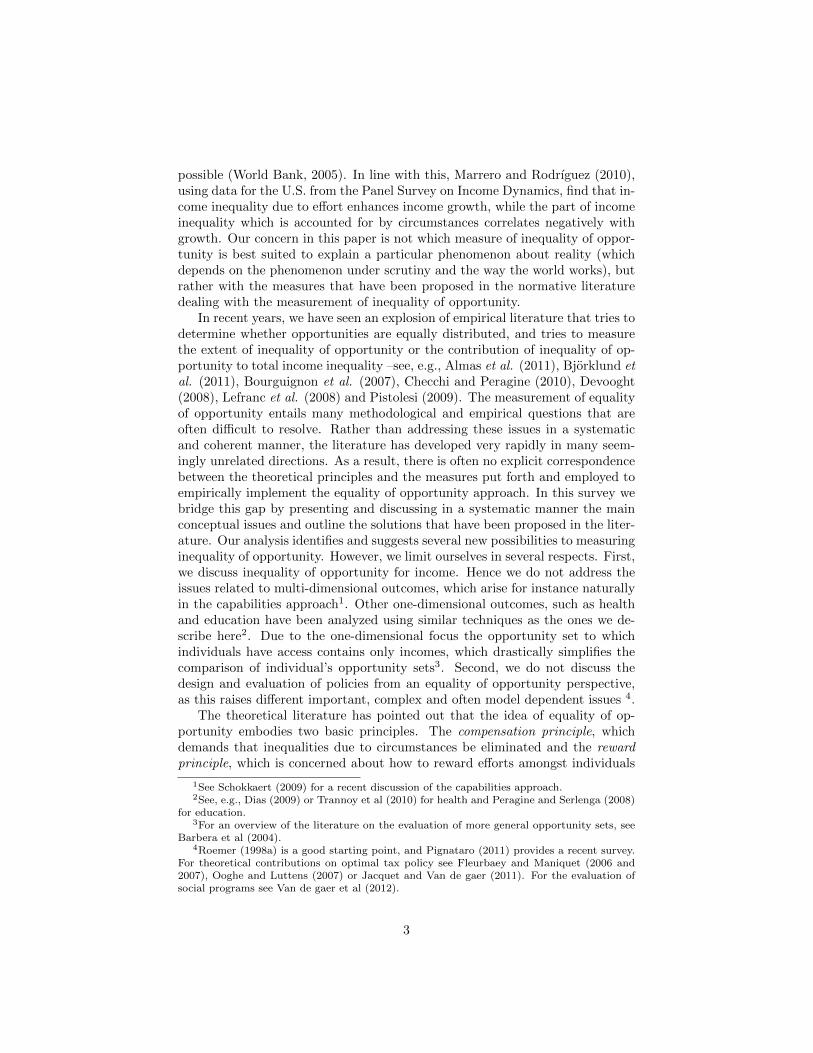
1 Introduction

Beyond the mere concern for individual differences or disparities in outcomes,which has dominated distributive concerns for many decades, the theory ofequality of opportunity (Dworkin, 1981a,b; Arneson, 1989; Cohen, 1989) putsindividual responsibility in the forefront when assessing situations of economicadvantage and disadvantage. It is argued that outcomes such as income level, ed-ucation attainment or health status, are determined by factors or variables thatare beyond individuals’ responsibility (so-called circumstances) and by factorsfor which individuals are deemed responsible (so-called effort or responsibilityvariables). Inequalities that are due to circumstances are deemed ethically un-acceptable while those arising from efforts are not considered offensive. Thatis, the ‘ideal’ situation or benchmark is not perfect equality per se, as in themeasurement of inequality of outcome, but a distribution where efforts are re-warded adequately and the effect of circumstances is compensated for, so thatonly disparities due to efforts remain.

Both attitude survey research (see, e.g., Schokkaert and Devooght (2003) andGaertner and Schwettmann (2007)), and experimental evidence (see Cappelen etal (2010)) provide strong evidence that, in judging income distributions, peoplelargely distinguish between circumstances and efforts in the way suggested byequality of opportunity theories. For instance, Cappelen et al (2010) elicitinformation on what people hold each other responsible for, by means of adictator game where the distribution phase is preceded by a production phase,and find that a large majority of the participants did not hold people responsiblefor the randomly assigned price, an impersonal factor beyond individual control,but did hold them responsible for their choice of working time.

This evidence about the social preferences people endorse should be dis-tinguished from the influence of inequality of opportunity on preferences forredistribution, political orientation and actual behavior. A growing amount ofempirical evidence shows that preferences for redistribution and political ori-entation are shaped by fairness concerns. For instance, Alesina and La Fer-rara (2005) show for the United States that people who believe that individualeconomic success is related to individual effort rather than family backgroundor luck, have lower preferences for redistribution, while Alesina and Angeletos(2005), using data from the World Value Survey, find that fairness perceptionsare associated with the individuals’ political orientation: when people believethat effort is the main determinant of economic advantage, redistribution andtaxes are low, whereas in societies where people think of birth and connectionsas the main determinants of economic success, taxes and redistribution willbe higher. Since the determinants of economic inequality (circumstances ver-sus efforts) influence individual incentives, these determinants are related withaggregate economic outcomes, such as economic growth. In its World Devel-opment Report of 2006, the World Bank argues that income inequality due tocircumstances may lead to suboptimal accumulation of human capital and thusto lower growth, while income inequality due to responsibility-related variablesmay encourage individuals to invest in human capital and exert the largest effort

2

possible (World Bank, 2005). In line with this, Marrero and Rodrıguez (2010),using data for the U.S. from the Panel Survey on Income Dynamics, find that in-come inequality due to effort enhances income growth, while the part of incomeinequality which is accounted for by circumstances correlates negatively withgrowth. Our concern in this paper is not which measure of inequality of oppor-tunity is best suited to explain a particular phenomenon about reality (whichdepends on the phenomenon under scrutiny and the way the world works), butrather with the measures that have been proposed in the normative literaturedealing with the measurement of inequality of opportunity.

In recent years, we have seen an explosion of empirical literature that tries todetermine whether opportunities are equally distributed, and tries to measurethe extent of inequality of opportunity or the contribution of inequality of op-portunity to total income inequality –see, e.g., Almas et al. (2011), Bjorklund etal. (2011), Bourguignon et al. (2007), Checchi and Peragine (2010), Devooght(2008), Lefranc et al. (2008) and Pistolesi (2009). The measurement of equalityof opportunity entails many methodological and empirical questions that areoften difficult to resolve. Rather than addressing these issues in a systematicand coherent manner, the literature has developed very rapidly in many seem-ingly unrelated directions. As a result, there is often no explicit correspondencebetween the theoretical principles and the measures put forth and employed toempirically implement the equality of opportunity approach. In this survey webridge this gap by presenting and discussing in a systematic manner the mainconceptual issues and outline the solutions that have been proposed in the liter-ature. Our analysis identifies and suggests several new possibilities to measuringinequality of opportunity. However, we limit ourselves in several respects. First,we discuss inequality of opportunity for income. Hence we do not address theissues related to multi-dimensional outcomes, which arise for instance naturallyin the capabilities approach1. Other one-dimensional outcomes, such as healthand education have been analyzed using similar techniques as the ones we de-scribe here2. Due to the one-dimensional focus the opportunity set to whichindividuals have access contains only incomes, which drastically simplifies thecomparison of individual’s opportunity sets3. Second, we do not discuss thedesign and evaluation of policies from an equality of opportunity perspective,as this raises different important, complex and often model dependent issues 4.

The theoretical literature has pointed out that the idea of equality of op-portunity embodies two basic principles. The compensation principle, whichdemands that inequalities due to circumstances be eliminated and the rewardprinciple, which is concerned about how to reward efforts amongst individuals

1See Schokkaert (2009) for a recent discussion of the capabilities approach.2See, e.g., Dias (2009) or Trannoy et al (2010) for health and Peragine and Serlenga (2008)

for education.3For an overview of the literature on the evaluation of more general opportunity sets, see

Barbera et al (2004).4Roemer (1998a) is a good starting point, and Pignataro (2011) provides a recent survey.

For theoretical contributions on optimal tax policy see Fleurbaey and Maniquet (2006 and2007), Ooghe and Luttens (2007) or Jacquet and Van de gaer (2011). For the evaluation ofsocial programs see Van de gaer et al (2012).

3

with identical circumstances.Regarding the compensation principle, an important methodological issue

has to do with whether we want to take an ex-ante or rather an ex-post approachto compensation. The ex-post approach looks at each individual’s actual out-come and is concerned with outcome differences amongst individuals with thesame responsibility characteristics –and different circumstances. This approachis very demanding on the data since we need to observe responsibility variables.When, as it is often the case, no direct observations on responsibility variablesare available, we need to impose working assumptions about the relationshipbetween responsibility characteristics and outcomes that enable the identifica-tion of an underlying responsibility variable. The ex-ante approach, instead,focuses on prospects, so there is equality of opportunity if all individuals facethe same set of opportunities (or sets that are equally valued), regardless oftheir circumstances. The ex-ante approach is interesting per se if we believethat opportunity ought to be measured by the set of opportunities that indi-viduals face, but it is also useful when effort has not been exerted as yet. Oneempirical advantage of this approach is that efforts need not be identified, sinceoutcome prospects are usually measured by some measure of centrality of thedistribution of the outcome amongst individuals with identical circumstances.Using the framework in Fleurbaey and Peragine (2011), we illustrate their resultthat the ex-ante and ex-post approach are incompatible.

Regarding the reward principle, the focal points in the literature are liberalreward and utilitarian reward. The former says that the government should notredistribute income between those that share all circumstance characteristics,as their income differences are exclusively due to differences in efforts. Thelatter says that we should not be concerned with (i.e. express zero inequalityaversion with respect to) income differences that are only due to differences inefforts, such that we should only be concerned with the sum of the incomes ofthose that only differ in terms of effort. We introduce a third reward principle,“inequality averse reward”, which is motivated by either the stochastic natureof incomes and risk aversion (see Lefranc et al (2009)) or the existence of unjus-tified inequalities in incomes after conditioning on circumstances (see Roemer(2010)). All three reward principles are shown to be incompatible with ex-postcompensation.

Several approaches to measure inequality of opportunity, based on informa-tion on outcomes, circumstances and efforts have been proposed in the literature.We distinguish direct measures that measure how much inequality remains whenonly inequality due to circumstances is left from indirect measures that measurehow much inequality remains after opportunities are equalized. We also discussthe rationale for the stochastic dominance and norm based approaches found inthe literature.

When researchers want to compute inequality of opportunity, they are con-fronted with several difficulties. They have to decide which outcomes to focuson, which variables are circumstances and which efforts. This is a normativeissue, but sensitivity analysis with respect to the circumstances-effort split helpsto establish the robustness of the results. Not all circumstances are always ob-

4

served. Unobserved circumstances typically lead to an underestimation of theamount of inequality of opportunity. Efforts are often unobserved and observedefforts are correlated with circumstances. The former problem can be resolvedusing a non-parametric technique proposed by Roemer (1993) or parametrictechniques (Bjorklund et al. (2011) or Salvi (2007)). The latter is typically re-solved using regression analysis, as suggested by Bourguignon et al. (2007). Weanalyze the implications of these issues and the solutions used in the literature.To give the reader a flavor of the kinds of results that can be obtained with thevarious approaches, we discuss the empirical findings of some selected recentstudies. As the empirical literature is booming the last few years and severalnew studies appear every month, no attempt is made to be exhaustive in theoverview of empirical findings.

The paper is structured as follows. Section 2 first uses a simplified ver-sion of the framework recently developed by Fleurbaey and Peragine (2011)to illustrate the incompatibilities between ex-post and ex-ante compensationand between ex-post compensation and the different reward principles. Thenext section discusses how the insights from the ex-post versus ex-ante compen-sation debate and reward principles have been used to construct measures ofinequality of opportunity. Section 4 discusses several data imperfections: unob-served circumstances, construction of measures of efforts, luck and econometricerror terms. Section 5 illustrates the issues discussed in the previous sectionsby presenting the results of some empirical studies. Section 6 concludes.

2 Principles

In this section we introduce the major insights from the theoretical literatureon the evaluation of distributions of incomes from a perspective of equality ofopportunity. We assume that we only observe (or want to use) informationabout individuals’ incomes, their circumstances and their efforts. In particular,let N = {1, 2, . . . , n} with n ≥ 2 be the set of individuals. For each individual

k ∈ N , we observe yk ∈ R++, his income, aRk ∈ RdR

, a vector of character-

istics for which individual k is responsible (efforts) and aCk ∈ RdC

, a vectorof characteristics for which he is not responsible (circumstances). A type is aset of individuals sharing the same circumstances: for every value of the dC-dimensional vector aCk that occurs in the population, a type is defined.5 Letthere be mC such types, indexed by i ∈

{1, . . . ,mC

}. Similarly, a tranche is a

set of individuals sharing the same efforts: for every value of the dR-dimensionalvector aRk that occurs in the population, a new tranche is defined.6 Let therebe mR such tranches, indexed by j ∈

{1, . . . ,mR

}.

In this section we assume that incomes are exclusively determined by effortsand circumstances such that all those having the same circumstances and ef-forts obtain the same outcome. Hence, the relevant data can be summarized

5This definition of “type” was introduced by Roemer (1993).6This definition of “tranche” was introduced by Peragine (2004).

5

by the mC ×mR−dimensional matrix of incomes Y = [Yij ] ∈ RmC×mR

++ , givingthe income for each circumstance-effort combination occurring in the popula-tion, and the matrix P = [Pij ], giving the frequency with which circumstance-effort combination ij occurs in the population. Naturally, all Pij ≥ 0 and∑mR

j=1

∑mC

i=1 Pij = 1. The frequency of type i in the population is Pi. =∑mR

j=1 Pij

and the frequency of tranche j is P.j =∑mC

i=1 Pij . We only consider situations

where all Pij > 0.7 Let P ={P ∈ RmC×mR

++ |∑mR

j=1

∑mC

i=1 Pij = 1}

. Our pur-

pose is to find an ordering �P of matrices Y for every P ∈ P. Observe that thisordering is conditional on P ; in this section the types and tranches, as well asthe distribution of the population over types and tranches are kept fixed whenwe compare different income matrices.

2.1 Ex-ante versus ex-post

The first fundamental idea in the literature on equality of opportunity is thatdifferences that are due to circumstances should be compensated. As stated byFleurbaey and Peragine (2011), compensation can be done using an ex-post orex-ante approach. Ex-post compensation tries to make the outcomes for thoseindividuals having the same effort as equal as possible. Formally,

EPC (Ex-Post Compensation): For all Y, Y ′ ∈ RmC×mR

++ : Y �P Y ′ if thereexists Y ′ij ≥ Yij ≥ Ylj ≥ Y ′lj with either the first or the last inequality holdingstrict and for all ab /∈ {ij, lj} : Y ′ab = Yab.

The condition in the axiom requires that, for effort j, the distribution of out-comes is more equal in matrix Y than in Y ′. Ex-ante compensation, on theother hand, prefers redistribution from a type that is unambiguously better-offto a type that is unambiguously worse-off.

EAC (Ex-Ante Compensation): For all Y, Y ′ ∈ RmC×mR

++ : Y �P Y ′ if (i) thereexists i and l such that for all j ∈

{1, . . . ,mR

}: Yij ≥ Ylj and (ii) there exists

j, q ∈{

1, . . . ,mR}

: Y ′ij > Yij , Ylq > Y ′lq and for all ab /∈ {ij, lq} : Y ′ab = Yab.

Condition (i) guarantees that in matrix Y type i is unambiguously better-offthan type l, while condition (ii) implies that the inequalities between types iand l are larger in matrix Y ′ than in matrix Y .

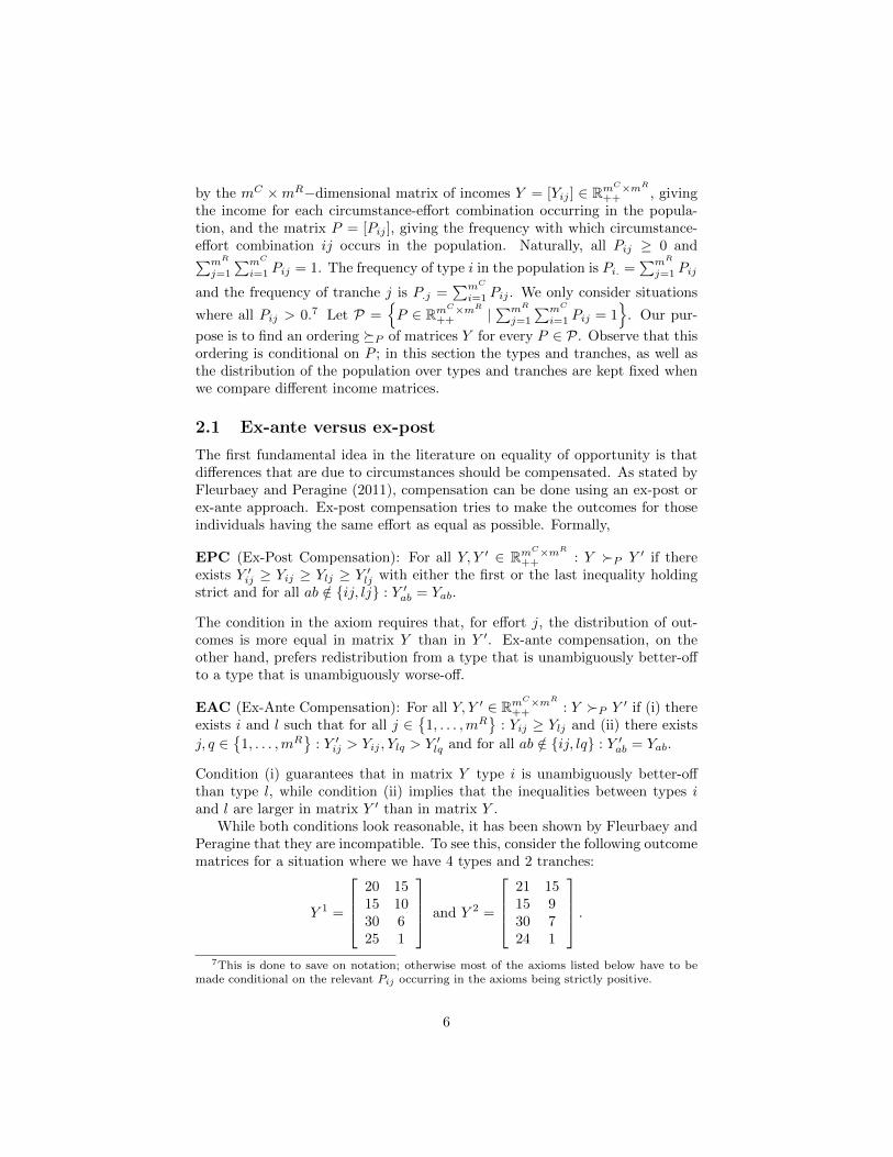
While both conditions look reasonable, it has been shown by Fleurbaey andPeragine that they are incompatible. To see this, consider the following outcomematrices for a situation where we have 4 types and 2 tranches:

Y 1 =

20 1515 1030 625 1

and Y 2 =

21 1515 930 724 1

.

7This is done to save on notation; otherwise most of the axioms listed below have to bemade conditional on the relevant Pij occurring in the axioms being strictly positive.

6

Starting from Y 1, we observe that the first row has better opportunities than thesecond and the third row has better opportunities than the fourth. Increasingthe inequalities between the first and second row (by increasing Y 1

11 and decreas-ing Y 1

22) and increasing the inequalities between the third and fourth row (byincreasing Y 1

32 and decreasing Y 141) results in Y 2, such that, by EAC, we have

Y 1 �P Y 2. Now, start from Y 2, increase the inequalities in the first column (bydecreasing Y 2

11 and increasing Y 241) and increase the inequalities in the second

column (by increasing Y 222 and decreasing Y 2

32) and we get Y 1. Hence, by EPC,Y 2 �P Y 1, contradicting our previous finding. We have thus illustrated thefollowing proposition.

Proposition 1 (Fleurbaey and Peragine (2011)): EPC and EAC are incom-patible.

The existence of this incompatibility implies that, if one wants to evaluate out-come matrices from the perspective of equality of opportunity, a choice has tobe made between ex-ante and ex-post compensation.

2.2 Reward principles

The second fundamental idea in the literature on equality of opportunity is thatefforts should be adequately rewarded. Liberal reward is the first and mostprominent reward principle in the axiomatic literature on fair allocations (see,e.g., Bossert (1995), Fleurbaey (1995a) and Bossert and Fleurbaey (1996)) andfair social orderings (see, e.g. Fleurbaey and Maniquet (2005, 2008)). It statesthat government taxes and transfers should respect differences in incomes thatare due to differences in responsibility. Take two individuals belonging to thesame type but that have exerted different efforts resulting in different pre-taxincomes. According to the liberal reward principle, the tax policy has to respectthe income differences that are due to differences in exerted effort, which impliesthat these individuals should pay the same tax. Let Tij be tax on individuals oftype i and tranche j. The liberal reward principle can then be stated formallyas follows.

LR (Liberal Reward): ∀i ∈{

1, . . . ,mC}

: Tij = Tik for all j, k ∈{

1, . . . ,mR}

.

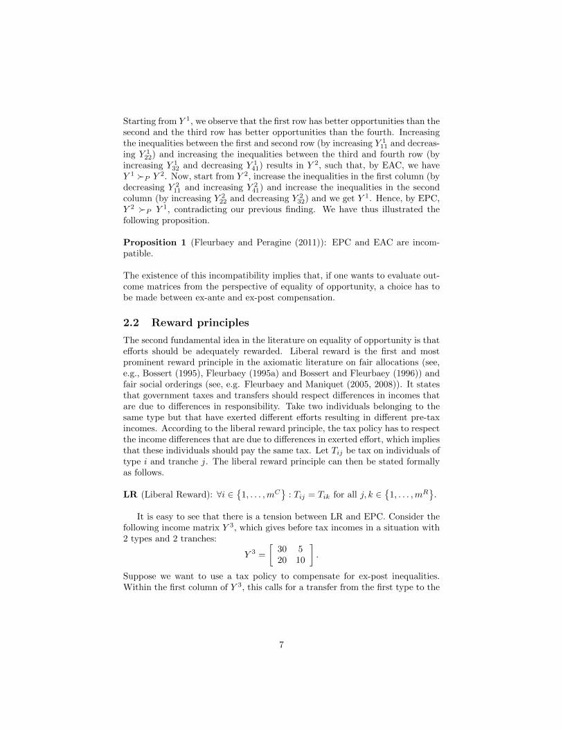
It is easy to see that there is a tension between LR and EPC. Consider thefollowing income matrix Y 3, which gives before tax incomes in a situation with2 types and 2 tranches:

Y 3 =

[30 520 10

].

Suppose we want to use a tax policy to compensate for ex-post inequalities.Within the first column of Y 3, this calls for a transfer from the first type to the

7

second type. Within the second column, an opposite transfer is required. Conse-quently, ex-post compensation can go against LR. Bossert (1995) and Fleurbaey(1995a) have shown that the two principles are, in general, incompatible8.

Proposition 2 (Bossert (1995) and Fleurbaey (1995)): LR and EPC are in-compatible.

A second reward principle which Fleurbaey (2008) calls utilitarian reward hasbeen used more frequently in the empirical literature. The principle says thatrespecting the income differences that are due to differences in effort requireszero inequality aversion with respect to differences in incomes that are due todifferences in efforts, hence we have to focus on the sum of the incomes of thosethat share the same circumstances, leading to the following axiom9.

UR (Utilitarian Reward): For all Y, Y ′ ∈ RmC×mR

++ : Y �P Y ′ if there exists

i ∈{

1, . . . ,mC}

such that∑mR

j=1 YijPij >∑mR

j=1 Y′ijPij and for all l 6= i we have∑mR

j=1 YljPlj =∑mR

j=1 Y′ljPlj .

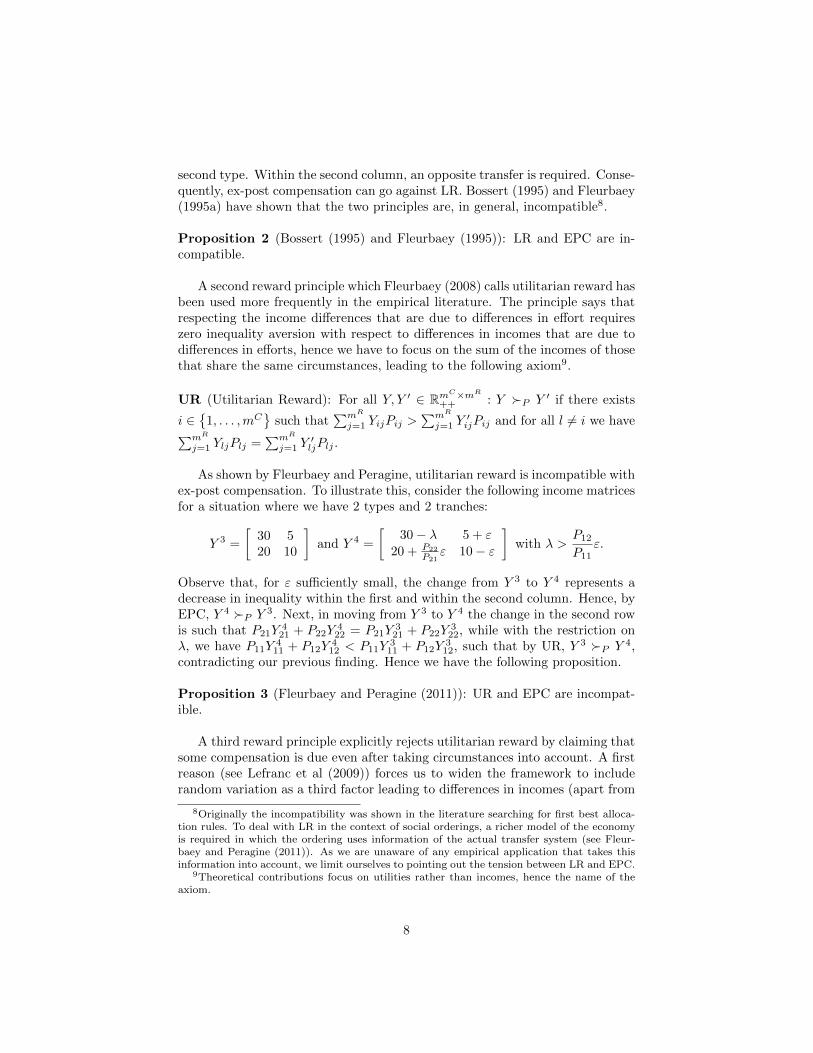
As shown by Fleurbaey and Peragine, utilitarian reward is incompatible withex-post compensation. To illustrate this, consider the following income matricesfor a situation where we have 2 types and 2 tranches:

Y 3 =

[30 520 10

]and Y 4 =

[30− λ 5 + ε

20 + P22

P21ε 10− ε

]with λ >

P12

P11ε.

Observe that, for ε sufficiently small, the change from Y 3 to Y 4 represents adecrease in inequality within the first and within the second column. Hence, byEPC, Y 4 �P Y 3. Next, in moving from Y 3 to Y 4 the change in the second rowis such that P21Y

421 + P22Y

422 = P21Y

321 + P22Y

322, while with the restriction on

λ, we have P11Y411 + P12Y

412 < P11Y

311 + P12Y

312, such that by UR, Y 3 �P Y 4,

contradicting our previous finding. Hence we have the following proposition.

Proposition 3 (Fleurbaey and Peragine (2011)): UR and EPC are incompat-ible.

A third reward principle explicitly rejects utilitarian reward by claiming thatsome compensation is due even after taking circumstances into account. A firstreason (see Lefranc et al (2009)) forces us to widen the framework to includerandom variation as a third factor leading to differences in incomes (apart from

8Originally the incompatibility was shown in the literature searching for first best alloca-tion rules. To deal with LR in the context of social orderings, a richer model of the economyis required in which the ordering uses information of the actual transfer system (see Fleur-baey and Peragine (2011)). As we are unaware of any empirical application that takes thisinformation into account, we limit ourselves to pointing out the tension between LR and EPC.

9Theoretical contributions focus on utilities rather than incomes, hence the name of theaxiom.

8

effort and circumstances): after conditioning on circumstances, incomes arestochastic and since individuals are risk averse, we should evaluate opportu-nity sets in a risk averse way. A second reasoning is ex-post and rejects liberaland utilitarian reward as still some compensation is due after conditioning onan incomplete list of circumstances. Roemer (2010) attacks the liberal rewardprinciple, because liberal reward holds that no more compensation should bemade than that needed to correct inequalities due to different (measured) cir-cumstances. As such, current property rights are no more adjusted than isnecessary to compensate people for disadvantageous circumstances. His pointis that it is difficult to see why the current property rights should be the bench-mark. Hence, he advocates not to focus on incomes, but to take an increasingconcave (inequality adverse) transformation of incomes as the relevant outcomevariable. This can be called an inequality-averse reward principle.

IAR (Inequality Averse Reward): For all Y, Y ′ ∈ RmC×mR

++ : Y �P Y ′ if thereexists i ∈

{1, . . . ,mC

}and δ ∈ R++ such that Yij = Y ′ij − δ ≥ Yik = Y ′ik + δ

and for all ab /∈ {ij, ik} : Y ′ab = Yab.

Again, it is easy to see that this reward principle conflicts with EPC. Con-sider the following income matrices for a situation with 2 types and 2 tranches.

Y 5 =

[10 4020 30

]and Y 6 =

[10 4019 31

]From IAR it follows immediately that Y 5 �P Y 6, while from EPC, Y 6 �P Y 5,a contradiction. As a result, we have

Proposition 4 : IAR and EPC are incompatible.

Propositions 2, 3 and 4 illustrate the difficulty to reconcile EPC with rewardprinciples, a difficulty emphasized in Fleurbaey and Peragine (2011). No suchincompatibilities arise with EAC.

2.3 Luck

Luck is a complex and important factor, which determines most economicoutcomes. Many different factors have been put under the label “luck” byeconomists -see, e.g. Meade (1974). As Lefranc, Pistolesi and Trannoy (2009)neatly explain, different forms of luck deserve different treatment. We distin-guish between forms of luck that require full, partial or no compensation.

The first form of luck reflects Rawl’s idea of social lottery, i.e. economicadvantage that is due to factors related to the family or social origin one hap-pens to fall into, such as family or social networks and influences. Such socialbackground luck is almost universally considered as a circumstance and oughtto be fully compensated for.

The second, genetic luck, captures Rawl’s concept of natural lottery, whereconstituent characteristics of the individual, such as genetically inherited factors

9

like talent, are responsible for differential success. These constituent attributesare thought to be pre-determined and exogenous to the individual and so, ceterisparibus, most authors agree that they are circumstances such that outcomesshould be equal regardless of them. This view is not uncontested, however. Forinstance, Nozick (1974)’s view of self-ownership argues that individuals deserveto benefit from their inborn traits.

The third corresponds to Dworkin’s brute luck, defined as those situationswhere the individual cannot alter the probability that an event takes place. Bydefinition, the individual is not responsible for such events happening and thusit seems reasonable to argue in favor of full compensation. However, since fullcompensation of brute luck may entail huge redistribution, cause large distor-tions thereby diminishing opportunities for all and implementation of compen-sation for brute luck requires a lot of information about individuals which isusually not available, some authors have put forward other, weaker justice re-quirements. For instance, Vallentyne (2002) suggests to compensate only forinitial brute luck, that is, brute luck that occurs before individuals are deemedresponsible for their choices and preferences.10

The last form of luck is Dworkin’s option luck and arises when individualsdeliberately take risk, which is assumed to be calculated, isolated, anticipatedand avoidable. Since by definition risks of option luck are avoidable and takendeliberately, some authors argue that the resulting differences in outcomes arelegitimate. Contrary to that, Fleurbaey (1995b) argues in favor of full com-pensation because with option luck small errors of choices may involve dispro-portionate penalties, which he considers unjust. In his recent book, though,Fleurbaey (2008) provides arguments for partial compensation. He sees optionluck as consisting of two distinct components: on the one hand, the individualdecision to choose a lottery, which is a voluntary act and thus does not deservecompensation, and on the other hand, the randomness intrinsic to any lottery,which should be at least partially compensated for.

To summarize: social background luck and brute luck are circumstances.Also genetic luck is generally considered to be a circumstance. Option luck iseither an effort or a partial circumstance.

3 Measures

The analysis in the previous section highlights the point made in Ooghe et al(2007) that ex-post inequality of opportunity is concerned with the inequalitieswithin each column of Y , while ex-ante inequality of opportunity is concernedwith the inequalities between the rows of Y . This has an important implica-tion: when effort is distributed independently of type 11, full equality of ex-post

10Vallentyne (2002) defines later brute luck as the brute lack that occurs after a ‘canonical’moment (Arneson, 1990) where individuals become responsible for their choices and prefer-ences. As Lefranc et al. (2009) suggest, as long as initial and later brute luck are related,compensation for the former implies at least partial compensation also for the latter.

11Formally, for all j ∈{

1, ...,mR}

and i, k ∈{

1, ...,mC}

with i 6= k it must be thatpij/pi. = pkj/pk.

10

opportunities (absence of inequalities within columns) implies full equality ofex-ante opportunities (equal rows).

When comparing actual income distributions from the perspective of in-equality of opportunity, the framework has to be adjusted to allow comparisonsbetween income distributions with different circumstance-effort distributions i.e.with different matrices P . In addition, the framework should allow for unob-served and random variables. Hence individual k ’s income, yk, is assumed todepend on his circumstances aCk , his efforts, aRk , unobserved variables uk and arandom term ek, such that

yk = g(aCk , a

Rk , uk, ek

)where g : RdC

× RdR

× R× R→ R++.

As the uk is unobserved, and the functional form g is unknown, the paramet-ric approach imposes a functional form to estimate the equation, yielding thefunction

g(aCk , a

Rk , ek

)where g : RdC

× RdR

× R→ R++.

An estimate of yk, yk, can be obtained by setting ek equal to zero in the aboveequation. Observe that the effect of the unobserved variable will be taken overby the effect of observed circumstances and efforts, to the extent that these arecorrelated with the unobserved variables. The rest of the effect of unobservablesas well as specification errors go into the estimated random variation, ek, whichis defined implicitly by the equation yk = g

(aCk , a

Rk , ek

). For some purposes,

it is convenient to estimate incomes as a function of, on the one hand, eithercircumstances or efforts and, on the other hand, random variation:

gC(aCk , ek

)where gC : RdC

× R→ R++,

gR(aRk , ek

)where gR : RdR

× R→ R++.

These equations can be used to estimate incomes by, respectively, yCk and yRkby setting ek equal to zero. In the first (second) case, the effect of both omit-ted efforts (circumstances) and unobservables are taken over by circumstances(efforts) to the extent that these are correlated. The rest of their effect as wellas specification errors go into the estimated random variation, eCk (eRk ) whichis defined implicitly by the equation yk = gC

(aCk , e

Ck

)(yk = gR

(aRk , e

Rk

)). For

future reference, let Nk. ={i ∈ N | aCi = aCk

}and N.k =

{i ∈ N | aRi = aRk

},

be the sets of individuals sharing the circumstances aCk (belong to the sametype) and efforts aRk (belong to the same tranche), respectively.

Following Pistolesi (2009), we can distinguish between a direct and indirectapproach to the measurement of inequality of opportunity. Other approaches inthe literature are based on stochastic dominance or deviations between actualincome and norm income. We discuss these approaches in turn and concludethe section with an overview.

3.1 Direct measures

A first approach determines the amount of inequality of opportunity directly byestimating the inequality in a counterfactual income distribution yc in which all

11

inequalities due to differences in effort have been eliminated, such that only theinequality that is due to differences in circumstances is left:

I (yc) . (1)

The crucial distinction between ex-ante and ex-post approaches lies in theconstruction of the counterfactual yc. From an ex-ante viewpoint, we shouldreplace every individual’s actual income by some evaluation of his opportunityset. Evidently, the value assigned to his opportunity set should not depend onhis own effort level.

So far the ex-ante approaches proposed to implement I (yc) rely mostly ona non-parametric estimate of the value of an individual’s opportunity set. Thefollowing proposals have been made in the literature:

yc1k =1

|Nk.|∑i∈Nk.

yi, (2)

yc2k =1

|Nk.|∑i∈Nk.

iyi, (3)

where yi is the i−th smallest level of income in the set Nk.. The first proposalis due to Van de gaer (1993) and measures the value of the opportunity set bythe average income of those that are of the same type as the individual consid-ered. This equals the surface under the Pen parade of the income distribution ofthe individual’s type. The income distribution yc1, in which every individual’sincome is replaced by the mean income of his type is called the “smoothed in-come distribution” by Checchi and Peragine (2010). As the specification impliesno inequality aversion for differences in incomes that are due to responsibility,this specification is inspired by utilitarian reward. Since all income differencesthat are due to circumstances are morally objectionable, Van de gaer proposesan inequality index with infinite inequality aversion.12 Checchi and Peragine(2010) and Ferreira and Gignoux (2011) point out that most standard inequal-ity indices measuring inequality of opportunity as inequality in the smoothedincome distribution satisfy, apart from utilitarian reward an additional desir-able property: when a transfer is made from an individual in a richer type toan individual in a poorer type, regardless of the former individual being poorerthan the latter, inequality of opportunity falls. They express a preference forthe mean log deviation, because the index allows an exact decomposition oftotal income inequality into (1) with (2) as the value of each individual’s op-portunity set and a counterfactual in which all types have an opportunity setof the same value13, since it is the only decomposable inequality measure thatis path independent (Foster and Shneyerov, 2000). Recently, Aaberge et al.(2011) proposed a rank dependent measure (which includes the Gini coefficient

12As this ordering is only sensitive to what happens to the worst-off type, it does not satisfyaxioms EAC nor UR defined in section 2. It is straightforward to formulate a leximin extensionof the ordering that satisfies both axioms, however.

13This counterfactual is equal to (12) below.

12

as a special case) as inequality index to measure ex-ante inequality in the vectoryc1. This procedure shares the two standard properties mentioned above, butdoes not have the exact decomposition property. The second proposal, (3), wasformulated by Lefranc et al (2008) and measures the value of the opportunityset by the surface under the generalized Lorenz curve of the income distribu-tion of the individual’s type. As such, it embodies the inequality averse rewardprinciple. They propose a Gini coefficient to measure ex-ante inequality in thevector yc2.

So far, the only parametric estimate of yc has been put forth by Ferreiraand Gignoux (2011). As efforts can be correlated with circumstances (see alsosection 4.2.4), they propose to measure the value of an individual’s opportunityset as

yc3k = gC(aCk , 0

), (4)

such that everybody’s opportunity set is valued by the reduced form estimateof his income, given his circumstances and with the random term equal to itsexpected value 0. As all within-type inequalities are eliminated in the vector yc3,this is indeed an ex-ante approach: only between type inequalities are relevant.Ferreira and Gignoux (2011) interpret the resulting inequality measure as aparametric estimate of (1) with (2) as the value of the opportunity sets, suchthat, for the reasons given above they advocate the use of the mean log deviationas inequality index.

An evident parametric alternative, closer in spirit to (2) would rely on theestimate of g rather than gC , and use

yc4k =1

|Nk.|∑i∈Nk.

g(aCi , a

Ri , 0

). (5)

Compared to the Ferreira and Gignoux measure described above, using yc4 ina measure of inequality of opportunity (1), has the advantage that it deals withthe covariance between aC and aR in a more flexible type-dependent way. Thedisadvantage is that, contrary to yc3 the estimation of g, requires observationson aR. We are unaware of any application of yc4.

From an ex-post point of view, to eliminate all inequalities that are dueto efforts, we replace every individual’s income by the income he could haveobtained if he would have put in a reference level of effort. Roemer (1993) wasthe first to propose such an ex-post approach to compute (1) and used a non-parametric procedure. He fixes a reference value for the responsibility variable

aR and defines set NaR

k. ={i ∈ Nk. | aRi = aR

}, which contains all individuals

that have the same circumstances as individual k and have the reference valuefor the responsibility vector. Next define

yc5k(aR)

=1∣∣NaR

k.

∣∣ ∑i∈NaR

k.

yi, (6)

the average income of those that are of the same type as individual k and have

13

the reference value for the responsibility characteristic.14 Applying (1) resultsin an inequality measure whose value depends on the reference value aR, whichwe denote by

I(yc5(aR)).

Roemer argues that the choice of reference value aR is arbitrary, and proposestherefore the following averaged inequality measure:

1

n

n∑l=1

I(yc5(aRl)). (7)

As all inequalities that are due to differences in circumstances are morally objec-tionable, Roemer proposes to apply an infinite inequality aversion to computeI(yc5(aRl))

in (7) and puts I(yc5(aRl))

equal to the lowest value of the vector

yc5(aRl)

divided by mean income.15 In a recent paper, Aaberge et al. (2011)

propose to use a rank dependent measure to compute I(yc5(aRl )

)in (7).

The ex-post approach to implement (1) semi-parametrically was proposedby Pistolesi (2009)16 and it is obtained by setting a reference value for theresponsibility variable, aR in the estimate of the function g

(aCk , a

Rk , ek

):

yc6k(aR)

= g(aCk , a

R, ek). (8)

Compared to the non-parametric methodology, the parametric methodology hasthe advantage that it always yields meaningful estimates for yc6k , even when thecombination

(aCk , a

R)

does not occur in the sample. Pistolesi experiments withdifferent inequality measures: he uses the Theil index, the mean log deviation,the half squared coefficient of variation and the standard deviation of logs. Inthe computation of yc6, ek can be set equal to zero, or to its estimated value ek.The former amounts to treating ek as an effort variable with reference value zero,the latter to treating it as a circumstance. Most authors take the mean value foreffort in the sample as the reference value aR. Following Roemer, one can use anaveraged inequality measure similar to (7), where yc6

(aRl)

replaces yc5(aRl). We

are unaware of any application of such a direct parametric averaged inequality ofopportunity measure. There exist some theoretical results on the consequencesof taking different reference values in the context of particular models -see, e.g.,Luttens and Van de gaer (2007), but the choice of reference value remains anunsettled issue.

3.2 Indirect measures

A second approach determines the amount of inequality of opportunity indi-rectly by comparing the inequality in the actual distribution of income, I (y),

14In case NaR

k. = ∅ this procedure runs into difficulties. If Roemer’s identification axiom isused to identify effort (see section 4.2.1) this does not occur.

15As it is only sensitive to the lowest income for each effort, the index does not satisfy EPCas defined in section 2. It is easy to formulate a leximin extension that satisfies it, however.

16Schokkaert el al. (1998) already applied a similar procedure in a health context.

14

to the inequality in a counterfactual income distribution where there is no in-equality of opportunity I

(yE0

). This results in the measure

ΘI

(y, yEO

)= I (y)− I

(yEO

). (9)

Almost all applications of indirect measures to inequality of opportunity con-struct a counterfactual income distribution that eliminates all inequality be-tween individuals having the same effort. As such, they are measures of ex-postinequality of opportunity, but, remember that when effort is distributed inde-pendently of type, absence of inequality of opportunity ex-post implies equalityof opportunity ex-ante. We show that for each of the counterfactuals listedin the previous subsection, there exists a dual counterfactual in the indirectapproach that implies ex-post equality of opportunity.

Consider first the dual counterfactuals associated with ex-ante approachesin section 3.1. The dual counterfactual to (2) was proposed by Checchi andPeragine (2010): they construct the counterfactual

yEO1k =

1

|N.k|∑i∈N.k

yi, (10)

which replaces every income by the average income of those sharing the sameefforts and compute (9), using the mean log deviation as inequality measure.Evidently, (10) expresses the idea of utilitarian reward. It is straightforward toprovide an alternative, based on inequality averse reward, by defining the dualto (3):

yEO2k =

1

|N.k|∑i∈N.k

iyi.

Also the duals to the parametric ex-ante approaches can be used to definecounterfactuals implying ex-post equality of opportunity: the first inspired by(4), the second by (5):

yEO3k = gR

(aRk , 0

),

yEO4k =

1

|N.k|∑i∈N.k

g(aCi , a

Ri , 0

).

To estimate the relevant equations in both cases we need observations on aR.The second alternative has the advantage of dealing with the correlation betweencircumstances and efforts in a more flexible tranche-dependent way.

Next, consider the duals based on the counterfactuals in the direct ex-postapproach. To obtain the dual to Roemer’s direct ex-post non-parametric ap-proach (6) and (7), fix a reference value for circumstances, aC . Next define

yEO5k

(aC)

=1∣∣NaC

.k

∣∣ ∑i∈NaC

.k

yi,

15

the average income of those that have the same responsibility vector as indi-vidual k and have the reference value for circumstances. In the vector yEO5

everybody with the same responsibility vector has the same income, such thatthere is full ex-post equality of opportunity. To eliminate the dependence ofthe resulting measure of inequality of opportunity on the choice of referencecircumstances, I

(yEO

)in (9) can be replaced by the averaged inequality index

1

n

n∑l=1

I(yEO5

(aCl)).

We have not yet seen anyone suggesting this approach.The dual to (8) is due to Bourguignon et al. (2007): fix a reference value

for the circumstance variable, aC to obtain

yEO6k

(aC)

= g(aC , aRk , ek

). (11)

They use the Theil index as inequality measure, Pistolesi (2009) uses, in addi-tion, the mean log deviation, the half squared coefficient of variation and thestandard deviation of logs. Also here ek can be set equal to zero or to its es-timated value ek. The former treats it as a circumstance with reference valuezero, the latter as an effort. Most authors take the mean value for circumstancesin the sample as the reference value aC . Again this choice can be criticized forbeing arbitrary. This can be overcome by replacing I

(yEO

)in (9) with the

averaged inequality index

1

n

n∑l=1

I(yEO6

(aCl)).

We are unaware of any application of such a parametric aggregate indirectinequality of opportunity measure.

All the above approaches rely on counterfactuals ensuring ex-post equality ofopportunity and thereby entail ex-ante equality of opportunity when efforts aredistributed independently of type. But even then, however, ex-post equality ofopportunity is not necessary for ex-ante equality of opportunity. In the literaturethere is only one proposal that assigns to individuals opportunity sets of equalvalue, without imposing full ex-post equality of opportunity. This proposal isthe non-parametric proposal by Checchi and Peragine (2011), which evaluatesindividual’s opportunity sets by (2) and constructs the counterfactual

yEO7k = yk

µ (y)

yc1k, (12)

where µ (y) is mean income of vector y such that everybody’s income is scaledup or down by the ratio of average income and the value of his opportunity setas measured by (2). Observe that 1

|Nk.|∑

i∈Nk.yEO7i = µ (y), such that, when

opportunity sets are measured as in (2), in distribution yEO7 everybody has

16

indeed an opportunity set of the same value. They use the mean log deviation asinequality measure. Evidently, this procedure can be applied when opportunitysets are valued differently, like, e.g., when they are valued according to (2). Thecorresponding counterfactual becomes

yEO8k = yk

µ (y)

yc2k.

3.3 Stochastic dominance

The stochastic dominance approach to the measurement of inequality of oppor-tunity originates from the ex-ante framework.17 In our discussion in section3.1, we have seen two non-parametric measures of the value of an opportunityset, (2) and (3), the first being inspired by utilitarian reward, the second by in-equality averse reward. In both cases, the value of an individual’s opportunityset is an increasing function of the outcomes obtained by those that belong tohis type. This is an uncontroversial starting point for an ex-ante approach andsuggests that ex-ante inequality of opportunity can be established as soon assome type’s cumulative distribution function of income first order stochasticallydominates another type’s cumulative distribution function. Hence the absenceof first order stochastic dominance between type’s cumulative distribution func-tions can be seen as a test for ex-ante equal opportunities. Formally, let, for alli ∈

{1, . . . ,mC

}, Fi (y) denote the cumulative distribution function of income

of type i. A weak test of ex-ante equality of opportunity tests the followingcondition.

AFOSD (Absence of First Order Stochastic Dominance): there does not existi, l ∈

{1, . . . ,mC

}, such that, for some y ∈ R+ : Fi (y) < Fl (y) and for all

y ∈ R+ : Fi (y) ≤ Fl (y).

If one adheres to an inequality averse reward principle, one can go further.In that case, as advocated persuasively by Lefranc et al. (2009), absence of firstorder stochastic dominance can be strengthened to the requirement of absenceof second order stochastic dominance between types’ cumulative distributionfunctions.

ASOSD (Absence of Second Order Stochastic Dominance): there does not existi, l ∈

{1, . . . ,mC

}, such that, for some y ∈ R+ :

∫ y

0Fi (y) dy <

∫ y

0Fl (y) dy and

for all y ∈ R+ :∫ y

0Fi (y) dy ≤

∫ y

0Fl (y) dy.

3.4 Norm based measures

We know from proposition 2 that liberal reward and ex-post compensation areincompatible. The axiomatic literature on (opportunity) fair allocations pro-

17In section 4.2.1, we will see that under a frequently made hypothesis in empirical work(Roemer’s identification axiom) the tests developed here become also relevant from an ex-postperspective.

17

ceeded by characterizing first best redistribution mechanisms that satisfy weak-ened versions of the principles -see, Fleurbaey (2008) for an overview. Suchredistribution mechanisms assign to every individual, as a function of his cir-cumstances and efforts, an income in such a way that both liberal reward andex-post compensation are to some extent satisfied. As shown by Devooght(2008) and Almas et al (2011), these (partial) solutions to the liberal reward/ ex-post compensation dilemma can be incorporated in a measure of equalityof opportunity or, in their language, a measure of offensive or unfair incomeinequality, respectively. The idea is to treat the level of income that these rulesassign to a particular individual as the norm that he should get, and measureoffensive inequality by the distance between the actual income vector y and thenorm income vector yn. Formally, one computes

I (y, yn) , (13)

where the function I (·, ·) has to satisfy at least two requirements. First, sinceit matters how far each individual is from his norm income, the measure mustsatisfy partial symmetry (i.e. be invariant to permutations of (yk, y

nk ) pairs),

but not full symmetry (where different permutations can be applied to the vec-tors y and yn). Second, due to the heterogeneity of the population in termsof compensation and responsibility characteristics, the usual transfer principledoes not apply. These arguments induce Devooght (2008) to propose Cowell’s(1985) measure of distributional change, a special case of which is the general-ized entropy class. Measures of distributional change have the property that atransfer from a rich to a poor person decreases the value of the measure if andonly if the ratio of the actual income of the rich and poor person is larger thanthe ratio of their norm incomes. Almas et al. (2011) define unfair treatment ofeach individual as the absolute value of the difference between his actual incomeand norm income and propose an unfairness Gini to aggregate these differences.Here, a transfer from a person who is less unfairly treated to a person who ismore unfairly treated diminishes the value of the index.

Devooght takes the egalitarian equivalent allocation, first suggested in theequality of opportunity context by Bossert and Fleurbaey (1996), as the norm.Almas et al. take in the main part of their analysis the generalized propor-tionality allocation, first proposed by Bossert (1995), as the norm.18 As a finalremark, the computation of the norm incomes proposed by Devooght and Al-mas requires estimation of the outcome function, g

(aCk , a

Rk , ek

). To compute

the norm, in both papers, the ek is replaced by its estimated value ek.Other first-best redistribution mechanisms exist that do not require the esti-

mation of g(aCk , a

Rk , ek

)and can be computed non-parametrically -see, e.g., the

18They do sensitivity analysis and report results for two versions of the egalitarian equivalentnorm –which requires the choice of reference circumstances– and also for the conditionalequality norm –which requires the choice of reference efforts. In both cases, without muchargument, the reference is set equal to its average value in the sample. Their empirical resultsappear insensitive to the choice of norm distribution, but it is unclear whether the choice ofthe reference value matters or not.

18

observable average conditional egalitarian and the observable average egalitar-ian mechanism proposed in Bossert et al (1999). They have not yet been usedin the norm based approach and can be combined with any inequality measurethat satisfies partial symmetry and does not satisfy the usual transfer principle(like the unfairness Gini, the generalized entropy or the divergence measuresdiscussed by Magdelou and Nock (2011)) to obtain valid non-parametric alter-natives for the norm based approach.

3.5 Overview

Table 1 summarizes our survey of approaches to the measurement of inequalityof opportunity. Six observations follow from our survey.

A first observation is that we propose several new measures. New indirectex-post measures (yEO2, yEO3, yEO5) are generated by constructing counterfac-tuals with complete ex-post equality on the basis of the counterfactuals used inthe direct approach. A new parametric measure of direct ex-ante (yc4) and itsdual indirect ex-post measure (yEO4) combines features of the non-parametricapproach (yc1 and yEO1, respectively) and the parametric approach (yc3 andyEO3, respectively). We also showed how Checchi and Peragine (2010)’s indi-rect ex-ante approach can be adjusted to deal with inequality averse reward inyEO8. We argued that for the approaches that require the choice of a referencevalue for either efforts (yc5 and yc6) or circumstances (yEO5 and yEO6) shouldreceive more attention. Roemer’s averaged inequality of opportunity measuremay overcome the arbitrariness of the choice of reference value to some ex-tent. Finally, we pointed out that the norm income approach can be appliednon-parametrically by using the observable average egalitarian equivalent or theobservable average conditional egalitarian allocation mechanisms, proposed byBossert et al (1999).

A second observation is that many different inequality measures have beenused, often without much justification. The only exceptions are in the normbased and in the direct measurement approach. In the former, an inequalitymeasure that replaces the standard transfer principle by a more suited transferprinciple and satisfies partial symmetry is necessary. In the latter, an infiniteinequality aversion was motivated from the normative point of view that allinequalities that are due to differences in circumstances are unacceptable. Webelieve that this argument is a powerful one for welfare measurement, but isless convincing for measuring inequality of opportunity as it ignores most in-equalities. The indirect approach is often used to answer the question to whichextent income inequality is due to inequality of opportunity. This is a mean-ingful question for any plausible measure of income inequality, but for trueopportunity egalitarians, those concerned with equality of opportunity ratherthan equality of outcome, the aswer to the question is irrelevant. Sometimesadditional arguments can be used to single out a particular measure or sets ofmeasures. For instance, Checchi and Peragine (2010) and Ferreira and Gig-noux (2011) motivate the use of the mean log deviation by pointing out that itis the only decomposable inequality measure that is path independent (Foster

19

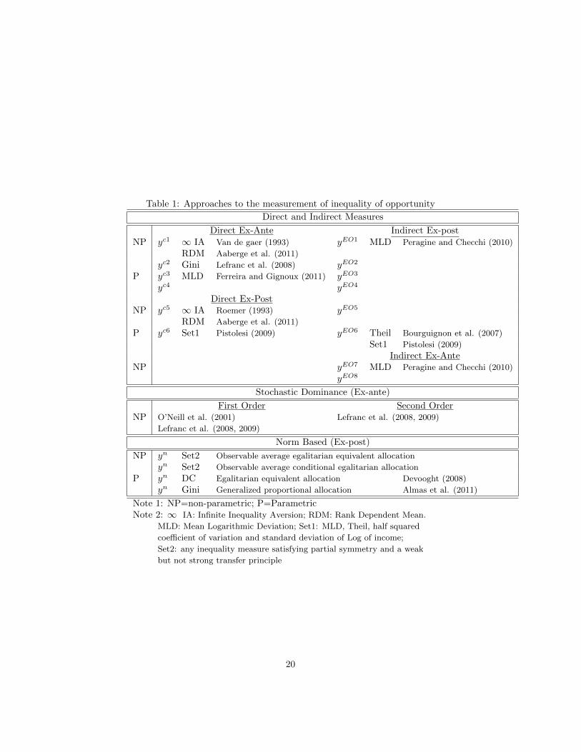
Table 1: Approaches to the measurement of inequality of opportunity

Direct and Indirect Measures

Direct Ex-Ante Indirect Ex-postNP yc1 ∞ IA Van de gaer (1993) yEO1 MLD Peragine and Checchi (2010)

RDM Aaberge et al. (2011)

yc2 Gini Lefranc et al. (2008) yEO2

P yc3 MLD Ferreira and Gignoux (2011) yEO3

yc4 yEO4

Direct Ex-PostNP yc5 ∞ IA Roemer (1993) yEO5

RDM Aaberge et al. (2011)

P yc6 Set1 Pistolesi (2009) yEO6 Theil Bourguignon et al. (2007)

Set1 Pistolesi (2009)

Indirect Ex-AnteNP yEO7 MLD Peragine and Checchi (2010)

yEO8

Stochastic Dominance (Ex-ante)

First Order Second OrderNP O’Neill et al. (2001) Lefranc et al. (2008, 2009)

Lefranc et al. (2008, 2009)

Norm Based (Ex-post)

NP yn Set2 Observable average egalitarian equivalent allocation

yn Set2 Observable average conditional egalitarian allocation

P yn DC Egalitarian equivalent allocation Devooght (2008)

yn Gini Generalized proportional allocation Almas et al. (2011)

Note 1: NP=non-parametric; P=ParametricNote 2: ∞ IA: Infinite Inequality Aversion; RDM: Rank Dependent Mean.

MLD: Mean Logarithmic Deviation; Set1: MLD, Theil, half squared

coefficient of variation and standard deviation of Log of income;

Set2: any inequality measure satisfying partial symmetry and a weak

but not strong transfer principle

20

and Shneyerov, 2000), which implies that non-parametric direct and indirectapproaches yield the same results.19 Pistolesi (2009) uses for the direct mea-surement approach a whole set of inequality measures, as his main concern isto compare direct and indirect parametric methodologies.

A third observation is that the stochastic dominance approach is by its verynature non-parametric. We motivated it so far from an ex-ante point of view,but in section 4.2.1, proposition 5, we will argue that, if Roemer’s identificationaxiom is assumed, rejection of the absence of first or second order stochasticdominance implies ex-post inequality of opportunity.

A fourth observation is that norm based approaches have only been appliedusing the income allocations from the axiomatic literature concerned with ex-post inequality of opportunity as the norm distribution. The counterfactualsused in the indirect approach can also be used as the norm income distribu-tion. Using either yEO7 or yEO8 yields a norm based on ex-ante equality ofopportunity without requiring ex-post equality of opportunity when efforts aredistributed independently of type.

Fifth, it is important to realize that the indirect approach cannot be in-terpreted as a norm based approach. In the norm based approach it cruciallymatters who gets what, while in the indirect approach this is not the case, asdifferent permutations can be applied to y and yEO in (9). This makes the indi-rect approach unattractive as a normative measure of inequality of opportunity.It can be used to decompose income inequality into inequality that is due to cir-cumstances and efforts, but only if a suitable inequality measure is chosen, suchthat the inequality that is due to circumstances is a meaningful direct estimateof inequality of opportunity -see the discussion following equation (3).

Finally, as especially the previous observations make clear, the theoreticalbasis for many of the inequality measures that are used or can be thought of,remains rather weak. A lot of work remains to be done to sort out the attractivefrom the unattractive ones.

4 Data imperfections

In this section we confront some important problems facing the application ofthe framework in the previous section: how to choose and measure circum-stances, how to measure efforts and the consequences of imperfectly measuringcircumstances or efforts.

4.1 Circumstances

Measured inequality of opportunity crucially depends on the set of circum-stances chosen. The larger the set of circumstances, the larger the inequalityof opportunity.20 Thus, a proper selection of the circumstances is paramount.

19From the discussion in the paragraph below equation (3), it follows that for the mean logdeviation, θI

(y, yEO7

)= I (y)− I

(yEO7

)= I

(yc1

).

20Notice, thought, that if there is a negative correlation between the ’new’ circumstances,which were previously classified as effort, and the ’old’ circumstances, which were already

21

Often researchers are limited by the scarcity of data on circumstances beyondbasic individual characteristics and family background, such that most empir-ical studies are confined to a small set of basic circumstances. We discuss thisissue in section 4.1.2. In principle, the set of circumstances that should be in-cluded follows from the answer to the question what should individuals be heldresponsible for. This is taken up next.

4.1.1 Selection of circumstances

Three prominent views can be found in the political philosophy literature onthe difficult and unsettled question what people are responsible for.

A first view argues that individuals ought to be held responsible only forwhat lies within their control –as defended, inter alia, by Arneson (1989), Co-hen (1989), and Roemer (1993, 1998a). Control is related to the recognitionof free will, the existence of which is sometimes disputed. Those who deny theexistence of free will, such as the hard determinists, take an extreme positionand include nearly all observables in the circumstance set and consider almostall inequalities as unfair. Most empirical studies, however, adopt a possibilistcriterion, which is consistent with the existence of free will, and classifies ascircumstance family background variables, such as parental education or occu-pation, individual characteristics, such as gender, ethnicity or age, and innatecharacteristics, such as IQ. Under this view, contextual variables such as ac-cess to basic services, e.g. clean water, sanitation, electricity or transportation,should also be included in the circumstance set.

A second approach contends that individuals ought to be held responsible fortheir preferences and the ensuing choices –as advocated, intera alia, by Rawls(1971), Dworkin (1981a, 1981b), Van Parijs (1995) and Fleurbaey (2008). Un-der this view, the set of circumstances gets reduced to a minimal set of variablesincluding innate characteristics or traits such as talent or beauty.21 In contrast,variables such as gender or ethnicity, which are typically classified as circum-stances in empirical analyses, should belong to the realm of responsibility if thedifferential effect they bring about reflects exclusively differences in preferences,i.e. are not the result of discriminatory treatment.22

included in the set, opportunity inequality may decrease, and not increase (Cappelen andTungodden, 2006).

21Since Hamermesh and Biddle (1994) we know that physically attractive workers obtainsizable rents from their looks. More recently, Mobius and Rosenblat (2006) identified threetransmission channels for such beauty premium.

22As Fleurbaey (2008) persuasively explains, under the believe that free will exists, thecontrol approach comes very close to the preference approach to responsibility, as genuinecontrol is “typically defined in terms of choices reflecting authentic preferences” (p. 250).In addition, the preference approach may be extended to hold people responsible for anypreference or characteristic which they endorse, i.e. which they would have chosen were theyin control. Notwithstanding all this, he goes on to argue, the two approaches may yieldsubstantively different conclusions when advantage results from preferences, which have notbeen chosen in any sense and are not endorsed by the individual. Since control, choice andendorsement are very hard to observe, it is very difficult to test empirically whether the controland the preference approach are close or far from each other.

22

In line with Nozick (1974)’s self-ownership argument,23 a third view consid-ers that individuals are entitled to the products of all personal characteristics,including genetic ones such as innate talent. This leads to the other extreme po-sition where the set of circumstances is empty, and all inequalities are legitimate.There is no room for equality of opportunity in this view.

4.1.2 Unobserved circumstances

As soon as we agree that there are circumstances for which people should becompensated, we enter the realm of equality of opportunity and need to measurethese circumstances: application of equal opportunity theories without observ-ing any circumstances is impossible. In practice, measuring circumstances iseasier than measuring efforts and different datasets can be combined to obtaina more comprehensive set of circumstances, as in Ferreira et al (2011). Eventhen an exhaustive list of circumstances is typically not available, however. As-sume that we have directly observed the relevant efforts, but did not observe allrelevant circumstances. In that case, the partitioning of the population in truetypes is a finer partitioning than the one on the basis of observed types and theoutcomes of the observed types is a weighted average of outcomes conditionedon true types with weights determined by the population frequency of the truetypes in the observed types. This leads to a downward bias in ex-post inequalityof opportunity, as the inequality within the columns based on observed typesis smaller than in the columns based on the true types. Similarly, as the rowsassociated with the observed types are weighted averages of the rows associatedwith the true types, unobserved circumstances lead to an underestimation ofex-ante inequality of opportunity. Ferreira and Gignoux (2011) in particularstress that estimates of inequality of opportunity based on an incomplete listof circummstances should be interpreted as a lower bound of true inequality ofopportunity.

4.1.3 Contribution of different circumstances to inequality of oppor-tunity

Consider the indirect measurement approach (see section 3.2), which determinesthe amount of income inequality that remains when there is no inequality ofopportunity left. The Bourguignon et al. (2007) approach determines thiscounterfactual income distribution as the one that results when everyone hasthe same reference circumstances -see (11). By not equalising all circumstancesat once Bourguignon et al. (2007), show that it is possible to estimate thepartial effect of one (or a set) of circumstance variables J , controlling for theothers (j 6= J). Following their specification of the function g

(aCk , a

Rk , ek

), let

ln yk = βCaCk + βRaRk + uk,

23The self-ownership argument states that individuals own themselves and thus have alegitimate claim over the products of their talents and abilities.

23

and construct alternative counterfactual distributions

yEO(J)k = exp

[βJaCJ

k + βj 6=JaCj 6=Jk + βRaRk + ek

],

where aCJk is the vector of reference values of the circumstances in set J and

aCj 6=Jk the vector of actual circumstances of individual k of the circumstances in

the complement of the set J . This allows to compute inequality of opportunitydue to a given (set of) circumstance(s), J in spirit of the indirect ex-ante para-metric approach by replacing yEO in (9) by yEO(J) defined above. To computeeach circumstance’s contribution to overall inequality one can use the Shapleydecomposition (Shorrocks, 1999), which avoids the path dependency problemwhereby results are sensitive to the ordering in which circumstances are put attheir reference value in the analysis. This approach has become quite popularrecently (see, e.g. Bjorklund et al. (2011)). Usually, the mean value of thecircumstance characteristic is taken as the reference value.

4.2 Constructing measures of effort

To apply ex-post compensation, we need to identify individuals’ efforts in a nor-matively attractive way. Effort variables are shaped by circumstances. Prefer-ences and tastes, for instance, are partly shaped by family background. Whetherwe should correct for this is closely related to the answer to the question whatpeople are responsible for (see subsection 4.1.1). Those defending responsibilityfor preferences (and the resulting choices) will typically argue that it does notmatter where these preferences come from, as long as people identify with them.Those defending responsibility by control (like Roemer (1993, 1998a and 1998b)argue that, as people do not control their circumstances, raw effort variablesshould be cleaned to obtain normatively relevant efforts. This view is dominantin most empirical applications to date. We discuss four different proceduresused in the literature to construct normatively relevant effort(s).

4.2.1 Unobservable effort, non-parametric identification

If no effort variables are observed, the lack of data can only be overcome withsome auxiliary hypotheses. The most elegant and frequently used comes fromJohn Roemer (1993), and is stated as follows.

RIA (Roemer’s Identification Assumption): those that are at the same per-centile of the distribution of income conditional on their type have exercised thesame degree of effort.

This assumption allows us to take the percentile within the income distri-bution of an individual’s type as the normatively relevant measure of his effort.By construction effort is distributed uniformly over [0, 1] for all types and con-sequently independently distributed of type.

RIA can be derived from more fundamental hypothesis about the incomegenerating process and the distribution of circumstances and effort. More in

24

particular, as pointed out by Fleurbaey (1998, p.221), RIA assumes that (A1)the multi-dimensional effort variables aRi can be aggregated into a scalar measureof responsibility ari in such a way that with every value for aRi correspondsexactly one value for ari and that income is a strictly increasing function of ariand (A2) ari is distributed independently of aCi . As argued by Roemer, while(A2) is, within the responsibility by control view, a natural assumption fornormatively relevant effort, assumption (A1) is very strong.

The assumption is very powerful, for, thanks to RIA, the equality of opportu-nity framework becomes operational even when effort is unobservable: one onlyneeds to compute the cumulative distribution of incomes conditional on types,and equate the percentile corresponding to each individual’s income within thecumulative distribution of his type to his level of effort. This allows the con-struction of a new matrix Y R, to which one can apply all the ideas mentionedin section 2 and all the non-parametric procedures from table 1. Observe that,by construction, all elements in the same row of Y R contain the same numberof individuals.

The plot of the inverse of the cumulative income distributions conditional ontypes gives for each percentile the corresponding income level. If the plots fortwo types differ at some percentile, we have ex-post inequality of opportunity:for the same degree of responsibility, two individuals of different types receivea different level of income. Fixing the percentile value and reading the corre-sponding income values for all types is like looking at a particular column in thematrix Y of the previous section; it amounts to taking an ex-post perspective.Alternatively, looking at the cumulative distribution function for each type isvery much like looking at a row in the matrix Y , with a continuous effort vari-able. Hence the cumulative distribution function also provides the informationnecessary for an ex-ante perspective.

The above insights provide the basis for analyzing conditional distributionfunctions from a perspective of equality of opportunity. At the one hand, withunobservable effort (and RIA), ex-post equality of opportunity is satisfied if andonly if the following property holds true.

ECDF (Equal Cumulative Distribution Functions): for all i, l ∈{

1, . . . ,mC}

and for all y ∈ R+ : Fi (y) = Fl (y).

At the other hand, ex-ante equality of opportunity directly leads to therequirement of the absence of first order stochastic dominance between types’cumulative distribution functions, i.e. condition AFOSD in section 3.3. Wenow have recovered the result that since effort is distributed independentlyof type, full equality of ex-post opportunities implies full equality of ex-anteopportunities, stated in the first paragraph of section 3.

Proposition 5: Accepting RIA, ex-post equality of opportunity implies ex-anteequality of opportunity.

When RIA is imposed, testing whether (AFOSD) can be rejected can thus beinterpreted as a weak test of ex-post equality of opportunity (ECDF).

25

Finally, suppose that we apply RIA and use the percentile within type as ameasure of effort to construct the matrix Y , but we only condition the cumula-tive distribution functions on the vector of observable circumstances aCO, not onthe entire vector of circumstances aC =

[aCO, aCU

], where aCU are unobserved

circumstances. Strong assumptions are necessary to relate the results obtainedon the basis of the constructed matrix Y to the true matrix Y . To see this,consider the simple case where aCO and aCU are one-dimensional. Moreover,assume that aCU is either aCU or aCU . In that case,

F(y | aCO

i

)= F

(y | aCO

i , aCU)pi(aCU

)+ F

(y | aCO

i , aCU)pi(aCU

),

where pi(aCU

)and pi

(aCU

)are the fraction of the observations with aCO =

aCOi that have aCU = aCU and aCU , respectively. The cumulative distribu-

tion function F(y | aCO

i

)serves as the basis to identify effort for observable

type aCOi , and is a weighted average of the cumulative distribution functions of

true types, F(y | aCO

i , aCU)

and F(y | aCO

i , aCU). The only case in which the

percentile of F(y | aCO

i

)provides correct information on the percentiles of the

true types is when F(y | aCO

i , aCU)

= F(y | aCO

i , aCU), meaning that, after

conditioning on observed circumstances, the unobserved circumstance does notaffect outcomes. In all other cases, effort will be wrongly identified and, thelarger the effect of the omitted circumstance on the true conditional cumulativedistribution functions, the less representative identified effort is for true effort.We summarize this point in the following proposition.

Proposition 6: Accepting RIA, omitted circumstances induce wrong iden-tification of effort unless the unobserved circumstances, after conditioning onobserved circumstances, no longer affect income.

4.2.2 Unobservable effort, parametric identification

The non-parametric methodology of the previous subsection allows to identifyeach individual’s (normatively relevant) effort as the percentile within the in-come distribution of his type. Clearly, this approximation works well only ifevery type contains a substantial number of individuals. If not, a parametricmethodology can be a better alternative.

With unobservable effort, Bjorklund et al. (2011) allow the distribution ofeffort conditional on type to have different variances, as initially suggested byRoemer (1998a). They assume that effort has two components: a type specificcomponent, ηik, whose variance (σ2

i ) differs across types i and which captures thepart of effort that is correlated with circumstances, and a second component,ωk, with a homogeneous variance, σ2. The latter is defined as a standardizationof the former, ωk = ηik/(σ

2i /σ

2), so that the income generating process can bewritten as:

ln yk = βCaCk + ηik = βCaCk + ηik + ωk, (14)

where ηik =(ηik − ωk

)measures the influence of circumstances on the conditional

variation of the outcome around the expected value for each type, i. The term

26

ηik, then, captures the indirect effect of circumstances, while ωk is assumed tocapture ‘pure’ effort.

Notice that the econometric error terms are lumped together with efforts,implying that everything that traditionally enters the error term (specificationerror, omitted variable bias) determines measured effort. Roemer’s approach isnon-parametric, such that it does not suffer from specification errors (unless theassumed one-dimensionality of effort is considered to be a specification error),but omitted variable bias (circumstances) is also for the Roemer approach anissue (see proposition 6).

4.2.3 Unobservable effort, panel data and parametric identification

Consider the case where no efforts are observed, but the researcher has access topanel data. In this case, Salvi (2007) shows that detailed modeling of the incomegenerating process can be helpful. She exploits the longitudinal features of paneldata to distinguish between time-varying and time-invariant circumstances andefforts. Efforts are assumed unobservable and divided into individual traits thatdo not change over time (aRk ), such as skills, preferences, aspirations or individ-ual talents, and the exertion of effort, which is time-varying (aRkt). Individualtraits, aRk , are modeled as unobservable time-invariant individual effects, whilethe exertion of effort, aRkt, cannot be distinguished from the idiosyncratic errorterm, υkt. Circumstance variables are also broken down into time-varying (aCkt)and time-invariant (aCk ), and are assumed observable. Thus, the income variableis modeled as:

error term, εit (15)

ln ykt = α1aCkt︸ ︷︷ ︸+α2a

Ck︸ ︷︷ ︸+ aRk︸︷︷︸+

︷ ︸︸ ︷aRkt︸︷︷︸ + υkt︸︷︷︸ .

t-v circ. t-inv circ. ind. traits exertion brute luck+white noise

Individual traits, aRk , are allowed to be correlated with circumstances, i.e. cir-cumstances may affect the individual preferences and aspirations but not herlevel of effort exertion, which is supposed to be orthogonal to circumstances.

Using the estimates(α1, α2, a

Rk , εkt

)of equation (15), Salvi proceeds to com-

pute a counterfactual distribution similar to (11) by setting (all) circumstancesat the sample mean value aCkt and aCk :

yEOkt = exp

[α1a

Ckt + α2a

Ck + aRk + εkt

].

She estimates inequality of opportunity by means of (9); her approach is indirectex-post parametric. Notice that, as in Bjorklund et al. (2011), the econometricerror terms are also lumped together with efforts.

4.2.4 Observable effort correlated with circumstances

A final case considered in the literature occurs when we observe (all) effort vari-ables, but they are correlated with circumstances. Roemer (1993 and 1998b)

27

gives the example of peoples’ occupation (circumstance) which affects both thenumber of cigarettes smoked (observable effort) and health (outcome). As whitecollar workers smoke on average less than blue collar workers, we cannot equatethe number of cigarettes smoked to normatively relevant effort because thatwould implicitly hold workers responsible for their circumstance (occupation).Hence, to obtain normatively relevant effort, we have to clean the number ofcigarettes smoked from the impact of occupation. Roemer suggests the tech-nique described in section 4.2.1, to determine an individual’s responsibility as hispercentile in his type’s distribution of number of cigarettes smoked. There existevident alternatives. As proposed by Schokkaert el al. (2004) and Bourguignonet al. (2007), a variety of econometric techniques, like regression analysis, canbe used to obtain cleaned normatively relevant effort variables. The norma-tively relevant effort level then becomes the disturbance term in a regression ofoccupation on number of cigarettes smoked.

Bourguignon et al. (2007), develop this idea and model earnings, yk, asfunction of effort

(aRk)

and circumstance(aCk)

variables,

ln yk = βCaCk + βRaRk + uk, (16)

and let endogenous effort depend on circumstances:

aRk = HaCk + vk, (17)

where βC and βR are parameter vectors, H is a matrix of parameters relatingcircumstances and efforts, and v and u denote pure random factors. Equation(17) allows correlation between aCk and aRk , and models the indirect effect of cir-cumstances on the outcome through their influence on efforts. This allows theestimation of direct and indirect effects of circumstances on earnings. The coun-terfactual distribution yEODT , which includes both direct and indirect effect of

circumstances, may be obtained by using the parameter estimates(βC , βR, H

)and setting the vector of circumstances at the sample mean aC in both equations(16) and (17). To do so we can estimate a reduced form of (16) and (17):

ln yak = ψaCk + εk, (18)

where ψ =[βC + βRH

]and εk = βRvk + uk resulting in estimates

(ψ, εk

)and

put

yEODTk = exp

[ψaC + εk

].

An estimate of the counterfactual distribution where only the direct effectsof circumstances are equalized, yEOD, may also be obtained by estimating (16)and computing

yEODk = exp

[βCaC + βRaRk + uk

]. (19)

Inequality of opportunity indices are then obtained by comparing actual inequal-ity I (y) to the inequality in the simulated earnings distributions, I

(yEODT

), i.e.

28

by computing (9), with an appropriate measure of inequality. The importanceof direct and indirect effects can be computed by means of the (simulated) dis-tribution of earnings yEOD, where circumstances are equal for the direct effectonly.

Using econometric techniques has the advantage that it allows the researcherto take more than one effort variable into account; contrary to Roemer’s ap-proach effort can be truly multi-dimensional. As compared to Roemer’s non-parametric methodology, the methodology in this subsection relies on functionalform assumptions to obtain inequality of opportunity estimates (but see Pistolesi(2009), discussed in section 5.2, for a semi parametric density estimation tech-nique to obtain the relevant counterfactual distributions). Three reasons mayjustify such cost. First, controlling for circumstances in a multivariate regres-sion framework uses data more efficiently, and allows for finer categories. Asthe vector of observed circumstances becomes larger (and the number of cat-egories within each variable increases) the number of types and tranches growexponentially, which leads to type-tranche combinations with very few (possiblyzero) observations, such that sampling variances are very large, and estimatesbecome unreliably imprecise24. Second, the above problem is even more se-vere when (some) circumstances are continuous variables. Clearly, there existnon-parametric techniques like kernel density estimation that have already beenused and allow one to deal with continuous circumstances (see section 5.3), butthese techniques require large data sets to yield reliable estimates. As a result,in case one only has small datasets, parametric approaches become an attractivealternative. Third, as explained in section 4.1.3, the parametric methodologypermits the estimation of the partial effect of one (or a set) of the circumstancevariables J , controlling for the others (j 6= J), such that we can compute in-equality of opportunity due to a given (set of) circumstance(s), J . However, alsoin this approach, the econometric error terms are lumped together with efforts,implying that everything that traditionally enters the error term (specificationerror, omitted variable bias) determines measured effort. In the next section,we reflect on how to deal with error terms.

4.3 Luck and error terms

In section 3 we introduced omitted variables uk and random variables ek inthe analysis. In practice, uk captures the effects of omitted circumstances andefforts, while specification errors heavily affect ek. Given the diversity of thesamples and econometric techniques used, it becomes difficult in general tosay much about the importance of error terms. Nevertheless, the followingobservations can be made.

Due to data limitations most empirical studies include a limited set of cir-cumstances in their list. Virtually all studies include a measure of social back-ground luck (parental income, parental education). Very few surveys have ob-

24In such cases, the proposal made in Donni et al. (2012), to use a latent class techniquethat endogenously determines the types (and number of types) provides a way out for non-parametric methodologies.

29

servations on genetic luck. An exception is Bjorklund et al. (2011): they findIQ, even though measured at the age of 18 considered to be a prominent ex-ponent of genetic luck, to be the most influential factor behind inequality ofopportunity in Sweden. This suggests that, if genetic luck is not included in thelist of circumstances, genetic luck can be an important contributor to the errorterm. We are unaware of forms of brute luck or option luck being included inthe list of circumstances such that they always enter the error terms. As it isusually claimed (see section 2.3) that genetic luck should be fully compensated,some compensation is due for brute luck, and we cannot know what part of theerror term should be included as a circumstance, the argument seems to call forsome compensation for the effects of luck such that the principle of utilitarianreward (using a full list of circumstances) has to be replaced by inequality aversereward (since one is typically using only a limited list of circumstances).

5 Empirical applications

In the light of the discussions in sections 3 and 4, this section reviews a selectedsample of studies that apply the concepts and techniques explained in these twoprevious sections. Our emphasis is not on the results obtained per se but inthe methodological choices taken and their bearing on inequality of opportunitycomparisons.

5.1 Direct measures

Cogneau and Mesple-Somps (2008) compute (1), to compare ex-ante and ex-post inequality of opportunity in five African countries. The outcome variable ishousehold consumption per head and circumstances are based on fathers’ socialorigins (farmers, non farmers with at most primary education and non farmerswith more than primary education) and region of birth. They measure ex-post inequality, identifying effort assuming RIA and using the minimum incomerelative to the mean as inequality index in (7). This is the inequality indexfollowing from Roemer’s work. Ex-ante individuals’ opportunity sets are valuedby average type income (2) and ex-ante inequality is measured by the lowestaverage type income divided by mean income in the country, which correspondsto the proposal by Van de gaer (1993). As the cumulative distribution functionsof different types do not cross, they find that the inequality of opportunityranking for the five countries does not depend on which of both measures istaken 25. Taking only fathers’ social origins as circumstances, inequality ofopportunity is largest in Madagascar, followed by Ghana in 98, Guinea, Uganda,Ivory Coast and Ghana in 88.

25This is a well known property of these specific measures. As the cumulative distributionfunctions do not cross, for a given percentile (level of effort), it will always be the same typethat has the lowest income. But then, the average over these lowest incomes has to coincidewith the average value of the opportunity set of the worst-off type.

30

Lefranc, Pistolesi and Trannoy (2008) provide a direct measurement of ex-ante income inequality by computing the Gini opportunity index for (1) with(3) measuring the value of each individual’s opportunity set. They comparenine Western countries from the perspective of opportunity equality by com-paring the distributions of the pre-tax as well as the net disposable income inthese countries for male-headed households aged 25-40, conditional on socialbackground, measured by 3 levels of father’s education (professional group forFrance and Great Britain). Italy has the highest inequality of opportunity,followed by the U.S., Belgium, France, Great Britain, the Netherlands, Nor-way, Sweden and West Germany. The value of the Gini opportunity inequalityindex is shown to be decomposable in a return (differences in the means ofthe conditional distribution) and a risk component (differences in the spread ofthe conditional distributions). In countries with the lowest value of opportunityinequality, the risk contribution is negative, meaning that inequality of risk mit-igates inequality of opportunity: those coming from disadvantaged backgroundshave less risky lotteries than those coming from advantaged backgrounds. Incountries with a high inequality of opportunity, risk exacerbates inequality ofopportunity. Finally, using the value for their Gini opportunity index, the au-thors notice that there is a positive correlation (0.67) between inequality ofopportunity and inequality of outcomes (measured by the standard Gini coeffi-cient), and that there is no trade-off in the sample between per-capita incomeand equality of opportunity.

Ferreira and Gignoux (2011) are the only ones that employ the direct ex-ante parametric approach based on (4). They compute direct inequality ofopportunity for household income per capita in six Latin American countries,using father’s and mother’s education, father’s occupation, ethnicity and regionof birth as circumstances. Ranking inequality of opportunity from high to low,Brazil is followed by Guatemala, Panama, Peru, Ecuador and Columbia. Theydo the same analysis using the direct non-parametric ex-ante measure based on(2), and find very similar results.

5.2 Indirect measures

Checchi and Peragine (2010) compute ex-ante and ex-post inequality of opportu-nity in Italy using a non-parametric methodology for the indirect approach (9).They apply this framework to gross annual earnings, take family background(measured by highest educational attainment of the parents) as the circum-stance variable and compare inequality of opportunity of different subgroups inthe population that share similar degrees of labor market conditions and femalelabor market participation (compare men versus women and Northern versusCentral and Southern Italy). In the ex-ante approach average type income (2)measures the value of the opportunity set; the counterfactual is given by (12).In the ex-post approach, effort is identified assuming RIA and inequality of op-portunity is thus measured as the difference between the inequality in the actualdistribution of income and the inequality in a counterfactual distribution, whereindividuals are assigned the mean income of their tranche as in (10). The mean

31

log deviation is used as inequality index. Ex-ante inequality of opportunity ac-counts for about 15 % of total income inequality whereas ex-post inequality ofopportunity accounts for 20 %. They also find that inequality of opportunity ishighest among women in southern Italy.

Bjorklund et al. (2011) use the parametric approach outlined in section 4.2.2to estimate ex-ante inequality of opportunity for total pre-tax income in Swedenindirectly and put together the most comprehensive set of circumstances seenso far by employing information from four different datasets for Sweden, whichcombine survey and register information. In particular, they have informationon parental long-run income, parental education, family structure, own IQ andown body mass index, which allows them to split the sample into 1152 types.They estimate the empirical type-specific variances from the OLS residuals of(14). With this large set of circumstances, they find that effort still accountsfor 70 percent of income inequality in Sweden. Amongst the circumstances, IQis the most influential variable, followed by the indirect effect of circumstancesas measured by the heterogeneous type-specific variances and parental income.

Salvi (2007) uses the panel data structure outlined in section 4.2.3 to iden-tify effort estimating (16) and computes ex-post inequality of opportunity inNepal for 1995 and 2003. Unlike other empirical applications, she uses localinfrastructure variables (presence of bus service and electric power in the vil-lage, and number of secondary schools) as circumstances and finds that familybackground has a small effect while infrastructure and ethnicity have a largeeffect. Rather surprisingly, when the MLD (instead of the Theil index) is usedto compute (9) estimates are negative. That is, consumption inequality is largerwhen circumstances are equalized than when they are not, and thus equalizingcircumstances would increase consumption inequality.

Bourguignon et al. (2007) developed a model to deal with the situationwhere efforts are correlated with circumstances –see section 4.2.4– and computeex-post inequality of opportunity indirectly, using (11) and (9). They use datafrom urban male hourly earnings in Brazil to quantify the effect on earnings offive circumstances (father’s and mother’s education, father’s occupation, race,and region of birth). The indirect effect of circumstances works through threeeffort variables (own education, migration out of hometown, and labor marketstatus).26 Their results show that, first, the group of five circumstances accountsfor about a quarter of total earnings inequality. The direct effect explains 60%of the reduction in inequality when circumstances are equalized, the remaining40% is due to the indirect effect. Second, family background is by far the mostimportant circumstance determining a person’s opportunities.

Pistolesi (2009) uses a semi-parametric density estimation approach to per-form an analysis similar to that by Bourguignon et al. (2007), where directand indirect effects of circumstances are separated out. He analyses the evolu-tion of opportunity inequality in the U.S. between 1968 and 2001, using PSIDdata. The income variable is averaged earnings (over 5 years), circumstances

26Labor market status: indicates whether the worker is a formal employee, an employer, aninformal employee or self-employed.

32

are age, years of education of both parents, father’s occupation, ethnicity andregion of birth. Effort is measured by the variation in schooling attainment andannual working hours unaccounted for by circumstances. Apart from the semi-parametric methodology, which makes it possible for explanatory variables tohave different effects at different points in the distribution, this paper makes an-other important contribution. He computes independently both inequality dueto effort (i.e. when circumstances have been equalized) and inequality due tocircumstances (i.e. where effort has been equalized at the mean of the estimatedconditional distribution of effort). The former allows him to compute (11) and(9), the latter (8) and (1). He finds that the direct and indirect ex-post ap-proaches provide very similar estimates of inequality of opportunity27. Finally,it is noteworthy that the econometric modeling shows that circumstances havea major impact on human capital accumulation decisions, but their impact onlabor supply decisions is limited.

5.3 Stochastic dominance

An application of the use of stochastic dominance is Lefranc, Pistolesi and Tran-noy (2008), who compare nine Western countries from the perspective of oppor-tunity equality by comparing the pre-tax and net disposable household incomedistributions in these countries for male-headed households aged 25-40, condi-tional on social background (see also the second paragraph of section 5.1). Theycompare pairwise the cumulative conditional distributions within each countryby means of first and second order stochastic dominance and are the first touse rigorous statistical test for stochastic dominance, using the non-parametricstochastic dominance tests developed by Davidson and Duclos (2000). Swedenis the only country for which equality of the conditional cumulative distributionfunctions cannot be rejected. Then comes West Germany, followed by a groupof 3 countries consisting out of Great Britain, Belgium and Norway. In France,Italy, the Netherlands and the U.S., they find second order stochastic dominancerelations between all conditional cumulative distribution functions, indicatingunequal opportunities between all social background groups. Observe that thestochastic dominance ordering of countries deviates somewhat from the orderingobtained from computation of the Gini opportunity index discussed in section5.1.

Things are only slightly trickier when (some) circumstances are continuousvariables. In this case, one can estimate the conditional distribution using den-sity estimation techniques. O’Neill et al (2000) propose to use a Kernel densityestimator to estimate the distribution of income conditional on parental incomeand use this procedure to depict the incomes of children, conditional on theincome percentile of their parents in the US, i.e. the opportunity set of a childwhose parent was at a particular percentile in the income distribution of hisgeneration. Individuals whose parents are at the 25th percentile of the income

27This holds true for the Theil index, the Gini index, the mean log deviation and thestandard deviation of logs. For the half squared coefficient of variation differences are morepronounced.

33

distribution have to be ranked 70-th (out of 100) to obtain average labor in-come, while the ranking is only 40-th when parents are at the 75th percentile.The income gap between individuals at the 50-th percentile with parents at the25-th and 75-the percentile is 56 %. One limitation of this procedure is that ittakes only one circumstance variable into account. Nilsson (2005) mends thisby using a semi-parametric approach, in which all conditioning variables otherthan parental income (such as stability of parental relationship, whether theparents were foreign born, characteristic of the parish where the family lived)enter linearly in the children’s’ labor income generating equation. The resultingopportunity sets can then be drawn conditional on parental income and a spe-cific value for the other circumstances. In his empirical application to Sweden,he finds that male individuals whose parents are at the 25th percentile of theincome distribution have to be ranked 52.3 (out of 100) to obtain average laborincome, while the ranking is only 42.6 when parents are at the 75th percentile.The income gap between two individuals at the 50th percentiles of their condi-tional distributions is nearly 10%. Compared to the results from O’Neill et al,the differences in opportunities seem to be smaller in Sweden than in the US.

5.4 Norm based measures

Devooght (2008) computes norm based inequality of opportunity taking theegalitarian equivalent solution as the norm and Cowell’s measures of distribu-tional change as inequality index. He uses households’ pre-tax labor incomein a sample of Belgian individuals in 1998. Income is estimated by means ofspecification (16), and the least favorable value of each circumstance character-istic is taken as reference value in the computation of the egalitarian equivalentnorm. The author experiments with different sets of circumstances and differ-ent values for the reference level of circumstance characteristics. He concludesthat, depending on the choices made in these respects “responsibility-sensitiveinequality measurement considers about 90-97.5% of traditionally measured in-come inequality as offensive” (p. 290), which is much larger than the inequalityof opportunity found with non-norm based approaches.

Almas et al. (2011) compute norm based inequality of opportunity takingthe generalized proportionality principle as the norm and a Gini index definedover deviations from the norm as inequality index. The empirical applicationis based on a large sample of Norwegian citizens. Households’ annual laborearnings are estimated as a function of effort and circumstance characteristics,the specification is again of the form (16), and a model enables the imputationof post-tax incomes. They experiment with different sets of circumstance andeffort variables. For post tax incomes, when the set of responsibility variablesis empty the unfairness Gini (which coincides with the standard Gini) equals0.205. As the set of responsibility characteristics is extended (to include, suc-cessively hours worked, years of education, working in the public sector, countyof residence, field of education and age), the unfairness Gini drops (thoughnot monotonically) to 0.152, which means that even with this extensive set ofresponsibility variables, unfair inequality is about 75 % of total inequality. In

34

addition, they find that, while the standard Gini index of inequality (which takescomplete equality as the norm distribution) was lower in 2005 than in 1986, theunfairness Gini index has increased, irrespective of the sets of circumstance andresponsibility variables used.

Both Devooght (2008) and Almas et al (2011) treat the error terms as acompensation variable, but acknowledge that the error term might contain un-observed effort variables, and so the choice to treat them as compensation vari-ables can be questioned.28 In another paper, Almas (2008) experiments with therole of the error terms from the estimated equation, treating it as a circumstancevariable (leading to an upper bound of unfairness) or as a responsibility variable(leading to a lower bound of unfairness) in the computation of the norm. From acomparison of the US and Germany, using data on pre- and post-tax incomes inthe year 2000 they find that for the upper bound of unfairness, Germany is con-sidered to be less unfair than the US whenever the set of compensation variablesis not empty, but for the lower bound, the US is less unfair than Germany.

6 Conclusion

We have seen that inequality of opportunity theories attempt to combine a com-pensation principle with a reward principle. Compensation can be done froman ex-ante or an ex-post perspective. Proposition 1 shows that the two are in-compatible. The two most common reward principles are utilitarian reward andliberal reward. Proposition 2 shows that the former is incompatible with ex-postcompensation and proposition 3 shows that the latter is also incompatible withex-post compensation. We proposed a third reward principle, inequality-aversereward which can be motivated if, after listing observed circumstances, thereremain factors for which compensation is due, like unobserved circumstancesor arbitrary property rights or if randomness of incomes within each type leadto the use of a risk-averse evaluation of the possible incomes. Proposition 4shows that also this reward principle is incompatible with ex-post compensa-tion. As a result, when measuring inequality of opportunity, important choiceshave to be made: is the perspective ex-ante or ex-post compensation and whatkind of reward principle should be used: utilitarian reward, liberal reward or aninequality-averse reward principle.

Empirical approaches fall into 3 categories. A first approach computes (dif-ferences in) standard inequality measures. Direct measures calculate the in-equality in a counterfactual distribution where all inequalities due to differencesin efforts have been eliminated. Indirect measures look at the difference betweeninequality in the actual income distribution and inequality in a counterfactualwithout inequality of opportunity. We stressed the duality between the counter-factuals used in both approaches and used it to formulate new indirect measuresof inequality of opportunity. Moreover, all indirect measures except one use a

28The contrast with the unobservable effort approach is striking, since there the error termis de facto treated as an effort variable.

35

counterfactual of ex-post equality of opportunity, which implies ex-ante equal-ity of opportunity if effort is distributed independently of type. The secondapproach looks for stochastic dominance between the cumulative distributionfunctions of different types. This approach is easiest to motivate from an ex-ante perspective, but if Roemer’s Identification Axiom is accepted, existence ofstochastic dominance also implies ex-post inequality of opportunity. A thirdapproach relies on the difference between the actual income vector and a normincome vector that (imperfectly) incorporates liberal reward and ex-post com-pensation. The applications in the literature rely on parametric estimation ofthe income function to compute the norm, but we pointed out that there existnon-parametric alternatives such as the observable average egalitarian equiva-lent and observable average conditional egalitarian mechanisms. In addition,one can consider all the equality of opportunity counterfactuals used in theindirect measurement approach as possible norm income vectors. This is anatural approach, which raises questions about the use of indirect measures ofinequality of opportunity. We feel that indirect measures should be consideredas an instrument to decompose income inequality into inequality that is dueto circumstances at the one hand and and efforts at the other hand, but thisquestion is of secondary importance only, as our main concern is with inequalityof opportunity itself, not with inequality of incomes, which is the concern in thedecomposition exercise. To measure inequality of opportunity, the direct mea-sures and the norm based approach are more suited. The indirect measurementand the norm based approaches as they have been used so far often rely oneconometric techniques to determine the counterfactual or norm income distri-bution, and therefore error terms due to random error and missing covariatesenter the picture. If the error terms are purely random, they should probably betreated as a compensation variable, as it is unacceptable to hold people account-able for brute luck. However, when there are missing covariates things becomemore blurred, as the effect of the missing covariates is partly taken over by thepresent covariates, and the remainder creeps in the error term. The error termthen contains random error, part of missing circumstances and part of missingeffort variables, in proportions that are unknown.

Although there are only few studies comparing the performance of differ-ent approaches and methods, some tentative conclusions may be drawn fromthe reviewed empirical literature. First, taking an ex-ante or an ex-post per-spective is an important choice which can affect the results, as in Checchi andPeragine (2010). Aaberge et al. (2011), however, find similar results when usingex-ante and ex-post approaches, which suggests that whether both approachesyield similar results or not might depend on the samples used or the exact wayof measuring the corresponding inequalities. Second, computing inequality ofopportunity as the difference between inequality in the actual distribution ofincome and inequality in a counterfactual distribution where circumstances areequalized, as defined in (9), or as the inequality in a counterfactual distribu-tion where there are no differences in effort, as defined in (1), yield similarresults (Pistolesi (2009), Ferreira and Gignoux (2011)). Third, norm based ap-proaches yield substantially different results than non-normed based methods

36

as the share of unfair inequality is much higher than in the non-norm basedapproaches. Fourth, while it can be insightful to model the direct and indirecteffects of circumstances (as the latter are found to account for a substantial partof overall opportunity inequality by Bourguignon et al. (2007) and Bjorklundet al.(2011)), if all one wants to do is assessing the extent of inequality of op-portunity from a responsibility as control approach, such that both direct andindirect effects of circumstances should be taken into account, a reduced formestimate, regressing only circumstances on incomes, is enough. Fifth, whentaking a parametric approach, treating error terms as circumstance or as effortmay make a whole difference, as Almas (2008) shows. Hence, the robustness ofthe results with respect to this choice should always be checked. Sixth, there islittle consensus about the most important circumstance variable: different cir-cumstances account for the largest share of income or consumption inequalityin regions with different economic conditions and degree of economic develop-ment. Bjorklund et al. (2011), using the largest set of circumstances of allstudies to date, find IQ to be the most influential circumstance for Sweden.Bourguignon et al. (2007), however, find parental education to be the mostinfluential circumstance for Brazil, whereas, for Nepal, Salvi (2007) concludesthat family background has little effect and instead infrastructure and ethnicityare the most influential circumstances.

We can conclude that a lot of work has been done so far, but also that alot remains to be done. Inequality of opportunity can be computed in manyways. The theoretical basis of many measures needs further scrutiny. At thepresent stage, especially the direct measurement and the norm based measureshave attractive features, but more thought on the choice of reference values isnecessary. It would also be interesting to know how sensitive the ranking ofdifferent countries is to the measure chosen, and whether differences in rankingsare due to conceptual differences between the measures. This requires that thesame data set is used to compute all measures.

37

References

Aaberge, R., M. Mogstad and V. Peragine (2011), Measuring long-term in-equality of opportunity, Journal of Public Economics 95, 193-204.

Alesina, A. and G.M. Angeletos (2005), Fairness and redistribution, Ameri-can Economic Review 95, 960-980.

Alesina, A. and E. La Ferrara (2005), Preferences for redistribution in theland of opportunities, Journal of Public Economics 89, 897-931.

Almas, I. (2008), Equalizing income versus equalizing opportunity: A com-parison of the United States and Germany, Research on Economic Inequality16, 129-156.

Almas, I., A.W. Cappelen, J.T. Lind, E.O. Sorensen and B. Tungodden(2011), Measuring unfair (in)equality, Journal of Public Economics 95, 488-499.

Arneson, R. (1989), Equality of opportunity for welfare, Philosophical Stud-ies 56, 77-93.

Barbera, S., W. Bossert ans P.K. Pattanaik(2004), Ranking sets of objects,in S. Barbera, P.J. Hammond and C. Seidl (eds.), Handbook of Utility TheoryVol. II, 893-977. Kluwer academic publishers, Dordrecht.

Bjorklund, A., M. Jantti and J.E. Roemer (2011), Equality of opportunityand the distribution of long-run income in Sweden, IZA DP 5466.

Bourguignon, F., F.H.G. Ferreira and M. Menendez (2007), Inequality ofopportunity in Brazil, Review of Income and Wealth 53, 585-618.

Bossert, W. (1995), Redistribution mechanisms based on individual charac-teristics, Mathematical Social Sciences 29, 1-17.

Bossert, W. and M. Fleurbaey (1996), Redistribution and compensation,Social Choice and Welfare 13, 343-355.

Bossert, W., Fleurbaey, M. and D. Van de gaer (1999), Responsibility, talent,and compensation: a second-best analysis, Review of Economic Design 4, 35-55.

Cappelen, A.W. and B. Tungodden (2006), Relocating the responsibility cut:Should more responsibility imply less redistribution?, Politics, Philosophy andEconomics 5, 353-362.

Cappelen, A.W., Sorenson, E.O. and B. Tungodden (2010), Responsibilityfor what? Fairness and individual responsibility, European Economic Review54, 429-441.

Checchi, D. and V. Peragine (2010), Inequality of opportunity in Italy, Jour-nal of Economic Inequality 8, 429-450.

Cogneau, D. and S. Masple-Somps (2008), Inequality of opportunity forincome in five countries of Africa, Research on Economic Inequality 16, 99-128.

Cohen, G.A. (1989), On the currency of egalitarian justice, Ethics 99, 906-944.

Cowell, F. (1985), The measurement of distributional change: An axiomaticapproach, Review of Economic Studies 52, 135-151.

Davidson, R. and J-Y. Duclos (2000), Statistical inference for stochasticdominance and for the measurement of poverty and inequality, Econometrica 6,1435-1464.

38

Devooght, K. (2008), To each the same and to each his own: a proposal tomeasure responsibility-sensitive income inequality, Economica 75, 280-295.

Dias, P.R. (2009). Inequality of opportunity in health: evidence from a UKcohort study. Health Economics 18 (9), 1057-1074.

Donni, P.L., Rodriguez, J.G. and P.R. Dias (2012), Empirical definitionof social types in the analysis of inequality of opportunity: a latent classesapproach, unpublished manuscript.

Dworkin, R. (1981a): What is equality? Part 1: Equality of Welfare, Phi-losophy & Public Affairs 10, 185-246.

Dworkin, R. (1981b): What is equality? Part 2: Equality of Resources,Philosophy & Public Affairs 10, 283-345.

Ferreira, F.H.G. and J. Gignoux (2011), The measurement of inequality ofopportunity: Theory and an application to Latin America, Review of Incomeand Wealth, 622-657.

Ferreira, F.H.G, J. Gignoux and M. Aran (2011), Measuring inequality ofopportunity with imperfect data: the case of Turkey, Journal of Economic In-aquality 9, 651-680.

Fleurbaey, M. (1995a), The requisites of equal opportunity, in W.A. Barnett,H. Moulin and N.J. Schofields (eds.), Social Choice, Welfare and Ethics, 37-53.Cambridge University Press, Cambridge.

Fleurbaey (1995b), Equal opportunity or equal social outcome?, Economicsand Philosophy 11, 25-55.

Fleurbaey, M. (1998), Equality among responsible individuals, in J.-F. Laslier,M. Fleurbaey, N. Gravel and A. Trannoy (eds.), Freedom in Economics: NewPerspectives in Normative Economics, 206-234. Routledge, London.

Fleurbaey M. (2008), Fairness, Responsibility and Welfare, Oxford: OxfordUniversity Press.

Fleurbaey, M. and F. Maniquet (2005), Fair social orderings when agentshave unequal production skills, Social Choice and Welfare 24, 93-127.

Fleurbaey, M. and F. Maniquet (2006), Fair income tax, Review of Economicstudies 73, 55-83.

Fleurbaey, M. and F. Maniquet (2007), Help the low skilled or let the hardworking thrive: a study of fairness in optimal income taxation, Journal of PublicEconomic Theory 9, 467-500.

Fleurbaey, M. and F. Maniquet (2008), Fair social orderings, Economic The-ory 34, 25-45.

Fleurbaey, M. and V. Peragine (2011), Ex ante versus ex post equality ofopportunity, Economica, forthcoming.

Foster J.E. and A. Shneyerov (2000), Path independent inequality measures,Journal of Economic Theory 91, 199-222.

Gaertner, W. and L. Schwettmann (2007), Equity, responsibility and thecultural dimension, Economica 74, 627-649.

Lefranc, A., N. Pistolesi and A. Trannoy (2008), Inequality of opportunitiesvs. inequality of outcomes: Are western societies all alike?, Review of Incomeand Wealth 54, 513-546.

39

Lefranc, A., N. Pistolesi and A. Trannoy (2009), Equality of opportunityand luck: definitions and testable conditions, with an application to income inFrance, Journal of Public Economics 93, 1189-1207.

Luttens, R.I. and D. Van de gaer (2007), Lorenz dominance and non-welfaristicredistribution, Social Choice and Welfare 28, 209-230.

Hamermesh, D.S. and J.E. Biddle (1994), Beauty and the labor market,American Economic Review 84(5), 1174-94.

Jacquet, L. and D. Van de gaer (2011), A comparison of optimal tax policieswhen compensation or responsibility matter, Journal of Public Economics 95,1248-1262.

Magdalou, B. and R. Nock (2011), Income distributions and decomposabledivergence measures, Journal of Economic Theory 146, 440-2454.

Marrero, A.J. and J.G Rodrıguez (2010), Inequality of opportunity andgrowth, Working Papers ECINEQ, 154.

Meade, J.E. (1974), The Inheritance of Inequalities: Some Biological, De-mographic, Social and Economic Factors. Oxford University Press, Oxford.

Mobius, M.M. and T.S. Rosenblat (2006), Why beauty matters, AmericanEconomic Review 96(1), 222-235.

Nilsson, W. (2005), Opportunities, preferences and incomes, Umea EconomicStudies 649.

Nozick, R. (1974), Anarchy, State and Utopia. Basic Books, New York.O’Neill, D., O. Sweetman and D. Van de gaer (2000), Equality of opportu-

nity and kernel density estimation, in T.B. Fomby and R. Carter Hill (eds.),Advances in Econometrics 14, 259-274. JAI Press, Stamford.

Ooghe, E. and R.I. Luttens (2007), Is it fair to make work pay?, Economica74, 599-626.

Ooghe, E., E. Schokkaert and D. Van de gaer (2007), Equality of opportunityversus equality of opportunity sets, Social Choice and Welfare 28, 209-230.

Peragine, V. (2004), Ranking income distributions according to equality ofopportunity, Journal of Economic Inequality 2, 11-30.

Peragine, V. and L. Serlenga (2008), Higher education and equality of op-portunity in Italy, Research on Economic Inequality 16, 67-97.

Pignataro, G. (2011), Equality of opportunity: Policy and measurementparadigms, Journal of Economic Surveys, doi: 10.1111/j.1467-6419.2011.00679.x

Pistolesi, N. (2009), Inequality of opportunity in the land of opportunities,1968-2001, Journal of Economic Inequality 7, 411-433.

Rawls, J. (1971), A Theory of Justice. Oxford University Press, Oxford.Roemer, J. E. (1993), A pragmatic theory of responsibility for the egalitarian

planner, Philosophy and public affairs 22, 146-166.Roemer, J.E. (1998a), Equality of Opportunity. Harvard University Press,

Cambridge.Roemer, J.E. (1998b), Equal opportunity for health, in J.-F. Laslier, M.

Fleurbaey, N. Gravel and A. Trannoy (eds.), Freedom in Economics: New Per-spectives in Normative Economics, 241-251. Routledge, London.

Roemer, J.E. (2010), On responsibility-sensitive egalitarian allocation rules,Harvard University, unpublished manuscript.

40

Salvi, A. (2007), An empirical approach to the measurement of equality ofopportunity, Universita degli Studi di Milano, unpublished manuscript.

Schokkaert, E. (2009), The capabilities approach, in P. Anand, P.K. Pat-tanaik and C. Puppe (eds.), The Handbook of Rational and Social Choice,542-566. Oxford University Press, Oxford.

Schokkaert, E. and K. Devooght (2003), Responsibility-sensitive fair com-pensation in different cultures, Social Choice and Welfare 21, 207-242.

Schokkaert, E., G. Dhaene and C. Van De Voorde (1998), Risk adjustmentand the trade-off between efficiency and risk selection: an application of thetheory of fair compensation, Health Economics 7, 465-480.

Schokkaert, E., D. Van de gaer, F. Vandenbroucke and R.I. Luttens (2004),Responsibility sensitive egalitarianism and optimal linear income taxation, Math-ematical Social Sciences 48, 151-182.

Shorrocks, A. F. (1999), Decomposition procedures for distributional anal-ysis: A unified framework based on the Shapley value, University of Essex,unpublished manuscript.

Trannoy, A., T. Sandy, F. Jusot, and M. Devaux (2010). Inequality ofopportunities in health in France: a first pass. Health Economics 19 (8), 921938.

Vallentyne, P. 2002), Brute luck, option luck, and equality of initial oppor-tunities, Ethics 112, 529-557.

Van de gaer, D. (1993), Equality of Opportunity and Investment in HumanCapital, Ph.D. dissertation. KULeuven, Leuven.

Van de gaer, D., J. Vandenbossche and J.L. Figueroa (2011), Children’shealth opportunities and project evaluation: Mexico’s oportunidades program,CORE DP 2012/15.

Van Parijs, P. (1995), Real Freedom for All. Oxford University Press, Ox-ford.

World Bank (2005), World Development Report 2006: Equity and Develop-ment. Washington, DC: World Bank.

41