The regime switching ACD framework:

the use of the comprehensive family of

distributions

Reinhard Hujer a,∗, Sandra Vuletic b

aUniversity of Frankfurt/M., IZA Bonn, ZEW MannheimbUniversity of Frankfurt/M.

Version: 12 January 2005

Abstract

In recent methodological work the well known autoregressive conditional durationapproach, originally introduced by Engle and Russell (1998), has been supplementedby the involvement of an unobservable stochastic process which accompanies theunderlying process of durations via a discrete mixture of distributions. The MixtureACD model, emanating from the specialized proposal of De Luca and Gallo (2004),has proved to be a moderate tool for description of financial duration data. Theuse of the same family of ordinary distributions has been common practice untilnow. Our contribution incites to use the rich parameterized comprehensive familyof distributions which allows for interacting different distributional idiosyncrasies.

Key words: Duration models, time series models, mixture models, financialtransaction data, market microstructure.

JEL classification: C41, C22, C25, C51, G14.

1 Introduction

Investigating the microstructure of financial markets has become very pop-

ular over the last twenty years. Theoretical assertions concerning the behavior

of market participants in the presence of asymmetric information are discussed

∗ Corresponding author. Johann Wolfgang Goethe-University, Department of Eco-nomics and Business Administration, Institute of Statistics and Econometrics, Mer-tonstrasse 17, 60054 Frankfurt/Main, Germany. Tel.: +49 69 798 28115; Fax: +4969 798 23673. E-mail: hujer@wiwi.uni-frankfurt.de (R. Hujer).

in many contributions. In this respect Easley et al. (1996) deliver a prominent

approach. Statistical methodology will be employed in order to check empir-

ically the validity of the implications of market microstructure models. Since

rich transaction data sets are available containing detailed information about

the timing of trades, prices, volume and other relevant characteristics for a

wide range of financial securities, it is possible to explore the structure of

financial markets. Theory and the application of a tailor - made statistical

instrument are combined in the analysis of Kokot (2004).

New econometric methods appear rapidly and they experience extensive

applications in studies of financial markets. The autoregressive conditional

duration model (ACD) introduced by Engle and Russell (1998) is a suitable

approach which links time series models with econometric tools for the analysis

of transition data. Ultra high frequency data, stemming from transaction data

sets and having the characteristic of irregular spacing in time, are an ideal

basis for the use of this innovative framework. The ACD model is perfectly

suitable for the analysis of dynamics of arbitrary events associated with the

trading process along time, and the durations between successive occurrences

of interesting market events are object of investigation.

As demonstrated by Bauwens et al. (2004) the periods of time elapsing

between successive trades exhibit an idiosyncrasy which could not even be

captured by extensions of the original model. For the first time the flexible

Markov switching ACD model developed by Hujer et al. (2002) is capable of

higher forecast accuracy of the trading process itself, but it requires much effort

and computing power in estimation. We intend to introduce an alternative

model with a parsimonious parameterization, called the Mixture ACD model

(MACD), which also attains to good performance. Integral part of the MACD

model is a latent discrete valued regime variable whose involvement can be

justified by recent market microstructure models. The unobservable regime

can be associated with the presence (or absence) of private information about

an asset’s value that is initially available exclusively to a subset of informed

traders and only eventually disseminates through the mere process of trading

to the broader public of all market participants.

The manageable MACD model bears a resemblance to the general switch-

ing autoregression model introduced by Hamilton (1989) and nests many of

the existing autoregression duration models as special cases. There are several

models that are closely related to our approach as well. Despite the affinity

to the duration model given by De Luca and Gallo (2004), the MACD model

differs substantially in the distributional assumption. It has the discrete mix-

2

ture in common with the threshold ACD model introduced by Zhang et al.

(2001).

This paper is structured as follows: The MACD model will be introduced

in Section 2. Techniques for its estimation will be discussed and a specification

test applicable to MACD models will be presented, too. Moreover we establish

a relationship to market microstructure theory. In an empirical application in

Section 3 we present estimation results employing a transaction data set for

the common share of Boeing traded on the New York Stock Exchange. Finally,

in Section 4 we summarize our main results.

2 The Mixture ACD model

2.1 The basic framework

Let xn = tn − tn−1 be the duration between the (n − 1)-th and the n-th

market event with deterministic conditional mean function

ψn = E(xn|Fn−1; θψ), (2.1)

where the information set Fn−1 consists of all preceding durations up to time

tn−1 and θψ is the corresponding set of parameters. The Mixture ACD model

(MACD) is defined by some linear or log linear recursion of this conditional

mean. The essential of the MACD model is that the duration process xn is

accompanied by an unobservable stochastic process sn composed of a sequence

of discrete valued random variables with finite support J = {j | 1 ≤ j ≤ J, J ∈

N}. The latent process sn has the task to represent the regime in which the

duration process xn prevails at time tn. The innovation process

εn =xn

ψn, (2.2)

has a known discrete mixture distribution with an unconditional expectation

equal to one and invariant higher moments across the N observations consid-

ered in the sample. The density of each innovation has the following general

form of appearance

g(εn; θε, θπ) =J

∑

j=1

π(j)g(εn | sn = j; θ(j)ε ), (2.3)

where each nonnegative weight π(j) represents the probability for prevailing

in state j and θ(j)ε is the corresponding parameter vector characterizing the

conditional density of the innovation process driven in the j-th regime. The

3

comprehensive family of distributions evolves from the F -distribution with

numerator and denominator degree of freedom ν1 and ν2 and nests the funda-

mental exponential distribution, the generalized gamma distribution and also

the popular life distributions developed by Weibull (1951) and Burr (1942) as

special cases. Therefore, it represents an eminent candidate for specifying the

regime specific distributions of the innovation process.

The expected value of each innovation is constrained to be equal to one

and at the same time this expected value turns out to be a discrete mixture

of regime specific expectations. This implies the maintenance of the equality

1 =J

∑

j=1

π(j)E(

εn|sn = j; θ(j)ε

)

(2.4)

which does not require that all the regime specific expectations are equal to

one. By the change of variable technique the relevant density for statistical

inference is the duration’s marginal density

f(xn | Fn−1; θ) =J

∑

j=1

π(j)f(

xn | sn = j; θ(j))

(2.5)

which depends on the parameter vector θ arising from the conjunction of

θ(j) = (θ(j)ε , θψ)′ for all j ≤ J and θπ = (π(1), . . . , π(J)).

2.2 Estimation of the Mixture ACD model

For discrete mixture models there are two practices by which maximum

likelihood estimates of the parameter vector θ may be obtained. The direct

numerical maximization of the log-likelihood function

L(θ) =N

∑

n=1

ln [f(xn | Fn−1; θ)] (2.6)

under the linear constraint∑Jj=1 π

(j) = 1 and additional restrictions for war-

ranty of equation (2.4), nonnegativity, stationarity and eventually for distri-

butional parameters is the standard approach. Unfortunately, log-likelihood

functions of mixture models are characterized by the existence of multiple lo-

cal maxima. In order to catch the global maximum, repetition of estimation

with different start values is strongly recommended. Since standard maximiza-

tion algorithms often fail or produce nonsensical results, maximum likelihood

estimates for discrete mixture models are often obtained by the use of the

robust Expectation-Maximization (EM) algorithm introduced by Dempster

et al. (1977).

4

2.3 Statistical inference

Diebold et al. (1998) propose a method to test the forecast performance

of general dynamic models. The idea behind this specification test has been

extensively used by Bauwens et al. (2004) to compare different types of ACD

models. Denote by {f(xn | Fn−1; θ)}Nn=1 the sequence of density forecasts

evaluated using the parameter vector estimate θ from some parametric model

and denote by {f(xn | Fn−1; θ)}Nn=1 the sequence of densities corresponding

to the true but unobservable data generating process of xn. As shown by

Rosenblatt (1952), under the null hypothesis H0 : {f(xn | Fn−1; θ)}Nn=1 =

{f(xn | Fn−1; θ)}Nn=1, the sequence of empirical integral transforms

ζn =

xn∫

−∞

fn(u | Fn−1; θ) du (2.7)

will be uniform i.i.d. on the unit interval. Any statistical test for uniformity

in the sequence of integral transforms can be used to assess the forecast per-

formance of the model under consideration. Consider partitioning the support

of ζ into K equally spaced bins and denote the number of observations falling

into the k-th bin by Nk. The confrontation of theoretical frequencies ςk = 1K

with observed relative frequencies ςk = Nk

Nconstitutes the fundament of the

statistic

RTζ = −2 ·K

∑

k=1

Nk · ln[

ςk

ςk

]

(2.8)

which has a χ2 distribution with (K − 1) degrees of freedom under the null

hypothesis. Checks for quantiles being equal to the population counterpart

implied by the standard uniform distribution can be conducted as well. Let

Np be the number of empirical integral transforms being less or equal than p,

then the statistic

Qζp =Np −N · p

√

N · p · (1 − p)(2.9)

follows approximately the standard normal distribution under the null hy-

pothesis H0 : ζp = p. The independence feature may be checked by computing

the Ljung and Box (1978) test for the sequence of empirical integral trans-

forms. The statistical tests for i. i. d. uniformity may be supplemented by

graphical tools. Departures from uniformity can easily be detected using a

histogram plot or quantile-quantile plot based on the sequence of ζn, while

5

the autocorrelogram for ζn can be used in order to assess the independence

property.

2.4 Link to market microstructure theory

The modern literature on the microstructure of financial markets broadens

in the style of Easley et al. (1996). The common aspect of this broad litera-

ture is the presence of diverse types of market participants. The initial position

is that the market participants are differentiated by the level of information

which they use privately. Consequently the trading mechanism will be dis-

cussed under the aspect of asymmetric information. The market development

can be explored against the background of the coexistence and interaction of

two categories of traders: informed traders catch a signal indicating that an

asset is either overpriced or underpriced while uninformed traders, also called

liquidity traders or followers, do not notice anything. The informed trader’s

strategy consists of making purchases and sales of assets in the immediate af-

termath of the recognition of favorable and unfavorable signals. The informed

traders encroach upon the market development conjunctly and trigger heaped

transactions as soon as they have notice of relevant news. Uninformed traders

are insensible in regard to the information processing and retain the habitual

trading activity.

The collectivity of transactions, carried out either by the large attendance

of uninformed traders or by sporadic emersions of informed traders can be

seen as a realization of a point process and the corresponding probability law

that governs the occurrence of trades can be specified by a duration statistic.

The presence of different traders acting on the financial market makes the

embedding of a conglomerate of trader specific characteristics into the ordinary

ACD framework, introduced by Engle and Russell (1998), reasonable. Because

a specific transaction does not reveal by which type of trader it has been

induced, the introduction of an underlying unobservable mixing variable with

discrete distribution is necessary.

This simple theoretical background is excellently reflected in the MACD

framework. Thereby the regime variable is in the capacity of the mixing vari-

able and the mixing parameters can be interpreted as fractions of the different

trader types acting on the market. The level of discrepancy between trader

specific peculiarities in trading behavior can be easily regulated by adapting

the parameters inside of equation (2.4). The instantaneous transaction rates

turn out to be different across the trader categories and this is what we want

6

to achieve primarily.

3 Empirical application

3.1 The data set

The data used in our empirical application consists of transactions of the

common stock of Boeing, recorded on the New York stock exchange from the

trades and quotes database provided by the NYSE Inc. The sampling period

spans 19 trading days from November 1 to November 27, 1996. We used all

transactions observed during the regular trading day (9:30 - 16:00). Similar to

the clearing out conducted by Engle and Russell (1998) transactions recorded

up to five minutes after the opening have been excluded from our analysis.

These opening transactions are suspected of being parts of the initial batch

auction which might cause a contamination of the model that will be used for

describing the trading velocity. The trading times have been recorded with a

precision measured in seconds. Observations occurring within the same second

have been aggregated to one trade. In the final data set we removed censored

observations: durations from the last trade of the day until the close and

durations from the open until the first trade of the day.

It is well known that the length of the durations varies in a deterministic

manner during the trading day that resembles an inverted U-shaped pattern.

Engle and Russell (1997) propose to decompose the duration series into a

deterministic time of day function Φ(tn−1) and a stochastic component xn,

so that the raw durations are generated from xn = xn · Φ(tn−1). In order to

remove the deterministic component we apply the two step method proposed

by Engle and Russell (1997) in which the time of day function is estimated

separately from other model parameters. 1 Dividing each raw duration xn in

the sample by an estimate of the time of day function Φ(tn−1), a sequence

of deseasonalized durations xn is obtained which is used in all subsequent

analyses. 2

Descriptive information about sample moments and Ljung Box statistics

1 Simultaneous ML-estimation as in Engle and Russell (1998) and Veredas et al.(2002) is also feasible. Engle and Russell (1998) report that both procedures givesimilar results if sufficient data is available.2 Estimates of the time of day function were obtained by conducting a semi-nonparametric regression of the durations on the time of day according to Gallant(1981) and Eubank and Speckman (1990). Details on the seasonality adjustmentstep are available from the authors upon request.

7

Table 1Descriptive Statistics for intertrade durations

Statistic Raw durations xn Adj. durations xn

Mean 48.4877 1.0012Standard deviation 62.0190 1.1949Minimum 1.0000 0.0141First Quartile 10.0000 0.2317Median 27.0000 0.5872Third Quartile 61.0000 1.2984Maximum 894.0000 16.1672N = N1 + . . . + N19 9012 9012Ljung Box statistic, ` = 300 5548.1807 3993.1492Ljung Box statistic, ` = 500 6647.8187 4541.3473Ljung Box statistic, ` = 750 6875.6406 4794.1642

a Three different lag orders ` are chosen to compute the Ljung Boxstatistic: ` = 300, ` = 500 and ` = 750. For a significance level of fivepercent the tabulated critical value is equal to 340.2941 for ` = 300,552.0195 for ` = 500 and 813.7106 for ` = 750.

of the raw and the seasonally adjusted duration data is reported in Table 1.

As expected, the series of adjusted durations has a mean of approximately

one. Both time series exhibit overdispersion relative to the exponential dis-

tribution which has standard error equal to mean. A mixture of distributions

will accommodate well to the stylized fact of overdispersion.

Another eyecatching characteristic of the data is the presence of strong

autocorrelation in the series of raw and adjusted intertrade durations as can

be seen from the cutout of the autocorrelation function displayed in Figure 1.

The series of raw durations seems to have a recurrent dependence structure for

each trading day environed by dotted vertical lines, i. e. the bathtub-shaped

evolution of the autocorrelation function recurs every day. In contrast, the

bathtub-shaped episode of the autocorrelation function for the adjusted dura-

tions recurs after a period length that covers three trading days. The seventh

(first) trading day consists of N7 = 301 (N1 = 746) usable transactions repre-

senting the day that has the lowest (highest) number of diurnal observations

and the rounded average number of daily durations is equal to N = 474.

Hence, the Ljung Box test statistic is used to check for the simultaneous dis-

appearance of the first 300, 500 and 750 autocorrelations. Because of each

8

Fig. 1. Autocorrelation function for intertrade durations

Raw durations xn Adjusted durations xn

lag order ` being extremely large the corresponding Ljung Box statistic fol-

lows approximately the normal distribution with expectation equal to ` and

variance equal to 2 · `. Even after seasonal adjustment, the Ljung-Box tests

reject the hypothesis of no autocorrelation up to 300, 500 and 750 lags at

the conventional significance level of five percent, although the shape of the

autocorrelation function changes dramatically. Therefore, an autoregressive

approach appears to be appropriate as a model for the transaction durations.

3.2 Model specification

The observed sequence of durations on a trading day will be treated in-

dependently of durations recorded on other trading days. This means that on

every trading day a recursion determining the duration process starts anew.

Consequently, the log likelihood function considering all available durations

can be expressed as the sum of 19 daily log likelihoods. The mean function

is chosen to be logarithmic and both lag orders p and q in the recursion are

equal to one, i. e.

ψd,n = exp(ω) · ψβ1

d,n−1 · xα1d,n−1 (3.1)

for n ≤ Nd and initial value ψd,1 = 1Nd

Nd∑

n=1xd,n associated with each trading

day d ∈ {1, . . . , 19}. This design circumvents any transmission of the trading

dynamic levelled off at the end of a trading day on the subsequent trading

day.

We estimate an ordinary ACD model and also a corresponding MACD

model with consideration of two regimes. Our fixing onto J = 2 is well founded

by the theoretical vision of the trading mechanism which is outlined in para-

graph 2.4. So we think of a news and no news regime mastering the trading

9

process interchangeably during the course of a trading day. The consideration

of three regimes can be motivated from theoretical point of view as well: the

distinction between favorable and unfavorable signals, catched by the informed

market participants, might be a reasonable amelioration of the trading process

under the news regime. We disregard this precision for our model specification

because the customary empirical detection is that there is no wide difference

between the corresponding good news and bad news regime, see Kokot (2004).

The ordinary ACD model is nested as a special case in the MACD framework

with J = 1. Since the comprehensive family of distributions overcoats all cus-

tomary duration distributions we zoom in on regime specific durations having

density

f(

xd,n | sd,n = j,Fd,n−1; θ(j)

)

=

[

ν(j)1

]

ν(j)12

[

ν(j)2

]

ν(j)22

B

(

ν(j)1

2,ν(j)2

2

) ·[

ρ(j)d,n

]γ(j)

γ(j)xγ(j)−1d,n ·

[

ρ(j)d,nxn

]γ(j)

(

ν(j)12

−1

)

[

ν(j)2 + ν

(j)1

(

ρ(j)d,nxd,n

)γ(j)]

ν(j)1

+ν(j)2

2

(3.2)

with time-invariant degrees of freedom ν(j)1 and ν

(j)2 entering the Beta func-

tion, regular time-invariant parameter γ(j) and time-variant parameter ρ(j)d,n =

ψ−1d,n · ρ

(j). Both degrees of freedom are of major importance for characterizing

the shape of the density and hazard rate. The Burr class of MACD models,

introduced by Hujer and Vuletic (2004) by combining the distributional pro-

posal of Grammig et al. (1998) and the mixture framework of De Luca and

Gallo (2004), emerges by imposing the restriction ν(j)1 = 2 for every regime

j ≤ J . Thereby, the corresponding distributional parameters turn out to be

µ(j)d,n = [ρ

(j)d,n]

γ(j), κ(j) = γ(j) and σ(j) = 2 · [ν(j)

2 ]−1. The distributional parameter

κ(j) is the sole control lever of the hazard function shape for the j-th regime.

For κ(j) ≤ 1 the Burr distribution implies a strong decreasing failure rate, while

the case κ(j) > 1 gives rise to a hunchbacked hazard function. Alternatively,

when the second degree of freedom ν(j)2 becomes very large then the density

given in (3.2) describes approximately the generalized gamma distribution

with parameters, λ(j)d,n = ρ

(j)d,n · [0.5 ·ν

(j)1 ]

1

γ(j) , η(j) = γ(j) and α(j) = 0.5 ·ν(j)1 . Dif-

ferent constellations for the parameters η(j) and α(j) divide the shape property

of the generalized gamma hazard function into the three general cases (con-

stant, monotonic and nonmonotonic). The generalized gamma hazard rate is

10

able to reproduce a decreasing (increasing) evolution in time as soon as the

inequalities η(j) · α(j) < 1 and η(j) ≤ 1 (η(j) · α(j) > 1 and η(j) ≥ 1) hold true.

Hunchbacked and bathtub graphs of the generalized gamma hazard function

are also possible to obtain for η(j) ·α(j) > 1, η(j) < 1 and η(j) ·α(j) < 1, η(j) > 1

respectively. A constant hazard rate is obtained when the parameters satisfy

the equalities η(j) ·α(j) = 1 and η(j) = 1 implying the exponential distribution

as a special case. The use of the generalized gamma distribution for ACD

modelling was initially advocated by Lunde (1999).

The regime specific distributions of a selective residual εd,n = ψ−1d,n ·xd,n are

allowed to be nearly different. All higher moments µ(j)m = E

(

εmd,n|sd,n = j; θ(j)ε

)

for arbitrary integer values m > 1 are generally regime specific but the fact

µ(j)1 = 1 has to be in mind for every regime of interest. The following equal-

ization

ρ(j) =Γ

(

ν(j)1

2+ 1

γ(j)

)

Γ(

ν(j)2

2− 1

γ(j)

)

Γ(

ν(j)1

2

)

Γ(

ν(j)2

2

) ·

ν(j)2

ν(j)1

1

γ(j)

(3.3)

reflects the requirement of unit mean for every regime specific processes of

innovations and ensures perennially the maintenance of condition (2.4) in the

course of model estimation.

3.3 Estimation results

Parameter estimates and standard errors 3 for all of the model specifica-

tions we estimated are presented in the upper panel of Table 2. By means of es-

timation results we carry out directly a couple of specification tests and we also

calculate some informational measures. The values of test statistics and the

corresponding p-values are given in the middle part of Table 2. The last rows

of Table 2 comprehend values of the log-likelihood function and the Bayesian

information criterion (BIC), which is computed as −2 · L + ln(N) · k where

k denotes the number of estimated parameters. We utilize some identifying

notation in order to distinguish between different specifications which are ap-

propriate candidates for framing a two-regime MACD model: the variable D(j)

denotes the distribution assumed for the j-th regime. The realization D(j) = C

indicates the use of the comprehensive distribution for the j-th regime, while

3 Standard errors have been computed based on numerical derivatives of the in-complete log likelihood function using the quasi - maximum likelihood estimates ofthe information matrix as suggested by White (1982).

11

the characters G and B stand for the generalized gamma distribution and the

Burr distribution respectively.

We have two kind of investigations in mind. First of all, we are interested

to examine the relation between the two-regime model specification that has

conditional comprehensive distribution for durations in both regimes (labelled

by D(1) = C, D(2) = C in Table 2 and denoted by {C, C} in the following

discussion) and the corresponding one regime counterpart (labelled by D(1) =

C). The incipient two-regime model specification {C, C} will be reference when

discussing other two-regime model specifications which are characterized by

the feature of different distributional assumptions across the regimes.

Clearly, theBIC does not support the ordinary ACD model which is nested

as a special case in the MACD framework. The test on the median argues

for the null hypothesis H0 : ζ0.5 = 0.5 from statistical point of view, but this

result is not so convincing. The negligible p-values obtained from the other two

quantile tests are sign of bad adaption in the tail of the distribution. Moreover,

the alternative histogram specification test does not support the one regime

model. This can be seen from the low p-value of the ratio test which is equal

to zero. Hence, the apparent defect of the ordinary ACD model stems from the

improper choice of distribution. However, the ordinary ACD model is able to

capture the autocorrelation pattern of the intertrade durations adequately as

indicated by the high p-value of the Ljung Box statistic up to 300, 500 and 750

lags for the series of empirical integral transforms. A significant improvement

on the performance of the ordinary ACD model is obtained by allowing for

interaction between a couple of regimes. Especially, the specification {C, C} for

the two-regime MACD model is able to eliminate the distributional problem

of the ordinary ACD model and the autocorrelation pattern in the duration

data will be still considered adequately. The p-value of the RTζ test and also

the p-values of the first two quantile tests increase by leaps and bounds while

H0 : ζ0.75 = 0.75 becomes statistical significant at the conventional significance

level of five percent.

12

Table 2. Estimation results and specification tests for a one-regime and various two-regime MACD models

D(1) = C D(1) = C, D(2) = C D(1) = G, D(2) = C D(1) = C, D(2) = B D(1) = G, D(2) = BParameter Estimate Stderr Estimate Stderr Estimate Stderr Estimate Stderr Estimate Stderr

ω 0.022 0.003 0.031 0.004 0.031 0.004 0.031 0.004 0.031 0.004α1 0.038 0.004 0.041 0.005 0.041 0.005 0.041 0.005 0.041 0.005β1 0.949 0.008 0.940 0.010 0.940 0.010 0.939 0.010 0.939 0.010η(1) 0.435 0.035 0.412 0.035γ(1) 0.369 0.016 0.477 0.026 0.464 0.022κ(2) 3.339 0.263 3.393 0.278γ(2) 2.024 0.446 1.997 0.413α(1) 5.337 0.774 5.906 0.890

ν(1)1 12.593 1.042 9.338 0.877 9.822 0.799

σ(2) 3.100 0.258 3.154 0.273

ν(2)1 5.657 3.187 5.989 3.315

ν(1)2 218.660 1.140 240.550 2.384 241.456 14.071

ν(2)2 1.077 0.244 1.091 0.232

π(1) 0.827 0.020 0.830 0.020 0.842 0.019 0.846 0.020

Statistic Test p-value Test p-value Test p-value Test p-value Test p-value

RTζ 94.606 0.000 17.281 0.571 17.061 0.586 21.538 0.308 21.061 0.333LBζ for ` = 300 288.913 0.667 301.067 0.472 300.930 0.474 302.189 0.454 301.984 0.457LBζ for ` = 500 478.498 0.748 494.156 0.565 493.964 0.568 495.509 0.548 495.196 0.552LBζ for ` = 750 719.998 0.779 734.620 0.649 734.435 0.651 735.863 0.637 735.549 0.640Qζ0.25 3.990 0.000 0.730 0.466 0.779 0.436 0.730 0.466 0.803 0.422Qζ0.50 -1.875 0.061 -0.126 0.899 -0.169 0.866 -0.063 0.950 -0.169 0.866Qζ0.75 -4.647 0.000 -1.873 0.061 -1.898 0.058 -1.946 0.052 -2.117 0.034

L(θ{D(1).D(2)}) -8529.90 -8462.34 -8461.42 -8464.20 -8463.12BIC{D(1).D(2)} 17114.44 17015.74 17004.79 17010.37 16999.10

13

For purposes of comparison Figure 2 contains histogram plots, QQ-plots

and graphs of the autocorrelation function for the series of integral transforms

for the one regime model {C} and the two-regime model specification {C, C}.

The plots clearly show that the estimated two-regime MACD model specifica-

tion produces empirical integral transforms that match the implied theoretical

density very well and tends to give accurate forecasts over the whole range

of observed values of x. In contrast, the plots for the one regime model show

that the empirical integral transforms disagree sharply with the theoretical

density, and that it tends to produce systematically biased forecasts for small

and large durations. The histogram for a couple of quantiles is outside of the

95 percent confidence interval and a multitude of points are far from the diag-

onal in the QQ-plot. For both models, autocorrelations up to 5000 lags remain

predominantly within the 95 percent confidence interval.

The primal two-regime model with comprehensive distribution of dura-

tions in both regimes is the easiest idea of multiple regime models which are

in principle able to pass all the specification tests that we performed. The

extraordinary improvement of the goodness of fit has been achieved by intro-

ducing four additional parameters compared to the one regime model. Three

parameters are required for the distributional matter while the remaining pa-

rameter gets in touch with the regime probability. But possibly, the additional

consideration of less than three distributional parameters makes the same fun-

damental result. In fact, improvement with no heavy losses is possible to reach

by using a two-regime model specification that has two extra distributional

parameters or even one (compare the results of specification tests given in the

last three column blocks of Table 2). The usable reduction of distributional

parameters reflects the use of the Burr or generalized gamma distribution in-

stead of the comprehensive distribution, either for one of the two regimes or

for both. The class of two-regime model specifications incorporating two extra

distributional parameters (compared to the one regime model) is characterized

by the feature that either the Burr or the generalized gamma distribution will

be assumed for one regime while the assumption of comprehensive distributed

durations retains for the other regime. Two-regime model specifications hav-

ing only one extra distributional parameter result from using the Burr or

generalized gamma distribution for both regimes.

As can be seen from the parameter estimates and standard errors, implied

by the initial two-regime model specification {C, C}, the null hypothesis H0 :

ν(2)1 = 2 cannot be rejected even at the ten percent significance level. This

points out that the first degree of freedom in the second regime is equal to two.

14

Fig. 2. Histograms and QQ-plots for integral transforms

One-regime model Two-regime model

Consequently, the Burr density might be absolutely appropriate to describe

the conditional distribution of durations in the second regime. The advantage

of using the Burr distribution instead of the comprehensive distribution can

be seen in the reduction of the number of distributional parameters. The

estimation results of a MACD model having the comprehensive distribution

in the first regime and the Burr distribution in the second regime, denoted

by {C,B} in the following, are gathered in the forth block column of Table

2. The loss on likelihood when replacing the comprehensive distribution with

the Burr distribution in the second regime is extremely small, i. e. the log-

likelihood value L(θ{C,C}) = −8462.32 falls on the level L(θ{C,B}) = −8461.42

representing a relative change of 0.02 percent only. According to the BIC, the

15

parsimonious model will be clearly preferred, because 17015.74 = BIC{C,C} >

BIC{C,B} = 17010.37.

Another obvious fact of the initial two-regime model specification {C, C}

is that the parameter estimate for the second degree of freedom in the first

regime ν(1)2 is extremely large. The estimation result ν

(1)2 = 240.550 and also

the acceptance of the null hypothesis H0 : ν(1)2 ≥ 200 even at the ten per-

cent significance level justify the use of the generalized gamma distribution

for the first regime. The third block column represents the estimation results

we obtained for a MACD model with generalized gamma distribution for the

first regime and comprehensive distribution for the second regime, denoted by

{G, C} in the following. This model specification is able to reduce the BIC

as well, but the reduction is more bigger than in our first proposal of replac-

ing the comprehensive distribution by the Burr distribution for the second

regime. This decrease comes into accordance with the increase of the value of

the log-likelihood function with respect to the reference model. The increase

of L(θ{C,C}) = −8462.32 by roughly 0.01 percent is plausible because the gen-

eralized gamma distribution results as a limiting case of the comprehensive

distribution as soon as the second degree of freedom tends to infinity.

We combine the two proposals. So, we test a two-regime model specifi-

cation which is based on the assumption of generalized gamma distributed

durations in the first regime and Burr distributed durations in the second

regime, denoted by {G,B} in the following. This specification is the most

parsimonious one of all two-regime models we discussed until now and its

estimation results are given in the last column block of Table 2. The BIC

marks it as the best model. The gain from the reference specification {C, C}

is small and the specification {G,B} serves the purpose of better forecast per-

formance effectively. Concerning the log-likelihood we find that the relation

L(θ{C,B}) < L(θ{G,B}) < L(θ{G,C}) holds true, so that the two-regime model

specification {G,B} turns out to be a reasonable compromise between two-

regime model specifications that assume the maintenance of the comprehen-

sive distribution for one regime only.

The comparison of each parsimonious specification with the reference spec-

ification {C, C} will be carried out in order to obtain information concerning

the apportionment of gained (lost) likelihood by preferring the parsimonious

specification. Let f(j)

{D(1),D(2)}(xd,n) = f(xd,n|sd,n = j,Fd,n−1; θ

(j)

{D(1),D(2)}) be the

estimated density characterizing the conditional distribution in the j-th regime

of the two-regime model specification {D(1), D(2)} for D(1) = C or D(1) = G on

the one hand and D(2) = C or D(2) = B on the other hand, and let π(j)

{D(1),D(2)}

16

be the corresponding estimated regime probability. Then we define for each

regime the following set of functions

d(j)1 (xd,n) = π

(j){C,B} · f

(j){C,B} (xd,n) − π

(j){C,C} · f

(j){C,C} (xd,n) (3.4)

d(j)2 (xd,n) = π

(j){G,C} · f

(j){G,C} (xd,n) − π

(j){C,C} · f

(j){C,C} (xd,n) (3.5)

d(j)3 (xd,n) = π

(j){G,B} · f

(j){G,B} (xd,n) − π

(j){C,C} · f

(j){C,C} (xd,n) (3.6)

expressing the differences between weighted regime specific likelihood con-

tributions of competing two-regime model specifications discussed above. A

visual impression on all these functions is given in Figure 3 which makes the

graph of d(j)r (xd,n) available in its r-th row and j-th column. Note, that large

durations are relative insensitive to an arbitrary change of the distributional

assumption, while small durations tend to react heavily. Another distinctive

feature seems to be that the amplitude of absolute likelihood changes for the

first regime is lower than the corresponding amplitude for the second regime,

but d(1)r (xd,n) needs more time to draw near zero. Because of the salient fact

of stable probability estimates across all model specifications involving two

regimes we can conclude that any parsimonious specification gives tendentially

more likelihood to the first regime compared to the corresponding likelihood of

the rich parameterized reference specification {C, C}. At the same time the sec-

ond regime takes a loss concerning the likelihood. Consequently, we have two

contrary effects acting on the change of the log likelihood value when passing

from the reference specification {C, C} into a parsimonious specification.

The dominance of one or the other effect depends on the choice of the

parsimonious specification and an elaborate discussion can be conducted by

using the two measures

s(j)r =

19∑

d=1

Nd∑

n=1

d(j)r (xd,n) (3.7)

h(j)r (c)=

19∑

d=1

Nd∑

n=11{|d

(j)r (xd,n)|>c}

19∑

d=1Nd

· 100 (3.8)

for r ≤ 3 and j ≤ 2 and appropriate non-negative values for c. Note that the

accumulation of marginal density differences, emerging from the confrontation

of the r-th parsimonious two-regime model specification with the reference

specification {C, C}, is given by

sr = s(1)r + s(2)

r (3.9)

17

Fig. 3. Likelihood differences between different two-regime model specifications

Regime j = 1 Regime j = 2

where s(j)r represents the part due to the j-th regime. Therefore, a comparison

between s(1)r and s(2)

r with respect to the magnitude and sign is conductive to

trace the regime from which likelihood changes run out mainly. The fraction

of values d(j)r (xd,n) for d ≤ 19 and n ≤ Nd being by absoluteness greater than

some prespecified limit criterion c ≥ 0 is given by h(j)r (c). Each proportion

function h(j)r (c) decreases as c increases and gives information about the mag-

nitude of durations that effectuate extraordinary weighted likelihood changes

within the j-th regime. The visual inspection of Figure 3 justifies the deci-

sion on c = 0.05 by which upper outliers of d(1)r (xd,n) and lower outliers of

d(2)r (xd,n) will be catched, while the alternative choice c = 0.01 cares for non-

extremal values. Table 3 collects all relevant measures we discussed above. For

the first specification adjustment we find that the inequality s(1)1 < −s(2)

1 holds

18

Table 3Informative measures for two-regime model specifications

Specification

pars. ref. r c s(1)r s

(2)r sr h

(1)r (c) h

(2)r (c)

{C,B} {C, C} 1 0.01 96.619 -98.12 -1.501 48.746 41.345{G, C} {C, C} 2 0.01 26.145 -25.163 0.982 4.372 8.855{G,B} {C, C} 3 0.01 137.807 -136.525 1.282 52.985 44.097

{C,B} {C, C} 1 0.02 96.619 -98.12 -1.501 18.065 24.223{G, C} {C, C} 2 0.02 26.145 -25.163 0.982 0.000 0.000{G,B} {C, C} 3 0.02 137.807 -136.525 1.282 37.261 30.681

{C,B} {C, C} 1 0.05 96.619 -98.12 -1.501 0.000 2.142{G, C} {C, C} 2 0.05 26.145 -25.163 0.982 0.000 0.000{G,B} {C, C} 3 0.05 137.807 -136.525 1.282 1.198 5.870

true which means that the replacement of the comprehensive distribution with

the Burr distribution for the second regime is responsible for the loss of log-

likelihood registered previously. The value h(2)1 (0.05) = 2.142 gives information

that this log-likelihood loss is predominantly caused by a relative small number

of durations (9012·0.02142 ≈ 193 observations) coming along with wide differ-

ences between regime specific weighted likelihood contributions. These dura-

tions are typically extremely small. The situation for the second specification

transfer is different from the first. The fact s(1)2 > −s(2)

2 implies that the gained

log-likelihood is caused by replacing the comprehensive distribution with the

generalized gamma distribution for the first regime. The log-likelihood gain

results from the majority of observations (100 − h(1)2 (0.01) = 95.628 percent)

having marginal differences between regime specific weighted likelihood con-

tributions. For the omnibus specification transfer we find s(1)3 > −s(2)

3 even

though we observed a loss of the log-likelihood value. But this contradiction

can be explained by the concave increase of the logarithm function. The func-

tion d(1)3 (xd,n) has slower convergence to zero than d

(2)3 (xd,n). The fraction of

values |d(1)3 (xd,n) | being greater than 0.01 is equal to 52.985 percent, while

the corresponding fraction amounts to 44.097 percent for the second regime.

The parameter estimates for ω, α1 and β1, which determine the evolution

of the duration’s conditional mean in time, differ only marginally across the

four two-regime model specifications we estimated. The same fact may be no-

ticed for the distributional parameters. The estimation results obtained from

19

the reference model specification {C, C} show that the three regular distribu-

tional parameters γ(j), ν(j)1 and ν

(j)2 vary vehemently across the regimes. Both

estimated degrees of freedom have larger values in the first regime than in the

second and we find that γ(1) < γ(2) holds true. This has a strong impact on

the shape of the hazard function considered for each regime separately. The

pair of regime specific hazard functions

λ(j)r (xd,n) =

f(j)

{D(1)(r),D(2)(r)}(xd,n)

1 −xd,n∫

0f

(j)

{D(1),D(2)}(u) du

(3.10)

for j ≤ 2 and also the regime unspecific hazard rate

λr (xd,n)=

J∑

j=1π(j) · f (j)

{D(1)(r),D(2)(r)}(xd,n)

J∑

j=1π(j) ·

[

1 −xd,n∫

0f

(j)

{D(1)(r),D(2)(r)}(u) du

] (3.11)

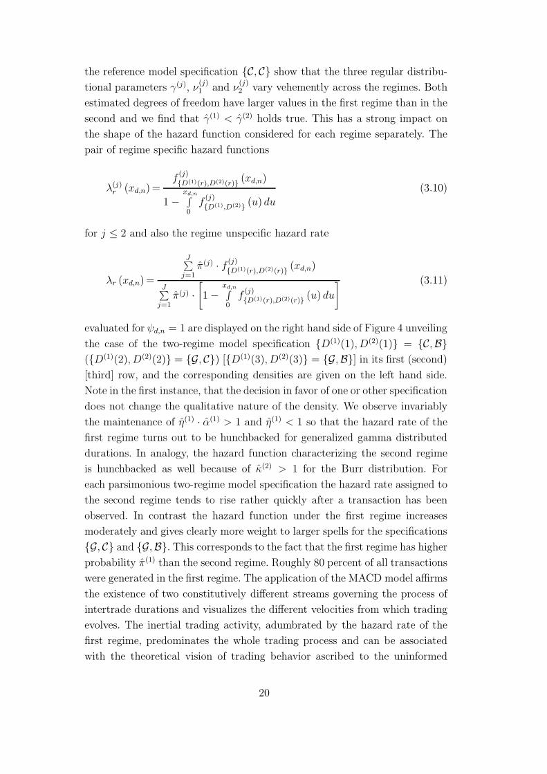
evaluated for ψd,n = 1 are displayed on the right hand side of Figure 4 unveiling

the case of the two-regime model specification {D(1)(1), D(2)(1)} = {C,B}

({D(1)(2), D(2)(2)} = {G, C}) [{D(1)(3), D(2)(3)} = {G,B}] in its first (second)

[third] row, and the corresponding densities are given on the left hand side.

Note in the first instance, that the decision in favor of one or other specification

does not change the qualitative nature of the density. We observe invariably

the maintenance of η(1) · α(1) > 1 and η(1) < 1 so that the hazard rate of the

first regime turns out to be hunchbacked for generalized gamma distributed

durations. In analogy, the hazard function characterizing the second regime

is hunchbacked as well because of κ(2) > 1 for the Burr distribution. For

each parsimonious two-regime model specification the hazard rate assigned to

the second regime tends to rise rather quickly after a transaction has been

observed. In contrast the hazard function under the first regime increases

moderately and gives clearly more weight to larger spells for the specifications

{G, C} and {G,B}. This corresponds to the fact that the first regime has higher

probability π(1) than the second regime. Roughly 80 percent of all transactions

were generated in the first regime. The application of the MACD model affirms

the existence of two constitutively different streams governing the process of

intertrade durations and visualizes the different velocities from which trading

evolves. The inertial trading activity, adumbrated by the hazard rate of the

first regime, predominates the whole trading process and can be associated

with the theoretical vision of trading behavior ascribed to the uninformed

20

Fig. 4. Density and hazard function

Density function Hazard function

traders. The second regime awards the image of succinct trading which can

be traced back to informed traders participating on the financial market.

Summarizing, our application illustrates that the conditional distribution

of durations in the first regime is generalized gamma while durations in the

second regime follow rather the Burr distribution. This empirical experience

makes the usual strategy of using one common distribution family for all

regimes problematic. Limitations concerning the intensity rate would be an

unavoidable consequence. An attractive possibility to avoid problems coming

from a distributional misspecification will be the use of the comprehensive

family of distributions which allows for extraordinary flexibility.

21

4 Conclusions

In this study combine the methodological background of mixture models

with the ACD modelling, originally introduced by Engle and Russell (1998).

Both, our discrete mixture ACD model which traces back to the basic con-

cept of De Luca and Gallo (2004) and the Markov Switching ACD model of

Hujer et al. (2002) act as a promising new approaches for modelling auto-

correlated durations obtained from high frequency data sets from stock and

foreign exchange markets. They are able to remove the distributional prob-

lem from which ordinary ACD models occasionally suffer. A further asset of

these models is that they can be interpreted in the context of recent market

microstructure models.

But until now one and the same family of distributions has been assumed

for specifying all regime specific densities of durations within the framework of

regime switching ACD models. Typically, either the class of Burr distributions

or the class of generalized gamma distributions has come into consideration so

far, as done by Hujer and Vuletic (2004) and Liu et al. (2004). The idea of using

an all-embracing distribution, which nests common waiting time distributions

as special cases, is the innovation we would like to provide. A distribution

belonging to the comprehensive family is rich in parameters but allows for

best customization. Moreover it makes possible to detect special distributions

for each regime of interest.

References

Bauwens, L., Giot, P., Grammig, J. Veredas, D., 2004. A comparison of finan-

cial duration models via density forecasts. International Journal of Fore-

casting 20, 589–609, forthcoming.

Burr, I. W., 1942. Cumulative frequency functions. Annals of Mathematical

Statistics 13, 215–232.

De Luca, G., Gallo, Giampiero, M., 2004. Mixture processes for financial in-

tradaily durations. Studies in Nonlinear Dynamics & Econometrics 8 (2),

1–18, article 8.

Dempster, A. P., Laird, N. M., Rubin, D. B., 1977. Maximum likelihood from

incomplete data via the EM algorithm. Journal of the Royal Statistical

Society 39, 1–38, series B.

Diebold, F. X., Gunther, T. A., Tay, A. S., 1998. Evaluating density forecasts

with applications to financial risk management. International Economic Re-

22

view 39 (4), 863–883.

Easley, D., Kiefer, N., O’Hara, M., Paperman, J. P., 1996. Liquidity, informa-

tion and infrequently traded stocks. Journal of Finance 51 (4), 1405–1436.

Engle, R. F., Russell, J. R., 1997. Forecasting the frequency of changes in

quoted foreign exchange prices with the autoregressive conditional duration

model. Journal of Empirical Finance 4 (2-3), 187–212.

Engle, R. F., Russell, J. R., 1998. Autoregressive conditional duration: A new

model for irregulary spaced transaction data. Econometrica 66 (5), 1127–

1162.

Eubank, R. L., Speckman, P., 1990. Curve fitting by polynomial-trigometric

regression. Biometrica 77 (1), 1–9.

Gallant, A. R., 1981. On the bias in flexible functional forms and an essentially

unbiased form. Journal of Econometrics 20 (2), 285–323.

Grammig, J., Hujer, R., Kokot, S., Maurer, K. O., 1998. Modeling the

Deutsche Telekom IPO using a new ACD specification - An application of

the Burr-ACD model using high frequency IBIS data. Discussion Paper 55,

Sonderforschungsbereich 373, Humboldt Universitat zu Berlin.

Hamilton, J. D., 1989. A new approach to the economic analysis of nonsta-

tionary time series and the business cycle. Econometrica 57 (2), 357–384.

Hujer, R., Vuletic, S., 2004. Econometric analysis of financial trade processes

by mixture duration models, J. W. Goethe University, Frankfurt/Main.

Hujer, R., Vuletic, S., Kokot, S., 2002. The markov switching ACD model.

Working Paper Series: Finance and Accounting 90, University of Frank-

furt/Main.

Kokot, S., 2004. The Econometrics of Sequential Trade Models : Theory and

Applications Using High Frequency Data. Springer Verlag.

Liu, Y., Hong, Y., Wang, S., 2004. How well can autoregressive duration mod-

els capture the price durations dynamics of foreign exchanges. Tech. Rep.

2004007 EN, The China Center for Financial Research, Tsinhghua Univer-

sity.

Ljung, G. M., Box, G. E. P., 1978. On a measure of lack of fit in time series

models. Biometrica 65 (2), 297–303.

Lunde, A., 1999. A generalized gamma autoregressive conditional duration

model, Department of Economics, Politics and Public Administration, Aal-

bourg University, Denmark.

Rosenblatt, M., 1952. Remarks on a multivariate transformation. Annals of

Mathematical Statistics 23 (3), 470–472.

Veredas, D., Rodriguez-Poo, J., Espasa, A., 2002. On the intradaily seasonal-

23

ity and dynamics of a financial point process: A semiparametric approach.

Discussion Paper 23, CORE, Universite Catholique de Louvain.

Weibull, W., 1951. A statistical distribution function of wide applicability.

Journal of Applied Mechanics Paper , 1–7.

White, H., 1982. Maximum likelihood estimation of misspecified models.

Econometrica 50 (1), 1–25.

Zhang, M. Y., Russell, J. R., Tsay, R. S., 2001. A nonlinear autoregressive

conditional duration model with applications to financial transaction data.

Journal of Econometrics 104 (1), 179–207.

24