Maarten Goos, Alan Manning, and Anna Salomons

Explaining job polarization: routine-biased technological change and offshoring Article (Published version) (Refereed)

Original citation: Goos, Maarten, Manning, Alan and Salomons, Anna (2014) Explaining job polarization: routine-biased technological change and offshoring. American Economic Review, 104 (8). pp. 2509-2526. ISSN 0002-8282 DOI: 10.1257/aer.104.8.2509 © 2014 American Economic Association This version available at: http://eprints.lse.ac.uk/59698/ Available in LSE Research Online: April 2016 LSE has developed LSE Research Online so that users may access research output of the School. Copyright © and Moral Rights for the papers on this site are retained by the individual authors and/or other copyright owners. Users may download and/or print one copy of any article(s) in LSE Research Online to facilitate their private study or for non-commercial research. You may not engage in further distribution of the material or use it for any profit-making activities or any commercial gain. You may freely distribute the URL (http://eprints.lse.ac.uk) of the LSE Research Online website.

American Economic Review 2014, 104(8): 2509–2526 http://dx.doi.org/10.1257/aer.104.8.2509

2509

Explaining Job Polarization: Routine-Biased Technological Change and Offshoring †

By Maarten Goos, Alan Manning, and Anna Salomons *

This paper documents the pervasiveness of job polarization in 16 Western European countries over the period 1993–2010. It then develops and estimates a framework to explain job polarization using routine-biased technological change and offshoring. This model can explain much of both total job polarization and the split into within-industry and between-industry components. (JEL J21, J23, J24, M55, O33)

The “Skill-Biased Technological Change” hypothesis (SBTC)—see Katz and Autor (1999); Goldin and Katz (2008, 2009); and Acemoglu and Autor (2011) for excellent overviews—arose from the observation that demand is shifting in favor of more educated workers. In spite of its success in explaining many decades of data, however, SBTC cannot explain the recent phenomenon of job polarization as documented by Autor, Katz, and Kearney (2006, 2008) and Autor and Dorn (2013) for the United States and Goos and Manning (2007) for the United Kingdom. Job polarization has also been documented for Germany (Spitz-Oener 2006; Dustmann, Ludsteck, and Schönberg 2009) and there are indications it is pervasive in European countries (Goos, Manning, and Salomons 2009; Michaels, Natraj, and Van Reenen 2014). The first contribution of this paper is to show that job polarization is pervasive across advanced economies by showing it holds in 16 Western European countries.

The main hypotheses put forward to explain job polarization are that recent tech-nological change is biased toward replacing labor in routine tasks (what we call rou-tine-biased technological change (RBTC)) and that there is task offshoring (itself partially influenced by technological change), and that both of these forces decrease the demand for middling relative to high-skilled and low-skilled occupations (Autor, Levy, and Murnane 2003; Autor, Katz, and Kearney 2006, 2008; Goos and Manning 2007; Autor and Dorn 2013). The second contribution of this paper is to develop and estimate a model—that has its roots in the canonical model first developed by Katz

* Goos: Department of Economics, University of Leuven, Naamsestraat 69, 3000 Leuven, Belgium (e-mail: maarten.goos@kuleuven.be); Manning: Centre for Economic Performance and Department of Economics, London School of Economics, Houghton Street, London WC2A 2AE, United Kingdom (e-mail: a.manning@lse.ac.uk); Salomons: Utrecht University School of Economics, Adam Smith Hall, International Campus Utrecht, Kriekenpitplein 21-22, 3584 EC Utrecht, The Netherlands (e-mail: a.m.salomons@uu.nl). We thank David Autor, Larry Katz, Thomas Lemieux, Stephen Machin, Guy Michaels, John Van Reenen, Ulrich Zierahn, and numerous seminar participants for excellent suggestions. The authors declare that they have no relevant or material financial interests that relate to the research described in this paper.

† Go to http://dx.doi.org/10.1257/aer.104.8.2509 to visit the article page for additional materials and author disclosure statement(s).

2510 THE AMERICAN ECONOMIC REVIEW AugusT 2014

and Murphy (1992) for the analysis of SBTC—to quantify the importance of RBTC and offshoring in explaining job polarization. Our estimates suggest that RBTC is much more important than offshoring. We show that this model explains not just overall job polarization but also its within-industry and between-industry compo-nents that are both empirically important. Within each industry there is a shift away from routine occupations leading to within-industry job polarization. But RBTC also leads to significant between-industry shifts in the structure of employment. On the one hand, an industry affected by RBTC will use less employment to produce a given level of output which will cause occupational employment shares to polarize even if output shares do not. On the other hand, industries intense in routine tasks will see a larger decrease in relative costs and output prices leading to a shift in product demand toward these industries (as was first pointed out by Baumol 1967). We show that, in our data, this effect attenuates between-industry job polarization but does not overturn it.

The remainder of this paper is organized as follows. Section I describes the data. Section II shows how the occupational employment structure between 1993 and 2010 in 16 Western European countries is polarizing both within and between industries. Section III presents our economic model. Section IV finally shows that the model can explain a large part of the changes in employment shares across occupations, both the total change and the split into within-industry and between-industry components.

I. Data

In this section we describe the data sources of our measures of employment, the routineness and offshorability of occupations as well as our measures of industry output and costs.1

A. Employment

Our main data source for employment is the harmonized individual level European Union Labour Force Survey (ELFS) for the 17-year period 1993–2010. The ELFS contains data on employment status, weekly hours worked, two-digit International Standard Occupational Classification (ISCO) codes and one-digit industry codes from the Classification of Economic Activities in the European Community (NACE revision 1). Throughout this paper, we use weekly hours worked as the measure of employment, although our results are not affected by using persons employed instead. Out of the 28 countries available in the ELFS, we exclude 11 new EU mem-ber countries and Iceland because of limited data availability. Because ELFS data for Germany only start in 2003, we use data from the German Federal Employment Agency’s SIAB dataset which is a 2 percent random sample of social security records for the period 1993–2008 instead. In sum, data for the following 16 European coun-tries is used in the analysis: Austria, Belgium, Denmark, Finland, France, Germany, Greece, Ireland, Italy, Luxembourg, the Netherlands, Norway, Portugal, Spain, Sweden, and the United Kingdom.

1 See online Appendix A for details on the measures discussed in this section.

2511goos et al.: Job PolarizationVol. 104 no. 8

Table 1 lists occupations ordered by their mean wage rank.2 Column 1 of Table 1 gives the 1993 employment share of each occupation after pooling employment across the 16 countries. For each occupation, column 2 of Table 1 gives the percent-age point change in the employment share between 1993 and 2010; we return to these numbers below.

B. Routineness and Offshorability of Occupations

Following the recommendation of Autor (2013) that researchers use, as far as is possible, off-the-shelf measures for the content of occupations, our measure of the routineness of an occupation is the Routine Task Intensity (RTI) index used by Autor and Dorn (2013) and Autor, Dorn, and Hanson (2013)3 mapped into our European occupational classification and normalized to have zero mean and unit standard deviation. The resulting RTI index is reported in column 3 of Table 1. RTI is highest at 2.24 for office clerks (41) and lowest at −1.52 for managers of small enterprises (13).

While the literature seems to be settling on using the RTI measure as the best way to capture the impact of recent technological progress, there is, as yet, no similar consensus measure about an occupation’s offshorability to capture the impact of offshoring. We use a measure taken from Blinder and Krueger (2013).4 Using the individual level Princeton Data Improvement Initiative (PDII) dataset, Blinder and Krueger (2013) report three measures of offshorability: one self-reported, one a combination of self-reported questions made internally consistent, and the last one which is based on professional coders’ assessment of the ease with which each occupation could potentially be offshored. Blinder and Krueger (2013) conclude that their third measure is preferred. For our analyses, we convert this preferred measure into our European occupational classification and normalize it to have zero mean and unit standard deviation. The resulting values are reported in column 4 of Table 1. The most offshorable are machine operators and assemblers (82) at 2.35 and the least offshorable are drivers and mobile plant operators (83) at −1.

2 To rank occupations, we use wages from the European Community Household Panel (ECHP) and European Union Statistics on Income and Living Conditions (EU-SILC), since the ELFS does not contain any earnings infor-mation. See online Appendix A for more details on our wage measures.

3 This RTI measure is based on Autor, Levy, and Murnane (2003) and Autor, Katz, and Kearney (2006, 2008). The five original DOT task measures of Autor, Levy, and Murnane (2003) are combined to produce three task aggregates: the Manual task measure corresponds to the DOT variable measuring an occupation’s demand for “eye-hand-foot coordination”; the Routine task measure is a simple average of two DOT variables, “set limits, tolerances and standards” measuring an occupation’s demand for routine cognitive tasks, and “finger dexterity,” measuring an occupation’s use of routine motor tasks; and the Abstract task measure is the average of two DOT variables: “direction control and planning,” measuring managerial and interactive tasks, and “GED Math,” measur-ing mathematical and formal reasoning requirements. From these three measures the Routine Task Intensity (RTI) index is constructed as the difference between the log of Routine tasks and the sum of the log of Abstract and the log of Manual tasks.

4 Online Appendix A provides some additional evidence in support of using this measure. In particular, we use data on actual instances of offshoring by European companies recorded in fact sheets compiled in the European Restructuring Monitor. These fact sheets contain considerable detail about offshoring events including which occu-pations are being offshored. We processed these fact sheets to construct an index of actual offshoring by occupa-tion. We then regress these measures of actual offshoring by occupation on Blinder and Krueger’s (2013) preferred measure of an occupation’s offshorability to find that they are strongly and positively correlated. Moreover, we show that competing indices of an occupation’s offshorability that have also been used in the literature do not have the same explanatory power.

2512 THE AMERICAN ECONOMIC REVIEW AugusT 2014

Table 1—Levels and Changes in the Shares of Hours Worked, 1993–2010

Occupations ranked by mean European wage

ISCOcode

Average employment share in 1993 (in percent)

Percentage point change 1993–2010 RTI

Offshor-ability Within Between

(1) (2) (3) (4) (5) (6)

High-paying occupations   31.67 5.62 −0.72 −0.12 3.11 2.51Corporate managers 12 5.65 0.59 −0.75 −0.32 0.49 0.10Physical, mathematical, and engineering professionals

21 2.93 1.36 −0.82 1.05 1.11 0.25

Life science and health professionals

22 2.01 0.57 −1.00 −0.76 0.23 0.34

Other professionals 24 2.79 1.38 −0.73 0.21 0.67 0.71Managers of small enterprises 13 4.16  0.17 −1.52 −0.63 −0.03 0.19Physical, mathematical, and engineering associate professionals

31 4.44  0.21 −0.40 −0.12 0.22 −0.01

Other associate professionals 34 7.24 0.79 −0.44 0.10 0.27 0.53Life science and health associate professionals

32 2.45 0.55 −0.33 −0.75 0.14 0.41

Middling occupations   46.75 −9.27 0.69 0.24 −4.77 −4.50Stationary plant and related operators

81 1.70 −0.25 0.32 1.59 0.06 −0.31

Metal, machinery, and related trade work

72 8.78 −2.08 0.46 −0.45 −0.81 −1.26

Drivers and mobile plant operators

83 5.03 −0.48 −1.50 −1.00 −0.11 −0.38

Office clerks 41 10.60 −2.06 2.24 0.40 −2.34 0.28Precision, handicraft, craft printing, and related trade workers

73 1.45 −0.54 1.59 1.66 −0.30 −0.24

Extraction and building trades workers

71 7.35 −0.64 −0.19 −0.93 0.39 −1.03

Customer service clerks 42 2.13 0.06 1.41 −0.25 −0.14 0.20Machine operators and assemblers

82 5.99 −1.63 0.49 2.35 −0.56 −1.07

Other craft and related trade workers

74 3.72 −1.66 1.24 1.15 −0.96 −0.69

Low-paying occupations   21.56 3.65 −0.08 −0.84 1.66 1.99Laborers in mining, construction, manufacturing, and transport

93 4.26 −0.55 0.45 −0.66 0.01 −0.55

Personal and protective service workers

51 6.86 2.36 −0.60 −0.94 0.65 1.71

Models, salespersons, and demonstrators

52 6.06 −0.11 0.05 −0.89 0.29 −0.40

Sales and service elementary occupations

91 4.38 1.95 0.03 −0.81 0.72 1.23

Notes: Occupations are ordered by their mean wage across the 16 European countries across all years. Columns 1, 2, 5, and 6: all countries, long difference 1993–2010, employment pooled across countries. Columns 3 and 4: mea-sures rescaled to mean 0 and standard deviation 1, a higher value means an occupation is more routine intense (col-umn 3) or more offshorable (column 4). The RTI index in column 3 is based on the five original DOT task measures in Autor, Levy, and Murnane (2003) and is identical to the index used in Autor and Dorn (2013) and Autor, Dorn, and Hanson (2013). The offshorability measure in column 4 is taken from Blinder and Krueger (2013) and is based on professional coders’ assessment of the ease with which an occupation could potentially be offshored. Columns 5 and 6: shiftshare analysis of occupational employment share changes, within and between industries.

2513goos et al.: Job PolarizationVol. 104 no. 8

The correlation coefficient between the RTI and offshorability measure is 0.46 and statistically significant suggesting that routineness and offshorability may be linked.5 But there are also some differences. For example, physical, mathemati-cal, and engineering professionals (21) is ranked as nonroutine but at the same time highly offshorable whereas office clerks (41) are very routine but not very offshorable.

C. Industry Output, Prices, and Costs

Measures of industry output, industry marginal costs, and relative output prices are taken from the OECD STAN Database for Industrial Analysis. Each of our 16 countries except Ireland is included in STAN. This data covers the period 1993–2010 for all 15 of these countries. STAN uses an industry list for all countries based on the International Standard Industrial Classification of all Economic Activities, Revision 3 (ISIC Rev.3) which covers all activities including services and is com-patible with NACE revision 1 used in the ELFS.

From STAN we use production, defined as the value of goods or services pro-duced in a year, whether sold or stocked. To obtain output, production is deflated using industry-country-year specific price indices also available from STAN. To obtain a measure of industry average costs—which in our model presented below will also be industry marginal costs—we use STAN’s net operating surplus data in addition to production and output, and take the difference between production and net operating surplus and divide this difference by output.

II. Job Polarization

To provide a snapshot of changes in the European job structure, columns 1 and 2 of Table 1 show the employment shares of occupations and their percentage point changes between 1993 and 2010 after pooling employment for each occupa-tion across our 16 European countries.6 This table shows that the highest-paying managerial (12,13), professional (21 to 24), and associate professional (31 to 34) occupations experienced the fastest increases in their employment shares. On the other hand, the employment shares of office clerks (41), craft and related trades workers (71 to 74), and plant and machine operators and assemblers (81 to 83), which pay around the median occupational wage, have declined. Similar to patterns found for the United States and United Kingdom, there has been an increase in the employment shares for some low-paid service workers (51, of which the main task consists of providing services related to travel, catering, and personal care; but not

5 This is in line with Blinder and Krueger (2013) who find that offshorability is conceptually distinct from, though related to, an occupation’s routineness. The authors argue that it is likely that jobs that can be broken down into simple, routine tasks are easier to offshore than jobs requiring complex thinking, judgment, and human interac-tion. However, a wide variety of complex tasks that involve high levels of skill and human judgment can also be offshored via telecommunication devices. Consequently, Blinder and Krueger (2013) conclude that their measure of offshorability is more germane to the offshoring issue than is the question of routineness but that the two criteria do overlap. As our RTI and offshorability measures are undoubtedly imperfect, and the extent of measurement error in them may also be different, one has to be careful in one’s claims about the ability to distinguish beyond reasonable doubt the separate effects of RBTC and offshoring.

6 Instead of pooling countries, reporting unweighted average employment shares and their changes across coun-tries would not qualitatively change the numbers in columns 1 and 2 of Table 1.

2514 THE AMERICAN ECONOMIC REVIEW AugusT 2014

52, of which the main task consists of selling goods in shops or at markets) and some low-paid elementary occupations (91), which are service elementary work-ers including cleaners, domestic helpers, doorkeepers, porters, security personnel, and garbage collectors; but not 93, which mainly includes low-educated laborers in manufacturing performing simple tasks including product-sorting and packing and unpacking produce). This is an indication that the existing evidence to date that there is job polarization in the United States, United Kingdom, or Germany is not an exception but rather the rule.

There may, of course, be heterogeneity across countries in the extent of job polar-ization. For ease of exposition, Table 2 groups the occupations into the three groups listed in Table 1: the four lowest-paid occupations, nine middling occupations, and the eight highest-paid occupations. We then compute the percentage point change in employment share for each of these groups in each country between 1993 and 2010. Table 2 confirms that employment polarization is pervasive across European coun-tries—the share of high-paying and low-paying occupations has increased relative to the middling occupations in each country.7

The final two columns of Table 1 decompose the overall change in employ-ment shares reported in column 2 of Table 1 into a within-industry (column 5) and between-industry (column 6) component. For the group of eight highest-paid and four lowest-paid occupations the within-industry and between-industry components are positive, and for the group of nine middling occupations they are both negative. What this shows is that overall job polarization can be split into a within-industry and between-industry component, each of which is too large quantitatively to be ignored.

In sum, the phenomenon of job polarization is pervasive across advanced econo-mies. Moreover, overall job polarization is driven by job polarization both within and between industries. The purpose of the model presented in the next section is to explain total job polarization and, more ambitiously, its split into within-industry and between-industry components.

III. A Framework to Understand Job Polarization

Our model is a two-stage setup for modeling the production process in which out-put in different industries is produced from a set of tasks, and where each task is pro-duced using a technology that combines labor from a specific occupation and other inputs. To capture RBTC and offshoring, the cost of these other inputs changes over time according to the routineness and offshorability of a task. This type of two-stage setup has also been used in recent work by, among others, Teulings (1995, 2005); Autor, Levy, and Murnane (2003); Autor, Katz, and Kearney (2006); Grossman and Rossi-Hansberg (2008); Costinot and Vogel (2010); Acemoglu and Autor (2011); and Autor and Dorn (2013). In relation to this literature our approach can be thought of as positioned between the very empirical analyses—that either estimate only within-industry effects, so can say nothing about the between-industry effects that we do find are important (e.g., Michaels, Natraj, and Van Reenen 2014), or

7 One might be concerned that our results are sensitive to the start and end years. However, online Appendix A presents the employment shares for all years showing that changes are close to linear trends.

2515goos et al.: Job PolarizationVol. 104 no. 8

reduced-form estimates that can say little about the transmission mechanism (e.g., Autor and Dorn 2013)—and the purely theoretical studies (e.g., Costinot and Vogel 2010) that put restrictions on the way technology varies across industries to derive comparative statics predictions (something that is impossible without imposing some structure on the problem) but cannot say anything about whether those restric-tions are satisfied in practice. All of these approaches have their advantages and disadvantages but we think our combination of theory and empirics is a useful one.

A. The Production of Goods

Assume that output in industry i is produced by combining certain common build-ing blocks that we will call tasks. In general, assume the following CES production function for industry i using tasks T 1 , … , T ij , … , T J as inputs:

(1) Y i ( T i1 , … , T ij , … , T iJ ) = [ ∑ j=1

J

[ β ij T ij ] η−1

_ η ] η

_ η−1

with η > 0,

where η is the elasticity of substitution between tasks in goods production and β ij is the intensity of the use of task j in industry i. The corresponding cost function for producing Y i is given by:

C i I ( c 1 T , … , c j T , … , c J T | Y i ) = Y i c i I ( c 1 T , … , c j T , … , c J T ),

Table 2—Initial Shares of Hours Worked and Percentage Changes over 1993–2010 (by Country)

Four lowest-paying occupations

Nine middling occupations

Eight highest-paying occupations

Employment share in 1993 (in percent)

Percentage point change 1993–2010

Employment share in 1993 (in percent)

Percentage point change 1993–2010

Employment share in 1993 (in percent)

Percentage point change 1993–2010

Austria 21.82 6.36 51.61 −10.44 26.57 4.08Belgium 17.49 3.00 48.50 −12.07 34.01 9.08Denmark 24.09 1.73 39.70 −10.30 36.21 8.56Finland 20.24 −1.50 39.69 −10.60 40.06 12.10France 19.92 4.19 46.69 −8.60 33.39 4.41Germany 20.71 2.37 48.03 −6.74 31.26 4.37Greece 21.66 4.81 47.81 −10.65 30.54 5.84Ireland 21.13 3.68 48.21 −14.85 30.66 11.17Italy 27.01 6.06 51.04 −10.59 21.94 4.53Luxembourg 21.70 −2.38 49.91 −10.76 28.40 13.15Netherlands 16.78 1.99 37.90 −7.56 45.33 5.57Norway 22.85 4.73 38.82 −8.47 38.34 3.74Portugal 25.75 0.73 47.46 −4.86 26.78 4.13Spain 28.02 1.01 48.67 −11.95 23.30 10.93Sweden 21.82 1.52 41.98 −9.55 36.20 8.03United Kingdom 16.88 4.17 43.64 −10.94 39.49 6.77

Notes: Long difference 1993–2010. Occupational employment pooled within each country. Occupations are grouped according to the mean European occupational wage as in Table 1.

2516 THE AMERICAN ECONOMIC REVIEW AugusT 2014

with c j T for j = 1, … , J the unit cost of task j and c i I ( c 1 T , … , c j T , … , c J T ) industry marginal cost. The demand for task j conditional on industry output Y i is then given by

(2) T ij ( c 1 T , … , c j T , … , c J T | Y i ) = Y i t ij ( c 1 T , … , c j T , … , c J T ),

where t ij ( c 1 T , … , c j T , … , c J T ) is the demand for task j to produce one unit of good i.

B. The Production of Tasks

We assume that output of task j is produced using labor of occupation j and some other inputs. The other inputs could be computers to capture recent technological change or offshored overseas employment to capture offshoring or some combina-tion of both. We proceed by assuming the other input is one-dimensional but that is just for simplicity and explicitly accounting for multiple inputs only adds algebraic complication. If industry i uses domestic labor of occupation j, N ij , and the other input, K ij , we assume that the total production of task j is given by a Cobb-Douglas production function that is common across industries:8

(3) T ij ( N ij , K ij ) = N ij κ K ij 1−κ with 0 < κ < 1.

The corresponding cost function for producing T ij is given by

C ij T ( w j , r j | T ij ) = T ij c j T ( w j , r j ),

with w j and r j the prices of N ij and K ij respectively. Note that it is assumed that the technology to produce task j together with factor prices w j and r j are common across industries such that the marginal cost to produce task j has no subscript i.9 The demand for occupation j conditional on task output T ij is then given by

(4) N ij ( w j , r j | T ij ) = T ij n j ( w j , r j ),

where n j ( w j r j ) is the demand for occupation j to produce one unit of task j.We model RBTC and offshoring as affecting the costs of the inputs other than

domestic labor, in particular that

(5) ∂ log r jt

_ ∂ t

= γ R R j + γ F F j ,

with R j the routineness and F j the offshorability measure discussed in Section I. Given that our measures R j and F j are increasing in routineness and offshorabil-ity respectively, we expect γ R < 0 and γ F < 0. Note that we model the impact of RBTC and offshoring as being in the cost of employing an effective unit of the other

8 The original version of this paper—Goos, Manning, and Salomons (2010)—allowed for a CES task production function. Online Appendix B shows that this specification makes little difference to the conclusions.

9 This assumption has been used in other models (e.g., Grossman and Rossi-Hansberg 2008).

2517goos et al.: Job PolarizationVol. 104 no. 8

input—it would be observationally equivalent to model it as changes in the produc-tion function not prices.

Substituting equation (2) into (4), taking logs and using equation (5) gives an expression for the log demand for occupation j in industry i conditional on industry output and marginal costs (and adding country and time subscripts):

(6) log N ijct = − [ (1 − κ) + κη ] log w jct

+ [ 1 − η ] [1 − κ] [ γ R R j + γ F F j ] × time

+ η log c ict I + log Y ict + (η − 1) log β ijc + ε ijct .

If η < 1, γ R < 0 and γ F < 0 such that [ 1 − η ] [1 − κ] [ γ R R j + γ F F j ] is negative for more routine and offshorable occupations, equation (6) predicts job polarization within each industry.

Table 3 reports some estimates of equation (6). Column 1 gives estimates of [ 1 − η ] [1 − κ] γ R as the coefficient on our RTI measure interacted with a linear time trend and of [ 1 − η ] [1 − κ] γ F as the coefficient on our offshorability measure interacted with a linear time trend, while modeling occupational wages by a set of country, occupation, and time dummies10 and industry output and marginal costs by industry-country-year dummies. The coefficient on RTI is negative and significantly different from zero at the 1 percent level. The magnitude of the estimated effects is such that an occupation that is one standard deviation more intense in RTI is grow-ing 0.90 percentage points less fast each year. The coefficient on offshorability is also negative, but small in absolute value and not statistically significantly different from zero.

The estimates in column 1 of Table 3 do not allow us to retrieve an estimate of η that will be necessary for the shift-share analysis in Section IV. To do this, column 2 of Table 3 replaces the industry-country-year dummies with our measures of indus-try marginal costs and industry output described in Section I above. The coefficient on log industry marginal cost—which is an estimate of η—is positive and significant as is predicted by our model. However, the coefficient on log industry output is less than unity which rejects our assumption of constant returns to scale in goods pro-duction. This is perhaps not surprising given that short-run movements in output are often not reflected in employment, so column 3 of Table 3 restricts the coefficient on log industry output to be equal to unity. This does not affect the RTI and offshorabil-ity coefficients and results in an estimate of 0.90 for η. Column 4 of Table 3 excludes offshorability from the regression equation to examine the impact of RBTC uncon-ditional on offshoring, and this does not affect the RTI point estimate. Column 5 of Table 3 excludes RTI from the regression equation instead to examine the impact of

10 Online Appendix B shows results are similar if wages are included. They are excluded here because the quality of wage data by country, occupation, and time is poor and because of concerns about their endogeneity (see Firpo, Fortin, and Lemieux 2011 and Ebenstein et al. forthcoming for US evidence on this). The earlier version of the paper—Goos, Manning, and Salomons (2010)—found little evidence for the endogeneity of wages as is perhaps plausible given the institutions of wage determination in Europe (though see Hummels et al. 2014 for evidence for Denmark that a firm’s wages respond to offshoring by that firm).

2518 THE AMERICAN ECONOMIC REVIEW AugusT 2014

offshoring unconditional on RBTC. The impact of offshoring is negative and sig-nificant in this case but this may well be because it is positively correlated with RTI and the earlier columns make clear that it loses a “horse race” against RTI. In sum, this is evidence that within industries there is a shift in relative demand away from occupations that are more routine and offshorable with the former being the much more important effect.11

C. The Demand for Goods

The analysis so far has been for given industry output. To account for the labor demand effects induced from shifts in relative product demand, we need to go fur-ther and not condition on industry output. To do this, assume that the log demand for industry output is given by

(7) log Y ict = −ε log P ict + log Y ct + ξ ict ,

with P ict the industry-country-year specific price indices available from STAN relative to a country-year aggregate price index, and Y ct a measure of aggregate income. This specification could be derived from an underlying CES utility function in which consumers have homothetic preferences.12 Estimating equation (7) gives a point estimate for ε of 0.42 with a standard error of 0.07.

11 This conclusion is robust to numerous sensitivity tests by estimating models separately for subsets of coun-tries, industries, and time periods. See online Appendix C for details.

12 The assumption of homotheticity implies that changes in both the level and the distribution of aggregate income have no effect on the distribution of demand across industries. This might be thought unduly restrictive because it has been argued (Manning 2004; and Mazzolari and Ragusa 2013) that job polarization might be caused by increasing inequality leading to increased demand for low-skill service sector jobs from high-wage workers to free up more of their time for market work. However, we cannot find evidence for non-homotheticity at our level of industry aggregation (Autor and Dorn 2013 arrive at similar conclusions). See online Appendix D for details.

Table 3—Estimating Labor Demand Dependent Variable: log (Hours worked/1,000)

Linear time-trend interacted with: (1) (2) (3) (4) (5)

RTI −0.900*** −0.888*** −0.866*** −0.868***(0.126) (0.135) (0.141) (0.129) —

Offshorability −0.013 −0.005 −0.006 −0.383**(0.159) (0.175) (0.180) — (0.165)

log industry marginal costs 0.854*** 0.895*** 0.895*** 0.899***— (0.145) (0.161) (0.161) (0.161)

log industry output 0.142** 1 1 1— (0.061)

Observations 48,139 44,062 44,062 44,062 44,062

R2 0.954 0.947

Notes: Point estimates (and standard errors in parentheses) on RTI and offshorability have been multiplied by 100. All regressions include occupation-industry-country fixed effects. The regression in column 1 contains industry-country-year fixed effects and regressions in columns 2–5 contain year fixed effects. Standard errors are clustered by occupation-industry-country.

*** Significant at the 1 percent level. ** Significant at the 5 percent level. * Significant at the 10 percent level.

2519goos et al.: Job PolarizationVol. 104 no. 8

If there is monopolistic competition within each industry we have that log P ict = log μ + log c ict I

with μ > 1 the price mark-up. Using this and substitut-ing equation (7) into (6) gives

(8) log N ijct = − [ (1 − κ) + κη ] log w jct

+ [1 − η][1 − κ] [ γ R R j + γ F F j ] × time

+ [η − ε] log c ict I + log Y ct − ε log μ

+ (η − 1) log β ijc + ε ijct ,

which is an equation we will use in the next section.

IV. Explaining Job Polarization within and between Industries

Our aim in this section is to consider how much of job polarization both within and between industries that was documented in Table 1 can be explained by our model above. To see how we can do this, note that in a standard shift-share analysis the share of occupation j in total employment at time t, s jt , can be written as (drop-ping country subscripts for simplicity)

(9) s jt = ∑ i=1

I

τ it s j | it ,

where s j | it is the share of occupation j in total employment of industry i at time t, and τ it is the share of employment in industry i in total employment at time t. Differentiating (9) we have that

(10) ∂ s jt

_ ∂ t

= ∑ i=1

I

τ it s j | it [ ∂ log s j | it _

∂ t +

∂ log τ it _ ∂ t

] ,where the first term in square brackets is the within-industry and the second term is the between-industry contribution to the total change in occupational employment shares.

Now consider the predictions of our model for the within-industry and between-industry components. To keep the algebra to a minimum we will assume there is only RBTC, but the same method can be used to analyze offshoring and our empirical analysis below accounts for RBTC as well as offshoring simultaneously. From (8) we can write the first term in square brackets in equation (10) as

(11) ∂ log s j | it

_ ∂ t

= ∂ log N ijt

_ ∂ t

− ∑ j′ =1

J

s j′ | it ∂ log N i j′ t

_ ∂ t

= [1 − η][1 − κ] γ R ( R j − ∑ j′ =1

J

s j′ | it R j′ )

= [1 − η][1 − κ] γ R ( R j − R it I ),

2520 THE AMERICAN ECONOMIC REVIEW AugusT 2014

with R it I = ∑ j′ =1

J s j′ | it R j′ the average of R j in industry i where the weights used,

s j′ | it , are the shares of different occupations in the industry at time t, i.e., is the aver-age level of routineness across occupations in industry i.

Now consider the second term in square brackets in equation (10). From (8) we have that

(12) ∂ log τ it _

∂ t =   ∑

j=1

J

s j | it ∂ log N ijt

_ ∂ t

− ∑ j′ =1

I

s j′ t ∂ log N j′ t

_ ∂ t

= [1 − ε][1 − κ] γ R ( R it I − ∑

i′ =1

I

τ i′ t R i′ t I )

= [1 − ε][1 − κ] γ R ( R it I − R t agg ),

with R t agg defined to be the average of R it I across industries where the weights used,

τ i′ t , are the shares of employment in industry i in total employment at time t.13

Substituting equations (11) and (12) into (10), we have that the shift-share decom-position can be written as

(13) ∂ s jt

_ ∂t

= s jt [1 − η][1 − κ] γ R

×   { ( R j − ∑ i=1

I

s i | jt R it I ) + 1 − ε _

1 − η ∑

i=1

I

s i | jt ( R it I − R t agg ) } ,

with s i | jt the share of occupation j in industry i at time t. The term before the curly brackets, s jt [ 1 − η ] [1 − κ] γ R , is occupation j’s share of total employment, s jt , mul-tiplied by the RTI coefficient in Table 3, [1 − η][1 − κ] γ R , which is negative.14

The first term in the curly brackets, ( R j − ∑ i=1 I s i | jt R it I

) , is the model’s prediction of the within-industry component. It captures the shift away from or toward occupa-tion j within industries by subtracting from R j the average routineness across indus-tries in which occupation j is employed. For example, if in every industry in which occupation j is used we have that R j is high relative to all other occupations, one would expect a large shift away from occupation j within each of those industries.

The second term in the curly brackets, [1 − ε]/[1 − η] ∑ i=1 I s i | jt ( R it I

− R t agg ), is the between-industry component. This can be thought of as having two parts. The first (which will be the total effect if industry outputs are fixed, i.e., assum-ing that product demands are perfectly inelastic or ε = 0) comes from variation in the employment intensity of output induced by RBTC. RBTC will typically cause less routine employment to be used in the production of a given level of output, so

13 This follows from the fact that ∂ log c ict I /∂ t = [1 − κ] γ R ∑ j=1

J s j | i R j and the simplifying assumption that the

share of task j in industry costs is the same as the share of employment of occupation j in that industry.14 Note that the predicted changes from equation (13) are precisely the effects from RBTC and offshoring and

cannot be explained by any industry or industry-time specific changes in employment shares.

2521goos et al.: Job PolarizationVol. 104 no. 8

differences in routineness across industries will cause industry employment shares to change even if industry output shares do not. For example, to produce the same level of output the demand for an occupation falls by more in industries that are

routine intense because R it I − R t agg and therefore 1/[1 − η] ∑ i=1

I s i | jt ( R it I

− R t agg ) will be larger. Because routine occupations are concentrated in routine intensive industries by definition, this channel predicts job polarization between industries if routine occupations are middling occupations.

The second part of the between-industry effect (i.e., assuming that ε > 0) comes from changes in the distribution of output induced by the changes in relative output prices and therefore shifting consumer demands that follow from RBTC. For exam-ple, routine intensive industries will see a larger fall in industry costs and therefore relative output prices. This will increase the demand for routine intensive goods and therefore the demand for all occupations used in routine intensive industries.

Because this implies that −ε/[1 − η] ∑ i=1 I s i | jt ( R it I

− R t agg ) will be larger in abso-lute value for more routine occupations, this channel will tend to attenuate the first part of the between-industry effect though will not overturn it as long as ε < 1 as our estimate for ε of 0.42 suggests.15

To summarize, equation (13) shows how a shift-share analysis—that is commonly thought of as merely an accounting exercise—can be rooted in our framework. In particular, equation (13) shows how changes in occupational employment shares can be decomposed into a within-industry and between-industry component and this is interesting for two reasons. Firstly, the conventional wisdom from the SBTC literature is that skill upgrading is almost entirely a within-industry phenomenon but equation (13) shows that RBTC has an important between-industry component as well. Secondly, the within-industry and between-industry effects in equation (13) are economically meaningful and depend on the different elasticities in the model. In particular, our estimates are such that RBTC and offshoring lead to job polariza-tion within and between industries, but one could easily imagine different elastici-ties—perhaps capturing different episodes of technological change or globalization and types of goods produced or traded—to come to different predictions.

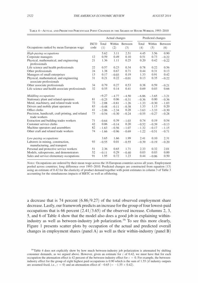
Columns 1 to 3 of Table 4 show the actual change in employment share for each occupation as well as the split into a within-industry and between-industry com-ponent, as was already shown in columns 2, 5, and 6 of Table 1 respectively. The remaining columns of Table 4 show the predictions of our model obtained from equation (13) while using an estimate of 0.42 for ε together with the point estimates in column 3 of Table 3. Column 4 of Table 4 shows the predicted total, column 5 the predicted within-industry and column 6 the predicted between-industry changes in occupational employment shares. Because the RTI index is much more important in column 3 of Table 3 almost all of these changes come from the RTI variable.

A comparison of columns 1 and 4 shows that our model explains most of overall job polarization. For the group of the eight highest-paid occupations, our model pre-dicts an increase in employment share that is 79 percent (4.45/5.62) of the increase actually observed. For the group of nine middling occupations, the model predicts

15 Also note that equation (12) predicts that employment shares in routine and offshorable industries decrease if ε < 1.

2522 THE AMERICAN ECONOMIC REVIEW AugusT 2014

a decrease that is 74 percent (6.86/9.27) of the total observed employment share decrease. Lastly, our framework predicts an increase for the group of four lowest-paid occupations that is 66 percent (2.41/3.65) of the observed increase. Columns 2, 3, 5, and 6 of Table 4 show that the model also does a good job in explaining within-industry as well as between-industry job polarization.16 To see this more clearly, Figure 1 presents scatter plots by occupation of the actual and predicted overall changes in employment shares (panel A) as well as their within-industry (panel B)

16 Table 4 does not explicitly show by how much between-industry job polarization is attenuated by shifting consumer demands, as we argued above. However, given an estimate for ε of 0.42, we must have that for each occupation the attenuation effect is 42 percent of the between-industry effect for ε = 0. For example, the between-industry effect for the group of eight highest paid occupations is 0.90 which is the sum of 1.55 (if industry outputs are assumed fixed, i.e., ε = 0) and an attenuation effect of −0.65 (= −1.55 × 0.42).

Table 4—Actual and Predicted Percentage Point Changes in the Shares of Hours Worked, 1993–2010

    Actual changes Predicted changes

  ISCO Total Within Between Total Within BetweenOccupations ranked by mean European wage code (1) (2) (3) (4) (5) (6)

High-paying occupations   5.62 3.11 2.51 4.45 3.56 0.90Corporate managers 12 0.59 0.49 0.10 0.51 0.73 −0.22Physical, mathematical, and engineering professionals

21 1.36 1.11 0.25 0.20 0.42 −0.22

Life science and health professionals 22 0.57 0.23 0.34 0.78 0.22 0.56Other professionals 24 1.38 0.67 0.71 0.44 0.31 0.13Managers of small enterprises 13 0.17 −0.03 0.19 1.33 0.91 0.42Physical, mathematical, and engineering associate professionals

31 0.21 0.22 −0.01 0.13 0.35 −0.22

Other associate professionals 34 0.79 0.27 0.53 0.38 0.59 −0.21Life science and health associate professionals 32 0.55 0.14 0.41 0.69 0.03 0.66

Middling occupations   −9.27 −4.77 −4.50 −6.86 −3.65 −3.21Stationary plant and related operators 81 −0.25 0.06 −0.31 −0.36 0.00 −0.36Metal, machinery, and related trade work 72 −2.08 −0.81 −1.26 −1.33 −0.30 −1.03Drivers and mobile plant operators 83 −0.48 −0.11 −0.38 1.33 1.13 0.20Office clerks 41 −2.06 −2.34 0.28 −3.63 −3.33 −0.30Precision, handicraft, craft printing, and related trade workers

73 −0.54 −0.30 −0.24 −0.55 −0.27 −0.28

Extraction and building trades workers 71 −0.64 0.39 −1.03 0.74 0.19 0.54Customer service clerks 42 0.06 −0.14 0.20 −0.52 −0.39 −0.13Machine operators and assemblers 82 −1.63 −0.56 −1.07 −1.32 −0.17 −1.15Other craft and related trade workers 74 −1.66 −0.96 −0.69 −1.22 −0.51 −0.71               Low-paying occupations   3.65 1.66 1.99 2.41 0.10 2.31Laborers in mining, construction, manufacturing, and transport

93 −0.55 0.01 −0.55 −0.39 −0.19 −0.20

Personal and protective service workers 51 2.36 0.65 1.71 2.33 0.32 2.01Models, salespersons, and demonstrators 52 −0.11 0.29 −0.40 0.03 0.03 0.00Sales and service elementary occupations 91 1.95 0.72 1.23 0.44 −0.06 0.50

Notes: Occupations are ordered by their mean wage across the 16 European countries across all years. Employment pooled across countries; long difference over 1993–2010. Predicted changes are constructed from equation (13) using an estimate of 0.42 for the elasticity of product demand together with point estimates in column 3 of Table 3 accounting for the simultaneous impacts of RBTC as well as offshoring.

2523goos et al.: Job PolarizationVol. 104 no. 8

Act

ual c

hang

e

2.5

1.5

0.5

–0.5

–1.5

–2.5

–3.5

Panel A. Total

–3.5 –2.5 –1.5 –0.5 0.5 1.5 2.5

Protct Svc

Pers Svcs

Tech Prof Oth Prof

Oth ParaProfHlth Prof

Hlth ParaProfCorp Mngr

Biz MngrTech ParaProf

Cust ClerkPlant Oper

Prec TradeSales

LaborerCons Trade

Transport

Oth Trade

Mach Prodn

Mach Oper

Ofc Clerk

Predicted change

Act

ual c

hang

e

1.5

0.5

–0.5

–1.5

–2.5

–3.5

–3.5 –2.5 –1.5 –0.5 0.5 1.5

Panel B. Within industries

Protct SvcPers Svcs

Tech Prof

Oth Prof

Oth ParaProfHlth ProfHlth ParaProf

Corp Mngr

Biz MngrCust ClerkPlant OperPrec Trade

Sales

Laborer

Cons Trade

Transport

Oth TradeMach Prodn

Mach Oper

Ofc Clerk

Predicted change

Figure 1. Actual versus Predicted Employment Share Changes (Continued)

2524 THE AMERICAN ECONOMIC REVIEW AugusT 2014

and between-industry (panel C) components taken from Table 4.17 Overall, our model and results suggest that RBTC and offshoring explain much of job polariza-tion and its within-industry and between-industry components, although the results certainly leave room for additional factors to play a role.

V. Conclusions

The employment structure in Western Europe has been polarizing with rising employment shares for high-paid professionals and managers as well as low-paid personal service workers and falling employment shares of manufacturing and routine office workers. The paper establishes that job polarization is pervasive across European economies in the period 1993–2010 and has within-industry and between-industry components that are both important. We develop a framework that builds on existing models but allows us to account for the different channels by which routine-biased technological change and offshoring affect the structure of employment. In particular, we decompose the total change in employment shares by occupation into a within-industry and a between-industry component in a way that is economically meaningful. We show that our economic model explains a sizable part not just of overall job polarization but also the split into within-industry and between-industry components.

17 In online Appendix E we replicate Table 4 and Figure 1 twice. Firstly, using point estimates in column 4 of Table 3, thereby using the estimated impact of RBTC unconditional on offshoring. Results are very similar to those presented in Table 4 and Figure 1. Secondly, using point estimates in column 5 of Table 3, thereby using the esti-mated impact of offshoring unconditional on RBTC. Given that our RTI and offshorability measures are correlated, offshoring while not conditioning on RBTC does appear to have some explanatory power but it is noticeable that the fit is poorer e.g., offshoring cannot explain the decline in the employment share of office clerks within industries.

Act

ual c

hang

e

2

1.5

1

0.5

0

–0.5

–1

–1.5

–1.5 –1 –0.5 0 0.5 1 1.5 2

Predicted change

Panel C. Between industries

Protct Svc

Pers Svcs

Tech Prof

Oth Prof

Oth ParaProf

Hlth ProfHlth ParaProf

Corp Mngr Biz MngrTech ParaProf

Cust Clerk

Plant OperPrec Trade

SalesLaborer

Cons Trade

Transport

Oth Trade

Mach ProdnMach Oper

Ofc Clerk

Figure 1. Actual versus Predicted Employment Share Changes

2525goos et al.: Job PolarizationVol. 104 no. 8

REFERENCES

Acemoglu, Daron, and David H. Autor. 2011. “Skills, Tasks and Technologies: Implications for Employment and Earnings.” In Handbook of Labor Economics. Vol. 4B, edited by Orley Ashen-felter and David E. Card, 1043–1171. Amsterdam: Elsevier B.V.

Autor, David H. 2013. “The ‘Task Approach’ to Labor Markets.” Journal of Labour Market Research 46 (3): 185–99.

Autor, David H., and David Dorn. 2013. “The Growth of Low-Skill Service Jobs and the Polarization of the US Labor Market.” American Economic Review 103 (5): 1553–97.

Autor, David H., David Dorn, and Gordon H. Hanson. 2013. “Untangling Trade and Technology: Evidence from Local Labor Markets.” Unpublished.

Autor, David H., Lawrence F. Katz, and Melissa S. Kearney. 2006. “The Polarization of the U.S. Labor Market.” American Economic Review 96 (2): 189–94.

Autor, David H., Lawrence F. Katz, and Melissa S. Kearney. 2008. “Trends in U.S. Wage Inequality: Revising the Revisionists.” Review of Economics and Statistics 90 (2): 300–23.

Autor, David H., Frank Levy, and Richard J. Murnane. 2003. “The Skill Content of Recent Tech-nological Change: An Empirical Exploration.” Quarterly Journal of Economics 118 (4): 1279–1333.

Baumol, William J. 1967. “Macroeconomics of Unbalanced Growth: Anatomy of an Urban Crisis.” American Economic Review 57 (3): 415–26.

Blinder, Alan S., and Alan B. Krueger. 2013. “Alternative Measures of Offshorability: A Survey Approach.” Journal of Labor Economics 31(2): S97–128.

Costinot, Arnaud, and Jonathan E. Vogel. 2010. “Matching and Inequality in the World Economy.” Journal of Political Economy 118 (4): 747–86.

Dustmann, Christian, Johannes Ludsteck, and Uta Schönberg. 2009. “Revisiting the German Wage Structure.” Quarterly Journal of Economics 124 (2): 843–81.

Ebenstein, Avraham, Ann Harrison, Margaret McMillan, and Shannon Philips. Forthcoming. “Esti-mating the Impact of Trade and Offshoring on American Workers Using the Current Population Surveys.” Review of Economics and Statistics.

Firpo, Sergio, Nicole M. Fortin, and Thomas Lemieux. 2011. “Occupational Tasks and Changes in the Wage Structure.” Unpublished.

Goldin, Claudia, and Lawrence F. Katz. 2008. The Race Between Education and Technology. Cam-bridge, MA: Harvard University Press.

Goldin, Claudia, and Lawrence F. Katz. 2009. “The Race Between Education and Technology: The Evolution of U.S. Wage Differentials, 1890–2005.” National Bureau of Economic Research Working Paper 12984.

Goos, Maarten, and Alan Manning. 2007. “Lousy and Lovely Jobs: The Rising Polarization of Work in Britain.” Review of Economics and Statistics 89 (1): 118–33.

Goos, Maarten, Alan Manning, and Anna Salomons. 2009. “Job Polarization in Europe.” American Economic Review 99 (2): 58–63.

Goos, Maarten, Alan Manning, and Anna Salomons. 2010. “Explaining Job Polarization: The Roles of Technology, Globalization and Institutions.” Center for Economic Performance Discussion Paper 1026.

Goos, Maarten, Alan Manning, and Anna Salomons. 2014. “Explaining Job Polarization: Routine-Biased Technological Change and Offshoring: Dataset.” American Economic Review. http://dx.doi.org/10.1257/aer.104.8.2509.

Grossman, Gene M., and Esteban Rossi-Hansberg. 2008. “Trading Tasks: A Simple Theory of Off-shoring.” American Economic Review 98 (5): 1978–97.

Hummels, David, Rasmus Jørgensen, Jakob Munch, and Chong Xiang. 2014. “The Wage Effects of Offshoring: Evidence from Danish Matched Worker-Firm Data.” American Economic Review 104 (6): 1597–1629.

Katz, Lawrence F., and David H. Autor. 1999. “Changes in the Wage Structure and Earnings Inequal-ity.” In Handbook of Labor Economics. Vol. 3A, edited by Orley Ashenfelter and David E. Card, 1463–1555. Amsterdam: Elsevier B.V.

Katz, Lawrence F., and Kevin M. Murphy. 1992. “Changes in Relative Wages, 1963–1987: Supply and Demand Factors.” Quarterly Journal of Economics 107 (1): 35–78.

Manning, Alan. 2004. “We Can Work it Out: The Impact of Technological Change on the Demand for Low-Skilled Workers.” Scottish Journal of Political Economy 51 (5): 581–608.

Mazzolari, Francesca, and Giuseppe Ragusa. 2013. “Spillovers from High-Skill Consumption to Low-Skill Labor Markets.” Review of Economics and Statistics 95 (1): 74–86.

2526 THE AMERICAN ECONOMIC REVIEW AugusT 2014

Michaels, Guy, Ashwini Natraj, and John Van Reenen. 2014. “Has ICT Polarized Skill Demand? Evidence from Eleven Countries over Twenty-Five Years.” Review of Economics and Statistics 96 (1): 60–77.

Spitz-Oener, Alexandra. 2006. “Technical Change, Job Tasks, and Rising Educational Demands: Looking Outside the Wage Structure.” Journal of Labor Economics 24 (2): 235–70.

Teulings, Coen. 1995. “The Wage Distribution in a Model of the Assignment of Skills to Jobs.” Journal of Political Economy 103 (2): 280–315.

Teulings, Coen N. 2005. “Comparative Advantage, Relative Wages, and the Accumulation of Human Capital.” Journal of Political Economy 113 (2): 425–61.

This article has been cited by:

1. David H. Autor. 2015. Why Are There Still So Many Jobs? The History and Future of WorkplaceAutomation. Journal of Economic Perspectives 29:3, 3-30. [Abstract] [View PDF article] [PDF withlinks]

2. Marco Leonardi. 2015. The Effect of Product Demand on Inequality: Evidence from the United Statesand the United Kingdom. American Economic Journal: Applied Economics 7:3, 221-247. [Abstract][View PDF article] [PDF with links]