M140: Summarising & Plotting Data Computer Book with Minitab
83
M140: Summarising & Plotting Data with Minitab Dr Jason Verrall [email protected] 07311 188800 This tutorial will begin at 7:30pm and will last for approximately an hour. This tutorial will be recorded. Please let me know if you have any questions or concerns about this. Things you might need for this tutorial: • M140 Computer Book & Handbook • Pen, paper & calculator • Drink of your choice Don’t forget to set up your audio using the Audio Wizard (in the ‘Meeting Menu’). Some headsets have independent volume controls so you may need to adjust these too. You will also need to set up your mic if you plan on using it. Clicking the Mic symbol at the top of you Adobe Connect Window will toggle it on/off. Not connected Connected and live Connected and muted TMA01 due by next Wednesday!
Transcript of M140: Summarising & Plotting Data Computer Book with Minitab
M140: Summarising & Plotting Data with Minitab
Dr Jason [email protected]
07311 188800
This tutorial will begin at 7:30pm and will last for approximately an hour.
This tutorial will be recorded. Please let me know if you have any questions or concerns about this.
Things you might need for this tutorial:• M140 Computer Book & Handbook• Pen, paper & calculator• Drink of your choice
Don’t forget to set up your audio using the Audio Wizard (in the ‘Meeting Menu’). Some headsets have independent volume controls so you may need to adjust these too.
You will also need to set up your mic if you plan on using it. Clicking the Mic symbol at the top of you Adobe Connect Window will toggle it on/off.
Not connected Connected and live Connected and muted
TMA01 due by next Wednesday!
Good evening!
2
Mics will be muted until towards the end of the tutorial, when I will also stoprecording.Do use the Chat Box if you have a question during the tutorial!I will email slides out after the tutorial.
Tutorials are enhanced by your interactionPlease vote in the polls, ask questions and work through the exercises
Feel free to ask any questions or provide feedback by emailafterwards, or use the Private Chat function if you prefer during thetutorial
Summarising & Plotting Data with Minitab
Scientific Skills • Sample or population?• Types of data• Locators & descriptors• Good graphs• Interpreting graphs
Minitab Skills• Calculating statistics• Plotting graphs• Customising graphs
3Computer Book has detailed instructions!
Summarising & Plotting Data with Minitab
Scientific Skills • Sample or population?• Types of data• Locators & descriptors• Good graphs• Interpreting graphs
Minitab Skills• Calculating statistics• Plotting graphs• Customising graphs
4Computer Book has detailed instructions!
Have you stated using Minitab
yet?

Sample or Population?
5http
s://
ww
w.p
inte
rest
.co.
uk/p
in/2
2539
1156
3259
5899
9/
Population

Sample or Population?
6
• We are unlikely to ever be able to study a whole population• Example: A fishing boat will not be able to catch all the fish in the sea• Whole population may be available in clinical trials or other highly controlled environments
http
s://
ww
w.p
inte
rest
.co.
uk/p
in/2
2539
1156
3259
5899
9/
Population
Sample or Population?
7
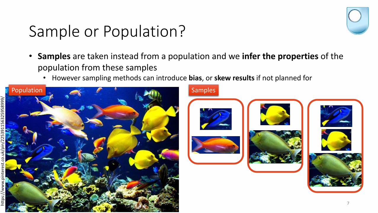
• Samples are taken instead from a population and we infer the properties of the population from these samples
• However sampling methods can introduce bias, or skew results if not planned for
http
s://
ww
w.p
inte
rest
.co.
uk/p
in/2
2539
1156
3259
5899
9/
Population Samples

Sample or Population?
8
• Samples are taken instead from a population and we infer the properties of the population from these samples
• However sampling methods can introduce bias, or skew results if not planned for
http
s://
ww
w.p
inte
rest
.co.
uk/p
in/2
2539
1156
3259
5899
9/
Samples
• Assume you are working with a sample from a population unless told otherwise
• Your statistics will thus be an estimateof the true population statistic• Don’t worry about this difference now!• M248 & M249 cover samples, estimators
and bias in more detail
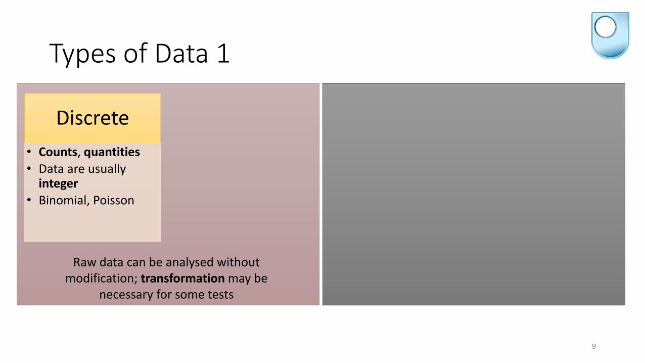
Discrete• Counts, quantities• Data are usually
integer• Binomial, Poisson
Types of Data 1
9
Raw data can be analysed without modification; transformation may be
necessary for some tests
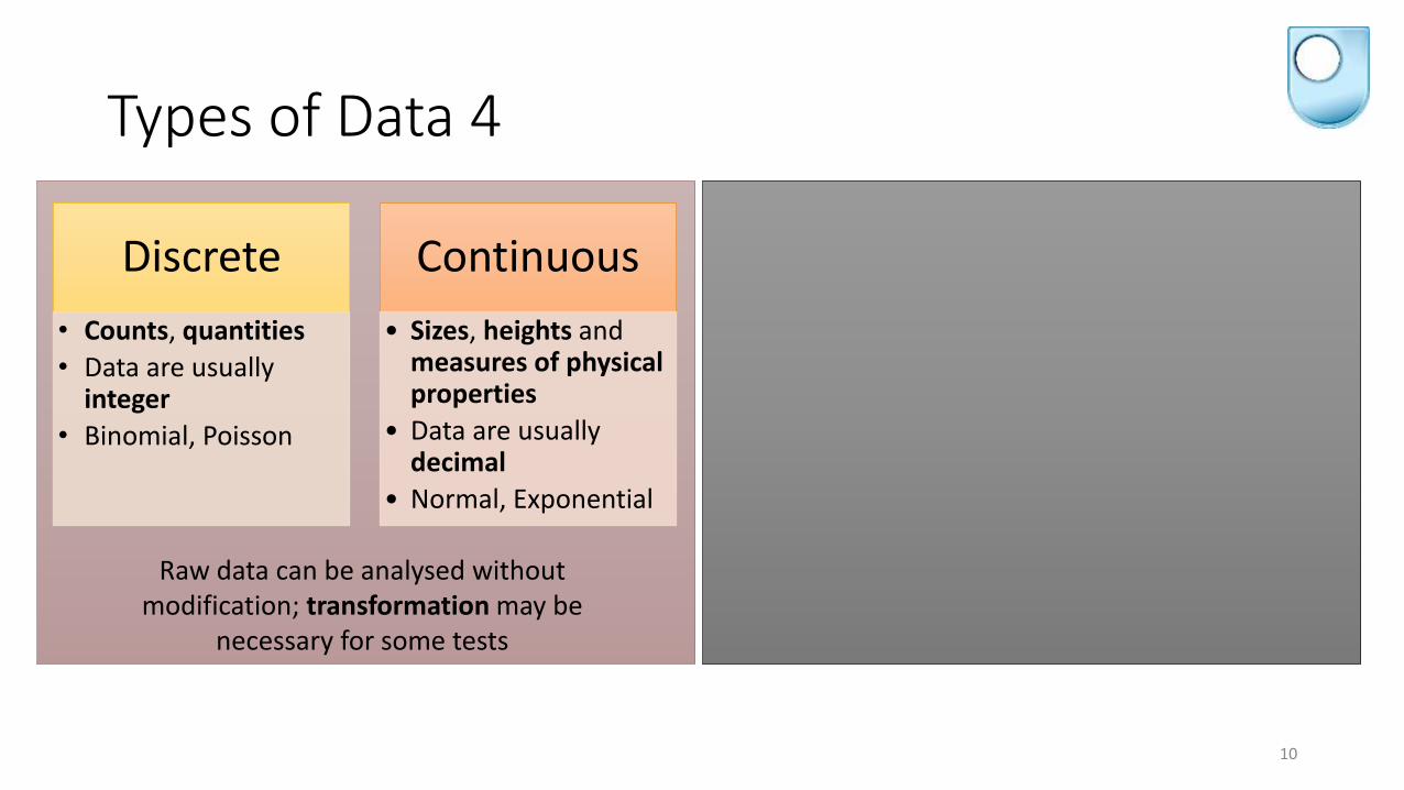
Discrete• Counts, quantities• Data are usually
integer• Binomial, Poisson
Continuous• Sizes, heights and
measures of physical properties
• Data are usually decimal
• Normal, Exponential
Types of Data 4
10
Raw data can be analysed without modification; transformation may be
necessary for some tests
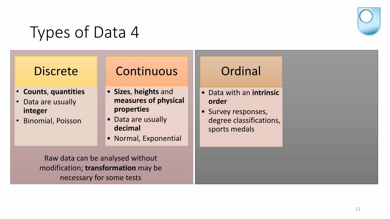
Discrete• Counts, quantities• Data are usually
integer• Binomial, Poisson
Continuous• Sizes, heights and
measures of physical properties
• Data are usually decimal
• Normal, Exponential
Ordinal• Data with an intrinsic
order• Survey responses,
degree classifications, sports medals
Types of Data 4
11
Raw data can be analysed without modification; transformation may be
necessary for some tests
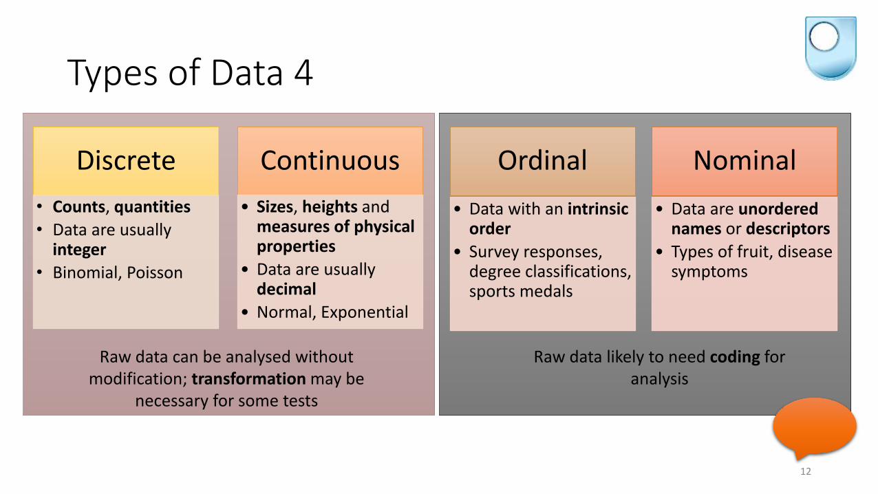
Discrete• Counts, quantities• Data are usually
integer• Binomial, Poisson
Continuous• Sizes, heights and
measures of physical properties
• Data are usually decimal
• Normal, Exponential
Ordinal• Data with an intrinsic
order• Survey responses,
degree classifications, sports medals
Nominal• Data are unordered
names or descriptors• Types of fruit, disease
symptoms
Types of Data 4
12
Raw data likely to need coding for analysis
Raw data can be analysed without modification; transformation may be
necessary for some tests
Locators & Descriptors
13
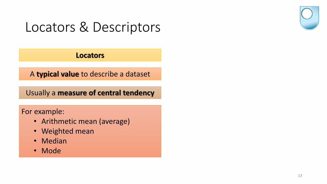
Locators
A typical value to describe a dataset
Usually a measure of central tendency
For example:• Arithmetic mean (average)• Weighted mean• Median• Mode

Locators & Descriptors
14
Locators
A typical value to describe a dataset
Usually a measure of central tendency
For example:• Arithmetic mean (average)• Weighted mean• Median• Mode
Descriptors
A value describing the shape of a dataset
Usually a measure of spread
For example:• Range• Standard deviation • Variance• Interquartile Range

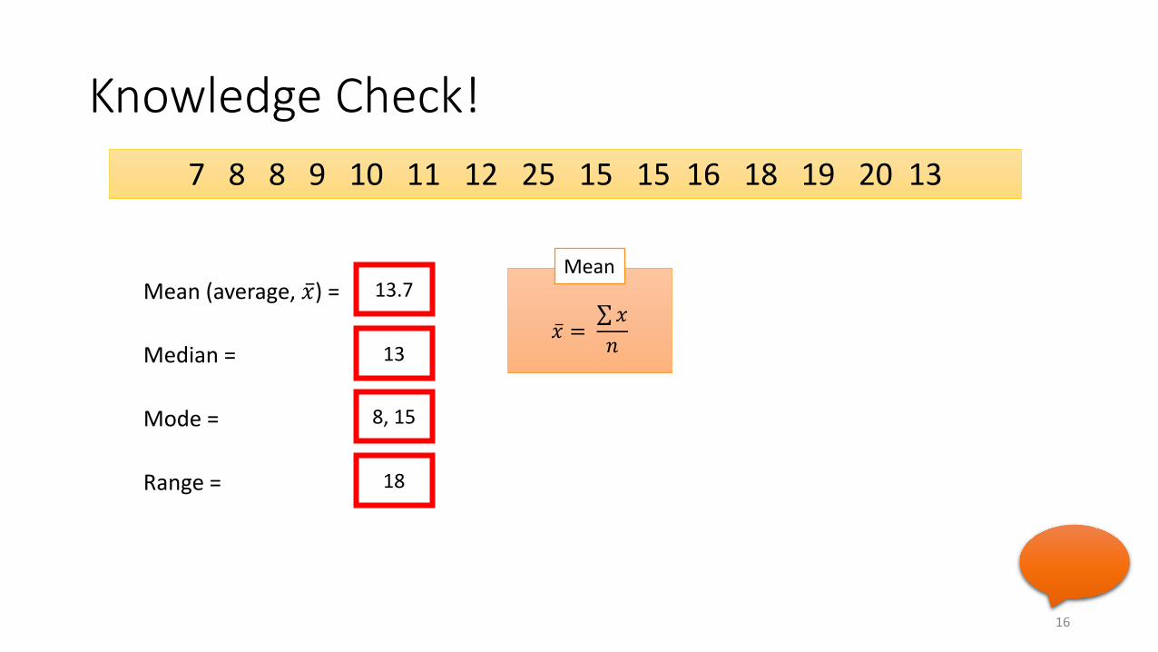
Knowledge Check!
15
7 8 8 9 10 11 12 25 15 15 16 18 19 20 13
Mean (average, �̅�𝑥) =
Median =
Mode =
Range =
�̅�𝑥 =∑𝑥𝑥𝑛𝑛
Mean
Fill in the blanks!(1 dp)
Knowledge Check!
16
7 8 8 9 10 11 12 25 15 15 16 18 19 20 13
Mean (average, �̅�𝑥) =
Median =
Mode =
Range =
�̅�𝑥 =∑𝑥𝑥𝑛𝑛
Mean13.7
13
8, 15
18
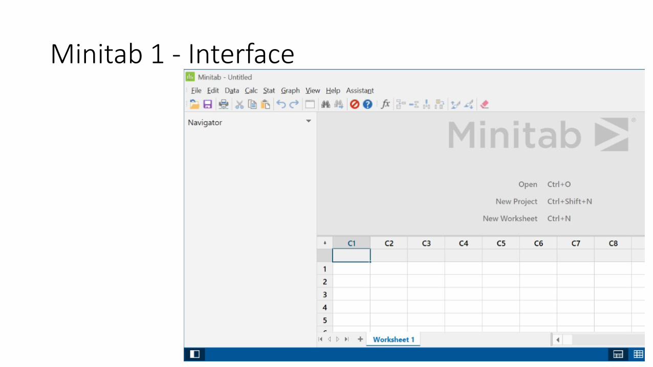
Minitab 1 - Interface
17
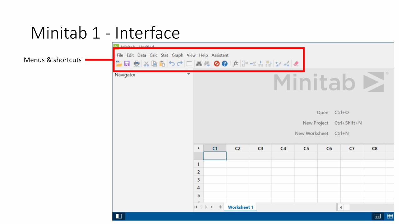
Minitab 1 - Interface
18
Menus & shortcuts
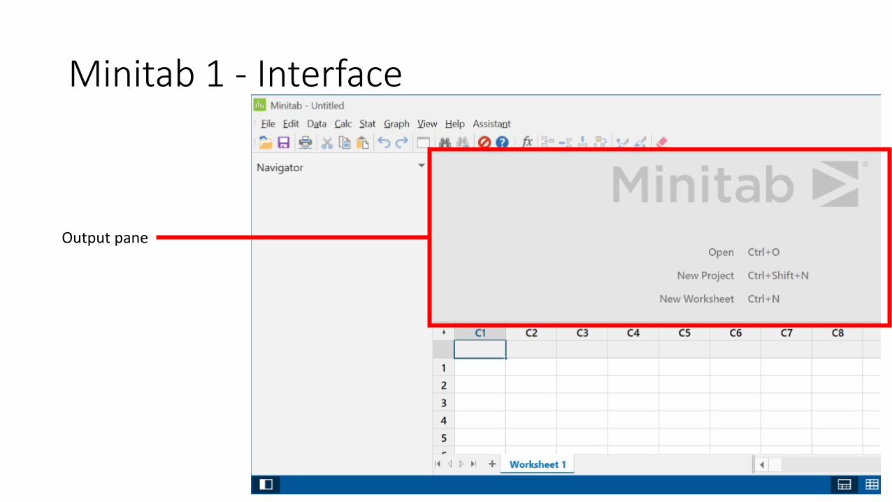
Minitab 1 - Interface
19
Output pane
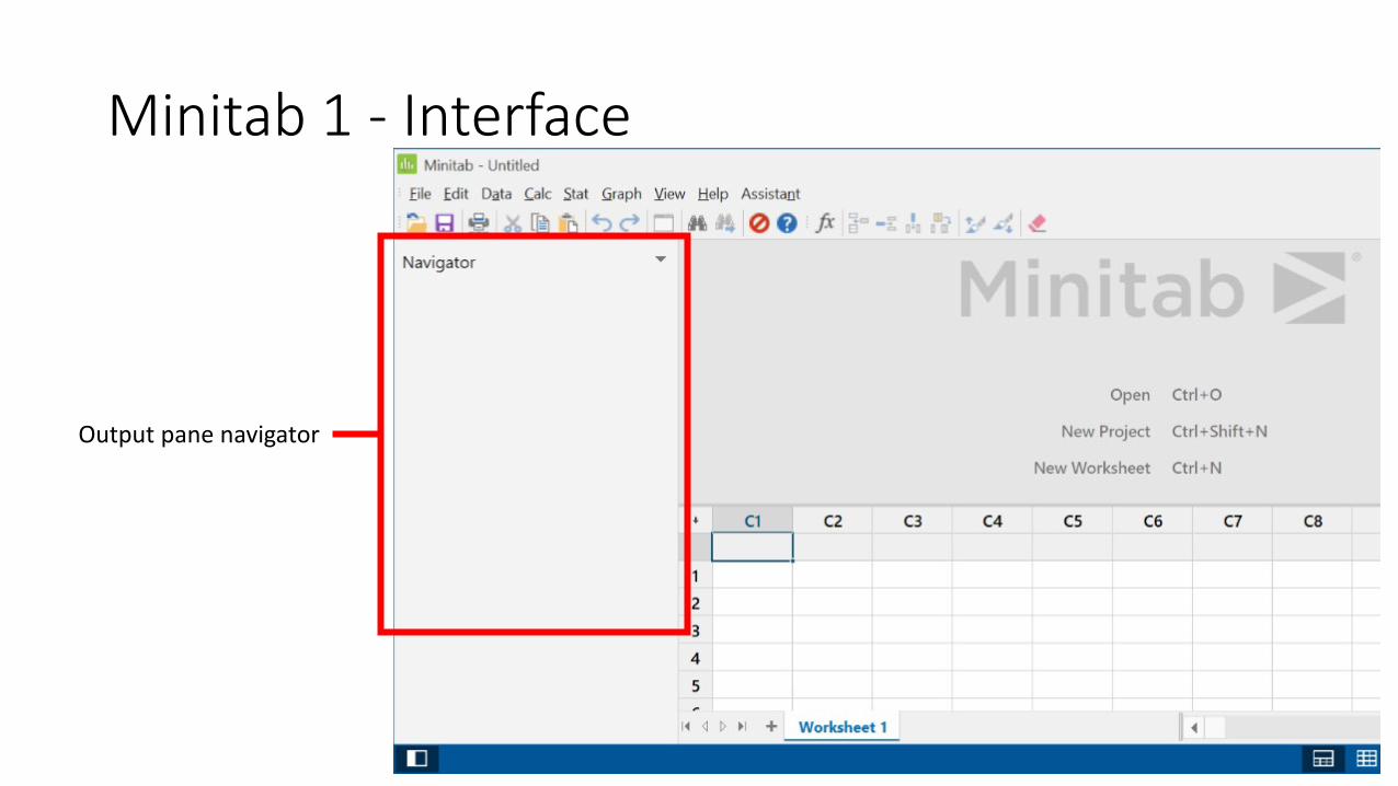
Minitab 1 - Interface
20
Output pane navigator
Minitab 1 - Interface
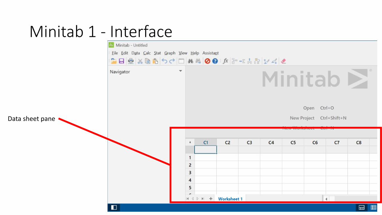
21
Data sheet pane
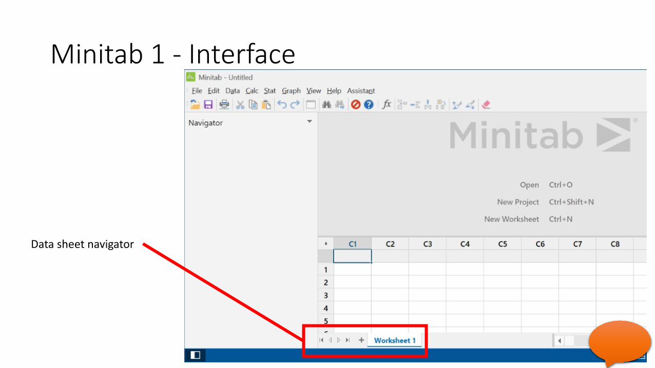
Minitab 1 - Interface
22
Data sheet navigator
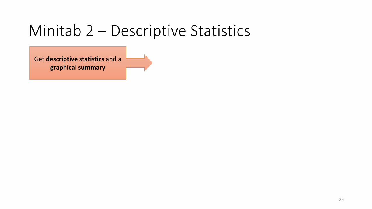
Minitab 2 – Descriptive Statistics
23
Get descriptive statistics and a graphical summary
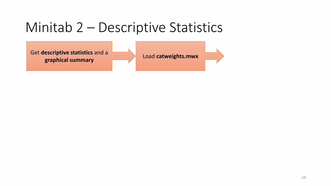
Minitab 2 – Descriptive Statistics
24
Get descriptive statistics and a graphical summary Load catweights.mwx
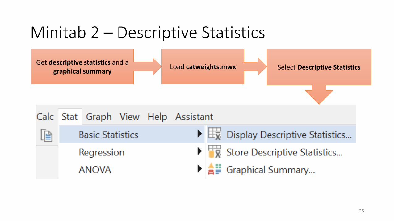
Minitab 2 – Descriptive Statistics
25
Get descriptive statistics and a graphical summary Load catweights.mwx Select Descriptive Statistics
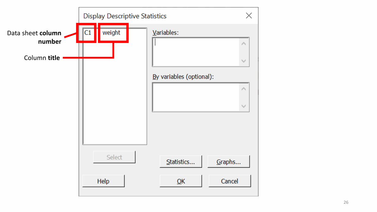
26
Data sheet column number
Column title
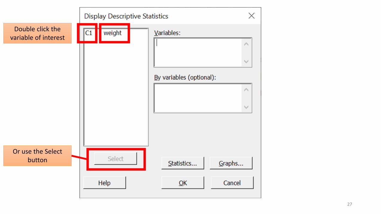
27
Double click the variable of interest
Or use the Select button
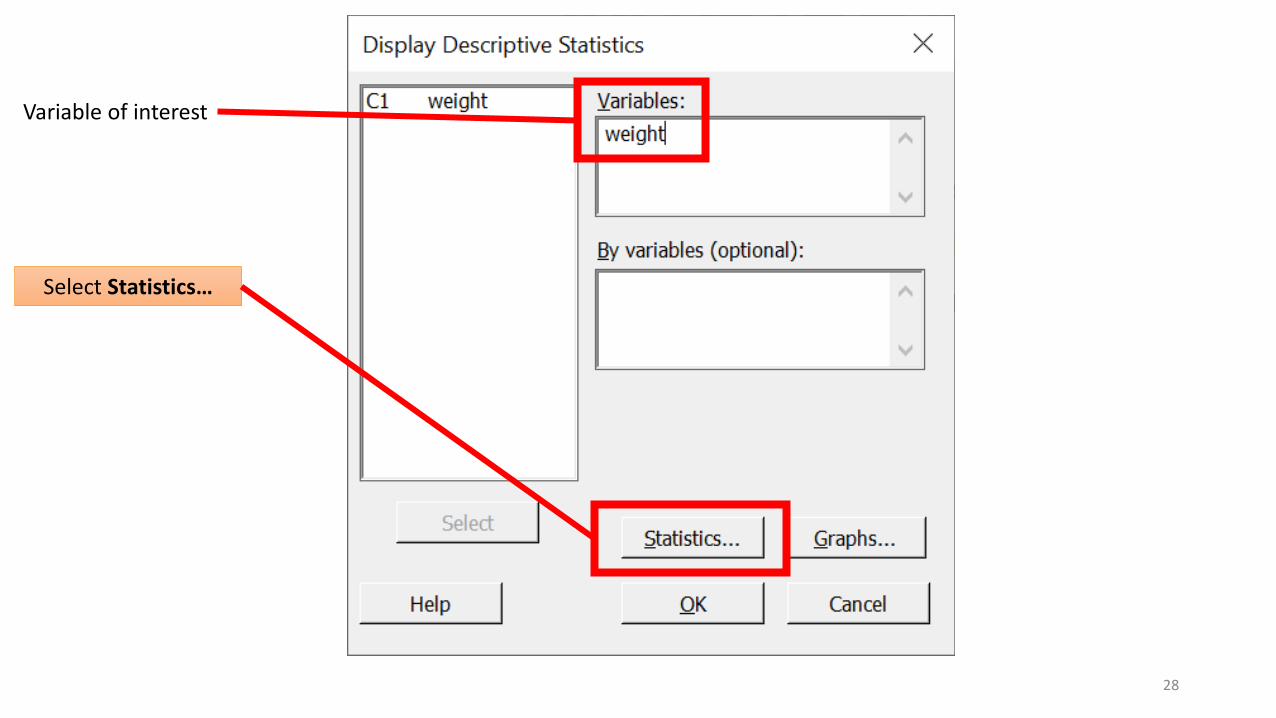
28
Variable of interest
Select Statistics…
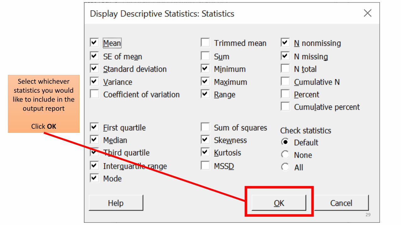
29
Select whichever statistics you would like to include in the
output report
Click OK

30
Ta da!

31
Output pane navigator

Charts Components Refresher
• Charts, graphs, plots – are all essential to explain any data or analysis• However, poor charts can unintentionally (or intentionally)
misrepresent data leading to inaccurate or erroneous interpretations by the viewer
• Example shortly…
• What are the key components for every chart and graph?
32

Essential Components
Figure 1. Simple exponential plot (𝑦𝑦 = 𝑥𝑥2).
Data
33
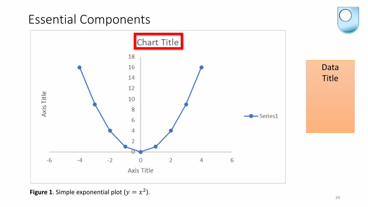
Essential Components
Figure 1. Simple exponential plot (𝑦𝑦 = 𝑥𝑥2).
DataTitle
34
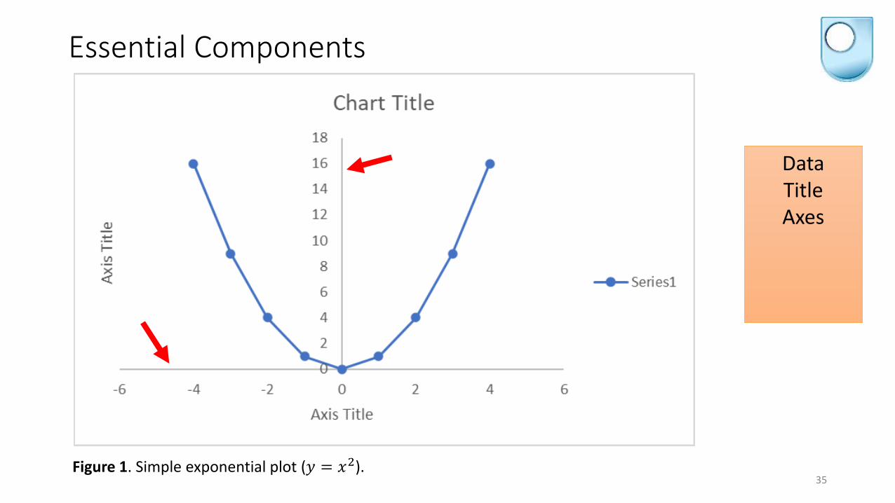
Essential Components
Figure 1. Simple exponential plot (𝑦𝑦 = 𝑥𝑥2).
DataTitleAxes
35
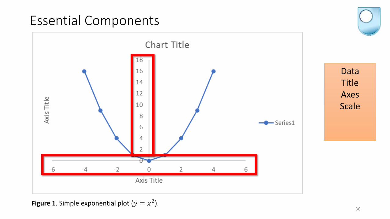
Essential Components
Figure 1. Simple exponential plot (𝑦𝑦 = 𝑥𝑥2).
DataTitleAxesScale
36

Essential Components
Figure 1. Simple exponential plot (𝑦𝑦 = 𝑥𝑥2).
DataTitleAxesScale
Labels
37

Essential Components
Figure 1. Simple exponential plot (𝑦𝑦 = 𝑥𝑥2).
DataTitleAxesScale
LabelsLegend
38
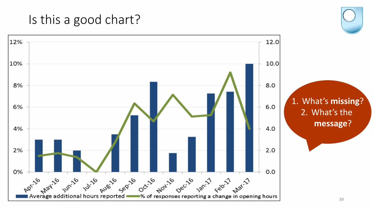
Is this a good chart?
39
1. What’s missing?2. What’s the
message?

Is this a good chart?
40
No titleNo axis labels
Graph purports to show how many shops are reporting a change in their opening hours and what those additional hours are.
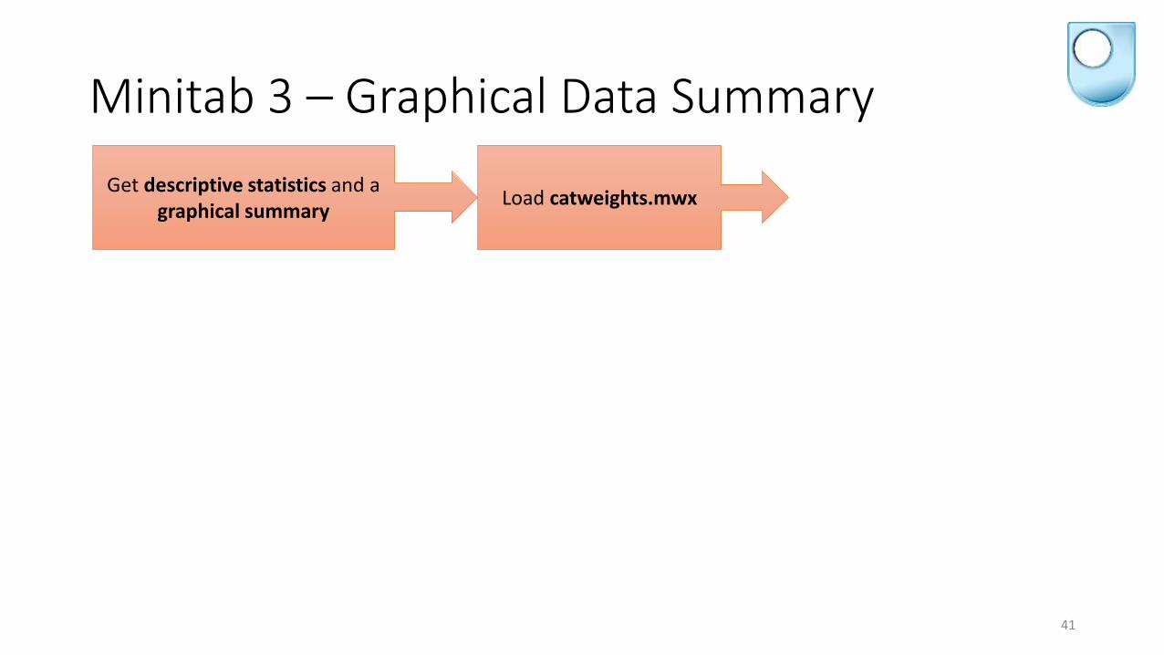
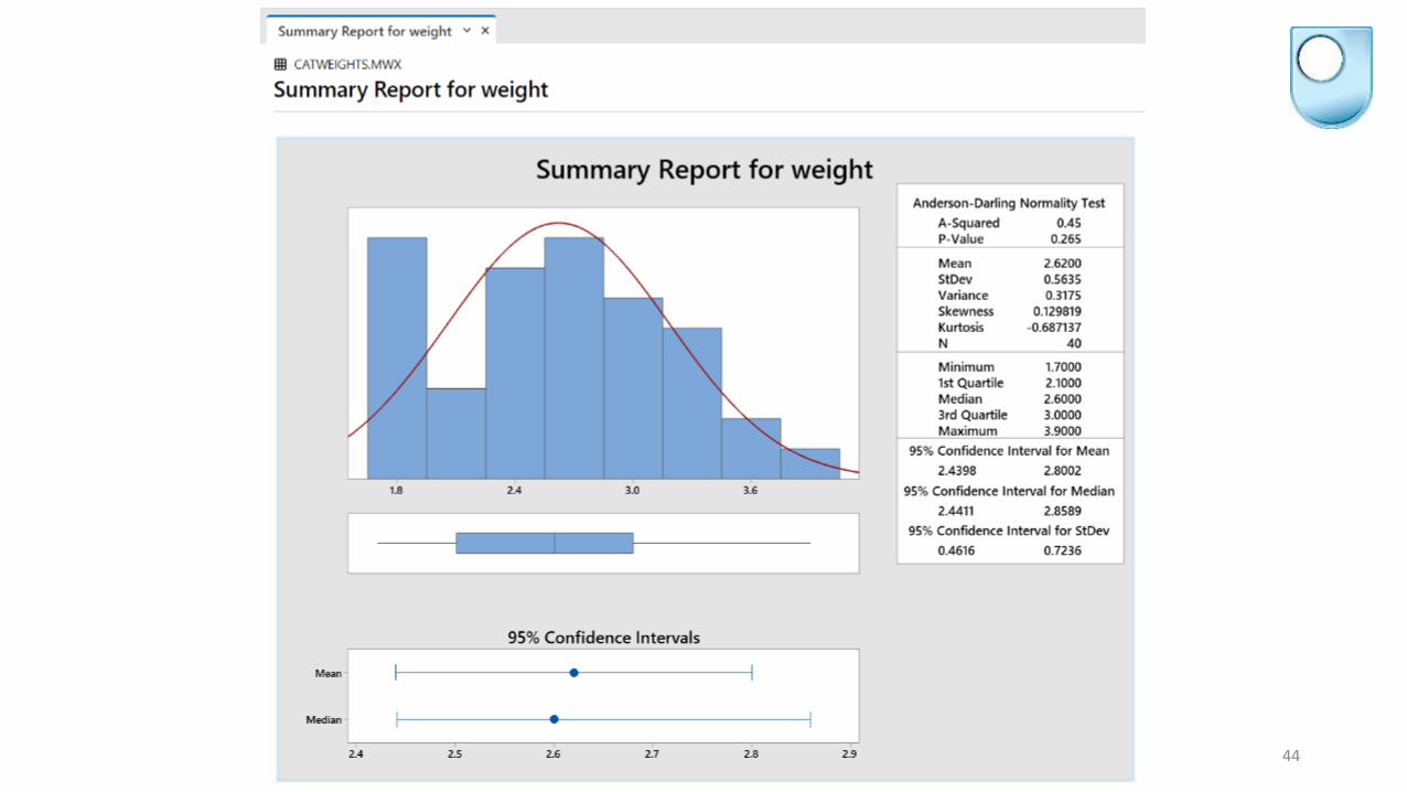
Minitab 3 – Graphical Data Summary
41
Get descriptive statistics and a graphical summary Load catweights.mwx
Minitab 3 – Graphical Data Summary
42
Get descriptive statistics and a graphical summary Load catweights.mwx Select Graphical Summary

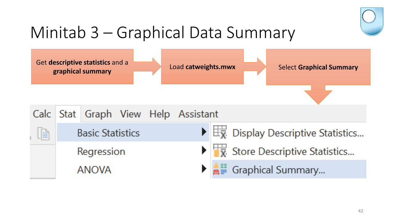
Minitab 3 – Graphical Data Summary
43
Get descriptive statistics and a graphical summary Load catweights.mwx Select Graphical Summary
Select the variable of interest and click OK
44
45
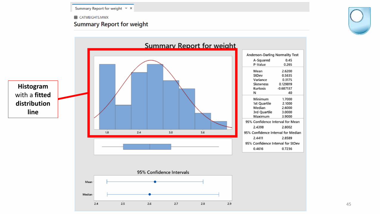
Histogramwith a fitted distribution
line
46
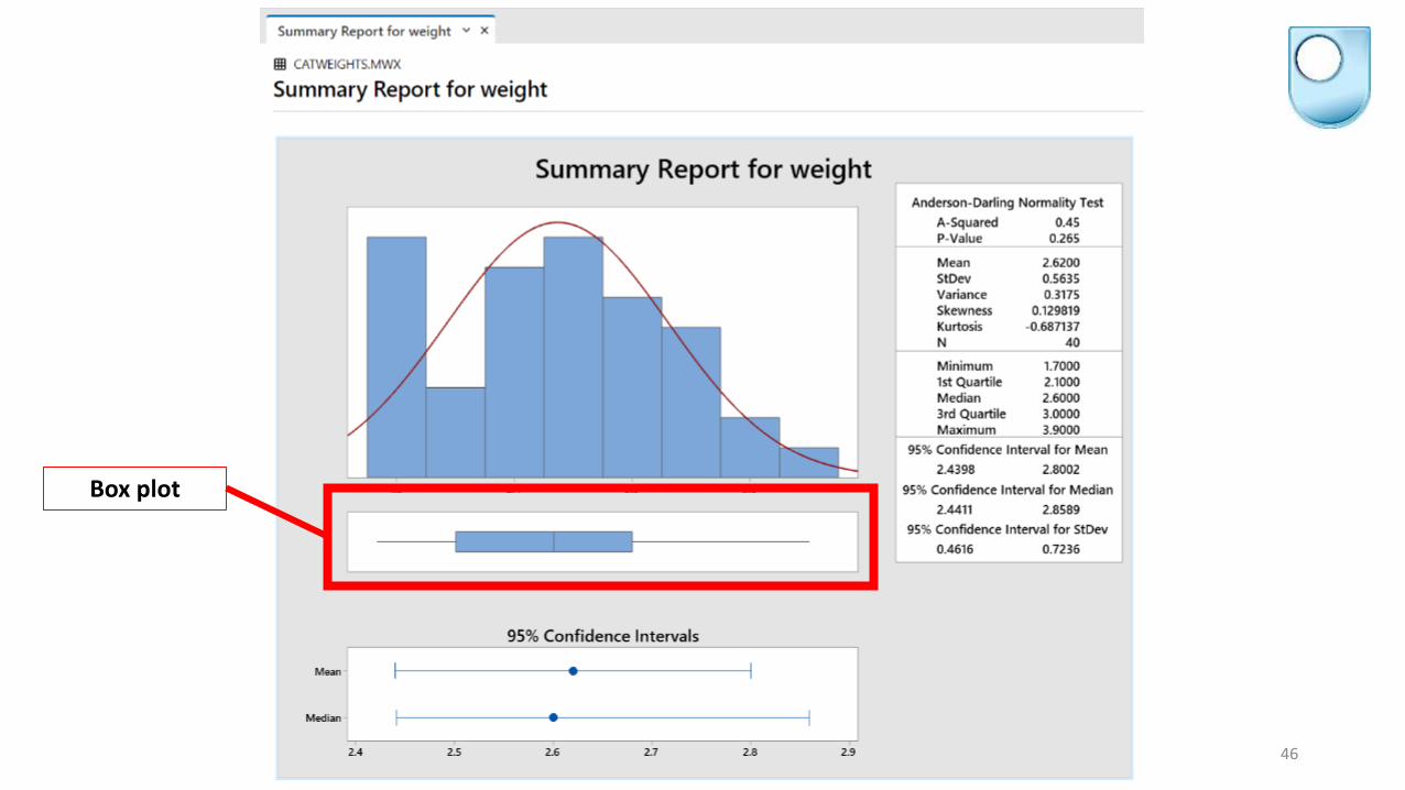
Box plot
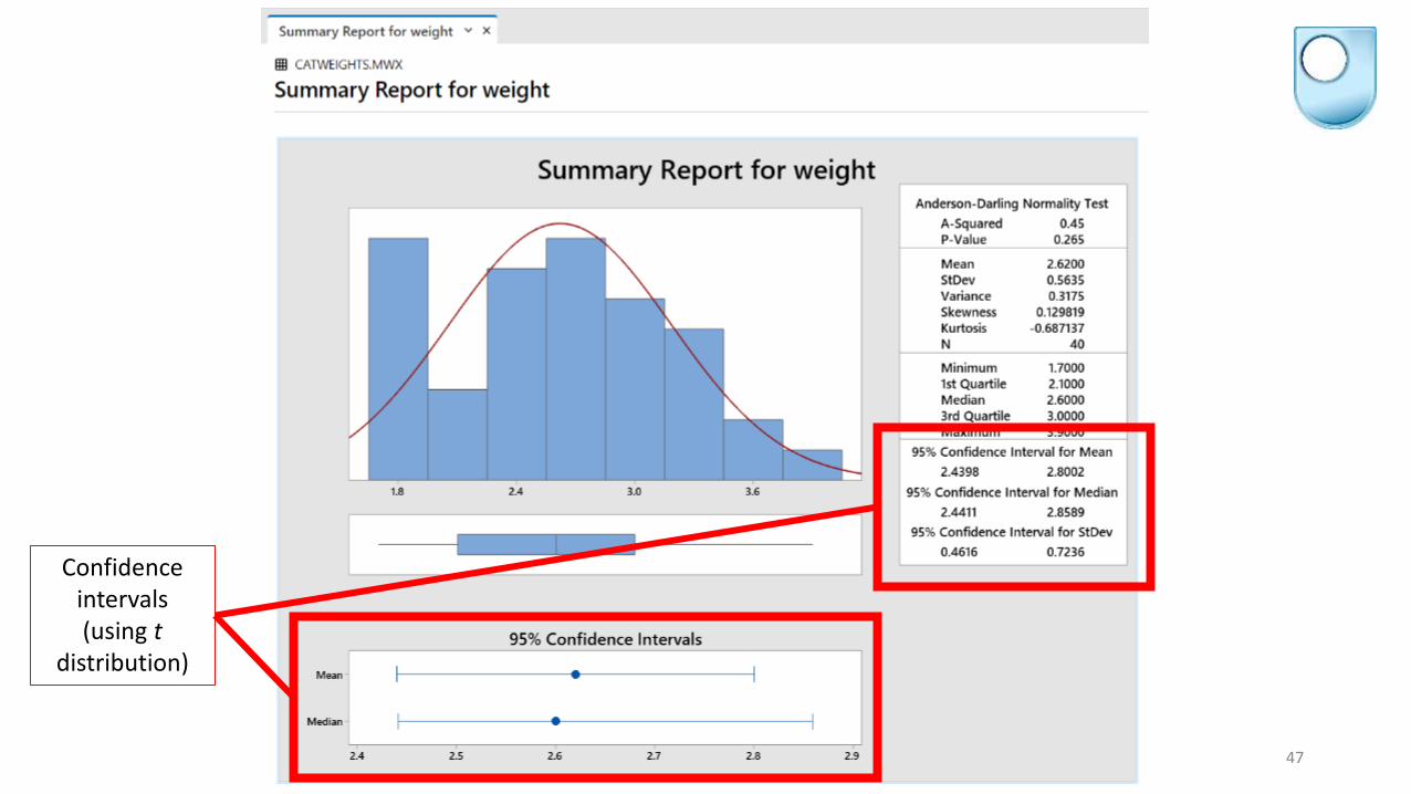
47
Confidence intervals(using t
distribution)
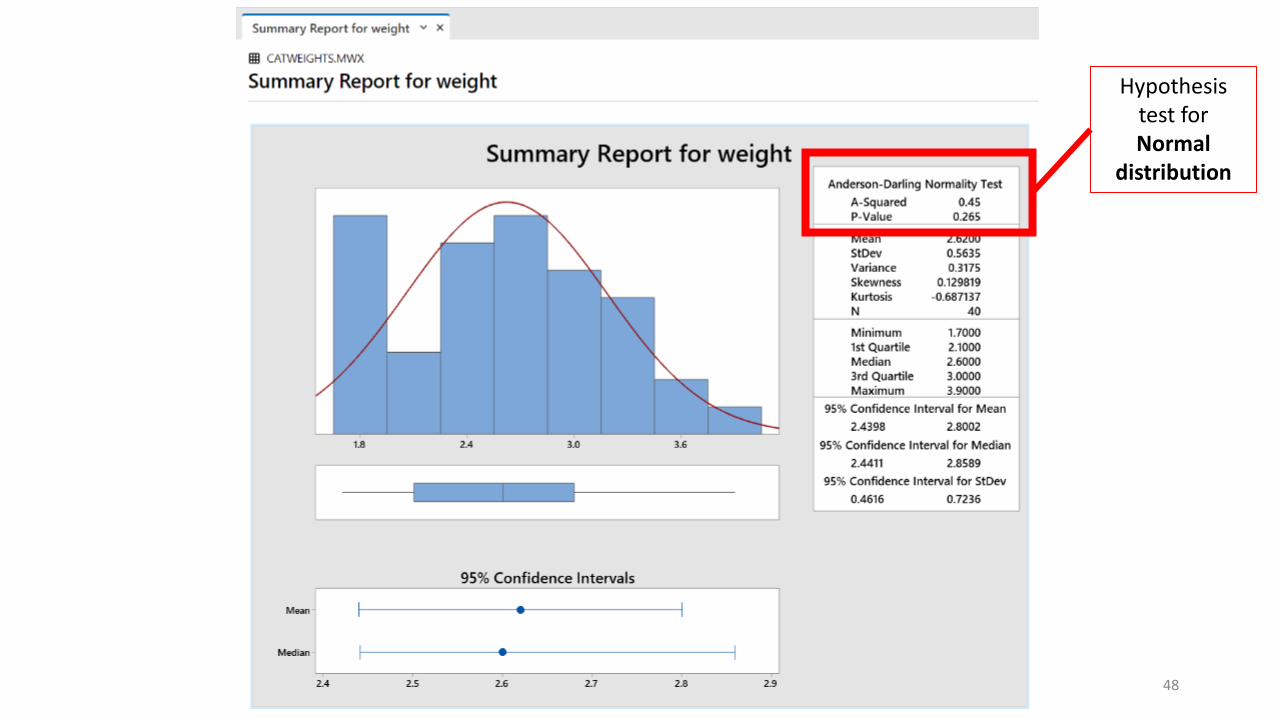
48
Hypothesis test for Normal
distribution
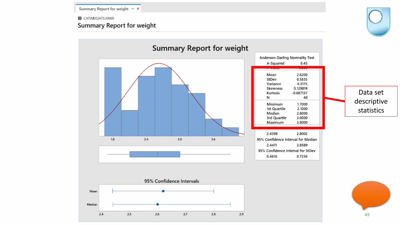
49
Data set descriptive
statistics

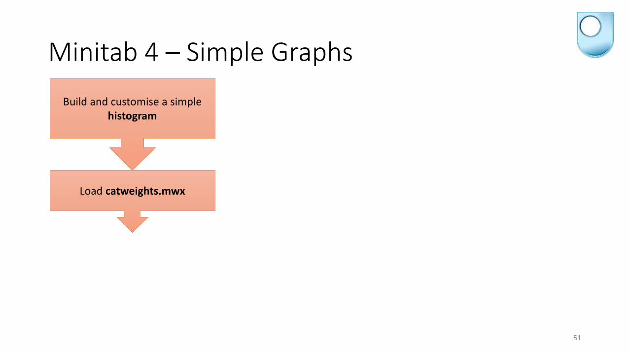
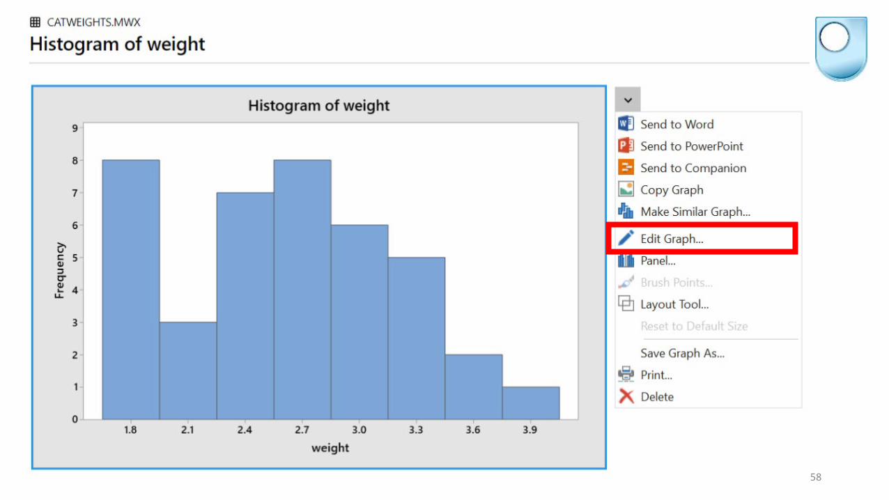
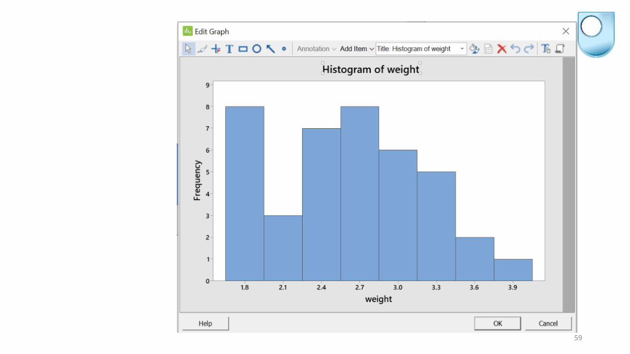
Minitab 4 – Simple Graphs
50
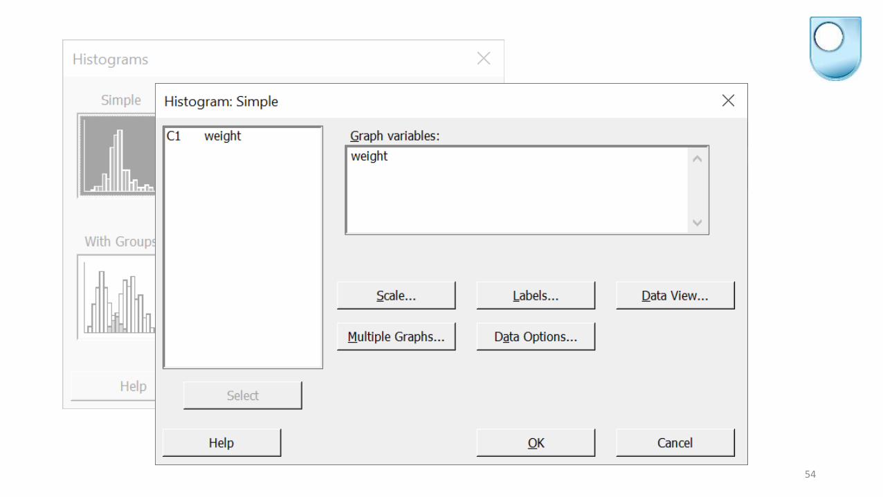
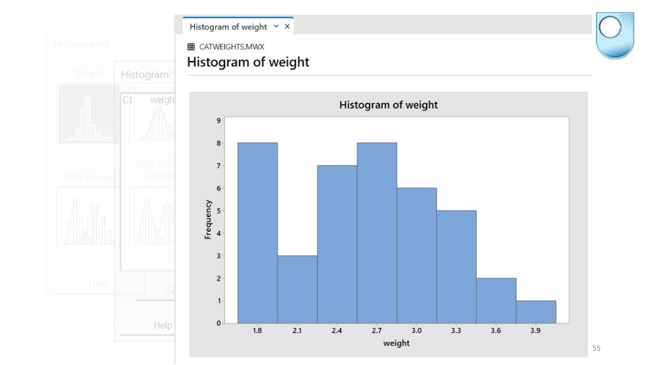
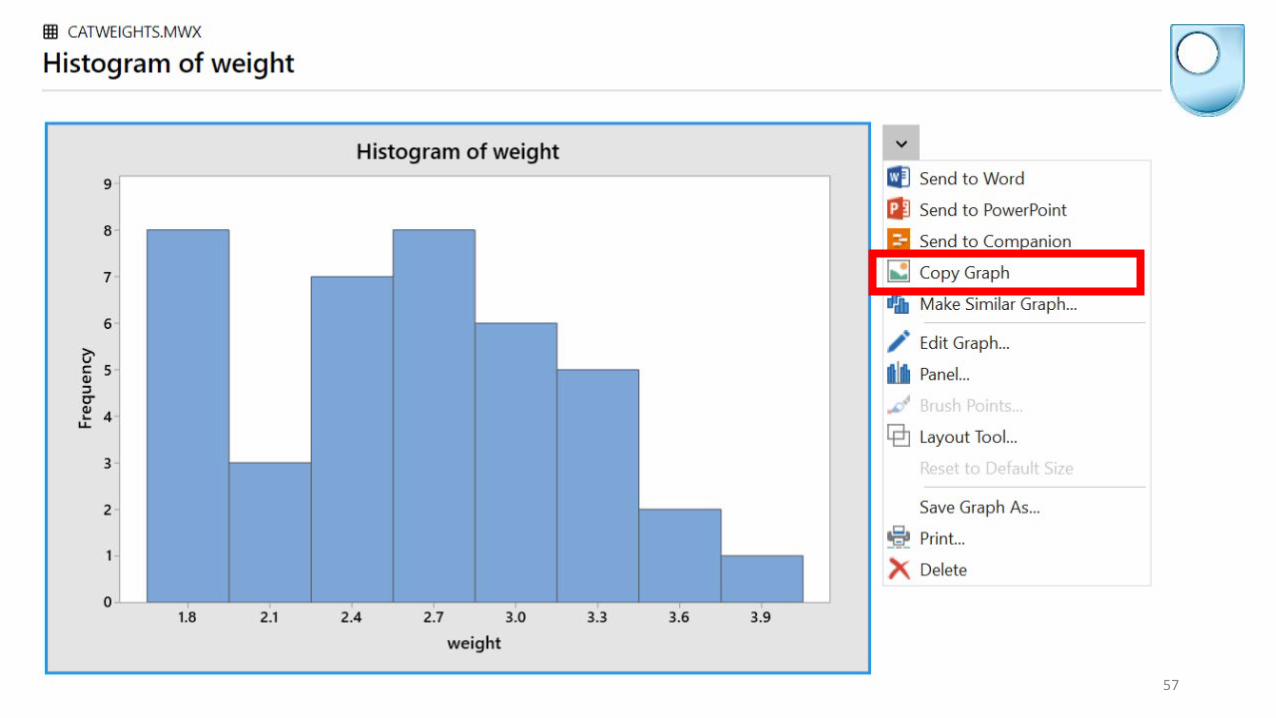
Build and customise a simple histogram
Minitab 4 – Simple Graphs
51
Build and customise a simple histogram
Load catweights.mwx
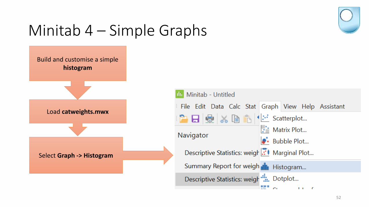
Minitab 4 – Simple Graphs
52
Build and customise a simple histogram
Load catweights.mwx
Select Graph -> Histogram
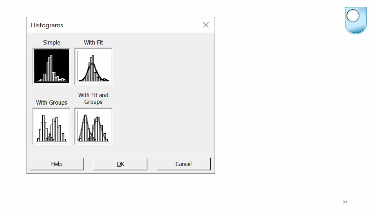
53
54
55

56
57
58
59
60
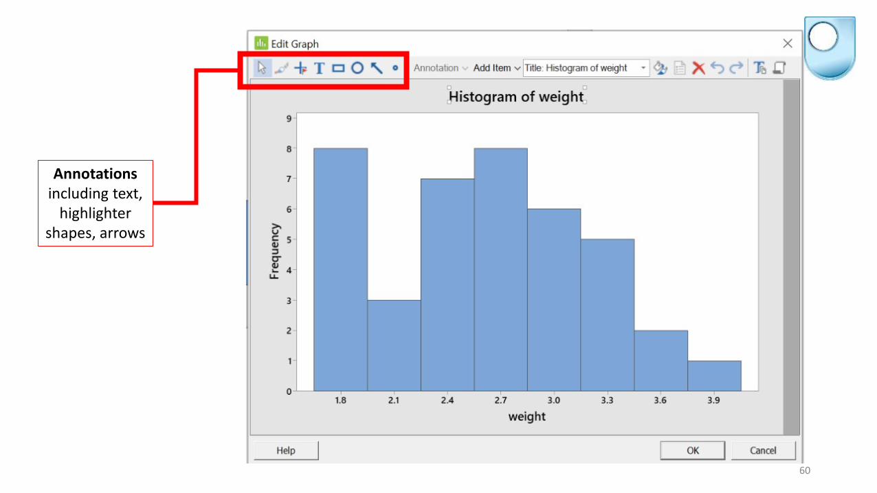
Annotationsincluding text,
highlighter shapes, arrows

61
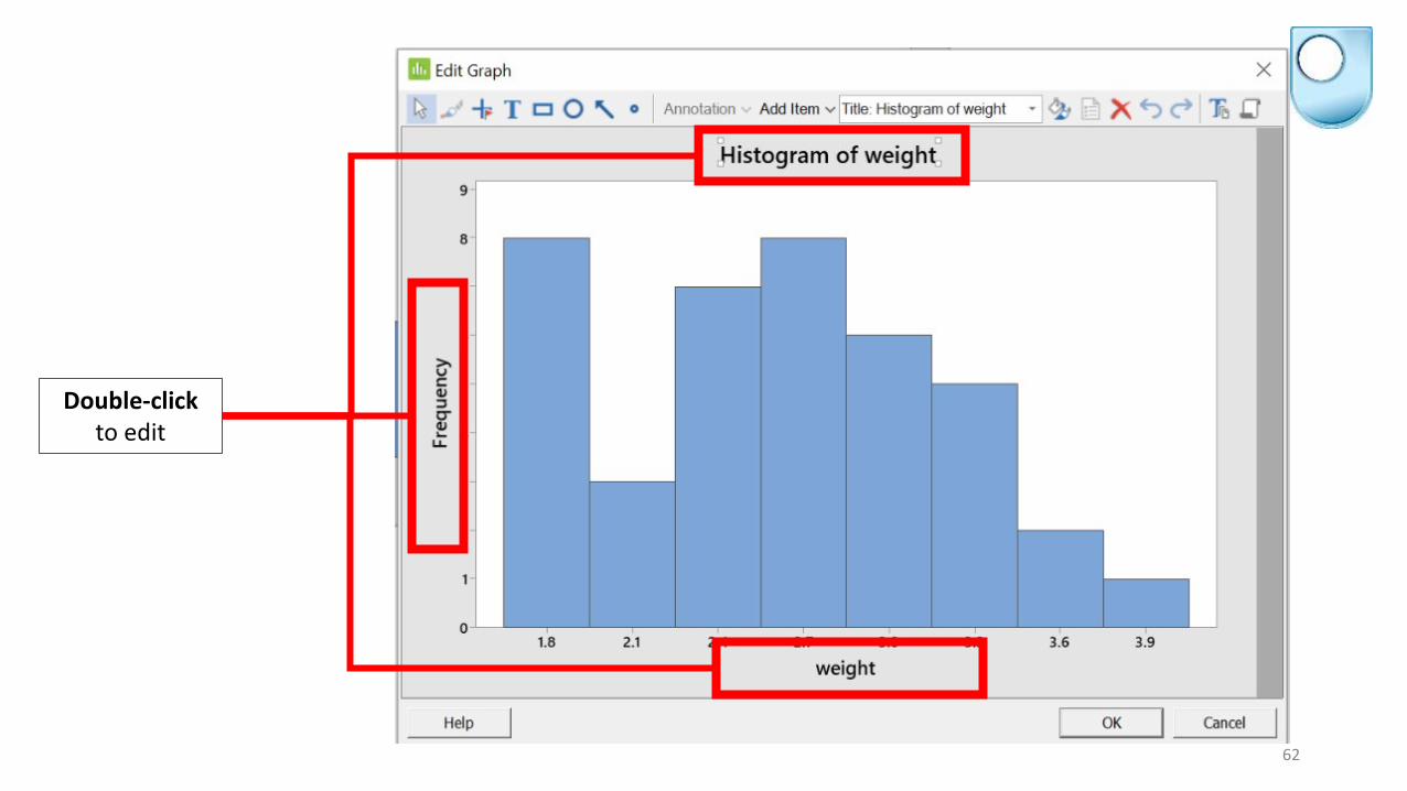
Additions & Edits
including grid lines, labels,
footnotes
62
Double-click to edit
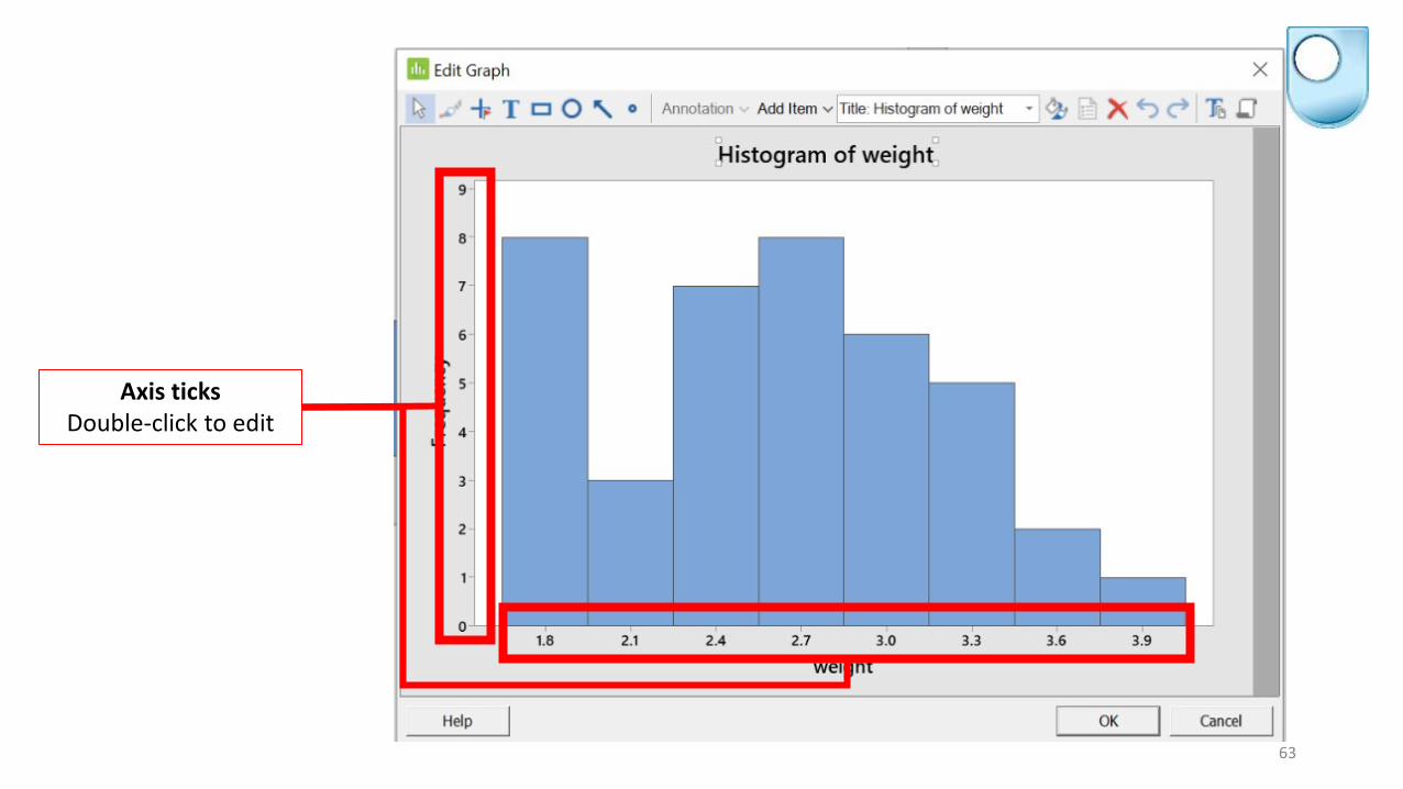
63
Axis ticksDouble-click to edit
64
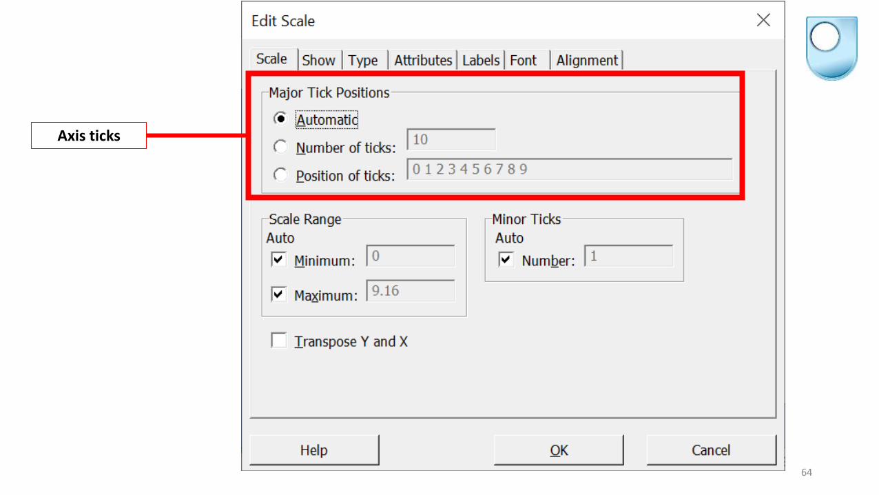
Axis ticks

65
Axis scale
66
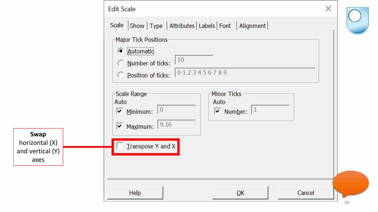
Swap horizontal (X)
and vertical (Y) axes
67
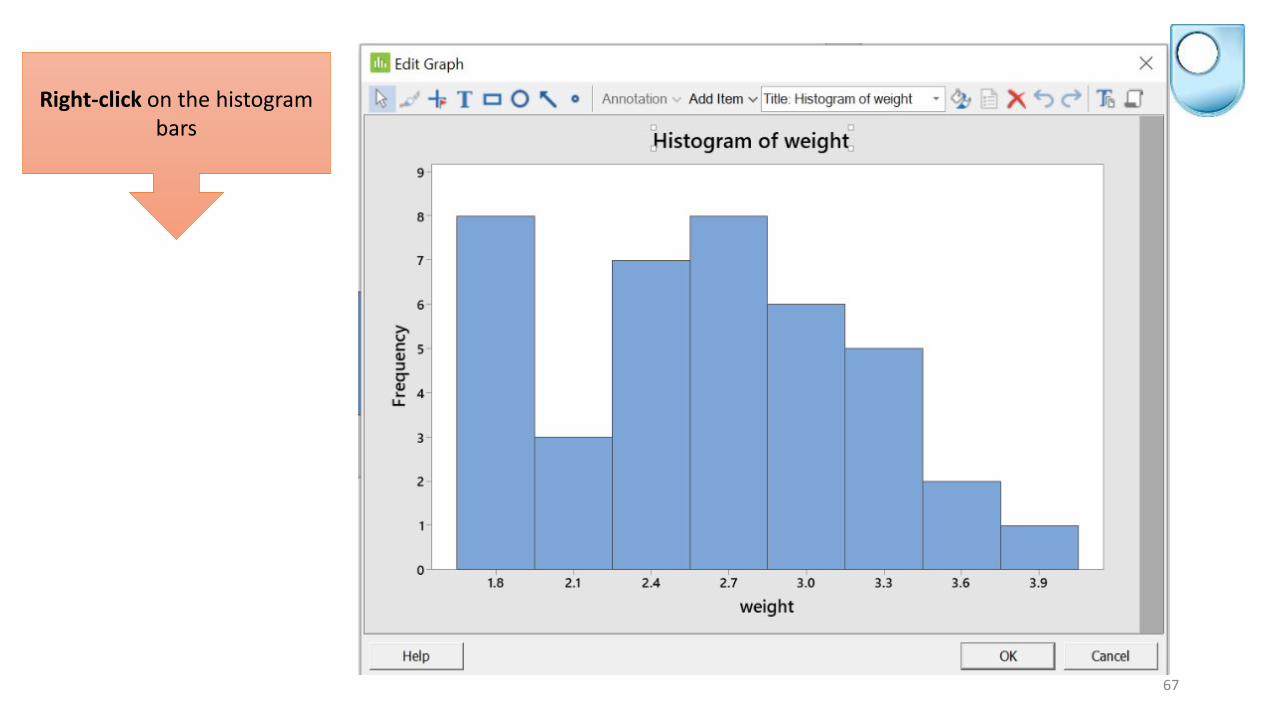
Right-click on the histogram bars
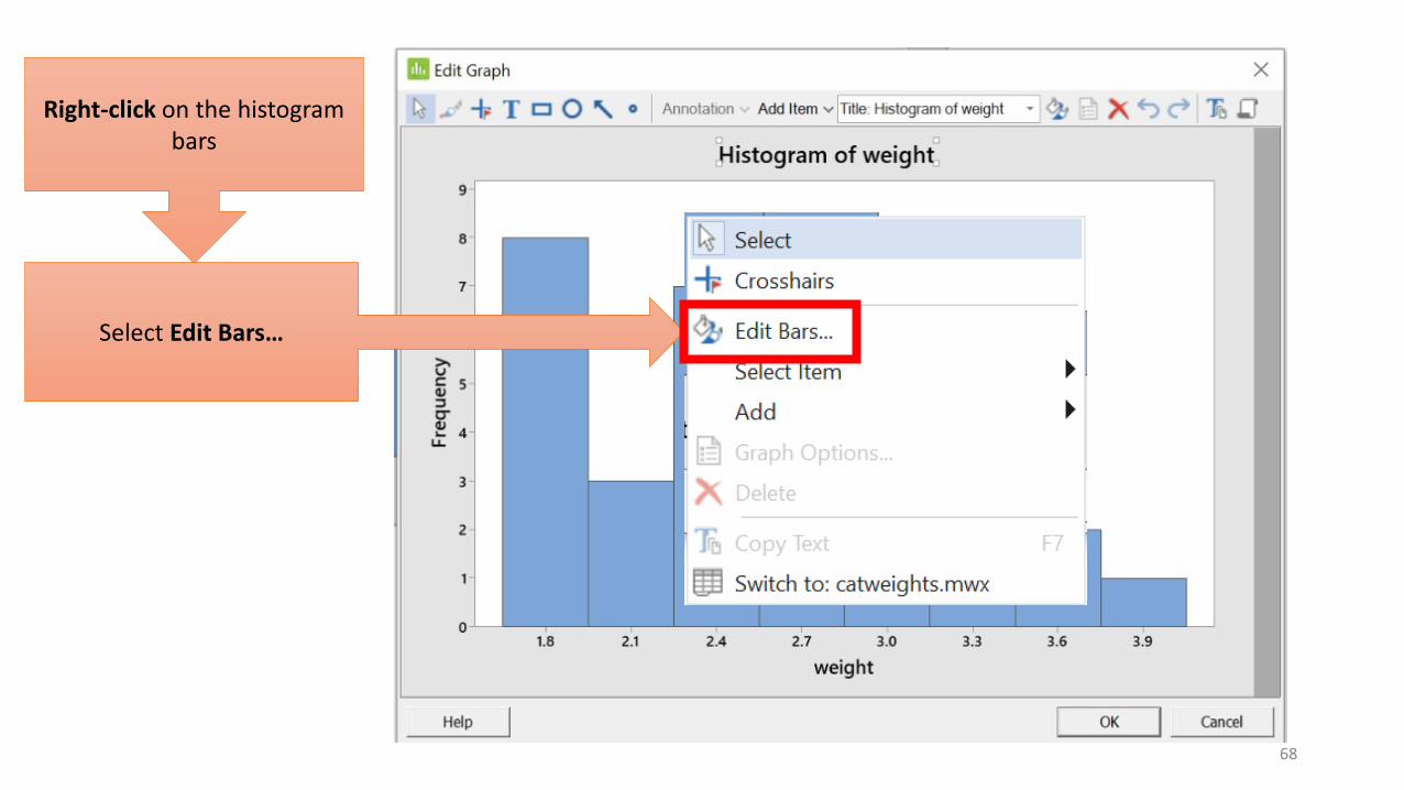
68
Right-click on the histogram bars
Select Edit Bars…
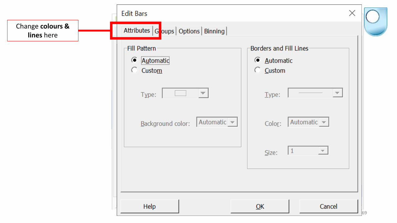
69
Change colours & lines here
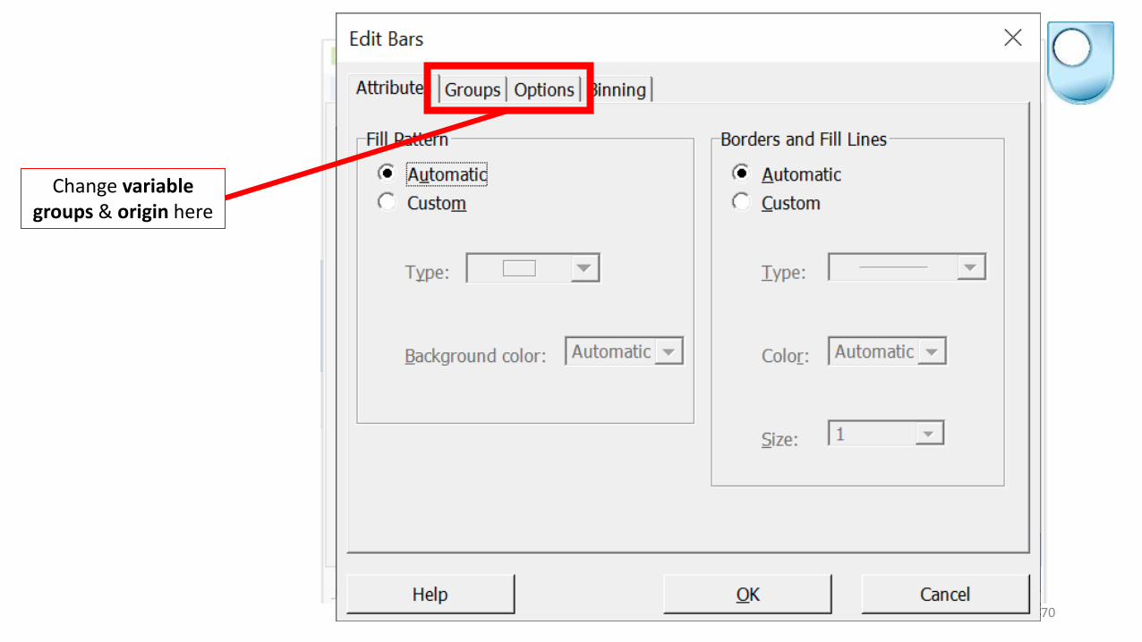
70
Change variable groups & origin here
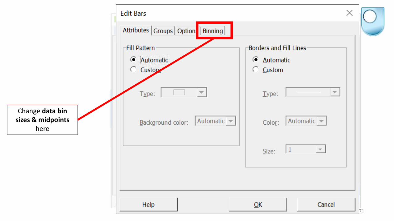
71
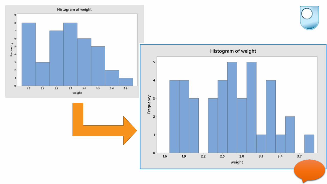
Change data bin sizes & midpoints
here

72
73
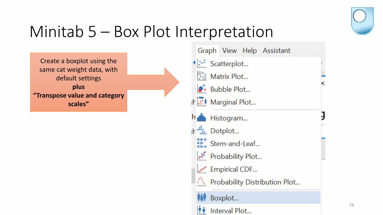
Minitab 5 – Box Plot Interpretation
74
Create a boxplot using the same cat weight data, with
default settingsplus
“Transpose value and category scales”

75
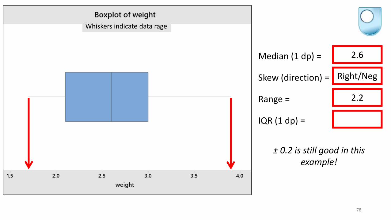
Fill in the blanks!
Whiskers indicate data rage
Median (1 dp) =
Skew (direction) =
Range =
IQR (1 dp) =
2.6
Right/Neg
2.2
0.9

76
Whiskers indicate data rage
Median (1 dp) =
Skew (direction) =
Range =
IQR (1 dp) =
2.6
Right/Neg
2.2
0.9
± 0.2 is still good in this example!

77
Right > left
Whiskers indicate data rage
Median (1 dp) =
Skew (direction) =
Range =
IQR (1 dp) =
2.6
Right/Pos
2.2
0.9
± 0.2 is still good in this example!
78
Whiskers indicate data rage
Median (1 dp) =
Skew (direction) =
Range =
IQR (1 dp) =
2.6
Right/Neg
2.2
0.9
± 0.2 is still good in this example!

79
Median (1 dp) =
Skew (direction) =
Range =
IQR (1 dp) =
2.6
Right/Neg
2.2
0.9
± 0.2 is still good in this example!
Whiskers indicate data range
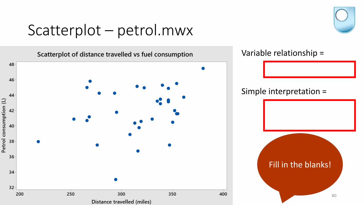
Scatterplot – petrol.mwx
80
Variable relationship =
Positive
Simple interpretation =
More miles are driven as petrol price rises
Fill in the blanks!
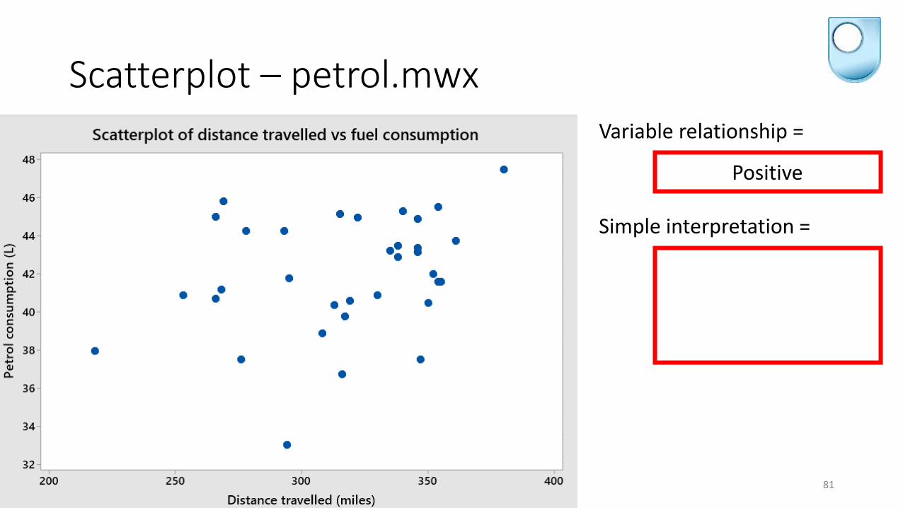
Scatterplot – petrol.mwx
81
Variable relationship =
Positive
Simple interpretation =
Petrol consumption increases with the amount of driving
miles

Scatterplot – petrol.mwx
82
Variable relationship =
Positive
Simple interpretation =
Petrol consumption increases with the amount of driving
miles
Thank you! Any questions?
• M140 materials online• Course Books & Screencasts• (https://learn2.open.ac.uk/course/view.php?id=208584&area=resources )
• M140 student forums• Wikipedia• CrossValidated (https://stats.stackexchange.com/ )• Minitab channel on YouTube:
• https://www.youtube.com/user/MinitabInc• Minitab help
• https://support.minitab.com/en-us/minitab/19/• Contact me:
• [email protected]• 07311 188 800
83Recording should be available in the M140 20J Online Tutorial Room• https://learn2.open.ac.uk/mod/connecthosted/viewrecordings.php?id=1644077&group=274133