M102. Circular motion of a rigid...

Pracownia Podstaw Fizyczne Laboratorium Mikrokomputerowe Wydział Fizyki Eksperymentu Fizycznego Filami UAM

M102. Circular motion of a rigid body

Aim:

Experimental characterisation of the circular motion of a rigid body, including

Determination of the angular rate of rotation from measurements of the position of a

rotating table as a function of time,

Experimental and theoretical determination of the moment of inertia of a rigid body,

Characterisation of the process of potential energy conversion into kinetic energy of

circular motion.

Physical problems:

The moment of inertia of a rigid body,

Equations of motion for a point of matter and a rigid body (Newton’s second law of

dynamics),

Potential and kinetic energy of a point of matter and a rigid body.

Experimental tasks:

Measurement of resistance by a serial port,

Measurement of position by a potentiometer, calibration of potentiometer (conversion of

resistance to position),

Determination of the conditions of the beginning and end of measurements (triggering

and stopping of measurement after reaching certain values),

Fitting of a square function to the experimental results,

Digital differentiation of experimental data (calculation of instantaneous velocities on the

basis of changes in position as a function of time).

References:

Henryk Szydłowski “ Pracownia Fizyczna”, Wyd. Nauk. PWN,Warszawa1994

David Halliday, Robert Resnick and Jearl Walker “Podstawyfizyki” Wyd.

Nauk.PWN,Warszawa2003

1. Introduction

The Newton‟s second law of dynamics for circular motion of a rigid body is:

IM , (1)

whereM is the resultant moment of force acting on the body, I– is the moment of inertia, and –

is the angular rate. The moment of inertia of a rotating body is defined as:


N

i

iirmI1

2 , (2)

where the summation goes over all particles of the body that can be treated as points of matter of

mass miat the distance from the axis of rotation ri. In practice the moment of inertia is calculated

by integration over volume:

dVrI 2 ,

whereris the density of the body. From eq. (3) you can find that the moment of inertia of a filled

cylinder(disc)of massmand radius r,rotating about its symmetry axis is:

2

21 mrI . (4)

If a body of mass m, whose moment of inertia with respect to the symmetry axis is I0,rotates

about the axis at a distance lfrom the symmetry axis, then its moment of inertia, according to the

Steiner theorem, is:

20 mlII . (5)

2. Measuring setup

The circular motion of a rigid body will be studied with the use of a rotating table, shown

schematically in Fig. 1.

Figure 1.Scheme of a setup for investigation of circular motion of a rigid body

A reel of thread

rotating table

potentiometer

FN

FN

weight

block

Fg=mg


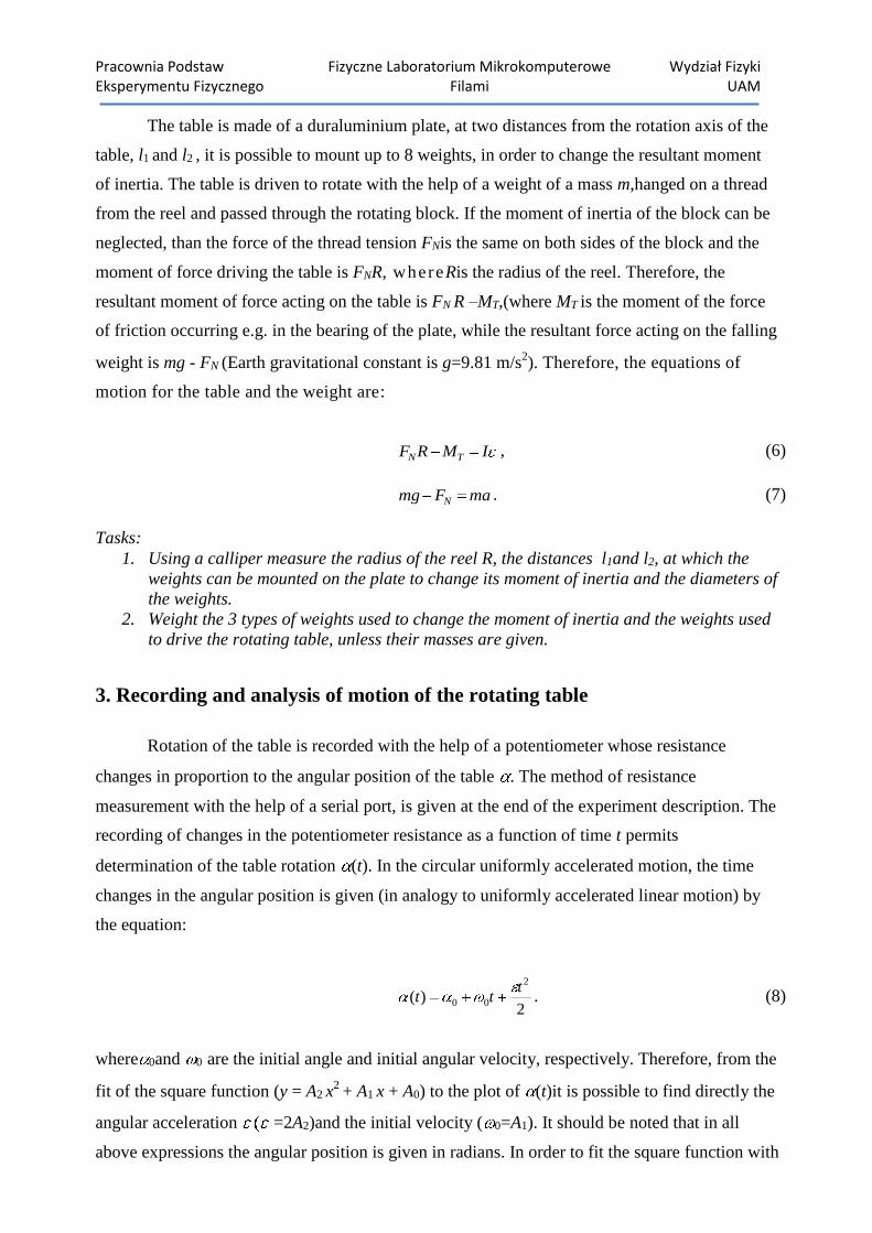
The table is made of a duraluminium plate, at two distances from the rotation axis of the

table, l1 and l2 , it is possible to mount up to 8 weights, in order to change the resultant moment

of inertia. The table is driven to rotate with the help of a weight of a mass m,hanged on a thread

from the reel and passed through the rotating block. If the moment of inertia of the block can be

neglected, than the force of the thread tension FNis the same on both sides of the block and the

moment of force driving the table is FNR, whereRis the radius of the reel. Therefore, the

resultant moment of force acting on the table is FN R –MT,(where MT is the moment of the force

of friction occurring e.g. in the bearing of the plate, while the resultant force acting on the falling

weight is mg - FN (Earth gravitational constant is g=9.81 m/s2). Therefore, the equations of

motion for the table and the weight are:

IMRF TN , (6)

maFmg N . (7)

Tasks:

1. Using a calliper measure the radius of the reel R, the distances l1and l2, at which the

weights can be mounted on the plate to change its moment of inertia and the diameters of

the weights.

2. Weight the 3 types of weights used to change the moment of inertia and the weights used

to drive the rotating table, unless their masses are given.

3. Recording and analysis of motion of the rotating table

Rotation of the table is recorded with the help of a potentiometer whose resistance

changes in proportion to the angular position of the table . The method of resistance

measurement with the help of a serial port, is given at the end of the experiment description. The

recording of changes in the potentiometer resistance as a function of time t permits

determination of the table rotation (t). In the circular uniformly accelerated motion, the time

changes in the angular position is given (in analogy to uniformly accelerated linear motion) by

the equation:

2)(

2

00

ttt . (8)

where 0and 0 are the initial angle and initial angular velocity, respectively. Therefore, from the

fit of the square function (y = A2 x2

+ A1 x + A0) to the plot of (t)it is possible to find directly the

angular acceleration =2A2)and the initial velocity ( 0=A1). It should be noted that in all

above expressions the angular position is given in radians. In order to fit the square function with


the use of LabViewyou should use the function General Polynomial Fit.vi (polynomial

order=2, the connector Polynomial Fit Coefficientsgives a table with the coefficients of the fit

Ai)

Tasks

1. Write a program in LabView permitting measurement of the potentiometer resistance with

the use of a serial port (e.g. similar to that shown in Fig. 5).Find out the values of

resistance corresponding to the upper and lower position of the weight, marking the

beginning and the end of measurement of motion. Convert the resistance values into the

angular position (one rotation corresponds to angular position change by2 radians).

2. Write a program in LabView, to measure the time changes in angular position of the

rotating table, fit the course of these changes with a square function and find out the

angular acceleration of the system. The program should start and end recording the

angular motion after the angular positions reach values specified by the user so that to

avoid recording the stable position before starting the fall of the weight and after the

weight has reached the ground, which would disturb the correct fit with the square

function. The exemplary course of the angular position changes and the fitting square

function are shown in Fig. 2. Estimate the uncertainty of the acceleration determined after

repeating the measurements for a few times. You could enrich the program with

additional options. For example you could give the initial angular velocity and the

duration of motion, which would be needed for the last task of this experiment.

Figure 2.Exemplary time changes in the angular position of the rotating tablewith

6 weights of the largest mass and for the driving weight of 200 g.


4. Determination of the moment of inertia

The equations of motion for the rotating table and the weight are given by formulae

( 6)and(7). Substituting FN from equation (7) to eq. (6) and using the relation a = Rbetween the

linear acceleration a of the falling weight and the angular acceleration of the table , you get

the following formula:

IMRRgm T)( . (9)

It has two unknown parameters (Iand MT), so determination of the angular acceleration for one

weight is insufficient for determination of the moment of inertia of the table and the moment of

friction. However, having determined the angular acceleration and for two different masses

of the weight m1 and m2, then we get a set of two equations (9) from which it is possible to find

the parameters needed:

21

2211 )()( RRgmRRgmI , (10)

111 )( IRRgmMT , (11)

Tasks:

1. With the use of the earlier written program, determine the angular acceleration of the

empty rotating plate for the falling weight of different masses. Make the necessary

conversions and calculations and draw the plot that can be described by eq. (9). Using

linear regression find the moment of inertia of the empty plate B0and the moment of

friction forceMT.

2. Perform the same measurements as above but for the plate with a few mounted weights.

Calculate the moment of inertia of the plate with the weights mounted on it using

equations (4) and (5), on the basis of the masses of the weights, their radii and distances

from the axis of rotation. Compare the moment of inertia determined from the

measurements of angular acceleration and from the Steiner theorem. Measurements

should be made for a few different arrangements of the weights on the plate. Find out if

the moment of friction force MT depends on the number and arrangement of the weights.


5. Potential and kinetic energy in circular and linear motions

Potential energy of the weight (EP) related to its position and change of height his

changed into kinetic energy (EK)of the weight and rotating plate. Assuming that the loss of

energy caused by friction is negligible, the principle of energy conservation for the system

studied at time ttakes the form:

2

)(

2

)()(

22 tItmvtmgh , (12)

If the initial angle and initial angular velocity are zero, the change in the height of the weight

hand its linear velocityvare related with the angular quantities through the relations h(t) = (t)

R and v(t) = (t) R. The formulae for the potential and kinetic energy take the form:

RmgEp , (13)

2)(

22 ImREK , (14)

When the initial angle and initial velocity are different from zero, their values should be

subtracted from the values of and .

You can calculate the potential and kinetic energies in two ways. In the first simpler

way find their final values directly from formulae (13) and (14). Assuming that the motion is

uniformly accelerate, the final angular velocity ( k) can be calculated from the following

formula, provided that the time of motion is known ( t) :

tK 0 , (15)

In the second way we do not assume what type of motion takes place and calculate

partial energies during the motion. To compare the time changes in potential and kinetic

energy, you should calculate the time changes in the angular velocity (t).These time changes

are related to the measured time changes of the angle (t) through the derivative

=d /dt.The time changes in (t)are described by the pairs of values ( i,ti),where the index

istands for the number of subsequent measurement of iat the timeti.Therefore, numerical

differentiation :


1

1

ii

iii

tt, (16)

permits getting the time changes in (t), provided that the time difference (ti- ti-1) between

subsequent measurements of the angular positions a is not too high. On the other hand, if the

measurements of aare charged with strong noise, the derivative cannot be calculated from the

difference between two subsequent measurements but from the differences between more pairs

of measurement points. You can also use a function filtering the course of time changes in

angular position a(t)(for instance Butterworth Filter.vi fromLabView). The angular velocity

(t) should linearly increase with time, which would confirm that the motion is uniformly

accelerated.

Tasks

1. For the systems for which you have made earlier measurements calculate now the

change in the potential energy of the falling weight from formula (13) and changes in the

kinetic energy of the falling weight and rotating plate from formulae (14)

and(15).Compare the values, identify the possible reasons for their differences. Find out

if the relative differences depend on the number and arrangement of weights on the

rotating plate. Estimate the contribution of the kinetic energy related to the motion of the

falling weight and that related to the motion of the rotating plate with weights in the

total kinetic energy.

2. Write a programworking inLabView to calculate the instantaneous values of angular

velocity by numerical differentiation of the course of (t)from formula (16)(it is

recommended to be an extension of the earlier written program). Find out if the angular

velocity increases linearly with time. For a selected arrangement of weights on the

rotating plate determine the time changes in potential and kinetic energies, similar to

those shown in Fig.3.

Figure 3.An exemplary plot showing the decrease in potential energy and increase in


kinetic energy for the rotating plate with the 6 weights of the greatest masses and

the falling weight of 200g. The time distance between subsequent points for

numerical calculations of the derivatives is 0.5s.

6. Recommendations on the way of measurements and program writing

1. The palette "Functions->User Libraries->Circular motion" contains 3subVI:

a) "Initiate (subVI)": which configures the measuring device,

b) "Measure the angle (subVI)": which reads off the instantaneous voltage drop on the

potentiometer, which is proportional to the angular position of the rotating plate. The

calibration constant permitting conversion of the voltage values into angular positions

must be preliminary measured and given as a parameter of the function "Measure the

angle".

c) "Close (subVI)": ends the communication with the measuring device.

2. The first step is the configuration of the measuring device with the use of the function

"Initiate(subVI)". This function gives the information on the device ("VISA name" ), that

must be delivered to the other measuring functions.

3. For cyclic reading of the angular position use the "While" loop. The loop should contain

the functions "Measure the angle (subVI)",draw a connection from "VISA" to a suitable

connector. Deliver the value of the calibration constant you have found in the procedure of

system calibration to connector "C [rad/V]" . The loop should preliminary end after

pressing the button "STOP". After leaving out the loop „while‟ use the function terminating

the communication with the device.

4. Check if the program reads off the instantaneous values of the angular positions. Check if

the values read changes in appropriate proportion with the movement of the plate (2 per a

single rotation).

5. Use the shift register and the function "build array" to collect the read values of angles and

store them in the table.

6. Use the function "Tick count", the shift register and the function "build array" to collect the

values of times and store them in the table.

7. Present the plot of (t) in the XY Graph. Test the program, check if the plot obtained

resembles a parabola.

8. Change the program so that the data would be collected if the following condition is

satisfied: the current value of the angle is higher than the value "angle_start" and (AND)

lower than the value "angle_stop". The values "angle_start" and "angle_stop" are

introduced through the controls on the front panel of the program.


9. Change the program so that the loop „While‟ would stop if the current angle exceeded the

value introduced in the control "angle_stop".

10. Test the program. If it works correctly, you should get in the XY graph only the parabola

suitable for further analysis. Instead of using the buttons "angle_start" and "angle_stop" ,

you can cut off a suitable fragment of the course of angular position changes with the use

of cursors. You will find the instruction how to do it in the description of experiment

M101.

11. Use the Shift Registers at the While Loop borders to access the Times and angles arrays

values.Use the function "general polynomial fit" to find the coefficients of the square

function. Besides the tables X (time) and Y (angle), the function"generalpolynomial fit"

requires the introduction of the polynomialorder. In our experiment it is "2". The function

gives the coefficients in the form of one-dimensional table. We are interested only in the

third coefficient. According to the equation for the path in the circular motion, the value of

this coefficient is half of the value of the desired angular acceleration.

7. Report preparation

1. Describe briefly the phenomenon studied and give the necessary equations.

2. Formulate the aims of the experiment.

3. Describe realisation of particular elements of the experiment. When writing a program

show the front panel and block diagram (or its most important part) and describe shortly

the most important elements of the program and possible difficulties in their realisation.

4. Present results in a way facilitating their evaluation.

a) Present individual results in bold or distinct it in another way,

b) Short series of results present in tables or lists, wherever recommended present them in

a plot.

c) Long series of measurements present in the form of plots; remember to define the axes

and give appropriate units. If you draw a few plots in the same figure, remember to give

a legend or caption.

5. If necessary, discuss the results.

6. Write a short summary of what you have done, preferably in points and your comments if

you have any.

7. Report structure

a) Report must contain the number and title of experiment, date of performance, date of

writing the report, name of the student or a couple of students making the experiment

and name of the teacher. It is recommended to give this information in the heading. A


table form is not necessary but you will find it helpful. If you write programs, the report

should give program codes and files with results as well as the name of the folder with

the data.

b) Particular parts of the report should be well identifiable. The titles of the parts should be

written in bold fonts and they can be numbered.

c) The formulae given in the report have to be numbered on the right hand side.

d) All tables given in the report should be numbered and labelled with the heading.

e) All figures have to numbered and given with captions. The term figures refers to all

graphical objects, screen copies, photographs, plots, schemes, diagrams and so on.

f) In the text refer to the tables, figures or equation by giving their numbers, avoid using

such expressions as the above equation, the equation given on the previous page, the

first, last equation on this page and so on.

8. Technical remarks for the interested

8.1. Serial communication in LabView

The functions used for establishing serial communication in LabView can be found in the palette of

functions “Instrument I/O” in subgroup “Serial”. The main block is the “VISA Configure Serial

Port”, that initiates connection through a serial port.

Figure4.

- “VISA resource name” permits identification of the number of port that will be used for

communication,

- “duplicate VISA resource name” is used for connection of subsequent tools for

communication that use the earlier defined parameters.

- “baud rate” is the declared rate of data transmission (bit/s),

- “data bits” ... “flow control” are the other parameters of transmission that must be set

according to the recommendations of the producer of the tool with which the program

communicates.


- In the program used in our experiment the default parameters work well so there is no need to

modify the transmission parameters, except for the baudrate that has to be set to 115200.

- “Termination char” is the sign that breaks the reception of data even if there still are signs in

the emitting buffer. The default termination char is the sign of the end of the line LF(#10).

- “Enable Termination Char” is the option that switches on or off the mechanism of data

transmission breaking after coming to the termination char.

The communication with the use of serial transmission is usually run through the ASCII texts.It

means that the numbers are sent in decimal notation and not in binary one. In order to read them

you should use the tools for conversion of the text into numbers. The simplest program for

communication with our measuring device is:

Figure5.

In this program “VISAWrite”is the tool for sending orders to the measuring device while

“VISARead”is the tool for receiving its responses. As our device sends the LF code in the content

of its communications, in the example presented the option of using the termination char for

braking data transmission is switched off. The program resets the device when the command “Rs”

is given (see the list of commands in the Supplement), and the device responds with a message

“OK”.From among the relatively short list of commands for driving the work of the card with the

DA/AD converter,in this experiment we will use only the command “1”, which (as shown in the

above scheme) is connected to the input “write buffer” of the tool “VISAWrite”.This command

means “give the values of voltage at the inputs 1, 2 and 3 (input 3 is inactive). As a result, at the

output “read buffer” of the device “VISA Read” a response appears in the form of a sequence of

three numbers separated with spaces, these numbers are the voltages at the inputs 1, 2 and3.

8.2. Operations on the text and conversion of text into numbers

From the text chain leaving “VISARead” you should draw the shorter chain containing the value of

voltage at channel 1. You can do it with the use of the tool “StringSubset” in which it is sufficient


to define the length of the chain fragment that you want to draw out and the number of the initial

signs in the whole text that you want to reject (offset). In the example given below, the offset is 0,

while the length of the chain fragment is 1, so finally from the initial text “123”fragment “1” will

be cut out and shown in the indicator. It will be displayed in the indicator not as a text but as a

number thanks to the use of the second block “Fract/Exp String To Number”, which can be found

in the palette “String”(„String/NumberConversion”).

Figure6.

8.3. Additional information on serial transmission

If you do not know exactly the format of the device response, so the number of bytes that

the device is to send, you should use the function “VISA Bytes at SerialPort”,which in the palette

of the function looks like that: , and transformed into a block diagram it looks like that:

. Using this function you should remember that it gives a correct value only after some

time from making the command, needed for passing the information from the device to the

computer, usually this time is 10-50 ms. This delay must be forced by introducing a sequence of

commands with the function “Wait” among them:

Figure7.

8.4. Cutting of the fragment of data presentation with the use of cursors

The fragment of the program showing how to cut out part of data from the table with the help of

cursors.


Code and effect of activity of the program permitting the choice of the fragment of data,

e.g. for further analysis.The part of the data selected to be cut out using cursors in the graph is

shown using dots-lines symbols.

M102. Circular motion of a rigid...

Documents

Transcript of M102. Circular motion of a rigid...