University of Nebraska - LincolnDigitalCommons@University of Nebraska - Lincoln

Publications from USDA-ARS / UNL Faculty U.S. Department of Agriculture: AgriculturalResearch Service, Lincoln, Nebraska

2013

Lysimetric evaluation of SEBAL using highresolution airborne imagery from BEAREX08George PaulKansas State University

Prasanna H. GowdaUSDA-ARS, Prasanna.Gowda@ars.usda.gov

P.V. Vara PrasadKansas State University

Terry A. HowellUSDA-ARS

Scott A. StaggenborgKansas State University

See next page for additional authors

Follow this and additional works at: http://digitalcommons.unl.edu/usdaarsfacpub

This Article is brought to you for free and open access by the U.S. Department of Agriculture: Agricultural Research Service, Lincoln, Nebraska atDigitalCommons@University of Nebraska - Lincoln. It has been accepted for inclusion in Publications from USDA-ARS / UNL Faculty by anauthorized administrator of DigitalCommons@University of Nebraska - Lincoln.

Paul, George; Gowda, Prasanna H.; Prasad, P.V. Vara; Howell, Terry A.; Staggenborg, Scott A.; and Neale, Christopher M.U.,"Lysimetric evaluation of SEBAL using high resolution airborne imagery from BEAREX08" (2013). Publications from USDA-ARS /UNL Faculty. 1170.http://digitalcommons.unl.edu/usdaarsfacpub/1170

AuthorsGeorge Paul, Prasanna H. Gowda, P.V. Vara Prasad, Terry A. Howell, Scott A. Staggenborg, and ChristopherM.U. Neale

This article is available at DigitalCommons@University of Nebraska - Lincoln: http://digitalcommons.unl.edu/usdaarsfacpub/1170

Lysimetric evaluation of SEBAL using high resolution airborne imageryfrom BEAREX08

George Paul a, Prasanna H. Gowda b,⇑, P.V. Vara Prasad a, Terry A. Howell b, Scott A. Staggenborg a,Christopher M.U. Neale c

a Agronomy, 2004 Throckmorton Hall, Kansas State University, Manhattan, KS 66506, USAb USDA-ARS Conservation and Production Research Laboratory, P.O. Drawer 10, Bushland, TX 79012, USAc Civil and Environmental Engineering, Utah State University, Logan, UT 84322, USA

a r t i c l e i n f o

Article history:Received 21 February 2012Received in revised form 23 May 2013Accepted 6 June 2013Available online 17 June 2013

Keywords:SEBALEvapotranspirationAirborne remote sensingEnergy balanceExcess resistanceAerodynamic roughness parameters

a b s t r a c t

In this study, Surface Energy Balance Algorithm for Land (SEBAL) was evaluated for its ability to deriveaerodynamic components and surface energy fluxes from very high resolution airborne remote sensingdata acquired during the Bushland Evapotranspiration and Agricultural Remote Sensing Experiment2008 (BEAREX08) in Texas, USA. Issues related to hot and cold pixel selection and the underlying assump-tions of difference between air and surface temperature (dT) being linearly related to the surface temper-ature were also addressed. Estimated instantaneous evapotranspiration (ET) and other components of thesurface energy balance were compared with measured data from four large precision weighing lysimeterfields, two each managed under irrigation and dryland conditions. Instantaneous ET was estimated withoverall mean bias error and root mean square error (RMSE) of 0.13 and 0.15 mm h�1 (23.8 and 28.2%)respectively, where relatively large RMSE was contributed by dryland field. Sensitivity analysis of thehot and cold pixel selection indicated that up to 20% of the variability in ET estimates could be attributedto differences in the surface energy balance and roughness properties of the anchor pixels. Adoption of anexcess resistance to heat transfer parameter model into SEBAL significantly improved the instantaneousET estimates.

Published by Elsevier Ltd.

1. Introduction

Evapotranspiration (ET) mapping has many applications includ-ing crop water management, climate change impact assessment,hydrological modeling, groundwater recharge studies, irrigationperformance, and land use planning [1]. At field scales, ET can bemeasured over a homogenous surface using conventional tech-niques such as the Bowen ratio (BR), eddy covariance (EC), waterbalance, and lysimeter systems; however, these systems do notprovide spatial trends at the regional scale, especially in heteroge-neous landscapes. Generally, large weighing lysimeters are consid-ered the most accurate instrument for direct ET measurement infield [2,3], while the tower based measurements of EC and BR,and water balance methods are commonly employed; each differin their achievable accuracy range and operational capabilities[2,4]. With the advent of earth observing satellites, numerous re-mote sensing based ET (RS–ET) algorithms were developed andvalidated. The need for spatial ET mapping was great and thereforeit became imperative to keep developing, modifying, and improv-

ing these RS–ET algorithms. Surface Energy Balance Algorithm forLand (SEBAL) developed by Bastiaanssen [5] in the early 90’s, isconsidered as one of the important RS–ET algorithms that has con-tinuously evolved and received wide acceptance around the world.According to the developers, by 2005, SEBAL was applied in morethan 30 countries for mapping ET [1], indicating that SEBAL isone of the widely used RS–ET algorithms.

Numerous validation studies of SEBAL have taken place involving:(a) satellite sensors with different spatial and spectral image reso-lutions such as MODIS (Moderate Resolution Imaging Spectroradi-ometer), AVHRR (Advanced Very High Resolution Radiometer),ASTER (Advanced Spaceborne Thermal Emission and Reflection)and ETM/TM (Enhanced Thematic Mapper); (b) ET measurementtechniques with varying accuracy such as BR, EC, lysimeter, andscintillometer; (c) time integration such as instantaneous, daily,monthly, and annual; (d) space integration such as field towatershed scale; and (e) agroclimatic regions. A large number ofunique combinations of validation scenarios remain unexplored.In a performance comparison between a two source model (TSM)and SEBAL using airborne sensors, yielded relatively large discrep-ancies over bare soil and dry/sparsely vegetated areas, where TSMwas in better agreement with the observations [6]. Another model

0309-1708/$ - see front matter Published by Elsevier Ltd.http://dx.doi.org/10.1016/j.advwatres.2013.06.003

⇑ Corresponding author. Tel.: +1 (806) 356 5730; fax: +1 (806) 356 5750.E-mail address: Prasanna.Gowda@ars.usda.gov (P.H. Gowda).

Advances in Water Resources 59 (2013) 157–168

Contents lists available at SciVerse ScienceDirect

Advances in Water Resources

journal homepage: www.elsevier .com/ locate/advwatres

intercomparison study [7] concluded that SEBAL is highly sensitiveto the parameter kB�1, leading to large errors for sparsely vege-tated drier regions. A summary of SEBAL validation studies pro-vided by Bastiaanssen et al. [1] and numerous other recentstudies [8–10] revealed that this algorithm has been extensivelyapplied. However, the range of typical accuracy across these stud-ies corroborated the reported range (67%–97%) by review studies[11–13]. SEBAL has come a long way since its inception in 1995[5] with several variant algorithms’ like METRIC (Mapping Evapo-transpiration at high Resolution and with Internalized Calibration)[14], SSEB (Simplified Surface Energy Balance) [15], ReSET (RemoteSensing of Evapotranspiration) [16], M-SEBAL (Modified SEBAL)[10], SEBTA (Surface Energy Balance with Topography Algorithm)[17] being developed over the years.

A distinctive approach in SEBAL is the calculation of a single tem-perature gradient, dT function for the study region using two pointsdenoting the hydrological contrast. The two pixels representing thehydrological contrast were termed as ‘Hot’ (dry) and ‘Cold’ (wet) pix-els, was first introduced in SEBAL, and adopted into at least five otherenergy balance algorithms. Hot and cold pixel selection (‘a’ and ‘b’coefficients of the temperature gradient function) forms the back-bone of SEBAL [6,8,18] and other similar single-source algorithms;however, a very few studies have explored the sensitivity of ‘a’ and‘b’ calculation [19] process in SEBAL and how errors are propagatedinto the ET estimation. In SEBAL, we see two different approachesfor handling excess resistance accounting for the discrepancy be-tween aerodynamic (To) and radiometric (Ts) temperatures: (i) useof an areal constant kB�1 value of 2.3 [6,20–22] and (ii) use of scalarroughness length for heat transfer (zoh or z1) value of 0.1 [1,23,24,44]or 0.01 [8,25–27]. In a study by Long and Singh [28], they concludedthat specifying zoh as 0.1 or introducing a fixed kB�1 parameter of 2.3had appreciable difference in the magnitude of resulting H fluxes.Numerous studies on kB�1 can be found in the literature; for moredetail, readers can refer to Verhoef et al. [29], Su et al. [30], andLhomme et al. [31]. It has been categorically stated that for remotesensing based single source bulk transfer schemes, a kB�1 parameter-ization is required [29,32]. Furthermore, a widely used kB�1 value of2 has been found to be too low in most cases [29,32,33]. Under bothsparse and full vegetation conditions, an appropriate value of kB�1 isrequired for accurate estimation of H using Ts [33–35].

Evaluation of uncertainties in remote sensing based models forestimation of surface energy fluxes is not an easy task [19], while atthe same time the need for validation studies across hydrologicalregimes and agroclimatological regions is advocated by reviewstudies [11–13]. Single source models like SEBAL considers the ex-change of heat and water in the soil-vegetation-atmosphere con-tinuum as a lumped composite of the underlying surface. Studieshave reported the biased performance of single source models inhandling extremes in moisture/vegetation cover conditions[7,36]. The indigenous approach of SEBAL, in the determinationof the temperature gradient using two extreme pixels representingthe hydrological end members (wet and dry) has been found to besubjective to analyst decision and domain size [6,28]. While theapproach of generating single linear temperature gradient functionfor the complete scene (study region) may be simplistic, however,the uncertainty in surface energy flux estimation resulting fromthis assumption is very large [6,8,18]. Testing and validation ofRS–ET algorithms across a range of hydrometeorological and sur-face cover conditions is important to fill in the existing gap inthe operationalization of these algorithms.

The Bushland Evapotranspiration and Agricultural RemoteSensing Experiment 2008 (BEAREX08) conducted during the 2008summer growing season in Bushland, Texas, provided a uniqueopportunity to evaluate the turbulent exchange of mass andenergy at the land surface. In the past decade, numerous multi-disciplinary, multi-institutional, intensive field campaigns includ-

ing, Southern Great Plains Hydrology Experiment (SGP97) [37],Exploitation of Angular effects in Land surface observations fromsatellite (EAGLE 2006) [38], Surface Processes and EcosystemChanges Through Response Analysis SPECTRA Barrax Campaign(SPARC 2004) [24,39], SENtinel-2 and Fluorescence Experiment(SEN2FLEX 2005) [40], Soil Moisture Atmosphere Coupling Experi-ment SMACEX [26], and BEAREX07 [41], were undertaken to aug-ment the understanding and improving the parameterization ofland surface hydrometeorological processes. These campaigns pro-vide datasets acquired over a diverse hydrological regimes, well sui-ted for evaluating remote sensing based evapotranspiration models.

The main objective of this study was to assess the performanceof SEBAL under both dryland and irrigated agricultural conditionsin the Texas High Plains using high resolution airborne images.Specific objectives of this evaluation study were to: (a) evaluatethe variability in the ‘a’ and ‘b’ coefficients of the dT function dueto the presence of multiple pixels fulfilling the hot and cold pixelselection criteria and how much influence this variability has onthe final instantaneous ET (ETi) estimates, (b) compare SEBAL ETi

estimates with lysimetric data, (c) incorporate a physically basedparameterization for excess resistance (kB�1) into SEBAL and testits performance, and (d) test the relationships to compute the var-ious aerodynamic roughness parameters.

2. Materials and methods

SEBAL was applied to five high resolution airborne images andvalidated against large precision weighing lysimeters. Validationpoints consisted of two irrigated and two dryland cotton fields sit-uated in the semi-arid Texas High Plains region known for signifi-cant advection and nighttime ET [42]. Detailed information on theexperimental set-up, algorithm description and evaluation processfollows.

2.1. Study area and data acquisition

The BEAREX08 was conducted at the USDA-ARS Conservationand Production Research Laboratory (CPRL) during the 2008 sum-mer cropping season. The CPRL is located in Bushland, TX (Fig. 1)with geographic coordinates of 35�110N, 102�060W and elevationof 1170 m above mean sea level. It is within the Texas High Plains,where semi-arid climatic conditions and strong advective currentsprevail during the summer cropping season. The CPRL has fourlarge weighing lysimeters (3 m long � 3 m wide � 2.4 m deep),each located in the middle of 4.3 ha fields arranged in a block pat-tern. The two lysimeter fields located on the east (NE and SE) weremanaged under irrigation and planted to cotton on 21 May, and theother two lysimeters on the west (NW and SW) were under dry-land management and planted to cotton on 5 June. Cotton (varietyDelta Pine 117) was seeded at 15.8 plants/m2 on raised bedsspaced at 0.76 m. Each lysimeter field was equipped with an auto-mated weather station that provided measurements for net radia-tion, radiometric surface temperature, soil heat flux, airtemperature, relative humidity, and wind speed (refer Chávezet al. [43] for details of field instrumentation). In addition, a grassreference ET weather station field (0.31 ha), which is a part of theTexas High Plains ET Network was located on the eastern edge ofthe irrigated lysimeter fields [44] (Fig. 1).

Flying expeditions during BEAREX08 were conducted to collectremotely sensed imagery using the Utah State University (USU)airborne digital multispectral system at high resolutions. Thesystem acquired high resolution imagery in the green (0.545–0.555 lm), red (0.665–0.675 lm), near infrared (0.790–0.810 lm),and thermal infrared (8–12 lm) portions of the electromagneticspectrum. Visible and near infrared images were acquired at 1 mspatial resolution, and the thermal images were acquired at 3 m.

158 G. Paul et al. / Advances in Water Resources 59 (2013) 157–168

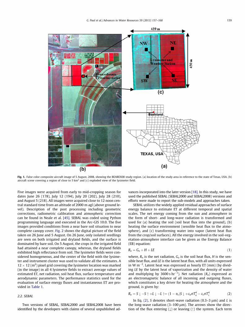
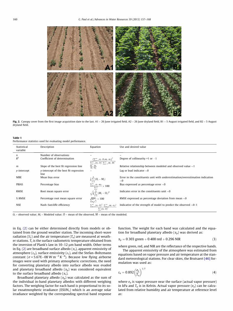
Five images were acquired from early to mid-cropping season fordates June 26 (178), July 12 (194), July 20 (202), July 28 (210),and August 5 (218). All images were acquired close to 12 noon cen-tral standard time from an altitude of 2000 m agl (above ground le-vel). Description of the post processing including geometriccorrections, radiometric calibration and atmospheric correctioncan be found in Neale et al. [45]. SEBAL was coded using Pythonprogramming language and executed in the Arc-GIS 10.0. The fiveimages provided conditions from a near bare soil situation to nearcomplete canopy cover. Fig. 2 shows the digital picture of the fieldtaken on 26 June and 5 August. On 26 June, only isolated seedlingsare seen on both irrigated and dryland fields, and the surface isdominated by bare soil. On 5 August, the crops in the irrigated fieldhad attained a near complete canopy, whereas, the dryland fieldsexhibited high reflectance from soil. The lysimeter fields were con-sidered homogeneous, and the center of the field with the lysime-ter and instrument cluster was used to validate all the estimates. A12 � 12 (m2) pixel grid covering the lysimeter location was marked(in the image) in all 4 lysimeter fields to extract average values ofestimated ET, net radiation, soil heat flux, surface temperature andaerodynamic parameters. The performance statistics used for theevaluation of surface energy fluxes and instantaneous ET are pro-vided in Table 1.

2.2. SEBAL

Two versions of SEBAL, SEBAL2000 and SEBAL2008 have beenidentified by the developers with claims of several unpublished ad-

vances incorporated into the later version [18]. In this study, we haveused the published SEBAL (SEBAL2000 and SEBAL2008) versions andefforts were made to report the sub-models and approaches taken.

SEBAL utilizes the widely applied residual approaches of surfaceenergy balance to estimate ET at different temporal and spatialscales. The net energy coming from the sun and atmosphere inthe form of short- and long-wave radiation is transformed andused for (a) heating the soil (soil heat flux into the ground), (b)heating the surface environment (sensible heat flux to the atmo-sphere), and (c) transforming water into vapor (latent heat fluxfrom the crop/soil surfaces). All the energy involved in the soil-veg-etation-atmosphere interface can be given as the Energy Balance(EB) equation:

Rn ¼ Go þ H þ LE ð1Þ

where, Rn is the net radiation, Go is the soil heat flux, H is the sen-sible heat flux, and LE is the latent heat flux, with all units expressedin W m�2. Latent heat was expressed as hourly ET (mm) (by divid-ing LE by the latent heat of vaporization and the density of waterand multiplying by 3600 s hr�1). Net radiation (Rn) expressed asan electromagnetic balance of all incoming and outgoing fluxes,which constitutes a key driver for heating the atmosphere and theground, is given by:

Rn ¼ S # �S " þL # �L "¼ ð1� asÞS # þearT4a � esrT4

s ð2Þ

In Eq. (2), S denotes short-wave radiation (0.3–3 lm) and L isthe long-wave radiation (3–100 lm). The arrows show the direc-tion of the flux entering (;) or leaving (") the system. Each term

Fig. 1. False color composite aircraft image of 5 August, 2008, showing the BEAREX08 study region. (a) location of the study area in reference to the state of Texas, USA. (b)aircraft scene covering a region of close to 5 km2 and (c) exploded view of the lysimeter field.

G. Paul et al. / Advances in Water Resources 59 (2013) 157–168 159

in Eq. (2) can be either determined directly from models or ob-tained from the ground weather station. The incoming short-waveradiation (S;) and the air temperature (Ta) are measured at weath-er stations. Ts is the surface radiometric temperature obtained fromthe inversion of Plank’s law in 10–12 lm band width. Other termsin Eq. (2) are broadband surface albedo (as), apparent emissivity ofatmosphere (ea), surface emissivity (es), and the Stefan–Boltzmannconstant (r = 5.67E�08 W m�2 K�4). Because low flying airborneimages were used with primary atmospheric corrections, the needfor converting planetary albedo into surface albedo was evadedand planetary broadband albedo (ap) was considered equivalentto the surface broadband albedo (as).

Broadband planetary albedo (ap) was calculated as the sum ofthe individual in-band planetary albedos with different weighingfactors. The weighing factor for each band is proportional to its so-lar exoatmospheric irradiance (ESUNk) which is an average solarirradiance weighted by the corresponding spectral band response

function. The weight for each band was calculated and the equa-tion for broadband planetary albedo (ap) was derived as:

ap ¼ 0:303 greenþ 0:400 redþ 0:296 NIR ð3Þ

where green, red, and NIR are the reflectance of the respective bands.The apparent emissivity of the atmosphere was estimated from

equations based on vapor pressure and air temperature at the stan-dard meteorological stations. For clear skies, the Brutsaert [46] for-mulation was used as:

ea ¼ 0:892ea

Ta

� �1=7

ð4Þ

where ea is vapor pressure near the surface (actual vapor pressure)in kPa and Ta is in Kelvin. Actual vapor pressure (ea) can be calcu-lated from relative humidity and air temperature at reference levelas:

Fig. 2. Canopy cover from the first image acquisition date to the last. A1 – 26 June irrigated field, A2 – 26 June dryland field, B1 – 5 August irrigated field, and B2 – 5 Augustdryland field.

Table 1Performance statistics used for evaluating model performance.

Statisticalvariable

Description Equation Use and desired value

n Number of observations – –R2 Coefficient of determination Pn

i¼1ðOi�OÞðMi�mÞ

� �2Pn

i¼1Oi�Oð Þ2 �

Pn

i¼1ðMi�MÞ

2

Degree of collinearity +1 or �1

m Slope of the best fit regression line M1�M2O1�O2

Relative relationship between modeled and observed value �1

y-intercept y-intercept of the best fit regressionline

– Lag or lead indicator �0

MBE Mean bias error 1N

Pni¼1ðOi �MiÞ

Error in the constituents unit with underestimation/overestimation indication�0

PBIAS Percentage biasPn

i¼1ðOi�MiÞPO

i

� 100Bias expressed as percentage error �0

RMSE Root mean square error ffiffiffi1N

q Pni¼1ðMi � OiÞ2

Indicates error in the constituents unit �0

% RMSE Percentage root mean square error RMSEPn

i¼1Oi

n

� 100 RMSE expressed as percentage deviation from mean �0

NSE Nash–Sutcliffe efficiency Pn

i¼1Oi�Oð Þ2�

Pn

i¼1ðMi�OiÞ2P

Oi�Oð Þ2Indicative of the strength of model to predict the observed �0–1

Oi – observed value; Mi – Modeled value; O – mean of the observed, M – mean of the modeled.

160 G. Paul et al. / Advances in Water Resources 59 (2013) 157–168

ea ¼RH

100esð5Þ

where ea is in kPa and es is the saturation vapor pressure in kPa gi-ven by:

es ¼ 0:6108 exp17:27� Ta

Ta þ 237:3

� �ð6Þ

Ta is the air temperature in degree Celsius (�C).The surface emissivity (es) is calculated from NDVI (Normalized

Difference Vegetation Index) as given by Van de Griend and Owe[47]:

es ¼ 1:009þ 0:047 lnðNDVIÞ ð7Þ

The above relationship is valid only for NDVI values over 0.16.For NDVI values below 0.16 (usually bare soils), emissivity was as-sumed to be 0.92 and for NDVI values below �0.1 (usually water),it was assumed to be 1.0.

The mathematical formulation of H is based on the single sourceresistance scheme of mass transport of heat and momentumbetween the surface and the overlying atmosphere. H is directlyrelated to the difference between the surface aerodynamic temper-ature (To) and above canopy air temperature (Ta):

H ¼ qaCpTo � Ta

rahð8Þ

where qa is the density of air (�1.17 kg m�3), Cp is the air specificheat at constant pressure (�1.005 J kg�1 K�1), and rah is the aerody-namic resistance to heat between the surface and the reference level(s m�1). Since To cannot be measured directly at source height, in sin-gle-source models the radiometric surface temperature (Ts) measuredby the remote sensing thermal sensors, is used as a surrogate. Toaccommodate this approximation, a dimensional parameter for ex-cess resistance to heat transfer (kB�1) is incorporated into the calcu-lation of rah. Studies [32,33] have shown that if an appropriate valueof kB�1 is determined, H can be estimated accurately using Ts. The SE-BAL model has used an areal constant kB�1 value of 2.3 for all surfacesand emphasized that the approach of hot and cold pixel for scalingthermal inertia would reduce the consequences of aerodynamic tem-perature inaccuracy on H estimation [20]. The classical aerodynamicresistance to heat transfer (rah) equation is given by

rah ¼1

ku�ln

zref � do

zoh

� �� wh

� �ð9Þ

where u� is the friction velocity defined by

u� ¼kub

ln zb�dozom

h i� wm

ð10Þ

The do is the zero plane displacement height, zom is the rough-ness length for momentum transport, zoh is the roughness lengthfor heat transport, zref (2 m) is the reference level at which the windspeed (uref) and Ta are measured, k is the von Karman’s constant(�0.41), zb is the blending height (100 m), ub is the wind speed atblending height, and wh and wm are the stability correction func-tions for heat and momentum as a function of Monin–Obukhovlength (L). Equations developed by Paulson [48] were used todetermine wh and wm. Sensible heat flux (H) can be calculated fromEqs. (8)–(10) by simultaneously solving for the stability functionsthrough an iterative process. Soil heat flux was derived from therelationship developed by Bastiaanssen et al. [20], given as:

Go ¼ðTs � 273:15Þ

100asðc1as þ c2a2

s Þð1� 0:98NDVI4Þ� �

� Rn ð11Þ

where c1 and c2 are locally calibrated coefficients with values of0.12 and 0.42, respectively. Other variables in Eq. (11) such as do,

zom, ub, and kB�1 can be solved with either empirical or physicallybased models. Appendix A lists the various parameterizations usedin the intermediate steps.

2.3. The excess resistance parameter (kB�1)

In Eq. (8), the aerodynamic temperature To, is defined as the airtemperature at effective height of the canopy at which the vegeta-tion component of H and LE fluxes arise given by do + zoh [49]. Fromthe Monin–Obukhov (M–O) similarity theory, the aerodynamicresistance, rah, is defined as the resistance from height zoh + do hav-ing an aerodynamic temperature, to the height zref. Eq. (9) can bewritten as:

rah ¼ ra þ rr ¼1

ku�ln

z� do

zom

� �� wh

� �þ 1

ku�ln

zom

zoh

� �ð12Þ

where, ra is the aerodynamic resistance between the air tempera-ture at a height do + zom and the reference height (zref). The formula-tion of H using the definition of To requires an additional resistancecalled the excess resistance and denoted by rr in Eq. (12). Followingmany authors [49,50], it is surmised that the aerodynamic resis-tance to heat transfer (rah) is greater than aerodynamic resistancefor momentum transfer (ra). Consequently, the roughness lengthfor heat transfer (zoh) is lower than the roughness length formomentum transfer (zom). The excess resistance (rr) is an integralpart of the aerodynamic resistance formulation (Eq. (12)) and takesinto account the fundamental difference in the mechanism deter-mining heat and momentum transfer. It is important to understandthat the excess resistance is attached to the aerodynamic tempera-ture, however, a practical problem arises when neither the To northe zoh could be measured. An alternative is to use the radiometricsurface temperature from the infrared sensors as a surrogate for To

and to accommodate this substitution a correction is performed onthe excess resistance term. Excess resistance (rr) formulation fromEq. (12) can be written as:

rr ¼1

ku�ln

zom

zoh

� �ð13Þ

Eq. (13) is commonly expressed as a function of the dimension-less bulk parameter B�1 [51]:

rr ¼B�1

u�ð14Þ

The parameter kB�1 is related to roughness height for heat zoh,by combining Eqs. (13) and (14), as:

kB�1 ¼ lnzom

zoh

� �ð15Þ

It must be emphasized here that kB�1 is the parameter describ-ing the excess resistance and should not be confused with the ex-cess resistance (rr). In context to heat transfer estimation from Ts,kB�1 is a mere fitting parameter no longer connected to its theoret-ical background and largely an empirical parameter [31,51].

In SEBAL, the kB�1 value of 2.3 [20] sets the value of roughnesslength for heat to 1/10 of roughness length for momentum. Severalstudies have shown that the value of kB�1 can range from 1 to 10depending on the dominant surface cover [30,32,33,52]. A physi-cally based model for zoh expressed in terms of kB�1 was incorpo-rated into SEBAL to see its influence on the estimation of ET. ThekB�1 model developed by Su et al. [30] that consists of terms rep-resenting the contribution of the soil alone, the canopy and thecanopy-soil interaction to resistance to heat transfer (Appendix B)was selected.

G. Paul et al. / Advances in Water Resources 59 (2013) 157–168 161

2.4. Aerodynamic roughness parameters

Roughness height for momentum (zom) greatly influences theturbulent characteristics near the surface where the heat fluxesoriginate. The zom depends on various factors such as wind direc-tion, vegetation height, canopy cover, vegetation type, and rowspacing. Estimating these factors using an empirical equation asa function of NDVI might be an over simplification; however, suchestimates are reasonably accurate for uniform cover and fairly flatterrains [50]. Although remote sensing observations provide vege-tation information, estimation of roughness height remains a chal-lenge for regional modeling of turbulent transport because ofhighly variable topographic and canopy structures, and windbehaviors. There are numerous methods to retrieve this parameterincluding wind profile methods, vegetation height, lookup tablebased on the land use classification, and empirical relationshipusing NDVI. Calibrating the empirical relationship for the study re-gion from the data collected during the campaign would be thebest available option. The following exponential relationship de-rived using NDVI and crop height information [5] was used to esti-mate zom

zom ¼ expðC1 þ C2 NDVIÞ ð16Þ

where C1 and C2 are regression constants derived separately foreach image from a plot of ln(zom) versus NDVI for pixels represent-ing varied vegetation heights and extremes of NDVI (Fig. 3). Forgenerating the relationship, zom was calculated from the height ofvegetation (zom = 0.13 h) [53] recorded for different crops duringthe campaign. One single set of coefficients for all five images,C1 = �5.5 and C2 = 5.8, from [5] was used to test the coefficient’ssensitivity on the ET estimation.

2.5. Selection of a dry (hot) and wet (cold) pixel

SEBAL uses the extreme pixels of the image (dry and wet pixel),to develop a relationship between Ts and the difference between To

and Ta given in the form of:

To � Ta ¼ dT ¼ aþ b � Ts ð17Þ

where ‘a’ and ‘b’ are the regression constants. The basic assumptionbehind this relationship is that the difference between To and Ta islinearly related to the Ts. A second assumption of the existence of

Fig. 3. Relationship for roughness length for momentum transport generated from plant height information for each image.

Fig. 4. Solving for coefficients ‘a’ and ‘b’ using the wet and dry pixel concept.

162 G. Paul et al. / Advances in Water Resources 59 (2013) 157–168

hydrological contrast (dry and wet area) in the study region must beimplemented. Fig. 4 illustrates the process of deriving the coeffi-cients from extreme dry and wet pixels. For the wet pixel, dT wasconsidered zero while for the dry pixel, dT was iteratively deter-mined by Eqs. ((8)–(10)) adjusting for the stability functions. Phys-ically, the wet pixel should be the surface transpiring at its potentiallimit (LE = LEmax and H = 0), and therefore dT = 0. The ideal locationof a wet pixel is a surface with full canopy vegetation growing un-der no soil moisture limitation. A dry pixel physically represents asurface with dry conditions and ET equal to zero. (LE = 0 orH = Hmax = Rn � Go). Ideally, bare soil with no residual moisture forevaporation should fit the dry pixel requirements. Selection of thesetwo extreme pixels in the image causes a bottleneck in the imple-mentation of SEBAL as it involves a subjective decision of the ana-lyst. Generally, the wet pixel is selected on the criteria of lowtemperature and high NDVI, whereas the dry pixel is characterizedby high temperature, low NDVI, and low albedo. Scatter plots ofNDVI-Ts and albedo-Ts along with histograms have been used toidentify the group of pixels fulfilling the extreme pixel criteria[6,9]; however, these methods do not help in secluding a singleset of pixels, which again largely depends on the analyst’s decision.Furthermore, different sets of pixels fulfilling the dry and wet pixelcriteria may exhibit entirely different surface energy balance androughness properties and lead to variations in the ‘a’ and ‘b’ coeffi-cients. In the present study, we harnessed the capability of the GISenvironment wherein classification, histogram generation, andoverlaying of the surface temperature, NDVI, and albedo maps couldbe done easily, leading to identification of a group of pixels that ful-filled the criteria. The identification of the wet pixel was easier be-cause of the presence of a grass reference ET weather station in thestudy region (Fig. 1) that typically exhibited the lowest surface tem-perature and greatest NDVI for all five images. Selection of the hotpixel was not easy because multiple pixels satisfied the conditions.We selected three sets of hot pixels well spread in the study domainto test the variations in the determination of ‘a’ and ‘b’ coefficientsand further its influence on final ET estimation.

3. Results and discussion

3.1. Net radiation, soil heat flux and surface temperature

Performance statistics for Rn, Go, and Ts for the complete data set(n = 20) are provided in Table 2. The Ts retrieved from the airbornethermal images was compared against the observed IRT (infra-redthermometer) values with a small RMSE value of 1.16 �C (3.36%). Itis within the range of Ts values (1–1.5 �C) reported in the literaturefor thermal imagery acquired from various airborne and satelliteplatforms [40]. Net radiation was under predicted with a smallRMSE of 17.98 W m�2 (3.1%) and an MBE of 6.61 W m�2 (1.14%),which was well within the typical error range of 5%–10%(�30–60 W m�2) [6,8,9] and most instrument measurementuncertainty [54]. The Rn estimates were comparable to thoseobserved by Jacob et al. [22], who attributed the low Rn estimationerrors to use of relatively accurate albedo estimates derived fromaircraft data. An overestimation error of 9.87 W m�2 (36.2%) andRMSE of 13.5 W m�2 (49.6%) was recorded for Go estimates. A large

discrepancy was evident from the low R2 value, with negative NSEindicating the model’s unsatisfactory performance in estimatingGo. Similar results with RMSE ranging from 20 to 40 W m�2 havebeen reported by various studies [8,22] for the present parameter-ization (Eq. (11)) using NDVI and Rn. Although Go estimates werenot accurate, it was not a major concern because the magnitudeof error was small (±13 W m�2) and was expected to have negligi-ble effect on the ET estimates. Moreover, the available energy (Rn -� Go) for convective fluxes resulting from the underestimation ofRn and overestimation of Go was 16.5 W m�2 (MBE), which was asmall underestimation. Nevertheless, several causes can explainthe poor performance of Go estimates in the evaluation’s statisticsincluding the spatial variability of Go, inaccuracies in the soil heatflux plate measurements and the limitations of NDVI based Go

parameterization.

3.2. ET flux variability due to selection of different dry and wet pixelend members

Three sets of ‘a’ and ‘b’ coefficients generated per image withtheir temperature, NDVI, albedo, and roughness properties are pre-sented in Table 3. It is evident from the Table 3 that end memberpixels of particular image exhibiting same temperature could stillproduce a different set of coefficients owing to their different sur-face energy balance and roughness properties. SEBAL was executedfor each set of ‘a’ and ‘b’ coefficients, and the estimated instanta-neous ET was analyzed using standard deviation and coefficientof variation (Table 4). The coefficient of variation (CV in%;SD � 100/Mean) for the irrigated lysimeter fields (SE and NE,Fig. 1) ranged from 0 to 22% while for the dryland lysimeter fields(NW and SW, Fig. 1), the CV ranged from 4 to 80%. Consistently lar-ger deviations (CV) were associated with dryland (sparse vegeta-tion) ETi estimations compared with irrigated fields (morecomplete vegetative cover). The reason for this biased behaviorof the algorithm for irrigated (full cover) and dryland (sparse cov-er) cropping systems lies in the fact Ts � To is minimal for full covercanopies [49], and a nominal correction of 2.3 (kB�1) provide goodET estimates [33]. However, on sparse canopy cover, the Ts � To isalways greater, and the correction applied (kB�1 = 2.3) could notaccount for the larger differences, thus providing unreliable ETestimates. This shows that the temperature gradient relationshipcannot completely address the spatial variability of kB�1. There-fore, inherent assumption that hot and cold pixel for scaling ther-mal inertia (dT) accommodates the consequences of aerodynamictemperature inaccuracy on H estimation may not be true.

3.3. Instantaneous ET by SEBAL

For each image, the average ETi derived from the three set of ‘a’and ‘b’ was compared against lysimeter values for the performanceevaluation of SEBAL. Evaluation statistics for the complete data setas well as for the irrigated and dryland fields are presented sepa-rately in Table 5a for thorough evaluation. An overall RMSE of0.15 mm h�1 (28.1%) and MBE of 0.13 mm h�1 (23.8%) were ob-served for ETi estimates from all four lysimeter fields. The positivebias indicated underestimation of ETi. This result is similar to the

Table 2Performance statistics for Ts(Obs. Mean: 34.4 �C), Rn(Obs. Mean: 579 W m�2), and Go(Obs. Mean: 27 W m�2) (No. of observations = 20).

Estimated parameter Mean MBE PBIAS RMSE %RMSE NSE Regression

R2 m y-intercept

Ts (�C) 34.3 0.04 0.13 1.16 3.36 0.96 0.96 0.95 1.59RN (W m�2) 573 6.61 1.14 17.98 3.10 0.86 0.91 1.10 �65.04GS (W m�2) 37 �9.87 �36.24 13.51 49.58 �3.96 0.02 0.18 32.19

G. Paul et al. / Advances in Water Resources 59 (2013) 157–168 163

accuracy (27.1% RMSE) that Tasumi et al. [55] reported for semi-arid Idaho conditions in their comparison of ETi versus lysimetervalues using Landsat imagery. In a comprehensive evaluation studyby the SEBAL developer, the overall accuracy of daily ET for scale ofthe order of 100 ha has been reported as ±15%, further stating thattime and space integration would improve accuracy [1]. SEBAL ETi

estimates explained 86% of the variability in the observed lysime-ter data with slope close to unity (0.98) and an intercept of�0.11 mm h�1, both significant at the 0.05 probability level (Fig. 5).

The evaluation of SEBAL model for irrigated and dryland lysim-eter fields with the high resolution imagery revealed an interestingbias in the model’s performance for the two agricultural watermanagement regimes. The ETi from the irrigated fields showedan RMSE of 0.14 mm h�1 contributing to 21.5% error, however,the dryland fields gave an RMSE of 0.15 mm h�1 which accountedfor 39.5% error, nearly double the error as compared to the irri-gated field. The NSE value for the dryland field ETi estimates was�0.81 and R2 was 0.35, as compared to NSE of 0.55 and R2 of0.95 from the irrigated field. Clearly, the biased performance ofSEBAL for dryland conditions affected the overall performance.

Similar gross under prediction results in relatively dry areas are re-ported by Timmermans et al. [6], Gowda et al. [56], and Gao andLong [7]. Timmermans et al. [6] made unsuccessful attempt to fixthis problem by adjusting the end-member temperatures andmomentum roughness length. In their study, they articulated thaterrors in H estimation over sparsely vegetated surfaces in singlesource models can be reduced by adjusting the kB�1 parameter.

3.4. SEBAL with kB�1 parameterization

Overall underperformance of SEBAL with variable accuracies forirrigated and dryland crops could be attributed to one or a combi-nation of reasons. In the present agriculture dominant landscapewith no forest cover and flat topography, the empirical parameter-ization of zom could not be the reason for deviations in ET esti-mates. At the same time, the aircraft image covered a small areawith a relatively less heterogeneous landscape, hence the assump-tion of linearity of dT versus Ts could be considered valid. However,there are no studies to prove that the dT versus Ts linearity assump-tion could adequately address the spatial variation of zoh (kB�1), orin other words address the differences between To and Ts; we be-lieve that this could be a reason for the biased results.

Results of SEBAL model estimates with kB�1 parameterizationshowed improvement in the ETi estimation (Fig. 6). Overall RMSEof 0.08 mm h�1 (16.3%) and MBE of �0.02 mm h�1 (�3.6%) wereobserved for the complete dataset (Table 5b). A 1:1comparison ofTables 5a and 5b clearly indicates that the SEBAL with kB�1 param-eterization substantially improved its performance in estimatingETi. The overall underestimation errors decreased considerablyfrom 24% to �3.6% (PBIAS). This can be seen clearly in plots ofETi for the irrigated and dryland field separately with and withoutthe kB�1 modifications (Figs. 5 and 6). Underestimated ETi associ-ated with partial canopy covers, moved closer to the observed val-ues after the introduction of kB�1 parameterization, while it did notaffect the higher ETi estimates associated with near completecanopy cover in the irrigated fields. This could be explained from

Table 3Selection of hot and wet pixel and the variability in the ‘a’ and ‘b’ coefficient.

Image acquisition date Cold/wet pixel Hot/dry pixel dT ¼ aþ bTs

Twet NDVI Tdry NDVI Albedo zom a b

26 June, 2008 301.09 0.704 315.42 0.143 0.162 0.012 �198.46 0.659301.09 0.704 315.42 0.122 0.180 0.010 �199.25 0.662301.09 0.704 315.98 0.153 0.185 0.013 �177.12 0.588

12 July, 2008 295.36 0.805 310.14 0.165 0.168 0.013 �172.07 0.582295.36 0.805 310.50 0.162 0.151 0.013 �172.41 0.583295.36 0.805 311.74 0.206 0.220 0.016 �129.09 0.437

20 July, 2008 297.47 0.790 317.42 0.232 0.178 0.012 �185.71 0.624297.47 0.790 316.94 0.138 0.172 0.007 �227.04 0.763297.47 0.790 316.99 0.176 0.166 0.009 �215.83 0.725

28 July, 2008 299.08 0.799 317.37 0.152 0.185 0.010 �220.95 0.738299.08 0.799 317.28 0.197 0.181 0.012 �201.89 0.675299.08 0.799 317.37 0.155 0.188 0.009 �212.95 0.712

05 August, 2008 300.50 0.800 334.35 0.152 0.161 0.012 �143.79 0.478300.50 0.800 334.59 0.150 0.146 0.012 �147.22 0.489300.50 0.800 335.45 0.157 0.149 0.013 �138.32 0.460

Table 4Influence of ‘a’ and ‘b’ coefficients on the final ET (mm h�1) value.

Image acquisition date Statistics Irrigated fields Dryland fields

NE SE NW SW

26 June, 2008 r 0.04 0.04 0.03 0.03%CV 21.10 18.22 14.11 12.29

12 July, 2008 r 0.08 0.08 0.11 0.11%CV 21.02 21.88 79.93 68.52

20 July, 2008 r 0.04 0.04 0.05 0.05%CV 6.70 8.59 21.25 19.21

28 July, 2008 r 0.01 0.01 0.02 0.02%CV 0.74 1.18 5.60 5.17

05 August, 2008 r 0.00 0.00 0.01 0.01%CV 0.12 0.06 4.33 4.23

r = standard deviation, %CV = coefficient of variation in percentage.

Table 5aPerformance statistics for Instantaneous ET (mm h�1) from SEBAL for all fields (Obs. Mean: 0.53 mm h�1) and for irrigated (Obs. Mean: 0.67 mm h�1) and dryland (Obs. Mean:0.40 mm h�1) fields separately.

Observation points n Mean MBE PBIAS RMSE %RMSE NSE Regression

R2 m y-intercept

All fields 20 0.41 0.13 23.82 0.15 28.15 0.55 0.88 0.98 �0.12Irrigated field 10 0.54 0.13 19.38 0.14 21.48 0.55 0.95 1.14 �0.23Dryland field 10 0.27 0.12 31.44 0.16 39.55 �0.80 0.35 0.41 0.11

164 G. Paul et al. / Advances in Water Resources 59 (2013) 157–168

Fig. 2, where the images under analysis are from early crop stage tonear complete canopy cover stage; hence, a sparse vegetation con-dition existed in most images. A nominal kB�1 value of 2.3 did notwork well under sparse vegetation conditions and generated lowerETi estimates. SEBAL is known to have problems estimating ET un-

der dry and sparse vegetation conditions [6,7]. Under these condi-tions, the difference between Ts and To was relatively large, and thiscould not be adequately addressed by the nominal kB�1 value of2.3, whereas the converse was true for complete canopies. There-fore, the improvement in the ETi estimates was solely due to anappropriate representation of spatially variable roughness lengthfor heat transport (zoh). Table 6 gives a comprehensive list of aero-dynamic roughness parameter estimates from the four fields.Marked difference in the zoh values with and without kB�1 param-eterization was observed.

3.5. Roughness length for momentum transport, excess resistance, androughness length for heat transport

Questions have been raised about the simplistic approach ofdetermining the complex roughness length for momentum trans-port (zom) from the empirical relationship, Eq. (16), as a functionof NDVI [6,19]. SEBAL developers suggested deriving local coeffi-cients for the zom relationship from the observed plant height overvaried canopy structure. Although the requirements of plant heightadd to the inputs, our results show that the relationship generatedrealistic zom values under the present agricultural landscape setup(Table 6). Furthermore, applying a single pair of coefficients for thezom relationship (derived from the Tomelloso super site, Cas de LasCarascas, Spain [5]) for all the images did not result in any notice-able difference in the ETi estimation; however, we must cautionthat the Tomelloso super site was also an agricultural region, andthese coefficients cannot be universally applied. The zom valuescompared well with the estimates obtained over an incompletecanopy cover of cotton using the profile method [33]. Also, thezom values were comparable with the Brutsaert [53] relationship(zom = 0.13 h) (Table 6).

The kB�1 parameter representing the excess resistance to heattransfer has been a matter of controversy since its inception intothe single source model. Nevertheless, the term cannot be avoidedbecause it accounts for the fact that Ts is frequently greater than To

[31]. In this study, the parameterized kB�1 values produced moreaccurate ETi estimates compared with the constant kB�1 value of2.3 proposed by the SEBAL developers. The value for kB�1 for allfour lysimeter fields is presented in Table 6. The value of kB�1 var-ied between 2 and 13 for most cases, with higher values associatedwith low canopy cover conditions. On 26 June, exceptionally highkB�1 values were found due to the fact that image was acquiredearly in the cropping season when the surface was bare soil withisolated cotton seedlings (see Fig. 2); such a surface is classifiedas bluff rough element with no consensus on appropriate kB�1 va-lue [29]. The kB�1 value for the irrigated fields were always lessthan that in the dryland fields (Table 6). This is because, at anypoint during the cropping season, irrigated fields had larger canopycover than the dryland fields. Consequently, the value of around2.3 was suitable for irrigated fields when the crop attained nearcomplete canopy cover conditions. The minimum value of kB�1

for the dryland fields was 5.3, which was estimated with the 5 Au-gust image. These results corroborate the conclusions from numer-ous studies on the excess resistance parameter (kB�1), that: (i) overa sparsely vegetated surface, the difference between Ts and To can

Fig. 5. SEBAL modeled versus observed instantaneous ET comparison for cottonfields under dryland and irrigation management.

Fig. 6. SEBAL with kB�1 parameterization modeled ET versus observed instanta-neous ET comparison for cotton fields under dryland and irrigation management.

Table 5bPerformance statistics for Instantaneous ET (mm h�1) computed from SEBAL with kB�1 parameterization.

Observation points n Mean MBE PBIAS RMSE %RMSE NSE Regression

R2 m y-intercept

All fields 20 0.55 �0.02 �3.56 0.08 16.27 0.85 0.92 0.68 0.19Irrigated field 10 0.64 0.03 4.89 0.07 10.15 0.89 0.95 0.79 0.12Dryland field 10 0.46 �0.07 �18.11 0.10 25.97 0.22 0.68 0.45 0.29

G. Paul et al. / Advances in Water Resources 59 (2013) 157–168 165

exceed 10 �C [49], so an adjustment is required (through kB�1), (ii)kB�1 value should range from 1 to 10, to obtain accurate estimatesof H [32,33], and (iii) H is more sensitive to kB�1 value of 2 than avalue of about 6 [29].

Roughness length for heat transport, zoh, expressed in terms ofkB�1 ½zoh ¼ zom=expðkB�1Þ� for four lysimeter fields over the five im-age acquisition dates are presented in Table 6. Comparison of zoh

values obtained from kB�1 parameterization and a constant kB�1

(of 2.3) reveals significant differences. To address the high kB�1

values obtained for the sparse vegetation conditions, we restrictedthe lower limit of zoh to 10�5 m.

4. Conclusions

SEBAL is thoroughly evaluated using extensive crop character-ization, ET, and high resolution remote sensing datasets acquiredduring the BEAREX08. The main distinguishing feature of thisstudy was the simultaneous evaluation of SEBAL for both irrigatedand dryland crops covering a range of conditions from sparse veg-etation to near complete canopy cover. This study also examinedthe issues of subjective selection of extreme pixels, dealt withaerodynamic roughness parameters, and showed improvement inET estimates through the introduction of kB�1 parameterizationinto the SEBAL model. On an average 20% uncertainty in term ofCV was observed as a result of subjectivity in the end memberselection process. The sensitivity to end member pixel selectionis crucial to the performance of SEBAL; hence, a clear methodologyfor the selection process is required to remove the subjective deci-sion and make the process more robust. A rigorous sensitivity anal-ysis of the ‘a’ and ‘b’ coefficients estimation in the temperaturegradient relationship is necessary because this forms the backboneof SEBAL. SEBAL ETi estimates compared reasonably well againstthe lysimeter values with underestimation error and RMSE closeto 0.15 mm h�1 (28%). Errors were relatively small for the irrigatedfields as compared with the dryland fields. Modifying the SEBALalgorithm by introducing kB�1 parameterization considerably im-proved the accuracy of ETi estimation, with an overall RMSE of

0.08 mm h�1 (16%). It can be concluded that the temperature gra-dient (dT) linear relationship does not have any component to con-sider for the differences arising due to use of Ts for To and hence arealistic correction factor in the form of kB�1 has to be incorporatedinto SEBAL. Furthermore, a kB�1 value of 2.3 would grossly under-estimate ET for sparse vegetation conditions. Locally calibratedcoefficients for the aerodynamic roughness parameters are crucialto the performance of the algorithm. SEBAL is a physically basedalgorithm, but the numerous empirical sub-models and require-ment for image specific calibrations, limits its operational capabil-ities. Nevertheless, results of the present study with the suggestedimprovements in the algorithm make it a viable tool for regionalscale ET mapping. The temperature gradient approach (dT estima-tion) is a novel approach indigenous to the SEBAL algorithm, how-ever, the underlying assumptions are many necessitating adetailed sensitivity study.

Acknowledgments

This research was supported by the Ogallala Aquifer Program, aconsortium between USDA � Agricultural Research Service, KansasState University, Texas AgriLife Research, Texas AgriLife ExtensionService, Texas Tech University, and West Texas A&M University.This is contribution number 12-284-J from the Kansas AgriculturalExperiment Station.

EEO/Non-Discrimination Statement: The US Department of Agri-culture (USDA) prohibits discrimination in all its programs andactivities on the basis of race, color, national origin, age, disability,and where applicable, sex, marital status, familial status, parentalstatus, religion, sexual orientation, genetic information, politicalbeliefs, reprisal, or because all or part of an individual’s income isderived from any public assistance program. (Not all prohibitedbases apply to all programs.) Persons with disabilities who requirealternative means for communication of program information(Braille, large print, audiotape, etc.) should contact USDA’s TARGETCenter at (202) 720-2600 (voice and TDD). To file a complaint ofdiscrimination, write to USDA, Director, Office of Civil Rights,

Table 6Aerodynamic roughness parameters for the four cotton fields under irrigation (NE and SE) and dryland (NW and SW) management.

Date Field zom_D (m) zom_E (m) zoh_C (m) kB�1 (m) zoh_S (m) C_ht (m) C_ht_O (m) zom_B (m)

26 June NE 0.011 0.009 0.0009 19.21 0.00001 0.084 0.152 0.020SE 0.010 0.008 0.0008 24.67 0.00001 0.076 0.178 0.023NW 0.008 0.007 0.0007 44.51 0.00001 0.063 0.089 0.012SW 0.008 0.007 0.0007 58.86 0.00001 0.060 0.114 0.015

12 July NE 0.052 0.044 0.0044 5.39 0.00026 0.382 0.457 0.059SE 0.048 0.041 0.0041 5.55 0.00020 0.352 0.330 0.043NW 0.018 0.015 0.0015 8.54 0.00001 0.137 0.356 0.046SW 0.026 0.022 0.0022 6.99 0.00003 0.190 0.292 0.038

20 July NE 0.082 0.102 0.0102 3.50 0.00268 0.602 0.559 0.073SE 0.073 0.092 0.0092 3.65 0.00213 0.540 0.406 0.053NW 0.009 0.011 0.0011 13.04 0.00001 0.066 0.432 0.056SW 0.019 0.025 0.0025 6.55 0.00008 0.142 0.356 0.046

28 July NE 0.123 0.182 0.0182 2.78 0.00780 0.902 0.559 0.073SE 0.115 0.168 0.0168 2.86 0.00717 0.843 0.610 0.079NW 0.012 0.013 0.0013 11.87 0.00001 0.087 0.508 0.066SW 0.021 0.024 0.0024 6.78 0.00007 0.153 0.457 0.059

05 August NE 0.146 0.265 0.0265 2.18 0.01662 1.073 0.635 0.083SE 0.199 0.401 0.0401 2.02 0.02684 1.468 0.559 0.073NW 0.017 0.016 0.0016 8.53 0.00003 0.126 0.533 0.069SW 0.028 0.030 0.0030 5.32 0.00023 0.207 0.432 0.056

MEAN 0.051 0.074 0.0074 12.14 0.00321 0.378 0.401 0.052

zom_D = Roughness length for momentum estimated from Eq. (16) using coefficients derived for each image as given in Fig. 3.zom_E = Roughness length for momentum estimated from Eq. (16) using constant coefficients C1 = �5.5 and C2 = 5.8, from [5].zoh_C = Roughness length for heat estimated from Eq. (15) using constant kB�1 value of 2.3.kB�1 = Excess resistance parameter for heat transfer estimated from parameterization given by Su et al. [30], Appendix B.zoh_S = Roughness length for heat estimated from Eq. (15) using kB�1 value from Su et al. [30], Appendix B.C_ht = Canopy height from Eq. (A2) (=zom_D/0.13).C_ht_O = Field measurement of canopy height.zom_B = Roughness length for momentum estimated from Brutsaert relationship, Eq. (A2) (=0.13�C_ht_O).

166 G. Paul et al. / Advances in Water Resources 59 (2013) 157–168

1400 Independence Avenue, S.W., Washington, DC 20250-9410, orcall (800) 795-3272 (voice) or (202) 720-6382 (TDD). USDA is anequal opportunity provider and employer.

Appendix A.

Various intermediate parameterizations used in the SEBALalgorithm.

Displacement height was computed from the model given byVerhoef et al. [57]:

do ¼ h 1� 1� e�ffiffiffiffiffiffiffiffiffic1 �LAIpffiffiffiffiffiffiffiffiffiffic1�LAIp

!ðA1Þ

where h is the canopy height and c1 is a free parameter with the va-lue 20.6.

Roughness length for momentum transport as given by Brutsa-ert [53]:

zom ¼ 0:13h ðA2Þ

Leaf Area Index model developed specifically for the Texas HighPlains region given by Gowda et al. [58]:

LAI ¼ 8:768� NDVI3:616 ðA3Þ

Fractional cover was derived from relationship taken from Jiaet al. [51]:

fc ¼ 1� NDVI� NDVImax

NDVImin � NDVImax

� �K

ðA4Þ

where K is taken as 0.4631.Wind speed at blending height

ub ¼ ureflnðzb � doÞ � lnðzomÞ

lnðzref � doÞ � lnðzomÞ

� �ðA5Þ

Monin Obukhov Length (L)

L ¼ �qaCpu3�Ts

kgHðA6Þ

where density of air (qa) = �1.17 kg m�3, specific heat capacityof air (Cp) = �1.005 J kg�1 K�1, gravitational acceleration (g) =9.81 m s�2.

Momentum transfer correction factor under unstable conditionfrom Paulson [36]:

wm ¼ 2 ln1þ xm

2

� �þ ln

1þ x2m

2

� �� 2 arctanðxmÞ þ

p2

ðA7Þ

where xm is defined as:

xm ¼ 1� 16zb � do

L

� �0:25

Heat transfer correction factor under unstable condition fromPaulson [36]:

wh ¼ 2 ln1þ x2

h

2

� �ðA8Þ

where xh is defined as:

xh ¼ 1� 16zref � d0

L

� �0:25

Appendix B.

Excess resistance to heat transfer formulation as given bySu.et al. [49]

kB�1 ¼ kCd

4Ctu�

uðhÞ ð1� e�nec=2Þ f2c þ

k � u�uðhÞ �

zomh

C�tf 2c f 2

s þ kB�1s f 2

s ðB1Þ

In Eq. (B1), kB�1s is the bare soil surface excess resistance com-

puted as:

kB�1s ¼ 2:46ðRe�Þ1=4 � lnð7:4Þ ðB2Þ

In Eq. (B1), nec is within-canopy wind speed profile extinctioncoefficient given by:

nec ¼Cd � LAI

2u2�=uðhÞ2

ðB3Þ

In Eq. (B1) and (B3), the ratio u�=uðhÞ is parameterized as:

u�uðhÞ ¼ c1 � c2 � e�c3 �Cd �LAI ðB4Þ

where c1 = 0.320, c2 = 0.264 and c3 = 15.1.In Eq. (B1), C�t is heat transfer coefficient of the soil given as:

C�t ¼ Pr�2=3Re�1=2� ðB5Þ

In Eq. (B2) and Eq. (B5), Re� is roughness Reynolds number cal-culated as:

Re� ¼ hsu�=m ðB6Þ

where hs is the roughness height for soil taken here as 0.009 m.In Eq. (B1), m is kinematic viscosity of the given by:

m ¼ 1:327� 10�5ðp0=pÞðTa=Ta0Þ1:81 ðB7Þ

where, p and Ta are ambient pressure and temperature andpo = 101.3 kPa and Tao = 273.15 K.

Other terms in Eqs. (B1)–(B7) are: Cd is the drag coefficient ofthe foliage elements taken as 0.2, Ct is heat transfer coefficient ofthe leaf with value 0.01, Pr is Prandtl number with value 0.71,u(h) is the horizontal wind speed at the canopy height, fc is thefractional canopy coverage and fs is its compliment, and k is vonKarman’s constant taken as 0.41.

References

[1] Bastiaanssen WGM, Noordman EJM, Pelgrum H, Davids G, Thoreson BP, AllenRG. SEBAL model with remotely sensed data to improve water-resourcesmanagement under actual field conditions. J Irrig Drain Eng 2005;131:85–93.http://dx.doi.org/10.1061/(ASCE)0733-9437(2005)131:1(85).

[2] Allen RG, Pereira LS, Howell TA, Jensen ME. Evapotranspiration informationreporting: I. Factors governing measurement accuracy. Agric Water Manage2011;98:899–920. http://dx.doi.org/10.1016/j.agwat.2010.12.015.

[3] Howell TA, Schneider AD, Dusek DA, Marek TM, Steiner JL. Calibration andscale performance of bushland weighing lysimeters. Trans ASAE1995;38:1019–24.

[4] Allen RG, Pereira LS, Howell TA, Jensen ME. Evapotranspiration informationreporting: II. Recommended documentation. Agric Water Manage2011;98:921–9. http://dx.doi.org/10.1016/j.agwat.2010.12.016.

[5] Bastiaanssen WGM. Regionalization of surface flux densities and moistureindicators in composite terrain. Ph.D. thesis, Wageningen AgricultureUniversity, 1995.

[6] Timmermans WJ, Kustas WP, Anderson MC, French AN. An intercomparison ofthe surface energy balance algorithm for land (SEBAL) and the two-sourceenergy balance (TSEB) modeling schemes. Remote Sens Environ2007;108:369–84. http://dx.doi.org/10.1016/j.rse.2006.11.028.

[7] Gao Y, Long D. Intercomparison of remote sensing-based models for estimationof evapotranspiration and accuracy assessment based on SWAT. HydrolProcess 2008;22:4850–69. http://dx.doi.org/10.1002/hyp.7104.

[8] Singh RK, Irmak A, Irmak S, Martin DL. Application of SEBAL model for mappingevapotranspiration and estimating surface energy fluxes in south-centralNebraska. J Irrig Drain Eng 2008;134:273–85. http://dx.doi.org/10.1061/(ASCE)0733-9437(2008)134:3(273).

[9] Choi M, Kustas WP, Anderson MC, Allen RG, Li F, Kjaersgaard JH. Anintercomparison of three remote sensing-based surface energy balancealgorithms over a corn and soybean production region (Iowa, US) duringSMACEX 2009. Agric For Meteorol 2009;149:2082–97. http://dx.doi.org/10.1016/j.agrformet.2009.07.002.

G. Paul et al. / Advances in Water Resources 59 (2013) 157–168 167

[10] Long D, Singh VP. A modified surface energy balance algorithm for land (M-SEBAL) based on a trapezoidal framework. Water Resour Res2012;48:W02528. http://dx.doi.org/10.1029/2011WR010607.

[11] Gowda PH, Chavez JL, Colaizzi PD, Evett SR, Howell TA, Tolk JA. ET mapping foragricultural water management: present status and challenges. Irrig Sci2008;26:223–37. http://dx.doi.org/10.1007/s00271-007-0088-6.

[12] Kalma JD, McVicar TR, McCabe MF. Estimating land surface evaporation: areview of methods using remotely sensed surface temperature data. SurvGeophys 2008;29:421–69. http://dx.doi.org/10.1007/s10712-008-9037-z.

[13] Li ZL, Tang R, Wan Z, Bi Y, Zhou C, Tang B. A review of current methodologiesfor regional evapotranspiration estimation from remotely sensed data. Sensors2009;9:3801–53. http://dx.doi.org/10.3390/s90503801.

[14] Allen RG, Tasurmi M, Morse AT, Trezza R. A landsat-based energy balance andevapotranspiration model in western US water rights regulation and planning.Irrig Drain Syst 2005;19:251–68. http://dx.doi.org/10.1007/s10795-005-5187-z.

[15] Senay GB, Budde ME, Verdin JP, Melesse AM. A coupled remote sensing andsimplified surface energy balance approach to estimate actualevapotranspiration from irrigated fields. Sensors 2007;7:979–1000. http://dx.doi.org/10.3390/s7060979.

[16] Elhaddad Ayman, Garcia Luis A. Surface energy balance-based model forestimating evapotranspiration taking into account spatial variability inweather. J Irrig Drain Eng 2008;134:681–9. http://dx.doi.org/10.1061/(ASCE)0733-9437(2008)134:6(681).

[17] Gao ZQ, Liu CS, Gao W, Chang NB. A coupled remote sensing and the surfaceenergy balance with topography algorithm (SEBTA) to estimate actualevapotranspiration over heterogeneous terrain. Hydrol Earth Syst Sci2011;15:119–39. http://dx.doi.org/10.5194/hess-15-119-2011.

[18] Bastiaanssen W, Thoreson B, Clark B, David G. Discussion of ‘‘Application ofSEBAL model for mapping evapotranspiration and estimating surface energyfluxes in south-central Nebraska’’ by R.K. Singh, Ayse Irmak, Suat Irmak, DerrelL. Martin. J Irrig Drain Eng 2010;134:282–3. http://dx.doi.org/10.1061/(ASCE)IR.1943-4774.0000216.

[19] Norman JM, Anderson MC, Kustas WP. Are single-source, remote-sensingsurface-flux models too simple? In: D’Urso G, Jochum MAO, Moreno J, editors.Proceedings of the international conference on earth observation forvegetation monitoring and water management, vol. 852. American Instituteof Physics; 2006. p. 170–7.

[20] Bastiaanssen WGM, Menenti M, Feddes RA, Holtslag AAM. A remote sensingsurface energy balance algorithm for land (SEBAL) 1. Formulation. J Hydrol1998;213:198–212. http://dx.doi.org/10.1016/S0022-1694(98)00253-4.

[21] Bastiaanssen WGM. SEBAL-based sensible and latent heat fluxes in theirrigated Gediz Basin, Turkey. J Hydrol 2000;229:87–100. http://dx.doi.org/10.1016/S0022-1694(99)00202-4.

[22] Jacob F, Olioso A, Gu XF, Su Z, Seguin B. Mapping surface fluxes using airbornevisible, near infrared, thermal infrared remote sensing data and a spatializedsurface energy balance model. Agronomie 2002;22:669–80. http://dx.doi.org/10.1051/agro:2002053.

[23] Bastiaanssen WGM, Ahmad MD, Chemin Y. Satellite surveillance ofevaporative depletion across the Indus Basin. Water Resour Res2002;38:1273–81. http://dx.doi.org/10.1029/2001WR000386.

[24] Wang J, Sammis TW, Gutschick VP, Gebremichael M, Miller DR. Sensitivityanalysis of the surface energy balance algorithm for land (SEBAL). Trans ASABE2009;52:801–11.

[25] Gieske Ambro, Meijninger Wouter. High density NOAA time series of ET in theGediz Basin, Turkey. Irrig Drain Syst 2005;19:285–99. http://dx.doi.org/10.1007/s10795-005-5191-3.

[26] Chandrapala Lalith, Wimalasuriya Malika. Satellite measurementsupplemented with meteorological data to operationally estimateevapotranspiration in Sri Lanka. Agric Water Manage 2003;58:89–107.http://dx.doi.org/10.1016/S0378-3774(02)00127-0.

[27] Allen RG, Bastiaanssen WGM, Tasumi M, Morse A, Evapotranspiration on thewatershed scale using the SEBAL model and landsat images. ASAE MeetingPaper No.01-2224 St. Joseph, Mich; 2001.

[28] Long D, Singh VP, Li ZL. How sensitive is SEBAL to changes in input variables,domain size and satellite sensor. J Geophys Res 2011;116:D21107. http://dx.doi.org/10.1029/2011JD016542.

[29] Verhoef A, De Bruin HAR, Van Den Hurk BJJM. Some practical notes on theparameter kB-1 for sparse vegetation. J Appl Meteorol 1997;36:560–72. http://dx.doi.org/10.1175/1520-0450(1997)036<0560:SPNOTP>2.0.CO;2.

[30] Su Z, Schmugge T, Kustas WP, Massman WJ. An evaluation of two models forestimation of the roughness height for heat transfer between the land surfaceand the atmosphere. J Appl Meteorol 2001;40:1933–51. http://dx.doi.org/10.1175/1520-0450(2001)040<1933:AEOTMF>2.0.CO;2.

[31] Lhomme JP, Chehbouni A, Monteny B. Sensible heat flux-radiometric surfacetemperature relationship over sparse vegetation: Parameterizing B-1. BoundLayer Meteorol 2000;97:431–57. http://dx.doi.org/10.1023/A:1002786402695.

[32] Stewart JB, Kustas WP, Humes KS, Nichols WD, Moran MS, De Bruin HAR.Sensible heat flux-radiometric surface temperature relationship for eight semiarid areas. J Appl Meteorol 1994;33:1110–7.

[33] Kustas WP, Choudhury BJ, Moran MS, Reginato RJ, Jackson RD, Gay LW, WeaverHL. Determination of sensible heat flux over sparse canopy using thermal

infrared data. Agric For Meteorol 1989;44:197–216. http://dx.doi.org/10.1016/0168-1923(89)90017-8.

[34] Kustas WP, Anderson MC, Norman JM, Li F. Utility of radiometric–aerodynamictemperature relations for heat flux estimation. Bound Layer Meteorol2007;122:167–87. http://dx.doi.org/10.1007/s10546-006-9093-1.

[35] Jia L, Su Z, van den Hurk B, Menenti M, Moene A, De Bruin HAR, et al.Estimation of sensible heat flux using the surface energy balance system(SEBS) and ATSR measurements. Phys Chem Earth Part B 2003;28:75–88.http://dx.doi.org/10.1016/S1474-7065(03)00009-3.

[36] Kustas W, Anderson M. Advances in thermal infrared remote sensing for landsurface modeling. Agric For Meteorol 2009;149:2071–81. http://dx.doi.org/10.1016/j.agrformet.2009.05.016.

[37] Jackson TJ, Vine DML, Hsu AY, Oldak A, Starks PJ, Swift CT, et al. Soil moisturemapping at regional scales using microwave radiometry: the southern greatplains hydrology experiment. IEEE Trans Geosci Remote Sens1999;37:2136–51. http://dx.doi.org/10.1109/36.789610.

[38] Su Z, Timmermans WJ, van der Tol C, Dost R, Bianchi R, Gomez JA, et al. EAGLE2006 – Multi-purpose, multi-angle and multi-sensor in-situ and airbornecampaigns over grassland and forest. Hydrol Earth Syst Sci 2009;13:833–45.

[39] Su Z, Timmermans W, Gieske A, Jia L, Elbers JA, Olioso A, et al. Quantification ofland atmosphere exchanges of water, energy and carbon dioxide in space andtime over the heterogeneous Barrax site. Int J Remote Sens 2008;29:5215–35.http://dx.doi.org/10.1080/01431160802326099.

[40] Sobrino JA, Muñoz JJC, Sòria G, Gómez M, Ortiz AB, Romaguera M, et al.Thermal remote sensing in the framework of the SEN2FLEX project: fieldmeasurements, airborne data and applications. Int J Remote Sens2008;29:4961–91. http://dx.doi.org/10.1080/01431160802036516.

[41] Kustas WP, Jackson TJ, Prueger JH, Hatfield JL, Anderson MC. Remote sensingfield experiments for evaluating soil moisture retrieval algorithms andmodeling land-atmosphere dynamics in central Iowa. EOS Trans AmGeophys Union 2003;84:485–93.

[42] Tolk JA, Evett SR, Howell TA. Advection influences on evapotranspiration ofAlfalfa in a semiarid climate. Agron J 2006;98:1646–54. http://dx.doi.org/10.2134/agronj2006.0031.

[43] Chávez JL, Gowda PH, Howell TA, Neale CMU, Copeland KS. Estimating hourlycrop ET using a two-source energy balance model and multispectral airborneimagery. Irrig Sci 2009;2009(28):79–91. http://dx.doi.org/10.1007/s00271-009-0177-9.

[44] Marek TH, Porter DO, Howell TA, Kenny N, Gowda, PH. Understanding ET andits use in irrigation scheduling (a TXHPET Network series user manual). TexasAgriLife Research at Amarillo, Publication No. 09–02, Texas A&M University,Amarillo, 6 Texas; 2009. p. 60.

[45] Neale CMU, Geli H, Kustas WP, Alfieri JG, Gowda PH, et al. Modeling the soilwater content profile using a remote sensing based hybrid evapotranspirationmodeling approach. Adv Water Resour 2012;50:152–61. http://dx.doi.org/10.1016/j.advwatres.2012.10.008.

[46] Brutsaert W. On a derivable formula for long-wave radiation from clear skies.Water Resour Res 1975;11:742–4.

[47] Van de Griend AA, Owe M. On the relationship between thermal emissivityand normalized difference vegetation index for natural surfaces. Int J RemoteSens 1993;14:1119–31.

[48] Paulson CA. The mathematical representation of wind speed and temperatureprofiles in the unstable atmospheric surface layer. J Appl Meteorol1970;9:856–61.

[49] Chehbouni A, Seen DL, Njoku EG, Monteny BM. Examination of the differencebetween radiative and aerodynamic surface temperatures over sparselyvegetated surfaces. Remote Sens Environ 1996;58:177–86.

[50] Kustas WP, Choudhury BJ, Kunkel KE, Gay LW. Estimation of the aerodynamicroughness parameters over an incomplete canopy cover of cotton. Agric ForMeteorol 1989;46:91–105. http://dx.doi.org/10.1016/S0034-4257(96)00037-5.

[51] Chamberlain AC. Transport of gases to and from surfaces with bluff and wave-like roughness elements. Q J R Meteorol Soc 1968;94:318–32. http://dx.doi.org/10.1002/qj.49709440108.

[52] Beljaars ACM, Holtslag AAM. Flux parameterization over land surfaces foratmospheric models. J Appl Meteorol 1991;30:327–41. http://dx.doi.org/10.1175/1520-0450(1991)030<0327:FPOLSF>2.0.CO;2.

[53] Brutsaert W. Evaporation into the atmosphere. Holland: D. Reidel Pub. Co.;1982.

[54] Field RT, Fritschen LJ, Kanemasu ET, Smith EA, Stewart JB, Verma SB, KustasWP. Calibration, comparison, and correction of net radiation instruments usedduring FIFE. J Geophys Res 1992;18:681–95.

[55] Tasumi M, Trezza R, Allen RG, Wright JL. Operational aspects of satellite-basedenergy balance models for irrigated crops in the semi-arid US. Irrig Drain Syst2005;19:355–76. http://dx.doi.org/10.1007/s10795-005-8138-9.

[56] Gowda PH, Howell TA, Chavez JL, Copeland KS, Paul G. Comparing SEBAL ETwith Lysimeter data in the semi-arid Texas High Plains. In: Proceedings ofworld environmental and water resources congress; 2008.

[57] Verhoef A, McNaughton KG, Jacobs AFG. A parameterization of momentumroughness length and displacement height for a wide range of canopydensities. Hydrol Earth Syst Sci 1997;1:81–91.

[58] Gowda PH, Chavez JL, Colaizzi PD, Howell TA, Schwartz RC. Relationshipbetween LAI and Landsat TM spectral vegetation indices in the TexasPanhandle. In: proceedings of the ASABE annual meeting; 2007.

168 G. Paul et al. / Advances in Water Resources 59 (2013) 157–168