Techniques for Processing Airborne Imagery for Multimodal ... · Techniques for Processing Airborne...

Techniques for Processing Airborne Imagery for

Multimodal Crop Health Monitoring and Early

Insect Detection

Daniel Scott Whitehurst

Thesis submitted to the faculty of the Virginia Polytechnic Institute and State University in

partial fulfillment of the requirements for the degree of

Master of Science

In

Mechanical Engineering

Kevin B. Kochersberger

Tomonari Furukawa

Devi Parikh

Wade E. Thomason

July 12, 2016

Blacksburg, Virginia

Keywords: UAV, Crop Monitoring, Remote Sensing, Hyperspectral,

Computer Vision, Stink Bug Detection

Copyright 2016 ©

Techniques for Processing Airborne Imagery for Multimodal Crop

Health Monitoring and Early Insect Detection


ABSTRACT

During their growth, crops may experience a variety of health issues, which often lead to a

reduction in crop yield. In order to avoid financial loss and sustain crop survival, it is imperative

for farmers to detect and treat crop health issues. Interest in the use of unmanned aerial vehicles

(UAVs) for precision agriculture has continued to grow as the cost of these platforms and

sensing payloads has decreased. The increase in availability of this technology may enable

farmers to scout their fields and react to issues more quickly and inexpensively than current

satellite and other airborne methods. In the work of this thesis, methods have been developed for

applications of UAV remote sensing using visible spectrum and multispectral imagery. An

algorithm has been developed to work on a server for the remote processing of images acquired

of a crop field with a UAV. This algorithm first enhances the images to adjust the contrast and

then classifies areas of the image based upon the vigor and greenness of the crop. The

classification is performed using a support vector machine with a Gaussian kernel, which

achieved a classification accuracy of 86.4%. Additionally, an analysis of multispectral imagery

was performed to determine indices which correlate with the health of corn crops. Through this

process, a method for correcting hyperspectral images for lighting issues was developed. The

Normalized Difference Vegetation Index values did not show a significant correlation with the

health, but several indices were created from the hyperspectral data. Optimal correlation was

achieved by using the reflectance values for 740 nm and 760 nm wavelengths, which produced a

correlation coefficient of 0.84 with the yield of corn. In addition to this, two algorithms were

created to detect stink bugs on crops with aerial visible spectrum images. The first method used a

superpixel segmentation approach and achieved a recognition rate of 93.9%, although the

processing time was high. The second method used an approach based upon texture and color

and achieved a recognition rate of 95.2% while improving upon the processing speed of the first

method. While both methods achieved similar accuracy, the superpixel approach allows for

detection from higher altitudes, but this comes at the cost of extra processing time.

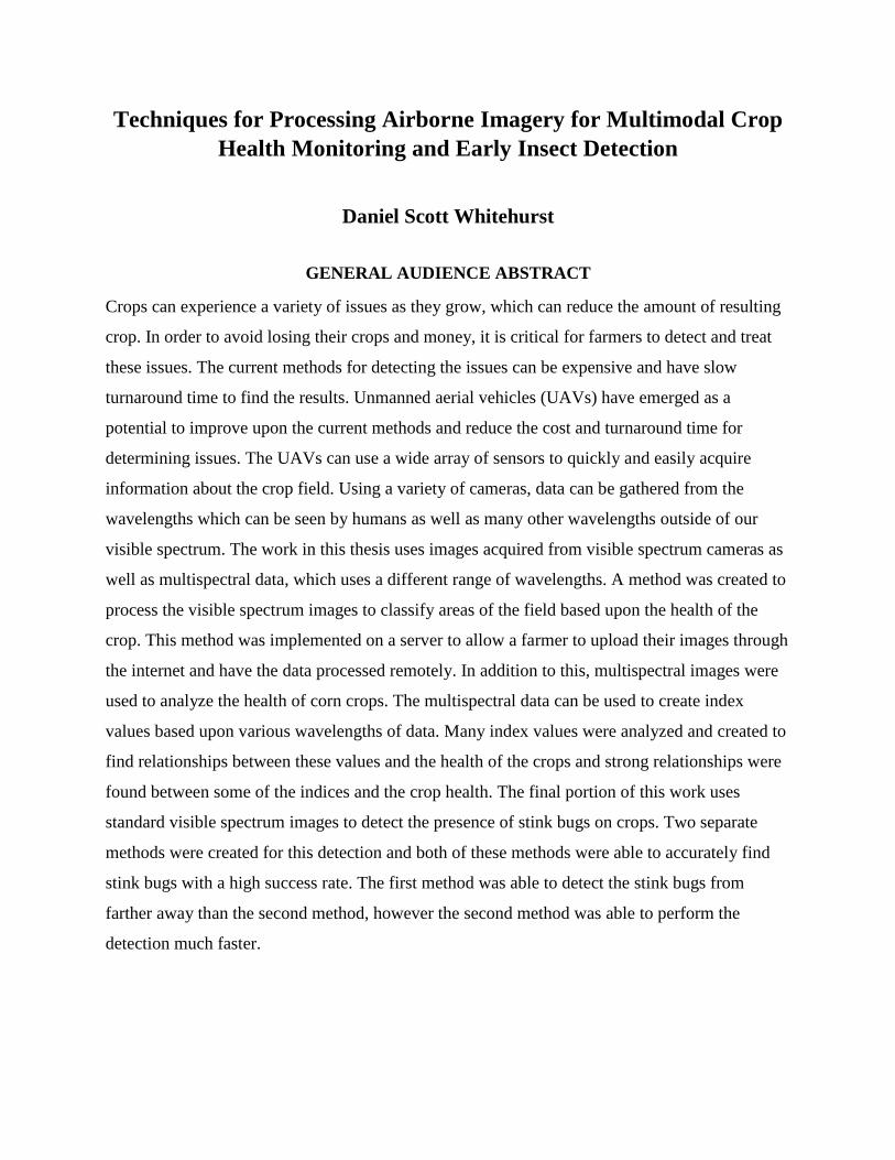
Techniques for Processing Airborne Imagery for Multimodal Crop

Health Monitoring and Early Insect Detection


GENERAL AUDIENCE ABSTRACT

Crops can experience a variety of issues as they grow, which can reduce the amount of resulting

crop. In order to avoid losing their crops and money, it is critical for farmers to detect and treat

these issues. The current methods for detecting the issues can be expensive and have slow

turnaround time to find the results. Unmanned aerial vehicles (UAVs) have emerged as a

potential to improve upon the current methods and reduce the cost and turnaround time for

determining issues. The UAVs can use a wide array of sensors to quickly and easily acquire

information about the crop field. Using a variety of cameras, data can be gathered from the

wavelengths which can be seen by humans as well as many other wavelengths outside of our

visible spectrum. The work in this thesis uses images acquired from visible spectrum cameras as

well as multispectral data, which uses a different range of wavelengths. A method was created to

process the visible spectrum images to classify areas of the field based upon the health of the

crop. This method was implemented on a server to allow a farmer to upload their images through

the internet and have the data processed remotely. In addition to this, multispectral images were

used to analyze the health of corn crops. The multispectral data can be used to create index

values based upon various wavelengths of data. Many index values were analyzed and created to

find relationships between these values and the health of the crops and strong relationships were

found between some of the indices and the crop health. The final portion of this work uses

standard visible spectrum images to detect the presence of stink bugs on crops. Two separate

methods were created for this detection and both of these methods were able to accurately find

stink bugs with a high success rate. The first method was able to detect the stink bugs from

farther away than the second method, however the second method was able to perform the

detection much faster.

iv

Acknowledgments

I would like to thank all of the people who have helped me through the course of the work that

went into this thesis. First, I want to thank my advisor Dr. Kochersberger for giving me this

opportunity and being a great advisor and a great person. He has been the best advisor that I

could have hoped for and was great at helping and pushing me along the way. I have been very

lucky to have him as an advisor and mentor through my graduate studies. I would also like to

thank the rest of my committee for their help throughout this work.

Next, I want to thank the corporate sponsors who have helped to make this work possible. I

would like to thank Tim Sexton at the Virginia Department of Conservation and Recreation for

providing the dataset used for the visual crop health monitoring work and helping me to

understand the crop issues and label the data. I also want to thank Larry Gaultney at DuPont for

providing me with a portion of the dataset used for the stink bug detection work.

My next acknowledgements go to several members of my lab. I want to thank Haseeb Chaudhry

for his help and advice with hardware, Gordon Christie for giving advice with computer vision

and machine learning topics, and Evan Smith for his help with the work in Chapter 3 as well as

always being there to help with anything I needed throughout this work and graduate school as a

whole. I would also like to thank Drew Morgan, Yuan Lin, and Jonah Fike for their help with

acquiring the images used for the work in Chapter 4.

Lastly, I would like to thank my family and friends for all of the support and encouragement they

have given to me along the way. I would not be the person I am today without the love, support,

and guidance of my parents throughout my life. And I want to thank my friends for their impact

on my life, including their help with my work, help with life, and just being there to hang out and

get away from school to relax for a while.

v

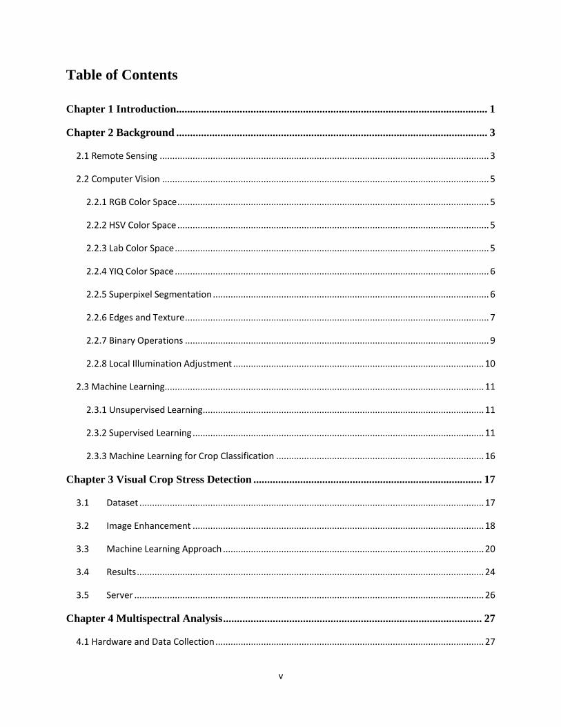
Table of Contents

Chapter 1 Introduction................................................................................................................. 1

Chapter 2 Background ................................................................................................................. 3

2.1 Remote Sensing .................................................................................................................................. 3

2.2 Computer Vision ................................................................................................................................. 5

2.2.1 RGB Color Space ........................................................................................................................... 5

2.2.2 HSV Color Space ........................................................................................................................... 5

2.2.3 Lab Color Space ............................................................................................................................ 5

2.2.4 YIQ Color Space ............................................................................................................................ 6

2.2.5 Superpixel Segmentation ............................................................................................................. 6

2.2.6 Edges and Texture ........................................................................................................................ 7

2.2.7 Binary Operations ........................................................................................................................ 9

2.2.8 Local Illumination Adjustment ................................................................................................... 10

2.3 Machine Learning .............................................................................................................................. 11

2.3.1 Unsupervised Learning ............................................................................................................... 11

2.3.2 Supervised Learning ................................................................................................................... 11

2.3.3 Machine Learning for Crop Classification .................................................................................. 16

Chapter 3 Visual Crop Stress Detection ................................................................................... 17

3.1 Dataset ........................................................................................................................................ 17

3.2 Image Enhancement ................................................................................................................... 18

3.3 Machine Learning Approach ....................................................................................................... 20

3.4 Results ......................................................................................................................................... 24

3.5 Server .......................................................................................................................................... 26

Chapter 4 Multispectral Analysis .............................................................................................. 27

4.1 Hardware and Data Collection .......................................................................................................... 27

vi

4.1.1 Cameras ..................................................................................................................................... 27

4.1.2 UAV Platform ............................................................................................................................. 28

4.1.3 Imaging Pole ............................................................................................................................... 30

4.1.4 Corn Test Plots ........................................................................................................................... 31

4.2 NDVI Analysis .................................................................................................................................... 32

4.2.1 Lighting Impact ........................................................................................................................... 32

4.2.2 Lightness Correction .................................................................................................................. 34

4.2.3 Trend Analysis ............................................................................................................................ 37

4.3 Hyperspectral Data Issues ................................................................................................................. 40

4.3.1 Referencing ................................................................................................................................ 40

4.3.2 Hyperspectral Camera Accuracy ................................................................................................ 42

4.3.3 Shadows and Light Variations .................................................................................................... 45

4.4 Hyperspectral Shadow Correction .................................................................................................... 46

4.5 Hyperspectral Indices ........................................................................................................................ 51

Chapter 5 Stink Bug Detection .................................................................................................. 64

5.1 Image Collection ............................................................................................................................... 64

5.2 Edge and Contour Methods .............................................................................................................. 64

5.3 Superpixel Segmentation .................................................................................................................. 67

5.4 Multispectral ..................................................................................................................................... 73

5.5 Additional Method ............................................................................................................................ 74

5.6 Results ............................................................................................................................................... 79

Chapter 6 Summary & Conclusions ......................................................................................... 80

Bibliography ................................................................................................................................ 83

vii

List of Figures

Figure 2.1: Representation of a support vector machine. ............................................................. 12

Figure 2.2: Data which is not separable with a linear hyperplane. ............................................... 14

Figure 2.3: 3-dimensional representation of the impact of the RBF kernel on the data from Figure

2.2.................................................................................................................................................. 15

Figure 3.1: An example of an image from the dataset, with an annotation provided. .................. 17

Figure 3.2: This is an example of an unlabeled image from the dataset showing corn with

multiple stressed areas. ................................................................................................................. 18

Figure 3.3: An image shown before (left) and after (right) the enhancement algorithm has been

applied. .......................................................................................................................................... 19

Figure 3.4: An image shown before (left) and after (right) the enhancement algorithm has been

applied ........................................................................................................................................... 20

Figure 3.5: Training image labeled using LabelMe. ..................................................................... 21

Figure 3.6: The classification accuracy of the SVM is plotted against the number of features used

to train the SVM. The accuracy can be seen to level off after 5 features. .................................... 24

Figure 3.7: Classification results from the support vector machine. The image of the field is

shown on the left and the right shows the classification results. The green corresponds to the

healthy class, the yellow is the class for potential problem areas, and the red is the class for dirt.

....................................................................................................................................................... 25

Figure 3.8: Classification results from the SVM for an image of a field. The image of the field is

shown on the left and the classification is shown on the right. This field can be seen to have

major issues with the crop health. ................................................................................................. 25

Figure 3.9: Classification results from the SVM for an image of a field. The image of the field is

shown on the left and the classification is shown on the right. This image shows a broad view of

field, which also contains areas not corresponding to crops. ........................................................ 26

Figure 4.1: Canon S100 camera, which is used as a visual camera as well as the near-infrared

camera. .......................................................................................................................................... 27

Figure 4.2: OCI-UAV-2000 hyperspectral camera that is being used. ......................................... 28

Figure 4.3: DJI S1000+ Octocopter used with the camera payload. ............................................ 29

viii

Figure 4.4: Our octocopter flying at Kentland Farm with all electronics and camera payload

attached. ........................................................................................................................................ 29

Figure 4.5: Set of three images taken simultaneously by each of the cameras during the flight at

Kentland Farm. It can be seen that the field of view for the hyperspectral camera is much smaller

than for the other two cameras. ..................................................................................................... 30

Figure 4.6: The height of the pole, relative to the corn, can be seen on the left and the imaging

payload attached to the pole is shown on the right. ...................................................................... 31

Figure 4.7: Aerial view of the nitrogen rate test plots used to acquire images of for analysis. Each

plot is labeled with the plot number as well as the nitrogen treatment in lbs/acre. ...................... 32

Figure 4.8: Images of corn test plot 105. The top left image is the visual image, the near-infrared

image is in the top right, and the bottom image is the NDVI of the plot. ..................................... 33

Figure 4.9: Plot of NDVI and Lightness of the images shown in Figure 4.8. A regression analysis

produced a coefficient of determination of 0.9488. ...................................................................... 34

Figure 4.10: Results of the Poisson image editing method. The original image and original NDVI

are shown on the top and the adjusted image and NDVI are on the bottom................................. 35

Figure 4.11: Images of corn test plot 105. The top left image is the visual image, the near-

infrared image is in the top right, the bottom left image is the NDVI of the plot before the

lightness adjustment, and the bottom right image is the NDVI after adjustment. ........................ 36

Figure 4.12: Plot of NDVI and Lightness after adjusting the images shown in Figure 4.10. A

regression analysis produced a coefficient of determination of 0.0295........................................ 37

Figure 4.13: Plot of the corn crop yield, in bushels/acre, and the nitrogen application rate, in

pounds/acre for the five test plots our images focused on. ........................................................... 37

Figure 4.14: Plot of the NDVI values against the nitrogen rates of the test plots for images

acquired on July 13, 2015. ............................................................................................................ 38

Figure 4.15: Plot of the NDVI values against the nitrogen rates of the test plots for images

acquired on July 22, 2015. ............................................................................................................ 39

Figure 4.16: NDVI of the corn after lightness adjustment plotted against the nitrogen application

for two different days. ................................................................................................................... 39

Figure 4.17: Corn yield plotted against the adjusted NDVI of the corn for two days. ................. 40

Figure 4.18: Raw image acquired of bushes when the referencing was not performed properly.

This image is overexposed and leads to bad data when processed. .............................................. 41

ix

Figure 4.19: The first band of the hyperspectral cube is shown in the left image. The

overexposure resulted in a mostly white image. The plot of the reflectance is shown on the right

for the two selected portions in the left image. ............................................................................. 42

Figure 4.20: Reflectance curves of concrete for each of the two hyperspectral devices. ............. 43

Figure 4.21: Reflectance curves of grass for each of the two hyperspectral devices. .................. 43

Figure 4.22: Reflectance curves of a leaf for each of the two hyperspectral devices. .................. 44

Figure 4.23: Reflectance curves of the three objects for each of the two devices. The top plot

shows the curves produced from the baseline camera and the bottom plot shows the curves

produced from our camera. ........................................................................................................... 45

Figure 4.24: Test plot image impacted by shadows. The visual image (top left) and

corresponding hyperspectral image (top right) are shown. Red and blue boxes on the

hyperspectral image correspond to the Reflectance curves on the plot. ....................................... 46

Figure 4.25: Plot of the hyperspectral data points for 20 bands at various lighting conditions.... 47

Figure 4.26: Plot of the average of the hyperspectral data points with various lighting conditions.

A trend line was fit to the data with an R2 value of 0.868. ........................................................... 48

Figure 4.27: The top image is the visual image which corresponds to the hyperspectral image for

test plot 101. A single band of the hyperspectral image is shown in the bottom left. The bottom

right image is that result of the reflectance adjustment code on the hyperspectral image. ........... 49

Figure 4.28: The top image is the visual image which corresponds to the hyperspectral image for

test plot 102. A single band of the hyperspectral image is shown in the bottom left. The bottom

right image is that result of the reflectance adjustment code on the hyperspectral image. ........... 50

Figure 4.29: Reflectance curves for shadowed areas of corn before and after adjustment. ......... 51

Figure 4.30: Reflectance curves for corn and soil in various stages of lighting before and after

adjustment. .................................................................................................................................... 51

Figure 4.31: Plots of the R780/R740 index. The top plot shows the index against the crop yield and

the bottom plot shows the index against the nitrogen application rate. ........................................ 53

Figure 4.32: Plots of the Normalized Difference Red Edge index. The top plot shows the index

against the crop yield and the bottom plot shows the index against the nitrogen application rate.

....................................................................................................................................................... 54

Figure 4.33: Plots of the relationship between the corn yield and the new index created from the

ratio between the reflectance at 760 nm and 740 nm. ................................................................... 55

x


normalized difference between the reflectance at 760 nm and 740 nm. ....................................... 56













Figure 5.1: Two example images from the dataset. The left image was provided by a contact at

DuPont and the image on the right was taken using canola at our lab. ........................................ 64

Figure 5.2: Contour extracted for a high resolution image of a stink bug on a plain white

background. ................................................................................................................................... 65

Figure 5.3: Edge segmentation results from the stink bug in Figure 5.2. ..................................... 65

Figure 5.4: Contour and edges extracted from a resized version of the stink bug in Figure 5.2.

The new image had a resolution of 2700 pixels. .......................................................................... 66

Figure 5.5: Contours and edges for a stink bug on leaves of a plant. ........................................... 66

Figure 5.6: Structured edge detection performed on an image with a stink bug on a plant. ........ 67

Figure 5.7: Structured edge detection performed on an image with a stink bug on a plant. ........ 67

Figure 5.8: Superpixel segmentation results for two images. The red lines indicate superpixel

borders. The bottom images zoom in on the stink bugs from the top images. ............................. 68

Figure 5.9: RGB image of a stink bug on a plant along with scaled representations of the red,

hue, and a* planes. The top right image shows the red values, the bottom left image shows the

hue, and the bottom right images shows the a* values. ................................................................ 69

Figure 5.10: Superpixel of a stink bug and the corresponding histogram of hue values. The

largest peak will be selected to represent the superpixel. ............................................................. 70

xi

Figure 5.11: Superpixel with a very odd shape, which will be filtered out with the bounding box

method........................................................................................................................................... 72

Figure 5.12: Stink bug detection result using the superpixel method. The detected stink bug is

shown on the right. ........................................................................................................................ 72

Figure 5.13: Superpixel stink bug detection results. The top shows a stink bug detected when

partially obscured by a leaf and the bottom shows a stink bug detected when perpendicular to the

camera. .......................................................................................................................................... 73

Figure 5.14: Reflectance curves for selected areas of vegetation (leaf), soil, and stink bugs. ..... 74

Figure 5.15: Result of filtering an image by hue. The hue filtering removes most of the

vegetation in the image while the stink bugs remain. ................................................................... 75

Figure 5.16: Entropy filtering of the resulting image from Figure 5.15. The image on the left

shows the scaled color representation of the entropy values and the image on the right shows the

image result after the entropy filtering process. ............................................................................ 76

Figure 5.17: Plot of the stink bug size against the height at which the image was acquired. A

curve was fit to the trend of the data. ............................................................................................ 77

Figure 5.18: Final detection result of the image from Figure 5.15. The top image shows the

detected results and the bottom two images show zoomed-in version of the detected stink bugs.

....................................................................................................................................................... 78

xii

List of Tables

Table 3.1: Linear SVM Optimal Features..................................................................................... 22

Table 3.2: Comparison Between Linear SVM and SVM with Gaussian Kernel .......................... 22

Table 3.3: Optimal Features for SVM with Gaussian Kernel ....................................................... 23

Table 4.1: Indices and Correlation to Corn Yield ......................................................................... 63

xiii

Nomenclature

ac Acre

lbs Pounds (mass)

NDVI Normalized Difference Vegetation Index

NIR Near-infrared

nm Nanometer

SVM Support Vector Machine

UAV Unmanned Aerial Vehicle

1

Chapter 1 Introduction

With increased access to unmanned aircraft that are capable of high-resolution overhead

imagery, farmers are now empowered to scout fields with much higher accuracy and coverage

area. This image acquisition capability is complemented by the ability to interpret the data so

that an appropriate response is taken.

Crops can regularly suffer from a variety of issues, which a farmer will want to address. The

issues suffered can include both biotic and abiotic stresses. These may involve diseases,

improper treatment with chemicals, misapplication of water, as well as insect problems. The

current methods of detecting and resolving these issues are lacking. These methods include

manual inspection, whole field treatment with pesticides or fungicides, and photographic

inspection. The current manual inspection methods involve the farmers looking through the

fields at ground level or from a slightly elevated height. These methods of inspection do not

provide proper scope to truly locate issues and also can be manually intensive to see the scope of

the field. A current method of photographic inspection involves aerial imagery, generally

acquired from a manned aircraft, which can be used for the crop inspection. This method is also

manually intensive and the cost for this inspection method is very high, which limits its

applicability for most farmers. The other current method is treating large portions of the field

based on field-average thresholds instead of targeting treatments to the specific problem areas.

Knowing the problem areas to target can help reduce the amount of treatment and save money

for the farmer.

The rise in availability and use of unmanned aircrafts can allow a farmer to improve upon the

current methods of inspection and treatment. With the use of an unmanned aerial vehicle (UAV),

a farmer has the ability to quickly and easily acquire airborne imagery of the field, which can

then be used for inspection. The goal of this work is to create tools and methods for farmers to

improve the health and yield of their crops from the analysis of images which can be acquired

from a UAV. Various types of images can be used to investigate the health of crops. The most

widely available and most inexpensive form of imagery is visual spectrum imagery. As a result,

the first goal of the work was to create image processing methods to detect crop stresses using

solely visual imagery. While it is unlikely that farmers will have access to near-infrared or

2

hyperspectral cameras, the information from these images can potentially provide a more

accurate representation of crop health than the simple visual imagery. As a result, the next goal

of this work was to examine the information obtained from multiple spectrums and the indices

this data can produce, including known indices and the creation of new indices.

In addition to locating and treating the issues after visual damage has been done to the crops, it

would be beneficial to detect some issues, such as the presence of insect pests, before the damage

has been done to the crop. This also has potential to be achieved through scouting of a field with

a UAV. The final goal of this work was to create methods for the detection of insects in a field

from airborne imagery. Specifically, the goal was to detect brown marmorated stink bugs since

these are an emerging pest in Virginia, which is the focus area of this work.

The organization of this thesis will be in the following form. Chapter 2 discusses all relevant

background information required to understand the methods presented in this thesis as well as

existing literature in these areas. The chapter will cover the topics of remote sensing, computer

vision, and machine learning. Chapter 3 discusses my method for processing visual imagery to

aid the detection of crop stress. This method includes image enhancement as well as an

implementation of a machine learning algorithm to classify the problem areas in the field.

Chapter 4 presents multispectral analysis for crop health monitoring, including NDVI analysis

from visual and near-infrared imagery as well as hyperspectral index analysis using a

hyperspectral camera. Chapter 5 covers multiple methods that have been developed to detect

stink bugs on vegetation from aerial images. Two different algorithms are presented, while

multiple other attempted methods are discussed. Chapter 6 will present a summary of the work in

this thesis along with the conclusions which were drawn from this work. Additionally, potential

areas of improvement for future work are discussed. This final chapter is then followed with the

references which were used during this work.

3

Chapter 2 Background

This chapter discusses the background information which is necessary to understand the work of

this thesis. The three main topics discussed in this section are remote sensing, computer vision,

and machine learning.

2.1 Remote Sensing

Remote sensing is observing an object without physically touching the object. In the field of

agriculture, remote sensing involves the ability for farmers to observe and acquire information

about their fields without physically touching the fields. This generally involves images acquired

from satellites and aircraft to provide a means to assess field conditions from a point of view

high above the field. Many different sensors can be used for remote sensing, including ones

which see in the visible wavelengths of light and others which can detect wavelengths not visible

to the human eye. With recent technological advances, remote sensing has become more

accessible to most agricultural producers. Images acquired through remote sensing can be used

for the identification of diseases, nutrient deficiencies, insect damage, herbicide damage, water

deficiencies or surpluses, and many other issues. This information allows farmers to focus

treatments on only the affected areas of a field [1].

Using remotely sensed data, indices have been created for the analysis of different features of

crop health. Many of these indices rely on data from wavelengths corresponding to the visible

and infrared regions of the electromagnetic spectrum. Visible light ranges from wavelengths

between around 400 nanometers and 700 nanometers. One portion of the infrared region of the

spectrum is near-infrared (NIR) light, which ranges from wavelengths of 700 nm to 1100 nm.

Chlorophyll, the pigment in plant leaves, strongly absorbs visible light for photosynthesis while

strongly reflecting NIR light. These properties of the plants cause the use of an index known as

the Normalized Difference Vegetation Index (NDVI), shown in Equation 2.1 [2].

𝑁𝐷𝑉𝐼 =𝑁𝐼𝑅 − 𝑉𝐼𝑆

𝑁𝐼𝑅 + 𝑉𝐼𝑆 (2.1)

In this equation, 𝑁𝐼𝑅 represents the spectral reflectance in the near-infrared wavelengths and 𝑉𝐼𝑆

represents the spectral reflectance in the visible (red) wavelengths. Values for the NDVI range

4

between −1 and +1. Areas with high NDVI values, from 0.6 to 0.9, generally correspond to

dense vegetation such as crops at their peak growth stages or forests. Sparse vegetation can result

in moderate NDVI values, around 0.2 to 0.5, and areas of barren rock, sand, or snow generally

result in very low NDVI values, usually 0.1 or less [3]. Many other indices can be created from

the use of hyperspectral data, which involves reflectance values at specific wavelengths across a

range of wavelengths. A list of crop indices was found in the dissertation work of Pavuluri [4].

From these, two indices were selected for further investigation in this thesis. The two indices

were selected because these were the only two which used wavelengths for which data could be

accurately acquired using our hyperspectral camera. The first of the indices was a ratio of the

reflectance values at 780 nm and 740 nm in the form shown in Equation 2.2.

𝐼𝑛𝑑𝑒𝑥 =𝑅780

𝑅740 (2.2)

An additional index taken from that work is known as the Normalized Difference Red Edge

index, which uses the reflectance values at 790 nm and 720 nm. The formula for this index is

shown in Equation 2.3. Many additional indices are used in remote sensing, but these were not

included in the scope of this thesis.

𝑁𝑜𝑟𝑚𝑎𝑙𝑖𝑧𝑒𝑑 𝐷𝑖𝑓𝑓𝑒𝑟𝑒𝑛𝑐𝑒 𝑅𝑒𝑑 𝐸𝑑𝑔𝑒 =𝑅790 − 𝑅720

𝑅790 + 𝑅720 (2.3)

Current satellite sensors for remote sensing have critical limitations of the lack of imagery with

optimum spatial and spectral resolutions as well as undesirable revisit time of the satellites.

Manned airborne platforms for remote sensing have the issue of high operational costs. With

remote sensing platforms for agriculture, high special resolution and quick turnaround times are

necessary for useful results. The use of UAVs with remote sensors provides a potential solution

to provide low-cost approaches for meeting the spatial, spectral, and temporal resolution

requirements, which was presented in the article by Berni et al. [5]. Additionally, this article

explored and validated the capabilities of thermal and narrowband multispectral remote sensing

from a UAV to monitor vegetation. The idea of low-altitude remote sensing from a UAV as a

potential substitute for satellite precision agriculture systems has also been explored in other

works of literature [6] and the use of UAVs for remote sensing applications in agriculture has

been investigated in many additional pieces of literature [7-9]. From these investigations, the use

5

of UAVs for remote sensing and precision agriculture is a very capable and cost-effective option

when appropriate sensors are used. This is an emerging and growing technology that will likely

have a large impact on the future directions of remote sensing for agriculture.

2.2 Computer Vision

Computer vision is a field which aims to make computers see. The field includes methods for

acquiring, processing, analyzing, and understand images and data from the real world to produce

information, such as in the form of decisions [10]. Generally, computer vision techniques are

developed to replicate the abilities of human vision through the use of a computer processing

images. The following will cover the computer vision concepts and techniques which have been

utilized in the course of this thesis.

2.2.1 RGB Color Space

The RGB color space is an additive color space which consists of red, green, and blue. This color

space is the most commonly used color space and is used by most cameras and for the related

applications.

2.2.2 HSV Color Space

The HSV color space is a cylindrical-coordinate representation of points in an RGB color mode.

This is one of the two most common cylindrical representations, alongside the HSL color space.

The HSV name stands for hue, saturation, and value. The color space was developed for

computer graphics applications and is currently used in color pickers, image editing software,

image analysis as well as computer vision. The hue component is the angular measure of the

color space and it represents a measure of the color. Saturation is the radial component and this

represents how colorful a color is relative to its own brightness. The value component is a

measure of the brightness [11].

2.2.3 Lab Color Space

The Lab color space is a color-opponent space, with the L component for lightness and a* and b*

for the color-opponent dimensions. The a* component represents the position of the color

between red/magenta and green and the b* component represents the position of the color

6

between yellow and blue. The lightness value ranges between 0 and 100, with 0 representing

black and 100 representing white. For a* and b*, negative values indicate green and blue and

positive values indicate red and yellow, respectively [12].

2.2.4 YIQ Color Space

The YIQ color space is the one that is used by the NTSC color TV system. The Y component

represents the luma values, which correspond to the brightness of the image. The I and Q

components represent the chrominance information. This color space representation can be used

in color image processing to adjust images without altering the color balance. This is done by

applying the adjustments only to the Y channel of the images [13]. The formula for converting

an RGB image into the YIQ color space is shown by Equation 2.4 [14].

[𝑌𝐼𝑄

] = [0.299 0.587 0.1440.596 −0.274 −0.3220.211 −0.523 0.312

] [𝑅𝐺𝐵

] (2.4)

2.2.5 Superpixel Segmentation

Superpixels are large pixels formed from combinations of many other pixels. This allows

redundancy in images to be captured and reduces the complexity of the image for later

processing. One method of superpixel segmentation, which is used in this thesis, is the method of

SLIC Superpixels. The algorithm for this method is called SLIC (Simple Linear Iterative

Clustering) and the method is detailed in the paper [15]. This method uses a five dimensional

space containing the L, a, and b values of the CIELAB color space as well as the x and y pixel

coordinates and performs local clustering of the pixels based on these five dimensions. The input

to this algorithm is the desired number of superpixels K, which would be approximately equal in

size. For an image with a size of N pixels, each superpixel is approximately N/K pixels in size.

With superpixels which are roughly equally sized, a superpixel center would be located at each

grid interval 𝑆 = √𝑁/𝐾. To begin the algorithm, K cluster centers 𝐶𝑘 = [𝑙𝑘, 𝑎𝑘 , 𝑏, 𝑥𝑘, 𝑦𝑘,]𝑇 are

chosen for the superpixels with 𝑘 = [1, 𝐾] at regular grid intervals 𝑆. Because the approximate

area of each of the superpixels is 𝑆2, it can be assumed that the pixels associated with this cluster

center are located in a 2𝑆 × 2𝑆 area around the superpixel center in the 𝑥𝑦 plane. As a result,

this area becomes the search area for the pixels closest to each cluster center. For the CIELAB

color space, Euclidean distances are perceptually meaningful for small distances. To prevent the

7

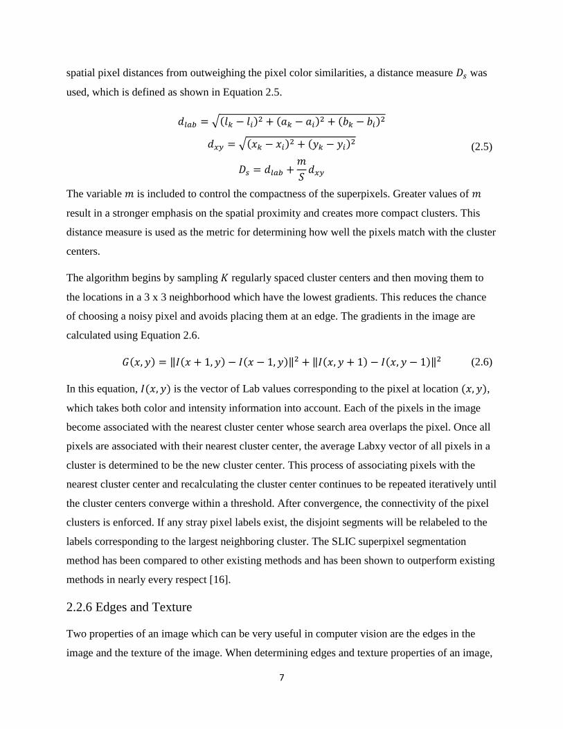
spatial pixel distances from outweighing the pixel color similarities, a distance measure 𝐷𝑠 was

used, which is defined as shown in Equation 2.5.

𝑑𝑙𝑎𝑏 = √(𝑙𝑘 − 𝑙𝑖)2 + (𝑎𝑘 − 𝑎𝑖)2 + (𝑏𝑘 − 𝑏𝑖)2

𝑑𝑥𝑦 = √(𝑥𝑘 − 𝑥𝑖)2 + (𝑦𝑘 − 𝑦𝑖)2

𝐷𝑠 = 𝑑𝑙𝑎𝑏 +𝑚

𝑆𝑑𝑥𝑦

(2.5)

The variable 𝑚 is included to control the compactness of the superpixels. Greater values of 𝑚

result in a stronger emphasis on the spatial proximity and creates more compact clusters. This

distance measure is used as the metric for determining how well the pixels match with the cluster

centers.

The algorithm begins by sampling 𝐾 regularly spaced cluster centers and then moving them to

the locations in a 3 x 3 neighborhood which have the lowest gradients. This reduces the chance

of choosing a noisy pixel and avoids placing them at an edge. The gradients in the image are

calculated using Equation 2.6.

𝐺(𝑥, 𝑦) = ‖𝐼(𝑥 + 1, 𝑦) − 𝐼(𝑥 − 1, 𝑦)‖2 + ‖𝐼(𝑥, 𝑦 + 1) − 𝐼(𝑥, 𝑦 − 1)‖2 (2.6)

In this equation, 𝐼(𝑥, 𝑦) is the vector of Lab values corresponding to the pixel at location (𝑥, 𝑦),

which takes both color and intensity information into account. Each of the pixels in the image

become associated with the nearest cluster center whose search area overlaps the pixel. Once all

pixels are associated with their nearest cluster center, the average Labxy vector of all pixels in a

cluster is determined to be the new cluster center. This process of associating pixels with the

nearest cluster center and recalculating the cluster center continues to be repeated iteratively until

the cluster centers converge within a threshold. After convergence, the connectivity of the pixel

clusters is enforced. If any stray pixel labels exist, the disjoint segments will be relabeled to the

labels corresponding to the largest neighboring cluster. The SLIC superpixel segmentation

method has been compared to other existing methods and has been shown to outperform existing

methods in nearly every respect [16].

2.2.6 Edges and Texture

Two properties of an image which can be very useful in computer vision are the edges in the

image and the texture of the image. When determining edges and texture properties of an image,

8

the use of a filter can be advantageous. A filter is a matrix which is applied to a neighborhood of

pixels around a specific pixel. Filters can be used in a variety of tasks which include smoothing,

sharpening, enhancing or detecting edges, and examining image texture [17]. Two of the

applications for filters which were used in the course of the work in this thesis are for edge

detection and texture.

To detect edges in an image, it is necessary to find the sharp changes in the image since these

correspond to edges. These changes in the image can be determined through the use of a gradient

in the image. The formula in Equation 2.7 gives the gradient of an image [18]. This formula is

comprised of the partial derivatives in both the x and y directions.

∇𝑓 = [𝜕𝑓

𝜕𝑥

𝜕𝑓

𝜕𝑦] (2.7)

When performing this gradient calculation on an image, it can be approximated through the use

of a filter. One such example of a filter which can be used is the Sobel operator. Equation 2.8

shows the Sobel operators for the horizontal and vertical gradients. These operators can be used

to determine the gradients in an image by convolving the operator with an image [19-21].

𝐺𝑥 = [−1 0 +1−2 0 +2−1 0 +1

] , 𝐺𝑦 = [+1 +2 +10 0 0

−1 −2 −1] (2.8)

To examine textures in an image, many different methods exist. The method used for the work in

this thesis was the entropy of the image. Entropy is a measure of the amount of disorder in a

system and a statistical measure of uncertainty. The entropy can be used to determine how ‘busy’

areas of an image are and the amount of variability in the areas. As a result, this quantity can be

used to find differences in the texture of an image. The formula to calculate the entropy is shown

in Equation 2.9. This equation is applied to a neighborhood, or window, around each of the

pixels in an image.

𝐸 = − ∑ 𝑝𝑖 log2 𝑝𝑖

𝑖

(2.9)

In the equation, E is the entropy and 𝑝𝑖 represents the histogram bin counts for the pixel values,

which corresponds with the probabilities of those specific pixel values [22-25].

9

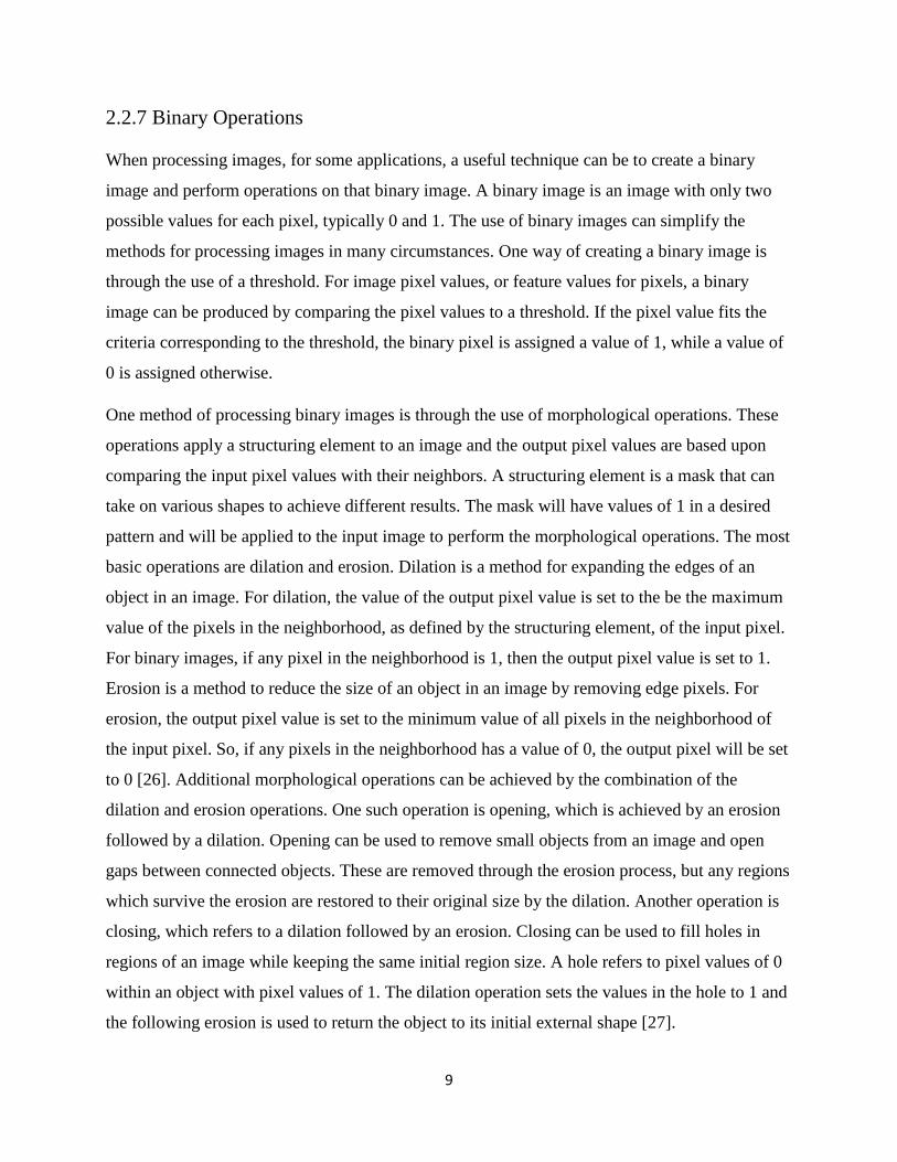
2.2.7 Binary Operations

When processing images, for some applications, a useful technique can be to create a binary

image and perform operations on that binary image. A binary image is an image with only two

possible values for each pixel, typically 0 and 1. The use of binary images can simplify the

methods for processing images in many circumstances. One way of creating a binary image is

through the use of a threshold. For image pixel values, or feature values for pixels, a binary

image can be produced by comparing the pixel values to a threshold. If the pixel value fits the

criteria corresponding to the threshold, the binary pixel is assigned a value of 1, while a value of

0 is assigned otherwise.

One method of processing binary images is through the use of morphological operations. These

operations apply a structuring element to an image and the output pixel values are based upon

comparing the input pixel values with their neighbors. A structuring element is a mask that can

take on various shapes to achieve different results. The mask will have values of 1 in a desired

pattern and will be applied to the input image to perform the morphological operations. The most

basic operations are dilation and erosion. Dilation is a method for expanding the edges of an

object in an image. For dilation, the value of the output pixel value is set to the be the maximum

value of the pixels in the neighborhood, as defined by the structuring element, of the input pixel.

For binary images, if any pixel in the neighborhood is 1, then the output pixel value is set to 1.

Erosion is a method to reduce the size of an object in an image by removing edge pixels. For

erosion, the output pixel value is set to the minimum value of all pixels in the neighborhood of

the input pixel. So, if any pixels in the neighborhood has a value of 0, the output pixel will be set

to 0 [26]. Additional morphological operations can be achieved by the combination of the

dilation and erosion operations. One such operation is opening, which is achieved by an erosion

followed by a dilation. Opening can be used to remove small objects from an image and open

gaps between connected objects. These are removed through the erosion process, but any regions

which survive the erosion are restored to their original size by the dilation. Another operation is

closing, which refers to a dilation followed by an erosion. Closing can be used to fill holes in

regions of an image while keeping the same initial region size. A hole refers to pixel values of 0

within an object with pixel values of 1. The dilation operation sets the values in the hole to 1 and

the following erosion is used to return the object to its initial external shape [27].

10

Additionally, for binary images, the region properties of the image can be useful. Regions are

areas in the image which contain pixel values of 1 and are connected together by being next to

the pixels. Many properties of the regions can be found and used for processing. The region

properties which are used in this thesis include area, perimeter, and eccentricity. The area is the

number of pixels, with a value equal to 1, contained in the region. The perimeter of a region is

the total distance around the boundary of the region. This is determined by the distance between

the adjoining pairs of pixels around the region. For determining the eccentricity of a binary

region, a built-in Matlab method was used. For this, the eccentricity is found for an ellipse which

has the same second-moments as the desired region. Once this ellipse is found, the eccentricity

can be found as the ratio of the distance between the foci of the ellipse and its major axis length.

This value varies between 0 and 1, with 0 representing a circle and 1 representing a line segment

[28].

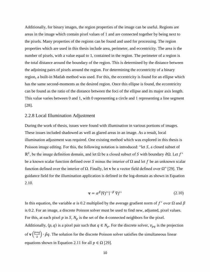
2.2.8 Local Illumination Adjustment

During the work of thesis, issues were found with illumination in various portions of images.

These issues included shadowed as well as glared areas in an image. As a result, local

illumination adjustment was required. One existing method which was explored in this thesis is

Poisson image editing. For this, the following notation is introduced: “let 𝑆, a closed subset of

ℝ2, be the image definition domain, and let Ω be a closed subset of 𝑆 with boundary 𝜕Ω. Let 𝑓∗

be a known scalar function defined over 𝑆 minus the interior of Ω and let 𝑓 be an unknown scalar

function defined over the interior of Ω. Finally, let v be a vector field defined over Ω” [29]. The

guidance field for the illumination application is defined in the log-domain as shown in Equation

2.10.

𝐯 = 𝛼𝛽|∇𝑓∗|−𝛽 ∇𝑓∗ (2.10)

In this equation, the variable 𝛼 is 0.2 multiplied by the average gradient norm of 𝑓∗ over Ω and 𝛽

is 0.2. For an image, a discrete Poisson solver must be used to find new, adjusted, pixel values.

For this, at each pixel 𝑝 in 𝑆, 𝑁𝑝 is the set of the 4-connected neighbors for the pixel.

Additionally, ⟨𝑝, 𝑞⟩ is a pixel pair such that 𝑞 ∈ 𝑁𝑝. For the discrete solver, 𝑣𝑝𝑞 is the projection

of 𝐯 (𝑝+𝑞

2) ∙ �⃗�𝑞. The solution for the discrete Poisson solver satisfies the simultaneous linear

equations shown in Equation 2.11 for all 𝑝 ∈ Ω [29].

11

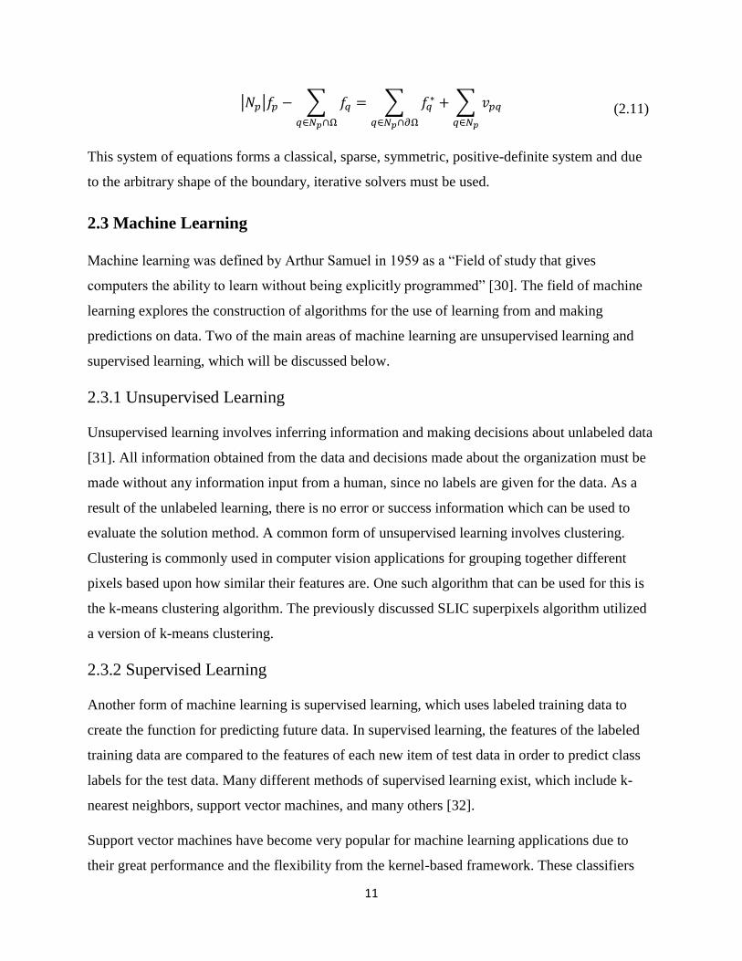
|𝑁𝑝|𝑓𝑝 − ∑ 𝑓𝑞

𝑞∈𝑁𝑝∩Ω

= ∑ 𝑓𝑞∗

𝑞∈𝑁𝑝∩𝜕Ω

+ ∑ 𝑣𝑝𝑞

𝑞∈𝑁𝑝

(2.11)

This system of equations forms a classical, sparse, symmetric, positive-definite system and due

to the arbitrary shape of the boundary, iterative solvers must be used.

2.3 Machine Learning

Machine learning was defined by Arthur Samuel in 1959 as a “Field of study that gives

computers the ability to learn without being explicitly programmed” [30]. The field of machine

learning explores the construction of algorithms for the use of learning from and making

predictions on data. Two of the main areas of machine learning are unsupervised learning and

supervised learning, which will be discussed below.

2.3.1 Unsupervised Learning

Unsupervised learning involves inferring information and making decisions about unlabeled data

[31]. All information obtained from the data and decisions made about the organization must be

made without any information input from a human, since no labels are given for the data. As a

result of the unlabeled learning, there is no error or success information which can be used to

evaluate the solution method. A common form of unsupervised learning involves clustering.

Clustering is commonly used in computer vision applications for grouping together different

pixels based upon how similar their features are. One such algorithm that can be used for this is

the k-means clustering algorithm. The previously discussed SLIC superpixels algorithm utilized

a version of k-means clustering.

2.3.2 Supervised Learning

Another form of machine learning is supervised learning, which uses labeled training data to

create the function for predicting future data. In supervised learning, the features of the labeled

training data are compared to the features of each new item of test data in order to predict class

labels for the test data. Many different methods of supervised learning exist, which include k-

nearest neighbors, support vector machines, and many others [32].

Support vector machines have become very popular for machine learning applications due to

their great performance and the flexibility from the kernel-based framework. These classifiers

12

have the ability to achieve high classification accuracy even with only a small amount of training

data. SVMs are inherently binary linear classifiers which use a set of labeled training data to

build models to assign new examples into one of two classes. The kernel-based framework of an

SVM also allows for efficient non-linear classification with the use of the kernel trick.

Additionally, multiple SVMs can be combined in order to classify instances into more than two

classes, which becomes a multiclass SVM. The algorithm for an SVM will be explained based

upon the information from [33] and [34].

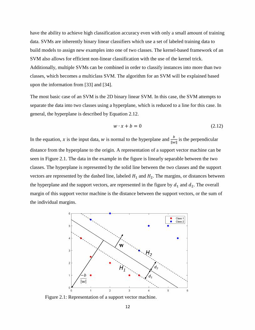
The most basic case of an SVM is the 2D binary linear SVM. In this case, the SVM attempts to

separate the data into two classes using a hyperplane, which is reduced to a line for this case. In

general, the hyperplane is described by Equation 2.12.

𝑤 ∙ 𝑥 + 𝑏 = 0 (2.12)

In the equation, 𝑥 is the input data, 𝑤 is normal to the hyperplane and 𝑏

‖𝑤‖ is the perpendicular

distance from the hyperplane to the origin. A representation of a support vector machine can be

seen in Figure 2.1. The data in the example in the figure is linearly separable between the two

classes. The hyperplane is represented by the solid line between the two classes and the support

vectors are represented by the dashed line, labeled 𝐻1 and 𝐻2. The margins, or distances between

the hyperplane and the support vectors, are represented in the figure by 𝑑1 and 𝑑2. The overall

margin of this support vector machine is the distance between the support vectors, or the sum of

the individual margins.

Figure 2.1: Representation of a support vector machine.

13

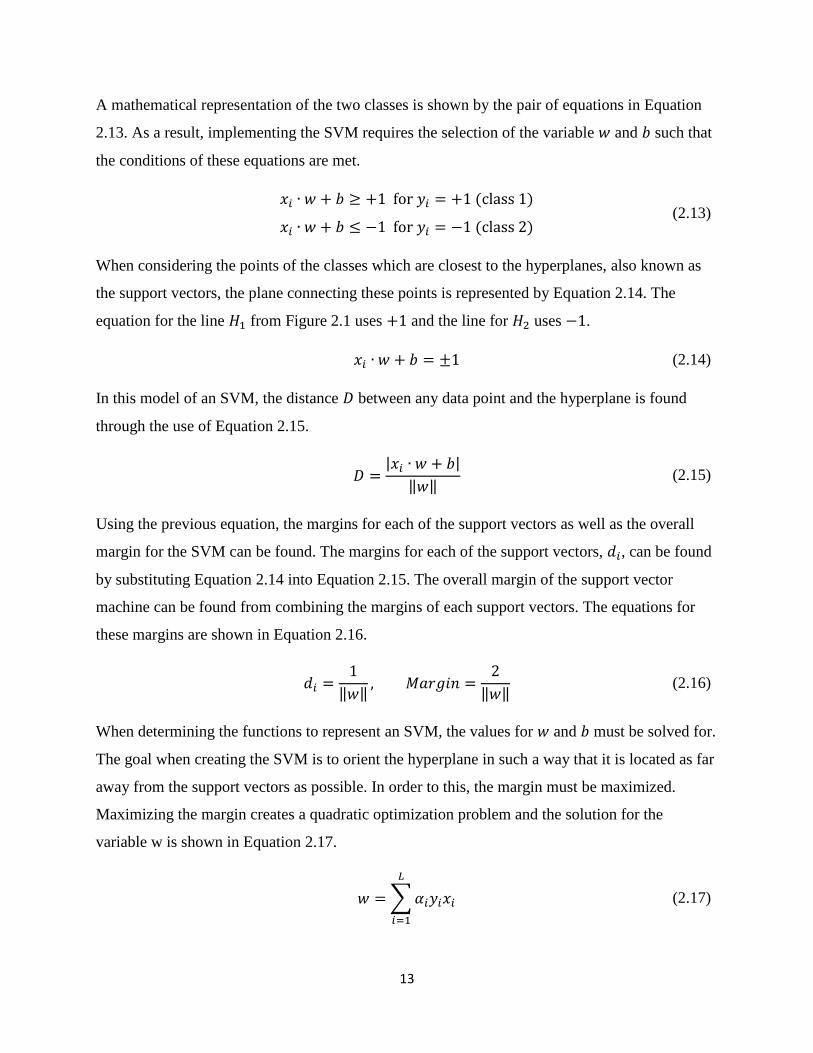
A mathematical representation of the two classes is shown by the pair of equations in Equation

2.13. As a result, implementing the SVM requires the selection of the variable 𝑤 and 𝑏 such that

the conditions of these equations are met.

𝑥𝑖 ∙ 𝑤 + 𝑏 ≥ +1 for 𝑦𝑖 = +1 (class 1)

𝑥𝑖 ∙ 𝑤 + 𝑏 ≤ −1 for 𝑦𝑖 = −1 (class 2) (2.13)

When considering the points of the classes which are closest to the hyperplanes, also known as

the support vectors, the plane connecting these points is represented by Equation 2.14. The

equation for the line 𝐻1 from Figure 2.1 uses +1 and the line for 𝐻2 uses −1.

𝑥𝑖 ∙ 𝑤 + 𝑏 = ±1 (2.14)

In this model of an SVM, the distance 𝐷 between any data point and the hyperplane is found

through the use of Equation 2.15.

𝐷 =|𝑥𝑖 ∙ 𝑤 + 𝑏|

‖𝑤‖ (2.15)

Using the previous equation, the margins for each of the support vectors as well as the overall

margin for the SVM can be found. The margins for each of the support vectors, 𝑑𝑖, can be found

by substituting Equation 2.14 into Equation 2.15. The overall margin of the support vector

machine can be found from combining the margins of each support vectors. The equations for

these margins are shown in Equation 2.16.

𝑑𝑖 =1

‖𝑤‖, 𝑀𝑎𝑟𝑔𝑖𝑛 =

2

‖𝑤‖ (2.16)

When determining the functions to represent an SVM, the values for 𝑤 and 𝑏 must be solved for.

The goal when creating the SVM is to orient the hyperplane in such a way that it is located as far

away from the support vectors as possible. In order to this, the margin must be maximized.

Maximizing the margin creates a quadratic optimization problem and the solution for the

variable w is shown in Equation 2.17.

𝑤 = ∑ 𝛼𝑖𝑦𝑖𝑥𝑖

𝐿

𝑖=1

(2.17)

14

For this equation, 𝛼 has been introduced as a weight variable. When using the SVM in

applications, the classifier function in Equation 2.18 is used. The use of the sign function for this

classifier results in output label values of −1 or +1, which correspond to the label values for

each of the classes.

𝑓(𝑥) = sign(𝑤 ∙ 𝑥 + 𝑏) (2.18)

The previous description works well for data which is linear separable, but this is not the case for

many applications. In many cases, the classes cannot be separated using a simple linear

classifier. An example of such data is shown in Figure 2.2. With this data, a line will not be able

to separate the two classes, so a nonlinear hyperplane and support vectors would be required.

Figure 2.2: Data which is not separable with a linear hyperplane.

A technique which can be used with SVMs to handle the classification of data which is not

linearly separable is the kernel trick. The feature vectors for the data can be mapped into higher

dimensional space using some mapping function 𝑥 → 𝜙(𝑥). Applying this mapping to the linear

classifier function produces the new classifier function in Equation 2.19.

𝑓(𝑥) = sign(∑ 𝛼𝑖𝑦𝑖𝑥𝑖 ∙ 𝑥

𝐿

𝑖=1

+ 𝑏) → 𝑓(𝑥) = sign(∑ 𝛼𝑖𝑦𝑖𝜙(𝑥𝑖) ∙ 𝜙(𝑥)

𝐿

𝑖=1

+ 𝑏) (2.19)

For the new mapping, the Kernel Function can be defined as shown in Equation 2.20.

15

𝐾(𝑥𝑖, 𝑥) = 𝜙(𝑥𝑖) ∙ 𝜙(𝑥) (2.20)

Using this definition of the Kernel Function, the classifier function can now be written in the

form of Equation 2.21.

𝑓(𝑥) = sign(∑ 𝛼𝑖𝑦𝑖𝐾(𝑥𝑖, 𝑥)

𝐿

𝑖=1

+ 𝑏) (2.21)

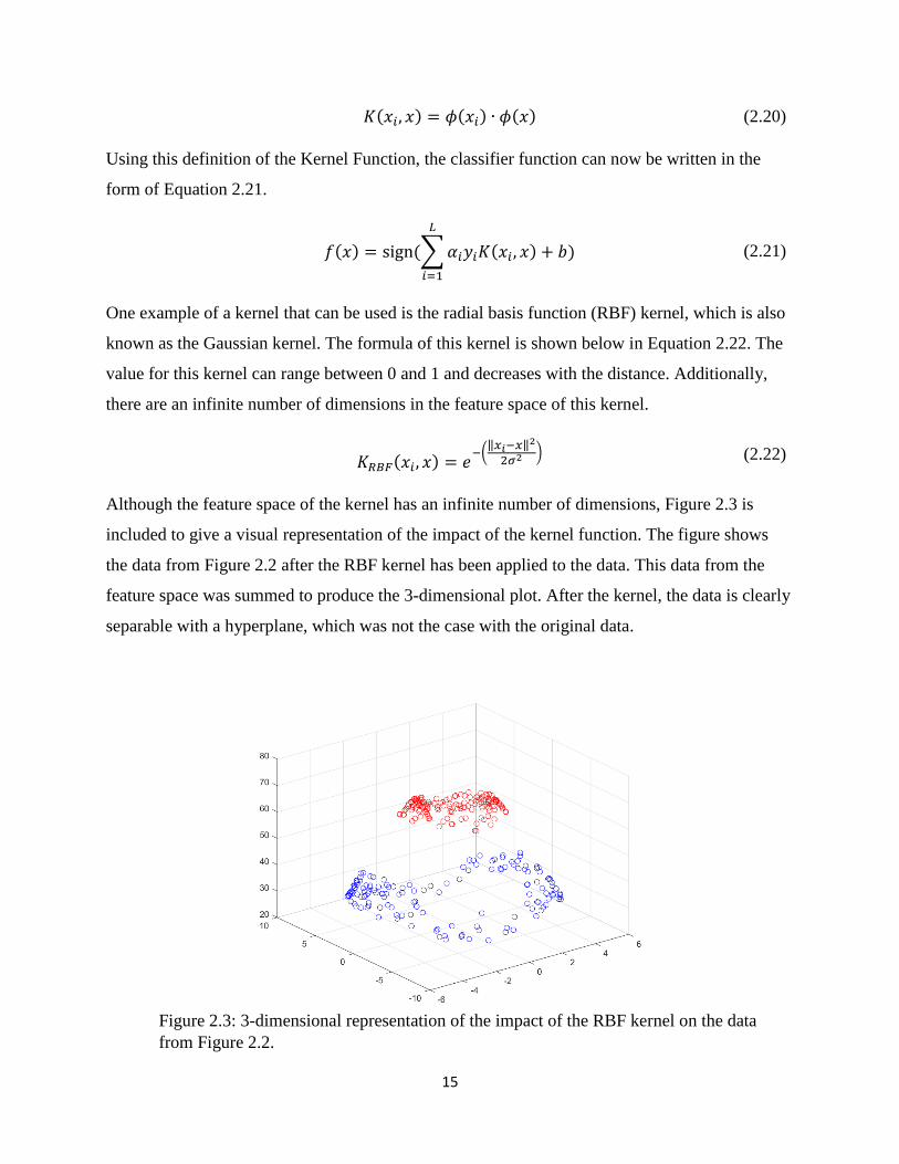
One example of a kernel that can be used is the radial basis function (RBF) kernel, which is also

known as the Gaussian kernel. The formula of this kernel is shown below in Equation 2.22. The

value for this kernel can range between 0 and 1 and decreases with the distance. Additionally,

there are an infinite number of dimensions in the feature space of this kernel.

𝐾𝑅𝐵𝐹(𝑥𝑖, 𝑥) = 𝑒−(

‖𝑥𝑖−𝑥‖2

2𝜎2 ) (2.22)

Although the feature space of the kernel has an infinite number of dimensions, Figure 2.3 is

included to give a visual representation of the impact of the kernel function. The figure shows

the data from Figure 2.2 after the RBF kernel has been applied to the data. This data from the

feature space was summed to produce the 3-dimensional plot. After the kernel, the data is clearly

separable with a hyperplane, which was not the case with the original data.

Figure 2.3: 3-dimensional representation of the impact of the RBF kernel on the data

from Figure 2.2.

16

Although SVMs are inherently binary classifiers, their use can be extended to perform multi-

class classification. Two primary methods of performing multi-class classification with SVMs

are the “one vs. all” method and the “one vs. one” method. For the one vs. all method, an SVM is

trained for each of the classes against all of the other data. To do this, the training data for one

class is set to be the first class and all other training data, from each of the rest of the classes, is

set to be the second class in this model. To perform the test stage on a test example, each SVM is

applied to the test example and the class assignment is selected as the class of the SVM which

returned the largest decision value. The one vs. all method requires the use of 𝐾 SVMs, where 𝐾

is the number of classes in the model. The second method is the one vs. one method, which

requires 𝐾(𝐾 − 1)/2 different SVM classifiers. The implementation of this classifier requires

creating an SVM for each possible pair of classes. During the test stage, each of these SVMs

classifies the test example between two classes and each of these is used as a vote for which class

to assign the test example. The class which receives the most votes for test example becomes the

classification of that test example [35, 36].

2.3.3 Machine Learning for Crop Classification

Some examples of using machine learning for crop classification exist in the literature. Those

examples used machine learning to classify the types of crops, but not the health of those crops.

One method used hyperspectral data and a support vector machine for the classification. This

was used to classify six different classes, which included corn, sugar beet, barley, wheat, alfalfa,

and soil. Each of these classes achieved recognition rates of greater than 90 percent [37].

Another example also used hyperspectral data for separating types of crops. For this, the five

crop species examined were soybean, canola, wheat, oat, and barley. This method used a

discriminant function analysis approach to classify the objects based on a measure of generalized

square distance. High classification accuracies were achieved throughout the growing season for

this approach [38].

17

Chapter 3 Visual Crop Stress Detection

This chapter discusses a method for crop stress detection through the use of visible spectrum

imagery. This would enable a farmer to investigate their field for health issues by flying a low-

cost UAV, with a standard camera, over the crops.

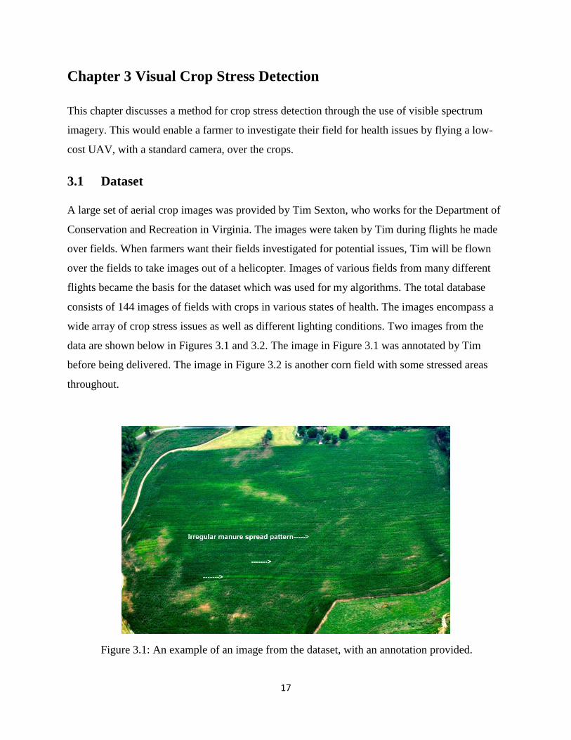
3.1 Dataset

A large set of aerial crop images was provided by Tim Sexton, who works for the Department of

Conservation and Recreation in Virginia. The images were taken by Tim during flights he made

over fields. When farmers want their fields investigated for potential issues, Tim will be flown

over the fields to take images out of a helicopter. Images of various fields from many different

flights became the basis for the dataset which was used for my algorithms. The total database

consists of 144 images of fields with crops in various states of health. The images encompass a

wide array of crop stress issues as well as different lighting conditions. Two images from the

data are shown below in Figures 3.1 and 3.2. The image in Figure 3.1 was annotated by Tim

before being delivered. The image in Figure 3.2 is another corn field with some stressed areas

throughout.

Figure 3.1: An example of an image from the dataset, with an annotation provided.

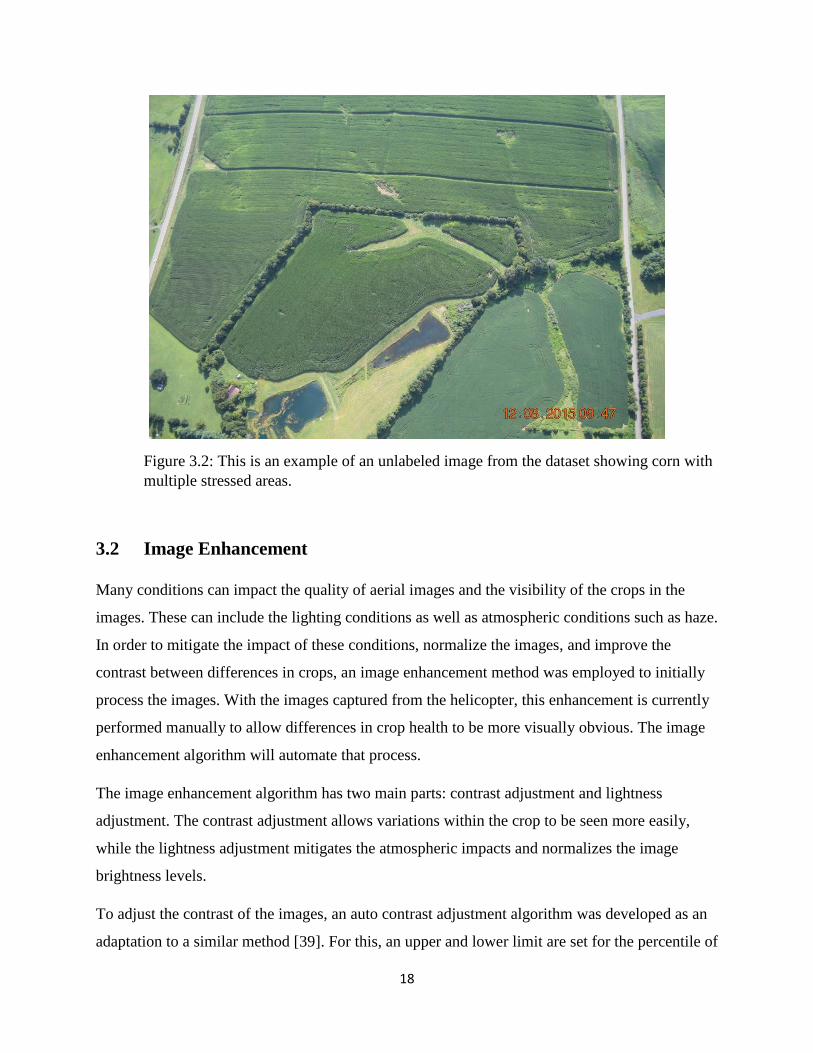
18

Figure 3.2: This is an example of an unlabeled image from the dataset showing corn with

multiple stressed areas.

3.2 Image Enhancement

Many conditions can impact the quality of aerial images and the visibility of the crops in the

images. These can include the lighting conditions as well as atmospheric conditions such as haze.

In order to mitigate the impact of these conditions, normalize the images, and improve the

contrast between differences in crops, an image enhancement method was employed to initially

process the images. With the images captured from the helicopter, this enhancement is currently

performed manually to allow differences in crop health to be more visually obvious. The image

enhancement algorithm will automate that process.

The image enhancement algorithm has two main parts: contrast adjustment and lightness

adjustment. The contrast adjustment allows variations within the crop to be seen more easily,

while the lightness adjustment mitigates the atmospheric impacts and normalizes the image

brightness levels.

To adjust the contrast of the images, an auto contrast adjustment algorithm was developed as an

adaptation to a similar method [39]. For this, an upper and lower limit are set for the percentile of

19

the values that the data will be scaled to. For this implementation, values of 0.005 and 0.995

were set for the low and high limits, respectively. The R, G, and B components of the image are

then sorted and the minimum and maximum RGB values are selected corresponding to the

location of the high and low limits multiplied by the number of pixels. The high and low RGB

pairs will then be converted to the YIQ color space for the Y, or luma, component to be used.

The Y component for the high and low pairs will then be used to rescale the image as a

percentage of these maximum and minimum values. The rescaling is done by Equation 3.1.

𝐼𝑚𝑎𝑑𝑗𝑢𝑠𝑡𝑒𝑑 =𝐼𝑚 − 𝑌𝑚𝑖𝑛

𝑌𝑚𝑎𝑥 − 𝑌𝑚𝑖𝑛 (3.1)

In this equation, Imadjusted is the output image, Im is the input image, Ymin is the low limit luma

component and Ymax is the high limit luma component. The output image will have values that

range from 0 to 1, so it must be multiplied by 255 to rescale the RGB values for the output.

To correct and normalize the brightness of the image, it is first converted into the Lab color

space. The L, or lightness, component is extracted and used for further processing. Through

analysis of manually enhanced images, the optimum median image lightness level was found to

be around a value of 40. As a result of this finding, the brightness correction algorithm was

designed to adjust the median lightness component of the image to be equal to a value of 40 by

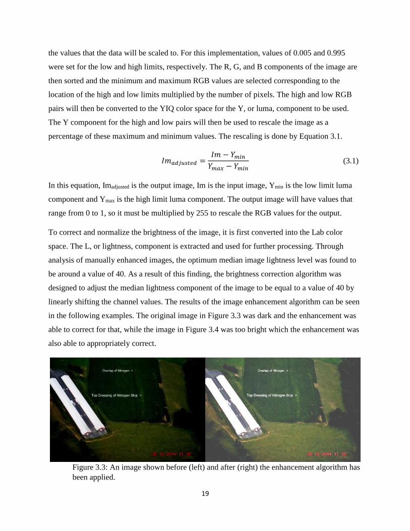
linearly shifting the channel values. The results of the image enhancement algorithm can be seen

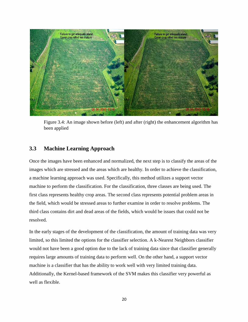
in the following examples. The original image in Figure 3.3 was dark and the enhancement was

able to correct for that, while the image in Figure 3.4 was too bright which the enhancement was

also able to appropriately correct.

Figure 3.3: An image shown before (left) and after (right) the enhancement algorithm has

been applied.

20

Figure 3.4: An image shown before (left) and after (right) the enhancement algorithm has

been applied

3.3 Machine Learning Approach

Once the images have been enhanced and normalized, the next step is to classify the areas of the

images which are stressed and the areas which are healthy. In order to achieve the classification,

a machine learning approach was used. Specifically, this method utilizes a support vector

machine to perform the classification. For the classification, three classes are being used. The

first class represents healthy crop areas. The second class represents potential problem areas in

the field, which would be stressed areas to further examine in order to resolve problems. The

third class contains dirt and dead areas of the fields, which would be issues that could not be

resolved.

In the early stages of the development of the classification, the amount of training data was very

limited, so this limited the options for the classifier selection. A k-Nearest Neighbors classifier

would not have been a good option due to the lack of training data since that classifier generally

requires large amounts of training data to perform well. On the other hand, a support vector

machine is a classifier that has the ability to work well with very limited training data.

Additionally, the Kernel-based framework of the SVM makes this classifier very powerful as

well as flexible.

21

The first step for creating the support vector machine is to train the classifier. This requires

labeling areas of the images in the dataset as one of the three classes. All images in the dataset

were labeled using LabelMe [40]. Appropriate areas in the images were selected to correspond

with the correct class. Figure 3.5 shows one of the training images being labeled in LabelMe.

Figure 3.5: Training image labeled using LabelMe.

Once the selected areas of the image have been labeled, features can be extracted from the image

in order to train the support vector machine. The features that have been selected for the support

vector machine lie solely in the color aspects of the images. Multiple color spaces have been

looked at, including RGB, HSV, and Lab. The decision to only use the color aspects of the image

was made due to limitations in the dataset. Different features, such as texture, would also be very

useful for detecting stresses and issues in the crops, however many images in the dataset did not

allow for the use of texture. This was due to a lack of the required resolution to analyze the

texture of the crops and to see rows of the crops.

The potential features within the color aspects of the image come from RGB, HSV, and Lab

color spaces, which produces nine potential features: red, green, blue, hue, saturation, value,

lightness, a* and b*. To select the best features to use, classifiers were trained using the different

combinations of these nine features and cross validation was performed to select the best

combination of features. For the cross validation, a subset of 10 percent of the training data was

22

held out as the test data set and the remaining 90 percent of the training data was used for

training these classifiers. Using these data sets, each combination of features was tested for

classification accuracy. The test began by using each feature individually, then using every

combination of two, followed by three, and so on. The initial classifier used was a linear support

vector machine, but other methods were tested in an attempt to improve upon the accuracy. A

second method that will be discussed is a Gaussian Kernel for the support vector machine. These

SVMs were implemented in Matlab through the use of the built-in function. This method uses

the one vs. one approach for the multiclass SVM. The test was first run on the linear support

vector machine using 10-fold cross validation and the optimal features for each step of the test

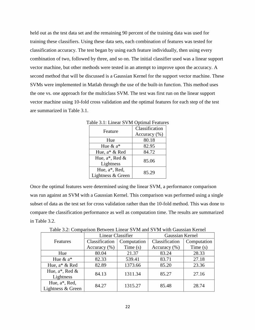
are summarized in Table 3.1.

Table 3.1: Linear SVM Optimal Features

Feature Classification

Accuracy (%)

Hue 80.18

Hue & a* 82.95

Hue, a* & Red 84.72

Hue, a*, Red &

Lightness 85.06

Hue, a*, Red,

Lightness & Green 85.29

Once the optimal features were determined using the linear SVM, a performance comparison

was run against an SVM with a Gaussian Kernel. This comparison was performed using a single

subset of data as the test set for cross validation rather than the 10-fold method. This was done to

compare the classification performance as well as computation time. The results are summarized

in Table 3.2.

Table 3.2: Comparison Between Linear SVM and SVM with Gaussian Kernel

Features

Linear Classifier Gaussian Kernel

Classification

Accuracy (%)

Computation

Time (s)

Classification

Accuracy (%)

Computation

Time (s)

Hue 80.04 21.37 83.24 28.33

Hue & a* 82.33 539.41 83.71 27.18

Hue, a* & Red 82.89 1373.66 85.20 23.36

Hue, a*, Red &

Lightness 84.13 1311.34 85.27 27.16

Hue, a*, Red,

Lightness & Green 84.27 1315.27 85.48 28.74

23

Due to the Gaussian Kernel performing much better than the Linear SVM, the original optimal

feature selection method, using 10-fold cross validation, was performed using the SVM with a

Gaussian Kernel. The results of the test and final feature selection are summarized in Table 3.3.

Table 3.3: Optimal Features for SVM with Gaussian Kernel

Feature Classification

Accuracy (%)

Hue 82.962

Hue & Green 84.512

Hue, Green &

Saturation 85.776

Hue, Green, Saturation

& a* 86.062

Hue, Green, Saturation,

a* & b* 86.127


a*, b* & Blue 86.157


a*, b*, Blue & Value 86.160

The classification accuracy from Table 3.3 is plotted against the number of features used for the

SVM in Figure 3.6. When the number of features used is very small, the addition of a single

feature can create a large increase in the classification accuracy. As the number of features

increases, the impact of adding features becomes much less significant. After a value of five

features is reached, the classification accuracy completely levels off and the gains in accuracy

from adding a feature are very small. Additionally, the addition of features to the algorithm

increases the complexity of the algorithm, which also can increase the required processing time.

Since the accuracy improvement is not significant after the addition of the fifth feature, the added

complexity of additional features is not justified. As a result, the final SVM uses only five

features, which are Green, Hue, Saturation, a*, and b*.

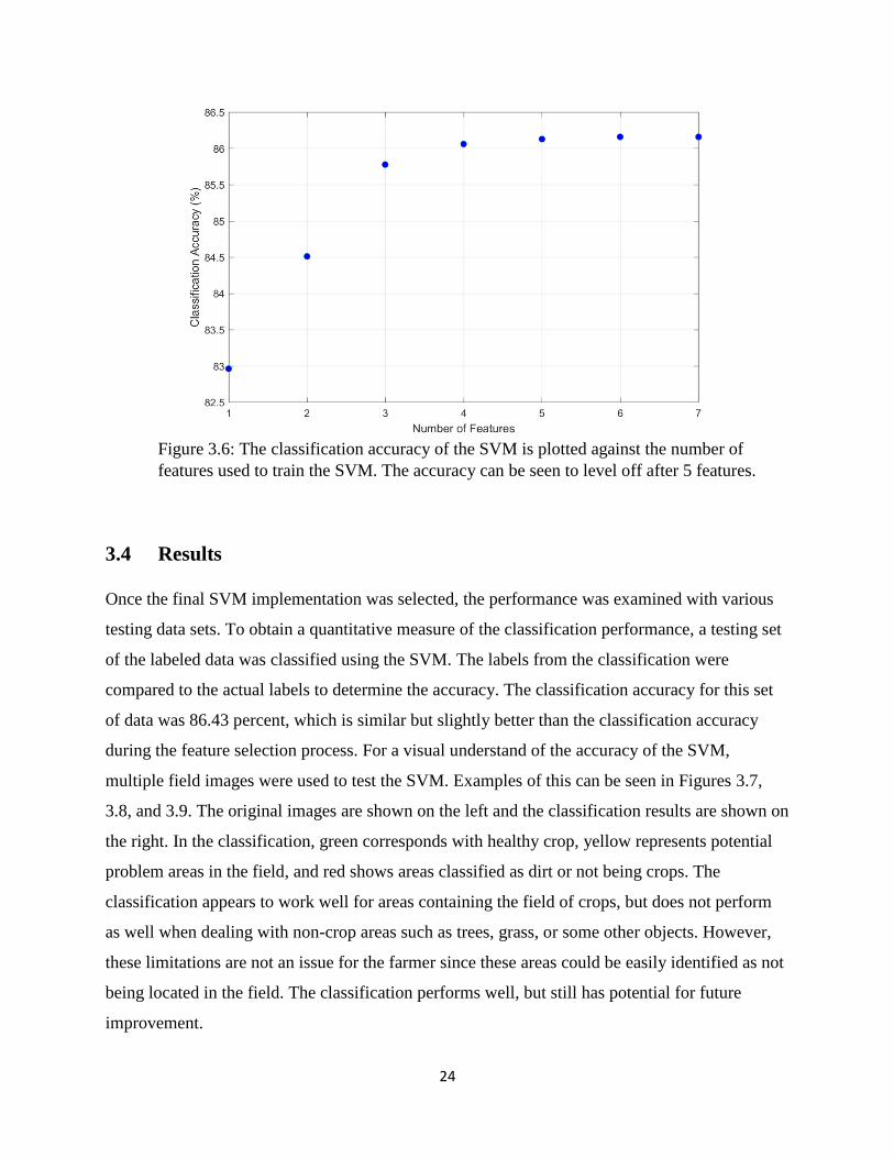
24

Figure 3.6: The classification accuracy of the SVM is plotted against the number of

features used to train the SVM. The accuracy can be seen to level off after 5 features.

3.4 Results

Once the final SVM implementation was selected, the performance was examined with various

testing data sets. To obtain a quantitative measure of the classification performance, a testing set

of the labeled data was classified using the SVM. The labels from the classification were

compared to the actual labels to determine the accuracy. The classification accuracy for this set

of data was 86.43 percent, which is similar but slightly better than the classification accuracy

during the feature selection process. For a visual understand of the accuracy of the SVM,

multiple field images were used to test the SVM. Examples of this can be seen in Figures 3.7,

3.8, and 3.9. The original images are shown on the left and the classification results are shown on

the right. In the classification, green corresponds with healthy crop, yellow represents potential

problem areas in the field, and red shows areas classified as dirt or not being crops. The

classification appears to work well for areas containing the field of crops, but does not perform

as well when dealing with non-crop areas such as trees, grass, or some other objects. However,

these limitations are not an issue for the farmer since these areas could be easily identified as not

being located in the field. The classification performs well, but still has potential for future

improvement.

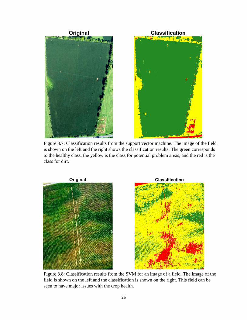
25

Figure 3.7: Classification results from the support vector machine. The image of the field

is shown on the left and the right shows the classification results. The green corresponds

to the healthy class, the yellow is the class for potential problem areas, and the red is the

class for dirt.

Figure 3.8: Classification results from the SVM for an image of a field. The image of the

field is shown on the left and the classification is shown on the right. This field can be

seen to have major issues with the crop health.

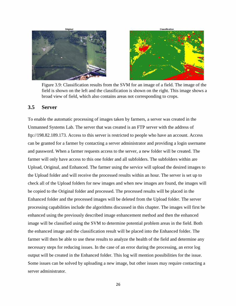
26

Figure 3.9: Classification results from the SVM for an image of a field. The image of the

field is shown on the left and the classification is shown on the right. This image shows a

broad view of field, which also contains areas not corresponding to crops.

3.5 Server

To enable the automatic processing of images taken by farmers, a server was created in the

Unmanned Systems Lab. The server that was created is an FTP server with the address of

ftp://198.82.189.173. Access to this server is restricted to people who have an account. Access

can be granted for a farmer by contacting a server administrator and providing a login username

and password. When a farmer requests access to the server, a new folder will be created. The

farmer will only have access to this one folder and all subfolders. The subfolders within are

Upload, Original, and Enhanced. The farmer using the service will upload the desired images to

the Upload folder and will receive the processed results within an hour. The server is set up to

check all of the Upload folders for new images and when new images are found, the images will

be copied to the Original folder and processed. The processed results will be placed in the

Enhanced folder and the processed images will be deleted from the Upload folder. The server

processing capabilities include the algorithms discussed in this chapter. The images will first be

enhanced using the previously described image enhancement method and then the enhanced

image will be classified using the SVM to determine potential problem areas in the field. Both

the enhanced image and the classification result will be placed into the Enhanced folder. The

farmer will then be able to use these results to analyze the health of the field and determine any

necessary steps for reducing issues. In the case of an error during the processing, an error log

output will be created in the Enhanced folder. This log will mention possibilities for the issue.

Some issues can be solved by uploading a new image, but other issues may require contacting a

server administrator.

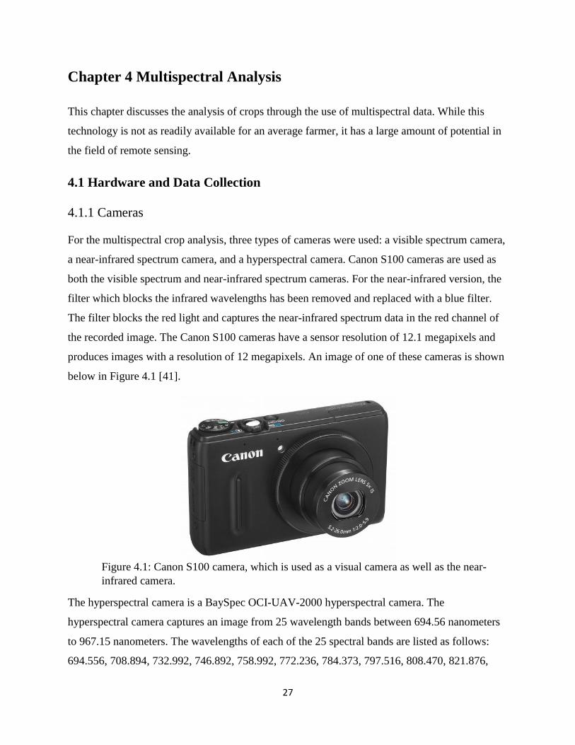
27

Chapter 4 Multispectral Analysis

This chapter discusses the analysis of crops through the use of multispectral data. While this

technology is not as readily available for an average farmer, it has a large amount of potential in

the field of remote sensing.

4.1 Hardware and Data Collection

4.1.1 Cameras

For the multispectral crop analysis, three types of cameras were used: a visible spectrum camera,

a near-infrared spectrum camera, and a hyperspectral camera. Canon S100 cameras are used as

both the visible spectrum and near-infrared spectrum cameras. For the near-infrared version, the

filter which blocks the infrared wavelengths has been removed and replaced with a blue filter.

The filter blocks the red light and captures the near-infrared spectrum data in the red channel of

the recorded image. The Canon S100 cameras have a sensor resolution of 12.1 megapixels and

produces images with a resolution of 12 megapixels. An image of one of these cameras is shown

below in Figure 4.1 [41].

Figure 4.1: Canon S100 camera, which is used as a visual camera as well as the near-

infrared camera.

The hyperspectral camera is a BaySpec OCI-UAV-2000 hyperspectral camera. The

hyperspectral camera captures an image from 25 wavelength bands between 694.56 nanometers

to 967.15 nanometers. The wavelengths of each of the 25 spectral bands are listed as follows:

694.556, 708.894, 732.992, 746.892, 758.992, 772.236, 784.373, 797.516, 808.470, 821.876,

28

839.886, 851.014, 860.955, 872.309, 881.561, 891.523, 900.802, 910.270, 925.705, 933.048,

941.019, 947.076, 956.318, 962.312, and 967.148 nanometers. The camera has a 16-degree field

of view lens and is very compact, weighing only 218 grams. Images can be recorded very fast,

up to 120 frames/second and are saved to a computer through a USB 3.0 connection. The

exposure time can be set between 1 and 300 milliseconds and is determined based on the lighting

conditions and the camera is referenced using a 95% white reference paper. This hyperspectral

camera can be seen, with dimensions, in Figure 4.2 [42].

Figure 4.2: OCI-UAV-2000 hyperspectral camera that is being used.

The imaging payload combines the three cameras that have been discussed. The three cameras

are mounted side by side to a piece of carbon fiber. Along with the cameras is a fit-PC to allow

for interfacing with the hyperspectral camera through a USB 3.0 connection. The hyperspectral

camera can be externally triggered by sending a voltage between 15 and 24 volts to the camera.

The two Canon S100 cameras were also triggered by a voltage signal and the two cameras were

synchronized through the use of Canon Hack Development Kit [43]. The voltage signals for

triggering the cameras were controlled by an Arduino, which was set up to be either triggered by

a switch or for continuous image capturing, depending on the intended mode.

4.1.2 UAV Platform

One method of acquiring aerial images with the camera payload is through the use of a UAV

platform. The UAV platform used for acquiring images is the DJI S1000+ octocopter. This UAV

was selected due to its ability to carry the weight of the required payload and have sufficient

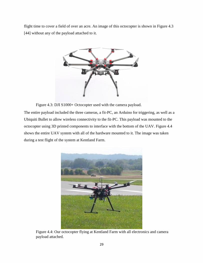
29

flight time to cover a field of over an acre. An image of this octocopter is shown in Figure 4.3

[44] without any of the payload attached to it.

Figure 4.3: DJI S1000+ Octocopter used with the camera payload.

The entire payload included the three cameras, a fit-PC, an Arduino for triggering, as well as a

Ubiquiti Bullet to allow wireless connectivity to the fit-PC. This payload was mounted to the

octocopter using 3D printed components to interface with the bottom of the UAV. Figure 4.4

shows the entire UAV system with all of the hardware mounted to it. The image was taken

during a test flight of the system at Kentland Farm.

Figure 4.4: Our octocopter flying at Kentland Farm with all electronics and camera

payload attached.

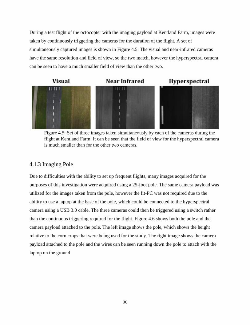
30

During a test flight of the octocopter with the imaging payload at Kentland Farm, images were

taken by continuously triggering the cameras for the duration of the flight. A set of

simultaneously captured images is shown in Figure 4.5. The visual and near-infrared cameras

have the same resolution and field of view, so the two match, however the hyperspectral camera

can be seen to have a much smaller field of view than the other two.

Figure 4.5: Set of three images taken simultaneously by each of the cameras during the

flight at Kentland Farm. It can be seen that the field of view for the hyperspectral camera

is much smaller than for the other two cameras.

4.1.3 Imaging Pole

Due to difficulties with the ability to set up frequent flights, many images acquired for the

purposes of this investigation were acquired using a 25-foot pole. The same camera payload was

utilized for the images taken from the pole, however the fit-PC was not required due to the

ability to use a laptop at the base of the pole, which could be connected to the hyperspectral

camera using a USB 3.0 cable. The three cameras could then be triggered using a switch rather

than the continuous triggering required for the flight. Figure 4.6 shows both the pole and the

camera payload attached to the pole. The left image shows the pole, which shows the height

relative to the corn crops that were being used for the study. The right image shows the camera

payload attached to the pole and the wires can be seen running down the pole to attach with the

laptop on the ground.

31

Figure 4.6: The height of the pole, relative to the corn, can be seen on the left and the

imaging payload attached to the pole is shown on the right.

4.1.4 Corn Test Plots

For the purposes of the multispectral crop analysis, plots of corn with various sidedress nitrogen

application rates were used as the test plots. The entire set of crops for the test plots contained

five different nitrogen applications: 0, 40, 80, 120, and 160 lbs/acre. Each of these treatments

were repeated four different times, for a total of 20 different test plots of corn. Each individual

test plot consisted of four rows of corn, which were 30 inches wide and 25 feet long. When

images were acquired of these plots, the cameras were aimed towards the center of the plots to

reduce any border effects of the treatments. The main plots that we acquired images of for the

analysis were plots 101, 102, 103, 104, and 105. The entire area of test corn test plots, with labels

for the plot number and the nitrogen application can be seen in Figure 4.7. This image was taken

during a flight over the field with a UAV.

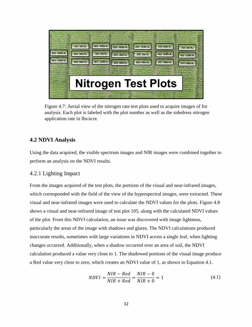
32

Figure 4.7: Aerial view of the nitrogen rate test plots used to acquire images of for

analysis. Each plot is labeled with the plot number as well as the sidedress nitrogen

application rate in lbs/acre.

4.2 NDVI Analysis

Using the data acquired, the visible spectrum images and NIR images were combined together to

perform an analysis on the NDVI results.

4.2.1 Lighting Impact

From the images acquired of the test plots, the portions of the visual and near-infrared images,

which corresponded with the field of the view of the hyperspectral images, were extracted. These

visual and near-infrared images were used to calculate the NDVI values for the plots. Figure 4.8

shows a visual and near-infrared image of test plot 105, along with the calculated NDVI values

of the plot. From this NDVI calculation, an issue was discovered with image lightness,

particularly the areas of the image with shadows and glares. The NDVI calculations produced

inaccurate results, sometimes with large variations in NDVI across a single leaf, when lighting

changes occurred. Additionally, when a shadow occurred over an area of soil, the NDVI

calculation produced a value very close to 1. The shadowed portions of the visual image produce

a Red value very close to zero, which creates an NDVI value of 1, as shown in Equation 4.1.

𝑁𝐷𝑉𝐼 =𝑁𝐼𝑅 − 𝑅𝑒𝑑

𝑁𝐼𝑅 + 𝑅𝑒𝑑=

𝑁𝐼𝑅 − 0

𝑁𝐼𝑅 + 0= 1 (4.1)

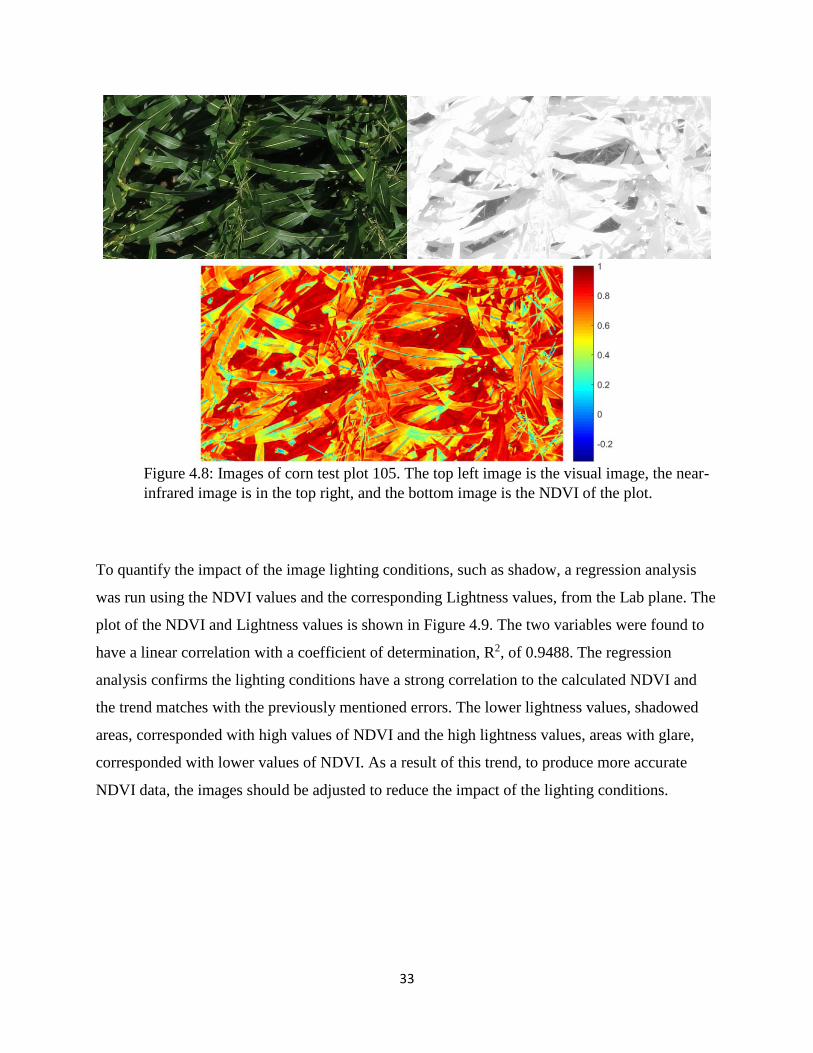
33


infrared image is in the top right, and the bottom image is the NDVI of the plot.

To quantify the impact of the image lighting conditions, such as shadow, a regression analysis

was run using the NDVI values and the corresponding Lightness values, from the Lab plane. The

plot of the NDVI and Lightness values is shown in Figure 4.9. The two variables were found to

have a linear correlation with a coefficient of determination, R2, of 0.9488. The regression

analysis confirms the lighting conditions have a strong correlation to the calculated NDVI and

the trend matches with the previously mentioned errors. The lower lightness values, shadowed

areas, corresponded with high values of NDVI and the high lightness values, areas with glare,

corresponded with lower values of NDVI. As a result of this trend, to produce more accurate

NDVI data, the images should be adjusted to reduce the impact of the lighting conditions.

34

Figure 4.9: Plot of NDVI and Lightness of the images shown in Figure 4.8. A regression

analysis produced a coefficient of determination of 0.9488.

4.2.2 Lightness Correction

Due to the correlation between the NDVI values and the lightness values of the images, the

method for correcting the NDVI values was to normalize and adjust the lightness of the visual

image. The first attempt to adjust the lightness was through the use of Poisson image editing,

since this can adjust local illumination. The method for performing this was explained in Section

2.2.8. This method allows for the selection of specific areas for which the illumination

adjustment is desired. This method was implemented in Matlab and tested on various images to

see the performance. One result of this implementation is shown below in Figure 4.10. The

image in the top left is the original image and the top right shows the NDVI calculation before

the adjustment, with scaled color corresponding to the color bar on the right. The bottom left

image is the image after the Poisson editing was performed and the bottom right shows the new

NDVI values after the editing. This method did not perform very well in correcting the lightness

for the NDVI. The adjustment changed the lightness, but the new image was slightly blurred and

the extreme values, such as the shadows, were not actually removed. As a result, the NDVI

calculation did not show any noticeable improvement. The Poisson image editing was also tested

on a large portion of an image and was found to perform worse on a large scale. When applying

to most of an image, the adjustment blurred the image into a very dark blob.

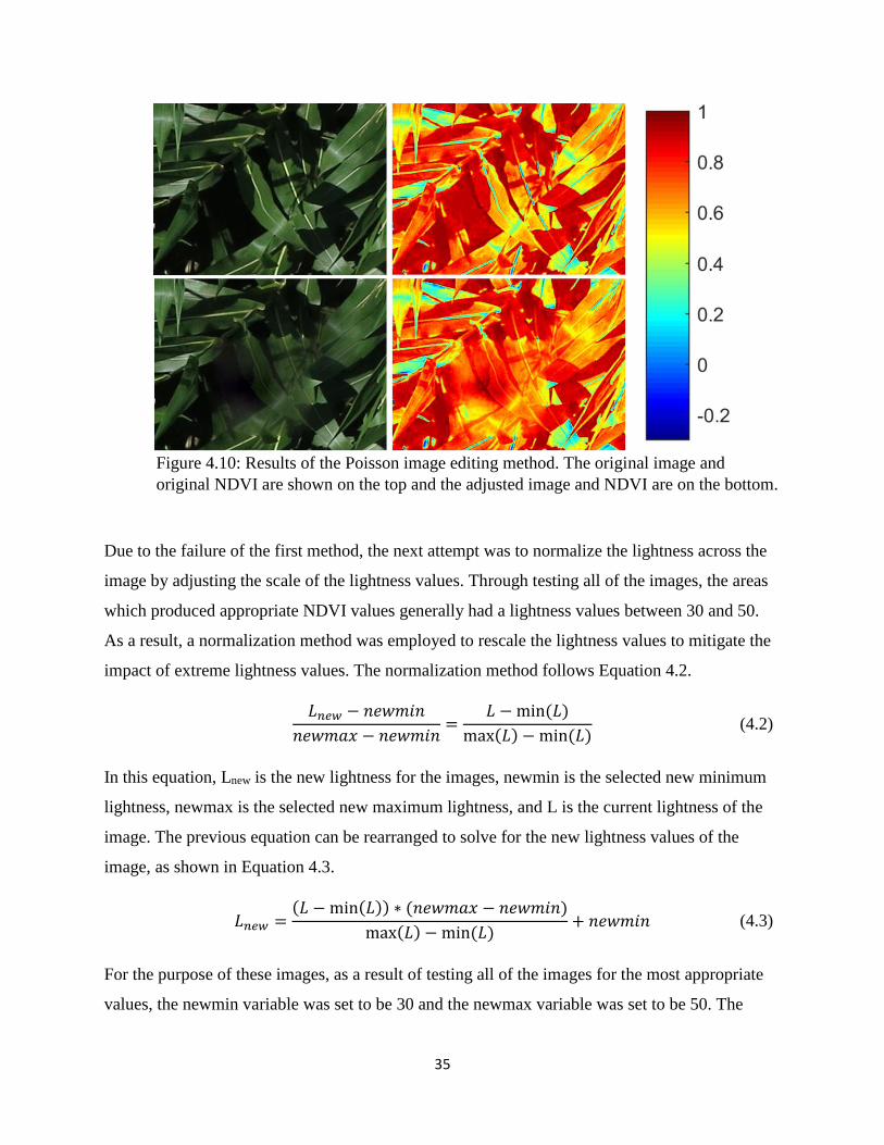
35

Figure 4.10: Results of the Poisson image editing method. The original image and

original NDVI are shown on the top and the adjusted image and NDVI are on the bottom.

Due to the failure of the first method, the next attempt was to normalize the lightness across the

image by adjusting the scale of the lightness values. Through testing all of the images, the areas

which produced appropriate NDVI values generally had a lightness values between 30 and 50.

As a result, a normalization method was employed to rescale the lightness values to mitigate the

impact of extreme lightness values. The normalization method follows Equation 4.2.

𝐿𝑛𝑒𝑤 − 𝑛𝑒𝑤𝑚𝑖𝑛

𝑛𝑒𝑤𝑚𝑎𝑥 − 𝑛𝑒𝑤𝑚𝑖𝑛=

𝐿 − min (𝐿)

max(𝐿) − min (𝐿) (4.2)

In this equation, Lnew is the new lightness for the images, newmin is the selected new minimum

lightness, newmax is the selected new maximum lightness, and L is the current lightness of the

image. The previous equation can be rearranged to solve for the new lightness values of the

image, as shown in Equation 4.3.

𝐿𝑛𝑒𝑤 =(𝐿 − min(𝐿)) ∗ (𝑛𝑒𝑤𝑚𝑎𝑥 − 𝑛𝑒𝑤𝑚𝑖𝑛)

max(𝐿) − min (𝐿)+ 𝑛𝑒𝑤𝑚𝑖𝑛 (4.3)

For the purpose of these images, as a result of testing all of the images for the most appropriate

values, the newmin variable was set to be 30 and the newmax variable was set to be 50. The

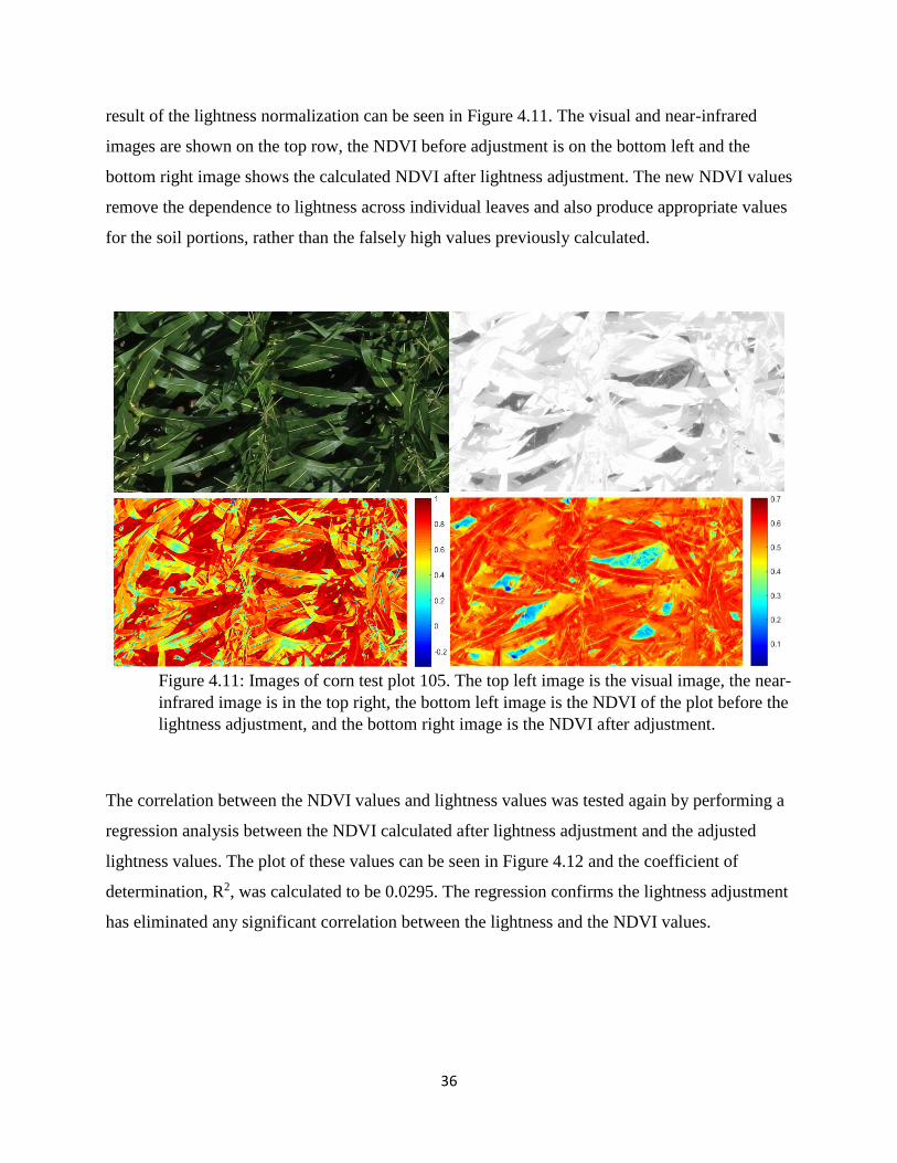
36

result of the lightness normalization can be seen in Figure 4.11. The visual and near-infrared

images are shown on the top row, the NDVI before adjustment is on the bottom left and the

bottom right image shows the calculated NDVI after lightness adjustment. The new NDVI values

remove the dependence to lightness across individual leaves and also produce appropriate values

for the soil portions, rather than the falsely high values previously calculated.


infrared image is in the top right, the bottom left image is the NDVI of the plot before the

lightness adjustment, and the bottom right image is the NDVI after adjustment.

The correlation between the NDVI values and lightness values was tested again by performing a

regression analysis between the NDVI calculated after lightness adjustment and the adjusted

lightness values. The plot of these values can be seen in Figure 4.12 and the coefficient of

determination, R2, was calculated to be 0.0295. The regression confirms the lightness adjustment

has eliminated any significant correlation between the lightness and the NDVI values.

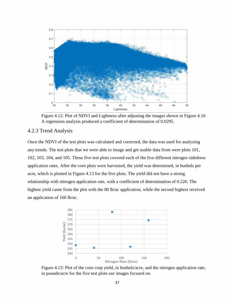
37

Figure 4.12: Plot of NDVI and Lightness after adjusting the images shown in Figure 4.10.

A regression analysis produced a coefficient of determination of 0.0295.

4.2.3 Trend Analysis

Once the NDVI of the test plots was calculated and corrected, the data was used for analyzing

any trends. The test plots that we were able to image and get usable data from were plots 101,

102, 103, 104, and 105. These five test plots covered each of the five different nitrogen sidedress

application rates. After the corn plots were harvested, the yield was determined, in bushels per

acre, which is plotted in Figure 4.13 for the five plots. The yield did not have a strong

relationship with nitrogen application rate, with a coefficient of determination of 0.226. The

highest yield came from the plot with the 80 lb/ac application, while the second highest received

an application of 160 lb/ac.

Figure 4.13: Plot of the corn crop yield, in bushels/acre, and the nitrogen application rate,

in pounds/acre for the five test plots our images focused on.

240

245

250

255

260

265

270

275

280

285

0 50 100 150 200

Yiel

d (

bu

/ac)

Nitrogen Rate (lb/ac)

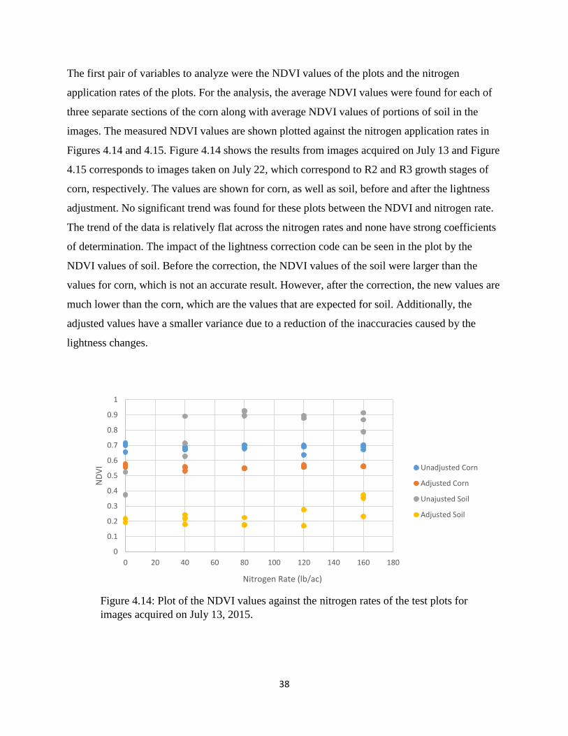
38

The first pair of variables to analyze were the NDVI values of the plots and the nitrogen

application rates of the plots. For the analysis, the average NDVI values were found for each of

three separate sections of the corn along with average NDVI values of portions of soil in the

images. The measured NDVI values are shown plotted against the nitrogen application rates in

Figures 4.14 and 4.15. Figure 4.14 shows the results from images acquired on July 13 and Figure

4.15 corresponds to images taken on July 22, which correspond to R2 and R3 growth stages of

corn, respectively. The values are shown for corn, as well as soil, before and after the lightness

adjustment. No significant trend was found for these plots between the NDVI and nitrogen rate.

The trend of the data is relatively flat across the nitrogen rates and none have strong coefficients

of determination. The impact of the lightness correction code can be seen in the plot by the

NDVI values of soil. Before the correction, the NDVI values of the soil were larger than the

values for corn, which is not an accurate result. However, after the correction, the new values are

much lower than the corn, which are the values that are expected for soil. Additionally, the

adjusted values have a smaller variance due to a reduction of the inaccuracies caused by the

lightness changes.

Figure 4.14: Plot of the NDVI values against the nitrogen rates of the test plots for

images acquired on July 13, 2015.

0

0.1

0.2

0.3

0.4

0.5

0.6

0.7

0.8

0.9

1

0 20 40 60 80 100 120 140 160 180

ND

VI


Unadjusted Corn

Adjusted Corn

Unajusted Soil

Adjusted Soil

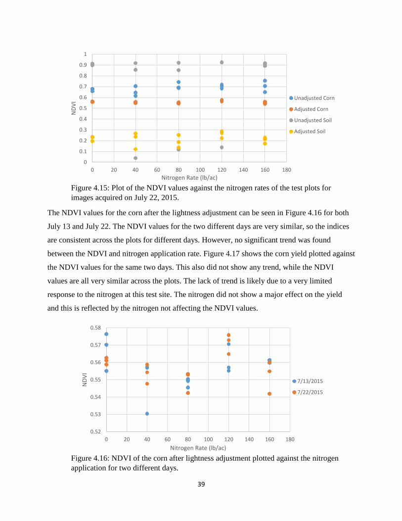
39

Figure 4.15: Plot of the NDVI values against the nitrogen rates of the test plots for

images acquired on July 22, 2015.

The NDVI values for the corn after the lightness adjustment can be seen in Figure 4.16 for both

July 13 and July 22. The NDVI values for the two different days are very similar, so the indices

are consistent across the plots for different days. However, no significant trend was found

between the NDVI and nitrogen application rate. Figure 4.17 shows the corn yield plotted against

the NDVI values for the same two days. This also did not show any trend, while the NDVI

values are all very similar across the plots. The lack of trend is likely due to a very limited

response to the nitrogen at this test site. The nitrogen did not show a major effect on the yield

and this is reflected by the nitrogen not affecting the NDVI values.

Figure 4.16: NDVI of the corn after lightness adjustment plotted against the nitrogen

application for two different days.

0

0.1

0.2

0.3

0.4

0.5

0.6

0.7

0.8

0.9

1

0 20 40 60 80 100 120 140 160 180

ND

VI


Unadjusted Corn

Adjusted Corn

Unadjusted Soil

Adjusted Soil

0.52

0.53

0.54

0.55

0.56

0.57

0.58

0 20 40 60 80 100 120 140 160 180

ND

VI


7/13/2015

7/22/2015

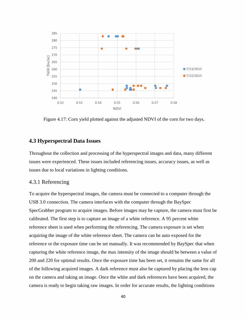
40

Figure 4.17: Corn yield plotted against the adjusted NDVI of the corn for two days.

4.3 Hyperspectral Data Issues

Throughout the collection and processing of the hyperspectral images and data, many different

issues were experienced. These issues included referencing issues, accuracy issues, as well as

issues due to local variations in lighting conditions.

4.3.1 Referencing

To acquire the hyperspectral images, the camera must be connected to a computer through the

USB 3.0 connection. The camera interfaces with the computer through the BaySpec

SpecGrabber program to acquire images. Before images may be capture, the camera must first be

calibrated. The first step is to capture an image of a white reference. A 95 percent white

reference sheet is used when performing the referencing. The camera exposure is set when

acquiring the image of the white reference sheet. The camera can be auto exposed for the

reference or the exposure time can be set manually. It was recommended by BaySpec that when

capturing the white reference image, the max intensity of the image should be between a value of

200 and 220 for optimal results. Once the exposure time has been set, it remains the same for all

of the following acquired images. A dark reference must also be captured by placing the lens cap

on the camera and taking an image. Once the white and dark references have been acquired, the

camera is ready to begin taking raw images. In order for accurate results, the lighting conditions

240

245

250

255

260

265

270

275

280

285

0.52 0.53 0.54 0.55 0.56 0.57 0.58

Yiel

d (

bu

/ac)

NDVI

7/13/2015

7/22/2015

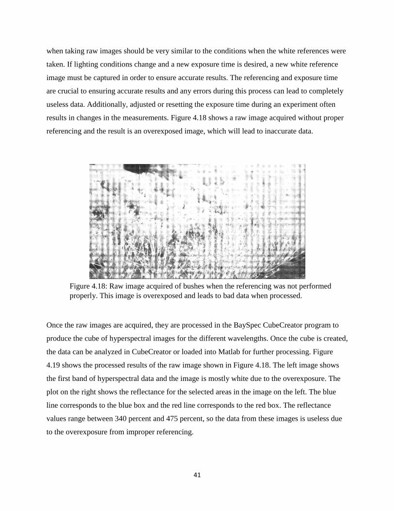
41

when taking raw images should be very similar to the conditions when the white references were

taken. If lighting conditions change and a new exposure time is desired, a new white reference

image must be captured in order to ensure accurate results. The referencing and exposure time

are crucial to ensuring accurate results and any errors during this process can lead to completely

useless data. Additionally, adjusted or resetting the exposure time during an experiment often

results in changes in the measurements. Figure 4.18 shows a raw image acquired without proper

referencing and the result is an overexposed image, which will lead to inaccurate data.

Figure 4.18: Raw image acquired of bushes when the referencing was not performed

properly. This image is overexposed and leads to bad data when processed.

Once the raw images are acquired, they are processed in the BaySpec CubeCreator program to

produce the cube of hyperspectral images for the different wavelengths. Once the cube is created,

the data can be analyzed in CubeCreator or loaded into Matlab for further processing. Figure

4.19 shows the processed results of the raw image shown in Figure 4.18. The left image shows

the first band of hyperspectral data and the image is mostly white due to the overexposure. The

plot on the right shows the reflectance for the selected areas in the image on the left. The blue

line corresponds to the blue box and the red line corresponds to the red box. The reflectance

values range between 340 percent and 475 percent, so the data from these images is useless due

to the overexposure from improper referencing.

42

Figure 4.19: The first band of the hyperspectral cube is shown in the left image. The

overexposure resulted in a mostly white image. The plot of the reflectance is shown on

the right for the two selected portions in the left image.

4.3.2 Hyperspectral Camera Accuracy

Once the issues in the reference process were resolved and images could be properly acquired,

the accuracy of the camera was analyzed. To look at the accuracy of the camera, it was compared

against a higher quality and more expensive hyperspectral imager, which is known to be

accurate. This device was used as the baseline comparison for investigating the accuracy of our

hyperspectral camera. The baseline device had a field of view of 8 degrees, while our camera has

a field of view of 16 degrees. To account for this, only the center portion of the image was used,

corresponding the 8-degree field of view of the other device. For the comparison test, three

different objects were used: concrete, a patch of grass, and a healthy leaf from a tree. For each

case, the two cameras were referenced at the same time and in the same lighting conditions.

Once the referencing was complete, the images of the objects were taken consecutively, while

lighting conditions were consistent. The baseline comparison device recorded the average

reflectance for wavelengths between 350 nm and 2500 nm, by increments of one nanometer. The

results of this comparison are shown in Figures 4.20, 4.21, and 4.22. Figure 4.20 shows the

comparison for the results with concrete and the two devices achieved similar results. Both

curves have a very flat shape across the wavelength spectrum, however there is a small bias

error. The comparison of the devices imaging grass is shown in Figure 4.21. The middle bands of

the data produce similar shapes, but there is still a bias error in the data, with our hyperspectral

camera recording slightly smaller reflectance values. The biggest difference occurs at the high

and low ends of the spectrum, with large error between the two devices. Similar results can be

seen in Figure 4.22, which shows the results from the leaf comparison. Again, the reflectance

43

curves have similar shapes in the middle wavelengths, but have a bias error, with our camera

recording smaller values. The error becomes very large at the high and low wavelengths, so our

camera does not appear to be very accurate at those ends of the spectrum. For wavelengths below

720 nm and above 940 nm, our camera appears to produce extremely inaccurate reflectance data

for vegetation, so as a result, the data from bands on those outside edges cannot be trusted to be

accurate.

Figure 4.20: Reflectance curves of concrete for each of the two hyperspectral devices.

Figure 4.21: Reflectance curves of grass for each of the two hyperspectral devices.

44

Figure 4.22: Reflectance curves of a leaf for each of the two hyperspectral devices.

A final comparison of this data can be seen in Figure 4.23, which shows reflectance curves of the

grass, concrete, and leaf for each of the two cameras. Despite the inaccuracies of our camera

from the baseline hyperspectral device, each similarly show distinct differences between the

grass, concrete, and leaf. The leaf had the highest reflectance over most of the spectrum, with the

grass being second, and the concrete having the lowest reflectance. The high and low ends of the

grass and leaf curves from our camera can be seen to display similar shapes, so the inaccurate

results are likely due to issues with our camera. As a result, the wavelengths below 720 nm and

above 940 nm will be ignored in future analysis due to the inaccuracies.

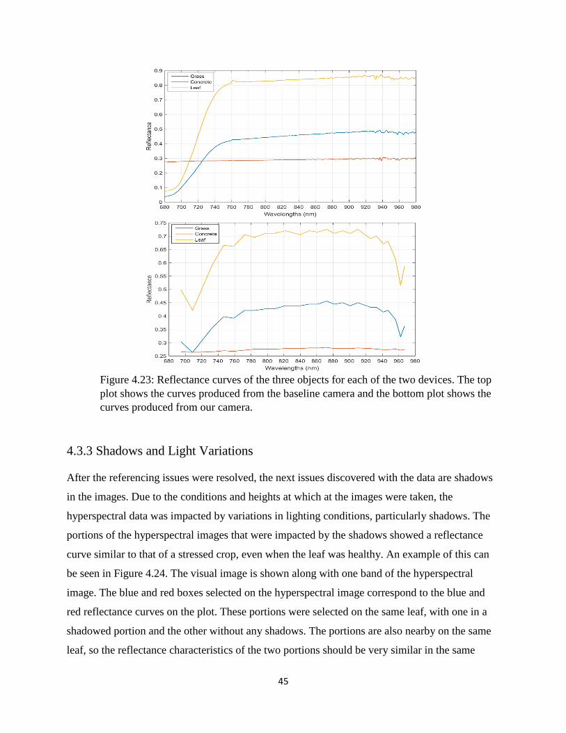
45

Figure 4.23: Reflectance curves of the three objects for each of the two devices. The top

plot shows the curves produced from the baseline camera and the bottom plot shows the

curves produced from our camera.

4.3.3 Shadows and Light Variations

After the referencing issues were resolved, the next issues discovered with the data are shadows

in the images. Due to the conditions and heights at which at the images were taken, the

hyperspectral data was impacted by variations in lighting conditions, particularly shadows. The

portions of the hyperspectral images that were impacted by the shadows showed a reflectance

curve similar to that of a stressed crop, even when the leaf was healthy. An example of this can

be seen in Figure 4.24. The visual image is shown along with one band of the hyperspectral

image. The blue and red boxes selected on the hyperspectral image correspond to the blue and

red reflectance curves on the plot. These portions were selected on the same leaf, with one in a

shadowed portion and the other without any shadows. The portions are also nearby on the same

leaf, so the reflectance characteristics of the two portions should be very similar in the same

46

lighting conditions. The reflectance curve plot shows that the shadowed portion of the leaf

resulted in much lower reflectance values, which would be similar to an unhealthy or stressed

leaf. The large differences in reflectance values due to variations in lighting conditions can be

problematic to ensuring the accuracy of the data.

Figure 4.24: Test plot image impacted by shadows. The visual image (top left) and

corresponding hyperspectral image (top right) are shown. Red and blue boxes on the

hyperspectral image correspond to the Reflectance curves on the plot.

4.4 Hyperspectral Shadow Correction

In order to ensure that the data acquired in the hyperspectral images is more accurate and usable,

it will be important to reduce the impact of the shadows on the data. A method for correcting the

shadows in the images was created through a combination of the visual and hyperspectral

images. To determine the relationship between the local lighting conditions of the image and the

hyperspectral reflectance, combinations of matched images were used. Using pairs of matched

visual and hyperspectral images, areas with varying lighting conditions were selected. The

conditions varied from shadowed to glared areas and included lighting conditions in between as

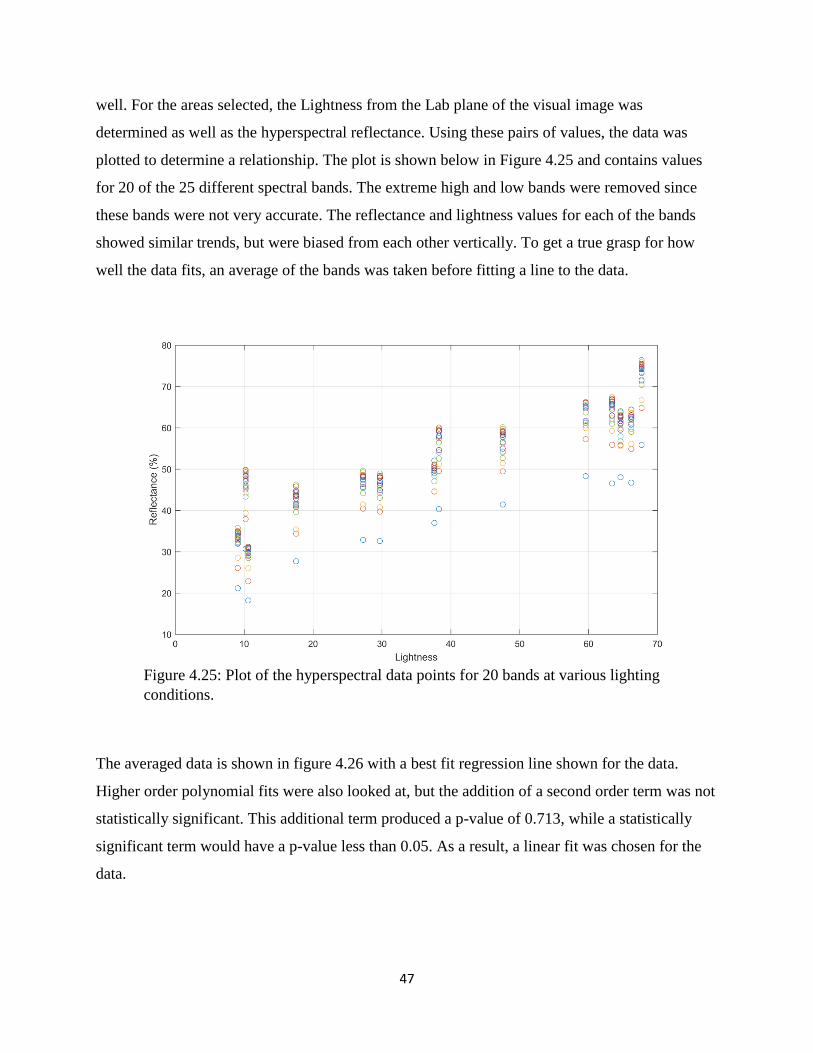
47

well. For the areas selected, the Lightness from the Lab plane of the visual image was

determined as well as the hyperspectral reflectance. Using these pairs of values, the data was

plotted to determine a relationship. The plot is shown below in Figure 4.25 and contains values

for 20 of the 25 different spectral bands. The extreme high and low bands were removed since

these bands were not very accurate. The reflectance and lightness values for each of the bands

showed similar trends, but were biased from each other vertically. To get a true grasp for how

well the data fits, an average of the bands was taken before fitting a line to the data.

Figure 4.25: Plot of the hyperspectral data points for 20 bands at various lighting

conditions.

The averaged data is shown in figure 4.26 with a best fit regression line shown for the data.

Higher order polynomial fits were also looked at, but the addition of a second order term was not

statistically significant. This additional term produced a p-value of 0.713, while a statistically

significant term would have a p-value less than 0.05. As a result, a linear fit was chosen for the

data.

48

Figure 4.26: Plot of the average of the hyperspectral data points with various lighting

conditions. A trend line was fit to the data with an R2 value of 0.868.

The trend line of best fit for the Lightness and Reflectance data was found to be Equation 4.4.

𝑅 = 0.51179 ∗ 𝐿 + 31.284 (4.4)

In this equation, R is the reflectance, in percent, and L is the Lightness value of the Lab plane of

the visual image. This line fit the data with a coefficient of determination of 0.868. After an

equation was determined for the relationship between the two variables, it could be implemented

as a method for correcting the lighting conditions in the hyperspectral images. The constant term

at the end of the equation can vary depending upon the magnitude of the reflectance values, so

this is set as a constant variable, c. The optimal image Lightness for the correction was

determined through investigating the dataset of images. Through manual tuning, a value of 45 for

the Lightness was found to be the optimal condition which contained hyperspectral reflectance

values corresponding to the healthy corn as well as the absence of both shadows and glare in the

visual image. The Lightness value of 45 was targeted when correcting the lighting conditions.

When plugging the Lightness value of 45 into Equation 4.4 to determine the final adjusted

reflectance value, the result is Equation 4.5.

𝑅𝑎𝑑𝑗𝑢𝑠𝑡𝑒𝑑 = 0.51179 ∗ (45) + 𝑐 (4.5)

From this equation, Radjusted is the new reflectance value after being adjusted for the shadows and

c is the constant term. To adjust an image, the current Lightness and reflectance values must also

49

be taken into account, so plugging these into Equation 4.4 creates the result shown below in

Equation 4.6.

𝑅 = 0.51179 ∗ (𝐿) + 𝑐 (4.6)

R represents the reflectance of the current hyperspectral image and L is the current lightness of

the visual image at the corresponding location. Rather than solving for the constant term, the

equations can be combined together by subtracting Equation 4.6 from Equation 4.5. Once the

two equations are subtracted, the constant value cancels out and after rearranging variables, the

final equation becomes Equation 4.7.

𝑅𝑎𝑑𝑗𝑢𝑠𝑡𝑒𝑑 = 𝑅 + 0.51179 ∗ (45 − 𝐿) (4.7)

These variables are the same as previously defined. Equation 4.7 was then used as the method for

removing the impact of the shadows from the hyperspectral reflectance values. The results of the

method can be seen in Figures 4.27 and 4.28. The results show the method reduces the impact of

the shadows and normalizes the reflectance across leaves and the image. The adjustment

performs well overall, however some areas in the images are not perfectly aligned between the

visual and hyperspectral and this can lead to undesired results in some small sections.

Figure 4.27: The top image is the visual image which corresponds to the hyperspectral

image for test plot 101. A single band of the hyperspectral image is shown in the bottom

left. The bottom right image is the result of the reflectance adjustment code on the

hyperspectral image.

50

Figure 4.28: The top image is the visual image which corresponds to the hyperspectral

image for test plot 102. A single band of the hyperspectral image is shown in the bottom

left. The bottom right image is the result of the reflectance adjustment code on the

hyperspectral image.

The impact of the reflectance adjustment can be seen across the entire spectrum of the camera in

Figure 4.29. The Soil and Healthy Corn curves correspond to reflectance curves of shadowed

areas before the adjustment and the Adjusted curves show the reflectance as a result of the

adjustment method. The reflectance of the shadowed areas increases from the adjustment. Figure

4.30 shows how well this method normalizes the reflectance in an image. The reflectance is

shown for a shadowed area of the corn as well as an area, on the same leaf, with a glare, both

before and after the adjustment. The adjusted results end up with reasonably close reflectance

curves over the middle portion of the spectrum, which is the desired result. The reflectance curve

is also shown for a shadowed portion of soil both before and after adjustment, which also

increases the reflectance to values still reasonable for soil.

51

Figure 4.29: Reflectance curves for shadowed areas of corn before and after adjustment.

Figure 4.30: Reflectance curves for corn and soil in various stages of lighting before and

after adjustment.

4.5 Hyperspectral Indices

The hyperspectral reflectance data for each of the plots can be used to investigate crop indices to

help indicate the vigor of the crops. A wide variety of indices have been discovered through

various research, however only a few known indices focus on the bands within the range of our

camera. Two known indices include R780/R740 as well as the normalized difference red edge. The

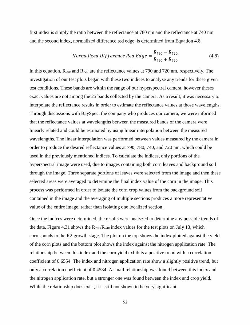
52

first index is simply the ratio between the reflectance at 780 nm and the reflectance at 740 nm

and the second index, normalized difference red edge, is determined from Equation 4.8.

𝑁𝑜𝑟𝑚𝑎𝑙𝑖𝑧𝑒𝑑 𝐷𝑖𝑓𝑓𝑒𝑟𝑒𝑛𝑐𝑒 𝑅𝑒𝑑 𝐸𝑑𝑔𝑒 =𝑅790 − 𝑅720

𝑅790 + 𝑅720 (4.8)

In this equation, R790 and R720 are the reflectance values at 790 and 720 nm, respectively. The

investigation of our test plots began with these two indices to analyze any trends for these given

test conditions. These bands are within the range of our hyperspectral camera, however theses

exact values are not among the 25 bands collected by the camera. As a result, it was necessary to

interpolate the reflectance results in order to estimate the reflectance values at those wavelengths.

Through discussions with BaySpec, the company who produces our camera, we were informed

that the reflectance values at wavelengths between the measured bands of the camera were

linearly related and could be estimated by using linear interpolation between the measured

wavelengths. The linear interpolation was performed between values measured by the camera in

order to produce the desired reflectance values at 790, 780, 740, and 720 nm, which could be

used in the previously mentioned indices. To calculate the indices, only portions of the

hyperspectral image were used, due to images containing both corn leaves and background soil

through the image. Three separate portions of leaves were selected from the image and then these

selected areas were averaged to determine the final index value of the corn in the image. This

process was performed in order to isolate the corn crop values from the background soil

contained in the image and the averaging of multiple sections produces a more representative

value of the entire image, rather than isolating one localized section.

Once the indices were determined, the results were analyzed to determine any possible trends of

the data. Figure 4.31 shows the R780/R740 index values for the test plots on July 13, which

corresponds to the R2 growth stage. The plot on the top shows the index plotted against the yield

of the corn plots and the bottom plot shows the index against the nitrogen application rate. The

relationship between this index and the corn yield exhibits a positive trend with a correlation

coefficient of 0.6554. The index and nitrogen application rate show a slightly positive trend, but

only a correlation coefficient of 0.4534. A small relationship was found between this index and

the nitrogen application rate, but a stronger one was found between the index and crop yield.

While the relationship does exist, it is still not shown to be very significant.

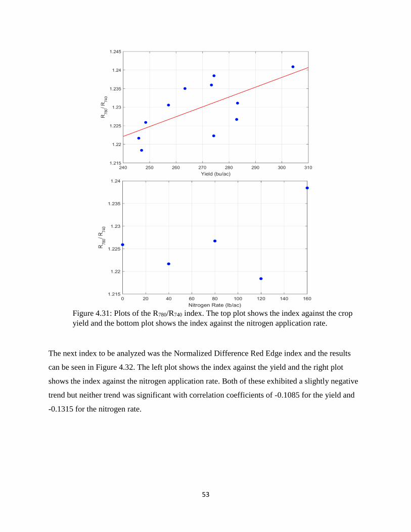
53

Figure 4.31: Plots of the R780/R740 index. The top plot shows the index against the crop

yield and the bottom plot shows the index against the nitrogen application rate.

The next index to be analyzed was the Normalized Difference Red Edge index and the results

can be seen in Figure 4.32. The left plot shows the index against the yield and the right plot

shows the index against the nitrogen application rate. Both of these exhibited a slightly negative

trend but neither trend was significant with correlation coefficients of -0.1085 for the yield and

-0.1315 for the nitrogen rate.

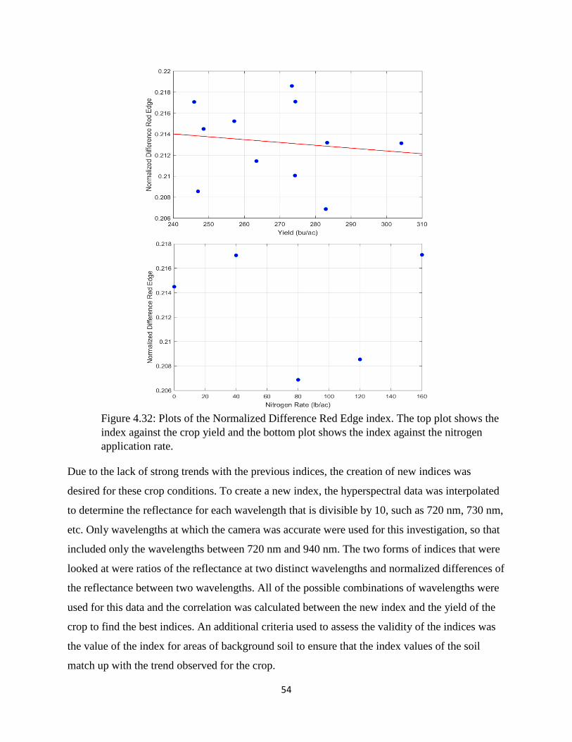
54

Figure 4.32: Plots of the Normalized Difference Red Edge index. The top plot shows the

index against the crop yield and the bottom plot shows the index against the nitrogen

application rate.

Due to the lack of strong trends with the previous indices, the creation of new indices was

desired for these crop conditions. To create a new index, the hyperspectral data was interpolated

to determine the reflectance for each wavelength that is divisible by 10, such as 720 nm, 730 nm,

etc. Only wavelengths at which the camera was accurate were used for this investigation, so that

included only the wavelengths between 720 nm and 940 nm. The two forms of indices that were

looked at were ratios of the reflectance at two distinct wavelengths and normalized differences of

the reflectance between two wavelengths. All of the possible combinations of wavelengths were

used for this data and the correlation was calculated between the new index and the yield of the

crop to find the best indices. An additional criteria used to assess the validity of the indices was

the value of the index for areas of background soil to ensure that the index values of the soil

match up with the trend observed for the crop.

55

After testing all combinations of wavelengths, the pair of wavelengths which produced the

highest correlation between the index and the crop yield were 760 and 740 nm. Two different

indices using these two bands were looked at. The first one is the ratio of the reflectance at each

of these wavelengths, which is shown in Figure 4.33. The top plot shows the index value plotted

against the yield of the corn in the plot. A least squares regression line was fit through the points,

which can be seen as the red line in this plot. The correlation coefficient between this index and

the yield was found to be 0.8404, which shows a much stronger correlation than the previous

indices. The bottom plot in the figure shows the same index values along with additional points

showing the index values for soil. These were plotted at a yield of zero to show the separation

between the index magnitudes and the index trend can be seen as an extension of the trend within

the corn.

Figure 4.33: Plots of the relationship between the corn yield and the new index created

from the ratio between the reflectance at 760 nm and 740 nm.

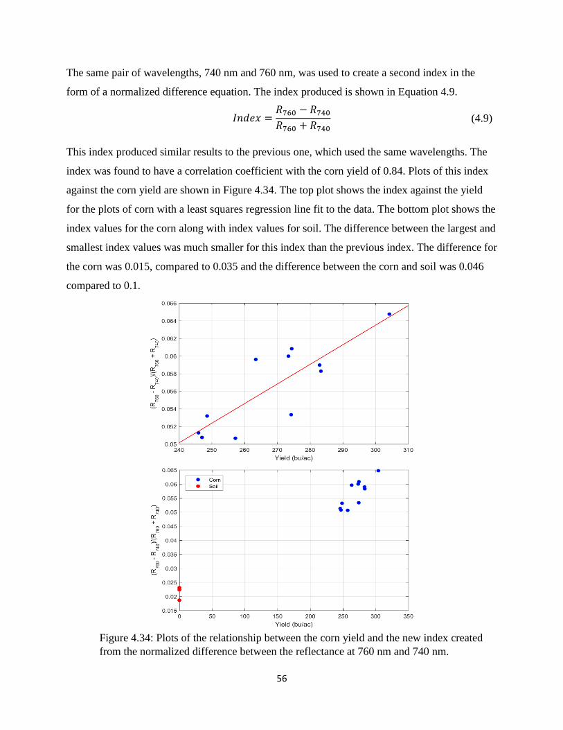
56

The same pair of wavelengths, 740 nm and 760 nm, was used to create a second index in the

form of a normalized difference equation. The index produced is shown in Equation 4.9.

𝐼𝑛𝑑𝑒𝑥 =𝑅760 − 𝑅740

𝑅760 + 𝑅740 (4.9)

This index produced similar results to the previous one, which used the same wavelengths. The

index was found to have a correlation coefficient with the corn yield of 0.84. Plots of this index

against the corn yield are shown in Figure 4.34. The top plot shows the index against the yield

for the plots of corn with a least squares regression line fit to the data. The bottom plot shows the

index values for the corn along with index values for soil. The difference between the largest and

smallest index values was much smaller for this index than the previous index. The difference for

the corn was 0.015, compared to 0.035 and the difference between the corn and soil was 0.046

compared to 0.1.


from the normalized difference between the reflectance at 760 nm and 740 nm.

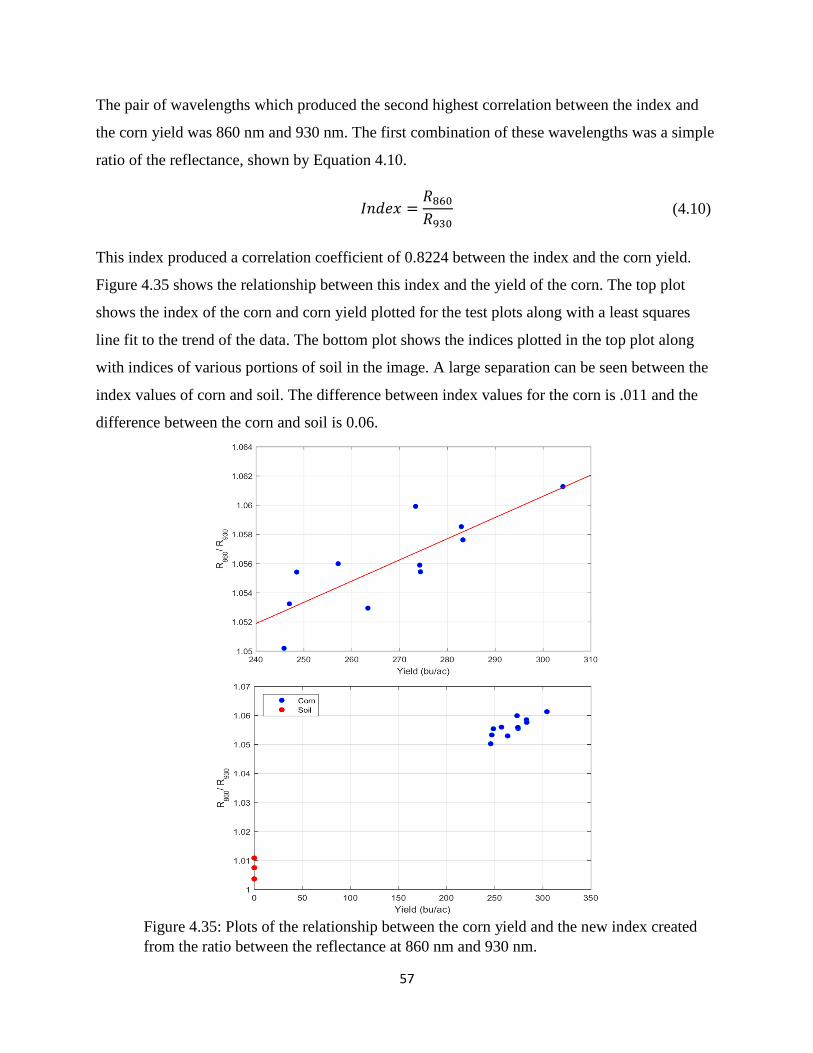
57

The pair of wavelengths which produced the second highest correlation between the index and

the corn yield was 860 nm and 930 nm. The first combination of these wavelengths was a simple

ratio of the reflectance, shown by Equation 4.10.


𝑅930 (4.10)

This index produced a correlation coefficient of 0.8224 between the index and the corn yield.

Figure 4.35 shows the relationship between this index and the yield of the corn. The top plot

shows the index of the corn and corn yield plotted for the test plots along with a least squares

line fit to the trend of the data. The bottom plot shows the indices plotted in the top plot along

with indices of various portions of soil in the image. A large separation can be seen between the

index values of corn and soil. The difference between index values for the corn is .011 and the

difference between the corn and soil is 0.06.



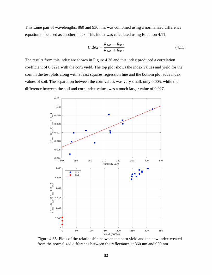
58

This same pair of wavelengths, 860 and 930 nm, was combined using a normalized difference

equation to be used as another index. This index was calculated using Equation 4.11.

𝐼𝑛𝑑𝑒𝑥 =𝑅860 − 𝑅930

𝑅860 + 𝑅930 (4.11)

The results from this index are shown in Figure 4.36 and this index produced a correlation

coefficient of 0.8221 with the corn yield. The top plot shows the index values and yield for the

corn in the test plots along with a least squares regression line and the bottom plot adds index

values of soil. The separation between the corn values was very small, only 0.005, while the

difference between the soil and corn index values was a much larger value of 0.027.



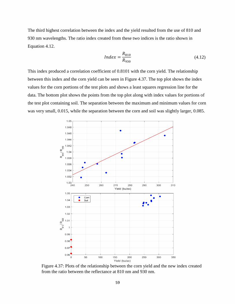
59

The third highest correlation between the index and the yield resulted from the use of 810 and

930 nm wavelengths. The ratio index created from these two indices is the ratio shown in

Equation 4.12.


𝑅930 (4.12)

This index produced a correlation coefficient of 0.8101 with the corn yield. The relationship

between this index and the corn yield can be seen in Figure 4.37. The top plot shows the index

values for the corn portions of the test plots and shows a least squares regression line for the

data. The bottom plot shows the points from the top plot along with index values for portions of

the test plot containing soil. The separation between the maximum and minimum values for corn

was very small, 0.015, while the separation between the corn and soil was slightly larger, 0.085.



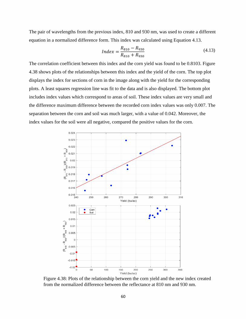
60

The pair of wavelengths from the previous index, 810 and 930 nm, was used to create a different

equation in a normalized difference form. This index was calculated using Equation 4.13.

𝐼𝑛𝑑𝑒𝑥 =𝑅810 − 𝑅930

𝑅810 + 𝑅930 (4.13)

The correlation coefficient between this index and the corn yield was found to be 0.8103. Figure

4.38 shows plots of the relationships between this index and the yield of the corn. The top plot

displays the index for sections of corn in the image along with the yield for the corresponding

plots. A least squares regression line was fit to the data and is also displayed. The bottom plot

includes index values which correspond to areas of soil. These index values are very small and

the difference maximum difference between the recorded corn index values was only 0.007. The

separation between the corn and soil was much larger, with a value of 0.042. Moreover, the

index values for the soil were all negative, compared the positive values for the corn.



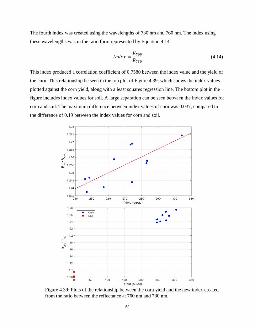
61

The fourth index was created using the wavelengths of 730 nm and 760 nm. The index using

these wavelengths was in the ratio form represented by Equation 4.14.


𝑅730 (4.14)

This index produced a correlation coefficient of 0.7580 between the index value and the yield of

the corn. This relationship be seen in the top plot of Figure 4.39, which shows the index values

plotted against the corn yield, along with a least squares regression line. The bottom plot in the

figure includes index values for soil. A large separation can be seen between the index values for

corn and soil. The maximum difference between index values of corn was 0.037, compared to

the difference of 0.19 between the index values for corn and soil.



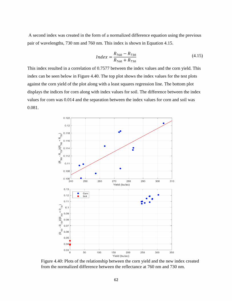
62

A second index was created in the form of a normalized difference equation using the previous

pair of wavelengths, 730 nm and 760 nm. This index is shown in Equation 4.15.

𝐼𝑛𝑑𝑒𝑥 =𝑅760 − 𝑅730

𝑅760 + 𝑅730 (4.15)

This index resulted in a correlation of 0.7577 between the index values and the corn yield. This

index can be seen below in Figure 4.40. The top plot shows the index values for the test plots

against the corn yield of the plot along with a least squares regression line. The bottom plot

displays the indices for corn along with index values for soil. The difference between the index

values for corn was 0.014 and the separation between the index values for corn and soil was

0.081.



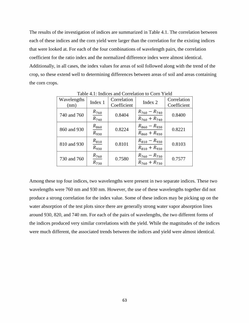
63

The results of the investigation of indices are summarized in Table 4.1. The correlation between

each of these indices and the corn yield were larger than the correlation for the existing indices

that were looked at. For each of the four combinations of wavelength pairs, the correlation

coefficient for the ratio index and the normalized difference index were almost identical.

Additionally, in all cases, the index values for areas of soil followed along with the trend of the

crop, so these extend well to determining differences between areas of soil and areas containing

the corn crops.

Table 4.1: Indices and Correlation to Corn Yield

Wavelengths

(nm) Index 1

Correlation

Coefficient Index 2

Correlation

Coefficient

740 and 760 𝑅760

𝑅740 0.8404

𝑅760 − 𝑅740

𝑅760 + 𝑅740 0.8400

860 and 930 𝑅860

𝑅930 0.8224

𝑅860 − 𝑅930

𝑅860 + 𝑅930 0.8221

810 and 930 𝑅810

𝑅930 0.8101

𝑅810 − 𝑅930

𝑅810 + 𝑅930 0.8103

730 and 760 𝑅760

𝑅730 0.7580

𝑅760 − 𝑅730

𝑅760 + 𝑅730 0.7577

Among these top four indices, two wavelengths were present in two separate indices. These two

wavelengths were 760 nm and 930 nm. However, the use of these wavelengths together did not

produce a strong correlation for the index value. Some of these indices may be picking up on the

water absorption of the test plots since there are generally strong water vapor absorption lines

around 930, 820, and 740 nm. For each of the pairs of wavelengths, the two different forms of

the indices produced very similar correlations with the yield. While the magnitudes of the indices

were much different, the associated trends between the indices and yield were almost identical.

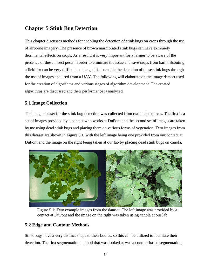
64

Chapter 5 Stink Bug Detection

This chapter discusses methods for enabling the detection of stink bugs on crops through the use

of airborne imagery. The presence of brown marmorated stink bugs can have extremely

detrimental effects on crops. As a result, it is very important for a farmer to be aware of the

presence of these insect pests in order to eliminate the issue and save crops from harm. Scouting

a field for can be very difficult, so the goal is to enable the detection of these stink bugs through

the use of images acquired from a UAV. The following will elaborate on the image dataset used

for the creation of algorithms and various stages of algorithm development. The created

algorithms are discussed and their performance is analyzed.

5.1 Image Collection

The image dataset for the stink bug detection was collected from two main sources. The first is a

set of images provided by a contact who works at DuPont and the second set of images are taken

by me using dead stink bugs and placing them on various forms of vegetation. Two images from

this dataset are shown in Figure 5.1, with the left image being one provided from our contact at

DuPont and the image on the right being taken at our lab by placing dead stink bugs on canola.

Figure 5.1: Two example images from the dataset. The left image was provided by a

contact at DuPont and the image on the right was taken using canola at our lab.

5.2 Edge and Contour Methods

Stink bugs have a very distinct shape to their bodies, so this can be utilized to facilitate their

detection. The first segmentation method that was looked at was a contour based segmentation

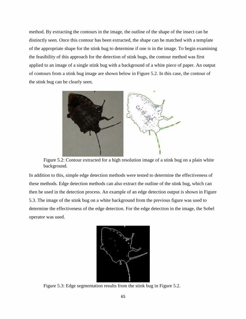
65

method. By extracting the contours in the image, the outline of the shape of the insect can be

distinctly seen. Once this contour has been extracted, the shape can be matched with a template

of the appropriate shape for the stink bug to determine if one is in the image. To begin examining

the feasibility of this approach for the detection of stink bugs, the contour method was first

applied to an image of a single stink bug with a background of a white piece of paper. An output

of contours from a stink bug image are shown below in Figure 5.2. In this case, the contour of

the stink bug can be clearly seen.

Figure 5.2: Contour extracted for a high resolution image of a stink bug on a plain white

background.

In addition to this, simple edge detection methods were tested to determine the effectiveness of

these methods. Edge detection methods can also extract the outline of the stink bug, which can

then be used in the detection process. An example of an edge detection output is shown in Figure

5.3. The image of the stink bug on a white background from the previous figure was used to

determine the effectiveness of the edge detection. For the edge detection in the image, the Sobel

operator was used.

Figure 5.3: Edge segmentation results from the stink bug in Figure 5.2.

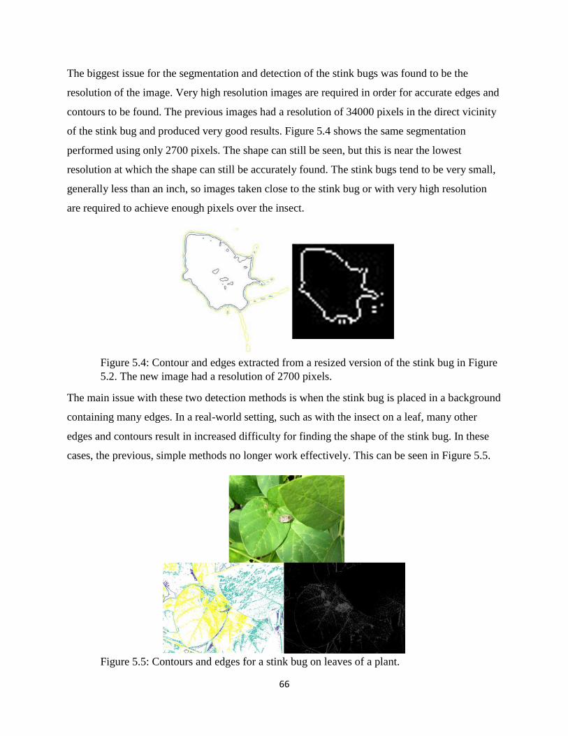
66

The biggest issue for the segmentation and detection of the stink bugs was found to be the

resolution of the image. Very high resolution images are required in order for accurate edges and

contours to be found. The previous images had a resolution of 34000 pixels in the direct vicinity

of the stink bug and produced very good results. Figure 5.4 shows the same segmentation

performed using only 2700 pixels. The shape can still be seen, but this is near the lowest

resolution at which the shape can still be accurately found. The stink bugs tend to be very small,

generally less than an inch, so images taken close to the stink bug or with very high resolution

are required to achieve enough pixels over the insect.

Figure 5.4: Contour and edges extracted from a resized version of the stink bug in Figure

5.2. The new image had a resolution of 2700 pixels.

The main issue with these two detection methods is when the stink bug is placed in a background

containing many edges. In a real-world setting, such as with the insect on a leaf, many other

edges and contours result in increased difficulty for finding the shape of the stink bug. In these

cases, the previous, simple methods no longer work effectively. This can be seen in Figure 5.5.

Figure 5.5: Contours and edges for a stink bug on leaves of a plant.

67

Due to the issues with the previous methods, more sophisticated methods were required. As a

result, a more sophisticated edge detection method was looked at. This was a structured edge

detection method [45, 46]. This was performed on some images of stink bugs and the results are

shown in Figures 5.6 and 5.7. This extracted the edges, which would allow the shape of the stink

bugs to be matched. Again, high resolution is required to achieve the accuracy needed.

Figure 5.6: Structured edge detection performed on an image with a stink bug on a plant.

Figure 5.7: Structured edge detection performed on an image with a stink bug on a plant.

5.3 Superpixel Segmentation

In an attempt to reduce the resolution required for the stink bug detection, a superpixel

segmentation method was investigated. To segment the image into superpixels, the SLIC

Superpixels method was used. The SLIC Superpixels method was implemented using an existing

version, which is publicly available [47]. Adult brown marmorated stink bugs have consistent

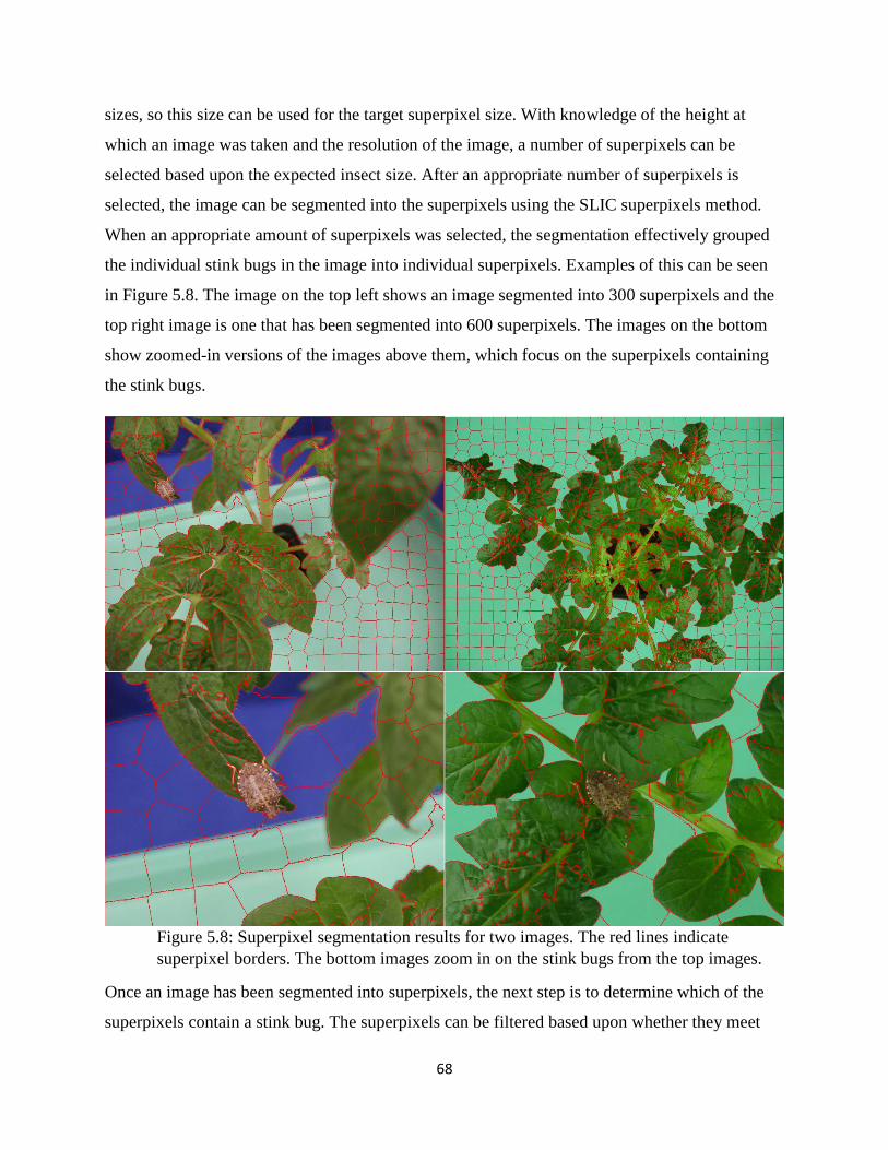
68

sizes, so this size can be used for the target superpixel size. With knowledge of the height at

which an image was taken and the resolution of the image, a number of superpixels can be

selected based upon the expected insect size. After an appropriate number of superpixels is

selected, the image can be segmented into the superpixels using the SLIC superpixels method.

When an appropriate amount of superpixels was selected, the segmentation effectively grouped

the individual stink bugs in the image into individual superpixels. Examples of this can be seen

in Figure 5.8. The image on the top left shows an image segmented into 300 superpixels and the

top right image is one that has been segmented into 600 superpixels. The images on the bottom

show zoomed-in versions of the images above them, which focus on the superpixels containing

the stink bugs.

Figure 5.8: Superpixel segmentation results for two images. The red lines indicate

superpixel borders. The bottom images zoom in on the stink bugs from the top images.

Once an image has been segmented into superpixels, the next step is to determine which of the

superpixels contain a stink bug. The superpixels can be filtered based upon whether they meet

69

specific criteria, which will eliminate the superpixels which do not contain a stink bug. The first

methods of filtering were based upon the color contents of the superpixels. Specifically, the hue,

red, and a* color channels of the image were used for the filtering process. These channels were

selected to be used for the filtering because they were found to have large distinctions between

the pixel values of the stink bugs and the values for the surrounding leaves. These distinctions

are demonstrated by the images in Figure 5.9, which shows an image of a stink bug on a plant in

the different color spaces. The image on the top left shows the RGB image of the stink bug on

the plant. The top right image shows a color-scaled representation of the red plane image values.

The bottom left image shows a scaled color representation of the hue values of the image and the

bottom right image shows a scaled color representation of the a* plane. These planes, especially

the hue and a* planes show very distinct differences between the stink bugs and the surrounding

leaves.

Figure 5.9: RGB image of a stink bug on a plant along with scaled representations of the

red, hue, and a* planes. The top right image shows the red values, the bottom left image

shows the hue, and the bottom right images shows the a* values.

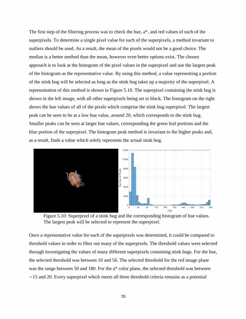
70

The first step of the filtering process was to check the hue, a*, and red values of each of the

superpixels. To determine a single pixel value for each of the superpixels, a method invariant to

outliers should be used. As a result, the mean of the pixels would not be a good choice. The

median is a better method than the mean, however even better options exist. The chosen

approach is to look at the histogram of the pixel values in the superpixel and use the largest peak

of the histogram as the representative value. By using this method, a value representing a portion

of the stink bug will be selected as long as the stink bug takes up a majority of the superpixel. A

representation of this method is shown in Figure 5.10. The superpixel containing the stink bug is

shown in the left image, with all other superpixels being set to black. The histogram on the right

shows the hue values of all of the pixels which comprise the stink bug superpixel. The largest

peak can be seen to be at a low hue value, around 20, which corresponds to the stink bug.

Smaller peaks can be seen at larger hue values, corresponding the green leaf portions and the

blue portion of the superpixel. The histogram peak method is invariant to the higher peaks and,

as a result, finds a value which solely represents the actual stink bug.

Figure 5.10: Superpixel of a stink bug and the corresponding histogram of hue values.

The largest peak will be selected to represent the superpixel.

Once a representative value for each of the superpixels was determined, it could be compared to

threshold values in order to filter out many of the superpixels. The threshold values were selected

through investigating the values of many different superpixels containing stink bugs. For the hue,

the selected threshold was between 10 and 56. The selected threshold for the red image plane

was the range between 50 and 180. For the a* color plane, the selected threshold was between

−15 and 20. Every superpixel which meets all three threshold criteria remains as a potential

71

candidate for a stink bug while all other superpixels are classified as not being a stink bug and

are eliminated.

After the superpixels have been filtered through the color thresholds, the superpixels get filtered

by their shape and size. One of the shape characteristics examined is the eccentricity of the

superpixel. Eccentricity is a measure of the amount that a conic section deviates from being

circular. A circle has an eccentricity of 0 and an ellipse has an eccentricity greater than 0 but less

than 1 [48]. The shapes of stink bugs, and as a result, the corresponding superpixels containing

stink bugs, were found to generally be an elliptical shape with an eccentricity of less than 0.83.

This eccentricity threshold was used for the superpixels to filter out inappropriately shaped

pixels. Additionally, the size of the superpixels was taken into account by examining that number

of pixels in the superpixels. Using the number of superpixels, the target superpixel size can be

calculated from the image resolution. The target size can be compared to the actual size of the

superpixel to check if the superpixel corresponds to a size which is appropriate for a stink bug.

During the filtering process, superpixels which are much larger, determined to be greater than

1.75 times the size of the target size, are classified as not being a stink bug. The final method of

filtering is by examining another characteristic of the stink bug shape. This method aims at

removing very oddly shaped superpixels. This is done by comparing the size of the bounding box

of the superpixel to the filled area of the superpixel. This method is effective for eliminated

superpixels with very odd shapes, which likely correspond to a pixel without a stink bug. An

example of such a superpixel can be seen in Figure 5.11. The very thin and long portions of the

superpixel create a wide bounding box with only a small percentage of the bounding box

containing the superpixel. The threshold of the ratio of the number of pixels in the bounding box

to the number of pixels in the superpixel was set to a value of 4. All superpixels which have a

ratio less than 4 remain as potential stink bug candidates, while all other superpixels will be

classified as not containing a stink bug.

72

Figure 5.11: Superpixel with a very odd shape, which will be filtered out with the

bounding box method.

The superpixel segmentation method worked very effectively at detecting stink bugs, even when

the stink bug has a low resolution. An example of this can be seen in Figure 5.12 with a stink bug

detected with only 666 pixels in the superpixel. The left image shows the original image and the

image on the right shows the detected stink bug. Despite the low resolution on the stink bug, the

detection method was able to accurately detect the presence of the stink bug in the image.

Figure 5.12: Stink bug detection result using the superpixel method. The detected stink

bug is shown on the right.

In addition to low resolution cases, this method also detected stink bugs which were positioned at

angles as well as ones which were partially obscured by leaves. These detection cases can be

seen in Figure 5.13. The top images show the detection of a stink bug, which is partially covered

by a leaf and the bottom pair of images shows a detected stink bug facing perpendicular to the

camera. Despite these conditions, the superpixels allowed the pixels representing the stink bug to

be grouped together and the color and shape characteristics can be matched up with values

corresponding to a stink bug in order to allow detection.

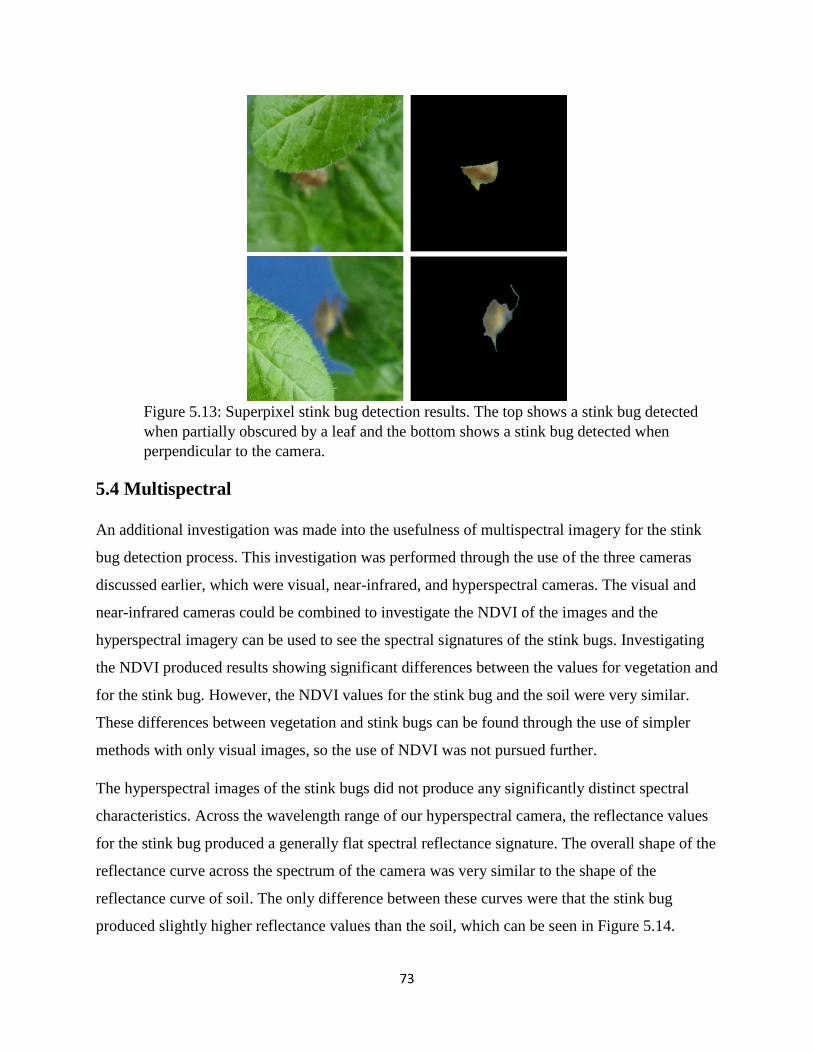
73

Figure 5.13: Superpixel stink bug detection results. The top shows a stink bug detected

when partially obscured by a leaf and the bottom shows a stink bug detected when

perpendicular to the camera.

5.4 Multispectral

An additional investigation was made into the usefulness of multispectral imagery for the stink

bug detection process. This investigation was performed through the use of the three cameras

discussed earlier, which were visual, near-infrared, and hyperspectral cameras. The visual and

near-infrared cameras could be combined to investigate the NDVI of the images and the

hyperspectral imagery can be used to see the spectral signatures of the stink bugs. Investigating

the NDVI produced results showing significant differences between the values for vegetation and

for the stink bug. However, the NDVI values for the stink bug and the soil were very similar.

These differences between vegetation and stink bugs can be found through the use of simpler

methods with only visual images, so the use of NDVI was not pursued further.

The hyperspectral images of the stink bugs did not produce any significantly distinct spectral

characteristics. Across the wavelength range of our hyperspectral camera, the reflectance values

for the stink bug produced a generally flat spectral reflectance signature. The overall shape of the

reflectance curve across the spectrum of the camera was very similar to the shape of the

reflectance curve of soil. The only difference between these curves were that the stink bug

produced slightly higher reflectance values than the soil, which can be seen in Figure 5.14.

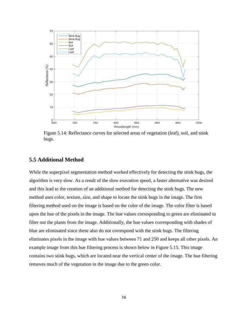
74

Figure 5.14: Reflectance curves for selected areas of vegetation (leaf), soil, and stink

bugs.

5.5 Additional Method

While the superpixel segmentation method worked effectively for detecting the stink bugs, the

algorithm is very slow. As a result of the slow execution speed, a faster alternative was desired

and this lead to the creation of an additional method for detecting the stink bugs. The new

method uses color, texture, size, and shape to locate the stink bugs in the image. The first

filtering method used on the image is based on the color of the image. The color filter is based

upon the hue of the pixels in the image. The hue values corresponding to green are eliminated to

filter out the plants from the image. Additionally, the hue values corresponding with shades of

blue are eliminated since these also do not correspond with the stink bugs. The filtering

eliminates pixels in the image with hue values between 71 and 250 and keeps all other pixels. An

example image from this hue filtering process is shown below in Figure 5.15. This image

contains two stink bugs, which are located near the vertical center of the image. The hue filtering

removes much of the vegetation in the image due to the green color.

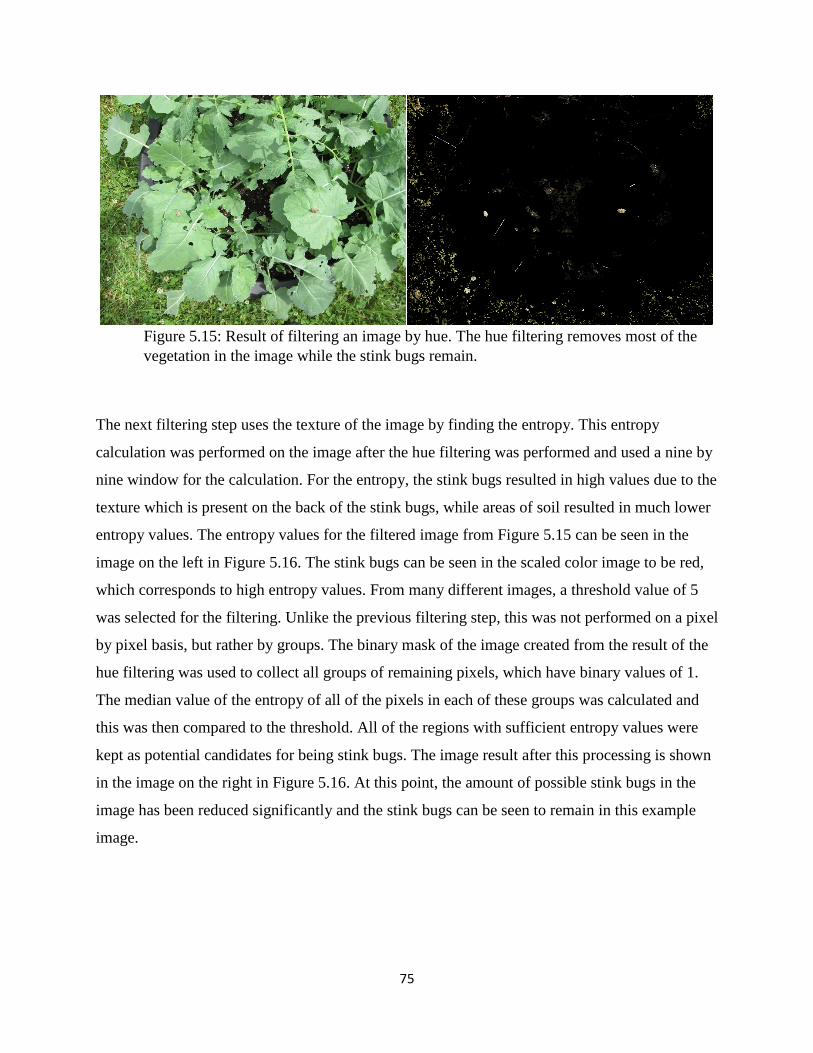
75

Figure 5.15: Result of filtering an image by hue. The hue filtering removes most of the

vegetation in the image while the stink bugs remain.

The next filtering step uses the texture of the image by finding the entropy. This entropy

calculation was performed on the image after the hue filtering was performed and used a nine by

nine window for the calculation. For the entropy, the stink bugs resulted in high values due to the

texture which is present on the back of the stink bugs, while areas of soil resulted in much lower

entropy values. The entropy values for the filtered image from Figure 5.15 can be seen in the

image on the left in Figure 5.16. The stink bugs can be seen in the scaled color image to be red,

which corresponds to high entropy values. From many different images, a threshold value of 5

was selected for the filtering. Unlike the previous filtering step, this was not performed on a pixel

by pixel basis, but rather by groups. The binary mask of the image created from the result of the

hue filtering was used to collect all groups of remaining pixels, which have binary values of 1.

The median value of the entropy of all of the pixels in each of these groups was calculated and

this was then compared to the threshold. All of the regions with sufficient entropy values were

kept as potential candidates for being stink bugs. The image result after this processing is shown

in the image on the right in Figure 5.16. At this point, the amount of possible stink bugs in the

image has been reduced significantly and the stink bugs can be seen to remain in this example

image.

76

Figure 5.16: Entropy filtering of the resulting image from Figure 5.15. The image on the

left shows the scaled color representation of the entropy values and the image on the right

shows the image result after the entropy filtering process.

The next step in the filtering process is to look at the shape and size characteristics of the binary

blobs which remain in the image. A binary closing operation is first performed on the image

mask to remove the small holes in the blobs in the image, then shape and size characteristics are

examined. The image is filtered based upon the ratio of the area to the perimeter of each of the

binary regions. All regions which are greater than a threshold remain in the binary mask as

potential stink bugs. This step can remove very oddly shaped regions, with large perimeters and

small areas, as well as many small regions in the image.

The size of the regions in the image are examined to determine if they match well with the size

of the stink bug. This portion of the algorithm requires the knowledge of the height, relative to

the crop, at which the image was taken. The size of stink bugs tends to be relatively uniform,

with the length of an adult being around 17 mm or 0.67 inches [49]. As a result, regions in the

image which are larger than the size corresponding to an average stink bug can be removed. To

determine this size, images were acquired of a large stink bug at various heights and these

heights were recorded along with the amount of pixels contained in the stink bug and the image

resolution. Using this information, the ratio between the number of pixels in the stink bug and

the number of pixels of the image was plotted against the height at which the image was taken to

determine the trend of the data. The plot of this data is shown below in Figure 5.17. A curve was

fit to this data and the best curve was the power function in Equation 5.1.

𝑆𝑖𝑧𝑒 = 0.1071𝐻−1.878 (5.1)

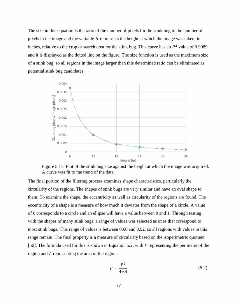
77

The size in this equation is the ratio of the number of pixels for the stink bug to the number of

pixels in the image and the variable 𝐻 represents the height at which the image was taken, in

inches, relative to the crop or search area for the stink bug. This curve has an 𝑅2 value of 0.9989

and it is displayed as the dotted line on the figure. The size function is used as the maximum size

of a stink bug, so all regions in the image larger than this determined ratio can be eliminated as

potential stink bug candidates.

Figure 5.17: Plot of the stink bug size against the height at which the image was acquired.

A curve was fit to the trend of the data.

The final portion of the filtering process examines shape characteristics, particularly the

circularity of the regions. The shapes of stink bugs are very similar and have an oval shape to

them. To examine the shape, the eccentricity as well as circularity of the regions are found. The

eccentricity of a shape is a measure of how much it deviates from the shape of a circle. A value

of 0 corresponds to a circle and an ellipse will have a value between 0 and 1. Through testing

with the shapes of many stink bugs, a range of values was selected as ones that correspond to

most stink bugs. This range of values is between 0.68 and 0.92, so all regions with values in this

range remain. The final property is a measure of circularity based on the isoperimetric quotient

[50]. The formula used for this is shown in Equation 5.2, with 𝑃 representing the perimeter of the

region and 𝐴 representing the area of the region.

𝐶 =𝑃2

4𝜋𝐴 (5.2)

0

0.0005

0.001

0.0015

0.002

0.0025

0.003

0.0035

0.004

6 12 18 24 30 36

Size

(b

ug

pix

els/

imag

e p

ixel

s)

Height (in)

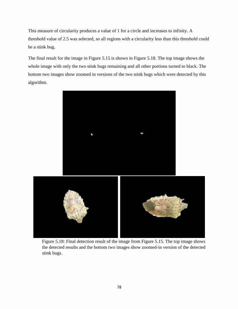
78

This measure of circularity produces a value of 1 for a circle and increases to infinity. A

threshold value of 2.5 was selected, so all regions with a circularity less than this threshold could

be a stink bug.

The final result for the image in Figure 5.15 is shown in Figure 5.18. The top image shows the

whole image with only the two stink bugs remaining and all other portions turned to black. The

bottom two images show zoomed in versions of the two stink bugs which were detected by this

algorithm.

Figure 5.18: Final detection result of the image from Figure 5.15. The top image shows

the detected results and the bottom two images show zoomed-in version of the detected

stink bugs.

79

5.6 Results

Two potential methods for detection of the stink bugs have been proposed. Each of these

methods successfully detected stink bugs in various settings, but each have some disadvantages.

For the method using the superpixel segmentation, in an image set containing 33 stink bugs, 31

of those were successfully detected, which is a recognition rate of 93.9%. In these cases, there

were also two false positives detected. The detection was able to work in cases with very low

stink bug pixel resolution, as low as 666 pixels for a bug. The biggest problem with this method

is the processing time. The processing required around 30 seconds for images very close to the

stink bug, which require only 300 superpixels. In images much higher up, for instance one

requiring 4000 superpixels, the processing required as much as 3 minutes to complete. However,

this algorithm was not optimized and could likely be speed up substantially through the use of

another coding language, such as C instead of Matlab.

The second method performed well on a small test set of images and did the processing much

faster than the first method. In a set of 11 images which contained 21 stink bugs, the algorithm

correctly detected 20, 95.2%, of these stink bugs, but did also have one image with 2 false

positives. The algorithm processed a 16-megapixel image in approximately 17 seconds. Most of

the processing time is spent on the entropy filtering portion. This algorithm is written in Matlab

and the entropy filtering portion utilizes a built-in function that runs using a MEX file. The MEX

file is written in C, so it would likely be difficult to achieve large improvements in processing

speed by writing the code in a different language, such as C. This method has some potential

failure cases when the images do not achieve required resolution. The entropy method requires

high resolution on the back of the stink bug to detect the texture on the back of the stink bug. The

one failed detection in the dataset was a stink bug that was not well focused in the image, so

texture could not be detected. The test of the code worked up to a height of 36 inches and the

smallest detected stink bug had a resolution of 1137 pixels across the stink bug. Other potential

issues with this algorithm contain cases where stink bugs are obscured by the leaves or sideways

at odd angles. If a stink bug is oriented in a way that the texture of it cannot be picked up by the

camera, it will likely not be detected and if the stink bug is partially or completely obscured by

leaves, it will also not be detected.

80

Chapter 6 Summary & Conclusions

The current methods for monitoring crop health and detecting issues in crop fields are lacking in

many areas, such as the cost and turnaround times. Satellite or airplane remote sensing can be

very expensive and very slow to detect the issues, which can also limit the treatment

possibilities. A potential improvement on these current methods is through the use of UAVs for

remote sensing. This thesis has presented methods for UAV remote sensing using visible

spectrum and multispectral images. A method has been proposed to use an SVM for the

detection of crop issues from the use of airborne images of corn fields. The created SVM

achieved a detection accuracy of 86.4% over a test set of images. Additionally, multispectral

analysis was performed to determine indices appropriate for determining the health of corn.

Along the way of this process, a method for correcting hyperspectral images for shadows and

other lighting issues was created. Several indices were created and the best performance was

achieved using 760 and 740 nm wavelengths, which produced a correlation coefficient of 0.84

with the corn yield. In addition to this, stink bug detection algorithms were also created to detect

stink bugs on crops using aerial visible spectrum images. Two methods for this were created,

which include a superpixel segmentation method and a color and texture filtering method. The

superpixel method achieved a recognition rate of 93.9%, but had high processing times in some

cases. The second method achieved a recognition rate of 95.2%, while improving upon the speed

of the first method.

For each of the algorithms which have been presented, there are potential areas of improvement

and future work. For the crop health detection using only visible spectrum imagery, which was

the work in Chapter 3, the biggest area for future work is the addition of features outside of

color, such as texture. Currently, this work is limited by the training data lacking the resolution

necessary for texture features. Training data would need to be acquired by flying UAVs over

fields to acquire high resolution imagery of the fields. In addition to this, the current training data

lacks ground truth data for specific issues. The current data is labeled for areas which are known

to have crop health issues, but the ground truth data does not exist to identify the specific issues.

If this data can also be acquired, the machine learning algorithm could be extended to detect

specific health issues, such as water stress, nutrient deficiency, or specific abiotic or biotic stress

impacts, which could include stink bugs and nematodes. Another possibility to examine for the

81

machine learning approach is the use of superpixels for the classification in order to reduce the

required processing as well as reduce the impacts of noisy pixels. Additional improvements to

the image enhancement method could be made by using a localized adjustment approach to

reduce the impacts of localized shadows in the images.

Future work for the multispectral crop analysis would include another repeated test of the index

study to validate the determined indices. Additionally, it would be useful to examine index

values throughout the crop growth stages to see how the indices vary from early stage growth to

late stage crops. This additional data would allow for further validation and the potential to

improve upon the indices. Additional improvements in the system could be obtained through the

use of a light sensor to determine the lighting conditions during the image acquisition. This study

did not include any way to measure the lighting changes, outside of watching the sky to notice

when clouds obscure the sun. The addition of lighting condition values would allow for more

robust results, which can be more invariant to changes in lighting conditions.

For the stink bug detection, additional testing is required to determine the performance of these

algorithms in a real crop field. The images used to test the algorithms were acquired from a

stationary person taking an image of a stink bug on a plant, rather than from a UAV flying over a

field. To better evaluate the performance of these algorithms, images should be acquired by

flying a UAV over a field of crops to obtain realistic testing images for the algorithms.

Additionally, my implementations of these algorithms have not been optimized for speed, so

reducing the processing time will be an important step for implementing these in practice.

From the work in this thesis, the most significant contribution, with the most potential for future

application, is the work from Chapters 3 and 5. The work from each of these sections has

significant potential to be improved upon and implemented in practice by farmers. The

combination of the methods presented in these two chapters could allow for the detection and

prevention of many issues in a field. The work presented here creates a foundation for a method

to allow a farmer to use a UAV to automatically scout a field for the presence of bugs,

specifically stink bugs from this work, as well as issues with the field. The detection of these

issues would allow the farmer to treat the appropriate areas of the field to reduce the impact of

these issues and improve upon the yield of the crop. Additional development of these methods

would be required to achieve that goal, but this potential exists.

82

The work presented in this thesis can hopefully be built upon for the benefit of farmers to

analyze the conditions of their fields and improve the health and yield of their crops with proper

treatments. The use of UAVs in the area of remote sensing has a large amount of potential to

overtake other methods for remote sensing in agriculture, which can allow for more widespread

use of remote sensing by average farmers.

83

Bibliography

[1] J. Nowatzki, R. Andres, and K. Kyllo. (2004). Agricultural Remote Sensing Basics.

Available: https://www.ag.ndsu.edu/pubs/ageng/gis/ae1262.pdf

[2] Measuring Vegetation (NDVI & EVI). Available:

http://earthobservatory.nasa.gov/Features/MeasuringVegetation/measuring_vegetation_2.

php

[3] (2015). NDVI, the Foundation for Remote Sensing Phenology. Available:

http://phenology.cr.usgs.gov/ndvi_foundation.php

[4] K. Pavuluri, "Winter Barley as a Commodity Cover Crop in the Mid-Atlantic Coastal

Plain and Evaluation of Soft Red Winter Wheat Nitrogen Use Efficiency by Genotype,

and its Prediction of Nitrogen Use Efficiency through Canopy Spectral Reflectance in the

Eastern USA" Ph.D., Crop and Soil Environmental Sciences, Virginia Polytechnic

Institute and State University, 2013.

[5] J. A. J. Berni, P. J. Zarco-Tejada, L. Suárez, and E. Fereres, "Thermal and Narrowband

Multispectral Remote Sensing for Vegetation Monitoring From an Unmanned Aerial

Vehicle," IEEE Transactions on Geoscience and Remote Sensing, 2009.

[6] K. C. Swain, H. P. W. Jayasuriya, and V. M. Salokhe. “Low Altitude Remote Sensing

with Unmanned Radio-Controlled Helicopter Platforms: A Potential Substitution to

Satellite-based Systems for Precision Agriculture Adoption under Farming Conditions in

Developing Countries”. Agricultural Engineering International: the CIGR Ejournal. Vol.

IX. September, 2007.

[7] A. Rango, A. Laliberte, J. E. Herrick, C. Winters, K. Havstad, C. Steele, and D.

Browning. “Unmanned aerial vehicle-based remote sensing for rangeland assessment,

monitoring, and management”. Journal of Applied Remote Sensing. Vol. 3. August,

2009.

[8] T. Udelhoven. (2012), The use of an UAV as a remote sensing platform in agricultural

applications. Available:

https://www.microdrones.com/fileadmin/web/PDF/Referenzen/Fallstudien/use-of-uav-

remote-sensing-platform-agriculture-microdrones.pdf

[9] I. Colomina, P. Molina. “Unmanned aerial systems for photogrammetry and remote

sensing: A review”. ISPRS Journal of Photogrammetry and Remote Sensing, Vol. 92, pp.

79-92, 2014.

[10] (2016). Computer Vision. [Online]. Available:

https://en.wikipedia.org/wiki/Computer_vision

[11] (2016). HSL and HSV. [Online]. Available: https://en.wikipedia.org/wiki/HSL_and_HSV

84

[12] (2016). Lab color space. [Online]. Available:

https://en.wikipedia.org/wiki/Lab_color_space

[13] (2016). YIQ. [Online]. Available: https://en.wikipedia.org/wiki/YIQ

[14] (2016). Convert RGB color values to NTSC color space – MATLAB rgb2ntsc. [Online].

Available: https://www.mathworks.com/help/images/ref/rgb2ntsc.html

[15] R. Achanta, A. Shaji, K. Smith, A. Lucchi, P. Fua, and S. Süsstrunk. “SLIC Superpixels”.

EPFL Technical Report 149300, June 2010.

[16] R. Achanta, A. Shaji, K. Smith, A. Lucchi, P. Fua, and S. Süsstrunk. “SLIC Superpixels

Compared to State-of-the-art Superpixel Methods”. Journal of LATEX Class Files, Vol.

6. No. 1, December 2011.

[17] (2016). What Is Image Filtering in the Spatial Domain? – MATLAB & Simulink.

[Online]. Available: https://www.mathworks.com/help/images/what-is-image-filtering-

in-the-spatial-domain.html

[18] (2016). Image Gradient. [Online]. Available:

https://en.wikipedia.org/wiki/Image_gradient

[19] (2016). Edge Detection. [Online]. Available:

https://en.wikipedia.org/wiki/Edge_detection

[20] (2016). Sobel operator. [Online]. Available: https://en.wikipedia.org/wiki/Sobel_operator

[21] R. Fisher, S. Perkins, A. Walker, and E. Wolfart. (2003). Sobel edge Detector. [Online].

Available: http://homepages.inf.ed.ac.uk/rbf/HIPR2/sobel.htm

[22] (2016). Entropy of grayscale image – MATLAB entropy. [Online]. Available:

https://www.mathworks.com/help/images/ref/entropy.html?refresh=true

[23] (2016). Local entropy of grayscale image – MATALB entropyfilt. [Online]. Available:

https://www.mathworks.com/help/images/ref/entropyfilt.html

[24] D. O’Brien. Image Entropy. [Online]. Available:

http://www.astro.cornell.edu/research/projects/compression/entropy.html

[25] J. Loomis. (1998, June 10). Entropy. [Online]. Available:

http://www.johnloomis.org/ece563/notes/basics/entropy/entropy.html

[26] (2016). Morphological Dilation and Erosion – MATLAB & Simulink. [Online].

Available: https://www.mathworks.com/help/images/morphological-dilation-and-

erosion.html

[27] Morphological Image Processing. [Online]. Available:

https://www.cs.auckland.ac.nz/courses/compsci773s1c/lectures/ImageProcessing-

html/topic4.htm

85

[28] (2016). Measure properties of image regions – MATLAB regionprops. [Online].

Available: https://www.mathworks.com/help/images/ref/regionprops.html

[29] P. Pérez, M. Gangnet, A. Blake. “Poisson Image Editing”. ACM Transactions on

Graphics, Vol. 22(3), pp. 313-318, July 2003.

[30] (2016). Machine learning. [Online]. Available:

https://en.wikipedia.org/wiki/Machine_learning

[31] (2016). Unsupervised learning. [Online]. Available:

https://en.wikipedia.org/wiki/Unsupervised_learning

[32] (2016). Supervised learning. [Online]. Available:

https://en.wikipedia.org/wiki/Supervised_learning

[33] T. Fletcher. (2009, Mar. 1). “Support Vector Machines Explained”. Available:

http://www.tristanfletcher.co.uk/SVM%20Explained.pdf

[34] C. Cortes, V. Vapnik. “Support-Vector Networks”. Machine Learning, 20, pp. 273-297,

1995.

[35] G. Anthony, H. Gregg, and M. Tshilidzi. “Image Classification Using SVMs: One-

against-One VS One-against-All”. Available:

https://arxiv.org/ftp/arxiv/papers/0711/0711.2914.pdf

[36] C. Hsu and C. Lin. “A Comparison of Methods for Multi-class Support Vector

Machines,” IEEE Transactions on Neural Networks, Vol. 13(2), pp. 415-425, Mar. 2002.

[37] G. Camps-Valls, L. Gómez-Chova, J. Calpe-Maravilla, E. Soria-Olivas, J. D. Martín-

Guerrero, and J. Moreno. “Support Vector Machines for Crop Classification Using

Hyperspectral Data,” Pattern Recognition and Image Analysis, vol. 2652, pp. 134-141,

2003.

[38] J. H. Wilson, C. Zhang, and J. M. Kovacs. “Separating Crop Species in Northeastern

Ontario Using Hyperspectral Data,” Remote Sensing, vol. 6, pp. 925-945, 2014.

[39] D. Roy. (2009, May 25). Auto contrast. [Online]. Available:

https://www.mathworks.com/matlabcentral/fileexchange/10566-auto-contrast

[40] B. Russell, A. Torralba. LabelMe. [Online]. Available:

http://labelme2.csail.mit.edu/Release3.0/index.php

[41] (2011, Sept. 19). Canon Powershot S100 Black. [Online]. Available:

http://www.digicamreview.com/2011/09/canon-powershot-s100-announced.html/s100-

fsr-hor-black

[42] OCITM UAV Airborne Hyperspectral Camera. [Online]. Available:

http://www.bayspec.com/spectroscopy/oci-uav-hyperspectral-camera/

[43] (2016). CHDK Wiki. [Online]. Available: http://chdk.wikia.com/wiki/CHDK

86

[44] Spreading Wings S1000. [Online]. Available: http://www.dji.com/product/spreading-

wings-s1000

[45] P. Dollár, C. L. Zitnick. “Structured Forests for Fast Edge Detection.” In 2013 IEEE

International Conference on Computer Vision, pp. 1841-1848, 2013.

[46] P. Dollár. GitHub – pdollar/edges: Structured Edge Detection Toolbox. [Online].

Available: https://github.com/pdollar/edges

[47] EPFL. (2016). SLIC Superpixels. [Online]. Available:

http://ivrl.epfl.ch/research/superpixels

[48] E. W. Weisstein. "Eccentricity." From MathWorld--A Wolfram Web Resource. [Online].

Available: http://mathworld.wolfram.com/Eccentricity.html

[49] (2016). Brown marmorated stink bug. [Online]. Available:

https://en.wikipedia.org/wiki/Brown_marmorated_stink_bug

[50] (2016). Shape factor (image analysis and microscopy). [Online]. Available:

https://en.wikipedia.org/wiki/Shape_factor_(image_analysis_and_microscopy)

http://mathworld.wolfram.com/about/author.html

http://mathworld.wolfram.com/

http://mathworld.wolfram.com/Eccentricity.html

Techniques for Processing Airborne Imagery for Multimodal ... · Techniques for Processing Airborne...

Documents

Transcript of Techniques for Processing Airborne Imagery for Multimodal ... · Techniques for Processing Airborne...