Luxembourg Income Study Working Paper No. 299

(RE-) DISTRIBUTION OF PERSONAL INCOMES,EDUCATION AND ECONOMIC PERFORMANCE

ACROSS COUNTRIES

Günther Rehme

March 2002

(Re-)Distribution of Personal Incomes, Educationand Economic Performance Across Countries∗

Gunther Rehme

Technische Universitat Darmstadt†

March 8, 2002

Abstract

In many OECD countries income inequality has risen, but surprisingly re-distribution as well. The theory attributes this partly to the redistributiveeffect of education spending. In the model income inequality and growthdepend in an inverted U-shaped way on education. To maintain a givenlevel of human capital it is shown that a less efficient schooling technol-ogy requires more resources, which lowers pre-tax and post-tax incomeinequality as well as growth. Using consistently defined income data fromthe Luxembourg Income Study suggests that there is a negative relation-ship between growth and income inequality in rich countries. It is arguedthat using some unadjusted inequality measures in growth regressions mayyield estimates that are biased upwards. The evidence suggests that a richcountry would raise growth with lower pre-tax and post-tax inequality ifit spent more on education.

Keywords: Growth, Redistribution, Inequality, Education

JEL classification: O4

∗I am grateful for helpful comments made by Theo Eicher, Danny Quah, Cecilia Garcıa-Penalosa and the participants at the conferences ”Growth and Inequality: Issues and PolicyImplications” at CESifo, Munich, and Schloss Elmau, Bavaria, in 2001/2, and the Develop-ment Conference on Growth and Poverty at UNU/WIDER in Helsinki, May 2001. I havealso benefited from useful conversations with Ingo Barens, Volker Caspari and Rafael Gerke.Furthermore, I owe a special thanks to Rafael Domenech and an anonymous referee for theirinsightful comments and suggestions. Of course, all errors are my own.

†Correspondence: TU Darmstadt, FB 1/VWL 1, Schloss, D-64283 Darmstadt, Germany.phone: +49-6151-162219; fax: +49-6151-165553; E-mail: rehme@hrzpub.tu-darmstadt.de

1 Introduction

According to Kuznets (1955) an inverted U-shaped relationship between income

and inequality should be observed in the course of development. Thus, redistri-

bution which makes the income distribution more unequal should be beneficial

in the earlier stages of development. The opposite would hold at later stages of

development.

Following Perotti (1996) and the references cited there, the recent theoreti-

cal literature on inequality, redistribution and growth can be divided into four

main approaches. The fiscal policy approach argues that the income distribu-

tion affects growth through its effects on government expenditure and taxation.

Due to the disincentive effect on private savings and investment growth decreases

as distortionary taxation increases. Redistributive government expenditure and

distortionary taxation decrease as equality increases.

The political instability approach argues that in more unequal societies individ-

uals are more prone to engage in rent-seeking activities or other manifestations of

sociopolitical instability. As the latter decrease, investment and growth increase.

Furthermore, sociopolitical instability decreases as equality increases.

Another strand of the literature stresses the link between borrowing con-

straints, the distribution of income and wealth and investment in human capital.

These models usually show that growth increases as investment in human capital

increases. For any given degree of imperfection in the capital market, investment

in human capital increases as equality increases.

Related to the latter link some authors concentrate on the connection between

education and fertility. Here fertility and schooling decisions are the result of the

interplay of the direct cost of raising children and the opportunity cost of the

1

parents’ human capital. Growth is shown to be higher when investment in human

capital is raised, and fertility is lower. In turn, fertility decreases and investment

in human capital is raised as equality increases.

All these approaches predict that growth increases as inequality decreases.

Indeed a number of studies such as Alesina and Rodrik (1994), Persson and

Tabellini (1994) or Perotti (1996) find that growth is negatively associated with

income inequality across countries. This has established what may be called the

Conventional Consensus View (CCV).

However, based on inequality data compiled by Deininger and Squire (1996)

that consensus has been challenged by e.g. Li and Zou (1998), Forbes (2000), or

Barro (2000) who find a non-robust or even positive association, especially for

rich countries.1 These results may therefore be called the New Challenge View

(NCV).

Although Banerjee and Duflo (2000) have recently attempted to reconcile the

two conclusions, they ended up with a negative result. Based on Deininger and

Squire’s data and most NCV authors’ use of unadjusted inequality measures they

show that the data cannot really tell us very much about the relationship between

inequality and growth, especially once you account for possible nonlinearities.

Whatever the association between growth and inequality might be, it would

entail important consequences for the effect of redistribution on growth. One

should bear in mind that income inequality and (income) redistribution are two

distinct things. But they are related as follows: The economic system produces

an income distribution and then the state intervenes to redistribute income by

levying taxes and granting subsidies to satisfy some welfare target. After the

1Even though these authors are careful to mention that it would be too early to draw policyconclusions from their findings, they call for a reassessment of the relationship. However, theirdata and their results are based on problematic features. See Atkinson and Brandolini (2001),Rehme (1999) and the discussion below.

2

state intervention another income distribution emerges that may look quite dif-

ferent from the one before the intervention. The net effect of the intervention

is usually called redistribution. Thus, a comparison between the distribution of

personal incomes before and after taxes provides one with a picture of the level

of redistribution.

The evidence about the link between redistribution and growth across coun-

tries is mixed.2 Clearly any study which finds that inequality is bad for growth

somehow implies that redistribution generating more equality should be beneficial

for growth. Of course, the opposite holds when finding a positive association.

For instance, Perotti (1993), Bertola (1993), Alesina and Rodrik (1994) or

Persson and Tabellini (1994) show that redistribution causes lower growth. How-

ever, empirical studies such as Easterly and Rebelo (1993), Perotti (1994) or

Sala-i-Martin (1996) find that there is a positive relation across countries. These

results can be reconciled with theory by models along the lines of e.g. Galor and

Zeira (1993), Saint-Paul and Verdier (1996), Chiu (1998), Aghion et al. (1999) or

Jovanovic (2000).

Much recent research explains these links by skill-biased technical change or

by politico-economic arguments. This paper, in turn, focuses on the schooling link

and argues that public education, its finance and the way it is undertaken (school-

ing technology) are important determinants of income inequality and growth.3

In the model human capital simultaneously determines growth and income

inequality. In this framework the paper identifies two redistribution mechanisms.

2This literature is surveyed by e.g. Benabou (1996), Bertola (2000), Aghion, Caroli andGarcıa-Penalosa (1999), or Zweimuller (2000).

3 Thus, the paper builds on recent research by Eicher and Garcıa-Penalosa (2001) who showthat human capital plays a dual role in development due to the interaction between forces ofsupply and demand for education when there is skill biased technical change. Here the focusis on the education technology itself. For empirical evidence of the link between skill-biasedtechnical change and inequality see e.g. Murphy, Riddel and Romer (1998), Krusell, Ohanian,Rıos-Rull and Violante (2000) or Beaudry and Green (2000).

3

One the one hand redistribution occurs by means of direct fiscal redistribution

from the well-off to the not so well-off. On the other hand there is redistribution

through taxes used for expenditure on public education, which redistributes in-

come by changing the relative wages. It is shown that growth and pre-tax and

post-tax income inequality - measured by the Gini coefficient - are first increas-

ing and then decreasing in human capital. For a given level of human capital a

less efficient education technology implies lower growth, but also lower after-tax

income inequality and higher measured income redistribution. The intuition for

this is straightforward: To maintain a given level of public education a less effi-

cient education sector requires higher, redistributive taxes. In contrast, a more

skill intensive technology does not affect the education sector directly, but it im-

plies higher growth and more inequality and lower measured redistribution for a

given level of human capital.

Most of the recent NCV proponents have based their results on unadjusted

inequality measures using the secondary data-set of Deininger and Squire (1996).

As shown by Atkinson and Brandolini (2001) there are pitfalls when using these

data. In particular, they argue (p. 796) that ’there is no real alternative to seeking

data-sets where the observations are as fully consistent as possible; at the same

time, the choice of definition on which to standardize may affect the conclusions

drawn.’

Therefore, this paper uses reliable and consistently defined income data from

the Luxembourg Income Study for a sample of relatively rich countries. With

these data the model’s implications are then set against the empirical evidence.

The data suggest the following:

The association between the education as well as the distributional variables

and growth is not very strong. More secondary as well as tertiary education or

4

more spending on overall education appear to be associated with higher growth.

Pre-tax and post-tax income inequality are negatively related to growth, even

when controlling for fertility.4 Thus, the situation after redistribution is not

conducive to growth, suggesting that more redistribution might raise long-run

growth. These results remain robust when using larger samples with less consis-

tent inequality data from the World Income Inequality Database (WIID).5

The consistently found negative association between growth and inequality

of incomes before and after taxes is interpreted in light of research that mixes

Gini coefficients for income before and after taxes. It is argued that the coeffi-

cients on unadjusted Gini coefficients are most likely to be biased upwards. The

implications of that are discussed in the text.

Controlling for standard variables such as initial income or fertility, the data

reveal that the government expenditure on (all levels of) education is negatively

associated with pre-tax and post-tax income inequality and positively related to

redistribution. That suggests a redistributive, but also positive growth effect of

education spending.

However, education spending is policy driven and the policies may be very

diverse across countries. Under some strong assumptions the data provide sug-

gestive evidence that controlling for education spending and policy interaction, a

higher dropout rate in tertiary education, taken as a proxy for a less efficient use

of resources for education or for a less productive education sector, imply lower

income inequality and redistribution, but also higher growth. In turn, when

controlling for the dropout and policy interaction, more education spending is

4For instance, Barro (2000) finds for his data and for unadjusted inequality measures thatinequality is positively associated with growth when looking at a sub-sample of rich countriesand when including fertility as an additional control variable.

5Similar results are obtained in Rehme (1999) for pre-tax inequality measured by consistentlydefined inequality data from Deininger and Squire (1996).

5

associated with less pre-tax and post-tax income inequality and less redistribu-

tion but with higher growth.

Thus, the data suggest that the typical (rich) country would have higher

growth and less inequality if it spent more on education given its education tech-

nology.6 If the latter becomes worse, higher inequality and lower growth might

ensue, once policy reactions have responded to that change.

The paper is organized as follows: Section 2 presents the theoretical model

and derives testable predictions. Section 3 confronts the model with empirical

evidence. Section 4 provides concluding remarks.

2 The Model

Consider an economy that is populated by N (large) members of two represen-

tative dynasties of infinitely lived individuals. The two dynasties are made up of

high-skilled people, Lh, and low-skilled people, Ll, where Lh, Ll denote the total

numbers of the respective agents in each dynasty. The difference between the

agents is ”lumpy”, that is, either an individual has received education certified in

the form of a degree and is then considered high-skilled or it has no degree and

remains in the low-skilled labour pool.

By assumption the population is stationary with Lh ≡ xN and Ll ≡ (1−x)N

where x denotes the percentage of high-skilled people in the population. Each

individual supplies one unit of either high or low-skilled labour inelastically over

time. Furthermore, the high-skilled agents own an equal share of the total capital

stock, which is held in the form of shares of many identical firms operating in a

world of perfect competition. Thus, high-skilled agents receive wage and capital

6This finding is a cross-country analogue to recent research by Goodspeed (2000), who showsthis to be the case for the U.S. over time.

6

income and make investment decisions, whereas low-skilled agents do not, as they

do not own capital by assumption.7

Aggregating over firms overall output is produced according to

Yt = Bt K1−αt Hα, Hα = [(Lh + Ll)

α + βLαh ] , 0 < α < 1, (1)

where Kt denotes the aggregate capital stock including disembodied technological

knowledge, H measures effective labour in production, and Bt is a productivity

index. The production function is a reduced form (see Appendix A.2) of the fol-

lowing relationship: By assumption effective labour depends on tasks requiring

basic skills and tasks requiring high skills. These tasks are imperfect substitutes in

production. On the other hand low and high-skilled people are taken to be perfect

substitutes in performing basic tasks. Thus, high-skilled people always perform

the tasks of low-skilled people in the model, but low-skilled people can never exe-

cute tasks that require a degree. Modelling production in this way relates to work

that distinguishes between tasks performed for a given educational attainment of

the labour force and education mixes for given tasks. See e.g. Tinbergen (1975),

chpt. 5, and Lindbeck and Snower (1996)

The parameter β measures skill-biased productivity differences, that is, it

captures how productively tasks, which require high skills, contribute to the gen-

eration of output in relation to tasks requiring low skills.8 Notice that each type

7This captures two empirical observations: First, the more educated usually derive a largershare of the total capital income than the uneducated. Second, the educated commonly haveeducated offspring, whereas the uneducated often do not, that is, the proportion of young peoplewho receive higher education whose parents have not is low. For an alternative justificationof the assumption in a two period OLG setting see Appendix A.1. It is important to noticethat in this model the family background does not determine whether a child receives highereducation or not.

8A constant β implies that the diversity in it across countries is structurally fixed for a longtime. Thus, the paper abstracts from skill-biased technical change and should, therefore, beviewed as complementary to research along the lines of Galor and Tsiddon (1997), Acemoglu

7

of labour alone is not taken to be an essential input in production.

The government runs a balanced budget and uses its tax revenues to finance

public education and to grant direct transfers to the low-skilled workers.9 Thus,

the paper contemplates two redistributive mechanisms. On the one hand re-

sources are redistributed directly from the currently working, relatively rich high

skilled people to the currently working, relatively poor low skilled individuals. On

the other hand there is intertemporal redistribution from the currently working

high skilled to the future high skilled individuals whose parents in turn may be

low or high skilled.

For this the government taxes the accumulated factor of production, that is,

it taxes the high skilled agents’ capital income at a constant rate ϑ ≡ τ + φ.

The capital stock (wealth) of the representative high-skilled agent is kht = Kt

Lhso

that Gt = ϑrtkhtLh = ϑrtKt where rt denotes the return on capital. This implies

that Gt

rtKt= ϑ for all t. Thus, real resources ϑrtKt = (τ + φ)rtKt are taken from

the private sector where the amount τrtKt is used to finance public education,

which generates high-skilled agents.10 In turn the amount φrtKt is granted as

(1998), or Caselli (1999).9Capital income taxes keep the analysis simple and are supposed to capture a broad class of

redistributive tax arrangements. For a similar approach in a different context see Alesina andRodrik (1994). In this context the data appendix provides some evidence that across countriescapital income taxes are indeed significantly positively related to expenditure on education.Constancy of the tax rate is imposed in order to focus on long-run, time-consistent equilibriawith steady state, balanced growth. For a discussion of private vs. public education see, forinstance, Glomm and Ravikumar (1992) or Fernandez and Rogerson (1998).

10In the model agents are endowed by the same basic ability and receive basic training whichis produced and provided costlessly. Education is always meant to be higher education. Exante everybody is a candidate for receiving (higher) education and once chosen to be in theeducation process will complete the degree. Thus, the education sector is characterized bycontinuous excess demand due to rationing, which seems realistic for most education systems.Furthermore, the education process is taken to be sufficiently productive in converting no skillsinto high-skills. The model ignores problems arising from the time spent receiving education byassuming that education is provided as a public good and that all people spend the same time inschool, but attend different courses leading to different degrees. Opportunity costs of educationmight easily be introduced into the model by subtracting a fixed amount of happiness from ahigh-skilled person for having spent time in school. The paper’s results would not change in

8

transfers to the low-skilled and captures that the government directly affects the

net income distribution by correcting for post-education income differentials.

Of course, redistribution may take other forms in reality. For instance, sup-

pose that in contrast to this model’s assumptions education is privately costly.

Public expenditures on higher education might then be regressive if higher income

families have better access to educational opportunities. Redistribution in the

form of social transfers might in fact have a growth impact by loosening liquidity

constraints that prevent individuals in poor families from taking advantage of ed-

ucational opportunities. In that sense redistribution corrects for ex ante (wealth

or income) inequality in the paper, because education is provided costlessly and

ex ante the family background of a student does not matter in the model. Sec-

ond, there is redistribution ex post which corrects for inequality in income after

education has taken place.

In general, public education depends on government resources and other fac-

tors such as high-skilled labour itself. That is captured by the following reduced

form of the education technology

x =(τ

c

)ε

where 0 < ε < 1, c ≥ 1 xτ > 0, and xττ < 0. (2)

Thus, if the government channels more resources into education, it will generate

more high-skilled people. However, doing this becomes more difficult at the

margin, as more resources provided to the education sector lead to a decreasing

marginal product of those resources due to congestion effects.

The parameter c measures the efficiency by which government resources are

used in education. It captures to what extent public funds ultimately affect

that case. Notice that Gt is taken to be rising over time.

9

education output. One way to think about 1c

is as a survival rate in a particular

education programme. If the latter is higher it would make funds more efficient

when generating graduates and the study times were of equal length.

In turn, ε measures the productivity of the whole education sector. A lower ε

implies that the education sector is more productive and that a marginal increase

in taxes would increase education output relatively more.11 This productivity

may depend on the duration of studies, the quality of education, student-teacher

ratios or how capital (computers) and students are combined for given resources

in efficiency units ( τc).

Underlying equation (2) is the description of an education sector with spillovers

from, for instance, high-skilled to new high-skilled people or where the capital

equipment such as computers makes the education technology very productive.

For a justification of the set-up see Appendix A.3.

The Private Sector. There are as many identical, price-taking firms as indi-

viduals and the firms face perfect competition and maximize profits. By assump-

tion they are subject to knowledge spillovers, which take the form Bt = A(

Kt

N

)η=

Akηt with η ≥ α. Thus, the average stock of capital, kt = Kt

N, which includes dis-

embodied technological knowledge, is the source of a positive externality.12 Then

simplify by setting η = α which allows one to concentrate on steady state be-

haviour. For a justification see Romer (1986). As the firms cannot influence the

11The reduced form directly relates the percentage of high-skilled people (x) to the percentageof efficiently used resources (wealth) going into the education sector (τ ≡ τ

c ). If pr = xτ = τ ε−1

denotes the productivity of the education sector in terms of efficiently used resources, then pris decreasing in ε for given policy.

12Here the assumption is that regardless of the source of new ideas or blueprints productionis undertaken so that all agents are affected relatively equally from knowledge spillovers. Theresults would not change if the externality depended on the entire capital stock instead.

10

externality, it does not enter their decision directly so that

r = (1− α)Akαt K−α

t Hα,

wh = αAkαt K1−α

t

[(Lh + Ll)

α−1 + βLα−1h

],

wl = αAkαt K1−α

t (Lh + Ll)α−1 .

(3)

All agents act price-takingly and have logarithmic utility. The low-skilled

do not invest and consume their entire wage and transfer income so that their

intertemporal utility is given by13

∫ ∞

0

c1−νl − 1

1− νe−ρt dt where cl = wl + φr

K

Ll

. (4)

In contrast, the high-skilled own all the assets which are collateralized one-to-one

by capital. A representative high-skilled agent takes the paths of r, wh, wl, ϑ as

given and solves

maxch

∫ ∞

0

c1−νh − 1

1− νe−ρt dt (5a)

s.t. kh = wh + (1− ϑ)rkh − ch (5b)

kh(0) = given, kh(∞) = free. (5c)

This problem is standard and involves the following growth rate of consumption

γ ≡ ch

ch

=(1− ϑ)r − ρ

ν. (6)

which depends on the after-tax return on capital. As the high-skilled agents own

the initial capital stock equally and as they have identical utility functions, their

investment decisions are the same. But then the wealth distribution will not

13From now time subscripts are dropped for convenience.

11

change over time and only high-skilled agents continue to own equal shares of the

total capital stock over time.

Market Equilibrium. For the rest of the paper normalize the population by

setting N = 1 so that the factor rewards in (3) are given by

r = (1− α)A(1 + βxα) , wh = αAkt(1 + βxα−1) and wl = αAkt. (7)

The return on capital is constant over time and wages grow with the capital

stock. Note that wl(t) does not directly depend on x. It only does so indirectly

through kt and so γ(x) when t 6= 0. It is frequently shown that an increase in

human capital raises the wages of the low-skilled. In this model such an increase

(higher x) would not affect the low-skilled people’s wages initially. But over time

it would either raise the wage flow when x < x and growth is raised, or lower it

when growth is reduced by too much human capital substituting for low-skilled

people.14

As wh = wl (1+βxα−1), high-skilled labour receives a premium over what their

low-skilled counterpart gets, regardless of whether high skilled labour is taken as

scarce - as in most models - or not. This reflects that the high-skilled may always

(perfectly) substitute for low-skilled labour so that both types of labour receive

the same wage wl for routine tasks and that performing high-skilled tasks is

remunerated by the additional amount wl β xα−1. The wage premium depends

on the percentage of high-skilled labour in the population, grows over time at the

14It is often argued that human capital raises the wages of the low-skilled due to the comple-mentarity of these two (usually assumed essential) labour inputs in production. See e.g. Cic-cone, Peri and Almond (1999). Here neither input is essential in production and any observedreaction of more high-skilled people is attributed to the indirect effect that capital exerts onthe wages of the low-skilled. See e.g. Johnson (1984). Thus, more human capital is taken tohave a stronger immediate impact on the wages of the high-skilled than on the wages of thelow-skilled. For empirical evidence on this see e.g. Buttner and Fitzenberger (1998).

12

rate γ and is decreasing in x for a given capital stock.15

On the other hand the (relative) wage premium wh

wlincreases when production

is getting more (high-)skill biased (higher β). This feature of the model is in line

with explanations which attribute the recent increase in wage inequality in the

U.S.A. to skill biased technological change. The latter is often shown to have had

a stronger impact on the U.S. distribution of wages than the observed increase

in the number of high-skilled people. Notice, however, that the U.S. experience

is not shared by many other countries where the wage premium has remained

relatively flat, but the number of high-skilled people has also increased. One

explanation of the latter experience would be to attribute this to a cancellation

of the counteracting effects of β and x.16

From the production function one immediately gets γy = γk so that for given

x per capita output and the capital-labour ratio grow at the same rate. With

constant N and x total output also grows at the same rate as the aggregate capital

stock. From (6) the consumption of the representative high-skilled agent grows

at γ. Each high-skilled worker owns kh0 = K0

Lhunits of the initial capital stock.

Equation (5b) implies kh = wh + (1− ϑ)rkh − ch so that γkh= wh−ch

kh− (1− ϑ)r

where (1 − ϑ)r is constant. In steady state, γkh= γk is constant by definition.

But wi

k, i = h, l is constant as well, because from (7)

wh

kt

=αAkt(1 + βxα−1)

kt

= αA(1 + βxα−1) andwl

kt

= αA,

which implies γk = γ. But then consumption of the low-skilled also grows at the

15The wage premium depends negatively on the number of high-skilled people, which capturesan important and realistic aspect in the explanation of wage inequality. See, for instance, Boundand Johnson (1992), Katz and Murphy (1992) or Autor, Krueger and Katz (1998).

16The idea that skill biased technological change within firms with its corresponding demandfor high-skilled labour and the (education system’s) supply of high-skilled people are in a ’run’determining wage inequality over time can e.g. be found in Tinbergen (1975).

13

rate γ. Thus, the economy is characterized by balanced growth in steady state

with γY = γK = γy = γk = γch= γcl

. From (6), (7) and τ = c x1ε one obtains

γ =(1− c x

1ε − φ)(1− α)A (1 + βxα)− ρ

ν(8)

which is first increasing and then decreasing, that is, concave in x.17 Thus, in

the model it is possible that an economy has high-skilled workers, but does not

necessarily do better than another economy with less high-skilled people.

For given x ∈ (0, 1) the effect of a change in the productivity of the education

sector is given by dγdε

= ln(x) c x1ε r

ε2 ν< 0. One also verifies dγ

dc< 0 and dγ

dβ> 0 for given

x. Furthermore, the direct transfers to the low-skilled workers are unproductive

in the model and granting more of them (higher φ) leads to lower growth.

Proposition 1 The long-run growth rate γ is first increasing and then decreasing

in x. For given x, a less productive education technology (higher ε) or a less effi-

cient use of public resources in education (higher c) imply lower growth, whereas

a more skill-biased technology (higher β) implies higher growth. An increase in

direct, purely redistributive transfers to the low-skilled (higher φ) lowers long-run

growth.

Income Inequality. When relating growth to income inequality one should

look at an average of incomes over time. But data for such averages are rarely

available. Thus, the paper concentrates on simple inequality measures for current

income such as the Lorenz curve and the Gini coefficient, because these concepts

17This follows because dγdx = 1

ν [−∆1 + ∆2] where ∆1 = cεx

1ε−1(1− α)A(1 + βxα) and ∆2 =

(1 − cx1ε − φ)(1 − α)Aαβxα−1. For x → 0 we have dγ

dx = +∞. When x → 1 we havedγdx = − 1

ε c(1− a)A(1+β)+ (1− cφ)(1−α)Aαβ < 0. Furthermore, d∆1dx > 0 and d∆2

dx < 0 implyd2γdx2 < 0. These properties capture that expanding education may lead to lower growth undersome, especially congestive circumstances. See, for example, Temple (1999), p. 140.

14

have been used extensively in the recent growth literature.18 Note that average

current income before (g) and after (n) taxes depends on time and is given by

µg ≡ wl(1− x) + whx + rkt and µn ≡ wl(1− x) + φrkt + whx + (1− φ− τ)rkt.

However, the gross and net income shares of the low-skilled are constant and given

by

σgl ≡

wlt(1− x)

µgt

=α(1− x)

1 + βxa(9a)

σnl ≡

wlt(1− x) + φrkt

µnt

=α(1− x) + φ(1− α)(1 + βxa)

(1 + βxa)(1− (1− α)cx1ε )

, (9b)

where use has been made of τ = cx1ε . The corresponding Lorenz Curve (LC),

which relates population shares to income shares, is presented in Figure 1.

Figure 1: Ordinary Lorenz Curve

share in population

share in total income

1− x

σl

0 10

1

A

......................................................................................................................................................................................................................................................................................................................................................................................................................

..................................................

..................................................

..................................................

.......................................................................................................................................................................................

........

.....

........

.....

........

..... ............. ............. .............

The LC has a kink at the point A at which (1− x) percent of the population

receive σl percent of total income. The Gini coefficient is then calculated as

G = 1− 2

[(1− x) σl

2+ xσl +

(1− σl) x

2

]= 1− (σl + x)

where the expression in square brackets represents the area under the LC.

18For a discussion of problems caused by using current income and a measure such as theGini coefficient in a world where income is growing, see e.g. Shorrocks (1983), Fields (1987), orAmiel and Cowell (1999).

15

It is easy to see that σnl > σg

l so that the low-skilled get a larger share of

income after taxes than before taxes. If point A corresponds to the situation

before taxation then the income distribution after taxes would have a kink at a

point strictly above A and would imply a less unequal income distribution. See

Atkinson (1970). Furthermore, the Gini coefficients for gross (Gg) and for net

(Gn) incomes, i.e.

Gg = 1− (σgl + x) and Gn = 1− (σn

l + x), (10)

would report that as well, because σnl > σg

l implies Gg > Gn. Thus, taxation

for education as well as direct transfers have a long-run redistributive impact

reflected in the difference between the respective Gini coefficients. For that reason

the paper uses (see e.g. Lambert (1993), chpt. 2)

Definition 1 (Redistribution) Income redistribution is measured by Π ≡ Gg−Gn and captures the long-run redistributive impact of taxation used for education

and of the direct transfers granted to the low-skilled workers.

As a lot of current empirical growth research employs Gini coefficients for the

measurement of income inequality, the definition appears to be a natural one to

make. The difference in Gini coefficients is related to the income shares and given

by

Π = σnl − σg

l =(1− α)

(φ(1 + βxα) + α(1− x)cx

1ε

)

(1 + β xα)(1− (1− α)c x1ε )

. (11)

Growth, inequality and redistribution are complicated functions of x in the

model. In order to get an impression of its qualitative features I have calibrated

the model using the paper’s data for 13 OECD countries. Focusing on the per-

16

centage of the population with tertiary education, which ranges from 10 to 26

percent with a sample mean of 15 percent, the following table presents simulations

based on ’reasonable’ parameter values.

Table 1: Numerical Simulation

x Gg Gn Π γ τ

0.10 0.386 0.342 0.044 0.0195 0.027

0.15 0.392 0.345 0.047 0.0201 0.054

0.20 0.390 0.339 0.051 0.0202 0.089

0.25 0.382 0.327 0.056 0.0200 0.131

0.30 0.370 0.310 0.059 0.0194 0.179

Parameter values:α = 0.7, β = 1.13, c = 1.43, ε = 0.58φ = 0.13, ν = 3.55, ρ = 0.01

Thus, income inequality - as measured by the Gini coefficient - as well as

growth first increases, and then decreases with a rising number of people with

tertiary education.19 These simulated effects are small. In particular, they are

smaller for the growth rate than for the distributional variables.

Clearly, measured redistribution is higher if the government directly transfers

more resources to the low-skilled (higher φ). However, in the relevant range

measured redistribution is also increasing in x and hence in τ . But there is no

clear (functional) relation between inequality and redistribution. For instance,

when plotting Π(x) against Gg(x), it would be possible that two values of Π are

associated with the same Gg. Furthermore, higher x implies higher redistribution

Π but also first higher and then lower growth.

19In an economy with income growth such as the one modelled here this property of the Ginicoefficients often follows by construction. See Fields (1987).

17

Proposition 2 For a given production and education technology and many pa-

rameter constellations (β, c, ε),

1. the Gini coefficients (Gg, Gn) for pre-tax or post-tax income inequality are

inverted U-shaped in x.

2. two economies with x1 > x may be characterized by Gg1 = Gg but Π1 > Π

and γ1 R γ.

Thus, for sufficiently high x an increase in it would lower pre-tax and post-tax

income inequality. Furthermore, such an increase would often also widen the gap

between them and with it redistribution as defined here.

As x is an increasing function of τ for given parameters it follows that income

inequality is also inverted U-shaped in τ . However, for the rest of the theoret-

ical analysis it is convenient to continue to work with x. Thus, the subsequent

analysis is phrased conditional on x, bearing in mind that x(τ(i), i) where i are

exogenously given, economically important fundamentals like the model’s α or ε.

These results, esp. the simulation results have to interpreted with some cau-

tion as they are sensitive to changes in the institutional and production features.

Using (9), (10) and (11) one obtains for parametric changes

d σnl

d β<

d σgl

d β< 0, d Gn

d β> d Gg

d β> 0 ⇒ d Π

d β< 0 (12a)

d σnl

d c> 0,

d σgl

d c= 0, d Gn

d c< 0, d Gg

d c= 0 ⇒ d Π

d c> 0 (12b)

d σnl

d ε> 0,

d σgl

d ε= 0, d Gn

d ε< 0, d Gg

d ε= 0 ⇒ d Π

d ε> 0 (12c)

Proposition 3 For a given level of human capital (x),

1. a more skill-biased production (higher β) entails higher pre-tax and (even)

higher post-tax inequality and so lower redistribution.

18

2. a less efficient use of public resources in education (higher c) or a less

productive education sector (higher ε) imply no change in pre-tax, but a

reduction in post-tax inequality and hence more redistribution.

The first result follows because a higher β has a direct and positive bearing on

the wages of the high-skilled and pre-tax capital income, but has no direct effect

on tax revenues. As a consequence there is lower redistribution. The intuition for

the second result is the following: If it is relatively more difficult to generate more

high-skilled people, higher taxes are called for. Thus, if two economies have the

same x the one with a less productive education sector must use more resources

to have that x, thereby redistributing relatively more income.20

The last result captures how differences in economic fundamentals may shape

the education-distribution-growth nexus. For instance, suppose two economies

have similarly productive education systems, ε = ε1, have the same level of human

capital and equal φs. Assume that country 1 uses a more skill-biased technology

β1 > β = 1, but uses public funds less efficiently c1 > c = 1. Then depending on

the relative magnitude of c1 and β1, country 1 definitely exhibits more pre-tax

income inequality, but may be observed to redistribute more or less income.

20Recall that the result is conditional on x. Given that policy may react to a change in fun-damentals there is nothing to preclude the possibility that a change in them produces differenteffects in total. Notice also that the result applies only when income inequality is measured bythe Gini coefficient. For instance, a higher ε may increase income inequality (given τ) whenmeasuring it by the concept of Generalized Lorenz Curve Dominance. See Shorrocks (1983).Thus, the results depend on which measurement concept one uses.

19

3 Empirical Evidence

3.1 Data and Methodology

Human capital is measured by the percentage of the population from 25 to 64

years of age which has attained at least upper secondary education (SECP) or

at least university-level (tertiary) education (TERP). Data for these variables

are provided by the OECD for 1996 and 34 countries. They collapse the time

series dimension into a single number by attaching weights to the human capital

composition of different generations at a particular point in time and are taken to

represent a long-run process which is approximated by their time-averages over

the sample period.21

The nature of the human capital data also serves as a justification for the

methodology employed. Although authors such as Caselli, Esquivel and Lefort

(1996) argue that growth should be investigated by means of dynamic panel data

methods, these methods may have their own problems as e.g. argued by Barro

(1997), p. 37, or Temple (1999), p. 132 and analyzed by Banerjee, Marcellino

and Osbat (2000). Therefore, the paper uses time averaged data and concen-

trates on simple statistics, the properties of which may also be relevant for more

sophisticated methods.

Valuable sources for data on income distributions for many countries are the

Luxembourg Income Study (LIS) and the secondary data-set of the World Income

Inequality Database (WIID). Both satisfy many minimum quality requirements.

But given that LIS provides a consistent data source which features as a large

21Notice the binary nature of the variables. Breaking them down by age cohorts reveals thatin almost all countries these percentages have risen over time. For a critical assessment of otherfrequently employed data sources measuring human capital see de la Fuente and Domenech(2000).

20

subset of the WIID, income inequality is measured by Gini coefficients based on

LIS data first.22

In an intertemporal framework one should measure inequality in long-run in-

comes. That would require calculating time-averages of incomes. Gini coefficients

of such averages for large samples of countries do not exist. As an approximation

I take averages of Gini coefficients over time and interpret those averages as the

Gini coefficient of an average of income distributions at different dates. Here

averages of Gini coefficients for each country are taken for the period 1970-90

and are meant to reflect long-run within-country inequality.23

The income and recipient concept employed here is gross or net income per

household where the latter has been adjusted by the square root of household

members. For the LIS data these concepts are strictly adhered to.

For instance, Deininger and Squire (1998), Forbes (2000), Barro (2000), Baner-

jee and Duflo (2000), and others construct unadjusted inequality measures by

taking averages of Gini coefficients based on gross or net income or adjusted (add

6 percentage points) Gini coefficients based on expenditure, each for individual

or household income recipients, for each country and year according to some data

quality criteria. That procedure may yield large samples, but a lot of important

information is lost. On the importance of income and recipient concepts in the

measurement of inequality see, for instance, Cowell (1995) or Atkinson (1983).

22Another valuable source is the data-set compiled by Deininger and Squire (1996) whichforms a subset of WIID. Although their data-set covers more countries than LIS, it has manyproblematic features that are discussed in detail by Atkinson and Brandolini (2001). Further-more, note that LIS satisfies all the quality requirements of Deininger and Squire, namely thatthe data be based on (1) actual observation of individual units drawn from household surveys,(2) a representative sample covering all of the population, and (3) comprehensive coverage ofdifferent income sources as well as population groups.

23Based on their own data-set Deininger and Squire (1998) also run their regressions on anaverage of Gini coefficients for the whole sample period. For the justification, which is satisfiedhere as well, see p. 268 of their paper. Thus, growth is not predicted to depend just on theinitial income distribution.

21

The paper’s strict adherence to the income and recipient concepts minimizes

measurement error, but leads to a small sample. However, as a sensitivity check

results are also presented which are based on WIID data with some inconsistencies

that lead to larger samples.

Finally, long-run growth rates were calculated using the Penn World Table

(Mark 5.6) from Summers and Heston (1991). All the other data are taken from

Barro and Lee (1994). Combining these data sources with LIS data yields a

sample of 13 relatively rich countries for the period 1970-90 for which reliable

(good) inequality data are available.

3.2 Findings

For the LIS data the Gini coefficient for individual households’ gross incomes

is denoted by LIS.G and that for individual households’ net incomes by LIS.N.

Furthermore, RE ≡ LIS.G - LIS.N denotes redistribution. In the sample the Gini

coefficients are characterized as follows:

Over the sample period income inequality has risen in some countries, but not

in all. Redistribution has increased in almost all. For instance, in the U.S. the

Gini coefficient went up from 35.05 in 1974 to 41.81 in 1997. Thus, there was

a marked increase in pre-tax income inequality. For the same period the Gini

coefficient for net income goes up from 31.46 in 1974 to 37.24 in 1997. On the

other hand redistribution (RE) goes up from 3.59 in 1974 to 4.57 in 1997. Thus,

policy in the U.S. has corrected slightly increasingly for some of the increase in

pre-tax inequality. A similar picture holds for the UK so that higher inequality

in pre-tax incomes often seems to be associated with more redistribution within

countries over time.

In France pre-tax income inequality has fallen over time, but redistribution

22

has fallen too. Sweden has low pre-tax inequality which fell over the period

(1967: 32.05; 1995: 26.2). It reduced redistribution from 6 in 1967 to 4.2 in 1995.

Thus, Sweden and the U.S. have very different pre-tax income inequality, but

redistribute approximately the same.

On period averages the U.S. redistributes more (RE: 4.4) than e.g. Germany

(RE: 3.7), France (RE: 2.49) or Canada (RE: 3.4). All the latter countries have

lower pre-tax inequality than the U.S. In Canada pre-tax inequality is low and

has hardly changed over the sample period. However, redistribution increased,

especially since the late 80s (RE 1971: 2.8; RE 1994: 4.3).

Due to the small sample size most of the simple correlations between the vari-

ables turn out to be statistically insignificant. Somewhat surprisingly the simple

correlation between pre-tax income inequality LIS.G and redistribution RE is

negative and quite low (-0.08), suggesting that countries with higher inequal-

ity redistribute less. However, the relationship is only negative when approxi-

mated linearly (OLS) but it is U-shaped when approximated by a cubic spline

function.24 This would confirm recent studies by e.g. Benabou (2000), Lee and

Roemer (1998), or Figini (1999).

Clearly, growth of GDP per capita should be controlled for by many factors.

This is done here by means of simple growth regressions and by focussing on

parsimonious models. Following a common procedure, a benchmark model with

often used robust regressors is used to add education and distributional variables

to see what the latter contribute to the ’explanation’ of long-run growth across

countries.

24The descriptive statistics and details of the empirical results are presented in the appendix.

23

Tab

le2:

Gro

wth

Reg

ress

ions

(LIS

)

(1)

(2)

(3)

(4)

(5)

(6)

(7)

(8)

(9)

(10)

(11)

(12)

(13)

(14)

(15)

(16)

Const

.23.2

25

(6.3

44)

[0.0

04]

23.3

75

(5.2

09)

[0.0

01]

16.6

56

(5.9

59)

[0.0

23]

16.3

74

(6.1

98)

[0.0

30]

23.0

08

(5.7

08)

[0.0

04]

24.7

55

(6.8

67)

[0.0

06]

22.1

29

(8.8

86)

[0.0

38]

22.9

54

(9.4

39)

[0.0

41]

25.8

86

(7.8

57)

[0.0

11]

22.4

03

(6.5

85)

[0.0

08]

21.0

92

(8.6

65)

[0.0

41]

22.1

02

(9.0

62)

[0.0

41]

22.9

72

(7.0

91)

[0.0

12]

20.4

97

(8.2

41)

[0.0

34]

20.9

11

(8.4

69)

[0.0

36]

23.3

34

(6.9

31)

[0.0

08]

LY

70

−2.2

62

(0.6

38)

[0. 0

05]

−2.5

87

(0.5

41)

[0. 0

01]

−1.8

25

(0.6

41)

[0. 0

21]

−1.8

44

(0.6

49)

[0. 0

22]

−2.5

63

(0.5

80)

[0. 0

02]

−2.4

49

(0.7

07)

[0. 0

07]

−2.1

21

(0.9

85)

[0. 0

64]

−2.2

36

(1.0

32)

[0. 0

62]

−2.5

54

(0.7

97)

[0. 0

13]

−2.2

35

(0.6

53)

[0. 0

08]

−2.0

59

(0.9

78)

[0. 0

69]

−2.1

96

(1.0

15)

[0. 0

63]

−2.2

87

(0.7

02)

[0. 0

12]

0.1

83

(1.6

09)

[0.9

12]

−1.9

90

(0.9

10)

[0. 0

57]

−2.2

70

(0.6

87)

[0. 0

09]

LA

FE

RT

−0.5

34

(0.9

05)

[0.5

68]

0.4

07

(0.8

40)

[0.6

39]

2.4

13

(1.3

40)

[0.1

09]

2.2

53

(1.3

06)

[0.1

23]

0.4

34

(0.8

94)

[0.6

40]

−0.6

56

(0.9

45)

[0.5

06]

0.0

25

(1.6

81)

[0.9

88]

−0.2

66

(1.6

44)

[0.8

75]

−0.7

12

(1.0

06)

[0.4

99]

−0.4

24

(0.9

38)

[0.6

62]

−0.0

61

(1.7

40)

[0.9

73]

−0.3

52

(1.7

03)

[0.8

42]

−0.4

25

(0.9

87)

[0.6

78]

0.1

83

(1.6

09)

[0.9

12]

−0.0

09

(1.5

28)

[0.9

96]

−0.5

38

(0.9

56)

[0.5

87]

SE

CP

0.0

29

(0.0

12)

[0.0

39]

0.0

36

(0.0

11)

[0.0

14]

0.0

36

(0.0

12)

[0.0

15]

0.0

30

(0.0

13)

[0.0

49]

TE

RP

0.0

19

(0.0

27)

[0.5

01]

0.0

18

(0.0

28)

[0.5

35]

0.0

17

(0.0

29)

[0.5

69]

0.0

24

(0.0

31)

[0.4

70]

GE

DU

0.0

86

(0.1

16)

[0.4

77]

0.0

71

(0.1

35)

[0.6

11]

0.0

82

(0.1

46)

[0.5

90]

0.1

06

(0.1

33)

[0.4

49]

LIS

.G−0

.077

(0.0

43)

[0.1

08]

−0.0

30

(0.0

59)

[0.6

30]

−0.0

17

(0.0

65)

[0.8

10]

−0.0

31

(0.0

57)

[0.5

96]

LIS

.N−0

.067

(0.0

39)

[0.1

21]

−0.0

16

(0.0

53)

[0.7

73]

−0.0

03

(0.0

63)

[0.9

60]

−0.0

22

(0.0

51)

[0.6

72]

RE

0.0

25

(0.1

02)

[0.8

14]

−0.0

50

(0.1

39)

[0.7

24]

−0.0

51

(0.1

37)

[0.7

19]

−0.0

07

(0.1

23)

[0.9

54]

R2

0.6

42

0.7

83

0.8

46

0.8

42

0.7

84

0.6

61

0.6

71

0.6

64

0.6

66

0.6

63

0.6

65

0.6

63

0.6

68

0.6

54

0.6

50

0.6

42

Obs.

13

13

13

13

13

13

13

13

13

13

13

13

13

13

13

13

The

dep

enden

tvari

able

isth

eaver

age

gro

wth

rate

ofre

alG

DP

per

capit

aover

the

per

iod

1970-9

0.

The

esti

mati

on

met

hod

isO

LS.Sta

ndard

erro

rsare

show

nin

pare

nth

eses

and

t-pro

babilit

ies

are

report

edin

square

bra

cket

s.

24

The benchmark model used here for i countries is γi = α + β1 LY70i +

β2 LAFERTi + β3 CVLIBi + εi where LY70 denotes the (natural) logarithm of

GDP per capita in 1970, LAFERT represents the logarithm of the average fer-

tility rate for the period 1960-84, CVLIB is Gastil’s index of civil liberties (from

1 to 7; 1=most freedom) for the period 1972-89 and εi is a disturbance term.

According to the estimated coefficients CVLIB does not really add to the ’expla-

nation’ of growth and is dropped in the subsequent analysis, because it is not the

main variable of interest.25

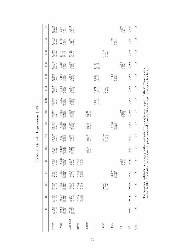
In Table 2 model (1) is the reduced benchmark model. In all models the

estimated coefficient on LY70 is always negative and that on fertility (LAFERT)

is negative in ten out of the sixteen models. The estimates then suggest the

following:

The association between the human capital variables as well as the distribu-

tional variables and growth is not very strong. Most of the coefficients on these

variables are statistically insignificant. However, even small effects may have

important and economically significant consequences in the long run.26 Bearing

in mind that due to the consistency requirement the sample size is small and

although given statistical insignificance the focus of this paper is on the point

estimates and their economic significance, but not on inferential statistics.

1) The coefficients on education are positive in all models. However, sec-

ondary education (SECP) appears to contribute more to linear ’explanations’

of long-run growth than tertiary education (TERP) or education expenditure

(GEDU). As an indication notice the relatively high R2s in models (2)-(5). For

instance, the latter models suggest that an increase of one standard deviation

25The estimate for β3 was 0.082 with a standard error of 0.378 and a t−probability of 0.832.26On the distinction between statistical and economic significance see e.g. McCloskey (1985)

or McCloskey and Ziliak (1996).

25

(11 percentage points) in the percentage of people aged 25-65 who have at least

upper secondary education (SECP) raises long-run growth by 0.3 to 0.4 per-

centage points. Models (6)-(9) suggest that growth would be raised by 0.08 to

0.1 percentage points when increasing by one standard deviation (4.8 percentage

points) the percentage of people aged 25-65 who have at least tertiary education

(TERP). In turn, a one-standard-deviation change (1.04 percentage points) of

more education expenditure would increase the growth rate by around 0.08 to

0.1 percentage points.

2) The coefficients on redistribution (RE) are ambiguous and statistically

insignificant. When controlling for SECP they are positive, but they are negative

in all other cases. All coefficients on RE suggest that it does not add much to

’explaining’ the cross-country variation in growth rates over the sample period.

3) When controlling for initial income and fertility, the coefficients on pre-

tax and on post-tax income inequality are statistically insignificant but they

are always negative, no matter whether one also controls for education (SECP,

TERP, or GEDU). For instance, when controlling for secondary education SECP

in models (2)-(5) a one-standard-deviation change in pre-tax inequality (LIS.G)

of 3.67 lowers the long-run growth rate by 0.28 percentage points. The same

change for post-tax inequality (LIS.N) amounts to 3.88 and lowers the growth

rate by 0.26. Barro (2000) p. 18 and Perotti (1996) report similar magnitudes

for these effects.

But when controlling for tertiary education (TERP) or overall spending on

education (GEDU) these effects become quite smaller. E.g. in model (11) which

controls for GEDU a one-standard-deviation change in LIS.G (LIS.N) reduces

the growth rate by only 0.06 (0.01) percentage points.

4) Pre-tax income inequality (LIS.G) appears to be more strongly, negatively

26

related to growth than post-tax income inequality (LIS.N).27

These findings suggest that more inequality in gross incomes seems to imply

lower growth for the typical country in the sample. Then the state intervenes

by redistribution. That intervention does not appear to affect growth very much

in the typical country. However, the resulting inequality in personal incomes

after taxes is still negative. But that means that the state may not have inter-

vened enough to generate a situation where after-tax income inequality would

not negatively affect growth anymore.

The negative association between pre-tax or post-tax income inequality and

growth also allows for an interpretation of results based on some forms of unad-

justed inequality measures. See Appendix A.5.

Lemma 1 If the ’true’ association between growth and pre-tax income inequality,

measured by the Gini coefficient, is negative, then the estimated coefficients on

unadjusted inequality measures based on mixes of Gini coefficients for net and for

gross incomes are most likely to be biased upwards.

This means that the estimated non-negative signs found on the coefficients

for unadjusted inequality measures used in the growth regressions of Barro (2000)

or Forbes (2000) allow for another interpretation: The ’true’ association between

pre-tax inequality and growth is negative. Post-tax inequality depends on pre-tax

inequality and redistribution. If you use the mix-generated unadjusted inequality

measure, you really run a regression on a variable containing information about

pre-tax inequality and redistribution, which - as argued before - are two different,

although related things. Thus, a positive coefficient in a growth regression may

27This may be discerned from Table 2 when comparing the estimated coefficients for pre-tax(LIS.G) and post-tax inequality (LIS.N). The ones for the latter are consistently smaller andcloser to zero than those found for LIS.G.

27

also indicate that pre-tax inequality negatively ’affects’ growth and redistribution

strongly positively ’affects’ growth. Given this interpretation the call for a re-

assessment of the inequality-growth relationship may be premature.

Determinants of Inequality. The theory argues that education spending de-

termines human capital which in turn shapes the relationship between income

inequality and growth. Table 3 presents the ’effects’ of some widely used deter-

minant factors of income inequality and redistribution.

Table 3: Determinants of Inequality (LIS)

(1) (2) (3) (4) (5) (6) (7) (8) (9)

DependentVariable LIS.G LIS.G LIS.G LIS.N LIS.N LIS.N RE RE RE

Const. −87.562(36.683)[0.038]

−79.199(35.545)[0.053]

−43.246(42.709)[0.341]

−104.390(41.330)[0.030]

−92.394(37.240)[0.035]

−59.485(45.991)[0.232]

14.814(17.153)[0.408]

11.109(16.805)[0.525]

13.734(22.422)[0.557]

LY70 10.903(3.687)[0.014]

10.627(3.527)[0.015]

7.789(3.939)[0.083]

12.268(4.154)[0.014]

11.872(3.695)[0.011]

9.275(4.241)[0.060]

−1.158(1.724)[0.517]

−1.035(1.668)[0.550]

−1.243(2.068)[0.565]

LAFERT 23.036(5.236)[0.001]

21.910(5.066)[0.002]

18.214(5.519)[0.011]

23.728(5.899)[0.002]

22.114(5.307)[0.002]

18.730(5.943)[0.014]

−0.525(2.448)[0.835]

−0.026(2.395)[0.992]

−0.296(2.897)[0.921]

CVLIB −3.163(2.289)[0.204]

−2.896(2.465)[0.274]

−0.231(1.202)[0.852]

GEDU −0.876(0.626)[0.195]

−1.438(0.722)[0.081]

−1.256(0.655)[0.088]

−1.771(0.777)[0.052]

0.388(0.296)[0.222]

0.347(0.379)[0.387]

R2 0.660 0.720 0.774 0.620 0.730 0.770 0.051 0.204 0.207

Obs. 13 13 13 13 13 13 13 13 13

OLS. Standard errors in parentheses and t-probabilities in square brackets.

These regressions indicate that initial income and fertility are negatively re-

lated to equality and redistribution. Interestingly, less civil liberties (higher

CVLIB) correlate positively with equality and negatively with redistribution.

In turn, government spending on overall education (GEDU) is consistently nega-

tively associated with pre-tax and post-tax inequality, but it is positively related to

28

redistribution. For instance, according to model (3), (6) and (9) a one-standard

deviation change (1.04 percentage points) in GEDU lowers pre-tax inequality

(LIS.G) by 1.5 percentage points, lowers post-tax inequality (LIS.N) by 1.8 per-

centage points and raises measured redistribution by 0.4 percentage points.

3.3 Sensitivity Analysis

In order to check whether the results carry over to less stringently defined data

I have used Gini coefficients for pre-tax and post-tax income provided by the

World Income Inequality Database (WIID).28 Only those coefficients of the data-

set were used that are representative of all areas and the population of a country.

The major difference from LIS is that now the data come from various sources.

In a first step only those entries were considered where the income recipient was

the household, unadjusted for its composition. In a second step a data-set was

created which does not distinguish whether and how the households have been

adjusted for their composition. Both procedures yield larger data-sets but the

results based on them are very similar. Therefore, I will only report the ones for

the first procedure here.

One difficulty with these data is that one cannot easily tell what redistribution

is, because the coefficients for gross and net income do not necessarily match. It

is possible that the time average of all the Gini coefficients for gross income of a

country, now called AIHG, are unrealistically smaller than those for net income,

called AIHN. In order to be as consistent as possible, I have only considered a

28Another sensitivity check would have been to break the LIS data up into 5 or 10 yearintervals in order to see if the results remain robust for shorter time periods. Unfortunately,this would have led to extremely small data-sets, making regression analysis almost impossible.Furthermore, the paper’s focus is on the long-run and it is, therefore, left an open questionwhether inequality and growth may be positively associated in the not so long run. For ananalysis relating inequality and growth over different time spans see e.g. Forbes (2000).

29

country’s coefficients that match in terms of time and source for the determination

of the redistribution variable RE. Interestingly, most of the entries then turn out

to originate from LIS, but for unadjusted households.

One advantage of being less stringent is that the sample size increases by up

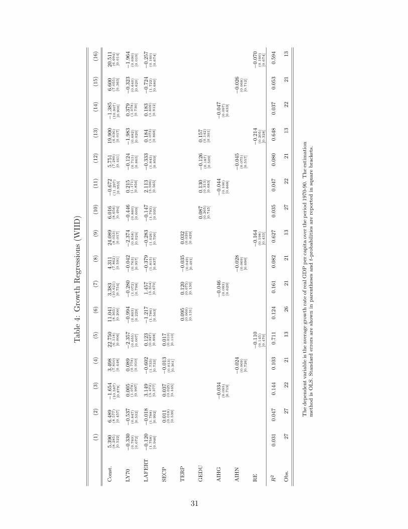
to 70 percent. Table 4 presents growth regressions using the WIID data.

Most of the coefficients are statistically insignificant. This holds even for so

called robust regressors such as fertility (LAFERT) and initial income (LY70).

The latter are, however, negatively related to growth in the majority of regres-

sions.

The educational variables (SECP, TERP, GEDU) are generally positively

related to growth, unless one controls for post-tax income inequality (AIHN).

However, the most important finding is that as with the LIS data the variables

for pre-tax inequality (AIHG) as well as those for post-tax inequality (AIHN) and

redistribution (RE) are negatively related to growth. The negative coefficients on

income inequality are generally more statistically insignificant than when using

the LIS data. Furthermore, the linear fits of most models are doing badly. As an

indication notice the R2s that are quite lower than the ones reported in Table 2.

30

Tab

le4:

Gro

wth

Reg

ress

ions

(WII

D)

(1)

(2)

(3)

(4)

(5)

(6)

(7)

(8)

(9)

(10)

(11)

(12)

(13)

(14)

(15)

(16)

Const

.5.3

90

(8.2

85)

[0.5

22]

6.4

89

(8.5

77)

[0.4

57]

−1.6

54

(10

.587)

[0.8

78]

3.4

98

(7.8

10)

[0.4

48]

22.7

50

(6.1

18)

[0.0

06]

11.0

41

(8.3

65)

[0.2

00]

3.3

83

(10

.621)

[0.7

54]

4.3

11

(7.8

62)

[0.5

91]

24.0

89

(8.0

53)

[0.0

17]

6.0

16

(8.6

56)

[0.4

94]

−0.6

72

(11

.297)

[0.9

53]

5.7

51

(7.2

80)

[0.4

41]

19.9

00

(6.6

36)

[0.0

17]

−1.3

85

(10

.907)

[0.9

00]

6.6

00

(7.0

55)

[0.3

63]

20.5

11

(6.6

94)

[0.0

14]

LY

70

−0.3

30

(0.7

69)

[0.6

72]

−0.5

37

(0.8

47)

[0.5

32]

0.0

05

(1.0

78)

[0.9

97]

0.0

89

(0.7

78)

[0.9

10]

−2.3

57

(0.6

55)

[0.0

07]

−0.9

94

(0.8

03)

[0.2

29]

−0.2

80

(1.0

72)

[0.7

98]

−0.0

42

(0.7

63)

[0.9

57]

−2.3

74

(0.8

58)

[0.0

24]

−0.4

46

(0.8

60)

[0.6

09]

0.2

15

(1.1

71)

[0.8

56]

−0.1

24

(0.7

15)

[0.8

65]

−1.9

83

(0.6

82)

[0.0

20]

0.3

79

(1.0

78)

[0.7

30]

−0.3

23

(0.6

40)

[0.6

20]

−1.9

64

(0.6

90)

[0.0

19]

LA

FE

RT

−0.1

20

(1.7

58)

[0.9

46]

−0.0

18

(1.7

88)

[0.9

92]

3.1

49

(3.4

72)

[0.3

77]

−0.6

02

(1.7

33)

[0.7

33]

0.1

23

(0.9

27)

[0.8

98]

−1.2

17

(1.7

86)

[0.5

03]

1.4

57

(3.3

54)

[0.6

70]

−0.3

79

(1.8

15)

[0.8

37]

−0.2

83

(1.0

26)

[0.7

90]

−0.1

47

(1.7

93)

[0.9

35]

2.1

13

(3.5

96)

[0.5

65]

−0.3

33

(1.8

43)

[0.8

59]

0.1

84

(1.0

73)

[0.8

68]

0.1

83

(1.6

09)

[0.9

12]

−0.7

24

(1.7

22)

[0.6

80]

−0.2

57

(0.1

60)

[0.6

74]

SE

CP

0.0

11

(0.0

18)

[0.5

39]

0.0

37

(0.0

25)

[0.1

65]

−0.0

13

(0.0

13)

[0.3

61]

0.0

17

(0.0

10)

[0.1

10]

TE

RP

0.0

95

(0.0

60)

[0.1

31]

0.1

20

(0.0

75)

[0.1

30]

−0.0

35

(0.0

49)

[0.4

91]

0.0

32

(0.0

39)

[0.4

29]

GE

DU

0.0

87

(0.2

65)

[0.7

45]

0.1

30

(0.3

13)

[0.6

83]

−0.1

26

(0.1

87)

[0.5

09]

0.1

57

(0.1

42)

[0.3

01]

AIH

G−0

.034

(0.0

95)

[0.7

19]

−0.0

46

(0.0

93)

[0.6

29]

−0.0

44

(0.1

00)

[0.6

68]

−0.0

47

(0.0

97)

[0.6

33]

AIH

N−0

.024

(0.0

69)

[0.7

26]

−0.0

28

(0.0

69)

[0.6

90]

−0.0

45

(0.0

75)

[0.5

57]

−0.0

26

(0.0

68)

[0.7

12]

RE

−0.1

10

(0.1

45)

[0.4

70]

−0.1

64

(0.1

98)

[0.4

33]

−0.2

14

(0.2

05)

[0.3

28]

−0.0

70

(0.1

60)

[0.6

74]

R2

0.0

31

0.0

47

0.1

44

0.1

03

0.7

11

0.1

24

0.1

61

0.0

82

0.6

27

0.0

35

0.0

47

0.0

80

0.6

48

0.0

37

0.0

53

0.5

94

Obs.

27

27

22

21

13

26

21

21

13

27

22

21

13

22

21

13

The

dep

enden

tvari

able

isth

eaver

age

gro

wth

rate

ofre

alG

DP

per

capit

aover

the

per

iod

1970-9

0.

The

esti

mati

on

met

hod

isO

LS.Sta

ndard

erro

rsare

show

nin

pare

nth

eses

and

t-pro

babilit

ies

are

report

edin

square

bra

cket

s.

31

The next table presents the results for the determinants of inequality. Here

the fits have quite high R2s but still most variables are statistically insignifi-

cant. Initial income (LY70) and fertility (LAFERT) are positively associated

with pre-tax (AIHG) and post-tax inequality (AIHN). In contrast to the LIS

data redistribution is now positively related to LY70 and LAFERT. See Table 3.

The important finding here is that the correlation between education spending

(GEDU) and pre-tax as well as post-tax income inequality is negative and that

between GEDU and redistribution is positive.29

As mentioned before all the results based on the WIID also hold when one

does not distinguish whether and how the households have been adjusted for their

composition.

Table 5: Determinants of Inequality (WIID)

(1) (2) (3) (4) (5) (6) (7) (8) (9)

DependentVariable AIHG AIHG AIHG AIHN AIHN AIHN RE RE RE

Const. −39.657(24.116)[0.117]

−40.871(24.886)[0.118]

−56.856(32.009)[0.094]

27.493(23.435)[0.256]

17.104(23.098)[0.469]

5.635(24.115)[0.818]

−12.468(12.625)[0.347]

−9.142(10.357)[0.400]

−19.033(11.097)[0.125]

LY70 5.525(2.209)[0.022]

5.831(2.401)[0.026]

7.275(3.014)[0.027]

−0.777(2.199)[0.728]

0.839(2.295)[0.719]

1.655(2.322)[0.486]

1.145(1.285)[0.287]

0.807(1.077)[0.473]

1.500(1.063)[0.196]

LAFERT 28.187(5.195)[0.000]

28.089(5.322)[0.000]

28.492(5.398)[0.000]

14.504(4.850)[0.008]

15.317(4.636)[0.004]

14.016(4.630)[0.008]

2.945(1.761)[0.125]

2.991(1.433)[0.066]

4.169(1.479)[0.023]

CVLIB 1.066(1.322)[0.431]

1.960(1.454)[0.197]

1.143(0.676)[0.129]

GEDU −0.279(0.737)[0.710]

−0.085(0.783)[0.915]

−0.949(0.556)[0.106]

−0.464(0.651)[0.486]

0.441(0.178)[0.035]

0.653(0.205)[0.013]

R2 0.781 0.783 0.791 0.738 0.776 0.799 0.220 0.536 0.658

Obs. 22 22 22 21 21 21 13 13 13

OLS. Standard errors in parentheses and t-probabilities in square brackets.

29The same conclusion can be reached when controlling for secondary (SECP) or tertiaryeducation (TERP) instead of education spending (GEDU). See the data appendix.

32

The sensitivity checks therefore suggest the following for the different data:

Being less consistent in the definition of key variables in order to get a larger sam-

ple and sharper results does not turn out to be a successful strategy. The results

based on the consistent data are broadly sharper in that the regression coeffi-

cients are usually more statistically significant and the regressions feature higher

R2s. But for both data-sets the association between distribution and growth as

well as distribution and education (finance) is generally found to be statistically

insignificant. However, there is some indication that income inequality before and

after taxes but also redistribution as measured here is bad for long-run growth.

Furthermore, more education and more resources spent on it are usually found

to be beneficial for long-run growth. They also seem to reduce income inequality

and are positively related to redistribution.

3.4 The Role of the Schooling Technology

A common measure of the (internal) inefficiency in schooling is the dropout rate

of students enrolled in particular educational programmes. Recently, the OECD

has provided data on dropout rates for students enrolled at the university-level

tertiary education, covering many OECD countries for the 1990s.30 These data

are used here under the heroic assumption that differences in these rates reflect

structural differences that have not changed much across countries and over a long

time horizon. Furthermore, it should be viewed as a composite index depending

on c and ε. Thus, the results below depend on these assumptions and are therefore

only suggestive.

30The World Bank and UNESCO also provide data on these rates for some coun-tries, but unfortunately only up to 8th grade and excluding important countries like theU.S. For more information consult: www.worldbank.org/data/wdi2000/pdfs/tab2 11.pdf andunescostat.unesco.org/en/stats/stats0.htm.

33

Dropout rates are available for ten of the countries in the LIS sample. In

order to relate consistently to the earlier findings based on the larger LIS sample

of 13 countries, the dropout rates for Norway, Sweden and Canada have been

set at the average dropout rate (30.1) of the sample excluding these countries.

The data appendix shows that all the results below would remain valid when

working with the reduced LIS sample of ten countries. Furthermore, it discusses

the sensitivity of the results to other interpolations.

Table 6 presents regression results when controlling for policy changes by

means of interaction terms. These capture how differences in structure affect

differences in policy.

Table 6: Determinants of Inequality and Growth 2 (LIS)

(1) (2) (3) (4) (5) (6) (7) (8)

DependentVariable LIS.G LIS.G LIS.N LIS.N RE RE G70-90 G70-90

Constant 68.567(20.248)[0.008]

93.025(44.176)[0.065]

60.354(23.019)[0.028]

84.568(46.297)[0.101]

8.960(5.833)[0.159]

10.267(12.523)[0.434]

0.635(3.795)[0.871]

−6.650(7.605)[0.405]

DROP −1.123(0.583)[0.086]

−1.753(1.403)[0.243]

−0.958(0.663)[0.183]

−1.538(1.470)[0.323]

−0.190(0.168)[0.288]

−0.274(0.398)[0.509]

0.044(0.109)[0.696]

0.270(0.242)[0.293]

TERP −3.117(1.663)[0.094]

−2.879(1.890)[0.162]

−0.305(0.479)[0.540]

0.194(0.312)[0.550]

TERP*DROP 0.094(0.048)[0.083]

0.085(0.055)[0.155]

0.011(0.014)[0.438]

−0.006(0.009)[0.520]

GEDU −12.267(8.871)[0.200]

−11.549(9.297)[0.246]

−1.104(2.515)[0.671]

1.938(1.527)[0.236]

GEDU*DROP 0.353(0.284)[0.245]

0.319(0.298)[0.312]

0.047(0.081)[0.572]

−0.061(0.049)[0.246]

R2 0.309 0.265 0.216 0.291 0.269 0.248 0.147 0.235

Obs. 13 13 13 13 13 13 13 13

OLS. Standard errors in parentheses and t-probabilities in square brackets.Means: µTERP = 14.80, µGEDU = 5.62, µDROP = 30.1

In terms of the paper’s theory the coefficients on these terms can take any

34

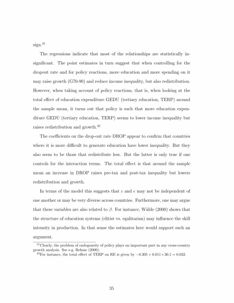
sign.31

The regressions indicate that most of the relationships are statistically in-

significant. The point estimates in turn suggest that when controlling for the

dropout rate and for policy reactions, more education and more spending on it

may raise growth (G70-90) and reduce income inequality, but also redistribution.

However, when taking account of policy reactions, that is, when looking at the

total effect of education expenditure GEDU (tertiary education, TERP) around

the sample mean, it turns out that policy is such that more education expen-

diture GEDU (tertiary education, TERP) seems to lower income inequality but

raises redistribution and growth.32

The coefficients on the drop-out rate DROP appear to confirm that countries

where it is more difficult to generate education have lower inequality. But they

also seem to be those that redistribute less. But the latter is only true if one

controls for the interaction terms. The total effect is that around the sample

mean an increase in DROP raises pre-tax and post-tax inequality but lowers

redistribution and growth.

In terms of the model this suggests that c and ε may not be independent of

one another or may be very diverse across countries. Furthermore, one may argue

that these variables are also related to β. For instance, Walde (2000) shows that

the structure of education systems (elitist vs. egalitarian) may influence the skill

intensity in production. In that sense the estimates here would support such an

argument.

31Clearly, the problem of endogeneity of policy plays an important part in any cross-countrygrowth analysis. See e.g. Rehme (2000).

32For instance, the total effect of TERP on RE is given by −0.305 + 0.011 ∗ 30.1 = 0.032.

35

4 Concluding Remarks

This paper argues that education directly affects growth and income inequality.

In the model pre-tax and post-tax income inequality - measured by the Gini

coefficient - as well as growth are first increasing and then decreasing in education.

It is shown that a less efficient schooling system would require more redistributive

education expenditure for a given level of education.

The data, which are based on consistent concepts for the measurement of

inequality, provide some evidence that, when controlling for various factors such

as initial income or fertility, long-run growth is higher for countries that (a) spend

more on education, (b) have lower pre-tax and lower post-tax income inequality.

The data also suggest that countries with a more productive, public education

technology exhibit lower income inequality and higher growth. The paper does

not find an indication that higher pre-tax or post-tax income inequality is good

for growth in rich countries.

The consistent negative relation between pre-tax and post-tax inequality and

growth in the data suggests that mixing Gini coefficients based on gross or on

net incomes is most likely to produce an upward bias when measuring the effect

of unadjusted measures of inequality on growth.

It also indicates that if a rich country spent more on public education it

could raise growth and lower pre-tax and post-tax inequality, given its education

technology.

However, a more precise disentanglement of the interaction between educa-

tion policy and education technology, and their effects on growth and inequality

appears to be called for and should be an interesting topic for further research.

36

A Technical Appendix

A.1 An Alternative OLG Set-Up

The assumption of unequal capital ownership may also be justified as follows: Consider a two-period OLG model, where each agent has one offspring. Assume that establishing a firm requiresa certificate which is related to education. At each moment the government picks some (newborn, no matter whether the parents are high or low-skilled) people to be educated in period1, who complete their degrees and open up their own firms in period 2. Those who are notpicked go to the same school but attend lower level courses in period 1, and consequently workas low-skilled workers in period 2. This means that old (dying) high-skilled people only pass oncapital to high skilled people, but never to low-skilled people, including their own (potentially)low skilled offspring. For if they did, the latter would not be allowed or be capable to operatethe firm and capital would depreciate instantaneously. This would mean that passing on capitalfrom a (dying) high-skilled entrepreneur to a low-skilled offspring who can only ’eat’ the capitalwould not be in the interest of all the other agents. The other low-skilled (offspring) would notlike it, because it would reduce their steady state wages. The high skilled (offspring) wouldnot like it because they would have to share less capital. By assumption the representativegovernment is taken to pass legislation to forbid such inefficient transfers.

A.2 Technology

By assumption Yt = AtHαt K1−α

t , where the index of effective labour H depends on labourrequiring basic skills (B) and labour requiring high skills (S). Labour requiring basic skillsis performed by high and low-skilled persons, B = B(Ll, Lh), whereas high-skilled labour isonly performed by high-skilled persons, S = S(Lh). High and low-skilled people are perfectsubstitutes to each other when performing basic skill (routine) tasks, i.e. B(Ll, Lh) = Ll + Lh.Thus, high-skilled people also perform those routine tasks a low-skilled person may do.33 On theother hand, only high-skilled people can perform high-skilled tasks (labour) and for simplicitylet S(Lh) = Lh. To capture the relationship between labour inputs assume H = [Bρ + βSρ]

1ρ =

[(Lh + Ll)ρ + βLρ

h]1ρ , where β measures the productivity with which tasks requiring high skills

contributes to the generation of output. For ρ < 1 labour requiring basic skills (B) and labourrequiring high skills (S) are imperfect (less than perfect) substitutes. For ease of calculationslet ρ = α < 1 which yields equation (1).

33For instance, Lindbeck and Snower (1996) show that firms may organize production sothat people perform one particular task (Tayloristic organization) or various tasks (holisticorganization). In the model only high-skilled people are capable of performing several tasksand firms use a mixture of Tayloristic and holistic organization.

37

A.3 Discrete Time Justification for x =(

τc

)ε

Equation (2) is compatible with many models that also use high-skilled labour as an inputgenerating education. For instance, let ht denote the total stock of human capital in theeconomy in a discrete time model. Assume that human capital evolves according to ht+1 =f(Gt,Kt, ht)ht where new human capital ht+1 is produced by non-increasing returns. Seee.g. Azariadis and Drazen (1990). Here human capital formation would depend on the level ofthe stock of knowledge ht, government resources provided for education Gt and the tax basertKt. The function f(·) governs the evolution of human capital. Assume that it is separable inthe form f(g(Gt, rtKt), ht). Let g = q

[Gt

rtKt

]= q(τ) and for simplicity

ht+1 = q(τ) hβt , where q ≥ 0, q′ > 0, q′′ ≤ 0, 0 < β < 1.

where β measures the productivity of the education sector and q(τ) captures the quality ofeducation, depending on the government resources channelled into education. See, for example,eqns. (1), (2) in Glomm and Ravikumar (1992).

In the model human capital is carried discretely so ht = xtN . Normalize population bysetting N = 1. Then total human capital at date t is given by xt. In steady state x = xt = xt+1

and so x = q(τ)1

1−β . Next suppose that the quality of education is described by q(τ) = τµ whereτ = τ

c denotes the efficiently used resources in education and 0 < µ < 0. For non-increasingreturns to scale it is necessary that µ + β ≤ 1. Let µ

1−β ≡ ε then the more explicit set-upwould be equivalent to (2) in steady state. As xε < 0, any increase ε would mean that lesshuman capital is generated in steady state. From non-increasing returns to scale it follows thatµ ≤ 1− β so that ε ≤ 1.

A.4 Calibration

Following Mankiw (1995) a high skilled worker is taken to earn three times as much as a lowskilled worker. As the correlation between total government spending and the share of thepopulation with tertiary education is quite high and given the data for the internal efficiencyin tertiary education, the paper calibrates the model for the share of the population that hastertiary education. The mean in the sample is 0.15. (See Table 7.) Thus, β satisfies

(1 + 0.15α−1) =wh

wl= 3.0 (A1)

I assume α = 0.7 so that β = 1.13. The capital/output ratio is taken be equal 3.0 so that

Y

K= A(1 + βxα) (A2)

from which A = 0.26. The discount factor ρ is set at 0.01. To get an estimate of the efficiencyc and of the productivity ε in schooling I have proceeded as follows:

The total government spending on education in terms of GDP (GEDU) is related to τ byτ = gx

YrK where gx is proxied by GEDU. Since Y

rK = 11−α = 10

3 the data imply a value of

38

τ = 0.18. I have then used the variable DROP to get an estimate of the efficiency of resourcesused in education. More precisely, I have taken 1 − DROP

100 as a measure of 1c . From the

regression lnTERP = constant + β1 ln( τc ) the resulting β1 provides one with an estimate of ε

in x =(

τc

)ε and is given by ε = 0.58.I have then chosen φ so that the ratio of the Gini coefficients before and after taxes is

87 percent as in the data and so that their difference is around 4 percentage points. The φ

necessary for that is φ = 0.13. Lastly, calibrating the growth rate required ν = 3.65 implyingan intertemporal elasticity of substitution of around 27 percent.

A.5 Unadjusted Inequality Measures

Suppose you mix Gini coefficients for net and gross incomes to get an unadjusted inequalityindex I which is then used in growth regressions.

The model really run: γui = a + b Gg

i + c Gni + εi

The model run: γui = a′ + b′i I(Gg

i , Gni ) + ε′i

where γui is the residual of the regression of γi on a vector of control variables. For simplicity

assume that the control variables are not correlated or even orthogonal to the distributionalvariables. Commonly γu

i is called the unexplained part of the growth rate. The latter isattempted to be explained by I() in the models above. In general, Gg

i = Gni +RA

i for country i.This is true by the definition of RA

i as a measure of redistribution. Not every observation in Ggi

may necessarily have a corresponding matching value of Gni in the data set. However, values

of Gni are included by many NCV proponents in order to boost the number of observations.

Now what is basically done is to create Ii = Ggi + Gn

i . But this means Ii = Ggi + Gg

i − RAi

where Ggi and RA

i may be unknown if there is no matching value for Ggi available in the

data set. This implies that their estimate for b′, call it b′, would contain information of thedistribution of gross incomes, but also information on redistribution. Thus, the model they runis γu

i = a + b Ggi + c Gg

i − c RAi + εi which puts a restriction on the effect that RA

i exerts.Relaxing it and noting that Gg

i and RAi are unknown, when there are no matching values in Gg

i ,the regression is really run on values of known Gini coefficients for gross incomes, some unknownGini values for gross income and some unknown values for redistribution. But consequentlytheir ’true’ model is

γui = a + b Gg

i + c Ggi + d RA

i + εi

where d = −c. But this suggests the following argument: The estimates for b and c have oftenbeen found to be negative in earlier contributions. Furthermore, there is an empirical literaturethat shows that the estimate for d is likely to be positive. Thus, you have an upward bias forthe estimate of b′. This bias may be so strong that you may even get a positive estimate forb′ = b + c + d, that is, b′ ≥ 0 is compatible with b < 0, c < 0 and d > 0.

39

References

Acemoglu, D., “Why Do New Technologies Complement Skills? Directed Technical Changeand Wage Inequality,” Quarterly Journal of Economics, 1998, 113, 1055–1089.

Aghion, P., E. Caroli, and C. Garcıa-Penalosa, “Inequality and Economic Growth: ThePerspective of the New Growth Theories,” Journal of Economic Literature, 1999, 37,1615–1660.

Alesina, A. and D. Rodrik, “Distributive Politics and Economic Growth,” Quarterly Journalof Economics, 1994, 109, 465–490.

Amiel, Y. and F. A. Cowell, Thinking about Inequality, Cambridge, UK: Cambridge Uni-versity Press, 1999.

Atkinson, A. B., “On the Measurement of Inequality,” Journal of Economic Theory, 1970,2, 244–263.

, The Economics of Inequality, 2nd ed., Oxford: Clarendon Press, 1983.

and A. Brandolini, “Promise and Pitfalls in the Use of ”Secondary” Data-Sets: IncomeInequality in OECD Countries as a Case Study,” Journal of Economic Literature, 2001,39, 771–799.

Autor, D., A. Krueger, and L. Katz, “Computing Inequality: Have Computers Changedthe Labour Market,” Quarterly Journal of Economics, 1998, 63, 1169–1213.

Azariadis, C. and A. Drazen, “Threshold Externalities in Economic Development,” Quar-terly Journal of Economics, 1990, 105, 501–526.

Banerjee, A., M. Marcellino, and C. Osbat, “Some Cautions on the Use of Panel Methodsfor Integrated Series of Macro-Economic Data,” Working Paper 170, IGIER, BocconiUniversity, Milano 2000.

Banerjee, A. V. and E. Duflo, “Inequality and Growth: What Can the Data Say?,” WorkingPaper 7793, NBER 2000.

Barro, R. J., Determinants of Economic Growth: A Cross-Country Empirical Study, Cam-bridge, Mass.: MIT Press, 1997.

, “Inequality and Growth in a Panel of Countries,” Journal of Economic Growth, 2000, 5,5–32.

and J.-W. Lee, “Sources of Economic Growth,” Carnegie Rochester Conference Serieson Public Policy, 1994, 40, 1–46.

Beaudry, P. and D. Green, “The Changing Structure of Wages in the US and Germany:What Explains the Difference?,” Working Paper 7697, NBER 2000.

Benabou, R., “Inequality and Growth,” in B. S. Bernanke and J. J. Rotemberg, eds., NBERMacroeconomics Annual 1996, Cambridge and London: MIT Press, 1996, pp. 11–73.

, “Unequal Societies: Income Distribution and the Social Contract,” American EconomicReview, 2000, 90, 96–129.

Bertola, G., “Factor Shares and Savings in Endogenous Growth,” American Economic Review,1993, 83, 1184–1198.

, “Macroeconomics of Distribution and Growth,” in A. B. Atkinson and F. Bourguignon,eds., Handbook of Income Distribution, Vol. 1, Amsterdam: Elsevier, 2000, pp. 477–540.

40

Bound, J. and G. Johnson, “Changes in the Structure of Wages in the 1980s: An Evaluationof Alternative Explanations,” American Economic Review, 1992, 82, 371–392.

Buttner, T. and B. Fitzenberger, “Central Wage Bargaining and Local Wage Flexibility:Evidence from the Entire Wage Distribution,” Discussion Paper 98-39, ZEW, Mannheim1998.

Caselli, F., “Technological Revolutions,” American Economic Review, 1999, 89, 78–102.

, G. Esquivel, and F. Lefort, “Reopening the Convergence Debate: A New Look atCross-Country Growth Empirics,” Journal of Economic Growth, 1996, 1, 363–389.

Chiu, W. H., “Income Inequality, Human Capital Accumulation and Economic Performance,”Economic Journal, 1998, 108, 44–59.

Ciccone, A., G. Peri, and D. Almond, “Capital, Wages, and Growth: Theory and Evi-dence,” Working Paper 152, IGIER, Bocconi University, Milano 1999.

Cowell, F. A., Measuring Inequality, 2nd ed., Hemel Hempstead, UK: Prentice Hall/HarvesterWheatsheaf, 1995.

de la Fuente, A. and R. Domenech, “Human Capital in Growth Regressions: How MuchDifference Does Data Quality Make?,” Working Paper 262, OECD 2000.

Deininger, K. and L. Squire, “A New Data Set Measuring Income Inequality,” World BankEconomic Review, 1996, 10, 565–591.

and , “New Ways of Looking at Old Issues: Inequality and Growth,” Journal ofDevelopment Economics, 1998, 57, 259–287.

Easterly, W. and S. Rebelo, “Fiscal policy and economic growth. An empirical investiga-tion,” Journal of Monetary Economics, 1993, 32, 417–458.

Eicher, T. and C. Garcıa-Penalosa, “Inequality and Growth: The Dual Role of HumanCapital in Development,” Journal of Development Economics, 2001, 66, 173–197.

Fernandez, R. and R. Rogerson, “Public Education and Income Distribution: A DynamicQuantative Evaluation of Education-Finance Reform,” American Economic Review, 1998,88, 813–833.

Fields, G. S., “Measuring inequality change in an economy with income growth,” Journal ofDevelopment Economics, 1987, 91, 611–625.

Figini, P., “Inequality and Growth Revisited,” Discussion Paper 99/2, Trinity College, Dublin,Ireland 1999.

Forbes, K. J., “A Reassessment of the Relationship between Inequality and Growth,” Amer-ican Economic Review, 2000, 90, 869–887.

Galor, O. and D. Tsiddon, “Technological Progress, Mobility, and Economic Growth,”American Economic Review, 1997, 87, 363–382.

and J. Zeira, “Income Distribution and Macroeconomics,” Review of Economic Studies,1993, 60, 35–52.

Glomm, G. and B. Ravikumar, “Public versus Private Investment in Human Capital:Endogenous Growth and Income Inequality,” Journal of Political Economy, 1992, 100,818–834.

Goodspeed, T. J., “Education Spending, Inequality and Economic Growth: Evidence fromUS States,” mimeo, Hunter College - CUNY, New York 2000.

41

Johnson, G. E., “Subsidies for Higher Education,” Journal of Labor Economics, 1984, 2,303–318.

Jovanovic, B., “Growth Theory,” Working Paper 7468, NBER 2000.

Katz, L. F. and K. M. Murphy, “Changes in Relative Wages, 1963-1987: Supply andDemand Factors,” Quarterly Journal of Economics, 1992, 107, 35–78.

Krusell, P., L. E. Ohanian, J.-V. Rıos-Rull, and G. L. Violante, “Capital-Skill Com-plementarity and Inequality: A Macroeconomic Analysis,” Econometrica, 2000, 68, 1029–1053.

Kuznets, S., “Economic growth and income inequality,” American Economic Review, 1955,45, 1–28.

Lambert, P. J., The Distribution and Redistribution of Income: A Mathematical Analysis,2nd ed., Manchester, UK: Manchester University Press, 1993.

Lee, W. and J. E. Roemer, “Income Distribution, Redistributive Politics, and EconomicGrowth,” Journal of Economic Growth, 1998, 3, 217–240.

Li, H. and H.-F. Zou, “Income Inequality is Not Harmful for Growth: Theory and Evidence,”Review of Development Economics, 1998, 2, 318–34.

Lindbeck, A. and D. J. Snower, “Reorganization of Firms and Labour-Market Inequality,”American Economic Review, Papers and Proceedings, 1996, 86, 315–321.

Mankiw, N. G., “The Growth of Nations,” Brookings Papers on Economic Activity, 1995, 1,275–310.

McCloskey, D. N., “The Loss Function Has Been Mislaid: The Rhetoric of SignificanceTests,” American Economic Review, 1985, 75, 201–205.

and S. T. Ziliak, “The Standard Error of Regressions,” Journal of Economic Literature,1996, 34, 97–114.

Murphy, K. M., W. C. Riddel, and P. M. Romer, “Wages, Skills, and Technology in theUnited States and Canada,” Working Paper 6638, NBER 1998.

Perotti, R., “Political Equilibrium, Income Distribution, and Growth,” Review of EconomicStudies, 1993, 60, 755–776.

, “Income distribution and investment,” European Economic Review, 1994, 38, 827–835.

, “Growth, Income Distribution, and Democracy: What the Data Say,” Journal of Eco-nomic Growth, 1996, 1, 149–187.

Persson, T. and G. Tabellini, “Is Inequality Harmful for Growth?,” American EconomicReview, 1994, 84, 600–621.

Rehme, G., “Education, Economic Growth and Personal Income Inequality Across Countries,”Working Paper ECO 99/42, European University Institute, Florence, Italy 1999.

, “Economic Growth and (Re-)Distributive Policies: A Comparative Dynamic Analysis,”Working Paper ECO 00/13, European University Institute, Florence, Italy 2000.

Romer, P. M., “Increasing Returns and Long-Run Growth,” Journal of Political Economy,1986, 94, 1002–1037.

Saint-Paul, G. and T. Verdier, “Inequality, Redistribution and Growth: A Challenge tothe Conventional Political Economy Approach,” European Economic Review, 1996, 40,719–728.

42

Sala-i-Martin, X., “A Positive Theory of Social Security,” Journal of Economic Growth, 1996,1, 277–304.

Shorrocks, A. F., “Ranking Income Distributions,” Economica, 1983, 50, 1–17.

Summers, R. and A. Heston, “The Penn World Table (Mark 5): An Expanded Set ofInternational Comparisons, 1950-1988,” Quarterly Journal of Economics, 1991, 106, 327–368.

Temple, J., “The New Growth Evidence,” Journal of Economic Literature, 1999, 37, 112–156.

Tinbergen, J., Income Distribution: Analysis and Policies, Amsterdam: North-Holland, 1975.

Walde, K., “Egalitarian and Elitist Education Systems as the Basis for Inernational Differ-ences in Wage Inequality,” European Journal of Political Economy, 2000, 16, 445–468.

Zweimuller, J., “Redistribution, Inequality and Growth,” Empirica, 2000, 27, 1–20.

43

2 Data Appendix

Data Sources

• Barro and Lee (1994). Web site: www.nber.org/data/.

• Summers and Heston (1991): Penn World Table (Mark 5.6). Web site:www.nber.org/data/.

• OECD Education Database: Education at a Glance 1998, Table A1.

• OECD Education Database: Education at a Glance 2000, Table C4.1.

• Deininger and Squire (1996). Web site:www.worldbank.org/research/growth/dddeisqu.htm.

• Luxembourg Income Study. Web site: www.lisproject.org.

• World Income Inequality Database (WIID). Web site:www.wider.unu.edu/wiid/wiid.htm

Definition of variables34

G70-90 Average growth rate of real GDP per capita for the period 1970-1990 in percentage points,

where G70-90 = ln yT−ln y0T

and yT denotes per capita GDP at final date T . (Source: Penn

World Tables, Mark 5.6.)

SECP Percentage of the population from 25 to 64 years of age who have attained at least upper

secondary education, 1996. (Source: OECD, 1998)

TERP Percentage of the population from 25 to 64 years of age who have attained at least university-

level education, 1996. (Source: OECD, 1998)

LIS.G Average Gini coefficient for gross income of households (adjusted for household size by the

square root of the number of household members) for the period 1970-1990. (Source: Lux-

embourg Income Study)

AIHG Average Gini coefficient for gross income of households for the period 1970-1990 (Source:

WIID)

LIS.N Average Gini coefficient for net income of households (adjusted for household size by the

square root of the number of household members) for the period 1970-1990. (Source: Lux-

embourg Income Study)

AIHN Average Gini coefficient for net income of households for the period 1960-1990 (Source:

WIID)

LY70 Natural logarithm of the level of real GDP per capita in 1970. (Source: Penn World Tables,

Mark 5.6; Variable: RGDPL, i.e. real GDP per capita in 1985 international prices.)

AFERT Average fertility rate (children per woman) for the period 1960-84. (Source: Barro-Lee).

GEDU Government expenditure on education as a fraction of GDP for the period 1960-1985 in

percentage points. (Source: Barro-Lee)

CVLIB Gastil’s index of civil liberties (from 1 to 7; 1 = most freedom) for the period 1972-1989.

(Source: Barro-Lee)

DROP Drop-out rates at the university-level tertiary education from 1985-96. (Source: OECD 2000)

34 A more detailed description of the data and the results is provided at:http://www.tu-darmstadt.de/∼rehme/project/data01.htm.

44

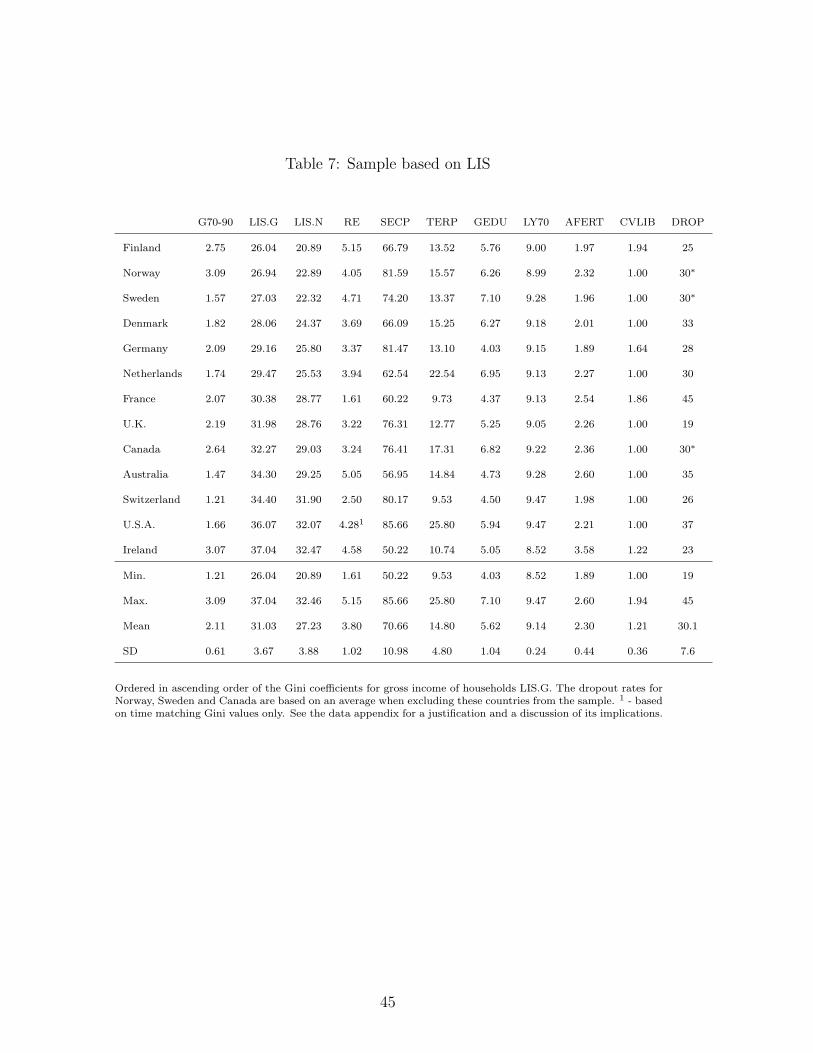
Table 7: Sample based on LIS

G70-90 LIS.G LIS.N RE SECP TERP GEDU LY70 AFERT CVLIB DROP

Finland 2.75 26.04 20.89 5.15 66.79 13.52 5.76 9.00 1.97 1.94 25

Norway 3.09 26.94 22.89 4.05 81.59 15.57 6.26 8.99 2.32 1.00 30∗

Sweden 1.57 27.03 22.32 4.71 74.20 13.37 7.10 9.28 1.96 1.00 30∗

Denmark 1.82 28.06 24.37 3.69 66.09 15.25 6.27 9.18 2.01 1.00 33

Germany 2.09 29.16 25.80 3.37 81.47 13.10 4.03 9.15 1.89 1.64 28

Netherlands 1.74 29.47 25.53 3.94 62.54 22.54 6.95 9.13 2.27 1.00 30

France 2.07 30.38 28.77 1.61 60.22 9.73 4.37 9.13 2.54 1.86 45

U.K. 2.19 31.98 28.76 3.22 76.31 12.77 5.25 9.05 2.26 1.00 19

Canada 2.64 32.27 29.03 3.24 76.41 17.31 6.82 9.22 2.36 1.00 30∗

Australia 1.47 34.30 29.25 5.05 56.95 14.84 4.73 9.28 2.60 1.00 35

Switzerland 1.21 34.40 31.90 2.50 80.17 9.53 4.50 9.47 1.98 1.00 26

U.S.A. 1.66 36.07 32.07 4.281 85.66 25.80 5.94 9.47 2.21 1.00 37

Ireland 3.07 37.04 32.47 4.58 50.22 10.74 5.05 8.52 3.58 1.22 23

Min. 1.21 26.04 20.89 1.61 50.22 9.53 4.03 8.52 1.89 1.00 19

Max. 3.09 37.04 32.46 5.15 85.66 25.80 7.10 9.47 2.60 1.94 45

Mean 2.11 31.03 27.23 3.80 70.66 14.80 5.62 9.14 2.30 1.21 30.1

SD 0.61 3.67 3.88 1.02 10.98 4.80 1.04 0.24 0.44 0.36 7.6

Ordered in ascending order of the Gini coefficients for gross income of households LIS.G. The dropout rates forNorway, Sweden and Canada are based on an average when excluding these countries from the sample. 1 - basedon time matching Gini values only. See the data appendix for a justification and a discussion of its implications.

45