SFB 823

Government spending shocks and labor productivity

Discussion P

aper

Ludger Linnemann, Gábor B. Uhrin, Martin Wagner

Nr. 9/2016

Government spending shocks and labor productivity

Ludger Linnemann∗ Gabor B. Uhrin† Martin Wagner‡

February 3, 2016

Abstract

A central question in the empirical fiscal policy literature is the magnitude, in fact even

the sign, of the fiscal multiplier. Standard identification schemes for fiscal VAR models

typically imply positive output as well as labor productivity responses to expansionary

government spending shocks. The standard macro assumption of decreasing returns to

labor, however, implies that expansionary government spending shocks should lead to

increasing output and hours, but to decreasing labor productivity. To potentially reconcile

theory and empirical analysis we impose, amongst other sign restrictions, opposite signs

of the impulse responses of output and labor productivity to government spending shocks

in eight- to ten-variable VAR models, estimated on quarterly US data. Doing so leads to

contractionary effects of positive government spending shocks. This potentially surprising

finding is robust to the inclusion of variable capital utilization rates and total factor

productivity.

JEL Classification: E32, E62, C32

Keywords: Fiscal policy, labor productivity, sign restrictions, structural VAR models

∗Corresponding author: Department of Economics, Technical University Dortmund, Vogelpothsweg 87,D-44221 Dortmund, Germany, email: ludger.linnemann@tu-dortmund.de, tel: +49/231/755-3102.

†Faculty of Economics, University of Gottingen.‡Faculty of Statistics, Technical University Dortmund; Institute for Advanced Studies, Vienna; Bank of

Slovenia, Ljubljana.

1

1 Introduction

There is a large empirical literature (starting with Blanchard and Perotti, 2002) that uses

structural VAR models to estimate the effects of shocks to government spending on the busi-

ness cycle. A particular focus of this literature is on the identification of the fiscal multiplier,

i.e., the effect of changes in government spending on aggregate output. Empirically, most

studies find that an unexpected increase in government spending raises real output for at least

a number of quarters, though the exact size of the multiplier is controversial. The central

problem for the empirical fiscal policy literature is, of course, the problem of identification of

exogenous changes in government spending. There is no consensus in the literature concern-

ing which set of identifying restrictions should be used to disentangle government spending

shocks from other shocks that affect cyclical variations in macroeconomic data.

In this paper, we propose to use the response of (hourly) labor productivity to help

identify government spending shocks. The basic idea is straightforward: Consider the fiscal

transmission mechanism that is embedded in most current DSGE models. If the government

unexpectedly increases its spending, the resulting intertemporal tax burden imparts a neg-

ative wealth effect on households, which consequently expand their labor supply. Since the

capital stock is predetermined in the short run, under a standard constant returns to scale

aggregate production function there are decreasing returns to labor. As a consequence, the

fiscal expansion should be associated with rising hours and output, but with decreasing hourly

productivity.1 Based on this stylized observation, we propose to use the restriction that out-

put and labor productivity should respond with opposite signs as one of the identification

conditions in a sign restricted VAR model.

We first review some popular alternative ways of identifying government shocks, namely

that of Blanchard and Perotti (2002) who rely on a recursive ordering where government

spending is assumed to be exogenous within the quarter; and the one proposed by Ramey

(2011) who additionally controls for anticipation effects by estimating responses to the in-

novations to her narrative measure of the present discounted value of expected military ex-

penditures. We demonstrate that either of these approaches implies an increase in labor

productivity after a positive government spending shock in quarterly US macroeconomic

data, opposite to the theoretical expectation based on the standard view of the fiscal trans-

mission mechanism. Utilizing the above considerations on the relation between output and

productivity responses to government spending shocks we estimate several variants of sign

1We consider the alternative possibility that government spending is productive in the sense of immediatelyshifting the aggregate production function unlikely for reasons discussed in section 3.2.

2

restricted VAR models for US quarterly macroeconomic time series. Sign restrictions have

been used earlier in the literature on fiscal policy effects, e.g., by Mountford and Uhlig (2009)

or Pappa (2009). The distinctive feature of our approach is the use of a sign restriction

invoking the response of labor productivity that forces the estimated government spending

shock responses to be compatible with the existence of an aggregate production function with

constant returns to scale. In particular, we identify a government spending shock through

the restrictions that the resultant impulse responses lead to positive comovement between

government spending and public deficits, positive comovement between hours and output,

and negative comovement between output (or hours) and labor productivity.

Using these restrictions, we find that the median target impulse response, as defined in

detail in appendix A, of private (non-farm business) output to a positive shock to government

spending is negative. Since negative output reactions to government spending increases are

in obvious contradiction to the consensus in the previous empirical literature, we undertake

various robustness checks. In particular, we allow for cyclical capital utilization, and also

include a measure of total factor productivity. The basic result remains: as soon as we impose

that productivity and output have to comove negatively after government spending shocks,

the median target impulse response implies a negative output reaction. Bootstrap confidence

bands around the median target impulse response indicate that this negative response is

statistically significantly different from zero for several periods.

Note that there are two possible interpretations of our result: First, it could be the case

that government spending shocks do indeed have negative short run consequences for output

and hours. In this case, one would have to assume that other identification schemes leading

to the opposite result tend to confound the fluctuations due to government spending shocks

with those due to other disturbances, e.g. technology shocks. Second, the transmission of

government spending shocks needs to be analyzed in a setting featuring increasing returns to

scale, since the data do not appear to be compatible with the combination of positive output

effects of government spending and a constant returns to scale production function.

The empirical result that government spending seems to increase labor productivity is, of

course, related to a finding emphasized earlier in the literature, viz., that positive government

spending shocks appear to have a positive effect on the real wage rate (e.g., Perotti, 2007,

Monacelli and Perotti, 2008). With decreasing returns to labor, the real wage is, from a

theory perspective, expected to fall if a government spending shock induces increasing labor

supply. However, several authors, e.g., Hall (2009), Monacelli and Perotti (2008), or Ravn et

al. (2007), have pointed out that higher wages may be compatible with higher employment if

3

the price-marginal cost markup that imperfectly competitive firms charge declines in response

to higher government spending. The point emphasized in the present paper is that even if

declining markups make rising employment compatible with higher real wages, the increase in

labor productivity that is also present in the data can still not be explained. Put differently,

whatever the behavior of the markup is, it does not contribute to solving the question how

sizably more output can be produced, following a government spending shock, with labor

input changing only weakly.

Methodologically, we essentially use sign restrictions to impose a log-linear approxima-

tion to a standard neoclassical production function on the impulse responses. We propose

to view this method as a combination of the a-theoretical nature of VAR modelling with a

structural assumption concerning an aggregate production function underlying the US econ-

omy, whilst leaving all other equations unrestricted. This approach is similar in spirit to

Arias et al. (2015), who use sign (and zero) restrictions to constrain impulse responses in a

monetary VAR model such that they are compatible with a plausible central bank reaction

function. Whereas Arias et al. (2015) require impulse responses to a monetary policy shock to

reproduce a standard monetary policy rule, we impose a standard production function on the

impulse responses to distinguish demand side disturbances, like government spending shocks,

from supply side shifts in the production function itself. In both instances, the idea is to

use only the structural information from relatively uncontroversial parts of a macroeconomic

model that is implicitly thought of as the data generating process.

The paper proceeds as follows. In section 2, we discuss the sign restrictions that are

used for identification of government spending shocks in more detail. In section 3, we first

demonstrate the tendency for procyclical productivity responses under the Blanchard and

Perotti (2002) and Ramey (2011) identifications of government spending shocks. We then

discuss possible interpretations and present our own results based on sign restrictions. Finally,

we show the central result to be robust to the inclusion of cyclical capacity utilization and total

factor productivity. When including both additional variables we combine sign restrictions

with standard short run (point) restrictions. Section 4 concludes. Two appendices follow the

main text. Appendix A presents some details of the econometric approach and appendix B

contains some further results.

2 Government spending shocks and labor productivity

Our main goal is to distinguish empirically between the effects of government spending shocks

and of productivity shocks on the private business sector. To this end, we start by assuming

4

that private (i.e., non-farm business) sector output Yt is generated by a constant returns to

scale production function that is standard in macroeconomics, i.e.,

Yt = F (Zt,Ht, St), (1)

where Zt is unobservable technology, Ht is labor input (measured in hours worked in the non-

farm business sector), and St are the services derived from the installed capital stock. We

concentrate on a log-linear approximation to this production function, where log-deviations

from the balanced growth path are denoted by lower case letters. The log-linear representation

of the production function is:

yt = zt + aht + (1− a)st, (2)

with a ∈ (0, 1). This representation is exact in the special case that the production function

is Cobb-Douglas, whereas for more general functional forms it is a first order approximation.

The parameter a ∈ (0, 1) is the production elasticity of labor input, which in the Cobb-

Douglas case is equal to the share of labor in total output. For other constant returns to

scale production functions, that do not imply constancy of the labor share, the parameter a

can also assume other values in the interval between zero and one. Macroeconomic models

typically calibrate values for a in the range from 0.6 to 0.7.

Now consider estimating a VAR model containing (among others) the variables from

above. Then, following any shock hitting the economy, the estimated impulse responses of

output, technology, hours worked and capital services should, to a first order approximation

at least, be related to each other as the variables in (2). In the following we will repeatedly

compare relations between impulse response functions of VAR models and log-linearized

structural economic relations.

We use this idea to disentangle government spending shocks from other shocks, in partic-

ular from technology shocks. If in period t a shock that does not change technology occurs,

then zt = 0 holds in this period and the impulse responses hence fulfill:

yt − ht = (a− 1)ht + (1− a)st. (3)

However, capital services are typically not directly observable. We consider two alternative

specifications to deal with this problem. The first assumes that capital services st are equal

to the stock of installed capital (or are a fixed proportion of it), and the second assumes that

5

capital services are given by the product of a time variable utilization rate and the capital

stock. We present the first specification in the current section, and defer the discussion of

the second as a robustness exercise to section 3.4.

If capital services are identical to the capital stock, then – since the capital stock is

predetermined in the short run and slowly moving in response to shocks in general – their

contribution can be neglected as long as the focus is on the economy’s behavior in the imme-

diate aftermath of a few quarters after a shock hits. Thus, the impact or short run effect of

a non-technological shock on labor productivity is well approximated by:

yt − ht ≈ (a− 1)ht, (4)

since st ≈ 0 on impact. Given the standard range of estimates of a ∈ [0.6, 0.7], this implies

that in the short run, if a non-technological shock increases hours worked by one percent,

labor productivity should decline by between −2.5 to −3.3 percent. In the limiting case

where a → 1, the effect on labor productivity vanishes. Importantly, however, it cannot be

positive for any value of a that implies decreasing or constant returns to labor in production.

While the exact value of a is unknown in general, (4) is nonetheless useful as the basis for

identifying government spending shocks based on the signs of impulse responses. In particular,

suppose we have estimates of a reduced form VAR model, and consider a particular candidate

orthogonalization of the residuals in order to identify structural government spending shocks.

Denote the impulse responses for the candidate orthogonalization at horizon j ≥ 0 to a

government spending shock ft by a tilde over variables (e.g., yj = ∂ log Yt+j/∂ft). Our

maintained hypothesis is that government spending does not have a direct effect on technology

(see below for further discussion of this point) and that the capital stock is predetermined

in the short run. Therefore, a structural government spending shock should produce impulse

responses that are compatible with (4) with a ∈ (0, 1) and that, hence, need to have the

following properties:

(i) yj and hj have the same sign;

(ii) yj and yj − hj have opposite signs.

Since these properties of impulse responses can be expected to be present, in the short

run, after any type of non-technological (or demand side) shock that leaves total factor

productivity unchanged, we need a further restriction to ensure that the particular demand

side shock we identify is indeed a government spending shock. Therefore, letting gj and dj

6

denote the impulse responses at horizon j of government spending and the deficit, respectively,

we add:

(iii) gj and dj have the same sign.

Below, we make use of these properties in the form of sign restrictions on the impulse re-

sponses of VAR models to identify government spending shocks. Restriction (i) requires that

output and labor must comove positively, which is a basic requirement if a non-technological

shock is considered and capital is predetermined in the short run. In this case labor is the

only variable factor that can adjust in the short run to produce more or less output. Re-

striction (ii) is crucial for our approach. It imposes the decreasing returns to labor property

following from a constant returns to scale production function with predetermined capital.

Under non-technological shocks, output can only rise if measured labor productivity declines,

such that we observe a positive response yj only if yj − hj declines at the same time, or

vice versa. This restriction is pivotal in the present context, since it imposes the condition

that a government spending shock is a pure demand side disturbance that does not shift the

aggregate production function as, e.g., a technology shock would. Finally, condition (iii)

serves to single out government spending shocks from other non-technological disturbances.

It imposes that government spending shocks are at least partly deficit financed over the short

run. This assumption is plausible in view of the political decision process, with spending

changes rarely linked to specific tax changes required to finance them.

Note, importantly, that conditions (i) to (iii) neither constrain the signs of the reactions

of output nor of hours worked to a government spending shock. It is only the relation between

these two reactions that is restricted. The idea is that the basic notion of a demand side

disturbance brought about by government spending changes imposes the required pattern

of comovement between the impulse responses, as long as the data generating process is

characterized by a constant returns to scale production function. It is left unrestricted,

and hence decided by the data, whether this implies that output and hours increase while

productivity decreases, or that output and hours decline while productivity rises.

In the next section, we proceed in three steps. First, in section 3.1 we review some

popular identification schemes that have been used in the fiscal VAR literature to identify

government spending shocks. We discuss whether the impulse response functions generated

by these models are compatible with the theoretical requirements that characterize responses

to government spending shocks as set out in conditions (i) to (iii) in section 3.2. Since the

answer turns out to be negative, we proceed in section 3.3 by directly imposing conditions

(i) to (iii) as the restrictions to identify government spending shocks via sign restrictions on

7

VAR model impulse responses. Finally, in section 3.4 we investigate the robustness of the

results with respect to allowing for variable capital utilization.

3 Empirical results

3.1 Review of existing fiscal VAR model results

We start off by reviewing standard findings of the empirical literature on the effects of govern-

ment spending shocks. Given the above discussion, negative comovement between the impulse

responses of output and labor productivity to government spending shocks should prevail.

Consequently, the first question we ask is whether the available fiscal VAR model results are

compatible with this restriction. The answer is no. In section 3.3 we therefore present results

where we impose this negative comovement between the output and productivity responses

to government spending shocks via sign restrictions.

All VAR models considered in this paper are estimated with quarterly US data from

1948q1 to 2013q4, which is the longest period over which all variables are available. The

variables used in the baseline specification in this section are the logarithm of real government

consumption and investment spending, logGt; the logarithm of real output in the non-farm

business sector, log Yt; the logarithm of hourly labor productivity, log Yt − logHt, where Ht

is hours worked in the non-farm business sector; the logarithm of real net taxes, log τt;2 the

nominal three months treasury bill rate, Rt; the inflation rate as measured by the annualized

log change in the deflator of non-farm business output, πt; the government deficit, Dt, defined

as minus total government saving as a fraction of GDP; and the logarithm of real private

nonresidential investment, log It.

We have checked the robustness of our results by using, instead of τt as defined above, the

Barro–Redlick (2011) measure of the average marginal tax rate, which is available only up to

2008q4 and thus requires using a shorter sample. The results do not change by much, and

therefore we use in our analysis the tax measure τt and the longer sample until 2013q4. The

data on hours worked and the Barro–Redlick tax rate have been downloaded from Valerie

Ramey’s website, the other variables are obtained from the Federal Reserve Bank of St. Louis

FRED database, except for private nonresidential investment, which is from the Bureau of

Economic Analysis. Expressing the flow variables as per capita values by dividing through

population does not change the results appreciably. To match the approach commonly used

in the literature, all models also contain a constant as well as linear and quadratic time trends

2Here τt is defined as government current tax receipts plus contributions for government social insuranceless government current transfer payments, deflated by the GDP implicit price deflator.

8

and are estimated with four lags of each endogenous variable.

Note that in all estimates below both output and hours, and thus productivity, are mea-

sured for the private (non-farm business) sector only. This seems important in the present

context, because using economy-wide measures – such as real GDP and total hours worked –

could be misleading. The reason for this is that GDP also contains the public sector output,

which is difficult to measure and for which the existence of a standard production function

is not necessarily guaranteed. Therefore, we only investigate the response of private output

and private hourly productivity to government spending shocks. That being said, the re-

sults reported below only change very little if economy-wide GDP based measures for output

and productivity are used instead of the non-farm business data, as we have ascertained by

running this specification as another robustness check.

For comparison with our own results shown in the next subsection, as a first step we show

the implications of three commonly used VAR identification methods for the response of labor

productivity in the private non-farm business sector to a government spending shock. The

first approach imposes Blanchard and Perotti’s (2002) assumption that government spending

does not react endogenously to the state of the economy within the quarter, but only with at

least a one quarter lag. Thus, the government spending shock is in this setting identified by

using the recursively orthogonalized residuals from a VARmodel with the variables mentioned

above with government spending ordered first. For brevity, this is called BP or recursive

identification, henceforth. The BP approach has been criticized by Ramey (2011), who argues

that the possible presence of anticipated changes in government expenditure invalidates the

BP identifying assumption. If news of future rising expenditure arise, the private sector will

respond before the econometrician actually observes an increase in measured spending. The

resulting mismatch of timing could then lead to erroneous estimates of the shock responses.

To overcome this problem, Ramey (2011) proposes the use of a narrative measure of the

present discounted value of anticipated military spending to identify government spending

shocks (orthogonal in addition to this variable). Therefore, the second approach shown below

adds Ramey’s (2011) variable for the present discounted value of expected future military

expenditure as the first variable in the VAR model, and calculates an anticipated government

shock as an orthogonalized innovation to this variable. This is called the Ramey identification

for short. The third approach uses the same VAR model specification as the previous one,

i.e., with the Ramey news variable ordered first and government spending ordered second, but

considers a shock not to the anticipation variable, but to the spending variable itself. In this

way, this identification can be seen as an attempt to capture an unanticipated spending shock

9

while at the same time controlling for anticipation effects through the inclusion of Ramey’s

news variable, which continues to be ordered first. This third specification is abbreviated as

BP-R below.

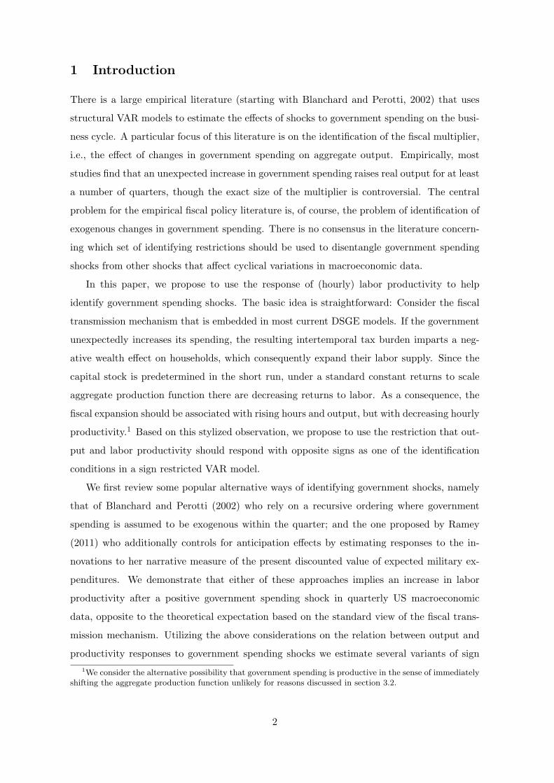
Figure 1 shows the results in terms of impulse responses to a one standard deviation

shock to government spending or Ramey’s (2011) news variable using these three identification

schemes, along with ±1.96 bootstrapped standard erros to capture symmetric 95% confidence

bands. For brevity, only the responses of the most interesting variables for the question at

hand are shown. The full set of impulse responses for all variables included in the VAR

models is available upon request.

0 5 10 15 20

Quarter

-0.02

0

0.02

0.04Spending: BP

0 5 10 15 20

Quarter

-5

0

5

10×10-3 Output: BP

0 5 10 15 20

Quarter

-5

0

5×10-3 Deficit: BP

0 5 10 15 20

Quarter

-5

0

5×10-3 Labprod: BP

0 5 10 15 20

Quarter

-0.02

-0.01

0

0.01Investment: BP

0 5 10 15 20

Quarter

-0.02

0

0.02

0.04Spending: Ramey

0 5 10 15 20

Quarter

-0.01

0

0.01Output: Ramey

0 5 10 15 20

Quarter

-5

0

5×10-3 Deficit: Ramey

0 5 10 15 20

Quarter

-5

0

5×10-3 Labprod: Ramey

0 5 10 15 20

Quarter

-5

0

5×10-3 Investment: Ramey

0 5 10 15 20

Quarter

-0.01

0

0.01

0.02Spending: BP-R

0 5 10 15 20

Quarter

-5

0

5

10×10-3 Output: BP-R

95% confidence band Impulse-response 95% confidence band

0 5 10 15 20

Quarter

-2

0

2

4×10-3 Deficit: BP-R

0 5 10 15 20

Quarter

-5

0

5×10-3 Labprod: BP-R

0 5 10 15 20

Quarter

-2

0

2

4×10-3 Investment: BP-R

Figure 1: Impulse responses to government spending shock: BP, Ramey and BP-R

identification schemes.

10

In all identification schemes, a positive government spending shock raises private sector

output (though only insignificantly so in the Ramey version), and the government deficit

(though less clearly and with a lag in the Ramey specification). Most importantly for the

present purpose, however, is the fact that under all identification schemes labor productivity

(shown in the last but one row of figure 1) rises slightly. The increase in productivity is

certainly not large, and in the Ramey case again not significantly different from zero. How-

ever, as argued above, if one believes that these models truly identify a government spending

shock, then one expects a pronounced decrease in labor productivity.

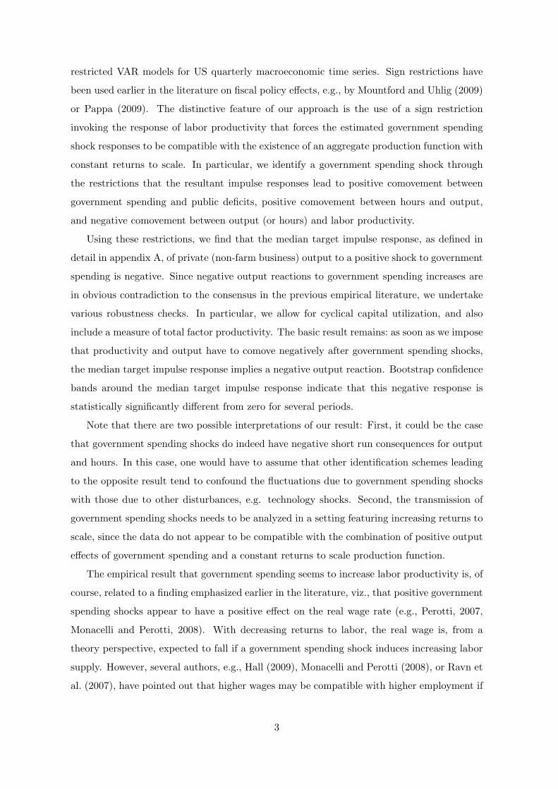
In principle, it is possible that the increase in measured labor productivity is explained

by the effect of a decline in hours worked on marginal productivity of labor. However, this

does not seem to be the case. Replacing the productivity variable log Yt − logHt, used in

the VAR models above, by the logarithm of hours worked, logHt, and re-estimating (leaving

the rest of the VAR model unchanged) yields the estimated impulse responses of hours to a

positive government spending shock in the three specifications shown in figure 2.

0 5 10 15 20

Quarter

-3

-2

-1

0

1

2

3

4×10-3 Hours: BP

0 5 10 15 20

Quarter

-6

-4

-2

0

2

4

6

8

10

12×10-3 Hours: Ramey

0 5 10 15 20

Quarter

-6

-4

-2

0

2

4

6×10-3 Hours: BP-R

95% confidence band Impulse-response 95% confidence band

Figure 2: Impulse response of non-farm business hours to government spending shock: BP,

Ramey and BP-R identification schemes.

In all cases, the response of hours appears to be close to zero or slightly positive, at

least for the first couple of quarters after the shock, but not markedly negative. Thus, the

behavior of hours does not seem to explain the estimated increase in productivity. Moreover,

even if the hours response were indeed negative, this would raise the question how, in that

11

case, a positive short run output response could be explained if the maintained assumption

that these models correctly identify a purely non-technological government spending shock

is correct. If technology does not change and the capital stock is predetermined in the short

run, then rising output is associated with increases in hours worked (the possible caveat in

the case that the output expansion is explained by a large concomitant increase in capital

utilization is explored in section 3.4 below).

To sum up, the conclusion obtained so far from standard structural VAR model ap-

proaches is that output increases following a government spending expansion are difficult

to explain without rising productivity. The very fact that the VAR model results point to

productivity increases following rising government spending, casts doubt on their ability to

identify a pure demand side innovation like a government spending shock. If the popular iden-

tification methods shown above truly identify government spending shocks, and if government

spending shocks are truly non-technological in nature, one expects that impulse responses

of output and hours have the same sign and are both of the opposite sign of the response

of labor productivity. Yet, in the estimates it appears that output comoves positively with

productivity, conditional on the identified shock, and weakly positively with hours. Thus, to

the extent that these conventional identification schemes indeed succeed in isolating govern-

ment spending shocks, one needs to explain how an increase in government spending is able

to raise labor productivity.

3.2 Discussion

While in the recent literature the debate has revolved around estimating the magnitude of

the effect of government spending shocks on output so far (the fiscal multiplier debate), the

empirical evidence provided above highlights a different aspect: However large the output

effects may be, they tend to derive not only from comparably large increases in hours or

employment, but also from increases in labor productivity.

This poses an interesting challenge to our understanding of the fiscal transmission mech-

anism. The evidence given above seems incompatible with the usual view of the way govern-

ment spending affects the economy, as it is embedded in most DSGE models. The standard

transmission mechanism implies that an increase in government spending raises output be-

cause higher spending, through its associated tax burden, exerts a negative wealth effect on

households. This gives households an incentive to reduce their consumption of leisure, which

boosts labor supply such that output rises. Along a neoclassical production function with

capital predetermined in the short run, this implies that decreasing returns to labor set in.

12

Hence, a decrease in measured labor productivity results.

Three principally different reactions to the apparent conflict between theory and empir-

ical evidence are conceivable. First, the standard view of the fiscal transmission mechanism

needs to be augmented. If the positive labor productivity response is structural, one has to

adjust theoretical models to accommodate it. Second, the identification methods discussed

above tend to confound government spending shocks with other shocks, in particular with

technological shocks that are known to raise productivity. A positive technology shock raises

productivity and could be mistaken for a government spending shock in a recursive identifi-

cation scheme, if the government immediately increases spending in response to the positive

technological shock. Third, an increase in activity following a government spending shock

triggers a rise in unmeasured factor utilization, in particular capital utilization. This might

counteract decreasing returns to labor since the unobserved variable utilization rate of capital

increases too. We discuss each of these possibilities in turn.

If one adopts the first view and maintains that the orthogonalizations applied in the VAR

models shown above succeed in identifying structural government spending shocks, it could

indeed be that the measured increase in labor productivity is structural. One possibility for

this is that government spending is productive, in the sense of entering private sector pro-

duction functions with a positive output elasticity. Higher government spending then shifts

up the production functions of private firms and leads to a labor productivity increase. How-

ever, direct productivity effects of government spending most likely result from investment

in public infrastructure. This, as a part of the economy’s total capital stock, only changes

slowly and therefore can be considered as predetermined in the short run following a spending

boost.

Another possibility is that there are increasing returns to scale, and more stringently

increasing returns to labor. In this case any increases in the scale of production, including

those brought about by an increase in government spending, lower average costs and thus

endogenously raise overall productivity. However, while this could, if the relevant effects are

strong enough, also lead to a rise in measured labor productivity, one expects that (as also

in the case of infrastructure effects from higher spending) private investment increases too,

since private investors would attempt to take advantage of higher productivity. The impulse

responses of investment are, however, not significantly different from zero in the three dis-

cussed structural VAR models. It is positive but not significantly different from zero in the

specifications using the Ramey news variable, and negative (albeit not significantly different

from zero) in the BP identification. Several other studies have also found negative invest-

13

ment responses to government spending shocks (e.g., Galı et al., 2007). Thus, the positive

investment response that one expects if higher government spending truly increases produc-

tivity (either by shifting the production function by adding public capital, or by shifting the

economy along an increasing returns to scale production function) does not seem to receive

much empirical support.

Hence, we conclude that while we cannot strictly rule out the possibility that procyclical

productivity is indeed a structural feature of government spending shocks, we consider the

evidence in favor of this hypothesis to be weak. Note that this also rules out the possibility

that labor productivity simply increases, because higher private investment raises the capital

stock quickly enough. Even if there were a positive private investment response, this effect is

expected to work intertemporally, with some delay because of the short run predetermined

nature of the capital stock. The productivity response instead appears to be immediate.

In sum, this leaves us with either the second or the third view, namely that the non-

negative productivity response either follows from failure to identify and disentangle govern-

ment spending shocks from technological shocks with the methods employed above, or that

it is the result of unaccounted increases of capacity utilization. The following two sections

are dedicated to our attempt to distinguish between these possibilities.

3.3 Results with sign restrictions imposed

In this subsection, we present the results when we impose the discussed sign restrictions on

the impulse responses from VAR models. We impose restrictions (i) to (iii) introduced above

(positive comovement of output and hours, negative comovement of output and productivity,

positive comovement of government spending and the budget deficit) on the impulse responses

of the VAR model to identify government spending shocks. The crucial restriction is (ii),

which has to be fulfilled by responses to demand side shocks like government spending shocks,

but not by responses to technology shocks. In this way, the sign restrictions are used to

separate government spending shocks, whose effects we want to analyze, from technology

shocks.

The estimated VAR model contains essentially the same variables as discussed in the

preceding subsection. The difference is that we include output and hours separately in order to

be able to constrain their impulse response relation. Thus, the following variables are included

logGt, log Yt, logHt, log τt, Rt, πt, Dt, log It. Furthermore, we again include four lags, a

constant and linear and quadratic time trends. We implement the sign restrictions following

the methodology outlined in Rubio-Ramırez et al. (2010). In brief (for more details see

14

appendix A), we randomly draw orthogonal matrices to rotate the so-called structural impact

matrix until we have 5000 models in which the impulse response patterns to a government

spending shock match restrictions (i) - (iii) over a horizon of four quarters. Robustness checks

show that imposing the restrictions only for one or two quarters following a shock does not

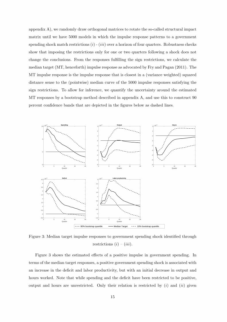
change the conclusions. From the responses fulfilling the sign restrictions, we calculate the

median target (MT, henceforth) impulse response as advocated by Fry and Pagan (2011). The

MT impulse response is the impulse response that is closest in a (variance weighted) squared

distance sense to the (pointwise) median curve of the 5000 impulse responses satisfying the

sign restrictions. To allow for inference, we quantify the uncertainty around the estimated

MT responses by a bootstrap method described in appendix A, and use this to construct 90

percent confidence bands that are depicted in the figures below as dashed lines.

0 5 10 15 20

Quarter

-5

0

5

10×10-3 Spending

0 5 10 15 20

Quarter

-5

-4

-3

-2

-1

0

1

2

3×10-3 Output

0 5 10 15 20

Quarter

-6

-5

-4

-3

-2

-1

0

1

2×10-3 Hours

0 5 10 15 20

Quarter

-0.5

0

0.5

1

1.5

2

2.5

3

3.5

4

4.5×10-3 Deficit

0 5 10 15 20

Quarter

-1.5

-1

-0.5

0

0.5

1

1.5

2

2.5

3×10-3 Labor productivity

90% bootstrap quantile Median Target 10% bootstrap quantile

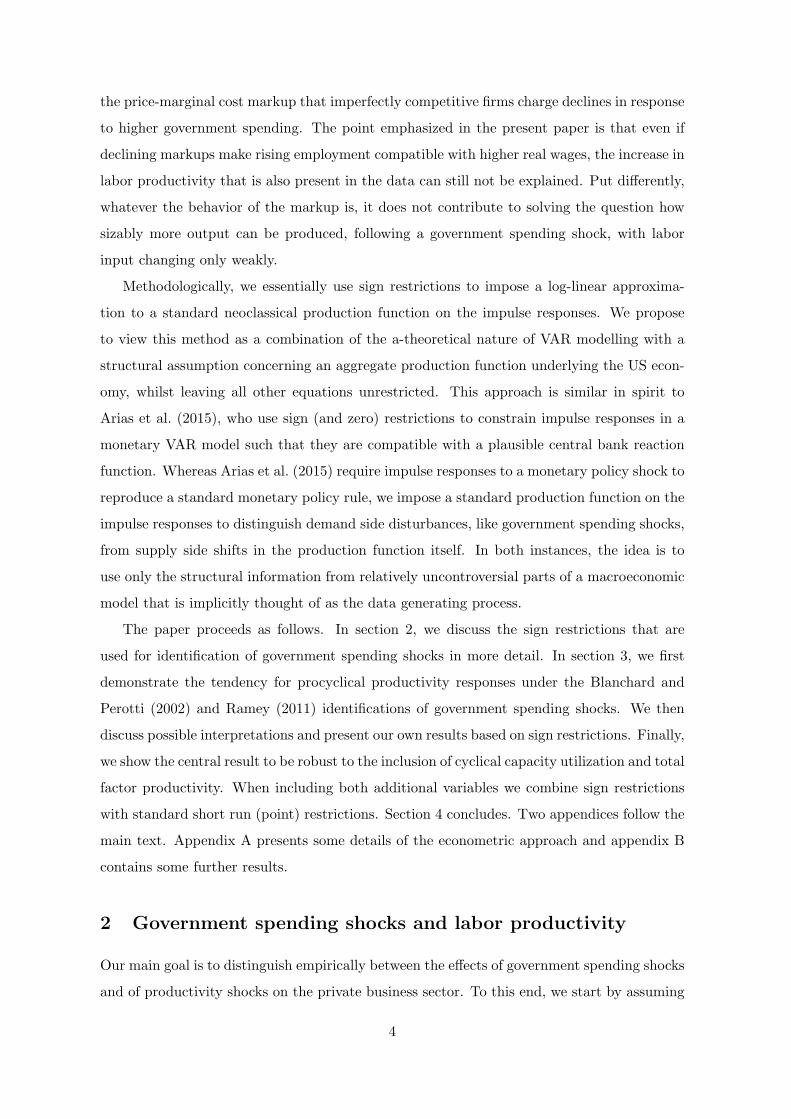
Figure 3: Median target impulse responses to government spending shock identified through

restrictions (i) – (iii).

Figure 3 shows the estimated effects of a positive impulse in government spending. In

terms of the median target responses, a positive government spending shock is associated with

an increase in the deficit and labor productivity, but with an initial decrease in output and

hours worked. Note that while spending and the deficit have been restricted to be positive,

output and hours are unrestricted. Only their relation is restricted by (i) and (ii) given

15

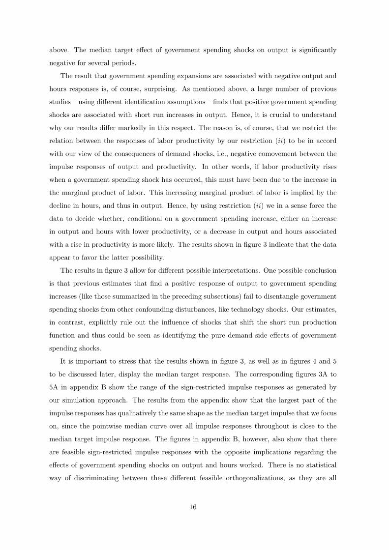
above. The median target effect of government spending shocks on output is significantly

negative for several periods.

The result that government spending expansions are associated with negative output and

hours responses is, of course, surprising. As mentioned above, a large number of previous

studies – using different identification assumptions – finds that positive government spending

shocks are associated with short run increases in output. Hence, it is crucial to understand

why our results differ markedly in this respect. The reason is, of course, that we restrict the

relation between the responses of labor productivity by our restriction (ii) to be in accord

with our view of the consequences of demand shocks, i.e., negative comovement between the

impulse responses of output and productivity. In other words, if labor productivity rises

when a government spending shock has occurred, this must have been due to the increase in

the marginal product of labor. This increasing marginal product of labor is implied by the

decline in hours, and thus in output. Hence, by using restriction (ii) we in a sense force the

data to decide whether, conditional on a government spending increase, either an increase

in output and hours with lower productivity, or a decrease in output and hours associated

with a rise in productivity is more likely. The results shown in figure 3 indicate that the data

appear to favor the latter possibility.

The results in figure 3 allow for different possible interpretations. One possible conclusion

is that previous estimates that find a positive response of output to government spending

increases (like those summarized in the preceding subsections) fail to disentangle government

spending shocks from other confounding disturbances, like technology shocks. Our estimates,

in contrast, explicitly rule out the influence of shocks that shift the short run production

function and thus could be seen as identifying the pure demand side effects of government

spending shocks.

It is important to stress that the results shown in figure 3, as well as in figures 4 and 5

to be discussed later, display the median target response. The corresponding figures 3A to

5A in appendix B show the range of the sign-restricted impulse responses as generated by

our simulation approach. The results from the appendix show that the largest part of the

impulse responses has qualitatively the same shape as the median target impulse that we focus

on, since the pointwise median curve over all impulse responses throughout is close to the

median target impulse response. The figures in appendix B, however, also show that there

are feasible sign-restricted impulse responses with the opposite implications regarding the

effects of government spending shocks on output and hours worked. There is no statistical

way of discriminating between these different feasible orthogonalizations, as they are all

16

observationally equivalent to the estimated reduced form VAR model. In the literature it

is customary to focus on either the pointwise median curve (not itself an impulse response

function) or the median target impulse response to capture the main tendency in the data.

Both lead to very similar conclusions in our case. Second, and more problematically, we have

thus far assumed that labor is the only variable factor of production that can adjust in the

short run. This is debatable when the amount of services derived from the capital stock

varies over the business cycle, as is implied by many theoretical models with variable capital

utilization. We thus turn to an enlarged model where we allow for utilization changes in the

following section.

3.4 Robustness checks: variable capital utilization and total factor pro-

ductivity

So far, we have assumed that capital services st are identical (or proportional) to the capital

stock kt. This is a useful simplification, because the capital stock is predetermined in the

short run, and moves only slowly even over the medium run. Hence, under this assumption it

is possible to abstract from changes in capital services, at least for the small number of time

periods for which sign restrictions are imposed on impulse responses. However, it is indeed

likely that capital services are more variable than the capital stock itself, if the utilization

rate of the latter is time varying. The question thus arises in how far our results are robust

to allowing for variable capital utilization.

Time varying capital utilization is found to be an important feature of business cycles in

several recent papers, e.g., Justiniano et al. (2010). Empirically, Fernald (2014) provides a

measure of the change in utilization that he computes based on the methodology described

in Basu et al. (2006).3 In the following, since the other variables in our VAR models are in

log-levels as well, we use his measure of utilization change and integrate it (from a starting

value of one) to obtain the level of utilization Ut (which is then taken to logarithms in the

empirical model), and allow the services of capital to depend on it through St = UtKt, where

Kt is the stock of installed capital.

Allowing for variable capital utilization, the log-linearly approximated production func-

tion thus reads as:

yt = zt + aht + (1− a)(ut + kt). (5)

3The data are available at John Fernald’s web site http://www.frbsf.org/economic-research/economists/john-fernald/.

17

Under non-technological shocks, i.e., with zt = 0, and upon neglecting movements in the

capital stock which continues to be predetermined, it follows that measured labor productivity

is approximately given by:

yt − ht ≈ (1− a)(ut − ht). (6)

Hence, given a ∈ (0, 1), labor productivity rises in response to a non-technological shock

only if utilization ut increases more strongly than hours worked ht. Thus, with variable

capital utilization our previous restriction (ii), which requires output and productivity to

have opposite signs, may be too restrictive.

We thus extend the VAR model of the previous section with the logarithm of the level

of utilization as an additional variable. The variables used are thus logGt, log Yt, logHt,

log τt, Rt, πt, Dt, log It, logUt. Using the same notation as in section 2, let uj denote

the impulse response at horizon j of logUt to a government spending shock. In terms of

identification restrictions on the impulse responses, we replace the sign restriction (ii) by a

new sign restriction (iv):

(iv) The difference of the impulse responses yj and hj has the same sign as the difference of

the impulse responses uj and hj .

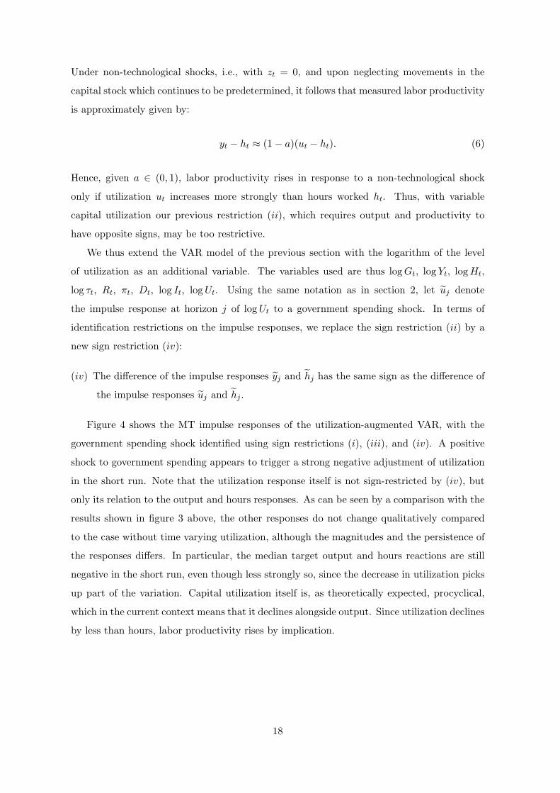
Figure 4 shows the MT impulse responses of the utilization-augmented VAR, with the

government spending shock identified using sign restrictions (i), (iii), and (iv). A positive

shock to government spending appears to trigger a strong negative adjustment of utilization

in the short run. Note that the utilization response itself is not sign-restricted by (iv), but

only its relation to the output and hours responses. As can be seen by a comparison with the

results shown in figure 3 above, the other responses do not change qualitatively compared

to the case without time varying utilization, although the magnitudes and the persistence of

the responses differs. In particular, the median target output and hours reactions are still

negative in the short run, even though less strongly so, since the decrease in utilization picks

up part of the variation. Capital utilization itself is, as theoretically expected, procyclical,

which in the current context means that it declines alongside output. Since utilization declines

by less than hours, labor productivity rises by implication.

18

0 5 10 15 20

Quarter

-5

0

5

10×10-3 Spending

0 5 10 15 20

Quarter

-5

-4

-3

-2

-1

0

1

2×10-3 Output

0 5 10 15 20

Quarter

-5

-4

-3

-2

-1

0

1

2×10-3 Hours

0 5 10 15 20

Quarter

-0.5

0

0.5

1

1.5

2

2.5

3

3.5

4×10-3 Deficit

0 5 10 15 20

Quarter

-2

-1.5

-1

-0.5

0

0.5

1

1.5

2×10-3 Util rate

0 5 10 15 20

Quarter

-3

-2

-1

0

1

2

3×10-3 Labor productivity

90% bootstrap quantile Median Target 10% bootstrap quantile

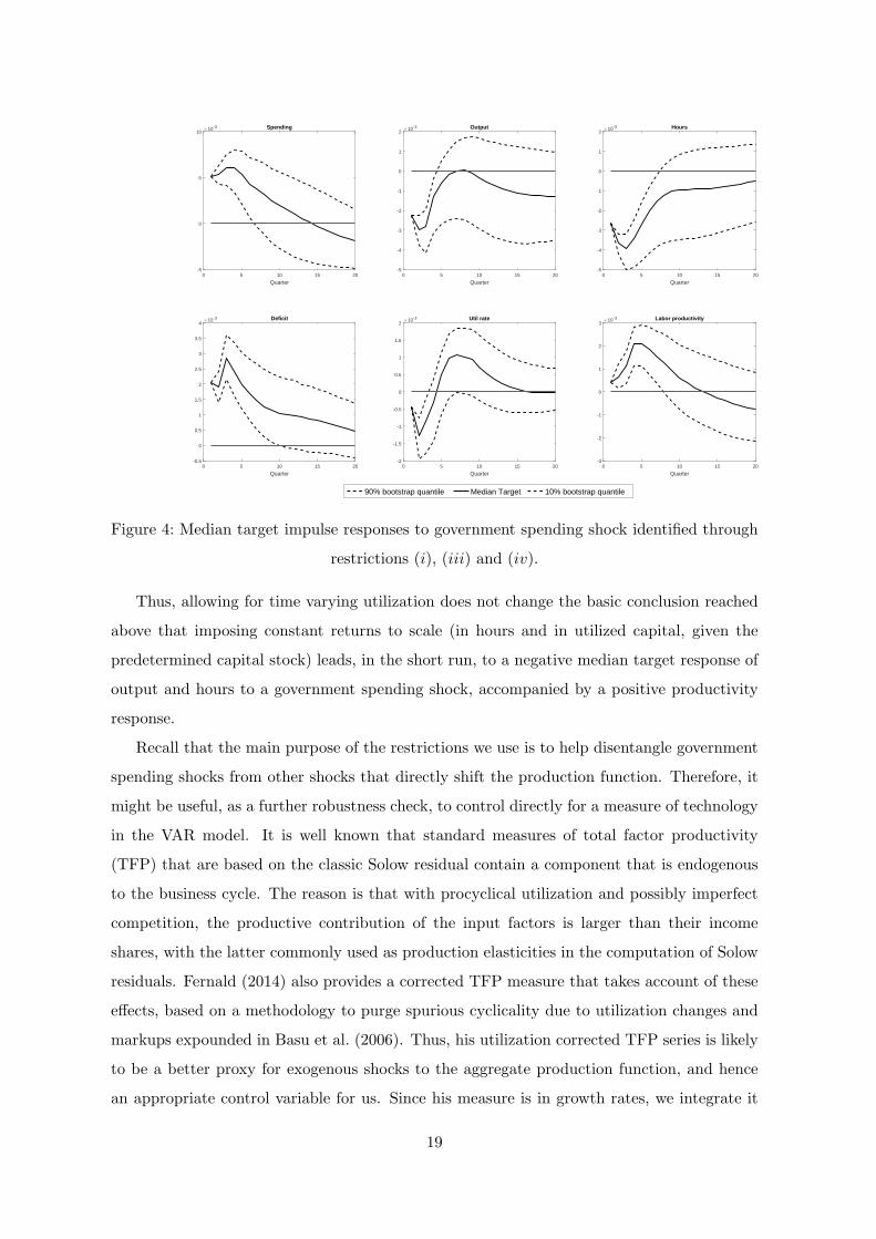
Figure 4: Median target impulse responses to government spending shock identified through

restrictions (i), (iii) and (iv).

Thus, allowing for time varying utilization does not change the basic conclusion reached

above that imposing constant returns to scale (in hours and in utilized capital, given the

predetermined capital stock) leads, in the short run, to a negative median target response of

output and hours to a government spending shock, accompanied by a positive productivity

response.

Recall that the main purpose of the restrictions we use is to help disentangle government

spending shocks from other shocks that directly shift the production function. Therefore, it

might be useful, as a further robustness check, to control directly for a measure of technology

in the VAR model. It is well known that standard measures of total factor productivity

(TFP) that are based on the classic Solow residual contain a component that is endogenous

to the business cycle. The reason is that with procyclical utilization and possibly imperfect

competition, the productive contribution of the input factors is larger than their income

shares, with the latter commonly used as production elasticities in the computation of Solow

residuals. Fernald (2014) also provides a corrected TFP measure that takes account of these

effects, based on a methodology to purge spurious cyclicality due to utilization changes and

markups expounded in Basu et al. (2006). Thus, his utilization corrected TFP series is likely

to be a better proxy for exogenous shocks to the aggregate production function, and hence

an appropriate control variable for us. Since his measure is in growth rates, we integrate it

19

from a starting value of one to get the variable TFPt, and use its log-level as an additional

variable in the VAR model.

After a government spending shock that has no impact on technology, the impulse re-

sponse at horizon j of the total factor productivity measure to this government spending

shock, tfpj , should be zero, at least in the vicinity of the shock impact at short horizons j.

We thus impose, as an additional identifying restriction, the exact zero-at-impact restriction:

(v) The impulse response tfpj does not change on impact under government spending shocks.

This model version thus mixes the sign restrictions (i), (iii), and (iv) with the exact zero

restriction (v). The implementation is based on the methodology set out in Arias et al. (2014)

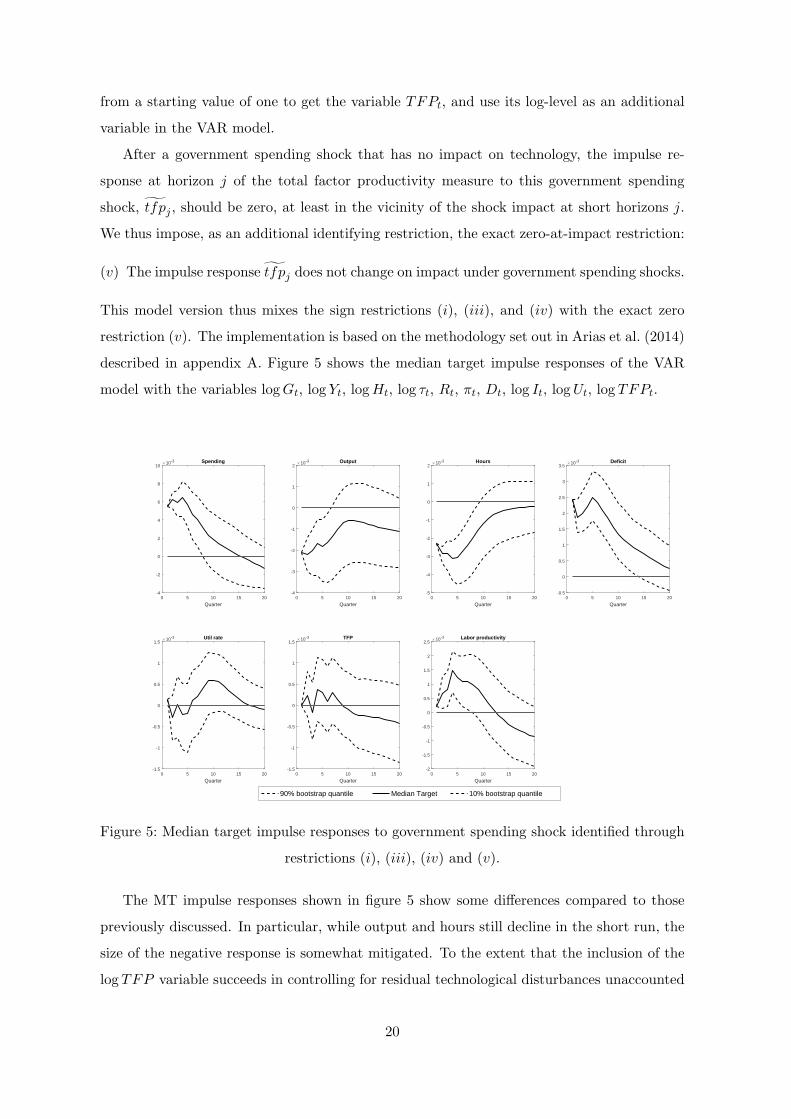
described in appendix A. Figure 5 shows the median target impulse responses of the VAR

model with the variables logGt, log Yt, logHt, log τt, Rt, πt, Dt, log It, logUt, log TFPt.

0 5 10 15 20

Quarter

-4

-2

0

2

4

6

8

10×10-3 Spending

0 5 10 15 20

Quarter

-4

-3

-2

-1

0

1

2×10-3 Output

0 5 10 15 20

Quarter

-5

-4

-3

-2

-1

0

1

2×10-3 Hours

0 5 10 15 20

Quarter

-0.5

0

0.5

1

1.5

2

2.5

3

3.5×10-3 Deficit

0 5 10 15 20

Quarter

-1.5

-1

-0.5

0

0.5

1

1.5×10-3 Util rate

0 5 10 15 20

Quarter

-1.5

-1

-0.5

0

0.5

1

1.5×10-3 TFP

0 5 10 15 20

Quarter

-2

-1.5

-1

-0.5

0

0.5

1

1.5

2

2.5×10-3 Labor productivity

90% bootstrap quantile Median Target 10% bootstrap quantile

Figure 5: Median target impulse responses to government spending shock identified through

restrictions (i), (iii), (iv) and (v).

The MT impulse responses shown in figure 5 show some differences compared to those

previously discussed. In particular, while output and hours still decline in the short run, the

size of the negative response is somewhat mitigated. To the extent that the inclusion of the

log TFP variable succeeds in controlling for residual technological disturbances unaccounted

20

for in the previous models, the estimates shown in figure 5 give a cleaner indication of the

consequences of a government spending shock. Most clearly visible, the response of utilization

now appears rather unclear, and statistically not significantly different from zero. This is also

true for the TFP response itself, which is only constrained to be exactly zero in the impact

period, and shows some endogenous but altogether insignificant variation thereafter. Labor

productivity reacts less strongly than in the previous models, but the response is still positive.

However, the main pattern found in the simpler models above still holds: Output and hours

tend to decline for some periods following a government spending increase, whereas labor

productivity rises slightly. We thus conclude that the central result presented in the previous

subsection is robust to the consideration of both variable capital utilization and total factor

productivity as additional control variables.

4 Conclusions

Taking stock, the estimates presented above all highlight the central point: As soon as we

impose the crucial requirement that the impulse responses of structural VAR models aimed

at identifying government spending shocks exhibit behavior required to be consistent with a

standard constant returns to scale aggregate production function, we find that the median

target responses to a government spending increase imply short run declines in private sector

output and hours, along with rising labor productivity. This result is robust to the inclusion

of variable capacity utilization and to additionally including a measure of utilization-adjusted

total factor productivity. Since the majority of previous studies has found positive output

responses following government spending increases, the question arises, of course, how to

interpret the results presented here.

Our results certainly cannot be taken to necessarily imply that other identification schemes

that tend to find positive output responses to government spending increases are wrong.

While there is the possibility that identification schemes that do not take into account the

restrictions we impose on productivity behavior confound demand shocks deriving from gov-

ernment spending variations with technology shocks, we need to be cautious here for at least

three reasons. First, sign restriction methods do not allow to exactly identify government

spending shocks, but only the set of admissible model impulse responses given the restric-

tions. The range of admissible models includes impulse responses for output and hours of

both signs. However, as demonstrated by the median target impulse responses shown above

(and by the figures in appendix B), the majority of admissible impulse responses points to-

wards a negative reaction of these variables, when forced to have a negative correlation of

21

the responses of output and labor productivity in the short run.

Second, we use an estimated regressor as our variable capital utilization rate, which itself

is not directly observable. Hence, although the measure is carefully constructed by Fernald

(2014), there might still be unaccounted residual variation in true capital utilization that

is not captured in the measured variable. As a consequence, observed labor productivity

behavior could still be misleading and not fully capture movements in the marginal product

of labor.

Finally, it might be that the main identifying restriction we use, namely constant returns

to scale in the aggregate production function, does not hold empirically. In this case, the

negative impulse response correlation between output and utilization-adjusted productivity

need not hold. This would invalidate our central identification assumption. While this is

possible in principle, we note that a large majority of business cycle models assumes the

standard assumption of constant returns to scale. Allowing for increasing returns to scale

requires an altogether rethinking of the fiscal transmission process in such models. The

distinction between these possibilities is arguably an important topic of future research. At

this point, we conclude that the data seem to imply that shocks to government spending

either have negative output consequences, or if they have not, then this can, in our view,

only be explained through the existence of aggregate increasing returns to scale.

Acknowledgements

Financial support from Deutsche Forschungsgemeinschaft via the Collaborative Research

Center 823: Statistical Modelling of Nonlinear Dynamic Processes (Projects A3 and A4) is

gratefully acknowledged. Work on this paper started whilst the second author was affiliated

with the Faculty of Statistics at TU Dortmund. We are grateful for the helpful comments of

seminar participants at the University of Graz. The usual disclaimer applies.

22

References

Arias, J.E., D. Caldara, and J.F. Rubio-Ramırez (2015), The systematic component of mon-

etary policy in SVARs: An agnostic identification procedure, Working Paper.

Arias, J.E., J.F. Rubio-Ramırez, and D.F. Waggoner (2014), Inference based on SVARs

identified with sign and zero restrictions: theory and applications, Working Paper.

Barro, R.J., and C.J. Redlick (2011), Macroeconomic effects from government purchases

and taxes, Quarterly Journal of Economics 126, 51–102.

Basu, S., J.G. Fernald, and M.S. Kimball (2006), Are technology improvements contrac-

tionary?, American Economic Review 96, 1418–1448.

Blanchard, O.J., and R. Perotti (2002), An empirical characterization of the dynamic ef-

fects of changes in government spending and taxes on output, Quarterly Journal of Economics

117, 1329–1368.

Fernald, J. (2014), A quarterly, utilization adjusted series on total factor productivity,

Federal Reserve Bank of St. Francisco, Working Paper 2012-19.

Fry, R., and A. Pagan (2011), Sign restrictions in structural vector autoregressions: a

critical review, Journal of Economic Literature 49, 938–60.

Galı, J., D. Lopez-Salido, and J. Valles (2007), Understanding the effects of government

spending on consumption, Journal of the European Economic Association 5, 227-270.

Hall, R.E (2009), Reconciling cyclical movements in the marginal value of time and the

marginal product of labor, Journal of Political Economy 117, 281–323.

Hannan, E.J., and M. Deistler (1988), The statistical theory of linear systems, Wiley and

Sons.

Justiniano, A., G.E. Primiceri, and A. Tambalotti (2010), Investment shocks and business

cycles, Journal of Monetary Economics 57, 132–145.

Kilian, L. (1998), Small-sample confidence intervals for impulse response functions, Re-

view of Economics and Statistics 80, 218–230.

Monacelli, T., and R. Perotti (2008), Fiscal policy, wealth effects, and markups, NBER

Working Paper no. 14584.

Mountford, A., and H. Uhlig (2009), What are the effects of fiscal policy shocks?, Journal

of Applied Econometrics 24, 960–992.

Pappa, E. (2009), The effects of fiscal shocks on employment and the real wage, Interna-

tional Economic Review 50, 217–244.

Perotti, R. (2007), In search of the transmission mechanism of fiscal policy, in D. Ace-

moglu, NBER Macroeconomics Annual 2007.

23

Ramey, V.A. (2011), Identifying government spending shocks: it’s all in the timing, Quar-

terly Journal of Economics 126, 1–50.

Ravn, M., S. Schmitt-Grohe, and M. Uribe (2008), Consumption, government spending,

and the real exchange rate, Journal of Monetary Economics 59, 215–234.

Rubio-Ramırez, J.F., D.F. Waggoner, and T. Zha (2010), Structural vector autoregres-

sions: theory of identification and algorithms for inference, Review of Economic Studies 77,

665–696.

24

Appendix A

The VAR model

We describe the employed econometric model in this section for the sake of completeness and,

mainly, to fix notation. A k-variable structural VAR model for xt is given by:

A0xt = µ+ C1t+ C2t2 +A1xt−1 +A2xt−2 + · · ·+Apxt−p + εt, (7)

where xt ∈ Rk, εt ∼ WN(0, Ik), A0, . . . , Ap ∈ Rk×k, µ,C1, C2 ∈ Rk. A0, the so-called

structural matrix, is assumed to be non-singular. In order to define a unique lag length p we

assume Ap = 0, in our application p = 4. The corresponding reduced form, obtained from

(7) by pre-multiplication with A−10 , is given by:

xt = ν +D1t+D2t2 +B1xt−1 + · · ·+Bpxt−p + ut, (8)

with Bi = A−10 Ai, i = 1, . . . , p, Dj = A−1

0 Cj , j = 1, 2, ν = A−10 µ, and A−1

0 εt = ut ∼

WN(0,Σu), with consequently Σu = A−10 A−1′

0 .

Denoting with B(z) = Ik − B1z − · · · − Bpzp, we impose the causality assumption,

det(B(z)) = 0 ∀ |z| ≤ 1. Under this assumption, the errors ut correspond to the one-

step prediction errors from the Wold decomposition, i.e., we obtain an infinite order moving

average representation of the form:

xt = ν + D1t+ D2t2 +

∞∑j=0

Φjut−j (9)

= ν + D1t+ D2t2 +

∞∑j=0

ΦjA−10 εt−j (10)

The (r, s)-element of Θj = ΦjA−10 describes the change of variable r to a unit increase of εt,s

after j-periods, i.e., at horizon j. In the main text we use the short-hand notation mj for

this, with m denoting an element of the vector of variables xt, since we are throughout only

interested in the effects of government spending shocks, i.e., for one particular s only.

Identification schemes

As is well-known, the structural form (7) is not identified, for a detailed discussion see Hannan

and Deistler (1988). The literature provides a large array of approaches to point or set

identification of structural VAR models. In our paper we employ the following ones:

25

(1) Recursive identification: The structural matrix, A0 is lower (upper) triangular, or,

equivalently, A−10 , the structural impact matrix, is lower (upper) triangular.

(2) Sign restrictions: Θ(r,s)j is restricted to be either nonnegative or nonpositive for some

combinations of (r, s, j), r, z ∈ { 1, . . . , k }, j ∈ N0.

(3) Zero and sign restrictions: Θ(r,s)

j= 0 for some (r, s, j), and some Θ

(r,s)j are sign restricted

as defined in the previous item (2). Note already here that in our paper we only consider

zero-at-impact restrictions, i.e., j = 0.

The recursive identification scheme yields an exactly identified structural VAR. It is im-

portant to note, however, that sign restrictions and the mixture of zero and sign restrictions,

in general do not yield exactly identified structural forms. The identified set for the impulse

responses is, thus, in general non-singleton for the second and third cases.4

Impulse response functions

The reduced form parameters are estimated by ordinary least squares, resulting in B1, . . . , Bp

and Σu. Thus, an estimate of the reduced form impulse response sequence (Φj)j≥0 follows

immediately. The approach to obtain structural impulse responses differs across cases (1) to

(3). In every case, however, the starting point is the identity Σu = A−10 A−1′

0 and the available

estimate Σu.

For recursive identification consider the (unique) Cholesky decomposition of Σu = LL′,

with L lower triangular (and positive elements along the diagonal), and set A−10 = L.

Now, observe that for any unitary matrix Q ∈ Rk×k, with QQ′ = Q′Q = Ik, it holds that

Σu = LQQ′L′ = LQL′Q (11)

is another valid decomposition of Σu. Thus, the whole range of structural impulse responses

consistent with the reduced form error variance matrix Σu is given by varying Q ∈ Rk×k

over all unitary matrices (for given Cholesky factor L). This is clearly not feasible and

thus approximate solutions are required. Here we follow the approach of Rubio-Ramırez et

al. (2010) to generate uniformly distributed Q-matrices:

1. Draw a matrixM with i.i.d. standard normal entries and perform the QR-decomposition

of the matrix M = QR. Doing so, Q is unitary and has the uniform (or Haar) distri-

bution.4Note that imposing too many sign restrictions can reduce the set of feasible impulse responses to the

empty set. The same is, a fortiori, true for the combination of zero and sign restrictions.

26

2. Calculate the corresponding structural impulse response function {ΘQj }j=0,...,J =

{ΦjLQ}j=0,...,J and verify whether the formulated sign restrictions are fulfilled. If so,

keep{ΘQ

j

}j=0,...,J

, otherwise discard it.

3. Repeat these calculations until the set of retained structural impulse responses contains

n = 5000 elements.

From the 5000 elements the median target impulse response function is then calculated as

described below.

It remains to discuss the implementation of the combination of zero and sign restrictions,

where we follow Arias et al. (2014). As can be guessed by now, the solution consists of

drawing random unitary matrices that imply that the resultant ΘQ0 satisfies the required

zero-at-impact restrictions in addition to the formulated sign restrictions. We describe the

approach here only for our specific application, in which TFP is ordered last in the VAR

model where we combine zero and sign restrictions:

1. Find a matrix N1 ∈ Rk×(k−1) with N ′1N1 = Ik−1 such that L[k,•]N1 = 0, with L[k,•]

denoting the k-th row of L.

2. Generate a vector z ∈ Rk with i.i.d. standard normally distributed entries and form

the vector:

q =1

||[N1 0k×1]z||[N1 0k×1]z, (12)

i.e., project the vector z on the space spanned by N1 and normalize it to unit length.

3. Find a matrix N2 ∈ Rk×(k−1) with N ′2N2 = Ik−1 such that q′N2 = 0.

4. Draw a matrix M ∈ R(k−1)×(k−1) with i.i.d. standard normal entries and calculate the

QR decomposition of N2M , i.e.,

N2M = [Q1 Q2]

R1

0

, (13)

with Q1 ∈ Rk×(k−1).

5. Form the matrix Q+ = [q Q1] and calculate the corresponding structural impulse re-

sponse function {ΘQ+

j }j=0,...,J = {ΦjLQ+}j=0,...,J , with LQ+ = LQ+, and verify whether

the formulated sign restrictions are fulfilled. If so, keep{ΘQ+

j

}j=0,...,J

, otherwise dis-

27

card it. Note that by construction, the zero-at-impact restriction on the structural

impulse response of log TFP holds for all draws.

6. Repeat these calculations until the set of retained structural impulse responses contains

n = 5000 elements.

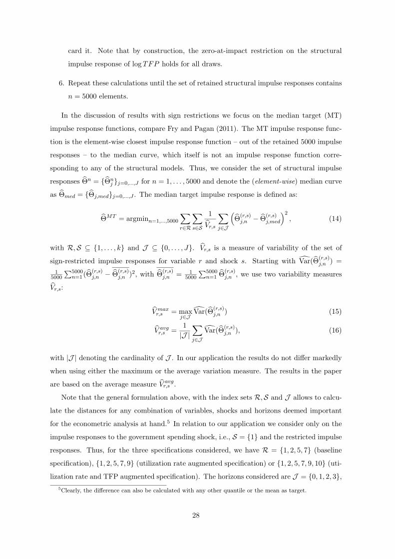
In the discussion of results with sign restrictions we focus on the median target (MT)

impulse response functions, compare Fry and Pagan (2011). The MT impulse response func-

tion is the element-wise closest impulse response function – out of the retained 5000 impulse

responses – to the median curve, which itself is not an impulse response function corre-

sponding to any of the structural models. Thus, we consider the set of structural impulse

responses Θn = {Θnj }j=0,...,J for n = 1, . . . , 5000 and denote the (element-wise) median curve

as Θmed = {Θj,med}j=0,...,J . The median target impulse response is defined as:

ΘMT = argminn=1,...,5000

∑r∈R

∑s∈S

1

Vr,s

∑j∈J

(Θ

(r,s)j,n − Θ

(r,s)j,med

)2, (14)

with R,S ⊆ {1, . . . , k} and J ⊆ {0, . . . , J}. Vr,s is a measure of variability of the set of

sign-restricted impulse responses for variable r and shock s. Starting with Var(Θ(r,s)j,n ) =

15000

∑5000n=1 (Θ

(r,s)j,n − Θ

(r,s)j,n )2, with Θ

(r,s)j,n = 1

5000

∑5000n=1 Θ

(r,s)j,n , we use two variability measures

Vr,s:

V maxr,s = max

j∈JVar(Θ

(r,s)j,n ) (15)

V avgr,s =

1

|J |∑j∈J

Var(Θ(r,s)j,n ), (16)

with |J | denoting the cardinality of J . In our application the results do not differ markedly

when using either the maximum or the average variation measure. The results in the paper

are based on the average measure V avgr,s .

Note that the general formulation above, with the index sets R,S and J allows to calcu-

late the distances for any combination of variables, shocks and horizons deemed important

for the econometric analysis at hand.5 In relation to our application we consider only on the

impulse responses to the government spending shock, i.e., S = {1} and the restricted impulse

responses. Thus, for the three specifications considered, we have R = {1, 2, 5, 7} (baseline

specification), {1, 2, 5, 7, 9} (utilization rate augmented specification) or {1, 2, 5, 7, 9, 10} (uti-

lization rate and TFP augmented specification). The horizons considered are J = {0, 1, 2, 3},5Clearly, the difference can also be calculated with any other quantile or the mean as target.

28

with the results robust to choosing only one or two quarters.

Inference on impulse response functions

The confidence bands for the recursive identification scheme are obtained using the bootstrap

algorithm proposed in Kilian (1998), which is based on a preliminary (simulation based) bias

correction step. The 5000 bootstrap samples are then drawn using bias corrected parameter

estimates.

Some more care has to be taken into account when bootstrapping the median target solu-

tion. The median target structural impulse response function by construction depends upon

B1, . . . , Bp as well as LQMT = LQMT , with QMT denoting the rotation matrix corresponding

to the minimizer of (14). Thus, resampling data from the reduced form model has to be

combined with the structural decomposition given by LQMT , which is done by a modification

of the previous algorithm:

1. As in the standard case, generate a bootstrap sample, x∗1, . . . , x∗T using the Kilian (1998)

bootstrap, i.e., bias corrected parameter estimates.

2. Estimate the parameters of the VAR model using x∗t , resulting in parameter estimates

B∗1 , . . . , B

∗p . Calculate the structural impulse response function using these parameter

estimates and the original LQMT .

3. Verify whether the impulse response function from the previous item, {ΘQMT ∗j }j=0,...,J ,

satisfies the formulated sign restrictions. If it does, keep it, otherwise discard it.

4. Repeat the above steps until 1000 impulse responses are retained and calculate pointwise

bootstrap confidence bands as usual from these 1000 impulse responses.

Appendix B

In Sections 3.3–3.4 in the main text we present the median target impulse responses as

summaries or typical representatives of the set of sign-restricted impulse responses. In the

following we augment this information by additionally plotting the element-wise median curve

as well as the element-wise 10-th and 90-th quantile curves. As already mentioned, the median

curve, and similarly the quantile curves, do not themselves correspond to structural models.

This is, since for any variable, shock and horizon the median or quantile may – and in general

will – correspond to a different structural model.

29

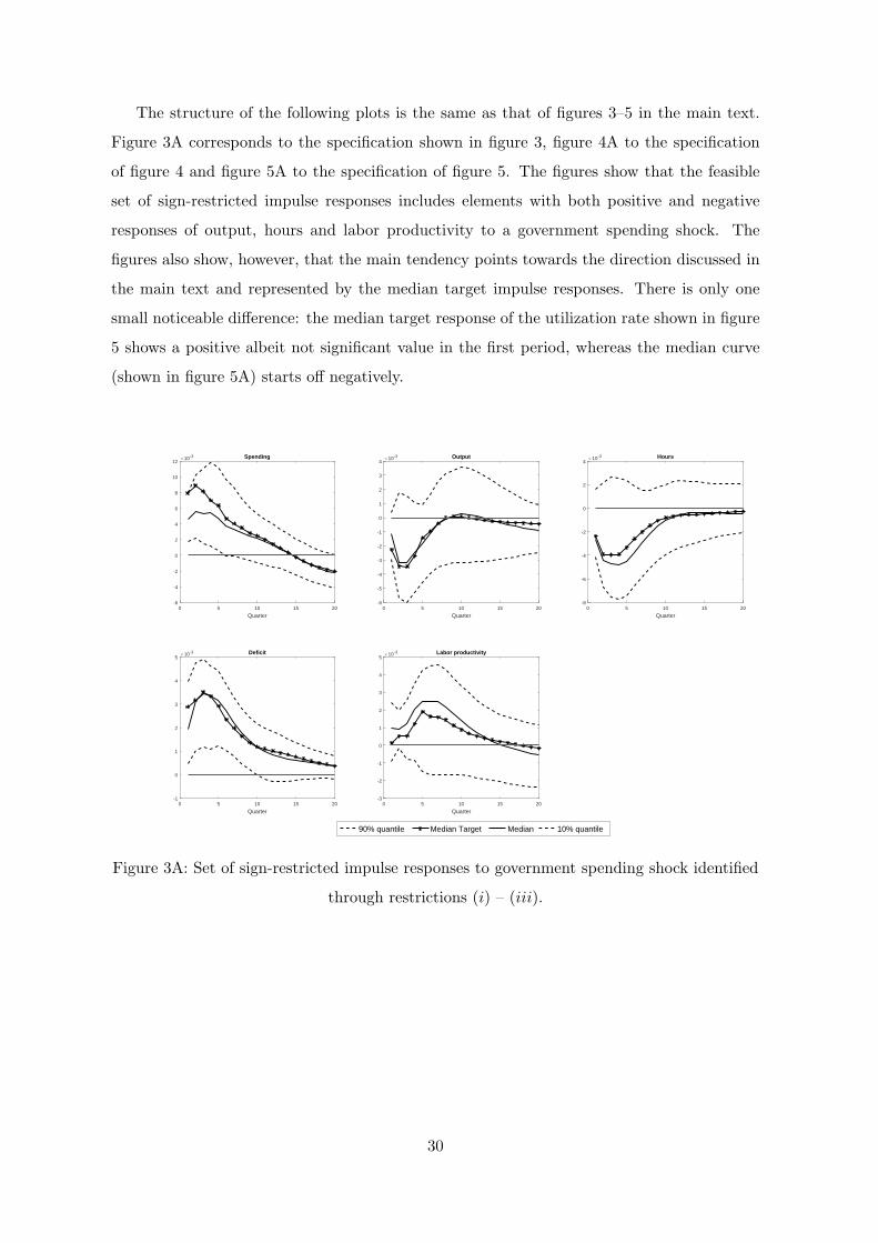
The structure of the following plots is the same as that of figures 3–5 in the main text.

Figure 3A corresponds to the specification shown in figure 3, figure 4A to the specification

of figure 4 and figure 5A to the specification of figure 5. The figures show that the feasible

set of sign-restricted impulse responses includes elements with both positive and negative

responses of output, hours and labor productivity to a government spending shock. The

figures also show, however, that the main tendency points towards the direction discussed in

the main text and represented by the median target impulse responses. There is only one

small noticeable difference: the median target response of the utilization rate shown in figure

5 shows a positive albeit not significant value in the first period, whereas the median curve

(shown in figure 5A) starts off negatively.

0 5 10 15 20

Quarter

-6

-4

-2

0

2

4

6

8

10

12×10-3 Spending

0 5 10 15 20

Quarter

-6

-5

-4

-3

-2

-1

0

1

2

3

4×10-3 Output

0 5 10 15 20

Quarter

-8

-6

-4

-2

0

2

4×10-3 Hours

0 5 10 15 20

Quarter

-1

0

1

2

3

4

5×10-3 Deficit

0 5 10 15 20

Quarter

-3

-2

-1

0

1

2

3

4

5×10-3 Labor productivity

90% quantile Median Target Median 10% quantile

Figure 3A: Set of sign-restricted impulse responses to government spending shock identified

through restrictions (i) – (iii).

30

0 5 10 15 20

Quarter

-4

-2

0

2

4

6

8

10

12×10-3 Spending

0 5 10 15 20

Quarter

-6

-5

-4

-3

-2

-1

0

1

2

3

4×10-3 Output

0 5 10 15 20

Quarter

-8

-6

-4

-2

0

2

4×10-3 Hours

0 5 10 15 20

Quarter

-0.5

0

0.5

1

1.5

2

2.5

3

3.5

4

4.5×10-3 Deficit

0 5 10 15 20

Quarter

-4

-3

-2

-1

0

1

2

3×10-3 Util rate

0 5 10 15 20

Quarter

-3

-2

-1

0

1

2

3

4

5×10-3 Labor productivity

90% quantile Median Target Median 10% quantile

Figure 4A: Set of sign-restricted impulse responses to government spending shock identified

through restrictions (i), (iii) and (iv).

0 5 10 15 20

Quarter

-4

-2

0

2

4

6

8

10

12×10-3 Spending

0 5 10 15 20

Quarter

-6

-5

-4

-3

-2

-1

0

1

2

3

4×10-3 Output

0 5 10 15 20

Quarter

-7

-6

-5

-4

-3

-2

-1

0

1

2

3×10-3 Hours

0 5 10 15 20

Quarter

-0.5

0

0.5

1

1.5

2

2.5

3

3.5

4

4.5×10-3 Deficit

0 5 10 15 20

Quarter

-3

-2.5

-2

-1.5

-1

-0.5

0

0.5

1

1.5

2×10-3 Util rate

0 5 10 15 20

Quarter

-2.5

-2

-1.5

-1

-0.5

0

0.5

1

1.5×10-3 TFP

0 5 10 15 20

Quarter

-3

-2

-1

0

1

2

3

4×10-3 Labor productivity

90% quantile Median Target Median 10% quantile

Figure 5A: Set of point- and sign-restricted impulse responses to government spending

shock identified through restrictions (i), (iii), (iv) and (v).

31