LTP Data Analysis Algorithms Development
27
LTP Data Analysis Algorithms Development Luigi Ferraioli 1 Luigi Ferraioli - 7th International LISA Symposium - 17 June 2008, Barcelona LTP Developers team: Mauro Hueller, Nicola Alex Tateo, Martin Hewiston, Anneke Monsky, Miquel Nofrarias, Gudrun Wanner, Ingo Diepholz, Adrien Grenagier, Walter Fichter, Josep Sanjuan, Alberto Lobo and Stefano Vitale
Transcript of LTP Data Analysis Algorithms Development

LTP Data Analysis Algorithms
Development
Luigi Ferraioli
1Luigi Ferraioli - 7th International LISA
Symposium - 17 June 2008, Barcelona
LTP Developers team: Mauro Hueller, Nicola Alex Tateo, Martin Hewiston, Anneke Monsky, Miquel Nofrarias,
Gudrun Wanner, Ingo Diepholz, Adrien Grenagier, Walter Fichter, Josep Sanjuan, Alberto Lobo and Stefano Vitale
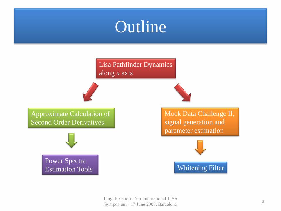
Outline
Lisa Pathfinder Dynamics
along x axis
Approximate Calculation of
Second Order Derivatives
Power Spectra
Estimation Tools
Mock Data Challenge II,
signal generation and
parameter estimation
Whitening Filter
2Luigi Ferraioli - 7th International LISA
Symposium - 17 June 2008, Barcelona

LTP Dynamics
0 i n
n
D q g
g g C o o g
o S q o
0
is a vector containing the dynamical coordinates
is a force-per-unit mass vector
is the force-per-unit mass disturbance (it summarize all the possible force-noise sources)
is a force-per-un
n
q
g
g
g
it mass vector purposely applied to the system
is the available signal vactor
is an input signal vector used to apply forces trough the control loops
is the dynamical matrix
is the feedback
i
o
o
D
C
circuit matrix. It converts available signals into commanded force
converts the coordinate vector into the measured signal vectorS
System Dynamics
3Luigi Ferraioli - 7th International LISA
Symposium - 17 June 2008, Barcelona

LTP Dynamics
Looking at the interferometer output…
11
o no D S C a o o
Is defined as the system nominal response
Is the colored noise output
11
o io D S C C o
11 1
n n no D S C g D S o
And going back…
1 11 1
o na D S C o D S C o o
Where…
1o
o
o
oo
o
and
1n
n
n
oo
o
4Luigi Ferraioli - 7th International LISA
Symposium - 17 June 2008, Barcelona
LTP Dynamics
In imaginary angular frequency notation s…
2 2 2 2
1 1 2 2 2 2
2 2 2 2
2 1 2 2
1
2
p p p
p p p
sD
s
Where…
2
0
df lfs
lfs
H hC
h
11 1
1
S SS
S S
1 1 2 2
2 1
1 n n
n
n n
g g Gg
g g
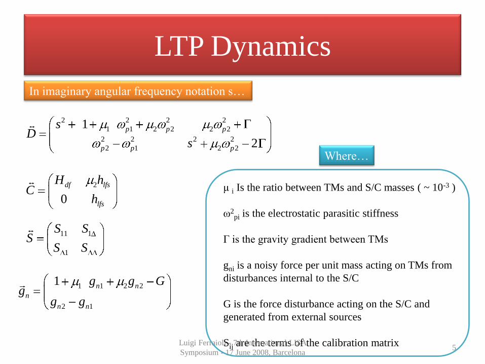
μ i Is the ratio between TMs and S/C masses ( ~ 10-3 )
ω2pi is the electrostatic parasitic stiffness
Γ is the gravity gradient between TMs
gni is a noisy force per unit mass acting on TMs from
disturbances internal to the S/C
G is the force disturbance acting on the S/C and
generated from external sources
Sij are the terms of the calibration matrix5
Luigi Ferraioli - 7th International LISA
Symposium - 17 June 2008, Barcelona

Derivative Estimation
We have a continuous dynamics and a discrete control circuit…
2 2 2 2
1 1 2 2 2 2
2 2 2 2
2 1 2 2
1
2
p p p
p p p
sD
s
We decided to make a discrete approximation
of the second derivative represented by s2…
2
0
df lfs
lfs
H hC
h
Parabolic fit approximation
to the second derivative
Taylor series expansion
approximation to the
second derivative
6Luigi Ferraioli - 7th International LISA
Symposium - 17 June 2008, Barcelona

Derivative Estimation – parabolic fit
approximation
22
0 1 2 22 2i
i
t kT
d o to k m T k k mT k mT
dt
0t kT mNote:
The fit procedure
22 1 1 2
2 2
1 2 1 2 1 2
7 7 7 7 7
dz z z z z
dt T
7Luigi Ferraioli - 7th International LISA
Symposium - 17 June 2008, Barcelona

Derivative Estimation – series expansion
approximation
2 3 4
5
0 0 0 0 0 02 6 24
I II III IVnT nT nTf x nT f x nTf x f x f x f x O T
22 1 1 2
2 2
1 1 16 30 16 1
12 12 12 12 12
dz z z z z
dt T
This method is based on the series expansion of a function representing data points…
We obtain a five point estimator if the
expansion is performed for:2, 1,0,1,2n
Putting the five expansions in a
system and solving out for the
second derivative f II[x0 ]
8Luigi Ferraioli - 7th International LISA
Symposium - 17 June 2008, Barcelona

Derivative Estimation – General equation
22 1 1 2
2 2
1dz az bz c bz az
dt T
The two methods are part of an entire family of derivative estimators…
The parameters a, b and c
are not independent:
iz e
In Laplace notation the second
derivative estimator is:
2 cos(2 ) 2 cos( )a b c
2 2s
We expect our estimator going
to zero at φ = 0 so:2 2 0a b c
Then we expect the estimator
tending to φ2 for small φ so:4 1a b
The final result is: 2 cos(2 ) 2 1 4 cos( ) 2 1 3a a a9
Luigi Ferraioli - 7th International LISA
Symposium - 17 June 2008, Barcelona

Derivative Estimation – General equation
Parabolic fit:2
7a Has a root at 2.42 0.39
s
frad
f
Series expansion:1
12a Does not have roots between 0 and π
Root at π :1
4a Has a root at π
0 0.5 1 1.5 2 2.5 3 3.5-10
-8
-6
-4
-2
0
2
[rad]
Am
pli
tud
e
s2
Parabolic Fit
Series Expansion
Zero at
10-6
10-4
10-2
100
10-15
10-10
10-5
100
105
f / fs
Am
pli
tud
e
s2
Parabolic Fit
Series Expansion
Zero at
10Luigi Ferraioli - 7th International LISA
Symposium - 17 June 2008, Barcelona

10-1
100
10-2
10-1
100
101
f / fs
Am
pli
tud
e
s2
Parabolic Fit
Series Expansion
Zero at
Derivative Estimation – General equation
Difference is roughly one
order of magnitude.
We know this can generate
problems in estimating the
PSD of the acceleration
noise at low frequencies
11Luigi Ferraioli - 7th International LISA
Symposium - 17 June 2008, Barcelona

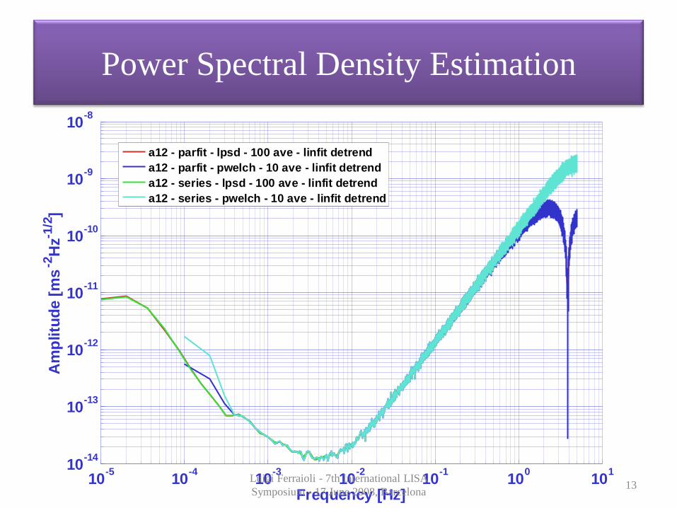
Power Spectral Density Estimation
We have to different tools in the toolbox
pwelch
Generalizes the standard Matlab pwelch
allowing for several detrending options
• linear frequency spacing
• FFT algorithm
lpsd*
• logarithmic frequency spacing
• DFT algorithm
* M. Tröbs and G. Heinzel, Measurement 39 (2006) 120-129 12Luigi Ferraioli - 7th International LISA
Symposium - 17 June 2008, Barcelona
Power Spectral Density Estimation
10-5
10-4
10-3
10-2
10-1
100
101
10-14
10-13
10-12
10-11
10-10
10-9
10-8
Am
plitu
de
[m
s-2
Hz-1
/2]
Frequency [Hz]
a12 - parfit - lpsd - 100 ave - linfit detrend
a12 - parfit - pwelch - 10 ave - linfit detrend
a12 - series - lpsd - 100 ave - linfit detrend
a12 - series - pwelch - 10 ave - linfit detrend
13Luigi Ferraioli - 7th International LISA
Symposium - 17 June 2008, Barcelona

Power Spectral Density Estimation
10-5
10-4
10-3
10-2
10-1
100
101
10-14
10-13
10-12
10-11
10-10
10-9
10-8
Am
plitu
de
[m
s-2
Hz-1
/2]
Frequency [Hz]
a12 - parfit - lpsd - 100 ave - linfit detrend
a12 - parfit - pwelch - 10 ave - linfit detrend
a12 - series - lpsd - 100 ave - linfit detrend
a12 - series - pwelch - 10 ave - linfit detrend
No difference between parfit
and series with lpsd
14Luigi Ferraioli - 7th International LISA
Symposium - 17 June 2008, Barcelona

Power Spectral Density Estimation
10-5
10-4
10-3
10-2
10-1
100
101
10-14
10-13
10-12
10-11
10-10
10-9
10-8
Am
plitu
de
[m
s-2
Hz-1
/2]
Frequency [Hz]
a12 - parfit - lpsd - 100 ave - linfit detrend
a12 - parfit - pwelch - 10 ave - linfit detrend
a12 - series - lpsd - 100 ave - linfit detrend
a12 - series - pwelch - 10 ave - linfit detrend
Different noise levels
between parfit and
series with pwelch
15Luigi Ferraioli - 7th International LISA
Symposium - 17 June 2008, Barcelona

Signal generation
We will adopt an analytical approach, where signal and colored noise are generated
apart and then added each other…
t s t n t
Colored noise generation with a defined spectrum…
n is assumed Gaussian and stationary
* †
n niS H S H H is the system transfer function
Sni is the input noise signal
Generating signals from white noise…
†*
nS h I h I is the cross spectral matrix of an unitary variance
white noise process
This is equivalent to…
1/2 1/2 1
nS V I V V is the eigenvector matrix and Λ is
the eigenvalue matrix of Sn 16Luigi Ferraioli - 7th International LISA
Symposium - 17 June 2008, Barcelona

Signal generation
From the equivalence…
The transfer function for noise generation can be found…
* 1/2h V We have written a LTPDA Toolbox function psd2tf
to perform the calculation of the innovation transfer
function h
And at the same time the whitening filter transfer function…
†*
nS h I h
A set of functions is now disposable in the LTPDA
Toolbox allowing for the whitening of the data starting
from a model of the frequency response of the noise
PSD and CSD
1/2 1/2 1
nS V I V
1w h
17Luigi Ferraioli - 7th International LISA
Symposium - 17 June 2008, Barcelona

Whitening Filter
Coming back to the system dynamics…
2 2 2 2
1 1 2 2 2 2
2 2 2 2
2 1 2 2
1
2
p p p
p p p
sD
s
We see the parameters to
be estimated…
2
0
df lfs
lfs
H hC
h
11 1
1
S SS
S S
1 1 2 2
2 1
1 n n
n
n n
g g Gg
g g
Hdf and Hlfs are the gains of the control circuit loops
ω2pi is the electrostatic parasitic stiffness
Γ is the gravity gradient between TMs
gni is a noisy force per unit mass acting on TMs from
disturbances internal to the S/C
G is the force disturbance acting on the S/C and
generated from external sources
Sij are the terms of the calibration matrix18
Luigi Ferraioli - 7th International LISA
Symposium - 17 June 2008, Barcelona

Whitening Filter
Parameters estimation can be afforded by maximum likelihood
estimation. That is equivalent to minimize the function…
2,
, , ,
, 1 , 1
, , , , , ,dataN
k j k i k j i j
k j
o t o D S C t o t o D S C t
Where…
, ,
1,
, ,n nk j o o sampR k j T R is the cross correlation between
the two channel signals noise
If the noise is white…
, ,, , ,n no oR k j
The minimization process
is highly simplified
19Luigi Ferraioli - 7th International LISA
Symposium - 17 June 2008, Barcelona

Whitening Filter
Model PSD
generation
mPSD o1
mPSD o12
mCSD
psd2wf
white filter
generation
wf11
wf12
wf21
wf22
Wf2_freq
white filter in
frequency domain
Input data (colored noise)
o1 o12
wo1
wo12
Output data (white noise)
20Luigi Ferraioli - 7th International LISA
Symposium - 17 June 2008, Barcelona

Whitening Filter
10-6
10-5
10-4
10-3
10-2
10-1
100
101
10-24
10-23
10-22
10-21
10-20
10-19
10-18
10-17
10-16
PS
D [
m2 H
z-1
]
Frequency [Hz]
moled So
So ave
+1/2 std
-1/2 std
PSD of interferometer output noise. Average on 11 simulated datasets
Method: pwelch, linear fit detrend, 10 average, BlackmannHarris window, 69% overlap
Spacecraft
Diff. Channel
21Luigi Ferraioli - 7th International LISA
Symposium - 17 June 2008, Barcelona
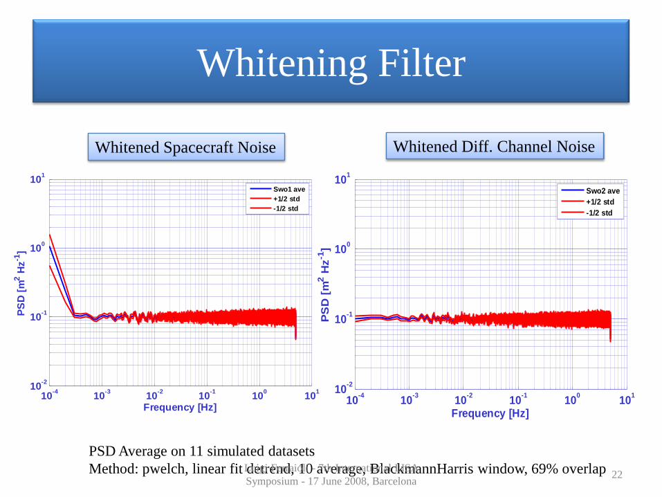
Whitening Filter
PSD Average on 11 simulated datasets
Method: pwelch, linear fit detrend, 10 average, BlackmannHarris window, 69% overlap
Whitened Spacecraft Noise Whitened Diff. Channel Noise
10-4
10-3
10-2
10-1
100
101
10-2
10-1
100
101
PS
D [
m2 H
z-1
]
Frequency [Hz]
Swo1 ave
+1/2 std
-1/2 std
10-4
10-3
10-2
10-1
100
101
10-2
10-1
100
101
PS
D [
m2 H
z-1
]
Frequency [Hz]
Swo2 ave
+1/2 std
-1/2 std
22Luigi Ferraioli - 7th International LISA
Symposium - 17 June 2008, Barcelona

Whitening Filter
Colored noise and model Whitened data
10-5
10-4
10-3
10-2
10-1
100
101
-0.3
-0.2
-0.1
0.0
0.1
0.2
0.3
Cro
ss C
oh
ere
nce
Frequency [ Hz ]
re - data
im - data
re - model
im - model
10-4
10-3
10-2
10-1
100
101
-0.3
-0.2
-0.1
0.0
0.1
0.2
0.3
Cro
ss C
ohere
nce
Frequency [ Hz ]
re - whiten data
im - whiten data
Cross Coherence is defined as1 12
CSD
PSD PSD
23Luigi Ferraioli - 7th International LISA
Symposium - 17 June 2008, Barcelona

Whitening Filter - Signals
Looking at the
interferometer
output…
o no o o
System response to a commanded
input in the control circuit
Is the colored noise output
11
o io D S C C o
11 1
n n no D S C g D S o
1 01 11
0
sin 2
sin 2
ii
i
i i
A f too
o A f t
6
1
7
3
1
3
1
1 10 [ ]
8 10 [ ]
3.45 10 [ ]
4.7 10 [ ]
0
i
i
i
i
i i
A x m
A x m
f x Hz
A x Hz
10-4
10-3
10-2
10-1
100
101
10-30
10-25
10-20
10-15
10-10
10-5
PS
D [
m2H
z-1]
Frequency [Hz]
oi1
oi
oo1
oo
24Luigi Ferraioli - 7th International LISA
Symposium - 17 June 2008, Barcelona
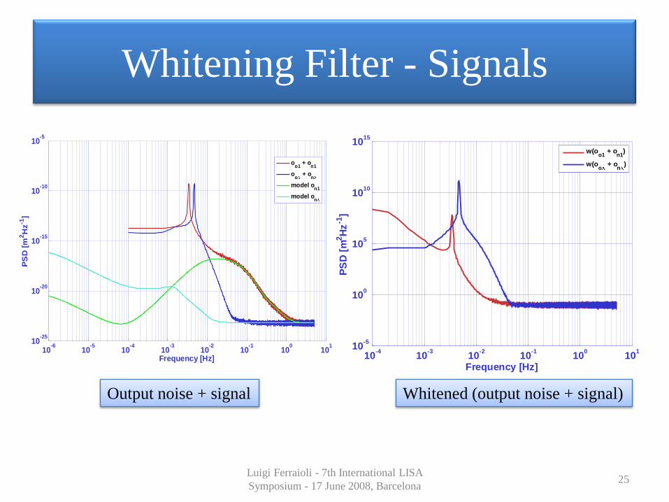
Whitening Filter - Signals
10-6
10-5
10-4
10-3
10-2
10-1
100
101
10-25
10-20
10-15
10-10
10-5
PS
D [
m2H
z-1
]
Frequency [Hz]
oo1
+ on1
oo
+ on
model on1
model on
10-4
10-3
10-2
10-1
100
101
10-5
100
105
1010
1015
PS
D [
m2H
z-1
]
Frequency [Hz]
w(oo1
+ on1
)
w(oo
+ on
)
Output noise + signal Whitened (output noise + signal)
25Luigi Ferraioli - 7th International LISA
Symposium - 17 June 2008, Barcelona

Whitening Filter - Signals
Real and Imaginary part of colored and whitened output noise + signal
10-4
10-3
10-2
10-1
100
101
-1
-0.8
-0.6
-0.4
-0.2
0
0.2
0.4
0.6
0.8
1
Cro
ss
Co
he
ren
ce
Frequency [Hz]
Re[oo1
+ on1
]
Im[oo1
+ on1
]
Re[w(oo1
+ on1
)]
Im[w(oo1
+ on1
)]
26Luigi Ferraioli - 7th International LISA
Symposium - 17 June 2008, Barcelona

Thank You
27Luigi Ferraioli - 7th International LISA
Symposium - 17 June 2008, Barcelona