LS-OPT User s Manual - LS-DYNAlstc.com/pdf/lsopt.pdf · LS-OPT Version 2 v 2.13 Sequential random...
407
LS-OPT User’s Manual A DESIGN OPTIMIZATION AND PROBABILISTIC ANALYSIS TOOL FOR THE ENGINEERING ANALYST NIELEN STANDER, Ph.D. WILLEM ROUX, Ph.D. TRENT EGGLESTON, Ph.D. KEN CRAIG, Ph.D. March, 2004 Version 2.2 Copyright © 1999-2004 LIVERMORE SOFTWARE TECHNOLOGY CORPORATION All Rights Reserved
Transcript of LS-OPT User s Manual - LS-DYNAlstc.com/pdf/lsopt.pdf · LS-OPT Version 2 v 2.13 Sequential random...

LS-OPT User’s Manual
A DESIGN OPTIMIZATION AND PROBABILISTIC ANALYSIS TOOL FOR THE ENGINEERING ANALYST
NIELEN STANDER, Ph.D. WILLEM ROUX, Ph.D.
TRENT EGGLESTON, Ph.D. KEN CRAIG, Ph.D.
March, 2004
Version 2.2
Copyright © 1999-2004 LIVERMORE SOFTWARE
TECHNOLOGY CORPORATION All Rights Reserved

Mailing address: Livermore Software Technology Corporation
2876 Waverley Way Livermore, California 94551
Support Address:
Livermore Software Technology Corporation 7374 Las Positas Road
Livermore, California 94551
FAX: 925-449-2507 TEL: 925-449-2500
EMAIL: [email protected]
Copyright © 1999-2004 by Livermore Software Technology Corporation All Rights Reserved

iii
Contents
Contents...........................................................................................................................................................iii
Preface to Version 1 ....................................................................................................................................xvii
Preface to Version 2 ....................................................................................................................................xvii
1. Introduction 1
THEORETICAL MANUAL .......................................................................................................................... 3
2. Optimization Methodology 5
2.1 Introduction ............................................................................................................................... 5
2.2 Theory of Optimization............................................................................................................. 7
2.3 Gradient Computation and the Solution of Optimization Problems ......................................... 8
2.4 Normalization of constraints and variables............................................................................... 9
2.5 Response Surface Methodology.............................................................................................. 10
2.5.1 Approximating the response ................................................................................................... 11
2.5.2 Factors governing the accuracy of the response surface......................................................... 12
2.5.3 Advantages of the method....................................................................................................... 12
2.5.4 Other types of response surfaces............................................................................................. 12
2.6 Experimental design................................................................................................................ 13
2.6.1 Factorial design ....................................................................................................................... 13
2.6.2 Koshal design .......................................................................................................................... 13
First order model ..................................................................................................................... 13
Second order model................................................................................................................. 13
2.6.3 Central Composite design ....................................................................................................... 14
2.6.4 D-optimal design..................................................................................................................... 15
2.6.5 Latin Hypercube Sampling (LHS) .......................................................................................... 15

CONTENTS
iv LS-OPT Version 2
Maximin .................................................................................................................................. 16
Centered L2-discrepancy ........................................................................................................ 16
2.6.6 Space-filling designs* ............................................................................................................. 17
Discussion of algorithms......................................................................................................... 19
2.6.7 Random number generator...................................................................................................... 20
2.7 Reasonable experimental designs* ......................................................................................... 20
2.8 Model adequacy checking....................................................................................................... 21
2.8.1 Residual sum of squares.......................................................................................................... 21
2.8.2 RMS error ............................................................................................................................... 21
2.8.3 Maximum residual .................................................................................................................. 22
2.8.4 Prediction error........................................................................................................................ 22
2.8.5 PRESS residuals...................................................................................................................... 22
2.8.6 The coefficient of multiple determination R2.......................................................................... 23
2.8.7 R2 for Prediction...................................................................................................................... 23
2.8.8 Iterative design and prediction accuracy................................................................................. 23
2.9 ANOVA .................................................................................................................................. 23
2.9.1 The confidence interval of the regression coefficients ........................................................... 24
2.9.2 The significance of a regression coefficient bj........................................................................ 24
2.10 Metamodeling techniques ....................................................................................................... 25
2.10.1 Neural network approximations*............................................................................................ 25
Model adequacy checking....................................................................................................... 27
Feed-forward neural networks ................................................................................................ 29
2.10.2 Kriging* .................................................................................................................................. 32
2.10.3 Concluding remarks: which metamodel?................................................................................ 34
2.11 Core optimization algorithm (LFOPC) ................................................................................... 34
2.12 Successive response surface method (SRSM) ........................................................................ 35

CONTENTS
LS-OPT Version 2 v
2.13 Sequential random search (SRS)............................................................................................. 37
2.14 Summary of the optimization process..................................................................................... 39
2.14.1 Design exploration .................................................................................................................. 40
2.14.2 Convergence to an optimal point ............................................................................................ 39
2.15 Applications of optimization................................................................................................... 40
2.15.1 Multicriteria Design Optimization .......................................................................................... 40
Euclidean Distance Function .................................................................................................. 40
Maximum distance .................................................................................................................. 41
2.15.2 Multidisciplinary Design Optimization .................................................................................. 42
2.15.3 Parameter Identification .......................................................................................................... 43
Maximum violation formulation............................................................................................. 44
2.15.4 Worst-case design ................................................................................................................... 44
2.15.5 Reliability-based design optimization (RBDO)*.................................................................... 45
3. Probabilistic Fundamentals 47
3.1 Introduction ............................................................................................................................. 47
3.2 Probabilistic variables ............................................................................................................. 47
3.2.1 Variable linking....................................................................................................................... 48
3.3 Basic computations ................................................................................................................. 48
3.3.1 Mean, variance, standard deviation, and coefficient of variation ........................................... 48
3.3.2 Correlation of responses.......................................................................................................... 49
3.4 Probabilistic methods.............................................................................................................. 49
3.4.1 Monte Carlo analysis............................................................................................................... 49
3.4.2 Monte Carlo analysis using metamodels................................................................................. 51
3.4.3 First-Order Second-Moment Method (FOSM) ....................................................................... 52
3.5 Required number of simulations ............................................................................................. 53
3.5.1 Overview................................................................................................................................. 53

CONTENTS
vi LS-OPT Version 2
3.5.2 Background ............................................................................................................................. 53
3.5.3 Competing role of variance and bias....................................................................................... 54
3.5.4 Confidence interval on the mean............................................................................................. 55
3.5.5 Confidence interval on a new evaluation ................................................................................ 55
3.5.6 Confidence interval on the random deviation (σ2) .................................................................. 56
3.5.7 Probability of observing a specific failure mode .................................................................... 57
3.6 Outlier analysis........................................................................................................................ 57
3.7 Stochastic contribution analysis.............................................................................................. 58
USER’S MANUAL........................................................................................................................................ 61
4. Design Optimization Process 63
4.1 LS-OPT Features..................................................................................................................... 63
4.2 A modus operandi for design using response surfaces ........................................................... 64
4.2.1 Preparation for design ............................................................................................................. 64
4.2.2 A step-by-step design optimization procedure........................................................................ 65
4.3 Recommended test procedure ................................................................................................. 67
4.4 Pitfalls in design optimization................................................................................................. 67
4.5 Advanced methods for design optimization............................................................................ 68
4.5.1 Neural Nets and Kriging* ....................................................................................................... 68
5. Graphical User Interface and Command Language 71
5.1 LS-OPT user interface (LS-OPTui) ........................................................................................ 71
5.2 Problem description and author name..................................................................................... 72
5.3 Command Language ............................................................................................................... 74
5.3.1 Names...................................................................................................................................... 74
5.3.2 Command lines ....................................................................................................................... 75
5.3.3 File names ............................................................................................................................... 75

CONTENTS
LS-OPT Version 2 vii
5.3.4 Command file structure........................................................................................................... 75
5.3.5 Environments .......................................................................................................................... 76
5.3.6 Expressions ............................................................................................................................. 76
6. Program Execution 77
6.1 Work directory ........................................................................................................................ 77
6.2 Execution commands .............................................................................................................. 77
6.3 Directory structure .................................................................................................................. 77
6.4 Job Monitoring........................................................................................................................ 78
6.5 Result extraction...................................................................................................................... 79
6.6 Restarting ................................................................................................................................ 79
6.7 Output files.............................................................................................................................. 80
6.8 Using a table of existing results to conduct an analysis.......................................................... 81
6.9 Log files and status files.......................................................................................................... 81
6.10 Managing disk space during run time ..................................................................................... 82
6.11 Error termination of a solver run............................................................................................. 83
6.12 Parallel processing .................................................................................................................. 83
6.13 Using an external queuing or job scheduling system.............................................................. 83
For all remote machines running LS-DYNA.......................................................................... 84
Local installation..................................................................................................................... 84
6.14 Database conversion................................................................................................................ 86
7. Interfacing to a solver or preprocessor 87
7.1 Labeling design variables in a solver and preprocessor.......................................................... 87
7.1.1 The LS-OPT Parameter Format .............................................................................................. 88
7.2 Interfacing to a Solver............................................................................................................. 90
7.2.1 Interfacing with LS-DYNA..................................................................................................... 92

CONTENTS
viii LS-OPT Version 2
The *PARAMETER format.................................................................................................. 92
7.2.2 Interfacing with LS-DYNA/MPP ........................................................................................... 93
7.2.3 Interfacing with a user-defined solver..................................................................................... 93
7.3 Preprocessors........................................................................................................................... 94
7.3.1 LS-INGRID............................................................................................................................. 94
7.3.2 TrueGrid.................................................................................................................................. 95
7.3.3 AutoDV................................................................................................................................... 95
7.3.4 HyperMorph............................................................................................................................ 97
7.3.5 DEP-Morpher.......................................................................................................................... 98
7.3.6 User-defined preprocessor ...................................................................................................... 99
8. Design Variables, Constants and Dependents 101
8.1 Selection of design variables................................................................................................. 102
8.2 Definition of upper and lower bounds of the design space................................................... 102
8.3 Size and location of region of interest (range) ...................................................................... 102
8.4 Local variables ...................................................................................................................... 103
8.5 Assigning variable to solver.................................................................................................. 103
8.6 Constants ............................................................................................................................... 103
8.7 Dependent Variables ............................................................................................................. 104
8.8 Worst-case design ................................................................................................................. 105
9. Probabilistic Modeling and Monte Carlo Simulation 107
9.1 Probabilistic problem modeling ............................................................................................ 107
9.2 Probabilistic Distributions..................................................................................................... 108
9.2.1 Beta distribution .................................................................................................................... 108
9.2.2 Binomial distribution ............................................................................................................ 109
9.2.3 Lognormal distribution ......................................................................................................... 110

CONTENTS
LS-OPT Version 2 ix
9.2.4 Normal Distribution .............................................................................................................. 111
9.2.5 Uniform distribution ............................................................................................................. 112
9.2.6 User defined distribution....................................................................................................... 113
9.2.7 Weibull distribution .............................................................................................................. 115
9.3 Probabilistic Variables .......................................................................................................... 116
9.3.1 Setting the Nominal Value of a Probabilistic Variable......................................................... 117
9.3.2 Bounds on Probabilistic Variable Values ............................................................................. 117
9.3.3 Noise Variable Subregion Size ............................................................................................. 118
9.4 Probabilistic Simulation........................................................................................................ 118
9.4.1 Monte Carlo Analyses........................................................................................................... 119
9.4.2 Monte Carlo analysis using a Metamodel............................................................................. 119
9.4.3 Accuracy of Metamodel Based Monte Carlo........................................................................ 120
9.4.4 Histograms of Responses ...................................................................................................... 120
9.4.5 Adding the Noise Component to Metamodel Monte Carlo Computations........................... 121
9.5 Stochastic Contribution Analysis.......................................................................................... 121
9.6 Covariance............................................................................................................................. 121
10. Metamodels and Point Selection 124
10.1 Metamodel definition ............................................................................................................ 124
10.1.1 Response Surface Methodology............................................................................................ 124
10.1.2 Neural Networks and Kriging * ............................................................................................ 125
10.2 Point Selection Schemes ....................................................................................................... 125
10.2.1 Overview............................................................................................................................... 125
10.2.2 D-Optimal point selection ..................................................................................................... 128
10.2.3 Latin Hypercube Sampling ................................................................................................... 128
10.2.4 Space filling* ........................................................................................................................ 129

CONTENTS
x LS-OPT Version 2
10.3 User-defined experiments ..................................................................................................... 130
10.4 Remarks: Point selection....................................................................................................... 130
10.5 Specifying an irregular design space*................................................................................... 130
10.6 Updating an experimental design.......................................................................................... 132
10.7 Duplicating an experimental design...................................................................................... 132
10.8 Using design sensitivities for optimization........................................................................... 133
10.8.1 Analytical sensitivities .......................................................................................................... 133
10.8.2 Numerical sensitivities .......................................................................................................... 133
11. History and Response Results 136
11.1 Defining a response history (vector) ..................................................................................... 136
11.2 Defining a response (scalar).................................................................................................. 138
11.3 Specifying the metamodel type............................................................................................. 139
11.4 Composite Functions............................................................................................................. 140
11.4.1 Expression Composite........................................................................................................... 140
11.4.2 Standard Composite .............................................................................................................. 141
Targeted Composite .............................................................................................................. 141
Weighted Composite............................................................................................................. 141
11.4.3 Defining the composite function........................................................................................... 142
11.4.4 Assigning design variable or response components to the composite ................................. 143
11.4.5 Composites vs. Response Expressions.................................................................................. 144
11.5 Extracting History and Response Quantities: LS-DYNA..................................................... 144
11.6 Extracting response quantities from ASCII output: LS-DYNA ........................................... 145
11.6.1 Mass ...................................................................................................................................... 145
11.6.2 Frequency of given modal shape number ............................................................................. 147
11.6.3 Response history ................................................................................................................... 148
11.7 Extracting Response Quantities From the LS-DYNA d3plot file......................................... 150

CONTENTS
LS-OPT Version 2 xi
11.8 Extracting Histories From The LS-DYNA d3plot file.......................................................... 150
11.9 Extracting Metal Forming Response Quantities: LS-DYNA................................................ 151
11.9.1 Thickness and thickness reduction........................................................................................ 151
11.9.2 FLD Constraint ..................................................................................................................... 151
Bilinear FLD Constraint........................................................................................................ 153
General FLD Constraint........................................................................................................ 154
11.9.3 Principal Stress...................................................................................................................... 155
11.10 Extracting data from the LS-DYNA Binout file ................................................................... 155
11.10.1 Binout Histories .................................................................................................................... 156
Averaging, Filtering, and Slicing Binout histories ............................................................... 157
11.10.2 Binout Responses .................................................................................................................. 157
Binout Injury Criteria............................................................................................................ 158
11.11 Translating ASCII output commands to Binout commands ................................................. 158
11.12 DynaStat*.............................................................................................................................. 159
11.13 User Interface for Extracting Results.................................................................................... 159
12. Objectives and Constraints 163
12.1 Formulation ........................................................................................................................... 163
12.2 Defining an objective function.............................................................................................. 164
12.3 Defining a constraint ............................................................................................................. 165
12.4 Bounds on the constraint functions ....................................................................................... 167
12.5 Minimizing the maximum response or violation* ................................................................ 167
13. Running the Design Task 171
13.1 Optimization.......................................................................................................................... 171
13.1.1 Number of optimization iterations ........................................................................................ 171
13.1.2 Optimization termination criteria.......................................................................................... 171
13.2 Probabilistic Evaluation ........................................................................................................ 172

CONTENTS
xii LS-OPT Version 2
13.3 Restarting .............................................................................................................................. 173
13.4 Job concurrency .................................................................................................................... 173
13.5 Job distribution...................................................................................................................... 173
13.6 Job and analysis monitoring.................................................................................................. 173
13.7 Repair or modification of an existing job ............................................................................. 173
14. Viewing Results 176
14.1 Metamodel accuracy ............................................................................................................. 176
14.2 Optimization history ............................................................................................................. 177
14.3 Trade-off and anthill plots..................................................................................................... 178
14.4 Variable screening................................................................................................................. 179
14.5 Histograms ............................................................................................................................ 180
14.6 Stochastic Contribution......................................................................................................... 181
14.7 Covariance and Correlation................................................................................................... 182
14.8 Plot generation ...................................................................................................................... 183
15. Applications of Optimization 185
15.1 Multidisciplinary Design Optimization (MDO) ................................................................... 185
15.1.1 Command file........................................................................................................................ 185
15.2 Worst-case design ................................................................................................................. 186
15.3 Reliability-based design optimization (RBDO)*.................................................................. 186
15.3.1 Metamodel based RBDO ...................................................................................................... 186
15.3.2 Monte Carlo based RBDO .................................................................................................... 187
16. Optimization Algorithm Selection and Settings 189
16.1 Selecting an optimization algorithm ..................................................................................... 189
16.2 Setting the subdomain parameters ........................................................................................ 189
16.3 Setting parameters in the LFOPC optimization algorithm.................................................... 191

CONTENTS
LS-OPT Version 2 xiii
17. LS-DYNA Results Statistics 193
17.1 Analysis................................................................................................................................. 194
17.2 Metamodels and outliers ....................................................................................................... 195
17.3 Displacement Magnitude* .................................................................................................... 195
17.4 Correlation............................................................................................................................. 198
17.5 Solver and Iteration ............................................................................................................... 199
17.6 Visualization in LS-PREPOST ............................................................................................. 199
17.7 Bifurcation investigations ..................................................................................................... 200
EXAMPLES................................................................................................................................................. 203
18. Example Problems 205
18.1 Two-bar truss (2 variables) ................................................................................................... 205
18.1.1 Description of problem ......................................................................................................... 205
18.1.2 A first approximation using linear response surfaces ........................................................... 208
18.1.3 Updating the approximation to second order ........................................................................ 211
18.1.4 Reducing the region of interest for further refinement ......................................................... 214
18.1.5 Conducting a trade-off study................................................................................................. 216
18.1.6 Automating the design process ............................................................................................. 217
18.2 Small car crash (2 variables) ................................................................................................. 221
18.2.1 Introduction ........................................................................................................................... 221
18.2.2 Design criteria and design variables ..................................................................................... 221
18.2.3 Design formulation................................................................................................................ 222
18.2.4 Modeling ............................................................................................................................... 222
18.2.5 First linear iteration ............................................................................................................... 224
18.2.6 First quadratic iteration ......................................................................................................... 227
18.2.7 Automated run....................................................................................................................... 229
CONTENTS
xiv LS-OPT Version 2
18.2.8 Trade-off using neural network approximation* .................................................................. 231
18.2.9 Reliability-based design optimization using MDO*............................................................. 233
18.2.10 Reliability-based design optimization using FOSM* ........................................................... 237
18.3 Impact of a cylinder (2 variables) ......................................................................................... 238
18.3.1 Problem statement................................................................................................................. 238
18.3.2 A first approximation ............................................................................................................ 240
18.3.3 Refining the design model using a second iteration.............................................................. 244
18.3.4 Third iteration........................................................................................................................ 246
18.3.5 Response filtering: using the peak force as a constraint ....................................................... 247
18.4 Sheet-metal forming (3 variables)......................................................................................... 251
18.4.1 Problem statement................................................................................................................. 251
18.4.2 First Iteration......................................................................................................................... 253
18.4.3 Automated design.................................................................................................................. 260
18.5 Material identification (airbag) (10 variables) ...................................................................... 264
18.5.1 Problem statement................................................................................................................. 264
18.5.2 Least-squares residual (LSR) formulation ............................................................................ 264
18.5.3 Maximum violation formulation........................................................................................... 265
18.5.4 Implementation ..................................................................................................................... 266
18.5.5 Results ................................................................................................................................... 274
18.6 Small car crash and NVH (MDO) (5 variables).................................................................... 278
18.6.1 Parameterization and Variable screening.............................................................................. 278
18.6.2 MDO with D-optimal experimental design and SRSM........................................................ 280
18.6.3 Sequential random search ..................................................................................................... 285
18.7 Large car crash and NVH (MDO) (7 variables).................................................................... 289
18.7.1 Modeling ............................................................................................................................... 289

CONTENTS
LS-OPT Version 2 xv
18.7.2 Formulation of optimization problem ................................................................................... 291
18.7.3 Implementation in LS-OPT................................................................................................... 292
18.7.4 Simulation results.................................................................................................................. 295
18.7.5 Optimization history results .................................................................................................. 295
18.7.6 Comparison of optimum designs .......................................................................................... 300
18.7.7 Convergence and computational cost.................................................................................... 301
18.8 Knee impact with variable screening (11 variables) ............................................................. 302
18.8.1 Problem statement................................................................................................................. 302
18.8.2 Definition of optimization problem ...................................................................................... 304
18.8.3 Implementation ..................................................................................................................... 304
18.8.4 Variable screening................................................................................................................. 307
18.8.5 Optimization with reduced variables .................................................................................... 309
18.9 Optimization with analytical design sensitivities.................................................................. 310
18.10 Probabilistic Analysis ........................................................................................................... 313
18.10.1 Overview............................................................................................................................... 313
18.10.2 Problem description .............................................................................................................. 313
18.10.3 Monte Carlo evaluation......................................................................................................... 314
18.10.4 Monte Carlo using metamodel .............................................................................................. 317
18.10.5 Bifurcation analysis............................................................................................................... 321
18.11 Bifurcation/Outlier Analysis ................................................................................................. 322
18.11.1 Overview............................................................................................................................... 322
18.11.2 Problem description .............................................................................................................. 322
18.11.3 Monte Carlo evaluation......................................................................................................... 322
18.11.4 Identification of buckling modes .......................................................................................... 323
Bibliography ................................................................................................................................................ 326

CONTENTS
xvi LS-OPT Version 2
Appendix A .................................................................................................................................................. 331
LS-DYNA ASCII Result Files and Components ...................................................................................... 331
Appendix B .................................................................................................................................................. 341
LS-DYNA Binary Result Components...................................................................................................... 341
Appendix C .................................................................................................................................................. 343
LS-DYNA Binout Result File and Components ....................................................................................... 343
Appendix D .................................................................................................................................................. 359
Database files ............................................................................................................................................... 359
Appendix E .................................................................................................................................................. 363
Mathematical Expressions.......................................................................................................................... 363
Appendix F................................................................................................................................................... 373
Simulated Annealing................................................................................................................................... 373
Appendix G.................................................................................................................................................. 377
Glossary........................................................................................................................................................ 377
Appendix H.................................................................................................................................................. 383
LS-OPT Commands: Quick Reference Manual....................................................................................... 383
LS-OPT Version 2 xvii
Preface to Version 1
LS-OPT originated in 1995 from research done within the Department of Mechanical Engineering, University of Pretoria, South Africa. The original development was done in collaboration with colleagues in the Department of Aerospace Engineering, Mechanics and Engineering Science at the University of Florida in Gainesville. Much of the later development at LSTC was influenced by industrial partners, particularly in the automotive industry. Thanks are due to these partners for their cooperation and also for providing access to high-end computing hardware. At LSTC, the author wishes to give special thanks to colleague and co-developer Dr. Trent Eggleston. Thanks are due to Mr. Mike Burger for setting up the examples. Nielen Stander Livermore, CA August, 1999
Preface to Version 2
Version 2 of LS-OPT evolved from Version 1 and differs in many significant regards. These can be summarized as follows:
1. The addition of a mathematical library of expressions for composite functions. 2. The addition of variable screening through the analysis of variance. 3. The expansion of the multidisciplinary design optimization capability of LS-OPT. 4. The expansion of the set of point selection schemes available to the user. 5. The interface to the LS-DYNA binary database. 6. Additional features to facilitate the distribution of simulation runs on a network. 7. The addition of Neural Nets and Kriging as metamodeling techniques. 8. Probabilistic modeling and Monte Carlo simulation. A sequential search method.
As in the past, these developments have been influenced by industrial partners, particularly in the automotive industry. Several developments were also contributed by Nely Fedorova and Serge Terekhoff of SFTI. Invaluable research contributions have been made by Professor Larsgunnar Nilsson and his group in the Mechanical Engineering Department at Linköping University, Sweden and by Professor Ken Craig’s group in the Department of Mechanical Engineering at the University of Pretoria, South Africa. The authors also wish to give special thanks to Mike Burger at LSTC for setting up further examples for Version 2. Nielen Stander, Ken Craig, Trent Eggleston and Willem Roux Livermore, CA January, 2003

PREFACE
xviii LS-OPT Version 2

1
1. Introduction
This LS-OPT manual consists of three parts. In the first part, the Theoretical Manual (Chapter 2), the theoretical background is given for the various features in LS-OPT. The next part is the User’s Manual (Chapters 4 through 16), which guides the user in the use of LS-OPTui, the graphical user interface. These chapters also describe the command language syntax. The final part of the manual is the Examples section (Chapter 18), where eight examples illustrate the application of LS-OPT to a variety of practical applications. Appendices contain interface features (Appendix A, Appendix B and Appendix C), database file descriptions (Appendix D), a mathematical expression library (Appendix E), advanced theory (Appendix F), a Glossary (Appendix G) and a Quick Reference Manual (Appendix H). Sections containing advanced topics are indicated with an asterisk (*). How to read this manual: Most users will start learning LS-OPT by consulting the User’s Manual section beginning with Chapter 4 (The design optimization process). The Theoretical Manual (Chapter 2) serves mainly as an in-depth reference section for the underlying methods. The Examples section is included to demonstrate the features and capabilities and can be read together with Chapters 3 to 14 to help the user to set up a problem formulation. The items in the Appendices are included for reference to detail, while the Quick Reference Manual provides an overview of all the features and command file syntax.

INTRODUCTION
2 LS-OPT Version 2

3
THEORETICAL MANUAL

4 LS-OPT Version 2

5
2. Optimization Methodology
2.1 Introduction In the conventional design approach, a design is improved by evaluating its response and making design changes based on experience or intuition. This approach does not always lead to the desired result, that of a ‘best’ design, since design objectives are sometimes in conflict, and it is not always clear how to change the design to achieve the best compromise of these objectives. A more systematic approach can be obtained by using an inverse process of first specifying the criteria and then computing the ‘best’ design. The procedure by which design criteria are incorporated as objectives and constraints into an optimization problem that is then solved, is referred to as optimal design. The state of computational methods and computer hardware has only recently advanced to the level where complex nonlinear problems can be analyzed routinely. Many examples can be found in the simulation of impact problems and manufacturing processes. The responses resulting from these time-dependent processes are, as a result of behavioral instability, often highly sensitive to design changes. Program logic, as for instance encountered in parallel programming or adaptivity, may cause spurious sensitivity. Roundoff error may further aggravate these effects, which, if not properly addressed in an optimization method, could obstruct the improvement of the design by way of corrupting the function gradients. Among several methodologies available to address optimization in this design environment, response surface methodology (RSM), a statistical method for constructing smooth approximations to functions in a multi-dimensional space, has achieved prominence in recent years. Rather than relying on local information such as a gradient only, RSM selects designs that are optimally distributed throughout the design space to construct approximate surfaces or ‘design formulae’. Thus, the local effect caused by ‘noise’ is alleviated and the method attempts to find a representation of the design response within a bounded design space or smaller region of interest. This extraction of global information allows the designer to explore the design space, using alternative design formulations. For instance, in vehicle design, the designer may decide to investigate the effect of varying a mass constraint, while monitoring the crashworthiness responses of a vehicle. The designer might also decide to constrain the crashworthiness response while minimizing or maximizing any other criteria such as mass, ride comfort criteria, etc. These criteria can be weighted differently according to importance and therefore the design space needs to be explored more widely. Part of the challenge of developing a design program is that designers are not always able to clearly define their design problem. In some cases, design criteria may be regulated by safety or other considerations and therefore a response has to be constrained to a specific value. These can be easily defined as mathematical constraint equations. In other cases, fixed criteria are not available but the designer knows whether the

CHAPTER 2: OPTIMIZATION METHODOLOGY
6 LS-OPT Version 2
responses must be minimized or maximized. In vehicle design, for instance, crashworthiness can be constrained because of regulation, while other parameters such as mass, cost and ride comfort can be treated as objectives to be weighted according to importance. In these cases, the designer may have target values in mind for the various response and/or design parameters, so that the objective formulation has to be formulated to approximate the target values as closely as possible. Because the relative importance of various criteria can be subjective, the ability to visualize the trade-off properties of one response vs. another becomes important. Trade-off curves are visual tools used to depict compromise properties where several important response parameters are involved in the same design. They play an extremely important role in modern design where design adjustments must be made accurately and rapidly. Design trade-off curves are constructed using the principle of Pareto optimality. This implies that only those designs of which the improvement of one response will necessarily result in the deterioration of any other response are represented. In this sense no further improvement of a Pareto optimal design can be made: it is the best compromise. The designer still has a choice of designs but the factor remaining is the subjective choice of which feature or criterion is more important than another. Although this choice must ultimately be made by the designer, these curves can be helpful in making such a decision. An example in vehicle design is the trade-off between mass (or energy efficiency) and safety. Adding to the complexity, is the fact that mechanical design is really an interdisciplinary process involving a variety of modeling and analysis tools. To facilitate this process, and allow the designer to focus on creativity and refinement, it is important to provide suitable interfacing utilities to integrate these design tools. Designs are bound to become more complex due to the legislation of safety and energy efficiency as well as commercial competition. It is therefore likely that in future an increasing number of disciplines will have be integrated into a particular design. This approach of multidisciplinary design requires the designer to run more than one case, often using more than one type of solver. For example, the design of a vehicle may require the consideration of crashworthiness, ride comfort, noise level as well as durability. Moreover, the crashworthiness analysis may require more than one analysis case, e.g. frontal and side impact. It is therefore likely that as computers become more powerful, the integration of design tools will become more commonplace, requiring a multidisciplinary design interface. Modern architectures often feature multiple processors and all indications are that the demand for distributed computing will strengthen into the future. This is causing a revolution in computing as single analyses that took a number of days in the recent past can now be done within a few hours. Optimization, and RSM in particular, lend themselves very well to being applied in distributed computing environments because of the low level of message passing. Response surface methodology is efficiently handled, since each design can be analyzed independently during a particular iteration. Needless to say, sequential methods have a smaller advantage in distributed computing environments than global search methods such as RSM. The present version of LS-OPT also features Monte Carlo based point selection schemes and optimization methods. The respective relevance of stochastic and response surface based methods may be of interest. In a pure response surface based method, the effect of the variables is distinguished from chance events while Monte Carlo simulation is used to investigate the effect of these chance events. The two methods should be used in a complimentary fashion rather than substituting the one for the other. In the case of events in which chance plays a significant role, responses of design interest are often of a global nature (being averaged or integrated over time). These responses are mainly deterministic in character. The full vehicle crash example

CHAPTER 2: OPTIMIZATION METHODOLOGY
LS-OPT Version 2 7
in this manual can attest to the deterministic qualities of intrusion and acceleration pulses. These types of responses may be highly nonlinear and have random components due to uncontrollable noise variables, but they are not random. Stochastic methods have also been touted as design improvement methods. In a typical approach, the user iteratively selects the best design results of successive stochastic simulations to improve the design. These design methods, being dependent on chance, are generally not as efficient as response surface methods. However, an iterative design improvement method based on stochastic simulation is available in LS-OPT. Stochastic methods have an important purpose when conducted directly or on the surrogate (approximated) design response in reliability based design optimization and robustness improvement. This methodology is currently under development and will be available in future versions of LS-OPT. 2.2 Theory of Optimization Optimization can be defined as a procedure for “achieving the best outcome of a given operation while satisfying certain restrictions” [20]. This objective has always been central to the design process, but is now assuming greater significance than ever because of the maturity of mathematical and computational tools available for design. Mathematical and engineering optimization literature usually presents the above phrase in a standard form as min )(xf (2.1) subject to
mjg j ,,2,1;0)( K=≤x and
lkhk ,,2,1;0)( K==x where f, g and h are functions of independent variables x1, x2, x3, …, xn. The function f, referred to as the cost or objective function, identifies the quantity to be minimized or maximized. The functions g and h are constraint functions which represent the design restrictions. The variables collectively described by the vector x are often referred to as design variables or design parameters. The two sets of functions gj and hk define the constraints of the problem. The equality constraints do not appear in any further formulations presented here because algorithmically each equality constraint can be represented by two inequality constraints in which the upper and lower bounds are set to the same number, e.g. 0)( =xkh ~ 0)(0 ≤≤ xkh (2.2) Equations (2.1) then become
min )(xf (2.3) subject to
mjg j ,,2,1;0)( K=≤x

CHAPTER 2: OPTIMIZATION METHODOLOGY
8 LS-OPT Version 2
The necessary conditions for the solution *x to Eq. (2.3) are the Karush-Kuhn-Tucker optimality conditions: ( ) ( ) 0=∇+∇ ** xgx Tf λλλλ (2.4)
( ) 0=*xgTλλλλ ( ) 0* ≤xg
0≥λλλλ .
These conditions are derived by differentiating the Lagrangian function of the constrained minimization problem ( ) ( ) ( )xgxx TfL λλλλ+= (2.5) and applying the conditions 0* ≥∂∇ xfT (optimality) (2.6) and 0≤∂∇ *xgT (feasibility) (2.7) to a perturbation *x∂ .
jλ are the Lagrange multipliers which may be nonzero only if the corresponding constraint is active, i.e.
( ) 0* =xjg . For *x to be a local constrained minimum, the Hessian of the Lagrangian function, ( ) ( )*2*2 xgx ∇+∇ Tf λ on the subspace tangent to the active constraint g must be positive definite at *x . These conditions are not used explicitly in LS-OPT and are not tested for at optima. They are more of theoretical interest in this manual, although the user should be aware that some optimization algorithms are based on these conditions. 2.3 Gradient Computation and the Solution of Optimization Problems Solving the optimization problem requires an optimization algorithm. The list of optimization methods is long and the various algorithms are not discussed in any detail here. For this purpose, the reader is referred to the texts on optimization, e.g. [38] or [20]. It should however be mentioned that the Sequential Quadratic Programming method is probably the most popular algorithm for constrained optimization and is considered to be a state-of-the-art approach for structural optimization [4, 68]. In LS-OPT, the subproblem is optimized by an accurate and robust gradient-based algorithm: the dynamic leap-frog method [62]. Both these algorithms and most others have in common that they are based on first order formulations, i.e. they require the first derivatives of the component functions
idxdf and ij dxdg

CHAPTER 2: OPTIMIZATION METHODOLOGY
LS-OPT Version 2 9
in order to construct the local approximations. These gradients can be computed either analytically or numerically. In order for gradient-based algorithms such as SQP to converge, the functions must be continuous with continuous first derivatives. Analytical differentiation requires the formulation and implementation of derivatives with respect to the design variables in the simulation code. Because of the complexity of this task, analytical gradients (also known as design sensitivities) are mostly not readily available. Numerical differentiation is typically based on forward difference methods that require the evaluation of n perturbed designs in addition to the current design. This is simple to implement but is expensive and hazardous because of the presence of round-off error. As a result, it is difficult to choose the size of the intervals of the design variables, without risking spurious derivatives (the interval is too small) or inaccuracy (the interval is too large). Some discussion on the topic is presented in Reference [20]. As a result, gradient-based methods are typically only used where the simulations provide smooth responses, such as linear structural analysis and certain types of nonlinear analysis. In non-linear dynamic analysis such as the analysis of impact or metal-forming, the derivatives of the response functions are mostly severely discontinuous. This is mainly due to the presence of friction and contact. The response (and therefore the sensitivities) may also be highly nonlinear due to the chaotic nature of impact phenomena and therefore the gradients may not reveal much of the overall behavior. Furthermore, the accuracy of numerical sensitivity analysis may also be adversely affected by round-off error. Analytical sensitivity analysis for friction and contact problems is a subject of current research. It is mainly for the above reasons that researchers have resorted to global approximation methods for smoothing the design response. The art and science of developing design approximations has been a popular theme in design optimization research for decades (for a review of the various approaches, see e.g. Reference [5] by Barthelemy). Barthelemy categorizes two main global approximation methods, namely response surface methodology [11] and neural networks [24]. In the present implementation, the gradient vectors of general composites based on mathematical expressions of the basic response surfaces are computed using numerical differentiation. A default interval of 1/1000 of the size of the design space is used in the forward difference method. 2.4 Normalization of constraints and variables It is a good idea to eliminate large variations in the magnitudes of design variables and constraints by normalization. In LS-OPT, the typical constraint is formulated as follows:
mjUgL jjj ,,2,1;)( K=≤≤ x (2.8)
which, when normalized becomes:

CHAPTER 2: OPTIMIZATION METHODOLOGY
10 LS-OPT Version 2
mjg
Ugg
gL
j
j
j
j
j
j ,,2,1;)()(
)()(
K=≤≤000 xx
xx
(2.9)
where x0 is the starting vector. The normalization is done internally. The design variables have been normalized internally by scaling the design space [xL ; xU] to [0;1], where xL is the lower and xU the upper bound. The formula
iLiU
iLii xx
xx−−=ξ (2.10)
is used to transform each variable xi to a normalized variable, iξ . When using LS-OPT to minimize maximum violations, the responses must be normalized by the user. This method is chosen to give the user the freedom in selecting the importance of different responses when e.g. performing parameter identification. Section 2.15.3 will present this application in more detail. 2.5 Response Surface Methodology An authoritative text on Response Surface Methodology [45] defines the method as “a collection of statistical and mathematical techniques for developing, improving, and optimizing processes.” Although an established statistical method for several decades [10], it has only recently been actively applied to mechanical design [69]. Due to the importance of weight as a criterion and the multidisciplinary nature of aerospace design, the application of optimization and RSM to design had its early beginnings in the aerospace industry. A large body of pioneering work on RSM was conducted in this and other mechanical design areas during the eighties and nineties [28, 56, 69, 70]. RSM can be categorized as a Metamodeling technique (see Section 2.10 for other Metamodeling techniques namely Neural Networks and Kriging available in LS-OPT). Although inherently simple, the application of response surface methods to mechanical design has been inhibited by the high cost of simulation and the large number of analyses required for many design variables. In the quest for accuracy, increased hardware capacity has been consumed by greater modeling detail and therefore optimization methods have remained largely on the periphery of the area of mechanical design. In lieu of formal methods, designers have traditionally resorted to experience and intuition to improve designs. This is seldom effective and also manually intensive. Moreover, design objectives are often in conflict, making conventional methods difficult to apply, and therefore more analysts are formalizing their design approach by using optimization.
CHAPTER 2: OPTIMIZATION METHODOLOGY
LS-OPT Version 2 11
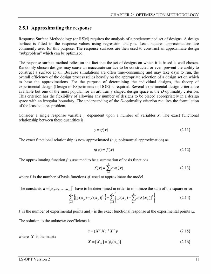
2.5.1 Approximating the response Response Surface Methodology (or RSM) requires the analysis of a predetermined set of designs. A design surface is fitted to the response values using regression analysis. Least squares approximations are commonly used for this purpose. The response surfaces are then used to construct an approximate design “subproblem” which can be optimized. The response surface method relies on the fact that the set of designs on which it is based is well chosen. Randomly chosen designs may cause an inaccurate surface to be constructed or even prevent the ability to construct a surface at all. Because simulations are often time-consuming and may take days to run, the overall efficiency of the design process relies heavily on the appropriate selection of a design set on which to base the approximations. For the purpose of determining the individual designs, the theory of experimental design (Design of Experiments or DOE) is required. Several experimental design criteria are available but one of the most popular for an arbitrarily shaped design space is the D-optimality criterion. This criterion has the flexibility of allowing any number of designs to be placed appropriately in a design space with an irregular boundary. The understanding of the D-optimality criterion requires the formulation of the least squares problem. Consider a single response variable y dependent upon a number of variables x. The exact functional relationship between these quantities is )(xη=y (2.11) The exact functional relationship is now approximated (e.g. polynomial approximation) as )()( xx f≈η (2.12) The approximating function f is assumed to be a summation of basis functions:
)()(1
xx ∑=
=L
iiiaf φ (2.13)
where L is the number of basis functions iφ used to approximate the model. The constants [ ]T
Laaa ,,, 21 K=a have to be determined in order to minimize the sum of the square error:
{ } ∑ ∑∑= ==
−=−
P
pp
L
iiip
P
ppp ayfy
1
2
11
2 )]()([)]()([ xxxx φ (2.14)
P is the number of experimental points and y is the exact functional response at the experimental points xi. The solution to the unknown coefficients is: yXXXa TT 1)( −= (2.15) where X is the matrix )]([][ uiuiX xX φ== (2.16)

CHAPTER 2: OPTIMIZATION METHODOLOGY
12 LS-OPT Version 2
The next critical step is to choose appropriate basis functions. A popular choice is the quadratic approximation T
nnn xxxxxxxx ],,,,,,,,,1[ 2121
211 KKK=φ (2.17)
but any suitable function can be chosen. LS-OPT allows linear, elliptical (linear and diagonal terms), interaction (linear and off-diagonal terms) and quadratic functions. 2.5.2 Factors governing the accuracy of the response surface Several factors determine the accuracy of a response surface [45]. 1. The size of the subregion.
For problems with smooth responses, the smaller the size of the subregion, the greater the accuracy. For the general problem, there is a minimum size at which there is no further gain in accuracy. Beyond this size, the variability in the response may become indistinguishable due to the presence of ‘noise’.
2. The choice of the approximating function.
Higher order functions are generally more accurate than lower order functions. Theoretically, over-fitting (the use of functions of too high complexity) may occur and result in suboptimal accuracy, but there is no evidence that this is significant for polynomials up to second order [45].
3. The number and distribution of the design points.
For smooth problems, the prediction accuracy of the response surface improves as the number of points is increased. However, this is only true up to roughly 50% oversampling [45] (very roughly).
2.5.3 Advantages of the method • Design exploration
As design is a process, often requiring feedback and design modifications, designers are mostly interested in suitable design formulae, rather than a specific design. If this can be achieved, and the proper design parameters have been used, the design remains flexible and changes can still be made at a late stage before verification of the final design. This also allows multidisciplinary design to proceed with a smaller risk of having to repeat simulations. As designers are moving towards computational prototyping, and as parallel computers or network computing are becoming more commonplace, the paradigm of design exploration is becoming more important. Response surface methods can thus be used for global exploration in a parallel computational setting. For instance, interactive trade-off studies can be conducted.
• Global optimization Response surfaces have a tendency to capture globally optimal regions because of their smoothness and global approximation properties. Local minima caused by noisy response are thus avoided.
2.5.4 Other types of response surfaces Neural network and Kriging approximations can also be used as response surfaces and are discussed in Sections 2.10.1 and 2.10.2.

CHAPTER 2: OPTIMIZATION METHODOLOGY
LS-OPT Version 2 13
2.6 Experimental design Experimental design is the selection procedure for finding the points in the design space that must be analyzed. Many different types are available [45]. The factorial, Koshal, composite, D-optimal and Latin Hypercube designs are detailed here. 2.6.1 Factorial design This is an nl grid of designs and forms the basis of many other designs. l is the number of grid points in one dimension. It can be used as a basis set of experiments from which to choose a D-optimal design. In LSOPT, the 3n and 5n designs are used by default as the basis experimental designs for first and second order D-optimal designs respectively. Factorial designs may be expensive to use directly, especially for a large number of design variables. 2.6.2 Koshal design This family of designs are saturated for modeling of any response surface of order d. First order model For n = 3, the coordinates are:
100010001000
321 xxx
As a result, four coefficients can be estimated in the linear model T
nxx ],,,1[ 1 K=φ (2.18) Second order model For n = 3, the coordinates are:

CHAPTER 2: OPTIMIZATION METHODOLOGY
14 LS-OPT Version 2
−−
−
110101011100010001100010001000321 xxx
As a result, ten coefficients can be estimated in the quadratic model T
nnn xxxxxxxx ],,,,,,,,,1[ 2121
211 KKK=φ (2.19)
2.6.3 Central Composite design This design uses the 2n factorial design, the center point, and the ‘face center’ points and therefore consists of P = 2n + 2n + 1 experimental design points. For n = 3, the coordinates are:
−−
−−−
−−−−−−−
−−
−
111111111111111111111111
000000
000000000321
αα
αα
αα
xxx
CHAPTER 2: OPTIMIZATION METHODOLOGY
LS-OPT Version 2 15
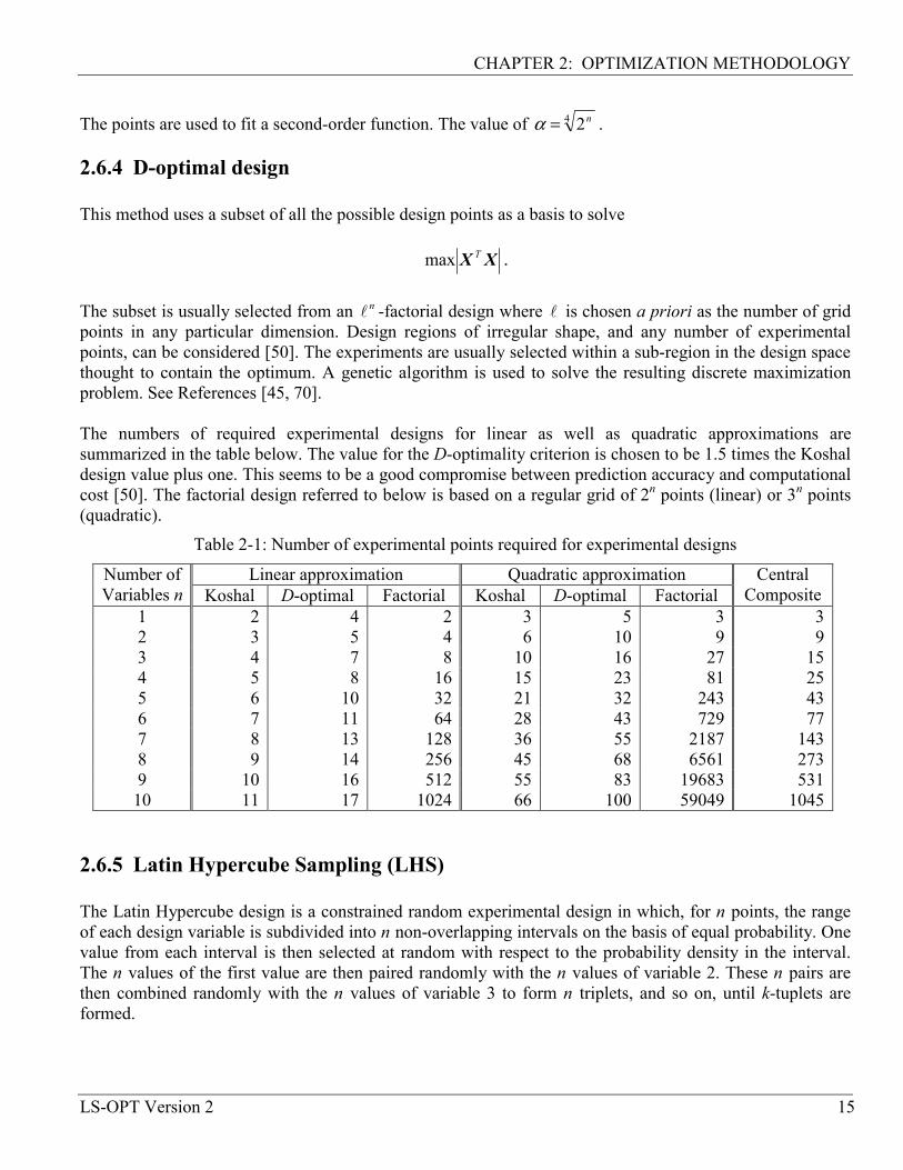
The points are used to fit a second-order function. The value of 4 2n=α . 2.6.4 D-optimal design This method uses a subset of all the possible design points as a basis to solve
XX Tmax . The subset is usually selected from an nl -factorial design where l is chosen a priori as the number of grid points in any particular dimension. Design regions of irregular shape, and any number of experimental points, can be considered [50]. The experiments are usually selected within a sub-region in the design space thought to contain the optimum. A genetic algorithm is used to solve the resulting discrete maximization problem. See References [45, 70]. The numbers of required experimental designs for linear as well as quadratic approximations are summarized in the table below. The value for the D-optimality criterion is chosen to be 1.5 times the Koshal design value plus one. This seems to be a good compromise between prediction accuracy and computational cost [50]. The factorial design referred to below is based on a regular grid of 2n points (linear) or 3n points (quadratic).
Table 2-1: Number of experimental points required for experimental designs
Linear approximation Quadratic approximation Number of Variables n Koshal D-optimal Factorial Koshal D-optimal Factorial
Central Composite
1 2 4 2 3 5 3 32 3 5 4 6 10 9 93 4 7 8 10 16 27 154 5 8 16 15 23 81 255 6 10 32 21 32 243 436 7 11 64 28 43 729 777 8 13 128 36 55 2187 1438 9 14 256 45 68 6561 2739 10 16 512 55 83 19683 53110 11 17 1024 66 100 59049 1045
2.6.5 Latin Hypercube Sampling (LHS) The Latin Hypercube design is a constrained random experimental design in which, for n points, the range of each design variable is subdivided into n non-overlapping intervals on the basis of equal probability. One value from each interval is then selected at random with respect to the probability density in the interval. The n values of the first value are then paired randomly with the n values of variable 2. These n pairs are then combined randomly with the n values of variable 3 to form n triplets, and so on, until k-tuplets are formed.

CHAPTER 2: OPTIMIZATION METHODOLOGY
16 LS-OPT Version 2
Latin Hypercube designs are independent of the mathematical model of the approximation and allow estimation of the main effects of all factors in the design in an unbiased manner. On each level of every design variable only one point is placed. There are the same number of levels as points, and the levels are assigned randomly to points. This method ensures that every variable is represented, no matter if the response is dominated by only a few ones. Another advantage is that the number of points to be analyzed can be directly defined. Let P denote the number of points, and n the number of design variables, each of which is uniformly distributed between 0 and 1. Latin hypercube sampling (LHS) provides a P-by-n matrix S = Sij that randomly samples the entire design space broken down into P equal-probability regions:
( ) PS ijijij ζη −= , (2.20)
where Pjj ηη ,,1 K are uniform random permutations of the integers 1 through P and ijζ independent random numbers uniformly distributed between 0 and 1. A common simplified version of LHS has centered points of P equal-probability sub-intervals: ( ) PS ijij 5.0−= η (2.21)
LHS can be thought of as a stratified Monte Carlo sampling. Latin hypercube samples look like random scatter in any bivariate plot, though they are quite regular in each univariate plot. Often, in order to generate an especially good space filling design, the Latin hypercube point selection S described above is taken as a starting experimental design and then the values in each column of matrix S is permuted so as to optimize some criterion. Several such criteria are described in the literature. Maximin One approach is to maximize the minimal distance between any two points (i.e. between any two rows of S). This optimization could be performed using, for example, Simulated Annealing (see Appendix F). The maximin strategy would ensure that no two points are too close to each other. For small P, maximin distance designs will generally lie on the exterior of the design space and fill in the interior as P becomes larger. See Section 2.6.6 for more detail. Centered L2-discrepancy Another strategy is to minimize the centered L2-discrepancy measure. The discrepancy is a quantitative measure of non-uniformity of the design points on an experimental domain. Intuitively, for a uniformly distributed set in the n-dimensional cube nI = [0,1]n, we would expect the same number of points to be in all subsets of nI having the same volume. Discrepancy is defined by considering the number of points in the subsets of nI . Centered L2 (CL2) takes into account not only the uniformity of the design points over the n-dimensional box region nI , but also the uniformity of all the projections of points over lower-dimensional subspaces:

CHAPTER 2: OPTIMIZATION METHODOLOGY
LS-OPT Version 2 17
( )
.22
5.02
5.011
25.0
25.0
12)1213(
1 1 12
1 1
222
∑ ∑ ∏
−−
−+
−++
∑ ∏
−−
−+−=
= = =
= =
Pk Pi nj
ijkjijkj
Pi nj
ijijn
SSSSP
SSP
CL
K K K
K K
(2.22)
2.6.6 Space-filling designs* In the modeling of an unknown nonlinear relationship, when there is no persuasive parametric regression model available, and the constraints are uncertain, one might believe that a good experimental design is a set of points that are uniformly scattered on the experimental domain (design space). Space-filling designs impose no strong assumptions on the approximation model, and allow a large number of levels for each variable with a moderate number of experimental points. These designs are especially useful in conjunction with nonparametric models such as neural networks (feed-forward networks, radial basis functions) and Kriging, [76, 79]. Space-filling points can be also submitted as the basis set for constructing an optimal (D-Optimal, etc.) design for a particular model (e.g. polynomial). Some space-filling designs are: random Latin Hypercube Sampling (LHS), Orthogonal Arrays, and Orthogonal Latin Hypercubes. The key to space-filling experimental designs is in generating 'good' random points and achieving reasonably uniform coverage of sampled volume for a given (user-specified) number of points. In practice, however, we can only generate finite pseudorandom sequences, which, particularly in higher dimensions, can lead to a clustering of points, which limits their uniformity. To find a good space-filling design is a nonlinear programming hard problem, which – from a theoretical point of view – is difficult to solve exactly. This problem, however, has a representation, which might be within the reach of currently available tools. To reduce the search time and still generate good designs, the popular approach is to restrict the search within a subset of the general space-filling designs. This subset typically has some good 'built-in' properties with respect to the uniformity of a design. The constrained randomization method termed Latin Hypercube Sampling (LHS) and proposed in [39], has become a popular strategy to generate points on the 'box' (hypercube) design region. The method implies that on each level of every design variable only one point is placed, and the number of levels is the same as the number of runs. The levels are assigned to runs either randomly or so as to optimize some criterion, e.g. so that the minimal distance between any two design points is maximized ('maximin distance' criterion). Restricting the design in this way tends to produce better Latin Hypercubes. However, the computational cost of obtaining these designs is high. In multidimensional problems, the search for an optimal Latin hypercube design using traditional deterministic methods (e.g. the optimization algorithm described in [47]) may be computationally prohibitive. This situation motivates the search for alternatives. Probabilistic search techniques, simulated annealing and genetic algorithms are attractive heuristics for approximating the solution to a wide range of optimization problems. In particular, these techniques are frequently used to solve combinatorial optimization problems, such as the traveling salesman problem. Morris and Mitchell [44] adopted the simulated annealing algorithm to search for optimal Latin hypercube designs.

CHAPTER 2: OPTIMIZATION METHODOLOGY
18 LS-OPT Version 2
In LS-OPT, space-filling designs can be useful for constructing experimental designs for the following purposes:
1. The generation of basis points for the D-optimality criterion. This avoids the necessity to create a very large number of basis points using e.g. the full factorial design for large n. E.g. for n=20 and 3 points per variable, the number of points = 320 ≈ 3.5*109.
2. The generation of design points for all approximation types, but especially for neural networks and Kriging.
3. The augmentation of an existing experimental design. This means that points can be added for each iteration while maintaining uniformity and equidistance with respect to pre-existing points.
LS-OPT contains 6 algorithms to generate space-filling designs (see Table 2-2). Only Algorithm 5 has been made available in the graphical interface. LS-OPTui.
Figure 2-1: Six space-filling designs: 5 points in a 2-dimensional box region

CHAPTER 2: OPTIMIZATION METHODOLOGY
LS-OPT Version 2 19
Table 2-2: Description of space-filling algorithms
Algorithm Number
Description
0 Random 1 'Central point' Latin Hypercube Sampling (LHS) design with random
pairing 2 'Generalized' LHS design with random pairing 3 Given an LHS design, permutes the values in each column of the LHS
matrix so as to optimize the maximin distance criterion taking into account a set of existing (fixed) design points. This is done using simulated annealing. Fixed points influence the maximin distance criterion, but are not allowed to be changed by Simulated Annealing moves.
4 Given an LHS design, moves the points within each LHS subinterval preserving the starting LHS structure, optimizing the maximin distance criterion and taking into consideration a set of fixed points.
5 given an arbitrary design (and a set of fixed points), randomly moves the points so as to optimize the maximin distance criterion using simulated annealing (see Appendix F).
Discussion of algorithms The Maximin distance space-filling algorithms 3, 4 and 5 minimize the energy function defined as the negative minimal distance between any two design points. Theoretically, any function that is a metric can be used to measure distances between points, although in practice the Euclidean metric is usually employed. The three algorithms, 3, 4 and 5, differ in their selection of random Simulated Annealing moves from one state to a neighboring state. For algorithm 3, the next design is always a 'central point' LHS design (Eq. 2.21). The algorithm swaps two elements of I, Sij and Skj, where i and k are random integers from 1 to N, and j is a random integer from 1 to n. Each step of algorithm 4 makes small random changes to a LHS design point preserving the initial LHS structure. Algorithm 5 transforms the design completely randomly - one point at a time. In more technical terms, algorithms 4 and 5 generate a candidate state, S ′ , by modifying a randomly chosen element Sij of the current design, S, according to: ξ+=′ ijij SS (2.23) where ξ is a random number sampled from a normal distribution with zero mean and standard deviation σξ ∈ [σmin, σmax]. In algorithm 4 it is required that both ijS ′ and ijS in Eq. (2.23) belong to the same Latin hypercube subinterval. Notice that maximin distance energy function does not need to be completely recalculated for every iterative step of simulated annealing. The perturbation in the design applies only to some of the rows and columns of S. After each step we can recompute only those nearest neighbor distances that are affected by the stepping procedures described above. This reduces the calculation and increased the speed of the algorithm. To perform an annealing run for the algorithms 3, 4 and 5, the values for Tmax and Tmin can be adapted to the scale of the objective function according to:

CHAPTER 2: OPTIMIZATION METHODOLOGY
20 LS-OPT Version 2
ETT ∆×= maxmax : (2.24) ETT ∆×= minmin : where ∆E > 0 is the average value of |E'-E| observed in a short preliminary run of simulated annealing and Tmax and Tmin are positive parameters. The basic parameters that control the simulated annealing in algorithms 3, 4 and 5 can be summarized as follows:
1 Energy function: negative minimal distance between any two points in the design.
2 Stepping scheme: depends on whether the LHS property is preserved or not.
3 Scalar parameters:
1. Parameters for the cooling schedule: - scaling factor for the initial (maximal) temperature, Tmax, in (2.24) - scaling factor for the minimal temperature, Tmin, in (2.24), - damping factor for temperature, µT, in (Eq. (F.5), Appendix F), - number of iterations at each temperature, νT (Appendix F).
2. Parameters that control the standard deviation of ξ in (2.23): - upper bound, σmax, - lower bound, σmin.
3. Termination criteria: - maximal number of energy function evaluations, Nit.
2.6.7 Random number generator A portable random number generator is used for the construction of D-optimal designs (using the genetic algorithm) and to generate Monte Carlo designs such as the Latin Hypercube. The algorithm employs a scheme by Bays and Durham, as described in Knuth [31], and resembles the Maclaren-Marsaglia method. It greatly increases the period of the basic linear congruential generator. In certain applications the Mersenne Twister is used. The Mersenne Twister (MT19937) is a pseudorandom number generator developed by Matsumoto and Nishimura [39] and has the merit that it has a far longer period and far higher order of equidistribution than any other implemented generators. It has been proved that the period is 219937-1, and a 623-dimensional equidistribution property is assured. LS-OPT will probably standardize on this generator in future versions. 2.7 Reasonable experimental designs* A ‘reasonable’ design space refers to a region of interest which, in addition to having specified bounds on the variables, is also bounded by specified values of the responses. This results in an irregular shape of the design space. Therefore, once the first approximation has been established, all the designs will be contained in the new region of interest. This region of interest is thus defined by approximate bounds.

CHAPTER 2: OPTIMIZATION METHODOLOGY
LS-OPT Version 2 21
One way of establishing a reasonable set of designs is to move the points of the basis experimental design to the boundaries of the reasonable design space in straight lines connecting to the central design xc so that )( cc xxxx −+=′ α (2.25) where α is determined by conducting a line search along )( cxx − . This step may cause near duplicity of design points that can be addressed by removing points from the set that are closer than a fixed fraction (typically 5%) of the design space size. The D-optimality criterion is then used to attempt to find a well-conditioned design from the basis set of experiments in the reasonable design space. Using the above approach, a poor distribution of the basis points may result in a poorly designed subset. 2.8 Model adequacy checking As indicated in the previous sections, response surfaces are useful for interactive trade-off studies. For the trade-off surface to be useful, its capability of predicting accurate response must be known. Error analysis is therefore an important aspect of using response surfaces in design. Inaccuracy is not always caused by random error (noise) only, but modeling error (sometimes called bias error), especially in a large subregion or where there is strong non-linearity present, could play a very significant role. There are several error measures available to determine the accuracy of a response surface. 2.8.1 Residual sum of squares For the predicted response iy and the actual response yi, this error is expressed as
( )∑=
−=P
iii yy
1
22 ˆε (2.26)
If applied only to the regression points, this error measure is not very meaningful unless the design space is oversampled. E.g. ε = 0 if the number of points P equals the number of basis functions L in the approximation. 2.8.2 RMS error The residual sum-of-squares is sometimes used in its square root form, RMSε , and called the “RMS error”:
( )∑=
−=P
iii yy
P 1
2RMS ˆ1ε (2.27)

CHAPTER 2: OPTIMIZATION METHODOLOGY
22 LS-OPT Version 2
2.8.3 Maximum residual This is the maximum residual considered over all the design points and is given by ii yy ˆmaxmax −=ε . (2.28) 2.8.4 Prediction error The same as the RMS error, but using only responses at preselected prediction points independent of the regression points. This error measure is an objective measure of the prediction accuracy of the response surface since it is independent of the number of construction points. It is important to know that the choice of a larger number of construction points will, for smooth problems, diminish the prediction error. The prediction points can be determined by adding rows to X
=
)()(
ppa xA
XxX (2.29)
and solving AAXXXX TT += maxmax a
Ta (2.30)
for xp. 2.8.5 PRESS residuals The prediction sum of squares residual (PRESS) uses each possible subset of P – 1 responses as a regression data set, and the remaining response in turn is used to form a prediction set [45]. PRESS can be computed from a single regression analysis of all P points.
∑=
−−=
P
i ii
ii
hyy
1
2
1ˆ
PRESS (2.31)
where hii are the diagonal terms of TH XXXX T 1)( −= (2.32) H is the “hat” matrix, the matrix that maps the observed responses to the fitted responses, i.e. Hyy =ˆ (2.33) The PRESS residual can also be written in its square root form
∑=
−−=
P
i ii
ii
hyy
1
2
1ˆ
SPRESS . (2.34)
For a saturated design, H equals the unit matrix I so that the PRESS indicator becomes undefined.

CHAPTER 2: OPTIMIZATION METHODOLOGY
LS-OPT Version 2 23
2.8.6 The coefficient of multiple determination R2 The coefficient of determination R2 is defined as:
( )
( )∑
∑
=
=
−
−= P
iii
P
iii
yy
yyR
1
2
1
2
2
ˆ (2.35)
where P is the number of design points and y , iy and yi represent the mean of the responses, the predicted response, and the actual response, respectively. This indicator, which varies between 0 and 1, represents the ability of the response surface to identify the variability of the design response. A low value of R2 usually means that the region of interest is either too large or too small and that the gradients are not trustworthy. The value of 1.0 for R2 indicates a perfect fit. However the value will not warn against an overfitted model with poor prediction capabilities. 2.8.7 R2 for Prediction For the purpose of prediction accuracy the 2
predictionR indicator has been devised [44].
yy
prediction SR PRESS12 −= (2.36)
where
P
yS
P
ii
Tyy
2
1
−=∑
=yy (2.37)
2predictionR represents the ability of the model to detect the variability in predicting new responses [45].
2.8.8 Iterative design and prediction accuracy In an iterative scheme with a shrinking region the R2 value tends to be small at the beginning, then approaches unity as the region of interest shrinks, thereby improving the modeling ability. It may then reduce again as the noise starts to dominate in a small region causing the variability to become indistinguishable. In the same progression, the prediction error will diminish as the modeling error fades, but will stabilize at above zero as the modeling error is replaced by the random error (noise). 2.9 ANOVA Since the number of regression coefficients determines the number of simulation runs, it is important to remove those coefficients or variables which have small contributions to the design model. This can be done by doing a preliminary study involving a design of experiments and regression analysis. The statistical results are used in an analysis of variance (ANOVA) to rank the variables for screening purposes. The

CHAPTER 2: OPTIMIZATION METHODOLOGY
24 LS-OPT Version 2
procedure requires a single iteration using polynomial regression, but results are produced after every iteration of a normal optimization procedure. 2.9.1 The confidence interval of the regression coefficients The 100(1 – α)% confidence interval for the regression coefficients Ljbj ,,1,0, K= is determined by the inequality
22
jjj
jj
bb
bb
∆+≤≤
∆− β (2.38)
where jjCtb LPj
2,2/ ˆ2)( σα α −=∆ (2.39)
and 2σ is an unbiased estimator of the variance 2σ given by
LP
yyLP
P
i ii
−−
=−
= ∑ =122
2 )ˆ(ˆ εσ (2.40)
jjC is the diagonal element of 1)( −XX T corresponding to bj and tα/2,P-L is Student’s t-Distribution.
100(1 – α)% therefore represents the level of confidence that bj will be in the computed interval. 2.9.2 The significance of a regression coefficient bj The contribution of a single regressor variable to the model can also be investigated. This is done by means of the partial F-test where F is calculated to be
)(][
2
22
LPr
Fcomplete
completereduced
−−
=ε
εε (2.41)
where r = 1 and the reduced model is the one in which the regressor variable in question has been removed. Each of the 2ε terms represents the sum of squared residuals for the reduced and complete models respectively. It turns out that the computation can be done without analyzing a reduced model by computing
.)(2
2
LPCb
Fcomplete
jjj
−=
ε (2.42)
F can be compared with the F-statistic Fα,1,P-L so that if F > Fα,1,P-L, βj is non-zero with (100 – α)% confidence. The confidence level α that βj is not zero can also be determined by computing the α for F = Fα,1,P-L. The importance of βj is therefore estimated by both the magnitude of bj as well as the level of confidence in a non-zero βj.

CHAPTER 2: OPTIMIZATION METHODOLOGY
LS-OPT Version 2 25
The significance of regressor variables may be represented by a bar chart of the magnitudes of the coefficients bj with an error bar of length )(2 αjb∆ for each coefficient representing the confidence interval for a given level of confidence α. The relative bar lengths allow the analyst to estimate the importance of the variables and terms to be included in the model while the error bars represent the contribution to noise or poorness of fit by the variable. All terms have been normalized to the size of the design space so that the choice of units becomes irrelevant and a reasonable comparison can be made for variables of different kinds, e.g. sizing and shape variables or different material constants. 2.10 Metamodeling techniques Metamodeling techniques allow the construction of surrogate design models for the purpose of design exploration such as variable screening, optimization and reliability. LS-OPT provides the capability of using three types of metamodeling techniques, namely polynomial response surfaces (already discussed, see Section 2.5), Neural Networks (NN’s) (Section 2.10.1) and Kriging1 (Section 2.10.2). All three these approaches can be useful to provide a predictive capability for optimization or reliability. In addition, linear polynomials, although perhaps less accurate, are highly suitable for variable screening (Section 2.9). At the core, these techniques differ in the regression methods that they employ to construct the surrogate models. The polynomial response surface method uses linear regression, while neural networks use nonlinear regression methods requiring optimization algorithms. Kriging is considered to be a Gaussian Process [15] which uses Bayesian regression, also requiring optimization. Not mentioned so far are other types of metamodeling techniques such as Space Mapping [48]. This technique make use of coarse approximate models which are iteratively refined using fine model simulations to improve the coarse model approximation locally. In Space Mapping, any of the first three approximation types can be used as coarse models. When using polynomials, the user is faced with the choice of deciding which monomial terms to include. In addition, polynomials, by way of their nature as Taylor series approximations, are not natural for the creation of updateable surfaces. This means that if an existing set of point data is augmented by a number of new points which have been selected in a local subregion (e.g. in the vicinity of a predicted optimum), better information could be gained from a more flexible type of approximation that will keep global validity while allowing refinement in a subregion of the parameter space. Such an approximation provides a more natural approach for combining the results of successive iterations. 2.10.1 Neural network approximations* Neural methods are natural extensions and generalizations of regression methods. Neural networks have been known since the 1940’s, but it took the dramatic improvements in computers to make them practical, [8]. Neural networks - just like regression techniques - model relationships between a set of input variables and an outcome. They can be thought of as computing devices consisting of numerical units (neurons), whose inputs and outputs are linked according to specific topologies. A neural model is defined by its free parameters - the inter-neuron connection strengths (weights) and biases. These parameters are typically
1 Available in Version 2.1

CHAPTER 2: OPTIMIZATION METHODOLOGY
26 LS-OPT Version 2
learned from the training data by some appropriate optimization algorithm. The training set consists of pairs of input (design) vectors and associated outputs (responses). The training algorithm tries to steer network parameters towards minimizing some distance measure, typically the mean squared error (MSE) of the model computed on the training data. Several factors determine the predictive accuracy of a neural network approximation and, if not properly addressed, may adversely affect the solution. For a neural network, as well as for any other data-derived model, the most critical factor is the quality of training data. In practical cases, we are limited to a given data set, and the central problem is that of not enough data. The minimal number of data points required for network training is related to the (unknown) complexity of the underlying function and the dimensionality of the design space. In reality, the more design variables, the more training samples are required. In the statistical and neural network literature this problem is known as the ’curse of dimensionality’. Most forms of neural networks (in particular, feed-forward networks) actually suffer less from the curse of dimensionality than some other methods, as they can concentrate on a lower-dimensional section of the high-dimensional space. For example, by setting the outgoing weights from a particular input to zero, a network can entirely ignore that input (Figure 2-2). Nevertheless, the curse of dimensionality is still a problem, and the performance of a network can certainly be improved by eliminating unnecessary input variables.
Figure 2-2: Schematic of a neural network with 2 inputs and a hidden layer of 4 neurons with activation function f
It is clear that if the number of network free parameters is sufficiently large and the training optimization algorithm is run long enough, it is possible to drive the training MSE error as close as one likes to zero. However, it is also clear that driving MSE all the way to zero is not a desirable thing to do. For noisy data, this may indicate over-fitting rather than good modeling. For highly discrepant training data, zero MSE makes no sense at all. Regularization means that some constraints are applied to the construction of the

CHAPTER 2: OPTIMIZATION METHODOLOGY
LS-OPT Version 2 27
neural model with the goal of reducing the generalization error, that is, the ability to predict (interpolate) the unobserved response for new data points that are generated by a similar mechanism as the observed data. A fundamental problem in modeling noisy and/or incomplete data, is to balance the ’tightness’ of the constraints with the ’goodness of fit’ to the observed data. This tradeoff is called the bias-variance tradeoff in the statistical literature.
Figure 2-3: Sigmoid transfer function ( )xey −+= 1/1 typically used with feed-forward networks
A multi-layer feed-forward network and a radial basis function network are two of the most common neural architectures used for approximating functions. Networks of both types have a distinct layered topology in the sense that their processing units (’neurons’) are divided into several groups (’layers’), the outputs of each layer of neurons being the inputs to the next layer (Figure 2-2). In a feed-forward network, each neuron performs a biased weighted sum of their inputs and passes this value through a transfer (activation) function to produce the output. Activation function of intermediate (’hidden’) layers is generally a sigmoidal function (Figure 2-3), while network input and output layers are usually linear (transparent). In theory, such networks can model functions of almost arbitrary complexity, see [27, 75]. All of the parameters in a feed-forward network are usually determined at the same time as part of a single (non-linear) optimization strategy based on the standard gradient algorithms (the steepest descent, RPROP, Levenberg-Marquardt, etc.). The gradient information is typically obtained using a technique called backpropagation, which is known to be computationally effective [53]. For feed-forward networks, regularization may be done by controlling the number of network weights (’model selection’), by imposing penalties on the weights (’ridge regression’), or by various combinations of these strategies. Model adequacy checking Nature is rarely (if ever) perfectly predictable. Real data never exactly fit the model that is being used. One must take into consideration that the prediction errors not only come from the variance error due to the intrinsic noise and unreliability in the measurement of the dependent variables but also from the systematic (bias) error due to model miss-specification. According to George E.P. Box’s famous maxim, ”all models are wrong, some are useful”. To be genuinely useful, a fitting procedure should provide the means to assess whether or not the model is appropriate and to test the goodness-of-fit against some statistical standard. There are several error measures available to determine the accuracy of the model. Among them are:

CHAPTER 2: OPTIMIZATION METHODOLOGY
28 LS-OPT Version 2
( )∑ −=P
iii PyyMSE ,/ˆ 2 (2.43)
MSERMS =
2σMSEnMSE =
2σRMSnRMS =
( )
( )∑
∑
=
=
−
−= P
iii
P
iii
yy
yyR
1
2
1
2
2
ˆ
( ) ( )∑∑
∑
==
=
−−
−−= P
iii
P
iii
P
iiiii
yyyy
yyyyR
1
2
1
2
1
ˆˆ
ˆˆ
where P denotes the number of data points, yi is the observed response value (’target value’), iy is the model’s
prediction of response, y is the mean (average) value of y , y is the mean (average) value of y, and 2σ is given by
( )
LPyy
LP
P
i ii
−−
=−
= ∑ =122
2ˆ
ˆ εσ (2.44)
Mean squared error (MSE for short) and root mean squared error (RMS) summarize the overall model error. Unique or rare large error values can affect these indicators. Sometimes, MSE and RMS measures are normalized with sample variance of the target value (see formulae for nMSE and nRMS) to allow for comparisons between different datasets and underlying functions. R2 and R are relative measures. The coefficient of multiple determination R2 (’R-square’) is explained variance relative to total variance in the target value. This indicator is widely used in linear regression analysis. R2 represents the amount of response variability explained by the model. R is the correlation coefficient between the network response and the target. It is a measure of how well the variation in the output is explained by the targets. If this number is equal to 1, then there is a perfect correlation between targets and outputs. Outliers can greatly affect the magnitudes of correlation coefficients. Of course, the larger the sample size, the smaller is the impact of one or two outliers. Training accuracy measures (MSE, RMS, R2, R, etc.) are computed along all the data points used for training. As mentioned above, the performance of a good model on the training set does not necessarily mean good prediction of new (unseen) data. The objective measures of the prediction accuracy of the model are test errors computed along independent testing points (i.e. not training points). This is certainly true provided that we have an infinite number of testing points. In practice, however, test indicators are usable, only if treated with appropriate caution. Actual problems are often characterized by the limited availability

CHAPTER 2: OPTIMIZATION METHODOLOGY
LS-OPT Version 2 29
of data, and when the training datasets are quite small and the test sets are even smaller, only quite large differences in performance can be reliably discerned by comparing training and test indicators. The generalized cross-validation (GCV) [73] and Akaike’s final prediction error (FPE) [1] provide computationally feasible means of estimating the appropriateness of the model. GCV and FPE estimates combine the training MSE with a measure of the model complexity:
,)1/( 2
PMSEMSEGCV
ν−= (2.45)
GCVGCV MSERMS =
2σGCV
GCVMSEnMSE =
2σGCV
GCVRMSnRMS =
where ν is the (effective) number of model parameters. In theory, GCV estimates should be related to ν. As a very rough approximation to ν, we can assume that all of the network free parameters are well determined so that ν = M, where M is the total number of network weights and biases. This is what we would expect to be the case for large P so that P >> M. Note that GCV is undefined when ν is equal to the number of training points (P). Feed-forward neural networks Feed-forward (FF) neural networks have a distinct layered topology. Each unit performs a biased weighted sum of their inputs and passes this value through a transfer (activation) function to produce the output. The outputs of each layer of neurons are the inputs to the next layer. In a feed-forward network, the activation function of intermediate (’hidden’) layers is generally a sigmoidal function (Figure 2-3), network input and output layers being linear. Consider a FF network with K inputs, one hidden layer with H sigmoid units and a linear output unit. For a given input vector ),,( 1 Kxx K=x and network weights
),,,,,,,( 111010 HKH WWWWWW KK=W , the output of the network is:
∑ ∑= =
++=H
h
K
kkhkhh xWWfWWy
1 100 ),(),(ˆ Wx (2.46)
where
xexf −+
=1
1)(
The computational graph of Eq. (2.46) is shown schematically in Figure 2-2. The extension to the case of more than one hidden layers can be obtained accordingly. It is straightforward to show that the derivative of the network Eq. (2.46) with respect to any of its inputs is given by:

CHAPTER 2: OPTIMIZATION METHODOLOGY
30 LS-OPT Version 2
∑ ∑= =
=+′=∂∂ H
h
H
hhhkh
k
KkWWfWWxy
1 10 .,,1),(
ˆK (2.47)
Neural networks have been mathematically shown to be universal approximators of continuous functions and their derivatives (on compact sets) [27]. In other words, when a network (Eq. (2.46)) converges towards the underlying function, all the derivatives of the network converge towards the derivatives of this function. Standard non-linear optimization techniques including a variety of gradient algorithms (the steepest descent, RPROP, Levenberg-Marquardt, etc.) are applied to adjust FF network’s weights and biases. For neural networks, the gradients are easily obtained using a chain rule technique called ’backpropagation’ [53]. The second-order Levenberg-Marquardt algorithm appears to be the fastest method for training moderate-sized FF neural networks (up to several hundred adjustable weights) [8]. However, when training larger networks, the first-order RPROP algorithm becomes preferable for computational reasons [49]. Regularization: For FF networks, regularization may be done by controlling the number of network weights (’model selection’), by imposing penalties on the weights (’ridge regression’), or by various combinations of these strategies. Model selection requires choosing the number of hidden units and, sometimes, the number of network hidden layers. Most straightforward is to search for an ’optimal’ network architecture that minimizes MSEGCV, MSEFPE or MSECV–k. Often, it is feasible to loop over 1,2,... hidden units and finally select the network with the smallest GCV error. In any event, in order for the GCV measure to be applicable, the number of training points P should not be too small compared to the required network size M. Over-fitting: To prevent over-fitting, it is always desirable to find neural solutions with the smallest number of parameters. In practice, however, networks with a very parsimonious number of weights are often hard to train. The addition of extra parameters (i.e. degrees of freedom) can aid convergence and decrease the chance of becoming stuck in local minima or on plateaus [34]. Weight decay regularization involves modifying the performance function F , which is normally chosen to be the mean sum of squares of the network errors on the training set (Eq. (2.43)). When minimizing MSE (Eq. (2.43)) the weight estimates tend to be exaggerated. We can impose a penalty for this tendency by adding a term that consists of the sum of squares of the network weights (see also Eq. (2.43)): WD EEF αβ += (2.48) where
,2
)ˆ( 21∑ =
−=
P
i iiD
yyE
,21
2∑ ==M
m mW
WE
where M is the number of weights and P the number of points in the training set. Notice that network biases are usually excluded from the penalty term EW. Using the modified performance function (Eq. (2.48)) will cause the network to have smaller weights, and this will force the network response to be smoother and less likely to overfit. This eliminates the guesswork required in determining the

CHAPTER 2: OPTIMIZATION METHODOLOGY
LS-OPT Version 2 31
optimum network size. Unfortunately, finding the optimal value for α and β is not a trivial task. If we make α /β too small, we may get over-fitting. If α /β is too large, the network will not adequately fit the training data. A rule of thumb is that a little regularization usually helps [54]. It is important that weight decay regularization does not require that a validation subset be separated out of the training data. It uses all of the data. This advantage is especially noticeable in small sample size situations. Another nice property of weight decay regularization is that it can lend numerical robustness to the Levenberg-Marquardt algorithm. The L-M approximation to the Hessian of Eq. (2.48) is moved further away from singularity due to a positive addend to its diagonal: IHA α+= (2.49) where
∑ ⋅≈∇∇==
P
i
TiiD xxE
1
)()( )()( ggH β
T
MWy
Wy )
ˆ,,
ˆ()(
1 ∂∂
∂∂= Kxg
In [8, 19, 41 and 42] the Bayesian (’evidence framework’ or ’type II maximum likelihood’) approach to regularization is discussed. The Bayesian re-estimation algorithm is formulated as follows. At first, we choose the initial values for α and β. Then, a neural network is trained using a standard non-linear optimization algorithm to minimize the error function (Eq. (2.48)). After training, i.e. in the minimum of Eq. (2.48), the values for α and β are re-estimated, and training restarts with the new performance function. Regularization hyperparameters are computed in a sequence of 3 steps:
αλλ
ν+
= ∑ =
m
M
m m1 (2.50)
where λm, m = 1,…,M are (positive) eigenvalues of matrix H in Eq. (2.49), ν is the estimate of the effective number of parameters of a neural network,
WE2
να = (2.51)
DE
P2
νβ −=
It should be noted that the algorithm (Eqs. (2.50) and (2.51)) relies on numerous simplifications and assumptions, which hold only approximately in typical real-world problems [13]. In the Bayesian formalism a trained network is described in terms of the posterior probability distribution of weight values. The method typically assumes a simple Gaussian prior distribution of weights governed by an inverse variance hyperparameter 2/1 weightsσα = . If we present a new input vector to such a network, then the distribution of weights gives rise to a distribution of network outputs. There will be also an addend to the output distribution arising from the assumed βσ /12 =noise Gaussian noise on the output variables: ).,0()( 2
noiseNxyy σ+= (2.52)

CHAPTER 2: OPTIMIZATION METHODOLOGY
32 LS-OPT Version 2
With these assumptions, the negative log likelihood of network weights W given P training points x(1), … , x(P) is proportional to MSE (Eq. (2.46)), i.e., the maximum likelihood estimate for W is that which minimizes (Eq. (2.46)) or, equivalently, ED. In order for Bayes estimates of α and β to do a good job of minimizing the generalization in practice, it is usually necessary that the priors on which they are based are realistic. The Bayesian formalism also allows us to calculate error bars on the network outputs, instead of just providing a single ’best guess’ output y . Given an unbiased model, minimization of the performance function (Eq. (2.46)) amounts to minimizing the variance of the model. The estimate for output variance
2ˆ xyσ of the network at a particular point x is given by:
)()( 12
ˆ xgAxg −≈ Txyσ (2.53)
Equation (2.53) is based on a second-order Taylor series expansion of Eq. (2.48) around its minimum and assumes that W∂∂y is locally linear. 2.10.2 Kriging* Kriging is named after D.G. Krige [35], who applied empirical methods for determining true ore grade distributions from distributions based on sampled ore grades. In recent years, the Kriging method has found wider application as a spatial prediction method in engineering design. Detailed mathematical formulations of Kriging are given by Simpson [58] and Bakker [5]. The basic postulate of this formulation [58] is :
y(x) = f(x) + Z(x)
where y is the unknown function of interest, f(x) is a known polynomial and Z(x) the stochastic component with mean zero and covariance:
Cov[Z(xi),Z(xj)] = σ 2R([R(xi,xj)]).
With L the number of sampling points, R is the L x L correlation matrix with R(xi,xj) the correlation function between data points xi and xj. R is symmetric positive definite with unit diagonal. Two commonly applied correlation functions used are:
Exponential: ∏==
Θ−n
k
dkkeR1
|| and
Gaussian: ∏==
Θ−n
k
dkkeR1
2

CHAPTER 2: OPTIMIZATION METHODOLOGY
LS-OPT Version 2 33
where n is the number of variables and dk = xki – xk
j, the distance between the kth components of points xi and xj
. There are n unknown θ -values to be determined. The default function in LS-OPT is Gaussian. Once the correlation function has been selected, the predicted esitimate of the response ŷ(x) is given by:
ŷ = ^β + rT(x)R-1(y-f
^β )
where rT(x) is the correlation vector (length L) between a prediction point x and the L sampling points, y represents the responses at the L points and f is an L-vector of ones (in the case that f(x) is taken as a
constant). The vector r and scalar^β are given by:
rT(x) = [R(x,x1),R(x,x2),…,R(x,xL)]T
^β = (f TR -1f)-1f TR -1y.
The estimate of variance from the underlying global model is:
L
T )()(^
1^
2^ ββσ fyRfy −−=−
.
The maximum likelihood estimates for kΘ , k = 1,…, n can be found by solving the following constrained maximization problem:
Max 2
|]|ln)ln([)(
2^RΘ +−=Φ σL , subject to 0>Θ .
where both ^
σ and |R| are functions of Θ . This is the same as minimizing
n12^
||Rσ , s.t. 0>Θ
This optimization problem is solved using the LFOPC algorithm (Section 2.11). Because of the possible ill-conditioning of R, a small constant number is adaptively added to its diagonal during optimization. The net effect is that the approximating functions no longer interpolate the observed response values exactly. However, these observations are still closely approximated.

CHAPTER 2: OPTIMIZATION METHODOLOGY
34 LS-OPT Version 2
2.10.3 Concluding remarks: which metamodel? There is little doubt that the polynomial-based response surfaces are the most robust. A negative aspect is the fact that the user has to choose the order of the polynomial and a greater possibility exists for bias error of a nonlinear response. Therefore linear approximations may only be useful within a certain subregion and quadratic polynomials may be required for greater global accuracy. However the linear SRSM method has proved to be excellent for optimization and can be used with confidence [63,64,65]. Neural Networks function well as global approximations and no serious deficiencies have been observed when used as prescribed in Section [4.5]. NN’s have been used successfully for optimization [65] and can be updated during the process. Although the literature seems to indicate that Kriging is one of the more accurate methods [54], there is evidence of Kriging having fitting problems with certain types of experimental designs [76]. Kriging is very sensitive to noise, since it interpolates the data [28]. The authors of this manual have also experienced fitting problems with non-smooth surfaces (Z(x) observed to peak at data points) in some cases, apparently due to large values of Θ that may be due to local optima of the maximum likelihood function. The model construction can be very time consuming [28] (also experienced with LS-OPT). Furthermore, the slight global altering of the Kriging surface due to local updating has also been observed [65]. Reference [65] compares the use of the three metamodeling techniques for crashworthiness optimization. This paper, which incorporates three case studies in crashworthiness optimization, concludes that while RSM, NN and Kriging were similar in performance, RSM and NN are the most robust for this application. 2.11 Core optimization algorithm (LFOPC) The optimization algorithm used to solve the approximate subproblem is the LFOPC algorithm of Snyman [62]. It is a gradient method that generates a dynamic trajectory path, from any given starting point, towards a local optimum. This method differs conceptually from other gradient methods, such as SQP, in that no explicit line searches are performed. The original leap-frog method [61] for unconstrained minimization problems seeks the minimum of a function of n variables by considering the associated dynamic problem of a particle of unit mass in an n-dimensional conservative force field, in which the potential energy of the particle at point x(t) at time t is taken to be the function f(x) to be minimized. The solution to the unconstrained problem may be approximated by applying the unconstrained minimization algorithm to a penalty function formulation of the original algorithm. The LFOPC algorithm uses a penalty function formulation to incorporate constraints into the optimization problem. This implies that when constraints are violated (active), the violation is magnified and added to an augmented objective function, which is solved by the gradient-based dynamic leap-frog method (LFOP). The algorithm uses three phases: Phase 0, Phase 1 and Phase 2. In Phase 0, the active constraints are introduced as mild penalties through the pre-multiplication of a moderate penalty parameter value. This allows for the solution of the penalty function formulation where the violation of the (active) constraints are premultiplied by the penalty value and added to the objective function in the minimization process. After the
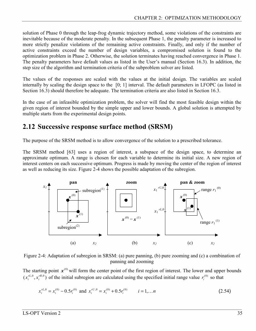
CHAPTER 2: OPTIMIZATION METHODOLOGY
LS-OPT Version 2 35
solution of Phase 0 through the leap-frog dynamic trajectory method, some violations of the constraints are inevitable because of the moderate penalty. In the subsequent Phase 1, the penalty parameter is increased to more strictly penalize violations of the remaining active constraints. Finally, and only if the number of active constraints exceed the number of design variables, a compromised solution is found to the optimization problem in Phase 2. Otherwise, the solution terminates having reached convergence in Phase 1. The penalty parameters have default values as listed in the User’s manual (Section 16.3). In addition, the step size of the algorithm and termination criteria of the subproblem solver are listed. The values of the responses are scaled with the values at the initial design. The variables are scaled internally by scaling the design space to the [0; 1] interval. The default parameters in LFOPC (as listed in Section 16.3) should therefore be adequate. The termination criteria are also listed in Section 16.3. In the case of an infeasible optimization problem, the solver will find the most feasible design within the given region of interest bounded by the simple upper and lower bounds. A global solution is attempted by multiple starts from the experimental design points. 2.12 Successive response surface method (SRSM) The purpose of the SRSM method is to allow convergence of the solution to a prescribed tolerance. The SRSM method [63] uses a region of interest, a subspace of the design space, to determine an approximate optimum. A range is chosen for each variable to determine its initial size. A new region of interest centers on each successive optimum. Progress is made by moving the center of the region of interest as well as reducing its size. Figure 2-4 shows the possible adaptation of the subregion.
x2 x2 x2
pan zoom pan & zoomx1
subregion(1)
subregion(2)
range r1 (0)
range r1 (1)
x (0)
x (1)
x (0) = x (1)
x1 rU,0
x1 rL,0
x (0)
x (1)
(a) (b) (c)
Figure 2-4: Adaptation of subregion in SRSM: (a) pure panning, (b) pure zooming and (c) a combination of panning and zooming
The starting point )0(x will form the center point of the first region of interest. The lower and upper bounds ),( 0,0, rR
irLi xx of the initial subregion are calculated using the specified initial range value )0(
ir so that
)0()0(0, 5.0 iirLi rxx −= and nirxx ii
rUi K,15.0 )0()0(0, =+= (2.54)

CHAPTER 2: OPTIMIZATION METHODOLOGY
36 LS-OPT Version 2
where n is the number of design variables. The modification of the ranges on the variables for the next iteration depends on the oscillatory nature of the solution and the accuracy of the current optimum. Oscillation: A contraction parameter γ is firstly determined based on whether the current and previous designs )(kx and )1( −kx are on the opposite or the same side of the region of interest. Thus an oscillation indicator c may be determined in iteration k as )1()()( −= k
ik
ik
i ddc (2.55) where
[ ]1;1;;/2 )()1()()()()()( −∈−=∆∆= − ki
ki
ki
ki
ki
ki
ki dxxxrxd (2.56)
The oscillation indicator (purposely omitting indices i and k) is normalized as c where
)(ˆ csigncc = . (2.57)
The contraction parameter γ is then calculated as
2
)ˆ1()ˆ1( oscpan cc −++=
γγγ . (2.58)
See Figure 2-5. The parameter oscγ is typically 0.5-0.7 representing shrinkage to dampen oscillation, whereas panγ represents the pure panning case and therefore unity is typically chosen.
|d|
λ,γ λ
η
0
1
-1
1
γosc
γpan
c
Figure 2-5: The sub-region contraction rate λ as a function of the oscillation indicator c and the absolute
move distance ||d

CHAPTER 2: OPTIMIZATION METHODOLOGY
LS-OPT Version 2 37
Accuracy: The accuracy is estimated using the proximity of the predicted optimum of the current iteration to the starting (previous) design. The smaller the distance between the starting and optimum designs, the more rapidly the region of interest will diminish in size. If the solution is on the bound of the region of interest, the optimal point is estimated to be beyond the region. Therefore a new subregion, which is centered on the current point, does not change its size. This is called panning (Figure 2-4(a)). If the optimum point coincides with the previous one, the subregion is stationary, but reduces its size (zooming) (Figure 2-4(b)). Both panning and zooming may occur if there is partial movement (Figure 2-4(c)). The range )1( +k
ir for the new subregion in the (k + 1)-th iteration is then determined by:
niterknirr kii
ki ,,0;,,1;)()1( KK ===+ λ (2.59)
where λi represents the contraction rate for each design variable. To determine λi, )(kid is incorporated by
scaling according to a zoom parameter η that represents pure zooming and the contraction parameter γ to yield the contraction rate
)()( ηγηλ −+= kii d (2.60)
for each variable (see Figure 2-5).
When used in conjunction with neural networks or Kriging, the same heuristics are applied as described above. However the nets are constructed using all the available points, including those belonging to previous iterations. Therefore the response surfaces are progressively updated in the region of the optimal point. Refer to Section 16.2 for the setting of parameters in the iterative Successive Response Surface Method. The above methodology can also be applied to sequential random searches. 2.13 Sequential random search (SRS) LS-OPT allows a sequential search method by which the best design is selected from each iteration without computing response surfaces. A sorting procedure is used to select the design with the lowest (for minimization) or highest (for maximization) objective from all the feasible designs. If no feasible design exists, the least infeasible design is chosen. An experimental design such as Latin Hypercube Sampling (LHS) allows a sequential random search procedure. LS-OPT automatically moves the region of interest by centering it on the most recent best design. The scheme also involves automatic subdomain reduction in which the subdomain is reduced by the zoom parameterη (see Section 2.12) if the best design is the same as the baseline design [21,22]. Otherwise γ pan is used. All the variable ranges are reduced by the same amount. The following example illustrates the convergence performance of the methodology. The example is an unconstrained minimization problem with starting point [1,1,1,…,1], solution [0,0,0,…,0] and an initial range of [0.5;1.5]n and the objective to minimize:
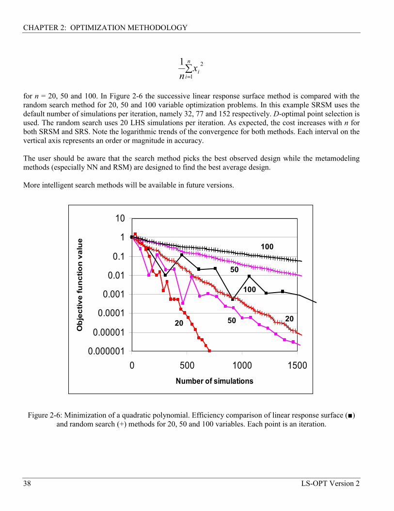
CHAPTER 2: OPTIMIZATION METHODOLOGY
38 LS-OPT Version 2
∑=
n
iix
n 1
21
for n = 20, 50 and 100. In Figure 2-6 the successive linear response surface method is compared with the random search method for 20, 50 and 100 variable optimization problems. In this example SRSM uses the default number of simulations per iteration, namely 32, 77 and 152 respectively. D-optimal point selection is used. The random search uses 20 LHS simulations per iteration. As expected, the cost increases with n for both SRSM and SRS. Note the logarithmic trends of the convergence for both methods. Each interval on the vertical axis represents an order or magnitude in accuracy. The user should be aware that the search method picks the best observed design while the metamodeling methods (especially NN and RSM) are designed to find the best average design. More intelligent search methods will be available in future versions.
Figure 2-6: Minimization of a quadratic polynomial. Efficiency comparison of linear response surface (■) and random search (+) methods for 20, 50 and 100 variables. Each point is an iteration.
0.000001
0.00001
0.0001
0.001
0.01
0.1
1
10
0 500 1000 1500Number of simulations
Obj
ectiv
e fu
nctio
n va
lue
20 50
100
20
50
100

CHAPTER 2: OPTIMIZATION METHODOLOGY
LS-OPT Version 2 39
2.14 Summary of the optimization process The following tasks may be identified in the process of an optimization cycle using response surfaces.
Table 2-3: Summary of optimization process
Item Input Output DOE Location and size of the subregion
in the design space. The experimental design desired. An approximation order. An affordable number of points.
Location of the experimental points.
Simulation Location of the experimental points. Analysis programs to be scheduled.
Responses at the experimental points.
Build response surface Location of the experimental points. Responses at the experimental points. Function types to be fitted.
The approximate functions (response surfaces). The goodness-of-fit of the approximate functions at the construction points.
Check adequacy The approximate functions (response surfaces). The location of the check points. The responses at the check points.
The goodness-of-fit of the approximate functions at the check points.
Optimization The approximate functions (response surfaces). Bounds on the responses and variables.
The approximate optimal design. The approximate responses at the optimal design. Pareto optimal curve data.
Two approaches may be taken: 2.14.1 Convergence to an optimal point • First-order approximations.
Because of the absence of curvature, it is likely that perhaps 5 to 10 iterations may be required for convergence. The first-order approximation method turns out to be robust thanks to the successive approximation scheme that addresses possible oscillatory behavior. Linear approximations may be rather inaccurate to study trade-off, i.e., in general they make poor global approximations, but this is not necessarily true and must be assessed using the error parameters.
• Second-order approximations. Due to the consideration of curvature, a successive quadratic response surface method is likely to be more robust, but can be more expensive, depending on the number of design variables.

CHAPTER 2: OPTIMIZATION METHODOLOGY
40 LS-OPT Version 2
• Other approximations. Neural networks (Section 2.10.1) and Kriging (Section 2.10.2) provide good approximations when many design points are used. A suggested approach is to start the optimization procedure in the full design space, with the number of points at least of the order of the minimum required for a quadratic approximation. To converge to an optimum, use the iterative scheme with domain reduction as with any other approximations, but choose to update the experimental design and response surfaces after each iteration (this is the default method for neural nets and Kriging). The response surface will be built using the total number of points. At the end of the iterative optimization procedure, the trade-off can be based on neural networks or Kriging surfaces using results from all the points calculated. See also Sections 2.10, 4.5.1 and 10.1.2.
• Random search methods. These methods can be used in very much the same way as first order approximations, but are bound to be more expensive (Section 2.13).
2.14.2 Design exploration Conduct one iteration, usually by utilizing second-order approximations with a large range. Then assess the adequacy of the surfaces using the error parameters. If the user is satisfied with the accuracy of the metamodel, a trade-off study can be conducted to visualize how a design might change in response to modified design criteria in the design formulation. Solutions to the trade-off optimization problem falling outside the region of interest are connected by dotted lines in the GUI to indicate extrapolation of the metamodel. To avoid extrapolation, points can be added to the design space and adaptable response surfaces such as neural networks can be used to improve prediction.
2.15 Applications of optimization 2.15.1 Multicriteria Design Optimization A typical design formulation is somewhat distinct from the standard formulation for mathematical optimization (Eq. 2.3). Most design problems present multiple objectives, design targets and design constraints whereas the standard mathematical programming problem is defined in terms of a single objective and multiple constraints. The standard formulation of Eq. (2.3) has been modified to represent the more general approach as applied in LS-OPT. Minimize the function )]([ xfp (2.61) subject to the inequality constraint functions
mjUgL jjj ,,2,1;)( K=≤≤ x The preference function p can be formulated to incorporate target values of objectives. Two methods for achieving this are given: Euclidean Distance Function

CHAPTER 2: OPTIMIZATION METHODOLOGY
LS-OPT Version 2 41
Designs often contain objectives that are in conflict so that they cannot be achieved simultaneously. If the one objective is improved, the other deteriorates and vice versa. The preference function )]([ xfp combines the various objectives fi. The Euclidean distance function allows the designer to find the design with the smallest distance to a specified set of target responses or design variables:
∑=
Γ
−=p
i i
iii
FfWp1
2)(x (2.62)
The symbols Fi represent the target values of the responses. A value Γi is used to normalize each response i. Weights Wi are associated with each quantity and can be chosen by the designer to convey the relative importance of each normalized response. Maximum distance Another approach to target responses is by using the maximum distance to a target value
Γ−
=i
ii
i
Ffp
)(max
x (2.63)
This form belongs to the same category of preference functions as the Euclidean distance function [15] and is referred to as the Tchebysheff distance function. A general distance function for target values Fi is defined as
rp
i
r
i
ii Ffp
1
1
)(
Γ−
= ∑=
x (2.64)
with r = 2 for the Euclidean metric and ∞→r for the min.-max. formulation (Tchebysheff metric). The approach for dealing with the Tchebysheff formulation differs somewhat from the explicit formulation. The alternative formulation becomes:
Minimize e (2.65) subject to
pieFfeFjU
i
i
i
ijL
i
i ,,1;)1()()1( K=−+Γ
≤Γ
≤−−Γ
αα x , mj ,,1K=
0≥e In the above equation, Γi is a normalization factor, e represents the constraint violation or target discrepancy and α represents the strictness factor. If α = 0, the constraint is slack (or soft) and will allow violation. If α = 1, the constraint is strict (or hard) and will not allow violation of the constraint.

CHAPTER 2: OPTIMIZATION METHODOLOGY
42 LS-OPT Version 2
The effect of distinguishing between strict and soft constraints on the above problem is that the maximum violation of the soft constraints is minimized. Because the user is seldom aware of the feasibility status of the design problem at the start of the investigation, the solver will automatically solve the above problem first to find a feasible region. If the solution to e is zero (or within a small tolerance) the problem has a feasible region and the solver will immediately continue to minimize the design objective using the feasible point as a starting point. A few points are notable: • The variable bounds of both the region of interest and the design space are always hard. This is enforced
to prevent extrapolation of the response surface and the occurrence of impossible designs. • Soft constraints will always be strictly satisfied if a feasible design is possible. • If a feasible design is not possible, the most feasible design will be computed. • If feasibility must be compromised (there is no feasible design), the solver will automatically use the
slackness of the soft constraints to try and achieve feasibility of the hard constraints. However, even when allowing soft constraints, there is always a possibility that some hard constraints must still be violated. In this case, the variable bounds could be violated, which is highly undesirable as the solution will lie beyond the region of interest and perhaps beyond the design space. If the design is reasonable, the optimizer remains robust and finds such a compromise solution without terminating or resorting to any specialized procedure.
Soft and strict constraints can also be specified for search methods. If there are feasible designs with respect to hard constraints, but none with respect to all the constraints, including soft constraints, the most feasible design will be selected. If there are no feasible designs with respect to hard constraints, the problem is ‘hard-infeasible’ and the optimization terminates with an error message. In the following cases the use of the Min-Max formulation can be considered: 1. Minimize the maximum of several responses, e.g. minimize the maximum knee force in a vehicle
occupant simulation problem. This is specified by setting both the knee force constraints to have zero upper bounds. The violation then becomes the actual knee force.
2. Minimize the maximum design variable, e.g. minimize the maximum of several radii in a sheet metal
forming problem. The radii are all incorporated into composite functions, which in turn are incorporated into constraints which have zero upper bounds.
3. Find the most feasible design. For cases in which a feasible design region does not exist, the user may be
content with allowing the violation of some of the constraints, but is still interested in minimizing this violation.
2.15.2 Multidisciplinary Design Optimization There is increasing interest in the coupling of other disciplines into the optimization process, especially for complex engineering systems like aircraft and automobiles [37]. The aerospace industry was the first to

CHAPTER 2: OPTIMIZATION METHODOLOGY
LS-OPT Version 2 43
embrace multidisciplinary design optimization (MDO) [58], because of the complex integration of aerodynamics, structures, control and propulsion during the development of air- and spacecraft. The automobile industry has followed suit [60]. In [60], the roof crush performance of a vehicle is coupled to its Noise, Vibration and Harshness (NVH) characteristics (modal frequency, static bending and torsion displacements) in a mass minimization study. Different methods have been proposed when dealing with MDO. The conventional or standard approach is to evaluate all disciplines simultaneously in one integrated objective and constraint set by applying an optimizer to the multidisciplinary analysis (MDA), similar to that followed in single-discipline optimization. The standard method has been called multidisciplinary feasible (MDF), as it maintains feasibility with respect to the MDA, but as it does not imply feasibility with respect to the disciplinary constraints, is has also been called fully integrated optimization (FIO). A number of MDO formulations are aimed at decomposing the MDF problem. The choice of MDO formulation depends on the degree of coupling between the different disciplines and the ratio of shared to total design variables [80]. It was decided to implement the MDF formulation in this version of LS-OPT as it ensures correct coupling between disciplines albeit at the cost of seamless integration being required between different disciplines that may contain diverse simulation software and different design teams. In LS-OPT, the user has the capability of assigning different variables, experimental designs and job specification information to the different solvers or disciplines. The file locations in Version 2 have been altered to accommodate separate Experiments, AnalysisResults and DesignFunctions files in each solver’s directory. An example of job-specific information is the ability to control the number of processors assigned to each discipline separately. This feature allows allocation of memory and processor resources for a more efficient solution process. Refer to the user’s manual (Section 15.1) for the details of implementing an MDO problem. There are two crashworthiness-modal analysis case studies in the examples chapter (Sections 18.6 and 18.7). 2.15.3 Parameter Identification In parameter identification, a computational model is calibrated to experimental results. The experimental results are set up as target values for a distance function (see Section 2.15.1). Constraints, such as to enforce monotonicity, can also be applied. The application of optimization to parameter identification is demonstrated in Section 18.5. Two formulations for parameter identification can be implemented using LS-OPT. The first is the standard least-squares residual, or LSR formulation, while the second uses the fact that LS-OPT solves an auxiliary problem to eliminate infeasibility to minimize the maximum violation of constraints. These two formulations are outlined below.
CHAPTER 2: OPTIMIZATION METHODOLOGY
44 LS-OPT Version 2
Least-squares residual (LSR) formulation For this formulation, a targeted composite function (see Equation (10.1) in Section 11.4) in LS-OPT is used to construct the residual:
∑=
Γ−
==R
j j
jj FfLSR
1
2)(xF (2.66)
where Fj are the experimental targets and jΓ are scaling factors required for the normalization or weighting of each respective response. Maximum violation formulation In this formulation, the deviations from the respective target values are incorporated as constraint violations, so that the optimization problem for parameter identification becomes: Minimize e, (2.67) subject to
eFf
j
jj ≤Γ
−)(x; j = 1,…,p
e ≥ 0 This formulation is automatically activated in LS-OPT when specifying both the lower and upper bounds of
jjf Γ/ equal to jjF Γ/ . There is therefore no need to define an objective function. This is due to the fact that an auxiliary problem is solved internally whenever an infeasible design is found, ignoring the objective function until a feasible design is found. When used in parameter identification, the constraint set is in general never completely satisfied due to the typically over-determined systems used. Since Γ defaults to 1.0, the user is responsible for the normalization in the maximum violation formulation. This can be done by e.g. using the target value to scale the response f(x) so that:
eF
f
j
j ≤−1)(x
; j = 1,…,p
e ≥ 0 Omitting the scaling may cause conditioning problems in some cases, especially where f is large. 2.15.4 Worst-case design Worst-case design involves minimizing an objective with respect to certain variables while maximizing the objective with respect to other variables. The solution lies in the so-called saddle point of the objective function and represents a worst-case design. This definition of a worst-case design is different to what is sometimes referred to as min-max design, where one multi-objective component is minimized while another is maximized, both with respect to the same variables.

CHAPTER 2: OPTIMIZATION METHODOLOGY
LS-OPT Version 2 45
There is an abundance of examples of worst-case scenarios in mechanical design. One class of problems involves minimization design variables and maximization case or condition variables. One example in automotive design is the minimization of head injury with respect to the design variables of the interior trim while maximizing over a range of head orientation angles. Therefore the worst-case design represents the optimal trim design for the worst-case head orientation. Another example is the minimization of crashworthiness-related criteria (injury, intrusion, etc.) during a frontal impact while maximizing the same criteria for a range of off-set angles in an oblique impact situation. Another class of problems involves the introduction of uncontrollable variables nizi ,,1, K= in addition to the controlled variables mjy j ,,1, K= . The controlled variables can be set by the designer and therefore optimized by the program. The uncontrollable variables are determined by the random variability of manufacturing processes, loadings, materials, etc. Controlled and uncontrollable variables can be independent, but can also be associated with one another, i.e. a controlled variable can have an uncontrollable component. The methodology requires three features: 1. The introduction of a constant range ρ of the region of interest for the uncontrollable variables. This
constant represents the possible variation of each uncontrollable parameter or variable. In LS-OPT this is introduced by specifying a lower limit on the range as being equal to the initial range ρ. The lower and upper bounds of the design space are set to ±ρ/2 for the uncontrollable variables.
2. The controlled and uncontrollable variables must be separated as minimization and maximization
variables. The objective will therefore be minimized with respect to the controlled variables and maximized with respect to the uncontrollable variables. This requires a special flag in the optimization algorithm and the formulation of Equation (2.1) becomes:
qpf ℜ∈ℜ∈ zyzyzy
,)},,(maxmin{ (2.68)
subject to ljg j ,,2,1;0),( K=≤zy
The algorithm remains a minimization algorithm but with modified gradients: yy ∇=∇ :mod zz −∇=∇ :mod
For a maximization problem the min and max are switched. 3. The dependent set (the subset of y and z that are dependent on each other) x = y + z must be defined as
input for each simulation, e.g. if the manufacturing tolerance on a thickness is specified as the uncontrollable component, it is defined as a variation added to a mean value, i.e. t = tmean + tdeviation, where t is the dependent variable.
2.15.5 Reliability-based design optimization (RBDO)*

CHAPTER 2: OPTIMIZATION METHODOLOGY
46 LS-OPT Version 2
LS-OPT allows a limited reliability-based design capability by computing the standard deviation of any response. Two methods are provided:
1. The standard deviation of a response can be computed using the metamodel gradients and variable standard deviations; no additional computational costs are therefore incurred to compute the reliability information. See Section 3.4.3 for more detail regarding the First Order Second Moment (FOSM) method.
2. The multidisciplinary optimization capability can be used to separate the mean and random responses components. The method above has the advantage that actual simulations are used to model stochastic behavior.
The standard deviations are assumed to be constant over the sub-region, but the method should converge if an iterative scheme is used. The methods are described in more detail in section 15.3 with the examples in Sections 18.2.9 and 18.2.10 illustrating the method. Care must be taken in interpreting the resulting reliability of the responses. Accuracy can be especially poor at the tail ends of the response distribution. What constitutes engineering accuracy at the low probabilities is an open question. A definition such as six-sigma may be the best way of specifying the engineering requirement; a precise numerical value may be not be meaningful. Accuracy at low probabilities requires firstly that the input data must be known accurate at these low probabilities, which may be prohibitively expensive. The choice of a uniform distribution for the design variable in the multidisciplinary formulation may contribute to the error in the estimated reliability. The analyst can adjust the distribution parameters (lower and upper bounds) for a more conservative estimate of failure. For a (very) conservative estimate of the failure, Tchebysheff’s Theorem can be considered:
( ) 21k
kYP ≤≥− σµ or equivalently, ( ) 211k
kYP −≥<− σµ
with Y the stochastic response with mean µ, and variance σ2, and k a positive constant. The Theorem says that the probability that the outcome lies outside k standard deviations of the mean is less than 2
1k .
Conversely, it also says that the probability that the outcome lies within k standard deviations of the mean is at least 2
11 k− . The relationship is valid for any probability distribution. Note that both tails of the
distribution are considered in the above.

47
3. Probabilistic Fundamentals
3.1 Introduction No system will be manufactured and operated exactly as designed. Adverse combinations of design and loading variation may lead to undesirable behavior or failure; therefore, if significant variation exists, a probabilistic evaluation may be desirable. Sources of variation are:
• Variation in structural properties; for example: variation in yield stress. • Variation in the environment; for example: variation in a load. • Variation in the problem modeling and analysis; for example: buckling initiation, mesh density, or
results output frequency.
From the probabilistic analysis we want to infer:
• Distribution of the response values. • Probability of failure. • Properties of the designs associated with failure.
o Variable screening - identify important noise factors. o Dispersion factors - factors whose settings may increase variability of the responses.
• Efficient redesign strategies.
3.2 Probabilistic variables The probabilistic component of a parameter is described using a probability distribution; for example, a normal distribution. The parameter will therefore have a mean or nominal value as specified by the distribution, though in actual use the parameter will have a value randomly chosen according to the probability density function of the distribution. The relationship between the control variables and the variance can be used to adjust the control process variables in order to have an optimum process. The variance of the control and noise variables can be used to predict the variance of the system, which may then be used for redesign. Knowledge of the interaction between the control and noise variables can be valuable; for example, information such as that the

CHAPTER 3: PROBABILISTIC FUNDAMENTALS
48 LS-OPT Version 2
dispersion effect of the material variation (a noise variable), may be less at a high process temperature (a control variable) can be used to selected control variables for a more robust manufacturing process. 3.2.1 Variable linking A single design parameter can apply to several statistically independent components in a system; for example: one joint design may be applicable to several joints in the structure. The components will then all follow the same distribution but the actual value of each component will differ. Each duplicate component is in effect an additional variable and will result in additional computational cost (contribute to the curse of dimensionality) for techniques requiring an experimental design to build an approximation or requiring the derivative information such as FORM. Direct Monte Carlo simulation on the other hand does not suffer from the curse of dimensionality but is expensive when evaluating events with a small probability. Design variables can be linked to have the same expected (nominal) value, but allowed to vary independently according to the statistical distribution during a probabilistic analysis. One can therefore have one design variable associated with many probabilistic variables. Three probabilistic associations between variables are possible:
• Their nominal values and distributions are the same. • Their nominal values differ but they refer to the same distribution. • Their nominal values are the same but their distributions differ.
3.3 Basic computations 3.3.1 Mean, variance, standard deviation, and coefficient of variation The mean of a set of responses is
1
1 n
ii
y yn =
= ∑
The variance is 2 2
1
1 ( )n
ii
s y yn =
= −∑
The standard deviation is simply the square root of the variance 2s s=
The coefficient of variation, the standard deviation as a proportion of the mean, is computed as
ysvoc =..

CHAPTER 3: PROBABILISTIC FUNDAMENTALS
LS-OPT Version 2 49
3.3.2 Correlation of responses Whether a variation in displacements in one location cause a variation in a response value elsewhere is not always clear. The covariance of two responses indicates whether a change in the one is associated with a change in the other.
)])([(),( 221121 µµ −−= YYEYYCov
)()(][),( 212121 YEYEYYEYYCov −=
The covariance can be difficult to use because it is unscaled. The standard deviation of the responses can be used for scaling. The coefficient of correlation is accordingly
21
21 ),(σσ
ρ YYCov=
The coefficient of correlation is usually considered significant [25] if the absolute value is larger than 0.3. 3.4 Probabilistic methods The reliability − the probability of not exceeding a constraint value − can be computed using probabilistic methods.
The current version of LS-OPT provides only Monte Carlo evaluation of using approximations. Methods considering the Most Probable Point (MPP) of failure will be included in future versions of LS-OPT. The accuracy can be limited by the accuracy of the data used in the computations as well as the accuracy of the simulation. The choice of methods depends on the desired accuracy and use of the reliability information.
More details on probabilistic methods can be found in, for example, the recent text by Haldar and Mahadevan [25].
3.4.1 Monte Carlo analysis In a Monte Carlo analysis we approximate the nominal value of a response using the mean of a number of computer experiments. The values of the random variables are selected considering their probability density function. Under the law of large numbers the solution will eventually converge.
Applications of a Monte Carlo investigation are:

CHAPTER 3: PROBABILISTIC FUNDAMENTALS
50 LS-OPT Version 2
• Compute the distribution of the responses, in particular the mean and standard deviation. • Compute reliability. • Investigate design space – search for outliers.
The approximation to the nominal value is:
∑= )(1)]([ iXfN
XfE
If the Xi are independent, then the laws of large numbers allow us any degree of accuracy by increasing N. The error of estimating the nominal value is a random variable with standard deviation
Nσσθ =ˆ
with σ the standard deviation of )(xf and N the number of sampling points. The error is therefore unrelated to the number of design variables. The error of estimating p, the probability of an event, is a random value with the following variance
Npp )1(2
ˆ−=θσ
Which can be manipulated to provide a minimum sampling. A suggestion for the minimum sampling size provided by Tu and Choi [70] is:
[ ]0)(10
≤=
xGPN
The above indicates that for a 10% estimated probability of failure; about 100 structural evaluations are required with some confidence on the first digit of failure prediction. To verify an event having a 1% probability; about a 1000 structural analyses are required, which usually would be too expensive. A general procedure of obtaining the minimum number of sampling points for a given accuracy is illustrated using an example at the end of this section. For more information, a statistics text (for example, reference [42]) should be consulted. A collection of statistical tables and formulae such as the CRC reference [34] will also be useful. The variance of the probability estimation must be taken into consideration when comparing two different designs. The error of estimating the difference of the mean values is a random variable with a variance of
2
22
1
212
ˆ NNσσσθ +=
with the subscripts 1 and 2 referring to the different design evaluations. The error of estimating the difference of sample proportions is a random variable with a variance of
2
22
1
112ˆ
)1()1(N
ppN
pp −+−=θσ

CHAPTER 3: PROBABILISTIC FUNDAMENTALS
LS-OPT Version 2 51
The Monte Carlo method can therefore become prohibitively expensive for computing events with small probabilities; more so if you need to compare different designs. The procedure can be sped up using Latin Hypercube sampling, which is available in LS-OPT. These sampling techniques are described elsewhere in the LS-OPT manual. The experimental design will first be computed in a normalized, uniformly distributed design space and then transformed to the distributions specified for the design variables. Example: The reliability of a structure is being evaluated. The probability of failure is estimated to be 0.1 and must be computed to an accuracy of 0.01 with a 95% confidence. The minimum number of function evaluations must be computed. For an accuracy of 0.01 we use a confidence interval having a probability of containing the correct value of 0.95. The accuracy of 0.01 is taken as 4.5 standard deviations large using the Tchebysheff’s theorem, which gives a standard deviation of 0.0022. The minimum number of sampling points is therefore:
2 2
(0.9)(0.1) 18595(0.0022)
pqNσ
= = =
Tchebysheff’s theorem is quite conservative. If we consider the response to be normally distributed then for an accuracy of 0.01 and a corresponding confidence interval having a probability of containing the correct value of 0.95, the a confidence interval 1.96 standard deviations wide is required. The resulting standard deviation is 0.051 and the minimum number of sampling points is accordingly:
3457)051.0(
)1.0)(9.0(22 ===
σpqN
3.4.2 Monte Carlo analysis using metamodels Performing the Monte Carlo analysis using approximations to the functions instead of FE function evaluations allows a significant reduction in the cost of the procedure. A very large number of function evaluations (millions) are possible considering that function evaluations using the metamodels are very cheap. Accordingly, given an exact approximation to the responses, the exact probability of an event can be computed. The choice of the point about which the approximation is constructed has an influence on accuracy. Accuracy may suffer if the metamodel is not accurate close to the failure initiation hyperplane, 0)( =xG . A metamodel accurate at the failure initiation hyperplane (more specifically the Most Probable Point of failure) is desirable in the cases of nonlinear responses. The results should however be exact for linear responses or quadratic responses approximated using a quadratic response surface.

CHAPTER 3: PROBABILISTIC FUNDAMENTALS
52 LS-OPT Version 2
Using approximations to search for improved designs can be very cost-efficient. Even in cases where absolute accuracy is not good, the technique can still indicate whether a new design is comparatively better. The number of FE evaluations required to build the approximations increases linearly with the number of variables for linear approximations (the default being 1.5n points) and quadratically for quadratic approximations (the default being 0.75(n+2)(n+1) points). 3.4.3 First-Order Second-Moment Method (FOSM) For these computations we assume a linear expansion of the response. The reliability index of a response
( )G X is computed as:
[ ][ ])(
)(XGDXGE=β
with E and D the expected value and standard deviation operators respectively. A normally distributed response is assumed for the estimation of the probability of failure giving the probability of failure as:
)( β−Φ=fP or 1 ( )β− Φ with Φ(x) the cumulative distribution function of the normal distribution. Caution is advised in the following cases:
• Nonlinear responses: Say we have a normally distributed stress responses - this implies that fatigue failure is not normally distributed.
• The variables are not normally distributed; for example, one is uniformly distributed. In which case: o A small number of variables may not sum up to a normally distributed response, even for a
linear response. o The response may be strongly dependent on the behavior of a single variable. The
distribution associated with this variable may then dominate the variation of the response.
The assumption is less valid at the tail regions of the distribution. Usually the tail regions are of specific interest. Accuracy, especially at the tail regions, requires the following conditions:
• The responses must be linear functions of the design variables. Or sufficiently linear, where sufficiently linear requires:
o The constraint associated with the response is active (it is being evaluated close to the most probable point).
o The linearized response is sufficiently accurate over a range encompassed by the variables. • Normally distributed design variables

CHAPTER 3: PROBABILISTIC FUNDAMENTALS
LS-OPT Version 2 53
3.5 Required number of simulations 3.5.1 Overview A single analysis of a noisy structural event yields a value drawn from an unexplored population. The population can be explored and quantified using a probabilistic investigation if the computational cost is reasonable. The cost of this probabilistic analysis is of quite some concern for FEA results and is therefore expounded in the following subsections. Rough rules of thumb:
• 20 FE evaluation, a maximum of 10 design variables, and a metamodel-based probabilistic analysis for design purposes
• 50 FE evaluations, about 5 design variables, and a metamodel-based probabilistic analysis for a detailed analysis of the scatter in the results and the role of the design variables
• 100 FE evaluations and a Monte Carlo analysis for very noisy behavior or a very large number of potentially significant variables. These would be cases where it is very difficult to associate the variation in results with the design variables and accordingly only quantifying the result is feasible.
3.5.2 Background The required number of the simulation depends on:
• Cost of creating an accurate metamodel • Cost of estimating the noise variation • Cost of observing low-probability events
If the variation in the responses is mainly due to the variation of the design variables, then the cost of creating an accurate metamodel dominates. The region of interest for a robustness analysis will not be as large as to contain significant curvature; therefore a linear or preferably a quadratic response surface should suffice. In past design optimization work, the number of experiments was successfully taken to be 1.5 times the number of terms (unknowns) in the metamodel to be estimated. For a robustness analysis, being conservative at this point in time, a value of twice the number of terms is recommended. The number of terms for a linear model is k+1 with k the number of design parameters. The number of terms for a quadratic response surface is (k+1)(k+2)/2. The variation in the responses may not be mainly due to the variation of the design variables. In this case, enough experiments much be conducted to estimate this noise variation with sufficient accuracy. This cost is additional to the cost of creating the metamodel. The number of experiments required will differ considering the criteria for accuracy used. For example, we can require the error of estimating the noise variation to be less than 10%; however, this requires about 150 experiments, which may be too expensive. Considering the practical constraints for vehicle crash analysis, useful results can be obtained with 25 or more degrees of freedom of estimating the noise variation. This gives a situation where the error bound on the standard deviation is about 20% indicating that it is becoming possible to distinguish the six sigma events from five sigma events.

CHAPTER 3: PROBABILISTIC FUNDAMENTALS
54 LS-OPT Version 2
For design purposes, the variation of the responses and the role of the design variables are of interest. High accuracy may be impossible due to lack of information or unreasonable computational costs. A metamodel-based investigation and 20 FE evaluations can achieve:
• Investigate up to 10 variable • Quantify the contribution of each variable • Estimate if the scatter in results is admissible
If the scatter in FE results is large, then the FE model must be improved, the product redesigned, or a more comprehensive probabilistic investigation performed. The study should indicate which is required. A more study employing more computational resources may not be meaningful considering the accuracy too which the variation of the variables are known. A study can be augmented to re-use the existing FE evaluations in a larger study. If higher accuracy is required, then for approximately 50 simulations one can compute:
• Better quantification of the role of the design variables: Investigate the effect of about five variables if a quadratic or neural network approximation is used or about 10 variables using linear approximations.
• Higher accuracy and better understanding of the scatter in the results. Predict effect of frequently occurring variation with a rare chance of being in error. Outliers may occur during the study and will be identified as such for investigation by the analyst. Structural events with a small (5% to 10%) probability of occurring might however not be observed.
The accuracy of these computations must be contrasted to the accuracy to which the variation of the design parameters is known. These limits on the accuracy, though important for the analyst to understand, should not prohibit useful conclusions regarding the probabilistic behavior of the structure. 3.5.3 Competing role of variance and bias In an investigation the important design variables are varied while other sources are kept at a constant value in order to minimize their influence. In practice the other sources will have an influence. Distinguishing whether a difference in a response value is due to a deterministic effect or other variation is difficult, because both always have a joint effect in the computer experiments being considered. In general [11] the relationship between the responses y and the variables x is:
εxxy ++= )()( δf with f(x) the metamodel; )()()( xxx f−= ηδ , the bias, the difference between the chosen metamodel and the true functional response )(xη ; and ε the random deviation. The bias (fitting error) and variance component both contribute to the residuals. If we compute the variance of the random deviation using the residuals then the bias component is included in our estimate of the variance. The estimate of the variance is usually too large in the case of a bias error. The bias error is minimized by:

CHAPTER 3: PROBABILISTIC FUNDAMENTALS
LS-OPT Version 2 55
• Choosing the metamodel to be the same as the functional response. The functional response is however unknown. A reliable approach in the presence of noise is difficult to establish. In particular, metamodels that can fit exactly to any set of points will fit to the noise thus erroneously stating that the random deviation is zero; inflexible metamodels will ascribe deterministic effects to noise.
• Reducing the region of interest to such a size that the difference between metamodel and true functional response is not significant.
• Large number of experimental points. This strategy should be used together with the correct metamodel or a sufficiently small region of interest.
The recommended approach is therefore to use a linear or quadratic response over a subregion small enough that the bias error should be negligible. 3.5.4 Confidence interval on the mean For multiple regression, the 100(1-α)% confidence limits on the mean value at 0X are obtained from
01
0,2/0 ' XX)(XX −−−± pnpn stY α
with 2pns − an estimate to 2σ . At the center of the region of interest for the coded variables the confidence
interval is
11,2/0 CstY pnpn −−± α
with 11C the first diagonal element of ( ) 1' −XX . The confidence bound therefore depends on the variance of the response and the quality of the experimental design. More details can be found in, for example, the text by Myers and Montgomery [45].
3.5.5 Confidence interval on a new evaluation For multiple regression, the 100(1-α)% confidence limits on a new evaluation at 0X are obtained from
01
0,2/0 '1 XX)(XX −−− +± pnpn stY α
The confidence interval for new observations of the mean is
11,2/0 1 CstY pnpn +± −−α In the following table we monitor the bounds for a new evaluation of the mean for a linear approximation using five design variables using a 95% confidence interval. The value of C11 is computed from D-optimal experimental designs generated using LS-OPT. The error bounds are close to 2σ for more than 25 existing runs (20 degrees of freedom).
n
p n-p C11 Bounds (σ=10% α=5%)
10 6 4 0.104 ±29% 15 6 9 0.070 ±23% 20 6 14 0.051 ±22%

CHAPTER 3: PROBABILISTIC FUNDAMENTALS
56 LS-OPT Version 2
25 6 19 0.041 ±21% 30 6 24 0.034 ±21% 50 6 44 0.020 ±20% 100 6 94 0.010 ±20%
3.5.6 Confidence interval on the random deviation (σ2) The error of estimating the random deviation is minimized by:
• Large number of points • Minimizing the bias error. Ideally one wants to observe many occurrences of the same design.
The residual mean square
)()(
)(1
2
1
2
2
pn
e
pn
ees
n
ii
n
ii
−=
−
−=
∑∑==
estimates 2σ with pn − degrees of freedom where n is the number of observations and p is the number of parameters including the mean. We want to find an interval [ ]21,bb such that [ ] 95.02
21 =≤≤ bsbP . We rewrite as
95.0222
212 =
−≤−≤− bpnspnbpnP
σσσ. We have 22 /)( σspn − is a chi-squared distribution with pn −
degrees of freedom. From the chi-squared table we can get [ ]21,aa such that 95.022
21 =
≤−≤ aspnaP
σ by
reading of the values for 0.975 and 0.025. Having [ ]21,aa we can compute for [ ]21,bb as
−− 2
2
1
2
, apn
sapn
s . The )%1(100 α− confidence interval on 2σ is therefore
−−
−−−2
,2/1
2
2,2/
2 )(,)(
pnpn Χspn
Χspn
αα
In the table below we monitor the error bounds on the variance for a problem with six parameters (including the mean).
Noise Variance Confidence Interval Lower Bound Upper Bound n n-p
α=5% α=10% α=20%
Value S α=20% α=10% α=5%
10 4 5.99 6.49 7.17 10 19.39 23.72 28.74 15 9 6.88 7.29 7.83 10 14.69 16.45 18.25 20 14 7.32 7.69 8.15 10 13.41 14.60 15.77
CHAPTER 3: PROBABILISTIC FUNDAMENTALS
LS-OPT Version 2 57
25 19 7.605 7.94 8.36 10 12.77 13.70 14.6 30 24 7.81 8.12 8.50 10 12.38 13.16 13.91 50 46 8.31 8.56 8.86 10 11.59 12.10 12.56 106 100 8.78 8.97 9.19 10 11.02 11.33 11.61 206 200 9.11 9.24 9.41 10 10.69 10.92 11.09
In the above it was assumed that the metamodel is a sufficiently accurate approximation to the mechanistic model (the bias error sufficiently small) and that the error are normally distributed. In general the estimate of 2σ will be depend on the approximation model. For a model-independent estimate, replicate runs (multiple observations for the same design) are required. If the bias error is significant then the estimate of
2σ will usually be too large [16]. 3.5.7 Probability of observing a specific failure mode A large number of runs may be required to be sure that an event with a specific probability is observed. Probability that the event will be observed at least once (one or more times): P[observing 0 events] = (1-P[event])n P[observing 1 or more events] = 1.0 - (1-P[event])n
Probability of event Required number of runs for observing 1 or more occurrences at 95% probability
0.45 5 0.26 10 0.14 20 0.095 30 0.06 50 0.03 100
3.6 Outlier analysis Outliers are values in poor agreement with the values expected or predicted for a specific combination of design variable values. Unexpected values may occur due to different buckling modes or modeling problems. Understanding the cause of the outliers can therefore lead to an improved structure or structural model. To be considered an outlier, the change in response value computed must not be completely explained by the change in design variable value. An expected value of the response value associated with a certain design is therefore required to judge whether a response is an outlier or not; the value predicted by the metamodel is used as the expected value.

CHAPTER 3: PROBABILISTIC FUNDAMENTALS
58 LS-OPT Version 2
Metamodels are therefore useful to separate the effect of design variable changes from the other types of variation. The design variable cause-effect relationship is contained by the metamodel. The residuals of the fitting procedure are the variation not explained by changes in the design variables. The outliers therefore contain amongst others the bifurcation (buckling) effects. The outliers are best investigated visually in LS-PrePost by considering the deformation of the structure. A useful metric is computing the outliers for the displacement of every node in the structure and to fringe plot the standard deviation of these outliers. Fringe plots of the index of the run associated with the maximum or minimum displacement outlier can be used to identify different buckling modes. 3.7 Stochastic contribution analysis The variation of each design variable contributes to the variation of a response. The contribution can be estimated as:
ixig xG
,, σσ ∂∂=
with ix,σ the standard deviation of the variable i and ig ,σ the standard deviation of the variation of function g due to the variation of variable i. The variance for all the variables is found as the sum of the variance:
∑= 22iT σσ

CHAPTER 3: PROBABILISTIC FUNDAMENTALS
LS-OPT Version 2 59
with 2Tσ the variation of the response due the variation of all the variables and 2
iσ the variation of response due to the variation of variable i. In the above it is assumed that the response is a linear response of the design variables and that the variables are normally distributed.


61
USER’S MANUAL

62 LS-OPT Version 2

63
4. Design Optimization Process
4.1 LS-OPT Features The program LS-OPT has been designed to address the simulation-based design optimization environment. The following list presents some of the main features of the program:
• LS-OPT is command-file based. A graphical user interface, LS-OPTui, allows the entry and modification of command files. The command language is flexible and easy-to-use. Simple problems do not require complex descriptions.
• Design variables can be specified in either the preprocessor input files or the solver input files. Solver input files are typically only useful for sizing or the variation of material constants or load curves or intensities. Interfacing with a parametric preprocessor allows the designer to use the full capability thereof for optimization, so that other forms of design such as shape optimization can be made possible. Standard interfaces are provided for a number of well-known geometrical preprocessors.
• The LS-DYNA interface is comprehensive. Response variables of the ASCII and binary databases (including the LS-DYNA Ver. 970 Binout database) can be extracted. The time-dependent responses are available at any time. Average, maximum and minimum responses over time can be extracted.
• Time-dependent LS-DYNA response can be post-processed by filtering or integration. • Metal forming criteria are provided. • Job execution and result extraction can be conducted on remote nodes in parallel. Finished jobs
are immediately replaced by waiting jobs until completion. File transfer to and from the remote nodes is automatic and occurs at standard file transfer (ftp) speed.
• Since designs are typically target-oriented, the post-processing utilities were designed to include a comprehensive array of multi-criteria optimization features. Design trade-off curves can be constructed. Min.-Max. problems, in which the objective is to minimize the maximum value of several variables, can be addressed.
• The design space can be bounded by the design variables as well as the response variables. Thus only ‘reasonable’ designs need to be analyzed. E.g. massive designs need not be incorporated.
• Multidisciplinary optimization (MDO) can be conducted using more than one solver and more than one analysis case for each solver. Variables can be defined to be exclusive to disciplines, but can also be shared. Experimental design and job execution data can be exclusive to each discipline. The software also features the restart of an aborted parallel multidisciplinary analysis schedule. Error terminations are tagged for post-processing purposes.
• Mode tracking can be activated for frequency based criteria (LS-DYNA interface).

CHAPTER 4: DESIGN OPTIMIZATION PROCESS
64 LS-OPT Version 2
• A response surface and its optimal solution can be improved to a desired tolerance by successive iteration. This process has been automated.
• An automated sequential random search method is available. • Dependent variables, responses and composite functions can be defined using C-like
mathematical expressions. • LS-OPT features a limited reliability-based design capability that allows simple statistical
analysis of result output. The computation of an optimum and reliable design has been automated. Random, uncontrollable variables are allowed.
• Probabilistic Modeling and Monte Carlo Simulation. • Version 3 of LS-OPT is being designed as a full Reliability-Based Design Optimization code.
4.2 A modus operandi for design using response surfaces 4.2.1 Preparation for design Since the design optimization process is expensive, the designer should avoid discovering major flaws in the model or process at an advanced stage of the design. Therefore the procedure must be carefully planned and the designer needs to be familiar with the model, procedure and design tools well in advance. The following points are considered important: 1. The user should be familiar with and have confidence in the accuracy of the model (e.g. finite element
model) used for the design. Without a reliable model, the design would make little or no sense. 2. Select suitable criteria to formulate the design. The responses represented in the criteria must be
produced by the analyses and be accessible to LS-OPT. 3. Request the necessary output from the analysis program and set appropriate time intervals for time-
dependent output. Avoid unnecessary output as a high rate of output will rapidly deplete the available storage space.
4. Run at least one simulation using LS-OPT. To save time, the termination time of the simulation can be reduced substantially. This exercise will test the response extraction commands and various other features.
5. Just as in the case of traditional simulation it is advisable to dump restart files for long simulations.
LS-OPT will automatically restart a design simulation if a restart file is available. For this purpose, the runrsf file is required when using LS-DYNA as solver.
6. Determine suitable design parameters. In the beginning it is important to select many rather than few
design variables. If more than one discipline is involved in the design, some interdisciplinary discussion is required with regard to the choice of design variables.
7. Determine suitable starting values for the design parameters. The starting values are an estimate of the
optimum design. These values can be acquired from a present design if it exists. The starting design will form the center point of the first region of interest.

CHAPTER 4: DESIGN OPTIMIZATION PROCESS
65
8. Choose a design space. This is represented by absolute bounds on the variables that you have chosen. The responses may also be bounded if previous information of the functional responses is available. Even a simple approximation of the design response can be useful to determine approximate function bounds for conducting an analysis.
9. Choose a suitable starting design range for the design variables. The range should be neither too small,
nor too large. A small design region is conservative but may require many iterations to converge or may not allow convergence of the design at all. It may be too small to capture the variability of the response because of the dominance of noise. It may also be too large, such that a large modeling error is introduced. This is usually less serious as the region of interest is gradually reduced during the optimization process.
10. Choose a suitable order for the design approximations when using polynomial response surfaces (the
default). A good starting approximation is linear because it requires the least number of analyses to construct. However it is also the least accurate. The choice therefore also depends on the available resources. However linear experimental designs can be easily augmented to incorporate higher order terms.
If a large parallel computer or nodes on a network are available for distributed computing, it may not be worth the trouble of first constructing a linear approximation, then continuing on to a higher order one. Before using neural nets or Kriging surfaces as approximations, please consult Section 4.5.
After suitable preparation, the optimization process may now be commenced. At this point, the user has to decide whether to use an automated iterative procedure or whether to firstly perform variable screening (through ANOVA) based on one or a few iterations. Variable screening is important for reducing the number of design variables, and therefore the overall computational time. An automated iterative procedure can be conducted with any choice of approximating function. It automatically adjusts the size of the subregion and automatically terminates whenever the stopping criterion is satisfied. If a single optimal point is desired, this is probably the procedure to use. If there is a large number of design variables, a linear approximation can be chosen. However a step-by-step semi-automated procedure can be just as useful, since it allows the designer to proceed more resourcefully. Computer time can be wasted with iterative methods, especially if handled carelessly. It mostly pays to pause after every iteration (especially the first) to allow verification of the data and design formulation and inspection of the results, including ANOVA data. In many cases it takes only 2 to 3 iterations to achieve a reasonably optimal design. An improvement of the design can usually be achieved within one iteration. A suggested step-by-step semi-automated procedure is outlined as follows: 4.2.2 A step-by-step design optimization procedure 1. Evaluate as many points as required to construct a linear approximation. Assess the accuracy of the
linear approximation using any of the error parameters. Inspect the main effects by looking at the

CHAPTER 4: DESIGN OPTIMIZATION PROCESS
66 LS-OPT Version 2
ANOVA results. This will highlight insignificant variables that may be removed from the problem. An ANOVA is simply a single iteration run, typically using a linear response surface to investigate main and/or interaction effects. The ANOVA results can be viewed in the post-processor.
2. If the linear approximation is not accurate enough, add enough points to enable the construction of a
quadratic approximation. Assess the accuracy of the quadratic approximation. Intermediate steps can be added to assess the accuracy of the interaction and /or elliptic approximations.
3. If the second-order approximation is not accurate enough, the problem may be twofold:
(a) There is significant noise in the design response. (b) There is a modeling error, i.e. the function is too nonlinear and the subregion is too large to enable an
accurate quadratic approximation. In case (3a), different approaches can be taken. Firstly, the user should try to identify the source of the noise. E.g., when considering acceleration-related responses, was filtering performed? Are sufficient significant digits available for the response in the extraction database? Is mesh adaptivity used correctly? Secondly, if the noise cannot be attributed to a specific numerical source, the process being modeled may be chaotic or random, leading to a noisy response. In this case, the user could implement reliability-based design optimization techniques as described in Section 2.15.5. Thirdly, other less noisy, but still relevant, design responses could be considered as alternative objective or constraint functions in the formulation of the optimization problem. In case (3b), the subregion can be made smaller. In most cases the source of discrepancy cannot be identified, so in either case a further iteration would be required to determine whether the design can be improved.
4. Optimize the approximate subproblem. The solution will be either in the interior or on the boundary of the subregion.
If the approximate solution is in the interior, the solution may be good enough, especially if it is close to the starting point. It is recommended to analyze the optimum design to verify its accuracy. If the accuracy of any of the functions in the current subproblem is poor, another iteration is required with a reduced subregion size. If the solution is on the boundary of the subregion the desired solution is probably beyond the region. Therefore, if the user wants to explore the design space more fully, a new approximation has to be built. The accuracy of the current response surfaces can be used as an indication of whether to reduce the size of the new region. The whole procedure can then be repeated for the new subregion and is repeated automatically when selecting a larger number of iterations initially.

CHAPTER 4: DESIGN OPTIMIZATION PROCESS
67
4.3 Recommended test procedure A full optimization run can be very costly. It is therefore recommended to proceed with care. Check that the LS-OPT optimization run is set up correctly before commencing to the full run. By far the most of the time should be spent in checking that the optimization runs will yield useful results. A common problem is to not check the robustness of the design so that some of the solver runs are aborted due to unreasonable parameters which may cause distortion of the mesh, interference of parts or undefinable geometry. The following general procedure is therefore recommended: 1. Test the robustness of the analysis model by running a few (perhaps two or three) designs in the extreme
corners of the chosen design space. Run these designs to their full term (in the case of time-dependent analysis). Two important designs are those with all the design variables set at their minimum and maximum values. The starting design can be run by selecting ‘0’ as the number of iterations in the Run panel.
2. Check that the design variables, dependents and/or constants are substituted into the input file as
intended.
3. Modify the input to define the experimental design for a full analysis. 4. For a time dependent analysis or non-linear analysis, reduce the termination time or load significantly to
test the logistics and features of the problem and solution procedure.
5. Execute LS-OPT with the full problem specified and monitor the process. Also refer to Section 4.2. 4.4 Pitfalls in design optimization A number of pitfalls or potential difficulties with optimization are highlighted here. The perils of using numerical sensitivity analysis have already been discussed and will not be repeated in detail. • Global optimality. The Karush-Kuhn-Tucker conditions [Eqs. (2.3)] govern the local optimality of a
point. However, there may be more than one optimum in the design space. This is typical of most designs, and even the simplest design problem (such as the well known 10-bar truss with 10 design variables), may have more than one optimum. The objective is, of course, to find the global optimum. Many gradient-based as well as discrete optimal design methods have been devised to address global optimality rigorously, but as there is no mathematical criterion available for global optimality, nothing short of an exhaustive search method can determine whether a design is optimal or not. Most global optimization methods require large numbers of function evaluations (simulations). In LS-OPT, global optimality is treated on the level of the approximate subproblem through a multi-start method originating at all the experimental design points.
• Noise. Although noise may evince the same problems as global optimality, the term refers more to a high frequency, randomly jagged response than an undulating one. This may be largely due to numerical

CHAPTER 4: DESIGN OPTIMIZATION PROCESS
68 LS-OPT Version 2
round-off and/or chaotic behavior. Even though the application of analytical or semi-analytical design sensitivities for ‘noisy’ problems is currently an active research subject, suitable gradient-based optimization methods which can be applied to impact and metal-forming problems are not likely to be forthcoming. This is largely because of the continuity requirements of optimization algorithms and the increased expense of the sensitivity analysis. Although fewer function evaluations are required, analytical sensitivity analysis is costly to implement and probably even more costly to parallelize.
• Non-robust designs. Because RSM is a global approximation method, the experimental design may
contain designs in the remote corners of the region of interest which are prone to failure during simulation (aside from the fact that the designer may not be remotely interested in these designs). An example is the identification of the parameters of a monotonic load curve which in some of the parameter sets proposed by the experimental design may be non-monotonic. This may cause unexpected behavior and possible failure of the simulation process. This is almost always an indication that the design formulation is non-robust. In most cases poor design formulations can be eliminated by providing suitable constraints to the problem and using these to limit future experimental designs to a ‘reasonable’ design space (see Section 2.7).
• Impossible designs. The set of impossible designs represents a ‘hole’ in the design space. A simple
example is a two-bar truss structure with each of the truss members being assigned a length parameter. An impossible design occurs when the design variables are such that the sum of the lengths becomes smaller than the base measurement, and the truss becomes unassemblable. It can also occur if the design space is violated resulting in unreasonable variables such as non-positive sizes of members or angles outside the range of operability. In complex structures it may be difficult to formulate explicit bounds of impossible regions or ‘holes’.
The difference between a non-robust design and an impossible one is that the non-robust design may show unexpected behavior, causing the run to be aborted, while the impossible design cannot be synthesized at all. Impossible designs are common in mechanism design. 4.5 Advanced methods for design optimization 4.5.1 Neural Nets and Kriging* The use of neural networks (Section 2.10.1) or Kriging (Section 2.10.2) combined with the space-filling point selection scheme (Section 2.6.6) are still considered to be advanced tools for optimal design. However, some experimentation with this methodology has been done to suggest the following procedure: 1. Conduct a variable screening procedure to determine important variables. Linear polynomials can be
used for this purpose. 2. Augment the existing design points with a space-filling method using approximately the same number of
points as would be required for a quadratic approximation. The greater the number of points, the better the approximation. To fully exploit the updating feature and the potential for tradeoff studies, it is recommended that the entire design space be used to construct the initial space-filling design.

CHAPTER 4: DESIGN OPTIMIZATION PROCESS
69
3. Execute the simulation runs and find the predicted optimum point. Verify the design accuracy by simulating the predicted design.
4. Combine with a second iteration if the first appears to be inaccurate. More iterations can be done depending on the convergence requirement. The NN/Kriging-based optimization is automated using the same domain-reduction scheme (see Section 2.12) as the successive polynomial response surface method. However, in the case of neural networks or Kriging approximations, it makes sense to update the experimental design, so updated (the default) should be selected.
An example is given in Section 18.2.8 . The advantage of using neural networks or Kriging surfaces is the avoidance of having to choose a polynomial order, the adaptability of the response surface, and the global nature of the final surface that can subsequently be used for trade-off studies or reliability investigations.

CHAPTER 4: DESIGN OPTIMIZATION PROCESS
70 LS-OPT Version 2

71
5. Graphical User Interface and Command Language
This chapter introduces the graphical user interface, the command language and describes syntax rules for names of variables, strings and expressions. 5.1 LS-OPT user interface (LS-OPTui) LS-OPT can be operated in one of two modes. The first is through a graphical user interface, LS-OPTui, and the second through the command line using the Design Command Language (DCL). The user interface is launched with the command lsoptui [command_file] The layout of the menu structure (Figure 5-1) mimics the optimization setup process, starting from the problem description, through the selection of design variables and experimental design, the definition and responses, and finally the formulation of the optimization problem (objectives and constraints). The run information (number of processors, monitoring and termination criteria) is also controlled via LS-OPTui.

CHAPTER 6: PROGRAM EXECUTION
72 LS-OPT Version 2
Figure 5-1: Main panel in LS-OPTui
5.2 Problem description and author name In LS-OPTui, the Info (main) panel has fields for the entering of the problem description and author information. Command file syntax: problem_descriptionauthor author_name
A description of the problem can be given in double quotes. This description is echoed in the lsopt_input and lsopt_output files and in the plot file titles.
CHAPTER 6: PROGRAM EXECUTION
73
Example: "Frontal Impact"author "Jim Brown"
The number of variables and constraints are echoed from the graphical user input. These can be modified by the user in the command file. Command file syntax: solvers number_of_solvers < 1 > constants number_of_constants < 0 > variables number_of_variablesdependents number_of_dependent_variables < 0 > histories number_of_response_histories < 0 > responses number_of_responsescomposites number_of_composites < 0 > objectives number_of_objectives < 0 > constraints number_of_constraints < 0 > distributions number_of_distributions < 0 > Example: variable 2constraint 1responses 2objectives 2 The most important data commands are the definitions. These serve to define the various entities which constitute the design problem namely solvers, variables, responses, objectives, constraints and composites. The definition commands are: solver package_nameconstant name valuevariable name valuedependent name valuehistory name stringresponse name stringcomposite name type typecomposite name stringobjective name entity weightconstraint name entity name Each definition identifies the entity with a name and must be placed before any other occurrence of the name.

CHAPTER 6: PROGRAM EXECUTION
74 LS-OPT Version 2
5.3 Command Language The command input file is a sequence of text commands describing the design optimization process. It is also written automatically by LS-OPTui. The Design Command Language (DCL) is used as a medium for defining the input to the design process. This language is based on approximately 70 command phrases drawing on a vocabulary of about 70 words. Names can be used to describe the various design entities. The command input file combines a sequence of text commands describing the design optimization process. The command syntax is not case sensitive. 5.3.1 Names Entities such as variables, responses, etc. are identified by their names. The following entities must be given unique names: solverconstantvariabledependenthistoryresponsecompositeobjectiveconstraint A name is specified in single quotes, e.g.
solver dyna ’DYNA_side_impact’constant ’Young_modulus’ 50000.0variable ’Delta’ 1.5dependent ’new_modulus’ {Young_modulus + Delta}History ’y_vel’ "DynaASCII nodout Y_VEL 187705 TIMESTEP 0 SAE 30"Response ’x_acc’ "DynaASCII rbdout X_ACC 21 AVE"composite ’deformation’ type targetedcomposite ’sqdef’ {sqrt(deformation)}objective ’deformation’ composite ’deformation’ 1.0constraint ’Mass’ response ’Mass’ In addition to numbers 0-9, upper or lower case letters, a name can contain any of the following characters:
_-. The leading character must be alphabetical. Spaces are not allowed. Note: Because mathematical expressions can be constructed using various entities in the same formula, duplication of names is not allowed.

CHAPTER 6: PROGRAM EXECUTION
75
5.3.2 Command lines Preprocessor commands, solver commands or response extraction commands are enclosed in double quotes, e.g.
$ SPECIFICATION OF PREPROCESSOR AND SOLVERpreprocessor command "/usr/ls-dyna/ingrid"solver command "/alpha6_2/usr/ls-dyna/bin/ls-dyna_9402_dec_40"$ IDENTIFICATION OF THE RESPONSEresponse ’displacement’ "DynaRelativeDisp 0.2"response ’Force’ "Myforce" In addition to numbers 0-9, upper or lower case letters and spaces, a command line can contain any of the following characters: _=-.’/<>;‘ In the command input file, a line starting with the character $ is ignored. A command must be specified on a single line. 5.3.3 File names Input file names for the solver and preprocessor must be specified in double quotes.
prepro input file "p11i"solver input file "side_impact"
5.3.4 Command file structure The commands are arranged in two categories: • problem data • solution tasks The only command for specifying a task is the iterate command. All the remaining commands are for the specification of problem data. A solution task command serves to execute a solver or processor while the other commands store the design data in memory. In the following chapters, the command descriptions can be easily found by looking for the large typescript bounded by horizontal lines. Otherwise the reader may refer to the quick reference manual that also serves as an index. The default values are given in angular brackets, e.g. < 1 >.

CHAPTER 6: PROGRAM EXECUTION
76 LS-OPT Version 2
5.3.5 Environments Environments have been defined to represent all dependent entities that follow. The only environments in LS-OPT are for • solver identifier_name
All responses, response histories, solver variables, solver experiments and solver-related job information defined within this environment are associated with the particular solver.
• strict, slack/soft Pertains to the strictness of constraints. See Sections 12.5. • move, stay Pertains to whether constraints should be used to define a reasonable design space or
not for the experimental design. See Section 10.5. 5.3.6 Expressions Each entity can be defined as a standard formula, a mathematical expression or can be computed with a user-supplied program that reads the values of known entities. The bullets below indicate which options apply to the various entities. Variables are initialized as specified numbers.
Table 5-1: Expression options of optimization entities
Entity Standard Expression User-defined Variable Dependent History Response Composite
● ● ●
● ● ● ●
● ●
A list of mathematical and special function expressions that may be used is given in Appendix E : Mathematical Expressions.

CHAPTER 6: PROGRAM EXECUTION
77
6. Program Execution This chapter describes the directory structure, output and status files, and logistical handling of a simulation-based optimization run. 6.1 Work directory Create a work directory to keep the main command file, input files and other command files as well as the LS-OPT program output. 6.2 Execution commands
lsoptui command_file_name Execute the graphical user interface lsopt command_file_name LS-OPT batch execution lsopt info Create a log file for licensing lsopt env Check the LSOPT environment settingviewer command_file_name Execute the graphical postprocessor
The LSOPT environment is automatically set to the location of the lsopt executable. 6.3 Directory structure When conducting an analysis in which response evaluations are done for each of the design points, a sub-directory will automatically be created for each analysis.

CHAPTER 6: PROGRAM EXECUTION
78 LS-OPT Version 2
Work directory
Solver 1 Solver 2
1.1 1.2 1.3 1.4 1.5 1.1 1.2 1.3 1.4 1.5
Run directories
Command fileInput filesOutput filesPlot files
Simulation filesIntermediate filesStatus filesPlot files, e.g. FLD
Database files
Work directory
Solver 1 Solver 2
1.1 1.2 1.3 1.4 1.5 1.1 1.2 1.3 1.4 1.5
Run directories
Command fileInput filesOutput filesPlot files
Simulation filesIntermediate filesStatus filesPlot files, e.g. FLD
Database files
Figure 6-1 : Directory structure in LS-OPT
These sub-directories are named solver_ name/mmm.nnnn, where mmm represents the iteration number and nnnn is a number starting from 1. solver_ name represents the solver interface specified with the command, e.g.
solver dyna ’side_impact’ In this case dyna is a reserved package name and side_impact is a solver name chosen by the user. The work directory needs to contain at least the command file and the template input files. Various other files may be required such as a command file for a preprocessor. An example of a sub-directory name, defined by LS-OPT, is side_impact/3.11, where 3.11 represents the design point number of iteration 3. The creation of subdirectories is automated and the user only needs to deal with the working directory. In the case of simulation runs being conducted on remote nodes, a replica of the run directory is automatically created on the remote machine. The response.n and history.n files will automatically be transferred back to the local run directory at the end of the simulation run. These are the only files required by LS-OPT for further processing. 6.4 Job Monitoring The job status is automatically reported at a regular interval. The user can also specify the interval. The interface, LS-OPTui reports the progress of the jobs in the Run panel (see Section 13.6). The text screen output while running both the batch and the graphical version also reports the status as follows: JobID Status PID Remaining----- ------ ----- ---------1 N o r m a l termination!2 Running 8427 00:01:38 (91% complete)3 Running 8428 00:01:16 (93% complete)4 Running 8429 00:00:21 (97% complete)5 Running 8430 00:01:13 (93% complete)

CHAPTER 6: PROGRAM EXECUTION
79
6 Running 8452 00:21:59 (0% complete)7 Waiting ...8 Waiting ... In the batch version, the user may also type control-C to get the following response:
Jobs startedGot control C. Trying to pause scheduler ...Enter the type of sense switch:sw1: Terminate all running jobssw2: Get a current job status report for all jobst: Set the report intervalv: Toggle the reporting status level to verbosestop: Suspend all jobscont: Continue all jobsc: Continue the program without taking any actionProgram will resume in 15 seconds if you do not enter a choice switch:If v is selected, more detailed information of the jobs is provided, namely event time, time step, internal energy, ratio of total to internal energy, kinetic energy and total velocity. 6.5 Result extraction Each simulation run is immediately followed by a result extraction to create the history.n and response.n files for that particular design point. For distributed simulation runs, this extraction process is executed on the remote machine. The history.n and response.n files are subsequently transferred to the local run directory. 6.6 Restarting Restarting is conducted by giving the command:
lsopt command_file_name, or by selecting the Run button in the Run panel of LS-OPTui.
Completed simulation runs will be ignored, while half completed runs will be restarted automatically. However, the user must ensure that an appropriate restart file is dumped by the solver by specifying its name and dump frequency. The following procedure must be followed when restarting a design run: 1. As a general rule, the run directory structure should not be erased. The reason is that on restart, LS-OPT
will determine the status of progress made during a previous run from status and output files in the directories. Important data such as response values (response.n files), response histories (history.n files) are kept only in the run directories and is not available elsewhere.
2. In most cases, after a failed run, the optimization run can be restarted as if starting from the beginning.
There are a few notable exceptions:

CHAPTER 6: PROGRAM EXECUTION
80 LS-OPT Version 2
a. A single iteration has been carried out but the design formulation is incorrect and must be changed. b. Incorrect data was extracted, e.g., for the wrong node or in the wrong direction. c. The user wants to change the response surface type, but keep the original experimental design. In the above cases, all the history.n and response.n files must be deleted. After restarting, the data will then be newly extracted and the subsequent phases will be executed. A restart will only be able to retain the data of the first iteration if more than one iteration was completed. The directories of the other higher iterations must be deleted in their entirety. Unless the database was deleted (by, e.g., using the clean file, see Section 6.10), no simulations will be unnecessarily repeated, and the simulation run should continue normally.
3. A restart can be made from any particular iteration by selecting the ‘Specify Starting Iteration’ button on
the Run panel, and entering the iteration number. The subdirectories representing this iteration and all higher-numbered iterations will be deleted after selecting the Run button and confirming the selection.
4. Version 2.1: The database files Experiments.iter, AnalysisResults.iter,
DesignFunctions.iter (Net.funcname.iter in the case of Neural Nets or Kriging) and Optimumresults.iter are used for restarting (see Section 6.7and Appendix D.1). In each phase, LS-OPT will therefore first try to read these files before looking e.g. for results of individual runs in the run directories. This feature has become necessary to accommodate restarting when using random processes such as Latin Hypercube Sampling (Section 2.6.5), Space Filling Designs (Section 2.6.6) and Neural Nets (Section 2.10.1). These experimental designs/approximations will differ each time a new optimization is started and must therefore rely on the database for repeatability.
Note: Starting with Version 2.1 the user must delete these files when attempting a clean start.
6.7 Output files The following files are intermediate database files containing ASCII data.
Table 6-1: Intermediate ASCII database files
Database file Description Directory
ExperimentsTrial designs computed as a result of the experimental design Solver
AnalysisResultsThe same trial designs and the responses extracted from the solver database Solver
DesignFunctions Parameters of the approximate functions Solver
OptimizationHistoryVariable, response and error history of the successive approximation process Work
ExtendedResultsAll variables, responses and extended results at each trial design point Solver
CHAPTER 6: PROGRAM EXECUTION
81
StatResults Statistical properties of each response in AnalysisResults
Work
Net.funcnameParameters of the neural net / Kriging surface of function with name funcname Solver
A more detailed description of the database is available in Appendix D. Thefollowing files are output files:
Table 6-2: Output files
lsopt_input Input in a formatted style Work
lsopt_output Results and some logging information Work
history_designTable of the objective and constraint values for each iteration (e.g. for plotting)
Work
history_variablesTable of the design variables, responses and composites for each iteration (e.g. for plotting)
Work
6.8 Using a table of existing results to conduct an analysis A table of existing results can be used to conduct an optimization or probabilistic analysis. The required format for the file is as described for the AnalysisResults file in D.2. A single line is required for each point to be analyzed. The file must be named AnalysisResults.PRE.solver_name and placed in the work directory. 6.9 Log files and status files The LS-OPT logfile is named: lsopt_logfile. Status files prepro, replace, started, finished, history.n, response.n and EXIT_STATUS are placed in the run directories to indicate the status of the solution progress. The directories can be cleaned to free disk space but selected status files must remain intact to ensure that a restart can be executed if necessary. A brief explanation is given below.

CHAPTER 6: PROGRAM EXECUTION
82 LS-OPT Version 2
Table 6-3: Status files generated by LS-OPT prepro The preprocessing has been done.replace The variables have been replaced in the input files.started The run has been started.finished The run has been completed. The completion status is given in the file.response.n Response number n has been extracted.history.n History number n has been extracted.EXIT_STATUS Error message after termination.
The user interface LS-OPTui uses the message in the EXIT_STATUS file as a pop-up message. The lfop.log file contains a log of the core optimization solver solution. The simulation run/extraction log is saved in a file called lognnnnnn in the local run directory, where nnnnnn represents the process ID number of the run. An example of a logfile name is log234771. Please refer to Section 6.6 for restarting an optimization run. 6.10 Managing disk space during run time During a successive approximation procedure, superfluous data can be erased after each run while keeping all the necessary data and status files (see above and example below). For this purpose the user can provide a file named clean containing the required erase statements such as:
rm -rf d3*rm -rf eloutrm -rf nodoutrm -rf rcforc The clean file will be executed immediately after each simulation and will clean all the run directories except the baseline (first or 1.1) and the optimum (last) runs. Care should be taken not to delete the lowest level directories or the log files prepro, started, replace, finished, response.n or history.n (which must remain in the lowest level directories). These directories and log files indicate different levels of completion status which are essential for effective restarting. Each file response.response_number contains the extracted value for the response: response_number. E.g., the file response.2 contains the extracted value of response 2. The data is thus preserved even if all solver data files are deleted. The response_number starts from 0. Complete histories are similarly kept in history.history_number. The minimal list to ensure proper restarting is: preproXPoint

CHAPTER 6: PROGRAM EXECUTION
83
replacestartedfinishedresponse.0response.1..history.0history.1.. Remarks:
1. The clean file must be created in the work directory. 2. If the clean file is absent, all data will be kept for all the iterations. 3. For remote simulations, the clean file will be executed on the remote machine.
6.11 Error termination of a solver run The job scheduler will mark an error-terminated job to avoid termination of LS-OPT. Results of abnormally terminated jobs are ignored. If there are not enough results to construct the approximate design surfaces, LS-OPT will terminate with an appropriate error message. 6.12 Parallel processing Runs can be executed simultaneously. The user has to specify how many processors are available. Command file syntax: concurrent jobs number_of_jobs
If a parallel solver is used, the number of concurrent jobs used for the solution will be number_of_jobs times the number of cpu’s specified for the solver. Example:
concurrent jobs 16
6.13 Using an external queuing or job scheduling system The LS-OPT Queuing Interface interfaces with load sharing facilities (e.g. LSF2
or LoadLeveler3) to enable running simulation jobs across a network. LS-OPT will automatically copy the simulation input files to each remote node, extract the results on the remote directory and transfer the extracted results to the local directory. This feature allows the progress of each simulation run to be monitored via LS-OPTui. The README.queue file should be consulted for more up to date information about the queuing interface.
2 Registered Trademark of Platform Computing Inc. 3 Registered Trademark of International Business Machines Corporation

CHAPTER 6: PROGRAM EXECUTION
84 LS-OPT Version 2
Command file syntax: Solver queuer [queuer name]
Table 6-4: Queuing options
queuer_ name Description lsf LSF loadleveler LoadLeveler pbs PBS4 nqe NQE5
To run LS-OPT with a queuing (load-sharing) facility the following binary files are provided in the /bindirectory which un-tars from the tar file during installation of LS-OPT: bin/wrappers/wrapper_*bin/wrappers/perl_*bin/wrappers/taurus_*bin/runqueuerbin/DynaMass The * represents platform details, e.g., wrapper_hp or wrapper_redhat72. The following instructions should be followed: For all remote machines running LS-DYNA 1. Create a directory on the remote machine for keeping all the executables including lsdyna.
(a) Copy the appropriate executable wrapper_* program located in the bin/wrappers directory to this directory. E.g. if you are running LS-DYNA on HP, place wrapper_hp on this machine. Rename it to wrapper.
(b) Do the same for the appropriate perl_* program and rename it to perl. (c) Do the same for the appropriate taurus_* program and rename it to taurus. (d) Copy the DynaMass script to the same directory.
Local installation 2. Select the queuer option in LS-OPTui or add a statement in the LS-OPT command file to identify the
queuing system, e.g.
Solver queuer lsf or
Solver queuer loadleveler
4 Portable Batch System. Registered Trademark of Veridian Systems 5 Network Queuing Environment. Registered Trademark of Cray Inc.

CHAPTER 6: PROGRAM EXECUTION
85
for each solver. Example:
solver command "rundyna.hp DynaOpt.inp single 970"solver input file "car6_crash.k"solver queuer lsf
3. Change the script you use to run the solver via the queuing facility by prepending wrapper to the solver execution command. Use full path names for both the wrapper and executable or make sure the path on the remote machine includes the directory where the executables are kept.
The argument for the input deck specified in the script must always be the LS-OPT reserved name for the chosen solver, e.g. for LS-DYNA use DynaOpt.inp.
Examples:
(a) Running an SMP (Shared Memory Parallel) LS-DYNA job
/vclass/user/bin/wrappers/wrapper_hp \/vclass/dyna/ls970 i=DynaOpt.inp memory=2m 2> a.err
(b) Running an MPP (Message Passing Parallel) LS-DYNA job
The following command is executed within a UNIX script which executes a second script to run the DYNA/MPP job: /vclass/user/bin/wrappers/wrapper_hp \
/vclass/dyna/mppscript mppopt DynaOpt.inp 2 where mppscript is as follows:
#!/bin/sh/opt/mpi/bin/mpirun /vclass/dyna/mpp970 -np $3 i=$2 2> $1.errcat dbout.* > dbout/vclass/dyna/dumpbdb dbout
The wrapper will not execute multiple commands and therefore a script is required in this case. Wrapping the entire script ensures (i) all the result files are available for extraction as soon as the wrapper is terminated and (ii) the sense switches will alow job termination.
An example of a LSF script (rundyna.hp) is as follows:
#!/bin/sh#inputfile=$1precision=$2version=$3#

CHAPTER 6: PROGRAM EXECUTION
86 LS-OPT Version 2
jobname=`echo $inputfile | sed 's/\./ /g' | awk '{print $1}'`#version='970'#input_dir=`pwd`local_cnt=`echo $input_dir | sed 's/\// /g' | wc | awk '{print $2}'`precnt=`expr $local_cnt - 1`local_pre=`echo $input_dir | sed 's/\// /g' | awk '{print $'"$precnt"'}'`local_dir=`echo $input_dir | sed 's/\// /g' | awk '{print $'"$local_cnt"'}'`#cd ${input_dir}#export WORKDIR="/net/o300"$input_dir#echo " ------------------------------------------"echo " This job will run under directory $WORKDIR"echo " ------------------------------------------"#cat > ${jobname}_${local_dir}.job << EOF#BSUB -J ${local_pre}_${local_dir}# /bin/sh#cd $WORKDIR#export LSTC_FILE=/usr/company/license/LSTC_FILEecho i=$inputfile memory=5000000 > commandline
if ( test $precision = 'single' )then/vclass/bin/wrappers/wrapper_hp_11 /vclass/tools/mppscript $jobname $inputfile 2else/vclass/bin/wrappers/wrapper_hp_11 /vclass/bin/ls970.double i=$inputfile \memory=2000000 2> $jobname.errfiexit#EOF## LSF queuing command#
bsub -m vclass.lstc.com < ${jobname}_${local_dir}.job &#
6.14 Database conversion A database which was produced by versions prior to 2a can be converted for use with LS-OPTui Version 2a. The command is lsopt <command_file_name> -convert ver20 This command produces a result database in a subdirectory called newdatabase. The Version 2a LS-OPTui can be executed from inside the newdatabase directory.

87
7. Interfacing to a solver or preprocessor
This chapter describes how to interface LS-OPT with a simulation package and/or a parametric preprocessor. Standard interfaces as well as interfaces for user-defined executables are discussed. 7.1 Labeling design variables in a solver and preprocessor Parameters specified in input files are automatically identified for the following packages:
Package
Native parameters recognized in
input file
LS-OPT Parameter Format recognized (see Section 7.1.1)
include files recognized in input file
LS-DYNA Yes Yes Yes DEP Morpher6 Yes Yes No HyperMorph7 Yes Yes No TrueGrid8 No Yes Yes LS-INGRID No Yes Yes User-defined N/A Yes No
LS-OPTui will automatically recognize the native and LS-OPT parameters for the formats indicated in the table and display them as ‘Constants’ against a blue background in the ‘Variables’ panel. The user can then change these constants to variables or dependents. The parameter names cannot be changed in the GUI so, if desired, must be changed in the original solver input file. A gray background indicates that the parameter name was specified in the GUI by the user or read from the LS-OPT command file and is not available in any of the input or include files. The ‘include’ files are also scanned wherever this feature is available making it nonessential to append any files. Include files which are specified with a path, e.g. “../../car5.k” or
6 Registered Trademark of Detroit Engineering Products 7 Registered Trademark of Altair Engineering, Inc. 8 Registered Trademark of XYZ Scientific Applications, Inc.

CHAPTER 8: DESIGN VARIABLES, CONSTANTS AND DEPENDENTS
88 LS-OPT Version 2
“/home/jim/ex4a/car6.k” are not copied to the run directories and no parameter substitutions will be made in these files. This is solely to prevent unnecessary file proliferation. The user must however ensure that files, which are to be distributed to remote nodes through a queuing system (see Section 6.13), do not contain any path specifications. These files are automatically transmitted to the relevant nodes where the solver will be executed. The LS-OPT parameter format described next is recognized in all types of input files. 7.1.1 The LS-OPT Parameter Format LS-OPT provides a generic format that allows the user to substitute parameters in any type of input file. The parameters or expressions containing parameters must be labeled using the double bracketed format <<expression:field-width>> in the input file where expression is a FORTRAN or C type mathematical expression which incorporates constants, design variables or dependents. The field width specification ensures that the number of significant digits is maximized within the field width limit. The default field width is 10 (commonly used in e.g. LS-DYNA input files). E.g. a number of 12.3456789123 will be represented as 12.3456789 and 12345678912345 will be represented as 1.23457e13 for a field-width of 10. A field width of zero implies that the number will be represented in the “%g” format (C language) and therefore trailing zeros and a trailing decimal point will not be printed. This format is not suitable for LS-DYNA as the field width is always limited. A record of the specified input files and parameters can also be checked in the lsopt_input file.
----------------------------------------------------------------------L I S T O F I N P U T F I L E S U S E D B Y L S - O P T
----------------------------------------------------------------------
SOLVER: 1--------------------------------|-----------|---------|-----------------|File name Type Utility Parameter Occur.
-----------------Native LS-OPT
--------------------------------|-----------|---------|--------|--------|main.k LS-DYNA 960 Rootfile 2 0../../car5.k LS-DYNA 960 Include 0 0--------------------------------|-----------|---------|-----------------|
---------------------------------------------------------------------------L I S T O F I N C L U D E F I L E S A N D P A R A M E T E R S
---------------------------------------------------------------------------========================================================================File Name Include Parameters Status Time Stamp
Files========================================================================main.k 1 2 OLD Thu Apr 1 14:39:11 2004========================================================================
List of Include Files for "main.k"

CHAPTER 8: DESIGN VARIABLES, CONSTANTS AND DEPENDENTS
89
-----------------Include File Name-----------------../../car5.k-----------------
List of Parameters found in "main.k"
----------------------------------------Parameter Name Value Type----------------------------------------tbumper 1 *PARAMETERthood 3 *PARAMETER----------------------------------------
Inserting the relevant design variable or expression into the preprocessor command file requires that a preprocessor command such as create fillet radius=5.0 line 77 line 89 be replaced with
create fillet radius=<<Radius*25.4:0>> line 77 line 89 where the design variable named Radius is the radius of the fillet and no trailing or leading spaces are desired. In this case, the radius multiplied by the constant 25.4 is replaced. Any expression can be specified. An alternative option would be to specify: create fillet radius=<<Radius_scaled:0>> line 77 line 89
while specifying the dependent Radius_scaled as a function of independent variable Radius, such that Radius_scaled = Radius * 25.4 . This specification is done in the ‘Variables’ panel or command file. Similarly if the design variables are to be specified using a Finite Element (LS-DYNA) input deck then data lines such as *SECTION_SHELL1, 10, , 3.0000.002, 0.002, 0.002, 0.002 can be replaced with
*SECTION_SHELL1, 10, , 3.000<<Thickness_3>>,<<Thickness_3>>,<<Thickness_3>>,<<Thickness_3>> to make the shell thickness a design variable. An example of an input line in a LS-DYNA structured input file is:

CHAPTER 8: DESIGN VARIABLES, CONSTANTS AND DEPENDENTS
90 LS-OPT Version 2
* shfact z-integr printout quadrule.0 5.0 1.0 .0* thickn1 thickn2 thickn3 thickn4 ref.surf<<Thick_1:10>><<Thick_1:10>><<Thick_1:10>><<Thick_1:10>> 0.0 The field-width specification used above is not required since the default is 10. Consult the relevant User’s manual for rules regarding specific input field-width limits. 7.2 Interfacing to a Solver In LS-OPTui, solvers are specified in the Solver panel (Figure 7-1): Both the preprocessor and solver input and append files are specified in this panel. Multiple solvers (as used in multi-case or multi-disciplinary applications) are defined by selecting ’Add solver’. The ’Replace’ button must be used after the modification of current data. The solver name is used as the name for the subdirectory. Execution command. The command to execute the solver must be specified. The command depends on the solver type and could be a script, but typically excludes the solver input file name argument as this is specified using a separate command. The execution command may include any number of additional arguments. Input template files. LS-OPT converts the input template to an input deck for the preprocessor or solver by replacing the original parameter values (or labels) with new values determined by the sampling procedure. During run-time, LS-OPT appends a standard input deck name to the end of the execution command. In the case of the standard solvers, the appropriate syntax is used (e.g. i=DynaOpt.inp for LS-DYNA). For a user-defined solver, the name UserOpt.inp is appended. The specification of an input file is not required for a user-defined solver. Appended file. Additional solver data can be appended to the input deck using the solver_append_file_name file. This file can contain variables to be substituted. Include files. These do not have to be specified as they are automatically and recursively searched by LS-OPT when given the name of the main input file (root file). .

CHAPTER 8: DESIGN VARIABLES, CONSTANTS AND DEPENDENTS
91
Figure 7-1: Solver panel in LS-OPTui
Command file syntax: solver software_package_identifier solver_namesolver input file "solver_input_file_name"solver command "solver_program_name"solver append file "solver_append_file_name"interval Time_interval_between_progress_reports < 15 > (not available in LS-OPTui) The following software package identifiers are available:
own user-defined solver dyna LS-DYNA Versions prior to 960 dyna960 LS-DYNA Version 960/970

CHAPTER 8: DESIGN VARIABLES, CONSTANTS AND DEPENDENTS
92 LS-OPT Version 2
7.2.1 Interfacing with LS-DYNA The first command demarcates the beginning of the solver environment. Example:
$ Define the solver software to be used.solver dyna960 ’SIDE_IMPACT’$ the data deck to be read by the solver.solver input file "ingrido"
$ the command to execute the solver.solver command "/alpha6_2/usr/ls-dyna/bin/ls970.single"
$ Extra commands to the solver.solver append file "ShellSetList"
More than one analysis case may be run using the same solver. If a new solver is specified, the data items not specified will assume previous data as default. All commands assume the current solver. Remarks: • The name of the solver will be used as the name of the sub-directory to the working directory. • The command solver package_identifier name initializes a new solver environment. All
subsequent commands up to the next “solver name” command will apply to that particular solver. This is particularly important when specifying response name commandline commands as each response is assigned to a specific solver and is recovered from the directory bearing the name of the solver. (See Section 11).
• Do not specify the command nohup before the solver command and do not specify the UNIX
background mode symbol &. These are automatically taken into account. • The solver command name must not be an alias. The full path name (or the full path name of a
script which contains the full solver path name) must be specified. The LS-DYNA restart command will use the same command line arguments as the starting command line, replacing the i=input file with r=runrsf. The *PARAMETER format The parameters specified under the LS-DYNA *PARAMETER keyword are recognized by LS-OPT and will be substituted with a new value for each of the multiple runs. These parameters should automatically appear in the Variable list of the GUI upon specification of the solver input file name. For details of the *PARAMETER format please refer to LS-DYNA User’s Manual.

CHAPTER 8: DESIGN VARIABLES, CONSTANTS AND DEPENDENTS
93
7.2.2 Interfacing with LS-DYNA/MPP The LS-DYNA MPP (Message Passing Parallel) version can be run using the LS-DYNA option in the ”Solver” window of LS-OPTui (same as the dyna option for the solver in the command file). However, the run commands must be specified in a script, e.g. the UNIX script runmpp: mpirun -np 2 lsdynampp i=DynaOpt.inpcat dbout.* > dboutdumpbdb dboutThe solver specification in the command file is as follows: solver dyna960 ’crash’solver command "../../runmpp"solver input file "car5.k"solver append file "rigid2"
Remarks: 1. DynaOpt.inp is the reserved name for the LS-DYNA MPP input file name. This file is normally
created in the run directory by LS-OPT after substitution of the variables or creation by a preprocessor. The original template file can have a different name and is specified as the input file in the solverinput file command.
2. lsdynampp is the name of the MPP executable. 3. The file dumpbdb for creating the ASCII database must be executable. 4. The script must be specified in one of the following formats:
(a) path relative to the run directory: two levels above the run directory (see example above). (b) absolute path, e.g. "/origin/users/john/crash/runmpp" (c) in a directory which is in the path. In this case the command is:
solver command "runmpp". 7.2.3 Interfacing with a user-defined solver An own solver can be specified using the solver own solvername command, or selecting User-defined in LS-OPTui. The solver command " " can either execute a command, or a script. The substituted input file UserOpt.inp will automatically be appended to the command or script. Variable substitution will be performed in the solver input file (which will be renamed UserOpt.inp) and the solverappend file. If the own solver does not generate a ‘Normal’ termination command to standard output, the solver command must execute a script that has as its last statement the command:
echo ‘N o r m a l’.

CHAPTER 8: DESIGN VARIABLES, CONSTANTS AND DEPENDENTS
94 LS-OPT Version 2
Example: solver own 'Analyzer'solver command "../../run_this_script"solver input file "setup.jou"
7.3 Preprocessors The preprocessor must be identified as well as the command used for the execution. The command file executed by the preprocessor to generate the input deck must also be specified. The preprocessor specification is valid for the current solver environment. Command file syntax: prepro software_package_identifierprepro command "prepro_program_name"prepro input file "pre_file_name"
The interfacing of a preprocessor involves the specification of the design variables, input files and the preprocessor run command. Interfacing with LS-INGRID, TrueGrid9, AutoDV and HyperMorph10
and DEP Morpher11 is detailed in this section. The identification of the design variables in the input file is detailed in Section 7.1. 7.3.1 LS-INGRID The identifier in the prepro section for the use of LS-INGRID is ingrid. The file ingridopt.inpis created from the LS-INGRID input template file. Example: $ the preprocessor software to be used.prepro ingrid$ the command to execute the preprocessorprepro command "ingrid"
$ the input file to be used by the preprocessorprepro input file "p9i"
This will allow the execution of LS-INGRID using the command “ingrid i=ingridopt.inp –dTTY”. The file ingridopt.inp is created by replacing the << name >> keywords in the p9i file with the relevant values of the design variables. 9Registered Trademark of XYZ Scientific Applications, Inc. 10 Registered Trademark of Altair Engineering, Inc. 11 Registered Trademark of Detroit Engineering Products

CHAPTER 8: DESIGN VARIABLES, CONSTANTS AND DEPENDENTS
95
7.3.2 TrueGrid The identifier in the prepro section for the use of TrueGrid is truegrid. This will allow the execution of TrueGrid using the command “prepro program_name i=TruOpt.inp". The file TruOpt.inpis created by replacing the << name >> keywords in the TrueGrid input template file with the relevant values of the design variables. Example:
$ the preprocessor software to be used.prepro truegrid$ the command to execute the preprocessorprepro command "tgx"
$ the input file to be used by the preprocessorprepro input file "cyl"
These lines will execute TrueGrid using the command “tgx i=cyl” having replaced all the keyword names << name >> in cyl with the relevant values of the design variables. The TrueGrid input file requires the line: write end at the very end. 7.3.3 AutoDV The geometric preprocessor AutoDV can be interfaced with LS-OPT which allows shape variables to be specified. The identifier in the prepro section for the use of AutoDV is templex (the name of an auxiliary product: Templex12). The use of AutoDV requires several input files to be available. 1. Input deck: At the top, the variables are defined as DVAR1, DVAR2, etc. along with their current values.
The default name is input.tpl. This file is specified as the prepro input file. 2. Control nodes file: This is a nodal template file used by Templex to produce the nodal output file using
the current values of the variables. This file is specified using the prepro controlnodescommand. The default name is nodes.tpl.
3. A coefficient file that contains original coordinates and motion vectors specified in two columns must be
available. The command used is prepro coefficient file and the default file name is nodes.shp.
12 Registered Trademark of Altair Engineering, Inc.

CHAPTER 8: DESIGN VARIABLES, CONSTANTS AND DEPENDENTS
96 LS-OPT Version 2
4. Templex produces a nodal output file that is specified under the solver append file command. The default name is nodes.include.
Example:
$$ DEFINITION OF SOLVER "1"$solver dyna ’1’solver command "lsdyna"solver append file "nodes.include"solver input file "dyna.k"prepro templexprepro command "/origin_2/user/mytemplex/templex"prepro input file "a.tpl"prepro coefficient file "a.dynakey.node.tpl"prepro controlnodes file "a.shp"
In the example, several files can be defaulted.
Table 7-1: Templex solver and prepro files and defaults
Command Description Default prepro input file Templex input file input.tpl
prepro coefficient file Coefficient file nodes.shp
prepro controlnodes file Control Nodes file nodes.tpl
solver append file Append file (same as templex output file) nodes.include
The prepro command will enable LS-OPT to execute the following command in the default case: /origin 2/john/mytemplex/templex input.tpl > nodes.include or if the input file is specified as in the example: /origin 2/user/mytemplex/templex a.tpl > nodes.include Remarks: 1. LS-OPT uses the name of the variable on the DVARi line of the input file:
{DVAR1=23.77}{DVAR2=49.05}
to replace the variables and bounds at the end of each line by the current values. The name DVAR1 (or DVAR2) is recognized by LS-OPT and displayed in the ‘Variables’ panel.

CHAPTER 8: DESIGN VARIABLES, CONSTANTS AND DEPENDENTS
97
7.3.4 HyperMorph To allow the specification of shape variables, the geometric preprocessor HyperMorph13 can be interfaced with LS-OPT. The identifier in the prepro section for the use of HyperMorph is hypermorph. The use of HyperMorph also requires a set of input files similar to those of AutoDV to be available. 1. Input deck: At the top, the variables are defined as DVAR1, DVAR2, etc. along with their current values.
The default name is input.tpl. This file is specified as the prepro input file. 2. Control nodes file: This is a nodal template file used to produce the nodal output file using the current
values of the variables. This file is specified using the prepro controlnodes command. The default name is nodes.tpl.
3. A coefficient file that contains original coordinates and motion vectors specified in two columns must be
available. The command used is prepro coefficient file and the default file name is nodes.shp.
4. Templex produces a nodal output file that is specified under the solver append file command.
The default name is nodes.include. Example:
$$ DEFINITION OF SOLVER "1"$solver dyna ’1’solver command "ls970.single"solver append file "nodes.include"solver input file "dyna.k"prepro hypermorphprepro command "/origin_2/user/mytemplex/templex"prepro input file "a.tpl"prepro coefficient file "a.dynakey.node.tpl"prepro controlnodes file "a.shp"
In the example, several files can be defaulted. 13 Registered Trademark of Altair Engineering, Inc.

CHAPTER 8: DESIGN VARIABLES, CONSTANTS AND DEPENDENTS
98 LS-OPT Version 2
Table 7-2: HyperMorph preprocesor input files and defaults
Command Description Default prepro input file Templex input file input.tpl
prepro coefficient file Coefficient file nodes.shp
prepro controlnodes file Control Nodes file nodes.tpl
solver append file Append file (same as templex output file) nodes.include
The prepro command will enable LS-OPT to execute the following command in the default case: /origin 2/john/mytemplex/templex input.tpl > nodes.include or if the input file is specified as in the example: /origin 2/user/mytemplex/templex a.tpl > nodes.include Remarks: 1. LS-OPT uses the name of the variable on the DVARi line of the input file:
{parameter(DVAR1,"Radius_1",1,0.5,3.0)}{parameter(DVAR2,"Radius_2",1,0.5,3.0)}
to replace the variables and bounds at the end of each line by the current values. This name, e.g. Radius_1 is recognized by LS-OPT and displayed in the ‘Variables’ panel. The DVARi designation is not changed in any way, so, in general there is no relationship between the number or rank of the variable specified in LS-OPT and the number or rank of the variable as represented by i in DVARi.
7.3.5 DEP-Morpher The DEP-Morpher preprocessor can be interfaced with LS-OPT allowing, amongst others, for shape changes to be specified. The identifier in the prepro section for DEP-Morpher is depmorpher. Several files must be specified: 1. Morpher batch executable. If the DEPMORPHER30_HOME environment variable is set, then LS-OPTUI
will default to $DEPMORPHER30_HOME/morpher3.0/Parametric_batch/console_morpher_exe.
2. Design parameter file. LS-OPT will read the DEP-Morpher design parameter names and values from this file. Parameters defined in the parameter file will become constants with the same name and value in LS-OPT. The user can change them to be design variables instead of constants in the variable panel of the GUI. If LS-OPT already has a design variable with the same name then this variable will be used to drive the value of the DEP-Morpher parameter.
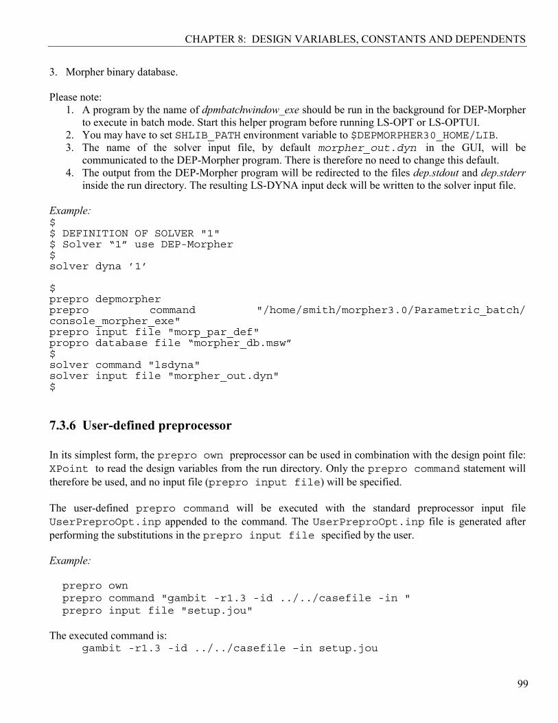
CHAPTER 8: DESIGN VARIABLES, CONSTANTS AND DEPENDENTS
99
3. Morpher binary database. Please note:
1. A program by the name of dpmbatchwindow_exe should be run in the background for DEP-Morpher to execute in batch mode. Start this helper program before running LS-OPT or LS-OPTUI.
2. You may have to set SHLIB_PATH environment variable to $DEPMORPHER30_HOME/LIB. 3. The name of the solver input file, by default morpher_out.dyn in the GUI, will be
communicated to the DEP-Morpher program. There is therefore no need to change this default. 4. The output from the DEP-Morpher program will be redirected to the files dep.stdout and dep.stderr
inside the run directory. The resulting LS-DYNA input deck will be written to the solver input file. Example:$$ DEFINITION OF SOLVER "1"$ Solver “1” use DEP-Morpher$solver dyna ’1’
$prepro depmorpherprepro command "/home/smith/morpher3.0/Parametric_batch/console_morpher_exe"prepro input file "morp_par_def"propro database file “morpher_db.msw”$solver command "lsdyna"solver input file "morpher_out.dyn"$ 7.3.6 User-defined preprocessor In its simplest form, the prepro own preprocessor can be used in combination with the design point file: XPoint to read the design variables from the run directory. Only the prepro command statement will therefore be used, and no input file (prepro input file) will be specified. The user-defined prepro command will be executed with the standard preprocessor input file UserPreproOpt.inp appended to the command. The UserPreproOpt.inp file is generated after performing the substitutions in the prepro input file specified by the user. Example: prepro ownprepro command "gambit -r1.3 -id ../../casefile -in "prepro input file "setup.jou"
The executed command is:
gambit -r1.3 -id ../../casefile –in setup.jou

CHAPTER 8: DESIGN VARIABLES, CONSTANTS AND DEPENDENTS
100 LS-OPT Version 2
Alternatively, a script can be executed with the prepro command to perform any number of command line commands that result in the generation of a file called: UserOpt.inp for use by an own solver, or DynaOpt.inp for use by LS-DYNA.

CHAPTER 8: DESIGN VARIABLES, CONSTANTS AND DEPENDENTS
101
8. Design Variables, Constants and Dependents
This chapter describes the definition of the input variables, constants and dependents, design space and the initial subregion. All the items in this chapter are specified in the Variables panel in LS-OPTui (Figure 8-1). Shown is a multidisciplinary design optimization (MDO) case where not all the variables are shared. E.g., t_bumper in Figure 8-1 is only associated with the solver CRASH.

CHAPTER 8: DESIGN VARIABLES, CONSTANTS AND DEPENDENTS
102 LS-OPT Version 2
Figure 8-1: Variables panel in LS-OPTui
8.1 Selection of design variables The variable command is the identification command for each variable. Command file syntax: variable variable_name value Example: $ DEFINE THE VARIABLE: ’Area’Variable ’Area’ 0.8 The value assigned is the initial value of the variable. 8.2 Definition of upper and lower bounds of the design space Command file syntax: Lower bound variable variable_name value <–10+30> Upper bound variable variable_name value <+10+30> Example:
Lower bound variable ’Area’ 0.1Upper bound variable ’Area’ 2.0 Both the lower and upper bounds must be specified, as they are used for scaling. 8.3 Size and location of region of interest (range) Command file syntax: range variable_name subregion_size
Example:
$ RANGE OF ’Area’range ’Area’ 0.4 This will allow ’Area’ to vary from 0.6 to 1.0. Remarks: 1. A value of 25-50% of the design space can be chosen if the user is unsure of a suitable value.

CHAPTER 8: DESIGN VARIABLES, CONSTANTS AND DEPENDENTS
103
2. The full design space is used if the range is omitted. 3. The region of interest is centered on a given design and is used as a sub-space of the design space to
define the experimental design. If the region of interest protrudes beyond the design space, it is moved without contraction to a location flush with the design space boundary.
8.4 Local variables For multidisciplinary design optimization (MDO) certain variables are assigned to some but not all solvers (disciplines). In the command file the following syntax defines the variable as local: Command file syntax: local variable_name
See Section 18.6 for an example. 8.5 Assigning variable to solver If a variable has been flagged as local, it needs to be assigned to a solver. The command file syntax is: Command file syntax: Solver variable variable_name
See Section 18.6 for an example. 8.6 Constants Each variable above can be modified to be a constant. See Figure 8-2 where this is the case for t_bumper. Constants are used: 1. to define constant values in the input file such as π, e or any other constant that may relate to the
optimization problem, e.g. initial velocity, event time, integration limits, etc. 2. to convert a variable to a constant. This requires only changing the designation variable to constant in
the command file without having to modify the input template. The number of optimization variables is thus reduced without interfering with the template files.

CHAPTER 8: DESIGN VARIABLES, CONSTANTS AND DEPENDENTS
104 LS-OPT Version 2
Command file syntax: constant constant_name value
Example:
constant ’Youngs_modulus’ 2.07e8constant ’Poisson_ratio’ 0.3dependent ’Shear_modulus’ {Youngs_modulus/(2*(1 + Poisson_ratio))} In this case, the dependent is of course not a variable, but a constant as well. 8.7 Dependent Variables Dependent variables (see Figure 8-2 for example of definition in Variables panel) are functions of the basic variables and are required to define quantities that have to be replaced in the input template files, but which are dependent on the optimization variables. They do therefore not contribute to the size of the optimization problem. Dependents can be functions of dependents. Dependent variables are specified using mathematical expressions (see Appendix E). Command file syntax: dependent variable_name expression
The string must conform to the rules for expressions and be placed in curly brackets. The dependent variables can be specified in an input template and will therefore be replaced by their actual values. Example:
variable ’Youngs_modulus’ 2.0e08variable ’Poisson_ratio’ 0.3dependent ’Shear_modulus’ {Youngs_modulus/(2*(1 + Poisson_ratio))}

CHAPTER 8: DESIGN VARIABLES, CONSTANTS AND DEPENDENTS
105
Figure 8-2: Variables panel in LS-OPTui with Constants and Dependents
8.8 Worst-case design Worst-case or saddle-point design is where the objective function is minimized (or maximized) with respect to some variables, while it is maximized (or minimized) with respect to the remaining variables in the variable set. The maximization variables are set using the Maximize option in the Saddle Direction field of the Variables panel. The default selection is Minimize. Command file syntax: Variable variable_name max
Example:variable ’head_orientation’ max


107
9. Probabilistic Modeling and Monte Carlo Simulation
Probabilistic evaluations investigate the effects of variations of the system parameters on the system responses. The variation of the system parameters is described using design variables with probabilistic distributions describing their variation around the mean design variable value. The concept of noise variables, which vary only according to a statistical distribution and of which the value is not under the control of the analyst, is introduced in addition to the control variables. Accordingly, the system responses will vary according to some statistical distribution. From this distribution, information such as the nominal value of the response, reliability, and extreme values is inferred. More background on the probabilistic methods is given in the theoretical manual (Section 3). The use of the probabilistic analysis techniques is clarified using examples. 9.1 Probabilistic problem modeling Introducing the probabilistic effects into analysis requires the specification of:
1. Statistical distributions. 2. Assigning the statistical distributions to design variables. 3. Specification of the experimental design. For a Monte Carlo analysis a suitable strategy for selecting
the experimental points must be specified; for example, a Latin Hypercube experimental design can be used to minimize the number of runs required to approximate the mean and standard deviation. However, if the Monte Carlo analysis is done using a metamodel, then the experimental design pertains to the construction of the metamodel.
4. The probabilistic analysis to be executed must be specified; for example, a Monte Carlo reliability analysis.

CHAPTER 9: Probabilistic Modeling and Monte Carlo Simulation
108 LS-OPT Version 2
9.2 Probabilistic Distributions The probabilistic component of a design variable is described using a probabilistic distribution. The distributions are created without referring to a variable. Many design variables can refer to a single distribution. 9.2.1 Beta distribution The beta distribution is quite versatile as well as bounded by two limits: a and b. The shape of the distribution is described by two parameters: q and r. Swapping the values of q and r produces a mirror image of the distribution.
Figure 15.5: Beta distribution
Command file syntax: distribution ‘name’ BETA a b q r
Item Description name Distribution name a Lower Bound b Upper Bound q Shape parameter q r Shape parameter r
Example: distribution 'distBeta' BETA 2.0 5.0 1.0 1.0

CHAPTER 9: Probabilistic Modeling and Monte Carlo Simulation
109
9.2.2 Binomial distribution The binomial distribution is a discrete distribution describing the expected number of events for an event with probability p evaluated over n trails. For n=1, it is the Bernoulli distribution (experiments with two possible outcomes ― success or failure) with probability of success p.
Figure 15.5: Binomial distribution
Command file syntax: distribution ‘name’ BINOMIAL p n
Item Description name Distribution name p Probability of event (Success) n Number of trials
Example: distribution 'distBin' BINOMIAL 0.1 3

CHAPTER 9: Probabilistic Modeling and Monte Carlo Simulation
110 LS-OPT Version 2
9.2.3 Lognormal distribution If X is a lognormal random variable with parameters µ and σ, then the random variable Y = ln X has a normal distribution with mean µ and variance σ2.
Figure 15-4: Lognormal distribution
Command file syntax: distribution ‘name’ LOGNORMAL mu sigma
Item Description name Distribution name mu Mean value in logarithmic domain sigma Standard deviation in logarithmic domain
Example: distribution 'logDist' LOGNORMAL 12.3 1.1

CHAPTER 9: Probabilistic Modeling and Monte Carlo Simulation
111
9.2.4 Normal Distribution The normal distribution is symmetric and centered about the mean µ with a standard deviation of σ.
Figure 9-1 Normal Distribution
Command file syntax: distribution ‘name’ NORMAL mu sigma
Item Description name Distribution name mu Mean value sigma Standard deviation
Example: distribution 'normalDist' NORMAL 12.2 1.1
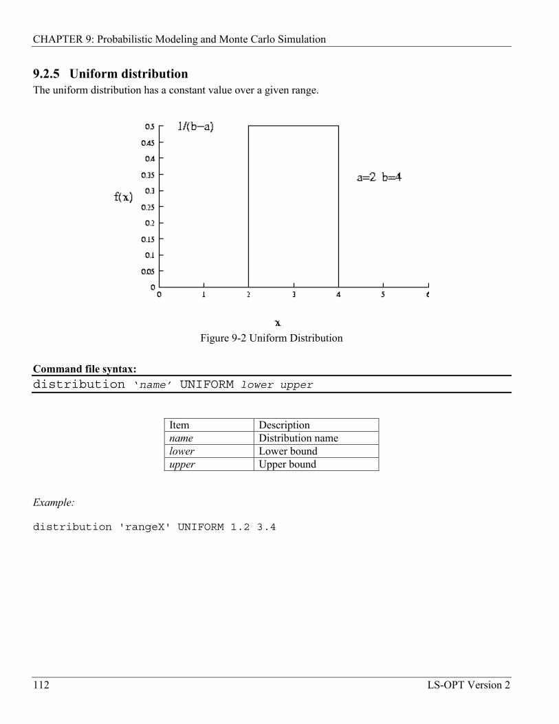
CHAPTER 9: Probabilistic Modeling and Monte Carlo Simulation
112 LS-OPT Version 2
9.2.5 Uniform distribution The uniform distribution has a constant value over a given range.
Figure 9-2 Uniform Distribution
Command file syntax: distribution ‘name’ UNIFORM lower upper
Item Description name Distribution name lower Lower bound upper Upper bound
Example: distribution 'rangeX' UNIFORM 1.2 3.4
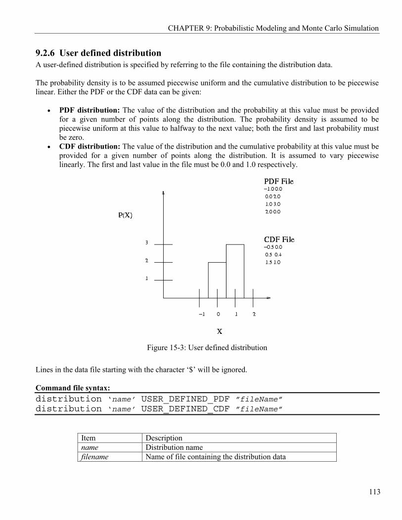
CHAPTER 9: Probabilistic Modeling and Monte Carlo Simulation
113
9.2.6 User defined distribution A user-defined distribution is specified by referring to the file containing the distribution data. The probability density is to be assumed piecewise uniform and the cumulative distribution to be piecewise linear. Either the PDF or the CDF data can be given:
• PDF distribution: The value of the distribution and the probability at this value must be provided for a given number of points along the distribution. The probability density is assumed to be piecewise uniform at this value to halfway to the next value; both the first and last probability must be zero.
• CDF distribution: The value of the distribution and the cumulative probability at this value must be provided for a given number of points along the distribution. It is assumed to vary piecewise linearly. The first and last value in the file must be 0.0 and 1.0 respectively.
Figure 15-3: User defined distribution
Lines in the data file starting with the character ‘$’ will be ignored. Command file syntax: distribution ‘name’ USER_DEFINED_PDF ”fileName”distribution ‘name’ USER_DEFINED_CDF ”fileName”
Item Description name Distribution name filename Name of file containing the distribution data

CHAPTER 9: Probabilistic Modeling and Monte Carlo Simulation
114 LS-OPT Version 2
Example: distribution 'bendDist' USER_DEFINED_PDF "bendingTest.pdf"distribution 'testDat' USER_DEFINED_CDF "threePointTest.dat"
The file “bendingTest.pdf” contains: $ Demonstration of user defined distribution with$ piecewise uniform PDF values$ x PDF$ First PDF value must be 0-5 0.00000-2.5 0.115940 0.144932.5 0.11594
$ Last PDF value must be 05 0.00000
The file “threePointTest.dat” contains: $ Demonstration of user defined distribution with$ piecewise linear CDF values$ x CDF$ First CDF value must be 0-5 0.00000-4.5 0.02174-3.5 0.09420-2.5 0.20290-1.5 0.32609-0.5 0.463770.5 0.608701.5 0.739132.5 0.855073.5 0.94928$ Last CDF value must be 14.5 1.00000

CHAPTER 9: Probabilistic Modeling and Monte Carlo Simulation
115
9.2.7 Weibull distribution The Weibull distribution is quite versatile – it has the ability to take on various shapes. The probability density function is skewed to the right, especially for low values of the shape parameter.
Figure 15.5: Weibull distribution
Command file syntax: distribution ‘name’ WEIBULL scale shape
Item Description name Distribution name scale Scale parameter shape Shape parameter
Example: distribution 'wDist' WEIBULL 2.3 3.1

CHAPTER 9: Probabilistic Modeling and Monte Carlo Simulation
116 LS-OPT Version 2
9.3 Probabilistic Variables A probabilistic variable has a mean or nominal value, a variation around this nominal value according to a statistical distribution, an optional upper bound, and an optional lower bound.
Figure 15.6: Probabilistic Variable
A distinction is made between control and noise variables:
• Control variables: Variables that can be controlled in the design, analysis, and production level; for example: a shell thickness. It can therefore be assigned a nominal value and will have a variation around this nominal value. The nominal value can be adjusted during the design phase in order to have a more suitable design.
• Noise variables: Variables that are difficult or impossible to control at the design and production level, but can be controlled at the analysis level; for example: loads and material variation. A noise variable will have the nominal value as specified by the distribution, that is follow the distribution exactly.
A variable is declared probabilistic by:
• Creating it as a noise variable • Assigning a distribution to a control variable • Creating it as linked to an existing probabilistic variable
Three associations between probabilistic variables are possible: • Their nominal values are the same but their distributions differ • Their nominal values and distributions are the same

CHAPTER 9: Probabilistic Modeling and Monte Carlo Simulation
117
• Their nominal values differ, but they refer to the same distribution
Command file syntax: noise variable ‘variableName’ distribution ‘distributionName’variable ‘variableName’ distribution ‘distributionName’variable ‘variableName’ link variable ‘variableName’
Item Description variableName Variable identifier distributionName Distribution identifier
Example: $ Create a noise variableNoise Variable ‘windLoadScatter’ distribution ‘windLoadData’$ Assigning a distribution to an existing control variableVariable 'Var-D-1' Distribution 'dist-1'$ Creating a variable by linking it to another.Variable 'Var-D-2' Link variable 'Var-D-1' 9.3.1 Setting the Nominal Value of a Probabilistic Variable If no nominal value is specified for a control variable, then the nominal value of the distribution is used. If the nominal value of a control variable is specified, then this value is used; the associated distribution will be used to describe the variation around this nominal value. For example: a variable with a nominal value of 7 is assigned a normal distribution with µ=0 and σ=2; the results values of the variable will be normally distributed around a nominal value of 7 with a standard deviation of 2. This behavior is only applicable to control variables; noise variables will always follow the specified distribution exactly. 9.3.2 Bounds on Probabilistic Variable Values Assigning a distribution to a control value may result in designs exceeding the bounds on the control variables. The default is not to enforce the bounds. The user can control this behavior. A noise variable is bounded by the distribution specified and does not have upper and lower bounds similar to control variables. However bounds are required for the construction of the approximating functions and are chosen as described in the next subsection.
CHAPTER 9: Probabilistic Modeling and Monte Carlo Simulation
118 LS-OPT Version 2
Command file syntax: set variable distribution bound state
Item Description state Whether the bounds must be enforced for the probabilistic
component of the variable.
Example: $ ignore bounds on control variablesset variable distribution bound 0$ Respect bounds on control variablesset variable distribution bound 1
9.3.3 Noise Variable Subregion Size Bounds are required for noise variables to construct the metamodels. The bounds are taken to a number of standard deviations away from the mean; the default being two standard deviations of the distribution. The number of standard deviations can however be set by the user. In general, a noise variable is bounded by the distribution specified and does not have upper and lower bounds similar to control variables. Command file syntax: set noise variable range standardDeviations
Item Description standardDeviations The subregion size in standard deviations for the noise
variable. Example: $ Set noise var bounds to 1.5 standard deviations$ for defining subregion for creating approximationset noise variable range 1.5
9.4 Probabilistic Simulation The following simulation methods are provided:
• Monte Carlo. • Monte Carlo using metamodels.
The upper and lower bounds on constraints will be used as failure values for the reliability computations.

CHAPTER 9: Probabilistic Modeling and Monte Carlo Simulation
119
9.4.1 Monte Carlo Analyses The Monte Carlo evaluation will:
• Select the random sample points according to a user specified strategy and the statistical distributions assigned to the variables.
• Evaluate the structural behavior at each point. • Collect the statistics of the responses.
The user must specify the experimental design strategy (sampling strategy) to be used in the Monte Carlo evaluation. The Monte Carlo, Latin Hypercube and space-filling experimental designs are available. The experimental design will first be computed in a normalized, uniformly distributed design space and then transformed to the distributions specified for the design variables. Only variables with a statistical distribution will be perturbed; all other variables will be considered at their nominal value. The following will be computed for all responses:
• Statistics such as the mean and standard deviation for all responses and constraints. • Reliability information regarding all constraints:
o The number of times a specific constraint was violated during the simulation. o The probability of violating the bounds and the confidence region of the probability. o A reliability analysis for each constraint assuming a normal distribution of the response.
The exact value at each point will be used. Composite functions referring to responses in more than one discipline will not be computed because the experimental designs will differ across disciplines. Command file syntax: analyze Monte Carlo
Example:
analyze Monte Carlo
9.4.2 Monte Carlo analysis using a Metamodel The Monte Carlo analysis will be done using the metamodels − response surfaces, neural networks, or Kriging − as prescribed by the user. The number of function evaluations using the metamodels can be set by the user. The default value is 106. The designs to be analyzed are chosen randomly respecting the distributions of the design variables. The following data will be collected:

CHAPTER 9: Probabilistic Modeling and Monte Carlo Simulation
120 LS-OPT Version 2
• Statistics such as the mean and standard deviation for all responses, constraints, and variables. • The reliability information for each constraint:
o The number of times a specific constraint was violated during the simulation. o The probability of violating the bounds and the confidence region of the probability.
Command file syntax: analyze metamodel monte carlo
Example:
analyze metamodel monte carlo
9.4.3 Accuracy of Metamodel Based Monte Carlo The number of function evaluations to be analyzed can be set by the user. The default value is 106. Command file syntax: set reliability resolution m
Item Description m Number of sample values
Example:
set reliability resolution 1000
9.4.4 Histograms of Responses This option outputs histograms of the variables, dependend variables, responses, and composite functions. This feature is only available for the Monte Carlo analysis procedures. It can be memory intensive for metamodel-based computations because all the responses values must be kept in memory. The default is not to output any histograms. The histograms can always be viewed in Viewer as a post-processing operation. Command file syntax: set histogram intervals

CHAPTER 9: Probabilistic Modeling and Monte Carlo Simulation
121
Item Description intervals Number of intervals in histogram
Example:
set histogram 12
9.4.5 Adding the Noise Component to Metamodel Monte Carlo Computations If noise was found when the metamodel was created, then this noise may be reproduced whenever the metamodel is used for reliability computations. This is possible only for the response surfaces and neural nets. The noise is normally distributed with a zero mean and a standard deviation computed from the residuals of the least square fit. The default is not to add the noise to the computations. Command file syntax: set metamodel noise true_false
Item Description true_false 0 for not adding noise; 1 otherwise
Example:
set metamodel noise 0 $ default: noise not added in computationset metamodel noise 1 $ noise included in computation
9.5 Stochastic Contribution Analysis It can be useful to know how the variation of each design variable contributes to the variation of a response. The stochastic contribution will be printed for all the responses in a metamodel-based procedure. If no metamodel is available the covariance of the responses with the variables can be investigated. The stochastic contributions of the variables can also be examined in the Viewer part of the GUI. The amount of variation due to noise or the residuals from the fitting procedure will be indicated. This term is taken as zero for composite functions. Theoretical concerns are discussed in Section 3.7. 9.6 Covariance The covariance and coefficient of correlation of the responses will be printed for a Monte Carlo analysis.

CHAPTER 9: Probabilistic Modeling and Monte Carlo Simulation
122 LS-OPT Version 2
The covariance and coefficient of the responses can also be examined in the Viewer part of the GUI. Theoretical concerns are discussed in Section 3.3.2.

CHAPTER 9: Probabilistic Modeling and Monte Carlo Simulation
123

124
10. Metamodels and Point Selection
This chapter describes the specification of the metamodel types and point selection schemes (design of experiments or DOE). The terms point selection and experimental design are used interchangeably. 10.1 Metamodel definition The user can select from three metamodel types in LS-OPT. The standard and default selection is the polynomial response surface method (RSM) where response surfaces are fitted to results at data points using polynomials. For global approximations, neural network or Kriging approximations are available. Sensitivity data (analytical or numerical) can also be used for optimization. This method is more suitable for linear analysis solvers. Command file syntax: Solver order [linear|interaction|elliptic|quadratic|FF|kriging]
The linear, interaction (linear with interaction effects), elliptic and quadratic options are for polynomials. FF represents the Feedforward Neural network.
10.1.1 Response Surface Methodology When polynomial response surfaces are constructed, the user can select from different approximation orders. The available options are linear, linear with interaction, elliptic and quadratic. Increasing the order of the polynomial results in more terms in the polynomial, and therefore more coefficients. In LSOPTui, the approximation order is set in the Order field. See Figure 10-1. The polynomial terms can be used during the variable screening process (see Section 2.9) to determine the significance of certain variables (main effects) and the cross-influence (interaction effects) between variables when determining responses. These results can be viewed graphically (Section 14.4). The recommended point selection scheme for polynomial response surfaces is the D-optimal scheme (Section 10.2.2).

CHAPTER 10: METAMODELS AND POINT SELECTION
125
10.1.2 Neural Networks and Kriging * To apply neural network or Kriging approximations, select the appropriate option in the Metamodel field in LS-OPTui. See Figure 10-2. The recommended Point Selection Scheme for neural networks and Kriging is the space filling method. The user can select either a sub-region (local) approach, or update the set of points for each iteration to form a global approximation. An updated network is fitted to all the points. See Section 10.6 for more detail on updating. Please refer to Section 4.5 for recommendations on how to use neural network and Kriging approximations. 10.2 Point Selection Schemes 10.2.1 Overview Table 10-1 shows the available point selection schemes (experimental design methods).
Table 10-1: Point selection schemes
Experiment Description Identifier Remark
Linear Koshal lin_koshal For polynomials
Quadratic Koshal quad_koshal
Central Composite composite
D-optimal designs
D-optimal dopt Polynomials
Factorial Designs
2n 2toK
3n 3toK
M M M
11n 11toK

CHAPTER 10: METAMODELS AND POINT SELECTION
126 LS-OPT Version 2
Random designs
Latin Hypercube latin_hypercube For probabilistic analysis or
Monte Carlo monte_carlo random search
Space filling designs
Space filling 5 (recommended) space_filling Algorithm 5 (Section 2.6.6)
Space filling 0 monte_carlo -
Space filling 1 lhd_centralpoint -
Space filling 2 lhd_generalized -
Space filling 3 maximin_permute - Space filling 4 maximin_subinterval -
User defined designs
User-defined own
Plan plan Command file syntax: Solver order [linear|interaction|elliptic|quadratic|FF|kriging]Solver experimental design point_selection_schemeSolver basis experiment basis_experimentSolver number experiment number_experimental_pointsSolver number basis experiments number_basis_experimental_points
Example 1:
Solver order quadraticSolver experimental design doptSolver basis experiment 5toK
Example 2: Solver order linearSolver experimental design doptSolver basis experiment latin_hypercubeSolver number experiments 40Solver number basis experiments 1000

CHAPTER 10: METAMODELS AND POINT SELECTION
127
In Example 1, the default number of experiments will be selected depending on the number of design variables. In Example 2, 40 points are selected from a total number of 1000. In LS-OPTui, the point selection scheme is selected using the Point Selection panel (Figure 10-1). The default options are preset, e.g., the D-optimal point selection scheme (basis type: Full Factorial, 3 points per variable) is the default for linear polynomials (Figure 10-1), and the space-filling scheme is the default for the Neural Net and Kriging methods (Figure 10-2).
Figure 10-1: Metamodel and Point Selection panel in LS-OPTui

CHAPTER 10: METAMODELS AND POINT SELECTION
128 LS-OPT Version 2
10.2.2 D-Optimal point selection The D-optimal design criterion can be used to select the best (optimal) set of points for a response surface from a given set of points. The basis set can be determined using any of the other point selection schemes and is referred to here as the basis experiment. The order of the functions used has an influence on the distribution of the optimal experimental design. The following must be defined to select D-optimal points.
Order The order of the functions that will be used. Linear, linear with interaction, elliptic or quadratic.
Number experiments The number of experimental points that must be selected. Basis experiment The set of points from which the D-optimal design points
must be chosen, e.g. 3tok Number basis experiments The number of basis experimental points (only random,
latin hypercube and space filling). The default basis experiment for the D-optimal design is 5n for quadratic and elliptic approximations and 3n for linear. The default number of points selected is int(1.5(n + 1)) + 1 for linear, int(1.5(2n + 1)) + 1 for elliptic, int(0.75(n2 + n + 2)) + 1 for interaction, and int(0.75(n + 1)(n + 2)) + 1 for quadratic. As a result, about 50% more points than the minimum required are generated. If the user wants to override this number of experiments, the command “solver number experiments” is required after “solverorder function_order”. 10.2.3 Latin Hypercube Sampling The Latin Hypercube point selection scheme is typically used for probabilistic analysis. The Latin Hypercube design is also useful to construct a basis experimental design for the D-optimal design for a large number of variables where the cost of using a full factorial design is excessive. E.g. for 15 design variables, the number of basis points for a 3n design is more than 14 million. The Monte Carlo, Latin Hypercube and Space-Filling point selection schemes require a user-specified number of experiments. Even if the Latin Hypercube design has enough points to fit a response surface, there is a likelihood of obtaining poor predictive qualities or near singularity during the regression procedure. It is therefore better to use the D–optimal experimental design for RSM. Example:
Solver order linearSolver experimental design latin_hypercubeSolver number experiment 20

CHAPTER 10: METAMODELS AND POINT SELECTION
129
The Latin Hypercube point selection scheme is also well suited to sequential random search methods (see Section 2.13). 10.2.4 Space filling* Only algorithm 5 (see Section 2.6.6) is available in LS-OPTui. This algorithm maximizes the minimum distance between experimental design points. The only item of information that the user must provide for this point selection scheme, is the number of experimental design points. Space filling is useful when applied in conjunction with the Neural Net (neural network) and Kriging methods (see Section 10.1.2).
Figure 10-2: Selecting the Neural network approximation method in the Point Selection panel

CHAPTER 10: METAMODELS AND POINT SELECTION
130 LS-OPT Version 2
10.3 User-defined experiments To retain existing (expensive) simulation data in the optimization process, it is advantageous to be able to augment an existing design with additional experimental points. This can be performed by constructing a user-defined experiment as follows. User-defined experiments can be placed in a file named Experiments.PRE.solver_name in the work directory. These will be used in the first iteration only for the solver with name solver_name. The user can augment this set D-optimally by requesting a number of experiments greater than the number of lines in Experiments.PRE.solver_name. Each experiment must appear on a separate line with spaces, commas or tabs between values. If the user wants to specify an experimental design plan in all iterations, a file Experiments.PLANmust be supplied. The point coordinates must be normalized to the bounds [-1; 1]. This unit experimental design will be scaled to the region of interest in each iteration. 10.4 Remarks: Point selection 1. The number of points specified in the “solver number experiment num” command is reduced
by the number already available in the Experiments.PRE.solver_name or AnalysisResults.PRE.solver_name files.
2. The files Experiments and AnalysisResults are synchronous, i.e. they will always have the same experiments after extraction of results. Both these files also mirror the result directories for a specific iteration.
3. Design points that replicate the starting point are omitted. 10.5 Specifying an irregular design space* An irregular (reasonable) design space refers to a region of interest that, in addition to having specified bounds on the variables, is also bounded by arbitrary constraints. This may result in an irregular shape of the design space. Therefore, once the first approximation has been established, all the designs will be contained in the new region of interest. This region of interest is thus defined by approximate constraint bounds and by variable bounds. The purpose of an irregular design space is to avoid designs which may be impossible to analyze. The move/stay commands can be used to define an environment in which the constraint bound commands (Section 12.4) can be used to double as bounds for the reasonable design space. If a reasonable experimental design is required from the start, a DesignFunctions.PRE.solver_name file can be provided by the user. This is however not necessary if explicit constraints, i.e. constraints that do not require simulations, are specified for the reasonable design space. An explicit constraint may be a simple relationship between the design variables.

CHAPTER 10: METAMODELS AND POINT SELECTION
131
The move start option moves the designs to the starting point instead of the center point (see Section 2.7). This option removes the requirement for having the center point inside the reasonable design space. Command file syntax: movestaymove start Example 1: $ SET THE BOUNDS ON THE REASONABLE DESIGN SPACELower bound constraint ’Energy’ 4963.0moveUpper bound constraint ’Energy’ 5790.0stayLower bound constraint ’Force’ -1.2Upper bound constraint ’Force’ 1.2
The example above shows the lines required to determine a set of points that will be bounded by an upper bound on the Energy. Example 2:
Variable ’Radius_1’ 20.0Variable ’Radius_2’ 20.0..Composite ’TotalR’ {Radius_1 + Radius_2}moveConstraint ’TotalR’Upper bound constraint ’TotalR’ 50 This specification of the move command ensures that the points are selected such that the sum of the two variables does not exceed 50. Remarks: 1. For constraints that are dependent on simulation results, a reasonable design space can only be created if
response functions have already been created by a previous iteration. The mechanism is as follows:
Automated design: After each iteration, the program converts the database file DesignFunctions to file DesignFunctions.PRE in the solver directory. DesignFunctions.PRE then defines a reasonable design space and is read at the beginning of the next design iteration.
Manual (semi-automated) Procedure: If a reasonable design space is to be used, the user must ensure that a file DesignFunctions.PRE.solver_name is resident in the working directory

CHAPTER 10: METAMODELS AND POINT SELECTION
132 LS-OPT Version 2
before starting an iteration. This file can be copied from the DesignFunctions file resulting from a previous iteration.
2. A reasonable design space can only be created using the D-optimal experimental design. 3. The reasonable design space will only be created if the center point (or the starting point in the case of
move start) of the region of interest is feasible. Feasibility is determined within a tolerance of 0.001*| fmax – fmin| where fmax and fmin are the maximum and minimum values of the interpolated response over all the points.
4. The move feature should be used with extreme caution, since a very tightly constrained experimental design may generate a poorly conditioned response surface.
10.6 Updating an experimental design Updating the experimental design involves augmenting an existing design with new points. Updating only makes sense if the response surface can be successfully adapted to the augmented points such as for neural nets or Kriging surfaces in combination with a space filling scheme. Command file syntax: solver update doe The new points have the following properties: • They are located within the current region of interest. • The minimum distance between the new points and between the new and existing points, is maximized
(space filling only).
10.7 Duplicating an experimental design When executing a search method (see e.g. Section 2.13) for a multi-case or multidisciplinary optimization problem, the design points of the various disciplines must be duplicated so that all the responses and composites can be evaluated for any particular design point. The command must appear in the environment of the solver requiring the duplicate points. An experimental design can therefore be duplicated as follows: Command file syntax: solver experiment duplicate string
where string is the name of the master solver in single quotes, e.g. Solver experiment duplicate ’CRASH’
‘CRASH’ is the master experimental design that must be copied exactly. See also the example in Section 18.6.3.

CHAPTER 10: METAMODELS AND POINT SELECTION
133
10.8 Using design sensitivities for optimization Both analytical and numerical sensitivities can be used for optimization. The syntax for the solverexperimental design command is as follows:
Experiment Description Identifier Numerical Sensitivity numerical_DSA Analytical Sensitivity analytical_DSA
10.8.1 Analytical sensitivities If analytical sensitivities are available, they must be provided for each response in its own file named Gradient. The values (one value for each variable) in Gradient should be placed on a single line, separated by spaces. In LS-OPTui, the Metamodel (Point Selection panel) must be set to Sensitivity Type Analytical. See Figure 10-3. Example: Solver experimental design analytical_DSA
A complete example is given in Section 18.9. 10.8.2 Numerical sensitivities To use numerical sensitivities, select Numerical Sensitivities in the Metamodel field in LS-OPTui and assign the perturbation as a fraction of the design space. Numerical sensitivities are computed by perturbing n points relative to the current design point x0, where the j-th perturbed point is:
( )LU0
iiijij
i xxεδxx −+=
0=ijδ if ji ≠ and 1.0 if ji = . The perturbation constant ε is relative to the design space size. The same value applies to all the variables and is specified as: Command file syntax: Solver perturb perturbation_value

CHAPTER 10: METAMODELS AND POINT SELECTION
134 LS-OPT Version 2
Example:
Solver experimental design numerical_DSASolver perturb 0.01
Figure 10-3: Selecting Sensitivities in the Point Selection panel

CHAPTER 10: METAMODELS AND POINT SELECTION
135

LS-OPT Version 2 136
11. History and Response Results
This chapter describes the specification of the history or response results to be extracted from the solver database. The chapter focuses on the standard response interfaces for LS-DYNA. 11.1 Defining a response history (vector) A response history can be defined by using the history command with an extraction or a mathematical expression. The extraction of the result can be done using a standard LS-DYNA interface (see Section 11.5) or with a user-defined program. Command file syntax: history history_name stringhistory history_name expression math_expression
The string is an interface definition (in double quotes), while the math_expression is a mathematical expression (in curly brackets). A user-defined program may be used to extract a history file from the database. The program must produce an output file with the reserved name LsoptHistory. This file contains two columns of data, separated by whitespace (a space or tab) or the following characters: comma (,), semi-colon (;) or equal sign(=). Lines that do not have the recognizable format will be ignored, so that files with headers or footers do not need to be specially modified. Example 1: history ’displacement_1’ "DynaASCII nodout r_disp 12789 TIMESTEP 0.0 SAE 60"history ’displacement_2’ "DynaASCII nodout r_disp 26993 TIMESTEP 0.0 SAE 60"history ’deformation’ expression {displacement_2 - displacement_1}response ’final_deform’ expression {deformation(200)}
Example 2: constant ’v0’ 15.65history ’bumper_velocity’ "DynaASCII nodout X_VEL 73579 TIMESTEP 0.0 SAE 30"history ’Apillar_velocity_1’ "DynaASCII nodout X_VEL 41195 TIMESTEP 0.0 SAE 30"history ’Apillar_velocity_2’ "DynaASCII nodout X_VEL 17251 TIMESTEP 0.0 SAE 30"history ’global_velocity’ "DynaASCII glstat X_VEL 0 TIMESTEP"

CHAPTER 11: HISTORY AND RESPONSE RESULTS
LS-OPT Version 2 137
history ’Apillar_velocity_average’ expression {(Apillar_velocity_1 + Apillar_velocity_2)/2}
$response ’time_to_bumper_zero’ expression {Lookup("bumper_velocity(t)",0)}response ’vel_A_bumper_zero’ expression {Apillar_velocity_average(time_to_bumper_zero)}response ’PULSE_1’ expression {Integral
("Apillar_velocity_average(t)",0,time_to_bumper_zero)/time_to_bumper_zero}
response ’time_to_zero_velocity’expression {Lookup("global_velocity(t)",0)}response ’velocity_final’ expression{Apillar_velocity_average(time_to_zero_velocity)}response ’PULSE_2’ expression {Integral
("Apillar_velocity_average(t)"time_to_bumper_zero,time_to_zero_velocity)
/(time_to_zero_velocity - time_to_bumper_zero)} Example 3: constant ’Event_time’ 200$ Results from a physical experimenthistory ’experiment_vel’ "cp /users/john/experiments/chest_results
./LsoptHistory"$ LS-DYNA resultshistory ’velocity’ "DynaASCII nodout X_VEL 12667 TIMESTEP"response ’RMS_error’ expression {Integral("(experiment_vel-velocity)**2",0,Event_time} Example 4: In this example a user-defined program (the post-processor LS-PREPOST) is used to produce a history file from the LS-DYNA database. The LS-PREPOST command file get_force: open d3plot d3plotascii rcforc open rcforc 0ascii rcforc plot 4 Ma-1xyplot 1 savefile xypair LsoptHistory 1deletewin 1quit produces the LsoptHistory file. history ’Force’ "lsprepost c=../../get_force"response ’Force1’ expression {Force(.002)}response ’Force2’ expression {Force(.004)}response ’Force3’ expression {Force(.006)}response ’Force4’ expression {Force(.008)}

CHAPTER 11: HISTORY AND RESPONSE RESULTS
138 LS-OPT Version 2
Remarks: 1. Histories are used by response definitions (see Section 11.2) to define a response surface. They are
therefore intermediate entities and cannot be used directly to define a response surface. Only response can define a response surface.
2. For LS-DYNA history definition and syntax, please refer to Section 11.5. In LS-OPTui, histories are defined in the Histories panel (Figure 11-1):
Figure 11-1: Histories panel in LS-OPTui
11.2 Defining a response (scalar) The extraction of responses consists of a definition for each response and a single extraction command or mathematical expression. A response is often the result of a mathematical operation of a response history,

CHAPTER 11: HISTORY AND RESPONSE RESULTS
LS-OPT Version 2 139
but can be extracted directly using the standard LS-DYNA interface (see Section 11.5) or a user-defined interface. Each extracted response is identified by a name and the command line for the program that extracts the results. The command line must be enclosed in double quotes. If scaling and/or offsetting of the response is required, the final response is computed as ( the extracted response x scale factor ) + offset. This operation can also be achieved with a simple mathematical expression. A mathematical expression for a response is defined in curly brackets after the response name. Command file syntax: response response_name {scale_factor offset} stringresponse response_name expression math_expression
Example:
response ’Displacement_x’ 25.4 0.0 "DynaASCII nodout ’r disp’ 63 TIMESTEP 0.1"response ’Force’ "$HOME/ownbin/calculate force"response ’Displacement_y’ "calc constraint2"response ’Disp’ expression {Displacement_x + Displacement_y} Remarks: 1. The first command will use a standard interface for the specified solver package. The standard interfaces
for LS-DYNA are described in Section 11.5. 2. The middle two commands are used for a user-supplied interface program (see Section 11.13). The
interface name must either be in the path or the full path name must be specified. Aliases are not allowed.
3. For the last command, the second argument expression is a reserved name. 11.3 Specifying the metamodel type The metamodel type can be specified for an individual reponse. Command file syntax: response response_name[linear|interaction|elliptic|quadratic|FF|kriging]
The default is the metamodel specified in Section 10.1. FF refers to the feed-forward neural network approximation method (see Sections 2.10.1 and 4.5). Example:
response ’Displacement’ kriging

CHAPTER 11: HISTORY AND RESPONSE RESULTS
140 LS-OPT Version 2
In LS-OPTui, responses are defined in the Responses panel (Figure 11-2):
Figure 11-2: Reponses panel in LS-OPTui
11.4 Composite Functions Composite functions can be used to combine response surfaces and variables as well as other composites. The objectives and constraints can then be constructed using the composite functions. There are three types: 11.4.1 Expression Composite A general expression can be specified for a composite. The composite can therefore consist of constants, variables, dependent variables, responses and other composites.

CHAPTER 11: HISTORY AND RESPONSE RESULTS
LS-OPT Version 2 141
11.4.2 Standard Composite
Targeted Composite This is a special composite in which a target is specified for each response or variable. The composite is formulated as the ‘distance’ to the target using a Euclidean norm formulation. The components can be weighted and normalized.
∑∑==
−+
−=
n
i i
iii
m
j j
jjj
XxFfW
1
2
1
2)(
χω
σxF (11.1)
where σ and χ are scale factors and W and ω are weight factors. These are typically used to formulate a multi-objective optimization problem in which F is the distance to the target values of design and response variables.
A suitable application is parameter identification. In this application, the target values Fj are the experimental results that have to be reproduced by a numerical model as accurately as possible. The scale factors σj and χi are used to normalize the responses. The second component, which uses the variables can be used to regularize the parameter identification problem. Only independent variables can be included. See Figure 11-3 for an example of a targeted composite response definition. Weighted Composite Weighted response functions and independent variables are summed in this standard composite. Each function component or variable is scaled and weighted.
∑∑==
+=n
i i
ii
m
j j
jj
xfW
11
)(χ
ωσ
xF (11.2)
These are typically used to construct objectives or constraints in which the responses and variables appear in linear combination.
The expression composite is a simple alternative to the weighted composite. Remarks: 1. An expression composite can be a function of any other composite.
2. An objective definition involving more than one response or variable requires the use of a composite
function. 3. In addition to specifying more than one function per objective, multiple objectives can be defined (see
Section 12.2).

CHAPTER 11: HISTORY AND RESPONSE RESULTS
142 LS-OPT Version 2
Figure 11-3: Definition of targeted composite response in LS-OPTui
11.4.3 Defining the composite function This command identifies the composite function. The type of composite is specified as weighted, targeted or expression. The expression composite type does not have to be declared and can simply be stated as an expression. Command file syntax: composite composite_name type [targeted|weighted]
Example:
composite ’Damage’ type targetedcomposite ’Acceleration’ type weighted
The expression composite is defined as follows:

CHAPTER 11: HISTORY AND RESPONSE RESULTS
LS-OPT Version 2 143
Command file syntax: composite composite_name math_expression
The math_expression is a mathematical expression given in curly brackets (see Appendix E). The number of composite functions to be employed must be specified in the problem description. 11.4.4 Assigning design variable or response components to the composite Command file syntax: composite name response response_name value <1> { scalescale_factor <1> }composite name variable variable_name value { scale scale_factor<1> } The value is the target value for type: targeted and the weight value for the type: weighted. The scale_factor is a divisor. Example:
composite ’damage’ type targetedcomposite ’damage’ response ’intrusion_3’ 20. scale 30.composite ’damage’ response ’intrusion_4’ -35. scale 25.
for the composite function .25
3530
20 24
23
−+
−= ff
damageF
The equivalent code using the expression composite is: composite ’damage’ {sqrt(((intrusion_3 - 20)/30)**2 +
((intrusion_4 + 35)/25)**2)} Example:
$----- x10 > x9 ---------------------------composite ’C9’ type weightedcomposite ’C9’ variable ’x_9’ -1.composite ’C9’ variable ’x_10’ 1.constraint ’C9’Lower bound constraint ’C9’ 0. for the composite function which defines the inequality x10 > x9. The equivalent code using the expression composite is:
$----- x10 > x9 ---------------------------composite ’C9’ {x_10 - x_9}

CHAPTER 11: HISTORY AND RESPONSE RESULTS
144 LS-OPT Version 2
constraint ’C9’Lower bound constraint ’C9’ 0.
Needless to say, this is the preferable way to describe this composite. If weights are required for the targeted function, an additional command may be given. Command file syntax: weight weight value <1> Example: composite ’damage’ type targetedcomposite ’damage’ response ’intrusion_3’ 20.weight 1.5composite ’damage’ response ’intrusion_4’ -35.
is used to specify ( ) ( ) .35205.1 24
23 −+−= ffdamageF
The weight applies to the last specified composite and response. 11.4.5 Composites vs. Response Expressions There is an important distinction between response expressions and composites. This distinction can have a major impact on the accuracy of the result. Response expressions are converted to response surfaces after applying the expression to the results of each sampling point in the design space. Composites, on the other hand, are computed by combining response surface results. Therefore the response expression will always be of the same order as the chosen response surface order while the composite can assume any complexity depending on the formula specified for the composite (which may be arbitrary). Example: If an response function is defined as f(x,y) = xy and linear response surfaces are used, the response expression will be a simple linear approximation ax + by whereas a composite expression specified as xy will be exact. 11.5 Extracting History and Response Quantities: LS-DYNA In LS-OPT the general functionality for reading histories and responses from the simulation output is achieved through the history and response definitions (see Section 11.1 and Section 11.2 respectively). For ASCII files, the syntax for the extraction commands for responses and histories is identical, except for the time attributes. The history function is included so that operations (such as subtracting two histories) can first be performed, after which a scalar (such as maximum over time) can be extracted from the resulting history. There are two types of interfaces namely

CHAPTER 11: HISTORY AND RESPONSE RESULTS
LS-OPT Version 2 145
1. Standard LS-DYNA result interfaces. This interface provides access to the ASCII and binary databases (d3plot or LSDA) of LS-DYNA. The interface is an integral part of LS-OPT except for the extraction of mass properties that relies on a Perl program, DynaMass. The perl compiler is included in the same directory as lsopt during installation.
2. User specified interface programs. These can reside anywhere. The user specifies the full path. Aside of the standard interfaces that are used to extract any particular data item from the database, specialized responses for metal-forming are also available. The computation and extraction of these secondary responses are discussed in Section 11.8. The user must ensure that the LS-DYNA program will provide the output files required by LS-OPT. As multiple result output sets are generated during a parallel run, the user must be careful not to generate unnecessary output. The following rules should be considered: • To save space, only those output files that are absolutely necessary should be requested. • A significant amount of disk space can be saved by judiciously specifying the time interval between
outputs (DT). E.g. in many cases, only the output at the final event time may be required. In this case the value of DT can be set slightly smaller than the termination time.
• The result extraction is done immediately after completion of each simulation run. Database files can be deleted immediately after extraction if requested by the user (clean file (see also Section 6.10)).
• If the simulation runs are executed on remote nodes, the responses of each simulation are extracted on the remote node and transferred to the local run directory.
For more specialized responses the Perl programs provided can be used as templates for the development of own routines. All the utilities can be specified through the command:
response response_name {scale_factor offset } command_line. or
history history_name command_line.
11.6 Extracting response quantities from ASCII output: LS-DYNA 11.6.1 Mass Command file syntax: DynaMass p1 p2 p3 ... pn mass_attribute

CHAPTER 11: HISTORY AND RESPONSE RESULTS
146 LS-OPT Version 2
Table 11-1: Mass item description
Item Description p1 ... pn Part numbers of the model. Omission implies the entire model. Mass_attribute Type of mass quantity (see table below).
Table 11-2: Mass attribute description
Attribute Description MASS Mass I11 Principal inertias I22 I33 IXX Components of inertia tensor IXY IXZ IYX IYY IYZ IZX IZY IZZ X_COORD x-coordinate of mass center Y_COORD y-coordinate of mass center Z_COORD z-coordinate of mass center
Example:
$ Specify the mass of material number 13, 14 and 16 as$ the response ’Component_mass’.response ’Component_mass’ "DynaMass 3 13 14 16 Mass"$ Specify the total principal inertial moment about the x-axis.response ’Inertia’ "DynaMass Ixx" Remarks: 1. A Perl utility is used to extract the desired responses. 2. The output file d3hsp must be produced by LS-DYNA. 3. Values are summed if more than one part is specified (so only the mass value will be correct). However
for the full model (part specification omitted) the correct values are given for all the quantities.

CHAPTER 11: HISTORY AND RESPONSE RESULTS
LS-OPT Version 2 147
11.6.2 Frequency of given modal shape number Command file syntax: DynaFreq mode_original modal_attribute
Table 11-3: Frequency item description
Item Description mode_original The number (sequence) of the baseline modal shape to be tracked. modal_attribute Type of modal quantity. (See table below).
Table 11-4: Frequency attribute description
Attribute Description
FREQ Frequency of current mode corresponding in modal shape to baseline mode specified.
NUMBERNumber of current mode corresponding in modal shape to baseline mode specified.
GENMASS ( ) ( )
jj
T
jMM φφ 2
121
00max
Theory: Mode tracking is required during optimization using modal analyses as mode switching (a change in the sequence of modes) can occur as the optimizer modifies the design variables. In order to extract the frequency of a specified mode, LS-OPT performs a scalar product between the baseline modal shape (mass-orthogonalized eigenvector) and each mode shape of the current design. The maximum scalar product indicates the mode most similar in shape to the original mode selected. To adjust for the mass orthogonalization, the maximum scalar product is found in the following manner:
( ) ( )
jj
T
jMM φφ 2
121
00max (11.3)
where M is the mass matrix (excluding all rigid bodies), φ is the mass-orthogonalized eigenvector and the subscript 0 denotes the baseline mode. This product can be extracted with the GENMASS attribute (see Table 11-4). Rigid body inertia and coupling will be incorporated in a later version. Example:
$ Obtain the frequency of the current mode corresponding to the$ baseline mode shape number 15 as the response ’Frequency’.response ’Frequency’ "DynaFreq 15 FREQ"$ Obtain the number (sequence) of the current mode corresponding to$ the baseline mode shape number 15 as the response ’Number of mode’.response ’Modal number’ "DynaFreq 15 NUMBER"

CHAPTER 11: HISTORY AND RESPONSE RESULTS
148 LS-OPT Version 2
Remarks: 1. The user must identify which baseline mode is of interest by viewing the baseline d3eigv file in LS-
PrePost. The baseline mode number should be noted. 2. The optimization run can now be started with the correct DynaFreq command (or select the Baseline
Mode Number in the GUI). 3. Additional files are generated by LS-DYNA and placed in the run directories to perform the scalar
product and extract the modal frequency and number. 4. mode_original cannot exceed 999. 11.6.3 Response history This is a generic interface for the extraction of simulation response histories from ASCII data files. Any variable available in any ASCII data file can be extracted as either a response or a history. Command file syntax: DynaASCII res_type cmp {g u} id {pos} time_att {t1{t2}}{filter_att{n}}}
Table 11-5: DynaASCII database description and defaults
Item Description Default Remarks res_ type Name of ASCII result file – 1 cmp Component of result – 1 g Gravitational acceleration – 2 u Time units: 1=seconds 2=milliseconds – 2 id ID number of entity – pos elout: Through-thickness shell position at which
stress/strain is evaluated (element output) – 3
time_att Time attribute: [MAX|MIN|AVE|TIMESTEP] – t1 Lower time limit (AVE, MIN, MAX), time
(TIMESTEP) 0 (AVE, MIN, MAX), tmax (TIMESTEP)
4
t2 Upper time limit (AVE, MIN, MAX) tmax 4 filter_att Filtering attribute [SAE|BUTT|AVER] SAE 5 n Frequency (SAE, BUTT). Number of points
(AVER). 60 cycles/time unit (SAE,BUTT). 5 points (AVER)
Remarks: The history and response syntax is the same, except that, for a history, the time attribute is always TIMESTEP.

CHAPTER 11: HISTORY AND RESPONSE RESULTS
LS-OPT Version 2 149
1. See Appendix A. The res_type is allowed to have the valid keyword as a substring, e.g. elout_beam. 2. Parameters g and u apply only to the injury components [HIC15|HIC36|CSI]. Not applicable to
histories. 3. Integration point for the elout results. Relates only to the shell element stress, thick shell element and
beam element types. For shell element strain the positions UPPER or LOWER must be specified. See ELOUT, Appendix A.
4. a. The time dependent response is integrated to find the average (AVE) response:
12
2
1)(tt
dttftt
−∫
b. The upper time limit is not applicable to the history command, while the time will be ignored in e.g.
History ’Z_acc’ ”DynaASCII NODOUT Z_ACC 27 TIMESTEP 0.0 SAE 60”
5. The SAE, BUTT (Butterworth) or point-wise averaging AVER filters can be applied. If the filter
attribute is not specified, no filtering will be done. If the attribute is specified without a value a 60 cycles/time unit (or 5 point averaging) filter is applied. Note: The user should be careful when specifying the filtering frequency, for instance if a filter of e.g. 60Hz is desired, but the time units are milliseconds, a value of 60/1000 = 0.06 must be specified.
Examples: Response ’x_acc’ "DynaASCII rbdout X_ACC 21 MAX"Response ’x_acc’ "DynaASCII rbdout X_ACC 21 MAX SAE 40.0"Response ’x_acc’ "DynaASCII rbdout X_ACC 21 AVE"Response ’x_acc’ "DynaASCII rbdout X_ACC 21 AVE SAE 40.0"Response ’x_acc’ "DynaASCII rbdout X_ACC 21 AVE 5.0"Response ’x_acc’ "DynaASCII rbdout X_ACC 21 AVE 5.0 80.0"Response ’x_acc’ "DynaASCII RBDOUT X_ACC 21 AVE 5.0 80.0 SAE"Response ’x_acc’ "DynaASCII rbdout X_ACC 21 AVE 5.0 80.0 SAE 40.0"Response ’Z_acc’ "DynaASCII NODOUT Z_ACC 27 TIMESTEP"Response ’Z_acc’ "DynaASCII NODOUT Z_ACC 27 TIMESTEP 10.0"Response ’Z_acc’ "DynaASCII NODOUT Z_ACC 27 TIMESTEP 10.0 SAE"Response ’Z_acc’ "DynaASCII NODOUT beam Z_ACC 7 TIMESTEP 10.0 SAE 50"History ’Z_acc’ "DynaASCII NODOUT beam Z_ACC 7 TIMESTEP"History ’Z_acc’ "DynaASCII NODOUT beam Z_ACC 7 TIMESTEP 0.0 SAE 50"Response ’HIC’ "DynaASCII nodout HIC36 9.81 2 40096"Response ’HIC’ "DynaASCII nodout HIC36 .00981 1 40096"Response ’Sigma_yy’ "DynaASCII elout YY_STRESS 989 2 MAX"Response ’Eps_xx’ "DynaASCII elout XX_STRAIN 2989 Upper MAX"Response ’Eps_xx’ "DynaASCII elout XX_STRAIN 2989 LOWER Min"Response ’Energy_I’ "DynaASCII glstat I_ENER 0 TIMESTEP"

CHAPTER 11: HISTORY AND RESPONSE RESULTS
150 LS-OPT Version 2
11.7 Extracting Response Quantities From the LS-DYNA d3plot file A generic interface exists for the extraction of binary data from the LS-DYNA d3plot files. All results produced are representative of the end of the simulation. All the quantities can be specified on a part basis as defined in the input deck for LS-DYNA. The user must ensure that the d3plot files are produced by the LS-DYNA simulation. The results are nodal data. If element data is required, the DynaD3plotHistory command must be used with the option for elements selected. Command file syntax: Dyna cn p1 p2 ... pn [MIN|MAX|AVE]
Table 11-6: Dyna item description
Item Description cn Component number of binary data (See Appendix B) p1…pn Part numbers of the model. Omission implies the entire model. MIN|MAX|AVE Minimum, maximum or average computed over all the elements of
the selected parts Example:
Response ’x_vel’ "Dyna 21 MAX"Response ’x_vel’ "Dyna 21 1 2 4 MAX" The former command requests the maximum value of component 21 over all parts while the latter command requests the same, but only over parts 1, 2 and 4. 11.8 Extracting Histories From The LS-DYNA d3plot file A generic interface exists for the extraction of histories from the LS-DYNA d3plot files. All the quantities can be specified on a part basis as defined in the input deck for LS-DYNA. A history point is created at each state available in the d3plot file. The user must therefore ensure that a sufficient number of states is produced by the LS-DYNA simulation. Command file syntax: DynaD3plotHistory cn p1 p2 ... pn [ELEMENT|NODE] [MIN|MAX|AVE]
Table 11-7: Dyna item description
Item Description

CHAPTER 11: HISTORY AND RESPONSE RESULTS
LS-OPT Version 2 151
cn Component number of binary data (See Appendix B) p1…pn Part numbers of the model. Omission implies the entire model. ELEMENT|NODE Element or nodal values MIN|MAX|AVE Minimum, maximum or average computed over all the elements of
the selected parts Example:
History ’VonMisesStress’ "DynaD3plotHistory 38 NODE MAX"History ’Thickness’ "DynaD3plotHistory 371 1 2 4 ELEMENT MAX"Response ’VonMisesStressMax’ {Max("VonMisesStress(t)")}Response ’ThicknessFinal’ {Final("Thickness(t)")}Response ’TimeAtMinStress’ {LookupMin("VonMisesStress(t)")} 11.9 Extracting Metal Forming Response Quantities: LS-DYNA Responses directly related to sheet-metal forming can be extracted, namely the final sheet thickness (or thickness reduction), Forming Limit criterion and principal stress. All the quantities can be specified on a part basis as defined in the input deck for LS-DYNA. Mesh adaptivity can be incorporated into the simulation run. The user must ensure that the d3plot files are produced by the LS-DYNA simulation. 11.9.1 Thickness and thickness reduction Either thickness or thickness reduction can be specified as follows. Command file syntax: DynaThick [THICKNESS|REDUCTION] p1 p2 ... pm [MIN|MAX|AVE]
Table 11-8: DynaThick item description
Item Description THICKNESS Final thickness of part REDUCTION A percentage thickness reduction of the part p1…pn The parts as defined in LS-DYNA. If they are omitted, all the parts
are used. MIN|MAX|AVE Minimum, maximum or average computed over all the elements of
the selected parts Example:
Response ’Thickness 1’ "DynaThick THICK 1 2 MAXIMUM"Response ’Thickness 1’ "DynaThick REDU 1 2 MINIMUM"
11.9.2 FLD Constraint

CHAPTER 11: HISTORY AND RESPONSE RESULTS
152 LS-OPT Version 2
The FLD constraint is shown in Figure 11-4. Two cases are distinguished for the FLD constraint. • The values of some strain points are located above the FLD curve. In this case the constraint is
computed as:
g = dmax with dmax the maximum smallest distance of any strain point above the FLD curve to the FLD curve.
• All the values of the strain points are located below the FLD curve. In this case the constraint is
computed as:
g = –dmin
with dmin the minimum smallest distance of any strain value to the FLD curve (Figure 11-4).
Constraint Active g = dmax
ε1
ε2
d1
d2
d3
a) FLD Constraint active

CHAPTER 11: HISTORY AND RESPONSE RESULTS
LS-OPT Version 2 153
Constraint Inactive g = –dmin
ε1
ε2
d1
d2
d3
b) FLD Constraint inactive
Figure 11-4: FLD curve – constraint definition
Bilinear FLD Constraint The values of both the principle upper and lower surface in-plane strains are used for the FLD constraint. Command file syntax: DynaFLD p1 p2 ... pn intercept negative_slope positive_slope
The following must be defined for the model and FLD curve:
Table 11-9: DynaFLD item description
Item Description p1…pn Part numbers of the model. Omission implies the entire model. intercept The FLD curve value at ε2 = 0 negative_slope The absolute value of the slope of the FLD curve value at ε2 < 0 positive_slope The absolute value of the slope of the FLD curve value at ε2 > 0
Example:
$ Specify the FLD Constraint to be usedResponse ’FLD’ "DynaFLD 1 2 3 0.25 1.833 0.5"

CHAPTER 11: HISTORY AND RESPONSE RESULTS
154 LS-OPT Version 2
General FLD Constraint A more general FLD criterion is available if the forming limit is represented by a general curve. Any of the upper, lower or middle shell surfaces can be considered. Remarks: 1. A piece-wise linear curve is defined by specifying a list of interconnected points. The abscissae (ε2) of
consecutive points must increase (or an error termination will occur). Duplicated points are therefore not allowed.
2. The curve is extrapolated infinitely in both the negative and positive directions of ε2. The first and last
segments are used for this purpose.
3. The computation of the constraint value is the same as shown in (Figure 11-4). Command file syntax: DynaFLDg [LOWER|CENTER|UPPER] p1 p2 ... pn load_curve_id
The following must be defined for the model and FLD curve:
Table 11-10: DynaFLDg item description
Item Description LOWER Lower surface of the sheet UPPER Upper surface of the sheet CENTER Middle surface of the sheet p1…pn Part numbers of the model. Omission implies the entire model. load_curve_id Identification number of a load curve in the LS-DYNA input file.
The *DEFINE_CURVE keyword must be used. Refer to the LS-DYNA User’s Manual for an explanation of this keyword.
Example:
$ Specify the general FLD Constraint to be usedResponse ’FLDL’ "DynaFLDg LOWER 1 2 3 23"Response ’FLDU’ "DynaFLDg UPPER 1 2 3 23"Response ’FLDC’ "DynaFLDg CENTER 23" For all three specifications load curve 23 is used. In the first two specifications, only parts 1, 2 and 3 are considered.

CHAPTER 11: HISTORY AND RESPONSE RESULTS
LS-OPT Version 2 155
Remarks: 1. The interface program produces an output file FLD_curve which contains the ε1 and ε2 values in the
first and second columns respectively. Since the program first looks for this file, it can be specified in lieu of the keyword specification. The user should take care to remove an old version of the FLD_curve if the curve specification is changed in the keyword input file. If a structured input file is used for LS-DYNA input data, FLD_curve must be created by the user.
2. The scale factor and offset values feature of the *DEFINE_CURVE keyword are not utilized. 11.9.3 Principal Stress Any of the principal stresses or the mean can be computed. The values are nodal stresses. Command file syntax: DynaPStress [S1|S2|S3|MEAN] p1 p2 ... pn [MIN|MAX|AVE]
Table 11-11: DynaPStress item description
Item Description S1, S2, S3 σ1, σ 2, σ 3 MEAN (σ1 + σ 2 + σ 3)/3 p1 ... pn Part numbers of the model. Omission implies the entire model.
MIN|MAX|AVEMinimum, maximum or average computed over all the elements of the selected parts
Example:
Response ’Stress 1’ "DynaPStress MEAN 14 17 MAX"
11.10 Extracting data from the LS-DYNA Binout file From Version 970 of LS-DYNA the ASCII output can be written to a binary file: the Binout file. The Binout commands differ from the DynaASCII commands in that a keyword must be specified to delimit an item in a command. For example: “–res_type nodout” instead of just “nodout”. The position of the items in a command is therefore not important for the Binout extraction commands. The LS-PREPOST Binout capability can be used for the graphical exploration and troubleshooting of the data.
CHAPTER 11: HISTORY AND RESPONSE RESULTS
156 LS-OPT Version 2
The response options are an extension of the history options – a history will be extracted as part of the response extraction. 11.10.1 Binout Histories Results can be extracted for the whole model or a finite element entity such as a node or element. For shell and beam elements the through-thickness position can be specified as well. Command file syntax:
BinoutHistory –res_type res_type {-sub sub} –cmp component {-invariantinvariant –id id –pos position –side side}
Item Description Default Remarksres_type Result type name - 1 sub Result subdirectory - 1 cmp Component of result - 2 invariant Invariant of results. Only MAGNITUDE is currently available. - 3 id ID number of entity - pos Through thickness shell position at which results are computed. 1 4 side Interface side for RCFORC data. MASTER or SLAVE. SLAVE
Example: history 'ELOUT1' "BinoutHistory -res_type Elout -sub shell -cmp sig_xx-id 1 -pos 1"history 'invarHis' "BinoutHistory -res_type nodout -cmp displacement-invariant MAGNITUDE –id 432"
Remarks: 1. The result types and subdirectories are as documented for the *DATABASE_OPTION LS-DYNA
keyword. 2. The component names are as listed in Appendix C: LS-DYNA Binout Result File and Components. 3. The individual components required to compute the invariant will be extracted automatically; for
example, “-cmp displacement –invariant MAGNITUDE” will result in the automatic extraction of the x, y and z components of the displacement.
4. For the shell and thickshell strain results the upper and lower surface results are written to the database using the component names such as lower_eps_xx and upper_eps_xx.

CHAPTER 11: HISTORY AND RESPONSE RESULTS
LS-OPT Version 2 157
Averaging, Filtering, and Slicing Binout histories These operations will be applied in the following order: averaging, filtering, and slicing. Command file syntax:
BinoutHistory {history_options} {–filter filter_type–filter_freq filter_freq –units units –ave_points ave_points–start_time start_time –end_time end_time }
Item Description Default history_options All available history options - filter_type Type of filter to use: SAE or BUTT - filter_freq Filter frequency 60 cycles / time unit units S=seconds MS=milliseconds S
ave_points Number of points to average - start_time Start time of history interval to extract using slicing 0 end_time End time of history interval to extract using slicing tmax
Example: history 'ELOUT12' "BinoutHistory -res_type Elout -sub shell -cmp sig_xx-id 1 -pos 2 -filter SAE –start_time 0.02 –end_time 0.04"history 'nodHist432acc_AVE' "BinoutHistory -res_type nodout-cmp x_acceleration -id 432 -ave_points 5"
11.10.2 Binout Responses A response is extracted from a history – all the history options are therefore applicable and options required for histories are required for responses as well. Command file syntax:
BinoutResponse {history_options} –select selection
Item Description Default Remarks
history_options All available history options including averaging, filtering, and slicing. -
selection MAX|MIN|AVE|TIME TIME 1 Example:
CHAPTER 11: HISTORY AND RESPONSE RESULTS
158 LS-OPT Version 2
response 'eTime' "BinoutResponse -res_type glstat -cmp kinetic_energy-select TIME -end_time 0.015"$response ‘nodeMax’ "BinoutResponse -res_type nodout -cmp x_acceleration-id 432 -select MAX -filter SAE -filter_freq 10"
Remarks: 1. The maximum, minimum, average, or value at a specific time must be selected. If selection is TIME
then the end_time history value will be used. If end_time is not specified, the last value (end of analysis) will be used.
Binout Injury Criteria Injury criteria such as HIC can be specified as the result component. The acceleration components will be extracted, the magnitude computed, and the injury criteria computed from the acceleration magnitude history. Command file syntax:
BinoutResponse {history_options} –cmp cmp {–gravity gravity–units units}
Item Description Default history_options All available history options including filtering and slicing. - cmp HIC15, HIC36, or CSI - gravity Gravitational acceleration 9.81 units S=seconds MS=milliseconds S
Example: response 'HIC_ms' 1 0 "BinoutResponse -res_type Nodout -cmp HIC15-gravity 9810. -units MS -id 432"
11.11 Translating ASCII output commands to Binout commands Translation of DynaASCII commands to Binout commands can be done in the GUI or specified in the command file. The translated commands will be available in the GUI and the lsopt_input file. Not all components are available for both the DynaASCII and the Binout extraction routines. In particular invariants such as the maximum principle stress may not be available in Binout. Some of these invariants

CHAPTER 11: HISTORY AND RESPONSE RESULTS
LS-OPT Version 2 159
can be constructed using expressions (see Appendix E: Mathematical Expressions). Error and warning messages will be generated. Command file syntax:
set Binout
Example: $ DynaASCII commands following this command should be$ translated to BinoutResponse and BinoutHistory commandsset Binout
11.12 DynaStat* When using LS-OPT for reliability-based design optimization, statistical quantities like the standard deviation of responses must be extracted. This command is only available in the current batch version. The syntax is: Command file syntax:
DynaStat STDDEV response_name
See Section 18.2.9 for an example. 11.13 User Interface for Extracting Results The user may provide an own extraction routine to output a single floating-point number to standard output. Examples of the output statement in such a program are: • The C language:
printf ("%lf\n", output_value);
or
fprintf (stdout, "%lf\n", output_value);
• The FORTRAN language:
write (6,*) output_value
• The Perl script language:
print "$output_value\n";

CHAPTER 11: HISTORY AND RESPONSE RESULTS
160 LS-OPT Version 2
The string “N o r m a l” must be written to the standard error file identifier (stderr in C) to signify a normal termination. (See Section 18.1 for an example). The command to use a user-defined program to extract a response is: Command file syntax:
response response_name { scale_factor offset } command_line
Examples: 1. The user has an own executable program ”ExtractForce” which is kept in the directory
$HOME/own/bin. The executable extracts a value from a result output file. The relevant response definition command must therefore be as follows: response ’Force’ "$HOME/own/bin/ExtractForce"
2. If Perl is to be used to execute the user script DynaFLD2, the command may be: response ’Acc’ "$LSOPT/perl $LSOPT/DynaFLD2 0.5 0.25 1.833" Remark: 1. An alias must not be used for an interface program.

CHAPTER 11: HISTORY AND RESPONSE RESULTS
LS-OPT Version 2 161


LS-OPT Version 2 163
12. Objectives and Constraints
This chapter describes the specification of objectives and constraints for the design formulation. 12.1 Formulation Multi-criteria optimal design problems can be formulated. These typically consist of the following:
• Multiple objectives (multi-objective formulation) • Multiple constraints
Mathematically, the problem is defined as follows: Minimize ),,,( 21 NΦΦΦ KF subject to 111 UgL ≤≤ 222 UgL ≤≤ M mmm UgL ≤≤ where F represents the multi-objective function, ),,,( 21 nii xxx KΦ=Φ represent the various objective functions and ),,,( 21 njj xxxgg K= represent the constraint functions. The symbols xi represent the n design variables. In order to generate a trade-off design curve involving objective functions, more than one objective iΦ must be specified so that the multi-objective
∑=
Φ=N
kkk
1.ωF (12.1)
A component function must be assigned to each objective function where the component function can be defined as a composite function F (see Section 11.4) or a response function f . The number of objectives, N, must be specified in the problem description (see Section 5.2).

CHAPTER 12: OBJECTIVES AND CONSTRAINTS
164 LS-OPT Version 2
12.2 Defining an objective function This command identifies each objective function. The name of the objective is the same as the component, which can be a response or composite. Command file syntax:
objective name { weight <1> }
Examples:
objective ’Intrusion_1’objective ’Intrusion_2’ 2.objective ’Acceleration’ 3.
for Multi-objective = 321 32 Φ+Φ+Φ=F
221 32 f++= FF Remarks: 1. The distinction between objectives is made solely for the purpose of constructing a Pareto-optimal curve
involving multiple objectives. However it is still better to construct a Pareto optimal curve using a varying constraint bound instead of varying weights. See Sections 12.4 and 14.3.
2. Objectives can be specified in terms of composite functions and/or response functions. 3. The weight applies to each objective as represented by ωk in Equation (11.1). The default is to minimize the objective function. The program can however be set to maximize the objective function. In LS-OPTui, maximization is activated in the Objective panel. Command file syntax:
Maximize
Example: Response ’Mass’ ”DynaMass 3 13 14 16 MASS”MaximizeObjective ’Mass’Constraint ’Acceleration’

CHAPTER 12: OBJECTIVES AND CONSTRAINTS
LS-OPT Version 2 165
In LS-OPTui, objectives are defined in the Objective panel (Figure 12-1):
Figure 12-1: Objective panel in LS-OPTui
12.3 Defining a constraint This command identifies each constraint function. The constraint has the same name as its component. A component can be a response or composite. Command file syntax:
constraint constraint_name
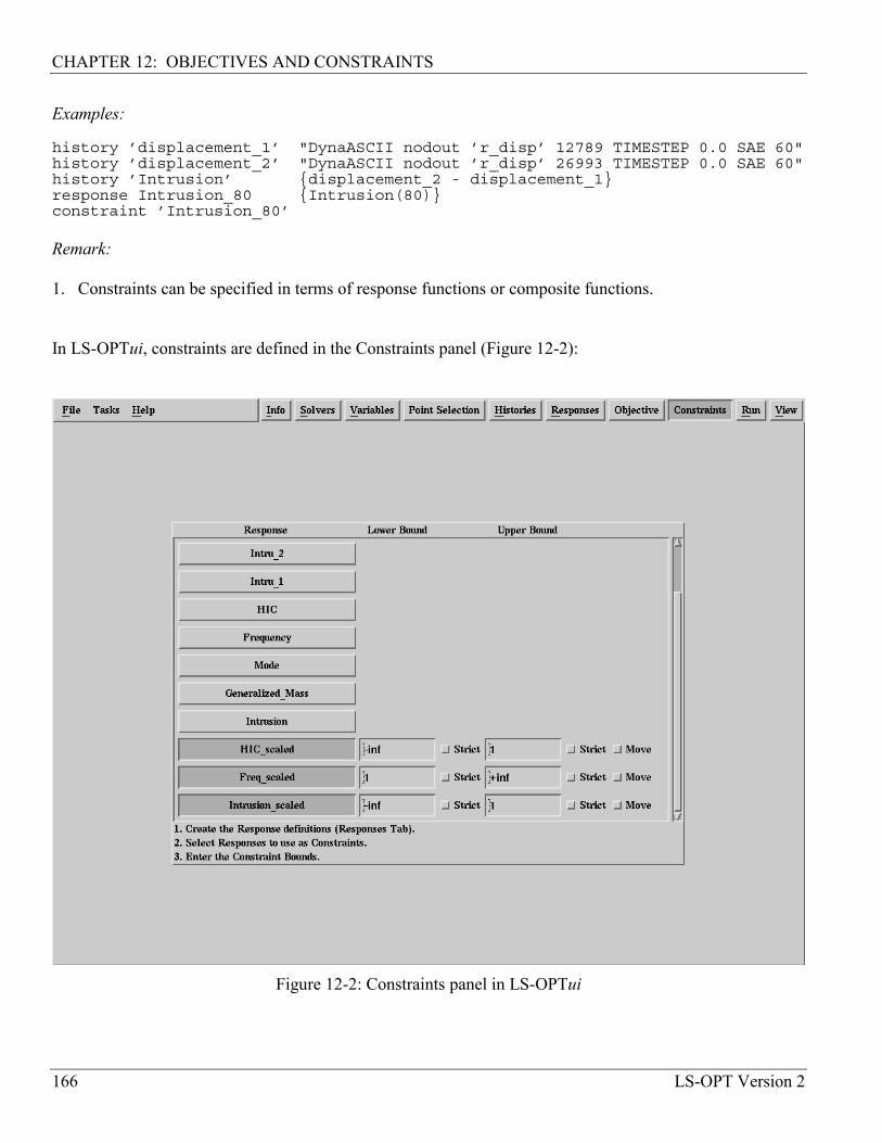
CHAPTER 12: OBJECTIVES AND CONSTRAINTS
166 LS-OPT Version 2
Examples:
history ’displacement_1’ "DynaASCII nodout ’r_disp’ 12789 TIMESTEP 0.0 SAE 60"history ’displacement_2’ "DynaASCII nodout ’r_disp’ 26993 TIMESTEP 0.0 SAE 60"history ’Intrusion’ {displacement_2 - displacement_1}response Intrusion_80 {Intrusion(80)}constraint ’Intrusion_80’ Remark: 1. Constraints can be specified in terms of response functions or composite functions. In LS-OPTui, constraints are defined in the Constraints panel (Figure 12-2):
Figure 12-2: Constraints panel in LS-OPTui

CHAPTER 12: OBJECTIVES AND CONSTRAINTS
LS-OPT Version 2 167
12.4 Bounds on the constraint functions Upper and lower bounds may be placed on the constraint functions. Command file syntax: Lower bound constraint constraint_name value <-10+30> Upper bound constraint constraint_name value <-10+30> Example:
Lower bound constraint ’Stress’ 1.e-6Upper bound constraint ’Stress’ 20.2 Remark: 1. A flag can be set to identify specific constraint bounds to define a reasonable design space. For this
purpose, the move environment must be specified (See Section 10.5). 12.5 Minimizing the maximum response or violation* Refer to Section 2.15.1 for the theory regarding strict and slack constraints. To specify hard (strict) or soft (slack) constraints, the following syntax is used: Command file syntax: strict strictness_factor <1> slack
Each command functions as an environment. Therefore all lower bound constraint or upperbound constraint commands which appear after a strict/slack command will be classified as strict or slack. In the following example, the first two constraints are slack while the last three are strict. The purpose of the formulation is to compromise only on the knee forces if a feasible design cannot be found. Example:
$ This formulation minimizes the average knee force but$ constrains the forces to 6500.$ If a feasible design is not available, the maximum violation$ will be minimized.$$ Objective:$-----------composite ’Knee_Forces’ type weightedcomposite ’Knee_Forces’ response ’Left_Knee_Force’ 0.5composite ’Knee_Forces’ response ’Right_Knee_Force’ 0.5
CHAPTER 12: OBJECTIVES AND CONSTRAINTS
168 LS-OPT Version 2
objective ’Knee_Forces’$$ Constraints:$-------------SLACKConstraint ’Left_Knee_Force’Upper bound constraint ’Left_Knee_Force’ 6500.$Constraint ’Right_Knee_Force’Upper bound constraint ’Right_Knee_Force’ 6500.$STRICTConstraint ’Left_Knee_Displacement’Lower bound constraint ’Left_Knee_Displacement’ -81.33$Constraint ’Right_Knee_Displacement’Lower bound constraint ’Right_Knee_Displacement’ -81.33$Constraint ’Kinetic_Energy’Upper bound constraint ’Kinetic_Energy’ 154000.
The composite function is explained in Section 11.4. Note that the same response functions appear both in the objective and the constraint definitions. This is to ensure that the violations to the knee forces are minimized, but if they are both feasible, their average will be minimized (as defined by the composite). The constraint bounds of all the soft constraints can also be set to a number that is impossible to comply with, e.g. zero. This will force the optimization procedure to always ignore the objective and it will minimize the maximum response. In the following example, the objective is to minimize the maximum of ’Left Knee Force’ or ’RightKnee Force’. The displacement and energy constraints are strict. Example:
$ This formulation minimizes the maximum knee force$ Because the knee forces are always positive,$ the objective will be ignored and the knee force$ minimized$$ Objective:$-----------composite ’Knee_Forces’ type weightedcomposite ’Knee_Forces’ response ’Left_Knee_Force’ 0.5composite ’Knee_Forces’ response ’Right_Knee_Force’ 0.5objective ’Knee_Forces’$$ Constraints:$-------------SLACKConstraint ’Left_Knee_Force’Upper bound constraint ’Left_Knee_Force’ 0.$

CHAPTER 12: OBJECTIVES AND CONSTRAINTS
LS-OPT Version 2 169
Constraint ’Right_Knee_Force’Upper bound constraint ’Right_Knee_Force’ 0.$STRICTConstraint ’Left_Knee_Displacement’Lower bound constraint ’Left_Knee_Displacement’ -81.33$Constraint ’Right_Knee_Displacement’Lower bound constraint ’Right_Knee_Displacement’ -81.33$Constraint ’Kinetic_Energy’Upper bound constraint ’Kinetic_Energy’ 154000. Remarks: 1. The objective function is ignored if the problem is infeasible. 2. The variable bounds of both the region of interest and the design space are always hard. 3. Soft constraints will be strictly satisfied if a feasible design is possible. 4. If a feasible design is not possible, the most feasible design will be computed. 5. If feasibility must be compromised (there is no feasible design), the solver will automatically use the
slackness of the soft constraints to try and achieve feasibility of the hard constraints. However, there is always a possibility that hard constraints must still be violated (even when allowing soft constraints). In this case, the variable bounds may be violated, which is highly undesirable as the solution will lie beyond the region of interest and perhaps beyond the design space. This could cause extrapolation of the response surface or worse, a future attempt to analyze a design which is not analyzable, e.g. a sizing variable might have become zero or negative.
6. Soft and strict constraints can also be specified for search methods. If there are feasible designs with
respect to hard constraints, but none with respect to all the constraints, including soft constraints, the most feasible design will be selected. If there are no feasible designs with respect to hard constraints, the problem is ‘hard-infeasible’ and the optimization terminates with an error message.

CHAPTER 12: OBJECTIVES AND CONSTRAINTS
170 LS-OPT Version 2

LS-OPT Version 2 171
13. Running the Design Task
This chapter explains simulation job-related information and how to execute a design task from the graphical user interface. The available tasks are optimization, probabilistic evaluation, and repair of an existing job. 13.1 Optimization The optimization process is triggered by the iterate command in the input file or by the Run command in the Run panel in LS-OPTui (Figure 13-1). The optimization history is written to the OptimizationHistory file and can be viewed using the View panel. 13.1.1 Number of optimization iterations The number of optimization iterations are specified in the appropriate field in the Run panel. If previous results exist, LS-OPT will recognize this (through the presence of results files in the Run directories) and not rerun these simulations. If the termination criteria described below are reached first, LS-OPT will terminate and not perform the maximum number of iterations. Command file syntax: iterate maximum_ number_of_iterations 13.1.2 Optimization termination criteria The user can specify tolerances on both the design change (∆xi) and the objective function change (∆f) and whether termination is reached if either, or both these criteria are met. The default selection is and, but the user can modify this by selecting or. Refer to Section 16.1 for the modification of the stopping type in the Command File.
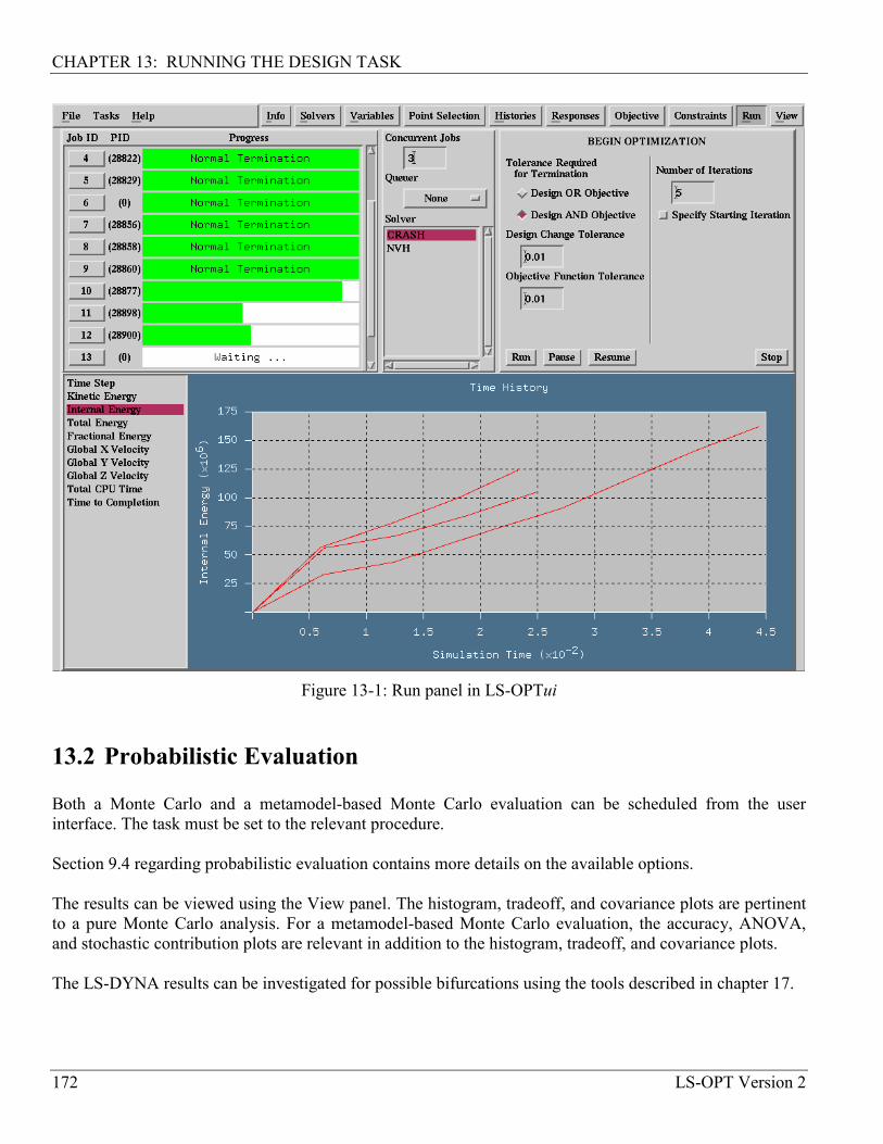
CHAPTER 13: RUNNING THE DESIGN TASK
172 LS-OPT Version 2
Figure 13-1: Run panel in LS-OPTui
13.2 Probabilistic Evaluation Both a Monte Carlo and a metamodel-based Monte Carlo evaluation can be scheduled from the user interface. The task must be set to the relevant procedure. Section 9.4 regarding probabilistic evaluation contains more details on the available options. The results can be viewed using the View panel. The histogram, tradeoff, and covariance plots are pertinent to a pure Monte Carlo analysis. For a metamodel-based Monte Carlo evaluation, the accuracy, ANOVA, and stochastic contribution plots are relevant in addition to the histogram, tradeoff, and covariance plots. The LS-DYNA results can be investigated for possible bifurcations using the tools described in chapter 17.
CHAPTER 13: RUNNING THE DESIGN TASK
LS-OPT Version 2 173
13.3 Restarting When a solution is interrupted (through the Stop button) or if a previous optimization run is to be repeated from a certain starting iteration, this can be specified in the appropriate field in the Run panel (Figure 13-1). 13.4 Job concurrency When LS-OPT is run on a multi-processor machine, the user can select how many simulations (jobs) can run concurrently on different processors (see Figure 13-1). Only the solver process and response extraction are parallellized. The preprocessor processes run serially. The number of Concurrent Jobs is ignored for jobs that are run by a queuing system. 13.5 Job distribution When a queuing system is available, its operation can be specified in the Run panel (Figure 13-1). 13.6 Job and analysis monitoring The Run panel allows a graphical indication of the job progress with the green horizontal bars linked to estimated completion time. This progress is only available for LS-DYNA jobs. The job monitoring is also visible when running remotely through a supported job distribution (queuing) system. When using LS-DYNA, the user can also view the progress (time history) of the analysis by selecting one of the available quantities (Time Step, Kinetic Energy, Internal Energy, etc.). 13.7 Repair or modification of an existing job Several kinds of repairs and modifications are possible for an existing optimization iteration or probabilistic analysis:
• Read Points. The experimental points can be extracted from the database in the job directories and the experimental design reconstructed.
• Augment Points for a Metamodel-based analysis. Adding extra points will augment the experimental design. This option is only available for the following experimental designs types: D-Optimal, space-filling, random, and Latin Hypercube. The D-Optimal and space-filling experimental designs will be computed taking in consideration the previously computed points. Both the random and the Latin Hypercube experimental design points will be computed using the number of previously computed points as a seed to random number generator.
• Augment Points of a Monte Carlo analysis. Adding extra points will augment the experimental design. This option is only available for the following experimental designs types: random and Latin

CHAPTER 13: RUNNING THE DESIGN TASK
174 LS-OPT Version 2
Hypercube. Both the random and the Latin Hypercube experimental design points will be computed using the number of previously computed points as a seed to random number generator.
• Run Jobs. The LS-DYNA jobs will be scheduled. • Extract Results. The results will be extracted from the runs. This option also allows the user to
change the responses for an existing iteration or Monte Carlo analysis. • Build Metamodels. The metamodels will be built. This option also allows revision of the
metamodels for an existing iteration or Monte Carlo analysis. • Optimize. The metamodels are user for metamodel optimization. A new optimum results database is
created.
All the subsequent operations must be explicitly performed for the iteration. For example, augmenting an experimental design will not cause the jobs to be run, the results to be extracted, or the metamodels to be recomputed. After repair of iteration n, and if the user is conducting an optimization task, verification runs of the optimized result must be done by switching back to the Metamodel-based optimization task and specifying the starting iteration as n+1 for a new run. Command file syntax: read experiments iteration_numberdesign more metamodel iteration_number design more monte carlo iteration_number run iteration_number extract results iteration_number approximate iteration_number optimize iteration_number

CHAPTER 13: RUNNING THE DESIGN TASK
LS-OPT Version 2 175

LS-OPT Version 2 176
14. Viewing Results
This chapter describes the viewing of metamodeling accuracy, optimization history, trade-off plots, ANOVA results, as well as statistical plots such as histograms, stochastic contribution of the variables, covariance, and coefficient of correlation plots. The View panel in LS-OPTui is used to view the results of the optimization process. The results include the metamodelling accuracy data, optimization history of the variables, dependents, responses, constraints and objective(s). Trade-off data can be generated using the existing response surfaces, and ANOVA results can be viewed. There are three options for viewing accuracy and tradeoff (anthill plots), namely viewing data for the current iteration, for all previous iterations simultaneously, all iterations (see e.g. Figure 14-1). The last option will also show the last verification point (optimal design) in green.
14.1 Metamodel accuracy The accuracy of the metamodel fit is illustrated in a Computed vs. Predicted plot (Figure 14-1). By clicking on any of the red squares, the data of the selected design point is listed. For LS-DYNA results, LS-PREPOST can then be launched to investigate the simulation results. The results of each iteration are displayed separately using the slider bar. The iterations can be viewed simultaneously by selecting All Previous or All. The All selection shows the final verification point in green (see Figure 14-1).

CHAPTER 14: VIEWING RESULTS
LS-OPT Version 2 177
Figure 14-1: Computed vs. Predicted plot in View panel in LS-OPTui
14.2 Optimization history The optimization history of a variable, dependent, response, constraint, objective, multi-objective or the approximation error parameters of pure responses (not composites or expressions) can be plotted by clicking on the Optimization History button (Figure 14-2). For the variables, the upper and lower bounds (subregion) are also displayed. For all the dependents, responses, objectives, constraints and maximum violation, a black solid line indicates the predicted values, while the red squares represent the computed values at the starting point of each iteration. For the error parameters, only one solid red line of the optimization history is plotted. RMS, Maximum and R2 error indicators are available. By clicking on any of the red squares, the data of the selected design point is listed. For LS-DYNA results, LS-PREPOST can then be launched to investigate the simulation results.

CHAPTER 14: VIEWING RESULTS
178 LS-OPT Version 2
Figure 14-2: Optimization History plot in View panel in LS-OPTui 14.3 Trade-off and anthill plots The results of all the simulated points appear as dots on the trade-off plots. This feature allows the two-dimensional plotting of any variable/response against any other variable/response. Trade-off studies can also be conducted based on the results of an optimization run. This is because the response surfaces for each response are at that stage available at each iteration for rapid evaluation. Trade-off is performed in LS-OPTui using the View panel and selecting Trade-off (Figure 14-3). Trade-off curves can be developed using either constraints or objectives. The curve can be plotted with any of the variables, responses, composites, constraints or objectives on either of the two axes. Care should be taken when selecting e.g. a certain constraint for plotting, as it may also be either a response or composite, and that this value maybe different from the constraint value, depending on whether the constraint is active during the trade-off process. The example in the picture below has Constraint: Intrusion selected for the X-Axis Entity, and not Composite: Intrusion.

CHAPTER 14: VIEWING RESULTS
LS-OPT Version 2 179
Solutions to the trade-off optimization problem falling outside the region of interest are connected by dotted lines to indicate extrapolation of the metamodel. To be able to view the results of composite functions spanning two or more disciplines or cases, the duplicate sampling method (Section 10.7) must be selected before starting an analysis. This also implies that the number of variables must be the same for all the disciplines involved and yields coincident experimental designs. An example of trade-off is given in Section 18.1 and 18.2.
Figure 14-3: Trade-off plot in View panel in LS-OPTui
14.4 Variable screening The Analysis of Variance (ANOVA) (refer to Section 2.9) of the approximation to the experimental design is automatically performed if a polynomial response surface method is selected. The ANOVA information can be used to screen variables (remove insignificant variables) at the start of or during the optimization process. The ANOVA method, a more sophisticated version of what is sometimes termed ‘Sensitivities’ or
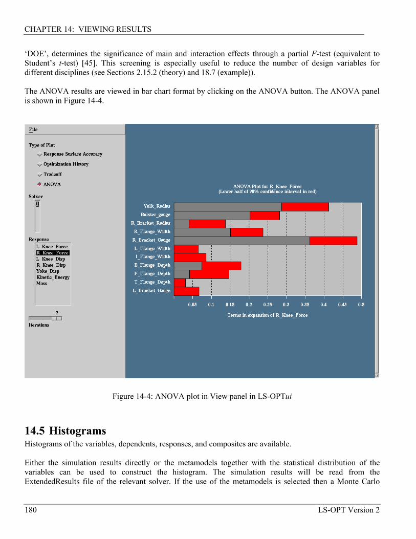
CHAPTER 14: VIEWING RESULTS
180 LS-OPT Version 2
‘DOE’, determines the significance of main and interaction effects through a partial F-test (equivalent to Student’s t-test) [45]. This screening is especially useful to reduce the number of design variables for different disciplines (see Sections 2.15.2 (theory) and 18.7 (example)). The ANOVA results are viewed in bar chart format by clicking on the ANOVA button. The ANOVA panel is shown in Figure 14-4.
Figure 14-4: ANOVA plot in View panel in LS-OPTui 14.5 Histograms Histograms of the variables, dependents, responses, and composites are available. Either the simulation results directly or the metamodels together with the statistical distribution of the variables can be used to construct the histogram. The simulation results will be read from the ExtendedResults file of the relevant solver. If the use of the metamodels is selected then a Monte Carlo

CHAPTER 14: VIEWING RESULTS
LS-OPT Version 2 181
simulation using a Latin Hypercube experimental design and the statistical distributions of the variables will be conducted on the metamodel to obtain the desired histogram. The user can control the number of points in this Monte Carlo simulation; the default value should however suffice for most cases. If desired, the residuals of the metamodel fit can be added to results of the Monte Carlo simulation as a normally distribution. For optimization results, an iteration can be selected. For probabilistic evaluations the default iteration, iteration 1, will automatically be selected. The histogram panel is shown in Figure 14-5.
Figure 14-5 Histogram plot
14.6 Stochastic Contribution The stochastic contribution of the variables to the variance of the responses and composites (see Section 3.7) can be displayed as a bar chart.

CHAPTER 14: VIEWING RESULTS
182 LS-OPT Version 2
Optionally the user can elect to display the influence of the residuals from the metamodel fit and the effect of all the variables summed together. Contrasting these two values indicates how well the cause-effect relationship for the specific response is resolved. The computations are done using the metamodels. The stochastic contribution panel is shown in Figure 14-6.
Figure 14-6 Stochastic Contribution plot
14.7 Covariance and Correlation Both the covariance and the coefficient of correlation of the responses and composites with respect to the design variables can be displayed. Either the simulated points or the metamodels together with the statistical distribution of the variables can be used. If a metamodel is used then a Monte Carlo simulation using a Latin Hypercube experimental design and the statistical distributions of the variables will be conducted on the metamodel to obtain the desired

CHAPTER 14: VIEWING RESULTS
LS-OPT Version 2 183
results. The user can control the number of points in this Monte Carlo simulation; the default value should however suffice for most cases. The plots can be used to estimate the stochastic contribution for an analysis without a metamodel. The covariance panel is shown in Figure 14-7.
Figure 14-7 Coefficient of Correlation plot
14.8 Plot generation Plots can be generated in LS-OPTui by selecting File>Export. The current supported format is postscript, both color and monochrome, either to a device or file.

CHAPTER 14: VIEWING RESULTS
184 LS-OPT Version 2

LS-OPT Version 2 185
15. Applications of Optimization
This chapter provides a brief description of some of the applications of optimization that can be performed using LS-OPT. It should be read in conjunction with Chapter 18, the Examples chapter, where the applications are illustrated with practical examples. 15.1 Multidisciplinary Design Optimization (MDO) The MDO capability in LS-OPT implies that the user has the option of assigning different variables, experimental designs and job specification information to different solvers or disciplines. The directory structure change that has been incorporated in this version, separates the number of experiments that needs to be run for each solver by creating separate Experiments, AnalysisResults, DesignFunctions and ExtendedResults files in each solver directory. Command file syntax: mdo mdotype
The only mdotype available is mdf, or multidisciplinary feasible. 15.1.1 Command file All variable definitions are defined first, as when solving non-MDO problems, regardless of whether they belong to all disciplines or solvers. This means that the variable starting value, bounds (minimum and maximum) and range (sub-region size) are defined together. If a variable is not shared by all disciplines, however, i.e., it belongs to some but not all of the disciplines (solvers), then it is flagged using the syntax local variable_name. At this stage, no mention is made in the command file to which solver(s) the particular variable belongs. This reference is made under the solver context, where the syntax Solvervariable variable_name is used, see next paragraph and example below. To limit the scope of a variable, an experimental design or job information to a particular solver, the prefix solver should be applied to the commands below. The solver definition must precede any commands having the solver prefix. Omission of the prefix implies that the specification is multidisciplinary, i.e., it is shared between all the specified solvers.

CHAPTER 14: APPLICATIONS OF OPTIMIZATION
186 LS-OPT Version 2
VariableConcurrent jobsOrderExperiment designBasis experimentNumber Basis experimentNumber experimentQueuerUpdate doeExperiment duplicate
See the examples in Sections 18.6 and 18.7 for the command file format. 15.2 Worst-case design The default setting in LS-OPT is that all design variables are treated as minimization variables. This means that the objective function is minimized (or maximized) with respect to all the variables. Maximization variables are selected in the Variables panel (see Figure 8-1) by toggling the required variables from ‘Minimize’ to ‘Maximize’. 15.3 Reliability-based design optimization (RBDO)* LS-OPT allows a limited reliability-based design capability by computing the standard deviation of any response. The standard deviation can be computed using a metamodel or a Monte Carlo analysis. The theoretical concerns are discussed in Section 2.15.5. Examples are given in Sections 18.2.9 and 18.2.10. 15.3.1 Metamodel based RBDO This method computes the standard deviation of the responses using the same metamodel as used for the deterministic optimization portion of the problem using the First Order Second Method (FOSM) method. No additional FE runs are therefore required for the probabilistic computations. The method requires very little information additionally to what is required for deterministic optimization. Specify the following:
1. Statistical distributions associated with the design variables 2. Probabilistic bounds on the constraints
The statistical distributions associated with the design variables are specified in the same manner as for a Monte Carlo analysis using a metamodel. The current GUI support is limited to what is available for deterministic design optimization and Monte Carlo analysis. Command file syntax: probability upper bound constraint ’con_name’ upper_bound

CHAPTER 14: VIEWING RESULTS
LS-OPT Version 2 187
probability lower bound constraint ’con_name’ lower_bounditerate number_of_iterations
An example is given in Section 18.2.10. 15.3.2 Monte Carlo based RBDO The procedure uses the multidisciplinary optimization capability to separate the mean and random responses components. The procedure is as follows:
1. Choose the design variables and divide them into pairs where each pair is represented by a mean component and a random component. Uncontrollable random variables must be included in the list.
2. Assign the mean variables to a solver MEAN and the random variables to a solver _RANDOM_. 3. Change those variables defined in the MEAN solver and that are uncontrollable to constants. 4. Also change the random variables that are not desired to be random to constants. 5. Select suitable lower and upper bounds for the MEAN variables as for a standard design
formulation. 6. The random variables are centered on the starting point so that the starting vector is [0, 0, …, 0].
Omit the range but choose the upper and lower bounds to conform to the design tolerance, e.g., [-ε /2, + ε /2] for a tolerance, ε. The tolerance allows a uniformly distributed scatter of the input variables.
7. The most suitable experimental design for the random variables is Latin Hypercube Sampling (LHS).
8. Define a dependent variable as the sum of the mean and random variables. There may be some constants in both categories.
9. Substitute the mean variable names in the MEAN solver simulation deck and the dependent variable names in the _RANDOM_ solver deck.
10. Define responses for the design criteria for both the MEAN and _RANDOM_ solvers. Also compute the standard deviations of the _RANDOM_ responses.
11. Add (or subtract) fractions of the standard deviations to (from) the mean corresponding responses to compensate for the sensitivity of the design.
The method above has the advantage that actual simulations are used to model stochastic behavior. The standard deviations are assumed to be constant over the sub-region, but the method should converge if an iterative scheme is used. An example is given in Section 18.2.9 to illustrate the method.


LS-OPT Version 2 189
16. Optimization Algorithm Selection and Settings
This chapter describes the parameter settings for the domain reduction and LFOPC methods that are used in LS-OPT. The default parameters for both the domain reduction scheme and the core optimization algorithm (LFOPC) should be sufficient for most optimization applications. The following sections describe how to modify the default settings. These can only be modified using the command language. 16.1 Selecting an optimization algorithm There are two optimization algorithms available namely the Successive Response Surface Method (SRSM) and the Sequential Random Search (SRS) method14. The syntax is as follows: Command file syntax: Optimization method [srsm|randomsearch]
SRSM is the default. 16.2 Setting the subdomain parameters To automate the successive subdomain scheme for both SRSM and Sequential Random Search, the size of the region of interest (as defined by the range of each variable) is adapted based on the accuracy of the previous optimum and, for SRSM, also on the occurrence of oscillation (see theory in Section 2.12). The following parameters can be adjusted (refer also to Section 2.12). A suitable default has been provided for each parameter but the user should not find it necessary to change any of these parameters.
14 Available in Version 2.1

CHAPTER 16: Optimization Algorithm Selection and Settings
190 LS-OPT Version 2
Table 16-1: Subdomain parameters and default values
Default Item Parameter SRSM SRS
objective Tolerance on objective function accuracy εf
0.01 0.01
design Tolerance on design accuracy εx 0.01 0.01 stoppingtype and: objective and design;
or: objective or design and and
psi γpan 1.0 1.0 gamma γosc 0.6 1.0 eta Zoom parameter η 0.6 0.5* rangelimit Minimum range 0.0 0.0 repeatlimit Limit on number of times solution is
repeated (SRS only) 5 5
* Applied when the design has not changed. Command file syntax: iterate param parameter_identifier value
The iterative process is terminated if the following convergence criteria become active:
fk
kk
fff ε<−−
−
)1(
)1()(
and/or
x
kk
ε<− −
dxx )1()(
where x refers to the vector of design variables, d is the size of the design space, f denotes the value of the objective function and, (k) and (k – 1) refer to two successive iteration numbers. The stoppingtypeparameter is used to determine whether (and) or (or) will be used, e.g.
iterate param design 0.001iterate param objective 0.001iterate param stoppingtype orimplies that the optimization will terminate when either criterion is met. The range limit can be used to specify the minimum size of the region of interest. This is not a stopping criterion so that the solver will still continue to iterate until any of the other stopping criteria are met. An application of the range limit is to maintain a constant tolerance on the random variables. See Section 18.2.9 for an example.

CHAPTER 16: OPTIMIZATION ALGORITHM SELECTION AND SETTINGS
LS-OPT Version 2 191
Command file syntax: iterate param rangelimit variable_name value
Example: iterate param rangelimit ’thickness 1’ 0.5iterate param rangelimit ’Radius’ 10 16.3 Setting parameters in the LFOPC optimization algorithm The values of the responses are scaled with the values at the initial design. The default parameters in LFOPC should therefore be adequate. Should the user have more stringent requirements, the following parameters may be set for LFOPC. These are only available in the command input file.
Table 16-2: LFOPC parameters and default values
Item Parameter Default value Remark mu Initial penalty value µ 1.0E+2 mumax Maximum penalty value µ max 1.0E+4 1 xtol Convergence tolerance εx on the step movement 1.0E-8 2 eg Convergence tolerance εf on the norm of the gradient 1.0E-5 2 delt Maximum step size δ See remark 3 steps Maximum number of steps per phase 1000 1 print Printing interval 10 4
Remarks: 1. For higher accuracy, at the expense of economy, the value of µ max can be increased. Since the
optimization is done on approximate functions, economy is usually not important. The value of steps must then be increased as well.
2. The optimization is terminated when either of the convergence criteria becomes active that is when
xε<∆ )(x
or ff ε<∇ )(x
3. It is recommended that the maximum step size, δ, be of the same order of magnitude as the “diameter of
the region of interest”. To enable a small step size for the successive approximation scheme, the value of
delt has been defaulted to ∑ == n
irange
12)(05.0δ .
4. If print = steps + 1, then the printing is done on step 0 and exit only. The values of the design
variables are suppressed on intermediate steps if print < 0.

CHAPTER 16: Optimization Algorithm Selection and Settings
192 LS-OPT Version 2
Command file syntax: lfop param parameter_identifier value
Example: lfop param eg 1.0e-6
In the case of an infeasible optimization problem, the solver will find the most feasible design within the given region of interest bounded by the simple upper and lower bounds. A global solution is attempted by multiple starts from a set of random points.

LS-OPT Version 2 193
17. LS-DYNA Results Statistics
Various statistics of the LS-DYNA d3plot displacements and history data can be computed using LS-OPT for viewing in LS-PREPOST. These statistics shows how the LS-DYNA results vary due to variation of the design parameters or bifurcations. The statistical results can be:
• Statistics of the data from the LS-DYNA jobs. These are the data from the experimental designs used. If the experimental design was for a Monte Carlo analysis then the experimental design reflects the variation of the design variables; however, if the experimental design was for creating a metamodel then the experimental design does not reflect the statistical variation of the design variables.
• Statistics of running a Monte Carlo analysis using approximations (metamodels) created from the LS-DYNA jobs. The distributions of the design variables will be used in the Monte Carlo analysis. If distributions were not assigned to the design variables then the resulting variation would be zero.
• Statistics of the outliers from the metamodels created from the LS-DYNA jobs. The outlier results are useful for finding bifurcations in the structural behavior because the outliers comprise the displacement changes not associated with a design variable change. See section 3.6 regarding the computation of outliers.
The displacement statistics are computed for every displacement direction at every node for every state in the d3plot database. Whether a displacement or history is correlated with an event (response) can be determined by investigating the coefficient of correlation with the event (response).

CHAPTER 17: LS-DYNA Results Statistics
194 LS-OPT Version 2
Figure 17-1 Computation of DYNA results statistics
17.1 Analysis Either the LS-DYNA displacement or history results can be analyzed. The resulting output can be viewed in LS-PREPOST. The results will be in the solver directory with extensions of .statdb and .history. Command file syntax: analyze dynastatanalyze dynastat history ‘history_name’
Item Description history_name Name of history

CHAPTER 17: LS-DYNA Results Statistics
LS-OPT Version 2 195
Example:
$ analyze displacementanalyze dynastat$ analyze historyanalyze dynastat history ‘nHist’
17.2 Metamodels and outliers Metamodels are used to predict the nodal displacements for specific designs. These approximations (metamodels) will be computed for all displacement components at all nodes for all time steps. The results for the metamodel are computed using a Monte Carlo analysis and 150 points from a Latin Hypercube design. The distribution assigned to the design variables are used to construct the Latin Hypercube design. The outliers are computed as the difference between the values computed using FEA and the values predicted using the metamodel (see Section 3.6 for more details). The displacement magnitude, having some special properties, is computed as described in the next section. A linear or a quadratic response surface can be used. The metamodel processing speed is approximately 10 000 finite element nodes a second. Command file syntax: dynastat outlier ON_OFFdynastat order approx_order
Item Description Default ON_OFF ON | OFF. OFF approx_order linear | quadratic Do not use a metamodel
Example:
dynastat outlier ONdynastat order linear
17.3 Displacement Magnitude*

CHAPTER 17: LS-DYNA Results Statistics
196 LS-OPT Version 2
Approximating the displacement magnitudes (resultants) requires special treatment. The magnitude is defined as the square root of a sum of squares, which is difficult to approximate around the origin, especially using linear approximations. Figure 17-2 illustrates. The x, y, and z displacement components do not suffer from this problem; the use of the displacement magnitude is however more convenient.
Figure 17-2 Displacement approximation scenarios
Unexpected results may occur even if the displacement magnitude is approximated correctly. The displacement magnitude is always a positive quantity, which, in addition to the fitting problems, can also cause problems when computing the coefficient of correlation with a response quantity. Figure 17-3 illustrates two buckling modes of a flange evaluated at two locations in space. The displacement magnitude variance differs for the two locations though the buckling modes are similar. The variance of the displacement magnitude will therefore be smaller than what would be found considering the components. Considering a displacement component will cure this problem, but a displacement component aligned with the required direction may not always exist. A solution using a maximum displacement vector is discussed in the following paragraphs.

CHAPTER 17: LS-DYNA Results Statistics
LS-OPT Version 2 197
Figure 17-3 Resultant displacements depends on aligment of flange with axis
The following options are available:
1. Resultant displacement approximated. 2. Resultant computed from the approximations to the displacement components. The displacement
magnitudes are not approximated directly but are computed from the approximations to the x, y, and z displacements. More accurate displacements to the x, y, and z displacement components are possible.
3. Maximum Vector. We compute the maximum (longest) vector spanning the displacements (see Figure 17-4). Each displacement magnitude is then computed considering the dot product of the displacement and the maximum vector. The maximum vector formulation allows, for some cases, (i) a better identification of bifurcation and (ii) an improved establishment of the coefficient of correlation.
Hints:
• Use the approximations to the displacement components. • For computing correlations the maximum vector may give better results.

CHAPTER 17: LS-DYNA Results Statistics
198 LS-OPT Version 2
Figure 17-4 Maximum vector computations
Command file syntax: dynastat max vector ON_OFFdynastat component vector ON_OFF
Item Description Default ON_OFF ON | OFF. OFF
Example:
$ Use maximum vectordynastat max vector ON$ Use approximations to components to compute resultantdynastat component vector ON
17.4 Correlation The correlation of the displacements or histories with a response can be computed. This quantity indicates whether the changes in the responses are associated with the changes in the displacement or history. Correlation coefficients larger than 0.3 are usually considered significant. If not enough FE evaluations were conducted, the resulting fringe plot can be visually noisy. 30 or more FE evaluations may be required to establish correlation. Note that the correlation of history is with respect to a response at a single time instance.

CHAPTER 17: LS-DYNA Results Statistics
LS-OPT Version 2 199
Command file syntax: dynastat correlation response ’name’
Item Description name Name of response or composite
Example:
dynastat correlation response ‘node_max’
17.5 Solver and Iteration Command file syntax: dynastat solver ‘solver_name‘dynastat iteration interation_number
Item Description Default solver_name Name of solver The first or only solver specified iteration_number Iteration number 1
Example:
dynastat solver ‘CRASH’dynastat iteration 1
17.6 Visualization in LS-PREPOST The user can select the LS-PREPOST plot details in LS-OPT (Figure 17-5). The GUI options will reflect whether displacements or history data is being investigated and whether coefficient of correlation results are requested.

CHAPTER 17: LS-DYNA Results Statistics
200 LS-OPT Version 2
Figure 17-5 LS-PREPOST viewing options
The Job Index field specifies the FE model used. The LS-PREPOST executable must be named lsprepost. The LS-PREPOST executable must be newer than December 2003. 17.7 Bifurcation investigations The outlier plots are useful for finding bifurcations. The standard deviation or range of the outliers indicate regions where the changes in displacements are not explained by changes in the design variable values ― it is therefore a plot of the unexpected displacements or ‘surprise factor’. The data plots can also be used to find bifurcations, though the metamodel plots cannot be used.

CHAPTER 17: LS-DYNA Results Statistics
LS-OPT Version 2 201
The steps are therefore:
1. Plot displacement magnitude outlier Range to identify location in FE model where the bifurcation occurred.
2. Identify job in which maximum value occurred using a Max Index plot 3. Identify job in which minimum value occurred using a Min Index plot 4. View the location in model for the jobs having the minimum and maximum value
Hints:
• Engineering knowledge of the structure is important • Look at the x, y, and z components in addition to the displacement magnitude to understand in which
direction the bifurcation occurred; some bifurcations are actually best identified considering a displacement component
• Using maximum vector displacement magnitude formulation may highlight bifurcations that would otherwise be missed; the displacement resultant formulation is not perfect.
• The history results may be useful to find the time at which a bifurcation occurred • The correlation between a response and displacements (or histories) indicates if variation of the
displacement is linked to variation of the response


203
EXAMPLES

204 LS-OPT Version 2

205
18. Example Problems
18.1 Two-bar truss (2 variables) This example has the following features: • A user-defined solver is used. • Extraction is performed using user-defined scripts. • First- and second-order response surface approximations are compared. • The effect of subregion size is investigated. • A trade-off study is performed. • The design optimization process is automated. 18.1.1 Description of problem This example problem as shown in Figure 18-1 has one geometric and one element sizing variable.
x2
x1
x2
F
Figure 18-1: The two-bar truss example

CHAPTER 18: EXAMPLE PROBLEMS
206 LS-OPT Version 2
The problem is statically determinate. The forces on the members depend only on the geometric variable. Only one load case is considered: F = (Fx,Fy) = (24.8kN, 198.4kN). There are two design variables: x1 the cross-sectional area of the bars, and x2 half of the distance (m) between the supported nodes. The lower bounds on the variables are 0.2cm2 and 0.1m, respectively. The upper bounds on the variables are 4.0cm2 and 1.6m, respectively. The objective function is the weight of the structure. 2
211 1)( xxCxf += (18.1)
The stresses in the members are constrained to be less than 100 MPa.
1181)(211
2221 ≤
++=
xxxxCxσ (18.2)
1181)(211
2222 ≤
−+=
xxxxCxσ (18.3)
where C1 = 1.0 and C2 = 0.124. Only the first stress constraint is considered since it will always have the larger value. The C language is used for the simulation program. The following two programs simulate the weight response and stress response respectively. gw.c#include <stdlib.h>#include <stdio.h>#include <math.h>
#define NUMVAR 2
main (int argc, char *argv[]){int i, flag;double x[NUMVAR], val;
for (i=0; i<NUMVAR; i++) {flag = sscanf (argv[i+1], "%lf", &x[i]);if (flag != 1) {
printf ("Error in calculation of Objective Function\n");exit (1);}
}
val = x[0] * sqrt(1 + x[1]*x[1]);
printf ("%lf\n", val);fprintf (stderr, "N o r m a l\n");

CHAPTER 18: EXAMPLE PROBLEMS
LS-OPT Version 2 207
exit (0);}
gs.c#include <stdlib.h>#include <stdio.h>#include <math.h>
#define NUMVAR 2
main (int argc, char *argv[]){int i, flag;double x[NUMVAR], val;double x2;
for (i=0; i<NUMVAR; i++) {flag = sscanf (argv[i+1], "%lf", &x[i]);if (flag != 1) {
printf ("Error in calculation of constraint1\n");exit (1);}
}x2 = 1 + x[1]*x[1];val = 0.124 * sqrt (x2) * (8/x[0] + 1/x[0]/x[1]);
printf ("%lf\n", val);fprintf (stderr, "N o r m a l\n");
exit (0);}The UNIX script program 2bar_com runs the C-programs gw and gss using the design variable file XPoint which is resident in each run directory, as input. For practical purposes, 2bar_com, gw and gshave been placed in a directory above the working directory (or three directories above the run directory). Hence the references ../../../2bar_com, ../../../gw, etc. in the LS-OPT input file. Note the output of the string "N o r m a l" so that the completion status may be recognized. 2bar_com: ../../../gw `cat XPoint` >wt; ../../../gss `cat XPoint` >str
The UNIX extraction scripts get_wt and get_str are defined as user interfaces: get_wt: cat wt get_str: cat str In Sections 18.1.2 to 18.1.4, a typical semi-automated optimization procedure is illustrated. Section 18.1.5 shows how a trade-off study can be conducted, while the last subsection 18.1.6 shows how an automated procedure can be specified for this example problem.

CHAPTER 18: EXAMPLE PROBLEMS
208 LS-OPT Version 2
18.1.2 A first approximation using linear response surfaces The first iteration is chosen to be linear. The input file for LS-OPT given below. The initial design is located at x = (2.0, 0.8). "2BAR1: Two-Bar Truss: A first approximation (linear)"$ Created on Wed Jul 10 17:41:03 2002$$ DESIGN VARIABLES$variables 2Variable 'Area' 2Lower bound variable 'Area' 0.2Upper bound variable 'Area' 4Range 'Area' 4
Variable 'Base' 0.8Lower bound variable 'Base' 0.1Upper bound variable 'Base' 1.6Range 'Base' 1.6
solvers 1responses 2$$ NO HISTORIES ARE DEFINED$$$ DEFINITION OF SOLVER "RUNS"$solver own 'RUNS'solver command "../../../2bar_com"
$$ RESPONSES FOR SOLVER "RUNS"$response 'Weight' 1 0 "cat wt"response 'Weight' linearresponse 'Stress' 1 0 "cat str"response 'Stress' linear
$$ NO HISTORIES DEFINED FOR SOLVER "RUNS"$$$ OBJECTIVE FUNCTIONS$objectives 1objective 'Weight' 1
$$ CONSTRAINT DEFINITIONS$constraints 1constraint 'Stress'upper bound constraint 'Stress' 1
$$ EXPERIMENTAL DESIGN$Order linearExperimental design dopt

CHAPTER 18: EXAMPLE PROBLEMS
LS-OPT Version 2 209
Basis experiment 3toKNumber experiment 5
$$ JOB INFO$concurrent jobs 4iterate param design 0.01iterate param objective 0.01iterate 1
STOP
The input is echoed in the file lsopt_input. The output is given in lsopt_output and in the View panel of LS-OPTui. A summary of the response surface statistics from the output file is given: Approximating Response 'Weight' using 5 points (ITERATION 1)----------------------------------------------------------------
Global error parameters of response surface-------------------------------------------
Linear Function Approximation:------------------------------Mean response value = 2.9413
RMS error = 0.7569 (25.73%)Maximum Residual = 0.8978 (30.52%)Average Error = 0.7131 (24.24%)Square Root PRESS Residual = 2.5054 (85.18%)Variance = 0.9549R^2 = 0.9217R^2 (adjusted) = 0.9217R^2 (prediction) = 0.1426Determinant of [X]'[X] = 3.5615
Approximating Response 'Stress' using 5 points (ITERATION 1)----------------------------------------------------------------
Global error parameters of response surface-------------------------------------------
Linear Function Approximation:------------------------------Mean response value = 4.6210
RMS error = 2.0701 (44.80%)Maximum Residual = 4.1095 (88.93%)Average Error = 1.6438 (35.57%)Square Root PRESS Residual = 3.9077 (84.56%)Variance = 7.1420R^2 = 0.8243R^2 (adjusted) = 0.8243R^2 (prediction) = 0.3738Determinant of [X]'[X] = 3.5615
The accuracy of the response surfaces can also be illustrated by plotting the predicted results vs. the computed results (Figure 18-2).

CHAPTER 18: EXAMPLE PROBLEMS
210 LS-OPT Version 2
Prediction accuracy of Weight
(Iteration 1 - Linear) Prediction accuracy of Stress
(Iteration 1 - Linear)
Figure 18-2: Prediction accuracy of Weight and Stress (Iteration 1 – Linear)
The R2 values are large. However the prediction accuracy, especially for weight, seems to be poor, so that a higher order of approximation will be required. Nevertheless an improved design is predicted with the constraint value (stress) changing from an approximate 4.884 (severely violated) to 1.0 (the constraint is active). Due to inaccuracy, the actual constraint value of the optimum is 0.634. The weight changes from 2.776 to 4.137 (3.557 computed) to accommodate the violated stress: DESIGN POINT------------Variable Name Lower Bound Value Upper Bound--------------------------------|-----------|----------|-----------Area 0.2 3.539 4Base 0.1 0.1 1.6--------------------------------|-----------|----------|-----------
RESPONSE FUNCTIONS:------------------
| Scaled | Unscaled ||---------------------|---------------------|
RESPONSE | Computed Predicted| Computed Predicted|--------------------------------|----------|----------|----------|----------|Weight | 3.557 4.137| 3.557 4.137|Stress | 0.6338 1| 0.6338 1|--------------------------------|----------|----------|----------|----------|

CHAPTER 18: EXAMPLE PROBLEMS
LS-OPT Version 2 211
OBJECTIVE:---------
Computed Value = 3.557Predicted Value = 4.137
OBJECTIVE FUNCTIONS:-------------------OBJECTIVE NAME | Computed Predicted WT.--------------------------------|----------|----------|----Weight | 3.557 4.137| 1--------------------------------|----------|----------|----
CONSTRAINT FUNCTIONS:--------------------CONSTRAINT NAME | Computed | Predicted| Lower | Upper |Viol?--------------------------------|----------|----------|----------|----------|-----Stress | 0.6338 1| -1e+30 1|no--------------------------------|----------|----------|----------|----------|-----
CONSTRAINT VIOLATIONS:---------------------
| Computed Violation | Predicted Violation |CONSTRAINT NAME |----------|----------|----------|----------|
| Lower | Upper | Lower | Upper |--------------------------------|----------|----------|----------|----------|Stress | - - | - - |--------------------------------|----------|----------|----------|----------|
MAXIMUM VIOLATION:------------------
| Computed | Predicted |Quantity |---------------------------|---------------------------|
| Constraint Value | Constraint Value |-------------------|----------------|----------|----------------|----------|Maximum Violation |Stress 0|Stress 6.995e-08|Smallest Margin |Stress 0.3662|Stress 6.995e-08|-------------------|----------------|----------|----------------|----------|
18.1.3 Updating the approximation to second order To improve the accuracy, a second run is conducted using a quadratic approximation. The following statements differ from the input file above: "2BAR2: Two-Bar Truss: Updating the approximation to 2nd order"response 'Weight' quadraticresponse 'Stress' quadratic$$ EXPERIMENTAL DESIGN$Order quadraticExperimental design doptBasis experiment 5toKNumber experiment 10

CHAPTER 18: EXAMPLE PROBLEMS
212 LS-OPT Version 2
The approximation results have improved considerably, but the stress approximation is still poor.
Approximating Response 'Weight' using 10 points (ITERATION 1)----------------------------------------------------------------
Global error parameters of response surface-------------------------------------------
Quadratic Function Approximation:---------------------------------Mean response value = 2.8402
RMS error = 0.0942 (3.32%)Maximum Residual = 0.1755 (6.18%)Average Error = 0.0737 (2.59%)Square Root PRESS Residual = 0.2815 (9.91%)Variance = 0.0177R^2 = 0.9983R^2 (adjusted) = 0.9983R^2 (prediction) = 0.9851Determinant of [X]'[X] = 14.6629
Approximating Response 'Stress' using 10 points (ITERATION 1)----------------------------------------------------------------
Global error parameters of response surface-------------------------------------------
Quadratic Function Approximation:---------------------------------Mean response value = 3.4592
RMS error = 1.0291 (29.75%)Maximum Residual = 2.0762 (60.02%)Average Error = 0.8385 (24.24%)Square Root PRESS Residual = 2.4797 (71.68%)Variance = 2.1182R^2 = 0.9378R^2 (adjusted) = 0.9378R^2 (prediction) = 0.6387Determinant of [X]'[X] = 14.6629
The fit is illustrated below in Figure 18-3:

CHAPTER 18: EXAMPLE PROBLEMS
LS-OPT Version 2 213
Prediction accuracy of Weight
(Iteration 1 - Quadratic) Prediction accuracy of Stress
(Iteration 1 - Quadratic)
Figure 18-3: Prediction accuracy of Weight and Stress (Iteration 1 – Quadratic)
An improved design is predicted with the constraint value (stress) changing from a computed 0.734 to 1.0 (the approximate constraint becomes active). Due to inaccuracy, the actual constraint value of the optimum is a feasible 0.793. The weight changes from 2.561 to 1.925 (1.907 computed).
DESIGN POINT------------Variable Name Lower Bound Value Upper Bound--------------------------------|-----------|----------|-----------Area 0.2 1.766 4Base 0.1 0.4068 1.6--------------------------------|-----------|----------|-----------
RESPONSE FUNCTIONS:------------------
| Scaled | Unscaled ||---------------------|---------------------|
RESPONSE | Computed Predicted| Computed Predicted|--------------------------------|----------|----------|----------|----------|Weight | 1.907 1.925| 1.907 1.925|Stress | 0.7927 1| 0.7927 1|--------------------------------|----------|----------|----------|----------|
OBJECTIVE:---------
Computed Value = 1.907Predicted Value = 1.925

CHAPTER 18: EXAMPLE PROBLEMS
214 LS-OPT Version 2
OBJECTIVE FUNCTIONS:-------------------OBJECTIVE NAME | Computed Predicted WT.--------------------------------|----------|----------|----Weight | 1.907 1.925| 1--------------------------------|----------|----------|----
CONSTRAINT FUNCTIONS:--------------------CONSTRAINT NAME | Computed | Predicted| Lower | Upper |Viol?--------------------------------|----------|----------|----------|----------|-----Stress | 0.7927 1| -1e+30 1|YES--------------------------------|----------|----------|----------|----------|-----
CONSTRAINT VIOLATIONS:---------------------
| Computed Violation | Predicted Violation |CONSTRAINT NAME |----------|----------|----------|----------|
| Lower | Upper | Lower | Upper |--------------------------------|----------|----------|----------|----------|Stress | - - | - 1.033e-06|--------------------------------|----------|----------|----------|----------|
MAXIMUM VIOLATION:------------------
| Computed | Predicted |Quantity |---------------------------|---------------------------|
| Constraint Value | Constraint Value |-------------------|----------------|----------|----------------|----------|Maximum Violation |Stress 0|Stress 1.033e-06|Smallest Margin |Stress 0.2073|Stress 1.033e-06|-------------------|----------------|----------|----------------|----------|
18.1.4 Reducing the region of interest for further refinement It seems that further accuracy can only be obtained by reducing the size of the subregion. In the following analysis, the current optimum (1.766; 0.4086) was used as a starting point while the region of interest was cut in half. The order of the approximation is quadratic. The modified statements are:
"2BAR3: Two-Bar Truss: Reducing the region of interest"$ Created on Thu Jul 11 07:46:24 2002$$ DESIGN VARIABLES
Range 'Area' 2Range 'Base' 0.8
The approximations have been significantly improved: Approximating Response 'Weight' using 10 points (ITERATION 1)----------------------------------------------------------------
Global error parameters of response surface-------------------------------------------
Quadratic Function Approximation:---------------------------------
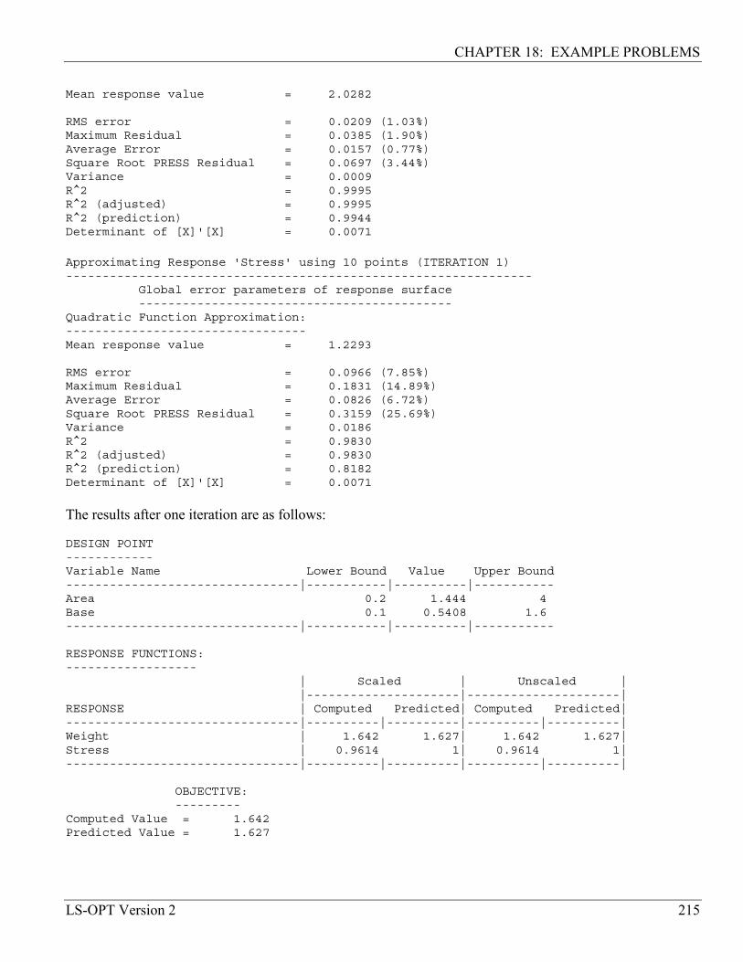
CHAPTER 18: EXAMPLE PROBLEMS
LS-OPT Version 2 215
Mean response value = 2.0282
RMS error = 0.0209 (1.03%)Maximum Residual = 0.0385 (1.90%)Average Error = 0.0157 (0.77%)Square Root PRESS Residual = 0.0697 (3.44%)Variance = 0.0009R^2 = 0.9995R^2 (adjusted) = 0.9995R^2 (prediction) = 0.9944Determinant of [X]'[X] = 0.0071
Approximating Response 'Stress' using 10 points (ITERATION 1)----------------------------------------------------------------
Global error parameters of response surface-------------------------------------------
Quadratic Function Approximation:---------------------------------Mean response value = 1.2293
RMS error = 0.0966 (7.85%)Maximum Residual = 0.1831 (14.89%)Average Error = 0.0826 (6.72%)Square Root PRESS Residual = 0.3159 (25.69%)Variance = 0.0186R^2 = 0.9830R^2 (adjusted) = 0.9830R^2 (prediction) = 0.8182Determinant of [X]'[X] = 0.0071
The results after one iteration are as follows:
DESIGN POINT------------Variable Name Lower Bound Value Upper Bound--------------------------------|-----------|----------|-----------Area 0.2 1.444 4Base 0.1 0.5408 1.6--------------------------------|-----------|----------|-----------
RESPONSE FUNCTIONS:------------------
| Scaled | Unscaled ||---------------------|---------------------|
RESPONSE | Computed Predicted| Computed Predicted|--------------------------------|----------|----------|----------|----------|Weight | 1.642 1.627| 1.642 1.627|Stress | 0.9614 1| 0.9614 1|--------------------------------|----------|----------|----------|----------|
OBJECTIVE:---------
Computed Value = 1.642Predicted Value = 1.627

CHAPTER 18: EXAMPLE PROBLEMS
216 LS-OPT Version 2
OBJECTIVE FUNCTIONS:-------------------OBJECTIVE NAME | Computed Predicted WT.--------------------------------|----------|----------|----Weight | 1.642 1.627| 1--------------------------------|----------|----------|----
CONSTRAINT FUNCTIONS:--------------------CONSTRAINT NAME | Computed | Predicted| Lower | Upper |Viol?--------------------------------|----------|----------|----------|----------|-----Stress | 0.9614 1| -1e+30 1|no--------------------------------|----------|----------|----------|----------|-----
CONSTRAINT VIOLATIONS:---------------------
| Computed Violation | Predicted Violation |CONSTRAINT NAME |----------|----------|----------|----------|
| Lower | Upper | Lower | Upper |--------------------------------|----------|----------|----------|----------|Stress | - - | - - |--------------------------------|----------|----------|----------|----------|
An improved design is predicted with the constraint value (stress) changing from an approximate 0.8033 (0.7928 computed) to 1.0 (the approximate constraint becomes active). Due to inaccuracy, the actual constraint value of the optimum is a feasible 0.961. This value is now much closer to the value of the simulation result. The weight changes from 1.909( 1.907 computed) to 1.627 (1.642 computed). 18.1.5 Conducting a trade-off study The present region of interest (2; 0.8) is chosen in order to conduct a study in which the weight is traded off against the stress constraint. The trade-off is performed by selecting the Trade-off option in the View panel of LS-OPTui. The upper bound of the stress constraint is varied from 0.2 to 2.0 with 20 increments. Select Constraint as the Trade-off option and enter the bounds and number of increments. Generate the trade-off. This initiates the solution of a series of optimization problems using the response surface generated in Section 18.1.4, with the constraint in each (constant coefficient of the constraint response surface polynomial) being varied between the limits selected. The resulting curve is also referred to as a Pareto optimality curve. When plotting, select the ‘Constraint’ Stress, and not the ‘Response’ Stress, as the latter represents only the left-hand side of the constraint equation (17.2).
The resulting trade-off diagram (Figure 18-4) shows the compromise in weight when the stress constraint is tightened.

CHAPTER 18: EXAMPLE PROBLEMS
LS-OPT Version 2 217
Figure 18-4: Trade-off of stress and weight
18.1.6 Automating the design process This section illustrates the automation of the design process for both a linear and a quadratic response surface approximation order. 10 iterations are performed for the linear approximation, with only 5 iterations performed for the more expensive quadratic approximation. The modified statements in the input file are as follows: Variable 'Area' 2
Range 'Area' 4Variable 'Base' 0.8Range 'Base' 1.6
$$ EXPERIMENTAL DESIGN$Order linearNumber experiment 5$$ JOB INFO$iterate 10
for the linear approximation, and $$ EXPERIMENTAL DESIGN$Order quadratic

CHAPTER 18: EXAMPLE PROBLEMS
218 LS-OPT Version 2
Number experiment 10$$ JOB INFO$iterate 5
The final results of the two types of approximations are as follows: Table 18-1: Summary of final results (2-bar truss)
Linear Quadratic Number of iterations 10 5
Number of simulations 51 51 Area 1.414 1.408 Base 0.3737 0.3845
Weight 1.51 1.509 Stress 0.9993 1.000
The optimization histories have been plotted to illustrate convergence in Figure 18-5.
a) Optimization history of Area (Linear) b) Optimization history of Area (Quadratic)

CHAPTER 18: EXAMPLE PROBLEMS
LS-OPT Version 2 219
c) Optimization history of Base (Linear) d) Optimization history of Base (Quadratic)
e) Optimization history of Weight (Linear) f) Optimization history of Weight (Quadratic)

CHAPTER 18: EXAMPLE PROBLEMS
220 LS-OPT Version 2
g) Optimization history of Stress (Linear) h) Optimization history of Stress (Quadratic)
Figure 18-5: Optimization history of design variables and responses (Linear and Quadratic) Remarks:
1. Note that the more accurate but more expensive quadratic approximation converges in about 3 design iterations (30 simulations), while it takes about 7 iterations (35 simulations) for the objective of the linear case to converge.
2. In general, the lower the order of the approximation, the more iterations are required to refine the
optimum.

CHAPTER 18: EXAMPLE PROBLEMS
LS-OPT Version 2 221
18.2 Small car crash (2 variables) This example has the following features: • An LS-DYNA explicit crash simulation is performed. • Extraction is performed using standard LS-DYNA interfaces. • First- and second-order response surface approximations are compared. • The design optimization process is automated. • A trade-off study is performed using both a quadratic and neural network approximation. • A limited reliability-based design optimization study is performed. 18.2.1 Introduction This example considers the crashworthiness of a simplified small car model. A simplified vehicle moving at a constant velocity of 15.64m.s-1 (35mph) impacts a rigid pole. See Figure 18-6. The thickness of the front nose above the bumper is specified as part of the hood. LS-DYNA is used to perform a simulation of the crash for a simulation duration of 50ms.
a) deformed (50ms) b) undeformed
Figure 18-6: Small car impacting a pole
18.2.2 Design criteria and design variables The objective is to minimize the Head Injury Criterion (HIC) over a 15ms interval of a selected point subject to an intrusion constraint of 550mm of the pole into the vehicle at 50ms. The HIC is based on linear head acceleration and is widely used in occupant safety regulations in the automotive industry as a brain injury criterion. In summary, the criteria of interest are the following: • Head injury criterion (HIC) of a selected point (15ms) • Peak acceleration of a chosen point filtered at 60Hz (SAE).
Bumper
Hood

CHAPTER 18: EXAMPLE PROBLEMS
222 LS-OPT Version 2
• Component Mass of the structural components (bumper, front, hood and underside) • Intrusion computed using the relative motion of two points Units are in mm and sec The design variables are the shell thickness of the car front (t_hood ) and the shell thickness of the bumper (t_bumper) (see Figure 18-6).
18.2.3 Design formulation The design formulation is as follows: Minimize HIC (15ms) (18.4) subject to
Intrusion (50ms) < 550mm
The intrusion is measured as the difference between the displacement of nodes 167 and 432. Remark: • The mass is computed but not constrained. This is useful for monitoring the mass changes. 18.2.4 Modeling The simulation is performed using LS-DYNA. An extract from the parameterized input deck is shown below. Note how the design variables are labeled for substitution through the characters << >>. The cylinder for impact is modeled as a rigid wall.
$$ DEFINITION OF MATERIAL 1$*MAT_PLASTIC_KINEMATIC1,1.000E-07,2.000E+05,0.300,400.,0.,0.0.,0.,0.*HOURGLASS1,0,0.,0,0.,0.*SECTION_SHELL1,2,0.,0.,0.,0.,02.00,2.00,2.00,2.00,0.*PARTmaterial type # 3 (Kinematic/Isotropic Elastic-Plastic)1,1,1,0,1,0$$ DEFINITION OF MATERIAL 2$*MAT_PLASTIC_KINEMATIC2,7.800E-08,2.000E+05,0.300,400.,0.,0.

CHAPTER 18: EXAMPLE PROBLEMS
LS-OPT Version 2 223
0.,0.,0.*HOURGLASS2,0,0.,0,0.,0.*SECTION_SHELL2,2,0.,0.,0.,0.,0<<t_bumper>>,<<t_bumper>>,<<t_bumper>>,<<t_bumper>>,0.*PARTmaterial type # 3 (Kinematic/Isotropic Elastic-Plastic)2,2,2,0,2,0$$ DEFINITION OF MATERIAL 3$*MAT_PLASTIC_KINEMATIC3,7.800E-08,2.000E+05,0.300,400.,0.,0.0.,0.,0.*HOURGLASS3,0,0.,0,0.,0.*SECTION_SHELL3,2,0.,0.,0.,0.,0<<t_hood>>,<<t_hood>>,<<t_hood>>,<<t_hood>>,0.*PARTmaterial type # 3 (Kinematic/Isotropic Elastic-Plastic)3,3,3,0,3,0$$ DEFINITION OF MATERIAL 4$*MAT_PLASTIC_KINEMATIC4,7.800E-08,2.000E+05,0.300,400.,0.,0.0.,0.,0.*HOURGLASS4,0,0.,0,0.,0.*SECTION_SHELL4,2,0.,0.,0.,0.,0<<t_hood>>,<<t_hood>>,<<t_hood>>,<<t_hood>>,0.*PARTmaterial type # 3 (Kinematic/Isotropic Elastic-Plastic)4,4,4,0,4,0$$ DEFINITION OF MATERIAL 5$*MAT_PLASTIC_KINEMATIC5,7.800E-08,2.000E+05,0.300,400.,0.,0.0.,0.,0.*HOURGLASS5,0,0.,0,0.,0.*SECTION_SHELL5,2,0.,0.,0.,0.,0<<t_hood>>,<<t_hood>>,<<t_hood>>,<<t_hood>>,0.*PARTmaterial type # 3 (Kinematic/Isotropic Elastic-Plastic)5,5,5,0,5,0$
CHAPTER 18: EXAMPLE PROBLEMS
224 LS-OPT Version 2
18.2.5 First linear iteration A design space of [1; 5] is used for both design variables with no range specified. This means that the range defaults to the whole design space. The LS-OPT input file is as follows:
"Small Car Problem: EX4a"$ Created on Mon Aug 26 19:11:06 2002solvers 1responses 5$$ NO HISTORIES ARE DEFINED$$$ DESIGN VARIABLES$variables 2Variable 't_hood' 1Lower bound variable 't_hood' 1Upper bound variable 't_hood' 5
Variable 't_bumper' 3Lower bound variable 't_bumper' 1Upper bound variable 't_bumper' 5
$$ DEFINITION OF SOLVER "1"$solver dyna '1'solver command "lsdyna"solver input file "car5.k"solver append file "rigid2"solver order linearsolver experiment design doptsolver number experiments 5solver basis experiment 3toKsolver concurrent jobs 1
$$ RESPONSES FOR SOLVER "1"$response 'Acc_max' 1 0 "DynaASCII Nodout X_ACC 432 Max SAE 60"response 'Acc_max' linearresponse 'Mass' 1 0 "DynaMass 2 3 4 5 MASS"response 'Mass' linearresponse 'Intru_2' 1 0 "DynaASCII Nodout X_DISP 432 Timestep"response 'Intru_2' linearresponse 'Intru_1' 1 0 "DynaASCII Nodout X_DISP 167 Timestep"response 'Intru_1' linearresponse 'HIC' 1 0 "DynaASCII Nodout HIC15 9810. 1 432"response 'HIC' linear
$$ NO HISTORIES DEFINED FOR SOLVER "1"$$$ HISTORIES AND RESPONSES DEFINED BY EXPRESSIONS$composites 1composite 'Intrusion' type weighted
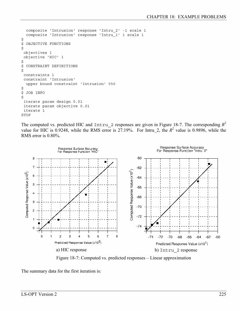
CHAPTER 18: EXAMPLE PROBLEMS
LS-OPT Version 2 225
composite 'Intrusion' response 'Intru_2' -1 scale 1composite 'Intrusion' response 'Intru_1' 1 scale 1
$$ OBJECTIVE FUNCTIONS$objectives 1objective 'HIC' 1
$$ CONSTRAINT DEFINITIONS$constraints 1constraint 'Intrusion'upper bound constraint 'Intrusion' 550
$$ JOB INFO$iterate param design 0.01iterate param objective 0.01iterate 1
STOP
The computed vs. predicted HIC and Intru_2 responses are given in Figure 18-7. The corresponding R2 value for HIC is 0.9248, while the RMS error is 27.19%. For Intru_2, the R2 value is 0.9896, while the RMS error is 0.80%.
a) HIC response b) Intru_2 response
Figure 18-7: Computed vs. predicted responses – Linear approximation
The summary data for the first iteration is:

CHAPTER 18: EXAMPLE PROBLEMS
226 LS-OPT Version 2
Baseline: ---------------------------------------ITERATION NUMBER (Baseline)---------------------------------------
DESIGN POINT------------Variable Name Lower Bound Value Upper Bound--------------------------------|-----------|----------|-----------t_hood 1 1 5t_bumper 1 3 5--------------------------------|-----------|----------|-----------
RESPONSE FUNCTIONS:------------------
| Scaled | Unscaled ||---------------------|---------------------|
RESPONSE | Computed Predicted| Computed Predicted|--------------------------------|----------|----------|----------|----------|Acc_max | 8.345e+04 1.162e+05| 8.345e+04 1.162e+05|Mass | 0.4103 0.4103| 0.4103 0.4103|Intru_2 | -736.7 -738| -736.7 -738|Intru_1 | -161 -160.7| -161 -160.7|HIC | 68.26 74.68| 68.26 74.68|--------------------------------|----------|----------|----------|----------|
and 1st optimum:
DESIGN POINT------------Variable Name Lower Bound Value Upper Bound--------------------------------|-----------|----------|-----------t_hood 1 1.549 5t_bumper 1 5 5--------------------------------|-----------|----------|-----------
RESPONSE FUNCTIONS:------------------
| Scaled | Unscaled ||---------------------|---------------------|
RESPONSE | Computed Predicted| Computed Predicted|--------------------------------|----------|----------|----------|----------|Acc_max | 1.248e+05 1.781e+05| 1.248e+05 1.781e+05|Mass | 0.6571 0.657| 0.6571 0.657|Intru_2 | -713.7 -711.4| -713.7 -711.4|Intru_1 | -164.6 -161.4| -164.6 -161.4|HIC | 126.7 39.47| 126.7 39.47|--------------------------------|----------|----------|----------|----------|
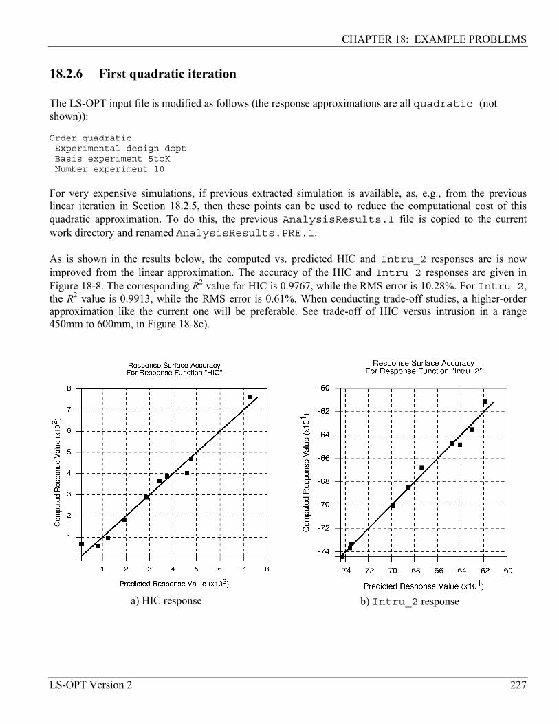
CHAPTER 18: EXAMPLE PROBLEMS
LS-OPT Version 2 227
18.2.6 First quadratic iteration The LS-OPT input file is modified as follows (the response approximations are all quadratic (not shown)):
Order quadraticExperimental design doptBasis experiment 5toKNumber experiment 10
For very expensive simulations, if previous extracted simulation is available, as, e.g., from the previous linear iteration in Section 18.2.5, then these points can be used to reduce the computational cost of this quadratic approximation. To do this, the previous AnalysisResults.1 file is copied to the current work directory and renamed AnalysisResults.PRE.1. As is shown in the results below, the computed vs. predicted HIC and Intru_2 responses are is now improved from the linear approximation. The accuracy of the HIC and Intru_2 responses are given in Figure 18-8. The corresponding R2 value for HIC is 0.9767, while the RMS error is 10.28%. For Intru_2, the R2 value is 0.9913, while the RMS error is 0.61%. When conducting trade-off studies, a higher-order approximation like the current one will be preferable. See trade-off of HIC versus intrusion in a range 450mm to 600mm, in Figure 18-8c).
a) HIC response b) Intru_2 response

CHAPTER 18: EXAMPLE PROBLEMS
228 LS-OPT Version 2
c) Trade-off of HIC versus Intrusion
Figure 18-8: Computed vs. predicted responses and trade-off – Quadratic approximation
The summary data for the first iteration is: Baseline: ---------------------------------------ITERATION NUMBER (Baseline)---------------------------------------
DESIGN POINT------------Variable Name Lower Bound Value Upper Bound--------------------------------|-----------|----------|-----------t_hood 1 1 5t_bumper 1 3 5--------------------------------|-----------|----------|-----------
RESPONSE FUNCTIONS:------------------
| Scaled | Unscaled ||---------------------|---------------------|
RESPONSE | Computed Predicted| Computed Predicted|--------------------------------|----------|----------|----------|----------|Acc_max | 8.345e+04 1.385e+05| 8.345e+04 1.385e+05|Mass | 0.4103 0.4103| 0.4103 0.4103|Intru_2 | -736.7 -736| -736.7 -736|Intru_1 | -161 -160.3| -161 -160.3|HIC | 68.26 10.72| 68.26 10.72|--------------------------------|----------|----------|----------|----------|

CHAPTER 18: EXAMPLE PROBLEMS
LS-OPT Version 2 229
and 1st optimum:
DESIGN POINT------------Variable Name Lower Bound Value Upper Bound--------------------------------|-----------|----------|-----------t_hood 1 1.653 5t_bumper 1 3.704 5--------------------------------|-----------|----------|-----------
RESPONSE FUNCTIONS:------------------
| Scaled | Unscaled ||---------------------|---------------------|
RESPONSE | Computed Predicted| Computed Predicted|--------------------------------|----------|----------|----------|----------|Acc_max | 1.576e+05 1.985e+05| 1.576e+05 1.985e+05|Mass | 0.6017 0.6018| 0.6017 0.6018|Intru_2 | -712.7 -711.9| -712.7 -711.9|Intru_1 | -163.3 -161.9| -163.3 -161.9|HIC | 171.4 108.2| 171.4 108.2|--------------------------------|----------|----------|----------|----------|
18.2.7 Automated run An automated optimization is performed with a linear approximation. The LS-OPT input file is modified as follows:
Order linearExperimental design doptBasis experiment 3toKNumber experiment 5
iterate 8 It can be seen in Figure 18-9 that the objective function (HIC) and intrusion constraint are approximately optimized at the 5th iteration. It takes about 8 iterations for the approximated (solid line) and computed (square symbols) HIC to correspond. The approximation improves through the contraction of the subregion. As the variable t_hood never moves to the edge of the subregion during the optimization process, the heuristic in LS-OPT enforces pure zooming (see Figure 18-10). For t_bumper, panning occurs as well due to the fact that the linear approximation predicts a variable on the edge of the subregion.

CHAPTER 18: EXAMPLE PROBLEMS
230 LS-OPT Version 2
a) Optimization history of HIC b) Optimization history of Intrusion
Figure 18-9: Optimization history of HIC and Intrusion
a) Optimization history of t_hood b) Optimization history of t_bumper
Figure 18-10: Optimization history of design variables

CHAPTER 18: EXAMPLE PROBLEMS
LS-OPT Version 2 231
18.2.8 Trade-off using neural network approximation* In order to build a more accurate response surface for trade-off studies, the Neural Net method is chosen under the ExpDesign panel. This results in a feed-forward (FF) neural network (Section 0) being solved for the points selected. The recommended point selection scheme (Space Filling) is used. One iteration is performed to analyze only one experimental design with 25 points. The modifications to the command input file are as follows: $$ DEFINITION OF SOLVER "1"$solver dyna '1'solver command "lsdyna"solver input file "car5.k"solver append file "rigid2"solver order FFsolver update doesolver experiment design space_fillingsolver number experiments 25
iterate 1
The response surface accuracy is illustrated in Figure 18-11 for the HIC and Intru_2 responses. The HIC has more scatter than Intru_2 for the 25 design points used.
a) HIC response b) Intru_2 constraint
Figure 18-11: Response surface accuracy using neural network approximation
A trade-off study considers a variation in the Intrusion constraint (originally fixed at 550mm) between 450 and 600mm, the same as in Figure 18-8c). The experimental design used for the responses in Figure 18-11
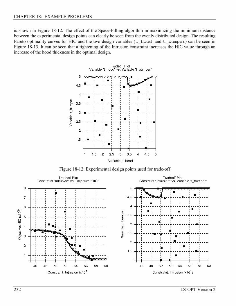
CHAPTER 18: EXAMPLE PROBLEMS
232 LS-OPT Version 2
is shown in Figure 18-12. The effect of the Space-Filling algorithm in maximizing the minimum distance between the experimental design points can clearly be seen from the evenly distributed design. The resulting Pareto optimality curves for HIC and the two design variables (t_hood and t_bumper) can be seen in Figure 18-13. It can be seen that a tightening of the Intrusion constraint increases the HIC value through an increase of the hood thickness in the optimal design.
Figure 18-12: Experimental design points used for trade-off
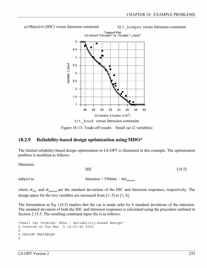
CHAPTER 18: EXAMPLE PROBLEMS
LS-OPT Version 2 233
a) Objective (HIC) versus Intrusion constraint b) t_bumper versus Intrusion constraint
c) t_hood versus Intrusion constraint
Figure 18-13: Trade-off results – Small car (2 variables)
18.2.9 Reliability-based design optimization using MDO* The limited reliability-based design optimization in LS-OPT is illustrated in this example. The optimization problem is modified as follows: Minimize HIC (18.5) subject to Intrusion < 550mm – Intrusion6σ where HICσ and Intrusionσ are the standard deviations of the HIC and Intrusion responses, respectively. The design space for the two variables are increased from [1; 5] to [1; 6]. The formulation in Eq. (18.5) implies that the car is made safer by 6 standard deviations of the intrusion. The standard deviation of both the HIC and Intrusion responses is calculated using the procedure outlined in Section 2.15.5. The resulting command input file is as follows: "Small Car Problem: EX4a – Reliability-based design"$ Created on Tue Mar 5 14:03:45 2002$$ DESIGN VARIABLES$

CHAPTER 18: EXAMPLE PROBLEMS
234 LS-OPT Version 2
solvers 2variables 4Variable 't_hood_m' 1Lower bound variable 't_hood_m' 1Upper bound variable 't_hood_m' 6range 't_hood_m' 2Local 't_hood_m'
Variable 't_bumper_m' 3Lower bound variable 't_bumper_m' 1Upper bound variable 't_bumper_m' 6range 't_bumper_m' 2Local 't_bumper_m'
Variable 't_hood_s' 0Lower bound variable 't_hood_s' -.05Upper bound variable 't_hood_s' +.05range 't_hood_s' 0.1iterate param rangelimit 't_hood_s' 0.1Local 't_hood_s'
Variable 't_bumper_s' 0Lower bound variable 't_bumper_s' -.05Upper bound variable 't_bumper_s' +.05range 't_bumper_s' 0.1iterate param rangelimit 't_bumper_s' 0.1Local 't_bumper_s'
dependents 2$$ DEPENDENTS$Dependent 't_hood' {t_hood_m + t_hood_s}Dependent 't_bumper' {t_bumper_m + t_bumper_s}
responses 10$$ NO HISTORIES ARE DEFINED$$ DEFINITION OF SOLVER "MEAN"$solver dyna 'MEAN'solver command "lsdyna"solver input file "car5.k"solver append file "rigid2"
$$ RESPONSES FOR SOLVER "1"$response 'Intru_2_m' 1 0 "DynaASCII Nodout X_DISP 432 Timestep"response 'Intru_1_m' 1 0 "DynaASCII Nodout X_DISP 167 Timestep"response 'Intrusion_m' expression {Intru_1_m - Intru_2_m}response 'HIC_m' 1 0 "DynaASCII Nodout HIC15 9810. 1 432"
$$ LOCAL VARIABLES$solver variable 't_hood_m'solver variable 't_bumper_m'
$$ EXPERIMENTAL DESIGN$Solver Order linearSolver Experimental design dopt

CHAPTER 18: EXAMPLE PROBLEMS
LS-OPT Version 2 235
Solver Basis experiment 5toKSolver Number experiment 5
$$ JOB INFO$concurrent jobs 1
$$ DEFINITION OF SOLVER "_RANDOM_"$solver dyna '_RANDOM_'solver command "lsdyna"solver input file "car5s.k"solver append file "rigid2"
$$ LOCAL VARIABLES$solver variable 't_hood_s'solver variable 't_bumper_s'
$$ RESPONSES FOR SOLVER "1"$response 'Intru_2_s' 1 0 "DynaASCII Nodout X_DISP 432 Timestep"response 'Intru_1_s' 1 0 "DynaASCII Nodout X_DISP 167 Timestep"response 'Intrusion_s' expression {Intru_1_s - Intru_2_s}response 'HIC_s' 1 0 "DynaASCII Nodout HIC15 9810. 1 432"response 'Intrusion_dev' "DynaStat STDDEV Intrusion_s"response 'HIC_dev' "DynaStat STDDEV HIC_s"
$$ EXPERIMENTAL DESIGN$Solver Experimental design latin_hypercubeSolver Number experiment 20
$$ JOB INFO$concurrent jobs 1
$$ COMPOSITES$composites 1composite 'Intrusion' {Intru_1_m - Intru_2_m + 6*Intrusion_dev}
$$ OBJECTIVE FUNCTIONS$objectives 1objective 'HIC_m' 1
$$ CONSTRAINT DEFINITIONS$constraints 1constraint 'Intrusion'upper bound constraint 'Intrusion' 550
$$ OPTIMIZATION METHOD$iterate param design 0.01iterate param objective 0.01

CHAPTER 18: EXAMPLE PROBLEMS
236 LS-OPT Version 2
iterate 15STOP
Remarks: 1. Note that the stochastic (random) solver name must be ‘_RANDOM_’. 2. The dependent variables are substituted in the _RANDOM_ solver input deck (car5s.k) only. 3. The aim of the _RANDOM_ solver is only to provide the standard deviations of the responses. 4. The reliability of the design is improved by increasing the Intrusion response before it is compared to
the 550mm upper constraint limit. The result of the optimization process is given in Figure 18-14. Shown are both the Intrusion and HIC responses. The reliability limit on the Intrusion response is shown as a dashed line. This corresponds to the left-hand side of the constraint in Eq. (17.5), rewritten as
Intrusion + Intrusion6σ < 550mm. A 6-sigma range is given in the plot for the HIC response. It can be seen that the mean HIC-value is reduced in the presence of the reliability constraint.
0
50
100
150
200
250
300
0 2 4 6 8 10Iteration Number
HIC
530
540
550
560
570
580
590
600
610
620
630
Intr
usio
n
HIC_meanHIC (Mean + 6sigma)HIC (Mean - 6sigma)Intrusion_meanIntrusion (Mean + 6sigma)
Figure 18-14: Reliability-based design results – Small car (2 variables)

CHAPTER 18: EXAMPLE PROBLEMS
LS-OPT Version 2 237
18.2.10 Reliability-based design optimization using FOSM* The First Order Second Moment reliability-based design optimization in LS-OPT is illustrated in this example. The optimization problem is modified as follows: Minimize HIC (18.6) subject to Probability[Intrusion > 550mm ] < 610− The formulation in Eq. HIC (18.6 implies that the car is made safer by 6 standard deviations of the intrusion. The following commands must be added to the LS-OPT input file used for the automated run (Section 18.2.7): $$ Define distributions$Distributions 2distribution ‘hood_dist’ UNIFORM –0.05 0.05distribution ‘bumper_dist’ UNIFORM –0.05 0.05
$$ Assign distributions to variables$variable 't_hood' distribution ‘hood_dist’variable 't_bumper' distribution ‘bumper_dist’$$ Assign probabilistic bounds to constraints$probability upper bound constraint ‘Intrusion’ 1e-6
The results are: x = <1.78, 3.44>, a HIC value of 182, and an intrusion of 545 with a standard deviation of 1.06.

CHAPTER 18: EXAMPLE PROBLEMS
238 LS-OPT Version 2
18.3 Impact of a cylinder (2 variables) This example has the following features: • An LS-DYNA explicit impact simulation is performed. • An independent parametric preprocessor is used to incorporate shape optimization. • Extraction is performed using standard ASCII LS-DYNA interfaces. • Second-order response surface approximations are compared using different subregions. • The design optimization process is automated. • Noisy response variables are improved using filtering. The example in this chapter is modeled on one by Yamazaki [78]. 18.3.1 Problem statement The problem consists of a tube impacting a rigid wall as shown in Figure 18-15. The energy absorbed is maximized subject to a constraint on the rigid wall impact force. The cylinder has a constant mass of 0.54 kg with the design variables being the mean radius and thickness. The length of the cylinder is thus dependent on the design variables because of the mass constraint. A concentrated mass of 500 times the cylinder weight is attached to the end of the cylinder not impacting the rigid wall. The deformed shape at 20ms is shown in Figure 18-16 for a typical design.
x1 x2
l
10m/s
Figure 18-15: Impacting cylinder

CHAPTER 18: EXAMPLE PROBLEMS
LS-OPT Version 2 239
Figure 18-16: Deformed finite element model (time = 20ms)
The optimization problem is stated as:
Maximize 02.021internal ),( =txxE subject to
00070),( 21 ≤average
wallnormal xxF
21252.0)(
xxxl
πρ=
where the design variables x1 and x2 are the radius and the thickness of the cylinder respectively.
02.0internal )( =txE is the objective function and constraint functions averagewall
normal xF )( and l(x) are the average normal force on the rigid wall and the length of the cylinder, respectively. The problem is simulated using LS-DYNA. The following TrueGrid input file including the <<name>> statements is used to create the FE input deck with the FE model as shown in Figure 18-16. Note that the design variables have been scaled. c cyl2 - crush cylinder - constant volumelsdyna3d keywordlsdyopts secforc .00002 rwforc .00002 ;lsdyopts endtim .02 d3plot dtcycl .0001 ; ;lsdyopts thkchg 2 ;lsdyopts elout 0.001lsdyopts glstat 0.001lsdymats 1 3 rho 2880 shell elfor bt tsti 4
e 71.38e9 pr .33 sigy 102.0e6 etan 0.2855e9 ;lsdymats 2 20 rho 14.3e6 e 7.138e10 pr .33 cmo con 4 7 shell elfor bt tsti 4;parar [<<Radius>>/1000.0]l [3.0e+1/<<Radius>>/<<Wall_Thickness>>]h [<<Wall_Thickness>>/1000.0]

CHAPTER 18: EXAMPLE PROBLEMS
240 LS-OPT Version 2
l2 [75.0/<<Radius>>*0.02]h2 .002v0 10.n .33pi 3.14159
;plane 1 0 0 -.002 0 0 1 .001 ston pen 2. stick ;sid 1 lsdsi 13 slvmat 1;scoef .4 dcoef .4 sfsps 1.5 ; ; ;c ************** part 1 mat 1 ************* shellcylinder-1; 1 60; 1 50 51;%r0 3600 %l [%l2+%l]dom 1 1 1 1 2 3
x=x+.01*%h*sin(%pi*z*57.3/(%pi*(%r*%r*%h*%h/(12*(1-%n*%n)))**.25))thick %hthi ;;2 3; %h2c bi ; ;-3 0 -3; dx 1 dy 1 rx 1 ry 1 rz 1 ;c interruptswi ;; ;1velocity 0 0 [-%v0]mate 1mti ;; 2 3; 2c element spring blockepb 1 1 1 1 2 3endpartmergestp .000001writeend
18.3.2 A first approximation In the first iteration, a quadratic approximation is chosen from the beginning. The ASCII database is suitable for this analysis as the energy and impact force can be extracted from the glstat and rwforc databases respectively. Five processors are available. The region of interest is arbitrarily chosen to be about half the size of the design space. The following LS-OPT command input deck was used to find the approximate optimum solution:
"Cylinder Impact Problem"$ Created on Thu Jul 11 11:37:33 2002$$ DESIGN VARIABLES$variables 2Variable 'Radius' 75Lower bound variable 'Radius' 20Upper bound variable 'Radius' 100Range 'Radius' 50
Variable 'Wall_Thickness' 3Lower bound variable 'Wall_Thickness' 2Upper bound variable 'Wall_Thickness' 6

CHAPTER 18: EXAMPLE PROBLEMS
LS-OPT Version 2 241
Range 'Wall_Thickness' 2solvers 1responses 2$$ NO HISTORIES ARE DEFINED$$$ DEFINITION OF SOLVER "RUN1"$solver dyna960 'RUN1'solver command "lsdyna"solver input file "trugrdo"prepro truegridprepro command "/net/src/ultra4_4/common/hp/tg2.1/tg"prepro input file "cyl2"
$$ RESPONSES FOR SOLVER "RUN1"$response 'Internal_Energy' 1 0 "DynaASCII Glstat I_Ener 0 Timestep"response 'Internal_Energy' quadraticresponse 'Rigid_Wall_Force' 1 0 "DynaASCII rwforc normal 1 ave"response 'Rigid_Wall_Force' quadratic
$$ NO HISTORIES DEFINED FOR SOLVER "RUN1"$$$ OBJECTIVE FUNCTIONS$objectives 1maximizeobjective 'Internal_Energy' 1
$$ CONSTRAINT DEFINITIONS$constraints 1constraint 'Rigid_Wall_Force'upper bound constraint 'Rigid_Wall_Force' 70000
$$ EXPERIMENTAL DESIGN$Order quadraticExperimental design doptBasis experiment 5toKNumber experiment 10
$$ JOB INFO$concurrent jobs 5iterate param design 0.01iterate param objective 0.01iterate 1
STOP
The curve-fitting results below show that the internal energy is approximated reasonably well whereas the average force is poorly approximated. The accuracy plots confirm this result (Figure 18-17).

CHAPTER 18: EXAMPLE PROBLEMS
242 LS-OPT Version 2
Approximating Response 'Internal_Energy' using 10 points (ITERATION 1)----------------------------------------------------------------
Global error parameters of response surface-------------------------------------------
Quadratic Function Approximation:---------------------------------Mean response value = 10686.0081
RMS error = 790.3291 (7.40%)Maximum Residual = 1538.9208 (14.40%)Average Error = 654.4415 (6.12%)Square Root PRESS Residual = 2213.7994 (20.72%)Variance = 1249240.2552R^2 = 0.9166R^2 (adjusted) = 0.9166R^2 (prediction) = 0.3453Determinant of [X]'[X] = 1.3973
Approximating Response 'Rigid_Wall_Force' using 10 points (ITERATION 1)----------------------------------------------------------------
Global error parameters of response surface-------------------------------------------
Quadratic Function Approximation:---------------------------------Mean response value = 121662.9474
RMS error = 24730.1732 (20.33%)Maximum Residual = 48569.4162 (39.92%)Average Error = 21111.3307 (17.35%)Square Root PRESS Residual = 75619.5531 (62.15%)Variance = 1223162932.2092R^2 = 0.8138R^2 (adjusted) = 0.8138R^2 (prediction) = -0.7406Determinant of [X]'[X] = 1.3973
The initial design below shows that the constraint is severely exceeded.
DESIGN POINT------------Variable Name Lower Bound Value Upper Bound--------------------------------|-----------|----------|-----------Radius 20 75 100Wall_Thickness 2 3 6--------------------------------|-----------|----------|-----------
RESPONSE FUNCTIONS:------------------
| Scaled | Unscaled ||---------------------|---------------------|
RESPONSE | Computed Predicted| Computed Predicted|--------------------------------|----------|----------|----------|----------|Internal_Energy | 1.296e+04 1.142e+04| 1.296e+04 1.142e+04|Rigid_Wall_Force | 1.749e+05 1.407e+05| 1.749e+05 1.407e+05|--------------------------------|----------|----------|----------|----------|

CHAPTER 18: EXAMPLE PROBLEMS
LS-OPT Version 2 243
Figure 18-17: Prediction accuracy of Internal Energy and Rigid Wall Force (One Quadratic iteration)
Despite the relatively poor approximation a prediction of the optimum is made based on the approximation response surface. The results are shown below. The fact that the optimal Radius is on the lower bound of the subregion specified (Range = 50), suggests an optimal value below 50.
DESIGN POINT------------Variable Name Lower Bound Value Upper Bound--------------------------------|-----------|----------|-----------Radius 20 50 100Wall_Thickness 2 2.978 6--------------------------------|-----------|----------|-----------
RESPONSE FUNCTIONS:------------------
| Scaled | Unscaled ||---------------------|---------------------|
RESPONSE | Computed Predicted| Computed Predicted|--------------------------------|----------|----------|----------|----------|Internal_Energy | 7914 8778| 7914 8778|Rigid_Wall_Force | 4.789e+04 7e+04| 4.789e+04 7e+04|--------------------------------|----------|----------|----------|----------|

CHAPTER 18: EXAMPLE PROBLEMS
244 LS-OPT Version 2
18.3.3 Refining the design model using a second iteration During the previous optimization step, the Radius variable was reduced from 75 to 50 (on the boundary of the region of interest). It was also apparent that the approximations were fairly inaccurate. Therefore, in the new iteration, the region of interest is reduced from [50;2] to [35;1.5] while retaining a quadratic approximation order. The starting point is taken as the current optimum: (50,2.978). The modified commands in the input file are as follows:
$$ DESIGN VARIABLES$variables 2Variable 'Radius' 50Lower bound variable 'Radius' 20Upper bound variable 'Radius' 100Range 'Radius' 35
Variable 'Wall_Thickness' 2.9783Lower bound variable 'Wall_Thickness' 2Upper bound variable 'Wall_Thickness' 6Range 'Wall_Thickness' 1.5
As shown below, the accuracy of fit improves but the average rigid wall force is still inaccurate.
Approximating Response 'Internal_Energy' using 10 points (ITERATION 1)----------------------------------------------------------------
Global error parameters of response surface-------------------------------------------
Quadratic Function Approximation:---------------------------------Mean response value = 8640.2050
RMS error = 526.9459 (6.10%)Maximum Residual = 890.0759 (10.30%)Average Error = 388.4472 (4.50%)Square Root PRESS Residual = 1339.4046 (15.50%)Variance = 555344.0180R^2 = 0.9632R^2 (adjusted) = 0.9632R^2 (prediction) = 0.7622Determinant of [X]'[X] = 0.0556
Approximating Response 'Rigid_Wall_Force' using 10 points (ITERATION 1)----------------------------------------------------------------
Global error parameters of response surface-------------------------------------------
Quadratic Function Approximation:---------------------------------Mean response value = 82483.2224
RMS error = 19905.3990 (24.13%)Maximum Residual = 35713.1794 (43.30%)Average Error = 17060.6074 (20.68%)Square Root PRESS Residual = 54209.4513 (65.72%)Variance = 792449819.5138

CHAPTER 18: EXAMPLE PROBLEMS
LS-OPT Version 2 245
R^2 = 0.8949R^2 (adjusted) = 0.8949R^2 (prediction) = 0.2204Determinant of [X]'[X] = 0.0556 The goodness of fit diagrams are shown in Figure 18-18.
Figure 18-18: Prediction accuracy of Internal Energy and Rigid Wall Force (One Quadratic iteration)
Nevertheless an optimization is conducted of the approximate subproblem, yielding a much improved feasible result. The objective function increases to 9575 (9777 computed) whereas the constraint is active at 70 000. The computed constraint is lower at 64 170. However the Wall_Thickness is now on the upper bound, suggesting an optimal value larger than 3.728.
DESIGN POINT------------Variable Name Lower Bound Value Upper Bound--------------------------------|-----------|----------|-----------Radius 20 42.43 100Wall_Thickness 2 3.728 6--------------------------------|-----------|----------|-----------
RESPONSE FUNCTIONS:------------------
| Scaled | Unscaled ||---------------------|---------------------|
RESPONSE | Computed Predicted| Computed Predicted|--------------------------------|----------|----------|----------|----------|Internal_Energy | 9777 9575| 9777 9575|Rigid_Wall_Force | 6.417e+04 7e+04| 6.417e+04 7e+04|--------------------------------|----------|----------|----------|----------|

CHAPTER 18: EXAMPLE PROBLEMS
246 LS-OPT Version 2
18.3.4 Third iteration Because of the large change in the Wall_Thickness on to the upper bound of the region of interest, a third iteration is conducted, keeping the region of interest the same. The starting point is the previous optimum: Variable 'Radius' 42.43Variable 'Wall_Thickness' 3.728
The approximation improves as shown below:
Approximating Response 'Internal_Energy' using 10 points (ITERATION 1)----------------------------------------------------------------
Global error parameters of response surface-------------------------------------------
Quadratic Function Approximation:---------------------------------Mean response value = 9801.0070
RMS error = 439.8326 (4.49%)Maximum Residual = 834.5960 (8.52%)Average Error = 372.3133 (3.80%)Square Root PRESS Residual = 1451.3233 (14.81%)Variance = 386905.5050R^2 = 0.9618R^2 (adjusted) = 0.9618R^2 (prediction) = 0.5842Determinant of [X]'[X] = 0.0131
Approximating Response 'Rigid_Wall_Force' using 10 points (ITERATION 1)----------------------------------------------------------------
Global error parameters of response surface-------------------------------------------
Quadratic Function Approximation:---------------------------------Mean response value = 81576.0534
RMS error = 12169.4703 (14.92%)Maximum Residual = 26348.0687 (32.30%)Average Error = 10539.2275 (12.92%)Square Root PRESS Residual = 37676.3033 (46.19%)Variance = 296192016.4365R^2 = 0.9301R^2 (adjusted) = 0.9301R^2 (prediction) = 0.3303Determinant of [X]'[X] = 0.0131
Because the size of the region of interest remained the same, the curve-fitting results show only a slight change (because of the new location), in this case an improvement. However, as the optimization results below show, the design is much improved, i.e. the objective value has increased whereas the approximate constraint is active. Unfortunately, due to the poor fit of the Rigid_Wall_Force, the simulation result exceeds the force constraint by about 10kN (14%). Further reduction of the region of interest is required to reduce the error, or filtering of the force can be considered to reduce the noise on this response.

CHAPTER 18: EXAMPLE PROBLEMS
LS-OPT Version 2 247
DESIGN POINT------------Variable Name Lower Bound Value Upper Bound--------------------------------|-----------|----------|-----------Radius 20 36.51 100Wall_Thickness 2 4.478 6--------------------------------|-----------|----------|-----------
RESPONSE FUNCTIONS:------------------
| Scaled | Unscaled ||---------------------|---------------------|
RESPONSE | Computed Predicted| Computed Predicted|--------------------------------|----------|----------|----------|----------|Internal_Energy | 1.129e+04 1.075e+04| 1.129e+04 1.075e+04|Rigid_Wall_Force | 8.007e+04 7e+04| 8.007e+04 7e+04|--------------------------------|----------|----------|----------|----------|
The table below gives a summary of the three iterations of the step-by-step procedure.
Table 18-2: Comparison of results (Cylinder impact)
Variable Initial Iteration 1 Iteration 2 Iteration 3 Radius 75 50 42.43 36.51 Wall_thickness 3 2.978 3.728 4.478 Energy (Computed) 12960 7914 9777 11290 Force (Computed) 174900 47890 64170 80070 It is apparent that the result of the second iteration is a dramatic improvement on the starting design and a good approximation to the converged optimum design. 18.3.5 Response filtering: using the peak force as a constraint Because of the poor accuracy of the response surface fit for the rigid wall force above, it was decided to modify the force constraint so that the peak filtered force is used instead. Therefore, the previous response definition for Rigid_Wall_Force is replaced with a command that extracts the maximum rigid wall force from a response from which frequencies exceeding 300Hz are excluded. The upper bound of the force constraint is changed to 80000.
response ’Rigid_Wall_Force’ "DynaASCII RWForc Normal 1 Max SAE 300" 20 iterations are specified with a 1% tolerance for convergence. As expected, the response histories (Figure 18-19) show that the baseline design is severely infeasible (the first peak force is about 1.75 x 10⁶ vs. the constraint value of 0.08 x 10⁶. A steady reduction in the error of the response surfaces is observed up to about iteration 5. The optimization terminates after 16 iterations, having reached the 1% threshold for both objective and design variable changes.

CHAPTER 18: EXAMPLE PROBLEMS
248 LS-OPT Version 2
a) Radius
b) Wall_Thickness
c) Internal_Energy
d) Rigid_Wall_Force

CHAPTER 18: EXAMPLE PROBLEMS
LS-OPT Version 2 249
e) RMS error of Internal_Energy f) RMS error of Rigid_Wall_Force
Figure 18-19: Optimization history of automated design (filtered force)
The optimization process steadily reduces the infeasibility, but the force constraint is still slightly violated when convergence is reached. The internal energy is significantly lower than previously:
DESIGN POINT------------Variable Name Lower Bound Value Upper Bound--------------------------------|-----------|----------|-----------Radius 20 20.51 100Wall_Thickness 2 4.342 6--------------------------------|-----------|----------|-----------
RESPONSE FUNCTIONS:------------------
| Scaled | Unscaled ||---------------------|---------------------|
RESPONSE | Computed Predicted| Computed Predicted|--------------------------------|----------|----------|----------|----------|Internal_Energy | 8344 8645| 8344 8645|Rigid_Wall_Force | 8.112e+04 8e+04| 8.112e+04 8e+04|--------------------------------|----------|----------|----------|----------|
Figure 18-20 below confirms that the final design is only slightly infeasible when the maximum filtered force exceeds the specified limit for a short duration at around 9ms.

CHAPTER 18: EXAMPLE PROBLEMS
250 LS-OPT Version 2
Figure 18-20: Cylinder: Constrained rigid wall force: F(t) < 80000 (SAE 300Hz filtered)

CHAPTER 18: EXAMPLE PROBLEMS
LS-OPT Version 2 251
18.4 Sheet-metal forming (3 variables) A sheet-metal forming example in which the design involves thinning and FLD criteria is demonstrated in this chapter. The example has the following features: • The maximum of all the design variables is minimized. • Adaptive meshing is used in the finite element analysis. • The binary LS-DYNA database is used. • The example employs the sheet metal forming interface utilities. • Composite functions are used. • An appended file containing extra input is used. • The example utilizes the independent parametric preprocessor, Truegrid15. 18.4.1 Problem statement The design parameterization for the sheet metal forming example is shown in Figure 18-21.
t
F1
F2
r1
r3
r2 die
punch
Figure 18-21: Parameterization of cross-section
15 Registered Trademark of XYZ Scientific Applications Inc.
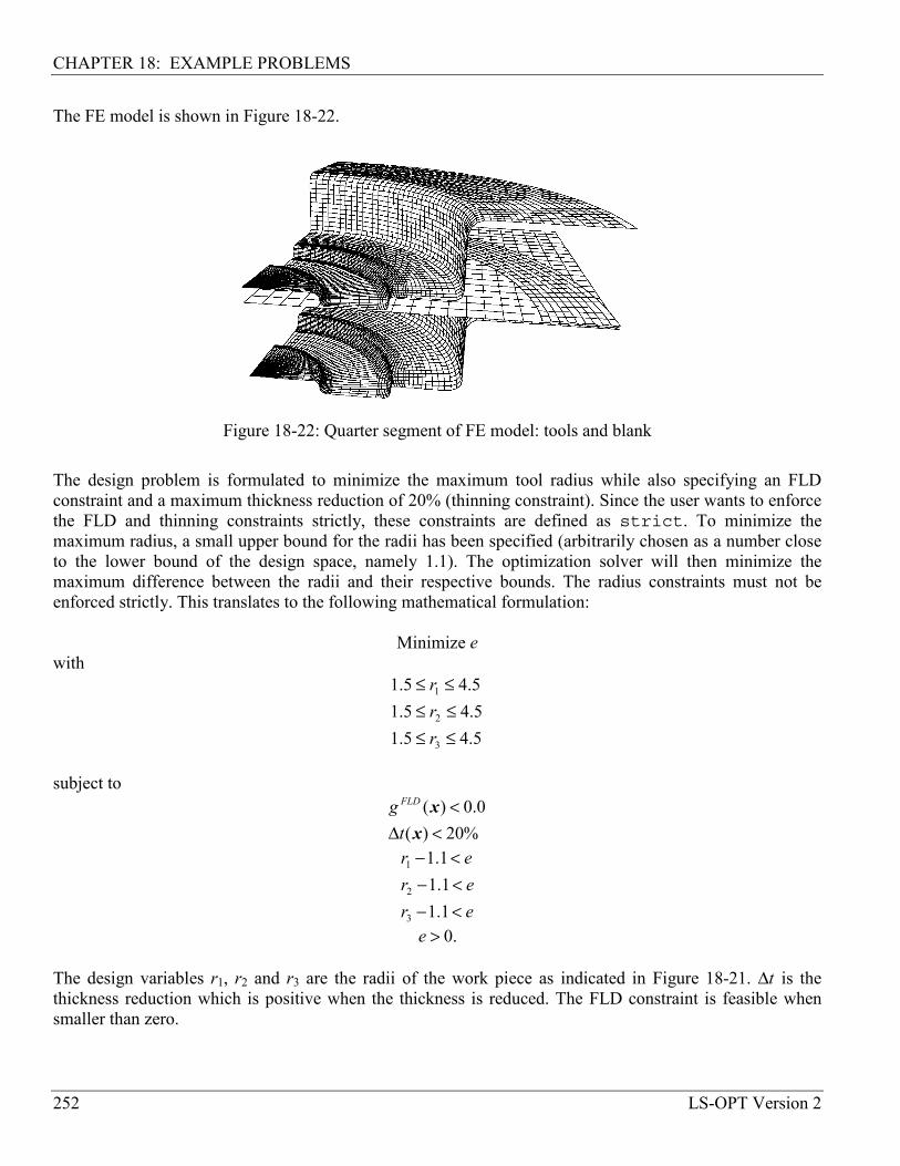
CHAPTER 18: EXAMPLE PROBLEMS
252 LS-OPT Version 2
The FE model is shown in Figure 18-22.
Figure 18-22: Quarter segment of FE model: tools and blank
The design problem is formulated to minimize the maximum tool radius while also specifying an FLD constraint and a maximum thickness reduction of 20% (thinning constraint). Since the user wants to enforce the FLD and thinning constraints strictly, these constraints are defined as strict. To minimize the maximum radius, a small upper bound for the radii has been specified (arbitrarily chosen as a number close to the lower bound of the design space, namely 1.1). The optimization solver will then minimize the maximum difference between the radii and their respective bounds. The radius constraints must not be enforced strictly. This translates to the following mathematical formulation:
Minimize e with
5.45.15.45.15.45.1
3
2
1
≤≤≤≤≤≤
rrr
subject to
%20)(0.0)(
<∆<
xx
tg FLD
ererer
<−<−<−
1.11.11.1
3
2
1
.0>e The design variables r1, r2 and r3 are the radii of the work piece as indicated in Figure 18-21. ∆t is the thickness reduction which is positive when the thickness is reduced. The FLD constraint is feasible when smaller than zero.

CHAPTER 18: EXAMPLE PROBLEMS
LS-OPT Version 2 253
18.4.2 First Iteration The initial run is a quadratic analysis designed as an initial investigation of the following issues: • The dependency of the through thickness strain constraint on the radii. • The dependency of the FLD constraint on the radii. • The location of the optimal design point. The subregion considered for this study is 2.0 large in r1, r2 and r3 and is centered about (1.5, 1.5, 1.5)T. The FLD constraint formulation tested in this phase is based on the maximum perpendicular distance of a point violating the FLD constraint to the FLD curve (see Section 11.9.2). The LS-OPT command file used to run the problem is: "Sheet: Minimization of Maximum Tool Radius"Author "Aaron Spelling"$ Created on Wed May 29 19:23:20 2002$$ DESIGN VARIABLES$variables 3Variable 'Radius_1' 1.5Lower bound variable 'Radius_1' 1Upper bound variable 'Radius_1' 4.5Range 'Radius_1' 4
Variable 'Radius_2' 1.5Lower bound variable 'Radius_2' 1Upper bound variable 'Radius_2' 4.5Range 'Radius_2' 4
Variable 'Radius_3' 1.5Lower bound variable 'Radius_3' 1Upper bound variable 'Radius_3' 4.5Range 'Radius_3' 4
solvers 1responses 2$$ NO HISTORIES ARE DEFINED$$$ DEFINITION OF SOLVER "DYNA1"$solver dyna 'DYNA1'solver command "lsdyna"solver input file "trugrdo"solver append file "ShellSetList"prepro truegridprepro command "/net/src/ultra4_4/common/hp/tg2.1/tg"prepro input file "m3.tg.opt"
$$ RESPONSES FOR SOLVER "DYNA1"

CHAPTER 18: EXAMPLE PROBLEMS
254 LS-OPT Version 2
$response 'Thinning' 1 0 "DynaThick REDUCTION MAX"response 'Thinning' linearresponse 'FLD' 1 0 "DynaFLDg CENTER 1 2 3 90"response 'FLD' linear
$$ NO HISTORIES DEFINED FOR SOLVER "DYNA1"$$$ HISTORIES AND RESPONSES DEFINED BY EXPRESSIONS$composites 4composite 'Rad1' type weightedcomposite 'Rad1' variable 'Radius_1' 1 scale 1
composite 'Rad2' type weightedcomposite 'Rad2' variable 'Radius_2' 1 scale 1
composite 'Rad3' type weightedcomposite 'Rad3' variable 'Radius_3' 1 scale 1
composite 'Thinning_scaled' {Thinning/100}$$ NO OBJECTIVES DEFINED$objectives 0
$$ CONSTRAINT DEFINITIONS$constraints 5constraint 'FLD'strictupper bound constraint 'FLD' 0.0
constraint 'Rad1'slackupper bound constraint 'Rad1' 1.1
constraint 'Rad2'upper bound constraint 'Rad2' 1.1
constraint 'Rad3'upper bound constraint 'Rad3' 1.1
constraint 'Thinning_scaled'strictupper bound constraint 'Thinning_scaled' 0.2
$$ EXPERIMENTAL DESIGN$Order quadraticExperimental design doptBasis experiment 3toKNumber experiment 16
$$ JOB INFO$concurrent jobs 8iterate param design 0.01iterate param objective 0.01iterate 1
STOP

CHAPTER 18: EXAMPLE PROBLEMS
LS-OPT Version 2 255
The file ShellSetList contains commands for LS-DYNA in addition to the preprocessor output. It is slotted into the input file. Adaptive meshing is chosen as an analysis feature for the simulation. The FLD curve data is also specified in this file. The extra commands are: *DATABASE_BINARY_RUNRSF70*DATABASE_EXTENT_BINARY0, 0, 0, 1, 0, 0, 0, 10, 0, 0, 0, 0, 0$$ SLIDING INTERFACE DEFINITIONS$$ TrueGrid Sliding Interface # 1$*CONTACT_FORMING_ONE_WAY_SURFACE_TO_SURFACE$ workpiece vs punch0.1000000 0.000 0.000
1 2 3 3 1
0.0$*CONTACT_FORMING_ONE_WAY_SURFACE_TO_SURFACE$ workpiece vs die
1 3 3 3 1 10.1000000 0.000 0.000
0.0$*CONTACT_FORMING_ONE_WAY_SURFACE_TO_SURFACE$ workpiece vs blankholder
1 4 3 3 1 10.1000000 0.000 0.000
0.0$*CONTROL_ADAPTIVE$ ADPFREQ ADPTOL ADPOPT MAXLVL TBIRTH TDEATH LCADP IOFLAG0.100E-03 5.000 2 3 0.000E+00 1.0000000 0 1$ ADPSIZE ADPASS IREFLG ADPENE0.0000000 1 0 3.0000*LOAD_RIGID_BODY
$ rbID dir lcID scale2 3 2 1.0000000
*LOAD_RIGID_BODY$ rbID dir lcID scale
4 3 3 1.0000000*DEFINE_CURVE$ FLD curve90$-1,2.0830,.251,.75*END The input file (file m3.tg.opt) used to generate the FE mesh in Truegrid is:
c generate LS-DYNA input deck for sheet metal examplelsdyna keywordlsdyopts endtim .0009 nodout 1.e-6 d3plot dtcycl .0001 ; ;lsdyopts istupd 1 ;c lsdymats 1 37 shell elfor bt rho 7.8e-9 e 2.e5 pr .28
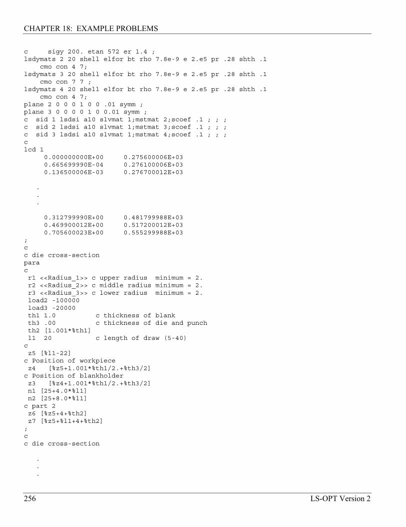
CHAPTER 18: EXAMPLE PROBLEMS
256 LS-OPT Version 2
c sigy 200. etan 572 er 1.4 ;lsdymats 2 20 shell elfor bt rho 7.8e-9 e 2.e5 pr .28 shth .1
cmo con 4 7;lsdymats 3 20 shell elfor bt rho 7.8e-9 e 2.e5 pr .28 shth .1
cmo con 7 7 ;lsdymats 4 20 shell elfor bt rho 7.8e-9 e 2.e5 pr .28 shth .1
cmo con 4 7;plane 2 0 0 0 1 0 0 .01 symm ;plane 3 0 0 0 0 1 0 0.01 symm ;c sid 1 lsdsi a10 slvmat 1;mstmat 2;scoef .1 ; ; ;c sid 2 lsdsi a10 slvmat 1;mstmat 3;scoef .1 ; ; ;c sid 3 lsdsi a10 slvmat 1;mstmat 4;scoef .1 ; ; ;clcd 1
0.000000000E+00 0.275600006E+030.665699990E-04 0.276100006E+030.136500006E-03 0.276700012E+03
.
.
.
0.312799990E+00 0.481799988E+030.469900012E+00 0.517200012E+030.705600023E+00 0.555299988E+03
;cc die cross-sectionparacr1 <<Radius_1>> c upper radius minimum = 2.r2 <<Radius_2>> c middle radius minimum = 2.r3 <<Radius_3>> c lower radius minimum = 2.load2 -100000load3 -20000th1 1.0 c thickness of blankth3 .00 c thickness of die and punchth2 [1.001*%th1]l1 20 c length of draw (5-40)
cz5 [%l1-22]
c Position of workpiecez4 [%z5+1.001*%th1/2.+%th3/2]
c Position of blankholderz3 [%z4+1.001*%th1/2.+%th3/2]n1 [25+4.0*%l1]n2 [25+8.0*%l1]
c part 2z6 [%z5+4+%th2]z7 [%z5+%l1+4+%th2]
;cc die cross-section
.
.
.

CHAPTER 18: EXAMPLE PROBLEMS
LS-OPT Version 2 257
c punch cross-section (closed configuration)ld 2lod 1 [%th2+%th3]
c punch cross-section (withdrawn configuration)ld 3 lstl 2 0 [%z5+26]
.
.
.
endpartc ***************** part 2 mat 2 ********* punchcylinder1 8 35 40 67 76 [76+%n1] [70+%n1+10]; 1 41 ; -1 ;.001 17. 23. 36. 44. 50. 75. 100.0. 90.%z7
.
.
.
thick %th3mate 2endpart
c *********** part 3 mat 4 ********* blankholdercylinder1 10 ; 1 41 ; -1 ;80. 100.0. 90.[%z3]b 0 0 0 0 0 0 dx 1 dy 1 rx 1 ry 1 rz 1;thick %th3mate 4endpart
c *********** part 4 mat 1 workpieceblock1 21 ; 1 21 ; -1 ;0. 100.0. 100.[%z4]thick [%th1]mate 1endpartmergewriteend
The error parameters for the fitted functions are given in the following output (from lsopt_outputfile):
Approximating Response 'Thinning' using 16 points (ITERATION 1)

CHAPTER 18: EXAMPLE PROBLEMS
258 LS-OPT Version 2
----------------------------------------------------------------Global error parameters of response surface-------------------------------------------
Quadratic Function Approximation:---------------------------------Mean response value = 27.8994
RMS error = 0.6657 (2.39%)Maximum Residual = 1.2932 (4.64%)Average Error = 0.5860 (2.10%)Square Root PRESS Residual = 2.0126 (7.21%)Variance = 1.0130R^2 = 0.9913R^2 (adjusted) = 0.9826R^2 (prediction) = 0.9207Determinant of [X]'[X] = 2231.5965
Approximating Response 'FLD' using 16 points (ITERATION 1)----------------------------------------------------------------
Global error parameters of response surface-------------------------------------------
Quadratic Function Approximation:---------------------------------Mean response value = 0.0698
RMS error = 0.0121 (17.33%)Maximum Residual = 0.0247 (35.35%)Average Error = 0.0103 (14.74%)Square Root PRESS Residual = 0.0332 (47.59%)Variance = 0.0003R^2 = 0.9771R^2 (adjusted) = 0.9542R^2 (prediction) = 0.8272Determinant of [X]'[X] = 2231.5965
The thinning has a reasonably accurate response surface but the FLD approximation requires further refinement. The initial design has the following response surface results which fail the criteria for maximum thinning, but not for FLD: DESIGN POINT------------Variable Name Lower Bound Value Upper Bound--------------------------------|-----------|----------|-----------Radius_1 1 1.5 4.5Radius_2 1 1.5 4.5Radius_3 1 1.5 4.5--------------------------------|-----------|----------|-----------
CONSTRAINT FUNCTIONS:--------------------CONSTRAINT NAME | Computed | Predicted| Lower | Upper |Viol?--------------------------------|----------|----------|----------|----------|-----FLD | 0.09123 0.1006| -1e+30 0|YESRad1 | 1.5 1.5| -1e+30 1.1|YES

CHAPTER 18: EXAMPLE PROBLEMS
LS-OPT Version 2 259
Rad2 | 1.5 1.5| -1e+30 1.1|YESRad3 | 1.5 1.5| -1e+30 1.1|YESThinning_scaled | 0.2957 0.3078| -1e+30 0.2|YES--------------------------------|----------|----------|----------|----------|-----CONSTRAINT VIOLATIONS:---------------------
| Computed Violation | Predicted Violation |CONSTRAINT NAME |----------|----------|----------|----------|
| Lower | Upper | Lower | Upper |--------------------------------|----------|----------|----------|----------|FLD | - 0.09123| - 0.1006|Rad1 | - 0.4| - 0.4|Rad2 | - 0.4| - 0.4|Rad3 | - 0.4| - 0.4|Thinning_scaled | - 0.09567| - 0.1078|--------------------------------|----------|----------|----------|----------|
As shown below, after 1 iteration, a feasible design is generated. The simulation response of the optimum is closely approximated by the response surface. DESIGN POINT------------Variable Name Lower Bound Value Upper Bound--------------------------------|-----------|----------|-----------Radius_1 1 3.006 4.5Radius_2 1 3.006 4.5Radius_3 1 3.006 4.5--------------------------------|-----------|----------|-----------
CONSTRAINT FUNCTIONS:--------------------CONSTRAINT NAME | Computed | Predicted| Lower | Upper |Viol?--------------------------------|----------|----------|----------|----------|-----FLD | -0.04308 -0.03841| -1e+30 0|noRad1 | 3.006 3.006| -1e+30 1.1|YESRad2 | 3.006 3.006| -1e+30 1.1|YESRad3 | 3.006 3.006| -1e+30 1.1|YESThinning_scaled | 0.2172 0.2| -1e+30 0.2|no--------------------------------|----------|----------|----------|----------|-----
CONSTRAINT VIOLATIONS:---------------------
| Computed Violation | Predicted Violation |CONSTRAINT NAME |----------|----------|----------|----------|
| Lower | Upper | Lower | Upper |--------------------------------|----------|----------|----------|----------|FLD | - - | - - |Rad1 | - 1.906| - 1.906|Rad2 | - 1.906| - 1.906|Rad3 | - 1.906| - 1.906|Thinning_scaled | - 0.01718| - - |--------------------------------|----------|----------|----------|----------|

CHAPTER 18: EXAMPLE PROBLEMS
260 LS-OPT Version 2
18.4.3 Automated design The optimization process can also be automated so that no user intervention is required. The starting design, lower and upper bounds, and region of interest is modified from the 1 iteration study above. The input file is modified as follows: The variable definitions are as follows: Variable 'Radius_1' 1.5
Lower bound variable 'Radius_1' 1Upper bound variable 'Radius_1' 4.5Range 'Radius_1' 1
Variable 'Radius_2' 1.5Lower bound variable 'Radius_2' 1Upper bound variable 'Radius_2' 4.5Range 'Radius_2' 1
Variable 'Radius_3' 1.5Lower bound variable 'Radius_3' 1Upper bound variable 'Radius_3' 4.5Range 'Radius_3' 1
The number of D-optimal experiments is reduced because of the linear approximation used: Order linearExperimental design doptBasis experiment 3toKNumber experiment 7
The optimization is run for 10 iterations: iterate 10
The optimization history is shown in Figure 18-23 for the design variables and responses:

CHAPTER 18: EXAMPLE PROBLEMS
LS-OPT Version 2 261
a) Optimization history of variable ‘Radius_1’ b) Optimization history of variable ‘Radius_2’
c) Optimization history of variable ‘Radius_3’ d) Optimization history of response ‘Thinning’

CHAPTER 18: EXAMPLE PROBLEMS
262 LS-OPT Version 2
e) Optimization history of response FLD
Figure 18-23: Optimization history of design variables and responses (automated design)
The details of the 10th iteration have been extracted: DESIGN POINT------------Variable Name Lower Bound Value Upper Bound--------------------------------|-----------|----------|-----------Radius_1 1 2.653 4.5Radius_2 1 2.286 4.5Radius_3 1 2.004 4.5--------------------------------|-----------|----------|-----------
RESPONSE FUNCTIONS:------------------
| Scaled | Unscaled ||---------------------|---------------------|
RESPONSE | Computed Predicted| Computed Predicted|--------------------------------|----------|----------|----------|----------|Thinning | 19.92 19.6| 19.92 19.6|FLD | -0.000843 -0.002907| -0.000843 -0.002907|--------------------------------|----------|----------|----------|----------|
A comparison between the starting and the final values is tabulated below:

CHAPTER 18: EXAMPLE PROBLEMS
LS-OPT Version 2 263
Table 18-3: Comparison of results (Sheet-metal forming)
Variable Start (Computed) Optimal (Predicted) Optimal (Computed) Thinning 29.57 19.92 19.6 FLD 0.09123 -0.000843 -0.002907 Radius_1 1.5 2.653 Radius_2 1.5 2.286 Radius_3 1.5 2.004
The FLD diagrams (Figure 18-24) for the baseline design and the optimum illustrate the improvement of the FLD feasibility:
Baseline FLD diagram FLD diagram of 10th iteration
Figure 18-24: FLD diagrams of baseline and 10th iteration
A typical deformed state is depicted in Figure 18-25 below.
Figure 18-25: Deformed state

CHAPTER 18: EXAMPLE PROBLEMS
264 LS-OPT Version 2
18.5 Material identification (airbag) (10 variables) (Example by courtesy of DaimlerChrysler) A methodology for deriving material parameters from experimental results, known as material parameter identification, is applied here using optimization. The example has the following features: • Composite functions are used • The problem is unconstrained • Two formulations are used: A least-squares residual and a maximum violation approach 18.5.1 Problem statement The problem [64] is illustrated in Figure 18-26. Shown is an impacting mass (chest form) and a deploying airbag. The experimental results contain the acceleration of the mass for two impacting velocities, namely 4 and 5m.s-1. The velocity and displacement data are derived from the acceleration through time integration. Altogether 54 responses, 9 per time history curve (acceleration, velocity and displacement for both impacting velocities), are used in the regression. This represents a monitoring increment of 5ms. The design variables (x) are the ordinates on the leakage coefficient-pressure curve that is used as a material load curve in LS-DYNA, when simulating the impact depicted in Figure 18-26. Results are shown for both 5 and 10 design variables. The load curve used is implemented as a piece-wise linear table lookup of the leakage curve data.
Deploying Impact (33ms) Rebound (50ms)
Figure 18-26: Snapshots of mass impacting a deploying airbag
18.5.2 Least-squares residual (LSR) formulation For this formulation, a targeted composite function (see Equation (10.1) in Section 11.4) in LS-OPT is used to construct the residual:
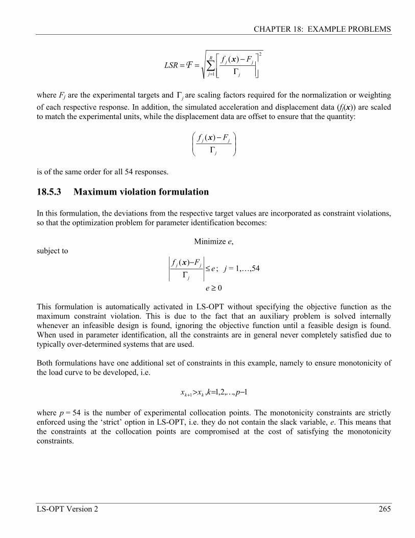
CHAPTER 18: EXAMPLE PROBLEMS
LS-OPT Version 2 265
∑=
Γ−
==R
j j
jj FfLSR
1
2)(xF
where Fj are the experimental targets and jΓ are scaling factors required for the normalization or weighting of each respective response. In addition, the simulated acceleration and displacement data (fj(x)) are scaled to match the experimental units, while the displacement data are offset to ensure that the quantity:
Γ−
j
jj Ff )(x
is of the same order for all 54 responses. 18.5.3 Maximum violation formulation In this formulation, the deviations from the respective target values are incorporated as constraint violations, so that the optimization problem for parameter identification becomes:
Minimize e, subject to
eFf
j
jj ≤Γ
−)(x; j = 1,…,54
e ≥ 0
This formulation is automatically activated in LS-OPT without specifying the objective function as the maximum constraint violation. This is due to the fact that an auxiliary problem is solved internally whenever an infeasible design is found, ignoring the objective function until a feasible design is found. When used in parameter identification, all the constraints are in general never completely satisfied due to typically over-determined systems that are used. Both formulations have one additional set of constraints in this example, namely to ensure monotonicity of the load curve to be developed, i.e.
1,,2,1,1 −=>+ pkxx kk K where p = 54 is the number of experimental collocation points. The monotonicity constraints are strictly enforced using the ‘strict’ option in LS-OPT, i.e. they do not contain the slack variable, e. This means that the constraints at the collocation points are compromised at the cost of satisfying the monotonicity constraints.

CHAPTER 18: EXAMPLE PROBLEMS
266 LS-OPT Version 2
18.5.4 Implementation The LS-OPT input files for this problem are shown below: LSR formulation (10 design variables): Note the use of a Targeted Composite for the objective (‘Residual’). The initial leakage curve is horizontal. The two LS-DYNA solvers (4MPS and 5MPS) with input decks (sim4mpros.inp and sim5mpros.inp) refer to the two cases, i.e., 4 and 5 m.s-1 approach velocity, respectively. "Parameter Estimation (Airbag) (10 variables)"$ Created on Thu Aug 30 17:16:28 2001$$ DESIGN VARIABLES$variables 10Variable 'Leakage_1' 6e-08Lower bound variable 'Leakage_1' 2e-08Upper bound variable 'Leakage_1' 4e-07Range 'Leakage_1' 1e-07
Variable 'Leakage_2' 6e-08Lower bound variable 'Leakage_2' 2e-08Upper bound variable 'Leakage_2' 4e-07Range 'Leakage_2' 1e-07
Variable 'Leakage_3' 6e-08Lower bound variable 'Leakage_3' 2e-08Upper bound variable 'Leakage_3' 4e-07Range 'Leakage_3' 1e-07
Variable 'Leakage_4' 6e-08Lower bound variable 'Leakage_4' 2e-08Upper bound variable 'Leakage_4' 4e-07Range 'Leakage_4' 1e-07
Variable 'Leakage_5' 6e-08Lower bound variable 'Leakage_5' 2e-08Upper bound variable 'Leakage_5' 4e-07Range 'Leakage_5' 1e-07
Variable 'Leakage_6' 6e-08Lower bound variable 'Leakage_6' 2e-08Upper bound variable 'Leakage_6' 4e-07Range 'Leakage_6' 1e-07
Variable 'Leakage_7' 6e-08Lower bound variable 'Leakage_7' 2e-08Upper bound variable 'Leakage_7' 4e-07Range 'Leakage_7' 1e-07
Variable 'Leakage_8' 6e-08Lower bound variable 'Leakage_8' 2e-08Upper bound variable 'Leakage_8' 4e-07Range 'Leakage_8' 1e-07
Variable 'Leakage_9' 6e-08Lower bound variable 'Leakage_9' 2e-08Upper bound variable 'Leakage_9' 4e-07Range 'Leakage_9' 1e-07
Variable 'Leakage_10' 6e-08Lower bound variable 'Leakage_10' 2e-08
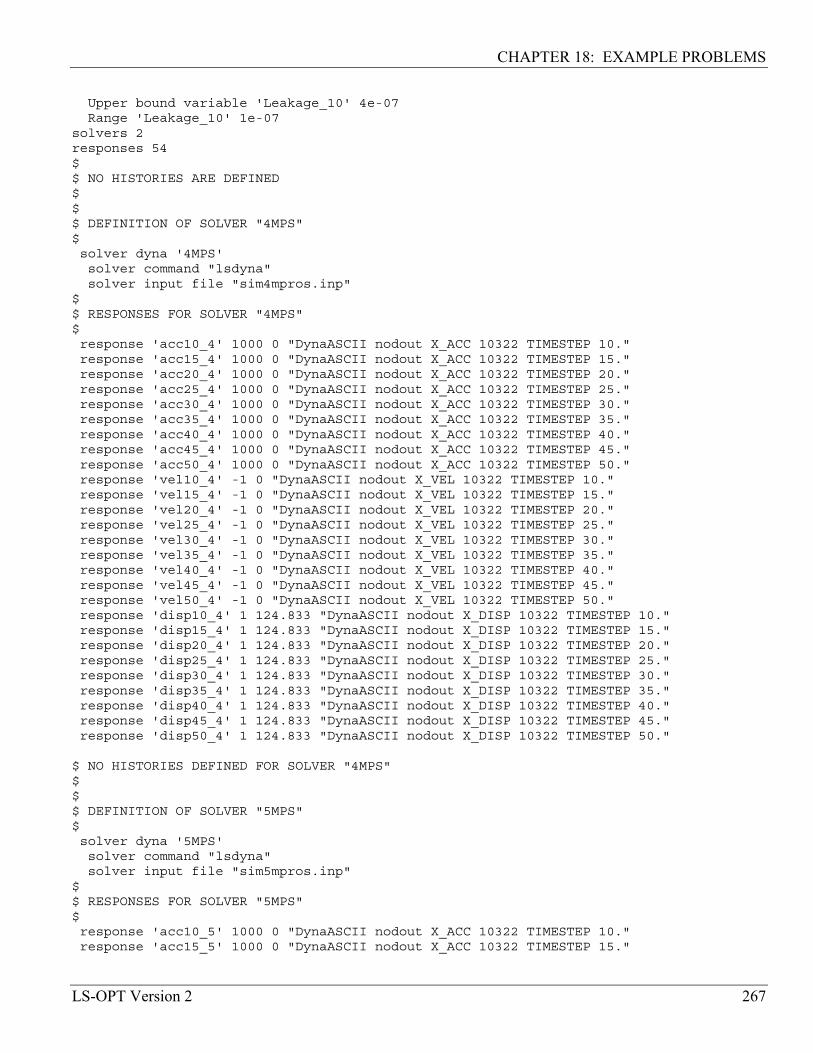
CHAPTER 18: EXAMPLE PROBLEMS
LS-OPT Version 2 267
Upper bound variable 'Leakage_10' 4e-07Range 'Leakage_10' 1e-07
solvers 2responses 54$$ NO HISTORIES ARE DEFINED$$$ DEFINITION OF SOLVER "4MPS"$solver dyna '4MPS'solver command "lsdyna"solver input file "sim4mpros.inp"
$$ RESPONSES FOR SOLVER "4MPS"$response 'acc10_4' 1000 0 "DynaASCII nodout X_ACC 10322 TIMESTEP 10."response 'acc15_4' 1000 0 "DynaASCII nodout X_ACC 10322 TIMESTEP 15."response 'acc20_4' 1000 0 "DynaASCII nodout X_ACC 10322 TIMESTEP 20."response 'acc25_4' 1000 0 "DynaASCII nodout X_ACC 10322 TIMESTEP 25."response 'acc30_4' 1000 0 "DynaASCII nodout X_ACC 10322 TIMESTEP 30."response 'acc35_4' 1000 0 "DynaASCII nodout X_ACC 10322 TIMESTEP 35."response 'acc40_4' 1000 0 "DynaASCII nodout X_ACC 10322 TIMESTEP 40."response 'acc45_4' 1000 0 "DynaASCII nodout X_ACC 10322 TIMESTEP 45."response 'acc50_4' 1000 0 "DynaASCII nodout X_ACC 10322 TIMESTEP 50."response 'vel10_4' -1 0 "DynaASCII nodout X_VEL 10322 TIMESTEP 10."response 'vel15_4' -1 0 "DynaASCII nodout X_VEL 10322 TIMESTEP 15."response 'vel20_4' -1 0 "DynaASCII nodout X_VEL 10322 TIMESTEP 20."response 'vel25_4' -1 0 "DynaASCII nodout X_VEL 10322 TIMESTEP 25."response 'vel30_4' -1 0 "DynaASCII nodout X_VEL 10322 TIMESTEP 30."response 'vel35_4' -1 0 "DynaASCII nodout X_VEL 10322 TIMESTEP 35."response 'vel40_4' -1 0 "DynaASCII nodout X_VEL 10322 TIMESTEP 40."response 'vel45_4' -1 0 "DynaASCII nodout X_VEL 10322 TIMESTEP 45."response 'vel50_4' -1 0 "DynaASCII nodout X_VEL 10322 TIMESTEP 50."response 'disp10_4' 1 124.833 "DynaASCII nodout X_DISP 10322 TIMESTEP 10."response 'disp15_4' 1 124.833 "DynaASCII nodout X_DISP 10322 TIMESTEP 15."response 'disp20_4' 1 124.833 "DynaASCII nodout X_DISP 10322 TIMESTEP 20."response 'disp25_4' 1 124.833 "DynaASCII nodout X_DISP 10322 TIMESTEP 25."response 'disp30_4' 1 124.833 "DynaASCII nodout X_DISP 10322 TIMESTEP 30."response 'disp35_4' 1 124.833 "DynaASCII nodout X_DISP 10322 TIMESTEP 35."response 'disp40_4' 1 124.833 "DynaASCII nodout X_DISP 10322 TIMESTEP 40."response 'disp45_4' 1 124.833 "DynaASCII nodout X_DISP 10322 TIMESTEP 45."response 'disp50_4' 1 124.833 "DynaASCII nodout X_DISP 10322 TIMESTEP 50."
$ NO HISTORIES DEFINED FOR SOLVER "4MPS"$$$ DEFINITION OF SOLVER "5MPS"$solver dyna '5MPS'solver command "lsdyna"solver input file "sim5mpros.inp"
$$ RESPONSES FOR SOLVER "5MPS"$response 'acc10_5' 1000 0 "DynaASCII nodout X_ACC 10322 TIMESTEP 10."response 'acc15_5' 1000 0 "DynaASCII nodout X_ACC 10322 TIMESTEP 15."

CHAPTER 18: EXAMPLE PROBLEMS
268 LS-OPT Version 2
response 'acc20_5' 1000 0 "DynaASCII nodout X_ACC 10322 TIMESTEP 20."response 'acc25_5' 1000 0 "DynaASCII nodout X_ACC 10322 TIMESTEP 25."response 'acc30_5' 1000 0 "DynaASCII nodout X_ACC 10322 TIMESTEP 30."response 'acc35_5' 1000 0 "DynaASCII nodout X_ACC 10322 TIMESTEP 35."response 'acc40_5' 1000 0 "DynaASCII nodout X_ACC 10322 TIMESTEP 40."response 'acc45_5' 1000 0 "DynaASCII nodout X_ACC 10322 TIMESTEP 45."response 'acc50_5' 1000 0 "DynaASCII nodout X_ACC 10322 TIMESTEP 50."response 'vel10_5' -1 0 "DynaASCII nodout X_VEL 10322 TIMESTEP 10."response 'vel15_5' -1 0 "DynaASCII nodout X_VEL 10322 TIMESTEP 15."response 'vel20_5' -1 0 "DynaASCII nodout X_VEL 10322 TIMESTEP 20."response 'vel25_5' -1 0 "DynaASCII nodout X_VEL 10322 TIMESTEP 25."response 'vel30_5' -1 0 "DynaASCII nodout X_VEL 10322 TIMESTEP 30."response 'vel35_5' -1 0 "DynaASCII nodout X_VEL 10322 TIMESTEP 35."response 'vel40_5' -1 0 "DynaASCII nodout X_VEL 10322 TIMESTEP 40."response 'vel45_5' -1 0 "DynaASCII nodout X_VEL 10322 TIMESTEP 45."response 'vel50_5' -1 0 "DynaASCII nodout X_VEL 10322 TIMESTEP 50."response 'disp10_5' 1 140.841 "DynaASCII nodout X_DISP 10322 TIMESTEP 10."response 'disp15_5' 1 140.841 "DynaASCII nodout X_DISP 10322 TIMESTEP 15."response 'disp20_5' 1 140.841 "DynaASCII nodout X_DISP 10322 TIMESTEP 20."response 'disp25_5' 1 140.841 "DynaASCII nodout X_DISP 10322 TIMESTEP 25."response 'disp30_5' 1 140.841 "DynaASCII nodout X_DISP 10322 TIMESTEP 30."response 'disp35_5' 1 140.841 "DynaASCII nodout X_DISP 10322 TIMESTEP 35."response 'disp40_5' 1 140.841 "DynaASCII nodout X_DISP 10322 TIMESTEP 40."response 'disp45_5' 1 140.841 "DynaASCII nodout X_DISP 10322 TIMESTEP 45."response 'disp50_5' 1 140.841 "DynaASCII nodout X_DISP 10322 TIMESTEP 50."
$$ NO HISTORIES DEFINED FOR SOLVER "5MPS"$$$ HISTORIES AND RESPONSES DEFINED BY EXPRESSIONS$composites 10composite 'Residual' type targetedcomposite 'Residual' response 'acc10_4' 44.9417 scale 100composite 'Residual' response 'acc15_4' 75.4247 scale 100composite 'Residual' response 'acc20_4' 118.58 scale 100composite 'Residual' response 'acc25_4' 176.239 scale 100composite 'Residual' response 'acc30_4' 221.678 scale 100composite 'Residual' response 'acc35_4' 227.923 scale 100composite 'Residual' response 'acc40_4' 182.374 scale 100composite 'Residual' response 'acc45_4' 121.8 scale 100composite 'Residual' response 'acc50_4' 72.7288 scale 100composite 'Residual' response 'vel10_4' 3.49244 scale 1composite 'Residual' response 'vel15_4' 3.19588 scale 1composite 'Residual' response 'vel20_4' 2.71324 scale 1composite 'Residual' response 'vel25_4' 1.9779 scale 1composite 'Residual' response 'vel30_4' 0.973047 scale 1composite 'Residual' response 'vel35_4' -0.169702 scale 1composite 'Residual' response 'vel40_4' -1.21011 scale 1composite 'Residual' response 'vel45_4' -1.97152 scale 1composite 'Residual' response 'vel50_4' -2.44973 scale 1composite 'Residual' response 'disp10_4' 88.0516 scale 100composite 'Residual' response 'disp15_4' 71.2695 scale 100composite 'Residual' response 'disp20_4' 56.4066 scale 100composite 'Residual' response 'disp25_4' 44.5582 scale 100composite 'Residual' response 'disp30_4' 37.0841 scale 100composite 'Residual' response 'disp35_4' 35.0629 scale 100

CHAPTER 18: EXAMPLE PROBLEMS
LS-OPT Version 2 269
composite 'Residual' response 'disp40_4' 38.6093 scale 100composite 'Residual' response 'disp45_4' 46.6906 scale 100composite 'Residual' response 'disp50_4' 57.8468 scale 100composite 'Residual' response 'acc10_5' 72.3756 scale 100composite 'Residual' response 'acc15_5' 97.7004 scale 100composite 'Residual' response 'acc20_5' 168.931 scale 100composite 'Residual' response 'acc25_5' 264.071 scale 100composite 'Residual' response 'acc30_5' 311.405 scale 100composite 'Residual' response 'acc35_5' 244.28 scale 100composite 'Residual' response 'acc40_5' 130.942 scale 100composite 'Residual' response 'acc45_5' 51.7805 scale 100composite 'Residual' response 'acc50_5' 12.3231 scale 100composite 'Residual' response 'vel10_5' 4.705 scale 1composite 'Residual' response 'vel15_5' 4.24697 scale 1composite 'Residual' response 'vel20_5' 3.59243 scale 1composite 'Residual' response 'vel25_5' 2.51584 scale 1composite 'Residual' response 'vel30_5' 1.03072 scale 1composite 'Residual' response 'vel35_5' -0.393792 scale 1composite 'Residual' response 'vel40_5' -1.33087 scale 1composite 'Residual' response 'vel45_5' -1.76819 scale 1composite 'Residual' response 'vel50_5' -1.91663 scale 1composite 'Residual' response 'disp10_5' 91.7493 scale 100composite 'Residual' response 'disp15_5' 69.4946 scale 100composite 'Residual' response 'disp20_5' 49.7515 scale 100composite 'Residual' response 'disp25_5' 34.2808 scale 100composite 'Residual' response 'disp30_5' 25.3116 scale 100composite 'Residual' response 'disp35_5' 23.8644 scale 100composite 'Residual' response 'disp40_5' 28.4147 scale 100composite 'Residual' response 'disp45_5' 36.3297 scale 100composite 'Residual' response 'disp50_5' 45.6215 scale 100
composite 'C1' type weightedcomposite 'C1' variable 'Leakage_1' -1 scale 1e-07composite 'C1' variable 'Leakage_2' 1 scale 1e-07
composite 'C2' type weightedcomposite 'C2' variable 'Leakage_2' -1 scale 1e-07composite 'C2' variable 'Leakage_3' 1 scale 1e-07
composite 'C3' type weightedcomposite 'C3' variable 'Leakage_3' -1 scale 1e-07composite 'C3' variable 'Leakage_4' 1 scale 1e-07
composite 'C4' type weightedcomposite 'C4' variable 'Leakage_4' -1 scale 1e-07composite 'C4' variable 'Leakage_5' 1 scale 1e-07
composite 'C5' type weightedcomposite 'C5' variable 'Leakage_5' -1 scale 1e-07composite 'C5' variable 'Leakage_6' 1 scale 1e-07
composite 'C6' type weightedcomposite 'C6' variable 'Leakage_6' -1 scale 1e-07composite 'C6' variable 'Leakage_7' 1 scale 1e-07
composite 'C7' type weightedcomposite 'C7' variable 'Leakage_7' -1 scale 1e-07composite 'C7' variable 'Leakage_8' 1 scale 1e-07
composite 'C8' type weightedcomposite 'C8' variable 'Leakage_8' -1 scale 1e-07composite 'C8' variable 'Leakage_9' 1 scale 1e-07
composite 'C9' type weightedcomposite 'C9' variable 'Leakage_9' -1 scale 1e-07composite 'C9' variable 'Leakage_10' 1 scale 1e-07

CHAPTER 18: EXAMPLE PROBLEMS
270 LS-OPT Version 2
$$ OBJECTIVE FUNCTIONS$objectives 1objective 'Residual' 1
$$ CONSTRAINT DEFINITIONS$constraints 9move
constraint 'C1'lower bound constraint 'C1' 0
constraint 'C2'lower bound constraint 'C2' 0
constraint 'C3'lower bound constraint 'C3' 0
constraint 'C4'lower bound constraint 'C4' 0
constraint 'C5'lower bound constraint 'C5' 0
constraint 'C6'lower bound constraint 'C6' 0
constraint 'C7'lower bound constraint 'C7' 0
constraint 'C8'lower bound constraint 'C8' 0
constraint 'C9'lower bound constraint 'C9' 0
$$ EXPERIMENTAL DESIGN$Order linearExperimental design doptBasis experiment 3toKNumber experiment 17
$$ JOB INFO$concurrent jobs 9iterate param design 0.01iterate param objective 0.01iterate 20
STOP

CHAPTER 18: EXAMPLE PROBLEMS
LS-OPT Version 2 271
Maximum violation formulation (5 design variables): The LS-OPT input file is the same for this formulation as before for all sections but the constraints. As the formulation is driven by the violation of the constraints, they are defined as equality constraints (identical upper and lower bounds). In addition, the monotonicity constraints are defined as hard by using the ‘strict’ option: $$ CONSTRAINT DEFINITIONS$constraints 58constraint 'acc10_4'lower bound constraint 'acc10_4' 0.449417upper bound constraint 'acc10_4' 0.449417
constraint 'acc15_4'lower bound constraint 'acc15_4' 0.754247upper bound constraint 'acc15_4' 0.754247
constraint 'acc20_4'lower bound constraint 'acc20_4' 1.1858upper bound constraint 'acc20_4' 1.1858
constraint 'acc25_4'lower bound constraint 'acc25_4' 1.76239upper bound constraint 'acc25_4' 1.76239
constraint 'acc30_4'lower bound constraint 'acc30_4' 2.21678upper bound constraint 'acc30_4' 2.21678
constraint 'acc35_4'lower bound constraint 'acc35_4' 2.27923upper bound constraint 'acc35_4' 2.27923
constraint 'acc40_4'lower bound constraint 'acc40_4' 1.82374upper bound constraint 'acc40_4' 1.82374
constraint 'acc45_4'lower bound constraint 'acc45_4' 1.218upper bound constraint 'acc45_4' 1.218
constraint 'acc50_4'lower bound constraint 'acc50_4' 0.727288upper bound constraint 'acc50_4' 0.727288
constraint 'vel10_4'lower bound constraint 'vel10_4' 3.49244upper bound constraint 'vel10_4' 3.49244
constraint 'vel15_4'lower bound constraint 'vel15_4' 3.19588upper bound constraint 'vel15_4' 3.19588
constraint 'vel20_4'lower bound constraint 'vel20_4' 2.71324upper bound constraint 'vel20_4' 2.71324
constraint 'vel25_4'lower bound constraint 'vel25_4' 1.9779upper bound constraint 'vel25_4' 1.9779
constraint 'vel30_4'lower bound constraint 'vel30_4' 0.973047upper bound constraint 'vel30_4' 0.973047
constraint 'vel35_4'lower bound constraint 'vel35_4' -0.169702upper bound constraint 'vel35_4' -0.169702

CHAPTER 18: EXAMPLE PROBLEMS
272 LS-OPT Version 2
constraint 'vel40_4'lower bound constraint 'vel40_4' -1.21011upper bound constraint 'vel40_4' -1.21011
constraint 'vel45_4'lower bound constraint 'vel45_4' -1.97152upper bound constraint 'vel45_4' -1.97152
constraint 'vel50_4'lower bound constraint 'vel50_4' -2.44973upper bound constraint 'vel50_4' -2.44973
constraint 'disp10_4'lower bound constraint 'disp10_4' 0.880516upper bound constraint 'disp10_4' 0.880516
constraint 'disp15_4'lower bound constraint 'disp15_4' 0.712695upper bound constraint 'disp15_4' 0.712695
constraint 'disp20_4'lower bound constraint 'disp20_4' 0.564066upper bound constraint 'disp20_4' 0.564066
constraint 'disp25_4'lower bound constraint 'disp25_4' 0.445582upper bound constraint 'disp25_4' 0.445582
constraint 'disp30_4'lower bound constraint 'disp30_4' 0.370841upper bound constraint 'disp30_4' 0.370841
constraint 'disp35_4'lower bound constraint 'disp35_4' 0.350629upper bound constraint 'disp35_4' 0.350629
constraint 'disp40_4'lower bound constraint 'disp40_4' 0.386093upper bound constraint 'disp40_4' 0.386093
constraint 'disp45_4'lower bound constraint 'disp45_4' 0.466906upper bound constraint 'disp45_4' 0.466906
constraint 'disp50_4'lower bound constraint 'disp50_4' 0.578468upper bound constraint 'disp50_4' 0.578468
constraint 'acc10_5'lower bound constraint 'acc10_5' 0.723756upper bound constraint 'acc10_5' 0.723756
constraint 'acc15_5'lower bound constraint 'acc15_5' 0.977004upper bound constraint 'acc15_5' 0.977004
constraint 'acc20_5'lower bound constraint 'acc20_5' 1.68931upper bound constraint 'acc20_5' 1.68931
constraint 'acc25_5'lower bound constraint 'acc25_5' 2.64071upper bound constraint 'acc25_5' 2.64071
constraint 'acc30_5'lower bound constraint 'acc30_5' 3.11405upper bound constraint 'acc30_5' 3.11405
constraint 'acc35_5'lower bound constraint 'acc35_5' 2.4428upper bound constraint 'acc35_5' 2.4428
constraint 'acc40_5'lower bound constraint 'acc40_5' 1.30942upper bound constraint 'acc40_5' 1.30942

CHAPTER 18: EXAMPLE PROBLEMS
LS-OPT Version 2 273
constraint 'acc45_5'lower bound constraint 'acc45_5' 0.517805upper bound constraint 'acc45_5' 0.517805
constraint 'acc50_5'lower bound constraint 'acc50_5' 0.123231upper bound constraint 'acc50_5' 0.123231
constraint 'vel10_5'lower bound constraint 'vel10_5' 4.705upper bound constraint 'vel10_5' 4.705
constraint 'vel15_5'lower bound constraint 'vel15_5' 4.24697upper bound constraint 'vel15_5' 4.24697
constraint 'vel20_5'lower bound constraint 'vel20_5' 3.59243upper bound constraint 'vel20_5' 3.59243
constraint 'vel25_5'lower bound constraint 'vel25_5' 2.51584upper bound constraint 'vel25_5' 2.51584
constraint 'vel30_5'lower bound constraint 'vel30_5' 1.03072upper bound constraint 'vel30_5' 1.03072
constraint 'vel35_5'lower bound constraint 'vel35_5' -0.393792upper bound constraint 'vel35_5' -0.393792
constraint 'vel40_5'lower bound constraint 'vel40_5' -1.33087upper bound constraint 'vel40_5' -1.33087
constraint 'vel45_5'lower bound constraint 'vel45_5' -1.76819upper bound constraint 'vel45_5' -1.76819
constraint 'vel50_5'lower bound constraint 'vel50_5' -1.91663upper bound constraint 'vel50_5' -1.91663
constraint 'disp10_5'lower bound constraint 'disp10_5' 0.917493upper bound constraint 'disp10_5' 0.917493
constraint 'disp15_5'lower bound constraint 'disp15_5' 0.694946upper bound constraint 'disp15_5' 0.694946
constraint 'disp20_5'lower bound constraint 'disp20_5' 0.497515upper bound constraint 'disp20_5' 0.497515
constraint 'disp25_5'lower bound constraint 'disp25_5' 0.342808upper bound constraint 'disp25_5' 0.342808
constraint 'disp30_5'lower bound constraint 'disp30_5' 0.253116upper bound constraint 'disp30_5' 0.253116
constraint 'disp35_5'lower bound constraint 'disp35_5' 0.238644upper bound constraint 'disp35_5' 0.238644
constraint 'disp40_5'lower bound constraint 'disp40_5' 0.284147upper bound constraint 'disp40_5' 0.284147
constraint 'disp45_5'lower bound constraint 'disp45_5' 0.363297upper bound constraint 'disp45_5' 0.363297

CHAPTER 18: EXAMPLE PROBLEMS
274 LS-OPT Version 2
constraint 'disp50_5'lower bound constraint 'disp50_5' 0.456215upper bound constraint 'disp50_5' 0.456215move
constraint 'C1'strictlower bound constraint 'C1' 0
constraint 'C2'lower bound constraint 'C2' 0
constraint 'C3'lower bound constraint 'C3' 0
constraint 'C4'lower bound constraint 'C4' 0
$$ EXPERIMENTAL DESIGN$Order linearExperimental design doptBasis experiment 3toKNumber experiment 10
$$ JOB INFO$concurrent jobs 10iterate param design 0.001iterate param objective 0.001iterate 20
STOP
The residual is retained in the formulation as the objective although it is not used in the optimization process. This is so that the residual can be monitored, and used for comparison with the LSR formulation results. 18.5.5 Results The result of the optimization is shown in Figure 18-27. Shown are the leakage curves for a 5 and 10-variable model. It can be seen that the introduction of more points on the leakage curve allows more resolution in the low-pressure range of the material model.

CHAPTER 18: EXAMPLE PROBLEMS
LS-OPT Version 2 275
Figure 18-27: Leakage curve: Airbag material identification
As an example, the matching between the experimental and simulated acceleration, velocity and displacement is depicted for both 4 and 5m/s chest form velocities in Figure 18-28 for the 10-variable LSR Formulation case. It can be seen that the displacement and velocity curves are closely matched by the optimum curve parameters, and that the discrepancy as exhibited by the residual is mainly due to the acceleration curve not being matched exactly.

CHAPTER 18: EXAMPLE PROBLEMS
276 LS-OPT Version 2
a) Chest form velocity = 4m/s b) Chest form velocity = 5m/s
Figure 18-28: Comparison of experimental and computational displacement, velocity and acceleration results – 10 variables, Formulation 2 (LSR) – Airbag material identification
The optimization history of the objective (residual) and of one of the variables are shown in Figure 18-29 and Figure 18-30, respectively. In Figure 18-29, it can be seen that the case with less design variables converges more rapidly, while the activation of first the panning, and secondly the zooming heuristic in LS-OPT is clearly evident in the optimization history of the variable Leakage_5 (Figure 18-30).
Figure 18-29: Optimization history: Residual (LSR Formulation)
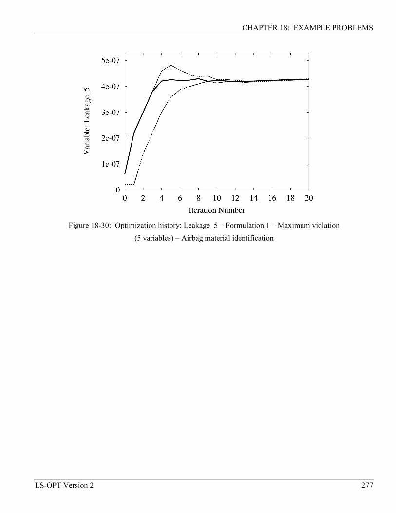
CHAPTER 18: EXAMPLE PROBLEMS
LS-OPT Version 2 277
Figure 18-30: Optimization history: Leakage_5 – Formulation 1 – Maximum violation
(5 variables) – Airbag material identification

CHAPTER 18: EXAMPLE PROBLEMS
278 LS-OPT Version 2
18.6 Small car crash and NVH (MDO) (5 variables) This example has the following features: • LS-DYNA is used for both explicit crash and implicit NVH simulations. • Variable screening is performed. • Multidisciplinary design optimization (MDO) is illustrated with a simple example. • Mode tracking is used. • The standard LS-DYNA interface is used to extract the results. 18.6.1 Parameterization and Variable screening To illustrate a relatively simple example of multidisciplinary design optimization (MDO), the small car of Section 18.2 is extended to have five variables. In addition, one Noise, Vibration and Harshness (NVH) parameter is considered as a constraint, i.e. the first torsional vibrational mode frequency. Figure 18-31 shows the modified small car. Rails are added, and the combined bumper-hood section is separated into a grill, hood and bumper. The mass of the affected components in the initial design is 1.328 units while the torsional mode frequency is 2.281Hz. This corresponds to mode number 15. The Head Injury Criterion (HIC) based on a 15ms interval is initially 17500. The initial intrusion of the bumper is 531 mm.
Hood thickness Grill thickness
Bumper thickness
Roof thickness
Rail_front thickness
Rail_backthickness
Figure 18-31: Small car with crash rails – definition of design variables

CHAPTER 18: EXAMPLE PROBLEMS
LS-OPT Version 2 279
The optimization problem is defined as follows:
Minimize Mass(xcrash) subject to HIC(xcrash) < 900 Intrusion(xcrash) < 500mm Torsional mode frequency(xNVH) > 3Hz where xcrash = (t_hood, t_bumper, t_rail_back, t_rail_front, t_roof) and xNVH = (t_hood). These variables were selected by first conducting an LS-OPT run in which all five variables were included for both crash and NVH (linear response surfaces). Figure 18-32 shows the ANOVA charts produced from these results using the Viewer. Using these charts, all five variables were selected for crash while only t_hood was kept for NVH. Note that, in this first iteration, there is a significant error in the intrusion prediction while mass has no error because of its linearity.
0.1 0.2 0.3 0.4 0.5 0.6 0.7 0.8 0.9
t_rail_back
t_hood
t_bumper
t_roof
t_rail_front
ANOVA Plot for Mass(Lower half of 90% confidence interval in red)
(a) (b)
(c) (d)
Figure 18-32: ANOVA plots for small car response

CHAPTER 18: EXAMPLE PROBLEMS
280 LS-OPT Version 2
18.6.2 MDO with D-optimal experimental design and SRSM The LS-OPT input file below illustrates how the variables were reduced for the NVH solver. Note how the two solvers, i.e., crash and NVH, are specified. Variables are flagged as local with the Local variable_name statement, and then linked to a solver using the Solver variablevariable_name command. "Small Car Problem: Five variables: Partial variables Crash-NVH MDF"$ Created on Sun Jan 5 16:12:00 2003solvers 2responses 8$$ NO HISTORIES ARE DEFINED$$ DESIGN VARIABLES$variables 5Variable 't_rail_back' 2Lower bound variable 't_rail_back' 1Upper bound variable 't_rail_back' 6Range 't_rail_back' 2Local 't_rail_back'
Variable 't_hood' 2Lower bound variable 't_hood' 1Upper bound variable 't_hood' 6Range 't_hood' 2
Variable 't_bumper' 3Lower bound variable 't_bumper' 1Upper bound variable 't_bumper' 6Range 't_bumper' 2Local 't_bumper'
Variable 't_roof' 2Lower bound variable 't_roof' 1Upper bound variable 't_roof' 6Range 't_roof' 2Local 't_roof'
Variable 't_rail_front' 5Lower bound variable 't_rail_front' 1Upper bound variable 't_rail_front' 6Range 't_rail_front' 2Local 't_rail_front'
$$$$$$$$$$$$$$$$$$$$$$$$$$$$$$$$$ SOLVER "CRASH"$$$$$$$$$$$$$$$$$$$$$$$$$$$$$$$$$$ DEFINITION OF SOLVER "CRASH"$solver dyna960 'CRASH'solver command "lsdyna.single"solver input file "car6_crash.k"solver order linearsolver experiment design doptsolver basis experiment 3toK

CHAPTER 18: EXAMPLE PROBLEMS
LS-OPT Version 2 281
solver concurrent jobs 1$$ LOCAL DESIGN VARIABLES FOR SOLVER "CRASH"$
solver variable 't_rail_back'solver variable 't_bumper'solver variable 't_roof'solver variable 't_rail_front'
$$ RESPONSES FOR SOLVER "CRASH"$response 'Acc_max' 1 0 "DynaASCII Nodout X_ACC 432 Max SAE 60"response 'Mass' 1 0 "DynaMass 2 3 4 5 6 7 MASS"response 'Intru_2' 1 0 "DynaASCII Nodout X_DISP 432 Timestep"response 'Intru_1' 1 0 "DynaASCII Nodout X_DISP 184 Timestep"response 'HIC' 1 0 "DynaASCII Nodout HIC15 9810. 1 432"
$$$$$$$$$$$$$$$$$$$$$$$$$$$$$$$$$ SOLVER "NVH"$$$$$$$$$$$$$$$$$$$$$$$$$$$$$$$$$$ DEFINITION OF SOLVER "NVH"$solver dyna960 'NVH'solver command "lsdyna.double"solver input file "car6_NVH.k"solver order linearsolver experiment design doptsolver basis experiment 5toKsolver concurrent jobs 1
$$ RESPONSES FOR SOLVER "NVH"$response 'Frequency' 1 0 "DynaFreq 15 FREQ"response 'Mode' 1 0 "DynaFreq 15 NUMBER"response 'Generalized_Mass' 1 0 "DynaFreq 15 GENMASS"
composites 4$$ COMPOSITE RESPONSES$composite 'Intrusion' type weightedcomposite 'Intrusion' response 'Intru_2' -1 scale 1composite 'Intrusion' response 'Intru_1' 1 scale 1
composite 'HIC_scaled' type targetedcomposite 'HIC_scaled' response 'HIC' 0 scale 900weight 1
composite 'Freq_scaled' type targetedcomposite 'Freq_scaled' response 'Frequency' 0 scale 3weight 1
$$ COMPOSITE EXPRESSIONS$composite 'Intrusion_scaled' {Intrusion/500}
$$ OBJECTIVE FUNCTIONS$objectives 1

CHAPTER 18: EXAMPLE PROBLEMS
282 LS-OPT Version 2
objective 'Mass' 1$$ CONSTRAINT DEFINITIONS$constraints 3constraint 'HIC_scaled'upper bound constraint 'HIC_scaled' 1
constraint 'Freq_scaled'lower bound constraint 'Freq_scaled' 1
constraint 'Intrusion_scaled'upper bound constraint 'Intrusion_scaled' 1
$$ JOB INFO$iterate param design 0.01iterate param objective 0.01iterate param stoppingtype anditerate 10
STOP
The optimization results are shown in Figure 18-33 for the objective, three constraints, mode sequence number and maximum constraint violation. The initial design is infeasible due to too high a HIC value, too high an intrusion and too low a torsional frequency. To meet all these constraints, the mass of the affected components has to increase substantially. Convergence is obtained at about the 8th iteration, and when the optimization terminates, a 0.0003 violation in the scaled constraints remains. The mode tracking feature in LS-DYNA is used to keep track of the frequency mode (Figure 18-33(e)). Note that the mode number changes from 15 to 18.

CHAPTER 18: EXAMPLE PROBLEMS
LS-OPT Version 2 283
a) Objective (Mass) b) HIC
c) Torsional mode frequency
d) Intrusion

CHAPTER 18: EXAMPLE PROBLEMS
284 LS-OPT Version 2
e) Mode sequence f) Maximum constraint violation
Figure 18-33: Optimization histories (Small car MDO) – D-optimal (SRSM)

CHAPTER 18: EXAMPLE PROBLEMS
LS-OPT Version 2 285
18.6.3 Sequential random search The small car crash design problem was also optimized using the Sequential Random Search procedure described in Section 2.13. Because of the multidisciplinary nature of the problem, all the variables were selected to be fully shared. The design points for the NVH discipline were forced to be coincident with the points of the crash discipline (see Section 10.7). The number of simulations per iteration is 16. The input file is therefore as follows: "Small Car Problem: Five variables: Partial variables Crash-NVH MDF"$ Created on Tue Feb 4 17:27:53 2003solvers 2responses 8$$ NO HISTORIES ARE DEFINED$$$ DESIGN VARIABLES$variables 5Variable 't_rail_back' 2Lower bound variable 't_rail_back' 1Upper bound variable 't_rail_back' 6Range 't_rail_back' 2
Variable 't_hood' 2Lower bound variable 't_hood' 1Upper bound variable 't_hood' 6Range 't_hood' 2
Variable 't_bumper' 3Lower bound variable 't_bumper' 1Upper bound variable 't_bumper' 6Range 't_bumper' 2
Variable 't_roof' 2Lower bound variable 't_roof' 1Upper bound variable 't_roof' 6Range 't_roof' 2
Variable 't_rail_front' 5Lower bound variable 't_rail_front' 1Upper bound variable 't_rail_front' 6Range 't_rail_front' 2
$$ SEQUENTIAL RANDOM SEARCH$optimization method randomsearch$$$$$$$$$$$$$$$$$$$$$$$$$$$$$$$$$$ SOLVER "CRASH"$$$$$$$$$$$$$$$$$$$$$$$$$$$$$$$$$$ DEFINITION OF SOLVER "CRASH"$solver dyna960 'CRASH'solver command "ls970.single"solver input file "car6_crash.k"

CHAPTER 18: EXAMPLE PROBLEMS
286 LS-OPT Version 2
solver experiment design latin_hypercubesolver number experiments 16solver concurrent jobs 1
$$ RESPONSES FOR SOLVER "CRASH"$response 'Acc_max' 1 0 "DynaASCII Nodout X_ACC 432 Max SAE 60"response 'Mass' 1 0 "DynaMass 2 3 4 5 6 7 MASS"response 'Intru_2' 1 0 "DynaASCII Nodout X_DISP 432 Timestep"response 'Intru_1' 1 0 "DynaASCII Nodout X_DISP 184 Timestep"response 'HIC' 1 0 "DynaASCII Nodout HIC15 9810. 1 432"
$$$$$$$$$$$$$$$$$$$$$$$$$$$$$$$$$ SOLVER "NVH"$$$$$$$$$$$$$$$$$$$$$$$$$$$$$$$$$$ DEFINITION OF SOLVER "NVH"$solver dyna960 'NVH'solver command "ls970.double"solver input file "car6_NVH.k"solver concurrent jobs 1solver experiment duplicate 'CRASH'
$$ RESPONSES FOR SOLVER "NVH"$response 'Frequency' 1 0 "DynaFreq 15 FREQ"response 'Mode' 1 0 "DynaFreq 15 NUMBER"response 'Generalized_Mass' 1 0 "DynaFreq 15 GENMASS"
composites 4$$ COMPOSITE RESPONSES$composite 'Intrusion' type weightedcomposite 'Intrusion' response 'Intru_2' -1 scale 1composite 'Intrusion' response 'Intru_1' 1 scale 1
composite 'HIC_scaled' type targetedcomposite 'HIC_scaled' response 'HIC' 0 scale 900weight 1
composite 'Freq_scaled' type targetedcomposite 'Freq_scaled' response 'Frequency' 0 scale 3weight 1
$$ COMPOSITE EXPRESSIONS$composite 'Intrusion_scaled' {Intrusion/500}
$$ OBJECTIVE FUNCTIONS$objectives 1objective 'Mass' 1
$$ CONSTRAINT DEFINITIONS$constraints 3constraint 'HIC_scaled'

CHAPTER 18: EXAMPLE PROBLEMS
LS-OPT Version 2 287
upper bound constraint 'HIC_scaled' 1constraint 'Freq_scaled'lower bound constraint 'Freq_scaled' 1
constraint 'Intrusion_scaled'upper bound constraint 'Intrusion_scaled' 1
$$ JOB INFO$iterate param design 0.001iterate param objective 0.001iterate param stoppingtype oriterate 40
STOP
The results are presented in Figure 18-34 (a) to (f). The random search method converges after approximately 105 crash + 105 NVH simulations (7 iterations) while the response surface approach requires about 60 crash + 30 NVH simulations (6 iterations). These numbers might vary because of the random nature of the methods involved. Note the effects of mode tracking in Figure 18-34 (e).
a) Objective (Mass) b) HIC
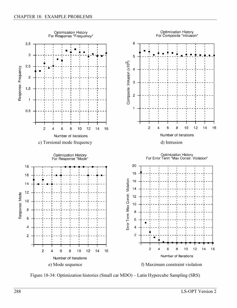
CHAPTER 18: EXAMPLE PROBLEMS
288 LS-OPT Version 2
c) Torsional mode frequency
d) Intrusion
e) Mode sequence f) Maximum constraint violation
Figure 18-34: Optimization histories (Small car MDO) – Latin Hypercube Sampling (SRS)

CHAPTER 18: EXAMPLE PROBLEMS
LS-OPT Version 2 289
18.7 Large car crash and NVH (MDO) (7 variables) (Example by courtesy of DaimlerChrysler) This example has the following features: • LS-DYNA is used for both explicit full frontal crash and implicit NVH simulations. • Multidisciplinary design optimization (MDO) is illustrated with a realistic full vehicle example. • Extraction is performed using standard LS-DYNA interfaces. This example illustrates a realistic application of Multidisciplinary Design Optimization (MDO) and concerns the coupling of the crash performance of a large vehicle with one of its Noise Vibration and Harshness (NVH) criteria, namely the torsional mode frequency [14]. The MDO formulation used is depicted in Figure 18-35.
System-level Optimizer Goal: Minimize Mass s.t. Crashworthiness and NVH constraints
Multidisciplinary Analyses
Crashworthiness analysis
NVH analysis
State variables
Design variables
Figure 18-35: Multidisciplinary feasible (MDF) MDO architecture
18.7.1 Modeling The crashworthiness simulation considers a model containing approximately 30 000 elements of a National Highway Transportation and Safety Association (NHTSA) vehicle [46] undergoing a full frontal impact. A modal analysis is performed on a so-called ‘body-in-white’ model containing approximately 18 000 elements. The crash model for the full vehicle is shown in Figure 18-36 for the undeformed and deformed (time = 78ms) states, and with only the structural components affected by the design variables, both in the undeformed and deformed (time = 72ms) states, in Figure 18-37. The NVH model is depicted in Figure 18-38 in the first torsion vibrational mode. Only body parts that are crucial to the vibrational mode shapes are retained in this model. The design variables are all thicknesses or gages of structural components in the

CHAPTER 18: EXAMPLE PROBLEMS
290
engine compartment of the vehicle (Figure 18-37), parameterized directly in the LS-DYNA input file. Twelve parts are affected, comprising aprons, rails, shotguns, cradle rails and the cradle cross member (Figure 18-37). LS-DYNA v.960 is used for both the crash and NVH simulations, in explicit and implicit modes respectively.
(a) (b)
Figure 18-36: Crash model of vehicle showing road and wall
(a) Undeformed (b) Deformed (78ms)
Left and rightapron Left and right
cradle rails
Shotgun outer and inner
Inner and outer rail
(a)
Figure 18-37: Structural co
(a) Undefor
Front cradle upper and lower cross members
LS-OPT Version 2
(b)
mponents affected by design variables –
med and (b) deformed (time = 72ms)

CHAPTER 18: EXAMPLE PROBLEMS
LS-OPT Version 2 291
Figure 18-38: Body-in-white model of vehicle in torsional vibration mode (38.7Hz)
18.7.2 Formulation of optimization problem To illustrate the effect of coupling between the disciplines, both full and partial sharing of the design variables are considered. In addition, different starting designs are considered in a limited investigation of the global optimality of the design. The optimization problem for the different starting designs considered is defined as follows: Minimize Mass subject to Maximum intrusion(xcrash) > 551.8mm
(Fully-shared variables) Maximum intrusion(xcrash) = 551.8mm (Partially-shared variables) Stage 1 pulse(xcrash) > 14.34g Stage 2 pulse(xcrash) > 17.57g Stage 3 pulse(xcrash) > 20.76g 37.77Hz < Torsional mode frequency(xNVH) < 39.77Hz (Fully-shared variables) 38.27Hz < Torsional mode frequency(xNVH) < 39.27Hz (Partially-shared variables)
Fully-shared variables: xcrash = xNVH = [rail_inner, rail_outer, cradle_rails, aprons, shotgun_inner, shotgun_outer, cradle_crossmember]T. Partially-shared variables – Starting design 1 (Baseline): xcrash = [rail_inner, rail_outer, cradle_rails, aprons, shotgun_inner, shotgun_outer]T; xNVH = [cradle_rails, shotgun_inner, shotgun_outer, cradle_crossmember]T.
CHAPTER 18: EXAMPLE PROBLEMS
292 LS-OPT Version 2
Partially-shared variables – Starting design 2 (Minimum weight): xcrash = [rail_inner, rail_outer, cradle_rails, aprons]T; xNVH = [cradle_rails, shotgun_inner, shotgun_outer, cradle_crossmember]T.
Partially-shared variables – Starting design 3 (Maximum weight): xcrash = [rail_inner, rail_outer, cradle_rails, aprons, shotgun_inner, shotgun_outer, cradle crossmember]T; xNVH = [cradle_rails, shotgun_inner, shotgun_outer, cradle_crossmember]T. The different variables set above were obtained by using ANOVA variable screening (Section 14.4). The Mass objective in each case incorporates all the components defined in Figure 18-37. The allowable torsional mode frequency band is reduced to 1Hz for the partially-shared cases to provide an optimum design that is more similar to the baseline. The three stage pulses are calculated from the SAE filtered (60Hz) acceleration and displacement of a left rear sill node in the following fashion: Stage i pulse = – k ∫ 2
1dd
d xa ; k = 0.5 for i = 1, 1.0 otherwise; with the limits (d1;d2) = (0;184); (184;334); (334;Max(displacement)) for i = 1,2,3 respectively, all displacement units in mm and the minus sign to convert acceleration to deceleration. The Stage 1 pulse is represented by a triangle with the peak value being the value used. The constraints are scaled using the target values to balance the violations of the different constraints. This scaling is only important in cases where multiple constraints are violated as in the current problem. 18.7.3 Implementation in LS-OPT The LS-OPT input file is given below. Note how the two disciplines (crash and NVH) are treated separately. Variables are flagged as local with the Local variable_name statement, and then linked to a solver using the Solver variable variable_name command. "Full Vehicle MDO : Crash and NVH"$$ DEFINITION OF MULTIDISCIPLINARY QUANTITIES$solvers 2variables 7responses 12histories 2composites 5$$ SHARED DESIGN VARIABLES$Variable 'cradle_rails' 1.93
Lower bound variable 'cradle_rails' 1Upper bound variable 'cradle_rails' 3Range 'cradle_rails' 0.4

CHAPTER 18: EXAMPLE PROBLEMS
LS-OPT Version 2 293
Variable 'cradle_csmbr' 1.93Lower bound variable 'cradle_csmbr' 1Upper bound variable 'cradle_csmbr' 3Range 'cradle_csmbr' 0.4
Variable 'shotgun_inner' 1.3Lower bound variable 'shotgun_inner' 1Upper bound variable 'shotgun_inner' 2.5Range 'shotgun_inner' 0.3
Variable 'shotgun_outer' 1.3Lower bound variable 'shotgun_outer' 1Upper bound variable 'shotgun_outer' 2.5Range 'shotgun_outer' 0.3
Variable 'rail_inner' 2Lower bound variable 'rail_inner' 1Upper bound variable 'rail_inner' 3Range 'rail_inner' 0.4Local 'rail_inner'
Variable 'rail_outer' 1.5Lower bound variable 'rail_outer' 1Upper bound variable 'rail_outer' 3Range 'rail_outer' 0.4Local 'rail_outer'
Variable 'aprons' 1.3Lower bound variable 'aprons' 1Upper bound variable 'aprons' 2.5Range 'aprons' 0.3Local 'aprons'
$$ DEFINITION OF SOLVER "CRASH"$solver dyna 'CRASH'
$$ VARIABLES FOR SOLVER "CRASH"$Solver Variable 'rail_inner'Solver Variable 'rail_outer'Solver Variable 'aprons'
$$ EXPERIMENTAL DESIGN OF SOLVER "CRASH"$Solver Order linearSolver Experimental design doptSolver Basis experiment 3toKSolver Number experiment 13
$$ SOLVER AND PREPROCESSOR COMMANDS OF SOLVER "CRASH"$
solver command "lsdyna.single"solver input file "dyna.input"
$$ HISTORIES DEFINED FOR SOLVER "CRASH"$history 'XDISP' "DynaASCII Nodout X_DISP 26730 TIMESTEP"history 'XACCEL' "DynaASCII Nodout X_ACC 26730 TIMESTEP SAE 60"
$$ RESPONSES FOR SOLVER "CRASH"$

CHAPTER 18: EXAMPLE PROBLEMS
294 LS-OPT Version 2
response 'Vehicle_Mass_crash' 2204.62 0 "DynaMass 29 30 32 33 34 35 79 81 82 83 MASS"response 'Vehicle_Mass_crash' linearresponse 'Disp' 1 0 "DynaASCII Nodout X_DISP 26730 MAX"response 'Disp' linearresponse 'time_to_184' expression {Lookup("XDISP(t)",184)}response 'time_to_334' expression {Lookup("XDISP(t)",334)}response 'time_to_max' expression {LookupMax("XDISP(t)")}response 'Integral_0_184' expression {Integral("XACCEL(t)",0,time_to_184,"XDISP(t)")}response 'Integral_184_334' expression
{Integral("XACCEL(t)",time_to_184,time_to_334,"XDISP(t)")}response 'Integral_334_max' expression
{Integral("XACCEL(t)",time_to_334,time_to_max,"XDISP(t)")}response 'Stage1Pulse' expression {(Integral_0_184/(-9810))*2/184}response 'Stage2Pulse' expression {(Integral_184_334/(-9810))/(334-184)}response 'Stage3Pulse' expression {(Integral_334_max/(-9810))/(Disp-334)}
$$ HISTORIES AND RESPONSES DEFINED BY EXPRESSIONS FOR SOLVER "CRASH"$composite 'Disp_scaled' type targetedcomposite 'Disp_scaled' response 'Disp' 0 scale 551.81
weight 1composite 'Stage1Pulse_scaled' {Stage1Pulse/14.34}composite 'Stage2Pulse_scaled' {Stage2Pulse/17.57}composite 'Stage3Pulse_scaled' {Stage3Pulse/20.76}
$$ SOLVER SPECIFIC JOB INFO FOR SOLVER "CRASH"$solver concurrent jobs 4
$$ DEFINITION OF SOLVER "NVH"$solver dyna 'NVH'
$$ VARIABLES FOR SOLVER "NVH"$$$ EXPERIMENTAL DESIGN OF SOLVER "NVH"$Solver Order linearSolver Experimental design doptSolver Basis experiment 3toKSolver Number experiment 8
$$ SOLVER AND PREPROCESSOR COMMANDS OF SOLVER "NVH"$
solver command "lsdyna.double"solver input file "dyna_biw.input"
$$ RESPONSES FOR SOLVER "NVH"$response 'Frequency' 1 0 "DynaFreq 1 FREQ"response 'Frequency' linear
$$ NO HISTORIES DEFINED FOR SOLVER "NVH"$$$ HISTORIES AND RESPONSES DEFINED BY EXPRESSIONS FOR SOLVER "NVH"

CHAPTER 18: EXAMPLE PROBLEMS
LS-OPT Version 2 295
$composite 'Frequency_scaled' type targetedcomposite 'Frequency_scaled' response 'Frequency' 0 scale 38.77weight 1
$$ SOLVER SPECIFIC JOB INFO FOR SOLVER "NVH"$Solver concurrent jobs 1
$$ OBJECTIVE FUNCTIONS$objectives 1objective 'Vehicle_Mass_crash' 1
$$ CONSTRAINT DEFINITIONS$constraints 5constraint 'Disp_scaled'lower bound constraint 'Disp_scaled' 1upper bound constraint 'Disp_scaled' 1
constraint 'Stage1Pulse_scaled'lower bound constraint 'Stage1Pulse_scaled' 1
constraint 'Stage2Pulse_scaled'lower bound constraint 'Stage2Pulse_scaled' 1
constraint 'Stage3Pulse_scaled'lower bound constraint 'Stage3Pulse_scaled' 1
constraint 'Frequency_scaled'lower bound constraint 'Frequency_scaled' 0.98710upper bound constraint 'Frequency_scaled' 1.01290
$$ MULTIDISCIPLINARY JOB INFO$iterate param design 0.01iterate param objective 0.01iterate 10
STOP
18.7.4 Simulation results The deceleration versus displacement curves of the baseline crash model and Iteration 6 design are shown in Figure 18-39 for the partially-shared variable case. The stage pulses as calculated by Equation 4 are also shown, with the optimum values only differing slightly from the baseline. The reduction in displacement at the end of the curve shows that there is spring-back or rebound at the end of the simulation. 18.7.5 Optimization history results The bounds on the design variables are given in Table 18-4 together with the different initial designs or starting locations used. Starting design 1 corresponds to the baseline model as shown in Figure 18-36 through Figure 18-38, while the other two designs correspond to the opposite corners of the design space hypercube, i.e. the lightest design and heaviest design possible with the design variables used.

CHAPTER 18: EXAMPLE PROBLEMS
296 LS-OPT Version 2
0
5
10
15
20
25
30
35
0 100 200 300 400 500 600
Displacement [mm]
Dec
eler
atio
n [g
]accel_vs_displacement: baselineaccel_vs_displacement: Iteration 6StagePulses: baselineStagePulses: Iteration 6
Figure 18-39: Deceleration (Filtered: SAE 60Hz) versus displacement of baseline and Iteration 6 design – (Partially-shared variables): Starting design 1
Table 18-4: Bounds on design variables and starting designs for optimization
Rail_ inner mm]
Rail_ outer [mm]
Cradle rail
[mm]
Aprons[mm]
Shotgun inner [mm]
Shotgun outer [mm]
Cradle cross member
[mm] Lower bound 1 1 1 1 1 1 1 Upper bound 3 3 2.5 2.5 3 3 2.5
Starting design 1
(Baseline) 2 1.5 1.93 1.3 1.3 1.3 1.93
Starting design 2
(Minimum weight)
1 1 1 1 1 1 1
Starting design 3
(Maximum weight)
3 3 2.5 2.5 3 3 2.5

CHAPTER 18: EXAMPLE PROBLEMS
LS-OPT Version 2 297
Table 18-5: Comparison of objective and constraints for all optimization cases
Case It. No.
Mass [kg]
Maximum displacement
[mm]
Stage 1 pulse [g]
Stage 2 pulse [g]
Stage 3 pulse [g]
Frequency [Hz]
Constraint 551.8 14.34 17.57 20.76 [37.77;39.77] or [38.27;39.27]
Fully shared
Starting design 1 (base)
9 42.9 552.0 14.74 17.46 20.73 38.48
Starting design 1 (base)
9 42.4 551.6 14.62 17.53 20.77 38.26
Starting design 2
(min) 8 43.2 552.5 14.66 17.56 20.69 38.15
Parti
ally
shar
ed
Starting design 3 (max)
6 43.8 553.7 14.46 17.48 20.61 39.07
Beginning with starting design 1, the optimization history of the objective and constraints are shown for the full and partially-shared variable cases in Figure 18-40 through Figure 18-43. Most of the reduction in mass occurs in the first iteration (Figure 18-40), although this results in a significant violation of the maximum displacement and second stage pulse constraints, especially in the fully-shared variable case. The second iteration corrects this, and from here the optimizer tries to reconcile four constraints that are marginally active. Most of the intermediate constraint violations (see e.g. Figure 18-41) can be ascribed to the difference between the value predicted by the response surface and the value computed by the simulation. The torsional frequency remains within the bounds set during the optimization for the full-shared case.
42
42.5
43
43.5
44
44.5
0 1 2 3 4 5 6 7 8 9
Iteration
Mas
s [k
g]
Fully sharedPartially shared
Figure 18-40: Optimization history of component mass (Objective) – Starting design 1

CHAPTER 18: EXAMPLE PROBLEMS
298 LS-OPT Version 2
544
546
548
550
552
554
556
0 1 2 3 4 5 6 7 8 9 10
Iteration
Max
imum
dis
plac
emen
t [m
m]
Maximum displacement (Full)
Maximum displacement (Partial)
Lower bound
Figure 18-41: Optimization history of maximum displacement – Starting design 1
14
15
16
17
18
19
20
21
22
0 1 2 3 4 5 6 7 8 9 10Iteration
Acc
eler
atio
n [g
]
Stage1Pulse (Full)Stage2Pulse (Full)Stage3Pulse (Full)Stage1Pulse (Partial)Stage2Pulse (Partial)Stage3Pulse (Partial)Lower bound: Stage 1Lower bound: Stage 2Lower bound: Stage 3
Figure 18-42: Optimization history of Stage pulses – Starting design 1

CHAPTER 18: EXAMPLE PROBLEMS
LS-OPT Version 2 299
37.5
38
38.5
39
39.5
40
0 1 2 3 4 5 6 7 8 9 10
Iteration
Freq
uenc
y [H
z]Frequency (Full)
Frequency (Partial)
Upper bound (Full)
Lower bound (Full)
Upper bound (Partial)
Lower bound (Partial)
Figure 18-43: Optimization history of torsional mode frequency – Starting design 1
1. The results of the partially-shared variable case for starting design 1 (Figure 18-42) can be seen to be superior to the fully-shared case. The reason for this is that all the disciplinary responses are now sensitive to their respective variables, allowing faster convergence. Interestingly, most of the mass reduction in this case occurs in the cradle cross member, a variable that is only included in the NVH simulation. The variation of the remaining variables is however enough to meet all the crash constraints. The reduction in the allowable frequency band made the NVH performance more interesting in Phase 1 than Phase 2. It can be seen in Figure 18-43 that the lower bound becomes active during the optimization process, but that the optimizer then pulls the torsional mode frequency within the prescribed range. The final design iteration considered (iteration 9) was repeated (see point 10 in Figure 18-41 through Figure 18-43) with the variables rounded to the nearest 0.1mm due to the 0.1mm manufacturing tolerance typically used in the stamping of automotive parts. It is shown that the design is lighter by 4.75% from the baseline, but at the cost of a 2.4% violation in the Stage 2 pulse. The other constraints are satisfied. A summary result for the heaviest and lightest starting designs (2 and 3) is given in Figure 18-44 for the objective function. In both cases, an ANOVA was performed after one iteration of full sharing only, in order to reduce the number of discipline-specific variables using variable screening. The optimization was then restarted using the variable sets as defined above. As expected, both designs converge to an intermediate mass in an attempt to satisfy all the constraints. The heaviest design history exhibits the largest mass change because of the significant increase in the thickness of the components over the baseline design. The initial allowable range or move limit on the design variables was doubled in the heaviest design case, to investigate the effect of the initial subregion size on the convergence rate. It can be seen that this resulted in the objective being minimized in relatively few iterations.

CHAPTER 18: EXAMPLE PROBLEMS
300 LS-OPT Version 2
25
35
45
55
65
75
0 1 2 3 4 5 6 7 8 9 10
Iteration
Mas
s [k
g]Max DesignMin Design
Figure 18-44: Optimization history of component mass (Objective) – Starting designs 2 and 3
Table 18-6: Comparison of design variables for all optimization cases
Case Rail_ inner [mm]
Rail_ outer [mm]
Cradle rail
[mm]
Aprons [mm]
Shotgun inner [mm]
Shotgun outer [mm]
Cradle cross member
[mm]
Fully shared
Starting design 1 (base)
2.322 1.286 1.842 1.158 1.196 1.614 1.486
Starting design 1 (base)
1.948 1.475 1.275 1.992 1.346 1.383 1
Starting design 2 (lightest)
2.04 1.884 1.507 1.441 1.11 1.372 1.161
Parti
ally
shar
ed
Starting design 3
(heaviest) 1.95 1.765 1.469 1.303 2.123 1.391 1.208
18.7.6 Comparison of optimum designs The optimum designs obtained in each case above are compared in Table 18-5 for the objective function and constraints, and in Table 18-6 for the design variables. Note how the partially shared variable Starting design 1 case has the lowest mass while performing the best as far as the constraints are concerned. The extreme starting designs gave interesting results. After rapidly improving from the initial violations, they both converged to local minima. The maximum design (Starting design 3) started the furthest away from the optimum design, but converged rapidly due to the increased initial move limit. This highlights the need for a global optimization algorithm, even for these costly simulation-based MDO problems. All the designs

CHAPTER 18: EXAMPLE PROBLEMS
LS-OPT Version 2 301
converge to different design vectors, with different combinations of the component thicknesses resulting in similar performance. 18.7.7 Convergence and computational cost Comparing the fully- and partially-shared variable cases for starting design 1, it can be seen that the optimization process converged in 9 iterations in the first case, while in the latter, a good compromised design was found in only 6 iterations. Coupled to the reduction in design variables, especially for the NVH simulations, the reduction in the number of simulations as shown in Table 18-7 is the result. To explain the number of simulations, clarification of the experimental design used is in order. A 50% over-sampled D-optimal experimental design is used, whereby the number of experimental points for a linear approximation is determined from the formula: 1.5(n + 1) + 1, where n refers to the number of design variables. Consequently, for the full sharing, 7 variables imply 13 experimental design points, while for the partial sharing, 6 variables for crash imply 11 design points, and 4 variables for NVH imply 8 points (see Chapter 8). The NVH simulations, although not time-consuming due to their implicit formulation, involve a large use of memory due to double-precision matrix operations. Crashworthiness simulations, on the other hand, require little memory because of single-precision vector operations, but are time-consuming due to their explicit nature. It is therefore preferable to assign as many processors as possible to the crashworthiness simulations, while limiting the number of simultaneous NVH simulations to the available computer memory to prevent swapping.
Table 18-7: Number of simulations for Fully- and Partially-Shared Variable Cases (Starting design 1)
Case Number of crash simulations for ‘convergence’
Number of NVH simulations for ‘convergence’
Fully-shared variables 9 x 13 = 127 9 x 13 = 127 Partially-shared variables 6 x 11 = 66 6 x 8 = 48

CHAPTER 18: EXAMPLE PROBLEMS
302 LS-OPT Version 2
18.8 Knee impact with variable screening (11 variables) (Example by courtesy of Visteon and Ford Motor Company) This example has the following features: • Variable screening is illustrated for a knee impact minimization study for a problem with both thickness
and shape variables. • The use of ANOVA for variable screening is shown. • LS-DYNA is used for the explicit impact simulation. • An independent parametric preprocessor is used. • Extraction is performed using standard LS-DYNA interfaces. • The minimum of two maxima is obtained in the objective (multi-criteria or multi-objective problem). 18.8.1 Problem statement Figure 18-45 shows the finite element model of a typical automotive instrument panel (IP) [2]. For model simplification and reduced per-iteration computational times, only the driver's side of the IP is used in the analysis, and consists of around 25 000 shell elements. Symmetry boundary conditions are assumed at the centerline, and to simulate a bench component "Bendix" test, body attachments are assumed fixed in all 6 directions. Also shown in Figure 18-45 are simplified knee forms which move in a direction as determined from prior physical tests. As shown in the figure, this system is composed of a knee bolster (steel, plastic or both) that also serves as a steering column cover with a styled surface, and two energy absorption (EA) brackets (usually steel) attached to the cross vehicle IP structure. The brackets absorb a significant portion of the lower torso energy of the occupant by deforming appropriately. Sometimes, a steering column isolator (also known as a yoke) may be used as part of the knee bolster system to delay the wrap-around of the knees around the steering column. The last three components are non-visible and hence their shape can be optimized. The 11 design variables are shown in Figure 18-46. The three gauges and the yoke cross-sectional radius are also considered in a separate sizing (4 variable) optimization.

CHAPTER 18: EXAMPLE PROBLEMS
LS-OPT Version 2 303
Styled surface, non-optimizable
Non-visible, optimizable structural part
Simplified knee forms
Figure 18-45: Typical instrument panel prepared for a "Bendix" component test
Knee Bolster Gauge
Right Bracket Gauge
Yoke Cross-section Radius
Left EA Width
Left EA Depth Front
Left EA Depth
Bottom
Left EA Inner Flange Width
Left EA Depth Top
Oblong Hole Radius
Right EA Width
Left Bracket Gauge
Figure 18-46: Typical major components of a knee bolster system and definition of design variables

CHAPTER 18: EXAMPLE PROBLEMS
304 LS-OPT Version 2
The simulation is carried out for a 40 ms duration by which time the knees have been brought to rest. It may be mentioned here that the Bendix component test is used mainly for knee bolster system development; for certification purposes, a different physical test representative of the full vehicle is performed. Since the simulation used herein is at a subsystem level, the results reported here may be used mainly for illustration purposes. 18.8.2 Definition of optimization problem The optimization problem is defined as follows: Minimize ( max (Knee_F_L, Knee_F_R) ) Subject to
Left Knee intrusion < 115mm Right Knee intrusion < 115mm
Yoke displacement < 85mm
Minimization over both knee forces is achieved by constraining them to impossibly low values. The optimization algorithm will therefore always try to minimize the maximum knee force. The knee forces have been filtered, SAE 60 Hz, to improve the approximation accuracy. 18.8.3 Implementation Truegrid is used to parameterize the geometry. The section of the Truegrid input file (s7.tg) where the design variables are substituted, is shown below. para
w1 <<L_Flange_Width>> c Left EA flange widthw2 <<R_Flange_Width>> c Right EA flange widththick1 <<L_Bracket_Gauge>> c Left bracket gaugethick2 <<R_Bracket_Gauge>> c Right bracket gaugethick3 <<Bolster_gauge>> c Knee bolster gaugef1 <<T_Flange_Depth>> c Left EA Depth Topf2 <<F_Flange_Depth>> c Left EA Depth Frontf3 <<B_Flange_Depth>> c Left EA Depth Bottomf4 <<I_Flange_Width>> c Left EA Inner Flange Widthr1 <<Yolk_Radius>> c Yolk bar radiusr2 <<R_Bracket_Radius>> c Oblong hole radius
The LS-OPT input file is shown below for the 11-variable shape optimization case: "Knee Impact Simulation (Shape Optimization)"$ Created on Wed Oct 4 13:31:36 2000$$ DESIGN VARIABLE DEFINITIONS$variables 11Variable 'L_Bracket_Gauge' 1.1Lower bound variable 'L_Bracket_Gauge' 0.7Upper bound variable 'L_Bracket_Gauge' 3Range 'L_Bracket_Gauge' 2

CHAPTER 18: EXAMPLE PROBLEMS
LS-OPT Version 2 305
Variable 'T_Flange_Depth' 28.3Lower bound variable 'T_Flange_Depth' 20Upper bound variable 'T_Flange_Depth' 50Range 'T_Flange_Depth' 10
Variable 'F_Flange_Depth' 27.5Lower bound variable 'F_Flange_Depth' 20Upper bound variable 'F_Flange_Depth' 50Range 'F_Flange_Depth' 10
Variable 'B_Flange_Depth' 22.3Lower bound variable 'B_Flange_Depth' 15Upper bound variable 'B_Flange_Depth' 50Range 'B_Flange_Depth' 10
Variable 'I_Flange_Width' 7Lower bound variable 'I_Flange_Width' 5Upper bound variable 'I_Flange_Width' 25Range 'I_Flange_Width' 5
Variable 'L_Flange_Width' 32Lower bound variable 'L_Flange_Width' 20Upper bound variable 'L_Flange_Width' 50Range 'L_Flange_Width' 10
Variable 'R_Bracket_Gauge' 1.1Lower bound variable 'R_Bracket_Gauge' 0.7Upper bound variable 'R_Bracket_Gauge' 3Range 'R_Bracket_Gauge' 2
Variable 'R_Flange_Width' 32Lower bound variable 'R_Flange_Width' 20Upper bound variable 'R_Flange_Width' 50Range 'R_Flange_Width' 10
Variable 'R_Bracket_Radius' 15Lower bound variable 'R_Bracket_Radius' 10Upper bound variable 'R_Bracket_Radius' 25Range 'R_Bracket_Radius' 5
Variable 'Bolster_gauge' 3.5Lower bound variable 'Bolster_gauge' 1Upper bound variable 'Bolster_gauge' 6Range 'Bolster_gauge' 3
Variable 'Yolk_Radius' 4Lower bound variable 'Yolk_Radius' 2Upper bound variable 'Yolk_Radius' 8Range 'Yolk_Radius' 2
solvers 1responses 7$$ DEFINITION OF SOLVER "1"$solver dyna '1'solver command "lsdyna"solver input file "trugrdo"solver insert file "ford7.k"prepro truegridprepro command "cp ../../curves .; cp ../../node .; cp ../../elem .; cp ../../elem-
bar .; tg"prepro input file "s7.tg"
$$ DESIGN FUNCTIONS FOR SOLVER "1"$response 'L_Knee_Force' 0.000153846 0 "DynaASCII rcforc R_FORCE 1 MAX SAE 60.0"

CHAPTER 18: EXAMPLE PROBLEMS
306 LS-OPT Version 2
response 'R_Knee_Force' 0.000153846 0 "DynaASCII rcforc R_FORCE 2 MAX SAE 60.0"response 'L_Knee_Disp' 0.00869565 0 "DynaASCII Nodout R_DISP 24897 MAX"response 'R_Knee_Disp' 0.00869565 0 "DynaASCII Nodout R_DISP 25337 MAX"response 'Yoke_Disp' 0.0117647 0 "DynaASCII Nodout R_DISP 28816 MAX"response 'Kinetic_Energy' 6.49351e-06 0 "DynaASCII glstat K_ENER 0 TIMESTEP"response 'Mass' 638.162 0 "DynaMass 7 8 48 62 MASS"$$ (DUMMY) OBJECTIVE FUNCTION$objectives 1objective 'Mass' response 'Mass' 1
$$ CONSTRAINT DEFINITIONS$constraints 6constraint 'L_Knee_Force' response 'L_Knee_Force'upper bound constraint 'L_Knee_Force' 0.5
constraint 'R_Knee_Force' response 'R_Knee_Force'upper bound constraint 'R_Knee_Force' 0.5
constraint 'L_Knee_Disp' response 'L_Knee_Disp'strictupper bound constraint 'L_Knee_Disp' 1
constraint 'R_Knee_Disp' response 'R_Knee_Disp'upper bound constraint 'R_Knee_Disp' 1
constraint 'Yoke_Disp' response 'Yoke_Disp'upper bound constraint 'Yoke_Disp' 1
constraint 'Kinetic_Energy' response 'Kinetic_Energy'upper bound constraint 'Kinetic_Energy' 1
$$ EXPERIMENTAL DESIGN$Order linearExperimental design doptBasis experiment 3toKNumber experiment 19
$$ JOB INFO$concurrent jobs 5iterate param design 0.01iterate param objective 0.01iterate 5
STOP

CHAPTER 18: EXAMPLE PROBLEMS
LS-OPT Version 2 307
Results of initial optimization (shape and size)
Table 18-8: Knee impact optimization results
Parameter Baseline Shape Optimized (11 variables)
Sizing (4 variables)
Left Bracket Gauge [mm] 1.1 0.94 1.22 Right Bracket Gauge [mm] 1.1 0.7* 0.7 Knee Bolster Gauge [mm] 3.5 5.58 5.7 Yoke Cross-Section Radius [mm] 4 2.90 2.69 Oblong Hole Radius [mm] 15 14.4 15 Right EA Width [mm] 32 15.4 32 Left EA Depth Top [mm] 28.3 25.2 28.3 Left EA Depth Front [mm] 27.5 26.4 27.5 Left EA Depth Bottom [mm] 22.3 14.9 22.3 Left EA Inner Flange Width [mm] 7 6.9 7 Left EA Width [mm] 32 46.8 32 Maximum Left Knee Force [N] 6626 6045 6136 Maximum Right Knee Force [N] 8602 5763 6110 Maximum Left Knee Disp.[mm] 96.4 100.9 97.2 Maximum Right Knee Disp.[mm] 98.7 99.9 91.9 Yoke displacement [mm] 85.9 70.4 93.8
18.8.4 Variable screening Using the ANOVA technique (Section 2.9), the number of design variables are reduced from 11 to 7. An extract from the lsopt_anova file is given below, where the ranked factors (more detail below) are rounded to the nearest 10%. From this output, it was decided to eliminate the variables (T_Flange_Depth, F_Flange_Depth, B_Flange_Depth, and I_Flange_Width) from the optimization process.
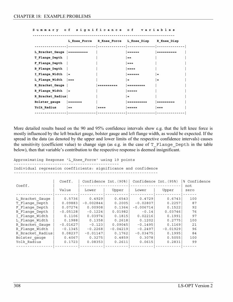
CHAPTER 18: EXAMPLE PROBLEMS
308 LS-OPT Version 2
S u m m a r y o f s i g n i f i c a n c e o f v a r i aS u m m a r y o f s i g n i f i c a n c e o f v a r i a b l e sb l e s
------------------------------------------------------------------------------------------------------------------------------------------------
L_Knee_Force R_Knee_Force L_Knee_L_Knee_Force R_Knee_Force L_Knee_DispDisp R_Knee_R_Knee_DispDisp
--------------------------------||----------------------------||----------------------------||----------------------------||----------------------------||
L_Bracket_Gauge |========== | |====== |=L_Bracket_Gauge |========== | |====== |========== |========= |
T_Flange_Depth | | |== |T_Flange_Depth | | |== | ||
F_Flange_Depth | | |=== |F_Flange_Depth | | |=== | ||
B_Flange_Depth | | |==== |B_Flange_Depth | | |==== | ||
I_Flange_Width |= | |====== |=I_Flange_Width |= | |====== |= ||
L_Flange_Width |=== | |= |=L_Flange_Width |=== | |= |= ||
R_Bracket_Gauge | |========== |========= |R_Bracket_Gauge | |========== |========= | ||
R_Flange_Width |= | |===== |R_Flange_Width |= | |===== | ||
R_Bracket_Radius| | |= |R_Bracket_Radius| | |= | ||
Bolster_gauge |======= | |========== |=Bolster_gauge |======= | |========== |========= |======== |
Yolk_Radius |== |==== |===== |=Yolk_Radius |== |==== |===== |=== |== |
--------------------------------||----------------------------||----------------------------||----------------------------||----------------------------||
More detailed results based on the 90 and 95% confidence intervals show e.g. that the left knee force is mostly influenced by the left bracket gauge, bolster gauge and left flange width, as would be expected. If the spread in the data (as denoted by the upper and lower limits of the respective confidence intervals) causes the sensitivity (coefficient value) to change sign (as e.g. in the case of T_Flange_Depth in the table below), then that variable’s contribution to the respective response is deemed insignificant. Approximating Response 'L_Knee_Force' using 19 points----------------------------------------------Individual regression coefficients: significance and confidence---------------------------------------------------------------
| Coeff. | Confidence Int.(90%)| Confidence Int.(95%) |% ConfidenceCoeff. | |---------------------|----------------------| not
| Value | Lower | Upper | Lower | Upper | zero----------------|----------|----------|----------|----------|-----------|------L_Bracket_Gauge | 0.5736| 0.4929| 0.6543| 0.4729| 0.6743| 100T_Flange_Depth | 0.09883| -0.002844| 0.2005| -0.02807| 0.2257| 87F_Flange_Depth | 0.07274| 0.00908| 0.1364| -0.006714| 0.1522| 92B_Flange_Depth | -0.05128| -0.1224| 0.01982| -0.14| 0.03746| 76I_Flange_Width | 0.1106| 0.03974| 0.1815| 0.02216| 0.1991| 97L_Flange_Width | 0.1988| 0.1358| 0.2618| 0.1202| 0.2775| 100R_Bracket_Gauge | -0.01627| -0.123| 0.09045| -0.1495| 0.1169| 21R_Flange_Width | -0.1345| -0.2268| -0.04219| -0.2497| -0.01929| 96R_Bracket_Radius| 0.08237| -0.01147| 0.1762| -0.03475| 0.1995| 84Bolster_gauge | 0.4067| 0.3275| 0.4859| 0.3078| 0.5055| 100Yolk_Radius | 0.1723| 0.08353| 0.2611| 0.0615| 0.2831| 99----------------|----------|----------|----------|----------|-----------|------
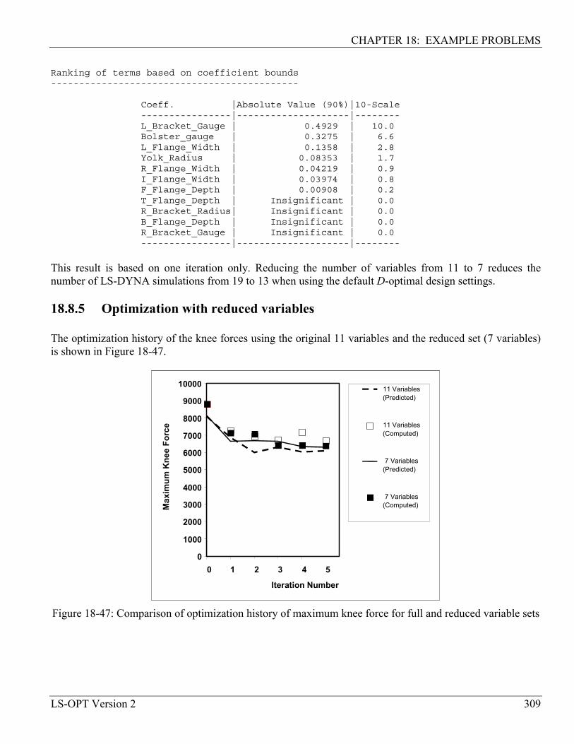
CHAPTER 18: EXAMPLE PROBLEMS
LS-OPT Version 2 309
Ranking of terms based on coefficient bounds--------------------------------------------
Coeff. |Absolute Value (90%)|10-Scale----------------|--------------------|--------L_Bracket_Gauge | 0.4929 | 10.0Bolster_gauge | 0.3275 | 6.6L_Flange_Width | 0.1358 | 2.8Yolk_Radius | 0.08353 | 1.7R_Flange_Width | 0.04219 | 0.9I_Flange_Width | 0.03974 | 0.8F_Flange_Depth | 0.00908 | 0.2T_Flange_Depth | Insignificant | 0.0R_Bracket_Radius| Insignificant | 0.0B_Flange_Depth | Insignificant | 0.0R_Bracket_Gauge | Insignificant | 0.0----------------|--------------------|--------
This result is based on one iteration only. Reducing the number of variables from 11 to 7 reduces the number of LS-DYNA simulations from 19 to 13 when using the default D-optimal design settings. 18.8.5 Optimization with reduced variables The optimization history of the knee forces using the original 11 variables and the reduced set (7 variables) is shown in Figure 18-47.
0
1000
2000
3000
4000
5000
6000
7000
8000
9000
10000
0 1 2 3 4 5
Iteration Number
Max
imum
Kne
e Fo
rce
11 Variables(Predicted)
11 Variables(Computed)
7 Variables(Predicted)
7 Variables(Computed)
0
1000
2000
3000
4000
5000
6000
7000
8000
9000
10000
0 1 2 3 4 5
Iteration Number
Max
imum
Kne
e Fo
rce
11 Variables(Predicted)
11 Variables(Computed)
7 Variables(Predicted)
7 Variables(Computed)
Figure 18-47: Comparison of optimization history of maximum knee force for full and reduced variable sets

CHAPTER 18: EXAMPLE PROBLEMS
310 LS-OPT Version 2
18.9 Optimization with analytical design sensitivities This example demonstrates how analytical gradients (Section 10.8) provided by a solver can be used for optimization using the SLP algorithm and the domain reduction scheme [63] (Section 2.12). The solver, a Perl program is shown below, followed by the command file for optimization. In this example the input variables are read from the file: XPoint placed in the run directory by LS-OPT. The input variables can also be read by defining this file as an input file and using the <<variable_name>> format to label the variable locations for substitution. Note that each response requires a unique Gradient file. Solver program:
# Open output files for response results#open(FOUT,">fsol");open(G1OUT,">g1sol");open(G2OUT,">g2sol");## Output files for gradients#open(DF,">Gradf");open(DG1,">Gradg1");open(DG2,">Gradg2");## Open the input file "XPoint" (automatically# placed by LS-OPT in the run directory)#open(X,"<XPoint");## Compute results and write to the files# (i.e. conduct the simulation)#while (<X>) {
($x1,$x2) = split;}#print FOUT ($x1*$x1) + (4*($x2-0.5)*($x2-0.5)),"\n";# Derivative of f(x1,x2)#-----------------------print DF (2*$x1)," "; # df/dx1print DF (8*($x2-0.5)),"\n"; # df/dx2#print G1OUT $x1 + $x2,"\n";# Derivative of g1(x1,x2)#------------------------print DG1 1," ";print DG1 1,"\n";#print G2OUT (-2*$x1) + $x2,"\n";# Derivative of g2(x1,x2)#------------------------print DG2 -2," ";print DG2 1,"\n";#

CHAPTER 18: EXAMPLE PROBLEMS
LS-OPT Version 2 311
# Signal normal termination#print "N o r m a l\n";
Command file: "Example 2b: QP problem (analytical sensitivity analysis)"solvers 1responses 3$$ DESIGN VARIABLES$variables 2Variable 'x1' 1Lower bound variable 'x1' -3Upper bound variable 'x1' 3Range 'x1' 1
Variable 'x2' 1Lower bound variable 'x2' 0Upper bound variable 'x2' 2Range 'x2' 1
$$$$$$$$$$$$$$$$$$$$$$$$$$$$$$$$$ SOLVER "1"$$$$$$$$$$$$$$$$$$$$$$$$$$$$$$$$solver own '1'
solver command "/home/LSOPT_EXE/perl ../../ex2"solver experimental design analytical_DSA
$$ RESPONSES FOR SOLVER "1"$ The Gradf, Gradg1 and Gradg2 files are individually copied to "Gradient"response 'f' 1 0 "cp Gradf Gradient; cat fsol"response 'g1' 1 0 "cp Gradg1 Gradient; cat g1sol"response 'g2' 1 0 "cp Gradg2 Gradient; cat g2sol"
$$ OBJECTIVE FUNCTIONS$objectives 1maximizeobjective 'f' 1
$$ CONSTRAINT DEFINITIONS$constraints 2constraint 'g1'upper bound constraint 'g1' 1
constraint 'g2'upper bound constraint 'g2' 2
$$ JOB INFO$iterate param design 0.01iterate param objective 0.01iterate param stoppingtype anditerate 5
STOP

CHAPTER 18: EXAMPLE PROBLEMS
312 LS-OPT Version 2
Typical ″Gradient″ file (e.g. for f): 1.8000000000 –3.20000000000
The optimization results are shown in the plots below. An iteration represents a single simulation. The dots represent the computed results while the solid line represents a linear approximation constructed from the gradient information of the previous point.

CHAPTER 18: EXAMPLE PROBLEMS
LS-OPT Version 2 313
18.10 Probabilistic Analysis 18.10.1 Overview This example has the following features: • Probabilistic analysis • Monte Carlo analysis • Monte Carlo analysis using a metamodel • Bifurcations analysis 18.10.2 Problem description A symmetric short crush tube impacted by a moving wall as shown in the figure is considered. The design criterion is the intrusion of the wall into the space initially occupied by the tube (alternatively, how much the structure is shortened by the impact with the wall).
Figure 18-48: Tube impact

CHAPTER 18: EXAMPLE PROBLEMS
314 LS-OPT Version 2
Both the shell thickness and the yield strength of the structure follow a probabilistic distribution. The shell thickness is normally distributed around a value of 1.0 with a standard deviation of 5% while the yield strength is normally distributed around a value scaled to 1.0 with a standard deviation of 10%.
The nominal design has an intrusion of 144.4 units. The probability of the intrusion being greater than 150 units is computed. The best-known results are obtained using a Monte Carlo analysis of 1500 runs. The problem is analyzed using a Monte-Carlo evaluation of 60 runs and a quadratic response surface build using a 3k experimental design. The results from the different methods are close to each other as can be seen in the following table.
Response Monte Carlo 1500 runs
Monte Carlo 60 runs
Response Surface 9 runs
Average Intrusion 141.3 141.8 141.4 Intrusion Standard Deviation 15.8 15.2 15.0 Probability of Intrusion > 150 0.32 0.33 0.29
Using the response surface, the derivatives of the intrusions with respect to the design variables are computed as given in the following table.
Variable Intrusion derivative Shell Thickness 208 Yield Strength 107
The quadratic response surface also allows the investigation of the dependence of the response variation on each design variable variation. The values of the intrusion standard deviation given in the following table are computed considering the variable as the only source of variation in the structure (the variation of the other design variables are set to zero).
Source of variation Intrusion Standard Deviation Shell Thickness 10.4 Yield Strength 10.7
The details of the analyses are given the following subsections. 18.10.3 Monte Carlo evaluation The probabilistic variation is described by specifying statistical distributions and assigning the statistical distributions to noise variables.
"Tube Crush Monte Carlo "$ Created on Tue Apr 1 11:26:07 2003solvers 1$distribution 2distribution 't' NORMAL 1.0 0.05distribution 'y' NORMAL 1.0 0.10

CHAPTER 18: EXAMPLE PROBLEMS
LS-OPT Version 2 315
$$ DESIGN VARIABLES$variables 2noise variable 'T1' distribution 't'noise variable 'YS' distribution 'y'
$$ DEFINITION OF SOLVER "SOLVER_1"$solver dyna960 'SOLVER_1'solver command "ls970.single"solver input file "tube.k"solver experiment design lhd centralpointsolver number experiments 60
$$ HISTORIES FOR SOLVER "SOLVER_1"$histories 1history 'NHist' "BinoutHistory -res_type nodout -cmp z_displacement -id 486"
$$ RESPONSES FOR SOLVER "SOLVER_1"$responses 2response 'NodDisp' 1 0 "BinoutResponse -res_type nodout -cmp z_displacement -id 486
-select MIN "response 'DispT' {LookupMin("NHist(t)")}
$$$constraints 1constraint 'NodDisp'lower bound constraint 'NodDisp' -150
$$ JOB INFO$analyze monte carlo
STOP
The LS-OPT output:
###############################################################Direct Monte Carlo simulation considering 2 stochastic variables.###############################################################
#####################################################STATISTICS OF VARIABLES#####################################################
Variable 'T1'Distribution Information------------------------Number of points : 60Mean Value : 1Standard Deviation : 0.04948

CHAPTER 18: EXAMPLE PROBLEMS
316 LS-OPT Version 2
Coef of Variation : 0.04948Maximum Value : 1.12Minimum Value : 0.8803
Variable 'YS'Distribution Information------------------------Number of points : 60Mean Value : 1Standard Deviation : 0.09895Coef of Variation : 0.09895Maximum Value : 1.239Minimum Value : 0.7606
#####################################################STATISTICS OF RESPONSES#####################################################
Response 'NodDisp'Distribution Information------------------------Number of points : 60Mean Value : -141.8Standard Deviation : 15.21Coef of Variation : 0.1073Maximum Value : -102.3Minimum Value : -168.9
Response 'DispT'Distribution Information------------------------Number of points : 60Mean Value : 7.726Standard Deviation : 0.6055Coef of Variation : 0.07837Maximum Value : 8.4Minimum Value : 5.5
#####################################################STATISTICS OF COMPOSITES#####################################################
#####################################################STATISTICS OF CONSTRAINTS#####################################################
Constraint 'NodDisp'Distribution Information------------------------

CHAPTER 18: EXAMPLE PROBLEMS
LS-OPT Version 2 317
Number of points : 60Mean Value : -141.8Standard Deviation : 15.21Coef of Variation : 0.1073Maximum Value : -102.3Minimum Value : -168.9
Lower Bound:------------
Bound .................................... -150Evaluations exceeding this bound ......... 20Probability of exceeding bound ........... 0.3333Confidence Interval on Probability.
Standard Deviation of Prediction Error: 0.06086Lower Bound | Probability | Higher Bound
0.2116 | 0.3333 | 0.455Confidence Interval of 95% assuming Normal DistributionConfidence Interval of 75% using Tchebysheff's Theorem
Reliability Assuming Normal Distribution========================================Lower Bound:------------
Bound ............................ -150Probability of exceeding Bound ... 0.2956Reliability Index (Beta) ......... 0.5372
ANALYSIS COMPLETED
18.10.4 Monte Carlo using metamodel The bounds on the design variables are set to be two standard distributions away from the mean (the default for noise variables). Noise variables are not used because of the need to have more control over the variable bounds — specifically we want to change the standard deviation of some variables without affecting the variable bounds (the metamodel is computed scaled with respect to the upper and lower bounds on the variables). The command file for using a metamodel is: $"Tube Crush Metamodel Monte Carlo"$ Created on Tue Apr 1 11:26:07 2003solvers 1$distribution 2distribution 't' NORMAL 1.0 0.05distribution 'y' NORMAL 1.0 0.10
$$ DESIGN VARIABLES$variables 2variable 'T1' 1.0

CHAPTER 18: EXAMPLE PROBLEMS
318 LS-OPT Version 2
upper bound variable 'T1' 1.1lower bound variable 'T1' 0.9variable 'T1' distribution 't'
variable 'YS' 1.0upper bound variable 'YS' 1.2lower bound variable 'YS' 0.8variable 'YS' distribution 'y'
$$ DEFINITION OF SOLVER "SOLVER_1"$solver dyna960 'SOLVER_1'solver command "ls970.single"solver input file "tube.k"solver experiment design 3toKsolver order quadratic
$$ HISTORIES FOR SOLVER "SOLVER_1"$histories 1history 'NHist' "BinoutHistory -res_type nodout -cmp z_displacement -id 486"
$$ RESPONSES FOR SOLVER "SOLVER_1"$responses 2response 'NodDisp' 1 0 "BinoutResponse -res_type nodout -cmp z_displacement -id 486 -
select MIN"response 'DispT' {LookupMin("NHist(t)")}
$$$constraints 1constraint 'NodDisp'lower bound constraint 'NodDisp' -150.0
$$ JOB INFO$analyze metamodel monte carlo
STOP
The accuracy of the response surface is of interest: Approximating Response 'NodDisp' (ITERATION 1)----------------------------------------------------------------Polynomial approximation: using 9 points
Global error parameters of response surface-------------------------------------------
Quadratic Function Approximation:---------------------------------Mean response value = -142.0087
RMS error = 2.0840 (1.47%)Maximum Residual = 3.3633 (2.37%)Average Error = 1.6430 (1.16%)

CHAPTER 18: EXAMPLE PROBLEMS
LS-OPT Version 2 319
Square Root PRESS Residual = 6.2856 (4.43%)Variance = 13.0296R^2 = 0.9928R^2 (adjusted) = 0.9856R^2 (prediction) = 0.9346
The probabilistic evaluation results:
###############################################################Monte Carlo simulation considering 2 stochastic variables.Computed using 1000000 simulations###############################################################
--------------------------------------------------------------Results for reliability analysis using approximate functions--------------------------------------------------------------
#####################################################STATISTICS OF VARIABLES#####################################################
Variable 'T1'Distribution Information------------------------Number of points : 1000000Mean Value : 1Standard Deviation : 0.04997Coef of Variation : 0.04997Maximum Value : 1.227Minimum Value : 0.7505
Variable 'YS'Distribution Information------------------------Number of points : 1000000Mean Value : 1Standard Deviation : 0.09994Coef of Variation : 0.09994Maximum Value : 1.472Minimum Value : 0.5187
#####################################################STATISTICS OF RESPONSES#####################################################Response 'NodDisp'Distribution Information------------------------Number of points : 1000000

CHAPTER 18: EXAMPLE PROBLEMS
320 LS-OPT Version 2
Mean Value : -141.4Standard Deviation : 14.95Coef of Variation : 0.1058Maximum Value : -68.5Minimum Value : -206.3Response 'DispT'Distribution Information------------------------Number of points : 1000000Mean Value : 7.68Standard Deviation : 0.546Coef of Variation : 0.0711Maximum Value : 9.267Minimum Value : 2.565
#####################################################STATISTICS OF COMPOSITES#####################################################
#####################################################STATISTICS OF CONSTRAINTS#####################################################
Constraint 'NodDisp'Distribution Information------------------------Number of points : 1000000Mean Value : -141.4Standard Deviation : 14.95Coef of Variation : 0.1058Maximum Value : -68.5Minimum Value : -206.3
Lower Bound:------------
Bound .................................... -150Evaluations exceeding this bound ......... 285347Probability of exceeding bound ........... 0.2853Confidence Interval on Probability.
Standard Deviation of Prediction Error: 0.0004516Lower Bound | Probability | Higher Bound
0.2844 | 0.2853 | 0.2863Confidence Interval of 95% assuming Normal DistributionConfidence Interval of 75% using Tchebysheff's Theorem
ANALYSIS COMPLETED

CHAPTER 18: EXAMPLE PROBLEMS
LS-OPT Version 2 321
18.10.5 Bifurcation analysis A bifurcation analysis of the tube is conducted as described in Section 3.6, Section 17, and Example 18.11. The resulting buckling modes found for the metamodel-based analysis are as shown in Figure 18-49. An extra half wave is formed for the one design.
Figure 18-49 Tube Buckling

CHAPTER 18: EXAMPLE PROBLEMS
322 LS-OPT Version 2
18.11 Bifurcation/Outlier Analysis 18.11.1 Overview This example has the following features: • Monte Carlo analysis • Identification of different buckling modes in the structure 18.11.2 Problem description The plate as shown in Figure 18-50 has two buckling modes. Buckling in the positive z-direction occurs with a probability of 80% while buckling in the negative z-direction occurs with a probability of 20%. Assigning a distribution to an imperfection at tip nodes allows control of the probability of buckling.
Figure 18-50 Plate Buckling Example
18.11.3 Monte Carlo evaluation A Latin hypercube experimental design is used for the Monte Carlo analysis. We analyze only five points. Given that the probability of 20% of buckling in the negative z-direction and a Latin hypercube experimental design, one run will buckle in the negative z-direction. The next section will demonstrate how to find out which run contains the different buckling mode. "Monte Carlo Analysis; 2 buckling modes"$solvers 1$distribution 1distribution 'i' UNIFORM -0.001 0.004
$$ DESIGN VARIABLES$variables 1noise variable 'Imp' distribution 'i'
$$$ SOLVER_1

CHAPTER 18: EXAMPLE PROBLEMS
LS-OPT Version 2 323
$solver dyna960 'SOLVER_1'
solver command "ls970.single"solver input file "plate.k"solver experiment design lhd centralpointsolver number experiments 5
$$ RESPONSES$responses 4response 'tip_x' 1 0 "BinoutResponse -res_type nodout -cmp x_displacement -id 12 -
select TIME "response 'tip_y' 1 0 "BinoutResponse -res_type nodout -cmp y_displacement -id 12 -
select TIME "response 'tip_z' 1 0 "BinoutResponse -res_type nodout -cmp z_displacement -id 12 -
select TIME "response 'tip_r' 1 0 "BinoutResponse -res_type nodout -cmp displacement -invariant
MAGNITUDE -id 12 -select TIME "$$$ JOB$analyze monte carlo
STOP
18.11.4 Identification of buckling modes The different buckling modes are identified using the DYNA Stats panel in LS-OPT. Firstly, the D3Plot outlier statistics are computed a linear response surface. Next, LS-PREPOST can be launched to investigate the range (or standard deviation) of all the displacement components. From the displacement resultant plot, amongst others, it is clear that the bifurcation is at the tip. Looking at the other component plots, we find the z-displacement has a range of 5.3 and the x-displacement a range of 4.5. The displacement magnitude computed using the maximum vector has a range of 6.9.
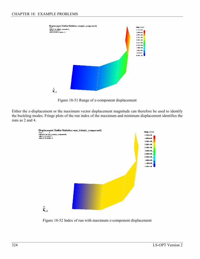
CHAPTER 18: EXAMPLE PROBLEMS
324 LS-OPT Version 2
Figure 18-51 Range of z-component displacement
Either the z-displacement or the maximum vector displacement magnitude can therefore be used to identify the buckling modes. Fringe plots of the run index of the maximum and minimum displacement identifies the runs as 2 and 4.
Figure 18-52 Index of run with maximum z-component displacement
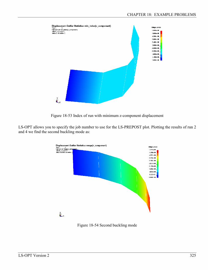
CHAPTER 18: EXAMPLE PROBLEMS
LS-OPT Version 2 325
Figure 18-53 Index of run with minimum z-component displacement
LS-OPT allows you to specify the job number to use for the LS-PREPOST plot. Plotting the results of run 2 and 4 we find the second buckling mode as:
Figure 18-54 Second buckling mode

326
Bibliography 1234567891011121314151617181920212223242526272829303132333435363738394041424344454647484950515253545556575859606162636465666768697071727374757677787980
[1] Akaike, H. Statistical predictor identification. Ann.Inst.Statist.Math., 22, pp. 203-217, 1970. [2] Akkerman, A., Thyagarajan, R., Stander, N., Burger, M., Kuhn, R., Rajic, H. Shape optimization for
crashworthiness design using response surfaces. Proceedings of the 1st International Workshop on Multidisciplinary Design Optimization, Pretoria, South Africa, 8-10 August 2000, pp. 270-279.
[3] Arora, J.S. Introduction to Optimum Design. 1st ed. McGraw-Hill, 1989. [4] Arora, J.S. Sequential linearization and quadratic programming techniques. In Structural
Optimization: Status and Promise, Ed. Kamat, M.P., AIAA, 1993. [5] Bakker, T.M.D. Design Optimization with Kriging Models. WBBM Report Series 47, Ph.D. thesis,
Delft University Press, 2000. [6] Barthelemy, J.-F. M. Function Approximation. In Structural Optimization: Status and Promise, Ed.
Kamat, M.P., 1993. [7] Basu, A., Frazer, L.N. Rapid determination of the critical temperature in simulated annealing
inversion, Science, 249, pp. 1409-1412, 1990. [8] Bishop, C.M. Neural Networks for Pattern Recognition. Oxford University Press, 1995. [9] Bounds, D. G., New optimization methods from physics and biology, Nature, 329, pp. 215-218, 1987. [10] Box, G.E.P., Draper, N.R. A basis for the selection of a response surface design. Journal of the
American Statistical Association, 54, pp. 622-654, 1959. [11] Box., G.E.P., Draper, N.R. Empirical Model Building and Response Surfaces, Wiley, New York,
1987. [12] Burgee, S., Giunta, A. A., Narducci, R., Watson, L. T., Grossman, B. and Haftka, R. T. A coarse
grained parallel variable-complexity multidisciplinary optimization paradigm, The International Journal of Supercomputer Applications and High Performance Computing, 10(4), pp. 269-299, 1996.
[13] Cohn, D. Neural network exploration using optimal experiment design, Neural Networks, (9)6, pp. 1071-1083, 1996.
[14] Craig K.J., Stander, N., Dooge, D., Varadappa, S. MDO of automotive vehicle for crashworthiness and NVH using response surface methods. Paper AIAA2002_5607, 9th AIAA/ISSMO Symposium on Multidisciplinary Analysis and Optimization, 4-6 Sept 2002, Atlanta, GA.
[15] Daberkow, D.D. and Mavris, D.N. An investigation of metamodeling techniques for complex systems design. Symposium on Multidisciplinary Analysis and Design, Atlanta, October 2002.
[16] Draper and Smith H; Applied Regression Analysis, Second Edition, Wiley, New York, 1981. [17] Eschenauer, H., Koski, J., Osyczka, A. Multicriteria Design Optimization. Procedures and
Applications. Springer-Verlag, Berlin, 1990. [18] Fedorova, N.N., Terekhoff, S.A. Space Filling Designs, Internal Report, April 2002. [19] Foresee, F. D., Hagan, M. T. Gauss-Newton approximation to Bayesian regularization. Proceedings of
the 1997 International Joint Conference on Neural Networks, pp. 1930-1935, 1997. [20] Forsberg, J. Simulation Based Crashworthiness Design – Accuracy Aspects of Structural optimization
using Response Surfaces. Thesis No. 954. Division of Solid Mechanics, Department of Mechanical Engineering, Linköping University, Sweden, 2002.
[21] Giger, M., Redhe, M. and Nilsson, L, Division of Mechanics, Department of Mechanical Engineering, Linköping University, Sweden. Personal Communication, January 2003.
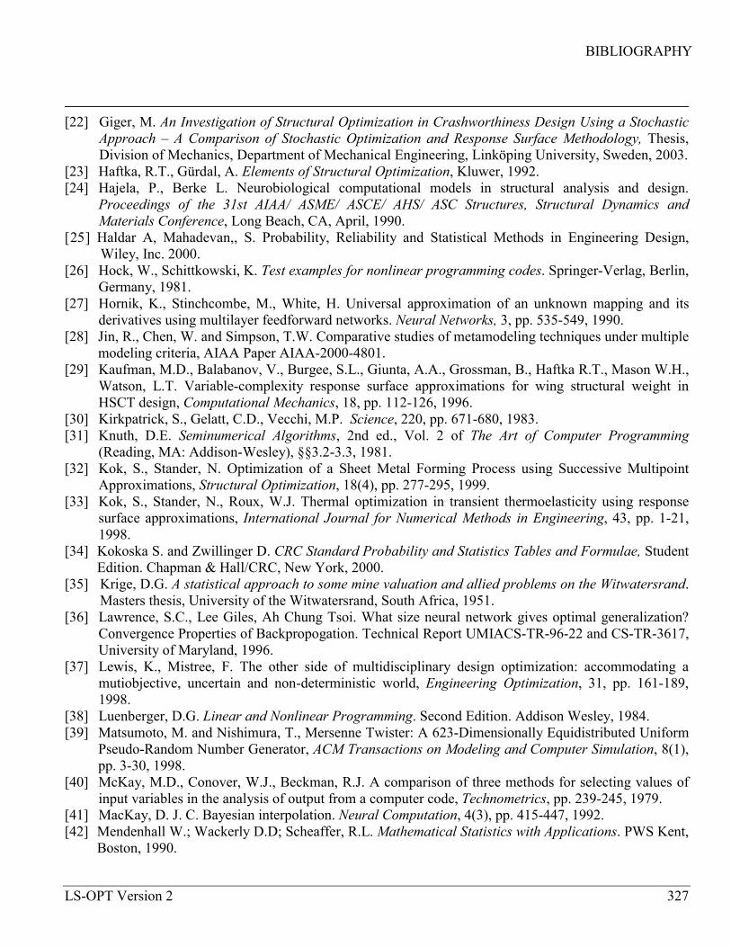
BIBLIOGRAPHY
LS-OPT Version 2 327
[22] Giger, M. An Investigation of Structural Optimization in Crashworthiness Design Using a Stochastic
Approach – A Comparison of Stochastic Optimization and Response Surface Methodology, Thesis, Division of Mechanics, Department of Mechanical Engineering, Linköping University, Sweden, 2003.
[23] Haftka, R.T., Gürdal, A. Elements of Structural Optimization, Kluwer, 1992. [24] Hajela, P., Berke L. Neurobiological computational models in structural analysis and design.
Proceedings of the 31st AIAA/ ASME/ ASCE/ AHS/ ASC Structures, Structural Dynamics and Materials Conference, Long Beach, CA, April, 1990.
[25] Haldar A, Mahadevan,, S. Probability, Reliability and Statistical Methods in Engineering Design, Wiley, Inc. 2000.
[26] Hock, W., Schittkowski, K. Test examples for nonlinear programming codes. Springer-Verlag, Berlin, Germany, 1981.
[27] Hornik, K., Stinchcombe, M., White, H. Universal approximation of an unknown mapping and its derivatives using multilayer feedforward networks. Neural Networks, 3, pp. 535-549, 1990.
[28] Jin, R., Chen, W. and Simpson, T.W. Comparative studies of metamodeling techniques under multiple modeling criteria, AIAA Paper AIAA-2000-4801.
[29] Kaufman, M.D., Balabanov, V., Burgee, S.L., Giunta, A.A., Grossman, B., Haftka R.T., Mason W.H., Watson, L.T. Variable-complexity response surface approximations for wing structural weight in HSCT design, Computational Mechanics, 18, pp. 112-126, 1996.
[30] Kirkpatrick, S., Gelatt, C.D., Vecchi, M.P. Science, 220, pp. 671-680, 1983. [31] Knuth, D.E. Seminumerical Algorithms, 2nd ed., Vol. 2 of The Art of Computer Programming
(Reading, MA: Addison-Wesley), §§3.2-3.3, 1981. [32] Kok, S., Stander, N. Optimization of a Sheet Metal Forming Process using Successive Multipoint
Approximations, Structural Optimization, 18(4), pp. 277-295, 1999. [33] Kok, S., Stander, N., Roux, W.J. Thermal optimization in transient thermoelasticity using response
surface approximations, International Journal for Numerical Methods in Engineering, 43, pp. 1-21, 1998.
[34] Kokoska S. and Zwillinger D. CRC Standard Probability and Statistics Tables and Formulae, Student Edition. Chapman & Hall/CRC, New York, 2000.
[35] Krige, D.G. A statistical approach to some mine valuation and allied problems on the Witwatersrand. Masters thesis, University of the Witwatersrand, South Africa, 1951.
[36] Lawrence, S.C., Lee Giles, Ah Chung Tsoi. What size neural network gives optimal generalization? Convergence Properties of Backpropogation. Technical Report UMIACS-TR-96-22 and CS-TR-3617, University of Maryland, 1996.
[37] Lewis, K., Mistree, F. The other side of multidisciplinary design optimization: accommodating a mutiobjective, uncertain and non-deterministic world, Engineering Optimization, 31, pp. 161-189, 1998.
[38] Luenberger, D.G. Linear and Nonlinear Programming. Second Edition. Addison Wesley, 1984. [39] Matsumoto, M. and Nishimura, T., Mersenne Twister: A 623-Dimensionally Equidistributed Uniform
Pseudo-Random Number Generator, ACM Transactions on Modeling and Computer Simulation, 8(1), pp. 3-30, 1998.
[40] McKay, M.D., Conover, W.J., Beckman, R.J. A comparison of three methods for selecting values of input variables in the analysis of output from a computer code, Technometrics, pp. 239-245, 1979.
[41] MacKay, D. J. C. Bayesian interpolation. Neural Computation, 4(3), pp. 415-447, 1992. [42] Mendenhall W.; Wackerly D.D; Scheaffer, R.L. Mathematical Statistics with Applications. PWS Kent,
Boston, 1990.
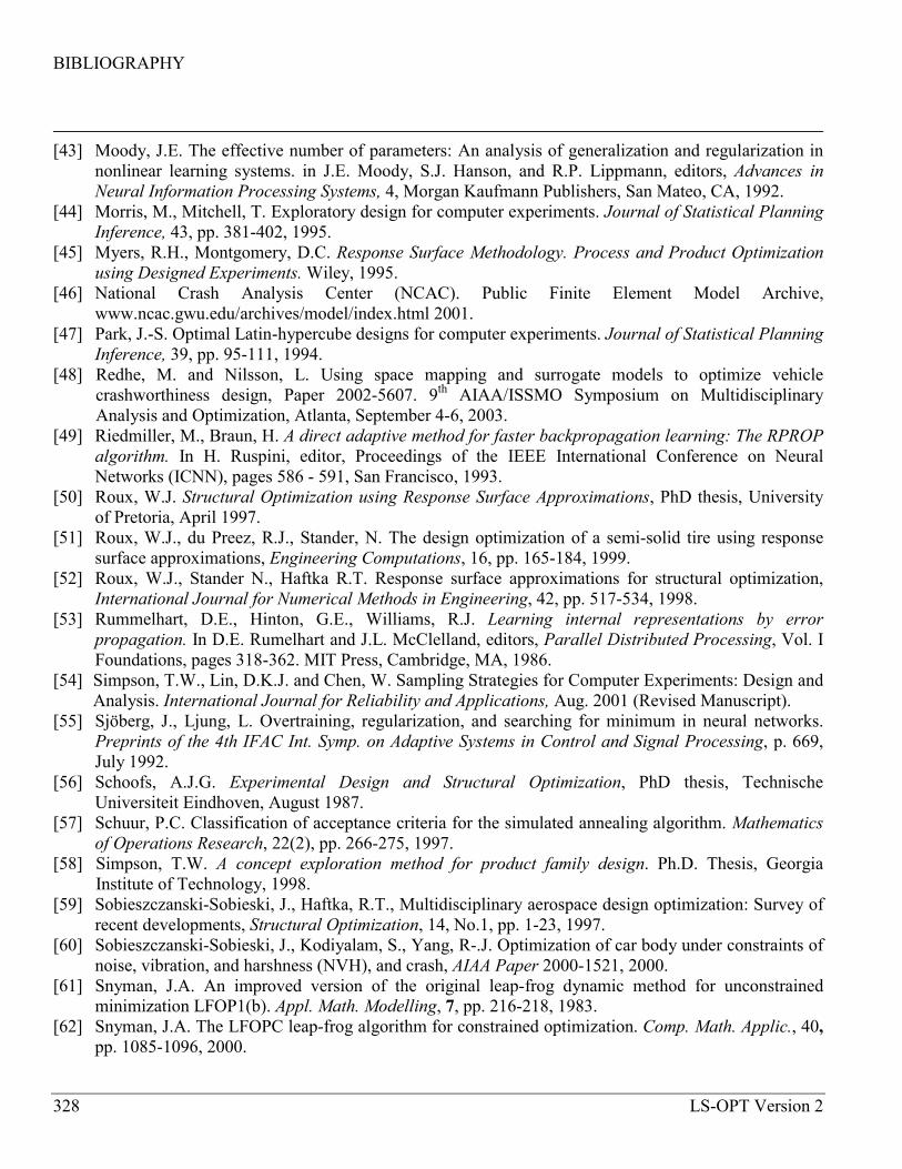
BIBLIOGRAPHY
328 LS-OPT Version 2
[43] Moody, J.E. The effective number of parameters: An analysis of generalization and regularization in
nonlinear learning systems. in J.E. Moody, S.J. Hanson, and R.P. Lippmann, editors, Advances in Neural Information Processing Systems, 4, Morgan Kaufmann Publishers, San Mateo, CA, 1992.
[44] Morris, M., Mitchell, T. Exploratory design for computer experiments. Journal of Statistical Planning Inference, 43, pp. 381-402, 1995.
[45] Myers, R.H., Montgomery, D.C. Response Surface Methodology. Process and Product Optimization using Designed Experiments. Wiley, 1995.
[46] National Crash Analysis Center (NCAC). Public Finite Element Model Archive, www.ncac.gwu.edu/archives/model/index.html 2001.
[47] Park, J.-S. Optimal Latin-hypercube designs for computer experiments. Journal of Statistical Planning Inference, 39, pp. 95-111, 1994.
[48] Redhe, M. and Nilsson, L. Using space mapping and surrogate models to optimize vehicle crashworthiness design, Paper 2002-5607. 9th AIAA/ISSMO Symposium on Multidisciplinary Analysis and Optimization, Atlanta, September 4-6, 2003.
[49] Riedmiller, M., Braun, H. A direct adaptive method for faster backpropagation learning: The RPROP algorithm. In H. Ruspini, editor, Proceedings of the IEEE International Conference on Neural Networks (ICNN), pages 586 - 591, San Francisco, 1993.
[50] Roux, W.J. Structural Optimization using Response Surface Approximations, PhD thesis, University of Pretoria, April 1997.
[51] Roux, W.J., du Preez, R.J., Stander, N. The design optimization of a semi-solid tire using response surface approximations, Engineering Computations, 16, pp. 165-184, 1999.
[52] Roux, W.J., Stander N., Haftka R.T. Response surface approximations for structural optimization, International Journal for Numerical Methods in Engineering, 42, pp. 517-534, 1998.
[53] Rummelhart, D.E., Hinton, G.E., Williams, R.J. Learning internal representations by error propagation. In D.E. Rumelhart and J.L. McClelland, editors, Parallel Distributed Processing, Vol. I Foundations, pages 318-362. MIT Press, Cambridge, MA, 1986.
[54] Simpson, T.W., Lin, D.K.J. and Chen, W. Sampling Strategies for Computer Experiments: Design and Analysis. International Journal for Reliability and Applications, Aug. 2001 (Revised Manuscript).
[55] Sjöberg, J., Ljung, L. Overtraining, regularization, and searching for minimum in neural networks. Preprints of the 4th IFAC Int. Symp. on Adaptive Systems in Control and Signal Processing, p. 669, July 1992.
[56] Schoofs, A.J.G. Experimental Design and Structural Optimization, PhD thesis, Technische Universiteit Eindhoven, August 1987.
[57] Schuur, P.C. Classification of acceptance criteria for the simulated annealing algorithm. Mathematics of Operations Research, 22(2), pp. 266-275, 1997.
[58] Simpson, T.W. A concept exploration method for product family design. Ph.D. Thesis, Georgia Institute of Technology, 1998.
[59] Sobieszczanski-Sobieski, J., Haftka, R.T., Multidisciplinary aerospace design optimization: Survey of recent developments, Structural Optimization, 14, No.1, pp. 1-23, 1997.
[60] Sobieszczanski-Sobieski, J., Kodiyalam, S., Yang, R-.J. Optimization of car body under constraints of noise, vibration, and harshness (NVH), and crash, AIAA Paper 2000-1521, 2000.
[61] Snyman, J.A. An improved version of the original leap-frog dynamic method for unconstrained minimization LFOP1(b). Appl. Math. Modelling, 7, pp. 216-218, 1983.
[62] Snyman, J.A. The LFOPC leap-frog algorithm for constrained optimization. Comp. Math. Applic., 40, pp. 1085-1096, 2000.

BIBLIOGRAPHY
LS-OPT Version 2 329
[63] Stander, N., Craig, K.J. On the robustness of a simple domain reduction scheme for simulation-based
optimization, Engineering Computations, 19(4), pp. 431-450, 2002. [64] Stander, N.; Reichert, R.; Frank, T. 2000: Optimization of nonlinear dynamic problems using
successive linear approximations. AIAA Paper 2000-4798. [65] Stander, N., Roux, W.J., Giger, M., Redhe, M., Fedorova, N. and Haarhoff, J. Crashworthiness
optimization in LS-OPT: Case studies in metamodeling and random search techniques. Proceedings of the 4th European LS-DYNA Conference, Ulm, Germany, May 22-23, 2003. (Also www.lstc.com).
[66] Stander, N., Snyman, J.A., Coster, J.E., On the robustness and efficiency of the SAM algorithm for structural optimization. International Journal for Numerical Methods in Engineering, 38, pp. 119-135, 1995.
[67] Sunar, M., Belegundu, A.D. Trust region methods for structural optimization using exact second order sensitivity. International Journal for Numerical Methods in Engineering, 32, pp. 275-293, 1991.
[68] Thanedar, P.B., Arora, J.S., Tseng, C.H., Lim, O.K., Park, G.J. Performance of some SQP algorithms on structural design problems. International Journal for Numerical Methods in Engineering, 23, pp. 2187-2203, 1986.
[69] Toropov, V.V. Simulation approach to structural optimization. Structural Optimization, 1, pp. 37-46, 1989.
[70] Tu, J. and Choi, K.K. Design potential concept for reliability-based design optimization. Technical report R99-07. Center for computer aided design and department of mechanical engineering. College of engineering. University of Iowa. December 1999.
[71] Van Campen, D.H., Nagtegaal R., Schoofs, A.J.G. Approximation methods in structural optimization using experimental designs for multiple responses, In: Eschenauer, H.; Koski, J.; Osyczka, A. (Eds.) Multicriteria Design Optimization - Procedures and Applications, Springer-Verlag: Berlin, Heidelberg, New York, pp. 205-228, 1990.
[72] Vanderplaats, G.N. Numerical Optimization Techniques for Engineering Design: with Applications. McGraw-Hill, New York, 1984.
[73] Wahba, G. Spline Models for Observational Data. Volume 59 of Regional Conference Series in Applied Mathematics. SIAM Press, Philadelphia, 1990.
[74] Wall, L., Christiansen, T., Schwartz, R. Programming Perl, O’Reilly & Associates, Inc., Cambridge, 1991.
[75] White, H., Hornik, K., Stinchcombe, M. Universal approximation of an unknown mapping and its derivatives. Artificial Neural Networks: Approximations and Learning Theory, H. White, ed., Oxford, UK: Blackwell, 1992.
[76] Wilson, B., Cappelleri, D.J., Frecker, M.I. and Simpson, T.W. Efficient Pareto Frontier Exploration using surrogate approximations. Optimization and Engineering, 2 (1), pp.31-50, 2001.
[77] Xu, Q-S., Liang, Y-Z., Fang, K-T., The effects of different experimental designs on parameter estimation in the kinetics of a reversible chemical reaction. Chemometrics and Intelligent Laboratory Systems, 52, pp. 155-166, 2000.
[78] Yamazaki, K., Han, J., Ishikawa, H., Kuroiwa, Y. Maximation of crushing energy absorption of cylindrical shells – simulation and experiment, Proceedings of the OPTI-97 Conference, Rome, Italy, September 1997.
[79] Ye, K., Li, W., Sudjianto, A., Algorithmic construction of optimal symmetric Latin Hypercube designs, Journal of Statistical Planning and Inferences, 90, pp. 145-159, 2000.
[80] Zang, T.A., Green, L.L., Multidisciplinary Design Optimization techniques: Implications and opportunities for fluid dynamics research, AIAA Paper 99-3798, 1999.

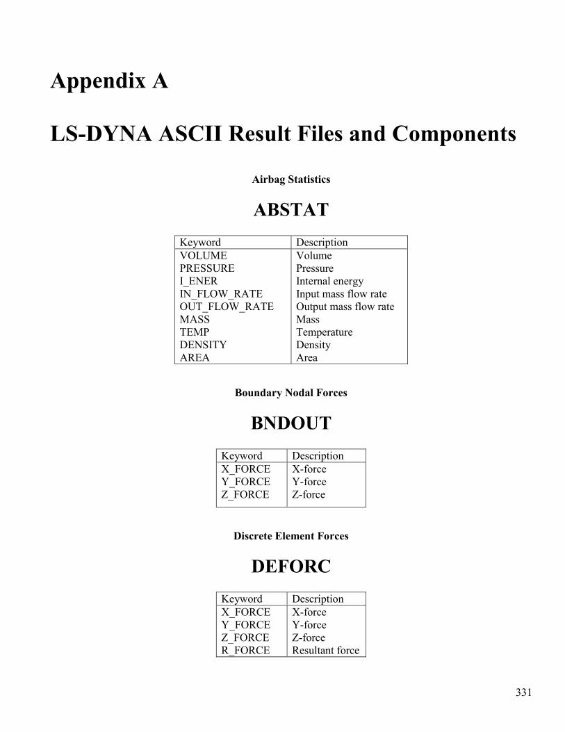
331
Appendix A
LS-DYNA ASCII Result Files and Components
Airbag Statistics
ABSTAT
Keyword Description VOLUME PRESSURE I_ENER IN_FLOW_RATE OUT_FLOW_RATE MASS TEMP DENSITY AREA
Volume Pressure Internal energy Input mass flow rate Output mass flow rate Mass Temperature Density Area
Boundary Nodal Forces
BNDOUT
Keyword Description X_FORCE Y_FORCE Z_FORCE
X-force Y-force Z-force
Discrete Element Forces
DEFORC
Keyword Description X_FORCE Y_FORCE Z_FORCE R_FORCE
X-force Y-force Z-force Resultant force

APPENDIX A: LS-DYNA ASCII RESULT FILES AND COMPONENTS
332 LS-OPT Version 2
Element Output: Brick and Beam Elements
ELOUT
Keyword Element Description BXX_STRESS BYY_STRESS BZZ_STRESS BXY_STRESS BYZ_STRESS BZX_STRESS YIELD BE_STRESS BPRESSURE BMAX_SHEAR BMAX_P_STRESS BMIN_P_STRESS
Brick XX-stress YY-stress ZZ-stress XY-stress YZ-stress ZX-stress Yield function Effective stress Pressure Maximum shear stress Maximum principal stress Minimum principal stress
AXIAL S_SHEAR T_SHEAR S_MOMENT T_MOMENT TORSION SIG_11 SIG_12 SIG_31 PLASTIC
Beam Axial force resultant s-Shear resultant t-Shear resultant s-Moment resultant t-Moment resultant Torsional resultant σ11 σ12 σ31 Plastic strain

APPENDIX A: LS-DYNA ASCII RESULT FILES AND COMPONENTS
LS-OPT Version 2 333
Element Output: Shell Elements
ELOUT
Keyword Element Description XX_STRESS YY_STRESS ZZ_STRESS XY_STRESS YZ_STRESS ZX_STRESS P_STRAIN PRESSURE E_STRESS MAX_SHEAR MAX_P_STRESS MIN_P_STRESS
Shell element stress
XX-stress YY-stress ZZ-stress XY-stress YZ-stress ZX-stress Plastic strain Pressure Effective stress Maximum shear stress Maximum principal stress Minimum principal stress
XX_STRAIN YY_STRAIN ZZ_STRAIN XY_STRAIN YZ_STRAIN ZX_STRAIN E_STRAIN MAX_S_STRAIN MAX_P_STRAIN MIN_P_STRAIN
Shell element strain
XX-strain YY-strain ZZ-strain XY-strain YZ-strain ZX-strain Effective strain Maximum shear strain Maximum principal strain Minimum principal strain
TXX_STRESS TYY_STRESS TZZ_STRESS TXY_STRESS TYZ_STRESS TZX_STRESS TP_STRAIN TPRESSURE TE_STRESS TMAX_SHEAR TMAX_P_STRESS TMIN_P_STRESS
Thick shell stress
XX-stress YY-stress ZZ-stress XY-stress YZ-stress ZX-stress Plastic strain Pressure Effective stress Maximum shear stress Maximum principal stress Minimum principal stress

APPENDIX A: LS-DYNA ASCII RESULT FILES AND COMPONENTS
334 LS-OPT Version 2
Contact Entities Resultants
GCEOUT
Keyword Description X_FORCE Y_FORCE Z_FORCE R_FORCE X_MOMENT Y_MOMENT Z_MOMENT R_MOMENT
X-force Y-force Z-force Force magnitude X-moment Y-moment Z-moment Moment magnitude
Global Statistics
GLSTAT
Keyword Description K_ENER I_ENER T_ENER RATIO SW_ENER D_ENER HG_ENER SI_ENER EW_ENER X_VEL Y_VEL Z_VEL T_VEL
Kinetic energy Internal energy Total energy Ratio Stonewall energy Spring & Damper energy hourglass energy sliding interface energy external work global x-velocity global y-velocity global z-velocity velocity

APPENDIX A: LS-DYNA ASCII RESULT FILES AND COMPONENTS
LS-OPT Version 2 335
Joint Element Forces
JNTFORC
Keyword Description X_FORCE Y_FORCE Z_FORCE X_MOMENT Y_MOMENT Z_MOMENT R_FORCE R_MOMENT
X-force Y-force Z-force X-moment Y-moment Z-moment R-force R-moment
Material Summary
MATSUM
Keyword Description K_ENER I_ENER X_MOMENTUM Y_MOMENTUM Z_MOMENTUM MOMENTUM XRB_VEL YRB_VEL ZRB_VEL RB_VEL TK_ENER TI_ENER
Kinetic energy Internal energy X-momentum Y-momentum Z-momentum Momentum X-rigid body velocity Y-rigid body velocity Z-rigid body velocity Rigid body velocity Total kinetic energy Total internal energy

APPENDIX A: LS-DYNA ASCII RESULT FILES AND COMPONENTS
336 LS-OPT Version 2
Contact Node Forces
NCFORC
Keyword Description X_FORCE Y_FORCE Z_FORCE R_FORCE PRESSURE
X-force Y-force Z-force R-force Pressure
Nodal Point Response
NODOUT
Keyword Description X_DISP Y_DISP Z_DISP R_DISP X_VEL Y_VEL Z_VEL R_VEL X_ACC Y_ACC Z_ACC R_ACC
X-displacement Y-displacement Z-displacement Resultant displacement X-velocity Y-velocity Z-velocity Resultant velocity X-acceleration Y-acceleration Z-acceleration R-acceleration
Rotational components RX_DISP RY_DISP RZ_DISP RX_VEL RY_VEL RZ_VEL RX_ACC RY_ACC RZ_ACC
XX-rotation YY-rotation ZZ-rotation XX-rotational velocity YY-rotational velocity ZZ-rotational velocity XX-rotational acceleration YY-rotational acceleration ZZ-rotational acceleration
Injury coefficients CSI HIC15 HIC36
Chest Severity Index Head Injury Coefficient (15 ms) Head Injury Coefficient (36 ms)
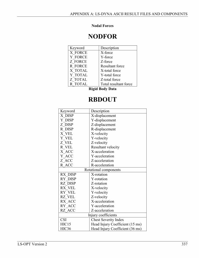
APPENDIX A: LS-DYNA ASCII RESULT FILES AND COMPONENTS
LS-OPT Version 2 337
Nodal Forces
NODFOR
Keyword Description X_FORCE Y_FORCE Z_FORCE R_FORCE X_TOTAL Y_TOTAL Z_TOTAL R_TOTAL
X-force Y-force Z-force Resultant force X-total force Y-total force Z-total force Total resultant force
Rigid Body Data
RBDOUT
Keyword Description X_DISP Y_DISP Z_DISP R_DISP X_VEL Y_VEL Z_VEL R_VEL X_ACC Y_ACC Z_ACC R_ACC
X-displacement Y-displacement Z-displacement R-displacement X-velocity Y-velocity Z-velocity Resultant velocity X-acceleration Y-acceleration Z-acceleration R-acceleration
Rotational components RX_DISP RY_DISP RZ_DISP RX_VEL RY_VEL RZ_VEL RX_ACC RY_ACC RZ_ACC
X-rotation Y-rotation Z-rotation X-velocity Y-velocity Z-velocity X-acceleration Y-acceleration Z-acceleration
Injury coefficients CSI HIC15 HIC36
Chest Severity Index Head Injury Coefficient (15 ms) Head Injury Coefficient (36 ms)

APPENDIX A: LS-DYNA ASCII RESULT FILES AND COMPONENTS
338 LS-OPT Version 2
Reaction Forces
RCFORC
Keyword Description X_FORCE Y_FORCE Z_FORCE R_FORCE XS FORCE YS FORCE ZS FORCE RS FORCE
X-force Y-force Z-force R-force X-slave force Y-slave force Z-slave force R-slave force
RigidWall Forces
RWFORC
Keyword Description NORMAL X_FORCE Y_FORCE Z_FORCE
normal X-force Y-force Z-force
Section Forces
SECFORC
Keyword Description X_FORCE Y_FORCE Z_FORCE X_MOMENT Y_MOMENT Z_MOMENT X_CENTER Y_CENTER Z_CENTER R_FORCE R_MOMENT
X-force Y-force Z-force X-moment Y-moment Z-moment X-center Y-center Z-center R-force R-moment

APPENDIX A: LS-DYNA ASCII RESULT FILES AND COMPONENTS
LS-OPT Version 2 339
Single Point Constraint Reaction Forces
SPCFORC
Keyword Description X_FORCE Y_FORCE Z_FORCE R_FORCE X_RES Y_RES Z_RES X_MOMENT Y_MOMENT Z_MOMENT R_MOMENT
X-force Y-force Z-force R-force Total X-force Total Y-force Total Z-force X-moment Y-moment Z-moment R-moment
Spotweld and Rivet Forces
SWFORC
Keyword Description AXIAL SHEAR
Axial force Shear force

APPENDIX A: LS-DYNA ASCII RESULT FILES AND COMPONENTS
340 LS-OPT Version 2
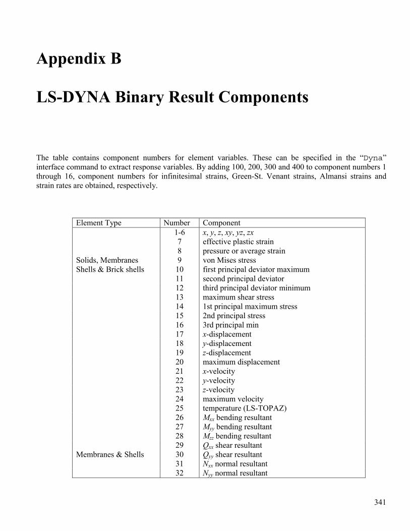
341
Appendix B
LS-DYNA Binary Result Components
The table contains component numbers for element variables. These can be specified in the “Dyna” interface command to extract response variables. By adding 100, 200, 300 and 400 to component numbers 1 through 16, component numbers for infinitesimal strains, Green-St. Venant strains, Almansi strains and strain rates are obtained, respectively.
Element Type Number Component 1-6 x, y, z, xy, yz, zx 7 effective plastic strain 8 pressure or average strain Solids, Membranes 9 von Mises stress Shells & Brick shells 10 first principal deviator maximum 11 second principal deviator 12 third principal deviator minimum 13 maximum shear stress 14 1st principal maximum stress 15 2nd principal stress 16 3rd principal min 17 x-displacement 18 y-displacement 19 z-displacement 20 maximum displacement 21 x-velocity 22 y-velocity 23 z-velocity 24 maximum velocity 25 temperature (LS-TOPAZ) 26 Mxx bending resultant 27 Myy bending resultant 28 Mzz bending resultant 29 Qxx shear resultant Membranes & Shells 30 Qyy shear resultant 31 Nxx normal resultant 32 Nyy normal resultant

APPENDIX B: LS-DYNA BINARY RESULT COMPONENTS
342 LS-OPT Version 2
Element type Number Component 33 Nxy normal resultant 34 Surface stress Nxx/t + 6Mxx/t2 35 Surface stress Nxx/t – 6Mxx/t2 36 Surface stress Nyy/t – 6Myy/t2 37 Surface stress Nyy/t + 6Myy/t2 38 Surface stress Nxy/t – 6Mxy/t2 39 Surface stress Nxy/t + 6Mxy/t2 40 effective upper surface stress 41 effective lower surface stress 42 maximum effective surface stress 43 lower surface effective plastic strain 44 upper surface effective plastic strain 45-50 lower surface x, y, z, xy, yz, zx strain 51-56 upper surface x, y, z, xy, yz, zx strain 57-62 middle surface x, y, z, xy, yz, zx strain 63 internal energy density 64 xy-displacement 65 yz-displacement 66 zx-displacement 67 shell thickness 68 shell thickness reduction (%) 69-80 lower, upper, middle principal + effective strains 81+n n-th history variable 507 FLD - criterion (brick) 508-509 in-plane 1st - 2nd principal strains 543-544 lower-upper surface FLD criterion 546-547 lower-upper surface in-plane 1st principal strain 549-550 lower-upper surface in-plane 2nd principal strain

343
Appendix C
LS-DYNA Binout Result File and Components
Airbag Statistics
ABSTAT
DynaASCII Keyword
Binout Component
Description VOLUME PRESSURE I_ENER IN_FLOW_RATE OUT_FLOW_RATE MASS TEMP DENSITY AREA -
volume pressure internal_energy dm_dt_in dm_dt_out total_mass gas_temp density surface_area reaction
Volume Pressure Internal energy Input mass flow rate Output mass flow rate Mass Temperature Density Area Reaction

APPENDIX C: LS-DYNA BINOUT RESULT FILE AND COMPONENTS
344 LS-OPT Version 2
Boundary Nodal Forces
BNDOUT
DynaASCII Keyword
Binout Component
Description
Binout subdirectory discrete/nodes X_FORCE Y_FORCE Z_FORCE - - - - -
x_force y_force z_force x_total y_total z_total energy etotal
X-force Y-force Z-force Total X-force Total Y-force Total Z-force Energy Total Energy
Discrete Element Forces
DEFORC
DynaASCII Keyword
Binout Component
Description X_FORCE Y_FORCE Z_FORCE R_FORCE -
x_force y_force z_force resultant_force displacement
X-force Y-force Z-force Resultant force Change in length

APPENDIX C: LS-DYNA BINOUT RESULT FILE AND COMPONENTS
LS-OPT Version 2 345
Element Output: Brick and Beam Elements
ELOUT
DynaASCII Keyword
Binout Component
Description Binout subdirectory solid
BXX_STRESS BYY_STRESS BZZ_STRESS BXY_STRESS BYZ_STRESS BZX_STRESS YIELD BE_STRESS BPRESSURE BMAX_SHEAR BMAX_P_STRESS BMIN_P_STRESS - - - - - -
sig_xx sig_xy sig_yy sig_yz sig_zx sig_zz yield effsg - - - - eps_xx eps_xy eps_yy eps_yz eps_zx eps_zz
XX-stress YY-stress ZZ-stress XY-stress YZ-stress ZX-stress Yield function Effective stress Pressure Maximum shear stress Maximum principal stress Minimum principal stress XX-strain YY-strain ZZ-strain XY-strain YZ-strain ZX-strain
Binout subdirectory beam AXIAL S_SHEAR T_SHEAR S_MOMENT T_MOMENT TORSION SIG_11 SIG_12 SIG_31 PLASTIC
axial shear_s shear_t moment_s moment_t torsion - - - -
Axial force resultant s-Shear resultant t-Shear resultant s-Moment resultant t-Moment resultant Torsional resultant σ11 σ12 σ31 Plastic strain

APPENDIX C: LS-DYNA BINOUT RESULT FILE AND COMPONENTS
346 LS-OPT Version 2
Element Output: Shell Elements
ELOUT
DynaASCII Keyword
Binout Component
Description Binout subdirectory shell – stress components
XX_STRESS YY_STRESS ZZ_STRESS XY_STRESS YZ_STRESS ZX_STRESS P_STRAIN PRESSURE E_STRESS MAX_SHEAR MAX_P_STRESS MIN_P_STRESS
sig_xx sig_yy sig_zz sig_xy sig_yz sig_zx plastic_strain - - - - -
XX-stress YY-stress ZZ-stress XY-stress YZ-stress ZX-stress Plastic strain Pressure Effective stress Maximum shear stress Maximum principal stress Minimum principal stress
Binout subdirectory shell – strain components XX_STRAIN YY_STRAIN ZZ_STRAIN XY_STRAIN YZ_STRAIN ZX_STRAIN E_STRAIN MAX_S_STRAIN MAX_P_STRAIN MIN_P_STRAIN
upper_eps_xx lower_eps_xx upper_eps_yy lower_eps_yy upper_eps_zz lower_eps_zz upper_eps_xy lower_eps_xy upper_eps_yz lower_eps_yz upper_eps_zx lower_eps_zx - - - -
XX-strain YY-strain ZZ-strain XY-strain YZ-strain ZX-strain Effective strain Maximum shear strain Maximum principal strain Minimum principal strain

APPENDIX C: LS-DYNA BINOUT RESULT FILE AND COMPONENTS
LS-OPT Version 2 347
DynaASCII Keyword
Binout Component
Description Binout subdirectory thickshell
TXX_STRESS TYY_STRESS TZZ_STRESS TXY_STRESS TYZ_STRESS TZX_STRESS - TP_STRAIN TPRESSURE TE_STRESS TMAX_SHEAR TMAX_P_STRESS TMIN_P_STRESS - - - - - - - - - - - -
sig_xx sig_yy sig_zz sig_xy sig_yz sig_zx yield - - - - - - upper_eps_xx lower_eps_xx upper_eps_yy lower_eps_yy upper_eps_zz lower_eps_zz upper_eps_xy lower_eps_xy upper_eps_yz lower_eps_yz upper_eps_zx lower_eps_zx
XX-stress YY-stress ZZ-stress XY-stress YZ-stress ZX-stress Yield Plastic strain Pressure Effective stress Maximum shear stress Maximum principal stress Minimum principal stress XX-strain - YY-strain - ZZ-strain - XY-strain - YZ-strain - ZX-strain -

APPENDIX C: LS-DYNA BINOUT RESULT FILE AND COMPONENTS
348 LS-OPT Version 2
Contact Entities Resultants
GCEOUT
DynaASCII Keyword
Binout Component
Description X_FORCE Y_FORCE Z_FORCE R_FORCE X_MOMENT Y_MOMENT Z_MOMENT R_MOMENT
x_force y_force z_force force_magnitude x_moment y_moment z_moment moment_magnitude
X-force Y-force Z-force Force magnitude X-moment Y-moment Z-moment Moment magnitude
Global Statistics
GLSTAT
DynaASCII Keyword
Binout Component
Description K_ENER I_ENER T_ENER RATIO SW_ENER D_ENER HG_ENER SI_ENER EW_ENER X_VEL Y_VEL Z_VEL T_VEL - - - -
kinetic_energy internal_energy total_energy energy_ratio stonewall_energy spring_and_damper_energyhourglass_energy sliding_interface_energy external_work global_x_velocity global_y_velocity global_z_velocity - system_damping_energy energy_ratio_wo_eroded eroded_internal_energy eroded_kinetic_energy
Kinetic energy Internal energy Total energy Ratio Stonewall energy Spring & Damper energy Hourglass energy Sliding interface energy External work Global x-velocity Global y-velocity Global z-velocity Velocity System damping energy Energy ratio w/o eroded Eroded internal energy Eroded kinetic energy

APPENDIX C: LS-DYNA BINOUT RESULT FILE AND COMPONENTS
LS-OPT Version 2 349
Joint Element Forces
JNTFORC
DynaASCII Keyword
Binout Component
Description Binout subdirectory joints
X_FORCE Y_FORCE Z_FORCE X_MOMENT Y_MOMENT Z_MOMENT R_FORCE R_MOMENT
x_force y_force z_force x_moment y_moment z_moment resultant_force resultant_moment
X-force Y-force Z-force X-moment Y-moment Z-moment R-force R-moment
Binout subdirectory type0 - - - - - - - - - - - - - - - -
d(phi)_dt d(psi)_dt d(theta)_dt joint_energy phi_degrees phi_moment_damping phi_moment_stiffness phi_moment_total psi_degrees psi_moment_damping psi_moment_stiffness psi_moment_total theta_degrees theta_moment_damping theta_moment_stiffness theta_moment_total
d(phi)/dt d(psi)/dt (degrees) d(theta)/dt (degrees) joint energy phi (degrees) phi moment-damping phi moment-stiffness phi moment-total psi (degrees) psi-moment-damping psi-moment-stiffness psi-moment-total theta (degrees) theta-moment-damping theta-moment-stiffness theta-moment-total

APPENDIX C: LS-DYNA BINOUT RESULT FILE AND COMPONENTS
350 LS-OPT Version 2
Material Summary
MATSUM
DynaASCII Keyword
Binout Component
Description K_ENER I_ENER X_MOMENTUM Y_MOMENTUM Z_MOMENTUM MOMENTUM XRB_VEL YRB_VEL ZRB_VEL RB_VEL TK_ENER TI_ENER -
kinetic_energy internal_energy x_momentum y_momentum z_momentum - x_rbvelocity y_rbvelocity z_rbvelocity - - - hourglass_energy
Kinetic energy Internal energy X-momentum Y-momentum Z-momentum Momentum X-rigid body velocity Y-rigid body velocity Z-rigid body velocity Rigid body velocity Total kinetic energy Total internal energy -
Contact Node Forces
NCFORC
DynaASCII Keyword
Binout Component
Description Binout subdirectory master_00001 and slave_00001 X_FORCE Y_FORCE Z_FORCE R_FORCE PRESSURE - - -
x_force y_force z_force - pressure x y z
X-force Y-force Z-force Resultant Force Pressure X coordinate Y coordinate Z coordinate

APPENDIX C: LS-DYNA BINOUT RESULT FILE AND COMPONENTS
LS-OPT Version 2 351
Nodal Point Response
NODOUT
DynaASCII Keyword
Binout Component
Description X_DISP Y_DISP Z_DISP R_DISP X_VEL Y_VEL Z_VEL R_VEL X_ACC Y_ACC Z_ACC R_ACC - - -
x_displacement y_displacement z_displacement - x_velocity y_velocity z_velocity - x_acceleration y_acceleration z_acceleration - x_coordinate y_coordinate z_coordinate
X-displacement Y-displacement Z-displacement Resultant displacement X-velocity Y-velocity Z-velocity Resultant velocity X-acceleration Y-acceleration Z-acceleration Resultant acceleration X-coordinate Y-coordinate Z-coordinate
Rotational components RX_DISP RY_DISP RZ_DISP RX_VEL RY_VEL RZ_VEL RX_ACC RY_ACC RZ_ACC
rx_acceleration rx_displacementrx_velocity ry_acceleration ry_displacement ry_velocity rz_acceleration rz_displacement rz_velocity
XX-rotation YY-rotation ZZ-rotation XX-rotational velocity YY-rotational velocity ZZ-rotational velocity XX-rotational acceleration YY-rotational acceleration ZZ-rotational acceleration
Injury coefficients CSI HIC15 HIC36
CSI HIC15 HIC36
Chest Severity Index Head Injury Coefficient (15 ms) Head Injury Coefficient (36 ms)

APPENDIX C: LS-DYNA BINOUT RESULT FILE AND COMPONENTS
352 LS-OPT Version 2
Nodal Forces
NODFOR
DynaASCII Keyword
Binout Component
Description X_FORCE Y_FORCE Z_FORCE R_FORCE X_TOTAL Y_TOTAL Z_TOTAL R_TOTAL - - - - -
x_force y_force z_force - x_total y_total z_total - x_local y_local z_local energy etotal
X-force Y-force Z-force Resultant force X-total force Y-total force Z-total force Total resultant force - - - Energy Total Energy

APPENDIX C: LS-DYNA BINOUT RESULT FILE AND COMPONENTS
LS-OPT Version 2 353
Rigid Body Data
RBDOUT
DynaASCII Keyword
Binout Component
Description X_DISP Y_DISP Z_DISP R_DISP X_VEL Y_VEL Z_VEL R_VEL X_ACC Y_ACC Z_ACC R_ACC - - - - - - - - - - - -
global_dx global_dy global_dz - global_vx global_vy global_vz - global_ax global_ay global_az - global_x global_y global_z local_dx local_dy local_dz local_vx local_vy local_vz local_ax local_ay local_az
X-displacement Y-displacement Z-displacement Resultant displacement X-velocity Y-velocity Z-velocity Resultant velocity X-acceleration Y-acceleration Z-acceleration Resultant acceleration X-coordinate Y-coordinate Z-coordinate Local X-displacement Local Y-displacement Local Z-displacement Local X-velocity Local Y-velocity Local Z-velocity Local X-acceleration Local Y-acceleration Local Z-acceleration

APPENDIX C: LS-DYNA BINOUT RESULT FILE AND COMPONENTS
354 LS-OPT Version 2
Rigid Body Data
RBDOUT
Rotational components DynaASCII
Keyword Binout
Component Description
RX_DISP RY_DISP RZ_DISP RX_VEL RY_VEL RZ_VEL RX_ACC RY_ACC RZ_ACC - - - - - - - - -
global_rax global_ray global_raz global_rdx global_rdy global_rdz global_rvx global_rvy global_rvz local_rdx local_rdy local_rdz local_rvx local_rvy local_rvz local_rax local_ray local_raz
X-rotation Y-rotation Z-rotation X-velocity Y-velocity Z-velocity X-acceleration Y-acceleration Z-acceleration Local X-rotation Local Y-rotation Local Z-rotation Local X-velocity Local Y-velocity Local Z-velocity Local X-acceleration Local Y-acceleration Local Z-acceleration
Direction cosines - - - - - - - - -
dircos_11 dircos_12 dircos_13 dircos_21 dircos_22 dircos_23 dircos_31 dircos_32 dircos_33
11 direction cosine 12 direction cosine 13 direction cosine 21 direction cosine 22 direction cosine 23 direction cosine 31 direction cosine 32 direction cosine 33 direction cosine
Injury coefficients CSI HIC15 HIC36
CSI HIC15 HIC36
Chest Severity Index Head Injury Coefficient (15 ms) Head Injury Coefficient (36 ms)

APPENDIX C: LS-DYNA BINOUT RESULT FILE AND COMPONENTS
LS-OPT Version 2 355
Reaction Forces
RCFORC
DynaASCII Keyword
Binout Component
Description X_FORCE Y_FORCE Z_FORCE R_FORCE XS FORCE YS FORCE ZS FORCE RS FORCE -
x_force y_force z_force - - - - - mass
X-force Y-force Z-force Resultant force X-slave force Y-slave force Z-slave force R-slave force Mass
RigidWall Forces
RWFORC
DynaASCII Keyword
Binout Component
Description Binout subdirectory forces
NORMAL X_FORCE Y_FORCE Z_FORCE
normal_force x_force y_force z_force
normal X-force Y-force Z-force

APPENDIX C: LS-DYNA BINOUT RESULT FILE AND COMPONENTS
356 LS-OPT Version 2
Section Forces
SECFORC
DynaASCII Keyword
Binout Component
Description X_FORCE Y_FORCE Z_FORCE X_MOMENT Y_MOMENT Z_MOMENT X_CENTER Y_CENTER Z_CENTER R_FORCE R_MOMENT -
x_force y_force z_force x_moment y_moment z_moment x_centroid y_centroid z_centroid total_force total_moment area
X-force Y-force Z-force X-moment Y-moment Z-moment X-center Y-center Z-center Resultant force Resultant moment Area
Single Point Constraint Reaction Forces
SPCFORC
DynaASCII Keyword
Binout Component
Description X_FORCE Y_FORCE Z_FORCE R_FORCE X_RES Y_RES Z_RES X_MOMENT Y_MOMENT Z_MOMENT R_MOMENT
x_force y_force z_force - x_resultant y_resultant z_resultant x_moment y_moment z_moment -
X-force Y-force Z-force Resultant force Total X-force Total Y-force Total Z-force X-moment Y-moment Z-moment Resultant moment

APPENDIX C: LS-DYNA BINOUT RESULT FILE AND COMPONENTS
LS-OPT Version 2 357
Spotweld and Rivet Forces
SWFORC
DynaASCII Keyword
Binout Component
Description AXIAL SHEAR -
axial shear failure_flag
Axial force Shear force Failure flag

APPENDIX C: LS-DYNA BINOUT RESULT FILE AND COMPONENTS
358 LS-OPT Version 2

359
Appendix D
Database files
D.1 Design flow
Source Database file Process Output Database file Level of directory for output database
Command file (com) Point selection Experiments Solver Experiments Simulation runs Solver output files Run Solver output files Result extraction AnalysisResults
StatResultsSolver Work
AnalysisResults Approximation DesignFunctionsNet
Solver
DesignFunctions Optimize OptimumResultsOptimizationHistory
Work Work
D.2 Database file formats The “Experiments” file This file appears in the solver directory and is used to save the experimental point coordinates for the analysis runs. The file consists of lines having the following format repeated for each experimental point. x[1], x[2], ..., x[n] where x[1] to x[n] are the values of the n solver design variables at the experimental point. The “AnalysisResults” file This file is used to save the responses at the experimental points and appears in the solver directory. Every line describes an experimental point and gives the response values at the experimental point. The file consists of lines having the following format repeated for each experimental point.
x[1], x[2], ..., x[n],RespVal[1], RespVal[2], ..., RespVal[m] where x[1] to x[n] are the values of the n solver design variables at the experimental point. RespVal[1] to RespVal[m] are the values of the m solver responses. Values of 2.0*1030 are assigned to responses of simulations with error terminations. The AnalysisResults file is synchronous with the Experiments file.
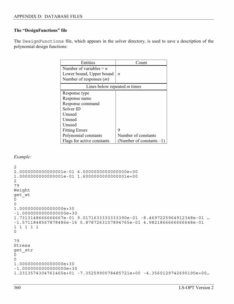
APPENDIX D: DATABASE FILES
360 LS-OPT Version 2
The “DesignFunctions” file The DesignFunctions file, which appears in the solver directory, is used to save a description of the polynomial design functions:
Entities Count Number of variables = n Lower bound, Upper boundNumber of responses (m)
n
Lines below repeated m times Response type Response name Response command Solver ID Unused Unused Unused Fitting Errors Polynomial constants Flags for active constants
9 Number of constants (Number of constants –1)
Example: 22.0000000000000001e-01 4.0000000000000000e+001.0000000000000001e-01 1.6000000000000001e+00279Weightget_wt001.0000000000000000e+30-1.0000000000000000e+301.7313148666666667e-01 9.0171633333333390e-01 -8.4697225964912348e-01 …-1.5711848567878486e-16 5.8787263157894765e-01 4.9821866666666648e-011 1 1 1 10
79Stressget_str001.0000000000000000e+30-1.0000000000000000e+301.2313574304761465e+01 -7.3525990078485721e+00 -4.3560129742690190e+00…

APPENDIX D: DATABASE FILES
LS-OPT Version 2 361
1.1417587257617741e+00 1.8766964912280690e-01 2.1619635555555621e+001 1 1 1 10
The flags for active coefficients exclude the constant a0. The “OptimizationHistory” file This file is used to save the optimization history results and appears in the work directory. Each line contains the values at the optimum point of an iteration.
Entities Count Objective values Number of objectives Variables Number of variables Variable lower bounds Number of variables Variable upper bounds Number of variables RMS errors Number of responses Average errors Number of responses Maximum errors Number of responses R2 errors Number of responses Adjusted R2 errors Number of responses PRESS errors Number of responses Prediction R2 Number of responses Maximum prediction error Number of responses Responses Number of responses Multi-objective 1 Constraint values Number of constraints Composite values Number of composites Responses (computed) Number of responses Max. constraint violation 1 Composites (computed) Number of composites Constraints (computed) Number of constraints Objectives (computed) Number of objectives Multi-objective (computed) 1 Max. constraint violation (computed) 1 Constants Number of constants Dependents Number of dependents
Values of 2.0*1030 are assigned to responses of error terminations.

APPENDIX D: DATABASE FILES
362 LS-OPT Version 2
The “ExtendedResults” file This file contains all points represented in the AnalysisResults file and appears in the solver directory. All values are based on the simulation results. A line has the following format:
Entities Count Objective weights Number of objectives Objective values Number of objectives Variables Number of solver variables Responses Number of solver responses Multi-objective 1 Constraint values Number of constraints Composite values Number of composites Max. constraint violation 1 Constants Number of constants Dependents Number of dependents
Values of 2.0*1030 are assigned to responses of simulations with error terminations. The “OptimumResults” file This file contains just the optimum design point data and appears in the solver directory. All values are metamodel values, i.e. interpolated.
Entities Count Objective weights Number of objectives Objective values Number of objectives Variables Number of variables Responses Number of responses Multi-objective 1 or 0 (no objectives) Constraint values Number of constraints Composite values Number of composites Max. constraint violation 1 Constants Number of constants Dependents Number of dependents

363
Appendix E
Mathematical Expressions
Mathematical expressions are available for the following entities:
dependenthistoryresponsecompositemultiobjective E.1 Syntax rules 1. Mathematical expressions are placed in curly brackets in the command file or in double angular brackets
(e.g. <<Thickness*25.4>>) in the input template files. 2. Expressions consist of parameters and constants. A parameter can be any previously defined entity. 3. Expressions can be wrapped to appear on multiple lines. 4. Mathematical expressions can be used for any floating-point number, e.g. upper bound of constraint,
convergence tolerance, objective weight, etc. 5. An expression is limited to 1024 characters.

APPENDIX E: MATHEMATICAL EXPRESSIONS
364 LS-OPT Version 2
E.2 Intrinsic functions
int(a) integer nint(a) nearest integer abs(a) absolute value mod(a,b) remainder of a/b sign(a,b) transfer of sign from b to |a| max(a,b) maximum of a and b min(a,b) minimum of a and b sqrt(a) square root exp(a) ea pow(a,b) ab log(a) natural logarithm log10(a) base 10 logarithm sin(a) sine cos(a) cosine tan(a) tangent asin(a) arc sine acos(a) arc cosine atan(a) arc tangent atan2(a,b) arc tangent of a/b sinh(a) hyperbolic sine cosh(a) hyperbolic cosine tanh(a) hyperbolic tangent asinh(a) arc hyperbolic sine acosh(a) arc hyperbolic cosine atanh(a) arc hyperbolic tangent sec(a) secant csc(a) cosecant ctn(a) cotangent

APPENDIX E: MATHEMATICAL EXPRESSIONS
LS-OPT Version 2 365
E.3 Special functions Special response functions can be specified to apply to response histories. These include integration, minima and maxima and finding the time at a specific value of the function. General expressions (in double quotes) can be used for limits and for the integration variable. Histories must be defined as strings in double quotes and functions of time using the symbol t, e.g. ”Velocity(t)”. Expression Symbols Integral(expression[,t_lower,t_upper,variable]) ∫
b
atdgtf )()(
Derivative(expression[,T_constant]) Tttf =∆∆ |/ ~ Tttf =|d/d
Min(expression[,t_lower,t_upper]) )]([minmin tfft
=
Max(expression[,t_lower,t_upper]) )]([maxmax tfft
=
Initial(expression) First function value on record Final(expression) Last function value on record Lookup(expression,value) Inverse function t(f = F) LookupMin(expression[,t_lower,t_upper]) Inverse function t(f = fmin) LookupMax(expression[,t_lower,t_upper]) Inverse function t(f = fmax)
The arguments used in the expressions have the following explanations:
Argument Explanation Symbol Type t_lower lower limit of integration or range a generic t_upper upper limit of integration or range b generic variable integration variable g(t) generic expression history defined as an expression string f(t) generic value value for which lookup is required F generic T_constant specific time Τ generic
“Generic” implies that the quantity can be an expression, a previously defined entity or a constant number. An entity (which may be specified in an expression) can be any previously defined LS-OPT entity. Thus constant, variable, dependent, history, response and composite are acceptable. An expression is given in double quotes, e.g., ”Displacement(t)”. E.4 Reserved variable names
Name Explanation t Time LowerLimit 0.0 UpperLimit Maximum event time over all histories of all solvers
Omitting the lower and upper bounds implies operation over the entire available history.

APPENDIX E: MATHEMATICAL EXPRESSIONS
366 LS-OPT Version 2
The Lookup function allows finding the value of t for a specified value of f(t) = F. If such a value cannot be found, the largest value of t in the history is returned. The LookupMin and LookupMax functions return the value of t at the minimum or maximum respectively. The implied variable represented in the first column of any history file is t. Therefore all history files produced by the DynaASCII extraction command contain functions of t. The fourth argument of the Integral function defaults to t. The variable t must increase monotonically. The derivative assumes a piecewise linear function defined by the points in the history.n file. T_constant in the Derivative function defaults to the end time. If a time is specified smaller than the smallest time value of the computed history, the first value is returned (same as Initial). If a time is specified larger than the largest time value of the computed history, the last value is returned (same as Final). For derivatives the first or last slopes are returned respectively. E.5 Constants associated with histories The following commands can be given to override defaults for history operations: Constant Explanation Default variable fdstepsize Finite difference step size for
numerical derivatives with respect to variables
0.0001*(Upper bound – Lower bound)
historysize Number of time points for new history
10000
Command file syntax: variable fdstepsize valuehistorysize integer value
• The variable fdstepsize is used to find the gradients of expression composite functions. These
are used in the optimization process. • The historysize is used when new histories are generated.

APPENDIX E: MATHEMATICAL EXPRESSIONS
LS-OPT Version 2 367
E.6 Generic expressions Expressions can be specified for any floating-point number. In some cases, previously defined parameters can be used as follows:
Number type Parameter type Constant none Starting variable constant Range variable Variable bounds variable Shift factor for response variable Scale factor for response variable Constraint bounds variable Objective weight variable Target value (composite) variable Scale factor (composite) variable Weight (composite) variable Parameters of SRSM none Parameters of LFOPC none
The parameter type represents the highest entity in the hierarchy. Thus constants are included in the variable parameters. In LS-OPT, expressions can be entered for variables, constants, dependents, histories, responses constraints and objectives. Example: constant ’Target1’ {12756.333/1000.}constant ’Target2’ {966002/1000.}variable ’Emod’ 1e7composite ’Residual’ type targetedcomposite ’Residual’ response ’F1’ {Target1} scale {Target1}composite ’Residual’ response ’F2’ {Target2} scale {Target2}objective ’Residual’$variable fdstepsize {1/500.}time fdstepsize {1/300.}history size 10000

APPENDIX E: MATHEMATICAL EXPRESSIONS
368 LS-OPT Version 2
E.7 Examples illustrating syntax of expressions Example 1: The following example shows a simple evaluation of variables and functions. The histories are specified in plot files his1 and his2. A third function his3 is constructed from the files by averaging. File his1: 0 0.0100 1000200 500300 500
File his2: 0 0.0100 2000200 2000300 2000
Input file: "Mathematical Expressions"$$ CONSTANTS$constants 3constant ’lowerlimit’ 0constant ’upperlimit’ .200constant ’angle’ 30$$ DESIGN VARIABLE DEFINITIONS$variables 2Variable ’x1’ 45Lower bound variable ’x1’ -10Upper bound variable ’x1’ 50Variable ’x2’ 45Lower bound variable ’x2’ -10Upper bound variable ’x2’ 50$$ DEPENDENT VARIABLES$dependents 2dependent ’ll’ {lowerlimit * 1000}dependent ’ul’ {upperlimit * 1000}$...

APPENDIX E: MATHEMATICAL EXPRESSIONS
LS-OPT Version 2 369
$$ HISTORIES$history 3history ’his1’ "cat ../../his1 > LsoptHistory"history ’his2’ "cat ../../his2 > LsoptHistory"history ’his3’ {(his1(t) + his2(t))/2}$$ RESPONSES$responses 42response ’LOWER’ expression {LowerLimit}response ’UPPER’ expression {UpperLimit}response ’UL’ expression {ul}response ’First’ expression {Initial("his1(t)")}response ’Last’ expression {Final("his1(t)")}response ’Last3’ expression {Final("(his1(t) + his2(t))/2")}response ’Max1’ expression {Max("his1(t)")}response ’Max2’ expression {Max("his1(t)","ll * 1.0")}response ’Maximum11’ expression {Max("his1(t)","ll",ul)}response ’Maximum32’ expression {Max("his3(t)",ll,ul)}response ’Minimum32’ expression {Min("his3(t)",ll,ul)}response ’Inverse11’ expression {Lookup("his1(t)",75)}response ’Inverse21’ expression {Lookup("his2(t)",75)}response ’Inverse31’ expression {Lookup("his3(t)",75)}response ’Inverse33’ expression {Lookup("(his1(t) + his2(t))/2",75)}response ’MaxI’ expression {max(Inverse11,Inverse21)}response ’MinI’ expression {min(Inverse11,Inverse21)}response ’hist’ expression {his3(Inverse31)}response ’hist66’ expression {his3(66.1) + 0.1}response ’nhist66’ expression {nint(hist66)}response ’ihist66’ expression {int(hist66)}response ’Integ11’ expression {Integral("his1(t)")}response ’Integ14’ expression {Integral("his1(t)",ll,ul,"t")}response ’Integ15’ expression {Integral("his1(t)",ll,UPPER,"t")}response ’Integ22’ expression {Integral("his2(t)",ll,ul,"t")}response ’Integ32’ expression {Integral("his3(t)",ll,ul,"t")}response ’Integ33’ expression {Integral("(his1(t) + his2(t))/2",ll,ul,"t")}response ’Integ34’ expression {Integral("his3(t)")}response ’Integ35’ expression {Integral("his3(t)",ll)}response ’Integ36’ expression {Integral("his3(t)",ll,ul)}$$ Cross-functional integrals$response ’Integ2’ expression {Integral("his1(t)",ll,ul,"his2(t)")}response ’Integ3a’ expression {Integral("his1(t)",0,30,"his2(t)")}response ’Integ3b’ expression {Integral("his1(t)",30,100,"his2(t)")}response ’Integ4’ expression {Integ1 + Integ2}response ’Integ5’ expression {Integral("sin(t) * his1(t) * his2(t)",ll,ul,"t")}response ’Integ7’ expression {Integral("sin(t) * his1(t) * his2(t)")}response ’Velocity1’ expression {Derivative(”Displacement(t)”,0.08)}response ’Velocity2’ expression {Derivative(”Displacement(t)”)}$$ COMPOSITE FUNCTIONS$composites 1composite ’Integ6’ {(Integ3a/(4*Maximum11) + Integ2/2)**.5}$

APPENDIX E: MATHEMATICAL EXPRESSIONS
370 LS-OPT Version 2
$ OBJECTIVE FUNCTIONS$objectives 1objective ’Integ6’$$ CONSTRAINT FUNCTIONS$constraints 1constraint ’Integ1’$iterate 0STOP Example 2:
constant ’v0’ 15.65$----------------------------------------------------------------------------$ Extractions$----------------------------------------------------------------------------history ’engine_velocity’ "DynaASCII nodout X_VEL 73579 TIMESTEP 0.0 SAE 30"history ’Apillar_velocity_1’ "DynaASCII nodout X_VEL 41195 TIMESTEP 0.0 SAE 30"history ’Apillar_velocity_2’ "DynaASCII nodout X_VEL 17251 TIMESTEP 0.0 SAE 30"history ’global_velocity’ "DynaASCII glstat X_VEL 0 TIMESTEP 0.0"$----------------------------------------------------------------------------$ Mathematical Expressions for dependent histories$----------------------------------------------------------------------------history ’Apillar_velocity_average’ {(Apillar_velocity_1 +
Apillar_velocity_2)/2}$$ Find the time when the engine velocity = 0$response ’time_to_engine_zero’ expression {Lookup("engine_velocity(t)",0)}$$ Find the average velocity at time of engine velocity = 0$response ’vel_A_engine_zero’ expression {Apillar_velocity_average
(time_to_engine_zero)}$$ Integrate the average A-pillar velocity up to zero engine velocity$ Divide by the time to get the average$response ’PULSE_1’ expression {Integral
("Apillar_velocity_average(t)",0,time_to_engine_zero)/time_to_engine_zero}
$$ Find the time at which the global velocity is zero$response ’time_to_zero_velocity’ expression {Lookup("global_velocity(t)",0)}$$ Find the average A-pillar velocity where global velocity is zero$response ’velocity_final’ {Apillar_velocity_average(time_to_zero_velocity)}response ’PULSE_2’ expression {Integral
("Apillar_velocity_average(t)",time_to_engine_zero,

APPENDIX E: MATHEMATICAL EXPRESSIONS
LS-OPT Version 2 371
time_to_zero_velocity)/(time_to_zero_velocity - time_to_engine_zero)}

APPENDIX E: MATHEMATICAL EXPRESSIONS
372 LS-OPT Version 2

373
Appendix F
Simulated Annealing
The Simulated Annealing (SA) algorithm for global optimization can be viewed as an extension to local stochastic optimization techniques. The basic idea is very simple. SA takes a (biased) random walk through the space and aims to find a global optimum from among multiple local solutions. In trying to minimize a function, instead of always going downhill, SA algorithm goes downhill most of the time. It means that the SA process sometimes goes uphill. This allows simulated annealing to move consistently towards lower function values, yet still 'jump' out of local minima and globally explore different states of the optimized system. The SA algorithm was first formulated for various combinatorial problems, [30]. The approach was later extended to continuous optimization problems. In [44] the simulated annealing algorithm was adopted to search for optimal Latin hypercube designs. The term 'simulated annealing' derives from the rough analogy of the way that the liquids freeze and crystallize, or metals cool and anneal, starting at a high temperature, [30]. When the liquid is hot, the molecules move freely, and very many changes of energy can occur. When the liquid is cooled, this thermal mobility is partially lost. If the rate of cooling is sufficiently slow, the atoms are often able to line themselves up and form a pure crystal, which is the state of minimum (most stable) energy for this physical system. If a liquid metal is cooled quickly or 'quenched', it usually does not reach this state but rather ends up in a polycrystalline or amorphous state having somewhat higher energy. So the essence of the whole process is slow cooling. Nature's minimization algorithm is based on the fact that a system in thermal equilibrium at temperature T has its energy, E, probabilistically distributed among all different energy states as determined by the Boltzmann distribution:
Probability( E ) ~ exp(-E / κBT ). (F.1)
Hence, even at low temperature, there is a chance, albeit very small, of a system being in a high-energy state. This slight probability of choosing a state that gives higher energy is what allows the physical system to get out of local (i.e. amorphous) minima in favor of finding a better, more stable, orientation. The quantity κB (Boltzmann's constant) is a constant of nature that relates temperature to energy. In simulated annealing algorithm parlance, the objective function of the optimization problem is often called 'energy'. The optimization algorithm proceeds in small iterative steps. At each iteration, SA algorithm randomly generates a candidate state and, through a random mechanism (controlled by a parameter called temperature in view of the analogy with the physical process) decide whether to move to the candidate state or to stay in the current one at the next iteration. More formally, a general SA algorithm can be described as follows.

APPENDIX F: SIMULATED ANNEALING
374 LS-OPT Version 2
Step 0. Let x(0) ∈ X be a given starting state of the optimized system, E = E(x). Start the sequence of observed states: X(0)={x(0)}. Set the starting temperature T(0) to a high value: T(0) = Tmax, and initialize the counter of iterations to k = 0. Step 1. Sample a point x' from the candidate distribution, D( X(k) ), and set X(k+1) = X(k) U {x'). The sequence X(k+1) contains all the states observed up to iteration k. Step 2. Sample a uniform random number ζ in [0,1] and set
x(k+1) = x' if ζ ≤ A(x',x(k),T(k)) or (F.2) x(k+1) = x(k) otherwise.
Step 3. Apply the cooling schedule to the temperature, i.e. set T(k+1) = C( X(k+1), T(k) ). Step 4. Check a stopping criterion and if it fails set k := k+1 and go back to Step 1.
The distribution of the next candidate state, D, the acceptance function, A, the cooling schedule, C, and the stopping criterion must be specified in order to define the SA algorithm. Appropriate choices are essential to guarantee the efficiency of the algorithm. Many different definitions of the above entities have been given in the existing literature about SA. These will be discussed in the next few paragraphs, trying to emphasize some key ideas that have driven the choices of the researches in this field.
In the existing literature about SA algorithms very few acceptance functions have been employed. In most cases the acceptance function is the so-called Metropolis function:
−′−=′
TxExETxxA ))()((exp(,1min),,( (F.4)
Another possibility is the so-called Barker criterion:
−′
+=′
TxExE
TxxA))()(exp((1
1),,( (F.5)
The theoretical motivation for such a restricted choice of acceptance functions can be found in [57]. It is shown that under appropriate assumptions, many acceptance functions, which share some properties, are equivalent to (F.4) or (F.5) after a monotonic transformation of the temperature T. Due to the difficult nature of the problems solved by SA algorithms, it is hard, if not impossible, to define a general stopping rule, which guarantees to stop when the global optimum has been detected or when there is a sufficiently high probability of having detected it. Thus the stopping rules proposed in the literature about SA all have a heuristic nature and are, in fact, more problem dependent than SA algorithm dependent. These

APPENDIX F: SIMULATED ANNEALING
LS-OPT Version 2 375
heuristics are usually based on the idea to stop the iterative algorithm when it does not make a noticeable progress over a number of iterations. The choice of the next candidate distribution and the cooling schedule for the temperature are typically the most important (and strongly interrelated) issues in the definition of a SA algorithm. The next candidate state, x', is usually selected randomly among all the neighbors of the current solution, x, with the same probability for all neighbors. However, with a complicated neighbor structure, a non-uniformly random selection might be appropriate. The choice of the size of the neighborhood typically follows the idea that when the current function value is far from the global minimum, the algorithm should have more freedom, i.e. larger 'step sizes' are allowed. The basic idea of the cooling schedule is to start the algorithm off at high temperature and then gradually to drop the temperature to zero. The primary goal is to quickly reach the so called effective temperature, roughly defined as the temperature at which low function values are preferred but it is still possible to explore different states of the optimized system, [7]. After that the simulated annealing algorithm lowers the temperature by slow stages until the system 'freezes' and no further changes occur. A straightforward and most popular strategy is to decrement T by a constant factor every νT iterations: TTT µ=: (F.6) where µT is slightly greater than 1 (e.g. µT = 1.001). The value of νT should be large enough, so that 'thermal equilibrium' is achieved before reducing the temperature. A rule of thumb is to take νT proportional to the size of neighborhood of the current solution. Often, the cooling schedule (F.6) also provides a condition for terminating SA iterations: minTT < (F.7) Some of the convergence results for SA rely on the fact that the support of the next candidate distribution is the whole feasible region (though in some cases the probability of sampling states far from the current one decreases to 0 as the iteration counter increases). For these convergence results it is often only required that the temperature decreases to 0, no matter at which rate. For some other convergence results the support of the next candidate distribution is only a neighborhood of the current state, and to make the algorithm able to climb the barriers separating the different local minima, it is required that the temperature decreases to 0 slowly enough. It is clear that the selection of the initial temperature, Tmax, has a profound influence on the rate of convergence of the SA algorithm. At temperatures much higher than the effective temperature, the algorithm behaves very much like a random search, while at temperatures much lower than the effective temperature it behaves like (an inefficient implementation of) a deterministic algorithm for local optimization. Intuitively, the cooling schedule (F.6) should begin one order of magnitude higher than the effective temperature and end one order of magnitude lower, [7]. It is difficult to give the initial temperature directly, because this value depends on the neighborhood structure, the scale of the objective function, the initial solution, etc. In [30] a suitable initial temperature is one that results in an average uphill move acceptance probability of about 0.8. This Tmax can be estimated by
APPENDIX F: SIMULATED ANNEALING
376 LS-OPT Version 2
conducting an initial search, in which all uphill moves are accepted and calculating the average objective increase observed. In some other papers it is suggested that parameter Tmax is set to a value, which is larger than the expected value of |E'-E| that is encountered from move to move. In [7] it is suggested to spend most of the computational time in short sample runs with different Tmax in order to detect the effective temperature. In practice, the optimal control of T may require physical insight and trial-and-error experiments. According to [9], "choosing an annealing schedule for practical purposes is still something of a black art". Simulated annealing has proved surprisingly effective for a wide variety of hard optimization problems in science and engineering. Many of the applications in our list of references attest to the power of the method. This is not to imply that a serious implementation of simulated annealing to a difficult real world problem will be easy. In the real-life conditions, the energy trajectory, i.e. the sequence of energies following each move accepted, and the energy landscape itself can be terrifically complex. Note that state space, which consists of wide areas with no energy change, and a few "deep, narrow valleys", or even worse, "golf-holes", is not suited for simulated annealing, because in a "long, narrow valley" almost all random steps are uphill. Choosing a proper stepping scheme is crucial for SA in these situations. However, experience has shown that simulated annealing algorithms get more likely trapped in the largest basin, which is also often the basin of attraction of the global minimum or of the deep local minimum. Anyway, the possibility, which can always be employed with simulated annealing, is to adopt a multistart strategy, i.e. to perform many different runs of the SA algorithm with different starting points. Another potential drawback of using SA for hard optimization problems is that finding a good solution can often take an unacceptably long time. While SA algorithms may detect quickly the region of the global optimum, they often require many iterations to improve its approximation. For small and moderate optimization problems, one may be able to construct effective procedures that provide similar results much more quickly, especially in cases when most of the computing time is spent on calculations of values of the objective function. But it should be noted that for the large-scale multidimensional problems an algorithm, which always (or often) obtains a solution near the global optimum is valuable, since various local deterministic optimization methods allow quick refinement of a nearly correct solution. In summary, simulated annealing is a powerful method for global optimization in challenging real world problems. Certainly, some "trial and error" experimentation is required for an effective implementation of the algorithm. The energy (cost) function should employ some heuristic related to the problem at hand, clearly reflecting how 'good' or 'bad' is a given solution. Random perturbations of the system state and corresponding cost change calculations should be simple enough, so that SA algorithm can perform its iterations very fast. The scalar parameters of the simulated annealing algorithm (Tmax, µT, νT, in particular) have to be chosen carefully. If the parameters are chosen such that the optimization evolves too fast, the solution converges directly to some, possibly good, solution depending on the initial state of the problem.

377
Appendix G
Glossary
ANOVA. Analysis of variance. Used to perform variable screening by identifying insignificant variables. Variable regression coefficients are ranked based on their significance as obtained through a partial F-test. (See also variable screening). Bias error. The total error – the difference between the exact and computed response - is composed of a random and a bias component. The bias component is a systematic deviation between the chosen model (approximation type) and the exact response of the structure (FEA analysis is usually considered to be the exact response). Also known as the modeling error. (See also random error). Binout. The name of the binary output file generated by LS-DYNA (Version 970 onwards). Composite function. A function constructed by combining responses and design variables into a single value. Symbolized by F. Concurrent simulation. The running of simulation tasks in parallel without message passing between the tasks. Confidence interval. The interval in which a parameter may occur with a specified level of confidence. Computed using Student’s t-test. Typically applied to accompany the significance of a variable in the form of an error bar. Constraint. An absolute limit on a response variable specified in terms of an upper or lower limit. Constrained optimization. The mathematical optimization of a function subject to specified limits on other functions. Conventional Design. The procedure of using experience and/or intuition and/or ad hoc rules to improve a design. Dependent. A function which is dependent on variables. Dependent variable. Design of Experiments. See experimental design. Design parameter. See design variable.

APPENDIX G: GLOSSARY
378 LS-OPT Version 2
Design formula. A simple mathematical expression which gives the response of a design when the design variables are substituted. See response surface. Design space. A region in the n-dimensional space of the design variables (x1 through xn to which the design is limited. The design space is specified by upper and lower bounds on the design variables. Response variables can also be used to bound the design space. Design surface. The response variable as a function of the design variables, used to construct the formulation of a design problem. (See also response surface, design rule). Design sensitivity. The gradient vector of the response. The derivatives of the response function in terms of the design variables. df /dxi. Design variable. An independent design parameter which is allowed to vary in order to change the design. Symbolized by (xi or x (vector containing several design variables)). Discipline. An area of analysis requiring a specific set of simulation tools, usually because of the unique nature of the physics involved, e.g. structural dynamics or fluid dynamics. In the context of MDO, often used interchangeably with solver. DOE. Design of Experiments. See experimental design. D-optimal. The state of an experimental design in which the determinant of the moment matrix XX T of the least squares formulation is maximized. DSA. Design sensitivity analysis. Elliptic approximation. An approximation in which only the diagonal Hessian terms are used. Experiment. Evaluation of a single design.
Experimental Design. The selection of designs to enable the construction of a design response surface. Sometimes referred to as the Point Selection Scheme. Feasible Design. A design which complies with the constraint bounds. Function. A mathematical expression for a response variable in terms of design variables. Often used interchangeably with “response”. Symbolized by f. Functionally efficient. See Pareto optimal. Function evaluation. Using a solver to analyze a single design and produce a result. See Simulation. Global variable. A variable of which the scope spans across all the design disciplines or solvers. Used in the MDO context.

APPENDIX G: GLOSSARY
LS-OPT Version 2 379
Global approximation. A design function which is representative of the entire design space. Global Optimization. The mathematical procedure for finding the global optimum in the design space. E.g. Genetic Algorithm, Particle Swarm, etc. Gradient vector. A vector consisting of the derivatives of a function f in terms of a number of variables x1 to xn. s = [df /dxi]. See Design Sensitivity. History. Response history containing two columns of (usually time) data generated by a simulation. Importance. See Weight. Infeasible Design. A design which does not comply with the constraint functions. An entire design space or region of interest can sometimes be infeasible. Iteration. A cycle involving an experimental design, function evaluations of the designs, approximation and optimization of the approximate problem. Kriging. A Metamodeling technique using Bayesian regression. (see e.g. [5,20]). Latin Hypercube Sampling. The use of a constrained random experimental design as a point selection scheme for response approximation. Least Squares Approximation. The determination of the coefficients in a mathematical expression so that it approximates certain experimental results by the minimization of the sum of the squares of the approximation errors. Used to determine response surfaces as well as calibrating analysis models. Local Approximation. See Gradient vector. Local variable. A variable of which the scope is limited to a particular discipline or disciplines. Used in the MDO context. Material identification. See parameter identification. MDO. Multidisciplinary design optimization. Metamodeling. The construction of surrogate design models such as polynomial response surfaces, Artificial Neural Networks or Kriging surfaces from simulations at a set of design points. Min-Max optimization problem. An optimization problem in which the maximum value considering several responses or functions is minimized. Model calibration. The optimal adjustment of parameters in a numerical model to simulate the physical model as closely as possible. Modeling error. See bias error.

APPENDIX G: GLOSSARY
380 LS-OPT Version 2
Multidisciplinary design optimization (MDO). The inclusion of multiple disciplines in the design optimization process. In general, only some design variables need to be shared between the disciplines to provide limited coupling in the optimization of a multidisciplinary target or objective. Multi-objective. An objective function which is constituted of more than one objective. Symbolized by F. Multi-criteria. Refers to optimization problems in which several criteria are considered. MP. Mathematical Programming. Mathematical optimization. Neural network approximation. The use of trained feed-forward neural networks to perform non-linear regression, thereby constructing a non-linear response surface. Numerical sensitivity. A derivative of a function computed by using finite differences. Noise. See random error. Objective. A function of the design variables that the designer wishes to minimize or maximize. If there exists more than one objective, the objectives have to be combined mathematically into a single objective. Symbolized by Φ . Optimal design. The methodology of using mathematical optimization tools to improve a design iteratively with the objective of finding the ‘best’ design in terms of predetermined criteria. Point selection scheme. Same as experimental design. Parameter identification. A procedure in which a numerical model is calibrated by optimizing selected parameters in order to minimize the response error with respect to certain targeted responses. The targeted responses are usually derived from experimental results. Pareto optimal. A multi-objective design is Pareto-optimal if none of the objectives can be improved without at least one objective being affected adversely. Also referred to as functionally efficient. Preference function. A function of objectives used to combine several objectives into a single one suitable for the standard MP formulation. Preprocessor. A graphical tool used to prepare the input for a solver. Random error. The total error – the difference between the exact and computed response - is composed of a random and a bias component. The random component is, as the name implies, a random deviation from the nominal value of the exact response, often assumed to be normally distributed around the nominal value. (See also bias error). Reasonable design space. A subregion of the design space within the region of interest. It is bounded by lower and upper bounds of the response values.

APPENDIX G: GLOSSARY
LS-OPT Version 2 381
Region of interest. A sub-region of the design space. Usually defined by a mid-point design and a range of each design variable. Usually dynamic. Reliability-based design optimization (RBDO). The performing of design optimization while considering reliability-based failure criteria in the constraints of the design optimization formulation. This implies the inclusion of random variables in the generation of responses and then extracting the standard deviation of the responses about their mean values due to the random variance and including the standard deviation in the constraint(s) calculation. Residual. The difference between the computed response (using simulation) and the predicted response (using a response surface). Response quantity. See response. Response Surface. A mathematical expression which relates the response variables to the design parameters. Typically computed using statistical methods. Response. A numerical indicator of the performance of the design. A function of the design variables approximated using response surface methodology which can be considered for optimization. Symbolized by f. Collected over all design iterations for plotting. (See also history).
RSM. Response Surface Methodology. Run directory. The directory in which the simulations are done. Two levels below the Work directory. The run directory contains status files, the design coordinate file XPoint and all the simulation output. Saturated design. An experimental design in which the number of points equals the number of unknown coefficients of the approximation. For a saturated design no test can be made for the lack of fit. Scale factor. A factor which is specified as a divisor of a response in order to normalize the response. Sensitivity. See Design sensitivity. Sequential Random Search. An iterative method in which the best design is selected from all the simulation results of each iteration. A Monte Carlo based point selection scheme is typically applied to generate a set of design points. Slack constraint. A constraint with a slack variable. The violation of this constraint can be minimized. Slack variable. The variable which is minimized to find a feasible solution to an optimization problem, e.g. e in: min e subject to .0;)( ≥≤ eexg j See Strictness. Simulation. The analysis of a physical process or entity in order to compute useful responses. See Function evaluation.
APPENDIX G: GLOSSARY
382 LS-OPT Version 2
Solver. A computational tool used to analyze a structure or fluid using a mathematical model. See Discipline.
Solver directory. A subdirectory of the work directory that bears the name of a solver and where database files resulting from extraction and the optimization process are stored.
Space Filling Experimental Design. A class of experimental designs that employ an algorithm to maximize the minimum distance between any two points.
Space Mapping. A technique which uses a fine design model to improve a coarse surrogate model. The hope is, that if the misalignment between the coarse and fine models is not too large, only a few fine model simulations will be required to significantly improve the coarse model. The coarse model can be a response surface.
Stochastic. Involving or containing random variables. Involving probability or chance.
Stopping Criterion. A mathematical criterion for terminating an iterative procedure.
Strictness. A number between 0 and 1 which signifies the strictness with which a design constraint must be treated. A zero value implies that the constraint may be violated. If a feasible design is possible all constraints will be satisfied. Used in the design formulation to minimize constraint violations. See Slack variable.
Subproblem. The approximate design subproblem constructed using response surfaces. It is solved to find an approximate optimum.
Subregion. See region of interest.
Successive Approximation Method. An iterative method using the successive solution of approximate subproblems.
Target. A desired value for a response. The optimizer will not use this value as a rigid constraint. Instead, it will try to get as close as possible to the specified value.
Template. An input file in which some of the data has been replaced by variable names, e.g. <<Radius>>.
Trade-off curve. A curve constructed using Pareto optimal designs.
Transformed variables. Variables which are transformed (mapped) to a different n-space using a functional relationship. The experimental design and optimization are performed in this space.
Variable screening. Method to remove insignificant variables from the design optimization process based on a ranking of regression coefficients using analysis of variance (ANOVA). (See also ANOVA).
Weight. A measure of importance of a response function or objective. Typically varies between 0 and 1.
Work directory. The directory is which the input files reside and where output is produced. See also Run directory.
383
Appendix H
LS-OPT Commands: Quick Reference Manual
Note: All commands are case insensitive. The commands which are definitions are given in boldface. Page reference numbers of the syntax definition are given in the last column. Command phrases in { } are optional. string: Extraction command, solver/preprocessor command or file name in double quotes name: Name in single quotes expression: Mathematical expression in curly brackets H.1 Problem description Constants number The number of constants in the problem 73 Variables number The number of variables in the problem 73 Dependents number The number of dependent variables 73 Histories number The number of histories 73 Responses number The number of responses 73 Composites number The number of composite functions 73 Objectives number The number of objectives 73 Constraints number The number of constraints 73 Solvers number The number of solvers 73 Distribution number The number of probabilistic distributions 73 H.2 Parameter definition Constant name value constant 104

APPENDIX H: QUICK REFERENCE MANUAL
384 LS-OPT Version 2
H.3 Probabilistic distributions Distribution name type values 108 type values NORMAL mu sigma UNIFORM lower upper USER_DEFINED_PDF filename USER_DEFINED_CDF filename LOGNORMAL mu sigma WEIBULL scale shape BETA lower upper shape1 shape2 H.4 Design space and region of interest Variable name value Starting value for design variable 102 Range name value Range of variable to define region of interest 102 Lower bound variable name value Lower bound of Variable 102 Upper bound variable name value Upper bound of Variable 102 Dependent name expression Dependent variable 104 Variable name max Saddle direction flag 105 Constant name value Value of constant 104 Local name Variable is not global 103 H.5 Multidisciplinary environment Solver package_name name software package identifier 91 Solver input file name solver input file name 91 Solver command string solver command line 91 Solver append file string name of file to be appended to input 91 Prepro name software package identifier 94 Prepro command string pre-processor command file 94 Prepro input file name pre-processor input file 94 Prepro controlnodes file name control nodes file for Templex 95 Prepro coefficient file name shape vector file for Templex 95 Queuer queuer type queuer for workload scheduling 84 Interval value time interval for progress reports 91 Concurrent jobs number number of concurrent jobs 83 Solver variable Flag for solver variable 103

APPENDIX H: QUICK REFERENCE MANUAL
LS-OPT Version 2 385
H.6 Package identifiers ingrid LS-INGRID 94 truegrid TrueGrid 95 templex Templex 95 hypermorph HyperMorph 97 dyna LS-DYNA (versions prior to 960) 92 dyna960 LS-DYNA Version 960/970 92 own user-defined 93 depmorpher DEP-Morpher 98 H.7 Queuer identifiers lsf Load Sharing Facility loadleveler IBM LoadLeveler pbs PBS nqe NQE
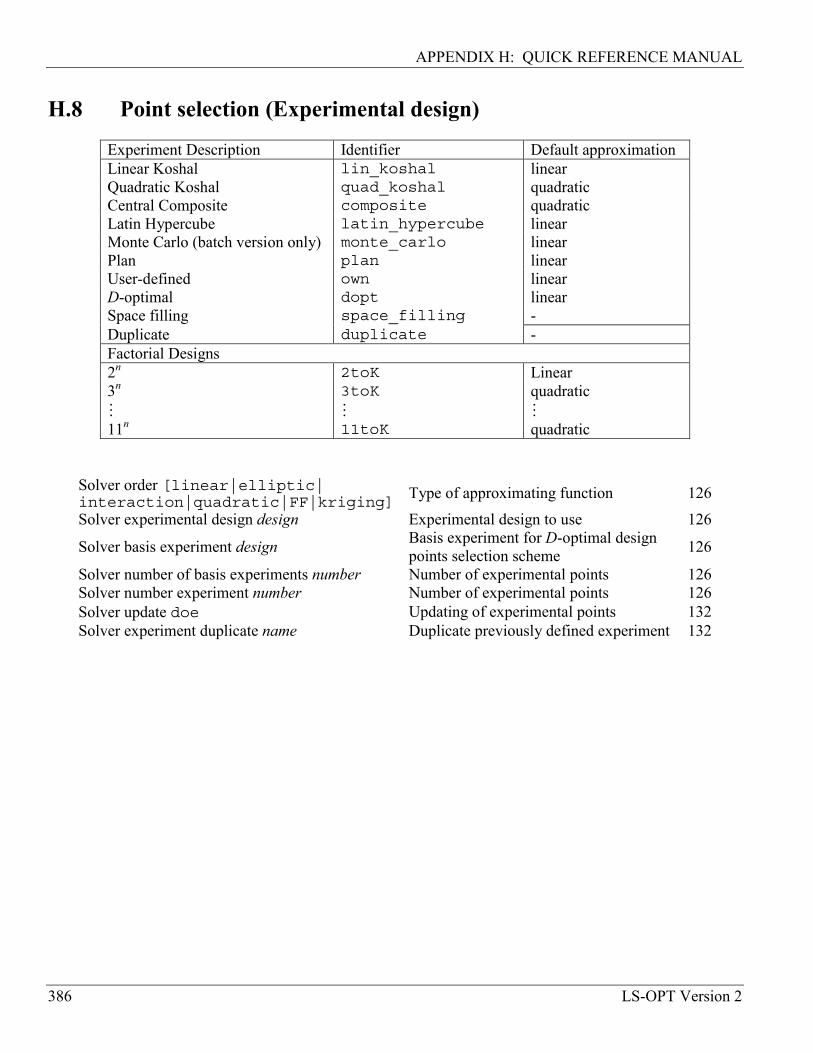
APPENDIX H: QUICK REFERENCE MANUAL
386 LS-OPT Version 2
H.8 Point selection (Experimental design)
Experiment Description Identifier Default approximation Linear Koshal lin_koshal linear Quadratic Koshal quad_koshal quadratic Central Composite composite quadratic Latin Hypercube latin_hypercube linear Monte Carlo (batch version only) monte_carlo linear Plan plan linear User-defined own linear D-optimal dopt linear Space filling space_filling - Duplicate duplicate - Factorial Designs 2n 2toK Linear 3n 3toK quadratic M M M 11n 11toK quadratic
Solver order [linear|elliptic|interaction|quadratic|FF|kriging] Type of approximating function 126
Solver experimental design design Experimental design to use 126
Solver basis experiment design Basis experiment for D-optimal design points selection scheme 126
Solver number of basis experiments number Number of experimental points 126 Solver number experiment number Number of experimental points 126 Solver update doe Updating of experimental points 132 Solver experiment duplicate name Duplicate previously defined experiment 132

APPENDIX H: QUICK REFERENCE MANUAL
LS-OPT Version 2 387
H.9 Design problem formulation History name string Defines history function 136 History name expression Defines history function 136 Historysize number Defines maximum number of data points in history function 366 Response name string Defines response function 139 Response name expression Defines response function 139 Response [linear|elliptic|quadratic|FF|kriging] Type of approximation 143 Composite name type [weighted|targeted] Type of composite function 142 Composite name expression Defines composite function 143 Composite name response name value* { scale factor } Component definition 143 Composite name variable name value* { scale factor } Component definition 143 Weight value Weight (only targeted) 144 Objective name { weight } Objective definition 164 Constraint name Constraint definition 165 Lower bound constraint name value Lower bound on constraint 167 Upper bound constraint name value Upper bound on constraint 167 Strict [0 to 1] / slack Strictness environment 167 Move / stay / move start Reasonable space 131 Maximize Maximize objective 164 * value = target value for type = targeted, weight for type = weighted
H.10 LS-DYNA result interfaces DynaMass p1 p2 p3 ... pn mass_attribute Mass 145 DynaASCII rslt cmp {g u} id {pos} {t_at {t1{t2}}{f_at{n}} ASCII results 148
Dyna cn p1 p2 ... pn [MIN|MAX|AVE] d3plot 150 DynaD3plotHistory cn p1 p2 … pn [ELEMENT|NODE][MIN|MAX|AVE] d3plot 150 DynaThick [THICKNESS|REDUCTION] p1 p2 ... pm[MIN|MAX|AVE] Shell thickness 151 DynaFLD p1 p2 ... pn intercept neg_slope pos_slope FLD 153 DynaFLDg [LOWER|CENTER|UPPER] p1 p2 ... pn load_curve_id General FLD 154 DynaPStress [S1|S2|S3|MEAN] p1 p2 ... pn [MIN|MAX|AVE] Principal stress 155 DynaStat STDDEV response_name Std deviation 159 DynaFreq mode_original [FREQ|NUMBER|GENMASS] Modal data 147 BinoutHistory {history_options} Binout 156 BinoutResponse {response_options} Binout 157 Set Binout Translate 158

APPENDIX H: QUICK REFERENCE MANUAL
388 LS-OPT Version 2
H.11 Solution tasks Iterate n Iterate over n successive approximations 171 Analyze Monte Carlo Monte Carlo evaluation 119 Analyze Metamodel Monte Carlo Monte Carlo evaluation with metamodel 119 H.12 LS-DYNA Results Statistics analyze dynastat {history name} Compute LS-DYNA results statistics 194 dynastat order approx_order Use metamodels; order of metamodel 195 dynstat outlier ON/OFF Report metamodel outliers 195 dynastat max vector ON/OFF Displacement magnitude formulation 195 dynastat component vector ON/OFF Displacement magnitude formulation 195 dynastat correlation response name Correlation 198 dynstat solver name Solver 199 dynastat iteration number Iteration 199 H.13 Intrinsic functions for mathematical expressions
int(a) integer nint(a) nearest integer abs(a) absolute value mod(a,b) remainder of a/b sign(a,b) transfer of sign from b to |a| max(a,b) maximum of a and b min(a,b) minimum of a and b sqrt(a) square root exp(a) ea pow(a,b) ab log(a) natural logarithm log10(a) base 10 logarithm sin(a) sine cos(a) cosine tan(a) tangent asin(a) arc sine acos(a) arc cosine atan(a) arc tangent atan2(a,b) arc tangent of a/b sinh(a) hyperbolic sine cosh(a) hyperbolic cosine tanh(a) hyperbolic tangent asinh(a) arc hyperbolic sine

APPENDIX H: QUICK REFERENCE MANUAL
LS-OPT Version 2 389
acosh(a) arc hyperbolic cosine atanh(a) arc hyperbolic tangent sec(a) secant csc(a) cosecant ctn(a) Cotangent
H.14 Special functions for mathematical expressions Expression Symbols
Integral(expression[,t_lower,t_upper,variable]) ∫b
atdgtf )()(
Derivative(expression[,T_constant]) Tttf =∆∆ |/ ~ Tttf =|d/d
Min(expression[,t_lower,t_upper]) )]([minmin tfft
=
Max(expression[,t_lower,t_upper]) )]([maxmax tfft
=
Initial(expression) First function value on record Final(expression) Last function value on record Lookup(expression,value) Inverse function t(f = F) LookupMin(expression[,t_lower,t_upper]) Inverse function t(f = fmin) LookupMax(expression[,t_lower,t_upper]) Inverse function t(f = fmax)
H.15 Selecting an optimization method Optimization method srsm Successive Response Surface Method (SRSM) 189 Optimization method randomsearch Sequential Random Search (SRS) 189
H.16 Setting parameters for optimization algorithm iterate param identifier value Define parameters in LFOPC 190 iterate param rangelimit variable value Define minimum range of variable in SRSM 191